anomalies and symmetry fractionalization - arxiv
TRANSCRIPT
arX
iv:2
206.
1511
8v1
[he
p-th
] 3
0 Ju
n 20
22
Anomalies and Symmetry Fractionalization
Diego Delmastro,ab 1 Jaume Gomis,b 2 Po-Shen Hsin,c 3 Zohar Komargodskid 4
aPerimeter Institute for Theoretical Physics,
Waterloo, Ontario, N2L 2Y5, Canada
b Department of Physics, University of Waterloo,
Waterloo, ON N2L 3G1, Canada
cMani L. Bhaumik Institute for Theoretical Physics,
475 Portola Plaza, Los Angeles, CA 90095, USA
dSimons Center for Geometry and Physics,
SUNY, Stony Brook, NY 11794, USA
Abstract
We study ordinary, zero-form symmetry G and its anomalies in a system with a one-
form symmetry Γ. In a theory with one-form symmetry, the action of G on charged line
operators is not completely determined, and additional data, a fractionalization class,
needs to be specified. Distinct choices of a fractionalization class can result in different
values for the anomalies of G if the theory has an anomaly involving Γ. Therefore, the
computation of the ’t Hooft anomaly for an ordinary symmetry G generally requires
first discovering the one-form symmetry Γ of the physical system. We show that the
multiple values of the anomaly for G can be realized by twisted gauge transformations,
since twisted gauge transformations shift fractionalization classes. We illustrate these
ideas in QCD theories in diverse dimensions. We successfully match the anomalies of
time-reversal symmetries in 2+1d gauge theories, across the different fractionalization
classes, with previous conjectures for the infrared phases of such strongly coupled
theories, and also provide new checks of these proposals. We perform consistency checks
of recent proposals about two-dimensional adjoint QCD and present new results about
the anomaly of the axial Z2N symmetry in 3 + 1d N = 1 super-Yang-Mills. Finally,
we study fractionalization classes that lead to 2-group symmetry, both in QCD-like
theories, and in 2 + 1d Z2 gauge theory.
[email protected]@[email protected]@gmail.com
Contents
1 Introduction 2
2 Quantum Mechanics 10
2.1 One-form symmetry . . . . . . . . . . . . . . . . . . . . . . . . . . . . . . . . 13
2.2 Time-reversal symmetry . . . . . . . . . . . . . . . . . . . . . . . . . . . . . 15
2.3 Anomalies and fractionalization in CT . . . . . . . . . . . . . . . . . . . . . 21
3 QED and QCD in 1+1 Dimensions 23
3.1 Fermionic Z2 symmetry in 1+1 Dimensions . . . . . . . . . . . . . . . . . . . 27
3.1.1 The mixed Z2 − (−1)F anomaly . . . . . . . . . . . . . . . . . . . . . 29
3.2 A Few Remarks on Adjoint QCD in 1+1 Dimensions . . . . . . . . . . . . . 30
4 Time-Reversal and Symmetry Fractionalization in 2+1 Dimensions 32
4.1 Different symmetry fractionalizations and their anomalies . . . . . . . . . . . 33
4.2 SU(N) with adjoint quark . . . . . . . . . . . . . . . . . . . . . . . . . . . . 35
4.3 Other gauge groups and matter content . . . . . . . . . . . . . . . . . . . . . 38
4.4 Magnetic symmetry: gauging the one-form symmetry . . . . . . . . . . . . . 40
5 QCD in 3+1 Dimensions 40
5.1 Discrete axial zero-form symmetry and its anomaly . . . . . . . . . . . . . . 40
5.2 SU(N) gauge theory with one adjoint fermion . . . . . . . . . . . . . . . . . 42
5.3 Different fractionalization classes, and one-form symmetry anomaly . . . . . 44
5.4 Domain walls . . . . . . . . . . . . . . . . . . . . . . . . . . . . . . . . . . . 45
A Congruence Vector of Simple Lie Algebras 46
B One-Form Symmetry Anomaly in QCD0+1 47
B.1 SU(N) gauge theory with an adjoint fermion . . . . . . . . . . . . . . . . . . 49
B.1.1 Even N . . . . . . . . . . . . . . . . . . . . . . . . . . . . . . . . . . 49
B.1.2 Odd N . . . . . . . . . . . . . . . . . . . . . . . . . . . . . . . . . . . 50
C U(1) Gauge Theory in 1+1d 50
D Fermionic Z2 Gauge Theory with Z2 Symmetry in 1+1d 51
E Z2 Gauge Theory with Two-group Symmetry in 2+1d 53
E.1 Intrinsic symmetries and their anomalies . . . . . . . . . . . . . . . . . . . . 53
E.2 Unitary ZC
2 symmetry . . . . . . . . . . . . . . . . . . . . . . . . . . . . . . . 54
E.2.1 Anomaly . . . . . . . . . . . . . . . . . . . . . . . . . . . . . . . . . . 54
E.3 Anti-unitary Z2 symmetry that acts as charge conjugation . . . . . . . . . . 55
1
E.3.1 Anomaly . . . . . . . . . . . . . . . . . . . . . . . . . . . . . . . . . . 56
E.4 ZT
2 symmetry that does not permute anyons . . . . . . . . . . . . . . . . . . 56
F Two-Groups for Fractionalization Classes of Charge Conjugation 56
F.1 ZN one-form symmetry . . . . . . . . . . . . . . . . . . . . . . . . . . . . . . 57
F.2 Z2 × Z2 one-form symmetry . . . . . . . . . . . . . . . . . . . . . . . . . . . 57
G Twisted Gauge Bundle and Two-Group Symmetry 58
1 Introduction
The study of the symmetries of Quantum Field Theory (QFT) and quantum many-body
systems has been an indispensable tool for several decades. Symmetries provide a robust
concept that remains valid at strong coupling. As such, symmetry considerations oftentimes
have inspired far-reaching insights into non-perturbative physics.
A zero-form symmetry group G in a QFT comes equipped with a collection of co-
dimension one topological, invertible operators which under fusion form the group G. The
Ward identities satisfied by correlation functions of local operators transforming in represen-
tations of G are a consequence of enriching the correlation functions of local operators with
topological operators that implement the action of G.
Stronger dynamical constraints arise if the QFT has an ’t Hooft anomaly [1,2] for G. The
presence of an ’t Hooft anomaly can be diagnosed by coupling to a background gauge field
for the symmetry G. This corresponds to laying down a network of topological junctions of
the topological co-dimension one operators for G. The symmetry G has an ’t Hooft anomaly
if under gauge transformations of the background gauge fields for G the partition function
is not invariant. More precisely, the symmetry G has an ’t Hooft anomaly only when the
non-invariance of the partition function cannot be cured by adding local counterterms for
the background gauge fields. Equivalently, the ’t Hooft anomaly can be described as a failure
of the network of topological junctions to consistently reconnect modulo phases assigned to
each junction, since gauge transformations act by recombining the network of topological
junctions. The implementation of the symmetry action of G, and of its ’t Hooft anomalies,
requires defining the network of topological junctions for the symmetry G.
The reason that ’t Hooft anomalies are interesting and powerful observables is that they
are characterized by topological invariants in one dimension higher [3, 4] and hence they
cannot depend on continuous couplings, and also cannot evolve under the renormalization
group. Indeed, ’t Hooft anomalies for a symmetry G admit a topological classification in
terms of a cobordism group [5–19], the details of which depend on the spacetime dimension,
whether the system is bosonic or fermionic, whether the symmetry acts unitarily or anti-
unitarily, etc. While the early literature on ’t Hooft anomalies focused mostly on the case
of continuous groups G, it has become clear in recent years that there is a rich array of
anomalies for discrete symmetries as well, and that their consequences for strong coupling
dynamics are often striking.
The classification of ’t Hooft anomalies for a symmetry G is intrinsic. It does not depend
on whether the system has additional or yet to be discovered global symmetries. Of course,
the existence of additional symmetries can lead to mixed ’t Hooft anomalies between G and
the new symmetries, but the classification of ’t Hooft anomalies for G is insensitive to the
existence of additional global symmetries.5
Since anomalies are invariants of the renormalization group, they can be computed by
analyzing the theory with an arbitrarily low energy cutoff. In order to compute anomalies,
there is no need to discuss the degrees of freedom that may have been present at high energy.
Technically, the unknown high energy degrees of freedom induce local counter-terms upon
integrating them out, and as we remarked above, the anomaly is defined modulo such terms.
Therefore, conventional wisdom says that anomalies are unambiguously determined given
the low energy degrees of freedom and the action of the symmetry G on these degrees of
freedom. These properties of ’t Hooft anomalies are, in part, why anomalies are so robust
and useful.
In this paper we show that these general expectations about ’t Hooft anomalies for G
need to be revised if a physical system is endowed with a one-form symmetry6 group Γ. The
study of higher symmetry and anomalies has enjoyed ample recent activity, see [24–26] for
early papers on the subject. See [27–29] for reviews and additional references.
We will see that in the presence of one-form symmetry Γ, additional discrete data needs
to be specified in order to unambiguously determine the action of the G symmetry. The
additional data takes values in the cohomology group H2ρ(G,Γ) (see below for details). This
admits several complimentary physical interpretations, which we will elucidate. Importantly,
the ’t Hooft anomalies for G can depend on the choice of class in H2ρ(G,Γ), thus yielding
a spectrum of values for the ’t Hooft anomalies. We will show that distinct choices of the
action of G can result in different ’t Hooft anomalies for G if the theory is endowed with an
’t Hooft anomaly for Γ or there is a mixed G–Γ ’t Hooft anomaly. We emphasize that this
occurs in the absence of any mixing of G with Γ into a higher structure, such as a 2-group
or a higher generalized symmetry structure. It happens when the symmetry of the theory is
the direct product G× Γ.
5This can fail if the zero-form symmetry G “mixes” in a non-trivial fashion with a higher-form symmetry.
For example, G can mix with a one-form symmetry and form a two-group. Then, one should classify the
two-group anomalies. It is still meaningful to discuss ’t Hooft anomalies for G in this case, but the two-group
structure can change the classification of the G anomalies. For instance, some G anomalies can be cancelled
by local counterterms of the two-group background gauge field and becomes trivial [20, 21], which is the
analogue of the Green-Schwarz mechanism [22] for background gauge fields. Some two-group symmetries
that involve a spacetime symmetry can also allow more anomalies for the zero-form G symmetry [23].6More generally, any higher-form symmetry.
3
There are several ways of describing the physical meaning of the additional data that
needs to be given to fully specify the G symmetry and ’t Hooft anomalies for G. In one
perspective, the additional data can be ascribed to inequivalent ways of adding massive
degrees of freedom that are charged under Γ and transform in a (projective) representation
of G. While these heavy degrees of freedom are of no direct consequence at low energies,
they determine the value of the ’t Hooft anomalies for G.7 The reason this statement
is not at odds with usual decoupling arguments is that these massive particles modify the
symmetry structure of theory, and adding them changes the theory in a discontinuous fashion.
Therefore, to evaluate ’t Hooft anomalies for a (zero-form) symmetry G, one must first
discover all the one-form symmetries Γ of the theory and, subsequently, characterize all the
inequivalent choices of adding massive charged particles that break the one-form symmetry.8
This additional data can also be understood as specifying the possible ways the symmetry
G can act on the line operators of the theory that carry charge under Γ.9 These two view-
points are complementary, since line operators insert non-dynamical, heavy particles into
the system.
Line operators can carry projective representation under the zero-form symmetry. The
projective representation is specified by the cohomology classH2(Gstab, U(1)) of the stabilizer
subgroup Gstab ⊂ G that leaves the label of the line invariant [34]. In various special
cases (such as conformal or topological lines), the defect Hilbert space in the presence of
an insertion of a line at a point on Sd is isomorphic to the space of end-points of the line
defect. Then the above projective representation is realized on the space of end-points. Thus,
while local operators are in a vector representation of G, line operators are in a projective
representation of G. In a theory without a one-form symmetry Γ, the cohomology class of
the projective representation of G under which a given line operator transforms is unique
and unambiguously determined.10
In a theory with a one-form symmetry Γ, additional choices need to be made to fully
specify the action of the symmetry G on the theory. That is, while the action of G on local
operators is unique, the action of G on line operators depends on discrete choices when Γ
7We would like to thank T. Senthil for insightful discussions on the role of massive particles. Aspects of
this appeared in [30, 31].8More generally, one needs to discover all higher-form symmetries of the theory, and investigate the
spectrum of extended excitations such as strings (in the case of two-form symmetry).9A line operator that carries vanishing one-form charge transforms in a fixed cohomology class of projective
representations of the zero-form symmetry G. The general statement is [32,33] that lines not charged under
one-form or non-invertible symmetries should be endable and hence admit a nonempty Hilbert space on Sd
whose transformation properties under the various symmetries can be studied.10For example, a 2 + 1d SU(2) gauge theory with a fermion in the 2 of SU(2) has G = SO(3) global
symmetry. Wilson lines Wj with j ∈ Z are in a vector representation of SO(3) while those with j ∈ 1/2+Z
are in a projective representation of SO(3). Line defects in a projective representation of the global symmetry
exist also in Landau-Ginzburg models, for instance, in standard Wilson-Fisher fixed points, see [35–38] and
references therein.
4
L
Ug
g · L
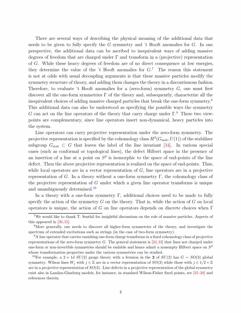
Figure 1: The type of line operator can change from L to g·L when it pierces the codimension-
one symmetry generator labelled by g ∈ G.
is non-trivial. The distinct ways that G is realized on the line operators describe different
G “symmetry fractionalization” classes. Once the symmetry fractionalization class is fully
specified, the ’t Hooft anomalies for G are completely fixed. We will show that distinct
choices of the action of G can result in different ’t Hooft anomalies for G if the theory is
endowed with an ’t Hooft anomaly for Γ or there is a mixed G–Γ ’t Hooft anomaly.
The phenomenon of symmetry fractionalization is well-known in the condensed matter lit-
erature for topological quantum field theories (TQFTs), see e.g. [39–48]11 and the references
therein. Examples with more general quantum systems are discussed in [48, 50–52].
A simple way to understand that additional choices can be made is by considering the
topological junctions for the G symmetry. The topological defects in a junction intersect in
co-dimension two. A one-form symmetry Γ comes equipped with a collection of co-dimension
two topological, invertible defects that fuse according to Γ. Therefore, if the theory has a one-
form symmetry Γ, the junction can be decorated with a topological defect for the one-form
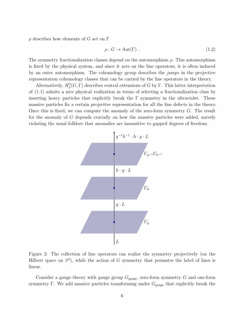
symmetry Γ.12 This decoration of the topological junction changes the symmetry action of
G on lines that carry charge under Γ, since they are acted on by the topological defect for
Γ sitting at the junction, changing the action of G on charged lines by a phase. This can
shift the cohomology class of projective representation of the charged lines (see figure 3).
Consistency of fusion of the junctions and one-form charge implies that distinct choices of
the symmetry fractionalization are related to each other by a class in13
H2ρ(G,Γ) . (1.1)
11See also [49] for the mathematical framework describing symmetry-enriched 2+1d bosonic TQFTs. The
relation with one-form symmetry is discussed in [21].12One may ask whether enriching junctions with non-invertible co-dimension two topological operators
is possible. This would, however, be inconsistent with the fusion of junctions of a G symmetry. Such a
construction could give rise to a higher categorical symmetry, while the phenomena we are studying if for
systems with G× Γ symmetry.13The precise statement is that fractionalization classes form a torsor over this group. When G is an
extension of “bosonic symmetry” Gb by the fermion parity symmetry ZF2 , we consider the classes given by
pullback of H2ρ(Gb,Γ) under the projection G → Gb = G/ZF
2 [46, 47].
5
ρ describes how elements of G act on Γ
ρ : G→ Aut(Γ) . (1.2)
The symmetry fractionalization classes depend on the automorphism ρ. This automorphism
is fixed by the physical system, and since it acts on the line operators, it is often induced
by an outer automorphism. The cohomology group describes the jumps in the projective
representation cohomology classes that can be carried by the line operators in the theory.
Alternatively, H2ρ(G,Γ) describes central extensions of G by Γ. This latter interpretation
of (1.1) admits a nice physical realization in terms of selecting a fractionalization class by
inserting heavy particles that explicitly break the Γ symmetry in the ultraviolet. These
massive particles fix a certain projective representation for all the line defects in the theory.
Once this is fixed, we can compute the anomaly of the zero-form symmetry G. The result
for the anomaly of G depends crucially on how the massive particles were added, naively
violating the usual folklore that anomalies are insensitive to gapped degrees of freedom.
L
Ug
Uh
Ug−1Uh−1
g · L
h · g · L
g−1h−1 · h · g · L
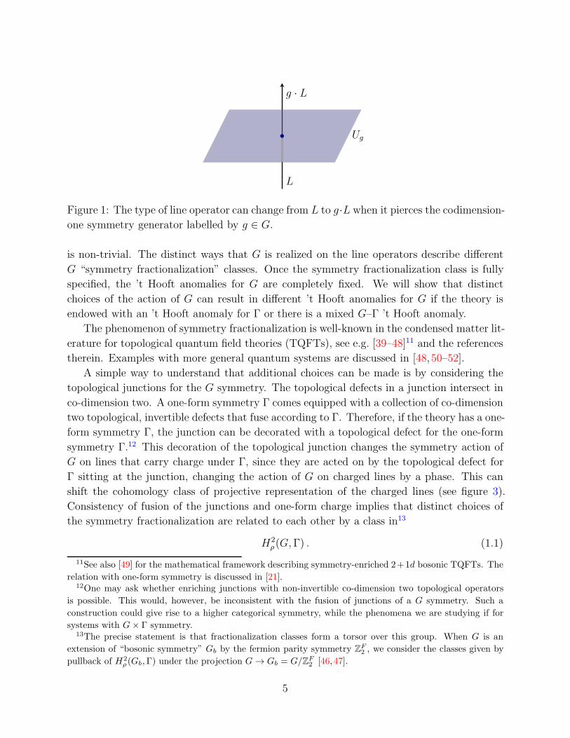
Figure 2: The collection of line operators can realize the symmetry projectively (on the
Hilbert space on Sd), while the action of G symmetry that permutes the label of lines is
linear.
Consider a gauge theory with gauge group Ggauge, zero-form symmetry G and one-form
symmetry Γ. We add massive particles transforming under Ggauge that explicitly break the
6
Ugh
UgUh
Figure 3: Junctions of co-dimension one symmetry defects are important in the study of
’t Hooft anomalies. In theories with one-form symmetry, a co-dimension two invertible
topological defect can be inserted in the junction.
one-form symmetry Γ. These massive particles transform in a representation of an extension
of the ordinary global symmetry, which we denote by G, such that a center subgroup Z ⊂ G
is identified with a subgroup in the center of the gauge group Ggauge. The faithful global
symmetry is therefore G/Z = G. The symmetry of the classical action with the massive
matter fields is [53]Ggauge × G
Z . (1.3)
(We have assumed a direct product for simplicity.) Then, at low energy, the one-form
symmetry of the theory without the charged massive particles emerges in the infrared, that
is ΓIR = Γ = Z. The Wilson line of the massive matter fields that were added in the
ultraviolet transform as a linear representation of G, which is a projective representation of
G. Adding massive matter picks out the particular fractionalization class specified by the
extension G by Γ, which we denoted by G, dictated by a class in H2ρ(G,Γ).
Turning on a background gauge field for G that cannot be lifted to a G gauge field, the
Ggauge gauge bundle is also modified to be a Ggauge/Z bundle, by virtue of the symmetry
structure (1.3). This modification of the gauge bundle induced by adding the massive matter
fields can contribute an ’t Hooft anomaly of G symmetry.14
An elementary way of inducing a change of fractionalization class is to twist the action of
G with gauge transformations ofGgauge that do not modify theG symmetry algebra on the ele-
mentary fields that enjoyed the one-form symmetry (those present before adding the one-form
breaking heavy fields). These gauge transformations can be thought of de-fractionalizing the
symmetry of the additional massive particles, so that they do not contribute to the ’t Hooft
14For example, consider the SU(2)k Chern-Simons theory in 2 + 1d with two massive scalars in the
fundamental representation that breaks the one-form symmetry. Since flipping the sign of the scalar field
can be identified with a gauge transformation, the faithful zero-form symmetry is G = U(2)/Z2. The
symmetry structure is (SU(2)gauge × U(2)) /Z2, with G = U(2). In the presence of background gauge field
for G zero-form symmetry that cannot be lifted to a G background gauge field, the SU(2)gauge gauge bundle
is modified to be an SO(3) bundle, and the Chern-Simons term for SO(3) gauge bundle is not well-defined
for k 6= 0 mod 4. Thus the massive matter field contributes an ’t Hooft anomaly for the G symmetry [53].
7
anomalies for G, and the anomalies are fully captured by the original elementary fields. The
twisted action can change the value of the anomaly because the charges of the elementary
fields under G are modified by the gauge transformation, thus giving rise to distinct values
of the ’t Hooft anomaly. Moreover, the twisted transformations induce a non-trivial phase
that multiplies the Wilson lines of the gauge theory carrying one-form charge. This phase
has a pleasing interpretation, it captures the change of projective representation of the lines
under G, and thus these twisted transformations can be seen to induce a change of frac-
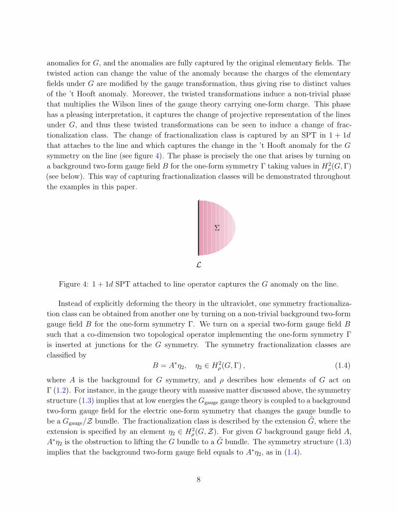
tionalization class. The change of fractionalization class is captured by an SPT in 1 + 1d
that attaches to the line and which captures the change in the ’t Hooft anomaly for the G
symmetry on the line (see figure 4). The phase is precisely the one that arises by turning on
a background two-form gauge field B for the one-form symmetry Γ taking values in H2ρ(G,Γ)
(see below). This way of capturing fractionalization classes will be demonstrated throughout
the examples in this paper.
Σ
L
Figure 4: 1 + 1d SPT attached to line operator captures the G anomaly on the line.
Instead of explicitly deforming the theory in the ultraviolet, one symmetry fractionaliza-
tion class can be obtained from another one by turning on a non-trivial background two-form
gauge field B for the one-form symmetry Γ. We turn on a special two-form gauge field B
such that a co-dimension two topological operator implementing the one-form symmetry Γ
is inserted at junctions for the G symmetry. The symmetry fractionalization classes are
classified by
B = A∗η2, η2 ∈ H2ρ(G,Γ) , (1.4)
where A is the background for G symmetry, and ρ describes how elements of G act on
Γ (1.2). For instance, in the gauge theory with massive matter discussed above, the symmetry
structure (1.3) implies that at low energies theGgauge gauge theory is coupled to a background
two-form gauge field for the electric one-form symmetry that changes the gauge bundle to
be a Ggauge/Z bundle. The fractionalization class is described by the extension G, where the
extension is specified by an element η2 ∈ H2ρ(G,Z). For given G background gauge field A,
A∗η2 is the obstruction to lifting the G bundle to a G bundle. The symmetry structure (1.3)
implies that the background two-form gauge field equals to A∗η2, as in (1.4).
8
Picking different fractionalization classes can yield distinct values of the ’t Hooft anomaly
for the zero-form symmetry G. Indeed, when the theory has one-form anomalies for Γ or
mixed Γ–G anomalies, the topological actions (inflow terms) for these anomalies in one
dimension higher can produce, upon shifting the background B field for Γ by B ∈ H2ρ(G,Γ),
a pure G anomaly topological action. This is the mechanism behind different symmetry
fractionalization classes resulting in different ’t Hooft anomalies for G. In theories with
one-form symmetry there is no canonical choice for B, as B = 0 is not preferred in any way
(there is no canonical choice for B since symmetry fractionalization classes form a torsor over
H2ρ(G,Γ)). Instead, one has to consider all possible values of B and compute the anomalies
accordingly for each.
When the action of the zero-form symmetry G does not commute with the action of the
one-form symmetry Γ, a change of fractionalization class for the G symmetry can transmute
the symmetry structure of the theory from a G× Γ symmetry into a two-group. We demon-
strate this in the 2+1d Z2 gauge theory for the unitary Z2 and time-reversal ZT
2 symmetries
that exchange the e andm particles (see appendix E). In a gauge theory, this can occur when
G includes charge conjugation. We show that 3+1d N = 1 SU(N) super-Yang-Mills admits,
for a choice of fractionalization class, a two-group between the G = ZC
2 charge conjugation
symmetry and Γ = ZN one-form symmetry (see section 5 and appendix F). In the examples
we will study, when the zero-form symmetry does not involve the charge conjugation sym-
metry that acts on the gauge group, it does not participate in a two-group as discussed in
appendix G.
Our goal in this work is twofold. First, we will go over many examples of systems with one-
form symmetry and investigate the anomalies of ordinary symmetries in such circumstances.
The models we will mostly discuss are quantum chromodynamics (QCD) theories: Yang-
Mills theory coupled to quarks. We will devise general rules in 0 + 1, 1 + 1, 2 + 1, and
3+ 1 dimensions of how to compute the anomalies of zero-form symmetries given some data
about the one-form symmetries of such theories. We will see that the ambiguity of anomalies
of zero-form symmetries appears in a peculiar way, through the “non-gauge invariance” of
the anomaly. While 0 + 1 dimensional theories do not have a one-form symmetry in the
usual sense, one can still discuss defects extended in time and one can still discuss projective
representations associated with those defects. Therefore, examples in quantum mechanics
that we study already capture some of the physics, including the fact that the choice of
fractionalization class can manifest itself through the non-gauge invariance of the ’t Hooft
anomaly. Second, we use our improved understanding of anomalies of ordinary symmetries
in the presence of one-form symmetry to test various proposed dualities for adjoint QCD
(and other related theories with other quark content) both in 1 + 1 and 2 + 1 dimensions.
We show that the zero-form anomalies, with the ambiguities due to fractionalization classes
carefully taken into account, match beautifully in previously proposed scenarios for the
infrared physics of adjoint QCD in 1 + 1 and 2 + 1 dimensions. In the latter case, the
9
comparison of the anomalies necessitates a study of the anomalies of certain non-trivial
TQFTs.
The outline of the paper is as follows. In section 2 we discuss pedagogical examples in
0 + 1 dimensions. There is a sense of one-form symmetry in quantum mechanics, and quite
many of the ideas discussed in this paper can be already demonstrated in this setting. In
section 3 we consider 1+1 dimensions, including bosonic quantum electrodynamics in 1+1d
(QED2), Z2 gauge theory, fermionic QED2, and adjoint QCD2. We discuss the anomalies
of various Z2 global symmetries, perform consistency checks of some proposals, and devise
the rules for how to compute the anomalies of such Z2 symmetries properly. In section 4 we
discuss time-reversal symmetry in 2+1 dimensions. Depending on properties of the one-form
symmetry, we devise the rules for how the choice of a fractionalization class influences the
mod 16 time-reversal symmetry anomaly. We perform new consistency checks of proposed
infrared dualities. There are important differences between T and CT which we discuss in
detail and we perform consistency checks for both. In section 5 we discuss super Yang-
Mills theory in 3 + 1 dimensions (aka massless adjoint QCD) and compute the anomalies
of its Z2N zero-form symmetry and also show how the anomaly depends on the choice of
fractionalization class. Appendices cover some technical details.
Note added: This work is submitted in coordination with [54], which has some overlap
with ours.
2 Quantum Mechanics
In this section we study the phenomena discussed in the introduction in an elementary
setting. We consider the ’t Hooft anomalies of a 0 + 1d system with ZT
2 × ZF2 zero-form
symmetry, where ZT
2 is generated by time-reversal T and ZF2 by fermion parity (−1)F , with
T2 =
(
(−1)F)2
= 1. ’t Hooft anomalies for this symmetry are classified by the cobordism
group ΩPin−
2 = Z8 [55]. A diagnostic of an ’t Hooft anomaly in 0 + 1 dimensions is that
the symmetry is realized projectively on the Hilbert space. For an early study of ’t Hooft
anomalies in quantum mechanics see [56].
The above Z8 ’t Hooft anomaly is captured via inflow by the 1+1d topological invariant
S =2πν
8
∫
Σ2
ABK , (2.1)
with ν ∈ Z8, and ABK the Arf-Brown-Kervaire invariant [10] of the surface Σ2.
Free massless Majorana fermions in 0+1d have ZT
2 ×ZF2 zero-form symmetry. The action
of ZT
2 on a Majorana fermion λ depends on the choice of a sign
T : λ(t) → ±λ(−t) , (2.2)
while the action of ZF2 is
(−1)F : λ(t) → −λ(t) . (2.3)
10
Since the Hermitian mass term iλλ′ is T-invariant when λ and λ′ transform with opposite
signs under ZT
2 , the ’t Hooft anomaly is given by
ν = n+ − n− mod 8 , (2.4)
where n± is the number of Majorana fermions transforming with a ± under ZT
2 in (2.2). The
fact that ν ∈ Z8 in this system follows from the existence [55] of a ZT
2 -symmetric quartic
interaction that gaps out the fermions for ν = 8.
Let us now consider QCD0+1: gauge fields with simple and simply-connected gauge
group Ggauge coupled to quarks in a representation R of Ggauge. QCD0+1 is obtained by
gauging a subgroup Ggauge ⊂ SO(dimR(R)) of the flavor symmetry of the free fermion theory.
Gauge fields in 0+ 1d have no dynamics, but they constrain the Hilbert space and the local
operators of the free fermion theory by virtue of the Gauss’s law implied by the gauge field
equation of motion.15 Moreover, the gauge theory can be enriched by adding a static Wilson
line stretched along time. Strictly speaking, this changes the theory, since the Wilson line
insertion modifies Gauss’s law, resulting in a different Hilbert space.
QCD0+1 preserves the ZT
2 ×ZF2 symmetry of the free fermion theory. Our goal is to study
the ZT
2 anomalies of this theory. A conventional choice for the action of ZT
2 on QCD0+1 is16
T :
ψ(t) → ψ∗(−t)A0(t) → −A∗
0(−t) ,(2.5)
where ψ is the quark in a representation R ofGgauge. Conventional wisdom would suggest that
the ’t Hooft anomaly for ZT
2 can be be computed in the ultraviolet, where gauge interactions
can be neglected, with the conclusion that the ’t Hooft anomaly for the ZT
2 symmetry (2.5)
of QCD0+1 is the number of Majorana fermions
ν = dimR(R) mod 8 . (2.6)
This wisdom will now be scrutinized and shown to fail in QCD0+1 theories with anomalous
one-form symmetry. (We will soon explain what one-form symmetry means in quantum
mechanics.)
For concreteness we consider adjoint QCD0+1, i.e., with quarks in the adjoint represen-
tation of Ggauge. We first analyze the theory in the presence of a background gauge field for
Ggauge, and discuss the effects of integrating over the gauge fields later. The Hilbert space
can be straightforwardly constructed by splitting the fermions into creation and annihilation
15For now we ignore the difficulty with the cases of odd dimR(R), where there is no Z2-graded Hilbert
space. We will take care of it later.16Other time-reversal symmetries can be defined by combining T with a unitary global Z2 symmetry of
the QCD0+1 theory.
11
operators.17 The dimension of the Hilbert space is 2dimGgauge/2. These states furnish the two
complex spinor representations of Spin(dimG); one spinor represents the bosonic states and
the other the fermionic states.
We now consider the partition function on a circle with anti-periodic boundary conditions
in the presence of a background gauge field a, which can be brought to the Cartan subalgebra
of ggauge by a gauge transformation. Either by computing the fermion determinant, or by
evaluating the Hamiltonian on the Hilbert space, we find that
ZNS(a) = 2rank(G)/2∏
α>0
(
eiπα(a) + e−iπα(a))
, (2.7)
where the product runs over the positive roots α of the Lie algebra of Ggauge. The residual
gauge transformations after gauge fixing are the time independent gauge transformations,
which act by conjugation. This implies that the partition function is a class function of
U = e2πia, i.e., it must admit a decomposition into characters of Ggauge.
A computation shows that the partition function of adjoint QCD0+1 can be expressed
as the character in the representation of Ggauge with highest weight the Weyl vector ρ =
(1, 1, . . . , 1). It is given by
ZNS = 2rank(Ggauge)/2χ(1,1,...,1)(U) , (2.8)
where
χ(1,1,...,1)(U) =Wρ ≡ trρ P exp
(
i
∮
a
)
. (2.9)
Therefore, the partition function can be described as the insertion of a Wilson line Wρ in
the representation ρ of G in the theory without fermions. So far a was a fixed Lie algebra
element.
For Ggauge = SU(N), the theory has a faithful PSU(N) global symmetry acting on the
quarks ψ in the adjoint representation, but on the Hilbert space, the symmetry is realized
projectively corresponding to a 1 + 1d SPT phase for the PSU(N) global symmetry with
coefficient N/2 mod N for even N and 0 mod N otherwise. A similar discussion holds for
all simple and simply-connected Ggauge.
We now proceed to gauge the Ggauge symmetry. This requires path integrating over
the gauge fields, i.e. carefully summing over all group elements∫
[DU ] with [DU ] the Haar
measure on Ggauge.18 The theory we obtain in this way is adjoint QCD0+1.
17In order to simplify the discussion, we add an uncharged Majorana fermion when dimGgauge is odd so
that the theory is endowed with a conventional graded Hilbert space. Whenever we write dimGgauge we
refer to the setup where the total number of fermions is even, and includes the case where we may have
added one decoupled Majorana fermion to make the total number of fermions even.18For details how the integration measure over ggauge transmutes to the Haar measure of Ggauge upon
gauge fixing, see e.g. Appendix C in [57].
12
The presentation of the partition function in (2.8) makes it clear that the Hilbert space
of adjoint QCD0+1 is empty. This is simply because integrating the character χ(1,1,...,1)(U)
we find a vanishing partition function due to the orthogonality of characters∫
[DU ]χR1(U)χR2(U∗) = δR1,R2 , (2.10)
that is ZQCD0+1= 0. The Gauss’s law constraint eliminates all the states and the physical
Hilbert space is empty.
2.1 One-form symmetry
It is useful to think about these cases where the partition function vanishes as due to a one-
form symmetry with an ’t Hooft anomaly, in a sense we now explain. Consider the following
Hilbert space
H =⊕
r∈Z[Ggauge]∨
Hr , (2.11)
where Z[Ggauge] is the center of Ggauge (see table 1). A state in Hr carries charge r ∈Z[Ggauge]
∨. Therefore on Hr the zero-form symmetry Ggauge is realized with an anomaly
since it acts projectively. The same coefficient r ∈ Z[Ggauge]∨ will be soon interpreted as a
one-form symmetry anomaly after gauging Ggauge. The operators that interpolate between
Hilbert spaces with different charges are line operators charged under Z[Ggauge].19 Of course,
in 0 + 1d inserting a Wilson line changes the theory, so that the Hilbert space above can
be regarded as the Hilbert space of decoupled 0 + 1d theories. It is in this sense that it is
meaningful to assign one-form charge r ∈ Z[Ggauge]∨ to the partition function of Hr after
gauging Ggauge, and the assigned charge is compatible with the fusion of line operators.
The one-form charge r ∈ Z[Ggauge]∨ will be now interpreted as the one-form symmetry
anomaly. Whenever the one-form symmetry anomaly is nonzero, the corresponding theory
has a vanishing partition function because the one-form symmetry charge allows to rotate the
partition function by a phase which is some non-trivial root of unity (and the only partition
function that may be compatible with that is the vanishing one).20
An invertible theory of a two-form gauge field in 1+ 1d captures via inflow the one-form
anomalies of the boundary 0+ 1d theory. One-form anomalies for a ZM one-form symmetry
are classified by ΩSpin2 (B2
ZM ) = Z2 × ZM . The first factor corresponds to the Arf invariant
and the second to
S =2πk
M
∫
Σ2
B k = 0, 1, . . . ,M − 1 . (2.12)
19This resembles what happens in 1 + 1d, where Hilbert spaces graded by different one-form charge are
decoupled and can only be interpolated by acting with a line operator that is charged under the one-form
symmetry.20The Hilbert space might be empty also in the absence of one-form anomaly, e.g., for SU(N) with N odd,
the theory has one-form symmetry ZN , there is no anomaly, and yet ZQCD = 0.
13
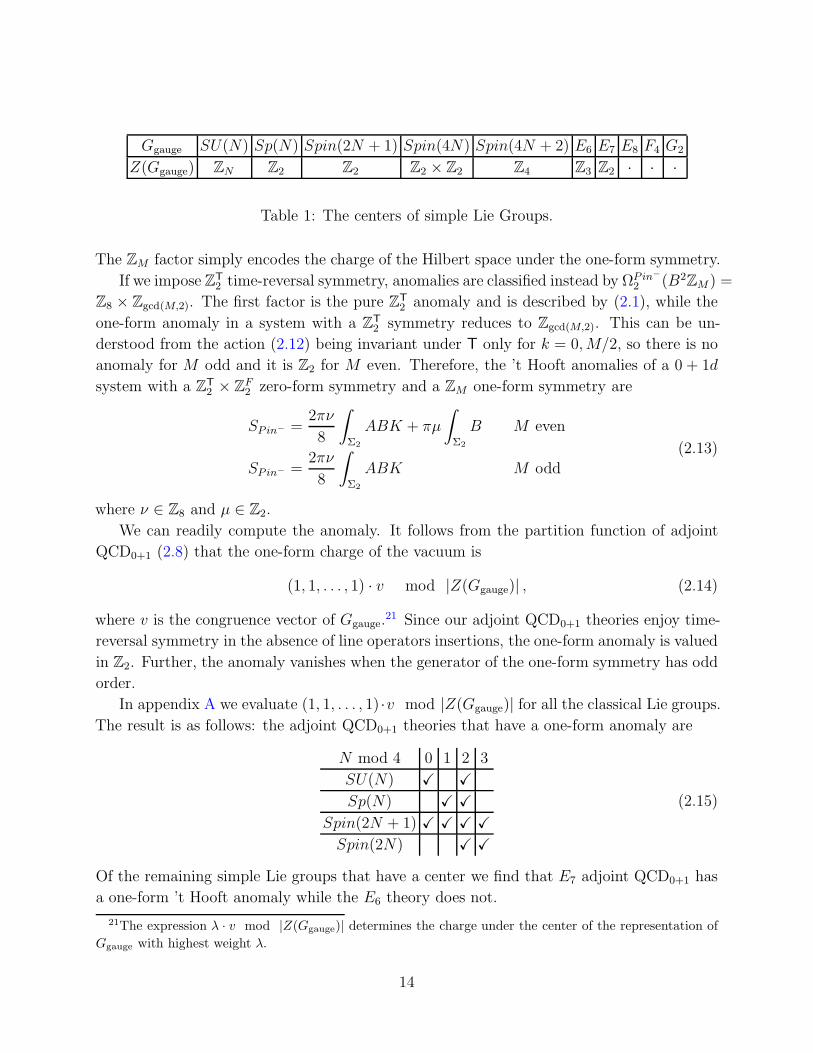
Ggauge SU(N) Sp(N) Spin(2N + 1) Spin(4N) Spin(4N + 2) E6 E7 E8 F4 G2
Z(Ggauge) ZN Z2 Z2 Z2 × Z2 Z4 Z3 Z2 · · ·
Table 1: The centers of simple Lie Groups.
The ZM factor simply encodes the charge of the Hilbert space under the one-form symmetry.
If we impose ZT
2 time-reversal symmetry, anomalies are classified instead by ΩPin−
2 (B2ZM ) =
Z8 × Zgcd(M,2). The first factor is the pure ZT
2 anomaly and is described by (2.1), while the
one-form anomaly in a system with a ZT
2 symmetry reduces to Zgcd(M,2). This can be un-
derstood from the action (2.12) being invariant under T only for k = 0,M/2, so there is no
anomaly for M odd and it is Z2 for M even. Therefore, the ’t Hooft anomalies of a 0 + 1d
system with a ZT
2 × ZF2 zero-form symmetry and a ZM one-form symmetry are
SPin− =2πν
8
∫
Σ2
ABK + πµ
∫
Σ2
B M even
SPin− =2πν
8
∫
Σ2
ABK M odd
(2.13)
where ν ∈ Z8 and µ ∈ Z2.
We can readily compute the anomaly. It follows from the partition function of adjoint
QCD0+1 (2.8) that the one-form charge of the vacuum is
(1, 1, . . . , 1) · v mod |Z(Ggauge)| , (2.14)
where v is the congruence vector of Ggauge.21 Since our adjoint QCD0+1 theories enjoy time-
reversal symmetry in the absence of line operators insertions, the one-form anomaly is valued
in Z2. Further, the anomaly vanishes when the generator of the one-form symmetry has odd
order.
In appendix A we evaluate (1, 1, . . . , 1) ·v mod |Z(Ggauge)| for all the classical Lie groups.The result is as follows: the adjoint QCD0+1 theories that have a one-form anomaly are
N mod 4 0 1 2 3
SU(N) X X
Sp(N) X X
Spin(2N + 1) X X X X
Spin(2N) X X
(2.15)
Of the remaining simple Lie groups that have a center we find that E7 adjoint QCD0+1 has
a one-form ’t Hooft anomaly while the E6 theory does not.
21The expression λ · v mod |Z(Ggauge)| determines the charge under the center of the representation of
Ggauge with highest weight λ.
14
One may diagnose the one-form ’t Hooft anomaly by attempting to gauge it. This
corresponds to studying QCD0+1 with gauge group Ggauge/Γ. If Γ has a ’t Hooft anomaly,
then the theory with gauge group Ggauge/Γ suffers from a global gauge anomaly, and it is an
inconsistent model: the theory is not invariant under large Ggauge/Γ gauge transformations
(see e.g. [56]).
The theories with the one-form anomaly have an empty Hilbert space, but they can be
enriched so that the Hilbert space is non empty by considering a Wilson line insertion Wρ in
the representation of Ggauge with highest weight given by the Weyl vector ρ = (1, 1, . . . , 1).22
We will denote this Hilbert space by Hρ.
2.2 Time-reversal symmetry
We proceed now to determine the ZT
2 time-reversal anomaly by analyzing how T is realized
on the Hilbert space Hρ. We recall that local operators are in a (vector) representation of ZT
2 ,
but line operators can be in a projective representation of ZT
2 . For a line operator with one-
form charge, the projective representation carried by the line takes values in H2(ZT
2 ,ZM) =
Zgcd(2,M), where ZM is the one-form symmetry. The line Wρ in adjoint QCD0+1 carries one-
form charge precisely when the theory has a one-form anomaly (see (2.15)). This means that
in the adjoint QCD0+1 theories with no ’t Hooft anomaly for the the one-form symmetry,
the action of ZT
2 on the local and line operators is completely fixed. This, in turn, implies
that for these theories the ZT
2 ’t Hooft anomaly takes values in Z8. The ZT
2 ’t Hooft anomaly
of the adjoint QCD0+1 theories that have one-form symmetry with anomaly require picking
an element H2(ZT
2 ,ZM) = Z2, which corresponds to fixing the action of ZT
2 on Wρ (and
all charged lines). Indeed, Wρ can be either in a Kramers singlet or Kramers doublet
representation of ZT
2 , and as we will show the ZT
2 ’t Hooft anomaly depends crucially on this
choice.
The action of T when Wρ is a Kramers singlet is
T|Wρ〉 =12dimGgauge∏
n=1
ψ†n|Wρ〉 . (2.16)
Time-reversal acts as particle-hole symmetry. This is to be contrasted with the action of
time-reversal when Wρ is in a Kramers doublet
T|Wρ〉+ =
12dimGgauge∏
n=1
ψ†n|Wρ〉−
T|Wρ〉− = −12dimGgauge∏
n=1
ψ†n|Wρ〉+ .
(2.17)
22The insertion of any other Wilson line would lead to an empty Hilbert space by the orthogonality of
characters.
15
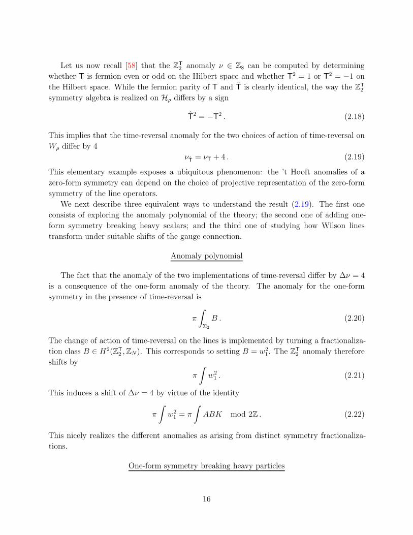
Let us now recall [58] that the ZT
2 anomaly ν ∈ Z8 can be computed by determining
whether T is fermion even or odd on the Hilbert space and whether T2 = 1 or T2 = −1 on
the Hilbert space. While the fermion parity of T and T is clearly identical, the way the ZT
2
symmetry algebra is realized on Hρ differs by a sign
T2 = −T
2 . (2.18)
This implies that the time-reversal anomaly for the two choices of action of time-reversal on
Wρ differ by 4
νT= νT + 4 . (2.19)
This elementary example exposes a ubiquitous phenomenon: the ’t Hooft anomalies of a
zero-form symmetry can depend on the choice of projective representation of the zero-form
symmetry of the line operators.
We next describe three equivalent ways to understand the result (2.19). The first one
consists of exploring the anomaly polynomial of the theory; the second one of adding one-
form symmetry breaking heavy scalars; and the third one of studying how Wilson lines
transform under suitable shifts of the gauge connection.
Anomaly polynomial
The fact that the anomaly of the two implementations of time-reversal differ by ∆ν = 4
is a consequence of the one-form anomaly of the theory. The anomaly for the one-form
symmetry in the presence of time-reversal is
π
∫
Σ2
B . (2.20)
The change of action of time-reversal on the lines is implemented by turning a fractionaliza-
tion class B ∈ H2(ZT
2 ,ZN). This corresponds to setting B = w21. The Z
T
2 anomaly therefore
shifts by
π
∫
w21 . (2.21)
This induces a shift of ∆ν = 4 by virtue of the identity
π
∫
w21 = π
∫
ABK mod 2Z . (2.22)
This nicely realizes the different anomalies as arising from distinct symmetry fractionaliza-
tions.
One-form symmetry breaking heavy particles
16
We will now show an additional derivation of the 4 mod 8 ambiguity in the time-reversal
anomaly due to the one-form symmetry anomaly. We will break the one-form symmetry
explicitly by adding massive particles. The anomaly is sensitive to such massive particles and
we will see that distinct ways of adding such massive particles result in a 4 mod 8 freedom in
the time-reversal anomaly (2.19). The sensitivity of the anomaly to these massive particles
can be established in several ways, as we will see. In particular, one way concerns with
composing T with various gauge transformations, which we will show directly leads to the
fractionalization classes B ∈ H2(ZT
2 ,ZN).
The Wilson lines from before are now interpreted as the wordline of these massive par-
ticles; as such, the symmetry fractionalization is now detected as a fractionalized action on
the massive scalars.
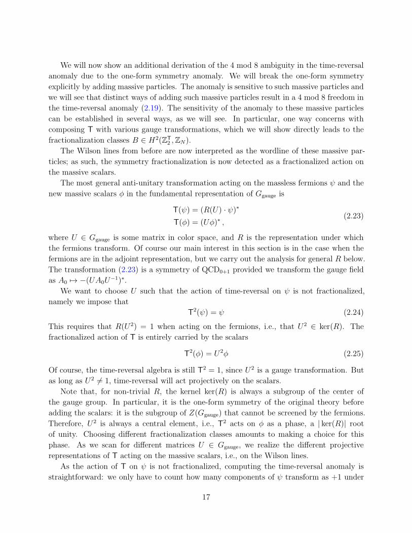
The most general anti-unitary transformation acting on the massless fermions ψ and the
new massive scalars φ in the fundamental representation of Ggauge is
T(ψ) = (R(U) · ψ)∗
T(φ) = (Uφ)∗ ,(2.23)
where U ∈ Ggauge is some matrix in color space, and R is the representation under which
the fermions transform. Of course our main interest in this section is in the case when the
fermions are in the adjoint representation, but we carry out the analysis for general R below.
The transformation (2.23) is a symmetry of QCD0+1 provided we transform the gauge field
as A0 7→ −(UA0U−1)∗.
We want to choose U such that the action of time-reversal on ψ is not fractionalized,
namely we impose that
T2(ψ) = ψ (2.24)
This requires that R(U2) = 1 when acting on the fermions, i.e., that U2 ∈ ker(R). The
fractionalized action of T is entirely carried by the scalars
T2(φ) = U2φ (2.25)
Of course, the time-reversal algebra is still T2 = 1, since U2 is a gauge transformation. But
as long as U2 6= 1, time-reversal will act projectively on the scalars.
Note that, for non-trivial R, the kernel ker(R) is always a subgroup of the center of
the gauge group. In particular, it is the one-form symmetry of the original theory before
adding the scalars: it is the subgroup of Z(Ggauge) that cannot be screened by the fermions.
Therefore, U2 is always a central element, i.e., T2 acts on φ as a phase, a | ker(R)| rootof unity. Choosing different fractionalization classes amounts to making a choice for this
phase. As we scan for different matrices U ∈ Ggauge, we realize the different projective
representations of T acting on the massive scalars, i.e., on the Wilson lines.
As the action of T on ψ is not fractionalized, computing the time-reversal anomaly is
straightforward: we only have to count how many components of ψ transform as +1 under
17
R(U), and how many as −1. Note that, since R(U) has eigenvalues ±1, the anomaly is easily
calculated as ν = trR(U) := trR(U). This is invariant under conjugation and thus we can
assume without loss of generality that U sits in some maximal torus of Ggauge.
Let us now quote the results for the adjoint representation R = adj, which acts as
R(U) ·ψ = UψU−1. Clearly, ker(adj) = Z(Ggauge), and the one-form symmetry is the center
of the gauge group. In the orthogonal case we make no distinction between Spin(N) and
SO(N), since the central Z2 does not act on the adjoint representation.
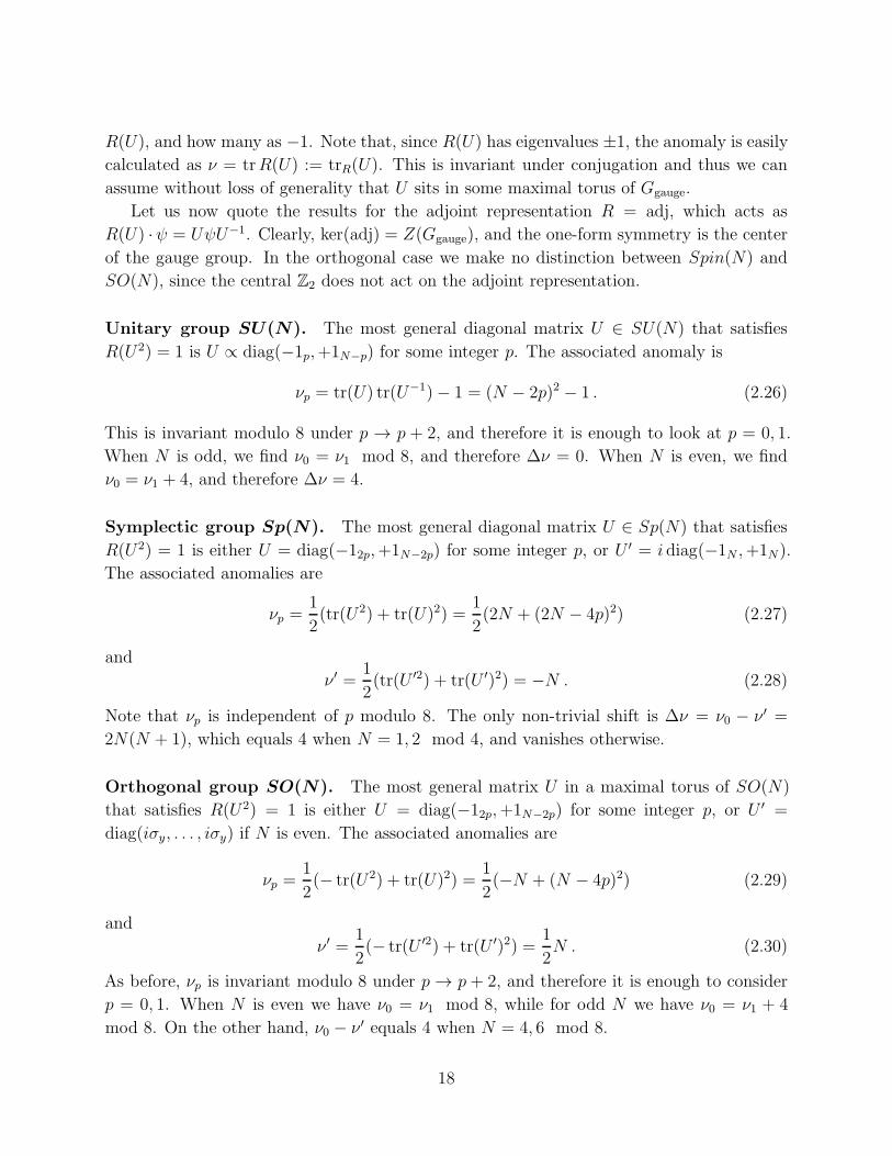
Unitary group SU(N). The most general diagonal matrix U ∈ SU(N) that satisfies
R(U2) = 1 is U ∝ diag(−1p,+1N−p) for some integer p. The associated anomaly is
νp = tr(U) tr(U−1)− 1 = (N − 2p)2 − 1 . (2.26)
This is invariant modulo 8 under p → p + 2, and therefore it is enough to look at p = 0, 1.
When N is odd, we find ν0 = ν1 mod 8, and therefore ∆ν = 0. When N is even, we find
ν0 = ν1 + 4, and therefore ∆ν = 4.
Symplectic group Sp(N). The most general diagonal matrix U ∈ Sp(N) that satisfies
R(U2) = 1 is either U = diag(−12p,+1N−2p) for some integer p, or U ′ = i diag(−1N ,+1N).
The associated anomalies are
νp =1
2(tr(U2) + tr(U)2) =
1
2(2N + (2N − 4p)2) (2.27)
and
ν ′ =1
2(tr(U ′2) + tr(U ′)2) = −N . (2.28)
Note that νp is independent of p modulo 8. The only non-trivial shift is ∆ν = ν0 − ν ′ =
2N(N + 1), which equals 4 when N = 1, 2 mod 4, and vanishes otherwise.
Orthogonal group SO(N). The most general matrix U in a maximal torus of SO(N)
that satisfies R(U2) = 1 is either U = diag(−12p,+1N−2p) for some integer p, or U ′ =
diag(iσy, . . . , iσy) if N is even. The associated anomalies are
νp =1
2(− tr(U2) + tr(U)2) =
1
2(−N + (N − 4p)2) (2.29)
and
ν ′ =1
2(− tr(U ′2) + tr(U ′)2) =
1
2N . (2.30)
As before, νp is invariant modulo 8 under p → p + 2, and therefore it is enough to consider
p = 0, 1. When N is even we have ν0 = ν1 mod 8, while for odd N we have ν0 = ν1 + 4
mod 8. On the other hand, ν0 − ν ′ equals 4 when N = 4, 6 mod 8.
18
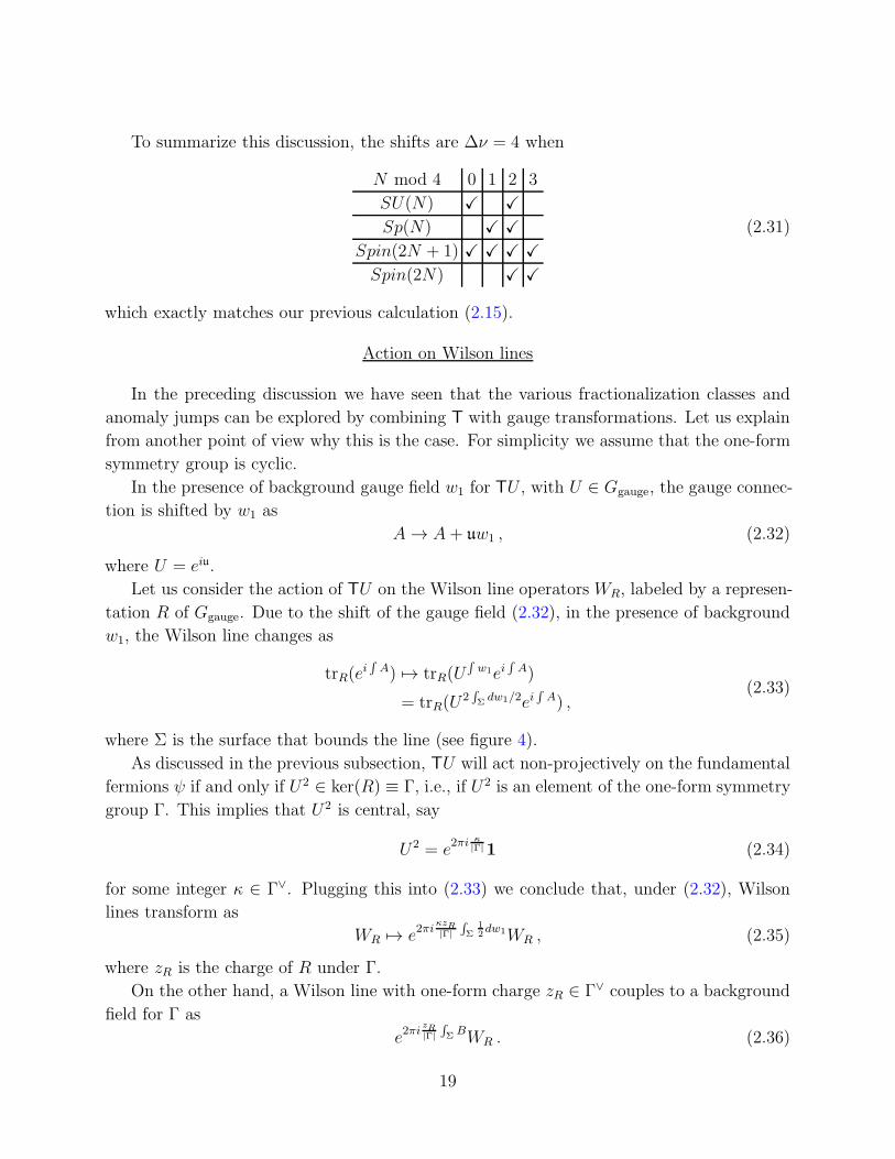
To summarize this discussion, the shifts are ∆ν = 4 when
N mod 4 0 1 2 3
SU(N) X X
Sp(N) X X
Spin(2N + 1) X X X X
Spin(2N) X X
(2.31)
which exactly matches our previous calculation (2.15).
Action on Wilson lines
In the preceding discussion we have seen that the various fractionalization classes and
anomaly jumps can be explored by combining T with gauge transformations. Let us explain
from another point of view why this is the case. For simplicity we assume that the one-form
symmetry group is cyclic.
In the presence of background gauge field w1 for TU , with U ∈ Ggauge, the gauge connec-
tion is shifted by w1 as
A→ A+ uw1 , (2.32)
where U = eiu.
Let us consider the action of TU on the Wilson line operators WR, labeled by a represen-
tation R of Ggauge. Due to the shift of the gauge field (2.32), in the presence of background
w1, the Wilson line changes as
trR(ei∫A) 7→ trR(U
∫w1ei
∫A)
= trR(U2∫Σdw1/2ei
∫A) ,
(2.33)
where Σ is the surface that bounds the line (see figure 4).
As discussed in the previous subsection, TU will act non-projectively on the fundamental
fermions ψ if and only if U2 ∈ ker(R) ≡ Γ, i.e., if U2 is an element of the one-form symmetry
group Γ. This implies that U2 is central, say
U2 = e2πi κ
|Γ|1 (2.34)
for some integer κ ∈ Γ∨. Plugging this into (2.33) we conclude that, under (2.32), Wilson
lines transform as
WR 7→ e2πiκzR|Γ|
∫Σ
12dw1WR , (2.35)
where zR is the charge of R under Γ.
On the other hand, a Wilson line with one-form charge zR ∈ Γ∨ couples to a background
field for Γ as
e2πizR|Γ|
∫Σ BWR . (2.36)
19
Therefore, by combining time-reversal symmetry with the gauge transformation U , we have
induced the following background field
B = κdw1
2. (2.37)
When κ is even, or when |Γ| is odd, B is pure gauge and cohomologically trivial, thus not
resulting in a shift of the ZT
2 anomaly. Instead, for even |Γ| and odd κ, the shift induces a
non-trivial fractionalization class.
As an illustration, in SU(N) we argued that the matrices that resulted in a non-fractionalized
action on the fundamental fermions were U = eiπp/N diag(−1p, 1N−p). For these matrices we
find U2 = e2iπp/N1N , i.e., κ ≡ p. We see that pdw1/2 is a coboundary for any N, p unless
N is even and p is odd, which precisely matches our computation in the previous subsection
(cf. the discussion below (2.26)).
We remark that the manipulations in this subsection are correct for the time-reversal
symmetry T but they fail for CT because the gauge symmetry and CT do not commute. We
shall return to CT presently.
Fractionalization classes and twisted gauge bundles
Another way to see the gauge bundle is modified is by computing the magnetic fluxes.
Let us consider the SU(N) gauge theory example above. If we change T to TU and turn
on a non-trivial background for the time-reversal symmetry, i.e. place the theory on an
unorientable pin− manifold, we will see that the sum over the gauge bundles is modified.
If we consider gauge field in the Cartan torus, A = (a1, · · · , aN−1,−(a1 + · · ·+ aN−1)), the
Stiefel-Whitney class is
w(N)2 = N
N−1∑
i=1
dai2π
mod N . (2.38)
For ordinary SU(N) gauge field, ai are properly quantized and the Stiefel-Whitney class is
always trivial. In the presence of background B for the ZN one-form symmetry, the bundle
is modified to PSU(N) bundle with w(N)2 = B.
The shift of the gauge field (2.32) changes the sum of GNO fluxes to be
w(N)2 = N
1
2π
(
−π pNdw1
)
= −pdw1
2mod N . (2.39)
Thus this is equivalent to shifting the B field as
B → B − pdw1
2mod N . (2.40)
When p is even, pdw1/2 = (p/2)dw1 is exact, and this a trivial shift in the B field. For odd
N , the shift is exact for every p, since 2 is invertible in ZN . For even N and odd p, this is a
non-trivial change in the background B.
20
In particular, this implies that the line operators that transform under the one-form
symmetry with odd charge carry a projective representation of the time-reversal symmetry
TU . Under a background gauge transformation of time-reversal symmetry
w1 → w1 + dλ0 + 2λ1, B → B − pdλ1 , (2.41)
where we take a lift of w1 to an integer one-cochain and different lifts are related by 2λ1 for
integer one-cochain λ1. Thus the time-reversal transformation induces a one-form transfor-
mation, which acts on the line operators. We note that the above discussion about the shift
in B background gauge field works in general spacetime dimension.
2.3 Anomalies and fractionalization in CT
It is also interesting to perform the same analysis for CT. This is a distinct symmetry from
T whenever the gauge group admits non-trivial outer automorphisms, i.e., when the Dynkin
diagram has a reflection symmetry. This is so for the ADE algebras. For concreteness we
focus on SU(N). We follow the strategy of adding massive fundamental scalars in order to
detect the fractionalized action on the Wilson lines.
For complex representations, νCT = 0. This follows from the fact that the real and
imaginary parts of ψ transform with opposite sign; equivalently, one can write down a CT-
symmetric mass term ψψ. Therefore, we only expect non-trivial νCT for real representations
(where the mass term above vanishes by fermi statistics, since the singlet in R ⊗ R is sym-
metric). We consider the adjoint representation.
In adjoint SU(N) enriched with massive fundamental scalars, CT acts as
CT(ψ) = UψU−1
CT(φ) = Uφ(2.42)
where U ∈ SU(N) is some matrix in color space. In the case of T we argued that we could
always conjugate U to a maximal torus of the gauge group. The reason is that change of
bases acted as U 7→ V UV −1, and this can always be used to diagonalize U . On the other
hand, for CT, change of bases act as U 7→ V ∗UV −1, and this cannot always be used to
diagonalize U . Therefore, here we cannot assume that U lies in some maximal torus of
SU(N). We need to work a little harder.23
23If the use the diagonal transformation U , the gauge bundle is not twisted by a quotient for CTU .
Since the time-reversal action includes the charge conjugation C, let us first review the properties of the
bundle SU(N) ⋊ ZC2 . In the presence of background B1 for the charge conjugation symmetry, the flux
quantization for SU(N)⋊ ZC2 bundle is instead (see e.g. [59])
N
N−1∑
i=1
DB1ai
2π= 0 mod N , (2.43)
21
To begin with, we require CT to act non-projectively on the fermions, CT2(ψ) = ψ, which
yields the condition
(U∗U)ψ(U∗U)−1 = ψ . (2.45)
This means that U∗U must commute with ψ, i.e., it must be a multiple of the identity.
Therefore, U t = cU for some constant c; taking the transpose of this equation and plugging
it back into itself we derive the condition U = c2U , namely U must satisfy U t = ±U .In conclusion, the most general matrix U ∈ SU(N) such that CT acts non-projectively
on ψ is either a symmetric matrix or an anti-symmetric matrix. For odd N the latter option
is incompatible with det(U) = 1. The action of such a matrix on the scalars becomes
CT2(φ) = U∗Uφ ≡ ±φ (2.46)
when U t = ±U . We thus see that a symmetric matrix U does not lead to a fractionalized
action on φ, while an anti-symmetric matrix does. Moreover, the possible projective actions
are only a sign ±, as opposed to an arbitrary N -th root of unity as was the case for T.
We now proceed to compute the anomaly νCT. We exploit the freedom to change bases
U 7→ V ∗UV −1 to bring U into a canonical form. Note that this redefinition preserves
whether U is symmetric or anti-symmetric. Using this change of basis, we can always bring
any unitary matrix into the following form:
U ∝ 1, if U is symmetric
U ∝ diag(iσy, . . . , iσy), if U is anti-symmetric .(2.47)
Calculating νCT for these matrices is straightforward. As this symmetry acts non-projectively
on ψ, we just need to count signs under the transformation.
The case of U ∝ 1 is trivial. Given that CT(ψ) = ψ, the off-diagonal components of ψ
do not contribute, since they are complex and the real and imaginary parts transform with
opposite signs. Only the Cartan subalgebra contributes: all diagonal components transform
with sign +1, and therefore
νCT = N − 1 (2.48)
Consider now N even and U ∝ diag(iσy, . . . , iσy). We break ψ into two-by-two blocks.
As before, the off-diagonal blocks do not contribute, since real and imaginary parts transform
where the covariant derivative can be unpacked by choosing a gauge and embedding B1 instead of a U(1)
gauge field, as DB1ai = dai − 2B1ai [59].
In our case, B1 = w1, and we take a lift to ZN such that w1 = 0, 1 mod N . Then dw1/2 = w21 = 0, 1.
Then shifting the gauge field changes the flux quantization by
N
2π
(
−πp
Ndw1 − 2w1
(
−πp
Nw1
))
= −p
(
dw1
2− w2
1
)
= 0 mod N . (2.44)
Thus we find that changing CT to CTU does not produce an non-trivial background B, and the symmetry
fractionalization class remains unchanged.
22
with opposite signs. Let us, then, focus on a certain 2 × 2 block on the diagonal. Under
CT(ψ) = UψU−1 such block transforms as
(
a b
b∗ c
)
7→ (iσy)
(
a b
b∗ c
)
(−iσy) ≡(
c −b∗−b a
)
(2.49)
In other words, a and c are interchanged, and both re(b) and im(b) pick up a minus sign.
This contributes ν = −2. Adding up all diagonal blocks, and subtracting 1 for the trace, we
arrive at
ν ′CT
= −2(N/2)− 1 ≡ −N − 1 (2.50)
In conclusion, the anomalies for CT in adjoint SU(N) are νCT = −1±N when N is even,
and νCT = −1 + N for odd N . The lower sign corresponds to a projective action on the
Wilson lines.
For N odd we find ∆νCT = 0, while for N even we find ∆νCT = 2N , which equals 4 mod 8
when N is 2 mod 4 and vanishes when N is 0 mod 4.
3 QED and QCD in 1+1 Dimensions
Consider a free U(1) gauge field in 1 + 1d, described by the Lagrangian
L =1
4e2da ∧ ⋆da+ i
θ
2πda . (3.1)
The parameter θ is as usual compact, θ ≃ θ + 2π.
The theory has a U(1) one-form symmetry, the conserved current being the topological
local operator ⋆da.24 In addition, at θ = 0 and at θ = π there is charge conjugation
symmetry acting as C : a → −a. For the remaining of the discussion of this theory, we
will add a massive charge 2 boson particle B which transforms under charge conjugation as
C : B → B∗. This reduces the one-form symmetry group to Z2. Standard arguments [63]
show that there is a mixed anomaly between charge conjugation symmetry and the Z2 one-
form symmetry at θ = π but not at θ = 0. Since there is no mixed anomaly at θ = 0, there
will be no ambiguity in the ’t Hooft anomaly of C, as we will see.
An interesting question is to ask whether there is an ’t Hooft anomaly for C (and not just
a mixed anomaly with the one-form symmetry). Indeed, the anomalies of Z2 symmetries in
bosonic systems are valued in H3(BZ2, U(1)) = Z2. Therefore, one should be able to decide
if C has an ’t Hooft anomaly or not.
At θ = π this is a simple example of a situation where the anomaly depends on additional
data, i.e. the choice of a fractionalization class.
24Topological local operators in 1 + 1d have been emphasized in [60]. See also [61] and the review [62] for
the study of CFTs with topological local operators.
23
A standard way to diagnose ’t Hooft anomalies in 1 + 1d is through the study of Hilbert
spaces with topological defects.25 According to [8, 64–66] (and see references therein), if
the defect Hilbert space consists of Kramers doublets T2 = −1 then C has an anomaly.
Otherwise, if the ground state is unique, then there is no anomaly for C. As we will now see
this prescription is insufficient in the theory (3.1).
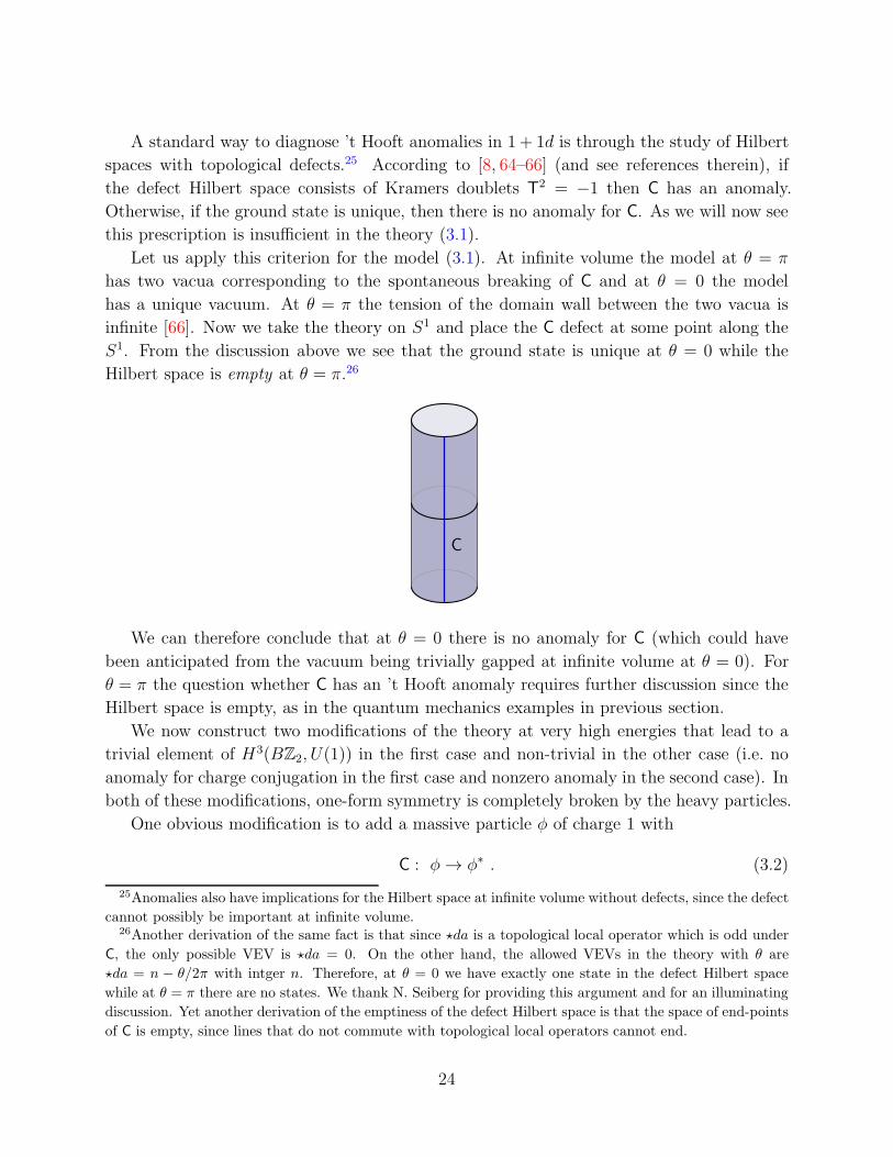
Let us apply this criterion for the model (3.1). At infinite volume the model at θ = π
has two vacua corresponding to the spontaneous breaking of C and at θ = 0 the model
has a unique vacuum. At θ = π the tension of the domain wall between the two vacua is
infinite [66]. Now we take the theory on S1 and place the C defect at some point along the
S1. From the discussion above we see that the ground state is unique at θ = 0 while the
Hilbert space is empty at θ = π.26
C
We can therefore conclude that at θ = 0 there is no anomaly for C (which could have
been anticipated from the vacuum being trivially gapped at infinite volume at θ = 0). For
θ = π the question whether C has an ’t Hooft anomaly requires further discussion since the
Hilbert space is empty, as in the quantum mechanics examples in previous section.
We now construct two modifications of the theory at very high energies that lead to a
trivial element of H3(BZ2, U(1)) in the first case and non-trivial in the other case (i.e. no
anomaly for charge conjugation in the first case and nonzero anomaly in the second case). In
both of these modifications, one-form symmetry is completely broken by the heavy particles.
One obvious modification is to add a massive particle φ of charge 1 with
C : φ→ φ∗ . (3.2)
25Anomalies also have implications for the Hilbert space at infinite volume without defects, since the defect
cannot possibly be important at infinite volume.26Another derivation of the same fact is that since ⋆da is a topological local operator which is odd under
C, the only possible VEV is ⋆da = 0. On the other hand, the allowed VEVs in the theory with θ are
⋆da = n − θ/2π with intger n. Therefore, at θ = 0 we have exactly one state in the defect Hilbert space
while at θ = π there are no states. We thank N. Seiberg for providing this argument and for an illuminating
discussion. Yet another derivation of the emptiness of the defect Hilbert space is that the space of end-points
of C is empty, since lines that do not commute with topological local operators cannot end.
24
We can add an arbitrary potential V (|φ|2). It is clear that this model has no C anomaly
since we could choose to condense φ – in that phase, there is a single trivial vacuum. One
can also explicitly study the defect Hilbert space and see that there are no Kramers doublets
and time-reversal symmetry in the defect Hilbert space satisfies T2 = 1.
Another possible modification of the theory at high energies is to add two species of a
charge 1 boson, φ1, φ2, with a potential V (|φ1|2, |φ2|2). The potential is constrained by a
particular charge conjugation symmetry
C : φ1 → (φ2)∗ , φ2 → −(φ1)∗ . (3.3)
Note that C2 = −1 on the scalar fields, but that is a gauge transformation and hence as
a symmetry operator C is of order 2. We can therefore say that C is fractionalized on the
gauge non-invariant fields φi.
To understand the anomaly of C in this situation, we can take several approaches. One
is to again consider the defect Hilbert space. The defect Hilbert space is given by states
which live on the double cover of the circle such that as we go from one copy to the next
we implement a symmetry transformation. Therefore there is an approximate four-fold
degeneracy whereby we can excite the particles φ1,φ2, and their complex conjugates. Each
of these pairs is a Kramers doublet with T2 = −1:
T|φ1〉 = |φ2〉 , T|φ2〉 = −|φ1〉 , T|(φ1)∗〉 = |(φ2)∗〉 , T|(φ2)∗〉 = −|(φ1)∗〉 (3.4)
Upon taking into account non-perturbative corrections in the length of the circle the degen-
eracy between these two Kramers pairs is lifted and the ground state consists of a single
Kramers pair. We conclude that the anomaly of the charge conjugation symmetry is now 1
mod 2. Another way to deduce the anomaly in the presence of the massive φ1, φ2 particles
is to consider the following potential:
V = −M2(|φ1|2 + |φ2|2) + λ(|φ1|2 + |φ2|2)2 (3.5)
with λ > 0 and M2 > 0. Minimizing the potential we see that the U(1) gauge symmetry is
everywhere Higgsed completely but there is a low energy mode which lives on a two-sphere.
The low energy theory is SU(2)1 WZW model and charge conjugation is embedded as the
matrix diag(−1,−1,−1) acting on the embedding coordinates of the S2. This symmetry is
known to have a Z2 anomaly.
A possible interpretation of the results is to say that the massive particles transforming
as (3.3) contribute 1 mod 2 to the Z2 anomaly.
A general lesson that will guide us later is that in (3.3), before gauging the U(1) symmetry,
the particles are not in a representation of Z2 – it is fractionalized to Z4.27 This will be a
27Since the one-form symmetry is Z2, the map ρ (1.2) here is trivial. The fractionalization classes are
H2ρ(Z2,Z2) = Z2.
25
general rule – massive particles can alter the anomaly only if before gauging they are in
fractionalized representations of the zero-form symmetry G.
Above we have seen that the (non-gauge invariant fields) φi are in a projective represen-
tation of C. It is important to emphasize that this is independent of whether we use the
above action of C or compose C with an arbitrary gauge transformation which implements
a rotation by angle α, Uα. Indeed, CUα acts by
CUα : φ1 → eiα(φ2)∗ , φ2 → −eiα(φ1)∗ . (3.6)
And it is straightforward to verify that on the fields φi we have (CUα)2 = −1. Therefore it
impossible to use gauge transformations to make the particles φi sit in a non-fractionalized
representation of C. This will be important later.
Finally, we would like to give a simple interpretation of how it is possible for massive
particles to contribute to the Z2 anomaly in theories with one-form symmetry. Consider the
theory of the single massive complex particle φ and couple to the U(1) and C background
gauge fields. This leads to the gauge group O(2) = SO(2)⋊ Z2∼= Pin+(2). On the other
hand, for the case of the two particles φ1,2 with the action of C in (3.3) the gauge group is28
SO(2)⋊ Z4
Z2
∼= Pin−(2) . (3.7)
In the case of O(2) = SO(2)⋊Z2∼= Pin+(2), the O(2) bundles always have integer magnetic
flux. In the case of SO(2)⋊Z4
Z2, we can have half-integer magnetic fluxes for SO(2), if the Z2
bundle for the charge conjugation symmetry cannot be lifted to a Z4 bundle. The appearance
of half-integer SO(2) fluxes in the presence of non-trivial background fields for C is why
the massive particles can affect the anomalies. Since the half-integer flux modifies the θ
periodicity, θ = π no longer preserves the charge conjugation symmetry, and this contributes
an ’t Hooft anomaly for the charge conjugation symmetry. A similar interpretation is possible
in all the examples below – fractionalization classes are essentially a way to allow for more
general gauge bundles than naively appears possible.
The statements above about the anomaly of the Z2 symmetry in free U(1) gauge theory
can be understood intrinsically from the point of view of the low-energy Z2 gauge theory:
S = π
∫
a(0) ∪ δb(1) (3.8)
where a(0), b(1) are dynamical Z2 0- and 1-cochains, respectively, and δ is the coboundary
operator. The content of this topological theory is that it has 2 vacua and a topological Z2
symmetry line that is a domain wall between these two vacua.
28The two fractionalization classes considered here correspond to the two extensions Pin±(2) of Z2 charge
conjugation by U(1) = SO(2) ∼= Spin(2). In particular, for these fractionalization classes, the charge
conjugation symmetry does not participate in a two-group.
26
We couple this system to a background Z2 gauge field A(1) for the Z2 zero-form symmetry.
A(1) is represented by a closed one-cochain.
S = π
∫
(
a(0) ∪ δb(1) + A(1) ∪ b(1))
. (3.9)
The gauge transformations act as (λ is the parameter for the background gauge transforma-
tion of the Z2 symmetry)
a(0) → a(0) + λ , b(1) → b(1) + δω , A(1) → A(1) + δλ . (3.10)
The action is perfectly gauge invariant and there is no anomaly for the Z2 symmetry. We
can see that the ω gauge transformations leave the action invariant by virtue of A(1) being
flat.
An interesting coupling that we could add is
S = π
∫
(
a(0) ∪ δb(1) + A(1) ∪ b(1) + a(0) ∪ A(1) ∪A(1)
)
. (3.11)
The background gauge transformation now is
A(1) → A(1) + δλ, a(0) → a(0) + λ, b(1) → b(1) + λ ∪A(1) + A(1) ∪ λ+ λ ∪ δλ . (3.12)
The action is not invariant, but transforms by an anomalous shift. To cancel the shift we
can introduce a bulk term π∫
3dA(1) ∪A(1) ∪A(1). To see that the bulk is sufficient to make
the theory invariant under the background gauge transformation of A(1), let us write the
boundary-bulk terms together as
π
∫
3d
(
δa(0) + A(1)
)
∪(
δb(1) + A(1) ∪ A(1)
)
(3.13)
= π
∫
2d
(
a(0) ∪ δb(1) + A(1) ∪ b(1) + a(0) ∪A(1) ∪A(1)
)
+ π
∫
3d
A(1) ∪ A(1) ∪A(1) mod 2π ,
where the equality used δA(1) = 0 mod 2. The left hand side is invariant under background
gauge transformation, and thus the right hand side, which consists of (3.11) and the bulk
term π∫
3dA(1) ∪A(1) ∪A(1), is also invariant under background gauge transformation.
We therefore see that in some version of the Z2 gauge theory in 1+1d there is an anomaly
for the zero-form Z2 symmetry and in another version there is no anomaly. The theories
only differ by the couplings to background fields.
3.1 Fermionic Z2 symmetry in 1+1 Dimensions
In this subsection we repeat the discussion above in a fermionic theory with Z2 unitary
symmetry. In theories with fermions a Z2 symmetry with algebra g2 = 1 has anomalies
27
in ΩSpin3 (BZ2) = Z8. We will study a system with a Z2 one-form symmetry and a mixed
anomaly between the one-form and zero-form symmetry. As a result, the ordinary familiar
zero-form anomaly in Z8 is ambiguous in units of 4 mod 8 depending on the fractionalization
class.
Consider QED2 with a massless charge 2 Dirac fermion Ψ and a charge 2 boson Φ. We
will denote by ΨL and ΨR the respective left and right moving complex fermions. This
theory has an axial Z2 symmetry:
g : ΨL → −ΨL , ΨR → ΨR , Φ → Φ (3.14)
We can ask if g has an ’t Hooft anomaly.
One approach is to condense Φ – then the low energy theory consists of one massless
Dirac fermion and the Z2 gauge theory studied in the previous subsection. The Dirac
fermion contributes 2 mod 8 to the anomaly, but the Z2 gauge theory, as we saw, may
either contribute the term π∫
3dA(1) ∪ A(1) ∪A(1) to the inflow invertible phase or not. The
term π∫
3dA(1)∪A(1) ∪A(1) amounts to a contribution of 4 mod 8 to the anomaly. Therefore
we infer that the anomaly for Z2 is either 2 mod 8 or (−2) mod 8, depending on the frac-
tionalization class. Indeed by a gauge transformation we can write an equivalent expression
for the action of g:
ge−iπ/2 : ΨL → ΨL , ΨR → −ΨR , Φ → −Φ , (3.15)
where e−iπ/2 stands for a 90 degrees gauge transformation. Since the boson Φ is not frac-
tionalized and it can be easily gapped it does not contribute to the anomaly, so, in this
presentation, the anomaly −2 mod 8 is more natural.
Of course g and ge−iπ/2 define the exact same symmetry (only differing by a gauge
transformation). This trick of composing g with a gauge transformation allows to quickly
predict that the two possible outcomes for the anomaly are ±2 mod 8. This is a general
theme, which we have already encountered in the previous section.
To see more formally why this heuristic rule works we can add a massive charge 1 boson
u and break the one-form symmetry completely. We must specify how the new boson u
transforms under g, and we have two choices, which we denote by g, and g′, which are now
genuinely different symmetries, not related to each other by gauge transformations:
g : ΨL → −ΨL, ΨR → ΨR, Φ → Φ, u→ u ,
g′ : ΨL → −ΨL, ΨR → ΨR, Φ → Φ, u→ iu .(3.16)
Note that both g2 = 1 and g′2 = 1. Since now the one-form symmetry is completely
broken the anomaly of both g and g′ should be in Z8. In the case of g the boson u is in a
non-fractionalized representation and hence the anomaly is given by the low energy fields and
is equal to 2 mod 8. In the case of g′ the massive boson u is in a fractionalized representation
28
and to account for its contribution to the anomaly it is again useful to perform a e−iπ/2 gauge
transformation and obtain
g′e−iπ/2 : ΨL → ΨL,ΨR → −ΨR,Φ → −Φ, u → u . (3.17)
Now the boson u is in a non-fractionalized representation and does not contribute to the
anomaly, but the price to pay is that the right moving fermion now picks a minus sign and
hence the anomaly is −2 mod 8.29
In summary, we see that in fermionic theories in 1 + 1d with G = Γ = Z2 and with a
mixed anomaly between the zero-form and 1-form symmetries, the anomaly of G is classified
as usual mod 8, but it depends on a choice of a fractionalization class in H2(Z2,Z2) = Z2
(in this case ρ is trivial).
3.1.1 The mixed Z2 − (−1)F anomaly
Here we are dealing with a fermionic theory, and therefore we have to discuss the symmetry
(−1)F as well
(−1)F : ΨL → −ΨL , ΨR → −ΨR , Φ → Φ . (3.18)
Mixed Z2 − (−1)F anomalies in 1+1d are classified by Z2, namely the anomaly is either 0
or 1 mod 2.
QED2 with a massless charge 2 Dirac fermion Ψ and a charge 2 boson Φ has a vanish-
ing mixed anomaly between g (3.14) and (−1)F since there are two left moving Majorana
fermions transforming under both (−1)F and g. We need to discuss if this mixed anomaly
can be altered by changing fractionalization classes. So far we discussed the fractionaliza-
tion class corresponding to B = 12qρ(A), where we denote the spin structure by ρ, and the g
background gauge field by A. We have seen that this allows to shift the pure Z2 anomaly in
units of 4 mod 8 but it does not affect the mixed Z2 − (−1)F anomaly.
Indeed, to change the mixed anomaly we would have to consider the fractionalization class
B = Arf, which, roughly speaking, fractionalizes fermion number symmetry. However, there
is no sense in adding relativistic massive degrees of freedom with such a fractionalization
class since it requires an odd number of Majorana fermions. In addition, a 0+1 dimensional
model with an odd number of Majorana fermions breaks fermion number symmetry due to
a nonzero expectation value of a product of an odd number of fermions.
Therefore, the mixed anomaly between (−1)F and Z2 symmetry is unambiguously 0 mod
2. In the following subsection we will see a model where this mixed anomaly is 1 mod 2, but
again, it will be unambiguous.
29The same conclusion can be arrived at by observing that the gauge invariant operators are ΨLu2,ΨRu
2,
and in the case of the symmetry g it is the left moving composite fermion that picks up a minus sign while
for g′ it is the right moving composite fermion that picks a sign. These composites directly translate to the
massless modes if u condenses.
29
3.2 A Few Remarks on Adjoint QCD in 1+1 Dimensions
We consider SU(N) gauge theory with a massless non-chiral Majorana fermion in the adjoint
representation
S =
∫
d2x
( −1
4g2YM
trF 2 + i tr ΨT /DΨ
)
. (3.19)
The study of the infrared dynamics of 1 + 1d adjoint gauge theory goes back to [67,68] and
there was progress on it recently [69–75], and see references therein.
This theory has a ZA2 axial symmetry acting as ΨL → −ΨL,ΨR → ΨR. Furthermore, the
theory has ZN one-form symmetry and there is a mixed anomaly between the zero-form Z2
symmetry and the one-form ZN symmetry for even N [69]. Now we will attempt to compute
the mod 8 anomaly for ZA2 – which we anticipate is ambiguous for even N but unambiguous
for odd N (ambiguous in the sense that it depends on the choice of action of ZA2 on lines).
In addition, for even N , the model has a mixed anomaly between the ZA2 axial symmetry
and fermion number symmetry, which as we have discussed above, will be unambiguously 1
mod 2.
First we will consider the anomaly as computed in the ultraviolet taking into account
the possible dependence on the choice of fractionalization classes and then we will contrast
our results with some conjectures about the infrared dynamics of this theory.
We can compute the anomaly in the UV from the fact that N2 − 1 chiral Majorana
fermions flip sign under ZA2 . Therefore we find N2 − 1 mod 8. For N even the anomaly is
either 3 or 7 mod 8 depending on whether N = 2 mod 4 or N = 0 mod 4, respectively and
for N odd the anomaly always vanishes. We can compose ZA2 with a gauge transformation in
order to scan over the possible fractionalization classes. It is sufficient to consider diagonal
matrices for the gauge transformations U = α diag(−1, . . . ,−1, 1, . . . , 1) with the minus sign
appearing p times on the diagonal and αN = (−1)p. If we consider ZA2 · U as our new
axial symmetry then 2p(N − p) right moving fermions pick up a minus sign under ZA2 · U
while N2 − 1 − 2p(N − p) left moving fermions pick up a minus sign. The anomaly is thus
N2 − 1 − 4p(N − p). We see that the correction 4p(N − p) is divisible by 4 signifying that
the anomaly can only jump by 4 mod 8 due to changing the fractionalization class. For even
N , by choosing any odd p we therefore can shift the anomaly of ZA2 from N2 − 1 mod 8 to
N2+3 mod 8. For odd N , 4p(N−p) is always divisible by 8 and the anomaly is independent
of the fractionalization class, in line with our expectations.
In summary, ZA2 has anomaly 3 or 7 mod 8 for even N and no anomaly for odd N .
Further, for even N we have a mixed anomaly with (−1)F and no mixed anomaly for odd
N .30 It is now time to see how this is matched by the conjectured infrared phase of this
theory.
30A similar analysis shows that the anomalies of ZA2 (−1)F (the diagonal Z2 subgroup of ZA
2 and (−1)F ),
are 1 or 5 mod 8, depending on the fractionalization class for even N , while for odd N they are again 0 mod
8.
30
To simplify the infrared dynamics we consider the ZA2 invariant four-fermion deformation
of [69, 70] (for a similar discussion in QED2 see [76])
tr(ΨLΨR) tr(ΨLΨR) . (3.20)
This deformation preserves the one-form symmetry, fermion number symmetry and it also
preserves the axial symmetry. The ground state is conjectured to be doubly degenerate due
to a fermion condensate that breaks the ZA2 symmetry spontaneously.
For even N all the Wilson lines in a representation with the number of boxes not divisible
by N/2 obey an area law. The Wilson lines with the number of boxes divisible by N/2 obey
instead a perimeter law [69, 70]. For odd N , all the Wilson lines obey an area law.
The low-energy theory is therefore again Z2 gauge theory for both even and odd N .
The topological line operator for even N originates in the ultraviolet from a Wilson line in
a representation with N/2 boxes. For odd N the topological line originates from a finite
tension domain wall (kink).
For odd N the one-form symmetry does not couple to the infrared degrees of freedom of
Z2 gauge theory. This is why the dependence on the fractionalization class completely drops
out and the anomaly in this case is universally 0 mod 8.
For even N we now have to understand how the Z2 gauge theory reproduces the various
values of the anomaly we have seen above. As we have shown, the ’t Hooft anomaly for the
zero-form symmetry in ordinary, bosonic, Z2 gauge theory is either 0 or 4 mod 8. However,
here we are dealing with a fermionic theory, which allows an additional term
π
∫
2d
a0 ∪Arf , (3.21)
with the Arf invariant of the Poincare dual of a0. The Lagrangian (3.21) makes sense for
constant a0. A precise Lagrangian and treatment of the anomalies of this theory is in
appendix D. Here we just summarize the main results.
The two vacua of Z2 gauge theory now have different Arf counter-terms (i.e. carry different
invertible phases) and therefore the defect Hilbert space would contain an extra Majorana
fermion [10,14]. Furthermore the spin structure entering in the Arf invariant can be shifted
by the background gauge field of ZA2 which allows to change the chirality under time-reversal
of this extra Majorana fermion in the defect Hilbert space. Such a modification of Z2 gauge
theory allows to obtain all the required values for the anomaly.
It remains to explain why the ultraviolet gauge theory dictates the appearance of the
term (3.21). We have a condensate 〈ΨLΨR〉 6= 0 breaking spontaneously the ZA2 symmetry.
Due to the mixed anomaly between (−1)F and ZA2 symmetry, the two vacua must have a
different Arf SPT phase. The term (3.21) therefore reproduces this mixed anomaly. It is
very nice that this modification of the Z2 gauge theory also simultaneously reproduces the
ZA2 anomalies of the theory.
31
4 Time-Reversal and Symmetry Fractionalization in
2+1 Dimensions
We study 2 + 1d systems with time-reversal symmetry. There are two versions of the time-
reversal symmetry operator, one of which we denote T and the other we denote by CT. If
charge conjugation C is a symmetry in its own right then both T and CT exist simultaneously.
The algebra of these symmetries is
T2 = (−1)F , (CT)2 = (−1)F . (4.1)
Charge conjugation C is a symmetry in gauge theory if the gauge group admits an outer
automorphism and the matter fields respect the symmetry, which will be the case in examples
below. We denote the associated symmetry groups by G = ZT
4 and G = ZCT
4 respectively.
The anomaly classification for these time-reversal symmetries is well known [10,77–80], they
take values in Ω4Pin+
(pt) = Z16, and we denote them by νT and νCT.
Suppose the system also has Γ = Zn one-form symmetry in addition to the time-reversal
symmetry. Let us define time-reversal T and CT to be such that CT leaves the one-form
symmetry charges invariant, while T acts on the one-form symmetry by the Z2 charge con-
jugation symmetry on the Zn charges: q → −q mod n.31
One-form symmetries can have an ’t Hooft anomaly in 2+1d. With no other symmetries,
in theories with fermions, the anomaly is valued is p ∈ Zn and the anomaly is determined
from the spin of the generator, h = p/2n [81]. In time-reversal invariant theories, the allowed
anomalies for one-form symmetry are restricted. The anomaly for the one-form symmetry
is now classified by the subgroup of Ω4Pin+(B2
Zn) generated by the elements that are not in
Ω4Pin+
(pt). The anomaly is in Z4 for n even and trivial for n odd. This is true for both T
and CT.
To understand the origin of this Z4, we observe that in time-reversal invariant theories,
the generator of the Zn one-form symmetry has to be left (almost) invariant under time-
reversal; the generating line a of the symmetry therefore satisfies either
• Ta = a, in such case its spin h satisfies h = −h mod 1
• Ta = aψ with transparent fermion line ψ, in such case its spin h satisfies h + 12= −h
mod 1.
Thus the generator of the Zn one-form symmetry can only have spin h = 0, 12,±1
4mod 1.
The same discussion holds for CT.
31Note an important fact: T reverses the electric charge and hence the electric field is odd under time-
reversal while the magnetic field is even. Since the electric two-form gauge field B couples to the electro-
magnetic field via BµνFµν , as a two-form, B is even under T and odd under CT while the corresponding
one-form symmetry charge,∫
Σ⋆F , is odd under T and even under CT. This reversal of odd/even between
the charges and the corresponding background fields is particular to time-reversal symmetry.
32
One can arrive at the same conclusion about the allowed anomalies in time-reversal in-
variant theories by investigating the anomaly inflow term 2πi p2n
∫
4dP(B). On spin orientable
manifolds p = 0, ..., n−1 describes the distinct allowed possibilities [26,81]. For this counter-
term to be time-reversal invariant we must require 2p = 0 mod n. For even n the solutions
are p = n/2 mod n or p = 0 mod n which allow for the spins h = 0, 12,±1
4while for odd
n only p = 0 mod n is allowed but that corresponds to a trivial invertible theory (which
furthermore remains trivial on non-orientable manifolds, unlike the even n case).
The anomaly in time-reversal invariant theories can be written using the 3 + 1d bulk
action
2πh
∫
qρ(B mod 2), h ∈
0,1
2,±1
4
, (4.2)
where B is the background for Zn one-form symmetry for even n, q is the Z4-valued quadratic
function that depends on Wu3 structure ρ [23, 82, 83], and on pin+ manifolds ρ = w1 ∪ ρ1with ρ1 being the pin+ structure. For n = 2, the effective action is discussed in [84].
The anomaly (4.2) for h = 12mod 1 can be interpreted as a mixed anomaly between
the one-form symmetry and time-reversal symmetry. Similar mixed anomalies in 2 + 1d
were discussed in [85]. Indeed, as remarked above, h = 1/2 is trivial without time-reversal
symmetry because we can simply dress the generator a with the transparent fermion and
gauge this spin-less line. But with time-reversal symmetry aψ would be a Kramers doublet:
h =1
2: π
∫
qρ(B mod 2) = π
∫
B ∪ B = π
∫
B ∪ (w2 + w21) = π
∫
B ∪ w21 mod 2π .
(4.3)
where in the second equality we used the Wu formula x2 ∪ x2 = x2 ∪ (w2 + w21) for Z2
two-cocycle x2 on 4-manifolds [86], and in the last equality we used w2 is trivial on pin+
manifolds [87].
4.1 Different symmetry fractionalizations and their anomalies
Due to the one-form symmetry, the anomalies for the time-reversal symmetry are potentially
ambiguous. This can be traced to the fact that the coupling to an unorientable manifold is
ambiguous due to the existence of fractionalization classes. The story is pretty similar both
for T and CT even though the former does not act on the two-form background gauge field
for the one-form symmetry while the latter flips the sign of the two-form background gauge
field. We will only discuss explicitly the case of T and quote the results for CT at the end.
The corresponding fractionalization classes are labeled by Z2. The non-trivial fractional-
ization class corresponds to the shift B → B + dw1/2, where dw1/2 mod n is the image of
w1 under the Bockstein for the short exact sequence 1 → Zn → Z2n → Z2 → 1.
If the one form symmetry has ’t Hooft anomalies, the shift B → B + dw1/2 would lead
to various “jumps” for the time-reversal symmetry anomaly.
33
• When h = 0: the one-form symmetry does not have anomaly, and the shift does not
produce additional anomaly.
• When h = 12, the one-form symmetry has a mixed anomaly with the time-reversal
symmetry, and the shift produces additional time-reversal anomaly νT = 8 as described
by the bulk effective action
π
∫
w21 ∪ w2
1 = π
∫
w41 , (4.4)
where we used dw1/2 mod 2 = w21.
• When h = ±14, using the quadratic property q(x+ y) = q(x) + q(y) + 2x∪ y mod 4 for
x = B, y = w21, one finds the shift produces additional time-reversal anomaly νT = ±4,
in addition to extra mixed anomaly between the one-form symmetry and time-reversal
symmetry, as described by the bulk effective action
π
∫
B ∪ w21 ±
π
2
∫
qρ(w21) . (4.5)
Let us explain why the last term in (4.5) is the bulk effective action for νT = ±4. We
can describe the invertible phase with νT = ±2 using an auxiliary dynamical Z2 two-form
gauge field b, with the action [23]π
2
∫
qρ(b) . (4.6)
The signs of νT = ±2 are related by shifting the pin+ structure ρ1 in ρ = w1 ∪ ρ1 by
ρ1 → ρ1 + w1. For a suitable convention of ρ1, we can take the sign to be νT = +2 for the
above theory. Under the field redefinition b→ b+w21, using the quadratic function property
q(x+ y) = q(x) + q(y) + 2x ∪ y mod 4, the action changes to
π
2
∫
qρ(b) +π
2
∫
qρ(w21) + π
∫
b ∪ w21 = −π
2
∫
qρ(b) +π
2
∫
qρ(w21) mod 2π , (4.7)
where the equality uses [w2] = 0 on pin+ manifold, and thus w21 = w2 + w2
1 = v2, w21 ∪ b =
v2 ∪ b = b ∪ b. Since the field redefinition does not change the partition function,
ZνT=±2 = (ZνT=±2)∗e
πi2
∫qρ(w2
1) , (4.8)
where ZνT=±2 is the partition function for the two-form gauge theory (4.6) that is the invert-
ible theory with νT = ±2. Thus we find that the theory with effective action ±π2
∫
qρ(w21)
corresponds to the anomaly
νT = (±2)− (∓2) = ±4 . (4.9)
This concludes our discussion of the time-reversal anomaly. We see that the jumps in the
anomaly due to the different fractionalization classes are always in multiples of 4 mod 16.
34
We summarize the results in the following table:
Z(1)n Z
(1)n − Z
T
4 ∆νT mod 16
h ∈ Z X X 0
h ∈ 1/2 + Z X X 8
h ∈ ±1/4 + Z X X ±4
(4.10)
The column Z(1)n stands for pure one-form symmetry anomaly, the column Z
(1)n − Z
T
4 stands
for the mixed anomaly between time-reversal symmetry and one-form symmetry and, finally,
the column with ∆νT mod 16 describes the allowed jumps due to different fractionalization
classes.
We now proceed to study symmetry fractionalization in QCD3 theories, where we will
apply the results above to test some proposals about the behavior of such theories in the
deep infrared.
4.2 SU(N) with adjoint quark
Let us remind some basic facts about adjoint QCD in 2+1 dimensions, namely SU(N) gauge
theory with Chern-Simons level k and an adjoint Majorana fermion λ valued in the su(N)
Lie algebra. For recent work on QCD theories in 2+1 dimensions of the type discussed here
see [31, 88–94]. One has to specify the Chern-Simons level k for the gauge group and one
can write a mass term m trλλ. An important consistency condition for this theory to exist
is
k +N/2 ∈ Z . (4.11)
All these theories have a one-form symmetry ZN with anomaly p = k + N/2 mod N . The
case particularly interesting to us here is that with even N and k = 0. In this special case
the theory with a massless adjoint quark, m = 0, enjoys time-reversal symmetry. Indeed,
the one form symmetry anomaly is p = N/2 which leads to the spin of the generator being
h = ±14, which is one of the values allowed in time-reversal invariant theories, as we have
seen above.
A free massless Majorana fermion in 3d has a ZT
4 time-reversal symmetry, which can be
taken to act as
T : λ→ γ0λ . (4.12)
Since T is anti-unitary, it acts on a Dirac fermion ψ = λ1 + iλ2 as
T : ψ → γ0ψ∗ . (4.13)
On a Dirac fermion we can also define the action of ZCT
4 , which acts instead as
CT : ψ → γ0ψ . (4.14)
35
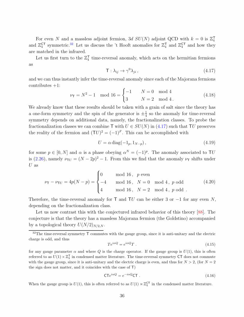
For even N and a massless adjoint fermion, 3d SU(N) adjoint QCD with k = 0 is ZT
4
and ZCT
4 symmetric.32 Let us discuss the ’t Hooft anomalies for ZT
4 and ZCT
4 and how they
are matched in the infrared.
Let us first turn to the ZT
4 time-reversal anomaly, which acts on the hermitian fermions
as
T : λij → γ0λji , (4.17)
and we can thus instantly infer the time-reversal anomaly since each of the Majorana fermions
contributes +1:
νT = N2 − 1 mod 16 =
−1 N = 0 mod 4
3 N = 2 mod 4 .(4.18)
We already know that these results should be taken with a grain of salt since the theory has
a one-form symmetry and the spin of the generator is ±14so the anomaly for time-reversal
symmetry depends on additional data, namely, the fractionalization classes. To probe the
fractionalization classes we can combine T with U ∈ SU(N) in (4.17) such that TU preserves
the reality of the fermion and (TU)2 = (−1)F . This can be accomplished with
U = α diag(−1p, 1N−p) , (4.19)
for some p ∈ [0, N ] and α is a phase obeying αN = (−1)p. The anomaly associated to TU
is (2.26), namely νTU = (N − 2p)2 − 1. From this we find that the anomaly νT shifts under
U as
νT − νTU = 4p(N − p) =
0 mod 16 , p even
−4 mod 16 , N = 0 mod 4 , p odd
4 mod 16 , N = 2 mod 4 , p odd .
(4.20)
Therefore, the time-reversal anomaly for T and TU can be either 3 or −1 for any even N ,
depending on the fractionalization class.
Let us now contrast this with the conjectured infrared behavior of this theory [88]. The
conjecture is that the theory has a massless Majorana fermion (the Goldstino) accompanied
by a topological theory U(N/2)N/2,N .
32The time-reversal symmetry T commutes with the gauge group, since it is anti-unitary and the electric
charge is odd, and thus
TeiαQ = eiαQT . (4.15)
for any gauge parameter α and where Q is the charge operator. If the gauge group is U(1), this is often
referred to as U(1)×ZT4 in condensed matter literature. The time-reversal symmetry CT does not commute
with the gauge group, since it is anti-unitary and the electric charge is even, and thus for N > 2, (for N = 2
the sign does not matter, and it coincides with the case of T)
CTeiαQ = e−iαQCT . (4.16)
When the gauge group is U(1), this is often referred to as U(1)⋊ ZCT4 in the condensed matter literature.
36
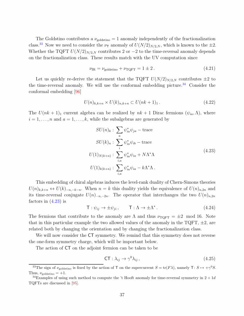
The Goldstino contributes a νgoldstino = 1 anomaly independently of the fractionalization
class.33 Now we need to consider the νT anomaly of U(N/2)N/2,N , which is known to the ±2.
Whether the TQFT U(N/2)N/2,N contributes 2 or −2 to the time-reversal anomaly depends
on the fractionalization class. These results match with the UV computation since
νIR = νgoldstino + νTQFT = 1± 2 . (4.21)
Let us quickly re-derive the statement that the TQFT U(N/2)N/2,N contributes ±2 to
the time-reversal anomaly. We will use the conformal embedding picture.34 Consider the
conformal embedding [96]
U(n)k,k+n × U(k)n,k+n ⊂ U(nk + 1)1 . (4.22)
The U(nk + 1)1 current algebra can be realized by nk + 1 Dirac fermions (ψia,Λ), where
i = 1, . . . , n and a = 1, . . . , k, while the subalgebras are generated by
SU(n)k :∑
a
ψ∗iaψja − trace
SU(k)n :∑
i
ψ∗iaψib − trace
U(1)N(k+n) :∑
i,a
ψ∗iaψia +NΛ∗Λ
U(1)k(k+n) :∑
i,a
ψ∗iaψia − kΛ∗Λ .
(4.23)
This embedding of chiral algebras induces the level-rank duality of Chern-Simons theories
U(n)k,k+n ↔ U(k)−n,−k−n. When n = k this duality yields the equivalence of U(n)n,2n and
its time-reversal conjugate U(n)−n,−2n. The operator that interchanges the two U(n)n,2nfactors in (4.23) is
T : ψij → ±ψji , T : Λ → ±Λ∗ . (4.24)
The fermions that contribute to the anomaly are Λ and thus νTQFT = ±2 mod 16. Note
that in this particular example the two allowed values of the anomaly in the TQFT, ±2, are
related both by changing the orientation and by changing the fractionalization class.
We will now consider the CT symmetry. We remind that this symmetry does not reverse
the one-form symmetry charge, which will be important below.
The action of CT on the adjoint fermion can be taken to be
CT : λij → γ0λij , (4.25)
33The sign of νgoldstino is fixed by the action of T on the supercurrent S = tr(Fλ), namely T : S 7→ +γ0S.
Thus, νgoldstino = +1.34Examples of using such method to compute the ’t Hooft anomaly for time-reversal symmetry in 2 + 1d
TQFTs are discussed in [95].
37
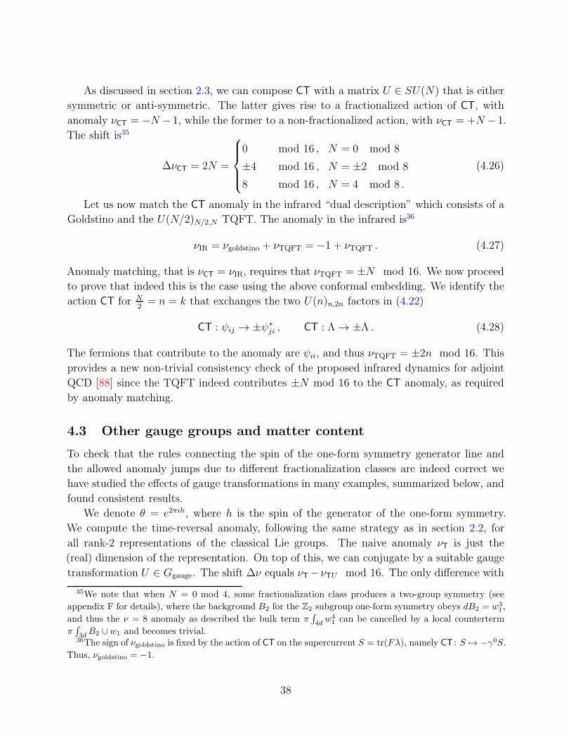
As discussed in section 2.3, we can compose CT with a matrix U ∈ SU(N) that is either
symmetric or anti-symmetric. The latter gives rise to a fractionalized action of CT, with
anomaly νCT = −N −1, while the former to a non-fractionalized action, with νCT = +N −1.
The shift is35
∆νCT = 2N =
0 mod 16 , N = 0 mod 8
±4 mod 16 , N = ±2 mod 8
8 mod 16 , N = 4 mod 8 .
(4.26)
Let us now match the CT anomaly in the infrared “dual description” which consists of a
Goldstino and the U(N/2)N/2,N TQFT. The anomaly in the infrared is36
νIR = νgoldstino + νTQFT = −1 + νTQFT . (4.27)
Anomaly matching, that is νCT = νIR, requires that νTQFT = ±N mod 16. We now proceed
to prove that indeed this is the case using the above conformal embedding. We identify the
action CT for N2= n = k that exchanges the two U(n)n,2n factors in (4.22)
CT : ψij → ±ψ∗ji , CT : Λ → ±Λ . (4.28)
The fermions that contribute to the anomaly are ψii, and thus νTQFT = ±2n mod 16. This
provides a new non-trivial consistency check of the proposed infrared dynamics for adjoint
QCD [88] since the TQFT indeed contributes ±N mod 16 to the CT anomaly, as required
by anomaly matching.
4.3 Other gauge groups and matter content
To check that the rules connecting the spin of the one-form symmetry generator line and
the allowed anomaly jumps due to different fractionalization classes are indeed correct we
have studied the effects of gauge transformations in many examples, summarized below, and
found consistent results.
We denote θ = e2πih, where h is the spin of the generator of the one-form symmetry.
We compute the time-reversal anomaly, following the same strategy as in section 2.2, for
all rank-2 representations of the classical Lie groups. The naive anomaly νT is just the
(real) dimension of the representation. On top of this, we can conjugate by a suitable gauge
transformation U ∈ Ggauge. The shift ∆ν equals νT−νTU mod 16. The only difference with
35We note that when N = 0 mod 4, some fractionalization class produces a two-group symmetry (see
appendix F for details), where the background B2 for the Z2 subgroup one-form symmetry obeys dB2 = w31 ,
and thus the ν = 8 anomaly as described the bulk term π∫
4dw4
1 can be cancelled by a local counterterm
π∫
3dB2 ∪w1 and becomes trivial.
36The sign of νgoldstino is fixed by the action of CT on the supercurrent S = tr(Fλ), namely CT : S 7→ −γ0S.
Thus, νgoldstino = −1.
38
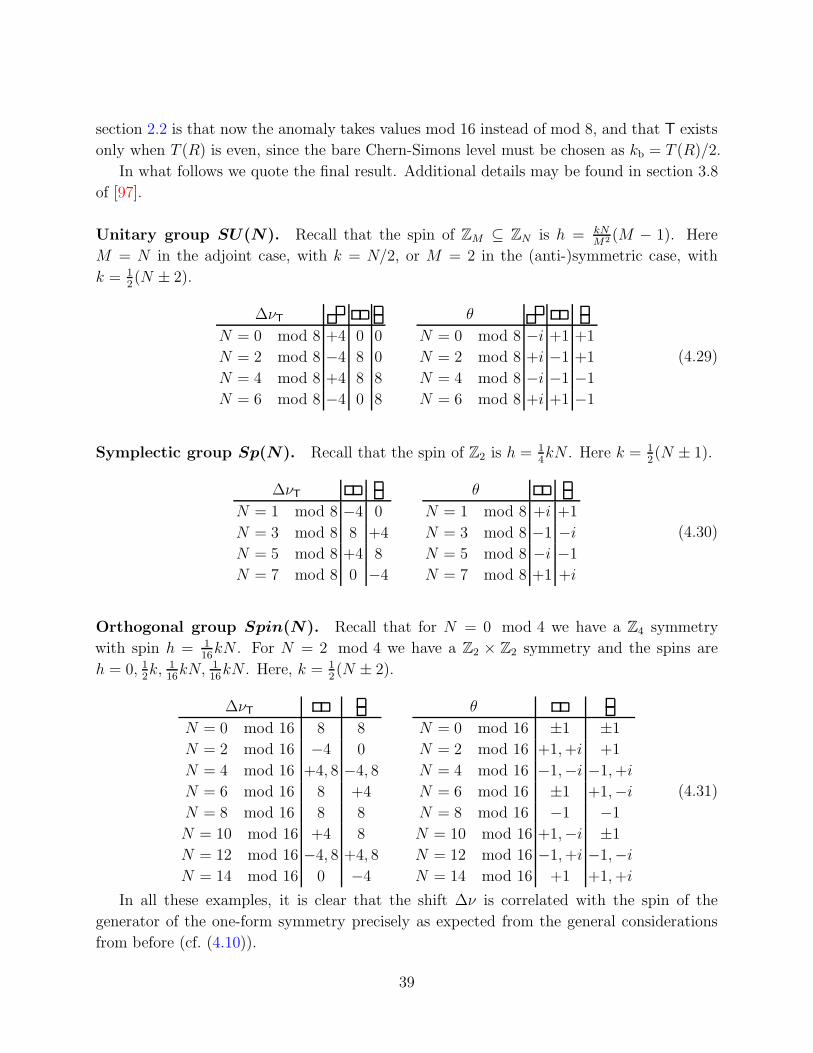
section 2.2 is that now the anomaly takes values mod 16 instead of mod 8, and that T exists
only when T (R) is even, since the bare Chern-Simons level must be chosen as kb = T (R)/2.
In what follows we quote the final result. Additional details may be found in section 3.8
of [97].
Unitary group SU(N). Recall that the spin of ZM ⊆ ZN is h = kNM2 (M − 1). Here
M = N in the adjoint case, with k = N/2, or M = 2 in the (anti-)symmetric case, with
k = 12(N ± 2).
∆νTN = 0 mod 8 +4 0 0
N = 2 mod 8 −4 8 0
N = 4 mod 8 +4 8 8
N = 6 mod 8 −4 0 8
θ
N = 0 mod 8 −i +1 +1
N = 2 mod 8 +i −1 +1
N = 4 mod 8 −i −1 −1
N = 6 mod 8 +i +1 −1
(4.29)
Symplectic group Sp(N). Recall that the spin of Z2 is h = 14kN . Here k = 1
2(N ± 1).
∆νTN = 1 mod 8 −4 0
N = 3 mod 8 8 +4
N = 5 mod 8 +4 8
N = 7 mod 8 0 −4
θ
N = 1 mod 8 +i +1
N = 3 mod 8 −1 −iN = 5 mod 8 −i −1
N = 7 mod 8 +1 +i
(4.30)
Orthogonal group Spin(N). Recall that for N = 0 mod 4 we have a Z4 symmetry
with spin h = 116kN . For N = 2 mod 4 we have a Z2 × Z2 symmetry and the spins are
h = 0, 12k, 1
16kN, 1
16kN . Here, k = 1
2(N ± 2).
∆νTN = 0 mod 16 8 8
N = 2 mod 16 −4 0
N = 4 mod 16 +4, 8 −4, 8
N = 6 mod 16 8 +4
N = 8 mod 16 8 8
N = 10 mod 16 +4 8
N = 12 mod 16 −4, 8 +4, 8
N = 14 mod 16 0 −4
θ
N = 0 mod 16 ±1 ±1
N = 2 mod 16 +1,+i +1
N = 4 mod 16 −1,−i −1,+i
N = 6 mod 16 ±1 +1,−iN = 8 mod 16 −1 −1
N = 10 mod 16 +1,−i ±1
N = 12 mod 16 −1,+i −1,−iN = 14 mod 16 +1 +1,+i
(4.31)
In all these examples, it is clear that the shift ∆ν is correlated with the spin of the
generator of the one-form symmetry precisely as expected from the general considerations
from before (cf. (4.10)).
39
4.4 Magnetic symmetry: gauging the one-form symmetry
We close our study of 2+ 1d theories with a brief discussion of an apparent paradox, and its
resolution. Consider a time-reversal invariant theory with one-form symmetry Z(1)2 . As above,
this one-form symmetry may make the anomaly ν ambiguous with its corresponding ∆ν. A
natural question one may ask is: what happens when we gauge Z(1)2 ? Clearly, the resulting
theory no longer has this one-form symmetry, and therefore ν should become unambiguous,
with ∆ν = 0. How can we reconcile this with the ungauged theory having ∆ν 6= 0?
To be more precise, the symmetry Z(1)2 can only be gauged when it does not have a
pure one-form ’t Hooft anomaly. This anomaly is measured by the spin of the generating
line, namely 2h mod 1. Therefore, the one-form symmetry can only be gauged when the
generating line is either a boson or a fermion. As discussed above, these two options lead to
∆ν = 0 and ∆ν = 8, respectively. The subtle case is the latter, since the ungauged theory
has ∆ν 6= 0, while the gauged theory should have ∆ν = 0.
The resolution is the following. When we gauge Z(1)2 we get a dual (magnetic) zero-form
symmetry Z(0)2 , generated by a topological operator M. The mixed anomaly between time-
reversal and the one-form symmetry implies that, upon gauging the latter, the former gets
extended [90, 98], and the algebra becomes
T2 = (−1)FM2h (4.32)
This follows from the term π∫
B ∪w21, since the dual symmetry with background B′ couples
as π∫
B ∪ B′, and the mixed anomaly can be cancelled by demanding dB′ = w21. This
describes an extended T algebra, as specified by the element w21 ∈ H2(ZT
4 ,Z2) = Z2.
This way, we see that when the generating line is a boson, the algebra is still T2 = (−1)F ,
with unambiguous anomaly ν. On the other hand, when the generating line is a fermion,
the algebra becomes T2 = (−1)FM, and the anomaly is no longer given by a class ν ∈ Ω4Pin+.
Thus, it no longer makes sense to talk about ∆ν, since the anomaly of the extended algebra
is given by an entirely different bordism group.
It would be interesting to repeat the analysis of this paper in theories with extended
algebra T2 = (−1)FM, and the associated constraints on QCD phase diagrams.
5 QCD in 3+1 Dimensions
5.1 Discrete axial zero-form symmetry and its anomaly
In this section we discuss 3 + 1d systems with the unitary Z2n symmetry
gn = (−1)F , (5.1)
40
with (−1)F being fermion number. The tangential structure describing this symmetry is
H =Spin× Z2n
ZF2
. (5.2)
The ’t Hooft anomalies for this symmetry can be realized by free fermions, and they are
classified by the following cobordism group [99, 100]
ΩH5 = Za × Zb , (5.3)
where
a =
24n n = 0 mod 6
8n n 6= 0 mod 3, n = 0 mod 2
3n n = 0 mod 3, n 6= 0 mod 2
n otherwise
b =
n/6 n = 0 mod 6
n/2 n 6= 0 mod 3, n = 0 mod 2
n/3 n = 0 mod 3, n 6= 0 mod 2
n otherwise
(5.4)
Thus, this symmetry is endowed with a large group anomalies.37
The symmetry (5.1) is ubiquitous in 3 + 1d gauge theories. Indeed, a gauge theory with
gauge group Ggauge and quarks in a (possibly reducible) representation R of Ggauge has the
discrete symmetry (5.1) for some n. When Ggauge is simply-connected, the symmetry is
Z2T (R), with T (R) the Dynkin index of R. This symmetry is the unbroken subgroup of the
classical chiral U(1) symmetry that survives integrating over the Ggauge gauge fields.
The anomaly can be computed by first embedding the Z2n into U(1), then compute the
anomaly perturbatively [99].38 Let us denote the background U(1) gauge field by A′. More
37An even larger group of anomalies can be studied by also considering charge conjugation, which satisfies
(gC)2 = 1 . (5.5)
The extended symmetry is the dihedral group D2n∼= Z2 ⋉ Z2n. Anomalies for (Spin × D2n)/Z
F2 are less
understood and therefore we shall stick to the Z2n subgroup in what follows.38The two generators for the anomaly can be chosen as follows. For Za it can be obtained from [99]
νa =a
48n((2n2 + n+ 1)q3 − (n+ 3)q1) mod a , (5.6)
where qk :=∑
i qki and a in (5.4). The anomaly for Zb is known explicitly for n a power of 2, in which case
b = n/2. It reads [101]
νb =b
4n((n+ 1)(2n+ 1)q3 − (n+ 1)q1) mod b . (5.7)
We would like to thank Joe Davighi for discussions on this. In the following discussion, we will not need
these generators.
41
precisely, due to the quotient in (5.2), it is a spinc connection. This means that on non-spin
manifolds, the flux of dA′ is a multiple of π:
dA′
2π=
1
2w2(TM) mod Z . (5.8)
We restrict to the background field configuration such that A′ has holonomy in 2π2nZ. Consider
a collection of left-handed Weyl fermions with charges qi under the Z2n symmetry, the
anomaly can be described by the bulk effective action (see e.g. [102, 103])
Sanom = 2π
∫
5d
((
∑
i
q3i
)
1
3!(2π)3A′dA′dA′ −
(
∑
i
qi
)
A′
2π
1
24p1(TM)
)
, (5.9)
which can be written as the boundary term of 2π∫
6dtr(
edA′/2πA(R)
)
for Riemann curvature
two-form R.
Since A′ has holonomy in Z2n, the anomaly takes discrete values. Let us consider the
anomaly for a single Weyl fermion with unit charge,
I1 = 2π
∫
5d
(
1
3!(2π)3A′dA′dA′ − 1
24(2π)A′p1(TM)
)
. (5.10)
The bulk action I1 is a multiple of 2π/(48n), and thus kI1 for integer k only depends on k
mod 48n. If we consider 1 Weyl fermion of charge 3 and 27 Weyl fermions of charge (−1),
this gives a mixed global-gravity anomaly
I2 = 2π
∫
5d
A′
2πp1(TM) . (5.11)
The bulk action I2 is a multiple of 2π/(2n), and thus k′I2 for integer k′ only depends on k′
mod 2n.
5.2 SU(N) gauge theory with one adjoint fermion
We now proceed to study the dependence of these anomalies on a choice of fractionalization
class. For definiteness, we consider 3+1d SU(N) gauge theory with a quark ψ in the adjoint
representation, that is, N = 1 SU(N) super-Yang-Mills. This theory enjoys a G = Z2N
chiral zero-form symmetry as well as Γ = ZN one-form symmetry. Therefore, the changes of
fractionalization class take values in H2(Z2N ,ZN) = ZN .39
The canonical Z2N chiral symmetry acts on the N2 − 1 adjoint fermions with charge
qi = 1, so that in N = 1 SU(N) super-Yang-Mills, the anomaly is described by the bulk
effective action
Sanom = (N2 − 1)I1 = 2π(N2 − 1)
∫
5d
(
1
3!(2π)3A′dA′dA′ − 1
24(2π)A′p1(TM)
)
. (5.12)
39If we include the charge conjugation zero-form symmetry, then different fractionalization classes can
produce a two-group for N = 0 mod 4 as discussed in appendix F.
42
We explore the dependence of the anomalies on the choice of fractionalization class by
following the by-now familiar route of composing g with gauge transformations U such
that (gU)N = (−1)F on the fermions. For adjoint fields, the most general diagonal SU(N)
transformation with adj(UN ) = 1 is
U ∝ diag(1p0, ζ1p1, ζ21p2 , · · · , ζN−11pN−1
) (5.13)
where ζ := e2πi/N , and pI are non-negative integers obeying∑
I pI = N . The global phase
is fixed by unitarity, but it is irrelevant since it drops out when acting on fermions in the
adjoint representation.
Collecting the components of ψ into pI × pJ blocks ψIJ , U acts on each block as
ψIJ 7→ e2πi(I−J)/NψIJ . (5.14)
Therefore, the Z2N charge of such a block is q = 1 + 2(I − J), and
∑
qki = −1 +N−1∑
I,J=0
pIpJ(
1 + 2(I − J))k. (5.15)
This allows us to compute the shifts of the charges of the fermions that enter in the compu-
tation of the anomalies
∆(
∑
qi
)
= −2N−1∑
I,J=0
pIpJ(I − J) = 0
∆(
∑
q3i
)
= −2
N−1∑
I,J=0
pIpJ(I − J)(3 + 6(I − J) + 4(I − J)2)
= −24NN−1∑
I=0
pII2 + 24
(N−1∑
I=0
pII
)2
.
(5.16)
Thus we find that the anomaly changes by the bulk effective action
∆Sanom = 2π∆(
∑
q3i
)
∫
5d
1
3!(2π)3A′dA′dA′
= 2π(
∆(
∑
q3i
)
mod 48N)
∫
5d
1
3!(2π)3A′dA′dA′ , (5.17)
where we used the property that the effective action takes value in 2π/(48N). Let us denote
ℓ ≡∑
I
IpI . (5.18)
43
Since
∆(
∑
q3i
)
mod 48N = −24N
(
∑
I
pII
)
+ 24ℓ2 mod 48N = 24(−N + 1)ℓ2 mod 48N ,
(5.19)
we find the anomaly changes by
∆Sanom = 2π · 24(−N + 1)ℓ2∫
5d
1
3!(2π)3A′dA′dA′
=(−N + 1)ℓ2
π2
∫
5d
A′dA′dA′
= 24(−N + 1)ℓ2I1 + (−N + 1)ℓ2I2 .
(5.20)
5.3 Different fractionalization classes, and one-form symmetry anomaly
SU(N) gauge theory with one adjoint fermion has ZN one-form symmetry. The one-form
symmetry has a mixed anomaly with the Z2N axial zero-form symmetry. Under an axial
rotation labelled by k ∈ Z2N
ψi → ψie2πik2N . (5.21)
The Adler-Bell-Jackiw anomaly [104, 105] implies that the θ angle is shifted by
θ → θ + 2πk . (5.22)
In the presence of background gauge field B for the ZN one-form symmetry that changes the
θ periodicity, the transformation does not leave the theory invariant, but produces [26, 81]
2πk(N − 1)
2N
∫
4d
P(B) . (5.23)
Thus there is a mixed anomaly between the chiral symmetry and the one-form symmetry.
The anomaly is described by the 4 + 1d effective action (the overall sign depends on the
orientation)40
− 2πN − 1
2N
∫
5d
P(B) ∪ A mod 2πZ , (5.25)
40For odd N , the action is a multiple of 2π/N , and since dA = 0 mod N , the action is well-defined. For
even N , the action is a multiple of 2π/(2N), and it can be shown to be well-defined by extending it to the
bulk
−2πN − 1
2N
∫
6d
P(B) ∪ dA = −π
∫
B ∪B ∪w2(TM) = −π
∫
6d
Sq1(B)Sq1(B)
= π
∫
6d
Sq1(
BSq1(B))
= π
∫
6d
w1(TM)BSq1(B) mod 2π , (5.24)
which is trivial for orientable manifolds, where w1(TM) = 0, and we used Sq2(B ∪ B) = Sq1(B)Sq1(B)
and Sqkxd−k = vk(TM) ∪ xd−k for Z2 (d − k) cocycle on d-dimensional manifold [86]. Thus the action is
well-defined in 4 + 1d.
44
where A is the background gauge field for the Z2N chiral symmetry, that satisfies
dA = Nw2(TM) mod 2N . (5.26)
Different fractionalization classes are obtained by turning on background41
B = ℓdA
Nmod N, ℓ = 0, 1, · · · , N − 1 . (5.27)
We note that for even N , ℓ can be N/2, then the corresponding fractionalization class is
B = N2w2(TM) mod N . For fractionalization class ℓ, the mixed one-form/zero-form anomaly
gives additional anomaly for the zero-form symmetry
− 2π(N − 1)ℓ2
2N
∫
5d
P(
dA
N
)
∪ A . (5.28)
Written in terms of A′ = 2π2NA, this is
− 2π(N − 1)ℓ2
2N
∫
5d
(
dA′
π
)22N
2πA′ =
(−N + 1)ℓ2
π2
∫
5d
A′dA′dA′ . (5.29)
Thus changing the fractionalization classes reproduces the jump of the anomaly as in (5.20).
5.4 Domain walls
In this section we make a few comments about the matching of the Z2n anomaly by the
low-energy effective theory. We consider N = 1 super-Yang-Mills, that is, adjoint QCD with
some gauge group Ggauge. In this case, the axial symmetry is Z2h, where h = T (adj) is the
Coxeter number of Ggauge.
It is a well-known fact that 3+1d N = 1 super-Yang-Mills with simply-connected gauge
group is gapped and confining, and that the infrared consists of h discrete vacua as a result
of the spontaneous breaking of the Z2h symmetry down to ZF2 . These vacua are separated
by domain walls, which carry non-trivial 2 + 1d degrees of freedom. Specifically, the wall
separating p ∈ Zh units of vacua supports a 2 + 1d N = 1 super-Yang-Mills theory with
the same gauge group and a Chern-Simons level k = h/2− p [92,106]. It is these degrees of
freedom what matches the Z2h anomaly as computed in the ultraviolet.
For simplicity, here we will restrict ourselves to the parity-symmetric wall p = h/2 that
exists when h is even. This wall is special since the CPT wall construction [66] implies that
the unitary axial symmetry in the bulk is transmuted to an anti-unitary symmetry on the
41Following the same analysis as in section 2.2, we learn that the fractionalization class induced by U is
given by the phase of UN , which equals UN = ζ−ℓ1N and only depends on the combination ℓ =
∑
I pII.
This implies that the change in the fractionalization class (and thus the change in the anomaly) only depends
on the integers pI via the combination ℓ =∑
I IpI .
45
wall. In this case, it is very easy to show that the ultraviolet anomaly is matched by the 3d
degrees of freedom.
The time-reversal symmetric wall corresponds to the Z2 subgroup of Zh, i.e., to a spon-
taneously broken g2 = (−1)F symmetry. In the bulk, anomalies for such unitary symmetry
are classified by Za×Zb, where a, b are given by (5.4) at n = 2, namely a = 16 and b = 1. In
other words, the anomalies take values in Z16. On the wall, this a time-reversal symmetry,
whose anomalies are also classified by Z16. It is easy to show that these anomalies indeed
match.
The Z16 anomaly in the bulk is given by (5.6) with n = 2, to wit,
νa =11q3 − 5q1
6mod 16 . (5.30)
If we let n± be the number of fermions that transform with sign ±1, then qk = n+−n−, and
the anomaly simplifies to
νa = n+ − n− mod 16 , (5.31)
which precisely matches the time-reversal anomaly νT of the wall, namely the time-reversal
anomaly of 3d adjoint QCD.
The non-parity-symmetric walls require a more careful study that we leave to future work.
In this case, non-invertible topological defects are potentially important, as well as junctions
of domain walls. See [70, 107–116] for related work in various dimensions.
Acknowledgement
We thank M. Cheng, J. Davighi, C.-M. Jian, N. Seiberg, T. Senthil and M. Yu for dis-
cussions. We thank Maissam Barkeshli, Anton Kapustin, Shu-Heng Shao, Juven Wang for
comments on a draft. P.-S. H. is supported by the Simons Collaboration on Global Categor-
ical Symmetries. D.D. and J.G. acknowledge support by Perimeter Institute for Theoretical
Physics. Research at Perimeter Institute is supported in part by the Government of Canada
through the Department of Innovation, Science and Economic Development Canada and by
the Province of Ontario through the Ministry of Colleges and Universities. Any opinions,
findings, and conclusions or recommendations expressed in this material are those of the
authors and do not necessarily reflect the views of the funding agencies.
A Congruence Vector of Simple Lie Algebras
In this appendix we quote the value of ρ · v mod |Z(Ggauge)| for the classical Lie groups,
where ρ = (1, 1, . . . , 1) is the Weyl vector.
46
Unitary group SU(N). The congruence vector is v = (1, 2, . . . , N − 1). Thus,
ρ · v = 1
2N(N − 1) mod N (A.1)
which is nonzero when N is even.
Symplectic group Sp(N). The congruence vector is v = (1, 2, . . . , N). Thus,
ρ · v =1
2N(N + 1) mod 2 (A.2)
which is nonzero when N = 1, 2 mod 4.
Orthogonal group SO(N). The congruence vectors depend on N mod 4, which we
consider in turn.
• In SO(2n+ 1), the congruence vector is v = (0, 0, . . . , 1). Thus,
ρ · v = 1 mod 2 (A.3)
which is always nonzero.
• In SO(4n+ 2), the congruence vector is v = (2, 4, 6, . . . ,−2n + 1,−2n− 1). Thus,
ρ · v = −2n mod 4 (A.4)
which is nonzero when n is odd.
• In SO(4n), the congruence vectors are v1 = (0, 0, . . . , 1, 1) and v2 = (1, 2, 3, . . . , 1 −n,−n). Thus,
ρ · v1 = 0 mod 2
ρ · v2 = −n mod 2(A.5)
and the latter is nonzero when n is odd.
These results are summarized in table (2.15).
B One-Form Symmetry Anomaly in QCD0+1
Consider QCD in 0+1d with simple gauge group Ggauge and a fermion in some representation
R. The one-form symmetry Γ is the subgroup of the center of gauge group that acts trivially
on the representation R. We would like to compute the ’t Hooft anomaly of the one-form
symmetry.
Since the background for the one-form symmetry changes the Ggauge gauge field into
Ggauge/Γ gauge field, to address the question we can compute the partition function of the
free fermion theory in the presence of a background gauge field for Ggauge/Γ. While the
47
partition function with background Ggauge is well-defined (and thus the QCD0+1 with the
corresponding gauge group is free of gauge anomalies), the partition function with back-
ground Ggauge/Γ can have ambiguities, which is the anomaly of the one-form symmetry Γ in
QCD0+1 with gauge group Ggauge. Such anomaly arises if and only if the symmetry Ggauge/Γ
is realized projectively on the Hilbert space of the free fermions.
Consider the embedding of ggauge inside so(dim(R)) via the representation R. This em-
bedding is defined by the branching rule
so(dim(R)) ⊇ ggauge
7→ R .(B.1)
Let us first turn on holonomy U of background gauge field that takes value in Spin(dim(R)).
Since the Hilbert space realizes a spinor representation s of Spin(dim(R)), the partition
function can be expressed in terms of the character of such spinor representation:
Z±(U) = χs(U)± χs(U), dim(R) even
Z+(U) =√2χs(U), dim(R) odd
Z−(U) = 0, dim(R) odd .
(B.2)
where ± denotes the spin structure, and s the spinor representation of Spin(dim(R)) (and
s the conjugate representation). When we restrict the holonomy U to take value in Ggauge,
the partition function is
Z±(U) = χs(R)(U)± χs(R)(U), dim(R) even
Z+(U) =√2χs(R)(U), dim(R) odd
Z−(U) = 0, dim(R) odd .
(B.3)
where s(R) ∈ Rep(Ggauge) is the image of s ∈ Rep(Spin(dim(R))) under the embedding (B.1),
so(dim(R)) ⊇ ggauge
s 7→ s(R) .(B.4)
(In general, s(R) is a reducible representation even if R is irreducible.) The partition function
without insertion transforms under the center Γ according to the transformation of s(R).
Thus in the Ggauge gauge theory, the one-form symmetry has anomaly if and only if s(R)
transforms under Γ in the center of Ggauge. The anomaly can be described by the bulk term
∫
2d
〈q(s(R)), B〉 , (B.5)
where q(s(R)) ∈ Hom(Γ, U(1)) is the one-form charge of s(R) under Γ in the center of Ggauge,
and B is the background two-form gauge field for the Γ one-form symmetry.
48
As an application of this result, let us show that fermions in complex representation does
not contribute to the anomaly of the one-form symmetry. When R is complex, the branching
rules are
s(R) 7→⌊dim(R)/2⌋⊕
j=0
∧2jR
s(R) 7→⌈dim(R)/2⌉−1⊕
j=0
∧2j+1R .
(B.6)
Of course, ∧nR is not charged under ker(R) for any n, and therefore complex representations
never lead to an anomaly for one-form symmetry.
Anomalies are only present in the case of real representations. As a simple illustration,
consider adjoint QCD. Here the embedding becomes so(dimGgauge) ⊃ ggauge, and the spinor
representation branches as
s 7→ 2⌈r/2⌉−1ρ , (B.7)
where ρ is the Weyl vector of ggauge and r = rank(ggauge). Therefore, the one-form symmetry
of adjoint QCD is anomalous if and only if ρ is charged under it, in agreement with section 2.1.
An equivalent way to phrase this discussion is in terms of how exactly Ggauge embeds into
Spin(dim(R)). We sketch the argument for adjoint SU(N) below.
B.1 SU(N) gauge theory with an adjoint fermion
Consider SU(N) gauge theory with an adjoint fermion in 0+1d. We would like to understand
whether the ZN one-form symmetry is anomalous.
This is equivalent to asking whether the PSU(N) zero-form symmetry that acts on
N2 − 1 free Majorana fermions is anomalous. In other words, whether the Hilbert space of
the free fermions transforms as projective representation of PSU(N) symmetry. When N is
odd, there is an even number of Majorana fermions and a properly Z2-graded Hilbert space;
when N is even, we add one extra singlet Majorana fermion to form a well-defined Hilbert
space.
The discussion divides into two cases: N even and N odd.
B.1.1 Even N
When N is even, we add one additional Majorana fermion that is singlet under PSU(N)
to obtain a well-defined Hilbert space. We quantize the fermions, which form the Clifford
algebra of rankN2. The Hilbert space forms the spinor representation of Spin(N2) symmetry.
The states generated by the N2 − 1 Majorana fermions form spinor of Spin(N2 − 1). We
have the embedding
Spin(N2 − 1) ⊂ SU(N)/ZN/2 , (B.8)
49
where both sides have Z2 center. Thus the spinor representation decomposes into SU(N)
representation with non-trivial N -ality, and thus the PSU(N) symmetry acts projectively
on the Hilbert space. This means the PSU(N) symmetry is anomalous, with the anomaly
2π(N/2)
N
∫
wPSU(N)2 = π
∫
wPSU(N)2 . (B.9)
We note that this implies that the Hilbert space of SU(N) gauge theory with adjoint fermion
is empty (since the vacuum carries non-trivial SU(N) representation) unless considering the
twisted Hilbert space with insertion of Wilson line of N -ality N/2 in the time direction.
In the SU(N) gauge theory with adjoint fermion, this implies the one-form symmetry is
anomalous. In terms of the one-form symmetry gauge field B2, the anomaly is
π
∫
B2 . (B.10)
B.1.2 Odd N
When N is odd, N2 − 1 is even, and there is a well-defined Hilbert space. Let us quantize
the fermions, which give Clifford algebra of rank N2−1. The Hilbert space forms the spinor
representations of Spin(N2 − 1). Let us study how the Hilbert space transforms under
SU(N) symmetry. Since SU(N) for odd N does not have a Z2 subgroup center, the spinor
representation of Spin(N2 − 1) decompose into SU(N) representation with 0 N -ality, and
thus we have the embedding
Spin(N2 − 1) ⊃ PSU(N) . (B.11)
Thus the PSU(N) symmetry acts linearly on the Hilbert space, and it does not have an
anomaly. Thus we conclude that when N is odd, the ZN one-form symmetry in SU(N)
gauge theory with one adjoint fermion is non-anomalous.
C U(1) Gauge Theory in 1+1d
In this appendix we use one-form symmetry to discuss the anomaly of Z2 charge conjugation
symmetry in U(1) gauge theory in 1 + 1d for different fractionalization classes.
Consider the U(1) gauge theory with θ = π
1
2e2da ⋆ da+
1
2da . (C.1)
The theory has Γ = U(1) one-form symmetry that shifts a, and Z2 charge conjugation
symmetry that acts as a→ −a.
50
Let us compute the anomaly for the symmetries. We turn on background B2 for the U(1)
one-form symmetry, and B1 for the Z2 charge conjugation symmetry. This replaces da by
DB1a− B2 = (d− 2B1)a−B2 . (C.2)
Thus the theta term contributes the bulk dependence
∫
1
2(2B1da− dB2) =
∫
B1B2 −1
2dB2 = −1
2
∫
DB1B2 . (C.3)
This is a mixed anomaly between the one-form symmetry and charge conjugation zero-form
symmetry.
There are two fractionalization classes for the Z2 charge conjugation 0-form symmetry,
classified by H2(BZ2,Z2) = Z2:
• B2 = 0, then the zero-form symmetry is not anomalous.
• B2 = πB21 , then the zero-form symmetry has an anomaly
π
∫
B31 . (C.4)
This agrees with the discussion in section 3.
D Fermionic Z2 Gauge Theory with Z2 Symmetry in
1+1d
Let us consider Z2 gauge theory in 1 + 1d, viewed as a fermionic theory, and enriched with
unitary Z2 × ZF2 symmetry, where Z
F2 is the fermion parity symmetry.
The action without any background gauge fields is
π
∫
a0 ∪ δb1 . (D.1)
If we integrate out b1, this sets δa0 = 0 mod 2. Such condition will be modified in the
presence of background gauge field.
The theory has Z2 one-form symmetry that acts on the Wilson line, and different symme-
try fractionalizations in fermionic world admits a classification using the spin bordism group
Ωspin2 (BZ2)
Hom(Ωspin2 (BZ2),Z2) . (D.2)
The group is Z2 × Z2, generated by the Arf invariant, and the quadratic function 12qρ(A),
where we denote the spin structure by ρ, and the Z2 background gauge field by A. If we
51
denote the symmetry fractionalization by (m,n) ∈ Z2×Z2, then the path integral is modified
to be
Z =
∫
Da0e2πim
8Arf(PD2d(a0))e
nπi2
∫PD2d(φ0)
qρ(A), (D.3)
where PD2d(φ0) is the two-cycle that is Poincare dual to φ0. It is closed in Z2 homology, since
δφ0 = 0 mod 2, and thus the above partition function is well-defined. We note that PD2d(φ0)
is orientable,42 and thus qρ is even, and Arf is a multiple of 4 in the above normalization,
and the phases in the path integral are signs. We can also include (−1)ℓ∫PD(φ0)
A∪Afor ℓ ∈ Z2,
which is trivial for δφ0 = 0.
The theory also has Z2 zero-form symmetry that acts on the Z2 vortex point operator.
Let us consider the Z2 unitary symmetry that acts on such operators. Then, in the presence
of background A, φ0 is no longer closed in Z2,
δφ0 = A , (D.4)
and PD2d(φ0) has a boundary that is non-trivial in Z2 homology
∂PD2d(φ0) = PD2d(dφ0) = PD2d(A) . (D.5)
In such a case, the partition function is no longer well-defined. This is a manifestation
of an anomaly for the Z2 symmetry. One way to cure the problem is by introducing a 3d
bulk, and attaching the boundary surface to another surface in the bulk that anchors on the
boundary along PD2d(A), to form a closed surface, so the phases in the partition function
evaluated on the 2-cycle Σ2-cycle can be defined, where
Σ2-cycle = PD2d(φ0) ∪ Σbulk, ∂Σbulk = PD2d(A) . (D.6)
For instance, if 2d spacetime has trivial topology and we take the bulk direction to be z
coordinate, then such a bulk surface can be a cigar with base PD2d(A) and extends along z
direction.
If we consider two bulks, the choice of bulk surface Σbulk depends on PD3d(A), which is
a surface in the bulk (note it may be a unorientable surface embedded in an orientable bulk,
if A has a non-trivial bundle in the bulk). When the bulk surface is unorientable, we need
to refine the Arf invariant into ABK invariant. Then the phases depend on the bulk by
e2πim
8ABK(PD3d(A))e
nπi2
∫PD3d(A)
qρ(A)(−1)
ℓ∫PD3d(A)
A∪A, (D.7)
where the first term is the partition function for the root phase of the Z8 invertible phases
in 2+ 1d with Z2 ×ZF2 symmetry and zero thermal Hall conductance. The second term can
be written as an odd-level Chern-Simons term for the gauge field A. The third term is the
42For a 2d surface D embedded in 2d orientable spacetime M , TM | = TD + ND, but ND = 0 since it
has zero dimension, and thus TM | = TD, and for orientable TM , TD is also orientable.
52
partition function for the bosonic SPT phase with Z2 symmetry. The above decomposition
represents the Arf layer, ψ layer and bosonic layer in [58]. In particular, m,n now have
extended range, with the identification
(m+ 2, n, ℓ) ∼ (m,n+ 1, ℓ), (m,n+ 2, ℓ) ∼ (m,n, ℓ+ 1) . (D.8)
E Z2 Gauge Theory with Two-group Symmetry in 2+1d
E.1 Intrinsic symmetries and their anomalies
Untwisted Z2 gauge theory in 2 + 1d has Z2 × Z2 one-form symmetry generated by the
electric and magnetic line operators. The theory also has unitary ZC
2 zero-form symmetry
that exchanges the electric and magnetic lines. Let us denote the background for zero-form
symmetry by B1, the background for the diagonal Z2 one-form symmetry generated by the
dyon by B2, and the background for the Z2 one-form symmetry generated by the Wilson
line by B′2. They they obey the twisted cocycle condition
dB2 = B1 ∪ B′2, dB′
2 = 0, dB1 = 0 . (E.1)
To understand this relation, we note that in the presence of backgrounds B′2, B1, there must
also be a non-trivial background for B2 due to the action of the zero-form symmetry on the
one-form symmetry, and this is captured by the first relation.
More generally, we can consider Spin(4k)1 Chern-Simons theory for integer k, which has
Z2×Z2 one-form symmetry generated by the lines in the spinor and cospinor representation,
and Z2 charge conjugation 0-from symmetry that exchanges the two lines. The Toric Code
Z2 gauge theory corresponds to k = 0.
In addition, the theory has ZT
2 time-reversal that does not permute the line operators.
Let us turn on background field by placing the theory on an unorientable manifold with first
Stiefel-Whitney class w1. Then the twisted cocycle condition is modified to be [117]
dB2 = B1 ∪ (B′2 + w1 ∪ B1) . (E.2)
We note that under a Z2 one-form transformation for B′2, B
′2 → B′
2+dλ1, the background B2
is shifted by B2 → B2+B1∪λ1, where we used dB1 = 0. When later we focus on unitary ZC
2
zero-form symmetry or time-reversal symmetry that acts as charge conjugation, this implies
that the non-trivial fractionalization classes only come from shifting B′2 but not B2.
53
The zero-form and one-form symmetries have an anomaly, described by the bulk term [117]
Sbulk SPT = π
∫
P(B2) + π
∫
B2 ∪ (B′2 + w1 ∪B1) + π
∫
w1 ∪B1 ∪ B2
+ π
∫
B1 ∪ [(B1 ∪ (B′2 + w1 ∪B1)) ∪2 (B
′2 + w1 ∪B1) +B1 ∪ (B′
2 + w1 ∪ B1)]
+π
2
∫
B21 ∪ (B′
2 + w1 ∪ B1) , (E.3)
where in the last term we take a lift of B1 to Z4 cochain that takes value in 0, 1.
E.2 Unitary ZC2 symmetry
Let us consider unitary ZC
2 symmetry, with w1 = 0. The twisted cocycle condition for B2, B′2
becomes
dB2 = B1 ∪B′2 . (E.4)
We note that the global transformation B′2 → B′
2+dB1 = B′2 induces the equivalence relation
B2 ∼ B2 +B21 .
Let us consider the following symmetry fractionalizations:
• B′2 = 0: charge conjugation squares to +1 on the dyon. Then dB2 = 0, and the
zero-form symmetry does not participate in a non-trivial two-group with the one-form
symmetry.
• B′2 = B2
1 : charge conjugation squares to −1 on the dyon. Then dB2 = B31 , the zero-
form symmetry participates in a two-group with the one-form symmetry, with Postnikov
class B31 .
E.2.1 Anomaly
The zero-form and one-form symmetry has an anomaly, described by the bulk term [117]
π
∫
P(B2) + π
∫
B2 ∪B′2 + π
∫
B1 ∪ ((B1 ∪ B′2) ∪2 B
′2 +B1 ∪ B′
2) +π
2
∫
B21 ∪B′
2 , (E.5)
where in the last term we take a lift of B1 to Z4 cochain that takes value in 0, 1.
Thus for B′2 = 0, the zero-form symmetry by itself does not have an anomaly.
For B′2 = B2
1 , there is a 2-group anomaly:
π
∫
P(B2) + π
∫
B2 ∪B21 + π
∫
B1 ∪(
(B31) ∪2 B
21
)
+3π
2
∫
B41 . (E.6)
54
The last term B41 can be canceled by a local 3d counterterm, and we are left with the
first three terms.43 Thus the Z2 gauge theory gives an example with anomalous 2-group
symmetry.
E.3 Anti-unitary Z2 symmetry that acts as charge conjugation
Let us consider instead Z2 time-reversal symmetry that acts as charge conjugation symmetry,
i.e. diagonal Z2 subgroup zero-form symmetry for ZC
2 × ZT
2 . In other words, we restrict to
B1 = w1. Then the twisted cocycle conditions for B2, B′2 becomes
dB2 = w1 ∪(
B′2 + w2
1
)
. (E.7)
We note that the global transformation B′2 → B′
2+dw1 = B′2 induces the equivalence relation
B2 ∼ B2 + w21.
Let us consider the following symmetry fractionalization for the Z2 anti-unitary symme-
try:
• B′2 = 0: time-reversal squares to +1 on the dyon. Then dB2 = w3
1, and the zero-form
symmetry participates in a two-group with the one-form symmetry, with Postnikov
class w31.
• B′2 = w2
1: time-reversal squares to −1 on the dyon. Then dB2 = 0, and the zero-form
symmetry does not participate in a non-trivial two-group with the one-form symmetry.
The condition that only certain fractionalization class leads to a symmetry that does not
participate in a two-group is also discussed in equation (234) of [40]. See also [118] for related
examples.44
43To see the anomaly is well-defined, we can extend it to 5d, and use π∫
B51 = πSq2(B2
1) ∪ B1 =
π∫
Sq2(B31) = π
∫
dP(B2) + π∫
dζ(B1, B21), where ζ(B1, B
21) is the Cartan coboundary given by the term
that depends only on B1, and we used dP(B2) = dB2 ∪1 dB2 = Sq2(B31) mod 2 with dB2 = B3
1 .44We note that in the case of two-group, one can still discuss different fractionalization classes by shifting
the background gauge field, where background B2 for the one-form symmetry and the background B1 for
the zero-form symmetry satisfies
dρB2 = B∗
1Θ , (E.8)
for Postnikov class Θ. When Θ is non-trivial, the symmetry mixes to form a two-group, this implies that
under a zero-form symmetry transformation with parameter λ, [21]
B1 → Bλ1 , B2 → B2 + ζ(λ,B1) , (E.9)
and this gives additional equivalence relation on the shift B2 → B2 + B∗1η that implements different frac-
tionalization classes [21].
55
E.3.1 Anomaly
The zero-form and one-form symmetries have an anomaly, described by the bulk term [117]
Sbulk SPT = π
∫
P(B2) + π
∫
B2 ∪ (B′2 + w2
1) + π
∫
w21 ∪ B2
+ π
∫
w1 ∪[
(w1 ∪ (B′2 + w2
1)) ∪2 (B′2 + w2
1) + w1 ∪ (B′2 + w2
1)]
+π
2
∫
w21 ∪ (B′
2 + w21) , (E.10)
For B′2 = w2
1, where there is no 2-group symmetry, the anomaly is
π
∫
P(B2) + π
∫
w21 ∪ B2 . (E.11)
For B′2 = 0, where there is 2-group symmetry, the anomaly is
π
∫
P(B2) + π
∫
w21 ∪1 w
31 + π
∫
w1 ∪(
w31 ∪2 w
21
)
+3π
2
∫
w41 . (E.12)
E.4 ZT2 symmetry that does not permute anyons
We remark that we can also consider the case when the time-reversal symmetry does not
act as charge conjugation. In such a case, we substitute B1 = 0 instead of B1 = w1. Then
dB2 = 0 for all symmetry fractionalization classes, and the zero-form symmetry does not
participate in a non-trivial two-group with the one-form symmetry. There are four fractional
classes, labelled by (n,m) ∈ Z2 ×Z2, corresponding to B2 = nw21, B
′2 = mw2
1, with anomaly
n(m+ 1)π
∫
w41 . (E.13)
The class n = 1, m = 0 is the eTmT phase [119, 120], where electric and magnetic particles
are both Kramers doublet.
F Two-Groups for Fractionalization Classes of Charge
Conjugation
In this appendix we discuss fractionalization classes for Z2 zero-form symmetry that acts as
charge conjugation on ZN or Z2 × Z2 one-form symmetry. We will show that the zero-form
charge conjugation symmetry with different fractionalization classes participates in different
two-groups, for ZN one-form symmetry with N = 0 mod 4 and Z2 ×Z2 one-form symmetry.
The discussion applies to all spacetime dimensions.
56
F.1 ZN one-form symmetry
For odd N , there is only one fractionalization class. Therefore let us focus on even N ,
where there are two fractionalization classes for the charge conjugation zero-form symmetry.
We will investigate whether some fractionalization class leads to zero-form symmetry that
participates in a two-group.
When N = 2 mod 4, N/2 is odd, ZN∼= ZN/2×Z2, and the charge conjugation symmetry
acts non-trivially only on ZN/2, while the non-trivial fractionalization class lives in the other
Z2. Thus changing the fractionalization classes of the zero-form symmetry does not make
the symmetry participates in a two-group.
Let us turn to N = 0 mod 4, where ZN contains Z4 subgroup. The charge conjugation
symmetry sends Q ∈ ZN to −Q. In particular, for Q = N/4 the difference is the non-trivial
element in the Z2 subgroup. We can express the ZN two-form gauge field for the one-form
symmetry as Z2 gauge field B and ZN/2 = ZN/Z2 two-form gauge field B′. In the presence
of the background A for the charge conjugation symmetry and a background for the, they
obey
dB =dB′
(N/2)+B′ ∪ A mod 2 . (F.1)
This implies that the fractionalization class B′ = dA2
mod N/2 gives zero-form symmetry
that participates in a two-group with the Z2 subgroup one-form symmetry invariant under
the charge conjugation symmetry,
dB = A ∪ dA
2mod 2 , (F.2)
where by suitable redefinition of B this is the same as dB = A3 mod 2.
We remark that another fractionalization class that corresponds to shifting B → B+dA/2
does not give rise to a two-group, since dB is not affected by the shift.
F.2 Z2 × Z2 one-form symmetry
Consider Z2 × Z2 one-form symmetry with the charge conjugation exchanging the two Z2s.
Denote the background two-form gauge field for the diagonal Z2 generator by B, and the
background for one of the Z2 generator by B′, and the background for the charge conjugation
symmetry by A, then they satisfy
dB = B′ ∪ A mod 2, dB′ = 0 mod 2 . (F.3)
This implies that the fractionalization class B′ = A ∪ A gives zero-form symmetry that
participates in a two-group with the Z2 subgroup one-form symmetry invariant under charge
conjugation symmetry,
dB = A3 mod 2 . (F.4)
57
G Twisted Gauge Bundle and Two-Group Symmetry
Let us consider gauge theory with simply-connected gauge group Ggauge and matter fields
that transform under global symmetry Gglobal which commutes with the gauge group (and
in particular, does not act on the center one-form symmetry). Denote by Γ the center
subgroup of the gauge group that acts trivially on the matter fields, which gives one-form
symmetry in the gauge theory. The action of a center subgroup Z ⊂ Gglobal is identified with
a transformation in the center of the gauge group. The symmetry of the classical action is
(Ggauge/Γ)× Gglobal
Z . (G.1)
We note that Z in the gauge group participates in a central extension
1 → Γ → Z → Z → 1 , (G.2)
where Z/Γ = Z, and Z is a subgroup in the center of Ggauge that is larger than Γ. When
we turn on a background two-form gauge field B2 for the Γ one-form symmetry and the
background for the Gglobal = Gglobal/Z zero-form symmetry, the gauge bundle is twisted
to be a Ggauge/Z bundle. The background for Gglobal symmetry can be described by an
obstruction class wG2 to lifting the bundle to a Gglobal, and it is a two-form that takes value
in Z. Concretely, on triple overlap of coordinate patches, the transition functions that take
value in Gglobal only multiply to an element in Z ⊂ Gglobal for Gglobal = Gglobal/Z bundles,
and the equivalence class of the element under redefinition of each transition function by
elements in Z gives wG2 . The two-forms wG
2 and B2 combine into a two-form gauge field for
Z, and this implies that they obey the constraint
dB = Bock(wG2 ) , (G.3)
where Bock is the Bockstein homomorphism for the short exact sequence (G.2). This implies
that if wG2 , which is a Z-valued two-cocycle, cannot be lifted into a Z-valued two-cocycle,
then the zero-form symmetry combines with the one-form symmetry into a two-group sym-
metry, where the Postnikov class that characterized the two-group is [21, 121]
Θ3 = Bock(wG2 ) ∈ H3(BGglobal,Γ) . (G.4)
Examples of such theories with two-group symmetry are discussed in [21, 121].
In particular, consider the case Gglobal = Zn, Γ = ZN and Gglobal is a central extension of
Gglobal by Z = Zm, then
wG2 = r
dA
nmod m (G.5)
where r is an integer that specifies the extension Gglobal, A is the Gglobal background gauge
field. Then
Bock(wG2 ) = r′
dwG2
mmod N = 0 , (G.6)
58
where r′ is an integer that specifies the extension Z of Z by Γ. Thus such zero-form symmetry
does not participate in a two-group.
References
[1] G. Hooft, “Naturalness, chiral symmetry, and spontaneous chiral symmetry
breaking,” in Recent developments in gauge theories, pp. 135–157. Springer, 1980.
[2] Y. Frishman, A. Schwimmer, T. Banks, and S. Yankielowicz, “The Axial Anomaly
and the Bound State Spectrum in Confining Theories,”
Nucl. Phys. B 177 (1981) 157–171.
[3] L. D. Faddeev and S. L. Shatashvili, “Algebraic and Hamiltonian Methods in the
Theory of Nonabelian Anomalies,” Teor. Mat. Fiz. 60 (1984) 206–217.
[4] C. G. Callan, Jr. and J. A. Harvey, “Anomalies and Fermion Zero Modes on Strings
and Domain Walls,” Nucl. Phys. B 250 (1985) 427–436.
[5] Z.-C. Gu and X.-G. Wen, “Symmetry-protected topological orders for interacting
fermions: Fermionic topological nonlinear σ models and a special group
supercohomology theory,” Phys. Rev. B 90 no. 11, (2014) 115141,
arXiv:1201.2648 [cond-mat.str-el].
[6] X.-G. Wen, “Classifying gauge anomalies through symmetry-protected trivial orders
and classifying gravitational anomalies through topological orders,”
Phys. Rev. D 88 no. 4, (2013) 045013, arXiv:1303.1803 [hep-th].
[7] A. Kitaev, “Homotopy-theoretic approach to spt phases in action: Z16 classification
of three-dimensional superconductors,” IPAM program Symmetry and Topology in
Quantum Matter. 2015. Lecture notes available at ipam.ucla.edu.
[8] X. Chen, Y.-M. Lu, and A. Vishwanath, “Symmetry-protected topological phases
from decorated domain walls,” Nature Communications 5 no. 1, (Mar, 2014) .
https://doi.org/10.1038%2Fncomms4507.
[9] A. Kapustin, “Symmetry Protected Topological Phases, Anomalies, and Cobordisms:
Beyond Group Cohomology,” arXiv:1403.1467 [cond-mat.str-el].
[10] A. Kapustin, R. Thorngren, A. Turzillo, and Z. Wang, “Fermionic Symmetry
Protected Topological Phases and Cobordisms,” JHEP 12 (2015) 052,
arXiv:1406.7329 [cond-mat.str-el].
[11] D. S. Freed and M. J. Hopkins, “Reflection positivity and invertible topological
phases,” arXiv:1604.06527 [hep-th].
[12] C. Z. Xiong, “Minimalist approach to the classification of symmetry protected
topological phases,” J. Phys. A 51 no. 44, (2018) 445001,
arXiv:1701.00004 [cond-mat.str-el].
59
[13] D. Gaiotto and A. Kapustin, “Spin TQFTs and fermionic phases of matter,”
Int. J. Mod. Phys. A 31 no. 28n29, (2016) 1645044,
arXiv:1505.05856 [cond-mat.str-el].
[14] A. Kapustin and R. Thorngren, “Fermionic SPT phases in higher dimensions and
bosonization,” JHEP 10 (2017) 080, arXiv:1701.08264 [cond-mat.str-el].
[15] D. Gaiotto and T. Johnson-Freyd, “Symmetry Protected Topological phases and
Generalized Cohomology,” JHEP 05 (2019) 007, arXiv:1712.07950 [hep-th].
[16] R. Thorngren, “Anomalies and Bosonization,”
Commun. Math. Phys. 378 no. 3, (2020) 1775–1816,
arXiv:1810.04414 [cond-mat.str-el].
[17] Q.-R. Wang and Z.-C. Gu, “Construction and classification of symmetry protected
topological phases in interacting fermion systems,”
Phys. Rev. X 10 no. 3, (2020) 031055, arXiv:1811.00536 [cond-mat.str-el].
[18] K. Yonekura, “On the cobordism classification of symmetry protected topological
phases,” Commun. Math. Phys. 368 no. 3, (2019) 1121–1173,
arXiv:1803.10796 [hep-th].
[19] E. Witten and K. Yonekura, “Anomaly Inflow and the η-Invariant,” in The
Shoucheng Zhang Memorial Workshop. 9, 2019. arXiv:1909.08775 [hep-th].
[20] C. Cordova, T. T. Dumitrescu, and K. Intriligator, “Exploring 2-Group Global
Symmetries,” JHEP 02 (2019) 184, arXiv:1802.04790 [hep-th].
[21] F. Benini, C. Cordova, and P.-S. Hsin, “On 2-Group Global Symmetries and their
Anomalies,” JHEP 03 (2019) 118, arXiv:1803.09336 [hep-th].
[22] M. B. Green and J. H. Schwarz, “Anomaly Cancellation in Supersymmetric D=10
Gauge Theory and Superstring Theory,” Phys. Lett. B 149 (1984) 117–122.
[23] P.-S. Hsin, W. Ji, and C.-M. Jian, “Exotic Invertible Phases with Higher-Group
Symmetries,” arXiv:2105.09454 [cond-mat.str-el].
[24] A. Kapustin and R. Thorngren, “Higher symmetry and gapped phases of gauge
theories,” arXiv:1309.4721 [hep-th].
[25] A. Kapustin and N. Seiberg, “Coupling a QFT to a TQFT and Duality,”
JHEP 04 (2014) 001, arXiv:1401.0740 [hep-th].
[26] D. Gaiotto, A. Kapustin, N. Seiberg, and B. Willett, “Generalized Global
Symmetries,” JHEP 02 (2015) 172, arXiv:1412.5148 [hep-th].
[27] E. Sharpe, “Notes on generalized global symmetries in QFT,”
Fortsch. Phys. 63 (2015) 659–682, arXiv:1508.04770 [hep-th].
60
[28] J. McGreevy, “Generalized Symmetries in Condensed Matter,”
arXiv:2204.03045 [cond-mat.str-el].
[29] C. Cordova, T. T. Dumitrescu, K. Intriligator, and S.-H. Shao, “Snowmass White
Paper: Generalized Symmetries in Quantum Field Theory and Beyond,” in 2022
Snowmass Summer Study. 5, 2022. arXiv:2205.09545 [hep-th].
[30] Z. Bi and T. Senthil, “Adventure in Topological Phase Transitions in 3+1 -D:
Non-Abelian Deconfined Quantum Criticalities and a Possible Duality,”
Phys. Rev. X 9 no. 2, (2019) 021034, arXiv:1808.07465 [cond-mat.str-el].
[31] C. Choi, D. Delmastro, J. Gomis, and Z. Komargodski, “Dynamics of QCD3 with
Rank-Two Quarks And Duality,” JHEP 03 (2020) 078,
arXiv:1810.07720 [hep-th].
[32] T. Rudelius and S.-H. Shao, “Topological Operators and Completeness of Spectrum
in Discrete Gauge Theories,” JHEP 12 (2020) 172, arXiv:2006.10052 [hep-th].
[33] B. Heidenreich, J. McNamara, M. Montero, M. Reece, T. Rudelius, and I. Valenzuela,
“Non-invertible global symmetries and completeness of the spectrum,”
JHEP 09 (2021) 203, arXiv:2104.07036 [hep-th].
[34] P.-S. Hsin, 2017. unpublished.
[35] S. Sachdev, C. Buragohain, and M. Vojta, “Quantum impurity in a nearly critical
two-dimensional antiferromagnet,” Science 286 no. 5449, (1999) 2479–2482.
[36] M. Vojta, C. Buragohain, and S. Sachdev, “Quantum impurity dynamics in
two-dimensional antiferromagnets and superconductors,” Physical Review B 61
no. 22, (2000) 15152.
[37] S. Liu, H. Shapourian, A. Vishwanath, and M. A. Metlitski, “Magnetic impurities at
quantum critical points: Large-n expansion and connections to symmetry-protected
topological states,” Physical Review B 104 no. 10, (2021) 104201.
[38] G. Cuomo, Z. Komargodski, M. Mezei, and A. Raviv-Moshe, “Spin Impurities,
Wilson Lines and Semiclassics,” arXiv:2202.00040 [hep-th].
[39] T. Senthil and M. P. A. Fisher, “Z2 gauge theory of electron fractionalization in
strongly correlated systems,” Phys. Rev. B 62 (Sep, 2000) 7850–7881.
https://link.aps.org/doi/10.1103/PhysRevB.62.7850.
[40] M. Barkeshli, P. Bonderson, M. Cheng, and Z. Wang, “Symmetry Fractionalization,
Defects, and Gauging of Topological Phases,”
Phys. Rev. B 100 no. 11, (2019) 115147, arXiv:1410.4540 [cond-mat.str-el].
[41] X. Chen, F. J. Burnell, A. Vishwanath, and L. Fidkowski, “Anomalous Symmetry
Fractionalization and Surface Topological Order,”
Phys. Rev. X 5 no. 4, (2015) 041013, arXiv:1403.6491 [cond-mat.str-el].
61
[42] J. C. Teo, T. L. Hughes, and E. Fradkin, “Theory of twist liquids: Gauging an
anyonic symmetry,” Annals of Physics 360 (Sep, 2015) 349–445.
https://doi.org/10.1016%2Fj.aop.2015.05.012.
[43] N. Tarantino, N. H. Lindner, and L. Fidkowski, “Symmetry fractionalization and
twist defects,” New Journal of Physics 18 no. 3, (Mar, 2016) 035006.
https://doi.org/10.1088%2F1367-2630%2F18%2F3%2F035006.
[44] X. Chen, “Symmetry fractionalization in two dimensional topological phases,”
Reviews in Physics 2 (Nov, 2017) 3–18.
https://doi.org/10.1016%2Fj.revip.2017.02.002.
[45] M. Barkeshli and M. Cheng, “Relative Anomalies in (2+1)D Symmetry Enriched
Topological States,” SciPost Phys. 8 (2020) 028,
arXiv:1906.10691 [cond-mat.str-el].
[46] D. Aasen, P. Bonderson, and C. Knapp, “Characterization and Classification of
Fermionic Symmetry Enriched Topological Phases,”
arXiv:2109.10911 [cond-mat.str-el].
[47] D. Bulmash and M. Barkeshli, “Fermionic symmetry fractionalization in (2+1)
dimensions,” Phys. Rev. B 105 no. 12, (2022) 125114,
arXiv:2109.10913 [cond-mat.str-el].
[48] M. Cheng, P.-S. Hsin, and C.-M. Jian, “Gauging Lie group symmetry in (2+1)d
topological phases,” arXiv:2205.15347 [cond-mat.str-el].
[49] P. Etingof, D. Nikshych, V. Ostrik, and E. Meir, “Fusion Categories and Homotopy
Theory,” Quantum Topology 1 (2010) 209–273, arXiv:0909.3140 [math.QA].
[50] Z. Wan, J. Wang, and Y. Zheng, “Quantum 4d Yang-Mills Theory and
Time-Reversal Symmetric 5d Higher-Gauge Topological Field Theory,”
Phys. Rev. D 100 no. 8, (2019) 085012, arXiv:1904.00994 [hep-th].
[51] P.-S. Hsin and A. Turzillo, “Symmetry-enriched quantum spin liquids in (3 + 1)d,”
JHEP 09 (2020) 022, arXiv:1904.11550 [cond-mat.str-el].
[52] P.-S. Hsin and S.-H. Shao, “Lorentz Symmetry Fractionalization and Dualities in
(2+1)d,” SciPost Phys. 8 (2020) 018, arXiv:1909.07383 [cond-mat.str-el].
[53] F. Benini, P.-S. Hsin, and N. Seiberg, “Comments on global symmetries, anomalies,
and duality in (2 + 1)d,” JHEP 04 (2017) 135,
arXiv:1702.07035 [cond-mat.str-el].
[54] D. Brennan, C. Cordova, and T. Dumitrescu. “Line Defect Quantum Numbers and
Anomalies”.
[55] L. Fidkowski and A. Kitaev, “The effects of interactions on the topological
classification of free fermion systems,” Phys. Rev. B 81 (2010) 134509,
arXiv:0904.2197 [cond-mat.str-el].
62
[56] S. Elitzur, Y. Frishman, E. Rabinovici, and A. Schwimmer, “Origins of Global
Anomalies in Quantum Mechanics,” Nucl. Phys. B 273 (1986) 93–108.
[57] J. Gomis and F. Passerini, “Holographic Wilson Loops,” JHEP 08 (2006) 074,
arXiv:hep-th/0604007.
[58] D. Delmastro, D. Gaiotto, and J. Gomis, “Global anomalies on the Hilbert space,”
JHEP 11 (2021) 142, arXiv:2101.02218 [hep-th].
[59] Z. Komargodski, A. Sharon, R. Thorngren, and X. Zhou, “Comments on Abelian
Higgs Models and Persistent Order,” SciPost Phys. 6 no. 1, (2019) 003,
arXiv:1705.04786 [hep-th].
[60] S. Hellerman, A. Henriques, T. Pantev, E. Sharpe, and M. Ando, “Cluster
decomposition, T-duality, and gerby CFT’s,”
Adv. Theor. Math. Phys. 11 no. 5, (2007) 751–818, arXiv:hep-th/0606034.
[61] D. G. Robbins, E. Sharpe, and T. Vandermeulen, “Anomaly resolution via
decomposition,” Int. J. Mod. Phys. A 36 no. 29, (2021) 2150220,
arXiv:2107.13552 [hep-th].
[62] E. Sharpe, “An introduction to decomposition,” arXiv:2204.09117 [hep-th].
[63] D. Gaiotto, A. Kapustin, Z. Komargodski, and N. Seiberg, “Theta, Time Reversal,
and Temperature,” JHEP 05 (2017) 091, arXiv:1703.00501 [hep-th].
[64] Y.-H. Lin and S.-H. Shao, “Anomalies and Bounds on Charged Operators,”
Phys. Rev. D 100 no. 2, (2019) 025013, arXiv:1904.04833 [hep-th].
[65] C. Cordova, K. Ohmori, S.-H. Shao, and F. Yan, “Decorated Z2 symmetry defects
and their time-reversal anomalies,” Phys. Rev. D 102 no. 4, (2020) 045019,
arXiv:1910.14046 [hep-th].
[66] I. Hason, Z. Komargodski, and R. Thorngren, “Anomaly Matching in the Symmetry
Broken Phase: Domain Walls, CPT, and the Smith Isomorphism,”
SciPost Phys. 8 no. 4, (2020) 062, arXiv:1910.14039 [hep-th].
[67] J. Boorstein and D. Kutasov, “Symmetries and mass splittings in QCD in
two-dimensions coupled to adjoint fermions,” Nucl. Phys. B 421 (1994) 263–277,
arXiv:hep-th/9401044.
[68] D. J. Gross, I. R. Klebanov, A. V. Matytsin, and A. V. Smilga, “Screening versus
confinement in (1+1)-dimensions,” Nucl. Phys. B 461 (1996) 109–130,
arXiv:hep-th/9511104.
[69] A. Cherman, T. Jacobson, Y. Tanizaki, and M. Unsal, “Anomalies, a mod 2 index,
and dynamics of 2d adjoint QCD,” SciPost Phys. 8 no. 5, (2020) 072,
arXiv:1908.09858 [hep-th].
63
[70] Z. Komargodski, K. Ohmori, K. Roumpedakis, and S. Seifnashri, “Symmetries and
strings of adjoint QCD2,” JHEP 03 (2021) 103, arXiv:2008.07567 [hep-th].
[71] R. Dempsey, I. R. Klebanov, and S. S. Pufu, “Exact symmetries and threshold states
in two-dimensional models for QCD,” JHEP 10 (2021) 096,
arXiv:2101.05432 [hep-th].
[72] M. Nguyen, Y. Tanizaki, and M. Unsal, “Noninvertible 1-form symmetry and
Casimir scaling in 2D Yang-Mills theory,” Phys. Rev. D 104 no. 6, (2021) 065003,
arXiv:2104.01824 [hep-th].
[73] A. V. Smilga, “A comment on instantons and their fermion zero modes in adjoint
QCD2,” SciPost Phys. 10 no. 6, (2021) 152, arXiv:2104.06266 [hep-th].
[74] D. Delmastro, J. Gomis, and M. Yu, “Infrared phases of 2d QCD,”
arXiv:2108.02202 [hep-th].
[75] A. Cherman, T. Jacobson, and M. Neuzil, “Universal Deformations,”
SciPost Phys. 12 (2022) 116, arXiv:2111.00078 [hep-th].
[76] A. Cherman, T. Jacobson, M. Shifman, M. Unsal, and A. Vainshtein, “Four-fermion
deformations of the massless Schwinger model and confinement,”
arXiv:2203.13156 [hep-th].
[77] L. Fidkowski, X. Chen, and A. Vishwanath, “Non-abelian topological order on the
surface of a 3d topological superconductor from an exactly solved model,”.
https://arxiv.org/abs/1305.5851.
[78] C. Wang and T. Senthil, “Interacting fermionic topological
insulators/superconductors in three dimensions,”
Physical Review B 89 no. 19, (May, 2014) .
https://doi.org/10.1103%2Fphysrevb.89.195124.
[79] M. A. Metlitski, L. Fidkowski, X. Chen, and A. Vishwanath, “Interaction effects on
3d topological superconductors: surface topological order from vortex condensation,
the 16 fold way and fermionic kramers doublets,” 2014.
https://arxiv.org/abs/1406.3032.
[80] A. Y. Kitaev, “Homotopy-theoretic approach to spt phases in action: Z16
classification of three-dimensional superconductors.” Lecture notes available at
http://www.ipam.ucla.edu/abstract/?tid=12389&pcode=STQ2015, 2015.
[81] P.-S. Hsin, H. T. Lam, and N. Seiberg, “Comments on One-Form Global Symmetries
and Their Gauging in 3d and 4d,” SciPost Phys. 6 no. 3, (2019) 039,
arXiv:1812.04716 [hep-th].
[82] W. Browder, “The Kervaire Invariant of Framed Manifolds and its Generalization,”
Annals of Mathematics 90 no. 1, (1969) 157–186.
http://www.jstor.org/stable/1970686.
64

[83] E. H. Brown, “Generalizations of the Kervaire Invariant,” Annals of Mathematics 95
no. 2, (1972) 368–383. http://www.jstor.org/stable/1970804.
[84] Z. Wan and J. Wang, “Higher anomalies, higher symmetries, and cobordisms I:
classification of higher-symmetry-protected topological states and their boundary
fermionic/bosonic anomalies via a generalized cobordism theory,”
Ann. Math. Sci. Appl. 4 no. 2, (2019) 107–311, arXiv:1812.11967 [hep-th].
[85] L. Bhardwaj, M. Bullimore, A. E. V. Ferrari, and S. Schafer-Nameki, “Anomalies of
Generalized Symmetries from Solitonic Defects,” arXiv:2205.15330 [hep-th].
[86] J. Milnor, J. Stasheff, J. Stasheff, and P. University, Characteristic Classes. Annals
of mathematics studies. Princeton University Press, 1974.
https://books.google.com/books?id=5zQ9AFk1i4EC.
[87] R. Kirby and L. Taylor, Pin structures on low-dimensional manifolds, vol. 2 of
London Mathematical Society Lecture Note Series, p. 177–242. Cambridge University
Press, 1991.
[88] J. Gomis, Z. Komargodski, and N. Seiberg, “Phases Of Adjoint QCD3 And
Dualities,” SciPost Phys. 5 no. 1, (2018) 007, arXiv:1710.03258 [hep-th].
[89] C. Cordova, P.-S. Hsin, and N. Seiberg, “Global Symmetries, Counterterms, and
Duality in Chern-Simons Matter Theories with Orthogonal Gauge Groups,”
SciPost Phys. 4 no. 4, (2018) 021, arXiv:1711.10008 [hep-th].
[90] C. Cordova, P.-S. Hsin, and N. Seiberg, “Time-Reversal Symmetry, Anomalies, and
Dualities in (2+1)d,” SciPost Phys. 5 no. 1, (2018) 006,
arXiv:1712.08639 [cond-mat.str-el].
[91] C. Choi, “Phases of Two Adjoints QCD3 And a Duality Chain,”
JHEP 04 (2020) 006, arXiv:1910.05402 [hep-th].
[92] D. Delmastro and J. Gomis, “Domain walls in 4dN = 1 SYM,” JHEP 03 (2021) 259,
arXiv:2004.11395 [hep-th].
[93] N. Lohitsiri and T. Sulejmanpasic, “Comments on QCD3 and anomalies with
fundamental and adjoint matter,” arXiv:2205.07825 [hep-th].
[94] A. Armoni, “Dualities of Adjoint QCD3 from Branes,” arXiv:2205.15706 [hep-th].
[95] M. Cheng, “Microscopic theory of surface topological order for topological crystalline
superconductors,” Physical Review Letters 120 no. 3, (Jan, 2018) .
https://doi.org/10.1103%2Fphysrevlett.120.036801.
[96] I. B. Frenkel, “Representations of affine lie algebras, hecke modular forms and
korteweg—de vries type equations,” in Lie Algebras and Related Topics, D. Winter,
ed., pp. 71–110. Springer Berlin Heidelberg, Berlin, Heidelberg, 1982.
65
[97] Delmastro, Diego, Non-perturbative aspects of gauge theories. PhD thesis, 2022.
http://hdl.handle.net/10012/18352.
[98] Y. Tachikawa, “On gauging finite subgroups,” SciPost Phys. 8 no. 1, (2020) 015,
arXiv:1712.09542 [hep-th].
[99] C.-T. Hsieh, “Discrete gauge anomalies revisited,” arXiv:1808.02881 [hep-th].
[100] M. Guo, K. Ohmori, P. Putrov, Z. Wan, and J. Wang, “Fermionic Finite-Group
Gauge Theories and Interacting Symmetric/Crystalline Orders via Cobordisms,”
Commun. Math. Phys. 376 no. 2, (2020) 1073–1154, arXiv:1812.11959 [hep-th].
[101] J. Davighi and N. Lohitsiri, “The algebra of anomaly interplay,”
SciPost Phys. 10 no. 3, (2021) 074, arXiv:2011.10102 [hep-th].
[102] L. Alvarez-Gaume, S. Della Pietra, and G. W. Moore, “Anomalies and Odd
Dimensions,” Annals Phys. 163 (1985) 288.
[103] A. Bilal, “Lectures on Anomalies,” arXiv:0802.0634 [hep-th].
[104] S. L. Adler, “Axial-vector vertex in spinor electrodynamics,”
Phys. Rev. 177 (Jan, 1969) 2426–2438.
https://link.aps.org/doi/10.1103/PhysRev.177.2426.
[105] J. S. Bell and R. Jackiw, “A pcac puzzle: π0→γγ in the σ-model,”
Il Nuovo Cimento A (1965-1970) 60 no. 1, (Mar, 1969) 47–61.
https://doi.org/10.1007/BF02823296.
[106] B. S. Acharya and C. Vafa, “On domain walls of N=1 supersymmetric Yang-Mills in
four-dimensions,” arXiv:hep-th/0103011.
[107] J. A. Damia, R. Argurio, and L. Tizzano, “Continuous Generalized Symmetries in
Three Dimensions,” arXiv:2206.14093 [hep-th].
[108] C.-M. Chang, Y.-H. Lin, S.-H. Shao, Y. Wang, and X. Yin, “Topological Defect Lines
and Renormalization Group Flows in Two Dimensions,” JHEP 01 (2019) 026,
arXiv:1802.04445 [hep-th].
[109] Y. Choi, C. Cordova, P.-S. Hsin, H. T. Lam, and S.-H. Shao, “Non-Invertible Duality
Defects in 3+1 Dimensions,” arXiv:2111.01139 [hep-th].
[110] J. Kaidi, K. Ohmori, and Y. Zheng, “Kramers-Wannier-like Duality Defects in
(3+1)D Gauge Theories,” Phys. Rev. Lett. 128 no. 11, (2022) 111601,
arXiv:2111.01141 [hep-th].
[111] M. Nguyen, Y. Tanizaki, and M. Unsal, “Semi-Abelian gauge theories, non-invertible
symmetries, and string tensions beyond N -ality,” JHEP 03 (2021) 238,
arXiv:2101.02227 [hep-th].
66
[112] K. Roumpedakis, S. Seifnashri, and S.-H. Shao, “Higher Gauging and Non-invertible
Condensation Defects,” arXiv:2204.02407 [hep-th].
[113] L. Bhardwaj, L. Bottini, S. Schafer-Nameki, and A. Tiwari, “Non-Invertible
Higher-Categorical Symmetries,” arXiv:2204.06564 [hep-th].
[114] Y. Choi, C. Cordova, P.-S. Hsin, H. T. Lam, and S.-H. Shao, “Non-invertible
Condensation, Duality, and Triality Defects in 3+1 Dimensions,”
arXiv:2204.09025 [hep-th].
[115] Y. Choi, H. T. Lam, and S.-H. Shao, “Non-invertible Global Symmetries in the
Standard Model,” arXiv:2205.05086 [hep-th].
[116] C. Cordova and K. Ohmori, “Non-Invertible Chiral Symmetry and Exponential
Hierarchies,” arXiv:2205.06243 [hep-th].
[117] M. Barkeshli, Y.-A. Chen, P.-S. Hsin, and N. Manjunath, “Classification of (2+1)D
invertible fermionic topological phases with symmetry,”
arXiv:2109.11039 [cond-mat.str-el].
[118] D. Bulmash and M. Barkeshli, “Anomaly cascade in (2+1)-dimensional fermionic
topological phases,” Phys. Rev. B 105 no. 15, (2022) 155126,
arXiv:2109.10922 [cond-mat.str-el].
[119] A. Vishwanath and T. Senthil, “Physics of three-dimensional bosonic topological
insulators: Surface-deconfined criticality and quantized magnetoelectric effect,”
Phys. Rev. X 3 (Feb, 2013) 011016.
https://link.aps.org/doi/10.1103/PhysRevX.3.011016.
[120] C. Wang and T. Senthil, “Boson topological insulators: A window into highly
entangled quantum phases,” Phys. Rev. B 87 (Jun, 2013) 235122.
https://link.aps.org/doi/10.1103/PhysRevB.87.235122.
[121] F. Apruzzi, L. Bhardwaj, D. S. W. Gould, and S. Schafer-Nameki, “2-Group
symmetries and their classification in 6d,” SciPost Phys. 12 no. 3, (2022) 098,
arXiv:2110.14647 [hep-th].
67