analysis on the impacts of electricity tariffs on ... - dspace@mit
TRANSCRIPT
Analysis on the impacts of electricity tariffs on the attractiveness of gas fired distributed combined heat and power systems
By Yichen Du
B.S., Physics, Peking University, 2013 B.S., Economics, Peking University, 2013
Submitted to the Engineering Systems Division In partial fulfillment of the requirements for the degree of
Master of Science in Technology and Policy At the
MASSACHUSETTS INSTITUTE OF TECHNOLOGY June 2015
©2015 Massachusetts Institute of Technology. All rights reserved.
Signature of Author__________________________________________________________________________ Engineering Systems Division
May 7, 2015
Certified by___________________________________________________________________________________ Jose Ignacio Perez-‐Arriaga
Visiting Professor, Engineering Systems Division Thesis Supervisor
Certified by___________________________________________________________________________________ Karen Tapia-‐Ahumada
Research Scientist, MIT Energy Initiative Thesis Supervisor
Accepted by__________________________________________________________________________________ Dava Newman
Professor of Aeronautics and Astronautics and Engineering Systems Director, Technology and Policy Program

Abstract In order to achieve a more sustainable energy system, regulators and the industry are trying to balance among many challenging issues such as environmental concerns, economic efficiency and security of supply. In Europe, the environmental concerns are getting a higher weight in current discussions. While it is important to continue exploring the potential of renewables as well as other clean energy sources, finding a more effective way to utilize existing resources is also a viable solution. Combined heat and Power (CHP), also known as cogeneration, denotes a group of technologies that generate electricity and useful heat concurrently. Benefits of distributed CHP technologies arise from their direct connection to distribution and customer facilities, which can potentially alleviate transmission and distribution network constraints, lower network energy losses, improve system reliability, and result in CO2 emissions reductions and overall capital cost. This thesis focuses on understanding the technological, social and economic attractiveness of CHP technologies under different tariff designs, market conditions and incentives. It not only looks at the optimum economic value of CHP to individual customers, but also impacts on the system peak load and the environment. For that purpose, the thesis develops a methodology that focuses on analyzing customers’ reactions to various exogenous parameters by looking at their CHP installation and operation decisions. Moreover, it adopts an overarching framework that integrates and streamlines the processes from simulation of customers’ energy loads, representation of regulatory and market conditions, to the generation and interpretation of the installation and operations decisions. Results suggest that many distributed CHP technologies could bring positive economic value to the customers even without considering incentives. In the meanwhile, metrics like CO2 emissions, overall efficiency and system peak reduction all improved with the introduction of NGDCHPs. These observations confirm that NGDCHP systems have the potential to reduce costs at both the individual customers’ level and at the system level. Moreover, we find that customers’ decisions are noticeably influenced by the tariffication and incentive methods. Volumetric-‐only tariffs suffer from potential cross-‐subsidization and insufficient remuneration for network companies, but encourage higher utilization rate and installations because of the higher variable electricity price. In comparison, breaking down the electricity prices based on different cost drivers could send the correct economic signals to the customers while still meeting the sustainability principle for tariff designs. Additionally, we find that changing market conditions can have significant effects on the economic value of CHP systems installed on-‐site, and the annual savings are most sensitive to electricity purchase prices.

In conclusion, the goal of this research is to explore the value of gas fired distributed CHP systems under different settings. It informs the private sector as well as the policymakers by how to realize the potential benefits of distributed CHP systems. In the future, the methodology and framework developed in this thesis could be further applied to analyze scenarios where distributed CHP penetration is high and is coupled with other distributed energy resources.

Acknowledgement I would like to express my sincere gratitude to many people who generously offered intellectual enlightenment, advice, encouragement and support, not only during the development of my thesis, but throughout my study at the Technology and Policy Program at MIT. First and foremost, thanks to my advisor, Professor Ignacio Perez-‐Arriaga, for his continuous support of my study and research, for his patience, motivation, enthusiasm, and immense knowledge in the energy industry. His guidance helped me navigate through the research and writing of this thesis. I could not have imagined a better advisor and mentor for my study at MIT. My sincere thanks also go to Karen Tapia-‐Ahumada, my supervisor at MIT Energy Initiative, for her understanding, patience, suggestions and unconditional support in my research project and the thesis. I thank my fellow classmates at TPP and group mates at the MIT Energy Initiative: Scott Burger, Nora Xu, Ash Bharatkumar, Jesse Jenkins, Arthur Yip, Danwei Zhang, Jiakun Zhao, Xiaohu Luo, Victoria Clark and Josh Wolf, for the stimulating discussions, for the sleepless nights working together for classes and deadlines, and for all the fun we have had in the past two years. I am very grateful for MIT and the TPP program, which gave me the opportunity to learn from the best people in this field. Thanks to Barb, Frank and Ed for your help and advise. I would also like to convey my gratitude to the Eni S.p.A, which sponsored my research at MIT Energy Initiative and provided valuable feedback. Last but not the least, I would like to thank my family and my girl friend: my parents Jun Du and Chunming Huang, for always believing in me and supporting me when I needed; my girlfriend Muxi Li, for her understanding when I get busy with coursework and thesis, and giving me so much happiness during her presence.

Table of Contents ABSTRACT ................................................................................................................................................ 2 ACKNOWLEDGEMENT .......................................................................................................................... 4 TABLE OF CONTENTS ........................................................................................................................... 5 1. INTRODUCTION ............................................................................................................................... 11 1.1. RESEARCH MOTIVATION .............................................................................................................................. 12 1.1.1. The European Context ......................................................................................................................... 12 1.1.2. Natural Gas Fired Distributed CHP (NGDCHP) Technologies ............................................ 13 1.1.3. Challenges for NGDCHP ...................................................................................................................... 14
1.2. RESEARCH QUESTION .................................................................................................................................... 15 1.3. METHODOLOGY .............................................................................................................................................. 16 1.4 RESEARCH OUTLINE ....................................................................................................................................... 17
2. LITERATURE REVIEW .................................................................................................................... 18 2.1. DISTRIBUTED ENERGY SYSTEMS AND THEIR IMPACT ............................................................................. 18 2.1.1. The benefits of NGDCHP ...................................................................................................................... 18 2.1.2. Distributed Energy Resources Changing the Utility Landscape ........................................ 20 2.1.3. Review of NGDCHPs with Capacities up to 10MWe ................................................................ 21
2.2. TARIFF DESIGN ............................................................................................................................................... 33 2.2.1. The Process and Principles for Tariffication .............................................................................. 33 2.2.2. Old Network Tariffs Create Perverse Effects in Face of DER penetration .................... 35 2.2.3. A New Proposal of Tariff Framework ........................................................................................... 36 2.2.4. Related Research .................................................................................................................................... 38
3. REPRESENTATION AND MODELING METHODOLOGIES ..................................................... 39 3.1. FRAMEWORK ................................................................................................................................................... 39 3.2. A DESCRIPTION OF DERCAM ..................................................................................................................... 40 3.3. EQUEST AND THE CONSTRUCTION OF LOAD PROFILES ........................................................................ 41 3.4 MARKET DATA ................................................................................................................................................ 45 3.4.1 Gas Price ..................................................................................................................................................... 45 3.4.2 Electricity Tariff ...................................................................................................................................... 46
3.4.3 CONSTRUCTION AND SUMMARY OF DIFFERENT TARIFF STRUCTURES ............................................. 51 RESULTS AND SENSITIVITY ANALYSIS ......................................................................................... 55 4.1 ANALYSIS METRICS ......................................................................................................................................... 55 4.2 SENSITIVITY ANALYSIS CONSTRUCTION ..................................................................................................... 57 4.3 RESULTS FROM THE FOOD PROCESSING FACTORY CASE ......................................................................... 62 4.3.1. Business as Usual Reference Case ................................................................................................... 62
4.3.2. WHEN NO INCENTIVE IS IMPLEMENTED ................................................................................................ 62 4.3.3 German Cogeneration Law Implementation .............................................................................. 69 4.3.4. CAPEX Incentive is Implementation .............................................................................................. 73 4.3.5. Sensitivity Analysis ................................................................................................................................ 77 4.3.6. Summary of the Industrial Case ...................................................................................................... 81
4.4. RESULTS FROM THE MULTI-‐FAMILY CASE ................................................................................................ 83 4.4.1. Business as Usual Reference Case ................................................................................................... 83 4.4.2 When no Incentive is Implemented ................................................................................................. 83 4.4.3. German Cogeneration Law Implementation ............................................................................. 91 4.4.4. When CAPEX Incentive is Implemented ....................................................................................... 96 4.4.5. Sensitivity Analysis ................................................................................................................................ 99

4.4.6. Summary of the Multi-‐family Building Case ........................................................................... 105 5. CONCLUSIONS ................................................................................................................................ 107 5.1. SUMMARY AND CONTRIBUTIONS .............................................................................................................. 107 5.2. FINDINGS AND DISCUSSION ........................................................................................................................ 108 5.3. FUTURE RESEARCH ...................................................................................................................................... 109 5.3.1. Areas of improvement ....................................................................................................................... 109 5.3.2. Areas for additional research ........................................................................................................ 110
BIBLIOGRAPHY ................................................................................................................................. 112 APPENDICES ....................................................................................................................................... 116 APPENDIX A: MANUFACTURERS DATABASE .................................................................................................... 116 Appendix A.1: Reciprocating Engines .................................................................................................... 116 Appendix A.2: Turbines ................................................................................................................................. 118 Appendix A.3: Microturbines ...................................................................................................................... 118 Appendix A.4: Stirling Engines .................................................................................................................. 119
APPENDIX A.5: FUEL CELLS ............................................................................................................................... 119 APPENDIX B: GERMAN ELECTRICITY PRICE BREAKDOWN ACCORDING TO COST DRIVERS ..................... 120 APPENDIX C: NUMBER OF DAYS FOR THREE DIFFERENT DAY TYPES IN EACH MONTH ............................ 120 Appendix D: Hourly Marginal CO2 Emission rate on the grid. .................................................... 120 Appendix E: Other assumptions ................................................................................................................ 121
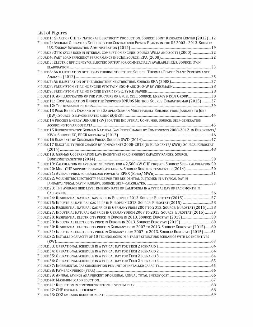
List of Figures FIGURE 1: SHARE OF CHP IN NATIONAL ELECTRICITY PRODUCTION. SOURCE: JOINT RESEARCH CENTER (2012) ... 12 FIGURE 2: AVERAGE OPERATING EFFICIENCY FOR CENTRALIZED POWER PLANTS IN THE US 2003 -‐ 2013. SOURCE:
U.S. ENERGY INFORMATION ADMINISTRATION (2014) ............................................................................................... 19 FIGURE 3: OTTO CYCLE USED IN INTERNAL COMBUSTION ENGINES: SOURCE WILLS AND SCOTT (2000) ....................... 22 FIGURE 4: PART LOAD EFFICIENCY PERFORMANCE IN ICES. SOURCE: EPA (2008) ........................................................... 22 FIGURE 5: ELECTRIC EFFICIENCY VS. ELECTRIC OUTPUT FOR COMMERCIALLY AVAILABLE ICES. SOURCE: OWN
ELABORATION ....................................................................................................................................................................... 23 FIGURE 6: AN ILLUSTRATION OF THE GAS TURBINE STRUCTURE. SOURCE: THERMAL POWER PLANT PERFORMANCE
ANALYSIS (2012) ................................................................................................................................................................ 25 FIGURE 7: AN ILLUSTRATION OF THE MICROTURBINE STRUCTURE. SOURCE: EPA (2008) ............................................... 27 FIGURE 8: FREE PISTON STIRLING ENGINE VITOTWIN 350-‐F AND 300-‐W BY VIESSMANN ............................................. 28 FIGURE 9: FREE PISTON STIRLING ENGINE HYBRIGEN SE. BY KD NAVIEN ........................................................................... 28 FIGURE 10: AN ILLUSTRATION OF THE STRUCTURE OF A FUEL CELL. SOURCE: ENERGY NEXUS GROUP ........................... 30 FIGURE 11: COST ALLOCATION UNDER THE PROPOSED DNUOS METHOD. SOURCE: BHARATKUMAR (2015) ........... 37 FIGURE 12: THE RESEARCH PROCESS ........................................................................................................................................... 39 FIGURE 13 PEAK ENERGY DEMAND OF THE SAMPLE GERMAN MULTI-‐FAMILY BUILDING FROM JANUARY TO JUNE
(KW). SOURCE: SELF-‐GENERATED USING EQUEST ...................................................................................................... 44 FIGURE 14 PROCESS ENERGY DEMAND (KW) FOR THE INDUSTRIAL CONSUMER. SOURCE: SELF-‐GENERATION
ACCORDING TO VARIOUS DATA ........................................................................................................................................... 45 FIGURE 15 REPRESENTATIVE GERMAN NATURAL GAS PRICE CHANGE BY COMPONENTS 2008-‐2012. IN EURO CENTS/
KWH. SOURCE: EC, EPCR METADATA (2013) ............................................................................................................. 46 FIGURE 16 ELEMENTS OF CONSUMER PRICES. SOURCE: SWD (2014) ................................................................................ 47 FIGURE 17 ELECTRICITY PRICE CHANGE BY COMPONENTS 2008-‐2013 (IN EURO CENTS/ KWH). SOURCE: EUROSTAT
(2014) .................................................................................................................................................................................. 48 FIGURE 18: GERMAN COGERENATION LAW INCENTIVES FOR DIFFERENT CAPACITY RANGES. SOURCE:
BUNDESNETZAGENTUR (2014) ........................................................................................................................................ 50 FIGURE 19: CALCULATION OF AVERAGE INCENTIVES FOR A 2,500 KW CHP PROJECT. SOURCE: SELF-‐ CALCULATION . 50 FIGURE 20: MINI-‐CHP SUPPORT PROGRAM CATEGORIES. SOURCE: BUNDESNETZAGENTUR (2014) .............................. 50 FIGURE 21: AVERAGE PRICE FOR BASELOAD POWER AT EPEX (EURO/ MWH) .................................................................. 51 FIGURE 22: VOLUMETRIC ELECTRICITY PRICE FOR THE RESIDENTIAL CUSTOMER IN A TYPICAL DAY IN
JANUARY.TYPICAL DAY IN JANUARY. SOURCE: SELF-‐ CALCULATED. ............................................................................ 53 FIGURE 23: THE AVERAGE GRID LEVEL EMISSION RATE OF CALIFORNIA IN A TYPICAL DAY OF EACH MONTH IN
CALIFORNIA. .......................................................................................................................................................................... 56 FIGURE 24: RESIDENTIAL NATURAL GAS PRICE IN EUROPE IN 2013. SOURCE: EUROSTAT (2015) ................................ 57 FIGURE 25: INDUSTRIAL NATURAL GAS PRICE IN EUROPE IN 2013. SOURCE: EUROSTAT (2015). ................................. 58 FIGURE 26: RESIDENTIAL NATURAL GAS PRICE IN GERMANY FROM 2007 TO 2013. SOURCE: EUROSTAT (2015) ..... 58 FIGURE 27: INDUSTRIAL NATURAL GAS PRICE IN GERMANY FROM 2007 TO 2013. SOURCE: EUROSTAT (2015) ....... 59 FIGURE 28: RESIDENTIAL ELECTRICITY PRICE IN EUROPE IN 2013. SOURCE: EUROSTAT (2015) .................................. 59 FIGURE 29: INDUSTRIAL ELECTRICITY PRICE IN EUROPE IN 2013. SOURCE: EUROSTAT (2015) .................................... 60 FIGURE 30: RESIDENTIAL ELECTRICITY PRICE IN GERMANY FROM 2007 TO 2013. SOURCE: EUROSTAT (2015) ....... 60 FIGURE 31: INDUSTRIAL ELECTRICITY PRICE IN GERMANY FROM 2007 TO 2013. SOURCE: EUROSTAT (2015) ......... 61 FIGURE 32: INSTALLED CAPACITY OF 10 TECHNOLOGIES IN 4 TARIFF STRUCTURE SCENARIOS WITH NO INCENTIVES
(KW). ..................................................................................................................................................................................... 63 FIGURE 33: OPERATIONAL SCHEDULE IN A TYPICAL DAY FOR TECH 2 SCENARIO 1 ............................................................. 64 FIGURE 34: OPERATIONAL SCHEDULE IN A TYPICAL DAY FOR TECH 2 SCENARIO 2 ............................................................. 64 FIGURE 35: OPERATIONAL SCHEDULE IN A TYPICAL DAY FOR TECH 2 SCENARIO 3 ............................................................. 64 FIGURE 36: OPERATIONAL SCHEDULE IN A TYPICAL DAY FOR TECH 2 SCENARIO 4 ............................................................. 65 FIGURE 37: INCREMENTAL GAS CONSUMPTION PER UNIT OF INSTALLED CAPACITY. ............................................................ 65 FIGURE 38: PAY-‐BACK PERIOD (YEAR) ........................................................................................................................................ 66 FIGURE 39: ANNUAL SAVINGS AS A PERCENT OF ORIGINAL ANNUAL TOTAL ENERGY COST ................................................. 66 FIGURE 40: MAXIMUM LOAD REDUCTION .................................................................................................................................... 67 FIGURE 41: REDUCTION IN CONTRIBUTION TO THE SYSTEM PEAK .......................................................................................... 68 FIGURE 42: CHP OVERALL EFFICIENCY ....................................................................................................................................... 68 FIGURE 43: CO2 EMISSION REDUCTION RATE ............................................................................................................................ 69

FIGURE 44: INSTALLED CAPACITY OF 10 TECHNOLOGIES IN 4 TARIFF STRUCTURE SCENARIOS (KW) ............................. 69 FIGURE 45: INCREMENTAL GAS CONSUMPTION PER UNIT OF INSTALLED CAPACITY. ............................................................ 70 FIGURE 46: PART LOAD EFFICIENCY PERFORMANCE IN ICES (LEFT) AND ELECTRICITY EXPORT PERCENTAGE (RIGHT).
SOURCE: EPA (2008), SELF-‐CALCULATION ................................................................................................................... 71 FIGURE 47: ANNUAL SAVINGS AS A PERCENT OF ORIGINAL ANNUAL TOTAL ENERGY COST ................................................. 71 FIGURE 48: ANNUAL INCENTIVES RECEIVED BY THE CUSTOMER AS A PERCENTAGE OF ANNUAL TOTAL ENERGY COST .. 72 FIGURE 49: PAY-‐BACK PERIOD (YEAR) ........................................................................................................................................ 72 FIGURE 50: INSTALLED CAPACITY OF 10 TECHNOLOGIES IN 4 TARIFF STRUCTURE SCENARIOS (KW) ............................. 73 FIGURE 51: INCREMENTAL GAS CONSUMPTION PER UNIT OF INSTALLED CAPACITY. ............................................................ 73 FIGURE 52: OPERATIONAL SCHEDULE IN A TYPICAL DAY FOR TECH 2 SCENARIO 4 WHEN THERE IS EXPORT INCENTIVE
IN PLACE ................................................................................................................................................................................. 74 FIGURE 53: OPERATIONAL SCHEDULE IN A TYPICAL DAY FOR TECH 2 SCENARIO 4 WHEN THERE IS NO EXPORT
INCENTIVE IN PLACE ............................................................................................................................................................. 74 FIGURE 54: ANNUAL SAVINGS AS A PERCENT OF ORIGINAL ANNUAL TOTAL ENERGY COST ................................................. 75 FIGURE 55: ANNUALIZED CAPEX INCENTIVES RECEIVED BY THE CUSTOMER AS A PERCENTAGE OF ANNUAL TOTAL
ENERGY COST ......................................................................................................................................................................... 75 FIGURE 56: MAXIMUM LOAD REDUCTION .................................................................................................................................... 76 FIGURE 57: REDUCTION IN CONTRIBUTION TO THE SYSTEM PEAK .......................................................................................... 76 FIGURE 58: CHP OVERALL EFFICIENCY ....................................................................................................................................... 77 FIGURE 59: CO2 EMISSION REDUCTION RATE ............................................................................................................................ 77 FIGURE 60: OPERATIONAL SCHEDULE IN A TYPICAL DAY FOR TECH 2 SCENARIO 4 -‐BASE CASE ....................................... 78 FIGURE 61: OPERATIONAL SCHEDULE IN A TYPICAL DAY FOR TECH 2 SCENARIO 4 -‐DECREASED ELECTRICITY PRICE .. 78 FIGURE 62: OPERATIONAL SCHEDULE IN A TYPICAL DAY FOR TECH 2 SCENARIO 4 -‐INCREASED ELECTRICITY PRICE .... 79 FIGURE 63: OPERATIONAL SCHEDULE IN A TYPICAL DAY FOR TECH 2 SCENARIO 4 -‐DECREASE NG PRICE ..................... 79 FIGURE 64: OPERATIONAL SCHEDULE IN A TYPICAL DAY FOR TECH 2 SCENARIO 4 -‐INCREASE NG PRICE ....................... 79 FIGURE 65: OPERATIONAL SCHEDULE IN A TYPICAL DAY FOR TECH 2 SCENARIO 4 -‐DOUBLE PX PRICE .......................... 80 FIGURE 66: ANNUAL SAVINGS THROUGH OPERATIONS FOR TECH 2 SCENARIO 4 IN DIFFERENT MARKET CONDITIONS . 80 FIGURE 67: CHP OVERALL EFFICIENCIES FOR TECH 2 SCENARIO 4 IN DIFFERENT MARKET CONDITIONS ....................... 81 FIGURE 68: INCREMENTAL NG PURCHASES FOR TECH 2 SCENARIO 4 IN DIFFERENT MARKET CONDITIONS ................... 81 FIGURE 69: INSTALLED CAPACITY OF 10 TECHNOLOGIES IN 4 TARIFF STRUCTURE SCENARIOS ......................................... 84 FIGURE 70: OPERATIONAL SCHEDULE IN A TYPICAL DAY FOR TECH 1 SCENARIO 1 ............................................................. 85 FIGURE 71: OPERATIONAL SCHEDULE IN A TYPICAL DAY FOR TECH 1 SCENARIO 2 ............................................................. 86 FIGURE 72: OPERATIONAL SCHEDULE IN A TYPICAL DAY FOR TECH 1 SCENARIO 3 AND 4 ................................................. 87 FIGURE 73: INCREMENTAL GAS CONSUMPTION PER UNIT OF INSTALLED CAPACITY. ............................................................ 87 FIGURE 74: PAY-‐BACK PERIOD (YEAR) ........................................................................................................................................ 88 FIGURE 75: ANNUAL SAVINGS AS A PERCENT OF ORIGINAL ANNUAL TOTAL ENERGY COST ................................................. 88 FIGURE 76: MAXIMUM LOAD REDUCTION .................................................................................................................................... 89 FIGURE 77: CONTRACTED CAPACITY REDUCTION ...................................................................................................................... 89 FIGURE 78: REDUCTION IN CONTRIBUTION TO THE SYSTEM PEAK .......................................................................................... 90 FIGURE 79: CHP OVERALL EFFICIENCY ....................................................................................................................................... 90 FIGURE 80: CO2 EMISSION REDUCTION RATE ............................................................................................................................ 91 FIGURE 81: INSTALLED CAPACITY OF 10 TECHNOLOGIES IN 4 TARIFF STRUCTURE SCENARIOS ......................................... 91 FIGURE 82: OPERATIONAL SCHEDULE IN A TYPICAL DAY FOR TECH 1 SCENARIO 4 -‐WITH INCENTIVE ............................ 92 FIGURE 83: OPERATIONAL SCHEDULE IN A TYPICAL DAY FOR TECH 1 SCENARIO 4 –BASE CASE ....................................... 93 FIGURE 84: INCREMENTAL GAS CONSUMPTION PER UNIT OF INSTALLED CAPACITY. ............................................................ 93 FIGURE 85: ANNUAL INCENTIVES RECEIVED BY THE CUSTOMER AS A PERCENTAGE OF ANNUAL TOTAL ENERGY COST .. 94 FIGURE 86: PAY-‐BACK PERIOD (YEAR) ........................................................................................................................................ 94 FIGURE 87: REDUCTION IN CONTRIBUTION TO THE SYSTEM PEAK .......................................................................................... 95 FIGURE 88: CHP OVERALL EFFICIENCY ....................................................................................................................................... 95 FIGURE 89: CO2 EMISSION REDUCTION RATE ............................................................................................................................ 96 FIGURE 90: INSTALLED CAPACITY OF 10 TECHNOLOGIES IN 4 TARIFF STRUCTURE SCENARIOS ......................................... 96 FIGURE 91: INCREMENTAL GAS CONSUMPTION PER UNIT OF INSTALLED CAPACITY ............................................................. 97 FIGURE 92: ANNUALIZED CAPEX INCENTIVES RECEIVED BY THE CUSTOMER AS A PERCENTAGE OF ANNUAL TOTAL
ENERGY COST ......................................................................................................................................................................... 97 FIGURE 93: PAY-‐BACK PERIOD (YEAR) ........................................................................................................................................ 98

FIGURE 94: CHP OVERALL EFFICIENCY ....................................................................................................................................... 98 FIGURE 95: CO2 EMISSION REDUCTION RATE ............................................................................................................................ 99 FIGURE 96: OPERATIONAL SCHEDULE IN A TYPICAL DAY FOR TECH 2 SCENARIO 4 -‐BASE CASE .................................... 100 FIGURE 97: OPERATIONAL SCHEDULE IN A TYPICAL DAY FOR TECH 2 SCENARIO 4 -‐ELECTRICITY PRICE DECREASE .. 100 FIGURE 98: OPERATIONAL SCHEDULE IN A TYPICAL DAY FOR TECH 2 SCENARIO 4 -‐ELECTRICITY PRICE INCREASE ... 101 FIGURE 99: OPERATIONAL SCHEDULE IN A TYPICAL DAY FOR TECH 2 SCENARIO 4 -‐GAS PRICE DECREASE ................. 102 FIGURE 100: OPERATIONAL SCHEDULE IN A TYPICAL DAY FOR TECH 2 SCENARIO 4 -‐GAS PRICE INCREASE ................ 102 FIGURE 101: OPERATIONAL SCHEDULE IN A TYPICAL DAY FOR TECH 2 SCENARIO 4 -‐DOUBLE EXPORT PRICE ............. 103 FIGURE 102: ANNUAL SAVINGS THROUGH OPERATIONS FOR TECH 2 SCENARIO 4 IN DIFFERENT MARKET CONDITIONS
.............................................................................................................................................................................................. 104 FIGURE 103: CHP OVERALL EFFICIENCIES FOR TECH 2 SCENARIO 4 IN DIFFERENT MARKET CONDITIONS .................. 104 FIGURE 104: INCREMENTAL NG PURCHASES FOR TECH 2 SCENARIO 4 IN DIFFERENT MARKET CONDITIONS ............. 105
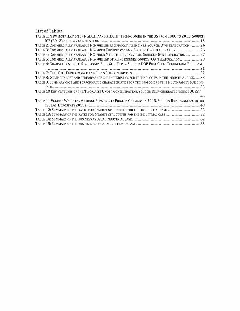
List of Tables TABLE 1: NEW INSTALLATION OF NGDCHP AND ALL CHP TECHNOLOGIES IN THE US FROM 1900 TO 2013; SOURCE:
ICF (2013) AND OWN CALCULATION ............................................................................................................................... 13 TABLE 2: COMMERCIALLY AVAILABLE NG-‐FUELLED RECIPROCATING ENGINES. SOURCE: OWN ELABORATION ............. 24 TABLE 3: COMMERCIALLY AVAILABLE NG-‐FIRED TURBINE SYSTEMS. SOURCE: OWN ELABORATION .............................. 26 TABLE 4: COMMERCIALLY AVAILABLE NG-‐FIRED MICROTURBINE SYSTEMS. SOURCE: OWN ELABORATION .................. 27 TABLE 5: COMMERCIALLY AVAILABLE NG-‐FUELLED STIRLING ENGINES. SOURCE: OWN ELABORATION ......................... 29 TABLE 6: CHARACTERISTICS OF STATIONARY FUEL CELL TYPES. SOURCE: DOE FUEL CELLS TECHNOLOGY PROGRAM
................................................................................................................................................................................................. 31 TABLE 7: FUEL CELL PERFORMANCE AND COSTS CHARACTERISTICS ..................................................................................... 32 TABLE 8: SUMMARY COST AND PERFORMANCE CHARACTERISTICS FOR TECHNOLOGIES IN THE INDUSTRIAL CASE ........ 33 TABLE 9: SUMMARY COST AND PERFORMANCE CHARACTERISTICS FOR TECHNOLOGIES IN THE MULTI-‐FAMILY BUILDING
CASE ........................................................................................................................................................................................ 33 TABLE 10 KEY FEATURES OF THE TWO CASES UNDER CONSIDERATION. SOURCE: SELF-‐GENERATED USING EQUEST
................................................................................................................................................................................................. 43 TABLE 11 VOLUME WEIGHTED AVERAGE ELECTRICITY PRICE IN GERMANY IN 2013. SOURCE: BUNDESNETZAGENTUR
(2014), EUROSTAT (2015) .............................................................................................................................................. 49 TABLE 12: SUMMARY OF THE RATES FOR 4 TARIFF STRUCTURES FOR THE RESIDENTIAL CASE. ........................................ 52 TABLE 13: SUMMARY OF THE RATES FOR 4 TARIFF STRUCTURES FOR THE INDUSTRIAL CASE ........................................... 52 TABLE 14: SUMMARY OF THE BUSINESS AS USUAL INDUSTRIAL CASE ..................................................................................... 62 TABLE 15: SUMMARY OF THE BUSINESS AS USUAL MULTI-‐FAMILY CASE ................................................................................ 83
1. Introduction In order to achieve a more sustainable energy system, regulators and the industry are trying to balance among many challenging issues such as environmental concerns, economic efficiency and security of supply, with an increasing weight on the first factor in recent years (EU 2012). While it is important to continue exploring the potential of renewables, which provide alternative sources of energy, as well as other clean energy sources, finding a more effective way to utilize existing resources is also considered, by both the industry and the regulators, as a viable solution. Indeed, around 65% of all energy used to generate electricity is lost during the energy conversion, transmission and distribution processes (US Energy Information Administration 2009) (European Environment Agency 2015). The room for efficiency improvement is ample for combined heat and power (CHP) technologies on the distributed level. Benefits of distributed generators arise from their direct connection to distribution and customer facilities, which can potentially alleviate transmission and distribution network constraints, lower network energy losses, improve system reliability, and result in CO2 emissions reductions and overall capital cost (Strachan 2002) (Gil 2006). However, distributed combined heat and power systems (DCHP) still faces techno-‐economic challenges, ranging from high initial investment to relatively low electric efficiencies, flexibilities and reliability. Their penetration is influenced by regulatory and market conditions such as fuel price, overall energy mix in the wholesale market, electricity tariff structure, subsidies and incentives. This thesis tries to understand the value of CHP, not only to the energy consumers, but also to the system and society, based on different scenarios that are both representative and realistic. From the individual customer’s perspective, the essence of this research is to have a relatively realistic representation of the techno-‐economic scenarios that typical customers face, and draw general insights on how the attractiveness and value of CHP technologies are influenced by external factors. On the other hand, from the viewpoint of regulator, this thesis tries to address the question “What are the merits and drawbacks of various tariffication method based on economic, environmental and efficiency metrics?” This thesis develops a framework and methodology that can take in energy, technology and market information and find the optimal installation and operation decisions for different CHP technologies. This methodology focuses on analyzing customers’ reactions to various exogenous parameters and utilizes multiple metrics to show the consequent impacts on the energy bill, the grid and the environment.

1.1. Research Motivation
1.1.1. The European Context Europe is making great efforts to limit greenhouse gas emissions, promote renewable energy resources and improve energy efficiency, as is evidenced by the sustained commitment to the so-‐called “20-‐20-‐20” target, a legally binding climate and energy package established by the European Commission (European Commission 2014). These efforts have given rise to the rapid growth of not only various renewable energy systems, but also distributed energy resources and CHP technologies1. For instance as early as 2005, 15 European states had already achieved a distributed generation penetration rate of more than 10% (Frias 2008). The Joint Research of European Commission’s research has shown (see Figure 1) that CHP penetration had reached significant value in certain Northern European nations by 20122. Moreover, the CODE 2 project, funded by the European Union, has estimated that CHP could generate 20% of the EU’s electricity by 2030, if proper policies and subsidies are implemented (CODE 2 2015).
Figure 1: Share of CHP in National Electricity Production. Source: Joint Research Center (2012)
This transformative energy landscape will have significant influence on all stakeholders, ranging from governments and regulatory agencies, to equipment manufacturers, utilities, gas companies and customers, especially in the context of the liberalization of the electricity and gas sectors in the EU. It has prompted the interest not only from academia, but also industry. For instance, European conglomerates like ABB and Siemens have articulated their views on a future power system and utility sector with increased integration of decentralized resources (ABB 2010) (Utility Dive n.d.).
1 These three concepts are not mutually exclusive. For example, a small concentrated solar power (CSP) system that can provide both electricity and heat could be categorized as any one of the three concepts. 2 For comparison, in 2008, cogeneration accounted for 9 percent of the total U.S. electricity generating capacity.

1.1.2. Natural Gas Fired Distributed CHP (NGDCHP) Technologies Admittedly, the rapid growth of distributed energy resources (DER) and CHP technologies in Europe should be attributed to various tailwinds, ranging from falling costs due to technical advancement and liberalization of the retail market, to the increasing emphasis on policy goals such as reliability and decarbonization (J.A.P. Lopes 2007). However, it is noticeable that the success in the renewable sector and the larger CHP technologies is not observed in the distributed CHP system. The potential opportunities and barriers to distributed CHP systems are less understood. A distributed level system refers to technologies with electric capacities below 10 MW, a rough threshold for generators connected to distribution networks. Technologies in this range can be further classified as Micro (<50 kW), mini (<500kW), and small (<1MW) respectively. Combined heat and Power (CHP), also known as cogeneration, denotes a group of technologies that generate electricity and useful heat concurrently. While a detailed discussion of technologies in each category can be found in the next chapter, it is worth noting that in general, the cogeneration feature gives these technologies much higher overall efficiency than the separate generation of electricity and useful heat. In fact, it has a long history within large industrial applications. Several energy intense industries such as chemicals, metal, oil refining and pulp and paper manufacturing account for more than 80 percent of the total global electric CHP capacity (Center for Climate and Energy Solutions 2010)3. These low hanging fruits have been long recognized by the industry and thus are mature and saturated. However, there is a clear trend for CHPs to move to smaller applications. For instance, as is shown in Table 1, the newly installed capacity of NGDCHP as a percentage of the total CHP installation has increased steadily from 1900 to 2012 in the US, especially after 2008.
Period NGDCHP (kW) Total CHP (kW) NGDG Penetration 1900-‐2000 1,806,066 66,901,837 2.70% 2001-‐2007 634,593 13,559,976 4.68% 2008-‐2011 418,703 1,975,691 21.19% 2012-‐ 2013 Q1 105,610 468,840 22.53% Table 1: New Installation of NGDCHP and all CHP Technologies in the US from 1900 to 2013; Source: ICF (2013) and own calculation
3 However, these CHP systems are generally very large and are beyond the scope of this research.

Finally, this thesis focuses on natural gas fired CHP systems specifically because the potentially higher scalability compared with some other fuel sources such as biofuels, hydrogen and diesels4.
1.1.3. Challenges for NGDCHP Gas fired distributed CHP projects can yield numerous private and public benefits. As mentioned above, they tend to have higher overall efficiencies and can reduce the environmental impact of power generation. Moreover, on-‐site generation can reduce peak electrical demand on the grid and thus alleviate electric grid constraints and losses, if the customers receive proper economic signals. Prior research also identified other advantages such as better resilience in the face of grid outages, deferred in vestment in the network, potential improvement on the stability from reactive power and voltage support and reduced fuel price volatilities, which will be discussed in more detail in the next chapter. However, several barriers and technical limitations have hindered the full realization of these benefits. In order to successfully promote and integrate distributed energy resources, efforts must be made not only on improving the current network infrastructure and information and communication technologies, but also updating regulatory and policy frameworks, technical standards, and industry structures. The tariff scheme is the key issue among all these factors, as it connects the upstream regulatory objectives and the downstream industries and customers, with a significant influence on infrastructure investment and operational decisions. Current tariffication methods may not be suitable for the rapidly evolving environment. Electric utilities may apply different rates and special charges to distributed energy projects than that to non-‐producing customers. While the legitimacy of these practices lies in the need to recover reduced income and additional costs associated with special services required for the DGs, if not well designed, they can pose significant and unnecessary obstacles to tap the full potential of these opportunities. An appropriate tariff design should allow the utilities to recover costs and reasonable profits while sending correct economic signals to the end-‐users and on-‐site generators. In addition to the general issues that DGs face, another four barriers should be addressed to mobilize CHP potential in Europe: insufficient recognition and reward to CHP’s efficiency gains at the energy system level; hurdles for distributed generators in connecting to and operating on the network; uncertainties and risks associated with regulations, and a lack of understanding and planning of usable heat (CODE 2 2015). 4 Besides the advantage of wide availability, factors such as ease of maintenance and low impurity and pollution are also clear advantages. Moreover, as shale gas and Caspian gas are being developed, sufficient supply may also drive down the fuel cost.

1.2. Research Question This thesis focuses on understanding the technological, social and economic attractiveness of CHP technologies under different tariff designs, market conditions and incentives. It not only looks at the optimum economic value of CHP to individual customers, but also impacts on the system’s peak load and the environment. The premise is that, even if individual customers are only reacting to economic signals and regulatory constraints, without explicit considerations on the overall social and grid level costs, a good tariff design should be able to send the correct economic signals to all participants so that the welfare of both individual customers and the overall society is improved. Therefore, the main questions that this thesis attempts to answer are:
• How does relative economic attractiveness of different CHP technologies look like from the perspective of individual customers?
• How do different tariff structures influence the decision making process of individual customers who are considering having distributed CHP technologies on-‐site? More specifically, how do the customers respond to the economic signals by changing their installation capacity and the operation schedules?
• What are the effects in terms of energy efficiency, contribution to peak load, CO2 emissions and natural gas consumption, all of them with implications in the system’s costs and social welfare?
• How sensitive are these observations in relation to key market conditions, technology and regulatory requirements?
On the one hand, from the individual customer’s perspective, the essence of this research is to have a relatively realistic representation of the techno-‐economic scenarios that typical customers face, and draw general insights on how the attractiveness and value of CHP technologies are influenced by external factors. On the other hand, from the regulator’s viewpoint, this thesis tries to address the question “What are the merits and drawbacks of various tariff methods based on economic, environmental and efficiency metrics?” Complex and interesting dynamics are expected between the overall system’s cost and the individual customers’ decision-‐making, especially when the penetration rate of distributed CHP technologies increases over time. For instance, when lots of distributed CHP technologies are generating electricity at the same time in the peak hours, it is likely that both the short-‐term marginal electricity price and the long-‐term network investment on the grid level would be different from that in the business as usual case. However, it is beyond the scope of this research to model such interplay. Rather, this thesis focuses on the early adoption phase, when the penetration of distributed CHP is low and their influence on the system is not

significant. This assumption is also in line with the current situation within the European energy sector, as discussed above. Moreover, this thesis looks at the “economically optimal” decisions that a customer would make when faced with various economic signals. Generally, it is expected that, rational customers will react to economic signals through both demand response, i.e. changing their consumption patterns, and on-‐site generation. As the focus of this research is on CHP technologies, it is assumed that customers do not change their consumption behavior in response to prices, but rather shift their energy source between electricity and gas. In addition, in order to get an “optimal” outcome, CHP technologies should have the flexibility to react in a timely manner to the economic signals. In theory, this would provide CHPs with the potential to create additional value by participating in ancillary markets. However, this mechanism is not widely applied to generators on the distributed level and, thus, has not been included in this analysis. Therefore, the thesis calibrates the maximum value of distributed CHP technologies when holding energy consumption loads fixed and without explicitly including the potential value of providing ancillary services.
1.3. Methodology In order to understand the impact of different regulatory tariffs on the attractiveness of different CHP technologies, and their complex interactions with other techno-‐economic parameters, the thesis develops a methodology that focuses on analyzing customers’ behavior to various exogenous parameters by looking at their CHP installation and operation decisions. Moreover, it adopts an overarching framework that integrates and streamlines the various processes from the simulation of customers’ energy loads, the representation of regulatory and market conditions, to the generation and interpretation of the installation and operations decisions. To analyze a specific application case, we first accrue, triangulate and compile three categories of data relevant to the case: energy load, technology specifics and market conditions. First, a thorough review of currently available CHP technologies is conducted, and we parameterize the technologies using some key techno-‐economic metrics such as capital cost, electric efficiency and heat-‐to-‐power ratio. Secondly, we use raw data on weather, building design and end-‐user demand patterns to construct and simulate the energy load profile for a particular customer over a year. For computational efficiency, we then synthesize the data to get load profiles for representative days in a year. Thirdly, we analyze the regulations and price information of the selected market, and construct different tariff structures, incentives and price level scenarios. Then an optimization model is adopted to determine the economically optimal installation and operational decisions for different CHP technologies, for the

customer utilizing the aforementioned three categories of data. The output from the model in each scenario is then compared with the business as usual (BAU) scenario. The BAU scenario is that when the customer imports electricity solely from the grid and generates heat using a conventional boiler or furnace. Besides comparing the total installation and hourly operation, several metrics are used to show the impacts of CHPs on the environment, peak demand, and the customer’s energy bill. Finally, we conduct a sensitivity analysis to see how changes in market conditions influence our findings.
1.4 Research Outline The thesis is structured as follows: Chapter 2 starts with a literature review on the recent advances and impacts of distributed energy systems; categories, characteristics and parameters of distributed cogeneration technologies; and a discussion on the topic of the tariff designs and recent developments in this area. Chapter 3 is devoted to explain the methodology, tools and models that are adopted and developed for the analysis; the required data; the assumptions and processes involved in constructing different scenarios; and it defines the metrics to interpret and evaluate the output from the model. Chapter 4 shows and compares the results of different scenarios; and performs sensitivity analyses to critical variables including fuel prices, electricity purchase prices, and electricity export prices. Chapter 5 summarizes the findings, discusses the implications for different stakeholders; and finally identifies the areas of improvement and additional research.

2. Literature Review
2.1. Distributed Energy Systems and their impact
2.1.1. The benefits of NGDCHP Natural gas fired distributed cogeneration systems have started to attract interest from both the industry and the academia in recent years (MIT Energy Initiative 2014), which should be seen in the context of the overall popularity of distributed energy systems. Like many other DERs, NGDCHP has the potential to improve the energy system on multiple fronts:
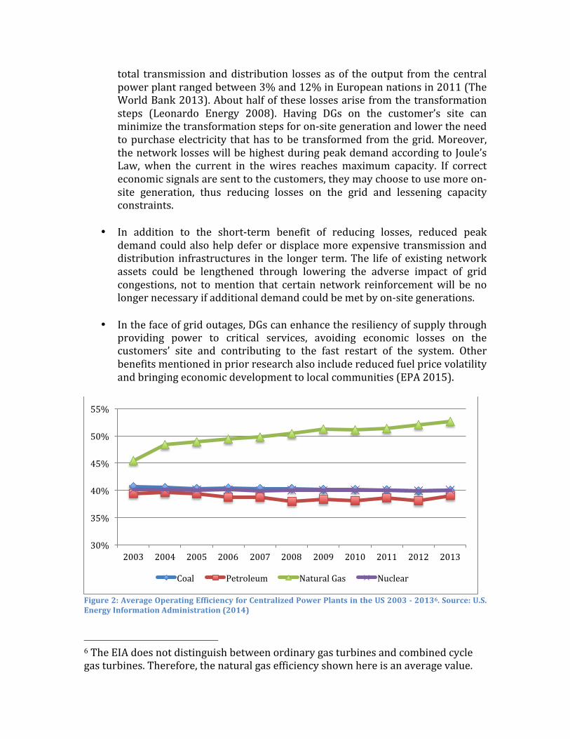
• The most obvious advantage of gas fired combined heat and power is higher efficiencies. The typical method of centralized electricity generation and on-‐site heat generation results in lower usage of the total energy input. As shown in Figure 2, the efficiencies of typical coal and petroleum power plants average around 40% and have not shown an overall improvement in the past decade5. The efficiency of natural gas fired central plants benefited from the introduction and improvement of combined cycle gas turbine technology (CCGT), but still falls short of the overall efficiency of 80% that many cogeneration systems can achieve. Admittedly, electricity in general has higher value than heat, and centralized power plants make economic sense in many cases. From the perspective of primary energy saving, however, cogeneration makes better use of the waste heat from the electricity generation process, and thus yields a more attractive outcome. Alternatively, cogeneration reduces the energy consumption in standalone boilers and furnaces devoted to satisfy heat demand as well as the purchase of electricity from the grid, which may result in better economics for individual customers.
• Cogeneration reduces the environmental impact of power and heat generation as it requires less fuel input to achieve the same level of output and, therefore, can lower CO2 emissions. This effect is compounded with the fact that natural gas contains much lower carbon content on a per energy unit basis compared with coal and oil, which makes NGDCHP systems a valuable alternative on the decarbonization roadmap. Besides CO2, other air pollutants such as SO2, NOx and Hg can also be reduced if proper treatment technologies are in place.
• On-‐site DG systems are usually connected to the power grid, and the
customers can choose to purchase from or sell electricity back to the grid. This feature gives the technology the potential to reduce peak electrical demand on the grid as well as alleviate constraints and network losses. The
5 Not taking into account transformation losses and heat resistance losses on the grid.
total transmission and distribution losses as of the output from the central power plant ranged between 3% and 12% in European nations in 2011 (The World Bank 2013). About half of these losses arise from the transformation steps (Leonardo Energy 2008). Having DGs on the customer’s site can minimize the transformation steps for on-‐site generation and lower the need to purchase electricity that has to be transformed from the grid. Moreover, the network losses will be highest during peak demand according to Joule’s Law, when the current in the wires reaches maximum capacity. If correct economic signals are sent to the customers, they may choose to use more on-‐site generation, thus reducing losses on the grid and lessening capacity constraints.
• In addition to the short-‐term benefit of reducing losses, reduced peak demand could also help defer or displace more expensive transmission and distribution infrastructures in the longer term. The life of existing network assets could be lengthened through lowering the adverse impact of grid congestions, not to mention that certain network reinforcement will be no longer necessary if additional demand could be met by on-‐site generations.
• In the face of grid outages, DGs can enhance the resiliency of supply through
providing power to critical services, avoiding economic losses on the customers’ site and contributing to the fast restart of the system. Other benefits mentioned in prior research also include reduced fuel price volatility and bringing economic development to local communities (EPA 2015).
Figure 2: Average Operating Efficiency for Centralized Power Plants in the US 2003 -‐ 20136. Source: U.S. Energy Information Administration (2014)
6 The EIA does not distinguish between ordinary gas turbines and combined cycle gas turbines. Therefore, the natural gas efficiency shown here is an average value.
30%
35%
40%
45%
50%
55%
2003 2004 2005 2006 2007 2008 2009 2010 2011 2012 2013
Coal Petroleum Natural Gas Nuclear

On top of the benefits of distributed energy systems discussed above, NGDCHP have unique advantages over other DG technologies. As a relatively mature technology, CHPs can bring positive economic value with minimum or no government subsidies compared with most solar, electric storage and wind projects. There are many models and package solutions readily available on the market, which is also different from many renewable technologies. Natural gas, as a dominant fuel in many industrial, commercial and residential applications, is also widely accessible, which lowers the barrier of entry for customers. Finally, compared with intermittent energy sources, NGDCHP enjoys the benefit of controllability. Customers can take advantage of the economic signals by more smart usage of the co-‐generator, which can enhance both individual and social welfare. Research has shown that controllable DGs have the potential to provide additional reserve power and improve stability from reactive power and voltage support (Evans 2005).
2.1.2. Distributed Energy Resources Changing the Utility Landscape With the development of DERs, the energy landscape today is gradually transitioning from one of centralized generation and distribution networks that have largely consisted of predictable and, passive loads, to a network of increasingly decentralized generation and diverse system users. Indeed, as observed by many researchers, the challenges in the electricity sector have shifted from the generation/ transmission level to that of distribution, where sound planning and tariff methodologies are needed to cope with the increasing diversity in both consumption and generation patterns (THINK, 2013a) (Bharatkumar 2015). DERs have initiated the transformation of customers from passive consumers in a traditional utility business model to active “prosumers”, who both produce and consume energy and interact with the grid. Given the increasingly diverse technologies adopted, and the fact that the activities behind the electricity meter are generally a black box to distribution utilities, it is no longer possible or meaningful to continue using existing customer classification or the tariffs associated with it. This transition has raised several interesting questions:
• How to give the correct economic signals and by doing so achieve better performance at the system level? Here, regulators must carefully weigh between policy goals such as economic efficiencies, cost causality and transparency. The next section is devoted to this topic.
• What are the optimum penetration levels of DGs and what policies are needed to achieve that goal? To answer this question, policy makers first need to have a better understanding of the value DGs create by, for example, lowering system costs and CO2 emissions.
• How to better calibrate the economics of DGs from the individual customers’ point of view? To fully release the value of DGs, the installation and operation decisions on these technologies must take into

account various technical-‐economic inputs. This increases the complexity and renders the traditional method of levelized electricity cost less efficient. For instance, the rates applied to the services associated with interconnection and to buy back electricity from DGs have a significant effect on the economic viability of the projects. In a market where electricity import and export price varies on an hourly basis, decision makers would change their operations accordingly. But levelized electricity price can hardly reach such granularity and thus make it hard to compare between different scenarios. More specifically, levelized electricity cost have to assume an average utilization rate throughout the year, which is neither accurate nor realistic. Therefore, tools that can model the decision making process in more detail is needed.
2.1.3. Review of NGDCHPs with Capacities up to 10MWe
2.1.3.1. Reciprocating Engines Reciprocating engines represent a widespread and mature technology. Besides co-‐generation, they are used for varied types of applications ranging from standby and emergency power, peaking service, intermediate and base-‐load power. Reciprocating engines can be characterized by two main engines designs: Spark Ignition (SI) Otto-‐cycle and Compression Ignition (CI) Diesel-‐cycle engines. Both have cylindrical combustion chambers, in which pistons travel the length of the cylinders. The pistons are linked to a crankshaft by connecting rods that transform the linear motion into rotary motion. Most engines have multiple cylinders that power a single crankshaft. As it injects fuel and air into the cylinders where combustion occurs, people also refer this kind of technologies as internal combustion engine, in comparison with external combustion engines such as sterling engines and rankine engines.
The Otto-‐cycle completes a power cycle in four strokes of the piston within the cylinder (see Figure 3 for an illustration). The intake stroke takes air mixed with fuel into the cylinder. Then the compression stroke compresses the air-‐fuel mixture within the cylinder, which is ignited by an ignition source. As the combustion process takes place, this produces pressure and heat to move the piston in the power stroke. Finally, in the exhaust stroke the exhaust of the combustion process is removed from the engine through the exhaust port (Willis and Scott 2000). As the piston moves, the crankshaft rotates. This mechanical energy is used to drive a generator. The exhaust heat, as well as the heat from the lubricating air cooler and the jacket water cooler of the engine, is recovered using heat exchangers, and then supplied to the heating system.
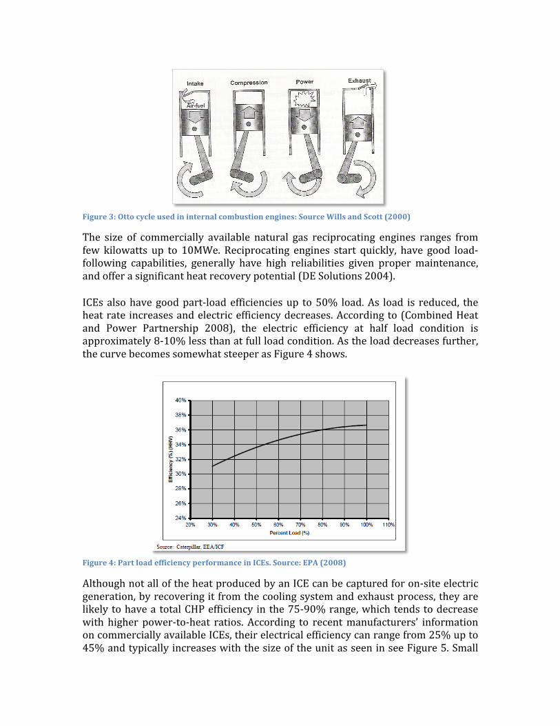
Figure 3: Otto cycle used in internal combustion engines: Source Wills and Scott (2000)
The size of commercially available natural gas reciprocating engines ranges from few kilowatts up to 10MWe. Reciprocating engines start quickly, have good load-‐following capabilities, generally have high reliabilities given proper maintenance, and offer a significant heat recovery potential (DE Solutions 2004).
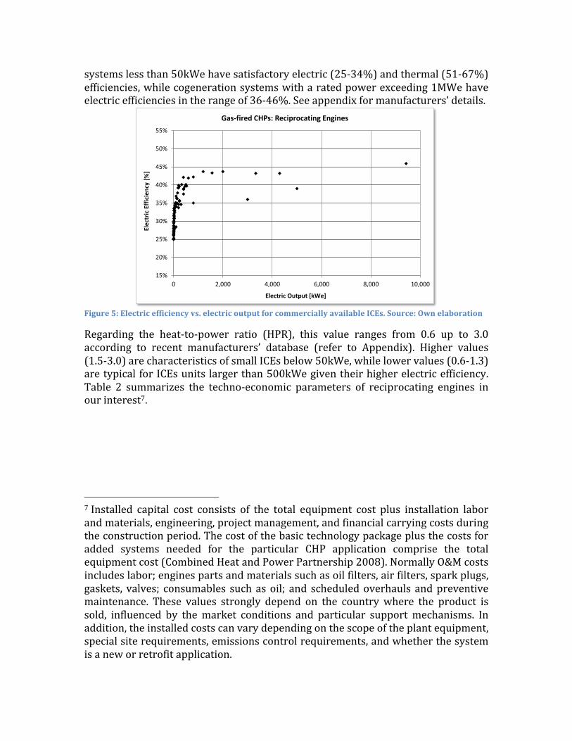
ICEs also have good part-‐load efficiencies up to 50% load. As load is reduced, the heat rate increases and electric efficiency decreases. According to (Combined Heat and Power Partnership 2008), the electric efficiency at half load condition is approximately 8-‐10% less than at full load condition. As the load decreases further, the curve becomes somewhat steeper as Figure 4 shows.
Figure 4: Part load efficiency performance in ICEs. Source: EPA (2008)
Although not all of the heat produced by an ICE can be captured for on-‐site electric generation, by recovering it from the cooling system and exhaust process, they are likely to have a total CHP efficiency in the 75-‐90% range, which tends to decrease with higher power-‐to-‐heat ratios. According to recent manufacturers’ information on commercially available ICEs, their electrical efficiency can range from 25% up to 45% and typically increases with the size of the unit as seen in see Figure 5. Small
systems less than 50kWe have satisfactory electric (25-‐34%) and thermal (51-‐67%) efficiencies, while cogeneration systems with a rated power exceeding 1MWe have electric efficiencies in the range of 36-‐46%. See appendix for manufacturers’ details.
Figure 5: Electric efficiency vs. electric output for commercially available ICEs. Source: Own elaboration
Regarding the heat-‐to-‐power ratio (HPR), this value ranges from 0.6 up to 3.0 according to recent manufacturers’ database (refer to Appendix). Higher values (1.5-‐3.0) are characteristics of small ICEs below 50kWe, while lower values (0.6-‐1.3) are typical for ICEs units larger than 500kWe given their higher electric efficiency. Table 2 summarizes the techno-‐economic parameters of reciprocating engines in our interest7.
7 Installed capital cost consists of the total equipment cost plus installation labor and materials, engineering, project management, and financial carrying costs during the construction period. The cost of the basic technology package plus the costs for added systems needed for the particular CHP application comprise the total equipment cost (Combined Heat and Power Partnership 2008). Normally O&M costs includes labor; engines parts and materials such as oil filters, air filters, spark plugs, gaskets, valves; consumables such as oil; and scheduled overhauls and preventive maintenance. These values strongly depend on the country where the product is sold, influenced by the market conditions and particular support mechanisms. In addition, the installed costs can vary depending on the scope of the plant equipment, special site requirements, emissions control requirements, and whether the system is a new or retrofit application.
15%
20%
25%
30%
35%
40%
45%
50%
55%
0 2,000 4,000 6,000 8,000 10,000
Electric Efficien
cy [%
]
Electric Output [kWe]
Gas-‐fired CHPs: Reciprocating Engines

Table 2: Commercially available NG-‐fuelled reciprocating engines. Source: Own elaboration
2.1.3.2. Turbines A gas turbine (also called a combustion turbine) has three major parts. The upstream rotating compressor takes in ambient air and compresses it into higher pressure flow. The midstream combustion chamber sprays and ignites fuel8 in the air, raising the temperature and pressure of the flow, which passes energy onto the downstream turbine through pushing the turbine shaft. The turbine shaft is usually connected to drive the upstream compressor as well as other energy consuming devices such as electric generators or mechanical motors (see Figure 6). There are mainly two different kinds of gas turbine designs: aero-‐derivative, i.e. adapted aircraft engine for stationary usage; and industrial/frame structure. Although aero-‐derivative gas turbines enjoy the advantage of light weight and high efficiency, they are generally too expensive to be implemented in CHP applications. On the other hand, frame structure turbines are widely used in industrial applications and are technically and commercially mature.
8 For the scope of this report, we only discuss natural gas.
Electric(output(range [kWe] (1.0(6(9,500(Thermal(output(range [kWth] (2.5(6(8,750(Electric(efficiency((1) [%] (25(6(46(Thermal(efficiency [%] (35(6(67(Overall(efficiency [%] (73(6(96(Heat6to6power(ratio [p.u.] (0.6(6(3.0(Noise((2) [dBA] (41(6(74(Capital(cost [$/kWe] (1,400(6(3,000(if(>100kWe(
(3,500(6(5,000(if(5(6(100kWe((6,000(6(24,000(if(<(5kWe(
O&M(costs [$/kWhe] (0.009(6(0.022(Availability [%] (>(95(Hours(to(overhaul [hr] (25,000650,000(Start6up(time [sec] 10Heat(exhaust(temperature [°C] (480(6(570(Emissions [kg/MWh] (NOx:(0.045(6(0.68;(CO:(0.145(6(0.82;(CO2:(462(6(635(Fuels (Natural(Gas(6(LPG(6(Biodiesel(6(Biogas(6(Fuel(Oil(6(Butane(6(Sewage(gas(6(Vegetable(oil(
Applications(for(heat(recovery (Process(drying(6(Space(heating(6(Hot(water(6(Low(pressure(steam(6(Absorption(chillers(
Part6load(performance (OK(
Development(status (Mature(technology(6(Commercially(available(
Deployment (Europe,(Japan,(Russia,(Canada,(US(
Sources:(Own(elaboration(based(on(manufacturers(datasheets,(Angrisani(et(al.((2012),(Maghanki(et(al.((2013),(Barbieri(et(al.((2012),(EU(Joint(Research(Centre((2012),(EPA(Report((2008)((2014),(NREL((2003)
Notes:((1)(LHV(efficiency.((2)(Noise(at(162m(of(distance.

Figure 6: An illustration of the gas turbine structure. Source: Thermal Power Plant Performance Analysis (2012)
The power output of gas turbines can range from 500kWe up to 300MWe. For the interest of this project, we only focus on the small (500kWe-‐1MWe) and distributed (1MWe-‐10MWe) level systems. Applications of gas turbines in this range are becoming increasingly popular, estimated to take up more than half of the newly installed capacities worldwide (Goncharov 2013). Multiple factors such as ambient air pressure, maximum combustion temperature, fuel supply pressure, load and the design of turbine internal mechanical parts, have direct influence on the electric efficiency of the cycle of a turbine. According to manufacturers’ product information, the electric efficiency of small and distributed gas turbines can range from 17% up to 40% (see Appendix). Moreover, gas turbines are designed to achieve highest efficiency on certain output levels and are thus not as efficient during part-‐load operations. In such scenarios, the combustion temperature will be lower than optimal, resulting in less utilization of energy in the turbine shaft, as well as more NOx, CO and VOCs emissions. A summary of the performance and costs characteristics found in commercially available NG-‐fired turbines systems is shown in Table 3. The list of manufactures is provided in the Appendix for further reference.
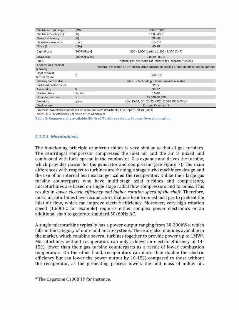
Table 3: Commercially available NG-‐fired Turbine systems. Source: Own elaboration
2.1.3.3. Microturbines The functioning principle of microturbines is very similar to that of gas turbines. The centrifugal compressor compresses the inlet air and the air is mixed and combusted with fuels spread in the combustor. Gas expands and drives the turbine, which provides power for the generator and compressor (see Figure 7). The main differences with respect to turbines are the single stage turbo machinery design and the use of an internal heat exchanger called the recuperator. Unlike their large gas turbine counterparts who have multi-‐stage axial turbines and compressors, microturbines are based on single stage radial flow compressors and turbines. This results in lower electric efficiency and higher rotation speed of the shaft. Therefore, most microturbines have recuperators that use heat from exhaust gas to preheat the inlet air flow, which can improve electric efficiency. Moreover, very high rotation speed (1,600Hz for example) requires either complex power electronics or an additional shaft to generate standard 50/60Hz AC. A single microturbine typically has a power output ranging from 30-‐300kWe, which falls in the category of mini-‐ and micro-‐systems. There are also modules available in the market, which combine several turbines together to provide power up to 1MW9. Microturbines without recuperators can only achieve an electric efficiency of 14-‐15%, lower than their gas turbine counterparts as a result of lower combustion temperature. On the other hand, recuperators can more than double the electric efficiency but can lower the power output by 10-‐15% compared to those without the recuperator, as the preheating process lowers the unit mass of inflow air.
9 The Capstone C1000HP for instance.
!Electric!output!range! ![kWe]! !500!5!1,000!!Electric!efficiency!(1)! ![%]! !16.8!5!40.1!!Overall!efficiency! ![%]! !68!5!88!!Heat5to5power!ratio! ![p.u.]! !1.05!2.0!!Noise!(2)! ![dBA]! !60590!!Capital!cost! ![2007$/kWe]! !800!5!1,900!(basic)!/!1,100!5!3,300!(CHP)!
!O&M!cost! ![2007$/kWhe]! !0.0049!5!0.011!!Fuels! !Natural!gas5!synthetic!gas5!landfill!gas5!propane5fuel!oils!!Applications!for!heat!recovery!
!heating,!hot!water,!LP5HP!steam,!drive!absorption!cooling!or!dehumidification!equipment!
!Heat!exhaust!termperature!
!°C! !3605510!
!Development!status! !Mature!technology!5!Commercially!available!!Part5load!Performance! !Poor!!Availability! !%! !92597!!Start5up!time! minutes 0.5510!Hours!to!overhual! !hr! !25,000550,000!!Emissions! !ppmv! !NOx:!15542;!CO:!20525;!CO2:!110051900!lb/MWh!!Deployment! !Europe,!Canada,!US!!!!Sources:!Own!elaboration!based!on!manufacturers!datasheets,!EPA!Report!(2008)!(2014)!!Notes:!(1)!LHV!efficiency.!(2)!Noise!at!1m!of!distance.!

Microturbines generally show good part-‐load performance since they are less sensitive to changes in combustion temperature.
Figure 7: An illustration of the microturbine structure. Source: EPA (2008)
A summary of the performance and costs characteristics found in commercially available NG-‐fired microturbines systems is shown in Table 4 10 . The list of manufactures is provided in the Appendix for further reference.
Table 4: Commercially available NG-‐fired Microturbine systems. Source: Own elaboration
2.1.3.4. Stirling Engines Stirling engines work by alternatively heating and cooling a working gas and the combustion process takes place externally in a separate burner. The working fluid -‐-‐ usually nitrogen, hydrogen or helium -‐-‐ is enclosed within a hermetically sealed pressure vessel. Heat is provided at a constant temperature at one end of a cylinder
10 The capital cost analysis is severely limited by the data availability as a result of recent industry shakeout. Many of the models that were in the market are no longer sold. Therefore, we estimated the cost based on information from various sources. See our process in the Appendix
!Electric!output!range! ![kWe]! !3!4!1,000!!Electric!efficiency!(1)! ![%]! !15!4!33!!Overall!efficiency! ![%]! !68!4!88!!Heat4to4power!ratio! ![p.u.]! !1.3!4!5.0!!Noise!(2)! ![dBA]! !65!!Capital!cost! ![$/kWe]! !1,300!4!1,400!(basic)!/!2,500!4!4,400!(CHP)!!O&M!cost! ![2007$/kWhe]! !0.01!4!0.02!!Fuels! !Natural!Gas!4!Biogas!4!Flare!gas!4!Diesel!4!Propane!4!Kerosene!!Applications!for!heat!recovery! !Space!heating!4!Hot!water!4!Low!Pressure!Steam!!Heat!exhaust!termperature! !°C! !2704310!!Development!status! !Mature!technology!4!Commercially!available!!Part4load!Performance! !OK!!Availability! !%! !95499!!Start4up!time! minutes 142!Hours!to!overhual! !hr! !20,000440,000!!Emissions! !ppmv! !NOx:!449;!CO:!5440;!THP:!549;!CO2:!140041700!lb/MWh!!Deployment! !Limited!market!growth!4!Only!3!manufacturers!!Sources:!Own!elaboration!based!on!manufacturers!datasheets,!EPA!Report!(2008)!(2014)!!Notes:!(1)!LHV!efficiency.!(2)!Noise!at!10m!of!distance.!

(the hot end), while heat is rejected at a constant temperature at the opposite end (the cold end). Work is created as the expanding gas pushes against a piston. The working gas is transferred back and forth between the two chambers, often with the aid of a displacer piston (see Figure 8 and 9). While the gas moves from the hot to the cold chamber, a regenerator captures the heat from the gas and then returns the heat to the gas as it moves back to the hot chamber, which enhances the energy-‐conversion efficiency of the process.
Figure 8: Free Piston Stirling engine Vitotwin 350-‐F and 300-‐W by Viessmann
Figure 9: Free Piston Stirling engine Hybrigen SE. by KD Navien
Since this technology is based on an external combustion system, it is possible to use different primary energy sources including fossil fuels (oil, natural gas) and even renewable energy sources (solar, biomass). This flexibility is one of the attractive features of these engines, and since the combustor is independent of the power section of the engine, it is possible to achieve low emissions and optimum heat transfer to the hot end (Goldstein 2003). The size of natural gas Stirling engines ranges from typically 1kWe up to 10kWe, with most of the commercially available technologies having an electrical output of 1kWe, while other technologies still under development. Stirling engines have good performance at partial load, offer fuel flexibility, have low emissions level and have low vibration and acceptable noise levels. However, compared to reciprocating engines, these engines need a few minutes to warm up,

have very low electric efficiency, and have a more complex power control system (Angrisani et al., 2012). The electrical efficiency is relatively low compared to other NG distributed generation technologies, ranging from 12 up to 25%. A summary of the performance and costs characteristics found in commercially available NG-‐fired SE systems is shown in Table 511.
Table 5: Commercially available NG-‐fuelled Stirling engines. Source: Own elaboration
11 Cost figures for SEs are quite dissimilar based on the little information available. EPRI (2009) states prices that range from 10,000 up to 21,000$/kWe with a long-‐term target price of about 4,500-‐10,000$/kWe. Angrisani et al. (2012) notes that the cost of SE systems decreases as the electrical capacity of the system increases, with a cost value higher than 6,500$/kWe for a system smaller than 2kWe. and Leach (2008) estimate the cost to be above 4,000$/kWe based on the expected performance of mature systems, while Houwing (2010) estimates a price above 7,000$/kWe based on expected prices at market introduction. Given the uncertainties related to expected price achievable when the technology matures, we are using the cost for commercially available technologies.
Electric(output(range [kWe] (1.0(6(9.0(Thermal(output(range((1) [kWth] (3.0(6(30.0(Electric(efficiency [%] 12(6(25Thermal(efficiency [%] (70(6(83(Overall(efficiency [%] (90(6(96(Heat6to6power(ratio((2) [p.u.] (2.8(6(6.9(Noise((3) [dBA] (46(6(65(Capital(cost [$/kWe] (10,000(6(21,000(O&M(costs [$/kWhe] (666(Availability [%] (666(Hours(to(overhaul [hr] (40,000660,000(Start6up(time [min] ~(minutesHeat(exhaust(temperature [°C] (666(Emissions [kg/MWh] (NOx:(0.05;(CO:(0.08(Fuels (Natural(Gas(6(LPG(6(LNG(6(Biogas(6(Biofuel(6(Wood(Pellets(6(Lanfill(Gas(6(Solar(
Applications(for(heat(recovery (Space(heating(6(Cooking(6(Potable(hot(water(6(Low(temperature(processes((below(140°F)(
Part6load(performance (OK(Development(status (Under(development(6(Some(models(already(market6ready(Deployment (Europe,(Japan,(Korea,(Russia,(China(
Sources:(Own(elaboration(based(on(manufacturers(datasheets,(Angrisani(et(al.((2012),(EPA(Report((2008)((2014),(NREL((2003),(Hawkes(and(Leach((2008),(Houwing((2010)
Notes:((1)(With(supplementary(firing.((2)(Based(on(engine(outputs.(3)(Noise(at(162m(of(distance.

2.1.3.5. Fuel Cells Unlike other generation technologies that we have covered, which need to first convert energy into heat through combustion, fuel cells use an electrochemical process that directly converts the chemical energy of hydrogen into electricity, making the conversion more quite, efficient and environmentally friendly. A fuel cell system is typically composed of four primary subsystems: the fuel cell stack that generates direct current electricity; the fuel processor that converts and purifies the fuel (i.e. natural gas) into a hydrogen-‐rich feed stream; a power conditioner that processes the electric energy into alternating current or regulated direct current; and a heat recovery system in CHP applications (Carter and Wing 2013). As shown below, a fuel cell has a pair of cathode and anode that pass charged ions in an electrolyte to generate electricity and heat. However, a single operating fuel cell can only provide a voltage between 0.55-‐0.80 volts, insufficient to power most appliances. Therefore, fuel cells are usually combined into electrical series -‐-‐i.e. fuel cell stacks-‐-‐ to achieve higher output voltages. Typically, there are several hundred cells in a single cell stack (Combined Heat and Power Partnership 2008).
Figure 10: An illustration of the structure of a fuel cell. Source: Energy Nexus Group
Reformers can be categorized into 3 types: steam reformers, auto-‐thermal reformers, and partial oxidation reformers. The fundamental difference is the source of oxygen used to combine with the carbon within the fuel. However, some fuel cells (e.g. Solid Oxide Fuel Cells, which will be discussed later) that operate at high temperatures can reform the molecules internally without the help of external fuel processors. While such a process can be more complex and harder to control, it is believed by many to be the more competitive technology in the future. There are six different sub-‐categories of fuel cell technologies based on the electrolyte or ion conduction material being utilized, and their application scenarios include stationary, transportation and portable generators. Four technologies are suitable and currently commercially available for stationary combined heat and power applications: phosphoric acid (PAFC), molten carbonate (MCFC), solid oxide (SOFC), and proton exchange membrane (PEMFC). PEMFC is currently the most competitive in small residential applications and requires additional reformers to

generate, purify and store hydrogen. On the other hand, MCFC and SOFC are for larger stationary applications (although SOFC has small applications as well) and they do not need fuel processors. The other two additional primary fuel cell types -‐-‐direct methanol (DMFC) and alkaline (AFC)-‐-‐ are used primarily in transportation and non-‐stationary fuel cell applications, which is beyond the scope of this analysis. A more detailed comparison between the four technologies and their global shipment is shown in Table 6 below.
Table 6: Characteristics of Stationary Fuel Cell Types. Source: DOE Fuel Cells Technology Program
The power output of fuel cells range from 1 to 2,000 kW, which covers all the categories of our interest, i.e. mini, micro, and small distributed systems. The electric efficiency is influenced by factors such as ambient temperature, site elevation, operating temperature and the type of fuel cell under analysis. It is given by the various efficiencies of each individual section such as fuel processing, H2 utilization, stack and electric conversion efficiencies. According to manufacturers' product information, the electric efficiency of different fuel cells range from 38-‐62%, at ISO conditions of 25°C and 0.987 atmospheres (1 bar) pressure. As a rule of thumb, electrical efficiency increases as the operating temperature of the fuel cell increases. For instance, SOFC fuel cells have the highest operating temperatures and they also have the highest electric efficiencies. But the tradeoff is more expensive materials and shorter lifetime. The electric efficiency is relatively steady down to one-‐third to one-‐quarter of rated capacity. This provides systems with a good potential to follow the load. However, MCFC and SOFC fuel cells require long heat-‐up and cool-‐down periods, which can restrict their ability to operate in many cyclic applications. This is less of a concern for PEMFCs.

A summary of the performance and costs characteristics found in commercially available fuel cells is shown in Table 7. A table of characteristics of each fuel cell technology and a list of previous fuel cell CHP projects are provided in the Appendix for further reference
Table 7: Fuel Cell Performance and Costs Characteristics
2.1.3.6 Summary of Technologies Used in Simulations Table 8 and Table 9 below each show 10 different technologies that have suitable sizes for the industrial and multi-‐family cases respectively (discussed in the next chapter). Preliminary research show that the economically optimal unit size of the technologies should be close to the average energy load. For instance, a 10 MW gas turbine is obviously too large for a residential application while per kW capital cost would be too high if an industrial user installs 100 units of a 10 kW technology instead of a single 1 MW technology. All technologies listed are real models available on the market and the technical characteristics are retrieved from manufacturers’ website and (Combined Heat and Power Partnership 2014).
Electric output range [kWe] 1 -‐ 2,000Electric efficiency (1) [%] 38-‐62Overall efficiency [%] 80 -‐ 95Heat-‐to-‐power ratio [p.u.] 0.5-‐1.2Noise (2) [dBA] 60Capital cost [2007$/kWe] 4,600-‐ 23,000O&M cost [2007$/kWhe] 0.032-‐0.038Fuels Hydrogen-‐Natural Gas-‐Propane-‐MethanolApplications for heat recovery Space heating -‐ Hot water -‐ Low and Medium Pressure SteamHeat exhaust termperature °C 100-‐700Development status Immature technology -‐ Commercially availablePart-‐load Performance GoodAvailability % >90Start-‐up time hours 3-‐48Hours to overhual hr 32,000-‐64,000Emissions ppmv NOx: <1; CO: <2; THP: 5-‐9; CO2: 180-‐250 kg/MWhDeployment small but growingSources: Own elaboration based on manufacturers datasheets, EPA Report (2014)Notes: (1) LHV efficiency. (2) Noise at 10m of distance.

Max Power Lifetime Capital
Cost O&M Electric Efficiency Heat-‐to-‐Power Ratio
[kWe] [yr] [US$/kWe] [US$/kWhe] [pu] [pu] T1 Internal Combustion Engine 9341 10 1433 0.0085 0.416 0.84
T2 Internal Combustion Engine 3326 10 1801 0.016 0.404 0.94
T3 Internal Combustion Engine 1121 10 2366 0.018 0.368 1.10
T4 Internal Combustion Engine 633 10 2837 0.02 0.345 1.29
T5 Gas Turbine 3304 10 3281 0.0126 0.240 1.75 T6 Gas Turbine 7038 10 2080 0.0123 0.289 1.43 T7 Gas Turbine 9950 10 1976 0.012 0.273 1.54 T8 Steam Turbine 500 10 668 0.01 0.063 8.70 T9 Micro Turbine 1000 10 2500 0.012 0.295 1.37 T10 Fuel Cell 1400 12 4600 0.04 0.425 0.94
Table 8: Summary cost and performance characteristics for technologies in the industrial case12
Max Power Lifetime Capital Cost O&M Electric
Efficiency Heat-‐to-‐Power Ratio
[kWe] [yr] [US$/kWe] [US$/kWhe] [pu] [pu] T1 Internal Combustion Engine 100 10 2900 0.024 0.270 1.96
T2 Internal Combustion Engine 30 10 3870 0.024 0.310 1.64
T3 Internal Combustion Engine 65 10 3220 0.013 0.220 1.97
T4 Internal Combustion Engine 200 10 3150 0.016 0.267 1.37
T5 Micro Turbine 30 10 4300 0.013 0.220 2.2 T6 Micro Turbine 65 10 3220 0.013 0.238 1.95 T7 Fuel Cell Solid Oxide 1.5 12 23000 0.055 0.544 0.4 T8 Fuel Cell MCFC 100 12 10000 0.045 0.470 1.00 T9 Fuel Cell PAFC 100 12 7000 0.036 0.343 1.20 T10 Stirling Engine 1 10 10000 0.019 0.20 3.00
Table 9: Summary cost and performance characteristics for technologies in the multi-‐family building case
2.2. Tariff Design
2.2.1. The Process and Principles for Tariffication Electricity tariff is generally determined in four steps, including estimate of cost components, specification of the tariff structure, cost component assignment and 12 All costs are in US dollars as shown in manufacturers’ brochure. Converted to Euro using an exchange rate of 0.8 (early 2014 level).

computation for each end-‐user (Alt 2006) (Reneses, Rodriguez and Perez-‐Arriaga 2013). In a traditional central planning system, for example, the whole process begins with utility companies providing regulators with their asset base13 and detailed proposal on capital and operation & maintenance costs in the next period. Regulators will examine the estimated cost components and approve the portions that are deemed prudent, which serve as the basis for the calculation of utilities’ total collectible revenues14. Then the regulator should determine how the tariff structure should look like. For instance, a flat volumetric price is applied to residential customers in many power systems, which means that cost of distribution network is bundled together with that of surcharges, generation costs and taxes. Thirdly, the total recoverable costs in each service category are allocated among and within different customer classes, i.e. residential, commercial and industrial ones, based on their estimated contribution15. For instance, for residential customers, the energy related costs are allocated based on their share of total electricity consumption in the system, and the energy charge is calculated by dividing the energy cost by the total kWh of electricity consumed by residential end-‐users over the billing period. There are multiple principles and objectives that guide a well-‐designed tariff (Bonbright 1961) (Ignacio Perez-‐Arriaga 2013):
• Adequacy: the tariff must provide the utilities to sufficiently recover their prudently incurred costs, so that the functioning of the system is sustainable.
• Economic efficiency: economic signals should be sent to customers to incentivize behaviors that can lower system costs.
• Cost causality/ cost-‐reflectivity: costs should be allocated to those who cause them to be incurred.
• Equity: the tariffs should not be discriminatory, and should apply the same method to determine charges for all network users.
• Transparency: the method utilized to compute the costs and tariffs should be publicized and made easily available.
• Simplicity and stability: the tariff should, if possible, be easy to understand to both end users and utilities, and should be stable enough to reduce regulatory uncertainties.
However, there are internal conflicts amongst these criteria and regulators have to make tradeoffs between these principles. For instance, under certain assumptions,
13 That is prior year investments, which are depreciated over time and are allowed to be recovered. 14 Regulators will also allow “reasonable” profit as part of the revenue to the utility companies, and at the end of the billing period, review and verify these costs. 15 Although other considerations may also factor in. For instance, in many countries, industrial users are given favorable treatment as governments consider their competitiveness critical to the economic well-‐being of the country.
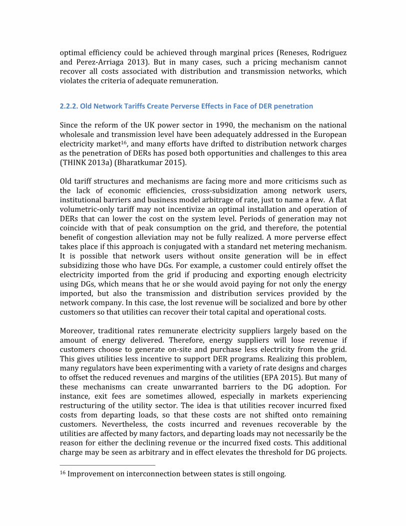
optimal efficiency could be achieved through marginal prices (Reneses, Rodriguez and Perez-‐Arriaga 2013). But in many cases, such a pricing mechanism cannot recover all costs associated with distribution and transmission networks, which violates the criteria of adequate remuneration.
2.2.2. Old Network Tariffs Create Perverse Effects in Face of DER penetration Since the reform of the UK power sector in 1990, the mechanism on the national wholesale and transmission level have been adequately addressed in the European electricity market16, and many efforts have drifted to distribution network charges as the penetration of DERs has posed both opportunities and challenges to this area (THINK 2013a) (Bharatkumar 2015). Old tariff structures and mechanisms are facing more and more criticisms such as the lack of economic efficiencies, cross-‐subsidization among network users, institutional barriers and business model arbitrage of rate, just to name a few. A flat volumetric-‐only tariff may not incentivize an optimal installation and operation of DERs that can lower the cost on the system level. Periods of generation may not coincide with that of peak consumption on the grid, and therefore, the potential benefit of congestion alleviation may not be fully realized. A more perverse effect takes place if this approach is conjugated with a standard net metering mechanism. It is possible that network users without onsite generation will be in effect subsidizing those who have DGs. For example, a customer could entirely offset the electricity imported from the grid if producing and exporting enough electricity using DGs, which means that he or she would avoid paying for not only the energy imported, but also the transmission and distribution services provided by the network company. In this case, the lost revenue will be socialized and bore by other customers so that utilities can recover their total capital and operational costs. Moreover, traditional rates remunerate electricity suppliers largely based on the amount of energy delivered. Therefore, energy suppliers will lose revenue if customers choose to generate on-‐site and purchase less electricity from the grid. This gives utilities less incentive to support DER programs. Realizing this problem, many regulators have been experimenting with a variety of rate designs and charges to offset the reduced revenues and margins of the utilities (EPA 2015). But many of these mechanisms can create unwarranted barriers to the DG adoption. For instance, exit fees are sometimes allowed, especially in markets experiencing restructuring of the utility sector. The idea is that utilities recover incurred fixed costs from departing loads, so that these costs are not shifted onto remaining customers. Nevertheless, the costs incurred and revenues recoverable by the utilities are affected by many factors, and departing loads may not necessarily be the reason for either the declining revenue or the incurred fixed costs. This additional charge may be seen as arbitrary and in effect elevates the threshold for DG projects. 16 Improvement on interconnection between states is still ongoing.

Another mechanism is standby charges, which covers the additional costs to supply intermittent services to customers when DG is unavailable. The underlying assumption is that DG users may require significant power when the electricity is scarce and at a premium price. However, the probability and severity of such extreme conditions may be low and do not warrant the rates that utilities are claiming. As a result, better tariffication methods are needed to more accurately recognize and reflect the benefits and costs DGs bring to the system.
2.2.3. A New Proposal of Tariff Framework Many governments, utilities and academia agree that new rate designs should “decouple” utility revenues from pure sales volume; however, there is little agreement on the specific tariff structure and cost allocation. In a recent publication by researchers of the European University Institute, a new framework for distribution network use-‐of-‐system (DNUoS) was proposed (Ignacio Perez-‐Arriaga 2013). The core idea of this framework is to allocate costs according to cost driver profiles, which are the key factors that contribute to the total cost of the system. Besides the criteria of having relevant impact on the network cost, meaningful cost drivers should also be easy to measure and related to customers’ decisions on where and how to consume (Rodriguez-‐Ortega 2008). The premise is that, by sending signals to customers on how their behavior impact system costs and their share of those costs, higher efficiency as well as better equity could be achieved. This approach is different from current practices in the industry where users are charged for average rates computed for a pre-‐determined class and region. It is believed that such a mechanism is better suited for an environment where customers’ energy production and consumption profiles continue to diversify. A subsequent paper further developed this framework and proposed steps to allocate total collectible revenue among customers during a specific period (Bharatkumar 2015). As is shown in Figure 11, after the determination of the revenue requirement, the total network cost is split at each voltage level by each cost driver, and then further split across regions. Finally, the figure is used to calculate the rates for each end-‐user in the region according to their profiles.
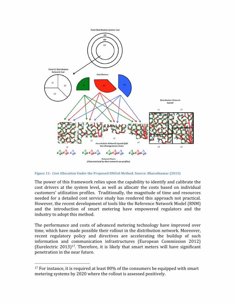
Figure 11: Cost Allocation Under the Proposed DNUoS Method. Source: Bharatkumar (2015)
The power of this framework relies upon the capability to identify and calibrate the cost drivers at the system level, as well as allocatr the costs based on individual customers’ utilization profiles. Traditionally, the magnitude of time and resources needed for a detailed cost service study has rendered this approach not practical. However, the recent development of tools like the Reference Network Model (RNM) and the introduction of smart metering have empowered regulators and the industry to adopt this method. The performance and costs of advanced metering technology have improved over time, which have made possible their rollout in the distribution network. Moreover, recent regulatory policy and directives are accelerating the buildup of such information and communication infrastructures (European Commission 2012) (Eurelectric 2013)17. Therefore, it is likely that smart meters will have significant penetration in the near future. 17 For instance, it is required at least 80% of the consumers be equipped with smart metering systems by 2020 where the rollout is assessed positively.

On the other hand, distribution system planning models such as RNM have been utilized by both the industry and regulators to aid the process of prudent network investment assessment. This large-‐scale distribution planning model can automatically extract geographic and customer distribution information from satellite images and estimate fixed and variable costs of the network according to the technological and economic characteristics of various network components. RNM can serve as a handy tool for cost determination and allocation. A detailed description of this model can be found at (Domingo and Roman 2010) and its application in the context of DNUoS can be found at (Bharatkumar 2015).
2.2.4. Related Research This thesis focuses on quantitatively assessing the attractiveness of NGDCHP technologies under various regulatory, economic and technical settings. It not only looks at the optimum economic value of CHP to individual customers, but also peak loads and environmental impacts at the system level. Prior research in this area is limited. Some authors have focused on the impact of large-‐scale CHP deployment on the distribution network costs, technical effects and reliability gains (Thomson 2008) (Cossent 2009), without addressing the economic value and incentives to the end-‐users. Others have examined long term planning and short-‐term operational effects of having important volume of CHPs, but did not examine in detail how various tariff structures could influence the conclusions (Tapia-‐Ahumada 2011). There have been also analysis on how rate structure affects the electricity savings for CHP projects, but they only focused in the United States and did not take into account detailed operational decisions of the DGs (Miller, Haefke and Cuttica 2012) (EPA 2006).

3. Representation and Modeling Methodologies
3.1. Framework
Figure 12: The research process
In Figure 12, we depict the framework of the research process. Through detailed and comprehensive literature research, we accrue three categories of raw data: energy-‐related data, market conditions, and technology characteristics. In the second step, we transform this raw data into inputs that the Distributed Energy Resource Customer Adoption Model (DERCAM) uses. For instance, energy-‐related raw data such as weather, building design and end-‐user demand patterns are used to derive the hourly electric and heat loads through eQUEST simulation software. Then, these time series datasets are cleaned and summarized using a MATLAB code, whose output is directly readable by DERCAM. On the other hand, technology and market information is synthesized and transformed into different technology and market scenarios. To efficiently run a large amount of scenarios, we developed overarching control software that functions a loop control to automate multiple runs on DERCAM. Finally, we use excel and VBA models to interpret and summarize the output of each DERCAM run. We have addressed the economic and technical characteristics of different CHP systems in the previous chapter. In the following sections in this chapter, we will first introduce the DERCAM and eQUEST models. Then, we will construct a residential case and an industrial case. Next, we will quickly review the current market conditions in EU and more specifically those in Germany, and explain in detail how different scenarios are constructed. Finally, we conclude this chapter by highlighting the key assumptions adopted in our methodology.

3.2. A Description of DERCAM The Distributed Energy Resources Customer Adoption Model is an economic and environmental optimization tool developed by the Laurence Berkeley National Lab (LBNL) and funded by the U.S. Department of Energy. DER-‐CAM has been evolving and improving for more than a decade and has multiple versions tailored for different objectives. In the version used for this thesis, the objective function is set to minimize the total energy related cost of utility customers by adopting various optimal distributed energy technologies and their respective operating schedules. The model is based on mixed integer linear programing and utilizes CPLEX as a solver (Cardoso, Stadler and Bozchalui 2014). 𝑂𝑏𝑗𝑒𝑐𝑡𝑖𝑣𝑒 𝐹𝑢𝑛𝑐𝑡𝑖𝑜𝑛:𝑚𝑖𝑛.𝐴𝑛𝑛𝑢𝑎𝑙 𝐸𝑛𝑒𝑟𝑔𝑦 𝐵𝑖𝑙𝑙 𝐴𝑛𝑛𝑢𝑎𝑙 𝐸𝑛𝑒𝑟𝑔𝑦 𝐵𝑖𝑙𝑙 =𝐸𝑛𝑒𝑟𝑔𝑦 𝑎𝑛𝑑 𝑆𝑒𝑟𝑣𝑖𝑐𝑒 𝑃𝑢𝑟𝑐ℎ𝑎𝑠𝑒 𝑐𝑜𝑠𝑡𝑠 + 𝐴𝑚𝑜𝑟𝑡𝑖𝑧𝑒𝑑 𝐷𝐸𝑅 𝑇𝑒𝑐ℎ𝑛𝑜𝑙𝑜𝑔𝑦 𝐶𝑎𝑝𝑖𝑡𝑎𝑙 𝐶𝑜𝑠𝑡𝑠 + 𝑎𝑛𝑛𝑢𝑎𝑙 𝑂&𝑀 𝑐𝑜𝑠𝑡𝑠 − 𝐸𝑛𝑒𝑟𝑔𝑦 𝑆𝑎𝑙𝑒𝑠 − 𝐼𝑛𝑐𝑒𝑛𝑡𝑖𝑣𝑒𝑠 Equation 1 Objective Function of DERCAM
The figure below illustrates the structure of DER-‐CAM. The model takes into consideration end-‐user load profiles, market information and DER technologies and their relevant characteristics, etc. and chooses the optimal installation and operation of generation technologies. Other key outputs include emissions, fuel consumption and total energy costs.
Some of the main inputs can are as follows:

• Customers’ typical hourly end-‐use load profiles such as electricity-‐only, gas-‐only, space heating, hot water, cooling and refrigeration loads on weekdays, weekends and peak time slots;
• Electricity and gas tariffs; • Incentives for various technologies, such as feed-‐in-‐tariffs or capital
expenditure remunerations; • Economic features of different DER technologies, such as capital cost,
operating and maintenance cost and lifetime; • Performance characteristics of these DER technologies, e.g. heat-‐to-‐power
ratio, electric efficiency and maximum power; • System or regulatory constraints, such as minimum CHP efficiency, maximum
payback period and maximum operation hours in a given year. Considering the computational complexity and the research questions, several assumptions have been made. To begin with, the customers are assumed to be price takers and their behavior is not expected to influence the overall utility system. In other words, the model does not consider the dynamic interplay between the market and individual customer’s behavior, which is a reasonable assumption when the penetration rate of DERs is low or the market price is insensitive to the overall demand. Moreover, the heat-‐to-‐power ratio and electric efficiency of the generating technologies are not variable in accordance to their output. Thirdly, decisions are made based only on economic criteria, which mean that customers’ sole goal is to minimize their total energy bill18. In order to facilitate the analysis of a time-‐dependent energy price, this thesis implemented an hourly tariff feature in the original DERCAM code. Certain changes also took place in the data input, constraint and objective functions.
3.3. eQUEST and the Construction of Load Profiles eQUEST is a building design and energy simulation tool supported as part of the Energy Design Resource program19 (James J. Hirsch & Associates 2004). It gives designers and researchers the capability to perform detailed energy analysis of different building designs in a relatively simple and intuitive way. DOE-‐2 is the simulation “engine” with in eQUEST. It is the most widely recognized and utilized building energy analysis software on the market. Its origins can be traced back to 1970’s, when ASHRAE, NASA, the U.S. Postal Service and the electric 18 For more information about DER-‐CAM, readers can refer to the website: https://der.lbl.gov/der-cam and https://building-microgrid.lbl.gov/projects/der-cam 19 Funded by California utility customers and administered by Pacific Gas and Electric Company, San Diego Gas & Electric, and Southern California Edison, under the auspices of the California Public Utilities Commission

and gas utility industries first funded and developed such a program. Since then, it has been widely applied and validated under various scenarios. eQUEST adopted the latest version of DOE-‐2 and made multiple expansions and improvements. It added a building creation wizard, an energy efficiency measure wizard, a graphical results display model and industry standard input defaults to the basket, which not only streamlined the simulation process but also made the results more reliable and comparable. The first step of the simulation is to develop a model of the building under consideration. The default design and schedule assumes a minimum level of efficiency20 . Researchers/ designers can make changes to adjust to different requirements/ situations in other regions. More specifically, users input detailed information of the building utilization schedule and design parameters, such as occupant schedule, lighting, equipment, thermostat settings as well as building envelope, HVAC control, shading and fenestration, etc21. The software generates hourly building energy consumption over 8760 hours (a year) based on weather data of the location chosen. Later on, researchers can use the built-‐in economic analysis tools to see how building design changes can impact the payback period and life cycle costs. A detailed data requirement for a complete simulation on eQUEST can be found in the Appendix22. For the interest of our research, we mainly utilized the energy load simulation capability to simulate two cases in Berlin: a medium size factory and a multi-‐family building. This provides us with hourly energy consumption data broken down into categories such as domestic hot water, lighting, heating, cooling and refrigeration, etc. This information is then taken in by a MATLAB code, which generates the load profile in “typical” time slots that can be read by DERCAM. A brief description of these two cases is shown in Table 10.
20 Conforming to California Title 24 or ASHRAE 90.1, for example. 21 The appliance data is extracted from the following link: http://www.kingslocal.net/Departments/Business/Documents/Appliance_energy_consumption.pdf 22 For more information, readers can refer to eQUEST official website: http://www.doe2.com/equest/ and the EDR Building Simulation Design Brief http://www.energydesignresources.com/Resources/Publications/DesignBriefs.aspx.

Multi-‐family House
Size: 150,000 ft2 ( ~15,000 m2) Floors: 20 -‐ 30 families/floor (3 persons per family)* 8 floors Total Annual Energy Consumption: 1655 MWh Total Heat Load: 893 MWh (54%) Total Electric Load: 762 MWh (47%)
Average Heat Load: 103 kW Average Electricity Load: 88 kW Average Heat-‐to-‐Power Ratio Load: 1.17 Average Energy Consumption: 110 kWh/m2-‐yr
Food Processing Factory Total Annual Energy Consumption: 100,976 MWh Total Heat Load: 53,922 MWh (53%) Total Electric Load: 47,054 MWh (47%)
Average Heat Load: 6,155 kW Average Electricity Load: 5,372 kW Average Heat-‐to-‐Power Ratio Load: 1.146
Table 10 Key Features of the Two Cases Under Consideration. Source: Self-‐generated using eQUEST
The multi-‐family building consumes 1.6 GWh end-‐use energy each year, 54% of which is for heating and hot water, typical in Northern European nations. The average 110 kWh/m2-‐yr energy intensity figure is also in line with the results of a survey on average residential customer in Germany (Economidou 2011)23. The peak load profile from January to June is shown in Figure 13, which displays a representative intraday and seasonal variation for residential customers.
23 Apartments and houses built in different times show very diverse heating requirement as a result of improving building standards over time. We are assuming a relatively new apartment built after 2010 in this case.

Figure 13 Peak Energy Demand of the Sample German Multi-‐family Building from January to June (KW). Source: Self-‐generated using eQUEST
On the other hand, we modeled a relatively large food-‐processing factory connected at distribution level that consumes 100GWh end-‐use energy each year. This case is constructed by adding the industrial process energy load on top of the non-‐process energy consumption load of a regular one-‐floor building. The representative industrial electricity-‐only, gas-‐only, heating and refrigeration process loads are shown below in Figure 14. The total energy consumption data is from a case study provided by Eni Corp., and the load profile is constructed based on (Starke and Alkadi 2013).

Figure 14 Process Energy Demand (kW) for The Industrial Consumer. Source: Self-‐generation according to various data
3.4 Market Data
3.4.1 Gas Price European nations have significantly different retail gas prices, with the level of the prices paid in the most expensive members being several times that paid in the cheapest ones. In general, the difference is greater for the households than for businesses, and there is indication that the gap has widened in recent years (EC 2014). A more detailed discussion is presented in the next Chapter. For Germany, there is one gas exchange market named European Gas Exchange (EGEX). As shown in Figure 15, the natural gas price for both households and industries in German has declined between 2008 and 2012. Given the total gas demand of the multi-‐family building and the food-‐processing factory, the gas price has been set at 3.38 Euro cents/KWh and 4.93 Euro cents/KWh respectively24 (Bundesnetzagentur 2014) (Eurostat 2015). In addition, a 40% tax and levy rate has been applied.
24 Corresponding to the residential band: annual consumption >200GJ, and the industrial band: 100,000GJ< annual consumption < 1,000,000GJ
0
5000
10000
15000
20000
25000
30000
1 2 3 4 5 6 7 8 9 10 11 12 13 14 15 16 17 18 19 20 21 22 23 24
Electricity-‐only Cooling
Refrigeration Space heating and process steam
Water heating Gas-‐ony

Figure 15 Representative German Natural Gas Price Change by Components 2008-‐2012 (in Euro cents/KWh). Source: EC, EPCR metadata (2013)
3.4.2 Electricity Tariff The average prices that European customers pay for electricity reflect various elements that intend to reflect energy costs, network costs, and other costs that reflect various government policies, ranging from taxation, surcharges to wholesale price pegging. Despite the diverse organizations and tariff structures, the cost components that customers bear can be categorized in general into three major elements (shown in Figure 16). The energy element of the bill consists of two sub-‐categories: a wholesale part that reflects the costs incurred to deliver energy to the grid, and a retail part that covers the costs related to the sale of energy to the end-‐users. The wholesale part includes fuel acquirement costs, as well as CAPEX and OPEX for the central power plants. For simplicity, this element can be assumed to be only related to the volumetric quantity of electricity consumed by the customers. The network element represents the costs associated with the transmission and distribution networks. It includes the infrastructure costs, maintenance costs, as well as system services (e.g. standby generation capacity and contingency reserves) and losses. The cost drivers associated to these costs could be complicated to determine, which is further discussed below. Finally, taxes, levies and regulatory charges may be applied on top of the baseline costs. Taxes generally include value added taxes (VAT) and excise duties. Levies can be related to public services obligations, and technology support on the local level. Regulatory charges are used to support renewable energy programs, recover stranded assets or implement smart meters (SWD 2014). These costs are assumed to be proportional to the baseline costs.

Figure 16 Elements of Consumer Prices. Source: SWD (2014)
3.4.2.1. German Tariff Overview The Federal Network Agency for Electricity, Gas Telecommunications, Posts and Railways (known as Bundesnetzagentur) is the German national regulator. The German market can be seen as relatively competitive both on the wholesale and the retail levels. The wholesale prices on the spot and forward markets have been drifting downward over time. Electricity customers can also choose among a large number of suppliers, with the supplier-‐switching rate being one of the highest in Europe (EC 2014). Despite these favorable factors, however, the retail prices -‐-‐especially those for residential customers-‐-‐ have been increasing in recent years (see Figure 17), making its electricity one of the most expensive ones in Europe. For instance, according to a survey conducted by the Bundesnetzagentur, taxes (electricity and VAT) accounted for 27.9% of the baseline costs for an industrial player with annual electricity consumption of about 20 GWh, and the sum of all levies and surcharges under the EEG, KWKG, section 19 StromNEV and for offshore liability, as well as concession fees amounted to approximately 32.3% in 2013 (Bundesnetzagentur 2014).
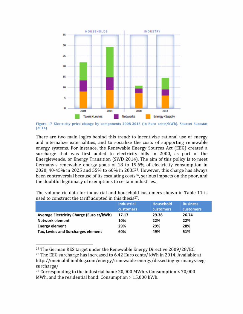
Figure 17 Electricity price change by components 2008-‐2013 (in Euro cents/kWh). Source: Eurostat (2014)
There are two main logics behind this trend: to incentivize rational use of energy and internalize externalities, and to socialize the costs of supporting renewable energy systems. For instance, the Renewable Energy Sources Act (EEG) created a surcharge that was first added to electricity bills in 2000, as part of the Energiewende, or Energy Transition (SWD 2014). The aim of this policy is to meet Germany’s renewable energy goals of 18 to 19.6% of electricity consumption in 2020, 40-‐45% in 2025 and 55% to 60% in 203525. However, this charge has always been controversial because of its escalating costs26, serious impacts on the poor, and the doubtful legitimacy of exemptions to certain industries. The volumetric data for industrial and household customers shown in Table 11 is used to construct the tariff adopted in this thesis27.
Industrial customers
Household customers
Business customers
Average Electricity Charge (Euro ct/kWh) 17.17 29.38 26.74 Network element 10% 22% 22% Energy element 29% 29% 28% Tax, Levies and Surcharges element 60% 49% 51%
25 The German RES target under the Renewable Energy Directive 2009/28/EC. 26 The EEG surcharge has increased to 6.42 Euro cents/ kWh in 2014. Available at http://oneinabillionblog.com/energy/renewable-‐energy/dissecting-‐germanys-‐eeg-‐surcharge/ 27 Corresponding to the industrial band: 20,000 MWh < Consumption < 70,000 MWh, and the residential band: Consumption > 15,000 kWh.

Table 11 Volume Weighted Average Electricity Price in Germany in 2013. Source: Bundesnetzagentur (2014), Eurostat (2015)
3.4.2.2. Network Cost Breakdown In general, transmission and distribution charges can range from 15% to 40% on customers’ final electricity bills. According to Bharatkumar (2015) and Perez-‐Arriaga (2013), the cost drivers behind those charges can be categorized in three main types:
• Connection: the minimum network required to provide users with connectivity, which is only related to the geographic locations and minimal loads. According to the authors, the associated costs can be either calculated based on the customers’ relevant profile, or socialized within network zones.
• Capacity: the additional network elements needed to accommodate peak power flows. The costs associated with capacity requirements should be assigned to network users based on their contributions to peak consumption in the LV, MV, and HV networks28. Traditionally, regulators have used contracted capacity as a proxy. This method may work well in industrial cases where the consumption profile is less volatile and the contracted capacity is close to the contribution in peak hours. However, this may not be suitable for residential customers. Therefore, the authors recommend a “coincident charge”, which is based on the customers’ contribution to the system peak. In this thesis, we assume that customers pay for their maximum contribution to the system peak in a given month if a coincident peak rate is applied.
• Reliability and losses: the reinforcements and services required to increase the security margin of the system capacity29 and the extra costs associated to losses. These authors propose that these costs should be allocated to users volumetrically.
As discussed in the literature review chapter, the RNM can be used in network cost allocation by isolating the incremental network cost attributable to each of the network cost drivers. These results are highly dependent on the system configuration as well as model assumptions. Bharatkumar recommends a 50-‐25-‐25 breakdown, which is used as the starting point in this thesis. In theory, the network tariff should be dynamic and respond to the overall shift of customers’ load profile. For instance, if every end-‐user in the system reduced their peak contribution for the same amount, the capacity related rate should increase proportionally in the short-‐run to make sure that utility companies recover their costs. But a static rate is used in this thesis, which can be a reasonable
28 Ideally, it should also consider their contributions to reverse power flows through injection. 29 In anticipation of possible demand estimation errors, equipment failures, or faults and outages.

approximation when the penetration rate of distributed DERs is low, and the influence of the customers’ decision on the system is negligible.
3.4.2.3. Incentives To encourage the penetration and utilization of DERs, regulators provide a variety of incentives ranging from non-‐monetary ones like priority grid connection, to tax credits and direct monetary subsidies. Under the current Cogeneration Law of Germany, CHPs could be eligible for feed-‐in-‐tariff. This bonus payment can be received by high efficient CHP projects, and it depends on the size of the technology. Figure 18 shows the rate customers can receive per kWh electricity generated on-‐site within each capacity range.
Figure 18: German Cogerenation Law incentives for different capacity ranges. Source: Bundesnetzagentur (2014)
Figure 19 shows the calculation of the Cogeneration Law incentive for a CHP project with a 2,500 kW electric capacity. It is easy to see that the average rate decreases as the CHP capacity increases.
Figure 19: Calculation of average incentives for a 2,500 kW CHP project. Source: Self-‐ calculation
Another incentive that is available is the Mini-‐CHP support program. It provides a one-‐time investment grant to CHP projects smaller than 20kWe. Figure 20 summarizes the incentives for different electric capacity ranges.
Figure 20: Mini-‐CHP support program categories. Source: Bundesnetzagentur (2014)
A distinct advantage of NGDCHP over intermittent technologies is its controllability, which can potentially create additional value to both the customers and the grid. Introducing a sale-‐back mechanism has the potential to incentivize customers to

export electricity to the grid when electricity is scarce, increase the utilization of the generators and, in effect, reduce the economic barriers. German regulators have also implemented a bonus payment for the fed-‐back (exported) electricity of CHP projects smaller than 2,000kWe. The rate is set at 3.15 Euro cent/kWh, which is close to the average wholesale electricity price.
Figure 21: Average price for baseload power at EPEX (Euro/ MWh)
However, according to the Renewable Energy Act 2014, electricity generated on-‐site would also be charged for EEG in the future. The rate is set to be 30% of full EEG charge for new installations until 2016, which translates into 1.87 Euro cents/ kWh.
3.4.3 Construction and Summary of Different Tariff Structures For the natural gas price, we apply a 3.38 Euro cent/ kWh flat volumetric rate in the industrial case and a 4.93 Euro cent/kWh flat volumetric rate in the residential case. In both cases, a natural gas tax and surcharge of 40% is applied. When constructing different electricity tariff structures, this thesis first calculates the total electricity charge the customer would pay if the average electricity price in Table 11 were applied and if no NGDCHP were installed, i.e. BAU scenario. Then, costs are assigned proportionally to each category (energy, network, and taxes and surcharges) and subcategories (connection, network capacity, and losses and reliability) according to Bharatkumar’s recommendation and Table 11. In this way, customers would pay the same total amount in the BAU scenario, which can facilitate comparison across structures. We constructed four tariff structure scenarios. In the first scenario (from now on referred to as Sc1), a flat rate is applied to each kWh of electricity purchased from the grid and does not have any fixed nor capacity-‐related charges. In the second scenario (Sc2), the tariff is an hourly volumetric rate, with the price varying according to the wholesale price. The price is higher when the demand in the system is high (e.g. 8am-‐11am and 4pm-‐8pm during the weekdays). In the third scenario (Sc3), the tariff has three parts, i.e. a fixed portion (representing 50% of the BAU network costs), a capacity portion (25% of the BAU network costs) and a volumetric

portion (representing 100% of the energy costs and 25% of the BAU network costs). Here, a capacity rate is derived through dividing 25% of the BAU network costs by the BAU contracted capacity (assumed to be the maximum net electric load of the month); and the volumetric rate is set to be flat. In the fourth scenario (Sc4), the capacity rate is replaced by a coincident rate, while the flat volumetric rate is replaced by an hourly volumetric rate. The coincident rate is derived through dividing 25% of the BAU network costs by the BAU maximum net load at 6p.m. in the month. Tables 12 and 13 present a summary of the specific rates used for the residential and industrial cases. Volumetric rate Fixed rate Capacity rate Coincidence rate Tax+ levies+
surcharge Euro cents/ kWh Euro/ Month Euro/kW/Month Euro/kW/ Month Percentage of
baseline costs Sc1 14.98 -‐ -‐ -‐ 100% Sc2 2.866*wholesale
price -‐ -‐ -‐
Sc3 10.1037 2053 3.9363 -‐ Sc4 1.939* wholesale
price 2053 -‐ 4.1152
Table 12: Summary of the rates for 4 tariff structures for the residential case.
Volumetric rate Fixed rate Capacity rate Coincidence rate Tax+ levies+
surcharge Euro cents/ kWh Euro/ Month Euro/kW/Month Euro/kW/ Month Percentage of
baseline costs Sc1 6.83 -‐ -‐ -‐ 100% Sc2 1.307* wholesale
price -‐ -‐ -‐ Sc3 5.5 34898 1.5573 -‐ Sc4 1.052*wholesale
price 34898 -‐ 2.2727 Table 13: Summary of the rates for 4 tariff structures for the industrial case

Figure 22: Volumetric electricity price for the residential customer in a typical day in January. Source: Own calculations.
As for incentives, we model three different situations:
1. When no incentive is implemented: it is meant to uncover the intrinsic economic value of different CHP technologies. In this scenario, there is no electricity export price.
2. When the Cogeneration Law is implemented: for the industrial application, we assume a 2.1 Euro cent/kWh bonus payment and a 1.87 Euro cent/ kWh EEG charge on the on-‐site generation (a net of 0.2 Euro cent/kWh incentive). For the residential customer, we assume a 5.41 Euro cent/kWh bonus payment and a 1.87 Euro cent/ kWh EEG charge on the on-‐site generation (a net of 3.5 Euro cent/kWh incentive). An export incentive of 3.15 Euro cent/ kWh is also applied.
3. When a capital expenditure (CAPEX) incentive is implemented: we assume a 30% upfront CAPEX reduction in both residential and industrial cases. An export incentive of 3.15 Euro cent/ kWh is also applied.
Some key assumptions and inputs are used in the model formulation and to construct the scenarios:
1. Rational customers: the installation and operations decisions are only based on an economic criteria.
2. “Tariff parity”: in the business as usual scenario (when no NGDCHP is installed), the customer pays the same amount in total for the energy purchased.
3. Low penetration rate: the influence of individual customer’s decision on the system is not significant
4. Smart meter is available: as discussed above, this is not an unreasonable assumption given the EU Directive to introduce smart meters. Smart meters could enable time dependent energy prices.
0
0.05
0.1
0.15
0.2
0.25
1 2 3 4 5 6 7 8 9 10 11 12 13 14 15 16 17 18 19 20 21 22 23 24
Sc 1
Sc 2
Sc 3
Sc 4

5. No demand response: the purpose of this thesis is to evaluate the value of NGDCHPs under different tariff structures and this value is isolated from that of demand response.

Results and Sensitivity Analysis
4.1 Analysis Metrics In this thesis, four categories of outputs from the model are examined and compared in different applications and scenarios:
• We start with the customers’ installation and operation decisions. Installed capacity represents how much electric capacity is installed on-‐site and the unit is kW. This might not be the “optimal” capacity because of the lumpiness of the technologies, but it is a more realistic representation because the technologies are not divisible in real life. The hourly operations of one technology will be shown as an example of how different tariff and market conditions would change the operations patterns in a typical day of the year. This part would include both electric load and heating load. Besides, a ratio that represents the overall utilization rate of the technology is examined. The formula is 𝑈𝑡𝑖𝑙𝑖𝑧𝑎𝑡𝑖𝑜𝑛 𝑟𝑎𝑡𝑒 = 𝐶𝑜𝑛𝑠𝑡𝑎𝑛𝑡 ∗ !"#$%&%"'() !"# !"#$%&'()"# %
!"#$%&&'( !"#"!$%&. The
numerator indicates how much more gas is consumed on-‐site as a percentage of the original consumption, and the constant is 100,000 in the industrial case and 1,000 in the multi-‐family case. Therefore, this ratio measures how much incremental natural gas each kW of installed CHP electric capacity consumes. Finally, the export ratio is discussed when appropriate, which represents the portion of on-‐site generated electricity that is exported to the grid, i.e. 𝐸𝑥𝑝𝑜𝑟𝑡 𝑟𝑎𝑡𝑖𝑜 = !"#$%&!' !"!#$%&#&$!
!"!#$ !"!#$%&#&$' !"#"$%&'(# !"!!"#$.
• Next, when analyzing the economic and financial impacts of the installation and operation decisions, we look at the annual savings through operations, pay-‐back (PB) period, and in some cases the incentives received. The annual savings through operations show how much total energy costs are saved compared to the business as usual scenario (when there is no CHP installation). Here, 𝐴𝑛𝑛𝑢𝑎𝑙 𝑡𝑜𝑡𝑎𝑙 𝑒𝑛𝑒𝑟𝑔𝑦 𝑐𝑜𝑠𝑡 = 𝐸𝑙𝑒𝑐𝑡𝑟𝑖𝑐𝑖𝑡𝑦 𝑝𝑢𝑟𝑐ℎ𝑎𝑠𝑒 +𝑁𝑎𝑡𝑢𝑟𝑎𝑙 𝑔𝑎𝑠 𝑝𝑢𝑟𝑐ℎ𝑎𝑠𝑒 + 𝑂𝑝𝑒𝑟𝑎𝑡𝑖𝑜𝑛𝑠 𝑎𝑛𝑑 𝑚𝑎𝑖𝑛𝑡𝑒𝑛𝑎𝑛𝑐𝑒 𝑐𝑜𝑠𝑡𝑠 𝑜𝑓 𝐷𝐺 −𝑟𝑒𝑚𝑢𝑛𝑒𝑟𝑎𝑡𝑖𝑜𝑛𝑠 𝑓𝑜𝑟 𝑒𝑙𝑒𝑐𝑡𝑟𝑖𝑐𝑖𝑡𝑦 𝑒𝑥𝑝𝑜𝑟𝑡. It does not include subsidies or the amortization costs of installed CHP technologies. In some cases, the government provides subsidies to the on-‐site generation, and we show the annual incentives received by the customers as a percentage of their original energy bill. The PB period shows how long it takes for the customers to recover their upfront capital expenditure through subsequent savings, and the equation is 𝑃𝐵 𝑝𝑒𝑟𝑖𝑜𝑑 = !"#$%
!""#$% !"#$%&! !!!"#$! !"#$%&'!"#!!"#$"%&'$( !"#"$%"&.
• Thirdly, the impact of CHP installation on the system is examined using mainly three metrics. The maximum load reduction (MLR) refers to the reduction of the maximum electric load of the year, and the equation is 𝑀𝐿𝑅 = 1− !"# !"!#. !"#$ !" !!! !"#$ !"#$% !"#$%&&!"' !"#
!"# !"# !"!#.!"#$ !" !!! !"#$ !"#!!"# !"#. The average contracted
capacity reduction (ACCR), on the other hand, focuses on the reduction of the maximum net electric load of each month. The equation is 𝐴𝐶𝐶𝑅 = 𝑀𝐿𝑜𝑀𝑖!"
! / 𝑀𝐿𝑜𝑀0!"! , where MLoM represents maximum load of

the month, 0 stands for the business as usual scenario and i stands for the scenario where technology i is installed. This is a proxy in the scenario where the customers are charged on their monthly contracted capacity. Lastly, the coincident peak reduction (RPC) focuses on the maximum net electric load during the system peak (set to be at 6 p.m.). The equation is 𝑅𝑃𝐶 =
𝑀𝐿𝑑𝑆𝑃𝑖!"! / 𝑀𝐿𝑑𝑆𝑃0!"
! , where MLdSP represents maximum load during system peak. RPC is intended to measure peak demand and its impact on lowering system’s congestions.
• Last but not least, we examine environmental and efficiency impacts through the total CO2 emissions savings and the distributed generation efficiency. The DG efficiency refers to the total useful energy output as a percentage of total energy input, and the output includes both electricity and useful heat30. Total CO2 emissions savings compare the CO2 emissions when CHP is installed with that when all electricity is provided from the grid and heat is provided from alternative heating methods such as a boiler and furnace. Here, the natural gas emissions rate is set to be 0.1808 kg/ kWh and an 80% natural gas to heat conversion ratio is assumed, both based on the reference EU primary energy saving metrics. Due to lack of information, we use as a proxy to the hourly marginal CO2 emission rate the data from the California electric grid as both CA and Germany have relatively high clean energy penetration. As can be seen in Figure 23, the average grid level emission rate over the year is around 0.5kg/ kWh.
•
Figure 23: The average grid level emission rate of California in a typical day of each month in California. Source:???
30 Admittedly, there are other metrics like effective electric efficiency and total primary energy savings, which looks at the efficiency from different angles.
0.4
0.45
0.5
0.55
0.6
0.65
0.7
1 3 5 7 9 11 13 15 17 19 21 23
January
February
March
April
May
June
July
August
September
October
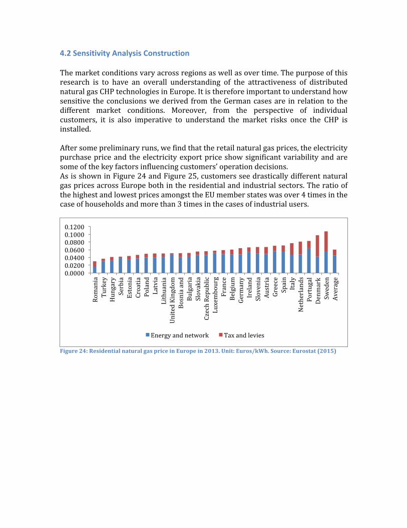
4.2 Sensitivity Analysis Construction The market conditions vary across regions as well as over time. The purpose of this research is to have an overall understanding of the attractiveness of distributed natural gas CHP technologies in Europe. It is therefore important to understand how sensitive the conclusions we derived from the German cases are in relation to the different market conditions. Moreover, from the perspective of individual customers, it is also imperative to understand the market risks once the CHP is installed. After some preliminary runs, we find that the retail natural gas prices, the electricity purchase price and the electricity export price show significant variability and are some of the key factors influencing customers’ operation decisions. As is shown in Figure 24 and Figure 25, customers see drastically different natural gas prices across Europe both in the residential and industrial sectors. The ratio of the highest and lowest prices amongst the EU member states was over 4 times in the case of households and more than 3 times in the cases of industrial users.
Figure 24: Residential natural gas price in Europe in 2013. Unit: Euros/kWh. Source: Eurostat (2015)
0.0000 0.0200 0.0400 0.0600 0.0800 0.1000 0.1200
Romania
Turkey
Hungary
Serbia
Estonia
Croatia
Poland
Latvia
Lithuania
United Kingdom
Bosnia and
Bulgaria
Slovakia
Czech Republic
Luxembourg
France
Belgium
Germany
Ireland
Slovenia
Austria
Greece
Spain
Italy
Netherlands
Portugal
Denm
ark
Sweden
Average
Energy and network Tax and levies
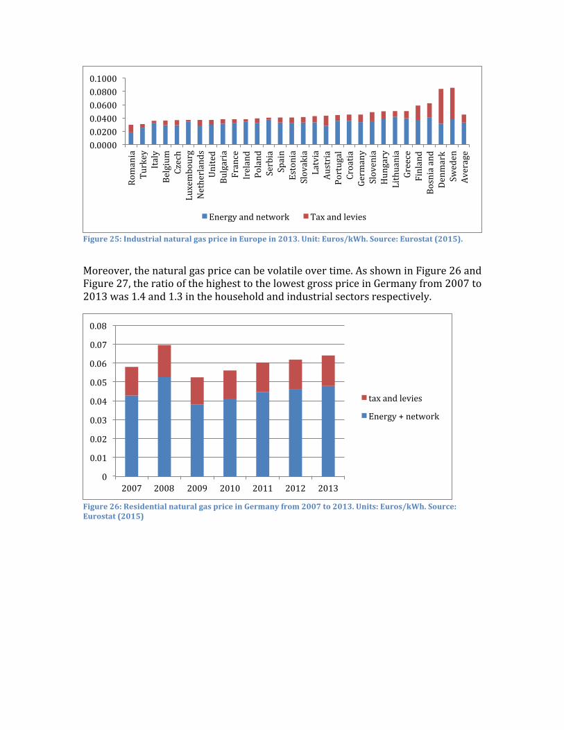
Figure 25: Industrial natural gas price in Europe in 2013. Unit: Euros/kWh. Source: Eurostat (2015).
Moreover, the natural gas price can be volatile over time. As shown in Figure 26 and Figure 27, the ratio of the highest to the lowest gross price in Germany from 2007 to 2013 was 1.4 and 1.3 in the household and industrial sectors respectively.
Figure 26: Residential natural gas price in Germany from 2007 to 2013. Units: Euros/kWh. Source: Eurostat (2015)
0.0000 0.0200 0.0400 0.0600 0.0800 0.1000
Romania
Turkey
Italy
Belgium
Czech
Luxembourg
Netherlands
United
Bulgaria
France
Ireland
Poland
Serbia
Spain
Estonia
Slovakia
Latvia
Austria
Portugal
Croatia
Germany
Slovenia
Hungary
Lithuania
Greece
Finland
Bosnia and
Denm
ark
Sweden
Average
Energy and network Tax and levies
0
0.01
0.02
0.03
0.04
0.05
0.06
0.07
0.08
2007 2008 2009 2010 2011 2012 2013
tax and levies
Energy + network
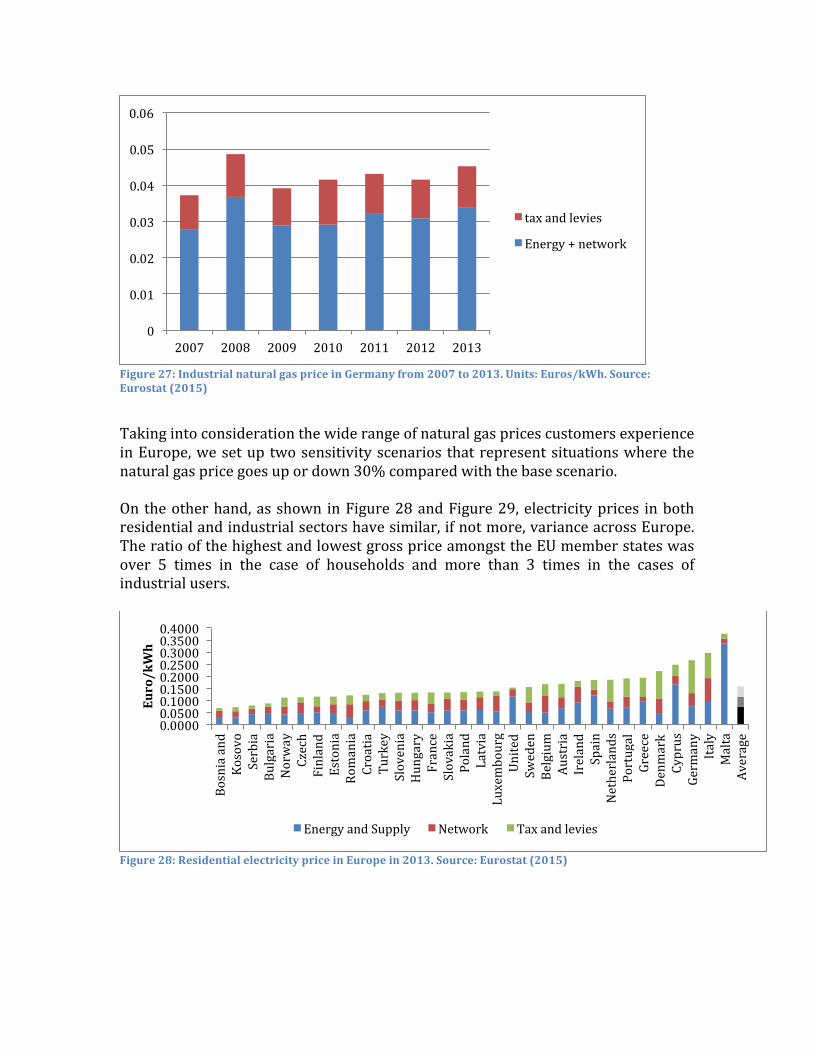
Figure 27: Industrial natural gas price in Germany from 2007 to 2013. Units: Euros/kWh. Source: Eurostat (2015)
Taking into consideration the wide range of natural gas prices customers experience in Europe, we set up two sensitivity scenarios that represent situations where the natural gas price goes up or down 30% compared with the base scenario. On the other hand, as shown in Figure 28 and Figure 29, electricity prices in both residential and industrial sectors have similar, if not more, variance across Europe. The ratio of the highest and lowest gross price amongst the EU member states was over 5 times in the case of households and more than 3 times in the cases of industrial users.
Figure 28: Residential electricity price in Europe in 2013. Source: Eurostat (2015)
0
0.01
0.02
0.03
0.04
0.05
0.06
2007 2008 2009 2010 2011 2012 2013
tax and levies
Energy + network
0.0000 0.0500 0.1000 0.1500 0.2000 0.2500 0.3000 0.3500 0.4000
Bosnia and
Kosovo
Serbia
Bulgaria
Norway
Czech
Finland
Estonia
Romania
Croatia
Turkey
Slovenia
Hungary
France
Slovakia
Poland
Latvia
Luxembourg
United
Sweden
Belgium
Austria
Ireland
Spain
Netherlands
Portugal
Greece
Denm
ark
Cyprus
Germany
Italy
Malta
Average
Euro/kWh
Energy and Supply Network Tax and levies

Figure 29: Industrial electricity price in Europe in 2013. Source: Eurostat (2015) 31
Similar to the natural gas price, we see the electricity price changing over time in Germany. As is shown in Figure 30 and Figure 31, the electricity price has increased 50% and 37% from 2007 through 2013 in the residential and industrial sector respectively.
Figure 30: Residential electricity price in Germany from 2007 to 2013. Units: Euro/ kWh. Source: Eurostat (2015)
31 In the German price, the EEG charge is excluded as large industrial customers are eligible for EEG exemption, since the government tries to preserve the competitiveness of local heavy industries.
0.0000
0.0500
0.1000
0.1500
0.2000
Bosnia and
Kosovo
Serbia
Bulgaria
Sweden
Norway
Finland
Luxembourg
Romania
Croatia
France
Turkey
Poland
Netherlands
Slovenia
Estonia
Belgium
Austria
Spain
Denm
ark
Portugal
Czech Republic
Greece
Hungary
Ireland
Slovakia
Latvia
United Kingdom
Germany
Italy
Malta
Cyprus
Average
Euro/kWh
Energy supply network Tax and levies
0.0000
0.0500
0.1000
0.1500
0.2000
0.2500
0.3000
2007 2008 2009 2010 2011 2012 2013
Taxes and levies
network
Energy and supply

Figure 31: Industrial electricity price in Germany from 2007 to 2013. Units: Euros/ kWh. Source: Eurostat (2015)
Based on the range of electricity gas prices that a customer could see in Europe, we set up another two sensitivity scenarios that represent situations where the electricity price goes up or down 30% compared with the base scenario, while holding other parameters constant. Currently, Germany has a 3 Euro cents/kWh incentive on the electricity exported to the grid from distributed CHP systems, which is close to the average electricity price on the wholesale market -‐-‐this is a very low incentive. In comparison, in many states of the US, a net metering mechanism is implemented, which essentially pays the customer the retail price of electricity for their export. Considering that regulators may try to encourage more installations through higher export prices, we construct a sensitivity scenario where the customer receives twice the wholesale electricity price for the exported electricity.
0.0000
0.0200
0.0400
0.0600
0.0800
0.1000
0.1200
2007 2008 2009 2010 2011 2012 2013
Taxes and levies
network
Energy and supply

4.3 Results from the Food Processing Factory Case
4.3.1. Business as Usual Reference Case
Total Annual Energy Costs [$] 10,246,871
Annual non-‐DER Electricity Purchase [$] 7,359,085
Annual NG Purchase [$] 2,887,786
Annual Total Energy Demand [kWh] 100,975,546
Total Electricity Load [kWh] 47,053,872
Annual Electricity-‐Only Load32 [kWh] 30,989,466
Annual Cooling Load [kWh] 2,076,294
Annual Refrigeration Load [kWh] 13,988,112
Total Heat Load [kWh] 53,921,672
Annual Space Heating and Process Heating Load [kWh] 47,413,884
Annual Water Heating Load [kWh] 3,408,841
Annual Natural Gas-‐Only Load [kWh] 3,098,947
Annual Total Emissions [kgCO2] 36,041,784
Table 14: Summary of the business as usual industrial case
As shown in Table 14, the annual 100GWh energy demand comprises 47% electricity load and 53% gas load when there are no CHP installations. As for the energy cost, 71% comes from electricity bill and 29% from natural gas bill. Annual CO2 emissions stand at 36,000 tons.
4.3.2. When no Incentive is implemented
4.3.2.1 Decisions Starting from the installation decisions, we notice that the industrial customer’s installed capacity of technology 1, 2, 6 and 7 does not show much variability because
32 Energy consumption for electronic devices.

they are relatively large technologies and close to the maximum load of the factory. Specifically, Tech 1 is a 9.3 MW internal combustion engine; Tech 6 and Tech 7 are 7MW and 10 MW gas turbines respectively. Therefore, the customer is in fact facing binary choices. In comparison, technology 3, 4, 5, 9 and 10 have smaller unit capacities, and show higher variability in their installation decisions in different tariff structure scenarios. Tech 2 represents a 3.3 MW internal combustion turbine technology. It is interesting because the customer has the option to install different number of the machines on-‐site but decided to have 3 machines in all tariff structure scenarios. Technology 8 is the steam turbine and is not picked because of its low electric efficiency. Additionally, from this chart, we can conclude that internal combustion engines, as well as certain types of fuel cells, gas turbines and micro turbines are economically viable in current market conditions without any incentives.
Figure 32: Installed capacity of 10 technologies in 4 tariff structure scenarios (kW).
As to operations, we use Tech 2 as an example because it has the same installed capacity in different tariff structures so that we can focus on the interplay between the tariffs and operations. First of all, we notice that not all peak electricity demand is met by the DG because of the lumpiness of Tech 2 -‐having another 3.3 MW machine installed on-‐site will result in lower utilization rate and high idleness during off-‐peak hours. Moreover, certain amount of heat is wasted in off-‐peak hours because the customer tries to lower their electric purchase even though their heat demand is very low in those hours. Thirdly, tariff structure scenario 1 and 3 give the same operations in this case because the volumetric prices are flat (though different) and are both at a level beyond the cost of on-‐site generation33. Fourthly, in tariff structure scenario 2 and 4, where hourly electricity price is applied, the prosumer takes advantage of the lower price of the grid in off-‐peak hours which results in lower production. Finally, we noticed that the operations during the system peak 33 After considering the heating load savings.
0
2000
4000
6000
8000
10000
12000
sc1
sc2
sc3
sc4

hours are not changing in different scenarios. This is because the generator is already operating at maximum capacity then.
Figure 33: Operational schedule in a typical day for Tech 2 scenario 1
Figure 34: Operational schedule in a typical day for Tech 2 scenario 2
Figure 35: Operational schedule in a typical day for Tech 2 scenario 3
0
2000
4000
6000
8000
10000
12000
0
2000
4000
6000
8000
10000
12000
1 2 3 4 5 6 7 8 9 10 11 12 13 14 15 16 17 18 19 20 21 22 23 24
Energy [k
Wh/h]
Electricity -‐ January
Electricity Generation Electricity Import from the Grid Electricity Sales Total Electricity Load
0
2000
4000
6000
8000
10000
12000
0
2000
4000
6000
8000
10000
12000
1 2 3 4 5 6 7 8 9 10 11 12 13 14 15 16 17 18 19 20 21 22 23 24
Energy [k
Wh/h]
Electricity -‐ January
Electricity Generation Electricity Import from the Grid Electricity Sales Total Electricity Load
-‐6000
-‐1000
4000
9000
14000
-‐6000
-‐1000
4000
9000
14000
1 2 3 4 5 6 7 8 9 10 11 12 13 14 15 16 17 18 19 20 21 22 23 24
Energy [k
Wh/h]
Heat -‐ January
Heat Loss in Storage Heat Collected from DG Natural-‐gas Only Load Heat from Other Sources
Heat Taken from Storage Heat Supplied to Storage Total Water Heating Load Total Heat Load
0
2000
4000
6000
8000
10000
12000
0
2000
4000
6000
8000
10000
12000
1 2 3 4 5 6 7 8 9 10 11 12 13 14 15 16 17 18 19 20 21 22 23 24
Energy [k
Wh/h]
Electricity -‐ January
Electricity Generation Electricity Import from the Grid Electricity Sales Total Electricity Load
-‐6000
-‐1000
4000
9000
14000
-‐6000
-‐1000
4000
9000
14000
1 2 3 4 5 6 7 8 9 10 11 12 13 14 15 16 17 18 19 20 21 22 23 24
Energy [k
Wh/h]
Heat -‐ January
Heat Loss in Storage Heat Collected from DG Natural-‐gas Only Load Heat from Other Sources
Heat Taken from Storage Heat Supplied to Storage Total Water Heating Load Total Heat Load

Figure 36: Operational schedule in a typical day for Tech 2 scenario 4
As is shown in Figure 37 and demonstrated in the discussions above, the utilization rate and incremental natural gas consumption of unit installed capacity is generally higher when flat volumetric rate (sc 1 and 3) is applied, because they encourage more on-‐site generation in off-‐peak hours while the influence on the on-‐peak hours is limited.
Figure 37: Incremental gas consumption per unit of installed capacity.
4.3.2.2. Economic and financial impacts As discussed in the methodology chapter, the objective function of DER-‐CAM is to minimize the annual total energy costs, including amortized CHP capital costs. The underlying assumption is that the customer makes decisions based on discounted cash flow and essentially has to weigh between the upfront capital cost and the annual operational savings and incentives received. This is different from criteria such as maximizing annual energy cost savings from operations and minimizing the pay-‐back period, which may result in different installation and operation decisions. However, customers may take all these objectives into consideration in real life, and pay-‐back periods and annual savings through operations can be more intuitive compared with discounted cash flow method. In this work, we will take PB period and annual savings as a metric, instead of the discounted cash flow method.
0
2000
4000
6000
8000
10000
12000
0
2000
4000
6000
8000
10000
12000
1 2 3 4 5 6 7 8 9 10 11 12 13 14 15 16 17 18 19 20 21 22 23 24
Energy [k
Wh/h]
Electricity -‐ January
Electricity Generation Electricity Import from the Grid Electricity Sales Total Electricity Load
-‐6000
-‐1000
4000
9000
14000
-‐6000
-‐1000
4000
9000
14000
1 2 3 4 5 6 7 8 9 10 11 12 13 14 15 16 17 18 19 20 21 22 23 24
Energy [k
Wh/h]
Heat -‐ January
Heat Loss in Storage Heat Collected from DG Natural-‐gas Only Load Heat from Other Sources
Heat Taken from Storage Heat Supplied to Storage Total Water Heating Load Total Heat Load
0
5
10
15
20
25
sc1
sc2
sc3
sc4

From Figure 38, it is easy to see that the pay-‐back period of viable technologies lies in a wide range between 4 to 9 years. Tariff structure scenario 3 and 4 result in longer PB period and even render certain technologies economically unattractive.
Figure 38: Pay-‐back period (year)
Overall, internal combustion engines show the best economics amongst all the technologies under analysis because they yield higher annual savings and shorter-‐payback periods. Results indicate that targeted incentives are needed to promote fuel cells and micro turbines if higher penetration rates are desirable.
Figure 39: Annual savings as a percent of original annual total energy cost
-‐ 1.00 2.00 3.00 4.00 5.00 6.00 7.00 8.00 9.00 10.00
sc1
sc2
sc3
sc4
-‐5%
0%
5%
10%
15%
20%
25%
30%
35%
40%
sc1
sc2
sc3
sc4
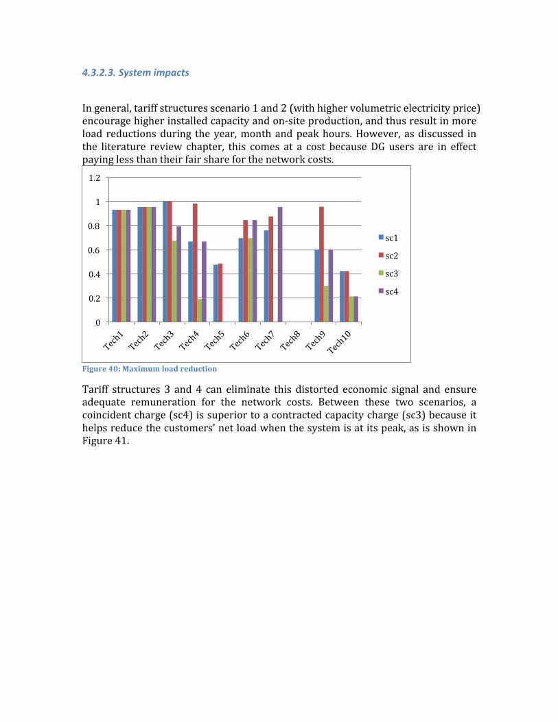
4.3.2.3. System impacts
In general, tariff structures scenario 1 and 2 (with higher volumetric electricity price) encourage higher installed capacity and on-‐site production, and thus result in more load reductions during the year, month and peak hours. However, as discussed in the literature review chapter, this comes at a cost because DG users are in effect paying less than their fair share for the network costs.
Figure 40: Maximum load reduction
Tariff structures 3 and 4 can eliminate this distorted economic signal and ensure adequate remuneration for the network costs. Between these two scenarios, a coincident charge (sc4) is superior to a contracted capacity charge (sc3) because it helps reduce the customers’ net load when the system is at its peak, as is shown in Figure 41.
0
0.2
0.4
0.6
0.8
1
1.2
sc1
sc2
sc3
sc4
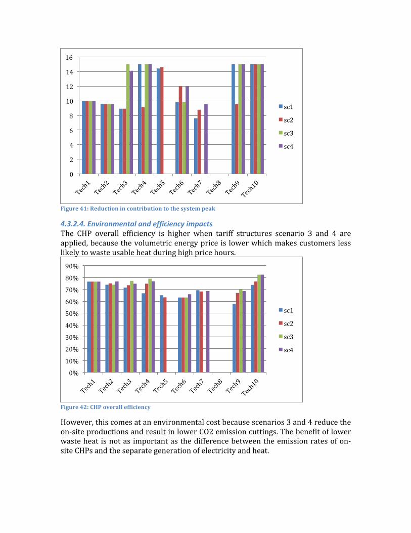
Figure 41: Reduction in contribution to the system peak
4.3.2.4. Environmental and efficiency impacts The CHP overall efficiency is higher when tariff structures scenario 3 and 4 are applied, because the volumetric energy price is lower which makes customers less likely to waste usable heat during high price hours.
Figure 42: CHP overall efficiency
However, this comes at an environmental cost because scenarios 3 and 4 reduce the on-‐site productions and result in lower CO2 emission cuttings. The benefit of lower waste heat is not as important as the difference between the emission rates of on-‐site CHPs and the separate generation of electricity and heat.
0
2
4
6
8
10
12
14
16
sc1
sc2
sc3
sc4
0%
10%
20%
30%
40%
50%
60%
70%
80%
90%
sc1
sc2
sc3
sc4

Figure 43: CO2 emission reduction rate
4.3.3 German Cogeneration Law Implementation
4.3.3.1 Decisions In Figure 44, we can see that the installed capacities do not change when the Cogeneration Law is considered (compared with the no incentive scenarios), except for a minor increase in Tech 3 when tariff structure scenario 3 is applied. An analysis on the operations of Tech 2 also shows that there is almost no impact on the utilization patterns of this technology.
Figure 44: Installed capacity of 10 technologies in 4 tariff structure scenarios (kW)
0
0.05
0.1
0.15
0.2
0.25
0.3
0.35
sc1
sc2
sc3
sc4
0
2000
4000
6000
8000
10000
12000
0
2000
4000
6000
8000
10000
12000
sc1
sc2
sc3
sc4
sc1 no incentive
sc2 no incentive
sc3 no incentive
sc4 no incentive

The utilization rate has little change in most technologies. The only exceptions are Tech 1 and Tech 7, as their utilization rate increased significantly. This is not because that the Cogeneration Law has any special effects on these two technologies in itself, but rather because the configuration of our model.
Figure 45: Incremental gas consumption per unit of installed capacity.
In real life, the electric efficiency of a generator decreases as the output goes down. Alternatively speaking, part-‐load generation results in lower electric efficiencies. The decrease is relatively small in the beginning and then accelerates as the percent of load goes down. Besides worse economics, such a decline would generally result in higher NOx and CO2 emissions as the system is not operating at a normal state. Therefore, to take into account this feature, we introduced an artificial part-‐load cut-‐off rate of 30%, meaning that the generator cannot produce at less than 30% of its designed electric capacity. In the industrial case, the electric load in off-‐peak hours is slightly below 30% of the designed capacity for Tech 1 and Tech 7, and when there is no incentive applied, the customer decides to turn off the generator and import from the grid. But when the cogeneration law is applied, the customer realizes that it is more profitable to generate during the off-‐peak hours and have the small amount of extra electricity generated exported to the grid. Although this change has a big impact on the utilization rate and the natural gas consumption, it does not influence the savings and economics in a significant way (discussed in the next section). Therefore, the anomalies shown in the case of Tech 1 and Tech 7 do not change the conclusion that the Cogeneration Law incentives are not set to be high enough to change the behavior of the industrial customers.
0
5
10
15
20
25
0.00
5.00
10.00
15.00
20.00
25.00
sc1
sc2
sc3
sc4
sc1 no incentive
sc2 no incentive
sc3 no incentive
sc4 no incentive

Figure 46: Part load efficiency performance in ICEs (left) and electricity export percentage (right). Source: EPA (2008)
The amount of exported electricity is very small compared with the total generation figure, and as discussed above is mainly in off-‐peak hours when the electric demand is low.
4.3.3.2. Economic and financial impacts Figure 47 shows that the annual savings through operations (not including generation incentives) changed little, which resonates with the finding above that the Cogeneration Law incentives had limited effect on the installation and operations of the technologies. Tech 1 and Tech 7 enjoyed higher annual savings because they received remuneration through exporting electricity and reduced purchase from the grid.
Figure 47: Annual savings as a percent of original annual total energy cost
0.00%
1.00%
2.00%
3.00%
4.00%
5.00%
sc1
sc2
sc3
sc4
-‐5%
0%
5%
10%
15%
20%
25%
30%
35%
40%
-‐5%
0%
5%
10%
15%
20%
25%
30%
35%
40%
sc1
sc2
sc3
sc4
sc1 no incentive
sc2 no incentive
sc3 no incentive
sc4 no incentive

Figure 48: Annual incentives received by the customer as a percentage of annual total energy cost
The pay-‐back periods are shortened because they receive generation subsidies from the Cogeneration Law, but only by a small margin in most cases. The main reason is that the incentive is set to be very low for large technologies while EEG charge on on-‐site generation is high, which further diminishes the total amount of feed-‐in-‐tariffs the industrial CHP customers receive. As is Shown in Figure 49, the net incentives received by the customer are less than 1% of its annual energy cost, which is too moderate to change their behaviors. Overall, Cogeneration Law has little impact on the system peak, the environment and the DG efficiency.
Figure 49: Pay-‐back period (year)
0.00%
0.20%
0.40%
0.60%
0.80%
1.00%
1.20%
Tech1 Tech2 Tech3 Tech4 Tech5 Tech6 Tech7 Tech8 Tech9 Tech10
sc1
sc2
sc3
sc4
0 1 2 3 4 5 6 7 8 9 10
-‐ 1.00 2.00 3.00 4.00 5.00 6.00 7.00 8.00 9.00 10.00
sc1
sc2
sc3
sc4
sc1 no incentive
sc2 no incentive
sc3 no incentive
sc4 no incentive

4.3.4. CAPEX Incentive is Implementation
4.3.4.1. Decisions When 30% capital incentive is applied, the installed capacity increased in the smaller technologies. The installations are now at a similar level for tariff structure scenario 1 and 2 versus 3 and 4. Moreover, even Tech 8 is made economically viable, though the installed capacity is still very small.
Figure 50: Installed capacity of 10 technologies in 4 tariff structure scenarios (kW)
In theory, CAPEX incentives should have no effect on the operations if the installation is the same, because they do not distort subsequent economic signals for operations. This is exactly what we observed in the case of Tech 2 and Tech 6 (Figure 51) where the utilization rate stays unchanged.
Figure 51: Incremental gas consumption per unit of installed capacity.
0
2000
4000
6000
8000
10000
12000
0
2000
4000
6000
8000
10000
12000
sc1
sc2
sc3
sc4
sc1 no incentive
sc2 no incentive
sc3 no incentive
sc4 no incentive
0
5
10
15
20
25
0.00
5.00
10.00
15.00
20.00
25.00
sc1
sc2
sc3
sc4
sc1 no incentive
sc2 no incentive
sc3 no incentive
sc4 no incentive

However, what is interesting is the operations of Tech 1 and 7, where the installation stayed the same while operations vary. This is again because of the aforementioned artificial part-‐load cut-‐off rate and the electricity export remunerations. Figure 52 and Figure 53 show the hourly heat and electric load and output of Tech 1 when tariff structure scenario 4 is in place. It is easy to see that the customer decides to generate during certain off-‐peak hours and export the excess to the grid when an export incentive is applied. Similar to the Cogeneration Law scenarios, the exported electricity is still a very small proportion of total on–site generation.
Figure 52: Operational schedule in a typical day for Tech 2 subject to scenario 4 when there is export incentive in place
Figure 53: Operational schedule in a typical day for Tech 2 subject to scenario 4 when there is no export incentive in place
4.3.4.2. Economic and financial impacts Annual savings through operations increased more than the Cogeneration Law scenarios, as the CAPEX incentive encourages more installation and thus more electricity and heat are produced using CHPs.
0
2000
4000
6000
8000
10000
12000
0
2000
4000
6000
8000
10000
12000
1 2 3 4 5 6 7 8 9 10 11 12 13 14 15 16 17 18 19 20 21 22 23 24
Energy [k
Wh/h]
Electricity -‐ January
Electricity Generation Electricity Import from the Grid Electricity Sales Total Electricity Load-‐6000
-‐1000
4000
9000
14000
-‐6000
-‐1000
4000
9000
14000
1 2 3 4 5 6 7 8 9 10 11 12 13 14 15 16 17 18 19 20 21 22 23 24
Energy [k
Wh/h]
Heat -‐ January
Heat Loss in Storage Heat Collected from DG Natural-‐gas Only Load Heat from Other Sources
Heat Taken from Storage Heat Supplied to Storage Total Water Heating Load Total Heat Load
0
2000
4000
6000
8000
10000
12000
0
2000
4000
6000
8000
10000
12000
1 2 3 4 5 6 7 8 9 10 11 12 13 14 15 16 17 18 19 20 21 22 23 24
Energy [k
Wh/h]
Electricity -‐ January
Electricity Generation Electricity Import from the Grid Electricity Sales Total Electricity Load
-‐6000
-‐1000
4000
9000
14000
-‐6000
-‐1000
4000
9000
14000
1 2 3 4 5 6 7 8 9 10 11 12 13 14 15 16 17 18 19 20 21 22 23 24
Energy [k
Wh/h]
Heat -‐ January
Heat Loss in Storage Heat Collected from DG Natural-‐gas Only Load Heat from Other Sources
Heat Taken from Storage Heat Supplied to Storage Total Water Heating Load Total Heat Load

Figure 54: Annual savings as a percent of original annual total energy cost
The pay-‐back periods are significantly shortened in many cases (even in those where installation increased), as the increased investment cost is more than off-‐set by the 30% price cut and the increased annual operational savings. However, the effectiveness of this incentive comes at a high price from the regulator’s perspective because the government has to provide substantial subsidies. Figure 55 plots the annualized capital incentives received by the customer as a proportion of their original annual total energy cost34. The ratio could reach as high as 7% when compared with 1% in the Cogeneration Law scenarios.
Figure 55: Annualized CAPEX incentives received by the customer as a percentage of annual total energy cost
34 Assuming a 10-‐year depreciation period.
-‐5%
0%
5%
10%
15%
20%
25%
30%
35%
40%
-‐5%
0%
5%
10%
15%
20%
25%
30%
35%
40%
sc1
sc2
sc3
sc4
sc1 no incentive
sc2 no incentive
sc3 no incentive
sc4 no incentive
0.00%
1.00%
2.00%
3.00%
4.00%
5.00%
6.00%
7.00%
8.00%
sc1
sc2
sc3
sc4
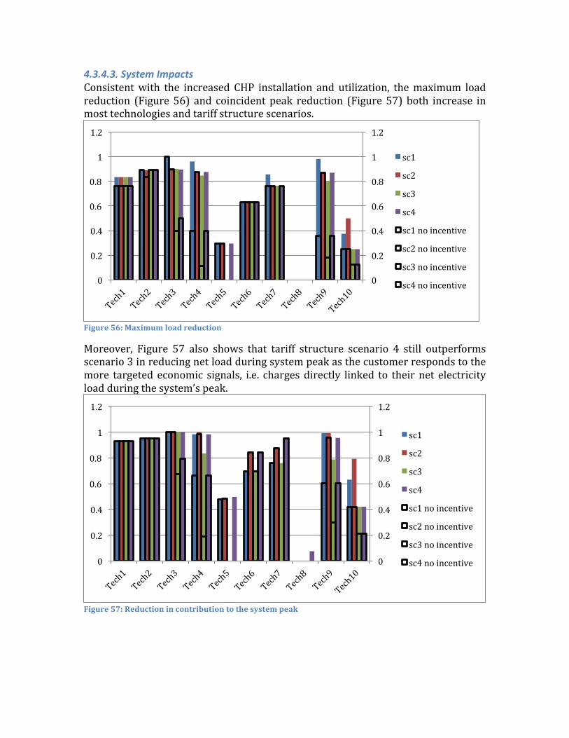
4.3.4.3. System Impacts Consistent with the increased CHP installation and utilization, the maximum load reduction (Figure 56) and coincident peak reduction (Figure 57) both increase in most technologies and tariff structure scenarios.
Figure 56: Maximum load reduction
Moreover, Figure 57 also shows that tariff structure scenario 4 still outperforms scenario 3 in reducing net load during system peak as the customer responds to the more targeted economic signals, i.e. charges directly linked to their net electricity load during the system’s peak.
Figure 57: Reduction in contribution to the system peak
0
0.2
0.4
0.6
0.8
1
1.2
0
0.2
0.4
0.6
0.8
1
1.2
sc1
sc2
sc3
sc4
sc1 no incentive
sc2 no incentive
sc3 no incentive
sc4 no incentive
0
0.2
0.4
0.6
0.8
1
1.2
0
0.2
0.4
0.6
0.8
1
1.2
sc1
sc2
sc3
sc4
sc1 no incentive
sc2 no incentive
sc3 no incentive
sc4 no incentive

4.3.4.4 Environmental and Efficiency Impacts The CAPEX Incentives have very limited impact on the DG efficiencies as customers still try to avoid wasting usable heat. On the other hand, CO2 emissions further reduced thanks to the higher overall efficiency of on-‐site generation.
Figure 58: CHP overall efficiency
Figure 59: CO2 emission reduction rate
4.3.5. Sensitivity Analysis As discussed in section 4.2, the German energy market conditions, as well as those in other EU nations, have changed quickly over the years. This may exert impacts on the subsequent operations and economics of future CHP projects, once the system has been installed on-‐site. Here, we examine the hourly operation decisions of the Tech 2 systems when tariff structure scenario 4 is applied and there are no incentives. Metrics such as annual savings and DG overall efficiency are also
0%
10%
20%
30%
40%
50%
60%
70%
80%
90%
0%
10%
20%
30%
40%
50%
60%
70%
80%
90%
sc1
sc2
sc3
sc4
sc1 no incentive
sc2 no incentive
sc3 no incentive
sc4 no incentive
0
0.05
0.1
0.15
0.2
0.25
0.3
0.35
0
0.05
0.1
0.15
0.2
0.25
0.3
0.35
sc1
sc2
sc3
sc4
sc1 no incentive
sc2 no incentive
sc3 no incentive
sc4 no incentive

analyzed. The goal is to understand how sensitive our previously established conclusions are in relation to various market conditions.
Figure 60: Operational schedule in a typical day for Tech 2 scenario 4 -‐Base case
Comparing Figure 60, Figure 61 and Figure 62, we can see that the customer chooses to buy more (less) electricity from the grid in off-‐peak hours when electricity price is 30% lower (higher) than in the base case. This is intuitive, since the grid level electricity become less (more) expensive compared with generating on-‐site35.
Figure 61: Operational schedule in a typical day for Tech 2 scenario 4 -‐Decreased electricity price
35 Remember, the natural gas price, the electric efficiency and heat to power ratio are constant.
-‐6000
-‐1000
4000
9000
14000
-‐6000
-‐1000
4000
9000
14000
1 2 3 4 5 6 7 8 9 10 11 12 13 14 15 16 17 18 19 20 21 22 23 24
Energy [k
Wh/h]
Heat -‐ January
Heat Loss in Storage Heat Collected from DG Natural-‐gas Only Load Heat from Other Sources
Heat Taken from Storage Heat Supplied to Storage Total Water Heating Load Total Heat Load
0
2000
4000
6000
8000
10000
12000
0
2000
4000
6000
8000
10000
12000
1 2 3 4 5 6 7 8 9 10 11 12 13 14 15 16 17 18 19 20 21 22 23 24
Energy [k
Wh/h]
Electricity -‐ January
Electricity Generation Electricity Import from the Grid Electricity Sales Total Electricity Load
-‐6000
-‐1000
4000
9000
14000
-‐6000
-‐1000
4000
9000
14000
1 2 3 4 5 6 7 8 9 10 11 12 13 14 15 16 17 18 19 20 21 22 23 24
Energy [k
Wh/h]
Heat -‐ January
Heat Loss in Storage Heat Collected from DG Natural-‐gas Only Load Heat from Other Sources
Heat Taken from Storage Heat Supplied to Storage Total Water Heating Load Total Heat Load
0
2000
4000
6000
8000
10000
12000
0
2000
4000
6000
8000
10000
12000
1 2 3 4 5 6 7 8 9 10 11 12 13 14 15 16 17 18 19 20 21 22 23 24
Energy [k
Wh/h]
Electricity -‐ January
Electricity Generation Electricity Import from the Grid Electricity Sales Total Electricity Load

Figure 62: Operational schedule in a typical day for Tech 2 scenario 4 -‐Increased electricity price
The influence of 30% lower (higher) natural gas price is conjugating with, though not exactly the same as, that in the 30% higher (lower) electricity prices. After all, decreasing (increasing) natural gas price is in effect making grid electricity price relatively less (more) expensive to serve the same energy demand.
Figure 63: Operational schedule in a typical day for Tech 2 scenario 4 -‐Decrease NG price
Figure 64: Operational schedule in a typical day for Tech 2 scenario 4 -‐Increase NG price
-‐6000
-‐1000
4000
9000
14000
-‐6000
-‐1000
4000
9000
14000
1 2 3 4 5 6 7 8 9 10 11 12 13 14 15 16 17 18 19 20 21 22 23 24
Energy [k
Wh/h]
Heat -‐ January
Heat Loss in Storage Heat Collected from DG Natural-‐gas Only Load Heat from Other Sources
Heat Taken from Storage Heat Supplied to Storage Total Water Heating Load Total Heat Load
0
2000
4000
6000
8000
10000
12000
0
2000
4000
6000
8000
10000
12000
1 2 3 4 5 6 7 8 9 10 11 12 13 14 15 16 17 18 19 20 21 22 23 24
Energy [k
Wh/h]
Electricity -‐ January
Electricity Generation Electricity Import from the Grid Electricity Sales Total Electricity Load
-‐6000
-‐1000
4000
9000
14000
-‐6000
-‐1000
4000
9000
14000
1 2 3 4 5 6 7 8 9 10 11 12 13 14 15 16 17 18 19 20 21 22 23 24
Energy [k
Wh/h]
Heat -‐ January
Heat Loss in Storage Heat Collected from DG Natural-‐gas Only Load Heat from Other Sources
Heat Taken from Storage Heat Supplied to Storage Total Water Heating Load Total Heat Load
0
2000
4000
6000
8000
10000
12000
0
2000
4000
6000
8000
10000
12000
1 2 3 4 5 6 7 8 9 10 11 12 13 14 15 16 17 18 19 20 21 22 23 24
Energy [k
Wh/h]
Electricity -‐ January
Electricity Generation Electricity Import from the Grid Electricity Sales Total Electricity Load

If we double the electric export price, the customer would be incentivized to have more on-‐site generation and sell the extra electricity to the grid when the price is high. But this may also lead to more waste heat.
Figure 65: Operational schedule in a typical day for Tech 2 scenario 4 -‐Double PX price
From Figure 66 we can see that the annual savings through operations are more sensitive to the electricity price. The elasticities for electricity price, gas price and export price are 2.0, 0.9 and 0.07 respectively.
Figure 66: Annual savings through operations for Tech 2 scenario 4 in different market conditions. Units: Euros
Figure 67 shows that the DG overall efficiency does not vary too much (<4%) in responds to different market conditions.
-‐6000
-‐1000
4000
9000
14000
-‐6000
-‐1000
4000
9000
14000
1 2 3 4 5 6 7 8 9 10 11 12 13 14 15 16 17 18 19 20 21 22 23 24
Energy [k
Wh/h]
Heat -‐ January
Heat Loss in Storage Heat Collected from DG Natural-‐gas Only Load Heat from Other Sources
Heat Taken from Storage Heat Supplied to Storage Total Water Heating Load Total Heat Load
0
2000
4000
6000
8000
10000
12000
0
2000
4000
6000
8000
10000
12000
1 2 3 4 5 6 7 8 9 10 11 12 13 14 15 16 17 18 19 20 21 22 23 24
Energy [k
Wh/h]
Electricity -‐ January
Electricity Generation Electricity Import from the Grid Electricity Sales Total Electricity Load
-‐ 500,000
1,000,000 1,500,000 2,000,000 2,500,000 3,000,000 3,500,000 4,000,000 4,500,000 5,000,000
no change elec price -‐30%
elec price +30%
elec export price*2
gas price -‐30% gas price +30%

Figure 67: CHP overall efficiencies for Tech 2 scenario 4 in different market conditions
Finally, the incremental natural gas purchase shows a ±10% among all the conditions. It is especially interesting to see that a higher electricity export price has the most impact on the natural gas usage and thus the gas suppliers’ revenue, even though its implications for the customer are limited.
Figure 68: Incremental NG purchases for Tech 2 scenario 4 in different market conditions
4.3.6. Summary of the Industrial Case To summarize some of the key findings in the 4.4 section:
1. Tariff structure has significant influence on the installation decisions of smaller industry level distributed CHP systems, but not so much on the larger ones. The customers face a binary choice if the unit size of a technology is commensurable with the electric load, and thus the influence of different tariff structures is not fully realized.
72%
73%
74%
75%
76%
77%
78%
79%
no change elec price -‐30% elec price +30%
elec export price*2
gas price -‐30% gas price +30%
0% 10% 20% 30% 40% 50% 60% 70% 80% 90% 100%
no change elec price -‐30%
elec price +30%
elec export price*2
gas price -‐30%
gas price +30%

2. Internal combustion engines and certain fuel cells, gas turbines and micro turbines are economically viable technologies even without any incentives and in any tariff structures. However, ICEs are still a much more mature and attractive technology for CHP applications. Thus, targeted subsidies for new technologies such as fuel cells and micro turbines may be necessary.
3. Flat volumetric electricity rate encourages higher a utilization rate, because customers are incentivized to generate electricity during off-‐peak hours. However, this may result in more waste heat if no heat storage is available.
4. A coincident charge is effective in incentivizing generation during system’s peak compared with traditional contracted capacity charges.
5. CHP technologies show very high overall efficiencies in all tariff structure scenarios and have noticeable environment benefits.
6. The current Cogeneration Law implemented in Germany does not have enough incentives for industrial customers and has negligible influence on the decision making process of these customers. This is mainly because industrial players can benefit significantly from distributed CHP systems without any incentives.
7. CAPEX incentives can shorten the pay-‐back period while not distorting the short-‐term economic signals essential for having efficient operations.
8. The annual savings are most sensitive to electricity purchase price, and not so much to gas price or electricity export rate. Energy efficiency did not show to be sensitive to the market conditions in the industrial case.

4.4. Results from the Multi-‐family Case
4.4.1. Business as Usual Reference Case
Total Annual Energy Costs [$] 277,612
Annual non-‐DER Electricity Purchase [$] 209,282
Annual NG Purchase [$] 68,330
Annual Total Energy Demand [kWh] 1,655,938
Total Electricity Load [kWh] 762,646
Annual Electricity-‐Only Load [kWh] 676,911
Annual Cooling Load [kWh] 85,735
Annual Refrigeration Load [kWh] -‐
Total Heat Load [kWh] 893,292
Annual Space Heating Load [kWh] 320,916
Annual Water Heating Load [kWh] 429,361
Annual Natural Gas-‐Only Load [kWh] 143,015
Annual Total Emissions [kgCO2] 585,565
Table 15: Summary of the business as usual multi-‐family case
As shown in Table 15, the annual 1GWh energy demand comprises 47% electricity load and 53% gas load when there are no CHP installations. The size of the multi-‐family application is 1% of the food-‐processing factory analyzed in Section 4.3 from the perspective of energy consumption. As for the energy cost, 75% comes from electricity bills and 25% from natural gas bills. Annual CO2 emissions stand at 586 tons.
4.4.2 When no Incentive is Implemented
4.4.2.1. Decisions Similar to the industrial case, there are several technologies that are relatively large and the capacity of a single unit is close to the average electric load of the multi-‐family building (around 100kW). For instance, Tech 1 and 4 are 100kW and 200kW

ICEs respectively. Tech 8 and 9 are large fuel cell technologies, both with a unit capacity of 100kW. For these technologies, the customer is in fact facing binary choices, i.e. either install one unit or have no installation at all. Tech 4 has a capacity size close to the maximum electric load of the building. But given the variability of the load profile, the utilization rate would be so low that the annual savings cannot justify the high upfront capital expenditure. As a result, the customer decides not to install any Tech 4 on-‐site. In comparison, Tech 2, 3, 5, 7 and 10 are smaller technologies and show higher variability in their installation decisions for different tariff structure scenarios. Similar to the findings in the industrial case, tariff structures scenario 3 and 4 encourage less installation compared with scenario 1 and 2, because the volumetric electricity prices are lower and the annual saving potential is reduced. Tech 7 represents small solid oxide fuel cell technology, which has a very high per kW CAPEX as it is still in the early stage of commercialization. The high upfront cost deters customers from installing this technology.
Figure 69: Installed capacity of 10 technologies in 4 tariff structure scenarios
For the purpose of comparing the operation decisions in different tariff structure scenarios, we pick Tech 1 as an example because it has the same installed capacity in all scenarios. Unlike industrial applications, residential cases show more seasonality. As a result, we are including operations in a typical day in both January and July to have a better representation of the different patterns during summer and winter. From Figure 70 we can easily see that both the electric and heat load show significant monthly as well as daily variability. The heat and electric load don’t match well during the summer, when air-‐conditioners have an important contribution to the load while the heat demand is very low. This gives rise to the problem of waste heat as shown in the lower right hand side of Figure 70. In this context, it might be beneficial to have tri-‐generation rather than cogeneration, which could utilize the exhaust heat from the generator to drive heat pumps in the summer. Similar to the findings in the industrial case, the customer would take
0
20
40
60
80
100
120
Tech1 Tech2 Tech3 Tech4 Tech5 Tech6 Tech7 Tech8 Tech9 Tech10
sc1
sc2
sc3
sc4
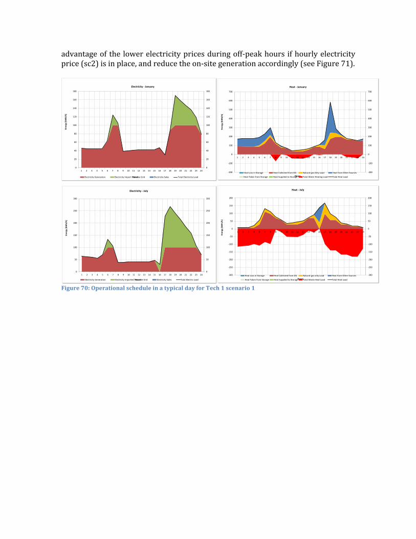
advantage of the lower electricity prices during off-‐peak hours if hourly electricity price (sc2) is in place, and reduce the on-‐site generation accordingly (see Figure 71).
Figure 70: Operational schedule in a typical day for Tech 1 scenario 1
-‐200
-‐100
0
100
200
300
400
500
600
700
-‐200
-‐100
0
100
200
300
400
500
600
700
1 2 3 4 5 6 7 8 9 10 11 12 13 14 15 16 17 18 19 20 21 22 23 24
Energy [k
Wh/h]
Hours
Heat -‐ January
Heat Loss in Storage Heat Collected from DG Natural-‐gas Only Load Heat from Other Sources
Heat Taken from Storage Heat Supplied to Storage Total Water Heating Load Total Heat Load
-‐300
-‐250
-‐200
-‐150
-‐100
-‐50
0
50
100
150
200
-‐300
-‐250
-‐200
-‐150
-‐100
-‐50
0
50
100
150
200
1 2 3 4 5 6 7 8 9 10 11 12 13 14 15 16 17 18 19 20 21 22 23 24
Energy [k
Wh/h]
Hours
Heat -‐ July
Heat Loss in Storage Heat Collected from DG Natural-‐gas only Load Heat from Other Sources
Heat Taken from Storage Heat Supplied to Storage Total Waste Heat Load Total Heat Load
0
20
40
60
80
100
120
140
160
180
0
20
40
60
80
100
120
140
160
180
1 2 3 4 5 6 7 8 9 10 11 12 13 14 15 16 17 18 19 20 21 22 23 24
Energy [k
Wh/h]
Hours
Electricity -‐ January
Electricity Generation Electricity Import from the Grid Electricity Sales Total Electricity Load
0
50
100
150
200
250
300
0
50
100
150
200
250
300
1 2 3 4 5 6 7 8 9 10 11 12 13 14 15 16 17 18 19 20 21 22 23 24
Energy [k
Wh/h]
Hours
Electricity -‐ July
Electricity Generation Electricity Imported from the Grid Slectricity Sales Total Electric Load

Figure 71: Operational schedule in a typical day for Tech 1 scenario 2
Operations under tariff structure 3 and 4 are not drastically different. In the two examples of operation schedules in January and July, the on-‐site generation shows identical patterns (see Figure 72). But as it is shown in the utilization rate chart (Figure 73), there is a slight difference on the operations of Tech 1 in scenario 3 and 4.
-‐200
-‐100
0
100
200
300
400
500
600
700
-‐200
-‐100
0
100
200
300
400
500
600
700
1 2 3 4 5 6 7 8 9 10 11 12 13 14 15 16 17 18 19 20 21 22 23 24
Energy [k
Wh/h]
Hours
Heat -‐ January
Heat Loss in Storage Heat Collected from DG Natural-‐gas Only Load Heat from Other Sources
Heat Taken from Storage Heat Supplied to Storage Total Water Heating Load Total Heat Load
-‐300
-‐250
-‐200
-‐150
-‐100
-‐50
0
50
100
150
200
-‐300
-‐250
-‐200
-‐150
-‐100
-‐50
0
50
100
150
200
1 2 3 4 5 6 7 8 9 10 11 12 13 14 15 16 17 18 19 20 21 22 23 24
Energy [k
Wh/h]
Hours
Heat -‐ July
Heat Loss in Storage Heat Collected from DG Natural-‐gas only Load Heat from Other Sources
Heat Taken from Storage Heat Supplied to Storage Total Waste Heat Load Total Heat Load
0
20
40
60
80
100
120
140
160
180
0
20
40
60
80
100
120
140
160
180
1 2 3 4 5 6 7 8 9 10 11 12 13 14 15 16 17 18 19 20 21 22 23 24
Energy [k
Wh/h]
Hours
Electricity -‐ January
Electricity Generation Electricity Import from the Grid Electricity Sales Total Electricity Load
0
50
100
150
200
250
300
0
50
100
150
200
250
300
1 2 3 4 5 6 7 8 9 10 11 12 13 14 15 16 17 18 19 20 21 22 23 24
Energy [k
Wh/h]
Hours
Electricity -‐ July
Electricity Generation Electricity Imported from the Grid Slectricity Sales Total Electric Load

Figure 72: Operational schedule in a typical day for Tech 1 scenario 3 and 4
The utilization rates in tariff structure scenario 1 and 2 are higher than those in scenario 3 and 4 mainly because the higher volumetric electricity price sends a stronger economic signal to incentivize on-‐site generation. The only outliers are Tech 10 and Tech 5. In scenario 3 of Tech 10, the utilization rate is higher mainly because the installed capacity is much smaller than that in other scenarios. Similarly, scenario 1 and 2 of Tech 10, the utilization rate is lower than scenario 3 because the customer decided to have more installed capacity. It should be noted that the utilization rates of the industrial case and the multi-‐family case are not directly comparable because different constants are used.
Figure 73: Incremental gas consumption per unit of installed capacity.
-‐200
-‐100
0
100
200
300
400
500
600
700
-‐200
-‐100
0
100
200
300
400
500
600
700
1 2 3 4 5 6 7 8 9 10 11 12 13 14 15 16 17 18 19 20 21 22 23 24
Energy [k
Wh/h]
Hours
Heat -‐ January
Heat Loss in Storage Heat Collected from DG Natural-‐gas Only Load Heat from Other Sources
Heat Taken from Storage Heat Supplied to Storage Total Water Heating Load Total Heat Load
-‐300
-‐250
-‐200
-‐150
-‐100
-‐50
0
50
100
150
200
-‐300
-‐250
-‐200
-‐150
-‐100
-‐50
0
50
100
150
200
1 2 3 4 5 6 7 8 9 10 11 12 13 14 15 16 17 18 19 20 21 22 23 24
Energy [k
Wh/h]
Hours
Heat -‐ July
Heat Loss in Storage Heat Collected from DG Natural-‐gas only Load Heat from Other Sources
Heat Taken from Storage Heat Supplied to Storage Total Waste Heat Load Total Heat Load
0
20
40
60
80
100
120
140
160
180
0
20
40
60
80
100
120
140
160
180
1 2 3 4 5 6 7 8 9 10 11 12 13 14 15 16 17 18 19 20 21 22 23 24
Energy [k
Wh/h]
Hours
Electricity -‐ January
Electricity Generation Electricity Import from the Grid Electricity Sales Total Electricity Load
0
50
100
150
200
250
300
0
50
100
150
200
250
300
1 2 3 4 5 6 7 8 9 10 11 12 13 14 15 16 17 18 19 20 21 22 23 24
Energy [k
Wh/h]
Hours
Electricity -‐ July
Electricity Generation Electricity Imported from the Grid Slectricity Sales Total Electric Load
0
2
4
6
8
10
12
14
Tech1 Tech2 Tech3 Tech4 Tech5 Tech6 Tech7 Tech8 Tech9 Tech10
sc1
sc2
sc3
sc4

4.4.2.2. Economic and financial impacts Similar to the industrial case, the payback period of the viable residential CHP technologies show a wide range (from 3.5 years up to 9 years). Thanks to a larger difference between the residential electricity price and natural gas price, the payback period is commensurable with that in the industrial case despite more expensive technologies on a per kW basis and lower electric efficiency due to reduced sizes.
Figure 74: Pay-‐back period (year)
However, because of a higher load variability and thus lower installed capacity to average electric load ratio, residential CHP in general cannot achieve the same level of annual savings through operations (as a percentage of original energy bill) as their counterparts in the industrial applications (Figure 75 and Figure 39). The only outliers are the fuel cells technologies. But their higher operational savings are more than offset by their high capital cost, resulting in a long pay-‐back period.
Figure 75: Annual savings as a percent of original annual total energy cost
-‐ 1.00 2.00 3.00 4.00 5.00 6.00 7.00 8.00 9.00 10.00
sc1
sc2
sc3
sc4
-‐5%
0%
5%
10%
15%
20%
25%
30%
35%
40%
sc1
sc2
sc3
sc4

4.4.2.3. System Impact As a result of lower installed capacity to peak electric load ratio, the maximum load reduction in the multi-‐family case is lower than that in the industrial case (Figure 76 and Figure 40).
Figure 76: Maximum load reduction
From Figure 77 and Figure 78, we can see that in general tariff structure 3 results in higher contracted capacity reduction while scenario 4 encourages higher coincident peak reduction. This is in line with our observation in the industrial case and proves a coincident tariff can be an effective economic signal to incentivize customers reduce their contribution to the system peak and thus achieve better system’s cost savings.
Figure 77: Contracted capacity reduction
0
0.05
0.1
0.15
0.2
0.25
0.3
sc1
sc2
sc3
sc4
0 0.05 0.1 0.15 0.2 0.25 0.3 0.35 0.4 0.45 0.5
sc1
sc2
sc3
sc4

Figure 78: Reduction in contribution to the system peak
4.4.2.4. Environmental and efficiency impacts: Consistent with our findings in section 4.3.2.4, CHP overall efficiency is higher under tariff structure 3 and 4 because the volumetric electricity price is lower and customers are more cautious not to waste usable heat.
Figure 79: CHP overall efficiency
In terms of CO2 reduction, residential CHP projects underperform compared with industrial ones mainly because a lower installation and operation level36 (see Figure 80 and Figure 43). 36 Except for the 100kW fuel cells (Tech 8 and 9), which benefit from larger capacity compared with the average load and a higher electric efficiency.
0 0.05 0.1 0.15 0.2 0.25 0.3 0.35 0.4 0.45 0.5
sc1
sc2
sc3
sc4
0%
10%
20%
30%
40%
50%
60%
70%
80%
90%
sc1
sc2
sc3
sc4

Figure 80: CO2 emission reduction rate
4.4.3. German Cogeneration Law Implementation
4.4.3.1. Decisions In Figure 81 we can see that the installed capacities increased significantly in many cases, especially when tariff structures scenario 3 and 4 are applied. This differs from our observation in the industrial case, where the Cogeneration Law has little impact on the installation decisions. Moreover, we can see large technologies like Tech 4 become economically viable due to the subsidy. However, Tech 7 remains unattractive, indicating that solid oxide technology may be still “deep under water”.
Figure 81: Installed capacity of 10 technologies in 4 tariff structure scenarios
0
0.05
0.1
0.15
0.2
0.25
0.3
0.35
sc1
sc2
sc3
sc4
0
50
100
150
200
250
0
50
100
150
200
250
sc1
sc2
sc3
sc4
sc1 no incentive
sc2 no incentive
sc3 no incentive
sc4 no incentive

Taking Tech 1 under tariff structure scenario 4 as an example, we can see from Figure 82 and Figure 83 that the customer decides to increase the production during the summer even though that gives rise to more waste heat.
Figure 82: Operational schedule in a typical day for Tech 1 scenario 4 -‐With Incentive
-‐200
-‐100
0
100
200
300
400
500
600
700
-‐200
-‐100
0
100
200
300
400
500
600
700
1 2 3 4 5 6 7 8 9 10 11 12 13 14 15 16 17 18 19 20 21 22 23 24
Energy [k
Wh/h]
Hours
Heat -‐ January
Heat Loss in Storage Heat Collected from DG Natural-‐gas Only Load Heat from Other Sources
Heat Taken from Storage Heat Supplied to Storage Total Water Heating Load Total Heat Load
-‐300
-‐250
-‐200
-‐150
-‐100
-‐50
0
50
100
150
200
-‐300
-‐250
-‐200
-‐150
-‐100
-‐50
0
50
100
150
200
1 2 3 4 5 6 7 8 9 10 11 12 13 14 15 16 17 18 19 20 21 22 23 24
Energy [k
Wh/h]
Hours
Heat -‐ July
Heat Loss in Storage Heat Collected from DG Natural-‐gas only Load Heat from Other Sources
Heat Taken from Storage Heat Supplied to Storage Total Waste Heat Load Total Heat Load
0
20
40
60
80
100
120
140
160
180
0
20
40
60
80
100
120
140
160
180
1 2 3 4 5 6 7 8 9 10 11 12 13 14 15 16 17 18 19 20 21 22 23 24
Energy [k
Wh/h]
Hours
Electricity -‐ January
Electricity Generation Electricity Import from the Grid Electricity Sales Total Electricity Load
0
50
100
150
200
250
300
0
50
100
150
200
250
300
1 2 3 4 5 6 7 8 9 10 11 12 13 14 15 16 17 18 19 20 21 22 23 24
Energy [k
Wh/h]
Hours
Electricity -‐ July
Electricity Generation Electricity Imported from the Grid Slectricity Sales Total Electric Load

Figure 83: Operational schedule in a typical day for Tech 1 scenario 4 –Base case
Consequently, the utilization rate in general increased, though in certain circumstances decreased as more capacity was installed to only generate during the peak hours (see Figure 84). As for the electricity export, the ratio is negligible except for Tech 4, where 9% of on-‐site generation is fed-‐back into the grid.
Figure 84: Incremental gas consumption per unit of installed capacity.
-‐200
-‐100
0
100
200
300
400
500
600
700
-‐200
-‐100
0
100
200
300
400
500
600
700
1 2 3 4 5 6 7 8 9 10 11 12 13 14 15 16 17 18 19 20 21 22 23 24
Energy [k
Wh/h]
Hours
Heat -‐ January
Heat Loss in Storage Heat Collected from DG Natural-‐gas Only Load Heat from Other Sources
Heat Taken from Storage Heat Supplied to Storage Total Water Heating Load Total Heat Load
-‐300
-‐250
-‐200
-‐150
-‐100
-‐50
0
50
100
150
200
-‐300
-‐250
-‐200
-‐150
-‐100
-‐50
0
50
100
150
200
1 2 3 4 5 6 7 8 9 10 11 12 13 14 15 16 17 18 19 20 21 22 23 24
Energy [k
Wh/h]
Hours
Heat -‐ July
Heat Loss in Storage Heat Collected from DG Natural-‐gas only Load Heat from Other Sources
Heat Taken from Storage Heat Supplied to Storage Total Waste Heat Load Total Heat Load
0
20
40
60
80
100
120
140
160
180
0
20
40
60
80
100
120
140
160
180
1 2 3 4 5 6 7 8 9 10 11 12 13 14 15 16 17 18 19 20 21 22 23 24
Energy [k
Wh/h]
Hours
Electricity -‐ January
Electricity Generation Electricity Import from the Grid Electricity Sales Total Electricity Load
0
50
100
150
200
250
300
0
50
100
150
200
250
300
1 2 3 4 5 6 7 8 9 10 11 12 13 14 15 16 17 18 19 20 21 22 23 24
Energy [k
Wh/h]
Hours
Electricity -‐ July
Electricity Generation Electricity Imported from the Grid Slectricity Sales Total Electric Load
0
5
10
15
20
25
0.00
5.00
10.00
15.00
20.00
25.00
sc1
sc2
sc3
sc4
sc1 no incentive
sc2 no incentive
sc3 no incentive
sc4 no incentive

4.4.3.2. Economic and financial impacts The annual savings through operations do not change much. As is shown in Figure 85, however, the Cogeneration Law incentive is substantial for residential CHP projects. It can account for up to 10% of the original energy bill of the customer (in comparison, it only represent less than 1% in the industrial case). This further supports the theory that the Cogeneration Law is tilted toward smaller residential customers rather than larger industrial players.
Figure 85: Annual incentives received by the customer as a percentage of annual total energy cost Consequently, the payback period decreased significantly for most technologies, as can be seen in Figure 86.
Figure 86: Pay-‐back period (year)
0.00%
2.00%
4.00%
6.00%
8.00%
10.00%
12.00%
sc1
sc2
sc3
sc4
0
2
4
6
8
10
12
-‐
2.00
4.00
6.00
8.00
10.00
12.00
sc1
sc2
sc3
sc4
sc1 no incentive
sc2 no incentive
sc3 no incentive
sc4 no incentive

At the system level, the Cogeneration Law encourages higher load reduction because customers tend to increase their installation and operation of on-‐site CHPs.
Figure 87: Reduction in contribution to the system peak
However, it also comes at a price of lower overall efficiency and CO2 emission reductions in certain cases. Customers may choose to have more exhaust heat from the generator as the increased incentive revenue compensates them for an amount more than the extra generation.
Figure 88: CHP overall efficiency
0
0.1
0.2
0.3
0.4
0.5
0.6
0.7
0.8
0.9
1
0
0.1
0.2
0.3
0.4
0.5
0.6
0.7
0.8
0.9
sc1
sc2
sc3
sc4
sc1 no incentive
sc2 no incentive
sc3 no incentive
sc4 no incentive
0%
10%
20%
30%
40%
50%
60%
70%
80%
90%
0%
10%
20%
30%
40%
50%
60%
70%
80%
90%
sc1
sc2
sc3
sc4
sc1 no incentive
sc2 no incentive
sc3 no incentive
sc4 no incentive
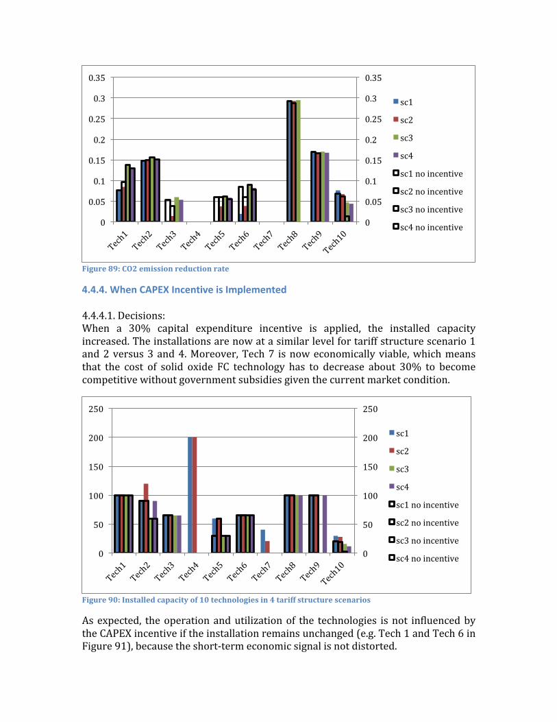
Figure 89: CO2 emission reduction rate
4.4.4. When CAPEX Incentive is Implemented 4.4.4.1. Decisions: When a 30% capital expenditure incentive is applied, the installed capacity increased. The installations are now at a similar level for tariff structure scenario 1 and 2 versus 3 and 4. Moreover, Tech 7 is now economically viable, which means that the cost of solid oxide FC technology has to decrease about 30% to become competitive without government subsidies given the current market condition.
Figure 90: Installed capacity of 10 technologies in 4 tariff structure scenarios
As expected, the operation and utilization of the technologies is not influenced by the CAPEX incentive if the installation remains unchanged (e.g. Tech 1 and Tech 6 in Figure 91), because the short-‐term economic signal is not distorted.
0
0.05
0.1
0.15
0.2
0.25
0.3
0.35
0
0.05
0.1
0.15
0.2
0.25
0.3
0.35
sc1
sc2
sc3
sc4
sc1 no incentive
sc2 no incentive
sc3 no incentive
sc4 no incentive
0
50
100
150
200
250
0
50
100
150
200
250
sc1
sc2
sc3
sc4
sc1 no incentive
sc2 no incentive
sc3 no incentive
sc4 no incentive

Figure 91: Incremental gas consumption per unit of installed capacity
4.4.4.2. Economic and financial impacts Annual savings through operations remain flat as long as the installation decision does not change. The economic benefits mainly come through the capital incentives, and customers installing larger and more expensive technologies gain the most (see Figure 92).
Figure 92: Annualized CAPEX incentives received by the customer as a percentage of annual total energy cost
The effect on the payback periods is similar to that in the Cogeneration Law scenarios. More technologies are made economically viable, especially when tariff structure scenario 3 and 4 are applied.
0
2
4
6
8
10
12
14
0.00
2.00
4.00
6.00
8.00
10.00
12.00
14.00
sc1
sc2
sc3
sc4
sc1 no incentive
sc2 no incentive
sc3 no incentive
sc4 no incentive
0.00%
1.00%
2.00%
3.00%
4.00%
5.00%
6.00%
7.00%
8.00%
9.00%
10.00%
Tech1 Tech2 Tech3 Tech4 Tech5 Tech6 Tech7 Tech8 Tech9 Tech10
sc1
sc2
sc3
sc4

Figure 93: Pay-‐back period (year)
The 30% CAPEX incentive has similar impact on the maximum load reduction and the peak load reduction. But it is more favorable from the environmental perspective, since the short-‐term economic signal is not distorted and the customers are not incentivized to waste heat. As a result, the overall efficiency (Figure 94 and Figure 58) and the CO2 emissions savings (Figure 95 and Figure 59) are higher in the CAPEX incentive scenarios than that in the Cogeneration Law scenarios.
Figure 94: CHP overall efficiency
0
2
4
6
8
10
12
-‐
2.00
4.00
6.00
8.00
10.00
12.00
sc1
sc2
sc3
sc4
sc1 no incentive
sc2 no incentive
sc3 no incentive
sc4 no incentive
0%
10%
20%
30%
40%
50%
60%
70%
80%
90%
0%
10%
20%
30%
40%
50%
60%
70%
80%
90%
sc1
sc2
sc3
sc4
sc1 no incentive
sc2 no incentive
sc3 no incentive
sc4 no incentive

Figure 95: CO2 emission reduction rate
4.4.5. Sensitivity Analysis As discussed in section 4.2, the German energy market condition for residential customers experienced many changes over the past few years and remains volatile in the future. Situation is similar in many other EU nations as well. This may exert impacts on the subsequent operations and economics of the CHP projects once the system has been installed on-‐site. Here, we examine the hourly operation decisions of the installed Tech 2 systems when tariff structure scenario 4 is applied and there are no incentives. The goal is to understand the sensitivity of the operations decisions as well as the economic values of CHP systems. Similar to our findings in the industrial case, we can see from Figure 96, Figure 97 and Figure 98 that the customer chooses to buy more (less) electricity from the grid in off-‐peak hours when electricity price is 30% lower (higher) than in the base case. This is intuitive, since the grid level electricity become less (more) expensive compared with generating on-‐site.
0
0.05
0.1
0.15
0.2
0.25
0.3
0.35
0
0.05
0.1
0.15
0.2
0.25
0.3
0.35
sc1
sc2
sc3
sc4
sc1 no incentive
sc2 no incentive
sc3 no incentive
sc4 no incentive

Figure 96: Operational schedule in a typical day for Tech 2 scenario 4 -‐Base case
Figure 97: Operational schedule in a typical day for Tech 2 scenario 4 -‐Electricity price decrease
-‐200
-‐100
0
100
200
300
400
500
600
700
-‐200
-‐100
0
100
200
300
400
500
600
700
1 2 3 4 5 6 7 8 9 10 11 12 13 14 15 16 17 18 19 20 21 22 23 24
Energy [k
Wh/h]
Hours
Heat -‐ January
Heat Loss in Storage Heat Collected from DG Natural-‐gas Only Load Heat from Other Sources
Heat Taken from Storage Heat Supplied to Storage Total Water Heating Load Total Heat Load
-‐300
-‐250
-‐200
-‐150
-‐100
-‐50
0
50
100
150
200
-‐300
-‐250
-‐200
-‐150
-‐100
-‐50
0
50
100
150
200
1 2 3 4 5 6 7 8 9 10 11 12 13 14 15 16 17 18 19 20 21 22 23 24
Energy [k
Wh/h]
Hours
Heat -‐ July
Heat Loss in Storage Heat Collected from DG Natural-‐gas only Load Heat from Other Sources
Heat Taken from Storage Heat Supplied to Storage Total Waste Heat Load Total Heat Load
0
20
40
60
80
100
120
140
160
180
0
20
40
60
80
100
120
140
160
180
1 2 3 4 5 6 7 8 9 10 11 12 13 14 15 16 17 18 19 20 21 22 23 24
Energy [k
Wh/h]
Hours
Electricity -‐ January
Electricity Generation Electricity Import from the Grid Electricity Sales Total Electricity Load
0
50
100
150
200
250
300
0
50
100
150
200
250
300
1 2 3 4 5 6 7 8 9 10 11 12 13 14 15 16 17 18 19 20 21 22 23 24
Energy [k
Wh/h]
Hours
Electricity -‐ July
Electricity Generation Electricity Imported from the Grid Slectricity Sales Total Electric Load
-‐200
-‐100
0
100
200
300
400
500
600
700
-‐200
-‐100
0
100
200
300
400
500
600
700
1 2 3 4 5 6 7 8 9 10 11 12 13 14 15 16 17 18 19 20 21 22 23 24
Energy [k
Wh/h]
Hours
Heat -‐ January
Heat Loss in Storage Heat Collected from DG Natural-‐gas Only Load Heat from Other Sources
Heat Taken from Storage Heat Supplied to Storage Total Water Heating Load Total Heat Load
-‐300
-‐250
-‐200
-‐150
-‐100
-‐50
0
50
100
150
200
-‐300
-‐250
-‐200
-‐150
-‐100
-‐50
0
50
100
150
200
1 2 3 4 5 6 7 8 9 10 11 12 13 14 15 16 17 18 19 20 21 22 23 24
Energy [k
Wh/h]
Hours
Heat -‐ July
Heat Loss in Storage Heat Collected from DG Natural-‐gas only Load Heat from Other Sources
Heat Taken from Storage Heat Supplied to Storage Total Waste Heat Load Total Heat Load
0
20
40
60
80
100
120
140
160
180
0
20
40
60
80
100
120
140
160
180
1 2 3 4 5 6 7 8 9 10 11 12 13 14 15 16 17 18 19 20 21 22 23 24
Energy [k
Wh/h]
Hours
Electricity -‐ January
Electricity Generation Electricity Import from the Grid Electricity Sales Total Electricity Load
0
50
100
150
200
250
300
0
50
100
150
200
250
300
1 2 3 4 5 6 7 8 9 10 11 12 13 14 15 16 17 18 19 20 21 22 23 24
Energy [k
Wh/h]
Hours
Electricity -‐ July
Electricity Generation Electricity Imported from the Grid Slectricity Sales Total Electric Load

Figure 98: Operational schedule in a typical day for Tech 2 scenario 4 -‐Electricity price increase
The influence of 30% lower (higher) natural gas price is similar to that in the 30% higher (lower) electricity prices. After all, decreasing (increasing) natural gas price is in effect making grid electricity price less (more) expensive to serve the same energy demand.
-‐200
-‐100
0
100
200
300
400
500
600
700
-‐200
-‐100
0
100
200
300
400
500
600
700
1 2 3 4 5 6 7 8 9 10 11 12 13 14 15 16 17 18 19 20 21 22 23 24
Energy [k
Wh/h]
Hours
Heat -‐ January
Heat Loss in Storage Heat Collected from DG Natural-‐gas Only Load Heat from Other Sources
Heat Taken from Storage Heat Supplied to Storage Total Water Heating Load Total Heat Load
-‐300
-‐250
-‐200
-‐150
-‐100
-‐50
0
50
100
150
200
-‐300
-‐250
-‐200
-‐150
-‐100
-‐50
0
50
100
150
200
1 2 3 4 5 6 7 8 9 10 11 12 13 14 15 16 17 18 19 20 21 22 23 24
Energy [k
Wh/h]
Hours
Heat -‐ July
Heat Loss in Storage Heat Collected from DG Natural-‐gas only Load Heat from Other Sources
Heat Taken from Storage Heat Supplied to Storage Total Waste Heat Load Total Heat Load
0
20
40
60
80
100
120
140
160
180
0
20
40
60
80
100
120
140
160
180
1 2 3 4 5 6 7 8 9 10 11 12 13 14 15 16 17 18 19 20 21 22 23 24
Energy [k
Wh/h]
Hours
Electricity -‐ January
Electricity Generation Electricity Import from the Grid Electricity Sales Total Electricity Load
0
50
100
150
200
250
300
0
50
100
150
200
250
300
1 2 3 4 5 6 7 8 9 10 11 12 13 14 15 16 17 18 19 20 21 22 23 24
Energy [k
Wh/h]
Hours
Electricity -‐ July
Electricity Generation Electricity Imported from the Grid Slectricity Sales Total Electric Load
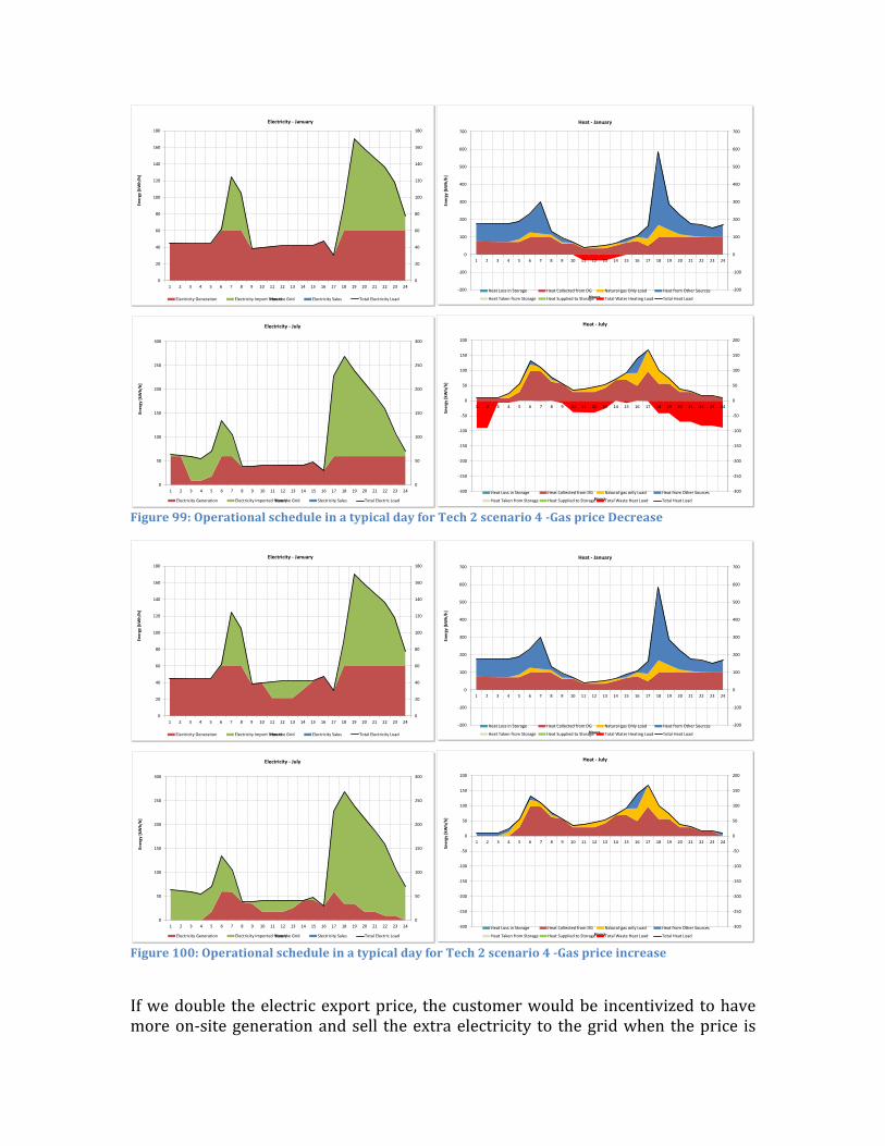
Figure 99: Operational schedule in a typical day for Tech 2 scenario 4 -‐Gas price Decrease
Figure 100: Operational schedule in a typical day for Tech 2 scenario 4 -‐Gas price increase
If we double the electric export price, the customer would be incentivized to have more on-‐site generation and sell the extra electricity to the grid when the price is
-‐200
-‐100
0
100
200
300
400
500
600
700
-‐200
-‐100
0
100
200
300
400
500
600
700
1 2 3 4 5 6 7 8 9 10 11 12 13 14 15 16 17 18 19 20 21 22 23 24
Energy [k
Wh/h]
Hours
Heat -‐ January
Heat Loss in Storage Heat Collected from DG Natural-‐gas Only Load Heat from Other Sources
Heat Taken from Storage Heat Supplied to Storage Total Water Heating Load Total Heat Load
-‐300
-‐250
-‐200
-‐150
-‐100
-‐50
0
50
100
150
200
-‐300
-‐250
-‐200
-‐150
-‐100
-‐50
0
50
100
150
200
1 2 3 4 5 6 7 8 9 10 11 12 13 14 15 16 17 18 19 20 21 22 23 24
Energy [k
Wh/h]
Hours
Heat -‐ July
Heat Loss in Storage Heat Collected from DG Natural-‐gas only Load Heat from Other Sources
Heat Taken from Storage Heat Supplied to Storage Total Waste Heat Load Total Heat Load
0
20
40
60
80
100
120
140
160
180
0
20
40
60
80
100
120
140
160
180
1 2 3 4 5 6 7 8 9 10 11 12 13 14 15 16 17 18 19 20 21 22 23 24
Energy [k
Wh/h]
Hours
Electricity -‐ January
Electricity Generation Electricity Import from the Grid Electricity Sales Total Electricity Load
0
50
100
150
200
250
300
0
50
100
150
200
250
300
1 2 3 4 5 6 7 8 9 10 11 12 13 14 15 16 17 18 19 20 21 22 23 24
Energy [k
Wh/h]
Hours
Electricity -‐ July
Electricity Generation Electricity Imported from the Grid Slectricity Sales Total Electric Load
-‐200
-‐100
0
100
200
300
400
500
600
700
-‐200
-‐100
0
100
200
300
400
500
600
700
1 2 3 4 5 6 7 8 9 10 11 12 13 14 15 16 17 18 19 20 21 22 23 24
Energy [k
Wh/h]
Hours
Heat -‐ January
Heat Loss in Storage Heat Collected from DG Natural-‐gas Only Load Heat from Other Sources
Heat Taken from Storage Heat Supplied to Storage Total Water Heating Load Total Heat Load
-‐300
-‐250
-‐200
-‐150
-‐100
-‐50
0
50
100
150
200
-‐300
-‐250
-‐200
-‐150
-‐100
-‐50
0
50
100
150
200
1 2 3 4 5 6 7 8 9 10 11 12 13 14 15 16 17 18 19 20 21 22 23 24
Energy [k
Wh/h]
Hours
Heat -‐ July
Heat Loss in Storage Heat Collected from DG Natural-‐gas only Load Heat from Other Sources
Heat Taken from Storage Heat Supplied to Storage Total Waste Heat Load Total Heat Load
0
20
40
60
80
100
120
140
160
180
0
20
40
60
80
100
120
140
160
180
1 2 3 4 5 6 7 8 9 10 11 12 13 14 15 16 17 18 19 20 21 22 23 24
Energy [k
Wh/h]
Hours
Electricity -‐ January
Electricity Generation Electricity Import from the Grid Electricity Sales Total Electricity Load
0
50
100
150
200
250
300
0
50
100
150
200
250
300
1 2 3 4 5 6 7 8 9 10 11 12 13 14 15 16 17 18 19 20 21 22 23 24
Energy [k
Wh/h]
Hours
Electricity -‐ July
Electricity Generation Electricity Imported from the Grid Slectricity Sales Total Electric Load

high. However, in this case, the customer chooses minimize wasted heat, which is in contrast with the industrial case, where the increased export comes at a higher waste heat ratio.
Figure 101: Operational schedule in a typical day for Tech 2 scenario 4 -‐double export price
From Figure 102 we can see that the annual savings through operations are more sensitive to the electricity price, as the elasticities for electricity price, gas price and export price are 2.0, 0.78 and 0.05 respectively.
-‐200
-‐100
0
100
200
300
400
500
600
700
-‐200
-‐100
0
100
200
300
400
500
600
700
1 2 3 4 5 6 7 8 9 10 11 12 13 14 15 16 17 18 19 20 21 22 23 24
Energy [k
Wh/h]
Hours
Heat -‐ January
Heat Loss in Storage Heat Collected from DG Natural-‐gas Only Load Heat from Other Sources
Heat Taken from Storage Heat Supplied to Storage Total Water Heating Load Total Heat Load
-‐300
-‐250
-‐200
-‐150
-‐100
-‐50
0
50
100
150
200
-‐300
-‐250
-‐200
-‐150
-‐100
-‐50
0
50
100
150
200
1 2 3 4 5 6 7 8 9 10 11 12 13 14 15 16 17 18 19 20 21 22 23 24
Energy [k
Wh/h]
Hours
Heat -‐ July
Heat Loss in Storage Heat Collected from DG Natural-‐gas only Load Heat from Other Sources
Heat Taken from Storage Heat Supplied to Storage Total Waste Heat Load Total Heat Load
0
20
40
60
80
100
120
140
160
180
0
20
40
60
80
100
120
140
160
180
1 2 3 4 5 6 7 8 9 10 11 12 13 14 15 16 17 18 19 20 21 22 23 24
Energy [k
Wh/h]
Hours
Electricity -‐ January
Electricity Generation Electricity Import from the Grid Electricity Sales Total Electricity Load
0
50
100
150
200
250
300
0
50
100
150
200
250
300
1 2 3 4 5 6 7 8 9 10 11 12 13 14 15 16 17 18 19 20 21 22 23 24
Energy [k
Wh/h]
Hours
Electricity -‐ July
Electricity Generation Electricity Imported from the Grid Slectricity Sales Total Electric Load

Figure 102: Annual savings through operations for Tech 2 scenario 4 in different market conditions
Comparing Figure 103 and Figure 67, we can see that the overall efficiency of residential CHPs has a higher sensitivity to the market conditions than that of industrial CHPs (12% vs. 4% variability).
Figure 103: CHP overall efficiencies for Tech 2 scenario 4 in different market conditions
Finally, the incremental natural gas purchase shows a ±30% difference among all the conditions, which is higher than that in the industrial case (10%). The natural gas consumption is highest when the gas price is 30% lower. From the perspective of the natural gas company, however, the increased natural gas sales is not enough to offset the loss due to lower gas price. A special reduced gas price scheme for CHP owners has to be carefully designed in order to account for the quantity vs price effect
-‐
10,000.00
20,000.00
30,000.00
40,000.00
50,000.00
60,000.00
no change elec price -‐30%
elec price +30%
PX*2 gas price -‐30%
gas price +30%
62% 64% 66% 68% 70% 72% 74% 76% 78% 80% 82% 84%
no change elec price -‐30%
elec price +30%
PX*2 gas price -‐30%
gas price +30%
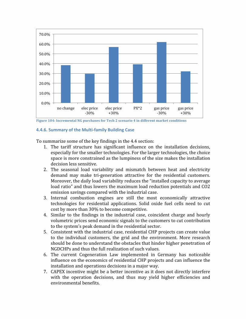
Figure 104: Incremental NG purchases for Tech 2 scenario 4 in different market conditions
4.4.6. Summary of the Multi-‐family Building Case To summarize some of the key findings in the 4.4 section:
1. The tariff structure has significant influence on the installation decisions, especially for the smaller technologies. For the larger technologies, the choice space is more constrained as the lumpiness of the size makes the installation decision less sensitive.
2. The seasonal load variability and mismatch between heat and electricity demand may make tri-‐generation attractive for the residential customers. Moreover, the daily load variability reduces the “installed capacity to average load ratio” and thus lowers the maximum load reduction potentials and CO2 emission savings compared with the industrial case.
3. Internal combustion engines are still the most economically attractive technologies for residential applications. Solid oxide fuel cells need to cut cost by more than 30% to become competitive.
4. Similar to the findings in the industrial case, coincident charge and hourly volumetric prices send economic signals to the customers to cut contribution to the system’s peak demand in the residential sector.
5. Consistent with the industrial case, residential CHP projects can create value to the individual customers, the grid and the environment. More research should be done to understand the obstacles that hinder higher penetration of NGDCHPs and thus the full realization of such values.
6. The current Cogeneration Law implemented in Germany has noticeable influence on the economics of residential CHP projects and can influence the installation and operations decisions in a major way.
7. CAPEX incentive might be a better incentive as it does not directly interfere with the operation decisions, and thus may yield higher efficiencies and environmental benefits.
0.0%
10.0%
20.0%
30.0%
40.0%
50.0%
60.0%
70.0%
no change elec price -‐30%
elec price +30%
PX*2 gas price -‐30%
gas price +30%

8. The annual savings are most sensitive to electricity purchase prices, not so much to the gas price or electricity export rate. The energy efficiency is more sensitive to the market conditions in the residential case compared with the industrial one.

5. Conclusions
5.1. Summary and Contributions This thesis examines the value of gas fired distributed CHP systems under different market scenarios. Gas fired distributed CHPs are chosen because they present a more effective way to utilize existing resources and the potential to gain more popularity under today’s carbon constrained energy roadmap. The adopted methodology focuses on the analysis of the economically rational decisions of consumers, regarding the installation and operation of CHP devices, when subject to a diversity of external conditions that can be characterized by a number of parameters. The general approach can be dissected into three main steps: first, construct the business as usual scenario without the presence of CHPs; second, find the optimal CHP installation and operations under different tariff structures and incentives scenarios; finally, assess the various values and benefits of different technologies which are contrasted using various metrics and representative operation schedules. In particular, the main contributions of this thesis are three-‐fold:
• Develop a framework to represent and simulate the decision making process of individual customers, as well as the environment in which such process takes place. The framework focuses on how rational customers would respond to economic signals given the characteristics of available technologies and their load profiles, and explores the sensitivity of such conclusions in relation to different energy price levels. As more details can be included in the analysis, the results drawn from this framework can be a more realistic representation than that done by more simplified models based on levelized electricity costs.
• Quantitatively assess the value of distributed CHPs, not only to the individual customers, but also to the grid and the environment. On the one hand, it compares the economic values of generation technologies to the customer, ranging from more mature internal combustion engines and gas turbines, to emerging technologies like fuel cells and micro turbines. On the other hand, the thesis also explores non-‐financial effects in terms of efficiency, CO2 emissions and peak-‐load reductions using various metrics.
• Inform policymakers on how to realize the potential benefits of distributed CHP systems while meeting other regulatory principles and goals. This research achieves that through, first discussing the merits and disadvantages of various tariff methods and, then comparing the influence of different tariff structures and incentives on the installation and operation of various technologies.

5.2. Findings and discussion In the analysis of the German industrial and multi-‐family cases, we observed that many NGDCHP technologies could bring positive economic value to the customers even without considering incentives. In the meanwhile, metrics like CO2 emissions, overall efficiency, and system’s peak reduction all improved with the introduction of NGDCHPs. These observations confirm that NGDCHP systems have the potential to reduce costs at both the individual customers’ level and at the system level. Among all technologies investigated in this thesis, internal combustion engines are the most economically attractive ones. The implication is two-‐fold: if the policy maker is interested in incentivizing CHP penetrations at minimum incentives in the near term, they should promote the awareness of ICEs and encourage technical improvement of this mature technology; however, if the policy maker is more concerned about technical breakthrough in the long term, especially within the fuel cell field -‐-‐where electric efficiency can be much higher while pollution and noise can be significantly reduced-‐-‐ then stimuli targeting emerging technologies should be warranted. Otherwise, they would not be competitive with ICEs in current market conditions. We also contrasted customers’ installations and operations decisions under various tariff structures scenarios. The decisions are noticeably influenced by the tariff methods. Volumetric-‐only tariffs suffer from potential cross-‐subsidization. They also encourage higher CHP utilization rates and installations because of the higher variable electricity price. In comparison, calculating electricity prices based on different cost drivers could send the correct economic signals to the customers while still meeting the sustainability principle for tariff designs. Regulators can introduce incentives to achieve a more desirable CHP installation and utilization level. With the advent of smart meters and grid analysis tools like RNM, more accurate measurement and estimation of the cost components as well as time-‐dependent tariff rates are now made possible. Coincident charges and hourly volumetric electricity prices can effectively incentivize CHP generation during system’s peak compared with traditional contracted capacity charges and flat volumetric prices. Regulators should consider implementing these methods when feasible. The current Cogeneration Law implemented in Germany, and the incentives derived from it, has major implications for the residential customers, but not so much for the industrial players. We believe it is because German regulators recognize that industrial players have strong motivations to install CHP systems even without government subsidies. We also explored the effects of a CAPEX incentive, which can shorten the payback period while not distorting the short-‐term economic signals. Such method can result in higher upfront costs for the government, but the annualized subsidy is commensurable with the current production-‐based incentive scheme.

Changing market conditions can have significant effects on the economic value of CHP systems installed on-‐site. The annual savings are most sensitive to electricity purchase prices. If electricity prices keep rising or are expected to rise in the future, then we might see more penetration of distributed CHPs even without incentives or major technical breakthroughs. On the other hand, however, if the future electricity price is considered uncertain, customers may become reluctant to install CHPs as they are concerned about the risk of lower annual savings and longer payback periods.
5.3. Future Research
5.3.1. Areas of improvement As noted in sections 4.3.2.1 and 4.4.2.1, we chose certain representative models of various CHP technologies with discrete unit capacities. However, this is by no means a comprehensive representation of the technical and economic characteristics of the technologies. In particular, the lumpiness of the larger models renders the installation decisions binary, which limit the different tariff designs to achieve their full potentials. This drawback is carefully weighed against the benefits and disadvantages of a semi-‐continuous unit capacity. If we set the unit capacity of a technology to a small number, say 1 kW, then the customer would pick the “optimal” installed size according to the economic signals received. However, the validity of this method requires a strong assumption that the unit size of the technology is independent from other techno-‐economic parameters like capital costs per kW, electric efficiency and heat-‐to-‐power ratio, which is not realistic given our discussion in Section 2.1.3. A better compromise is to include more models with different unit sizes in the analysis, but time and data availability should be considered when deciding to what extent the technology pool can be expanded. In Section 4.3.3.1. we discussed how the artificial minimum part-‐load constraint distorts the optimal operation decisions of certain large CHP technologies. The constraint is in place to reflect the fact that the electric efficiency of generators deteriorates when the electric output decrease. A better way to model this phenomenon is to implement variable efficiencies that change according to the electric output, even though such a method could also result in longer computational times. The thesis could explore and draw more general conclusions and insights through incorporating more diverse energy load conditions and market conditions. The research energy loads are based on the profiles of a food processing factory and a multi-‐family residential building in Berlin, Germany. The electricity and fuel prices are also specific to the region. However, as discussed in section 4.2, market conditions vary widely across Europe, among industries and over time. Thus, it will be helpful to incorporate more scenarios for different applications and in different European nations. In a relevant research project sponsored by Eni Corporation, we

find the regulations and incentives for CHPs can be very different in different EU nations. For instance, while direct monetary remuneration is implemented in Germany, Italian regulators adopted a more complex non-‐monetary CHP incentive that provides CHP systems with dispatch priority and energy saving certificates. There are also certain constraints on the minimum overall efficiency of the CHP systems to be considered for these types of incentives. As a result, the installation and operation decisions might vary even, if the price level and tariff structure are the same. Finally, we broke down the network charges into different cost-‐driver categories taking Bharakumar’s (2015) work based on specific distribution systems in the US. Although we find the system of choice to be general and representative enough, there might still be important differences between systems in different regions. Therefore, it would be helpful to simulate a distribution system in the Berlin area using RNM in order to get representative costs for that system
5.3.2. Areas for additional research The framework developed for this thesis could be used to explore other questions of interest. For example, this work assumed low penetration of distributed CHP systems and pre-‐determined rate of charges. However, as the penetration rate increase, the accommodation of distributed CHP systems can have noticeable impact on the system’s cost and grid operations and the rates may be calculated dynamically to illustrate such effects and ensure an adequate remuneration level for the utility company. To understand these effects, some of the results of this thesis can be combined with the Reference Network Model (RNM) and simulate the expansion process of the grid, while integrating DGs and identify the costs of having important DG penetration. Moreover, further research could be done incorporating demand response and other secondary services that distributed CHP systems can provide. This research fixes the energy load to focus on the customers’ reactions to economic signals only through installation and operations of CHPs. However, in real life, customers can shift or cut their energy needs when the system is at its peak, if correct economic signals are sent. Introducing demand response may reduce the attractiveness of CHP systems as the customers now have more choices. Also, given the controllability of gas fired distributed DGs, customers may receive extra benefits through providing secondary services such as voltage and frequency regulations. Finally, customers and regulators could be interested in how CHPs compete and coordinate with other distributed energy technologies like small wind turbines, batteries, heat storage and solar photovoltaic (PV) panels. In addition, as discussed in 4.4.3.1, gas powered space conditioning technologies (like heat pumps) as well as the notion of tri-‐generation are also worth exploring. Indeed, the presence of other

technologies is significant in certain regions of Europe 37 , where the CHP technologies face both competition and opportunities from the synergies that may arise with other technologies.
37 For instance, the installed capacity of PV panels in Germany reached 38GW by the end of 2014 and 60% of these capacities are at the distribution level, according to Bundesnetzagentur.

Bibliography
1. ABB. ABB’s Vision for the Power System of the Future. Toward a smarter grid., 2010.
2. Ahumada, Karen Tapia, and Yichen Du. Natural Gas Fueled Distributed Generation (NGDG): Opportunities & Challenges . Cambridge: MIT, 2015.
3. Alt, Lowell E. Energy Utility Rate Setting. Lulu.com, 2006. 4. Bard Skagestad, Peter Mildenstein. District Heating and Cooling Connection
Handbook . Paris: IEA, 2002. 5. Bharatkumar, Ashwini. Distribution Network Use-‐of-‐System Charges Under
High Penetration of Distributed Energy Resources . Engineering Systems Division , Massachusetts Institute of Technology , Cambridge: MIT, 2015.
6. Bonbright, James. Principles of Public Utility Rates. 1961. 7. Breakthrough Technologies Institute. Fuel Cell Technologies Market Report.
Washington: US Department of Energy, 2012. 8. Bundesnetzagentur. Monitoring Report 2013. Bonn: BUNDESKARTELLAMT,
2014. 9. Cardoso, G., M. Stadler, and M.C. Bozchalui. "Optimal investment and
scheduling of distributed energy resources with uncertainty in electric vehicle driving schedules." Energy (Elsevier), 2014.
10. Carter, Dan, and Jonathan Wing. The Fuel Cell Industry Review. Royston: Fuel Cell Today, 2013.
11. Center for Climate and Energy Solutions. COGENERATION / COMBINED HEAT AND POWER (CHP). 2010. http://www.c2es.org/technology/factsheet/CogenerationCHP (accessed 3 18, 2015).
12. CODE 2. European Cogeneration Roadmap . Cogeneration Observatory and Dissemination Europe, 2015.
13. Combined Heat and Power Partnership. Catalog of CHP technologies. Washington, DC: U.S. Environmental Protection Agency, 2008.
14. Combined Heat and Power Partnership. CHP Technology Catalog. Washington: U.S. Environmental Protection Agency, 2014.
15. Combined Heat and Power Partnership. CHP Technology Catalog. EPA, Washington: EPA, 2008.
16. Cossent, Rafael, et al. "Vol. 222 Part A: J. Power and Energy, pp. 697-‐706." 6th International Conference on the European Energy Market. Leuven: EEM, 2009.
17. DE Solutions. Clean Distributed Generation Performance and Cost Analysis. Oak Ridge National Laboratory and and U.S. Department of Energy, 2004.
18. Domingo, C.M., and T.G.S Roman. "A Reference Network Model for Large-‐Scale Distribution Planning With Automatic Street Map Generation." (IEEE) 2010: 190 -‐ 197.
19. EC. Energy Market in the European Union in 2011. Belgium: European Union, 2012.
20. EC. "Energy markets in the European Union in 2013." SWD (SWD), 2014: 368.

21. EC. EU Energy Market in 2014. Luxembough: Publications Office of the European Union, 2014.
22. EC-‐JRC. Best available technologies for the heat and cooling market in the European Union. European Commission, 2012.
23. Economidou, Marina. Europe’s Buildings under the Microscope. Brussels : Buildings Performance Institute Europe , 2011.
24. ENATEC micro-‐cogen B.V. Technology. http://www.enatec.com/home.html (accessed Aoril 15, 2010).
25. energi, Dansk. "Den lille blå om varmepumper." Danish Energy Association, 2011.
26. EPA. "Clean Energy-‐Environment Guide to Action." 2006. 27. —. Utility Rates Fact Sheet. 2 13, 2015.
http://www.epa.gov/chp/policies/utility_fs.html (accessed 3 18, 2015). 28. EU. EU Energy Efficiency Directive (2012/27/EU). The European Parliament
and the Council of the European Union, 2012. 29. Eurelectric. Active Distribution System Management. Brussels: Union of the
Electricity Industry -‐ EURELECTRIC, 2013. 30. European Commission. "Commission Recommendation on preparations for
the roll-‐out of smart metering systems." 2012. 31. European Commission. Energy prices and costs in Europe. Brussels: SWD,
2014. 32. —. The 2020 Climate and Energy Package. 11 12, 2014.
http://ec.europa.eu/clima/policies/package/index_en.htm (accessed 3 28, 2015).
33. European Environment Agency. Overview of the European energy system (ENER 036) -‐ Assessment published Mar 2013. 1 1, 2015. http://www.eea.europa.eu/data-‐and-‐maps/indicators/overview-‐of-‐the-‐european-‐energy-‐system-‐2/assessment (accessed 3 24, 2015).
34. Eurostat. Database. 2015. http://ec.europa.eu/eurostat/data/database (accessed 2015).
35. Evans, Peter B. Optimal Portfolio Methodology forAssessing Distributed Energy Resources Benefits for the Energynet. Los Altos Hills: California Energy Commission, 2005.
36. Frias, P., G6mez, T., Rivier, J. Integration of distributed generation in distribution networks: regulatory challenges. Madrid: Instituto de Investigaci6n Tecnol6gica, University Pontificia Comillas, 2008.
37. Gil, Hugo A and Joos, Geza. "On the Quantification of the Network Capacity Deferral Value of Distributed Generation." IEEE Transactions on Power Systems, 2006: Vol 21 pp. 1592-‐1599.
38. Goldstein, L., Hedman, B., Knowles, D., Freedman, S., Woods, R., and Schweizer, T. Gas-‐Fired Distributed Energy Resource Technology Characterizations. National Renewable Energy Laboratory, 2003.
39. Goncharov, V. V. "The Forecast of the Development of the Market for Gas Turbine." Thermal Engineering, 2013: Vol. 60, No. 9, pp. 676–678.
40. Hawkes, A.D., and M.A. Leach. "On policy instruments for support of micro combined heat and power." (Energy Policy) 2008.

41. Hedman, Bruce, Eric Wong, Ken Darrow, and Anne Hampson. Combined Heat and Power: policy analysis and 2011-‐2030 market assessment . Sacramento: ICF International, 2012.
42. IEA. Technology Roadmap, energy Efficient Buildings: Heating and cooling Equipment. Paris: IEA, 2011.
43. Ignacio Perez-‐Arriaga, Sophia Ruester, Sebastian Schwenen, Carlos Batlle, and Jean-‐Michel Glachant. From Distribution Networks to Smart Distribution Systems: Rethinking the Regula-‐ tion of European Electricity DSOs. Florence: European University Institute, 2013.
44. Industrial Technologies Program. Waste Heat Recovery: Technologies and Opportunities in the United States. DOE, Washington: DOE, 2009.
45. Infinia. Applications: Micro-‐CHP. http://www.infiniacorp.com/micro-‐chp.html (accessed April 15, 2010).
46. International, ICF. Combined Heat and Power Installation Database. http://www.eea-‐inc.com/chpdata/ (accessed Dec 12, 2014).
47. J.A.P. Lopes, N. Hatziargyriou, J. Mutale, P. Djapic, and N. Jenkins. "Integrating distributed generation into electric power systems: A review of drivers, challenges and opportunities." Electric Power Systems Research, , 2007: 77(9):1189 – 1203.
48. James J. Hirsch & Associates. Energy Simulation Training for Design & Construction Professionals . Energy Design Resources, 2004.
49. James, Larminie, and Andrew Dicks. Fuel Cell Systems Explained. West Sussex: John Whiley & Sons, Ltd., 2000.
50. Jesus, Fernando, Guevara Carazas, and Gilberto Francisco. "Reliability Analysis of Gas Turbine." In Thermal Power Plant Performance Analysis , 189-‐220. London: Springer, 2012.
51. Kamna, Rene, and Martijn Elbury. Ecodesign preparatory study of Boilers. Brussels: European Commission, 2007.
52. Leonardo Energy. Reducing Electricity Network Losses. Brussels: The European Copper Institute, 2008.
53. Miller, Graeme H., Clifford P. Haefke, and John J. Cuttica. Iowa On-‐Site Generation Tariff Barrier Overview. US DOE Midwest Clean Energy Application Center, 2012.
54. MIT Energy Initiative. Prospectus for an Interdisciplinary MIT Energy Initiative Consortium. Cambridge: MIT, 2014.
55. Ohkubo, Yoichiro. "Outlook on Gas Turbine." R&D Review of Toyota CRDL, 2005: Vol.4 No.1.
56. Onovwionaa, H.I., and V.I. Ugursalb. "Residential cogeneration systems: review of the current technology." (Renewable and Sustainable Energy Reviews) 2006.
57. Pehnt, M., et al. Micro Cogeneration: Towards Decentralized Energy Systems. Berlin: Springer Berlin Heidelberg, 2006.
58. Reneses, Javier, Maria Pia Rodriguez, and Ignacio Perez-‐Arriaga. Regulation of the Power Sector. London: Springer, 2013.
59. Rodríguez Ortega, M.P., J.I. Pérez-‐Arriaga, J.R. Abbad. "Distribution network." Energy Policy, 2008: 36(5): 1712-‐1725.
60. Rodriguez-‐Ortega, Maria Pia. "Distribution network tariffs: A closed question?" Energy Policy, 2008: 1712-‐1725.
61. Starke, Michael, and Nasr Alkadi. Assessment of Industrial Load for Demand Response across U.S. Regions of the Western Interconnect . Oak Ridge: Oak Ridge National Laboratory, 2013.
62. Steve Doty, Wayne C. Turner. Energy Management Handbook. Fairmont Press, 2012.
63. Strachan, Neil and Dowlatabadi, Hadi. "Distributed generation and distribution utilities." Energy Policy, 2002: Vol. 30.
64. SWD. "Energy markets in the European Union in 2013." SWD (EC), 2014: 368. 65. SWD. Energy prices and costs report . Brussels : European Commision, 2014. 66. Tapia-‐Ahumada, Karen. Understanding the Impact of Large-‐Scale Penetration
of Micro Combined Heat & Power Technologies within Energy Systems. Cambridge: MIT, 2011.
67. The World Bank. Electric power transmission and distribution losses. 2013. http://data.worldbank.org/indicator/EG.ELC.LOSS.ZS (accessed 3 25, 2015).
68. THINK. From Distribution Networks to Smart Distribution Systems: Rethinking the Regulation of European Electricity DSOs. Firenze: European University Institute, 2013a.
69. THINK. Shift, Not Drift: Towards Active Demand Response and Beyond. Firenze: European University Institute, 2013b.
70. Thomson, M. and Infield, D. "Modelling the impact of micro-‐combined heat and power generators on electricity distribution networ." Proc. IMechE, 2008: Vol. 222 Part A: J. Power and Energy, pp. 697-‐706.
71. US Energy Information Administration. Annual Energy Review. Washington: EIA, 2009.
72. Utility Dive . The State of the Electric Utility . 2014: Siemens. 73. Willis, Lee H., and Walter G. Scott. Distributed Power Generation: Planning and
Evaluation. New York: Marcel Dekker, Inc., New York Basel, 2000.
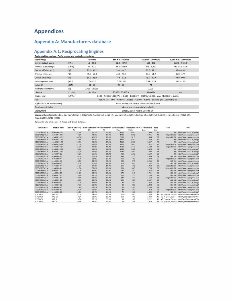
Appendices
Appendix A: Manufacturers database
Appendix A.1: Reciprocating Engines
Technology < 50kWe 50kWe -‐ 500kWe 500kWe -‐ 1000kWe 1000kWe -‐ 10,000kWeElectric output range [kWe] 1.0 -‐ 50.0 51.0 -‐ 497.0 532 -‐ 800 1,200 -‐ 9,425.0
Thermal output range [kWth] 2.5 -‐ 91.0 84.0 -‐ 632.0 348 -‐ 1,260 746.0 -‐ 8,745.0
Electric efficiency (1) [%] 25.0 -‐ 34.2 28.4 -‐ 44.0 35.0 -‐ 42.2 36.0 -‐ 45.9
Thermal efficiency [%] 51.0 -‐ 67.0 43.0 -‐ 56.5 44.0 -‐ 51.2 35.0 -‐ 47.5
Overall efficiency [%] 84.0 -‐ 96.0 78.6 -‐ 91.3 79.0 -‐ 90.9 73.0 -‐ 90.8
Heat-‐to-‐power ratio [p.u.] 1.54 -‐ 3.0 0.76 -‐ 1.8 0.64 -‐ 1.29 0.62 -‐ 1.29
Noise (2) [dBA] 41 -‐ 68 63 -‐ 72 74 -‐-‐-‐-‐
Maintenance interval [hr] 1,400 -‐ 10,000 -‐-‐-‐-‐-‐-‐ 1,000 -‐-‐-‐-‐
Lifetime [yr -‐ hr] 10 -‐ 20 yr 50,000 -‐ 60,000 hr 50,000 hr -‐-‐-‐-‐
Capital cost [$/kWe]
Fuels
Applications for heat recovery
Development status
Deployment
Reciprocating engines -‐ Performance and costs characteristics
Natural Gas -‐ LPG -‐ Biodiesel -‐ Biogas -‐ Fuel Oil -‐ Butane -‐ Sewage gas -‐ Vegetable oil
Mature and commercially available
Europe, Japan, Russia, Canada, US
1,100 -‐ 2,200 (if >100kWe); 2,500 -‐ 4,000 (if 5 -‐ 100kWe); 6,000 -‐ over 24,000 (if < 5kWe)
Notes: (1) LHV efficiency. (2) Noise at 1-‐2m of distance.
Space heating -‐ Hot water -‐ Low Pressure Steam
Sources: Own elaboration based on manufacturers datasheets, Angrisani et al. (2012), Maghanki et al. (2013), Barbieri et al. (2012), EU Joint Research Centre (2012), EPA Report (2008), NREL (2003)
Manufacturer Product Name Electrical efficiency Thermal efficiency Overall efficiency Electrical output Heat output Heat-‐to-‐Power ratio Noise Fuel Link[%] [%] [%] [kWe] [kWth] [p.u.] [db]
COGENGREEN S.A. ecoGEN402-‐SG 37.5% 52.5% 90.0% 402.0 563.0 1.400 72 NG http://www.valiza.es/imag/gas/FTC-‐VALIZA-‐ecoGEN-‐402SG.jpgCOGENGREEN S.A. ecoGEN340SH 44.0% 43.0% 87.0% 340.0 320.0 0.941 70 Vegetable Oil http://www.cogengreen.com/images_cogeneration/pdf/FTecoGEN-‐340SH-‐cogengreen.pdfCOGENGREEN S.A. ecoGEN250-‐SH 43.0% 45.0% 88.0% 250.0 261.0 1.044 68 Vegetable Oil http://www.cogengreen.com/images_cogeneration/pdf/FTecoGEN-‐250SH-‐cogengreen.pdfCOGENGREEN S.A. ecoGEN237-‐SG 35.5% 55.5% 91.0% 237.0 372.0 1.570 70 NG http://www.valiza.es/imag/gas/FTC-‐VALIZA-‐ecoGEN-‐237SG.jpgCOGENGREEN S.A. ecoGEN201-‐SG 33.7% 55.8% 89.5% 201.0 333.0 1.657 70 NG http://www.valiza.es/imag/gas/FTC-‐VALIZA-‐ecoGEN-‐201SG.jpgCOGENGREEN S.A. ecoGEN180-‐SH 42.0% 45.0% 87.0% 180.0 193.0 1.072 70 Vegetable Oil http://www.cogengreen.com/images_cogeneration/pdf/FTecoGEN-‐180SH-‐cogengreen.pdfCOGENGREEN S.A. ecoGEN150-‐SH 41.0% 45.0% 86.0% 150.0 165.0 1.100 70 Vegetable Oil http://www.cogengreen.com/images_cogeneration/pdf/FTecoGEN-‐150SH-‐cogengreen.pdfCOGENGREEN S.A. ecoGEN140-‐SG 35.0% 56.0% 91.0% 140.0 216.0 1.543 66 NG http://www.valiza.es/imag/gas/FTC-‐VALIZA-‐ecoGEN-‐140SG.jpgCOGENGREEN S.A. ecoGEN113-‐SG 34.0% 55.0% 89.0% 113.0 180.0 1.593 68 NG http://www.valiza.es/imag/gas/FTC-‐VALIZA-‐ecoGEN-‐113SG.jpgCOGENGREEN S.A. ecoGEN70-‐SG 34.5% 56.5% 91.0% 70.0 114.0 1.629 68 NG http://www.valiza.es/imag/gas/FTC-‐VALIZA-‐ecoGEN-‐70SG.jpgCOGENGREEN S.A. ecoGEN48-‐SG 33.0% 55.0% 88.0% 48.0 77.0 1.604 68 NG, LPG http://www.cogengreen.com/images_cogeneration/pdf/FTecoGEN-‐48SG-‐cogengreen.pdfCOGENGREEN S.A. ecoGEN30-‐AH 32.0% 58.0% 90.0% 30.0 52.0 1.733 65 Vegetable Oil http://www.cogengreen.com/images_cogeneration/pdf/FTecoGEN-‐30AH-‐cogengreen.pdfCOGENGREEN S.A. ecoGEN30-‐AG 28.0% 62.0% 90.0% 30.0 67.0 2.233 53 NG, LPG http://www.cogengreen.com/images_cogeneration/pdf/FTecoGEN-‐30AG-‐cogengreen.pdfCOGENGREEN S.A. ecoGEN30-‐SG 28.0% 60.0% 88.0% 30.0 65.0 2.167 60 NG, LPG http://www.valiza.es/imag/gas/FTC-‐VALIZA-‐ecoGEN-‐30SG.jpgCOGENGREEN S.A. ecoGEN25-‐AH 31.0% 57.0% 88.0% 25.0 44.0 1.760 60 Vegetable Oil http://www.cogengreen.com/images_cogeneration/pdf/FTecoGEN-‐25AH-‐cogengreen.pdfCOGENGREEN S.A. ecoGEN20-‐AH 31.0% 57.0% 88.0% 20.0 35.0 1.750 60 Vegetable Oil http://www.cogengreen.com/images_cogeneration/pdf/FTecoGEN-‐20AH-‐cogengreen.pdfCOGENGREEN S.A. ecoGEN18-‐AG 33.0% 57.0% 90.0% 18.0 32.0 1.778 53 NG, LPG http://www.cogengreen.com/images_cogeneration/pdf/FTecoGEN-‐18AG-‐cogengreen.pdfCOGENGREEN S.A. ecoGEN18-‐SG 31.5% 55.5% 87.0% 17.7 31.0 1.751 68 NG, LPG http://www.valiza.es/imag/gas/FTC-‐VALIZA-‐ecoGEN-‐18SG.jpgCOGENGREEN S.A. ecoGEN12-‐AG 28.5% 61.5% 90.0% 12.0 27.0 2.250 53 NG, LPG http://www.cogengreen.com/images_cogeneration/pdf/FTecoGEN-‐12AG-‐cogengreen.pdfCOGENGREEN S.A. ecoGEN12-‐AH 28.5% 61.5% 90.0% 12.0 26.0 2.167 58 Vegetable Oil http://www.cogengreen.com/images_cogeneration/pdf/FTecoGEN-‐12AH-‐cogengreen.pdfCOGENGREEN S.A. ecoGEN12-‐SG 28.0% 60.0% 88.0% 12.0 26.0 2.167 58 NG, LPG http://www.valiza.es/imag/gas/FTC-‐VALIZA-‐ecoGEN-‐12SG.jpgCOGENGREEN S.A. ecoGEN10-‐AG 27.0% 62.0% 89.0% 9.9 23.0 2.323 55 NG, LPG http://www.valiza.es/imag/gas/FTC-‐VALIZA-‐ecoGEN-‐10AG.jpgCOGENGREEN S.A. ecoGEN10-‐SG 27.0% 60.0% 87.0% 9.9 22.0 2.222 58 NG, LPG http://www.valiza.es/imag/gas/FTC-‐VALIZA-‐ecoGEN-‐10SG.jpgCOGENGREEN S.A. ecoGEN08-‐AG 27.4% 61.6% 89.0% 8.0 18.0 2.250 53 NG, LPG http://www.cogengreen.com/images_cogeneration/pdf/FTecoGEN-‐08AG-‐cogengreen.pdfCOGENGREEN S.A. ecoGEN08-‐AH 28.0% 62.0% 90.0% 8.0 18.0 2.250 53 Vegetable Oil http://www.cogengreen.com/images_cogeneration/pdf/FTecoGEN-‐08AH-‐cogengreen.pdfCOGENGREEN S.A. ecoGEN08-‐SG 25.3% 60.7% 86.0% 7.5 18.0 2.400 57 NG, LPG http://www.valiza.es/imag/gas/FTC-‐VALIZA-‐ecoGEN-‐7,5SG.jpgEC POWER XRGI 20 32.0% 64.0% 96.0% 20.0 40.0 2.000 49 NG, Propane, Butane http://typo3.ecpower.dk/fileadmin/user_upload/EN/DOWNLOADS/ECP_EN_Technical_data_XRGI_15_20.pdfEC POWER XRGI 15 30.0% 62.0% 92.0% 15.0 30.0 2.000 49 NG, Propane, Butane http://typo3.ecpower.dk/fileadmin/user_upload/EN/DOWNLOADS/ECP_EN_Technical_data_XRGI_15_20.pdfEC POWER XRGI 9 29.5% 63.5% 93.0% 9.0 20.0 2.222 49 NG, Propane, Butane http://typo3.ecpower.dk/fileadmin/user_upload/EN/DOWNLOADS/ECP_EN_Technical_data_XRGI_6_9.pdfEC POWER XRGI 6 29.5% 63.5% 93.0% 6.0 13.5 2.250 49 NG, Propane, Butane http://typo3.ecpower.dk/fileadmin/user_upload/EN/DOWNLOADS/ECP_EN_Technical_data_XRGI_6_9.pdf
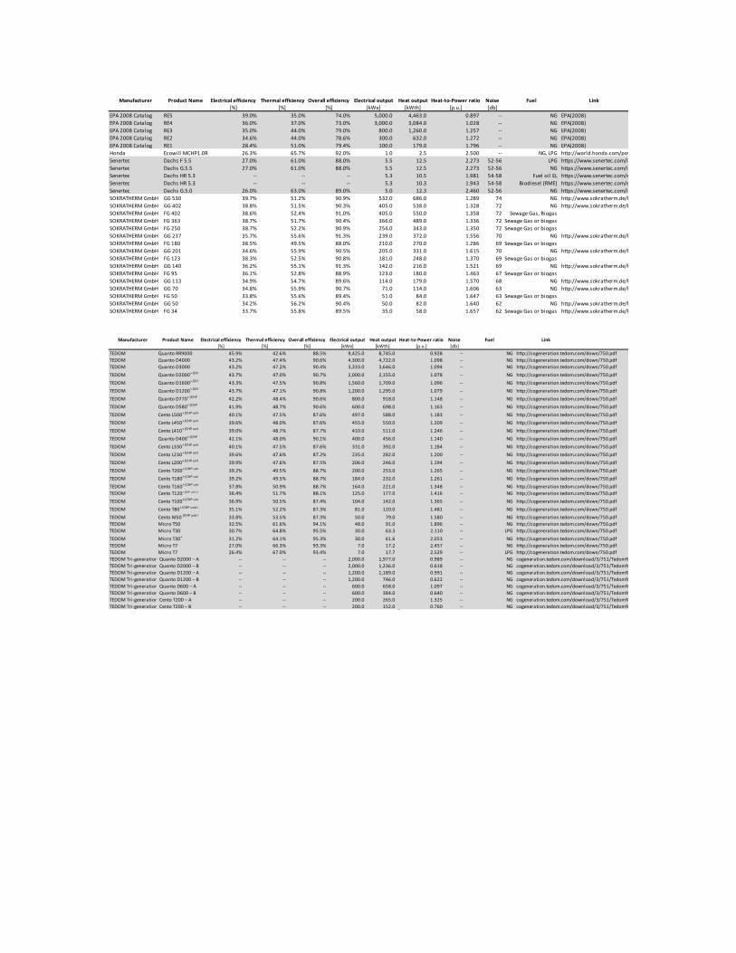
Manufacturer Product Name Electrical efficiency Thermal efficiency Overall efficiency Electrical output Heat output Heat-‐to-‐Power ratio Noise Fuel Link[%] [%] [%] [kWe] [kWth] [p.u.] [db]
EPA 2008 Catalog RE5 39.0% 35.0% 74.0% 5,000.0 4,463.0 0.897 -‐-‐ NG EPA(2008)EPA 2008 Catalog RE4 36.0% 37.0% 73.0% 3,000.0 3,084.0 1.028 -‐-‐ NG EPA(2008)EPA 2008 Catalog RE3 35.0% 44.0% 79.0% 800.0 1,260.0 1.257 -‐-‐ NG EPA(2008)EPA 2008 Catalog RE2 34.6% 44.0% 78.6% 300.0 632.0 1.272 -‐-‐ NG EPA(2008)EPA 2008 Catalog RE1 28.4% 51.0% 79.4% 100.0 179.0 1.796 -‐-‐ NG EPA(2008)Honda Ecowill MCHP1.0R / RP 26.3% 65.7% 92.0% 1.0 2.5 2.500 -‐-‐ NG, LPG http://world.honda.com/power/cogenerator/; http://world.honda.com/power/guide/pdf/Honda_Power_Products.pdf; http://world.honda.com/news/2012/p120925Gas-‐Engine-‐Cogeneration-‐Unit/index.htmlSenertec Dachs F 5.5 27.0% 61.0% 88.0% 5.5 12.5 2.273 52-‐56 LPG https://www.senertec.com/index.php?eID=tx_nawsecuredl&u=0&file=uploads/media/technical_data_dachs_EN_04.pdf&t=1402164440&hash=45bb6c996130649bfb5977955136397eSenertec Dachs G.5.5 27.0% 61.0% 88.0% 5.5 12.5 2.273 52-‐56 NG https://www.senertec.com/index.php?eID=tx_nawsecuredl&u=0&file=uploads/media/technical_data_dachs_EN_04.pdf&t=1402164440&hash=45bb6c996130649bfb5977955136397eSenertec Dachs HR 5.3 -‐-‐ -‐-‐ -‐-‐ 5.3 10.5 1.981 54-‐58 Fuel oil EL https://www.senertec.com/en/derdachs/technology.htmlSenertec Dachs HR 5.3 -‐-‐ -‐-‐ -‐-‐ 5.3 10.3 1.943 54-‐58 Biodiesel (RME) https://www.senertec.com/en/derdachs/technology.htmlSenertec Dachs G.5.0 26.0% 63.0% 89.0% 5.0 12.3 2.460 52-‐56 NG https://www.senertec.com/index.php?eID=tx_nawsecuredl&u=0&file=uploads/media/technical_data_dachs_EN_04.pdf&t=1402164440&hash=45bb6c996130649bfb5977955136397eSOKRATHERM GmbH GG 530 39.7% 51.2% 90.9% 532.0 686.0 1.289 74 NG http://www.sokratherm.de/htcms/get_file.php5?did=106&tid=324SOKRATHERM GmbH GG 402 38.8% 51.5% 90.3% 405.0 538.0 1.328 72 NG http://www.sokratherm.de/htcms/get_file.php5?did=106&tid=324SOKRATHERM GmbH FG 402 38.6% 52.4% 91.0% 405.0 550.0 1.358 72 Sewage Gas, BiogasSOKRATHERM GmbH FG 363 38.7% 51.7% 90.4% 366.0 489.0 1.336 72 Sewage Gas or biogasSOKRATHERM GmbH FG 250 38.7% 52.2% 90.9% 254.0 343.0 1.350 72 Sewage Gas or biogasSOKRATHERM GmbH GG 237 35.7% 55.6% 91.3% 239.0 372.0 1.556 70 NG http://www.sokratherm.de/htcms/get_file.php5?did=106&tid=324SOKRATHERM GmbH FG 180 38.5% 49.5% 88.0% 210.0 270.0 1.286 69 Sewage Gas or biogasSOKRATHERM GmbH GG 201 34.6% 55.9% 90.5% 205.0 331.0 1.615 70 NG http://www.sokratherm.de/htcms/get_file.php5?did=106&tid=324SOKRATHERM GmbH FG 123 38.3% 52.5% 90.8% 181.0 248.0 1.370 69 Sewage Gas or biogasSOKRATHERM GmbH GG 140 36.2% 55.1% 91.3% 142.0 216.0 1.521 69 NG http://www.sokratherm.de/htcms/get_file.php5?did=106&tid=324SOKRATHERM GmbH FG 95 36.1% 52.8% 88.9% 123.0 180.0 1.463 67 Sewage Gas or biogasSOKRATHERM GmbH GG 113 34.9% 54.7% 89.6% 114.0 179.0 1.570 68 NG http://www.sokratherm.de/htcms/get_file.php5?did=106&tid=324SOKRATHERM GmbH GG 70 34.8% 55.9% 90.7% 71.0 114.0 1.606 63 NG http://www.sokratherm.de/htcms/get_file.php5?did=106&tid=324SOKRATHERM GmbH FG 50 33.8% 55.6% 89.4% 51.0 84.0 1.647 63 Sewage Gas or biogasSOKRATHERM GmbH GG 50 34.2% 56.2% 90.4% 50.0 82.0 1.640 62 NG http://www.sokratherm.de/htcms/get_file.php5?did=106&tid=324SOKRATHERM GmbH FG 34 33.7% 55.8% 89.5% 35.0 58.0 1.657 62 Sewage Gas or biogas http://www.sokratherm.de/htcms/get_file.php5?did=91&tid=328
Manufacturer Product Name Electrical efficiency Thermal efficiency Overall efficiency Electrical output Heat output Heat-‐to-‐Power ratio Noise Fuel Link[%] [%] [%] [kWe] [kWth] [p.u.] [db]
TEDOM Quanto RR9000 45.9% 42.6% 88.5% 9,425.0 8,745.0 0.928 -‐-‐ NG http://cogeneration.tedom.com/down/750.pdfTEDOM Quanto D4000 43.2% 47.4% 90.6% 4,300.0 4,722.0 1.098 -‐-‐ NG http://cogeneration.tedom.com/down/750.pdfTEDOM Quanto D3000 43.2% 47.2% 90.4% 3,333.0 3,646.0 1.094 -‐-‐ NG http://cogeneration.tedom.com/down/750.pdfTEDOM Quanto D2000+ (CHP unit in container) 43.7% 47.0% 90.7% 2,000.0 2,155.0 1.078 -‐-‐ NG http://cogeneration.tedom.com/down/750.pdfTEDOM Quanto D1600+ (CHP unit in container) 43.3% 47.5% 90.8% 1,560.0 1,709.0 1.096 -‐-‐ NG http://cogeneration.tedom.com/down/750.pdfTEDOM Quanto D1200+ (CHP unit in container) 43.7% 47.1% 90.8% 1,200.0 1,295.0 1.079 -‐-‐ NG http://cogeneration.tedom.com/down/750.pdfTEDOM Quanto D770+ (CHP unit in container) 42.2% 48.4% 90.6% 800.0 918.0 1.148 -‐-‐ NG http://cogeneration.tedom.com/down/750.pdfTEDOM Quanto D580+ (CHP unit in container) 41.9% 48.7% 90.6% 600.0 698.0 1.163 -‐-‐ NG http://cogeneration.tedom.com/down/750.pdfTEDOM Cento L500+ (CHP unit in container) 40.1% 47.5% 87.6% 497.0 588.0 1.183 -‐-‐ NG http://cogeneration.tedom.com/down/750.pdfTEDOM Cento L450+ (CHP unit in container) 39.6% 48.0% 87.6% 455.0 550.0 1.209 -‐-‐ NG http://cogeneration.tedom.com/down/750.pdfTEDOM Cento L410+ (CHP unit in container) 39.0% 48.7% 87.7% 410.0 511.0 1.246 -‐-‐ NG http://cogeneration.tedom.com/down/750.pdfTEDOM Quanto D400+ (CHP unit in container) 42.1% 48.0% 90.1% 400.0 456.0 1.140 -‐-‐ NG http://cogeneration.tedom.com/down/750.pdfTEDOM Cento L330+ (CHP unit in container) 40.1% 47.5% 87.6% 331.0 392.0 1.184 -‐-‐ NG http://cogeneration.tedom.com/down/750.pdfTEDOM Cento L230+ (CHP unit in container) 39.6% 47.6% 87.2% 235.0 282.0 1.200 -‐-‐ NG http://cogeneration.tedom.com/down/750.pdfTEDOM Cento L200+ (CHP unit in container) 39.9% 47.6% 87.5% 206.0 246.0 1.194 -‐-‐ NG http://cogeneration.tedom.com/down/750.pdfTEDOM Cento T200+ (CHP unit in container) 39.2% 49.5% 88.7% 200.0 253.0 1.265 -‐-‐ NG http://cogeneration.tedom.com/down/750.pdfTEDOM Cento T180+ (CHP unit in container) 39.2% 49.5% 88.7% 184.0 232.0 1.261 -‐-‐ NG http://cogeneration.tedom.com/down/750.pdfTEDOM Cento T160+ (CHP unit in container) 37.8% 50.9% 88.7% 164.0 221.0 1.348 -‐-‐ NG http://cogeneration.tedom.com/down/750.pdfTEDOM Cento T120+ (CHP unit in container) 36.4% 51.7% 88.1% 125.0 177.0 1.416 -‐-‐ NG http://cogeneration.tedom.com/down/750.pdfTEDOM Cento T100+ (CHP unit in container) 36.9% 50.5% 87.4% 104.0 142.0 1.365 -‐-‐ NG http://cogeneration.tedom.com/down/750.pdfTEDOM Cento T80+ (CHP unit in container) 35.1% 52.2% 87.3% 81.0 120.0 1.481 -‐-‐ NG http://cogeneration.tedom.com/down/750.pdfTEDOM Cento M50 (CHP unit in container) 33.8% 53.5% 87.3% 50.0 79.0 1.580 -‐-‐ NG http://cogeneration.tedom.com/down/750.pdfTEDOM Micro T50 32.5% 61.6% 94.1% 48.0 91.0 1.896 -‐-‐ NG http://cogeneration.tedom.com/down/750.pdfTEDOM Micro T30 30.7% 64.8% 95.5% 30.0 63.3 2.110 -‐-‐ LPG http://cogeneration.tedom.com/down/750.pdfTEDOM Micro T30+ 31.2% 64.1% 95.3% 30.0 61.6 2.053 -‐-‐ NG http://cogeneration.tedom.com/down/750.pdfTEDOM Micro T7 27.0% 66.3% 93.3% 7.0 17.2 2.457 -‐-‐ NG http://cogeneration.tedom.com/down/750.pdfTEDOM Micro T7 26.4% 67.0% 93.4% 7.0 17.7 2.529 -‐-‐ LPG http://cogeneration.tedom.com/down/750.pdfTEDOM Tri-‐generation Quanto D2000 – A -‐-‐ -‐-‐ -‐-‐ 2,000.0 1,977.0 0.989 -‐-‐ NG cogeneration.tedom.com/download/3/751/Tedom%20Trigeneration%20EN.pdfTEDOM Tri-‐generation Quanto D2000 – B -‐-‐ -‐-‐ -‐-‐ 2,000.0 1,236.0 0.618 -‐-‐ NG cogeneration.tedom.com/download/3/751/Tedom%20Trigeneration%20EN.pdfTEDOM Tri-‐generation Quanto D1200 – A -‐-‐ -‐-‐ -‐-‐ 1,200.0 1,189.0 0.991 -‐-‐ NG cogeneration.tedom.com/download/3/751/Tedom%20Trigeneration%20EN.pdfTEDOM Tri-‐generation Quanto D1200 – B -‐-‐ -‐-‐ -‐-‐ 1,200.0 746.0 0.622 -‐-‐ NG cogeneration.tedom.com/download/3/751/Tedom%20Trigeneration%20EN.pdfTEDOM Tri-‐generation Quanto D600 – A -‐-‐ -‐-‐ -‐-‐ 600.0 658.0 1.097 -‐-‐ NG cogeneration.tedom.com/download/3/751/Tedom%20Trigeneration%20EN.pdfTEDOM Tri-‐generation Quanto D600 – B -‐-‐ -‐-‐ -‐-‐ 600.0 384.0 0.640 -‐-‐ NG cogeneration.tedom.com/download/3/751/Tedom%20Trigeneration%20EN.pdfTEDOM Tri-‐generation Cento T200 – A -‐-‐ -‐-‐ -‐-‐ 200.0 265.0 1.325 -‐-‐ NG cogeneration.tedom.com/download/3/751/Tedom%20Trigeneration%20EN.pdfTEDOM Tri-‐generation Cento T200 – B -‐-‐ -‐-‐ -‐-‐ 200.0 152.0 0.760 -‐-‐ NG cogeneration.tedom.com/download/3/751/Tedom%20Trigeneration%20EN.pdf

Appendix A.2: Turbines
Appendix A.3: Microturbines
Manufacturer Model name Power capacity Electric efficiency Source / Link
[kWe] [%]
Dresser Rand Company KG2-‐3E Gas Turbine 1,934 16.8 http://www.dresser-‐rand.com/literature/turbo/2173_KG2_3E.pdfDresser Rand Company KG2-‐3G Gas Turbine 2,000 25.5 http://www.dresser-‐rand.com/literature/turbo/KG2_3G_flier.pdfKawasaki Turbines M7A-‐03SD 7,810 33.6 Kawasaki Turbines M7A-‐02D 6,780 30.4 Kawasaki Turbines M1A-‐17D 1,690 26.9 Kawasaki Turbines S2A-‐01 634 19.4 Kawasaki Turbines M1A-‐13A 1,490 24.2 Kawasaki Turbines M1A-‐13D 1,490 24.0 Kawasaki Turbines M1A-‐13X 1,430 23.6 Kawasaki Turbines M1A-‐17 1,690 26.6 Kawasaki Turbines M1A-‐17D 1,690 26.6 Kawasaki Turbines M1T-‐13A 2,930 23.8 Kawasaki Turbines M1T-‐13D 2,930 23.6 Kawasaki Turbines M7A-‐01 5,530 29.6 Kawasaki Turbines M7A-‐01D 5,400 29.2 Kawasaki Turbines M7A-‐02 6,800 30.3 Kawasaki Turbines M7A-‐02D 6,740 30.2 Kawasaki Turbines M7A-‐03 7,450 33.1 Kawasaki Turbines M7A-‐03D 7,440 33.1 Rolls-‐Royce 501-‐KB5S 3,897 29.0 Rolls-‐Royce 501-‐KB7S 5,245 31.5 Rolls-‐Royce 501-‐KH5 6,447 40.1 Solar Turbines Saturn 20 1,210 24.4 Solar Turbines Centaur 40 3,515 27.9 Solar Turbines Centaur 50 4,600 29.3 Solar Turbines Mercury 50 4,600 38.4 Solar Turbines Taurus 60 5,670 31.5 Solar Turbines Taurus 65 6,300 32.8 Solar Turbines Taurus 70 7,965 34.3 Siemens SGT-‐100 5,400 31.0 Siemens SGT-‐200 6,750 31.5 Siemens SGT-‐300 7,900 30.6 Vericor VPS1 487 20.4 Vericor VPS3 3,086 26.8 Vericor VPS4 3,451 28.4 Centrax CX501-‐KB5 3,900 29.1 Centrax CX501-‐KB7 5,300 32.1 Centrax CX300 7,900 31.0 Nigata EGT 5,736 -‐ http://www.niigata-‐power.com/english/Products/turbines/index.htmlMan Diesel & Turbo MGT6100 6,530 32.0
Man Diesel & Turbo 1304-‐10N 10,080 29.2
http://www.mandieselturbo.com/0000795/Solutions-‐and-‐Applications/Power/Turbine-‐Based-‐Power-‐Plants/Gas-‐Turbines.html
http://www.energy.siemens.com/hq/en/fossil-‐power-‐generation/gas-‐turbines/
http://www.vericor.com/vps-‐series-‐gensets.html
http://www.centraxgt.com/products/generator-‐set-‐cx501-‐kb5-‐39-‐mwe
http://www.kawasakigasturbines.com/files/gtgs100621.pdf
http://www.rolls-‐royce.com/energy/energy_products/gas_turbines/501/
http://mysolar.cat.com/cda/files/255309/7/bpgpsg.pdf; http://mysolar.cat.com/cda/layout?m=41100&x=7
Company Model name Power capacity (kWe) Electric efficiency LHP(%) Link / Source[kWe] [%]
Capstone C30 LP 28 26.1 Capstone C30 HP 30 26.1 Capstone C30 HZLC 30 26.1 Capstone C65 65 29.0 Capstone C65 ICHP 65 29.0 Capstone C65 CARB 65 27.9 Capstone C65 CARB 65 29.0 Capstone C65 HZLC 65 27.9 Capstone C200 LP 190 31.0 Capstone C200 HP 200 33.0 Capstone C200 HZLC 200 33.0 Capstone C600 LP 570 31.0 Capstone C600 HP 600 33.0 Capstone C800 LP 760 31.0 Capstone C800 HP 800 33.0 Capstone C1000 LP 950 31.0 Capstone C1000 HP 1,000 33.0 FlexEnergy MT250 250 30.0 http://www.flexenergy.com/pdfs/FlexEnergy_MT250_Spec_Sheet.pdfFlexEnergy MT333 333 32.0 http://www.flexenergy.com/pdfs/FlexEnergy_MT333_Spec_Sheet.pdfMTT Micro Turbine Technology Enertwin (CHP) 3 15.0 http://www.enertwin.com/cms/files/EnerTwin-‐specifications-‐2014-‐MR.pdf
http://www.microturbine.com/_docs/Product%20Catalog_ENGLISH_LR.pdf

Appendix A.4: Stirling Engines
Appendix A.5: Fuel Cells
Manufacturer Product NameElectrical efficiency
Thermal efficiency
Overall efficiency
Electrical output
Heat output
Heat output w/o suppl.
Heat-‐to-‐Power ratio Noise Fuel Source / Link
[%] [%] [%] [kWe] [kWth] [kWth] [p.u.] [db]
Microgen Engine Corporation (MEC) -‐-‐ 19.0% 73.0% 92.00% 1.0 6.0 3.84 3.842 -‐-‐ NG EPRI (2009)
ENATEC / Rinnai -‐-‐ 12.0% 83.0% 95.00% 1.0 7.0 6.92 6.917 -‐-‐ NG EPRI (2009)
Whisper Tech/Efficient Home Energy (EHE) -‐-‐ 12.0% 78.0% 90.00% 1.0 14.0 6.50 6.500 -‐-‐ NG EPRI (2009)
Disenco -‐-‐ 15.0% 77.0% 92.00% 3.0 12.0 15.40 5.133 NG, Biogas EPRI (2009)
Qnergy under development -‐-‐ -‐-‐ -‐-‐ 3.5 14.0 -‐-‐ -‐-‐ Very low NG, Propane, Wood
pellets, Biofuel http://www.qnergy.com/products_overview
Qnergy QCHP7500 20.0% 75.00% 95.00% 7.5 30.0 28.13 3.75 65 dBA@1 m NG, Propane, Wood
pellets, Biofuel http://www.qnergy.com/sites/Qnergy/UserContent/files/SAL-‐DataSheet-‐CHP-‐v15b-‐140700.pdf
Inspirit Energy (former Disenco) Inspirit mCHP 16.0% 76.0% 92.00% 3.0 15.0 14.25 4.750 50dBA@1m NG http://www.inspirit-‐energy.com/mchp.html
Innova -‐ MEC FPSETrinum -‐ dish Stirl ing solar cogeneration 13.8% 41.4% 55.20% 1.0 3.0 3.00 3.000 SOLAR http://www.innova.co.it/eng/catalog/products/trinum.html; http://www.innova.co.it/files/pdf-‐prodotti/datasheet-‐trinum-‐eng_93484.pdf
BDR Thermea -‐ MEC FPSE Baxi Ecogen 24/1.0 13.0% 77.9% 90.9% 1.0 24.0 6.00 6.000 <46dbA@1m NG http://www.baxiknowhow.co.uk/campaigns/about-‐the-‐ecogen.htm; http://www.baxiknowhow.co.uk/campaigns/documents/baxi-‐ecogen.pdf
BDR Thermea -‐ MEC FPSE Baxi Ecogen 24/1.0 LPG 13.0% 76.6% 89.6% 1.0 23.8 5.90 5.900 <46dbA@1m LPG http://www.baxiknowhow.co.uk/campaigns/about-‐the-‐ecogen.htm; http://www.baxiknowhow.co.uk/campaigns/documents/baxi-‐ecogen.pdf
KD Navien HYBRIGEN SE NCM-‐1030HH 15.4% 81.5% 96.92% 1.0 28.3 5.30 5.300 46dBA http://en.kdnavien.com/product/product_view?SchCatCd1=AC&Seq=68
ViessmannVitotwin 350-‐F w/DHW cilinder 750lt / Compact 15.0% 81.0% 96.00% 1.0 26.0 5.40 5.400 https://www.viessmann.com/com/content/dam/internet-‐global/pdf_documents/com/brochures_englisch/ppr-‐micro_chp_boiler.pdf
Viessmann Vitotwin 300-‐W / Compact 15.0% 81.0% 96.00% 1.0 26.0 5.40 5.400 https://www.viessmann.com/com/content/dam/internet-‐global/pdf_documents/com/brochures_englisch/ppr-‐micro_chp_boiler.pdf
CleaNergy C9G 25.0% 70.0% 95.00% 9.0 26.0 25.20 2.800 <58db NG, LPG, LNG, biogas,
landfil l gas http://www.stirl ingenergy.cz/obsah/mikrokogeneracni-‐jednotka-‐cleanergy-‐9-‐kwe/technicka-‐data; http://cleanergy.com/wp-‐content/uploads/2014/06/cleanergy_brochure_chp_lowres.pdf; http://cleanergy.com/wp-‐content/uploads/2014/06/cleanergy_gasbox_landfil ls_lowres1.pdf
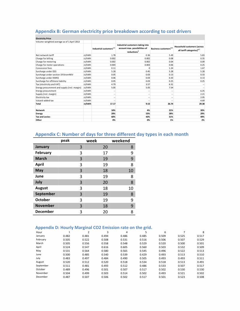
Appendix B: German electricity price breakdown according to cost drivers
Appendix C: Number of days for three different day types in each month peak week weekend January 3 20 8 February 3 17 9 March 3 19 9 April 3 19 8 May 3 18 10 June 3 19 8 July 3 20 8 August 3 18 10 September 3 19 8 October 3 19 9 November 3 18 9 December 3 20 8
Appendix D: Hourly Marginal CO2 Emission rate on the grid.
Electricity PriceVolume-‐weighted average as of 1 April 2013
Industrial customers1,2Industrial customers taking into account max. possibilities of
reductions3Business customers4,5
Household customers (across all tariff categories)6,7
Net network tariff ct/kWh 1.78 0.36 5.49 5.83Charge for billing ct/kWh 0.002 0.002 0.08 0.35Charge for metering ct/kWh 0.002 0.002 0.04 0.09Charge for meter operations ct/kWh 0.003 0.003 0.06 0.25Concession fees ct/kWh 0.11 0 1.24 1.67Surcharge under EEG ct/kWh 5.28 0.45 5.28 5.28Surcharge under section 19 StromNEV ct/kWh 0.05 0.03 0.13 0.33Surcharge under KWKG ct/kWh 0.06 0.03 0.33 0.13Surcharge for offshore liability ct/kWh 0.05 0.03 0.25 0.25Tax (electricity and VAT) ct/kWh 4.79 3.57 6.31 -‐-‐Energy procurement and supply (incl. margin) ct/kWh 5.05 5.05 7.54 -‐-‐Energy procurement ct/kWh -‐-‐ -‐-‐ -‐-‐ 6.25Supply (incl. margin) ct/kWh -‐-‐ -‐-‐ -‐-‐ 2.21Electricity tax ct/kWh -‐-‐ -‐-‐ -‐-‐ 2.05Valued-‐added tax ct/kWh -‐-‐ -‐-‐ -‐-‐ 4.69Total ct/kWh 17.17 9.53 26.74 29.38
Network 10% 4% 21% 20%Energy 29% 53% 28% 29%Tax and Levies 60% 43% 51% 49%Other 0% 0% 1% 2%
Hour 1 2 3 4 5 6 7 8January 0.482 0.481 0.494 0.486 0.485 0.509 0.525 0.517February 0.505 0.522 0.508 0.531 0.516 0.506 0.507 0.529March 0.505 0.556 0.558 0.548 0.529 0.520 0.500 0.501April 0.524 0.547 0.616 0.605 0.560 0.503 0.532 0.509May 0.531 0.564 0.580 0.565 0.545 0.496 0.522 0.513June 0.500 0.485 0.540 0.539 0.429 0.493 0.513 0.510July 0.483 0.497 0.484 0.490 0.505 0.493 0.493 0.511August 0.520 0.512 0.520 0.518 0.534 0.518 0.513 0.491September 0.511 0.481 0.493 0.512 0.486 0.533 0.507 0.517October 0.489 0.496 0.501 0.507 0.517 0.502 0.530 0.530November 0.504 0.499 0.503 0.514 0.502 0.493 0.521 0.502December 0.487 0.507 0.506 0.502 0.517 0.501 0.523 0.508

* all numbers in kgC02/kWh
Appendix E: Other assumptions
Natural gas conversion efficiency of alternative technologies: space-‐heating 0.8 water-‐heating 0.8 naturalgas-‐only 1.0 * kW of heat produced from one kW of natural gas CO2 emission rate of natural gas: 0.18084 kg/ kWh
Hour 9 10 11 12 13 14 15 16January 0.507 0.498 0.504 0.504 0.509 0.492 0.511 0.525February 0.510 0.504 0.493 0.486 0.490 0.501 0.497 0.496March 0.486 0.484 0.475 0.482 0.482 0.487 0.494 0.495April 0.508 0.502 0.503 0.507 0.499 0.506 0.507 0.480May 0.500 0.486 0.483 0.491 0.481 0.482 0.497 0.518June 0.460 0.484 0.496 0.470 0.502 0.515 0.514 0.520July 0.518 0.518 0.516 0.539 0.557 0.515 0.482 0.453August 0.505 0.519 0.536 0.541 0.532 0.544 0.511 0.542September 0.527 0.519 0.518 0.541 0.541 0.511 0.543 0.491October 0.513 0.505 0.515 0.510 0.523 0.509 0.510 0.513November 0.523 0.509 0.510 0.503 0.516 0.511 0.516 0.512December 0.518 0.504 0.497 0.506 0.522 0.511 0.511 0.527
Hour 17 18 19 20 21 22 23 24January 0.521 0.512 0.507 0.488 0.519 0.510 0.498 0.474February 0.528 0.540 0.515 0.507 0.495 0.498 0.492 0.489March 0.488 0.499 0.491 0.484 0.485 0.488 0.491 0.514April 0.518 0.517 0.487 0.581 0.541 0.508 0.516 0.506May 0.534 0.484 0.493 0.527 0.497 0.482 0.499 0.512June 0.557 0.508 0.494 0.468 0.502 0.501 0.467 0.477July 0.525 0.530 0.529 0.533 0.523 0.512 0.489 0.478August 0.516 0.528 0.545 0.564 0.532 0.511 0.511 0.527September 0.528 0.545 0.549 0.543 0.540 0.536 0.502 0.514October 0.528 0.522 0.523 0.519 0.499 0.489 0.495 0.492November 0.523 0.519 0.504 0.505 0.512 0.504 0.492 0.489December 0.532 0.527 0.518 0.506 0.504 0.495 0.507 0.486