Measurement 44 (2011) 1229–1242

Contents lists available at ScienceDirect

Measurement

journal homepage: www.elsevier .com/ locate/measurement

Analysis of jitter influence in fast frequency measurements

Oleg Sergiyenko a,⇑, Daniel Hernández Balbuena b, Vera Tyrsa c, Patricia Luz A. Rosas Méndez b,Moises Rivas Lopez a, Wilmar Hernandez d, Mikhail Podrygalo e, Alexander Gurko e

a Engineering Institute of Autonomous University of Baja California, Blvd. Benito Juárez y Calle de la Normal S/N, Col. Insurgentes Este, 21280, Mexicali, BC, Mexicob Engineering Faculty of Autonomous University of Baja California, Blvd. Benito Juárez y Calle de la Normal S/N, Col. Insurgentes Este, 21280, Mexicali, BC, Mexicoc Polytechnic University of Baja California, Mexicod Polytechnic University of Madrid, Spaine Kharkov National Highway and Automobile University, Ukraine

a r t i c l e i n f o a b s t r a c t

Article history:Received 26 September 2009Received in revised form 21 September2010Accepted 6 April 2011Available online 21 April 2011

Keywords:Frequency measurementNoise sourcesTiming jitterUncertaintyMeasured value approximation by mediantfractions

0263-2241/$ - see front matter � 2011 Elsevier Ltddoi:10.1016/j.measurement.2011.04.001

⇑ Corresponding author. Tel.: +52 686 566 41 50.E-mail address: srgnk@iing.mxl.uabc.mx (O. Serg

This paper presents a theoretical analysis of possible jitter impact in application of numericcriterion for fast measurement of frequency by coincidence principle. The primary goal isthe generation of a signal containing a known amount of each jitter components. This sig-nal was used for testing signals with regular pulse trains. Initially, jitter components areanalyzed and modeled individually. Next, sequences for combining different kinds of jitterare modeled, simulated and evaluated. Jitter model simulation in Matlab is utilized to showthe independence of frequency measurement results on the total jitter present in the ref-erence and desired pulse trains independently. A good agreement between previouslyintroduced theory of fast measurement of frequency and simulation in jitter presence isverified; these results allows to engineers use the numeric criterion for fast measurementof frequency in spite to interactions among jitter components in various applications forfrequency domain sensors.

� 2011 Elsevier Ltd. All rights reserved.

1. Introduction measurement method it is also important to note that both

It is well known that many practical applications in var-ious fields of modern electronic technology, mentioned in[1, p. 136], are strongly dependant on frequency measure-ment exactitude. Also it is well known [2] that the bestway for correct frequency estimation is the long term signalobservation with Allan deviation curve registering. Thenecessity of Allan’s curve it is caused, first of all, by the pres-ence in any electrical pulse train of such natural phenom-ena like a jitter. The rigorous definition and systematicanalysis of the jitter phenomena will be given below, in Sec-tion 3. Now we just will consider the jitter like arbitrary dis-placement of the electrical pulse from its theoreticallyconsidered position. This displacement, as shown in [3,see Fig. 2 on p. 2], affects both pulse parameters: its ampli-tude and position in time domain. Due to frequency

. All rights reserved.

iyenko).

of pulse trains, unknown and reference, has jitter. The men-tioned circumstances lead to that the coincidences betweentwo pulse trains, unknown and reference (see Fig. 1), mightbe difficult to register by recently known electronic devices.But in [1] such coincidence existence is necessary conditionfor theoretical method functioning. In a worst case, the sim-ple coincidence between two overlapped in time domainpulses can be missed because of jitter and own time delayin input–output of the &-gate. So, it is evident the impor-tance of the research and analysis of jitter influence in fastfrequency measurement method offered in [1]. Firstly, willremind some basic points of this theoretical method.

2. Fast frequency measurement method: briefdescription

In [1] it is presented detailed description of the methodfor fast frequency measurement based on the direct com-parison of two regular independent trains of narrow

XT

0T

0

0

t

t

t

1

1

2

2 3

Xn

0n

XXTn

00Tn

( )tS X

( )tS0

( )tSSX 0&

ε τ

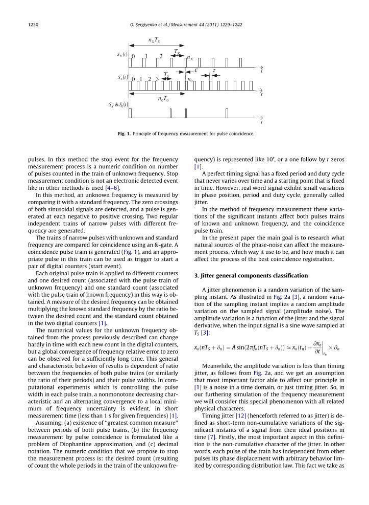
Fig. 1. Principle of frequency measurement for pulse coincidence.

1230 O. Sergiyenko et al. / Measurement 44 (2011) 1229–1242

pulses. In this method the stop event for the frequencymeasurement process is a numeric condition on numberof pulses counted in the train of unknown frequency. Stopmeasurement condition is not an electronic detected eventlike in other methods is used [4–6].

In this method, an unknown frequency is measured bycomparing it with a standard frequency. The zero crossingsof both sinusoidal signals are detected, and a pulse is gen-erated at each negative to positive crossing. Two regularindependent trains of narrow pulses with different fre-quency are generated.

The trains of narrow pulses with unknown and standardfrequency are compared for coincidence using an &-gate. Acoincidence pulse train is generated (Fig. 1), and an appro-priate pulse in this train can be used as trigger to start apair of digital counters (start event).

Each original pulse train is applied to different countersand one desired count (associated with the pulse train ofunknown frequency) and one standard count (associatedwith the pulse train of known frequency) in this way is ob-tained. A measure of the desired frequency can be obtainedmultiplying the known standard frequency by the ratio be-tween the desired count and the standard count obtainedin the two digital counters [1].

The numerical values for the unknown frequency ob-tained from the process previously described can changehardly in time with each new count in the digital counters,but a global convergence of frequency relative error to zerocan be observed for a sufficiently long time. This generaland characteristic behavior of results is dependent of ratiobetween the frequencies of both pulse trains (or similarlythe ratio of their periods) and their pulse widths. In com-putational experiments which is controlling the pulsewidth in each pulse train, a nonmonotone decreasing char-acteristic and an alternating convergence to a local mini-mum of frequency uncertainty is evident, in shortmeasurement time (less than 1 s for given frequencies) [1].

Assuming: (a) existence of ‘‘greatest common measure’’between periods of both pulse trains, (b) the frequencymeasurement by pulse coincidence is formulated like aproblem of Diophantine approximation, and (c) decimalnotation. The numeric condition that we propose to stopthe measurement process is: the desired count (resultingof count the whole periods in the train of the unknown fre-

quency) is represented like 10r, or a one follow by r zeros[1].

A perfect timing signal has a fixed period and duty cyclethat never varies over time and a starting point that is fixedin time. However, real word signal exhibit small variationsin phase position, period and duty cycle, generally calledjitter.

In the method of frequency measurement these varia-tions of the significant instants affect both pulses trainsof known and unknown frequency, and the coincidencepulse train.

In the present paper the main goal is to research whatnatural sources of the phase-noise can affect the measure-ment process, which way it use to be, and how much it canaffect the process of the best coincidence registration.

3. Jitter general components classification

A jitter phenomenon is a random variation of the sam-pling instant. As illustrated in Fig. 2a [3], a random varia-tion of the sampling instant implies a random amplitudevariation on the sampled signal (amplitude noise). Theamplitude variation is a function of the jitter and the signalderivative, when the input signal is a sine wave sampled atTS [3]:

xoðnTS þ dnÞ ¼ A sinð2pfoðnTS þ dnÞÞ � xoðtnÞ þ@xo

@t

����tn

� @n

Meanwhile, the amplitude variation is less than timingjitter, as follows from Fig. 2a, and we get an assumptionthat most important factor able to affect our principle in[1] is a noise in a time domain, or just timing jitter. So, inour furthering simulation of the frequency measurementwe will consider this special phenomenon with all relatedphysical characters.

Timing jitter [12] (henceforth referred to as jitter) is de-fined as short-term non-cumulative variations of the sig-nificant instants of a signal from their ideal positions intime [7]. Firstly, the most important aspect in this defini-tion is the non-cumulative character of the jitter. In otherwords, each pulse of the train has independent from otherpulses its phase displacement with arbitrary behavior lim-ited by corresponding distribution law. This fact we take as

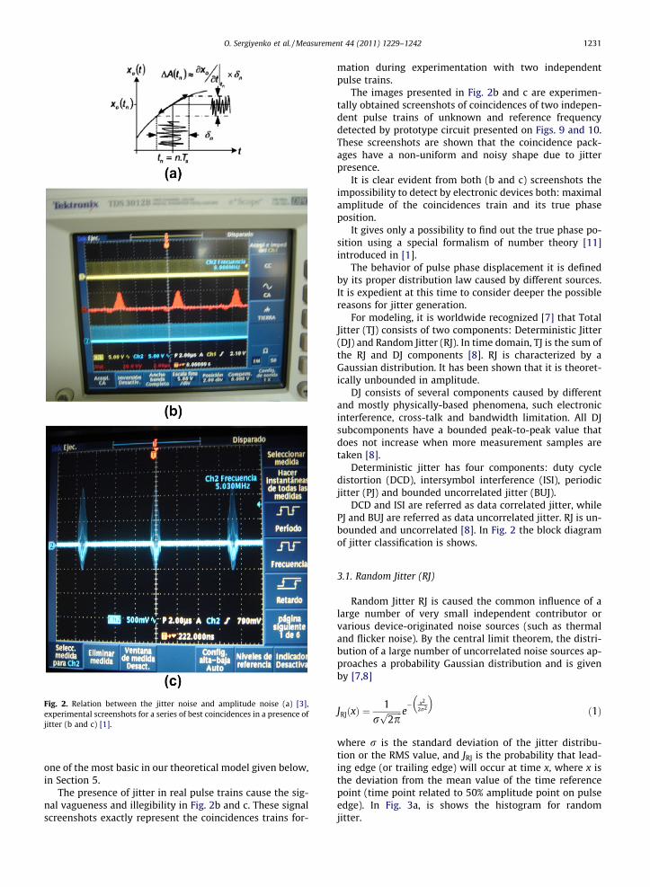
Fig. 2. Relation between the jitter noise and amplitude noise (a) [3],experimental screenshots for a series of best coincidences in a presence ofjitter (b and c) [1].

O. Sergiyenko et al. / Measurement 44 (2011) 1229–1242 1231

one of the most basic in our theoretical model given below,in Section 5.

The presence of jitter in real pulse trains cause the sig-nal vagueness and illegibility in Fig. 2b and c. These signalscreenshots exactly represent the coincidences trains for-

mation during experimentation with two independentpulse trains.

The images presented in Fig. 2b and c are experimen-tally obtained screenshots of coincidences of two indepen-dent pulse trains of unknown and reference frequencydetected by prototype circuit presented on Figs. 9 and 10.These screenshots are shown that the coincidence pack-ages have a non-uniform and noisy shape due to jitterpresence.

It is clear evident from both (b and c) screenshots theimpossibility to detect by electronic devices both: maximalamplitude of the coincidences train and its true phaseposition.

It gives only a possibility to find out the true phase po-sition using a special formalism of number theory [11]introduced in [1].

The behavior of pulse phase displacement it is definedby its proper distribution law caused by different sources.It is expedient at this time to consider deeper the possiblereasons for jitter generation.

For modeling, it is worldwide recognized [7] that TotalJitter (TJ) consists of two components: Deterministic Jitter(DJ) and Random Jitter (RJ). In time domain, TJ is the sum ofthe RJ and DJ components [8]. RJ is characterized by aGaussian distribution. It has been shown that it is theoret-ically unbounded in amplitude.

DJ consists of several components caused by differentand mostly physically-based phenomena, such electronicinterference, cross-talk and bandwidth limitation. All DJsubcomponents have a bounded peak-to-peak value thatdoes not increase when more measurement samples aretaken [8].

Deterministic jitter has four components: duty cycledistortion (DCD), intersymbol interference (ISI), periodicjitter (PJ) and bounded uncorrelated jitter (BUJ).

DCD and ISI are referred as data correlated jitter, whilePJ and BUJ are referred as data uncorrelated jitter. RJ is un-bounded and uncorrelated [8]. In Fig. 2 the block diagramof jitter classification is shows.

3.1. Random Jitter (RJ)

Random Jitter RJ is caused the common influence of alarge number of very small independent contributor orvarious device-originated noise sources (such as thermaland flicker noise). By the central limit theorem, the distri-bution of a large number of uncorrelated noise sources ap-proaches a probability Gaussian distribution and is givenby [7,8]

JRJðxÞ ¼1

rffiffiffiffiffiffiffi2pp e

� x2

2r2

� �ð1Þ

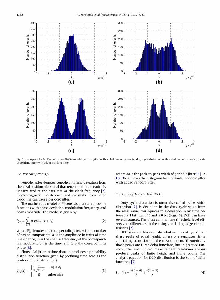
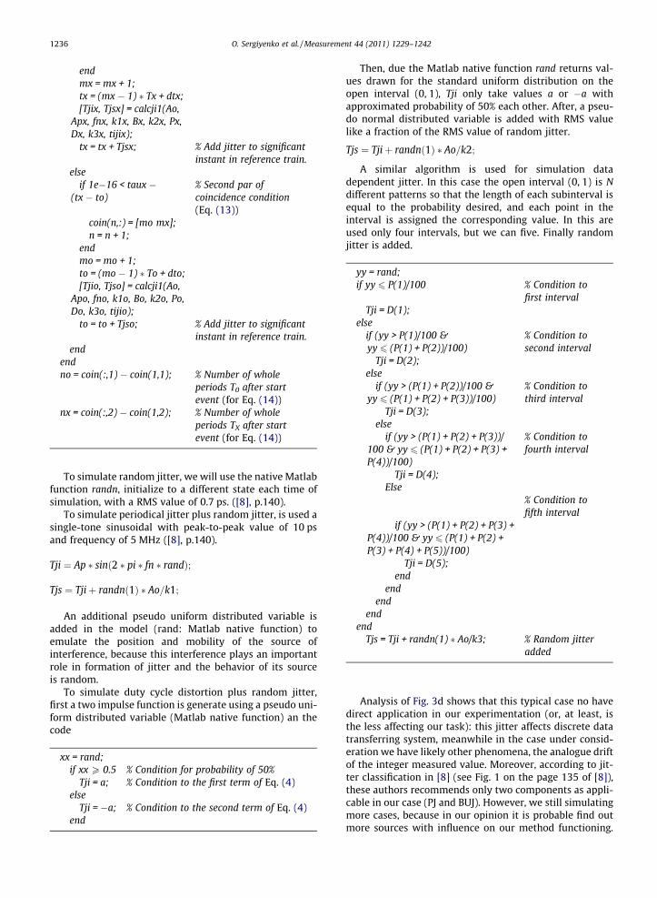
where r is the standard deviation of the jitter distribu-tion or the RMS value, and JRJ is the probability that lead-ing edge (or trailing edge) will occur at time x, where x isthe deviation from the mean value of the time referencepoint (time point related to 50% amplitude point on pulseedge). In Fig. 3a, is shows the histogram for randomjitter.

-3 -2 -1 0 1 2 3x 10-12

0

50

100

150

200

250

300

350

400

s

Num

ber o

f eve

nts

-3 -2 -1 0 1 2 3x 10-12

0

50

100

150

200

250

300

s

Num

ber o

f eve

nts

-3 -2 -1 0 1 2 3x 10-12

0

50

100

150

200

250

300

s

Num

ber o

f eve

nts

-3 -2 -1 0 1 2 3x 10-12

0

50

100

150

200

250

300

s

Num

ber o

f eve

nts

(a) (b)

(d)(c)Fig. 3. Histogram for (a) Random jitter, (b) Sinusoidal periodic jitter with added random jitter, (c) duty cycle distortion with added random jitter y (d) datadependent jitter with added random jitter.

1232 O. Sergiyenko et al. / Measurement 44 (2011) 1229–1242

3.2. Periodic jitter (PJ)

Periodic jitter denotes periodical timing deviation fromthe ideal position of a signal that repeat in time, is typicallyuncorrelated to the data rate or the clock frequency [7].Electromagnetic interference and crosstalk from someclock line can cause periodic jitter.

The mathematic model of PJ consists of a sum of cosinefunctions with phase deviation, modulation frequency, andpeak amplitude. The model is given by

PJT ¼Xn

i¼0

ai cosðxit þ hiÞ ð2Þ

where PJT denotes the total periodic jitter, n is the numberof cosine components, ai is the amplitude in units of timein each tone, xi is the angular frequency of the correspond-ing modulation, t is the time, and hi is the correspondingphase [8].

Sinusoidal jitter in time domain produces a probabilitydistribution function given by (defining time zero as thecenter of the distribution)

JPJiðxÞ ¼

1pffiffiffiffiffiffiffiffiffia2

i�x2

p jxj 6 ai

0 otherwise

8<: ð3Þ

where 2a is the peak-to-peak width of periodic jitter [5]. InFig. 3b is shows the histogram for sinusoidal periodic jitterwith added random jitter.

3.3. Duty cycle distortion (DCD)

Duty cycle distortion is often also called pulse widthdistortion [7], is deviation in the duty cycle value fromthe ideal value, this equates to a deviation in bit time be-tween a 1 bit (logic 1) and a 0 bit (logic 0). DCD can haveseveral sources. The most common are threshold level off-sets and differences in the rising and falling edge charac-teristics [7].

DCD yields a binomial distribution consisting of twosharp peaks of equal height, unless one separates risingand falling transitions in the measurement. Theoreticallythose peaks are Dirac delta functions, but in practice ran-dom jitter and limited measurement resolution alwaysproduce peaks of finite height and finite width. Theanalytic equation for DCD distribution is the sum of deltafunctions [7]:

JDCDðxÞ ¼dðx� aÞ

2þ dðxþ aÞ

2ð4Þ

O. Sergiyenko et al. / Measurement 44 (2011) 1229–1242 1233

where 2a is the peak-to-peak width of the DCD. In Fig. 3c isshows the histogram for duty cycle distortion with addedrandom jitter.

3.4. Data Dependent Jitter (DDJ)

Data dependent jitter describes timing errors that de-pend on the preceding sequence of data bits [7]. DDJ is apredominant form of DJ caused by bandwidth limitationsof the system or electromagnetic reflections of the signal[9,10]. Since there is always only a limited number of dif-ferent possible patterns in a data stream of limited length,data dependent timing errors always produce a discretetiming jitter, theoretically DDJ distribution is the sum oftwo o more delta functions [7]:

JDDJðxÞ ¼XN

i¼1

pidðx� tiÞf g ð5Þ

wherePN

i¼1pi ¼ 1 N is number of distinct patterns, pi is theprobability of the particular pattern occurring, and ti is thetiming displacement of the edge following this pattern. InFig. 3d is shows the histogram for data dependent jitterwith added random jitter.

Each histogram of Fig. 3a–d was independently con-structed with data obtained from the jitter simulation intime domain. These simulations are made basing on theknown jitters models from the literature sources [7,8] andsections of computation programs described below inSection 6. These four kinds of jitter were simulated inMatlab, using mathematic models introduced in subsec-tions above.

These histograms are obtained like a print for 10,000points by Matlab native function ‘‘hist’’, or 10,000 eventsof jitter discrete values according to previous formulas.

Later these forms of jitter were applied in the timedomain to the simulated signals as shown on Fig. 7.

4. Jitter influence in the frequency measurementmethod

Let us consider two trains of narrow pulses SXðtÞ andS0ðtÞ with period TX and T0 respectively, which have pulsewidth s. Both pulse trains are generated by detection ofzero crossings of two sinusoidal signal of frequencies: f0

(standard frequency) and fX (unknown frequency). Supposethat both pulse trains start in phase, i.e. a time shift is 0. Ifboth pulse trains are applied to the input ports of an AND-gate, an irregular pulse train is formed by pulses from par-tial and total coincidences is generated, it is shown in Fig. 1.

For frequency measurement, the time intervals n0T0 andnXTX are compared (Fig. 1), where n0 is the amount of peri-ods T0 in the measurement time and nX is the amount ofperiods TX in the same time interval. Measurement timecan be defined by the time interval between the first onepulse of coincidence (start event) after beginning the mea-surement process, and by any other following pulse ofcoincidence (stop event).

As it were mentioned in the previous section, n0 and nX

are the counts of pulses obtained in two independent dig-ital counters.

Mathematical condition to pulse coincidences is

jnXTX � n0T0j 6 e ð6Þ

where e is the acceptable tolerance (reasonable error valuebetween time intervals n0T0 and nXTX) [1,7]. From Eq. (6),measure frequency is expressed by

fX �nX

n0f0

�������� 6

efX

n0T0ð7Þ

And relative error of measurement (frequency offset) b canbeen expressed by

b ¼fX � nX

n0f0

������

fX6

en0T0

: ð8Þ

We can see in (8) that relative error of measurement is lim-ited by the ratio between the acceptable tolerance of thecomparison error between time intervals n0T0 and nXTX

and, the time interval n0T0. Value of n0T0 is approximatelythe measurement time (see Fig. 1).

5. Pulse trains jitter simulation (computationalexperiment)

In computational experiments the time reference pointof each pulse in both trains of narrow pulses SX(t) and S0(t)are calculated using the equations

tXðmXÞ ¼ ðmX � 1ÞTX þ tuX ð9Þ

and

t0ðm0Þ ¼ ðm0 � 1ÞT0 þ tu0 ð10Þ

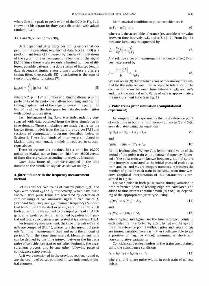
for the leading edge. Where TX is hypothetical value of theperiod of the pulse train with unknown frequency, T0 per-iod of the pulse train with known frequency, tuX and tu0 aretime intervals associated to the initial phase of each pulsetrain and, mX and m0 are integers numbers, represents thenumber of pulse in each train in the simulation time win-dow. Graphical interpretation of this parameters is pre-sented in Fig 4a.

For each pulse in both pulse trains, timing variation intime reference point of leading edge are calculated andadded to time instants obtained with (9) and (10), depend-ing of the appropriated jitter type, using

tXjðmXÞ ¼ tXðmXÞ þ DtX ð11Þ

and

t0jðm0Þ ¼ t0ðm0Þ þ Dt0 ð12Þ

where tXj(mX) and t0j(m0) are the time reference points ineach pulse trains affected by jitter, tX(mX) and t0(m0) arethe time reference points without jitter and, DtX and Dt0

are timing variation from each other (both are able to geta positive or negative value), assuming as short-termnon-cumulative variations.

Coincidences between pulses in the trains are obtainedusing the coincidence conditions

sX < tXjðmXÞ � t0jðm0Þ < s0 ð13Þ

where sX and s0 are pulse widths in each train of narrowpulses.

(a)

(b)Fig. 4. Graphic interpretation of parameters used in simulation of pulse coincidence process.

1234 O. Sergiyenko et al. / Measurement 44 (2011) 1229–1242

A pulse coincidence is selected as ‘‘start event of mea-surement’’ in the computational experiments. Using to thiscoincidence as a counting reference, the number of pulsesto the next coincidences is continually counted and, n0 andnX is calculated for each next coincidence.

For each next coincidence from the selected coincidenceas ‘‘start event of measurement’’ a measure of frequency iscalculated by

fXm ¼nX

n0f0 ð14Þ

and the relative error of measurement using (8).

6. Experimental results

In [1] it is mentioned that the best approximation rationXn0

appears several times during relatively short time of fX

and f0 pulse trains observation. It is extremely clear shown

0 0.1 0.2 0.3 0.4 0-1

-0.5

0

0.5

1

1.5 x 10-11

Masureme

β , F

requ

ency

offs

et 1 2 3

Fig. 5. Frequency count results for a series of b

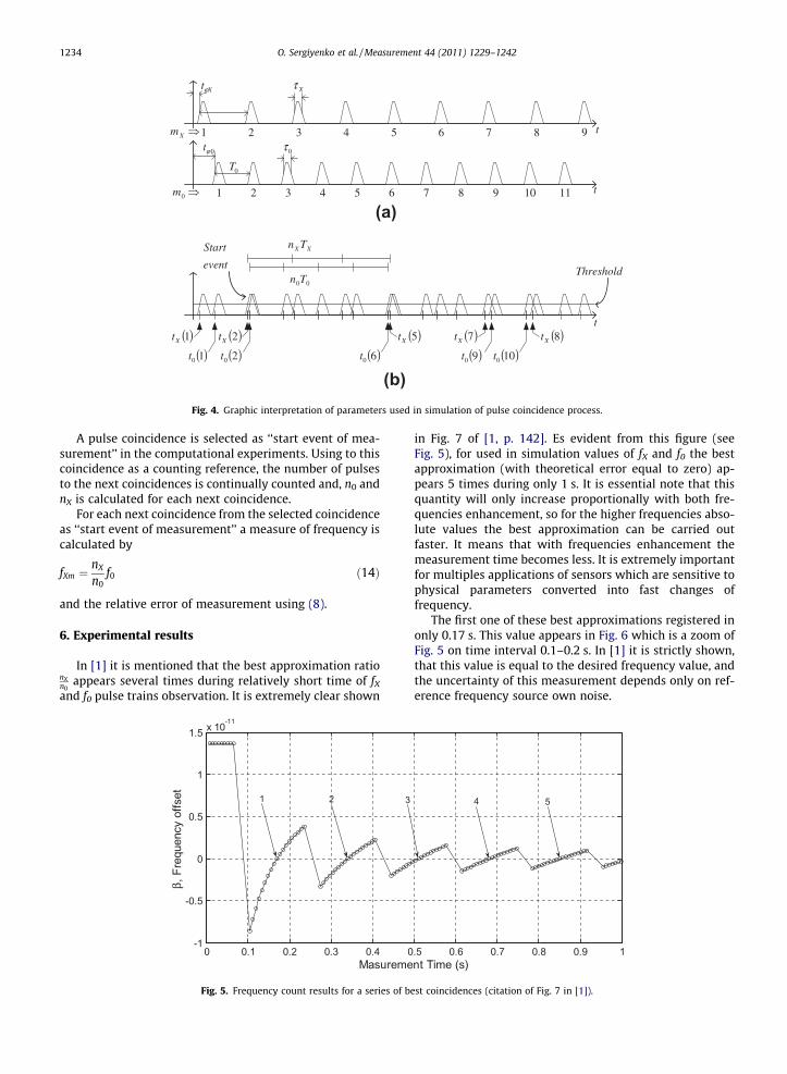
in Fig. 7 of [1, p. 142]. Es evident from this figure (seeFig. 5), for used in simulation values of fX and f0 the bestapproximation (with theoretical error equal to zero) ap-pears 5 times during only 1 s. It is essential note that thisquantity will only increase proportionally with both fre-quencies enhancement, so for the higher frequencies abso-lute values the best approximation can be carried outfaster. It means that with frequencies enhancement themeasurement time becomes less. It is extremely importantfor multiples applications of sensors which are sensitive tophysical parameters converted into fast changes offrequency.

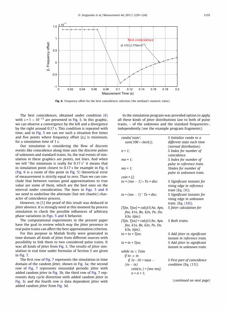
The first one of these best approximations registered inonly 0.17 s. This value appears in Fig. 6 which is a zoom ofFig. 5 on time interval 0.1–0.2 s. In [1] it is strictly shown,that this value is equal to the desired frequency value, andthe uncertainty of this measurement depends only on ref-erence frequency source own noise.

.5 0.6 0.7 0.8 0.9 1nt Time (s)

4 5

est coincidences (citation of Fig. 7 in [1]).

0 0.02 0.04 0.06 0.08 0.1 0.12 0.14 0.16 0.18 0.2-1

-0.5

0

0.5

1

1.5 x 10-11

Masurement Time (s)

β , F

requ

ency

offs

et (0.1701,2.7755x10-17)

best coincidence

Fig. 6. Frequency offset for the best coincidences selection (the mediant’s numeric value).

O. Sergiyenko et al. / Measurement 44 (2011) 1229–1242 1235

The best coincidences, obtained under condition (6)with e = 1 � 10�12 are presented in Fig. 5. In this graphic,we can observe a convergence by the left and a divergenceby the right around 0.17 s. This condition is repeated withtime, and in Fig. 5 we can see such a situation five timesand five points where frequency offset |bx| is minimum,for a simulation time of 1 s.

Our simulation is considering the flow of discreteevents like coincidence along time axis the discrete pulsesof unknown and standard trains. So, the real events of sim-ulation in these graphics are points, not lines. And whenwe tell ‘‘the minimum is really for 0.17 s’’ it means thatin simulation point closest to 0.17 s for example in Fig. 6(Fig. 6 is a zoom of this point in Fig. 5) theoretical errorof measurement is strictly equal to zero. Than we can con-clude that between various good approximations to truevalue are some of them, which are the best ones on theinterval under consideration. The lines in Figs. 5 and 6we need to underline the alternate (but not chaotic) char-acter of coincidence process.

However, in [1] the proof of this result was deduced injitter absence. It is strongly need at this moment by processsimulation to check the possible influences of arbitraryphase variations in Figs. 5 and 6 behavior.

The computational experiments in the present paperhave the goal to review which way the jitter presence inreal pulse trains can affect the best approximation criterion.

For this purpose in Matlab firstly were generated intime domain all kinds of jitter from different sources withpossibility to link them to two considered pulse trains. Itwas all kinds of jitter from Fig. 3. The results of jitter sim-ulation in real time under formulas of Section 5 are givenin Fig. 7.

The first row of Fig. 7 represents the simulation in timedomain of the random jitter, shown in Fig. 3a; the secondrow of Fig. 7 represents sinusoidal periodic jitter withadded random jitter in Fig. 3b, the third row of Fig. 7 rep-resents duty cycle distortion with added random jitter inFig. 3c and the fourth row is data dependent jitter withadded random jitter from Fig. 3d.

In the simulation program was provided option to applyall these kinds of jitter distributions law to both of pulsetrains, – of the unknown and the standard frequencies-,independently (see the example program fragments):

randn(‘state’,sum(100 � clock));

% Initialize randn to adifferent state each time(normal distribution).

n = 1;

% Index for number ofcoincidence.

mo = 1;

% Index for number ofpulse in reference train.

mx = 1;

%Index for number ofpulse in unknown train.

coin = [];

to = (mo � 1) � To + dto; % Significant instants for

rising edge in referencetrain (Eq. (9)).

tx = (mx � 1) � Tx + dtx;

% Significant instants forrising edge in unknowntrain. (Eq. (10)).

[Tjio, Tjso] = calcji1(Ao, Apo,fno, k1o, Bo, k2o, Po, Do,k3o, tijio);

% Jitter calculation for

[Tjix, Tjsx] = calcji1(Ao, Apx,fnx, k1x, Bx, k2x, Px, Dx,k3x, tijix);

% Both trains.

to = to + Tjso;

% Add jitter to significantinstant in reference train.

tx = tx + Tjsx;

% Add jitter to significantinstant in unknown train.

while to 6 Tsim

if to P tx

if 1e�16 < taux �(to � tx)

% First part of coincidencecondition (Eq. (13))

coin(n,:) = [mo mx];

n = n + 1;

(continued on next page)

1236 O. Sergiyenko et al. / Measureme

end

mx = mx + 1; tx = (mx � 1) � Tx + dtx; [Tjix, Tjsx] = calcji1(Ao,

Apx, fnx, k1x, Bx, k2x, Px,Dx, k3x, tijix);

tx = tx + Tjsx;

% Add jitter to significantinstant in reference train.

else

if 1e�16 < taux �

(tx � to)

% Second par ofcoincidence condition(Eq. (13))

coin(n,:) = [mo mx];

n = n + 1;

end

mo = mo + 1; to = (mo � 1) � To + dto; [Tjio, Tjso] = calcji1(Ao,

Apo, fno, k1o, Bo, k2o, Po,Do, k3o, tijio);

to = to + Tjso;

% Add jitter to significantinstant in reference train.

end

end no = coin(:,1) � coin(1,1); % Number of whole

periods T0 after startevent (for Eq. (14))

nx = coin(:,2) � coin(1,2);

% Number of wholeperiods TX after startevent (for Eq. (14))

To simulate random jitter, we will use the native Matlabfunction randn, initialize to a different state each time ofsimulation, with a RMS value of 0.7 ps. ([8], p.140).

To simulate periodical jitter plus random jitter, is used asingle-tone sinusoidal with peak-to-peak value of 10 psand frequency of 5 MHz ([8], p.140).

Tji ¼ Ap � sinð2 � pi � fn � randÞ;

Tjs ¼ Tjiþ randnð1Þ � Ao=k1;

An additional pseudo uniform distributed variable isadded in the model (rand: Matlab native function) toemulate the position and mobility of the source ofinterference, because this interference plays an importantrole in formation of jitter and the behavior of its sourceis random.

To simulate duty cycle distortion plus random jitter,first a two impulse function is generate using a pseudo uni-form distributed variable (Matlab native function) an thecode

xx = rand;

if xx P 0.5 % Condition for probability of 50%

Tji = a;

% Condition to the first term of Eq. (4) else

Tji = �a;

% Condition to the second term of Eq. (4) end

Then, due the Matlab native function rand returns val-ues drawn for the standard uniform distribution on the

open interval (0, 1), Tji only take values a or �a withapproximated probability of 50% each other. After, a pseu-do normal distributed variable is added with RMS valuelike a fraction of the RMS value of random jitter.

Tjs ¼ Tjiþ randnð1Þ � Ao=k2;

A similar algorithm is used for simulation datadependent jitter. In this case the open interval (0, 1) is Ndifferent patterns so that the length of each subinterval isequal to the probability desired, and each point in theinterval is assigned the corresponding value. In this areused only four intervals, but we can five. Finally randomjitter is added.

nt 44 (2011) 1229–1242

yy = rand;

if yy 6 P(1)/100 % Condition to

first interval

Tji = D(1);

else

if (yy > P(1)/100 &yy 6 (P(1) + P(2))/100)

% Condition tosecond interval

Tji = D(2);

else

if (yy > (P(1) + P(2))/100 &yy 6 (P(1) + P(2) + P(3))/100)

% Condition tothird interval

Tji = D(3);

else

if (yy > (P(1) + P(2) + P(3))/100 & yy 6 (P(1) + P(2) + P(3) +P(4))/100)

% Condition tofourth interval

Tji = D(4);

Else

% Condition tofifth interval

if (yy > (P(1) + P(2) + P(3) +P(4))/100 & yy 6 (P(1) + P(2) +P(3) + P(4) + P(5))/100)

Tji = D(5);

end

end

end

end

end

Tjs = Tji + randn(1) � Ao/k3;

% Random jitteradded

Analysis of Fig. 3d shows that this typical case no havedirect application in our experimentation (or, at least, isthe less affecting our task): this jitter affects discrete datatransferring system, meanwhile in the case under consid-eration we have likely other phenomena, the analogue driftof the integer measured value. Moreover, according to jit-ter classification in [8] (see Fig. 1 on the page 135 of [8]),these authors recommends only two components as appli-cable in our case (PJ and BUJ). However, we still simulatingmore cases, because in our opinion it is probable find outmore sources with influence on our method functioning.

0 1000 2000 3000 4000 5000 6000 7000 8000 9000 10000-1

-0.5

0

0.5

1 x 10-12

Number of events

0 1000 2000 3000 4000 5000 6000 7000 8000 9000 10000-5

0

5 x 10-13

Number of events

s

0 1000 2000 3000 4000 5000 6000 7000 8000 9000 10000-5

0

5 x 10-13

Number of events

s

0 1000 2000 3000 4000 5000 6000 7000 8000 9000 10000-5

0

5 x 10-13

Number of events

s

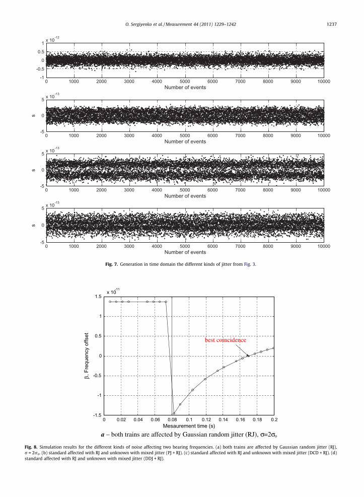
Fig. 7. Generation in time domain the different kinds of jitter from Fig. 3.

a – both trains are affected by Gaussian random jitter (RJ), σ=2σo

0 0.02 0.04 0.06 0.08 0.1 0.12 0.14 0.16 0.18 0.2-1.5

-1

-0.5

0

0.5

1

1.5x 10

-11

Mesaurement time (s)

β, F

requ

ency

offs

et

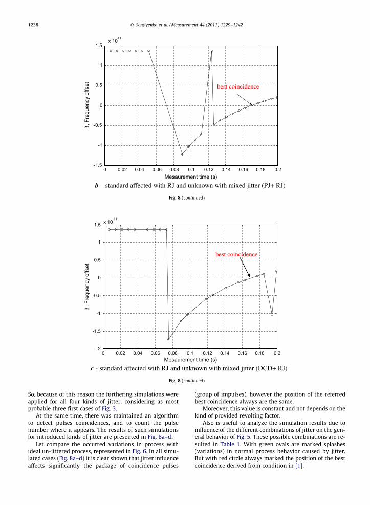
best coincidence

Fig. 8. Simulation results for the different kinds of noise affecting two bearing frequencies. (a) both trains are affected by Gaussian random jitter (RJ),r = 2ro. (b) standard affected with RJ and unknown with mixed jitter (PJ + RJ). (c) standard affected with RJ and unknown with mixed jitter (DCD + RJ). (d)standard affected with RJ and unknown with mixed jitter (DDJ + RJ).

O. Sergiyenko et al. / Measurement 44 (2011) 1229–1242 1237

c - standard affected with RJ and unknown with mixed jitter (DCD+ RJ)

0 0.02 0.04 0.06 0.08 0.1 0.12 0.14 0.16 0.18 0.2-2

-1.5

-1

-0.5

0

0.5

1

1.5 x 10-11

Mesaurement time (s)

β, F

requ

ency

offs

et

best coincidence

Fig. 8 (continued)

b – standard affected with RJ and unknown with mixed jitter (PJ+ RJ)

0 0.02 0.04 0.06 0.08 0.1 0.12 0.14 0.16 0.18 0.2-1.5

-1

-0.5

0

0.5

1

1.5x 10

-11

Mesaurement time (s)

β, F

requ

ency

offs

et best coincidence

Fig. 8 (continued)

1238 O. Sergiyenko et al. / Measurement 44 (2011) 1229–1242

So, because of this reason the furthering simulations wereapplied for all four kinds of jitter, considering as mostprobable three first cases of Fig. 3.

At the same time, there was maintained an algorithmto detect pulses coincidences, and to count the pulsenumber where it appears. The results of such simulationsfor introduced kinds of jitter are presented in Fig. 8a–d:

Let compare the occurred variations in process withideal un-jittered process, represented in Fig. 6. In all simu-lated cases (Fig. 8a–d) it is clear shown that jitter influenceaffects significantly the package of coincidence pulses

(group of impulses), however the position of the referredbest coincidence always are the same.

Moreover, this value is constant and not depends on thekind of provided revolting factor.

Also is useful to analyze the simulation results due toinfluence of the different combinations of jitter on the gen-eral behavior of Fig. 5. These possible combinations are re-sulted in Table 1. With green ovals are marked splashes(variations) in normal process behavior caused by jitter.But with red circle always marked the position of the bestcoincidence derived from condition in [1].

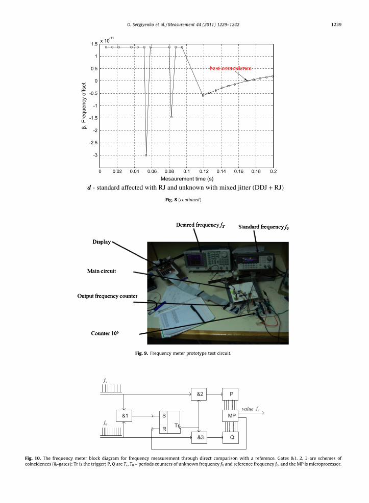
Fig. 9. Frequency meter prototype test circuit.

xf

0f

value xf

Fig. 10. The frequency meter block diagram for frequency measurement through direct comparison with a reference. Gates &1, 2, 3 are schemes ofcoincidences (&-gates); Tr is the trigger; P, Q are Tx, T0 – periods counters of unknown frequency fX and reference frequency f0, and the MP is microprocessor.

d - standard affected with RJ and unknown with mixed jitter (DDJ + RJ)

0 0.02 0.04 0.06 0.08 0.1 0.12 0.14 0.16 0.18 0.2

-3

-2.5

-2

-1.5

-1

-0.5

0

0.5

1

1.5 x 10-11

Mesaurement time (s)

β, F

requ

ency

offs

et

best coincidence

Fig. 8 (continued)

O. Sergiyenko et al. / Measurement 44 (2011) 1229–1242 1239

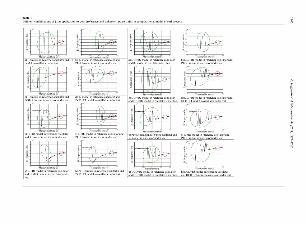
Table 1Different combinations of jitter application to both (reference and unknown) pulse trains in computational model of real process.

β β β β

β β

β β

β β β β

β β β β

1240O

.Sergiyenkoet

al./Measurem

ent44

(2011)1229–

1242

O. Sergiyenko et al. / Measurement 44 (2011) 1229–1242 1241

However, analyzing all the variations in Table 1, thesecases also proofs that mentioned splashes and imperfec-tions can affects only pulses packages at its boundaries. Po-sition of the center never is variable, and it is definedexclusively by process nature, number theory laws, andnumerical condition [1] at the same time.

7. Discussions

As shown by computational experiment results, the bestapproximation condition, derived in [1] it is invariant(independent) to jitter. This statement it is rigorous forany kind of jitter. This main contribution of the presentresearch gives more backgrounds for the method of the fastfrequency measurement implementation, especially forvarious practical applications [16,17] of the sensorssensitive in frequency domain, or repetitive measurementprocesses with possibility to apply the principle ofcontinuous coincidences of two independent scales [18,19].

It is only one circumstance maybe critical in the pre-sented above: all these simulation results are derived inassumption stated at the beginning of Chapter 3, thattiming jitter has non-cumulative variations. There is noone another suggestion about different jitter behavior inmost fundamental references in this field [7,8,12]. How-ever, for completed analysis of all noise effects at fre-quency measurement according to [1], in our opinion itis desirable the research of possible accumulative ther-mal drift of pulses in train at the temperature changes.It is clear that such task more proper for real experimen-tation than for computer simulation. For this goal wasmade an experimental prototype of the measuring sys-tem in Fig. 9.

The simplified functional diagram of a frequency meterof Fig. 9 is presented in Fig. 10 [1, p. 139]. Pulse signalswith frequencies fX and f0 inputs into three &-gates. Priorto the first coincidence in the gate &1 the trigger Tr pre-vents elements &2, &3 from being active.

After the occurrence of a coincidence, the counters Pand Q keep a count of the pulses of both frequencies untilcounter P receives a result in the form of

PmPn ¼ 1� 10r .

This signal results in feedback that resets the trigger toits initial state. The measurement is completed.

We assert that at the end of the measurement, the read-out result in the counter

PmQ n is the best proportional

approximation of the measured frequency’s true value onthe given interval of time.

Influence analysis of thermal long-term accumulativedrift of pulses from their ideal positions in time will be asubject for our future publications.

8. Conclusions

Assuming the analysis of simulation results of the pos-sible practical jitter influence for frequency measurementmethod introduced in [1] we can declare the next.

� Random and deterministic components of jitter aremodeled, and each one of them affects in a differentway the general behavior of pulses on the two pulse

trains used in the method, and the train resulted astheir intersections in time domain.� Under inspection in this work were provided in compu-

tational simulation four different known and describedin recent literature sources of jitter.� The results of simulation proofs the invariance (inde-

pendence) of best approximation position on anydescribed in literature sources of short-term non-cumu-lative variations of the significant instants of a signalfrom their ideal positions in time domain.

Acknowledgments

Particular results of this investigation herein describedwere reported in several congresses [13–15], we are grate-ful to congress organizers for fruitful discussions. Theauthors dedicate this article to the grateful memory ofour teacher, Dr. Valentin Tyrsa; and would like to thankto anonymous reviewers for valuable comments andremarks.

References

[1] Daniel Hernández Balbuena, Oleg Sergiyenko, Vera Tyrsa, LarysaBurtseva, Moisés Rivas López, Signal frequency measurement byrational approximations, Measurement, vol. 42, no. 1, Elsevier, 2009,pp. 136–144. doi:10.1016/j.measurement.2008.04.009. ISSN: 0263-2241.

[2] D.W. Allan, Time and frequency (time-domain) characterization,estimation, and prediction of precision clocks and oscillators, IEEETrans. Ultrason. Ferroelectr. Freq. Control 34 (752) (1987) 647–654.

[3] G. Monnerie et al., Internal Jitter noise measurement procedure of aswitched capacitor circuit, Measurement, vol. 42, no. 1, Elsevier,2009, pp. 1–8.

[4] V.E. Tyrsa, Error reduction in conversion of quantities to digitalizedtime intervals, Measurement Techniques, vol. 18, no. 3, Springer,New York, 1975, pp. 357–360.

[5] J.C. Fletcher, Frequency measurement by coincidence detection withstandard frequency, US Patent 3, 924,183, 1975.

[6] Z. Wei, The greatest common factor frequency and its application inthe accurate measurement of periodic signals, in: Proceedings of theIEEE Frequency Control Symposium, 1992, pp. 270–273.

[7] W. Maichen, Digital Timing Measurement, From Scope and Probes toTiming and Jitter, FRET 33, Frontier in Electronic Testing, Springer,Netherland, 2006, p. 240. ISBN: 0-387-31418-0.

[8] K.K. Kim et al., Analysis and simulation of jitter sequences for testingserial data channels, IEEE Trans. Ind. Inf. 4 (2) (2008) 134–143.

[9] J. Buckwalter et al., Predicting data-dependent jitter, IEEE Trans. Circ.Systems-II: Express Briefs 51 (9) (2004) 453–457.

[10] B. Analui et al., Data-dependent jitter in serial communications, IEEETrans. Microwave Theory Tech. 53 (11) (2005) 3388–3397.

[11] Robert Daniel Carmichael, The Theory of Numbers and DiophantineAnalysis, Courier Dover Publications, Dover Phoenix Editions, 2004,p. 118. ISBN: 0486438031.

[12] I.S. Gonorovsky, Radio Circuits and Signals, MIR Publishers, Moscow,1981, p. 639 (translated to English).

[13] B. Daniel Hernández, L. Moisés Rivas, Larisa Burtseva, OlegSergiyenko, Vera Tyrsa, Method for phase shift measurement usingfarey fractions, in: IEEE-LEOS Proceedings Multiconference onElectronics and Photonics (MEP-2006), Guanajuato, Mexico,Guanajuato, November, 7–10, 2006, pp. 181–184. ISBN: 1-4244-0627-7, ISSN/Library of Congress Number 2006932321.

[14] Daniel Hernandez Balbuena, Oleg Sergiyenko, Vera Tyrsa, LarisaBurtseva, Frequency measurement method for mechatronic andtelecommunication applications, in: IEEE-IES ProceedingsInternational Symposium on Industrial Electronics (ISIE-2008),Cambridge, United Kingdom, June 30–July 2, 2008, pp. 1452–1457.ISBN: 978-1-4244-1665-3, ISSN/Library of Congress Number2007936380.

[15] Daniel Hernandez Balbuena, Oleg Sergiyenko, Vera Tyrsa, LarisaBurtseva, Method for fast and accurate frequency

1242 O. Sergiyenko et al. / Measurement 44 (2011) 1229–1242

measurement, in: Proceedings of 16th IMEKO TC4 SymposiumExploring New Frontiers of Instrumentation and Methods forElectrical and Electronic Measurements, Florence, Italy, 20–22September, 2008, pp. 367–373 [CD-ROM]. ISBN: 978-88-903149-3-3.

[16] Fabián N. Murrieta Rico, O. Yu Sergiyenko, V.V. Tyrsa, D. Hernández-Balbuena, W. Hernandez, Frequency domain automotive sensors:resolution improvement by novel principle of rationalapproximation, in: Proceedings of IEEE-ICIT InternationalConference on Industrial Technology (ICIT’10), 14–17 March, Viña-del-Mar, Valparaiso, Chile, 2010, pp. 1293–1298. ISBN: 978-1-4244-5697-0/10.

[17] Oleg Starostenko, Vicente Alarcon-Aquino, Wilmar Hernandez, OlegSergiyenko, Vera Tyrsa, Algorithmic Error Correction of Impedance

Measuring Sensors, vol. 9, no. 12, MDPI, Sensors, 2009, Basel,Switzerland, pp. 10341–10355. doi:10.3390/s91210341. ISSN:1424-8220.

[18] Moisés Rivas López, Oleg Sergiyenko, Vera Tyrsa, Wilmar HernandezPerdomo, Daniel Hernández Balbuena, Luis Devia Cruz, LarisaBurtseva, Juan Iván Nieto Hipólito, Optoelectronic method forstructural health monitoring, International Journal of StructuralHealth Monitoring, vol. 9, no. 2, SAGE Publications, March, 2010, pp.105–120. Issue Online, September, 24, 2009. doi:10.1177/1475921709340975. ISSN: 1475-9217.

[19] O. Yu. Sergiyenko, Optoelectronic system for mobile robotnavigation, Optoelectronics, Instrumentation and Data Processing,Vol. 46, no. 5, Springer/Allerton Press, Inc., October, 2010, pp. 414–428. doi:10.3103/S8756699011050037. ISSN: 8756-6990.