analysis of cluttered scenes using an elastic matching approach for stereo images

LETTER Communicated by Gustavo Deco

Analysis of Cluttered Scenes Using an Elastic MatchingApproach for Stereo Images

Christian [email protected] Institute for Media Communications IMK, D-53754 Sankt Augustin,Germany

Jochen [email protected] of Cognitive Science, University of California, San Diego, La Jolla,CA 92093-0515, U.S.A.

Christoph von der [email protected] fur Neuroinformatik, Ruhr-Universitat Bochum, D-44780 Bochum, Germany

We present a system for the automatic interpretation of cluttered scenescontaining multiple partly occluded objects in front of unknown, com-plex backgrounds. The system is based on an extended elastic graphmatching algorithm that allows the explicit modeling of partial occlu-sions. Our approach extends an earlier system in two ways. First, weuse elastic graph matching in stereo image pairs to increase matchingrobustness and disambiguate occlusion relations. Second, we use richerfeature descriptions in the object models by integrating shape and tex-ture with color features. We demonstrate that the combination of bothextensions substantially increases recognition performance. The systemlearns about new objects in a simple one-shot learning approach. De-spite the lack of statistical information in the object models and thelack of an explicit background model, our system performs surprisinglywell for this very difficult task. Our results underscore the advantagesof view-based feature constellation representations for difficult objectrecognition problems.

1 Introduction

The analysis of complex natural scenes with many partly occluded objectsis among the most difficult problems in computer vision (Rosenfeld, 1984).The task is illustrated in Figure 1 and may be defined as follows: Givenan input image with multiple, potentially partly occluded objects in frontof an unknown complex background, recognize the identities and spatial

Neural Computation 18, 1441–1471 (2006) C© 2006 Massachusetts Institute of Technology

1442 C. Eckes, J. Triesch, and C. von der Malsburg

Figure 1: Scene analysis overview. Given a set of object models (examples on theleft) and an input image of a complex scene (middle), the task of scene analysisis to compute a high-level interpretation of the scene giving the identities andlocations of all known objects, as well as their occlusion relations (right). Ourobject models take the form of labeled graphs with a gridlike topology.

locations of all known objects present in the scene. Clearly, the ability tomaster this task is a fundamental prerequisite for countless applicationdomains. Unknown backgrounds and partial occlusions of objects will bethe order of the day whenever computer vision systems or visually guidedrobots are deployed in complex, natural environments. In such situations,it may be that segmentation cannot be decoupled from recognition, butthe two problems have to be treated in an integrated manner. In fact, eventoday’s best “pure” segmentation approaches (e.g., Ren & Malik, 2002) seemto be severely limited in their ability to find object contours when comparedto human observers.

The system developed and tested here follows the popular approach ofelastic graph matching (EGM), a biologically inspired object recognitionapproach that represents views of objects as 2D constellations of wavelet-based features (Lades et al., 1993; Triesch & Eckes, 2004). EGM is an exampleof a class of architectures that represent particular views of objects as 2Dconstellations of image features (Fischler & Elschlager, 1973). EGM does notrely on initial segmentation, but directly matches observed image featuresto stored model features. It has been used successfully for recognizingobjects, faces (including identity, pose, gender, and expression; Wiskott,Fellous, Kruger, & von der Malsburg, 1997), and hand gestures (Triesch &von der Malsburg, 2002), and has already demonstrated its potential forcomplex scene analysis in an earlier study (Wiskott & von der Malsburg,1993). The description of object views as constellations of local features ispotentially very powerful for dealing with partial occlusions, because theeffect of features missing due to occlusion can be modeled explicitly in thisapproach. For example, missing features of the object “pig” in Figure 1 canbe discounted if it is recognized that they are occluded by the object in front.In Bayesian terms, the missing features are explained away by the presenceof the occluding object. In this capacity, our approach stands in contrast to

Analysis of Cluttered Scenes 1443

schemes employing more holistic object representations such as eigenspaceapproaches (Turk & Pentland, 1991; Murase & Nayar, 1995).

The philosophy behind our current approach is to integrate multiplesources of information within an EGM framework. The motivation for thisphilosophy is that when dealing with very difficult (vision) problems, oneis often well advised to follow the honorable “use all the help you can get”rationale. Recent research in the computer vision and machine learningcommunities has repeatedly highlighted the often surprising capabilitiesof systems that integrate many weak (i.e., individually poor) cues or clas-sifiers. Our current system for scene analysis uses two extensions to thebasic graph matching technique, both integrating a new source of infor-mation into the system. First, we use an extension of EGM to stereo imagepairs, where object graphs are matched simultaneously in the left and rightimages subject to epipolar constraints (Triesch, 1999; Kefalea, 2001). Thedisparity information estimated during stereo graph matching is used todisambiguate occlusion relations during scene analysis. Second, we utilizericher features in the object description that fuse information from differ-ent visual cues (shape and texture, color) (Triesch & Eckes, 1998; Triesch &von der Malsburg, 2001). The combination of both extensions is shown todramatically increase recognition performance.

The remainder of the letter is organized as follows. In section 2 we de-scribe conventional EGM in the context of scene analysis. Section 3 describesthe extension of EGM for stereo image pairs. In section 4 we discuss ourextension to richer feature descriptions—so-called compound feature sets.Section 5 presents our method for scene analysis in stereo images. Section 6covers the results of our experiments. Finally, section 7 discusses the workfrom a broader perspective and relates it to other approaches in the field.

2 Elastic Graph Matching

2.1 Object Representation. In elastic graph matching (EGM), views ofobjects are described as 2D constellations of features represented as labeledgraphs. In particular, the representation of an object m ∈ {1, . . . , M} is anundirected, labeled graph Gm with NV(m) nodes or vertices (set Vm) andNE (m) edges (set Em):

Gm = (Vm, Em) withVm = {nm

i , i = 1, . . . , NV(m)}Em = {em

j , j = 1, . . . , NE (m)}. (2.1)

Each node nmi is labeled with its corresponding position �xm

i in the trainingimage I m and with a feature set extracted from this position denoted asF(�xm

i , I m). The feature set provides a local description of the appearance ofthe object m at location �xm

i . The edges emj = (i, i ′) connect neighboring nodes,

nmi and nm

i ′ (i < i ′), and are labeled with displacement vectors �dmj = �xm

i − �xmi ′


encoding the spatial arrangement of the features. For our experiments, weuse graphs with a simple grid-like topology. The distance between nodesin x- and y-direction is 5 pixels, and each node is connected to its fournearest neighbors (see Figure 1). Thus, the number of nodes in the graphvaries with object size. Our object database contains graphs of various sizesranging from 30 to 35 nodes covering the small tea box up to 198 nodesfor the large stuffed pig. Note that in many applications of EGM, graphtopologies are adapted to the particular problem domain (e.g., for faces orhand gestures).

2.2 Gabor Features. The features labeling the graph nodes are typicallyvectors of responses of Gabor-based wavelets, so-called Gabor jets (Ladeset al., 1993). These features have been shown to be more robust with respectto small translations and rotations than raw pixel values, and they areheavily used in biological vision systems (Jones & Palmer, 1987). Thesewavelets can be thought of as plane waves restricted by a gaussian envelopefunction. They come in quadrature pairs (with odd and even symmetrycorresponding to sine and cosine functions) and can be compactly writtenas a single complex wavelet:

ψ�k (�x) =�k2

σ 2 · e− �k2 �x2

2σ2

[ei�k·�x − e−σ 2/2

]. (2.2)

For σ , we chose 2π . This choice leads to larger spatial filters than the choiceσ = 2, which is sometimes preferred in the literature. Convolving the gray-level component I (�x) of an image at a certain position �x0 with a filter kernelψ�k yields a complex number, which is denoted by J�k(�x0, I (�x)):

J�k (�x0, I (�x)) =∫

ψ�k(�x0 − �x)I (�x)d2x. (2.3)

The family of filters in equation 2.2 is parameterized by the wave vector �k.To construct a set of features for a node of a model graph, different filtersare obtained by choosing a discrete set of L × D vectors �k of L = 3 differentfrequency levels and D = 8 different directions. In particular, we use:

�kl,d = π

2·(

1√2

)l(

cos πD d

sin πD d

)l = {0, 1, . . . , L − 1}d = {0, 1, . . . , D − 1}

. (2.4)

The set of all complex filter responses J�kl,dis aggregated into a complex

vector called a Gabor-wavelet jet or just Gabor jet. It is often convenient to


represent the complex filter responses as magnitude and phase values:

J�kl,d= |J�kl,d

| exp(

iφ�kl,d

). (2.5)

Previous studies have suggested that the information contained in the mag-nitudes of the filter responses is most informative for recognition purposes(Lades et al., 1993), and Shams and von der Malsburg (2002) have arguedthat their “population responses contain sufficient information to capturethe perceptual essence of images.” On this basis, we decided to use onlythe magnitude information to construct feature sets to be used in the objectrepresentations. The feature set F(�xm

i , I m) for node i of model m is thus areal vector with L × D components:

F(�xmi , I m) ≡ Fm

i =(|J�k0,0

(�xmi , I m)|, . . . , |J�kL−1,D−1

(�xmi , I m)|

)T. (2.6)

During recognition, we will attempt to establish correspondences betweenmodel features and image features in a matching process. To do so, we needto compare Gabor jets attached to the model nodes with Gabor jets extractedfrom specific points in the input image. We use the similarity function

Snode(F,F ′) = [cos

(F,F ′)]4 =

[ F · F ′

‖F‖ ‖F ′‖]4

, (2.7)

where ‘·’ denotes the dot or inner product. This similarity function measuresthe angle between the Gabor jets. It is invariant to changes in the length ofthe Gabor jets, which provides some robustness to changes in local imagecontrast. The fourth power helps to better discriminate closely matchingjets from just average matching jets by making the distribution of similar-ity values sparser, leading to fewer occurrences of high similarities, whilespreading out the range of interesting similarity values (those close to 1)(Wiskott & von der Malsburg, 1993). Note that the computationally costlydivision by ‖F‖ and ‖F ′‖ can be avoided by using normalized Gabor jetswith ‖F‖ = ‖F ′‖ = 1.

2.3 Elastic Matching Process. The goal of elastic matching is to estab-lish correspondences between model features and image features. Matchingof individual model features to the image independent of each other suf-fers from considerable ambiguity. Robust matches can be obtained only bysimultaneously matching constellations of many features. EGM performsa topographically constrained feature matching by comparing the entiremodel graph Gm with parameterized image graphs G I (α, m). Such imagegraphs are generated by parameterized transformations Tα that can accountfor different transformations of the object in the image with respect to the


model, such as translation, scaling, rotation in plane, and (limited) rotationin depth. In particular, the transformation Tα maps the position of a modelnode �xm

i to a new position Tα(�xmi ). The model feature set attached to a par-

ticular node of the object model must be compared to features extractedat the transformed location of that node in the input image. This featurevector is denoted F(Tα(�xm

i ), I ). The similarity of model feature set i with afeature set extracted at a transformed node location in an input image I iswritten as

Si (α, m, I ) = Snode (Fmi ,F(Tα(�xm

i ), I )) , (2.8)

where Snode is defined in equation 2.7. The similarity between the entireimage graph corresponding to Tα and the model graph is defined as themean similarity of the corresponding feature sets attached at each node:

Sgraph

(Gm, G I (α, m)

) = 1NV(m)

NV (m)∑i=1

Si (α, m, I ). (2.9)

EGM is an optimization process that maximizes this similarity function tofind the best matching image graph over the predefined space of allowedtransformations Tα, α = 1, . . . , A:

α = arg maxα

Sgraph

(Gm, G I (α, m)

). (2.10)

The optimal transformation parameters α depend on the particular objectmodel m and the image I under consideration: α = α(I, m). Note that it isoften useful in EGM to add a term to the graph similarity function Sgraph

that punishes geometric distortions of the matched graph compared to themodel graph, but this did not improve recognition performance in ourparticular application.

In summary, the matching process yields a set of optimal correspon-dences {Tα(�xm

i )}, the local similarity at each node of the matched graphSi (α, m, I ), and the global similarity for the complete graph defined asS(α, m, I ) = Sgraph

(Gm, G I (α, m)

). These quantities are used in the follow-

ing scene analysis to recognize the different objects and infer occlusionrelations, as will be discussed below (see section 5).

2.4 Remarks on EGM. Before we go into the details, let us review ourapproach from a broader perspective. Graph matching in computer visionaims at solving the correspondence problem in object recognition and stemsfrom the family of NP-complete problems for which no efficient algorithmsexist. Heuristics are therefore unavoidable. We follow a template-based ap-proach to detect correspondences by generating (graph) templates for each


object that contains features at the nodes to describe local surface prop-erties. This is a view-based approach to object recognition that preservesthe local feature topology and is well supported by view-based theoriesof human vision (see, e.g., Tarr & Bulthoff, 1998, or Edelman, 1995, 1998;Ullman, 1998). It is related to approachs based on matching deformablemodels to image features (see, e.g., Duc, Fischer, & Bigun, 1999) for faceauthentification and many other registration methods based on articulatedtemplate matching (see the pioneering work of Yuille, 1991).

EGM aims at establishing a correspondence between image graphs andgraphs taken from the model domain. In solving this problem, heuristicsmust be applied, despite some progress in generating model representa-tion optimized for detecting subgraph isomorphisms (see, e.g., Messmer& Bunke, 1998). But how can we solve this problem more efficiently? Onepossibility is to perform hierarchical graph matching (see, e.g., Buhmann,Lades, & von der Malsburg, 1990) following a coarse-to-fine strategy (foran application in face detection, see Fleuret & Geman, 2001). However,this work focuses on how stereo and color features can be used to ana-lyze complex scenes, so we had to refrain from implementing many of theideas mentioned above. We have chosen a rather algorithmic version ofthe matching process in order to obtain a system with real-time or almostreal-time capabilities. Without this, no sound judgment on the usefulness ofour approach to cue combination can be made since large-scale cross-runscannot be avoided.

Our system selects graphs of an extended model domain able to sam-ple translation, rotation, and scale and matches these graphs to the imagedomain. It is evident that the space of possible translations scalings androtations in plane and depth is too large to be searched exhaustively. Sincewe consider only moderate changes in scale and aspect here, fortunately, afew simple heuristics can be used to make the matching problem tractable.Typically, a coarse-to-fine strategy is employed, where an initial searchcoarsely locates the object by evaluating the similarity function on a coarsescan grid and taking the global maximum, while subsequent optimizationsteps estimate the exact scale, rotation, and any nonrigid deformation pa-rameters. This approach exploits the robustness of the Gabor features tosmall changes in scale and aspect of the object. We discuss the details of ourmatching scheme when we introduce the extension to matching in stereoimage pairs in section 3.

3 Elastic Graph Matching in Stereo Image Pairs

The discussion so far has considered a single model graph being matchedto a single input image. In this section, we extend this approach to matchingin stereo image pairs. Stereo vision is traditionally considered in terms ofattempting to recover the 3D layout of the scene given two images takenfrom slightly different viewpoints to produce a dense depth map of the


scene. The aim of scene analysis, however, is just to identify known objectsin the scene and establish their locations and depth order. This does notnecessarily imply recovering fine-grained three-dimensional shape infor-mation. Estimates of the relative distances for the different objects may besufficient, and the computation of dense disparity maps may not be neces-sary. For this reason, we attempt to integrate the information from the leftand right images at the level of entire object hypotheses rather than at thelevel of individual image and background features.

The stereo problem is essentially a correspondence problem. Elasticgraph matching is a successful strategy for solving correspondence prob-lems, and its extension to stereo image pairs is straightforward (Triesch,1999; Kefalea, 2001). Stereo graph matching searches in the product spaceof the allowed left and right correspondences for a combined best match;that is, image graphs for the left and right input image are optimized simul-taneously. This product space of simultaneous graph transformations in theleft and right images, however, is far too large to be searched exhaustivelyas it scales quadratically O(A2) with the number A of transformations usedin monocular matching. However, we can again speed up the search bya coarse-to-fine search heuristic. Also, just as in conventional stereo algo-rithms, it is possible to reduce the search space by exploiting the epipolargeometry, and in addition, we limit the allowed disparity range betweenthe left and right image graphs to further reduce the search space. We ex-tend the notation from above to distinguish left and right images, modelgraphs extracted from left and right training images, and node positions.Note that these two model graphs created from the left and right trainingimages may have different numbers of nodes and edges. We denote thetransformed node positions during matching as

Tα p (�xmp

i ) with p ∈ {R, L}, (3.1)

where �xmL

i denotes the position of the ith node in the left training image formodel m. The set of {TαL , TαR} encodes the space of allowed transformations(translation, scaling, and combinations thereof) of model graphs to imagegraphs. A = {1, . . . , A} is the set of A transformations applied to the modelpositions. The similarity functions between the left and right image graphsand the left and right model graphs are defined by

Sgraph

(Gmp

, G I p(α p, mp)

) = 1NV(mp)

NV (mp)∑i=1

Snode

(Fmp

i ,F(TαP (�xmP

i ), I p))

.

(3.2)

To obtain a combined or fused match similarity, we simply compute theaverage of the left and right matching similarities, resulting in the following


combined similarity function:

Sstereo

(GmL

, GmR, G I L

(αL , mL ), G I R(αR, mR)

)

= 12Sgraph

(GmL

, G I L (αL , mL)) + 1

2Sgraph

(GmR

, G I R (αR, mR))

. (3.3)

If the transformation parameters αL and αR were optimized independently,then we would have two independent matching processes, which woulddouble the complexity of the search. Such an increase in complexity, how-ever, can be avoided if we exploit the epipolar constraint, which implies aset of allowed combinations of αL and αR. The epipolar constraint can beformalized as

�xR ∈ E(�xL) =⇒ TαR

(�xmR

)∈ E

(TαL

(�xmL

)), (3.4)

where E(�xL

)denotes the epipolar plane defined by the point �xL and the

cameras’ nodal points. This limits the product space of allowed transfor-mation pairs (αL , αR) ∈ A × A to a subspace AE ⊂ A × A:

AE ={

(αL , αR) ∈ A × A | TαR

(�xmR

)∈ E

(TαL

(�xmL

))}. (3.5)

Given the definitions above, stereo graph matching aims at optimizing thecombined similarity function in the subset of transformations fulfilling thestereo constraints E :

α ≡ (αL , αR) = arg max(αL ,αR)∈AE

Sstereo

(GmL

, GmR, G I L


).

(3.6)

In analogy to the previous section, the matching process computes a set ofoptimal correspondences for the left and right images {Tα p (�xmp

i )}, the localsimilarity at each node of the matched graphs Sp

i (α p, mp, I p), and the globalsimilarity for the best stereo match:

S(α, mL , mR, I L , I R) = Sstereo

(GmL

, GmR, G I L


).

(3.7)

Additionally, it will provide a disparity estimate for the optimal match formodel m, which we denote by �d(m, α), which we compute from the mean


position of the matched left and right model graphs in the image pair:

�d(m, α) = < TαR (�xmR

i ) >i − < TαL (�xmL

j ) >j

(3.8)

The x-component of this disparity estimate plays an important role in es-tablishing occlusion relations in our scene analysis algorithm described insection 5.

3.1 Matching Schedule. For the experiments described below, we use acoarse-to-fine search heuristic for the stereo matching process. Since we useapproximately parallel camera axes, the epipolar geometry is particularlysimple. In a first, coarse matching step, the left and right image graphsare scanned across the image on a grid with 4 pixel spacing in x- and y-direction. The disparity is allowed to vary in a range of 3 to 40 pixels in thex-direction and 9 pixels in the y-direction. In a second, fine, matching step,the graphs are allowed to be scaled by a factor ranging from 0.9 to 1.1 infive discrete steps independently from each other, while at the same timetheir locations are scanned across a fine grid with 2 pixel spacing in the xand y directions. At the same time, disparity is allowed to be corrected byup to 2 pixels relative to the result from the first matching step.

An example of stereo graph matching is shown in Figure 2, where wecompare stereo graph matching with two independent matching processesin the left and right images. Due to proper handling of the epipolar con-straint, stereo graph matching is able to avoid some matching errors thatcan occur with two independent matching processes.

The matching schedule realizes a greedy optimization strategy and con-verges to a local maximum of the graph matching similarity of equation 3.7by definition. It should be noted that there is no standard matching sched-ule for template-based approaches that ensures convergence to a globalmaximum. Since the search space is huge, prior knowledge, or brute force,must be used. A common approach to face detection by Rowley, Baluja, &Kanade (1998) samples all possible translations, scale, and rotations beforecomparing the feature data extracted from the image with a statistical facemodel realized as a neural network. Only a more hierarchical and complexapproach, such as by Viola & Jones (2001b), may eventually help to over-come this problem. We refer to Forsyth & Ponce (2002) for a discussion oftemplate-based approaches and their relation to alternative approaches toobject recognition.

4 Compound Feature Sets

Our second extension to the standard EGM approach outlined so far isthe introduction of richer feature combinations at the graph nodes, whichwe first introduced in Triesch & Eckes (1998). There are several ways of


b c

a

Figure 2: Stereo matching versus two independent monocular matching steps:(a) Original stereo image pair. (b) Example result of stereo matching of the model“yellow duck” exploiting the epipolar constraint. (c) Result of two independentmatching processes in the left and right images. In the right image, a backgroundregion obtained a higher similarity than the correct match. This solution wasruled out by the epipolar constraint in b.

introducing richer and more specific features. A standard approach is toassemble information from a bigger support area around the point of in-terest, that is, to somehow make the features less local. This approach isemployed frequently, and the general idea is often referred to as consider-ing a context patch. Example techniques using this approach are set out inNelson & Selinger (1998) and Belongie, Malik, and Puzicha (2002). Whilethis indeed leads to more specific features, a potential drawback of thisidea has received little attention. The robust extraction of these kinds offeatures requires the entire context patch to be visible. In the presence ofpartial occlusions, however, features covering large regions of the objectare more prone to being compromised by occlusions. Hence, it seems thatjust using “larger” features may turn out to be problematic in situationswhere partial occlusions are prevalent. At this point, more work is neededto assess this trade-off. Our approach in this article is to consider richerkinds of features but keep the support area corresponding to a particularnode relatively small. In particular, we are interested in investigating thebenefits of additional color features, since color has been shown to be apowerful cue in object recognition (Swain & Ballard, 1991). Since we areusing a view-based feature constellation technique, we want to extract localcolor descriptions that we can use to label the graph nodes rather than using


a holistic description of object color in the form of a histogram, as in Swain& Ballard (1991).

We label a node with a set of two feature vectors: a Gabor jet extractedfrom the gray-level image and a separate feature vector based on local colorinformation. To this end, we use a simple local average of the color arounda particular pixel position. We need to choose a suitable color space. Weexperimented with RGB, HSI, and RY-Y-BY spaces. The last color spaceis also often called YCbCr since R-Y (Cr) and B-Y (Cb) are croma differ-ences (Cb, Cr) and Y is the luma or brightness information (e.g., Pratt, 2001;Gonzales & Woods, 1992). The transformation from RGB to RY-Y-BY colorspace and from RGB to HSI color space is given in the appendix. A color fea-ture vector is extracted at a particular image location by simply averagingthe colors of the node’s neighborhood covering a region of 5 × 5 pixels. Theresulting three component feature vectors are compared with the followingsimilarity function, which is based on a weighted Euclidean distance:

Sr

(Jc,J ′

c, s1, s2, s3) = 1 −

√∑3c=1 (sc Jc − sc J′c)2√∑3

c=1 (255sc)2. (4.1)

This similarity function guarantees that the similarity falls in the interval[0, 1]. The scale factors sc are used to enhance certain dimensions of thecolor space.1 Note that we make no effort to incorporate color constancymechanisms, so performance must be expected to suffer in the presence ofillumination changes.

With the graph nodes now being labeled with a set of feature vectors,or a compound feature set, where each feature has an associated similarityfunction, we need a way of fusing the individual similarities into one nodesimilarity measure. Let a compound feature set be denoted by FC , whereasan individual feature set is denoted Fm:

FC := {Fm, m = 1, . . . , M}. (4.2)

We compare compound feature sets by a weighted average over the outputof the individual similarity functions defined for each feature set Fm:

Scompound

(FC,FC ′) =

M∑m=1

wm · Sm(Fm,F ′

m)

, where∑

m

wm = 1. (4.3)

1 We used the relative scaling of 1:1:1 in the RY-Y-BY space and 0.75:1:0 in the HSIspace.


This similarity function simply replaces Snode in the previous discussion.This strategy avoids early decisions and characterizes this approach as anexample of weak fusion. Weights are chosen to optimize performance. Notethat overfitting is not a serious problem since the number of objects in allscenes is 858, much higher than the number of weights used in the system.

5 Scene Analysis

With our extended matching machinery in place, we are now ready topresent our algorithm for scene analysis. It basically operates in two phases.In the first phase, we use the stereo graph matching technique describedabove to match object models to the input image pairs. In the second phase,we use an iterative method to evaluate matching similarities and disparityinformation to estimate occlusion relations and to accept or reject (partial)candidate matches. Objects are accepted in a front-to-back order so thatpossible occlusions can be properly taken into account when an objectcandidate is considered. The result of this analysis, the scene interpretation,lists all recognized objects and their locations and specifies the occlusionrelations between them.

One advantage of the graph representation used is that it allows us toexplicitly represent partial occlusions of the object. To this end, we introducea binary label v

R/Li ∈ {1, 0} for each node of each matched object model that

indicates if this node is visible (vi = 1) or occluded (vi = 0). Given thisdefinition, the average similarity of the visible part of the matched graph,here denoted as Svis

m , is defined as

Svism = 1

2

∑i vL

m,i SLi (αL , mL , I L )∑

i vLm,i

+ 12

∑i vR

m,i SRi (αR, mR, I R)∑

i vRm,i

. (5.1)

This quantity is interesting because it explicitly discounts information fromobject parts that are estimated to be occluded. The (usually) low similaritiesof such nodes are explained away by the occlusion. The following algo-rithm for scene analysis simultaneously estimates the presence or absenceof objects, their locations, and the visibility of individual nodes, thereby seg-menting the scene into known objects and background regions. It iteratesthrough the following steps (summarized in Figure 3):

1. INITIALIZATION: All image regions are marked as free, and all objectmodels are matched to the image pair as described above. The nodesof all objects are marked as visible: vR

oi = 1 ∀ o, i and vLoi = 1 ∀ o, i .

2. FIND CANDIDATES: From all object models that have not alreadybeen accepted or rejected (see below), select a set candidate of objectsfor recognition. An object enters the set of candidates if two conditionshold:


Algorithm for Scene Analysis:

1. Initialization: mark all image areas as free, then match

all object models.

2. Find candidate objects. IF set of candidates is empty

THEN END.

3. Determine closest candidate object.

4. Accept or reject closest candidate object.

5. If accepted, mark corresponding image region as occu-

pied and update node visibilities of all remaining object

models and re-compute their match similarities.

6. Go to step 2.

Figure 3: Overview of scene analysis algorithm.

a. A sufficient portion of it is estimated to be visible. Since we areconsidering left and right images at the same time and since the leftand right model graphs for an object may have different numbersof nodes, and because different numbers of nodes may be visiblein left and right image, we define the number of visible nodes tobe the maximum number of visible nodes in either the left or rightimage. This number has to be above a threshold of φ = 20:

max

(∑i

vRo,i ,

∑i

vLo,i

)> φ.


Robust recognition and, in particular, correct rejection on the basisof matching similarities can be made only if a sufficient number ofsimilarity measurements are available. This limits the degree ofocclusion the system can cope with. The threshold of 20 nodescorresponds to a minimum required visibility of 60% of the surfacearea for small objects (e.g., the tea box) and down to 10% for thelargest objects (e.g., the toy pig), respectively. This is plausible sincevery small objects are more likely overlooked in heavily clutteredscenes than larger objects.

b. The mean similarity of the visible nodes of left and right graphs,denoted by Svis

o , lies above a threshold θ :

Sviso > θ.

If the candidate set is empty because no more object hypotheses fulfillthese requirements, the algorithm terminates.

3. FIND FRONT-MOST CANDIDATE: The identification of the front-most candidate is based on the fusion of a disparity cue and a nodesimilarity cue. We evaluate all pairwise comparisons between candi-dates. The candidate judged to be “in front” most often is selected.

The disparity cue simply compares the disparities of two candidatesto select the closer object. The assumption behind the node similaritycue is that if the matched object graphs for two objects o and o ′ overlapin the image, then the closer object must occlude the other, and theimage region in question should look more similar to the model of theoccluding object than the model of the occluded object. Consequently,we can define the left and right node similarity occlusion index C R/L

oo ′

as follows:

C R/Loo ′ =

∑(i, j)

(SR/L

oi − SR/Lo ′ j

)∀ (i, j) with

∣∣∣�xL/Roi − �xR/L

o ′ j

∣∣∣ ≤ d.

The distance threshold d was set to 5 pixels. We also define the averageocclusion index Coo ′ as the mean of left and right occlusion indices:

Coo ′ = 12

(C Roo ′ + C L

oo ′ ).

We fuse the estimates of the disparity and the node similarity cuesas follows: if the absolute difference between the disparities is abovea threshold of θd = 5 pixels, we use the estimate of the disparitycue to determine which of two objects is in front. Otherwise, weuse the estimate of the node similarity cue. This choice reflects ourobservation that the disparity cue is reliable only for large disparitydifferences. This is also supported by studies on the use of disparityin biological vision (see, e.g., Harwerth, Moeller, & Wensveen, 1998).


4. ACCEPT/REJECT CANDIDATE: The algorithm now accepts thefront-most candidate. If, however, this object graph shows a higherdisparity than the maximum disparity of all previously accepted ob-jects, this candidate is rejected, because in this case, the analysis indi-cates that the candidate should have already been selected during anearlier iteration but was not.

5. UPDATE NODE VISIBILITIES: After a candidate has been accepted,we mark free image regions that are covered by the object as occupied.The nodes of other objects that have not been accepted or rejectedearlier are now labeled as occluded if they fall in the image regioncovered by the just accepted object.

6. GO TO STEP 2.

The proposed algorithm is conceptually simple and effective, but it hassome important limitations. Most prominent, the initial matching of allobject models does not take occlusions into account. A more elaborate (butslower) scheme would be to rematch all object models after a new candidatehas been accepted, properly taking the occlusions due to all previouslyaccepted objects into account. We also do not allow multiple matches of thesame object model in different places. Finally, occlusions by objects that areunknown to the system are not handled in this approach. Although localocclusion can also be determined on the basis of local matching similarity(see Wiskott & von der Malsburg, 1993), future research must address thisissue more thoroughly.

6 Results

6.1 The Database. We have recorded a database of stereo image pairsof cluttered scenes composed of 18 different objects in front of uniform andcomplex backgrounds.2 The database is available for download (Eckes &Triesch, 2004). A collage of the 18 objects is shown in Figure 4. Note that thereis considerable variation in object shape and size (compare the objects “pig”and “cell-phone” in the upper right corner), but there are also objects withnearly identical shapes, differing only in color and surface texture (compareobjects “Oliver Twist” and “Life of Brian” in the upper left corner.)

The database has two parts. Part A, the training part, is formed by onetraining image pair of each object in front of a uniform blue cloth back-ground. Part B, the test part, contains image pairs of scenes with simpleand complex backgrounds. There are 80 scenes composed of two to five

2 Images were acquired through a pair of SONY XC-999P cameras with 6 mm lens,mounted on a modified ZEBRA TRC stereo head with a baseline of 30 cm. We used twoIC-P-2M frame grabber boards with AM-CLR module from Imaging Technology.


Figure 4: Object database. A collage of the 18 objects used. See the text for adescription.

objects in front of the same uniform blue cloth background. The total num-ber of objects in these scenes is 280. The test part also contains 160 scenescomposed of two to five objects in front of one of four structured back-grounds. Here, we have a total of 558 objects. Finally, the test part has fivescenes without any objects—just the blue cloth and the four complex back-grounds. Thus, the test part has 263 scenes in total. Some example imagesare shown in Figure 5.

6.2 Evaluation. Every recognition system able to reject unknown ob-jects uses confidence values in order to judge whether a given object hasbeen localized and identified correctly. If the confidence value falls belowa certain threshold—the so-called rejection threshold—the correspondingrecognition hypothesis is discarded since it is most likely incorrect. In manyapplications, missing an object is a much less severe mistake than a so-called false-positive error, such as incorrectly recognizing an object that isnot present in the scene at all (e.g., in security applications). Hence, theproper value for the rejection threshold depends on the application. Al-ternatively, the area above the receiver-operator characteristic (ROC) curve(and the upper limit of 100% recognition performance) measures the totalerror regardless of the application scenario in mind (see e.g., Duda & Hart,1973).


a b c

fed

Figure 5: Example scenes with simple and complex backgrounds: (a, b) Twoscenes with uniform background. Note the variation in size for object “pig” andthe different color appearance. Image a stems from the left camera and b fromthe right. (c–f) Examples of scenes with the four complex backgrounds.

The most important parameter of our system is the similarity threshold θ ,which we use as the rejection threshold. θ determines if a model’s matchingsimilarity was high enough to allow it to enter the set of candidates duringscene analysis (compare section 5). A low-threshold θ will result in manyfalse-positive recognitions, while a high θ will cause many false rejections.Depending on the kind of application, one type of error may be moreharmful than the other, and θ should be chosen to reflect this trade-off forany particular application.3 An example of the effect of varying θ is givenin Figure 6.

In the following, we report our results in the form of ROC curves ob-tained by systematically varying θ for different versions of the system. Theparameter θ was modified in all experiments within the interval [0.32, 0.84]in steps of 0.01, the corresponding system was tested on the completedatabase, and the number of correct object recognitions and the number offalse-positive recognitions was recorded. Hence, the parameter θ is usedas the rejection threshold that determines the working point of the inves-tigated system. All other parameters are left constant at the values given

3 One could also learn a threshold that depends on the specific object model m, that is,θ = θ (m), but this was not attempted in this work.


L R

a) θ = 0.43 θ = 0.49 θ = 0.50

b) θ = 0.67 θ = 0.68 θ = 0.685

Figure 6: Rejection performance of different systems for an example scene:(L+R) Complex scene with five objects. (a) Results of the stereo recognition us-ing intensity-based Gabor processing (color-blind features) with three differentvalues of θ . A higher rejection threshold leads to fewer false positives but alsotends to remove some true positives. (b) Results of the same stereo scene recog-nition system when raw color Gabor features taken in HSI color space are usedinstead. Here, a higher rejection threshold is able to suppress false-positiverecognitions without influencing already correct recognitions. The additionalcolor information clearly improves the recognition performance. The systemstill misses the highly occluded gray toy ape in the background though.

above. A recognition result is considered correct if the object position esti-mated by the matching process is within a radius of 7 pixels distance to thehand-labeled ground truth position.

Our main results are shown in Figure 7. It compares the ROC curves forthe base system using only Gabor features and monocular analysis withour full system employing stereo graph matching and using compoundfeatures incorporating color information. The monocular system analyzedleft and right images independently, and the results were simply averaged.Note that for the determination of occlusion relations during scene analysis,the monocular system must rely on the node similarity cue alone sincedisparity information is not available. The performance of the stereo graph


0 500 1000number of false positives

0

100

200

300

400

500

600

700

800

num

ber

of c

orre

ct o

bjec

t rec

ogni

tions

0% 2% 4% 6% 8% 10% 12% 14% 16% 18% 20%false positive rate

0

10%

20%

30%

40%

50%

60%

70%

80%

90%

100%

corr

ect o

bjec

t rec

ogni

tions

(%

)

mono-greylevelstereo-greylevelmono-rc-hsimono-rc-rgbmono-rc-ryybystereo-rc-hsistereo-rc-rgbstereo-rc-ryyby

0.510.710.71

0.65

0.720.66 0.68

0.48

Figure 7: Comparison by ROC analysis. Systematic variation of the rejectionparameter θ from [0.32, 0.84] in steps of 0.01 and recording of correct objectrecognitions and false positives lead to this ROC plot for all investigated sys-tems. We have marked data values with peak performance with the corre-sponding rejection value (see Table 1 for a summary). The three stereo systemsusing compound feature sets incorporating color information in HSI, RY-Y-BY,or RGB color (stereo-rc-lines) clearly outperform the monocular systems. Theyalso outperform the stereo system using only gray-level features (stereo-graylevelline) over a large range of rejection parameters and corresponding false-positiverates.

matching using only intensity-based Gabor wavelets has also been addedfor comparison. Table 1 gives an overview over the performance of thedifferent systems. All scenes with complex and simple backgrounds withtwo up to five objects per scene were used in these experiments.

We have also investigated which of the two different types of colorfeature sets, raw color compound or color Gabor compounds, show superiorperformance. The complete results, presented in Eckes (2006), revealed thatraw color compound features support a better recognition performancethan color Gabor features. This is understandable since the first type offeature set explictly encodes the local surface color, whereas the latter typeof feature set encodes the color texture of the objects. Hence, we refrainfrom presenting any results based on the inferior Gabor color features inthe following in order to keep the discussion simple.


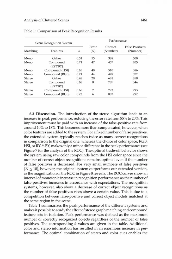
Table 1: Comparison of Peak Recognition Results.

PerformanceScene Recognition System

Error Correct False PositivesMatching Features θ (%) (Number) (Number)

Mono Gabor 0.51 55 388 500Mono Compound

(RYYBY)0.71 47 457 205

Mono Compound (HSI) 0.65 40 510 386Mono Compound (RGB) 0.71 44 478 372Stereo Gabor 0.48 20 681 850Stereo Compound

(RYYBY)0.68 8 787 544

Stereo Compound (HSI) 0.66 7 793 293Stereo Compound (RGB) 0.72 6 803 292

6.3 Discussion. The introduction of the stereo algorithm leads to anincrease in peak performance, reducing the error rate from 55% to 20%. Thisimprovement must be paid with an increase of the false-positive rate fromaround 10% to 18%. This becomes more than compensated, however, whencolor features are added to the system. For a fixed number of false positives,the extended system typically reaches twice as many correct recognitionsin comparison to the original one, whereas the choice of color space, RGB,HSI, or RY-Y-BY, makes only a minor difference in the peak performance (seeFigure 7 for the analysis of the ROC). The optimal trade-off behavior showsthe system using raw color compounds from the HSI color space since thenumber of correct object recognitions remains optimal even if the numberof false positives is decreased. For very small numbers of false positives(N ≤ 10), however, the original system outperforms our extended version,as the magnification of the ROC in Figure 8 reveals. The ROC curves show aninterval of monotonic increase in recognition performance as the number offalse positives increases in accordance with expectations. The recognitionsystems, however, also show a decrease of correct object recognitions asthe number of false positives rises above a certain value. This is due to acompetition between false-positive and correct object models matched atthe same region in the scene.

Table 1 summarizes the peak performance of the different systems andmakes it possible to study the effect of stereo graph matching and compoundfeature sets in isolation. Peak performance was defined as the maximumnumber of correctly recognized objects regardless of the number of falsepositives. The corresponding θ values are given in the table. Additionalcolor and stereo information has resulted in an enormous increase in per-formance. The optimal combination of stereo and color cues enables the


0 10 20 30 40 50 60 70 80 90 100number of false positives

0

100

200

300

400

500

600

700

800

num

ber

of c

orre

ct o

bjec

t rec

ogni

tions

0% 1% 2%false positive rate

0

10%

20%

30%

40%

50%

60%

70%

80%

90%

100%

corr

ect o

bjec

t rec

ogni

tions

(%

)

mono-greylevelstereo-greylevelmono-rc-hsimono-rc-rgbmono-rc-ryybystereo-rc-hsistereo-rc-rgbstereo-rc-ryyby

0.68

0.710.74

0.57

0.690.740.76

0.55

Figure 8: Comparison by ROC analysis (magnification of Figure 7). For morethan eight false positives (0.1% FPR), the stereo-based color compound sys-tems outperforms the original system. Interestingly, the stereo algorithm withintensity-based Gabor features shows worse performance than the original sys-tem until more than 54 false positives (1.2% FPR) are allowed.

system to reduce its error rate by almost a factor of 8. Interestingly, theuse of the stereo algorithm with color-blind features increases the numberof false positives significantly, but the combination of both extensions ac-tually reduces the number of false positives in comparison to the originalsystem dramatically. The best performance is achieved with color featuresrepresented in the HSI color space. As Figure 7 has shown, the differencebetween the different color compound features is small when looking at thepeak performance, but the stereo system based on HSI color compound fea-tures outperforms all other systems as it keeps the optimal balance betweenperformance and false-positive rate (FPR).

6.4 Efficiency. It takes roughly 30 seconds on a 1 GHz Pentium III with512 MB RAM to analyze a 2562 stereo image pair if 18 objects have beenenrolled. Transformation and feature extraction takes 2 seconds, and stereomatching takes 1 to 2 seconds per object. The time for the final scene analysisis negligible. Hence, most time is spent in the matching routines, whichscales linear with the number of objects n, O(n). A recognition system of21 objects working on image sizes of 1282 performs on the given hardware


in almost real time. Note that the research code is not optimized for speed.A system for face detection, tracking, and recognition based on the samemethod, Gabor wavelet preprocessing and graph matching, performs inreal time on similar image sizes (see Steffens, Elagin, & Neven, 1998).

7 Discussion

The system we have proposed is able to recognize and segment partiallyoccluded objects in cluttered scenes with complex backgrounds on the basisof known shape, color, and texture. The specific approach we presented hereis based on elastic graph matching, an object recognition architecture thatmodels views of objects as 2D constellations of image features representedas labeled graphs. The graph representation is particularly powerful forobject recognition under partial occlusions because it naturally allows usto explicitly model occlusions of object parts (Wiskott & von der Malsburg,1993). Contributions of this article have been the incorporation of richerobject descriptions in the form of compound feature sets (Triesch & Eckes,1998), the extension to graph matching in stereo image pairs (Triesch, 1999;Kefalea, 2001), and the introduction of a scene analysis algorithm utilizingthe disparity information provided in the stereo graph matching to dis-ambiguate occlusion relations. The combination of these innovations leadsto substantial performance improvements. At a more abstract level, it ap-pears that the major reason for the significant boost in performance is thecombined use of different modalities or cues: stereo, color, shape, texture,and occlusion. We are unaware of any other system that has attempted tointegrate such a wide range of cues for the purpose of object recognitionand scene analysis. The endeavor to integrate a wide range of cues maybe motivated through studies of the development of different modalitiesin infants, indicating that the human visual system tries to exploit everyavailable cue in order to recognize objects (Wilcox, 1999).

Note that stereo information is typically used as a low-level cue; thatis, information from left and right images is typically fused at a very earlyprocessing stage, while here we fuse the images only at the level of full (orpartial) object descriptions. This may not be very plausible from a biolog-ical perspective since fusion of information from the left and right eyes inmammalian vision systems seems to occur quite early. Nevertheless, theresults we obtained are promising.

Another point worth highlighting is our system’s ability to learn aboutnew objects in a one-shot fashion, which is quite valuable. Also, our system’sability to handle unknown backgrounds is worth mentioning. That is not tosay that the system could not be substantially improved by gathering andutilizing statistical information about objects and backgrounds from manytraining images. On the contrary, we would expect this to substantiallyimprove the system (e.g., Duc et al., 1999). A statistical well-founded systemfor object detection was presented in Viola and Jones (2001a, 2001b) in which


the type of features as well as the detection classifiers were learned frommany training examples. Its high efficiency and its well-founded learningarchitecture make it very attractive, although it is unclear how it can beextended to deal with occlusions. However, we view the good performanceobtained in our study despite the lack of such statistical descriptions asstrong testimony to the power of the chosen object representation.

We must admit that our system is shaped by a number of somewhatarbitrary choices concerning, for instance, the sequence of events, rela-tive weights in the creation of compound features, and the rather algo-rithmic nature of the system. It is our vision that the coordination ofprocesses that together constitute the analysis of a visual scene will even-tually be described as a dynamical system shaped by self-organization onboth the timescales of learning and brain state organization. The actualsequence of events may then depend on particular features of a givenscene.

In the following, we dicuss some related work. The number of articleson object recognition is vast, and the goal of this section is to discuss ourwork in the light of some specific example approaches. We restrict ourdiscussion to appearance-based object recognition approaches. There havebeen a number of models of object recognition in the primate visual sys-tem proposed in the literature. Examples are Fukushima, Miyake, and Ito(1983), Mel (1997), and Deco and Schurmann (2000) (see the overview inRiesenhuber & Poggio (2000)). However, none of these systems tries to ex-plicitly model partial occlusions. Some more closely related work has beenproposed in the computer vision literature.

7.1 Modeling Occlusions in Object Recognition. Of particular interestis the work by Perona’s group (Burl & Perona, 1996; Moreels, Maire, &Perona, 2004), which also describes objects as a 2D constellation of features.Their approach is cast in a probabilistic formulation. However, they restrictanalysis to the use of binary features—features that either are or are notpresent. Thus, their method must make “hard” decisions at the early levelof feature extraction, which is often problematic. A similar approach hasalso been proposed in Pope and Lowe (1996, 2000) and, more recently Lowe(2004). Such object recognition models rely on detecting stable key points onthe object surface from which robust features (e.g., extrema in scale-space)are extracted and compared to features stored in memory. The matchedfeatures vote for the most likely affine transformation on the basis of aHough transformation, thereby establishing the correspondences betweentraining image and the current input scene. The matching is fast and ableto detect highly occluded objects in some complicated scenes. To this end,either features are made so specific that detection of a small number of them,say three, is sufficient evidence for the presence of the object (Lowe), ormissing features are accounted for by simply specifying a prior probabilityof any feature missing (Perona). Thus, these systems do not explicitly try


to model occlusions due to recognized objects to explain away missingfeatures in partly occluded objects as our approach does.

7.2 Integrating Segmentation and Recognition. The analysis of com-plex cluttered scenes is one of the most challenging problems in computervision. Progress in this area has been comparatively slow, and we feel thata reason is that researchers have usually tried to decompose the problem inthe wrong way. A specific problem may have been a frequent insistence ontreating segmentation and recognition as separate problems, to be solvedsequentially. We believe that this approach is inherently problematic, andthis work is to be seen as a first step toward finding integrated solutions toboth problems. Similarly, other classic computer vision problems such asstereo, shape from shading, and optic flow have been studied mostly in iso-lation, despite their ill-posed nature. From this perspective, we feel that thegreatest progress may result from breaking with this tradition and buildingvision systems that try to find integrated solutions to several of these prob-lems. This is a challenging endeavor, but we feel that it is time to addressit. With respect to segmentation and recognition, there is striking evidencefor a very early combination of top-down and bottom-up processing inthe human visual system (see, e.g., the work of Peterson and colleagues:Peterson, Harvey, & Weidenbacher, 1991; Peterson & Gibson, 1994; Peterson,1999 or neurophysical studies such as Mumford (1991) or Lee, Mumford,Romero, and Lamme (1998)). In our current system, segmentation is purelymodel driven. But earlier work has also demonstrated the benefits of in-tegrating bottom-up and model-driven processing for segmentation andobject learning (Eckes & Vorbruggen, 1996; Eckes, 2006). In these studies,even partial object knowledge was able to disambiguate the otherwise no-toriously error-prone data-driven segmentation. Such an approach leads toa more robust object segmentation that adapts and refines the object modelin a stabilizing feedback loop.

An interesting alternative to that approach is work by Ullman and col-leagues (Borenstein, Sharon, & Ullman, 2004; Borenstein & Ullman, 2002,2004) in which bottom-up segmentation is combined with a learned objectrepresentation of a particular object class. The system is able to segmentother objects within this category from the background. Images of differ-ent horses were used to learn a “patch representation” of the object class“horse,” which is used to recognize subpatterns in horse images afterward.This top-down information becomes fused with a low-level segmentationby minimizing a cost function and improves the segmentation performance.In contrast to our work, the focus here is on improving segmentation basedon prior object knowledge, assuming the object has already been recog-nized. We believe that the close integration of bottom-up segmentationand recognition processes may also benefit recognition performance dueto the explaining away of occluded object parts and due to removal of un-wanted features likely not belonging to the object, which would otherwise


introduce noise into higher-level object representations based on large re-ceptive fields.

Another interesting segmentation architecture able to integrate low-leveland high-level segmentation was presented in Tu, Chen, Yuille, & Zhu(2003). Low-level segmentation based on Markov random field (MRF) mod-els based on intensity values is combined with high-level object modulesfor faces and text detection. An input image is parsed into low-level regions(based on brightness cues) and the object regions by a Metropolis-Hastingsdynamics that minimizes a cost function of a combined MRF model. Tuet al. trained prior models for facial and textural regions in the image withhelp of ADA boost from training examples. The output of the probabilisticmodel are combined with an MRF segmentation model. The additive priorsin the energy function of the MRF model favors step-wise homogeneous re-gions in gray-level intensity with smooth borders and not-too-small regionsizes. This system has a nice probabilistic formulation, but the data-drivenMarkov chain Monte Carlo method used for inference tends to be very slow.In addition, the system is unlikely to handle large occlusions because theobject recognizers for text and faces are not very robust to partial occlusions.

Combining recognition with attention (e.g., Itti & Koch, 2000) is alsoa mandatory extension to our system. The recognition process might fo-cus on areas with salient image features first, which significantly reducesthe rather sequential graph matching effort. These features may also helpto preselect or activate feature constellations in the model domain andmay bias the recognition system to start with only a promising subset ofknown objects. In general, combining low-level segmentation and attentionapproaches such as (Poggio, Gamble, & Little, 1988) with recognition ap-proaches is very promising and biologically highly relevant (see, e.g., Lee &Mumford, 2003). However, we believe that a more dynamical formulation ofthe matching process (e.g., in the style of the neocognitron; see Fukushima,2000), in combination with a recurrent and continously refined low-levelsegmentation, must be established. Such an integrated model may help usunderstand how the brain is solving the very difficult problem of visionand may also help us develop better machine vision.

Despite a number of drawbacks, our method and the methods discussedhere are promising examples of what integrated segmentation and objectrecognition systems might look like. There are still many open questions,and a biologically plausible dynamic formulation is desirable.

8 Conclusion

We have presented a system for the automatic analysis of cluttered scenesof partially occluded objects that obtained good results by integrating anumber of visual cues that are typically treated separately. The addition ofthese cues has increased the performance of the scene analysis considerablyby reducing the error rate by roughly a factor of 8. Only the combined use of


stereo and color cues was responsible for this unusual large improvementin performance. Our study of the different systems has shown that allproposed systems based on color and stereo cues outperform the monocularand color-blind recognition system over a large range of rejection settingswhen more than 20 false positives (0.4% false-positive rate) can be tolerated.

Future research should try to incorporate bottom-up segmentation mech-anisms and the learning of statistical object descriptions—ideally in an onlyweakly supervised fashion. A direct comparison of different scene analysisapproaches is still difficult at present because there is no standard databaseavailable. The FERET test in face recognition (Phillips, Moon, Rizvi, &Rauss, 2000) has demonstrated the benefits of independent databases andbenchmarks. We hope that the publication of our data set (Eckes & Triesch,2004) will help fill this gap and facilitate future work in this area.

Appendix: Color Space Transformations

Let us specify the type of color transformation we have used in this workby following Gonzales & Woods (1992), since there is often confusion aboutcolor spaces in both the research literature and in documents on ITU orISO/IEC standards. The transformation from RGB to RY-Y-BY color spaceis given by

RY

YBY

=

0.500 −0.419 −0.081

0.299 0.587 0.114−0.169 −0.331 0.500

R

GB

+

127

0127

. (A.1)

The transformation from RGB to HSI color space is given by

H = arccosR − B + R − G√

(R − G) + (R − B) (G − B)

S = 1 − 3max (R, G, B)

R + G + B

I = 13

(R + G + B). (A.2)

Acknowledgments

This work was in part supported by grant 0208451 from the National Sci-ence Foundation. We thank the developers of the FLAVOR software envi-ronment, which served as the platform for this research.


References

Belongie, S., Malik, J., & Puzicha, J. (2002). Shape matching and object recognitionusing shape contexts. IEEE Trans. PAMI, 24(4), 509–522.

Borenstein, E., Sharon, E., & Ullman, S. (2004). Combining top-down and bottom-upsegmentations. In IEEE Workshop on Perceptual Organization in Computer Vision.Washington, DC.

Borenstein, E., & Ullman, S. (2002). Class-specific, top-down segmentation. In ECCV-2002, 7th European Conference on Computer Vision (pp. 109–122). Berlin: Springer.

Borenstein, E., & Ullman, S. (2004). Learning to segment. In The 8th European Confer-ence on Computer Vision—ECCV 2004, Prague. Berlin: Springer-Verlag.

Buhmann, J., Lades, M., & von der Malsburg, C. (1990). Size and distortion invariantobject recognition by hierarchical graph matching. In IJCNN International Confer-ence on Neural Networks (pp. 411–416). San Diego, CA: IEEE.

Burl, M., & Perona, P. (1996). Recognition of planar object classes. In 1996 Conference onComputer Vision and Pattern Recognition. Piscataway, NJ: IEEE Computer Society.

Deco, G., & Schurmann, B. (2000). A hierarchical neural system with attentionaltop-down enhancement of the spatial resolution for object recognition. VisionResearch, 40(20), 2845–2859.

Duc, B., Fischer, S., & Bigun, J. (1999). Face authentication with Gabor informationon deformable graphs. IEEE Transactions on Image Processing, 8(4), 504–516.

Duda, R. O., & Hart, P. E. (1973). Pattern classification and scene analysis. New York:Wiley.

Eckes, C. (2006). Fusion of visual cues for segmentation and object recognition. In prepa-ration.

Eckes, C., & Triesch, J. (2004). Stereo cluttered scenes image database (SCS–IDB). Available online at http://greece.imk.fraunhofer.de/publications/data/SCS/SCS.zip.

Eckes, C., & Vorbruggen, J. C. (1996). Combining data-driven and model-based cuesfor segmentation of video sequences. In World Conference on Neural Networks(pp. 868–875). Mahwah, NJ: INNS Press and Erlbaum.

Edelman, S. (1995). Representation of similarity in three-dimensional object discrim-ination. Neural Computation, 7, 408–423.

Edelman, S. (1998). Representation is representation of similarities (Tech. Rep. No. CS96-08, 1996). Jerusalem: Weizmann Science Press.

Fischler, M. A., & Elschlager, R. A. (1973). The representation and matching of pic-torial structures. IEEE Trans. Computers, 22(1), 67–92.

Fleuret, F., & Geman, D. (2001). Coarse-to-fine face detection. International Journal ofComputer Vision, 41(1/2), 85–107.

Forsyth, D. A., & Ponce, J. (2002). Computer vision: A modern approach. Upper SaddleRiver, NJ: Prentice Hall.

Fukushima, K. (2000). Active and adaptive vision: Neural network models. InS.-W. Lee, H. H. Bulthoff, & T. Poggio (Eds.), Biologically motivated computer vision.Berlin: Springer.

Fukushima, K., Miyake, S., & Ito, T. (1983). Neocognitron: A neural network modelfor a mechanism of visual pattern recognition. IEEE Trans. Systems, Man, andCybernetics, SMC–13(5), 826–834.


Gonzales, R. C., & Woods, R. E. (Eds.). (1992). Digital image processing. Reading, MA:Addison-Wesley.

Harwerth, R., Moeller, M., & Wensveen, J. (1998). Effects of cue context on theperception of depth from combined disparity and perspective cues. Optometryand Vision Science, 75(6), 433–444.

Itti, L., & Koch, C. (2000). A saliency-based search mechanism for overt and covertshifts of visual attention. Vision Research, 40(12), 1489–1506.

Jones, J. P., & Palmer, L. A. (1987). An evaluation of the two-dimensional Gaborfilter model of simple receptive fields in cat striate cortex. J. Neurophysiol., 56(6),1233–1258.

Kefalea, E. (2001). Flexible object recognition for a grasping robot. Unpublished doctoraldissertation, Universitat Bonn.

Lades, M., Vorbruggen, J. C., Buhmann, J., Lange, J., von der Malsburg, C., Wurtz,R. P., & Konen, W. (1993). Distortion invariant object recognition in the dynamiclink architecture. IEEE Trans. Computers, 42, 300–311.

Lee, T. S., & Mumford, D. (2003). Hierarchical Bayesian inference in the visual cortex.Journal of Optical Society of America A, 20(7), 1434–1448.

Lee, T. S., Mumford, D., Romero, R., & Lamme, V. A. (1998). The role of the primaryvisual cortex in higher level vision. Vision Research, 38(15/16), 2429–2454.

Lowe, D. G. (2004). Distinctive image features from scale-invariant keypoints. Inter-national Journal of Computer Vision, 60(2), 91–110.

Mel, B. W. (1997). SEEMORE: Combining color, shape, and texture. Neural Computa-tion, 9(4), 777–804.

Messmer, B. T., & Bunke, H. (1998). A new algorithm for error-tolerent subgraph iso-morphism detection. IEEE Transactions on Pattern Analysis and Machine Learning,20(5), 493–504.

Moreels, P., Maire, M., & Perona, P. (2004). Recognition by probabilistic hypothesisconstruction. In Eighth European Conference on Computer Vision. Berlin: Springer.

Mumford, D. (1991). On the computational architecture of the neocortex. I. The roleof the thalamo-cortical loop. Biological Cybernetics, 65(2), 135–145.

Murase, H., & Nayar, S. K. (1995). Visual learning and recognition of 3-D objectsfrom appearance. Int. J. of Computer Vision, 14(2), 5–24.

Nelson, R. C., & Selinger, A. (1998). Large-scale tests of a keyed, appearance-based3-D object recognition system. Vision Research, 38(15–16), 2469–2488.

Peterson, M. (1999). Knowledge and intention can penetrate early vision. Behavioraland Brain Sciences, 22(3), 389.

Peterson, M. A., & Gibson, B. S. (1994). Must figure ground organization pre-cede object recognition? An assumption in peril. Psychological Science, 7(5), 253–259.

Peterson, M. A., Harvey, E. M., & Weidenbacher, H. J. (1991). Shape recognitioncontributes to figure-ground reversal: Which route counts? Journal of ExperimentalPsychology: Human Perception and Performance, 17(4), 1075–1089.

Phillips, P., Moon, H., Rizvi, S., & Rauss, P. (2000). The FERET evaluation method-ology for face-recognition algorithms. IEEE Transactions on Pattern Analysis andMachine Intelligence, 22(10), 1090–1104.

Poggio, T., Gamble, E., & Little, J. (1988). Parallel integration of vision modules.Science, 242, 436–440.


Pope, A. R., & Lowe, D. G. (1996). Learning appearance models for object recognition.In J. Ponce, A. Zisserman, & Hebert (Eds.), Object representation in computer visionII (pp. 201–219). Berlin: Springer.

Pope, A. R., & Lowe, D. G. (2000). Probabilistic models of appearance for 3-D objectrecognition. International Journal of Computer Vision, 40(2), 149–167.

Pratt, W. K. (2001). Digital image processing. New York: Wiley.Ren, X., & Malik, J. (2002). A probabilistic multi-scale model for contour completion

based on image statistics. In Proceedings of the Seventh European Conference onComputer Vision (pp. 312–327). Berlin: Springer.

Riesenhuber, M., & Poggio, T. (2000). Models of object recognition. Nature of Neuro-science, 3(Supp.), 1199–1204.

Rosenfeld, A. (1984). Image analysis: Problems, progress, and prospects. PatternRecognition, 17, 3–12.

Rowley, H., Baluja, S., & Kanade, T. (1998). Neural network–based face detec-tion. IEEE Transactions on Pattern Analysis and Machine Intelligence, 20(1), 23–38.

Shams, L., & von der Malsburg, C. (2002). The role of complex cells in object recog-nition. Vision Research, 42, 2547–2554.

Steffens, J., Elagin, E., & Neven, H. (1998). Personspotter—fast and robust system forhuman detection, tracking and recognition. In Proceedings of the Third InternationalConference on Face and Gesture Recognition (pp. 516–521). Piscataway, NJ: IEEEComputer Society.

Swain, M., & Ballard, D. H. (1991). Color indexing. Int. J. of Computer Vision, 7(1),11–32.

Tarr, M., & Bulthoff, H. (1998). Image-based object recognition in man, monkey andmachine. Cognition, 67(1–2), 1–20.

Triesch, J. (1999). Vision-based robotic gesture Recognition. Aachen, Germany: ShakerVerlag.

Triesch, J., & Eckes, C. (1998). Object recognition with multiple feature types. In L.Niklasson, M. Boden, & T. Ziemke (Eds.), Proceedings ICANN 98 (pp. 233–238).Berlin: Springer.

Triesch, J., & Eckes, C. (2004). Object recognition with deformable feature graphs:Faces, hands, and cluttered scenes. In C. H. Chen (Ed.), Handbook of pattern recog-nition and computer vision. Singapore: World Scientific.

Triesch, J., & von der Malsburg, C. (2001). A system for person-independent handposture recognition against complex backgrounds. IEEE Trans. PAMI, 23(12),1449–1453.

Triesch, J., & von der Malsburg, C. (2002). Classification of hand postures againstcomplex backgrounds using elastic graph matching. Image and Vision Computing,20(13–14), 937–943.

Tu, Z., Chen, X., Yuille, A., & Zhu, S. (2003). Image parsing: Unifying segmentation,detection, and recognition. In Proceedings of the Ninth IEEE International Conferenceon Computer Vision. Piscataway, NJ: IEEE Computer Society.

Turk, M., & Pentland, A. (1991). Eigenfaces for recognition. Journal of Cognitive Neu-roscience, 3(1), 71–86.

Ullman, S. (1998). Three-dimensional object recognition based on the combinationof views. Cognition, 67(1–2), 21–44.


Viola, P., & Jones, M. J. (2001a). Rapid object detection using a boosted cascade ofsimple features. In Proceedings of the 2001 IEEE Computer Society Conference onComputer Vision and Pattern Recognition. Piscataway, NJ: IEEE Computer Society.

Viola, P., & Jones, M. J. (2001b). Robust real-time object detection (Tech. Rep. CRL2001/01). Cambridge, MA: Cambridge Research Laboratory.

Wilcox, T. (1999). Object individuation: Infants’ use of shape, size, pattern, and color.Infant Behavior and Development, 72(2), 125–166.

Wiskott, L., Fellous, J., Kruger, N., & von der Malsburg, C. (1997). Face recognition byelastic bunch graph matching. IEEE Transactions on Pattern Analysis and MachineIntelligence, 19(7), 775–779.

Wiskott, L., & von der Malsburg, C. (1993). A neural system for the recognition ofpartially occluded objects in cluttered scenes: A pilot study. International Journalof Pattern Recognition and Artificial Intelligence, 7(4), 935–948.

Yuille, A. L. (1991). Deformable templates for face recognition. Journal of CognitiveNeuroscience, 3(1), 59–70.

Received July 20, 2004; accepted August 10, 2005.

analysis of cluttered scenes using an elastic matching approach for stereo images

Documents