WORKING PAPER SERIES

Universidade dos Açores Universidade da Madeira

CEEAplA WP No. 03/2009 Analysing the Impacts of Closure of a Military Base Using a Dynamic CGE Model Ali Bayar Cristina Mohora Mário Fortuna Sameer Rege Suat Sisik March 2009

Analysing the Impacts of Closure of a Military Base Using a Dynamic CGE Model

Ali Bayar Universite Libre de Bruxelles

Departement D’Economie Appliquee EcoMod

Cristina Mohora

Universite Libre de Bruxelles Departement D’Economie Appliquee

EcoMod

Mário Fortuna Universidade dos Açores (DEG)

e CEEAplA

Sameer Rege Universidade dos Açores (DEG)

e CEEAplA

Suat Sisik Universite Libre de Bruxelles

Departement D’Economie Appliquee EcoMod

Working Paper n.º 03/2009 Março de 2009

CEEAplA Working Paper n.º 03/2009 Março de 2009

RESUMO/ABSTRACT

Analysing the Impacts of Closure of a Military Base Using a Dynamic CGE

Model

Military bases are commonplace in many countries and may have a significant impact in the communities where they are integrated. Impacts of military bases have been analysed through different perspectives. Our aim is to analyse their economic impact. The importance of military bases has become a topic of discussion particularly when base closures or base activity reductions are under consideration. In a previous paper the authors looked at the issue using a static CGE model applied to the analysis of the economic impact of a US base located in the island of Terceira in the Azores. In the current paper a dynamic model is used to study the same issue, using more recent data and disaggregating the impact among different household categories. A base closure scenario is created and the impacts traced through various economic indicators. It is concluded that GDP falls, relative to the base scenario for a number of years recovering after some time, assuming that worsened trade balances are compensated by other transfers. This fall is prompted by a fall in employment, personal income and consumption. The model also predicts that the impact hurts different household income groups with diverse intensity. Lower income households are hurt more in relative terms but generate a smaller absolute impact. With time, the negative impact tapers off for most income groups except for the lowest which keeps on loosing more until the end of the simulation period. Ali Bayar Universite Libre de Bruxelles Departement D’Economie Appliquee Avenue Paul Heger 2 B-1000 Bruxelles Cristina Mohora Universite Libre de Bruxelles Departement D’Economie Appliquee Avenue Paul Heger 2 B-1000 Bruxelles Mário Fortuna Departamento de Economia e Gestão Universidade dos Açores Rua da Mãe de Deus, 58 9501-801 Ponta Delgada

Sameer Rege Departamento de Economia e Gestão Universidade dos Açores Rua da Mãe de Deus, 58 9501-801 Ponta Delgada Suat Sisik Universite Libre de Bruxelles Departement D’Economie Appliquee Avenue Paul Heger 2 B-1000 Bruxelles

ANALYSING THE IMPACTS OF CLOSURE OF A MILITARY BASE USING A

DYNAMIC CGE MODEL

Ali Bayar** Cristina Mohora**

Mário Fortuna* Sameer Rege* Suat Sisik**

Abstract Military bases are commonplace in many countries and may have a significant impact in the communities where they are integrated. Impacts of military bases have been analysed through different perspectives. Our aim is to analyse their economic impact. The importance of military bases has become a topic of discussion particularly when base closures or base activity reductions are under consideration. In a previous paper the authors looked at the issue using a static CGE model applied to the analysis of the economic impact of a US base located in the island of Terceira in the Azores. In the current paper a dynamic model is used to study the same issue, using more recent data and disaggregating the impact among different household categories. A base closure scenario is created and the impacts traced through various economic indicators. It is concluded that GDP falls, relative to the base scenario for a number of years recovering after some time, assuming that worsened trade balances are compensated by other transfers. This fall is prompted by a fall in employment, personal income and consumption. The model also predicts that the impact hurts different household income groups with diverse intensity. Lower income households are hurt more in relative terms but generate a smaller absolute impact. With time, the negative impact tapers off for most income groups except for the lowest which keeps on loosing more until the end of the simulation period.

* CEEAplA, University of the Azores ** ECOMOD, ULB

2

1. Introduction

Military bases are commonplace in many countries and may have a significant impact

in the communities where they are integrated. Impacts of military bases have been

analysed through different perspectives. Our aim is to analyse their economic impact.

The importance of military bases has become a topic of discussion particularly when

base closures or base activity reductions are under consideration. In a previous ,

Bayar, et al (2007) looked at the issue using a static CGE model applied to the

analysis of the economic impact of a US base located in the island of Terceira in the

Azores.

The model used was a standard static CGE model calibrated using a SAM constructed

with 1998 data, with sixteen sectors. Based on that data it was found that closure of

the base would represent a fall of 0,89% of GDP, a fall in equivalent variation of 27,9

million euros and a fall in employment of about 1,2% of an active population of

around 100 thousand.

In the current paper a dynamic model is used to study the same issue, using more

recent data (2001) and disaggregating the impact among different household

categories, different government levels and different trade blocks.

Discussions over the importance and the impact of the base for the local economy are

recurrent in an attempt, on the part of the participants, to advance arguments in favour

or against its presence. The current paper tries to contribute with a quantification of

the economic impact of the base using a dynamic CGE model of the Azorean

economy.

A closure scenario is created and the impacts traced through various economic

indicators including some household detail.

Hoffmann, et al (1996) analyze the impact of defense cuts on the economy in

California using a computable general equilibrium (CGE) model. Their focus is on the

migration of factors from California to other states and the impact of this migration on

the economy. CGE models are better suited to analyze the economy wide impact of

these defense cuts and their study shows that the impacts are highly sensitive to the

assumption of inter-state mobility.

Other studies have taken a less elaborate approach looking mostly at lost direct

expenditures and jobs on an accounting approach and looking other social and

environmental impacts.

3

In what follows section 2 presents the main variables that characterize the impact of

the base on the local economy. Section 3 reviews the main characteristics of a

dynamic CGE model of the Azores. Section 4 reviews the results of calibration of the

model and the results of the closure scenario developed. Section 5 presents some of

the main conclusions that can be drawn from application of the model.

2. The Military Base in Terceira/Azores The base in Terceira/Azores houses both US and Portuguese military activities. It

comprises an airport adequate for landing any known type of aircraft, fuel storage

tanks and port facilities. This base has been extensively used in various international

conflicts, namely those that have occurred in the last half century and in the Middle

East during recent times.

The impact of the American component of the base can be simulated by the model

using data on the main variables. In the simulation undertaken here the relevant data

collected characterizes expenditures on construction works and repair, employment

and private consumption by the US military, servicemen and civilians.

Access of locals to purchases in the base’s stores can also be taken into consideration.

It is common for some locals to make their purchases in the base stores at prices that

are lower than those practiced in the local stores, for a wider variety of products.

There are no good estimates for the total value of the purchases made in these stores,

which is equivalent to purchasing the goods abroad. Given that there are no good

estimates of the values involved, two scenarios will be created to test the impact of

these “imports”: one where the import effect is zero, the reference scenario and one in

which 50% of the income is spent on these “foreign” stores.

The main elements of the data on the activity of the US military are summarized in

tables 1 and 2. Table 1 provides an estimate of the value (in US Dollars) of the

construction works and repair commissioned by the Lajes Field Base for 2004 and for

2005.

4

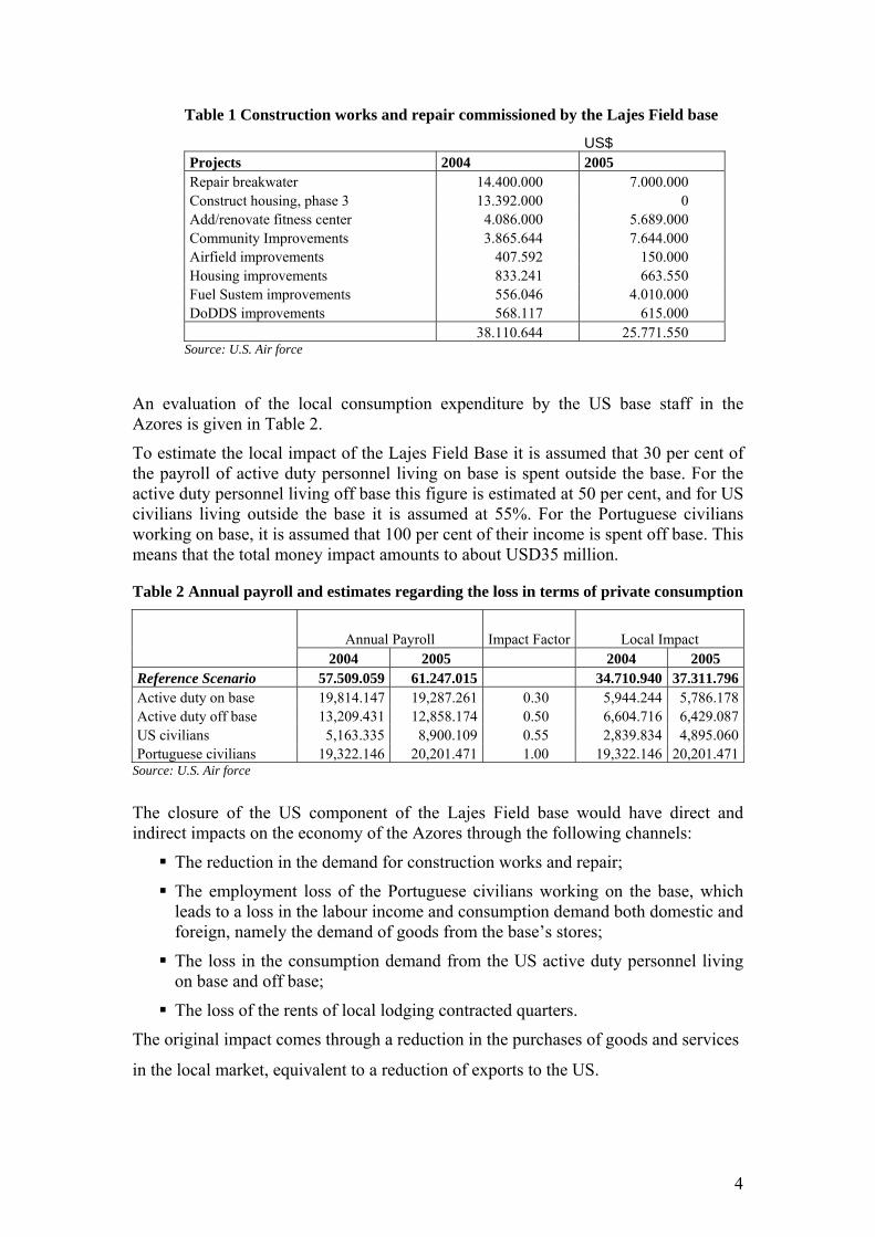
Table 1 Construction works and repair commissioned by the Lajes Field base

US$ Projects 2004 2005 Repair breakwater 14.400.000 7.000.000 Construct housing, phase 3 13.392.000 0 Add/renovate fitness center 4.086.000 5.689.000 Community Improvements 3.865.644 7.644.000 Airfield improvements 407.592 150.000 Housing improvements 833.241 663.550 Fuel Sustem improvements 556.046 4.010.000 DoDDS improvements 568.117 615.000 38.110.644 25.771.550

Source: U.S. Air force

An evaluation of the local consumption expenditure by the US base staff in the Azores is given in Table 2.

To estimate the local impact of the Lajes Field Base it is assumed that 30 per cent of the payroll of active duty personnel living on base is spent outside the base. For the active duty personnel living off base this figure is estimated at 50 per cent, and for US civilians living outside the base it is assumed at 55%. For the Portuguese civilians working on base, it is assumed that 100 per cent of their income is spent off base. This means that the total money impact amounts to about USD35 million.

Table 2 Annual payroll and estimates regarding the loss in terms of private consumption

Annual Payroll Impact Factor Local Impact 2004 2005 2004 2005 Reference Scenario 57.509.059 61.247.015 34.710.940 37.311.796Active duty on base 19,814.147 19,287.261 0.30 5,944.244 5,786.178Active duty off base 13,209.431 12,858.174 0.50 6,604.716 6,429.087US civilians 5,163.335 8,900.109 0.55 2,839.834 4,895.060Portuguese civilians 19,322.146 20,201.471 1.00 19,322.146 20,201.471

Source: U.S. Air force

The closure of the US component of the Lajes Field base would have direct and indirect impacts on the economy of the Azores through the following channels:

The reduction in the demand for construction works and repair;

The employment loss of the Portuguese civilians working on the base, which leads to a loss in the labour income and consumption demand both domestic and foreign, namely the demand of goods from the base’s stores;

The loss in the consumption demand from the US active duty personnel living on base and off base;

The loss of the rents of local lodging contracted quarters.

The original impact comes through a reduction in the purchases of goods and services

in the local market, equivalent to a reduction of exports to the US.

5

3. The Model

The current version of the modelling platform of the Azores economy was first

presented in Bayar, et. al (2007b). For this reason, only the main characteristics of the

model will be presented here. All derived equations of the model are presented in the

annex to the current paper as are lists of relevant variables and parameters.

It is a dynamic multi-sectoral computable general equilibrium model (CGE), which

incorporates the economic behaviour of six economic agents: firms, households,

regional government, Mainland government, European Commission and the external

sector.

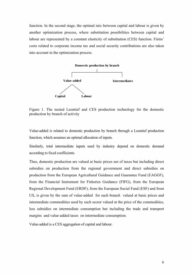
The goods-producing sectors, consisting of both public and private enterprises, are

disaggregated into 45 branches of activity. Households are divided into six income

groups, to analyze the distributional effects of various policy measures. Special

attention is paid to the economic links between the regional government, the

Mainland government and the European Commission. With regard to the rest of the

world the economy is treated as a small open economy with no influence on (given)

world market prices. Trade relations are differentiated according to four main trade

partners: Mainland, EU, US and the rest of the world. The behaviour of each agent in

the model is described in detail below.

The model has been solved by using the general algebraic modelling system GAMS

(Rosenthal, 2006).

3. Firms

Producers are assumed to operate in 45 perfectly competitive markets, corresponding

to an equal number of branches as listed in Table 1, and maximize profits (or

minimize costs for each level of output) to determine the optimal levels of inputs and

output. Furthermore, production prices equal average and marginal costs, a condition

implied by profit maximization for constant returns to scale technology.

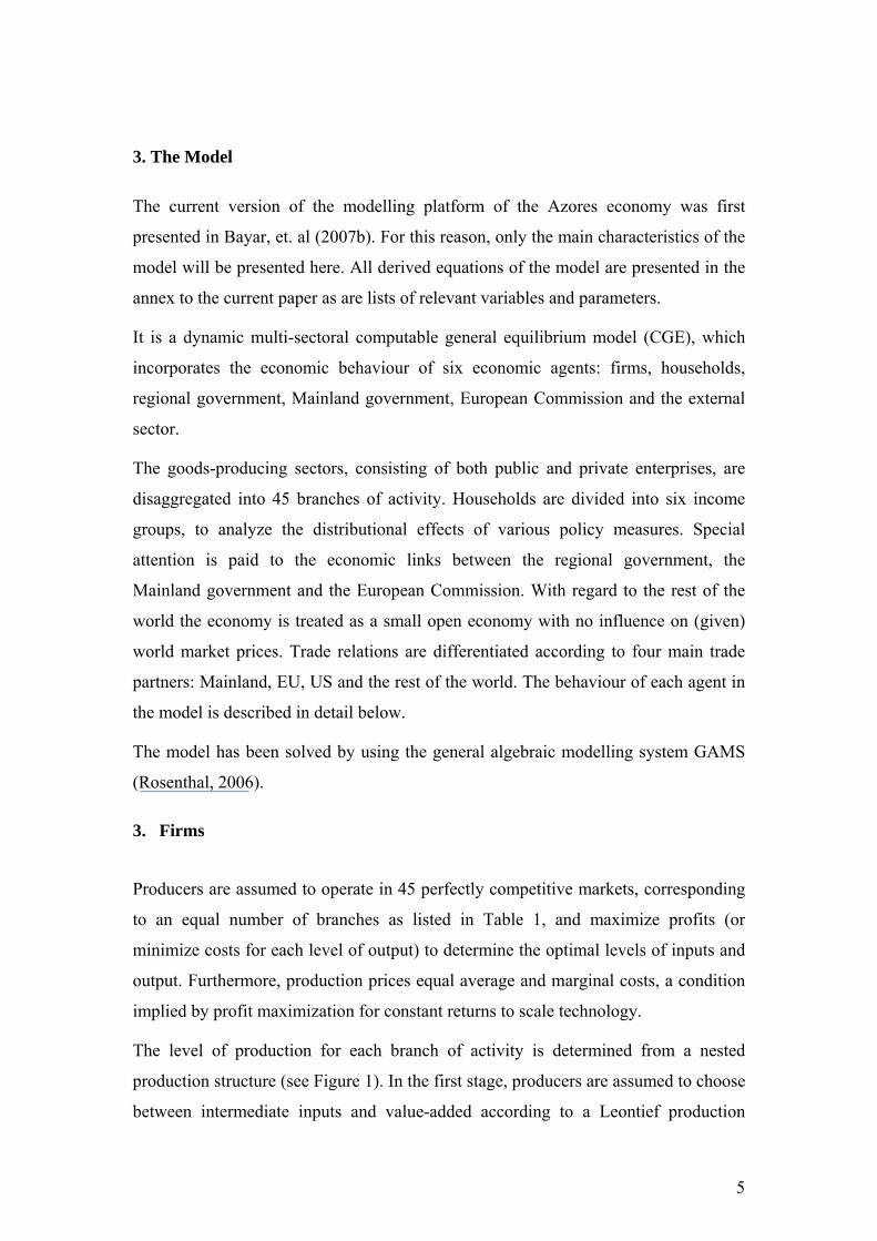
The level of production for each branch of activity is determined from a nested

production structure (see Figure 1). In the first stage, producers are assumed to choose

between intermediate inputs and value-added according to a Leontief production

6

function. In the second stage, the optimal mix between capital and labour is given by

another optimization process, where substitution possibilities between capital and

labour are represented by a constant elasticity of substitution (CES) function. Firms’

costs related to corporate income tax and social security contributions are also taken

into account in the optimization process.

Figure 1. The nested Leontief and CES production technology for the domestic production by branch of activity

Value-added is related to domestic production by branch through a Leontief production

function, which assumes an optimal allocation of inputs.

Similarly, total intermediate inputs used by industry depend on domestic demand

according to fixed coefficients.

Thus, domestic production are valued at basic prices net of taxes but including direct

subsidies on production from the regional government and direct subsidies on

production from the European Agricultural Guidance and Guarantee Fund (EAGGF),

from the Financial Instrument for Fisheries Guidance (FIFG), from the European

Regional Development Fund (ERDF), from the European Social Fund (ESF) and from

US, is given by the sum of value-added for each branch valued at basic prices and

intermediate commodities used by each sector valued at the price of the commodities,

less subsidies on intermediate consumption but including the trade and transport

margins and value-added taxes on intermediate consumption.

Value-added is a CES aggregation of capital and labour.

Domestic production by branch

Value-added Intermediates

Capital Labour

7

Table 1: Activity and commodity desegregation in AzorMod

8

1 Agriculture, hunting and forestry, logging2 Fishing3 Mining and quarrying4 Production of meat and meat products5 Processing of fish and fish products6 Manufacture of dairy products7 Prepared animal feeds8 Beverages & tobacco products9 Fruits, vegetables, animal oils, grain mill, starches10 Textiles and leather11 Wood and products of wood and cork12 Pulp, paper products; publishing and printing13 Coke, refined petroleum products and nuclear fuel14 Chemicals and chemical products15 Rubber and plastic products16 Other non-metallic mineral products17 Basic metals and fabricated metal products18 Machinery and equipment n.e.c.19 Electrical and optical equipment20 Transport equipment21 Manufacturing n.e.c.22 Electricity, gas, steam and hot water supply23 Collection, purification and distribution of water24 Construction25 Sale, maintenance, repair of motor vehicles and motorcycles26 Wholesale trade and commission trade, except of motor vehicles and

motorcycles27 Retail trade, except of motor vehicles and motorcycles28 Hotels and restaurants29 Land transport; transport via pipelines30 Water transport31 Air transport32 Supporting transport activities; activities of travel agencies33 Post and telecommunications34 Financial intermediation, excluding insurance and pension funding35 Insurance and pension funding, except compulsory social security36 Activities auxiliary to financial intermediation37 Real estate activities38 Renting of machinery and equipment without operator39 Computer and related activities; research and development40 Other business activities41 Public administration and defence; compulsory social security42 Education43 Health and social work44 Other community, social and personal service activities45 Activities of households as employers of domestic staff

9

Capital is industry specific, introducing rigidities in the capital market. The inter-sectoral

wage differential is a parameter derived as the ratio between the wage by branch and the

national average wage (Dervis, De Melo and Robinson, 1982). Holding the inter-sectoral

wage differentials constant in counterfactual policy simulations introduces rigidities in the

labour market.

Each branch of activity in AzorMod produces several types of goods and services. The

optimal allocation of domestic production between the different types of commodities is

given by a Leontief function.

4. Households

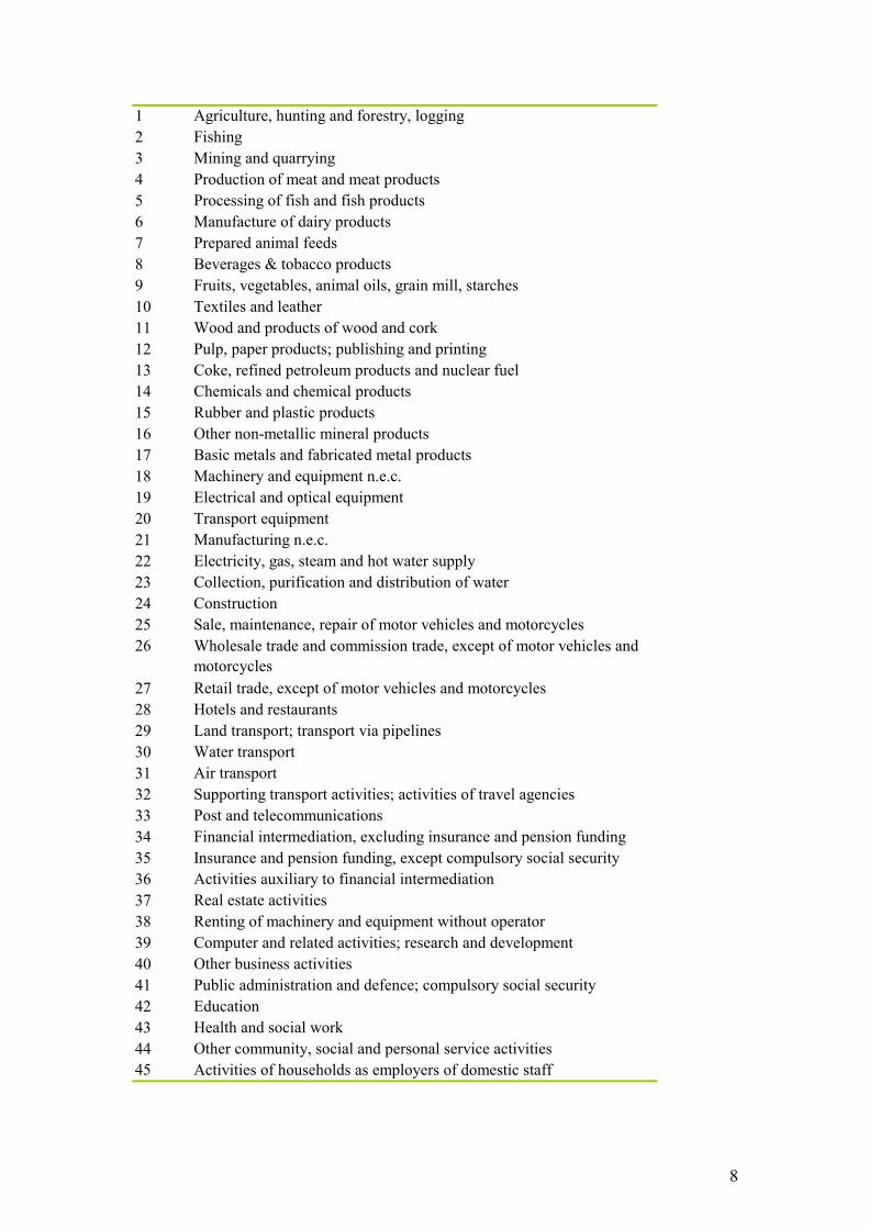
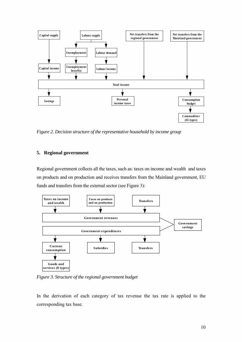
Households are split into six income groups, the first group being the poorest one. The

representative household in each income group receives a part of the capital income (net

operating surplus), a part of the labour income, unemployment benefits from the Mainland

government and other net transfers from the regional and Mainland governments. The

representative household in each income group pays income taxes and saves a share of the

net income.

Household propensity to save reacts to changes in the after-tax average return to capital.

The disposable budget for consumption is allocated between different goods and services

according to a Stone-Geary utility function.

In the allocation process, the consumer first decides on the minimum (subsistence) level of

consumption of commodity. Then, the marginal income is allocated between different

types of commodities according to the marginal budget shares. A schematic representation

of households’ decisions, by income group, is given in Figure 2.

Household welfare gains/losses are valued using the equivalent variation in income, which

is based on the concept of a money metric indirect utility function (Varian, 1992).

Equivalent variation measures the income needed to make the household as well off as she

is in the new counter-factual equilibrium (policy scenario) evaluated at benchmark prices.

Thus, the equivalent variation is positive for welfare gains from the policy scenario and

negative for losses.

10

Capital supply Labour supply

Unemployment Labour demand

Unemploymentbenefits Labour incomeCapital income

Total income

Savings Personalincome taxes

Consumptionbudget

Net transfers from theregional government

Net transfers from theMainland government

Commodities(45 types)

Figure 2. Decision structure of the representative household by income group

5. Regional government

Regional government collects all the taxes, such as: taxes on income and wealth and taxes

on products and on production and receives transfers from the Mainland government, EU

funds and transfers from the external sector (see Figure 3):

Figure 3. Structure of the regional government budget

In the derivation of each category of tax revenue the tax rate is applied to the

corresponding tax base.

Government revenues

Currentconsumption Subsidies Transfers

Government expenditures

Governmentsavings

Goods andservices (8 types)

Taxes on incomeand wealth

Taxes on productsand on production Transfers

11

Taxes on products are differentiated in the model according to the category of

consumption on which they apply: intermediate consumption, private consumption, and

gross capital formation.

The total transfers received by the regional government are given by transfers from

the Mainland government, transfers from EU as direct subsidies on production and

other transfers from EU, transfers from US and transfers from the rest of the world.

Regional government expenditures comprise the public current consumption, total

transfers by the government and subsidies on products and on production.

The optimal allocation of the public current consumption between different types of goods

and services is given by the maximization of a Cobb-Douglas function, subject to the

budget constraint.

The maximization of the utility function yields the demand equations for public current

consumption by type of commodity.

Total transfers by the regional government include transfers to the households.

The difference between the regional government revenues and the government

expenditures yields the government savings, which are set to zero in all cases to reflect the

fact that the regional government is not allowed to incur new debt.

6. Mainland government

Mainland government collects all the social security contributions, provides

unemployment benefits and makes transfers to the households and to the regional

government.

Social security contributions are derived by applying the social contributions rate to

gross wages. Unemployment benefits received by each household income group are

determined by the combination of the replacement rate, the national average wage, the

total number of unemployed, and the share of unemployed subject to unemployment

benefits in each household income group.

7. European Commission

European Commission provides EU funds as direct subsidies to the production sectors

and other EU funds to the regional government.

12

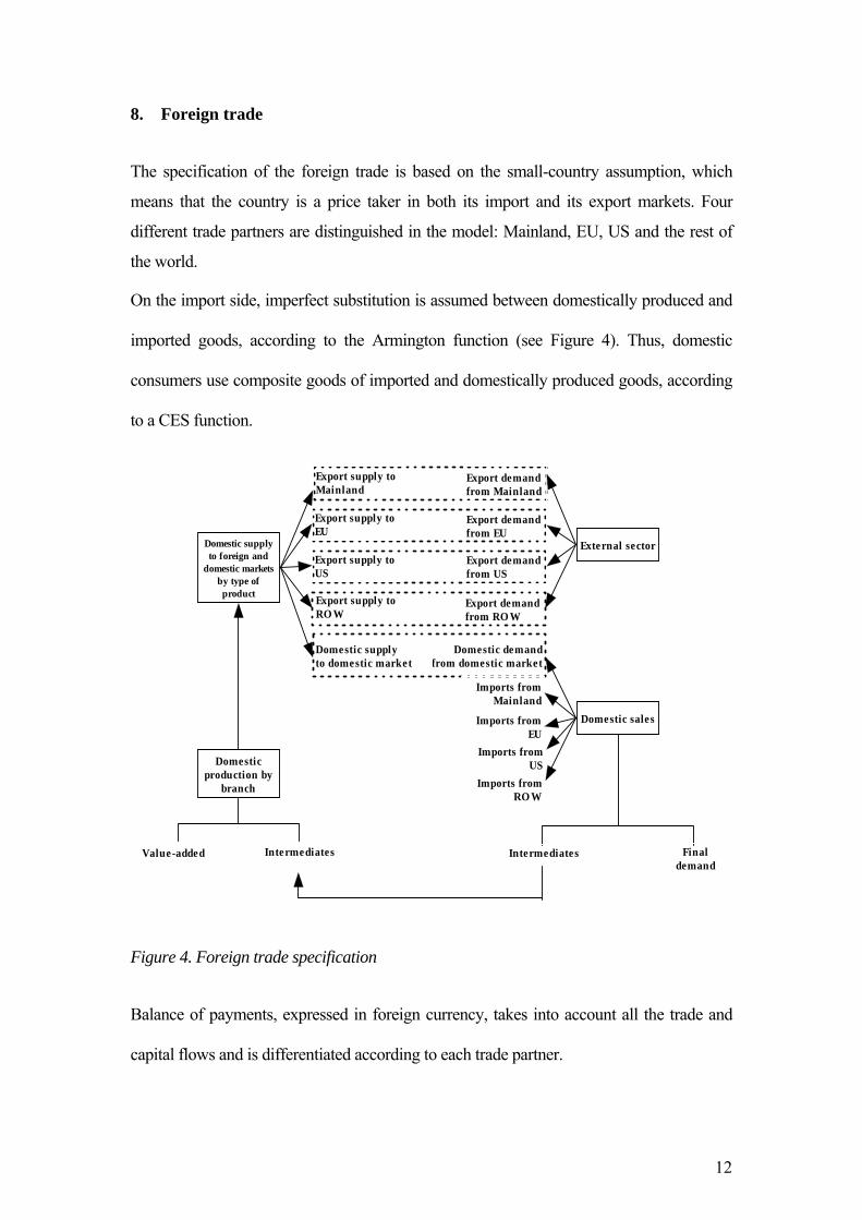
8. Foreign trade

The specification of the foreign trade is based on the small-country assumption, which

means that the country is a price taker in both its import and its export markets. Four

different trade partners are distinguished in the model: Mainland, EU, US and the rest of

the world.

On the import side, imperfect substitution is assumed between domestically produced and

imported goods, according to the Armington function (see Figure 4). Thus, domestic

consumers use composite goods of imported and domestically produced goods, according

to a CES function.

Figure 4. Foreign trade specification

Balance of payments, expressed in foreign currency, takes into account all the trade and

capital flows and is differentiated according to each trade partner.

Domestic supplyto foreign and

domestic marketsby type ofproduct

Domestic sales

Imports fromUS

Domestic demandfrom domestic market

Export supply toRO W

Value-added Intermediates Intermediates

Domestic supplyto domestic market

Finaldemand

Domesticproduction by

branch

Export demandfrom RO W

External sectorExport supply toUS

Export demandfrom US

Export supply toEU

Export demandfrom EU

Export supply toMainland

Export demandfrom Mainland

Imports fromMainland

Imports fromEU

Imports fromRO W

13

9. Investment demand

Total savings, used to buy investment goods, are given by the sum of savings from the

different agents and the trade partners.

Total investments in real terms are given by the difference between savings and

inventories.

The optimal allocation of total investments between different types of investment

commodities is given by the Leontief function.

The composite price (unit cost) of investments is defined as the weighted average of the

price of investment goods.

10. Price equations

A common assumption for CGE models, which has also been adopted here, is that the

economy is initially in equilibrium with the quantities normalized in such a way that prices

of commodities equal unity. Due to the homogeneity of degree zero in prices, the model

only determines the relative prices. Therefore, a particular price is selected to provide the

numeraire against which all relative prices in the model will be measured. We choose the

GDP deflator as the numeraire.

Different prices are defined for all the branches, exports and imports. As already

explained, trade and transport margins are paid on all categories of demand in AzorMod

except the government consumption (on intermediate consumption, on private

consumption and on investment goods).

The domestic price of imports from Mainland is determined by the price of imports from

Mainland expressed in foreign currency and the exchange rate.

Similarly, the domestic price of imports from EU is given by the price of imports from EU

expressed in foreign currency and the corresponding exchange rate.

The domestic price of imports from US and from ROW, further include the tariff rate on

each commodity for imports from US and the tariff rate on imports from ROW.

14

The consumer price index ( PCINDEX ) used in the model is defined as:

c ctm,c,qu ctm c,qu c,qu c,qu c,quc,qu ctm

c ctm,c,qu ctm c,qu c,qu c,qu c,quc,qu ctm

PCINDEX = {[P + tchtm P ] (1+texc ) (1+tc +vatc ) CZ } /

{[PZ + tchtmz PZ ] (1+texcz ) (1+tcz +vatcz ) CZ }

⋅ ⋅ ⋅ ⋅

⋅ ⋅ ⋅ ⋅

∑ ∑

∑ ∑

where cP is the price index of commodity c net of taxes and cPZ gives its benchmark

level, ctm,c,qutchtm represents the trade and transport margin rate on private consumption and

ctm,c,qutchtmz is its benchmark level, c,qutexc gives the excise duties rate and c ,qutexcz its

benchmark level, c ,quvatc provides the value-added tax rate and c ,quvatcz its benchmark level

and c,qutc gives the tax rate corresponding to other taxes on private consumption, while

c ,qutcz is its benchmark level. Finally, c ,quCZ accounts for the benchmark level of private

consumption of commodity c by income group qu.

Consumer prices c ,qu( PCT ) are further defined as:

c,qu c ctm,c,qu ctm c,qu c,qu c,quctm

PCT = [P + tchtm P ] (1+texc ) (1+tc +vatc )⋅ ⋅ ⋅∑

11. Labour market

The following identity defines the relation between the labour supply, the labour demand,

and unemployment:

ss

LSK = LSR UNEMP−∑

where sLSK stands for the number of employees in industry s, UNEMP represents the

number of unemployed and LSR reflects the active population.

The responsiveness of real wage to the labour market conditions is surprised by a wage

curve (Sanz-de-Galdeano & Turunen, 2006):

log(PL/PCINDEX) = elasU log(UNRATE)+ err ⋅

where PL is the nominal average wage corresponding to national employment (net of

social security contributions), PCINDEX is the consumer price index, UNRATE provides

the unemployment rate, err is the error term and elasU is the unemployment elasticity.

The labour supply is provided by the following equation:

elasLSLSR = LSRI { [PL (1 tyavr) PCINDEXZ]/[PLZ (1 tyavrz) PCINDEX]}⋅ ⋅ − ⋅ ⋅ − ⋅

15

where LSRI is the benchmark level corresponding to the active population, tyavr is the

average personal income tax rate and tyavrz its benchmark level, and PLZ and PCINDEXZ

are the benchmark levels corresponding to the nominal national wage and CPI,

respectively. elasLS further provides the elasticity of labour supply.

The average personal income tax rate is determined as:

qu qu ququ qu

tyavr = (ty YH ) / YH⋅∑ ∑

where quty stands for the personal income tax rate levied on the household income group

qu and quYH gives the total income of the household income group qu.

The national employment ( EMPN ) is defined as:

EMPN = LSR UNEMP−

The national average wage including social security contributions( PLAVRT ) is determined

as:

s s s ss

PLAVRT (LSR UNEMP) = [PL (1+tl /(1 tl )) (1+premLSK ) LSK ]⋅ − ⋅ − ⋅ ⋅∑

where PL is the national average wage, spremLSK gives the wage premium is sector s and

stl provides the social contributions rate in sector s.

12. Market clearing equations

The equilibrium in the product, capital and labour markets requires that demand equals

supply at prevailing prices (taking into account unemployment for the labour market).

Labour market clearing equation has already been presented above. Capital stock is sector

specific, such that the equality between capital demand and supply determines the return to

capital by branch of activity.

Separate market clearing equations are distinguished in the model for each commodity.

For the trade and transport services, the sum of demand for intermediate consumption of

each commodity, the private demand for each commodity, the public demand for each

commodity the demand for investment goods, the demand for inventories and the demand

for trade and transport services which are invoiced separately (trade and transport margins)

16

should be equal with the total supply of each commodity from imports and domestic

production:

The demand for trade and transport services, invoiced separately (Löfgren, Harris and

Robinson, 2002), is further derived as the sum of demand for trade and transport services

on private consumption, of demand for trade and transport services on investment goods

and of demand for trade and transport services on intermediate consumption.

The demand for inventories for each commodity is defined as a fixed share of domestic

sales.

13. Incorporation of dynamics

AzorMod has a recursive dynamic structure composed of a sequence of several temporary

equilibria. The first equilibrium in the sequence is given by the benchmark year. In each

time period, the model is solved for an equilibrium given the exogenous conditions

assumed for that particular period. The equilibria are connected to each other through

capital accumulation. Thus, the endogenous determination of investment behaviour is

essential for the dynamic part of the model. Investment and capital accumulation in year t

depend on expected rates of return for year t+1, which are determined by actual returns on

capital in year t.

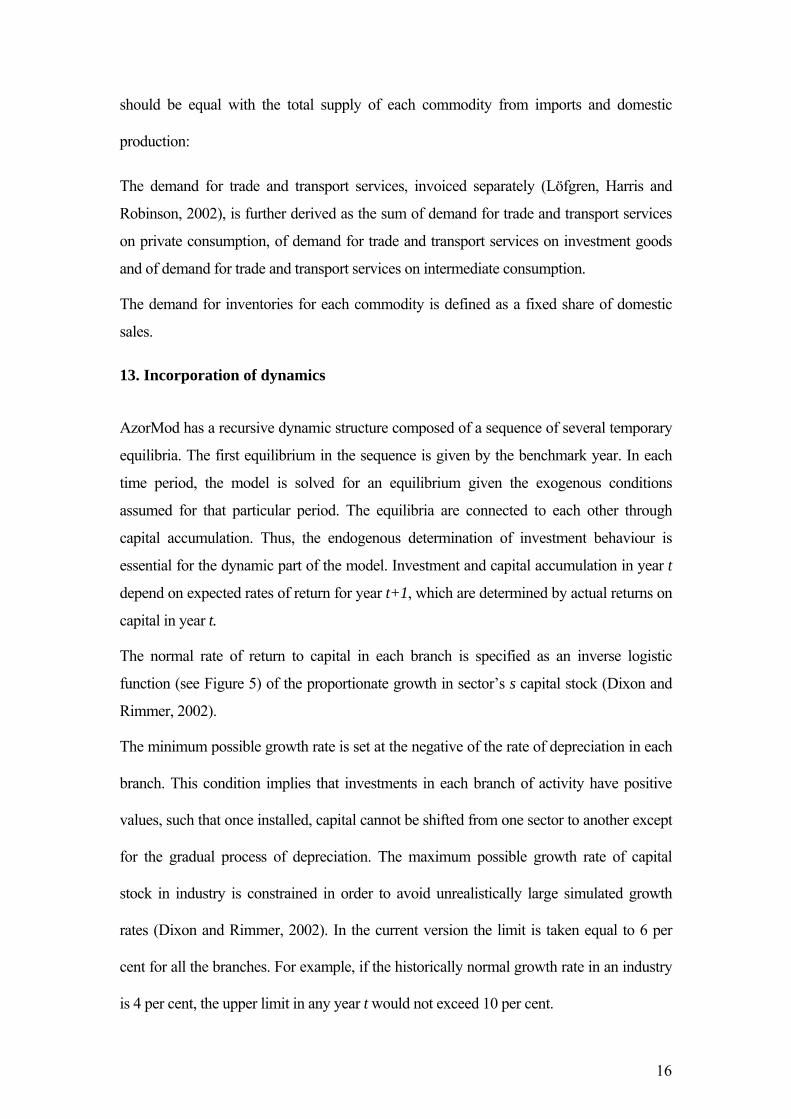
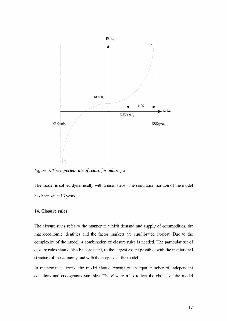
The normal rate of return to capital in each branch is specified as an inverse logistic

function (see Figure 5) of the proportionate growth in sector’s s capital stock (Dixon and

Rimmer, 2002).

The minimum possible growth rate is set at the negative of the rate of depreciation in each

branch. This condition implies that investments in each branch of activity have positive

values, such that once installed, capital cannot be shifted from one sector to another except

for the gradual process of depreciation. The maximum possible growth rate of capital

stock in industry is constrained in order to avoid unrealistically large simulated growth

rates (Dixon and Rimmer, 2002). In the current version the limit is taken equal to 6 per

cent for all the branches. For example, if the historically normal growth rate in an industry

is 4 per cent, the upper limit in any year t would not exceed 10 per cent.

17

RORs

RORHs

0.06

KSKtrends

KSKgs

KSKgmaxsKSKgmins

R

R'

Figure 5. The expected rate of return for industry s

The model is solved dynamically with annual steps. The simulation horizon of the model

has been set at 13 years.

14. Closure rules

The closure rules refer to the manner in which demand and supply of commodities, the

macroeconomic identities and the factor markets are equilibrated ex-post. Due to the

complexity of the model, a combination of closure rules is needed. The particular set of

closure rules should also be consistent, to the largest extent possible, with the institutional

structure of the economy and with the purpose of the model.

In mathematical terms, the model should consist of an equal number of independent

equations and endogenous variables. The closure rules reflect the choice of the model

18

builder of which variables are exogenous and which variables are endogenous, so as to

achieve ex-post equality.

Three macro balances are usually identified in CGE models that can be a potential source

of ex-ante disequilibria and must be reconciled ex-post (Adelman and Robinson, 1989):

The savings-investment balance;

The government balance;

The external balance.

The most widely used macro closure rule for CGE models is based on the investment and

savings balance. In the model, the investment is assumed to adjust to the available

domestic and foreign savings. This reflects an economy in which savings form a binding

constraint.

Additional assumptions are needed with regard to regional government behaviour in

AzorMod. First, regional government savings are fixed in real terms while regional

government total current consumption adjusts to achieve the target set with respect to the

government savings. The allocation between the consumption of different goods and

services is provided by a Cobb-Douglas function. Secondly, the transfers received by the

regional government from the Mainland government, from the EU, from the US and from

the ROW are fixed in real terms. On the expenditure side, the regional government

transfers to the households are also fixed in real terms.

For the external balance, the exchange rates are kept unchanged in the simulations, while

the balances of the current accounts adjust. An alternative closure is also possible where

the balances of the current accounts corresponding to US and ROW are set while the real

exchange rates adjust.

The setup of the closure rules is important in determining the mechanisms governing the

model. Therefore, the closure rules should be established also taking into account the

policy scenario in question.

According to Walras’ law if (n-1) markets are cleared the nth one is cleared as well.

Therefore, in order to avoid over-determination of the model, the current account balance

with respect to ROW is dropped. However, the system of equations guarantees, through

Walras’ law, that the total imports from ROW less the total exports to ROW and the

transfers from ROW equals the current account balance.

19

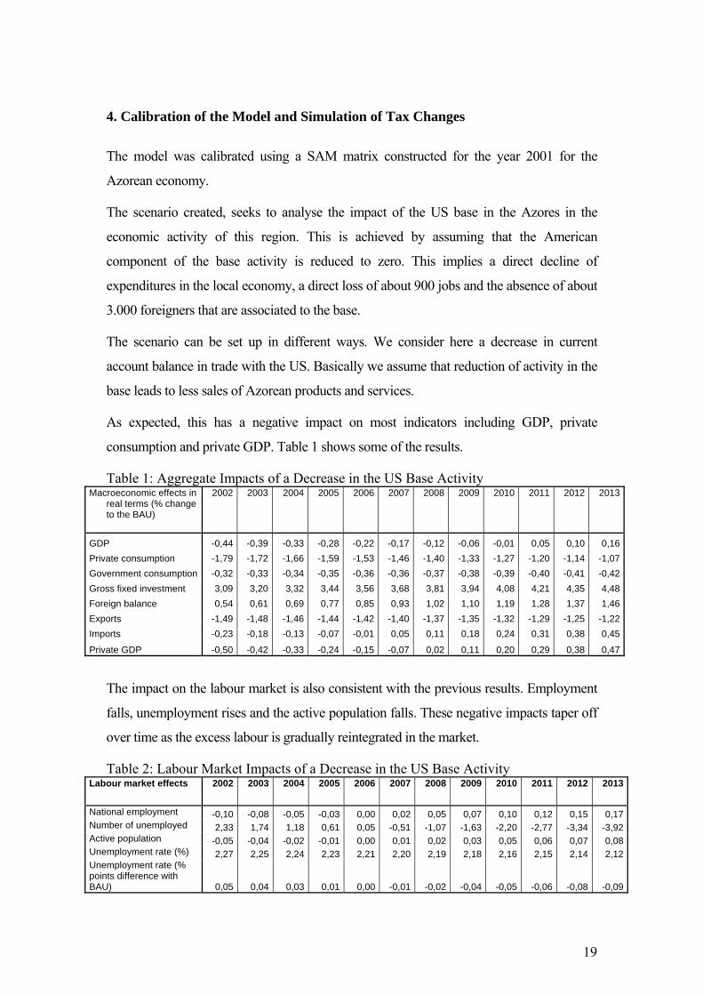
4. Calibration of the Model and Simulation of Tax Changes

The model was calibrated using a SAM matrix constructed for the year 2001 for the

Azorean economy.

The scenario created, seeks to analyse the impact of the US base in the Azores in the

economic activity of this region. This is achieved by assuming that the American

component of the base activity is reduced to zero. This implies a direct decline of

expenditures in the local economy, a direct loss of about 900 jobs and the absence of about

3.000 foreigners that are associated to the base.

The scenario can be set up in different ways. We consider here a decrease in current

account balance in trade with the US. Basically we assume that reduction of activity in the

base leads to less sales of Azorean products and services.

As expected, this has a negative impact on most indicators including GDP, private

consumption and private GDP. Table 1 shows some of the results.

Table 1: Aggregate Impacts of a Decrease in the US Base Activity Macroeconomic effects in

real terms (% change to the BAU)

2002 2003 2004 2005 2006 2007 2008 2009 2010 2011 2012 2013

GDP -0,44 -0,39 -0,33 -0,28 -0,22 -0,17 -0,12 -0,06 -0,01 0,05 0,10 0,16Private consumption -1,79 -1,72 -1,66 -1,59 -1,53 -1,46 -1,40 -1,33 -1,27 -1,20 -1,14 -1,07Government consumption -0,32 -0,33 -0,34 -0,35 -0,36 -0,36 -0,37 -0,38 -0,39 -0,40 -0,41 -0,42Gross fixed investment 3,09 3,20 3,32 3,44 3,56 3,68 3,81 3,94 4,08 4,21 4,35 4,48Foreign balance 0,54 0,61 0,69 0,77 0,85 0,93 1,02 1,10 1,19 1,28 1,37 1,46Exports -1,49 -1,48 -1,46 -1,44 -1,42 -1,40 -1,37 -1,35 -1,32 -1,29 -1,25 -1,22Imports -0,23 -0,18 -0,13 -0,07 -0,01 0,05 0,11 0,18 0,24 0,31 0,38 0,45

Private GDP -0,50 -0,42 -0,33 -0,24 -0,15 -0,07 0,02 0,11 0,20 0,29 0,38 0,47

The impact on the labour market is also consistent with the previous results. Employment

falls, unemployment rises and the active population falls. These negative impacts taper off

over time as the excess labour is gradually reintegrated in the market.

Table 2: Labour Market Impacts of a Decrease in the US Base Activity Labour market effects 2002 2003 2004 2005 2006 2007 2008 2009 2010 2011 2012 2013

National employment -0,10 -0,08 -0,05 -0,03 0,00 0,02 0,05 0,07 0,10 0,12 0,15 0,17Number of unemployed 2,33 1,74 1,18 0,61 0,05 -0,51 -1,07 -1,63 -2,20 -2,77 -3,34 -3,92Active population -0,05 -0,04 -0,02 -0,01 0,00 0,01 0,02 0,03 0,05 0,06 0,07 0,08Unemployment rate (%) 2,27 2,25 2,24 2,23 2,21 2,20 2,19 2,18 2,16 2,15 2,14 2,12Unemployment rate (% points difference with BAU) 0,05 0,04 0,03 0,01 0,00 -0,01 -0,02 -0,04 -0,05 -0,06 -0,08 -0,09

20

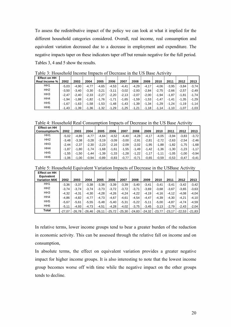
To assess the redistributive impact of the policy we can look at what it implied for the

different household categories considered. Overall, real income, real consumption and

equivalent variation decreased due to a decrease in employment and expenditure. The

negative impacts taper on these indicators taper off but remain negative for the full period.

Tables 3, 4 and 5 show the results.

Table 3: Household Income Impacts of Decrease in the US Base Activity Effect on HH

Real Income % 2002 2003 2004 2005 2006 2007 2008 2009 2010 2011 2012 2013 HH1 -5,03 -4,90 -4,77 -4,65 -4,53 -4,41 -4,29 -4,17 -4,06 -3,95 -3,84 -3,74HH2 -3,50 -3,40 -3,30 -3,21 -3,11 -3,02 -2,93 -2,84 -2,75 -2,66 -2,57 -2,49HH3 -2,47 -2,40 -2,33 -2,27 -2,20 -2,13 -2,07 -2,00 -1,94 -1,87 -1,81 -1,74HH4 -1,94 -1,88 -1,82 -1,76 -1,71 -1,65 -1,59 -1,53 -1,47 -1,41 -1,35 -1,29HH5 -1,67 -1,63 -1,58 -1,53 -1,48 -1,43 -1,39 -1,34 -1,29 -1,24 -1,19 -1,14HH6 -1,43 -1,39 -1,36 -1,32 -1,29 -1,25 -1,21 -1,18 -1,14 -1,10 -1,07 -1,03

Table 4: Household Real Consumption Impacts of Decrease in the US Base Activity Effect on HH

Consumption% 2002 2003 2004 2005 2006 2007 2008 2009 2010 2011 2012 2013 HH1 -5,02 -4,89 -4,77 -4,64 -4,52 -4,40 -4,28 -4,17 -4,05 -3,94 -3,83 -3,72HH2 -3,48 -3,38 -3,28 -3,19 -3,09 -3,00 -2,91 -2,81 -2,72 -2,63 -2,54 -2,46HH3 -2,44 -2,37 -2,30 -2,23 -2,16 -2,09 -2,02 -1,95 -1,88 -1,82 -1,75 -1,68HH4 -1,87 -1,80 -1,74 -1,68 -1,61 -1,55 -1,49 -1,42 -1,36 -1,30 -1,23 -1,17HH5 -1,55 -1,50 -1,44 -1,39 -1,33 -1,28 -1,22 -1,17 -1,11 -1,05 -1,00 -0,94HH6 -1,06 -1,00 -0,94 -0,89 -0,83 -0,77 -0,71 -0,65 -0,59 -0,53 -0,47 -0,41

Table 5: Household Equivalent Variation Impacts of Decrease in the USBase Activity

Effect on HH Equivalent

Variation Mil€ 2002 2003 2004 2005 2006 2007 2008 2009 2010 2011 2012 2013 HH1 -3,36 -3,37 -3,38 -3,38 -3,39 -3,39 -3,40 -3,41 -3,41 -3,41 -3,42 -3,42HH2 -3,74 -3,74 -3,74 -3,73 -3,72 -3,72 -3,71 -3,69 -3,68 -3,67 -3,65 -3,63HH3 -4,32 -4,31 -4,30 -4,28 -4,26 -4,24 -4,22 -4,19 -4,16 -4,12 -4,08 -4,04HH4 -4,86 -4,82 -4,77 -4,73 -4,67 -4,61 -4,54 -4,47 -4,39 -4,30 -4,21 -4,10HH5 -5,67 -5,61 -5,55 -5,48 -5,40 -5,31 -5,22 -5,11 -5,00 -4,87 -4,74 -4,59HH6 -5,11 -4,93 -4,73 -4,51 -4,28 -4,02 -3,75 -3,45 -3,13 -2,79 -2,43 -2,04Total -27,07 -26,78 -26,46 -26,11 -25,72 -25,30 -24,83 -24,32 -23,77 -23,17 -22,53 -21,83

In relative terms, lower income groups tend to bear a greater burden of the reduction

in economic activity. This can be assessed through the relative fall on income and on

consumption,

In absolute terms, the effect on equivalent variation provides a greater negative

impact for higher income groups. It is also interesting to note that the lowest income

group becomes worse off with time while the negative impact on the other groups

tends to decline.

21

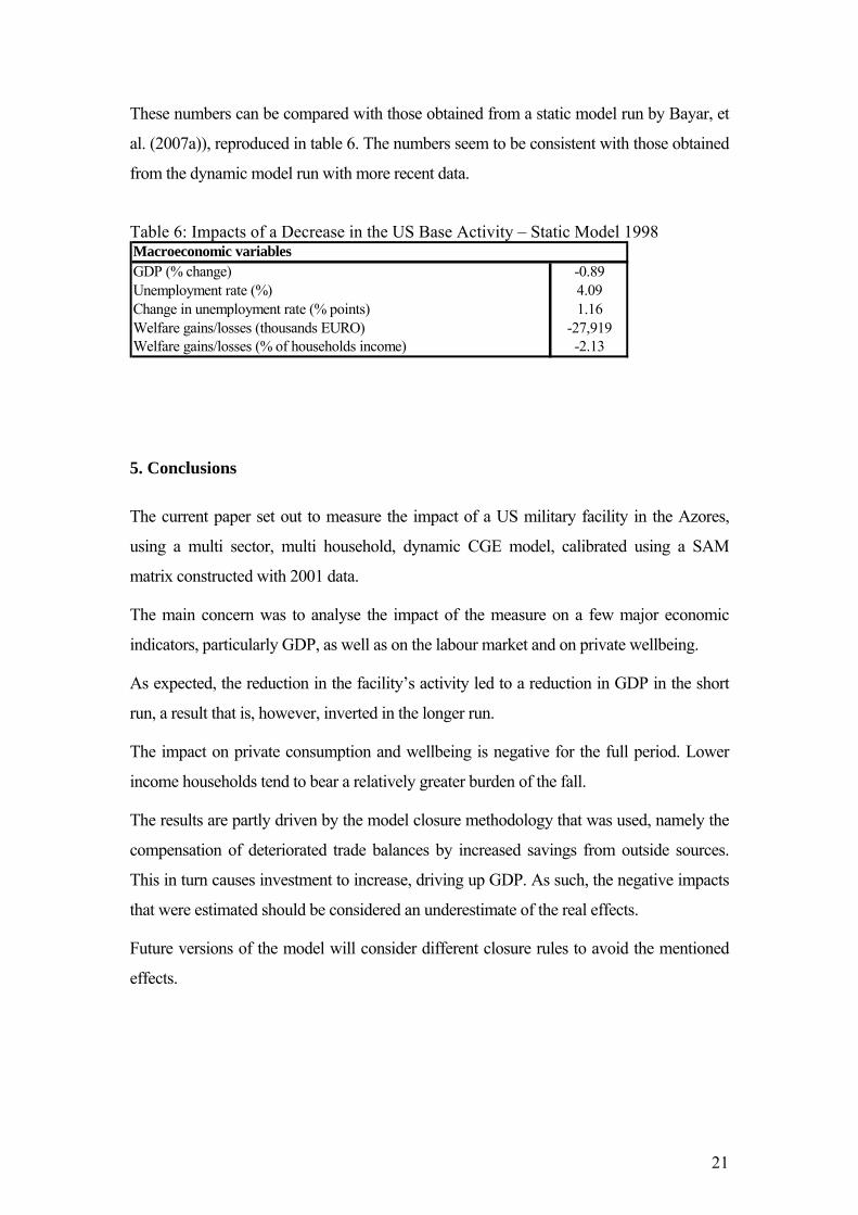
These numbers can be compared with those obtained from a static model run by Bayar, et

al. (2007a)), reproduced in table 6. The numbers seem to be consistent with those obtained

from the dynamic model run with more recent data.

Table 6: Impacts of a Decrease in the US Base Activity – Static Model 1998

GDP (% change) -0.89Unemployment rate (%) 4.09Change in unemployment rate (% points) 1.16Welfare gains/losses (thousands EURO) -27,919Welfare gains/losses (% of households income) -2.13

Macroeconomic variables

5. Conclusions The current paper set out to measure the impact of a US military facility in the Azores,

using a multi sector, multi household, dynamic CGE model, calibrated using a SAM

matrix constructed with 2001 data.

The main concern was to analyse the impact of the measure on a few major economic

indicators, particularly GDP, as well as on the labour market and on private wellbeing.

As expected, the reduction in the facility’s activity led to a reduction in GDP in the short

run, a result that is, however, inverted in the longer run.

The impact on private consumption and wellbeing is negative for the full period. Lower

income households tend to bear a relatively greater burden of the fall.

The results are partly driven by the model closure methodology that was used, namely the

compensation of deteriorated trade balances by increased savings from outside sources.

This in turn causes investment to increase, driving up GDP. As such, the negative impacts

that were estimated should be considered an underestimate of the real effects.

Future versions of the model will consider different closure rules to avoid the mentioned

effects.

22

References Adelman, I., & Robinson, S. (1989). Income distribution and development. In H. Chenery & T. N. Srinivasan (Eds.), Handbook of development economics, vol. 2 (pp. 949-1003). Amsterdam: North-Holland.

Bayar, A. Fortuna, Mario, Mohara, Cristina, Sasik, Suat, Rege, Sameer (2007-a). Impacts of Closure of a Military Base on a Small Open Economy. In Proceedings of the 13th Annual Meeting of APDR (PortugueseRegional Development Association. University of the Azores, July 5-7. Bayar, A. Fortuna, Mario, Mohara, Cristina, Sasik, Suat, Rege, Sameer (2007-b). Measuring the Impacts of Personal and Corporate Income Tax Cuts on a Small Open Economy. In Proceedings ECOMOD2007 International Conference on Policy Modeling. EcoMod, S. Paulo Brasil, July 11-13

Dervis, K., De Melo, J., & Robinson, S. (1982). General equilibrium models for development policy. Cambridge, UK: Cambridge University Press.

Dixon, P.B., & Rimmer, M.T. (2002). Dynamic general equilibrium modeling for forecasting and policy: A practical guide and documentation of MONASH. In R. Blundell, R. Caballero, J.-J. Laffont & T. Persson (Eds.), Contributions to economic analysis, vol. 256. Amsterdam: North-Holland.

Harrison, G.W., & Kriström, B. (1997). General equilibrium effects of increasing carbon taxes in Sweden. Retrived from: http://dmsweb.badm.sc.edu/Glenn/papers/

Löfgren, H., Harris, R. L., & Robinson, S. (2002). A standard computable general equilibrium (CGE) in GAMS. IFPRI, Microcomputers in Policy Research, 5. Retrived from: http://www.ifpri.org/pubs/microcom/micro5.htm.

Rosenthal, R.E. (2006). GAMS – A user’s guide. Washington: GAMS Development Corporation.

Sanz-de-Galdeano, A., & Turunen, J. (2006). The euro area wage curve. Economics Letters, 92, 93-98.

Varian, H.R. (1992). Microeconomic analysis. New York: W.W. Norton.

23

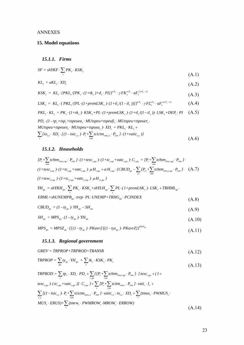
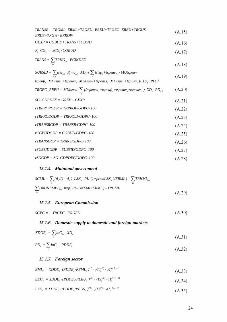
ANNEXES

15. Model equations

15.1.1. Firms

s ss

SF = shYKF PK KSK⋅ ⋅∑ (A.1)

s s sKL = aKL XD⋅ (A.2) s s sF F ( F 1)

s s s s s s s sKSK = KL {PKL /[PK (1+tk )+d PI]} FK aFσ σ σγ −⋅ ⋅ ⋅ ⋅ ⋅ (A.3) s s sF F ( F 1)

s s s s s s s sLSK = KL { PKL /[PL (1+premLSK ) (1+tl /(1 tl ))]} FL aFσ σ σγ −⋅ ⋅ ⋅ − ⋅ ⋅ (A.4)

s s s s s s s s s sPKL KL = PK (1+tk ) KSK +PL (1+premLSK ) (1+tl /(1 tl )) LSK +DEP PI⋅ ⋅ ⋅ ⋅ ⋅ − ⋅ ⋅ (A.5)

s s s s s s

s s s s s

c,s s c,s c ctm,c,s ctm c,sc ctm

PD (1 tp +tsp +tspeuea MUtspeu+tspeufi MUtspeu+tspeuerMUtspeu+tspeues MUtspeu+tspusa ) XD = PKL KL

{io XD [(1 tsic ) P + tcictm P ] (1+vatic )}

⋅ − ⋅ ⋅ ⋅

⋅ ⋅ ⋅ +

⋅ ⋅ − ⋅ ⋅ ⋅∑ ∑ (A.6)

15.1.2. Households

c ctm,c,qu ctm c,qu c,qu c,qu c,qu c ctm,c,qu ctmctm ctm

c,qu c,qu c,qu c,qu c,qu qu cc ctm,cc,qu ctmcc ctm

cc,qu

[P + tchtm P ] (1+texc ) (1+tc +vatc ) C = [P + tchtm P ]

(1+texc ) (1+tc +vatc ) H H {CBUD [P + tchtm P ]

(1+texc ) (

µ α

⋅ ⋅ ⋅ ⋅ ⋅ ⋅

⋅ ⋅ + ⋅ − ⋅ ⋅

⋅

∑ ∑

∑ ∑cc,qu cc,qu cc,qu1+tc +vatc ) H }µ⋅

(A.7)

qu qu s s qu s s qus s

qu qu

YH = shYKH PK KSK +shYLH PL (1+premLSK ) LSK TRHML

ERML+shUNEMPB trep PL UNEMP+TRHG PCINDEX

⋅ ⋅ ⋅ ⋅ ⋅ + ⋅

⋅ ⋅ ⋅ ⋅

∑ ∑

(A.8)

qu qu qu quCBUD = (1 ty ) YH SH− ⋅ − (A.9)

qu qu qu quSH = MPS (1 ty ) YH⋅ − ⋅ (A.10) quelasS

qu qu qu quMPS = MPSZ {[(1 ty ) PKavr]/[(1 tyz ) PKavrZ]}⋅ − ⋅ − ⋅ (A.11)

15.1.3. Regional government

GREV = TRPROP+TRPROD+TRANSR (A.12)

qu qu s s squ s

TRPROP = ty YH + tk KSK PK⋅ ⋅ ⋅∑ ∑ (A.13)

s s s c ctm,c,qu ctm c,qus c ,qu ctm

c,qu c,qu c,qu c,qu c ctm,c ctm c cc ctm

c,s c ctm,c,s ctm c,s c,s sctm

TRPROD = tp XD PD {[P + tchtm P ] [ texc (1

texc ) ( tc +vatc )] C } [P + tcitm P ] vati I

[(1 tsic ) P + tcictm P ] vatic io XD

⋅ ⋅ + ⋅ ⋅ + +

⋅ ⋅ + ⋅ ⋅ ⋅ +

− ⋅ ⋅ ⋅ ⋅ ⋅

∑ ∑ ∑

∑ ∑

∑ c cc ,s c

c c c cc

(tmus PWMUS

MUS ERUS)+ (tmrw PWMROW MROW ERROW)

+ ⋅ ⋅

⋅ ⋅ ⋅ ⋅

∑ ∑

∑ (A.14)

24

TRANSR = TRGML ERML+TRGEU EREU+TRGEC EREU+TRGUSERUS+TRGW ERROW

⋅ ⋅ ⋅ ⋅⋅

(A.15)

GEXP = CGBUD+TRANS+SUBSID (A.16)

c c cP CG = CG CGBUD α⋅ ⋅ (A.17)

ququ

TRANS = TRHG PCINDEX⋅∑ (A.18)

c,s c c,s s s sc ,s s

s s s s s s

SUBSID = tsic P io XD [(tsp +tspeuea MUtspeu+

tspeufi MUtspeu+tspeuer MUtspeu+tspeues MUtspeu+tspusa ) XD PD ]

⋅ ⋅ ⋅ + ⋅

⋅ ⋅ ⋅ ⋅ ⋅

∑ ∑ (A.19)

s s s s s ss

TRGEC EREU = MUtspeu [(tspeuea +tspeufi +tspeuer +tspeues ) XD PD ]⋅ ⋅ ⋅ ⋅∑ (A.20)

SG GDPDEF = GREV GEXP⋅ − (A.21) rTRPROPGDP = TRPROP/GDPC 100⋅ (A.22) rTRPRODGDP = TRPROD/GDPC 100⋅ (A.23) rTRANSRGDP = TRANSR/GDPC 100⋅ (A.24) rCGBUDGDP = CGBUD/GDPC 100⋅ (A.25) rTRANSGDP = TRANS/GDPC 100⋅ (A.26) rSUBSIDGDP = SUBSID/GDPC 100⋅ (A.27) rSGGDP = SG GDPDEF/GDPC 100⋅ ⋅ (A.28)

15.1.4. Mainland government

s s s s qus qu

ququ

SGML = [tl /(1 tl ) LSK PL (1+premLSK )/ERML ] TRHML

(shUNEMPB trep PL UNEMP/ERML ) TRGML

− ⋅ ⋅ ⋅ − −

⋅ ⋅ ⋅ −

∑ ∑

∑ (A.29)

15.1.5. European Commission

SGEC = TRGEC TRGEU− − (A.30)

15.1.6. Domestic supply to domestic and foreign markets

c s,c ss

XDDE = ioC XD⋅∑ (A.31)

s s,c cc

PD = ioC PDDE⋅∑ (A.32)

15.1.7. Foreign sector

c c cT T ( T 1)c c c c c cEML = XDDE (PDDE /PEML ) T1 aTσ σ σγ −⋅ ⋅ ⋅ (A.33)

c c cT T ( T 1)c c c c c cEEU = XDDE (PDDE /PEEU ) T2 aTσ σ σγ −⋅ ⋅ ⋅ (A.34)

c c cT T ( T 1)c c c c c cEUS = XDDE (PDDE /PEUS ) T3 aTσ σ σγ −⋅ ⋅ ⋅ (A.35)

25

c c cT T ( T 1)c c c c c cEROW = XDDE (PDDE /PEROW ) T4 aTσ σ σγ −⋅ ⋅ ⋅ (A.36)

c c cT T ( T 1)c c c c c cXDD = XDDE (PDDE /PDD ) T5 aTσ σ σγ −⋅ ⋅ ⋅ (A.37)

c c c c c c c c c c

c c

PDDE XDDE = PDD XDD +PEML EML +PEEU EEU +PEUS EUSPEROW EROW

⋅ ⋅ ⋅ ⋅ ⋅ +⋅ (A.38)

c c c c c c c c c cE = (PEML EML +PEEU EEU +PEUS EUS +PEROW EROW )/INDEXE⋅ ⋅ ⋅ ⋅ (A.39) celasE

c c c cEDML = EDIML (PWEML ERML/PEML )⋅ ⋅ (A.40) celasE

c c c cEDEU = EDIEU (PWEEU EREU/PEEU )⋅ ⋅ (A.41) celasE

c c c cEDUS = EDIUS (PWEUS ERUS/PEUS )⋅ ⋅ (A.42) celasE

c c c cEDROW = EDIROW (PWEROW ERROW/PEROW )⋅ ⋅ (A.43) c c cA A ( A 1)

c c c c c cMML = X (P /PMML ) A1 aAσ σ σγ −⋅ ⋅ ⋅ (A.44) c c cA A ( A 1)

c c c c c cMEU = X (P /PMEU ) A2 aAσ σ σγ −⋅ ⋅ ⋅ (A.45) c c cA A ( A 1)

c c c c c cMUS = X (P /PMUS ) A3 aAσ σ σγ −⋅ ⋅ ⋅ (A.46) c c cA A ( A 1)

c c c c c cMROW = X (P /PMROW ) A4 aAσ σ σγ −⋅ ⋅ ⋅ (A.47) c c cA A ( A 1)

c c c c c cXDD = X (P /PDD ) A5 aAσ σ σγ −⋅ ⋅ ⋅ (A.48)

c c c c c c c c c c

c c

P X = PMML MML +PMEU MEU +PMUS MUS +PMROW MROW + PDD XDD⋅ ⋅ ⋅ ⋅ ⋅

⋅ (A.49)

c c c c c c c

c c c

M = (PWMML ERML MML +PWMEU EREU MEU +PWMUS ERUS MUS +PWMROW ERROW MROW )/INDEXM

⋅ ⋅ ⋅ ⋅ ⋅ ⋅⋅ ⋅ (A.50)

c c c cc

SML = (MML PWMML EML PEML /ERML)+SGML⋅ − ⋅∑ (A.51)

c c c cc

SEU = (MEU PWMEU EEU PEEU /EREU)+SGEC⋅ − ⋅∑ (A.52)

c c c cc

SUS = (MUS PWMUS EUS PEUS /ERUS) TRGUS⋅ − ⋅ −∑ (A.53)

c c c cc

SROW = (MROW PWMROW EROW PEROW /ERROW) TRGW⋅ − ⋅ −∑ (A.54)

15.1.8. Investment

ququ

ss

S = SH +SF+SG GDPDEF+SML ERML+SEU EREU+SUS ERUS+SROW

ERROW+ DEP PI

⋅ ⋅ ⋅ ⋅ ⋅

⋅

∑

∑ (A.55)

c cI = ioI ITT⋅ (A.56)

c c ctm,c ctm cc ctm

PI = {(1+vati ) [P + tcitm P ] ioI }⋅ ⋅ ⋅∑ ∑ (A.57)

26

c cc

PI ITT = S SV P⋅ − ⋅∑ (A.58)

c c cSV = svr X⋅ (A.59)

s s sDEP = d KSK⋅ (A.60)

15.1.9. Labor market

log(PL/PCINDEX) = elasU log(UNRATE)+err⋅ (A.61) elasLSLSR = LSRI { [PL (1 tyavr) PCINDEXZ]/[PLZ (1 tyavrz) PCINDEX]}⋅ ⋅ − ⋅ ⋅ − ⋅ (A.62)

qu qu ququ qu

tyavr = (ty YH ) / YH⋅∑ ∑ (A.63)

EMPN = LSR UNEMP− (A.64) UNRATE = UNEMP/LSR (A.65)

15.1.10. Trade and transport margins

ctm ctm,c,qu c,qu ctm,c c ctm,c,s c,s sc,qu c s,c

MARGTM = tchtm C + tcitm I + tcictm io XD⋅ ⋅ ⋅ ⋅∑ ∑ ∑ (A.66)

15.1.11. Market clearing

ss

LSK = LSR UNEMP−∑ (A.67)

ctm,s s ctm,qu ctm ctm ctm ctm ctms qu

io XD C +CG +I +SV +MARGTM X⋅ + =∑ ∑ (A.68)

nctm,s s nctm,qu nctm nctm nctm nctms qu

io XD C +CG +I +SV X⋅ + =∑ ∑ (A.69)

c cEML = EDML (A.70)

c cEEU = EDEU (A.71)

c cEUS = EDUS (A.72)

c cEROW = EDROW (A.73)

15.1.12. Price definitions

c ctm,c,qu ctm c,qu c,qu c,qu c,quc,qu ctm

c ctm,c,qu ctm c,qu c,qu c,qu c,quc,qu ctm

PCINDEX = {[P + tchtm P ] (1+texc ) (1+tc +vatc ) CZ } /

{[PZ + tchtmz PZ ] (1+texcz ) (1+tcz +vatcz ) CZ }

⋅ ⋅ ⋅ ⋅

⋅ ⋅ ⋅ ⋅

∑ ∑

∑ ∑ (A.74)

c c c c c c c c c

c c c c c c c c

INDEXE = (PEML EMLZ +PEEU EEUZ +PEUS EUSZ +PEROW EROWZ )/(PEMLZ EMLZ +PEEUZ EEUZ +PEUSZ EUSZ +PEROWZ EROWZ )

⋅ ⋅ ⋅ ⋅

⋅ ⋅ ⋅ ⋅ (A.75)

c c c c c c

c c c c c c

c c c c c

INDEXM = (PWMML ERML MMLZ +PWMEU EREU MEUZ +PWMUS ERUSMUSZ +PWMROW ERROW MROWZ )/(PWMMLZ ERMLZ MMLZ +PWMEUZEREUZ MEUZ +PWMUSZ ERUSZ MUSZ +PWMROWZ ERROWZ MROWZ )

⋅ ⋅ ⋅ ⋅ ⋅ ⋅

⋅ ⋅ ⋅ ⋅ ⋅⋅ ⋅ ⋅ ⋅ ⋅ (A.76)

27

c cPMML = PWMML ERML⋅ (A.77)

c cPMEU = PWMEU EREU⋅ (A.78)

c c cPMUS = PWMUS ERUS (1+tmus )⋅ ⋅ (A.79)

c c cPMROW = PWMROW ERROW (1+tmrw )⋅ ⋅ (A.80)

s s s ss s

RINT = [(PK /PD ) KSK ]/ KSK⋅∑ ∑ (A.81)

s s ss s

PKavr = [(PK /PCINDEX) KSK ]/ KSK⋅∑ ∑ (A.82)

c,qu c ctm,c,qu ctm c,qu c,qu c,quctm

PCT = [P + tchtm P ] (1+texc ) (1+tc +vatc )⋅ ⋅ ⋅∑ (A.83)

s s s ss

PLAVRT (LSR UNEMP) = [PL (1+tl /(1 tl )) (1+premLSK ) LSK ]⋅ − ⋅ − ⋅ ⋅∑ (A.84)

15.1.13. Gross domestic product at current and constant market prices

c,qu c ctm,c,qu ctm c,qu c,qu c,quc,qu ctm

c c c c c ctm,c ctm c c c cc c ctm c c

c c c c c cc c c

c

GDPC = {C [ P + tchtm P ] (1+texc ) (1+tc +vatc )}

CG P {I (1+vati ) [P + tcitm P ]}+ SV P EML PEML

EEU PEEU EUS PEUS EROW PEROW

MML

⋅ ⋅ ⋅ ⋅ +

⋅ + ⋅ ⋅ ⋅ ⋅ + ⋅

+ ⋅ + ⋅ + ⋅ −

⋅

∑ ∑

∑ ∑ ∑ ∑ ∑

∑ ∑ ∑

c c cc c

c c c cc c

PWMML ERML MEU PWMEU EREU

MUS PWMUS ERUS MROW PWMROW ERROW

⋅ − ⋅ ⋅ −

⋅ ⋅ − ⋅ ⋅

∑ ∑

∑ ∑ (A.85)

c,qu c ctm,c,qu ctm c,qu c,qu c,quc,qu ctm

c c c c c ctm,c ctm c cc c ctm c

c c c c c c cc c c

GDP = {C [ PZ + tchtmz PZ ] (1+texcz ) (1+tcz +vatcz )}

CG PZ {I (1+vatiz ) [PZ + tcitmz PZ ]}+ SV PZ

EML PEMLZ EEU PEEUZ EUS PEUSZ EROW

⋅ ⋅ ⋅ ⋅ +

⋅ + ⋅ ⋅ ⋅ ⋅ +

⋅ + ⋅ + ⋅ + ⋅

∑ ∑

∑ ∑ ∑ ∑

∑ ∑ ∑ cc

c c c cc c

c c c cc c

PEROWZ

MML PWMMLZ ERMLZ MEU PWMEUZ EREUZ

MUS PWMUSZ ERUSZ MROW PWMROWZ ERROWZ

−

⋅ ⋅ − ⋅ ⋅ −

⋅ ⋅ − ⋅ ⋅

∑

∑ ∑

∑ ∑ (A.86)

c,qu c ctm,c,qu ctm c,qu c,qu c,quc,qu ctm

c c c ctm,c ctm c c c cc ctm c c

c c c c c cc c c

GDPP = {C [ PZ + tchtmz PZ ] (1+texcz ) (1+tcz +vatcz )}

{I (1+vatiz ) [PZ + tcitmz PZ ]}+ SV PZ EML PEMLZ

EEU PEEUZ EUS PEUSZ EROW PEROWZ

⋅ ⋅ ⋅ ⋅ +

⋅ ⋅ ⋅ ⋅ + ⋅ +

⋅ + ⋅ + ⋅

∑ ∑

∑ ∑ ∑ ∑

∑ ∑ ∑

c c c cc c

c c c cc c

MML PWMMLZ ERMLZ MEU PWMEUZ EREUZ

MUS PWMUSZ ERUSZ MROW PWMROWZ ERROWZ

−

⋅ ⋅ − ⋅ ⋅ −

⋅ ⋅ − ⋅ ⋅

∑ ∑

∑ ∑

GDPDEF = GDPC/GDP (A.87)

28

15.1.14. Components of GDP at constant prices

c,qu c ctm,c,qu ctm c,qu c,qu c,quc,qu ctm

CT {C [ PZ + tchtmz PZ ] (1+texcz ) (1+tcz +vatcz )}= ⋅ ⋅ ⋅ ⋅∑ ∑ (A.88)

c cc

CGT CG PZ= ⋅∑ (A.89)

c c c ctm,c ctm c cc ctm c

IT {I (1+vatiz ) [PZ + tcitmz PZ ]} SV PZ= ⋅ ⋅ ⋅ + ⋅∑ ∑ ∑ (A.90)

c c c c c c c cc

ET (EML PEMLZ EEU PEEUZ EUS PEUSZ EROW PEROWZ )= ⋅ + ⋅ + ⋅ + ⋅∑ (A.91)

c c c cc

c c c c

MT (MML PWMMLZ ERMLZ MEU PWMEUZ EREUZ+

MUS PWMUSZ ERUSZ+MROW PWMROWZ ERROWZ)

= ⋅ ⋅ + ⋅ ⋅

⋅ ⋅ ⋅ ⋅

∑

(A.92)

15.1.15. Equivalent variation in income

c,qu

qu qu c ctm,c ,qu ctm c,qu c,qu c,quc ctm

c,qu c,qu c ctm,c,qu ctm c,qu c,quctmc

Hc,qu

VU = {CBUD [P + tchtm P ] (1+texc ) (1+tc +vatc )

H } { H /{[P + tchtm P ] (1+texc ) (1+tc +

vatc )}}α

µ α

− ⋅ ⋅ ⋅ ⋅

⋅ ⋅ ⋅ ⋅

∑ ∑

∑∏

(A.93)

c,qu

qu qu c ctm,c ,qu ctm c,qu c,qu c,quc ctm

c,qu c,qu c ctm,c,qu ctm c,qu c,quctmc

Hc,qu

VUI = {CBUDZ [PZ + tchtmz PZ ] (1+texcz ) (1+tcz +vatcz )

H } { H /{[PZ + tchtmz PZ ] (1+texcz ) (1+tcz +

vatcz )}}α

µ α

− ⋅ ⋅ ⋅ ⋅

⋅ ⋅ ⋅ ⋅

∑ ∑

∑∏ (A.94)

c,qu

qu c ctm,c,qu ctm c,qu c,qu c,quctmc

Hc,qu qu qu

EV = {{[PZ + tchtmz PZ ] (1+texcz ) (1+tcz +vatcz )} /

H } (VU VUI )αα

⋅ ⋅ ⋅

⋅ −

∑∏ (A.95)

15.1.16. Capital accumulation

s,t s,t t tROR = 1+(PK /PI +1)/(1+RINT )− (A.96) s,t s s s s s s s{[(ROR RORH ) (KSKgmax KSKgmin )]/[(KSKgmax KSKtrend ) (KSKtrend KSKgmin )]}

s,tROR = eα − ⋅ − − ⋅ −

(A.97)

s,t s,t s,t s s s s

s s s,t s s

s s s s,t

INVS = KSK [ ROR KSKgmax (KSKtrend KSKgmin )+ KSKgmin(KSKgmax KSKtrend )]/[ ROR (KSKtrend KSKgmin )+(KSKgmax KSKtrend )]+d KSK

αα

⋅ ⋅ ⋅ − ⋅

− ⋅ −

− ⋅ (A.98)

s,t s,t ss,t t c,t c,t tss c

INV = INVS / INVS (S SV P )/PI⋅ − ⋅∑ ∑ (A.99)

s,t+1 s s,t s,tKSK = (1 d ) KSK +INV− ⋅ (A.100)

29

16.

17.

18.

19. List of Endogenous variables

CBUDqu households budget disposable for consumption by income group Cc,qu consumer demand for commodity c by income group qu CGBUD regional government current expenditures CGc public current consumption of commodity c by the regional

government CGT total public consumption by the regional government at constant

prices CT total private consumption at constant prices DEPs depreciation related to public and private capital stock EDEUc export demand of commodity c from EU EDMLc export demand of commodity c from Mainland EDROWc export demand of commodity c from the rest of the world EDUSc export demand of commodity c from US EEUc export supply of commodity c by the domestic producers to EU EMLc export supply of commodity c by the domestic producers to

Mainland EMPN national employment EROWc export supply of commodity c by the domestic producers to the

rest of the world ET total exports at constant prices EUSc export supply of commodity c by the domestic producers to US EVqu equivalent variation in income, by household income group GDP gross domestic product at constant prices GDPC gross domestic product at current market prices GDPP private gross domestic product at constant prices GEXP total regional government expenditures GREV total regional government revenues Ic demand for investment good c INDEXEc price index corresponding to exports by type of commodity c INDEXMc price index corresponding to imports by type of commodity c INVs investments carried out in branch s (actual level) INVSs investments carried out in branch s (first estimate) IT total gross capital formation at constant prices (including

inventories) ITT total investments in real terms KLs value-added by branch LSKs number of employees in branch s LSR active population MARGTMctm trade and transport margins

30

MEUc imports of commodity c from EU MMLc imports of commodity c from Mainland MPSqu households propensity to save, by income group MROWc imports of commodity c from the rest of the world MT total imports at constant prices MUSc imports of commodity c from US Pc price level of domestic sales (composite commodities coming

from imports and domestic production) PCINDEX consumer price index PCTc,qu consumer prices (including taxes) PDDc price index of domestic production delivered to home market by

type of good c PDDEc price index of domestic production delivered to home and foreign

markets by type of good c PDs price index of domestic production by branch of activity PEEUc domestic price of exports to EU received by the domestic

producers PEMLc domestic price of exports to Mainland received by the domestic

producers PEROWc domestic price of exports to the rest of the world received by the

domestic producers PEUSc domestic price of exports to US received by the domestic

producers PI price index corresponding to composite investment good PKavr real average return to capital received by the household PKLs price index corresponding to value-added by branch of activity PKs return to capital by branch of activity PL national average wage (excluding social security contributions) PLAVRT national average wage (including social security contributions) PMEUc domestic price of imports from EU PMMLc domestic price of imports from Mainland PMROWc domestic price of imports from the rest of the world (including

tariffs) PMUSc domestic price of imports from US (including tariffs) RINT average return to capital corresponding to firms RORs,t normal rate of return to capital rSGGDP regional government savings to the GDP ratio rSUBSIDGDP total subsidies by the regional government to the GDP ratio rTRANSGDP total transfers by the regional government to the GDP ratio rTRANSRGDP total transfers received by the regional government to the GDP

ratio rTRPRODGDP regional government revenues from taxes on products and on

production to the GDP ratio rTRPROPGDP regional government revenues from taxes on income and wealth

to the GDP ratio S total savings SEU balance of the current account with respect to EU SF firms savings SGEC net transfers by the European Commission to Azores SGML net transfers by the Mainland government to Azores

31

SHqu households savings by income group SML balance of the current account with respect to Mainland SROW balance of the current account with respect to ROW SUBSID total subsidies by the regional government SUS balance of the current account with respect to US SVc inventories TRANS total transfers by the regional government TRANSR total transfers received by the regional government TRPROD regional government revenues from taxes on products and on

production TRPROP regional government revenues from taxes on income and wealth tyavr average personal income tax rate UNEMP number of unemployed UNRATE unemployment rate VUqu level of indirect utility corresponding to the households, by

income group Xc domestic sales of composite commodities coming from imports

and domestic production XDDc domestic production delivered to home market XDDEc domestic production delivered to home and foreign markets (by

type of commodity) XDs domestic production by branch of activity YHqu households income, by income group αRORs,t parameter in the supply of capital function

32

20. List of Exogenous variables

CZc,qu consumer demand for commodity c (benchmark value) EDIEUc export demand of commodity c from EU (benchmark value) EDIMLc export demand of commodity c from the Mainland (benchmark

value) EDIROWc export demand of commodity c from the rest of the world

(benchmark value) EDIUSc export demand of commodity c from US (benchmark value) EREU exchange rate with respect to EU EREUZ exchange rate with respect to EU (benchmark value) ERML exchange rate with respect to Mainland ERMLZ exchange rate with respect to Mainland (benchmark value) ERROW exchange rate with respect to the rest of the world ERROWZ exchange rate with respect to the rest of the world (benchmark

value) ERUS exchange rate with respect to US ERUSZ exchange rate with respect to US (benchmark value) GDPDEF GDP deflator KSKs capital demand by branch (capital stock) LSRI active population (benchmark value) MPSZqu households propensity to save, by income group (benchmark

value) PCINDEXZ consumer price index (benchmark value) PEEUZc domestic price of exports to EU received by the domestic

producers (benchmark value) PEMLZc domestic price of exports to Mainland received by the domestic

producers (benchmark value) PEROWZc domestic price of exports to the rest of the world received by the

domestic producers (benchmark value) PEUSZc domestic price of exports to US received by the domestic

producers (benchmark value) PKavrZ real average return to capital received by the household

(benchmark value) PLZ national average wage (excluding social security contributions) –

benchmark value PWEEUc price of exports to EU in foreign currency PWEMLc price of exports to Mainland in foreign currency PWEROWc price of exports to ROW in foreign currency PWEUSc price of exports to US in foreign currency PWMEUc price of imports from EU in foreign currency PWMEUZc price of imports from EU in foreign currency (benchmark value) PWMMLc price of imports from Mainland in foreign currency PWMMLZc price of imports from Mainland in foreign currency (benchmark

value) PWMROWc price of imports from ROW in foreign currency

33

PWMROWZc price of imports from ROW in foreign currency (benchmark value)

PWMUSc price of imports from US in foreign currency PWMUSZc price of imports from US in foreign currency (benchmark value) PZc price level of domestic sales (composite commodities coming

from imports and domestic production) – benchmark value RORHs historically normal rate of return to capital SG regional government savings TRGEC transfers received by the regional government from EU as direct

subsidies on production TRGEU other transfers received by the regional government from EU TRGML transfers received by the regional government from the Mainland

government TRGUS transfers received by the regional government from US TRGW transfers received by the regional government from the rest of the

world TRHGqu transfers received by the households from the regional

government, by income group TRHMLqu transfers received by the households from the Mainland

government, by income group VUIqu level of indirect utility corresponding to the household, by

income group (benchmark level)

34

21. List of Parameters

aAc efficiency parameter in the Armington function for imports aFs efficiency parameter in the CES production function of the firm aKLs Leontief parameter - share of value added in domestic production aTc efficiency parameter in the CET function for exports ds depreciation rate by branch of activity elasEc price elasticity of export demand elasLS elasticity of labour supply elasSqu elasticity of private savings with respect to after-tax rate of

return, by income group elasU unemployment elasticity err error term in the wage curve equation ioc,s technical coefficients corresponding to intermediate consumption ioCs,c shares of domestic production delivered to home and foreign

markets by branch of activity and commodity ioIc Leontief parameter for the investment demand by type of

investment good KSKgmaxs maximum possible growth rate of capital stock in branch s KSKgmins minimum possible growth rate of capital stock in branch s (equal

to the negative of the rate of depreciation in branch s) KSKtrends industry’s historically normal growth rate premLSKs wage premium over the average wage in domestic employment

by branch shUNEMPBqu share of unemployment benefits received by the households, by

income group shYKF share of the net operating surplus retained by the firms shYKHqu share of the net operating surplus received by the households, by

income group shYLHqu share of labour income received by the households, by income

group svrc share of inventories in domestic sales tcc,qu tax rate corresponding to other taxes on private consumption of

commodity c tchtmctm,c,qu quantity of commodity ctm as trade and transport services per

unit of private consumption tchtmzctm,c,qu quantity of commodity ctm as trade and transport services per

unit of private consumption (benchmark value) tcictmctm,c,s quantity of commodity ctm as trade and transport services per

unit of intermediate consumption tcitmctm,c quantity of commodity ctm as trade and transport services per

unit of investment goods tcitmzctm,c quantity of commodity ctm as trade and transport services per

unit of investment goods (benchmark value) tczc,qu tax rate corresponding to other taxes on private consumption of

commodity c (benchmark value) texcc,qu excise duties rate on private consumption of commodity c

35

texczc,qu excise duties rate on private consumption of commodity c (benchmark value)

tks corporate tax rate in branch s tls social security contributions rate in branch s tmrwc tariff rate applied on imports of commodity c from ROW tmusc tariff rate applied on imports of commodity c from US tps tax rate on production in branch s trep replacement rate out of national average wage (net of social

security contributions) tsicc,s subsidy rate on intermediate consumption tspeueas subsidy rate on production from the European Agricultural

Guidance and Guarantee Fund (EAGGF) tspeuers subsidy rate on production from the European Regional

Development Fund (ERDF) tspeuess subsidy rate on production from the European Social Fund (ESF) tspeufis subsidy rate on production from the Financial Instrument for

Fisheries Guidance (FIFG) tsps subsidy rate on production in branch s tspusas subsidy rate on production from US tyavrz average personal income tax rate (benchmark level) tyqu personal income tax rate by income group tyzqu personal income tax rate by income group (benchmark level) vatcc,qu value-added tax rate on private consumption of commodity c vatczc,qu value-added tax rate on private consumption of commodity c

(benchmark value) vatic value-added tax rate on investment good c vaticc,s value-added tax rate on intermediate consumption of commodity

c vatizc value-added tax rate on investment goods (benchmark level) αCGc Cobb-Douglas preference parameter in the regional government

utility function αHc,qu marginal budget shares in the Stone-Geary utility function γA1c CES distribution parameter for imports from Mainland in the

Armington function γA2c CES distribution parameter for imports from EU in the

Armington function γA3c CES distribution parameter for imports from US in the

Armington function γA4c CES distribution parameter for imports from ROW in the

Armington function γA5c CES distribution parameter for the domestic demand from the

domestic producers in the Armington function γFKs CES distribution parameter for capital in the production function

of the firm γFLs CES distribution parameter for labour in the production function

of the firm γT1c CET distribution parameter for exports to Mainland γT2c CET distribution parameter for exports to EU γT3c CET distribution parameter for exports to US γT4c CET distribution parameter for exports to ROW

36

γT5c CET distribution parameter for domestic production delivered to home markets

µHc,qu subsistence level out of consumer demand for commodities σAc substitution elasticities for the Armington function σFs CES capital-labour substitution elasticities by branch σTc elasticities of transformation in the CET function

37

22. List of indices used in the model

c a subscript for one of the commodities (45 types of commodities) cc the same as c (used for exposition purposes) ctm a subscript for trade and transport services (7 types of trade and

transport services) nctm a subscript for all the other commodities except trade and transport

services (38 types of commodities) qu a subscript for one of the households income groups (6 households

income groups) s a subscript for one of the production activities (45 branches of

activity) ss the same as s (used for exposition purposes) t a subscript for year t