an introduction to extra dimensions - iopscience
TRANSCRIPT

Journal of Physics Conference Series
OPEN ACCESS
An introduction to extra dimensionsTo cite this article Abdel Peacuterez-Lorenzana 2005 J Phys Conf Ser 18 224
View the article online for updates and enhancements
You may also likeDirect dark matter searches - recenthighlightsTimothy J Sumner
-
Five years of development and growthEnnio Arimondo
-
Comparison of diatom records of theHeinrich event 1 in the Western NorthAtlanticIsabelle M Gil Lloyd D Keigwin andFatima G Abrantes
-
This content was downloaded from IP address 652122984 on 19072022 at 1724
An Introduction to Extra Dimensions
Abdel Perez-LorenzanaDepartamento de Fısica Centro de Investigacion y de Estudios Avanzados del IPNApdo Post 14-740 07000 Mexico DF Mexico
E-mail aplorenzfiscinvestavmx
Abstract Models that involve extra dimensions have introduced completely new ways oflooking up on old problems in theoretical physics The aim of the present notes is to provide abrief introduction to the many uses that extra dimensions have found over the last few yearsmainly following an effective field theory point of view Most parts of the discussion are devotedto models with flat extra dimensions covering both theoretical and phenomenological aspectsWe also discuss some of the new ideas for model building where extra dimensions may play a roleincluding symmetry breaking by diverse new and old mechanisms Some interesting applicationsof these ideas are discussed over the notes including models for neutrino masses and protonstability The last part of this review addresses some aspects of warped extra dimensions andgraviton localization
1 Introduction Why Considering Extra DimensionsPossible existence of new spatial dimensions beyond the four we see have been underconsideration for about eighty years already The first ideas date back to the early works ofKaluza and Klein around the 1920rsquos [1] who tried to unify electromagnetism with Einsteingravity by proposing a theory with a compact fifth dimension where the photon was originatedfrom the extra components of the metric In the course of the last few years there has been someconsiderable activity in the study of models that involve new extra spatial dimensions mainlymotivated from theories that try to incorporate gravity and gauge interactions in a uniquescheme in a reliable manner Extra dimensions are indeed a known fundamental ingredient forString Theory since all versions of the theory are naturally and consistently formulated only ina space-time of more than four dimensions (actually 10 or 11 if there is M-theory) For sometime however it was conventional to assume that such extra dimensions were compactified tomanifolds of small radii with sizes about the order of the Planck length P sim 10minus33 cmsuch that they would remain hidden to the experiment thus explaining why we see only fourdimensions In this same pictures it was believed that the relevant energy scale where quantumgravity (and stringy) effects would become important is given by the Planck mass which isdefined through the fundamental constants including gravity Newton constant as
MP c2 =
[hc5
8πGN
]12
sim 24 times 1018 GeV (1)
from where one defines P = hMP c It is common to work in natural units system whichtake c = 1 = h such that distance and time are measured in inverse units of energy We
Institute of Physics Publishing Journal of Physics Conference Series 18 (2005) 224ndash269doi1010881742-6596181006 XI Mexican School on Particles and Fields
224copy 2005 IOP Publishing Ltd
will do so hereafter unless otherwise stated Since MP is quite large there was little hope forexperimentally probing such a regime at least in the near future
From the theoretical side this point of view yet posses a fundamental puzzle related to thequantum instability of the Higgs vacuum that fixes the electroweak scale around mEW sim 1 TeV Problem is that from one loop order corrections using a cut-off regularization one gets baremass independent quadratic divergences for the physical Higgs mass
δm2H =
18π2
(λH minus λ2
F
)Λ2 + (log div) + finite terms (2)
where λH is the self-couplings of the Higgs field H and λF is the Yukawa coupling to fermionsAs the natural cut-off Λ of the theory is usually believed to be the Planck scale MP or theGUT scale MGUT sim 1016 GeV this means that in order to get m2
H sim m2EW we require to adjust
the counterterm to at least one part in 1015 Moreover this adjustment must be made at eachorder in perturbation theory This large fine tuning is what is known as the hierarchy problemOf course the quadratic divergence can be renormalized away in exactly the same manner as it isdone for logarithmic divergences and in principle there is nothing formally wrong with this finetuning In fact if this calculation is performed in the dimensional regularization scheme DRone obtains only 1ε singularities which are absorbed into the definitions of the counterterms asusual Hence the problem of quadratic divergences does not become apparent there It arisesonly when one attempts to give a physical significance to the cut-off Λ In other words if the SMwere a fundamental theory then using DR would be justified However most theorists believethat the final theory should also include gravity then a cut-off must be introduced in the SMregarding this fine tuning as unattractive Explaining the hierarchy problem has been a leadingmotivation to explore new physics during the last twenty years including Supersymmetry [2]and compositeness [3]
Recent developments based on the studies of the non-perturbative regime of the E8 times E8
theory by Witten and Horava [4] have suggested that some if not all of the extra dimensionscould rather be larger than P Perhaps motivated by this some authors started to askthe question of how large could these extra dimensions be without getting into conflictwith observations and even more interesting where and how would this extra dimensionsmanifest themselves The intriguing answer to the first question point towards the possibilitythat extra dimensions as large as millimeters [5] could exist and yet remain hidden to theexperiments [6 7 8 9 10 11] This would be possible if our observable world is constrained tolive on a four dimensional hypersurface (the brane) embedded in a higher dimensional space (thebulk) such that the extra dimensions can only be tested by gravity a picture that resemblesD-brane theory constructions Although it is fair to say that similar ideas were already proposedon the 80rsquos by several authors [12] they were missed by some time until the recent developmentson string theory provided an independent realization of such models [4 13 14 15] giventhem certain credibility Besides it was also the intriguing observation that such large extradimensions would accept a scale of quantum gravity much smaller than MP even closer to mEW thus offering an alternative solution to the hierarchy problem which attracted the attention ofthe community towards this ideas
To answer the second question many phenomenological studies have been done often based onsimplified field theoretical models that are built up on a bottom-up approach using an effectivefield theory point of view with out almost any real string theory calculations In spite of beingquite speculative and although it is unclear whether any of those models is realized in naturethey still might provide some insights to the low energy manifestations of the fundamental theorysince it is still possible that the excited modes of the string could appear on the experimentsway before any quantum gravity effect in which case the effective field theory approach wouldbe acceptable
225
The goal for the present notes is to provide a general and brief introduction to the field forthe beginner Many variants of the very first scenario proposed by Arkani-Hammed Dimopoulosand Drsquovali (ADD) [5] have been considered over the years and there is no way we could commentall Instead we shall rather concentrate on some of the most common aspects shared by thosemodels This in turn will provide us with the insight to extend our study to other moreelaborated ideas for the use of extra dimensions
The first part of these notes will cover the basics of the ADD model We shall start discussinghow the fundamental gravity scale departs from MP once extra dimensions are introduced andthe determination of the effective gravity coupling Then we will introduce the basic field theoryprescriptions used to construct brane models and discuss the concept of dimensional reductionon compact spaces and the resulting Kaluza-Klein (KK) mode expansion of bulk fields whichprovide the effective four dimensional theory on which most calculations are actually done Weuse these concepts to address some aspects of graviton phenomenology and briefly discuss someof the phenomenological bounds for the size of the extra dimensions and the fundamental gravityscale
Third section is devoted to present some general aspects of the use of extra dimensionsin model building Here we will review the KK decomposition for matter and gauge fieldsand discuss the concept of universal extra dimensions We will also address the possiblephenomenology that may come with KK matter and gauge fields with particular interest on thepower law running effect on gauge couplings Our fourth section intends to be complementaryto the third one It provides a short review on many new ideas for the use of extra dimensionson the breaking of symmetries Here we include spontaneous breaking on the bulk shinningmechanism orbifold breaking and Scherk-Schwarz mechanisms
As it is clear with a low fundamental scale as pretended by the ADD model all the particlephysics phenomena that usually invokes high energy scales does not work any more Thenstandard problems as gauge coupling unification the origin of neutrino masses and mixingsand proton decay should be reviewed Whereas the first point is being already addressed onthe model building section we dedicate our fifth section to discuss some interesting ideas tocontrol lepton and baryon number violation in the context of extra dimension models Ourdiscussion includes a series of examples for generating neutrino masses in models with lowfundamental scales which make use of bulk fields We also address proton decay in the contextof six dimensional models where orbifold spatial symmetries provide the required control of thisprocess The concept of fermion wave function localization on the brane is also discussed
Finally in section six we focus our interest on Randall and Sundrum models [16 17 18 19]for warped backgrounds for both compact and infinite extra dimensions We will show in detailhow these solutions arise as well as how gravity behaves in such theories Some further ideasthat include stabilization of the extra dimensions and graviton localization at branes are alsocovered
Due to the nature of these notes many other topics are not being covered including braneintersecting models cosmology of models with extra dimensions both in flat and warped bulkbackgrounds KK dark matter an extended discussion on black hole physics as well as manyothers The interested reader that would like to go beyond the present notes can consult anyof the excellent reviews that are now in the literature for references some of which are given inreferences [20 21] Further references are also given at the conclusions
2 Flat and Compact Extra Dimensions ADD Model21 Fundamental vs Planck scalesThe existence of more than four dimensions in nature even if they were small may not becompletely harmless They could have some visible manifestations in our (now effective) fourdimensional world To see this one has first to understand how the effective four dimensional
226
theory arises from the higher dimensional one Formally this can be achieve by dimensionallyreducing the complete theory a concept that we shall further discuss later on For the momentwe must remember that gravity is a geometric property of the space Then first thing tonotice is that in a higher dimensional world where Einstein gravity is assumed to hold thegravitational coupling does not necessarily coincide with the well known Newton constant GN which is nevertheless the gravity coupling we do observe To explain this more clearly let usassume as in Ref [5] that there are n extra space-like dimension which are compactified intocircles of the same radius R (so the space is factorized as a M4 timesTn manifold) We will call thefundamental gravity coupling Glowast and then write down the higher dimensional gravity action
Sgrav = minus 116πGlowast
intd4+nx
radic|g(4+n)| R(4+n) (3)
where g(4+n) stands for the metric in the whole (4 + n)D space ds2 = gMNdxMdxN for which
we will always use the (+minusminusminus ) sign convention and MN = 0 1 n+ 3 The aboveaction has to have proper dimensions meaning that the extra length dimensions that come fromthe extra volume integration have to be equilibrated by the dimensions on the gravity couplingNotice that in natural units S has no dimensions whereas if we assume for simplicity that themetric g(4+n) is being taken dimensionless so [R(4+n)] = [Length]minus2 = [Energy]2 Thus thefundamental gravity coupling has to have dimensions [Glowast] = [Energy]minus(n+2) In contrast forthe Newton constant we have [GN ] = [Energy]minus2 In order to extract the four dimensionalgravity action let us assume that the extra dimensions are flat thus the metric has the form
ds2 = gmicroν(x)dxmicrodxν minus δabdyadyb (4)
where gmicroν gives the four dimensional part of the metric which depends only in the fourdimensional coordinates xmicro for micro = 0 1 2 3 and δabdy
adyb gives the line element on thebulk whose coordinates are parameterized by ya a = 1 n It is now easy to see thatradic|g(4+n)| =
radic|g(4)| and R(4+n) = R(4) so one can integrate out the extra dimensions in Eq (3)
to get the effective 4D action
Sgrav = minus Vn
16πGlowast
intd4x
radic|g(4)| R(4) (5)
where Vn stands for the volume of the extra space For the torus we simply take Vn = RnEquation (5) is precisely the standard gravity action in 4D if one makes the identification
GN = GlowastVn (6)
Newton constant is therefore given by a volumetric scaling of the truly fundamental gravity scaleThus GN is in fact an effective quantity Notice that even if Glowast were a large coupling (as anabsolute number) one can still understand the smallness of GN via the volumetric suppression
To get a more physical meaning of these observations let us consider a simple experiment Letus assume a couple of particles of masses m1 and m2 respectively located on the hypersurfaceya = 0 and separated from each other by a distance r The gravitational flux among bothparticles would spread all over the whole (4 + n) D space however since the extra dimensionsare compact the effective strength of the gravity interaction would have two clear limits (i) Ifboth test particles are separated from each other by a distance r R the torus would effectivelydisappear for the four dimensional observer the gravitational flux then gets diluted by the extravolume and the observer would see the usual (weak) 4D gravitational potential
UN (r) = minusGNm1m2
r (7)
227
(ii) However if r R the 4D observer would be able to feel the presence of the bulk throughthe flux that goes into the extra space and thus the potential between each particle wouldappear to be stronger
Ulowast(r) = minusGlowastm1m2
rn+1 (8)
It is precisely the volumetric factor which does the matching of both regimes of the theory Thechange in the short distance behavior of the Newtonrsquos gravity law should be observable in theexperiments when measuring U(r) for distances below R Current search for such deviationshas gone down to 160 microns so far with no signals of extra dimensions [6]
We should now recall that the Planck scale MP is defined in terms of the Newton constantvia Eq (1) In the present picture it is then clear that MP is not fundamental anymore Thetrue scale for quantum gravity should rather be given in terms of Glowast instead So we define thefundamental (string) scale as
Mlowastc2 =
[h1+nc5+n
8πGlowast
]1(2+n)
(9)
where for comparing to Eq (1) we have inserted back the corresponding c and h factorsClearly coming back to natural units both scales are then related to each other by [5]
M2P = Mn+2
lowast Vn (10)
From particle physics we already know that there is no evidence of quantum gravity (neithersupersymmetry nor string effects) well up to energies around few hundred GeV which says thatMlowast ge 1 TeV If the volume were large enough then the fundamental scale could be as low as theelectroweak scale and there would be no hierarchy in the fundamental scales of physics whichso far has been considered as a puzzle Of course the price of solving the hierarchy problemthis way would be now to explain why the extra dimensions are so large Using V sim Rn onecan reverse above relation and get a feeling of the possible values of R for a given Mlowast This isdone just for our desire of having the quantum gravity scale as low as possible perhaps to beaccessible to future experiments although the actual value is really unknown As an exampleif one takes Mlowast to be 1 TeV for n = 1 R turns out to be about the size of the solar system(R sim 1011 m) whereas for n = 2 one gets R sim 02 mm that is just at the current limit of shortdistance gravity experiments [6] Of course one single large extra dimension is not totally ruledout Indeed if one imposes the condition that R lt 160microm for n = 1 we get Mlowast gt 108GeV More than two extra dimensions are in fact expected (string theory predicts six more) but inthe final theory those dimensions may turn out to have different sizes or even geometries Morecomplex scenarios with a hierarchical distributions of the sizes could be possible For gettingan insight of the theory however one usually relies in toy models with a single compact extradimension implicitly assuming that the effects of the other compact dimensions do decouplefrom the effective theory
22 Brane and Bulk Effective Field Theory prescriptionsWhile submillimeter dimensions remain untested for gravity the particle physics forces havecertainly been accurately measured up to weak scale distances (about 10minus18 cm) Thereforethe Standard Model (SM) particles can not freely propagate in those large extra dimensionsbut must be constrained to live on a four dimensional submanifold Then the scenario we havein mind is one where we live in a four dimensional surface embedded in a higher dimensionalspace Such a surface shall be called a ldquobranerdquo (a short name for membrane) This picture issimilar to the D-brane models [15] as in the Horava-Witten theory [4] We may also imagine
228
our world as a domain wall of size Mminus1lowast where the particle fields are trapped by some dynamicalmechanism [5] Such hypersurface or brane would then be located at an specific point on theextra space usually at the fixed points of the compact manifold Clearly such picture breakstranslational invariance which may be reflected in two ways in the physics of the model affectingthe flatness of the extra space (which compensates for the required flatness of the brane) andintroducing a source of violation of the extra linear momentum First point would drive us tothe Randall-Sundrum Models that we shall discuss latter on Second point would be a constantissue along our discussions
What we have called a brane in our previous paragraph is actually an effective theorydescription We have chosen to think up on them as topological defects (domain walls) of almostzero width which could have fields localized to its surface String theory D-branes (Dirichletbanes) are however surfaces where open string can end on Open strings give rise to all kindsof fields localized to the brane including gauge fields In the supergravity approximation theseD-branes will also appear as solitons of the supergravity equations of motion In our approachwe shall care little about where these branes come from and rather simply assume there is someconsistent high-energy theory that would give rise to these objects and which should appear atthe fundamental scale Mlowast Thus the natural UV cutoff of our models would always be givenby the quantum gravity scale
D-branes are usually characterized by the number of spatial dimensions on the surface Hencea p-brane is described by a flat space time with p space-like and one time-like coordinates Thesimplest model we just mentioned above would consist of SM particles living on a 3-braneThus we need to describe theories that live either in the brane (as the Standard Model) or inthe bulk (like gravity and perhaps SM singlets) as well as the interactions among these twotheories For doing so we use the following field theory prescriptions
(i) Bulk theories are described by the higher dimensional action defined in terms of aLagrangian density of bulk fields φ(x y) valued on all the space-time coordinates of thebulk
Sbulk[φ] =intd4x dny
radic|g(4+n)|L(φ(x y)) (11)
where as before x stands for the (3+1) coordinates of the brane and y for the n extradimensions
(ii) Brane theories are described by the (3+1)D action of the brane fields ϕ(x) which isnaturally promoted into a higher dimensional expression by the use of a delta density
Sbrane[ϕ] =intd4x dny
radic|g(4)|L(ϕ(x)) δn(y minus y0) (12)
where we have taken the brane to be located at the position y = y0 along the extradimensions and g(4) stands for the (3+1)D induced metric on the brane Usually we willwork on flat space-times unless otherwise stated
(iii) Finally the action may contain terms that couple bulk to brane fields Last are localizedon the space thus it is natural that a delta density would be involved in such terms sayfor instance int
d4x dnyradic|g(4)| φ(x y) ψ(x)ψ(x) δn(y minus y0) (13)
23 Dimensional ReductionThe presence of delta functions in the previous action terms does not allow for a transparentinterpretation nor for an easy reading out of the theory dynamics When they are present it ismore useful to work in the effective four dimensional theory that is obtained after integrating
229
over the extra dimensions This procedure is generically called dimensional reduction It alsohelps to identify the low energy limit of the theory (where the extra dimensions are not visible)
A 5D toy model- To get an insight of what the effective 4D theory looks like let us consider asimplified five dimensional toy model where the fifth dimension has been compactified on a circleof radius R The generalization of these results to more dimensions would be straightforwardLet φ be a bulk scalar field for which the action on flat space-time has the form
S[φ] =12
intd4x dy
(partAφpartAφminusm2φ2
) (14)
where now A = 1 5 and y denotes the fifth dimension The compactness of the internalmanifold is reflected in the periodicity of the field φ(y) = φ(y+2πR) which allows for a Fourierexpansion as
φ(x y) =1radic2πR
φ0(x) +infinsum
n=1
1radicπR
[φn(x) cos
(ny
R
)+ φn(x) sin
(ny
R
)] (15)
The very first term φ0 with no dependence on the fifth dimension is usually referred as the zeromode Other Fourier modes φn and φn are called the excited or Kaluza-Klein (KK) modesNotice the different normalization on all the excited modes with respect to the zero modeSome authors prefer to use a complex einyR Fourier expansion instead but the equivalence ofthe procedure should be clear
By introducing last expansion into the action (14) and integrating over the extra dimensionone gets
S[φ] =infinsum
n=0
12
intd4x
(partmicroφnpartmicroφn minusm2
nφ2n
)+
infinsumn=1
12
intd4x
(partmicroφnpartmicroφn minusm2
nφ2n
) (16)
where the KK mass is given as m2n = m2 + n2
R2 Therefore in the effective theory the higherdimensional field appears as an infinite tower of fields with masses mn with degenerated massivelevels but the zero mode as depicted in figure 1 Notice that all excited modes are fields withthe same spin and quantum numbers as φ They differ only in the KK number n which is alsoassociated with the fifth component of the momentum which is discrete due to compatificationThis can be also understood in general from the higher dimensional invariant pApA = m2 whichcan be rewritten as the effective four dimensional squared momentum invariant pmicropmicro = m2+pperp 2where pperp stands for the extra momentum components
n=0
n=1n=2n=3
1R 2
Figure 1 KK mass spectrum for a fieldon the circle
Dimensionally reducing any higher dimensional field theory (on the torus) would give a similarspectrum for each particle with larger level degeneracy (2n states per KK level) Differentcompactifications would lead to different mode expansions Eq (15) would had to be chosenaccordingly to the geometry of the extra space by typically using wave functions for free particleson such a space as the basis for the expansion Extra boundary conditions associated to specifictopological properties of the compact space may also help for a proper selection of the basis
230
A useful example is the one dimensional orbifold U(1)Z2 which is built out of the circle byidentifying the opposite points around zero so reducing the physical interval of the originalcircle to [0 π] only Operatively this is done by requiring the theory to be invariant under theextra parity symmetry Z2 y rarr minusy Under this symmetries all fields should pick up a specificparity such that φ(minusy) = plusmnφ(y) Even (odd) fields would then be expanded only into cosine(sine) modes thus the KK spectrum would have only half of the modes (either the left or theright tower in figure 1) Clearly odd fields do not have zero modes and thus do not appear atthe low energy theory
For m = 0 it is clear that for energies below 1R only the massless zero mode will be
kinematically accessible making the theory looking four dimensional The appreciation of theimpact of KK excitations thus depends on the relevant energy of the experiment and on thecompactification scale 1
R
(i) For energies E 1R physics would behave purely as four dimensional
(ii) At larger energies 1R lt E lt Mlowast or equivalently as we do measurements at shorter distances
a large number of KK excitations sim (ER)n becomes kinematically accessible and theircontributions relevant for the physics Therefore right above the threshold of the firstexcited level the manifestation of the KK modes will start evidencing the higher dimensionalnature of the theory
(iii) At energies above Mlowast however our effective approach has to be replaced by the use of thefundamental theory that describes quantum gravity phenomena
Coupling suppressions- Notice that the five dimensional scalar field φ we just consideredhas mass dimension 3
2 in natural units This can be easily seeing from the kinetic part of theLagrangian which involves two partial derivatives with mass dimension one each and the factthat the action is dimensionless In contrast by similar arguments all excited modes havemass dimension one which is consistent with the KK expansion (15) In general for n extradimensions we get the mass dimension for an arbitrary field to be [φ] = d4 + n
2 where d4 is thenatural mass dimension of φ in four dimensions
Because this change on the dimensionality of φ most interaction terms on the Lagrangian(apart from the mass term) would all have dimensionful couplings To keep them dimensionlessa mass parameter should be introduced to correct the dimensions It is common to use as thenatural choice for this parameter the cut-off of the theory Mlowast For instance let us consider thequartic couplings of φ in 5D Since all potential terms should be of dimension five we shouldwrite down λ
Mlowastφ4 with λ dimensionless After integrating the fifth dimension this operator will
generate quartic couplings among all KK modes Four normalization factors containing 1radicR
appear in the expansion of φ4 Two of them will be removed by the integration thus we areleft with the effective coupling λMR By introducing Eq (10) we observe that the effectivecouplings have the form
λ
(MlowastMP
)2
φkφlφmφk+l+m (17)
where the indices are arranged to respect the conservation of the fifth momentum From the lastexpression we conclude that in the low energy theory (E lt Mlowast) even at the zero mode level theeffective coupling appears suppressed respect to the bulk theory Therefore the effective fourdimensional theory would be weaker interacting compared to the bulk theory Let us recall thatsame happens to gravity on the bulk where the coupling constant is stronger than the effective4D coupling due to the volume suppression given in Eq (6) or equivalently in Eq (10)
Similar arguments apply in general for brane-bulk couplings Let us for instance considerthe case of a brane fermion ψ(x) coupled to our bulk scalar φ field For simplicity we assumethat the brane is located at the position y0 = 0 which in the case of orbifolds corresponds to
231
a fixed point Thus as the part of the action that describes the brane-bulk coupling we choosethe term
intd4x dy
hradicMlowast
ψ(x)ψ(x)φ(x y = 0) δ(y) =intd4x
MlowastMP
h middot ψψ(φ0 +
radic2
infinsumn=1
φn
) (18)
Here the Yukawa coupling constant h is dimensionless and the suppression factor 1radicM has
been introduce to correct the dimensions On the right hand side we have used the expansion(15) and Eq (10) From here we notice that the coupling of brane to bulk fields is genericallysuppressed by the ratio M
MP Also notice that the modes φn decouple from the brane Through
this coupling we could not distinguish the circle from the orbifold compactificationLet us stress that the couplings in Eq (18) do not conserve the KK number This reflects the
fact that the brane breaks the translational symmetry along the extra dimension Neverthelessit is worth noticing that the four dimensional theory is still Lorentz invariant Thus if we reachenough energy on the brane on a collision for instance as to produce real emission of KKmodes part of the energy of the brane would be released into the bulk This would be the caseof gravity since the graviton is naturally a field that lives in all dimensions
Next let us consider the scattering process among brane fermions ψψ rarr ψψ mediated by allthe KK excitations of some field φ A typical amplitude will receive the contribution
M = h2
(1
q2 minusm2+ 2
sumn=1
1q2 minusm2
n
)D(q2) (19)
where h = (MlowastMP )h represents the effective coupling and D(q2) is an operator that onlydepends on the 4D Feynman rules of the involved fields The sum can easily be performed inthis simple case and one gets
M =h2πRradicq2 minusm2
cot[πR
radicq2 minusm2
]D(q2) (20)
In more than five dimensions the equivalent to the above sum usually diverges and has to beregularized by introducing a cut-off at the fundamental scale
We can also consider some simple limits to get a better feeling on the KK contribution tothe process At low energies for instance by assuming that q2 m2 1R2 we may integrateout all the KK excitations and at the first order we get the amplitude
M asymp h2
m2
(1 +
π2
3m2R2
)D(q2) (21)
Last term between parenthesis is a typical effective correction produced by the KK modesexchange to the pure four dimensional result
On the other hand at high energies qR 1 the overall factor becomes h2N whereN = MR = M2
P M2lowast is the number of KK modes up to the cut-off This large number of modes
would overcome the suppression in the effective coupling such that one gets the amplitudeM asymp h2D(q2)q2 evidencing the 5D nature of the theory that is there is actually just a singlehigher dimensional field being exchange but with a larger coupling
24 Graviton Phenomenology and Some Bounds241 Graviton couplings and the effective gravity interaction law One of the first physicalexamples of a brane-bulk interaction one may be interested in analyzing with some care is the
232
effective gravitational coupling of particles located at the brane which needs to understand theway gravitons couple to brane fields The problem has been extendedly discussed by GiudiceRatazzi and Wells [7] and independently by Han Lykken and Zhang [8] assuming a flat bulkHere we summarize some of the main points We start from the action that describes a particleon the brane
S =intd4xdny
radic|g(ya = 0)| L δ(n)(y) (22)
where the induced metric g(ya = 0) now includes small metric fluctuations hMN over flat spacewhich are also called the graviton such that
gMN = ηMN +1
2Mn2+1lowast
hMN (23)
The source of those fluctuations are of course the energy on the brane ie the matter energymomentum tensor
radicg Tmicroν = δSδgmicroν that enters on the RHS of Einstein equations
RMN minus 12R(4+n)gMN = minus 1
M2+nlowastTmicroνη
microMη
νNδ
(n)(y)
The effective coupling at first order in h of matter to graviton field is then described by theaction
Sint =intd4x
hmicroν
Mn2+1lowast
Tmicroν (24)
It is clear from the effective four dimensional point of view that the fluctuations hMN wouldhave different 4D Lorentz components (i) hmicroν clearly contains a 4D Lorentz tensor the true fourdimensional graviton (ii) hamicro behaves as a vector the graviphotons (iii) Finally hab behavesas a group of scalars (graviscalar fields) one of which corresponds to the partial trace of h (ha
a)that we will call the radion field To count the number of degrees of freedom in hMN we shouldfirst note that h is a DtimesD symmetric tensor for D = 4+n Next general coordinate invarianceof general relativity can be translated into 2n independent gauge fixing conditions half usuallychosen as the harmonic gauge partMh
MN = 1
2partNhMM In total there are n(n minus 3)2 independent
degrees of freedom Clearly for n = 4 one has the usual two helicity states of a massless spintwo particle
All those effective fields would of course have a KK decomposition
hMN (x y) =sumn
h(n)MN (x)radicVn
einmiddotyR (25)
where we have assumed the compact space to be a torus of unique radius R also heren = (n1 nn) with all na integer numbers Once we insert back the above expansion intoSint it is not hard to see that the volume suppression will exchange the Mn2+1
lowast by an MP
suppression for the the effective interaction with a single KK mode Therefore all modes couplewith standard gravity strength Briefly only the 4D gravitons Gmicroν and the radion field b(x)get couple at first order level to the brane energy momentum tensor [7 8]
L = minus 1MP
sumn
[G(n)microν minus 1
3
radic2
3(n+ 2)b(n)ηmicroν
]Tmicroν (26)
Notice that G(0)microν is massless since the higher dimensional graviton hMN has no mass itselfThat is the source of long range four dimensional gravity interactions It is worth saying that on
233
the contrary b(0) should not be massless otherwise it should violate the equivalence principlesince it would mean a scalar (gravitational) interaction of long range too b(0) should get a massfrom the stabilization mechanism that keeps the extra volume finite
Now that we know how gravitons couple to brane matter we can use this effective field theorypoint of view to calculate what the effective gravitational interaction law should be on the braneKK gravitons are massive thus the interaction mediated by them on the brane is of short rangeMore precisely each KK mode contribute to the gravitational potential among two test particlesof masses m1 and m2 located on the brane separated by a distance r with a Yukawa potential
∆nU(r) minusGNm1m2
reminusmnr = UN (r)eminusmnr (27)
Total contribution of all KK modes the sum over all KK masses m2n = n2R can be estimated
in the continuum limit to get
UT (r) minusGNVn(nminus 1)m1m2
rn+1 Ulowast(r) (28)
as mentioned in Eq (8) Experimentally however for r just around the threshold R only thevery first excited modes would be relevant and so the potential one should see in short distancetests of Newtonrsquos law [6] should rather be of the form
U(r) UN (r)(1 + αeminusrR
) (29)
where α = 8n3 accounts for the multiplicity of the very first excited level As already mentionedrecent measurements have tested inverse squared law of gravity down to about 160 microm and nosignals of deviation have been found [6]
242 Collider physics As gravity may become comparable in strength to the gauge interactionsat energies Mlowast sim TeV the nature of the quantum theory of gravity would become accessible toLHC and NLC Indeed the effect of the gravitational couplings would be mostly of two types(i) missing energy that goes into the bulk and (ii) corrections to the standard cross sectionsfrom graviton exchange [9] A long number of studies on this topics have appeared [7 8 9]and some nice and short reviews of collider signatures were early given in [21] Here we justbriefly summarize some of the possible signals Some indicative bounds one can obtain from theexperiments on the fundamental scale are also shown in tables 1 and 2 Notice however thatprecise numbers do depend on the number of extra dimensions At e+eminus colliders (LEPLEPIIL3) the best signals would be the production of gravitons with Z γ or fermion pairs ff Inhadron colliders (CDF LHC) one could see graviton production in Drell-Yang processes andthere is also the interesting monojet production [7 8] which is yet untested LHC could actuallyimpose bounds up to 4 TeV for Mlowast for 10 fbminus1 luminosity
Graviton exchange either leads to modifications of the SM cross sections and asymmetriesor to new processes not allowed in the SM at tree level The amplitude for exchange of theentire tower naively diverges when n gt 1 and has to be regularized as already mentioned Aninteresting channel is γγ scattering which appears at tree level and may surpasses the SMbackground at s = 05 TeV for Mlowast = 4 TeV Bi-boson productions of γγ WW and ZZ mayalso give some competitive bounds [7 8 9] Some experimental limits most of them based onexisting data are given in Table 2 The upcoming experiments will easily overpass those limits
Another intriguing phenomena in colliders associated to a low gravity scale is the possibleproduction of microscopic Black Holes [22] Given that the (4 + n)D Schwarzschild radius
rS sim(MBH
Mlowast
) 11+n 1
Mlowast(30)
234
Table 1 Collider limits for the fundamental scale Mlowast Graviton Production
Process Background Mlowast limit Collider
e+eminus rarr γG e+eminus rarr γνν 1 TeV L3
e+eminus rarr ZG e+eminus rarr Zνν
515 GeV600 GeV
LEPIIL3
Z rarr ffG Z rarr ff νν 04 TeV LEP
Table 2 Collider limits for the fundamental scale Mlowast Virtual Graviton exchange
Process Mlowast limit Collider
e+eminus rarr ff 094 TeV Tevatron amp HERA
e+eminus rarr γγWWZZ
07 minusminus1 TeV08 TeV
LEPL3
All above 1 TeV L3Bhabha scattering 14 TeV LEPqq rarr γγgg rarr γγ
09 TeV CDF
may be larger than the impact parameter in a collision at energies larger than Mlowast it has beenconjecture that a Black Hole may form with a mass MBH =
radics Since the geometrical cross
section of the Black Hole goes as σ sim πr2S sim TeV minus2 asymp 400 pb it has been pointed out that LHCrunning at maximal energy could even be producing about 107 of those Black Holes per year ifMlowast sim TeV However such tiny objects are quite unstable Indeed they thermally evaporate ina life time
τ asymp 1Mlowast
(MBH
Mlowast
)(3n+1)(n+1)
(31)
by releasing all its energy into Hawking radiation containing predominantly brane modes Forabove parameters one gets τ lt 10minus25 sec This efficient conversion of collider energy into thermalradiation would be a clear signature of having reached the quantum gravity regime
243 Cosmology and Astrophysics Graviton production may also posses strong constraints onthe theory when considering that the early Universe was an important resource of energy Howmuch of this energy could had gone into the bulk without affecting cosmological evolution Forlarge extra dimensions the splitting among two excited modes is pretty small 1R For n = 2and Mlowast at TeV scale this means a mass gap of just about 10minus3 eV For a process where thecenter mass energy is E up to N = (ER)n KK modes would be kinematically accessible DuringBig Bang Nucleosynthesis (BBN) for instance where E was about few MeV this already meansmore than 1018 modes for n = 2 So many modes may be troublesome for a hot Universe thatmay release too much energy into gravitons One can immediately notice that the gravitoncreation rate per unit time and volume from brane thermal processes at temperature T goesas
σtotal =(TR)n
M2P
=Tn
Mn+2lowast
235
The standard Universe evolution would be conserved as far as the total number density ofproduced KK gravitons ng remains small when compared to photon number density nγ Thisis a sufficient condition that can be translated into a bound for the reheating energy since ashotter the media as more gravitons can be excited It is not hard to see that this conditionimplies [5]
ng
nγasymp Tn+1MP
Mn+2lowastlt 1 (32)
Equivalently the maximal temperature our Universe could reach with out producing to manygravitons must satisfy
Tn+1r lt
Mn+2lowastMP
(33)
To give numbers consider for instance Mlowast = 10 TeV and n = 2 which means Tr lt 100 MeV just about to what is needed to have BBN working [23] (see also [24]) The brane Universe withlarge extra dimensions is then rather cold This would be reflected in some difficulties for thosemodels trying to implement baryogenesis or leptogenesis based in electroweak energy physics
Thermal graviton emission is not restricted to early Universe One can expect this to happenin many other environments We have already mention colliders as an example But even the hotastrophysical objects can be graviton sources Gravitons emitted by stellar objects take awayenergy this contributes to cool down the star Data obtained from the supernova 1987a givesMlowast gtsim 10
15minus45nn+2 which for n = 2 means Mlowast gt 30 TeV [10] Moreover the Universe have been
emitting gravitons all along its life Those massive gravitons are actually unstable They decayback into the brane re-injecting energy in the form of relativistic particles through channels likeGKK rarr γγ e+eminus within a life time
τg asymp 1011 yrs times(
30MeV
mg
)3
(34)
Thus gravitons with a mass about 30 MeV would be decaying at the present time contributingto the diffuse gamma ray background EGRET and COMPTEL observations on this windowof cosmic radiation do not see an important contribution thus there could not be so many ofsuch gravitons decaying out there Quantitatively it means that Mlowast gt 500 TeV [24 25]
Stringent limits come from th observation of neutron stars Massive KK gravitons have smallkinetic energy so that a large fraction of those produced in the inner supernovae core remaingravitationally trapped Thus neutron stars would have a halo of KK gravitons which is darkexcept for the few MeV neutrinos e+eminus pairs and γ rays produced by their decay Neutronstars are observed very close (as close as 60 pc) and so one could observe this flux coming fromthe stars GLAST for instance could be in position of finding the KK signature well up to afundamental scale as large as 1300 TeV for n = 2 [26] KK decay may also heat the neutron starup to levels above the temperature expected from standard cooling models Direct observationof neutron star luminosity provides the most restrictive lower bound on Mlowast at about 1700 TeVfor n = 2 Larger number of dimensions results in softer lower bounds since the mass gap amongKK modes increases These bounds however depend on the graviton decaying mainly into thevisible Standard Model particles Nevertheless if heavy KK gravitons decay into more stablelighter KK modes with large kinetic energies such bounds can be avoided since these lastKK modes would fly away from the star leaving no detectable signal behind This indeed mayhappen if for instance translational invariance is broken in the bulk such that inter KK modedecay is not forbidden [27] Supernova cooling and BBN bounds are on the hand more robust
Microscopic Black Holes may also be produced by ultra high energy cosmic rays hittingthe atmosphere since these events may reach center mass energies well above 105 GeV
236
Black Hole production due to graviton mediated interactions of ultra high energy neutrinosin the atmosphere would be manifested by deeply penetrating horizontal air showers with acharacteristic profile and at a rate higher than in the case of Standard interactions Providedof course the fundamental scale turns out to be at the TeV range [28] Auger for instance maybe able to observe more than one of such events per year
3 Model BuildingSo far we have been discussing the simple ADD model where all matter fields are assumed tolive on the brane However there has been also quite a large interest on the community instudying more complicated constructions where other fields besides gravity live on more thanfour dimensions The first simple extension one can think is to assume than some other singletfields may also propagate in the bulk These fields can either be scalars or fermions and canbe useful for a diversity of new mechanisms One more step on this line of thought is to alsopromote SM fields to propagate in the extra dimensions Although this is indeed possible somemodifications have to be introduced on the profile of compact space in order to control thespectrum and masses of KK excitations of SM fields These constructions contain a series ofinteresting properties that may be of some use for model building and it is worth paying someattention to them
31 Bulk FermionsWe have already discussed dimensional reduction with bulk scalar fields Let us now turn ourattention towards fermions We start considering a massless fermion Ψ in (4+n)D Naivelywe will take it as the solution to the Dirac equation ipartMΓMΨ(x y) = 0 where ΓM satisfies theClifford algebra
ΓM ΓN
= 2ηMN The algebra now involves more gamma matrices than in
four dimensions and this have important implications on degrees of freedom of spinors Considerfor instance the 5D case where we use the representation
Γmicro = γmicro =(
0 σmicro
σmicro 0
) and Γ4 = iγ5 = γ0γ1γ2γ3 =
(1 00 minus1
) (35)
where as usual σmicro = (1 σ) and σmicro = (1minusσ) with σi the three Pauli matrices With γ5 includedamong Dirac matrices and because there is no any other matrix with the same properties of γ5that is to say which anticommutes with all γM and satisfies (γ)2 = 1 there is not explicitchirality in the theory In this basis Ψ is conveniently written as
Ψ =(ψR
ψL
) (36)
and thus a 5D bulk fermion is necessarily a four component spinor This may be troublesomegiven that known four dimensional fermions are chiral (weak interactions are different for leftand right components) but there are ways to fix this as we will comment below
Increasing even more the number of dimensions does not change this feature For 6D thereare not enough four by four anticummuting gamma matrices to satisfy the algebra and oneneeds to go to larger matrices which can always be built out of the same gamma matrices usedfor 5D The simplest representation is made of eight by eight matrices that be can be chosen as
Γmicro = γmicro otimesσ1 =(
0 γmicro
γmicro 0
) Γ4 = iγ5 otimesσ1 =
(0 iγ5
iγ5 0
) Γ5 = 1otimes iσ2 =
(0 1minus1 0
)
(37)6D spinor would in general have eight components but there is now a Γ7 = Γ0Γ1 middot middot middotΓ5 =diag(1minus1) which anticommute with all other gammas and satisfy (Γ7)2 = 1 thus one can
237
define a 6D chirality in terms of the eigenstates of Γ7 however the corresponding chiral statesΨplusmn are not equivalent to the 4D ones they still are four component spinors with both left andright components as given in Eq (36)
In general for 4 + 2k dimensions gamma matrices can be constructed in terms of thoseused for (4 + 2k minus 1)D following a similar prescription as the one used above In the simplestrepresentation for both 4+2k and 4+2k+1 dimensions they are squared matrices of dimension2k+2 In even dimensions (4+2k) we always have a Γ prop Γ0 middot middot middotΓ3+2k that anticommutes with allDirac matrices in the algebra and it is such that (Γ)2 = 1 Thus one can always introduce theconcept of chirality associated to the eigenstates of Γ but it does not correspond to the known4D chirality [29] In odd dimensions (4 + 2k + 1) one may always choose the last Γ4+2k = iΓand so there is no chirality
For simplicity let us now concentrate in the 5D case The procedure for higher dimensionsshould then be straightforward To dimensionally reduce the theory we start with the action fora massless fermion
S =intd4xdy iΨΓApartAΨ =
intd4xdy
[iΨγmicropartmicroΨ + Ψγ5partyΨ
] (38)
where we have explicitely used that Γ4 = iγ5 Clearly if one uses Eq (36) the last term on theRHS simply reads ψLpartyψR minus (L harr R) Now we use the Fourier expansion for compactificationon the circle
ψ(x y) =1radic2πR
ψ0(x) +infinsum
n=1
1radicπR
[ψn(x) cos
(ny
R
)+ ψn(x) sin
(ny
R
)]
where LR indices on the spinors should be understood By setting this expansion into theaction it is easy to see that after integrating out the extra dimension the first term on theRHS of Eq (38) precisely gives the kinetic terms of all KK components whereas the last termsbecome the KK Dirac-like mass terms
infinsumn=1
intd4x
(n
R
) [ψnLψnR minus (Lharr R)
] (39)
Notice that each of these terms couples even (ψn) to odd modes (ψn) and the two zero modesremain massless Regarding 5D mass terms two different Lorentz invariant fermion bilinearsare possible in five dimensions Dirac mass terms ΨΨ and Majorana masses ΨTC5Ψ whereC5 = γ0γ2γ5 These terms do not give rise to mixing among even and odd KK modes ratherfor a 5D Dirac mass term for instance one gets
intdymΨΨ =
infinsumn=0
mΨnΨn +infinsum
n=1
m ˆΨnΨn (40)
5D Dirac mass however is an odd function under the orbifold symmetry y rarr minusy under whichΨ rarr plusmnγ5Ψ where the overall sign remains as a free choice for each field So if we use theorbifold U(1)Z2 instead of the circle for compactifying the fifth dimension this term should bezero The orbifolding also takes care of the duplication of degrees of freedom Due to the wayψLR transform one of this components becomes and odd field under Z2 and therefore at zeromode level the theory appears as if fermions were chiral
238
32 Bulk VectorsLets now consider a gauge field sited on five dimensions For simplicity we will consider onlythe case of a free gauge abelian theory The Lagrangian as usual is given as
L5D = minus14FMNF
MN = minus14FmicroνF
microν +12Fmicro5F
micro5 (41)
where FMN = partMAN minus partNAM and AM is the vector field which now has an extra degreeof freedom A5 that behaves as an scalar field in 4D Now we proceed as usual with thecompactification of the theory starting with the mode expansion
AM (x y) =1radic2πR
A(0)M (x) +
sumn=1
1radicπR
[A
(n)M (x) cos
(ny
R
)+ A
(n)M (x) sin
(ny
R
)] (42)
Upon integration over the extra dimension one gets the effective Lagrangian [30]
Leff =sumn=0
minus1
4F (n)
microν Fmicroν(n) +
12
[partmicroA
(n)5 minus
(n
R
)A(n)
micro
]2
+ (Aharr A) (43)
Notice that the terms within squared brackets mix even and odd modes Moreover theLagrangian contains a quadratic term in Amicro which then looks as a mass term Indeed sincegauge invariance of the theory AM rarr AM + partMΛ(x y) can also be expressed in terms of the(expanded) gauge transformation of the KK modes
A(n)micro rarr A(n)
micro + partmicroΛ(n)(x) A(n)5 rarr A
(n)5 +
(n
R
)Λ(n)(x) (44)
with similar expressions for odd modes We can use this freedom to diagonalize the mixedterms in the affective Lagrangian by fixing the gauge We simply take Λ(n) = minus(Rn)A(n)
5 (andΛ(n) = minus(Rn)A(n)
5 ) to get
Leff =sumn=0
minus1
4F (n)
microν Fmicroν(n) +
12
(n
R
)2
A(n)micro Amicro
(n) +12
(partmicroA
(0)5
)2
+ (odd modes) (45)
Hence the only massless vector is the zero mode all KK modes acquire a mass by absorbing thescalars A(n)
5 This resembles the Higgs mechanism with A(n)5 playing the role of the Goldston
bosons associated to the spontaneous isometry breaking [31] Nevertheless there remain amassless U(1) gauge field and a massless scalar at the zero mode level thus the gauge symmetryat this level of the effective theory remains untouched Once more if one uses an orbifold theextra degree of freedom A(0)
5 that appears at zero level can be projected out This is becauseunder Z2 A5 can be chosen to be an odd function
Gauge couplings- We have already mention that for bulk theories the coupling constantsusually get a volume suppression that makes the theory looking weaker in 4D With the gaugefields on the bulk one has the same effect for gauge couplings Consider for instance the covariantderivative of a U(1) which is given by DM = partM minus igAM Since mass dimension of our gaugefield is [AM ] = 1 + n
2 thus gauge coupling has to have mass dimension [g] = minusn2 We can
explicitely write down the mass scale and introduce a new dimensionless coupling glowast as
g =glowast
Mn2lowast
(46)
239
To identify the effective coupling we just have to look at the zero mode level Consider forinstance the gauge couplings of some fermion Ψ for which the effective Lagrangian comes asint
dny i ΨΓMDMΨ = minusi glowastradicMnlowast Vn
A(0)micro Ψ0ΓmicroΨ0 + middot middot middot (47)
where on the RHS we have used the generic property that the zero mode always comes with avolume suppression Ψ = Ψ0
radicVn + middot middot middot Thus if the effective coupling geff = glowast
radicMnlowast Vn is of
order one we are led to the conclusion that glowast must be at least as large asradicMnlowast Vn
We must stress that this effective theories are essentially non renormalizable for the infinitenumber of fields that they involve However the truncated theory that only considers a finitenumber of KK modes is renormalizable The cut-off for the inclusion of the excited modes willbe again the scale Mlowast
Non abelian bulk gauge theories follow similar lines although they involve the extra wellknown ingredient of having interaction among gauge fields which now will have a KK equivalentwhere vector lines can either be zero or excited modes only restricted by conservation of theextra momentum (when it is required) at each vertex
33 Short and large extra dimensionsSM fields may also reside on the extra dimensions however there is no experimental evidenceon the colliders of any KK excitation of any known particle that is well up to some hundredGeV If SM particles are zero modes of a higher dimensional theory as it would be the case instring theory the mass of the very first excited states has to be larger than the current colliderenergies According to our above discussion this would mean that the size of the compactdimensions where SM particle propagate has to be rather small This do not mean howeverthat the fundamental scale has to be large A low Mlowast is possible if there are at least two differentclasses of compact extra dimensions (i) short where SM matter fields can propagate of sizer and (ii) large of size R tested by gravity and perhaps SM singlets One can imagine thescenario as one where SM fields live in a (3 + δ)D brane with δ compact dimensions embeddedin a larger bulk of 4 + δ+ n dimensions In such a scenario the volume of the compact space isgiven by Vn = rδRn and thus one can write the effective Planck scale as
M2P = M2+δ+n
lowast rδRn (48)
Keeping Mlowast around few tenths of TeV only requires that the larger compactification scaleMc = 1r be also about TeV provided R is large enough say in the submillimeter range Thisway short distance gravity experiments and collider physics could be complementary to test theprofile and topology of the compact space
A priori due to the way the models had been constructed there is no reason to belive thatall SM particles could propagate in the whole 4 + δ dimensions and there are many differentscenarios considering a diversity of possibilities When only some fields do propagate in thecompact space one is force to first promote the gauge fields to the bulk since otherwise gaugeconservation would be compromised When all SM fields do feel such dimensions the scenariois usually referred as having Universal Extra Dimensions (UED)
Phenomenology would of course be model dependent and rather than making an exhaustivereview we will just mention some general ideas Once more the effects of an extra dimensionalnature of the fields can be studied either on the direct production of KK excitations or throughthe exchange of these modes in collider processes [11 21 32 33] In non universal extradimension models KK number is not conserved thus single KK modes can be produced directlyin high energy particle collisions Future colliders may be able to observe resonances due to KKmodes if the compactification scale 1r turns out to be on the TeV range This needs a collider
240
energyradics gtsim Mc = 1r In hadron colliders (TEVATRON LHC) the KK excitations might be
directly produced in Drell-Yang processes pp(pp) rarr minus+X where the lepton pairs ( = e micro τ)are produced via the subprocess qq rarr ++X This is the more useful mode to search forZ(n)γ(n) even W (n) Current search for Z prime on this channels (CDF) impose Mc gt 510 GeV Future bounds could be raised up to 650 GeV in TEVATRON and 45 TeV in LHC which with100 fbminus1 of luminosity can discover modes up to Mc asymp 6 TeV
In UED models due to KK number conservation things may be more subtle since pairproduction of KK excitations would require more energy to reach the threshold On the otherhand the lighter KK modes would be stable and thus of easy identification either as largemissing energy when neutral or as a heavy stable particles if charged It can also be a candidatefor dark matter [34]
Precision test may be the very first place to look for constraints to the compactification scaleMc [11 32 21] For instance in non UED models KK exchange contributions to muon decaygives the correction to Fermi constant (see first reference in [11])
GeffFradic2
=GSM
Fradic2
[1 +
π2
3m2
W r2]
(49)
which implies that Mc gtsim 16 TeV Deviations on the cross sections due to virtual exchange ofKK modes may be observed in both hadron and lepton colliders With a 20 fbminus1 of luminosityTEVATRONII may observe signals up to Mc asymp 13 TeV LEPII with a maximal luminosity of200 fbminus1 could impose the bound at 19 TeV while NLC may go up to 13 TeV which slightlyimproves the bounds coming from precision test
SUSY- Another ingredient that may be reinstalled on the theory is supersymmetry Althoughit is not necessary to be considered for low scale gravity models it is an interesting extensionAfter all it seems plausible to exist if the high energy theory would be string theory If thetheory is supersymmetric the effective number of 4D supersymmetries increases due to theincrement in the number of fermionic degrees of freedom [29] For instance in 5D bulk fieldscome in N = 2 supermultiplets [33 35] The on-shell field content of the a gauge supermultipletis V = (Vmicro V5 λ
iΣ) where λi (i = 1 2) is a symplectic Majorana spinor and Σ a real scalar inthe adjoint representation (Vmicro λ
1) is even under Z2 and (V5Σ λ2) is odd Matter fields on theother hand are arranged in N = 2 hypermultiplets that consist of chiral and antichiral N = 1supermultiplets The chiral N = 1 supermultiplets are even under Z2 and contain masslessstates These will correspond to the SM fermions and Higgses
Supersymmetry must be broken by some mechanisms that gives masses to all superpartnerswhich we may assume are of order Mc [33] For some possible mechanism see Ref [35] Incontrast with the case of four dimensional susy where no extra effects appear at tree level afterintegrating out the superpartners in the present case integrating out the scalar field Σ mayinduces a tree-level contribution to MW [32] that could in principle be constraint by precisiontests
34 Power Law Running of Gauge CouplingsOnce we have assumed a low fundamental scale for quantum gravity the natural question iswhether the former picture of a Grand Unified Theory [36] should be abandoned and with ita possible gauge theory understanding of the quark lepton symmetry and gauge hierarchy Onthe other hand if string theory were the right theory above Mlowast an unique fundamental couplingconstant would be expect while the SM contains three gauge coupling constants Then it seemsclear that in any case a sort of low energy gauge coupling unification is required As pointedout in Ref [30] and later explored in [37 38 39 40 41] if the SM particles live in higherdimensions such a low GUT scale could be realized
241
For comparison let us mention how one leads to gauge unification in four dimensions Keyingredient in our discussion are the renormalization group equations (RGE) for the gaugecoupling parameters that at one loop in the MS scheme read
dαi
dt=
12πbiα
2i (50)
where t = lnmicro αi = g2i 4π i = 1 2 3 are the coupling constants of the SM factor
groups U(1)Y SU(2)L and SU(3)c respectively The coefficient bi receives contributionsfrom the gauge part and the matter including Higgs field and its completely determined by4πbi = 11
3 Ci(vectors) minus 23Ci(fermions) minus 1
3Ci(scalars) where Ci(middot middot middot) is the index of therepresentation to which the (middot middot middot) particles are assigned and where we are considering Weylfermion and complex scalar fields Fixing the normalization of the U(1) generator as in the SU(5)model we get for the SM (b1 b2 b3) = (4110minus196minus7) and for the Minimal SupersymmetricSM (MSSM) (335 1minus3) Using Eq (50) to extrapolate the values measured at the MZ
scale [42] αminus11 (MZ) = 5897 plusmn 05 αminus1
2 (MZ) = 2961 plusmn 05 and αminus13 (MZ) = 847 plusmn 22 (where
we have taken for the strong coupling constant the global average) one finds that only in theMSSM the three couplings merge together at the scale MGUT sim 1016 GeV This high scalenaturally explains the long live of the proton and in the minimal SO(10) framework one getsvery compelling and predictive scenarios
A different possibility for unification that does not involve supersymmetry is the existenceof an intermediate left-right model [36] that breaks down to the SM symmetry at 1011minus13 GeV It is worth mentioning that a non canonical normalization of the gauge coupling may howeversubstantially change above pictures predicting a different unification scale Such a differentnormalization may arise either in some no minimal (semi simple) unified models or in stringtheories where the SM group factors are realized on non trivial Kac-Moody levels [43 44] Suchscenarios are in general more complicated than the minimal SU(5) or SO(10) models since theyintroduce new exotic particles
It is clear that the presence of KK excitations will affect the evolution of couplings in gaugetheories and may alter the whole picture of unification of couplings This question was firststudied by Dienes Dudas and Gherghetta (DDG)[30] on the base of the effective theory approachat one loop level They found that above the compactification scale Mc one gets
αminus1i (Mc) = αminus1
i (Λ) +bi minus bi
2πln
(ΛMc
)+bi4π
int wMminus2c
wΛminus2
dt
t
ϑ3
(it
πR2
)δ
(51)
with Λ as the ultraviolet cut-off and δ the number of extra dimensions The Jacobi theta functionϑ(τ) =
suminfinminusinfin eiπτn2
reflects the sum over the complete tower Here bi are the beta functionsof the theory below Mc and bi are the contribution to the beta functions of the KK statesat each excitation level The numerical factor w depends on the renormalization scheme Forpractical purposes we may approximate the above result by decoupling all the excited stateswith masses above Λ and assuming that the number of KK states below certain energy microbetween Mc and Λ is well approximated by the volume of a δ-dimensional sphere of radius micro
Mc
given by N(microMc) = Xδ
(micro
Mc
)δ with Xδ = πδ2Γ(1 + δ2) The result is a power law behavior
of the gauge coupling constants [45]
αminus1i (micro) = αminus1
i (Mc) minus bi minus bi2π
ln(micro
Mc
)minus bi
2πmiddot Xδ
δ
[(micro
Mc
)δ
minus 1
] (52)
which accelerates the meeting of the αirsquos In the MSSM the energy range between Mc and Λndashidentified as the unification (string) scale Mndash is relatively small due to the steep behavior in
242
the evolution of the couplings [30 38] For instance for a single extra dimension the ratio ΛMc
has an upper limit of the order of 30 and it substantially decreases for larger δ This would onthe other hand requires the short extra dimension where SM propagates to be rather closer tothe fundamental length
This same relation can be understood on the basis of a step by step approximation [39] asfollows We take the SM gauge couplings and extrapolate their values up to Mc then we add tothe beta functions the contribution of the first KK levels then we run the couplings upwards upto just below the next consecutive level where we stop and add the next KK contributions andso on until the energy micro Despite the complexity of the spectra the degeneracy of each levelis always computable and performing a level by level approach of the gauge coupling runningis possible Above the N -th level the running receives contributions from bi and of all the KKexcited states in the levels below in total fδ(N) =
sumNn=1 gδ(n) where gδ(n) represent the total
degeneracy of the level n Running for all the first N levels leads to
αminus1i (micro) = αminus1
i (Mc) minus bi2π
ln(micro
Mc
)minus bi
2π
[fδ(N) ln
(micro
Mc
)minus 1
2
Nsumn=1
gδ(n) lnn
] (53)
A numerical comparison of this expression with the power law running shows the accuracy ofthat approximation Indeed in the continuous limit the last relation reduces into Eq (52)Thus gauge coupling unification may now happen at TeV scales [30]
Next we will discuss how accurate this unification is Many features of unification can bestudied without bothering about the detailed subtleties of the running Consider the genericform for the evolution equation
αminus1i (MZ) = αminus1 +
bi2π
ln(MlowastMZ
)+bi2πFδ
(MlowastMc
) (54)
where we have changed Λ to Mlowast to keep our former notation Above α is the unified couplingand Fδ is given by the expression between parenthesis in Eq (53) or its correspondent limitin Eq (52) Note that the information that comes from the bulk is being separated into twoindependent parts all the structure of the KK spectra Mc and Mlowast are completely embeddedinto the Fδ function and their contribution is actually model independent The only (gauge)model dependence comes in the beta functions bi Indeed Eq (54) is similar to that ofthe two step unification model where a new gauge symmetry appears at an intermediateenergy scale Such models are very constrained by the one step unification in the MSSMThe argument goes as follows let us define the vectors b = (b1 b2 b3) b = (b1 b2 b3) a =(αminus1
1 (MZ) αminus12 (MZ) αminus1
3 (MZ)) and u = (1 1 1) and construct the unification barometer [39]∆α equiv (u times b) middot a For single step unification models the unification condition amounts to thecondition ∆α = 0 As a matter of fact for the SM ∆α = 4113 plusmn 0655 while for the MSSM∆α = 0928plusmn 0517 leading to unification within two standard deviations In this notation Eq(54) leads to
∆α = [(u times b) middot b]12πFδ (55)
Therefore for the MSSM we get the constrain [46]
(7b3 minus 12b2 + 5b1)Fδ = 0 (56)
There are two solutions to the this equation (a) Fδ(MlowastMc) = 0 which means Mlowast = Mcbringing us back to the MSSM by pushing up the compactification scale to the unification
243
scale (b) Assume that the beta coefficients b conspire to eliminate the term between brackets(7b3 minus 12b2 + 5b1) = 0 or equivalently [30]
B12
B13=B13
B23= 1 where Bij =
bi minus bjbi minus bj
(57)
The immediate consequence of last possibility is the indeterminacy of Fδ which means that wemay put Mc as a free parameter in the theory For instance we could choose Mc sim 10 TeVto maximize the phenomenological impact of such models It is compelling to stress that thisconclusion is independent of the explicit form of Fδ Nevertheless the minimal model whereall the MSSM particles propagate on the bulk does not satisfy that constrain [30 38] Indeedin this case we have (7b3 minus 12b2 + 5b1) = minus3 which implies a higher prediction for αs at lowMc As lower the compactification scale as higher the prediction for αs However as discussedin Ref [38] there are some scenarios where the MSSM fields are distributed in a nontrivialway among the bulk and the boundaries which lead to unification There is also the obviouspossibility of adding matter to the MSSM to correct the accuracy on αs
The SM case has similar complications Now Eq (54) turns out to be a system of threeequation with three variables then within the experimental accuracy on αi specific predictionsfor Mlowast Mc and α will arise As ∆α = 0 the above constrain does not apply instead the mattercontent should satisfy the consistency conditions [39]
Sign(∆α) = Sign[(u times b) middot b] = minusSign(∆α) (58)
where ∆α equiv (u times b) middot a However in the minimal model where all SM fields are assumed tohave KK excitations one gets ∆α = 38973 plusmn 0625 and (u times b) middot bSM = 115 Hence theconstraint (58) is not fulfilled and unification does not occur Extra matter could of courseimprove this situation [30 38 39] Models with non canonical normalization may also modifythis conclusion [39] A particularly interesting outcome in this case is that there are some caseswhere without introducing extra matter at the SM level the unification scale comes out tobe around 1011 GeV (for instance SU(5) times SU(5) [SU(3)]4 and [SU(6)]4) These models fitnicely into the new intermediate string scale models recently proposed in [47] and also with theexpected scale in models with local BminusL symmetry High order corrections has been consideredin Ref [40] It is still possible that this aside to the threshold corrections might also correct thissituation improving the unification so one can not rule it out on the simple basis of one-looprunning Examples of he analysis for the running of other coupling constants could be foundin [30 41] Two step models were also studied in [39]
4 Symmetry Breaking with Extra DimensionsOld and new ideas on symmetry breaking have been revisited and further developed in thecontext of extra dimension models by many authors in the last few years Here we providea short overview of this topic Special attention is payed to spontaneous symmetry breakingand the possible role compactification may play to induce the breaking of some continuoussymmetries An extended review can be found in the lectures by M Quiros in reference [20]
41 Spontaneous BreakingThe simplest place to start is reviewing the spontaneous symmetry breaking mechanism asimplemented with bulk fields as it would be the case in a higher dimensional SM Let usconsider the usual potential for a bulk scalar field
V (φ) = minus12m2φ2 +
λlowast4Mlowastnφ
4 (59)
244
First thing to notice is the suppression on the quartic coupling Minimization of the potentialgives the condition
〈φ〉2 =m2Mlowastn
λ (60)
RHS of this equation is clearly a constant which means that in the absolute minimum onlythe zero mode is picking up a vacuum expectation value (vev) As the mass parameter m isnaturally smaller than the fundamental scale Mlowast this naively implies that the minimum hasan enhancement respect to the standard 4D result Indeed if one considers the KK expansionφ = φ0
radicVn + middot middot middot is easy to see that the effective vacuum as seen in four dimensions is
〈φ0〉2 =m2VnMlowastn
λ=
m2
λeff (61)
The enhancement can also be seen as due to the suppression of the effective λeff couplingThe result can of course be verified if calculated directly in the effective theory (at zero modelevel) obtained after integrating out the extra dimensions Higgs mechanism on the other handhappens as usual Consider for instance a bulk U(1) gauge broken by the same scalar field wehave just discussed above The relevant terms contained in the kinetic terms (DMφ)2 are asusual g2φ2AM (x y)AM (x y) Setting in the vev and Eq (46) one gets the global mass term
g2lowastVnMnlowast
〈φ0〉2AM (x y)AM (x y) = g2eff 〈φ0〉2AM (x y)AM (x y) (62)
Thus all KK modes of the gauge field acquire a universal mass contribution from the bulkvacuum
42 Shinning vevsSymmetries can also be broken at distant branes and the breaking be communicated by themediation of bulk fields to some other brane [48] Consider for instance the following toy modelWe take a brane located somewhere in the bulk let say at the position y = y0 where there isa localized scalar field ϕ which couples to a bulk scalar χ such that the Lagrangian in thecomplete theory is written as
L4D(ϕ)δn(y minus y0) +12partMχpart
Mχminus 12m2
χχ2 minus V (φ χ) (63)
For the brane field we will assume the usual Higgs potential V (ϕ) = minus12m
2ϕϕ
2 + λ4ϕ
4 such thatϕ gets a non zero vev For the interaction potential we take
V (ϕ χ) =micro2
Mn2lowast
ϕχ δn(y minus y0) (64)
with micro a mass parameter Thus 〈ϕ〉 acts as a point-like source for 〈χ〉(y)(nabla2
perp +m2χ
)〈χ〉(y) = minus micro2
Mn2lowast
〈ϕ〉 δn(y minus y0) (65)
The equation has the solution
〈χ〉(y) = ∆(mχ y0 minus y)〈ϕ〉 (66)
245
with ∆(mχ y0 minus y) the physical propagator of the field Next we would be interested in what asecond brane localized in y = 0 would see for which we introduce the coupling of the bulk fieldto some fermion on the second brane hradic
Mnlowastψcψ χ δn(y) If we assume that all those fields carry
a global U(1) charge this last coupling will induce the breaking of such a global symmetry onthe second brane by generating a mass term
[∆(mχ y0)radic
Mnlowast
]h 〈ϕ〉ψcψ (67)
Since this requires the physical propagation of the information through the distance the secondbrane sees a suppressed effect which results in a small breaking of the U(1) symmetry Thisway we get a suppressed effect with out the use of large energy scales This idea has been usedwhere small vevs are needed as for instance to produce small neutrino masses [49 50] It mayalso be used to induce small SUSY breaking terms on our brane [51]
43 Orbifold Breaking of SymmetriesWe have mentioned in previous sections that by orbifolding the extra dimensions one can getchiral theories In fact orbifolding can actually do more than that It certainly projects out partof the degrees of freedom of the bulk fields via the imposition of the extra discrete symmetriesthat are used in the construction of the orbifold out of the compact space However it givesenough freedom as to choose which components of the bulk fields are to remain at zero modelevel In the case of fermions on 5D for instance we have already commented that under Z2
the fermion generically transform as Ψ rarr plusmnγ5ψ where the plusmn sign can be freely chosen Thecomplete 5D theory is indeed vector-like since chirality can not be defined which means thetheory is explicitely left-right symmetric Nevertheless when we look up on the zero mode levelthe theory would have less symmetry than the whole higher dimensional theory since only aleft (or right) fermion do appears This can naturally be used to break both global and localsymmetries [52 53] and so it has been extendedly exploited in model building Breaking ofparity due to the projection of part of the fermion components with well defined 4D chiralityis just one of many examples A nice model where parity is broken using bulk scalars waspresented in Ref [52] for instance In what follows we will consider the case of breaking nonabelian symmetries through a simple example
Toy Model Breaking SU(2) on U(1)Z2- Consider the following simple 5D model We takea bulk scalar doublet
Φ =(φχ
) (68)
and assume for the moment that the SU(2) symmetry associated to it is global Next weassume the fifth dimension is compactified on the orbifold U(1)Z2 where as usual Z2 meansthe identification of points y rarr minusy For simplicity we use y in the unitary circle defined by theinterval [minusπ π] before orbifolding Z2 has to be a symmetry of the Lagrangian and that is theonly constrain in the way Φ should transforms under Z2 As the scalar part of the Lagrangiangoes as L = 1
2(partMΦ)2 the most general transformation rule would be
Φ rarr PgΦ (69)
where Pg satisfies P daggerg = Pminus1
g thus the simplest choices are Pg = plusmn1 plusmnσ3 up to a global phasethat we will neglect for the moment Clearly the first option only means taking both fieldson the doublet to be simultaneously even or odd with no further implication for the theoryHowever the second choice is some what more interesting Taking for instance Pg = σ3 this
246
selection explicitely means that under Z2(φχ
)rarr
(φminusχ
) (70)
That is χ is force to be an odd field Therefore at the zero mode level one would only seethe φ field and thus the original SU(2) symmetry would not be evident In fact the lack ofthe whole symmetry would be clear by looking at the whole KK spectrum where at each levelthere is not appropriate pairing of fields that may form a doublet Either φn or χn is missing
The effect of this non trivial Z2 transformation can also be understood via the boundaryconditions Whereas φ has been chosen to be an even field whose KK expansion only containscosine functions which are non zero at both ends of the space located at y = 0 and y = πχ vanishes at those points χ(0) = χ(π) = 0 Hence the boundaries are forced to have lesssymmetry than the bulk in fact only a residual U(1) symmetry which is reflected in the effectivetheory Thus the selection of the orbifold condition (70) results in the effective breaking of SU(2)down to U(1) We should notice that the transformation (69) is an inner automorphism whichtriggers a breaking that preserves the range of the original group If fact all inner automorphismdo To reduce the rank of the group one can use outer automorphism (see for instance Hebeckerand March-Russell in Ref [53] and Quiros in Ref [20])
Let us now see what happens if SU(2) is assumed to be a local symmetry In this case weshould ask the covariant derivative DMΦ to have proper transformation rules
DmicroΦa rarr PgDmicroΦa and D5Φa rarr minusPgD5Φa (71)
This fixes the way the gauge fields AM = AaM σa
radic2 should transform
Amicro rarr PgAmicroPminus1g and A5 rarr minusPgA5P
minus1g (72)
Now for Pg = σ3 we get the following assignment of parities W 3micro(+) Wplusmn
micro (minus) W 35 (minus) and
Wplusmn5 (+) Clearly as only even modes are non zero at the boundaries only the U(1) associated
to W 3micro remains intact as expected
Notice that we are projecting out the zero mode of the charged vector bosons to the priceof leaving instead two massless charged scalars Wplusmn
5 in the effective theory These extra fieldscan be removed by a further orbifolding of the compact space Indeed if one uses instead theorbifold U(1)Z2timesZ prime
2 where the second identification of points is defined by the transformationZ prime
2 yprime rarr minusyprime where yprime = y + π2 one can freely choose another set of parities for the field
components in the doublet corresponding to the transformation properties of the doublet underZ prime
2 Φ rarr P primegΦ Therefore the KK wave functions along the fifth dimensions will be now
classified under both these parities We will then have
ξ(++) sim cos(2n yR) ξ(+minus) sim cos[(2nminus 1) yR]
ξ(minus+) sim sin(2n yR) ξ(minusminus) sim sin[(2nminus 1) yR](73)
up to a normalization factor Clearly only the completely even function ξ(++) do contain azero mode If we now take the transformations to be given by Pg = 1 and P prime
g = σ3 for Z2 andZ prime
2 respectively then we then get the parity assignments W 3micro(++) Wplusmn
micro (minus+) but W 35 (minusminus)
and Wplusmn5 (+minus) Therefore at zero mode level only W 3
micro would appear
44 Scherk-Schwarz mechanismWhen compactifying one assumes that the extra dimensions form a quoting space C = MGwhich is constructed out of a non compact manifold M and a discrete group G acting on M
247
with the identification of points y equiv τg(y) for τg a representation of G which means thatτg1τg2 = τg1 middot τg2 G should be acting freely meaning that only τe has fixed points in M wheree is the identity in G M becomes the covering space of C After the identification physicsshould not depend on individual points in M but only on on points in C (the orbits) suchthat L[φ(y)] = L[φ(τg(y))] To satisfy this in ordinary compactification one uses the sufficientcondition φ(y) = φ(τg(y)) For instance if we use τn(y) = y + 2nπ for y isin R and n an integernumber the identification leads to the fundamental interval (y 2π] that is equivalent to theunitary circle The open interval only states that both the ends describe the same point Oneusually writes a close interval with the implicit equivalence of ends Any choice of y leads to aequivalent fundamental domain in the covering space R One can take for example y = minusπ sothat the intervale becomes (minusπ π]
There is however a more general necessary and sufficient condition for the invarianceof the Lagrangian under the action of G which is given by the so called Scherk-Schwarzcompactification [54]
φ(τg(y)) = Tgφ(y) (74)
where Tg is a representation of G acting on field space usually called the twist Unlike ordinarycompactification given for a trivial twist for Scherk-Schwarz compactification twisted fields arenot single value functions on C T must be an operator corresponding to a symmetry of theLagrangian A simple example is the use the Z2 symmetry for which the twisted condition wouldbe φ(minusπ) equiv Tφ(π) = minusφ(π)
Notice that the orbifold is somewhat a step beyond compactification For orbifolding wetake a compact manifold C and a discrete group H represented by some operator ζh acting nonfreely on C Thus we mode out C by identifying points on C such that y equiv ζh(y) for someh on H and require that fields defined at these two points differ by some transformation Zhφ(x ζh(y)) = Zhφ(x y) which is a symmetry of the theory The resulting space CH is not asmooth manifold but it has singularities at the fixed points
Scherk-Schwarz boundary conditions can change the properties of the effective 4D theory andcan also be used to break some symmetries of the Lagrangian Consider the simple toy modelwhere we take M = R and the group G = Z as for the circle Thus we use the identificationon R τn(y) = y + 2nπR with R the radius of the circle as before The group Z has aninfinite number of elements but all of them can be obtained from just one generator the simpletranslation by 2π Thus there is only one independent twist φ(y + 2πR) = Tφ(y) and otherelements of Z are just given by Tn = Tn We can then choose the transformation to be
φ(y + 2πR) = e2π i βφ(y) (75)
where β is called the Scherk-Schwarz charge Thus with this transformation rule instead of theusual Fourier expansion for the fields we get
φ(x y) = ei βyRinfinsum
n=minusinfinφn(x) ei n yR (76)
At the level of the KK excitations we see that fifth momentum is less trivial than usualindeed acting p5 = minusiparty on the field one sees that the KK mass is now given as
mn =n+ β
R (77)
Therefore in this model all modes are massive including the zero mode This particular propertycan be used to break global symmetries For instance if we assume a Global SU(2) and considera doublet representation of fields
Φ =(φχ
) (78)
248
one can always choose the non trivial twist
Φ minusrarr(ei βyRφ
χ
) (79)
which explicitely breaks the global symmetry Whereas the zero mode of χ appears masslessthis does not happen for φ Moreover the effective theory does not present the SU(2) symmetryat any level
Similar Scherk-Schwarz mechanism can be used to break local gauge symmetries The result isactually equivalent to the so called WilsonHosotani mechanism [55 56] where the A3
5 componentof the gauge vector A3
M may by some dynamics acquire a non zero vev and induce a massterm for the 4D gauge fields Aa
micro through the term 〈A35〉2 (Amicro 1A1
micro +Amicro 2A2micro) which is contained
in Tr FMNFMN Thus SU(2) would be broken down to U(1) Another interesting use of this
mechanism could be the breaking of supersymmetry [57] For more discussions see M Quirosin Ref [20] and references therein
5 L and B in Low Gravity Scale ModelsBaryon number (B) and Lepton number (L) are conserved quantities in the SM However itis believe that such global symmetries may not be respected by the physics that lays beyondelectroweak scale Well known examples are GUT theories which contain new quark-leptoninteractions that violate baryon number R parity breaking terms in supersymmetric theoriesusually include lepton and baryon number violation too It is also believe that quantum gravitywould not conserve any global symmetry
Regarding lepton number several experiments have provided conclusive evidence for theoscillation of neutrinos and this only takes place if neutrinos are massive [58] The mostappealing four dimensional mechanisms which generates masses for the SM left handed neutrinois see-saw which also introduce right handed Majorana masses that violate lepton number Thegenerated mass appears effectively through the non renormalizable operators
(LH)2
Λ (80)
where L is the lepton doublet and H the Higgs field In order to get the right order for the massone has to invoke high energy physics with scales about Λ sim 1013 GeV or so That should bethe mass scale for right handed neutrinos
Possible evidence of the violation of baryon number can be found in the baryon dominationin the universe The simplest effective operator that would produce proton decay for instancehas the form
QcQQcL
Λ2 (81)
where Q stands for the quark representations and color index sum is implicit Since the protonhas a life time larger than 1033 yrs (for the decay into a pion and a positron) this implies thatthe suppression on this operator has to be large enough in fact Λ ltsim 1016 GeV
Obviously with a fundamental scale at the TeV range understanding the small neutrinomasses and controlling proton decay poses a theoretical challenge to the new theories Theproblem seems worsen because given that the SM has to be treated only as an effective theoryone is in principle entitled to write all operators that are consistent with the known symmetriesof the theory However because now the non renormalizable operators can only be suppressedby powers of 1Mlowast the effects of this operators may be greatly enhanced Particularly neutrinomass would be large of order 〈H〉2M whereas proton decay may be too fast
249
To exclude or properly suppress these operators one has to make additional assumptionsor work out explicit models Unfortunately it is not possible to elaborate here on all ideas inthe literature Thus we will rather just comment some interesting possibilities given particularexamples in the case of neutrino masses For proton decay on the other hand we shall discussthe two ideas we believe are the most promising 6D orbifolded theories [59] and wave functionlocalization [60]
51 Neutrino Mass ModelsRegarding neutrino mass the simplest way to control the unwanted operators is by adding leptonnumber as a real symmetry whose eventual breaking should generate only small masses Wecan classify the models into two classes depending on whether lepton number or equivalentlyB minus L is a global or local symmetry
511 Models with global L symmetry In the context of models that have a global U(1)L
symmetry one can get small neutrino masses by introducing isosinglet neutrinos in the bulk [61]which carry lepton number As this is a sterile neutrino it comes natural to assume that itmay propagate into the bulk as well as gravity while the SM particles remain attached to thebrane These models are interesting since they lead to small neutrino masses without any extraassumptions
Let νB(xmicro y) be a bulk neutrino living on the U(1)Z2 orbifold which we take to be masslesssince the Majorana mass violates conservation of Lepton number and the five dimensional Diracmass is forbidden by the orbifold symmetry This neutrino couples to the standard leptondoublet and to the Higgs field via hradic
MLHνBR δ(y) Once the Higgs develops its vacuum this
coupling generates the four dimensional Dirac mass terms
mνL
(ν0R +
radic2
infinsumn=1
νnR
) (82)
where the mass m is given by [62]
m = hvMlowastMP
sim 10minus2 eV times hMlowast100 TeV
(83)
Therefore if Mlowast sim 100 TeV we get just the right order of magnitude on the mass as requiredby the experiments Moreover even if the KK decouple for a small R we will still get the sameDirac mass for νL and ν0R as far as Mlowast remains in the TeV range The general result is actuallyR independent provided the bulk neutrino propagates in the whole bulk After including theKK masses we may write down all mass terms in the compact form [63]
(νeLνprimeBL)
(m
radic2m
0 part5
) (ν0B
ν primeBR
) (84)
where the notation is as follows ν primeB represents the KK excitations The off diagonal termradic
2mis actually an infinite row vector of the form
radic2m(1 1 middot middot middot) and the operator part5 stands for the
diagonal and infinite KK mass matrix whose n-th entrance is given by nR Using this short handnotation it is straightforward to calculate the exact eigensystem for this mass matrix [64] Simplealgebra yields the characteristic equation 2λn = πξ2 cot(πλn) with λn = mnR ξ =
radic2mR and
where mn is the mass eigenvalue [61 62] The weak eigenstate is given in terms of the masseigenstates νnL as
νL =infinsum
n=0
1Nn
νnL (85)
250
where the mixingNn is given byN2n =
(λ2
n + f(ξ))ξ2 with f(ξ) = ξ22+π2ξ44 [64] Therefore
νL is actually a coherent superposition of an infinite number of massive modes As they evolvedifferently on time the above equation will give rise to neutrino oscillations ν rarr νB eventhough there is only one single flavor This is a totally new effect that was thought it may bean alternative to explain neutrino anomalies unfortunately it does not seem to be detectablein current neutrino experiments An analysis of the implications of the mixing profile in thesemodels for solar neutrino deficit was presented in [62] Implications for atmospheric neutrinoswere discussed in [65] and some early phenomenological bounds were given in [65 66] Acomprehensive analysis for three flavors is given in [67] Overall the non observation of anyeffects attainable to extra dimensional oscillations means that the first excited level (so thetower) is basically decoupled from the zero mode which means that 1R gtsim 10eV or equivalentlyR ltsim 10minus2 microm
The extension of this model to three brane generations νemicroτ is straightforward However togive masses to the three standard generations three bulk neutrinos are needed [64] This comesout from the fact that with a single bulk neutrino only one massless right handed neutrino ispresent (the zero mode) then the coupling to brane fields will generate only one new massiveDirac neutrino After introducing a rotation by an unitary matrix U on the weak sector themost general Dirac mass terms with three flavors and arbitrary Yukawa couplings may be writtendown as
minusL =3sum
α=1
[mαναLν
αBR(y = 0) +
intdy να
BLpart5ναBR + hc
] (86)
where νaL = UaαναL with a = e micro τ and α = 1 2 3 The mass parameters mα are theeigenvalues of the Yukawa couplings matrix multiplied by the vacuum v and as stated beforeare naturally of the order of eV or less This reduces the analysis to considering three sets ofmixings given as in the previous case Each set (tower) of mass eigenstates is characterized byits own parameter ξα equiv radic
2mαR When this is small only the mass terms that involve zeromode would be relevant and one indeed gets three Dirac massive neutrinos να with the mixingangles given by Uaα
512 Models for Majorana masses Some extended scenarios that consider the generationof Majorana masses from the spontaneous breaking of lepton number either on the bulk oron a distant brane have been considered in Refs [50 68] Shinning vevs have been alreadymentioned above With spontaneous breaking by a bulk scalar field one can introduce a χ fieldthat carries lepton number 2 It develops a small vacuum and gives mass to the neutrinos whichare generically of the form
mν sim 〈H〉2M2lowast
〈χ〉BM
n2lowast
(87)
then for n=2 and Mlowast of the order of 100 TeV we need 〈χ〉B sim (10 GeV )2 to get mν sim 10 eV Such small vacuums are possible in both this models though it is usually needed a small massfor χ Obviously with Majorana masses a bulk neutrino is not needed but new physics mustbe invoked We should notice the there is also a Majoron field associated to the spontaneousbreaking of the lepton number symmetry Its phenomenology depends on the details of thespecific model In the simplest scenario the coupling (LH)2χ is the one responsible forgenerating Majorana masses It also gives an important contribution for neutrinoless doublebeta decay which is just right at the current experimental limits [68]
513 Models with local BminusL symmetry Here we give an example of a simple model that usesthe spontaneous breaking of a local BminusL symmetry to generate neutrino masses [69] Consider
251
a 5D model based in the gauge group SU(2)timesU(1)I timesU(1)BminusL built as usual on the orbifoldU(1)Z2 with the matter content
L(2 0minus1) =(νe
) E(1minus12minus1) (88)
The scalar sector is chosen to contain a doublet H(2minus12 0) and a singlet χ(1 12 1) whichare used to break the symmetry down to the electromagnetic U(1)em Particularly 〈χ〉 producethe breaking of U(1)I times U(1)BminusL down to the hypercharge group U(1)Y Also electric chargeis given by the linear combination
Q = T3 + I +12(B minus L) (89)
As for the Z2 parities of the fermion sector we take the following fields L = LL and eR = ERto be even and thus LR and EL should be odd fields Thus at zero mode level we get usualSM lepton content With this parities since there is no right handed zero mode neutrino thetheory has not Dirac mass terms LHνR
Next we look for the simplest non-renormalizable operator that can generate neutrino massesIt is the dimension 10 operator in 5D [69 70] (LH)2χ2 which in the effective theory after settingin the scalar vevs generates the Majorana mass term
h
(Mlowastr)2(LHχ)2
M3lowast (90)
If one takes 〈χ〉 sim 800 GeV assuming that Mlowastr sim 100 as suggested from the running of gaugecouplings and Mlowast sim 100 TeV one easily gets a neutrino mass in the desired range mν sim h middot eV
52 Proton Stability in 6D modelsKeeping under control proton stability is more subtle One might of course invoke globalsymmetries again but this is less natural since baryogenesis seems to require some degree ofviolation of the baryon number thus without the knowledge of the theory aboveMlowast it is difficultjust to assume that such operators are not being induced
In a recent paper [59] a solution to the proton decay problem was proposed in the contextof the so called universal extra dimension models (UED) [71] where the number of space-timedimensions where all standard model (SM) fields reside is six and the fundamental scale ofnature is in the TeV range The main observation of [59] is that in six dimensional UED modelsthe extra space-time dimensions (the fifth and sixth dimensions) provide a new U(1) symmetryunder which the SM fermions are charged and enough of this symmetry survives the processof orbifold compactification that it suppresses proton decay to a very high degree Besides 6DSM have the remarkable property of being and anomaly free theory only if the model containsa minimum of three generations [72]
521 Aspects of 6D SM Let us consider a six dimensional model [72] based on the standardgauge group SU(3)c times SU(2)L times U(1)Y with the following fermion content
Qminus(3 2 13) Lminus(1 2minus1) U+(3 1 43) D+(3 1minus23) E+(1 1minus2) N+(1 1 0) (91)
where the numbers within parentheses are the gauge quantum numbers Here the subscriptsplusmn denote the six dimensional chirality The corresponding six dimensional chirality projectionoperator is defined as Pplusmn = 1
2(1 plusmn Γ7) where Γ7 is itself given by the product of the six Dirac
252
matrices already presented in Eq (37) As shown these are are eight by eight matrices builtout of the well known γmicro of the four dimensional representation In that representation one getsΓ7 = diag(14times4minus14times4)
With the above assignments the model describes chiral interactions that should be madeanomaly free to be consistent There are two classes of anomalies local and global anomalies (fora discussion see [72 73]) Local anomalies are related to infinitesimal gauge andor coordinatetransformations whereas global anomalies are essentially nonperturbative
Each of above fermion fields is a four component field with two 4-dimensional 2 componentspinors with opposite 4D chirality eg Qminus has a left chiral QminusL and a right chiral field QminusRAs such the effective 4D theory is vector like at this stage and we will need orbifold projectionsto obtain a chiral theory This is reflected in the fact that the theory contains no triangularanomalies In six dimensions local anomalies arise from box one-loop diagrams where theexternal legs are either gauge bosons or gravitons Diagrams with only gauge bosons in theexternal legs correspond to the pure gauge anomaly whereas those with only gravitons givethe pure gravitational anomaly Diagrams with both gauge bosons and gravitons correspond tomixed anomalies
Cancellation of local anomalies- In the present model SU(3) is vector-like due to thereplication of representations with opposite chiralities U(1) and SU(3)c times U(1)BminusL anomaliesdo cancel within each generation Same holds for the subgroup U(1)Q In fact the model has noirreducible local gauge anomalies The only possible anomalies of this kind which are [U(1)]4 and[SU(3)]3U(1) vanish identically All other anomalies associated to [SU(2)]4 [SU(3)]2[SU(2)]2and [SU(2)]2[U(1)]2 are reducible They are not a matter of concern because they can becanceled through the Green-Schwarz mechanism [74] by the introduction of an appropriate setof two index antisymmetric tensors The presence of reducible anomalies is rather generic insix dimensional chiral theories thus antisymmetric tensor are likely to be an ingredient of anysix dimensional model (see for instance the models in Refs [71 73 75]) Notice that in fact alllocal gauge anomalies completely cancel
As the total number of fermions with chirality + is equal to the number of fermions withchirality minus there is no pure gravitational anomaly Regarding mixed anomalies only thoseassociated to diagrams with two gravitons in the external legs can be non zero [76] Again suchanomalies do vanish for U(1) and SU(3) Mixed anomalies that involve SU(2) are all reducibleand canceled by the same tensors that take care of the reducible pure gauge anomalies
Global anomalies and the number of generations- Global anomalies are on the other handmore restrictive for the fermion content of the model These anomalies are related to localsymmetries that can not be deduced continuously from the identity Cancellation of the of globalgravitational anomalies in six dimensions however is automatically insured by the cancellationof the local gravitational anomaly Therefore only global gauge anomalies are possible Ingeneral they are associated to a non trivial topology of the gauge group Particularly they arisein six dimensional theories when the sixth homotopy group π6 of the gauge groups is non trivialCancellation of such an anomaly needs an appropriate matter content As a matter of fact theymay occur for SU(3) as well as SU(2) gauge theories [77 78] Given that π6[SU(3)] = Z6 andπ6[SU(2)] = Z12 the cancellation of the global gauge anomalies constrains the number of chiraltriplet color representations in the model Nc(3plusmn) to satisfy
Nc(3+) minusNc(3minus) = 0 mod 6 (92)
As SU(3) is vector like this condition is naturally fulfilled For the number of SU(2) chiraldoublets N(2plusmn) it also requires that
N(2+) minusN(2minus) = 0 mod 6 (93)
253
Last condition indicates that the global anomaly does not cancel within a single family becauseall doublets are all of the same chirality One easily sees that the above constraint can bewritten in a unique way in terms of the number of generations ng which is the number of exactreplications of our matter content as follows [72]
ng = 0 mod 3 (94)
Hence 3 is the minimal number of generations for which the theory is mathematically consistentThis is a remarkable result that survives even in some extensions as in some left-rightmodels [79] which also account for the generation of neutrino mass with the same fermioncontent
522 Lorentz invariance and Baryon non conservation As in the standard 4D theory toconsider which processes are possible we will require all renormalizable and non renormalizableoperators to obey all symmetries of the theory Apart from SM gauge transformations thetheory now has to be invariant under a larger Lorentz group given by SO(1 5) Of courseusual 4D Lorentz transformations are included in this extended Lorentz group as the SO(1 3)subgroup If we denote the six space-time coordinates by (x0 x1 x2 x3 x4 x5) we can identifythe transformation group associated to pure rotations in the plane formed by the fifth and sixthextra dimensions by U(1)45 which is contained in SO(1 5) The generator of this group in therepresentation given above [see Eq (37)] is Σ45 = i
2 [Γ4Γ5] equiv γ5 otimes σ3 Since Σ45 is diagonal itis a well defined quantum number for the left and right components of the fermions In generalone can easily see that
Σ45Ψplusmn = plusmnγ5Ψplusmn (95)
Hence 4D chiral parts have indeed an explicit Σ45 charge Particularly we get that Ψ+R andΨminusL have both Σ45 = 1 Looking at the fermion sector given in Eq (91) we straightforwardlyidentify this components as those containing the zero mode part of the theory such that thematter content at low energy would be precisely that of the SM Thus Σ45 = minus1 fields shouldonly appear at the excited level
That all SM fields are equally charged under Σ45 has important consequences for the nonrenormalizable operators responsible of proton decay Consider for instance QcQQcL where6D charge conjugation is defined by Ψc = CΨT where C = Γ0Γ2Γ4 One immediately noticethat this operator has ∆Σ45 = 4 thus it is non Lorentz invariant in 6D and so it is forbiddenClearly all operators of this sort have same fate The first non renormalizable operators thatmay account for baryon number violation one can write are dimension 16 operators [59] as(LD)
(QcN)(Dc DN) Notice the operator involve only bilinears that are Lorentz invariantalready and since for proton decay one needs to involve at least three quarks six differentfermions are needed to built up the operator Therefore the simplest proton decay processesshould involve three leptons in the final states (see references [59 79] for some explicit examples)For instance for the nucleon decay N rarr πνeνsνs one estimates the life time to be
τp asymp 6 times 1030 yr middot[10minus4
Φn
] (πrMlowast
10
)10 (Mlowast
10 TeV
)12
(96)
which is large enough as to be consistent with the experiment even with a fundamental scale aslow as 10 TeV For comparison searches for the decays prarr eminusπ+πminus and nrarr eminusπ+ set limits inabout τp gt 3 middot1031 yrs [80] and τn gt 65 middot1031 yrs [81] respectively In above equation νs standsfor the sterile neutrino contained in N+ and we have explicitly introduced the contribution ofthe kinematical phase space factor Φn which depends in the specific process with n final statesAlso a possible order one form factor which enters in the case of two pion production has not
254
been written As usual r represents the size of the compact space Among other baryon numberviolating processes there is also an intriguing invisible decay for the neutron nrarr νeνsνs [59 79]that is still above current experimental limits for which a life time τn gt 2 middot 1029 yrs applies [82]
x 5
x 4
T Z2
2
Figure 2 Fixed points of the Z2 orbifoldingof the torus here represented by the wholesquared in the x4-x5 plane For simplicitythe coordinates are given in units of r Theshadowed region corresponds to the actualfundamental space
It is certainly impressive that the extra symmetries of the space are just enough as to provideus with an understanding of proton stability However the argument has a weakness It relieson a symmetry which is usually broken by compactification It is then important to know upto what extent the argument holds on compact space It actually does provided the rotationalsymmetry U(1)45 is not completely broken Consider for instance the orbifold T 2Z2 whereT 2 is the torus and Z2 the identification y rarr minusy where y = (x4 x5) As it can be seen fromFig 2 where we have represented the physical compact space on the covering space R2 thecompactification breaks the SO(1 5) group down to SO(1 3) times Z4 where Z4 is the group ofdiscrete rotations in the x4 minus x5 plane around the origin by π2 a subgroup of U(1)45 Clearlythis rotation maps fixed points into themselves For fermions Z4 rotations become Z8 rotationsAny operator in the effective theory should be invariant under these transformations generatedby the same Σ45 matrix Therefore any fermionic operator should satisfy the selection rule
∆Σ45 = 0 mod 8 (97)
Usual dimension 10 operators LQQQ (dimension 6 in 4D) do not fulfill this rule and thusthey remain forbidden The dimension 16 operators mentioned above do remain and so does asuppressed proton decay
It is worth noticing that because charge conjugation operator C is such that it commuteswith 6D chiral operator Γ7 which implies that (Ψplusmn)C = (ΨC)plusmn and also because Canticommutes with Σ45 there are not Majorana mass terms for neutrinos in these theoriesThe neutrino should rather be a Dirac field In the SM presented above if NR is the evenpart of the field then Dirac mass terms LHNR are indeed possible Smallness is howeverunnatural One should relay in very small Yukawa couplings On the other hand if one ratherchoose NR to be and odd field so that NL is even and extend the gauge sector to contain BminusLa solution may be at hand [79] In such a case LHNR does not give neutrino masses (NR hasonly KK modes) but these may be introduced via non renormalizable operators
53 Split Fermions Hierarchies without SymmetriesAnother interesting mechanism that explain how proton decay could get suppressed at theproper level appeared in [60] It relays on the idea that the branes are being formed froman effective mechanism that traps the SM particles in it resulting in a wall with thicknessL sim Mminus1lowast where the fermions are stuck at different points Then fermion-fermion couplingsget suppressed due to the exponentially small overlaps of their wave functions This providesa framework for understanding both the fermion mass hierarchy and proton stability without
255
imposing extra symmetries but rather in terms of a higher dimensional geography [83] Notethat the dimension where the gauge fields propagate does not need to be orthogonal to themillimetric dimensions but gauge fields may be restricted to live in a smaller part of that extradimensions Here we briefly summarize those ideas
531 Localizing wave functions on the brane Let us start by assuming that translationalinvariance along the fifth dimension is being broken by a bulk scalar field Φ which developsa spatially varying expectation value 〈Φ〉(y) We assume that this expectation value have theshape of a domain wall transverse to the extra dimension and is centered at y = 0 With thisbackground a bulk fermion will have a zero mode that is stuck at the zero of 〈Φ(y)〉 To see thislet us consider the action
S =intd4x dyΨ
[iΓMpartM + 〈Φ〉(y)
]Ψ (98)
in the chiral basis given by Eqs (35) and (36) By introducing the expansions
ψL(x y) =sumn
fn(y)ψnL(x) and ψR(x y) =sumn
gn(y)ψnR(x) (99)
where ψn are four dimensional spinors we get for the y-dependent functions fn and gn theequations
(part5 + 〈Φ〉) fn +mngn = 0 and (minuspart5 + 〈Φ〉) gn +mnfn = 0 (100)
where now m2n = pmicrop
micro stands for the 4D mass parameter Therefore the zero modes have theprofiles [60]
f0(y) sim exp[minus
int y
0ds〈Φ〉(s)
]and g0(y) sim exp
[int y
0ds〈Φ〉(s)
] (101)
up to normalization factors Notice that when the extra space is supposed to be finite bothmodes are normalizable For the special choice 〈Φ〉(y) = 2micro2
0y we get f0 centered at y = 0 withthe gaussian form
f0(y) =micro
120
(π2)14exp
[minusmicro2
0y2] (102)
The other mode has been projected out from our brane by being pushed away to the end of thespace Thus our theory in the wall is a chiral theory Notice that a negative coupling among Ψand φ will instead project out the left handed part
The generalization of this technique to the case of several fermions is straightforward Theaction (98) is generalized to
S =intd5x
sumij
Ψi[iΓMpartM + λ〈Φ〉 minusm]ijΨj (103)
where general Yukawa couplings λ and other possible five dimensional masses mij have beenconsidered For simplicity we will assume both terms diagonal The effect of these newparameters is a shifting of the wave functions which now are centered around the zeros ofλi〈Φ〉 minusmi Taking λi = 1 with the same profile for the vacuum leads to gaussian distributionscentered at yi = mi2micro2
0 Thus at low energies the above action will describe a set of noninteracting four dimensional chiral fermions localized at different positions in the fifth dimension
256
Localization of gauge and Higgs bosons needs extra assumptions The explanation of thisphenomena is close related with the actual way the brane was formed A field-theoreticmechanism for localizing gauge fields was proposed by Dvali and Shifman [84] and was laterextended and applied in [5] There the idea is to arrange for the gauge group to confine outsidethe wall the flux lines of any electric sources turned on inside the wall will then be repelled bythe confining regions outside and forced them to propagate only inside the wall This traps amassless gauge field on the wall Since the gauge field is prevented to enter the confined regionthe thickness L of the wall acts effectively as the size of the extra dimension in which the gaugefields can propagate In this picture the gauge couplings will exhibit power law running abovethe scale Lminus1
532 Fermion mass hierarchies and proton decay Let us consider the Yukawa coupling amongthe Higgs field and the leptons κHLTEc where the massless zero mode l from L is localizedat y = 0 while e from Ec is localized at y = r Let us also assume that the Higgs zero mode isdelocalized inside the wall Then the zero modes term of this coupling will generate the effectiveYukawa action
SY uk =intd4xκh(x)l(x)ec(x)
intdy φl(y) φec(y) (104)
where φl and φec represent the gaussian profile of the fermionic modes Last integral gives theoverlap of the wave functions which is exponentially suppressed [60] asint
dy φl(y) φec(y) = eminusmicro20r22 (105)
This is a generic feature of this models The effective coupling of any two fermion fields isexponentially suppressed in terms of their separation in the extra space Thus the explanationfor the mass hierarchies becomes a problem of the cartography on the extra dimension A moredetailed analysis was presented in [83]
Let us now show how a fast proton decay is evaded in these models Assume for instancethat all quark fields are localized at y = 0 whereas the leptons are at y = r Then let us considerthe following baryon and lepton number violating operator
S simintd5x
(QTC5L)dagger(U cTC5Dc)
M3 (106)
In the four dimensional effective theory once we have introduced the zero mode wave functionswe get the suppressed action [60]
S simintd4x λtimes (ql)dagger(ucdc)
M2(107)
where λ sim intdy
[eminusmicro2
0y2]3eminusmicro2
0(yminusr)2 sim eminus34micro20r2
Then for a separation of micro0r = 10 we obtainλ sim 10minus33 which renders these operators completely safe even for M sim 1 TeV Therefore wemay imagine a picture where quarks and leptons are localized near opposite ends of the wall sothat r sim L This mechanism however does not work for suppressing the another dangerousoperator (LH)2M responsible of a large neutrino mass
6 Warped Extra DimensionsSo far we have been working in the simplest picture where the energy density on the brane doesnot affect the space time curvature but rather it has been taken as a perturbation on the flatextra space However for large brane densities this may not be the case The first approximation
257
to the problem can be done by considering a five dimensional model where branes are locatedat the two ends of a closed fifth dimension Clearly with a single extra dimension the gravityflux produced by a single brane at y = 0 can not softly close into itself at the other end thespace making the model unstable just as a charged particle living in a closed one-dimensionalworld does not define a stable configuration Stability can only be insured by the introductionof a second charge (brane) Furthermore to balance branes energy and still get flat (stable)brane metrics one has to compensate the effect on the space by the introduction of a negativecosmological constant on the bulk Hence the fifth dimension would be a slice of an Anti de-Siter space with flat branes at its edges Thus one can keep the branes flat paying the price ofcurving the extra dimension Such curved extra dimensions are usually referred as warped extradimensions Historically the possibility was first mentioned by Rubakov and Shaposhnikov inRef [12] who suggested that the cosmological constant problem could be understood under thislight the matter fields vacuum energy on the brane could be canceled by the bulk vacuumleaving a zero (or almost zero) cosmological constant for the brane observer No specific modelwas given there though It was actually Gogberashvili [16] who provided the first exact solutionfor a warped metric nevertheless this models are best known after Randall and Sundrum(RS) who linked the solution to the the hierarchy problem [17] Later developments suggestedthat the warped metrics could even provide an alternative to compactification for the extradimensions [18 19] In what follows we shall discuss a concrete example as presented by Randalland Sundrum
61 Randall-Sundrum Background and the Hierarchy Problem611 Randall-Sundrum background Lets consider the following setup A five dimensionalspace with an orbifolded fifth dimension of radius r and coordinate y which takes values in theinterval [0 πr] Consider two branes at the fixed (end) points y = 0 πr with tensions τ andminusτ respectively For reasons that should become clear later on the brane at y = 0 (y = πr)is usually called the hidden (visible) or Planck (SM) brane We will also assign to the bulk anegative cosmological constant minusΛ Contrary to our previous philosophy here we shall assumethat all parameters are of the order of the Planck scale Next we ask for the solution thatgives a flat induced metric on the branes such that 4D Lorentz invariance is respected To get aconsistent answer one has to require that at every point along the fifth dimension the inducedmetric should be the ordinary flat 4D Minkowski metric Therefore the components of the 5Dmetric only depend on the fifth coordinate Hence one gets the ansatz
ds2 = gABdxAdxB = ω2(y)ηmicroνdx
microdxν minus dy2 (108)
where we parameterize ω(y) = eminusβ(y) The metric of course can always be written in differentcoordinate systems Particularly notice that one can easily go to the conformally flat metricwhere there is an overall factor in front of all coordinates ds2 = ω2(z)[ηmicroνdx
microdxν minus dz2] wherethe new coordinate z is a function of the old coordinate y only
Classical action contains S = Sgrav + Sh + Sv where
Sgrav =intd4x dy
radicg(5)
(1
2k2lowastR5 + Λ
) (109)
gives the bulk contribution whereas the visible and hidden brane parts are given by
Svh = plusmn τ
intd4x
radicminusgvh (110)
where gvh stands for the induced metric at the visible and hidden branes respectively Hereκ2lowast = 8πGlowast = Mminus3lowast
258
Five dimensional Einstein equations for the given action become
GMN = minusk2lowastΛ gMN + k2
lowastτradicminusgh
g(5)δmicroMδ
νNgmicroνδ(y) minus k2
lowastτradicminusgv
g(5)δmicroMδ
νNgmicroνδ(y minus πr) (111)
where the Einstein tensor GMN = RMN minus 12gMNR(5) as usual They are easily reduced into
two simple independent equations First we can expand the GMN tensor components on lastequation using the metric ansatz (108) to show
Gmicroν = minus3 gmicroν
(minusβprimeprime + 2(βprime)2
) Gmicro5 = 0 and G55 = minus6 g55(βprime)2 (112)
Next using the RHS of Eq (111) one gets that 6(βprime)2 = k2lowastΛ and
3βprimeprime = k2lowastτ [δ(y) minus δ(y minus πr)] (113)
Last equation clearly defines the boundary conditions for the function βprime(y) at the two branes(Israel conditions) Clearly the solution is β(y) = micro|y| where
micro2 =k2lowastΛ6
=Λ
6M3lowast (114)
with the subsidiary fine tuning condition
Λ =τ2
6M3lowast (115)
obtained from the boundary conditions that is equivalent to the exact cancellation of theeffective four dimensional cosmological constant The background metric is therefore
ds2 = eminus2micro|y|ηmicroνdxmicrodxν minus dy2 (116)
The effective Planck scale in the theory is then given by
M2P =
M3lowastmicro
(1 minus eminus2microrπ
) (117)
Notice that for large r the exponential piece becomes negligible and above expression has thefamiliar form given in Eq (10) for one extra dimension of (effective) size 1micro
612 Visible versus Hidden Scales Hierarchy The RS metric has a peculiar feature Considera given distance ds20 defined by fixed intervals dxmicrodx
micro from brane coordinates If one mapsthe interval from hidden to visible brane it would appear here exponentially smaller than whatis measured at the hidden brane ie ds20|v = ω2(πr)ds20|h This scaling property would haveinteresting consequences when introducing fields to live on any of the branes Particularly letus discuss what happens for a theory defined on the visible brane
The effect of RS background on visible brane field parameters is non trivial Consider forinstance the scalar field action for the visible brane at the end of the space given by
SH =intd4xω4(πr)
[ωminus2(πr)partmicroHpartmicroH minus λ
(H2 minus v2
0
)2]
259
As a rule we choose all dimensionful parameters on the theory to be naturally given in termsof Mlowast and this to be close to MP So we take v0 sim Mlowast After introducing the normalizationH rarr ωminus1(πr)H = emicrorπH to recover the canonical kinetic term the above action becomes
SH =intd4x
[partmicroHpartmicroH minus λ
(H2 minus v2
)2] (118)
where the actual vacuum v = eminusmicrorπv0 Therefore by choosing micror sim 12 the physical mass of thescalar field and its vacuum would naturally appear at the TeV scale rather than at the Planckscale without the need of any large hierarchy on the radius [17] Notice that on the contraryany field located on the other brane will get a mass of the order of Mlowast Moreover it also impliesthat no particles exist in the visible brane with masses larger than TeV This observation hasbeen consider a nice possible way of solving the scales hierarchy problem For this reason theoriginal model proposed that our observable Universe resides on the brane located at the end ofthe space the visible brane So the other brane really becomes hidden This two brane modelis sometimes called RSI model
62 KK Decomposition on RSAs a further note notice that since there is everywhere 4D Poincare invariance every bulk fieldon the RS background can be expanded into four dimensional plane waves φ(x y) prop eipmicroxmicro
ϕ(y)This would be the basis for the Kaluza Klein decomposition that we shall now discuss Notealso that the physical four momentum of the particle at any position of the brane goes aspmicro
phys(y) = ωminus1(y)pmicro Therefore modes which are soft on the hidden brane become harder atany other point of the bulk
Lets consider again a bulk scalar field now on the RS background metric The action is then
S[φ] =12
intd4x dy
radicg(5)
(gMNpartMφpartNφminusm2φ2
) (119)
By introducing the factorization φ(x y) = eipmicroxmicroϕ(y) into the equation of motion one gets that
the KK modes satisfy[minuspart2
y + 4micro sgn(y)party +m2 + ωminus2(y) p2]ϕ(y) = 0 (120)
where p2 = pmicropmicro can also be interpreted as the effective four dimensional invariant mass m2n It
is possible through a functional re-parameterization and a change of variable to show that thesolution for ϕ can be written in terms of Bessel functions of index ν =
radic4 +m2micro2 [85 86] as
followsϕn(y) =
1Nnω2(y)
[Jν
(mn
microω(y)
)+ bnνYν
(mn
microω(y)
)] (121)
where Nn is a normalization factor n labels the KK index and the constant coefficient bnν hasto be fixed by the continuity conditions at one of the boundaries The other boundary conditionwould serve to quantize the spectrum For more details the reader can see Ref [85] Here wewill just make some few comments about First for ω(πr) 1 the discretization conditionthat one gets for xnmicro = mnmicroω(y) looks as
2Jν(xnmicro) + xnνJprimeν(xnmicro) = 0 (122)
Therefore the lowest mode satisfies x1micro sim O(1) which means that m1 microeminusmicrorπ For the samerange of parameters we considered before to solve the hierarchy problem one gets that lightestKK mode would have a mass of order TeV or so Next for the special case of a originally
260
massless field (m = 0) one has ν = 2 and thus the first solution to Eq (122) is just x12 = 0which indicates the existence of a massless mode in the spectrum The next zero of the equationwould be of order one again thus the KK tower would start at microeminusmicrorπ The spacing among twoconsecutive KK levels would also be of about same order There is no need to stress that thiswould actually be the case of the graviton spectrum This makes the whole spectrum completelydistinct from the former ADD model With such heavy graviton modes one would not expectto have visible deviations on the short distance gravity experiments nor constrains from BBNstar cooling or astrophysics in general Even colliders may not be able to test direct productionor exchange of such heavy gravitons
63 Radius StabilizationThe way RSI model solves the hierarchy problem between mEW and MP depends on theinterbrane spacing πr Stabilizing the bulk becomes in this case an important issue if one iswilling to keep this solution The dynamics of the extra dimension would give rise to a runningaway radion field similarly as it does for the ADD case A simple exploration of the metric(116) by naively setting a slowly time dependent bulk radius r(t) shows that
ds2 rarr eminus2micror(t)|φ|ηmicroνdxmicrodxν minus r2(t)dθ2 (123)
with θ the angular coordinate on the half circle [0 π] This suggest that if the interbrane distancechanges the visible brane expands (or contracts) exponentially The radion field associated to thefluctuations of the radius b(t) = r(t) minus r is again massless and thus it violates the equivalenceprinciple Moreover without a stabilization mechanism for the radius our brane could expandforever Some early discussions on this and other issues can be found in Refs [87 88 89]
The simplest and most elegant solution for stabilization in RSI was proposed by Goldbergerand Wise [87] The central idea is really simple if there is a vacuum energy on the bulkwhose configuration breaks translational invariance along fifth dimension say 〈E〉(y) then theeffective four dimensional theory would contain a radius dependent potential energy
V (r) =intdy ω4(y) 〈E〉(y)
Clearly if such a potential has a non trivial minimum stabilization would be insured Theradion would feel a force that tends to keep it at the minimum The vacuum energy 〈E〉(y) maycome from many sources The simplest possibility one could think up on is a vacuum inducedby a bulk scalar field with non trivial boundary conditions
〈φ〉(0) = vh and 〈φ〉(πr) = vv (124)
The boundary conditions would amount for a non trivial profile of 〈φ〉(y) along the bulk Suchboundary conditions may arise for instance if φ has localized interaction terms on the branes asλhv(φ2 minus v2
hv)2 which by themselves develop non zero vacuum expectation values for φ located
on the branes The vacuum is then the x independent solution to the equation of motion (120)which can be written as 〈φ〉(y) = ωminus1(y) [Aωminusν(y) +Bων(y)] where A and B are constants tobe fixed by the boundary conditions One then obtains the effective 4D vacuum energy
Vφ(r) = micro(ν + 2)A2(ωminus2ν(πr) minus 1
)+ micro(ν minus 2)B2
(1 minus ω2ν(πr)
)(125)
After a lengthly calculation in the limit where m micro one finds that above potential has a nontrivial minimum for
micror =(
4π
)micro2
m2ln
[vh
vv
] (126)
261
Hence for ln(vhvv) of order one the stable value for the radius goes proportional to thecurvature parameter micro and inversely to the squared mass of the scalar field Thus one onlyneeds that m2micro2 sim 10 to get micror sim 10 as needed for the RSI model
One can get a bit suspicious about whether the vacuum energy 〈φ〉(y) may disturb thebackground metric It actually does although the correction is negligible as the calculations forthe Einstein-scalar field coupled equations may show [87 89]
64 RSII A Non Compact Extra DimensionThe background metric solution (116) does not actually need the presence of the negative tensionbrane to hold as an exact solution to Einstein equations Indeed the warp factor ω(y) = eminusmicro|y|has been determined only by the Israel conditions at the y = 0 boundary That is by usingωprimeprime = micro2ω minus microωδ(y) in Einstein equations which implies equations (114) and (115) It is thentempting to lsquomoversquo the negative tension brane to infinity which renders a non compact fifthdimension The picture becomes esthetically more appealing it has no need for compactificationNevertheless one has to ask now the question of whether such a possibility is at all consistentwith observations It is clear that the Newtonrsquos constant is now simply
GN = microGlowast (127)
ndashjust take the limit r rarr infin in Eq (117)ndash this reflects the fact that although the extra dimensionis infinite gravity remains four dimensional at large distances (for micror 1) This is in otherwords only a consequence of the flatness of the brane We shall expand our discussion on thispoint in following sections Obviously with this setup usually called the RSII model [18] we aregiving up the possibility of explaining the hierarchy between Planck and electroweak scales Theinterest on this model remains however due to potentially interesting physics at low energyand also due to its connection to the AdSCFT correspondence [90]
Although the fifth dimension is infinite the point y = infin is in fact a particle horizonIndeed the first indication comes from the metric since ω(y rarr infin) = 0 The confirmationwould come from considering a particle moving away from the brane on the geodesics yg(t) =12micro ln(1 + micro2t2) [91] The particle accelerates towards infinity and its velocity tends to speed oflight The proper time interval is then
dτ2 = ω2(yg(t))dt2 minus(dyg
dt
)2
dt2 (128)
Thus the particle reaches infinity at infinite time t but in a finite proper time τ = π2micro
65 Graviton LocalizationIn order to understand why gravity on the brane remains four dimensional at large distanceseven though the fifth dimension is non compact one has to consider again the KK decompositionfor the graviton modes with particular interest on the shape for the zero mode wave function [18]Consider first the generic form of the perturbed background metric
ds2 = ω2(y)gmicroνdxmicrodxν +Amicrodx
micrody minus b2dy2
Due to the orbifold projection y rarr minusy the vector component Amicro has to be odd and thus it doesnot contain a zero mode Therefore at the zero mode level only the true four dimensional gravitonand the scalar (radion) should survive Let us concentrate on the 4D graviton perturbationsonly Introducing the small field expansion as gmicroν = ηmicroν + ωminus2hmicroν and using the gauge fixingconditions partmicroh
microν = 0 = hmicro
micro one obtains the wave equation[part2
y minus 4micro2 minus m2
ω2(y)minus 4microδ(y)
]h = 0 (129)
262
where the Lorentz indices should be understood In the above equation the mass m2 stands forthe effective four dimensional mass pmicropmicro = m2 It should be noticed that the mass spectrumwould now be continuous and starts at m = 0 In this situation the KK are normalized to adelta function
intdy ωminus2(y)hm(y)hmprime = δ(mminusmprime)
Introducing the functional re-parameterization z = sgn(y)(ωminus1(y) minus 1
)micro and Ψ(z) =
ωminus12(y) h(y) one can write the equation of motion for the KK modes as the Scrhodingerequation [18] [
minus12part2
z + V (z)]Ψ(z) = m2Ψ(z) (130)
with a lsquovolcano potentialrsquo
V (z) =15micro2
8(micro|z| + 1)2minus 3micro
2δ(z) (131)
which peaks as |z| rarr 0 but has a negative singularity right at the origin It is well known fromthe quantum mechanics analog that such delta potential has a bound state whose wave functionis peaked at z = 0 which also means at y = 0 In other words there is a mode that appearsas to be localized at the brane Such a state is identified as our four dimensional graviton Itslocalization is the physical reason why gravity still behaves as four dimensional at the brane
Indeed the wave function for the localized state goes as
Ψo(z) =1
micro(|z| + 1micro)32(132)
whereas KK mode wave functions in the continuum are written in terms of Bessel functions inclose analogy to Eq (121) as
Ψm sim s(z)
[Y2
(m|z| + 1
micro
)+
4micro2
πm2J2
(m|z| + 1
micro
)]
where s(z) = (|z|+1micro)12 By properly normalizing these wave functions using the asymptoticfor of Bessel functions it is possible to show that for m lt micro the wave function at brane has thevalue
hm(0) asympradicm
micro (133)
The coupling of gravitons to the brane is therefore weak for the lightest KK graviton statesThe volcano potential acts as a barrier for those modes The production of gravitons at lowenergies would then be negligible
The immediate application of our last calculations is on the estimation of the effectivegravitational interaction law at the brane The reader should remember that the effectiveinteraction of brane matter to gravitons goes as hmicroν(0)Tmicroν So it does involve the evaluation ofthe graviton wave function at the brane position Graviton exchange between two test particleson the brane separated by a distance r then gives the effective potential [92]
URSII(r) asymp UN (r)[1 +
int infin
0
dm
micro
m
microeminusmr
]UN (r)
[1 +
1micro2r2
] (134)
Notice that the correction looks exactly as in the two extra dimensional ADD case with 1micro asthe effective size of the extra dimensions Thus to the brane the bulk should appear as compactat least from the gravitational point of view The conclusion is striking There could be noncompact extra dimensions and yet scape to our observations
263
66 Beyond RSII More Infinite Extra DimensionsThe RSII model which provides a serious alternative to compactification can immediately beextended to have a larger number of dimensions First notice that the metric (116) cameout of the peculiar properties of co-dimension one objects in gravity Thus it is obvious thatthe straightforward generalization should also contain some co-dimension one branes in theconfiguration Our brane however should have a larger co-dimension Lets consider a systemof n mutually intersecting (2 + n) branes in a (4 + n) dimensional AdS space of cosmologicalconstant minusΛ All branes should have a positive tension τ Clearly the branes intersection is a 4dimensional brane where we assume our Universe lives Intuitively each of the (2 + n) braneswould try to localize the graviton to itself just as the RSII brane does As a consequence thezero mode graviton would be localized at the intersection of all branes This naive observationcan indeed be confirmed by solving the Einstein equations for the action [19]
S =intd4x dny
radic|g(4+n)|
(1
2klowastR(4+n) + Λ
)minus
sumall branes
τ
intd4x dnminus1y
radic|g(3+n)| (135)
If the branes are all orthogonal to each other it is straightforward to see that the space consistof 2n equivalent slices of AdS space glued together along the flat branes The metric thereforewould be conformally flat Thus one can write it down using appropriate bulk coordinates as
ds2(4+n) = Ω(z)(ηmicroνdx
microdxν minus δkl dzkdzl
)(136)
with the warp factor Ω(z) = (microsum
j |zi| + 1)minus1 where the micro curvature parameter is now
micro2 =2k2lowastΛ
n(n+ 2)(n+ 3) (137)
which is a generalization of the relation given in Eq (114) Similarly the fine tuning condition(115) now looks as
Λ =n(n+ 3)8(n+ 2)
τ2k2lowast (138)
Effective Planck scale is now calculated to be
M2P = M
(n+2)lowast
intdnzΩ(2+n) =
2nnn2
(n+ 1)M
(n+2)lowast Ln (139)
for L = 1radicnmicro Notice this expression resembles the ADD relationship given in Eq (10) with
the effective size of the extra dimensions proportional to LGraviton localization can be now seen by perturbing the metric with ηmicroν rarr ηmicroν + hmicroν in
Eq (136) and writing down the equation of motion for hmicroν in the gauge hmicromicro = 0 = partmicroh
microν andin conformal coordinates to get for Ψ = Ω(n+2)2h the linearized equation[
minus12m2 +
(minus1
2nabla2
z + V (z))]
Ψ = 0 (140)
which is again nothing but a Schrodinger equation with the effective potential
V (z) =n(n+ 2)(n+ 4)micro2
8Ω minus (n+ 2)micro
2Ω
sumj
δ(zj) (141)
Indeed the spectrum has a massless bound state localized around the intersection of all deltafunction potentials (z = 0) which goes as Ψbound sim Ω(n+2)2(z) Since the potential falls off to
264
zero at large z there would also be a continuum of modes Since the height of the potential nearthe origin goes as micro2 all modes with small masses m lt micro will have suppressed wave functionswhereas those with large masses will be un-suppressed at the origin Therefore the contributionof the lightest modes to gravitational potential for two test particles at the brane would againcome suppressed as in the RSII case The correction to Newtonrsquos law goes as [19]
∆U(r) sim UN (r)(L
r
)n
(142)
which again behaves as in the ADD case mimicking the case of compact dimensions thoughtthere are not so
7 Concluding remarksAlong the present notes we have introduced the reader to some aspects of models with extradimensions where our Universe is constrained to live on a four dimensional hypersurface Thestudy of models with extra dimensions has become a fruitful industry that has involved severalareas of theoretical physics in matter of few years It is fair to say however that many of thecurrent leading directions of research obey more to speculative ideas that to well establishedfacts Nevertheless as it happens with any other physics speculation the studies on the braneworld are guided by the principle of physical and mathematical consistency and inspired onthe possibility of connecting the models with a more fundamental theory perhaps String theoryfrom where the idea of extra dimensions and branes had been borrowed Further motivationalso comes from the possibility of experimentally testing these ideas within the near futuresomething that was just unthinkable in many old models where the fundamental gravity scalewas the Planck scale
It is hard to address the too many interesting topics of the area in detail as we would haveliked without facing trouble with the limiting space of this short notes In exchange we haveconcentrated the discussion to the construction of the main frameworks (ADD and RS models)paying special attention to dimensional reduction and some of the interesting phenomenologyof quantum gravity in colliders as well as in BBN and astrophysics We have also discussed atsome extend the calculation of the effective gravity interactions on the brane Some applicationsand uses in model building for the extra dimensions have also been addressed including thepromotion of SM fields to the bulk and the consequent power law running of couplings as well assome ideas on symmetry breaking with extra dimensions We have also commented some ideasto get a small neutrino mass and a very stable proton despite the possibility of having a lowfundamental scale The basis of RS models have also been discussed in some detail
I hope these notes could serve the propose of been a brief introducing to this area ofresearch The list of topics we have been unable to cover is extensive it includes many issueson cosmology of models with flat and warped extra dimensions [93 94] the discussions on thecosmological constant problem [95] higher dimensional warped spaces [96] dark matter fromKK modes [97] many ideas on Black Holes in both ADD and RS models [22 98] deconstructionof extra dimensions [99] and the list go on We hope the interested readers could consult otherreviews [20] and hunt for further references
AcknowledgmentsThe authorrsquos work is supported in part by CONACyT Mexico under grant J44596-F
References[1] Th Kaluza Sitzungober Preuss Akad Wiss Berlin (1921) 966
O Klein Z Phys 37 (1926) 895[2] For a review see SP Martin Preprint hep-ph9709356
265
J D Lykken Preprint hep-th9612114[3] For reviews see K Lane Preprint hep-ph0006143
MS Chanowitz Ann Rev Nucl Part Sci 38 (1988) 323[4] E Witten Nucl Phys B471 (1996) 135
P Horava and E Witten Nucl Phys B460 (1996) 506idem B475 (1996) 94
[5] N Arkani-Hamed S Dimopoulos and G Dvali Phys Lett B429 (1998) 263I Antoniadis et al Phys Lett B436 (1998) 257I Antoniadis S Dimopoulos G Dvali Nucl Phys B516 (1998) 70
[6] JC Long HW Chan and JC Price Nucl Phys B539 (1999) 23EG Adelberger et al Preprint hep-ex0202008Hoyle et al Phys Rev Lett 86 (2001) 1418JC Long et al Nature 421 (2003) 27Hoyle et al Phys Rev D70 (2004) 042004
[7] G Giudice R Rattazzi and J Wells Nucl Phys B544 (1999) 3[8] T Han J Lykken and R J Zhang Phys Rev D 59 (1999) 105006[9] See for instance E Mirabelli M Perelstein and M Peskin Phys Rev Lett 82 (1999) 2236
S Nussinov R Shrock Phys Rev D59 (1999) 105002C Balasz et al Phys Rev Lett 83 (1999) 2112J L Hewett Phys Rev Lett 82 (1999) 4765P Mathew K Sridhar and S Raichoudhuri Phys Lett B450S (1999) 343T G Rizzo Phys Rev D 59 (1999) 115010K Aghase and N G Deshpande Phys Lett B456 (1999) 60K Cheung and W Y Keung Phys Rev D60 (1999) 112003L3 Coll Phys Lett B464 (1999) 135GF Giudice R Rattazzi and JD Wells Nucl Phys B595 (2001) 250GF Giudice A Strumia Nucl Phys B663 (2003) 377
[10] N Arkani-Hamed S Dimopoulos and G Dvali Phys Rev D59 (1999) 086004V Barger et al Phys Lett B461 (1999) 34LJ Hall and D Smith Phys Rev D60 (1999) 085008S Cullen M Perelstein Phys Rev Lett 83 (1999) 268C Hanhart et al Nucl Phys B595 (2001) 335
[11] See for instance P Nath and M Yamaguchi Phys Rev D60 (1999) 116004idem Phys Rev D60 (1999) 116006P Nath Y Yamada and M Yamaguchi Phys Lett B466 (1999) 100R Casalbuoni et al Phys Lett B462 (1999) 48M Masip and A Pomarol Phys Rev D60 (1999) 096005W J Marciano Phys Rev D60 (1999) 093006I Antoniadis K Benakli M Quiros Phys Lett B460 (1999) 176M L Graesser Phys Rev D61 (2000) 074019T G Rizzo J D Wells Phys Rev D61 (2000) 016007
[12] V A Rubakov and M E Shaposhnikov Phys Lett B152 (1983) 136K Akama in Lecture Notes in Physics 176 Gauge Theory and Gravitation Proceedings of the International
Symposium on Gauge Theory and Gravitation Nara Japan August 20-24 1982 edited by K KikkawaN Nakanishi and H Nariai (Springer-Verlag 1983) 267
M Visser Phys Lett B159 (1985) 22EJ Squires Phys Lett B167 (1986) 286GW Gibbons and DL Wiltshire Nucl Phys B287 (1987) 717
[13] I Antoniadis Phys Lett B246 (1990) 377I Antoniadis K Benakli and M Quiros Phys Lett B331 (1994) 313
[14] J Lykken Phys Rev D54 (1996) 3693[15] For a review see J Polchinski Preprint hep-th9611050[16] G Gogberashvili Int J of Mod Phys D11 (2002) 1635 (Preprint hep-ph9812296)[17] L Randall and R Sundrum Phys Rev Lett 83 (1999) 3370[18] L Randall and R Sundrum Phys Rev Lett 83 (1999) 4690[19] N Arkani-Hamed et al Phys Rev Lett 84 (2000) 586[20] A Perez-Lorenzana 9th Mexican School on Particles and Fields Metepec Puebla Mexico 2000 AIP Conf
Proc 562 (2001) 53 (Preprint hep-ph0008333)VA Rubakov Phys Usp 44 (2001) 871 (Preprint hep-ph0104152)
266
M Quiros Preprint hep-ph0302189C Csaki Preprint hep-ph0404096P Brax and C van de Bruck Class Quant Grav 20 (2003) R201 (Preprint hep-th0303095)A Perez-Lorenzana Preprint hep-ph040627
[21] TG Rizzo Preprint hep-ph9910255K Cheung Preprint hep-ph0003306I Antoniadis and K Benakli Int J Mod Phys A15 (2000) 4237 (Preprint hep-ph0007226) and references
therein[22] SB Giddings E Katz and L Randall J High Energy Phys 03 (2000) 023
SB Giddings and S Thomas Phys Rev D 65 (2000) 056010[23] S Hannestad Phys Rev D70 (2004) 043506[24] S Hannestad Phys Rev D64 (2001) 023515[25] S Hannestad and G Raffelt Phys Rev Lett 87 (2001) 051301
idem Phys Rev D67 (2003) 125008idem Erratum Phys Rev D69 (2004) 0229901
[26] S Hannestad and G Raffelt Phys Rev Lett 88 (2002) 171301[27] RN Mohapatra S Nussinov and A Perez-Lorenzana Phys Rev D68 (2003) 116001[28] R Emparan M Masip and R Rattazzi Phys rev D65 (2002) 064023
L Anchordoqui and H Goldberg Phys Rev D65 (2002) 047502L Anchordoqui JL Feng H Goldberg and AD Shapere Phys Rev D65 (2002) 124027
[29] M F Sohnius Phys Rep 128 (1985) 39[30] KR Dienes E Dudas and T Gherghetta Phys Lett B436 (1998) 55
idem Nucl Phys B537 (1999) 47[31] For a discussion see for instance A Dobado AL Maroto Nucl Phys B592 (2001) 203[32] A Delgado A Pomarol and M Quiros JHEP 0001 (2000) 030[33] A Pomarol and M Quiros Phys Lett B438 (1998) 255
I Antoniadis et al Nucl Phys B544 (1999) 503A Delgado A Pomarol and M Quiros Phys Rev D60 (1999) 095002M Masip and A Pomarol Phys Rev D60 (1999) 096005C D Carone PhysRev D61 (2000) 015008
[34] HC Cheng JL Feng and KT Matchev Phys Rev Lett 89 (2002) 211301[35] E A Mirabelli and M E Peskin Phys Rev D58 (1998) 065002[36] For a recent review see R N Mohapatra Preprint hep-ph9911272[37] Z Kakushadze Nucl Phys B548 (1999) 205[38] D Ghilencea and GG Ross Phys Lett B442 (1998) 165
CD Carone Phys Lett B454 (1999) 70P H Frampton and A Rasin Phys Lett B460 (1999) 313A Delgado and M Quiros Nucl Phys B559 (1999) 235D Dumitru S Nandi PhysRev D62 (2000) 046006
[39] A Perez-Lorenzana and RN Mohapatra Nucl Phys B559 (1999) 255[40] H-C Cheng BA Dobrescu and CT Hill Nucl Phys B573 (2000) 597
Z Kakushadze and TR Taylor Nucl Phys B562 (1999) 78K Huitu and T Kobayashi Phys Lett B470 (1999) 90
[41] SA Abel SF King Phys Rev D59 (1999) 095010T Kobayashi et al NuclPhys B550 (1999) 99
[42] S Eidelman et al Phys Lett B592 (2004) 1[43] See for instance A Perez-Lorenzana WA Ponce and A Zepeda Europhys Lett 39 (1997) 141
idem Mod Phys Lett A 13 (1998) 2153idem PhysRev D59 (1999) 116004A Perez-Lorenzana and WA Ponce Europhys Lett 49 (2000) 296
[44] KR Dienes Nucl Phys B488 (1997) 141KR Dienes AE Faraggi and J March-Russell Nucl Phys B467 (1996) 44
[45] This power law running was early noted by T Taylor and G Veneziano Phys Lett B212 (1988) 147[46] B Brahmachari and RN Mohapatra Int J of Mod Phys A 10 (1996) 1699[47] K BenakliPhys Lett B447 (1999) 51
C Burgess L Ibanez and F Quevedo Phys Lett B447 (1999) 257[48] N Arkani-Hamed S Dimopoulos Phys Rev D65 (2002) 052003[49] N Arkani-Hamed L Hall D Smith N Weiner Phys Rev D61 (2000) 116003[50] A Ioannisian and J W F Valle Preprint hep-ph9911349
267
E Ma M Raidal and U Sarkar Phys Rev Lett 85 (2000) 3769E Ma G Rajasekaran U Sarkar Phys Lett B495 (2000) 363
[51] DE Kaplan GD Kribs and M Schmaltz Phys Rev D62 (2000) 035010Z Chacko MA Luty AE Nelson and E Ponton JHEP 0001 (2000) 003
[52] RN Mohapatra and A Perez-Lorenzana Phys Lett B468 (1999) 195[53] Y Kawamura Prog Theor Phys 105 (2001) 999
A Hebecker J March-Russell Nucl Phys B625 (2002) 128L Hall and Y Nomura Phys Rev D64 (2001) 055003A Hebecker J March-Russell Nucl Phys B613 (2001) 3LJ Hall H Murayama and Y Nomura NuclPhys B645 (2002) 85G von Gersdorff N Irges and M Quiros Nucl Phys B635 (2002) 127
[54] J Scherk and JH Schwarz Phys Lett B82 (1979) 60idem Nucl Phys B153 (1979) 61E Cremmer J Scherk and JH Schwarz Phys Lett B84 (1979) 83
[55] Y Hosotani Phys Lett B126 (1983) 309idem Phys Lett B129 (1983) 193idem Annals of Phys 190 (1989) 233
[56] HC Cheng K T Matchev and M Schmaltz Phys Rev D66 (2003) 036005[57] A Delgado A Pomarol and M Quiros Phys Lett B438 (1998) 255[58] For recent reviews and references see RN Mohapatra Preprint hep-ph0211252
P Langacker this conference[59] T Appelquist BA Dobrescu E Ponton Ho-U Yee Phys Rev Lett 87 (2001) 181802[60] N Arkani-Hamed M Schmaltz Phys Rev D61 (2000) 033005[61] KR Dienes E Dudas and T Gherghetta Nucl Phys B557 (1999) 25
N Arkani-Hamed et al Phys Rev D65 (2002) 024032[62] G Dvali and AYu Smirnov Nucl Phys B563 (1999) 63[63] R N Mohapatra S Nandi and A Perez-Lorenzana Phys Lett B466 (1999) 115[64] R N Mohapatra and A Perez-Lorenzana Nucl Phys B576 (2000) 466[65] R Barbieri P Creminelli and A Strumia Nucl Phys B585 (2000) 28[66] A Faraggi and M Pospelov Phys Lett B458 (1999) 237
G C McLaughlin J N Ng Phys Lett B470 (1999) 157idem Phys Rev D63 (2001) 053002A Ioannisian A Pilaftsis Phys Rev D62 (2000) 066001A Lukas et al Phys Lett B495 (2000) 136
[67] R N Mohapatra and A Perez-Lorenzana NuclPhys B593 (2001) 451[68] R N Mohapatra A Perez-Lorenzana and C A de S Pires Phys Lett B491 (2000) 143[69] R N Mohapatra and A Perez-Lorenzana Phys Rev D66 (2002) 035005[70] This class of operators has been studied in 4D theories to generate neutrino masses with out large scales See
for instance A Perez-Lorenzana and CA de S Pires Phys Lett B522 (2001) 297[71] T Appelquist H C Cheng and B Dobrescu Phys Rev D64 (2001) 035002[72] B Dobrescu and E Poppitz Phys Rev Lett 87 (2001) 031801[73] N Borghini Y Gouverneur M HG Tytgat Phys Rev D65 (2002) 025017[74] MB Green H Schwarz Phys Lett B149 (1984) 117[75] M Fabrichesi M Piai G Tasinato Phys Rev D64 (2001) 116006[76] L Alvarez-Gaume E Witten Nuc Phys B234 (1984) 269[77] E Witten Phys Lett B117 (1982) 324[78] S Elitzur V P Nair Nucl Phys B243 (1984) 205
E Kiritsis Phys Lett B178 (1986) 53M Bershadsky and C Vafa Preprint hep-th9703167
[79] RN Mohapatra and A Perez-Lorenzana Phys Rev D67 (2003) 075015[80] C Berger et al [Frejus Collaboration] Phys Lett B269 (1991) 227[81] S Seidel et al Phys Rev Lett 61 (1988) 2522[82] SN Ahmed et al [SNO Collaboration] Phys Rev Lett 92 (2004) 102004[83] N Arkani-Hamed Y Grossman and M Schmaltz Phys Rev D61 (2000) 115004
EA Mirabelli and M Schmaltz Phys Rev D61 (2000) 113011[84] GR Dvali MA Shifman Phys Lett B396 (1997) 64[85] WD Goldberger and MB Wise Phys Rev D 60 (1999) 107505[86] SL Dubovsky VA Rubakov and PG Tinyakov Phys Rev D62 (2000) 105011[87] WD Goldberger and MB Wise Phys Rev Lett 83 (1999) 4922
268
[88] C Csaki ML Greasser L Randall and J Terning Phys Rev D62 (2000) 045015WD Goldberger and MB Wise Phys Lett B475 (2000) 275C Charmousis R Gregory and VA Rubakov Phys Rev D62 (2000) 067505
[89] C Csaki J Erlich C Grogjean and TJ Hollowood Nucl Phys B584 (2000) 359C Csaki ML Greasser and GD Kribs Phys Rev D 63 (2000) 065002
[90] For a review see for instance ET Akhmedov Preprint hep-th9911095[91] W Muck KS Viswanathan and IV Volovich Phys Rev D62 (2000) 105019
R Gregory VA Rubakov and PG Tinyakov Phys Rev D62 (2000) 105011[92] J Lykken and L Randall JHEP 0006 (2000) 014[93] D H Lyth Phys Lett B448 (1999) 191
N Kaloper and A Linde Phys Rev D59 (1999) 101303RN Mohapatra A Perez-Lorenzana and CA de S Pires Phys Rev D 62 (2000) 105030S Tsujikawa JHEP 0007 (2000) 024A Mazumdar and A Perez-Lorenzana Phys Lett B508 (2001) 340AM Green and A Mazumdar Phys Rev D65 (2002) 105022N Arkani-Hamed et al Nucl Phys B567 (2000) 189G Dvali S H H Tye Phys Lett B450 (1999) 72A Mazumdar and A Perez-Lorenzana Phys Rev D65 (2002) 107301EW Kolb G Servant and TMP Tait JCAP 0307 (2003) 008A Mazumdar RN Mohapatra and A Perez-Lorenzana JCAP 0406 (2004) 004
[94] P Binetruy C Deffayet and D Langlois Nucl Phys B565 (2000) 269P Binetruy C Deffayet U Ellwanger and D Langlois Phys Lett B477 (2000) 285EE Flanagan S-H H Tye and I Wasserman Phys Rev D62 (2000) 024011A Lukas B A Ovrut and D Waldram Phys Rev D60 (1999) 086001idem Phys Rev D61 (2000) 023506C Csaki M Graesser C Kolda and J Terning Nucl Phys Proc Suppl 79 (1999) 169JM Cline C Grojean and G Servant Phys Rev Lett 83 (1999) 4245RN Mohapatra A Perez-Lorenzana CA de S Pires Int J of Mod Phys A 16 (2001) 1431T Shiromizu K Maeda and M Sasaki Phys Rev D62 (2000) 024012R Martens D Wands BA Basset and IPC Heard Phys Rev D62 (2000) 041301EJ Copeland AR Liddle and JE Lidsey Phys Rev D64 (2001) 023509R Allahverdi A Mazumdar and A Perez-Lorenzana Phys Lett B516 (2001) 431
[95] N Arkani-Hamed et al Phys Lett B480 (2000) 193S Kachru M B Schulz and E Silverstein Phys Rev D62 (2000) 045021S Forste Z Lalak S Lavignac and H P Nilles Phys Lett B481 (2000) 360C Csaki J Erlich C Grojean and T J Hollowood Nucl Phys B584 (2000) 359C Csaki J Erlich and C Grojean Nucl Phys B604 (2001) 312
[96] A G Cohen and D B Kaplan Phys Lett B470 (1999) 52T Gherghetta and M E Shaposhnikov Phys Rev Lett 85 (2000) 240A Chodos and E Poppitz Phys Lett B471 (1999) 119
[97] G Servant and TMP Tait Nucl Phys B650 (2003) 391idem New J Phys 4 (2002) 99HC Cheng JL Feng and KT Matchev Phys Rev Lett 89 (2002) 211301D Hooper and GD Kribs Phys Rev D67 (2003) 055003
[98] A Chamblin S W Hawking and H S Reall Phys Rev D61 (2000) 065007J Garriga and M Sasaki Phys Rev D62 (2000) 043523R Emparan G T Horowitz and R C Myers JHEP 0001 (2000) 007R Emparan G T Horowitz and R C Myers Phys Rev Lett 85 (2000) 499A Chamblin C Csaki J Erlich and T J Hollowood Phys Rev D62 (2000) 044012
[99] N Arkani-Hamed A G Cohen and H Georgi Phys Rev Lett 86 (2001) 4757C T Hill S Pokorski and J Wang Phys Rev D64 (2001) 105005
269
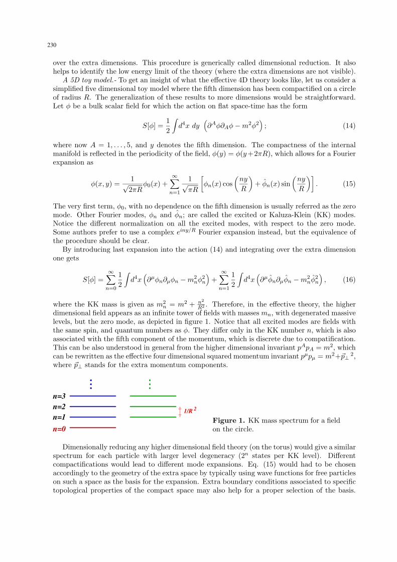
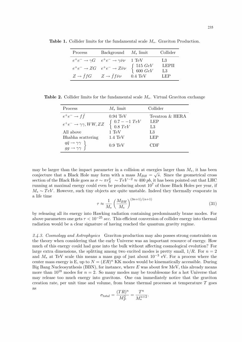
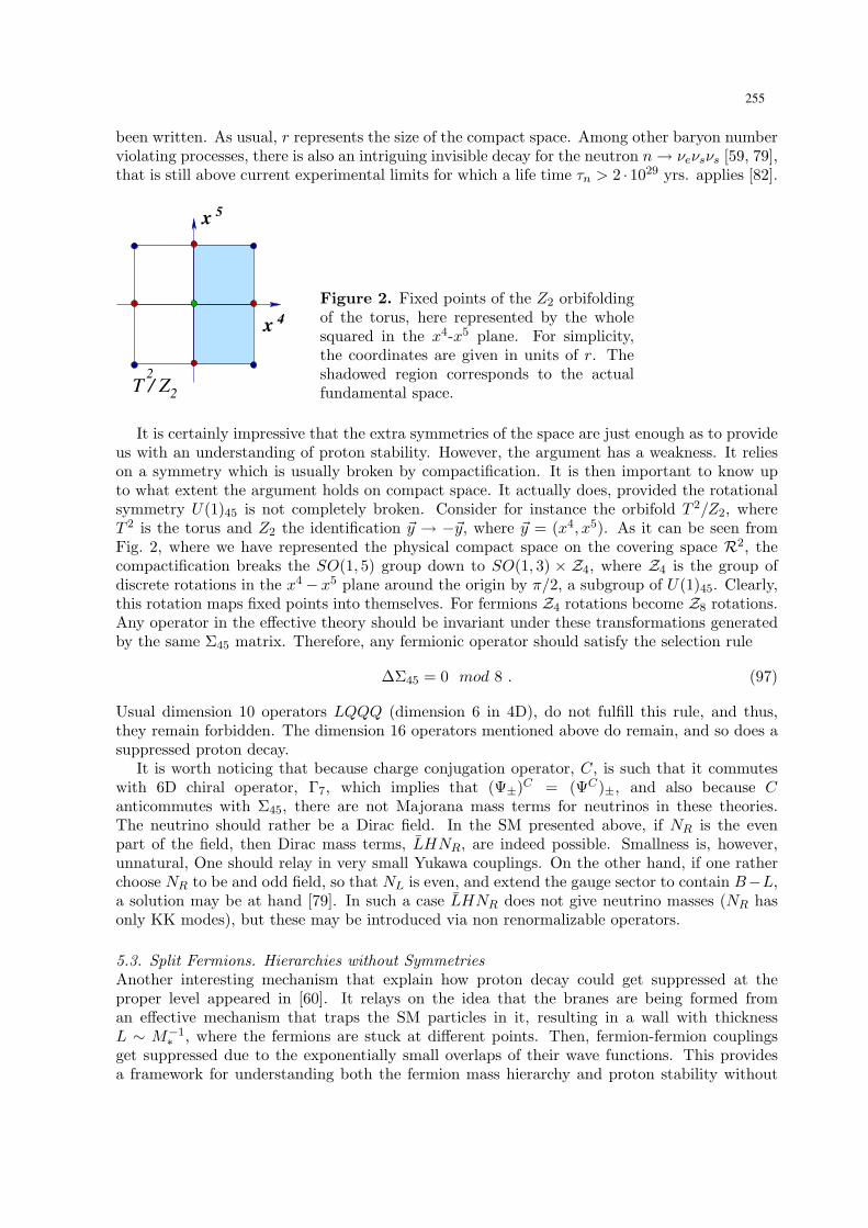