an introduction to dynamic universe model

Gupta S N P IJSRR 2013, 2(1) Suppl., 203-226

IJSRR 2013, 2(1) Special Issue April-May 2013 Page 203

Research article Available online www.ijsrr.org ISSN: 2279-0543

International Journal of Scientific Research and Reviews

An Introduction to Dynamic Universe Model Gupta S N P

AGM (ERP&MES) Bhilai Steel Plant, Bhilai , 490001, (CG) INDIA

ABSTRACT: This is solution for N-body problem without singularities and collisions using only Newtonian Physics. Here all bodies move and keep themselves in dynamic equilibrium with all other bodies depending on their present positions, velocities and masses. This model provides solution to problems, like Missing mass in Galaxies, Blue & red shifted Galaxies co-existence, Pioneer anomaly, New-horizons satellite trajectory calculations etc. Non collapsing large-scale mass structures formed when non-uniform density distributions of masses were used. This model explains the force behind expansion of universe and explains the large voids and non-uniform matter densities in universe. There are no Blackholes and Bigbang in this mathematical Model.

*Corresponding Author:- S N P GUPTA AGM (ERP&MES) Bhilai Steel Plant, Bhilai , 490001, (CG) INDIA E Mail - [email protected]


IJSRR 2013, 2(1) Special Issue April-May 2013 04

INTRODUCTION: Dynamic Universe Model is a totally non-general relativistic algorithm. Here in no way

General Relativistic (GR) effects, are taken into consideration and this model doesn’t reduce to GR on

any condition. There is no space-time continuum. In this Dynamic Universe Model all the bodies in

Universe are assumed to be dynamically moving.

This Dynamic Universe Model is a set of MATH equations for solving N-body problem. With SITA

software it behaves like a hand held Calculator. SITA software in a PC will work like a Calculator for

solving a typical N-body problem. Using the same set of equations one can give different initial values

numerically to solve various different problems at different scales. These initial values (the Cartesian x,

y, z positions and velocities & time step) are different for different applications. The distant Galaxies or

distant local systems can be assumed as point masses with mass at their center of Gravity. That way the

number of masses can be as low as 133 and otherwise this simulation can be done on higher number of

masses also.

There are many secrets embedded in the Universe that are still unexplored. A simple uniform law may

not explain all the peculiarities in the ever changing Dynamic universe. In fact, the uniform density is

not observable at any scale because of large Voids and Great walls present in the Universe. Earth is not

the center of universe. Our universe is finite. The view from earth is not being uniform in all the

directions.

In this Dynamic Universe Model, bodies move in dynamic equilibrium to compensate for the

continuous Gravitational attractions. Rotational Centrifugal forces are sufficient for compensating

gravitational attraction forces. No additional repulsive forces like “Einstein’s ” are necessary. No

symmetries were assumed. Our universe is not a Newtonian type static universe. Ours is not a

contracting universe. It is an expanding universe with blue shifted galaxies present in it. It is not

infinite but it is a closed finite universe. There are many images, sometimes more than one for each

Galaxy. Our universe is neither isotropic nor homogeneous. It is LUMPY. But it is not empty. It may

not hold an infinite sink at the infinity to hold all the energy that is escaped. This is closed universe and

no energy will go out of it. Ours is not a steady state universe in the sense, it does not require matter

generation through empty spaces. No starting point of time is required. Time and spatial coordinates



can be chosen as required. No imaginary time, perpendicular to normal time axis, is required. No baby

universes, black holes or warm holes were built in.

Earlier authors like Chandrasekhar3 developed energy tensor. Dynamic Universe Model uses Virial

theorem and uses a new type of tensor mathematics without any differential equations for solving an

age old N-body problem. This new method developed has its application into cosmological problems

also. The co-existence of Blue shifted Galaxies is one of such an application.

There is a fundamental difference between ‘galaxies / systems of galaxies’ and ‘systems that normally

use statistical mechanics’, such as molecules in a box. The molecules repel each other. However, in

gravitation we have not yet experienced any repulsive forces. (See for ref: Binny and Tremaine

(1987))1. Only attraction forces were seen. Einstein introduced cosmological constant to introduce

repulsive forces at large scales like inter galactic distances in his General relativity based cosmological

considerations in for expanding universe (1917)2. Many people did not like , and this created

turbulence in the scientific world. One of the reasons for his cosmological constant is that he disliked

the picture at infinity given by Newtonian gravitation. Though his ideas were good, the path chosen by

him was rough and turbulent. Almost every worker faced / scientist in this field either faced problems

conceptually or mathematically with Bigbang based cosmologies. Singularities were big hurdles for

many of us.

This Dynamic Universe Model can be used not only for cosmological models, but also for exact

prediction of trajectories of satellites by considering gravitation effects of various Planets and moons in

solar system.

MATHEMATICAL BACKGROUND: Let us assume an inhomogeneous and anisotropic set of N point masses moving under mutual

gravitation as a system and these point masses are also under the gravitational influence of other

additional systems with a different number of point masses in these different additional systems. For a

broader perspective see the author’s work3, let us call this set of all the systems of point masses as an

Ensemble. Let us further assume that there are many Ensembles each consisting of a different number

of systems with different number of point masses. Similarly, let us further call a group of Ensembles



as Aggregate. Let us further define a Conglomeration as a set of Aggregates and let a further higher

system have a number of conglomerations and so on and so forth.

Initially, let us assume a set of N mutually gravitating point masses in a system under Newtonian

Gravitation. Let the thpoint mass has mass m, and is in position x. In addition to the mutual

gravitational force, there exists an external ext, due to other systems, ensembles, aggregates, and

conglomerations etc., which also influence the total force F acting on the point mass . In this case,

the ext is not a constant universal Gravitational field but it is the total vectorial sum of fields at xdue

to all the external to its system bodies and with that configuration at that moment of time, external to its

system of N point masses.

Total Mass of system =

N

mM1

(1)

Total force on the point mass is F , Let F is the gravitational force on the thpoint mass due to

thpoint mass.

)(1

ext

N

mFF

(2)

Moment of inertia tensor

Consider a system of N point masses with mass m, at positions X, =1, 2,…N; The moment of

inertia tensor is in external back ground field ext.

kj

N

jk xxmI

1 (3)

Its second derivative is

kjkj

N

kjjk xxxxxxm

dtId .

12

2

(4)

The total force acting on the point mass is and F^

is the unit vector of force at that place of that

component.

mxx

xxmGmxmF jext

Njj

jj

F,

13

^

(5)



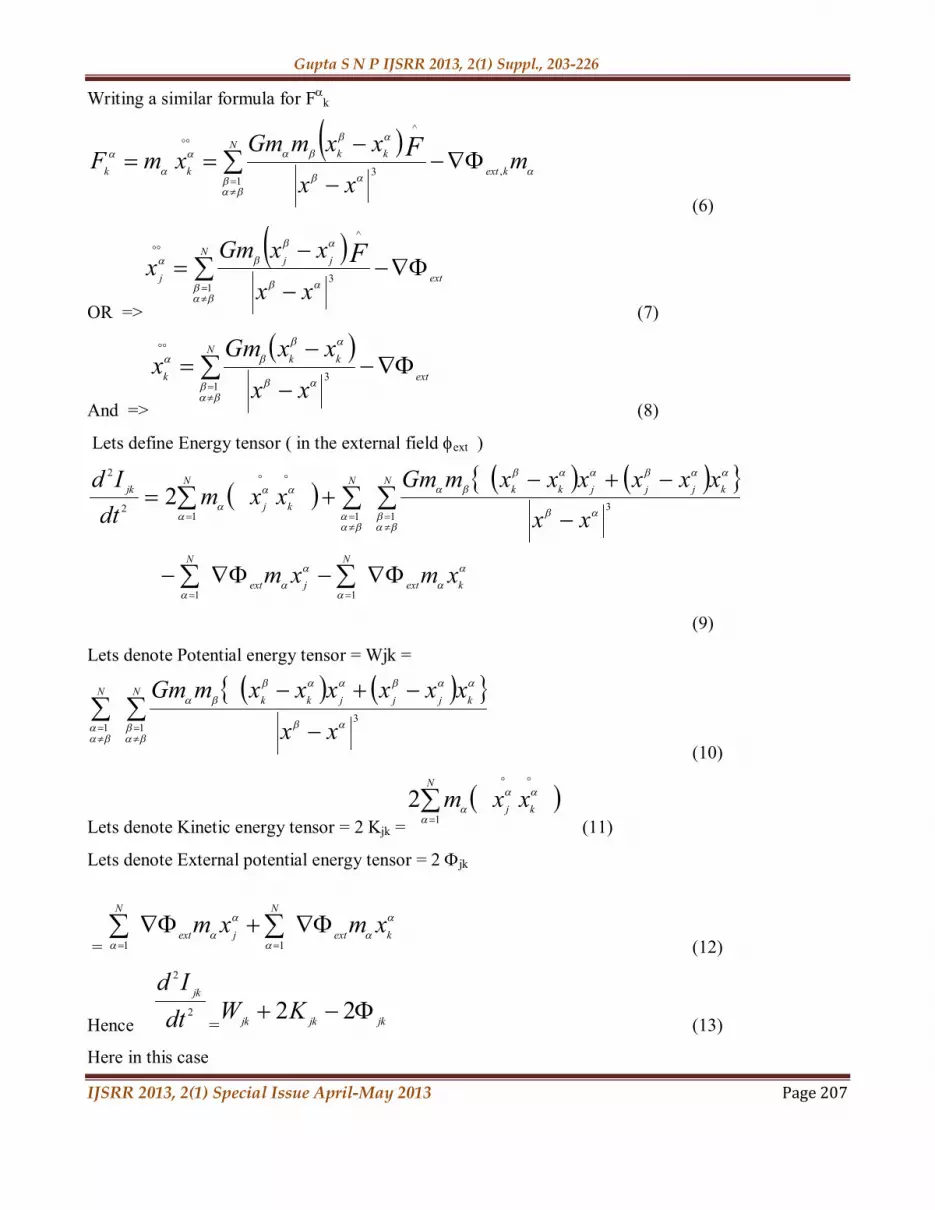
Writing a similar formula for Fk

mxx

xxmGmxmF kext

Nkk

kk

F,

13

^

(6)

OR =>

ext

Njj

jxx

xxGmx F

13

^

(7)

And =>

ext

Nkk

kxx

xxGmx

13

(8)

Lets define Energy tensor ( in the external field ext )

kext

N

jext

N

Nkjjjkk

N

kj

Njk

xmxm

xxxxxxxxmGm

xxmdt

Id

11

13

112

2

2

(9)

Lets denote Potential energy tensor = Wjk =

Nkjjjkk

N

xx

xxxxxxmGm

1

31

(10)

Lets denote Kinetic energy tensor = 2 Kjk =

kj

N

xxm1

2 (11)

Lets denote External potential energy tensor = 2 jk

=

kext

N

jext

N

xmxm 11 (12)

Hence 2

2

dtId jk

= jkjkjk KW 22 (13)

Here in this case



mxx

xxmGm

mFF

ext

N

ext

N

13

1

(14)

=

mx ext

int (15)

ext

N

xx

xxGmx

1

3

(16)

We know that the total force at totFx mtot

Total PE at dxFm tottot

dxmmx ext

N

int1

dxmdx

xx

xxmGmext

N

1

3

(17)

Therefore total Gravitational potential tot (α) at x (α) per unit mass

N

exttotxx

Gm

1

(18-s)

Lets discuss the properties of ext :-

ext can be subdivided into 3 parts mainly

ext due to higher level system, ext -due to lower level system, ext due to present level. [ Level : when

we are considering point mass in the same system (Galaxy) it is same level, higher level is cluster of

galaxies, and lower level is planets & asteroids].

ext due to lower levels : If the lower level is existing, at the lower level of the system under

consideration, then its own level was considered by system equations. If this lower level exists



anywhere outside of the system, center of (mass) gravity outside systems (Galaxies) will act as unit its

own internal lower level practically will be considered into calculations. Hence consideration of any

lower level is not necessary.

SYSTEM – ENSEMBLE:

Until now we have considered the system level equations and the meaning of ext. Now let’s

consider an ENSEMBLE of system consisting of N1, N2 … Nj point masses in each. These systems are

moving in the ensemble due to mutual gravitation between them. For example, each system is a

Galaxy, and then ensemble represents a local group. Suppose number of Galaxies is j, Galaxies are

systems with point masss N1, N2 ….NJ, we will consider ext as discussed above. That is we will

consider the effect of only higher level system like external Galaxies as a whole, or external local

groups as a whole.

Ensemble Equations (Ensemble consists of many systems)

2

2

dtId jk

=

jkjkjk KW 22 (18-E)

Here γ denotes Ensemble.

This γjk is the external field produced at system level. And for system

2

2

dtId jk

= jkjkjk KW 22 (13)

Assume ensemble in a isolated place. Gravitational potential ext()produced at system level is

produced by Ensemble and γ ext() = 0 as ensemble is in a isolated place.

N

exttotxx

Gm1

(19)

There fore

N

exttotxx

Gm1

(20)



And jk2 = -

2

2

dtId jk

+ jkjk KW 2 (13)

kext

N

jext

N

xmxm 11 (21)

AGGREGATE Equations(Aggregate consists of many Ensembles )

2

2

dtId jk

=

jkjkjk KW 22 (18-A)

Here δ denotes Aggregate.

This δγjk is the external field produced at Ensemble level. And for Ensemble

2

2

dtId jk

=

jkjkjk KW 22 (18-E)

Assume Aggregate in an isolated place. Gravitational potential ext () produced at Ensemble level is

produced by Aggregate and δγ ext() = 0 as Aggregate is in a isolated place.

N

exttotxx

Gm1

(22)

Therefore

N

EnsembleextAggregatetotxx

Gm1

(23)

And

kext

N

jext

N

jk xmxm 11 (24)

Total AGGREGATE Equations :( Aggregate consists of many Ensembles and systems)

Assuming these forces are conservative, we can find the resultant force by adding separate forces

vectorially from equations (20) and (23).



N N

extxx

Gm

xx

Gm1 1

(25)

This concept can be extended to still higher levels in a similar way.

Corollary 1:

2

2

dtId jk

= jkjkjk KW 22 (13)

The above equation becomes scalar Virial theorem in the absence of external field, that is =0 and in

steady state,

i.e. 2

2

dtId jk

=0 (27)

2K+ W = 0 (28)

But when the N-bodies are moving under the influence of mutual gravitation without external field

then only the above equation (28) is applicable.

Corollary 2:

Ensemble achieved a steady state,

i.e. 2

2

dtId jk

= 0 (29)

jkjkjk KW 22 (30)

This jk external field produced at system level. Ensemble achieved a steady state; means system also

reached steady state.

i.e. 2

2

dtId jk

=0 (27)

jkjkjk KW 22 (31)



The Equation 25 is the main powerful equation, which gives many results that are not possible

otherwise today. This tensor can be subdivided into 21000 small equations without any differential

equations or integral equations. Hence, this set up gives a unique solution of Cartesian X, Y, Z

components of coordinates, velocities and accelerations of each point mass in the setup for that

particular instant of time. A point to be noted here is that the Dynamic Universe Model never reduces

to General relativity on any condition. It uses a different type of mathematics based on Newtonian

physics. This mathematics used here is simple and straightforward. All the mathematics and the Excel

based software details are explained in the three books published by the author14, 15, 16 In the first book,

the solution to N-body problem-called Dynamic Universe Model (SITA) is presented; which is

singularity-free, inter-body collision free and dynamically stable. This is the Basic Theory of Dynamic

Universe Model published in 2010 14. The second book in the series describes the SITA software in

EXCEL emphasizing the singularity free portions. It explains more than 21,000 different equations

(2011)15. The third book describes the SITA software in EXCEL in the accompanying CD / DVD

emphasizing mainly HANDS ON usage of a simplified version in an easy way. The third book contains

explanation for 3000 equations instead of earlier 21000 (2011)16.

INITIAL CONDITIONS FOR DYNAMIC UNIVERSE MODEL Now lets discuss supporting observations for initial conditions based on Anisotropy and heterogeneity

of Universe:

Our galaxy the Milky way is moving with a speed 454 ± 125 km/sec towards l=63 ± 15° and b=-11 ±

14°relative to distant part of samples and 474 ± 164 km/sec towards l=167 ± 20° and b=5 ±

20°relative to nearer part of samples. (JV.Narlikar, (1983)4). The local group comprising of Milky way,

NGC6822, Andromida galaxy and other dwarf elliptical galaxies, Magellanic clouds rotate about their

centers and revolve around a common center. S.M.Faber and David Burstain (1988)5 described the

STREEMING motions towards the Great Attractor (located at l =309 and b=+18) by the local

group, Virgo cluster, Ursa major, Centaurus, Camelopardalis, Perseus-Pisces etc ., clusters with speeds

ranging up to 1000km/sec. Please notice the difference in directions of movement as well as speeds.

All these clusters form a super cluster which also rotate and revolve about each other. Groups of super

clusters form Filament structures and to grate walls and so on. This is how our universe is lumpy and

anisotropic even at large scale.



Another piece of supporting evidence for the Dynamic Universe Model is here. There is a considerable

discussion, as to whether GA: the Great attractor exists at all. For example D.A. Mathewson, V.L.

Ford, and M. Buckhorn6 have measured the peculiar velocities 1355 spiral Galaxies. They find no

backside in fall into GA region, rather a bulk flow of about 400 km/sec on the scales of 100 ho-1 MPC.

Thus there is a considerable doubt about the existing of an attracting mass there. Both the parties find

streaming motions or bulk flow. If there is no attracting mass, then why they are moving? This super

cluster must be in revolution motion.

Birch (1982)7, has discovered the asymmetric distribution of the angles of rotation of polarization

vectors of 132 radio sources and tried to explain this via the Global rotation. We think that the

asymmetric distribution of the angles of rotation of polarization vectors, is due to the galaxies or parts

of clusters revolving in different directions.

Our universe is not having a uniform mass distribution. Isotropy & homogeneity in mass distribution

is not observable at any scale. We can see present day observations in ‘2dFGRS survey’ publications

for detailed surveys especially by Colless et al in MNRAS (2001)8 for their famous DTFE mappings,

where we can see the density variations and large-scale structures. The universe is lumpy as you can

see in the picture given here in Wikipedia.

The universe is lumpy as you can see the voids and structures in the picture given by Fairall et al

(1990)9 and in Wikipedia for a better picture. WMAP also detected cold spot see the report given by

Cruz et al (2005)10. They say ‘A cold spot at (b = -57, l = 209) is found to be the source of this non-

Gaussian signature’ which is approximately 5 degree radius and 500 million light years. This is closely

related with Lawrence Rudnick et al’s (2007)11 work, which says that there are no radio sources even in

a larger area, centered with WMAP cold spot. It is generally known as ‘Great void’, which is of the

order of 1 billion light years wide; where nothing is seen. They saw…” little or no radio sources in a

volume that is about 280 mega-parsecs or nearly a billion light years in diameter. The lack of radio

sources means that there are no galaxies or clusters in that volume, and the fact that the CMB is cold

there suggests the region lacks dark matter, too. There are other big voids also upto 80 mpc found

earlier which are optical.”



There is the Sloan Great Wall, the largest known structure, a giant wall of galaxies as given by J. R.

Gott III et al., (2005)12 ‘Logarithmic Maps of the Universe’. They say “The wall measures 1.37 billion

light years in length and is located approximately one billion light-years from Earth….The Sloan Great

Wall is nearly three times longer than the Great Wall of galaxies, the previous record-holder”.

. Hence such types of observations indicate that our Universe is lumpy. After seeing all these we can

say that uniform density as prevalent in Bigbang based cosmologies is not a valid assumption. Hence,

in this paper we have taken the mass of moon as moon & Galaxy as Galaxy employing non uniform

mass densities.

We can use Galactic dynamics say up to 30kpc (radius of the Milky-way) without any problem. But

just after 30kpc General relativity comes into picture. Why? We are using Galactic dynamics for

finding out missing mass of the universe as required for General relativity, without using General

relativistic effects. Everybody accepts this. But if it is a nearby galaxy named NGC6822, which is at a

center-to-center distance of 48kpc from Milkyway, then General relativity comes into picture. We have

to use some General relativistic models like Friedmann-Robertson-Walker13 model, why? Just after the

boundaries of Milkyway? Why can’t we use Galactic dynamic models and equations extended further

to inter galactic forces also?

Here in this model the present measured CMB is from stars, galaxies and other astronomical bodies.

We know that the CMB isotropy is not entirely due to Galaxies. Nevertheless, there are other factors

also. The stars and other astronomical bodies also contribute for CMB. Moreover, factors like

Scattering of rays done by ISM and sidelobe gains & backlobe gains of Microwave dish antenna cannot

be excluded they are not less. There are CMB cold spots, where nothing is seen. Observed anisotropies

of CMB are in the order of 1 to 20 in million, whereas the anisotropies of in large scale structures are

coming up to 7% in the observational scales.

RESULTS: This Dynamic Universe Model approach solves many unsolved problems. In this proposal I want to

submit the Following paper subjects for Dynamic Universe Model. Only differences used between the

various simulations are in the initial values & the time steps. The structure of masses is different. In the

first 2 cases, approximate values of masses and distances were used. In the third and fourth case, real



values of masses and distances for a close approximation were used. Some of the output graphs or

output tables for some select results are shown with a brief explanation further below in this section.

1. Galaxy Disk formation using Dynamic Universe Model (Dense mass) Equations

2. Solution to Missing mass in Galaxies: It proves that there is no missing mass in Galaxy due to

circular velocity curves No Dark matter is required + Poster presented in (COSPAR12)

3. Withstands 105 (One Hundred Thousand) times the Normal Jeans5 swindle test

4. Blue shifted and red shifted Galaxies co-existence… Explaining the Existence of large number of

blue shifted Galaxies, Prediction of Blue shifted Galaxies, initial values you can see in the paper

DSR894, Submitted in 20041.

5. Explains gravity disturbances like Pioneer anomaly.

6. Proving Dynamic Universe Model is singularity free and collision free in the first book ‘Dynamic

Universe Model: A singularity-free N-body problem solution [ISBN 978-3-639-29436-1]’

7. New revised paper on Dynamic universe model for co-existence red and blue shifted Galaxies in the

Universe , Showing quasars are blue shifted Galaxies

8. Predicts the trajectory of New Horizons satellite and its trajectory initial values can be seen Book

‘Dynamic Universe Model: A singularity-free N-body problem solution [ISBN 978-3-639-29436-1]

(COSPAR 12).’

9. Working software file containing full set of all 21000 equations in EXCEL. All these equations are

explained in Book 2

10. Effect of Universal Gravitational Force on Radio photon explains Very Long Baseline

Interferometry Observations (COSPAR 12)

RESULT 1: GALAXY DISK FORMATION

In this experiment, point masses were kept in Cartesian three-dimensional random positions as shown

in Fig 1. They were allowed to move under their own gravitation. They form a disk shape as shown in

Fig 2.



Figure 1

Figure 2

RESULT 2: MISSING MASS IN GALAXIES:

Now for the second result, SITA simulations for Dynamic Universe Model were used to find out

theoretical star circular velocity curves in a Galaxy (star circular velocity verses star distance from the

center of galaxy). There is a usual conceptual mistake: Newtonian Gravitation or Einstein’s General

theory of Relativity treated the Multi-body dynamical problem as a single body static problem.

In Bigbang cosmologies, theoretical star circular velocities in a Galaxy are predicted as shown in the

left of Pic 1. The observed rotation curves are shown on the right side of same picture. They use

spectroscopic 21-cm maps of neutral hydrogen for finding the rotation curve of the Galaxy, which stays



flat out to large distances, instead of falling off as in the Pic 1. Does this mean that the mass of the

Galaxy increases with increasing distance from the center, as said by Bigbang?

No, Dynamic universe Model explains this phenomenon. Because of the dynamism of the point masses

(stars) after some radial distance from the centre of the Galaxy under observation, appear to have

achieved some higher velocities, when there is gravitational effect of huge (self) Galaxy center-mass

called densemass and the gravitational effect of external Galaxies acting on the stars, when both

gravitational effects are simultaneously present. This condition is clearly indicated in the fallowing

graph table below.

Pic 1 Missing Mass in Galaxies: The theoretical star circular velocities in a Galaxy are predicted as

shown in the left of Pic 1. The observed rotation curves are shown on the right side of same picture.



Graph Table : Theoretical Galaxy Circular Vel vs radius Graphs in different cases with start end of 100 iterations positions Case Starting positions End of 100

iterations Velocity vs Gal Radius

1 Case 1 : From starting positions to positions after 100 iterations showing disk formation and velocities achieved graph. This is with a Huge central mass at the center of galaxy, sun like stars and external galaxies xy, zx position graphs.

2 Case 2 : From starting positions to positions after 100 iterations showing disk formation and velocities achieved graph. This is without a Huge central mass at the center of galaxy, sun like stars and external galaxies xy, zx position graphs.

3 Case 3 : From starting positions to positions after 100 iterations showing disk formation and velocities achieved graph. This is wih a

Star t Galaxy xy

0

2 E+2 0

4 E+2 0

6 E+2 0

8 E+2 0

1 E+2 1

1. 2 E+2 1

0 2 E+2 0 4 E +2 0 6 E+2 0 8 E+2 0 1E +2 1 1. 2 E +2 1

New galaxy xy(100)

0

5E+21

1E+22

2E+22

2E+22

3E+22

3E+22

4E+22

4E+22

5E+22

5E+22

0 1E+22 2E+22 3E+22 4E+22 5E+22 6E+22

Dist-Vel-Galaxy cg

1.00 E+0 0

1.00 E+0 1

1.00 E+0 2

1.00 E+0 3

1.00 E+0 4

1.00 E+0 5

1.00 E+0 6

1.00 E+0 7

1.00 E+0 8

1.00 E+0 9

1.00 E+1 0

1.00 E+1 1

1.00 E+1 2

1.00 E+1 3

0 5E +21 1E+2 2 1.5E +22 2 E+2 2 2.5E +22 3 E+22 3 .5E +22

Start Galaxy xy

0

2 E+20

4 E+20

6 E+20

8 E+20

1E+21

1. 2 E+21

0 2E +2 0 4E +2 0 6E +2 0 8E +2 0 1E +2 1 1. 2 E+21

New galaxy xy(100)

1.02E+22

1.04E+22

1.06E+22

1.08E+22

1.1E+22

1.12E+22

1.14E+22

7.4E+21 7.6E+21 7.8E+21 8E+21 8.2E+21 8.4E+21 8.6E+21

Dist-Vel-Galaxy cg

1.00E +00

1.00E +01

1.00E +02

1.00E +03

1.00E +04

1.00E +05

1.00E +06

1.00E +07

1.00E +08

1.00E +09

1.00E +10

1.00E +11

1.00E +12

1.00E +13

0 2E+2 0 4E+20 6E+20 8 E+20 1 E+21 1.2E +21

Start Galaxy xy

0

2 E+20

4 E+20

6 E+20

8 E+20

1E +21

1. 2E +21

0 2 E +20 4E +2 0 6 E+20 8E +2 0 1E+2 1 1. 2E +2 1

New galaxy xy(100)

- 5E+22

0

5E+22

1E+23

1.5E+23

2E+23

-8E+22 - 6E+22 -4E+22 -2E+22 0 2E+22 4E+22 6E+22 8E+22 1E+23

Dist-Vel-Galaxy cg

1.00E +00

1.00E +01

1.00E +02

1.00E +03

1.00E +04

1.00E +05

0 5 E+22 1E+2 3 1.5 E+23 2E+23 2.5E +23



Huge central mass at the center of galaxy, sun like stars and no external galaxies xy, zx position graphs.

4 Case 4: From starting positions to positions after 100 iterations showing no disk formation and velocities achieved graph. This is wihout a Huge central mass at the center of galaxy, sun like stars and no external galaxies xy, zx position graphs.

5 Case 5: Theoretical star circular velocity curves in a Galaxy (star circular velocity verses star distance from the center of galaxy) in gravitationally stabilized system of masses after forming a galaxy disk when it’s stability analysis was done by giving perturbations and jeans swindle test

Graph Table: Missing Mass in Galaxies: In Cases 1,2,3 & 4 show cases with and without central

mass and / or external galaxies. We can see clearly external Galaxies and Central mass in Galaxy is

Start Galaxy xy

0

2 E+2 0

4 E+2 0

6 E+2 0

8 E+2 0

1E+21

1. 2 E+21

0 2 E+20 4 E+2 0 6E +2 0 8 E+20 1E+2 1 1. 2 E+21

New galaxy xy(100)

- 1.5E+21

- 1E+21

- 5E+20

0

5E+20

1E+21

1.5E+21

2E+21

2.5E+21

-1.5E+21 -1E+21 -5E+20 0 5E+20 1E+21 1.5E+21 2E+21 2.5E+21

Dist-Vel-all

1 .00E +00

1 .00E +01

1 .00E +02

1 .00E +03

1E +19 1E+20 1E+2 1 1 E+22

Dist-Vel-Galaxy cg

1.0 0E+25

1.0 0E+26

1.0 0E+27

1.0 0E+28

0 1 E+42 2E+42 3E+4 2 4E +42 5E +42 6E+42 7E+42 8E+42 9E +42

Start Galaxy xy

-4 E+20

-3 E+20

-2 E+20

-1E+2 0

0

1E+20

2 E+20

3 E+20

4 E+20

5 E+20

-4E +2 0 - 3E +20 -2 E+20 -1E+20 0 1E +20 2 E+20 3 E+2 0 4E +2 0

New galaxy xy(100)

-4E+43

-3.5E+43

-3E+43

-2.5E+43

-2E+43

- 1.5E+43

- 1E+43

-5E+42

- 3.71382E+27-4E+42 -2E+42 0 2E+42 4E+42 6E+42 8E+42 1E+43



required as dist velocity curves are near to actual observational results. These N-body calculations and

results are showing theoretical star circular velocity curves. Do the Galaxies have to be assumed to

have some missing mass? Is that required?

RESULT 4: BLUE SHIFTED AND RED SHIFTED GALAXIES CO-EXISTENCE (2004)

In this dynamic universe model – Galaxies in a cluster are rotating and revolving. Depending on the

position of observer’s position relative to the set of galaxies. Some may appear to move away, and

some may appear to come near. The observer may also be residing in a solar system, revolving around

the center of Milky Way in a local group. He is observing the galaxies outside. Many times he can

observe only the coming near or going away component of the light ray called Hubble components.

The other direction cosines of the movement may not be possible to measure exactly in many cases.

-1.5E+25

-1E+25

-5E+24

0

5E+24

1E+25

-2E+25 -2E+25 -1E+25 -5E+24 0 5E+24 1E+25

Graph G8 represent the positions of all masses in this simulation, after four time-steps and seven time-

steps. We can see the formation of some three-dimensional circles clearly.



RESULT 7: BLUE SHIFTED AND RED SHIFTED GALAXIES CO-EXISTENCE (2012)

Here in this example (in this new simulation), in the above figure, graphs was with the name New

Ensemble xy. The ZX plots of positions of Globular Clusters and Galaxies approximately have the

mass of about 100 million to a billion or 1012 solar masses. All these are point masses for Galaxies of

normal sizes. The word ‘new’ in the name is an indicative word for the result of that particular

iteration in the simulation. The first iteration is the starting positions of the Galaxies in xy or zx plots.

From that with a time step of 3.15576E+16 seconds or one billion years is allowed for the free fall of

all the Galaxies. Next set of positions is shown in the iteration 1. After that is iteration 2 and so on. One

can see the rotations of these masses. In addition, the marked change of positions from iteration to

iteration when we look through the series of graphs.

In the particular graph shown above started from random positions in the beginning, now shows circle

formations and movement. This graph indicate all Galaxies are rotating about. This graph show to the

observer, some Galaxies are coming near and some are going away. Hence these galaxies are either red

shifted or blue shifted.

RESULT 8: TRAJECTORY OF NEW HORIZONS SATELLITE

In this paper the effect of Universal Gravitational Force is calculated on New Horizons Satellite, by

using a singularity free and collision free N-body problem solution called Dynamic Universe Model.

New Horizons is NASA’s artificial satellite now going towards to the dwarf planet Pluto. It has crossed

Jupiter. It is expected to be the first spacecraft to go near and study Pluto and its moons, Charon, Nix,

and Hydra. These are the predictions for New Horizons (NH) space craft as on A.D. 2009-Aug-09

00:00:00.0000 hrs. The behavior of NH is similar to Pioneer Space craft as NH traveling is alike to

Pioneer. NH is supposed to reach Pluto in 2015 AD. There was a gravity assist taken at Jupiter about a

year back. Exact details can be found at ref 22 [22]. As Dynamic universe model explains Pioneer



anomaly and the higher gravitational attraction forces experienced towards SUN, It can explain NH

also in a similar fashion.

Table 1: SITA Calculation sample OUTPUTS for NH( 1st row): after 220 iterations with 24hrs Time-

step

Mass

No.

u x ( b1)

velocity x

m/sec

u y (b2)

velocity y

m/sec

u z (b3)

velocity z

m/sec

s x (a1)

Position x

meters

Sy (a2)

Position y

meters

Sz (a3)

Position z

meters

1 5910.475287 -

15727.84869 602.0358627 1.31442E+11

-

2.10854E+12 60123860323

2 1515.491698 -

31300.09708

-

2695.918095

-

1.08644E+11

-

62585674556 4859539426

3 -

1828.169074 31741.76598 540.3752709 1.27107E+11 9429186696 -7205348169

4 21967.05386 17694.02539 -0.7613474 1.07025E+11 -

1.22802E+11 3983952.514

5 -

15140.39422 20071.13526 792.4411952 1.61332E+11 1.51712E+11

-

782015907.2

6 7997.051973 10844.24963 -

223.9644393 5.90358E+11

-

4.69402E+11

-

11262026007

7 -

1603.042402

-

9612.751852 230.898668

-

1.40105E+12 1.58683E+11 52994601955

8 661.9794762 6461.3927 15.46063671 2.99041E+12 -

3.09864E+11

-

39882635995

9 3101.241258 4483.443198 -

163.7665483 3.67452E+12

-

2.58398E+12

-

31471133568

10 5556.287859 -

819.2750731

-

1509.729058 1.74961E+11

-

4.71521E+12 4.54158E+11

11 22681.82274 16251.78272 18.70934883 1.04161E+11 -

1.30332E+11

-

135710382.3



12 2.209718569 -

3.110434811

-

0.033286597 17900665.41

-

28360265.62

-

205941.1773

13 -

0.002464296 0.000158851

-

0.001357868

-

3.07379E+16

-

2.48085E+16 5.99014E+15

14 -

0.051559836

-

0.032426184

-

0.023584373

-

1.70141E+16

-

4.49612E+13 3.79378E+16

15 0.039925529 0.028281984 0.017840304 -

1.71774E+16

-

1.53305E+14 3.78638E+16

16 -

0.002468035 0.000155086

-

0.001369146

-

1.85801E+15 1.6393E+15

-

5.61485E+16

17 -

0.002470093 0.000156481

-

0.001368848 9.02924E+15

-

7.13182E+15

-

7.77879E+16

RESULT 10: VLBI

Large variation in the Gravitational bending results of VLBI:

Very long baseline interferometry (VLBI) , in the field of Radio astronomical observations of

quasars, Galaxies etc

This variation is clearly visible when the solar gravitational bending / deflection angle is plotted

against Solar Elongation angle.

Here the capabilities of this Dynamic Universe Model are extended into micro world i.e. to light

photons and Radio wavelength photons and Neutrinos etc. By doing so a real world Very long baseline

interferometry (VLBI) observations are explained. The present day Physics considers gravitation

effects of only the main gravitating body, whereas Dynamic Universe Model considers the

Gravitational effect of Sun, Planets, Globular clusters, Milky-way, Local systems etc., and finds the

Universal gravitational force vector at that instant of time, for that configuration of the Universe.

Can the gravitational effect of Universe be neglected near Sun ?

Tide caused by Sun and Moon in oceans-- We observe high tide and low tide in the mornings

and evenings, or on full-moon-day and no-moon-day.

These tides are caused by gravitation of Sun and Moon only. So we can not neglect gravitation

effect of Sun and Moon on Earth.


IJSRR 2013, 2(1) Special Issue April-May 2013 4

For better accuracies we have to consider planets also….

The resulting bending angles shown in Figure 1.

-These points were falling into vertical lines, when plotted against Solar Elongation Angle.

-In GR, or direct Newtonian gravitation (classical) the resulting theoretical bending calculation

depends on the mass and radius of Sun.

-Hence result depends only on radius, but never on Solar Elongation Angle.

-Whereas Dynamic Universe Model considers Gravitational effect of Sun, Planets, Globular clusters,

Milky-way, Local systems etc., and finds the Universal gravitational force vector for that instant of

time for that configuration of the Universe on the Radio photon.

-Hence bending angle depends more on surrounding configuration and on relative position of Radio

photon in the solar system.

ACKNOWLEDGEMENTS:

Goddess Vak continuously guided this work. However, any mistakes came out due to improper

implementations / misunderstandings etc are totally mine. I am very much thankful to Prof. K. N.

Mishra, BHILAI for his constant persuasion to write this paper.



REFERENCES:

1. James Binny, Scott Tremaine in Galactic Dynamics 1987,Princeton Uty Press, Princeton New

Jersey, USA.

2. Einstein, A. 1911, “On the influence of Gravitation on the propagation of light”, Methuen and

company, 1923, Reprinted, Dover publications, 1952, New York, USA.

3. http://members.wap.org/kevin.parker/Densemass/VakPioneerAnom.doc

http://vaksdynamicuniversemodel.blogspot.in/p/cv.html

4. Jayant. V. Narlikar 1983, ‘Introduction to cosmology’, Cambridge University press, In India

Foundation books 2/19 Ansari Road, Daryaganj New Delhi-110002.

5. S.M.Faber and David Burstain (1988) in their paper “ Motions of galaxies in the neighborhood

of Local group “ {presented in a symposium,’ Large scale motions of universe’ Princeton

1988,p118}

6. D.A. Mathewson, V.L. Ford, and M. Buckhorn 1992, ApJ, 389, L5

7. Birch P. (1982), Nature 208, 451

8. F. Hoyle, MNRAS, 108,372(1948).

9. V.A. Korotky, Yu. N. Obukhov, (1996), In Gravity Particles and Space time- edited by P.

Pronin, and G. Sardanashvly, ( world Scientific, Singapore) p 142. also preprint gr-qc /

9604049.

10. S.W. Hawking, MNRAS 142, 129, (1969).

11. Einstein, A. 1916, “The foundation of General theory of relativity ”, Methuen and company,

1923, Reprinted, Dover publications, 1952, New York, USA.

12. Yu. N. Obukhov, GRG, 1992, Vol 24, No2 , Page 121

13. Friedmann-Robertson-Walker, L. Bergström, A. Goobar (2006), Cosmology and Particle

Astrophysics (2nd ed.),Sprint, p. 61, ISBN 3-540-32924-2

14. SNP.GUPTA, Book1. Dynamic Universe Model: A singularity-free N-body problem solution

[ISBN 978-3-639-29436-1]---2010 October----VDM Germany

https://www.morebooks.de/store/gb/book/dynamic-universe-model/isbn/978-3-639-29436-1

http://vaksdynamicuniversemodel.blogspot.in/p/books-published.html

15. SNP.GUPTA, Book2. Dynamic Universe Model: SITA singularity free software ---2011

March --- VDM n Germany, March- 2011, ISBN 978-3-639-33501-9,

https://www.morebooks.de/store/gb/book/dynamic-universe-model/isbn/978-3-639-33501-9



16. SNP.GUPTA, Book3. Dynamic Universe Model: SITA software simplified [ISBN 978-3-639-

36469-9]---Aug-2011----VDM Germany

https://www.morebooks.de/store/fr/book/dynamic-universe-model/isbn/978-3-639-36469-9 …---===xxxXxxx===----…

an introduction to dynamic universe model

Documents