an integrated collision prediction and avoidance scheme for mobile robots in non-stationary...

Automatica, Vol. 29, No. 2, pp. 309-322, 1993 0005-1098/93 $6.00 + 0.00 Printed in Great Britain. © 1993 Pergamon Press Ltd

An Integrated Collision Prediction and Avoidance Scheme for Mobile Robots in

Non-stationary Environments*

K. J. KYRIAKOPOULOSt and G. N. SARIDIS,

A scheme integrating simple and fast collision prediction and a reactive type (feedback solution) o f avoidance for mobile robots in environments containing moving obstacles is computationally efficient and appropriate for real time implementation.

Key Words--Mobile robots; motion planning; collision prediction; collision avoidance; potential functions; Lyapunov stability.

Al~t rae t - -A formulation that makes possible the integration of collision prediction and avoidance stages for mobile robots moving in general terrains containing moving obstacles is presented. A dynamic model of the mobile robot and the dynamic constraints are derived. Collision avoidance is guaranteed if the distance between the robot and a moving obstacle is nonzero. A nominal trajectory is assumed to be known from off-line planning. The main idea is to change the velocity along the nominal trajectory so that collisions are avoided. A feedback control is developed and local asymptotic stability is proved if the velocity of the moving obstacle is bounded. Furthermore, a solution to the problem of inverse dynamics for the mobile robot is given. Simulation results verify the value of the proposed strategy.

1. INTRODUCTION

THE PROBLEM OF efficiently planning the motion of a mobile robot in an environment containing moving obstacles (Fig. 1) is difficult and computationally intensive. Although it has been stated as early as 1984 (Freund and Hoyer, 1984) ad hoc solutions were given (Liu et al. (1989); Tournassoud (1986)). Reif and Sharir (1985) gave an algorithmic solution to the problem but they were restricted to some categories of shapes of objects and their approach is not suitable for an on-line implementation. Search based ap- proaches for solving the above problem have also been presented in Fujimura and Samet (1990) and Shih et al. (1990). On the other hand,

* Received 1 October 1991; revised 11 April 1992; received in final form 9 June 1992. The original version of this paper was not presented at any IFAC meeting. This paper was recommended for publication in revised form by Editor A. P. Sage.

t New York State Center for Advanced Technology in Automation and Robotics, Rensselaer Polytechnic Institute Troy, NY 12180-3590, U.S.A.

~t NASA Center of Intelligent Robotic Systems for Space Exploration, Rensselaer Polytechnic Institute, Troy, NY 12180-3590, U.S.A.

309

Kant and Zucker (1984, 1986, 1988) used the decomposition of the motion planning problem to the find-path, and move-along-path problems. Their proposal is that the avoidance of moving obstacles can be done by adjusting the speed along the geometric path. The same approach was adopted in Wu and Jou (1988) and in Griswold and Eem (1990). The basic idea of this approach is utilized in this work.

To facilitate a fast solution a hierarchical decomposition has been proposed Kant and Zucker (1988) and adopted and extended in our work. The problem is divided as follows.

• Off-line path and motion planning. • On-line motion replanning.

In the off-line stage, two problems are solved; First, path planning, the "find path" problem, i.e. the search for a connected curve r(s)= [x(s)y(s)z(s)] r on the terrain described by a surface g(x, y, z ) = 0; s is the trajectory parametrization variable (e.g. path length). The path should connect the initial and target points without colliding with the stationary objects while satisfying certain criteria. Second, motion planning, that is to find a "nominal" motion function sn(t) along this path that does not violate the kinematic and dynamic constraints of the robot, and some performance criterion (e.g. time) is minimized.

The subject of this paper is the development of an algorithm for the on-line stage. This algorithm has to act in a supervisory mode during motion execution and make sure that the robot is going to move from its current state (position So, velocity Vo) to the target one

310 K . J . KYRIAKOPOULOS and G. N. SARID1S

~ r(s)

/ / / , I Mo .o / R o b o t , ^ ,

'- . . . . . . 2 M o v m g Obs t ac l e

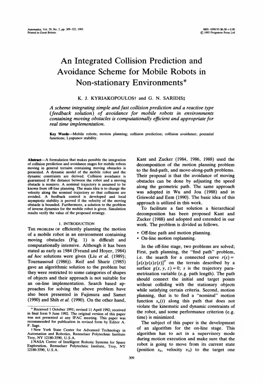
FIG. 1. Environment with a mobile robot and multiple moving obstacles.

(position s I, velocity vl) avoiding collisions with those moving obstacles with which collision is predicted based on sensory input. The basic idea is to alter the velocity along the path r(s) without changing its geometry. This is useful only if the following fundamental assumption is satisfied:

Temporary obstruction assumption. The mobile robot moving along path r(s) can only be obstructed during a bounded amount of time, i.e. the moving object is assumed not to permanently stay on, or move parallel to r(s).

The new plan must satisfy the dynamic constraints and stay as close as possible to the nominal plan.

In our prior developments the objects were modeled as convex polyhedra and based on this assumption an approach to predict collisions (Kyriakopoulos and Saridis (1990a, 1992a)) was developed. For the case of a planar terrains a real time collision avoidance scheme, the Minimum Interference Strategy (MIS) and the Optimal Control Strategy (OCS) (Kyriakopoulos and Saridis (1990b, 1991, 1992b)), have been proposed. There, in addition to collision avoidance, time consistency with the nominal plan was sought.

In this paper the potential fields strategy (PFS) is presented. Potential fields were originally introduced by Khatib (1985) and furthermore

investigated by Rimon and Koditschek (1989) and applied for mobile robots by Kant and Zucker. It is a computationally inexpensive but local method providing only collision avoidance capabilities while performance is not guaranteed.

Here, a reformulation of the potential fields approach is attempted, so that performance as well as collision avoidance are sought without significantly increasing the computational load. Performance is expressed in terms of proximity of the final time of the new plan to the final time of the off-line plan. Performance is achieved by the following.

• Introducing a simple collision prediction stage in order to determine if action should be taken.

• Utilizing the information of the nominal plan.

In Section 2 the definitions, modeling and the mathematical problem are stated. The theoreti- cal analysis and the presentation of the Potential Fields Strategy (PFS) is done in Section 3. Finally, in Sections 4 and 5 simulation results and suggestions for future research are presented, respectively.

2. PROBLEM FORMULATION The mobile robot is a kinematic mechanism

composed of the body and the rolling wheels. Its kinematics and dynamics can be modeled based on the necessary assumption that the wheels are

Mobile robot collision prediction and avoidance 311

Pz

C = C.

, ,,,~-~ \S(t)

Wheel 'T ' \ / ~ Wheel "j"

"-.. ....: "'. Trajectory J . ....."

""'" ...'" pB

. -""" "" MOBILE ROBOT . . - - " p

. . . . . . " ~ O ( s ) x

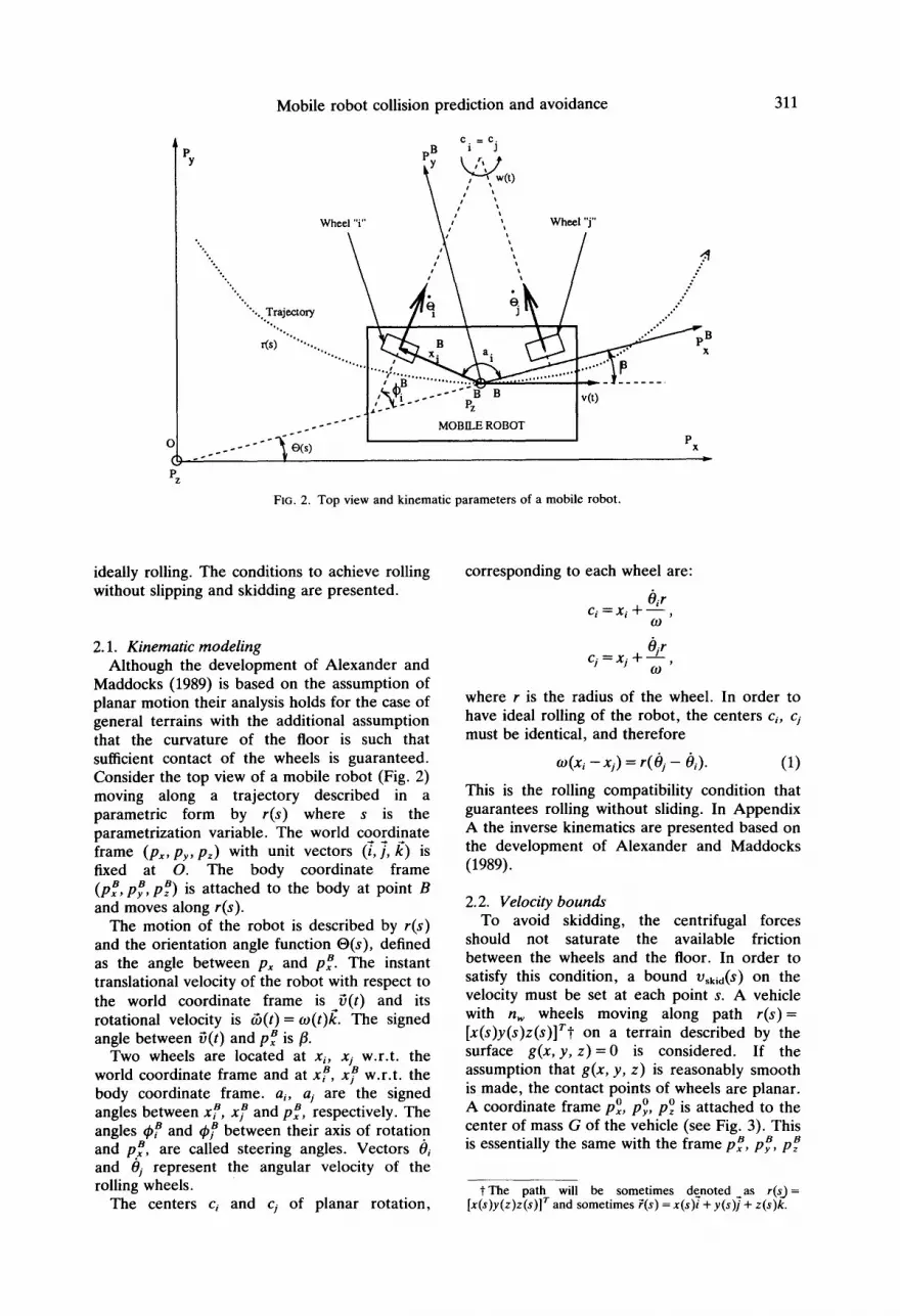
FIG. 2. Top view and kinematic parameters of a mobile robot.

ideally rolling. The conditions to achieve rolling without slipping and skidding are presented.

2.1. Kinematic modeling Although the development of Alexander and

Maddocks (1989) is based on the assumption of planar motion their analysis holds for the case of general terrains with the additional assumption that the curvature of the floor is such that sufficient contact of the wheels is guaranteed. Consider the top view of a mobile robot (Fig. 2) moving along a trajectory described in a parametric form by r(s) where s is the parametrization variable. The world coordinate frame (Px, Py, Pz) with unit vectors (i, j, k) is fixed at O. The body coordinate frame (pff, p~, p~) is attached to the body at point B and moves along r(s).

The motion of the robot is described by r(s) and the orientation angle function O(s), defined as the angle between px and pff. The instant translational velocity of the robot with respect to the world coordinate frame is ~(t) and its rotational velocity is tb ( t )= to(t)/~. The signed angle between ~(t) and px B is/3.

Two wheels are located at xi, xj w.r.t, the world coordinate frame and at xff, x~ w.r.t, the body coordinate frame, a~, aj are the signed angles between x~, x~ and px B, respectively. The angles tp~ and tp~ between their axis of rotation and p~, are called steering angles. Vectors 0i and 0~ represent the angular velocity of the rolling wheels.

The centers ci and cj of planar rotation,

corresponding to each wheel are:

Oir Ci ~ X i -~- - - ~

O)

cj= xj 4 @ ,

where r is the radius of the wheel. In order to have ideal rolling of the robot, the centers ci, cj must be identical, and therefore

(I)(X i -- Xj) = r( Oj - Oi). (1)

This is the rolling compatibility condition that guarantees rolling without sliding. In Appendix A the inverse kinematics are presented based on the development of Alexander and Maddocks (1989).

2.2. Velocity bounds To avoid skidding, the centrifugal forces

should not saturate the available friction between the wheels and the floor. In order to satisfy this condition, a bound Vskid(S) on the velocity must be set at each point s. A vehicle with nw wheels moving along path r ( s ) = [x(s)y(s)z(s)]r~ on a terrain described by the surface g ( x , y , z ) = O is considered. If the assumption that g(x, y, z) is reasonably smooth is made, the contact points of wheels are planar. A coordinate frame pO, pO, pO is attached to the center of mass G of the vehicle (see Fig. 3). This is essentially the same with the frame pff, pff, p~

-tThe path will be sometimes denoted as r(s.)= [x(s)y(z)z(s)] r and sometimes F(s) = x(s)i + y(s)j + z(s)k.

312 K . J . KYRIAKOPOULOS and G. N. SARIDIS

P /z Px

o P

z

~-p Y

W

f. 1 pO

X

FiG. 3. Forces acting on a mobile robot moving on general terrain.

O P

of the previous section assuming B = G and /3 = 0. If pO is tangent to r(s), pO is normal to the plane tangent to the surface of the floor, and pyO is normal to both then the unit vectors (~'o, ]0,/~o) corresponding to (px °, pO, p0) are

Cg ~°(s) = dr(s) ~°(s) =/~° X ~' ' /~°(s) = Ii~gll

ds '

(2)

Since coordinate frame px °, pO, pO moves w.r.t. time

_ _ = 7o dP d~° ~bxi = ) - ~ - ~ = ~ b x P , dt

_ _ = 7o -- d i ° . d] ° a X 1 =2 - -~ s = Co x -] °, dt

= "o d/~° '

d/~---~°dt ( S x k ~ - - ~ = (5 x/~ °,

(3)

where & is the vector of angular velocity. If equations (3) are solvedt then & has the form

th = f i -~. (4)

t This set of equations is not actually overdetermined. This is because the z(s) of vector ~(s) can be determined by x(s), y(s) and g(x, y, z) = O.

Similarly,

d270 dth d~° -- d2~° -2 dt----T = & X (& X7 °) +--~- X t° :~>--~-s +--~-T s

d& = ~ x ( ~ x 7 °) +--~-- x P,

d] ° d27 ° ° x dt ~ = <Z, x (<Z, x ~ ) + -~-

= a x ( ~ x ] °) + d ~ x -"° S,

d2k "0 dff~ r o ~ d / ~ ° . . , dZk ° d/2 = (~ X((~ x]~O)+-~ "XK : ~ - ' ~ - S - t - - - ~ z a S 2

d& = ~, x ( ~ x 17o) + - ~ x £o,

(5)

and the angular acceleration has the form

d& g~ = - ~ = Az(s)g + f l l (s)g z. (6)

Unit vector ~ lies on the (pO, pz o) plane and points towards the center of curvature or r(s).

dZ~/ds 2

= iid~/~211. (7)


The acting forces on the vehicle are; the weight ff = mgk, the reaction forces ~ = F/k "° i = 1 , . . . , nw from the floor to the wheels and the friction forces 7//= f / ~ + f/,-y~, i = 1 . . . . . n~ between the floor and the wheels. When the robot moves with a speed ~ and acceleration ~" a centripetal force

an inertial force

= ( 8 )

F1 = ms~ °, (9)

and an inertial torque of the form

/~o = I~ + t~ x ( I~) (4,6)= fftz(s)g + / ~ ( s ) g 2, (10)

should be exerted. (J is the inertia matrix of the mobile robot around its center of gravity.)

The motion equations of the vehicle are

nw

~ + ~ ) + ~ + F c + ~ = O , (11) i= l

nw ~ + ~) x ( ~ - lk °) + z(.l o = O, (12)

i=1

where 1 is the height difference between the contact points of the wheels and the center of mass G.

The slide constraints for the wheels are:

If/I = V( f / ix ) 2 "[- (f//y)2 ~ ~F / , i = 1 . . . . . n~, (13)

F/->0, i = 1 . . . . . nw, (14)

where r/ is the friction coefficient between the wheels and the floor.

The actuator constraints are

- ~ 2 ~ Ui =fix sin tp/° +f/y COS q~0 _< -~1,

i = 1 . . . . . n , , (15)

where ( -~2 , ~ ) are the brake and accelerating bounds of the actuators, respectively.

The maximum velocity so that skidding is avoided is given by the mathematical program

V2kid(S) = max {~2/(11)-(15) are satisfied}. (16)

If a vector X of unknowns is formulated, where

X = [fix f l y " " f , . J ~ y F ~ . . . F, ~z], (17)

then mathematical program (16) has linear objective and constraints, except (13) which is convex though.

2.3. Dynamic modeling The simplying assumptions made to obtain the

dynamic model of the mobile robot are:

• No slipping: rolling compatibility conditions are satisfied.

• No skidding: [v(s)[ -< Vskid(S). • The rotational kinetic energy of the rotating

wheels is not considered. • Frictionless motion (w.r.t. the robot's kinema-

tic mechanism).

The kinetic and potential energies of the moving robot are:

K = ½(~, ItS) + ½m~ 2, (18)

P = mgz(s) . (19)

where I is the moment of inertia of the robot around G, m is its mass, g is the gravity vector and z(s) is the height of the center of gravity w.r.t, a world coordinate frame.

Since t~(s)=i f (s )5 , where f ( s ) is the curvature at s, the kinetic energy becomes

K ( s , = ½Jc(S)f2(s) 2 + (20)

where /~(s)= (5, J3) is the reflected inertia matrix. The Lagrangian is

L(s, ~) = K - e = ½Ic(s)f2(s)~ 2

+ ½mA 2 - mgz(s) .

The Euler-Lagrange equations, assuming no nonconservative forces, such as friction, are:

d aL 0L

dt a~ as

where u is the steering force of the robot tangent to r(s) at every instant. Using (20), the dynamic equation is

(m + Ic(s)f2(s(t)))~'(t) + (½1"(s)fZ(s) + Ic(s)

x f (s ( t ) ) f ' ( s ( t ) ) )~2( t ) + mgz(s ) = u(t), (21)

where ( . ) '&d( . ) /ds . An equivalent useful formulation may be obtained using parameter s as an independent variable instead of time t. This is accomplished by introducing v(s) & ds/dt(s). Therefore

(m + Ic(s) f2(s))v(s)v ' (s) + (½1"(s)f2(s) + It(s)

x f ( s ) f ' ( s ) ) vZ( s ) + mgz(s ) = u(s). (22)

The steering force u is the sum of the projections of the nw actuator forces on the tangent of r(s)

nw

u(t) = u(s(t)) = ~, ui sin (qh°(s(t))). (23) i=1

The py0 components of uls are absorbed by friction. Usually, the steering angles q~o of the wheels have a limited range of deviation around 90 ° . Therefore

cl -< Isin (q~°(s(t)))l -< 1, (24)

314 K . J . KYRIAKOPOULOS and G. N. SAR1DIS

where Ca is a positive constant. From (15), (23) and (24)

where - U2 -< u -< U1, ( 2 5 )

U1 = Clnw~l, (26)

U 2 -- Clnw,.~2.

This is an acceptable approximation of the input space because it is on the safe side.

2.4. Collision avoidance constraints Collision avoidance is guaranteed if the

distance d(s, t) (Gilbert and Johnson, 1985) between the robot and the object is greater than a safety positive constant d °, i.e.

d(s, t) = min {llzi - zjll: zi • Cr(S), i , j

z jeCo( t )} ->d ° , Vs, t, (27)

where

C~(s) = {x/x • ~3 9 ArR;-I(S)X < b~

- ArR;-I(s)Tr(s), Ar • g~m×3, br • .~"}, (28)

Co(t) = {y /y • ~}~3 9 AoRol( t )y <_ bo

AoRo~(t)To(t), Ao • ~t×3, bo • ~ '} , (29)

are convex polyhedra representing the convex hulls of the mobile robot and the moving obstacle, respectively. (Ar, br) and (Ao, bo) are the parameters that define the convex poly- hedron description of the robot and the object, respectively, with respect to their fixed coordinate frame. Rr, Ro, Tr, To represent the rotation and translation of the frames of the robot and the object with respect to the world frame and must be known in order to compute d(s, t). Rr(s), Tr(s) can be easily derived from r(s). Ro(t), To(t) are not well known and are estimated based on sensory input. Distance d(s, t) can be computed by a mathematical program of the form:

d(t) = min II x -YlI~ x , y

s. t Ar(t)x(t) <- br(t), (30)

Ao(t)y(t) <- bo(t).

Normally one would choose the Euclidean distance (a = 2) to represent the distance, and have to solve a quadratic programming type of problem. However if a = 1 or ~ then a linear programming type of problem can be formulated and gain in terms of computational efficiency.

2.5. Mathematical problem statement The dynamic equations and the constraints are

summarized as follows:

System (equation (22))

Yc(t) = A(x(t)) + B(x(t))u(s),

where x(t) = [s(t)v(t)] r, with v(t) = ~(t)

A(x) =

(31)

v(t) 1 1 t 2 ~lc(s)f (s) + l f ( s ) f ' ( s ) v2(t ) /(32)

m + Ic(s)f2(s)

and

E ° 1 B(x) = 1 . (33)

m + lc(s)f2(s)

Initial-final conditions

x(so) = [0 Vo] r, x(sr) = [free vf] r. (34)

Input constraint (equation (25))

-U2 <- u(s) <- U1, (35)

State constraint (equation (16))

V(S)I ~ Vskid(S), (36)

Collision avoidance constraint (equation (27))

do - d(s, t) <- O. (37)

The final equality constraint (34) can be imposed using inequalities. Consider as upper and lower velocity bounds the two velocity arcs starting from (s r, vr) and going backwards with input -U2, UI until they meet (Vskid(S), V(S)=0), respectively. Thus Vmax(S) and Vmi,(S) are constructed. This is demonstrated in Fig. 4. Thus, a new set of inequalities

0 ~ Vmin(S ) <: IV(S)I --< Vmax(S), (38)

are used to satisfy (34) and (36). The problem is to find a feedback control of

the form u(s, v, t) such that (35), (37), and (38) are satisfied.

3. THE POTENTIAL FIELDS STRATEGY (PFS) The potential fields approach does not

generically address the performance issue. Stability, in the sense of collision avoidance and convergence to the goal state, is the main issue. Furthermore, being a local method, it is computationally efficient but on the other hand it does not handle constraints well. The main problem with a naive application of this approach is the existence of local minima in the overall potential field. A considerable research effort has been done Rimon and Koditschek (1989) on constructing globally converging fields, but this has been achieved only for special categories of shapes of objects (e.g. "star-like"). The above issues become more complicated if


V(s)

V (s) ,u=-U2 Vmax(s~

(So.Vo) Vn(s)

V = 0 rain

(s)

skid

", Vmax(s)

"" " . ' '~ (Sf, VO u=U1 ,"

,'V . (s) / m l n

t lit

s

FIG. 4. Feasible velocities space.

the objects move and the system becomes non-autonomous.

In the problem at hands, the application of potential fields is done in the (s, t) space since the problem has been reduced to a unidimen- sional one by considering motions only along the off-line trajectory r(s). A Lyapunov function approach was adopted. In order to aim for both stability and performance, two generic states are considered for the case of having only one moving object:

• Alarming state. Collision is possible unless action is taken. The inverse of the distance between the robot and the moving obstacle is penalized. The attractive goal is state (s = sy, v = v i = O).

• Non-alarming state. The main task is to track the nominal plan. Therefore the attractive state is s.(t), v,(t).

This decomposition demonstrates the necessity of development of a fast but generic scheme that classifies the current state of the system as alarming or not.

3.1. Fast collision prediction--the alarm function In our previous developments the Minimum

Interference Strategy (MIS) and the Optimal Control Strategy (OC) Kyriakopoulos and Saridis (1990b, 1991, 1992b), have been proposed. Those are global methods and require the accurate knowledge of parameters such as collision time (to), collision point (so), etc. In the case of PFS, collision prediction is only required to test if the local configurations and velocities of the mobile robot and the moving obstacle may lead to a collision.

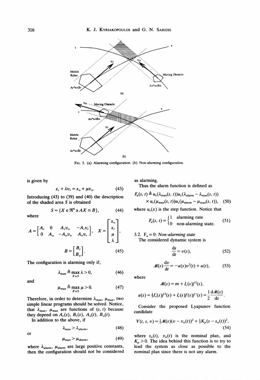
Consider Fig. 5. A mobile robot is moving along its Cartesian path and has an instan-

z taneous translational velocity JR = J r -~- V Rk, while a moving obstacle is detected to have an instantaneous translational velocity? Vo = Vo v~/~. Configuration (a) is considered as alarming because the shaded area (volume) which is the interaction of the swept areas (volumes) of the polyhedra along their instantaneous translational motion lines lie on the side of positive direction of both velocity vectors. Configuration (b) is considered as non-alarming because the shaded area lies on the negative side for velocity vector Vo. A mathematical methodology to construct an alarm function F~(s, t) indicating the "degree of alarm" of a configuration is presented below.

Consider the convex polyhedral descriptions of the mobile robot and the moving obstacle, respectively:

A,Xr <-- Br, (39) Ao" Xo --< Bo, (40)

xr, Xo e ~2. Notice that (Ar, Br) are functions of s, while (Ao, Bo) are functions of t. The swept areas (volumes) of the mobile robot and the moving obstacle under a horizontal translation can be parametrized by

XSr = X r "~- Z V r , (41)

x~, = Xo +/~Vo, (42)

where Xr, Xo satisfy (39) and (40), respectively. Their intersection (shaded area of Figs 5a and b)

t Obviously fi,, ~,, are the horizontal components of the velocities of the mobile robot and the moving obstacle, respectively.

316 K . J . KYRIAKOPOULOS and G. N. SARID|S

"', r'

t .-Y .....,,. ""-. = ,....__.__...~.............

A r * x < B ~ . . . . . . . \ (a)

Vo .. Moving Obstacle ...""

. ' " " Vr .. . . . . ... ............ ........... ............. .i

A r * x < B r / ~ , , ~ \

(b)

F]C. 5. (a) Alarming configuration. (b) Non-alarming configuration•

is given by

xr + ~.v, = xo +/~vo. (43)

Introducing (43) to (39) and (40) the description of the shaded area S is obtained

S = { X ~ ~6 ~ A X <-- B} , (44) where [xi] [mr o a,oo Arvr X xr A = Ao - A o v o Aovr J '

B,] (45) B = Bo "

The configuration is alarming only if;

~.0,~ ___a max ~ > 0, X~S

and

(46)

A /~.,ax = max/~ > 0. (47) x¢s

Therefore, in order to determine ~, . . . . /~ . . . . two simple linear programs should be solved. Notice, that ~.max, /~ma~ are functions of (s, t) because they depend on Ar(s) , Br(s), Ao(t) , Bo(t).

In addition to the above, if

/ ] ' m a x > /~al . . . . (48) o r

#.,~x >/~al . . . . (49)

where ~'a] . . . . /~t~,,, are large positive constants, then the configuration should not be considered

as alarming. Thus the alarm function is defined as

F~(s, t) ~ Us(•max(S , t))Us(Zalar m - - ~!,max(S , t))

× Us(I, tmax(S, t))Us(~alarm --/,tmax(S , t)), (50)

where us(x) is the step function. Notice that

1 alarming rate F~(s, t) = 0 non-alarming state.

(51)

3.2. Fa = 0: Non-alarming state The considered dynamic system is

ds dt v(s) , (52)

dv uCl(s) - ~ = -a ( s ) v2 ( t ) + u(t) , (53)

where

~ ( s ) = m + Ic(s)f2(s),

1 d ~ ( s ) a(s) = ½1"(s)fZ(s) + Ic(s ) f ( s ) f ' ( s ) = 2 ds

Consider the proposed Lyapunov function candidate

~(t , s, v) = ½Jt~(s)(v - v , ( t ) ) z + ½Kp(s - s,(t)) 2,

(54)

where sn(t), v , ( t ) is the nominal plan, and Kp > 0. The idea behind this function is to try to lead the system as close as possible to the nominal plan since there is not any alarm.


In general, OF(t, s, v)¢:> (s, v) = (sn, on). Furthermore, OF(t, s, v) is continuously differentiable and bounded from below by a decrescent function. Therefore it is a valid Lyapunov function candidate. Its time derivative is:

doF aoF aoF aoF d---t = 3t + 3----s v + ~ v O, (55)

and if (54) is substituted, then

doF d--T = (v - un)[Kp(s - s . ) - a(s)vvn

- ~ ( s ) 0 n + u]. (56) For

u(t, s, v) = - K p ( s - sn(t)) - K~(v - vn(t))

+ a(s)vvn(t) + d~(s)i)n, (57)

(K~ > 0) equation (56) becomes

doF - - = - K , , ( v - vn) 2. (58) dt

Using a well-known result by Hale (1980) (see Appendix B) and the fact that sn(t), vn(t) are uniformly bounded in t,

lim (v( t ) - vn(t)) = O. t-.-.~o~

Notice that

sn( t )=s f , Vn( t )= i )n ( t )=O t>-T, (59)

where T is the motion time of the nominal plan. Since u( t , s , v) is continuous and uniformly bounded in t then v, 0 are continuous and uniformly bounded, and using a well-known

result (see Appendix B)

lim (0(t) - 0n(t)) = 0.

Thus, from (53) and (57) we deduce that

lim (s(t) - sn(t) ) = O.

3.3. Fa = 1; Alarming state In this case, both collision avoidance and

convergence to the final state (sf, vf = 0) should be satisfied. Therefore the proposed Lyapunov function candidate is

OF(t, s, v) = ½~(s )v z + ½(Kp + cKv) As 2

+ ½c~(s) Asv + G(d(s, t)), (60)

where As = (s - st), Kp, K, > 0. be everywhere positive if

0 < c <

°F(t, s, v) will

Ko + VK~ + UoG <_ Kv + VK~ + ~ G M d~ '

2 2 (61)

where Mo - ~ ( s ) -< M, and

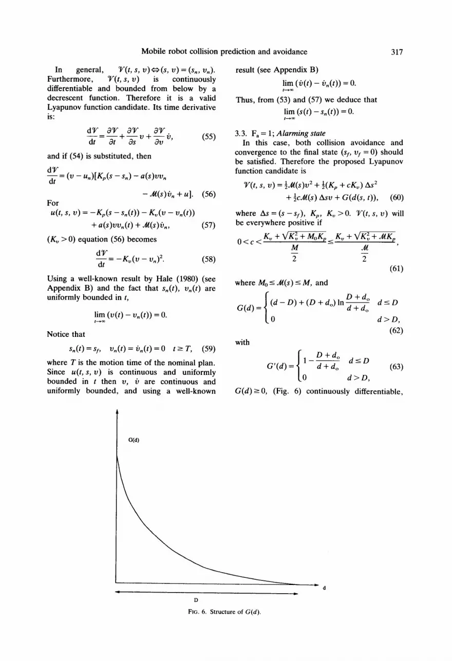
~ ( d - D) + (D + do) l nD + d o d + d o d < - D G(d)

(o d > D ,

(62)

with

G(d) >- O,

{ ~ D + d o G ' (d ) = d + do d <- D

d > D ,

(63)

(Fig. 6) continuously differentiable,

C(d)

9

D

FI6.6. Structure of G(d).


and decreasing (G'(d) - 0) w.r.t, its argument d. D is the largest distance for which we are concerned, and do is appropriately chosen to define G(0). The idea behind such a construction of ~V(t, s, v) is to try to lead the state of the system to this of the desired state, and at the same time to penalize proximity with the moving obstacle when the configuration of the system may lead to a collision. ~V(t, s, v) is continuous and bounded from below by a decrescent function. Therefore it is a valid Lyapunov function candidate.

In the following analysis cOd~cOs, cOd~cOt are required. Distance function d(s, t) is well known to be continuous but not continuously differentiable Gilbert and Johnson (1985). A way to bypass this difficulty is to predict the "singularity" points where the derivative is discontinuous based on the estimate of the motion vector of the moving obstacles and interpolate locally with a signoid function. This approach was used in the case study and did not create any numerical problems. Thus, the notation cOd~cOs, cOd~cOt is going to be used rather loosely here.

d~V , cOd - - = G (d) - ~ + a(s)l) 3 + (gp + cgv ) A S V dt

+ ca(s) Asv 2 + Id/(s)v 2 + G ' ( d ) cOd + 24(s)vi) cOs

cOd + 1~(s) as~ + (o + lc a s ) ~ ( s ) O = C ' (d ) T t

+ a(s )v 3 + (Kp + c K , ) Asv + ca(s) Asv 2

+ ~at(s)v ~ + C' (d) aa + a~(s)v~ cOs

+ ½~(s) Asi, + (v + lc As)(-av ~ + v). (64)

If a control

Od u(t, s, v) = - a ( s ) v z - Kp AS - 2Kov - G ' ( d ) Os '

(65)

is chosen, then

cOd cOd - C ' (d) -gs As - a(s)~ ~ + C' (d ) - g . (66)

Notice that if

c ~ 4K~ 41(o

(67)

then

m i n { ~ - e ' 2 K ~ - 7 } :cKp>0'2

(68)

fci¢. - T } = 2Ko - T max 1.--2-' 2Ko cdt cd4

It can be easily tested that for Ko, K p > O constraint (67) is more constraining than (61). Similarly,

- ao <- a ( s )

= ½I'(s)f2(s) + l~ ( s ) f ( s ) f ' ( s ) <-- ao

1 , 2 , cOd = ~ I . . . . f m a x "It- Ic.,xfmaxfmax, -So <-~ ~s <-~ SO

= 1 + 6rf~ax, (69)

where It(s) is the reflected moment of inertia of the mobile robot at point s, It=a. & maxs I t(s) , i I A r .... =maxslc(s) , f m a x & m a x s f ( s ) , fmax&maxs f ' ( s ) and 6r the diameter of the robots convex hull.

The required analysis is very difficult because the system is nonautonomous, and the distance function is not explicitly known as a function of (s, t). A local analysis assuming that

- - S f <~ A s <--- A s t < O,

A Iv l ~ V~ax ---- m a x Vmax(S),

s

( 7 0 )

will be performed. cOd

(A) Stationary obstacle. - ~ = O.

In this case

Q

CG, d cOd - 2 ( ) -~s As - a ( s )v 3. (71)

From Lasalles' invariance principle, is

~¢g {(s, v):V(s, u)

f cKp 2

then the state of the system asymptotically goes to the largest invariant set of ~ , denoted as {~'}, i.e. (se, re) satisfying

~Je ~ 07

3d g p ( s e - st') = - G ( d ( s e ) ) ~ s . . . . "

(73)


Obviously, the equilibrium point (se, r e ) • {o/¢.} depends on the initial state. For example, if ad(s)/as > o Vs ~ [sp, sf] and So e [sp, sy] then (s,, v~) = (s~, o) ~ { ~r).

(B) Moving obstacle, ad 4= 0 at "

The analysis of this case is very difficult for the general case and can be only local Khalil and Kokotovic (1991). The following analysis is based on the assumption that the velocity of the moving obstacle is bounded. Thus,

_ V <Od Ot <- V, (74)

then Od <

G'(d) - -~ - -G'(O)V. (75)

The requirement that

d-----~=-{~-£As2+(2K~-C~2)VZ}dt

c G'(d) ad - ~ --~s As -a(s )v3 + G'(d) Od< Ot O, (76)

is satisfied if

d ~ cKp 2 c - - < - m a x (,'(s, 2 Ast - 2 G'(O)S°st

3 G'(O)V < 0 , (77) + a o V m a x - -

which is true for

K,--- 3 G'(O)V a 0 V m a x - -

2 As 2 ' (78)

and 3 (a0Vma x - - G'(O)V)M - 4KoG'(O)Sosf

Kp ~ 2Kv As 2 - 3 a o V m a x "4- G'(O)V (79)

as it is shown in Appendix C. Depending upon the assumptions for Od/at,

several conclusions about the stability properties can be drawn from inequality (76) based on the development of Khalil and Kokotovic (1991). For example, if in addition to the boundedness of ad/at, we have ad/at--->O as t--*0 then we can conclude that (s(t), v(t))---> (se, r e ) • {°W}.

The algorithm for the Potential Fields Strategy is: Algorithm for PFS. Step 1. Collision prediction

Solve (46) and (47) for 3. . . . . # . . . . respectively;

Find Fo(s, t) from (50); if Fa(s, t) = 1 GOTO 2; else (Fa(s, t) = GOTO 3.

Step 2. Collison avoidance Find minimum distance d(s, t);

Find u(t, s, v) from (65); GOTO 1.

Step 3. Tracking stage Find u(t, s, v) from (57); GOTO 1.

3.4. Implementation issues The control input u(t, s, v) obtained from (57)

or (65) may violate the limits imposed by (25), vmax(s) and Vmin(S ). This can be avoided by imposing

U(t, S, V):=

max {U1, u(t, s, v), .~(S)Vmax(S ) X V~nax(S )

+ a(s)V2ax(S)), u(t, S, V) >--0, ,

min{-- U2, u(t, s, v), M(S)Vmi,(s) X Vmi,(S)

+ a(s)V2in(S)}, u(t, S, V) <-- O. ( 8 0 )

Obviously, the system may approach the limits of the feasible space but it will never violate it.

If d(s, t) becomes very small then the input u becomes very large. However in reality -Ue-< u -< U~, indicating that collision avoidance is not always guaranteed because of the limited capacity of the actuators.

After those practical constraints are considered, stability analysis becomes a formidable task. However, the stability for the unbounded case shows that the proposed strategy: (a) tries to classify the moving obstacles as disrupting or not, (b) tends to avoid the disrupting ones, and finally (c) when avoidance has been achieved, tracking of the nominal plan is its main purpose. The simulation results of the next section demonstrate those stages.

3.5. Inverse dynamics The control force u given by equation (80) is

actually the sum of the projections of the individual control forces ui, given their linear combination u, is by solving the following nonlinear programming problem

max min ~72F 2 - - (f2 x +f2y) i = 1 . . . . . n w

s.t equation (11)-(15) (81) n w

ui sin (~°(s(t))) = u (given), i = l

that can be reformulated as

max w X

w -< r/EF 2 - 2 2 ( f ix+f/y) , i = 1 . . . . . nw,

w_>0

equation (11)-(15) n w

ui × sin (tp°(s(t))) i = 1

-- u (given in equation (80)),

(82)


where X = [f ixf ly" ' fn,xf~,y F l ' ' ' F~w~2wl . The idea behind this optimization is to try to allocate the forces ui in a such a way so that saturation of the available friction at each wheel is avoided.

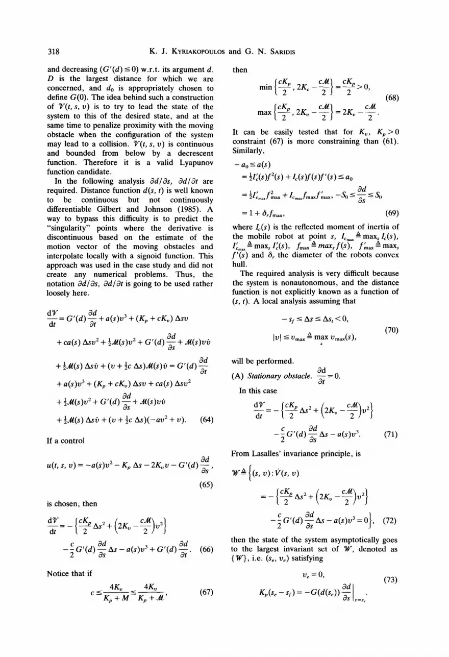
4. SIMULATION RESULTS In this section a case study is presented. A

mobile robot and a moving obstacle with geometric shapes, moving in the same environment (Fig. 7). The shape of both the mobile robot and the moving obstacle is rectangle with dimensions 0.3 m x 0.52 m and 0.28 m x 0.28 m, respectively. The scenario is that when the mobile robot is about to start moving, an obstacle with kinematic parameters x0 = 4.0 m, Y0 = 7.0 m, Vx = 0.04 m sec -1, vy = -0 .075 m sec -1, ax = 0.094 m sec -2, Or = -0.041 m sec -2, is going to collide with it under the current plan.

The mobile robot has parameters:

Mass (M) : 60 kg. Inertia (Izz) : 32 kg m 2. Maximum accelerating force (U1): 140 N. Minimum decelerating force (U2) : -60 N. Maximum velocity (Vmax) : 8 m sec -2. Wheel-f loor friction coefficient (r/) : -0 .12 .

It has the task of going from configuration A to configuration B within T = 12.1753 sec. An offline path planning stage is done and a path r(s) O<-s<-s I with total length s 1 ~ 1 4 . 6 0 m is

computed. The parameters of r(s) are indicated on Fig. 7.

Initial and final velocities are zero (VA = VB = 0).

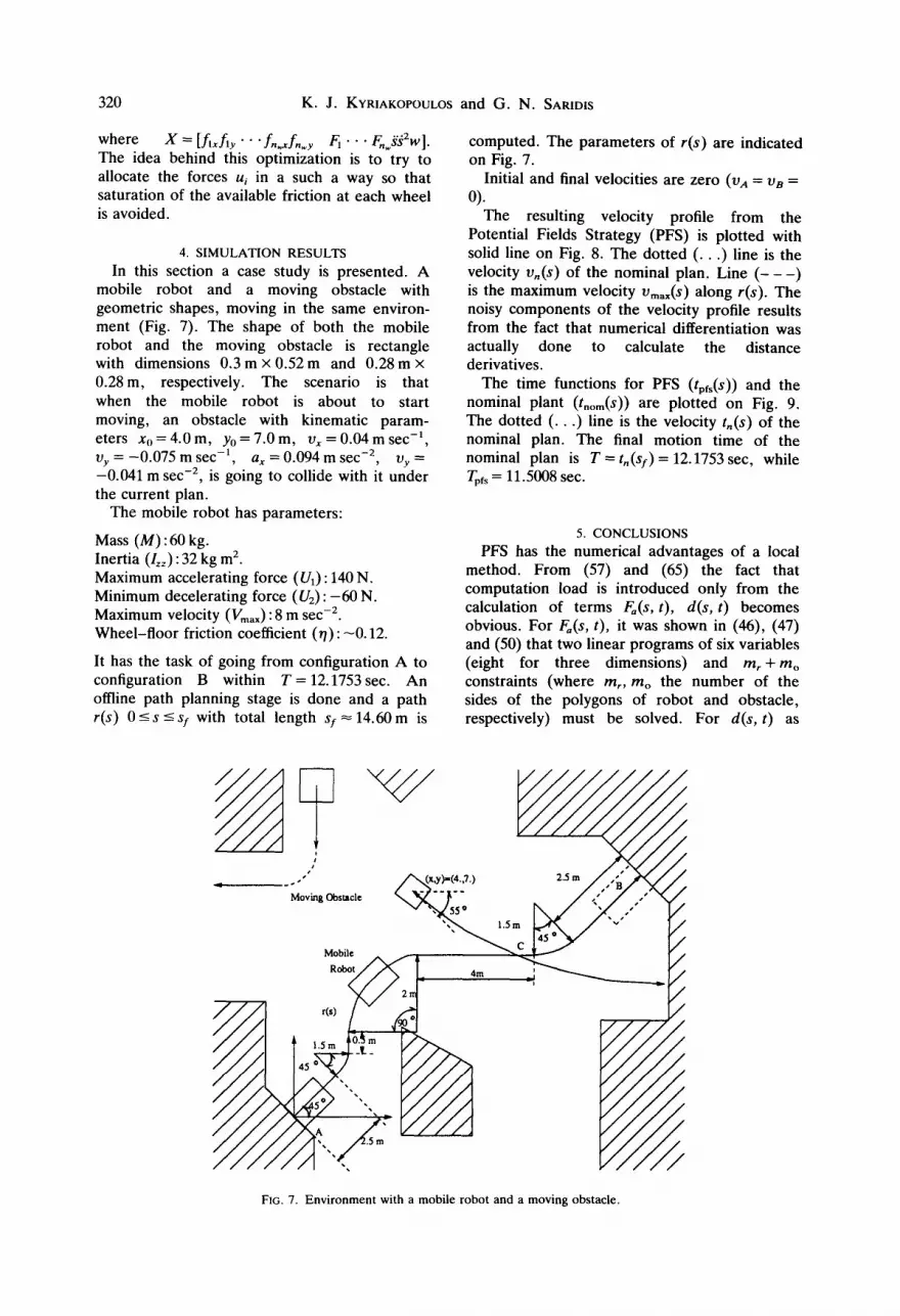
The resulting velocity profile from the Potential Fields Strategy (PFS) is plotted with solid line on Fig. 8. The dotted ( . . . ) line is the velocity vn(s) of the nominal plan. Line ( - - - ) is the maximum velocity Vmax(S) along r(s). The noisy components of the velocity profile results from the fact that numerical differentiation was actually done to calculate the distance derivatives.

The time functions for PFS (tpfs(s)) and the nominal plant (thorn(S)) are plotted on Fig. 9. The dotted ( . . . ) line is the velocity t,(s) of the nominal plan. The final motion time of the nominal plan is T = t , ( s r ) = 12.1753sec, while Tpfs = 11.5008 sec.

5. CONCLUSIONS PFS has the numerical advantages of a local

method. From (57) and (65) the fact that computation load is introduced only from the calculation of terms Fa(s, t), d(s, t) becomes obvious. For Fa(S, t), it was shown in (46), (47) and (50) that two linear programs of six variables (eight for three dimensions) and m r + m o constraints (where m,, mo the number of the sides of the polygons of robot and obstacle, respectively) must be solved. For d(s, t) as

fSJJJ

FIG, 7. Environment with a mobile robot and a moving obstacle.

3.5

Mobile robot collision prediction and avoidance

T T 1

321

v

O

2.5

1.5

0.5

0 t-

0

0s ' ,

#s •

i

i s

a

f J

0 i

s t

s o

s S J

/

/': r f a i t ~ . . . . . . . . . . . .

_j " ' " . . . . . . . . .

t ~

~ A -

2 4 6 8 10 12 14 16

s:distance along r(s) (m)

FIG. 8. Velocity profile from PFS (solid).

discussed in Section 2.4, if I1"111 or I1"11~ norms are used then a linear program should be solved. Obviously the solution of linear programs of such a small number of variables and constraints does not impose any real-time computational constraint. Therefore this feedback control can be easily recomputed at every sampling interval without any problem.

Currently our efforts are focused at the implementation and comparison of the collision avoidance schemes developed in Kyriakopoulos

(1991). It is well understood that the proposal of moving always along the same path will not always prevent collisions. Our research direc- tions include the problem of replanning the shape of r(s) by incorporating the nonholonomic constraints of the rolling motion.

Acknowledgement--This work has been supported by the NASA Center for Intelligent Robotic Systems for Space Exploration (CIRSSE) under the NASA Grant NAGW- 1333. The first author has been partially supported by a fellowship of Alexander Onasis Foundation.

14

12

10

0 0

. . . . . . . . . . . . . . . . . . . . ~ . . . . . . . . . . . . . . . . . . . . . ! . . . . . . . . . . . . . . . . . . . ! . . . . . . . . . . . . . . . . . . . . ~ . . . . . . . . . . . . . . . . . . . . ~ . . . . . . . . . . . . . . . . . . . . . ~ . . . . . . . . . . . . . . . . . . . . ! . . . . . . . . . . . . . . . . . .

: : : : : : : p : : : : : : : a : : : : : : • a : : : : : : . # : : , : : : : s

. . . . . . . . . . . . . . . . . . . : . . . . . . . . . . . . . . . . . . . . . ~ . . . . . . . . . . . . . . . . . . . . : . . . . . . . . . . . . . . . . . . . . ; . . . . . . . . . . . . . . . . . . . . ; . . . . . . . . . . . . . . . . . . . . ~ . . . . . . . . . . . . . . . . . . i . g . . . . . . . . . . . . . . . .

I

2 4 6 8 10 12 14 16

FIG. 9. Time functions for PFS (--) and the nominal plan (solid).


REFERENCES

Alexander, J. and J. Maddocks (1989). On the kinematics of wheeled mobile robots. Int. J. of Robotics Research, g, 15-27.

Freund, E. and H. Hoyer (1984). Collision avoidance for industrial robots with arbitrary motion. J. of Robotic Systems.

Fukimura, K. and H. Samet (1990). Motion planning in a dynamic domain. In Proc. of the 1990 IEEE Int. Conf. on Robotics and Automation, pp. 324-330.

Gilbert, E. and D. Johnson (1985). Distance functions and their application to robot path planning in the presence of obstacles. IEEE J. of Robotics and Automation, pp. 21-30.

Griswold, N. and J. Eem (1990). Control of mobile robots in the presence of moving objects. IEEE Trans. Robotics and Automation, pp. 263-268.

Hale, J. (1980) Ordinary Differential Equations. R. E. Krieger, Huntington, NY.

Kant, K. and S. Zucker (1984). Trajectory planning problems, i: Determining velocity along a fixed path. In Proc. of the IEEE 8th Int. Conf. Pattern Recogn., pp. 196-198.

Kant, K. and S. Zucker (1986). Toward efficient trajectory planning; The path-velocity decomposition. Int. J. of Robotics Research, pp. 72-89.

Kant, K. and S. Zucker (1988). Planning collision-free trajectories in time-varying environments: A two-level hierarchy. In Proc. of the 1988 IEEE Int. Conf. on Robotics and Automation, pp. 1644-1649.

Khalil, H. K. and P. V. Kokotovic (1991). On stability properties of nonlinear systems with slowly varying inputs. IEEE Trans. Aut. Control, p. 229.

Khatib, O. (1985). Real time obstacle avoidance for manipulators and mobile robots. In Proc. of the IEEE Int. Conf. on Robotics and Automation.

Kyriakopoulos, K. (1991). A supervisory control strategy for navigation of mobile robots in dynamic environments Ph.D thesis. Technical report, ECSE-RPI.

Kyrikopoulos K. and G. Saridis (1990a). Minimum distance estimation and collision prediction under uncertainty for on-line robotic motion planning. In Proc. of the 1990 IFAC World Congress.

Kyriakopoulos, K. and G. Saridis (1990b). On-line motion planning for mobile robots in non-stationary environments. In Proc. of 1990 1EEE Int. Symposium on Intelligent Control.

Kyriakopoulos, K. and G. Saridis (1991). Collision avoidance of mobile robots in non-stationary environments. In Proc. of the 1991 Int. Conf. on Robotics and Automation.

Kyriakopoulos, K. and G. Saridis (1992a). Minimum distance estimation and collision prediction under uncertainty for on-line robotic motion planning. Automatica, 28, 389-394.

Kyriakop-oulos, K. and G. Saridis (1992b). Optimal motion planning for collision avoidance of mobile robots in non-stationary environments. In 1992 American Control Conf. and Tran. Aut. Control.

Liu, Y., S. Kuroda, T. Naniwa, H. Noborio and S. Arimoto (1989). A practical algorithm for planning collision free coordinated motion of multiple mobile robots. In Proc. of the 1989 IEEE Int. Conf. on Robotics and Automation, pp. 1427-1432.

Rimon, E. and D. Koditschek (1989). The construction of analytic diffeomorphisms for exact robot navigation on star worlds. In Proc. of the IEEE Int. Conf. on Robotics and Automation, pp. 21-26.

Reif, J. and M. Sharir (1985). Motion planning in the presence of moving obstacles. Technical Report TR-06-85, Harvard University, Center for Research in Computing Technology.

Shih, C., T. Lee and W. Gruver (1990). Motion planning with time-varying polyhedral obstacles based on graph

search and mathematical programming. In Proc. of the 1990 IEEE Int. Conf. on Robotics and Automation, pp. 331-337.

Tournassoud, P. (1986). A strategy for obstacle avoidance and its applications to multi-robot systems. In Proc. of the 1988 IEEE Int. Conf. on Robotics and Automation, pp. 1224-1229.

Wu, C. and C. Jou (1988). Design of a controlled spatial curve trajectory for robot manipulators. In Proc. of the 27th Conf. on Decision and Control, pp. 161-166.

APPENDIX A: ROBOT INVERSE DYNAMICS

If it is known that the object has, at instant t, translational velocity, v(t), orientation angle O and rotational velocity to(t) = O(t) (Fig. 2). Then the instantaneous angular velocity and steering angle of the wheel i, are (Alexander and Maddocks 0989)):

b, = 1 r

X ~/Iv(t) 2 + Ixffl 2 (to(t)) 2 - 2

× Io(t)l txffl to(t) cos (fl - ai - O(s(t))), (A.1)

& =

t - l / v(t)l sin )6 - Ix~l to(t) sin (o<i + O(s(t))) '~ an ~,lv(t)l cos fl - Ix~l to(t) cos ( ~ + O(s(t)))] - O(s(t)).

(A.2)

There are the inverse kinematics equations for a general mobile robot, i.e. given v(t), O(t), O(t) equation (A.2) gives the angular velocities Oi(t ) and steering angles ~b~a(t) of every wheel i.

APPENDIX B: RESULTS NEEDED IN SECTION 3.2

Result 1. Consider the system

2 =f(t, x). (B.1)

Let ~ be a Lyapunov function candidate for (B.5). Suppose that

~(t, x) -< - ~¢/'(x) -< 0 Vt -> t o x e ~", (B.2)

where ~¢'(x) is a continuous function of x. Define

5e a= {x/°W(x) = 0}, (B.3) if Vp e !~t n :l neighborhood N(p) 9 Vx ~ N(p), f(t, x) is uniformly bounded in t, then

x(t)----~ 5e as t---~ ~.

Result 2. If 3~(t) and f( t) are continuous and uniformly bounded then

lim f ( t) = 0 :~ lim f( t ) = 0. t ~ t ~

APPENDIX C: INDICATION OF THE VALIDITY OF EQUATIONS (78) AND (79)

From (77) and (67) it suffices that

c g p 2 _4g, G,(O)aos f 3 -- 2 Ast Kp + M + a ° O m a x - - G'(O) V <O. (C.l)

Solving for c and introducing (67)

2 Kp As: ( a°v3ax - G'(O)V - ~ G'(O)Sosf )

g p ~ lVl /

4Ko ~--C<-Kp + M. (C.2)

This inequality is satisfied if (78) and (79) are satisfied.

an integrated collision prediction and avoidance scheme for mobile robots in non-stationary...

Documents