an innovative degraded adhesion model for railway vehicles: development and experimental validation

1 23

MeccanicaAn International Journal of Theoreticaland Applied Mechanics AIMETA ISSN 0025-6455Volume 49Number 4 Meccanica (2014) 49:919-937DOI 10.1007/s11012-013-9839-z

An innovative degraded adhesion modelfor railway vehicles: development andexperimental validation

E. Meli, A. Ridolfi & A. Rindi

1 23

Your article is protected by copyright and all

rights are held exclusively by Springer Science

+Business Media Dordrecht. This e-offprint

is for personal use only and shall not be self-

archived in electronic repositories. If you wish

to self-archive your article, please use the

accepted manuscript version for posting on

your own website. You may further deposit

the accepted manuscript version in any

repository, provided it is only made publicly

available 12 months after official publication

or later and provided acknowledgement is

given to the original source of publication

and a link is inserted to the published article

on Springer's website. The link must be

accompanied by the following text: "The final

publication is available at link.springer.com”.

Meccanica (2014) 49:919–937DOI 10.1007/s11012-013-9839-z

An innovative degraded adhesion model for railwayvehicles: development and experimental validation

E. Meli · A. Ridolfi · A. Rindi

Received: 27 May 2013 / Accepted: 7 November 2013 / Published online: 5 December 2013© Springer Science+Business Media Dordrecht 2013

Abstract The realistic description of the wheel-railinteraction is crucial in railway systems because thecontact forces deeply influence the vehicle dynamics,the wear of the contact surfaces and the vehicle safety.In the modelling of the wheel-rail contact, the de-graded adhesion represents a fundamental open prob-lem. In fact an accurate adhesion model is quite hardto be developed due to the presence of external un-known contaminants (the third body) and the complexand highly non-linear behaviour of the adhesion coef-ficient; the problem becomes even more complicatedwhen degraded adhesion and large sliding between thecontact bodies (wheel and rail) occur.

In this work the authors describe an innovative ad-hesion model aimed at increasing the accuracy in re-producing degraded adhesion conditions. The new ap-proach has to be suitable to be used inside the wheel-rail contact models usually employed in the multibodyapplications. Consequently the contact model, com-prising the new adhesion model, has to assure both agood accuracy and a high numerical efficiency to beimplemented directly online within more general ve-

E. Meli (B) · A. Ridolfi · A. RindiDepartment of Industrial Engineering, Universityof Florence, Via S. Marta 3, 50139 Florence, Italye-mail: [email protected]

A. Ridolfie-mail: [email protected]

A. Rindie-mail: [email protected]

hicle multibody models (e.g. in Matlab-Simulink orSimpack environments).

The model studied in the work considers some ofthe main phenomena behind the degraded adhesion:the large sliding at the contact interface, the high en-ergy dissipation, the consequent cleaning effect on thecontact surfaces and, finally, the adhesion recoverydue to the external unknown contaminant removal.

The new adhesion model has been validated throughexperimental data provided by Trenitalia S. p. A.and coming from on-track tests carried out in Velim(Czech Republic) on a straight railway track char-acterised by degraded adhesion conditions. The testshave been performed with the railway vehicle UIC-Z1equipped with a fully-working Wheel Slide Protection(WSP) system.

The validation showed the good performances ofthe adhesion model both in terms of accuracy and interms of numerical efficiency. In conclusion, the ad-hesion model highlighted the capability of well repro-ducing the complex phenomena behind the degradedadhesion.

Keywords Multibody modelling of railwayvehicles · Wheel-rail contact · Degraded adhesion ·Adhesion recovery

1 Introduction

The realistic description of the wheel-rail interaction iscrucial in railway systems because the contact forces

Author's personal copy

mailto:[email protected]



920 Meccanica (2014) 49:919–937

deeply influence the vehicle dynamics, the wear of thecontact surfaces and the vehicle safety.

Since the numerical performances (computationtimes and memory consumption) are very importantin the multibody applications, the contact phenomenacannot be usually modelled, in practise, by consider-ing the wheel and the rail as generic elastic continuousbodies. To overcome these limitations, the multibodycontact models are generally characterised by threemain logical parts: the contact point detection, the nor-mal problem solution and the tangential problem solu-tion, that comprises the adhesion model.

The detection of the contact point permits tocalculate the contact point position on the wheeland rail surfaces. The main approaches employ ei-ther constraint equations [42, 43] or exact analyti-cal methods aimed at the reduction of the algebraicproblem dimension [9, 10, 15, 22, 23, 34]. Generally,the normal problem solution is based on the La-grange multipliers [42, 43] and on improvements ofHertz theory [6, 11, 29]. Finally, concerning the so-lution of the tangential problem, different strategieshave been considered in the last decades [14, 45].The most significant approaches include the lin-ear Kalker theory (saturated through the Johnson-Vermeulen formula) [19, 21, 28–30], the non-linearKalker theory implemented in the FASTSIM algo-rithm [25–27, 29, 30, 32, 53, 54] and the Polach the-ory [38–41] that allows the description of the ad-hesion coefficient decrease with increasing creepage(excluding the spin creepage) and to well fit the ex-perimental data. All the three steps of the contactmodel have to assure a good accuracy and, at the sametime, a high numerical efficiency. High numerical per-formances are fundamental to implement the contactmodel directly online inside more general multibodyvehicle models (developed in dedicated environmentslike Matlab-Simulink and Simpack), without employ-ing discretized look-up table (LUT) [1, 2].

The main strategies employed to solve the tangen-tial problem (comprising the adhesion model) usuallydo not take into account the important topic of the de-graded adhesion between wheel and rail, that still re-mains an open problem. The substantial lack of litera-ture characterising these issues is mainly caused by thedifficulty to get a realistic adhesion law because of thepresence of external unknown contaminants (the thirdbody) and the complex and non-linear behaviour of theadhesion coefficient. The problem becomes even morecomplicated when degraded adhesion yields a high en-

ergy dissipation and, consequently, an adhesion recov-ery.

Many important analyses have been carried outover the years to investigate the role of so-called thirdbody between the contact surfaces. More particularlythe analyses have been performed both on laboratorytest rigs and through on-track railway tests by consid-ering natural and artificial external contaminants andfriction modifiers [7, 8, 16, 18, 20, 24, 36, 50].

Contemporaneously, to better study the degradedadhesion non-linear behaviour, also the high energydissipation at the contact interface and the consequentadhesion recovery have begun to be more accuratelyinvestigated [4, 5, 12, 13, 17, 33, 35, 49, 51, 52].

In this work the authors describe an innovativeadhesion model aimed at increasing the accuracy inreproducing degraded adhesion conditions in multi-body vehicle dynamics and railway systems. The newmodel, according to the recent trends of the state ofthe art (see the previous bibliographic references), fo-cuses on the main phenomena behind the degraded ad-hesion, with particular attention to the energy dissi-pation at the contact interface, the consequent clean-ing effect and the resulting adhesion recovery due tothe removal of external unknown contaminants. More-over, the followed approach minimises the number ofhardly measurable physical quantities required by themodel; this is a very important feature because mostof the physical characteristics of the contaminants aretotally unknown in practise.

The new model will have to assure a good accuracyto well reproduce the non-linear phenomena character-ising the degraded adhesion; at the same time, it willhave to guarantee high computational performances sothat the whole contact model (including the adhesionmodel) could be implemented directly online withinmore general multibody models of railway vehicles.


The structure of the paper is the following: the gen-eral architecture of the model will be illustrated inSect. 2 while in Sect. 3 the multibody model, compris-ing the railway vehicle model and the wheel-rail con-tact model, will be described in detail. In Sect. 4 the


Meccanica (2014) 49:919–937 921

Fig. 1 Architecture of the multibody model

experimental data will be introduced and in Sects. 5,6 and 7 the validation of the new model will be dis-cussed. Finally conclusions and further developmentswill be proposed in Sect. 8.

2 General architecture of the model

The architecture of the multibody model is briefly re-ported in Fig. 1.

From a logical point of view, the multibody modelconsists of two different parts that mutually inter-act, directly online, during the dynamical simulation(at each integration time step): the three-dimensional(3D) model of the railway vehicle (the geometricaland physical characteristics of which are known) andthe 3D wheel-rail contact model. At each time step themultibody vehicle model calculates the kinematic vari-ables of each wheel (position Gw , orientation Φw , ve-locity vw and angular velocity ωw) while the contactmodel, starting from the knowledge of these quanti-ties, of the track geometry and of the wheel and railprofiles, evaluates the normal and tangential contactforces Nc , T c (applied to the wheel in the contactpoint P c) and the adhesion coefficient f , needed tocarry on the dynamical simulation. Both the vehiclemodel and the contact model have been implementedin the Matlab-Simulink environment.

The wheel-rail contact model comprises three dif-ferent steps (see Fig. 2). The detection of the con-tact points P c is based on some innovative proce-dures recently developed by the authors in previousworks [10, 22, 34]. The normal contact problem isthen solved through the global Hertz theory [6, 11, 29]to evaluate the normal contact forces Nc. Finally

Fig. 2 Architecture of the wheel-rail contact model

the solution of the tangential contact problem is per-formed by means of the global Kalker-Polach theory[38–41] to compute the tangential contact forces T c

and the adhesion coefficient f .The strategy to solve the tangential contact problem

includes the innovative degraded adhesion model de-veloped by the authors in this work (see Fig. 3). Themain inputs of the degraded adhesion model are thewheel velocity vw , the wheel angular velocity ωw , thenormal force at the contact interface Nc and the posi-tion of the contact points P c . The model also requiresthe knowledge of some wheel-rail and contact param-


922 Meccanica (2014) 49:919–937

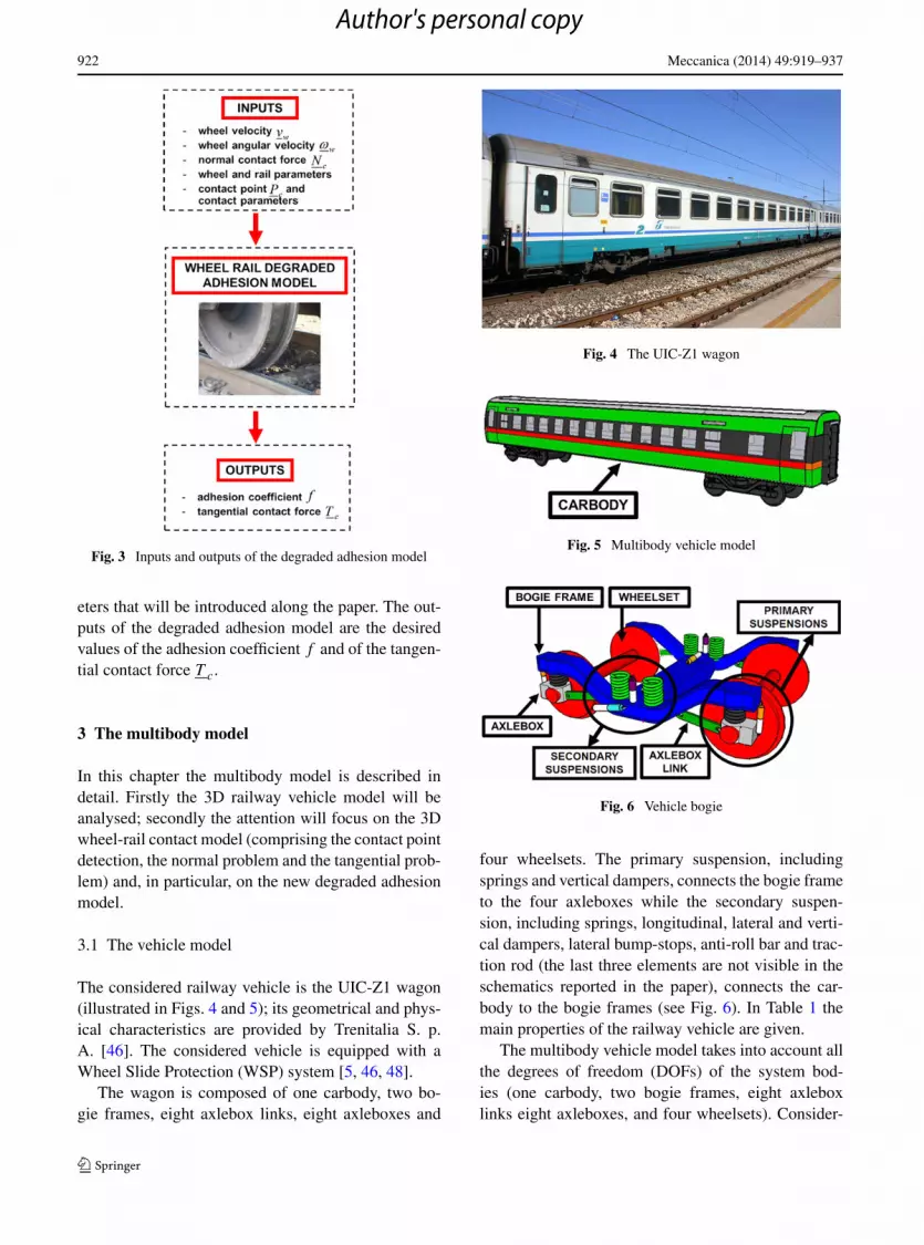
Fig. 3 Inputs and outputs of the degraded adhesion model

eters that will be introduced along the paper. The out-puts of the degraded adhesion model are the desiredvalues of the adhesion coefficient f and of the tangen-tial contact force T c .

3 The multibody model

In this chapter the multibody model is described indetail. Firstly the 3D railway vehicle model will beanalysed; secondly the attention will focus on the 3Dwheel-rail contact model (comprising the contact pointdetection, the normal problem and the tangential prob-lem) and, in particular, on the new degraded adhesionmodel.

3.1 The vehicle model

The considered railway vehicle is the UIC-Z1 wagon(illustrated in Figs. 4 and 5); its geometrical and phys-ical characteristics are provided by Trenitalia S. p.A. [46]. The considered vehicle is equipped with aWheel Slide Protection (WSP) system [5, 46, 48].

The wagon is composed of one carbody, two bo-gie frames, eight axlebox links, eight axleboxes and

Fig. 4 The UIC-Z1 wagon

Fig. 5 Multibody vehicle model

Fig. 6 Vehicle bogie

four wheelsets. The primary suspension, includingsprings and vertical dampers, connects the bogie frameto the four axleboxes while the secondary suspen-sion, including springs, longitudinal, lateral and verti-cal dampers, lateral bump-stops, anti-roll bar and trac-tion rod (the last three elements are not visible in theschematics reported in the paper), connects the car-body to the bogie frames (see Fig. 6). In Table 1 themain properties of the railway vehicle are given.

The multibody vehicle model takes into account allthe degrees of freedom (DOFs) of the system bod-ies (one carbody, two bogie frames, eight axleboxlinks eight axleboxes, and four wheelsets). Consider-


Meccanica (2014) 49:919–937 923

Table 1 Main characteristics of the railway vehicle

Parameter Units Value

Total mass [kg] ≈43000

Wheel arrangement – 2–2

Bogie wheelbase [m] 2.56

Bogie distance [m] 19

Wheel diameter [m] 0.89

Primary suspended masses own frequency [Hz] ≈4.5

Secondary suspended masses (carbody)own frequency

[Hz] ≈0.8

Table 2 Inertial properties of the rigid bodies

Body Mass[kg]

Ixx

[kg m2]Iyy

[kg m2]Izz

[kg m2]

Carbody ≈29000 76400 1494400 1467160

Bogie Frame ≈3000 2400 1900 4000

Wheelset ≈1300 800 160 800

Axlebox ≈200 3 12 12

Axlebox Link ≈60 0.5 4 4

Fig. 7 Primary suspensions

ing the kinematic constraints that link to each otherbogie frames, axlebox links, axleboxes and wheelsets(all cylindrical 1DOF joints) and without including thewheel-rail contacts, the whole system has 40 DOFs.The main inertial properties of the bodies are sum-marised in Table 2 [46].

Both the primary suspension (springs and verticaldampers) and the secondary suspension (springs, lon-gitudinal, lateral and vertical dampers, lateral bump-stops, anti-roll bar and traction rod) have been mod-elled through 3D visco-elastic force elements able todescribe all the main non-linearities of the system (seeFigs. 6, 7 and 8).

Fig. 8 Secondary suspensions

In Table 3 the characteristics of the main linearelastic force elements (springs, anti-roll bar) of boththe suspension stages are reported [46]. The non-linearelastic force elements (dampers, lateral bump-stops,traction rod) have been modelled through non-linearfunctions that correlate the displacements and the rela-tive velocities of the force elements connection pointsto the elastic and damping forces exchanged by thebodies. By way of example the non-linear characteris-tic of a vertical damper of the primary suspension isillustrated in Fig. 9.

The characteristics of the non-linear force elements(dampers, lateral bump-stops, traction rod) have beendirectly provided by Trenitalia S. p. A. More specif-ically, these mechanical nonlinear force elements aredeveloped to satisfy the technical specifications re-quired by the considered vehicle project and then ex-perimentally tested to properly verify the desired per-formance [46]. Finally, also the Wheel Slide Protec-tion (WSP) system of the railway wagon UIC-Z1 hasbeen modelled to better investigate the vehicle be-haviour during the braking phase under degraded ad-hesion conditions [5, 48]. The whole vehicle modelhas been implemented in the Matlab-Simulink envi-ronment [1].

3.2 The wheel-rail contact model

In this section the three logical parts of the wheel-railcontact model (contact point detection, normal prob-lem and tangential problem) will be analysed with par-ticular regard to the new degraded adhesion model.The model inputs are the kinematic variables of eachwheel (position Gw , orientation Φw , velocity vw and


924 Meccanica (2014) 49:919–937

Table 3 Main linear elastic characteristics of the two stage suspensions

Element Transl. stiff. x

[N/m]Transl. stiff. y

[N/m]Transl. stiff. z

[N/m]Rotat. stiff. x

[N m/rad]Rotat. stiff. y

[N m/rad]Rotat. stiff. z

[N m/rad]

Springs of the primary suspension 844000 844000 790000 10700 10700 0

Springs of the secondary suspension 124000 124000 340000 0 0 0

Anti-roll bar 0 0 0 2.5 × 106 0 0

Fig. 9 Example of non-linear characteristic: vertical damper ofthe primary suspension

angular velocity ωw) together with the track geometryand the wheel and rail profiles while the outputs thenormal and tangential contact forces Nc , T c (appliedto the wheel in the contact point P c) and the adhesioncoefficient f .

3.2.1 The contact point detection

Referring to Fig. 2 the contact point detection al-gorithm allows the calculation of the contact pointsP c starting from the wheel position Gw and orienta-tion Φw , the track geometry and the wheel and railprofiles. The detection procedure has been developedby the authors in previous works [10, 22, 34] and isbased on the reduction of the algebraic problem di-mension through exact analytical techniques; this re-duction represents the main feature of the new algo-rithm. The main characteristics of the innovative pro-cedure can be summarised as follows:

– it is a fully 3D algorithm that takes into account allthe six relative DOFs between wheel and rail;

– it is able to support generic railway tracks andgeneric wheel and rail profiles;

– it assures a general and accurate treatment of themultiple contact without introducing simplifying

assumptions on the problem geometry and kinemat-ics and limits on the number of contact points de-tected;

– it assures high numerical efficiency making possiblethe online implementation within the commercialmultibody software (like Simpack Rail and AdamsRail) without discrete LUT [1, 2].

The contact point position can be evaluated imposingthe following parallelism conditions [15]:

nrr

(P r

r

) × nrw

(P r

w

) = nrr

(P r

r

) × Rrwnw

w

(P w

w

) = 0

nrr

(P r

r

) × dr = 0(1)

where

P ww(xw,yw) = (

xw yw −√

w(yw)2 − x2w

)T

P rr (xr , yr) = (

xr yr r(yr))T

(2)

are the positions of the generic points on the wheel sur-face and on the rail surface (expressed in the referencesystems Gwxwywzw and Orxryrzr ), w(yw) and r(yr )

are the wheel and rail profiles (supposed to be known),nw

w and nrr are the outgoing normal unit vectors to

the wheel and rail surfaces (in the reference systemsGwxwywzw and Orxryrzr ), Rr

w is the rotation matrixthat links the reference system Gwxwywzw to the ref-erence system Orxryrzr and dr is the distance vectorbetween two generic points on the wheel surface andon the rail surface (both referred to the reference sys-tem Orxryrzr ): dr(xw, yw, xr , yr ) = P r

w(xw, yw) −P r

r(xr , yr) in which P rw = Or

w + RrwP w

w(xw,yw) isthe position of the generic point of the wheel sur-face expressed in the reference system Orxryrzr (seeFig. 10).

The first condition of the system (1) imposes theparallelism between the normal unit vectors, while thesecond one requires the parallelism between the nor-mal unit vector to the rail surface and the distance vec-tor. The system (1) consists of six non-linear equationsin the unknowns (xw, yw, xr , yr ) (only four equationsare independent and therefore the problem is 4D).


Meccanica (2014) 49:919–937 925

Fig. 10 Wheel-rail contact point detection

However it is possible to exactly express three of thefour variables (in this case (xw, xr , yr )) as a functionof yw , reducing the original 4D problem to a single 1Dscalar equation in the variable yw [10, 22, 34]:

F(yw) = 0. (3)

At this point the simple scalar Eq. (3) can be eas-ily solved through appropriate numerical algorithms.Finally, once obtained the generic solution ywc ofEq. (3), the complete solution (xwc, ywc, xrc, yrc) ofthe system (1) and consequently the contact pointsP r

wc = P rw(xwc, ywc) and P r

rc = P rr(xrc, yrc) can be

found by substitution.

3.2.2 The normal contact problem

Starting from the kinematic variables of the wheeland the contact point position P c, the normal forcesNc are calculated through the global Hertz theory foreach contact point (see the Figs. 2, 10, 11 and 12)[6, 10, 11, 29]:

Nc = Ncnw, Nc = ‖Nc‖. (4)

The main physical hypotheses behind the Hertz globaltheory are the following [6, 10, 11, 29]:

– linear elasticity;– contact patch dimensions small if compared to the

curvature radii of the contact bodies surfaces;– not-conformal contact;

Fig. 11 Contact forces

Fig. 12 Contact surfaces

– elliptic contact area.

The scalar value Nc of Nc can be evaluated as follows:

Nc =[−kh|pn|γ + kv|vn| sign(vn) − 1

2

]

× sign(pn) − 1

2(5)

where pn = max(dr · nrw,0) is the normal penetration,

γ is the Hertz’s exponent equal to 3/2, kv is the contactdamping constant, vn = V c · nr

r is the normal penetra-tion velocity (V = vw +ωw × (P c −Gw) is the veloc-ity of the contact point rigidly connected to the wheel).The quantity kh is the Hertzian constant, function bothof the material properties (the Young modulus E, theshear modulus G and the Poisson coefficient σ ) and ofthe contact bodies geometry through the curvatures ofthe contact surfaces (easily computable if the contactpoint position P c is known).

Finally it is worth noting that the Hertz theory al-lows also the calculation of the semi-axes a and b ofthe elliptical contact patch, depending on the materialproperties, the curvatures of the contact surfaces andthe normal contact force Nc (or, equivalently, the nor-mal penetration pn) [6, 10, 11, 29].


926 Meccanica (2014) 49:919–937

3.2.3 The tangential contact problem and thedegraded adhesion model

In this section the tangential contact forces T c and theadhesion coefficient f will be calculated solving thetangential contact problem [38–41]. Particularly theattention will focus on the new adhesion model es-pecially developed for degraded adhesion conditions.The inputs of the model are kinematic variables of thewheel (position Gw , orientation Φw , velocity vw andangular velocity ωw), the contact point position P c

and the normal contact forces Nc (see the Figs. 2, 3,10, 11 and 12).

In this case the main hypotheses behind the Kalker-Polach global theory, on which the new adhesionmodel is based, can be summarised as follows [38–41]:

– linear proportionality between tangential displace-ments and tangential stresses;

– subdivision of the contact patch into adhesion areaand slip area;

– constant friction coefficient inside the contact patch.

The global Hertz and Kalker-Polach theories are usu-ally employed in the railway field because they permitto study most of the interesting physical cases and rep-resent a very good compromise between accuracy andnumerical efficiency in this research area.

With regard to Figs. 11 and 12, for each contactpoint P c , it is possible to determine the sliding s (withits longitudinal and lateral components sx , sy ):

s = vw + ωw × (P c − Gw)

s = ‖s‖, sx = s · t1w, sy = s · t2w

(6)

where nw , t1w and t1w are respectively the normal unitvector and the tangential unit vectors (in longitudi-nal and lateral direction) corresponding to the genericcontact point P c (see Fig. 12). Subsequently the creep-age e can be introduced

e = s

vw

, vw = ‖vw‖ex = e · t1w, ey = e · t2w

(7)

together with the adhesion coefficient f and the spe-cific dissipated energy Wsp at the contact area:

e = ‖e‖, Tc = ‖T c‖Tx = T c · t1w = Tc

ex

e, Ty = T c · t2w = Tc

ey

e

f = Tc

Nc

, Wsp = T c · e = Tce = f Nce

(8)

in this way the specific dissipated energy Wsp can alsobe interpreted as the energy dissipated at the contactfor unit of distance travelled by the railway vehicle(see Eqs. (7) and (8)).

The main phenomena characterising the degradedadhesion are the large sliding occurring at the contactinterface and, consequently, the high energy dissipa-tion. Such a dissipation causes a cleaning effect onthe contact surfaces and finally an adhesion recoverydue to the removal of external contaminants. When thespecific dissipated energy Wsp is low the cleaning ef-fect is almost absent, the contaminant level h does notchange and the adhesion coefficient f is equal to itsoriginal value in degraded adhesion conditions fd . Asthe energy Wsp increases, the cleaning effect increasestoo, the contaminant level h becomes thinner and theadhesion coefficient f raises. In the end, for large val-ues of Wsp , all the contaminant is removed (h is null)and the adhesion coefficient f reaches its maximumvalue fr ; the adhesion recovery due to the removal ofexternal contaminants is now completed. At the sametime if the energy dissipation begins to decrease, duefor example to a lower sliding, the reverse process oc-curs (see Figs. 13 and 14).

Since the contaminant level h and its characteris-tics are usually totally unknown, it is useful tryingto experimentally correlate the adhesion coefficient f

directly with the specific dissipated energy Wsp (seeEq. (8)). To reproduce the qualitative trend previouslydescribed and to allow the adhesion coefficient to varybetween the extreme values fd and fr , the followingexpression for f is proposed:

f = [1 − λ(Wsp)

]fd + λ(Wsp)fr (9)

where λ(Wsp) is an unknown transition function be-tween degraded adhesion and adhesion recovery. Thefunction λ(Wsp) has to be positive and monotonous in-creasing; moreover the following boundary conditionsare supposed to be verified: λ(0) = 0 and λ(+∞) = 1.

This way the authors suppose that the transition be-tween degraded adhesion and adhesion recovery onlydepends on Wsp . This hypothesis is obviously onlyan approximation but, as it will be clearer in the nextchapters, it well describes the adhesion behaviour. Ini-tially, to catch the physical essence of the problemwithout introducing a large number of unmanageableand unmeasurable parameters, the authors have chosenthe following simple expression for λ(Wsp):

λ(Wsp) = 1 − e−τWsp (10)


Meccanica (2014) 49:919–937 927

Fig. 13 Standard behaviour of the adhesion coefficient f

Fig. 14 The adhesion coefficient f and the specific dissipatedenergy Wsp under degraded adhesion conditions

where τ is now the only unknown parameter to betuned on the base of the experimental data.

At this step of the research activity, the analyticaltransition function λ(Wsp) has been thought to de-scribe in the best possible way the asymptotic tran-sition from degraded adhesion (low dissipated energy)to full adhesion recovery (high dissipated energy). Inparticular, the choice of function and boundary condi-tions has been inspired by the asymptotic behaviour ofthe experimental transition function λsp(W

spsp ) (clearly

visible in the Figs. 18, 19, 20 of Sect. 5.1 and Figs. 24,25, 26 of Sect. 5.2).

Concerning the choice of the specific transitionfunction, there are different possible functions (obvi-ously satisfying the previous boundary conditions) tocorrectly approximate the experimental data. In thiscircumstance, an exponential function seems to repro-duce in a very natural way the qualitative behaviour ofthe experimental transition function λsp(W

spsp ). More-

over the chosen function is very simple: it is charac-terised by only one unknown parameter and, conse-quently, it is very easy to be tuned. This is a funda-

mental feature because a larger number of unknownparameters would make the model more difficult to betuned and validated and more depending on the spe-cific considered scenario.

In this research activity the two main adhesion co-efficients fd and fr (degraded adhesion and adhesionrecovery) have been calculated according to Polach[29, 38, 39]:

fd = 2μd

π

[kadεd

1 + (kadεd)2+ arctg(ksdεd)

]

fr = 2μr

π

[karεr

1 + (karεr )2+ arctg(ksrεr )

] (11)

where

εd = 2

3

Cπa2b

μdNc

e, εr = 2

3

Cπa2b

μrNc

e. (12)

The quantities kad , ksd and kar , ksr are the Polach re-duction factors (for degraded adhesion and adhesionrecovery respectively) and μd , μr are the friction co-efficient defined as follows

μd =(

μcd

Ad

− μcd

)e−γds + μcd

μr =(

μcr

Ar

− μcr

)e−γr s + μcr

(13)

in which μcd , μcr are the kinetic friction coefficients,Ad , Ar are the ratios between the kinetic friction coef-ficients and the static ones and γd , γd are the frictiondecrease rates. The Polach approach (see Eq. (11)) hasbeen followed since it permits to describe the decreaseof the adhesion coefficient with increasing creepageand to better fit the experimental data (see Figs. 13and 14).

Finally it has to be noticed that the semi-axes a andb of the contact patch (see Eq. (12)) depend only onthe material properties, the contact point position Pc

on wheel and rail (through the curvatures of the con-tact surfaces in the contact point) and the normal forceNc, while the contact shear stiffness C (N/m3) is afunction only of material properties, the contact patchsemi-axes a and b and the creepages. More particu-larly, the following relation holds [29]:

C = 3G

8a

√(c11

ex

e

)2

+(

c22ey

e

)2

(14)

where c11 = c11(σ, a/b) and c22 = c22(σ, a/b) are theKalker coefficients.

In the end, the desired values of the adhesion coef-ficient f and of the tangential contact force Tc = f Nc


928 Meccanica (2014) 49:919–937

can be evaluated by solving the algebraic Eq. (9) inwhich the explicit expression of Wsp has been inserted(see Eq. (8)):

f = �(f, t) (15)

where � indicates the generic functional dependence.Due to the simplicity of the transition function λ(Wsp),the solution can be easily obtained through standardnon-linear solvers [31]. From a computational pointof view, the adhesion coefficient fi can be computedat each integration time ti as follows

fi = �(fi, ti). (16)

Eventually, the vector tangential contact force T c hasto be calculated. To this aim the creepage e can be em-ployed:

Tx = Tc

ex

e, Ty = Tc

ey

e

T c = Txtw1 + Tytw2.(17)

In this phase of the research activity concerning thedegraded adhesion, the contact spin at the wheel-railinterface has not been considered. The components ofthe spin moment Msp = Mspnw produced by the spincreepage esp = ωw · nw/vw and by the lateral creep-age ey can be neglected because they are quite small.On the other hand the effect of the spin creepage esp

on the lateral contact force Ty may be not negligible.This limitation can be partially overcome thanks to thePolach theory [38, 39] that takes into account, in anapproximated way, the effect of the spin creepage onthe lateral contact force Tsp:

Tx = T ′c

ex

em

Ty = T ′c

ey

em

+ Tsp

esp

em

(18)

where em is the modulus of the modified translationalcreepage em, Tsp is the lateral contact force caused bythe spin creepage esp and T ′

c is the modulus of the oldtangential contact force calculated before. The quan-tities Tsp and em are evaluated in [38] starting fromthe geometrical and physical characteristics of the sys-tem; however Tsp , differently from T ′

c , does not con-sider the decrease of the adhesion coefficient with in-creasing creepage and the adhesion recovery under de-graded adhesion conditions introduced by the authors.

More in general, the role of the contact spin underdegraded adhesion conditions, especially in presenceof adhesion recovery, is still an open problem.

Table 4 Main wheel, rail and contact parameters

Parameter Units Value

Young modulus [Pa] 2.1 × 1011

Shear modulus [Pa] 8.0 × 1010

Poisson coefficient [N s/m] 0.3

Contact damping constant – 1.0 × 105

Polach reduction factor kad – 0.3

Polach reduction factor ksd – 0.1

Polach reduction factor kar – 1.0

Polach reduction factor ksr – 0.4

Kinetic friction coefficient μcd – 0.06

Kinetic friction coefficient μcr – 0.28

Friction ratio Ad – 0.40

Friction ratio Ar – 0.40

Friction decrease rate γd [s/m] 0.20

Friction decrease rate γr [s/m] 0.60

4 The experimental data

The degraded adhesion model has been validated bymeans of experimental data [47], provided by Treni-talia S. p. A., coming from on-track tests performed inVelim (Czech Republic) with the coach UIC-Z1 (seeFigs. 4 and 5). The considered vehicle is equipped witha fully-working Wheel Slide Protection (WSP) system[46, 48].

The experimental tests have been carried out on astraight railway track. The wheel profile is the ORES1002 (with a wheelset width dw equal to 1.5 m anda wheel radius r equal to 0.445 m) while the rail pro-file is the UIC60 (with a gauge dr equal to 1.435 mand a laying angle equal to 1/20 rad). In Table 4 themain wheel, rail and contact parameters are reported[3, 38, 39].

The value of the kinetic friction coefficient underdegraded adhesion conditions μcd depends on the testperformed on the track; the degraded adhesion condi-tions are usually reproduced using a watery solutioncontaining surface-active agents, e.g. a solution sprin-kled by a specially provided nozzle directly on thewheel-rail interface on the first wheelset in the run-ning direction. The surface-active agent concentrationin the solution varies according to the type of test andthe desired friction level. The value of the kinetic fric-tion coefficient under full adhesion recovery μcs cor-responds to the classical kinetic friction coefficient un-der dry conditions.


Meccanica (2014) 49:919–937 929

Table 5 Test initial velocities

Initial velocities Units Value

Group A, I test [m/s] 42.3

Group A, II test [m/s] 40.4

Group A, III test [m/s] 40.8

Group B, I test [m/s] 40.8

Group B, II test [m/s] 41.1

Group B, III test [m/s] 41.8

During the experimental campaign six differentbraking tests have been performed. The six tests havebeen split into two groups (A and B): the first grouphas been used to tune the degraded adhesion model (inparticular the unknown parameter τ , see Sect. 3.2.3,Eq. (10)) while the second one to properly validate thetuned model. The initial vehicle velocities correspond-ing to the considered tests are reported in Table 5.

For each test the following physical quantities havebeen experimentally measured (with a sample timets equal to 0.01 s):

– the longitudinal vehicle velocity vspv . For the sake of

simplicity all the longitudinal wheel velocities vspwj

(j represents the j -th wheel) are considered equalto v

spv . The acceleration of the vehicle a

spv and of

the wheels aspwj can be obtained by derivation and

by properly filtering the numerical noise.– the rotation velocities of all the wheels ω

spwj .

– the vertical loads Nspwj on the wheels. The vertical

contact forces Nspcj can be approximately evaluated

starting from Nspwj by taking into account the weight

of the wheels. Also in this case the angular accel-erations ω̇

spwj can be calculated by derivation and by

properly filtering.– the traction or braking torques C

spwj applied to the

wheels.

By way of example in Fig. 15 the wheel translationaland rotational velocities v

sp

w1 and rωsp

w1 are reported forthe I test of the group A; both the WSP interventionand the adhesion recovery in the second part of thebraking manoeuvre are clearly visible.

On the base of the measured data, the experimentaloutputs of the degraded adhesion model, e.g. the adhe-sion coefficient f

spj , the tangential contact force T

spcj

and the transition function λspj have now to be com-

puted for all the tests. These experimental quantitiesare fundamental for the validation both of the degraded

Fig. 15 Wheel translational and rotational velocities vsp

w1 andrω

sp

w1 for the I test of the group A

adhesion model (Sect. 5) and of the whole multibodymodel (Sect. 6). To reach this goal and to effectivelyexploit the measured data, in this phase the wheelsetis supposed to be placed in its centred position; in thisway the position of the single contact point Pc can besupposed to be known and nearly constant and the sur-face curvatures in the contact points, the semi-axes ofthe contact patch a, b and the contact shear stiffnessC can be easily calculated [29]. Moreover the follow-ing simplified expressions for the sliding s

spj , for the

creepage espj and for C hold:

sspj = v

spwj − rω

spwj , e

spj = s

spj

vspwj

C = 3Gc11

8a.

(19)

Starting from sspj and e

spj , T

spcj can be estimated

through the rotational equilibrium of the wheel withrespect to the origin Gw:

Jwω̇spwj = C

spwj − rT

spcj (20)

in which Jw = 160 kg m2 is the wheel inertia. Subse-quently Eq. (8) permits to calculate f

spj and the spe-

cific dissipation energy Wspspj while f

spdj , f

sprj can be

computed directly through Eq. (11). Finally, from theknowledge of W

spspj and f

spj , f

spdj , f

sprj , the trend of the

experimental transition function λspj (W

spspj ) can be de-

termined by means of Eq. (9). For instance in Fig. 16the adhesion coefficient f

sp

1 and its limit values fsp

d1 ,f

sp

r1 under degraded adhesion and adhesion recoveryare illustrated always for the I test of the group A (theadhesion recovery in the second part of the brakingmanoeuvre is clear). Figure 17 shows the experimen-tal trend of the transition function λ

sp

1 .


930 Meccanica (2014) 49:919–937

Fig. 16 Adhesion coefficient fsp

1 and its limit values fsp

d1 , fsp

r1for the I test of the group A

Fig. 17 Experimental transition function λsp

1 (Wsp

sp1) for the Itest of the group A

5 Tuning and validation of the degraded adhesionmodel

In this chapter the tuning and the validation of the de-graded adhesion model will be described. Both thetuning and the validation will be performed with-out considering the complete vehicle dynamics that,on the contrary, will be taken into account in theSect. 6.

5.1 Model tuning

During this phase of the research activity, the degradedadhesion model has been tuned on the base of the threeexperimental braking tests of the group A. In partic-ular the attention focused on the transition functionλ(Wsp) and on the τ parameter. Starting from the ex-perimental transition functions λ

spj (W

spspj ) correspond-

ing to the three tests of the group A, the parameter τ

within λ(Wsp) has been tuned through a Non-linearLeast Square Optimisation (NLSO) by minimising the

Fig. 18 Comparison between λ(Wsp) and λsp

1 (Wsp

sp1) for the Itest of the group A


1 (Wsp

sp1) for the IItest of the group A

following error function [1, 31, 37]:

g(τ) =3∑

k=1

Nt∑

i=1

Nw∑

j=1

[λ

spjk

(W

spjk (ti)

) − λ(W

spjk (ti)

)]2

(21)

where Nw is the wheel number and Nt is the mea-sured sample number; this time the index k indicatesthe k-th test of the group A. In this case the op-timisation process provided the optimum value τ =1.9×10−4 m/J. For instance the comparisons betweenthe optimised analytical transition function λ(Wsp)

and the experimental transition function λsp

1 (Wsp

sp1) areshown for the three tests of the group A in Figs. 18, 19and 20.

Subsequently, always for the tests of the group A,the adhesion coefficient fj has been calculated ac-cording to Sect. 3.2.3 by means of Eq. (16) startingfrom the knowledge of the experimental inputs v

spwj ,

ωspwj and N

spcj ; as in Sect. 4, the simplified relations

of Eq. (19) have been employed. In this circumstancethe optimised analytical transition function λ(Wsp)


Meccanica (2014) 49:919–937 931


1 (Wsp

sp1) for the IIItest of the group A

Fig. 21 Comparison between f1 and fsp

1 for the I test of thegroup A


1 for the II test of thegroup A

has been used. The behaviour of the calculated adhe-sion coefficient fj has been compared with the exper-imental one f

spj (see Sect. 4). By way of example, in

Figs. 21, 22, 23 the time histories of f1 and fsp

1 arereported for all the tests of the group A.

The results of the tuning process highlight the goodcapability of the simple analytical transition func-tion, λ(Wsp) in reproducing the experimental trend of


1 for the III test of thegroup A


1 (Wsp

sp1) for the Itest of the group B

λspj (W

spspj ) for all the tests of the group A. The good be-

haviour of the analytical transition function despite itssimplicity (only one unknown parameter is involved),allows also a good matching of the experimental datain terms of the adhesion coefficient (see the trend of fj

and fspj and the adhesion recovery in the second part

of the braking manoeuvre).

5.2 Model validation

The real validation of the degraded adhesion modelhas been carried out by means of the three experimen-tal braking tests of the group B. Also in this case theattention focused, first of all, on the analytical transi-tion function λ(Wsp) (the same tuned in Sect. 5.1 withτ = 1.9 × 10−4 m/J) and on its capability in match-ing the behaviour of the experimental transition func-tions λ

spj (W

spspj ). The comparison between λ(Wsp) and

λsp

1 (Wsp

sp1) is illustrated in Figs. 24, 25, 26 for the testsof the group B.

Similarly to Sect. 5.1 the adhesion coefficient fj

has been calculated for the tests of the group B (seeSect. 3.2.3 and Eq. (16)) starting from the knowledge


932 Meccanica (2014) 49:919–937


1 (Wsp

sp1) for the IItest of the group B


1 (Wsp

sp1) for the IIItest of the group B


1 for the I test of thegroup B

of the experimental inputs vspwj , ω

spwj and N

spcj (the

simplified relations of Eq. (19) in Sect. 4 have beenused). Obviously, the same analytical transition func-tion λ(Wsp) optimised in Sect. 5.1 has been employed.The behaviour of the calculated adhesion coefficientfj and the experimental one f

spj (see Sect. 4) have

been compared again. For instance in Figs. 27, 28, 29the time histories of f1 and f

sp

1 are reported for all thetests of the group B.


1 for the II test of thegroup B


1 for the III test of thegroup B

The results of the model validation are encouragingand highlight the good matching between the analyt-ical transition function λ(Wsp) (tuned in Sect. 5.1 onthe base of the tests of the group A) and the new ex-perimental data λ

spj (W

spspj ) corresponding to the tests

of the group B. At the same time, also for the groupB, there is a good correspondence between the timehistories of the calculated adhesion coefficient fj andthose of the experimental one f

spj (see the adhesion

recovery in the second part of the braking manoeu-vre). The satisfying results obtained for the validationgroup B confirm the capability of the simple analyticaltransition function λ(Wsp) in approximating the com-plex and highly non-linear behaviour of the degradedadhesion.

Moreover the new degraded adhesion model pres-ent two important advantages. Firstly, it only intro-duces one additional parameter (e.g. the τ rate), veryeasy to be experimentally tuned, without requiring theknowledge of further unknown physical properties ofthe contaminant. Secondly, the model guarantees avery low computational load, making possible the on-line implementation of the procedure within more gen-


Meccanica (2014) 49:919–937 933

eral multibody models built in dedicated environments[1, 2].

On the other hand, at this phase of the research ac-tivity, the adhesion model is characterised by two mainlimitations:

– the limitedness of the experimental campaign (need-ed for the model tuning and validation), especiallyin terms of analysed scenarios (in this case brakingon straight track under degraded adhesion condi-tions). Anyway the two different sets of experimen-tal tests employed in this work for the model tun-ing and validation are completely independent. Thisconfirms the accuracy of the model in reproducingthe complex system behaviour despite the criticalityof the considered scenario and the nonlinearity andthe chaoticity of the phenomenon;

– the considered transition function λ(Wsp) (that isthe relation between the adhesion coefficient f andthe specific dissipated energy Wsp) is based on thefitting of experimental data and not on more ele-mentary physical phenomena.

The next steps of the research will be fundamental toovercome the previous limitations and to better inves-tigate the degraded adhesion from a physical view-point (see Sect. 8).

6 The validation of the whole multibody model

In this chapter the behaviour of the complete multi-body model described in Sect. 3 will be analysed. Thevehicle dynamic analysis is focused on the translationand rotational wheel velocities vwj , rωwj correspond-ing to the tests of the tuning group A and the val-idation group B; more precisely, in this case vwj isthe longitudinal component of vwj , ωwj is the com-ponent of ωwj along the wheel rotation axis and, forthe sake of simplicity, r is always the nominal wheelradius. These variables have been chosen because theyare the most important physical quantities in a brakingmanoeuvre under degraded adhesion conditions. Thevariables coming from the 3D multibody model havebeen compared with the correspondent experimentalquantities v

spwj , rω

spwj (see Sect. 4).

Firstly, to better highlight the role played by the ad-hesion recovery in the 3D analysis of the completevehicle dynamics, the authors report the comparisonbetween the new degraded adhesion model and a clas-sic adhesion model equal to the previous one but not

Fig. 30 Experimental velocity vsp

w1, the velocity provided bythe new model vnew

w1 and the velocity provided by the classicmodel vcl

w1 for the I test of group A

taking into account the adhesion recovery due to thecleaning effect of the friction forces (Fig. 30).

The comparison (performed for the I test of groupA) focuses on the translational velocities of vehiclewheels: the experimental velocity v

sp

w1, the velocityprovided by the new model vnew

w1 and the velocity vclw1

provided by the classic model. This simple examplewell underlines the importance of the adhesion recov-ery (caused by the energy dissipation at the contactinterface) during the braking of railway vehicles underdegraded adhesion conditions. More particularly suchexample effectively highlights the absence of adhesionrecovery in the second phase of the braking manoeu-vre, in disagreement with the experimental data.

Secondly, by way of example the time histories ofthe translational velocities vw1, v

sp

w1 and the rotationalvelocities rωw1, rω

sp

w1 are reported in Figs. 31, 32, 33and Figs. 34, 35, 36 for all the three tests of the groupsA and B.

Additionally the maximum velocity errors Ej forall the performed tests are considered as well (see theTable 6 for E1):

Ej = maxt∈[TI ,TF ]

∣∣vspwj − vwj

∣∣. (22)

The results of the analysis show a good agreementin terms of translational velocities vwj , v

spwj , especially

in the second part of the braking manoeuvre where theadhesion recovery occurs. Concerning the rotationalvelocities rωwj , rω

spwj (and thus the angular veloci-

ties) the matching is satisfying. However these physi-cal quantities cannot be locally compared to each otherbecause of the complexity and the chaoticity of thesystem due, for instance, to the presence of discontin-uous and non-linear threshold elements like the WSP.


934 Meccanica (2014) 49:919–937

Fig. 31 Translational velocities vw1, vsp

w1 and rotational veloci-ties rωw1, rω

sp

w1 of the I test of the group A



sp

w1 of the II test of the group A



sp

w1 of the III test of the group A

To better evaluate the behaviour of rωwj and rωspwj

from a global point of view, it is useful to introducethe statistical means s̄j , s̄

spj and standard deviations

j , spj of the calculated slidings sj and of the exper-

imental ones sspj :

sj = vwj − rωwj

sspj = v

spwj − rω

spwj ;

(23)



sp

w1 of the I test of the group B



sp

w1 of the II test of the group B



sp

w1 of the III test of the group B

Table 6 Maximum velocity errors E1, sliding means s̄1, s̄sp

1and sliding standard deviations 1,

sp

1

Parameter Units A1 A2 A3 B1 B2 B3

E1 [m/s] 2.05 0.90 1.84 1.51 0.91 1.68

s̄sp

1 [m/s] 5.00 5.25 4.23 5.49 5.41 5.83

s̄1 [m/s] 5.61 4.96 4.61 5.14 5.30 5.73

sp

1 [m/s] 1.72 2.19 1.59 1.75 1.77 1.78

1 [m/s] 1.49 1.79 1.59 1.58 1.45 1.84


Meccanica (2014) 49:919–937 935

the statistical indices are then evaluated as follows:

s̄j = 1

TF − TI

∫ TF

TI

sj dt

s̄spj = 1

TF − TI

∫ TF

TI

sspj dt

j =√

1

TF − TI

∫ TF

TI

(sj − s̄j )2dt

spj =

√1

TF − TI

∫ TF

TI

(sspj − s̄

spj

)2dt

(24)

where TI and TF are initial and final times of the simu-lation respectively. For instance the means s̄1, s̄

sp

1 andthe standard deviations 1,

sp

1 of the slidings s1, sspj

are summarised in Table 6 for all the three tests of thegroups A and B; they confirm the good matching alsoin terms of slidings and rotational velocities.

In conclusion, the numerical simulations of the ve-hicle dynamics during the braking manoeuvre high-light again the capability of the developed model inapproximating the complex and highly non-linear be-haviour of the degraded adhesion. The result is en-couraging especially considering the simplicity of thewhole model (only one unknown parameter is in-volved) and the computational times are very low.

7 Computational times

As previously said inside the paper, the wheel-railcontact model comprising the new degraded adhesionmodel is suitable for multibody applications, very im-portant in the study of the railway vehicle dynamics.In particular high computational performances are re-quired so that the contact model could be directly im-plemented online within more general multibody mod-els developed in dedicated environments (in this caseMatlab-Simulink) [1, 2].

The data corresponding to the CPU employed in thenumerical simulations (see Sect. 6) and the main inte-gration parameters of the ordinary differential equa-tions (ODE) solver are reported in Table 7 [1, 44].

To verify the computational efficiency of the newdegraded adhesion model, the simulation times con-cerning the whole railway vehicle model (3D multi-body model of the vehicle and 3D wheel rail con-tact model) have been measured. The computationtimes reported in Table 8 are referred to the I test

Table 7 CPU data and integration parameters

Parameter Units Parameter

CPU – INTEL Xeon E5430 2.66 GHz,8 GB RAM

Integrator type – ODE5

Algorithm – Dormand-Prince

Order – 5

Step type – Fixed

Stepsize t [s] 10−4

Table 8 Computation times of the different wheel-rail contactmodels

Contact model type 3D multibodyvehicle model

3D contactmodel

Wholemodel

Global Kalker theory 232 s 118 s 350 s

Kalker FASTSIMalgorithm

235 s 213 s 449 s

Polach model 232 s 128 s 360 s

New degraded adhesionmodel

232 s 130 s 362 s

of the group A and are divided into the computa-tion times related to the 3D multibody vehicle modeland the ones related to the 3D wheel-rail contactmodel. More particularly, four different contact mod-els (always implemented directly online within themultibody model of the vehicle) have been consid-ered. All the contact models share the same contactpoint detection algorithm [10, 22, 34] and the solutionof the normal problem [6, 11, 29] while, as regardsthe tangential contact problem, the following optionshave been taken into account: the global Kalker the-ory saturated through the Johnson-Vermeulen formula[28, 29], the Kalker FASTSIM algorithm [29, 30], thePolach model [38, 39] and the new degraded adhesionmodel.

As the results summarised in Table 8 show, thenumerical efficiency of the new degraded adhesionmodel is substantially the same of the other wheel-railcontact models that do not consider degraded adhesionconditions. The achievement of this goal has been pos-sible thanks to the simplicity of the new procedure andallows an easy and efficient online implementabilityof the adhesion model within more generic multibodymodels.


936 Meccanica (2014) 49:919–937

8 Conclusions and further developments

In this paper the authors described a model aimedto obtain a better accuracy in reproducing degradedadhesion conditions in vehicle dynamics and railwaysystems. The followed approach turns out to be quitesuitable for the multibody modelling (for instance inMatlab-Simulink and Simpack environments), a veryimportant tool in the considered research areas; fur-thermore it assures high computational performancesthat permit to implement the degraded adhesion modeldirect online within more general multibody models ofrailway vehicles.

The innovative model focuses on the main phe-nomena characterising the degraded adhesion: the en-ergy dissipation at the contact interface, the conse-quent cleaning effect and the resulting adhesion re-covery due to the removal of external unknown con-taminants. Moreover, the simplicity of the followedapproach allows the minimisation of the number ofhardly measurable physical quantities required by themodel. This interesting feature is fundamental becausemost of the physical characteristics of the contami-nants are totally unknown in practise.


Concerning the future developments, firstly furtherand more exhaustive experimental campaigns are cur-rently being carried out by Trenitalia and Rete Fer-roviaria Italiana to test the new degraded adhesionmodel on a large number of different scenarios and,in particular, on generic curvilinear tracks (negotiat-ing them at different travelling speeds and with differ-ent kinds and levels of contaminants). The new exper-imental data will allow a better tuning of the modelgeometrical and physical parameters and a better vali-dation of the model itself. The model will be also com-pared to other contact models which do not considerthe adhesion recovery to better investigate the role ofthis phenomenon.

Secondly many model improvements will be takeninto account. More particularly, new theoretical andexperimental relations among the adhesion coefficient

f , the specific dissipated energy Wsp and the limit ad-hesion levels fd , fr (degraded adhesion and adhesionrecovery) will be introduced and analysed. This waythe physical origin and meaning of the transition func-tion λ(Wsp) will be better investigated, trying to con-nect it to more elementary physical and tribologicalphenomena (for example phenomena related to wearof the wheel and rail profiles on which the authorshave recently worked; see for instance the references[9, 25, 53, 54]).

Finally the new degraded adhesion model will beimplemented within 3D multibody models of differ-ent railway vehicles (developed in dedicated environ-ments like Matlab-Simulink, Simpack, etc.) operat-ing on generic railway tracks. This way the degradedadhesion effect on the railway vehicle dynamics, thewheel-rail contact and the wear affecting the wheeland rail surfaces will be better investigated.

Acknowledgements The authors would like to thank theTrenitalia archives for supplying the experimental data relativeto the braking tests under degraded adhesion conditions.

References

1. Official Site of Mathworks, Natick, MA, USA (2012).www.mathworks.com

2. Official Site of Simpack GmbH, Gilching, Germany(2012). www.simpack.com

3. UNI EN 15595 (2009) Railway applications, braking,wheel slide protection. Milano, Maggio

4. Allotta B, Conti R, Malvezzi M, Meli E, Pugi L, Ridolfi A(2012) Numerical simulation of a HIL full scale roller-rigmodel to reproduce degraded adhesion conditions in rail-way applications. In: European Congress on computationalmethods in applied sciences and engineering (ECCOMAS2012), Austria

5. Allotta B, Malvezzi M, Pugi L, Ridolfi A, Rindi A, Vet-tori G (2012) Evaluation of odometry algorithm perfor-mances using a railway vehicle dynamic model. Veh SystDyn 50(5):699–724

6. Antoine J, Visa C, Sauvey C, Abba G (2006) Approximateanalytical model for hertzian elliptical contact problems. JTribol 128:660–664

7. Arias-Cuevas O, Li Z, Lewis R (2011) A laboratory inves-tigation on the influence of the particle size and slip duringsanding on the adhesion and wear in the wheel–rail contact.Wear 271:14–24

8. Arias-Cuevas O, Li Z, Lewis R, Gallardo-Hernandez E(2010) Rolling–sliding laboratory tests of friction modifiersin dry and wet wheel–rail contacts. Wear 268:543–551

9. Auciello J, Ignesti M, Marini L, Meli E, Rindi A (2013)Development of a model for the analysis of wheel wear inrailway vehicles. Meccanica 48(3):681–697


http://www.mathworks.com

http://www.simpack.com

Meccanica (2014) 49:919–937 937

10. Auciello J, Meli E, Falomi S, Malvezzi M (2009) Dynamicsimulation of railway vehicles: wheel/rail contact analysis.Veh Syst Dyn 47:867–899

11. Ayasse J, Chollet H (2005) Determination of the wheel railcontact patch in semi-hertzian conditions. Veh Syst Dyn43:161–172

12. Blau PJ (2009) Embedding wear models into friction mod-els. Tribol Lett 34:75–79

13. Boiteux M (1986) Le probleme de l’adherence en freinage.Revue generale des chemins de fer pp 59–72

14. Carbone G, Bottiglione F (2011) Contact mechanics ofrough surfaces: a comparison between theories. Meccanica46(3):557–665

15. Cheli F, Pennestri E (2006) Cinematica e dinamica dei sis-temi multibody. CEA, Milano

16. Chen H, Ban T, Ishida M, Nakahara T (2008) Experimen-tal investigation of influential factors on adhesion betweenwheel and rail under wet conditions. Wear 265:1504–1511

17. Conti B, Meli E, Pugi L, Malvezzi M, Bartolini F, Allotta B,Rindi A, Toni P (2012) A numerical model of a hil scaledroller rig for simulation of wheel–rail degraded adhesioncondition. Veh Syst Dyn 50(5):775–804

18. Descartes S, Desrayaud C, Niccolini E, Berthier Y (2005)Presence and role of the third body in a wheel–rail contact.Wear 258:1081–1090

19. Dukkipati R, Amyot J (1988) Computer aided simulationin railway dynamics. Dekker, New York

20. Eadie D, Kalousek J, Chiddick K (2002) The role of highpositive friction (hpf) modifier in the control of short pitchcorrugations and related phenomena. Wear 253:185–192

21. Esveld C (2001) Modern railway track. Delft University ofTechnology, Delft

22. Falomi S, Malvezzi M, Meli E (2011) Multibody modelingof railway vehicles: innovative algorithms for the detectionof wheel–rail contact points. Wear 271(1–2):453–461

23. Falomi S, Malvezzi M, Meli E, Rindi A (2009) Determi-nation of wheel–rail contact points: comparison betweenclassical and neural network based procedures. Meccanica44(6):661–686

24. Gallardo-Hernandez E, Lewis R (2008) Twin disc assess-ment of wheel/rail adhesion. Wear 265:1309–1316

25. Ignesti M, Malvezzi M, Marini L, Meli E, Rindi A(2012) Development of a wear model for the prediction ofwheel and rail profile evolution in railway systems. Wear284–285:1–17

26. Iwnicki S (2003) Simulation of wheel–rail contact forces.Fatigue Fract Eng Mater Struct 26:887–900

27. Iwnicki S (2006) Handbook of railway vehicle dynamics.Taylor & Francis, London

28. Johnson K (1985) Contact mechanics. Cambridge Univer-sity Press, Cambridge

29. Kalker J (1990) Three-dimensional elastic bodies in rollingcontact. Kluwer Academic, Norwell

30. Kalker JJ (1982) A fast algorithm for the simplified theoryof rolling contact. Veh Syst Dyn 11:1–13

31. Kelley C (1995) Iterative methods for linear and nonlinearequations. SIAM, Philadelphia

32. Magheri S, Malvezzi M, Meli E, Rindi A (2011) An inno-vative wheel–rail contact model for multibody applications.Wear 271(1–2):462–471

33. Malvezzi M, Pugi L, Ridolfi A, Cangioli F, Rindi A (2011)Three dimensional modelling of wheel–rail degraded adhe-

sion conditions. In: Proceedings of IAVSD 2011, Manch-ester

34. Meli E, Falomi S, Malvezzi M, Rindi A (2008) Determina-tion of wheel–rail contact points with semianalytic meth-ods. Multibody Syst Dyn 20(4):327–358

35. Meli E, Pugi L, Ridolfi A (2013) An innovative de-graded adhesion model for multibody applications in therailway field. Multibody Syst Dyn. doi:10.1007/s11044-013-9400-9

36. Niccolini E, Berthier Y (2005) Wheel–rail adhesion: lab-oratory study of “natural” third body role on locomotiveswheels and rails. Wear 258:1172–1178

37. Nocedal J, Wright S (1999) Numerical optimisation.Springer series in operation research. Springer, Berlin

38. Polach O (1999) A fast wheel–rail forces calculation com-puter code. Veh Syst Dyn 33:728–739

39. Polach O (2005) Creep forces in simulations of traction ve-hicles running on adhesion limit. Wear 258:992–1000

40. Pombo J, Ambrosio J (2008) Application of a wheel–railcontact model to railway dynamics in small radius curvedtracks. Multibody Syst Dyn 19:91–114

41. Pombo J, Silva A (2007) A new wheel–rail contact modelfor railway dynamics. Veh Syst Dyn 45:165–189

42. Shabana A, Tobaa M, Sugiyama H, Zaazaa K (2005) On thecomputer formulations of the wheel/rail contact problem.Nonlinear Dyn 40:169–193

43. Shabana A, Zaazaa K, Escalona JE, Sany JR (2004) Devel-opment of elastic force model for wheel/rail contact prob-lems. J Sound Vib 269:295–325

44. Shampine L, Reichelt M (1997) The Matlab ode suite.SIAM J Sci Comput 18:1–22

45. Tasora A, Anitescu M (2013) A complementarity-basedrolling friction model for rigid contacts. Meccanica48(7):1643–1659

46. TrenitaliaSpA: UIC-Z1 coach (2000) Internal report ofTrenitalia, Rome, Italy

47. TrenitaliaSpA: On-track braking tests (2005) Internal re-port of Trenitalia, Rome, Italy

48. TrenitaliaSpA: WSP systems (2006) Internal report ofTrenitalia, Rome, Italy

49. Voltr P, Lata M, Cerny O (2012) Measuring of wheel–railadhesion characteristics at a test stand. In: XVIII interna-tional conference on engineering mechanics, Czech Repub-lic

50. Wang W, Zhang H, Wang H, Liu Q, Zhu M (2011) Studyon the adhesion behaviour of wheel/rail under oil, water andsanding conditions. Wear 271:2693–2698

51. Zhang W, Chen J, Wu X, Jin X (2002) Wheel/rail adhesionand analysis by using full scale roller rig. Wear 253:82–88

52. Allotta B, Meli E, Ridolfi A, Rindi A (2013) Developmentof an innovative wheel-rail contact model for the analysis ofdegraded adhesion in railway systems. Tribol Int 69:128–140

53. Auciello J, Ignesti M, Malvezzi M, Meli E, Rindi A (2012)Development and validation of a wear model for the anal-ysis of the wheel profile evolution in railway vehicles. VehSyst Dyn 50(11):1707–1734

54. Innocenti A, Marini L, Meli E, Pallini G, Rindi A (2013)Development of a wear model for the analysis of complexrailway networks. Wear. doi:10.1016/j.wear.2013.11.010


http://dx.doi.org/10.1007/s11044-013-9400-9

http://dx.doi.org/10.1007/s11044-013-9400-9

http://dx.doi.org/10.1016/j.wear.2013.11.010

an innovative degraded adhesion model for railway vehicles: development and experimental validation

Documents