An examination of investor sentiment effect

on G7 stock market returns

Deven BathiaUniversity College Dublin∗

Don BredinUniversity College Dublin†

Abstract

This paper examines the relationship between investor sentiment and G7 stockmarket returns. Using a range of investor sentiment proxies, viz. investors’ survey,equity fund flow, closed-end equity fund discount and equity put-call ratio, we exam-ine if investor sentiment has significant influence on aggregate market returns, valuestocks returns and growth stocks returns. Using monthly data for the period January1995 to December 2007, our results indicate that investor sentiment has significantinfluence on stock market returns for different forecasting horizons. We find consis-tent results to previous studies in that when investor sentiment is high (low), futurereturns are low (high), thus showing negative relationship between investor senti-ment and future returns. In addition, our results also show that the effect of surveysentiment is stronger for value stocks than for growth stocks whereas equity fundflow has significant effect on aggregate market returns and value stocks returns. Ourresults of closed-end equity fund discount show significant negative effect on valuestocks returns and significant positive effect on growth stocks returns. And lastly,our findings of equity put-call ratio (PCR) indicate that when PCR is low, valuestocks outperforms over next month by 6 basis points. However we did not find anyevidence of the effect of PCR on aggregate market returns and growth stocks returns.

Preliminary draft

Keywords: Investor sentiment, Consumer confidence, Mutual funds, Closed-endfunds, Put-Call ratioJEL Classification: G12, G14, G23, G13

∗E-mail: deven.bathia@ucdconnect.ie.†E-mail: don.bredin@ucd.ie. Corresponding author: Don Bredin, Graduate School of Business,

University College Dublin, Blackrock, Co Dublin, Ireland.

1 Introduction

Classical asset pricing theory (e.g. CAPM) assumes financial markets to be always effi-

cient, though degree of efficiency may vary. It rules out the element of investor sentiment

in asset pricing. It states that securities prices will be at par with its fundamental value

due to the presence of rational investors. It further states that arbitrageurs play significant

role in minimizing the volatility in security prices which may be due to the presence of

irrational investors. Empirically there is evidence of prolonged price anomalies in the stock

market. Previous literature attempted to relate these price anomalies to the presence of

investors’ under-reaction and overreaction, De Bondt and Thaler (1985, 1987), Barberis et

al (1998) and Daniel et al (1998). Researchers also attempted to link the price anomalies

to noise trader theory and found that some investors do indeed trade on noise instead of

fundamentals, De Long et al (1990) and Black (1986). Often lately, different terminologies

viz. confidence, anxiousness, optimism, pessimism, nervousness or irrational exuberance1,

have been used by media to describe the behavior of stock market investors. Recent evi-

dence [including Baker and Wurgler (2006) and Brown and Cliff (2005)] have highlighted

the role of uninformed demand shocks and limits to arbitrage as potential explanations.

Brown and Cliff (2005) highlight that investor sentiment is driven by a persistent unin-

formed demand shocks, while limits to arbitrage will deter informed traders from trading.

Limits to arbitrage may be either due to high trading costs, financing costs or information

costs that rational investors may have to incur in order to take an advantage of market

mispricing. Shliefer and Vishny (1997) derive a model where they show that in extreme

circumstances, professional arbitrageurs may not be successful in bringing security prices

back to its fundamental values. Hence the recent finding of investor sentiment and stock

returns relationship is not consistent with the classical framework.

The behavioral explanation2 of the presence of investor sentiment causing securities

mispricing still continue to remain widely controversial topic in finance literature. Many

researchers therefore continue to explore in defense for different sentiment measures; some

of these measures till date still remains highly debatable. For instance, closed-end fund dis-

1Alan Greenspan first used the term ‘irrational exuberance’ at black tie meeting in Washington D.C.

in December 1996 to describe the behavior of stock market investors. The immediate follow up televised

speech rattled the world stock market by an average of 3%2See Subrahmanyam (2007) for detailed literature of behavioral finance

1

count, which is considered as a measure of small investor sentiment, still remains a puzzle3.

Previous literature have linked IPO first day returns to investor enthusiasm thus conclud-

ing that IPO are mostly underpriced4. Other sentiment measures like investors’ survey,

trading volume, mutual fund flow, retail investors trade, dividend premium and insider

trading have all been considered as behavioral factors in explaining investors’ optimism

and pessimism5

With the exception of survey data6, this is the first international study examining

the role of investor sentiment, using an extensive set of proxies, on the aggregate market

returns, value stocks returns and growth stocks returns of G7 nations7. A range of sentiment

proxies included in our study are consumer confidence index, equity fund flow8, closed-end

equity fund discount and equity put-call ratio. We examine the role of sentiment for the

individual countries and a panel of G7 countries cases. The cross sectional nature of both

sentiment proxies and the cross country analysis will provide considerably greater power

to our tests and a natural sensitivity test to the previously reported results predominantly

on U.S. data. Previous studies mainly attempted to find the effect of investor sentiment

on overall market returns. Only handful of studies account for investor sentiment effect

on value stocks returns and growth stocks returns. For instance, Brown and Cliff (2004)

find strongest relationship between institutional investor sentiment and large stocks and

ruled out the conventional belief of individual investor sentiment affecting only small stocks

returns.

Our results show that consumer confidence and equity fund flow have significant effect

on stock returns. We find that when the beginning of period survey sentiment is high

(low), subsequent returns are low (high)9. Further, the effect of survey sentiment decreases

with the increase in forecast horizon. Our cross country results are particularly informative

in relation to the role of limits to arbitrage. The effect of survey sentiment over next 3

month horizon is usually greater for all the countries if a particular country has significant

3See Lee et al (1991), Chen et al (1993), Chopra et al (1993a, 1993b), Brauer (1993), Elton et al (1998),

and Russel (2005) for detailed study of closed-end fund discount4See Ritter (2003) and Ljungqvist (2006) for detailed discussion of IPO underpricing5See Baker and Wurgler (2007) for detailed explanation of each of these sentiment measures6See Schmeling (2009) and Verma and Soydemir (2006); their research is mentioned in brief later in

literature review section7G7 nations include U.S., Canada, U.K., France, Germany, Italy and Japan8Equity fund flow and net sales are used interchangeably in rest of the paper9See Fisher and Statman (2000, 2003), Baker and Wurgler (2006) and Brown and Cliff (2005)

2

coefficient in 1 month forecast horizon except France. For the U.S. we find consistent

results in which only growth stocks are victim of survey sentiment, Brown and Cliff (2005).

Our study of equity fund flow effect on stock returns show that the concurrent equity

fund flow is positively related to stock returns and lagged equity fund flow is negatively

related to stock returns. Our panel study findings indicate the presence of temporary price

pressure on aggregate market and value stocks. We found France to be only country that

displays an evidence of price pressure on value stocks due to an increase in equity fund flow

at time t. The study of closed-end equity fund (CEEF) discount effect on stock returns

indicate the presence of significant negative relationship between CEEF discount and value

stocks returns and significant positive relationship between CEEF discount and growth

stocks returns. Further, the CEEF discount effect minimizes but remains significant when

we introduce industry-return indices in our calculation. This indicates that when CEEF

discount decreases at time t, value stock increases in the same month whereas growth stocks

decreases for the same period. Our CEEF discount study of individual countries show

negative relationship between CEEF discount and the U.S. value stocks returns and positive

relationship between growth stocks returns and CEEF discount for the U.S., Canada and

U.K. When we examine the effect of equity put-call ratio (PCR) on future stock returns,

we find that when PCR is low, value stocks yields positive returns over next month by

6 basis points. Our individual country study of PCR effect on stock returns show that

low PCR yields positive returns in aggregate market and growth stocks in the U.S. and

negative returns in aggregate market and growth stocks in Canada over next month.

2 Related Literature

Previous papers have identified different sentiment proxies and performed empirical stud-

ies to determine its influence on aggregate market returns and its ability to predict future

returns. There are a number of methods to proxy market sentiment. Surveys are regularly

being conducted in many countries to see how investors foresee the direction of both stock

market and the overall economy. In the US, investors’ surveys are regularly conducted by

many organization; e.g. American Association of Individual Investors (AAII), Investors In-

telligence (II), University of Michigan’s Consumer Confidence Index Survey, the Conference

Board, UBS Gallup Survey, to name a few. Fisher and Statman (2003) find that increase

in the consumer confidence index is associated with an increase in the bullishness of indi-

3

vidual investors. Lemmon and Portniaguina (2006) find consumer confidence index to be

useful in both forecasting small-cap stock returns and also the returns of stocks with low

institutional ownership. Using II survey data as a measure of investor sentiment, Brown

and Cliff (2004) find that investor optimism is associated with low subsequent returns as

valuation levels return to intrinsic value. Similarly, Qiu and Welch (2006) find consumer

confidence index to be useful predictor of excess returns on small deciles stocks.

Some researchers have used closed end fund discount (CEFD) as sentiment proxy to

determine its effect on stock market returns. The size of discount (difference between fund’s

NAV and its market value) determines the level of investor sentiment. The smaller the size

of discount, the greater is the bullishness observed in investors’ behavior; and larger the

size of discount, the greater is the bearish behavior observed. Zweig (1973) finds CEFD

to be a measure of an individual investors’ expectations. Using CEFD data, Lee et al

(1991) find that when CEFD is high, investors are pessimistic about the future returns

and when CEFD is low, investors are optimistic about the future returns, thus concluding

CEFD as a measure of investor sentiment. By using three different sentiment proxies -

CEFD, the ratio of odd-lot sales to purchases and net mutual fund redemptions - Neal

and Wheatley (1998) find closed-end fund discounts and mutual fund net redemptions

to be positively related to small firm expected returns and very little evidence of odd-

lot ratio to be predictor of the small firm returns. Using individual investor survey data

from American Association of Individual Investor (AAII), Brown (1999) finds unusual

level of individual investor sentiment to be associated with greater volatility in closed end

funds. Elton et al (1998) and Doukas and Milonas (2004) find no evidence of small investor

sentiment, measured by closed-end funds discount, as a priced factor in return generating

process. Thus there have been mixed opinions in past literature about whether closed end

fund discount, as a measure of small investor sentiment, has any role in return generating

process.

Recently derivatives data, as sentiment proxy, have been widely studied to determine

its importance in predicting future returns. Despite the constraints in derivatives data

availability for international markets (excluding the U.S.), handful of research has been

undertaken in this area. Put-Call ratio (PCR) which is constructed from equity options

volume data is widely used sentiment measure besides VIX, open interest and options pre-

mium. A high PCR indicates pessimism in the market whereas low PCR indicates optimism

in the market. Pan and Poteshman (2006) examined the information contained in option

4

volume in future stock price movement and find that stocks with low PCR outperforms

stocks with high PCR over next day by 40 basis points and by 1% over 1 week. Bandopad-

hyaya and Jones (2008) finds PCR to be better measure than Volatility Index (VIX) for

predicting future returns. Lee and Song (2003) find that value stocks outperforms growth

stocks when PCR is low and growth stocks outperforms marginally or performs equally

well to value stocks when PCR is high.

Many practitioners also consider equity fund flow to be a measure of investor sentiment.

Warther (1995) studies the relationship between US mutual fund flows and market returns.

By using weekly data, he finds positive relationship between fund flows and subsequent

returns and with monthly data, he finds negative relationship between returns and subse-

quent fund flows. By using daily equity fund flow data, Edelen and Warner (1998) find

positive relationship between equity fund flow and concurrent market returns. Similarly,

Brown et al (2002) find evidence of relationship between daily mutual fund flows and stock

market returns of the U.S. and Japan and concludes that daily mutual fund flows can be

used as a proxy for investor sentiment. Frazzini and Lamont (2006) use mutual fund flows

as sentiment proxy and find high sentiment predicts low future returns and growth stocks

tend to be usual victim of high sentiment. Indro (2004) examines the relationship between

net aggregate equity fund flow and investors’ survey and finds when net aggregate equity

fund flow is higher during any given week, individual investor becomes more bullish in that

same week.

As noted earlier, vast majority of literature focused mainly on study of investor sen-

timent effect on the U.S. stock market returns. Very few international studies have been

conducted to measure sentiment effect on stocks returns; and these studies considered only

investors’ survey sentiment measure. For instance, Schmeling (2009) examines the effect of

consumer confidence index on stock market returns of 18 industrialized countries and finds

negative relationship between consumer confidence and forecasted aggregate stock market

returns. By investigating the degree of sentiment effect on stock market returns, Schmeling

finds sentiment effects to be greater for countries where stock market is less institutional-

ized, have low market integrity and where investor are more prone to herd like behavior.

Similarly, Verma and Soydemir (2006) study the US individual and institutional investor

sentiment effects on international stock market returns by using survey data conducted by

AAII and II. They find US investor sentiment had significant influence on international

stock market returns; though the effect of sentiment on stock market returns were differ-

5

ent for different countries depending on trade ties with US and its institutional structure.

This paper will be the first international study that attempts to find the effects of differ-

ent sentiment proxies on aggregate market returns, value stocks returns and growth stocks

returns.

3 Data and Methodology

To study the effect of investor sentiment on aggregate market returns, value stocks returns

and growth stocks returns10 of G7 nations, we employ monthly returns data for the period

January 1995 to December 2007 from the Kenneth French’s data library11.

Please insert table 1 about here

Table 1 provides a detail account of different sentiment proxies that are adopted. Con-

sumer confidence index data for the U.S. market is taken from the University of Michigan

Surveys of Consumers. The consumer confidence index data for Canada and Japan12 are

obtained from the Conference Board of Canada and the Cabinet Office, Japan respectively.

While data for the U.K., France, Germany and Italy are obtained from “Directorate Gen-

erale for Economic and Financial Affairs” (DG ECFIN). The details of consumer confidence

index calculation is given in Appendix A.

We obtain the equity fund flow data for the U.S. from the Investment Company Institute

(ICI) and that of Canada from the Investment Funds Institute of Canada (IFIC). The fund

flow data for the U.K market is sourced from the Investment Management Association,

U.K (IMA). The equity fund flow data and total net equity fund assets of Canada and the

U.K. are converted in U.S. Dollars by considering the month end foreign exchange rate.

The data for France, Germany, Italy and Japan are all obtained from Lipper, Thomson

10Stock market returns are from value weighted portfolio including dividends in US Dollar. We segregate

the aggregate stock market returns into value and growth stocks returns by considering the top 30% of

stocks sorted by book-to-market ratio as value stocks and the bottom 30% of stocks sorted by book-to-

market ratio as growth stocks.11http://mba.tuck.dartmouth.edu/pages/faculty/ken.french/data library.html12The consumer confidence index data for Canada (available until December 2001) and Japan (available

until March 2004) is only available on a quarterly frequency. Monthly observations were estimated via

interpolation by adopting a piecewise cubic spine methodology

6

Reuters and were made available in the U.S. Dollars. The equity fund flow data from

Lipper is available from January 2002 onwards whereas that of U.S., Canada and U.K. is

available from January 1995 onwards13. We normalize the equity fund flow for each country

by taking the percentage of current equity fund flow to its respective total net equity fund

assets, Indro (2004).

The closed-end equity fund (CEEF) data for G7 nations are obtained from the Morn-

ingstar 14. We specifically exclude bond funds within closed-end fund family. For each

country, we obtain CEEF’s monthly NAV and price data in U.S. dollars and then calcu-

late each fund’s discount. Following Lee et al (1991) and Doukas and Milonas (2004), we

construct value-weighted index of discount (VWD) for each country at monthly level:

VWDt = Σnti=1 weightt Discountit (1)

where,

weighti =NAVit

Σnti=1 NAVit

(2)

Discountit =( NAVit − Priceit)

NAVit

X 100 (3)

NAVit = Net asset value of each individual CEEF i at time t

Priceit = Market price of each individual CEEF i at time t

nt = the number of funds with the available NAVit and Priceit

We also construct change in value weighted index of discount (∆VWD) and used that as

a proxy to measure CEEF effect on value stocks returns and growth stocks returns:

∆ VWDt = VWDt − VWDt−1 (4)

13We use net equity fund flow data including distributions for the reasons given in Appendix B. This

Appendix also details the procedure of collecting and maintaining equity fund flow data by different sources14Refer Appendix C for detailed data description of closed end equity funds considered in our research

7

To calculate equity put-call ratio, we obtain equity options volume data from various

sources. The equity derivatives data for the U.S., Italy and Japan15 is obtained from

Chicago Board of Options Exchange (CBOE), Borsa Italiana and Tokyo Derivatives Ex-

change respectively; while those of Canada and Germany16 is obtained from Montreal

Derivatives Exchange and Deutsche Borse Group respectively. The equity derivatives data

for both the U.K. and France is sourced from NYSE Euronext17. Following Pan and

Poteshman (2006), we calculate equity put-call ratio (PCR) as follows:

Put-Call Ratioit =Put Volumeit

Put Volumeit + Call Volumeit(5)

where, put volume for country i is total number of put contracts traded in a month t and

call volume in country i is total number of call contracts traded in a month t. In our com-

putation of equity PCR, we consider total equity options volume data (including European

and American options). Hence it takes into account all the four different equity options

trades, viz. ‘open-buys’ and ‘close-buys’ initiated by the buyer to open new long position

and close existing short position respectively and ‘open-sells’ and ‘close-sells’ initiated by

a seller to open new position and close existing long position respectively. Our constructed

equity PCR differs from that of Pan and Poteshman (2006) where they study the effect of

open-buy PCR in predicting t day ahead stock returns.

Please insert table 2 and 3 about here

The descriptive statistics of stock market returns, consumer confidence index and equity

fund flow is reported in table 2. We calculate the presence of autocorrelation in the con-

sumer confidence index series at different lags. Due to the presence of high autocorrelation

in the series, we tested for a unit root in the series. The results of the panel unit root test

in table 3 confirms our belief that the consumer confidence index series is stationary. In

order to study the effect of consumer confidence index on aggregate market returns, value

15End of the month total equity call and put options traded were made available16End of the month total call and put options traded for each individual security was made available17End of the day equity put and call options traded for each individual security was made available for

the U.K. and France. To arrive at the total equity call and put options traded in any given month, we

summed end of the day each individual security call and put contracts traded

8

stocks returns and growth stocks returns, we estimate panel fixed effect regression of the

following form:

rit+k = δi,(k)0 + δ

(k)1 CCi

t + δ(k)2 γ

i,(k)t + ξ

i,(k)t+k (6)

where, k is the number of months from time t for each country i. The right hand side of

the equation includes consumer confidence (CC) index for each country i and several other

macro economic variables, e.g. annual CPI inflation, annual percentage change in indus-

trial production, de-trended 6-month CD rate, term spread and dividend yield which are

incorporated in γ. These macro-economic variables are considered in our regression so as

to remove the effect of common risk factors on returns18. We estimate the above equation

using panel fixed-effects approach in which all countries enter the regression jointly. This

approach will allow us to have different intercepts for each countries and constant slope co-

efficients. The panel fixed effect is studied over forecast horizon from 1 month to 24 months.

We employ moving-block-bootstrap simulation procedure to overcome predictive nature of

regression and so as to account for biased coefficient estimates and standard errors. The

moving block bootstrap is performed by employing block length of 6 observations19. The

influence of survey sentiment measure of individual G7 countries’ on its respective stocks

returns is also examined over the forecast horizon of 1 month to 12 months. We estimate

its coefficient by employing GMM (exactly identified) and employ a similar bootstrapping

procedure to that used by Schmeling (2009). The coefficient of individual countries for

forecast horizon from 12 month to 24 months is insignificant and therefore not reported

here to conserve space.

Please insert table 4 about here

Due to the presence of high autocorrelation in fund flow series (refer table 2), we tested

for a unit root in the series. The result of panel unit root test is given in table 4. The null

hypothesis of a unit root is strongly rejected, a result which is consistent with the consumer

confidence survey measure. The presence of high autocorrelation in the series indicate that

fund flow is highly predictable. As a result, we employ traditional Box-Jenkins method to

identify time-series properties of the equity fund flow and decompose the net equity fund

18See Baker and Wurgler (2006), Lemmon and Portniaguina (2006) and Schmeling (2009)19We also adopted different block lengths and found consistent results

9

flow into expected and unexpected equity fund flow, Warther (1995). By performing the

Breusch and Gofrey test of autocorrelation, we determine different AR model (refer table

2) for each country and use that model to find the expected net sales. The unexpected net

sales is then calculated by taking the difference between the actual net sales and expected

net sales. To study the effect of equity fund flow onto aggregate market returns, value

stocks returns and growth stocks returns, we again run the panel fixed effect regression of

the following form:

rit = δi,(k)0 + δ

(k)1 FFit−k + ξ

i,(k)t (7)

where, k is the number of lags employed from time t for each country i. We study the effect

of equity fund flow (FF) at different lags on stock returns. We also study the individual

country equity fund flow effect on stock returns in which we run the similar regression for

each individual country at different lags.

Please insert table 5 about here

The descriptive statistics of value-weighted index of (CEEF) discounts and equity PCR

is given in table 5. From the table, it is evident that Canadian market has the highest mean

VWD of 22.84% with high standard deviation of 4.70% followed after Japan. Despite Japan

having highest standard deviation of 5.56%, it is the only country with the lowest mean

VWD of 5.15%. In order to study the effect of CEEF discount on stocks returns, we run

two different models. In model 1, we run panel fixed effect regression where we study

the relation between value stocks returns and growth stocks returns against ∆VWD and

aggregate market returns, Lee et al (1991) and Doukas and Milonas (2004).

rit = δi0 + δ1∆VWDit + δ2 Aggregate returnsit + ξit (8)

where, r is either value stocks returns or growth stocks returns at time t for each country

i, ∆VWD is change is value-weighted index of discounts for each country i at time t.

Consistent with Elton et al (1998) and Doukas and Milonas (2004), in model 2 we adopt

industry-return indices, an unsystematic component, along with ∆VWD and aggregate

market returns. This test will allow us to determine the sensitivity of value stocks returns

and growth stocks returns against ∆VWD, industry-return indices and aggregate market

10

returns. We choose FTSE industry-return indices20 (viz. Banking, Basic materials, Indus-

trials and Consumer goods) for two main reasons, viz. a) they represent almost more than

three-quarters of the the stocks in which CEEF invests in for each of the respective markets

and b) the ease in data availability for the same time horizon. Similarly, we also run model

1 and model 2 for each individual country so as to determine the significance of investor

sentiment, measured by ∆VWD, in return generating process.

Looking at the statistics of equity PCR given in table 5, we see that Japan is the only

market that has highest mean PCR of 0.49 and high standard deviation of 20.32% whereas

Canadian derivatives market has both lowest mean PCR of 0.28 and standard deviation of

4.44%. To study the effect of equity PCR on future returns, we again run panel fixed effect

regression of the following form:

rit+k = δi,(k)0 + δ

(k)1 PCRi

t + ξi,(k)t+k (9)

where, k is the number of months from time t for each country i. We decided to run

panel fixed effect regression starting from the year January 2002 as for almost all the

countries, equity derivatives data is available from 2002 onwards21 except for the countries

like the U.S. and Japan for which data is available from Jan 1995 and July 1997 onwards

respectively. We also run similar regression for each individual countries starting from the

date from which data is first available.

4 Empirical Results

4.1 Consumer confidence Index:

The results of the panel fixed effects regression of stock returns on consumer confidence

index is given in table 6.

Please insert table 6 about here

It can be seen that there is negative survey sentiment-return relationship for aggregate

market returns, value stock returns and growth stock returns over different forecast horizon

20FTSE industry indices are taken from Datastream21Refer table 1 for detailed data source and time horizon for which equity derivatives data is available

11

from 1 month to 24 months. Panel A reports the effect of sentiment on aggregate market

returns. The results indicate that one standard deviation shock in survey sentiment leads to

aggregate market returns (refer Panel A) decrease by 48 basis points over next month and

by 60 basis points over the next 3 months at 1% significance level. However, the decrease in

returns is gradually reduced over 6 month, 12 month and 24 month forecast horizon. The

effect of survey sentiment on value stock returns and growth stock returns are similar. For

instance, we find one standard deviation shock in survey sentiment decreases value stock

returns (refer Panel B) by 59 basis points over next month. Also the decrease in returns

over the next 3 month is greater i.e. 79 basis points, than that in the first month.

The reduction in persistence of sentiment on returns for aggregate market, value stocks

and growth stocks are similar across all the forecast horizons. We also find that consumer

confidence has consistently greater impact on value stock returns than the aggregate market

and growth stock returns for all horizons. For instance at 1% significance level, aggregate

market and growth stock returns decreases by an average of 60 basis points over the next

3 months whereas value stock returns decreases by 79 basis points for the same time hori-

zon. Our results are consistent with the previous studies [see Lemmon and Portniaguina

(2006) and Schmeling (2009)] where they all find both a negative survey sentiment-return

relationship and value stocks being more influenced by survey sentiment than the growth

stocks. However, our results differ from that of Brown and Cliff (2005) and Baker and

Wurgler (2006) where they find survey sentiment effect to be stronger for growth stocks

than on the value stocks.

Please insert table 7 about here

The table 7 shows the results of predictive power of survey sentiment for individual

countries on stock returns for different forecast horizons from 1 month to 12 months22.

It can be seen that survey sentiment has a significant negative effect on stock returns

over 3 month forecast horizon for all the countries except U.K. and Japan. The impact

of sentiment disappears for all the countries beyond the 6 month forecast horizon except

for value stock returns in Italy and growth stock returns in U.K. Although the consumer

confidence survey for Japan represents the most comprehensive survey (accounting for 6,000

households), there is no significant effect of survey sentiment on aggregate market returns,

22The coefficient of survey sentiment is statistically insignificant for the forecast horizon greater than 12

months. Hence they are not reported here to conserve space

12

value stocks returns and growth stocks returns. Overall, the results show that the effect of

survey sentiment on stock returns gradually decreases with the increase in forecast horizon

as well as the existence of a negative relationship between survey sentiment and future

stocks returns.

4.2 Equity Fund Flow:

We run panel fixed effect regression for three different model to study the effect of equity

fund flow on aggregate stock market returns, value and growth stock returns. The coefficient

and p-value of all the three models are reported in table 8.

Please insert table 8 about here

In model 1, we regress stock returns at t on equity fund flow at t to t-3. The results

show that the stock returns are significant and positively related to concurrent net equity

fund flow and significant and negatively related to lagged equity fund flow23. It can be

seen that one standard deviation shock, 0.95%, to equity fund flow, is associated with an

increase in aggregate market returns by 59 basis points in the same month. The increase

in returns is greater for value stocks than that for the growth socks. For instance, value

stocks increases by 84 basis points at time t, whereas growth stocks increases by only 56

basis points. However the aggregate market returns, value stock returns and growth stock

returns decreases at subsequent months indicating the presence of negative relation between

returns and lagged equity fund flows.

Warther (1995) pointed out that the negative coefficient of lagged sales could be due

to the possibility of stock prices overreacting to net sales at time t and then reverting in

subsequent months or the lagged sales could be responsible for expected concurrent equity

fund flows thus affecting returns in subsequent months. Therefore in model 2, we regress

returns at t on equity fund flow at t-1 to t-3. The insignificant negative coefficients at all

lags of model 2 indicate the presence of lagged sales effect on expected concurrent net equity

fund flow. We therefore estimate model 3 in which we regress returns at time t on expected

and unexpected concurrent equity fund flow and unexpected net equity fund flow at t-1 and

t-2. The results of model 3 shows that the coefficient of unexpected concurrent equity fund

23We do not report the insignificant coefficient at lags greater than 3 to conserve space

13

flow is highly significant and has positive effect on aggregate market returns, value stocks

returns and growth stocks returns. However, the coefficients of expected concurrent net

equity fund flow and unexpected lagged equity fund flow are insignificant. For instance, one

standard deviation shock, 0.95%, to the unexpected concurrent equity fund flow will power

up the aggregate stock market returns by 0.82% and value stock returns and growth stock

returns by 1.02% and 0.81% respectively. The results indicate the possibility of presence

of temporary price pressure due to an increase in concurrent returns.

We therefore perform reversal test in the last column of table 8, where we regress

unexpected net sales on aggregate market returns, value stock returns and growth stock

returns at t-1, t and t+1. If the increase in unexpected equity fund flow causes temporary

price pressure on concurrent returns, than we should get significant negative coefficient of

subsequent returns. From the results, it can be seen that there is no evidence for the support

of feedback trader hypothesis which states that fund flow should lag returns, as mutual

fund investors are generally considered to be feedback traders. If mutual fund investor

indeed chases past returns, than we would have gotten significant positive coefficient of

lagged returns, which is not the case here. The results further shows the evidence of price

reversals for aggregate market returns and value stock returns as we get significant negative

coefficient of subsequent returns. Therefore in our panel study, we find an evidence that

increase in equity fund flow has significant effect on security prices; in other words, an

increase in unexpected inflow of equity funds leads to an increase in prices in concurrent

month and price reversals in subsequent month for aggregate market and value stocks.

Our findings are not consistent with the findings by the previous authors, [Warther (1995)

and Edelen and Warner (2001)], where they do not find any support for price pressure

hypothesis.

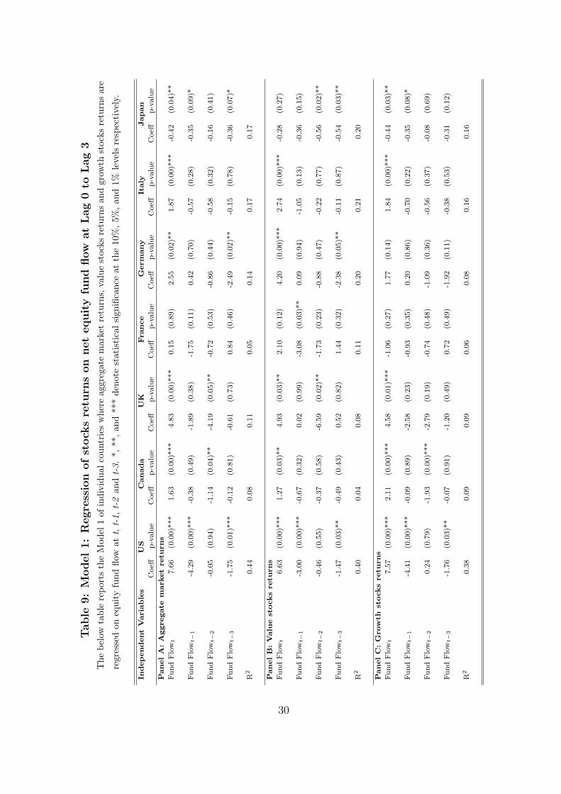
We run the above regression of each model for individual countries. The results of

model 1 for individual countries are reported in table 9.

Please insert table 9 and 10 about here

From Panel A of table 9, it is evident that coefficient for all the countries except France

is positive and significant at time t for aggregate market returns (refer Panel A). France

displays zero effect of concurrent and lagged equity fund flow on aggregate market returns

and growth stock returns. Japan is the only country that shows a negative effect of equity

fund flow on aggregate market returns and growth stock returns at t and t-1. This means

14

one standard deviation shock, 2.41%, to equity fund flow will lead to decrease in aggregate

market returns and growth stocks returns by an average of 1.03% at t and 0.84% at t-1.

Table 10 reports the results of model 2 for individual countries. Overall, the table shows

that lagged net equity fund flow has insignificant effect on stock returns except for the

U.K., France and Japan where coefficient of equity fund flow is statistically significant for

value stocks returns at t-1 and t-2.

The model 3 for individual countries are reported in table 11.

Please insert table 11 and 12 about here

The coefficients of concurrent expected fund flow of all the countries are insignificant.

Overall, the results show that unexpected concurrent net equity fund flow has a signif-

icant positive effect on aggregate market returns, value stock returns and growth stock

returns. The lagged component of unexpected equity fund flow for all the countries is sta-

tistically insignificant except for the value stock returns of U.K. The negative coefficient of

unexpected equity fund flow at t-2 indicates the possibility of price pressure effect on value

stock returns of U.K. Both France and Germany display no effect of concurrent unexpected

equity fund flow on growth stock returns; and Japan displays no evidence of unexpected

concurrent equity fund flow effect on value stock returns. Overall the result suggest that

unexpected equity fund flow has significant effect on aggregate market returns, value stock

returns and growth stocks returns; and this may be due to the presence of price pressure

effect or an information effect. To confirm if the effect of unexpected equity fund flow is

due to price pressure or new information, we perform reversal tests in which we regress

unexpected equity fund flow on stock returns at t-1, t and t+1. The results are reported in

table 12. We find evidence that inflow of unexpected equity fund flow has significant effect

on value stocks returns in France as we get significant positive coefficients at t followed by

significant negative coefficient at t+1. Thus there is evidence of a price pressure hypothesis

that exists in France as previous returns are reversed in the following month. Further,

we find Japan is the only country where inflow of unexpected equity funds has a negative

effect on aggregate market returns and growth stocks returns at t and t+1. Overall, our

individual country study findings (except France and Japan) show positive effect of unex-

pected equity fund flow on stock returns; this effect may be either due to price pressure or

the arrival of new positive information causing security prices to rise.

15

4.3 Closed end equity funds:

The results of panel fixed effect regression of both, model 1 and model 2, are given in table

13. As mentioned earlier, in model 1, we regress value stocks returns and growth stocks

returns at time t on ∆VWD and aggregate market returns.

Please insert table 13 about here

From model 1, it is evident that 1% decrease in ∆VWD is associated with an increase

in value stocks returns by 19 basis points. However with the drop of 1% in ∆VWD, growth

stocks returns decrease by 11 basis points. The significant coefficient of ∆VWD suggest

that investor sentiment as measured by ∆VWD has significant influence on both value

stocks returns and growth stocks returns. The decrease in discount has positive effect on

value stocks returns and negative effect on growth stocks returns. Our findings indicate

that investors’ optimism is associated with increase in returns along with decrease in CEEF

discount of value stocks returns. These findings contradicts with the findings of Lee et al

(1991) where they find smaller stocks, which usually tends to be growth stocks, to be usual

victims of investor sentiment. Besides, we found growth stocks to be mainly affected with

narrowing CEEF discounts. In order to study the relativeness of ∆VWD to aggregate

market returns and industry-return indices, we also run panel fixed effect regression in

model 2. Contrary to the previous findings by Elton et al (1998) and Doukas and Milonas

(2004), we find significant coefficient of both value stocks returns and growth stocks returns

at 5% and 1% significance level respectively. Our results show that 1% decrease in ∆VWD

leads to increase in value stocks returns by 10 basis points and decrease in growth stocks

returns by 7 basis points. Except for consumer goods returns, we further find that industry-

return indices do enter in return generating process as we get significant coefficients. Also

at the same time we see, that there is an increase in R2 for both value stocks returns and

growth stocks returns. Thus our findings indicate that CEEF discount does enter into

return generating process, similar to the results obtained by Lee et al (1991).

Please insert table 14 and 15 about here

The study of CEFF discount effect on value and growth stocks returns for individual

countries is given in table 14 and 15. Model 1 of table 14 shows that for value stocks re-

turns, we get significant negative coefficient of ∆VWD for the U.S., Canada and Germany

16

indicating that the decrease in ∆VWD is associated with an increase in value stocks re-

turns. Similarly for growth stock returns, we get significant positive coefficient of ∆VWD

for the U.S., Canada, U.K. and Italy indicating that increase in ∆VWD leads to increase

in growth stocks returns and vice-versa. Model 2 of table 15 shows the effect of ∆VWD

on value and growth stocks returns after considering industry-return indices and aggregate

market returns. For value stocks returns, we find U.S. as only country that is affected

by ∆VWD. For the U.S. market, except for industrials, all other industry-return indices

are significant at 1% level indicating that they also enter into return generating process.

Growth stocks returns are also significantly affected by ∆VWD for the U.S., Canada and

U.K. We get significant positive coefficient for these countries indicating positive relation-

ship between ∆VWD and growth stocks returns. The effect of industry-return indices in

return generating process is mixed for different countries. Model 2 also shows significant

improvement in R2 over model 1 for both value stocks returns and growth stocks returns

for each individual countries.

4.4 Equity Put-Call ratio:

Table 16 presents the results of panel fixed effect regression of current t returns and fore-

casted t+k returns on equity PCR. The significant and negative coefficient of equity PCR

in month t indicates the presence of influence of equity PCR in the same month t returns.

Further, our results indicate that only value stocks are significantly affected over next

month t+1, a finding similar to the one obtained by Lee and Song (2003). The coefficient

of equity PCR for value stocks is significant and negative for t+1 month, which indicates

that if one buys value stocks when equity PCR is low or sells value stocks when equity PCR

is high, can yield 6 basis points over next month. The fact that investor can yield very

low returns in t+1 is because information content in options volume is almost incorporated

in the stock price in the month t. Our findings are similar to previous literature where

authors have found the fading effect of equity PCR on stock returns, Pan and Poteshman

(2006). For t+1 month, we get insignificant coefficient for growth stocks and aggregate

market. The effect of equity PCR in t+2 is nil for aggregate market returns, value stocks

returns and growth stocks returns.

Please insert table 16 and 17 about here

17

Table 17 shows the effect of equity PCR on returns for each individual countries. It

is interesting to note that for the U.S. and Canada market, information content in equity

options volume gets slowly incorporated in stock price as investors have an opportunity to

gain in month t+1. For instance in the U.S., when equity PCR is low an investor can gain

aggregate market returns of 7 and 6 basis points in the month t+1 and t+2 respectively.

Also if an investor invests in growth stocks with low equity PCR in t, then it would yield him

8 and 7 basis points in the month t+1 and t+2 respectively. However, we get contradicting

results for Canadian aggregate market returns and growth stocks returns. For instance, an

investment in growth stocks with high equity PCR can help an investor to fetch 46 and 37

basis points in the month t+1 and t+2 respectively. In the case of value stocks, we did not

find significant coefficient for all countries in the month t+1. Similarly in the month t+2,

all countries except for the U.S. and Canada, we did not find any effect of equity PCR on

aggregate market returns, value stocks returns and growth stocks returns.

5 Conclusion

In this paper, we study the effect of consumer confidence index, equity fund flow, closed-

end fund equity (CEEF) discount and equity put-call ratio, widely considered as sentiment

proxies amongst many practitioners, on aggregate market returns, value stocks returns and

growth stocks returns. We find that there is a significant negative relationship between

survey sentiment and stocks returns. When investor sentiment is high (low) in the given

month, subsequent stocks returns are low (high). Our findings indicate that the effect

of survey sentiment is stronger on value stocks than that on the growth stocks which is

consistent with the previous empirical evidence [e.g. Schmeling (2009) and Lemmon and

Portniaguina (2006)]. The results are similar for net equity fund flow where we find negative

relationship between returns and subsequent equity fund flow. We find that the increase

in an unexpected concurrent equity fund flow has a positive effect on stock returns. In our

equity fund flow panel study, we find an evidence of temporary price pressure on aggregate

market returns and value stocks returns as we get highly significant estimates of return

reversal test. The increase in concurrent price of growth stocks and its subsequent decrease

may be either due to price pressure effect or an information effect.

Further, we find that value stocks returns and growth stocks returns are significantly

affected by the change in the CEEF discount. When CEEF discount narrows, value stocks

18

outperforms and growth stocks under performs; therefore indicating negative relationship

between CEEF discount and value stocks returns and positive relationship between CEEF

discount and growth stocks returns. Our results remain the same when we add industry-

return indices as natural candidates so as to measure the relativity of CEEF discount with

industry-return indices. Our findings are similar to that of Lee et al (1991) but contradicts

the findings of Elton et al (1998) and Doukas and Milonas (2004); therefore we conclude

that CEEF discount plays significant role in return generating process. Our results of eq-

uity PCR indicate that only value stocks yields positive returns in t+1 when PCR is low in

the month t. However, we did not find any evidence of equity PCR influencing aggregate

market returns and growth stocks returns.

19

Appendix A: Consumer Confidence Index Data Calculation:

Consumer surveys have been carried out in almost all the developed countries for more

than 20 years. These surveys are conducted to study consumers’ present and future fi-

nancial situation and their outlook on the economy over next year. The questions in the

surveys are usually standardized across all the countries. For instance, the University of

Michigan surveys at least 500 consumers households about their present and future finan-

cial situation, their business and economic outlook over next 1 year and 5 years respectively

and also about their willingness to spend on durable goods in the near future. Similarly,

the Conference Board of Canada surveys Canadian households about their present and fu-

ture financial situation and their level of optimism about the current economic conditions

and over the next 6 months. Besides studying the consumers’ current and future financial

situation and their outlook on the economy, DG ECFIN also seeks to find the likelihood of

consumers ability to save money over the next 12 months. DG ECFIN conduct consumer

survey on at least 2,000 households of U.K., Germany and Italy each and 3,300 households

of France. Of all, Japan surveys maximum household, i.e. 6,000 households. Their survey

questionnaire consists questions similar to that of U.S. and Canada, viz. consumers’ per-

ception of the economy, price expectation and their present and future financial situation.

Overall, the consumer survey questions are similar across the G7 countries and hence the

outcome of the survey can be made easily comparable. However, the calculation of index

differs across countries. For instance, DG ECFIN employs ‘Dainties’ method and Japan

employs X-11 of the Census Bureau USA. For ease of comparison, we standardize consumer

confidence survey measure across all the countries.

Appendix B: Equity Fund Flow Data Calculation:

This appendix details the reason for using the net equity fund flow data including dis-

tributions. Equity Fund Flow data has been widely used as sentiment proxy by many

practitioners. The net sales of new equity funds is considered as an increase in confidence

in the economy by an investor as they are willing to display bullish behavior in the stock

market. The Investment Company Institute of U.S. is the national trade association for

the investment company industry. Almost all the mutual funds, closed-end equity funds,

exchange-traded funds (ETF) and unit investment trust (UIT). domiciled in the U.S. are

the members of ICI. For each fund, ICI collects the following information, viz. net new

sales, reinvested dividends, net redemptions and net switches between the funds. In order

20

to study the effect of net equity fund flow, previous authors, Warther (1995) and Indro

(2004), have used net sales excluding distributions. The similar breakdown of net sales

including and excluding distributions is maintained by The Investment Fund Institute of

Canada (IFIC). The Investment Management Association, U.K. (IMA), maintains the net

sales of equity funds of all the mutual fund managers domiciled in United Kingdom. The

net sales data maintained by IMA includes distributions and is net of switches made be-

tween the funds and net redemptions. Lipper, subsidiary of Thomson Reuters maintains

the database of net equity fund flow including distributions for France, Germany, Italy and

Japan with effect from January 2002. They calculate net sales as a difference between total

equity fund assets between two months after stripping the performance of all the assets

within the funds. The data maintained by them includes reinvested distributions and also

takes into account both net redemptions and net switches between the funds. In order to

consider consistent data across all the countries, we decide to use net equity fund flow data

including distributions valued in U.S. Dollars. For this reason, we employ value weighted

stocks returns including re-invested distributions provided by Kenneth French24.

Appendix C: Details of closed-end equity funds data considered:

This appendix discuss different type of closed-end funds collected by Morningstar that

are considered in our research. For each fund, Morningstar gathers net asset value (NAV)

and price data. NAV data are sourced directly from the fund manager whereas price data

are obtained from trading exchanges. In our research, we have considered only conventional

closed end equity funds. Bond funds are specifically excluded. Also within closed end equity

funds, we do not consider fund warrants, C-shares and split funds in our analysis. Fund

Warrants are not considered as they don’t have NAV; C-shares are a way of existing funds

raising money and hence are not considered as conventional closed end funds. Split funds

are investment trusts with a fixed life, where the shares are divided into more than one

category. The simplest form of split funds is a split between capital shares and income

shares. The other variation of closed-end funds, which are not in their conventional form,

includes zero dividend preference shares, highly geared shares, participating income shares

and stepped preference shares. These funds have been specifically excluded in our discount

calculation. Lastly, CEEF for which either NAV data or price data is not available are

excluded in our VWD calculation.

24http://mba.tuck.dartmouth.edu/pages/faculty/ken.french/data library.html

21

References

[1] Baker, M., and Wurgler, J., 2006. Investor Sentiment and the Cross-Section of Stock

Returns. Journal of Finance 61. 1645-1680.

[2] Baker, M., and Wurgler, J., 2007. Investor Sentiment in the Stock Market. Journal of

Economic Perspectives 21. 129-151.

[3] Bandopadhyaya, A., and Jones, A., 2008. Measures of Investor Sentiment: A compar-

ative analysis Put-Call Ratio vs Volatility Index. Journal of Business & Economics

Research 6. 27-34.

[4] Barberis, N., Shleifer, A., and Vishny, R., 1998. A model of investor sentiment. Journal

of Financial Economics 49. 307-343.

[5] Black, F., 1986. Noise. Journal of Finance 41. 529-543.

[6] Brauer, G., 1993. Investor sentiment and the closed-end fund puzzle: A 7 percent

solution. Journal of Financial Services Research 7. 199-216.

[7] Brown, G., 1999. Volatility, Sentiment and Noise Traders. Financial Analysts Journal

55. 82-90.

[8] Brown, G., and Cliff, M., 2004. Investor Sentiment and the near term stock market.

Journal of Empirical Finance 11. 1-27.

[9] Brown, G., and Cliff, M., 2005. Investor Sentiment and Asset Valuation. Journal of

Business 78. 405-440.

[10] Brown, S., Goetzmann, W., Hiraki, T., Shiraishi, N., and Watanabe, N., 2003. Investor

Sentiment in Japanese and US Daily Mutual Fund Flows. Working Paper. NBER 9470.

[11] Chen, N., Kan, R., and Miller, M., 1993. Are the discounts on closed-end funds a

sentiment index?. Journal of Finance 58. 795-800.

[12] Chopra, N., Lee, C., Shleifer, A., and Thaler, R., 1993a. Yes. Discounts on closed-end

funds are a sentiment index. Journal of Finance 48. 801-808.

[13] Chopra, N., Lee, C., Shleifer, A., and Thaler, R., 1993b, Summing up. Journal of

Finance 48. 811-812.

22

[14] Daniel, K., Hirshleifer, D., and Subrahmanyam, A., 1998. Investor psychology and

security market under and overreactions. Journal of Finance 53. 1839 1886.

[15] De Bondt, W., and Thaler, R., 1985. Does the stock market overreact?. Journal of

Finance 40. 793-805.

[16] DeBondt, W., and Thaler, R. H., 1987. Further evidence on investor overreaction and

stock market seasonality. Journal of Finance 42. 557-581

[17] De Long, J.B., Shleifer, A., Summers, L. and Waldmann, R., 1990. Noise Trader Risk

in Financial Markets. Journal of Political Economy 98. 703-738.

[18] Doukas, J., and Milonas, N., 2004. Investor Sentiment and the closed end fund puzzle:

Out of sample evidence. European Financial Management 10. 235-266.

[19] Edelen, R., and Warner, J., 2001. Aggregate price effects of institutional trading: A

study of mutual fund flow and market returns. Journal of Financial Economics 59.

195-220.

[20] Elton, E., Gruber, M., and Busse, J., 1998. Do investors care about sentiment?. Journal

of Business 71. 477-500.

[21] Fisher, K., and Statman, M., 2000. Investor Sentiment and Stock Returns. Financial

Analysts Journal 56. 16-23.

[22] Fisher, K., and Statman, M., 2003. Consumer Confidence and Stock Returns. Journal

of Portfolio Management 30. 115-127.

[23] Frazzini, A., and Lamont, O., 2006. ‘Dumb Money: Mutual Fund Flows and the Cross

Section of Stock Returns. Journal of Financial Economics 88. 299-322.

[24] Indro, D., 2004. Does Mutual Fund Flow Reflect Investor Sentiment?. Journal of Be-

havioral Finance 5. 105-115.

[25] Lee, C., Shleifer, A., and Thaler, R., 1991. Investor Sentiment and the Closed End

Puzzle. Journal of Finance 46(1). 75-109.

[26] Lee, Y. and Song, Z., 2003. When do value stocks outperform growth stocks? Investor

Sentiment and Equity Style Rotation Strategies. Working Paper. University of Rhode

Island.

23

[27] Lemmon, M., and Portniaguina, E., 2006. Consumer confidence and Asset Prices:

Some Empirical Evidence. Review of Financial Studies 19. 1499-1529.

[28] Ljungqvist, A., 2006. IPO Underpricing. Handbook of Corporate Finance: Empirical

Corporate Finance Chapter 7. Elsevier/North-Holland Publication.

[29] Neal, R., and Wheatley, S., 1998. Do Measures of Investor Sentiment Predict Returns?.

Journal of Financial and Quantitative Analysis 33. 523-547.

[30] Pan, J., and Poteshman, A., 2006. The Information in Option Volume for Future Stock

Prices. Review of Financial Studies 19. 871-908.

[31] Qiu, L., and Welch, I., 2006. Investor Sentiment Measures. Working Paper. Brown

University.

[32] Ritter, J., 2003. Investment Banking and Securities Issuance. Handbook of the Eco-

nomics of Finance Chapter 5. Elsevier Science Publication.

[33] Russel, P., 2005. Closed-End Fund Pricing: The Puzzle, The Explanations, and Some

New Evidence. Journal of Business and Economic Studies 11. 34-49.

[34] Schmeling, M., 2009. Investor Sentiment and Stock Returns: Some International Evi-

dence. Journal of Empirical Finance 16. 394-408.

[35] Shiller, R., 2005. Irrational Exuberance. Princeton, NJ: Princeton University Press.

[36] Shleifer, A., and Vishny, R., 1997. The limits of arbitrage. Journal of Finance 52.

35-55.

[37] Subrahmanyam, A., 2007. Behavioral Finance: A Review and Synthesis. European

Financial Management 14. 12-29.

[38] Verma, R., and Soydemir, G., 2006. The Impact of US Individual and Institutional

Investor Sentiment on Foreign Stock Market. Journal of Behavioral Finance 7. 128-144.

[39] Warther, V., 1995. Aggregate mutual fund flows and security returns. Journal of Fi-

nancial Economics 39. 209-235.

[40] Zweig, M., 1973. An investor expectations stock price predictive model using closed-

end premiums. Journal of Finance 28. 67-78.

24

Table 1: Data Sources:

The below table details data sources of different sentiment proxies, viz. consumer confidence index, equity

fund flow, closed-end equity fund discount and equity put-call options volume. This table also list the

time horizon for each data source and for each individual country.

Country Time Horizon Source

Panel A: Consumer Confidence Index

U.S. Jan 1995-Dec 2007 The University of Michigan Consumer Surveys

Canada Jan 1995-Dec 2007 The Conference Board, Canada

U.K. Jan 1995-Dec 2007 Directorate Generale for Economic & Financial Affairs (DG ECFIN)

France Jan 1995-Dec 2007 Directorate Generale for Economic & Financial Affairs (DG ECFIN)

Germany Jan 1995-Dec 2007 Directorate Generale for Economic & Financial Affairs (DG ECFIN)

Italy Jan 1995-Dec 2007 Directorate Generale for Economic & Financial Affairs (DG ECFIN)

Japan Jan 1995-Dec 2007 The Cabinet Office, Japan

Panel B: Equity Fund Flow

U.S. Jan 1995-Dec 2007 The Investment Company Institute

Canada Jan 1995-Dec 2007 The Investment Fund Institute of Canada

U.K. Jan 1995-Dec 2007 The Investment Management Association, U.K.

France Jan 2002-Dec 2007 Lipper, Thomson Reuters

Germany Jan 2002-Dec 2007 Lipper, Thomson Reuters

Italy Jan 2002-Dec 2007 Lipper, Thomson Reuters

Japan Jan 2002-Dec 2007 Lipper, Thomson Reuters

Panel C: Closed End Equity Fund

U.S. Jan 1995-Dec 2007 Morningstar, Inc

Canada Jan 1995-Dec 2007 Morningstar, Inc

U.K. Jan 1995-Dec 2007 Morningstar, Inc

France Jan 1995-May 2004 Morningstar, Inc

Germany Jan 1995-Dec 2007 Morningstar, Inc

Italy Jan 1995-Jan 2003 Morningstar, Inc

Japan Jan 1995-Dec 2007 Morningstar, Inc

Panel D: Individual Equity Options Volume

U.S. Jan 1995-Dec 2007 The Chicago Board of Options Exchange

Canada Dec 2000-Dec 2007 Bourse De Montreal Inc

U.K. Jan 2000-Dec 2007 NYSE Euronext

France Jan 2002-Dec 2007 NYSE Euronext

Germany Jan 2001-Dec 2007 Deutsche Borse Group

Italy Jan 2001-Dec 2007 Borsa Italiana

Japan Jul 1997-Dec 2007 Tokyo Stock Exchange

25

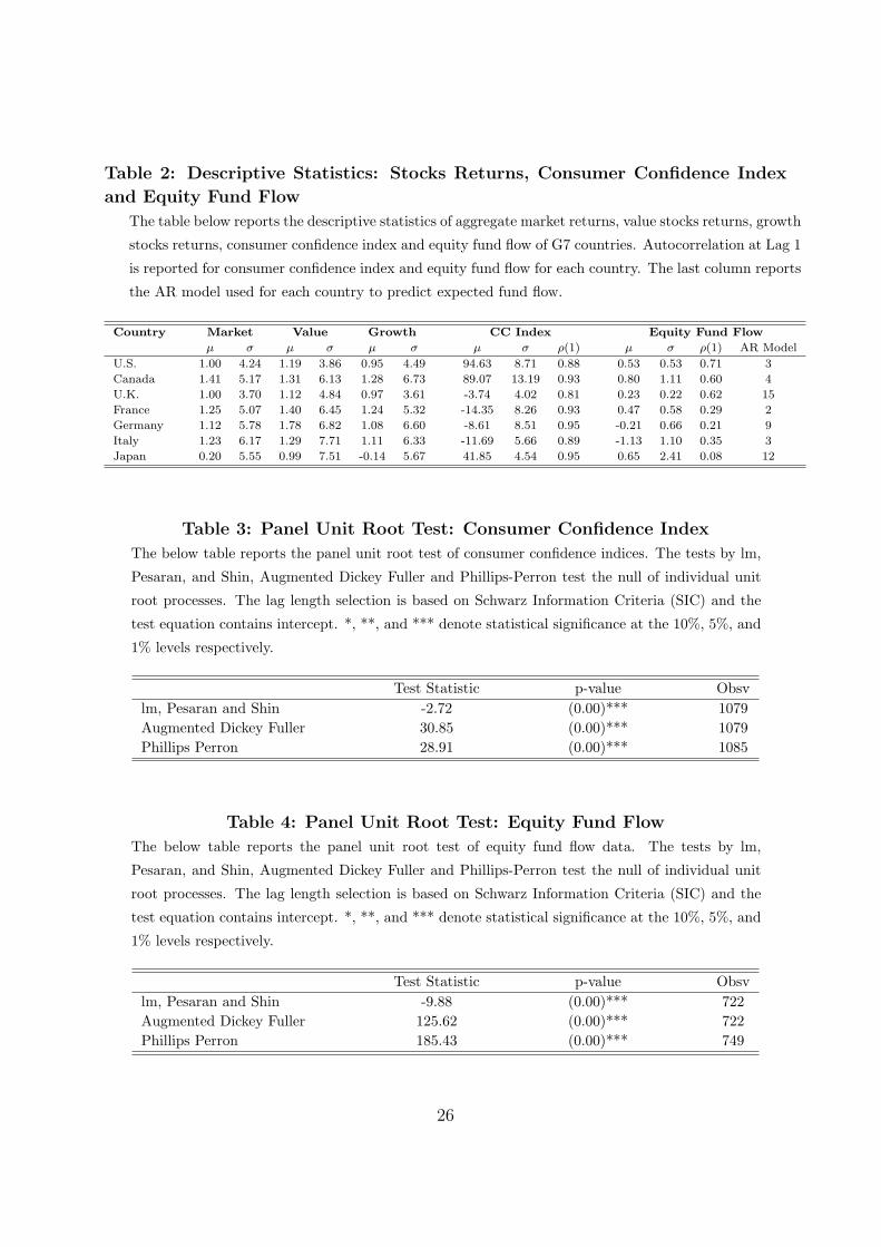
Table 2: Descriptive Statistics: Stocks Returns, Consumer Confidence Index

and Equity Fund Flow

The table below reports the descriptive statistics of aggregate market returns, value stocks returns, growth

stocks returns, consumer confidence index and equity fund flow of G7 countries. Autocorrelation at Lag 1

is reported for consumer confidence index and equity fund flow for each country. The last column reports

the AR model used for each country to predict expected fund flow.

Country Market Value Growth CC Index Equity Fund Flow

µ σ µ σ µ σ µ σ ρ(1) µ σ ρ(1) AR Model

U.S. 1.00 4.24 1.19 3.86 0.95 4.49 94.63 8.71 0.88 0.53 0.53 0.71 3

Canada 1.41 5.17 1.31 6.13 1.28 6.73 89.07 13.19 0.93 0.80 1.11 0.60 4

U.K. 1.00 3.70 1.12 4.84 0.97 3.61 -3.74 4.02 0.81 0.23 0.22 0.62 15

France 1.25 5.07 1.40 6.45 1.24 5.32 -14.35 8.26 0.93 0.47 0.58 0.29 2

Germany 1.12 5.78 1.78 6.82 1.08 6.60 -8.61 8.51 0.95 -0.21 0.66 0.21 9

Italy 1.23 6.17 1.29 7.71 1.11 6.33 -11.69 5.66 0.89 -1.13 1.10 0.35 3

Japan 0.20 5.55 0.99 7.51 -0.14 5.67 41.85 4.54 0.95 0.65 2.41 0.08 12

Table 3: Panel Unit Root Test: Consumer Confidence Index

The below table reports the panel unit root test of consumer confidence indices. The tests by lm,

Pesaran, and Shin, Augmented Dickey Fuller and Phillips-Perron test the null of individual unit

root processes. The lag length selection is based on Schwarz Information Criteria (SIC) and the

test equation contains intercept. *, **, and *** denote statistical significance at the 10%, 5%, and

1% levels respectively.

Test Statistic p-value Obsvlm, Pesaran and Shin -2.72 (0.00)*** 1079Augmented Dickey Fuller 30.85 (0.00)*** 1079Phillips Perron 28.91 (0.00)*** 1085

Table 4: Panel Unit Root Test: Equity Fund Flow

The below table reports the panel unit root test of equity fund flow data. The tests by lm,

Pesaran, and Shin, Augmented Dickey Fuller and Phillips-Perron test the null of individual unit

root processes. The lag length selection is based on Schwarz Information Criteria (SIC) and the

test equation contains intercept. *, **, and *** denote statistical significance at the 10%, 5%, and

1% levels respectively.

Test Statistic p-value Obsvlm, Pesaran and Shin -9.88 (0.00)*** 722Augmented Dickey Fuller 125.62 (0.00)*** 722Phillips Perron 185.43 (0.00)*** 749

26

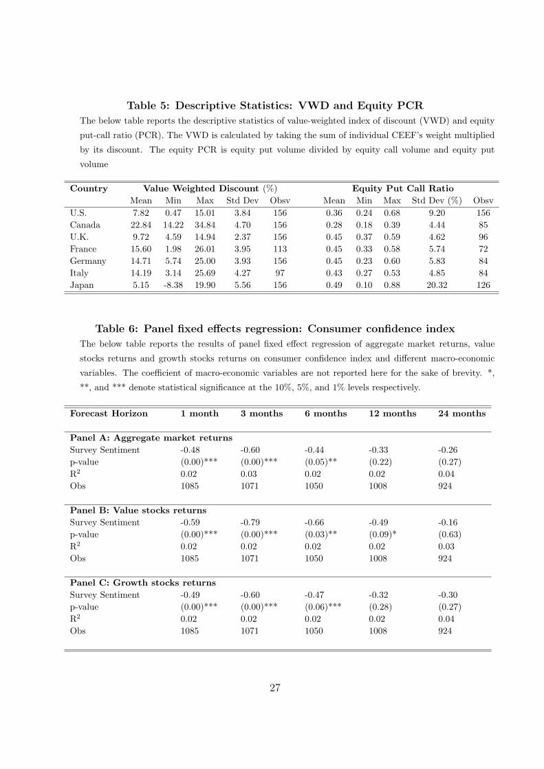
Table 5: Descriptive Statistics: VWD and Equity PCR

The below table reports the descriptive statistics of value-weighted index of discount (VWD) and equity

put-call ratio (PCR). The VWD is calculated by taking the sum of individual CEEF’s weight multiplied

by its discount. The equity PCR is equity put volume divided by equity call volume and equity put

volume

Country Value Weighted Discount (%) Equity Put Call RatioMean Min Max Std Dev Obsv Mean Min Max Std Dev (%) Obsv

U.S. 7.82 0.47 15.01 3.84 156 0.36 0.24 0.68 9.20 156Canada 22.84 14.22 34.84 4.70 156 0.28 0.18 0.39 4.44 85U.K. 9.72 4.59 14.94 2.37 156 0.45 0.37 0.59 4.62 96France 15.60 1.98 26.01 3.95 113 0.45 0.33 0.58 5.74 72Germany 14.71 5.74 25.00 3.93 156 0.45 0.23 0.60 5.83 84Italy 14.19 3.14 25.69 4.27 97 0.43 0.27 0.53 4.85 84Japan 5.15 -8.38 19.90 5.56 156 0.49 0.10 0.88 20.32 126

Table 6: Panel fixed effects regression: Consumer confidence index

The below table reports the results of panel fixed effect regression of aggregate market returns, value

stocks returns and growth stocks returns on consumer confidence index and different macro-economic

variables. The coefficient of macro-economic variables are not reported here for the sake of brevity. *,

**, and *** denote statistical significance at the 10%, 5%, and 1% levels respectively.

Forecast Horizon 1 month 3 months 6 months 12 months 24 months

Panel A: Aggregate market returnsSurvey Sentiment -0.48 -0.60 -0.44 -0.33 -0.26p-value (0.00)*** (0.00)*** (0.05)** (0.22) (0.27)R2 0.02 0.03 0.02 0.02 0.04Obs 1085 1071 1050 1008 924

Panel B: Value stocks returnsSurvey Sentiment -0.59 -0.79 -0.66 -0.49 -0.16p-value (0.00)*** (0.00)*** (0.03)** (0.09)* (0.63)R2 0.02 0.02 0.02 0.02 0.03Obs 1085 1071 1050 1008 924

Panel C: Growth stocks returnsSurvey Sentiment -0.49 -0.60 -0.47 -0.32 -0.30p-value (0.00)*** (0.00)*** (0.06)*** (0.28) (0.27)R2 0.02 0.02 0.02 0.02 0.04Obs 1085 1071 1050 1008 924

27

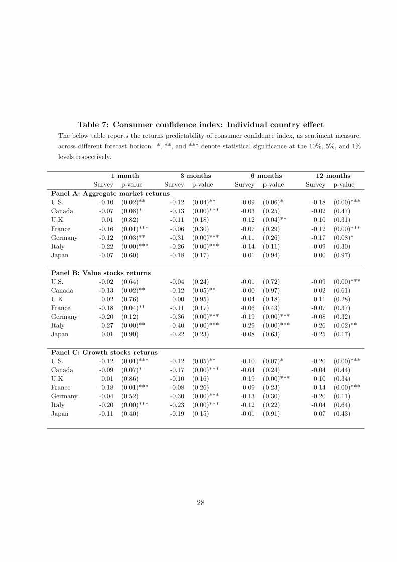
Table 7: Consumer confidence index: Individual country effect

The below table reports the returns predictability of consumer confidence index, as sentiment measure,

across different forecast horizon. *, **, and *** denote statistical significance at the 10%, 5%, and 1%

levels respectively.

1 month 3 months 6 months 12 monthsSurvey p-value Survey p-value Survey p-value Survey p-value

Panel A: Aggregate market returnsU.S. -0.10 (0.02)** -0.12 (0.04)** -0.09 (0.06)* -0.18 (0.00)***Canada -0.07 (0.08)* -0.13 (0.00)*** -0.03 (0.25) -0.02 (0.47)U.K. 0.01 (0.82) -0.11 (0.18) 0.12 (0.04)** 0.10 (0.31)France -0.16 (0.01)*** -0.06 (0.30) -0.07 (0.29) -0.12 (0.00)***Germany -0.12 (0.03)** -0.31 (0.00)*** -0.11 (0.26) -0.17 (0.08)*Italy -0.22 (0.00)*** -0.26 (0.00)*** -0.14 (0.11) -0.09 (0.30)Japan -0.07 (0.60) -0.18 (0.17) 0.01 (0.94) 0.00 (0.97)

Panel B: Value stocks returnsU.S. -0.02 (0.64) -0.04 (0.24) -0.01 (0.72) -0.09 (0.00)***Canada -0.13 (0.02)** -0.12 (0.05)** -0.00 (0.97) 0.02 (0.61)U.K. 0.02 (0.76) 0.00 (0.95) 0.04 (0.18) 0.11 (0.28)France -0.18 (0.04)** -0.11 (0.17) -0.06 (0.43) -0.07 (0.37)Germany -0.20 (0.12) -0.36 (0.00)*** -0.19 (0.00)*** -0.08 (0.32)Italy -0.27 (0.00)** -0.40 (0.00)*** -0.29 (0.00)*** -0.26 (0.02)**Japan 0.01 (0.90) -0.22 (0.23) -0.08 (0.63) -0.25 (0.17)

Panel C: Growth stocks returnsU.S. -0.12 (0.01)*** -0.12 (0.05)** -0.10 (0.07)* -0.20 (0.00)***Canada -0.09 (0.07)* -0.17 (0.00)*** -0.04 (0.24) -0.04 (0.44)U.K. 0.01 (0.86) -0.10 (0.16) 0.19 (0.00)*** 0.10 (0.34)France -0.18 (0.01)*** -0.08 (0.26) -0.09 (0.23) -0.14 (0.00)***Germany -0.04 (0.52) -0.30 (0.00)*** -0.13 (0.30) -0.20 (0.11)Italy -0.20 (0.00)*** -0.23 (0.00)*** -0.12 (0.22) -0.04 (0.64)Japan -0.11 (0.40) -0.19 (0.15) -0.01 (0.91) 0.07 (0.43)

28

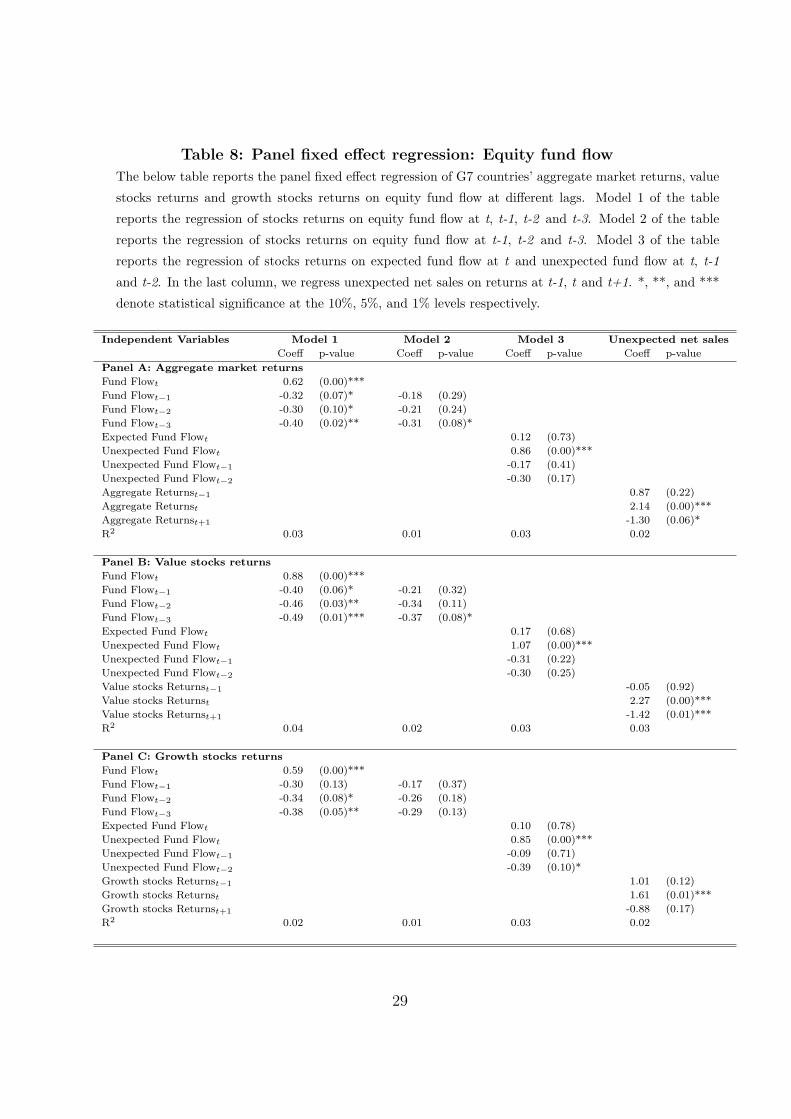
Table 8: Panel fixed effect regression: Equity fund flow

The below table reports the panel fixed effect regression of G7 countries’ aggregate market returns, value

stocks returns and growth stocks returns on equity fund flow at different lags. Model 1 of the table

reports the regression of stocks returns on equity fund flow at t, t-1, t-2 and t-3. Model 2 of the table

reports the regression of stocks returns on equity fund flow at t-1, t-2 and t-3. Model 3 of the table

reports the regression of stocks returns on expected fund flow at t and unexpected fund flow at t, t-1

and t-2. In the last column, we regress unexpected net sales on returns at t-1, t and t+1. *, **, and ***

denote statistical significance at the 10%, 5%, and 1% levels respectively.

Independent Variables Model 1 Model 2 Model 3 Unexpected net sales

Coeff p-value Coeff p-value Coeff p-value Coeff p-value

Panel A: Aggregate market returns

Fund Flowt 0.62 (0.00)***

Fund Flowt−1 -0.32 (0.07)* -0.18 (0.29)

Fund Flowt−2 -0.30 (0.10)* -0.21 (0.24)

Fund Flowt−3 -0.40 (0.02)** -0.31 (0.08)*

Expected Fund Flowt 0.12 (0.73)

Unexpected Fund Flowt 0.86 (0.00)***

Unexpected Fund Flowt−1 -0.17 (0.41)

Unexpected Fund Flowt−2 -0.30 (0.17)

Aggregate Returnst−1 0.87 (0.22)

Aggregate Returnst 2.14 (0.00)***

Aggregate Returnst+1 -1.30 (0.06)*

R2 0.03 0.01 0.03 0.02

Panel B: Value stocks returns

Fund Flowt 0.88 (0.00)***

Fund Flowt−1 -0.40 (0.06)* -0.21 (0.32)

Fund Flowt−2 -0.46 (0.03)** -0.34 (0.11)

Fund Flowt−3 -0.49 (0.01)*** -0.37 (0.08)*

Expected Fund Flowt 0.17 (0.68)

Unexpected Fund Flowt 1.07 (0.00)***

Unexpected Fund Flowt−1 -0.31 (0.22)

Unexpected Fund Flowt−2 -0.30 (0.25)

Value stocks Returnst−1 -0.05 (0.92)

Value stocks Returnst 2.27 (0.00)***

Value stocks Returnst+1 -1.42 (0.01)***

R2 0.04 0.02 0.03 0.03

Panel C: Growth stocks returns

Fund Flowt 0.59 (0.00)***

Fund Flowt−1 -0.30 (0.13) -0.17 (0.37)

Fund Flowt−2 -0.34 (0.08)* -0.26 (0.18)

Fund Flowt−3 -0.38 (0.05)** -0.29 (0.13)

Expected Fund Flowt 0.10 (0.78)

Unexpected Fund Flowt 0.85 (0.00)***

Unexpected Fund Flowt−1 -0.09 (0.71)

Unexpected Fund Flowt−2 -0.39 (0.10)*

Growth stocks Returnst−1 1.01 (0.12)

Growth stocks Returnst 1.61 (0.01)***

Growth stocks Returnst+1 -0.88 (0.17)

R2 0.02 0.01 0.03 0.02

29

Table

9:

Model

1:

Regre

ssio

nof

stock

sre

turn

son

net

equit

yfu

nd

flow

at

Lag

0to

Lag

3

The

belo

wta

ble

repo

rts

the

Mod

el1

ofin

divi

dual

coun

trie

sw

here

aggr

egat

em

arke

tre

turn

s,va

lue

stoc

ksre

turn

san

dgr

owth

stoc

ksre

turn

sar

e

regr

esse

don

equi

tyfu

ndflo

wat

t,t-1,

t-2

and

t-3.

*,**

,an

d**

*de

note

stat

isti

cal

sign

ifica

nce

atth

e10

%,

5%,

and

1%le

vels

resp

ecti

vely

.

Ind

ep

en

dent

Varia

ble

sU

SC

an

ad

aU

KFran

ce

Germ

any

Italy

Jap

an

Coeff

p-v

alu

eC

oeff

p-v

alu

eC

oeff

p-v

alu

eC

oeff

p-v

alu

eC

oeff

p-v

alu

eC

oeff

p-v

alu

eC

oeff

p-v

alu

e

Pan

el

A:

Aggregate

market

retu

rn

s

Fu

nd

Flo

wt

7.6

6(0

.00)*

**

1.6

3(0

.00)*

**

4.8

3(0

.00)*

**

0.1

5(0

.89)

2.5

5(0

.02)*

*1.8

7(0

.00)*

**

-0.4

2(0

.04)*

*

Fu

nd

Flo

wt−

1-4

.29

(0.0

0)*

**

-0.3

8(0

.49)

-1.8

9(0

.38)

-1.7

5(0

.11)

0.4

2(0

.70)

-0.5

7(0

.28)

-0.3

5(0

.09)*

Fu

nd

Flo

wt−

2-0

.05

(0.9

4)

-1.1

4(0

.04)*

*-4

.19

(0.0

5)*

*-0

.72

(0.5

3)

-0.8

6(0

.44)

-0.5

8(0

.32)

-0.1

6(0

.41)

Fu

nd

Flo

wt−

3-1

.75

(0.0

1)*

**

-0.1

2(0

.81)

-0.6

1(0

.73)

0.8

4(0

.46)

-2.4

9(0

.02)*

*-0

.15

(0.7

8)

-0.3

6(0

.07)*

R2

0.4

40.0

80.1

10.0

50.1

40.1

70.1

7

Pan

el

B:

Valu

est

ocks

retu

rn

s

Fu

nd

Flo

wt

6.6

3(0

.00)*

**

1.2

7(0

.03)*

*4.9

3(0

.03)*

*2.1

0(0

.12)

4.2

0(0

.00)*

**

2.7

4(0

.00)*

**

-0.2

8(0

.27)

Fu

nd

Flo

wt−

1-3

.00

(0.0

0)*

**

-0.6

7(0

.32)

0.0

2(0

.99)

-3.0

8(0

.03)*

*0.0

9(0

.94)

-1.0

5(0

.13)

-0.3

6(0

.15)

Fu

nd

Flo

wt−

2-0

.46

(0.5

5)

-0.3

7(0

.58)

-6.5

9(0

.02)*

*-1

.73

(0.2

3)

-0.8

8(0

.47)

-0.2

2(0

.77)

-0.5

6(0

.02)*

*

Fu

nd

Flo

wt−

3-1

.47

(0.0

3)*

*-0

.49

(0.4

3)

0.5

2(0

.82)

1.4

4(0

.32)

-2.3

8(0

.05)*

*-0

.11

(0.8

7)

-0.5

4(0

.03)*

*

R2

0.4

00.0

40.0

80.1

10.2

00.2

10.2

0

Pan

el

C:

Grow

thst

ocks

retu

rn

s

Fu

nd

Flo

wt

7.5

7(0

.00)*

**

2.1

1(0

.00)*

**

4.5

8(0

.01)*

**

-1.0

6(0

.27)

1.7

7(0

.14)

1.8

4(0

.00)*

**

-0.4

4(0

.03)*

*

Fu

nd

Flo

wt−

1-4

.41

(0.0

0)*

**

-0.0

9(0

.89)

-2.5

8(0

.23)

-0.9

3(0

.35)

0.2

0(0

.86)

-0.7

0(0

.22)

-0.3

5(0

.08)*

Fu

nd

Flo

wt−

20.2

4(0

.79)

-1.9

3(0

.00)*

**

-2.7

9(0

.19)

-0.7

4(0

.48)

-1.0

9(0

.36)

-0.5

6(0

.37)

-0.0

8(0

.69)

Fu

nd

Flo

wt−

3-1

.76

(0.0

3)*

*-0

.07

(0.9

1)

-1.2

0(0

.49)

0.7

2(0

.49)

-1.9

2(0

.11)

-0.3

8(0

.53)

-0.3

1(0

.12)

R2

0.3

80.0

90.0

90.0

60.0

80.1

60.1

6

30

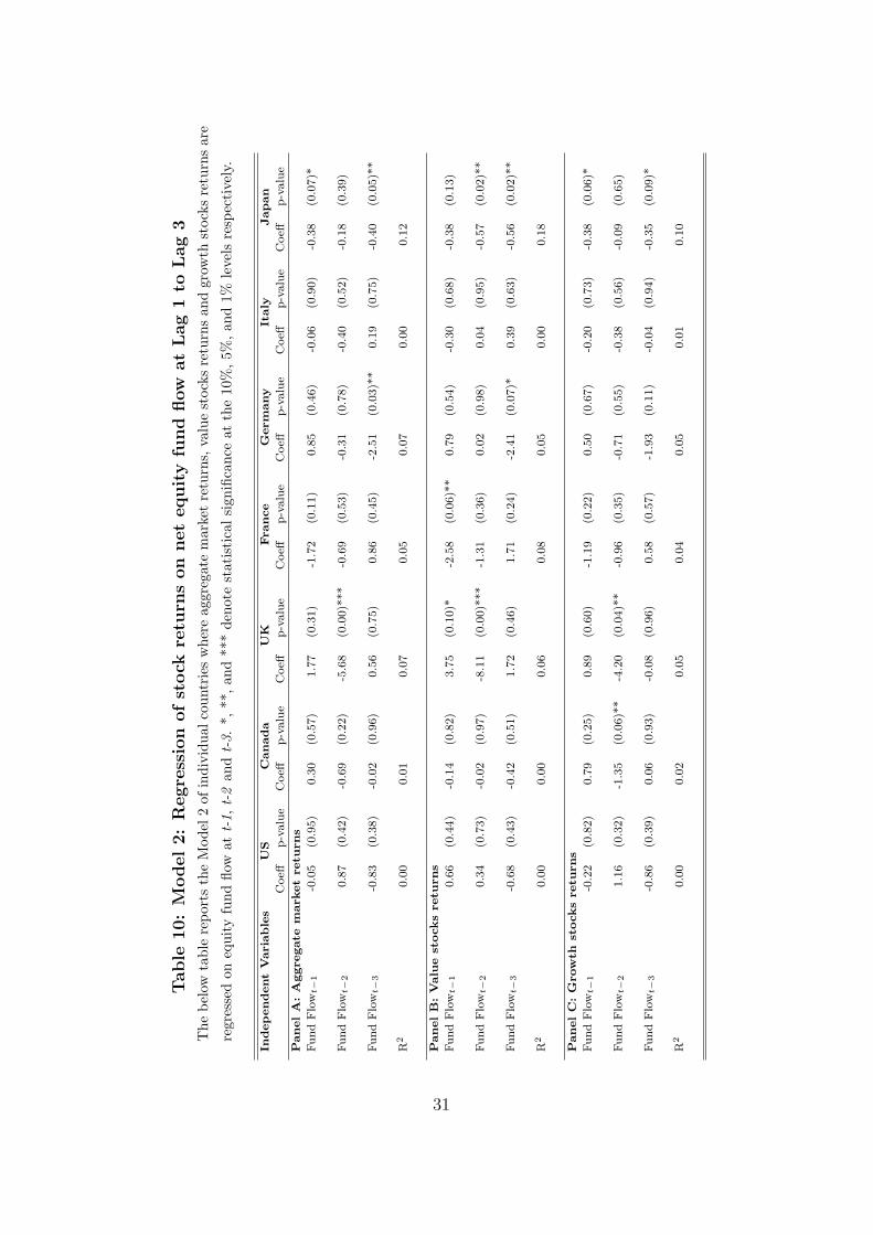
Table

10:

Model

2:

Regre

ssio

nof

stock

retu

rns

on

net

equit

yfu

nd

flow

at

Lag

1to

Lag

3

The

belo

wta

ble

repo

rts

the

Mod

el2

ofin

divi

dual

coun

trie

sw

here

aggr

egat

em

arke

tre

turn

s,va

lue

stoc

ksre

turn

san

dgr

owth

stoc

ksre

turn

sar

e

regr

esse

don

equi

tyfu

ndflo

wat

t-1,

t-2

and

t-3.

*,**

,an

d**

*de

note

stat

isti

cal

sign

ifica

nce

atth

e10

%,

5%,

and

1%le

vels

resp

ecti

vely

.

Ind

ep

en

dent

Varia

ble

sU

SC

an

ad

aU

KFran

ce

Germ

any

Italy

Jap

an

Coeff

p-v

alu

eC

oeff

p-v

alu

eC

oeff

p-v

alu

eC

oeff

p-v

alu

eC

oeff

p-v

alu

eC

oeff

p-v

alu

eC

oeff

p-v

alu

e

Pan

el

A:

Aggregate

market

retu

rn

s

Fu

nd

Flo

wt−

1-0

.05

(0.9

5)

0.3

0(0

.57)

1.7

7(0

.31)

-1.7

2(0

.11)

0.8

5(0

.46)

-0.0

6(0

.90)

-0.3

8(0

.07)*

Fu

nd

Flo

wt−

20.8

7(0

.42)

-0.6

9(0

.22)

-5.6

8(0

.00)*

**

-0.6

9(0

.53)

-0.3

1(0

.78)

-0.4

0(0

.52)

-0.1

8(0

.39)

Fu

nd

Flo

wt−

3-0

.83

(0.3

8)

-0.0

2(0

.96)

0.5

6(0

.75)

0.8

6(0

.45)

-2.5

1(0

.03)*

*0.1

9(0

.75)

-0.4

0(0

.05)*

*

R2

0.0

00.0

10.0

70.0

50.0

70.0

00.1

2

Pan

el

B:

Valu

est

ocks

retu

rn

s

Fu

nd

Flo

wt−

10.6

6(0

.44)

-0.1

4(0

.82)

3.7

5(0

.10)*

-2.5

8(0

.06)*

*0.7

9(0

.54)

-0.3

0(0

.68)

-0.3

8(0

.13)

Fu

nd

Flo

wt−

20.3

4(0

.73)

-0.0

2(0

.97)

-8.1

1(0

.00)*

**

-1.3

1(0

.36)

0.0

2(0

.98)

0.0

4(0

.95)

-0.5

7(0

.02)*

*

Fu

nd

Flo

wt−

3-0

.68

(0.4

3)

-0.4

2(0

.51)

1.7

2(0

.46)

1.7

1(0

.24)

-2.4

1(0

.07)*

0.3

9(0

.63)

-0.5

6(0

.02)*

*

R2

0.0

00.0

00.0

60.0

80.0

50.0

00.1

8

Pan

el

C:

Grow

thst

ocks

retu

rn

s

Fu

nd

Flo

wt−

1-0

.22

(0.8

2)

0.7

9(0

.25)

0.8

9(0

.60)

-1.1

9(0

.22)

0.5

0(0

.67)

-0.2

0(0

.73)

-0.3

8(0

.06)*

Fu

nd

Flo

wt−

21.1

6(0

.32)

-1.3

5(0

.06)*

*-4

.20

(0.0

4)*

*-0

.96

(0.3

5)

-0.7

1(0

.55)

-0.3

8(0

.56)

-0.0

9(0

.65)

Fu

nd

Flo

wt−

3-0

.86

(0.3

9)

0.0

6(0

.93)

-0.0

8(0

.96)

0.5

8(0

.57)

-1.9

3(0

.11)

-0.0

4(0

.94)

-0.3

5(0

.09)*

R2

0.0

00.0

20.0

50.0

40.0

50.0

10.1

0

31

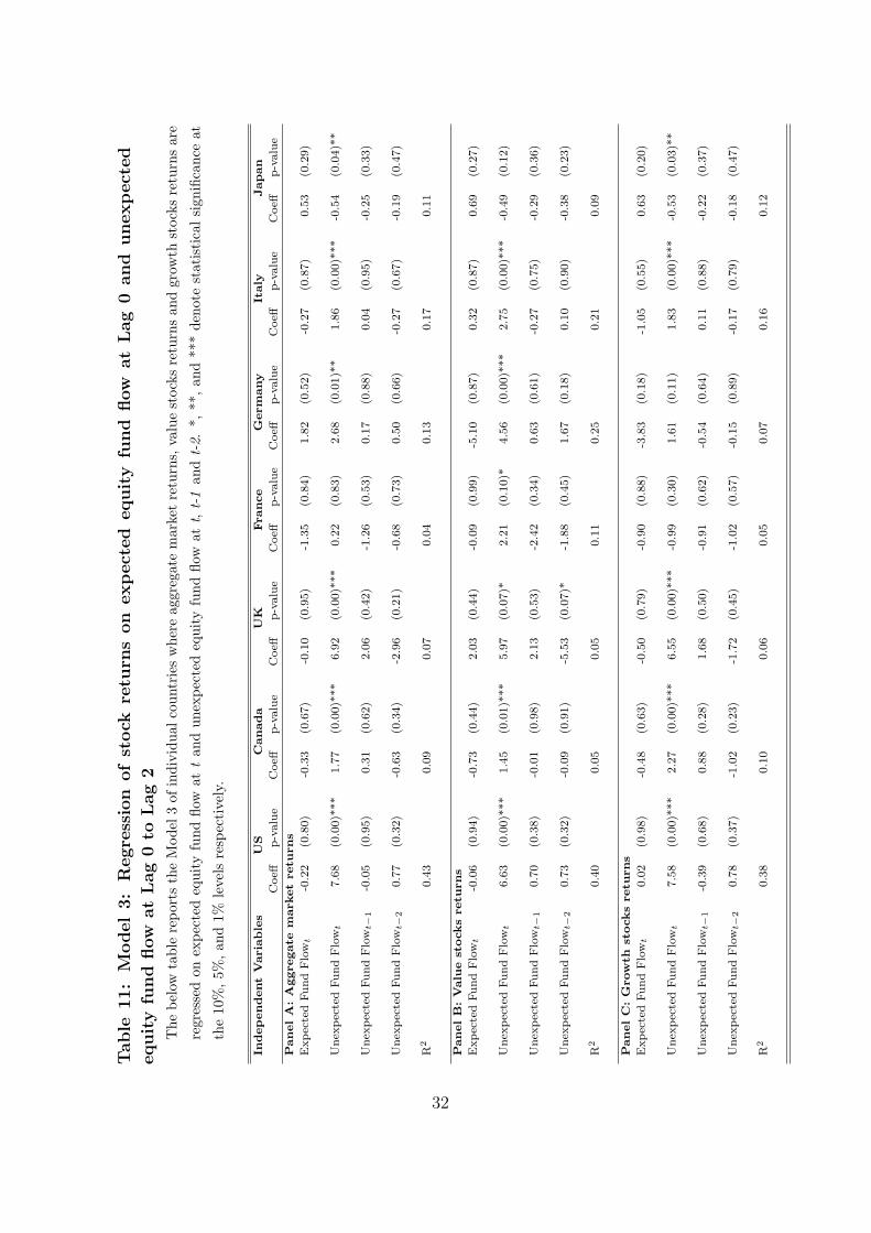
Table

11:

Model

3:

Regre

ssio

nof

stock

retu

rns

on

exp

ect

ed

equit

yfu

nd

flow

at

Lag

0an

du

nexp

ect

ed

equit

yfu

nd

flow

at

Lag

0to

Lag

2

The

belo

wta

ble

repo

rts

the

Mod

el3

ofin

divi

dual

coun

trie

sw

here

aggr

egat

em

arke

tre

turn

s,va

lue

stoc

ksre

turn

san

dgr

owth

stoc

ksre

turn

sar

e

regr

esse

don

expe

cted

equi

tyfu

ndflo

wat

tan

dun

expe

cted

equi

tyfu

ndflo

wat

t,t-1

and

t-2.

*,**

,an

d**

*de

note

stat

isti

cal

sign

ifica

nce

at

the

10%

,5%

,an

d1%

leve

lsre

spec

tive

ly.

Ind

ep

en

dent

Varia

ble

sU

SC

an

ad

aU

KFran

ce

Germ

any

Italy

Jap

an

Coeff

p-v

alu

eC

oeff

p-v

alu

eC

oeff

p-v

alu

eC

oeff

p-v

alu

eC

oeff

p-v

alu

eC

oeff

p-v

alu

eC

oeff

p-v

alu

e

Pan

el

A:

Aggregate

market

retu

rn

s

Exp

ecte

dF

un

dF

low

t-0

.22

(0.8

0)

-0.3

3(0

.67)

-0.1

0(0

.95)

-1.3

5(0

.84)

1.8

2(0

.52)

-0.2

7(0

.87)

0.5

3(0

.29)

Un

exp

ecte

dF

un

dF

low

t7.6

8(0

.00)*

**

1.7

7(0

.00)*

**

6.9

2(0

.00)*

**

0.2

2(0

.83)

2.6

8(0

.01)*

*1.8

6(0

.00)*

**

-0.5

4(0

.04)*

*

Un

exp

ecte

dF

un

dF

low

t−1

-0.0

5(0

.95)

0.3

1(0

.62)

2.0

6(0

.42)

-1.2

6(0

.53)

0.1

7(0

.88)

0.0

4(0

.95)

-0.2

5(0

.33)

Un

exp

ecte

dF

un

dF

low

t−2

0.7

7(0

.32)

-0.6

3(0

.34)

-2.9

6(0

.21)

-0.6

8(0

.73)

0.5

0(0

.66)

-0.2

7(0

.67)

-0.1

9(0

.47)

R2

0.4

30.0

90.0

70.0

40.1

30.1

70.1

1

Pan

el

B:

Valu

est

ocks

retu

rn

s

Exp

ecte

dF

un

dF

low

t-0

.06

(0.9

4)

-0.7

3(0

.44)

2.0

3(0

.44)

-0.0

9(0

.99)

-5.1

0(0

.87)

0.3

2(0

.87)

0.6

9(0

.27)

Un

exp

ecte

dF

un

dF

low

t6.6

3(0

.00)*

**

1.4

5(0

.01)*

**

5.9

7(0

.07)*

2.2

1(0

.10)*

4.5

6(0

.00)*

**

2.7

5(0

.00)*

**

-0.4

9(0

.12)

Un

exp

ecte

dF

un

dF

low

t−1

0.7

0(0

.38)

-0.0

1(0

.98)

2.1

3(0

.53)

-2.4

2(0

.34)

0.6

3(0

.61)

-0.2

7(0

.75)

-0.2

9(0

.36)

Un

exp

ecte

dF

un

dF

low

t−2

0.7

3(0

.32)

-0.0

9(0

.91)

-5.5

3(0

.07)*

-1.8

8(0

.45)

1.6

7(0

.18)

0.1

0(0

.90)

-0.3

8(0

.23)

R2

0.4

00.0

50.0

50.1

10.2

50.2

10.0

9

Pan

el

C:

Grow

thst

ocks

retu

rn

s

Exp

ecte

dF

un

dF

low

t0.0

2(0

.98)

-0.4

8(0

.63)

-0.5

0(0

.79)

-0.9

0(0

.88)

-3.8

3(0

.18)

-1.0

5(0

.55)

0.6

3(0

.20)

Un

exp

ecte

dF

un

dF

low

t7.5

8(0

.00)*

**

2.2

7(0

.00)*

**

6.5

5(0

.00)*

**

-0.9

9(0

.30)

1.6

1(0

.11)

1.8

3(0

.00)*

**

-0.5

3(0

.03)*

*

Un

exp

ecte

dF

un

dF

low

t−1

-0.3

9(0

.68)

0.8

8(0

.28)

1.6

8(0

.50)

-0.9

1(0

.62)

-0.5

4(0

.64)

0.1

1(0

.88)

-0.2

2(0

.37)

Un

exp

ecte

dF

un

dF

low

t−2

0.7

8(0

.37)

-1.0

2(0

.23)

-1.7

2(0

.45)

-1.0

2(0

.57)

-0.1

5(0

.89)

-0.1

7(0

.79)

-0.1

8(0

.47)

R2

0.3

80.1

00.0

60.0

50.0

70.1

60.1

2

32

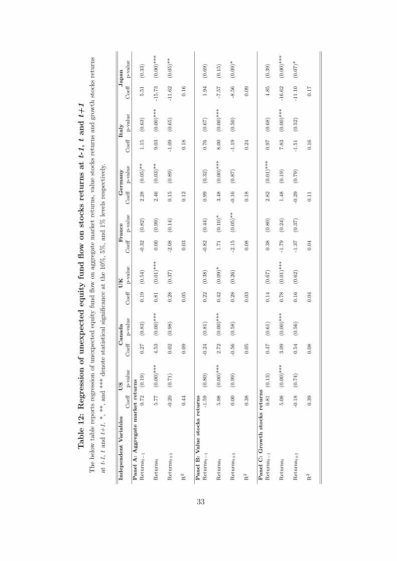
Table

12:

Regre

ssio

nof

unexp

ect

ed

equit

yfu

nd

flow

on

stock

sre

turn

satt-1,t

an

dt+

1

The

belo

wta

ble

repo

rts

regr

essi

onof

unex

pect

edeq

uity

fund

flow

onag

greg

ate

mar

ket

retu

rns,

valu

est

ocks

retu

rns

and

grow

thst

ocks

retu

rns

att-1,

tan

dt+

1.*,

**,

and

***

deno

test

atis

tica

lsi

gnifi

canc

eat

the

10%

,5%

,an

d1%

leve

lsre

spec

tive

ly.

Ind

ep

en

dent

Varia

ble

sU

SC

an

ad

aU

KFran

ce

Germ

any

Italy

Jap

an

Coeff

p-v

alu

eC

oeff

p-v

alu

eC

oeff

p-v

alu

eC

oeff

p-v

alu

eC

oeff

p-v

alu

eC

oeff

p-v

alu

eC

oeff

p-v

alu

e

Pan

el

A:

Aggregate

market

retu

rn

s

Ret

urn

s t−

10.7

2(0

.19)

0.2

7(0

.83)

0.1

9(0

.54)

-0.3

2(0

.82)

2.2

8(0

.05)*

*1.1

5(0

.63)

5.5

1(0

.33)

Ret

urn

s t5.7

7(0

.00)*

**

4.5

3(0

.00)*

**

0.8

1(0

.01)*

**

0.0

0(0

.99)

2.4

6(0

.03)*

*9.0

3(0

.00)*

**

-15.7

3(0

.00)*

**

Ret

urn

s t+

1-0

.20

(0.7

1)

0.0

2(0

.98)

0.2

8(0

.37)

-2.0

8(0

.14)

0.1

5(0

.89)

-1.0

9(0

.65)

-11.6

2(0

.05)*

*

R2

0.4

40.0

90.0

50.0

30.1

20.1

80.1

6

Pan

el

B:

Valu

est

ocks

retu

rn

s

Ret

urn

s t−

1-1

.59

(0.8

0)

-0.2

4(0

.81)

0.2

2(0

.38)

-0.8

2(0

.44)

0.9

9(0

.32)

0.7

6(0

.67)

1.9

4(0

.69)

Ret

urn

s t5.9

8(0

.00)*

**

2.7

2(0

.00)*

**

0.4

2(0

.09)*

1.7

1(0

.10)*

3.4

8(0

.00)*

**

8.0

0(0

.00)*

**

-7.5

7(0

.15)

Ret

urn

s t+

10.0

0(0

.99)

-0.5

6(0

.58)

0.2

8(0

.26)

-2.1

5(0

.05)*

*-0

.16

(0.8

7)

-1.1

9(0

.50)

-8.5

6(0

.09)*

R2

0.3

80.0

50.0

30.0

80.1

80.2

40.0

9

Pan

el

C:

Grow

thst

ocks

retu

rn

s

Ret

urn

s t−

10.8

1(0

.13)

0.4

7(0

.61)

0.1

4(0

.67)

0.3

8(0

.80)

2.8

2(0

.01)*

**

0.9

7(0

.68)

4.8

5(0

.39)

Ret

urn

s t5.0

8(0

.00)*

**

3.0

9(0

.00)*

**

0.7

8(0

.01)*

**

-1.7

9(0

.24)

1.4

8(0

.19)

7.8

3(0

.00)*

**

-16.6

2(0

.00)*

**

Ret

urn

s t+

1-0

.18

(0.7

4)

0.5

4(0

.56)

0.1

6(0

.62)

-1.3

7(0

.37)

-0.2

9(0

.79)

-1.5

1(0

.52)

-11.1

0(0

.07)*

R2

0.3

90.0

80.0

40.0

40.1

10.1

60.1

7

33

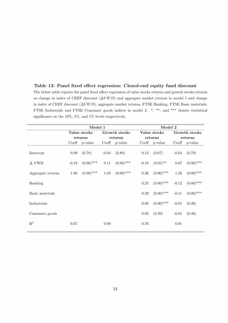
Table 13: Panel fixed effect regression: Closed-end equity fund discount

The below table reports the panel fixed effect regression of value stocks returns and growth stocks returns

on change in index of CEEF discount (∆V WD) and aggregate market returns in model 1 and change

in index of CEEF discount (∆V WD), aggregate market returns, FTSE Banking, FTSE Basic materials,

FTSE Industrials and FTSE Consumer goods indices in model 2. *, **, and *** denote statistical

significance at the 10%, 5%, and 1% levels respectively.

Model 1 Model 2Value stocks Growth stocks Value stocks Growth stocks

returns returns returns returnsCoeff p-value Coeff p-value Coeff p-value Coeff p-value

Intercept 0.09 (0.78) -0.04 (0.80) 0.13 (0.67) -0.04 (0.79)

∆ VWD -0.19 (0.00)*** 0.11 (0.00)*** -0.10 (0.05)** 0.07 (0.00)***

Aggregate returns 1.00 (0.00)*** 1.03 (0.00)*** 0.36 (0.00)*** 1.29 (0.00)***

Banking 0.25 (0.00)*** -0.12 (0.00)***

Basic materials 0.29 (0.00)*** -0.11 (0.00)***

Industrials 0.08 (0.00)*** -0.01 (0.26)

Consumer goods 0.02 (0.29) -0.01 (0.38)

R2 0.67 0.89 0.76 0.91

34

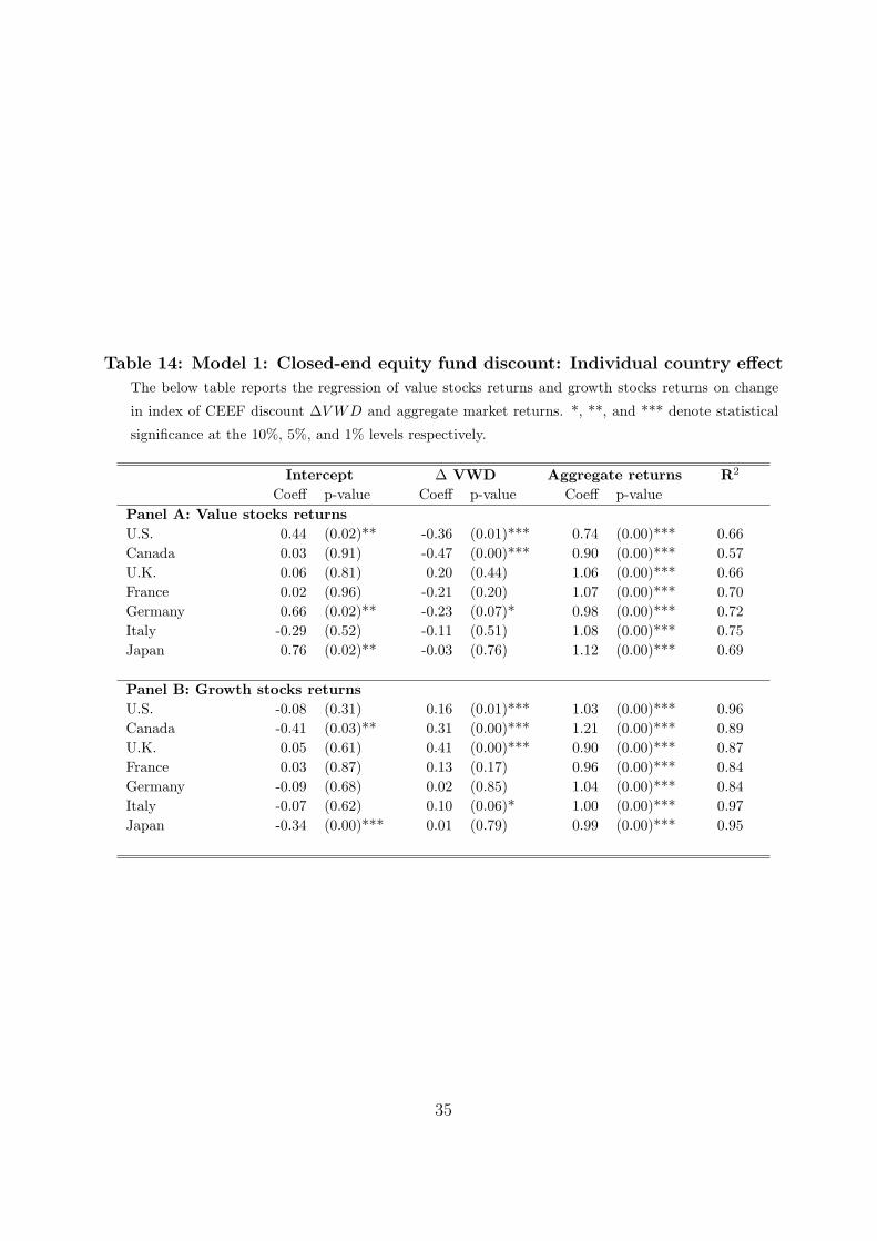
Table 14: Model 1: Closed-end equity fund discount: Individual country effect

The below table reports the regression of value stocks returns and growth stocks returns on change

in index of CEEF discount ∆V WD and aggregate market returns. *, **, and *** denote statistical

significance at the 10%, 5%, and 1% levels respectively.

Intercept ∆ VWD Aggregate returns R2

Coeff p-value Coeff p-value Coeff p-valuePanel A: Value stocks returnsU.S. 0.44 (0.02)** -0.36 (0.01)*** 0.74 (0.00)*** 0.66Canada 0.03 (0.91) -0.47 (0.00)*** 0.90 (0.00)*** 0.57U.K. 0.06 (0.81) 0.20 (0.44) 1.06 (0.00)*** 0.66France 0.02 (0.96) -0.21 (0.20) 1.07 (0.00)*** 0.70Germany 0.66 (0.02)** -0.23 (0.07)* 0.98 (0.00)*** 0.72Italy -0.29 (0.52) -0.11 (0.51) 1.08 (0.00)*** 0.75Japan 0.76 (0.02)** -0.03 (0.76) 1.12 (0.00)*** 0.69

Panel B: Growth stocks returnsU.S. -0.08 (0.31) 0.16 (0.01)*** 1.03 (0.00)*** 0.96Canada -0.41 (0.03)** 0.31 (0.00)*** 1.21 (0.00)*** 0.89U.K. 0.05 (0.61) 0.41 (0.00)*** 0.90 (0.00)*** 0.87France 0.03 (0.87) 0.13 (0.17) 0.96 (0.00)*** 0.84Germany -0.09 (0.68) 0.02 (0.85) 1.04 (0.00)*** 0.84Italy -0.07 (0.62) 0.10 (0.06)* 1.00 (0.00)*** 0.97Japan -0.34 (0.00)*** 0.01 (0.79) 0.99 (0.00)*** 0.95

35

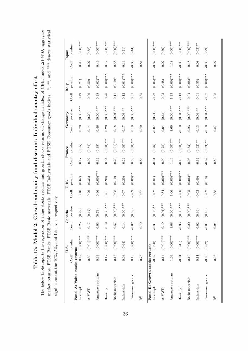
Table

15:

Model

2:

Clo

sed-e

nd

equit

yfu

nd

dis

count:

Indiv

idual

cou

ntr

yeff

ect

The

belo

wta

ble

repo

rts

the

regr

essi

onof

valu

est

ocks

retu

rns

and

grow

thst

ocks

retu

rns

onch

ange

inin

dex

ofC

EE

Fin

dex

∆V

WD

,ag

greg

ate

mar

ket

retu

rns,

FT

SEB

anks

,F

TSE

Bas

icm

ater

ials

,F

TSE

Indu

stri

als

and

FT

SEC

onsu

mer

good

sin

dice

s.*,

**,

and

***

deno

test

atis

tica

l

sign

ifica

nce

atth

e10

%,

5%,

and

1%le

vels

resp

ecti

vely

.

U.S

.C

an

ad

aU

.K.

Fran

ce

Germ

any

Italy

Jap

an

Coeff

p-v

alu

eC

oeff

p-v

alu

eC

oeff

p-v

alu

eC

oeff

p-v

alu

eC

oeff

p-v

alu

eC

oeff

p-v

alu

eC

oeff

p-v

alu

e

Pan

el

A:

Valu

est

ocks

retu

rn

s

Inte

rcep

t0.4

9(0

.00)*

**

0.2

5(0

.29)

0.1

0(0

.67)

0.1

7(0

.55)

0.7

9(0

.00)*

**

0.4

9(0

.21)

0.9

0(0

.00)*

**

∆V

WD

-0.3

0(0

.01)*

**

-0.1

7(0

.17)

0.2

6(0

.33)

-0.0

2(0

.84)

-0.1

4(0

.20)

0.0

9(0

.50)

-0.0

7(0

.38)

Aggre

gate

retu

rns

0.3

3(0

.00)*

**

0.0

3(0

.73)

0.9

6(0

.00)*

**

-0.1

2(0

.38)

0.4

6(0

.00)*

**

0.2

8(0

.02)*

*0.4

9(0

.00)*

**

Ban

kin

g0.1

2(0

.00)*

**

0.1

9(0

.00)*

**

0.0

1(0

.90)

0.3

4(0

.00)*

**

0.2

9(0

.00)*

**

0.2

6(0

.00)*

**

0.1

7(0

.00)*

**

Basi

cm

ate

rials

0.1

6(0

.00)*

**

0.5

7(0

.00)*

**

0.0

8(0

.19)

0.2

0(0

.01)*

**

0.1

8(0

.01)*

**

0.1

1(0

.10)*

0.5

8(0

.00)*

**

Ind

ust

rials

0.0

3(0

.64)

0.1

4(0

.00)*

**

0.0

7(0

.20)

0.2

2(0

.00)*

**

-0.1

7(0

.03)*

*0.1

2(0

.01)*

**

-0.1

4(0

.21)

Con

sum

ergood

s0.1

6(0

.00)*

**

-0.0

2(0

.48)

-0.0

9(0

.03)*

*0.3

8(0

.00)*

**

0.1

8(0

.00)*

**

0.3

1(0

.00)*

**

-0.0

6(0

.44)

R2

0.7

80.7

90.6

70.8

50.7

90.8

50.8

4

Pan

el

B:

Grow

thst

ocks

retu

rn

s

Inte

rcep

t-0

.09

(0.2

0)

-0.3

1(0

.03)*

*0.0

2(0

.81)

-0.0

1(0

.96)

-0.0

7(0

.71)

-0.2

2(0

.05)*

*-0

.37

(0.0

0)*

**

∆V

WD

0.1

4(0

.01)*

**

0.1

9(0

.01)*

**

0.3

4(0

.00)*

**

0.0

9(0

.28)

-0.0

4(0

.64)

0.0

3(0

.48)

0.0

2(0

.50)

Aggre

gate

retu

rns

1.0

3(0

.00)*

**

1.6

8(0

.00)*

**

1.0

6(0

.00)*

**

1.4

4(0

.00)*

**

1.6

0(0

.00)*

**

1.2

3(0

.00)*

**

1.1

8(0

.00)*

**

Ban

kin

g-0

.01

(0.4

1)

-0.3

5(0

.00)*

**

-0.0

8(0

.00)*

**

-0.1

8(0

.00)*

**

-0.1

0(0

.01)*

**

-0.1

3(0

.00)*

**

-0.0

5(0

.00)*

**

Basi

cm

ate

rials

-0.1

0(0

.00)*

**

-0.2

0(0

.00)*

**

-0.0

5(0

.06)*

-0.0

6(0

.33)

-0.2

3(0

.00)*

**

-0.0

4(0

.06)*

-0.1

8(0

.00)*

**

Ind

ust

rials

0.1

1(0

.00)*

**

0.0

2(0

.36)

-0.0

2(0

.49)

-0.1

2(0

.02)*

*-0

.13

(0.0

3)*

*-0

.01

(0.5

5)

0.0

8(0

.03)*

*

Con

sum

ergood

s-0

.00

(0.8

2)

-0.0

1(0

.45)

0.0

2(0

.18)

-0.0

9(0

.03)*

*-0

.10

(0.0

1)*

**

-0.0

7(0

.00)*

**

-0.0

3(0

.29)

R2

0.9

60.9

40.8

80.8

90.8

70.9

80.9

7

36

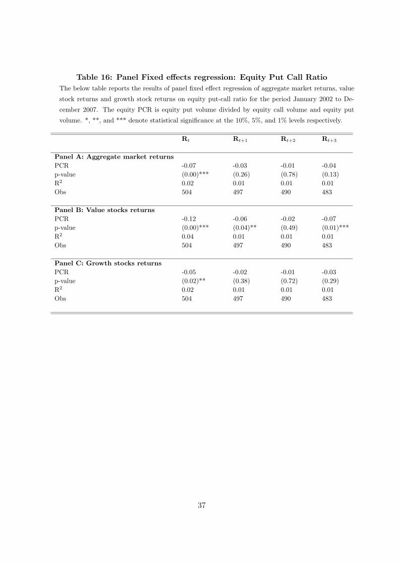
Table 16: Panel Fixed effects regression: Equity Put Call Ratio

The below table reports the results of panel fixed effect regression of aggregate market returns, value

stock returns and growth stock returns on equity put-call ratio for the period January 2002 to De-

cember 2007. The equity PCR is equity put volume divided by equity call volume and equity put

volume. *, **, and *** denote statistical significance at the 10%, 5%, and 1% levels respectively.

Rt Rt+1 Rt+2 Rt+3

Panel A: Aggregate market returnsPCR -0.07 -0.03 -0.01 -0.04p-value (0.00)*** (0.26) (0.78) (0.13)R2 0.02 0.01 0.01 0.01Obs 504 497 490 483

Panel B: Value stocks returnsPCR -0.12 -0.06 -0.02 -0.07p-value (0.00)*** (0.04)** (0.49) (0.01)***R2 0.04 0.01 0.01 0.01Obs 504 497 490 483

Panel C: Growth stocks returnsPCR -0.05 -0.02 -0.01 -0.03p-value (0.02)** (0.38) (0.72) (0.29)R2 0.02 0.01 0.01 0.01Obs 504 497 490 483

37

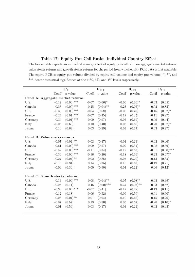
Table 17: Equity Put Call Ratio: Individual Country Effect

The below table reports an individual country effect of equity put-call ratio on aggregate market returns,

value stocks returns and growth stocks returns for the period from which equity PCR data is first available.

The equity PCR is equity put volume divided by equity call volume and equity put volume. *, **, and

*** denote statistical significance at the 10%, 5%, and 1% levels respectively.

Rt Rt+1 Rt+2 Rt+3

Coeff p-value Coeff p-value Coeff p-value Coeff p-valuePanel A: Aggregate market returnsU.S. -0.12 (0.00)*** -0.07 (0.06)* -0.06 (0.10)* -0.03 (0.45)Canada -0.33 (0.00)*** 0.25 (0.04)** 0.23 (0.07)* -0.02 (0.85)U.K. -0.36 (0.00)*** -0.04 (0.68) -0.06 (0.49) -0.16 (0.07)*France -0.24 (0.01)*** -0.07 (0.45) -0.12 (0.25) -0.11 (0.27)Germany -0.30 (0.01)*** -0.00 (0.97) -0.05 (0.69) -0.09 (0.44)Italy -0.06 (0.60) 0.10 (0.40) 0.06 (0.60) -0.20 (0.07)*Japan 0.10 (0.69) 0.03 (0.29) 0.03 (0.17) 0.03 (0.27)

Panel B: Value stocks returnsU.S. -0.07 (0.02)** -0.02 (0.47) -0.04 (0.23) -0.02 (0.46)Canada -0.61 (0.00)*** 0.09 (0.57) 0.09 (0.54) -0.08 (0.59)U.K. -0.52 (0.00)*** -0.11 (0.34) -0.12 (0.33) -0.31 (0.00)***France -0.34 (0.00)*** -0.16 (0.20) -0.18 (0.16) -0.23 (0.07)*Germany -0.27 (0.04)** -0.02 (0.88) -0.05 (0.70) -0.13 (0.35)Italy -0.15 (0.31) 0.14 (0.35) 0.15 (0.32) -0.19 (0.21)Japan -0.04 (0.30) 0.00 (0.90) 0.04 (0.22) 0.06 (0.12)

Panel C: Growth stocks returnsU.S. -0.13 (0.00)*** -0.08 (0.04)** -0.07 (0.08)* -0.03 (0.39)Canada -0.25 (0.11) 0.46 (0.00)*** 0.37 (0.03)** 0.03 (0.82)U.K. -0.30 (0.00)*** -0.07 (0.41) -0.12 (0.17) -0.13 (0.11)France -0.12 (0.18) -0.06 (0.52) -0.06 (0.50) -0.01 (0.90)Germany -0.28 (0.04)** -0.01 (0.94) -0.10 (0.46) -0.15 (0.26)Italy -0.07 (0.57) 0.13 (0.30) 0.05 (0.67) -0.20 (0.10)*Japan 0.01 (0.59) 0.03 (0.17) 0.03 (0.22) 0.02 (0.43)

38