arX

iv:h

ep-p

h/06

1129

5v2

1 D

ec 2

006

LPT - Orsay 06/73RM3-TH/06-22

An estimate of the B → K∗γ

decay form factor

Damir Becirevica, Vittorio Lubiczb and Federico Mesciac

a Laboratoire de Physique Theorique (Bat. 210),Universite Paris Sud, Centre d’Orsay,

F-91405 Orsay-Cedex, France.

b Dip. di Fisica, Univ. di Roma Tre and INFN, Sezione di Roma III,Via della Vasca Navale 84, I-00146 Rome, Italy.

c INFN, Laboratori Nazionali di Frascati,Via E. Fermi 40, I-00044 Frascati, Italy.

Abstract

We present the results of a lattice QCD calculation of the form factor relevantto B → K∗γ decay. Our final value, T (0) = 0.24 ± 0.03+0.04

−0.01, is obtained in the

quenched approximation, and by extrapolating M3/2H × TH→K∗

(q2 = 0) from thedirectly accessed H-heavy mesons to the meson B. We also show that the extrap-olation from B → K∗γ∗ (q2 6= 0) to B → K∗γ (q2 = 0), leads to a result consis-tent with the one quoted above. On the other hand, our results are not accurateenough to solve the SU(3) flavor breaking effects in the form factor and we quoteTB→K∗

(0)/TB→ρ(0) = 1.2(1), as our best estimate.

PACS: 12.38.Gc, 13.25.Hw, 13.25.Jx, 13.30.Ce, 13.75Lb

1 Introduction

The flavour changing neutral decays, B → V γ (V = K∗, ρ, ω), are induced by penguindiagrams. Their accurate experimental measurement gives us information about the heavyparticle content in the loops, and thus might be a window to the physics beyond theStandard Model (SM). This is why a huge amount of both experimental and theoreticalresearch has been invested in studying these modes over the past decade.

The experimenters at CLEO were first to observe and measure the B → K∗γ decayrate [1]. Averaging over the neutral and charged B-mesons they reported

B (B → K∗γ) = (4.5 ± 1.5 ± 0.9) × 10−5. (1)

Today, the unprecedented statistical quality of the data collected at the B-factories madeit possible to do precision measurements separately for B0 and B± decays, namely

B(B0 → K∗0γ

)=

(3.92 ± 0.20 ± 0.24) × 10−5 BaBar [2]

(4.01 ± 0.21 ± 0.17) × 10−5 Belle [3],

(2)

B(B+ → K∗+γ

)=

(3.87 ± 0.28 ± 0.26) × 10−5 BaBar [2]

(4.25 ± 0.31 ± 0.24) × 10−5 Belle [3].

Besides, the first significant measurements of B → ρ(ω)γ [4], opened a discussion onthe possibility of constraining |Vtd/Vts|, thus providing an alternative to the constraint

arising from the ratio of the oscillation frequencies in the B0

s − B0s and B

0

d − B0d systems,

∆mBs/∆mBd

[5].However, when looking for non-SM effects in these decays, one should be able to con-

front the above experimental results to the corresponding theoretical estimates within theSM. 1 As usual, the main obstacle is a lack of good theoretical control over the hadronicuncertainties. The hadronic matrix element entering the analysis of these, electromagneticpenguin induced, decays is

〈V (p′; eλ)|T µν(0)|B(p)〉 = e∗α(p′, λ) × T αµν ,

T αµν = ǫαµνβ

[(pβ + p′β − M2

B − m2V

q2qβ

)T1(q

2) +M2

B − m2V

q2qβT2(q

2)

]

+2pα

q2ǫµνσλpσp

′λ

(T2(q

2) − T1(q2) +

q2

M2B − m2

V

T3(q2)

), (3)

where q = p−p′, the tensor current T µν = isσµνb for V = K∗, and T µν = idσµνb for V = ρ,with σµν = i

2[γµ, γν]. The above definition is suitable for the extraction of the form factors

from the correlation functions computed on the lattice. The form factors T1,2,3(q2) are the

1A review on rare B-decays, containing an extensive list of references can be found in [6].

2

same as those computed by the QCD sum rules [7, 8]. For the physical photon (q2 = 0),the form factors T1(0) = T2(0), while the coefficient multiplying T3(0) is zero.

In this paper we show that the strategy which we previously employed to computethe B → π semileptonic form factors [9] can be used to compute the radiative decays aswell. Although the attainable accuracy is quite limited, we believe the values we get arestill phenomenologically useful. In what follows we will show how we obtain TB→K∗

(0) =0.24(3)

(+4−1

), from our quenched QCD calculations with O(a) improved Wilson quarks at

two lattice spacings. We also obtain TB→K∗

(0)/TB→ρ(0) = 1.2(1) although that result isunstable when applying different strategies and using different lattice spacings.

2 Methods to approaching q2 = 0 and MB

Even though we work with ever smaller lattice spacings (“a”), we are still not able to workdirectly with the heavy b-quark. Instead of simulating a meson with MB = 5.28 GeV, wecompute the form factors with fictitious heavy-light mesons (H) of masses MB > MH ≥MD, and then extrapolate them in 1/MH to 1/MB, guided by the heavy quark scalinglaws. Alternatively one can discretise the nonrelativistic QCD (NRQCD) which basicallymeans the inclusion of 1/(amb)-corrections to the static limit. This, in the lattice QCDcommunity, is known as the “NRQCD approach”. Finally, one can build an effective theorythat combines the above two, which is known as the “Fermilab approach”. Each of thementioned approaches has its advantages and drawbacks. They were all used in computingthe B → π semileptonic form factors and the results show a pleasant overall agreement(see e.g. fig.3 in the first ref. [10]).

Concerning the methodology employed while working with propagating heavy quarks,one should keep in mind that the form factors are accessed for all q2 ∈ [0, (MH − mV )2].Only after extrapolating to MB, at fixed values of v ·p′, the q2-region becomes large andthe form factors are shifted to large q2’s. 2 The assumption underlying this extrapolationis that the HQET scaling laws [11] remain valid when E = v ·p′ > mV . In the case ofB → πℓν, it appears that this assumption is not particularly worrisome as the form factors,after extrapolating to MB [9, 12], are consistent with those obtained by the effective heavyquark approaches [13, 14], at large q2’s. If one is interested in the form factor at q2 = 0,then in order to extrapolate from large q2’s one has to make some physically motivatedassumption about the q2-shapes of the form factors.

Otherwise, when working with propagating heavy quarks, one can extrapolate the formfactors directly computed on the lattice at q2 = 0 in 1/MH to 1/MB . The useful scalinglaw relevant to this situation was first noted in the framework of the light cone QCD sumrules (LCSR) [15], then generalised to the large energy effective theory in ref. [16], andfinally confirmed in the soft collinear effective theory [17]. The underlying assumption inthis extrapolation is that the scaling law would remain valid even when the light mesonis not very energetic (in the rest frame of the heavy, the q2 = 0 point corresponds toE = (M2

H + m2V )/2MH).

2v stands for the heavy quark (meson) four-velocity, so that q2 = M2B + m2

V − 2MBv ·p′. In the restframe of the heavy meson, E = v ·p′ is the energy of the light meson emerging from the decay.

3

In ref. [9] we showed that the results for the B → πℓν form factor at q2 = 0, obtained byemploying either of these two different ways of extrapolating to MB, are fully compatible.The method of extrapolating in 1/MH at q2 = 0 fixed is particularly useful for B → K∗(ρ)γ,where the main goal is to compute the form factor when the photon is on-shell, T (q2 = 0).This is what we do in this paper. As a cross-check of our result we also use the standardmethod (extrapolating in 1/MH prior to the extrapolation in q2, down to q2 = 0).

3 Raw Lattice Results

The form factors are extracted from the study of suitable ratios of three- and two-pointcorrelation functions, namely

Rζµν(ty) =C(3)

ζµν(tx, ty; ~q, ~pH)

13

3∑

α=0

C(2)αα(ty, ~p

′) C(2)HH(tx − ty, ~pH)

×√

ZH

√ZV , (4)

where ~p ′ = ~pH − ~q. The correlation functions and their asymptotic behavior are given by

C(2)HH(t, ~p) =

∑

~x

ei~p·~x〈P5(~x, t)P †5 (0)〉 t≫0−→ ZH

2EHe−EH t ,

C(2)αβ (t, ~p ′) =

∑

~x

ei~p ′·~x〈Vα(~x, t)V †β (0)〉 t≫0−→

∑

λ

ZV

2EVe∗α(p′, λ)eβ(p′, λ)e−EV t ,

C(3)ζµν(tx, ty; ~q, ~pH) =

∑

~x,~y

ei(~q·~y−~pH ·~x)〈Vζ(0)Tµν(y)P †5 (x)〉

tx≫ty≫0−→∑

λ

√ZV

2EVe∗ζ(p

′, λ) e−EV ty × 〈V (~p ′, λ)|Tµ,ν(0)|H(~pH)〉 ×√ZH

2EHe−EH(tx−ty)

=

√ZV ZH

4EV EH

∑

λ

e∗ζ(p′, λ)eα(p′, λ) Tαµν e−EH tx+(EH−EV )ty . (5)

For the interpolating field we choose P5 = qiγ5Q and Vµ = qγµq, with q and Q being lightand heavy quark respectively. We also defined

√ZH = |〈0|P5|H〉|, and

√ZV e∗µ(p′, λ) =

|〈0|Vµ|V (p′, λ)〉|. The hat over the tensor current indicates that it is O(a) improved andrenormalised at some scale µ, i.e.,

Tµν(µ) = Z(0)T (g2

0, µ)[1 + bT (g2

0) am)] [

iQσµνq + acT (g20)

(∂µQγνq − ∂νQγµq

)], (6)

where amq{Q} = (1/κq{Q}−1/κcr)/2, and m = (mq+mQ)/2. The renormalisation constant,

Z(0)T (g2

0, µ) and the operator improvement coefficients, bT (g20) and cT (g2

0), are specified intable 1, where we also give the basic information about our lattices. By using the standard

4

Set 1 243 × 64, β = 6.2, cSW = 1.614

200 configs; a−1 = 2.7(1) GeV; tx = 27

κQ 0.125; 0.122; 0.119; 0.115

κq 0.1344; 0.1349; 0.1352

Z(0)T = 0.876(2); bbpt

T = 1.22; cT = 0.06

Set 2 243 × 64, β = 6.2, cSW = 1.614

200 configs; a−1 = 2.8(1) GeV; tx = 31

κQ 0.128; 0.125; 0.122; 0.119; 0.116

κq 0.1344; 0.1346; 0.1348; 0.1350; 0.1352

Z(0)T = 0.876(2); bbpt

T = 1.22; cT = 0.06

Set 3 323 × 70, β = 6.45, cSW = 1.509

100 configs; a−1 = 3.8(1) GeV; tx = 34

κQ 0.1285; 0.125; 0.122; 0.119; 0.116; 0.114

κq 0.1349; 0.1351; 0.1352; 0.1353

Z(0)T = 0.883(2); bbpt

T = 1.20; cbptT = 0.02

Table 1: Details on the lattices used in this work including the values of the Wilson heavy (κQ)and light (κq) mass parameters; O(a) improvement coefficient of the action cSW [18] and of the

tensor current cT [20], bT ; renormalisation constant Z(0)T (1/a) [19]. When a nonperturbative value

is not available, we take its estimate in boosted perturbation theory (“bpt”).

definition of the vector current form factor

〈V (p′, λ)|V µ(0)|B(p)〉 = ǫµναβe∗ν(p′, λ)pαp′β

2 V (q2)

MB + mV, (7)

one can easily see that the improvement of the bare tensor current leaves the form factorT2(q

2) unchanged, whereas the form factor T1(q2) is modified as

T impr.1 (q2) = T1(q

2) − acTq2

MB + mVV (q2) . (8)

5

To study the form factors’ q2-dependence we considered the following 12 combinationsof ~pH , and ~q:

~pH = (0, 0, 0) & ~q ∈ { (0, 0, 0)1 ; (1, 0, 0)4 ; (1, 1, 0)6 ; (1, 1, 1)4 ; (2, 0, 0)4 }, (9)

~pH = (1, 0, 0) & ~q ∈ { (0, 0, 0)4 ; (0, 1, 0)12 ; (0, 1, 1)6 ; (1, 0, 0)4 ; (1, 1, 0)12 ; (1, 1, 1)12 ; (2, 0, 0)4 },

in units of (2π/La), the elementary momentum on the lattice with periodic boundaryconditions. The index after each parenthesis in (9) denotes the number of independent

correlation functions C(3)ζµν(tx, ty; ~q, ~pH), for a given combination of ~pH and ~q. Those are

deduced after applying the symmetries: parity, charge conjugation, and the discrete cubicrotations. The plateaux of the ratios (4) are typically found for ty ∈ [10, 15]. 3 Theform factors T1,2,3(q

2) are then extracted by minimising the χ2 on the corresponding set ofplateaux of (4). When both mesons are at rest only the form factor T2 can be computed,whereas in other kinematical situations we obtain all 3 form factors. In the following wewill focus on T1 and T2.

4 TB→K∗(0) and TB→K∗

(0)/TB→ρ(0)

4.1 Extrapolating to B at q2 = 0

As we already mentioned, in our lattice study we can extract the form factors at q2 = 0,for each combination of κQ-κq, in all three of our datasets (see table 1). The form factorsthat we directly compute on the lattice cover a range of q2’s straddling around zero, sothat either one of the kinematical configurations (9) coincides with q2 = 0, or we have tointerpolate the form factors calculated in the vicinity of q2 = 0 to q2 = 0. In the lattercase the results are insensitive to the interpolation formula used. 4

A smooth linear mass interpolation (extrapolation) is needed to reach the H → K∗

(H → ρ) form factor, where H is our fictitious heavy-light meson that is accessible fromour lattice. This is done by fitting to

TH→V1 (q2 = 0) = TH→V

2 (q2 = 0) ≡ TH→V (0) = αH + βHm2P , (10)

where mP is the light pseudoscalar meson, while αH and βH are the fit parameters.TH→K∗

(0) (TH→ρ(0)) is then obtained after choosing mP = mphys.K (mphys.

π ), where mK(π)phys.

are identified on the lattice by using the method of physical lattice planes [22]. Such

3Even after applying the available symmetries to the problem in hands, for each combination of κQ-κq

we still have 73 correlation functions C(3)ζαβ(tx, ty) when running over the ensemble of momenta (9). That

means inspecting 4453 ratios (4) and from the corresponding plateaux we extracted 671 values for T1,3(q2),

and 732 values of T2(q2) form factor. We decided not to insert such formidable tables of numbers in this

paper. A reader interested in those numbers can obtain them upon request from the authors.4To check the insensitivity to the interpolation formula we used the forms discussed in eqs. (18,19)

of the present paper, in addition to the pole/dipole form, i.e., T1(q2) = T (0)/(1 − q2/m2

1)2, T2(q

2) =T (0)/(1 − q2/m2

2).

6

obtained values for T (0), together with the masses in physical units, are given in ta-ble 2. We also list our results for TH→K∗

(0)/TH→ρ(0), which are simply obtained as(1 + mphys.

K βH/αH)/(1 + mphys.π βH/αH).

κQ MHs[GeV] TH→K∗

(0) TH→ρ(0)TH→K∗

(0)

TH→ρ(0)

Set 1 0.125 1.79(5) 0.74(5) 0.70(6) 1.06(3)

0.122 2.05(5) 0.70(5) 0.66(7) 1.07(3)

0.119 2.29(6) 0.65(6) 0.60(8) 1.09(4)

0.115 2.59(7) 0.60(7) 0.55(9) 1.10(6)

Set 2 0.128 1.57(4) 0.80(11) 0.75(16) 1.05(5)

0.125 1.87(6) 0.77(8) 0.73(12) 1.06(4)

0.122 2.13(7) 0.72(7) 0.68(10) 1.05(5)

0.119 2.39(7) 0.67(7) 0.63(10) 1.06(7)

0.116 2.62(8) 0.62(8) 0.57(11) 1.09(9)

Set 3 0.1285 1.80(6) 0.75(7) 0.72(10) 1.02(3)

0.125 2.26(7) 0.65(6) 0.61(9) 1.04(3)

0.122 2.62(9) 0.57(5) 0.51(7) 1.07(4)

0.119 2.96(10) 0.50(5) 0.43(7) 1.09(5)

0.116 3.28(11) 0.44(5) 0.38(7) 1.11(6)

0.114 3.48(12) 0.42(4) 0.35(7) 1.13(8)

Table 2: The form factors at q2 = 0 computed directly on the lattice at a fixed value of theheavy quark and for all of our datasets.

To extrapolate in the heavy quark mass we then use the heavy quark scaling law whichtells us that TH→V (0) × m

3/2Q should scale as a constant, up to corrections proportional

to 1/mnQ. Instead of the heavy quark mass, we may take the mass of the corresponding

heavy-light meson consisting of a heavy Q-quark and the light s-quark. The reason forusing the strange light quark is that it is directly accessible on our lattices whereas forthe light u/d-quark one needs to make an extrapolation which increases the error on theheavy-light meson mass. In other words we fit our data to

TH→V (0) × M3/2Hs

= c0 +c1

MHs

+c2

MHs

2 , (11)

where c0,1,2 are the fit parameters. From the plot in fig. 1 we see a pronounced linearbehavior in 1/MHs

, which is why we will take the result of the linear extrapolation (c2 = 0)

7

0.2 0.3 0.4 0.5 0.61/MHs

[GeV−1

]

1.5

2.5

3.5

4.5

T(0

) ×

MH

s3/2 [G

eV3/

2 ] H→K

*γ B→K

*γ (quad.) B→K

*γ (lin.)

0.2 0.3 0.4 0.5 0.61/MHs

[GeV−1

]

1.0

1.2

1.4

TH

→K

* (0)

/ TH

→ρ (0

)

TH→K*

(0)/TH→ρ

(0)T

B→K*(0)/T

B→ρ(0) (quad.)

TB→K*

(0)/TB→ρ

(0) (lin.)

Figure 1: In the upper plot we show the extrapolation of the H → K∗γ form factor (multiplied

by M3/2Hs

) from 1/MHs , directly accessible on the lattice at β = 6.45, to 1/MBs . Linear and

quadratic fit to the data are denoted by the full and dotted lines respectively. The result of the

quadratic extrapolation (empty square) is slightly shifted to left to make it discernible from the

linear extrapolation result (filled square). The equivalent situation for the SU(3) breaking effect

is shown in the lower plot.

8

as our main result. As it could be guessed from fig. 1, at β = 6.45, the extrapolated valuedoes not change if we leave out from the fit the point corresponding to the lightest of ourheavy quarks. Since we have more (and heavier) masses at β = 6.45, we prefer to quotethe results obtained from that dataset (Set 3), namely,

TB→K∗

lin. (0) = 0.24(3) , TB→K∗

quad. (0) = 0.23(4) , (12)

where “lin.” and “quad.” stand for the linearly and quadratically extrapolated form factorsto 1/MBs

. The results of the strategy discussed in this subsection for all our lattices arelisted in table 3.

TB→K∗

lin. (0) TB→K∗

quad. (0) TB→K∗

lin. (0)/TB→ρlin. (0) TB→K∗

quad. (0)/TB→ρquad.(0)

Set 1 0.25(3) 0.28(7) 1.14(11) 1.24(22)

Set 2 0.28(6) 0.29(9) 1.08(12) 1.17(31)

Set 3 0.24(3) 0.23(4) 1.15(7) 1.25(14)

Table 3: The form factors resulting from the linear and quadratic extrapolation (11) as obtainedfrom all of our 3 datasets specified in table 1.

As an illustration, the linear fit with our data at β = 6.45 gives

TB→K∗

(0) =3.6(7) GeV3/2

M3/2Bs

×[1 − 0.9(1) GeV

MBs

]. (13)

The slope in 1/MBsis very close to what has been observed in the lattice studies of the

heavy-light decay constants [21], and of the B → π semileptonic decay form factor (seeeq. (19) in ref. [9]).

From table 3 we see that the ratio of B → K∗ and B → ρ form factors has a largeerror. This error comes from TB→ρ(0), and in particular from the light mass extrapolationof the form factors to reach TH→ρ(0). That error is larger for larger mH , which gets furtherinflated after extrapolating to B. In contrast, the extrapolation to reach TH→K∗

(0) is notneeded as the K∗ mass falls in the range of the vector meson masses that are directlysimulated on our lattices. When extrapolated to B-meson, the SU(3) breaking ratio of theform factor has a large error and is very sensitive to the inclusion of the quadratic term inthe extrapolation.

Before closing this subsection, let us also mention that, contrary to HQET, one cannotmatch the short distance behaviour of our QCD results to the soft collinear effective theory(SCET) in which the TH→V (0) × m

3/2Q scaling law is manifest. This is still an unsolved

theoretical problem and hopefully a recent development based on ref. [23] will help solvingit. We note however that the inclusion of the matching of the tensor current anomalousdimension of QCD with HQET produces a numerically marginal effect (1 ÷ 2% on thecentral values). We hope that the similar will hold once such a matching of QCD withSCET becomes possible.

9

4.2 Extrapolating to B at q2 6= 0 and then to q2 = 0

To check on the results obtained in the previous subsection we now also employ the standardmethod and extrapolate our results at fixed v·p′ to MB. The main assumption here is thatthe HQET scaling laws are valid for all our v·p′, i.e., not only for those that are very smallcompared to the heavy meson mass.

• From our directly accessed masses and q2’s, one identifies v·p′ = (M2H+m2

V −q2)/2MH ,where H is the heavy-light meson and V stands for either K∗ or ρ. In physical units,the range of available v ·p′ is nearly equal for all of our lattices, namely 0.9 GeV .

v ·p′ . 1.8 GeV. We emphasize that the kinematical configurations which we wereable to explore are those listed in eq. (9). Proceeding like in ref. [9], we chose 5,6, 7 equidistant v ·p′ points for our dataset 1, 2, 3, respectively. The form factors,T1,2(v ·p′), are then linearly interpolated (extrapolated) to mK∗ (mρ) for each of ourheavy quarks.

• We construct

Φ1(MH , v ·p′) = w(MH)T1(v ·p′)√

MH

, Φ2(MH , v ·p′) = w(MH)T2(v ·p′) ×√

MH , (14)

which, in HQET, are expected to scale as constants, up to corrections ∝ 1/MnH .

Fitting our data to

Φ1,2(MH , v ·p′) = d0(v ·p′) +d1(v ·p′)

MH+

d2(v ·p′)M2

H

, (15)

either linearly (d2 = 0) or quadratically (d2 6= 0), we can extrapolate to the B-mesonmass. Since we use the scaling law which is manifest in HQET the factor w(MH)in eq. (14) accounts for the mismatch of the leading order anomalous dimensions inQCD (γT = 8/3) and in HQET (γT = −4) for the tensor density, namely,

w(MH) =

(αs(MH)

αs(MB)

)−γT −eγT

2β0

×(

αs(1/a)

αs(MH)

)−γT2β0

[1 − JT

αs(1/a) − αs(MH)

4π

]. (16)

The numerator in the first factor match our QCD form factors with their HQETcounterparts, while the dominator does the opposite to the result of the extrapolationto MB. The second factor, instead, provides the NLO evolution from µ = 1/a toµ = MH . For Nf = 0, β0 = 11, and JT = 2.53.

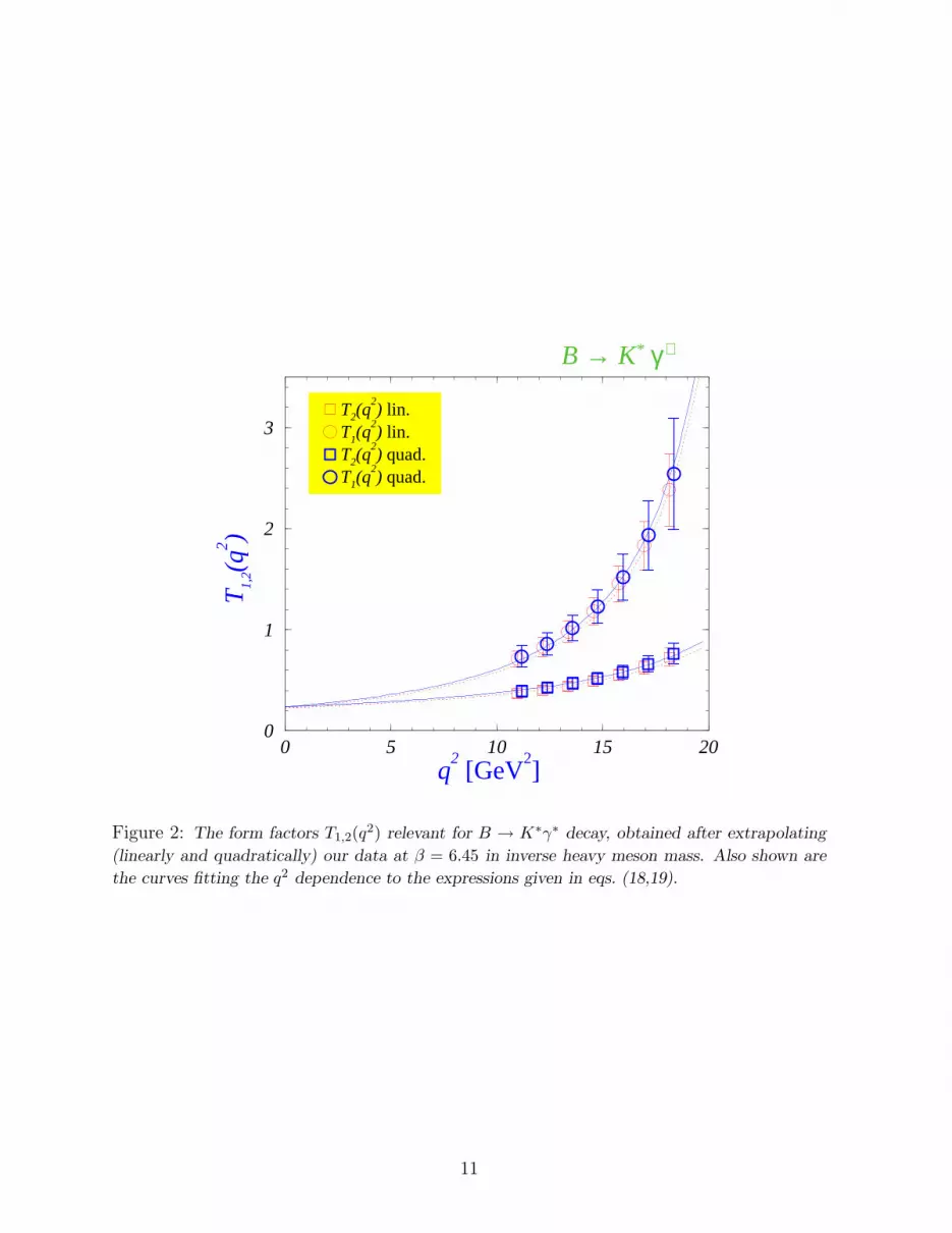
• The extrapolation (15) is made both linearly and quadratically. The differencesbetween the corresponding results are essentially indistinguishable, as it can be seenin fig. 2 where we plot the results for B → K∗γ∗ form factors (γ∗ stands for theoff-shell photon) obtained at β = 6.45 (Set 3). These and the similar results weobtained at β = 6.2 are collected in table 4.

To reach the physically interesting case of the photon on-shell one needs to assume somefunctional dependence of the form factors and extrapolate the results of table 4 down to

10

0 5 10 15 20q

2 [GeV

2]

0

1

2

3

T1,

2(q2 )

B → K* γ∗

T2(q2) lin.

T1(q2) lin.

T2(q2) quad.

T1(q2) quad.

Figure 2: The form factors T1,2(q2) relevant for B → K∗γ∗ decay, obtained after extrapolating

(linearly and quadratically) our data at β = 6.45 in inverse heavy meson mass. Also shown are

the curves fitting the q2 dependence to the expressions given in eqs. (18,19).

11

Set 1 Set 2

q2 [GeV2] TB→K∗

1 (q2) TB→K∗

2 (q2) q2 [GeV2] TB→K∗

1 (q2) TB→K∗

2 (q2)

12.2 0.76(24)+.00−.02 0.50(13)+.00

−.07 13.5 0.70(17)+.13−.00 0.52(9)+.00

−.14

13.6 0.94(22)+.00−.06 0.54(12)+.00

−.07 14.4 0.81(18)+.11−.00 0.56(9)+.00

−.15

15.1 1.19(19)+.00−.12 0.60(10)+.00

−.07 15.3 0.95(19)+.07−.00 0.61(9)+.00

−.16

16.5 1.53(17)+.00−.21 0.64(6)+.00

−.07 16.1 1.11(21)+.03−.0 0.66(9)+.00

−.15

17.9 2.03(21)+.00−.37 0.72(2)+.00

−.07 17.0 1.32(26)+.00−.04 0.72(9)+.00

−.15

– − − 17.8 1.56(36)+.00−.12 0.80(9)+.00

−.15

Set 3

q2 [GeV2] TB→K∗

1 (q2) TB→K∗

2 (q2)

11.2 0.73(10)+.00−.02 0.39(6)+.00

−.02

12.4 0.86(11)+.00−.03 0.43(6)+.00

−.03

13.6 1.02(13)+.00−.04 0.47(6)+.00

−.03

14.7 1.23(16)+.00−.05 0.52(6)+.00

−.03

16.0 1.52(23)+.00−.07 0.58(7)+.00

−.03

17.2 1.93(34)+.00−.10 0.66(8)+.00

−.03

18.3 2.54(55)+.00−.16 0.76(10)+.00

−.03

Table 4: The values of the B → K∗γ∗ form factors at several values of q2. The first error in each

result is statistical and the second is the difference between the results of linear and quadratic

extrapolation in 1/MH to 1/MB .

12

q2 = 0. It is very easy to convince oneself that the form factors T1 and T2 satisfy theconstraints very similar to those that govern the shapes of F+ and F0 semileptonic heavyto light pseudoscalar form factors. More specifically:

◦ The nearest pole in the crossed channel, JP = 1−, which contributes to the formfactor T1, is MB∗

s= 5.42 GeV in B → K∗ transition. The form factor T2, instead,

receives the contribution from heavy JP = 1+ resonances and multiparticle statesboth below and above the cut (MB + mV )2.

◦ HQET, which is relevant to the region of large q2’s, suggests that the form factorsscale with heavy quark/meson mass as T1 ∼

√M and T2 ∼ 1/

√M [11], and therefore

both form factors cannot be fit to the pole-like shapes.

◦ For the high energy region of the light meson in the rest frame of the heavy (q2 → 0),we also have the scaling laws T1(E) ∼

√M/E2 ∼ M−3/2. Similar holds for the T2(E)

form factor, i.e., both form factors scale as M−3/2 [16, 17]. Moreover, the two arerelated via

T1(E) =M

2ET2(E) . (17)

Thus the situation is analogous to the one in B → πℓν decay, and we can use the simpleparameterisation of ref. [24],

T1(q2) =

T (0)

(1 − q2)(1 − αq2), T2(q

2) =T (0)

1 − q2/β, (18)

where q2 = q2/M2B∗

s. If we relax the T1/T2 = M/2E constraint, then a simple form (18)

becomes

T1(q2) =

C1

1 − q2+

C2

1 − C3q2, T2(q

2) =C1 + C2

1 − C4q2. (19)

Our data from table 4 cannot distinguish between the two of the above parameterisationsand in both cases we end up with the same value for T (0). As in the previous subsection,as our final results we will quote those obtained at β = 6.45, for which more and heaviermesons were accessible,

TB→K∗

lin. (0) = 0.22(3) , TB→K∗

quad. (0) = 0.24(4) . (20)

The results for all three datasets are collected in table 5.

5 Final results and conclusion

As our final results we will quote those obtained at β = 6.45, since they have smallerdiscretisation errors. As central value we take the results obtained from the first method(subsec. 4.1) which are given in table 3 at µ = 1/a, in the (Landau) RI/MOM scheme.

13

TB→K∗

lin. (0) TB→K∗

quad. (0) TB→K∗

lin. (0)/TB→ρlin. (0) TB→K∗

quad. (0)/TB→ρquad.(0)

Set 1 0.25(6) 0.28(10) 1.2(3) 1.3(7)

Set 2 0.23(6) 0.23(6) 1.1(3) 1.1(2)

Set 3 0.22(3) 0.24(4) 1.3(2) 1.3(3)

Table 5: The results of the extrapolation of the form factors from table 4 assuming the q2-dependence given in eqs. (18,19).

The matching to the MS scheme is 1 at 2-loop accuracy, but we still need to run our resultfrom µ = 1/a to mb which is made via

TB→K∗

(0; mb) = T (0; 1/a)

(αs(1/a)

αs(mb)

)−γT /2β0[1 − JT

αs(1/a) − αs(mb)

4π

]. (21)

For Nf = 0 and mb = 4.6(1) GeV, the running factor is very close to 1, i.e., 0.99 (0.97) forthe form factors computed at β = 6.45 (β = 6.2). Our final result is

TB→K∗

(q2 = 0; µ = mb) = 0.24 ± 0.03+0.04−0.01 . (22)

The spread of central values presented in table 3 at β = 6.2 (when multiplied by 0.97)are used to attribute a systematic error to our final result (22). The values in table 5are already at the scale µ = MB ≈ mb, and those given in eq. (20) are fully consistentwith (22). Our number is smaller when compared to the QCD sum rule results,

TB→K∗

(0) = 0.33(3) [7], 0.38(6) [8], (23)

although the recent progress show the tendency of lowering the ccentral value obtained byusing LCSR, i.e., TB→K∗

(0) = 0.31(4) [25]. Concerning the previous lattice studies [26],

most of them were made at the time before the T (0)M3/2H -scaling law was known or before

a significant statistical quality of the lattice data was feasible.Our values for the ratio TB→K∗

(0)/TB→ρ(0), on the other hand, are unstable, and wewill only quote the average of the values obtained by using two methods discussed in thispaper at β = 6.45,

TB→K∗

(0)/TB→ρ(0) = 1.2(1) , (24)

as our best estimate. This result agrees with the most recent LCSR estimate, TB→K∗

(0)/TB→ρ(0) =1.17(9) [27].

The method employed in this work relies on the use of a propagating heavy quark. Inorder to reach smaller values of q2’s in an effective theory of heavy quark the so calledmoving NRQCD has been developed, but the numerical quality of the signal does notappear very encouraging so far [28]. Clearly, our method cannot be used to obtain a very

14

accurate value of T (0), mainly because the heavy quark extrapolations are involved. Ifwe are to work with the physical b-quark mass on the lattice, we would need a very smalllattice spacing, i.e., at least a−1 ≃ 10 GeV. For the volume corresponding to the latticesize La = 2 fm that would require the simulations on the lattice with 1003 spatial points.Moreover, on the lattice with the periodic boundary conditions, the q2 = 0 point is reachedwhen the energy of the vector meson (in the rest frame of the heavy) is

E2 = m2K∗ +

(2π

La

)2

|~n|2 ↓=

(M2

B + m2K∗

2MB

)2

⇒ |~n| =M2

B − m2K∗

4πMB× La = (2.07 fm−1) × La . (25)

Therefore on a lattice of the size La = 2 fm, one needs to give the kaon a momentum |~n| ≈ 4,for which it is highly unlikely to observe any signal of the correlation functions (5). Even ifone organises the kinematics so that the momenta are shared between B- and K∗-mesons,the required spatial momenta are still too large for the reasonably accurate computationof the correlation functions (5). Therefore, a progress in improving the quality of signalsof correlation functions when the spatial momenta |~n| > 1 would be highly welcome.Summarising, as of now, a significant improvement on the precision of the B → K∗ formfactors does not look promising even in quenched approximation. The methodology ofthe extraction of the form factors can, however, be improved by combining the correlationfunctions (5) in double ratios, in a way similar to what has recently been implemented inthe lattice computation of heavy→heavy [29] and light→light pseudoscalar meson decayform factors [30].

References

[1] R. Ammar et al. [CLEO Collaboration], Phys. Rev. Lett. 71 (1993) 674.

[2] B. Aubert et al. [BABAR Collaboration], Phys. Rev. D 70 (2004) 112006 [hep-ex/0407003].

[3] M. Nakao et al. [BELLE Collaboration], Phys. Rev. D 69 (2004) 112001 [hep-ex/0402042].

[4] K. Abe et al., Phys. Rev. Lett. 96 (2006) 221601 [hep-ex/0506079]; see also BABAR Collaboration,hep-ex/0607099.

[5] S. W. Bosch and G. Buchalla, JHEP 0501 (2005) 035 [hep-ph/0408231].

[6] T. Hurth, Rev. Mod. Phys. 75 (2003) 1159 [hep-ph/0212304]; M. Misiak, hep-ph/0609289; T. Hurthand E. Lunghi, eConf C0304052 (2003) WG206 [hep-ph/0307142]; A. Ali, hep-ph/0312303; L. Sil-vestrini, Int. J. Mod. Phys. A 21 (2006) 1738 [hep-ph/0510077].

[7] P. Ball and R. Zwicky, Phys. Rev. D 71 (2005) 014029 [hep-ph/0412079] and JHEP 0604 (2006) 046[hep-ph/0603232]; A. Khodjamirian, T. Mannel and N. Offen, hep-ph/0611193.

[8] P. Colangelo et al., Phys. Rev. D 53 (1996) 3672 [Erratum-ibid. D 57 (1998) 3186] [hep-ph/9510403].

[9] A. Abada, D. Becirevic, P. Boucaud, J. P. Leroy, V. Lubicz and F. Mescia, Nucl. Phys. B 619 (2001)565 [hep-lat/0011065].

15

[10] D. Becirevic, hep-ph/0211340; S. Hashimoto and T. Onogi, Ann. Rev. Nucl. Part. Sci. 54 (2004) 451[hep-ph/0407221].

[11] N. Isgur and M. B. Wise, Phys. Rev. D42 (1990) 2388.

[12] K. C. Bowler et al. [UKQCD Collaboration], Phys. Lett. B 486 (2000) 111 [hep-lat/9911011].

[13] S. Hashimoto, K. Ishikawa, H. Matsufuru, T. Onogi and N. Yamada, Phys. Rev. D58 (1998) 014502[hep-lat/9711031].

[14] S. M. Ryan, A. X. El-Khadra, A. S. Kronfeld, P. B. Mackenzie and J. N. Simone, Phys. Rev. D 64

(2001) 014502 [hep-ph/0101023].

[15] V. L. Chernyak and I. R. Zhitnitsky, Nucl. Phys. B345 (1990) 137.

[16] J. Charles, A. LeYaouanc, L. Oliver, O. Pene and J. C. Raynal, Phys. Rev. D60 (1999) 014001[hep-ph/9812358].

[17] M. Beneke and D. Yang, Nucl. Phys. B 736 (2006) 34 [hep-ph/0508250]; T. Becher, R. J. Hill andM. Neubert, Phys. Rev. D 72 (2005) 094017 [hep-ph/0503263]; D. Pirjol and I. W. Stewart, eConfC030603 (2003) MEC04 [hep-ph/0309053].

[18] M. Luscher, S. Sint, R. Sommer, P. Weisz and U. Wolff, Nucl. Phys. B491 (1997) 323 [hep-lat/9609035].

[19] D. Becirevic, V. Gimenez, V. Lubicz, G. Martinelli, M. Papinutto and J. Reyes, JHEP 0408 (2004)022 [hep-lat/0401033].

[20] T. Bhattacharya, R. Gupta, W. Lee and S. R. Sharpe, Phys. Rev. D 73 (2006) 114507 [hep-lat/0509160].

[21] J. Rolf et al. [ALPHA collaboration], Nucl. Phys. Proc. Suppl. 129 (2004) 322 [hep-lat/0309072].D. Becirevic, P. Boucaud, J. P. Leroy, V. Lubicz, G. Martinelli, F. Mescia and F. Rapuano, Phys.Rev. D60 (1999) 074501 [hep-lat/9811003]. H. Wittig, Int. J. Mod. Phys. A 12 (1997) 4477 [hep-lat/9705034].

[22] C. R. Allton, V. Gimenez, L. Giusti and F. Rapuano, Nucl. Phys. B 489 (1997) 427 [hep-lat/9611021].

[23] A. V. Manohar and I. W. Stewart, hep-ph/0605001.

[24] D. Becirevic, A. Kaidalov, Phys. Lett. B478 (2000) 417 [hep-ph/9904490].

[25] P. Ball and R. Zwicky, hep-ph/0608009.

[26] C. W. Bernard, P. Hsieh and A. Soni, Phys. Rev. Lett. 72 (1994) 1402 [hep-lat/9311010]; K. C. Bowleret al. [UKQCD Collaboration], Phys. Rev. Lett. 72 (1994) 1398 [hep-lat/9311004]; A. Abada et

al. [APE Collaboration], Phys. Lett. B 365 (1996) 275 [hep-lat/9503020]; T. Bhattacharya andR. Gupta, Nucl. Phys. Proc. Suppl. 42 (1995) 935 [hep-lat/9501016]; L. Del Debbio et al. [UKQCDCollaboration], Phys. Lett. B 416, 392 (1998) [hep-lat/9708008].

[27] P. Ball and R. Zwicky, JHEP 0604 (2006) 046 [hep-ph/0603232].

[28] S. Hashimoto and H. Matsufuru, Phys. Rev. D 54 (1996) 4578 [hep-lat/9511027]; J. E. Mandulaand M. C. Ogilvie, Phys. Rev. D 57 (1998) 1397 [hep-lat/9703020]; A. Dougall, K. M. Foley,C. T. H. Davies and G. P. Lepage, PoS LAT2005 (2006) 219 [hep-lat/0509108].

16

[29] S. Hashimoto et al., Phys. Rev. D 61 (2000) 014502 [hep-ph/9906376]; ibid 66 (2002) 014503 [hep-ph/0110253].

[30] D. Becirevic et al., Nucl. Phys. B 705 (2005) 339 [hep-ph/0403217]; C. Dawson et al., hep-ph/0607162; D. Guadagnoli, F. Mescia and S. Simula, Phys. Rev. D 73 (2006) 114504 [hep-lat/0512020]; N. Tsutsui et al. [JLQCD Collaboration], PoS LAT2005 (2006) 357 [hep-lat/0510068];D. J. Antonio et al., hep-lat/0610080.

17