An Econometric Analysis of Wilderness Area UseAuthor(s): Gordon C. Rausser and Ronald A. OliveiraSource: Journal of the American Statistical Association, Vol. 71, No. 354 (Jun., 1976), pp. 276-285Published by: American Statistical AssociationStable URL: http://www.jstor.org/stable/2285298Accessed: 18/10/2010 17:06

Your use of the JSTOR archive indicates your acceptance of JSTOR's Terms and Conditions of Use, available athttp://www.jstor.org/page/info/about/policies/terms.jsp. JSTOR's Terms and Conditions of Use provides, in part, that unlessyou have obtained prior permission, you may not download an entire issue of a journal or multiple copies of articles, and youmay use content in the JSTOR archive only for your personal, non-commercial use.

Please contact the publisher regarding any further use of this work. Publisher contact information may be obtained athttp://www.jstor.org/action/showPublisher?publisherCode=astata.

Each copy of any part of a JSTOR transmission must contain the same copyright notice that appears on the screen or printedpage of such transmission.

JSTOR is a not-for-profit service that helps scholars, researchers, and students discover, use, and build upon a wide range ofcontent in a trusted digital archive. We use information technology and tools to increase productivity and facilitate new formsof scholarship. For more information about JSTOR, please contact support@jstor.org.

American Statistical Association is collaborating with JSTOR to digitize, preserve and extend access to Journalof the American Statistical Association.

http://www.jstor.org

An Econometric Analysis of Wilderness Area Use GORDON C. RAUSSER and RONALD A. OLIVEIRA*

Although outdoor recreational use fluctuates daily, this time-varying feature has received little attention by economists and statisticians. In this paper, wilderness recreational use relationships are estimated, based on daily observations over the length of a given season, by (i) traditional econometric techniques and via (ii) time series analysis procedures promoted by Box and Jenkins (3]. In applying both sets of estimated relationships for forecasting purposes, the econometric equations generally proved superior. However, when predictions from both sets of equations were combined, the resultingforecasts obtained proved more accurate than either of the separate forecasts.

1. INTRODUCTION A common feature of outdoor recreation activity is the

fluctuation in use levels from day to day and throughout the year. However, this time-varying feature of outdoor recreation use has received little, if any, attention in recreation economics research. Recreation economists have traditionally concentrated on "explaining" the use of a certain recreation activity over a cross section of such activities.' Time series analysis in this area has centered on predicting annual participation rates or levels.2

However, an analysis structured around the daily or weekly fluctuations in use levels throughout the year would prove useful for planning and management pur- poses. This analysis would provide a formal basis for minimizing scheduling problems. For example, additional personnel may be needed for maintenance during days when heavy use occurs. In addition, a large amount of use (or pressure on resources) at any one time may cause more damage to the environment than "moderate" use over an extended period of time. To properly manage these areas, one should understand the fluctuating pat- tern of use and, it is hoped, be able to forecast such fluctuations with reasonable accuracy.

Given this motivation, the purpose of- this paper is to estimate time series relationships for a particular recrea- tion activity, viz., wilderness area use over the length of a given season. Empirical use functions will be examined via traditional econometric techniques and via time series analysis procedures promoted by Box and Jenkins [3]. The estimated use functions will be used as fore- casting equations, and predictions will be combined to

* Gordon C. Rausser is visiting professor of business administration, Harvard University, Boston, MA 02163. Ronald A. Oliveira is assistant professor, De- partment of Forestry, University of Wisconsin, Madison, WI 53706. This re- sarch was supported by the College of Agricultural and Life Sciences, the Gradu- ate School, University of Wisconsin, Madison, WI, and the U.S. Forest Service, Pacific Southwest Forest and Range Experiment Station, Berkeley, CA.

1 Some of the more often referenced outdoor recreation economics works are C4, 7 and 83.

2 For instance, see the,discussion in CO6 on procedures used for forecasting recrea- tion activity.

form composite forecasts. The theoretical rationale under- lying the specified forecasting equations will be briefly presented in Section 2.

2. THEORETICAL FORMULATION It is assumed in the subsequent analysis that the

demand for wilderness area use is directly affected by the characteristics of the areas and by the time con- sumers allocate to such activities. The theoretical founda- tions for these assumptions are based on the household production function approach to consumer demand theory (see [12, 20]) and the characteristics approach to demand theory (see [16]), which is viewed as a special case of the former. The household or consuming unit demand for use of a particular wilderness area is assumed to be the result of a three-stage utility maximization process. This three-stage process may be considered a heuristic extension of the two-stage process discussed in [14 and 22].

In the first stage, the amount of "full real income" allocated to recreation in general is determined.3 Given this allocation, the second stage determines the amount of full real income the household will "spend" on specific recreation activities. It is assumed that one of these specific recreation activities is wilderness area use. Actually, the allocations to wilderness area may be the result of more than two stages, i.e., first, an allocation may be made to general recreation and then to general outdoor recreation, and so on, until the activity of wilder- ness area use is defined. However, since this study is concerned with what happens after the allocation to wilderness area use is determined, the actual number of preceding stages is not relevant.

The allocation of "full income" to wilderness area use, say M., is the amount of time and expenditures that the household needs to achieve the desired amount of a general wilderness area characteristic. It is assumed that this general wilderness area characteristic is a function of a subvector of specific wilderness area characteristics, say, Xw1, Xw2, ..., X,H. A household is assumed to derive utility from these characteristics, which are ob- tained through the household production relationships as defined in [20]. Since the amount of time and ex-

3 By combining the household's time and income constraints, one may obtain a single resource constraint of the household's "full income" [21.

? Journal of the American Statistical Association June 1976, Volume 71, Number 354

Applications Section

276

Econometric Analysis of Wilderness Use 277

penditures that the household will allocate to wilderness area use, MW, was determined in the second stage, the third stage will determine the wilderness area selected and when it will be utilized.

Obviously, only one wilderness area can be visited at a time. Therefore, the choice will depend on the relative efficiency with which the household can obtain the de- sired characteristics, Ww,i, i = 1, 2, ..., H, from each wilderness area and the amount of "full income" available for this "production" task, M,,. In other words, the wilderness area subvector of the household's utility func- tion is maximized, subject to the wilderness area pro- duction relationship and the allocation M.. The resulting derived-demand relationship for use of wilderness area j by the household may be expressed as a function of the relative characteristics possessed by wilderness area j, Mw, and the state of the art or level of technology under which the household production process takes place, which we shall denote by a vector C. Aggregate demand for using area j on day t (in terms of number of people) will be the sum of all the individual household demands. This aggregate demand may be expressed as

Z=t - Z(Xwi21 Xw25, . * XwH. , C p Mwp) ? j = ...,I G; t = 1, ..., T, (2.1)

where Xwti1 i = 1, ..., H, is the amount of characteristic X,,,i possessed by area j, Cp represents an index of the environmental variables C across all households, and Mw,, represents the full income allocation for wilderness area use for all households.

Equation (2.1) could be employed directly if the supply associated with each recreational area is fixed. In reality, although the stock of supply (the physical area itself and nontime-varying characteristics, e.g., altitude) is approximately fixed in the short run, the quality dimensions of supply are not constant. The flow of supply recognizing these dimensions is directly associated with the availability of the supply stock. This availability in turn is influenced largely by weather conditions. Thus, the supply of an area may be expressed as

Sit = s(Xjt j Xi) j =i , ... I ; t = 1,.. T, (2.2) where Sit is the wilderness (or campground) supply of area j on day t, Xt is a vector of time-varymg charac- teristics associated with the area, and Xj is a vector of nontime-varying (in the short run) characteristics as- sociated with area j.

The supply relationship (2.2) may now be viewed as one part of a simultaneous system, the reduced form of which is wilderness area use. More explicitly, (2.1) and (2.2) are the demand and supply relationships, respec- tively, of the structural form of a wilderness use model. The reduced form of this model, or actual use, may be stated as

=t z(X, X,, C7,, Mw7,)? j=1,...,G;t=1,...,T, (2.3)

where Z,t iS now defined as the use (number of people)

at area i on day t, and the other terms are as defined previously.

Relationship (2.3) would be very difficult to analyze empirically on two accounts. First, the index variable CG is difficult to describe theoretically and cannot be measured empirically. Obvriously, in light of the brief theoretical discussion just presented, such variables are important to demand and use. However, since empirical measurements are unavailable, these environmental vari- ables will be omitted from the subsequent analysis. Such an omission is not viewed as critical, given the lack of variation in these factors over the short run.

Similar to Cp, the full income allocation for wilderness area use for all households, MW cannot be measured empirically. In this case, it seems reasonable to use the actual total use at all areas on day t, or ZTt, as a proxy variable for M7,,4 Obviously, these two measurements are not equivalent, but it is reasonable to assume a direct positive relationship between them.'

Two other factors which may influence use but do not appear in (2.3) are past use at area i and institutional calendar events. For example, past use may be treated as a time-varying characteristic of the area which in- fluences the household's expectations of congestion (or lack of congestion) at the area. This interpretation of past use, however, is the result of only one possible structural formulation. A priori one would expect in- stitutional calendar events such as holidays and weekends to have a positive influence on use, an influence tempered by expected crowded conditions on holidays.

In light of this discussion, the use function to be addressed empirically in the subsequent analysis may be represented as

=it = Z(Xit, Xi, Zi,t-k, ZTt) Xdty Uit) X

1=1, ... G; t=1, ..., T (2.4)

where Xdt is a vector representing institutional calendar events, Uit is a stochastic error term, and the other variables are as previously defined.

3. ECONOMETRIC USE MODEL Given the use function specified in (2.4) and available

data, an econometric representation may be expressed as a pooled cross section and time series (cTs) model. In this context, relationship (2.4) is interpreted as a single- equation model with N = G X T observations, i.e.,

r b q

Z-t = a + E 'YkZi,t-k + E I3ji?i + E khXt-k + A, k-l j_i k=O

i= l . y.G;T=1 ...IT, (3.1)

where Zit 'is the number of people at area i on day t, xi,

4 Given that an exogenous factor varies and is unobservable, it follows from the viewpoint of bias that it is better to use a proxy rather than omit this exogenous variable [28).

5 Note also that the variable ZTr could appear in a use function which was motivated by a different structural specification. For instance, it would appear directly if (2.7) were based on an allocative mechanism which allocates a given sum of use over all the possible areas.

278 Journal of the American Statistical Association, June 1976

is the jth nontime-varying characteristic variable as- sociated with area i xt is a h X 1 vector of time series exogenous variables associated with area i on day t, and ttit is the disturbance term associated with area i on day t. The structure for the residual term in (3.1) is assumed to follow a first-order autoregressive scheme,

Ait - piAi'ttl + (zi:t (3.2)

where pi is an unknown autoregressive parameter and fit is an independent, identically distributed random variable which is assumed to have the properties,

tt N(0, +) E(gi, t-1, e,t) 0 , E(ei tEt) = 0 (i $ j) E(eitej) =0 (t # s), i, j = l *..* G

In addition to the explicit assumption of first-order autoregressive residual terms, the residual terms are specified as cross-sectionally heteroscedastic and mutually uncorrelated; i.e., E(Guitjit) = Sojii2, where aii denotes the variance of the disturbance term for the ith cross section and bSj is the Kronecker delta. Furthermore, it is assumed that the initial disturbance terms of (3.1), ui.,, are independent random variables which have the prop- erties, E(A i0) = 0 and E(asxo2) = f/(1 - p,2), for all t *- G.6

One of the difficulties in estimating the parameters of (3.1) is that the lagged dependent variables, given (3.2), are related to the error terms. To account for the esti- mation problems associated with lagged dependent vari- ables, we may eliminate the relationship between these variables and the error term Utt by the use of an instru- mental variable approach. That is, we first form the equation

Z =, t-k = tO + altit + a2Xf,t1 t+' + an$i t-n-1

+ Wi,ti-k, k = 1, . . ,r r (3.3)

where Xit is the vector of all exogenous variables at t, wi,t-, is an error term, and the value of n is optional (see [9, 17]). By applying ordinary least squares (oLs) to (3.3), one may obtain estimated values of the lagged dependent variables, Zi, -k' and the error terms of (3.3). If the OLS estimates Zi, t-k are substituted for the actual values in (3.1), the error terms for this altered relation- ship are - ,tt + 5ioi,t_j' (assuming for notational ease that there is only one lagged dependent variable, i.e., r = 1), where ci, -i' denotes the OLS estimated error term of (3.3).

Consistent estimates of the parameters of (3.1) may now be obtained through four additional stages. First, OLS is applied to (3.1), using the zi,t-l' as instrumental variables. The resulting OLS residuals are used to esti- mate the Ai,,

w i t = eite + l ici,s the (3L4) where Ait"tiS the OLS estimate of -i,, 11 is the OLS estimate

I These two properties insure, that the initial disturbances have the same mean and variance as the subsequent disturbances generated by the autoregressive process and that symmetry conditions will be met for the covariance matrix [273.

of ye in (3.1) and ci,t_,' is the OLS residual estimated from (3.3). In turn the residuals -it are used to estimate the pi. The estimates pi are then used to transform the instrument variable form of (3.1) to obtain

r b

Zit = =axio*+ E 'YkZi,t-k* + E, fj3Xj* k=1 j=1

q

+ E tkXi,tk* + fit (3-5) k=O

where

Zit Zit - ,iZi,tt-i , =iO- 1 -P i

Z~~~pij - 1-P)z} i t itt -

1 p

and

C-it = Ait -P -,t t 3= ..., T, and i = I2, ,GI and where the degrees superscript has been omitted in (3.5) for notational ease.

OLS is then applied to (3.5) to obtain consistent esti- mates of the oii2.7 The resulting estimates ai are then used to transform the variables in (3.5) to obtain

r b

Zit = ati, + , TykZit-k** + E, /jij2 k=1

+ } # tkXi, t-k + fit"I (3.6) k=O

where zit** 0= t iij*A2

Xit** = a and Eit** = ,/oF, t = 3, ...7 T, and i = 1, 2, ... CG. The disturbance eit* is (approximately) asymptotically nonautoregressive and homoseedastic.8 The unknown parameters appearing in (3.6) can then be consistently estimated by OLs, using G(T - 2) observations.9

3.1 Empirical Estimation of CTS Model The wilderness area use series, zit, was obtained from

1971 wilderness area entry permits for six California Wilderness Areas, viz., Desolation, Emigrant Basin, Marble Mountain, San Gorgonio, San Jacinto, and Ventana. Although the original wilderness area use series were daily observations, the econometric model was estimated employing only Saturday observations. The original daily use series reveals Saturday as the heaviest use day of the week. In addition, it was felt that forecasts of Saturday use would be sufficient for most management purposes.10

7 That is, i2 =ll(T - P - 2) 2X_3T (fj;*)2, where git*'8 are the OLS estimates of the residual terms of (3.5) and P is the total number of predetermined variables.

8 As illustrated in U28], the use of proxy variables will alter the disturbances of the original equation. It can easily be shown that the error term of (3.6) is equal to Ett/ti 2_-1/ffi2(iie' - p itw-2'). It is assumed that the magnitude of the right- side porion (i.e., that involving the disturbances of (3.3)) is negligible.

9 Although the resulting five-step procedure provides consistent estimates, it does not result in efficient estimates of the parameters [18].

10 Furthermore, the daily observations are most likely characterized by such random fluctuations that it would be very difficult to obtain stable economic predic- tions for this data base.

Econometric Analysis of Wilderness Use 279

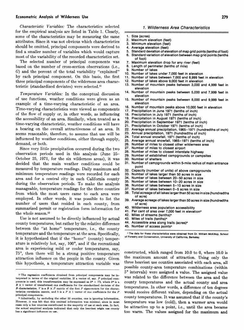
Characteristic Variables: The characteristics selected for the empirical analysis are listed in Table 1. Clearly, some of the characteristics may be measuring the same attributes. Since it was not obvious which characteristics should be omitted, principal components were derived to find a smaller number of variables which would capture most of the variability of the recorded characteristics set.

The selected number of principal components was based on the number of cross-section observations (i.e., G) and the percent of the total variability "explained" by each principal component. On this basis, the first three principal components of the wilderness area charac- teristic (standardized deviates) were selected."

Temperature Variables: In the conceptual discussion of use functions, weather conditions were given as an example of a time-varying characteristic of an area. Time-varying characteristics were viewed as components of the flow of supply or, in other words, as influencing the accessibility of an area. Similarly, when treated as a time-varying characteristic, weather conditions will have a bearing on the overall attractiveness of an area. It seems reasonable, therefore, to assume that use will be influenced by weather conditions, either through supply, demand, or both.

Since very little precipitation occurred during the two observation periods used in this analysis (June 25- October 25, 1971, for the six wilderness areas), it was decided that the main weather conditions could be measured by temperature readings. Daily maximum and minimum temperature readings were recorded for each area and for a central city in each California county during the observation periods. To make the analysis manageable, temperature readings for the three counties from which the most users came to each area were employed. In other words, it was possible to list the number of users that resided in each county, from summarized permit or registration form information for the whole season.'2

Use is not assumed to be directly influenced by actual county temperatures, but rather by the relative difference between the "at home" temperature, i.e., the county temperature and the temperature at the area. Specifically, it is hypothesized that if the "home" (county) temper- ature is relatively hot, say, 1000, and if the recreational area is experiencing mild or cooler temperatures, say, 750, then there will be a strong positive temperature attraction influence on the people in the county. Given this hypothesis, a temperature attraction variable was

11 The regression coefficients obtained from principal components may be in- terpreted in terms of the original variables. If a vector of, say, P principal com- ponents is used, this transformation may be expressed as b* = Vb, where b* is a B X 1 vector of transformed OLS coefficients for the standardized deviates of the B characteristics, V is a B X P matrix of the first P eigenvectors for the charac- teristics correlation matrix, and b is a P X 1 vector of OLS coefficients for the P principal components.

12 Admittedly, by excluding the other 55 counties, one is ignoring information. However, it was felt that this omitted information was minimal, since in most cases only a few counties contributed to the majority of use at each area. In fact, the actual empirical analysis indicated that only the heaviest origin use county has a significant influence on use.

1. Wilderness Area Characteristics

1. Size (acres) 2. Maximum elevation (feet) 3. Minimum elevation (feet) 4. Average elevation (feet) 5. Standard deviation of elevation of map grid points (tenths of foot) 6. Standard variation of elevation between map grid points (tenths

of foot) 7. Maximum elevation drop for any river (feet) 8. Length of perimeter (tenths of mile) 9. Number of lakes

10. Number of lakes under 7,000 feet in elevation 11. Number of lakes between 7,000 and 8,999 feet in elevation 12. Number of lakes above 9,000 feet in elevation 13. Number of mountain peaks between 3,000 and 4,999 feet in

elevation 14. Number of mountain peaks between 5,000 and 7,999 feet in

elevation 15. Number of mountain peaks between 8,000 and 9,999 feet in

elevation 16. Number of mountain peaks above 10,000 feet in elevation 17. Precipitation in June 1971 (tenths of inch) 18. Precipitation in July 1971 (tenths of inch) 19. Precipitation in August 1971 (tenths of inch) 20. Precipitation in September 1971 (tenths of inch) 21. Precipitation in October 1971 (tenths of inch) 22. Average annual precipitation, 1965-1971 (hundredths of inch) 23. Annual precipitation, 1971 (hundredths of inch) 24. Total annual snowfall, 1971 (tenths of inch) 25. Average annual snowfall, 1965-1971 (tenths of inch) 26. Number of miles to closest other wilderness area 27. Number of miles to closest airport 28. Number of miles to closest interstate highway 29. Number of established campgrounds or campsites 30. Number of shelters 31. Number of campgrounds within 5-mile radius of main entrance

point 32. Capacity (number of units) of above campgrounds 33. Number of lakes larger than 50 acres in size 34. Number of lakes between 20-50 acres in size 35. Number of lakes between 10-20 acres in size 36. Number of lakes between 5-10 acres in size 37. Number of lakes between 0-5 acres in size 38. Total acreage of all lakes larger than 50 acres in size (hundredths

of acre) 39. Average acreage of lakes larger than 50 acres in size (hundredths

of acre) 40. Wilderness area population accessibility 41. Per cent of area over 7,000 feet in elevationa 42. Miles of streams (tenths)a 43. Miles of trails (tenths)a 44. Accessible area along trails (acres)a 45. Number of access pointsa

a The data for these characteristics were obtained from Dr. William McKillop, School of Forestry and Conservation, University of California, Berkeley.

constructed, which ranged from 10.0 to 0, where 10.0 is the maximum amount of attraction. Using only the three heaviest use counties associated with each area, all possible county-area temperature combinations (within 50 intervals) were assigned a value. The assigned value was related to the difference between the area and the county temperatures and the actual county and area temperatures. In other words, a difference of ten degrees would receive different values, depending on the actual county temperatures. It was assumed that if the county's temperature was low (cold), then a warmer area would be attractive up to a point, i.e., until the area became too warm. The values assigned for the maximum and

280 Journal of the American Statistical Association, June 1976

minimum county-area temperature combinations are re- ported elsewhere."

3.2 Empirical Results

Combining the wilderness area cross-section obser- vations and Saturday time series observations provided 96 observations for the pooled model. Alternative forms of time series exogenous variables were eliminated due to extremely high intercorrelations-the temperature attraction variables associated with the three heaviest use counties for each area were often highly correlated due to similarities in temperatures as well as similarities in travel times.

The following variables were selected as predetermined variables for the final model:

Total use at all six areas on day t '(X,) 14

Use lagged seven days (or lagged one observation using Satur- days only) (zt-1); Temperature attraction variable associated with maximum temperature for heaviest use county, lagged one week (xlt7); Interaction term of xit (without lag) divided by travel time in minutes from the heaviest use county to the area (XV);

Dummy variable, equal to one if the Saturday was part of a three-day weekend, equal to zero otherwise (xae); First characteristic principal component (based on standardized deviates) of the area which did not change during the sample period (X1); Second characteristic principal component of the area (92) Third characteristic principal component of the area (?3).

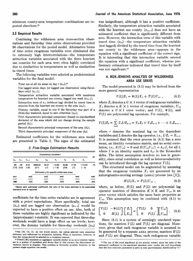
Estimated coefficients for the wilderness area model are presented in Table 2. The signs of the estimated

2. Five-Stage Estimation Results

Explanatory variables, A'

xot Zt-l xit-7 X2t X3f k1 2 X3 xa

.09 .28 9.43 2658.23 33.41 -13.64 35.66 17.55 -114.23 .74 (7.3) (3.2) (1.6) (2.7) (.7) (-1.6) (2.6) (.7) (-.4)

Estimated p for specific wilderness areas

WAl WA2 WA3 WA4 WA5 WA6

.896 .423 .623 .678 6830 .322

4 Below each estimated coefficient, the ratio of the mean estimate to its associated standard error is reported.

coefficients for the time series variables are in agreement with a priori expectations. More specifically, total use (x0t) and use lagged one observation (zt-1) would be expected to have a positive effect on use. Also, both of these variables are highly significant as indicated by the (approximate) t-statistic. It was expected that three-day weekends would have a large effect on use levels; how- ever, the dummy variable for three-day weekends (x3,)

1See [24, Ch. 51. As one would expect, the values selected were somewhat arbitrary and influenced by subjective opinions. What is important, however, is that the values should be selected in a consistent manner.

14 Powell [26J examines an aggregate variable similar to xot as a common regres- sor in a system of equations and shows that in this context the disturbance co- variance matrix is singular. This problem is obviously avoided, however, in the present single equation cTs model.

was insignificant, although it has a positive coefficient. Similarly, the temperature attraction variable associated with the heaviest use county (Xlt 7) does not have an estimated coefficient that is significantly different from zero. However, the interaction term of this variable with travel time (x2t)-the temperature attraction variable (not lagged) divided by the travel time from the heaviest use county to the wilderness area-appears in the equation with a significant coefficient of the correct sign. It is interesting that this interaction variable entered the equation with a significant coefficient, whereas pre- liminary estimations indicated that travel time by itself was not significant.15

4. BOX-JENKINS ANALYSIS OF WILDERNESS AREA USE SERIES

The model presented in (3.1) may be derived from the more general representation

r(L)Zt = w(L)Xt + T(L)Uzt , (4.1)

where Zt denotes a G X 1 vector of endogenous variables; Xt denotes a K X 1 vector of exogenous variables; Ut denotes a G X 1 error vector; and r (L), 4 (L), and T(L) are polynomial lag operators. For example,

r (L)Zt = E rPLiZt_1 =ro Zt+PrZt-1 + +rrZtr I i=O

where r denotes the maximal lag on the dependent variables and L denotes the lag operator, i.e., LiZt = Zt-i. It is assumed that the error process in (4.1) has a zero mean, an identity covariance matrix, and no serial corre- lation, i.e., E(Uzg) = 0 and E(Uz1tUTt') = etS"I, for all t4 where I is an identity matrix and 8tt, is the Kronecker delta. The latter assumption involves no loss in gener- ality, since serial correlation as well as heteroscedasticity can be introduced through the lag operator T(L).

This structural model can be augmented by assuming that the exogenous variables Xt are generated by an autoregressive-moving average (ARMA) process (see [31),

H(L)Xt = F(L)UXt , (4.2)

where, as before, H(L) and F(L) are polynomial lag operator matrices of dimension K X K and U.t is an error vector which satisfies the same basic properties as U,t. This assumption may be combined with (4.1) to obtain

rr(L) -*(L)- Zzt _ T(L) O luztl (3

L H B(L) x LtJ L F(L) JuztJ

Since (4.1) is a system of seemingly unrelated equa- tions, the matrices r (L) and T (L) are diagonal. More- over, given that each exogenous variable is assumed to be generated by a separate ARMA process, matrices H (L) and F (L) are diagonal. Thus, each endogenous variable

15 The use of the word significant is not strictly correct, since the ratio of the estimated coefficient to its associated standard error (under the null hypothesis that the true unknown parameter is zero) is only approximately distributed as ".'

Econometric Analysis of Wilderness Use 281

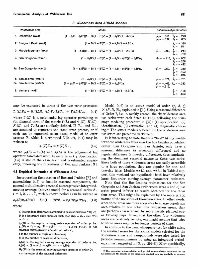
3. Wilderness Area ARIMA Models

Wilderness area Model Estimates of parameters

1. Desolation (wAI) (1 - ftB - 02B2)(1 - B)(1 - B7)Zt = (1 - 08B6)(1 - 0B7)at $1 = .351, = -.223 ck2--.192, A7 .8 02 = 1 3 =2 .685

2. Emigrant Basin (wA2) (1 - B)(1 - B7)Zt = (1 - 01B)(1 - 07B7)a= -.325 07 .541

3. Marble Mountain (wA3) (I - 41B)(1 - B)(1 - B7)Zt = (1 - 06BI)(1 - 0B')at $ = .292, = -.244 07 .709

4. San Gorgonio (wA4.1) (i - 47B7)(I - B7) ( - 01B - 08B8)(1 - 0B7)a ?7= -.413 0 802 = -.266

07 = -.492 4a. San Gorgonio (wA4.2) (1 - 03B3)(1 - B)(1 - B7)Zt = (1 - 01B - 02B2)(1 - 07B7)at $3 = -.059 0, .350

02 = .403 07= -.045

5. San Jacinto (wA5.1) (1 - AB7)(1 - B7)Zt = (I - 01B)at 47 = -.371, tX = -.761 5a. San Jacinto (wA5.2) (1 - B2 78)(1 - B)(1 - B7)Zt = (1 - 020B20)at 2=-.403, O> = -.233

47 - -.312, 6. Ventana (wA6) (1 - B)(1 - B7)Zt = (1 - 0,B)(1 - 07B7)at 01 = -.128

07= .823

may be expressed in terms of the two error processes,

ri(L)Zit = *j(L)Ht-1(L)FiWUzxt + Tj(L)Uni , (4.4)

where rP(L) is a polynomial lag operator pertaining to ith diagonal term of the matrix r(L) and tj(L), Hi%(L) Fi(L), and T(L) are similarly defined. If Ui and U22i are assumed to represent the same error process, or if each can be expressed as an ARMA model of an error process Ut which is distributed N(O, o-2), (4.4) may be written as

i(L)Zit = i(L)Ut , (4.5)

where t(L) = ri(L) and 0X(L) is the polynomial lag operator associated with the error term Ut. Specification (4.5) is also of the ARMA form and is estimated empiri- cally, following the procedures of Box and Jenkins [3].

4.1 Empirical Estimation of Wilderness Area Incorporating the notation of Box and Jenkins [3] and

generalizing (4.5) to include seasonal components, the general multiplicative seasonal autoregressive-integrated- moving-average (ARMA) model for a seasonal series Zt t = 1, 2, ..., T, with a known period s can be written as

#, (B)Pp (BS) (1 - b)d(1- B)DZt = 6q(B)GQ(B*)at , (4.6)

where at is a random disturbance assumed to be distributed as N(O,, o2) B is a backward shift operator such that BZ = Zc-i and BkZt

f,(B) is the regular autoregressive operator of order p, i.e., ckp(B) = (1 - c/n B - 02B2 -, . . - *-cpB:); cFp(Bs) is the seasonal autoregressive operator of order P; d is the number of regular differences D is the number of seasonal differences; 4(B) is the regular moving average operator of order q, i.e.,

(B) (1 - 0 B - 2B2, - ' B) OQ(BB) is the seasonal moving average operator of order Q; s is the order of the seasonal diffrence.

Model (4.6) is an ARIMA model of order (p, d, q) X (P, D, Q), explained in [3]. Using a seasonal difference of Order 7, i.e., a weekly season, the six wilderness area use series were each fitted to (4.6), following the four- stage modeling procedure in [3]: (1) specification, (2) identification, (3) estimation, and (4) diagnostic check- ing.'6 The ARIMA models selected for the wilderness area use series are presented in Table 3.

It is interesting to note that the "best" fitting models for those wilderness areas near the Los Angeles population center, San Gorgonio and San Jacinto, only have a seasonal difference (a seven-day difference) and no regular difference (a one-day difference), thus emphasiz- ing the dominant seasonal nature in these two series. Since both of these N dlderness areas are easily accessible to a large population, they are popular for one- and two-day trips. Models wA4.1 and wA5.1 in Table 3 sup- port this weekend use hypothesis: both have relatively large first-order moving-average parameter estimates.

Note that the Box-Jenkins estimations for the San Gorgonio and San Jacinto (wilderness areas 4 and 5) use series proved inferior to results obtained for the other four areas. This might be explained by the more erratic nature of the use series of these two areas. In other words, since these areas are more accessible to a large population area relative to the other four wilderness areas, they are perhaps characterized by more hastily planned one- or two-day trips. Given that the other four wilderness areas are relatively remote, one might assume that trips to those areas may be for longer periods of time.

In addition to the usual chi-square test for white noise, the residual series for the ARIMA models selected for the wilderness areas and campgrounds were also tested for periodic nonrandomness by using an integrated period- ogram test suggested in [3, pp. 294-8]. More specifically,

16 The estimated autocorrelation and partial autocorrelation functions for the use series and the results of the diagnostic residual tests are avaiLable on request.

282 Journal of the American Statistical Association, June 1976

the Kolmogorov-Smirnov test statistic was used to determine if the estimated residual cumulative period- ogram values were significantly different from the corresponding values for the theoretical cumulative spectrum of a white noise process (see [5, p. 28]). For each of the models tested, the null hypothesis-that the estimated residual integrated periodogram was selected from a population whose theoretical integrated period- ogram is that of a random series-was not rejected.

5. FORECASTING WILDERNESS AREA USE Using the parameters obtained from the sample period

data, the post-construction sample forecasts from the econometric model are

Zp = Xpb (5.1)

where 2, is a m X 1 vector of forecasts, X. is a m X h matrix of post-construction observations on the ex- ogenous variables, and b is the vector of parameter estimates. It follows that the post-construction forecast errors are

ep-= Zp- Zp, (5.2)

where ep is a m X 1 vector of forecast errors and Z, is a m X 1 vector of actual values of the endogenous variables for the post-construction sample containing m observations. For the six wilderness areas, use data available for 1972 served as post-sample period obser- vations. In what follows, after analyzing the performance of the econometric and Box-Jenkins forecasts, the results obtained from forming composite forecasts are presented.

5.1 Econometric and Box-Jenkins Forecasts

Independent econometric and Box-Jenkins (or ARIMA)

sample period estimations and post-sample period pre- dictions were made for 7-, 14- and 28-day estimation and forecast spans. These timespans were considered to be adequate for testing the short-run forecasting perform- ances of the models. As previously noted, the econometric model was based on Saturday observations and, thus, the preceding forecast spans would correspond to 1-, 2- and 4-period ahead predictions. For the ARIMA estima- tions and projections, however, actual 7-, 14- and 28-day spans were used, since these models were estimated with daily observations. For the econometric estimations and predictions, the exogenous variables were set at their actual levels, leading to ex post forecasts from the econo- metric model. Such predictions may be viewed as fore- casts which would have been made by a forecaster endowed with perfect foresight with regard to future values of exogenous variables.

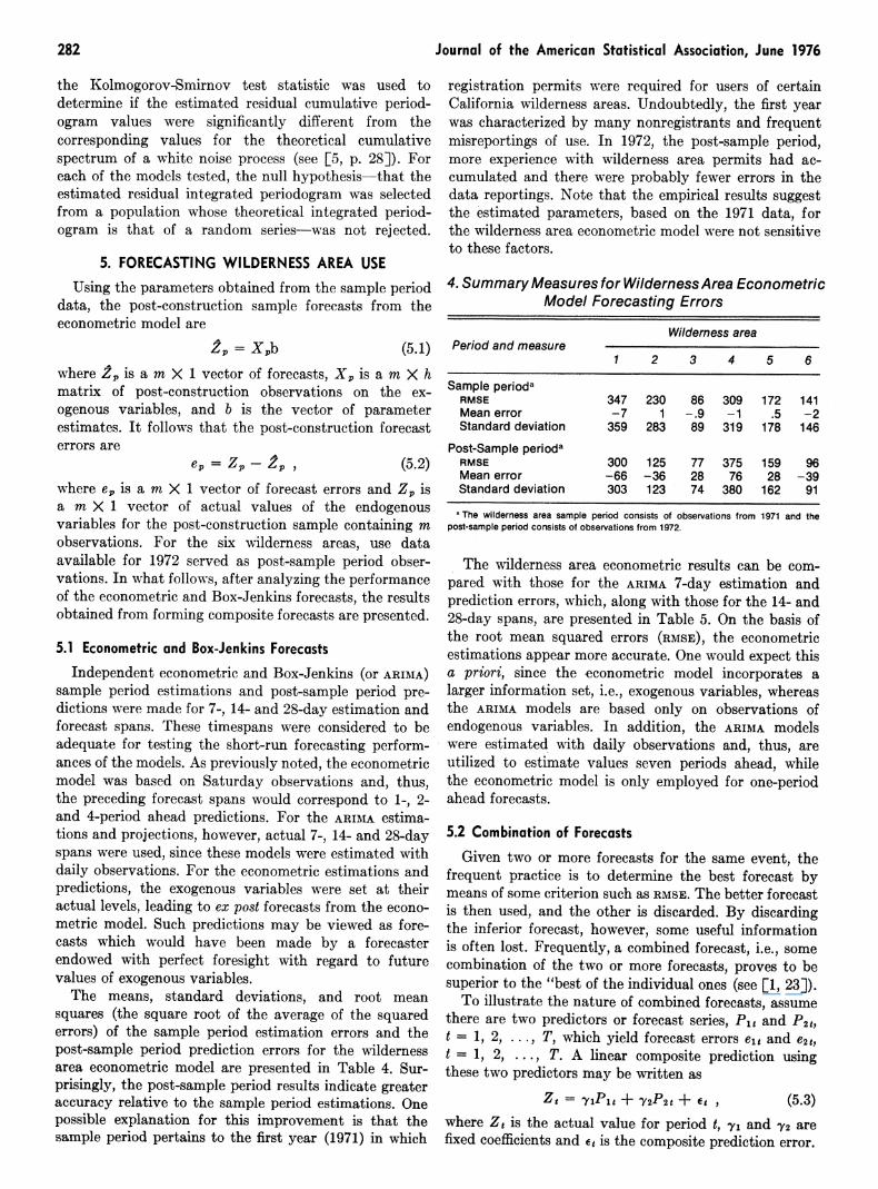
The means, standard deviations, and root mean squares (the square root of the average of the squared errors) of the sample period -estimation errors and the post-sample period prediction errors for the wilderness area econometric model are presented in Table 4. Sur- prisingly, the post-sample period results indicate greater accuracy relative to the sample period estimations. One possible explanation for this improvement is that the sample period pertains to the first year (1971) in which

registration permits were required for users of certain California wilderness areas. Undoubtedly, the first year was characterized by many nonregistrants and frequent misreportings of use. In 1972, the post-sample period, more experience with wilderness area permits had ac- cumulated and there were probably fewer errors in the data reportings. Note that the empirical results suggest the estimated parameters, based on the 1971 data, for the wilderness area econometric model were not sensitive to these factors.

4. Summary Measures for Wilderness Area Econometric Model Forecasting Errors

Wilderness area Period and measure

1 2 3 4 5 6

Sample perioda RMSE 347 230 86 309 172 141 Mean error -7 1 -.9 -1 .5 -2 Standard deviation 359 283 89 319 178 146

Post-Sample perioda RMSE 300 125 77 375 159 96 Mean error -66 -36 28 76 28 -39 Standard deviation 303 123 74 380 162 91

aThe wilderness area sample period consists of observations from 1971 and the post-sample period consists of observations from 1972.

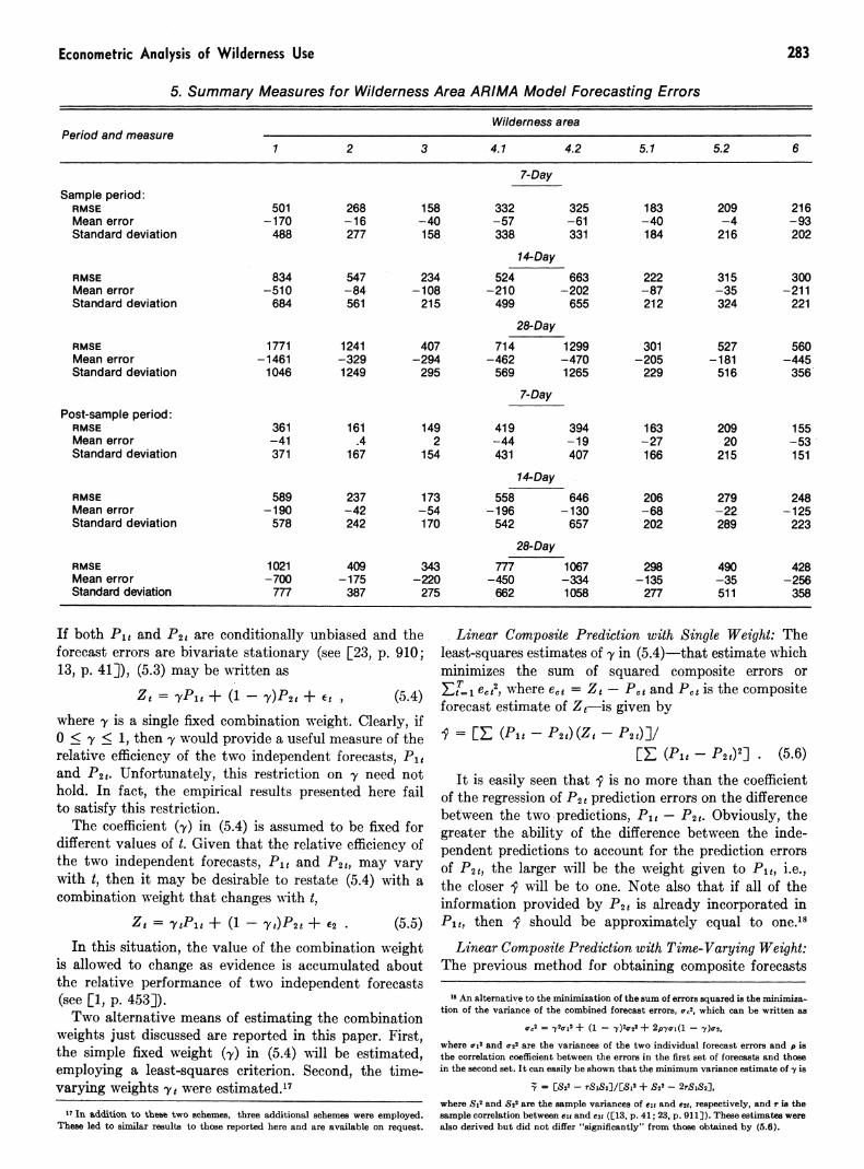
The wilderness area econometric results can be com- pared with those for the ARIMA 7-day estimation and prediction errors, which, along with those for the 14- and 28-day spans, are presented in Table 5. On the basis of the root mean squared errors (RMSE), the econometric estimations appear more accurate. One would expect this a priori, since the econometric model incorporates a larger information set, i.e., exogenous variables, whereas the ARIMA models are based only on observations of endogenous variables. In addition, the ARIMA models were estimated with daily observations and, thus, are utilized to estimate values seven periods ahead, while the econometric model is only employed for one-period ahead forecasts.

5.2 Combination of Forecasts Given two or more forecasts for the same event, the

frequent practice is to determine the best forecast by means of some criterion such as RMSE. The better forecast is then used, and the other is discarded. By discarding the inferior forecast, however, some useful information is often lost. Frequently, a combined forecast, i.e., some combination of the two or more forecasts, proves to be superior to the "best of the individual ones (see [1, 23]).

To illustrate the nature of combined forecasts, assume there are two predictors or forecast series, Pit and P2k, t = 1, 2, ..., T, which yield forecast errors e1t and e2g, t 1, 2, ..., T. A linear composite prediction using these two predictors may be written as

Zt= el1Pst + y2P2t + et, (5.3) where Zt iS the actual value for period I, 'y1 and 72 are fixed coefficients and it iS the composite prediction error.

Econometric Analysis of Wilderness Use 283

5. Summary Measures for Wilderness Area ARIMA Model Forecasting Errors

Wilderness area Period and measure

1 2 3 4.1 4.2 5.1 5.2 6

7-Day Sample period:

RMSE 501 268 158 332 325 183 209 216 Mean error -170 -16 -40 -57 -61 -40 -4 -93 Standard deviation 488 277 158 338 331 184 216 202

14-Day RMSE 834 547 234 524 663 222 315 300 Mean error -510 -84 -108 -210 -202 -87 -35 -211 Standard deviation 684 561 215 499 655 212 324 221

28-Day RMSE 1771 1241 407 714 1299 301 527 560 Mean error -1461 -329 -294 -462 -470 -205 -181 -445 Standard deviation 1046 1249 295 569 1265 229 516 356

7-Day Post-sample period:

RMSE 361 161 149 419 394 163 209 155 Mean error -41 .4 2 -44 -19 -27 20 -53 Standard deviation 371 167 154 431 407 166 215 151

14-Day RMSE 589 237 173 558 646 206 279 248 Mean error -190 -42 -54 -196 -130 -68 -22 -125 Standard deviation 578 242 170 542 657 202 289 223

28-Day RMSE 1021 409 343 777 1067 298 490 428 Mean error -700 -175 -220 -450 -334 -135 -35 -256 Standard deviation 777 387 275 662 1058 277 511 358

If both Pit and P2, are conditionally unbiased and the forecast errors are bivariate stationary (see [23, p. 910; 13, p. 41]), (5.3) may be written as

Zt = yPit + (1 - T)P2t + Et (5.4) where y is a single fixed combination weight. Clearly, if 0 < y < 1, then y would provide a useful measure of the relative efficiency of the two independent forecasts, Pi, and P2 t. Unfortunately, this restriction on oy need not hold. In fact, the empirical results presented here fail to satisfy this restriction.

The coefficient (-y) in (5.4) is assumed to be fixed for different values of t. Given that the relative efficiency of the two independent forecasts, Pit and P2t, may vary with t, then it may be desirable to restate (5.4) with a combination weight that changes with t,

Zt = 7tPlt + (1 - -Yt)P2t + E2 . (5.5) In this situation, the value of the combination weight

is allowed to change as evidence is accumulated about the relative performance of two independent forecasts (see [1, p. 453]).

Two alternative means of estimating the combination weights just discussed are reported in this paper. First, the simple fixed weight (') in (5.4) will be estimated, employing a least-squares criterion. Second, the time- varying weights yt were estimated."7

17 In addition to these two schemes, three additional schemes were employed. These led to similar results to those reported here and are available on request.

Linear Composite Prediction with Single Weight: The least-squares estimates of y in (5.4)-that estimate which minimizes the sum of squared composite errors or ZL1 ~ec where e, = Zt-P, and P,, is the composite forecast estimate of Zt-is given by

ey = [E (P1l - P2t)(Zt -P201/

[E (P1l - P2t)2] (5.6)

It is easily seen that I is no more than the coefficient of the regression of P2t prediction errors on the difference between the two predictions, P1 t- P2 t. Obviously, the greater the ability of the difference between the inde- pendent predictions to account for the prediction errors of P2t, the larger will be the weight given to P1i, i.e., the closer -j will be to one. Note also that if all of the information provided by P2t is already incorporated in Pit, then I should be approximately equal to one.18

Linear Composite Prediction with Time-Varying Weight: The previous method for obtaining composite forecasts

18 An alternative to the minimization of the sum of errors squared is the minimiza- tion of the variance of the combined forecast errors, aC2, which can be written as

0f,2 = y2f 2 + (1 - -Y)2ff22 + 2pyoi(l -Y)2,

where oi2 and 0T22 are the variances of the two individual forecast errors and p is the correlation coefficient between the errors in the first set of forecasts and those in the second set. It can easily be shown that the minimum variance estimate of -y is

5 = [S22 - rSlS2/1ES12 + S22 - 2rSlS2],

where S12 and S22 are the sample variances of elt and e2f, respectively, and r is the sample correlation between 6it and e2 (C13, p. 41; 23, p. 911]). These estimates were also derived but did not differ "significantly" from those obtained by (5.6).

284 Journal of the American Statistical Association, June 1976

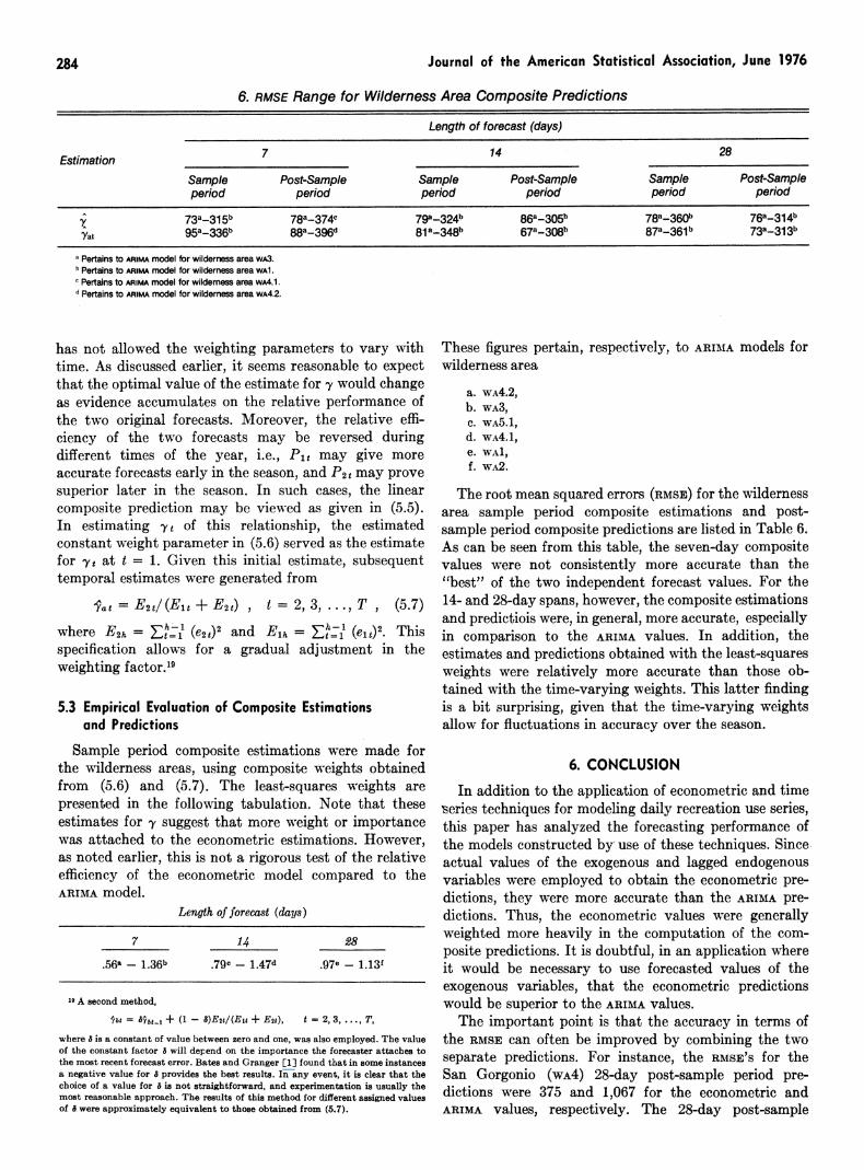
6. RMSE Range for Wilderness Area Composite Predictions

Length of forecast (days)

7 14 28 Estimation

Sample Post-Sample Sample Post-Sample Sample Post-Sample period period period period period period

73a-315b 78a-374C 79a-324 86a305b 78a-360b 76a-314b

Yat 95a-336b 88a-396d 81a-348b 67a-308b 87a-361b 73a-313b

Pertains to ARIMA model for wildern.ess area wA3. b Pertains to ARIMA model for wilderness area wAl. b Pertains to ARIMA model for wildemess area wA4.1. e Pertains to ARIMA model for wildeness area wA4.2.

has not allowed the weighting parameters to vary with time. As discussed earlier, it seems reasonable to expect that the optimal value of the estimate for -y would change as evidence accumulates on the relative performance of the two original forecasts. Moreover, the relative effi- ciency of the two forecasts may be reversed during different times of the year, i.e., Pit may give more accurate forecasts early in the season, and P2t may prove superior later in the season. In such cases, the linear composite prediction may be viewed as given in (5.5). In estimating 'yt of this relationship, the estimated constant weight parameter in (5.6) served as the estimate for -yt at t = 1. Given this initial estimate, subsequent temporal estimates were generated from

lat = E2t/(Elt + E2t) t = 2, 3, ..,T (5.7)

where E2h - . (e, )2 and Elh = E (e,t)'. This specification allows for a gradual adjustment in the weighting factor.'9

5.3 Empirical Evaluation of Composite Estimations and Predictions

Sample period composite estimations were made for the Nwilderness areas, using composite weights obtained from (5.6) and (5.7). The least-squares weights are presented in the following tabulation. Note that these estimates for y suggest that more weight or importance was attached to the econometric estimations. However, as noted earlier, this is not a rigorous test of the relative efficiency of the econometric model compared to the ARIMA model.

Length of foreat (days)

7 14 .28

.56t - 1.36b 79e - 1.47d ,97e - 1.13f

19 A second method,

ibt = 5Ybj-I + (1 -)E2V/(Eit + E2v), t = 2, 3, ..., T, where a is a constant of value between zero and one, was also employed. The value of the constant factor a will depend on the importance the forecaster attaches to the most recent forecast error. Bates and Granger [1] found that in some instances a negative value for a provides the best results. In any event, it is clear that the choice of a value for 5 is not straightforward, and experimentation is usually the most reasonable approach. The results of this method for different assigned values of 5a were approximately equivalent to those obtained from (5.7).

These figures pertain, respectively, to ARIMA models for wilderness area

a. WA4.2, b. WA3, C. WA5.1l

d. wA4.1, e. WAl, f. wA2.

The root mean squared errors (RMSE) for the wilderness area sample period composite estimations and post- sample period composite predictions are listed in Table 6. As can be seen from this table, the seven-day composite values were not consistently more accurate than the "best" of the two independent forecast values. For the 14- and 28-day spans, however, the composite estimations and predictiois were, in general, more accurate, especially in comparison to the ARIMA values. In addition, the estimates and predictions obtained with the least-squares weights were relatively more accurate than those ob- tained with the time-varying weights. This latter finding is a bit surprising, given that the time-varying weights allow for fluctuations in accuracy over the season.

6. CONCLUSION In addition to the application of econometric and time

series techniques for modeling daily recreation use series, this paper has analyzed the forecasting performance of the models constructed by' use of these techniques. Since actual values of the exogenous and lagged endogenous variables were employed to obtain the econometric pre- dictions, they were more accurate than the ARIMA pre- dictions. Thus, the econometric values were generally weighted more heavily in the computation of the com- posite predictions. It is doubtful, in an application where it would be necessary to use forecasted values of the exogenous variables, that the econometric predictions would be superior to the ARIMA values.

The important point is that the accuracy in terms of the RMSE can often be improved by combining the two separate predictions. For instance, the RMSE'S for the San Gorgonio (wA4) 28-day post-sample period pre- dictions were 375 and 1,067 for the econometric and ARIMA values, respectively. The 28-day post-sample

Econometric Analysis of Wilderness Use 285

period least-squares composite RMSE for this wilderness area was 236.

One might question the value of forecasting based on an econometric model if it is necessary to forecast the values of the exogenous variables. Obviously, use of such a forecasting model would not be as convenient as the ARIMA models which require no external forecasts, though the exogenous variables included in the wilderness area econometric models should not present difficult fore- casting problems. For instance, the weather variables can be forecasted with some efficiency, given the sophisti- cation of modern meteorology methods. On the other hand, the variables xogt i.e., total use at all areas, is not as easily predicted. The coefficient for this variable (in both models) is relatively small, compared to the vari- able's magnitude, and thus, forecasted values for xot would not have to be extremely accurate.

The main conclusion of this study is that daily recrea- tion use levels over a season can be modeled with some success. As noted in Section 1, such models may prove useful as management forecasting tools. A fruitful application would involve employing the use equations in a larger recreational model. Specifically, these use equations could serve as an input into a wilderness area simulation model in which the environment and manage- ment effects of use are analyzed. Further extensions would be to develop similar models for arrival rates as well as length-of-stay periods.

[Received June 1974. Revised October 1975.]

REFERENCES [1] Bates, J.M. and Granger, C.W.J., "The Combination of Fore-

casts," Operational Research Quarterly, 20, No. 4 (1969), 451-68. [2] Becker, Gary S., "A Theory of the Allocation of Time," The

Econom7ic Journal, 75, No. 299 (September 1965), 493-517. [3] Box, George E.P. and Jenkins, Gwilym M., Time Series

Analysis, Forecasting, and Control, San Francisco: Holden-Day, Inc., 1970.

[4] Boyet, W.E. and Tolley, G.E., "Recreation Projection Based on Demand Analysis," Joural of Farm Economics, 48 (Novem- ber 1966), 984-1001.

[5] Cargill, Thomas F. and Rausser, Gordon C., "Time and Fre- quency Domain Representations of Futuires Prices as a Sto- chastic Process," Journal of the American Stistical Association, 67 (March 1972), 23-30.

[6] Cicchetti, C.J., Fisher, A.C. and Smith, V.K., "Economic Models and Planning Outdoor Recreation," Operations Re- search, 21, No. 5 (September-October 1973), 1104-113.

[7] 'Seneca, J.J. and Davidson, P., The Demand and Supply of Outdoor Recreation, Washington, D.C.: Bureau of Outdoor Recreation, 1969.

[8] Clawson, Marion and Knetsch, Jack L., Economics of Outdoor Recreation, Baltimore: The Johns Hopkins Press (published for Resources for the Future, Inc.), 1966.

[9] Dhrymes, Phoebus J., "Efficient Estimation of Distributed Lags with Autocorrelated Errors," International Economic Review, 10, No. 1 (February 1969), 47-67.

[10] , Econometrics-Statistical Foundations and Applications, New York: Harper and Row, 1970.

[11] ,et at., "Criteria for Evaluation of Econometric Models," Annals of Economic and Social Measurement, 1, No. 3 (July 1972), 291-324.

[12] Ghez, Gilbert R. and Becker, Gary S., "A Theory of the Alloca- tion of Time and Goods Over the Life Cycle," Unpublished manuscript, National Bureau of Econiomic R esearch, New York, 1972.

[13] Granger, C.W.J. and Newbold, P., "Some Comments on the Evaluation of Economic Forecasts," Applied Economics, 5, No. 1 (1973), 35-47.

[14] Green, H.A.J., Aggregation in Economic Analysis: An Introduc- tory Survey, Princeton, N.J.: Princeton University Press, 1964.

[15] Gupta, Y.P., "Least-Squares Variant of the Dhrymes Two- Step Estimation Procedure of the Distributed Lag Model,"

nternational Economic Review, 10, No. 1 (February 1969), 112-3.

[16] Lancaster, Kelvin, Consumer Demand-A New Approach, New York: Columbia University Press, 1971.

[17] Liviatan, N., "Consistent Estimation of Distributed Lags," International Economic Review, 4, No. 1 (1963), 44-52.

[18] Maddala, G.S., "Generalized Least Squares with an Estimated Covariance Matrix," Econometrica, 39 (January 1971), 23-33.

[19] Micahel, Robert T., The Effect of Education on Efficiency in Consumption, National Bureau of Economic Research, New York, 1972.

[20] ^- and Becker, Gary S., "On the Theory of Consumer Demand," Unpublished paper, National Bureau of Economic Research, Inc., New York, September 1972.

[21] Morrison, Donald F., Multivariate Statistical Methods, New York: McGraw-Hill Book Co., 1967.

[22] Muth, Richard F., "Household Production and Consumer De- mand Functions," Econometrica, 34 (July 1966), 669-708.

[23] Nelson, Charles R., "The Prediction Performance of the FRB- MIT-PENN Model of the U.S. Economy," The American Eco- nomic Review, 62, No. 5 (December 1972), 902-17.

[24] Oliveira, Ronald A., "An Econometric Analysis of Wilderness Area and Campground Use," Unpublished Ph.D. dissertation, Department of Agricultural Economics, University of Cali- fornia, Davis, December 1973.

[25] Parks, Richard W., "Efficient Estimation of a System of Re- gression Equations When Disturbances Are Both Serially and Contemporaneously Correlated," Journal of the American Statistical Association, 62, No. 318 (June 1967), 500-9.

[26] Powell, Allan, "Aitken Estimators as a Tool in Allocating Pre- determined Aggregates," Journal of the American Statistical Association, 64, No. 327 (September 1969), 913-22.

[27] Rausser, Gordon C., "Alternative Econometric Model Forms, Forecasting, and Naive Model Comparisons," Unpublished manuscript, Department of Economics, University of Chicago, 1974.

[28] Wickens, Michael R., "A Note on the Use of Proxy Variables," Econometrica, 40, No. 4 (July 1972), 759-61.

[29] Zellner, Arnold, "An Efficient Method of Estimating Seemingly Unreleated Regressions and Tests for Aggregation Bias," Journal of the American Statistical Association, 57, No. 3 (June 1962), 343-68.