an anomalous extra z prime from intersecting branes with drell–yan and direct photons at the lhc
TRANSCRIPT

arX
iv:0
809.
3772
v2 [
hep-
ph]
4 O
ct 2
008
An Anomalous Extra Z Prime from Intersecting Branes
with Drell-Yan and Direct Photons at the LHC
Roberta Armillisa, Claudio Coriano a b, Marco Guzzi a and Simone Morellia
aDipartimento di Fisica, Universita del Salento
and INFN Sezione di Lecce, Via Arnesano 73100 Lecce, Italy
andbDepartment of Physics and Institute of Plasma Physics
University of Crete, 71003 Heraklion, Greece
Abstract
We quantify the impact of gauge anomalies at the Large Hadron Collider by studying the invariant
mass distributions in Drell-Yan and in double prompt photon, using an extension of the Standard Model
characterized by an additional anomalous U(1) derived from intersecting branes. The approach is rather
general and applies to any anomalous abelian gauge current. Anomalies are cancelled using either the
Wess-Zumino mechanism with suitable Peccei-Quinn-like interactions and a Stuckelberg axion, or by the
Green-Schwarz mechanism. We compare predictions for the corresponding extra Z prime to anomaly-free
realizations such as those involving U(1)B−L. We identify the leading anomalous corrections to both
channels, which contribute at higher orders, and compare them against the next-to-next-to-leading order
(NNLO) QCD background. Anomalous effects in these inclusive observables are found to be very small, far
below the percent level and below the size of the typical QCD corrections quantified by NNLO K-factors.
1
1 Introduction
The study of anomalous gauge interactions at the LHC and at future linear colliders is for sure a difficult
topic, but also an open possibility that deserves close theoretical and experimental attention. Hopefully,
these studies will be able to establish if an additional anomalous extra Z ′ is present in the spectrum,
introduced by an abelian extension of the gauge structure of the Standard Model (SM), assuming that extra
neutral currents will be found in the next several years of running of the LHC [1]. The interactions that we
discuss are characterized by genuine anomalous vertices in which gauge anomalies cancel in some non trivial
way, not by a suitable (anomaly-free) charge assignment of the chiral fermion spectrum for each generation.
The phenomenological investigation of this topic is rather new, while various mechanisms of cancellation
of the gauge anomalies involving axions have been around for quite some time. Global anomalies, for
instance, introduced for the solution of the strong CP problem, such as the Peccei-Quinn (PQ) solution
[2, 3, 4, 5, 6, 7, 8, 9] (reviewed in [10]) require an axion, while local anomalies, cancelled by a Wess-Zumino
counterterm, allow an axion-like particle in the spectrum, whose mass and gauge coupling - differently from
PQ axions - are independent. Similar constructions hold also in the supersymmetric case and a generalization
of the WZ mechanism is the Green-Schwarz mechanism (GS) of string theory. The two mechanisms are
related but not identical [11], the first of them being characterized by a unitarity bound. Details on the
relation between the two at the level of effective field theory can be found in [11, 12].
Intersecting brane models, in which several anomalous U(1)’s and Stuckelberg mass terms are present,
may offer a realization of these constructions [13, 14, 15, 16], which can also be investigated in a bottom-
up approach by using effective lagrangeans built out of the requirements of gauge invariance of the 1-loop
effective action [17]. In our analysis we will consider the simplest extension of these anomalous abelian gauge
factors, which involves a single anomalous U(1), denoted as U(1)B . The corresponding anomalous gauge
boson (B) gets its mass via a combination of the Higgs and of Stuckelberg mechanisms. Axions play a key
role in the cancellation of the anomalies in these theories although they may appear in other constructions
as well, due to the decoupling of a chiral fermion in anomaly-free theories [18].
The presence of an anomalous U(1) in effective models derived from string theory is quite common,
although in all the previous literature before [17] and [18, 19, 20] the phenomenological relevance of the
anomalous U(1) had not been worked out in any detail. In particular, the dynamics of the anomalous extra
gauge interaction had been neglected, by invoking a decoupling of the anomalous sector on the assumption
of a large mass of the extra gauge boson. In [17] it was shown that only one physical axion appears in
the spectrum of these models, independently of the number of abelian factors, which is the most important
feature of these realizations. In our case, the axion can be massless or massive, depending on the structure
of the scalar potential. Recent developements in the study of these models include their supersymmetric
extensions [21] and their derivations as symplectic forms of supergravity [22, 23]. Other interesting variants
include the Stuckelberg extensions considered in [24, 25, 26] which depart significantly from the Minimal
Low Scale Orientifold Model (MLSOM) introduced in [17] and discussed below. Specifically these models
are also characterized by the presence of two mechanisms of symmetry breaking (Higgs and Stuckelberg)
2
but do not share the anomalous structure. As such they do not describe the anomalous U(1)’s of these
special vacua of string theory.
Axion-like particles, beside being a natural candidate for dark matter, may play a role in explaining
some puzzling results regarding the propagation of high energy gamma rays [27, 28] due to the oscillations
of photons into axions in the presence of intergalactic magnetic field. In general, the presence of independent
mass/coupling relations for these particles allows to evade most of the experimental bounds coming from
CAST and other experiments on the detection of PQ axions, characterized by a suppression of both mass
and gauge couplings of this particle by the same large scale (1010 − 1012 GeV), (see [29, 30]). While a
phenomenological study of Stuckelberg axions is underway in a related work, here we focus our attention on
the gauge sector, quantifying the rates for the detection of anomalous neutral currents at the LHC in some
specific and very important channels.
• Drell-Yan
Being leptoproduction the best way to search for extra neutral interactions, it is then obvious that the study
of the anomalous vertices and of possible anomalous extra Z ′ should seriously consider the investigation
of this process. We describe the modifications induced on Drell-Yan computed in the Standard Model
(SM) starting from the description of some of the properties of the new anomalous vertices and of the
corresponding 1-loop counterterms, before moving to the analysis of the corrections. These appear - both in
the WZ and GS cases in the relevant partonic channels at NNLO in the strong coupling constant (O(α2s)).
We perform several comparisons between anomalous and non-anomalous extra Z ′ models and quantify the
differences with high accuracy.
• Direct Photons (Di-photon, DP)
Double prompt (direct) photons offer an interesting signal which is deprived of the fragmentation contribu-
tions especially at large values of their invariant mass Q, due to the steep falling of the photon fragmentation
functions. In addition, photon isolation may provide an additional help in selecting those events coming
from channels in which the contribution of the anomaly is more sizeable, such as gluon fusion. Also in this
case we perform a detailed investigation of this sector. For direct photons, the anomaly appears in gluon
fusion -at parton level - in a class of amplitudes which are characterized by two-triangles graphs - or BIM
amplitudes - using the definitions of [11].
In both cases the quantification of the background needs extreme care, due to the small signal, and the
investigation of the renormalization/factorization scale dependence of the predictions is of outmost impor-
tance. In particular, we consider all the sources of scale-dependence in the analysis, including those coming
from the evolution of the parton densities (Pdf’s) which are just by themeselves enough to overshadow
the anomalous corrections. For this reason we have used the program Candia in the evolution of the
Pdf’s, which has been documented in [31]. The implementations of DY and DP are part of two programs
CandiaDY and CandiaAxion for the study of the QCD background with the modifications induced by the
3

anomalous signal. The QCD background in DP is computed using Diphox [32] and Gamma2MC based
on Ref. [33]. The NLO corrections to DP before the implementation of Diphox have been computed by
Gordon and one of the authors back in 1995 [34] and implemented in a Monte Carlo based on the phase
space slicing method.
In the numerical analysis that we present we have included all the contributions coming from the two
mechanisms as separate cases, corrections that are implemented in DY and DP. We will start analyzing the
contributions to these processes in more detail in the next sections, discussing the specific features of the
anomalous contributions and of the corresponding counterterms at a phenomenological level. To make our
treatment self-contained we have summarized some of the properties of effective vertices in these models,
relevant for our analysis.
Our work is organized as follows. After a brief description of the anomalous interactions and of the
counterterms that appear either at lagrangean level (WZ case) or at the level of the trilinear gauge vertex
(GS case), we discuss the main properties of these vertices and we address the structure of the corrections in
DY and in DP. Our study is mainly focused on the invariant mass distributions in the two cases. The need
for performing these types of analysis in parallel will be explained below, and there is the hope that it may
be extended to other processes and observables in the future, such as rapidity distributions and rapidity
correlations [35]. We present high precision estimates of the QCD background at NNLO, which is the order
where, in these processes, the anomalous corrections start to appear. Other analysis, of course, are also
possible, such as those involving 4-fermion decays in trilinear gauge interactions which could, in principle, be
sensitive to Chern-Simons terms [17, 36] if at least two anomalous U(1)’s are present in the spectrum. These
additional interactions are allowed [37] whenever the distribution of the partial anomalies on a diagram is
not fixed by symmetry requirements. A complete description of these vertices has been carried out in [37],
useful for direct phenomenological studies. This search, however, is expected to be experimentally also very
difficult.
As we are going to show, the search for effects due to anomalous U(1) at the LHC in pp collisions cannot
avoid an analysis of the QCD background at NNLO. DY and DP are the only two cases where this level
of precision has been obtained in perturbation theory. As we are going to show, the anomalous effects at
the LHC in these two key processes are tiny, since the invariant mass distributions are down by a factor of
103 − 104 compared to the NNLO (QCD) background. The accuracy required at the LHC to identify these
effects on these observables should be of a fraction of a percent (0.1% and below), which is beyond reach at
a hadron collider due to the larger indetermination intrinsic in QCD factorization and the parton model.
2 Anomaly-free versus an anomalous extra Z ′ in Drell-Yan
As we have already mentioned, the best mode to search for extra Z ′ at the LHC is in the production of
a lepton pair via the Drell-Yan mechanism (qq annihilation) mediated by neutral currents. The final state
is easily tagged and resonant due to the s-channel exchange of the extra gauge boson. In particular, a
4

new heavier gauge boson modifies the invariant mass distribution also on the Z peak due to the small
modifications induced on the couplings and to the Z − Z ′ interference. In the anomalous model that we
have investigated, though based on a specific charge assignment, we find larger rates for these distributions
both on the peak of the Z and of the Z ′ compared to the other models investigated, if the extra resonance
is around 1 TeV. This correlation is expected to drop as the mass of the extra Z ′ increases. In our case, as
we will specify below, the mass of the extra resonance is given by the Stuckelberg (M1) mass, which appears
also (as a suppression scale) in the interaction of the physical axion to the gluons and is essentially a free
parameter.
In DY, the investigation of the NNLO hard scatterings goes back to [38], with a complete computation of
the invariant mass distributions, made before that the NNLO corrections to the DGLAP evolution had been
fully completed. In our analysis we will compare three anomaly-free models against a model of intersecting
brane with a single anomalous U(1). The anomaly-free charge assignments come from a gauged B − L
abelian symmetry, a “q + u” model -both described in [39] - and the free fermionic model analyzed in [40].
We start by summarizing our definitions and conventions.
In the anomaly-free case we address abelian extensions of the gauge structure of the form SU(3) ×SU(2) × U(1)Y × U(1)z , with a covariant derivative in the W 3
µ , BµY , B
µz (interaction) basis defined as
Dµ =[
∂µ − ig2(
W 1µT
1 +W 2µT
2 +W 3µT
3)
− igY2Y Bµ
Y − igz2zBµ
z
]
(1)
where we denote with g2, gY , gz the couplings of SU(2), U(1)Y and U(1)z , with tan θW = gY /g2. After the
diagonalization of the mass matrix we have
Aµ
Zµ
Z ′µ
=
sin θW cos θW 0
cos θW − sin θW ε
−ε sin θW ε sin θW 1
W 3µ
BYµ
Bzµ
(2)
where ε is a perturbative parameter which is around 10−3 for the models analyzed, introduced in [39] and
[40]. It is defined as
ε =δM2
ZZ′
M2Z′ −M2
Z
(3)
while the mass of the Z boson and of the extra Z ′ are
M2Z =
g22
4 cos2 θW(v2H1
+ v2H2
)[
1 +O(ε2)]
M2Z′ =
g2z
4(z2H1v2H1
+ z2H2v2H2
+ z2φv
2φ)[
1 +O(ε2)]
δM2ZZ′ = − g2gz
4 cos θW(z2H1v2H1
+ z2H2v2H2
). (4)
In this class of models we have two Higgs doublet H1 and H2, whose vevs are vH1and vH2
and an extra
SU(2)W singlet φ whose vev is vφ. The extra U(1)z charges of the Higgs doublet are respectively zH1and
5
zH2, while for the singlet this is denoted as zφ. Taking the value of vH2
of the order of the electroweak scale
(≈ 246 GeV), we fix vH1with tan β = vH2
/vH1, and we still have one free parameter, vφ, which enters in the
calculation of the mass of the extra Z ′. Then it is obvious that we can take the mass MZ′ and the coupling
constant gz as free parameters. We choose tan β ≈ 40 in order to reproduce the mass of the Z boson at
91.187 GeV, choice that is performed, for consistency, also in the anomalous model. In this last case the
Higgs sector is characterized only by 2 Higgs doublets, with the vev of the extra singlet being replaced by
the Stuckelberg mass. We define g2 sin θW = gY cos θW = e and construct the W± charge eigenstates and
the corresponding generators T± as usual
W± =W1 ∓ iW2√
2
T± =T1 ± iT2√
2, (5)
while in the neutral sector we introduce the rotation matrix
W 3µ
BYµ
Bzµ
=
sin θW (1+ε2)1+ε2
cos θW
1+ε2ε cos θW
1+ε2cos θW (1+ε2)
1+ε2− sin θW
1+ε2ε sin θW
1+ε2
0 ε1+ε2
11+ε2
Aµ
Zµ
Z ′µ
(6)
which relates the interaction and the mass eigenstates. Substituting these expression in the covariant
derivative we obtain
Dµ =
[
∂µ − iAµ
(
g2T3 sin θW + gY cos θWY
2
)
− ig2(
W−
µ T− +W+
µ T+)
−iZµ(
g2 cos θWT3 − gY sin θWY
2+ gzε
z
2
)
−iZ ′
µ
(
−g2 cos θWT3ε+ gY sin θWY
2ε+ gz
z
2
)]
(7)
where we have neglected all the O(ε2) terms. Sending gz → 0 and ε → 0 we obtain the SM expression.
The vector and the axial couplings of the Z and Z ′ to the fermions are expressed equivalently in terms of
the left - (zL) and right - (zR) U(1)z chiral charges and hypercharges (YR, YL) of the models that we have
implemented. These can be found in [40] for the free fermionic case and in [39] for the remaining models
with a V-A structure given by
−ig24cw
γµgVZ,j =
−ig2cw
1
2
[
c2wTL,j3 − s2w(
Y jL
2+Y jR
2) + ε
gzg2cw(
zL,j2
+zR,j2
)
]
γµ
−ig24cw
γµγ5gAZ,j =
−ig2cw
1
2
[
−c2wTL,j3 − s2w(Y jR
2− Y j
L
2) + ε
gzg2cw(
zR,j2
− zL,j2
)
]
γµγ5
6
−ig24cw
γµgVZ′,j =
−ig2cw
1
2
[
−εc2wTL,j3 + εs2w(Y jL
2+Y jR
2) +
gzg2cw(
zL,j2
+zR,j2
)
]
γµ
−ig24cw
γµγ5gAZ′,j =
−ig2cw
1
2
[
εc2wTL,j3 + εs2w(
Y jR
2− Y j
L
2) +
gzg2cw(
zR,j2
− zL,j2
)
]
γµγ5,
(8)
where j is an index which represents the quark or the lepton and we have set sin θW = sw, cos θW = cw for
brevity.
2.1 An anomalous extra Z ′
In presence of anomalous interactions we can use the same formalism developed so far for anomaly-free
models with some appropriate changes. Since the effective lagrangean of the class of the anomalous models
that we are investigating includes both a Stuckelberg and a two-Higgs doublet sector, the masses of the
neutral gauge bosons are provided by a combination of these two mechanisms. In this case we take as
free parameters the Stueckelberg mass M1 and the anomalous coupling constant gB , with tanβ as in the
remaining anomaly-free models. As we have already stressed, the analysis does not depend significantly on
the choice of this parameter. The value of the Stuckelberg mass M1 is loosely constrained by the D-brane
model in terms of suitable wrappings (n) of the 4-branes which define the charge embedding [41, 14] reported
in Tabs. 1,2,3 and 4.
The mass-matrix in the neutral gauge sector is given by
Lmass = (W3, Y, B)M2
W3
Y
B
,
where B is the Stuckelberg field and the mass matrix is defined as
M2 =1
4
g22v2 −g2 gY v2 −g2 xB
−g2 gY v2 gY2v2 gY xB
−g2 xB gY xB 2M21 +NBB
(9)
with
NBB =(
qB 2u v 2
u + qB 2d v 2
d
)
g 2B , xB =
(
qBu v2u + qBd v
2d
)
gB . (10)
Here vu and vd denote the vevs of the two Higgs fields Hu,Hd while qBu and qBd are the Higgs charges
under the extra anomalous U(1)B . We have also defined v =√
v2u + v2
d and g =√
g22 + g2
Y . The massless
eigenvalue of the mass matrix is associated to the photon Aγ , while the two non-zero mass eigenvalues
denote the masses of the Z and of the Z ′ vector bosons. These are given by
M2Z =
1
4
(
2M21 + g2v2 +NBB −
√
(
2M21 − g2v2 +NBB
)2+ 4g2x2
B
)
(11)
7

≃ g2v2
2− 1
M21
g2x2B
4+
1
M41
g2x2B
8(NBB − g2v2),
M2Z′ =
1
4
(
2M21 + g2v2 +NBB +
√
(
2M21 − g2v2 +NBB
)2+ 4g2x2
B
)
(12)
≃ M21 +
NBB
2.
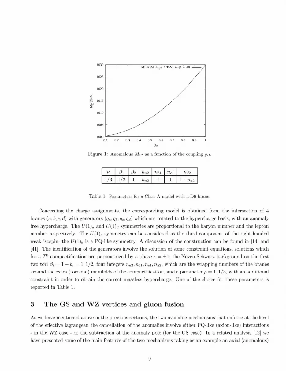
The mass of the Z gauge boson gets corrected by terms of the order v2/M1, see Fig. 1, converging to the
SM value as M1 → ∞, while the mass of the Z ′ gauge boson can grow large with M1. The physical gauge
fields can be obtained from the rotation matrix OA
Aγ
Z
Z ′
= OA
W3
AY
B
(13)
which can be approximated at the first order as
OA ≃
gY
g
g2g
0g2g
+O(ǫ21) − gY
g+O(ǫ21)
g2ǫ1
− g22 ǫ1
gY
2 ǫ1 1 +O(ǫ21)
(14)
which is the analogue of the matrix in Eq. (2) for the anomaly-free models, but here the role of the mixing
parameter ǫ1 is taken by the expression
ǫ1 =xBM2
1
. (15)
A relation between the two expansion parameters can be easily obtained in an approximate way by a direct
comparison. For simplicity we take all the charges to be O(1) in all the models obtaining
M2Z ∼ g2
2v2
M2Z′ −M2
Z ∼ g2zv
2φ
δM2ZZ′ ∼ g2gzv
2 (16)
giving
ǫ1 ∼ v2
M21
, (17)
which is the analogue of Eq. (15), having identified the Stuckelberg mass with the vev of the extra singlet
Higgs, M1 ∼ gzvφ. This is natural since the Stuckelberg mechanism can be thought of as the low energy
remnant of an extra Higgs whose radial fluctuations have been frozen and with the imaginary phase surviving
at low energy as a CP-odd scalar [18].
8
1000
1005
1010
1015
1020
1025
1030
0.1 0.2 0.3 0.4 0.5 0.6 0.7 0.8 0.9 1
MZ
' [G
eV]
gB
MLSOM, M1 = 1 TeV, tanβ = 40
Figure 1: Anomalous MZ′ as a function of the coupling gB.
ν β1 β2 na2 nb1 nc1 nd2
1/3 1/2 1 na2 -1 1 1 - na2
Table 1: Parameters for a Class A model with a D6-brane.
Concerning the charge assignments, the corresponding model is obtained form the intersection of 4
branes (a, b, c, d) with generators (qa, qb, qc, qd) which are rotated to the hypercharge basis, with an anomaly
free hypercharge. The U(1)a and U(1)d symmetries are proportional to the baryon number and the lepton
number respectively. The U(1)c symmetry can be considered as the third component of the right-handed
weak isospin; the U(1)b is a PQ-like symmetry. A discussion of the construction can be found in [14] and
[41]. The identification of the generators involve the solution of some constraint equations, solutions which
for a T 6 compactification are parametrized by a phase ǫ = ±1; the Neveu-Schwarz background on the first
two tori βi = 1 − bi = 1, 1/2, four integers na2, nb1, nc1, nd2, which are the wrapping numbers of the branes
around the extra (toroidal) manifolds of the compactification, and a parameter ρ = 1, 1/3, with an additional
constraint in order to obtain the correct massless hypercharge. One of the choice for these parameters is
reported in Table 1.
3 The GS and WZ vertices and gluon fusion
As we have mentioned above in the previous sections, the two available mechanisms that enforce at the level
of the effective lagrangean the cancellation of the anomalies involve either PQ-like (axion-like) interactions
- in the WZ case - or the subtraction of the anomaly pole (for the GS case). In a related analysis [12] we
have presented some of the main features of the two mechanisms taking as an example an axial (anomalous)
9

Y XA XB
Hu 1/2 0 2
Hd 1/2 0 -2
Table 2: Higgs charges in the Madrid model.
qa qb qc qd
QL 1 -1 0 0
uR -1 0 1 0
dR -1 0 -1 0
L 0 -1 0 -1
eR 0 0 -1 1
NR 0 0 1 1
Table 3: SM spectrum charges in the D-brane basis for the Madrid model.
version of QED to illustrate the cancellation of the anomaly in the two cases. In the GS case, the anomaly
of a given diagram is removed by subtracting the longitudinal pole of the triangle amplitude in the chiral
limit. We have stressed in [37] that the counterterm (the pole subtraction) amounts to the removal of one of
the invariant amplitudes of the anomaly vertex (the longitudinal component) and corresponds to a vertex
re-definition.
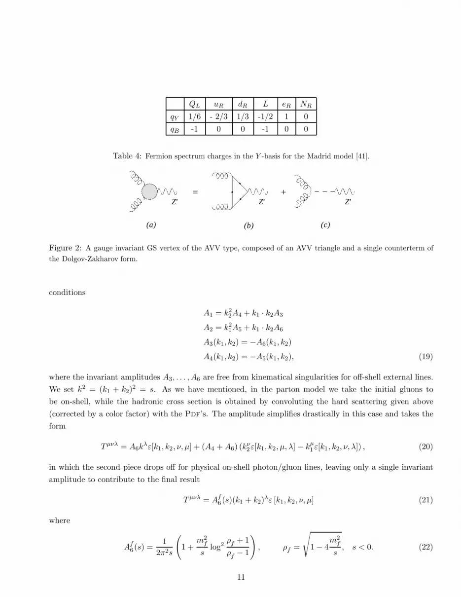
The procedure is exemplified in Fig. 2 where we show the triangle anomaly and the pole counterterm
which is subtracted from the first amplitude. The combination of the two contributions defines the GS
vertex, which is made of purely transverse components in the chiral limit [12] and satisfies an ordinary Ward
identity. Notice that the vertex does not require an axion as an asymptotic state in the related S-matrix;
for a non-zero fermion mass in the triangle diagram, the vertex satisfies a broken Ward identity. We now
proceed and summarize some of these properties, working in the chiral limit.
Processes such as gg → γγ, mediated by an anomalous gauge boson Z ′, can be expressed in a simplified
form in which only the longitudinal component of the anomaly appears. We therefore set k21 = k2
2 = 0 and
mf = 0, which are the correct kinematical conditions to obtain the anomaly pole, necessary for a parton
model (factorized) description of the cross section in a pp collision at the LHC, where the initial state of the
partonic hard-scatterings are on-shell.
We start from the Rosenberg form of the AV V amplitude, which is given by
T λµν = A1ε[k1, λ, µ, ν] +A2ε[k2, λ, µ, ν] +A3kµ1 ε[k1, k2, ν, λ]
+A4kµ2 ε[k1, k2, ν, λ] +A5k
ν1ε[k1, k2, µ, λ] +A6k
ν2ε[k1, k2, µ, λ] , (18)
and imposing the Ward identities to bring all the anomaly on the axial-vector vertex, we obtain the usual
10
QL uR dR L eR NR
qY 1/6 - 2/3 1/3 -1/2 1 0
qB -1 0 0 -1 0 0
Table 4: Fermion spectrum charges in the Y -basis for the Madrid model [41].
=
(a)
+
(c)(b)
Z’ Z’Z’
Figure 2: A gauge invariant GS vertex of the AVV type, composed of an AVV triangle and a single counterterm of
the Dolgov-Zakharov form.
conditions
A1 = k22A4 + k1 · k2A3
A2 = k21A5 + k1 · k2A6
A3(k1, k2) = −A6(k1, k2)
A4(k1, k2) = −A5(k1, k2), (19)
where the invariant amplitudes A3, . . . , A6 are free from kinematical singularities for off-shell external lines.
We set k2 = (k1 + k2)2 = s. As we have mentioned, in the parton model we take the initial gluons to
be on-shell, while the hadronic cross section is obtained by convoluting the hard scattering given above
(corrected by a color factor) with the Pdf’s. The amplitude simplifies drastically in this case and takes the
form
T µνλ = A6kλε[k1, k2, ν, µ] + (A4 +A6) (kν2ε[k1, k2, µ, λ] − kµ1 ε[k1, k2, ν, λ]) , (20)
in which the second piece drops off for physical on-shell photon/gluon lines, leaving only a single invariant
amplitude to contribute to the final result
T µνλ = Af6 (s)(k1 + k2)λε [k1, k2, ν, µ] (21)
where
Af6 (s) =1
2π2s
(
1 +m2f
slog2
ρf + 1
ρf − 1
)
, ρf =
√
1 − 4m2f
s, s < 0. (22)
11
(a)
Z’+ +
(b) (c)
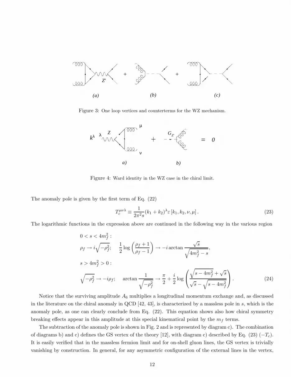
Figure 3: One loop vertices and counterterms for the WZ mechanism.
µ
ν
kλ λ Z
a)
= 0GZ’
b)
Figure 4: Ward identity in the WZ case in the chiral limit.
The anomaly pole is given by the first term of Eq. (22)
T µνλc ≡ 1
2π2s(k1 + k2)
λε [k1, k2, ν, µ] . (23)
The logarithmic functions in the expression above are continued in the following way in the various region
0 < s < 4m2f :
ρf → i√
−ρ2f ;
1
2log
(
ρf + 1
ρf − 1
)
→ −i arctan√s
√
4m2f − s
,
s > 4m2f > 0 :
√
−ρ2f → −iρf ; arctan
1√
−ρ2f
→ π
2+i
2log
√
s− 4m2f +
√s
√s−
√
s− 4m2f
. (24)
Notice that the surviving amplitude A6 multiplies a longitudinal momentum exchange and, as discussed
in the literature on the chiral anomaly in QCD [42, 43], is characterized by a massless pole in s, which is the
anomaly pole, as one can clearly conclude from Eq. (22). This equation shows also how chiral symmetry
breaking effects appear in this amplitude at this special kinematical point by the mf terms.
The subtraction of the anomaly pole is shown in Fig. 2 and is represented by diagram c). The combination
of diagrams b) and c) defines the GS vertex of the theory [12], with diagram c) described by Eq. (23) (−Tc).It is easily verified that in the massless fermion limit and for on-shell gluon lines, the GS vertex is trivially
vanishing by construction. In general, for any asymmetric configuration of the external lines in the vertex,
12

λ
µ
ν
Z’
a)
kλ= 0
λ
µ
ν
GZ’
c)
GZ’
b)
Figure 5: Generalized Ward identity in the WZ case.
even in the massless limit, the vertex has non-zero transverse components [44, 45]. The expression is well
known [46, 45] in the chiral limit and has been shown to satisfy the Adler-Bardeen theorem [45].
For a non-vanishing mf the GS vertex, for generic virtualities, can be defined to be the general AV V
vertex, for instance extracted from [47] or, in the longitudinal/transverse formulation, by the amplitudes
given in [45], with the subtraction of the anomaly pole, as given in [12]. We will refer to the anomaly
(subtraction) counterterm of diagram b) as to the Dolgov-Zakharov [43] (DZ) counterterm. The anomaly
diagram reduces to its DZ form for two on-shell gauge lines (photons/gluons) and in this case the transverse
components completely disappear. There are other cases in which, instead, the longitudinal components
cancel. This occurs if, for instance, a conserved current is attached to the anomalous line, rendering the
anomaly ”harmless”, as explained in [12].
The analogous interaction in the WZ case is shown in Fig. 3, where we have attached a fermion pair in the
final state to better identify the contributions. In this case, beside the anomalous contribution of diagram
a), the mechanism will require the exchange of a physical axion, shown in diagram b) and c). Diagram b)
is the usual WZ counterterm (or generalized PQ interaction) while the third diagram is non-vanishing only
in the presence of fermions of non-zero mass. This third contribution is numerically irrelevant and in DY
is usually omitted. The WZ mechanism re-establish gauge invariance of the effective lagrangean but is not
based on a vertex re-definition and, furthermore, involves an asymptotic axion state. As shown in [11] the
presence of a unitarity bound in this mechanism is a signal of its limitation as an effective theory (see also
the discussion in [12]). We have summarized in an appendix the discussion of this point in a simple case.
3.1 Ward identities
Both vertices satisfy ordinary Ward identities in the chiral limit and generalized Ward identities away from
it. In the chiral limit, for instance, the WZ mechanism adds to the effective action of the anomalous theory
an interaction of the Stuckelberg field (b) with the gluons (bG ∧G), shown in diagram b) of Fig. 4. In this
figure we have shown a diagrammatic realization of the Ward identity for this case.
In WZ, being the cancellation based on a local field theory, the derivation of the generalized Ward
identity can be formally obtained from the requirement of BRST invariance of the gauge-fixed effective
action, as we have shown in [37]. This is illustrated in Fig. 5, in the case of an anomalous Z ′, where we
13
λ
µ
ν
Z’
µ
ν
a) b) c)
+ +λ λ
= 0
µ
ν
kλ
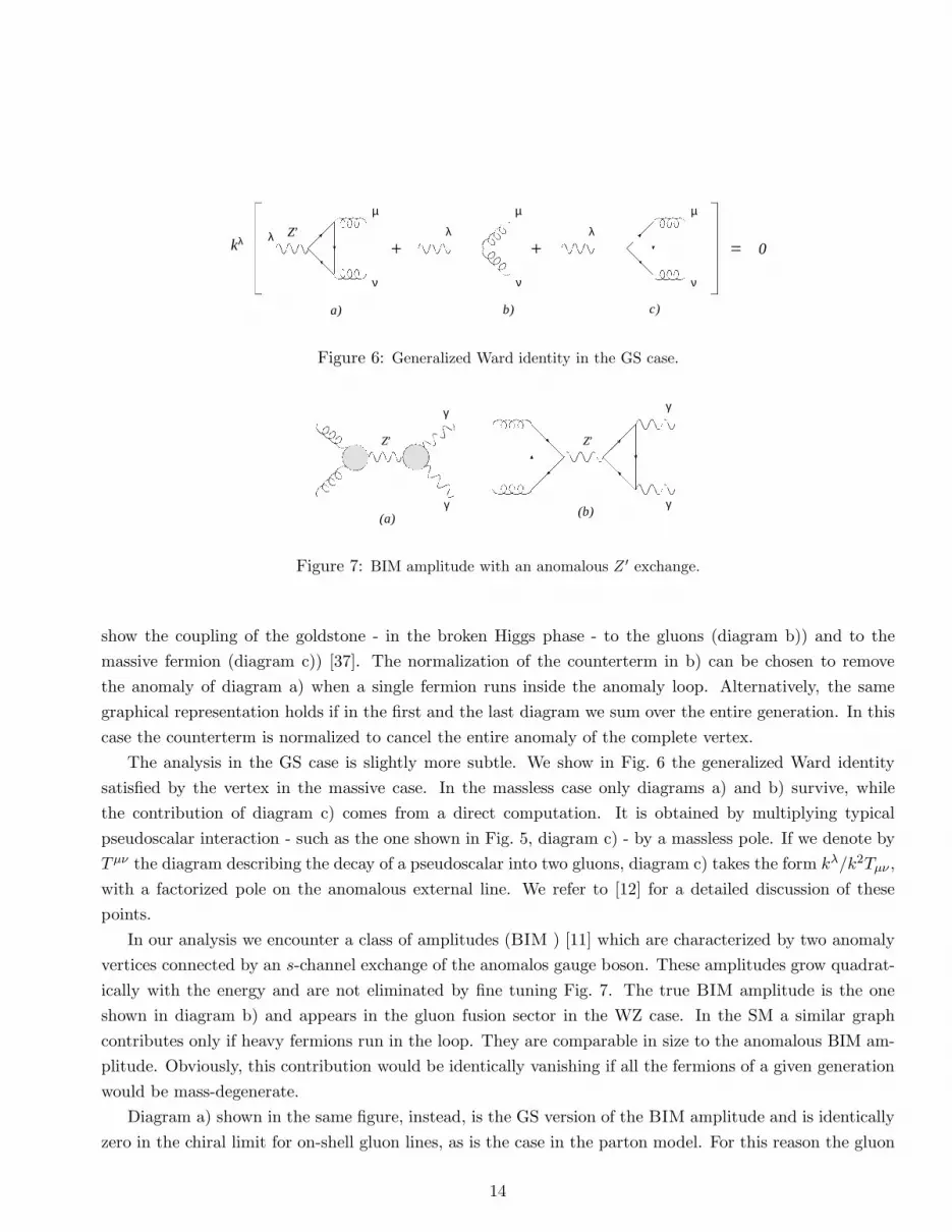
Figure 6: Generalized Ward identity in the GS case.
(a)(b)
Z’
γ
γ
Z’
γ
γ
Figure 7: BIM amplitude with an anomalous Z ′ exchange.
show the coupling of the goldstone - in the broken Higgs phase - to the gluons (diagram b)) and to the
massive fermion (diagram c)) [37]. The normalization of the counterterm in b) can be chosen to remove
the anomaly of diagram a) when a single fermion runs inside the anomaly loop. Alternatively, the same
graphical representation holds if in the first and the last diagram we sum over the entire generation. In this
case the counterterm is normalized to cancel the entire anomaly of the complete vertex.
The analysis in the GS case is slightly more subtle. We show in Fig. 6 the generalized Ward identity
satisfied by the vertex in the massive case. In the massless case only diagrams a) and b) survive, while
the contribution of diagram c) comes from a direct computation. It is obtained by multiplying typical
pseudoscalar interaction - such as the one shown in Fig. 5, diagram c) - by a massless pole. If we denote by
T µν the diagram describing the decay of a pseudoscalar into two gluons, diagram c) takes the form kλ/k2Tµν ,
with a factorized pole on the anomalous external line. We refer to [12] for a detailed discussion of these
points.
In our analysis we encounter a class of amplitudes (BIM ) [11] which are characterized by two anomaly
vertices connected by an s-channel exchange of the anomalos gauge boson. These amplitudes grow quadrat-
ically with the energy and are not eliminated by fine tuning Fig. 7. The true BIM amplitude is the one
shown in diagram b) and appears in the gluon fusion sector in the WZ case. In the SM a similar graph
contributes only if heavy fermions run in the loop. They are comparable in size to the anomalous BIM am-
plitude. Obviously, this contribution would be identically vanishing if all the fermions of a given generation
would be mass-degenerate.
Diagram a) shown in the same figure, instead, is the GS version of the BIM amplitude and is identically
zero in the chiral limit for on-shell gluon lines, as is the case in the parton model. For this reason the gluon
14
fusion sector disappears completely for DP (in the GS mechanism), since the BIM amplitude in this case is
obtained by replacing diagram b) of this figure with diagram a) which is indeed vanishing.
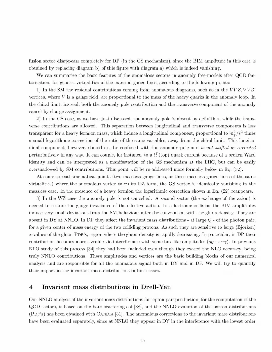
We can summarize the basic features of the anomalous sectors in anomaly free-models after QCD fac-
torization, for generic virtualities of the external gauge lines, according to the following points:
1) In the SM the residual contributions coming from anomalous diagrams, such as in the V V Z, V V Z ′
vertices, where V is a gauge field, are proportional to the mass of the heavy quarks in the anomaly loop. In
the chiral limit, instead, both the anomaly pole contribution and the transverse component of the anomaly
cancel by charge assignment.
2) In the GS case, as we have just discussed, the anomaly pole is absent by definition, while the trans-
verse contributions are allowed. This separation between longitudinal and transverse components is less
transparent for a heavy fermion mass, which induce a longitudinal component, proportional to m2f/s
2 times
a small logarithmic correction of the ratio of the same variables, away from the chiral limit. This longitu-
dinal component, however, should not be confused with the anomaly pole and is not shifted or corrected
perturbatively in any way. It can couple, for instance, to a tt (top) quark current because of a broken Ward
identity and can be interpreted as a manifestation of the GS mechanism at the LHC, but can be easily
overshadowed by SM contributions. This point will be re-addressed more formally below in Eq. (32).
At some special kinematical points (two massless gauge lines, or three massless gauge lines of the same
virtualities) where the anomalous vertex takes its DZ form, the GS vertex is identically vanishing in the
massless case. In the presence of a heavy fermion the logarithmic correction shown in Eq. (22) reappears.
3) In the WZ case the anomaly pole is not cancelled. A second sector (the exchange of the axion) is
needed to restore the gauge invariance of the effective action. In a hadronic collision the BIM amplitudes
induce very small deviations from the SM behaviour after the convolution with the gluon density. They are
absent in DY at NNLO. In DP they affect the invariant mass distributions - at large Q - of the photon pair,
for a given center of mass energy of the two colliding protons. As such they are sensitive to large (Bjorken)
x-values of the gluon Pdf’s, region where the gluon density is rapidly decreasing. In particular, in DP their
contribution becomes more sizeable via intereference with some box-like amplitudes (gg → γγ). In previous
NLO study of this process [34] they had been included even though they exceed the NLO accuracy, being
truly NNLO contributions. These amplitudes and vertices are the basic building blocks of our numerical
analysis and are responsible for all the anomalous signal both in DY and in DP. We will try to quantify
their impact in the invariant mass distributions in both cases.
4 Invariant mass distributions in Drell-Yan
Our NNLO analysis of the invariant mass distributions for lepton pair production, for the computation of the
QCD sectors, is based on the hard scatterings of [38], and the NNLO evolution of the parton distributions
(Pdf’s) has been obtained with Candia [31]. The anomalous corrections to the invariant mass distributions
have been evaluated separately, since at NNLO they appear in DY in the interference with the lowest order
15
graph, and added to the standard QCD background. It is important to recall that lepton pair production
at low Q via Drell-Yan is sensitive to the Pdf’s at small-x values, while in the high mass region this process
is essential in the search of additional neutral currents. In our analysis we have selected a mass of 1 TeV
for the extra gauge boson and analyzed the signal and the background both on the peaks of the Z and of
the of the new resonance.
At hadron level the colour-averaged inclusive differential cross section for the reaction H1 + H2 →l1 + l2 +X, is given by the expression [38]
dσ
dQ2= τσZ(Q2,M2
Z)WZ(τ,Q2) τ =Q2
S, (25)
where Z ≡ Z,Z ′ is the point-like cross section and all the information from the hadronic initial state is
contained in the Pdf’s. The hadronic structure function WZ(τ,Q2) is given by a convolution product
between the parton luminosities Φij(x, µ2R, µ
2F ) and the Wilson coefficients ∆ij(x,Q
2, µ2R, µ
2F )
WZ(τ,Q2, µ2R, µ
2F ) =
∑
i,j
∫ 1
τ
dx
xΦij(x, µ
2R, µ
2F )∆ij(
τ
x,Q2, µ2
F ), (26)
where the luminosities are given by
Φij(x, µ2R, µ
2F ) =
∫ 1
x
dy
yfi(y, µ
2R, µ
2F )fj
(
x
y, µ2
R, µ2F
)
≡ [fi ⊗ fj] (x, µ2R, µ
2F ) (27)
and the Wilson coefficients (hard scatterings) depend on both the factorization (µF ) and renormalization
scales (µR), formally expanded in the strong coupling αs as
∆ij(x,Q2, µ2
F ) =
∞∑
n=0
αns (µ2R)∆
(n)ij (x,Q2, µ2
F , µ2R). (28)
We will vary µF and µR independently in order to determine the sensitivity of the prediciton on their
variations and their optimal choice.
The anomalous corrections to the hard scatterings computed in the SM will be discussed below. We just
recall that the relevant point-like cross sections appearing in the factorization formula (25) and which are
part of our analysis include, beside the Z and the Z ′ resonance, also the contributions due to the photon
and the γ − Z, γ − Z ′ interferences. For instance in the Z ′ case we have
σγ(Q2) =
4πα2em
3Q4
1
Nc
σZ′(Q2) =παem
4MZ′ sin2 θW cos2 θWNc
ΓZ′→ll
(Q2 −M2Z′)2 +M2
Z′Γ2Z′
σZ′,γ(Q2) =
πα2em
6Nc
gZ′,l
V gγ,lVsin2 θW cos2 θW
(Q2 −M2Z′)
Q2(Q2 −M2Z′)2 +M2
Z′Γ2Z′
,
16

(a) (c)(b)
Figure 8: qq → Z,Z ′ at LO and NLO (virtual corrections).
Z, Z’, γ
(d) (f)(e)
Figure 9: qq → Z,Z ′ at NNLO (virtual corrections).
σZ′,Z(Q2) =πα2
em
96
[
gZ′,l
V gZ,lV + gZ′,l
A gZ,lA
]
sin4 θW cos4 θWNc
(Q2 −M2Z)(Q2 −M2
Z′) +MZΓZMZ′ΓZ′
[
(Q2 −M2Z′)2 +M2
Z′Γ2Z′
] [
(Q2 −M2Z)2 +M2
ZΓ2Z
] .
(29)
where NC is the number of colours, ΓZ′→ll is the partial decay width of the gauge boson and the total
hadronic widths are defined by
ΓZ ≡ Γ(Z → hadrons) =∑
i
Γ(Z → ψiψi)
ΓZ′ ≡ Γ(Z ′ → hadrons) =∑
i
Γ(Z ′ → ψiψi), (30)
where we refer to hadrons not containing bottom and top quarks (i.e. i = u, d, c, s). We also ignore
electroweak corrections of higher order and we have included the top-quark mass and QCD corrections. We
have included only tree level decays into SM fermions, with a total decay rate for the Z and Z ′ which is
given by
ΓZ =∑
i=u,d,c,s
Γ(Z → ψiψi) + Γ(Z → bb) + 3Γ(Z → ll) + 3Γ(Z → νlνl)
ΓZ′ =∑
i=u,d,c,s
Γ(Z ′ → ψiψi) + Γ(Z ′ → bb) + Γ(Z ′ → tt) + 3Γ(Z ′ → ll) + 3Γ(Z ′ → νlνl).
(31)
Coming to illustrate the contributions included in our analysis, these are shown in some representative
17
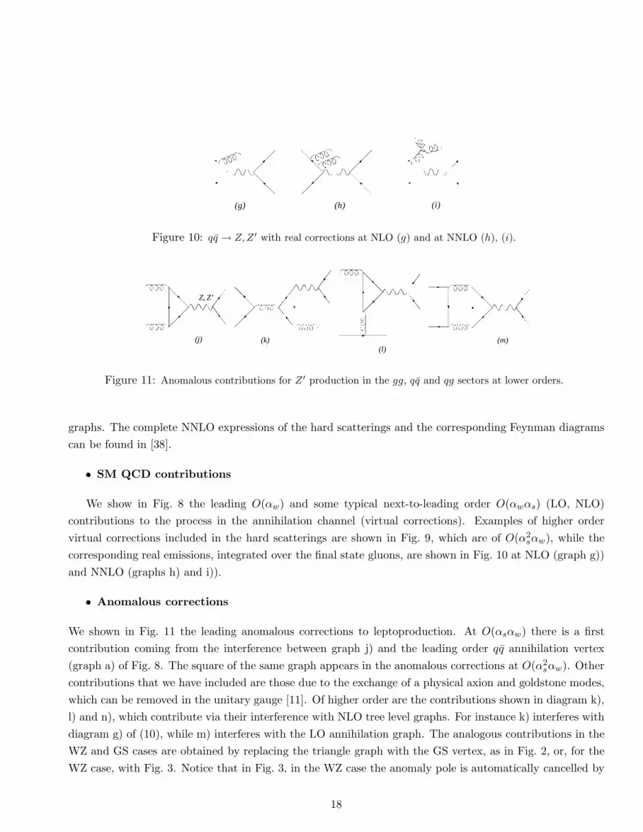
(g) (h) (i)
Figure 10: qq → Z,Z ′ with real corrections at NLO (g) and at NNLO (h), (i).
(l)
Z, Z’
(j) (k) (m)
Figure 11: Anomalous contributions for Z ′ production in the gg, qq and qg sectors at lower orders.
graphs. The complete NNLO expressions of the hard scatterings and the corresponding Feynman diagrams
can be found in [38].
• SM QCD contributions
We show in Fig. 8 the leading O(αw) and some typical next-to-leading order O(αwαs) (LO, NLO)
contributions to the process in the annihilation channel (virtual corrections). Examples of higher order
virtual corrections included in the hard scatterings are shown in Fig. 9, which are of O(α2sαw), while the
corresponding real emissions, integrated over the final state gluons, are shown in Fig. 10 at NLO (graph g))
and NNLO (graphs h) and i)).
• Anomalous corrections
We shown in Fig. 11 the leading anomalous corrections to leptoproduction. At O(αsαw) there is a first
contribution coming from the interference between graph j) and the leading order qq annihilation vertex
(graph a) of Fig. 8. The square of the same graph appears in the anomalous corrections at O(α2sαw). Other
contributions that we have included are those due to the exchange of a physical axion and goldstone modes,
which can be removed in the unitary gauge [11]. Of higher order are the contributions shown in diagram k),
l) and n), which contribute via their interference with NLO tree level graphs. For instance k) interferes with
diagram g) of (10), while m) interferes with the LO annihilation graph. The analogous contributions in the
WZ and GS cases are obtained by replacing the triangle graph with the GS vertex, as in Fig. 2, or, for the
WZ case, with Fig. 3. Notice that in Fig. 3, in the WZ case the anomaly pole is automatically cancelled by
18

+ +
(o) (p) (q)
*
(n)
Z, Z’
Figure 12: Anomalous contributions for the gg → gg process mediated by an anomalous Z ′ at higher perturbative
orders.
the Ward identity on the lepton pair of the final state, if the two leptons are taken to be massless at high
energy, as is the case. Then, the only new contributions from the anomaly vertex that survive are those
related to the transverse component of this vertex. This is an example, as we have discussed in [12], of a
”harmless” anomaly vertex. A similar situation occurs whenever there is no coupling of the longitudinal
component of the anomaly to the (transverse) external leptonic current. This property continues to hold
also away from the chiral limit, since the corrections due to the fermion mass in the anomaly have the typical
structure
∆µνρ(q, k)anomaly =∑
f
gZ′
A,fe2Q2
fan(q − k)ν(q − k)2
(
1
2− 2m2
fC0
)
ǫµραβqαkβ + ∆trans , (32)
where ∆trans is the truly transversal component away from the chiral limit. The most general expression of
the coefficient C0 is given in Eq.(A.8) of ref. [47]. C0 is the scalar 3-point function with a fermion of mass
mf circulating in the loop. In both mechanisms anomaly (strictly massless) effects are comparable with the
corresponding contributions coming from the SM for massive fermions. It should be clear by now that in
the WZ case the anomaly pole is not cancelled, rather an additional exchange is necessary to re-establish
the gauge independence of the S-matrix (the axion). In DY this sector does not play a significant role due
to the small mass of the lepton pair. As we have discussed above, the cancellation of the anomaly is due, in
this case, to the Ward identity of the leptonic current and there is no axion exchanged in the s-channel.
4.1 Precision studies on the Z resonance
The quantification of the corrections due to anomalous abelian gauge structures in DY requires very high
precision, being these of a rather high order. For this reason we have to identify all the sources of in-
determinations in QCD which come from the factorization/renormalization scale dependence of the cross
section, keeping into account the dependence on µF and µR both in the DGLAP evolution and in the hard
scatterings. The set-up of our analysis is similar to that used for a study of the NNLO DGLAP evolution
in previous works [48, 49], where the study has covered every source of theoretical error, including the one
related to the various possible resummations of the DGLAP solution, which is about 2 − 3% in DY and
would be sufficient to swamp away any measurable deviation due to new physics at the LHC.
19
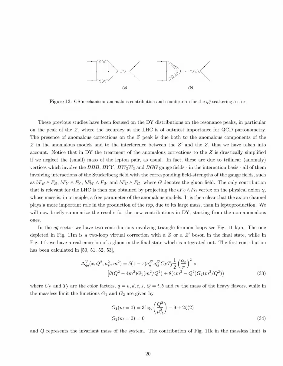
(a) (b)
Figure 13: GS mechanism: anomalous contribution and counterterm for the qq scattering sector.
These previous studies have been focused on the DY distributions on the resonance peaks, in particular
on the peak of the Z, where the accuracy at the LHC is of outmost importance for QCD partonometry.
The presence of anomalous corrections on the Z peak is due both to the anomalous components of the
Z in the anomalous models and to the interference between the Z ′ and the Z, that we have taken into
account. Notice that in DY the treatment of the anomalous corrections to the Z is drastically simplified
if we neglect the (small) mass of the lepton pair, as usual. In fact, these are due to trilinear (anomaly)
vertices which involve the BBB, BY Y , BW3W3 and BGG gauge fields - in the interaction basis - all of them
involving interactions of the Stuckelberg field with the corresponding field-strengths of the gauge fields, such
as bFB ∧ FB , bFY ∧ FY , bFW ∧ FW and bFG ∧ FG, where G denotes the gluon field. The only contribution
that is relevant for the LHC is then one obtained by projecting the bFG∧FG vertex on the physical axion χ,
whose mass is, in principle, a free parameter of the anomalous models. It is then clear that the axion channel
plays a more important role in the production of the top, due to its large mass, than in leptoproduction. We
will now briefly summarize the results for the new contributions in DY, starting from the non-anomalous
ones.
In the qq sector we have two contributions involving triangle fermion loops see Fig. 11 k,m. The one
depicted in Fig. 11m is a two-loop virtual correction with a Z or a Z ′ boson in the final state, while in
Fig. 11k we have a real emission of a gluon in the final state which is integrated out. The first contribution
has been calculated in [50, 51, 52, 53],
∆Vqq(x,Q
2, µ2F ,m
2) = δ(1 − x)aZ′
q aZ′
Q CFTf1
2
(αsπ
)2×
[
θ(Q2 − 4m2)G1(m2/Q2) + θ(4m2 −Q2)G2(m
2/Q2))
(33)
where CF and Tf are the color factors, q = u, d, c, s, Q = t, b and m the mass of the heavy flavors, while in
the massless limit the functions G1 and G2 are given by
G1(m = 0) = 3 log
(
Q2
µ2R
)
− 9 + 2ζ(2)
G2(m = 0) = 0 (34)
and Q represents the invariant mass of the system. The contribution of Fig. 11k in the massless limit is
20
given by
∆Rqq(x,Q
2, µ2F ,m = 0) = aZ
′
q aZ′
Q CFTf1
2
(αsπ
)2×{
(1 + x)
(1 − x)+[−2 + 2x(1 − log(x))]
}
, (35)
while in the qg sector we have the contribution shown in Fig. 11l which is given by
∆qg(x,Q2, µ2
F ,m2) = aZ
′
q aZ′
Q T2f
1
2
(αsπ
)2×[
θ(Q2 − 4m2)H1(x,Q2,m2) + θ(4m2 −Q2)H2(x,Q
2,m2)]
(36)
with the massless limit of H1(x,Q2,m2) given by
H1(x,Q2,m = 0) = 2x
[
log
(
1
x
)
log
(
1
x− 1
)
+ Li2
(
1 − 1
x
)]
+ 2
(
1 − 1
x
)[
1 − 2x log
(
1
x
)]
. (37)
Separating the anomaly-free from the anomalous contributions, the factorization formula for the invariant
mass distribution in DY is given by
dσ
dQ2= τσZ(Q2,M2
Z){
WZ(τ,Q2) +W anomZ (τ,Q2)
}
W anomZ (τ,Q2) =
∑
i,j
∫ 1
τ
dx
xΦij(x, µ
2R, µ
2F )∆anom
ij (τ
x,Q2, µ2
F )
∆anomij (x,Q2, µ2
F ) = ∆Vqq(x,Q
2, µ2F ,m = 0) + ∆R
qq(x,Q2, µ2
F ,m = 0) + ∆qg(x,Q2, µ2
F ,m = 0)
(38)
that we will be using in our numerical analysis below.
4.2 Di-lepton production: numerical results
We have used the MRST-2001 set of Pdf’s given in [54] and [55]. We start by showing in Fig. 14 various
zooms of the differential cross section on the peak of the Z - for all the models - both at NLO and at NNLO.
We have kept the factorization and renormalization scales coincident and equal to Q, while the mass of
the extra Z ′ has been chosen around 1 TeV. The anomaly-free models, from the SM to the three abelian
extensions that we have considered (free fermionic [40] and U(1)B−L [39] in Fig. 14, while U(1)q+u appears
in Tab. (7) ) show that the cross section is more enhanced for the MLSOM, illustrated in Fig. 14a,c. The
plots show a sizeable difference (at a 3.5 % level) between the anomalous and all the remaining anomaly-free
models. A comparison between (a) and (c) indicates, however, that this difference has to be attributed to
the specific charge assignment of the anomalous model and not to the anomalous partonic sector, which is
present in (c) but not in (a). The anomalous corrections in DY appear at NNLO and not at NLO, while in
both figures the difference between the SM and the MLSOM remains almost unchanged.
Moving from NLO to NNLO the cross section is reduced. Defining the K-factor
σNNLO − σNLOσNLO
≡ KNLO (39)
21

495
500
505
510
515
520
525
91.1 91.15 91.2 91.25 91.3
dσ/d
Q [
pb/G
eV]
Q [GeV]
SM NLOMLSOM NLO gB = 1
(a) SM vs MLSOM at NLO
498.5
499
499.5
500
500.5
501
501.5
502
502.5
503
91.1 91.15 91.2 91.25 91.3
dσ/d
Q [
pb/G
eV]
Q [GeV]
SM NLOFree Ferm., NLO
U(1)B-L
(b) SM vs Anomaly free models at NLO
475
480
485
490
495
500
91.1 91.15 91.2 91.25 91.3
dσ/d
Q [
pb/G
eV]
Q [GeV]
SM NNLOMLSOM NNLO gB = 1
(c) SM vs MLSOM at NNLO
476.5
477
477.5
478
478.5
479
479.5
480
480.5
91.1 91.15 91.2 91.25 91.3
dσ/d
Q [
pb/G
eV]
Q [GeV]
SM NNLOFree Ferm., NNLO
U(1)B-L
(d) SM vs Anomaly free models at NNLO
Figure 14: Zoom on the Z resonance for anomalous Drell-Yan in the µF = µR = Q at NLO/NNLO for all the models.
in the case of the MLSOM this factor indicates a reduction of about 4% on the peak and can be attributed
to the NNLO terms in the DGLAP evolution, rather than to the NNLO corrections to the hard scatterings.
This point can be explored numerically by the (order) variation [56, 48]
∆σ ∼ ∆σ ⊗ φ+ σ ⊗ ∆φ
∆σ ≡ |σNNLO − σNLO| (40)
which measures the “error” change in the hadronic cross section σ going from NLO to NNLO (∆σ) in terms
of the analogous changes in the hard scatterings (∆σ) and parton luminosities ∆φ). The dominance of the
first or the second term on the rhs of Eq. (39) is an indication of the dominance of the hard scatterings or of
the evolution in moving from lower to higher order. The same differences emerge also from Tab. (5) and (6).
22
dσnlo/dQ [pb/GeV] for the MLSOM with M1 = 1 TeV, tan β = 40, Candia evol.
Q [GeV] gB = 0.1 gB = 0.36 gB = 0.65 gB = 1 σSMnlo (Q)
90.50 3.8551 · 10+2 3.8711 · 10+2 3.9106 · 10+2 3.9902 · 10+2 3.8543 · 10+2
90.54 3.9712 · 10+2 3.9877 · 10+2 4.0284 · 10+2 4.1105 · 10+2 3.9704 · 10+2
90.59 4.0861 · 10+2 4.1030 · 10+2 4.1449 · 10+2 4.2294 · 10+2 4.0852 · 10+2
90.63 4.1988 · 10+2 4.2162 · 10+2 4.2592 · 10+2 4.3461 · 10+2 4.1979 · 10+2
90.68 4.3084 · 10+2 4.3263 · 10+2 4.3705 · 10+2 4.4596 · 10+2 4.3075 · 10+2
90.99 4.9041 · 10+2 4.9245 · 10+2 4.9749 · 10+2 5.0766 · 10+2 4.9031 · 10+2
91.187 5.0254 · 10+2 5.0463 · 10+2 5.0981 · 10+2 5.2024 · 10+2 5.0243 · 10+2
91.25 5.0143 · 10+2 5.0352 · 10+2 5.0869 · 10+2 5.1911 · 10+2 5.0133 · 10+2
91.56 4.6103 · 10+2 4.6296 · 10+2 4.6772 · 10+2 4.7732 · 10+2 4.6094 · 10+2
91.77 4.1178 · 10+2 4.1350 · 10+2 4.1776 · 10+2 4.2635 · 10+2 4.1170 · 10+2
92.0 3.5297 · 10+2 3.5444 · 10+2 3.5810 · 10+2 3.6547 · 10+2 3.5289 · 10+2
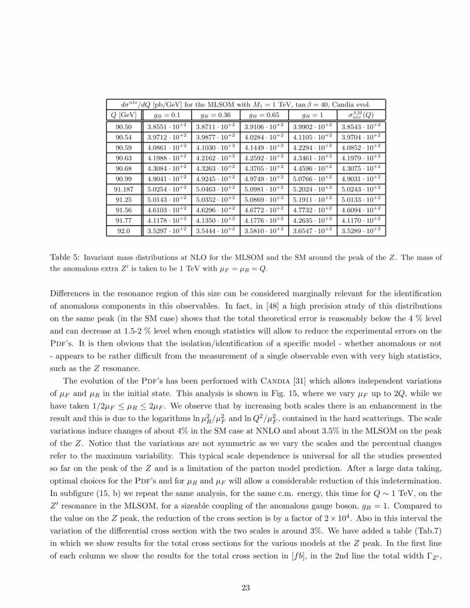
Table 5: Invariant mass distributions at NLO for the MLSOM and the SM around the peak of the Z. The mass of
the anomalous extra Z ′ is taken to be 1 TeV with µF = µR = Q.
Differences in the resonance region of this size can be considered marginally relevant for the identification
of anomalous components in this observables. In fact, in [48] a high precision study of this distributions
on the same peak (in the SM case) shows that the total theoretical error is reasonably below the 4 % level
and can decrease at 1.5-2 % level when enough statistics will allow to reduce the experimental errors on the
Pdf’s. It is then obvious that the isolation/identification of a specific model - whether anomalous or not
- appears to be rather difficult from the measurement of a single observable even with very high statistics,
such as the Z resonance.
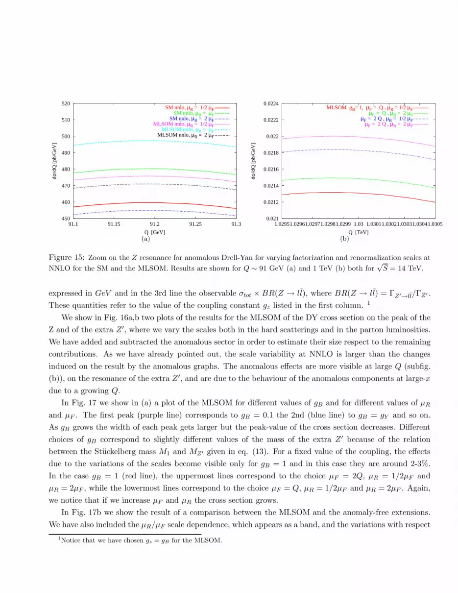
The evolution of the Pdf’s has been performed with Candia [31] which allows independent variations
of µF and µR in the initial state. This analysis is shown in Fig. 15, where we vary µF up to 2Q, while we
have taken 1/2µF ≤ µR ≤ 2µF . We observe that by increasing both scales there is an enhancement in the
result and this is due to the logarithms lnµ2R/µ
2F and lnQ2/µ2
F , contained in the hard scatterings. The scale
variations induce changes of about 4% in the SM case at NNLO and about 3.5% in the MLSOM on the peak
of the Z. Notice that the variations are not symmetric as we vary the scales and the percentual changes
refer to the maximum variability. This typical scale dependence is universal for all the studies presented
so far on the peak of the Z and is a limitation of the parton model prediction. After a large data taking,
optimal choices for the Pdf’s and for µR and µF will allow a considerable reduction of this indetermination.
In subfigure (15, b) we repeat the same analysis, for the same c.m. energy, this time for Q ∼ 1 TeV, on the
Z ′ resonance in the MLSOM, for a sizeable coupling of the anomalous gauge boson, gB = 1. Compared to
the value on the Z peak, the reduction of the cross section is by a factor of 2× 10⁴. Also in this interval the
variation of the differential cross section with the two scales is around 3%. We have added a table (Tab.7)
in which we show results for the total cross sections for the various models at the Z peak. In the first line
of each column we show the results for the total cross section in [fb], in the 2nd line the total width ΓZ′ ,
23

dσnnlo/dQ [pb/GeV] for the MLSOM with M1 = 1 TeV, tan β = 40, Candia evol.
Q [GeV] gB = 0.1 gB = 0.36 gB = 0.65 gB = 1 σSMnnlo(Q)
90.50 3.6845 · 10+2 3.6997 · 10+2 3.7374 · 10+2 3.8132 · 10+2 3.6835 · 10+2
90.54 3.7956 · 10+2 3.8112 · 10+2 3.8500 · 10+2 3.9282 · 10+2 3.7945 · 10+2
90.59 3.9054 · 10+2 3.9215 · 10+2 3.9615 · 10+2 4.0419 · 10+2 3.9043 · 10+2
90.63 4.0132 · 10+2 4.0298 · 10+2 4.0708 · 10+2 4.1535 · 10+2 4.0121 · 10+2
90.68 4.1180 · 10+2 4.1351 · 10+2 4.1772 · 10+2 4.2621 · 10+2 4.1169 · 10+2
90.99 4.6879 · 10+2 4.7073 · 10+2 4.7554 · 10+2 4.8523 · 10+2 4.6866 · 10+2
91.187 4.8040 · 10+2 4.8239 · 10+2 4.8733 · 10+2 4.9727 · 10+2 4.8027 · 10+2
91.25 4.7935 · 10+2 4.8134 · 10+2 4.8627 · 10+2 4.9619 · 10+2 4.7922 · 10+2
91.56 4.4076 · 10+2 4.4259 · 10+2 4.4713 · 10+2 4.5628 · 10+2 4.4064 · 10+2
91.77 3.9371 · 10+2 3.9535 · 10+2 3.9941 · 10+2 4.0759 · 10+2 3.9360 · 10+2
92.0 3.3750 · 10+2 3.3891 · 10+2 3.4239 · 10+2 3.4942 · 10+2 3.3741 · 10+2
Table 6: Invariant mass distributions at NNLO for the MLSOM and the SM around the peak of the Z. The mass of
the anomalous extra Z ′ is taken to be 1 TeV with µF = µR = Q.
σnnlotot [fb],
√
S = 14 TeV, M1 = 1 TeV, tanβ = 40
gz MLSOM U(1)B−L U(1)q+u FreeFerm.
0.1 5.982 3.575 2.701 1.274
0.173 0.133 0.177 0.122
0.277 0.445 0.252 0.017
0.36 106.674 105.567 53.410 42.872
2.248 1.733 2.308 1.583
4.937 13.138 4.991 0.586
0.65 240.484 143.455 108.344 51.155
7.396 5.700 7.592 5.205
11.127 17.853 10.124 0.699
1 532.719 317.328 239.401 113.453
17.810 13.720 18.274 12.530
24.639 39.491 22.370 1.550
Table 7: Total cross sections, widths and σtot ×BR(Z → ll), where BR(Z → ll) = ΓZ′→ll/ΓZ′ , for the MLSOM and
three anomaly-free extensions of the SM; they are all shown as functions of the coupling constant.
24
450
460
470
480
490
500
510
520
91.1 91.15 91.2 91.25 91.3
dσ/d
Q [
pb/G
eV]
Q [GeV]
SM nnlo, µR = 1/2 µFSM nnlo, µR = µF
SM nnlo, µR = 2 µFMLSOM nnlo, µR = 1/2 µF
MLSOM nnlo, µR = µFMLSOM nnlo, µR = 2 µF
(a)
0.021
0.0212
0.0214
0.0216
0.0218
0.022
0.0222
0.0224
1.02951.02961.02971.02981.0299 1.03 1.03011.03021.03031.03041.0305
dσ/d
Q [
pb/G
eV]
Q [TeV]
MLSOM gB = 1, µF = Q , µR = 1/2 µFµF = Q , µR = 2 µF
µF = 2 Q , µR = 1/2 µFµF = 2 Q , µR = 2 µF
(b)
Figure 15: Zoom on the Z resonance for anomalous Drell-Yan for varying factorization and renormalization scales at
NNLO for the SM and the MLSOM. Results are shown for Q ∼ 91 GeV (a) and 1 TeV (b) both for√S = 14 TeV.
expressed in GeV and in the 3rd line the observable σtot × BR(Z → ll), where BR(Z → ll) = ΓZ′→ll/ΓZ′ .
These quantities refer to the value of the coupling constant gz listed in the first column. 1
We show in Fig. 16a,b two plots of the results for the MLSOM of the DY cross section on the peak of the
Z and of the extra Z ′, where we vary the scales both in the hard scatterings and in the parton luminosities.
We have added and subtracted the anomalous sector in order to estimate their size respect to the remaining
contributions. As we have already pointed out, the scale variability at NNLO is larger than the changes
induced on the result by the anomalous graphs. The anomalous effects are more visible at large Q (subfig.
(b)), on the resonance of the extra Z ′, and are due to the behaviour of the anomalous components at large-x
due to a growing Q.
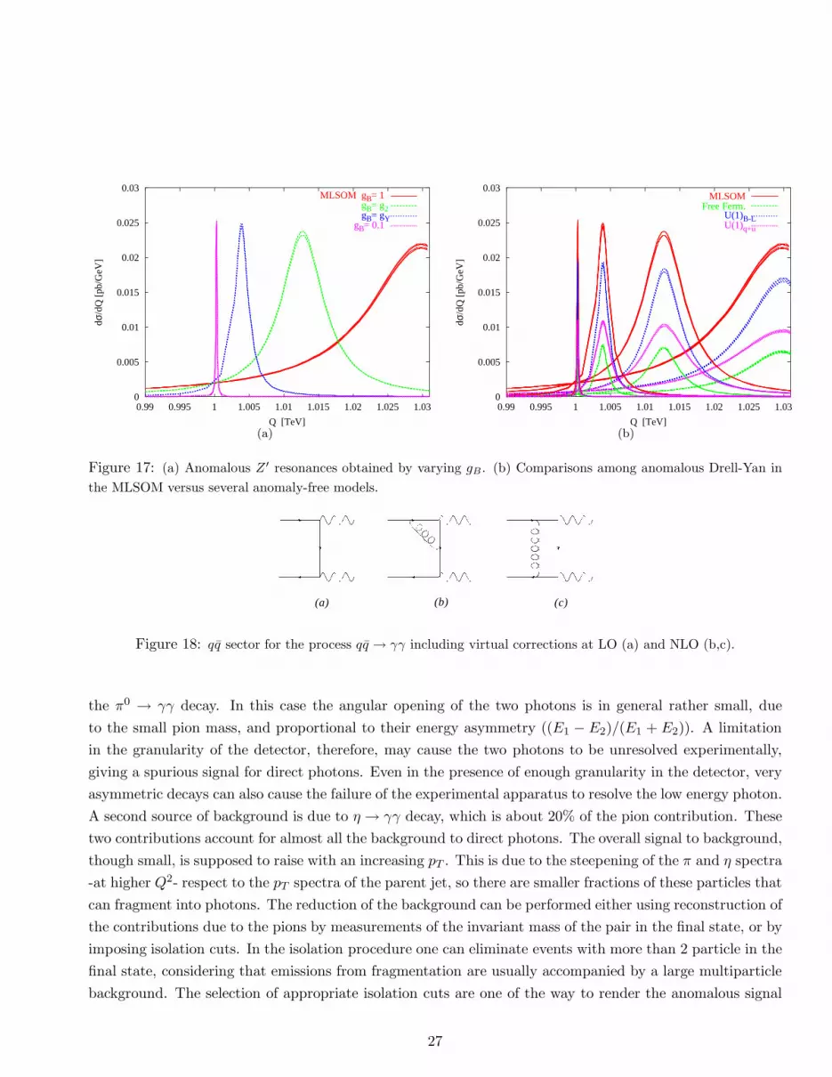
In Fig. 17 we show in (a) a plot of the MLSOM for different values of gB and for different values of µR
and µF . The first peak (purple line) corresponds to gB = 0.1 the 2nd (blue line) to gB = gY and so on.
As gB grows the width of each peak gets larger but the peak-value of the cross section decreases. Different
choices of gB correspond to slightly different values of the mass of the extra Z ′ because of the relation
between the Stuckelberg mass M1 and MZ′ given in eq. (13). For a fixed value of the coupling, the effects
due to the variations of the scales become visible only for gB = 1 and in this case they are around 2-3%.
In the case gB = 1 (red line), the uppermost lines correspond to the choice µF = 2Q, µR = 1/2µF and
µR = 2µF , while the lowermost lines correspond to the choice µF = Q, µR = 1/2µF and µR = 2µF . Again,
we notice that if we increase µF and µR the cross section grows.
In Fig. 17b we show the result of a comparison between the MLSOM and the anomaly-free extensions.
We have also included the µR/µF scale dependence, which appears as a band, and the variations with respect
1Notice that we have chosen gz = gB for the MLSOM.

460
470
480
490
500
510
520
91 91.05 91.1 91.15 91.2 91.25 91.3 91.35 91.4
dσ/d
Q [
pb/G
eV]
Q [GeV]
MLSOM NNLO gB = 1 with anom.triang. Q = µF = µR Q = µF = 2 µR
Q = µF = 1/2 µR Q = µF = 2 µR , Φ(µR /µF )
Q = µF = 1/2 µR , Φ(µR /µF )with no anom.triang.
(a)
0.02
0.0205
0.021
0.0215
0.022
0.0225
1.027 1.0275 1.028 1.0285 1.029 1.0295 1.03
dσ/d
Q [
pb/G
eV]
Q [TeV]
MLSOM NNLO gB = 1 with anom.triang. Q = µF = µR Q = µF = 2 µR
Q = µF = 1/2 µR Q = µF = 2 µR , Φ(µR /µF )
Q = µF = 1/2 µR , Φ(µR /µF )with no anom.triang.
(b)
Figure 16: Plot of the DY invariant mass distributions on the peak of the Z (a) and of the Z ′ (b). Shown are the
total contributions of the MLSOM and those in which the anomalous terms have been removed. The variation of the
result on µF and µR is included both in the hard scatterings and in the luminosities (Φ(µF /µR)).
to gB . As shown in this figure, the red lines correspond to the MLSOM, the blue lines to the U(1)B−L model,
the green lines to the free fermionic model and the purple lines to U(1)q+u. Right as before, the first peak
corresponds to gB = 0.1, the 2nd to gB = gY etc. The peak-value of the anomalous model is the largest of
all, with a cross section which is around 0.022 [pb/GeV], the free fermionic appears to be the smallest with
a value around 0.006 [pb/GeV].
5 Direct Photons with GS and WZ interactions
The analysis of pp→ γγ proceeds similarly to the DY case, with a numerical investigation of the background
and of the anomalous signal at parton level.
We start classifying the strong/weak interference effects that control the various sectors of the process
and then identify the leading contributions due to the presence of anomaly diagrams.
Direct photons are one of the possible channels to detect anomalous gauge interactions, although, as we
are going to see, also in this case the anomalous signal remains rather small. Direct photons are produced by
partonic interactions rather than as a result of the electromagnetic decay of hadronic states. At leading order
(LO) they carry the transverse momentum of the hard scatterers, offering a direct probe of the underlying
quark-gluon dynamics. The two main channels in pp collisions are the annihilation qq and Compton (q g),
the second one being roughly 80% of the entire signal at large pT (from pT = 4 GeV on). The annihilation
channel is subleading, due to the small antiquark densities in the proton. The cross section is also strongly
suppressed (by a factor of approximately 10−3) compared to the jet cross section. For this reason the
electromagnetic decay of the produced hadrons is a significant source of background, coming mostly from
26
0
0.005
0.01
0.015
0.02
0.025
0.03
0.99 0.995 1 1.005 1.01 1.015 1.02 1.025 1.03
dσ/d
Q [
pb/G
eV]
Q [TeV]
MLSOM gB = 1gB = g2gB = gY
gB = 0.1
(a)
0
0.005
0.01
0.015
0.02
0.025
0.03
0.99 0.995 1 1.005 1.01 1.015 1.02 1.025 1.03
dσ/d
Q [
pb/G
eV]
Q [TeV]
MLSOMFree Ferm.
U(1)B-L U(1)q+u
(b)
Figure 17: (a) Anomalous Z ′ resonances obtained by varying gB. (b) Comparisons among anomalous Drell-Yan in
the MLSOM versus several anomaly-free models.
(b)(a) (c)
Figure 18: qq sector for the process qq → γγ including virtual corrections at LO (a) and NLO (b,c).
the π0 → γγ decay. In this case the angular opening of the two photons is in general rather small, due
to the small pion mass, and proportional to their energy asymmetry ((E1 − E2)/(E1 + E2)). A limitation
in the granularity of the detector, therefore, may cause the two photons to be unresolved experimentally,
giving a spurious signal for direct photons. Even in the presence of enough granularity in the detector, very
asymmetric decays can also cause the failure of the experimental apparatus to resolve the low energy photon.
A second source of background is due to η → γγ decay, which is about 20% of the pion contribution. These
two contributions account for almost all the background to direct photons. The overall signal to background,
though small, is supposed to raise with an increasing pT . This is due to the steepening of the π and η spectra
-at higher Q2- respect to the pT spectra of the parent jet, so there are smaller fractions of these particles that
can fragment into photons. The reduction of the background can be performed either using reconstruction of
the contributions due to the pions by measurements of the invariant mass of the pair in the final state, or by
imposing isolation cuts. In the isolation procedure one can eliminate events with more than 2 particle in the
final state, considering that emissions from fragmentation are usually accompanied by a large multiparticle
background. The selection of appropriate isolation cuts are one of the way to render the anomalous signal
27

(e) (f) (g)
Figure 19: Real emissions for qq → γγ at NLO.
(g) (i)(h)
Figure 20: qg sector for the process qg → γγ.
more significant, considering that the tagged photon signal, although being of higher order in αs (NNLO in
QCD), is characterized by a two-photon-only final state. As we are going to see this signal is non-resonant,
even in the presence of an s-channel exchange, due to the anomaly.
We show in Fig. 18 a partial list of the various background contributions to the DP channel in pp
collisions. We show the leading order (LO) contribution in diagram (a) with some of the typical virtual
corrections included in (b) and (c). These involve the qq sector giving a cross section of the form
σqq = α2em(c1 + c2αs). (41)
These corrections are the NLO ones in this channel. The infrared safety of the process is guaranteed at the
same perturbative order by the real emissions in Fig. 19 with an integrated gluon in the final state, which
are also of O(α2emαs).
A second sector is the qg one, which is shown in Fig. 20, also of the same order (O(αsαem)). These
corrections are diagrammatically the NLO ones. In general, the NLO prediction for this process are improved
by adding a part of the NNLO (or O(α2emα
2s)) contributions, such as the box contribution (j) of the gg sector
which is of higher order (O(α2emα
2s)) in αs, the reason being that these contributions have been shown to
be sizeable and comparable with the genuine NLO ones. All these corrections have been computed long ago
[34] and implemented independently in a complete Monte Carlo in [32, 57] with a more general inclusion of
the fragmentation. More recently, other NNLO contributions have been added to the process, such as those
involving the gg sector through O(α2emα
3s),
σgg = α2em(d1α
2s + d2α
3s), (42)
28
(j) (k) (l) (m)
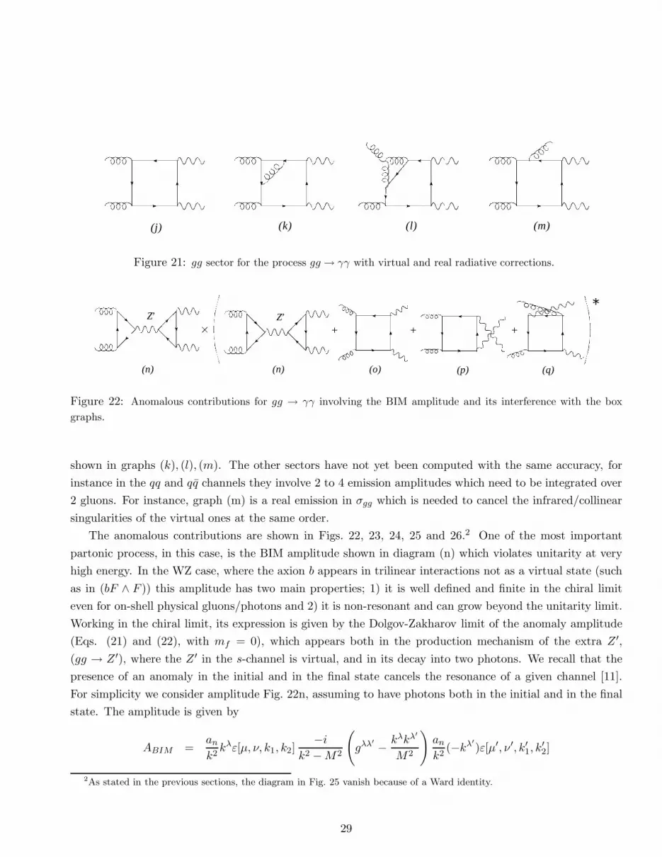
Figure 21: gg sector for the process gg → γγ with virtual and real radiative corrections.
+ + +
(q)(p)(o)(n)
Z’
(n)
Z’
Figure 22: Anomalous contributions for gg → γγ involving the BIM amplitude and its interference with the box
graphs.
shown in graphs (k), (l), (m). The other sectors have not yet been computed with the same accuracy, for
instance in the qq and qq channels they involve 2 to 4 emission amplitudes which need to be integrated over
2 gluons. For instance, graph (m) is a real emission in σgg which is needed to cancel the infrared/collinear
singularities of the virtual ones at the same order.
The anomalous contributions are shown in Figs. 22, 23, 24, 25 and 26.2 One of the most important
partonic process, in this case, is the BIM amplitude shown in diagram (n) which violates unitarity at very
high energy. In the WZ case, where the axion b appears in trilinear interactions not as a virtual state (such
as in (bF ∧ F )) this amplitude has two main properties; 1) it is well defined and finite in the chiral limit
even for on-shell physical gluons/photons and 2) it is non-resonant and can grow beyond the unitarity limit.
Working in the chiral limit, its expression is given by the Dolgov-Zakharov limit of the anomaly amplitude
(Eqs. (21) and (22), with mf = 0), which appears both in the production mechanism of the extra Z ′,
(gg → Z ′), where the Z ′ in the s-channel is virtual, and in its decay into two photons. We recall that the
presence of an anomaly in the initial and in the final state cancels the resonance of a given channel [11].
For simplicity we consider amplitude Fig. 22n, assuming to have photons both in the initial and in the final
state. The amplitude is given by
ABIM =ank2kλε[µ, ν, k1, k2]
−ik2 −M2
(
gλλ′ − kλkλ
′
M2
)
ank2
(−kλ′)ε[µ′, ν ′, k′1, k′2]
2As stated in the previous sections, the diagram in Fig. 25 vanish because of a Ward identity.
29

+ ...
Z’
(r)(h)
Figure 23: Total amplitude for qg → γγ.
+ ...
(h)
Z’
(t)
Figure 24: Another configuration for the total amplitude of the qg → γγ process.
=ank2ε[µ, ν, k1, k2]
−ik2 −M2
kλ′
(M2 − k2)
M2
ank2
(−kλ′)ε[µ′, ν ′, k′1, k′2]
=ank2ε[µ, ν, k1, k2]
(−ik2
M2
)
ank2ε[µ′, ν ′, k′1, k
′
2]
= −anMε[µ, ν, k1, k2]
i
k2
anMε[µ′, ν ′, k′1, k
′
2]. (43)
where M denotes, generically, the mass of the anomalous gauge boson in the s-channel. If we multiply this
amplitude by the external polarizators of the photons, square it and perform the usual averages, one finds
that it grows quadratically with energy. The additional contributions in the s-channel that accompany this
amplitude are shown in Fig. 27. The exchange of a massive axion (Fig. 27b), due to a mismatch between
the coupling and the parameteric dependence between Fig. 27a and b, does not erase the growth (see the
discussion in the appendix). This mismatch is at the origin of the unitarity bound for this theory analyzed
in [11]. The identification of this scale in the context of QCD is quite subtle, since the lack of unitarity in
a partonic process implies a violation of unitarity also at hadron level, but at a different scale compared to
the partonic one, which needs to be determined numerically directly from the total hadronic cross section
σpp. Overall, the convolution of a BIM amplitude with the parton distributions will cause a suppression of
the rising partonic contributions, due to the small gluon density at large Bjorken x. Therefore, the graphs
do not generate a large anomalous signal in this channel. However, the problem of unitarizing the theory
30
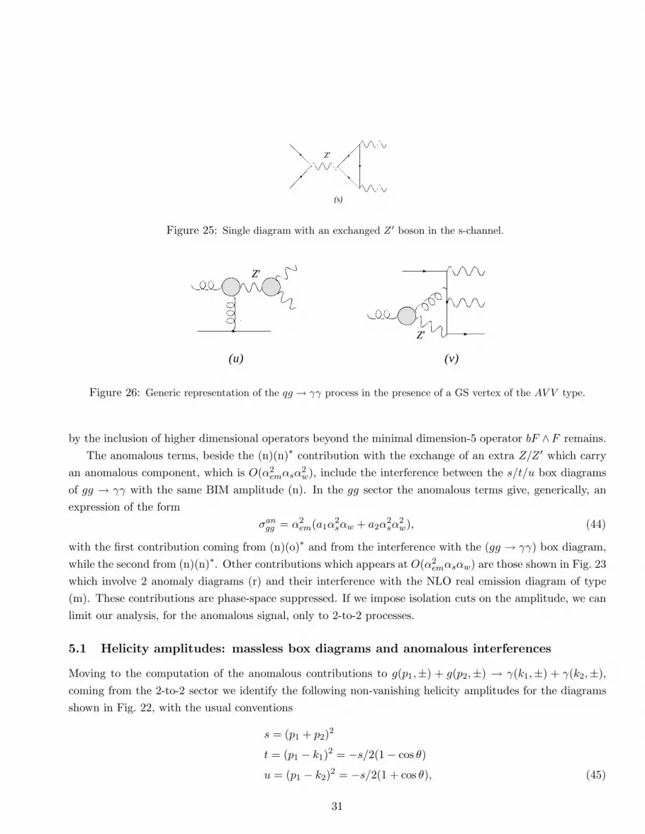
Z’
(s)
Figure 25: Single diagram with an exchanged Z ′ boson in the s-channel.
(u) (v)
Z’
Z’
Figure 26: Generic representation of the qg → γγ process in the presence of a GS vertex of the AV V type.
by the inclusion of higher dimensional operators beyond the minimal dimension-5 operator bF ∧F remains.
The anomalous terms, beside the (n)(n)∗ contribution with the exchange of an extra Z/Z ′ which carry
an anomalous component, which is O(α2emαsα
2w), include the interference between the s/t/u box diagrams
of gg → γγ with the same BIM amplitude (n). In the gg sector the anomalous terms give, generically, an
expression of the form
σangg = α2em(a1α
2sαw + a2α
2sα
2w), (44)
with the first contribution coming from (n)(o)∗ and from the interference with the (gg → γγ) box diagram,
while the second from (n)(n)∗. Other contributions which appears at O(α2emαsαw) are those shown in Fig. 23
which involve 2 anomaly diagrams (r) and their interference with the NLO real emission diagram of type
(m). These contributions are phase-space suppressed. If we impose isolation cuts on the amplitude, we can
limit our analysis, for the anomalous signal, only to 2-to-2 processes.
5.1 Helicity amplitudes: massless box diagrams and anomalous interferences
Moving to the computation of the anomalous contributions to g(p1,±) + g(p2,±) → γ(k1,±) + γ(k2,±),
coming from the 2-to-2 sector we identify the following non-vanishing helicity amplitudes for the diagrams
shown in Fig. 22, with the usual conventions
s = (p1 + p2)2
t = (p1 − k1)2 = −s/2(1 − cos θ)
u = (p1 − k2)2 = −s/2(1 + cos θ), (45)
31
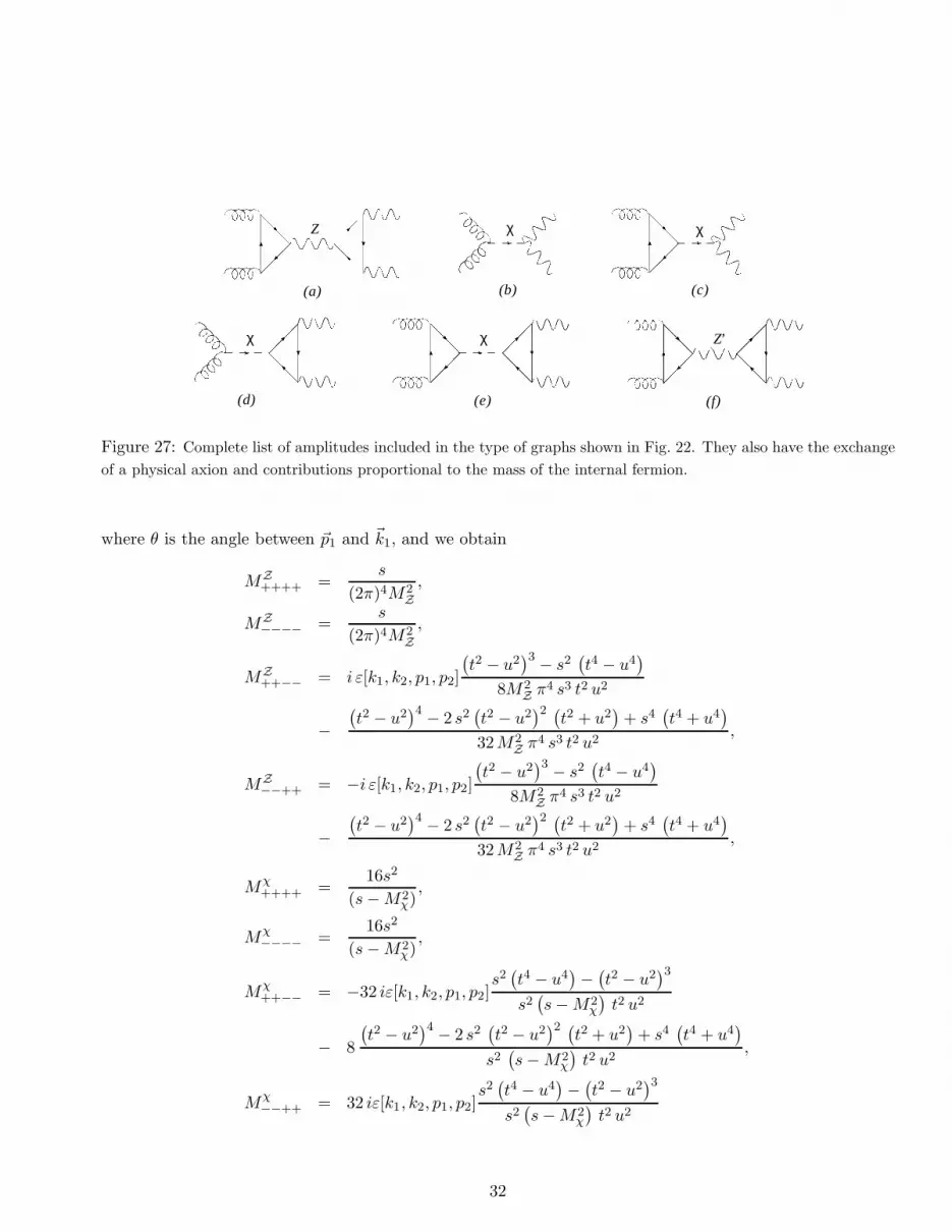
χ
(d)
χ
(e)
χ
(c)
χ
(b)
Z
(a)
Z’
(f)
Figure 27: Complete list of amplitudes included in the type of graphs shown in Fig. 22. They also have the exchange
of a physical axion and contributions proportional to the mass of the internal fermion.
where θ is the angle between ~p1 and ~k1, and we obtain
MZ
++++ =s
(2π)4M2Z
,
MZ
−−−− =s
(2π)4M2Z
,
MZ
++−− = i ε[k1, k2, p1, p2]
(
t2 − u2)3 − s2
(
t4 − u4)
8M2Zπ4 s3 t2 u2
−(
t2 − u2)4 − 2 s2
(
t2 − u2)2 (
t2 + u2)
+ s4(
t4 + u4)
32M2Zπ4 s3 t2 u2
,
MZ
−−++ = −i ε[k1, k2, p1, p2]
(
t2 − u2)3 − s2
(
t4 − u4)
8M2Zπ4 s3 t2 u2
−(
t2 − u2)4 − 2 s2
(
t2 − u2)2 (
t2 + u2)
+ s4(
t4 + u4)
32M2Zπ4 s3 t2 u2
,
Mχ++++ =
16s2
(s−M2χ),
Mχ−−−− =
16s2
(s−M2χ),
Mχ++−− = −32 iε[k1, k2, p1, p2]
s2(
t4 − u4)
−(
t2 − u2)3
s2(
s−M2χ
)
t2 u2
− 8
(
t2 − u2)4 − 2 s2
(
t2 − u2)2 (
t2 + u2)
+ s4(
t4 + u4)
s2(
s−M2χ
)
t2 u2,
Mχ−−++ = 32 iε[k1, k2, p1, p2]
s2(
t4 − u4)
−(
t2 − u2)3
s2(
s−M2χ
)
t2 u2
32
− 8
(
t2 − u2)4 − 2 s2
(
t2 − u2)2 (
t2 + u2)
+ s4(
t4 + u4)
s2(
s−M2χ
)
t2 u2, (46)
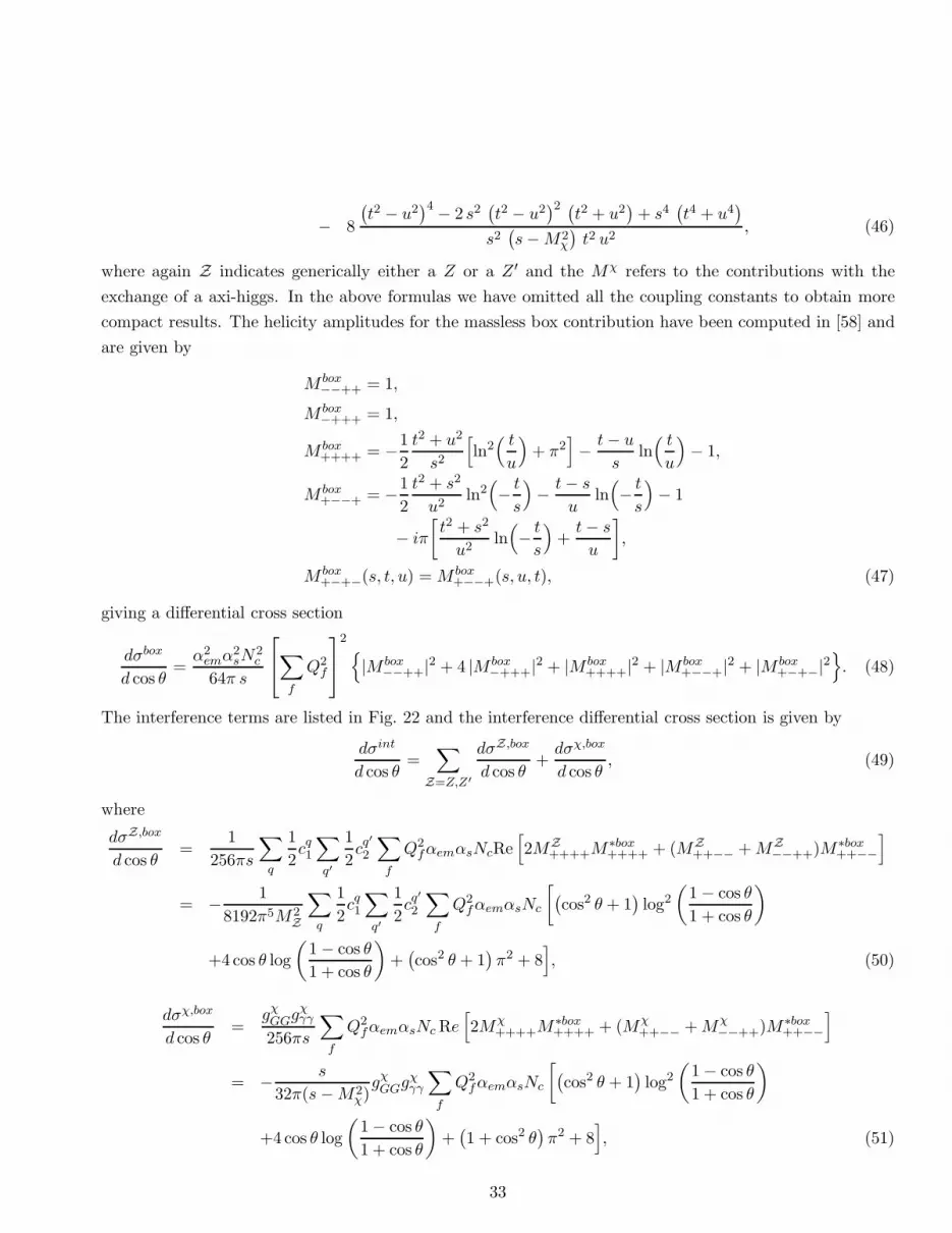
where again Z indicates generically either a Z or a Z ′ and the Mχ refers to the contributions with the
exchange of a axi-higgs. In the above formulas we have omitted all the coupling constants to obtain more
compact results. The helicity amplitudes for the massless box contribution have been computed in [58] and
are given by
M box−−++ = 1,
M box−+++ = 1,
M box++++ = −1
2
t2 + u2
s2
[
ln2( t
u
)
+ π2]
− t− u
sln( t
u
)
− 1,
M box+−−+ = −1
2
t2 + s2
u2ln2(
− t
s
)
− t− s
uln(
− t
s
)
− 1
− iπ
[
t2 + s2
u2ln(
− t
s
)
+t− s
u
]
,
M box+−+−(s, t, u) = M box
+−−+(s, u, t), (47)
giving a differential cross section
dσbox
d cos θ=α2emα
2sN
2c
64π s
∑
f
Q2f
2{
|M box−−++|2 + 4 |M box
−+++|2 + |M box++++|2 + |M box
+−−+|2 + |M box+−+−|2
}
. (48)
The interference terms are listed in Fig. 22 and the interference differential cross section is given by
dσint
d cos θ=
∑
Z=Z,Z′
dσZ,box
d cos θ+dσχ,box
d cos θ, (49)
where
dσZ,box
d cos θ=
1
256πs
∑
q
1
2cq1∑
q′
1
2cq
′
2
∑
f
Q2fαemαsNcRe
[
2MZ
++++M∗box++++ + (MZ
++−− +MZ
−−++)M∗box++−−
]
= − 1
8192π5M2Z
∑
q
1
2cq1∑
q′
1
2cq
′
2
∑
f
Q2fαemαsNc
[
(
cos2 θ + 1)
log2
(
1 − cos θ
1 + cos θ
)
+4cos θ log
(
1 − cos θ
1 + cos θ
)
+(
cos2 θ + 1)
π2 + 8]
, (50)
dσχ,box
d cos θ=
gχGGgχγγ
256πs
∑
f
Q2fαemαsNcRe
[
2Mχ++++M
∗box++++ + (Mχ
++−− +Mχ−−++)M∗box
++−−
]
= − s
32π(s −M2χ)gχGGg
χγγ
∑
f
Q2fαemαsNc
[
(
cos2 θ + 1)
log2
(
1 − cos θ
1 + cos θ
)
+4cos θ log
(
1 − cos θ
1 + cos θ
)
+(
1 + cos2 θ)
π2 + 8]
, (51)
33

Here M box++−− = M box
−−++ and we have introduced the parameters of the model, explicitly given in [11].
These correspond to the chiral asymmetries (DBY Y ) of the anomalous U(1)B in the BY Y mixed anomalous
diagram whose anomaly is an; rotation matrix elements from the interaction eigenstates to the physical basis
after electroweak symmetry breaking (OA); rotation matrix elements in the CP-odd sector (Oχ), the strong
coupling constant g3, the anomalous coupling constant gB and the axial-vector coupling of the neutral gauge
bosons (Z = Z,Z ′) to a quark flavour q (gZA,q). These parameters combine to define the coupling of the
physical axion to the various gauge fields (gχgg, gχγγ)
gZA,q =1
2(QR,q
Z−QL,q
Z),
gχgg =D
M1Oχ31,
gχγγ =
[
F
M1(OAWγ)
2 +CY YM1
(OAY γ)2
]
Oχ31 (52)
and
D = igBg23anD
(L)B , D
(L)B = −1
8
∑
f
QLB,f
F = igBg22
an2D
(L)B ,
CY Y = igBg2Y
an2DBY Y , DBY Y = −1
8
∑
f
[
QLB,f (QLY,f )
2 −QRB,f (QRY,f )
2]
.
(53)
More details can be found in [11, 19, 20, 37].
5.2 Numerical analysis for direct photons
In our numerical implementation of double prompt photon production we compare the size of the anomalous
corrections respect to the SM background evaluated by a Monte Carlo [32, 33]. Since the anomalous
signal is small compared to that of the SM, we have extracted both for the SM case and the anomalous
case the gg sector and compared them at hadron level by convoluting the partonic contributions with the
Pdf’s (see Fig. 28). In this comparison, the SM sector is given by the graphs shown in Fig. 21 plus the
interference graphs shown in Fig. 22. In the SM case this second set of graphs contributes proportionally
to the mass of the heavy quarks in the anomaly loop. At high energy the hard scatterings coming from
this interference are essentially due to the mass of the top quark running inside a BIM amplitude and are,
therefore, related to heavy quark effects. In the anomalous case the same set of graphs is considered, but
now the anomaly contributions are explicitly included. The hadronic differential cross section due to the
anomalous interactions for massless quarks is given by
dσ
dQ=
∫ 2π
0dφ
∫ 1
−1d cos θ
τ
4Q
∫ 1
τ
dx
xΦgg(
τ
x)∆(x, θ),
34

1
100
10000
1e+06
1e+08
1e+10
1e-05 0.0001 0.001 0.01 0.1
Glu
on L
umin
osity
τ
g ⊗ g(τ), Q ∈ [0.9,1] TeV, √S=14 TeV √S=10 TeV √S=8 TeV √S=5 TeV
Q ∈ [90,100] GeV, √S=14 TeV √S=10 TeV √S=8 TeV √S=5 TeV
Figure 28: The NNLO gluon luminosity as a function of τ = Q2/S for various value of the invariant mass of the
photon pair (Q) and energy of the hadronic beam (S) at the LHC evolved with Candia.
Φgg(y) =
∫ 1
y
dz
zg(y/z)g(z),
∆(x) = δ(1 − x)
[
dσZd cos θ
+dσZ′
d cos θ+
dσχd cos θ
+dσintd cos θ
]
dσintd cos θ
=dσZ,box
d cos θ+dσZ
′,box
d cos θ+dσχ,box
d cos θ. (54)
The contributions which are part of this sector due to exchange of a Z or a Z ′ and a χ (see (a), (b) and (f)
of the BIM set in Fig. 27) are those labelled above, while σint refers to the interferences shown in Fig. 22,
with the inclusion of a Z ′ and a physical axion (such as Fig. 27b).
Defining
σgg→γγ ≡∫ 2π
0dφ
∫
d cos θ ∆(x, θ) (55)
the hadronic cross section takes the form of a product of the gluon luminosity and the partonic gg → γγ
cross section
dσ
dQ=
Q
4Sσgg→γγΦ(τ). (56)
5.3 The gg sector
Coming to the analysis of the gluon fusion sector, the result of this study is shown in Fig. 29 where we
plot the gluon contribution to the hadronic cross section for both the SM and the MLSOM, having chosen
M1 = 1 TeV. We have used the MRST99 set of parton distributions to generate the NNLO gluon luminosity
35
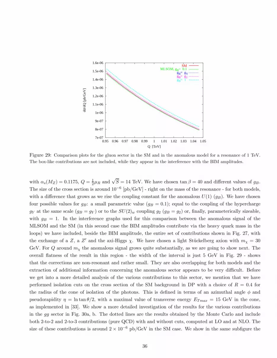
7e-07
8e-07
9e-07
1e-06
1.1e-06
1.2e-06
1.3e-06
1.4e-06
1.5e-06
1.6e-06
0.95 0.96 0.97 0.98 0.99 1 1.01 1.02 1.03 1.04 1.05
dσ/d
Q [
pb/G
eV]
Q [TeV]
SMMLSOM, gB = 0.1
gB = gY gB = g2 gB = 1
Figure 29: Comparison plots for the gluon sector in the SM and in the anomalous model for a resonance of 1 TeV.
The box-like contributions are not included, while they appear in the interference with the BIM amplitudes.
with αs(MZ) = 0.1175, Q = 12µR and
√S = 14 TeV. We have chosen tan β = 40 and different values of gB .
The size of the cross section is around 10−6 [pb/GeV] - right on the mass of the resonance - for both models,
with a difference that grows as we rise the coupling constant for the anomalous U(1) (gB). We have chosen
four possible values for gB : a small parametric value (gB = 0.1); equal to the coupling of the hypercharge
gY at the same scale (gB = gY ) or to the SU(2)w coupling g2 (gB = g2) or, finally, parameterically sizeable,
with gB = 1. In the interference graphs used for this comparison between the anomalous signal of the
MLSOM and the SM (in this second case the BIM amplitudes contribute via the heavy quark mass in the
loops) we have included, beside the BIM amplitude, the entire set of contributions shown in Fig. 27, with
the exchange of a Z, a Z ′ and the axi-Higgs χ. We have chosen a light Stuckelberg axion with mχ = 30
GeV. For Q around mχ the anomalous signal grows quite substantially, as we are going to show next. The
overall flatness of the result in this region - the width of the interval is just 5 GeV in Fig. 29 - shows
that the corrections are non-resonant and rather small. They are also overlapping for both models and the
extraction of additional information concerning the anomalous sector appears to be very difficult. Before
we get into a more detailed analysis of the various contributions to this sector, we mention that we have
performed isolation cuts on the cross section of the SM background in DP with a choice of R = 0.4 for
the radius of the cone of isolation of the photons. This is defined in terms of an azimuthal angle φ and
pseudorapidity η = ln tan θ/2, with a maximal value of transverse energy ETmax = 15 GeV in the cone,
as implemented in [33]. We show a more detailed investigation of the results for the various contributions
in the gg sector in Fig. 30a, b. The dotted lines are the results obtained by the Monte Carlo and include
both 2-to-2 and 2-to-3 contributions (pure QCD) with and without cuts, computed at LO and at NLO. The
size of these contributions is around 2 × 10⁻⁶ pb/GeV in the SM case. We show in the same subfigure the
36

1e-10
1e-09
1e-08
1e-07
1e-06
1e-05
0.0001
0.001
0.95 0.96 0.97 0.98 0.99 1 1.01 1.02 1.03 1.04 1.05
dσ/d
Q [
pb/G
eV]
Q [TeV]
SM gg LO no cutsSM gg LO standard cuts
SM gg NLO standard cutsSM gg NLO no cuts
MLSOM M1 = 1 TeV, gB = 0.1 gB = gY gB = g2 gB = 1
(a)
1e-10
1e-09
1e-08
1e-07
1e-06
1e-05
0.0001
0.001
0.01
0.95 0.96 0.97 0.98 0.99 1 1.01 1.02 1.03 1.04 1.05
dσ/d
Q [
pb/G
eV]
Q [TeV]
SM gg NLO standard cutsSM QQ NLO standard cuts
MLSOM M1 = 1 TeV, gB = 0.1 gB = gY gB = g2 gB = 1
(b)
Figure 30: (a): SM contributions for the gluon-gluon channel obtained with the Monte Carlo Gamma2MC. These
are indicated by dotted lines and include all the interferences and the box graphs. Shown are also the anomalous
contributions of the MLSOM (no box). (b): as in (a) but we have included the Monte Carlo results for the SM qq
channel at NLO.
anomalous corrections in the MLSOM, which vary between 10−9 and 10−7 pb/GeV. Therefore, for gB ∼ 1,
the anomalous sector of the MLSOM (the square of the box terms here are not included for the MSLOM) is
suppressed by a factor of 10 respect to the signal from the same sector coming from the SM. In subfig. (b)
we show the same contributions but we include in the SM also the quark channel (shown separately from
the gluon channel), which is around 10−4 pb/GeV. Therefore, the quark sector overshadows the anomalous
corrections by a factor of approximately 103, which are difficult to extract at this value of the invariant
mass.
A comparison between the differential cross section obtained by the Monte Carlo and the anomalous
contributions is shown in Fig. 31a, from which one can see that the anomalous components are down by a
factor of 103 − 107 respect to the background, depending on the value of the anomalous coupling gB .
A similar comparison between anomalous signal and background for a 1 TeV extra gauge boson but at
larger invariant mass (2 TeV) of the di-photon is shown in Fig. 31b. In both cases the ratio between the size
of the anomalous signal and the background is 10−3, showing the large suppression as in the other regions.
• Anatomy of the gluon sector
We show in Fig. 32a and b) two plots that illustrate the size of the various contributions to the gg sector
in the SM and in the anomalous model. We have separated these contributions into several components in
the MLSOM and SM cases.
In the anomalous model we have “pure BIM-like” amplitudes:
1) the square of the “BIM set” shown in Fig. 27, which contains the s-channel exchanges of the Z, of
the Z ′ and of the χ. In Figs. 32a and b these contributions are indicated as “BIM + χ”.
37
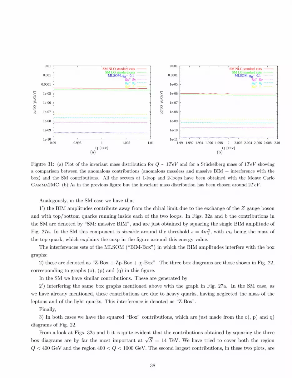
1e-10
1e-09
1e-08
1e-07
1e-06
1e-05
0.0001
0.001
0.01
0.99 0.995 1 1.005 1.01
dσ/d
Q [
pb/G
eV]
Q [TeV]
SM NLO standard cutsSM LO standard cuts
MLSOM, gB = 0.1 gB = gY gB = g2 gB = 1
(a)
1e-11
1e-10
1e-09
1e-08
1e-07
1e-06
1e-05
0.0001
0.001
1.99 1.992 1.994 1.996 1.998 2 2.002 2.004 2.006 2.008 2.01
dσ/d
Q [
pb/G
eV]
Q [TeV]
SM NLO standard cutsSM LO standard cuts
MLSOM, gB = 0.1 gB = gY gB = g2 gB = 1
(b)
Figure 31: (a) Plot of the invariant mass distribution for Q ∼ 1TeV and for a Stuckelberg mass of 1TeV showing
a comparison between the anomalous contributions (anomalous massless and massive BIM + interference with the
box) and the SM contributions. All the sectors at 1-loop and 2-loops have been obtained with the Monte Carlo
Gamma2MC. (b) As in the previous figure but the invariant mass distribution has been chosen around 2TeV .
Analogously, in the SM case we have that
1′) the BIM amplitudes contribute away from the chiral limit due to the exchange of the Z gauge boson
and with top/bottom quarks running inside each of the two loops. In Figs. 32a and b the contributions in
the SM are denoted by “SM: massive BIM”, and are just obtained by squaring the single BIM amplitude of
Fig. 27a. In the SM this component is sizeable around the threshold s = 4m2t , with mt being the mass of
the top quark, which explains the cusp in the figure around this energy value.
The interferences sets of the MLSOM (“BIM-Box”) in which the BIM amplitudes interfere with the box
graphs:
2) these are denoted as “Z-Box + Zp-Box + χ-Box”. The three box diagrams are those shown in Fig. 22,
corresponding to graphs (o), (p) and (q) in this figure.
In the SM we have similar contributions. These are generated by
2′) interfering the same box graphs mentioned above with the graph in Fig. 27a. In the SM case, as
we have already mentioned, these contributions are due to heavy quarks, having neglected the mass of the
leptons and of the light quarks. This interference is denoted as “Z-Box”.
Finally,
3) In both cases we have the squared “Box” contributions, which are just made from the o), p) and q)
diagrams of Fig. 22.
From a look at Figs. 32a and b it is quite evident that the contributions obtained by squaring the three
box diagrams are by far the most important at√S = 14 TeV. We have tried to cover both the region
Q < 400 GeV and the region 400 < Q < 1000 GeV. The second largest contributions, in these two plots, are
38
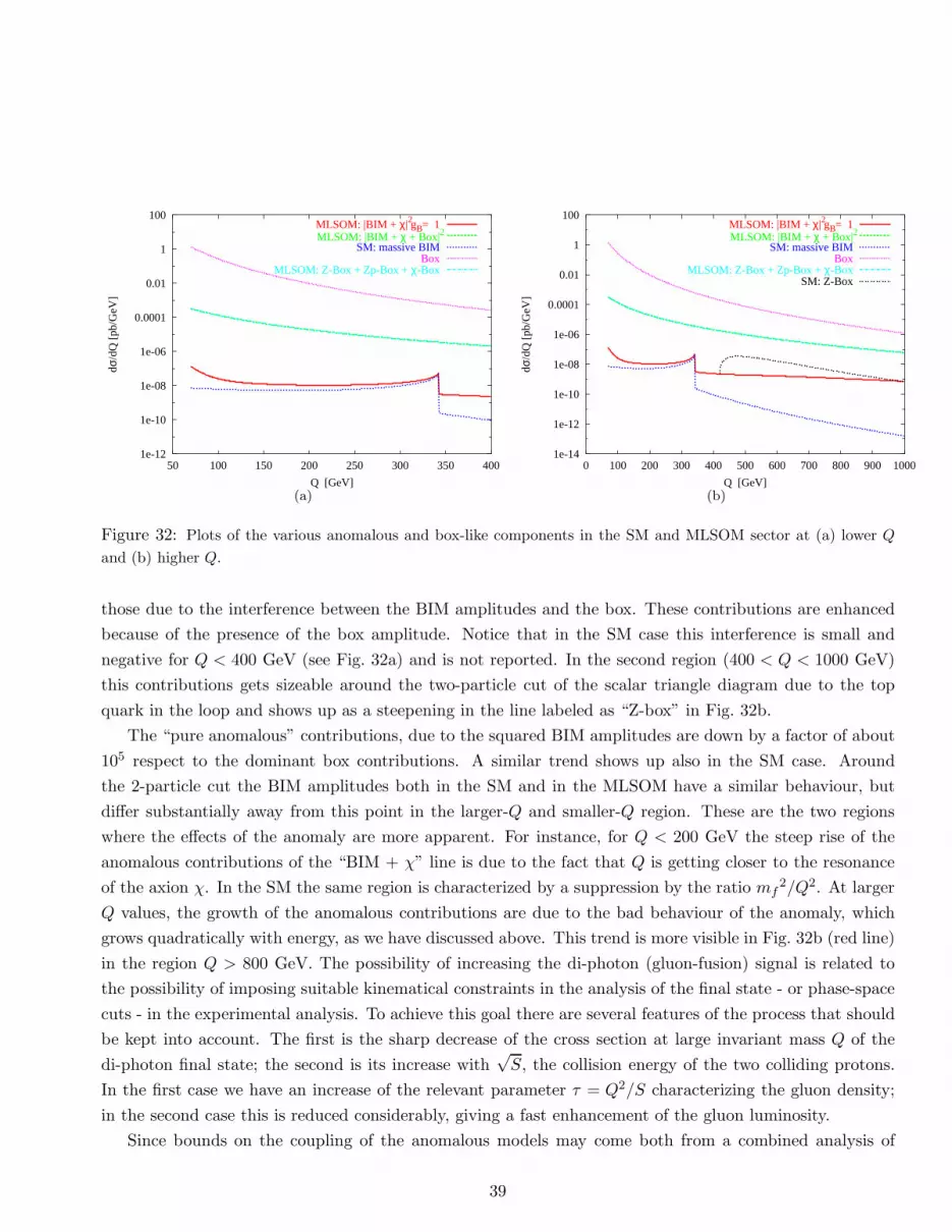
1e-12
1e-10
1e-08
1e-06
0.0001
0.01
1
100
50 100 150 200 250 300 350 400
dσ/d
Q [
pb/G
eV]
Q [GeV]
MLSOM: |BIM + χ|2 gB = 1MLSOM: |BIM + χ + Box|2
SM: massive BIMBox
MLSOM: Z-Box + Zp-Box + χ-Box
(a)
1e-14
1e-12
1e-10
1e-08
1e-06
0.0001
0.01
1
100
0 100 200 300 400 500 600 700 800 900 1000
dσ/d
Q [
pb/G
eV]
Q [GeV]
MLSOM: |BIM + χ|2 gB = 1MLSOM: |BIM + χ + Box|2
SM: massive BIMBox
MLSOM: Z-Box + Zp-Box + χ-BoxSM: Z-Box
(b)
Figure 32: Plots of the various anomalous and box-like components in the SM and MLSOM sector at (a) lower Q
and (b) higher Q.
those due to the interference between the BIM amplitudes and the box. These contributions are enhanced
because of the presence of the box amplitude. Notice that in the SM case this interference is small and
negative for Q < 400 GeV (see Fig. 32a) and is not reported. In the second region (400 < Q < 1000 GeV)
this contributions gets sizeable around the two-particle cut of the scalar triangle diagram due to the top
quark in the loop and shows up as a steepening in the line labeled as “Z-box” in Fig. 32b.
The “pure anomalous” contributions, due to the squared BIM amplitudes are down by a factor of about
105 respect to the dominant box contributions. A similar trend shows up also in the SM case. Around
the 2-particle cut the BIM amplitudes both in the SM and in the MLSOM have a similar behaviour, but
differ substantially away from this point in the larger-Q and smaller-Q region. These are the two regions
where the effects of the anomaly are more apparent. For instance, for Q < 200 GeV the steep rise of the
anomalous contributions of the “BIM + χ” line is due to the fact that Q is getting closer to the resonance
of the axion χ. In the SM the same region is characterized by a suppression by the ratio mf2/Q2. At larger
Q values, the growth of the anomalous contributions are due to the bad behaviour of the anomaly, which
grows quadratically with energy, as we have discussed above. This trend is more visible in Fig. 32b (red line)
in the region Q > 800 GeV. The possibility of increasing the di-photon (gluon-fusion) signal is related to
the possibility of imposing suitable kinematical constraints in the analysis of the final state - or phase-space
cuts - in the experimental analysis. To achieve this goal there are several features of the process that should
be kept into account. The first is the sharp decrease of the cross section at large invariant mass Q of the
di-photon final state; the second is its increase with√S, the collision energy of the two colliding protons.
In the first case we have an increase of the relevant parameter τ = Q2/S characterizing the gluon density;
in the second case this is reduced considerably, giving a fast enhancement of the gluon luminosity.
Since bounds on the coupling of the anomalous models may come both from a combined analysis of
39

1e-12
1e-10
1e-08
1e-06
0.0001
0.01
1
2 4 6 8 10 12 14
dσ/d
Q (
Q =
MZ )
[pb
/GeV
]
√S [TeV]
SMMLSOM, gB = 1
Figure 33: Double photon invariant mass cross section at Q = MZ plotted as a function of the energy. Here the SM
contributions include the massive BIM + Box + interference, while the MLSOM contributions include the massless
and massive BIM + interference.
both DY and of the di-photon cross section, we have chosen Q around the Z peak (small Q option) and the
same luminosity evaluated on the peak of the extra Z ′ (large Q option), both as a function of the collisional
energy S. This is shown in Fig. 33. The anomalous signal grows with√S but the non-unitary growth is
not apparent at LHC energies after convolution with the parton densities; on the other end, the growths in
the SM and in the anomalous sector of the MLSOM appear to be, at LHC energies, quite similar.
If an extra Z ′ is found in DY, then the analysis of di-photon both on the peak of the Z and on the peak
of the Z ′ could be used to set reasonable bounds on the coupling of the underlying model, trying to uncover
the possible presence of an anomalous signal. A τ ∼ 10−4 can be reached at the Z peak for a collision energy
of 10 TeV, which causes an enhancement of the anomalous cross section by a factor of approximately 104
respect to the same anomalous contribution measured for Q ∼ 1 TeV.
In a final figure we show the shapes of the distributions for the SM and the MLSOM using the Monte
Carlo with a binning of the cross section in both cases. This is provided in Fig. 34, where the colored lines
on top of each bin indicate the small anomalous signal in the cross section.
6 Summary and Conclusions
Both DY and DP have some special features, being characterized by a clean final state. In DY the identifica-
tion of a new resonance in the neutral current sector would bring to the immediate conclusion that an extra
Z ′ is present in the spectrum, but would give not specific indication concerning its true nature. Current
experimental bounds constrain the mixing of a possible extra neutral component with the Z gauge boson,
40

8.7e-07
8.8e-07
8.9e-07
9e-07
9.1e-07
9.2e-07
9.3e-07
9.4e-07
9.5e-07
9.6e-07
1.99 1.992 1.994 1.996 1.998 2 2.002 2.004 2.006 2.008 2.01
dσ/d
Q [
pb/G
eV]
Q [TeV]
SM NLO standard cutsSM + MLSOM, gB = 0.1
gB = gY gB = g2 gB = 1
Figure 34: Binned cross sections for the SM and the MLSOM. The small anomalous corrections are the thick lines
at the top of each bin.
with a mass which should be larger than 800 GeV, rendering the future search of extra neutral interactions,
at least for DY, quite delicate, being the allowed mass range at the tail of the invariant mass distribution of
this process. For this reason, the identification of a restricted mass range for the extra gauge boson would
be crucial for its discovery, but unfortunately, there is no extension of the SM that comes with a definite
prediction for it.
In intersecting brane models one encounters a similar indetermination and for this reason in our con-
struction the Stuckelberg mass has been assumed to be a free parameter. If an extra s-channel resonance
is found, then the investigation of its specific properties would require much more effort and several years
of data collection at the LHC, especially for larger mass values (above 1.5 TeV or so) of the extra Z ′. A
sizeable width of the resonance could then allow to study the V-A structure of the coupling, though this
study is quite complex. In most of the models studied so far the corresponding widths are expected to be
quite small ( ≪ 30 − 40 GeV) even for sizeable couplings (gB ∼ O(1)) [40], probably below or barely close
to the limits of the effective resolution of the detector.
Under these conditions, deciding over the true nature of the extra Z ′, whether anomalous or not, would
then be far more challenging and would require a parallel study of several independent channels. For this
reason we have analyzed two processes which are both affected by anomalous contributions and could be
used for correlated studies of the same interaction.
We have seen that changes in the factorization/renormalization scales both in the hard scatterings and in
the evolution of the PDF’s can easily overshadow the anomalous corrections, making a NLO/NNLO analysis
truly necessary. We have concentrated our investigation on an extra Z ′ of 1 TeV in mass and searched for
anomalous effects in the invariant mass distributions on the Z peak, at 1 TeV and for large Q values (up to 2
41

TeV’s). From our analysis the large suppression of the anomalous signal compared to the QCD background
is rather evident, although there are ways to improve on our results. In fact, our analysis has been based
on the characterization of inclusive observables, which are not sensitive to the geometric structure of the
final state. In principle, the shape of the final state event could be resolved at a finer level of detail, by
analyzing, for instance, the rapidity correlations between the di-photon and a jet, or other similar less
inclusive cross sections, as in other cases [35]. Obviously, these types of studies are theoretically challenging
and require an excellent knowledge of the QCD background at NNLO for these observables. This precision
could be achievable only by a combination of analytical and numerical methods at such perturbative order,
implemented in a flexible Monte Carlo program. This and other related issues are left to future studies.
Acknowledgements
We thank Nikos Irges for discussions. We thank Carl Schmidt for help on the use of the Gamma2MC code
for the NNLO study of the QCD background in di-photon and J.P. Guillet for exchanges concerning Diphox.
The work of C.C. was supported in part by the European Union through the Marie Curie Research and
Training Network “Universenet” (MRTN-CT-2006-035863) and by The Interreg II Crete-Cyprus Program.
7 Appendix
The decay rates into leptons for the Z and the Z ′ are universal and are given by
Γ(Z → ll) =g2
192πc2wMZ
[
(gZ,lV )2 + (gZ,lA )2]
=αem
48s2wc2w
MZ
[
(gZ,lV )2 + (gZ,lA )2]
,
Γ(Z → ψiψi) =Ncαem48s2wc
2w
MZ
[
(gZ,ψi
V )2 + (gZ,ψi
A )2]
×[
1 +αs(MZ)
π+ 1.409
α2s(MZ)
π2− 12.77
α3s(MZ)
π3
]
, (57)
where i = u, d, c, s and Z = Z,Z ′.
For the Z ′ and Z decays into heavy quarks we obtain
Γ(Z → bb) =Ncαem48s2wc
2w
MZ
[
(gZ,bV )2 + (gZ,bA )2]
×[
1 +αs(MZ)
π+ 1.409
α2s(MZ)
π2− 12.77
α3s(MZ)
π3
]
,
Γ(Z → tt) =Ncαem48s2wc
2w
MZ
√
1 − 4m2t
M2Z
×[
(gZ,tV )2(
1 + 2m2t
M2Z
)
+ (gZ,tA )2(
1 − 4m2t
M2Z
)]
×[
1 +αs(MZ)
π+ 1.409
α2s(MZ)
π2− 12.77
α3s(MZ)
π3
]
.
(58)
42
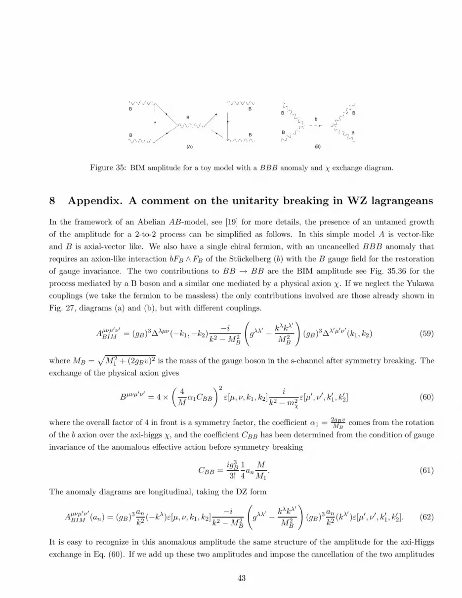
B
B
B
B
B
B
B B
Bb
(A) (B)
Figure 35: BIM amplitude for a toy model with a BBB anomaly and χ exchange diagram.
8 Appendix. A comment on the unitarity breaking in WZ lagrangeans
In the framework of an Abelian AB-model, see [19] for more details, the presence of an untamed growth
of the amplitude for a 2-to-2 process can be simplified as follows. In this simple model A is vector-like
and B is axial-vector like. We also have a single chiral fermion, with an uncancelled BBB anomaly that
requires an axion-like interaction bFB ∧FB of the Stuckelberg (b) with the B gauge field for the restoration
of gauge invariance. The two contributions to BB → BB are the BIM amplitude see Fig. 35,36 for the
process mediated by a B boson and a similar one mediated by a physical axion χ. If we neglect the Yukawa
couplings (we take the fermion to be massless) the only contributions involved are those already shown in
Fig. 27, diagrams (a) and (b), but with different couplings.
Aµνµ′ν′
BIM = (gB)3∆λµν(−k1,−k2)−i
k2 −M2B
(
gλλ′ − kλkλ
′
M2B
)
(gB)3∆λ′µ′ν′(k1, k2) (59)
where MB =√
M21 + (2gBv)2 is the mass of the gauge boson in the s-channel after symmetry breaking. The
exchange of the physical axion gives
Bµνµ′ν′ = 4 ×(
4
Mα1CBB
)2
ε[µ, ν, k1, k2]i
k2 −m2χ
ε[µ′, ν ′, k′1, k′
2] (60)
where the overall factor of 4 in front is a symmetry factor, the coefficient α1 = 2gBvMB
comes from the rotation
of the b axion over the axi-higgs χ, and the coefficient CBB has been determined from the condition of gauge
invariance of the anomalous effective action before symmetry breaking
CBB =ig3B
3!
1
4an
M
M1. (61)
The anomaly diagrams are longitudinal, taking the DZ form
Aµνµ′ν′
BIM (an) = (gB)3ank2
(−kλ)ε[µ, ν, k1, k2]−i
k2 −M2B
(
gλλ′ − kλkλ
′
M2B
)
(gB)3ank2
(kλ′
)ε[µ′, ν ′, k′1, k′
2]. (62)
It is easy to recognize in this anomalous amplitude the same structure of the amplitude for the axi-Higgs
exchange in Eq. (60). If we add up these two amplitudes and impose the cancellation of the two amplitudes
43

B
B
B
B
bB B
B B
B
B B
B
= +
G
Figure 36: Decomposition of the Stuckelberg axion in a goldstone boson and a physical axion
(which is a fine tuning) we obtain the condition
1
M2B
+(2gBv)
2
M2BM
21
= 0 (63)
in terms of the mass of the B and the Stuckelberg mass M1, which does not have a real solution. This is a
simple example that conveys the issue of the presence of unitarity limit for (local) WZ interactions.
References
[1] P. Langacker, (2008), 0801.1345.
[2] R.D. Peccei and H.R. Quinn, Phys. Rev. Lett. 38 (1977) 1440.
[3] R.D. Peccei and H.R. Quinn, Phys. Rev. D16 (1977) 1791.
[4] S. Weinberg, Phys. Rev. Lett. 40 (1978) 223.
[5] F. Wilczek, Phys. Rev. Lett. 40 (1978) 279.
[6] J.E. Kim, Phys. Rev. Lett. 43 (1979) 103.
[7] M.A. Shifman, A.I. Vainshtein and V.I. Zakharov, Nucl. Phys. B166 (1980) 493.
[8] M. Dine, W. Fischler and M. Srednicki, Phys. Lett. B104 (1981) 199.
[9] A.R. Zhitnitsky, Sov. J. Nucl. Phys. 31 (1980) 260.
[10] R.D. Peccei, Lect. Notes Phys. 741 (2008) 3, hep-ph/0607268.
[11] C. Coriano, M. Guzzi and S. Morelli, Eur. Phys. J. C55 (2008) 629, 0801.2949.
[12] R. Armillis, C. Coriano, M. Guzzi and S. Morelli, (2008), 0808.1882.
[13] I. Antoniadis, E. Kiritsis and T. Tomaras, Fortsch. Phys. 49 (2001) 573, hep-th/0111269.
[14] L.E. Ibanez, F. Marchesano and R. Rabadan, JHEP 11 (2001) 002, hep-th/0105155.
44
[15] E. Kiritsis, Fortsch. Phys. 52 (2004) 200, hep-th/0310001.
[16] R. Blumenhagen, B. Kors, D. Lust and S. Stieberger, Phys. Rept. 445 (2007) 1, hep-th/0610327.
[17] C. Coriano, N. Irges and E. Kiritsis, Nucl. Phys. B746 (2006) 77, hep-ph/0510332.
[18] C. Coriano and N. Irges, Phys. Lett. B651 (2007) 298, hep-ph/0612140.
[19] C. Coriano, N. Irges and S. Morelli, JHEP 07 (2007) 008, hep-ph/0701010.
[20] C. Coriano, N. Irges and S. Morelli, Nucl. Phys. B789 (2008) 133, hep-ph/0703127.
[21] P. Anastasopoulos, F. Fucito, A. Lionetto, G. Pradisi, A. Racioppi and Y.S. Stanev, (2008), 0804.1156.
[22] J. De Rydt, J. Rosseel, T. T. Schmidt, A. Van Proeyen and M. Zagermann, Class. Quant. Grav. 24
(2007) 5201, 0705.4216.
[23] J. De Rydt, T. T. Schmidt, M. Trigiante, A. Van Proeyen and M. Zagermann, (2008), 0808.2130.
[24] D. Feldman, Z. Liu and P. Nath, JHEP 11 (2006) 007, hep-ph/0606294.
[25] D. Feldman, Z. Liu and P. Nath, Phys. Rev. Lett. 97 (2006) 021801, hep-ph/0603039.
[26] D. Feldman, Z. Liu and P. Nath, Phys. Rev. D75 (2007) 115001, hep-ph/0702123.
[27] A. De Angelis, O. Mansutti and M. Roncadelli, Phys. Rev. D76 (2007) 121301, 0707.4312.
[28] A. De Angelis, O. Mansutti, M. Persic and M. Roncadelli, (2008), 0807.4246.
[29] J. Jaeckel, E. Masso, J. Redondo, A. Ringwald and F. Takahashi, Phys. Rev. D75 (2007) 013004,
hep-ph/0610203.
[30] M. Ahlers, H. Gies, J. Jaeckel, J. Redondo and A. Ringwald, Phys. Rev. D77 (2008) 095001, 0711.4991.
[31] A. Cafarella, C. Coriano and M. Guzzi, (2008), 0803.0462.
[32] T. Binoth, J.P. Guillet, E. Pilon and M. Werlen, Eur. Phys. J. C16 (2000) 311, hep-ph/9911340.
[33] Z. Bern, L.J. Dixon and C. Schmidt, Phys. Rev. D66 (2002) 074018, hep-ph/0206194.
[34] C. Coriano and L.E. Gordon, Nucl. Phys. B469 (1996) 202, hep-ph/9601350.
[35] S. Chang, C. Coriano and L.E. Gordon, Phys. Rev. D58 (1998) 074002, hep-ph/9709496.
[36] P. Anastasopoulos, M. Bianchi, E. Dudas and E. Kiritsis, JHEP 11 (2006) 057, hep-th/0605225.
[37] R. Armillis, C. Coriano and M. Guzzi, JHEP 05 (2008) 015, 0711.3424.
45
[38] R. Hamberg, W.L. van Neerven and T. Matsuura, Nucl. Phys. B359 (1991) 343.
[39] M.S. Carena, A. Daleo, B.A. Dobrescu and T.M.P. Tait, Phys. Rev. D70 (2004) 093009, hep-
ph/0408098.
[40] C. Coriano, A.E. Faraggi and M. Guzzi, Phys. Rev. D78 (2008) 015012, 0802.1792.
[41] D.M. Ghilencea, L.E. Ibanez, N. Irges and F. Quevedo, JHEP 08 (2002) 016, hep-ph/0205083.
[42] N.N. Achasov, Phys. Lett. B287 (1992) 213.
[43] A.D. Dolgov and V.I. Zakharov, Nucl. Phys. B27 (1971) 525.
[44] M. Knecht, S. Peris, M. Perrottet and E. de Rafael, JHEP 03 (2004) 035, hep-ph/0311100.
[45] F. Jegerlehner and O.V. Tarasov, Phys. Lett. B639 (2006) 299, hep-ph/0510308.
[46] M. Knecht, S. Peris, M. Perrottet and E. de Rafael, JHEP 11 (2002) 003, hep-ph/0205102.
[47] B.A. Kniehl and J.H. Kuhn, Nucl. Phys. B329 (1990) 547.
[48] A. Cafarella, C. Coriano and M. Guzzi, JHEP 08 (2007) 030, hep-ph/0702244.
[49] A. Cafarella, C. Coriano and M. Guzzi, Nucl. Phys. B748 (2006) 253, hep-ph/0512358.
[50] W. Bernreuther, R. Bonciani, T. Gehrmann, R. Heinesch, T. Leineweber and E. Remiddi, Nucl. Phys.
B723 (2005) 91, hep-ph/0504190.
[51] S.A. Larin, Phys. Lett. B303 (1993) 113, hep-ph/9302240.
[52] R.J. Gonsalves, C.M. Hung and J. Pawlowski, Phys. Rev. D46 (1992) 4930.
[53] P.J. Rijken and W.L. van Neerven, Phys. Rev. D52 (1995) 149, hep-ph/9501373.
[54] A.D. Martin, R.G. Roberts, W.J. Stirling and R.S. Thorne, Eur. Phys. J. C23 (2002) 73, hep-
ph/0110215.
[55] A.D. Martin, R.G. Roberts, W.J. Stirling and R.S. Thorne, Phys. Lett. B531 (2002) 216, hep-
ph/0201127.
[56] A. Cafarella, C. Coriano and M. Guzzi, AIP Conf. Proc. 964 (2007) 206, 0709.2115.
[57] T. Binoth, J.P. Guillet, E. Pilon and M. Werlen, (2001), hep-ph/0111043.
[58] Z. Bern, A. De Freitas and L.J. Dixon, JHEP 09 (2001) 037, hep-ph/0109078.
46