an analysis of mechanisms for submesoscale vertical motion at ocean fronts

Ocean Modelling 14 (2006) 241–256

www.elsevier.com/locate/ocemod

An analysis of mechanisms for submesoscalevertical motion at ocean fronts

Amala Mahadevan a,*, Amit Tandon b

a Department of Earth Sciences, Boston University, 685 Commonwealth Avenue, Boston, MA 02215, USAb Physics Department and SMAST, University of Massachusetts, Dartmouth, 285 Old Westport Road, North Dartmouth, MA 02747, USA

Received 3 April 2006; received in revised form 25 May 2006; accepted 26 May 2006Available online 30 June 2006

Abstract

We analyze model simulations of a wind-forced upper ocean front to understand the generation of near-surface sub-mesoscale, O(1 km), structures with intense vertical motion. The largest vertical velocities are in the downward direction;their maxima are situated at approximately 25 m depth and magnitudes exceed 1 mm/s or 100 m/day. They are correlatedwith high rates of lateral strain, large relative vorticity and the loss of geostrophic balance. We examine several mechanismsfor the formation of submesoscale structure and vertical velocity in the upper ocean. These include: (i) frontogenesis, (ii)frictional effects at fronts, (iii) mixed layer instabilities, (iv) ageostrophic anticyclonic instability, and (v) nonlinear Ekmaneffects. We assess the role of these mechanisms in generating vertical motion within the nonlinear, three-dimensionallyevolving flow field of the nonhydrostatic model. We find that the strong submesoscale down-welling in the model isexplained by nonlinear Ekman pumping and is also consistent with the potential vorticity arguments that analogizedown-front winds to buoyancy-forcing. Conditions also support the formation of ageostrophic anticyclonic instabilities,but the contribution of these is difficult to assess because the decomposition of the flow into balanced and unbalancedcomponents via semigeostrophic analysis breaks down at O(1) Rossby numbers. Mixed layer instabilities do not dominatethe structure, but shear and frontogenesis contribute to the relative vorticity and strain fields that generate ageostrophy.� 2006 Elsevier Ltd. All rights reserved.

1. Introduction

The mechanisms by which the physical exchange of water and properties is achieved between the activelyforced surface layer of the ocean and the relatively quiescent thermocline have posed some long-standing ques-tions in our understanding of the upper ocean. Vertical motion in the upper ocean is instrumental in supplyingnutrients to phytoplankton in the sunlit layers, conveying heat, salt and momentum fluxes, and exchanginggases with the atmosphere. But such motion is difficult to observe in the field because vertical velocities aretypically three to four orders of magnitude smaller than mesoscale horizontal velocities, which dominate

1463-5003/$ - see front matter � 2006 Elsevier Ltd. All rights reserved.

doi:10.1016/j.ocemod.2006.05.006

* Corresponding author. Tel.: +1 6173535511; fax: +1 6173533290.E-mail address: [email protected] (A. Mahadevan).

mailto:[email protected]

242 A. Mahadevan, A. Tandon / Ocean Modelling 14 (2006) 241–256

the energy of the upper ocean. Similarly, models have lacked the resolution and accuracy to produce reliablevertical velocity fields that can support the rates of vertical exchange inferred from tracer observations. Forexample, estimates of new production (phytoplankton production relying on a fresh, rather than recycled,supply of nutrients) based on oxygen utilization and cycling rates (Platt and Harrison, 1985, Jenkins andGoldman, 1985, Emerson et al., 1997) and helium fluxes (Jenkins, 1988), are much higher in the subtropicalgyres than can be accounted for through the physical circulation in global carbon cycle models (Najjar, 1990,Bacastow and Maier-Reimer, 1991, Najjar et al., 1992, Maier-Reimer, 1993). A number of studies, such asMcGillicuddy and Robinson (1997) and McGillicuddy et al. (1998), suggest that eddies, which proliferatethe ocean, act to pump nutrients to the euphotic zone. However, a basin-wide estimate for the eddy pumpingfluxes (Oschlies, 2002, Martin and Pondaven, 2003) shows that eddies, alone, cannot provide the nutrient fluxrequired to sustain the observed levels of productivity in the subtropical gyres. Modeling studies of frontalregions (Levy et al., 2001, Mahadevan and Archer, 2000) suggest that vertical exchange is enhanced at densityfronts, which are ubiquitous to the upper ocean. However, it is only through recent developments in numericalmodeling, field sampling and analysis, that we are able to resolve frontal processes at the O(1 km) horizontallength scale, referred to here as the submesoscale. At this scale, the Rossby and Richardson numbers becomeO(1) in localized regions, leading to intense ageostrophic secondary circulation and large vertical velocities, asis seen in models that resolve the submesoscale (e.g., Mahadevan, 2006, Capet et al., 2006). These motions arenot targeted by most extant mixing parameterization schemes and need to be resolved and understood beforetheir effects can be parameterized in the next generation of global circulation models.

In a preceding paper (Mahadevan, 2006), we described a suite of numerical modeling experiments with afully nonhydrostatic, three-dimensional, free-surface ocean model used to simulate the evolution of an upperocean front in a periodic channel setting. The model domain is rectangular in plan view, with periodic bound-aries set 48 km apart in the east–west direction, solid boundaries set 96 km apart in the north–south direction,and a flat bottom at a depth of 800 m. A horizontal grid resolution of 0.5 km is used for the flow fieldsanalyzed here, though 1 km and 0.25 km grid resolutions were also used for comparison and presented inMahadevan (2006). In the vertical, we use a stretched grid spacing varying from 10 m at the surface to75 m at depth. The domain is initialized with lighter water in the southern half of the upper ocean and denserwater to the north, as described in Appendix A. The west-to-east density front is most distinct at the surfaceand in the mixed layer extending to about 50 m depth, and weakens with depth over the pycnocline whichextends to approximately 250 m. As the flow field evolves, the front becomes baroclinically unstable and formsmesoscale meanders. When the model is forced with a westerly wind stress, we observe that submesoscalestructures with intense vertical velocities develop in the near surface region (upper 50 m). Down-welling is con-siderably more intense (�100 m/day) than up-welling, and is concentrated in narrow bands that are roughly2 km in width. Though the submesoscale structures are not a nonhydrostatic phenomenon, we prefer to usethe nonhydrostatic model for better accuracy. At a depth of 50–100 m, the vertical velocities are weaker(�10 m/day) and mesoscale in structure. Fig. 1 shows the surface density field and the vertical velocities attwo different depths as the flow evolves in time. The front, which is initially straight and oriented west-to-east,develops meanders, which in turn develop more complex submesoscale structure due to the interplay betweenwind, buoyancy gradients and Coriolis effects. Our objective is to understand the mechanisms that underlie thesubmesoscale vertical motion seen in the model.

Several mechanisms have been proposed for the development of submesoscale structure in the presence ofhorizontal density gradients. (i) Horizontal density gradients intensify in the presence of lateral strain andconvergence leading to frontogenesis and large vertical velocities (Hoskins and Bretherton, 1972). (ii) Mixingmomentum in the presence of horizontal density gradients also generates vertical motion (Garrett and Loder,1981). (iii) Molemaker et al. (2005) show that ageostrophic anticyclonic baroclinic instability can arise spon-taneously at submesoscales in the ocean from a loss of balance in regions where the local Rossby number islarge. (iv) Fox-Kemper et al. (2006) propose that mixed layer instabilities (MLI) arise as density fronts that areout of geostrophic balance, slump and re-stratify the upper ocean; these generate submesoscale structure inregions where the Richardson number is small. (v) Thomas and Lee (2005) suggest that along-front windscan generate intense down-welling due to cross-front Ekman transport at the surface. This transport drivesdense water over buoyant, resulting in secondary ageostrophic circulation cells that feed back upon themselvesand enable exchange with deeper waters.

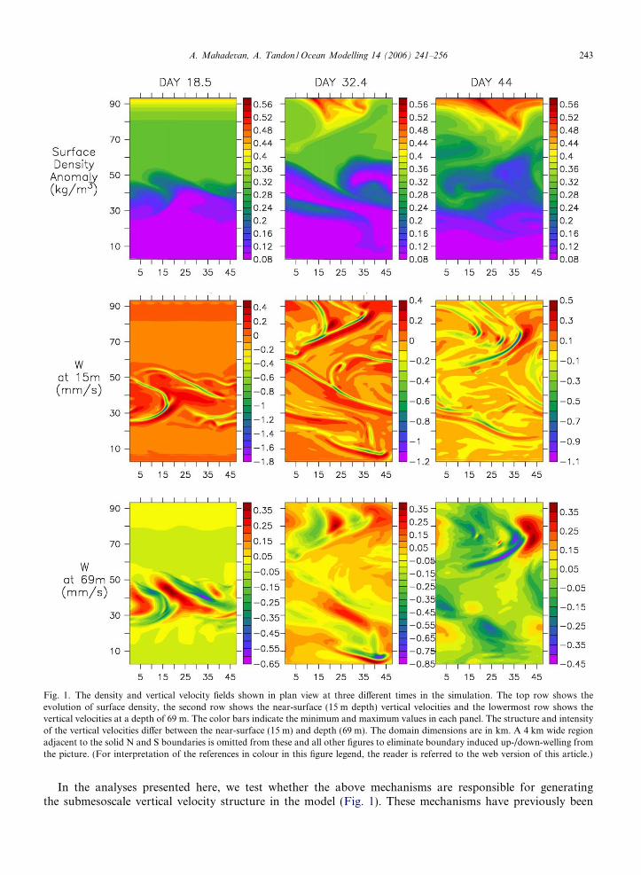
Fig. 1. The density and vertical velocity fields shown in plan view at three different times in the simulation. The top row shows theevolution of surface density, the second row shows the near-surface (15 m depth) vertical velocities and the lowermost row shows thevertical velocities at a depth of 69 m. The color bars indicate the minimum and maximum values in each panel. The structure and intensityof the vertical velocities differ between the near-surface (15 m) and depth (69 m). The domain dimensions are in km. A 4 km wide regionadjacent to the solid N and S boundaries is omitted from these and all other figures to eliminate boundary induced up-/down-welling fromthe picture. (For interpretation of the references in colour in this figure legend, the reader is referred to the web version of this article.)

A. Mahadevan, A. Tandon / Ocean Modelling 14 (2006) 241–256 243

In the analyses presented here, we test whether the above mechanisms are responsible for generatingthe submesoscale vertical velocity structure in the model (Fig. 1). These mechanisms have previously been


diagnosed in specific settings, some of which are two-dimensional, and analyzed in the linear regime. Here, weuse ideas from previous and recent studies to unravel the mechanisms acting three-dimensionally, and in con-cert, to generate the submesoscale structure seen in the model.

In what follows, we examine several mechanisms that might account for the submesoscale vertical velocitiesin the model. In Section 2, we examine frontal mechanisms that invoke strain, as well as vertical mixing, toexplain up- and down-welling. In Section 3, we estimate the vertical stability of the water column using the Rich-ardson number to determine whether mixed layer instabilities might develop (Fox-Kemper et al., 2006, Stone,1970). Next, we examine the criteria under which baroclinicity could give rise to submesoscale instabilities(Molemaker et al., 2005). We diagnose the balanced part of the vertical velocity field from the density structureusing the omega equation in order to determine whether the submesoscale velocity structure could be ascribed toa loss of balance (McWilliams et al., 2001). In Section 4, we examine forced vertical motion due to the nonlinearEkman effect (Thomas and Lee, 2005) and analyze the potential vorticity (PV) and PV fluxes to assess the role ofwind (Thomas, 2005). We test the scaling for the vertical nonlinear Ekman velocity (Thomas and Rhines, 2002)against the model within a localized region of the model domain. In conclusion, we discuss the combination ofeffects that lead to the submesoscale structure in the model. We speculate on the implications of such submes-oscale activity in the upper ocean and discuss some outstanding questions and future work.

2. Frontal mechanisms

Fronts, or lateral buoyancy gradients, are ubiquitous to the upper ocean (Ullman and Cornillon, 1999), andare sites where large vertical velocities can develop. Due to thermal wind balance, fronts are associated with asurface-intensified jet with strong shear and relative vorticity of opposite sign on either side. Here, we considertwo mechanisms that generate vertical motion at fronts. We diagnose their effectiveness and assess whetherthey account for the submesoscale vertical velocities in the model.

2.1. Strain driven frontogenesis

The first mechanism that we consider is frontogenesis (Hoskins and Bretherton, 1972), or the intensificationof fronts due to horizontal strain and convergence in the flow. Strain may be generated by nonlinear dynamicsin conjunction with wind forcing. Regions of high strain can be expected to be related to high vorticity due tolarge shear in the vicinity of high strain rates. The large relative vorticity, which implies large local Rossbynumber, generates a loss of geostrophic balance and ageostrophic motion. When fluid parcels cross fromone side of the front to the other, one can expect a change in the thickness of isopycnal layers due to theconservation of potential vorticity (PV), and hence the development of large vertical velocities (Pollard andRegier, 1990, Pollard and Regier, 1992, Voorhis and Bruce, 1982). This mechanism, by itself, is adiabatic,but can result in diabatic exchange and submesoscale structure when combined with other mechanismsdiscussed further below.

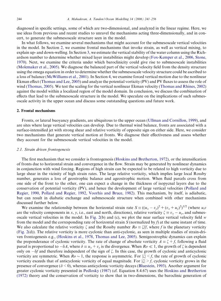
We examine the relationship between the horizontal strain rate S � ((ux � vy)2 + (vx + uy)2)1/2 (where u,vare the velocity components in x, y, i.e., east and north, directions), relative vorticity f � vx � uy, and submes-oscale vertical velocities in the model. In Fig. 2(b) and (c), we plot the near surface vertical velocity field w

from the model and the corresponding rate of horizontal strain S (normalized by f) at the same instant of time.We also calculate the relative vorticity f and the Rossby number Ro � f/f, where f is the planetary vorticity(Fig. 2(d)). The relative vorticity is more cyclonic than anti-cyclonic, as seen in multiple studies of strain-dri-ven frontogenesis e.g., (Hoskins et al., 1978, Thomas and Lee, 2005). Semigeostrophic dynamics can explainthe preponderance of cyclonic vorticity. The rate of change of absolute vorticity A � f + f, following a fluidparcel is proportional to �dA, where d � ux + vy is the divergence. When Ro� 1, the growth of f is dependentonly on �df and therefore independent of the sign of f. In this case, the growth of cyclonic and anticyclonicvorticity are symmetric. When Ro � 1, the response is asymmetric. For jfj < f, the rate of growth of cyclonicvorticity exceeds that of anticyclonic vorticity of equal magnitude. For jfj > f, cyclonic vorticity grows in thepresence of convergence (d < 0), whereas anticyclonic vorticity decays (Bluestein, 1993). Another argument forgreater cyclonic vorticity presented in Pedlosky (1987) (cf. Equation 8.4.67) uses the Hoskins and Bretherton(1972) theory and the conservation of vorticity to show that in two-dimensions, the baroclinic generation of

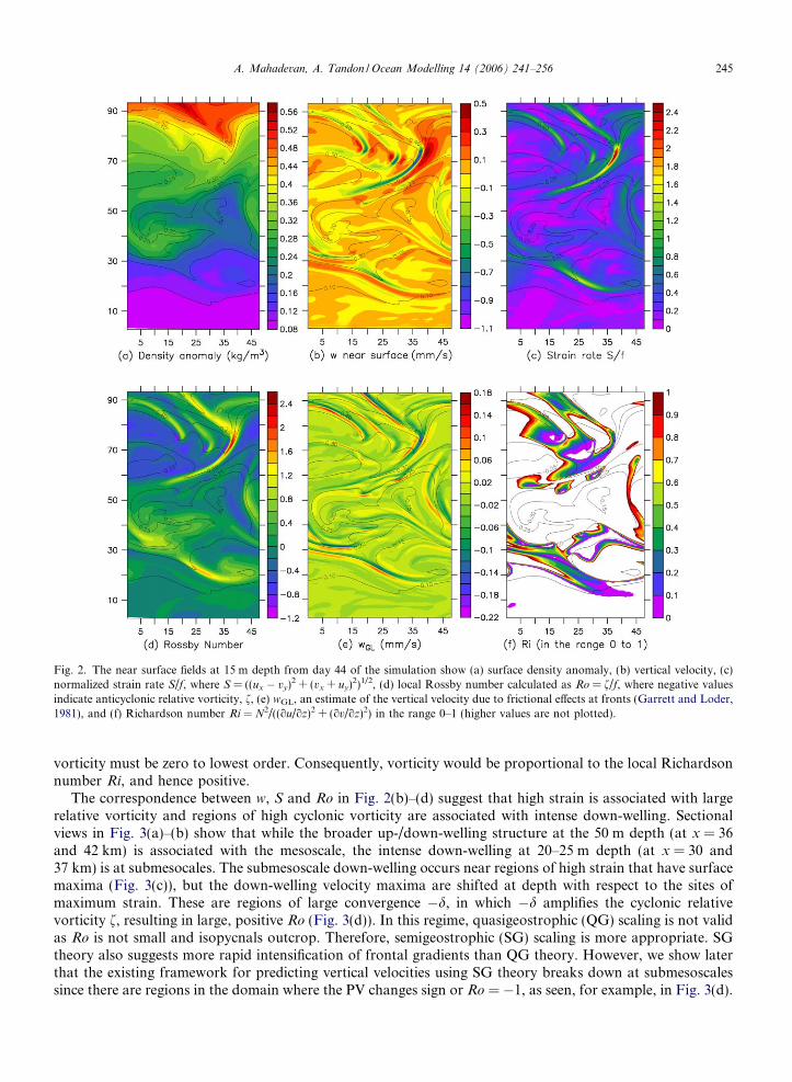
Fig. 2. The near surface fields at 15 m depth from day 44 of the simulation show (a) surface density anomaly, (b) vertical velocity, (c)normalized strain rate S/f, where S = ((ux � vy)2 + (vx + uy)2)1/2, (d) local Rossby number calculated as Ro = f/f, where negative valuesindicate anticyclonic relative vorticity, f, (e) wGL, an estimate of the vertical velocity due to frictional effects at fronts (Garrett and Loder,1981), and (f) Richardson number Ri = N2/((ou/oz)2 + (ov/oz)2) in the range 0–1 (higher values are not plotted).


vorticity must be zero to lowest order. Consequently, vorticity would be proportional to the local Richardsonnumber Ri, and hence positive.

The correspondence between w, S and Ro in Fig. 2(b)–(d) suggest that high strain is associated with largerelative vorticity and regions of high cyclonic vorticity are associated with intense down-welling. Sectionalviews in Fig. 3(a)–(b) show that while the broader up-/down-welling structure at the 50 m depth (at x = 36and 42 km) is associated with the mesoscale, the intense down-welling at 20–25 m depth (at x = 30 and37 km) is at submesocales. The submesoscale down-welling occurs near regions of high strain that have surfacemaxima (Fig. 3(c)), but the down-welling velocity maxima are shifted at depth with respect to the sites ofmaximum strain. These are regions of large convergence �d, in which �d amplifies the cyclonic relativevorticity f, resulting in large, positive Ro (Fig. 3(d)). In this regime, quasigeostrophic (QG) scaling is not validas Ro is not small and isopycnals outcrop. Therefore, semigeostrophic (SG) scaling is more appropriate. SGtheory also suggests more rapid intensification of frontal gradients than QG theory. However, we show laterthat the existing framework for predicting vertical velocities using SG theory breaks down at submesoscalessince there are regions in the domain where the PV changes sign or Ro = �1, as seen, for example, in Fig. 3(d).

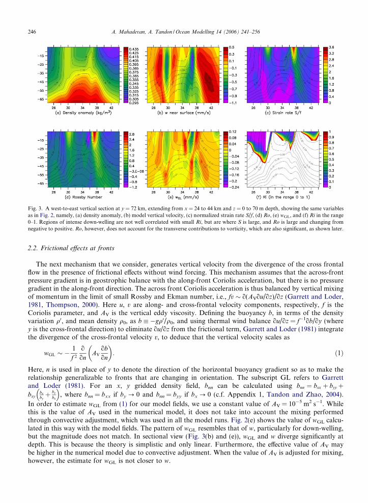
Fig. 3. A west-to-east vertical section at y = 72 km, extending from x = 24 to 44 km and z = 0 to 70 m depth, showing the same variablesas in Fig. 2, namely, (a) density anomaly, (b) model vertical velocity, (c) normalized strain rate S/f, (d) Ro, (e) wGL, and (f) Ri in the range0–1. Regions of intense down-welling are not well correlated with small Ri, but are where S is large, and Ro is large and changing fromnegative to positive. Ro, however, does not account for the transverse contributions to vorticity, which are also significant, as shown later.


2.2. Frictional effects at fronts

The next mechanism that we consider, generates vertical velocity from the divergence of the cross frontalflow in the presence of frictional effects without wind forcing. This mechanism assumes that the across-frontpressure gradient is in geostrophic balance with the along-front Coriolis acceleration, but there is no pressuregradient in the along-front direction. The across front Coriolis acceleration is thus balanced by vertical mixingof momentum in the limit of small Rossby and Ekman number, i.e., fv � o(AVou/oz)/oz (Garrett and Loder,1981, Thompson, 2000). Here u, v are along- and cross-frontal velocity components, respectively, f is theCoriolis parameter, and AV is the vertical eddy viscosity. Defining the buoyancy b, in terms of the densityvariation q0, and mean density q0, as b � �gq0/q0, and using thermal wind balance ou/oz = f�1ob/oy (wherey is the cross-frontal direction) to eliminate ou/oz from the frictional term, Garrett and Loder (1981) integratethe divergence of the cross-frontal velocity v, to deduce that the vertical velocity scales as

wGL � �1

f 2

o

onAV

obon

� �: ð1Þ

Here, n is used in place of y to denote the direction of the horizontal buoyancy gradient so as to make therelationship generalizable to fronts that are changing in orientation. The subscript GL refers to Garrettand Loder (1981). For an x, y gridded density field, bnn can be calculated using bnn ¼ bxx þ byy þbxy

bxbyþ by

bx

� �, where bnn = bxx if by ? 0 and bnn = byy if bx ? 0 (c.f. Appendix 1, Tandon and Zhao, 2004).

In order to estimate wGL from (1) for our model fields, we use a constant value of AV = 10�5 m2 s�1. Whilethis is the value of AV used in the numerical model, it does not take into account the mixing performedthrough convective adjustment, which was used in all the model runs. Fig. 2(e) shows the value of wGL calcu-lated in this way with the model fields. The pattern of wGL resembles that of w, particularly for down-welling,but the magnitude does not match. In sectional view (Fig. 3(b) and (e)), wGL and w diverge significantly atdepth. This is because the theory is simplistic and only linear. Furthermore, the effective value of AV maybe higher in the numerical model due to convective adjustment. When the value of AV is adjusted for mixing,however, the estimate for wGL is not closer to w.


3. Spontaneous instabilities

3.1. Mixed layer instability

Horizontal buoyancy gradients in the upper ocean store available potential energy. Fox-Kemper et al.(2006) discuss how this energy in the mixed layer is released by an unforced mixed layer instability (MLI) thataffects the restratification process as an unbalanced front slumps. Its characteristic vertical scale is the depth ofthe mixed layer, typical horizontal scales are a few kilometers, and growth rates are of the order of a day.Therefore, it is relevant to the development of submesoscale structure. In unstable regions, the local Richard-son number Ri, satisfies the relationship Ro2Ri � 1. Fox-Kemper et al. (2006) assume an idealized basic stateas a zero-PV initial state that becomes unstable at low, O(1) Ri and large, O(1) Ro. This is in contrast to smallRo baroclinic instability, where the vertical scale is the depth of the thermocline, typical horizontal scales are�10–100 km, Ri� 1, and Ro� 1.

In our numerical simulations, we marginally resolve the wavelength k and the time scale associated with thegrowth rate ri, governing the most unstable mode in the instability mechanism described by Stone (1970). This

forms the basis of MLI (Fox-Kemper et al., 2006); k and ri are given by k ¼ u0

f5=2

1þRi

� �12

m, where u0 is the along-

front velocity (in m s�1) generated from thermal wind balance and f is in s�1; ri ¼ f 5=541þRi

� �12

S�1. For example,

the wavelength of the most unstable mode is approximately 1 km for Ri = 2, f = 10�4 s�1 and a characteristichorizontal velocity of 0.1 m s�1; our horizontal grid resolution of 500 m would marginally resolve this. For ashort duration, we ran the model at a horizontal grid resolution of 250 m by interpolating the developed flowfields from the 500 m resolution model run as initial conditions. We did not find striking differences betweenresults of the 250 m and 500 m resolution runs (c.f. Fig. 6 Mahadevan, 2006). The e-folding time scale forgrowth of the most unstable mode is approximately half a day and is well resolved by the model, which usesa time step of 400 s. To test whether MLI contributes to the submesoscale structure observed in our simula-tions, we estimate the Richardson number Ri � N2/(ou/oz)2, for the model flow fields (see Figs. 2(f) and 3(f)).The correspondence between regions of small Ri and high vertical velocity is too weak to support the idea thatinstabilities associated with low Ri are the cause of the intense vertical submesoscale motion seen in the model.The finite amplitude version of MLI may differ substantially from the linear case (B. Fox-Kemper, personalcommunication (2006)), but if MLI does occur in our numerical simulations, it likely plays only a minor role.This is because we initialize the model with a geostrophically balanced state and force the surface continuallywith a wind stress. A larger model domain that allows for the interaction between submesoscales and meso-scale eddies and uses geostrophically unbalanced initial conditions would be conducive to MLI, as shown byB. Fox-Kemper (AGU, Ocean Sciences, 2006). In our model, we see the early development of MLI when usinghigher (250 m) grid resolution and no wind forcing.

3.2. Loss of balance and ageostrophic anticyclonic baroclinic instability

McWilliams et al. (2001) review three main routes to dissipation of energy from a balanced flow through theloss of balance. The conditions for all three of these are satisfied in our simulations. They are: (i) change in signof the absolute vorticity A, which gives rise to symmetric centrifugal instability1, (ii) change in sign of thevertical buoyancy gradient or N, which gives rise to convection, and (iii) change in sign of the differencebetween absolute vorticity and strain rate A–S, which gives rise to a new class of unbalanced ageostrophicinstabilities (Molemaker et al., 2005, McWilliams, 2003) that may explain the genesis of submesoscale motion.This class of instabilities has been investigated for a frontal situation by Molemaker et al. (2005), for a bound-ary current by McWilliams et al. (2004), and for a Taylor-Couette flow by Molemaker et al. (2001). For thefrontal initial state, the dynamics of hydrostatic and thermal-wind balance gives way to ageostrophic baro-clinic instabilities at length scales of 0.1–10 km. Significant ageostrophic modes arise for Ro between 0 and1 (e.g., for Ro ¼ 1=

ffiffiffi2p

, or Ri = 2) from a simple initial state of uniformly sheared parallel flow (Molemaker

1 A more general condition for symmetric instability is the change in sign of the Ertel PV.

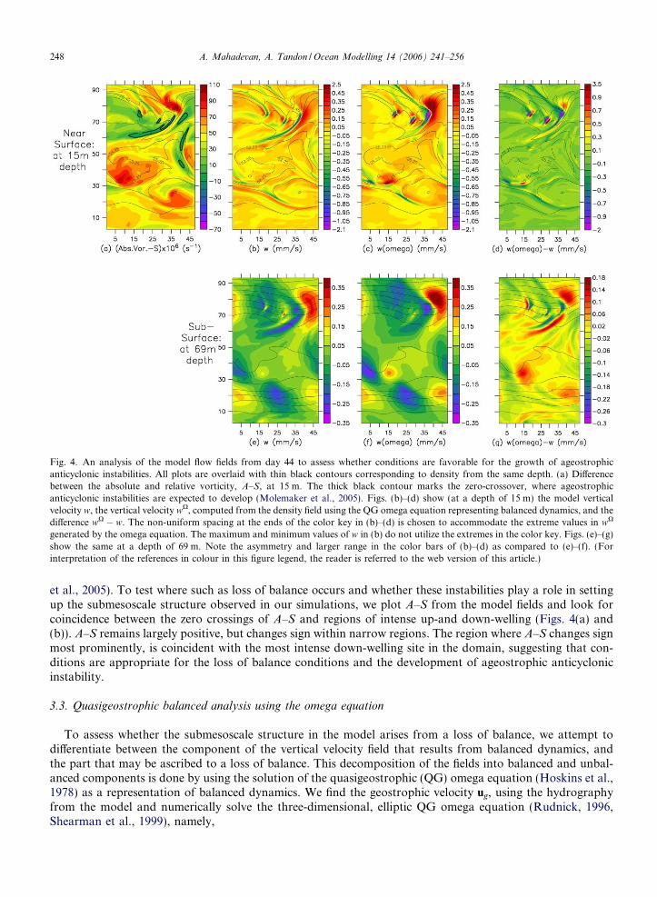
Fig. 4. An analysis of the model flow fields from day 44 to assess whether conditions are favorable for the growth of ageostrophicanticyclonic instabilities. All plots are overlaid with thin black contours corresponding to density from the same depth. (a) Differencebetween the absolute and relative vorticity, A–S, at 15 m. The thick black contour marks the zero-crossover, where ageostrophicanticyclonic instabilities are expected to develop (Molemaker et al., 2005). Figs. (b)–(d) show (at a depth of 15 m) the model verticalvelocity w, the vertical velocity wX, computed from the density field using the QG omega equation representing balanced dynamics, and thedifference wX � w. The non-uniform spacing at the ends of the color key in (b)–(d) is chosen to accommodate the extreme values in wX

generated by the omega equation. The maximum and minimum values of w in (b) do not utilize the extremes in the color key. Figs. (e)–(g)show the same at a depth of 69 m. Note the asymmetry and larger range in the color bars of (b)–(d) as compared to (e)–(f). (Forinterpretation of the references in colour in this figure legend, the reader is referred to the web version of this article.)


et al., 2005). To test where such as loss of balance occurs and whether these instabilities play a role in settingup the submesoscale structure observed in our simulations, we plot A–S from the model fields and look forcoincidence between the zero crossings of A–S and regions of intense up-and down-welling (Figs. 4(a) and(b)). A–S remains largely positive, but changes sign within narrow regions. The region where A–S changes signmost prominently, is coincident with the most intense down-welling site in the domain, suggesting that con-ditions are appropriate for the loss of balance conditions and the development of ageostrophic anticyclonicinstability.

3.3. Quasigeostrophic balanced analysis using the omega equation

To assess whether the submesoscale structure in the model arises from a loss of balance, we attempt todifferentiate between the component of the vertical velocity field that results from balanced dynamics, andthe part that may be ascribed to a loss of balance. This decomposition of the fields into balanced and unbal-anced components is done by using the solution of the quasigeostrophic (QG) omega equation (Hoskins et al.,1978) as a representation of balanced dynamics. We find the geostrophic velocity ug, using the hydrographyfrom the model and numerically solve the three-dimensional, elliptic QG omega equation (Rudnick, 1996,Shearman et al., 1999), namely,


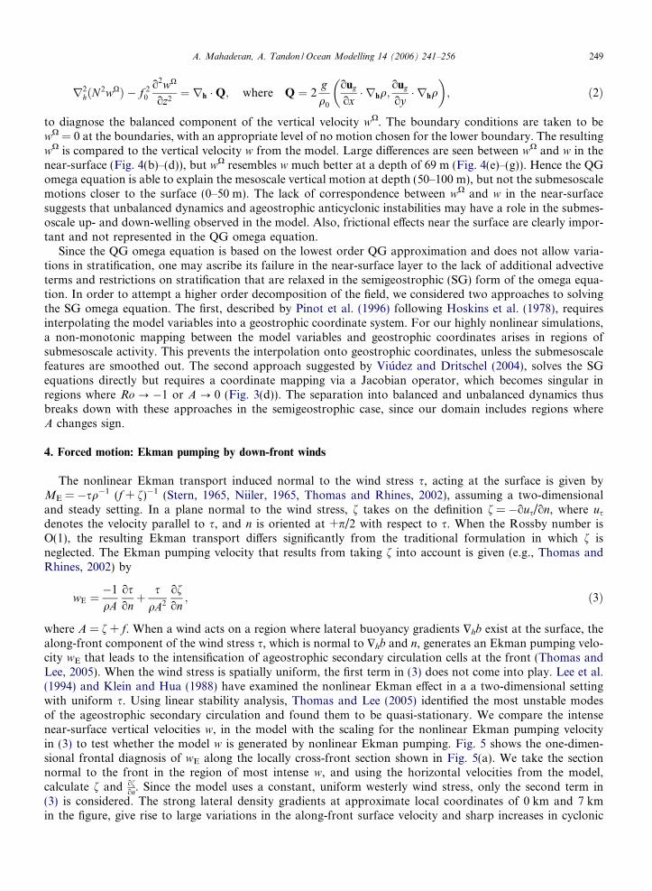
r2hðN 2wXÞ � f 2

0

o2wX

oz2¼ rh �Q; where Q ¼ 2

gq0

oug

ox� rhq;

oug

oy� rhq

� �; ð2Þ

to diagnose the balanced component of the vertical velocity wX. The boundary conditions are taken to bewX = 0 at the boundaries, with an appropriate level of no motion chosen for the lower boundary. The resultingwX is compared to the vertical velocity w from the model. Large differences are seen between wX and w in thenear-surface (Fig. 4(b)–(d)), but wX resembles w much better at a depth of 69 m (Fig. 4(e)–(g)). Hence the QGomega equation is able to explain the mesoscale vertical motion at depth (50–100 m), but not the submesoscalemotions closer to the surface (0–50 m). The lack of correspondence between wX and w in the near-surfacesuggests that unbalanced dynamics and ageostrophic anticyclonic instabilities may have a role in the submes-oscale up- and down-welling observed in the model. Also, frictional effects near the surface are clearly impor-tant and not represented in the QG omega equation.

Since the QG omega equation is based on the lowest order QG approximation and does not allow varia-tions in stratification, one may ascribe its failure in the near-surface layer to the lack of additional advectiveterms and restrictions on stratification that are relaxed in the semigeostrophic (SG) form of the omega equa-tion. In order to attempt a higher order decomposition of the field, we considered two approaches to solvingthe SG omega equation. The first, described by Pinot et al. (1996) following Hoskins et al. (1978), requiresinterpolating the model variables into a geostrophic coordinate system. For our highly nonlinear simulations,a non-monotonic mapping between the model variables and geostrophic coordinates arises in regions ofsubmesoscale activity. This prevents the interpolation onto geostrophic coordinates, unless the submesoscalefeatures are smoothed out. The second approach suggested by Viudez and Dritschel (2004), solves the SGequations directly but requires a coordinate mapping via a Jacobian operator, which becomes singular inregions where Ro ? �1 or A ? 0 (Fig. 3(d)). The separation into balanced and unbalanced dynamics thusbreaks down with these approaches in the semigeostrophic case, since our domain includes regions whereA changes sign.

4. Forced motion: Ekman pumping by down-front winds

The nonlinear Ekman transport induced normal to the wind stress s, acting at the surface is given byME = �sq�1 (f + f)�1 (Stern, 1965, Niiler, 1965, Thomas and Rhines, 2002), assuming a two-dimensionaland steady setting. In a plane normal to the wind stress, f takes on the definition f = �ous/on, where us

denotes the velocity parallel to s, and n is oriented at +p/2 with respect to s. When the Rossby number isO(1), the resulting Ekman transport differs significantly from the traditional formulation in which f isneglected. The Ekman pumping velocity that results from taking f into account is given (e.g., Thomas andRhines, 2002) by

wE ¼�1

qAosonþ s

qA2

ofon; ð3Þ

where A = f + f. When a wind acts on a region where lateral buoyancy gradients $hb exist at the surface, thealong-front component of the wind stress s, which is normal to $hb and n, generates an Ekman pumping velo-city wE that leads to the intensification of ageostrophic secondary circulation cells at the front (Thomas andLee, 2005). When the wind stress is spatially uniform, the first term in (3) does not come into play. Lee et al.(1994) and Klein and Hua (1988) have examined the nonlinear Ekman effect in a a two-dimensional settingwith uniform s. Using linear stability analysis, Thomas and Lee (2005) identified the most unstable modesof the ageostrophic secondary circulation and found them to be quasi-stationary. We compare the intensenear-surface vertical velocities w, in the model with the scaling for the nonlinear Ekman pumping velocityin (3) to test whether the model w is generated by nonlinear Ekman pumping. Fig. 5 shows the one-dimen-sional frontal diagnosis of wE along the locally cross-front section shown in Fig. 5(a). We take the sectionnormal to the front in the region of most intense w, and using the horizontal velocities from the model,calculate f and of

on. Since the model uses a constant, uniform westerly wind stress, only the second term in(3) is considered. The strong lateral density gradients at approximate local coordinates of 0 km and 7 kmin the figure, give rise to large variations in the along-front surface velocity and sharp increases in cyclonic

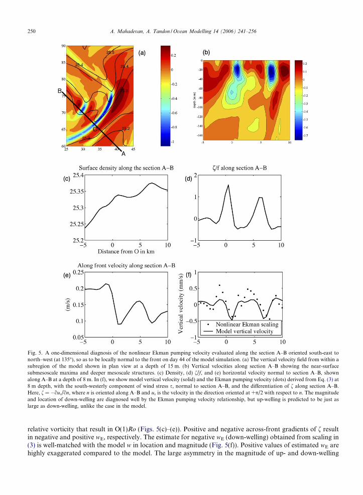
Fig. 5. A one-dimensional diagnosis of the nonlinear Ekman pumping velocity evaluated along the section A–B oriented south-east tonorth–west (at 135�), so as to be locally normal to the front on day 44 of the model simulation. (a) The vertical velocity field from within asubregion of the model shown in plan view at a depth of 15 m. (b) Vertical velocities along section A–B showing the near-surfacesubmesoscale maxima and deeper mesoscale structures. (c) Density, (d) f/f, and (e) horizontal velocity normal to section A–B, shownalong A–B at a depth of 8 m. In (f), we show model vertical velocity (solid) and the Ekman pumping velocity (dots) derived from Eq. (3) at8 m depth, with the south-westerly component of wind stress s, normal to section A–B, and the differentiation of f along section A–B.Here, f = �ous/on, where n is oriented along A–B and us is the velocity in the direction oriented at +p/2 with respect to n. The magnitudeand location of down-welling are diagnosed well by the Ekman pumping velocity relationship, but up-welling is predicted to be just aslarge as down-welling, unlike the case in the model.


relative vorticity that result in O(1)Ro (Figs. 5(c)–(e)). Positive and negative across-front gradients of f resultin negative and positive wE, respectively. The estimate for negative wE (down-welling) obtained from scaling in(3) is well-matched with the model w in location and magnitude (Fig. 5(f)). Positive values of estimated wE arehighly exaggerated compared to the model. The large asymmetry in the magnitude of up- and down-welling


seen in the model is thus not captured by the simple scaling. In this instance, the vorticity increase is sharper onthe buoyant side of the front and counter balances the decrease in wE’s magnitude due to the increase in A.Moreover, this scaling is two-dimensional and steady, and clearly does not apply when A approaches zero.

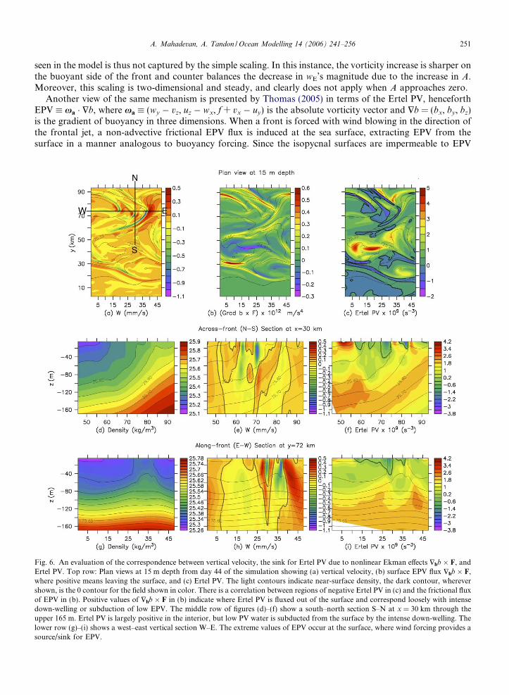
Another view of the same mechanism is presented by Thomas (2005) in terms of the Ertel PV, henceforthEPV � xa � $b, where xa � (wy � vz, uz � wx, f + vx � uy) is the absolute vorticity vector and $b = (bx, by, bz)is the gradient of buoyancy in three dimensions. When a front is forced with wind blowing in the direction ofthe frontal jet, a non-advective frictional EPV flux is induced at the sea surface, extracting EPV from thesurface in a manner analogous to buoyancy forcing. Since the isopycnal surfaces are impermeable to EPV

Fig. 6. An evaluation of the correspondence between vertical velocity, the sink for Ertel PV due to nonlinear Ekman effects $hb � F, andErtel PV. Top row: Plan views at 15 m depth from day 44 of the simulation showing (a) vertical velocity, (b) surface EPV flux $hb � F,where positive means leaving the surface, and (c) Ertel PV. The light contours indicate near-surface density, the dark contour, wherevershown, is the 0 contour for the field shown in color. There is a correlation between regions of negative Ertel PV in (c) and the frictional fluxof EPV in (b). Positive values of $hb � F in (b) indicate where Ertel PV is fluxed out of the surface and correspond loosely with intensedown-welling or subduction of low EPV. The middle row of figures (d)–(f) show a south–north section S–N at x = 30 km through theupper 165 m. Ertel PV is largely positive in the interior, but low PV water is subducted from the surface by the intense down-welling. Thelower row (g)–(i) shows a west–east vertical section W–E. The extreme values of EPV occur at the surface, where wind forcing provides asource/sink for EPV.


(Haynes and McIntyre, 1987), the extraction of EPV at the surface is accompanied by the subduction of lowEPV water and the resupply of EPV to the down-welling region through lateral convergence of fluid at thesurface. In the process, secondary circulations that scale as the surface frictional flux are set up, conveyingan advective EPV flux. The vertical component of the frictional EPV flux at the surface is given by $hb � F(Thomas, 2005), where F = oz(AVou/oz), oz(AVov/oz) is the non-conservative right hand side of the momentumequation, and is significant due to wind forcing. At the surface, z = 0, AVo(u,v)/oz = (sx,sy), where sx, sy arewind stress components acting in x and y directions. At the base of the Ekman layer z = �dE, we assume thatAVo(u,v)/oz is negligible in comparison to the surface, and hence F can be approximated asF = (Fx,Fy) = (sx,sy)/(q0dE). We take dE to be the turbulent Ekman layer depth, which is approximated asdE = 0.4u*/f, where u* = (s/q0)1/2. In our case, sx = 0.025 N m�2, and dE = 20 m.

To test whether wind is fluxing EPV out of the surface in the model, we compute the EPV and the verticalcomponent of the frictional EPV flux $hb � F. Fig. 6 shows the correspondence between the submesoscalenear-surface vertical velocities and the EPV in plan and sectional view. Regions of down-welling correspondto regions of negative EPV, while regions of up-welling correspond to positive EPV. There is also a correlationbetween low, i.e., O(1) or smaller, values of Ri in Fig. 2(f) and EPV in Fig. 6(c), suggesting that EPV is lost inregions of active mixing, which in the model, is performed through convective adjustment.

Forcing at the surface can drive EPV in or out of the surface depending on the sign of $hb � F. In regionswhere $hb � F is positive (Fig. 6(b)), EPV is lost at the surface and negative EPV water is advected downward(Fig. 6(a) and (c)). From the figures, we see that regions of positive $hb � F correspond to negative w

(although, not at the site of most intense down-welling) and a loss of EPV from the surface. This corroboratesthe idea that wind removes EPV from the surface in a manner analogous to buoyancy forcing (Thomas, 2005).The north–south section (Fig. 6(d)–(f)) shows that low EPV water subducts southward between density anom-

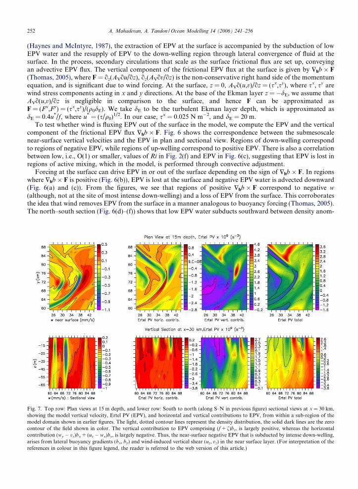
Fig. 7. Top row: Plan views at 15 m depth, and lower row: South to north (along S–N in previous figure) sectional views at x = 30 km,showing the model vertical velocity, Ertel PV (EPV), and horizontal and vertical contributions to EPV, from within a sub-region of themodel domain shown in earlier figures. The light, dotted contour lines represent the density distribution, the solid dark lines are the zerocontour of the field shown in color. The vertical contribution to EPV comprising (f + f)bz, is largely positive, whereas the horizontalcontribution (wy � vz)bx + (uz � wx)by, is largely negative. Thus, the near-surface negative EPV that is subducted by intense down-welling,arises from lateral buoyancy gradients (bx, by) and wind-induced vertical shear (uz, vz) in the near surface layer. (For interpretation of thereferences in colour in this figure legend, the reader is referred to the web version of this article.)


aly values of 25.3 and 25.4 reaching �60 m depth at x = 72 km. This is also seen in the east–west section.Fig. 6(g)–(i) show a bolus of low EPV water subducted by the intense submesoscale features, and carried fur-ther downward by the deeper down-welling that is characteristic of mesoscale meanders (and is well describedby QG dynamics). Temporal variations in EPV are neglected from these analyses.

To further ascertain the contribution to negative EPV near the surface, we plot the horizontal and verti-cal contributions to the EPV in plan and sectional views alongside the vertical velocity (Fig. 7). The EPVcontribution from the vertical component of vorticity, (f + f)bz is largely positive with small negative compo-nents near the surface. The contribution from (wy � vz)bx + (uz � wx)by, is largely negative, with small positivecomponents near the surface. The largest negative contribution to the EPV arises from the horizontal buoy-ancy gradients and vertical shear in the flow and is maximum at the surface where wind generated shear andlateral buoyancy gradients are most intense. This creates negative EPV at the surface, which can be subductedby intense submesoscale velocities.

5. Summary and discussion

Submesoscales have received relatively little attention until recently because they are notoriously difficult toobserve and model. Their presence has become evident through high frequency sampling from towed instru-ment platforms, high resolution measurements of fluorescence and temperature, high resolution modeling, andtheoretical studies such as those cited above. In this paper, we have analyzed the near-surface submesoscalestructure and intense vertical velocities that emerge in a three-dimensional, nonhydrostatic model of an upperocean front forced with down-front winds.

Several candidate mechanisms that can generate vertical motion or submesoscale structure are examined. Inthree-dimensions, we find that a combination of the mechanisms is necessary to explain the submesoscalestructure seen in the model. Baroclinic instability leads to meanders, meanders lead to regions of strain andvorticity; strain generates vertical motion by frontogenesis, vorticity generates non-linear feedback via theEkman effect which relies on friction and wind forcing to intensify up- and down-welling. Within submeso-scale regions the flow field also satisfies the conditions for loss of balance that make a forward energy cascadepossible.

The features that develop in our wind-forced model simulations at a horizontal grid resolution of 500 m arefiner in scale and different in character from the frontal up- and down-welling described in the modeling studyof Levy et al. (2001) using a horizontal grid resolution of 2 km. In the our model, wind plays a critical role ininducing submesoscale structure. The model domain is not large enough to allow the formation and interac-tion of multiple eddies, which would lead to a more developed strain field. It is conceivable that in such sit-uations submesoscale structure might emerge through some of the mechanisms addressed here, even whenwind is weak or absent. Processes such as frontal adjustment are also known to generate submesoscales(Fox-Kemper et al., 2006). Based on our analyses, it seems that the submesoscale structure in the model’s flowis dominated by wind. MLI and AAI are thought not to be as dominant, most likely due to the overpoweringeffect of wind forcing. Conditions in the developed flow field support the generation of AAI, but not MLI.However, we lack a systematic way of identifying the developed forms of AAI and MLI and may be glossingover them as a result.

Thomas and Lee (2005) show that the semigeostrophic Eliassen-Sawyer operator changes character fromelliptic to hyperbolic as the EPV changes sign from positive to negative. The hyperbolic nature of the solutionallows secondary circulation cells, with sub-surface maxima. The elliptic solutions decay away from theboundary. In the hyperbolic region, the solution to the linear stability problem is non-unique, and any ofan infinite number of unstable wavenumbers can be selected. The surface boundary condition on verticalvelocity or surface vorticity picks out the scale and the growth rate of the mode for areas with positiveEPV, whereas the nonlinear evolution selects the scale for hyperbolic cases, as seen in the the two-dimensionalnonhydrostatic simulations of Thomas and Lee (2005). Additionally, in the two-dimensional case, the basicstate considered has either positive EPV or negative EPV throughout the mixed layer, and the nature ofthe mathematical operator remains the same.

In the three dimensional simulations considered here, the situation is more complex. EPV does not have thesame sign throughout the region, so the nature of the operator changes from elliptic to hyperbolic in isolated


regions in both the horizontal and vertical. Mathematically, the local quasi-2d SG operator becomes singularwhen the EPV is zero, though it is well behaved with either sign. The SG approximation therefore breaksdown, as mentioned earlier.

We can still understand the solutions in the quasi-2d sense if we align ourselves locally with the along-frontal and across frontal direction. The down-welling regions are the regions of negative EPV (Fig. 7),and the quasi-2d SG operator is hyperbolic in these regions, i.e., secondary cells with sub-surface velocity max-ima appear, as expected. The up-welling regions in the solutions turn out to be regions with positive EPV(Fig. 7), and the quasi-2d SG operator is elliptic there, i.e., the vertical velocity decays as depth increases.The hyperbolic nature of negative EPV regions necessitates that down-welling is stronger than up-welling,which is associated with regions of elliptic character that are also broader.

It is interesting that the up-/down-welling features that are characteristically associated with mesoscales(deeper than 50 m in our simulations) can link with the intense down-welling zones generated at submesoscales(see Fig. 5(b)), providing an advective path for subduction of low EPV water into the relatively quiescentdeeper waters. Further analyses are needed to quantify the net effect of submesoscale to mesoscale couplingon the vertical transport of tracers and nutrients.

Since lateral buoyancy gradients and wind are ubiquitous to the oceans, submesoscale motions may be widelyprevalent in the near-surface ocean. An observational strategy needs to be developed in order to ascertain theexistence and nature of such motion. A better understanding of the phenomenon and its controlling parameterswould be helpful; several questions still remain to be answered in this regard. For example: What determines themagnitude of the vertical velocities? Is the length scale of the submesoscale structures determinable from the lin-earized equations, or is it dependent on the nonlinear advective terms indicating the beginning of a forwardenergy cascade? Though the vertical motion discussed here is advective, it would generate large variations inlateral gradients and hence facilitate diapycnal mixing. Hence, we would like to ask what effect such motionsmight have on mixing and transport. Further, how does the submesoscale-mesoscale link affect the net verticaltransport of nutrients and tracers? What are the cumulative rates of exchange that can be achieved between thesurface and subsurface ocean through these features? Understanding the mechanism that underlies thesemotions is only the first step. It is of further interest to assess their implications and parameterize them.

Acknowledgements

We thank Leif Thomas for helpful suggestions and feedback, and James McWilliams and Baylor Fox-Kem-per for insightful discussions. A.T. acknowledges support from NSF-OCE-0336786. A.M. acknowledgesNOAA.

Appendix A. Model initialization

The model is set up in a west-to-east (W–E) periodic channel domain extending 48 km in the W–E (peri-odic) direction, 96 km in the south-to-north (S–N) direction, and centered at a latitude of 25�N. Impermeablevertical walls form the S and N boundaries of the domain and a flat bottom forms the lower boundary at800 m. The domain is initialized with a sharp lateral S–N density gradient in the upper layers, such thatthe southern half of the domain has lighter water. This front, extending to a depth of 250 m, is representativeof deep, semi-permanent fronts in the ocean. The vertical stratification is prescribed from a spline fit to anobserved profile. The pycnocline, which is characterized by an approximate buoyancy frequencyN = 0.7 � 10�2 s�1, extends to about 250 m. It overlies a weakly stratified region and a nearly homogeneousdeeper layer. A S–N density variation, Dq is then superimposed on this vertical stratification. In the upper50 m Dq = 0.3 kg m�3, between 50 and 250 m Dq = 0.3(250 � z)/200 kg m�3, where z is the depth in m,and below 250 m, there is no horizontal density variation. The density variation in the S–N direction is dis-tributed according to (±Dq/2)(1 � exp(�yc/2))/(1 + exp(�yc/2)), where yc is the distance in km from the cen-ter (Northward positive), and the ± signs are used according as yc is positive or negative. The sea surfaceelevation is varied correspondingly over the same frontal region by 3.2 cm, being higher in the southernregion. Associated with the S–N density front is an W–E geostrophic jet. The model velocities and nonhyd-rostaic pressure are initialized to be in geostrophic balance as described in Mahadevan (2006).


References

Bacastow, R., Maier-Reimer, E., 1991. Dissolved organic carbon in modeling oceanic new production. Global Biogeochemical Cycles 5,71–86.

Bluestein, H.B., 1993. Synoptic-Dynamic Meteorology in Midlatitudes. Observations and Theory of Weather Systems, vol. 2. OxfordUniversity Press, USA.

Capet, X., McWilliams, J.C., Molemaker, J., Shchepetkin, A., 2006. Mixed-layer instabilities in an upwelling system: Mechanisms andimplications for the upper ocean dynamics. Eos Trans. AGU 87 (36), Ocean Sci. Meet. Suppl., Abstract OS23F-05.

Emerson, S., Quay, P., Karl, D., Winn, C., Tupas, L., Landry, M., 1997. Experimental determination of the organic carbon flux fromopen-ocean surface waters. Nature 389, 951–954.

Fox-Kemper, B., Ferrari, R., Hallberg, R.W., 2006. Modeling and parameterizing mixed layer eddies. Eos Trans. AGU 87 (36), Ocean Sci.Meet. Suppl., Abstract OS23F-06.

Garrett, C.J.R., Loder, J.W., 1981. Dynamical aspects of shallow sea fronts. Philosophical Transactions of the Royal Society of LondonSeries A 302, 563–581.

Haynes, P.H., McIntyre, M.E., 1987. On the evolution of vorticity and potential vorticity in the presence of diabatic heating and frictionalor other forces. Journal of the Atmospheric Sciences 44, 828–841.

Hoskins, B.J., Bretherton, Francis P., 1972. Atmospheric frontogenesis models: Mathematical formulation and solution. Journal of theAtmospheric Sciences 29 (6439), 11–37.

Hoskins, B.J., Draghici, I., Davies, H.C., 1978. A new look at the x-equation. Quarterly Journal of the Royal Meteorological Society 104,31–38.

Jenkins, W.J., 1988. Nitrate flux into the euphotic zone near Bermuda. Nature 331, 521–523.Jenkins, W.J., Goldman, J.C., 1985. Seasonal oxygen cycling and primary production in the Sargasso Sea. Journal of Marine Research 43,

465–491.Klein, P., Hua, B.L., 1988. Mesoscale heterogeneity of the wind-driven mixed layer: Influence of a quasigeostrophic flow. Journal of

Marine Research 46, 495–525.Lee, D., Niiler, P., Warn-Varnas, A., Piacsek, S., 1994. Wind-driven secondary circulation in ocean mesoscale. Journal of Marine

Research 52, 371–396.Levy, M., Klein, P., Treguier, A.-M., 2001. Impacts of sub-mesoscale physics on production and subduction of phytoplankton in an

oligotrophic regime. Journal of Marine Research 59, 535–565.Mahadevan, A., 2006. Modeling vertical motion at ocean fronts: Are nonhydrostatic effects relevant at submesoscales? Ocean Modelling

14 (3–4), 222–240.Mahadevan, A., Archer, D., 2000. Modeling the impact of fronts and mesoscale circulation on the nutrient supply and biogeochemistry of

the upper ocean. Journal of Geophysical Research 105 (C1), 1209–1225.Maier-Reimer, E., 1993. Geochemical cycles in an ocean general circulation model. Global Biogeochemical Cycles 7, 645–678.Martin, A.P., Pondaven, P., 2003. On estimates for the vertical nitrate flux due to eddy-pumping. Journal of Geophysical Research 108

(C11), 3359. doi:10.1029/2003JC001841.McGillicuddy Jr., D.J., Robinson, A.R., 1997. Eddy induced nutrient supply and new production in the Sargasso Sea. Deep Sea Research,

Part I 44 (8), 1427–1450.McGillicuddy Jr., D.J., Robinson, A.R., Siegel, D.A., Jannasch, H.W., Johnson, R., Dickey, T.D., McNeil, J., Michaels, A.F., Knap,

A.H., 1998. Influence of mesoscale eddies on new production in the Sargasso Sea. Nature 394, 263–266.McWilliams, J.C., 2003. Diagnostic force balance and its limits Nonlinear Processes in Geophysical Fluid Dynamics. Kluwer Academic

Publishers, pp. 287–304.McWilliams, J.C., Molemaker, M.J., Yavneh, I., 2001. From stirring to mixing of momentum: Cascades from balanced flows to

dissipation in the oceanic interior. Proceedings of the 12th ‘Aha Huliko’a Hawaiian Winter Workshop. SOEST, University of Hawaii,pp. 59–66.

McWilliams, J.C., Molemaker, M.J., Yavneh, I., 2004. Ageostrophic, anticyclonic instability of a geostrophic barotropic boundarycurrent. Physics of fluids 16 (10), 3720–3725.

Molemaker, M.J., McWilliams, J.C., Yavneh, I., 2001. Instability and equilibration of centrifugally-stable stratified Taylor–Couette flow.Physical Review Letters 23, 5270–5273.

Molemaker, M.J., McWilliams, J.C., Yavneh, I., 2005. Baroclinic instability and loss of balance. Journal of Physical Oceanography 35 (9),1505–1517.

Najjar, R.G., 1990. Simulations of the phosphorus and oxygen cycles in the world ocean using a general circulation model. Ph.D. thesis,Princeton University.

Najjar, R.G., Sarmiento, J.L., Toggweiler, J.R., 1992. Downward transport and fate of organic matter in the ocean: Simulations with ageneral circulation model. Global Biogeochemical Cycles 6, 45–76.

Niiler, P., 1965. On the Ekman divergence in an oceanic jet. Journal of Geophysical Research 74, 7048–7052.Oschlies, A., 2002. Can eddies make ocean deserts bloom? Global Biogeochemical Cycles 16, 1106. doi:10.1029/2001GB001830.Pedlosky, Joseph., 1987. Geophysical Fluid Dynamics, second ed. Springer-Verlag.Pinot, J.-M., Tintore, J., Wang, D.-P., 1996. A study of the omega equation for diagnosing vertical motions at ocean fronts. Journal of

Marine Research 54, 239–259.Platt, Trevor., Harrison, William G., 1985. Biogenic fluxes of carbon and oxygen in the ocean. Nature 318, 55–58.Pollard, R.T., Regier, L., 1990. Large variations in potential vorticity at small spatial scales in the upper ocean. Nature 348, 227–229.

http://dx.doi.org/10.1029/2003JC001841

http://dx.doi.org/10.1029/2001GB001830


Pollard, R.T., Regier, L.A., 1992. Vorticity and vertical circulation at an ocean front. Journal of Physical Oceanography 22, 609–625.Rudnick, Daniel L., 1996. Intensive surveys of the Azores front. Part II: Inferring the geostrophic and vertical velocity fields. Journal of

Geophysical Research 101 (C7), 16291–16303.Shearman, R.K., Barth, J.M., Kosro, P.M., 1999. Diagnosis of three-dimensional circulation associated with mesoscale motion in the

California current. Journal of Physical Oceanography 29, 651–670.Stern, M.E., 1965. Interaction of a uniform wind stress with a geostrophic vortex. Deep Sea Research 12, 355–367.Stone, P.H., 1970. On non-geostrophic baroclinic stability: Part II. Journal of the Atmospheric Sciences 27, 721–727.Tandon, A., Zhao, L., 2004. Mixed layer transformation for the North Atlantic for 1990–2000. Journal of Geophysical Research 109.

doi:10.1029/2003JC002059.Thomas, L.N., 2005. Destruction of potential vorticity by winds. Journal of Physical Oceanography 35, 2457–2466.Thomas, L.N., Lee, C.M., 2005. Intensification of ocean fronts by down-front winds. Journal of Physical Oceanography 35, 1086–1102.Thomas, L.N., Rhines, P.B., 2002. Nonlinear stratified spin up. Journal of Fluid Mechanics 473, 211–244.Thompson, L., 2000. Ekman layers and two-dimensional frontogenesis in the upper ocean. Journal of Geophysical Research 105, 6437–

6451.Ullman, D.S., Cornillon, P.C., 1999. Satellite-derived sea surface temperature fronts on the continental shelf of the northeast US coast.

Journal of Geophysical Research 104 (C10), 23459–23478.Viudez, A., Dritschel, D.G., 2004. Potential vorticity and the quasigeostrophic and semigeostrophic mesoscale vertical velocity. Journal of

Physical Oceanography 34, 865–887.Voorhis, A.D., Bruce, J.G., 1982. Small-scale surface stirring and frontogenesis in the subtropical convergence of the western North

Atlantic. Journal of Marine Research 40 (Suppl.), 801–821.

http://dx.doi.org/10.1029/2003JC002059

an analysis of mechanisms for submesoscale vertical motion at ocean fronts

Documents