an algebraic approach - automata learning - arxiv
TRANSCRIPT
arX
iv:1
911.
0087
4v3
[cs
.FL
] 2
8 A
ug 2
020
Automata Learning: An Algebraic Approach
Henning Urbat∗
Friedrich-Alexander-Universität Erlangen-NürnbergErlangen, Germany
Lutz Schröder∗
Friedrich-Alexander-Universität Erlangen-NürnbergErlangen, Germany
Abstract
We propose a generic categorical framework for learningunknown formal languages of various types (e.g. finite orinfinite words, weighted and nominal languages). Our ap-proach is parametric in a monad T that represents the giventype of languages and their recognizing algebraic struc-tures. Using the concept of an automata presentation ofT-algebras, we demonstrate that the task of learning a T-recognizable language can be reduced to learning an ab-stract form of algebraic automaton whose transitions aremodeled by a functor. For the important case of adjointautomata, we devise a learning algorithm generalizing An-gluin’s L∗. The algorithm is phrased in terms of categoricallydescribed extension steps; we provide for a termination andcomplexity analysis based on a dedicated notion of finite-ness. Our framework applies to structures likeω-regular lan-guages that were not within the scope of existing categori-cal accounts of automata learning. In addition, it yields newlearning algorithms for several types of languages for whichno such algorithms were previously known at all, includ-ing sorted languages, nominal languages with name bind-ing, and cost functions.
Keywords Automata Learning, Monads, Algebras
1 Introduction
Active automata learning is the task of inferring a finiterepresentation of an unknown formal language by askingquestions to a teacher. Such learning situations naturallyarise, e.g., in software verification, where the “teacher” issome reactive system and one aims to construct a formalmodel of it by running suitable tests [61]. Starting with An-gluin’s [8] pioneering work on learning regular languages,active learning algorithms have been developed for count-less types of systems and languages, including ω-regularlanguages [9, 32], tree languages [30], weighted languages[12, 63], and nominal languages [47]. Most of these exten-sions are tailor-made modifications of Angluin’s L∗ algo-rithm and thus bear close structural analogies. This has mo-tivated recent work towards a uniform category theoreticunderstanding of automata learning, based on modellingstate-based systems as coalgebras [14, 65]. In the present
∗The authors acknowledge support by Deutsche Forschungsgemeinschaft(DFG) under project SCHR 1118/8-2.
, ,
.
paper, we propose a novel algebraic approach to automatalearning.Our contributions are two-fold. First, we study the prob-
lem of learning an abstract form of automata originally in-troduced by Arbib and Manes [10] in the context of mini-mization: given an endofunctor F on a category D and ob-jects I ,O ∈ D , an F -automaton consists of an object Q ofstates and morphisms δQ , iQ and fQ as shown below, repre-senting transitions, initial states and final states (or outputs).
FQ
δQ��
IiQ
// QfQ
// O
Taking FQ = Σ ×Q on Set with I = 1 and O = {0, 1} yieldsclassical deterministic automata, but also several other no-tions of automata (e.g. weighted automata, residual nonde-terministic automata, and nominal automata) arise as in-stances. As our first main result, we devise a generalizedL∗ algorithm for adjoint F -automata, i.e. automata whosetype functor F admits a right adjoint G , based on alternat-ing moves along the initial chain for the functor I + F andthe final cochain for the functor O × G . Our generic algo-rithm subsumes known L∗-type algorithms for all the aboveclasses of automata, and its analysis yields uniform proofs oftheir correctness and termination. In addition, it also instan-tiates to a number of new learning algorithms, e.g. for sortedautomata and for several versions of nominal automata withname binding.We subsequently show that learning algorithms for F -
automata (including our generalized L∗ algorithm) apply farbeyond the realm of automata: they can be used to learnlanguages representable by monads [7, 59]. Given a monadT on the category D , we model a language as a morphismL : TI → O in D . At this level of generality, one obtainsa concept of T-recognizable language (i.e. a language recog-nized by a finite T-algebra) that uniformly captures numer-ous automata-theoretic classes of languages. For instance,regular andω-regular languages (the languages accepted byclassical finite automata and Büchi automata, respectively)correspond precisely to T-recognizable languages for themonads representing semigroups and Wilke algebras,
TI = I+ on Set and T(I , J ) = (I+, Iup + I ∗ × J ) on Set2.
Here Iup denotes the set of ultimately periodic infinite wordsover the alphabet I . For ω-regular languages, Farzan et al.
1
, , Henning Urbat and Lutz Schröder
[32] proposed an algorithm that learns a language L ⊆ Iω
of infinite words by learning the set of lassos in L, i.e. theregular language of finite words given by
lasso(L) = {u$v : u ∈ I ∗,v ∈ I+,uvω ∈ L } ⊆ (I + {$})∗.
We show that this idea extends to general T-recognizablelanguages, using the concept of an automata presenta-
tion. Such a presentation allows for the linearization of T-recognizable languages, i.e. a reduction to “regular” lan-guages accepted by finite F -automata for suitable F .In combination, our results yield a generic strategy for
learning an unknown T-recognizable language L : TI → O :(1) find an automata presentation for the free T-algebraTI ;(2) learn the minimal automaton for the linearization of L.This approach turns out to be applicable to a wide range oflanguages. In particular, it covers several settings for whichno learning algorithms are known, e.g. cost functions [23].
Related work. A categorical interpretation of several keyconcepts in Angluin’s L∗ algorithm for classical automatawas first given by Jacobs and Silva [37], and later extendedto F -automata in a category, i.e. to similar generality as inthe present paper, by van Heerdt, Sammartino, and Silva[64]. Their main contribution is an abstract categoricalframework (CALF) for correctness proofs of learning algo-rithms, while a concrete generic algorithm is not given. VanHeerdt et al. [65] also study learning automata with side ef-fects modelled via monads; this use of monads is unrelatedto the monad-based abstraction of algebraic recognition inthe present paper. Barlocco, Kupke, and Rot [14] developa learning algorithm for set coalgebras (with all underlyingconcepts phrased categorically), parametric in a coalgebraiclogic. Its scope is quite different from our generalized L∗ al-gorithm: via genericity over the branching type it covers,e.g., labeled transition systems, but unlike our algorithm itdoes not apply to, e.g., nominal automata. The connectionsbetween the two approaches are further discussed in Re-mark 4.16.Automata learning can be seen as an interactive ver-
sion of automata minimization, which has been extensivelystudied from a (co-)algebraic perspective [5, 10, 16, 24, 35,63]. In particular, our chain-based iterative learning algo-rithm resembles the coalgebraic approach to partition re-finement [1].
2 Preliminaries
We proceed to recall concepts from category theory andthe theory of nominal sets that we will use throughoutthe paper. Readers should be familiar with basic notionssuch as functors, (co-)limits and adjunctions; see, e.g., MacLane [41].
Functor (co-)algebras. Let H : D → D be an endofunctoron a category D . An H -algebra is a pair (A,α) consisting of
an object A ∈ D and a morphism α : HA→ A. A homomor-
phismh : (A,α) → (B, β) betweenH -algebras is a morphismh : A → B such that h · α = β · Fh. An H -algebra (A,α) isinitial if for every H -algebra (B, β) there is a unique homo-morphism (A,α) → (B, β); we generally denote the initialalgebra of H (unique up to isomorphism if it exists) as µH .IfD is cocomplete andH preserves filtered colimits, µH canbe constructed as the colimit of the initial ω-chain forH [6]:
µH = colim( 0¡−→ H0
H ¡−−→ H 20
H 2¡−−−→ H 30→ · · · ),
where ¡ is the unique morphism from the initial object 0of D into H0, and Hn means H applied n times. Lettingjn : Hn0 → µH (n ∈ N) denote the colimit cocone, we ob-tain theH -algebra structure on µH as the unique morphismα : H (µH ) → µH satisfying
α · Hjn = jn+1 for all n ∈ N.
Dually, one has notions of a coalgebra for the endofunctorH , a coalgebra homomorphism, and a final coalgebra. Coal-gebras provide an abstract notion of state-based transitionsystem: We think of the base object A of an H -coalgebra asan object of states, and of its structure map α : A→ HA asassigning to each state a structured collection of successors.Coalgebra homomorphisms are behaviour-preserving maps,and final coalgebras have abstracted behaviours as states.
Monad algebras. A monad T = (T , µ,η) on a category D
is given by an endofunctor T : D → D and two naturaltransformations η : IdD → T and µ : TT → T (the unit andmultiplication) such that the following diagrams commute:
TTTT µ
//
µT��
TTµ��
TTµ
// T
TTη
//
■■■■
■■■
■■■■
■■■ TT
µ��
TηT
oo
✉✉✉✉✉✉✉
✉✉✉✉✉✉✉
T
A T-algebra is an algebra (A,α) for the endofunctor T forwhich the following diagrams commute:
TTAµA
//
T�
TA
�
TAα
// A
A
■■■■
■■■
■■■■
■■■
ηA// TA
�
A
A homomorphism of T-algebras is just a homomorphism ofthe underlying T -algebras. For each X ∈ D , the T-algebraTX = (TX , µX ) is called the free T-algebra on X .
Monads form a categorical abstraction of algebraic theo-ries [43]. In fact, every algebraic theory (given by a finitarysignature Γ and a set E of equations between Γ-terms) in-duces of monad T on Set where TX is the underlying set ofthe free (Γ, E)-algebra on X (i.e. the set of all Γ-terms overX modulo equations in E), and the maps ηX : X → TX andµX : TTX → TX are given by inclusion of variables and
2
Automata Learning: An Algebraic Approach , ,
flattening of terms, respectively. Then the categories of T-algebras and (Γ, E)-algebras are isomorphic. Conversely, ev-erymonadT on SetwithT preserving filtered colimits arisesfrom some algebraic theory (Γ, E) in this way.Similarly, every ordered algebraic theory [17], given by
a signature Γ and a set E of inequations s ≤ t between Γ-terms, yields amonadT on the categoryPos of posets whosealgebras are ordered Γ-algebras (i.e. Γ-algebras on a posetwith monotone operations) satisfying the inequations in E.
Free monads. Let H : D → D be an endofunctor on acategory D with coproducts, and suppose that, for eachX ∈ D , the initial algebra µ(X + H ) for the functor X +H exists. Then H induces a monad TH , the free monad
over H [15]. It is given on objects by THX = µ(X + H ); itsaction on morphisms and the unit and multiplication aredefined via initiality of the algebras µ(X +H ). Then the cat-egories of TH -algebras and H -algebras are isomorphic: If
B+H (THB)[iB,αB ]−−−−−→ THB denotes the B+H -algebra structure
ofTHB = µ(B +H ), the isomorphism is given on objects by
(THBβ−→ B) 7→ (HB
HiB−−−→ H (THB)
αB−−→ THB
β−→ B)
and on morphisms by h 7→ h.
Factorization systems. A factorization system (E,M) in acategory D is given by two classes E andM of morphismssuch that (i) E and M are closed under composition andcontain all isomorphisms, (ii) every morphism f has a fac-torization f = m · e with e ∈ E and m ∈ M, and (iii) thediagonal fill-in property holds: given a commutative squarem · f = д · e with e ∈ E andm ∈ M, there exists a uniquemorphism d with f = d · e and д = m · d . The morphismsm and e in (i) are unique up to isomorphism and are calledthe image and coimage of f . Categories of (co-)algebras typ-ically inherit factorizations from their underlying category:(1) If H : D → D is an endofunctor with H (E) ⊆ E, thefactorization system (E,M) forD lifts to the category ofH -algebras, that is, every H -algebra homomorphism uniquelyfactorizes into a homomorphism in E followed by a homo-morphism inM. Dually, if H (M) ⊆ M, then the categoryof H -coalgebras has a factorization system lifting (E,M).(2) If T is a monad on D with T (E) ⊆ E, the factorizationsystem (E,M) for D lifts to the category of T-algebras.A factorization system (E,M) is proper if every morphismin E is epic and every morphism in M is monic. When-ever a proper factorization system (E,M) is fixed, quo-tients and subobjects in D are represented by morphismsin E andM, respectively. In particular, in the situation of(1) and (2) above, we represent quotient (co-)algebras andsub(co-)algebras by homomorphisms in E and M, respec-tively.
Closed categories. A symmetric monoidal category is a cat-egory D equipped with a functor ⊗ : D × D → D (tensor
product), an object ID ∈ D (tensor unit), and isomorphisms
(X⊗Y )⊗Z � X⊗(Y⊗Z ), X⊗Y � Y⊗X , ID⊗X � X � X⊗ID ,
natural in X ,Y ,Z ∈ D , satisfying coherence laws [41, Chap-ter VII].D is closed if the endofunctorX ⊗ (−) : D → D hasa right adjoint (denoted by [X ,−]) for everyX ∈ D , i.e. thereis a natural isomorphism D(X ⊗ Y ,Z ) � D(Y , [X ,Z ]).
Nominal sets. Fix a countably infinite set A of names, andlet Perm(A) be the group of all permutations π : A→ Awithπ (a) = a for all but finitely many a. A nominal set [51] is asetX with a group action · : Perm(A)×X → X subject to thefollowing property: for each x ∈ X there is a finite set S ⊆ A
(a support of x ) such that every π ∈ Perm(A) that leaves allelements of S fixed satisfies π ·x = x . This implies that x hasa least support supp(x) ⊆ A. The idea is that x is a syntacticobject with bound and free variables (e.g. a λ-term moduloα-equivalence), and that supp(x) is its set of free variables.A nominal set X is orbit-finite if the number of orbits (i.e.equivalence classes of the relation x ≡ y iff x = π · y forsome π ) is finite. A map f : X → Y between nominal sets isequivariant if f (π ·x) = π · f (x) for x ∈ X and π ∈ Perm(A).
3 Automata in a Category
We next develop the abstract categorical notion of automa-ton that underlies our generic learning algorithm.
Notation 3.1. For the rest of this paper, let us fix(1) a categoryD with a proper factorization system (E,M),(2) an endofunctor F : D → D , and(3) two objects I ,O ∈ D .
Definition 3.2 (Automaton (cf. [5, 10])). An (F -)automaton
is given by an objectQ ∈ D of states and three morphisms
δQ : FQ → Q, iQ : I → Q, fQ : Q → O,
representing transitions, initial states, and final states (oroutputs), respectively. A homomorphism between automata(Q, δQ , iQ , fQ ) and (Q ′, δQ ′, iQ ′, fQ ′) is a morphism h : Q →Q ′ in D such that the following diagrams commute:
FQδQ
//
Fh��
Q
h��
FQ ′δQ′
// Q ′
IiQ
//
iQ′ ##❋❋❋
❋❋❋❋ Q
h��
fQ// O
Q ′fQ′
;;✇✇✇✇✇✇
Example 3.3 (Σ-automata). Suppose that (D , ⊗, ID ) is asymmetric monoidal closed category. Choosing the data
F = Σ ⊗ (−), I = ID , and O ∈ D (arbitrary)
for a fixed input alphabet Σ ∈ D yields Goguen’s notionof a Σ-automaton [35]. In our applications, we shall workwith the categories Set (sets and functions), Pos (posets andmonotone maps), JSL (join-semilattices with ⊥ and semilat-tice homomorphisms preserving ⊥), K-Vec (vector spacesover field K and linear maps) and Nom (nominal sets andequivariant maps). The factorization systems and monoidal
3
, , Henning Urbat and Lutz Schröder
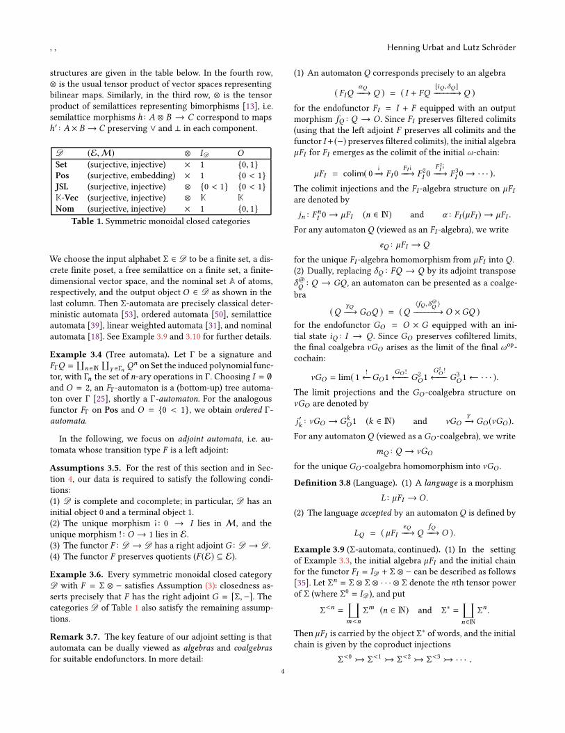
structures are given in the table below. In the fourth row,⊗ is the usual tensor product of vector spaces representingbilinear maps. Similarly, in the third row, ⊗ is the tensorproduct of semilattices representing bimorphisms [13], i.e.semilattice morphisms h : A ⊗ B → C correspond to mapsh′ : A × B → C preserving ∨ and ⊥ in each component.
D (E,M) ⊗ ID O
Set (surjective, injective) × 1 {0, 1}Pos (surjective, embedding) × 1 {0 < 1}JSL (surjective, injective) ⊗ {0 < 1} {0 < 1}K-Vec (surjective, injective) ⊗ K K
Nom (surjective, injective) × 1 {0, 1}
Table 1. Symmetric monoidal closed categories
We choose the input alphabet Σ ∈ D to be a finite set, a dis-crete finite poset, a free semilattice on a finite set, a finite-dimensional vector space, and the nominal set A of atoms,respectively, and the output object O ∈ D as shown in thelast column. Then Σ-automata are precisely classical deter-ministic automata [53], ordered automata [50], semilatticeautomata [39], linear weighted automata [31], and nominalautomata [18]. See Example 3.9 and 3.10 for further details.
Example 3.4 (Tree automata). Let Γ be a signature andFΓQ =
∐
n∈N
∐
γ ∈Γn Qn on Set the induced polynomial func-
tor, with Γn the set of n-ary operations in Γ. Choosing I = ∅and O = 2, an FΓ-automaton is a (bottom-up) tree automa-ton over Γ [25], shortly a Γ-automaton. For the analogousfunctor FΓ on Pos and O = {0 < 1}, we obtain ordered Γ-
automata.
In the following, we focus on adjoint automata, i.e. au-tomata whose transition type F is a left adjoint:
Assumptions 3.5. For the rest of this section and in Sec-tion 4, our data is required to satisfy the following condi-tions:(1) D is complete and cocomplete; in particular, D has aninitial object 0 and a terminal object 1.(2) The unique morphism ¡ : 0 → I lies in M, and theunique morphism ! : O → 1 lies in E.(3) The functor F : D → D has a right adjoint G : D → D .(4) The functor F preserves quotients (F (E) ⊆ E).
Example 3.6. Every symmetric monoidal closed categoryD with F = Σ ⊗ − satisfies Assumption (3): closedness as-serts precisely that F has the right adjoint G = [Σ,−]. Thecategories D of Table 1 also satisfy the remaining assump-tions.
Remark 3.7. The key feature of our adjoint setting is thatautomata can be dually viewed as algebras and coalgebras
for suitable endofunctors. In more detail:
(1) An automaton Q corresponds precisely to an algebra
( FIQαQ−−→ Q ) = ( I + FQ
[iQ ,δQ ]−−−−−−→ Q )
for the endofunctor FI = I + F equipped with an outputmorphism fQ : Q → O . Since FI preserves filtered colimits(using that the left adjoint F preserves all colimits and thefunctor I+(−) preserves filtered colimits), the initial algebraµFI for FI emerges as the colimit of the initial ω-chain:
µFI = colim( 0¡−→ FI0
FI ¡−−→ F 2I 0
F 2I¡
−−→ F 3I 0→ · · · ).
The colimit injections and the FI -algebra structure on µFIare denoted by
jn : FnI 0→ µFI (n ∈ N) and α : FI (µFI ) → µFI .
For any automaton Q (viewed as an FI -algebra), we write
eQ : µFI → Q
for the unique FI -algebra homomorphism from µFI into Q .(2) Dually, replacing δQ : FQ → Q by its adjoint transposeδ@Q: Q → GQ , an automaton can be presented as a coalge-
bra
(QγQ−−→ GOQ ) = (Q
〈fQ ,δ@Q〉
−−−−−−→ O ×GQ )
for the endofunctor GO = O × G equipped with an ini-tial state iQ : I → Q . Since GO preserves cofiltered limits,the final coalgebra νGO arises as the limit of the final ωop-cochain:
νGO = lim( 1!←− GO1
GO !←−−− G2
O1G2O !←−−− G3
O1← · · · ).
The limit projections and the GO -coalgebra structure onνGO are denoted by
j ′k : νGO → GkO1 (k ∈ N) and νGO
γ−→ GO (νGO ).
For any automatonQ (viewed as a GO -coalgebra), we write
mQ : Q → νGO
for the unique GO -coalgebra homomorphism into νGO .
Definition 3.8 (Language). (1) A language is a morphism
L : µFI → O .
(2) The language accepted by an automatonQ is defined by
LQ = ( µFIeQ−−→ Q
fQ−−→ O ).
Example 3.9 (Σ-automata, continued). (1) In the settingof Example 3.3, the initial algebra µFI and the initial chainfor the functor FI = ID + Σ ⊗ − can be described as follows[35]. Let Σn = Σ ⊗ Σ ⊗ · · · ⊗ Σ denote the nth tensor powerof Σ (where Σ0
= ID ), and put
Σ<n=
∐
m<n
Σm (n ∈ N) and Σ
∗=
∐
n∈N
Σn.
Then µFI is carried by the object Σ∗ of words, and the initialchain is given by the coproduct injections
Σ<0 Σ
<1 Σ
<2 Σ
<3 · · · .
4
Automata Learning: An Algebraic Approach , ,
(2) For the functorGO = O × [Σ,−] the final coalgebra νGO
is carried by the object [Σ∗,O] of languages and we have thefinal cochain
[Σ<0,O] ← [Σ<1
,O] ← [Σ<2,O] ← [Σ<3
,O] ← · · ·
with connectingmorphisms given by restriction. To see this,consider the contravariant functor P = [−,O] : D → Dop.It is not difficult to verify that P is a left adjoint (with rightadjoint Pop) and that there is a natural isomorphism
PFI � Gop
OP .
If Alg FI and CoalgGO denote the categories of FI -algebrasand GO -coalgebras, it follows [36, Theorem 2.4] that P liftsto a left adjoint P : Alg FI → (CoalgGO )
op given by
( FIQαQ−−→ Q ) 7→ ( PQ
PαQ−−−→ PFIQ � GOPQ ).
Since left adjoints preserve initial objects, P maps the initialalgebra µFI to the final coalgebra νGO , i.e. one has νGO =
P(µFI ) with the coalgebra structure
γ = (νGO = P(µFI )Pα−−→ PFI (µFI ) � GOP(µFI ) = GO (νGO ) ).
Moreover, applying P to the initial chain for FI yields thefinal cochain for GO :
( 1!←− GO1
GO !←−−− G2
O1 · · · ) = ( P0P ¡←− PFI 0
PFI ¡←−−− PF 2I 0 · · · ).
Since µFI = Σ∗ and P = [−,O], we obtain the above descrip-
tion of νGO and of the final cochain forGO .(3) For the categories of Table 1, the categorical notion of(accepted) language given in Definition 3.8 thus specializesto the familiar ones. For illustration, let us spell out the caseD = Set. A Σ-automaton in Set is precisely a classical deter-ministic automaton: it is given by a set Q of states, a transi-tion map δQ : Σ × Q → Q , a map iQ : 1 → Q (representingan initial state q0 = iQ (∗)), and a map fQ : Q → 2 (rep-resenting a set f −1Q [1] of final states). From (1) and (2) weobtain the well-known description of the initial algebra forFI = 1 + Σ × − as the set Σ∗ of finite words over Σ (withalgebra structure α : 1 + Σ × Σ
∗ → Σ∗ given by ∗ 7→ ε and
(a,w) 7→ wa) and of the final coalgebra for GO = 2 × [Σ,−]as the set [Σ∗, 2] � PΣ∗ of all languages L ⊆ Σ
∗ [55]. Theunique FI -algebra homomorphism eQ : Σ∗ → Q maps aword w ∈ Σ
∗ to the state of Q reached on input w . Thus,the language LQ = fQ · eQ accepted by Q is the usual con-cept: w lies in LQ if and only if Q reaches a final state oninput w .
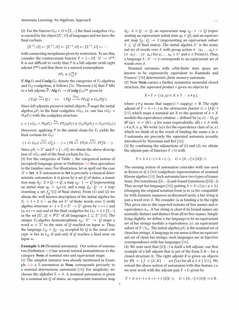
Example 3.10 (Nominal automata). Our notion of automa-ton (Definition 3.2) has several natural instantiations to thecategory Nom of nominal sets and equivariant maps.(1) The simplest instance was already mentioned in Exam-ple 3.3: a Σ-automaton in Nom corresponds precisely toa nominal deterministic automaton [18]. For simplicity, wechoose the alphabet Σ = A. A nominal automaton is givenby a nominal set Q of states, an equivariant transition map
δQ : A × Q → Q , an equivariant map iQ : 1 → Q (repre-senting an equivariant initial state q0 ∈ Q), and an equivari-ant map fQ : Q → 2 (representing an equivariant subsetF ⊆ Q of final states). The initial algebra A
∗ is the nomi-nal set of words over A with group action π · (a1 . . . an) =
(π ·a1) . . . (π ·an) for a1 . . . an ∈ A∗ and π ∈ Perm(A). Thus,
a language L : A∗ → 2 corresponds to an equivariant set of
words over A.Nominal automata with orbit-finite state space are
known to be expressively equivalent to Kaminski andFrancez’ [38] deterministic finite memory automata.(2) Now Nom carries a further symmetric monoidal closedstructure, the separated product ∗ given on objects by
X ∗ Y = { (x ,y) ∈ X × Y : x #y },
where x #y means that supp(x) ∩ supp(y) = ∅. The rightadjoint of F = A ∗ (−) is the abstraction functor G = [A](−)
[51] which maps a nominal set X to the quotient of A × X
modulo the equivalence relation ∼ defined by (a, x) ∼ (b,y)iff (ac) · x = (bc) · y for some (equivalently, all) c ∈ A withc #a,b, x ,y. We write 〈a〉x for the equivalence class of (a, x),which we think of as the result of binding the name a in x .F -automata are precisely the separated automata recentlyintroduced by Moerman and Rot [46].(3) By combining the adjunctions of (1) and (2), we obtainthe adjoint pair of functors F ⊣ G with
F = A × (−) + A ∗ (−), G = [A,−] × [A](−).
The ensuing notion of automaton coincides with one usedin Kozen et al.’s [40] coalgebraic representation of nominalKleene algebra [33]. Such automata have two types of transi-tions, free transitions ([A,−]) and bound transitions ([A](−)).They accept bar languages [56]: putting A = A∪{〈a | a ∈ A}
(changing the original notation from |a to 〈a for compatibil-ity with dynamic sequences as discussed next), a bar string isjust a word over A. We consider 〈a as binding a to the right.This gives rise to the expected notions of free names and α-equivalence ≡α . A bar string is clean if its bound names aremutually distinct and distinct from all its free names. Simpli-fying slightly, we define a bar language to be an equivariantset of bar strings modulo α-equivalence, i.e. an equivariantsubset of A∗/≡α . The initial algebra µF1 is the nominal set ofclean bar strings. A language in our sense is thus an equivari-ant set of clean bar strings; such languages are in bijectivecorrespondence with bar languages [56].(4) We note next that [A](−) is itself a left adjoint, our firstexample of a left adjoint that is not of the form Σ ⊗ − for aclosed structure ⊗. The right adjoint R is given on objectsby RX = { f ∈ [A,X ] : a # f (a) for all a ∈ A } [51]. Weextend the above notion of automaton with this feature, i.e.we now work with the adjoint pair F ⊣ G given by
F = A × (−) + A ∗ (−) + [A](−), G = [A,−] × [A](−) × R.
5
, , Henning Urbat and Lutz Schröder
The initial algebra µF1 now consists of words built fromthree types of letters; we denote the new type of letters in-duced by the new summand [A](−) in F by a〉 (for a ∈ A).Recalling that words grow to the right, we see that a〉 bindsto the left. We read a〉 as deallocating the name or resource a.Languages in this model consist of dynamic sequences [34].We associate such languages with a species of nominal au-tomata having three types of transitions: free and bound
transitions as above, and deallocating transitions qa 〉−−→ q′
with a #q′. To the best of our knowledge, this notion of nom-inal automaton has not appeared in the literature before.
Example 3.11 (Sorted Σ-automata). In our applications inSection 5, we shall encounter a generalized version of Σ-automata where (1) the input object I is arbitrary, not nec-essarily equal to the tensor unit ID , and (2) the automatonhas a sorted object of states and consumes sorted words.This reflects the fact that the algebraic structures arisingin algebraic language theory are often sorted. For brevity,we only treat the case of sorted automata in Set. Fix a setS of sorts and a family of sets Σ = (Σs,t )s,t ∈S ; we thinkof the elements of Σs,t as letters with domain sort s andcodomain sort t . We instantiate our setting to the adjointpair F ⊣ G : SetS → SetS defined as follows for Q ∈ SetS
and s, t ∈ S :
(FQ)t =∐
s ∈S Σs,t ×Qs , (GQ)s =∏
t ∈S [Σs,t ,Qt ].
Choosing I ∈ SetS arbitrary and the output object O = 2,the S-sorted set with two elements in each component, anF -automaton is a sorted Σ-automaton. It is given by an S-sorted set of states Q , transitions δQ,s,t : Σs,t × Qt → Qt
(s, t ∈ S), initial states i : I → Q and an output mapfQ : Q → 2 (representing an S-sorted set of final states). Theinitial algebra µFI is the S-sorted set of all well-sorted wordsover Σ with an additional first letter from I . More precisely,(µFI )t consists of all words xa1 . . . an with x ∈
∐
s ∈S Is anda1, . . . ,an ∈
∐
r ,s Σr ,s such that the sorts of consecutive let-ters match, i.e. there exist sorts s = s0, s1, . . . , sn = t ∈ S
such that x ∈ Is and ai ∈ Σsi−1,si for i = 1, . . . ,n. In particu-lar, in the single-sorted case we have µFI = I × Σ
∗. For anywell-sorted input wordw = xa1 . . . an one obtains the run
x−→ q0
a1−→ q1 → · · ·
an−−→ qn
in Q where q0 = iQ,s(x) and qi = δQ,si−1,si (ai ,qi−1) for i =1, . . . ,n, andw is accepted if and only if qn is a final state.
We conclude with a discussion of minimal automata.
Definition 3.12 (Minimal automaton). An automaton Q iscalled (1) reachable if the unique FI -algebra homomorphismeQ : µFI → Q lies in E, and (2) minimal if it is reachableand for every reachable automatonQ ′ with LQ = LQ ′ , thereexists a unique automata homomorphism from Q ′ to Q .
Theorem 3.13. For every language L there exists a minimal
automaton Min(L) accepting L, unique up to isomorphism.
Proof sketch. We describe the construction of the minimalautomaton. By equipping µFI with the final states L : µFI →O , we can view µFI as aGO -coalgebra. Consider the (E,M)-factorization of the unique coalgebra homomorphismmµFI :
mµFI = ( µFIeMin(L)
// // Min(L) //mMin(L)
// νGO ).
The object Min(L) can be uniquely equipped with an au-tomaton structure for which eMin(L) is an FI -algebra homo-morphism and mMin(L) is a GO -coalgebra homomorphism.This automaton is the minimal acceptor for L. �
The minimization theorem and its proof are closely re-lated to the classical work of Arbib and Manes [10] onthe minimal realization of dynamorphisms, i.e. F -algebrahomomorphisms from µFI into νGO . Under different as-sumptions on the type functor F and the base category D
(e.g. co-wellpoweredness), minimization results were alsoestablished by Adámek and Trnková [5] and, recently, byvan Heerdt et al. [63].
4 A Categorical L∗ Algorithm
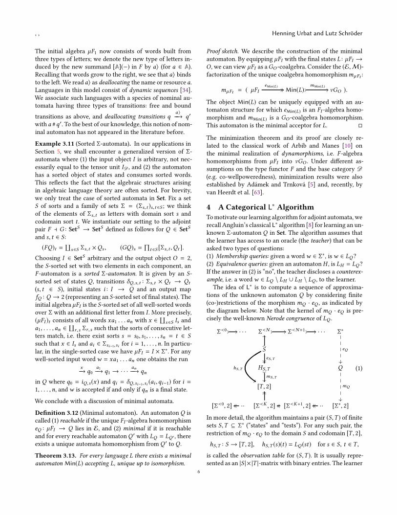
Tomotivate our learning algorithm for adjoint automata, werecall Angluin’s classical L∗ algorithm [8] for learning an un-known Σ-automaton Q in Set. The algorithm assumes thatthe learner has access to an oracle (the teacher) that can beasked two types of questions:(1) Membership queries: given a wordw ∈ Σ∗, isw ∈ LQ?(2) Equivalence queries: given an automatonH , is LH = LQ?If the answer in (2) is “no”, the teacher discloses a counterex-ample, i.e. a wordw ∈ LQ \ LH ∪ LH \ LQ , to the learner.The idea of L∗ is to compute a sequence of approxima-
tions of the unknown automaton Q by considering finite(co-)restrictions of the morphism mQ · eQ , as indicated bythe diagram below. Note that the kernel of mQ · eQ is pre-cisely the well-known Nerode congruence of LQ .
Σ<0 // // · · · Σ
<N // // Σ<N+1 // // · · · Σ
∗
eQ
��✤✤✤✤✤
S
hS,T
%%
eS,T����
OO
OO
HS,T��mS,T��
Q
mQ
��✤✤✤✤✤
[T , 2]
[Σ<0, 2] ··oooo [Σ<K
, 2]
OOOO
[Σ<K+1, 2]oooo ··oooo [Σ∗, 2]
(1)
In more detail, the algorithmmaintains a pair (S,T ) of finitesets S,T ⊆ Σ
∗ (“states” and “tests”). For any such pair, therestriction ofmQ · eQ to the domain S and codomain [T , 2],
hS,T : S → [T , 2], hS,T (s)(t) = LQ (st) for s ∈ S, t ∈ T ,
is called the observation table for (S,T ). It is usually repre-sented as an |S |× |T |-matrix with binary entries. The learner
6
Automata Learning: An Algebraic Approach , ,
can computehS,T via membership queries. The pair (S,T ) isclosed if for each s ∈ S and a ∈ Σ there exists s ′ ∈ S with
hS∪SΣ,T (sa) = hS,T (s′).
It is consistent if, for all s, s ′ ∈ S ,
hS,T (s) = hS,T (s′) implies hS,T∪ΣT (s) = hS,T∪ΣT (s
′).
Initially, one puts S = T = {ε}. If at some stage the pair(S,T ) is not closed or not consistent, either S or T can beextended by invoking one of the following two procedures:
Extend S
Input: A pair (S,T ) that is not closed.(0) Choose s ∈ S and a ∈ Σ such that
hS∪SΣ,T (sa) , hS,T (s′) for all s ′ ∈ S .
(1) Put S := S ∪ {sa}.
Extend T
Input: A pair (S,T ) that is not consistent.(0) Choose s, s ′ ∈ S , t ∈ T and a ∈ Σ such that
hS,T (s) = hS,T (s′) and hS,T∪ΣT (s)(at) , hS,T∪ΣT (s
′)(at).
(1) Put T := T ∪ {at}.
The two procedures are applied repeatedly until the pair(S,T ) is closed and consistent. Then, one constructs an au-tomaton HS,T , the hypothesis for (S,T ). Its set of states isthe image hS,T [S], the transitions δS,T : Σ × HS,T → HS,T
are given by δS,T (a,hS,T (s)) = hS∪SΣ,T (sa) for s ∈ S anda ∈ Σ, the initial state is hS,T (ε), and a state hS,T (s) is finalif s ∈ LQ (i.e. hS,T (s)(ε) = 1). Note that the well-definednessof δS,T is equivalent to (S,T ) being closed and consistent.The learner now tests whether LHS,T = LQ by asking
an equivalence query. If the answer is “yes”, the algorithmterminates successfully; otherwise, the teacher’s counterex-ample and all its prefixes are added to S . In summary:
L∗ Algorithm
Goal: Learn an automaton equivalent to an unknown au-tomaton Q .(0) Initialize S = T = {ε}.(1) While (S,T ) is not closed or not consistent:
(a) If (S,T ) is not closed: Extend S .(b) If (S,T ) is not consistent: Extend T .
(2) Construct the hypothesis HS,T .(a) If LHS,T = LQ : Return HS,T .(b) If LHS,T , LQ : Put S := S ∪C , whereC is the set of
prefixes of the teacher’s counterexample.(3) Go to (1).
The algorithm runs in polynomial time w.r.t. the sizeof the minimal automaton Min(LQ ) and the length ofthe longest counterexample provided by the teacher. Thelearned automaton (i.e. the correct hypothesis returnedin Step (2a)) is isomorphic to Min(LQ ). Correctness and
termination rest on the invariant that S is prefix-closedand T is suffix-closed. Note that if T ⊆ Σ
<K , then T yieldsa quotient [Σ<K
, 2] ։ [T , 2] given by restriction. In thefollowing,T is represented via this quotient.
We shall now develop all ingredients of L∗ for adjoint F -automata. This requires additional assumptions, which holdfor all the functors discussed in Example 3.3, 3.10 and 3.11:
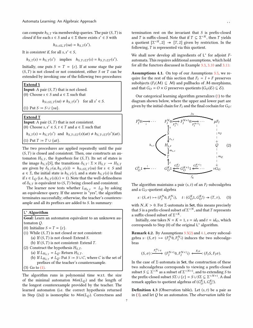
Assumptions 4.1. On top of our Assumptions 3.5, we re-quire for the rest of this section that FI = I + F preservessubobjects (FI (M) ⊆ M) and pullbacks ofM-morphisms,and that GO = O ×G preserves quotients (GO (E) ⊆ E).
Our categorical learning algorithm generalizes (1) to thediagram shown below, where the upper and lower part aregiven by the initial chain for FI and the final cochain forGO :
F 0I0 //
¡// · · · FN
I0
jN
))//
F NI¡// FN+1
I0 //
F N+1I
¡// · · · µFI
eQ
��✤✤✤✤✤
S
hs,t
''
es,t����
OOsOO
Hs,t��ms,t��
Q
mQ
��✤✤✤✤✤
T
G0O1 · · ·
!oooo GKO1
t
OOOO
GK+1O 1
GKO !
oooo · · ·GK+1O !
oooo νGO
j′K
ii
(2)
The algorithm maintains a pair (s, t) of an FI -subcoalgebraand a GO -quotient algebra
s : (S,σ ) (FNI 0, FNI¡), t : (GK
O1,GKO !)։ (T , τ ), (3)
with N ,K > 0. For Σ-automata in Set, this means preciselythat S is a prefix-closed subset of Σ<N , and thatT representsa suffix-closed subset of Σ<K .Initially, one takes N = K = 1, s = id I and t = idO , which
corresponds to Step (0) of the original L∗ algorithm.
Remark 4.2. By Assumptions 3.5(2) and 4.1, every subcoal-gebra s : (S,σ ) (FN
I0, FN
I¡) induces the two subcoalge-
bras
(S,σ ) //F NI¡·s
// (FN+1I
0, FN+1I
¡) (FIS, FIσ ).ooFI soo
In the case of Σ-automata in Set, the construction of thesetwo subcoalgebras corresponds to viewing a prefix-closedsubset S ⊆ Σ
<N as a subset of Σ<N+1, and to extending S tothe prefix-closed subset SΣ∪ {ε} = S ∪ SΣ ⊆ Σ
<N+1. A dualremark applies to quotient algebras of (GK
O1,GKO !).
Definition 4.3 (Observation table). Let (s, t) be a pair asin (3), and let Q be an automaton. The observation table for
7
, , Henning Urbat and Lutz Schröder
(s, t) w.r.t. Q is the morphism
hQs,t = ( S
s−→ FNI 0
jN−−→ µFI
eQ−−→ Q
mQ
−−−→ νGO
j′K−−→ GK
O1t−→ T ).
Its (E,M)-factorization is denoted by
hQs,t = ( S
eQs,t
// // HQs,t
//mQs,t
// T ).
In the following, we fix Q (the unknown automaton to belearned) and omit the superscripts (−)Q .
Remark 4.4. In our categorical setting, membershipqueries are replaced by the assumption that the learner cancompute the observation table hQs,t for each pair (s, t). Im-portantly, this morphism depends only on the language ofQ : one can show that for every automatonQ ′with LQ = LQ ′
one hasmQ · eQ =mQ ′ · eQ ′ , whence hQs,t = h
Q ′
s,t .
Definition 4.5 (Closed/Consistent pair). For any pair (s, t)as in (3), let cls,t and css,t be the unique diagonal fill-insmaking all parts of the diagram below commute:
Hs,GO t
css,t����✤✤
//ms,GOt
// GOT
τ��
S
es,GOt77 77♥♥♥♥♥♥♥♥♥ es,t// //
σ��
Hs,t//
ms,t//
��cls,t
��✤✤
T
FIS eFI s,t// // HFI s,t
66 mFI s,t
66♥♥♥♥♥♥♥♥♥♥
The pair (s, t) is closed if cls,t is an isomorphism, and consis-tent if css,t is an isomorphism.
If (s, t) is not closed or not consistent, at least one of thetwo dual procedures below applies. “Extend s” replaces S FNI0 by a new subcoalgebra S ′ FN+1
I0, i.e. it moves to
the right in the initial chain for FI . Analogously, “Extend t”replaces GK
O1 ։ T by a new quotient algebra GK+1O 1 ։ T ′,
and thus moves to the right in the final cochain forGO .
Extend s
Input: A pair (s, t) as in (3) that is not closed.(0) Choose an object S ′ andM-morphisms s0 : S S ′ and
s1 : S ′ FIS such that
σ = s1 · s0 and eFI s,t · s1 ∈ E .
(1) Replace s : (S,σ ) (FNI 0, FNI¡) by the subcoalgebra
FIs · s1 : (S′, FIs0 · s1) (F
N+1I 0, FN+1I
¡).
Remark 4.6. (1) One trivial choice in Step (0) is
S ′ = FIS s0 = σ , s1 = id.
To get an efficient implementation of the algorithm, oneaims to choose the subobject s1 : S ′ FIS as small as pos-sible.
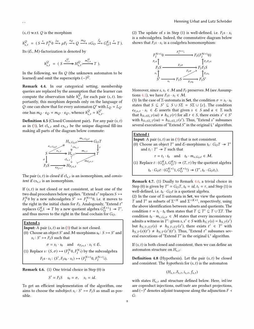
(2) The update of s in Step (1) is well-defined, i.e. FI s · s1is a subcoalgebra. Indeed, the commutative diagram belowshows that FIs · s1 is a coalgebra homomorphism:
FN+1I 0F N+1I
¡// FI (F
N+1I 0)
FIS
FI sOO
FIσ // FI FIS
FI FI sOO
S ′OO
s1
OO
s1// FIS
FIσ77♦♦♦♦♦♦♦♦
FI s0
// FIS′
OOFI s1
OO
Moreover, since s, s1 ∈ M and FI preservesM (see Assump-tions 4.1), we have FIs · s1 ∈ M.(3) In the case of Σ-automata in Set, the condition σ = s1 ·s0states that S ⊆ S ′ ⊆ S ∪ SΣ = SΣ ∪ {ε}. The conditioneFI s,t · s1 ∈ E asserts that given s ∈ S and a ∈ Σ suchthat hS∪SΣ,T (sa) , hS,T (r ) for all r ∈ S , there exists s ′ ∈ S ′
with hS∪SΣ,T (sa) = hS∪SΣ,T (s′). Thus, “Extend s” subsumes
several executions of “Extend S” in the original L∗ algorithm.
Extend t
Input: A pair (s, t) as in (3) that is not consistent.(0) Choose an object T ′ and E-morphisms t0 : GOT ։ T ′
and t1 : T ′ ։ T such that
τ = t1 · t0 and t0 ·ms,GO t ∈ M .
(1) Replace t : (GKO1,GK
O!)։ (T , τ ) by the quotient algebra
t0 ·GOt : (GK+1O 1,GK+1
O !)։ (T ′, t0 ·GOt1).
Remark 4.7. (1) Dually to Remark 4.6, a trivial choice inStep (0) is given byT ′ = GOT , t0 = id, t1 = τ , and Step (1) iswell-defined, i.e. t0 ·GOt is a quotient algebra.(2) In the case of Σ-automata in Set, we view the quotientsT and T ′ as subsets of Σ<K and Σ
<K+1, respectively, usingthe above identification between subsets and quotients. Thecondition τ = t1 · t0 then states that T ⊆ T ′ ⊆ T ∪ ΣT . Thecondition t0 ·ms,GO t ∈ M states that every inconsistencyadmits a witness inT ′: given s, s ′ ∈ S withhS,T (s) = hS,T (s ′)but hS,T∪ΣT (s) , hS,T∪ΣT (s
′), there exists t ′ ∈ T ′ withhS,T ′(s)(t
′) , hS,T ′(s′)(t ′). Thus, “Extend t” subsumes sev-
eral executions of “Extend T ” in the original L∗ algorithm.
If (s, t) is both closed and consistent, then we can define anautomaton structure on Hs,t :
Definition 4.8 (Hypothesis). Let the pair (s, t) be closedand consistent. The hypothesis for (s, t) is the automaton
(Hs,t , δs,t , is,t , fs,t )
with states Hs,t and structure defined below. Here, inl/inrare coproduct injections, outl/outr are product projections,and (−)# denotes adjoint transpose along the adjunction F ⊣G:
8
Automata Learning: An Algebraic Approach , ,
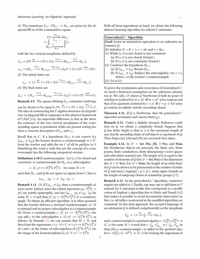
(1) The transitions δs,t : FHs,t → Hs,t are given by the di-agonal fill-in of the commutative square
FS
ls,t��
Fes,t// // FHs,t
δs,t
xxrr
rr #s,t��
Hs,t//ms,t
// T
with the two vertical morphisms defined by
ls,t = (FSinr−−→ I + FS = FIS
eFI s,t−−−−→ HFI s,t
cl−1s,t−−−→ Hs,t ),
rs,t = (Hs,t
cs−1s,t−−−→ Hs,GO t
ms,GOt
−−−−−−→ GOT = O ×GToutr−−−→ GT ).
(2) The initial states are
is,t = ( Iinl−−→ I + FS = FIS
eFI s,t−−−−→ HFI s,t
cl−1s,t−−−→ Hs,t ).
(3) The final states are
fs,t = (Hs,t
cs−1s,t−−−→ Hs,GO t
ms,GOt
−−−−−−→ GOT = O ×GToutl−−−→ O ).
Remark 4.9. The square defining δs,t commutes: both legs
can be shown to be equal to FSinr−−→ I + FS = FIS
hFI s,t−−−−→ T .
The idea of constructing the F -algebra structure of a hypoth-esis via diagonal fill-in originates in the abstract frameworkof CALF [64]. An important difference is that in the latterthe existence of the two vertical morphisms of the corre-sponding square is postulated, while our present setting fea-tures a concrete description of ls,t and rs,t .
Recall that in L∗, if a hypothesis HS,T is not correct (i.e.LHS,T , LQ ), the learner receives a counterexample w ∈ Σ∗
from the teacher and adds the set C of all its prefixes to S .Identifying the wordw with this set, the concept of a coun-terexample has the following categorical version:
Definition 4.10 (Counterexample). Let (s, t) be closed andconsistent. A counterexample for Hs,t is a subcoalgebra
c : (C,γ ) (FMI 0, FMI ¡) for someM > 0
such that Hs,t and Q do not agree on inputs from C , that is,
LHs,t · jM · c , LQ · jM · c .
Remark 4.11. (1) If LHs,t , LQ , then a counterexample al-ways exists. Indeed, since the colimit injections jM : FM
I0→
µFI are jointly epimorphic, one has LHs,t · jM , LQ · jM forsome M > 0 and thus (C,γ ) = (FMI 0, FMI
¡) is a counterex-ample. To obtain an efficient algorithm, it is often assumedthat the teacher delivers a minimal counterexample, i.e. Mis minimal and no proper subcoalgebra is a counterexample.(2) Given a counterexample c : (C,γ ) (FM
I0, FM
I¡), one
can add c to the subcoalgebra s : (S,σ ) (FNI0, FN
I¡) as
follows: by Remark 4.2, we can assume that M = N , andthen form the supremum s ∨c : (S ∨C,σ ∨γ ) (FN
I0, FN
I¡)
of s and c in the lattice of subcoalgebras of (FNI0, FN
I¡), viz.
the image of the homomorphism [s, c] : S +C → FNI0.
With all these ingredients at hand, we obtain the followingabstract learning algorithm for adjoint F -automata:
Generalized L∗ Algorithm
Goal: Learn an automaton equivalent to an unknown au-tomaton Q .(0) Initialize N = K = 1, s = idI and t = idO .(1) While (s, t) is not closed or not consistent:
(a) If (s, t) is not closed: Extend s .(b) If (s, t) is not consistent: Extend t .
(2) Construct the hypothesis Hs,t .(a) If LHs,t = LQ : Return Hs,t .(b) If LHs,t , LQ : Replace the subcoalgebra s by s ∨ c ,
where c is the teacher’s counterexample.(3) Go to (1).
To prove the termination and correctness of Generalized L∗,we need a finiteness assumption on the unknown automa-ton Q . We call a D-object Q Noetherian if both its poset ofsubobjects (ordered bym ≤ m′ iffm =m′ ·p for some p) andthat of its quotients (ordered by e ≤ e ′ iff e = q · e ′ for someq) contain no infinite strictly ascending chains.
Theorem 4.12. If Q is Noetherian, then the generalized L∗
algorithm terminates and returns Min(LQ ).
Remark 4.13. Under a slightly stronger finiteness condi-tion on Q , we obtain a complexity bound. Suppose thatQ has finite height n, that is, n is the maximum length ofany strictly ascending chain of subobjects or quotients ofQ .Then Steps (1a), (1b) and (2b) are executed O(n) times.
Example 4.14. In D = Set, Pos, JSL, K-Vec, and Nom,the Noetherian objects are precisely the finite sets, finiteposets, finite semilattices, finite-dimensional vector spacesand orbit-finite nominal sets. The height ofQ is equal to thenumber of elements ofQ (forD = Set, Pos) or the dimension(forD = K-Vec). For D = Nom, the height of an orbit-finitesetQ can be shown to be polynomial in the number of orbitsof Q and max{ | supp(q)| | q ∈ Q }, using upper bounds onthe length of subgroup chains in symmetric groups [11].
Remark 4.15. In the generalized L∗ algorithm, counterex-amples are added to S . Dually, one may opt to add them toTinstead; for Σ-automata in Set, this corresponds to a modifi-cation of Angluin’s algorithm due to Maler and Pnueli [42]that makes it possible to avoid inconsistent observation ta-bles, i.e. all tables constructed in the modified algorithm areconsistent. In this dual approach, the accepted language ofan automatonQ is defined coalgebraically as the morphism
L′Q = ( IiQ−−→ Q
mQ
−−−→ νGO ),
and a counterexample is a quotient algebra c : (GMO1,GM
O!)։
(C,γ ) for someM > 0 such that c · j ′M · L′Hs,t, c · j ′M · L
′Q . In
Step (2b), a counterexample c is added to the quotient alge-bra t : (GK
O1,G−OK !)։ (T , τ ) by forming the supremum of
9
, , Henning Urbat and Lutz Schröder
t and c . To guarantee termination, our original requirementthat FI preserves pullbacks ofM-morphisms (see Assump-tions 4.1) needs to be replaced by the dual requirement thatGO preserves pushouts of E-morphisms.
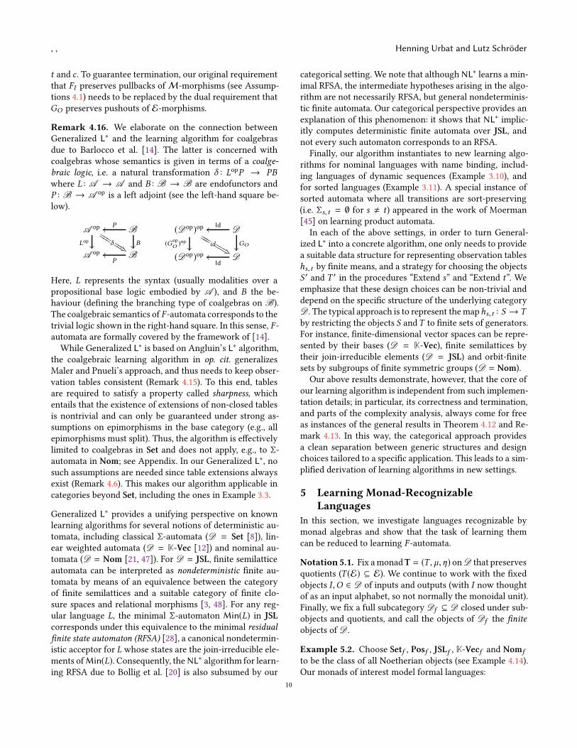
Remark 4.16. We elaborate on the connection betweenGeneralized L∗ and the learning algorithm for coalgebrasdue to Barlocco et al. [14]. The latter is concerned withcoalgebras whose semantics is given in terms of a coalge-
braic logic, i.e. a natural transformation δ : LopP → PB
where L : A → A and B : B → B are endofunctors andP : B → A op is a left adjoint (see the left-hand square be-low).
A op
δ❑❑❑❑❑❑
!)❑❑❑❑❑❑Lop
��
BPoo
B��
A op BP
oo
(Dop)op
(Gop
O)op
��id▲▲▲▲▲▲
"*▲▲
▲▲▲
▲
DIdoo
GO��
(Dop)op DId
oo
Here, L represents the syntax (usually modalities over apropositional base logic embodied by A ), and B the be-haviour (defining the branching type of coalgebras on B).The coalgebraic semantics of F -automata corresponds to thetrivial logic shown in the right-hand square. In this sense, F -automata are formally covered by the framework of [14].While Generalized L∗ is based on Angluin’s L∗ algorithm,
the coalgebraic learning algorithm in op. cit. generalizesMaler and Pnueli’s approach, and thus needs to keep obser-vation tables consistent (Remark 4.15). To this end, tablesare required to satisfy a property called sharpness, whichentails that the existence of extensions of non-closed tablesis nontrivial and can only be guaranteed under strong as-sumptions on epimorphisms in the base category (e.g., allepimorphisms must split). Thus, the algorithm is effectivelylimited to coalgebras in Set and does not apply, e.g., to Σ-automata in Nom; see Appendix. In our Generalized L∗, nosuch assumptions are needed since table extensions alwaysexist (Remark 4.6). This makes our algorithm applicable incategories beyond Set, including the ones in Example 3.3.
Generalized L∗ provides a unifying perspective on knownlearning algorithms for several notions of deterministic au-tomata, including classical Σ-automata (D = Set [8]), lin-ear weighted automata (D = K-Vec [12]) and nominal au-tomata (D = Nom [21, 47]). For D = JSL, finite semilatticeautomata can be interpreted as nondeterministic finite au-tomata by means of an equivalence between the categoryof finite semilattices and a suitable category of finite clo-sure spaces and relational morphisms [3, 48]. For any reg-ular language L, the minimal Σ-automaton Min(L) in JSL
corresponds under this equivalence to the minimal residualfinite state automaton (RFSA) [28], a canonical nondetermin-istic acceptor for L whose states are the join-irreducible ele-ments ofMin(L). Consequently, theNL∗ algorithm for learn-ing RFSA due to Bollig et al. [20] is also subsumed by our
categorical setting. We note that althoughNL∗ learns a min-imal RFSA, the intermediate hypotheses arising in the algo-rithm are not necessarily RFSA, but general nondeterminis-tic finite automata. Our categorical perspective provides anexplanation of this phenomenon: it shows that NL∗ implic-itly computes deterministic finite automata over JSL, andnot every such automaton corresponds to an RFSA.Finally, our algorithm instantiates to new learning algo-
rithms for nominal languages with name binding, includ-ing languages of dynamic sequences (Example 3.10), andfor sorted languages (Example 3.11). A special instance ofsorted automata where all transitions are sort-preserving(i.e. Σs,t = ∅ for s , t ) appeared in the work of Moerman[45] on learning product automata.In each of the above settings, in order to turn General-
ized L∗ into a concrete algorithm, one only needs to providea suitable data structure for representing observation tableshs,t by finite means, and a strategy for choosing the objectsS ′ and T ′ in the procedures “Extend s” and “Extend t”. Weemphasize that these design choices can be non-trivial anddepend on the specific structure of the underlying categoryD . The typical approach is to represent themaphs,t : S → T
by restricting the objects S andT to finite sets of generators.For instance, finite-dimensional vector spaces can be repre-sented by their bases (D = K-Vec), finite semilattices bytheir join-irreducible elements (D = JSL) and orbit-finitesets by subgroups of finite symmetric groups (D = Nom).Our above results demonstrate, however, that the core of
our learning algorithm is independent from such implemen-tation details; in particular, its correctness and termination,and parts of the complexity analysis, always come for freeas instances of the general results in Theorem 4.12 and Re-mark 4.13. In this way, the categorical approach providesa clean separation between generic structures and designchoices tailored to a specific application. This leads to a sim-plified derivation of learning algorithms in new settings.
5 Learning Monad-RecognizableLanguages
In this section, we investigate languages recognizable bymonad algebras and show that the task of learning themcan be reduced to learning F -automata.
Notation5.1. Fix amonadT = (T , µ,η) onD that preservesquotients (T (E) ⊆ E). We continue to work with the fixedobjects I ,O ∈ D of inputs and outputs (with I now thoughtof as an input alphabet, so not normally the monoidal unit).Finally, we fix a full subcategory Df ⊆ D closed under sub-objects and quotients, and call the objects of Df the finite
objects of D .
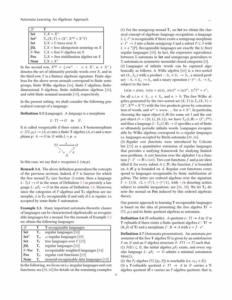
Example 5.2. Choose Setf , Posf , JSLf , K-Vecf and Nomf
to be the class of all Noetherian objects (see Example 4.14).Our monads of interest model formal languages:
10
Automata Learning: An Algebraic Approach , ,
D T
Set T+X = X+
Set2 T∞(X ,Y ) = (X+,X up
+ X ∗Y )
Set TΓX = Γ-trees over XJSL T∗X = free idempotent semiring on X
K-Vec T∗X = free K-algebra on X
Pos TSX = free stabilization algebra on X
Nom T∗X = X ∗
In the second row, X up= {vwω : v ∈ X ∗, w ∈ X+ }
denotes the set of ultimately periodic words over X , and inthe third row, Γ is a finitary algebraic signature. Finite alge-bras for the above seven monads correspond to finite semi-groups, finite Wilke algebras [66], finite Γ-algebras, finite-dimensional K-algebras, finite stabilization algebras [26],and orbit-finite nominal monoids [19], respectively.
In the present setting, we shall consider the following gen-eralized concept of a language:
Definition 5.3 (Language). A language is a morphism
L : TI → O in D .
It is called recognizable if there exists a T-homomorphisme : (TI , µI ) → (A,α) into a finite T-algebra (A,α) and a mor-phism p : A→ O in D with L = p · e .
TI
e ❆❆
❆❆❆
L // O
Ap
??⑧⑧⑧⑧⑧
In this case, we say that e recognizes L (via p).
Remark 5.4. The above definition generalizes the conceptsof the previous sections. Indeed, if F is functor for whichthe free monad TF (see Section 2) exists, then a languageL : TF I → O in the sense of Definition 5.3 is precisely a lan-guage L : µFI → O in the sense of Definition 3.8. Moreover,since the categories of F -algebras and TF -algebras are iso-morphic, L is TF -recognizable if and only if L is regular, i.e.accepted by some finite F -automaton.
Example 5.5. Many important automata-theoretic classesof languages can be characterized algebraically as recogniz-able languages for a monad. For the monads of Example 5.2we obtain the following languages:
D T T-recognizable languagesSet T+ regular languages [50]Set2 T∞ ω-regular languages [49]Set TΓ tree languages over Γ [25]JSL T∗ regular languages [52]K-Vec T∗ recognizable weighted languages [54]Pos TS regular cost functions [23]Nom T∗ monoid-recognizable data languages [19]
In the following, we focus on (ω-)regular languages and costfunctions; see [58, 60] for details on the remaining examples.
(1) For the semigroup monad T+ on Set we obtain the clas-sical concept of algebraic language recognition: a languageL ⊆ I+ is recognizable if there exists a semigroup morphisme : I+ → S into a finite semigroup S and a subset P ⊆ S withL = e−1[P]. Recognizable languages are exactly the (ε-free)regular languages [50]. In fact, the expressive equivalencebetween Σ-automata in Set and semigroups generalizes toΣ-automata in symmetric monoidal closed categories [4].(2) Languages of infinite words can be captured alge-braically as follows. A Wilke algebra [66] is a two-sortedset (S+, Sω) with a product · : S+ × S+ → S+, a mixed prod-uct · : S+ × Sω → Sω and a unary operation (−)ω : S+ → Sωsubject to the laws
(st)u = s(tu), (st)z = s(tz), s(ts)ω = (st)ω , (sn)ω = sω ,
for all s, t ,u ∈ S+, z ∈ Sω and n > 0. The free Wilke al-gebra generated by the two-sorted set (X ,Y ) is T∞(X ,Y ) =(X+,X up
+X ∗Y ) with the two products given by concatena-tion of words, andwω
= www . . . forw ∈ X+. In particular,choosing the input object (I , ∅) for some set I and the out-put object O = ({0, 1}, {0, 1}), we have T∞(I , ∅) = (I+, Iup),and thus a language L : T∞(I , ∅) → O specifies a set of finiteor ultimately periodic infinite words. Languages recogniz-able by Wilke algebras correspond to ω-regular languages,i.e. languages accepted by Büchi automata [49, 66].(3) Regular cost functions were introduced by Colcom-bet [23] as a quantitative extension of regular languagesthat provides a unifying framework for studying limited-ness problems. A cost function over the alphabet I is a func-tion f : I ∗ → N∪ {∞}. Two cost functions f and д are iden-tified if, for every subset A ⊆ N, the function f is boundedon A iff д is bounded on A. Regular cost functions corre-spond to languages recognizable by finite stabilization al-
gebras. The latter are ordered algebras over the signatureΓ = {1/0, ·/2, (−)#/1, (−)ω/1}, with −/n denoting arities,subject to suitable inequations; see [26, 58]. We let TS de-note the monad on Pos induced by this ordered algebraictheory.
Our generic approach to learning T-recognizable languagesis based on the idea of presenting the free algebra TI =
(TI , µI ) and its finite quotient algebras as automata:
Definition 5.6 (T-refinable). A quotient e : TI ։ A in D isT-refinable if there exists a finite quotient algebra e ′ : TI ։(B, β) of TI and a morphism f : B ։ A with e = f · e ′.
Definition 5.7 (Automata presentation). An automata pre-
sentation of the free T-algebra TI is given by an endofunctorF on D and an F -algebra structure δ : FT I → TI such that(1) F (E) ⊆ E, the initial algebra µFI exists, and every reg-ular language L : µFI → O admits a minimal automatonMin(L);(2) the FI -algebra (TI , [ηI , δ ]) is reachable (i.e. eT I ∈ E);(3) a T-refinable quotient e : TI ։ A in D carries a T-algebra quotient iff e carries an F -algebra quotient; that is,
11
, , Henning Urbat and Lutz Schröder
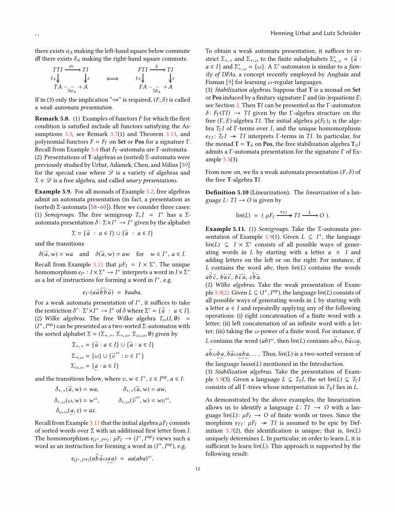
there exists αA making the left-hand square below commuteiff there exists δA making the right-hand square commute.
TTIµI
//
Te ����
TI
e����
TA∃αA
//❴❴❴ A
⇐⇒
FT Iδ //
Fe ����
TI
e����
FA∃δA
//❴❴❴ A
If in (3) only the implication “⇒” is required, (F , δ ) is calleda weak automata presentation.
Remark 5.8. (1) Examples of functors F for which the firstcondition is satisfied include all functors satisfying the As-sumptions 3.5, see Remark 3.7(1) and Theorem 3.13, andpolynomial functors F = FΓ on Set or Pos for a signature Γ.Recall from Example 3.4 that FΓ-automata are Γ-automata.(2) Presentations of T-algebras as (sorted) Σ-automata werepreviously studied by Urbat, Adámek, Chen, and Milius [59]for the special case where D is a variety of algebras andΣ ∈ D is a free algebra, and called unary presentations.
Example 5.9. For all monads of Example 5.2, free algebrasadmit an automata presentation (in fact, a presentation as(sorted) Σ-automata [58–60]). Here we consider three cases:(1) Semigroups. The free semigroup T+I = I+ has a Σ-automata presentation δ : Σ×I+→ I+ given by the alphabet
Σ = {→a : a ∈ I } ∪ {
←a : a ∈ I }
and the transitions
δ (→a ,w) = wa and δ (
←a ,w) = aw for w ∈ I+, a ∈ I .
Recall from Example 3.11 that µFI = I × Σ∗. The unique
homomorphism eI+ : I ×Σ∗→ I+ interprets a word in I ×Σ∗
as a list of instructions for forming a word in I+, e.g.
eI+ (a→a→
b←
b→a ) = baaba.
For a weak automata presentation of I+, it suffices to takethe restriction δ ′ : Σ′×I+ → I+ of δ where Σ′ = {
→a : a ∈ I }.
(2) Wilke algebras. The free Wilke algebra T∞(I , ∅) =
(I+, Iup) can be presented as a two-sorted Σ-automaton withthe sorted alphabet Σ = (Σ+,+, Σ+,ω, Σω,ω, ∅) given by
Σ+,+ = {→a : a ∈ I } ∪ {
←a : a ∈ I }
Σ+,ω = {ω} ∪ {→vω: v ∈ I+}
Σω,ω = {a←: a ∈ I }
and the transitions below, where v,w ∈ I+, z ∈ Iup, a ∈ I :
δ+,+(→a ,w) = wa, δ+,+(
←a ,w) = aw,
δ+,ω (ω,w) = wω, δ+,ω (
→vω,w) = wvω ,
δω,ω(a←, z) = az.
Recall from Example 3.11 that the initial algebra µFI consistsof sorted words over Σ with an additional first letter from I .The homomorphism e(I+, I up) : µFI → (I
+, Iup) views such a
word as an instruction for forming a word in (I+, Iup), e.g.
e(I+, I up)(a→
b→aωa
←a←) = aa(aba)ω .
To obtain a weak automata presentation, it suffices to re-strict Σ+,+ and Σ+,ω to the finite subalphabets Σ′
+,+= {
→a :
a ∈ I } and Σ′+,ω = {ω}. A Σ
′-automaton is similar to a fam-
ily of DFAs, a concept recently employed by Angluin andFisman [9] for learning ω-regular languages.(3) Stabilization algebras. Suppose that T is a monad on Set
orPos induced by a finitary signature Γ and (in-)equations E;see Section 2. Then TI can be presented as the Γ-automatonδ : FΓ(TI ) → TI given by the Γ-algebra structure on thefree (Γ, E)-algebraTI . The initial algebra µ(FΓ)I is the alge-bra TΓI of Γ-terms over I , and the unique homomorphismeT I : TΓI ։ TI interprets Γ-terms in TI . In particular, forthe monad T = TS on Pos, the free stabilization algebra TS Iadmits a Γ-automata presentation for the signature Γ of Ex-ample 5.5(3).
From now on, we fix a weak automata presentation (F , δ ) ofthe free T-algebra TI .
Definition 5.10 (Linearization). The linearization of a lan-guage L : TI → O is given by
lin(L) = ( µFIeT I // // TI
L // O ).
Example 5.11. (1) Semigroups. Take the Σ-automata pre-sentation of Example 5.9(1). Given L ⊆ I+, the languagelin(L) ⊆ I × Σ
∗ consists of all possible ways of gener-ating words in L by starting with a letter a ∈ I andadding letters on the left or on the right. For instance, ifL contains the word abc , then lin(L) contains the words
a→
b→c , b
←a→c , b
→c←a , c
←
b←a .
(2) Wilke algebras. Take the weak presentation of Exam-ple 5.9(2). Given L ⊆ (I+, Iup), the language lin(L) consists ofall possible ways of generating words in L by starting witha letter a ∈ I and repeatedly applying any of the followingoperations: (i) right concatenation of a finite word with aletter; (ii) left concatenation of an infinite word with a let-ter; (iii) taking the ω-power of a finite word. For instance, if
L contains the word (ab)ω , then lin(L) contains a→
bω, b→aωa
←,
a→
bωb←a←, b→aωa
←b←a←, . . .. Thus, lin(L) is a two-sorted version of
the language lasso(L) mentioned in the Introduction.(3) Stabilization algebras. Take the presentation of Exam-ple 5.9(3). Given a language L ⊆ TS I , the set lin(L) ⊆ TΓI
consists of all Γ-trees whose interpretation in TS I lies in L.
As demonstrated by the above examples, the linearizationallows us to identify a language L : TI → O with a lan-guage lin(L) : µFI → O of finite words or trees. Since themorphism eT I : µFI ։ TI is assumed to be epic by Def-inition 5.7(2), this identification is unique; that is, lin(L)uniquely determines L. In particular, in order to learn L, it issufficient to learn lin(L). This approach is supported by thefollowing result:
12
Automata Learning: An Algebraic Approach , ,
Theorem 5.12. If L : TI → O is a T-recognizable language,
then its linearization lin(L) : µFI → O is regular, i.e. accepted
by some finite F -automaton.
Proof sketch. Let e : TI → (A,α) be a T-homomorphism rec-ognizing L via p : A → O . By replacing e with its coimage,wemay assume that e ∈ E. Theweak automata presentationyields an F -algebra structure onAmaking e an F -algebra ho-momorphism. Then A, viewed as an automaton with initialstates e · ηI : I → A and final states p, accepts lin(L). �
In view of this theorem, one can apply any learning algo-rithm for finite F -automata (e.g. Generalized L∗ for the caseof adjoint automata, or a learning algorithm for tree au-tomata [30] if F is a polynomial functor) to learn the mini-mal automatonQL for lin(L). This automaton, together withthe epimorphism eT I , constitutes a finite representation ofthe unknown language L : TI → O . If the given automatapresentation for TI is non-weak, we can go one step furtherand infer from QL a minimal algebraic representation of L:
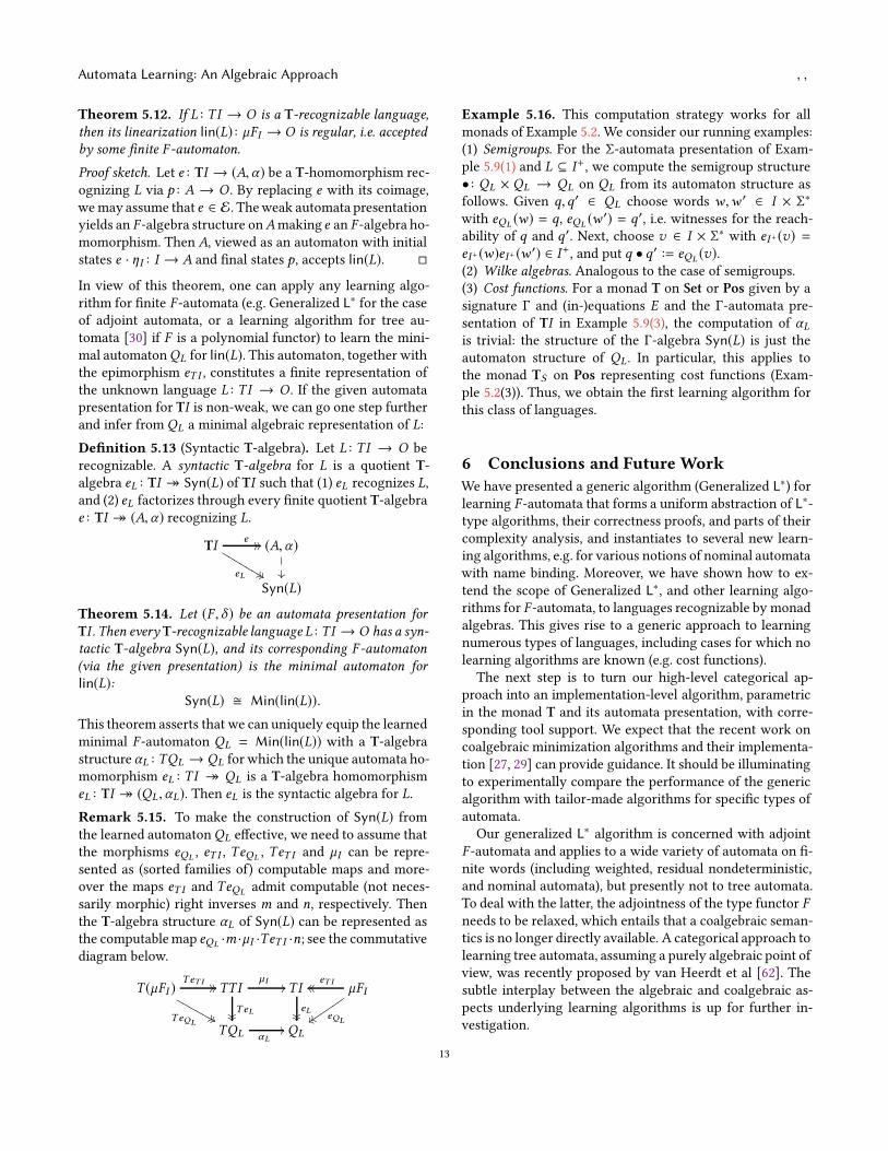
Definition 5.13 (Syntactic T-algebra). Let L : TI → O berecognizable. A syntactic T-algebra for L is a quotient T-algebra eL : TI ։ Syn(L) of TI such that (1) eL recognizes L,and (2) eL factorizes through every finite quotient T-algebrae : TI ։ (A,α) recognizing L.
TIe // //
eL %% %%▲▲▲
▲▲▲▲ (A,α)
��✤✤
Syn(L)
Theorem 5.14. Let (F , δ ) be an automata presentation for
TI . Then every T-recognizable language L : TI → O has a syn-
tactic T-algebra Syn(L), and its corresponding F -automaton
(via the given presentation) is the minimal automaton for
lin(L):
Syn(L) � Min(lin(L)).
This theorem asserts that we can uniquely equip the learnedminimal F -automaton QL = Min(lin(L)) with a T-algebrastructure αL : TQL → QL for which the unique automata ho-momorphism eL : TI ։ QL is a T-algebra homomorphismeL : TI ։ (QL,αL). Then eL is the syntactic algebra for L.
Remark 5.15. To make the construction of Syn(L) fromthe learned automatonQL effective, we need to assume thatthe morphisms eQL , eT I , TeQL , TeT I and µI can be repre-sented as (sorted families of) computable maps and more-over the maps eT I and TeQL admit computable (not neces-sarily morphic) right inverses m and n, respectively. Thenthe T-algebra structure αL of Syn(L) can be represented asthe computablemap eQL ·m ·µI ·TeT I ·n; see the commutativediagram below.
T (µFI )TeT I // //
TeQL&& &&▼
▼▼▼▼
▼TTI
TeL����
µI// TI
eL����
µFIeT Ioooo
eQLzzzz✉✉✉✉✉✉
TQL αL// QL
Example 5.16. This computation strategy works for allmonads of Example 5.2. We consider our running examples:(1) Semigroups. For the Σ-automata presentation of Exam-ple 5.9(1) and L ⊆ I+, we compute the semigroup structure• : QL × QL → QL on QL from its automaton structure asfollows. Given q,q′ ∈ QL choose words w,w ′ ∈ I × Σ
∗
with eQL (w) = q, eQL (w′) = q′, i.e. witnesses for the reach-
ability of q and q′. Next, choose v ∈ I × Σ∗ with eI+(v) =
eI+(w)eI+(w′) ∈ I+, and put q • q′ := eQL (v).
(2) Wilke algebras. Analogous to the case of semigroups.(3) Cost functions. For a monad T on Set or Pos given by asignature Γ and (in-)equations E and the Γ-automata pre-sentation of TI in Example 5.9(3), the computation of αLis trivial: the structure of the Γ-algebra Syn(L) is just theautomaton structure of QL . In particular, this applies tothe monad TS on Pos representing cost functions (Exam-ple 5.2(3)). Thus, we obtain the first learning algorithm forthis class of languages.
6 Conclusions and Future Work
We have presented a generic algorithm (Generalized L∗) forlearning F -automata that forms a uniform abstraction of L∗-type algorithms, their correctness proofs, and parts of theircomplexity analysis, and instantiates to several new learn-ing algorithms, e.g. for various notions of nominal automatawith name binding. Moreover, we have shown how to ex-tend the scope of Generalized L∗, and other learning algo-rithms for F -automata, to languages recognizable by monadalgebras. This gives rise to a generic approach to learningnumerous types of languages, including cases for which nolearning algorithms are known (e.g. cost functions).The next step is to turn our high-level categorical ap-
proach into an implementation-level algorithm, parametricin the monad T and its automata presentation, with corre-sponding tool support. We expect that the recent work oncoalgebraic minimization algorithms and their implementa-tion [27, 29] can provide guidance. It should be illuminatingto experimentally compare the performance of the genericalgorithm with tailor-made algorithms for specific types ofautomata.Our generalized L∗ algorithm is concerned with adjoint
F -automata and applies to a wide variety of automata on fi-nite words (including weighted, residual nondeterministic,and nominal automata), but presently not to tree automata.To deal with the latter, the adjointness of the type functor Fneeds to be relaxed, which entails that a coalgebraic seman-tics is no longer directly available. A categorical approach tolearning tree automata, assuming a purely algebraic point ofview, was recently proposed by van Heerdt et al [62]. Thesubtle interplay between the algebraic and coalgebraic as-pects underlying learning algorithms is up for further in-vestigation.
13
, , Henning Urbat and Lutz Schröder
References[1] Jiří Adámek, Filippo Bonchi, Mathias Hülsbusch, Barbara König, Ste-
fan Milius, and Alexandra Silva. 2012. A Coalgebraic Perspective onMinimization and Determinization. In Foundations of Software Scienceand Computational Structures, Lars Birkedal (Ed.). Springer BerlinHei-delberg, 58–73.
[2] Jiří Adámek, Horst Herrlich, and George Strecker. 2004. Abstract andConcrete Categories: The Joy of Cats. Dover Publications. 528 pages.
[3] Jiří Adámek, Stefan Milius, Robert S. R. Myers, and Henning Ur-bat. 2014. On Continuous Nondeterminism and State Minimality. InProc. Mathematical Foundations of Programming Science (MFPS XXX)
(Electron. Notes Theor. Comput. Sci., Vol. 308), Bart Jacobs, AlexandraSilva, and Sam Staton (Eds.). Elsevier, 3–23.
[4] J. Adámek, S. Milius, and H. Urbat. 2015. Syntactic Monoids in a Cate-gory. In Proc. CALCO’15 (LIPIcs). Schloss Dagstuhl–Leibniz-Zentrumfür Informatik.
[5] Jiří Adámek and Vera Trnková. 1989. Automata and Algebras in Cat-
egories. Springer.[6] Jiří Adámek. 1974. Free algebras and automata realizations in the
language of categories. Commentationes Mathematicae Universitatis
Carolinae 15, 4 (1974), 589–602. h�p://eudml.org/doc/16649
[7] Mikołaj Bojańczyk. 2015. Recognisable languages over monads. InProc. DLT 2015, Igor Potapov (Ed.). LNCS, Vol. 9168. Springer, 1–13.h�p://arxiv.org/abs/1502.04898.
[8] Dana Angluin. 1987. Learning Regular Sets from Queries and Coun-terexamples. Inf. Comput. 75, 2 (1987), 87–106.
[9] Dana Angluin and Dana Fisman. 2016. Learning regular omega lan-guages. Theoretical Computer Science 650 (2016), 57 – 72.
[10] Michael A. Arbib and Ernest G. Manes. 1975. Adjoint machines, state-behavior machines, and duality. Journal of Pure and Applied Algebra
6, 3 (1975), 313 – 344.[11] László Babai. 1986. On the length of subgroup chains in
the symmetric group. Comm. Alg. 14, 9 (1986), 1729–1736.h�ps://doi.org/10.1080/00927878608823393
[12] Borja Balle and Mehryar Mohri. 2015. Learning Weighted Automata.In Algebraic Informatics, Andreas Maletti (Ed.). Springer, 1–21.
[13] Bernhard Banaschewski and Evelyn Nelson. 1976. Tensor prod-ucts and biomorphisms. Can. Math. Bull. 19, 4 (1976), 385–402.h�ps://doi.org/10.4153/CMB-1976-060-2
[14] Simone Barlocco, Clemens Kupke, and Jurriaan Rot. 2019. CoalgebraLearning via Duality. In Proc. FOSSACS 2019. 62–79.
[15] Michael Barr. 1970. Coequalizers and free triples. Mathematische
Zeitschrift 116, 4 (1970), 307–322.[16] Nick Bezhanishvili, Clemens Kupke, and Prakash Panangaden. 2012.
Minimization via Duality. In Logic, Language, Information and Com-
putation, Luke Ong and Ruy de Queiroz (Eds.). Springer Berlin Hei-delberg, 191–205.
[17] S. L. Bloom. 1976. Varieties of ordered algebras. J. Comput. Syst. Sci.
2, 13 (1976), 200–212.[18] Mikołaj Bojańczyk, Bartek Klin, and Sławomir Lasota. 2014. Automata
theory in nominal sets. Log. Methods Comput. Sci. 10, 3:4 (2014), 44pp.
[19] Mikołaj Bojańczyk. 2013. Nominal Monoids. Theory of Computing
Systems 53, 2 (2013), 194–222.[20] Benedikt Bollig, Peter Habermehl, Carsten Kern, and Martin Leucker.
2009. Angluin-Style Learning of NFA. In 21st International Joint Con-
ference on Artifical Intelligence (IJCAI’09).[21] Benedikt Bollig, Peter Habermehl, Martin Leucker, and Benjamin
Monmege. 2014. A Robust Class of Data Languages and an Appli-cation to Learning. Logical Methods in Computer Science 10, 4 (2014).
[22] Venanzio Capretta, Tarmo Uustalu, and Varmo Vene. 2006. Recur-sive coalgebras from comonads. Information and Computation 204, 4(2006), 437 – 468.
[23] Thomas Colcombet. 2009. The Theory of Stabilisation Monoids andRegular Cost Functions. In Automata, Languages and Programming,Susanne Albers, Alberto Marchetti-Spaccamela, Yossi Matias, SotirisNikoletseas, andWolfgang Thomas (Eds.). Springer BerlinHeidelberg,139–150.
[24] Thomas Colcombet and Daniela Petrişan. 2017. Automata Minimiza-tion: a Functorial Approach. In 7th Conference on Algebra and Coalge-
bra in Computer Science (CALCO 2017) (Leibniz International Proceed-
ings in Informatics (LIPIcs), Vol. 72), Filippo Bonchi and Barbara König(Eds.). Schloss Dagstuhl–Leibniz-Zentrum fuer Informatik, 8:1–8:16.
[25] H. Comon, M. Dauchet, R. Gilleron, C. Löding, F. Jacque-mard, D. Lugiez, S. Tison, and M. Tommasi. 2007. TreeAutomata Techniques and Applications. Available on:h�p://www.grappa.univ-lille3.fr/tata.
[26] L. Daviaud, D. Kuperberg, and J.-É. Pin. 2016. Varieties of Cost Func-tions. In Proc. STACS 2016 (LIPIcs, Vol. 47), N. Ollinger and H. Vollmer(Eds.). Schloss Dagstuhl–Leibniz-Zentrum für Informatik, 30:1–30:14.
[27] Hans-Peter Deifel, Stefan Milius, Lutz Schröder, and Thorsten Wiß-mann. 2019. Generic Partition Refinement and Weighted Tree Au-tomata. In Formal Methods – The Next 30 Years, Maurice H. ter Beek,Annabelle McIver, and José N. Oliveira (Eds.). Springer InternationalPublishing, 280–297.
[28] François Denis, Aurélien Lemay, and Alain Terlutte. 2001. ResidualFinite State Automata. In STACS 2001, Afonso Ferreira and Horst Re-ichel (Eds.). 144–157.
[29] Ulrich Dorsch, Stefan Milius, Lutz Schröder, and Thorsten Wiß-mann. 2017. Efficient Coalgebraic Partition Refinement. InProc. 28th International Conference on Concurrency Theory (CONCUR
2017) (LIPIcs). Schloss Dagstuhl - Leibniz-Zentrum fuer Informatik.h�ps://arxiv.org/abs/1705.08362
[30] Frank Drewes and Johanna Högberg. 2003. Learning a RegularTree Language from a Teacher. In Developments in Language Theory,Zoltán Ésik and Zoltán Fülöp (Eds.). Springer Berlin Heidelberg, 279–291.
[31] M. Droste, W. Kuich, and H. Vogler (Eds.). 2009. Handbook of weightedautomata. Springer.
[32] Azadeh Farzan, Yu-Fang Chen, Edmund M. Clarke, Yih-Kuen Tsay,and Bow-YawWang. 2008. Extending Automated Compositional Veri-fication to the Full Class of Omega-regular Languages. In Proc. TACAS2008. 2–17.
[33] Murdoch James Gabbay and Vincenzo Ciancia. 2011. Fresh-ness and Name-Restriction in Sets of Traces with Names.In Foundations of Software Science and Computational Struc-
tures, FOSSACS 2011 (LNCS, Vol. 6604). Springer, 365–380.h�ps://doi.org/10.1007/978-3-642-19805-2
[34] Murdoch James Gabbay, Dan R. Ghica, and Daniela Petrişan. 2015.Leaving theNest: Nominal Techniques for Variables with InterleavingScopes. In Computer Science Logic, CSL 2015 (LIPIcs, Vol. 41). SchlossDagstuhl - Leibniz-Zentrum fuer Informatik, 374–389.
[35] Joseph A. Goguen. 1975. Discrete-TimeMachines in Closed MonoidalCategories. I. J. Comput. Syst. Sci. 10, 1 (1975), 1–43.
[36] Claudio Hermida and Bart Jacobs. 1998. Structural Induction andCoinduction in a Fibrational Setting. Information and Computation
145, 2 (1998), 107 – 152.[37] Bart Jacobs and Alexandra Silva. 2014. Automata Learning: A Categor-
ical Perspective. Springer, 384–406.[38] Michael Kaminski and Nissim Francez. 1994. Finite-memory au-
tomata. Theoret. Comput. Sci. 134, 2 (1994), 329 – 363.[39] Ondřej Klíma and Libor Polák. 2008. On varieties of meet automata.
Theoretical Computer Science 407, 1 (2008), 278 – 289.[40] DexterKozen, Konstantinos Mamouras, Daniela Petrişan, and Alexan-
dra Silva. 2015. Nominal Kleene Coalgebra. In Automata, Languages,
and Programming, ICALP 2015 (LNCS, Vol. 9135). Springer, 286–298.h�ps://doi.org/10.1007/978-3-662-47666-6
14
Automata Learning: An Algebraic Approach , ,
[41] S. Mac Lane. 1998. Categories for the Working Mathematician (2nd ed.).Springer.
[42] Oded Maler and Amir Pnueli. 1995. On the Learnability of InfinitaryRegular Sets. Inf. Comput. 118, 2 (1995), 316–326.
[43] E. G. Manes. 1976. Algebraic Theories. Graduate Texts in Mathematics,Vol. 26. Springer.
[44] Stefan Milius, Lutz Schröder, and Thorsten Wißmann. 2016. RegularBehaviours with Names. Appl. Categ. Structures 24, 5 (2016), 663–701.
[45] Joshua Moerman. 2019. Learning Product Automata. In Proc. 14th
International Conference on Grammatical Inference 2018 (Proceedings
of Machine Learning Research, Vol. 93), Olgierd Unold, Witold Dyrka,and Wojciech Wieczorek (Eds.). PMLR, 54–66.
[46] Joshua Moerman and Jurriaan Rot. 2019. Separation and Renamingin Nominal Sets. CoRR abs/1906.00763 (2019). arXiv:1906.00763
[47] Joshua Moerman, Matteo Sammartino, Alexandra Silva, Bartek Klin,andMichałSzynwelski. 2017. LearningNominal Automata. In Proceed-ings of the 44th ACM SIGPLAN Symposium on Principles of Program-
ming Languages (POPL 2017). ACM, 613–625.[48] Robert S. R. Myers, Jiří Adámek, Stefan Milius, and Henning Urbat.
2014. Canonical Nondeterministic Automata. In Proc. Coalgebraic
Methods in Computer Science (CMCS’14) (Lecture Notes Comput. Sci.,
Vol. 8446), Marcello M. Bonsangue (Ed.). Springer, 189–210.[49] D. Perrin and J.-É. Pin. 2004. Infinite Words. Elsevier.[50] J.-É. Pin. 2016. Mathematical Foundations of Au-
tomata Theory. (November 2016). Available ath�p://www.liafa.jussieu.fr/~jep/PDF/MPRI/MPRI.pdf.
[51] Andrew M. Pitts. 2013. Nominal Sets: Names and Symmetry in Com-
puter Science. Cambridge University Press.[52] L. Polák. 2001. Syntactic semiring of a language. In Proc. MFCS’01
(LNCS, Vol. 2136), J. Sgall, A. Pultr, and P. Kolman (Eds.). Springer, 611–620.
[53] Michael O. Rabin and Dana S. Scott. 1959. Finite Automata and TheirDecision Problems. IBM J. Res. Dev. 3, 2 (April 1959), 114–125.
[54] C. Reutenauer. 1980. Séries formelles et algèbres syntactiques. J. Al-gebra 66 (1980), 448–483.
[55] Jan J. M. M. Rutten. 2000. Universal coalgebra: a theory of systems.Theoret. Comput. Sci. 249, 1 (2000), 3–80.
[56] Lutz Schröder, Dexter Kozen, Stefan Milius, and ThorstenWißmann. 2017. Nominal Automata with Name Binding.In Foundations of Software Science and Computation Struc-
tures, FOSSACS 2017 (LNCS, Vol. 10203). Springer, 124–142.h�ps://doi.org/10.1007/978-3-662-54458-7
[57] Paul Taylor. 1999. Practical Foundations of Mathematics. CambridgeUniversity Press.
[58] Henning Urbat, Jirí Adámek, Liang-Ting Chen, and Stefan Milius.2017. Eilenberg Theorems for Free. CoRR abs/1602.05831 (2017).h�p://arxiv.org/abs/1602.05831
[59] Henning Urbat, Jiří Adámek, Liang-Ting Chen, and Stefan Milius.2017. Eilenberg Theorems for Free. In Proc. MFCS 2017 (LIPIcs, Vol. 83),Kim G. Larsen, Hans L. Bodlaender, and Jean-François Raskin (Eds.).Schloss Dagstuhl.
[60] Henning Urbat and Stefan Milius. 2019. Varieties of Data Languages.In Proc. 46th International Colloquium on Automata, Languages, and
Programming (ICALP 2019) (LIPIcs, Vol. 132), Christel Baier, IoannisChatzigiannakis, Paola Flocchini, and Stefano Leonardi (Eds.). 130:1–130:14.
(Presents the first Eilenberg-type correspondence for data languagesand a nominal Eilenberg-Schützenberger theorem characterizingpseudovarieties of nominal monoids.).
[61] Frits Vaandrager. 2017. Model Learning. Commun. ACM 60, 2 (2017),86–95.
[62] Gerco van Heerdt, Tobias Kappé, Jurriaan Rot, Matteo Sammartino,and Alexandra Silva. 2020. A Categorical Framework for LearningGeneralised Tree Automata. h�ps://arxiv.org/abs/2001.05786
[63] Gerco van Heerdt, Tobias Kappé, Jurriaan Rot, Matteo Sam-martino, and Alexandra Silva. 2019. Tree Automata as Algebras:Minimisation and Determinisation. CoRR abs/1904.08802 (2019).h�p://arxiv.org/abs/1904.08802
[64] Gerco van Heerdt, Matteo Sammartino, and Alexandra Silva. 2017.CALF: Categorical Automata Learning Framework. In Proc. CSL 2017.29:1–29:24.
[65] Gerco van Heerdt, Matteo Sammartino, and Alexandra Silva. 2017.Learning Automata with Side-Effects. CoRR abs/1704.08055 (2017).h�p://arxiv.org/abs/1704.08055
[66] T. Wilke. 1991. An Eilenberg Theorem for ∞-Languages. InProc. ICALP’91 (LNCS, Vol. 510). Springer, 588–599.
15
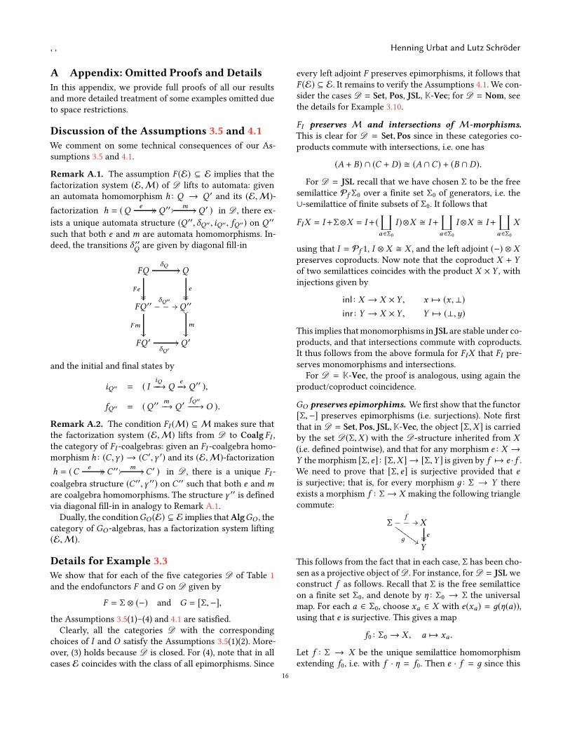
, , Henning Urbat and Lutz Schröder
A Appendix: Omitted Proofs and Details
In this appendix, we provide full proofs of all our resultsand more detailed treatment of some examples omitted dueto space restrictions.
Discussion of the Assumptions 3.5 and 4.1
We comment on some technical consequences of our As-sumptions 3.5 and 4.1.
Remark A.1. The assumption F (E) ⊆ E implies that thefactorization system (E,M) of D lifts to automata: givenan automata homomorphism h : Q → Q ′ and its (E,M)-
factorization h = (Qe // // Q ′′ //
m // Q ′ ) in D , there ex-
ists a unique automata structure (Q ′′, δQ ′′, iQ ′′, fQ ′′) on Q ′′
such that both e and m are automata homomorphisms. In-deed, the transitions δ ′′Q are given by diagonal fill-in
FQδQ
//
Fe����
Q
e����
FQ ′′δQ′′
//❴❴❴
Fm
��
Q ′′��
m
��
FQ ′δQ′
// Q ′
and the initial and final states by
iQ ′′ = ( IiQ−−→ Q
e−→ Q ′′ ),
fQ ′′ = (Q ′′m−→ Q ′
fQ′′−−−→ O ).
Remark A.2. The condition FI (M) ⊆ M makes sure thatthe factorization system (E,M) lifts from D to Coalg FI ,the category of FI -coalgebras: given an FI -coalgebra homo-morphism h : (C,γ ) → (C ′,γ ′) and its (E,M)-factorization
h = (Ce // // C ′′ //
m // C ′ ) in D , there is a unique FI -coalgebra structure (C ′′,γ ′′) on C ′′ such that both e andmare coalgebra homomorphisms. The structure γ ′′ is definedvia diagonal fill-in in analogy to Remark A.1.
Dually, the conditionGO (E) ⊆ E implies thatAlgGO , thecategory of GO -algebras, has a factorization system lifting(E,M).
Details for Example 3.3
We show that for each of the five categories D of Table 1and the endofunctors F andG on D given by
F = Σ ⊗ (−) and G = [Σ,−],
the Assumptions 3.5(1)–(4) and 4.1 are satisfied.Clearly, all the categories D with the corresponding
choices of I and O satisfy the Assumptions 3.5(1)(2). More-over, (3) holds because D is closed. For (4), note that in allcases E coincides with the class of all epimorphisms. Since
every left adjoint F preserves epimorphisms, it follows thatF (E) ⊆ E. It remains to verify the Assumptions 4.1. We con-sider the cases D = Set, Pos, JSL, K-Vec; for D = Nom, seethe details for Example 3.10.
FI preserves M and intersections of M-morphisms.
This is clear for D = Set, Pos since in these categories co-products commute with intersections, i.e. one has
(A + B) ∩ (C + D) � (A ∩C) + (B ∩ D).
For D = JSL recall that we have chosen Σ to be the freesemilattice Pf Σ0 over a finite set Σ0 of generators, i.e. the∪-semilattice of finite subsets of Σ0. It follows that
FIX = I+Σ⊗X = I+(∐
a∈Σ0
I )⊗X � I+∐
a∈Σ0
I ⊗X � I+∐
a∈Σ0
X
using that I = Pf 1, I ⊗ X � X , and the left adjoint (−) ⊗ Xpreserves coproducts. Now note that the coproduct X + Yof two semilattices coincides with the product X × Y , withinjections given by
inl : X → X × Y , x 7→ (x ,⊥)
inr : Y → X × Y , Y 7→ (⊥,y)
This implies thatmonomorphisms in JSL are stable under co-products, and that intersections commute with coproducts.It thus follows from the above formula for FIX that FI pre-serves monomorphisms and intersections.For D = K-Vec, the proof is analogous, using again the
product/coproduct coincidence.
GO preserves epimorphims. We first show that the functor[Σ,−] preserves epimorphisms (i.e. surjections). Note firstthat in D = Set, Pos, JSL,K-Vec, the object [Σ,X ] is carriedby the set D(Σ,X ) with the D-structure inherited from X
(i.e. defined pointwise), and that for any morphism e : X →Y themorphism [Σ, e] : [Σ,X ] → [Σ,Y ] is given by f 7→ e · f .We need to prove that [Σ, e] is surjective provided that eis surjective; that is, for every morphism д : Σ → Y thereexists a morphism f : Σ→ X making the following trianglecommute:
Σf
//❴❴❴
д ##❍❍❍
❍❍❍❍ X
e����
Y
This follows from the fact that in each case, Σ has been cho-sen as a projective object ofD . For instance, forD = JSLweconstruct f as follows. Recall that Σ is the free semilatticeon a finite set Σ0, and denote by η : Σ0 → Σ the universalmap. For each a ∈ Σ0, choose xa ∈ X with e(xa) = д(η(a)),using that e is surjective. This gives a map
f0 : Σ0 → X , a 7→ xa .
Let f : Σ → X be the unique semilattice homomorphismextending f0, i.e. with f · η = f0. Then e · f = д since this
16
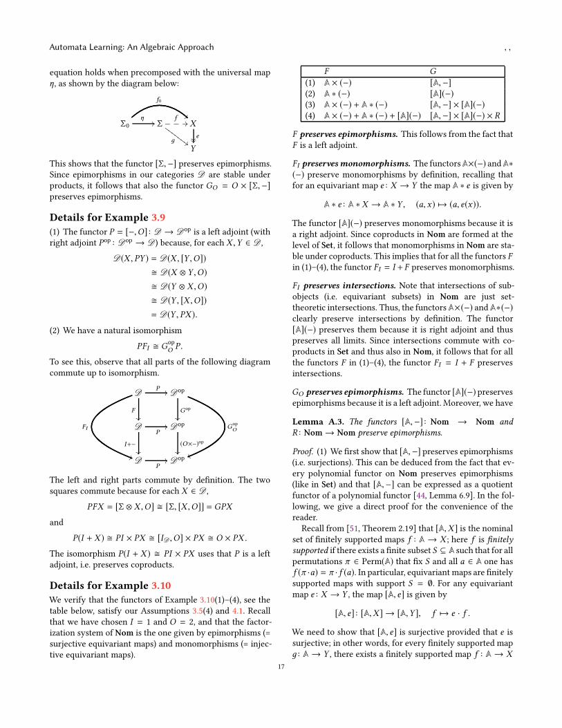
Automata Learning: An Algebraic Approach , ,
equation holds when precomposed with the universal mapη, as shown by the diagram below:
Σ0η
//
f0
!!
Σf
//❴❴❴
д ##●●●
●●●● X
e����
Y
This shows that the functor [Σ,−] preserves epimorphisms.Since epimorphisms in our categories D are stable underproducts, it follows that also the functor GO = O × [Σ,−]
preserves epimorphisms.
Details for Example 3.9
(1) The functor P = [−,O] : D → Dop is a left adjoint (withright adjoint Pop : Dop → D ) because, for each X ,Y ∈ D ,
D(X , PY ) = D(X , [Y ,O])
� D(X ⊗ Y ,O)
� D(Y ⊗ X ,O)
� D(Y , [X ,O])
= D(Y , PX ).
(2) We have a natural isomorphism
PFI � Gop
OP .
To see this, observe that all parts of the following diagramcommute up to isomorphism.
D
FI
))
F
��
P // Dop
Gop
��
Gop
O
vv
DP
//
I+−
��
Dop
(O×−)op
��
DP
// Dop
The left and right parts commute by definition. The twosquares commute because for each X ∈ D ,
PFX = [Σ ⊗ X ,O] � [Σ, [X ,O]] = GPX
and
P(I + X ) � PI × PX � [ID ,O] × PX � O × PX .
The isomorphism P(I + X ) � PI × PX uses that P is a leftadjoint, i.e. preserves coproducts.
Details for Example 3.10
We verify that the functors of Example 3.10(1)–(4), see thetable below, satisfy our Assumptions 3.5(4) and 4.1. Recallthat we have chosen I = 1 and O = 2, and that the factor-ization system of Nom is the one given by epimorphisms (=surjective equivariant maps) and monomorphisms (= injec-tive equivariant maps).
F G
(1) A × (−) [A,−]
(2) A ∗ (−) [A](−)
(3) A × (−) + A ∗ (−) [A,−] × [A](−)
(4) A × (−) + A ∗ (−) + [A](−) [A,−] × [A](−) × R
F preserves epimorphisms. This follows from the fact thatF is a left adjoint.
FI preservesmonomorphisms. The functorsA×(−) andA∗
(−) preserve monomorphisms by definition, recalling thatfor an equivariant map e : X → Y the map A ∗ e is given by
A ∗ e : A ∗ X → A ∗ Y , (a, x) 7→ (a, e(x)).
The functor [A](−) preserves monomorphisms because it isa right adjoint. Since coproducts in Nom are formed at thelevel of Set, it follows that monomorphisms in Nom are sta-ble under coproducts. This implies that for all the functors Fin (1)–(4), the functor FI = I +F preserves monomorphisms.
FI preserves intersections. Note that intersections of sub-objects (i.e. equivariant subsets) in Nom are just set-theoretic intersections. Thus, the functors A×(−) and A∗(−)
clearly preserve intersections by definition. The functor[A](−) preserves them because it is right adjoint and thuspreserves all limits. Since intersections commute with co-products in Set and thus also in Nom, it follows that for allthe functors F in (1)–(4), the functor FI = I + F preservesintersections.
GO preserves epimorphisms. The functor [A](−) preservesepimorphisms because it is a left adjoint. Moreover, we have
Lemma A.3. The functors [A,−] : Nom → Nom and
R : Nom→ Nom preserve epimorphisms.
Proof. (1) We first show that [A,−] preserves epimorphisms(i.e. surjections). This can be deduced from the fact that ev-ery polynomial functor on Nom preserves epimorphisms(like in Set) and that [A,−] can be expressed as a quotientfunctor of a polynomial functor [44, Lemma 6.9]. In the fol-lowing, we give a direct proof for the convenience of thereader.Recall from [51, Theorem 2.19] that [A,X ] is the nominal
set of finitely supported maps f : A → X ; here f is finitelysupported if there exists a finite subset S ⊆ A such that for allpermutations π ∈ Perm(A) that fix S and all a ∈ A one hasf (π ·a) = π · f (a). In particular, equivariant maps are finitelysupported maps with support S = ∅. For any equivariantmap e : X → Y , the map [A, e] is given by
[A, e] : [A,X ] → [A,Y ], f 7→ e · f .
We need to show that [A, e] is surjective provided that e issurjective; in other words, for every finitely supported mapд : A → Y , there exists a finitely supported map f : A → X
17
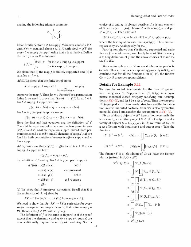
, , Henning Urbat and Lutz Schröder
making the following triangle commute:
Af
//❴❴❴
д ##❍❍❍
❍❍❍❍ X
e����
Y
Fix an arbitrary atom a < A\suppд. Moreover, choose x ∈ Xwith e(x) = д(a), and choose xb ∈ X with e(xb ) = д(b) forevery b ∈ suppд ∪ suppx , using that e is surjective. Definethe map f : A→ X as follows:
f (b) =
{
(b a) · x for b ∈ A \ (suppд ∪ suppx);
xb for b ∈ suppд ∪ supp x .
We claim that (i) the map f is finitely supported and (ii) itsatisfies e · f = д.
Ad (i). We show that the finite set of atoms
S = suppд ∪ suppx ∪⋃
b ∈suppд ∪ suppx
suppxb
supports themap f . Thus, let π ∈ Perm(A) be a permutationfixing S ; we need to prove that f (π ·b) = π · f (b) for allb ∈ A.For b ∈ suppд ∪ suppx , we have
f (π · b) = f (b) = xb = π · xb = π · f (b).
For b ∈ A \ (suppд ∪ suppx), we get
f (π · b) = (π (b)a) · x = π · (b a) · x = π · f (b).
Here the first and last equation use the definition of f .The middle equation holds because the two permutations(π (b)a) and π · (b a) are equal on suppx . Indeed, both per-mutations send a to π (b), and all elements of supp x \{a} arefixed by both permutations because b, π (b) < suppx and π
fixes supp x .
Ad (ii). We show that e(f (b)) = д(b) for all b ∈ A. For b ∈suppд ∪ suppx we have
e(f (b)) = e(xb ) = д(b)
by definition of f and xb . For b ∈ A \ (suppд ∪ suppx),
e(f (b)) = e((b a) · x) def. f
= (b a) · e(x) e equivariant
= (b a) · д(a) def. x
= д((b a) · a) a,b < suppд
= д(b) .
(2) We show that R preserves surjections. Recall that R isthe subfunctor of [A,−] given by
RX = { f ∈ [A,X ] : a # f (a) for every a ∈ A }.
We need to show that Re : RX → RY is surjective for everysurjective equivariant map e : X ։ Y ; that is, for every д ∈RY , there exists f ∈ RX with e · f = д.
The definition of f is the same as in part (1) of the proof,except that the elements x and xb (b ∈ suppд ∪ suppx ) arenow additionally required to satisfy a#x and b#xb . Such a
choice of x and xb is always possible: if x is any elementof X with e(x) = д(a), choose a′ with a′#д(a), x and putx ′ = (a′ a) · x . Then a#x ′ and
e(x ′) = e((a′ a) · x) = (a′ a) · e(x) = (a′ a) · д(a) = д(a),
where the last equation uses that a,a′#д(a). Thus, we canreplace x by x ′. Analogously for xb .Part (1) now shows that f is finitely supported and satis-
fies e · f = д. Moreover, we clearly have b#f (b) for everyb ∈ A by definition of f and the above choices of x and xb ,i.e. f ∈ RX . �
Since epimorphisms in Nom are stable under products(which follows from the corresponding property in Set), weconclude that for all the functors G in (1)–(4), the functorGO = 2 ×G preserves epimorphisms.
Details for Example 3.11
We describe sorted Σ-automata for the case of generalbase categories D . Suppose that (D , ⊗, ID ) is a sym-metric monoidal closed category satisfying our Assump-tions 3.5(1)–(2), and let S be a set of sorts. Then the categoryDS (equippedwith themonoidal structure and the factoriza-tion system inherited sortwise from D ) is also symmetricmonoidal closed and satisfies the Assumptions 3.5(1)–(2).Fix an arbitrary object I ∈ DS inputs (not necessarily the
tensor unit), an arbitrary object O ∈ DS of outputs, and afamily of objects Σ = (Σs,t )s,t ∈S in D ; we think of Σs,t asa set of letters with input sort s and output sort t . Take thefunctors
F : DS → D
S, (FQ)t =
∐
s ∈S
Σs,t ⊗ Qs (t ∈ S),
G : DS → D
S, (GQ)s =
∏
t ∈S
[Σs,t ,Qt ] (s ∈ S).
The functor F is a left adjoint of G: we have the isomor-phisms (natural in P,Q ∈ DS )
DS (FQ, P) =
∏
t ∈S
D((FQ)t , Pt )
=
∏
t ∈S
D(∐
s ∈S
Σs,t ⊗ Qs , Pt )
�
∏
t ∈S
∏
s ∈S
D(Σs,t ⊗ Qs , Pt )
�
∏
s ∈S
∏
t ∈S
D(Σs,t ⊗ Qs , Pt )
�
∏
s ∈S
∏
t ∈S
D(Qs , [Σs,t , Pt ])
�
∏
s ∈S
D(Qs ,
∏
t ∈S
[Σs,t , Pt ])
=
∏
s ∈S
D(Qs , (GP)s ).
= DS (Q,GP)
18
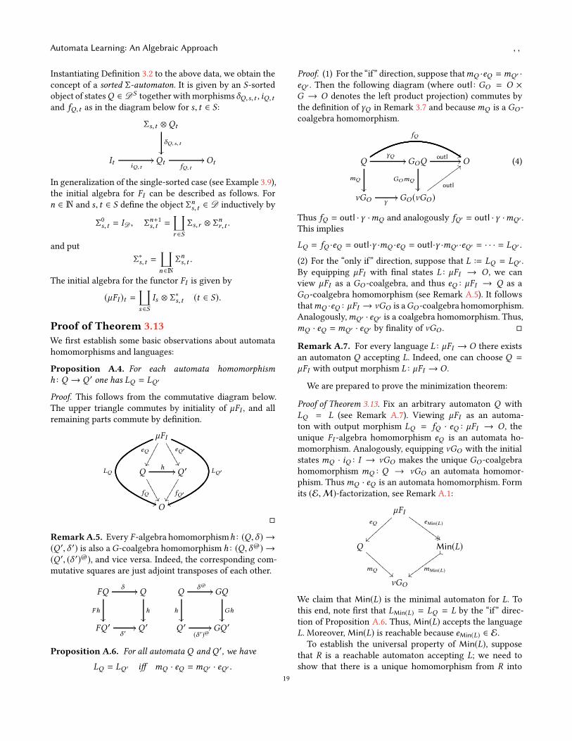
Automata Learning: An Algebraic Approach , ,
Instantiating Definition 3.2 to the above data, we obtain theconcept of a sorted Σ-automaton. It is given by an S-sortedobject of statesQ ∈ DS together withmorphisms δQ,s,t , iQ,t
and fQ,t as in the diagram below for s, t ∈ S :
Σs,t ⊗ Qt
δQ,s,t
��
ItiQ,t
// QtfQ,t
// Ot
In generalization of the single-sorted case (see Example 3.9),the initial algebra for FI can be described as follows. Forn ∈ N and s, t ∈ S define the object Σns,t ∈ D inductively by
Σ0s,t = ID , Σ
n+1s,t =
∐
r ∈S
Σs,r ⊗ Σnr ,t .
and put
Σ∗s,t =
∐
n∈N
Σns,t .
The initial algebra for the functor FI is given by
(µFI )t =∐
s ∈S
Is ⊗ Σ∗s,t (t ∈ S).
Proof of Theorem 3.13
We first establish some basic observations about automatahomomorphisms and languages:
Proposition A.4. For each automata homomorphism
h : Q → Q ′ one has LQ = LQ ′
Proof. This follows from the commutative diagram below.The upper triangle commutes by initiality of µFI , and allremaining parts commute by definition.
µFI
LQ
((
LQ′
vv
eQ
��✍✍✍✍✍✍ eQ′
��✶✶✶✶✶✶
Q
fQ��✵✵✵✵✵✵
h // Q ′
fQ′��☞☞☞☞☞☞
O
�
RemarkA.5. Every F -algebra homomorphismh : (Q, δ ) →(Q ′, δ ′) is also aG-coalgebra homomorphism h : (Q, δ@) →(Q ′, (δ ′)@), and vice versa. Indeed, the corresponding com-mutative squares are just adjoint transposes of each other.
FQδ //
Fh
��
Q
h
��
FQ ′δ ′
// Q ′
Qδ@
//
h
��
GQ
Gh
��
Q ′(δ ′)@
// GQ ′
Proposition A.6. For all automata Q and Q ′, we have
LQ = LQ ′ iff mQ · eQ =mQ ′ · eQ ′ .
Proof. (1) For the “if” direction, suppose thatmQ ·eQ =mQ ′ ·
eQ ′ . Then the following diagram (where outl : GO = O ×
G → O denotes the left product projection) commutes bythe definition of γQ in Remark 3.7 and becausemQ is a GO -coalgebra homomorphism.
QγQ
//
mQ
��
fQ
$$GOQ
GOmQ
��
outl // O
νGO γ// GO (νGO )
outl
;;✇✇✇✇✇✇✇✇✇
(4)
Thus fQ = outl ·γ ·mQ and analogously fQ ′ = outl ·γ ·mQ ′ .This implies
LQ = fQ ·eQ = outl·γ ·mQ ·eQ = outl·γ ·mQ ′ ·eQ ′ = · · · = LQ ′ .
(2) For the “only if” direction, suppose that L := LQ = LQ ′ .By equipping µFI with final states L : µFI → O , we canview µFI as a GO -coalgebra, and thus eQ : µFI → Q as aGO -coalgebra homomorphism (see Remark A.5). It followsthatmQ ·eQ : µFI → νGO is aGO -coalgebra homomorphism.Analogously,mQ ′ · eQ ′ is a coalgebra homomorphism. Thus,mQ · eQ =mQ ′ · eQ ′ by finality of νGO . �
Remark A.7. For every language L : µFI → O there existsan automaton Q accepting L. Indeed, one can choose Q =µFI with output morphism L : µFI → O .
We are prepared to prove the minimization theorem:
Proof of Theorem 3.13. Fix an arbitrary automaton Q withLQ = L (see Remark A.7). Viewing µFI as an automa-ton with output morphism LQ = fQ · eQ : µFI → O , theunique FI -algebra homomorphism eQ is an automata ho-momorphism. Analogously, equipping νGO with the initialstates mQ · iQ : I → νGO makes the unique GO -coalgebrahomomorphism mQ : Q → νGO an automata homomor-phism. ThusmQ · eQ is an automata homomorphism. Formits (E,M)-factorization, see Remark A.1:
µFIeQ
~~⑤⑤⑤⑤⑤⑤⑤⑤ eMin(L)
## ##❍❍❍
❍❍❍❍
❍❍
Q
mQ ❇
❇❇❇❇
❇❇❇ Min(L)
{{
mMin(L){{✈✈✈✈✈✈✈✈✈
νGO
We claim that Min(L) is the minimal automaton for L. Tothis end, note first that LMin(L) = LQ = L by the “if” direc-tion of Proposition A.6. Thus, Min(L) accepts the languageL. Moreover,Min(L) is reachable because eMin(L) ∈ E.
To establish the universal property of Min(L), supposethat R is a reachable automaton accepting L; we need toshow that there is a unique homomorphism from R into
19
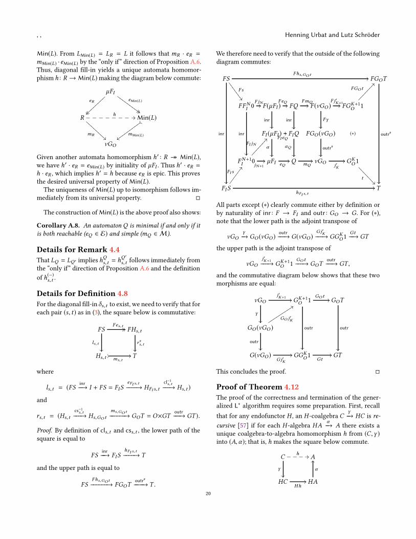
, , Henning Urbat and Lutz Schröder
Min(L). From LMin(L) = LR = L it follows that mR · eR =
mMin(L) · eMin(L) by the “only if” direction of Proposition A.6.Thus, diagonal fill-in yields a unique automata homomor-phism h : R → Min(L)making the diagram below commute:
µFIeR
~~~~⑥⑥⑥⑥⑥⑥⑥⑥ eMin(L)
## ##❍❍❍
❍❍❍❍
❍❍
R
mR ❇❇
❇❇❇❇
❇❇h //❴❴❴❴❴❴❴❴ Min(L)
{{
mMin(L){{✈✈✈✈✈✈✈✈✈
νGO
Given another automata homomorphism h′ : R ։ Min(L),we have h′ · eR = eMin(L) by initiality of µFI . Thus h′ · eR =h · eR , which implies h′ = h because eR is epic. This provesthe desired universal property of Min(L).The uniqueness ofMin(L) up to isomorphism follows im-
mediately from its universal property. �
The construction ofMin(L) is the above proof also shows:
Corollary A.8. An automaton Q is minimal if and only if it
is both reachable (eQ ∈ E) and simple (mQ ∈ M).
Details for Remark 4.4
That LQ = LQ ′ implies hQs,t = hQ ′
s,t follows immediately fromthe “only if” direction of Proposition A.6 and the definition
of h(−)s,t .
Details for Definition 4.8
For the diagonal fill-in δs,t to exist, we need to verify that foreach pair (s, t) as in (3), the square below is commutative:
FS
ls,t
��
Fes,t// // FHs,t
r #s,t
��
Hs,t//ms,t
// T
where
ls,t = (FSinr−−→ I + FS = FIS
eFI s,t−−−−→ HFI s,t
cl−1s,t−−−→ Hs,t )
and
rs,t = (Hs,t
cs−1s,t−−−→ Hs,GO t
ms,GO t
−−−−−−→ GOT = O×GToutr−−−→ GT ).
Proof. By definition of cls,t and css,t , the lower path of thesquare is equal to
FSinr−−→ FIS
hFI s,t−−−−→ T
and the upper path is equal to
FSFhs,GOt
−−−−−−→ FGOToutr#
−−−−→ T .
We therefore need to verify that the outside of the followingdiagram commutes:
FSFhs,GOt
//
F s
��✼✼
✼✼✼✼
✼
inr
��
FGOT
outr#
��
FFNI 0F jN//
inr
��
F (µFI )FeQ
//
inr
��
FQ
inr
��
FmQ// F (νGO )
F j′K+1//
Fγ
��
FGK+1O 1
(∗)
FGO t
@@�������
FI (µFI )
α
��
FI eQ
// FIQ
αQ
��
FGO (νGO )
outr#
��
FN+1I
0
FI jN
@@✂✂✂✂✂✂✂
jN+1// µFI eQ
// QmQ
// νGOj′K
// GKO1
t��❃❃
❃❃❃❃
❃
FIS
FI sCC✞✞✞✞✞✞
hFI s,t
// T
All parts except (∗) clearly commute either by definition orby naturality of inr : F → FI and outr : GO → G . For (∗),note that the lower path is the adjoint transpose of
νGO
γ−→ GO (νGO )
outr−−−→ G(νGO )
Gj′K
−−−→ GGKO1
Gt−−→ GT
the upper path is the adjoint transpose of
νGO
j′K+1−−−→ GK+1
O 1GO t−−−→ GOT
outr−−−→ GT ,
and the commutative diagram below shows that these twomorphisms are equal:
νGO
j′K+1 //
γ
��
GK+1O 1
GO t //
outr
��
GOT
outr
��
GO (νGO )
GO j′K
::ttttttttt
outr
��
G(νGO )Gj′K
// GGKO1 Gt
// GT
This concludes the proof. �
Proof of Theorem 4.12
The proof of the correctness and termination of the gener-alized L∗ algorithm requires some preparation. First, recall
that for any endofunctor H , an H -coalgebra Cγ−→ HC is re-
cursive [57] if for each H -algebra HAα−→ A there exists a
unique coalgebra-to-algebra homomorphism h from (C,γ )into (A,α); that is, h makes the square below commute.
Ch //❴❴❴❴
γ
��
A
HCHh
// HA
α
OO
20
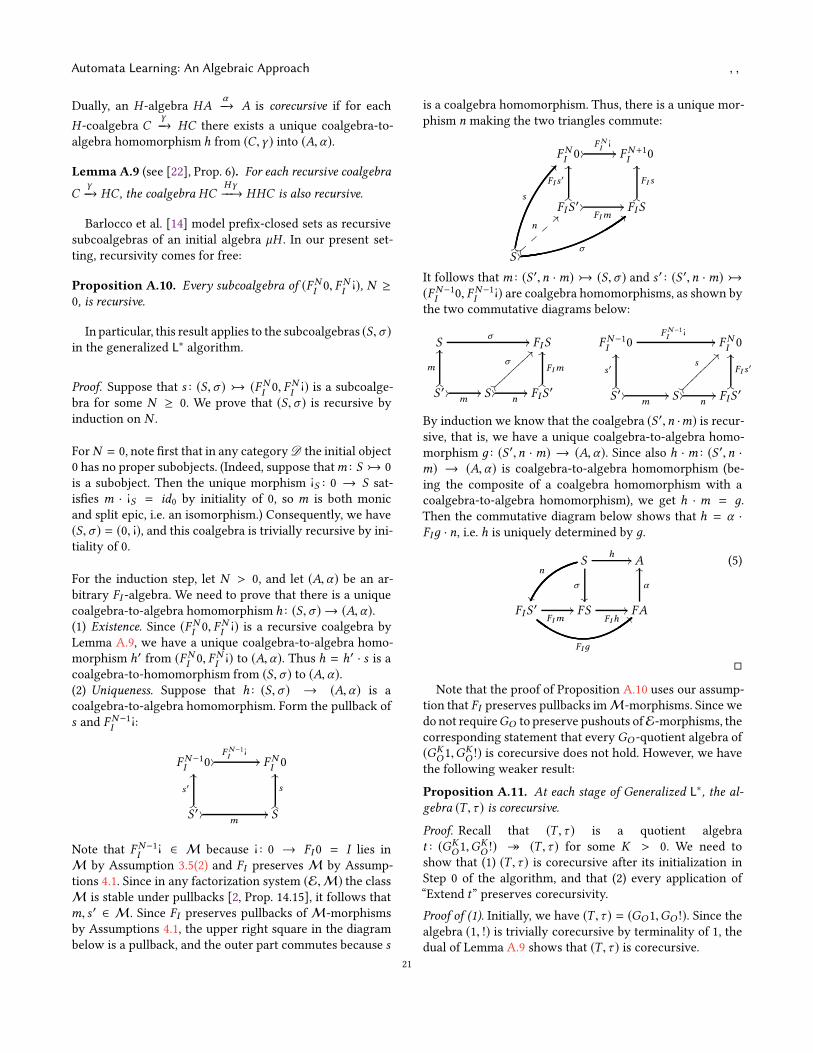
Automata Learning: An Algebraic Approach , ,
Dually, an H -algebra HAα−→ A is corecursive if for each
H -coalgebra Cγ−→ HC there exists a unique coalgebra-to-
algebra homomorphism h from (C,γ ) into (A,α).
Lemma A.9 (see [22], Prop. 6). For each recursive coalgebra
Cγ−→ HC , the coalgebra HC
Hγ−−→ HHC is also recursive.
Barlocco et al. [14] model prefix-closed sets as recursivesubcoalgebras of an initial algebra µH . In our present set-ting, recursivity comes for free:
Proposition A.10. Every subcoalgebra of (FNI0, FN
I¡), N ≥
0, is recursive.
In particular, this result applies to the subcoalgebras (S,σ )in the generalized L∗ algorithm.
Proof. Suppose that s : (S,σ ) (FNI0, FN
I¡) is a subcoalge-
bra for some N ≥ 0. We prove that (S,σ ) is recursive byinduction on N .
ForN = 0, note first that in any categoryD the initial object0 has no proper subobjects. (Indeed, suppose thatm : S 0is a subobject. Then the unique morphism ¡
S : 0 → S sat-isfies m · ¡S = id0 by initiality of 0, so m is both monicand split epic, i.e. an isomorphism.) Consequently, we have(S,σ ) = (0, ¡), and this coalgebra is trivially recursive by ini-tiality of 0.
For the induction step, let N > 0, and let (A,α) be an ar-bitrary FI -algebra. We need to prove that there is a uniquecoalgebra-to-algebra homomorphism h : (S,σ ) → (A,α).(1) Existence. Since (FN
I0, FN
I¡) is a recursive coalgebra by
Lemma A.9, we have a unique coalgebra-to-algebra homo-morphism h′ from (FN
I0, FN
I¡) to (A,α). Thus h = h′ · s is a
coalgebra-to-homomorphism from (S,σ ) to (A,α).(2) Uniqueness. Suppose that h : (S,σ ) → (A,α) is acoalgebra-to-algebra homomorphism. Form the pullback ofs and FN−1
I¡:
FN−1I 0 //F N−1I
¡// FNI 0
S ′OO
s ′
OO
//m
// SOO
s
OO
Note that FN−1I
¡ ∈ M because ¡ : 0 → FI 0 = I lies inM by Assumption 3.5(2) and FI preserves M by Assump-tions 4.1. Since in any factorization system (E,M) the classM is stable under pullbacks [2, Prop. 14.15], it follows thatm, s ′ ∈ M. Since FI preserves pullbacks ofM-morphismsby Assumptions 4.1, the upper right square in the diagrambelow is a pullback, and the outer part commutes because s
is a coalgebra homomorphism. Thus, there is a unique mor-phism n making the two triangles commute:
FNI0 //
F NI¡// FN+1
I0
FIS′
OO
FI s′
OO
//FIm
// FISOO
FI s
OO
S>>
n>>⑤
⑤⑤
⑤LL
s
@@
00σ
;;
It follows thatm : (S ′,n ·m) (S,σ ) and s ′ : (S ′,n ·m)(FN−1I 0, FN−1I
¡) are coalgebra homomorphisms, as shown bythe two commutative diagrams below:
Sσ // FIS
S ′ //m
//OO
m
OO
S //n
//>>
σ
>>⑥⑥⑥⑥⑥⑥⑥⑥FIS′
OO
FIm
OOFN−1I
0F N−1I
¡// FN
I0
S ′ //m
//OO
s ′
OO
S //n
//??
s??⑦⑦⑦⑦⑦⑦⑦⑦FIS′
OO
FI s′
OO
By induction we know that the coalgebra (S ′,n ·m) is recur-sive, that is, we have a unique coalgebra-to-algebra homo-morphism д : (S ′,n ·m) → (A,α). Since also h ·m : (S ′,n ·m) → (A,α) is coalgebra-to-algebra homomorphism (be-ing the composite of a coalgebra homomorphism with acoalgebra-to-algebra homomorphism), we get h · m = д.Then the commutative diagram below shows that h = α ·
FIд · n, i.e. h is uniquely determined by д.
Sn
��
h //
σ
��
A
FIS′
FIд
==FIm// FS
FIh// FA
α
OO (5)
�
Note that the proof of Proposition A.10 uses our assump-tion that FI preserves pullbacks imM-morphisms. Since wedo not requireGO to preserve pushouts ofE-morphisms, thecorresponding statement that everyGO -quotient algebra of(GK
O1,GKO !) is corecursive does not hold. However, we have
the following weaker result:
Proposition A.11. At each stage of Generalized L∗, the al-
gebra (T , τ ) is corecursive.
Proof. Recall that (T , τ ) is a quotient algebrat : (GK
O1,GKO !) ։ (T , τ ) for some K > 0. We need to
show that (1) (T , τ ) is corecursive after its initialization inStep 0 of the algorithm, and that (2) every application of“Extend t” preserves corecursivity.
Proof of (1). Initially, we have (T , τ ) = (GO1,GO !). Since thealgebra (1, !) is trivially corecursive by terminality of 1, thedual of Lemma A.9 shows that (T , τ ) is corecursive.
21
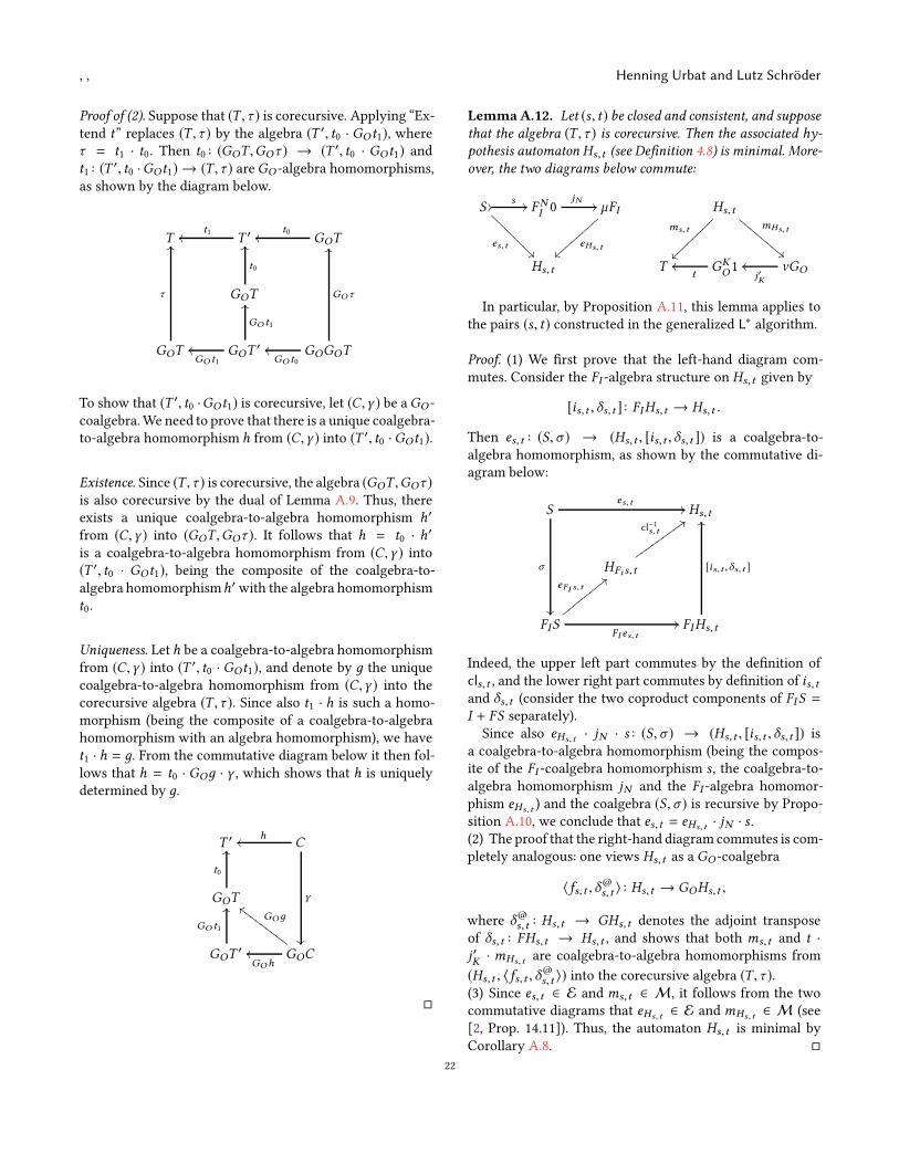
, , Henning Urbat and Lutz Schröder
Proof of (2). Suppose that (T , τ ) is corecursive. Applying “Ex-tend t” replaces (T , τ ) by the algebra (T ′, t0 · GOt1), whereτ = t1 · t0. Then t0 : (GOT ,GOτ ) → (T ′, t0 · GOt1) andt1 : (T ′, t0 ·GOt1) → (T , τ ) areGO -algebra homomorphisms,as shown by the diagram below.
T T ′t1oo GOT
t0oo
GOT
t0
OO
GOT
τ
OO
GOT′
GO t1
oo
GO t1
OO
GOGOT
GO τ
OO
GO t0
oo
To show that (T ′, t0 ·GOt1) is corecursive, let (C,γ ) be aGO -coalgebra.We need to prove that there is a unique coalgebra-to-algebra homomorphism h from (C,γ ) into (T ′, t0 ·GOt1).
Existence. Since (T , τ ) is corecursive, the algebra (GOT ,GOτ )
is also corecursive by the dual of Lemma A.9. Thus, thereexists a unique coalgebra-to-algebra homomorphism h′
from (C,γ ) into (GOT ,GOτ ). It follows that h = t0 · h′
is a coalgebra-to-algebra homomorphism from (C,γ ) into(T ′, t0 · GOt1), being the composite of the coalgebra-to-algebra homomorphismh′with the algebra homomorphismt0.
Uniqueness. Let h be a coalgebra-to-algebra homomorphismfrom (C,γ ) into (T ′, t0 · GOt1), and denote by д the uniquecoalgebra-to-algebra homomorphism from (C,γ ) into thecorecursive algebra (T , τ ). Since also t1 · h is such a homo-morphism (being the composite of a coalgebra-to-algebrahomomorphism with an algebra homomorphism), we havet1 · h = д. From the commutative diagram below it then fol-lows that h = t0 · GOд · γ , which shows that h is uniquelydetermined by д.
T ′ Choo
γ
��
GOT
t0
OO
GOT′
GO t1
OO
GOCGOhoo
GOдcc●●●●●●●●●
�
LemmaA.12. Let (s, t) be closed and consistent, and suppose
that the algebra (T , τ ) is corecursive. Then the associated hy-
pothesis automaton Hs,t (see Definition 4.8) is minimal. More-
over, the two diagrams below commute:
S // s //
es,t��❅❅
❅❅❅❅
❅❅FNI0
jN // µFI
eHs,t}}④④④④④④④④
Hs,t
Hs,t
ms,t
~~⑦⑦⑦⑦⑦⑦⑦⑦ mHs,t
!!❉❉❉
❉❉❉❉
❉
T GKO1t
oo νGOj′K
oo
In particular, by Proposition A.11, this lemma applies tothe pairs (s, t) constructed in the generalized L∗ algorithm.
Proof. (1) We first prove that the left-hand diagram com-mutes. Consider the FI -algebra structure on Hs,t given by
[is,t , δs,t ] : FIHs,t → Hs,t .
Then es,t : (S,σ ) → (Hs,t , [is,t , δs,t ]) is a coalgebra-to-algebra homomorphism, as shown by the commutative di-agram below:
Ses,t
//
σ
��
Hs,t
HFi s,t
cl−1s,t;;✈✈✈✈✈✈✈✈✈
FIS
eFI s,t<<②②②②②②②②
FI es,t
// FIHs,t
[is,t ,δs,t ]
OO
Indeed, the upper left part commutes by the definition ofcls,t , and the lower right part commutes by definition of is,tand δs,t (consider the two coproduct components of FIS =I + FS separately).
Since also eHs,t · jN · s : (S,σ ) → (Hs,t , [is,t , δs,t ]) isa coalgebra-to-algebra homomorphism (being the compos-ite of the FI -coalgebra homomorphism s , the coalgebra-to-algebra homomorphism jN and the FI -algebra homomor-phism eHs,t ) and the coalgebra (S,σ ) is recursive by Propo-sition A.10, we conclude that es,t = eHs,t · jN · s .(2) The proof that the right-hand diagram commutes is com-pletely analogous: one views Hs,t as a GO -coalgebra
〈fs,t , δ@s,t 〉 : Hs,t → GOHs,t ,
where δ@s,t : Hs,t → GHs,t denotes the adjoint transpose
of δs,t : FHs,t → Hs,t , and shows that both ms,t and t ·
j ′K · mHs,t are coalgebra-to-algebra homomorphisms from
(Hs,t , 〈fs,t , δ@s,t 〉) into the corecursive algebra (T , τ ).
(3) Since es,t ∈ E and ms,t ∈ M, it follows from the twocommutative diagrams that eHs,t ∈ E andmHs,t ∈ M (see[2, Prop. 14.11]). Thus, the automaton Hs,t is minimal byCorollary A.8. �
22
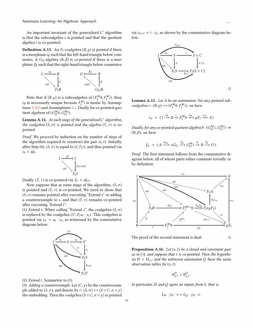
Automata Learning: An Algebraic Approach , ,
An important invariant of the generalized L∗ algorithmis that the subcoalgebra s is pointed and that the quotientalgebra t is co-pointed:
Definition A.13. An FI -coalgebra (R, ϱ) is pointed if thereis a morphism iR such that the left-hand triangle below com-mutes. A GO -algebra (B, β) is co-pointed if there is a mor-phism fR such that the right-hand triangle below commutes:
IiR //
inl ❅
❅❅❅❅
❅❅❅ R
ϱ
��
FIR
O BfB
oo
GOB
outl
aa❈❈❈❈❈❈❈❈β
OO
Note that if (R, ϱ) is a subcoalgebra of (FMI 0, FMI¡), then
iR is necessarily unique because FMI¡ is monic by Assump-
tions 3.5(2) and Assumptions 4.1. Dually for co-pointed quo-tient algebras of (GM
O 0,GMO !).
Lemma A.14. At each stage of the generalized L∗ algorithm,
the coalgebra (S,σ ) is pointed and the algebra (T , τ ) is co-
pointed.
Proof. We proceed by induction on the number of steps ofthe algorithm required to construct the pair (s, t). Initially,after Step (0), (S,σ ) is equal to (I , FI ¡), and thus pointed viaiS = idI .
Iid //
inl��❅❅
❅❅❅❅
❅❅I
FI ¡=inl
��
FI I
Dually, (T , τ ) is co-pointed via fT = idO .Now suppose that at some stage of the algorithm, (S,σ )
is pointed and (T , τ ) is co-pointed. We need to show that(S,σ ) remains pointed after executing “Extend s” or addinga counterexample to s , and that (T , τ ) remains co-pointedafter executing “Extend t”.(1) Extend s . When calling “Extend s”, the coalgebra (S,σ )is replaced by the coalgebra (S ′, FIs0 · s1). This coalgebra ispointed via iS ′ = s0 · iS , as witnessed by the commutativediagram below:
IiS //
iS′
!!
inl --
inl
++
Ss0 //
σ
❇❇❇
❇❇❇❇
❇ S ′
s1
��
FIS
FI s0
��
FIS′
(2) Extend t . Symmetric to (1).(3) Adding a counterexample. Let (C,γ ) be the counterexam-ple added to (S,σ ), and denote by i : (S,σ ) (S ∨C,σ ∨ γ )the embedding. Then the coalgebra (S ∨C,σ ∨γ ) is pointed
via iS∨C = i · iS , as shown by the commutative diagram be-low:
I
inl
99
iS //
iS∨C
$$
inl��❅❅
❅❅❅❅
❅❅S
σ
��
i // S ∨C
σ∨γ
��
FISFI i
// FI (S ∨C)
�
Lemma A.15. Let A be an automaton. For any pointed sub-
coalgebra r : (R, ϱ) (FMI 0, FMI¡), we have
iA = ( IiR−→ R
r−→ FMI 0
jM−−→ µFI
eA−−→ A )
Dually, for any co-pointed quotient algebrab : (GMO 1,GM
O !)։(B, β), we have
fA = (AmA−−→ νGO
j′M−−→ GM
O 1b−→ B
fB−−→ O ).
Proof. The first statement follows from the commutative di-agram below, all of whose parts either commute trivially orby definition.
IiA //
iR
��
inl
��✳✳✳✳✳✳✳✳✳✳✳✳✳✳✳
inl
%%❑❑❑
❑❑❑❑
❑❑❑❑
❑❑❑❑
❑❑❑❑
❑❑❑❑
❑❑
inl
%%
inl
,,❳❳❳❳❳❳❳❳❳
❳❳❳❳❳❳❳❳❳❳
❳❳❳❳❳❳❳❳❳❳
❳❳❳❳ A
FIA
αA
<<②②②②②②②②②
FIRFI r // FM+1I 0
FI jM //
jM+1((❘❘
❘❘❘❘❘❘
❘❘❘❘❘❘
❘❘FI (µFI )
FI eA
OO
α
!!❇❇❇
❇❇❇❇
❇❇
Rr
//
ϱ
BB☎☎☎☎☎☎☎☎FMI0
jM//
FMI¡
==⑤⑤⑤⑤⑤⑤⑤⑤µFI
eA
OO
The proof of the second statement is dual. �
Proposition A.16. Let (s, t) be a closed and consistent pair
as in (3), and suppose that t is co-pointed. Then the hypothe-
sis H = Hs,t and the unknown automaton Q have the same
observation tables for (s, t):
hHs,t = hQs,t .
In particular, H and Q agree on inputs from S , that is,
LH · jN · s = LQ · jN · s .
23
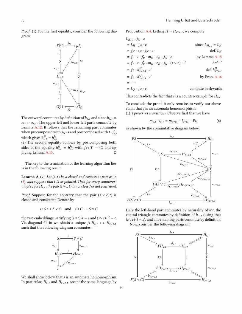
, , Henning Urbat and Lutz Schröder
Proof. (1) For the first equality, consider the following dia-gram:
FNI 0jN // µFI
eQ
��
eHs,t
��☛☛☛☛☛☛☛☛☛☛☛☛☛☛☛
S
s
OO
es,t����
Hs,t��
ms,t
��mHs,t
��✸✸
✸✸✸✸
✸✸✸✸
✸✸✸✸
✸Q
mQ
��
T
GKO1
t
OO
νGOj′K
oo
The outward commutes by definition ofhs,t and sincehs,t =ms,t · es,t . The upper left and lower left parts commute byLemma A.12. It follows that the remaining part commuteswhen precomposed with jN ·s and postcomposed with t · j ′K ,
which gives hHs,t = hQs,t .
(2) The second equality follows by postcomposing bothsides of the equality hHs,t = h
Qs,t with fT : T → O and ap-
plying Lemma A.15. �
The key to the termination of the learning algorithm liesis in the following result.
Lemma A.17. Let (s, t) be a closed and consistent pair as in
(3), and suppose that t is co-pointed. Then for every counterex-ample c forHs,t , the pair (s∨c, t) is not closed or not consistent.
Proof. Suppose for the contrary that the pair (s ∨ c, t) isclosed and consistent. Denote by
i : S S ∨C and i ′ : C → S ∨C
the two embeddings, satisfying (s∨c) ·i = s and (s∨c) ·i ′ = c .Via diagonal fill-in we obtain a unique j : Hs,t Hs∨c,t
such that the following diagram commutes:
S // i //
es,t����
S ∨C
es∨c,t����
Hs,t//
j//
��
ms,t
��
Hs∨c,t{{
ms∨c,t
{{✇✇✇✇✇✇✇✇✇
T
We shall show below that j is an automata homomorphism.In particular, Hs,t and Hs∨c,t accept the same language by
Proposition A.4. Letting H = Hs∨c,t , we compute
LHs,t · jN · c
= LH · jN · c since LHs,t = LH
= fH · eH · jN · c def. LH
= fT · t · j′K ·mH · eH · jN · c by Lemma A.15
= fT · t · j′K ·mH · eH · jN · (s ∨ c) · i
′ def. i ′
= fT · hHs∨c,t · i
′ def. hHs∨c,t
= fT · hQs∨c,t · i
′ by Prop. A.16
= · · ·
= LQ · jN · c compute backwards
This contradicts the fact that c is a counterexample for Hs,t .
To conclude the proof, it only remains to verify our aboveclaim that j is an automata homomorphism.(1) j preserves transitions. Observe first that we have
ms,t · ls,t =ms∨c,t · ls∨c,t · Fi, (6)
as shown by the commutative diagram below:
FS
F i
��
ls,t//
inr
&&▲▲▲
▲▲▲▲
▲▲▲▲
▲ Hs,t
ms,t
��
FISeFI s,t //
hFI s,t**❱❱❱
❱❱❱❱❱❱❱❱
❱❱❱❱❱❱❱❱
❱❱❱❱❱
FI i
��
HFI s,t
mFI s,t
%%❑❑❑
❑❑❑❑
❑❑❑
cl−1s,t
99ssssssssss
T
FI (S ∨C)
hFI (s∨c ),t
44✐✐✐✐✐✐✐✐✐✐✐✐✐✐✐✐✐✐✐✐✐✐
eFI (s∨c ),t// HFI (s∨c),t
mFI (s∨c ),t
99sssssssssss
cl−1s∨c,t %%❏❏❏
❏❏❏❏
❏❏
F (S ∨C)
inr
99rrrrrrrrrr
ls∨c,t
// Hs∨c,t
ms∨c,t
OO
Here the left-hand part commutes by naturality of inr, thecentral triangle commutes by definition of h−,t (using that(s∨c) ·i = s), and all remaining parts commute by definition.Now, consider the following diagram:
FSls,t
//
F i
��
Fes,t
((PPPPP
PPPP Hs,t
ms,t
��
FHs,t
δs,t//
F j
��
Hs,t
j
��
♣♣♣♣♣♣♣♣
♣♣♣♣♣♣♣♣
T
FHs∨c,tδs∨c,t
// Hs∨c,t
◆◆◆◆◆◆
◆
◆◆◆◆◆◆
◆
F (S ∨C)Fes∨c,t
77♥♥♥♥♥♥♥
ls∨c,t
// Hs∨c,t
ms∨c,t
OO
24
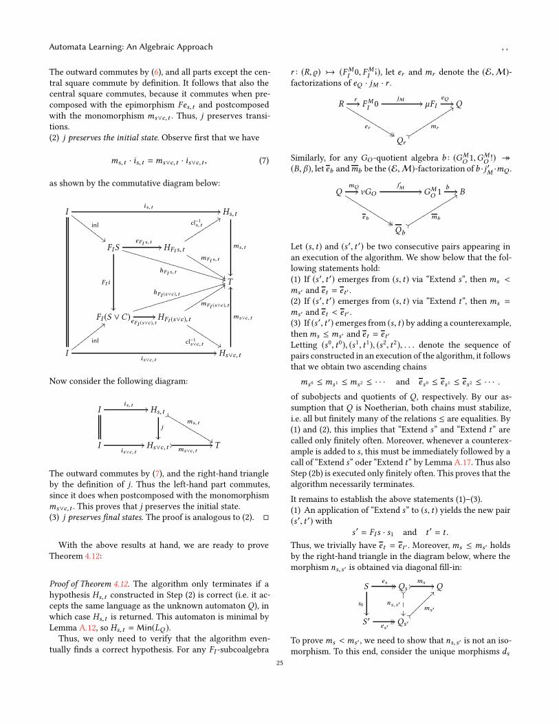
Automata Learning: An Algebraic Approach , ,
The outward commutes by (6), and all parts except the cen-tral square commute by definition. It follows that also thecentral square commutes, because it commutes when pre-composed with the epimorphism Fes,t and postcomposedwith the monomorphism ms∨c,t . Thus, j preserves transi-tions.(2) j preserves the initial state. Observe first that we have
ms,t · is,t =ms∨c,t · is∨c,t , (7)
as shown by the commutative diagram below:
Iis,t
//
inl
##❋❋❋
❋❋❋❋
❋❋❋ Hs,t
ms,t
��
FISeFI s,t //
hFI s,t**❱❱❱
❱❱❱❱❱❱❱❱
❱❱❱❱❱❱❱❱
❱❱❱❱❱
FI i
��
HFI s,t
mFI s,t
%%❑❑❑
❑❑❑❑
❑❑❑
cl−1s,t
99ssssssssss
T
FI (S ∨C)
hFI (s∨c ),t
44✐✐✐✐✐✐✐✐✐✐✐✐✐✐✐✐✐✐✐✐✐✐
eFI (s∨c ),t// HFI (s∨c),t
mFI (s∨c ),t
99sssssssssss
cl−1s∨c,t %%❏❏❏
❏❏❏❏
❏❏
I
inl
<<①①①①①①①①①①is∨c,t
// Hs∨c,t
ms∨c,t
OO
Now consider the following diagram:
Iis,t
// Hs,t %%ms,t
%%▲▲▲
▲▲▲▲
▲▲▲▲
▲
j
��
Iis∨c,t
// Hs∨c,t//ms∨c,t
// T
The outward commutes by (7), and the right-hand triangleby the definition of j . Thus the left-hand part commutes,since it does when postcomposed with the monomorphismms∨c,t . This proves that j preserves the initial state.(3) j preserves final states. The proof is analogous to (2). �
With the above results at hand, we are ready to proveTheorem 4.12:
Proof of Theorem 4.12. The algorithm only terminates if ahypothesis Hs,t constructed in Step (2) is correct (i.e. it ac-cepts the same language as the unknown automaton Q), inwhich case Hs,t is returned. This automaton is minimal byLemma A.12, so Hs,t = Min(LQ ).Thus, we only need to verify that the algorithm even-
tually finds a correct hypothesis. For any FI -subcoalgebra
r : (R, ϱ) (FMI 0, FMI¡), let er and mr denote the (E,M)-
factorizations of eQ · jM · r .
Rr //
er%% %%▲
▲▲▲▲
▲▲▲▲
▲▲▲▲ FM
I0
jM // µFIeQ
// Q
Qr
99
mr
99ssssssssssss
Similarly, for any GO -quotient algebra b : (GMO 1,GM
O !) ։(B, β), let eb andmb be the (E,M)-factorization ofb · j ′M ·mQ .
QmQ
//
eb%% %%❑
❑❑❑❑
❑❑❑❑
❑❑❑❑ νGO
j′M // GMO1
b // B
Qb
99mb
99sssssssssssss
Let (s, t) and (s ′, t ′) be two consecutive pairs appearing inan execution of the algorithm. We show below that the fol-lowing statements hold:(1) If (s ′, t ′) emerges from (s, t) via “Extend s”, then ms <
ms ′ and et = et ′ .(2) If (s ′, t ′) emerges from (s, t) via “Extend t”, then ms =
ms ′ and et < et ′ .(3) If (s ′, t ′) emerges from (s, t) by adding a counterexample,thenms ≤ ms ′ and et = et ′
Letting (s0, t0), (s1, t1), (s2, t2), . . . denote the sequence ofpairs constructed in an execution of the algorithm, it followsthat we obtain two ascending chains
ms0 ≤ ms1 ≤ ms2 ≤ · · · and es0 ≤ es1 ≤ es2 ≤ · · · .
of subobjects and quotients of Q , respectively. By our as-sumption that Q is Noetherian, both chains must stabilize,i.e. all but finitely many of the relations ≤ are equalities. By(1) and (2), this implies that “Extend s” and “Extend t” arecalled only finitely often. Moreover, whenever a counterex-ample is added to s , this must be immediately followed by acall of “Extend s” oder “Extend t” by Lemma A.17. Thus alsoStep (2b) is executed only finitely often. This proves that thealgorithm necessarily terminates.
It remains to establish the above statements (1)–(3).(1) An application of “Extend s” to (s, t) yields the new pair(s ′, t ′) with
s ′ = FIs · s1 and t ′ = t .
Thus, we trivially have et = et ′ . Moreover,ms ≤ ms ′ holdsby the right-hand triangle in the diagram below, where themorphism ns,s ′ is obtained via diagonal fill-in:
S
s0
��
es // // Qs//ms //
��
ns,s′
��✤✤✤
Q
S ′es′
// // Qs ′
??ms′
??⑦⑦⑦⑦⑦⑦⑦⑦
To provems <ms ′ , we need to show that ns,s ′ is not an iso-morphism. To this end, consider the unique morphisms ds
25
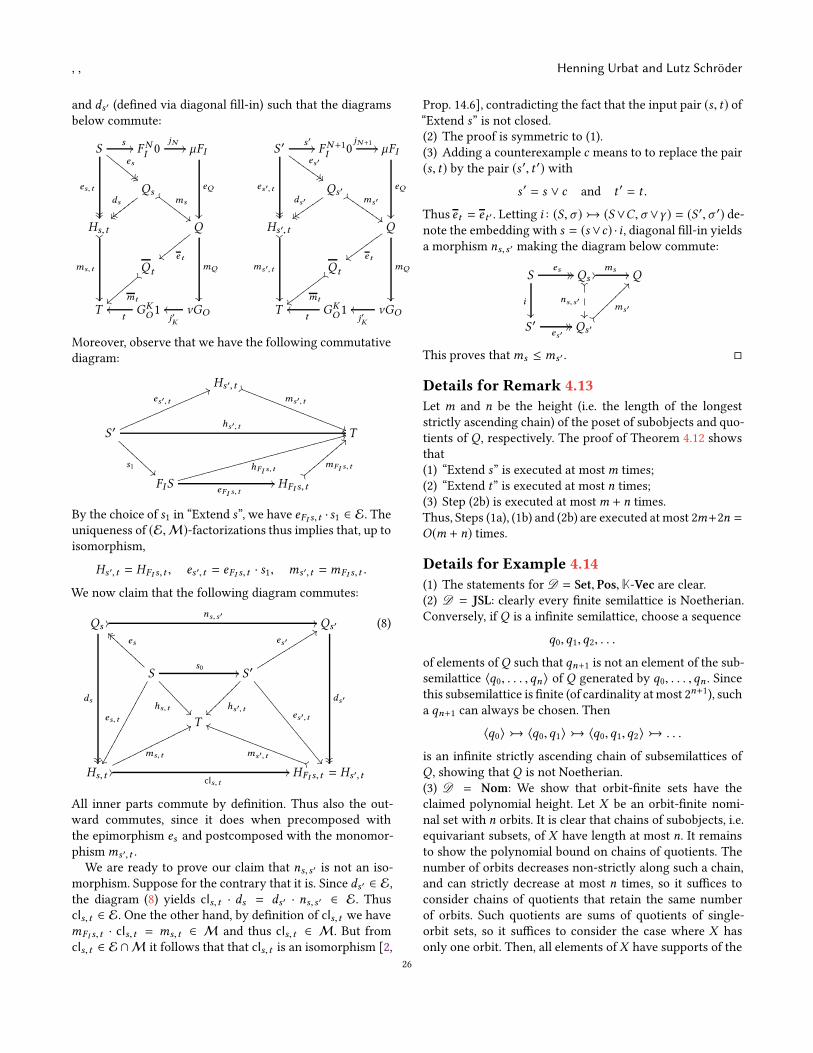
, , Henning Urbat and Lutz Schröder
and ds ′ (defined via diagonal fill-in) such that the diagramsbelow commute:
Ss //
es,t
����
es
"" ""❊❊❊
❊❊❊ FN
I0
jN // µFI
eQ
��
Qs ##ms
##●●●
●●●
ds
{{{{①①①①①①
Hs,t��
ms,t
��
Q
e t||②②②②②②
mQ
��
Qt}}
mt}}③③③③③③
T GKO1t
oo νGOj′K
oo
S ′s ′ //
es′,t
����
es′
$$ $$❍❍❍
❍❍❍❍
FN+1I
0jN+1 // µFI
eQ
��
Qs ′ $$ ms′
$$■■■
■■■■ds′
zzzz✉✉✉✉✉✉
Hs ′,t��
ms′,t
��
Q
e t{{✈✈✈✈✈✈✈
mQ
��
Qt{{
mt{{✇✇✇✇✇✇✇
T GKO1t
oo νGOj′K
oo
Moreover, observe that we have the following commutativediagram:
Hs ′,t ))
ms′,t
))❘❘❘❘❘
❘❘❘❘❘❘
❘❘❘❘❘❘
S ′hs′,t
//
es′,t
66♠♠♠♠♠♠♠♠♠♠♠♠♠♠♠
s1 ❆
❆❆❆❆
❆❆❆ T
FIS
hFI s,t
33❤❤❤❤❤❤❤❤❤❤❤❤❤❤❤❤❤❤❤❤❤❤❤❤❤❤❤eFI s,t
// HFI s,t
==mFI s,t
==③③③③③③③③③
By the choice of s1 in “Extend s”, we have eFI s,t · s1 ∈ E. Theuniqueness of (E,M)-factorizations thus implies that, up toisomorphism,
Hs ′,t = HFI s,t , es ′,t = eFI s,t · s1, ms ′,t =mFI s,t .
We now claim that the following diagram commutes:
Qs//
ns,s′//
ds
����
Qs ′
ds′
����
S
es,t
��✍✍✍✍✍✍✍✍✍✍✍✍✍✍✍
hs,t ��❃❃
❃❃❃❃
❃
es````❆❆❆❆❆❆❆❆
s0 // S ′
es′,t
��✾✾
✾✾✾✾
✾✾✾✾
✾✾✾✾
✾✾
es′99sssssssssss
hs′,t��⑧⑧⑧⑧⑧⑧⑧⑧
T
Hs,t
ms,t
77♦♦♦♦♦♦♦♦♦♦♦♦♦♦//
cls,t
// HFI s,t = Hs ′,t
iims′,t
ii❙❙❙❙❙❙❙❙❙❙❙❙❙❙❙❙
(8)
All inner parts commute by definition. Thus also the out-ward commutes, since it does when precomposed withthe epimorphism es and postcomposed with the monomor-phismms ′,t .We are ready to prove our claim that ns,s ′ is not an iso-
morphism. Suppose for the contrary that it is. Since ds ′ ∈ E,the diagram (8) yields cls,t · ds = ds ′ · ns,s ′ ∈ E. Thuscls,t ∈ E. One the other hand, by definition of cls,t we havemFI s,t · cls,t = ms,t ∈ M and thus cls,t ∈ M. But fromcls,t ∈ E ∩M it follows that that cls,t is an isomorphism [2,
Prop. 14.6], contradicting the fact that the input pair (s, t) of“Extend s” is not closed.(2) The proof is symmetric to (1).(3) Adding a counterexample c means to to replace the pair(s, t) by the pair (s ′, t ′) with
s ′ = s ∨ c and t ′ = t .
Thus et = et ′ . Letting i : (S,σ ) (S ∨C,σ ∨γ ) = (S ′,σ ′) de-note the embedding with s = (s∨c) · i , diagonal fill-in yieldsa morphism ns,s ′ making the diagram below commute:
S
i
��
es // // Qs//ms //
��
ns,s′
��✤✤✤
Q
S ′es′
// // Qs ′
??ms′
??⑦⑦⑦⑦⑦⑦⑦⑦
This proves thatms ≤ ms ′ . �
Details for Remark 4.13
Let m and n be the height (i.e. the length of the longeststrictly ascending chain) of the poset of subobjects and quo-tients of Q , respectively. The proof of Theorem 4.12 showsthat(1) “Extend s” is executed at mostm times;(2) “Extend t” is executed at most n times;(3) Step (2b) is executed at mostm + n times.Thus, Steps (1a), (1b) and (2b) are executed at most 2m+2n =O(m + n) times.
Details for Example 4.14
(1) The statements for D = Set, Pos,K-Vec are clear.(2) D = JSL: clearly every finite semilattice is Noetherian.Conversely, if Q is a infinite semilattice, choose a sequence
q0,q1,q2, . . .
of elements ofQ such that qn+1 is not an element of the sub-semilattice 〈q0, . . . ,qn〉 of Q generated by q0, . . . ,qn . Sincethis subsemilattice is finite (of cardinality atmost 2n+1), sucha qn+1 can always be chosen. Then
〈q0〉 〈q0,q1〉 〈q0,q1,q2〉 . . .
is an infinite strictly ascending chain of subsemilattices ofQ , showing that Q is not Noetherian.(3) D = Nom: We show that orbit-finite sets have theclaimed polynomial height. Let X be an orbit-finite nomi-nal set with n orbits. It is clear that chains of subobjects, i.e.equivariant subsets, of X have length at most n. It remainsto show the polynomial bound on chains of quotients. Thenumber of orbits decreases non-strictly along such a chain,and can strictly decrease at most n times, so it suffices toconsider chains of quotients that retain the same numberof orbits. Such quotients are sums of quotients of single-orbit sets, so it suffices to consider the case where X hasonly one orbit. Then, all elements of X have supports of the
26
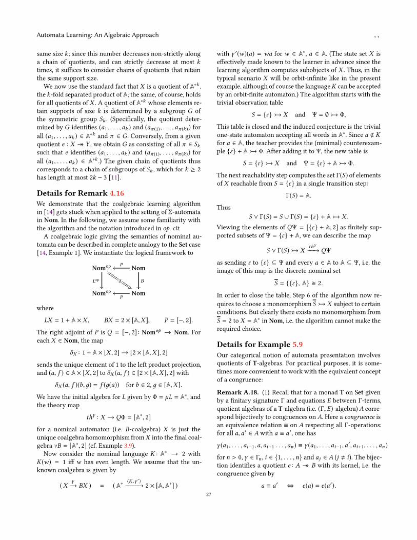
Automata Learning: An Algebraic Approach , ,
same size k; since this number decreases non-strictly alonga chain of quotients, and can strictly decrease at most ktimes, it suffices to consider chains of quotients that retainthe same support size.We now use the standard fact that X is a quotient of A
∗k ,the k-fold separated product of A; the same, of course, holdsfor all quotients of X . A quotient of A
∗k whose elements re-tain supports of size k is determined by a subgroup G ofthe symmetric group Sk . (Specifically, the quotient deter-mined by G identifies (a1, . . . ,ak ) and (aπ (1), . . . ,aπ (k)) forall (a1, . . . ,ak ) ∈ A
∗k and π ∈ G . Conversely, from a givenquotient e : X ։ Y , we obtain G as consisting of all π ∈ Sksuch that e identifies (a1, . . . ,ak ) and (aπ (1), . . . ,aπ (k)) forall (a1, . . . ,ak ) ∈ A
∗k .) The given chain of quotients thuscorresponds to a chain of subgroups of Sk , which for k ≥ 2has length at most 2k − 3 [11].
Details for Remark 4.16
We demonstrate that the coalgebraic learning algorithmin [14] gets stuck when applied to the setting of Σ-automatain Nom. In the following, we assume some familiarity withthe algorithm and the notation introduced in op. cit.
A coalgebraic logic giving the semantics of nominal au-tomata can be described in complete analogy to the Set case[14, Example 1]. We instantiate the logical framework to
Nomop
δ■■■
■■■■■
■■
(■■■
■■■■
■Lop
��
NomPoo
B
��
Nomop NomP
oo
where
LX = 1 + A × X , BX = 2 × [A,X ], P = [−, 2].
The right adjoint of P is Q = [−, 2] : Nomop → Nom. Foreach X ∈ Nom, the map
δX : 1 + A × [X , 2] → [2 × [A,X ], 2]
sends the unique element of 1 to the left product projection,and (a, f ) ∈ A × [X , 2] to δX (a, f ) ∈ [2 × [A,X ], 2]with
δX (a, f )(b,д) = f (д(a)) for b ∈ 2, д ∈ [A,X ].
We have the initial algebra for L given by Φ = µL = A∗, and
the theory map
thγ : X → QΦ = [A∗, 2]
for a nominal automaton (i.e. B-coalgebra) X is just theunique coalgebra homomorphism fromX into the final coal-gebra νB = [A∗, 2] (cf. Example 3.9).Now consider the nominal language K : A
∗ → 2 withK(w) = 1 iff w has even length. We assume that the un-known coalgebra is given by
(Xγ−→ BX ) = (A∗
〈K,γ ′〉−−−−−→ 2 × [A,A∗] )
with γ ′(w)(a) = wa for w ∈ A∗, a ∈ A. (The state set X is
effectively made known to the learner in advance since thelearning algorithm computes subobjects of X . Thus, in thetypical scenario X will be orbit-infinite like in the presentexample, although of course the languageK can be acceptedby an orbit-finite automaton.) The algorithm starts with thetrivial observation table
S = {ε} X and Ψ = ∅ Φ,
This table is closed and the induced conjecture is the trivialone-state automaton accepting all words in A
∗. Since a < Kfor a ∈ A, the teacher provides the (minimal) counterexam-ple {ε} + A Φ. After adding it to Ψ, the new table is
S = {ε} X and Ψ = {ε} + A Φ.
The next reachability step computes the set Γ(S) of elementsof X reachable from S = {ε} in a single transition step:
Γ(S) = A.
Thus
S ∨ Γ(S) = S ∪ Γ(S) = {ε} + A X .
Viewing the elements of QΨ = [{ε} + A, 2] as finitely sup-ported subsets of Ψ = {ε} + A, we can describe the map
S ∨ Γ(S) Xthγ
−−−→ QΨ
as sending ε to {ε} ⊆ Ψ and every a ∈ A to A ⊆ Ψ, i.e. theimage of this map is the discrete nominal set
S = {{ε}, A} � 2.
In order to close the table, Step 6 of the algorithm now re-quires to choose a monomorphism S X subject to certainconditions. But clearly there exists no monomorphism fromS = 2 to X = A
∗ in Nom, i.e. the algorithm cannot make therequired choice.
Details for Example 5.9
Our categorical notion of automata presentation involvesquotients of T-algebras. For practical purposes, it is some-times more convenient to work with the equivalent conceptof a congruence:
Remark A.18. (1) Recall that for a monad T on Set givenby a finitary signature Γ and equations E between Γ-terms,quotient algebras of a T-algebra (i.e. (Γ, E)-algebra)A corre-spond bijectively to congruences on A. Here a congruence isan equivalence relation ≡ on A respecting all Γ-operations:for all a,a′ ∈ A with a ≡ a′, one has
γ (a1, . . . ,ai−1,a,ai+1 . . . ,an) ≡ γ (a1, . . . ,ai−1,a′,ai+1, . . . ,an)
for n > 0, γ ∈ Γn , i ∈ {1, . . . ,n} and aj ∈ A (j , i). The bijec-tion identifies a quotient e : A ։ B with its kernel, i.e. thecongruence given by
a ≡ a′ ⇔ e(a) = e(a′).
27
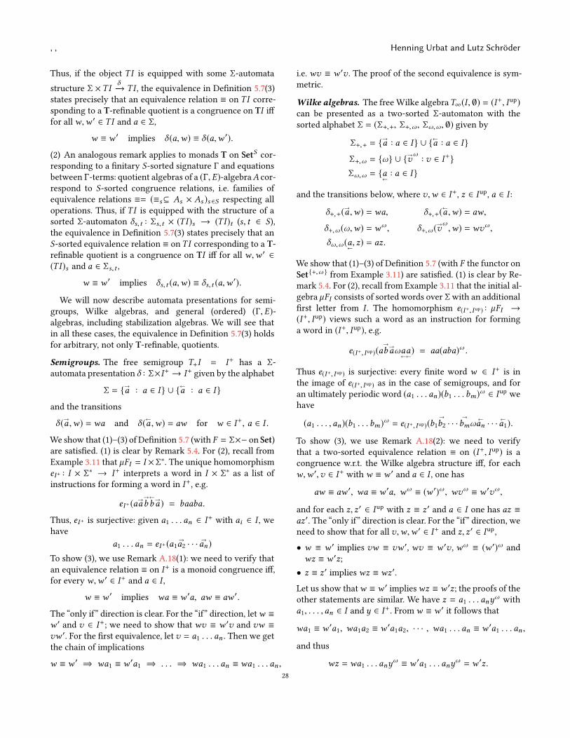
, , Henning Urbat and Lutz Schröder
Thus, if the object TI is equipped with some Σ-automata
structure Σ ×TIδ−→ TI , the equivalence in Definition 5.7(3)
states precisely that an equivalence relation ≡ on TI corre-sponding to a T-refinable quotient is a congruence on TI ifffor allw,w ′ ∈ TI and a ∈ Σ,
w ≡ w ′ implies δ (a,w) ≡ δ (a,w ′).
(2) An analogous remark applies to monads T on SetS cor-responding to a finitary S-sorted signature Γ and equationsbetween Γ-terms: quotient algebras of a (Γ, E)-algebraA cor-respond to S-sorted congruence relations, i.e. families ofequivalence relations ≡= (≡s⊆ As × As )s ∈S respecting alloperations. Thus, if TI is equipped with the structure of asorted Σ-automaton δs,t : Σs,t × (TI )s → (TI )t (s, t ∈ S),the equivalence in Definition 5.7(3) states precisely that anS-sorted equivalence relation ≡ onTI corresponding to a T-refinable quotient is a congruence on TI iff for all w,w ′ ∈(TI )s and a ∈ Σs,t ,
w ≡ w ′ implies δs,t (a,w) ≡ δs,t (a,w′).
We will now describe automata presentations for semi-groups, Wilke algebras, and general (ordered) (Γ, E)-algebras, including stabilization algebras. We will see thatin all these cases, the equivalence in Definition 5.7(3) holdsfor arbitrary, not only T-refinable, quotients.
Semigroups. The free semigroup T+I = I+ has a Σ-automata presentation δ : Σ×I+→ I+ given by the alphabet
Σ = {→a : a ∈ I } ∪ {
←a : a ∈ I }
and the transitions
δ (→a ,w) = wa and δ (
←a ,w) = aw for w ∈ I+, a ∈ I .
We show that (1)–(3) of Definition 5.7 (with F = Σ×− on Set)are satisfied. (1) is clear by Remark 5.4. For (2), recall fromExample 3.11 that µFI = I ×Σ∗. The unique homomorphismeI+ : I × Σ
∗ → I+ interprets a word in I × Σ∗ as a list of
instructions for forming a word in I+, e.g.
eI+ (a→a→
b←
b→a ) = baaba.
Thus, eI+ is surjective: given a1 . . . an ∈ I+ with ai ∈ I , wehave
a1 . . . an = eI+ (a1→a2 · · ·
→an)
To show (3), we use Remark A.18(1): we need to verify thatan equivalence relation ≡ on I+ is a monoid congruence iff,for every w,w ′ ∈ I+ and a ∈ I ,
w ≡ w ′ implies wa ≡ w ′a, aw ≡ aw ′.
The “only if” direction is clear. For the “if” direction, letw ≡w ′ and v ∈ I+; we need to show that wv ≡ w ′v and vw ≡vw ′. For the first equivalence, let v = a1 . . . an . Then we getthe chain of implications
w ≡ w ′ ⇒ wa1 ≡ w′a1 ⇒ . . . ⇒ wa1 . . . an ≡ wa1 . . . an ,
i.e. wv ≡ w ′v . The proof of the second equivalence is sym-metric.
Wilke algebras. The free Wilke algebraT∞(I , ∅) = (I+, Iup)can be presented as a two-sorted Σ-automaton with thesorted alphabet Σ = (Σ+,+, Σ+,ω, Σω,ω, ∅) given by
Σ+,+ = {→a : a ∈ I } ∪ {
←a : a ∈ I }
Σ+,ω = {ω} ∪ {→vω: v ∈ I+}
Σω,ω = {a←: a ∈ I }
and the transitions below, where v,w ∈ I+, z ∈ Iup, a ∈ I :
δ+,+(→a ,w) = wa, δ+,+(
←a ,w) = aw,
δ+,ω (ω,w) = wω, δ+,ω (
→vω,w) = wvω ,
δω,ω (a←, z) = az.
We show that (1)–(3) of Definition 5.7 (with F the functor onSet{+,ω } from Example 3.11) are satisfied. (1) is clear by Re-mark 5.4. For (2), recall from Example 3.11 that the initial al-gebra µFI consists of sorted words over Σwith an additionalfirst letter from I . The homomorphism e(I+, I up) : µFI →(I+, Iup) views such a word as an instruction for forminga word in (I+, Iup), e.g.
e(I+, I up)(a→
b→aωa
←a←) = aa(aba)ω .
Thus e(I+, I up) is surjective: every finite word w ∈ I+ is inthe image of e(I+, I up) as in the case of semigroups, and foran ultimately periodic word (a1 . . . an)(b1 . . . bm)ω ∈ Iup wehave
(a1 . . . ,an)(b1 . . . bm)ω= e(I+, I up)(b1
→
b2 · · ·→
bmω←an · · ·
←a1).
To show (3), we use Remark A.18(2): we need to verifythat a two-sorted equivalence relation ≡ on (I+, Iup) is acongruence w.r.t. the Wilke algebra structure iff, for eachw,w ′,v ∈ I+ with w ≡ w ′ and a ∈ I , one has
aw ≡ aw ′, wa ≡ w ′a, wω ≡ (w ′)ω , wvω ≡ w ′vω ,
and for each z, z′ ∈ Iup with z ≡ z′ and a ∈ I one has az ≡az′. The “only if” direction is clear. For the “if” direction, weneed to show that for all v,w,w ′ ∈ I+ and z, z′ ∈ Iup,
• w ≡ w ′ implies vw ≡ vw ′, wv ≡ w ′v , wω ≡ (w ′)ω andwz ≡ w ′z;
• z ≡ z′ implies wz ≡ wz′.
Let us show thatw ≡ w ′ implieswz ≡ w ′z; the proofs of theother statements are similar. We have z = a1 . . . any
ω witha1, . . . ,an ∈ I and y ∈ I+. Fromw ≡ w ′ it follows that
wa1 ≡ w′a1, wa1a2 ≡ w
′a1a2, · · · , wa1 . . . an ≡ w′a1 . . . an ,
and thus
wz = wa1 . . . anyω ≡ w ′a1 . . . any
ω= w ′z.
28
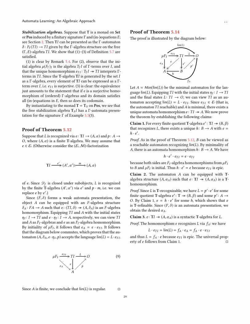
Automata Learning: An Algebraic Approach , ,
Stabilization algebras. Suppose that T is a monad on Set
or Pos induced by a finitary signature Γ and (in-)equationsE;see Section 2. Then TI can be presented as the Γ-automatonδ : FΓ(TI ) → TI given by the Γ-algebra structure on the free(Γ, E)-algebraTI . We show that (1)–(3) of Definition 5.7 aresatisfied.(1) is clear by Remark 5.4. For (2), observe that the ini-
tial algebra µ(FΓ)I is the algebra TΓI of Γ-terms over I , andthat the unique homomorphism eT I : TΓI ։ TI interprets Γ-terms inTI . Since the T-algebra TI is generated by the set Ias a Γ-algebra, every element of TI can be expressed as a Γ-term over I , i.e. eT I is surjective. (3) is clear: the equivalencejust amounts to the statement that if e is a surjective homo-morphism of (ordered) Γ-algebras and its domain satisfiesall (in-)equations in E, then so does its codomain.By instantiating to the monad T = TS on Pos, we see that
the free stabilization algebra TS I has a Γ-automata presen-tation for the signature Γ of Example 5.5(3).
Proof of Theorem 5.12
Suppose that L is recognized via e : TI → (A,α) and p : A→O , where (A,α) is a finite T-algebra. We may assume thate ∈ E. (Otherwise consider the (E,M)-factorization
TIe ′ // // (A′,α ′) //
m // (A,α)
of e . Since Df is closed under subobjects, L is recognizedby the finite T-algebra (A′,α ′) via e ′ and p ·m, i.e. we canreplace e by e ′.)Since (F , δ ) forms a weak automata presentation, the
object A can be equipped with an F -algebra structureδA : FA → A such that e : (TI , δ ) ։ (A, δA) is an F -algebrahomomorphism. Equipping TI and A with the initial statesηI : I → TI and e · ηI : I → A, respectively, we can view TI
andA as FI -algebras and e as an FI -algebra homomorphism.By initiality of µFI , it follows that eA = e · eT I . It followsthat the diagram below commutes, which proves that the au-tomaton (A, δA, e ·ηI ,p) accepts the language lin(L) = L ·eT I .
µFIeT I // //
eA!!❇
❇❇❇❇
❇❇❇
TI
e
��
L // O
A
p
??⑦⑦⑦⑦⑦⑦⑦⑦
(9)
Since A is finite, we conclude that lin(L) is regular. �
Proof of Theorem 5.14
The proof is illustrated by the diagram below:
µFIeT I // //
lin(L)
""
eA����
TI
e
}}}}⑤⑤⑤⑤⑤⑤⑤⑤
e ′
����
L // O
A
fA
MM
Bh
oo
p′
??⑦⑦⑦⑦⑦⑦⑦⑦
Let A = Min(lin(L)) be the minimal automaton for the lan-guage lin(L). EquippingTI with the initial states ηI : I → TI
and the final states L : TI → O , we can view TI as an au-tomaton accepting lin(L) = L · eT I . Since eT I ∈ E (that is,the automatonTI reachable) andA is minimal, there exists aunique automata homomorphism e : TI ։ A. We now provethe theorem by establishing the following claims:
Claim1. For every finite quotient T-algebra e ′ : TI ։ (B, β)that recognizes L, there exists a unique h : B → A with e =
h · e ′.
Proof. As in the proof of Theorem 5.12, B can be viewed asa reachable automaton recognizing lin(L). By minimality ofA, there is an automata homomorphismh : B → A. We have
h · e ′ · eT I = e · eT I
because both sides are FI -algebra homomorphisms from µFIto B and µFI is initial. Thus h · e ′ = e because eT I is epic.
Claim 2. The automaton A can be equipped with T-algebra structure (A,αA) such that e : TI ։ (A,αA) is a T-homomorphism.
Proof. Since L is T-recognizable, we have L = p ′ ·e ′ for somefinite quotient T-algebra e ′ : T ։ (B, β) and some p ′ : A →O . By Claim 1, e = h · e ′ for some h, which shows that eis T-refinable. Since (F , δ ) is an automata presentation, weobtain the desired αA.
Claim 3. e : TI ։ (A,αA) is a syntactic T-algebra for L.
Proof. The homomorphism e recognizes L via fA: we have
L · eT I = lin(L) = fA · eA = fA · e · eT I
and thus L = fA · e because eT I is epic. The universal prop-erty of e follows from Claim 1. �
29