An adaptive tracking controller for parallel robotic manipulators basedon fully tuned radial basic function networks

Tien Dung Le a, Hee-Jun Kang b,n

a Graduate School of Electrical Engineering, University of Ulsan, San 29, Muger 2 dong, Nam-gu, Ulsan 680-749, South Koreab School of Electrical Engineering, University of Ulsan, San 29, Muger 2 dong, Nam-gu, Ulsan 680-749, South Korea

a r t i c l e i n f o

Article history:Received 3 January 2013Received in revised form8 April 2013Accepted 15 April 2013Available online 18 February 2014

Keywords:Adaptive tracking controlRadial basis function networkFully tunedOnline tuningParallel manipulator

a b s t r a c t

Parallel robotic manipulators have a complicated dynamic model due to the presence of multi-closed-loop chains and singularities. Therefore, the control of them is a challenging and difficult task. In thispaper, a novel adaptive tracking controller is proposed for parallel robotic manipulators based on fullytuned radial basis function networks (RBFNs). For developing the controller, a dynamic model of ageneral parallel manipulator is developed based on D'Alembert principle and principle of virtual work.RBFNs are utilized to adaptively compensate for the modeling uncertainties, frictional terms and externaldisturbances of the control system. The adaptation laws for the RBFNs are derived to adjust on-line theoutput weights and both the centers and variances of Gaussian functions. The stability of the closed-loopsystem is ensured by using the Lyapunov method. Finally, a simulation example is conducted for a2 degree of freedom (DOF) parallel manipulator to illustrate the effectiveness of the proposed controller.

& 2014 Elsevier B.V. All rights reserved.

1. Introduction

Parallel robotic manipulators are the mechanisms whose kine-matic topology contains one or more closed-loops. They havepotential advantages in terms of high rigidity, high speed, highaccuracy and high load-carrying capacity over serial roboticmanipulators. Parallel manipulators are widely used in numerousapplications such as simulators, humanoid robots, medical robots,micro-robots, and are becoming increasingly popular in the high-precision machine tool industry [1]. However, there remain severaldrawbacks of parallel manipulators such as the relatively smallworkspace and difficult forward kinematic problems. In addition,the dynamic model of parallel manipulators is very complicatedand has many uncertainties by the presence of multiple closed-loops chains and singularities. Therefore, the control of themneeds more advanced control techniques than that of serialmanipulators.

Tracking control of parallel manipulators has attracted manyresearchers to study its potential performance. In literature, theerror based controllers such as proportional derivative (PD) con-troller [2,3], nonlinear PD controller [4], and the adaptive switch-ing learning PD control method (ASL-PD) [5] were proposed for

motion control of parallel manipulators. These controllers aredesigned just on the errors of joints and do not take the dynamicmodel of the robotic manipulator into consideration. Therefore,they are simple and easy to implement but do not perform well. Inaddition, the synchronization controllers were proposed for track-ing control of parallel manipulators [6,7]. This kind of controller,also just based on the kinematics of parallel manipulators, canimprove the performances of the trajectory tracking further butrequires more complicated computations. On the other hand, themodel based controllers were proposed for parallel manipulatorssuch as the computed torque controller [8,9], the model-basediterative learning controller [10], and the adaptive controller [11].These approaches are based on having full knowledge of thedynamic model of the parallel manipulators. However, it is almostimpossible to obtain a precise dynamic model of the parallelmanipulators in practice, due to the presence of multiple closed-loop chains, singularities, structured and unstructured uncertain-ties and external disturbances. Hence there exists a need forcontrol strategies for parallel manipulators with capability com-pensate the uncertainties and external disturbances, fast conver-gence and simple structure.

Neural networks (NNs) are increasingly recognized as a power-ful tool for controlling many complex dynamic systems thanks tothe advantages such as learning ability, adaptation and flexibility[12]. Recently, researchers have produced rich and varied litera-ture on adaptive tracking control using multilayer perceptron

Contents lists available at ScienceDirect

journal homepage: www.elsevier.com/locate/neucom

Neurocomputing

http://dx.doi.org/10.1016/j.neucom.2013.04.0560925-2312 & 2014 Elsevier B.V. All rights reserved.

n Corresponding author. Tel.: þ82 52 259 2207.E-mail addresses: dung.letien@gmail.com (T.D. Le),

hjkang@ulsan.ac.kr (H.-J. Kang).

Neurocomputing 137 (2014) 12–23

(MLP) for robotic manipulators [13–17]. These controllers do notrequire knowing precise dynamic model and have the ability toapproximate nonlinear uncertainties. However, MLP often hasmany layers of weights and a complex pattern of connectivity. Inaddition, the speed of weights convergence of the back-propagation training algorithm for MLP is not fast enough to givea good compensation for the variation of uncertainties in thetracking control of parallel manipulators.

Radial basis function network (RBFN), known as a candidate ofneural networks, has considerable advantages among which aresimplicity of its structure, capability of fast learning and approx-imation to arbitrary smooth nonlinear functions [18–22]. Incomparison with MLP, the RBFN results in the nonlinear maps inwhich the connection weights occur linearly. Thus the stability ofthe overall system is not difficult to accomplish, the updating lawcan be simply derived from Lyapunov stability theory, and theconverging speed of the connection weights is high. In addition,the original design of RBFN is similar to the fuzzy inference system[23]: first, the number of basis function units in the hidden layer ofthe RBFN is the same as the number of IF–THEN rules in the fuzzyinference system; second, the basis functions of the RBFN aresimilar to the membership function of the premise part in thefuzzy inference system; finally, both the RBFN and the fuzzyinference system use the same method to derive their overalloutputs. Therefore, RBFN is widely used in control of dynamicsystems. Numerous papers discussing adaptive tracking controlusing RBFN for robotic manipulators have been published in recentdecades. In Ref. [24], an adaptive neurocontroller was proposed forserial robot manipulators in which the RBFN is used to approx-imate nonlinear robot dynamics. An adaptive neural networkcontrol of robot manipulators in task space was developed inRef. [25]. The controller was developed based on RBFNs, requiringneither the evaluation of the inverse dynamic model nor theinverse of the Jacobian matrix. In Ref. [26], a neural network basedadaptive control law was proposed for tracking control of an n-linkrobot manipulator with unknown dynamic nonlinearities. TheRBFNs were employed to approximate the plant nonlinearities,and the bound on the network reconstruction error was assumedto be unknown. Also, Sunan Huang et al. [27] proposed adecentralized adaptive controller for uncertain mechanicalsystems where the RBFNs were used to approximate the nonlinearfunctions including both dynamic and interconnection uncertain-ties in each subsystem. In all the above-mentioned controllers, theRBFNs were used to learn the dynamic model or both dynamicmodel and uncertainties of robotic manipulators. However, thedynamic model of parallel manipulators is very complicated andtheir uncertainties are large and highly nonlinear. Therefore, it isdifficult to apply the above controllers to tracking control ofparallel manipulators for the large size of RBFNs and the enormousnumber of calculations. In other adaptive tracking controlapproaches, the RBFNs were used to learn the system uncertaintybounds [28] or approximate the discontinuous part of the controlsignal [29]. These controllers were successfully applied to serialrobotic manipulators. However, both centers and variances ofGaussian function in RBFNs are given and fixed. In addition, thetypical single-input single-output (SISO) RBFNs used in thesecontrollers cannot approximate precisely the complicated, highlynonlinear uncertainties and external disturbances of parallelrobotic manipulators.

In comparison with serial manipulators, the dynamic behaviorof parallel manipulators is more strongly nonlinear due to highlydynamic coupling between the links. In addition, the number oflinks in parallel manipulators is often double or triple the numberof links in serial manipulators with the same degree of freedom.Therefore, the modeling errors and uncertainties in parallelmanipulators are huger and more complicated in serial cases. This

makes it difficult to apply the control methods which wereproposed for serial manipulators to parallel ones. In this paper,we propose a new RBFN-based adaptive control scheme fortracking control of the parallel manipulators. The proposed con-troller is based on the combination of three parts. The first part isbased on the dynamic model of the parallel manipulators and onthe filtered tracking errors. The second one is a bank of RBFNs usedto adaptively learn the highly nonlinear uncertainties and externaldisturbances of the parallel manipulators. The final part is afeedback Proportional-Derivative controller. Moreover, the adapta-tion tuning laws for the RBFNs are derived to adjust on-line theoutput weights and both the centers and the variances of Gaussianfunctions as well. The stability and robustness of the closed-loopsystem are guaranteed under the presence of uncertainties andexternal disturbances.

The rest of the paper is organized as follows. In Section 2, thedynamic model of a general parallel robotic manipulator is pre-sented based on D'Alembert principle and principle of virtualwork. In Section 3, a short overview of the architecture of a RBFN isgiven. The proposed adaptive tracking controller using RBFNstogether with the adaptation tuning laws are presented inSection 4, and also the stability of the closed-loop system isproven. A 2 DOF planar parallel manipulator with planned trajec-tories is simulated to verify the validity of the proposed controlleras given in Section 5. Finally, a conclusion is reached in Section 6.

2. Dynamic model of general parallel manipulators

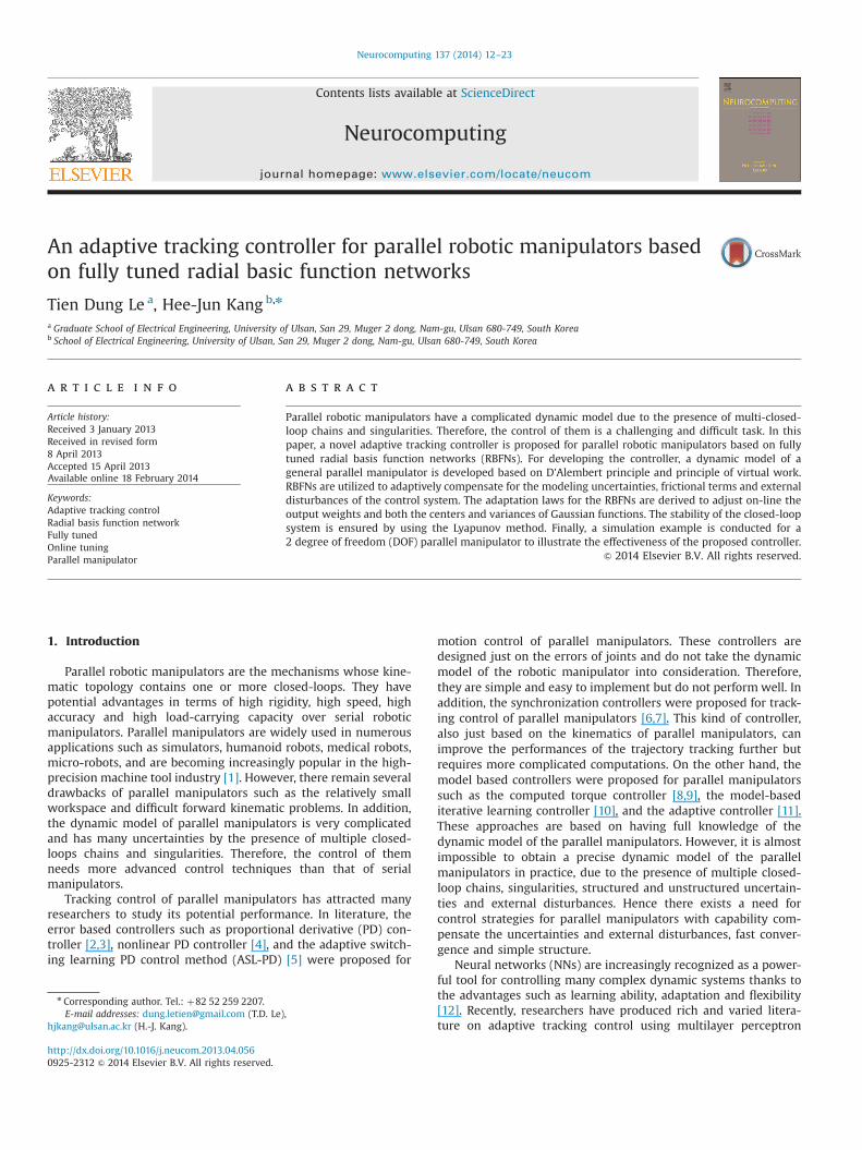
We consider a general parallel robotic manipulator consistingof a number of serial kinematic chains formed by rigid links andjoints as depicted in Fig. 1.

Let Na be the number of active joints, θaARNa the actuatedjoints, τaARNa the actuated torques, Np the number of passivejoints and θpARNp the passive joints. The active joints are actuatedby actuators while the passive joints are free to move. The parallelmanipulator works by torques/forces applied to the active joints,thus we need to derive the dynamic model in the active joint spaceas follows.

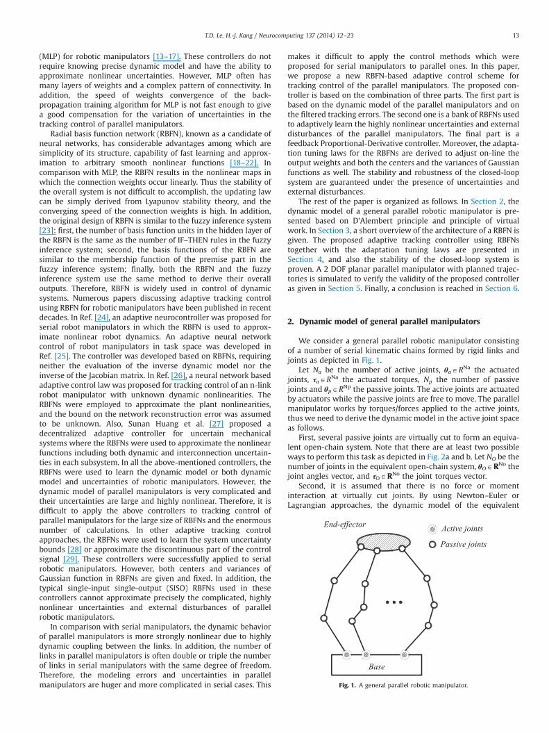
First, several passive joints are virtually cut to form an equiva-lent open-chain system. Note that there are at least two possibleways to perform this task as depicted in Fig. 2a and b. Let NO be thenumber of joints in the equivalent open-chain system, θOARNo thejoint angles vector, and τOARNo the joint torques vector.

Second, it is assumed that there is no force or momentinteraction at virtually cut joints. By using Newton–Euler orLagrangian approaches, the dynamic model of the equivalent

Fig. 1. A general parallel robotic manipulator.

T.D. Le, H.-J. Kang / Neurocomputing 137 (2014) 12–23 13

open-chain system can be computed and given as the followingequation:

MO€θOþCO

_θOþGOþFO ¼ τO ð1Þ

where MOARNo�No is the inertia matrix; COARNo�No is theCoriolis and centrifugal force matrix; GOARNo is the gravity forcevector; and FOARNo is the friction force vector.

Given a motion of the equivalent open-chain system whichsatisfies the loop constraints of the original parallel manipulator,the joint torques needed for generating this motion is τOARNo.Then, the joint torque of the original parallel manipulator requiredto generate the same motion is τaARNa. Following the D'Alembertprinciple and principle of virtual work, τO and τa satisfy thefollowing equation [30,31]:

τa ¼ Ψ TτO ð2Þ

where Ψ¼∂θO/∂θaARNo�Na is the Jacobian matrix of all the jointswith respect to the active joints given by the loop constraintsfollowing the algorithms presented in Ref. [32].

In addition, we have the following relationships:

_θO ¼ ∂θO∂θa

_θa ¼ Ψ _θa ð3Þ

€θO ¼ _Ψ _θaþΨ €θa ð4Þ

By multiplying both sides of (1) with ΨT, and then substituting(2)–(4) into the new equation we obtain

Ψ TMOΨ €θaþðΨ TMO_ΨþΨ TCOΨ Þ_θaþΨ TGOþΨ TFO ¼ τa ð5Þ

We defineþMa ¼ Ψ TMOΨARNa�Na as the estimated inertia matrix,þ Ca ¼ Ψ TMO

_ΨþΨ TCOΨARNa�Na as the estimated Coriolis andcentrifugal force matrix,

þ Ga ¼ Ψ TGOARNa as the estimated gravity force vector, andþFa ¼ Ψ TFOARNa as the vector of friction force of the parallel

manipulator.Then, the dynamic model of the general parallel manipulators

can be expressed by

Ma €θaþ Ca _θaþ GaþFa ¼ τa ð6Þ

Note that the effect of friction forces and external disturbanceson the passive joints is often much smaller than on the activejoints. Thus in order to simplify the dynamic model of parallelmanipulators, only those terms on the active joints are considered.

The dynamic model (6) of the general parallel manipulator hasthe following properties which were proven in Ref. [30]:

Property 1. Ma is a symmetric and positive definite matrix.

Property 2. _Ma�2Ca is a skew-symmetric matrix.

In practice, due to the presence of the highly nonlinearuncertainties, the exact dynamic model of parallel robotic manip-ulators will never be known. Hence in the presence of uncertain-ties, actual matrices Ma, Ca and Ga are in the forms

Ma ¼ MaþΔMa ð7Þ

Ca ¼ CaþΔCa ð8Þ

Ga ¼ GaþΔGa ð9Þwhere ΔMa, ΔCa and ΔGa are the unknown bounded modelingerrors.

Therefore, from (6) we can express the actual dynamic model ofparallel manipulators in the presence of uncertainties and externaldisturbances as follows:

Ma€θaþ Ca

_θaþ GaþΔτa ¼ τa ð10Þwhere Δτa ¼ΔMa €θaþΔCa _θaþΔGaþFaþdaðtÞ is the vector of theunknown uncertainties and external disturbances of the parallelmanipulator; da(t) is the external disturbances vector on activejoints.

3. Radial basis function network

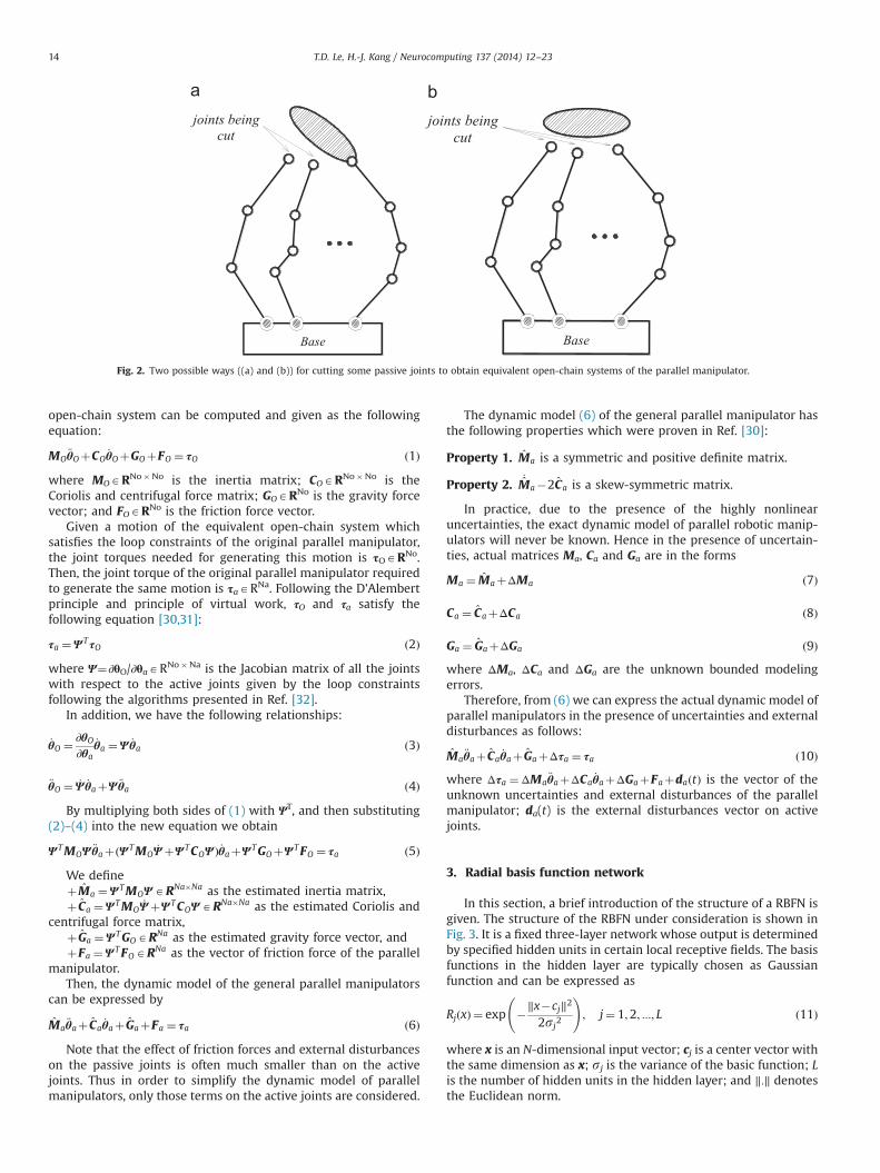
In this section, a brief introduction of the structure of a RBFN isgiven. The structure of the RBFN under consideration is shown inFig. 3. It is a fixed three-layer network whose output is determinedby specified hidden units in certain local receptive fields. The basisfunctions in the hidden layer are typically chosen as Gaussianfunction and can be expressed as

RjðxÞ ¼ exp �‖x�cj‖2

2sj2

!; j¼ 1;2; :::; L ð11Þ

where x is an N-dimensional input vector; cj is a center vector withthe same dimension as x; sj is the variance of the basic function; Lis the number of hidden units in the hidden layer; and ‖:‖ denotesthe Euclidean norm.

Fig. 2. Two possible ways ((a) and (b)) for cutting some passive joints to obtain equivalent open-chain systems of the parallel manipulator.

T.D. Le, H.-J. Kang / Neurocomputing 137 (2014) 12–2314

The output of the RBFN can be computed by the weighted summethod:

y¼ ∑L

j ¼ 1wjRjðxÞ ¼WTRðxÞ ð12Þ

or by the weighted average method

y¼∑L

j ¼ 1wjRjðxÞ∑L

j ¼ 1RjðxÞð13Þ

where wj is the weight or the strength of jth unit; W is the vectorof the weights connection hidden units and output layer; and R(x)is the vector of hidden units.

It is shown in Ref. [23] that the RBFN is functionally equivalentto the T–S model of the fuzzy inference system if a set ofconditions are satisfied. Therefore, we can apply what has beendiscovered for one model to the other, and vice versa. In this paper,we use fuzzy a priori knowledge to preconstructure the RBFNs inthe proposed adaptive tracking controller.

4. Proposed adaptive tracking controller

4.1. Architecture of the controller

Given a desired trajectory θdaARNa of the parallel manipulator,the tracking error is defined as

e¼ θa�θda ð14ÞThe filtered tracking error is

r¼ _eþΛe¼ _θa� _θar ð15Þwhere Λ¼ΛT40 is a design parameter matrix; and _θar ¼ _θda�Λe isdefined as the reference velocity vector.

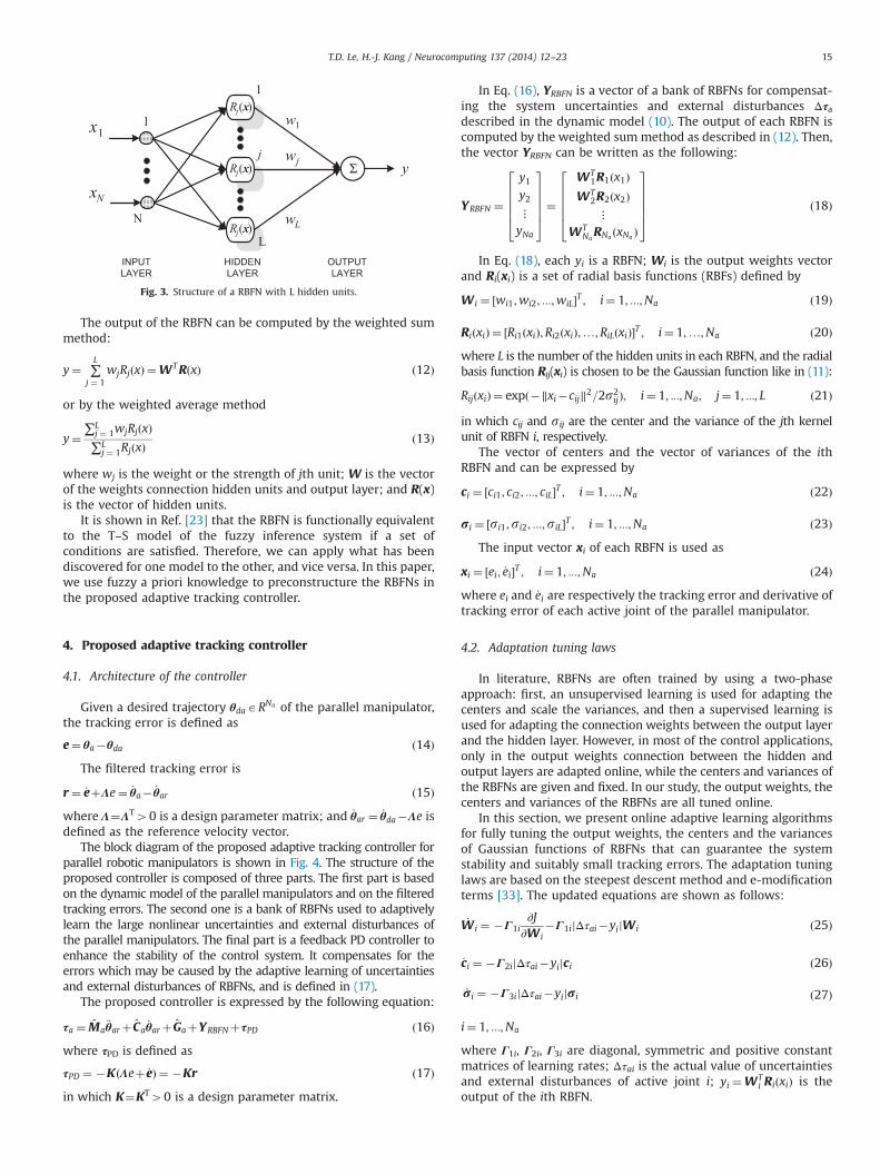
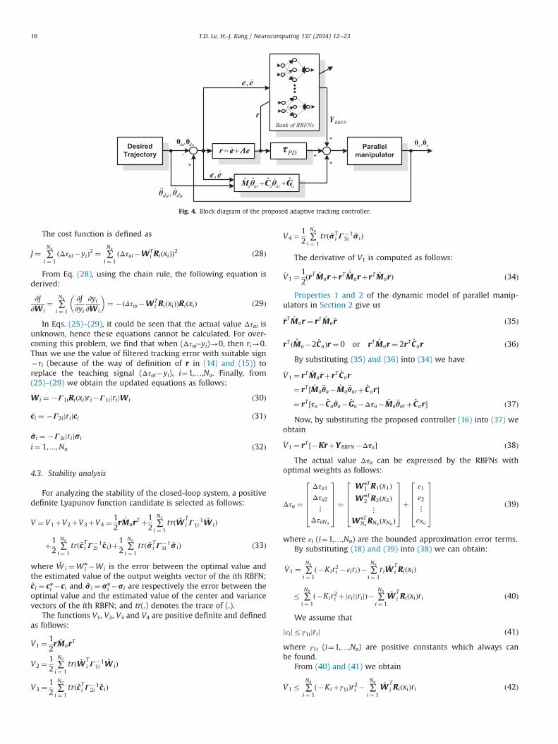
The block diagram of the proposed adaptive tracking controller forparallel robotic manipulators is shown in Fig. 4. The structure of theproposed controller is composed of three parts. The first part is basedon the dynamic model of the parallel manipulators and on the filteredtracking errors. The second one is a bank of RBFNs used to adaptivelylearn the large nonlinear uncertainties and external disturbances ofthe parallel manipulators. The final part is a feedback PD controller toenhance the stability of the control system. It compensates for theerrors which may be caused by the adaptive learning of uncertaintiesand external disturbances of RBFNs, and is defined in (17).

The proposed controller is expressed by the following equation:

τa ¼ Ma€θarþ Ca

_θarþ GaþYRBFNþτPD ð16Þwhere τPD is defined as

τPD ¼ �KðΛeþ _eÞ ¼ �Kr ð17Þin which K¼KT40 is a design parameter matrix.

In Eq. (16), YRBFN is a vector of a bank of RBFNs for compensat-ing the system uncertainties and external disturbances Δτadescribed in the dynamic model (10). The output of each RBFN iscomputed by the weighted sum method as described in (12). Then,the vector YRBFN can be written as the following:

YRBFN ¼

y1y2⋮yNa

266664

377775¼

WT1R1ðx1Þ

WT2R2ðx2Þ⋮

WTNaRNa ðxNa Þ

266664

377775 ð18Þ

In Eq. (18), each yi is a RBFN; Wi is the output weights vectorand Ri(xi) is a set of radial basis functions (RBFs) defined by

W i ¼ ½wi1;wi2; :::;wiL�T ; i¼ 1; :::;Na ð19Þ

RiðxiÞ ¼ ½Ri1ðxiÞ;Ri2ðxiÞ;…;RiLðxiÞ�T ; i¼ 1;…;Na ð20Þwhere L is the number of the hidden units in each RBFN, and the radialbasis function Rij(xi) is chosen to be the Gaussian function like in (11):

RijðxiÞ ¼ expð�‖xi�cij‖2=2s2ijÞ; i¼ 1; :::;Na; j¼ 1; :::; L ð21Þ

in which cij and sij are the center and the variance of the jth kernelunit of RBFN i, respectively.

The vector of centers and the vector of variances of the ithRBFN and can be expressed by

ci ¼ ½ci1; ci2; :::; ciL�T ; i¼ 1; :::;Na ð22Þ

ri ¼ ½si1;si2; :::;siL�T ; i¼ 1; :::;Na ð23ÞThe input vector xi of each RBFN is used as

xi ¼ ½ei; _ei�T ; i¼ 1; :::;Na ð24Þwhere ei and _ei are respectively the tracking error and derivative oftracking error of each active joint of the parallel manipulator.

4.2. Adaptation tuning laws

In literature, RBFNs are often trained by using a two-phaseapproach: first, an unsupervised learning is used for adapting thecenters and scale the variances, and then a supervised learning isused for adapting the connection weights between the output layerand the hidden layer. However, in most of the control applications,only in the output weights connection between the hidden andoutput layers are adapted online, while the centers and variances ofthe RBFNs are given and fixed. In our study, the output weights, thecenters and variances of the RBFNs are all tuned online.

In this section, we present online adaptive learning algorithmsfor fully tuning the output weights, the centers and the variancesof Gaussian functions of RBFNs that can guarantee the systemstability and suitably small tracking errors. The adaptation tuninglaws are based on the steepest descent method and e-modificationterms [33]. The updated equations are shown as follows:

_W i ¼ �Γ1i∂J

∂W i�Γ1ijΔτai�yi W ij ð25Þ

_ci ¼ �Γ2ijΔτai�yijci ð26Þ

_ri ¼ �Γ3ijΔτai�yijri ð27Þ

i¼ 1; :::;Na

where Γ1i, Γ2i, Γ3i are diagonal, symmetric and positive constantmatrices of learning rates; Δτai is the actual value of uncertaintiesand external disturbances of active joint i; yi ¼WT

i RiðxiÞ is theoutput of the ith RBFN.

Fig. 3. Structure of a RBFN with L hidden units.

T.D. Le, H.-J. Kang / Neurocomputing 137 (2014) 12–23 15

The cost function is defined as

J ¼ ∑Na

i ¼ 1ðΔτai�yiÞ2 ¼ ∑

Na

i ¼ 1ðΔτai�WT

i RiðxiÞÞ2 ð28Þ

From Eq. (28), using the chain rule, the following equation isderived:

∂J∂W i

¼ ∑Na

i ¼ 1

∂J∂yi

∂yi∂W i

� �¼ �ðΔτai�WT

i RiðxiÞÞRiðxiÞ ð29Þ

In Eqs. (25)–(29), it could be seen that the actual value Δτai isunknown, hence these equations cannot be calculated. For over-coming this problem, we find that when (Δτai–yi)-0, then ri-0.Thus we use the value of filtered tracking error with suitable sign�ri (because of the way of definition of r in (14) and (15)) toreplace the teaching signal (Δτai�yi), i¼1,…,Na. Finally, from(25)–(29) we obtain the updated equations as follows:

_W i ¼ �Γ1iRiðxiÞri�Γ1ijrijW i ð30Þ

_ci ¼ �Γ2ijrijci ð31Þ

_ri ¼ �Γ3ijrijri

i¼ 1; :::;Na ð32Þ

4.3. Stability analysis

For analyzing the stability of the closed-loop system, a positivedefinite Lyapunov function candidate is selected as follows:

V ¼ V1þV2þV3þV4 ¼12rMarT þ

12

∑Na

i ¼ 1trð ~W

Ti Γ

�11i

~W iÞ

þ12

∑Na

i ¼ 1trð ~cTi Γ �1

2i ~c iÞþ12

∑Na

i ¼ 1trð ~rT

i Γ�13i ~riÞ ð33Þ

where ~Wi ¼Wn

i �Wi is the error between the optimal value andthe estimated value of the output weights vector of the ith RBFN;~c i ¼ cni �ci and ~ri ¼rn

i �ri are respectively the error between theoptimal value and the estimated value of the center and variancevectors of the ith RBFN; and tr(.) denotes the trace of (.).

The functions V1, V2, V3 and V4 are positive definite and definedas follows:

V1 ¼12rMarT

V2 ¼12

∑Na

i ¼ 1trð ~W

Ti Γ

�11i

~W iÞ

V3 ¼12

∑Na

i ¼ 1trð ~cTi Γ �1

2i ~c iÞ

V4 ¼12

∑Na

i ¼ 1trð ~rT

i Γ�13i ~r iÞ

The derivative of V1 is computed as follows:

_V1 ¼12ð_rTMarþrT _MarþrTMa _rÞ ð34Þ

Properties 1 and 2 of the dynamic model of parallel manip-ulators in Section 2 give us

_rTMar¼ rTMa _r ð35Þ

rT ð _Ma�2CaÞr¼ 0 or rT _Mar¼ 2rT Car ð36ÞBy substituting (35) and (36) into (34) we have

_V1 ¼ rTMa _rþrT Car

¼ rT ½Ma€θa�Ma

€θarþ Car�¼ rT ½τa� Ca _θa� Ga�Δτa�Ma €θarþ Car� ð37Þ

Now, by substituting the proposed controller (16) into (37) weobtain

_V1 ¼ rT ½�KrþYRBFN�Δτa� ð38ÞThe actual value Δτa can be expressed by the RBFNs with

optimal weights as follows:

Δτa ¼

Δτa1Δτa2⋮

ΔτaNa

266664

377775¼

WnT1 R1ðx1Þ

WnT2 R2ðx2Þ⋮

WnTNaRNa ðxNa Þ

266664

377775þ

ε1

ε2

⋮εNa

266664

377775 ð39Þ

where εi (i¼1,…,Na) are the bounded approximation error terms.By substituting (18) and (39) into (38) we can obtain:

_V1 ¼ ∑Na

i ¼ 1ð�Kir2i �εiriÞ� ∑

Na

i ¼ 1ri ~W

Ti RiðxiÞ

r ∑Na

i ¼ 1ð�Kir2i þjεijjrijÞ� ∑

Na

i ¼ 1

~WTi RiðxiÞri ð40Þ

We assume that

jεijrγ1ijrij ð41Þwhere γ1i (i¼1,…,Na) are positive constants which always canbe found.

From (40) and (41) we obtain

_V1r ∑Na

i ¼ 1ð�Kiþγ1iÞr2i � ∑

Na

i ¼ 1

~WTi RiðxiÞri ð42Þ

Fig. 4. Block diagram of the proposed adaptive tracking controller.

T.D. Le, H.-J. Kang / Neurocomputing 137 (2014) 12–2316

Next, the derivative of V2 is computed as the following equation:

_V2 ¼ddt

12

∑Na

i ¼ 1trð ~W

Ti Γ

�11i

~W iÞ" #

¼ � ∑Na

i ¼ 1trð ~W

Ti Γ

�11i

_W iÞ ð43Þ

By substituting the adaptation tuning law (30) into Eq. (43) wehave

_V2 ¼ ∑Na

i ¼ 1

~WTi RiðxiÞriþ ∑

Na

i ¼ 1jrijtrð ~W

Ti W iÞ ð44Þ

In addition, we have the following property of the Frobeniusnorm [34,35]:

trð ~WTi W iÞ ¼ trð ~W

Ti ðWn

i � ~W iÞÞr‖ ~W i‖F‖Wn

i ‖F�‖ ~W i‖2F

r‖ ~W i‖Fwi max�‖ ~W i‖2F

r� ‖ ~W i‖F�12wi max

� �2

þ14w2

i max

r14w2

i max ð45Þ

where wi max is the maximum value of the Frobenius norm of theoutput weights vector Wn

i of the ith RBFN.By substituting (45) into (44) we obtain

_V2r ∑Na

i ¼ 1

~WTi RiðxiÞriþ

14∑Na

i ¼ 1rij jw2

i max

r ∑Na

i ¼ 1

~WTi RiðxiÞriþ

14∑Na

i ¼ 1γ2ir

2i ð46Þ

where γ2i (i¼1,…,Na) are positive constants satisfyingw2

i maxrγ2ijrij.In a similar way, by substituting (31) and (32) into the derivative

of V3 and V4 we have

_V3 ¼ � ∑Na

i ¼ 1trð ~cTi Γ�1

2i _ciÞ ¼ ∑Na

i ¼ 1jrijtrð ~cTi ciÞ

r14∑Na

i ¼ 1jrijc2i max

r14∑Na

i ¼ 1γ3ir

2i ð47Þ

_V4 ¼ � ∑Na

i ¼ 1trð ~rT

i Γ�13i _riÞ ¼ ∑

Na

i ¼ 1jrijtrð ~rT

i riÞ

r14∑Na

i ¼ 1jrijs2

i max

r14∑Na

i ¼ 1γ4ir

2i ð48Þ

where ci max and si max are the maximum values of the Frobeniusnorm of the center vector cni and variance vector sn

i in the ith RBFN;

γ3i, γ4i (i¼1,…,Na) are positive constants which satisfy c2i maxrγ3ijrijand s2

i maxrγ4ijrij.Finally, from (33), (42), (46)–(48), the derivative of the Lyapu-

nov function candidate can be expressed as follows:

_V ¼ _V1þ _V2þ _V3þ _V4

r ∑Na

i ¼ 1ð�Kiþγ1iÞr2i � ∑

Na

i ¼ 1

~WTi RiðxiÞriþ ∑

Na

i ¼ 1

~WTi RiðxiÞriþ

þ14∑Na

i ¼ 1γ2ir

2i þ

14∑Na

i ¼ 1γ3ir

2i þ

14∑Na

i ¼ 1γ4ir

2i

r ∑Na

i ¼ 1�Kiþγ1iþ

14γ2iþ

14γ3iþ

14γ4i

� �r2i ð49Þ

If the control gains Ki (i¼1,…,Na) are selected to satisfy thefollowing inequality:

KiZγ1iþ14γ2iþ

14γ3iþ

14γ4i; i¼ 1; :::;Na ð50Þ

then we have: _Vr0.Therefore, we can find that the stable tracking of the control

system is achieved based on the Lyanpunov theorem.

5. Simulation example

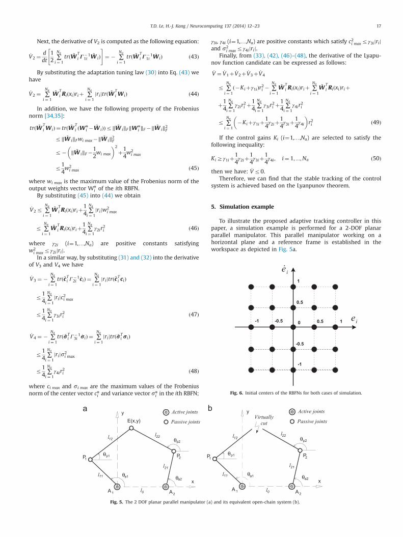
To illustrate the proposed adaptive tracking controller in thispaper, a simulation example is performed for a 2-DOF planarparallel manipulator. This parallel manipulator working on ahorizontal plane and a reference frame is established in theworkspace as depicted in Fig. 5a.

Fig. 6. Initial centers of the RBFNs for both cases of simulation.

Fig. 5. The 2 DOF planar parallel manipulator (a) and its equivalent open-chain system (b).

T.D. Le, H.-J. Kang / Neurocomputing 137 (2014) 12–23 17

In this parallel manipulator, the number of active joints is Na¼2and passive joints is Np¼3. We denote θa¼(θa1,θa2)T and θp¼(θp1,θp2)T corresponding to the active joint vector and passive joint

vector, respectively; X¼(x,y)T is the Cartesian coordinates; and E(x,y) is the end-effector of the parallel manipulators. The link lengthsof the parallel manipulators are l11¼A1P1, l12¼P1E, l21¼A2P2,l22¼P2E, and l0¼A1A2. The forward kinematics and inverse kine-matics of this parallel manipulator were presented in Ref. [9].

The parallel manipulator is virtually cut at the end-effector andform an equivalent open-chain system including two independent2-DOF serial manipulators as shown in Fig. 5b. The number ofjoints in the equivalent open-chain systems is NO¼4, the jointangles vector is θO ¼ ½θa1; θa2; θp1; θp2�T ; the joint torques vector isτO ¼ ½τa1; τa2; τp1; τp2�T , the friction vector is FO ¼ ½f a1; f a2;0;0�T .

The dynamic model of the 2-DOF planar parallel manipulator iscomputed following the process in Section 2. The parametermatrices in dynamic model (1) are obtained as follows:

MO ¼

α1 0 β1cap1 00 α2 0 β2cap2

β1cap1 0 δ1 00 β2cap2 0 δ2

266664

377775 ð51Þ

CO ¼

0 0 β1sap1 _θp1 0

0 0 0 β2sap2 _θp2�β1sap1 _θa1 0 0 0

0 �β2sap2 _θa2 0 0

2666664

3777775 ð52Þ

GO ¼ 0 ð53Þ

0 2 4 6 80

0.02

0.04

0.06

0.08

0.11NF

BRfo

sthgiewtu ptuo

gninnuT

Time [s]

W1,2W1,9W1,20W1,25

0 2 4 6 8-0.06

-0.04

-0.02

0

0.02

0.04

0.06

0.08

0.1

Time [s]

2NF

BRfo

sth gi ew tuptu o

gninn uT

W2,1W2,7W2,19W2,24

Fig. 9. Tuning results of typical output weights of (a) RBFN 1 and (b) RBFN 2 in the case of linear trajectory tracking control.

0 1 2 3 4 5 6 7 8

-1

-0.5

0

0.5

1

x 10-3

Time [s]

]m[

noitcerid -Xrorr e

gn ikcarT

0 1 2 3 4 5 6 7 8

-10

-8

-6

-4

-2

0

2x 10

-4

Time [s]

]m[

noitcer id-Yr orre

gnikc arT

Conventional Computed torque controllerProposed controller (Tuning output weights only)Proposed controller (Fully tuned)

Fig. 8. Linear trajectory tracking errors of the end-effector: (a) the X-direction and (b) the Y-direction.

0.04 0.05 0.06 0.07 0.08 0.09

0.13

0.14

0.15

0.16

0.17

0.18

0.19

0.2

0.21

X [m]

Y [m

]

Desired trajectoryConventional computed torque controllerProposed controller (Tuning output weights only)Proposed controller (Fully tuned)

Fig. 7. The linear trajectory of tracking control.

T.D. Le, H.-J. Kang / Neurocomputing 137 (2014) 12–2318

in which ai ¼mi1r2i1þ Izi1þmi2l2i1, βi¼mi2li1ri2, and di ¼mi2r2i2þ Izi2;

mi1, mi2 are the masses of links; li1, li2 are the link lengths; Izi1, Izi2 arethe inertias tensor of links of serial chain i; ri1, ri2 are the distancesfrom joint to the center of mass for each link; symbols capi and sapi arerespectively defined as capi¼cos(θai�θpi), sapi¼sin(θai�θpi), i¼1,2.

The Jacobian matrix Ψ in (2) is computed by

Ψ ¼ ½I; J�T ð54Þwhere IAR2�2 is identity matrix, and J¼∂θP/∂θaAR2�2 is com-puted from the loop constraint equation as the following equation:

J ¼ ∂θp∂θa

¼ ∂H∂θp

� ��1 ∂H∂θa

� �ð55Þ

where

H ¼hx

hy

" #¼

l11 cos θa1þ l12 cos θp1� l0� l21 cos θa2� l22 cos θp2

l11 sin θa1þ l12 sin θp1� l21 sin θa2� l22 sin θp2

" #ð56Þ

Simulation studies were conducted on Matlab-Simulink and themechanical model of the 2-DOF planar parallel manipulator was builton SimMechanics toolbox, following the method in Ref. [36].

To illustrate the improvement in performance, the proposedcontroller applying to the 2-DOF planar parallel manipulator iscompared with two other controllers:

� A conventional computed torque controller without uncer-tainties and external disturbances compensation [9]:

τa ¼ Mað€θdaþKv_EþKpEÞþ Ca

_θa ð57Þ

0 0.02 0.04 0.06 0.08 0.1 0.12

0.1

0.12

0.14

0.16

0.18

0.2

0.22

X [m]

Y [m

]

A0

Desired trajectoryConventional computed torque controllerProposed controller (tuning output weights only)Proposed controller (Fully tuned)

Fig. 12. The circular trajectory of tracking control.

0 1 2 3 4 5 6 7 8

0.1

0.11

0.12

0.13

0.14

0.15

1NF

BRfo

secnair avfogninuT

Time [s]

0 1 2 3 4 5 6 7 80.06

0.08

0.1

0.12

0.142NF

BRfo

secna iravfog ninuT

Time [s]

Fig. 11. Tuning results of variances of (a) RBFN 1 and (b) RBFN 2 in the case of linear trajectory tracking control.

0 1 2 3 4 5 6 7 8-1

-0.5

0

0.5

1

Time [s]

1NF

BRfo

sretnecgninuT

c1y(3,4)

c1y(5,3)c1y(4,5)

c1x(2,2)

c1x(1,1)

0 1 2 3 4 5 6 7 8-1

-0.5

0

0.5

1

2NF

BRfo

sret necg ninn uT

Time [s]

c2y(5,5)

c2y(2,2)

c2y(3,3)c2y(4,4)

c2y(1,1)

Fig. 10. Tuning results of typical centers of (a) RBFN 1 and (b) RBFN 2 in the case of linear trajectory tracking control.

T.D. Le, H.-J. Kang / Neurocomputing 137 (2014) 12–23 19

where E¼ θda�θa, _E¼ _θda� _θa; and Kp Aℜ2�2, Kv Aℜ2�2 arediagonal matrices with positive design parameter Kpi and Kvi

(i¼1,2) on the diagonal.� The proposed controller applied for the 2-DOF planar parallel

manipulator but only the output weights of the RBFNs are tuned.Parameters of links in the mechanical model were set to be

l11¼ l21¼0.102 m, l21¼ l22¼0.18 m, l0¼0.132 m, m11¼m21¼1 kg,m21¼m22¼1.2 kg, Iz11¼ Iz21¼0.0033 kgm2, Iz12¼ Iz22¼0.0072 kg m2,r11¼r21¼0.055m, r12¼r22¼0.09 m.

For making the modeling errors ΔMa, ΔCa we conducted thesimulations with different parameters in the mechanical model ofrobot and in the controllers: ri1 ¼ 0:9ri1 and ri2 ¼ 0:9ri2 where ri1,ri2 (i¼1,2) were used for calculating Ma, Ca in the controllers.

In the mechanical model, the frictions of system include theviscous friction and Coulomb friction torques defined as follows:

f ai ¼ Fcisignð_θaiÞþFvi _θai; i¼ 1;2 ð58Þ

where the coefficients are chosen as Fc1¼Fc2¼0.3 and Fv1¼Fv2¼2.2.

In simulations, the 2 DOF parallel manipulator is disturbed byexternal disturbance forces da(t)¼[da1(t), da2(t)]T¼[1,1]T at t¼2.5 s.

The simulations were carried out with respect to 2 cases whenthe end-effector of the 2-DOF parallel manipulator was driven totrack a linear trajectory and a circular trajectory on the XY plane.

In both cases of the simulations, the number of hidden unitsin each RBFN is L¼25. The initial centers of the RBFNs are shown inFig. 6.

5.1. Results of linear trajectory tracking control

In this case, the control gain matrices in the computed torquecontroller were set to be Kp¼[kp1, 0;0, kp2]¼[6000,0;0,6000],Kv¼[kv1, 0;0, kv2]¼[200,0;0,200]. These parameters wereobtained by the trial and error method.

In the proposed controller with only the output weights of theRBFNs tuned, the design parameter matrix is Λ¼[λ1, 0;0, λ2]¼[6,0;0,6]; the control gain matrix is K¼[15,0;0,15]. Note that theselection of K in the proposed controller is case dependent, and itshould be chosen such that to guarantee the convergence of trajectoryto the desired trajectory within finite time. Larger K leads to fasterconvergence, but also may increase the overshoot or oscillation of thecontrol inputs.

The number of hidden units in each RBFN is L¼25. The centers ofthe RBFNs were given and fixed the same as Fig. 6. The variances ofthe RBFNs were fixed as sij¼0.141, i¼1,2; j¼1,…,25. The outputweights of the RBFNs are tuned online by the proposed adaptationtuning law (30). The initial output weight matrices are Wi(0)¼0.1� Iwhere I is the identity matrix. The learning rate matrices areΓ11¼0.01� I and Γ12¼0.009� I.

In the proposed controller with fully tuned RBFNs, the designparameter matrix Λ and the control gain matrix K are set to be thesame with the second controller above. The number of hiddenunits in each RBFN is L¼25. All the parameters (the outputweights, the centers and the variances) of the RBFNs are tunedonline using the proposed adaptation tuning law (30)–(32).

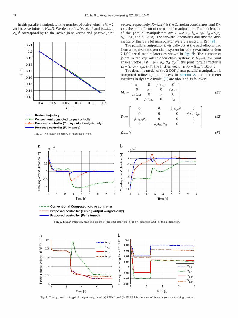
Fig. 7 shows the results of tracking a linear trajectory. Thestarting point of the desired trajectory is (0.04, 0.2) and the ending

0 2 4 6 8 10-0.2

-0.1

0

0.1

0.2

0.31NF

BRfo

sthgiewtuptuo

gninuT

Time [s]

W1,1 W1,8 W1,15 W1,25

0 2 4 6 8 10

-0.2

-0.1

0

0.1

0.2

0.3

Tuni

ng o

utpu

t wei

ghts

of R

BFN

2

Time [s]

W2,2 W2,11 W2,21 W2,24

Fig. 14. Tuning results of typical output weights of (a) RBFN 1 and (b) RBFN 2 in the case of circular trajectory tracking control.

0 2 4 6 8 10

-6

-4

-2

0

2

4

6

8x 10

-3

]m[

noitcerid-Xrorre

gnikcarT

Time [s]0 2 4 6 8 10

-6

-4

-2

0

2

4

6x 10

-3

Time [s]

]m[

noitcerid-Yrorre

gnikcarT

Conventional Computed torque controllerProposed controller (Tuning output weights only)Proposed controller (Fully tuned)

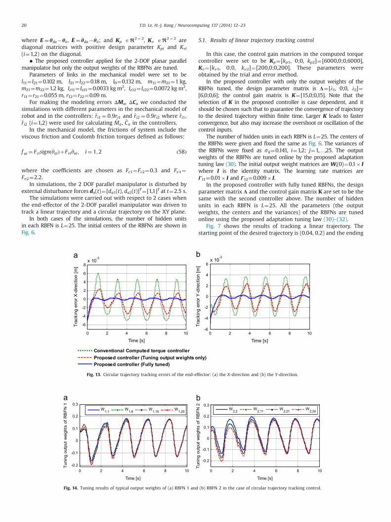
Fig. 13. Circular trajectory tracking errors of the end-effector: (a) the X-direction and (b) the Y-direction.

T.D. Le, H.-J. Kang / Neurocomputing 137 (2014) 12–2320

point is (0.088, 0.136). The time for tracking is 8 s. The initial pointof the end-effector of the 2-DOF parallel manipulator is (0.039,0.251). It can be seen that the end-effector of the manipulator cantrack the linear desired trajectory well.

Fig. 8 shows the tracking errors of the end-effector in the X-direction and in the Y-direction. As can be seen from the figure,the tracking errors caused by the proposed controller with onlyoutput weights tuning of RBFNs are much smaller than the errorsassociated with the conventional computed torque controllerwithout uncertainties compensation. Especially, the proposedcontroller with fully tuned RBFNs brings about the smallesttracking errors compared with the computed torque controllerand the proposed controller with only output weights tuning ofRBFNs. Also it can be seen that, the large model uncertainties andexternal disturbances are tolerated greatly using the proposedcontroller with fully tuned RBFNs.

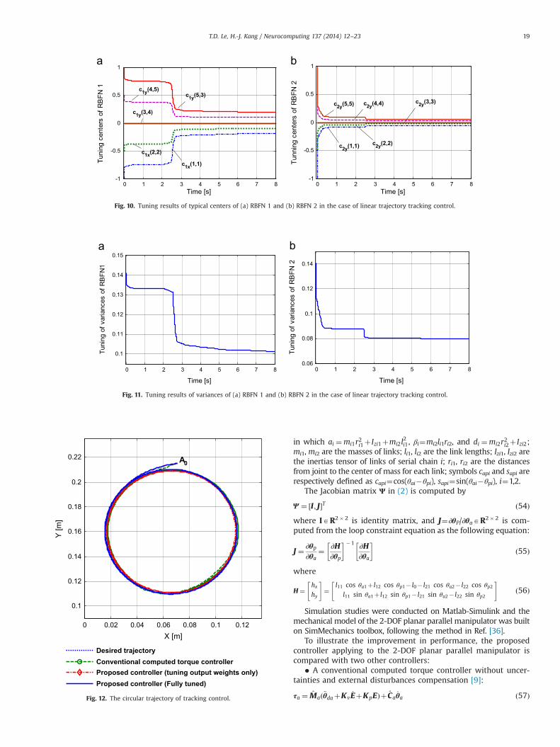
Figs. 9–11 show the results of online tuning of the outputweights, the centers and the variances of the proposed controllerwith fully tuned RBFNs. The initial output weight matrices areWi(0)¼0.1� I. The initial centers of RBFNs are shown in Fig. 6. Theinitial variances are sij(0)¼0.141, i¼1,2; j¼1,…,25. The learningrate matrices are Γ1i¼0.05� I, Γ2i¼0.05� I and Γ3i¼0.01� I. Wecan see that all the parameters are guaranteed to remain bounded,or the proposed online tuning algorithms (30)–(32) are converged.

5.2. Results of circular trajectory tracking control

In the case of circular trajectory tracking control, the controlgain matrices in the computed torque controller were set to be

Kp¼[kp1, 0;0, kp2]¼[7000,0;0,7000], Kv¼[kv1, 0;0, kv2]¼[300,0;0,300]. These parameters were also obtained by the trialand error method.

In the proposed controller with only the output weights of theRBFNs tuned, the number of hidden units of each RBFN is L¼25.The design parameter matrix Λ and the control gain matrix wereset the same as the case linear trajectory tracking: Λ¼[λ1, 0;0, λ2]¼[6,0;0,6] and K¼[15,0;0,15]. The centers of the RBFNs weregiven and fixed the same as Fig. 6. The variances of the RBFNswere fixed as sij¼0.141, i¼1,2; j¼1,…,25. The output weights ofthe RBFNs are tuned online by the proposed adaptation tuning law(30). The initial output weight matrices are Wi(0)¼0.1� I. Thelearning rate matrices are Γ1i¼0.05� I, i¼1,2.

In the proposed controller with fully tuned RBFNs, all theparameters: the output weights, the centers and the variances ofthe RBFNs are tuned online using the proposed adaptation tuninglaw (30)–(32). And the number of hidden units in each RBFN isL¼25.

Fig. 12 shows the comparison of the performance of circulartrajectory tracking among the conventional computed torquecontroller, the proposed controller with only output weights tunedand the proposed controller with fully tuned RBFNs. The centercoordinates of the circle are (0.066, 0.16) and radius is 0.05. Theinitial point of the end-effector of the 2-DOF parallel manipulatoris A0 (0.071, 0.215). The end-effector is driven to track the circulartrajectory 5 times during 10 s.

The results of tracking errors of the end-effector on the X-direction and the Y-direction in Fig. 13 prove the excellence incontrol performance of the proposed controller. As can be seen

0 2 4 6 8 100.09

0.1

0.11

0.12

0.13

0.14

0.15

Time [s]

Tuni

ng v

aria

nces

of R

BFN

1

0 2 4 6 8 100.09

0.1

0.11

0.12

0.13

0.14

0.15

Tuni

ng v

aria

nces

of R

BFN

2

Time [s]

Fig. 16. Tuning results of variances of (a) RBFN 1 and (b) RBFN 2 in the case of circular trajectory tracking control.

0 2 4 6 8 10-1

-0.5

0

0.5

1

Tuni

ng c

ente

rs o

f RB

FN 1

Time [s]

c1x(1,1)

c1x(2,2)

c1x(3,3)

c1y(4,4)

c1y(5,5)

0 2 4 6 8 10-1

-0.5

0

0.5

1

2NF

BRfo

sretn ecgninuT

Time [s]

c2x(1,1)

c2x(2,2)

c2y(3,3)

c2y(4,4)

c2y(5,5)

Fig. 15. Tuning results of typical centers of (a) RBFN 1 and (b) RBFN 2 in the case of circular trajectory tracking control.

T.D. Le, H.-J. Kang / Neurocomputing 137 (2014) 12–23 21

from the figure, our proposed controller with only output weightstuned produces smaller tracking errors compared to the conven-tional computed torque controller without uncertainties andexternal disturbances compensation. Interestingly, among thethree controllers, the proposed controller with fully tuned RBFNshas the smallest tracking errors. A look at the figure also revealsthat the large model uncertainties and external disturbances aretolerated greatly in the case of the proposed controller with fullytuned RBFNs.

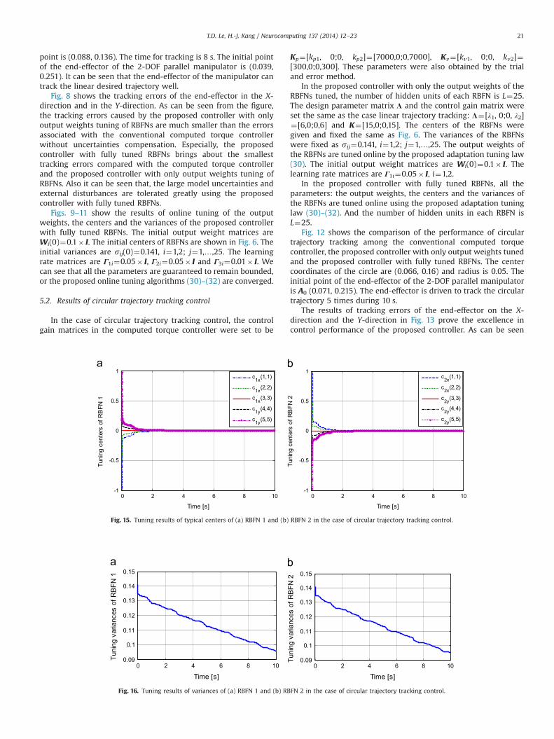
Figs. 14–16 show the results of online tuning of the outputweights, the centers and the variances of the proposed controllerwith fully tuned RBFNs. The initial output weight matrices areWi(0)¼0.1� I. The initial centers of RBFNs are shown in Fig. 6. Theinitial variances are sij(0)¼0.141, i¼1,2; j¼1,…,25. Note that in allsimulations we used the fuzzy a priori knowledge to preconstruc-ture the RBFNs. The learning rate matrices are Γ1i¼0.005� I,Γ2i¼0.02� I and Γ3i¼0.0005� I, which are obtained by the trial-and-error method.

6. Conclusion

In this paper, we have presented a novel adaptive trackingcontroller using fully tuned RBFNs for parallel robotic manipula-tors. The proposed controller is based on the combination ofthree ingredients. The first ingredient is based on the dynamicmodel of parallel manipulators and the filtered tracking errors. Thesecond one is a bank of RBFNs used to adaptively learn thelarge nonlinear uncertainties and external disturbances of theparallel manipulators. The final part is a feedback PD controller toenhance the stability of the control system. The adaptation tuninglaws for the RBFNs have been derived for the output weights andalso for the centers and variances of Gaussian functions. Thesetuning algorithms allow the RBFNs to be fully self-tuned onlineduring the trajectory tracking control of the parallel manipulatorswithout any offline training phase. Using the Lyapunov stabilitytheorem, the stability of the parallel manipulator system togetherwith the proposed controller and online tuning algorithms isproved.

In the simulation example, the proposed adaptive trackingcontroller is applied to a 2-DOF parallel manipulator. Simulationresults demonstrated the effectiveness of the proposed controllerin complicated situations of trajectory tracking control. It has beenshown that the proposed controller with fully tuning of the RBFNsbrings about the smallest tracking errors compared with thecase of tuning the output weights only and the case of usingconventional computed torque controller without disturbancescompensation.

Acknowledgment

The authors would like to express financial supports fromKorean Ministry of Knowledge Economy both under HumanResources Development Program for Convergence Robot Specia-lists and under Robot Industry Core Technology Project.

References

[1] J.P. Merlet, Parallel Robots, second ed., Springer, (Dordrecht, The Netherlands),2006.

[2] F.H. Ghorbel, O. Chetelat, R. Gunawardana, R. Longchamp, Modeling and setpoint control of closed-chain mechanisms: theory and experiment, IEEE Trans.Control Syst. Technol. 8 (2000) 801–815.

[3] C. Yang, Q. Huang, H. Jiang, O. Ogbobe Peter, J. Han, PD control with gravitycompensation for hydraulic 6-DOF parallel manipulator, Mech. Mach. Theory45 (2010) 666–677.

[4] P.R. Ouyang, W.J. Zhang, F.X. Wu, Nonlinear PD control for trajectory trackingwith consideration of the design for control methodology, in: Proceedings ofthe IEEE International Conference on Robotics and Automation, 2002. ICRA'02, vol. 4, 2002, pp. 4126–4131.

[5] P.R. Ouyang, W.J. Zhang, M.M. Gupta, An adaptive switching learning controlmethod for trajectory tracking of robot manipulators, Mechatronics 16 (2006)51–61.

[6] R. Lu, J.K. Mills, S. Dong, Trajectory tracking control for a 3-DOF planar parallelmanipulator using the convex synchronized control method, IEEE Trans.Control Syst. Technol. 16 (2008) 613–623.

[7] S. Weiwei, C. Shuang, Z. Yaoxin, L. Yanyang, Active joint synchronizationcontrol for a 2-DOF redundantly actuated parallel manipulator, IEEE Trans.Control Syst. Technol. 17 (2009) 416–423.

[8] Z. Yang, J. Wu, J. Mei, Motor-mechanism dynamic model based neural networkoptimized computed torque control of a high speed parallel manipulator,Mechatronics 17 (2007) 381–390.

[9] T.D. Le, H.-J. Kang, Y.-S. Suh, Y.-S. Ro, An online self-gain tuning method usingneural networks for nonlinear PD computed torque controller of a 2-dofparallel manipulator, Neurocomputing 116 (2012) 53–61.

[10] H. Abdellatif, B. Heimann, Advanced model-based control of a 6-DOF hexapodrobot: a case study, IEEE/ASME Trans. Mechatron. 15 (2010) 269–279.

[11] Z. Xiaocong, T. Guoliang, Y. Bin, C. Jian, Integrated direct/indirectadaptive robust posture trajectory tracking control of a parallel manipulatordriven by pneumatic muscles, IEEE Trans. Control Syst. Technol. 17 (2009)576–588.

[12] D.R. Hush, B.G. Horne, Progress in supervised neural networks, IEEE SignalProcess. Mag. 10 (1993) 8–39.

[13] B. Achili, B. Daachi, Y. Amirat, A. Ali-cherif, A robust adaptive control of aparallel robot, Int. J. Control 83 (2010) 2107–2119.

[14] Y. Tang, F. Sun, Z. Sun, Neural network control of flexible-link manipulatorsusing sliding mode, Neurocomputing 70 (2006) 288–295.

[15] R.-J. Wai, Tracking control based on neural network strategy for robotmanipulator, Neurocomputing 51 (2003) 425–445.

[16] D. Braganza, D.M. Dawson, I.D. Walker, N. Nath, A neural network controllerfor continuum robots, IEEE Trans. Robot. 23 (2007) 1270–1277.

[17] T.D. Le, Hee-Jun Kang, Suh Young-Soo, Chattering-free neuro-sliding modecontrol of 2-DOF planar parallel manipulators, Int. J. Adv. Robot. Syst. 10 (2013)22.

[18] J. Moody, C.J. Darken, Fast Learning in Networks of Locally-Tuned ProcessingUnits, Neural Comput. 1 (1989) 281–294 (1989/06/01).

[19] G.A. Montazer, R. Sabzevari, F. Ghorbani, Three-phase strategy for the OSDlearning method in RBF neural networks, Neurocomputing 72 (2009)1797–1802.

[20] D.-S. Huang, Radial basis probabilitistic neural networks: model and applica-tion, Int. J. Pattern Recognit. Artif. Intell. 13 (1999) 1083–1101.

[21] D.S. Huang, J.X. Du, A constructive hybrid structure optimization methodologyfor radial basis probabilistic neural networks, IEEE Trans. Neural Netw. 19(2008) 2099–2115.

[22] D.-S. Huang, W.-B. Zhao, Determining the centers of radial basis probabilisticneural networks by recursive orthogonal least square algorithms, Appl. Math.Comput. 162 (2005) 461–473.

[23] K.J. Hunt, R. Haas, R. Murray-Smith, Extending the functional equivalence ofradial basis function networks and fuzzy inference systems, IEEE Trans. NeuralNetw. 7 (1996) 776–781.

[24] L. Min-Jung, C. Young-Kiu, An adaptive neurocontroller using RBFN for robotmanipulators, IEEE Trans. Ind. Electron. 51 (2004) 711–717.

[25] S.G. Shuzhi, C.C. Hang, L.C. Woon, Adaptive neural network control of robotmanipulators in task space, IEEE Trans. Ind. Electron. 44 (1997) 746–752.

[26] F.C. Sun, Z.Q. Sun, R.J. Zhang, Y.B. Chen, Neural adaptive tracking controller forrobot manipulators with unknown dynamics, IEE Proc. Control Theory Appl.147 (2000) 366–370.

[27] H. Sunan, T. Kok Kiong, L. Tong Heng, A.S. Putra, Adaptive control ofmechanical systems using neural networks, IEEE Trans. Syst. Man Cybern.Part C: Appl. Rev. 37 (2007) 897–903.

[28] M. Zhihong, H.R. Wu, M. Palaniswami, An adaptive tracking controller usingneural networks for a class of nonlinear systems, IEEE Trans. Neural Netw. 9(1998) 947–955.

[29] N. Sadati, R. Ghadami, Adaptive multi-model sliding mode control ofrobotic manipulators using soft computing, Neurocomputing 71 (2008)2702–2710.

[30] C. Hui, Y. Yiu-Kuen, L. Zexiang, Dynamics and control of redundantly actuatedparallel manipulators, IEEE/ASME Trans. Mechatron. 8 (2003) 483–491.

[31] Y. Nakamura, K. Yamane, Dynamics computation of structure-varying kine-matic chains and its application to human figures, IEEE Trans. Robot. Autom.16 (2000) 124–134.

[32] H.-J. Kang, R.A. Freeman, Evaluation of loop constraints for kinematic anddynamic modeling of general closed-chain robotic systems, J. Mech. Sci.Technol. 8 (1994) 115–126.

[33] K. Narendra, A. Annaswamy, A new adaptive law for robust adaptationwithout persistent excitation, IEEE Trans. Autom. Control 32 (1987)134–145.

[34] A. Das, F. Lewis, K. Subbarao, Backstepping approach for controlling aQuadrotor using Lagrange form dynamics, J. Intell. Robot. Syst. 56 (2009)127–151.

T.D. Le, H.-J. Kang / Neurocomputing 137 (2014) 12–2322

[35] C. Gang, F.L. Lewis, Distributed adaptive tracking control for synchronizationof unknown networked Lagrangian Systems, IEEE Trans. Syst. Man Cybern.Part B: Cybern. 41 (2011) 805–816.

[36] D. Le Tien, K. Hee-Jun, R. Young-Shick, Robot manipulator modeling in Matlab-SimMechanics with PD control and online gravity compensation, 2010International Forum on Strategic Technology (IFOST), 2010, pp. 446–449.

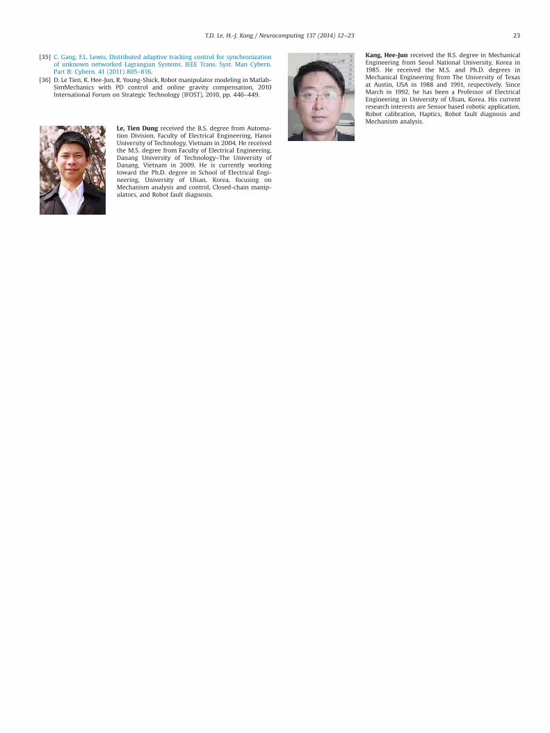
Le, Tien Dung received the B.S. degree from Automa-tion Division, Faculty of Electrical Engineering, HanoiUniversity of Technology, Vietnam in 2004. He receivedthe M.S. degree from Faculty of Electrical Engineering,Danang University of Technology–The University ofDanang, Vietnam in 2009. He is currently workingtoward the Ph.D. degree in School of Electrical Engi-neering, University of Ulsan, Korea, focusing onMechanism analysis and control, Closed-chain manip-ulators, and Robot fault diagnosis.

Kang, Hee-Jun received the B.S. degree in MechanicalEngineering from Seoul National University, Korea in1985. He received the M.S. and Ph.D. degrees inMechanical Engineering from The University of Texasat Austin, USA in 1988 and 1991, respectively. SinceMarch in 1992, he has been a Professor of ElectricalEngineering in University of Ulsan, Korea. His currentresearch interests are Sensor based robotic application,Robot calibration, Haptics, Robot fault diagnosis andMechanism analysis.

T.D. Le, H.-J. Kang / Neurocomputing 137 (2014) 12–23 23