Algorithms for Provisioning Virtual Private Networks in the HoseModel

Amit Kumar�

Rajeev RastogiAvi Silberschatz

Bulent Yener

600 Mountain AvenueMurray Hill, NJ 07974

AbstractVirtual Private Networks (VPNs) provide customers with predictable and secure network connections over ashared network. The recently proposed hose model for VPNs allows for greater flexibility since it permitstraffic to and from a hose endpoint to be arbitrarily distributed to other endpoints. In this paper, we develop novelalgorithms for provisioning VPNs in the hose model. We connect VPN endpoints using a tree structure and ouralgorithms attempt to optimize the total bandwidth reserved on edges of the VPN tree. We show that even for thesimple scenario in which network links are assumed to have infinite capacity, the general problem of computingthe optimal VPN tree is NP-hard. Fortunately, for the special case when the ingress and egress bandwidths foreach VPN endpoint are equal, we can devise an algorithm for computing the optimal tree whose time complexityis O�mn�, where m and n are the number of links and nodes in the network, respectively. We present a novelinteger programming formulation for the general VPN tree computation problem (that is, when ingress andegress bandwidths of VPN endpoints are arbitrary) and develop an algorithm that is based on the primal-dualmethod. Finally, we extend our proposed algorithms for computing VPN trees to the case when network linkshave capacity constraints. We show that in the presence of link capacity constraints, computing the optimal VPNtree is NP-hard even when ingress and egress bandwidths of each endpoint are equal. Our experimental resultswith synthetic network graphs indicate that the VPN trees constructed by our proposed algorithms dramaticallyreduce bandwidth requirements (in many instances, by more than a factor of 2) compared to scenarios in whichSteiner trees are employed to connect VPN endpoints.

1 Introduction

Virtual Private Networks (VPNs) are becoming an increasingly important source of revenue for Internet ServiceProviders (ISPs). Informally, a VPN establishes connectivity between a set of geographically dispersed endpointsover a shared network infrastructure. The goal is to provide VPN endpoints with a service comparable to a privatededicated network established with leased lines. Thus, providers of VPN services need to address the QoS andsecurity issues associated with deploying a VPN over a shared IP network. In recent years, substantial progressin the technologies for IP security [KA98, DGG�98] have enabled existing VPN service offerings to providecustomers with a level of privacy comparable to that offered by a dedicated line. However, ISPs have been slowto offer customers with guaranteed bandwidth VPN services since IP networks in the past had little support forenforcing QoS in the network. The recent emergence of IP technologies like MPLS and RSVP, however, havemade it possible to realize IP-based VPNs that can provide end customers with QoS guarantees. In this paper,we address the problem of provisioning VPN services with QoS guarantees, a problem which has received littleattention from the research community.

�Current Address: Department of Computer Science, Cornell University.

0

1.1 The Hose Model

There are two popular models for providing QoS in the context of VPNs - the “pipe” model and the “hose”model [DGG�98, DR00]. In the pipe model, the VPN customer specifies QoS requirements between every pairof VPN endpoints. Thus, the pipe model requires the customer to know the complete traffic matrix; that is, theload between every pair of endpoints. However, the number of endpoints per VPN is constantly increasing and thecommunication patterns between endpoints are becoming increasingly complex. As a result, it is almost impossibleto predict traffic characteristics between pairs of endpoints required by the pipe model.

The hose model alleviates the above-mentioned shortcomings of the pipe model. In the hose model, the VPNcustomer specifies QoS requirements per VPN endpoint and not every pair of endpoints. Specifically, associatedwith each endpoint, is a pair of bandwidths – an ingress bandwidth and an egress bandwidth. The ingress bandwidthfor an endpoint specifies the incoming traffic from all the other VPN endpoints into the endpoint, while the egressbandwidth is the amount of traffic the endpoint can send to the other VPN endpoints. Thus, in the hose model,the VPN service provider supplies the customer with certain guarantees for the traffic that each endpoint sendsto and receives from other endpoints of the same VPN. The customer does not have to specify how this traffic isdistributed among the other endpoints. As a result, in contrast to the pipe model, the hose model does not requirea customer to know its traffic matrix, which in turn, places less burden on a customer that wants to use the VPNservice.

In summary, the hose model provides customers with the following advantages over the pipe model [DGG�98]:

1. Ease of Specification. Only one ingress and egress bandwidth per hose endpoint needs to be specified,compared to bandwidth for each pipe between pairs of hose endpoints.

2. Flexibility. Traffic to and from a hose endpoint can be distributed arbitrarily over other endpoints as long asthe ingress and egress bandwidths of each hose endpoint are not violated.

3. Multiplexing Gain. Due to statistical multiplexing gain, hose ingress and egress bandwidths can be lessthan the aggregate bandwidth required for a set of point to point pipes.

4. Characterization. Hose requirements are easier of characterize because the statistical variability in theindividual source-destination traffic is smoothed by aggregation into hoses.

The multiplexing gain due to the hose model (point 3 above) can result in significant improvements in theutilization of network resources. For example, consider a VPN used to offer VoIP service to customers located atVPN endpoints in NY, LA and Chicago. Suppose N is the maximum volume of calls out of NY (bounded by thenumber of customers being served by the VPN endpoint in NY). Further, suppose that there is a large variability inthe destinations of the calls with as many as 80% of all calls out of NY being directed to LA at some times and toChicago at other times. Thus, in the pipe model, two pipes, one from NY to LA and another from NY to Chicago,each with bandwidth to carry ��� �N calls need to be reserved. As a result, in the pipe model, the total bandwidthreserved for traffic out of NY is ��� �N units. In contrast, in the hose model, bandwidth is reserved only for theaggregate traffic out of NY, which is N units. Thus, by reserving bandwidth for the aggregate traffic out of VPNendpoints, the hose model improves network bandwidth utilization because of statistical multiplexing effects.

From the above discussion, it follows that the hose model provides VPN customers with a simple mechanismfor specifying bandwidth requirements and enables VPN service providers to utilize network bandwidth moreefficiently. However, in order to realize these benefits, efficient algorithms must be devised for provisioning hoses.These hose provisioning algorithms need to set up paths between every pair of VPN endpoints such that theaggregate bandwidth reserved on the links traversed by the paths is minimum. A naive algorithm that sets upindependent shortest paths between every pair of endpoints, however, could lead to excessive bandwidth beingreserved. The reason for this is that the hose model provides the flexibility for traffic from a hose endpoint to bearbitrarily distributed to other endpoints. Consequently, the distribution of traffic between VPN endpoints is non-deterministic and the provisioning algorithms need to reserve sufficient bandwidth to accommodate the worst-case

1

1 (1)

2 (2) 3 (2)

(a) Graph (b) Independent Shortest Paths (c) Link Sharing Among Paths

1 (1)

2 (2) 3 (2)

1 (1)

2 (2) 3 (2)

1

2 2

1

1 1

1

1

2 2

A B

C

A B

C

A

C

Figure 1: Link Sharing Among Paths to Reduce Reserved Bandwidth

traffic distribution among endpoints that meets the ingress and egress bandwidth constraints of hose endpoints.Intuitively, in order to conserve bandwidth and realize the multiplexing benefits of the hose model, paths enteringinto and originating from each hose endpoint need to share as many links as possible. Thus, sophisticated hoseprovisioning algorithms need to be developed to ensure that the amount of bandwidth reserved in order to meet thehose traffic requirements is minimum.

Example 1.1: Consider the network graph in Figure 1(a). The 3 VPN hose endpoints 1, 2 and 3 have bandwidthrequirements of 1, 2 and 2 units, respectively (each endpoint has equal ingress and egress bandwidths). Figure 1(b)depicts the bandwidth reserved on relevant links of the network when a naive independent shortest paths approachis used to connect VPN endpoints. For instance, the shortest path between 1 and 2 passes through A, while theshortest path between endpoints 2 and 3 passes through C. Also, 1 unit of bandwidth needs to be reserved (in eachdirection) on the two links incident on A and on the shortest path from 1 to 2 since endpoint 1 can send/receive atmost 1 unit of traffic. Similarly, the bandwidth reserved on the two links incident on C is 2 units, the minimum ofthe bandwidth requirements of endpoints 2 and 3. Thus, the total reserved bandwidth using independent shortestpaths is 8 units (only considering one direction for each link).

The reserved bandwidth can be reduced from 8 to 6 by exploiting link sharing among paths connecting theVPN endpoints as illustrated in Figure 1(c). Here, both paths from endpoint 1 to the two other endpoints passthrough C, thus allowing the two links connecting 1 to C to be shared between them. (Note that the path from 1to 2 passing through C is longer than the path from 1 to 2 through A). Further, since endpoint 1 cannot receive orsend more than 1 unit of traffic, the bandwidth reserved on each of the two links is 1 unit (in each direction) and isshared between the two paths. Thus, the total bandwidth reserved decreases from 8 to 6 as a result of link sharingbetween paths.

Note that provisioning pipes between each pair of VPN endpoints in the pipe model is somewhat simplersince the traffic between every pair of endpoints is fixed and is input to the provisioning algorithm. Thus, theVPN provisioning problem simply reduces to that of computing a set of fixed bandwidth paths between VPNendpoint pairs, which is an instance of the well-studied multicommodity flow problem [AMO93, Hoc97]. However,as mentioned earlier, the drawback of the pipe model is the difficulty of capturing and specifying bandwidthrequirements between each pair of VPN endpoints. Thus, the hose model trades off provisioning simplicity forease of specification and multiplexing gains.

2

1.2 Our Contributions

In this paper, we develop novel algorithms for provisioning VPNs in the hose model. In order to take advan-tage of the multiplexing gain possible due to hoses, we connect VPN endpoints using a tree structure (instead ofindependent point-to-point paths between VPN endpoints). A VPN tree has several benefits, which we list below.

1. Sharing of bandwidth reservation. A single bandwidth reservation on a link of the tree can be shared bythe entire traffic between the two sets of VPN endpoints connected by the link. Thus, the bandwidth reservedon the link only needs to accommodate the aggregate traffic between the two sets of VPN endpoints.

2. Scalability. For a large number of VPN endpoints, a tree structure scales better than point-to-point pathsbetween all VPN endpoint pairs.

3. Simplicity of Routing. The structural simplicity of trees ensures that if MPLS [DR00] is used for setting uppaths between VPN endpoints, then fewer labels are required and label stacks on packets are not as deep.

4. Ease of Restoration. Trees also simplify restoration of paths in case of link failures, since all paths traversinga failed link can be restored as a single group, instead of each path being restored separately.

We develop algorithms for computing optimal VPN trees; that is, trees for which the amount of total bandwidthreserved on edges of the tree is minimum. Initially, we assume that network links have infinite capacity, and showthat even for this simple scenario, the general problem of computing the optimal VPN tree is NP-hard. However,for the special case when the ingress and egress bandwidths for each VPN endpoint are equal, we are able todevise a breadth first search algorithm for computing the optimal tree whose time complexity is O�mn�, wherem and n are the number of links and nodes in the network, respectively. We present a novel integer programmingformulation for the general VPN tree computation problem (that is, when ingress and egress bandwidths of VPNendpoints are arbitrary) and develop an algorithm that is based on the primal-dual method [Hoc97]. Finally, weextend our proposed algorithms for computing VPN trees to the case when network links have capacity constraints.We show that in the presence of link capacity constraints, computing the optimal VPN tree is NP-hard even wheningress and egress bandwidths of each endpoint are equal. Further, we also show that computing an approximatesolution that is within a constant factor of the optimum is as difficult as computing the optimal VPN tree itself.

In [DGG�98], the authors suggest that a Steiner tree can be employed to connect VPN endpoints. However,our experimental results with synthetic network graphs indicate that the VPN trees constructed by our proposedalgorithms require dramatically less bandwidth to be reserved (in many instances, by more than a factor of 2) com-pared to Steiner trees. Further, among the three algorithms, the primal-dual algorithm performs the best, reservingless bandwidth than both the breadth first search and Steiner tree algorithms over a wide range of parameter values.

2 System Model and Problem Formulation

We model the network as a graph G � �V�E� where V is a set of nodes and E is a set of bidirectional linksbetween the nodes. Each link �i� j� has associated capacities in the two directions – we denote the capacity fromnode i to j by Lij and the capacity (in the opposite direction) from node j to i by Lji. Also, Rij denotes theresidual capacity (that is, the available bandwidth) of link �i� j� for carrying traffic from node i to j.

In the hose model, each VPN specification consists of the following two components: (1) A set of nodesP � V corresponding to the VPN endpoints, and (2) For each node i � P , the hose ingress and egress bandwidthsBini and Bout

i , respectively. Without loss of generality, we assume that each node i � P is a leaf, that is, thereis a single (bidirectional) link incident on i�. As mentioned earlier, we consider tree structures to connect theVPN endpoints in P since trees are scalable, simplify routing and restoration. Further, trees allow the bandwidth

�In case there is a VPN endpoint i � P that is not a leaf, then we simply introduce a new node j in G and a new link �i� j� with verylarge capacity, and replace node i in P with node j.

3

Symbol DescriptionG � �V�E� Graph with nodes V and bidirectional edgesE

m Number of links in graphG (jEj)n Number of nodes in graphG (jV j)Lij Capacity of link �i� j� in the direction from node i to jRij Residual capacity of link �i� j� in the direction from node i to j

i� j� l� u� v�w Generic symbols for nodes in GP Set of VPN endpointsT Generic notation for VPN treeTv VPN tree rooted at node vBini Ingress bandwidth for node i

Bouti Egress bandwidth for node i

T�i�j�i Component of tree T containing i when link �i� j� is deleted from T

P�i�j�i VPN endpoints contained in T �i�j�

i

CT �i� j� Bandwidth reserved on link �i� j� of VPN tree TCT Sum of bandwidths reserved on all links of VPN tree T

dT �i� j� Distance (in number of links) between nodes i and j in tree TdG�i� j� Length of the shortest path (in number of links) between nodes i and j in graph G

Table 1: Notation Used in the Paper

reserved on a link to be shared by the traffic between the two sets of VPN endpoints connected by the link. Thus,the bandwidth reserved on a link must be equal to the maximum possible aggregate traffic between the two sets ofendpoints connected by the link.

Before we can compute the exact bandwidth to be reserved on each link of VPN tree T whose leaves are nodesfrom P , we need to develop some notation. For a link �i� j� in tree T , we denote by T

�i�j�i �T

�i�j�j the connected

component of T containing node i�j when link �i� j� is deleted from T . Also, let P �i�j�i and P �i�j�

j denote the set of

VPN endpoints in T �i�j�i and T �i�j�

j , respectively. Table 1 describes the notation used in the remainder of the paper.Observe that all traffic from one VPN endpoint to another traverses the unique path in the VPN tree T between

the two endpoints. Now consider link �i� j� that connects the two sets of VPN endpoints P �i�j�i and P

�i�j�j . The

traffic from node i to j cannot exceed minfP

l�P�i�j�i

Boutl �P

l�P�i�j�j

Binl g, that is, the minimum of the cumula-

tive egress bandwidths of endpoints in P�i�j�i and the sum of ingress bandwidths of endpoints in P

�i�j�j . This is

because the only traffic that traverses link �i� j� from i to j is the traffic originating from endpoints in P�i�j�i and

directed towards endpoints in P�i�j�j . The bound on the former is

Pl�P

�i�j�i

Boutl , while the latter is bounded by

Pl�P

�i�j�j

Binl . Thus, the bandwidth to be reserved on link �i� j� of T in the direction from i to j is given by

CT �i� j� � minfP

l�P�i�j�i

Boutl �P

l�P�i�j�j

Binl g. Similarly, the bandwidth that must be reserved on link �j� i� in

the direction from j to i can be shown to be CT �j� i� � minfP

l�P�i�j�i

Binl �P

l�P�i�j�j

Boutl g. Note that CT �i� j�

may not be equal to CT �j� i�.Thus, the total bandwidth reserved for tree T is given by CT �

P�i�j��T CT �i� j� (note that �i� j� and �j� i� are

considered as two distinct links in T ). Further, since we are interested in minimizing the reserved bandwidth fortree T , the problem of computing the optimal VPN tree becomes the following:

Problem Statement (Optimal VPN Tree without Link Capacity Constraints): Given a set of VPN end-points P , and their ingress and egress bandwidths, compute a VPN tree T whose leaves are nodes in P and forwhich CT is minimum.

4

0

2 3 4 5 61(1000) (1000)(1) (1) (1)(1)

2 3 4 5 61(1000) (1000)(1) (1) (1)(1)

0

2 3 4 5 61(1000) (1000)(1) (1) (1)(1)

(a) Graph (b) Steiner Tree (c) Optimal VPN Tree

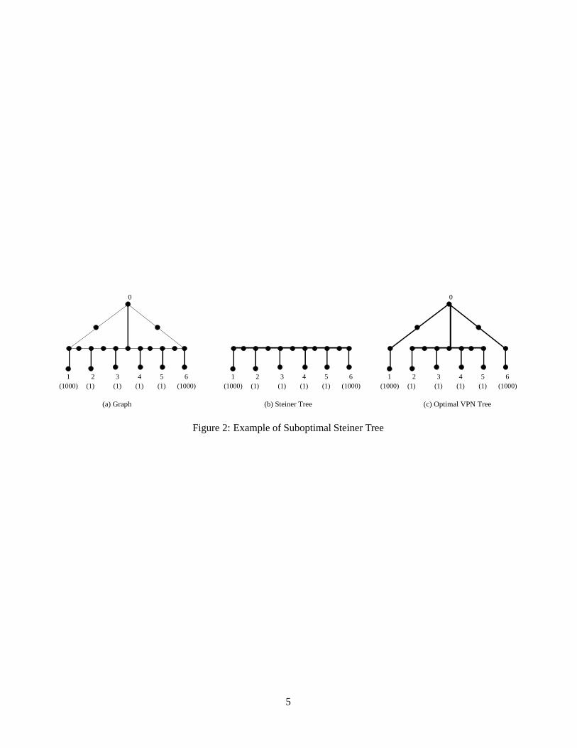
Figure 2: Example of Suboptimal Steiner Tree

5

In [DGG�98], it has been suggested that a Steiner tree can be used to connect the VPN endpoints. However,even though a Steiner tree has the smallest number of links, it may be suboptimal, as illustrated by the followingexample.

Example 2.1: Consider the network graph shown in Figure 2(a). Nodes �� �� � � � � � are the VPN endpoints andBin� � Bout

� � Bin� � Bout

� � ���� while Bini � Bout

i � � for i � �� � � � � . Figure 2(b) shows the Steiner treeconnecting the VPN endpoints in P and containing 16 edges. The total bandwidth reserved on the edges of theSteiner tree (in a single direction) is given by ���� � � ���� � � ���� � � ���� � � ���� � � � �����(this excludes the 2006 units that need to be reserved on the links incident on the VPN endpoints in P ). Thereason for this is that 1000 units need to be reserved on the two links connecting endpoints 1 and 2, 1001 unitsneed to be reserved on the two links connecting endpoints 2 and 3, and so on. However, the optimal VPN treecontaining 17 links is shown in Figure 2(c). The cumulative bandwidth reserved on all the links of the optimal treeis ���������������������� � ���� (again, in a single direction per link and excluding the 2006units that need to be reserved on the links incident on the VPN endpoints in P ). This is because the bandwidthreserved on the two links connecting endpoints 1 and 0 is 1000, the bandwidth for the two links between endpoints6 and 0 is 1000, the bandwidth for the link connecting 0 to endpoints �� � � � � is 4 units, and for the two linksconnecting endpoints 3 and 4 is 2 units, and so on.

Thus, in the above example, the bandwidth reserved for the Steiner tree is more than twice the optimumbandwidth. Further, note that, in the example, the performance of the Steiner tree can be made arbitrarily worsecompared to the optimum (by increasing the number of VPN endpoints between endpoints 1 and 6).

In our earlier formulation of the optimal VPN tree computation problem, we assumed that links do not havecapacity constraints. In the following, we present the problem formulation that also takes into account the residualbandwidths of network links.

Problem Statement (Optimal VPN Tree with Link Capacity Constraints): Given a set of VPN endpointsP , and their ingress and egress bandwidths, compute a tree T whose leaves are nodes in P such thatCT �i� j�� Rij

and CT is minimum.

In the remainder of the paper, we will refer to CT �i� j� as the cost of link �i� j� in tree T and CT as the cost oftree T . In the following two sections (Sections 3 and 4), we first develop algorithms to compute the optimal VPNtree ignoring link capacity constraints. We then show how the algorithms can be extended to handle link capacityconstraints in Section 5.

3 Symmetric Ingress and Egress Bandwidths

For symmetric ingress and egress bandwidths, that is, when B ini � Bout

i for each VPN endpoint i, one can deviseefficient algorithms for computing the minimum cost VPN tree if links do not have capacity constraints. In thissection, we present a polynomial time algorithm for computing the optimal VPN tree for the symmetric bandwidthcase under the assumption that the residual capacity of each edge is large. Since the ingress and egress bandwidthsare equal, in the following, we simply drop the superscripts in and out, and denote the bandwidth for endpoint isimply by Bi.

Before presenting our algorithm for computing the optimal tree (that is, tree with minimum cost), we firstdevelop some intuition for the cost CT of a tree T . Recall (from the previous section) thatCT �

P�i�j��T CT �i� j�.

For a set of leaves L � P , we define B�L� asP

l�LBl. Thus, CT �i� j� � minfB�P�i�j�i �� B�P

�i�j�j �g. It is

straightforward to observe that CT �i� j� � CT �j� i�, that is, the bandwidth reserved on link �i� j� in the twodirections is equal. Now suppose that for a tree T and a node v in T , we define the quantity Q�T� v� to be� �P

l�P Bl � dT �v� l�, where the sum is over all leaves l, and dT �v� l� denotes the length of the unique v to l pathin T . Then, for any tree T whose leaves are nodes in P , we can show thatCT satisfies the following two properties:

6

� Property 1. There exists a node w � T such that CT � Q�T� w�.

� Property 2. For all nodes v � T , CT � Q�T� v�.

In order to show the above two properties for tree T , we construct a directed tree Tdir from T by giving adirection to each edge e � �i� j� of T as follows:

� if B�P �i�j�i � � B�P

�i�j�j �, then direct the edge towards i.

� if B�P �i�j�j � � B�P

�i�j�i �, then direct the edge towards j.

� if B�P �i�j�i � � B�P

�i�j�j �, then direct the edge towards the component which contains a particular leaf, say,

�l.

Clearly, Tdir must contain a node whose indegree is 0 — we denote this node in Tdir with no incoming edges bya�T �. We show that a�T � is indeed unique and CT � Q�T� a�T ��. For this, we prove some properties about Tdirin the following lemma.

Lemma 3.1: Every edge e in Tdir is directed away from a�T �.

Proof: Let e � �i� j� be an edge in tree T such that i is closer to a�T � than j in T . We show that e is directedfrom i to j in Tdir. Consider the path in T from a�T � to i. We know that the first edge �u� v� along the path is

directed away from u � a�T �. So, B�P�u�v�v � � B�P

�u�v�u �. Since �u� v� is the first edge of the path from a�T �

to i, P �u�v�u � P

�i�j�i and also, P �i�j�

j � P�u�v�v . Thus, we get, B�P �i�j�

j � � B�P�u�v�v � � B�P

�u�v�u � � B�P

�i�j�i �.

If B�P �i�j�j � � B�P

�i�j�i �, then edge e is directed from i to j and we are done. The only other possibility is

B�P�i�j�j � � B�P

�i�j�i �. But then, it must be the case that P �u�v�

u � P�i�j�i , P �u�v�

v � P�i�j�j and B�P

�u�v�u � �

B�P�u�v�v �. As a result, it follows that u � i and v � j, and since edge �u� v� is directed from u to v, edge �i� j�

must also be directed from i to j.

Note that from the above lemma, one can easily show that a�T � is unique since every other node in Tdir hasan edge directed into it (and consequently, an indegree of 1). In the following lemma, we prove that Property 1mentioned above holds for w � a�T �.

Lemma 3.2: The cost of tree T , CT � Q�T� a�T ��.

Proof: Let l be a leaf and e � �i� j� be an edge on the path from a�T � to l (node i being closer to a�T �) —

note that Bl contributes to both CT �i� j� and CT �j� i�. The reason for this is that CT �i� j� is B�P �i�j�j � since due

to Lemma 3.1, the edge is directed from i to j in Tdir and so B�P�i�j�j � � B�P

�i�j�i �. Thus, since l � P

�i�j�j , Bl

contributes to each edge on the path from a�T � to l, and to no other edge. This proves the lemma.

Property 2 is a straightforward corollary of the following lemma (since CT � Q�T� a�T �� due to Lemma 3.2).

Lemma 3.3: Let v be any node in T . Then, Q�T� a�T ��� Q�T� v�.

Proof: We first show the following result: suppose e � �i� j� is an edge that is directed from i to j in T dir. Then,

Q�T� i�� Q�T� j�. We know that B�P �i�j�j � � B�P

�i�j�i �. Now,

Q�T� i��Q�T� j� � � �X

l�P�i�j�i

Bl � �dT �i� l�� dT �j� l�� � �X

l�P�i�j�j

Bl � �dT �i� l�� dT �j� l��

� �� �X

l�P�i�j�i

Bl � �X

l�P�i�j�j

Bl

� � �B�P�i�j�j �� � �B�P

�i�j�i � � �

7

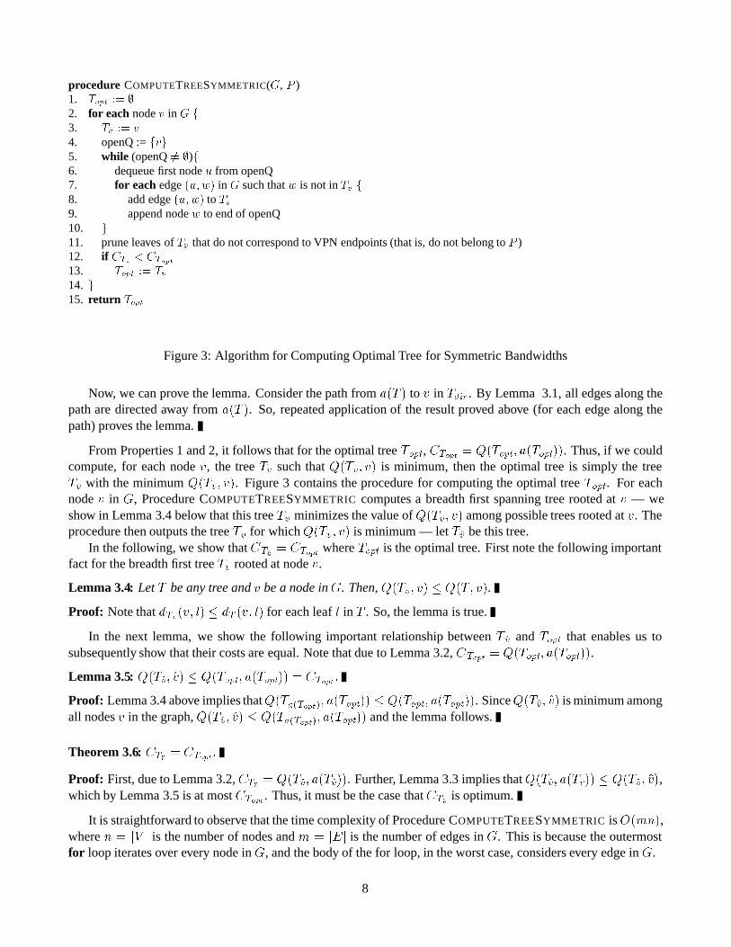
procedure COMPUTETREESYMMETRIC(G, P )1. Topt �� �2. for each node v in G f3. Tv �� v4. openQ := fvg5. while (openQ �� �)f6. dequeue first node u from openQ7. for each edge �u�w� in G such that w is not in Tv f8. add edge �u�w� to Tv9. append node w to end of openQ10. g11. prune leaves of Tv that do not correspond to VPN endpoints (that is, do not belong to P )12. if CTv � CTopt

13. Topt �� Tv14. g15. return Topt

Figure 3: Algorithm for Computing Optimal Tree for Symmetric Bandwidths

Now, we can prove the lemma. Consider the path from a�T � to v in Tdir. By Lemma 3.1, all edges along thepath are directed away from a�T �. So, repeated application of the result proved above (for each edge along thepath) proves the lemma.

From Properties 1 and 2, it follows that for the optimal tree Topt, CTopt � Q�Topt� a�Topt��. Thus, if we couldcompute, for each node v, the tree Tv such that Q�Tv� v� is minimum, then the optimal tree is simply the treeTv with the minimum Q�Tv� v�. Figure 3 contains the procedure for computing the optimal tree Topt. For eachnode v in G, Procedure COMPUTETREESYMMETRIC computes a breadth first spanning tree rooted at v — weshow in Lemma 3.4 below that this tree Tv minimizes the value of Q�Tv� v� among possible trees rooted at v. Theprocedure then outputs the tree Tv for which Q�Tv� v� is minimum — let T�v be this tree.

In the following, we show that CT�v � CTopt where Topt is the optimal tree. First note the following importantfact for the breadth first tree Tv rooted at node v.

Lemma 3.4: Let T be any tree and v be a node in G. Then, Q�Tv� v� � Q�T� v�.

Proof: Note that dTv�v� l�� dT �v� l� for each leaf l in T . So, the lemma is true.

In the next lemma, we show the following important relationship between T�v and Topt that enables us tosubsequently show that their costs are equal. Note that due to Lemma 3.2, CTopt � Q�Topt� a�Topt��.

Lemma 3.5: Q�T�v� �v� � Q�Topt� a�Topt�� � CTopt �

Proof: Lemma 3.4 above implies thatQ�Ta�Topt�� a�Topt�� � Q�Topt� a�Topt��. SinceQ�T�v� �v� is minimum amongall nodes v in the graph, Q�T�v� �v� � Q�Ta�Topt�� a�Topt�� and the lemma follows.

Theorem 3.6: CT�v � CTopt�

Proof: First, due to Lemma 3.2, CT�v � Q�T�v� a�T�v��. Further, Lemma 3.3 implies that Q�T�v� a�T�v�� � Q�T�v� �v�,which by Lemma 3.5 is at most CTopt. Thus, it must be the case that CT�v is optimum.

It is straightforward to observe that the time complexity of Procedure COMPUTETREESYMMETRIC is O�mn�,where n � jV j is the number of nodes and m � jEj is the number of edges in G. This is because the outermostfor loop iterates over every node in G, and the body of the for loop, in the worst case, considers every edge in G.

8

0

1

2

3

4

5

6

7

(3/6)

(3/6)

(3/4)

(3/4)

3

6

3

6

9

6

6

8

3

4

3

4

(3/4)

Figure 4: Example of Tree Cost for Asymmetric Bandwidths

4 Asymmetric Ingress and Egress Bandwidths

In this section, we address the case when VPN endpoint bandwidth requirements are asymmetric, that is, for a VPNendpoint j, Bin

j and Boutj may be unequal. Asymmetric ingress and egress bandwidths complicate the VPN tree

computation problem since for a VPN tree T connecting the VPN endpoints, the bandwidth reserved along edge�i� j� of T may not be identical in the two directions – that is,CT �i� j�may not be equal toCT �j� i�. This is becausefor an edge �i� j�,CT �i� j� � minf

Pl�P

�i�j�i

Boutl �P

l�P�i�j�j

Binl g andCT �j� i� � minf

Pl�P

�i�j�i

Binl �P

l�P�i�j�j

Boutl g.

Thus, in the asymmetric case, since Binl and Bout

l may not be equal, CT �i� j� and CT �j� i� may not be equal. Notethat this is different from the symmetric bandwidths case in which the bandwidths reserved in both directions alongan edge �i� j� of a tree T were equal.

Example 4.1: Consider the VPN tree shown in Figure 4 connecting the VPN endpoints in P � f�� �� � � � � �g. Thebandwidth requirements for the endpoints are as follows: for endpoints 0 and 1, B in � and Bout � �, and forendpoints 2, 3 and 4, Bin � and Bout � �. The bandwidths reserved in the two directions for the various edgesof the tree are shown adjacent to the edges in the figure. Thus, for instance, for edge �� ��, CT �� �� � � (sinceP

l�P������

Boutl � �� is greater than

Pl�P

������

Binl � �) and CT ��� � � � (since

Pl�P

������

Boutl � �� is greater

thanP

l�P������

Binl � �). Similarly, one can show that for edge ��� ��, CT ��� �� � � (since

Pl�P

������

Boutl � �� is

greater thanP

l�P������

Binl � �) and CT ��� �� � � (since

Pl�P

������

Boutl � � is less than

Pl�P

������

Binl � �).

For the asymmetric bandwidths case, the problem of computing the VPN tree with the minimum cost can beshown to be at least as difficult as that of computing a Steiner tree connecting the VPN endpoints. Since the Steinertree computation problem for a set of VPN endpoints is NP-hard [Hoc97, GJ79], it follows that the problem ofcomputing the optimal VPN tree is also NP-hard.

Theorem 4.2: For the asymmetric bandwidths case, the problem of computing the optimal VPN tree connectingthe set of VPN endpoints in P is NP-hard.

4.1 Integer Programming Formulation

In this section, we show that the problem of computing the optimal tree can be formulated as an integer pro-gramming problem. For this, we first need to examine the properties of VPN trees connecting endpoints withasymmetric bandwidths.

For an edge �i� j� of VPN tree T , we say that it is biased towards i if the following two conditions hold:

9

1. (P

l�P�i�j�i

Binl �P

l�P�i�j�j

Boutl ) or (

Pl�P

�i�j�i

Binl �P

l�P�i�j�j

Boutl and P �i�j�

i contains a special node, say

�l), and

2. (P

l�P�i�j�i

Boutl �

Pl�P

�i�j�j

Binl ) or (

Pl�P

�i�j�i

Boutl �

Pl�P

�i�j�j

Binl and P �i�j�

i contains a special node, say

�l).

An edge �i� j� is said to be biased if it is biased towards either i or j. An edge that is not biased is said to bebalanced. Also, we refer to a node of T as a core node if a balanced edge is incident on it.

Going back to Example 4.1, edge �� �� is a balanced edge (sinceP

l�P������

Binl � � is less than

Pl�P

������

Boutl �

�� andP

l�P������

Binl � � is less than

Pl�P

������

Boutl � ��). Thus, nodes 5 and 6 are core nodes. However, edge

��� �� is biased towards 7 sinceP

l�P������

Binl � � is less than

Pl�P

������

Boutl � �� and

Pl�P

������

Boutl � � is less

thanP

l�P������

Binl � �.

In the following, we state certain properties of balanced edges. Let M � minfP

l�P Binl �P

l�P Boutl g.

Lemma 4.3: The sum of the bandwidths reserved on a balanced edge �i� j� of a VPN tree T in both directions isM (that is, CT �i� j� CT �j� i� � M ).

Proof: For a balanced edge �i� j�, it must be the case that (1)P

l�P�i�j�i

Binl �P

l�P�i�j�j

Boutl or

Pl�P

�i�j�i

Boutl �

Pl�P

�i�j�j

Binl , and (2)

Pl�P

�i�j�i

Binl �

Pl�P

�i�j�j

Boutl or

Pl�P

�i�j�i

Boutl �

Pl�P

�i�j�j

Binl . We consider the two

cases involvingP

l�P�i�j�i

Binl �

Pl�P

�i�j�j

Boutl (the first term in (1)). The other two cases for

Pl�P

�i�j�i

Boutl �

Pl�P

�i�j�j

Binl (the second term in (1)) can be handled in a similar fashion. Without loss of generality, we assume

that M �P

l�P Binl .

Case 1. In this case,P

l�P�i�j�i

Binl �

Pl�P

�i�j�j

Boutl . Since M �

Pl�P B

inl , it follows that

Pl�P

�i�j�i

Boutl �

Pl�P

�i�j�j

Binl . Thus, it follows that CT �i� j� �

Pl�P

�i�j�j

Binl and CT �i� j� CT �j� i� �

Pl�P B

inl � M .

Case 2. In this case,P

l�P�i�j�i

Binl �P

l�P�i�j�j

Boutl and

Pl�P

�i�j�i

Boutl �

Pl�P

�i�j�j

Binl . Note that it must be the

case thatP

l�P�i�j�i

Binl �P

l�P�i�j�j

Boutl and

Pl�P

�i�j�i

Boutl �

Pl�P

�i�j�j

Binl , since otherwise, M �

Pl�P B

inl is

not possible. Thus, it follows that CT �i� j� CT �j� i� �P

l�P Binl � M .

Revisiting Example 4.1, the total bandwidth reserved on balanced edge �� �� is M �P

l�P Binl � �.

Lemma 4.4: The restriction of T to only balanced edges forms a connected component.

Note that, from the above lemma, it follows that the core nodes are connected by a tree consisting entirely ofbalanced edges. Thus, if we delete the balanced edges from T , then in each of the resulting connected components,there is a single core node. We refer to the component containing core node v by Cv. Of course, if T contains nobalanced edges, then there is only one component. Since all edges in the component are biased, one can show thatthere exists a unique node v in T such that every edge incident on v is biased away from it. This node v is thenconsidered to be the core node for the component.

Lemma 4.5: Consider the component Cv corresponding to core node v. Every edge �i� j� in Cv is biased towardsj (assuming j is further from node v than i).

Lemma 4.6: The cost of component Cv isP

l��Cv�P � dT �v� l� � �Binl Bout

l �.

10

Thus, a VPN tree T consists of a set of core nodes connected by balanced edges, and connected componentsCv for each core node containing only biased edges. Suppose that core�T � denotes the set of core nodes in T andbal�T � is the set of balanced edges in T . Then, from the above lemmas, we can infer that the cost of T , CT , isequal to M � jbal�T �j

Pv�core�T �

Pl��Cv�P � dT �v� l� � �B

inl Bout

l �.From the above discussion, it follows that each VPN tree, for the most part, can be completely characterized

by its set of core nodes. Consider a set of nodes S. We define the cost of the set of nodes S, denoted by CS , asM � b

Pl�P minv�SfdG�v� l�g � �B

inl Bout

l �. Here, b is the number of edges in the Steiner tree connectingthe nodes in S. Next, we show how to construct the tree T �S� for a set of nodes S such that CT �S� � CS . First,connect the nodes in S by a Steiner tree and add all the Steiner tree edges to T �S�. Next, coalesce all the nodesin S into one supernode, and construct a breadth first tree rooted at the supernode and connecting all the VPNendpoints in P (as the leaves). Add the edges of the breadth first tree to T �S�.

In the following, we show that the problem of computing the optimal VPN tree is equivalent to that of com-puting a set of nodes S for whom CS is minimum. Specifically, we show that if Topt is the optimal tree, then forthe minimum CS , CS � CTopt . Thus, once we determine S, we can always construct the tree T �S� whose cost isoptimal due to the following lemma.

Lemma 4.7: Let S be a set of nodes. Then CT �S� � CS .

The following lemma enables us to prove that computing the set of nodes S for which CS is minimum yieldsthe optimal VPN tree for the asymmetric case.

Lemma 4.8: For a VPN tree T , Ccore�T � � CT .

Theorem 4.9: Let S be a set of nodes for whom CS is minimum. Then T �S� is the optimal VPN tree.

Proof: Let Topt be the optimal tree. We know that CS � Ccore�Topt�. Due to Lemma 4.7, CT �S� � CS , and due toLemma 4.8, Ccore�Topt� � CTopt. As a result, it follows that CT �S� � CTopt. Thus, T �S� is the VPN tree with theminimum cost.

Thus, we have shown that, for the asymmetric case, to compute the optimal VPN tree, we simply need tocompute a set of nodes S whose cost CS is minimum; that is, a set S of nodes for whom the quantity b �M P

l�P minv�SfdG�v� l�g��Boutl Bin

l � is minimum, where b is the number of edges in the Steiner tree connectingthe nodes in S.

The problem of computing the set of nodes S with the minimum cost can be formulated as an integer programif we know the identity of one of the nodes in S. Let xij , yi and ze be 0-1 variables, where yi is 1 if node i belongsto S, xij is 1 if VPN endpoint j is assigned to node i and ze is 1 if edge e belongs to the Steiner tree connectingthe nodes in S. Also, let �� �V � denote the set of edges crossing sets �V and V � �V in G and Bj � Bin

j Boutj .

Suppose we know apriori that node v � S. Then, the solution to the following integer program yields the optimalset of nodes S containing v.

minimizeX

i�V�j�P

dG�i� j� �Bj � xij M �X

e�E

ze (1)

subject to the following constraints�j � P �

X

i�V

xij � �

�i � V� j � P � yi � xij � �

� �V V� v � �V � j � P �X

e��� �V �

ze �X

i��V

xij � �

xij � yi� ze � f�� �g

11

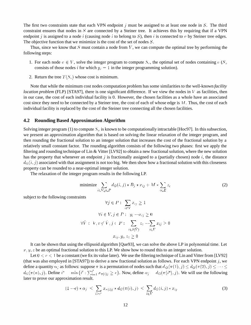
The first two constraints state that each VPN endpoint j must be assigned to at least one node in S. The thirdconstraint ensures that nodes in S are connected by a Steiner tree. It achieves this by requiring that if a VPNendpoint j is assigned to a node i (causing node i to belong to S), then i is connected to v by Steiner tree edges.The objective function that we minimize is the cost of the set of nodes S.

Thus, since we know that S must contain a node from V , we can compute the optimal tree by performing thefollowing steps:

1. For each node v � V , solve the integer program to compute Sv, the optimal set of nodes containing v (Svconsists of those nodes i for which yi � � in the integer programming solution).

2. Return the tree T �Sv� whose cost is minimum.

Note that while the minimum cost nodes computation problem has some similarities to the well-known facilitylocation problem (FLP) [STA97], there is one significant difference. If we view the nodes in V as facilities, thenin our case, the cost of each individual facility is 0. However, the chosen facilities as a whole have an associatedcost since they need to be connected by a Steiner tree, the cost of each of whose edge is M . Thus, the cost of eachindividual facility is replaced by the cost of the Steiner tree connecting all the chosen facilities.

4.2 Rounding Based Approximation Algorithm

Solving integer program (1) to compute Sv is known to be computationally intractable [Hoc97]. In this subsection,we present an approximation algorithm that is based on solving the linear relaxation of the integer program, andthen rounding the fractional solution to an integer solution that increases the cost of the fractional solution by arelatively small constant factor. The rounding algorithm consists of the following two phases: first we apply thefiltering and rounding technique of Lin & Vitter [LV92] to obtain a new fractional solution, where the new solutionhas the property that whenever an endpoint j is fractionally assigned to a (partially chosen) node i, the distancedG�i� j� associated with that assignment is not too big. We then show how a fractional solution with this closenessproperty can be rounded to a near-optimal integer solution.

The relaxation of the integer program results in the following LP.

minimizeX

i�V�j�P

dG�i� j� �Bj � xij M �X

e�E

ze (2)

subject to the following constraints�j � P �

X

i�V

xij � �

�i � V� j � P � yi � xij � �

� �V V� v � �V � j � P �X

e��� �V �

ze �X

i��V

xij � �

xij � yi� ze � �

It can be shown that using the ellipsoid algorithm [Que93], we can solve the above LP in polynomial time. Letx� y� z be an optimal fractional solution to this LP. We show how to round this to an integer solution.

Let � � c � � be a constant (we fix its value later). We use the filtering technique of Lin and Vitter from [LV92](that was also employed in [STA97]) to derive a new fractional solution as follows. For each VPN endpoint j, wedefine a quantity �j as follows: suppose � is a permutation of nodes such that dG������ j�� dG������ j�� � � � �

dG���n�� j�. Define i� � minfi� �Pi�

i�� x��i�j � cg. Now, define �j � dG���i��� j�. We will use the followinglater to prove our approximation result.

��� c� � �j �X

i�i�

x��i�j � dG���i�� j� �X

i�V

dG�i� j� � xij (3)

12

procedure COMPUTETREEROUNDING(F , �, G, P , v)1. Tv �� �2. activeSet�� P3. seedSet�� �4. for each VPN endpoint l in P5. let F �

l be the set of nodes i for which dG�i� l� � c��l

6. while activeSet �� � f7. let j be a VPN endpoint in activeSet with the minimum value of �j

8. seedSet := seedSet �fjg9. Sj �� fjg10. for each endpoint l in activeSet f11. if F �

j � Fl �� � or Fj � F �

l �� � f12. delete l from activeSet13. add l to Sj14. g15. g16. g17. let G� be the graph obtained from G as a result of coalescing all nodes in Fj into a supernode for each j in seedSet18. construct a Steiner tree T connecting the supernodes in G� /* v, if not coalesced, is considered a supernode */19. add edges in T to Tv20. let Tdir denote the tree T with edges in T directed to form an outgoing arborescence from v in G�

21. for each j in seedSet f22. let u � Fj denote the node with an incoming arc in Tdir23. for each w � Fj with an outgoing arc in Tdir24. add edges in the shortest path from u to w in G, to Tv25. g26. delete edges from Tv until it contains no loops27. return Tv

Figure 5: Algorithm for Computing VPN Tree from Fractional LP Solution

We define a new feasible fractional solution ��x� �y� �z� for the LP as follows: for each endpoint j, define cj �Pi�dG�i�j���j xij . Note that cj � c. Define �xij � xij�cj, if dG�i� j� � �j , and 0 otherwise. For each i, define

�yi � minf�� yi�cg. Finally, for each edge e, define �ze � minf�� ze�cg. It is easy to verify that this new solution isfeasible to the LP. We next show how to round the new fractional solution to a near-optimal integer solution suchthat each endpoint j is assigned to some node i such that �x ij � �. We denote by Fj � fi � �xij � �g the set ofeligible nodes for endpoint j.

Procedure COMPUTETREEROUNDING shown in Figure 5 computes a feasible integer solution ��x� �y� �z� that iswithin a constant factor of the fractional solution ��x� �y� �z�. The procedure begins by clustering the VPN endpointsin Steps 6–16. Each cluster has a VPN endpoint j that is the seed of the cluster. The set of seed endpoints are storedin seedSet and Sj is the cluster with endpoint j as the seed. Every endpoint l � S j has the following properties:(1) �j � �l, (2) for some node i � Fl, dG�i� j� � c��j or for some node i � Fj , dG�i� l� � c��l (here c� � � isa constant that we define later). We will assign each endpoint in Sj to some node in Fj , and the following lemmastates that this will not increase the overall cost by much.

Lemma 4.10: For each l � Sj and i � Fj , dG�i� l� � �c� �� � �l.

Proof: Consider an i � Fj . Due to the definition of Fj , it follows that dG�i� j� � �j . We consider the followingtwo cases, one of which must hold because l � Sj .

13

1. For some node i� � Fl, dG�i�� j� � c��j . Since i� � Fl, it must be the case that dG�i�� l� � �l. Thus, dueto the triangle inequality, dG�i� l� � dG�i� j� dG�i

�� j� dG�i�� l� � �c� ���j �l. Since �j � �l, the

lemma follows.

2. For some node i� � Fj , dG�i�� l� � c��l. Since i� � Fj , it must be the case that dG�i�� j� � �j . Thus, due tothe triangle inequality, dG�i� l�� dG�i� j�dG�i

�� j�dG�i�� l� � c��l� ��j . Since �j � �l, the lemma

holds.

In order to maintain feasibility of the solution once endpoints in S j are assigned to some node in Fj , weneed to construct a Steiner tree T that connects v to at least one node from Fj for each j belonging to seedSet.To accomplish this, in the graph G, for each endpoint j in seedSet, we contract the nodes in each Fj to a newsupernode. We then connect the supernodes by a Steiner tree T , thus ensuring that each supernode is connected tov (Step 18). However, note that although T connects the supernodes (and v) in G�, it may happen that T does notform a single connected subgraph in G. The reason for this is that edges of T may be incident on different nodesin an Fj . Thus, in order to ensure that T forms a connected subgraph even in G, in Steps 22–24, we select a nodeu in Fj and connect it to every other node of Fj on which an edge of T is incident.

In the following lemma, we show that the number of edges in Tv is within a constant factor ofP

e�E �ze.

Lemma 4.11: The number of edges in Tv is less than or equal to �c����c��� �

Pe�E �ze.

Proof: We first show that the number of edges in the Steiner tree T that connects the supernodes in G � � �V �� E��is at most �

Pe �ze. Consider any set S V � containing a proper subset of the set of supernodes. Without loss of

generality, we assume that S does not contain v (if S contains v, then we replace S by V � � S). Let S containthe supernode corresponding to endpoint j (resulting due to collapsing nodes in F j). Since ��x� �y� �z� is a feasiblesolution for LP (2),

Pe���S� �ze �

Pi�S �xij �

Pi�Fj

�xij � �. So, if we consider an instance of the Steiner treeproblem with the set of supernodes as the set of nodes to be connected inG �, then �ze is a feasible fractional solutionto this problem. Thus, it is possible to construct a Steiner tree T connecting the supernodes containing at most�P

e �ze edges [Hoc97].We next show that for every j in seedSet, connecting node u � Fj to every other nodew in Fj with an outgoing

arc in Tdir (in Steps 22-24) increases the number of edges in T by a factor of at most c���c��� . First, observe that the

length of the shortest path between u and w is at most � � �j (since endpoint j is at a distance of at most �j fromboth u and w). Also, in T , there must be a path from w to a node i belonging to Fl for some other l � j in seedSet.Furthermore, dG�i� j� � c��j , since otherwise j and l would belong to the same cluster. Thus, the length of thepath from w to i is at least �c� � ���j . We charge the cost of ��j of connecting u to w to this segment of T – it iseasy to show that disjoint segments of T will be charged in this manner. So, the number of edges in T increases bya factor of at most �c� ����c�� ��. This proves the lemma.

We are now in a position to show the near-optimality of the final rounded integer solution ��x� �y� �z�. In thissolution, in addition to setting �y v � �, for every j in seedSet, for node u � Fj that has an incoming arc in Tdir,�yu is set to 1, otherwise �yu is set to 0. Further, for every endpoint l � Sj , l is assigned to node u � Fj with theincoming arc, that is, �xul � �. Finally, for every edge e in Tv, �ze � � and �ze � � for all other edges. The integersolution is clearly feasible since Tv connects every u � Fj (that has an incoming arc in Tdir) to v.

Theorem 4.12: The cost of integer solution ��x� �y� �z� is within a factor of 10 of the cost of the optimal LP solution�x� y� z�.

Proof: The cost of the integer solution ��x� �y� �z� is given byP

i�V�j�P dG�i� j� �Bj � �xij M �P

e�E �ze. Due toLemma 4.10,

Pi�V�j�P dG�i� j� �Bj � �xij � �c� ��

Pj�P Bj � �j . Also, due to Lemma 4.11, M �

Pe�E �ze �

M � �c����c���

Pe�E �ze. Combining this with Equation (3) and since �ze � ze�c, we get that the cost of ��x� �y� �z� is

14

at most c����c

Pi�V�j�P dG�i� j� � Bj � xij

�c����c�c����M �

Pe�E ze. Thus, ��x� �y� �z� is within a constant factor of

the optimal fractional solution (to the LP). This constant turns out to be maxf c����c �

�c����c�c����g. Choosing c �

� andc� � �, we get a value of 10 for the constant.

Time Complexity. The time complexity of Procedure COMPUTETREEROUNDING can be shown to beO�n�lognp��, where p � jP j and n � jV j. The first term n logn is the time complexity of constructing a Steiner tree inStep 18 [Hoc97], while the second term np is due to the overhead of computing shortest paths for at most p �u� w�node pairs in Steps 21–25.

4.3 Primal-Dual Algorithm

While the rounding based algorithm gives a constant factor performance guarantee on the cost of the computedVPN tree (with respect to the cost of the optimal tree), it requires solving the LP relaxation of the integer program.This LP relaxation has a small number of variables, but an exponential number of constraints. Even though theellipsoid method can be used to solve the LP in polynomial time [Que93], it may not be computationally efficientand thus impractical.

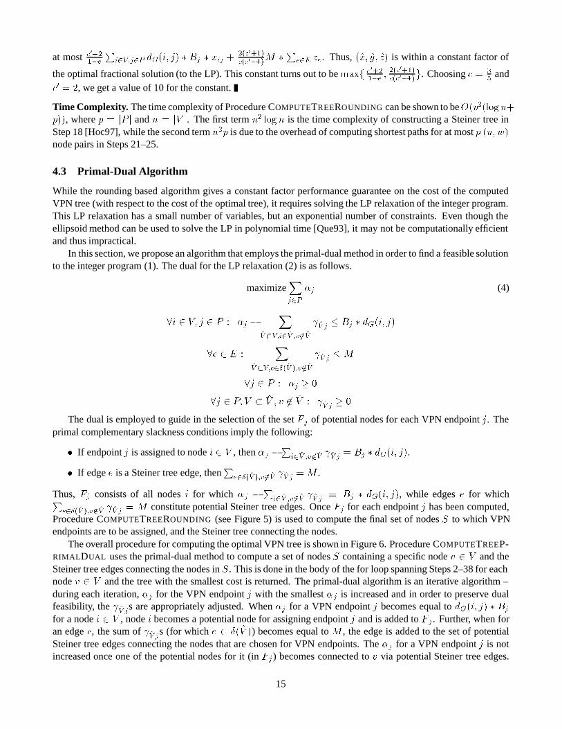
In this section, we propose an algorithm that employs the primal-dual method in order to find a feasible solutionto the integer program (1). The dual for the LP relaxation (2) is as follows.

maximizeX

j�P

�j (4)

�i � V� j � P � �j �X

�V�V�i��V �v ��V

�V j � Bj � dG�i� j�

�e � E �X

�V�V�e��� �V ��v ��V

�V j �M

�j � P � �j � �

�j � P� V �V � v � �V � �V j � �

The dual is employed to guide in the selection of the set F j of potential nodes for each VPN endpoint j. Theprimal complementary slackness conditions imply the following:

� If endpoint j is assigned to node i � V , then �j �P

i��V �v ��V �V j � Bj � dG�i� j�.

� If edge e is a Steiner tree edge, thenP

e��� �V ��v ��V �V j � M .

Thus, Fj consists of all nodes i for which �j �P

i��V �v ��V �V j � Bj � dG�i� j�, while edges e for whichPe��� �V ��v ��V �V j � M constitute potential Steiner tree edges. Once Fj for each endpoint j has been computed,

Procedure COMPUTETREEROUNDING (see Figure 5) is used to compute the final set of nodes S to which VPNendpoints are to be assigned, and the Steiner tree connecting the nodes.

The overall procedure for computing the optimal VPN tree is shown in Figure 6. Procedure COMPUTETREEP-RIMALDUAL uses the primal-dual method to compute a set of nodes S containing a specific node v � V and theSteiner tree edges connecting the nodes in S. This is done in the body of the for loop spanning Steps 2–38 for eachnode v � V and the tree with the smallest cost is returned. The primal-dual algorithm is an iterative algorithm –during each iteration, �j for the VPN endpoint j with the smallest �j is increased and in order to preserve dualfeasibility, the �V js are appropriately adjusted. When �j for a VPN endpoint j becomes equal to dG�i� j� � Bj

for a node i � V , node i becomes a potential node for assigning endpoint j and is added to F j . Further, when foran edge e, the sum of �V js (for which e � �� �V �) becomes equal to M , the edge is added to the set of potentialSteiner tree edges connecting the nodes that are chosen for VPN endpoints. The �j for a VPN endpoint j is notincreased once one of the potential nodes for it (in Fj ) becomes connected to v via potential Steiner tree edges.

15

This is because, as explained below, when �j is increased, dual feasibility cannot be maintained by increasing �V j ,

where v � �V .

Data Structures. The algorithm collects the potential nodes for a VPN endpoint j in Fj . These are the nodes ifor which �j � Bj � dG�i� j�. Also, for each edge e, we stores the sum of all the �V js that contribute to e – here�V does not contain v and e � �� �V �. Thus, when we � M , e becomes a potential Steiner tree edge. Also notethat for any potential Steiner tree edge e, if e � �� �V �, then �V j cannot be increased since this would result in aviolation of dual feasibility. In the procedure, Cu is used to store the nodes connected to u via potential Steinertree edges. Finally, Sj is used to store the set of all nodes connected to nodes in F j via potential Steiner tree edges(thus Fj � Sj). As mentioned earlier, once Sj contains v, then �j for endpoint j cannot be increased any further.

Algorithm. The complete primal-dual algorithm for computing the VPN tree with low cost is illustrated in Fig-ure 6. For each v � V (in the outermost for loop), the algorithm first employs the primal-dual method to computea set of potential nodes Fj for each VPN endpoint j and a set of potential Steiner tree edges that connect each Fjto v (Steps 3–30). It then invokes Procedure COMPUTETREEROUNDING to compute the Steiner tree containingv and connecting the nodes to which VPN endpoints are assigned. This tree is then extended to connect the VPNendpoints in P in Steps 32–35.

The variable activeSet stores the VPN endpoints j for which �j can still be incremented. The set Sj denotesthe smallest set �V of nodes for which �V j needs to be increased when �j for a VPN endpoint j is increased.The reason for this is that for every i � Fj , �j � Bj � dG�i� j�. Thus, in order to ensure that the dual equation�j �

Pi��V �v ��V �V j � Bj � dG�i� j� stays feasible when �j is incremented, �V j where i � �V must also be

incremented. Note also that �V j can be incremented only if �� �V � contains no potential Steiner tree edges. This is

because for a potential Steiner tree edge e,P

e��� �V ��v ��V �V j � M . As a result, increasing �V j if e � �� �V � couldcause the dual equation

Pe��� �V ��v ��V �V j � M to be violated. Thus, if �V j is the variable that is increased to

maintain dual feasibility when �j for a VPN endpoint j is increased, then �V must contain all the nodes in Ci forevery i � Fj , or alternately Sj � �V .

From the above discussion, it follows that if Sj for a VPN endpoint j contains v, then �j cannot be increasedany further. This is because there are no �V j variables for sets �V that contain node v. As a result, it is not possibleto increase �V j to ensure that the dual equation �j �

Pi��V �v ��V �V j � Bj � dG�i� j� stays feasible when �j is

incremented. Thus, activeSet only contains VPN endpoints j for whom Sj does not contain v.In each iteration of the while loop spanning Steps 7–30, �j for a single VPN endpoint j belonging to activeSet

is incremented by minf�� g, where j, � and are as defined in Steps 8–12. Note that increasing �j causes oneof the following to happen – (1) k to be added to Fj since �j � dG�j� k� (if � � ), or (2) edge e to become apotential Steiner tree edge since M � we (if � �). For the latter case, the connected components for nodesconnected to u and v need to be adjusted (Steps 23 and 24). In addition, Sjs for VPN endpoints j that containeither u or v need to be expanded as described in Steps 26 and 27.

Finally, note that in order to maintain feasibility of equations� j�P

i��V �v ��V �V j � Bj �dG�i� j� for endpointsi in Fj , Sjj is increased by �� when �j is increased by ��. This, in turn, contributes �� to we� for alledges e� � ��Sj� (Steps 15 and 22).

Time Complexity. The time complexity of Procedure COMPUTETREEPRIMALDUAL can be shown to beO�n�mpmnp n logn��, where p � jP j, m � jEj and n � jV j. The outermost for loop performs n iterations, one foreach node v � V . Further, for each iteration of the outermost loop, the body of the if condition (Steps 14–18)can be executed at most np times, once for each VPN endpoint node pair, while the body of the else condition(Steps 21–28) can be executed at most m times, once for each edge in E. Assuming that unions involving Sj canbe performed in O�n� steps and lookups of Sj can be carried out in constant time, the complexity of Steps 14-18can be shown to be O�m n�, while the complexity of Steps 21–28 can be shown to be O�mp np�. Finally,

16

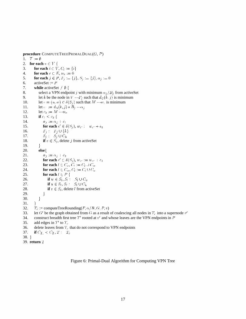
procedure COMPUTETREEPRIMALDUAL(G, P )1. T �� �2. for each v � V f3. for each i � V , Ci �� fig4. for each e � E, we �� �5. for each j � P , Fj �� fjg, Sj �� fjg� �j �� �6. activeSet := P7. while activeSet �� � f8. select a VPN endpoint j with minimum �j�Bj from activeSet9. let k be the node in V � Fj such that dG�k� j� is minimum10. let e � �u�w� � ��Sj� such that M � we is minimum11. let �� �� dG�k� j� �Bj � �j

12. let �� �� M �we

13. if �� � �� f14. �j �� �j � ��15. for each e� � ��Sj�, we� �� we� � ��16. Fj �� Fj � fkg17. Sj �� Sj �Ck

18. if v � Sj, delete j from activeSet19. g20. elsef21. �j �� �j � ��22. for each e� � ��Sj�, we� �� we� � ��23. for each l � Cu, Cl �� Cl �Cw

24. for each l � Cw, Cl �� Cl �Cu

25. for each l � P f26. if w � Sl, Sl �� Sl �Cu

27. if u � Sl, Sl �� Sl �Cw

28. if v � Sl, delete l from activeSet29. g30. g31. g32. Tv := computeTreeRounding(F� ��B�G� P� v)33. let G� be the graph obtained from G as a result of coalescing all nodes in Tv into a supernode v�

34. construct breadth first tree T � rooted at v� and whose leaves are the VPN endpoints in P35. add edges in T � to Tv36. delete leaves from Tv that do not correspond to VPN endpoints37. if CTv � CT , T �� Tv38. g39. return T

Figure 6: Primal-Dual Algorithm for Computing VPN Tree

17

as shown earlier, the time complexity of Procedure COMPUTETREEROUNDING is O�n logn np�. Thus, theProcedure COMPUTETREEPRIMALDUAL has an overall time complexity of O�n�mpmnp n logn��.

4.4 Breadth First Search Based Algorithm

The breadth first search algorithm presented in Section 3 can also be used to compute the VPN tree for the asym-metric bandwidth case (see Procedure COMPUTETREESYMMETRIC in Figure 3). However, since the VPN treecomputation problem for the asymmetric case is NP-hard, the algorithm may not return the optimal VPN tree.

Nevertheless, one can show that cost of the tree computed by the procedure is within a factor ofP

l�PBinl�Bout

l

Mof

the cost of the optimal VPN tree.

Theorem 4.13: The cost of the tree returned by Procedure COMPUTETREESYMMETRIC is within a factor ofPl�P

Binl�Bout

l

Mof the cost of the optimal VPN tree.

Proof: Let Bj � Binj Bout

j for VPN endpoint j. Consider the optimal tree Topt and let b � jbal�Topt�j be thenumber of balanced edges in Topt. Also let corej denote the core node closest to VPN endpoint j in Topt. Thus,the cost of Topt is at least

Pj�P dTopt�corej � j� �Bj b �M .

Now consider the breadth first tree Tv rooted at v, a core node, and computed by Procedure COMPUTE-TREESYMMETRIC. The quantity

Pj�P dTv�v� j� � Bj is an upper bound on the cost of the tree Tv (since the

bandwidth reserved on an edge �u� w� (w is further from v than u in Tv) is at mostP

l�P�u�w�w

Bl, each VPNendpoint j can contribute at most Bj to the reserved bandwidth on edges along the path from v to j). NowdTv�v� j�� bdTopt�corej � j�. As a result, the cost of Tv is no more than

Pj�P dTopt�corej � j��Bj

Pj�P b�Bj .

Thus, the ratio of the costs of trees Tv and Topt is less than or equal tob�P

j�PBj

b�M, which proves the lemma.

5 Incorporating Link Capacity Constraints

The algorithms for computing VPN trees in the previous two sections do not take into account link capacityconstraints, that is, the algorithms assume that each link has a large available bandwidth. In this section, weconsider the problem of provisioning VPN trees when edges of the graph G have associated capacity constraints.Recall that Rij denotes the residual capacity of edge �i� j� - thus, Rij is the available bandwidth on link �i� j�. Wesay that a VPN tree T is feasible if for each edge �i� j� in T , CT �i� j�� Rij . In this section, we develop algorithmsfor computing a feasible VPN tree T with the minimum possible cost.

In the presence of edge capacity constraints, the problem of computing the optimal VPN tree is NP-hard evenwhen endpoints have equal ingress and egress bandwidths. Further, one can show that unless P � NP , it isimpossible to approximate the optimal VPN tree to within a constant factor in polynomial time.

Theorem 5.1: In the presence of edge capacity constraints, the problem of determining if there exists a feasibleVPN tree T is NP-hard.

Corollary 5.2: In the presence of edge capacity constraints, the problem of determining if there exists a feasibleVPN tree whose cost is within a constant factor c of the optimal cost is NP-hard.

5.1 Symmetric Ingress and Egress Bandwidths

In Section 3, we showed that in the absence of link capacity constraints and when VPN endpoints had symmetricingress and egress bandwidth requirements, considering the breadth first tree rooted at each node v � V , yieldedthe optimal VPN tree (see Procedure COMPUTETREESYMMETRIC in Figure 3). In this subsection, we show howthe procedure can be extended to handle link bandwidth constraints.

18

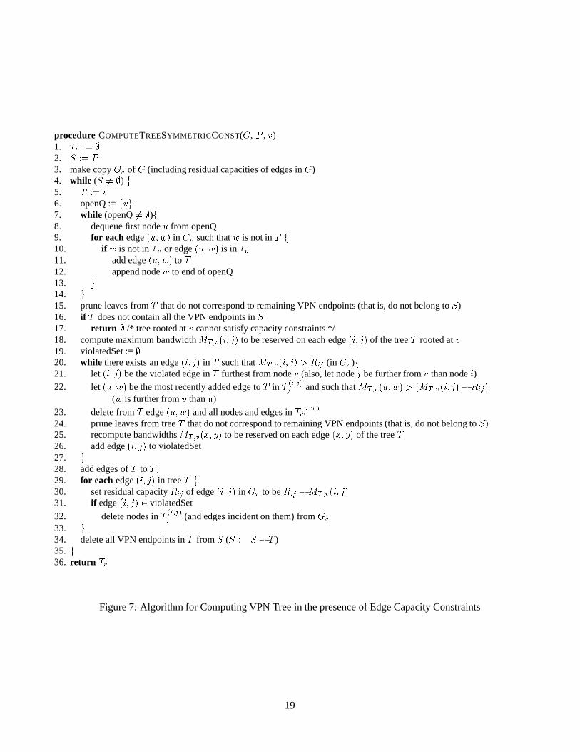
procedure COMPUTETREESYMMETRICCONST(G, P , v)1. Tv �� �2. S �� P3. make copy Gv of G (including residual capacities of edges in G)4. while (S �� �) f5. T �� v6. openQ := fvg7. while (openQ �� �)f8. dequeue first node u from openQ9. for each edge �u�w� in Gv such that w is not in T f10. if w is not in Tv or edge �u�w� is in Tv11. add edge �u�w� to T12. append node w to end of openQ13. g14. g15. prune leaves from T that do not correspond to remaining VPN endpoints (that is, do not belong to S)16. if T does not contain all the VPN endpoints in S17. return � /* tree rooted at v cannot satisfy capacity constraints */18. compute maximum bandwidth MT�v�i� j� to be reserved on each edge �i� j� of the tree T rooted at v19. violatedSet := �20. while there exists an edge �i� j� in T such that MT�v�i� j� � Rij (in Gv)f21. let �i� j� be the violated edge in T furthest from node v (also, let node j be further from v than node i)22. let �u�w� be the most recently added edge to T in T �i�j�

j and such that MT�v�u�w� � �MT�v�i� j�� Rij�

(w is further from v than u)23. delete from T edge �u�w� and all nodes and edges in T �u�w�

w

24. prune leaves from tree T that do not correspond to remaining VPN endpoints (that is, do not belong to S)25. recompute bandwidths MT�v�x� y� to be reserved on each edge �x� y� of the tree T26. add edge �i� j� to violatedSet27. g28. add edges of T to Tv29. for each edge �i� j� in tree T f30. set residual capacity Rij of edge �i� j� in Gv to be Rij �MT�v�i� j�31. if edge �i� j� � violatedSet

32. delete nodes in T �i�j�j (and edges incident on them) from Gv

33. g34. delete all VPN endpoints in T from S (S �� S � T )35. g36. return Tv

Figure 7: Algorithm for Computing VPN Tree in the presence of Edge Capacity Constraints

19

v vv

(a) Graph

1 2 3 4 5 6 1 2 3 5 64 1 2 3 4 5 6

(c) Feasible Breadth First Tree(b) Initial Breadth First Tree

Violated Link

Figure 8: Example of Feasible Tree When Links Have Bandwidth Constraints

Figure 7 depicts the procedure for computing a feasible VPN tree for the case of symmetric endpoint band-widths. The procedure has polynomial time complexity and as a result, due to Theorem 5.1, may not compute theVPN tree with the optimal cost. It computes a VPN tree Tv with low cost and rooted at node v. Thus, one option isto invoke the procedure for each v � V and then choose as the VPN tree, the Tv with the smallest cost. A differentoption is to invoke the procedure for only a small subset of nodes in V – this subset can be the k vertices that resultin the k smallest cost trees when link capacity constraints are not considered (Procedure COMPUTETREESYM-METRIC in Figure 3 is used to compute the minimum cost tree rooted at a vertex v).

Before describing the steps of Procedure COMPUTETREESYMMETRICCONST in more detail, we provide abrief overview of the key intuition underlying it. The spirit of the algorithm is similar to the optimal algorithmfor the symmetric bandwidth case when we did not take into account link constraints. Similar to Procedure COM-PUTETREESYMMETRIC (see Figure 3), the algorithm attempts to construct a breadth first tree rooted at vertex vthat is also feasible. If the breadth first tree rooted at v is already feasible, then we are done. However, the problemarises when the initial breadth first tree Tv rooted at v does not satisfy the link capacity constraints. Then, for eachviolated link �i� j� in Tv, the bandwidth reserved on the edge can be reduced by deleting some VPN endpoints fromTv. The algorithm thus deletes from the subtree of Tv rooted at node j, the minimum number of VPN endpointsso that the bandwidth reserved on link �i� j� is less than the link’s residual capacity. Thus, link �i� j� of T v is nolonger violated. Repeating this process for every violated link thus results in a feasible tree T v – however, Tv maynow no longer connect all the VPN endpoints in P . In order to connect the remaining VPN endpoints (that werepreviously deleted to ensure feasibility), we grow Tv once again in a breadth first fashion. But, this time we donot expand nodes in the subtree of Tv rooted at node j for a previously violated edge �i� j� – the reason for this isthat adding new VPN endpoints in this subtree could cause link �i� j� to be violated again. After T v is expanded toconnect all the remaining VPN endpoints, VPN endpoints are again deleted from Tv until it contains no violatedlinks, and the process of growing Tv is repeated.

Example 5.3: Consider the network graph shown in Figure 8(a). Suppose the residual bandwidth of each link ofthe graph is 2 units, and we are interested in provisioning a VPN tree for the set of VPN endpoints P containingnodes numbered from 1 to 6. Also, suppose that each endpoint has a bandwidth requirement of 1 unit. The breadthfirst tree Tv rooted at node v is shown in Figure 8(b). Tree Tv, however, is not feasible since the bandwidth to bereserved on the link connecting node v to the subtree containing nodes 1, 2 and 3, is 3 units, which exceeds theavailable capacity of the link, which is 2 units. (The violated link is marked in Figure 8(b)).

Thus, in order to make tree Tv feasible, VPN endpoint 3 is chosen as the victim and deleted from Tv. Tree Tvis then expanded in a breadth first fashion to also include VPN endpoint 3. However, the portion of T v rooted atthe violated link (subtree containing endpoints 1 and 2) is not expanded. Instead, endpoint 3 is added to T v alonga different link as shown in Figure 8(c) resulting in a final tree that is feasible.

We now describe the steps of Procedure COMPUTETREESYMMETRICCONST in more detail. Inputs to the

20

procedure include the graph G with residual link bandwidths and the set of VPN endpoints P . The procedurereturns a feasible VPN tree rooted at v if it can find one – otherwise, it simply returns �. Variable Tv in theprocedure, is used to store the feasible VPN tree rooted at v constructed so far, and S is used to store the set ofVPN endpoints that still remain to be connected to Tv. In each iteration of the for loop spanning Steps 4–35, Tvis expanded to connect the remaining VPN endpoints in S. This is carried out in Steps 5–14, where a new breadthfirst tree T rooted at v and whose leaves are endpoints in S, is constructed. The tree T is constructed in a mannerthat ensures that the restrictions of the two trees T and Tv are identical with respect to common nodes. Thus T ,in some respect, corresponds to an expansion of Tv. Note that in Steps 16–17, if T does not contain all the VPNendpoints in S, then it is not possible to expand T v to connect the remaining VPN endpoints and so a feasible treerooted at node v cannot be found.

Once the tree T connecting VPN endpoints in S has been computed, we need to delete endpoints from it ifthe bandwidth to be reserved on some link �i� j� of T exceeds the residual bandwidth R ij of the link. This isachieved in the while loop spanning Steps 20–27. MT�v�i� j� is the maximum bandwidth to be reserved on eachlink �i� j� of T and is simply equal to

Pl��T �i�j�

j�P �

Bl (the sum of bandwidth requirements of VPN endpoints in

T�i�j�j ). Thus, an edge �i� j� is violated if MT�v�i� j�� Rij . Now, in order to make edge �i� j� feasible, we need to

delete VPN endpoints from T�i�j�j , the sum of whose bandwidth requirements is at least the amount of the violation

MT�v�i� j�� Rij . Also, it would be preferable to choose as the “victims” VPN endpoints that are most distantfrom v since these require bandwidth to be reserved along more edges of T . Thus, in Steps 23-24, we identify thesubtree T �u�w�

w for edge �u� w� in T that is most distant from v and whose deletion from T would cause link �i� j�to be no longer violated. This process of deleting VPN endpoints is carried out until T contains no violated linksand the set of violated links is kept track of in the variable violatedSet.

After the while loop spanning Steps 20–27 completes execution, T is a feasible tree connecting some subsetof VPN endpoints in S. Thus, since T is consistent with Tv on portions they have in common, edges of T cansimply be added to Tv while preserving the property that Tv is a tree. Also, the bandwidth for each link �i� j�in T is reserved by adjusting the residual bandwidth for the link in G v by MT�v�i� j� (as described in Step 30).Reserving bandwidth for tree T independently during each iteration does not pose a problem since it is relativelystraightforward to show that the bandwidth that must be reserved for the union of the trees (generated across thevarious iterations) is equal to the sum of the bandwidths reserved for each individual tree. More specifically, ifT � T � in one iteration and T � T �� in another, then for any link �i� j� in T � T ��, MT �T ���v�i� j� � MT ��v�i� j�MT ���v�i� j�. Finally, since we don’t want to further expand portions of Tv rooted at violated links (since there isa high probability that these will be violated again), we delete these portions of T v from Gv (Steps 31–32). Thisensures that these subtrees rooted at violated edges will not be part of T when Tv is expanded in the next iteration,and thus no new VPN endpoints will ever be added to these subtrees.

5.2 Asymmetric Ingress and Egress Bandwidths

The procedure for computing the VPN tree when VPN endpoint bandwidths are asymmetric and in the presenceof link bandwidth constraints is similar to Procedure COMPUTETREEPRIMALDUAL (see Figure 6), except for thefollowing key differences.

1. As shown earlier in Lemma 4.3 (see Section 4), the balanced edges that connect the core nodes of a VPN treehave the property that the sum of the bandwidths reserved on each edge in the two directions is M . SupposeEM denotes the set of links in E for whom the residual capacity in each direction is at least M . Then, byrequiring that the potential steiner tree edges (that connect each Fj to node v) belong to EM , we can ensurethat there is sufficient capacity on each link to accommodate the M units of bandwidth distributed over thetwo directions. Thus, in Step 10, potential steiner tree edges are chosen from EM .

2. In Step 32, in the invocation of Procedure COMPUTETREEROUNDING, EM is passed as an input parameterinstead of E. This ensures that only edges in EM are used to construct the steiner tree Tv returned by the

21

procedure.

3. Since links have capacity constraints, instead of constructing a simple breadth first tree rooted at v � in Step 34,Procedure COMPUTETREESYMMETRICCONST is used to compute a feasible breadth first tree rooted at v�.

6 Experimental Study

We conducted an extensive empirical study to measure the performance of our breadth first search (BFS) andprimal-dual algorithms, and compared them with the approach of using a Steiner tree to connect VPN endpoints[DGG�98]. The major findings of our study can be summarized as follows:

� The primal-dual algorithm generates VPN trees with the smallest cost for a wide range of ingress/egressbandwidth ratios. It outperforms both the BFS and the Steiner tree algorithms for medium to large bandwidthratios.

� For low ingress/egress bandwidth ratios, the BFS and primal-dual algorithms consistently outperform theSteiner tree algorithm. In many cases, they construct VPN trees that reserve half the bandwidth reserved bySteiner trees.

� The BFS algorithm scales well for large networks containing several thousand nodes.

In our implementation of Steiner trees, we used the 2-approximation primal-dual algorithm from [Hoc97].

6.1 Network Generation Models

In our experiments, we used two different network generators, to generate random networks with different charac-teristics. One generator was based on work by Waxman [Wax88], the other on work by Faloutsos et al. [FFF99].We generated random and symmetric networks consisting of 50 to 5000 nodes connected by links with large resid-ual capacities. The generation algorithms use the following models.

� Waxman model [Wax88]. In this model, nodes are placed on a plane, and the probability for two nodes tobe connected by a link decreases exponentially with the Euclidean distance between them. In our experiments, weused the Waxman model to generate networks of size less than 1000 nodes. We set the value for the parameter thatcontrols the density of short edges in the network to 0.9 and the value of the parameter for the average node degreeto 0.1.

� Power-Law model [FFF99]. In this model, the node connectivity follows a power-law rule: very few nodeshave high connectivity, and the number of nodes with lower connectivity increases exponentially as the connectivitydecreases. This model is based on Internet measurements, where a node is an autonomous system (AS). In ourexperiments, we used the Power-Law model to generate large networks containing 1000 or more nodes.

A subset of the nodes in each network is chosen randomly and uniformly as the VPN endpoints. For thesymmetric bandwidth case, each VPN endpoint is assigned bandwidth uniformly chosen from an interval of 2-100Mbps. Further, to model asymmetric endpoint bandwidths, we introduce a new parameter, the asymmetry ratio r,which is essentially the ingress/egress bandwidth ratio for each VPN endpoint. The same ratio is also maintainedforP

lBlin and

PlB

lout, the sums of ingress and egress bandwidths over all VPN endpoints.

6.2 Experimental Results

We compare the provisioning cost (that is, the total bandwidth reserved on links of the VPN tree) of the algorithmsfor the symmetric as well as the asymmetric bandwidth models. In the study, we examined the effect of varying thefollowing three parameters on provisioning cost: (i) network size, (ii) number of VPN nodes, and (ii) asymmetryratio.

22

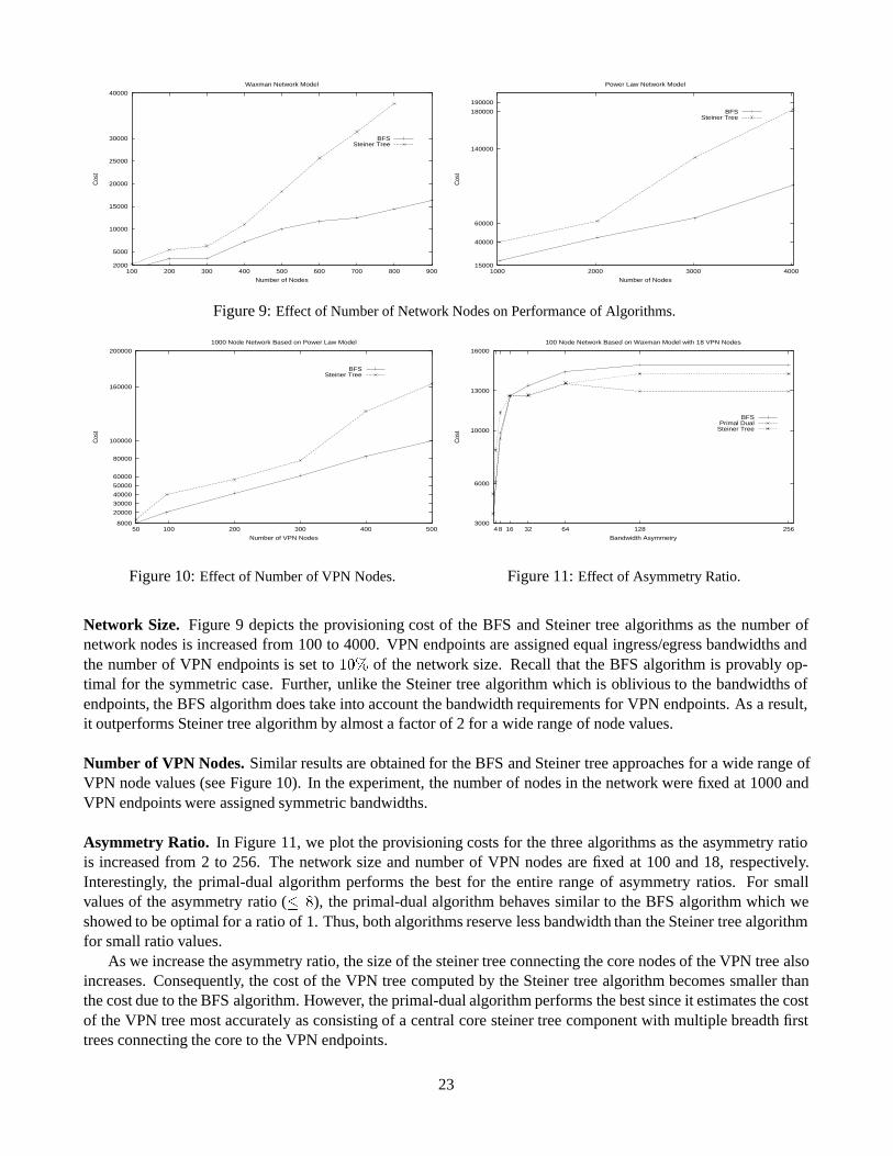
2000

5000

10000

15000

20000

25000

30000

40000

100 200 300 400 500 600 700 800 900

Cos

t

Number of Nodes

Waxman Network Model

BFSSteiner Tree

15000

40000

60000

140000

180000

190000

1000 2000 3000 4000

Cos

t

Number of Nodes

Power Law Network Model

BFSSteiner Tree

Figure 9: Effect of Number of Network Nodes on Performance of Algorithms.

8000

20000

30000

40000

50000

60000

80000

100000

160000

200000

50 100 200 300 400 500

Cos

t

Number of VPN Nodes

1000 Node Network Based on Power Law Model

BFSSteiner Tree

Figure 10: Effect of Number of VPN Nodes.

3000

6000

10000

13000

16000

48 16 32 64 128 256

Cos

t

Bandwidth Asymmetry

100 Node Network Based on Waxman Model with 18 VPN Nodes

BFSPrimal Dual

Steiner Tree

Figure 11: Effect of Asymmetry Ratio.

Network Size. Figure 9 depicts the provisioning cost of the BFS and Steiner tree algorithms as the number ofnetwork nodes is increased from 100 to 4000. VPN endpoints are assigned equal ingress/egress bandwidths andthe number of VPN endpoints is set to ��� of the network size. Recall that the BFS algorithm is provably op-timal for the symmetric case. Further, unlike the Steiner tree algorithm which is oblivious to the bandwidths ofendpoints, the BFS algorithm does take into account the bandwidth requirements for VPN endpoints. As a result,it outperforms Steiner tree algorithm by almost a factor of 2 for a wide range of node values.

Number of VPN Nodes. Similar results are obtained for the BFS and Steiner tree approaches for a wide range ofVPN node values (see Figure 10). In the experiment, the number of nodes in the network were fixed at 1000 andVPN endpoints were assigned symmetric bandwidths.

Asymmetry Ratio. In Figure 11, we plot the provisioning costs for the three algorithms as the asymmetry ratiois increased from 2 to 256. The network size and number of VPN nodes are fixed at 100 and 18, respectively.Interestingly, the primal-dual algorithm performs the best for the entire range of asymmetry ratios. For smallvalues of the asymmetry ratio (� �), the primal-dual algorithm behaves similar to the BFS algorithm which weshowed to be optimal for a ratio of 1. Thus, both algorithms reserve less bandwidth than the Steiner tree algorithmfor small ratio values.

As we increase the asymmetry ratio, the size of the steiner tree connecting the core nodes of the VPN tree alsoincreases. Consequently, the cost of the VPN tree computed by the Steiner tree algorithm becomes smaller thanthe cost due to the BFS algorithm. However, the primal-dual algorithm performs the best since it estimates the costof the VPN tree most accurately as consisting of a central core steiner tree component with multiple breadth firsttrees connecting the core to the VPN endpoints.

23

7 Concluding Remarks

In this paper, we developed novel algorithms for provisioning VPNs in the hose model. We connected VPNendpoints using a tree structure and our algorithms attempted to optimize the total bandwidth reserved on edges ofthe VPN tree. We showed that even for the simple scenario in which network links are assumed to have infinitecapacity, the general problem of computing the optimal VPN tree is NP-hard. However, for the special case whenthe ingress and egress bandwidths for each VPN endpoint are equal, we proposed a breadth first search (BFS)algorithm for computing the optimal tree whose time complexity is O�mn�, where m and n are the number oflinks and nodes in the network, respectively. We presented a novel integer programming formulation for the generalVPN tree computation problem (that is, when ingress and egress bandwidths of VPN endpoints are arbitrary) anddevised an algorithm that is based on the primal-dual method. Finally, we extended our proposed algorithmsfor computing VPN trees when network links have capacity constraints. We showed that in the presence of linkcapacity constraints, computing the optimal VPN tree is NP-hard even when ingress and egress bandwidths ofeach endpoint are equal. Further, we also showed that computing an approximate solution that is within a constantfactor of the optimum is as difficult as computing the optimal VPN tree itself.

Our experimental results indicate that the primal-dual algorithm performs the best over a wide range of pa-rameter values, reserving less bandwidth than both the BFS and Steiner tree algorithms for large ingress/egressbandwidth ratios. For small bandwidth ratios, the BFS and primal-dual algorithms consistently outperform theSteiner tree algorithm. In many cases, they construct VPN trees that reserve half the bandwidth reserved by Steinertrees.

References

[AMO93] R. K. Ahuja, T. L. Magnanti, and J. B. Orlin. “Network Flows”. Prentice Hall, 1993.

[DGG�98] N. G. Duffield, P. Goyal, A. Greenberg, P. Mishra, K. K. Ramakrishnan, and J. E. van der Merwe. A flexiblemodel for resource management in virtual private networks. In Proceedings ACM SIGCOMM, 1998.

[DR00] B. Davie and Y. Rekhter. “MPLS Technology and Applications”. Morgan Kaufmann Publishers, 2000.

[FFF99] M. Faloutsos, P. Faloutsos, and C. Faloutsos. On power-law relationships of the internet topology. In ProceedingsACM SIGCOMM, 1999.

[GJ79] M. R. Garey and D. S. Johnson. Computers and Intractability: A Guide to the Theory of NP-Completeness. W.H. Freeman and Company, 1979.

[Hoc97] D. S. Hochbaum. “Approximation Algorithms for NP-Hard Problems”. PWS Publishing Company, 1997.

[KA98] S. Kent and R. Atkinson. Security architecture for the internet protocol. RFC 2401, November 1998.

[LV92] J. H. Lin and J. H. Vitter. �-approximations with minimum packing constraint violation. In Proceedings ACMSymposium on Theory of Computing, 1992.

[Que93] M. Queyranne. Structure of a simple scheduling polyhedron. Mathematical Programming, 58:163–185, 1993.

[STA97] D. Shmoys, E. Tardos, and K Aardal. Approximation algorithms for facility location problems. In ProceedingsACM Symposium on Theory of Computing, 1997.

[Wax88] B. M. Waxman. Routing of multipoint connections. IEEE Journal on Selected Areas in Communications,6(9):1617–1622, December 1988.

24

– This appendix contains material that can be read at the discretion of the reviewer andhas been included only for the purpose of completeness. –

A Proofs for Asymmetric Ingress and Egress Bandwidths

Proof of Theorem 4.2: We reduce the Steiner tree problem to the problem of computing an optimal VPN tree.The Steiner tree problem is as follows: given a graph G and set of endpoints P , compute a tree connecting theendpoints and containing the minimum number of edges. Suppose for each VPN endpoint j, the ingress bandwidthrequirement is 1, that is, Bin

j � �, and the egress bandwidth requirement is a large constant greater than jP j, thatis, Bout

j � jP j. Note thatP

l�P Binl � jP j � Bout

j , for every VPN endpoint j. Thus, for each edge �i� j�, thebandwidth reserved in the two directions is bounded by the ingress bandwidths of VPN endpoints in P i and Pj –specifically, CT �i� j� �

Pl�P

�i�j�j

Binl and CT �j� i� �

Pl�P

�i�j�i

Binl . Thus, the total bandwidth reserved on edge

�i� j� in the two directions is CT �i� j� CT �j� i� �P

l�P Binl � jP j. Since jP j is a constant, the cost of a VPN

tree T connecting the endpoints in P is simply jP j times the number of edges in T . Thus, the optimal VPN tree isthe one with the fewest edges, or alternately, the Steiner tree connecting the VPN endpoints in P .

Proof of Lemma 4.4: We show that if an edge �i� j� is biased towards j, then every other edge �u� w� in P �i�j�j

(such that w is further from j than u) is also biased towards w. Thus, it is not possible for balanced edges to beseparated by biased edges – as a result, the set of balanced edges form a connected component.

For an edge �i� j� that is biased towards j, the following is true: (1)P

l�P�i�j�j

Binl �

Pl�P

�i�j�i

Boutl , and

(2)P

l�P�i�j�j

Boutl �

Pl�P

�i�j�i

Binl . For edge �u� w� in P

�i�j�j , P �u�w�

w P�i�j�j and P

�i�j�i P

�u�w�u . Thus, it

follows that (1)P

l�P�u�w�w

Binl �

Pl�P

�i�j�j

Binl �

Pl�P

�i�j�i

Boutl �

Pl�P

�u�w�u

Boutl , and (2)

Pl�P

�u�w�w

Boutl �

Pl�P

�i�j�j

Boutl �

Pl�P

�i�j�i

Binl �P

l�P�u�w�u

Binl . Thus, edge �u� w� is biased towardsw.

Proof of Lemma 4.5: We show that every biased edge �v� w� incident on v in Cv is biased toward w. Supposethis were not true and edge �v� w�were biased towards v. Then, due to Lemma 4.4, it follows that every other edgeincident on v would be biased away from v and thus, v cannot be a core node - which leads to a contradiction.Thus, if every edge �v� w� incident on v in Cv is biased toward w, then, due to Lemma 4.4, it follows that everyedge �i� j� in Cv is biased towards j.

Proof of Lemma 4.6: Due to Lemma 4.5, every edge �i� j� in Cv (with j further from node v than i) is biasedtowards j. As a result, the total bandwidth reserved on edge �i� j� is

Pl�P

�i�j�j

�Binl Bout

l �. Thus, VPN site l

contributes �Binl Bout

l � to the cost of each edge �i� j� on the path from v to l, and to no other edge. Thus, thecost of the component Cv is given by

Pl��Cv�P � dT �v� l� � �B

inl Bout

l �.

Proof of Lemma 4.7: The tree T �S� consists of two types of edges – (1) Steiner tree edges connecting the nodesin S, and (2) edges in the breadth first tree connecting the nodes in S to VPN endpoints in P . We show that thecost of the Steiner tree edges is at most M � b. Also, we show that each VPN endpoint l contributes no more thanminv�SfdG�v� l�g � �B

inl Bout

l � to the edges of the breadth first tree. This proves the lemma.Let B be the set of Steiner tree edges connecting nodes in S in T �S�. Note that the cost of each edge can be at

mostM . This is true of balanced edges inT �S� (due to Lemma 4.3). We show that this holds even for biased edges.Suppose edge �i� j� is biased towards i. Thus,

Pl�P

�i�j�i

Binl �P

l�P�i�j�j

Boutl and

Pl�P

�i�j�i

Boutl �

Pl�P

�i�j�j

Binl .

Thus, the total bandwidth reserved on edge �i� j� isP

l�P�i�j�i

Binl P

l�P�i�j�i

Boutl . Suppose M �

Pl�P B

inl . If

the bandwidth reserved on �i� j� exceeds M , then this would imply thatP

l�P�i�j�i

Boutl �

Pl�P

�i�j�j

Binl , which

would lead to a contradiction (since �i� j� is biased towards i). Thus, since the edges connecting the nodes in S

in T �S� form a Steiner tree each of whose cost is at most M , the cost of these edges in T �S� is less than M � b,

25

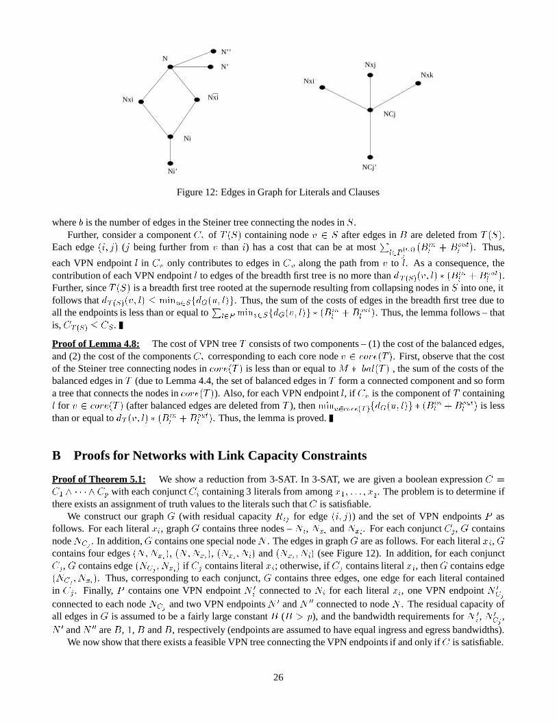
Nxj

NxkNxi

N

Nxi Nxi

Ni

NCj

N’

Ni’NCj’

N’’

Figure 12: Edges in Graph for Literals and Clauses

where b is the number of edges in the Steiner tree connecting the nodes in S.Further, consider a component Cv of T �S� containing node v � S after edges in B are deleted from T �S�.

Each edge �i� j� (j being further from v than i) has a cost that can be at mostP

l�P�i�j�j

�Binl Bout

l �. Thus,

each VPN endpoint l in Cv only contributes to edges in Cv along the path from v to l. As a consequence, thecontribution of each VPN endpoint l to edges of the breadth first tree is no more than dT �S��v� l� � �B

inl Bout

l �.Further, since T �S� is a breadth first tree rooted at the supernode resulting from collapsing nodes in S into one, itfollows that dT �S��v� l� � minu�SfdG�u� l�g. Thus, the sum of the costs of edges in the breadth first tree due toall the endpoints is less than or equal to

Pl�P minv�SfdG�v� l�g � �Bin

l Boutl �. Thus, the lemma follows – that

is, CT �S� � CS .

Proof of Lemma 4.8: The cost of VPN tree T consists of two components – (1) the cost of the balanced edges,and (2) the cost of the components Cv corresponding to each core node v � core�T �. First, observe that the costof the Steiner tree connecting nodes in core�T � is less than or equal to M � jbal�T �j, the sum of the costs of thebalanced edges in T (due to Lemma 4.4, the set of balanced edges in T form a connected component and so forma tree that connects the nodes in core�T �). Also, for each VPN endpoint l, if Cv is the component of T containingl for v � core�T � (after balanced edges are deleted from T ), then minu�core�T �fdG�u� l�g � �B

inl Bout

l � is lessthan or equal to dT �v� l� � �Bin

l Boutl �. Thus, the lemma is proved.

B Proofs for Networks with Link Capacity Constraints

Proof of Theorem 5.1: We show a reduction from 3-SAT. In 3-SAT, we are given a boolean expression C �C� � � � � � Cp with each conjunct Ci containing 3 literals from among x�� � � � � xq. The problem is to determine ifthere exists an assignment of truth values to the literals such that C is satisfiable.

We construct our graph G (with residual capacity Rij for edge �i� j�) and the set of VPN endpoints P asfollows. For each literal xi, graph G contains three nodes – Ni, Nxi and N �xi. For each conjunct Cj, G containsnode NCj

. In addition, G contains one special node N . The edges in graph G are as follows. For each literal xi, Gcontains four edges �N�Nxi�, �N�N �xi�, �Nxi� Ni� and �N �xi � Ni� (see Figure 12). In addition, for each conjunctCj, G contains edge �NCj

� Nxi� if Cj contains literal xi; otherwise, if Cj contains literal �xi, then G contains edge�NCj

� N �xi�. Thus, corresponding to each conjunct, G contains three edges, one edge for each literal containedin Cj . Finally, P contains one VPN endpoint N �

i connected to Ni for each literal xi, one VPN endpoint N �Cj

connected to each node NCjand two VPN endpoints N � and N �� connected to node N . The residual capacity of

all edges in G is assumed to be a fairly large constant B (B � p), and the bandwidth requirements for N �i , N

�Cj

,N � and N �� are B, �, B and B, respectively (endpoints are assumed to have equal ingress and egress bandwidths).

We now show that there exists a feasible VPN tree connecting the VPN endpoints if and only if C is satisfiable.

26

Suppose C is satisfiable. We show that there exists a feasible VPN tree. Since C is satisfiable, there exists anassignment of truth values to each literal xi such that each conjunct Cj is true. We construct the feasible VPNtree T as follows. First, note that T must contain the edges �Ni� N

�i�, �NCj

� N �Cj�, �N�N �� and �N�N ��� since

these are the only edges incident on the VPN endpoints. Further, for a literal xi, if xi is true in the assignment,then edges �N�N �xi� and �N �xi� Ni� are added to T ; otherwise, if xi is false in the assignment, then edges �N�Nxi�and �Nxi� Ni� are added to T . Note that the bandwidth to be reserved on each of these edges is at most B, thebandwidth requirement for VPN endpointN �

i . Next, for each conjunctCj, since it is true, there is some literal xi or�xi that is assigned a true value. Consider one such literal inCj that is assigned a true value. If Cj contains xi whichis true, then edges �N�Nxi� and �Nxi� NCj

� are added to T . On the other hand, ifCj contains �xi which is true, thenedges �N�N �xi� and �N �xi� NCj

� are added to T . For both cases, one can show that the reserved bandwidth doesnot exceed B. For example, the first case (when xi is true), the only edges in T incident on Nxi are �Nxi� NCj

�for conjunctsCj containing xi. Since the bandwidth requirement for each VPN endpoint N �

Cjis 1 and the number

of conjuncts p is less than B, the bandwidth to be reserved on edge �N�Nxi� is at most B. Thus, the constructedVPN tree T is feasible and connects the VPN endpoints in P .

We next show that if there exists a feasible VPN tree connecting the VPN endpoints in P , then C is satisfiable.Suppose there exists a feasible VPN tree T . We begin by showing that for every VPN endpoint N �

i , either edges�N�N �xi� and �N �xi� Ni� are in T or edges �N�Nxi� and �Nxi� Ni� are in T . To show this, first observe that sinceboth nodes N and Ni are connected to VPN endpoints, it must be the case that node Ni is connected to node Nin T . Suppose Ni is connected to N via the sequence of edges �Ni� Nxi�, �Nxi� NCj

�, �NCj� Nxl�, � � � to node N .

Then, since N �i and N �

Cj(connected to nodes Ni and NCj

) are both VPN endpoints with bandwidth requirementsB and �, respectively, and N � and N �� are VPN endpoints connected to N with a total bandwidth requirement of�B, the bandwidth to be reserved on edge �NCj

� Nxl� must be at least B �, which would make T infeasible.Thus, for every VPN endpointN �

i , either edges �N�N �xi� and �N �xi� Ni� are in T or edges �N�Nxi� and �Nxi� Ni�belong to T .

We assign xi a value true if edges �N�N �xi� and �N �xi � Ni� are in T ; else if edges �N�Nxi� and �Nxi� Ni� arein T , we assign �xi a value of true. Next, we show that if xi is assigned true, then edge �NCj

� N �xi� cannot belongto T . The reason for this is that then T would contain edges �N�N �xi�, �N �xi� Ni� and �NCj

� N �xi� causing thebandwidth to be reserved on edge �N�N �xi� to exceed B. Similarly, we can show that if �xi is assigned true, thenedge �NCj

� Nxi� cannot belong to T . Since T is a VPN tree, node NCjmust be connected to node N through an

edge �NCj� Nxi� or �NCj

� N �xi� for a literal xi or �xi contained in Cj . If �NCj� Nxi� is in T , then xi must be true

and Cj is true. On the other hand, if �NCj� N �xi� is in T , then �xi must be true and Cj is true. Thus, C is satisfiable.

Proof of Corollary 5.2: We show a reduction from 3-SAT to the problem of determining if there exists a feasibleVPN tree whose cost is within a factor c of the optimal cost. The graph G that we construct for the booleanexpressionC contains all the nodes and edges as described in the proof of Theorem 5.1 above. In addition, we adda separate path containing �qc pc

B edges between each node Ni andN . The residual capacity of each edge alongeach of the paths is B. Essentially, if any of these long paths is chosen in VPN tree T to connect N i and N , thenthe cost of T exceeds �qBc �pc, since �B is the bandwidth that needs to be reserved (B in each direction) oneach edge along the path. In the proof of Theorem 5.1, we showed that in a feasible VPN tree that does not containany of the long paths, each VPN endpoint N �

i or N �Cj

is connected to N via paths consisting of two edges (if wewere to include the edge incident on the endpoint itself, then each path would contain three edges). Thus, the costof a feasible VPN tree that excludes all long paths is at most �qB �p (excluding the cost of edges incident onVPN endpoints). As a result, one can show (in a manner similar to the proof of Theorem 5.1) that C is satisfiableif and only if there is a feasible VPN tree T whose cost is equal to �qB �p (that is, T does not contain any ofthe long paths). Since a long path adds �qBc �pc to the cost of a VPN tree, one can show that C is satisfiable ifand only if there is a feasible VPN tree T whose cost is less than or equal to �qBc �pc. Thus, it follows that theproblem of determining if there exists a feasible VPN tree whose cost is within a constant factor c of the optimalcost is NP-hard.

27