This article was downloaded by: [Fac Psicologia/Biblioteca]On: 20 June 2012, At: 01:26Publisher: Taylor & FrancisInforma Ltd Registered in England and Wales Registered Number: 1072954 Registeredoffice: Mortimer House, 37-41 Mortimer Street, London W1T 3JH, UK

International Journal of ComputerMathematicsPublication details, including instructions for authors andsubscription information:http://www.tandfonline.com/loi/gcom20

Algorithmic method to obtain abeliansubalgebras and ideals in Lie algebrasManuel Ceballos a , Juan Núñez a & Ángel F. Tenorio ba Departamento de Geometría y Topología, Facultad deMatemáticas., Universidad de Sevilla, Aptdo. 1160, 41080, Seville,Spainb Departamento de Economía, Métodos Cuantitativos e HistoriaEconómica, Escuela Politécnica Superior, Universidad Pablo deOlavide, Ctra. Utrera km. 1, 41013, Seville, Spain

Available online: 16 May 2012

To cite this article: Manuel Ceballos, Juan Núñez & Ángel F. Tenorio (2012): Algorithmic methodto obtain abelian subalgebras and ideals in Lie algebras, International Journal of ComputerMathematics, 89:10, 1388-1411

To link to this article: http://dx.doi.org/10.1080/00207160.2012.688112

PLEASE SCROLL DOWN FOR ARTICLE

Full terms and conditions of use: http://www.tandfonline.com/page/terms-and-conditions

This article may be used for research, teaching, and private study purposes. Anysubstantial or systematic reproduction, redistribution, reselling, loan, sub-licensing,systematic supply, or distribution in any form to anyone is expressly forbidden.

The publisher does not give any warranty express or implied or make any representationthat the contents will be complete or accurate or up to date. The accuracy of anyinstructions, formulae, and drug doses should be independently verified with primarysources. The publisher shall not be liable for any loss, actions, claims, proceedings,demand, or costs or damages whatsoever or howsoever caused arising directly orindirectly in connection with or arising out of the use of this material.

International Journal of Computer MathematicsVol. 89, No. 10, July 2012, 1388–1411

Algorithmic method to obtain abelian subalgebras and ideals inLie algebras

Manuel Ceballosa* Juan Núñeza and Ángel F. Tenoriob

aDepartamento de Geometría y Topología, Facultad de Matemáticas. Universidad de Sevilla, Aptdo. 1160.41080-Seville, Spain; bDepartamento de Economía, Métodos Cuantitativos e Historia Económica, Escuela

Politécnica Superior, Universidad Pablo de Olavide, Ctra. Utrera km. 1. 41013-Seville, Spain

(Received 20 September 2011; revised version received 8 February 2012; accepted 3 April 2012)

In this paper, we show an algorithmic procedure to compute abelian subalgebras and ideals of finite-dimensional Lie algebras, starting from the non-zero brackets in its law. In order to implement this method,we use the symbolic computation package MAPLE 12. Moreover, we also give a brief computational studyconsidering both the computing time and the memory used in the two main routines of the implementation.Finally, we determine the maximal dimension of abelian subalgebras and ideals for non-decomposablesolvable non-nilpotent Lie algebras of dimension 6 over both the fields R and C, showing the differencesbetween these fields.

Keywords: abelian Lie subalgebra; abelian ideal; α invariant; β invariant; algorithm

2000 AMS Subject Classifications: 17B30; 17B05; 68W40; 68Q25

1. Introduction

Nowadays, there exists an extensive research on Lie theory due to its own theoretical importanceand also due to its applications in many different fields, such as engineering, physics and appliedmathematics. However, some general aspects about Lie algebras remain unknown. For instance,the problem of classifying Lie algebras is still open, even for nilpotent and solvable ones anddespite being completely solved for some particular families of Lie algebras (like semisimple andsimple ones) since 1890. Hence, to solve these and other problems, the need for studying differentproperties of Lie algebras arises naturally. Taking a simple concerning example, conditions on thelattice of subalgebras of a Lie algebra often lead to information about the Lie algebra itself. In thisway, studying abelian Lie subalgebras and ideals of a finite-dimensional Lie algebra constitutesthe main goal of this paper, since this study would allow us to advance the classification problemin the future.

The topic to be studied in this paper consists of the maximal dimension of abelian subalgebras ina given finite-dimensional Lie algebra g. Although this concept has been previously worked in theliterature, most authors (e.g. [19]) have considered abelian ideals instead of abelian subalgebras,

*Corresponding author. Email: mceballos@us.es

ISSN 0020-7160 print/ISSN 1029-0265 online© 2012 Taylor & Francishttp://dx.doi.org/10.1080/00207160.2012.688112http://www.tandfonline.com

Dow

nloa

ded

by [

Fac

Psic

olog

ia/B

iblio

teca

] at

01:

26 2

0 Ju

ne 2

012

International Journal of Computer Mathematics 1389

involving the use of more restrictive hypotheses. However, we do not assume such restrictions,but our research considers all the subalgebras contained in a Lie algebra g.

Given a finite-dimensional Lie algebra g, the maximal dimension of its abelian subalgebrasand of its abelian ideas is denoted by α(g) and β(g), respectively. Note that these two valuesare invariants of the algebra g and they are important for many subjects. First of all, they areuseful for studying Lie algebra contractions and degenerations. Indeed, there exists an extensiveliterature on this subject, in particular, for low-dimensional Lie algebras (see e.g. [6,12,14] andthe references given therein).

Second, several results have been obtained concerning the question of how big or small thismaximal dimension can be, in comparison with the dimension of the Lie algebra. Some of themshow that a Lie algebra of a large dimension contains abelian subalgebras of a large dimension.For example, the dimension of a nilpotent Lie algebra g is bounded by dim(g) ≤ �(� + 1)/2,where α(g) = � (see [13,15]). Another states that if g is complex solvable Lie algebra, then itsdimension satisfies dim(g) ≤ �(� + 3)/2, where α(g) = � (see [10]). To prove these bounds,several additional conditions are also enforced for the value of β invariant.

For a semisimple Lie algebra s, Malcev [9] determined the invariant α(s). Due to the non-existence of abelian ideals in a simple Lie algebra s, β(s) = 0 trivially holds. In the last decades,the study of abelian ideals in a Borel subalgebra b of a simple complex Lie algebra s has drawnconsiderable attention. This is in part because α(s) = β(b) and hence β(b) can be computedpurely in terms of certain root system invariants, as can be seen in [17]. Let us note that the α

invariant can be usefully applied, for example, to characterize Lie algebras in several senses. SoTenorio [18] gave some criteria about solubility and nilpotency properties of Lie algebras startingfrom this notion. Moreover, this topic has already been studied by different authors, being classicaland fundamental, as can be seen in the following references: Krawtchouk [7], Laffey [8], whichcomputed the α invariant of the algebra of n × n matrices over any field; or Suprunenko andTyshkevich [16], which dealt with the problem of determining abelian subalgebras of maximaldimension of nilpotent type.

Previously, we have already studied abelian subalgebras from both points of view: theoreticaland computational. Furthermore, the α invariant was computed for two special families of complexLie algebras: gn, of n × n strictly upper-triangular matrices (see [1]) and hn, of n × n upper-triangular matrices (see [5]). This was done by applying to these algebras an algorithmic procedure,introduced in [1]. In the present paper, we show an algorithmic procedure which works for anyarbitrary finite-dimensional complex Lie algebra. The algorithm is expounded here by indicatingand explaining each of its steps. In addition, we show a computational and complexity studyof its implementation with MAPLE 12 and, as application, we compute the α and β invariantsfor six-dimensional non-decomposable solvable non-nilpotent Lie algebras over the field F, withF = R or C.

2. Theoretical background

In this section, we recall some concepts and results on Lie algebras, which will be necessarythroughout this paper. For a general overview, the interested reader can consult [21]. Let us notethat this work only considers finite-dimensional Lie algebras over the field F, where F can be R

or C.Given a Lie algebra g, a vector subspace h of g is a subalgebra if [u, v] ∈ h, ∀u, v ∈ h. Moreover,

h is an abelian subalgebra if [u, v] = 0, ∀u, v ∈ h. In addition, if the subalgebra h satisfies thecondition [h, g] ⊆ h, then we say that h is an ideal of g.

In order to compute the basis of an abelian subalgebra of maximal dimension of g, we considera basis Bn = {Zi}n

i=1 of g and another basis B = {vh}kh=1 of an arbitrary k-dimensional (abelian)

Dow

nloa

ded

by [

Fac

Psic

olog

ia/B

iblio

teca

] at

01:

26 2

0 Ju

ne 2

012

1390 M. Ceballos et al.

subalgebra h (with k ≤ n). Since each vector vh ∈ B is a linear combination of the vectors in Bn,we can express it as vh = ∑n

i=1 ah,iZi. In this way, the basis B is translated into the k × n matrixin which the hth row saves these coordinates of vh with respect to the basis Bn

⎛⎜⎝

a1,1 a1,2 · · · a1,n...

.... . .

...ak,1 ak,2 · · · ak,n

⎞⎟⎠ . (1)

The rank of the matrix (1) is obviously equal to k. Consequently, after applying elementaryrow and column transformations, its associated echelon form is as follows:

⎛⎜⎜⎜⎝

b1,1 0 · · · 0 b1,k+1 · · · b1,n

0 b2,2 · · · 0 b2,k+1 · · · b2,n...

.... . .

......

. . ....

0 0 · · · bk,k bk,k+1 · · · bk,n

⎞⎟⎟⎟⎠ . (2)

So, without loss of generality, we can assume that any basis B of h can be expressed by thematrix (2). Therefore, each vector in B is a linear combination of two different types of vectorsZi: the ones coming from the pivot positions and the remaining ones. The first are called mainvectors of B with respect to Bn, with the rest being called non-main vectors.

3. Algorithm computing abelian subalgebras

We consider a n-dimensional Lie algebra g with basis Bn = {Zi}ni=1. If n is small, we can easily

compute the abelian subalgebras and ideals of g because the number of non-zero brackets withrespect to Bn is quite greater in proportion to the dimension of g. Our solution to this computationalproblem consists in implementing an algorithmic procedure which computes a basis of each non-trivial abelian subalgebra of g. We want to emphasize the use of the main and non-main vectors inthe algorithm to express any given basis of the subalgebra and, hence, to determine the existenceof non-zero brackets for each subalgebra in g. The vectors in such a basis will be expressed aslinear combinations of the vectors in Bn.

Next, we show the different steps of our algorithm and later their corresponding implementa-tions:

1. Computing the Lie bracket between two arbitrary basis vectors in Bn.2. Computing the bracket between two vectors expressed as a linear combination of vectors

from the basis Bn.3. For each k-dimensional subalgebra h of g, computing the bracket between two arbitrary

vectors in the basis of h, these vectors being expressed as linear combinations of main andnon-main vectors.

4. Solving a system whose equations are obtained by imposing the abelian law to the bracketscomputed in the previous step for the subalgebra h.

5. Determining the existence of abelian subalgebras in a fixed dimension, starting from thesolutions of the system solved in the previous step.

6. Computing α(g) by ruling out dimensions for abelian subalgebras.7. Computing the basis of an abelian subalgebra for a fixed set of non-main vectors and some

restrictions given by the previous subroutines.8. Computing a list of all the abelian subalgebras of g with certain dimension k, including the

maximal dimension α(g).

Dow

nloa

ded

by [

Fac

Psic

olog

ia/B

iblio

teca

] at

01:

26 2

0 Ju

ne 2

012

International Journal of Computer Mathematics 1391

9. Computing a list with the bases of all the non-trivial abelian subalgebras of g, including thoseof dimension α(g).

10. Determining the existence of an abelian ideal associated with a given abelian subalgebra.11. Computing β(g), starting from the value of α(g) and the previous step.12. Computing a list with the bases of all the non-trivial abelian ideals of g, including those of

dimension β(g).

Once the algorithm has been outlined, we can pass to explain in detail how to implementeach step and which inputs are required. In our implementation, the structure of the algorithmconsists of two main routines (corresponding to Steps 9 and 12): one for both subalgebras andideals; calling several other subroutines and main routines (in the case of ideals) with differentfunctions.

We have implemented our algorithm using the symbolic computation package MAPLE 12.In the first place, we load the libraries linalg and ListTools to activate commands likeFlatten and others related to linear algebra, since Lie algebras are vector spaces endowedwith an additional inner structure called Lie bracket. Besides, we also have to load the librariescombinat and Maplets[Elements]. The first one is used to apply commands in the fieldof combinatorial algebra; and the second one to display a message so that the user introducesthe required input in the first subroutine, which will allow us to insert the law of the Lie algebrato be considered as input. Let us note that all the routines are written in the same worksheet inorder to run it after introducing the data asked for by the dialog window built with the libraryMaplets[Elements].

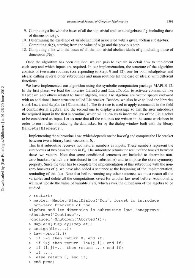
1. Implementing the subroutinelaw, which depends on the law of g and compute the Lie bracketbetween two arbitrary basis vectors in Bn.This first subroutine receives two natural numbers as inputs. These numbers represent thesubindexes of two basis vectors in Bn. The subroutine returns the result of the bracket betweenthese two vectors. Note that some conditional sentences are included to determine non-zero brackets (which are introduced in the subroutine) and to impose the skew-symmetryproperty. Since the user has to complete the implementation of this subroutine with the non-zero brackets of g, we have also added a sentence at the beginning of the implementation,reminding of this fact. Note that before running any other sentence, we must restart all thevariables and delete all the computations saved for another law used before. Additionally,we must update the value of variable dim, which saves the dimension of the algebra to bestudied.

> restart:> maplet:=Maplet(AlertDialog("Don’t forget to introduce

non-zero brackets of thealgebra and its dimension in subroutine law",’onapprove’=Shutdown("Continue"),’oncancel’=Shutdown("Aborted"))):> Maplets[Display](maplet):> assign(dim,...):> law:=proc(i,j)> if i=j then return 0; end if;> if i>j then return -law(j,i); end if;> if (i,j)=... then return ...; end if;> if ....> else return 0; end if;> end proc;

Dow

nloa

ded

by [

Fac

Psic

olog

ia/B

iblio

teca

] at

01:

26 2

0 Ju

ne 2

012

1392 M. Ceballos et al.

The ellipsis in command assign corresponds to writing the dimension of the algebra g to bestudied. The following two suspension points are associated with the computation of [Zi, Zj]:first, the value of the subindexes (i, j) and second, the result of [Zi, Zj] with respect to Bn. Thelast ellipsis denotes the rest of non-zero brackets. For each non-zero bracket, a new sentenceif has to be included in the cluster.

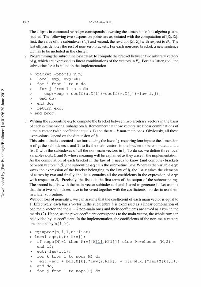
2. Programming the subroutine bracket to compute the bracket between two arbitrary vectorsof g, which are expressed as linear combinations of the vectors in Bn. For this latter goal, thesubroutine law is called in the implementation.

> bracket:=proc(u,v,n)> local exp; exp:=0;> for i from 1 to n do> for j from 1 to n do> exp:=exp + coeff(u,Z[i])*coeff(v,Z[j])*law(i,j);> end do;> end do;> return exp;> end proc:

3. Writing the subroutine eq to compute the bracket between two arbitrary vectors in the basisof each k-dimensional subalgebra h. Remember that those vectors are linear combinations ofa main vector (with coefficient equals 1) and the n − k non-main ones. Obviously, all theseexpressions depend on the dimension of h.This subroutine is executed after introducing the law of g, requiring four inputs: the dimensionn of g; the subindexes i and l, to fix the main vectors in the bracket to be computed; and alist M with the subindexes of all the non-main vectors in h. To do so, we define three localvariables eqt, L and P, whose meaning will be explained as they arise in the implementation.As the computation of each bracket in the law of h needs to know (and compute) bracketsbetween vectors in Bn, the subroutine eq calls the subroutine law. Whereas the variable eqtsaves the expression of the bracket belonging to the law of h, the list P takes the elementsof M two by two and finally, the list L contains all the coefficients in the expression of eqtwith respect to Bn. Precisely, the list L is the first term of the output of the subroutine eq.The second is a list with the main-vector subindexes i and l used to generate L. Let us notethat these two subindexes have to be saved together with the coefficients in order to use themin a later subroutine.Without loss of generality, we can assume that the coefficient of each main vector is equal to1. Effectively, each basis vector in the subalgebra h is expressed as a linear combination ofone main vector and the n − k non-main ones and their coefficients are saved as a row in thematrix (2). Hence, as the pivot coefficient corresponds to the main vector, the whole row canbe divided by its coefficient. In the implementation, the coefficients of the non-main vectorsare denoted by b[i,k].

> eq:=proc(n,i,l,M::list)> local eqt,L,P; L:=[];> if nops(M)=1 then P:=[[M[1],M[1]]] else P:=choose (M,2);

end if;> eqt:=law(i,l);> for k from 1 to nops(M) do> eqt:=eqt + b[l,M[k]]*law(i,M[k]) + b[i,M[k]]*law(M[k],l);> end do;> for j from 1 to nops(P) do

Dow

nloa

ded

by [

Fac

Psic

olog

ia/B

iblio

teca

] at

01:

26 2

0 Ju

ne 2

012

International Journal of Computer Mathematics 1393

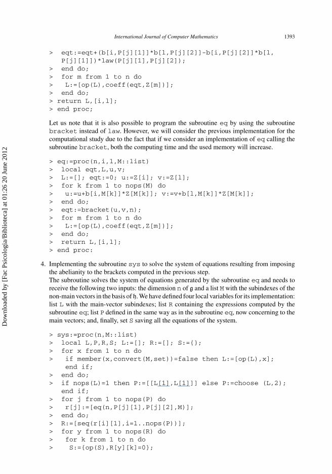
> eqt:=eqt+(b[i,P[j][1]]*b[l,P[j][2]]-b[i,P[j][2]]*b[l,P[j][1]])*law(P[j][1],P[j][2]);

> end do;> for m from 1 to n do> L:=[op(L),coeff(eqt,Z[m])];> end do;> return L,[i,l];> end proc;

Let us note that it is also possible to program the subroutine eq by using the subroutinebracket instead of law. However, we will consider the previous implementation for thecomputational study due to the fact that if we consider an implementation of eq calling thesubroutine bracket, both the computing time and the used memory will increase.

> eq:=proc(n,i,l,M::list)> local eqt,L,u,v;> L:=[]; eqt:=0; u:=Z[i]; v:=Z[l];> for k from 1 to nops(M) do> u:=u+b[i,M[k]]*Z[M[k]]; v:=v+b[l,M[k]]*Z[M[k]];> end do;> eqt:=bracket(u,v,n);> for m from 1 to n do> L:=[op(L),coeff(eqt,Z[m])];> end do;> return L,[i,l];> end proc:

4. Implementing the subroutine sys to solve the system of equations resulting from imposingthe abelianity to the brackets computed in the previous step.The subroutine solves the system of equations generated by the subroutine eq and needs toreceive the following two inputs: the dimension n of g and a list M with the subindexes of thenon-main vectors in the basis of h. We have defined four local variables for its implementation:list L with the main-vector subindexes; list R containing the expressions computed by thesubroutine eq; list P defined in the same way as in the subroutine eq, now concerning to themain vectors; and, finally, set S saving all the equations of the system.

> sys:=proc(n,M::list)> local L,P,R,S; L:=[]; R:=[]; S:={};> for x from 1 to n do> if member(x,convert(M,set))=false then L:=[op(L),x];

end if;> end do;> if nops(L)=1 then P:=[[L[1],L[1]]] else P:=choose (L,2);

end if;> for j from 1 to nops(P) do> r[j]:=[eq(n,P[j][1],P[j][2],M)];> end do;> R:=[seq(r[i][1],i=1..nops(P))];> for y from 1 to nops(R) do> for k from 1 to n do> S:={op(S),R[y][k]=0};

Dow

nloa

ded

by [

Fac

Psic

olog

ia/B

iblio

teca

] at

01:

26 2

0 Ju

ne 2

012

1394 M. Ceballos et al.

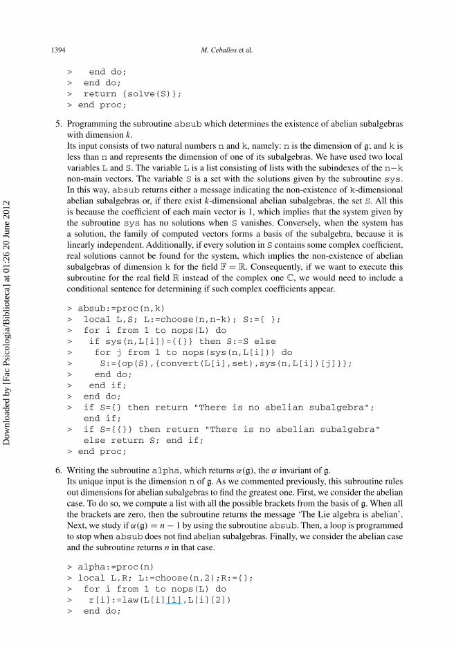
> end do;> end do;> return {solve(S)};> end proc;

5. Programming the subroutine absub which determines the existence of abelian subalgebraswith dimension k.Its input consists of two natural numbers n and k, namely: n is the dimension of g; and k isless than n and represents the dimension of one of its subalgebras. We have used two localvariables L and S. The variable L is a list consisting of lists with the subindexes of the n−knon-main vectors. The variable S is a set with the solutions given by the subroutine sys.In this way, absub returns either a message indicating the non-existence of k-dimensionalabelian subalgebras or, if there exist k-dimensional abelian subalgebras, the set S. All thisis because the coefficient of each main vector is 1, which implies that the system given bythe subroutine sys has no solutions when S vanishes. Conversely, when the system hasa solution, the family of computed vectors forms a basis of the subalgebra, because it islinearly independent. Additionally, if every solution in S contains some complex coefficient,real solutions cannot be found for the system, which implies the non-existence of abeliansubalgebras of dimension k for the field F = R. Consequently, if we want to execute thissubroutine for the real field R instead of the complex one C, we would need to include aconditional sentence for determining if such complex coefficients appear.

> absub:=proc(n,k)> local L,S; L:=choose(n,n-k); S:={ };> for i from 1 to nops(L) do> if sys(n,L[i])={{}} then S:=S else> for j from 1 to nops(sys(n,L[i])) do> S:={op(S),{convert(L[i],set),sys(n,L[i])[j]}};> end do;> end if;> end do;> if S={} then return "There is no abelian subalgebra";

end if;> if S={{}} then return "There is no abelian subalgebra"

else return S; end if;> end proc;

6. Writing the subroutine alpha, which returns α(g), the α invariant of g.Its unique input is the dimension n of g. As we commented previously, this subroutine rulesout dimensions for abelian subalgebras to find the greatest one. First, we consider the abeliancase. To do so, we compute a list with all the possible brackets from the basis of g. When allthe brackets are zero, then the subroutine returns the message ‘The Lie algebra is abelian’.Next, we study if α(g) = n − 1 by using the subroutine absub. Then, a loop is programmedto stop when absub does not find abelian subalgebras. Finally, we consider the abelian caseand the subroutine returns n in that case.

> alpha:=proc(n)> local L,R; L:=choose(n,2);R:={};> for i from 1 to nops(L) do> r[i]:=law(L[i][1],L[i][2])> end do;

Dow

nloa

ded

by [

Fac

Psic

olog

ia/B

iblio

teca

] at

01:

26 2

0 Ju

ne 2

012

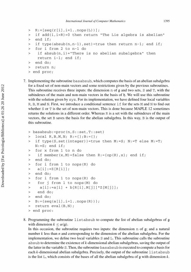
International Journal of Computer Mathematics 1395

> R:=[seq(r[i],i=1..nops(L))];> if add(i,i=R)=0 then return "The Lie algebra is abelian"> end if;> if type(absub(n,n-1),set)=true then return n-1; end if;> for i from 2 to n-1 do> if absub(n,i)="There is no abelian subalgebra" then

return i-1; end if;> end do;> return n;> end proc;

7. Implementing the subroutine basabsub, which computes the basis of an abelian subalgebrafor a fixed set of non-main vectors and some restrictions given by the previous subroutines.This subroutine receives three inputs: the dimension n of g and two sets, S and T, with thesubindexes of the main and non-main vectors in the basis of h. We will use this subroutinewith the solution given by sys. For its implementation, we have defined four local variablesR, B, M and N. First, we introduce a conditional sentence if for the sets M and N to find outwhether S or T is the set of non-main vectors. This is done because MAPLE 12 sometimesreturns the solutions in a different order. Whereas R is a set with the subindexes of the mainvectors, the set B saves the basis for the abelian subalgebra. In this way, B is the output ofthis subroutine.

> basabsub:=proc(n,S::set,T::set)> local R,B,M,N; R:={};B:={};> if type(S,set(integer))=true then M:=S; N:=T else M:=T;

N:=S; end if;> for x from 1 to n do> if member(x,M)=false then R:={op(R),x}; end if;> end do;> for i from 1 to nops(R) do> a[i]:=Z[R[i]];> end do;> for i from 1 to nops(R) do> for j from 1 to nops(M) do> a[i]:=a[i] + b[R[i],M[j]]*Z[M[j]];> end do;> end do;> B:={seq(a[i],i=1..nops(R))};> return eval(B,N);> end proc:

8. Programming the subroutine listabsub to compute the list of abelian subalgebras of g

with dimension k ≤ α(g).In this occasion, the subroutine requires two inputs: the dimension n of g; and a naturalnumber k less than n and corresponding to the dimension of the abelian subalgebra. For theimplementation, we define two local variables S and L. This subroutine calls the subroutineabsub to determine the existence of k-dimensional abelian subalgebras, saving the output ofthe latter in the variableS. Then, the subroutinebasabsub is executed to compute a basis foreach k-dimensional abelian subalgebra. Precisely, the output of the subroutine listabsubis the list L, which consists of the bases of all the abelian subalgebra of g with dimension k.

Dow

nloa

ded

by [

Fac

Psic

olog

ia/B

iblio

teca

] at

01:

26 2

0 Ju

ne 2

012

1396 M. Ceballos et al.

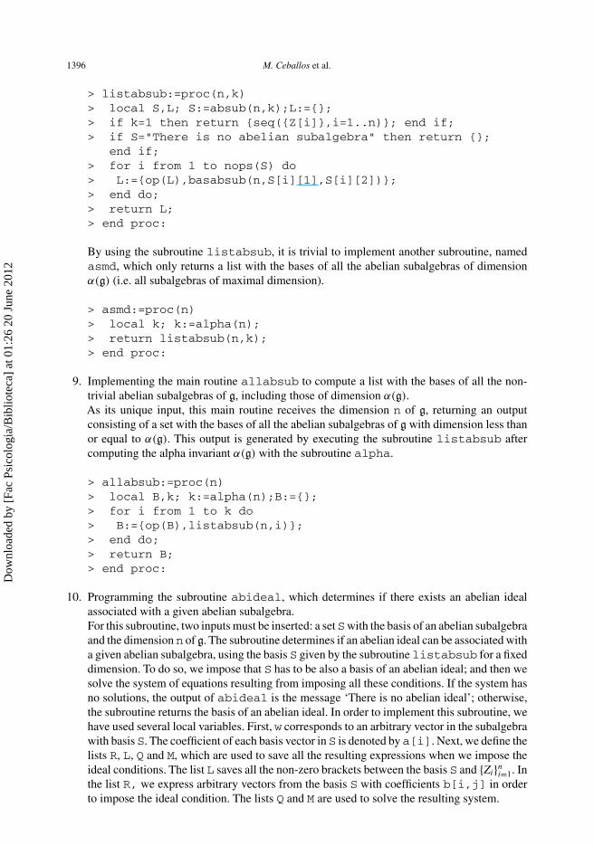
> listabsub:=proc(n,k)> local S,L; S:=absub(n,k);L:={};> if k=1 then return {seq({Z[i]},i=1..n)}; end if;> if S="There is no abelian subalgebra" then return {};

end if;> for i from 1 to nops(S) do> L:={op(L),basabsub(n,S[i][1],S[i][2])};> end do;> return L;> end proc:

By using the subroutine listabsub, it is trivial to implement another subroutine, namedasmd, which only returns a list with the bases of all the abelian subalgebras of dimensionα(g) (i.e. all subalgebras of maximal dimension).

> asmd:=proc(n)> local k; k:=alpha(n);> return listabsub(n,k);> end proc:

9. Implementing the main routine allabsub to compute a list with the bases of all the non-trivial abelian subalgebras of g, including those of dimension α(g).As its unique input, this main routine receives the dimension n of g, returning an outputconsisting of a set with the bases of all the abelian subalgebras of g with dimension less thanor equal to α(g). This output is generated by executing the subroutine listabsub aftercomputing the alpha invariant α(g) with the subroutine alpha.

> allabsub:=proc(n)> local B,k; k:=alpha(n);B:={};> for i from 1 to k do> B:={op(B),listabsub(n,i)};> end do;> return B;> end proc:

10. Programming the subroutine abideal, which determines if there exists an abelian idealassociated with a given abelian subalgebra.For this subroutine, two inputs must be inserted: a setSwith the basis of an abelian subalgebraand the dimensionn of g. The subroutine determines if an abelian ideal can be associated witha given abelian subalgebra, using the basis S given by the subroutine listabsub for a fixeddimension. To do so, we impose that S has to be also a basis of an abelian ideal; and then wesolve the system of equations resulting from imposing all these conditions. If the system hasno solutions, the output of abideal is the message ‘There is no abelian ideal’; otherwise,the subroutine returns the basis of an abelian ideal. In order to implement this subroutine, wehave used several local variables. First, w corresponds to an arbitrary vector in the subalgebrawith basis S. The coefficient of each basis vector in S is denoted by a[i]. Next, we define thelists R, L, Q and M, which are used to save all the resulting expressions when we impose theideal conditions. The list L saves all the non-zero brackets between the basis S and {Zi}n

i=1. Inthe list R, we express arbitrary vectors from the basis S with coefficients b[i,j] in orderto impose the ideal condition. The lists Q and M are used to solve the resulting system.

Dow

nloa

ded

by [

Fac

Psic

olog

ia/B

iblio

teca

] at

01:

26 2

0 Ju

ne 2

012

International Journal of Computer Mathematics 1397

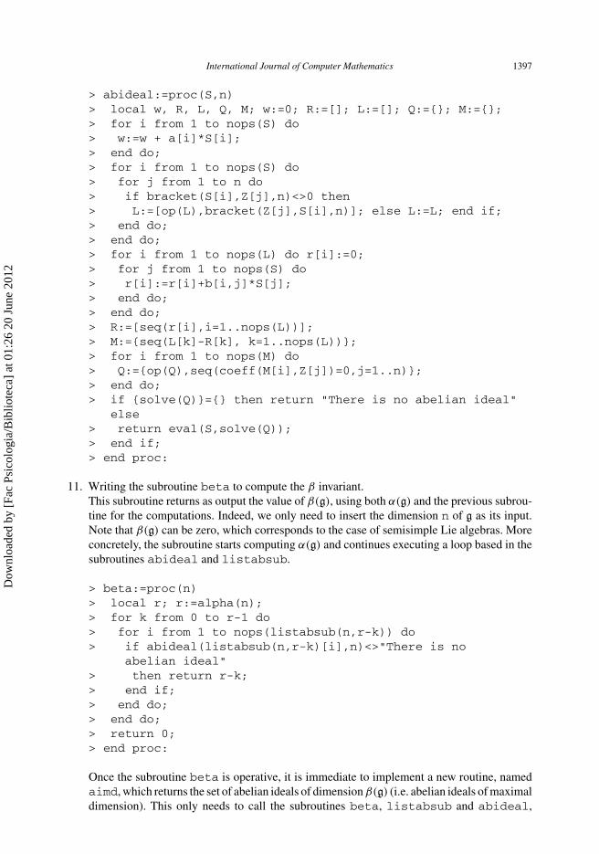
> abideal:=proc(S,n)> local w, R, L, Q, M; w:=0; R:=[]; L:=[]; Q:={}; M:={};> for i from 1 to nops(S) do> w:=w + a[i]*S[i];> end do;> for i from 1 to nops(S) do> for j from 1 to n do> if bracket(S[i],Z[j],n)<>0 then> L:=[op(L),bracket(Z[j],S[i],n)]; else L:=L; end if;> end do;> end do;> for i from 1 to nops(L) do r[i]:=0;> for j from 1 to nops(S) do> r[i]:=r[i]+b[i,j]*S[j];> end do;> end do;> R:=[seq(r[i],i=1..nops(L))];> M:={seq(L[k]-R[k], k=1..nops(L))};> for i from 1 to nops(M) do> Q:={op(Q),seq(coeff(M[i],Z[j])=0,j=1..n)};> end do;> if {solve(Q)}={} then return "There is no abelian ideal"

else> return eval(S,solve(Q));> end if;> end proc:

11. Writing the subroutine beta to compute the β invariant.This subroutine returns as output the value of β(g), using both α(g) and the previous subrou-tine for the computations. Indeed, we only need to insert the dimension n of g as its input.Note that β(g) can be zero, which corresponds to the case of semisimple Lie algebras. Moreconcretely, the subroutine starts computing α(g) and continues executing a loop based in thesubroutines abideal and listabsub.

> beta:=proc(n)> local r; r:=alpha(n);> for k from 0 to r-1 do> for i from 1 to nops(listabsub(n,r-k)) do> if abideal(listabsub(n,r-k)[i],n)<>"There is no

abelian ideal"> then return r-k;> end if;> end do;> end do;> return 0;> end proc:

Once the subroutine beta is operative, it is immediate to implement a new routine, namedaimd, which returns the set of abelian ideals of dimension β(g) (i.e. abelian ideals of maximaldimension). This only needs to call the subroutines beta, listabsub and abideal,

Dow

nloa

ded

by [

Fac

Psic

olog

ia/B

iblio

teca

] at

01:

26 2

0 Ju

ne 2

012

1398 M. Ceballos et al.

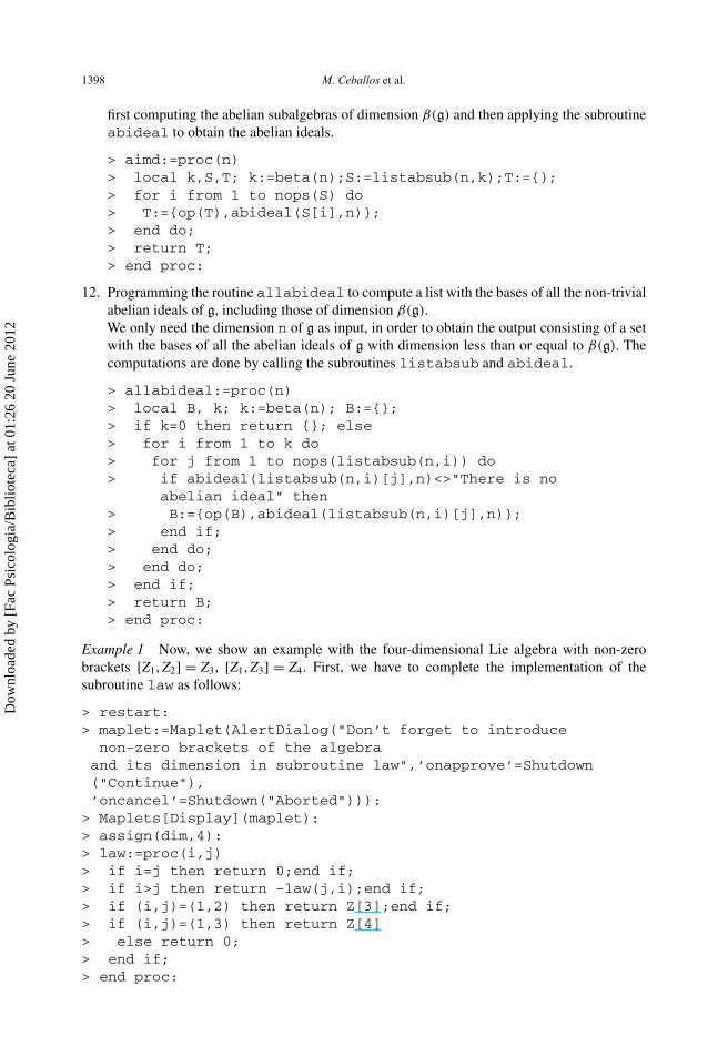
first computing the abelian subalgebras of dimension β(g) and then applying the subroutineabideal to obtain the abelian ideals.

> aimd:=proc(n)> local k,S,T; k:=beta(n);S:=listabsub(n,k);T:={};> for i from 1 to nops(S) do> T:={op(T),abideal(S[i],n)};> end do;> return T;> end proc:

12. Programming the routine allabideal to compute a list with the bases of all the non-trivialabelian ideals of g, including those of dimension β(g).We only need the dimension n of g as input, in order to obtain the output consisting of a setwith the bases of all the abelian ideals of g with dimension less than or equal to β(g). Thecomputations are done by calling the subroutines listabsub and abideal.

> allabideal:=proc(n)> local B, k; k:=beta(n); B:={};> if k=0 then return {}; else> for i from 1 to k do> for j from 1 to nops(listabsub(n,i)) do> if abideal(listabsub(n,i)[j],n)<>"There is no

abelian ideal" then> B:={op(B),abideal(listabsub(n,i)[j],n)};> end if;> end do;> end do;> end if;> return B;> end proc:

Example 1 Now, we show an example with the four-dimensional Lie algebra with non-zerobrackets [Z1, Z2] = Z3, [Z1, Z3] = Z4. First, we have to complete the implementation of thesubroutine law as follows:

> restart:> maplet:=Maplet(AlertDialog("Don’t forget to introduce

non-zero brackets of the algebraand its dimension in subroutine law",’onapprove’=Shutdown("Continue"),’oncancel’=Shutdown("Aborted"))):

> Maplets[Display](maplet):> assign(dim,4):> law:=proc(i,j)> if i=j then return 0;end if;> if i>j then return -law(j,i);end if;> if (i,j)=(1,2) then return Z[3];end if;> if (i,j)=(1,3) then return Z[4]> else return 0;> end if;> end proc:

Dow

nloa

ded

by [

Fac

Psic

olog

ia/B

iblio

teca

] at

01:

26 2

0 Ju

ne 2

012

International Journal of Computer Mathematics 1399

After that, we must run all the routines except for asmd and aimd, which could be consideredas loading a library containing them. Once this is done, we can compute the α and β invariants aswell as the set of abelian subalgebras and ideals of the Lie algebra g using the commands definedby the routines.

> alpha(dim);3

> listabsub(dim,alpha(dim));{{Z[2],Z[3],Z[4]}}

> allabsub(dim);{{{Z[2],Z[3],Z[4]}},{{Z[1]},{Z[2]},{Z[3]},{Z[4]}},{{Z[4],Z[1]+b[1,2]*Z[2]+b[1,3]*Z[3]},{Z[4],Z[2]+b[2,1]*Z[1]+b[2,3]*Z[3]},{Z[4],Z[3]+b[3,1]*Z[1]+b[3,2]*Z[2]},{Z[2]+b[2,3]*Z[3],Z[4]+b[4,3]*Z[3]},{Z[2]+b[2,4]*Z[4],Z[3]+b[3,4]*Z[4]},{Z[3]+b[3,2]*Z[2],Z[4]+b[4,2]*Z[2]}}}

> beta(dim);3

> allabideal(dim);{{Z[4]},{Z[3],Z[4]},{Z[2],Z[3],Z[4]}}

4. Statistical and computational data

Now, we present a computational study of the algorithm which was introduced in the previoussection and implemented in an Intel Core 2 Duo T 5600 with a 1.83 GHz processor and 2.00GB of RAM. Tables 1 and 2 reproduce computational data about both the computing time andthe memory used to obtain the outputs of allabsub and allabideal with respect to thedimension n of the algebra. For this study, we have considered the Lie algebras sn generated by{ei}n

i=1 with non-zero brackets

[ei, en] = ei ∀i < n.

This family constitutes a special subclass of non-nilpotent solvable Lie algebras, which allowsus to check empirically the computational data given for both the computing time and the usedmemory.

Table 1. Computing time and used memory for allabsub.

Input (n) Computing time (s) Used memory (MB)

2 0 03 0 04 0.11 3.135 0.15 5.066 0.43 5.387 1.05 5.568 2.67 6.069 6.98 7.06

10 20.27 8.2511 61.17 11.5012 187.89 13.8713 804.73 51.93

Dow

nloa

ded

by [

Fac

Psic

olog

ia/B

iblio

teca

] at

01:

26 2

0 Ju

ne 2

012

1400 M. Ceballos et al.

Table 2. Computing time and used memory for allabideal.

Input (n) Computing time (s) Used memory (MB)

2 0 03 0.08 3.314 0.50 5.755 1.98 5.886 8.03 6.507 35.97 6.948 169.54 7.569 779.37 8.19

10 4118.78 9.31

Table 1 was obtained from computing the set of all non-trivial abelian subalgebras for thealgebras sn up to dimension n = 13 inclusive. Note that the computing time is about three timesgreater when the dimension n is increased in one unit starting from n = 8.

Analogously, Table 2 shows the same variables when computing the set of all non-trivial abelianideals for the algebras sn, but up to dimension n = 10 inclusive for computational issues. We wantto remark that the increase in the computing time with respect to that of the dimension n in one unitis quite a lot greater than the one previously commented in Table 1.

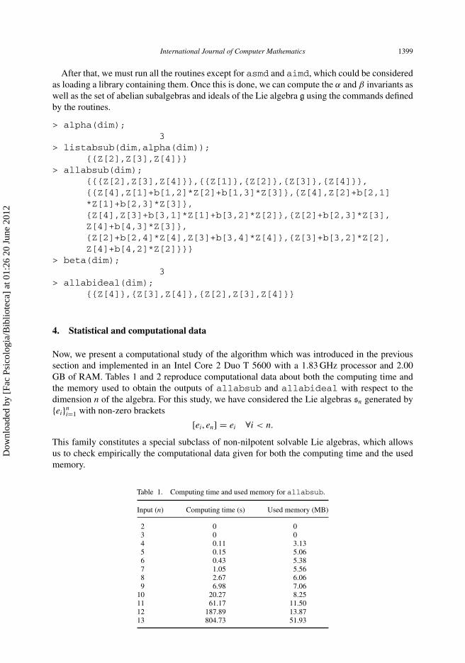
Figure 1. Graphs for the CT of allabsub with respect to the dimension.

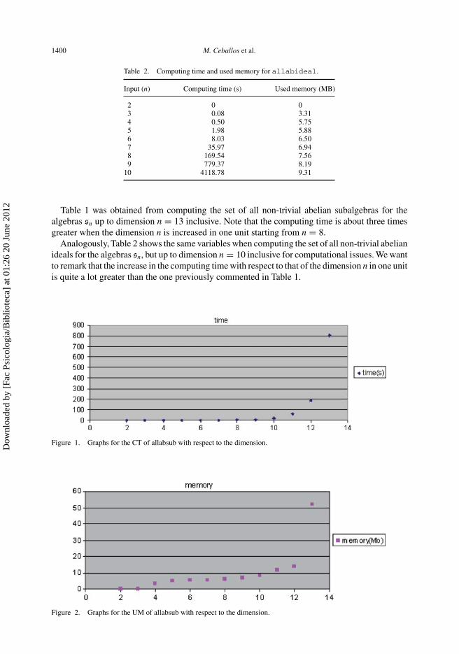
Figure 2. Graphs for the UM of allabsub with respect to the dimension.

Dow

nloa

ded

by [

Fac

Psic

olog

ia/B

iblio

teca

] at

01:

26 2

0 Ju

ne 2

012

International Journal of Computer Mathematics 1401

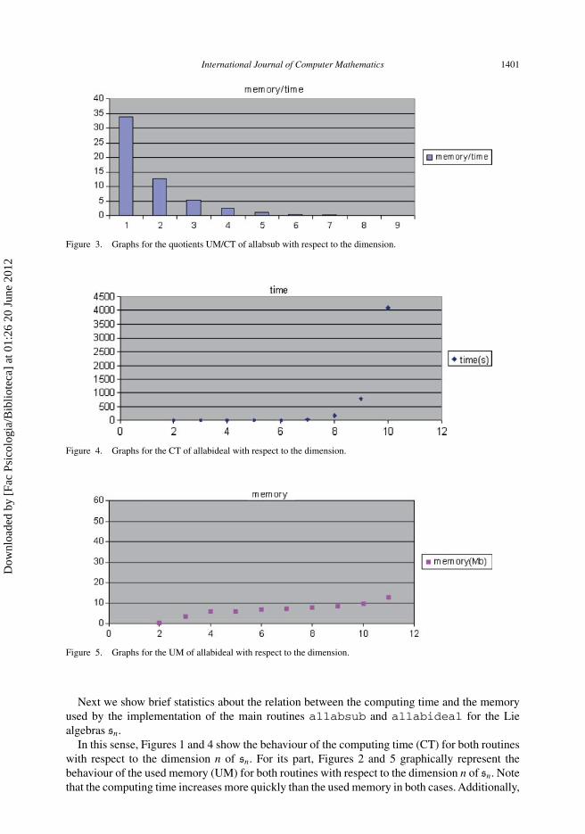
Figure 3. Graphs for the quotients UM/CT of allabsub with respect to the dimension.

Figure 4. Graphs for the CT of allabideal with respect to the dimension.

Figure 5. Graphs for the UM of allabideal with respect to the dimension.

Next we show brief statistics about the relation between the computing time and the memoryused by the implementation of the main routines allabsub and allabideal for the Liealgebras sn.

In this sense, Figures 1 and 4 show the behaviour of the computing time (CT) for both routineswith respect to the dimension n of sn. For its part, Figures 2 and 5 graphically represent thebehaviour of the used memory (UM) for both routines with respect to the dimension n of sn. Notethat the computing time increases more quickly than the used memory in both cases. Additionally,

Dow

nloa

ded

by [

Fac

Psic

olog

ia/B

iblio

teca

] at

01:

26 2

0 Ju

ne 2

012

1402 M. Ceballos et al.

Figure 6. Graphs for the quotients UM/CT of allabideal with respect to the dimension.

whereas the increase in the CT time fits a positive exponential model, the used memory does notfollow such a model.

Finally, we have studied the quotients between UM and CT, obtaining the frequency diagramshown in Figures 3 and 6. In this case, the behaviour also fits an exponential model, but beingnegative this time.

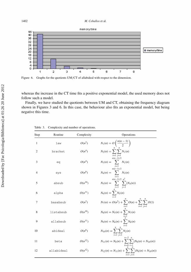
Table 3. Complexity and number of operations.

Step Routine Complexity Operations

1 law O(n2) N1(n) = O

(n(n − 1)

2

)

2 bracket O(n4) N2(n) =n∑

i=1

n∑j=1

N1(n)

3 eq O(n4) N3(n) =n(n−1)/2∑

j=1

N1(n)

4 sys O(n6) N4(n) =n(n−1)/2∑

i=1

N3(n)

5 absub O(n10) N5(n) =n(n−1)/2∑

i=1

n2∑j=1

(N4(n))

6 alpha O(n11) N6(n) =n∑

i=1

N5(n)

7 basabsub O(n2) N7(n) = O(n2) +n∑

i=1

O(n) +n∑

i=1

n∑j=1

O(1)

8 listabsub O(n10) N8(n) = N5(n) +n∑

i=1

N7(n)

9 allabsub O(n11) N9(n) = N6(n) +n∑

i=1

N8(n)

10 abideal O(n6) N10(n) =n∑

i=1

n∑j=1

N2(n)

11 beta O(n12) N11(n) = N6(n) +n−2∑k=0

n∑i=1

(N8(n) + N10(n))

12 allabideal O(n12) N12(n) = N11(n) +n∑

i=1

n∑j=1

(N8(n) + N10(n))

Dow

nloa

ded

by [

Fac

Psic

olog

ia/B

iblio

teca

] at

01:

26 2

0 Ju

ne 2

012

International Journal of Computer Mathematics 1403

5. Complexity of the algorithm

This section is devoted to computing the complexity of the algorithm, considering the number ofoperations carried out in the worst case. We have used the big O notation to express the complexity.To recall the big O notation, the reader can consult [22]: given two functions f , g : R → R, wecould say that f (x) = O(g(x)) if and only if there exist M ∈ R

+ and x0 ∈ R such that |f (x)| <

M · g(x), for all x > x0.We denote by Ni(n) the order of the operations when considering the step i. This function

depends on the dimension n of the Lie algebra. Table 3 shows the number of computations andthe complexity of each step, as well as indicating the name of the routine corresponding to eachstep. In fact, we determine that the complexity of the algorithm has a polynomial order, wherethe two last routines are the most computationally expensive.

6. Practical application of the algorithm

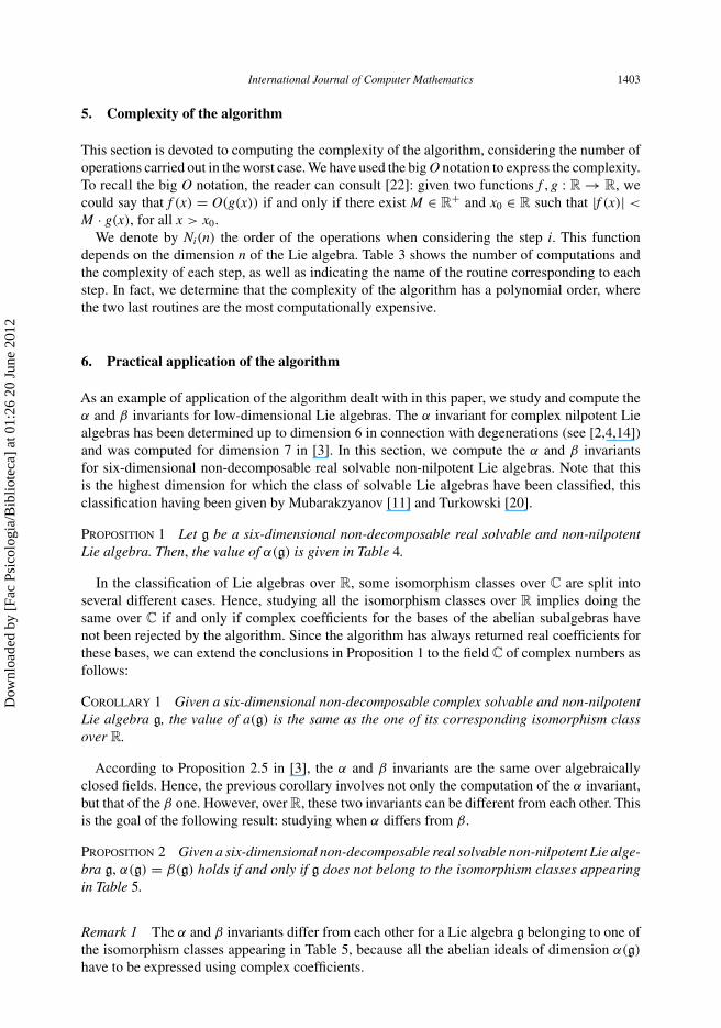
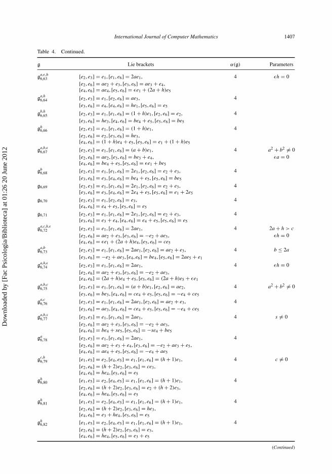
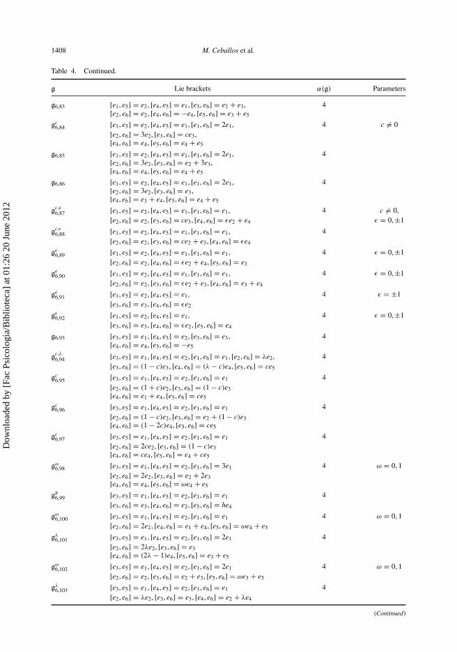
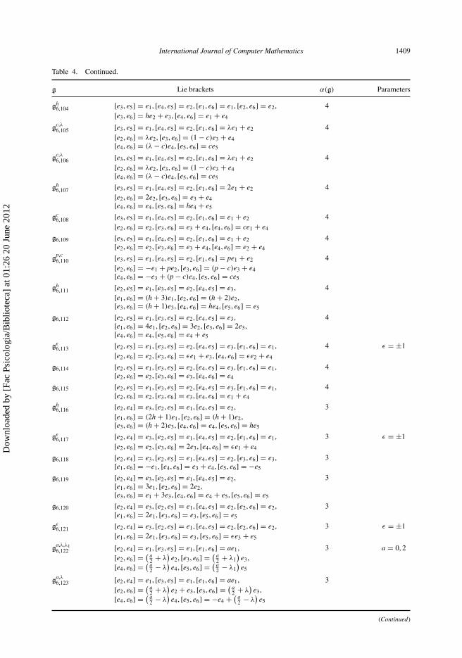
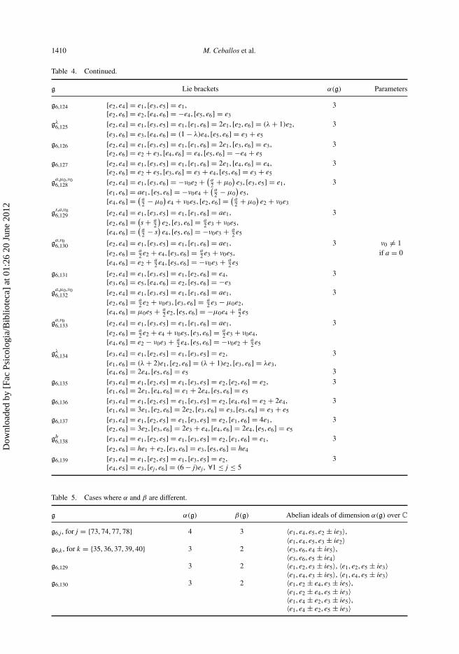
As an example of application of the algorithm dealt with in this paper, we study and compute theα and β invariants for low-dimensional Lie algebras. The α invariant for complex nilpotent Liealgebras has been determined up to dimension 6 in connection with degenerations (see [2,4,14])and was computed for dimension 7 in [3]. In this section, we compute the α and β invariantsfor six-dimensional non-decomposable real solvable non-nilpotent Lie algebras. Note that thisis the highest dimension for which the class of solvable Lie algebras have been classified, thisclassification having been given by Mubarakzyanov [11] and Turkowski [20].

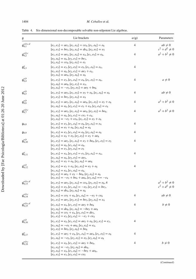
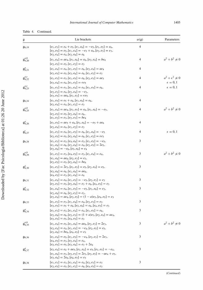
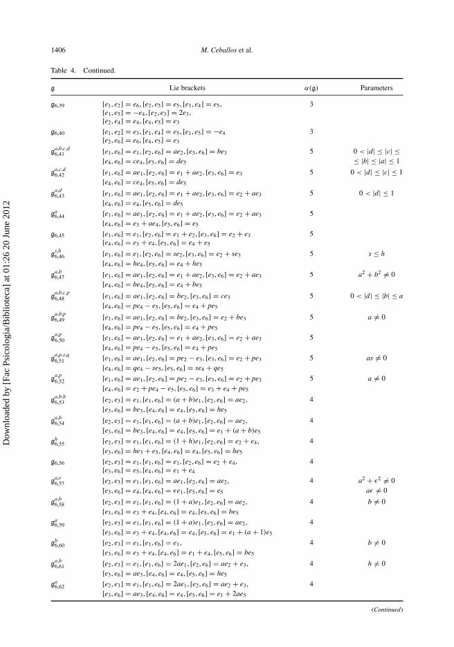
Proposition 1 Let g be a six-dimensional non-decomposable real solvable and non-nilpotentLie algebra. Then, the value of α(g) is given in Table 4.

In the classification of Lie algebras over R, some isomorphism classes over C are split intoseveral different cases. Hence, studying all the isomorphism classes over R implies doing thesame over C if and only if complex coefficients for the bases of the abelian subalgebras havenot been rejected by the algorithm. Since the algorithm has always returned real coefficients forthese bases, we can extend the conclusions in Proposition 1 to the field C of complex numbers asfollows:

Corollary 1 Given a six-dimensional non-decomposable complex solvable and non-nilpotentLie algebra g, the value of a(g) is the same as the one of its corresponding isomorphism classover R.

According to Proposition 2.5 in [3], the α and β invariants are the same over algebraicallyclosed fields. Hence, the previous corollary involves not only the computation of the α invariant,but that of the β one. However, over R, these two invariants can be different from each other. Thisis the goal of the following result: studying when α differs from β.

Proposition 2 Given a six-dimensional non-decomposable real solvable non-nilpotent Lie alge-bra g, α(g) = β(g) holds if and only if g does not belong to the isomorphism classes appearingin Table 5.

Remark 1 The α and β invariants differ from each other for a Lie algebra g belonging to one ofthe isomorphism classes appearing in Table 5, because all the abelian ideals of dimension α(g)

have to be expressed using complex coefficients.

Dow

nloa

ded

by [

Fac

Psic

olog

ia/B

iblio

teca

] at

01:

26 2

0 Ju

ne 2

012

1404 M. Ceballos et al.

Table 4. Six-dimensional non-decomposable solvable non-nilpotent Lie algebras.

g Lie brackets α(g) Parameters

ga,b,c,d6,1 [e1, e3] = ae3, [e1, e4] = ce4, [e1, e6] = e6 4 ab �= 0

[e2, e3] = be3, [e2, e4] = de4, [e2, e5] = e5 c2 + d2 �= 0

ga,b,c6,2 [e1, e3] = ae3, [e1, e4] = e4, [e1, e5] = e6, 4 a2 + b2 �= 0

[e2, e6] = e6, [e2, e3] = be3,[e2, e4] = ce4, [e2, e5] = e5

ga6,3 [e1, e3] = e3, [e2, e5] = e5, [e1, e4] = e4, 4

[e1, e5] = e6, [e2, e3] = ae3 + e4,[e2, e4] = ae4, [e2, e6] = e6

ga,b6,4 [e1, e3] = e3, [e1, e4] = e4, [e1, e5] = e6, 4 a �= 0

[e2, e6] = ae6, [e2, e3] = e4,[e2, e4] = −e3, [e2, e5] = ae5 + be6

ga,b6,5 [e1, e3] = ae3, [e1, e5] = e5 + e6, [e1, e6] = e6 4 ab �= 0

[e2, e3] = be3, [e2, e4] = e4

ga,b6,6 [e1, e3] = ae3, [e1, e4] = ae4, [e1, e5] = e5 + e6 4 a2 + b2 �= 0

[e1, e6] = e6, [e2, e3] = e3 + e4, [e2, e4] = e4

ga,b,c6,7 [e1, e3] = ae3, [e1, e4] = ae4, [e2, e5] = be6, 4 a2 + b2 �= 0

[e1, e6] = e6, [e2, e3] = ce3 + e4,[e2, e4] = −e3 + ce4, [e1, e5] = e5 + e6

g6,8 [e1, e3] = e3, [e1, e4] = e6, [e2, e4] = e4 4[e2, e5] = e5 + e6, [e2, e6] = e6

g6,9 [e1, e3] = e3, [e1, e4] = e6, [e2, e6] = e6 4[e2, e4] = e4 + e5, [e2, e5] = e5 + ae6

ga,b6,10 [e1, e3] = ae3, [e1, e4] = e3 + be6, [e1, e5] = e5 4

[e2, e5] = e6, [e1, e6] = e6,[e2, e3] = e3, [e2, e4] = e5

ga6,11 [e1, e3] = e4, [e2, e3] = e3, [e2, e4] = e4, 4

[e1, e6] = e6, [e2, e5] = ae5,[e1, e5] = e5 + e6, [e2, e6] = ae6

ga,b6,12 [e1, e3] = e3 + e4, [e1, e5] = e5 + e6 4

[e1, e4] = e4, [e1, e6] = e6,[e2, e3] = ae4 + e5 − be6, [e2, e4] = e6[e2, e5] = −e3 + be4 + ae6, [e2, e6] == −e4

ga,b,c,d6,13 [e1, e3] = ae3, [e1, e4] = ce4, [e1, e5] = e6, 4 a2 + b2 �= 0

[e2, e5] = e5, [e1, e6] = −e5, [e2, e3] = be3, c2 + d2 �= 0[e2, e4] = de4, [e2, e6] = e6

ga,b,c6,14 [e1, e5] = ce5 + e6, [e1, e6] = −e5 + ce6 4 ab �= 0

[e1, e3] = ae3, [e2, e3] = be3, [e2, e4] = e4

ga,b,c,d6,15 [e1, e4] = e4, [e1, e5] = ae5 + be6 4 b �= 0

[e2, e6] = de6, [e1, e6] = −be5 + ae6[e2, e3] = ce3 + e4, [e2, e5] = de5,[e1, e3] = e3, [e2, e4] = −e3 + ce4

ga,b6,16 [e1, e3] = e4, [e1, e5] = ae5 + e6, [e2, e3] = e3, 4

[e1, e6] = −e5 + ae6, [e2, e4] = e4,[e2, e5] = be5, [e2, e6] = be6

ga6,17 [e1, e3] = ae3 + e4, [e1, e4] = ae4, [e1, e5] = e6 4

[e1, e6] = −e5, [e2, e5] = e5, [e2, e6] = e6

ga,b,c6,18 [e1, e3] = e4, [e1, e5] = ae5 + be6, 4 b �= 0

[e1, e4] = −e3, [e2, e6] = de6,[e2, e4] = e4, [e1, e6] = −be5 + ae6,[e2, e3] = e3, [e2, e5] = ce5

(Continued)

Dow

nloa

ded

by [

Fac

Psic

olog

ia/B

iblio

teca

] at

01:

26 2

0 Ju

ne 2

012

International Journal of Computer Mathematics 1405

Table 4. Continued.

g Lie brackets α(g) Parameters

g6,19 [e1, e3] = e4 + e5, [e1, e6] = −e5, [e1, e5] = e6, 4[e2, e5] = e5, [e1, e4] = −e3 + e6, [e2, e3] = e3,[e2, e4] = e4, [e2, e6] = e6

ga,b6,20 [e1, e4] = ae4, [e1, e6] = e6, [e2, e4] = be4 4 a2 + b2 �= 0

[e2, e5] = e5, [e1, e2] = e3

ga6,21 [e1, e4] = e4, [e1, e5] = e6, [e2, e4] = ae4 4

[e2, e5] = e5, [e2, e6] = e6, [e1, e2] = e3

ga,ε6,22 [e1, e3] = e3, [e1, e5] = e6, [e2, e3] = ae3 4 a2 + ε2 �= 0

[e2, e4] = e4, [e1, e2] = εe5 ε = 0, 1

ga,ε6,23 [e1, e3] = e3, [e1, e4] = e4, [e1, e5] = e6, 4 ε = 0, 1

[e2, e3] = e4, [e2, e4] = −e3,[e2, e5] = ae6, [e1, e2] = εe5

g6,24 [e1, e5] = e5 + e6, [e1, e6] = e6, 4[e2, e4] = e4, [e1, e2] = e3

ga,b6,25 [e1, e4] = ae4, [e1, e5] = e6, [e1, e6] = −e5, 4 a2 + b2 �= 0

[e2, e5] = e5, [e2, e6] = e6,[e1, e2] = e3, [e2, e3] = be4

ga6,26 [e1, e5] = ae5 + e6, [e1, e6] = −e5 + ae6 4

[e2, e4] = e4, [e1, e2] = e3

gε6,27 [e1, e3] = e4, [e1, e5] = e6, [e1, e6] = −e5 4 ε = 0, 1[e2, e5] = e5, [e2, e6] = e6, [e1, e2] = εe3

g6,28 [e1, e3] = e3, [e4, e6] = e3, [e1, e5] = −e5, 3[e1, e6] = e6, [e2, e4] = e4, [e2, e5] = 2e5,[e2, e6] = −e6, [e5, e6] = e4

ga,b6,29 [e1, e3] = e3, [e4, e5] = e3, [e1, e4] = e4, 3 a2 + b2 �= 0

[e1, e6] = ae6, [e2, e3] = e3,[e2, e5] = e5, [e2, e6] = be6

ga6,30 [e1, e3] = 2e3, [e1, e5] = e5, [e2, e4] = e5, 3

[e2, e6] = e6, [e1, e6] = ae6,[e4, e5] = e3, [e1, e4] = e4

g6,31 [e1, e4] = e4, [e1, e5] = −e5, [e2, e3] = e3 3[e2, e5] = e5, [e2, e6] = e3 + e6, [e4, e5] = e3

ga6,32 [e1, e4] = e4, [e1, e5] = −e5, [e1, e6] = e3, 3

[e2, e6] = e6, [e2, e3] = e3,[e2, e4] = ae4, [e2, e5] = (1 − a)e5, [e4, e5] = e3

g6,33 [e1, e3] = e3, [e1, e4] = e4, [e2, e3] = e3 3[e2, e5] = e5 + e6, [e2, e6] = e6, [e4, e5] = e3

ga6,34 [e1, e3] = e3, [e1, e4] = e4, [e1, e5] = e6, 3

[e2, e6] = e6, [e2, e3] = (1 + a)e3, [e2, e4] = ae4,[e2, e5] = e5, [e4, e5] = e3

ga,b6,35 [e1, e4] = e5, [e1, e6] = ae6, [e2, e3] = 2e3, 3 a2 + b2 �= 0

[e2, e4] = e4, [e1, e5] = −e4, [e2, e5] = e5,[e2, e6] = be6, [e4, e5] = e3

g6,36 [e1, e4] = e5, [e1, e5] = −e4, [e2, e3] = 2e3, 3[e4, e5] = e3, [e2, e4] = e4,[e2, e5] = e5, [e2, e6] = e3 + 2e6

ga6,37 [e2, e4] = e4 + ae5, [e1, e4] = e5, [e1, e5] = −e4, 3

[e1, e6] = e3, [e2, e3] = 2e3, [e2, e5] = −ae4 + e5,[e2, e6] = 2e6, [e4, e5] = e3

g6,38 [e1, e3] = e3, [e1, e4] = e4, [e2, e3] = e3 3[e2, e5] = e5, [e1, e2] = e6, [e4, e5] = e3

(Continued)

Dow

nloa

ded

by [

Fac

Psic

olog

ia/B

iblio

teca

] at

01:

26 2

0 Ju

ne 2

012

1406 M. Ceballos et al.

Table 4. Continued.

g Lie brackets α(g) Parameters

g6,39 [e1, e2] = e6, [e2, e5] = e5, [e1, e4] = e5, 3[e1, e5] = −e4, [e2, e3] = 2e3,[e2, e4] = e4, [e4, e5] = e3

g6,40 [e1, e2] = e3, [e1, e4] = e5, [e1, e5] = −e4 3[e2, e6] = e6, [e4, e5] = e3

ga,b,c,d6,41 [e1, e6] = e1, [e2, e6] = ae2, [e3, e6] = be3 5 0 < |d| ≤ |c| ≤

[e4, e6] = ce4, [e5, e6] = de5 ≤ |b| ≤ |a| ≤ 1

ga,c,d6,42 [e1, e6] = ae1, [e2, e6] = e1 + ae2, [e3, e6] = e3 5 0 < |d| ≤ |c| ≤ 1

[e4, e6] = ce4, [e5, e6] = de5

ga,d6,43 [e1, e6] = ae1, [e2, e6] = e1 + ae2, [e3, e6] = e2 + ae3 5 0 < |d| ≤ 1

[e4, e6] = e4, [e5, e6] = de5

ga6,44 [e1, e6] = ae1, [e2, e6] = e1 + ae2, [e3, e6] = e2 + ae3 5

[e4, e6] = e3 + ae4, [e5, e6] = e5

g6,45 [e1, e6] = e1, [e2, e6] = e1 + e2, [e3, e6] = e2 + e3 5[e4, e6] = e3 + e4, [e5, e6] = e4 + e5

gs,h6,46 [e1, e6] = e1, [e2, e6] = se2, [e3, e6] = e2 + se3 5 s ≤ h

[e4, e6] = he4, [e5, e6] = e4 + he5

ga,b6,47 [e1, e6] = ae1, [e2, e6] = e1 + ae2, [e3, e6] = e2 + ae3 5 a2 + b2 �= 0

[e4, e6] = be4, [e5, e6] = e4 + be5

ga,b,c,p6,48 [e1, e6] = ae1, [e2, e6] = be2, [e3, e6] = ce3 5 0 < |d| ≤ |b| ≤ a

[e4, e6] = pe4 − e5, [e5, e6] = e4 + pe5

ga,b,p6,49 [e1, e6] = ae1, [e2, e6] = be2, [e3, e6] = e2 + be3 5 a �= 0

[e4, e6] = pe4 − e5, [e5, e6] = e4 + pe5

ga,p6,50 [e1, e6] = ae1, [e2, e6] = e1 + ae2, [e3, e6] = e2 + ae3 5

[e4, e6] = pe4 − e5, [e5, e6] = e4 + pe5

ga,p,s,q6,51 [e1, e6] = ae1, [e2, e6] = pe2 − e3, [e3, e6] = e2 + pe3 5 as �= 0

[e4, e6] = qe4 − se5, [e5, e6] = se4 + qe5

ga,p6,52 [e1, e6] = ae1, [e2, e6] = pe2 − e3, [e3, e6] = e2 + pe3 5 a �= 0

[e4, e6] = e2 + pe4 − e5, [e5, e6] = e3 + e4 + pe5

ga,b,h6,53 [e2, e3] = e1, [e1, e6] = (a + b)e1, [e2, e6] = ae2, 4

[e3, e6] = be3, [e4, e6] = e4, [e5, e6] = he5

ga,b6,54 [e2, e3] = e1, [e1, e6] = (a + b)e1, [e2, e6] = ae2, 4

[e3, e6] = be3, [e4, e6] = e4, [e5, e6] = e1 + (a + b)e5

gh6,55 [e2, e3] = e1, [e1, e6] = (1 + h)e1, [e2, e6] = e2 + e4, 4

[e3, e6] = he3 + e5, [e4, e6] = e4, [e5, e6] = he5

g6,56 [e2, e3] = e1, [e1, e6] = e1, [e2, e6] = e2 + e4, 4[e3, e6] = e5, [e4, e6] = e1 + e4

ga,ε6,57 [e2, e3] = e1, [e1, e6] = ae1, [e2, e6] = ae2, 4 a2 + ε2 �= 0

[e3, e6] = e4, [e4, e6] = εe1, [e5, e6] = e5 aε �= 0

ga,b6,58 [e2, e3] = e1, [e1, e6] = (1 + a)e1, [e2, e6] = ae2, 4 b �= 0

[e3, e6] = e3 + e4, [e4, e6] = e4, [e5, e6] = be5

ga6,59 [e2, e3] = e1, [e1, e6] = (1 + a)e1, [e2, e6] = ae2, 4

[e3, e6] = e3 + e4, [e4, e6] = e4, [e5, e6] = e1 + (a + 1)e5

gb6,60 [e2, e3] = e1, [e1, e6] = e1, 4 b �= 0

[e3, e6] = e3 + e4, [e4, e6] = e1 + e4, [e5, e6] = be5

ga,h6,61 [e2, e3] = e1, [e1, e6] = 2ae1, [e2, e6] = ae2 + e3, 4 h �= 0

[e3, e6] = ae3, [e4, e6] = e4, [e5, e6] = he5

ga6,62 [e2, e3] = e1, [e1, e6] = 2ae1, [e2, e6] = ae2 + e3, 4

[e3, e6] = ae3, [e4, e6] = e4, [e5, e6] = e1 + 2ae5

(Continued)

Dow

nloa

ded

by [

Fac

Psic

olog

ia/B

iblio

teca

] at

01:

26 2

0 Ju

ne 2

012

International Journal of Computer Mathematics 1407

Table 4. Continued.

g Lie brackets α(g) Parameters

ga,ε,h6,63 [e2, e3] = e1, [e1, e6] = 2ae1, 4 εh = 0

[e2, e6] = ae2 + e3, [e3, e6] = ae3 + e4,[e4, e6] = ae4, [e5, e6] = εe1 + (2a + h)e5

ga,h6,64 [e2, e3] = e1, [e2, e6] = ae3, 4

[e3, e6] = e4, [e4, e6] = he1, [e5, e6] = e5

gb,h6,65 [e2, e3] = e1, [e1, e6] = (1 + h)e1, [e2, e6] = e2, 4

[e3, e6] = he3, [e4, e6] = be4 + e5, [e5, e6] = be5

gh6,66 [e2, e3] = e1, [e1, e6] = (1 + h)e1, 4

[e2, e6] = e2, [e3, e6] = he3,[e4, e6] = (1 + h)e4 + e5, [e5, e6] = e1 + (1 + h)e5

ga,b,ε6,67 [e2, e3] = e1, [e1, e6] = (a + b)e1, 4 a2 + b2 �= 0

[e2, e6] = ae2, [e3, e6] = be3 + e4, εa = 0[e4, e6] = be4 + e5, [e5, e6] = εe1 + be5

gb6,68 [e2, e3] = e1, [e1, e6] = 2e1, [e2, e6] = e2 + e3, 4

[e3, e6] = e3, [e4, e6] = be4 + e5, [e5, e6] = be5

g6,69 [e2, e3] = e1, [e1, e6] = 2e1, [e2, e6] = e2 + e3, 4[e3, e6] = e3, [e4, e6] = 2e4 + e5, [e5, e6] = e1 + 2e5

g6,70 [e2, e3] = e1, [e2, e6] = e3, 4[e4, e6] = e4 + e5, [e5, e6] = e5

g6,71 [e2, e3] = e1, [e1, e6] = 2e1, [e2, e6] = e2 + e3, 4[e3, e6] = e3 + e4, [e4, e6] = e4 + e5, [e5, e6] = e5

ga,c,h,ε6,72 [e2, e3] = e1, [e1, e6] = 2ae1, 4 2a + h > c

[e2, e6] = ae2 + e3, [e3, e6] = −e2 + ae3, εh = 0[e4, e6] = εe1 + (2a + h)e4, [e5, e6] = ce5

ga,b6,73 [e2, e3] = e1, [e1, e6] = 2ae1, [e2, e6] = ae2 + e3, 4 b ≤ 2a

[e3, e6] = −e2 + ae3, [e4, e6] = be4, [e5, e6] = 2ae5 + e1

ga,h,ε6,74 [e2, e3] = e1, [e1, e6] = 2ae1, 4 εh = 0

[e2, e6] = ae2 + e3, [e3, e6] = −e2 + ae3,[e4, e6] = (2a + h)e4 + e5, [e5, e6] = (2a + h)e5 + εe1

ga,b,c6,75 [e2, e3] = e1, [e1, e6] = (a + b)e1, [e2, e6] = ae2, 4 a2 + b2 �= 0

[e3, e6] = be3, [e4, e6] = ce4 + e5, [e5, e6] = −e4 + ce5

ga,c6,76 [e2, e3] = e1, [e1, e6] = 2ae1, [e2, e6] = ae2 + e3, 4

[e3, e6] = ae3, [e4, e6] = ce4 + e5, [e5, e6] = −e4 + ce5

ga,b,s6,77 [e2, e3] = e1, [e1, e6] = 2ae1, 4 s �= 0

[e2, e6] = ae2 + e3, [e3, e6] = −e2 + ae3,[e4, e6] = be4 + se5, [e5, e6] = −se4 + be5

ga6,78 [e2, e3] = e1, [e1, e6] = 2ae1, 4

[e2, e6] = ae2 + e3 + e4, [e3, e6] = −e2 + ae3 + e5,[e4, e6] = ae4 + e5, [e5, e6] = −e4 + ae5

gc,h6,79 [e1, e5] = e2, [e4, e5] = e1, [e1, e6] = (h + 1)e1, 4 c �= 0

[e2, e6] = (h + 2)e2, [e3, e6] = ce3,[e4, e6] = he4, [e5, e6] = e5

gh6,80 [e1, e5] = e2, [e4, e5] = e1, [e1, e6] = (h + 1)e1, 4

[e2, e6] = (h + 2)e2, [e3, e6] = e2 + (h + 2)e3,[e4, e6] = he4, [e5, e6] = e5

gh6,81 [e1, e5] = e2, [e4, e5] = e1, [e1, e6] = (h + 1)e1, 4

[e2, e6] = (h + 2)e2, [e3, e6] = he3,[e4, e6] = e3 + he4, [e5, e6] = e5

gh6,82 [e1, e5] = e2, [e4, e5] = e1, [e1, e6] = (h + 1)e1, 4

[e2, e6] = (h + 2)e2, [e3, e6] = e3,[e4, e6] = he4, [e5, e6] = e3 + e5

(Continued)

Dow

nloa

ded

by [

Fac

Psic

olog

ia/B

iblio

teca

] at

01:

26 2

0 Ju

ne 2

012

1408 M. Ceballos et al.

Table 4. Continued.

g Lie brackets α(g) Parameters

g6,83 [e1, e5] = e2, [e4, e5] = e1, [e3, e6] = e2 + e3, 4[e2, e6] = e2, [e4, e6] = −e4, [e5, e6] = e3 + e5

gc6,84 [e1, e5] = e2, [e4, e5] = e1, [e1, e6] = 2e1, 4 c �= 0

[e2, e6] = 3e2, [e3, e6] = ce3,[e4, e6] = e4, [e5, e6] = e4 + e5

g6,85 [e1, e5] = e2, [e4, e5] = e1, [e1, e6] = 2e1, 4[e2, e6] = 3e2, [e3, e6] = e2 + 3e3,[e4, e6] = e4, [e5, e6] = e4 + e5

g6,86 [e1, e5] = e2, [e4, e5] = e1, [e1, e6] = 2e1, 4[e2, e6] = 3e2, [e3, e6] = e3,[e4, e6] = e3 + e4, [e5, e6] = e4 + e5

gc,ε6,87 [e1, e5] = e2, [e4, e5] = e1, [e1, e6] = e1, 4 c �= 0,

[e2, e6] = e2, [e3, e6] = ce3, [e4, e6] = εe2 + e4 ε = 0, ±1

gc,ε6,88 [e1, e5] = e2, [e4, e5] = e1, [e1, e6] = e1, 4

[e2, e6] = e2, [e3, e6] = ce2 + e3, [e4, e6] = εe4

gε6,89 [e1, e5] = e2, [e4, e5] = e1, [e1, e6] = e1, 4 ε = 0, ±1[e2, e6] = e2, [e4, e6] = εe2 + e4, [e5, e6] = e3

gε6,90 [e1, e5] = e2, [e4, e5] = e1, [e1, e6] = e1, 4 ε = 0, ±1[e2, e6] = e2, [e3, e6] = εe2 + e3, [e4, e6] = e3 + e4

gε6,91 [e1, e5] = e2, [e4, e5] = e1, 4 ε = ±1[e3, e6] = e3, [e4, e6] = εe2

gε6,92 [e1, e5] = e2, [e4, e5] = e1, 4 ε = 0, ±1[e3, e6] = e3, [e4, e6] = εe2, [e5, e6] = e4

g6,93 [e3, e5] = e1, [e4, e5] = e2, [e3, e6] = e3, 4[e4, e6] = e4, [e5, e6] = −e5

gc,λ6,94 [e3, e5] = e1, [e4, e5] = e2, [e1, e6] = e1, [e2, e6] = λe2, 4

[e3, e6] = (1 − c)e3, [e4, e6] = (λ − c)e4, [e5, e6] = ce5

gc6,95 [e3, e5] = e1, [e4, e5] = e2, [e1, e6] = e1 4

[e2, e6] = (1 + c)e2, [e3, e6] = (1 − c)e3[e4, e6] = e1 + e4, [e5, e6] = ce5

gc6,96 [e3, e5] = e1, [e4, e5] = e2, [e1, e6] = e1 4

[e2, e6] = (1 − c)e2, [e3, e6] = e2 + (1 − c)e3[e4, e6] = (1 − 2c)e4, [e5, e6] = ce5

gc6,97 [e3, e5] = e1, [e4, e5] = e2, [e1, e6] = e1 4

[e2, e6] = 2ce2, [e3, e6] = (1 − c)e3[e4, e6] = ce4, [e5, e6] = e4 + ce5

gω6,98 [e3, e5] = e1, [e4, e5] = e2, [e1, e6] = 3e1 4 ω = 0, 1[e2, e6] = 2e2, [e3, e6] = e2 + 2e3[e4, e6] = e4, [e5, e6] = ωe4 + e5

gh6,99 [e3, e5] = e1, [e4, e5] = e2, [e1, e6] = e1 4

[e3, e6] = e3, [e4, e6] = e2, [e5, e6] = he4

gω6,100 [e3, e5] = e1, [e4, e5] = e2, [e1, e6] = e1 4 ω = 0, 1[e2, e6] = 2e2, [e4, e6] = e1 + e4, [e5, e6] = ωe4 + e5

gλ6,101 [e3, e5] = e1, [e4, e5] = e2, [e1, e6] = 2e1 4[e2, e6] = 2λe2, [e3, e6] = e3[e4, e6] = (2λ − 1)e4, [e5, e6] = e3 + e5

gω6,102 [e3, e5] = e1, [e4, e5] = e2, [e1, e6] = 2e1 4 ω = 0, 1[e2, e6] = e2, [e3, e6] = e2 + e3, [e5, e6] = ωe3 + e5

gλ6,103 [e3, e5] = e1, [e4, e5] = e2, [e1, e6] = e1 4[e2, e6] = λe2, [e3, e6] = e3, [e4, e6] = e2 + λe4

(Continued)

Dow

nloa

ded

by [

Fac

Psic

olog

ia/B

iblio

teca

] at

01:

26 2

0 Ju

ne 2

012

International Journal of Computer Mathematics 1409

Table 4. Continued.

g Lie brackets α(g) Parameters

gh6,104 [e3, e5] = e1, [e4, e5] = e2, [e1, e6] = e1, [e2, e6] = e2, 4

[e3, e6] = he2 + e3, [e4, e6] = e1 + e4

gc,λ6,105 [e3, e5] = e1, [e4, e5] = e2, [e1, e6] = λe1 + e2 4

[e2, e6] = λe2, [e3, e6] = (1 − c)e3 + e4[e4, e6] = (λ − c)e4, [e5, e6] = ce5

gc,λ6,106 [e3, e5] = e1, [e4, e5] = e2, [e1, e6] = λe1 + e2 4

[e2, e6] = λe2, [e3, e6] = (1 − c)e3 + e4[e4, e6] = (λ − c)e4, [e5, e6] = ce5

gh6,107 [e3, e5] = e1, [e4, e5] = e2, [e1, e6] = 2e1 + e2 4

[e2, e6] = 2e2, [e3, e6] = e3 + e4[e4, e6] = e4, [e5, e6] = he4 + e5

gc6,108 [e3, e5] = e1, [e4, e5] = e2, [e1, e6] = e1 + e2 4

[e2, e6] = e2, [e3, e6] = e3 + e4, [e4, e6] = ce1 + e4

g6,109 [e3, e5] = e1, [e4, e5] = e2, [e1, e6] = e1 + e2 4[e2, e6] = e2, [e3, e6] = e3 + e4, [e4, e6] = e2 + e4

gp,c6,110 [e3, e5] = e1, [e4, e5] = e2, [e1, e6] = pe1 + e2 4

[e2, e6] = −e1 + pe2, [e3, e6] = (p − c)e3 + e4[e4, e6] = −e3 + (p − c)e4, [e5, e6] = ce5

gh6,111 [e2, e5] = e1, [e3, e5] = e2, [e4, e5] = e3, 4

[e1, e6] = (h + 3)e1, [e2, e6] = (h + 2)e2,[e3, e6] = (h + 1)e3, [e4, e6] = he4, [e5, e6] = e5

g6,112 [e2, e5] = e1, [e3, e5] = e2, [e4, e5] = e3, 4[e1, e6] = 4e1, [e2, e6] = 3e2, [e3, e6] = 2e3,[e4, e6] = e4, [e5, e6] = e4 + e5

gε6,113 [e2, e5] = e1, [e3, e5] = e2, [e4, e5] = e3, [e1, e6] = e1, 4 ε = ±1[e2, e6] = e2, [e3, e6] = εe1 + e3, [e4, e6] = εe2 + e4

g6,114 [e2, e5] = e1, [e3, e5] = e2, [e4, e5] = e3, [e1, e6] = e1, 4[e2, e6] = e2, [e3, e6] = e3, [e4, e6] = e4

g6,115 [e2, e5] = e1, [e3, e5] = e2, [e4, e5] = e3, [e1, e6] = e1, 4[e2, e6] = e2, [e3, e6] = e3, [e4, e6] = e1 + e4

gh6,116 [e2, e4] = e3, [e2, e5] = e1, [e4, e5] = e2, 3

[e1, e6] = (2h + 1)e1, [e2, e6] = (h + 1)e2,[e3, e6] = (h + 2)e3, [e4, e6] = e4, [e5, e6] = he5

gε6,117 [e2, e4] = e3, [e2, e5] = e1, [e4, e5] = e2, [e1, e6] = e1, 3 ε = ±1[e2, e6] = e2, [e3, e6] = 2e3, [e4, e6] = εe1 + e4

g6,118 [e2, e4] = e3, [e2, e5] = e1, [e4, e5] = e2, [e3, e6] = e3, 3[e1, e6] = −e1, [e4, e6] = e3 + e4, [e5, e6] = −e5

g6,119 [e2, e4] = e3, [e2, e5] = e1, [e4, e5] = e2, 3[e1, e6] = 3e1, [e2, e6] = 2e2,[e3, e6] = e1 + 3e3, [e4, e6] = e4 + e5, [e5, e6] = e5

g6,120 [e2, e4] = e3, [e2, e5] = e1, [e4, e5] = e2, [e2, e6] = e2, 3[e1, e6] = 2e1, [e3, e6] = e3, [e5, e6] = e5

gε6,121 [e2, e4] = e3, [e2, e5] = e1, [e4, e5] = e2, [e2, e6] = e2, 3 ε = ±1[e1, e6] = 2e1, [e3, e6] = e3, [e5, e6] = εe3 + e5

ga,λ,λ16,122 [e2, e4] = e1, [e3, e5] = e1, [e1, e6] = ae1, 3 a = 0, 2

[e2, e6] = ( a2 + λ

)e2, [e3, e6] = ( a

2 + λ1)

e3,[e4, e6] = ( a

2 − λ)

e4, [e5, e6] = ( a2 − λ1

)e5

ga,λ6,123 [e2, e4] = e1, [e3, e5] = e1, [e1, e6] = ae1, 3

[e2, e6] = ( a2 + λ

)e2 + e3, [e3, e6] = ( a

2 + λ)

e3,[e4, e6] = ( a

2 − λ)

e4, [e5, e6] = −e4 + ( a2 − λ

)e5

(Continued)

Dow

nloa

ded

by [

Fac

Psic

olog

ia/B

iblio

teca

] at

01:

26 2

0 Ju

ne 2

012

1410 M. Ceballos et al.

Table 4. Continued.

g Lie brackets α(g) Parameters

g6,124 [e2, e4] = e1, [e3, e5] = e1, 3[e2, e6] = e2, [e4, e6] = −e4, [e5, e6] = e3

gλ6,125 [e2, e4] = e1, [e3, e5] = e1, [e1, e6] = 2e1, [e2, e6] = (λ + 1)e2, 3[e3, e6] = e3, [e4, e6] = (1 − λ)e4, [e5, e6] = e3 + e5

g6,126 [e2, e4] = e1, [e3, e5] = e1, [e1, e6] = 2e1, [e3, e6] = e3, 3[e2, e6] = e2 + e3, [e4, e6] = e4, [e5, e6] = −e4 + e5

g6,127 [e2, e4] = e1, [e3, e5] = e1, [e1, e6] = 2e1, [e4, e6] = e4, 3[e2, e6] = e2 + e5, [e3, e6] = e3 + e4, [e5, e6] = e3 + e5

ga,μ0,ν06,128 [e2, e4] = e1, [e3, e6] = −ν0e2 + ( a

2 + μ0)

e3, [e3, e5] = e1, 3[e1, e6] = ae1, [e5, e6] = −ν0e4 + ( a

2 − μ0)

e5,[e4, e6] = ( a

2 − μ0)

e4 + ν0e5, [e2, e6] = ( a2 + μ0

)e2 + ν0e3

gs,a,ν06,129 [e2, e4] = e1, [e3, e5] = e1, [e1, e6] = ae1, 3

[e2, e6] = (s + a

2

)e2, [e3, e6] = a

2 e3 + ν0e5,[e4, e6] = ( a

2 − s)

e4, [e5, e6] = −ν0e3 + a2 e5

ga,ν06,130 [e2, e4] = e1, [e3, e5] = e1, [e1, e6] = ae1, 3 ν0 �= 1

[e2, e6] = a2 e2 + e4, [e3, e6] = a

2 e3 + ν0e5, if a = 0[e4, e6] = e2 + a

2 e4, [e5, e6] = −ν0e3 + a2 e5

g6,131 [e2, e4] = e1, [e3, e5] = e1, [e2, e6] = e4, 3[e3, e6] = e5, [e4, e6] = e2, [e5, e6] = −e3

ga,μ0,ν06,132 [e2, e4] = e1, [e3, e5] = e1, [e1, e6] = ae1, 3

[e2, e6] = a2 e2 + ν0e3, [e3, e6] = a

2 e3 − μ0e2,[e4, e6] = μ0e5 + a

2 e2, [e5, e6] = −μ0e4 + a2 e5

ga,ν06,133 [e2, e4] = e1, [e3, e5] = e1, [e1, e6] = ae1, 3

[e2, e6] = a2 e2 + e4 + ν0e5, [e3, e6] = a

2 e3 + ν0e4,[e4, e6] = e2 − ν0e3 + a

2 e4, [e5, e6] = −ν0e2 + a2 e5

gλ6,134 [e3, e4] = e1, [e2, e5] = e1, [e3, e5] = e2, 3[e1, e6] = (λ + 2)e1, [e2, e6] = (λ + 1)e2, [e3, e6] = λe3,[e4, e6] = 2e4, [e5, e6] = e5 3

g6,135 [e3, e4] = e1, [e2, e5] = e1, [e3, e5] = e2, [e2, e6] = e2, 3[e1, e6] = 2e1, [e4, e6] = e1 + 2e4, [e5, e6] = e5

g6,136 [e3, e4] = e1, [e2, e5] = e1, [e3, e5] = e2, [e4, e6] = e2 + 2e4, 3[e1, e6] = 3e1, [e2, e6] = 2e2, [e3, e6] = e3, [e5, e6] = e3 + e5

g6,137 [e3, e4] = e1, [e2, e5] = e1, [e3, e5] = e2, [e1, e6] = 4e1, 3[e2, e6] = 3e2, [e3, e6] = 2e3 + e4, [e4, e6] = 2e4, [e5, e6] = e5

gh6,138 [e3, e4] = e1, [e2, e5] = e1, [e3, e5] = e2, [e1, e6] = e1, 3

[e2, e6] = he1 + e2, [e3, e6] = e3, [e5, e6] = he4

g6,139 [e3, e4] = e1, [e2, e5] = e1, [e3, e5] = e2, 3[e4, e5] = e3, [ej , e6] = (6 − j)ej , ∀1 ≤ j ≤ 5

Table 5. Cases where α and β are different.

g α(g) β(g) Abelian ideals of dimension α(g) over C

g6,j , for j = {73, 74, 77, 78} 4 3 〈e1, e4, e5, e2 ± ie3〉,〈e1, e4, e5, e3 ± ie2〉

g6,k , for k = {35, 36, 37, 39, 40} 3 2 〈e3, e6, e4 ± ie5〉,〈e3, e6, e5 ± ie4〉

g6,129 3 2 〈e1, e2, e3 ± ie5〉, 〈e1, e2, e5 ± ie3〉〈e1, e4, e3 ± ie5〉, 〈e1, e4, e5 ± ie3〉

g6,130 3 2 〈e1, e2 ± e4, e3 ± ie5〉,〈e1, e2 ± e4, e5 ± ie3〉〈e1, e4 ± e2, e3 ± ie5〉,〈e1, e4 ± e2, e5 ± ie3〉

Dow

nloa

ded

by [

Fac

Psic

olog

ia/B

iblio

teca

] at

01:

26 2

0 Ju

ne 2

012

International Journal of Computer Mathematics 1411

Acknowledgements

This work has been partially supported by MTM2010-19336 and FEDER. Additionally, the authors want to thank thereferees for their helpful and useful comments and suggestions, which have allowed us to improve the quality of this paper.

References

[1] J.C. Benjumea, J. Núñez, and A.F. Tenorio, The maximal abelian dimension of linear algebras formed by strictlyupper triangular matrices, Theor. Math. Phys. 152 (2007), pp. 1225–1233.

[2] J.C. Benjumea, J. Núñez, and A.F. Tenorio, Maximal abelian dimensions in some families of nilpotent Lie algebras,Algebr. Represent. Theory (2010), doi:10.1007/s10468-010-9260-4.

[3] D. Burde and M. Ceballos, Abelian ideals of maximal dimension for solvable Lie algebras, J. Lie Theory 22(3)(2012), pp. 741–756.

[4] D. Burde and C. Steinhoff, Classification of orbit closures of 4-dimensional complex Lie algebras, J. Algebra. 214(1999), pp. 729–739.

[5] M. Ceballos, J. Núñez, and A.F. Tenorio, The computation of abelian subalgebras in the lie algebra of upper-triangular matrices, An. St. Univ. Ovidius Constanta 16 (2008), pp. 59–66.

[6] V.V. Gorbatsevich, On the level of some solvable Lie algebras, Siberian Math. J. 39 (1998), pp. 872–883.[7] M. Krawtchouk, Über vertauschbare Matrizen, Rend. Circolo Mat. Palermo Ser. I 51 (1927), pp. 126–130.[8] T.J. Laffey, The minimal dimension of maximal commutative subalgebras of full matrix algebras, Linear Alg. Appl.

71 (1985), pp. 199–212.[9] A. Malcev, Commutative subalgebras of semi-simple Lie algebras, Izv. Akad. Nauk SSSR Ser. Mat. 9(4) (1945),

pp. 291–300.[10] M.V. Milentyeva, On the dimensions of commutative subalgebras and subgroups, J. Math. Sci. 149 (2008),

pp. 1135–1145.[11] G.M. Mubarakzyanov, Classification of solvable Lie algebras of order 6 with one nilpotent basis element, Izv. Vyssh.

Uchebn. Zaved., Ser. Mat. 4(35) (1963), pp. 104–116.[12] M. Nesterenko and R. Popovych, Contractions of low-dimensional Lie algebras, J. Math. Phys. 47 (2006), 123515,

45 pp.[13] D.M. Riley, How abelian is a finite-dimensional Lie algebra? Forum Math. 15 (2003), pp. 455–463.[14] C. Seeley, Degenerations of 6–dimensional nilpotent Lie algebras over C, Comm.Algebra 18 (1990), pp. 3493–3505.[15] I. Stewart, Bounds for the dimensions of certain Lie algebras, J. London Math. Soc. (2) 3 (1971), pp. 731–732.[16] D.A. Suprunenko and R.I. Tyshkevich, Commutative Matrices, Academic Press, London, 1968.[17] R. Suter, Abelian ideals in a Borel subalgebra of a complex simple Lie algebra, Invent. Math. 156 (2004), pp. 175–221.[18] A.F. Tenorio, Solvable lie algebras and maximal abelian dimensions, Acta Math. Univ. Comenian. (N.S.) 77 (2008),

pp. 141–145.[19] J.-L. Thiffeault and P.J. Morrison, Classification and casimir invariants of lie-poisson brackets, Phys. D 136 (2000),

pp. 205–244.[20] P. Turkowski, Solvable Lie algebras of dimension six, J. Math. Phys. 31 (1990), pp. 1344–1350.[21] V.S. Varadarajan, Lie Groups, Lie Algebras and their Representations, Springer Verlag, Berlin, 1984.[22] H.S. Wilf, Algorithms and Complexity, Prentice-Hall, Englewood Cliffs, NJ, 1986.

Dow

nloa

ded

by [

Fac

Psic

olog

ia/B

iblio

teca

] at

01:

26 2

0 Ju

ne 2

012