algebraic multigrid for markov chains
TRANSCRIPT
SIAM Journal on Scientific Computing, accepted November 2009 (submitted March 2009)
ALGEBRAIC MULTIGRID FOR MARKOV CHAINS
H. DE STERCK∗‡, T.A. MANTEUFFEL†§, S.F. MCCORMICK†¶, K. MILLER∗‡‡, J. RUGE†‖,
AND G. SANDERS†∗∗
Abstract. An algebraic multigrid (AMG) method is presented for the calculation of the sta-tionary probability vector of an irreducible Markov chain. The method is based on standard AMGfor nonsingular linear systems, but in a multiplicative, adaptive setting. A modified AMG interpo-lation formula is proposed that produces a nonnegative interpolation operator with unit row sums.It is shown how the adoption of a previously described lumping technique maintains the irreduciblesingular M-matrix character of the coarse-level operators on all levels. Together, these properties aresufficient to guarantee the well-posedness of the algorithm. Numerical results show how it leads tonearly optimal multigrid efficiency for a representative set of test problems.
Key words. multilevel method, Markov chain, stationary probability vector, algebraic multigrid
AMS subject classifications. 65C40 Computational Markov chains, 60J22 Computationalmethods in Markov chains, 65F10 Iterative methods for linear systems, 65F15 Eigenvalues, eigenvec-tors
1. Introduction. This paper describes an algebraic multigrid (AMG) methodfor computing the stationary probability vector of large, sparse, irreducible Markovtransition matrices.
While multigrid methods of aggregation type have been considered before forMarkov chains [13, 10, 9], our present approach is based on standard AMG for non-singular linear systems, but in a multiplicative, adaptive setting. The current methodis, in fact, an extension to non-variational coarsening of the variational adaptive AMGscheme originally developed in the early stages of the AMG project by A. Brandt,S. McCormick, and J. Ruge [3] (described earlier in [18]). One of the features of theearlier approach is that it constructed interpolation to exactly match the minimaleigenvector of the matrix. A closely related technique called the Exact Interpola-tion Scheme (EIS) was proposed by Brandt and Ron [4]. The EIS has been applied toeigenvalue problems, for example, as a multigrid solver for one-dimensional Helmholtzeigenvalue problems [14]. Moreover, the current method also incorporates some as-pects of early work on aggregation multigrid for Markov chains. In particular, it usesa multiplicative correction form of the coarse-grid correction process that is similarto the two-level aggregated equations proposed in [21], and its framework is similarto the two-level iterative aggregation/disaggregation method for Markov chains pio-neered in [25] and since used and analyzed extensively (see [22] and [9] for references).The so-called square-and-stretch multigrid algorithm by Treister and Yavneh [26] is arecent aggregation-based multigrid method for Markov chains that is also related toour approach.
∗Department of Applied Mathematics, University of Waterloo, Waterloo, Ontario, Canada†Department of Applied Mathematics, University of Colorado at Boulder, Boulder, Colorado,
USA‡[email protected]§[email protected]¶[email protected]‡‡[email protected]‖[email protected]
1

2
Starting from the classical definition of AMG interpolation described in [6], wepropose a modified interpolation formula that produces a nonnegative interpolationoperator with unit row sums. Furthermore, it is shown how the adoption of a lumpingtechnique, which was recently employed in an aggregation-based method for Markovchains [9], maintains the irreducible singular M-matrix character of the coarse-leveloperators on all levels. Together, these properties are sufficient to prove the well-posedness of our algorithm. We show numerically that the resulting lumped AMGmethod for Markov chains (MCAMG) leads to nearly optimal multigrid efficiency fora representative set of test problems for which traditional iterative methods are slowto converge. The aim here is to use a sequence of successively coarser versions of theoriginal problem to remedy the slow convergence that plagues traditional one-leveliterative methods, like the power method, when the subdominant eigenvalue satisfies|λ2| ≈ 1 [17].
The set of test problems is composed of two classes, those for which the proba-bility transition matrix is similar to a symmetric matrix and for which the eigenvaluespectrum is thus real (their solution can be determined by an inexpensive, local cal-culation), and more challenging problems with non-symmetric sparsity structure, forwhich the spectrum is complex. Note that the use of AMG has already been exploredfor Markov chain problems [27], in the context of additive AMG used as a precon-ditioner for GMRES. Our formulation, however, is multiplicative, and near-optimalresults are obtained without GMRES acceleration. Our formulation is also differentin that it is related to adaptive AMG [5].
Large sparse Markov chains are of interest in a wide range of applications, includ-ing information retrieval and web ranking, performance modelling of computer andcommunication systems, dependability and security analysis, and analysis of biolog-ical systems [22]. Multilevel solvers for Markov problems with improved efficiency,thus, promise to have significant impact in many disciplines.
This paper is organized as follows. We begin with the problem formulation anddefinitions in Section 2 and, in Section 3, we provide some essential theoretical back-ground concerning the class of (irreducible) singular M-matrices. As such, it is ouraim that this paper be self-contained. In Section 4, we recall the general framework ofAMG methods for nonsingular systems and discuss where our method deviates fromthe classical approach. We present the MCAMG V-cycle algorithm in Section 4.6and, in Section 4.7, we rigorously prove the well-posedness of MCAMG. Numericalconvergence tests are presented for a set of representative test problems in Section 5.Conclusions and future work are discussed in Section 6.
2. Mathematical formulation. The problem of finding the stationary proba-bility vector of a Markov chain can be stated as follows. Given a column-stochastictransition-probability matrix, B ∈ R
n×n, i.e., 0 ≤ bij ≤ 1 and
1T B = 1T , (2.1)
we seek the vector x ∈ Rn, such that
B x = x, xi ≥ 0 ∀ i, ‖x‖1 = 1. (2.2)
Here, 1 is the column vector of all ones. It can be shown that, if B is irreducible, thenthere exists a unique solution to (2.2), with strictly positive components. This is aconsequence of the Perron-Frobenius theorem for nonnegative matrices [12]. In whatfollows, we consider the case where B is irreducible, a concept that we now formallydefine.
3
Definition 2.1 (Directed walk and directed path).For nodes u and v in a directed graph, D = (N ,A), with node set N and arc set A,a u-v walk in D is a finite sequence of nodes u = v0, v1, . . . , vk−1, vk = v, beginningat u and ending at v, such that (vi−1, vi) ∈ A for i = 1, . . . , k. A directed u-v path isa directed u-v walk in which no node is repeated.
Definition 2.2 (Directed graph of a matrix).The directed graph of A ∈ R
n×n, denoted by Γ(A), is the directed graph on n nodesv1, . . . , vn such that an arc exists from vi to vj if and only if aji 6= 0.
Definition 2.3 (Irreducible matrix).Matrix A ∈ R
n×n is called irreducible if and only if there exists a directed path fromvi to vj for any two distinct nodes vi, vj ∈ N (Γ(A)).
3. Singular M-matrices. Following the approach outlined in [27], we can,equivalently, restate the problem of finding the stationary probability vector as solvingfor a strictly positive vector of unit length in the null space of an irreducible singularM-matrix. Mathematically, we seek the vector x ∈ R
n such that
Ax = 0, xi > 0 ∀ i, ‖x‖1 = 1, (3.1)
where A := I −B. Here, A is an irreducible singular M-matrix and 1T A = 0.We now define singular M-matrices, show that A belongs to this class, and state
a number of properties shared by all singular M-matrices. These properties, togetherwith irreducibility, provide a solid theoretical foundation with which we can prove thewell-posedness of our algorithm, in the the sense that, given an iterate that is strictlypositive, the algorithm gives a proper definition for the next iterate. Let ρ(B) be thespectral radius of B. Then, we have the following definition:
Definition 3.1 (Singular M-matrix).A ∈ R
n×n is a singular M-matrix if and only if there exists B ∈ Rn×n, with bij ≥ 0
for all i, j, such that A = ρ(B)I −B.The justification that A = I −B is a singular M-matrix now follows readily from
Definition 3.1 and from the fact that ρ(B) = 1 for any column-stochastic matrix B.Furthermore, it is easy to see that, if B is irreducible, then A must also be irreducible,since subtracting B from I cannot zero out any off-diagonal elements of B (refer toDefinition 2.3). The following properties of singular M-matrices are used throughoutthis paper and can be found in [2, 9, 27].
Theorem 3.2 (Some properties of singular M-matrices).(1) Irreducible singular M-matrices yield a unique solution to Ax = 0, up to scaling,which can be chosen such that all components of x are strictly positive.(2) Irreducible singular M-matrices have nonpositive off-diagonal elements and strictlypositive diagonal elements (n > 1).(3) If A has a strictly positive vector in its left or right null space and its off-diagonalelements are nonpositive, then A is a singular M-matrix.(4) If A is an irreducible singular M-matrix, then each of its principal submatrices,other than A itself, is a nonsingular M-matrix.
As we shall see, property (2) allows us to construct an interpolation operator withnonnegative entries and unit row sums. These properties are also used below to provethat the coarse operators of our AMG method are irreducible singular M-matrices onall levels.
4. Algebraic multigrid for Markov Chains. In this section, we recall theprincipal features of the classical AMG V-cycle [3, 6, 24] on which our method is
4
based. We discuss how our approach for Markov chains deviates from the classicalapproach for nonsingular linear systems, and how it incorporates aspects of recentwork on aggregation multigrid for Markov chains [9]. We conclude this section bydescribing our V-cycle algorithm and proving well-posedness.
4.1. Multiplicative AMG method and coarsening. One major differencebetween our approach for Markov chains and that of classical AMG for nonsingularlinear systems is the use of multiplicative error, ei, defined by x = diag(xi) ei, wherex is the exact solution of (3.1) and xi is the ith iterate. As we see below, the xi
obtained by our algorithm have strictly positive components. Equation (3.1) canthen be rewritten as
Adiag(xi) ei = 0. (4.1)
We observe that, at convergence, xi = x and, hence, ei = 1. This motivates thefollowing definition of the multiplicative coarse-level error correction:
xi+1 = diag(xi)P ec, (4.2)
where P is the interpolation operator (see Section 4.2) and ec is the error approxi-mation on the coarse level. It is easy to see that (4.2) is the natural extension of theadditive coarse-level error correction to the multiplicative case.
Now consider the scaled fine-level operator given by A := Adiag(xi). By Theorem3.2(3), A is also an irreducible singular M-matrix. We can rewrite Equation (4.1) interms of A, which results in the following fine-level error equation:
A ei = 0. (4.3)
To seek a coarse representation of Equation (4.3), we first perform the two-pass AMGcoarsening routine described in [6], which determines the set of points on the coarselevel. The coarsening routine partitions the points on the current level into a set ofcoarse points, C, and a set of fine points, F . Its goal is to choose C large enoughso that interpolation is accurate, but not so large that the work done in a V-cycle isprohibitive. The first pass proceeds by constructing a preliminary partition of coarsepoints (C-points) and fine points (F -points), such that for any F -point i, there existsat least one C-point j that strongly influences i (see Equation 4.4). As well, thefirst pass attempts to satisfy the condition that C be a maximal subset with theproperty that no C-point strongly influences another. The second pass refines theinitial partition by changing some of the F -points into C-points. New C-points arechosen such that any point j that strongly influences F -point i either belongs to Ci,or is strongly influenced by at least one point in Ci. Here, Ci is the set of C-pointsthat strongly influence point i. Performing the second pass improves the accuracythat can be obtained by interpolation, and is necessary to ensure the well-posednessof the interpolation formula presented in Section 4.2.
We base strength of connection on the scaled operator, A, and not on A itself (seealso [10, 9]). On the finest level, we can offer a probabilistic justification for this: Fori 6= j, −aij is the probability of moving to state i given that the chain is currently instate j, i.e., −aij is a conditional probability. In order for conditional probabilitiesto be meaningful, they must be interpreted in terms of the underlying probabilitydistribution on which they are conditioned. For example, in terms of a Markov chain,Xn,
P(Xk+1 = i) =
n∑
j=1
P(Xk+1 = i |Xk = j)P(Xk = j).

5
Thus, the transition probabilities, P(Xk+1 = i |Xk = j), tell us little about P(Xk+1 =i), unless we know the P(Xk = j). This is an indication that basing strength ofconnection on A may not be meaningful and may result in poor convergence of ourmethod. Instead, by basing strength of connection on A, we make use of the mostcurrent information available on the underlying distribution and consider the jointprobability of being in state i.
Strength of connection for our multigrid method is defined as follows: given athreshold value, θ ∈ [0, 1], point j strongly influences point i if
−aij ≥ θ maxk 6=i{−aik}. (4.4)
In this paper, unless stated otherwise, we use strength threshold θ = 0.25. At conver-gence, 1 lies in the null space of A, so standard AMG coarsening and interpolationapproaches work well. The coarse-level version of (4.3) is given by
R AP ec = 0 or Ac ec = 0, (4.5)
with Ac := R AP and the restriction operator defined by the variational property,R = PT .
The attentive reader may question the well-posedness of the coarse-level equation:coarse-level operator Ac may not be an irreducible singular M-matrix, which impliesthat the coarse-level equation may not have a unique, strictly positive solution (up toscaling). As we show in Section 4.3, this problem is remedied by applying a lumpingmethod [9] to the coarse-level operator, whereby we obtain the lumped coarse-leveloperator, Ac. We prove below that Ac is an irreducible singular M-matrix, and thatthe exact solution, x, is a fixed point of the V-cycle with the lumped coarse-level errorequation, Ac ec = 0.
We conclude this section by stating two identities for the unlumped Ac, whichare used in Section 4.3. Let the coarse-level column vector of all ones be denoted by1c. We choose P such that P 1c = 1 (see below), which implies that
1Tc Ac = 0 ∀ xi, (4.6)
Ac 1c = 0 for xi = x. (4.7)
4.2. Interpolation. The interpolation operator, P , transfers information fromcoarse to fine levels. It is constructed in such a way that it accurately represents fine-level algebraically smooth components, by which we mean components whose error isnot effectively reduced by relaxation. In the AMG method, interpolation is accom-plished by approximating the error at each fine-level point (F -point) as a weightedsum of the error at coarse-level points (C-points). In what follows, we recall the def-inition of the AMG interpolation operator from [6], and explain how the formula forthe interpolation weights is modified to obtain the properties for P that are desirablefor Markov chain problems.
Suppose we have already performed coarsening on the current set of fine-levelpoints, H = {1, . . . , n}, and have, thus, partitioned H into a set of coarse (C) andfine (F ) points. Without restricting generality, we assume that H is ordered so that
H = {1, . . . , nc︸ ︷︷ ︸
C
, nc + 1, . . . , nc + nf︸ ︷︷ ︸
F
},
6
where |C| = nc, |F | = nf and n = nc + nf . Then, for any point i ∈ H = C ∪ F , werequire that
(P ec)i =
{
(ec)i if i ∈ C,∑
j∈Ciwij(ec)j if i ∈ F,
(4.8)
where ec is the coarse-level error approximation, wij are the interpolation weights, andCi is the set of C-points that strongly influence point i according to (4.4). Observethat, for any i ∈ C, row i of P is all zeros except for the entry corresponding to C-point i, which equals 1. A classical formula for AMG interpolation weights is derivedin [6]:
wij = −
aij +∑
m∈Dsi
(
aimamj∑
k∈Ciamk
)
aii +∑
r∈Dwi
air, (4.9)
where Ci∪Dsi ∪Dw
i = Ni, the directed neighborhood of point i, which is the set of allpoints k 6= i such that aik 6= 0. Here, Ds
i is the set of F -points that strongly influencei and Dw
i is the set of points in the neighborhood Ni that weakly influence i. Notethat Dw
i may contain both F -points and C-points.However, we desire an interpolation operator whose rows sum to unity, that is,
we desire a P such that P 1c = 1. This is a necessary condition to establish identities(4.6) and (4.7), which are essential for the well-posedness of our method (see below).To ensure that P enjoys this property, we simply rescale the wijs of (4.9) such thatthey sum to one, with the rescaled weights wij given by
wij =
aij +∑
m∈Dsi
(
aimamj∑
k∈Ciamk
)
∑
p∈Ciaip +
∑
r∈Dsiair
. (4.10)
Note that, in the case of singular M-matrices, the classical interpolation formula, (4.9),can lead to negative weights and division by zero. The rescaled formula, (4.10), doesnot suffer from these deficiencies. Indeed, under the premise that A is an irreduciblesingular M-matrix, Theorem 3.2(2) ensures that all matrix elements used in (4.10)are nonpositive. Since the two-pass AMG coarsening routine ensures that Ci 6= ∅, itfollows that the denominator in Equation (4.10) is nonzero. Furthermore, togetherwith the fact that Ci, Ds
i and Dwi do not have points in common (which precludes
diagonal elements amm from occurring in (4.10)), we find that wij > 0 for all i ∈ Fand j ∈ Ci. Thus, the redefined interpolation operator has nonnegative entries andunit row sums. Note that it is important to perform both passes of the coarseningroutine, since this ensures that
∑
k∈Ciamk 6= 0 for any i ∈ F and m ∈ Ds
i , which isrequired for the wijs to be well-defined. It is the second pass of the coarsening routinethat ensures that every point in Ds
i strongly depends on at least one point in Ci.
4.3. Lumping. As we mentioned at the close of Section 4.1, the coarse-leveloperator, Ac, may not be an irreducible singular M-matrix. To illustrate this point,let matrices D, L, and U be such that A = D − (L + U), where D is diagonal, L isstrictly lower triangular, and U is strictly upper triangular. Then
Ac = PT A P = PT D P − PT (L + U)P = S −G, (4.11)
7
where both S = PT D P and G = PT (L + U)P are nonnegative matrices becauseA is a singular M-matrix and P has nonnegative entries. PT D P is generally notdiagonal, so Ac may have positive off-diagonal entries, meaning it may not be asingular M-matrix. Furthermore, Ac may lose irreducibility due to new zero entriesbeing introduced. To rectify this problem, we adopt the lumping method described in[9] for smoothed aggregation multigrid methods for Markov chains. In what follows,we motivate why lumping is necessary for our algorithm and then provide an overviewof the lumping procedure.
If we do not perform lumping, then the irreducible singular M-matrix sign struc-ture of the coarse-level operators is not guaranteed. This leads in many cases to erraticconvergence of our method, and, in some cases, may even result in stalling or diver-gence. Indeed, many things can go wrong in the algorithm when coarse-level operatorsare not singular M-matrices. For example, incorrect signs in coarse-level operatorsmay produce negative interpolation weights. Coarse-grid correction may then lead tothe generation of multiplicative error vectors with some vanishing or negative compo-nents. Components with incorrect signs may also be generated after relaxation (seeSection 4.4). These pathological error vectors propagate incorrect signs upward in thecycle via coarse-grid correction, and downward via column-scaled operators that mayhave entire columns that vanish or have incorrect signs. A unique, strictly positivesolution is also no longer guaranteed for the coarse-level direct solve (see Section 4.4):it may become singular itself, or may produce a solution with incorrect signs thatpropagate upwards in the cycle. We have found that, in some cases, lumping is notnecessary, but unfortunately we know of no easy way to determine a priori whetheror not a particular problem requires lumping. In our experience, problem matricesthat are similar to symmetric matrices (and thus have real eigenvalue spectra) oftendo not require lumping, except sometimes in the first few cycles. In fact, for cer-tain subclasses of symmetric M-matrices (in particular, weakly diagonally dominantmatrices) and under some fairly restrictive assumptions on the coarsening and inter-polation routines, it can be shown that the AMG coarse-level Galerkin operator willalso be an M-matrix [19], in which case we expect lumping to be unnecessary, at leastclose to convergence. Even for cases like this, however, if lumping is not performed inthe early cycles, we have found that convergence may become erratic (especially forlarge problems). Problems with less symmetry typically require lumping in all cycles.In summary, we have found that lumping is required for the algorithm to be robust.
We thus consider a modified version, S, of S, obtained by lumping parts of S tothe diagonal (explained below), resulting in the modified coarse-level operator
Ac = S −G. (4.12)
Our goal is to modify S in such a way that Ac has nonpositive off-diagonal elementsand retains nonzero off-diagonal elements where G has them (to guarantee irreducibil-ity).
Define an offending index pair as a tuple (i, j) such that i 6= j and sij 6= 0 and(Ac)ij ≥ 0. It is for these indices that lumping is performed. Let (i, j) be an offending

8
index pair. To correct the sign in Ac at location (i, j), let
S{i,j} =
i j
. . ....
...i · · · β{i,j} · · · −β{i,j} · · ·
......
j · · · −β{i,j} · · · β{i,j} · · ·...
...
, (4.13)
where β{i,j} > 0 and the other elements are zero. We add S{i,j} to S, which cor-responds to lumping parts of S to the diagonal, in the sense that β{i,j} is removedfrom off-diagonal elements sij and sji and added to diagonal elements sii and sjj . Wechoose β{i,j} so that
sij − gij − β{i,j} < 0, (4.14)
sji − gji − β{i,j} < 0,
resulting in strictly negative off-diagonal elements in Ac at locations (i, j) and (j, i).Note that β{i,j} is chosen such that adding S{i,j} for correcting the sign at location(i, j) also corrects the sign at location (j, i), if necessary. This means that if both(i, j) and (j, i) are offending index pairs, then only one matrix S{i,j} has to be added
to S. In our implementation, β{i,j} = max(β
(1){i,j}, β
(2){i,j}
), with
sij − gij − β(1){i,j} = −η gij , (4.15)
sji − gji − β(2){i,j} = −η gji,
and η a fixed parameter ∈ (0, 1]. It is important to note that while lumping mayintroduce new nonzero entries into Ac, it cannot create a zero entry in Ac where G isnonzero. Finally, we experimentally observed that we should lump as little as possible,so η should be chosen small [9]. In practice, η = 0.01 seems to be a good choice.
Finally, symmetric matrices of the form in (4.13) are used to modify S so thatcolumn sums and row sums of Ac are conserved. This ensures that properties (4.6)and (4.7) are retained after lumping: Ac has 1 as a left-kernel vector on all levels and,at convergence, has 1 as a right-kernel vector. Indeed, since S − S =
∑S{i,j}, where
the sum is over all matrices S{i,j} added to S, it follows that
1Tc Ac = 1T
c Ac + 1Tc (S − S) = 1T
c Ac = 0 ∀ xi, (4.16)
Ac 1c = Ac 1c + (S − S)1c = Ac 1c = 0 for xi = x. (4.17)
4.4. Relaxation and coarsest level direct solve. This paper uses weightedJacobi for all relaxation operations. Decomposing matrix A into its diagonal andnegative strictly upper and lower triangular parts, A = D− (L + U), weighted Jacobifor solving Ax = 0 is given by
x(k+1) = (1− ω)x(k) + ωD−1(L + U)x(k) (4.18)
where ω ∈ (0, 1) is a fixed weight parameter. We observe that if A is an irreduciblesingular M-matrix, then Theorem 3.2 confirms that D−1 exists and, that D−1(L+U)

9
has nonnegative entries. Thus, x(k+1) has strictly positive entries if x(k) has strictlypositive entries and ω ∈ (0, 1). Since we can normalize the result after relaxation, theconstraint that x be a probability vector is easily obtained.
At the coarsest level, our goal is to perform a direct solve to obtain a nontrivialsolution of Ac ec = 0, where Ac is an irreducible singular M-matrix obtained by lump-ing. However, since Ac is singular we cannot use Gaussian elimination. Instead, weshow that the solution can be obtained by solving an equivalent nonsingular problem,to which Gaussian elimination can then be applied.
By Theorem 3.2(1), there exists a unique right-kernel solution, ec (up to scaling),whose components are positive. Without loss of generality, we can scale ec to ec, tohave its first component equal to 1. Thus, it is clear that
[zT
Ac
]
ec =
[10
]
, (4.19)
where z = (1, 0, . . . , 0)T . Dropping the second equation in the overdetermined systemabove, we see that ec also solves the resulting square system,
K ec =
[1 0T
a A
]
ec =
[10
]
:= z, (4.20)
where A is a principal submatrix of Ac and a is the vector of the off-diagonal entriesin the first column of Ac. Since A is a nonsingular M-matrix (see Theorem 3.2(4)),det(A) 6= 0 which implies that det(K) = 1 · det(A) 6= 0. Thus, ec is also the uniquesolution of Equation (4.20).
We conclude that, in order to obtain a nontrivial solution to Ac ec = 0, it issufficient to solve the invertible system K ec = z. In exact arithmetic, we are guar-anteed that the solution vector has positive components. For small problems on thecoarsest level, we perform a direct solve via Gaussian elimination and, for each ofour test cases, it was verified numerically that ec has strictly positive components.However, for larger problems, ec may have nonpositive components due to roundingerror incurred during Gaussian elimination. For example, this may be an issue if K isvery ill-conditioned. In our implementation we do not consider large problems on thecoarsest level. However, if nonpositivity were encountered, one possibility would beto replace Gaussian elimination by a sufficient number of weighted Jacobi relaxations.
4.5. MCAMG V-cycle algorithm. Now that our method has been described,we state our V-cycle algorithm for Markov chains:

10
Algorithm 1: MCAMG(A, x, ν1, ν2), AMG for Markov chains (V-cycle)
if not at the coarsest level thenx← Relax(A, x) ν1 timesA← A diag(x)Compute the set of coarse-level points CConstruct the interpolation operator PConstruct the coarse-level operator Ac ← PT A PObtain the lumped coarse-level operator Ac ← Lump(Ac, η)ec ← MCAMG(Ac, 1c, ν1, ν2) /* coarse-level solve */
x← diag(x)P ec /* coarse-level correction */
x← Relax(A, x) ν2 timeselse
x← direct solve of K x = z /* see Section 4.4 */
end
Note that the set of coarse-level points, C, and the interpolation operator, P ,are recalculated for each V-cycle on each level. In principle, however, the sets ofcoarse-level points and the interpolation operators can be “frozen” after a few cyclesto reduce the amount of work, but this is not done for the results presented in thispaper.
4.6. Well-posedness of MCAMG. We recall that we require well-posednessof this algorithm in the sense that, given an iterate that is strictly positive, thealgorithm gives a proper definition for the next iterate. We begin by proving thefollowing proposition, which is the key result necessary to prove irreducibility of Ac.
Proposition 4.1 (irreducibility of G).If A = D − (L + U) is an irreducible singular M-matrix, then G = PT (L + U)P isirreducible.
Proof. We need to show that, for any C-points with coarse-level labels I and J ,there exists a directed path from node I to node J in the directed graph of G. First,observe that if A is irreducible, then (L + U) is irreducible, since diagonal entries donot matter for irreducibility. Assume that (L + U)kl 6= 0 for some fine-level labels kand l and let I be any C-point that interpolates to l, that is, plI 6= 0. Similarly, letJ be any C-point that interpolates to k, that is, pkJ 6= 0. In Section 4.2, we showedthat every row of P contains at least one nonzero element, hence, indices I and Jexist. Now,
gIJ = pTI (L + U)pJ ,
where pI denotes column I of P and pJ denotes column J of P . Since both (pI)l
and (pJ)k are nonzero and (L + U)kl 6= 0, it follows by the nonnegativity of P and(L + U) that gIJ 6= 0. Thus, for any fine-level points l and k such that there existsan arc from node l to node k in Γ(A), there must also exist coarse-level points I andJ such that there is an arc from node I to node J in Γ(G).
Now, let I and J be any distinct C-points. Furthermore, let i and j be the fine-level labels of I and J , respectively. By the irreducibility of (L + U), there exists adirected path of distinct fine-level points from node i to node j. Denote this path by
i = v0, v1, . . . , vk−1, vk = j,

11
where the nodes v0, . . . , vk are fine-level points. By the result above, there must existcoarse-level points V0, . . . , Vk that form the directed walk (see Definition 2.1)
V0, V1, . . . , Vk−1, Vk
in Γ(G). However, any directed U -V walk contains a directed U -V path [7]. Thus,we can find a directed path in Γ(G) that begins at V0 and ends at Vk. Recall thatC-points V0 and Vk were chosen such that they interpolate to i and j, respectively.Now, since the only point that interpolates to a given C-point is the point itself (bythe definition of P ), it follows that V0 = I and Vk = J . Therefore, there exists adirected path from node I to node J in the directed graph of G. Since I and J werearbitrary, G is irreducible.
Well-posedness of the algorithm now follows from the first of the following twotheorems; the second theorem is a requirement for convergence of the method.
Theorem 4.2 (Singular M-matrix property of lumped coarse-level operator).Ac is an irreducible singular M-matrix on all coarse levels and, thus, has a uniqueright-kernel vector with positive components (up to scaling) on all levels.
Proof. Assume that A is an irreducible singular M-matrix and let A = D−(L+U).By Proposition 4.1, matrix G = PT (L + U)P is irreducible. Lumping ensures thatAc has nonzero entries where G has nonzero entries. Hence, Ac is irreducible. Toestablish the singular M-matrix property, observe that lumping ensures that Ac hasnonpositive off-diagonal entries. It follows by (4.16) and Theorem 3.2(3) that Ac is anirreducible singular M-matrix. By Theorem 3.2(1), Ac has a unique right-kernel vectorwith strictly positive components (up to scaling). The proof now follows formally byinduction over the levels.
Theorem 4.3 (Fixed-point property).The exact solution, x, is a fixed point of the MCAMG V-cycle.
Proof. Property (4.17) implies that ec = 1c is a solution of the coarse-levelequation Ac ec = 0 for xi = x. We note that this solution is unique (up to scaling)since Ac is an irreducible singular M-matrix. The coarse-level correction formula thengives xi+1 = diag(xi)P ec = diag(x)P 1c = x. The result now follows by the factthat the exact solution, x, is a fixed point of the weighted Jacobi relaxation scheme(see Section 4.4).
5. Numerical results. In this section we present numerical convergence resultsfor MCAMG. Testing is performed for a variety of problems that fall into two distinctcategories: those for which B has a real spectrum, and those for which the spectrumof B is complex. In the latter case, we plot the spectrum of B and, in both cases,we analyze how the magnitude of the subdominant eigenvalue approaches 1 as theproblem size increases. Recall that for irreducible stochastic matrices, a subdominanteigenvalue is an eigenvalue with magnitude |λ2| = maxλ∈Σ(B),|λ|<1{|λ|}, where Σ(B)is the spectrum of B. We are interested in the behaviour of the subdominant eigen-value as the problem size increases, since traditional one-level iterative methods, likethe power method, are increasingly slow to converge when |λ2| → 1 as n increases.
In the tables that follow, n is the number of degrees of freedom on the finest leveland γ is the geometric mean of the convergence factors of the last five V-cycles, whichare defined as the ratios of the one-norm of the residual, ‖Axi‖1, after and beforeeach cycle. Note that the xi are scaled such that ‖xi‖1 = 1. For all the numericalresults presented in this paper, we start from a random, strictly positive initial guessand iterate until the residual has been reduced by a factor of 10−8 measured in theone-norm. We perform a direct solve on the coarse level when n < 12. All V-cycles

12
used are (1, 1) cycles, with one pre-relaxation and one post-relaxation on each level.A scalable (or optimal) method requires γ to be uniformly bounded away from oneas n is increased, resulting in the number of required iterations to be bounded aswell. In the tables, it is the number of iterations performed and lev is the number oflevels in the last cycle. Initially, the number of levels may occasionally change slightlyfrom cycle to cycle. However, as the algorithm converges, the number of levels percycle becomes constant. This is due to the adaptive nature of the algorithm: as theapproximate solution converges, the aggregation hierarchy essentially becomes fixed.The weight in the weighted Jacobi relaxation is chosen as ω = 0.7. The operatorcomplexity of the last cycle, Cop, is defined as the sum of the number of nonzeroelements in all operators, A, on all levels divided by the number of nonzero elementsin the fine-level operator. This number gives a good indication of the amount of workrequired for a cycle and, for a scalable (or optimal) method, it should be bounded bya constant not too much larger than one as n increases. We also provide an effectiveconvergence factor, defined as γeff = γ1/Cop . This effective convergence factor takeswork into account and makes it easier to evaluate the overall efficiency of the methodas n increases. For a scalable method, γeff should be uniformly bounded below oneas the problem size increases. Finally, Rl is the lumping ratio of the last cycle, definedas the sum of the number of “offending” elements in operators A on all levels dividedby the sum of the number of nonzero elements in A on all levels. This ratio gives thefraction of matrix elements for which lumping is required, and is, thus, an indicationof the extra work required for lumping. Note that no lumping is required in thefine-level matrix, so lumping only contributes extra work starting from the secondlevel.
For each test problem, we compare our results with numerical tests performedusing Algebraic Smoothed Aggregation for Markov chains (A-SAM) in [9]. Dependingon the case, so-called distance-one or distance-two aggregations are employed (see [9]),whichever is the most efficient. Strength parameter θ = 0.25 is used for the A-SAMsimulations, except where noted.
5.1. Real spectrum problems. In this section, we consider test problemsfor which B has a real spectrum. These include a uniform chain, a uniform two-dimensional (2D) lattice, an anisotropic 2D lattice, and a random walk on an un-structured planar graph. Each test problem has also been considered in [9], so our de-scription is brief. The test problems are generated by undirected graphs with weightededges. The weights determine the transition probabilities: the transition probabilityfrom node i to j is given by the weight of the edge from node i to j, divided by the sumof the weights of all outgoing edges from node i. It is easy to show that the spectrumof the resulting transition matrices is real (they are similar to their symmetric weightmatrices). These problems are rather academic test problems, since the exact solutionin each node can easily be calculated using only local information. Nevertheless, theseproblems constitute interesting initial test cases for our algorithm, also because theyhave a strong connection with linear problems from PDEs, where much is understoodabout AMG.
The first test problem we consider is a one-dimensional Markov chain generated bya linear graph with weighted edges. We choose the weights equal to 1, so the transitionprobabilities from interior nodes are 1
2 , and 1 from the end nodes. Table 5.1 showsthe numerical convergence results for MCAMG. Observe that MCAMG V-cycles leadto computational complexity that is optimal: Cop is bounded, γ is constant and muchsmaller than one, and the number of required iterations is small and constant for
13
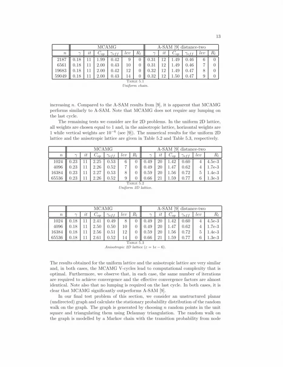
MCAMG A-SAM [9] distance-twon γ it Cop γeff lev Rl γ it Cop γeff lev Rl
2187 0.18 11 1.99 0.42 9 0 0.31 12 1.49 0.46 6 06561 0.18 11 2.00 0.43 10 0 0.31 12 1.49 0.46 7 0
19683 0.18 11 2.00 0.42 12 0 0.32 12 1.49 0.47 8 059049 0.18 11 2.00 0.43 14 0 0.32 12 1.50 0.47 9 0
Table 5.1Uniform chain.
increasing n. Compared to the A-SAM results from [9], it is apparent that MCAMGperforms similarly to A-SAM. Note that MCAMG does not require any lumping onthe last cycle.
The remaining tests we consider are for 2D problems. In the uniform 2D lattice,all weights are chosen equal to 1 and, in the anisotropic lattice, horizontal weights are1 while vertical weights are 10−6 (see [9]). The numerical results for the uniform 2Dlattice and the anisotropic lattice are given in Table 5.2 and Table 5.3, respectively.
MCAMG A-SAM [9] distance-twon γ it Cop γeff lev Rl γ it Cop γeff lev Rl
1024 0.23 11 2.25 0.53 6 0 0.49 20 1.42 0.60 4 4.5e-34096 0.23 11 2.26 0.52 7 0 0.49 20 1.47 0.62 4 1.7e-3
16384 0.23 11 2.27 0.53 8 0 0.59 20 1.56 0.72 5 1.4e-365536 0.23 11 2.26 0.52 9 0 0.66 21 1.59 0.77 6 1.3e-3
Table 5.2Uniform 2D lattice.
MCAMG A-SAM [9] distance-twon γ it Cop γeff lev Rl γ it Cop γeff lev Rl
1024 0.18 11 2.41 0.49 8 0 0.49 20 1.42 0.60 4 4.5e-34096 0.18 11 2.50 0.50 10 0 0.49 20 1.47 0.62 4 1.7e-3
16384 0.18 11 2.56 0.51 12 0 0.59 20 1.56 0.72 5 1.4e-365536 0.18 11 2.61 0.52 14 0 0.66 21 1.59 0.77 6 1.3e-3
Table 5.3Anisotropic 2D lattice (ε = 1e − 6).
The results obtained for the uniform lattice and the anisotropic lattice are very similarand, in both cases, the MCAMG V-cycles lead to computational complexity that isoptimal. Furthermore, we observe that, in each case, the same number of iterationsare required to achieve convergence and the effective convergence factors are almostidentical. Note also that no lumping is required on the last cycle. In both cases, it isclear that MCAMG significantly outperforms A-SAM [9].
In our final test problem of this section, we consider an unstructured planar(undirected) graph and calculate the stationary probability distribution of the randomwalk on the graph. The graph is generated by choosing n random points in the unitsquare and triangulating them using Delaunay triangulation. The random walk onthe graph is modelled by a Markov chain with the transition probability from node

14
i to node j given by the reciprocal of the number of edges incident on node i (equalweights). Table 5.4 shows good convergence results for the unstructured planar graph
MCAMG A-SAM [9] distance-onen γ it Cop γeff lev Rl γ it Cop γeff lev Rl
1024 0.44 16 2.15 0.68 6 0 0.53 20 1.69 0.68 5 2.6e-22048 0.36 14 2.20 0.62 6 6.4e-5 0.52 19 1.68 0.68 5 2.1e-24096 0.40 15 2.23 0.66 7 1.3e-4 0.61 21 1.80 0.76 5 2.4e-28192 0.40 15 2.27 0.67 8 1.1e-4 0.64 22 1.92 0.79 7 2.5e-2
16384 0.37 14 2.30 0.65 8 8.3e-5 0.76 30 2.03 0.87 7 2.4e-232768 0.37 14 2.29 0.65 9 1.0e-4 0.74 28 2.08 0.86 7 2.4e-2
Table 5.4Unstructured planar graph.
problem with very little lumping on the last cycle. It appears that Cop is bounded,and consideration of γ and the number of iterations suggest that the computationalcomplexity is optimal. Compared to the results from [9], it is evident that MCAMGagain significantly outperforms A-SAM.
To investigate the nature of these test problems, we seek the following asymptoticrelationship between the subdominant eigenvalue of B and the problem size n:
1− |λ2| ≈ C
(1
n
)p
, (5.1)
where C > 0 and p > 0 are constants. We are interested in the exponent p, whichdetermines how rapidly |λ2| → 1 as n→∞. An estimate of p provides insight into therate at which traditional one-level iterative methods converge for this type of problem.For problems for which |λ2| approaches 1 as in (5.1), we expect multilevel methodsto outperform traditional one-level iterative methods. Figure 5.1 shows log-log plotsof 1 − |λ2| as a function of n (hollow circles) and the linear best fit to these datapoints. For the uniform chain test problem, observe that p ≈ 2 and, for all othertest problems, that p ≈ 1. As expected, p ≈ 2/d, with d the dimensionality of theproblem.
5.2. Complex spectrum problems. In this section, we consider the test prob-lems for which B has a complex spectrum, and for which the exact solution cannoteasily be computed. These include a tandem queueing network, a stochastic Petri netproblem, an ATM queueing network and an octagonal mesh problem. The first threetest problems have also been considered in [9, 13, 17, 22]. We conclude this sectionwith an analysis of the subdominant eigenvalues and with plots of the spectra for eachtest problem. Note that, for brevity, we do not go into great detail describing our testcases, but instead we refer the reader to the appropriate sources.
The first test problem is an open tandem queueing network from [22]; see also[9]. Two finite queues with single servers are placed in tandem. Customers arriveaccording to a Poisson distribution with rate µ, and the service time distributionat the two single-server stations is Poisson with rates µ1 and µ2. In our numericalexperiments, we limit the number of customers in the queues to N = 31, 63, 127, 255.We choose (µ, µ1, µ2) = (10, 11, 10) for the weights. The states of the system can berepresented by tuples (n1, n2), with n1 the number of customers waiting in the firstqueue and n2 in the second queue. The total number of states is given by (N + 1)2.

15
101
102
103
104
10−6
10−5
10−4
10−3
problem size n
1−|λ
2|
Uniform chain, p = 2.0071
101
102
103
104
10−3
10−2
10−1
problem size n
1−|λ
2|
Uniform 2D lattice, p = 1.0428
101
102
103
104
10−9
10−8
10−7
problem size n
1−|λ
2|
Anisotropic 2D lattice, p = 1.0281
101
102
103
104
10−3
10−2
10−1
problem size n
1−|λ
2|
Unstructured planar graph, p = 1.0217
Fig. 5.1. Magnitude of subdominant eigenvalue as a function of problem size.
The states can be represented on a 2D regular lattice. In the directed graph, thetransition probability from node i to node j is given by the weight of the edge fromnode i to j, divided by the sum of the weights of all outgoing edges from node i.Table 5.5 shows the numerical results for the tandem queueing network test problem.Iteration numbers are constant and the operator complexity grows somewhat as a
MCAMG A-SAM [9] distance-twon γ it Cop γeff lev Rl γ it Cop γeff lev Rl
1024 0.31 15 4.68 0.78 7 1.2e-1 0.41 20 2.04 0.64 4 7.6e-24096 0.32 16 4.53 0.78 8 1.3e-1 0.45 24 2.12 0.69 5 5.5e-2
16384 0.32 15 4.57 0.78 10 1.1e-1 0.56 30 2.18 0.77 6 5.3e-265536 0.32 15 4.61 0.78 11 6.5e-2 0.71 37 2.37 0.86 6 1.3e-1
Table 5.5Tandem queueing network.
function of problem size for this nonsymmetric problem, but appears bounded. Theamount of lumping required for this nonsymmetric 2D problem is larger than for theprevious problems, but is still relatively small and does not add much extra work.These results are competitive with those obtained using A-SAM in [9].
The next problem we consider is derived from a stochastic Petri net (SPN). Petrinets are a formalism for the description of concurrency and synchronization in dis-tributed systems. They consist of: places, which model conditions or objects; tokens,which represent the specific value of the condition or object; transitions, which modelactivities that change the value of conditions or objects; and arcs, which specify in-terconnection between places and transitions. A stochastic Petri net is a standardPetri net, together with a tuple Λ = (r1, . . . , rn) of exponentially distributed transi-tion firing rates. Furthermore, we know from [15] that a finite place, finite transition,marked stochastic Petri net is isomorphic to a one-dimensional discrete-space Markov

16
process. For an in-depth discussion of Petri Nets, the reader is referred to [1, 15].We test MCAMG on the SPN described in [13]. Table 5.6 shows that the number
MCAMG (θ = 0.7) A-SAM [9] distance-two (θ = 0.5)n γ it Cop γeff lev Rl γ it Cop γeff lev Rl
1496 0.39 17 2.56 0.69 8 1.1e-3 0.40 17 3.76 0.79 5 1.5e-12470 0.38 17 2.62 0.69 8 1.4e-3 0.38 16 4.26 0.80 5 1.5e-13795 0.40 17 2.71 0.71 9 1.1e-3 0.37 16 4.53 0.80 5 1.5e-1
10416 0.41 18 2.92 0.74 10 1.1e-3 0.45 18 5.31 0.86 5 1.4e-116206 0.43 18 2.98 0.75 11 9.7e-4 0.45 18 5.55 0.87 5 1.3e-123821 0.46 18 3.08 0.78 11 9.1e-4 0.41 18 6.01 0.86 6 1.3e-133511 0.43 18 3.16 0.77 11 8.4e-4 0.45 18 6.57 0.88 6 1.2e-145526 0.42 18 3.22 0.76 12 7.6e-4 0.42 18 6.91 0.88 6 1.2e-1
Table 5.6Stochastic Petri net, Λ = (1, 3, 7, 9, 5).
of iterations is bounded and that the effective convergence factor, γeff , is boundedwell below one, from which we conclude that optimal computational complexity isachieved. Comparing the effective convergence factors of MCAMG and A-SAM, itis evident that MCAMG outperforms A-SAM. Note that in order to obtain optimalresults for MCAMG it was necessary to use θ = 0.7 instead of θ = 0.25.
The next test problem we consider is a multi-class, finite buffer, priority system.This model can be applied to telecommunications modelling, and has been used tomodel ATM queueing networks as discussed in [17]. For a complete description,including all the model parameters, see [22, 23]. The code and data files used to buildthe transition rate matrix corresponding to this Markov chain model are providedfreely on the web [23]. To obtain a column-stochastic transition probability matrix Bfrom the row-oriented transition rate matrix Q, we set
B = (diag(Q)−QT )(diag(Q))−1.
Transition rate matrices were constructed for buffer sizes 16, 20, 26, 32, 36, 42, 50.
MCAMG (θ = 0.5) A-SAM [9] distance-twon γ it Cop γeff lev Rl γ it Cop γeff lev Rl
1940 0.53 25 2.95 0.81 9 1.2e-2 0.26 14 3.23 0.66 5 1.6e-13060 0.48 21 2.85 0.77 8 9.4e-3 0.26 13 3.29 0.66 5 1.6e-15220 0.51 23 2.88 0.79 9 7.6e-3 0.25 14 3.50 0.67 5 1.6e-17956 0.45 21 2.87 0.76 10 6.6e-3 0.25 14 3.74 0.69 5 1.6e-1
10100 0.47 22 2.86 0.77 10 6.0e-3 0.25 13 3.98 0.71 5 1.6e-119620 0.42 20 2.83 0.73 11 4.3e-3 0.25 13 4.24 0.72 6 1.7e-132276 0.43 22 2.87 0.75 11 5.4e-3 0.25 14 4.54 0.74 6 1.7e-1
Table 5.7ATM queueing network.
Table 5.7 shows the numerical results for the MCAMG V-cycles. The number ofiterations and operator complexity are bounded and it appears that MCAMG per-forms optimally for this problem. Note that in our initial implementation of the firstpass of the coarsening routine, ties for C-point choice were broken in lexicographi-cal order. Due to the particular directionality of the ATM queueing problem, this

17
ordering led to a ‘worst-case’, unusually high number of levels and consequently topoor operator complexity of MCAMG. Instead, we now break ties in a different wayusing the natural ordering of the heap data structure we use, which has resolved thisdifficulty, and maintains good convergence properties for the other test problems.
The last test problem we consider is an octagonal mesh problem. This problemis constructed to have a full spectrum that fills a large part of the unit circle, andfeatures elements of web traffic modelling, restricted to a specific planar 2D graph.In what follows, we provide a complete description of how transition matrix B isconstructed. In general, consider graph H, represented by a n× n binary matrix,
Hij =
{1, if an arc exists from node j to node i0, otherwise
}
.
We assume that graph H has the following properties:
(P1) Every node has an outgoing arc.(At least one nonzero entry in every column of H .)
(P2) Every node has an incoming arc.(At least one nonzero entry of every row of H .)
(P3) There is a directed path between any two nodes.(H is irreducible.)
Then, for any node j in graph H, we assign the following probabilities:
µ+ Probability of moving forward, distributed equally among outgoing arcs.(Transition from state j to i for Hij = 1.)
µ0 Probability of staying at current node.(No transition.)
µ− Probability of moving backward, distributed equally among incoming arcs.(Transition from state j to i for Hji = 1.)
These values satisfy µ+ + µ0 + µ− = 1. We use matrix H diag(1T H)−1 for transitionalong outgoing arcs and matrix HT diag(1T HT )−1 for transition along incoming arcs.Our final column-stochastic matrix is then given by:
B = µ0I + µ+H diag(1T H)−1 + µ−HT diag(1T HT )−1.
Note that the graph associated with matrix B is the symmetrized version of graphH. The graph we use to construct B for the numerical test is pictured in Figure5.2. The transition probabilities used are µ+ = 0.80, µ0 = 0.15, and µ− = 0.05.
MCAMG A-SAM [9] distance-twon γ it Cop γeff lev Rl γ it Cop γeff lev Rl
1024 0.55 29 4.84 0.88 9 2.4e-2 0.37 18 2.88 0.71 5 1.8e-14096 0.55 29 5.41 0.90 11 2.2e-2 0.52 20 3.11 0.81 6 1.7e-1
16384 0.56 29 5.43 0.90 12 2.2e-2 0.60 22 3.17 0.85 6 1.6e-132768 0.56 29 5.60 0.90 12 2.2e-2 0.67 24 3.33 0.89 7 1.6e-165536 0.56 29 5.46 0.90 13 2.2e-2 0.65 26 3.28 0.88 7 1.6e-1
Table 5.8Octagonal mesh.
Table 5.8 shows good convergence results for both MCAMG and A-SAM. For each

18
Fig. 5.2. Graph H representing the octagonal mesh.
algorithm it appears that Cop is bounded, and consideration of γ and the numberof iterations suggests that the computational complexity is optimal. Note that theMCAMG operator complexity can be decreased by only performing the first pass ofthe coarsening routine together with a suitably redefined interpolation formula [11].
−1.5 −1 −0.5 0 0.5 1 1.5
−0.5
0
0.5
real axis
imag
inar
y ax
is
Tandem queueing network, n = 1024
−1.5 −1 −0.5 0 0.5 1 1.5
−0.5
0
0.5
real axis
imag
inar
y ax
is
Stochastic Petri net, n = 1496
−1.5 −1 −0.5 0 0.5 1 1.5
−0.5
0
0.5
real axis
imag
inar
y ax
is
ATM queueing network, n = 1940
−1.5 −1 −0.5 0 0.5 1 1.5
−0.5
0
0.5
real axis
imag
inar
y ax
is
Octagonal mesh, n = 1024
Fig. 5.3. Complex spectra Σ(B).
One further observation is that the number of levels used by A-SAM is always lessthan the number of levels used by MCAMG. This is a consequence of the fact that A-SAM coarsens faster than MCAMG, especially when distance-two aggregation is used,since this results in larger aggregates. The number of levels grows logarithmically withproblem size, since we coarsen until the coarsest problems are below a fixed size ratherthan up to a fixed number of levels, which would not ultimately yield a near-optimalmethod. For different problems with the same problem size, the number of levels
19
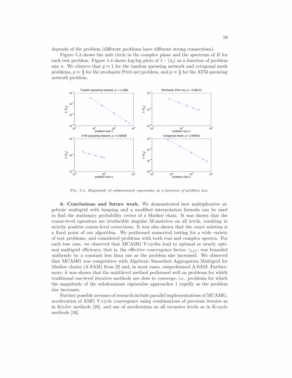
depends of the problem (different problems have different strong connections).Figure 5.3 shows the unit circle in the complex plane and the spectrum of B for
each test problem. Figure 5.4 shows log-log plots of 1− |λ2| as a function of problemsize n. We observe that p ≈ 1 for the tandem queueing network and octagonal meshproblems, p ≈ 2
3 for the stochastic Petri net problem, and p ≈ 12 for the ATM queueing
network problem.
101
102
103
104
10−4
10−3
10−2
10−1
problem size n
1−|λ
2|
Tandem queueing network, p = 1.1586
102
103
104
10−4
10−3
10−2
problem size n
1−|λ
2|
Stochastic Petri net, p = 0.68121
103
104
105
10−3
10−2
10−1
problem size n
1−|λ
2|
ATM queueing network, p = 0.48508
101
102
103
104
10−4
10−3
10−2
10−1
problem size n
1−|λ
2|
Octagonal mesh, p = 0.99453
Fig. 5.4. Magnitude of subdominant eigenvalue as a function of problem size.
6. Conclusions and future work. We demonstrated how multiplicative al-gebraic multigrid with lumping and a modified interpolation formula can be usedto find the stationary probability vector of a Markov chain. It was shown that thecoarse-level operators are irreducible singular M-matrices on all levels, resulting instrictly positive coarse-level corrections. It was also shown that the exact solution isa fixed point of our algorithm. We performed numerical testing for a wide varietyof test problems, and considered problems with both real and complex spectra. Foreach test case, we observed that MCAMG V-cycles lead to optimal or nearly opti-mal multigrid efficiency, that is, the effective convergence factor, γeff , was boundeduniformly by a constant less than one as the problem size increased. We observedthat MCAMG was competitive with Algebraic Smoothed Aggregation Multigrid forMarkov chains (A-SAM) from [9] and, in most cases, outperformed A-SAM. Further-more, it was shown that the multilevel method performed well on problems for whichtraditional one-level iterative methods are slow to converge, i.e., problems for whichthe magnitude of the subdominant eigenvalue approaches 1 rapidly as the problemsize increases.
Further possible avenues of research include parallel implementations of MCAMG,acceleration of AMG V-cycle convergence using combinations of previous iterates asin Krylov methods [20], and use of acceleration on all recursive levels as in K-cyclemethods [16].

20
REFERENCES
[1] Falko Bause and Pieter Kritzinger, Stochastic Petri Nets, Verlag Vieweg, Germany, 1996.[2] Abraham Berman and Robert J. Plemmons, Nonnegative Matrices in the Mathematical
Sciences, SIAM, Philadelphia, 1987.[3] Achi Brandt, Stephen F. McCormick, and John W. Ruge, Algebraic multigrid (AMG)
for sparse matrix equations, in Sparsity and Its Applications, D. J. Evans, ed., CambridgeUniversity Press, Cambridge, 1984.
[4] Achi Brandt and Dorit Ron, Multigrid solvers and multilevel optimization strategies, in Mul-tilevel Optimization and VLSICAD, J. Cong and J. R. Shinnerl, editors, Kluwer, Boston,pp. 1-69, 2003.
[5] Marian Brezina, Robert D. Falgout, Scott MacLachlan, Thomas A. Manteuffel,Stephen F. McCormick, and John W. Ruge, Adaptive algebraic multigrid, SIAM J.Sci. Comp. 27:1261-1286, 2006.
[6] William L. Briggs, Van Emden Henson, and Stephen F. McCormick, A Multigrid Tutorial,SIAM, Philadelphia, 2000.
[7] Gary Chartrand and Linda Lesniak, Graphs & Digraphs, Chapman and Hall/CRC, BocaRaton, 2005.
[8] Hans De Sterck, Robert D. Falgout, Josh Nolting, and Ulrike Meier Yang, Distance-two interpolation for parallel algebraic multigrid, Numerical Linear Algebra with Applica-tions 15, 115-139, 2008.
[9] Hans De Sterck, Thomas A. Manteuffel, Stephen F. McCormick, Killian Miller,James Pearson, John Ruge, and Geoffrey Sanders, Smoothed aggregation multigridfor Markov chains, SIAM J. Sci. Comp., accepted, 2009.
[10] Hans De Sterck, Thomas A. Manteuffel, Stephen F. McCormick, Quoc Nguyen, andJohn Ruge, Multilevel adaptive aggregation for Markov chains with application to webranking, SIAM J. Sci. Comp. 30:2235-2262, 2008.
[11] Hans De Sterck, Ulrike Meier Yang, and Jeffrey J. Heys, Reducing complexity in parallelalgebraic multigrid preconditioners, SIAM J. Matrix Anal. Appl. 27:1019-1039, 2006.
[12] Roger A. Horn and Charles R. Johnson, Matrix Analysis, Cambridge University Press,New York, 1985.
[13] Graham Horton and S.T. Leutenegger, A multi-level solution algorithm for steady-stateMarkov chains, ACM SIGMETRICS 191-200, 1994.
[14] Irene Livshits, An algebraic multigrid wave-ray algorithm to solve eigenvalue problems forthe Helmholtz operator, Numer. Linear Algebra Appl. 11:229-239, 2004.
[15] Michael K. Molloy, Performance analysis using stochastic Petri nets, IEEE Transactions onComputers C-31:913-917, 1982.
[16] Yvan Notay and Panayot S. Vassilevski, Recursive Krylov-based multigrid cycles, Numer.Linear Algebra Appl. 15:473-487, 2008.
[17] Bernard Philippe, Yousef Saad, and William J. Stewart, Numerical methods for Markovchain modeling, Operations Research 40:1156-1179, 1992.
[18] John W. Ruge, Algebraic multigrid (AMG) for geodetic survey problems, in Proceedings ofthe International Multigrid Conference, Copper Mountain, CO, 1983.
[19] John W. Ruge and Klaus Stueben, Algebraic Multigrid (AMG) in Multigrid Methods, Fron-tiers in Applied Mathematics, S. F. McCormick, editor, SIAM, Philadelphia, pp. 73-130,1987.
[20] Yousef Saad, Iterative Methods for Sparse Linear Systems, SIAM, Philadelphia, 2003.[21] Herbert A. Simon and Albert Ando, Aggregation of variables in dynamic systems, Econo-
metrica 29:111-138, 1961.[22] William J. Stewart, An Introduction to the Numerical Solution of Markov Chains, Princeton
University Press, Princeton, 1994.[23] William J. Stewart, MARCA Models, Retrieved August 5, 2008, from http://www4.ncsu.
edu/~billy/MARCA_Models/MARCA_Models.html.[24] Klaus Stueben, Algebraic multigrid (AMG): an introduction with applications, GMD Report
70, Institut fur Algorithmen und Wissenschaftliches Rechnen, November 1999.[25] Yukio Takahashi, A lumping method for numerical calculations of stationary distributions
of Markov chains, Research Report B-18, Department of Information Sciences, TokyoInstitute of Technology, 1975.
[26] Eran Treister and Irad Yavneh, Square and stretch multigrid for stochastic matrix eigen-problems, submitted, 2009.
[27] Elena Virnik, An algebraic multigrid preconditioner for a class of singular M-matrices, SIAMJ. Sci. Comp. 29:1982-1991, 2007.