arX

iv:1

102.

2789

v1 [

cs.C

C]

14

Feb

2011

Algebraic Independence and Blackbox Identity

Testing

Malte Beecken Johannes Mittmann Nitin Saxena

Hausdorff Center for Mathematics, Bonn, Germanymalte.beecken, johannes.mittmann, nitin.saxena@hcm.uni-bonn.de

Abstract

Algebraic independence is an advanced notion in commutative algebra thatgeneralizes independence of linear polynomials to higher degree. Polynomialsf1, . . . , fm ⊂ F[x1, . . . , xn] are called algebraically independent if there is nonon-zero polynomial F such that F (f1, . . . , fm) = 0. The transcendence degree,trdegf1, . . . , fm, is the maximal number r of algebraically independent polyno-mials in the set. In this paper we design blackbox and efficient linear maps ϕ

that reduce the number of variables from n to r but maintain trdegϕ(fi)i = r,assuming fi’s sparse and small r. We apply these fundamental maps to solveseveral cases of blackbox identity testing:

1. Given a polynomial-degree circuit C and sparse polynomials f1, . . . , fmwith trdeg r, we can test blackbox D := C(f1, . . . , fm) for zeroness inpoly(size(D))r time.

2. Define a ΣΠΣΠδ(k, s, n) circuit C to be of the form∑k

i=1

∏sj=1 fi,j, where

fi,j are sparse n-variate polynomials of degree at most δ. For k = 2 we give

a poly(δsn)δ2

time blackbox identity test.

3. For a general depth-4 circuit we define a notion of rank. Assuming thereis a rank bound R for minimal simple ΣΠΣΠδ(k, s, n) identities, we givea poly(δsnR)Rkδ2 time blackbox identity test for ΣΠΣΠδ(k, s, n) circuits.This partially generalizes the state of the art of depth-3 to depth-4 circuits.

The notion of trdeg works best with large or zero characteristic, but we also giveversions of our results for arbitrary fields.

Keywords: Algebraic independence, transcendence degree, arithmetic circuits,polynomial identity testing, blackbox algorithms, depth-4 circuits.

1

1 Introduction

Polynomial identity testing (PIT) is the problem of checking whether a given n-variatearithmetic circuit computes the zero polynomial in F[x1, . . . , xn]. It is a central ques-tion in complexity theory as circuits model computation and PIT leads us to a betterunderstanding of circuits. There are several classical randomized algorithms known[DL78, Sch80, Zip79, CK00, LV98, AB03] that solve PIT. The basic Schwartz-Zippeltest is: given a circuit C(x1, . . . , xn), check C(a) = 0 for a random a ∈ F

n. Finding a

deterministic polynomial time test, however, has been more difficult and is currentlyopen. Derandomization of PIT is well motivated by a host of algorithmic applica-tions, eg. bipartite matching [Lov79] and matrix completion [Lov89], and connectionsto sought-after super-polynomial lower bounds [HS80, KI04]. Especially, blackbox PIT(i.e. circuit C is given as a blackbox and we could only make oracle queries) has di-rect connections to lower bounds for the permanent [Agr05, Agr06]. Clearly, finding ablackbox PIT test for a family of circuits F boils down to efficiently designing a hittingset H ⊂ F

nsuch that: given a nonzero C ∈ F , there exists an a ∈ H that hits C, i.e.

C(a) 6= 0.The attempts to solve blackbox PIT have focused on restricted circuit families. A

natural restriction is constant depth. Agrawal & Vinay [AV08] showed that a blackboxPIT algorithm for depth-4 circuits would (almost) solve PIT for general circuits (andprove exponential circuit lower bounds for permanent). The currently known blackboxPIT algorithms work only for further restricted depth-3 and depth-4 circuits. The caseof bounded top fanin depth-3 circuits has received great attention and has blackbox PITalgorithms [DS06, KS07, KS08, SS, KS09, SS10, SS11]. The analogous case for depth-4circuits is open. However, with the additional restriction of multilinearity on all themultiplication gates, there is a blackbox PIT algorithm [KMSV10, SV11]. The latteris somewhat subsumed by the PIT algorithms for constant-read multilinear formulas[AvMV10]. To save space we would not go into the rich history of PIT and insteadrefer to the surveys [Sax09, SY10].

A recurring theme in the blackbox PIT research on depth-3 circuits has been that ofrank. If we consider a ΣΠΣ(k, d, n) circuit C =

∑k

i=1

∏d

j=1 ℓi,j, where ℓi,j are linear formsin F[x1, . . . , xn], then rk(C) is defined to be the linear rank of the set of forms ℓi,ji,jeach viewed as a vector in Fn. This raises the natural question: Is there a generalizednotion of rank for depth-4 circuits as well, and more importantly, one that is usefulin blackbox PIT? We answer this question affirmatively in this paper. Our notion ofrank is via transcendence degree (short, trdeg), which is a basic notion in commutativealgebra. To show that this notion applies to PIT requires relatively advanced algebraand new tools that we build.

Consider polynomials f1, . . . , fm in F[x1, . . . , xn]. They are called algebraicallyindependent (over F) if there is no nonzero polynomial F ∈ F[y1, . . . , ym] such thatF (f1, . . . , fm) = 0. When those polynomials are algebraically dependent then such an Fexists and is called the annihilating polynomial of f1, . . . , fm. The transcendence degree,trdegf1, . . . , fm, is the maximal number r of algebraically independent polynomials

2

in the set f1, . . . , fm. Though intuitive, it is nontrivial to prove that r is at most n[Mor96]. The notion of trdeg has appeared in complexity theory in several contexts.Kalorkoti [Kal85] used trdeg to prove an Ω(n3) formula size lower bound for n × ndeterminant. In the works [DGW09, DGRV11] studying the entropy of polynomialmappings (f1, . . . , fm) : Fn → Fm, trdeg is a natural measure of entropy when the fieldhas large or zero characteristic. It also appears implicitly in [Dvi09] while constructingextractors for varieties. Finally, the complexity of the annihilating polynomial is studiedin [Kay09]. However, our work is the first to study trdeg in the context of PIT.

1.1 Our main results

Our first result shows that a general arithmetic circuit is sensitive to the trdeg of itsinput.

Theorem 1. Let C be an m-variate circuit. Let f1, . . . , fm be ℓ-sparse, δ-degree, n-variate polynomials with trdeg r. Suppose we have oracle access to the n-variate d-degree circuit C ′ := C(f1, . . . , fm). There is a blackbox poly(size(C ′) · dℓδ)r time test tocheck C ′ = 0 (assuming a zero or larger than δr characteristic).

We also give an algorithm that works for all fields but has a worse time com-plexity. Note that the above theorem seems nontrivial even for a constant m, sayC ′ = C(f1, f2, f3), as the output of C ′ may not be sparse and fi’s are of arbitrarydegree and arity. In such a case r is constant too and the theorem gives a polynomialtime test. Another example, where r is constant but both m and n are variable, is:fi := (xi

1 + x22 + · · · + x2

n)xin for i ∈ [m]. (Hint: r ≤ 3.)

Our next two main results concern depth-4 circuits. By ΣΠΣΠδ(k, s, n) we denotecircuits (over a field F) of the form

C :=

k∑

i=1

s∏

j=1

fi,j, (1)

where fi,j’s are sparse n-variate polynomials of maximal degree δ. Note that when δ = 1this notation agrees with that of a ΣΠΣ circuit. Currently, the PIT methods are noteven strong enough to study ΣΠΣΠδ(k, s, n) circuits with both top fanin k and bottomfanin δ bounded. It is in this spectrum that we make exciting progress.

Theorem 2. Let C be a ΣΠΣΠδ(2, s, n) circuit over an arbitrary field. There is ablackbox poly(δsn)δ

2

time test to check C = 0.

Simple, minimal and rank Finally, we define a notion of rank for depth-4 cir-cuits and show its usefulness. For a circuit C, as in (1), we define its rank, rk(C) :=trdegfi,j | i ∈ [k], j ∈ [s]. Define Ti :=

∏s

j=1 fi,j, for all i ∈ [k], to be the multi-plication terms of C. We call C simple if Ti | i ∈ [k] are coprime polynomials. Wecall C minimal if there is no I ( [k] such that

∑

i∈I Ti = 0. Define Rδ(k, s) to be the

3

smallest r such that: any ΣΠΣΠδ(k, s, n) circuit C that is simple, minimal and zerohas rk(C) < r.

Theorem 3. Let r := Rδ(k, s) and the characteristic be zero or larger than δr. Thereis a blackbox poly(δrsn)rkδ

2

time identity test for ΣΠΣΠδ(k, s, n) circuits.

We give a lower bound of Ω(δk log s) on Rδ(k, s) and conjecture an upper bound(better than the trivial ks).

1.2 Organization and our approach

A priori it is not clear whether the problem of deciding algebraic independence of givenpolynomials f1, . . . , fm, over a field F, is even computable. Perron [Per27] proved thatfor m = (n+ 1) and any field, the annihilating polynomial has degree only exponentialin n. We generalize this to any m in Sect. 2.1, hence, deciding algebraic independence(over any field) is computable. When the characteristic is zero or large, there is a moreefficient criterion due to Jacobi (Sect. 2.2). For using trdeg in PIT we would need torelate it to the Krull dimension of algebras (Sect. 2.3).

The central concept that we develop is that of a faithful homomorphism. Thisis a linear map ϕ from R := F[x1, . . . , xn] to F[z1, . . . , zr] such that for polynomialsf1, . . . , fm ∈ R of trdeg r, the images ϕ(f1), . . . , ϕ(fm) are also of trdeg r. Additionally,to be useful, ϕ should be constructible in a blackbox and efficient way. We give suchconstructions in Sects. 3.1 and 3.2. The proofs here use Perron’s and Jacobi’s criterion,but require new techniques as well. The reason why such a ϕ is useful in PIT is becauseit preserves the nonzeroness of the circuit C(f1, . . . , fm) (Corollary 13). We prove thisby an elegant application of Krull’s principal ideal theorem.

Once the fundamental machinery is set up, we prove Theorem 1 by designing ahitting set. The zero or large characteristic case is handled in Sect. 4.1. The arbitrarycharacteristic case is in Sect. 4.2.

Finally, we apply the faithful homomorphisms to depth-4 circuits. The proof ofTheorem 2 is provided in Sect. 5.2. The rank-based hitting set is constructed in Sect.5.3 proving Theorem 3. The full proofs tend to be extremely technical and have beenmoved to the appendix.

2 Preliminaries: Perron, Jacobi & Krull

Let n ∈ Z+ and let K be a field of characteristic ch(K). Throughout this paper,K[x] = K[x1, . . . , xn] is a polynomial ring in n variables over K. K denotes thealgebraic closure of the field. We denote the multiplicative group of units of an algebraA by A∗. We use the notation [n] := 1, . . . , n. For 0 ≤ r ≤ n,

(

[n]r

)

denotes the set ofr-subsets of [n].

4

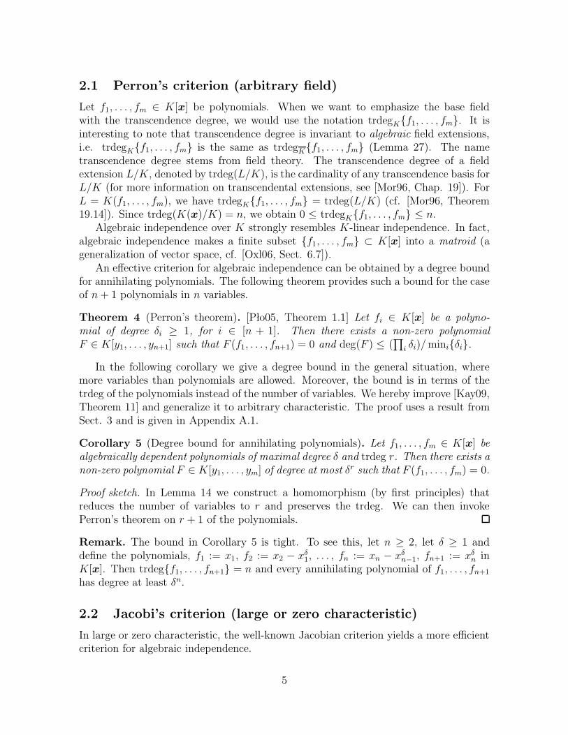
2.1 Perron’s criterion (arbitrary field)

Let f1, . . . , fm ∈ K[x] be polynomials. When we want to emphasize the base fieldwith the transcendence degree, we would use the notation trdegKf1, . . . , fm. It isinteresting to note that transcendence degree is invariant to algebraic field extensions,i.e. trdegKf1, . . . , fm is the same as trdegKf1, . . . , fm (Lemma 27). The nametranscendence degree stems from field theory. The transcendence degree of a fieldextension L/K, denoted by trdeg(L/K), is the cardinality of any transcendence basis forL/K (for more information on transcendental extensions, see [Mor96, Chap. 19]). ForL = K(f1, . . . , fm), we have trdegKf1, . . . , fm = trdeg(L/K) (cf. [Mor96, Theorem19.14]). Since trdeg(K(x)/K) = n, we obtain 0 ≤ trdegKf1, . . . , fm ≤ n.

Algebraic independence over K strongly resembles K-linear independence. In fact,algebraic independence makes a finite subset f1, . . . , fm ⊂ K[x] into a matroid (ageneralization of vector space, cf. [Oxl06, Sect. 6.7]).

An effective criterion for algebraic independence can be obtained by a degree boundfor annihilating polynomials. The following theorem provides such a bound for the caseof n + 1 polynomials in n variables.

Theorem 4 (Perron’s theorem). [P lo05, Theorem 1.1] Let fi ∈ K[x] be a polyno-mial of degree δi ≥ 1, for i ∈ [n + 1]. Then there exists a non-zero polynomialF ∈ K[y1, . . . , yn+1] such that F (f1, . . . , fn+1) = 0 and deg(F ) ≤ (

∏

i δi)/miniδi.

In the following corollary we give a degree bound in the general situation, wheremore variables than polynomials are allowed. Moreover, the bound is in terms of thetrdeg of the polynomials instead of the number of variables. We hereby improve [Kay09,Theorem 11] and generalize it to arbitrary characteristic. The proof uses a result fromSect. 3 and is given in Appendix A.1.

Corollary 5 (Degree bound for annihilating polynomials). Let f1, . . . , fm ∈ K[x] bealgebraically dependent polynomials of maximal degree δ and trdeg r. Then there exists anon-zero polynomial F ∈ K[y1, . . . , ym] of degree at most δr such that F (f1, . . . , fm) = 0.

Proof sketch. In Lemma 14 we construct a homomorphism (by first principles) thatreduces the number of variables to r and preserves the trdeg. We can then invokePerron’s theorem on r + 1 of the polynomials.

Remark. The bound in Corollary 5 is tight. To see this, let n ≥ 2, let δ ≥ 1 anddefine the polynomials, f1 := x1, f2 := x2 − xδ

1, . . . , fn := xn − xδn−1, fn+1 := xδ

n inK[x]. Then trdegf1, . . . , fn+1 = n and every annihilating polynomial of f1, . . . , fn+1

has degree at least δn.

2.2 Jacobi’s criterion (large or zero characteristic)

In large or zero characteristic, the well-known Jacobian criterion yields a more efficientcriterion for algebraic independence.

5

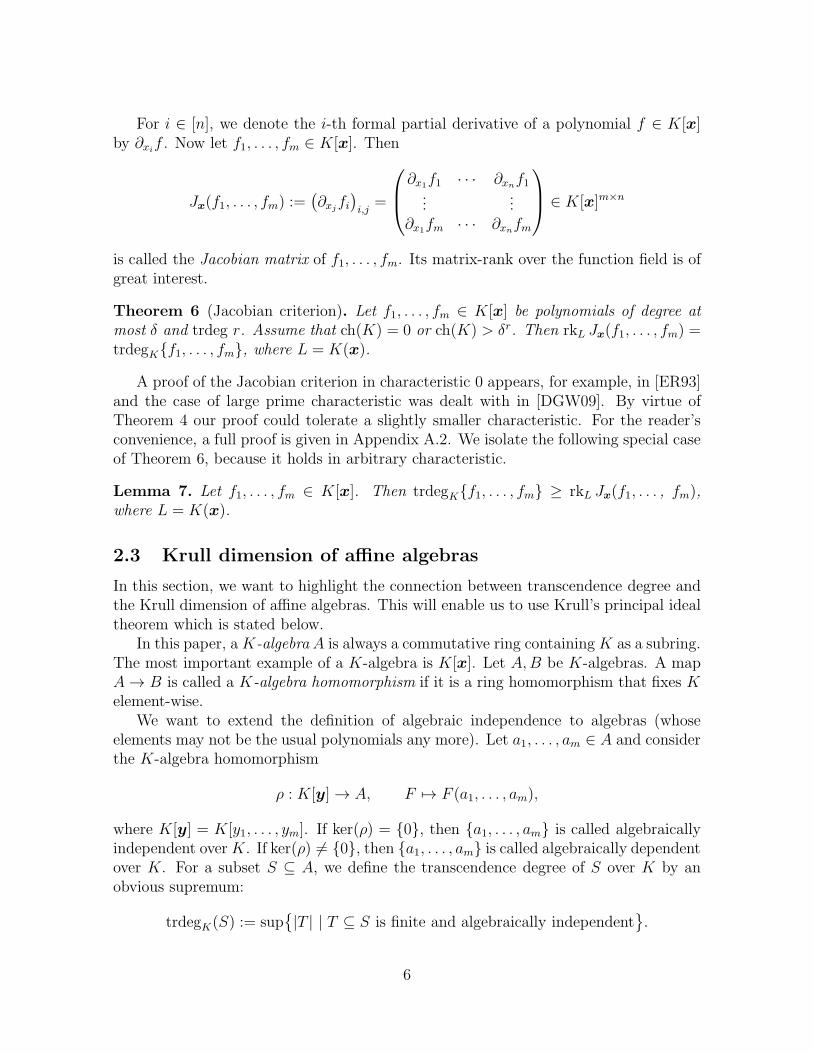
For i ∈ [n], we denote the i-th formal partial derivative of a polynomial f ∈ K[x]by ∂xi

f . Now let f1, . . . , fm ∈ K[x]. Then

Jx(f1, . . . , fm) :=(

∂xjfi)

i,j=

∂x1f1 · · · ∂xn

f1...

...∂x1

fm · · · ∂xnfm

∈ K[x]m×n

is called the Jacobian matrix of f1, . . . , fm. Its matrix-rank over the function field is ofgreat interest.

Theorem 6 (Jacobian criterion). Let f1, . . . , fm ∈ K[x] be polynomials of degree atmost δ and trdeg r. Assume that ch(K) = 0 or ch(K) > δr. Then rkL Jx(f1, . . . , fm) =trdegKf1, . . . , fm, where L = K(x).

A proof of the Jacobian criterion in characteristic 0 appears, for example, in [ER93]and the case of large prime characteristic was dealt with in [DGW09]. By virtue ofTheorem 4 our proof could tolerate a slightly smaller characteristic. For the reader’sconvenience, a full proof is given in Appendix A.2. We isolate the following special caseof Theorem 6, because it holds in arbitrary characteristic.

Lemma 7. Let f1, . . . , fm ∈ K[x]. Then trdegKf1, . . . , fm ≥ rkL Jx(f1, . . . , fm),where L = K(x).

2.3 Krull dimension of affine algebras

In this section, we want to highlight the connection between transcendence degree andthe Krull dimension of affine algebras. This will enable us to use Krull’s principal idealtheorem which is stated below.

In this paper, a K-algebra A is always a commutative ring containing K as a subring.The most important example of a K-algebra is K[x]. Let A,B be K-algebras. A mapA → B is called a K-algebra homomorphism if it is a ring homomorphism that fixes Kelement-wise.

We want to extend the definition of algebraic independence to algebras (whoseelements may not be the usual polynomials any more). Let a1, . . . , am ∈ A and considerthe K-algebra homomorphism

ρ : K[y] → A, F 7→ F (a1, . . . , am),

where K[y] = K[y1, . . . , ym]. If ker(ρ) = 0, then a1, . . . , am is called algebraicallyindependent over K. If ker(ρ) 6= 0, then a1, . . . , am is called algebraically dependentover K. For a subset S ⊆ A, we define the transcendence degree of S over K by anobvious supremum:

trdegK(S) := sup

|T | | T ⊆ S is finite and algebraically independent

.

6

The image of K[y] under ρ is the subalgebra of A generated by a1, . . . , am and is denotedby K[a1, . . . , am]. An algebra of this form is called an affine K-algebra, and it is calledan affine K-domain if it is an integral domain.

The Krull dimension of A, denoted by dim(A), is defined as the supremum over allr ≥ 0 for which there is a chain p0 ( p1 ( · · · ( pr of prime ideals pi ⊂ A. It measureshow far A is from a field.

Theorem 8 (Dimension and trdeg). Let A = K[a1, . . . , am] be an affine K-algebra.Then dim(A) = trdegK(A) = trdegKa1, . . . , am.

Proof. Cf. [Kem11, Theorem 5.9 and Proposition 5.10]. Also, the integral domain caseis in the standard text [Mat89, Theorem 5.6].

The following corollary is a simple consequence of Theorem 8. It shows that ho-momorphisms cannot increase the dimension of affine algebras. The proof is given inAppendix A.3.

Corollary 9. Let A,B be K-algebras and let ϕ : A → B be a K-algebra homomorphism.If A is an affine algebra, then so is ϕ(A) and we have dim(ϕ(A)) ≤ dim(A). If, inaddition, ϕ is injective, then dim(ϕ(A)) = dim(A).

In the next section we will need the following version of Krull’s principal idealtheorem.

Theorem 10 (Krull’s Hauptidealsatz). Let A be an affine K-domain and let a ∈A \ (A∗ ∪ 0). Then dim(A/〈a〉) = dim(A) − 1.

Proof. Cf. [Eis95, Corollary 13.11] or [Mat89, Theorem 13.5].

3 Faithful homomorphisms: Reducing the variables

Let f1, . . . , fm ∈ K[x] be polynomials and let r := trdegf1, . . . , fm. Intuitively, rvariables should suffice to define f1, . . . , fm without changing their algebraic relations.So let K[z] = K[z1, . . . , zr] be a polynomial ring with 1 ≤ r ≤ n. We want to finda homomorphism K[x] → K[z] that preserves the transcendence degree of f1, . . . , fm.First we give this property a name.

Definition 11. Let ϕ : K[x] → K[z] be a K-algebra homomorphism. We say ϕ isfaithful to f1, . . . , fm if trdegϕ(f1), . . . , ϕ(fm) = trdegf1, . . . , fm.

The following theorem shows that faithful homomorphisms are useful for us.

Theorem 12 (Faithful is useful). Let A = K[f1, . . . , fm] ⊆ K[x]. Then ϕ is faithful tof1, . . . , fm if and only if ϕ|A : A → K[z] is injective (iff A ∼= K[ϕ(f1), . . . , ϕ(fm)]).

7

Proof. We denote ϕA = ϕ|A and r = trdegf1, . . . , fm. If ϕA is injective, then

r = dim(A) = dim(ϕA(A)) = trdegϕ(f1), . . . , ϕ(fm)

by Theorem 8 and Corollary 9. Thus ϕ is faithful to f1, . . . , fm.Conversely, let ϕ be faithful to f1, . . . , fm. Then dim(ϕA(A)) = r. Now assume

for the sake of contradiction that ϕA is not injective. Then there exists an f ∈ A \ 0such that ϕA(f) = 0. We have f /∈ K, because ϕ fixes K element-wise, and hencef /∈ A∗. Since A is an affine domain, Theorem 10 implies dim(A/〈f〉) = r − 1. Sincef ∈ ker(ϕA), the K-algebra homomorphism

ϕA : A/〈f〉 → K[z], a + 〈f〉 7→ ϕA(a)

is well-defined and ϕA factors as ϕA = ϕA η, where η : A → A/〈f〉 is the canonicalsurjection. But then Corollary 9 implies

r = dim(ϕA(A)) = dim(ϕA(η(A))) ≤ dim(η(A)) = dim(A/〈f〉) = r − 1,

a contradiction. It follows that ϕA is injective.When ϕA is injective, clearly we have A ∼= ϕA(A) = K[ϕ(f1), . . . , ϕ(fm)].

Corollary 13. Let C be an m-variate circuit over K. Let ϕ be faithful to f1, . . . , fm⊂ K[x]. Then, C(f1, . . . , fm) = 0 iff C(ϕ(f1), . . . , ϕ(fm)) = 0.

Proof. Note that C(f1, . . . , fm) resp. C(ϕ(f1), . . . , ϕ(fm)) are elements in the algebrasK[f1, . . . , fm] resp. K[ϕ(f1), . . . , ϕ(fm)]. Since ϕ is an isomorphism between these twoalgebras, the corollary is evident.

3.1 A Kronecker-inspired map (arbitrary characteristic)

The following lemma shows that even linear faithful homomorphisms exist for all sub-sets of polynomials (provided K is large enough, for eg. move to K or a large enoughfield extension [AL86]). It is a generalization of [Kay09, Claim 11.1] to arbitrary char-acteristic. The proof is given in Appendix B.1.

Lemma 14 (Existence). Let K be an infinite field and let f1, . . . , fm ∈ K[x] be polyno-mials of trdeg r. Then there exists a linear K-algebra homomorphism ϕ : K[x] → K[z]which is faithful to f1, . . . , fm.

Proof sketch. We prove this by first principles. The proof is by identifying r variablesfrom x1, . . . , xn that we leave free and the rest n−r variables we fix to generic elementsfrom K. Using annihilating polynomials we could show that this map preserves thetrdeg.

8

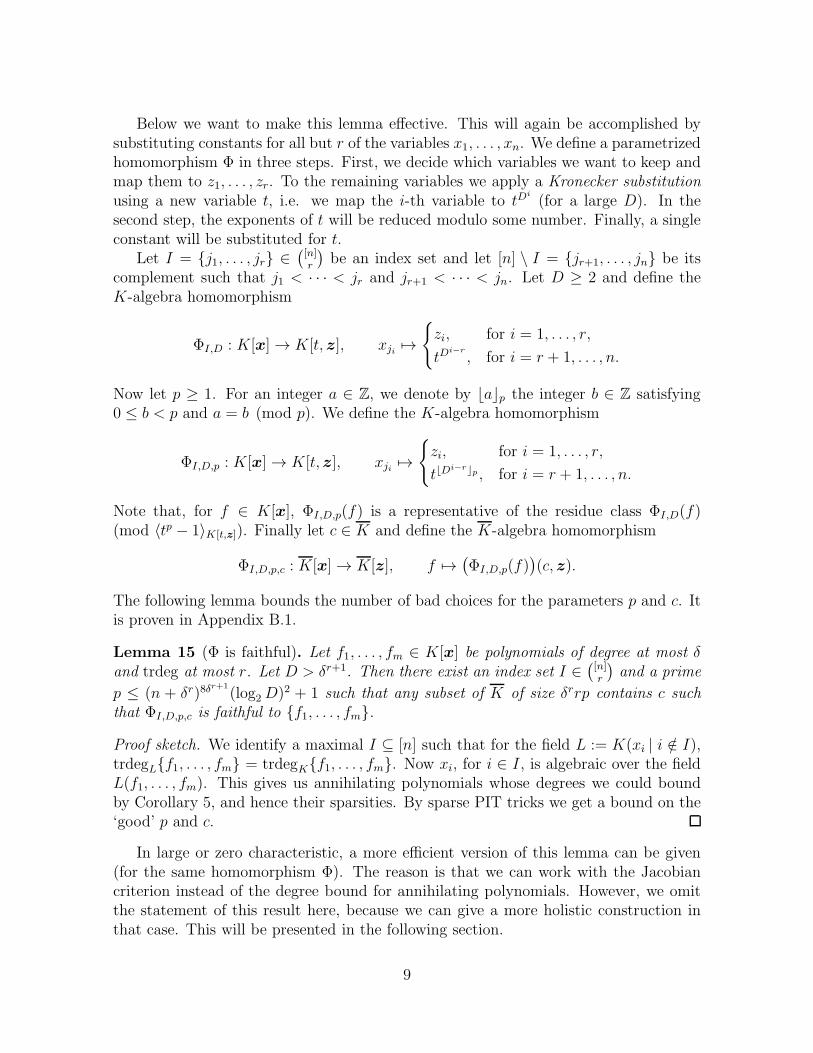
Below we want to make this lemma effective. This will again be accomplished bysubstituting constants for all but r of the variables x1, . . . , xn. We define a parametrizedhomomorphism Φ in three steps. First, we decide which variables we want to keep andmap them to z1, . . . , zr. To the remaining variables we apply a Kronecker substitutionusing a new variable t, i.e. we map the i-th variable to tD

i

(for a large D). In thesecond step, the exponents of t will be reduced modulo some number. Finally, a singleconstant will be substituted for t.

Let I = j1, . . . , jr ∈(

[n]r

)

be an index set and let [n] \ I = jr+1, . . . , jn be itscomplement such that j1 < · · · < jr and jr+1 < · · · < jn. Let D ≥ 2 and define theK-algebra homomorphism

ΦI,D : K[x] → K[t, z], xji 7→

zi, for i = 1, . . . , r,

tDi−r

, for i = r + 1, . . . , n.

Now let p ≥ 1. For an integer a ∈ Z, we denote by ⌊a⌋p the integer b ∈ Z satisfying0 ≤ b < p and a = b (mod p). We define the K-algebra homomorphism

ΦI,D,p : K[x] → K[t, z], xji 7→

zi, for i = 1, . . . , r,

t⌊Di−r⌋p , for i = r + 1, . . . , n.

Note that, for f ∈ K[x], ΦI,D,p(f) is a representative of the residue class ΦI,D(f)(mod 〈tp − 1〉K[t,z]). Finally let c ∈ K and define the K-algebra homomorphism

ΦI,D,p,c : K[x] → K[z], f 7→(

ΦI,D,p(f))

(c, z).

The following lemma bounds the number of bad choices for the parameters p and c. Itis proven in Appendix B.1.

Lemma 15 (Φ is faithful). Let f1, . . . , fm ∈ K[x] be polynomials of degree at most δand trdeg at most r. Let D > δr+1. Then there exist an index set I ∈

(

[n]r

)

and a prime

p ≤ (n + δr)8δr+1

(log2 D)2 + 1 such that any subset of K of size δrrp contains c suchthat ΦI,D,p,c is faithful to f1, . . . , fm.

Proof sketch. We identify a maximal I ⊆ [n] such that for the field L := K(xi | i /∈ I),trdegLf1, . . . , fm = trdegKf1, . . . , fm. Now xi, for i ∈ I, is algebraic over the fieldL(f1, . . . , fm). This gives us annihilating polynomials whose degrees we could boundby Corollary 5, and hence their sparsities. By sparse PIT tricks we get a bound on the‘good’ p and c.

In large or zero characteristic, a more efficient version of this lemma can be given(for the same homomorphism Φ). The reason is that we can work with the Jacobiancriterion instead of the degree bound for annihilating polynomials. However, we omitthe statement of this result here, because we can give a more holistic construction inthat case. This will be presented in the following section.

9

3.2 A Vandermonde-inspired map (large or zero characteris-

tic)

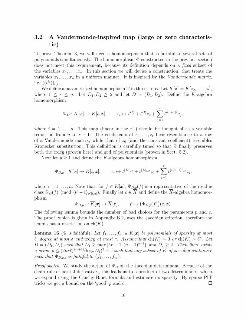
To prove Theorem 3, we will need a homomorphism that is faithful to several sets ofpolynomials simultaneously. The homomorphism Φ constructed in the previous sectiondoes not meet this requirement, because its definition depends on a fixed subset ofthe variables x1, . . . , xn. In this section we will devise a construction, that treats thevariables x1, . . . , xn in a uniform manner. It is inspired by the Vandermonde matrix,i.e. ((tij))i,j.

We define a parametrized homomorphism Ψ in three steps. Let K[z] = K[z0, . . . , zr],where 1 ≤ r ≤ n. Let D1, D2 ≥ 2 and let D = (D1, D2). Define the K-algebrahomomorphism

ΨD : K[x] → K[t, z], xi 7→ tDi1 + tD

i2z0 +

r∑

j=1

ti(n+1)jzj ,

where i = 1, . . . , n. This map (linear in the z’s) should be thought of as a variablereduction from n to r + 1. The coefficients of z1, . . . , zr bear resemblance to a rowof a Vandermonde matrix, while that of z0 (and the constant coefficient) resemblesKronecker substitution. This definition is carefully tuned so that Ψ finally preservesboth the trdeg (proven here) and gcd of polynomials (proven in Sect. 5.2).

Next let p ≥ 1 and define the K-algebra homomorphism

ΨD,p : K[x] → K[t, z], xi 7→ t⌊Di1⌋p + t⌊D

i2⌋pz0 +

r∑

j=1

t⌊i(n+1)j⌋pzj ,

where i = 1, . . . , n. Note that, for f ∈ K[x], ΨD,p(f) is a representative of the residueclass ΨD(f) (mod 〈tp−1〉K[t,z]). Finally let c ∈ K and define the K-algebra homomor-phism

ΨD,p,c : K[x] → K[z], f 7→(

ΨD,p(f))

(c, z).

The following lemma bounds the number of bad choices for the parameters p and c.The proof, which is given in Appendix B.2, uses the Jacobian criterion, therefore thelemma has a restriction on ch(K).

Lemma 16 (Ψ is faithful). Let f1, . . . , fm ∈ K[x] be polynomials of sparsity at mostℓ, degree at most δ and trdeg at most r. Assume that ch(K) = 0 or ch(K) > δr. LetD = (D1, D2) such that D1 ≥ maxδr + 1, (n + 1)r+1 and D2 ≥ 2. Then there existsa prime p ≤ (2nrℓ)2(r+1)(log2D1)

2 + 1 such that any subset of K of size δrp contains csuch that ΨD,p,c is faithful to f1, . . . , fm.

Proof sketch. We study the action of ΨD on the Jacobian determinant. Because of thechain rule of partial derivatives, this leads us to a product of two determinants, whichwe expand using the Cauchy-Binet formula and estimate its sparsity. By sparse PITtricks we get a bound on the ‘good’ p and c.

10

By trying larger p and c, we can find a Ψ that is faithful to several subsets ofpolynomials simultaneously. This is an advantage of Ψ over Φ, in addition to beingmore efficiently constructible.

4 Circuits with sparse inputs of low transcendence

degree (proving Theorem 1)

We can now proceed with the first PIT application of faithful homomorphisms. Weconsider arithmetic circuits of the form C(f1, . . . , fm), where C is a circuit comput-ing a polynomial in K[y] = K[y1, . . . , ym] and f1, . . . , fm are subcircuits computingpolynomials in K[x]. Thus, C(f1, . . . , fm) computes a polynomial in the subalgebraK[f1, . . . , fm].

Let C(f1, . . . , fm) be of maximal degree d, and let f1, . . . , fm be of maximal degreeδ, maximal sparsity ℓ and maximal transcendence degree r. First, we use a faithfulhomomorphism to transform C(f1, . . . , fm) into an r-variate circuit. Then, a hittingset for r-variate degree-d polynomials is used, given by the following version of theSchwartz-Zippel lemma.

Lemma 17 (Schwartz-Zippel). Let H ⊂ K be a subset of size d + 1. Then H = Hr isa hitting set for f ∈ K[z1, . . . , zr] | deg(f) ≤ d.

Proof. Cf. [Alo99, Lemma 2.1].

4.1 A hitting set (large or zero characteristic)

We use the map Ψ from Sect. 3.2. This hitting set construction is efficient for r constantand ℓ, d polynomial in the input size.

Let n, d, r, δ, ℓ ≥ 1 and let K[z] = K[z0, z1, . . . , zr]. We introduce the followingparameters.

1. Define D = (D1, D2) by D1 := (2δn)r+1 and D2 := 2.

2. Define pmax := (2nrℓ)2(r+1)⌈log2 D1⌉2 + 1.

3. Pick arbitrary H1, H2 ⊂ K of sizes δrpmax resp. d + 1.

Denote Ψ(i)D,p,c := ΨD,p,c(xi) ∈ K[z] for i = 1, . . . , n and define the subset

Hd,r,δ,ℓ =

(

Ψ(1)D,p,c(a), . . . ,Ψ

(n)D,p,c(a)

) ∣

∣ p ∈ [pmax], c ∈ H1, a ∈ Hr+12

⊂ Kn.

The following theorem shows that, over a large or zero characteristic, this is a hittingset for the class of circuits under consideration. A proof is given in Appendix C.1.

Theorem 18. Assume that ch(K) = 0 or ch(K) > δr. Then Hd,r,δ,ℓ is a hitting set forthe class of degree-d circuits with inputs being ℓ-sparse, degree-δ subcircuits of trdeg atmost r. It can be constructed in poly(drδℓn)r time.

11

4.2 A hitting set (arbitrary characteristic)

We use the map Φ from Sect. 3.1. This hitting set construction is efficient for δ, rconstants and d polynomial in the input size.

Let n, d, r, δ ≥ 1 and let K[z] = K[z1, . . . , zr]. We introduce the following parame-ters.

1. Define D := δr+1 + 1.

2. Define pmax := (n + δr)8δr+1

⌈log2D⌉2 + 1.

3. Pick arbitrary H1, H2 ⊂ K of sizes δrrpmax resp. d + 1.

Denote Φ(i)I,D,p,c := ΦI,D,p,c(xi) ∈ K[z] for i = 1, . . . , n and define the subset

Hd,r,δ =

(

Φ(1)I,D,p,c(a), . . . ,Φ

(n)I,D,p,c(a)

) ∣

∣ I ∈(

[n]r

)

, p ∈ [pmax], c ∈ H1, a ∈ Hr2

⊂ Kn.

The following theorem shows that this is a hitting set for the class of circuits underconsideration. A proof is given in Appendix C.2.

Theorem 19. The set Hd,r,δ is a hitting set for the class of degree-d circuits with inputsbeing degree-δ subcircuits of transcendence degree at most r. It can be constructed inpoly(drδn)rδ

r+1

time.

5 Depth-4 circuits with bounded top and bottom

fanin

The second PIT application of faithful homomorphisms is for ΣΠΣΠδ(k, s, n) circuits.Our hitting set construction is efficient when the top fanin k and the bottom fanin δare both bounded. Except for top fanin 2, our hitting set will be conditional in thesense that its efficiency depends on a good rank upper bound for depth-4 identities.

5.1 Gcd, simple parts and the rank bounds

Let C =∑k

i=1

∏s

j=1 fi,j be a ΣΠΣΠδ(k, s, n) circuit, as defined in Sect. 1.1. Note thatthe parameters bound the circuit degree, deg(C) ≤ δs. We define an S(·) operator as:

S(C) :=

fi,j | i ∈ [k] and j ∈ [s]

⊂ K[x].

It gives the set of sparse polynomials of C (wlog we assume them all to be nonzero).The following definitions are natural generalizations of the corresponding concepts fordepth-3 circuits. Recall Ti :=

∏

j fi,j, for i ∈ [k], are the multiplication terms of C. Thegcd part of C is defined as gcd(C) := gcd(T1, . . . , Tk) (we fix a unique representativeamong the associated gcds). The simple part of C is defined as sim(C) := C/ gcd(C) ∈ΣΠΣΠδ(k, s, n). For a subset I ⊆ [k] we denote CI :=

∑

i∈I Ti.

12

Recall that if C is simple then gcd(C) = 1 and if it is minimal then CI 6= 0 for allnon-empty I ( [k]. Also, recall that rk(C) is trdegK S(C), and that Rδ(k, s) strictlyupper bounds the rank of any minimal and simple ΣΠΣΠδ(k, s, n) identity. Clearly,Rδ(k, s) is at most | S(C)| ≤ ks (note: S(C) cannot all be independent in an identity).On the other hand, we could prove a lower bound on Rδ(k, s) by constructing identities.

From the simple and minimal ΣΠΣ identities constructed in [SS], we obtain the lowerbound R1(k, s) = Ω(k) if ch(K) = 0, and R1(k, s) = Ω(k logp s) if ch(K) = p > 0. Theseidentities can be lifted to ΣΠΣΠδ(k, s, n) identities by replacing each variable xi by aproduct xi,1 · · ·xi,δ of new variables. These examples demonstrate: Rδ(k, s) = Ω(δk) ifch(K) = 0, and Rδ(k, s) = Ω(δk logp s) if ch(K) = p > 0. This leads us to the followingnatural conjecture.

Conjecture 20. We conjecture

Rδ(k, s) =

poly(δk), if ch(K) = 0,

poly(δk log s), otherwise.

The following lemma is a vast generalization of [KS08, Theorem 3.4] to depth-4circuits. It suggests how a bound for Rδ(k, s) can be used to construct a hitting set forΣΠΣΠδ(k, s, n) circuits. The ϕ in the statement below should be thought of as a linearmap that reduces the number of variables from n to Rδ(k, s) + 1.

Lemma 21 (Rank is useful). Let C be a ΣΠΣΠδ(k, s, n) circuit, let r := Rδ(k, s) andlet ϕ : K[x] → K[z] = K[z0, z1, . . . , zr] be a linear K-algebra homomorphism that, forall I ⊆ [k], satisfies:

1. ϕ(sim(CI)) = sim(ϕ(CI)), and

2. rk(ϕ(sim(CI))) ≥ min

rk(sim(CI)), Rδ(k, s)

.

Then C = 0 if and only if ϕ(C) = 0.

Proof. If C = 0, then clearly ϕ(C) = 0. Conversely, let ϕ(C) = 0. Let I ⊆ [k] be anon-empty subset such that ϕ(CI) is a minimal circuit computing the zero polynomial.Then, by assumption (1.), ϕ(sim(CI)) = sim(ϕ(CI)) ∈ ΣΠΣΠδ(k, s, n) is a minimaland simple circuit computing the zero polynomial. Hence, rk(ϕ(sim(CI))) < Rδ(k, s).By assumption (2.), this implies rk(ϕ(sim(CI))) = rk(sim(CI)), thus ϕ is faithful toS(sim(CI)). Theorem 12 yields sim(CI) = 0, hence CI = 0. Since ϕ(C) is the sum ofzero and minimal circuits ϕ(CI) for some I ⊆ [k], we obtain C = 0 as required.

5.2 Preserving the simple part (towards Theorem 2)

The following lemma shows that Ψ meets condition (1.) of Lemma 21. The proof isgiven in Appendix D.1. This is also the heart of PIT when k = 2. The actual hittingset, though, we provide in the next subsection.

13

Lemma 22 (Ψ preserves the simple part). Let C be a ΣΠΣΠδ(k, s, n) circuit. LetD1 ≥ 2δ2 + 1, let D1 ≥ D2 ≥ δ + 1 and let D = (D1, D2). Then there exists a primep ≤ (2ksnδ2)8δ

2+2(log2D1)2 + 1 such that any subset S ⊂ K of size 2δ4k2s2p contains

c satisfying ΨD,p,c(sim(C)) = sim(ΨD,p,c(C)).

Proof sketch. For any coprime fi, fj ∈ S(C) we look at their images under Ψ. We viewΨ(fi) and Ψ(fj) as univariates wrt z0 and fix z1 = · · · = zr = 0. If we could keep thesetwo univariates monic (before the fixing) and their resultants nonzero (after the fixing),then the coprimality of Ψ(fi) and Ψ(fj) would be ensured. Both those requirementsare fulfilled by estimating the sparsity and using sparse PIT tricks.

5.3 A hitting set (proving Theorems 2 & 3)

Armed with Lemmas 21 and 22 we could now complete the construction of the hit-ting set for ΣΠΣΠδ(k, s, n) circuits using the faithful homomorphism Ψ with the rightparameters.

Let n, δ, k, s ≥ 1 and let r = Rδ(k, s). We introduce the following parameters. Theyare blown up so that they support 2k applications (one for each I ⊂ [k]) of Lemmas 16and 22.

1. Define D = (D1, D2) by D1 := (2δn)2r and D2 := δ + 1.

2. Define pmax := 22(k+1) · (2krsnδ2)8δ2+4δr⌈log2D1⌉

2 + 1.

3. Pick arbitrary H1, H2 ⊂ K of sizes 2k+2k2rs2δ4pmax resp. δs + 1.

Denote Ψ(i)D,p,c := ΨD,p,c(xi) ∈ K[z] for i = 1, . . . , n and define the subset

Hδ,k,s =

(

Ψ(1)D,p,c(a), . . . ,Ψ

(n)D,p,c(a)

) ∣

∣ p ∈ [pmax], c ∈ H1, a ∈ Hr+12

⊂ Kn.

The following theorem shows that, in large or zero characteristic, this is a hitting setfor ΣΠΣΠδ(k, s, n) circuits.

Theorem 23. Assume that ch(K) = 0 or ch(K) > δr. Then Hδ,k,s is a hitting set forΣΠΣΠδ(k, s, n) circuits. It can be constructed in poly(δrsn)δ

2kr time.

Since trivially Rδ(2, s) = 1, we obtain an explicit hitting set for the top fanin 2case. Moreover, in this case we can also eliminate the dependence on the characteristic(because Lemma 22 is field independent).

Corollary 24. Let K be of arbitrary characteristic. Then Hδ,2,s is a hitting set forΣΠΣΠδ(2, s, n) circuits. It can be constructed in poly(δsn)δ

2

time.

A proof of the theorem and the corollary can be found in Appendix D.2.

14

6 Conclusion

The notion of rank has been quite useful in depth-3 PIT. In this work we give thefirst generalization of it to depth-4 circuits. We used trdeg and developed fundamentalmaps – the faithful homomorphisms – that preserve trdeg of sparse polynomials in ablackbox and efficient way (assuming a small trdeg). Crucially, we showed that faithfulhomomorphisms preserve the nonzeroness of circuits.

Our work raises several open questions. The faithful homomorphism constructionover a small characteristic has restricted efficiency, in particular, it is interesting onlywhen the sparse polynomials have very low degree. Could Lemma 15 be improved tohandle larger δ? In general, the classical methods stop short of dealing with smallcharacteristic because the “geometric” Jacobian criterion is not there. We have givensome new tools to tackle that, for eg., Corollary 5 and Lemmas 14 and 15. But moretools are needed, for eg. a homomorphism like that of Lemma 16 for arbitrary fields.

Currently, we do not know a better upper bound for Rδ(k, s) other than ks. Forδ = 1, it is just the rank of depth-3 identities, which is known to be O(k2 log s) (O(k2)over R) [SS10]. Even for δ = 2 we leave the rank question open. We conjectureR2(k, s) = Ok(log s) (generally, Conjecture 20). Our hope is that understanding thesesmall δ identities should give us more potent tools to attack depth-4 PIT in generality.

Acknowledgements We are grateful to the Hausdorff Center for Mathematics, Bonn,for its kind support. The first two authors would also like to thank the Bonn Interna-tional Graduate School in Mathematics for research funding.

References

[AB03] M. Agrawal and S. Biswas. Primality and identity testing via Chinese re-maindering. Journal of the ACM, 50(4):429–443, 2003. (Conference versionin FOCS 1999).

[Agr05] M. Agrawal. Proving lower bounds via pseudo-random generators. In Pro-ceedings of the 25th Annual Foundations of Software Technology and Theo-retical Computer Science (FSTTCS), pages 92–105, 2005.

[Agr06] M. Agrawal. Determinant versus permanent. In Proceedings of the 25thInternational Congress of Mathematicians (ICM), volume 3, pages 985–997,2006.

[AL86] L. M. Adleman and H. W. Lenstra. Finding irreducible polynomials overfinite fields. In Proceedings of the 18th Annual ACM Symposium on Theoryof Computing (STOC), pages 350–355, 1986.

[Alo99] N. Alon. Combinatorial Nullstellensatz. Combinatorics, Probability andComputing, 8:7–29, 1999.

15

[AV08] M. Agrawal and V. Vinay. Arithmetic circuits: A chasm at depth four.In Proceedings of the 49th Annual Symposium on Foundations of ComputerScience (FOCS), pages 67–75, 2008.

[AvMV10] M. Anderson, D. van Melkebeek, and I. Volkovich. Derandomizing poly-nomial identity testing for multilinear constant-read formulae. TechnicalReport TR10-135, ECCC, 2010.

[BHLV09] M. Blaser, M. Hardt, R. J. Lipton, and N. K. Vishnoi. Deterministicallytesting sparse polynomial identities of unbounded degree. Information Pro-cessing Letters, 109(3):187–192, 2009.

[CK00] Z. Chen and M. Kao. Reducing randomness via irrational numbers. SIAM J.on Computing, 29(4):1247–1256, 2000. (Conference version in STOC 1997).

[CLO97] D. Cox, J. Little, and D. O’Shea. Ideals, Varieties, and Algorithms: An In-troduction to Computational Algebraic Geometry and Commutative Algebra.Springer-Verlag, New York, second edition, 1997.

[DGRV11] Z. Dvir, D. Gutfreund, G. Rothblum, and S. Vadhan. On approximatingthe entropy of polynomial mappings. In Proceedings of the 2nd Symposiumon Innovations in Computer Science (ICS), 2011.

[DGW09] Z. Dvir, A. Gabizon, and A. Wigderson. Extractors and rank extractors forpolynomial sources. Computational Complexity, 18(1):1–58, 2009. (Confer-ence version in FOCS 2007).

[DL78] Richard A. DeMillo and Richard J. Lipton. A probabilistic remark on alge-braic program testing. Information Processing Letters, 7(4):193–195, 1978.

[DS06] Z. Dvir and A. Shpilka. Locally decodable codes with 2 queries andpolynomial identity testing for depth 3 circuits. SIAM J. on Computing,36(5):1404–1434, 2006. (Conference version in STOC 2005).

[Dvi09] Z. Dvir. Extractors for varieties. In Proceedings of the 24th Annual IEEEConference on Computational Complexity (CCC), pages 102–113, 2009.

[Eis95] D. Eisenbud. Commutative Algebra with a View Toward Algebraic Geome-try. Springer-Verlag, New York, 1995.

[ER93] R. Ehrenborg and G. Rota. Apolarity and Canonical Forms for Homoge-neous Polynomials. Europ. J. Combinatorics, 14:157–181, 1993.

[HS80] J. Heintz and C. P. Schnorr. Testing polynomials which are easy to compute(extended abstract). In Proceedings of the twelfth annual ACM Symposiumon Theory of Computing, pages 262–272, New York, NY, USA, 1980.

16

[Kal85] K. Kalorkoti. A lower bound for the formula size of rational functions. SIAMJ. Comp., 14(3):678–687, 1985. (Conference version in ICALP 1982).

[Kay09] N. Kayal. The Complexity of the Annihilating Polynomial. In Proceedingsof the 24th Annual IEEE Conference on Computational Complexity (CCC),pages 184–193, 2009.

[Kem11] G. Kemper. A Course in Commutative Algebra. Springer-Verlag, Berlin,2011.

[KI04] V. Kabanets and R. Impagliazzo. Derandomizing polynomial identity testsmeans proving circuit lower bounds. Computational Complexity, 13(1):1–46,2004. (Conference version in STOC 2003).

[KMSV10] Z. Karnin, P. Mukhopadhyay, A. Shpilka, and I. Volkovich. Deterministicidentity testing of depth-4 multilinear circuits with bounded top fan-in. InProceedings of the 42nd ACM Symposium on Theory of Computing (STOC),pages 649–658, 2010.

[KS07] N. Kayal and N. Saxena. Polynomial identity testing for depth 3 circuits.Computational Complexity, 16(2):115–138, 2007. (Conference version inCCC 2006).

[KS08] Z. Karnin and A. Shpilka. Deterministic black box polynomial identity test-ing of depth-3 arithmetic circuits with bounded top fan-in. In Proceedingsof the 23rd Annual Conference on Computational Complexity (CCC), pages280–291, 2008.

[KS09] N. Kayal and S. Saraf. Blackbox polynomial identity testing for depth 3circuits. In Proceedings of the 50th Annual Symposium on Foundations ofComputer Science (FOCS), pages 198–207, 2009.

[Lan02] S. Lang. Algebra. Springer-Verlag, New York, third edition, 2002.

[Lov79] L. Lovasz. On determinants, matchings and random algorithms. In Funda-mentals of Computation Theory (FCT), pages 565–574, 1979.

[Lov89] L. Lovasz. Singular spaces of matrices and their applications in combina-torics. Bol. Soc. Braz. Mat, 20:87–99, 1989.

[LV98] D. Lewin and S. Vadhan. Checking polynomial identities over any field:Towards a derandomization? In Proceedings of the 30th Annual Symposiumon the Theory of Computing (STOC), pages 428–437, 1998.

[Mat89] H. Matsumura. Commutative Ring Theory. Cambridge Studies in AdvancedMathematics, Cambridge, UK, second edition, 1989.

17

[Mor96] P. Morandi. Field and Galois Theory. Springer-Verlag, New York, 1996.

[Oxl06] James Oxley. Matroid Theory. Oxford University Press, 2006.

[Pap95] C. H. Papadimitriou. Computational complexity. Addison-Wesley, Reading,Massachusetts, 1995.

[Per27] O. Perron. Algebra I (Die Grundlagen). Berlin, 1927.

[P lo05] A. P loski. Algebraic Dependence of Polynomials After O. Perron and SomeApplications. In Svetlana Cojocaru, Gerhard Pfister, and Victor Ufnarovski,editors, Computational Commutative and Non-Commutative Algebraic Ge-ometry, pages 167–173. IOS Press, 2005.

[Sax09] N. Saxena. Progress on polynomial identity testing. Bulletin of the Eu-ropean Association for Theoretical Computer Science (EATCS)- Computa-tional Complexity Column, (99):49–79, 2009.

[Sch80] J. T. Schwartz. Fast probabilistic algorithms for verification of polynomialidentities. Journal of the ACM, 27(4):701–717, 1980.

[SS] N. Saxena and C. Seshadhri. An Almost Optimal Rank Bound for Depth-3Identities. SIAM J. Comp. (to appear). (Conference version in CCC 2009).

[SS10] N. Saxena and C. Seshadhri. From Sylvester-Gallai configurations to rankbounds: Improved black-box identity test for depth-3 circuits. In Proceed-ings of the 51st Annual Symposium on Foundations of Computer Science(FOCS), pages 21–29, 2010.

[SS11] N. Saxena and C. Seshadhri. Blackbox identity testing for bounded topfanin depth-3 circuits: the field doesn’t matter. In Proceedings of the 43rdACM Symposium on Theory of Computing (STOC), 2011.

[SV11] S. Saraf and I. Volkovich. Black-box identity testing of depth-4 multilinearcircuits. In Proceedings of the 43rd ACM Symposium on Theory of Com-puting (STOC), 2011.

[SY10] A. Shpilka and A. Yehudayoff. Arithmetic Circuits: A survey of recent re-sults and open questions. Foundations and Trends in Theoretical ComputerScience, 5(3–4):207–388, 2010.

[vdE00] A. van den Essen. Polynomial Automorphisms and the Jacobian Conjecture.Birkhauser Verlag, Basel, 2000.

[Zen93] J. Zeng. A Bijective Proof of Muir’s Identity and the Cauchy-Binet Formula.Linear Algebra and its Applications, 184:79–82, 1993.

18

[Zip79] R. Zippel. Probabilistic algorithms for sparse polynomials. In Proceedingsof the International Symposium on Symbolic and Algebraic Manipulation(EUROSAM), pages 216–226, 1979.

A Proofs for Sect. 2: Preliminaries

A.1 Proofs for Sect. 2.1: Perron’s criterion

For the proof of Corollary 5 we will need three well-known lemmas. The first one isabout resultants. For more information about resultants, see [CLO97].

Lemma 25 (Resultant). Let f, g ∈ K[x] such that degxi(f) > 0 and degxi

(g) > 0for some i ∈ [n]. Then resxi

(f, g) = 0 if and only if f and g have a common factorh ∈ K[x] with degxi

(h) > 0.

Proof. Cf. [CLO97, Chap. 3, §6, Proposition 1].

The following lemma identifies a situation where annihilating polynomials are uniqueup to a factor in K∗.

Lemma 26 (Unique annihilating polynomials). Let f1, . . . , fm ∈ K[x] contain preciselym − 1 algebraically independent polynomials and let I ⊆ K[y1, . . . , ym] be the ideal ofalgebraic relations among f1, . . . , fm. Then I is principal.

Proof. We follow the instructions of [vdE00, Exercise 3.2.7]. Assume that f1, . . . , fm−1

are algebraically independent and let F1, F2 ∈ K[y1, . . . , ym] be non-zero irreduciblepolynomials satisfying Fi(f1, . . . , fm) = 0 for i = 1, 2. It suffices to show that F1 = cF2

for some c ∈ K∗.For this, view F1, F2 as elements of R[ym], where R = K[y1, . . . , ym−1], and consider

the ym-resultant g := resym(F1, F2) ∈ R. By [CLO97, Chap. 3, §5, Proposition 9], thereexist g1, g2 ∈ R[ym] such that g = g1F1 + g2F2. We have

g(f1, . . . , fm−1) = g1(f1, . . . , fm) · F1(f1, . . . , fm) + g2(f1, . . . , fm) · F2(f1, . . . , fm)

= 0.

Since f1, . . . , fm−1 are algebraically independent, it follows that g = 0. By Lemma25, F1, F2 have a non-trivial common factor in R[ym]. Since F1, F2 are irreducible, weobtain F1 = cF2 for some c ∈ K∗, as required.

The following lemma contains a useful fact about annihilating polynomials andalgebraic field extensions (cf. [Kay09, Claim 7.2] for a similar statement).

Lemma 27 (Going to a field extension). Let f1, . . . , fm ∈ K[x] and let L/K be analgebraic field extension. If there exists a non-zero polynomial F ∈ L[y] = L[y1, . . . , ym]such that F (f1, . . . , fm) = 0, then there exists a non-zero polynomial G ∈ K[y] suchthat G(f1, . . . , fm) = 0 and deg(G) ≤ deg(F ). In particular, f1, . . . , fm are algebraicallyindependent over K if and only if they are algebraically independent over L.

19

Proof. Let F ∈ L[y] be a non-zero polynomial such that F (f1, . . . , fm) = 0. Denoteby c1, . . . , cℓ ∈ L the non-zero coefficients of F . Replacing L by K(c1, . . . , cℓ), we mayassume that L/K is algebraic and finitely generated (as a field) over K. By [Lan02,Chapter V, §1, Proposition 1.6], this implies that [L : K] =: d < ∞. Let b1, . . . , bd ∈ Lbe a K-basis of L. Then we can write F as

F = F1 · b1 + · · · + Fd · bd

for some F1, . . . , Fd ∈ K[y], not all zero, such that deg(Fi) ≤ deg(F ) for all i = 1, . . . , d.Substituting f1, . . . , fm, we obtain

0 = F (f1, . . . , fm) = F1(f1, . . . , fm) · b1 + · · · + Fd(f1, . . . , fm) · bd.

The K-linear independence of b1, . . . , bd implies that all coefficients of

Fi(f1, . . . , fm) ∈ K[x]

are zero for i = 1, . . . , d. (Here we use that the indeterminates x1, . . . , xn are L-linearlyindependent, because L/K is algebraic.) Therefore, some non-zero Fi yields a G ∈ K[y]with the desired properties.

Corollary 5. Let f1, . . . , fm ∈ K[x] be algebraically dependent polynomials of maxi-mal degree δ and trdeg r. Then there exists a non-zero polynomial F ∈ K[y1, . . . , ym]of degree at most δr such that F (f1, . . . , fm) = 0.

Proof of Corollary 5. By Lemma 27, we may assume wlog that K is infinite. Fur-thermore, we may assume that m = r + 1 and f1, . . . , fr are algebraically indepen-dent. Let F ∈ K[y] = K[y1, . . . , yr+1] be a non-zero irreducible polynomial such thatF (f1, . . . , fr+1) = 0. By Lemma 14, there exists a linear K-algebra homomorphism

ϕ : K[x] → K[z] = K[z1, . . . , zr]

which is faithful to f1, . . . , fr+1. Set gi := ϕ(fi) ∈ K[z] for i = 1, . . . , r + 1. Theng1, . . . , gr+1 are of degree at most δ and by Theorem 4 there exists a non-zero polynomialG ∈ K[y] such that G(g1, . . . , gr+1) = 0 and deg(G) ≤ δr. But since

F (g1, . . . , gr+1) = F (ϕ(f1), . . . , ϕ(fr+1)) = ϕ(F (f1, . . . , fr+1)) = 0,

Lemma 26 implies that F divides G. Hence, deg(F ) ≤ deg(G) ≤ δr.

A.2 Proofs for Sect. 2.2: Jacobi’s criterion

In the proof of the Jacobian criterion we will make use of the following facts aboutpartial derivatives. Let f ∈ K[x]. First assume that ch(K) = 0. Then, for i ∈ [n], wehave

∂xif = 0 if and only if f ∈ K[x1, . . . , xi−1, xi+1, . . . , xn].

20

Therefore, we have ∂xi(f) = 0 for all i = 1, . . . , n if and only if f = 0. Now assume

ch(K) = p > 0. Then, for i ∈ [n], we have

∂xif = 0 if and only if f ∈ K[x1, . . . , xi−1, x

pi , xi+1, . . . , xn].

Hence, ∂xif = 0 for all i = 1, . . . , n if and only if f ∈ K[xp

1, . . . , xpn]. If, in addition, K is

a perfect field (in characteristic p this means that every element of K is a p-th power),then we have ∂xi

f = 0 for all i = 1, . . . , n if and only if f = gp for some g ∈ K[x]. Anexample of a perfect field is the algebraic closure K of K.

Now let K be an arbitrary field, let f1, . . . , fm ∈ K[x] and let F1, . . . , Fs ∈ K[y].Then, by the chain rule, we have

Jx(F1(f1, . . . , fm), . . . , Fs(f1, . . . , fm))

=(

Jy(F1, . . . , Fs))

(f1, . . . , fm) · Jx(f1, . . . , fm).

Now we are prepared to proceed with the proofs.

Lemma 7. Let f1, . . . , fm ∈ K[x]. Then trdegKf1, . . . , fm ≥ rkL Jx(f1, . . . , fm),where L = K(x).

Proof of Lemma 7. Let r = rkL Jx(f1, . . . , fm). We may assume that the first r rowsof J(f1, . . . , fm) are L-linearly independent. Assume, for the sake of contradiction,that f1, . . . , fr are algebraically dependent. Choose a non-zero polynomial F ∈ K[y] =K[y1, . . . , yr] of minimal degree such that F (f1, . . . , fr) = 0. Differentiating with respectto x1, . . . , xn using the chain rule yields the vector-matrix equation

(

(∂y1F )(f1, . . . , fr), . . . , (∂yrF )(f1, . . . , fr))

·

∂x1f1 · · · ∂xn

f1...

...∂x1

fr · · · ∂xnfr

= 0.

Since this matrix has rank r over L, it follows that (∂yiF )(f1, . . . , fr) = 0 for all i =1, . . . , r. Since the degree of F was chosen to be minimal, it follows that ∂yiF = 0 for alli = 1, . . . , r. If ch(K) = 0, this implies F = 0, a contradiction. If ch(K) = p > 0, thisimplies F ∈ K[yp1, . . . , y

pr ]. Since K is perfect and F 6= 0, there is a non-zero G ∈ K[y]

such that F = Gp. From

0 = F (f1, . . . , fr) = G(f1, . . . , fr)p

wee see that G(f1, . . . , fr) = 0. By Lemma 27, there exists a non-zero G′ ∈ K[y] suchthat G′(f1, . . . , fr) = 0 and deg(G′) ≤ deg(G) < deg(F ). This contradicts the choiceof F . Therefore, f1, . . . , fr are algebraically independent, hence trdeg(f1, . . . , fm) ≥r.

Theorem 6. Let f1, . . . , fm ∈ K[x] be polynomials of degree at most δ and trdeg r.Assume that ch(K) = 0 or ch(K) > δr. Then rkL Jx(f1, . . . , fm) = trdegKf1, . . . , fm,where L = K(x).

21

Proof of Theorem 6. Let r = trdegf1, . . . , fm. By Lemma 7, we have

r ≥ rkL J(f1, . . . , fm),

so it remains to show the converse inequality.After renumbering f1, . . . , fm and x1, . . . , xn, we may assume that the polyno-

mials f1, . . . , fr, xr+1, . . . , xn are algebraically independent. Consequently, for i =1, . . . , n, there exist non-zero polynomials Fi ∈ K[y0, . . . , yn] of minimal degree suchthat degy0

(Fi) > 0 and

Fi(xi, f1, . . . , fr, xr+1, . . . , xn) = 0. (2)

By Theorem 4 (with (n− r + 1) of the δi’s being 1), we have deg(Fi) ≤ δr. Hence, bythe assumptions on ch(K), we have ∂y0Fi 6= 0. Since the degree of Fi was chosen to beminimal, we have

(∂y0Fi)(xi, f1, . . . , fr, xr+1, . . . , xn) 6= 0.

DenoteGi,j := (∂yjFi)(xi, f1, . . . , fr, xr+1, . . . , xn)

for j = 0, . . . , n. Differentiating equation (2) with respect to xk using the chain ruleyields

Gi,0 · δi,k +r

∑

j=1

Gi,j · ∂xkfj +

n∑

j=r+1

Gi,j · δj,k = 0

for k = 1, . . . , n. Since Gi,0 6= 0, this can be rewritten as

r∑

j=1

−Gi,j

Gi,0· ∂xk

fj +

n∑

j=r+1

−Gi,j

Gi,0· δj,k = δi,k.

This shows that the block diagonal matrix

∂x1f1 · · · ∂xr

f1...

...∂x1

fr · · · ∂xrfr

1. . .

1

∈ Ln×n

is invertible. Therefore, the first r rows of J(f1, . . . , fm) are L-linearly independent andhence r ≤ rkL J(f1, . . . , fm).

22

A.3 Proofs for Sect. 2.3: Krull dimension

Corollary 9. Let A,B be K-algebras and let ϕ : A → B be a K-algebra homomor-phism. If A is an affine algebra, then so is ϕ(A) and we have dim(ϕ(A)) ≤ dim(A). If,in addition, ϕ is injective, then dim(ϕ(A)) = dim(A).

Proof of Corollary 9. Since A is an affine algebra, there exist a1, . . . , am ∈ A such thatA = K[a1, . . . , am]. Then ϕ(A) = K[ϕ(a1), . . . , ϕ(am)] is finitely generated as a K-algebra as well.

Now assume for the sake of contradiction that d := dim(ϕ(A)) > dim(A). ByTheorem 8, there exist a1, . . . , ad ∈ A such that ϕ(a1), . . . , ϕ(ad) are algebraically inde-pendent. Since d > dim(A), the elements a1, . . . , ad are algebraically dependent. Hence,there exists a non-zero polynomial F ∈ K[y1, . . . , yd] such that F (a1, . . . , ad) = 0. Itfollows that

0 = ϕ(F (a1, . . . , ad)) = F (ϕ(a1), . . . , ϕ(ad))

and this implies that ϕ(a1), . . . , ϕ(ad) are algebraically dependent, a contradiction.Therefore, dim(ϕ(A)) ≤ dim(A).

Now let ϕ be injective, let d := dim(A) and let a1, . . . , ad ∈ A be algebraicallyindependent. Assume for the sake of contradiction that ϕ(a1), . . . , ϕ(ad) are alge-braically dependent. Then there exists a non-zero polynomial F ∈ K[y1, . . . , yd] suchthat F (ϕ(a1), . . . , ϕ(ad)) = 0. From

0 = F (ϕ(a1), . . . , ϕ(ad)) = ϕ(F (a1, . . . , ad))

we see that F (a1, . . . , ad) = 0, because ϕ is injective. But this means that a1, . . . , adare algebraically dependent, a contradiction. Thus dim(ϕ(A)) ≥ dim(A).

B Proofs for Sect. 3: Faithful homomorphisms

Let P denote the set of prime numbers and sp(f) denote the sparsity of a polynomialf .

In the proofs of Lemmas 15, 16 and 22 we will use the following well-known facts.

Lemma 28 (Sparse PIT). Let ℓ ≥ 1 and d ≥ 2. Let R be a commutative ring and letf ∈ R[t] be a non-zero polynomial of sparsity at most ℓ and degree at most d. Thenthere are at most ℓ · log2(d) − 1 prime numbers p such that f = 0 (mod 〈tp − 1〉R[t]).

Proof. Cf. [BHLV09, Lemma 13] and note that the given proof also works for polyno-mials over a ring (instead of a field).

Lemma 29 (Primes). Let r ∈ R≥2. Then the interval [1, r2 + 1] contains at least ⌈r⌉prime numbers.

Proof. Cf. [Pap95, Claim on p. 478].

23

B.1 Proofs for Sect. 3.1: A Kronecker-inspired map

Lemma 14. Let K be an infinite field and let f1, . . . , fm ∈ K[x] be polynomials oftrdeg r. Then there exists a linear K-algebra homomorphism ϕ : K[x] → K[z] whichis faithful to f1, . . . , fm.

Proof of Lemma 14. After renumbering f1, . . . , fm and x1, . . . , xn, we may assume thatf1, . . . , fr, xr+1, . . . , xn are algebraically independent. Consequently, for i = 1, . . . , r,there exists a non-zero polynomial Gi ∈ K[y0, y1, . . . , yn] such that degy0

(Gi) > 0 and

Gi(xi, f1, . . . , fr, xr+1, . . . , xn) = 0.

Denote by gi ∈ K[y1, . . . , yn] the (non-zero) leading coefficient of Gi as a polyno-mial in y0 with coefficients in K[y1, . . . , yn]. The algebraic independence of f1, . . . , fr,xr+1, . . . , xn implies

gi(f1, . . . , fr, xr+1, . . . , xn) 6= 0.

Since K is infinite, there exist cr+1, . . . , cn ∈ K such that

(gi(f1, . . . , fr, xr+1, . . . , xn))(x1, . . . , xr, cr+1, . . . , cn) 6= 0

for all i = 1, . . . , r. Now define the K-algebra homomorphism

ϕ : K[x] → K[z], xi 7→

zi, if 1 ≤ i ≤ r,

ci, otherwise.

Then, by the choice of cr+1, . . . , cn, we have

Gi(y0, ϕ(f1), . . . , ϕ(fr), cr+1, . . . , cn) 6= 0

andGi(zi, ϕ(f1), . . . , ϕ(fr), cr+1, . . . , cn) = 0

for i = 1, . . . , r. This shows that zi is algebraically dependent on ϕ(f1), . . . , ϕ(fr) fori = 1, . . . , r. It follows that

trdegϕ(f1), . . . , ϕ(fm) = r = trdegf1, . . . , fm,

hence ϕ is faithful to f1, . . . , fm.

Lemma 15. Let f1, . . . , fm ∈ K[x] be polynomials of degree at most δ and trdegat most r. Let D > δr+1. Then there exist an index set I ∈

(

[n]r

)

and a prime

p ≤ (n + δr)8δr+1

(log2D)2 + 1 such that any subset of K of size δrrp contains c suchthat ΦI,D,p,c is faithful to f1, . . . , fm.

24

Proof of Lemma 15. We may assume wlog that trdegf1, . . . , fm = r and, after renum-bering f1, . . . , fm, that

f1, . . . , fr, xjr+1, . . . , xjn

are algebraically independent for some jr+1, . . . , jn ∈ [n] with jr+1 < · · · < jn. Denotethe complement [n] \ jr+1, . . . , jn by I = j1, . . . , jr, where j1 < · · · < jr. By Corol-lary 5, there exists a non-zero polynomial Gi ∈ K[y0, y1, . . . , yn] such that deg(Gi) ≤ δr,degy0

(Gi) > 0 andGi(xji , f1, . . . , fr, xjr+1

, . . . , xjn) = 0

for i = 1, . . . , r. Denote by gi ∈ K[y1, . . . , yn] the (non-zero) leading coefficient of Gi

as a polynomial y0 with coefficients in K[y1, . . . , yn]. The algebraic independence off1, . . . , fr, xjr+1

, . . . , xjn implies

gi(f1, . . . , fr, xjr+1, . . . , xjn) 6= 0.

We havedeg

(

gi(f1, . . . , fr, xjr+1, . . . , xjn)

)

≤ δr+1 < D.

Therefore, the polynomial

hi := gi(ΦI,D(f1), . . . ,ΦI,D(fr),ΦI,D(xjr+1), . . . ,ΦI,D(xjn)) ∈ K[t, z]

is non-zero (this is the classical Kronecker substitution: D is so large that the monomialsremain separated). We have

degt(hi) ≤ δr+1 · (D + D2 + · · · + Dn−r) ≤ Dn+1.

Also, the sparsity of hi (short, sp) can be bounded as:

sp(hi) = sp(

gi(f1, . . . , fr, xjr+1, . . . , xjn)

)

≤ sp(gi) · maxsp(f1), . . . , sp(fr)deg(gi)

≤

(

n + δr

δr

)

·

(

n + δ

δ

)δr

≤ (n + δr)δr

· (n + δ)δr+1

.

Let Bi ⊆ P be the set of all primes p satisfying hi = 0 (mod 〈tp − 1〉K[t,z]). Then

|Bi| < (n+ 1)(n+ δr)δr

(n+ δ)δr+1

log2D by Lemma 28. Finally set B := B1 ∪ · · · ∪Br.Then

|B| < r(n + 1)(n + δr)δr

(n + δ)δr+1

log2D ≤ (n + δr)4δr+1

log2D.

Now pick a suitable prime p ∈ P \ B (by Lemma 29). Let i ∈ [r]. Then hi 6= 0(mod 〈tp − 1〉K[t,z]). Define

h(p)i := gi(ΦI,D,p(f1), . . . ,ΦI,D,p(fr),ΦI,D,p(xjr+1

), . . . ,ΦI,D,p(xjn)) ∈ K[t, z].

25

Since h(p)i = hi 6= 0 (mod 〈tp − 1〉K[t,z]), we have h

(p)i 6= 0. Let Si ⊂ K be the set

of all c ∈ K such that h(p)i (c, z) = 0. Then |Si| ≤ degt(h

(p)i ) < δrp. Finally set

S := S1 ∪ · · · ∪ Sr. Then |S| < rδrp.Now let i ∈ [r] and c ∈ K \ S. Then

Gi

(

y0,ΦI,D,p,c(f1), . . . ,ΦI,D,p,c(fr), c⌊D1⌋p , . . . , c⌊D

n−r⌋p)

6= 0,

because h(p)i (c, z) 6= 0, and

Gi

(

zi,ΦI,D,p,c(f1), . . . ,ΦI,D,p,c(fr), c⌊D1⌋p , . . . , c⌊D

n−r⌋p)

= 0.

This shows that zi is algebraically dependent on ΦI,D,p,c(f1), . . . ,ΦI,D,p,c(fr) for i =1, . . . , r. It follows that

trdegΦI,D,p,c(f1), . . . ,ΦI,D,p,c(fm) = r = trdegf1, . . . , fm

for all c ∈ K \ S.

B.2 Proofs for Section 3.2: A Vandermonde-inspired map

Lemma 16. Let f1, . . . , fm ∈ K[x] be polynomials of sparsity at most ℓ, degree atmost δ and trdeg at most r. Assume that ch(K) = 0 or ch(K) > δr. Let D = (D1, D2)such that D1 ≥ maxδr + 1, (n + 1)r+1 and D2 ≥ 2. Then there exists a primep ≤ (2nrℓ)2(r+1)(log2D1)

2 +1 such that any subset of K of size δrp contains c such thatΨD,p,c is faithful to f1, . . . , fm.

Proof of Lemma 16. Let s := trdegf1, . . . , fm ≤ r and let i1, . . . , is ∈ [m] such thatfi1 , . . . , fis are algebraically independent. By the chain rule, we have

Jz1,...,zs(ΨD(fi1), . . . ,ΨD(fis))

=(

Jx(fi1 , . . . , fis))

(ΨD(x1), . . . ,ΨD(xn)) · Jz1,...,zs(ΨD(x1), . . . ,ΨD(xn)). (3)

We introduce some notation. Define the polynomial

f ′ := det Jz1,...,zs(ΨD(fi1), . . . ,ΨD(fis)) ∈ K[t, z]

and set f := f ′(t, 0, . . . , 0) ∈ K[t]. For an index set I = j1, . . . , js ∈(

[n]s

)

withj1 < · · · < js, denote

g′I :=(

det Jxj1,...,xjs

(fi1, . . . , fis))

(ΨD(x1), . . . ,ΨD(xn)) ∈ K[t, z]

andh′I := det Jz1,...,zs(ΨD(xj1), . . . ,ΨD(xjs)) ∈ K[t, z],

26

and set gI := g′I(t, 0 . . . , 0) ∈ K[t] and hI := h′I(t, 0, . . . , 0) ∈ K[t]. Applying the

Cauchy-Binet formula (cf. [Zen93]) to (3) and substituting (t, 0, . . . , 0) for (t, z0, . . . , zr),we obtain

f =∑

I∈I

gI · hI , (4)

where I := I ∈(

[n]s

)

| gI 6= 0. We want to prove that f 6= 0. It suffices to show thatthere is a unique I ∈ I for which deg(gI · hI) is maximal.

First we show that I 6= ∅. Since fi1, . . . , fis are algebraically independent, thereexists I = j1, . . . , js ∈

(

[n]s

)

with j1 < · · · < js such that

det Jxj1,...,xjs

(fi1 , . . . , fis) 6= 0

by Theorem 6. We have

deg(

det Jxj1,...,xjs

(fi1 , . . . , fis))

≤ δs ≤ δr.

Since D ≥ δr+ 1, it follows that gI 6= 0 (this is the classical Kronecker substitution: Dis so large that the monomials remain separated), hence I ∈ I.

Next we want to show that hI 6= 0 and deg(hI) < D for all I ∈(

[n]s

)

, and we

want to show that deg(hI) 6= deg(hI′) for all I, I ′ ∈(

[n]s

)

with I 6= I ′. To this end, let

I = j1, . . . , js ∈(

[n]s

)

with j1 < · · · < js. Then

hI = det

tj1(n+1)1 · · · tj1(n+1)s

......

tjs(n+1)1 · · · tjs(n+1)s

=

∑

σ∈Ss

sgn(σ) · tdσ ,

where Ss denotes the symmetric group on 1, . . . , s and

dσ := j1(n + 1)σ(1) + · · · + js(n + 1)σ(s) ∈ N.

It is not hard to show that did > dσ for all σ ∈ Ss \ id. This implies hI 6= 0 and

deg(hI) = j1(n + 1)1 + · · · + js(n + 1)s < (n + 1)s+1 ≤ (n + 1)r+1 ≤ D.

From the degree formula it is not hard to deduce that deg(hI) 6= deg(hI′) for all I, I ′ ∈(

[n]s

)

with I 6= I ′.Now denote by Imax ⊆ I the set of all I ∈ I such that deg(gI) is maximal. Let

I ∈ Imax and let I ′ ∈ I \ Imax. Observe that, by construction, we have deg(gI) −deg(gI′) ≥ D. Since deg(hI′) < D, it follows that

deg(gI · hI) ≥ deg(gI) ≥ deg(gI′) + D > deg(gI′) + deg(hI′) = deg(gI′ · hI′).

Therefore, the summands in (4) of maximal degree have an index set in Imax.Finally, let I ∈ Imax be the unique index set such that deg(hI) is maximal. Then

gI ·hI is the unique summand in (4) of maximal degree. This implies f 6= 0, as required.

27

By (4), we have

sp(f) ≤

(

n

s

)

· (s! · ℓs) · s! ≤ (nsℓ)s ≤ (nrℓ)r

and

deg(f) ≤ rδ · (D1 + D21 + · · · + Dn

1 ) + (n + 1)r+1 ≤ Dn+11 + D1 ≤ Dn+2

1 .

Let B ⊆ P be the set of all primes p satisfying f = 0 (mod 〈tp − 1〉K[t]). Then

|B| < (n + 2)(nrℓ)r log2D1 ≤ (2nrℓ)r+1 log2D1

by Lemma 28.Now pick a suitable prime p ∈ P\B (by Lemma 29). Then f 6= 0 (mod 〈tp−1〉K[t]).

This implies f ′ 6= 0 (mod 〈tp − 1〉K[t,z]). Define

f (p) := det Jz1,...,zs(ΨD,p(fi1), . . . ,ΨD,p(fis)) ∈ K[t, z].

Since f (p) = f ′ 6= 0 (mod 〈tp − 1〉K[t,z]), we have f (p) 6= 0. Let S ⊂ K be the set of allc ∈ K such that f (p)(c, z) = 0. Then |S| ≤ degt(f

(p)) < δsp ≤ δrp. Now let c ∈ K \ S.Then

det Jz1,...,zs(ΨD,p,c(fi1), . . . ,ΨD,p,c(fis)) = f (p)(c, z) 6= 0.

By Theorem 6, this means that ΨD,p,c(fi1), . . . ,ΨD,p,c(fis) are algebraically independent,hence

trdegΨD,p,c(f1), . . . ,ΨD,p,c(fm) = s = trdegf1, . . . , fm

for all c ∈ K \ S.

C Proofs for Sect. 4: Proving Theorem 1

C.1 Proofs for Sect. 4.1: A hitting set

Theorem 18. Assume that ch(K) = 0 or ch(K) > δr. Then Hd,r,δ,ℓ is a hitting set forthe class of degree-d circuits with inputs being ℓ-sparse, degree-δ subcircuits of trdegat most r. It can be constructed in poly(drδℓn)r time.

Proof of Theorem 18. Let C(f1, . . . , fm) be a non-zero circuit of degree at most d withsubcircuits f1, . . . , fm of sparsity at most ℓ, degree at most δ and trdeg at most r. Bythe choice of parameters, Lemma 16 implies that there exist a prime p ∈ [pmax] and anelement c ∈ H1 such that ΨD,p,c is faithful to f1, . . . , fm. Hence, by Theorem 12,

ΨD,p,c(C(f1, . . . , fm)) = C(ΨD,p,c(f1), . . . ,ΨD,p,c(fm))

is a non-zero circuit with at most r + 1 variables and of degree at most d. Nowthe first assertion follows from Lemma 17. The second assertion is obvious from theconstruction.

28

C.2 Proofs for Sect. 4.2: Arbitrary characteristic

Theorem 19. The set Hd,r,δ is a hitting set for the class of degree-d circuits with inputsbeing degree-δ subcircuits of transcendence degree at most r. It can be constructed inpoly(drδn)rδ

r+1

time.

Proof of Theorem 19. Let C(f1, . . . , fm) be a non-zero circuit of degree at most d withsubcircuits f1, . . . , fm of degree at most δ and trdeg at most r. By the choice ofparameters, Lemma 15 implies that there exist an index set I ∈

(

[n]r

)

, a prime p ∈ [pmax]and an element c ∈ H1 such that ΦI,D,p,c is faithful to f1, . . . , fm. Hence, by Theorem12,

ΦI,D,p,c(C(f1, . . . , fm)) = C(ΦI,D,p,c(f1), . . . ,ΦI,D,p,c(fm))

is a non-zero circuit with at most r variables and of degree at most d. Now the firstassertion follows from Lemma 17. The second assertion is obvious from the construction.

D Proofs for Sect. 5: Depth-4 circuits

D.1 Proofs for Sect. 5.2: Preserving the simple part

Lemma 22. Let C be a ΣΠΣΠδ(k, s, n) circuit. Let D1 ≥ 2δ2 + 1, let D1 ≥ D2 ≥δ + 1 and let D = (D1, D2). Then there exists a prime p ≤ (2ksnδ2)8δ

2+2(log2 D1)2

+1 such that any subset S ⊂ K of size 2δ4k2s2p contains c satisfying ΨD,p,c(sim(C))= sim(ΨD,p,c(C)).

Proof of Lemma 22. Let f1, . . . , fm ∈ K[x] be the non-constant irreducible factors ofthe polynomials in S(C). Then m ≤ ksδ and we have

deg(fi) ≤ δ and sp(fi) ≤

(

n + δ

δ

)

≤ (n + δ)δ

for all i = 1, . . . , m.First we make the following observation. If ϕ : K[x] → K[z] is a K-algebra homo-

morphism such that

1. ϕ(fi) is non-constant, for all i = 1, . . . , m, and

2. gcd(fi, fj) = 1 implies gcd(ϕ(fi), ϕ(fj)) = 1, for all 1 ≤ i < j ≤ m,

then ϕ(sim(C)) = sim(ϕ(C)). To satisfy the first condition we will ensure that theimages of f1, . . . , fm under Ψ are monic in z0. This will also facilitate our task ofmeeting the second condition. Here we will use resultants with respect to z0 to preservecoprimality.

So let i ∈ [m] and define

gi := fi(

tD12 , . . . , tD

n2

)

∈ K[t].

29

Since deg(fi) < D2, we have gi 6= 0 (Kronecker substitution). We have

deg(gi) ≤ δ · (D2 + D22 + · · · + Dn

2 ) ≤ Dn+12

and sp(gi) = sp(fi) ≤ (n + δ)δ. Let B1,i ⊆ P be the set of all primes p satisfying gi = 0(mod 〈tp − 1〉K[t]). Then |B1,i| < (n + 1)(n + δ)δ log2D2 by Lemma 28. Finally, setB1 := B1,1 ∪ · · · ∪ B1,m. Then

|B1| ≤ m(n + 1)(n + δ)δ log2D2 ≤ ksδ(n + 1)(n + δ)δ log2D2.

Now let i ∈ [m] and define

hi := fi(

x1 + tD12z0, . . . , xn + tD

n2 z0

)

∈ K[t, z0,x].

Then the leading term of hi as a polynomial in z0 is gi. In particular, hi 6= 0. We have

sp(hi) ≤ 2δ · sp(fi) ≤ 2δ(n + δ)δ.

Now let i, j ∈ [m] with i < j such that gcd(fi, fj) = 1. Then gcd(hi, hj) = 1,because the map:

K(t, z0)[x] → K(t, z0)[x], xi 7→ xi + tDi2z0 (i = 1, . . . , n)

is a K(t, z0)-algebra automorphism. This implies resz0(hi, hj) 6= 0. We have

degx

(

resz0(hi, hj))

≤ 2δ2 < D1,

therefore the polynomial

hi,j := resz0(

(ΨD(fi))(t, z0, 0, . . . , 0), (ΨD(fi))(t, z0, 0, . . . , 0))

∈ K[t, z0]

is non-zero (Kronecker substitution). We have

degt(hi,j) ≤ 2δ2 · (D1 + D21 + · · · + Dn

1 ) ≤ Dn+11

(using D1 ≥ D2) and

sp(hi,j) ≤ maxsp(hi), sp(hj)2δ ≤ 22δ2(n + δ)2δ

2

.

Let B2,i,j ⊆ P be the set of all primes p satisfying hi,j 6= 0 (mod 〈tp − 1〉K[t,z0]). Then

|B2,i,j| < (n+ 1)22δ2(n+ δ)2δ2

log2D1 by Lemma 28. Finally, set B2 :=⋃

i,j B2,i,j, wherethe union is over all i, j ∈ [m] with i < j such that gcd(fi, fj) = 1. Then

|B2| <12m2(n + 1)22δ2(n + δ)2δ

2

log2D1

≤ 12(ksδ)2(n + 1)22δ2(n + δ)2δ

2

log2D1.

30

Ultimately, set B := B1 ∪B2. Then

|B| ≤ 2 |B2| < (ksδ)2(n + 1)22δ2(n + δ)2δ2

log2D1

≤ (2ksnδ2)4δ2+1 log2D1.

Now pick a suitable prime p ∈ P \ B (by Lemma 29). First, let i ∈ [m]. Sincep /∈ B1, we have gi 6= 0 (mod 〈tp − 1〉K[t]). Define

g(p)i := fi

(

t⌊D12⌋p, . . . , t⌊D

n2 ⌋p

)

∈ K[t].

Since g(p)i = gi 6= 0 (mod 〈tp − 1〉K[t]), we have g

(p)i 6= 0. Let S1,i ⊂ K be the set

of all c ∈ K such that g(p)i (c) = 0. Then |S1,i| ≤ deg(g

(p)i ) < δp. Finally, set S1 :=

S1,1 ∪ · · · ∪ S1,m. Then |S1| < mδp ≤ ksδ2p. Now let i, j ∈ [m] with i < j such thatgcd(fi, fj) = 1. Since p /∈ B2, we have hi,j 6= 0 (mod 〈tp − 1〉K[t,z0]). Define

h(p)i,j := resz0

(

(ΨD,p(fi))(t, z0, 0, . . . , 0), (ΨD,p(fi))(t, z0, 0, . . . , 0))

∈ K[t, z0].

Since h(p)i,j = hi,j 6= 0 (mod 〈tp − 1〉K[t,z0]), we have h

(p)i,j 6= 0. Let S2,i,j ⊂ K be the set

of all c ∈ K such that h(p)i,j (c, z0) = 0. Then |S2,i,j| ≤ degt(h

(p)i,j ) < 2δ2p. Finally set

S2 :=⋃

i,j S2,i,j, where the union is over all i, j ∈ [m] with i < j such that gcd(fi, fj) = 1.

Then |S2| <12m2 · 2δ2p ≤ δ4k2s2p. Ultimately, set S := S1 ∪ S2. Then |S| < 2δ4k2s2p.

Let i ∈ [m]. Then ΨD,p,c(fi) is monic in z0 for all c ∈ K \S. Now let i, j ∈ [m] withi < j such that gcd(fi, fj) = 1. Then(

resz0(ΨD,p,c(fi),ΨD,p,c(fj)))

(z0, 0, . . . , 0)

= resz0(

(ΨD,p,c(fi))(z0, 0, . . . , 0), (ΨD,p,c(fi))(z0, 0, . . . , 0))

= h(p)i,j (c, z0) 6= 0

for all c ∈ K \ S. Thus, resz0(ΨD,p,c(fi),ΨD,p,c(fj)) 6= 0 and by Lemma 25 it followsthat gcd(ΨD,p,c(fi),ΨD,p,c(fj)) = 1 for all c ∈ K \ S.

D.2 Proofs for Sect. 5.3: A hitting set

Theorem 23. Assume that ch(K) = 0 or ch(K) > δr. Then Hδ,k,s is a hitting set forΣΠΣΠδ(k, s, n) circuits. It can be constructed in poly(δrsn)δ

2kr time.

Proof of Theorem 23. Let C ∈ ΣΠΣΠδ(k, s, n) be a non-zero circuit. First, let us showby a loose estimation that our parameters afford 2k applications of Lemmas 16 and 22(one for each S(CI) resp. CI , for all I ⊆ [k]). The number of ‘bad’ primes by the proofsof these lemmas are at most:

2k·(2nr(n + δ)δ)r+1 log2D1 + 2k · (2ksnδ2)4δ2+1 log2D1

< 2k · (2nr · 2nδ)δ(r+1) log2D1 + 2k · (2ksnδ2)4δ2+1 log2D1

< 2k · (2nrδ)2δ(r+1) log2D1 + 2k · (2ksnδ2)4δ2+1 log2D1

< 2k+1 · (2krsnδ2)4δ2+2δr log2 D1.

31

Thus, the set [pmax] would have a ‘good’ prime p (by Lemma 29). Next comes theestimate on the number of ‘bad’ c:

2kδrp + 2k · (2δ4k2s2p) < 2k+2k2rs2δ4p.

Thus, Lemma 16 and Lemma 22 imply that there exist a prime p ∈ [pmax] and anelement c ∈ H1 such that, for all I ⊆ [k], we have

1. ΨD,p,c(sim(CI)) = sim(ΨD,p,c(CI)), and

2. ΨD,p,c is faithful to some subset f1, . . . , fm ⊆ S(sim(CI)) of transcendence de-gree minrk(sim(CI)), r.

Hence, by Lemma 21, ΨD,p,c(C) is a non-zero circuit with at most r + 1 variables andof degree at most δs. Now the first assertion follows from Lemma 17. The secondassertion is obvious from the construction.

Corollary 24. Let K be of arbitrary characteristic. Then Hδ,2,s is a hitting set forΣΠΣΠδ(2, s, n) circuits. It can be constructed in poly(δsn)δ

2

time.

Proof of Corollary 24. First observe Rδ(2, s) = 1. Since Ψ sends non-constant sparsepolynomials of a circuit to non-constant polynomials (see the proof of Lemma 22), it isfaithful to sets of transcendence degree 1. Hence we do not need to invoke Lemma 16(where the dependence on the characteristic came from).

32