an excursion into algebraic worlds
TRANSCRIPT

Numbers, Polynomials, and Games:
An excursion into algebraic worlds
John Perry
August 24, 2016

Wonder is the desire to understand an observation whose cause eludes us
or exceeds our knowledge. So wonder can stimulate pleasure, insofar as
it stimulates a hope of understanding what we observe. This is why won-
drous things please us.
— Thomas Aquinas, Summa Teologica, Prima pars secundæ par-
tis, q. 32 art. 8 co. (loose translation)
Copyright 2015 by John Perry
Typeset using Lyx and LATEX, in the Gentium typeface, copyright SIL international. See
www.lyx.org, www.tug.org, www.sil.org for details.
Some quotes were found using the Mathematical Quotation Server at Furman Univer-
sity.

Contents
Preface viii
1 Noetherian behavior 11¨1 Two games . . . . . . . . . . . . . . . . . . . . . . . . . . . . . . . . . . . . . 1
Nim
Ideal Nim
1¨2 Sets . . . . . . . . . . . . . . . . . . . . . . . . . . . . . . . . . . . . . . . . . 7
Fundamental sets
Set arithmetic
1¨3 Orderings . . . . . . . . . . . . . . . . . . . . . . . . . . . . . . . . . . . . . . 11
Partial orderings
Linear orderings
1¨4 Well ordering and division . . . . . . . . . . . . . . . . . . . . . . . . . . . . . 18
Well ordering
Division
The equivalence of the Well-Ordering Principle and Induction
1¨5 Division on the lattice (optional) . . . . . . . . . . . . . . . . . . . . . . . . . 29
1¨6 Polynomial division . . . . . . . . . . . . . . . . . . . . . . . . . . . . . . . . 33
2 Algebraic systems and structures 372¨1 From symmetry to arithmetic . . . . . . . . . . . . . . . . . . . . . . . . . . . 37
“Nimbers”
Nimber equivalence
Nimber addition
What about Ideal Nim?
Self-canceling arithmetic
Clockwork arithmetic of integers
2¨2 Properties and structure . . . . . . . . . . . . . . . . . . . . . . . . . . . . . . 49
Properties with one operation
So does addition of remainders form a monoid, or even a group?
What about structures with two operations?
Cayley tables
2¨3 Isomorphism . . . . . . . . . . . . . . . . . . . . . . . . . . . . . . . . . . . . 59
The idea
The definition
i
CONTENTS ii
Sometimes, less is more
Direct Products
3 Common and important algebraic systems 693¨1 Polynomials, real and complex numbers . . . . . . . . . . . . . . . . . . . . . 69
Polynomial remainders
Real numbers
Complex numbers
3¨2 The roots of unity . . . . . . . . . . . . . . . . . . . . . . . . . . . . . . . . . . 77
A geometric pattern
A group!
3¨3 Cyclic groups; the order of an element . . . . . . . . . . . . . . . . . . . . . . 83
Exponents
Cyclic groups and generators
The order of an element
3¨4 An introduction to finite rings and fields . . . . . . . . . . . . . . . . . . . . . 90
Characteristics of finite rings
Evaluating positions in the game
3¨5 Matrices . . . . . . . . . . . . . . . . . . . . . . . . . . . . . . . . . . . . . . . 95
Matrix arithmetic
Properties of matrix arithmetic
3¨6 Symmetry in polygons . . . . . . . . . . . . . . . . . . . . . . . . . . . . . . . 106
Intuitive development of D3
Detailed proof that D3 contains all symmetries of the triangle
4 Subgroups and Ideals, Cosets and Quotients 1184¨1 Subgroups . . . . . . . . . . . . . . . . . . . . . . . . . . . . . . . . . . . . . . 118
4¨2 Ideals . . . . . . . . . . . . . . . . . . . . . . . . . . . . . . . . . . . . . . . . 126
Definition and examples
Important properties of ideals
4¨3 The basis of an ideal . . . . . . . . . . . . . . . . . . . . . . . . . . . . . . . . 132
Ideals generated by more than one element
Principal ideal domains
4¨4 Equivalence relations and classes . . . . . . . . . . . . . . . . . . . . . . . . . 138
4¨5 Clockwork rings and ideals . . . . . . . . . . . . . . . . . . . . . . . . . . . . . 144
4¨6 Partitioning groups and rings . . . . . . . . . . . . . . . . . . . . . . . . . . . 148
The idea
Properties of Cosets
4¨7 Lagrange’s Theorem . . . . . . . . . . . . . . . . . . . . . . . . . . . . . . . . 153
4¨8 Quotient Rings and Groups . . . . . . . . . . . . . . . . . . . . . . . . . . . . . 158
Quotient rings
“Normal” subgroups
Quotient groups
Conjugation
4¨9 The Isomorphism Theorem . . . . . . . . . . . . . . . . . . . . . . . . . . . . 172

CONTENTS iii
Motivating example
The Isomorphism Theorem
5 Number theory 1795¨1 The Euclidean Algorithm . . . . . . . . . . . . . . . . . . . . . . . . . . . . . . 179
Common divisors
The Euclidean Algorithm
The Euclidean Algorithm and Bezout’s Lemma
5¨2 A card trick . . . . . . . . . . . . . . . . . . . . . . . . . . . . . . . . . . . . . 187
The simple Chinese Remainder Theorem
A generalized Chinese Remainder Theorem
5¨3 The Fundamental Theorem of Arithmetic . . . . . . . . . . . . . . . . . . . . 193
5¨4 Multiplicative clockwork groups . . . . . . . . . . . . . . . . . . . . . . . . . . 196
Clockwork multiplication
A multiplicative clockwork group
5¨5 Euler’s Theorem . . . . . . . . . . . . . . . . . . . . . . . . . . . . . . . . . . 201
Computing φ pnq
Fast exponentiation
5¨6 RSA Encryption . . . . . . . . . . . . . . . . . . . . . . . . . . . . . . . . . . . 205
Description and example
Theory
Sage programs
Maple programs
6 Factorization 2136¨1 A wrinkle in “prime” . . . . . . . . . . . . . . . . . . . . . . . . . . . . . . . . 213
Prime and irreducible: a distinction
Prime and irreducible: a difference
6¨2 The ideals of factoring . . . . . . . . . . . . . . . . . . . . . . . . . . . . . . . 218
Ideals of irreducible and prime elements
How are prime and irreducible elements related?
6¨3 Time to expand our domains . . . . . . . . . . . . . . . . . . . . . . . . . . . . 224
Unique factorization domains
Euclidean domains
6¨4 Field extensions . . . . . . . . . . . . . . . . . . . . . . . . . . . . . . . . . . . 231
Extending a ring
Extending a field to include a root
6¨5 Finite Fields I . . . . . . . . . . . . . . . . . . . . . . . . . . . . . . . . . . . . 238
Quick review
Building finite fields
6¨6 Finite fields II . . . . . . . . . . . . . . . . . . . . . . . . . . . . . . . . . . . . 241
The existence of finite fields
Euler’s theorems
6¨7 Polynomial factorization in finite fields . . . . . . . . . . . . . . . . . . . . . . 246
Distinct degree factorization.

CONTENTS iv
Equal degree factorization
Squarefree factorization over a field of nonzero characteristic
6¨8 Factoring integer polynomials . . . . . . . . . . . . . . . . . . . . . . . . . . . 254
Squarefree factorization over a field of characteristic zero
One big irreducible.
Several small primes.
7 Some important, noncommutative groups and rings 2587¨1 Functions . . . . . . . . . . . . . . . . . . . . . . . . . . . . . . . . . . . . . . 258
Addition and multiplication of functions
Functions under composition
Differentiation and integration
7¨2 Permutations . . . . . . . . . . . . . . . . . . . . . . . . . . . . . . . . . . . . 263
Groups of permutations
A hint of things to come.
7¨3 Morphisms . . . . . . . . . . . . . . . . . . . . . . . . . . . . . . . . . . . . . 269
Homomorphisms
Isomorphisms
8 Groups of permutations 2748¨1 Cycle notation . . . . . . . . . . . . . . . . . . . . . . . . . . . . . . . . . . . 274
Cycles
Cycle arithmetic
Permutations as cycles
8¨2 Cayley’s Theorem . . . . . . . . . . . . . . . . . . . . . . . . . . . . . . . . . . 283
8¨3 Alternating groups . . . . . . . . . . . . . . . . . . . . . . . . . . . . . . . . . 287
Transpositions
Even and odd permutations
The alternating groups
8¨4 The 15-puzzle . . . . . . . . . . . . . . . . . . . . . . . . . . . . . . . . . . . . 292
9 Solving polynomials by radicals 2969¨1 Radical extensions of a field . . . . . . . . . . . . . . . . . . . . . . . . . . . . 296
Extending a field by a root
Complex roots
9¨2 The symmetries of the roots of a polynomial . . . . . . . . . . . . . . . . . . . 303
9¨3 Galois groups . . . . . . . . . . . . . . . . . . . . . . . . . . . . . . . . . . . . 306
Isomorphisms of field extensions that permute the roots
Solving polynomials by radicals
9¨4 “Solvable” groups . . . . . . . . . . . . . . . . . . . . . . . . . . . . . . . . . . 312
9¨5 The Theorem of Abel and Ruffini . . . . . . . . . . . . . . . . . . . . . . . . . 316
A “reverse-Lagrange” Theorem
We cannot solve the quintic by radicals
9¨6 The Fundamental Theorem of Algebra . . . . . . . . . . . . . . . . . . . . . . 324
Background from Calculus

CONTENTS v
Some more algebra
Proof of the Fundamental Theorem
10 Roots of polynomial systems 32810¨1 Gaussian elimination . . . . . . . . . . . . . . . . . . . . . . . . . . . . . . . . 329
10¨2 Monomial orderings . . . . . . . . . . . . . . . . . . . . . . . . . . . . . . . . 335
The lexicographic ordering
Monomial diagrams
The graded reverse lexicographic ordering
Admissible orderings
10¨3 A triangular form for polynomial systems . . . . . . . . . . . . . . . . . . . . 343
A matrix point of view
An ideal point of view
Buchberger’s algorithm
10¨4 Nullstellensatz . . . . . . . . . . . . . . . . . . . . . . . . . . . . . . . . . . . 354
10¨5 Elementary applications . . . . . . . . . . . . . . . . . . . . . . . . . . . . . . 356
A Grobner basis of an ideal
A Grobner basis and a variety

Nomenclature
rrs the element r ` nZ of Zn
〈g〉 the group (or ideal) generated by g
я the identity element of a monoid or group
Psq the sqare distance of the point P to the origin
a ”d b a is equivalent to b (modulo d)
A3 the alternating group on three elements
AŸ G for G a group, A is a normal subgroup of G
AŸ R for R a ring, A is an ideal of R
AutpSq the group of automorphisms on S
rG, Gs commutator subgroup of a group G
rx, ys for x and y in a group G, the commutator of x and y
Dn pRq the set of all diagonal matrices whose values along the diagonal is constant
dZ the set of integer multiples of d
F pαq field extension of F by alpha
GA the set of left cosets of A
GzA the set of right cosets of A
gA the left coset of A with g
GLm pRq the general linear group of invertible matrices
gz
for G a group and g, z P G, the conjugation of g by z, or zgz´1
H ă G for G a group, H is a subgroup of G
lcmpt, uq the least common multiple of the monomials t and u
vi

CONTENTS vii
lmppq the leading monomial of the polynomial p
lv ppq the leading variable of a linear polynomial p
N2the two-dimensional lattice of natural numbers, on which we play Ideal Nim.
NGpHq the normalizer of a subgroup H of G
Ωn the nth roots of unity; that is, all roots of the polynomial xn ´ 1
ord pxq the order of x
PpSq the power set of S
Q8 the group of quaternions
〈r1, r2, . . . , rm〉 the ideal generated by r1, r2, . . . , rm
R the set of real numbers, or all possible distances one can move along a line
Sn the group of all permutations of a list of n elements
sqdpP, Qq the sqare distance between the points P and Q
ω typically, a primitive root of unity
X the set of monomials, in either one or many variables (the latter sometimes as Xn
ZpGq centralizer of a group G
Zris the Gaussian integers, a` bi : a, b P Z
Z˚n
the set of elements of Zn that are not zero divisors

Preface
A wise man speaks because he has something to say; a fool because he has to say
something.
— Plato
Why this text?
This text has three goals.
The first goal is to introduce you to the algebraic view of the world. This view reveals
strange mathematical creatures that connect seemingly unrelated mathematical ideas. I have
tried to organize the excursion so that, by the time you’re done reading at least the first chap-
ter or two, you will understand that the world we inhabit is not merely different, but wonder-
fully different.
The second goal is to take you immediately into this wonderful world. While it is possible
to teach algebra without ever mentioning polynomials, and that is in fact how I learned it, a
student can find himself left with a gnawing question: What do groups, rings, etc. have to
do with “algebra”? Surely they hold some relationship to polynomials and solving equations?
The algebraic world strikes the newcomer as exotic, but there’s no reason it has to be esoteric.
You will encounter polynomials and their roots in the very first chapter — indeed, in the very
first pages, though how they appear won’t be clear until later.
The third goal is to lead you on an intuitive path into this world. Higher algebra is often
called “abstract” algebra, with reason. Abstraction is difficult, and requires a certain amount
of maturity, patience, and perseverance. Proofs are a big part of algebra, but many students
arrive in the course with no more experience than a survey on proof techniques. One class
on proofs does not a proof-writer make! Reflecting on my own experience as a student: I
reached the requisite maturity later than many of my fellow students. This initially deterred
me from pursuing doctoral studies, and even then it took me a while. I like to tell students
that I don’t have a PhD because I’m smart; I have a PhD because I was too dumb to quit. There’s
truth to that, but I was also lucky to have had two graduate professors who spent a lot of time
elaborating on both how to find justification for an idea, and how to write the proof. I try to
do that in class myself, and many exercises provide hints on how to begin and where to look.
What should you do?
Algebra is probably different from the math classes you’ve had before. Rather than computa-
tion, it expects explanation.
viii

CONTENTS ix
The word “proof” frightens students,1
but it’s really just another word for “explanation.”
The “Questions” in this text are not here to give you practice with a narrowly-tailored skill,
but to develop your ability to speak the algebraic language. Sometimes you’ll “see” an answer,
but find it difficult to put into words. That makes sense, because you don’t have much experi-
ence giving flesh to your ideas. It’s one thing to repeat someone else’s words; it’s altogether
something else to come up with your own. I would advise you to adopt a habit of memoriz-
ing the definitions! After all, you can’t answer algebraic questions if you don’t know what the
words mean.
Many students recoil from this suggestion, in part because lower-level mathematics classes
tend to emphasize computation over definition.2
Here, if you don’t know the definitions, you
won’t understand the question, let alone find the answer, so start by reviewing definitions.
When a student comes to me for help on a problem, I typically start with the question, “What
does [very important term in the problem] mean?” More often than not, the student will
shrug. Well, of course you can’t solve it: you don’t know what the words mean! Yet the defini-
tion is in the text; why didn’t you start there?
Don’t get the wrong idea: Knowing the definitions may be necessary, but it is rarely suffi-
cient.3
It is no less discouraging when the excitement of a seemingly great idea gives way to
the crushing realization that it won’t work out. That’s okay. You will likely see your instruc-
tor goof up from time to time, unless he’s the sort of stick-in-the-mud who comes to class
perfectly prepared with detailed, impeccable notes. My students don’t see that; there are
days where I ask them to believe ten impossible things before breakfast.4
I usually figure out
they’re impossible and set things straight, but that’s part of the point! Students without much
experience figuring things out need to see their professors do it.
You may be tempted to look up solutions elsewhere. Don’t do that. To start with, it’s often
futile; some of the problems are uniquely mine. If you do find one somewhere, you cheat your-
self out of both the pleasure of discovery, and the benefit of training your mind at problem-
solving skills. A better idea is to talk about the problem with other students, or to question
the instructor. Sometimes instructors are actually helpful.
Some of you won’t like to read this, but you also need to put aside your expectation of the
grades you’ve typically received heretofore. I’m not saying you won’t earn the grade you’re
accustomed to earn; you may well do so, and I’d be glad for it. Statistically speaking, though,
you won’t — and that’s okay. It makes you no less a person, no less a mathematician. I received
an F on one of my graduate-level algebra tests, yet here I am, teaching it & publishing the
occasional research article. Worry instead about this: did you learn something new every
time you sat to work on it? That includes mistakes — if you learned only that such-and-such
approach doesn’t work with this-or-that problem, you learned something! Even that is closer to
the end than it was before you started.
1When I started my PhD studies, I was astonished to learn that many of my classmates had earned their
undergraduate degrees without ever writing a proof.2If you doubt me, ask the average A student in Calculus I for the definition of a derivative — not how to
compute it, so not the formula, but the honest-to-goodness definition.3Well-begun is half done. . . but only half-done.
4With apologies to Humpty-Dumpty. For that matter, there are days when I discover these notes assert the
truth of “facts” that are, in “fact,” impossible.

Chapter 1
Noetherian behavior
This is a class on algebra, not on games, but we will allow ourselves a few moments now and
again with two games that distill some important ideas of algebra into a convenient, easily-
accessible package. The games are simple enough that children can play them, but some
rather deep questions lie behind them.
The unifying theme of this chapter is “Noetherian behavior,” named in honor of Emmy
Noether, a brilliant mathematician of the early 20th century. Noetherian behavior occurs
whenever an ordered chain of events must stabilize. For instance, consider the statement
a1 ě a2 ě a3 ě ¨ ¨ ¨
In certain contexts, this sequence must eventually “stabilizes,” by which we mean that
ai “ ai`1 “ ai`2 “ ¨ ¨ ¨
This is an example of Noetherian behavior. It should be obvious that Noetherian behavior is
not a universal principle; after all, the sequence
0 ą ´1 ą ´2 ą ´3 ą ¨ ¨ ¨
continues without stabilizing. Yet this behavior, when it does occur, is one of the most im-
portant tools of modern algebra.
1¨1 Two games
Mathematics is a game played according to certain simple rules with meaningless
marks on paper.
— David Hilbert, quoted by N. Rose, Mathematical Maxims and
Minims
You may have played Nim before, perhaps as part of a computer game; it’s rather famous in
the theory of games. You have almost certainly not played Ideal Nim before. Both are fairly
easy to play, and Nim turns out to be a special case of Ideal Nim. Yet while Nim is fairly easy to
analyze, Ideal Nim is not, even though you can play it according to the same basic principles.
1

CHAPTER 1. NOETHERIAN BEHAVIOR 2
Both Nim and Ideal Nim involve fundamental ideas of algebra, so we use them as tools to
introduce and illustrate these ideas.
Nim
The basic game of Nim has three rows of pebbles. The first row has seven pebbles; the
second row, five; the third row, three.
Players take turns doing the following:
1. Choose a row that still has pebbles in it, and choose a pebble.
2. Remove from that row all pebbles beneath and to the right of your finger.
The player who takes the last pebble wins.
In our examples, we always refer to the first player as Emmy, and the second player as David.
The “first” pebble lies leftmost, and we count pebbles from there.
Suppose Emmy chooses the last pebble in the first row, leaving six in that row.
David chooses the first pebble in the second row, leaving none in that row.
This was a terrible move,1
as Emmy now chooses the fourth pebble in the first row,
1To be fair, David has no good moves, so he might as well make that one and minimize the pain.
CHAPTER 1. NOETHERIAN BEHAVIOR 3
and David’s done for.
Question 1¨1 .Explain why we say, “David’s done for.” One way to explain this is to show that no matter
what move David makes from here on, Emmy always has at least one move left – not just on
the first turn, but on every turn from here on.
Question 1¨2 .Try playing several games of Nim against a friend (preferably one who has never played the
game before). See if you can work out any strategies for winning. Write them out in words.
(Surely you can find something, at least something similar to Question 1.1.)
A common mathematical technique is generalization: take a scenario with specific num-
bers, replace them with symbols that stand for general numbers, and see how the scenario
changes.
We can generalize Nim in the following way. Choose a number of rows, call it m, then
choose m numbers of pebbles, call them n1, n2, . . . , nm.2
Aside from that, the rules stay the
same.
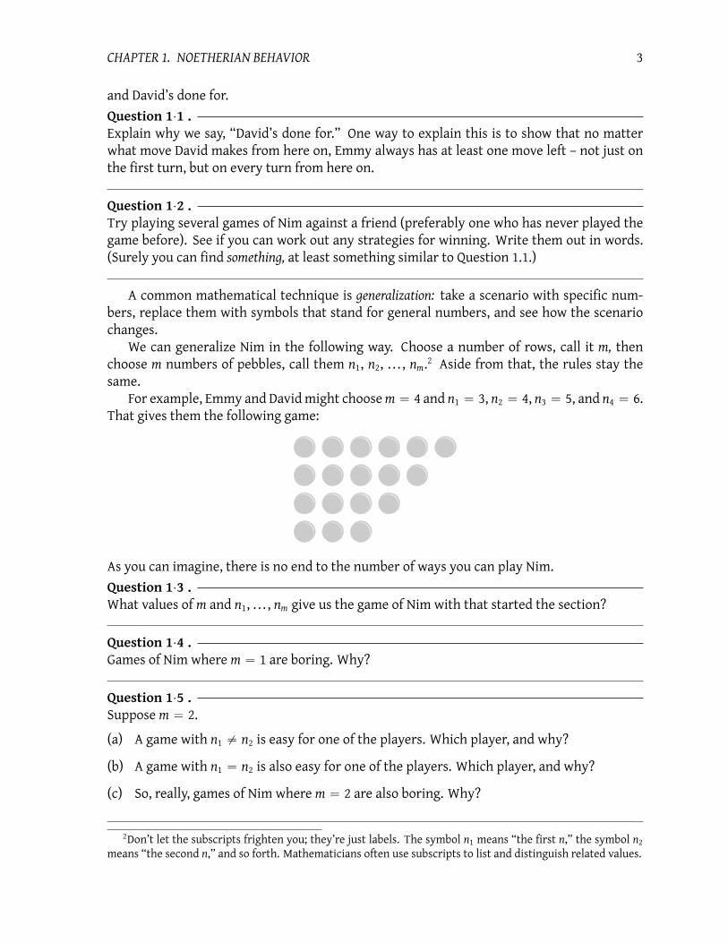
For example, Emmy and David might choosem “ 4 and n1 “ 3, n2 “ 4, n3 “ 5, and n4 “ 6.
That gives them the following game:
As you can imagine, there is no end to the number of ways you can play Nim.
Question 1¨3 .What values of m and n1, . . . , nm give us the game of Nim with that started the section?
Question 1¨4 .Games of Nim where m “ 1 are boring. Why?
Question 1¨5 .Suppose m “ 2.
(a) A game with n1 ‰ n2 is easy for one of the players. Which player, and why?
(b) A game with n1 “ n2 is also easy for one of the players. Which player, and why?
(c) So, really, games of Nim where m “ 2 are also boring. Why?
2Don’t let the subscripts frighten you; they’re just labels. The symbol n1 means “the first n,” the symbol n2
means “the second n,” and so forth. Mathematicians often use subscripts to list and distinguish related values.

CHAPTER 1. NOETHERIAN BEHAVIOR 4
Question 1¨6 .Suppose m ą 2 and ni “ nj for some i, j where i ‰ j.
(a) What do we mean by the phrase “m ą 2 and ni “ nj for some i, j where i ‰ j?” Try to
explain without using the symbols n, i, or j.
(b) With the given assumption, a player trying to decide on a good move might as well con-
sider rows i and j to be have been completely played out already. Why?
Question 1¨7 .Suppose you generalize Nim further by letting a row of pebbles extend without end to the
right. When this happens, we’ll say3
the number of pebbles in the row is ω. For example, the
Nim game with m “ 3 and n1 “ 3, n2 “ 5, and n3 “ ω would look like this:
Is it possible to play such a game indefinitely, making turns so that it never ends? If so, de-
scribe a sequence of moves that would never end. If, however, this is impossible, explain why.
Ideal Nim
Ideal Nim is another generalization of Nim. The playing board consists of points with
integer values in the first quadrant of the x-y axis. Choose a few4
points for a set F. Any point
not northeast of at least one point in F lies within a Forbidden Frontier. Shade those points
red. More precisely, pc, dq is red if for each pa, bq P F, we have 0 ď c ă a or 0 ď d ă b. There
is also a gray region G, which is “Gone from Gameplay,” but it begins empty.
Players take turns doing the following:
1. Choose a point pa, bq that is in neither the Forbidden Frontier, nor Gone from Gameplay.
2. Add to G the region of points pc, dq that are northeast of pa, bq. More precisely, add to G
all points pc, dq that satisfy c ě a and d ě b.
The player who makes the last move wins.
3The last symbol in this sentence is a letter in the Greek alphabet called “omega,” not the letter w in the
“Latin” alphabet. The letter ω will show up repeatedly in these notes, often with very different meanings, and
the letter w will show up, also with different meanings, so be careful.4Not too many points, nor too large in value. Certainly not infinitely many. It doesn’t change the properties
of the game, but you’d waste an awwwwful lot of time trying to figure out the gameplay.

CHAPTER 1. NOETHERIAN BEHAVIOR 5
In the example below, Emmy and David have chosen the points p0, 3q, p1, 2q, p4, 1q, and
p5, 0q for F. Emmy chose the position p3, 2q on her first turn; David chose p2, 5q on his first
turn; and Emmy chose p8, 0q on her second turn.
Don’t overlook a difference in the definition of the regions. Players may choose a point on
the border of the Forbidden Frontier; such points are northeast of a point in F. They may not
choose a point on the border of the region Gone from Gameplay, as such points are considered
northeast of G, and thus in G. So, Emmy was allowed to choose the point p3, 2q, which borders
the red region, but may not now choose the point p3, 3q, because it borders the current gray
region. She could, of course, choose the point p2, 2q, or even the point p1, 2q, as they border
the red region, but not the gray.5
When playing this game, certain questions might arise. They may not seem mathematical,
but all of them are! In fact, all of them are related to algebraic ideas!
• Must the game end? or is it possible to have a game that continues indefinitely? Why,
or why not? Does the answer change if we play in three dimensions, or more?
• Is there a way to count the number of moves available, even when there are infinitely
many?
• What strategy wins the game?
We consider these questions (and more!) throughout the text. We will not be able to answer
all of them; at least one is an open research question.6
Maybe you can solve them someday.
You should take from this introduction three main points.
• Mathematics can apply to problems that do not appear mathematical.
• Questions that seem unrelated to mathematics can be very important for mathematics.7
• It is a very, very good thing to ask questions!
5The game can be played so that players may not dance along the Forbidden Frontier, but then we’d have to
interpret the word “northeast” differently for this region than for the other.6An amazing aspect of mathematics is that simple questions can lead to profound results in research!
7This is not the same as the previous point. Make sure you understand why.

CHAPTER 1. NOETHERIAN BEHAVIOR 6
Meanwhile, play the game! A few example games appear below to help you along; some of
them will be “partially” played.
But don’t play thoughtlessly. As a student of mathematics, you should prepare yourself to
think carefully and precisely. Intuition and insight are good and necessary, but deduction and
dogged determination are no less required. When someone wins, talk about which moves
seemed “obvious,” and think about the strategy used. With enough effort, you should find a
winning strategy for all the games given, but don’t feel bad if you don’t.
Your explanations to the questions need not look “mathematical”, but they should be yours,
and they should be convincing, or at least reasonable. If you can formulate reasonable answers,
you will have succeeded at important tasks that helped solve important problems in mathe-
matics. That’s no small feat for someone just starting out in algebra!
Question 1¨8 .Play the following games with a friend. If you play carefully, you should find that Emmy (the
starting player) is guaranteed a win for each game.
Question 1¨9 .What characteristic do all the games in Question 1.8 share? How does that characteristic
guarantee Emmy a win? Hint: Think geometrically.
Question 1¨10 .Play the following games with a friend. They have already been partially played. It is Emmy’s
turn, but this time David is guaranteed a win for each game. Try to find how.
Question 1¨11 .What characteristic do all the games in Question 1.10 share? How does that characteristic
guarantee David a win? Hint: Think geometrically.
CHAPTER 1. NOETHERIAN BEHAVIOR 7
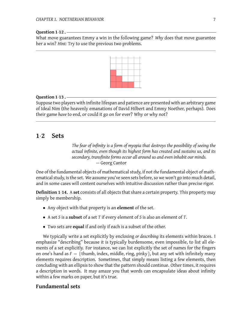
Question 1¨12 .What move guarantees Emmy a win in the following game? Why does that move guarantee
her a win? Hint: Try to use the previous two problems.
Question 1¨13 .Suppose two players with infinite lifespan and patience are presented with an arbitrary game
of Ideal Nim (the heavenly emanations of David Hilbert and Emmy Noether, perhaps). Does
their game have to end, or could it go on for ever? Why or why not?
1¨2 SetsThe fear of infinity is a form of myopia that destroys the possibility of seeing the
actual infinite, even though its highest form has created and sustains us, and its
secondary, transfinite forms occur all around us and even inhabit our minds.
— Georg Cantor
One of the fundamental objects of mathematical study, if not the fundamental object of math-
ematical study, is the set. We assume you’ve seen sets before, so we won’t go into much detail,
and in some cases will content ourselves with intuitive discussion rather than precise rigor.
Definition 1¨14. A set consists of all objects that share a certain property. This property may
simply be membership.
• Any object with that property is an element of the set.
• A set S is a subset of a set T if every element of S is also an element of T.
• Two sets are equal if and only if each is a subset of the other.
We typically write a set explicitly by enclosing or describing its elements within braces. I
emphasize “describing” because it is typically burdensome, even impossible, to list all ele-
ments of a set explicitly. For instance, we can list explicitly the set of names for the fingers
on one’s hand as F “ tthumb, index, middle, ring, pinkyu, but any set with infinitely many
elements requires description. Sometimes, that simply means listing a few elements, then
concluding with an ellipsis to show that the pattern should continue. Other times, it requires
a description in words. It may amaze you that words can encapsulate ideas about infinity
within a few marks on paper, but it’s true.
Fundamental sets

CHAPTER 1. NOETHERIAN BEHAVIOR 8
The fact that they are “fundamental” is a pretty big hint that you’ll need to remember the
following sets.
• The set of natural numbers is8
N “ t0, 1, 2, 3, . . . u .
The funny-looking N is a standard symbol to represent the natural numbers; the style
is called “blackboard bold”.9
• Since even a small plus sign can make a big difference, we adopt a similar symbol for
the set of positive numbersN` “ t1, 2, 3, . . . u .
The set of integers is
Z “ t. . . ,´2,´1, 0, 1, 2, . . . u .
We can also define it in set-builder notation,
Z “ NY t´x : x P Nu .
Don’t pass over that set-builder notation too quickly. Take a moment to decipher it, as this
notation pops up from time to time. Don’t let it intimidate you! The world is a complex place,
and it’s amazing how a good choice of words can simplify complexity.10
Transliterated, the
set-builder definition says,
The set of integers (Z) is (“) the union (Y) of the naturals (N) and
the set of elements (t. . . u) that are the opposite (´x) of any natural number (: x P N).
Translated, the integers are the union of the naturals with their opposites.
Some readers might think it clearer to write, “Z “ N Y p´Nq”, and I suppose we could
have, but then we’d have to explain what´N means, because that construction won’t always
make obvious sense. (Think about´F, where F is the set of fingers.) In fact, some authors use
´S to mean the complement of S, which you may have seen as„S or Sc, something completely
different from “the set of negatives.” Not everyone writes mathematics the same way.
Elements of a set can appear in other sets, as well; when all elements of one set appear
in another, the first is a subset of the second. When S is a subset of T, we write S Ď T; the
bottom bar emphasizes that a subset can equal its containers, in the same way thatď applies
to two equal numbers. You can chain these, so our fundamental sets so far satisfy
N` Ď N Ď Z.8Not everyone starts N with 0, and some authors refer to t0, 1, 2, 3, . . . u as the “whole numbers”. While this
can be confusing, it’s not uncommon, and highlights how you have to pay careful attention to definitions.9I’ve read somewhere (can’t remember where) that textbooks originally indicated these sets with bold char-
acters. Professors can’t write bold at the blackboard, or at least not easily, so they resorted to doubling the
letters. Textbooks nowadays have adopted the professors’ notation.10
“Brevity is the soul of wit.” — Shakespeare, Hamlet

CHAPTER 1. NOETHERIAN BEHAVIOR 9
When we know a subset S is not equal to its container T, and we want to emphasize this, we
cross out the bottom bar and write S Ĺ T.11
You can chain these, as well, so that
N` Ĺ N Ĺ Z.
Subsets of this latter variety are called proper subsets. Don’t confuse this with S Ę T, which
means that S is not a subset of T. This happens when at least one element of S is not in T,
whereas S Ĺ T means every element of S is in T, but at least one element of T is not in S.
Set arithmetic
We assume you’ve seen unions and intersections. We can define them with set-builder
notation:
SY T “ tx : x P S or x P Tu ;
SX T “ tx : x P S and x P Tu .
You may not have seen set difference; the difference of S and T is the set of elements in A
that are not in B. That is,
SzT “ ts P S : s R Tu .
For example, we could describe the set of negative numbers as ZzN.
A very useful construction is the Cartesian product, which creates new objects from two
sets, in the form of a sequence of two elements:
Sˆ T “ tps, tq : s P S and t P Tu .
You’ve already see an example of this; the playing field of Ideal Nim isNˆN, since any position
is a point “with integer values in the first quadrant of the x-y axis.” Points are pairs pa, bq, and
the qualified, “the first quadrant,” tells us that both a, b P N. The set N ˆ N is important
enough to remember by a name, and will appear again (at least when we play the game) so
we will call it the natural lattice, or just the lattice when we’re feeling a bit lazy, which we
usually are, since in any case we don’t typically deal with other lattices in this text.
Question 1¨15 .Suppose S “ t1, 3, 5, 7u, T “ t2, 4, 6, 8u, and U “ t3, 4, 5, 6u. Construct (a) S Y T, (b) S X T, (c)
pSY Tq zU, and (d) Sˆ T.
A “real-life” example of a Cartesian product that the author is all too familiar with is the
absent-minded tic of touching a hand’s fingers to each other. (Guess what I was doing a few
moments ago.) Each touch is a pairing of fingers, such as pthumb, middleq or ppinky, pinkyq.
Inasmuch as pairings correlate to Cartesian products, we can describe the pairings of all fin-
gers as F ˆ F, where F is again the set of all fingers.
Question 1¨16 .How large is F ˆ F? That is, how many elements does it have?
11Some authors useĂ, but other authors useĂ when the two sets are equal, so we avoidĂ altogether.

CHAPTER 1. NOETHERIAN BEHAVIOR 10
Question 1¨17 .If a set S has m elements and a set T has n elements, how many elements will S ˆ T have?
Explain why.
If S “ T, we can write S2
instead of SˆT. Hence we can abbreviate the lattice of Ideal Nim
as N2.
When needed, we can chain sets in the Cartesian product to make sequences longer than
mere pairs; we can even describe all infinite sequences of integers as
Z8 “8ź
i“1
Z “ Zˆ Zˆ Zˆ ¨ ¨ ¨ “ tpa, b, c, . . . q : a, b, c, . . . P Zu .
That new symbol,ś
, means “product”, much as Σ means “sum”. Writing phrases like “the
first element of P” or “the four hundred twenty-fifth element of P” all the time grows cum-
bersome, so we’ll adopt the convention that if P is a sequence of numbers, then pi will stand
for the ith element of P. For example, if P “ p5, 8, 3,´2q then p1 “ 5 and p4 “ ´2.
Definition 1¨18. Two sets S and T have the same size (or cardinality) if you can match each
element of S to a unique element of T, covering all the elements of T in the process. More
precisely, S and T have the same cardinality if you can create a mapping from S to T where
• each element of Smaps to a unique element of T (so the function is one-to-one), and
• for any element of T, you can find an element of S that maps there (so the function is
onto).
For example, the sets A “ t1, 2u and B “ t´1,´2u have the same cardinality because I
can match them as follows, while the sets C “ t1, 2, 3u and D “ t4, 5u do not, because I cannot
find a unique target for at least one element of C:
A B C D
1 // ´1 1 // 4
2 // ´2 2 // 5
3 // ?
CHAPTER 1. NOETHERIAN BEHAVIOR 11
Question 1¨19 .
(a) Show that S and T of Question 1.15 have the same cardinality. Don’t just count the ele-
ments; exhibit a unique matching. Is there more than one matching? If so, list a couple
more. How many do you think there are?
(b) Show that E “ t0, 2, 4, 6, . . . u and O “ t1, 3, 5, 7, . . . u have the same cardinality. In this
case, the number of elements is infinite, so you can’t count them, nor draw a complete
picture, so use words to describe the matching, or even a formula.
(c) Show that an arbitrary set S has the same size as itself. This may seem silly, but it forces
you to think about using the definition of cardinality, since you don’t know what the ele-
ments of S are. Don’t forget to think about the case where S is empty.
(d) Show that N and Z have the same cardinality. It helps if you map negative integers to Oand positive integers to E. This is a little weird, because N Ĺ Z, so you wouldn’t expect
them to be the same size, but weird things do happen when you start mucking around in
infinite sets.
1¨3 Orderings
The mathematical sciences particularly exhibit order, symmetry, and limitation;
and these are the greatest forms of the beautiful.
— Aristotle
A relation between two sets S and T is a subset of Sˆ T. For instance, the pairings of fingers
is a relation on F ˆ F, where the set of fingers, while Sˆ T is itself a relation.
A function is any relation F Ĺ S ˆ T such that every s P S corresponds to exactly one
ps, tq P F. Put another way, any two pa, bq and pc, dq in F satisfy a ‰ c (but b “ d is okay). If F is
a function, we write F : SÑ T instead of F Ď Sˆ T, and F psq “ t instead of ps, tq P F.
Two kinds of relations are essential to algebra. The first is a homomorphism, which is a
special kind of function; we talk about those later on, so pretend I didn’t mention them for
now. The second is a special subset of Sˆ S, called an ordering on S. There are several types
of orderings, so it’s important to make precise the kind of ordering you mean.
Partial orderings
A partial ordering on S is an ordering P that satisfies three properties. Let a, b, c P S be
arbitrary.
Reflexive? Every element is related to itself; that is, pa, aq P P.
Antisymmetric? Symmetry implies equality; that is, if pa, bq P P and pb, aq P P, then a “ b.

CHAPTER 1. NOETHERIAN BEHAVIOR 12
Transitive? If pa, bq P P and pb, cq P P, then pa, cq P P.
Suppose we let P be the ordering of your fingers from left to right, or in set-builder notation,
P “ tpx, yq P F ˆ F : x lies to the left of yu .
Then pthumb,middleq P P and pring,pinkyq P P but pindex,indexq R P. This is a partial order-
ing.
It is highly inconvenient to write orderings this way, so usually mathematicians adopt a
notation involving “ordering symbols” such as ď, ă, and so forth. This allows us to write
pa, bq P P more simply as a ă b, and we will do this from now on. That allows us to rewrite
the properties of a partial ordering as follows, using ĺ as our ordering:
Reflexive? a ĺ a.
Antisymmetric? If a ĺ b and b ĺ a, then a “ b.
Transitive? If a ĺ b and b ĺ c, then a ĺ c.
Now that things are a little easier to read, we introduce a few important orderings.
One example of a partial ordering is in the subset relation. If we fix a set S, then we can
viewĎ as a relation on the subsets of S. For instance, if S “ N then t1, 3u is “less than” t1, 3, 7u
inasmuch as t1, 3u Ď t1, 3, 7u.
Definition 1¨20. For any set S, let P pSq denote the set of all subsets of S. We call this the
power set of S.
Fact 1¨21. Let S be any set. The relation on P pSq defined byĎ is a partial ordering.
Why? Let A, B P P pSq. We need to show that Ď satisfies the three properties of a partial
ordering.
Reflexive? Certainly A Ď A, since any a P A is by definition an element of A. So Ď is
reflexive.
Antisymmetric? Assume A Ď B and B Ď A. By definition of set equality, A “ B.
Transitive? Assume A Ď B and B Ď C. We want to show A Ď C. The definition ofĎ tells us
this is true if every a P A is also in C, so let a P A be arbitrary. We know A Ď B, so by definition
a P B. We know B Ď C, so by definition a P C. Since a was arbitrary, A Ď C, as desired.
Next we look at the ordering you’re most accustomed to.
Definition 1¨22 (The natural ordering of Z). For any a, b P Z, we write a ď b if b´ a P N. We
can also write b ě a for this situation. If a ď b but a ‰ b, we write a ă b, or b ą a.
Figure 1¨1 illustrates this relationship by for the relation x ď y on N by plotting on the
lattice the elements of the set ď. Elements of ď are the black points whose y-value equals
or exceeds the x-value. White points are not in the set O. It’s worth asking yourself: which
ordering do those white points describe?
Fact 1¨23. The natural ordering of Z is a partial ordering.

CHAPTER 1. NOETHERIAN BEHAVIOR 13
Figure 1¨1: Diagram of the relationď on N.
Question 1¨24 .Fill in the blanks of Figure 1¨2 to show why Fact 1¨23 is true.
In the future, you can think of theď ordering in the intuitive manner you’re accustomed
to. Use it to answer the following questions.
Question 1¨25 .One of our claims in the proof amounts is equivalent to saying that if i, s, t P Z, then s ď t if
and only if s` i ď t ` i. Why is this true?
Question 1¨26 .Show that a ď |a| for all a P Z. Hint: You need to consider two cases: one where |a| “ a, the
other where |a| “ ´a. (Yes, the second case is quite possible! Look at some “small” integers
to see why.)
Question 1¨27 .Let a, b P N and assume that 0 ă a ă b. Let d “ b´ a. Show that d ă b.
Question 1¨28 .Let a, b, c P Z and assume that a ď b. Prove that
(a) a` c ď b` c;
(b) if c P N, then a ď a` c;
(c) if c P N, then ac ď bc; and
(d) if c P N` and also a P N`, then c ď ac.
What about the lattice?
Definition 1¨29 (The x-axis, y-axis, and lex orderings of the lattice). For any P, Q P N2, we
write
• P ăx Q if p1 ă q1;

CHAPTER 1. NOETHERIAN BEHAVIOR 14
Claim: The natural ordering of Z is a partial ordering.
Proof:
1. We claim thatď is reflexive. To see why, let a P Z.
(a) Observe that a´ a “____.
(b) This difference is an element of ____.
(c) By definition, a ď a.
(d) We chose a from Z arbitrarily, so this is true of ____ element of Z.
2. We claim thatď is antisymmetric. To see why, let a, b P Z.
(a) Assume that a ď b and ____.
(b) By definition, b´ a P N and ____.
(c) By the distributive property,´pb´ aq “____. (Write it as subtraction.)
(d) In (b), we explained that b´ a P N. In (c), we showed that´pb´ aq P N. The only
natural number whose opposite is also natural is ____.
(e) By substitution, b´ a “____.
(f) By definition, a “ b.
(g) We chose a and b from Z arbitrarily, so this is true of ____ pair of elements of Z.
3. We claim thatď is transitive. To see why, let a, b, c P Z.
(a) Assume that a ď b and ____.
(b) By definition, b´ a P N and ____.
(c) Elementary properties of arithmetic tell us that ____+____“ c ´ a.
(d) The sum of any two natural numbers is ____.
(e) By (c) and (d), then, c ´ a P____.
(f) By definition, ____.
(g) We chose a, b, and c from Z arbitrarily, so this is true of any three elements of Z.
Figure 1¨2: Material for Question 1.24

CHAPTER 1. NOETHERIAN BEHAVIOR 15
??
?
The ordering ăx judges
one point smaller than
another if the first is fur-
ther left. If the two
points are on the same
vertical line (p1 “ q1), it
makes no decision.
The ordering ăy judges
one point smaller than
another if the first is
below the second. If
the two points lie on
the same horizontal line
pp2 “ q2q, it makes no de-
cision.
The ordering ălex judges
one point smaller than
another if the first is fur-
ther left. If the two
points are on the same
vertical line, it judges the
lower point smaller.
Figure 1¨3: Diagrams of the lattice orderingsăx,ăy, andălex. Arrows point from larger points
to smaller ones.
• P ăy Q if p2 ă q2;
• P ălex Q if p1 ă q2, or if p1 “ q1 and q1 ă q2.
We also write P ĺx Q, Q ąx P, Q ľx P with meaning analogous toď, ą, andě; that is, P ĺx Q
if P ĺx Q or P “ Q, and so forth.
These orderings have natural visualizations; see Figure 1¨3.
Question 1¨30 .Order each set of lattice points according to the ăx, ăy, and ălex orderings. Indicate when
the ordering cannot decide which of two points is smaller.
(a) tp7, 2q , p1, 3q , p0, 8q , p2, 2qu
(b) tp2, 4q , p1, 5q , p5, 1q , p0, 6qu
The first question we want to consider is whether the orderings are partial orderings.
Determining whether an object has a certain property is very important in mathematics; ex-
plaining why it has that property is fundamental. Let’s consider that a moment.
Theorem 1¨31. The ordering ĺlex is a partial ordering of the lattice. The orderings ĺx and ĺy are
not.12
12As you should know, a theorem asserts that a claim is always true. This is also true about lemmas, propo-
sitions and facts. Most of the assumptions involved are implicit rather than explicit. If we cannot explain
convincingly that a claim is always true, we call it a conjecture. If you get far enough in your studies, you’ll find
that a lot of conjectures are themselves widely believed, though remain unproven, and mathematicians use in
day-to-day life. Students, however, are not generally allowed to do this on purpose!

CHAPTER 1. NOETHERIAN BEHAVIOR 16
Proof. Let P, Q, R P N2.
Reflexive? It is easy to verify that P ĺx P, P ĺy P, and P ĺlex P, so the orderings are reflexive.
Antisymmetric? Suppose P ĺlex Q and Q ĺlex P. By definition of the ordering, p1 ă q1 or
p1 “ q1 and p2 ď q2. Similarly, Q ĺlex P gives q1 ă p1 or q1 “ p1 and q2 ď p2. We consider
several cases. If p1 ă q1, then Q łlex P, contradicting a hypothesis. Similarly, if q1 ă p1,
then P łlex Q, contradicting a hypothesis. That leaves p1 “ q1 and p2 ď q2 and q2 ď p2. By
antisymmetry of the natural ordering, p2 “ q2, so P “ Q.
As for ĺx and ĺy, antisymmetry is the property they both fail. We leave it to you to find a
counterexample.
Transitive? Suppose P ĺx Q and Q ĺx R. Then p1 ď q1 and q1 ď r1. As in the antisymmetric
case, previous work implies p1 ď r1, so P ĺx Q. We assumed that P ĺx Q and Q ĺx R and found
that P ĺx R, so ĺx is transitive. A similar argument shows that ĺy and ĺlex are transitive.
Question 1¨32 .
(a) In the proof of Theorem 1¨31, we claimed that neither ĺx nor ĺy are antisymmetric. To
verify this claim, find P, Q P N2such that P ĺx Q and Q ĺx P, but P ‰ Q.
(b) In the proof of Theorem 1¨31, we claimed that the reason ĺx is transitive is similar to the
reasons ĺy and ĺlex are transitive. Show this explicitly for ĺlex.
Question 1¨33 .Define an ordering ĺx,y on N2
as follows. We say that P ĺx,y Q if p1 ď q1 and p2 ď q2. Is this a
partial ordering? Why or why not?
Question 1¨34 .Define an orderingăsums as follows. We say that P ăsums Q if p1`p2 ă q1`q2 or p1`p2 “ q1`q2
and p1 ă q1.
(a) Order each set of lattice points according to the ăx, ăy, and ălex orderings. Indicate
when the ordering cannot decide which of two points is smaller.
(i) tp7, 2q , p1, 3q , p0, 8q , p2, 2qu
(ii) tp2, 4q , p1, 5q , p5, 1q , p0, 6qu
(b) Is ăsums a partial ordering? Why or why not?
Hint: Try to look at it geometrically. In the spirit of Figure 1¨3, pick a not-too-large point
P, then determine which points are smaller than P.
Linear orderings
You can see from Figure 1¨3 that there is some ambiguity in the first two orderings, but not
in the last one — or not with the points diagrammed, at any rate. The absence of ambiguity
is always useful.

CHAPTER 1. NOETHERIAN BEHAVIOR 17
Definition 1¨35. An ordering ĺ on a set S is linear if for any s, t P S we can decide whether
s ĺ t or t ĺ s (or both).
Fact 1¨36. The orderingď on N is linear.
Why? Subtraction of naturals gives us an integer, and the opposite of a non-natural integer is a
natural integer. So, for anym, n P N, we know that eitherm´n P N or n´m “ ´pm´ nq P N.
In other words, either n ď m or m ď n.
We can extend the orderingď on N to an ordering on Z by using the same definition. For
example, we can argue that ´5 ď 3 because 3 ´ p´5q “ 8, and 8 is natural. On the other
hand,´10 ę ´15 because´15´ p´10q, and´5 is not natural.
Fact 1¨37. The orderingď on Z is also linear.
The reasoning is identical, so we omit it.
Question 1¨38 .Show that the ordering ă of Z generalizes “naturally” to an ordering ă of Q that is also a
linear ordering. Hint: Think of how you would decide that 2435 ă 2028, or that 351 ă 453, and
go from there.
On the other hand, the orderings ĺx and ĺy are not linear, since ĺx cannot decide if
p4, 1q ĺ p4, 3q or p4, 3q ĺ p4, 1q, and ĺy cannot decide if p1, 3q ĺ p4, 3q or p4, 3q ĺ p1, 3q.
The lex ordering is able to sort the points diagrammed in Figure 1¨3, but is this true for
any set of points?
Theorem 1¨39. The lex ordering is a linear ordering on the lattice.
Proof. Let P, Q P N2. If p1 ă q1, then P ĺlex Q, and we are done. If p1 ą q1, then Q ĺlex P, and
we are done. So suppose that p1 “ q1; we consider p2 and q2, instead. If p2 ă q2, then P ĺlex Q,
and we are done. If p2 ą q2, then Q ĺlex P, and we are done. So suppose that p2 “ q2. We
now have p1 “ q1 and p2 “ q2, so P “ Q. This satisfies the definition of P ĺlex Q, so we are
done.
Question 1¨40 .In the proof of Theorem 1¨39, we used implicitly the fact that ď is a linear ordering of the
natural numbers. We really ought to give some flesh to that argument, so fill in the blanks of
Figure with the correct reasons. (Notice that we actually prove it for Z, a superset of N. This
automatically proves it for N. It is often a good idea to prove a fact for a superset, if you can
succeed at doing so.)
Question 1¨41 .Is the ordering ĺx,y of Question 1.33 a linear ordering? Why or why not?

CHAPTER 1. NOETHERIAN BEHAVIOR 18
Let a, b P Z.
1. Suppose b´ a P N. By ______, a ď b.
2. Otherwise, b´a R N. We know from previous work that b´a P Z. That means
´pb´ aq P ______.
(a) By ______,´pb´ aq “ a´ b.
(b) By ______, a´ b P N.
(c) By ______, b ď a.
3. We assume that a, b P Z, and showed that a ď b or b ď a. By ______, we are
done.
Figure 1¨4: “Flesh” for Question 1.40.
Question 1¨42 .Is ăsums a linear ordering? Why or why not? Hint: Try to look at it geometrically. In the spirit
of Figure 1¨3, pick a not-too-large point P, then figure out which points are smaller than P,
shade that region, then ask yourself: “Do I know that all the unshaded points must be larger
than P?” That should give you some insight into how to answer the question.
1¨4 Well ordering and division
Can you do division? Divide a loaf by a knife — what’s the answer to that?
— Lewis Carroll
Well ordering
You know from experience that the ordering ď has a smallest element in N; namely, 0.
Rather interestingly, every subset of N has a smallest element. There is no largest element,
but The fact that any subset of N has a smallest element is very interesting.
Definition 1¨43. Awell ordering on a set S is a linear ordering on S for which each subset of
S has a smallest element.
You might assume that we are going to prove that N is well-ordered by ď, and in a way
we will, but in another way we won’t.
Axiom 1¨44 (The Well-Ordering Principle). N is well-ordered byď.
An “Axiom” is a statement you assume without proof. So, we are only going to assume this
property. In fact, it is impossible to prove it, unless you assume something else.
That “something else” is the proof-by-dominoes technique, also called induction.

CHAPTER 1. NOETHERIAN BEHAVIOR 19
Axiom 1¨45 (The Induction Principle). Let S be a subset ofN that satisfies the following properties.
(inductive base) 0 P S; and
(inductive step) for any s P S, we also have s` 1 P S.
Then S “ N.
Now, why should induction be true? You can’t prove that, unless you assume the well-
ordering of N. Do you see where this is going?
Fact 1¨46. Axiom 1¨44 is logically equivalent to Axiom 1¨45; that is, you can’t have one without the
other.
We put off an actual proof of this to the end of the section, and in fact you need not con-
cern yourself too much with it. Typically you won’t read that in this text, and I’m afraid that
you can’t appeal to such a judge yourself, but believe you me, this has been something mathe-
maticians hashed out pretty thoroughly in the early 20th century. Some things you just have
to accept on faith — which, contrary to popular belief, is not the opposite of reason, since
these things work out pretty well in practice, and it’s pretty reasonable to infer that things
that work out in practice really are true.
Example 1¨47. We will define a different ordering ĺ on N according to the following rule:
• even numbers are always smaller than odd numbers;
• otherwise, if a and b are both even or both odd, then a ĺ b if and only if a ď b in the
natural ordering.
This ordering sorts the natural numbers roughly so:
0, 2, 4, 6, . . . , 1, 3, 5, 7, . . . .
Is ĺ a well ordering? Indeed it is. Why?
First we show ĺ is a partial ordering:
• Is the ordering reflexive? Let a P N; we need to show that a ĺ a. We use the second
part of the rule here, since b “ a: since a ď a in the natural ordering, a ĺ a.
• Is the ordering symmetric? Let a, b P N, and assume a ĺ b and b ĺ a. If both numbers
are even or both numbers are odd, then our rule tells us a ď b and b ď a in the natural
ordering; since that is symmetric, we infer a “ b. Otherwise, a ĺ b implies a is even
while b is odd, whereas b ĺ a implies a is odd while b is even. That is a contradiction,
so a “ b is indeed the only possibility.
• Is the ordering transitive? Let a, b, c P N, and assume a ĺ b and b ĺ c. We consider
several subcases:

CHAPTER 1. NOETHERIAN BEHAVIOR 20
– a even?
Either c is odd, in which case a ĺ c, or c is even. If c is even, then b must also
be even; to be otherwise would contradict b ĺ c. All three numbers are even, in
which case our ordering tells us the natural ordering applies: a ď b and b ď c.
The natural ordering is transitive, so a ď c.
– a odd?
In this case, a ĺ b implies b is odd, and b ĺ c implies c is odd. All three numbers
are odd, in which case our ordering tells us the natural ordering applies: a ď b
and b ď c. The natural ordering is transitive, so a ď c.
Now we show ĺ is a linear ordering. Let a, b P N; we need to show that a ĺ b or b ĺ a.
Without loss of generality, we may assume that a is even. If b is odd then our rule tells us
a ĺ b, and we are done. Otherwise, b is even; in this case, our rule tells us to look at the
natural ordering. The natural ordering is linear, so a ď b or b ď a. By the definition of our
rule, then, a ĺ b or b ĺ a.
Finally, we show ĺ is a well ordering. Let S Ď N; we need to show that S has a least
element. Let E be the set of even elements of S, and O the set of odd elements. Observe that
E, O Ĺ N.
• If E ‰ H, the well-ordering property tells us that it has a least element; call it e. Let
s P S; if s is even, then s P E and by our choice of e, e ď s, so e ĺ s; otherwise, s is odd,
and our rule tells us e ĺ s.
• Otherwise, E “ H. The well-ordering property tells us that O has a least element; call
it o. Let s P S; if s is even, then s P E, a contradiction to E “ H, so s is odd, which puts
s P O, and by our choice of o, o ď s, so o ĺ s.
As S was an arbitrary subset of N, and we found a smallest element with respect to the new
ordering, every subset of N has a smallest element with respect to the new ordering.
What about the set Z? The ordering ď has neither smallest nor largest element, since
¨ ¨ ¨ ď ´3 ď ´2 ď ´1 ď 0 ď 1 ď ¨ ¨ ¨ . It is possible to order Z a different way, so that it
does have a smallest element, and in some cases that might be useful. That’s an interesting
question to ponder, and we leave it to you to pursue.
Question 1¨48 .Devise a different ordering of Z for which every subset of Z has a smallest element. Call this
orderingÌ, and prove that it really is a well ordering on Z.
So the definition depends on both the ordering and the set; change one of the two, and
the property may fail.
Let’s turn to a different set, the lattice N2. We have three different orderings to choose
from; we’ll start withĺx. Do subsets ofN2necessarily have smallest elements? Clearly not, as
ĺx is not even a linear ordering! We already saw that ĺx fails to order two points on a vertical
line, such as p2, 0q and p2, 1q. Elements like these are incomparable, so subsets containing
them lack a smallest element.

CHAPTER 1. NOETHERIAN BEHAVIOR 21
What if we try a different ordering? Again, ĺy is not linear, so that’s out. On the other
hand, ĺlex is linear, so it stands a chance of being a well-ordering.
Question 1¨49 .Show that the lex orderingĺlex is a well ordering of the latticeN2
. Hint: Use the Well-Ordering
Principle in one dimension to find a subset of elements that are smallest from a particular
point of view. Then use the Well-Ordering Principle in the other dimension to polish it off.
Question 1¨50 .While Question 1.49 refers to a two-dimensional lattice, explain that it doesn’t really matter;
you can use the same basic proof to show that Nnis well-ordered by a similar ordering. Also
describe the ordering.
Here’s another useful consequence of well ordering.
Fact 1¨51. Let S be a set well ordered byĺ, and s1 ľ s2 ľ ¨ ¨ ¨ be a nonincreasing sequence of elements
of S. The sequence eventually stabilizes; that is, at some index i, si “ si`1 “ ¨ ¨ ¨ .
Why? Let T “ ts1, s2, . . . u. By definition, T Ď S. By the definition of a well-ordering, S has
a least element; call it t. Let i P N` such that si “ t, and let j ą i. The sequence decreases,
which means si ľ sj. By substitution, t ľ sj. Remember that t is the smallest element of T; by
definition, sj ľ t. We have t ľ sj ľ t, which is possible only if t “ sj. We chose j ą i arbitrarily,
so every element of the sequence after t must equal t. In other words, si “ si`1 “ ¨ ¨ ¨ , as
claimed.
Question 1¨52 .We asserted that t ľ sj ľ t “is possible only if t “ sj.” This isn’t necessarily obvious, but
it is true. Why ? Hint: It’s one of the properties of the ordering. As to which property, you
may need to look further afield than the properties of well orderings; remember that a well
ordering is also a linear ordering, which is also a partial ordering. Those three give you a few
properties to consider!
We can use this fact to show one of the desired properties of the game.
Dickson’s Lemma. Ideal Nim terminates after finitely many moves.13
Before going into the details, let’s point out a basic, geometrically intuitive argument.
Let P “ pa, bq be the first position chosen, and Q1, Q2, . . . the subsequent positions chosen.
According to the rules, no move Q “ pc, dq can satisfy c ě a and d ě b, so c ă a or d ă b. In
the first case, Q is closer to the x-axis than P, or, Q ăx P. The set of their x-coordinates would
be a nonincreasing sequence of natural numbers, which allows us to apply Fact 1¨51. In the
second case, Q is closer to the y-axis than P, or, Q ăy P. That also allows us to apply Fact 1¨51.
Superficially, then, it looks as if only finitely many moves are possible. However, if we
play enough games, we see that players can sometimes choose positions Q1, Q2, . . . such that
Q1 ąx Q2 ¨ ¨ ¨ ąx Qi, but Qi ăx Qi`1. If Qj ąy Qi`1 for each j “ 1, 2, . . . , i, then, as mentioned
13Dickson actually proved an equivalent statement.

CHAPTER 1. NOETHERIAN BEHAVIOR 22
already, we’re dealing with Fact 1¨51. As long as we’re dealing with one of the two cases, we
can see that the game is ending.
What if some Qj ăy Qi`1? In this case, Qi`1 decreases neither the minimum x-coordinate
nor the minimum y-coordinate, and the chain is no longer a nondecreasing sequence. This is
really a temporary problem, though; sketch such a game on paper, and we see that any such
Qi`1 must lie in a rectangle:
min x valueQi
min y valueQi
This rectangle has only finitely many positions, and that finiteness means the players will
eventually have to break out, at which point either the smallest x-value or the smallest y-
value will decrease anew. Writing this precisely is a bit of a bear, but intuitively, it works
well.
That said, it’s simpler to try the following approach, which works both intuitively and
precisely. Essentially, we count the number of positions left. There can be infinitely many
positions left, so we organize the points in finite-sized bins. How? Use diagonals of the lattice.
Proof. For any points P of the lattice, let d pPq “ p1 ` p2 be the degree of P. Basically, d pPq
tells you how far away P is from the lower left corner, using lines of slope ´1. Recall that
the game is defined by a finite set of points F, which defines the red, forbidden region of the
gameboard. Let m be the sum of largest x and y values of points in F; notice that m ě deg Q
for any point Q P F.
Suppose we are the beginning of the ith turn of the game. Define Hi as the function on Nsuch that H pnq is the number of playable points P whose degree is n.
14For instance, in the
game illustrated by
14This function is related to an important function in commutative algebra, called theHilbert function, which
measures a different phenomenon which we can visualize in a fashion similar to this one.
CHAPTER 1. NOETHERIAN BEHAVIOR 23
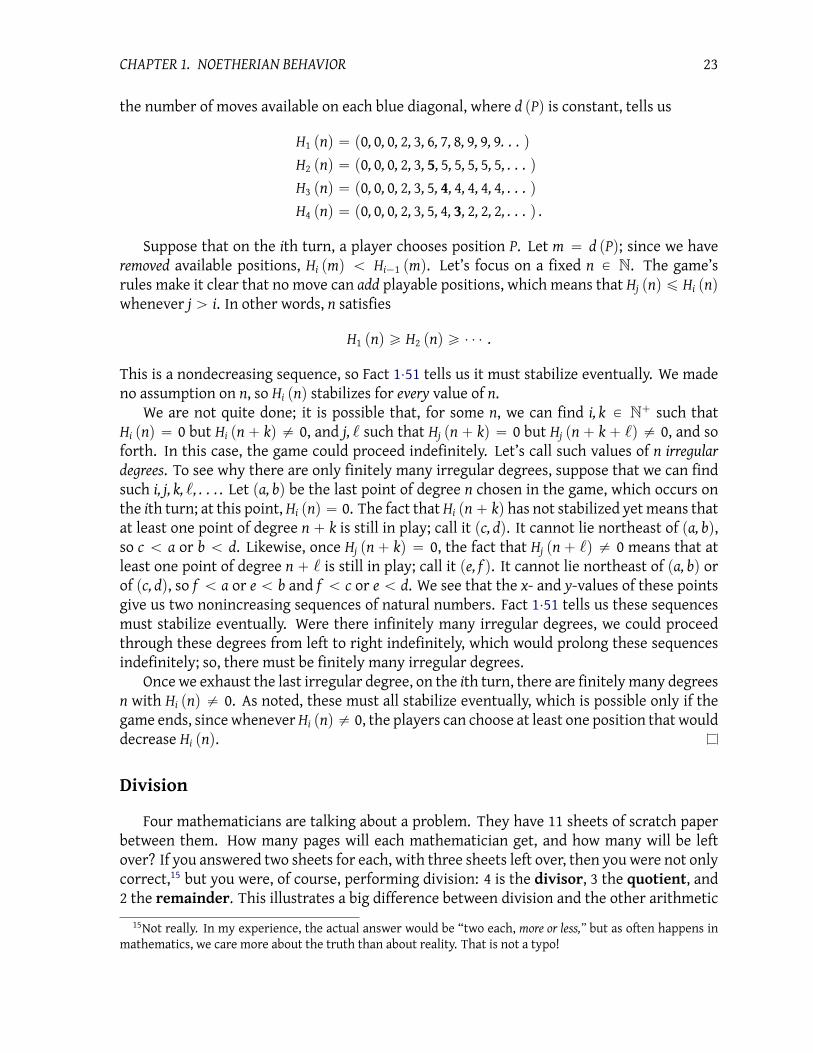
the number of moves available on each blue diagonal, where d pPq is constant, tells us
H1 pnq “ p0, 0, 0, 2, 3, 6, 7, 8, 9, 9, 9. . . q
H2 pnq “ p0, 0, 0, 2, 3, 5, 5, 5, 5, 5, 5, . . . qH3 pnq “ p0, 0, 0, 2, 3, 5, 4, 4, 4, 4, 4, . . . qH4 pnq “ p0, 0, 0, 2, 3, 5, 4, 3, 2, 2, 2, . . . q .
Suppose that on the ith turn, a player chooses position P. Let m “ d pPq; since we have
removed available positions, Hi pmq ă Hi´1 pmq. Let’s focus on a fixed n P N. The game’s
rules make it clear that no move can add playable positions, which means that Hj pnq ď Hi pnq
whenever j ą i. In other words, n satisfies
H1 pnq ě H2 pnq ě ¨ ¨ ¨ .
This is a nondecreasing sequence, so Fact 1¨51 tells us it must stabilize eventually. We made
no assumption on n, so Hi pnq stabilizes for every value of n.
We are not quite done; it is possible that, for some n, we can find i, k P N` such that
Hi pnq “ 0 but Hi pn` kq ‰ 0, and j, ` such that Hj pn` kq “ 0 but Hj pn` k` `q ‰ 0, and so
forth. In this case, the game could proceed indefinitely. Let’s call such values of n irregular
degrees. To see why there are only finitely many irregular degrees, suppose that we can find
such i, j, k, `, . . . . Let pa, bq be the last point of degree n chosen in the game, which occurs on
the ith turn; at this point, Hi pnq “ 0. The fact that Hi pn` kq has not stabilized yet means that
at least one point of degree n ` k is still in play; call it pc, dq. It cannot lie northeast of pa, bq,
so c ă a or b ă d. Likewise, once Hj pn` kq “ 0, the fact that Hj pn` `q ‰ 0 means that at
least one point of degree n ` ` is still in play; call it pe, f q. It cannot lie northeast of pa, bq or
of pc, dq, so f ă a or e ă b and f ă c or e ă d. We see that the x- and y-values of these points
give us two nonincreasing sequences of natural numbers. Fact 1¨51 tells us these sequences
must stabilize eventually. Were there infinitely many irregular degrees, we could proceed
through these degrees from left to right indefinitely, which would prolong these sequences
indefinitely; so, there must be finitely many irregular degrees.
Once we exhaust the last irregular degree, on the ith turn, there are finitely many degrees
n with Hi pnq ‰ 0. As noted, these must all stabilize eventually, which is possible only if the
game ends, since wheneverHi pnq ‰ 0, the players can choose at least one position that would
decrease Hi pnq.
Division
Four mathematicians are talking about a problem. They have 11 sheets of scratch paper
between them. How many pages will each mathematician get, and how many will be left
over? If you answered two sheets for each, with three sheets left over, then you were not only
correct,15
but you were, of course, performing division: 4 is the divisor, 3 the quotient, and
2 the remainder. This illustrates a big difference between division and the other arithmetic
15Not really. In my experience, the actual answer would be “two each, more or less,” but as often happens in
mathematics, we care more about the truth than about reality. That is not a typo!

CHAPTER 1. NOETHERIAN BEHAVIOR 24
operations. Addition, subtraction, and multiplication all give one result, but division gives
two: a quotient and a remainder.
It probably won’t surprise you that we can always divide two integers.16
The Division Theorem. Let n and d (the divisor) be two integers. If d ‰ 0, we can find exactly
one integer q (the quotient) and exactly one natural number r (the remainder) satisfying the two
conditions
D1) n “ qd` r, and
D2) r ă |d|.
Try to remember the meaning of “divisor”, “quotient”, and “remainder”, since I’ll use
them quite a bit from now on. Also try to remember the second criterion, since students have
a habit of forgetting it, especially in those moments when it’s most useful.
Example 1¨53. Division of 12 by 7 gives us a quotient of 1 and a remainder of 5. Division of
´12 by 7 gives us a quotient of´2 and a remainder of 2. (You can’t use a quotient of´1 and
a remainder of´5 because the Division Theorem wants a nonnegative remainder.)
Question 1¨54 .Identify the quotient and remainder when dividing:
(a) 10 by´5;
(b) ´5 by 10;
(c) ´10 by´4.
Proof of the Division Theorem. The proof relies on some concepts we just discussed, such as the
well ordering of N. Since it’s often easier to think about positive numbers, we consider two
cases: d P N` (positive), and d P ZzN (negative). First we consider d P N`; by definition of
absolute value, |d| “ d. We must show two things: first, that we can find a quotient q and
remainder r; second, that r is unique. We work on each claim separately.
Existence of q and r: First we show that we can find q and r that satisfy (D1). Again, we split
this into two cases: n nonnegative, and n negative.
First assume n is nonnegative; that is, n P N. We create a sequence of natural numbers in
the following way. Let r0 “ n. For i P N` we define
ri`1 “
#
ri ´ d, d ď ri;
ri, otherwise.(1.1)
We claim this sequence is nondecreasing. Why? If ri`1 ‰ ri, then by definition d ď ri, in
which case
ri`1 “ ri ´ d P N, which we rewrite as ri ´ ri`1 “ d P N, so ri ě ri`1.
16That’s a lie. Find the lie. (Hint: It’s a subtle detail.)

CHAPTER 1. NOETHERIAN BEHAVIOR 25
Fact 1¨51 tells us that this sequence of r’s must stabilize with a minimal element, r. This must
satisfy r ă d, since otherwise d ď r, which would allow us to create a subsequent, different
ri`1, contradicting the choice of r as the stable one. In addition, the definition of the sequence
requires r P N. Combining them, we see that r satisfies (D2). Let q be the index such that
rq “ r; a proof by induction shows that n “ qd` r, satisfying (D1).
Question 1¨55 .Provide this proof of induction. Use induction on q to show that the sequence of natural
numbers defined in formula 1.1 satisfies the property n “ qd ` rq. You’ll want to start with
q “ 0.
Proof (continued). Now suppose n P ZzN, so n is negative. As |n| is nonnegative, we can apply
the previous argument to find q1and r
1satisfying (D1) and (D2) for |n|. Unfortunately, we need
these statements for n, not |n|. Fortunately, n “ ´ |n|, so we can write
n “ ´ |n| “ ´ pq1d` r
1q “ p´q
1q d´ r
1.
Let q “ ´pq1 ` 1q and r “ d´ r1; we now have
qd` r “ r´ pq1` 1qs d` pd´ r
1q “ rp´q
1q d` ds ` pd´ r
1q “ p´q
1q d´ r
1“ n.
Written backwards and condensed, this equation says n “ qd ` r, satisfying (D1) for n. Cer-
tainly q is an integer by definition of Z, while r “ d´ r1 is natural because r1 ď d. So we have
0 ď r, and r ă d from Question 1.27. Combining them, we have 0 ď r ă d, satisfying (D2).
Uniqueness of q and r: Here we have to show that no other combination of an integer q1
and a natural number r1satisfy both (D1) and (D2). Suppose to the contrary that there exist
q1, r1 P Z such that n “ q1d` r1 and 0 ď r1 ă d. By substitution,
r1´ r “ pn´ q
1dq ´ pn´ qdq
“ pq´ q1q d. (1.2)
Subtraction of integers is closed, so r1 ´ r P N and pq´ q1q d are both integers. If 0 “ q ´ q1,
then substitution into equation (1.2) shows that r ´ r1 “ 0, as desired. If 0 ‰ q ´ q
1, we
consider two cases. If q´ q1 P N`, then Question 1.28 tells us that d ď pq´ q1q d (replacing a
by d and b by q´ q1). This gives us
0 ď r1´ r ď r ă d ď pq´ q
1q d “ r
1´ r,
a contradiction, so q´ q1 R N`. Likewise, if q´ q1 is negative, we have q1´ q P N`, so we play
the same game with r´ r1 to obtain a contradiction. (That is, we negate both sides of equation
(1.2).) Hence q´ q1 “ 0 and r ´ r1 “ 0.
We have shown that if d P N`, then there exist unique q, r P Z satisfying (D1) and (D2).
We still have to show that this is true for d P ZzN. In this case, |d| P N`, so we can apply the
former case to find unique q, r P Z such that n “ q |d| ` r and 0 ď r ă |d|. By properties of
arithmetic, q |d| “ q p´dq “ p´qq d, so n “ p´qq d` r.

CHAPTER 1. NOETHERIAN BEHAVIOR 26
Question 1¨56 .Another way to prove the existence part of the Division Theorem is to form two sets S “
tn´ qd : q P Zu and R “ S X N, prove that R ‰ H, and then use the well-ordering property
to identify the smallest element of R, which is the remainder from division. Fill in the blanks
of Figure 1¨5 to see why R is nonempty.
Question 1¨57 .If a and b are both natural numbers, and 0 ď a´ b, then (a) why is b ď a? Similarly, if |d| ď r,
then why are (b) 0 ď r ´ |d| and (c) r ´ |d| ď r?
Notation. If the Division Theorem tells us that the remainder is zero, then we write d | n. This
is shorthand for saying, d divides n. For instance, 2 | 6. Try not to confuse this with 62, which
means something 6 divided by 2. That is a completely different idea.
Question 1¨58 .Prove that if a P Z, b P N`, and a | b, then a ď b.
Definition 1¨59. We define lcm, the least common multiple of two integers, as
lcm pa, bq “ min
n P N` : a | n and b | n(
.
This is a set-builder expression of the definition that you should already be familiar with: it’s
the smallest (min) positive (n P N`) multiple of a and b (a | n, and b | n).
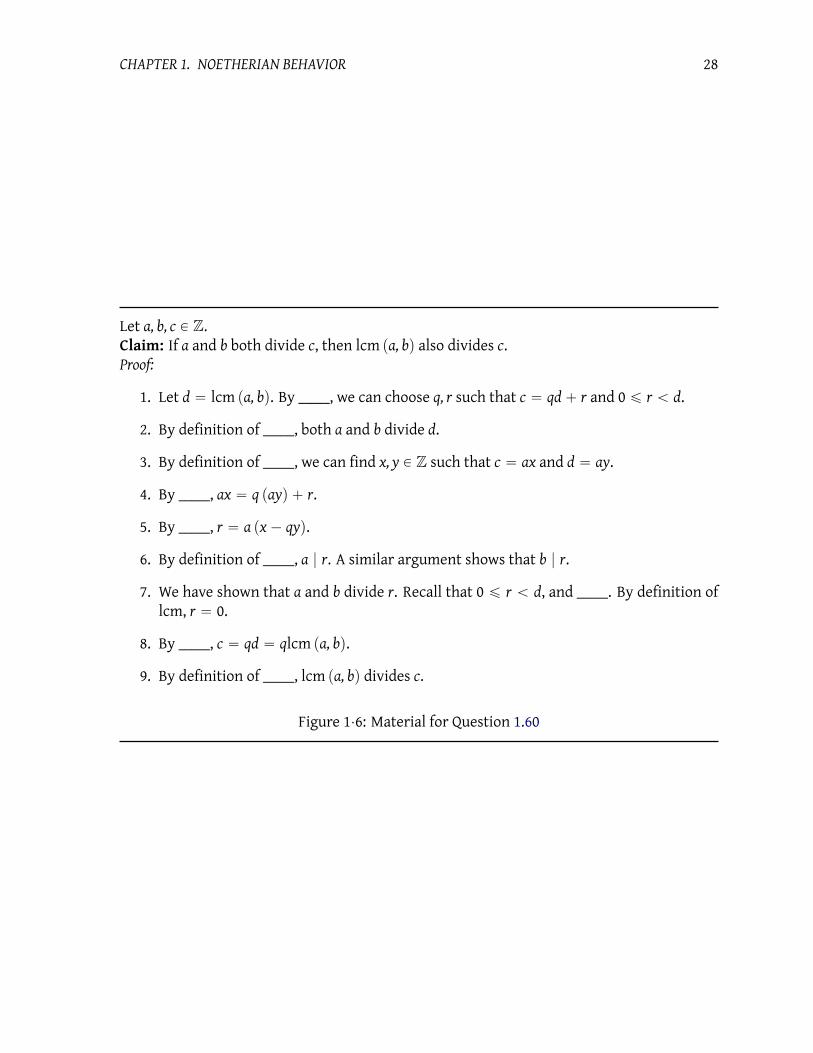
Question 1¨60 .
(a) Fill in each blank of Figure 1¨6 with the justification.
(b) One part of the proof claims that “A similar argument shows that b | r.” State this argu-
ment in detail.
The equivalence of the Well-Ordering Principle and Induction
Fact 1¨46 claims that the Well-Ordering Principle is equivalent to the Induction Principle.
Why? First we show the Induction Principle implies the Well-Ordering Principle. Assume that
the Induction Principle is true, and let S be any subset of N. Recall thatď is a linear ordering
of N, so we can compare any two elements of S. If S is finite with n elements, then we can
enumerate its elements as s1, . . . , sn, and sort them according to ď, so we can find a smallest
element.
Otherwise, suppose S is infinite. We proceed by induction. If 0 P S, then for any s P S, we
know that s ´ 0 “ s, and s is a natural number, so 0 ď s. That makes 0 a minimal element.
Now let i P N, and suppose that none of 0, . . . , i ´ 1 is in S, but i is. We claim that i is a

CHAPTER 1. NOETHERIAN BEHAVIOR 27
Let n, d P Z, where d P N`. Define S “ tn´ qd : q P Zu and R “ SX N.
Claim: R ‰ H.
Proof: We consider two cases.
1. First suppose n P N.
(a) Let q “_____. By definition of Z, q P Z.
(You can infer this answer by looking down a couple of lines.)
(b) By properties of arithmetic, qd “_____.
(c) By _____, n´ qd “ n.
(d) By hypothesis, n P_____.
(e) By _____, n´ qd P N.
2. It’s possible that n R N, so now let’s assume that, instead.
(a) Let q “_____. By definition of Z, q P Z.
(Again, you can infer this answer by looking down.)
(b) By substitution, n´ qd “_____.
(c) By _____, n´ qd “ ´n pd´ 1q.
(d) By _____, n R N, but it is in Z. Hence,´n P N`.
(e) Also by _____, d P N`, so arithmetic tells us that d´ 1 P N.
(f) Arithmetic now tells us that´n pd´ 1q P N. (posˆnatural=natural)
(g) By _____, n´ qd P N.
3. In both cases, we showed that n´ qd P N. By definition of _____, n´ qd P S.
4. By definition of _____, n´ qd P SX N.
5. By definition of _____, SX N ‰ H. Hence R ‰ H.
Figure 1¨5: Material for Question 1.56
CHAPTER 1. NOETHERIAN BEHAVIOR 28
Let a, b, c P Z.
Claim: If a and b both divide c, then lcm pa, bq also divides c.
Proof:
1. Let d “ lcm pa, bq. By _____, we can choose q, r such that c “ qd` r and 0 ď r ă d.
2. By definition of _____, both a and b divide d.
3. By definition of _____, we can find x, y P Z such that c “ ax and d “ ay.
4. By _____, ax “ q payq ` r.
5. By _____, r “ a px´ qyq.
6. By definition of _____, a | r. A similar argument shows that b | r.
7. We have shown that a and b divide r. Recall that 0 ď r ă d, and _____. By definition of
lcm, r “ 0.
8. By _____, c “ qd “ qlcm pa, bq.
9. By definition of _____, lcm pa, bq divides c.
Figure 1¨6: Material for Question 1.60

CHAPTER 1. NOETHERIAN BEHAVIOR 29
minimal element of S. To see why, consider the set T “ ts´ i : s P Su. This is also a subset of
N, because the definition of subtraction tells us s ´ i R N only when s P t0, . . . , i´ 1u, and
none of those numbers is in S by hypothesis. In addition, 0 P T because i P S, so putting s “ i
in the definition of T gives us i´ i P T. We already showed that any subset of N that contains
0 has 0 as a least element, so 0 is the least element of T. We return to S. Let s P S; we claim
that i ď s. To see why, consider i´ i “ 0 and s´ i. As previously discussed, both elements are
in T, and 0 ď s´ i. This is true if and only if 0` i ď ps´ iq ` i, or, i ď s. Since swas arbitrary,
i is indeed the smallest element of S.
We have shown that any subset S of N has a smallest element with respect to ď. This
proves that N is well ordered byď.
Now we show that the Well-Ordering Principle implies the Induction Principle. Assume
that the Well-Ordering Principle is true, and let S Ď N, satisfying both the inductive hypoth-
esis and the inductive step. Let N be the set of all such natural numbers that are not in S. If
N “ H, we are done. Otherwise, the Well-Ordering Principle tells us N has a smallest ele-
ment, which we call n. We cannot have n “ 0, as that would violate the inductive hypothesis,
which we assumed was true. Hence n ‰ 0, which means n ´ 1 P N. The choice of n as the
smallest element of N implies that n ´ 1 P S, since after all n ´ 1 ă n (this is easy to see if
you think about the definition). However, we also assumed S satisfies the inductive step, so
pn´ 1q ` 1 P S, but n “ pn´ 1q ` 1, contradicting the hypothesis that n P N. Hence N “ H,
and S “ N.
1¨5 Division on the lattice (optional)
Algebra is nothing more than geometry, in words;
geometry is nothing more than algebra, in pictures.
— Sophie Germain
We have shown that we can divide both integers and natural numbers to obtain a quotient
and remainder. Can we divide on the lattice, identifying a quotient and a remainder? If so, is
the result unique?
We can in fact perform division on the lattice. To do that, we first have to think about the
other operations: addition, subtraction, and multiplication. Let P “ pp, qq and R “ pr, sq be
points on L. We’ll define addition in a natural way,
P` R “ pp` r, q` sq .
For subtraction, use
P´ R “ pp´ r, q´ sq ,
but notice that this doesn’t always give us a point in the natural lattice. So, let’s expand our
view to the integer lattice, Z2; as with division of natural numbers, we can work first in Z2,then switch back to N2
once that’s out of the way.
What of multiplication? Since the lattice is two-dimensional, we’d like multiplication to
move us in two dimensions. We adopt the following convention:
• pp, qq ¨ pc, 0q “ ppc, qcq, the point on the line that connects the origin to pp, qq, but with
a length c times that from the origin to pp, qq;

CHAPTER 1. NOETHERIAN BEHAVIOR 30
(1,1)
(3,0) ·(1,1)
(−2,0) ·(1,1)
(1,1)
(0,3) ·(1,1)
(0,−2) ·(1,1)
Figure 1¨7: Multiplication on the lattice.
• pp, qq ¨ p0, dq “ p´qd, pdq, the point on the line perpendicular to the line that connects
the origin to pp, qq, but with a length d times that from the origin to pp, qq;
• pp, qq ¨ pc, dq “ pp, qq ¨ pc, 0q ` pp, qq ¨ p0, dq “ ppc ´ qd, pd` qcq, the vector sum of the
previous two.
See Figure 1.61. This may look odd, but it extends well to other problems, as you will learn
later.
Question 1¨61 .Suppose P “ p3, 1q.
(a) Calculate P ¨ pc, 0q for several different values of c. Sketch the resulting points on Z2.Observe how the results conform to the description in the text.
(b) With the same value of P, calculate P ¨ p0, dq for several different values of d. Sketch the
resulting points on Z2. Observe how the results conform to the description in the text.
(c) With the same value of P, calculate P ¨pc, dq for several different combinations of values of
c and d that you used in parts (a) and (b). Sketch the resulting points on Z2. How would
you describe the results geometrically?
As with division of natural numbers, the goal of dividing P “ pp, qq by D “ pc, dq will be
to move D “closer and closer” to P via subtraction from P, until the remaining distance is so
small that subtraction no longer makes it smaller. If we measure our distance with integers,
we can then apply the Well Ordering Principle via Fact 1¨51 to guarantee the division ends.
But how can we measure distance with integers? The traditional distance formula is based
on the Pythagorean Theorem, and relies on radicals:
the distance between pp, qq and pr, sq is
b
pp´ rq2` pq´ sq
2.

CHAPTER 1. NOETHERIAN BEHAVIOR 31
That’s bad, because Fact 1¨51 does not apply to radicals. For instance, the sequence
c
1
2ą
c
1
3ą
c
1
4ą
c
1
5ą ¨ ¨ ¨
consists of positive numbers, and continues indefinitely.
Don’t let that discourage you! It’s actually easy to get around this; we’ll just use a different
distance formula, modifying the traditional one so that it doesn’t use radicals,
the “square distance” between pp, qq and pr, sq is pp´ rq2` pq´ sq
2.
The square distance is always natural, opening the way to use Fact 1¨51. It’s a bit tedious to
write “square distance” all the time, so we’ll write sqd pP, Qq for the square distance between
P and Q. We consider the distance from a point to the origin to be its size, much like absolute
value, so we will write Rsq to indicate this value.
The Division Theorem for the lattice. Let N and D be two points of Z ˆ Z. If D ‰ 0, we can
find Q P Zˆ Z (the quotient) and R P Nˆ N (the remainder) satisfying the two conditions
D1) N “ QD` R, and
D2) 0 ď Rsq ă Dsq.
. However, the points Q and Rmay not be unique.
Proof. Let S0 “ N, and for i P N` define Si “ N ´ pi, 0q D. Let S “
Sisq : i P N(
. This is a set
of natural numbers, so by the well ordering of N, S has a smallest element, corresponding to
a particular Sa. Let T0 “ Sa. For j P N`, define Tj “ S0 ´ pa, jq D. Let T “
Tjsq : j P N(
. It
also has a smallest element, corresponding to a particular Tb. Let Q “ pa, bq and R “ Tb; by
definition and substitution, we have R “ N ´ Q ¨ D, or N “ QD` R. This satisfies (D1).
To show that Q and R also satisfy (D2), suppose the contrary, that is, Rsq ě Dsq. The set
U “ trQ˘ p1, 0qs ¨ D, rQ˘ p0, 1qs ¨ Du is finite, so one of its points has a distance to N that is
no larger than the other three. Now consider Figure 1¨8. At least two points of U form angles
with the line N ´ QD that are no larger than 90˝.
We consider two cases. If α “ β “ 45˝, the Law of Cosines tells us
a2“ b
2“ d
2` pd` kq
2´?2 ¨ d pd` kq .
We assumed Rsq ě Dsq. By substitution, N ´ QDsq ě Dsq. We chose Q to minimize the
square distance between QD and N, so N ´ QDsq ď a2. By substitution,
`
d` k2˘
ď d2` pd` kq
2´?2 ¨ d pd` kq .
Rewrite this as
0 ď d2´?2 ¨ d pd` kq .
Since d is positive, we can rewrite again as
0 ď d´ pd` kq?2,

CHAPTER 1. NOETHERIAN BEHAVIOR 32
QD N
QD+(1,0)D
QD+(0,−1)D
α
β
d+k
d
d
a
b
Figure 1¨8: Illustration of the proof of existence for the Division Theorem in N2. Let the Eu-
clidean distance from QD to QD`p1, 0q D and to QD`p0,´1q D be d. Suppose d is smaller than
the square distance from QD to N, which is then d ` k with some positive k. In this diagram,
α and β form acute angles between two extensions from QD to the segment joining QD and
N. Our task is to show that one of a or b is less than d ` k, contradicting the choice of Q to
minimize this distance.
but k ě 0 implies that d´ pd` kq?2 ă 0, contradicting the choice of Q.
In the case that α, β ‰ 45˝, one of the segments lengthens, while the other shortens,
making it smaller than d ` k; hence, one of them is closer to N than QD, contradicting the
choice of Q.
Figure 1¨8 also hints at why we might have two distinct quotients and remainders of the
same size. If two possible remainders are p1, 0q and p0, 1q, with Dsq ą 1, we cannot get closer,
and either solution works.
We can thus extend the notion of “division” that we gave above to anything we can “view” as
an integer lattice.
Question 1¨62 .Suppose N “ p10, 4q.
(a) Let D “ p3, 1q, and R “ N ´ p3, 0q ¨ D. Show that Rsq ă Dsq.
(b) Let D “ p1, 3q, and R “ N ´ p3,´3q ¨ D. Show that Rsq ă Dsq.
(c) Explain how the results of parts (a) and (b) conform to those described in the text.
(d) SupposeN “ p10, 4q andD “ p2, 2q. FindQ P L such that ifR “ N´Q¨D, then Rsq ă Dsq.
Sketch the geometry of N, D, QD, and R.
(e) Is the result unique? That is, could you have found Q1 P L such that R “ N ´ Q
1 ¨ D,
Rsq ă Dsq, and Q1 ‰ Q?
(f) Show that for any N, D P L with D ‰ p0, 0q, you can find Q, R P L such that N “ Q ¨ D ` R
and Rsq ă Dsq. Again, try to build on the geometric ideas you gave in (e).

CHAPTER 1. NOETHERIAN BEHAVIOR 33
1¨6 Polynomial division
He who can properly define and divide is considered to be a god.
— Plato
You may be wondering how the material we’ve studied so far is related to algebra, which you
probably associate more with polynomials than with games. Take a look back at Ideal Nim’s
playfield, the latticeN2. This game is related to polynomials, or at least tomonomials, which
are products of variables.
• Any point pa, bq on the lattice corresponds in unique fashion to a monomial in two vari-
ables, xayb.
• The choice pa, bq disqualifies other points pc, dq; we called them Gone from Gameplay.
The rule was that pc, dq is Gone from Gameplay if a ď c and b ď d. In this case, the
corresponding monomial xcyd
is divisible by xayb.
• Just as the lex ordering ĺlex is a well ordering of N2, it is a well ordering of monomials
in two variables.
By this reasoning, we could extend division with quotient and remainder on the lattice to
define division with quotient and remainder of monomials. Whether such a division with
remainder is useful, we leave to others to ponder; we merely point out that it exists.
Question 1¨63 .If you are so inclined, however, translate the results of Question 1.62 to monomials. “Multi-
plication” and “subtraction” in the Division Theorem actually translate to what operations
on monomials?
We turn instead to division with quotient and remainder of polynomials. When one poly-
nomial is a multiple of another, we would like the quotient and remainder to be consistent
with previous choices. For instance, dividing px` 1q px´ 1q by x´ 1 should clearly give us a
quotient of x` 1 and a remainder of 0.
We would also like to replicate the distinct behavior of integer division: that is, the re-
mainder r should in some manner be “smaller” than the divisor g. This isn’t too hard to grasp
if you think about what comes naturally: we want to subtract multiples of g in such a way as
to make f smaller.
Example 1¨64. Suppose f “ x2 ` 1 and g “ x ´ 1. A natural way to make f “smaller” is to
multiply x´ 1 by x and subtract:
f ´ xg “`
x2` 1
˘
´ x px´ 1q “ x` 1.
We end up with x` 1 as a remainder.
That hardly seems complete, as we can subtract another multiple of x´ 1:
pf ´ xgq ´ g “ px` 1q ´ px´ 1q “ 2.
Putting them together, we have
f “ px` 1q g` 2.
We now have 2 as our remainder, and it is not possible to remove any more multiples of x´ 1.

CHAPTER 1. NOETHERIAN BEHAVIOR 34
What the example should show you is that we make f “smaller” by reducing its largest
exponent. We call this largest exponent the degree of a polynomial. The degree makes a
“natural” target, not only because it seems to shrink the polynomial, but also because it re-
lates polynomial division to the Well Ordering Principle, which we used to set up division on
both the integers and the lattice.
We have to be a little careful here: what is deg 0? You might be tempted to say that
deg 0 “ 1 because 0 is a constant, so 0 “ 0 ¨ 1 “ 0 ¨ x0, but we could just as easily say that
0 “ 0 ¨ x1 or 0 “ 0 ¨ x2 or . . . You get the idea. To avoid this pickle, we agree that the term
“degree” applies only to nonzero polynomials, and that the zero polynomial has no degree.
Another complication lies hidden in the weeds. It isn’t too hard to divide 7 by 5, but what
do we do with 7x and 5x? Writing 7x “ 5 ¨ x ` 2x does not decrease the degree, and the joy
of decreasing the coefficient evaporates when we realize that we can decrease the coefficient
even more by writing 7x “ 5¨x`0x. In any case, this problem grows even more annoying when
dividing binomials, trinomials, and so forth. We will content ourselves to restrict divisors to
polynomials whose leading coefficients is 1. We call such polynomialsmonic.The Division Theorem for polynomials. Let f, g be polynomials in one variable with integer
coefficients, with the leading coefficient of g being 1. We can find exactly one polynomial q and exactly
one polynomial r, also with integer coefficients, satisfying the conditions
D1) f “ qg` r, and
D2) r “ 0 or 0 ď deg r ă deg g.
Proof. First we show that some sort of quotient and remainder exist. If deg f ă deg g, then
let r “ f and q “ 0; this satisfies both properties. For the case deg f ě deg g, we proceed by
induction on the difference in degree.
Question 1¨65 .Suppose that f “ 3x2` 2 and g “ x2´ x` 2. These have the same degree, so we can subtract
from f a constant multiple of g to obtain a remainder of smaller degree. Do that, then use the
result to follow through the next paragraph of the proof.
Continuation of proof. For the inductive base, assume deg f´deg g “ 0; that is, the polynomials
have the same degree. Write c for the leading coefficient of f . Let q “ c, and r “ f ´ cg. We
have
qg` r “ cg` pf ´ cgq “ f,
satisfying (D1). In addition, if deg f “ d, we can write f “ cxd ` f 1 and g “ xd ` g1, where the
degrees of f1and g
1are smaller than those of f and g, respectively. That gives us
f ´ cg “`
cxd` f
1˘
´ c`
xd` g
1˘
“
´
cxd` f
1¯
´
´
cxd` cg
1¯
“ f1´ cg
1.
We may not know the degree of f1 ´ cg1 with precision, but we can say that it’s smaller than
d. Since deg g “ deg f “ d, either r “ 0 or 0 ď deg r ă deg d, satisfying (D2).

CHAPTER 1. NOETHERIAN BEHAVIOR 35
Question 1¨66 .Suppose that f “ 2x3` x2` 4x` 2 and g “ x2´ x` 2. These have different degree. Subtract
from f a polynomial multiple of g to obtain a remainder of smaller degree. Do that, then use
the result to follow through the next paragraph of the proof. The remainder should look quite
familiar.
Continuation of proof. Now assume that the claim holds for deg f ´ deg g “ i whenever i “
0, 1, 2, . . . , n´1. What about i “ n? Again, write c for the leading coefficient of f . Let q1 “ cxn,
and r1 “ f ´ q1g. As before, if deg f “ d, we can write f “ cx
d ` f 1, where deg f1 ă d. If
deg g “ a, we can write g “ xa ` g1, where deg g1 ă a. We have
r1“`
cxd` f
1˘
´ cxnpxa` g
1q “
`
cxd` f
1˘
´`
cxa`n` cx
ng1˘
.
Recall that a` n “ deg g` pdeg f ´ deg gq “ deg f “ d, so substitution gives us
r1“
´
cxd` f
1¯
´
´
cxd` cx
ng1¯
“ f1´ cx
ng1.
We already pointed out that deg f1 ă deg d; we also have deg pcxng1q “ n`deg g
1 ă n`a “ d.
Again, r “ 0 or deg r1 ă deg f “ n. If r “ 0, we are done, so suppose r ‰ 0, in which case
deg r ă n. By the inductive hypothesis, we can find q2
and r2
such that r1 “ q
2g ` r2 and
deg r2 ă deg g. By substitution and rewriting,
f “ q1g` r
1“ q
1g` pq
2g` r
2q “ pq
1` q
2q g` r
2.
Let q “ q1 ` q2 and r “ r2, and we satisfy both (D1) and (D2).
How about the result’s uniqueness? Suppose we can find polynomials q1, q2, r1, and r2 such
that
f “ q1g` r1 “ q2g` r2 and for i “ 1, 2 ri “ 0 or 0 ď deg ri ă deg g.
Rewrite the first equations as
pq1 ´ q2q g “ r2 ´ r1.
If the polynomial on the left is nonzero, then its degree is no smaller than deg g. If the poly-
nomial on the right is nonzero, then its degree is smaller than deg g. It’s not possible to have
a nonzero polynomial with two different degrees — the definition of degree is unambiguous
— so the polynomials must be zero. That means r1 “ r2, which forces q1 “ q2; otherwise, the
degree on the left would be nonzero.
As with integer division, the proof of this theorem outlines an algorithm to compute the quo-
tient and remainder. (An algorithm is a finite list of instructions with a well-specified output,
which is guaranteed to terminate after finitely many operations.) We know that the method
will end after finitely many steps, because the degrees of the remainders form a decreasing
sequence of natural numbers, and the well-ordering applies. Indeed, this algorithm is some-
times called “long division” of polynomials.
Question 1¨67 .Divide f “ 10x6 ´ 3x4 ` 1 by g “ x3 ` x` 1.

CHAPTER 1. NOETHERIAN BEHAVIOR 36
In all these questions, both f and g are polynomials with integer coefficients.
Question 1¨68 .Sometimes we can divide f by a non-monic g, if we’re willing to surrender the requirements
that the resulting quotient and remainder have integer coefficients. Can you find an example
where g is non-monic, but the quotient and remainder do have integer coefficients? Try to
find a non-trivial example; that is, you should have f ‰ 0 and f ‰ qg for any polynomial q.
Question 1¨69 .The Factor Theorem claims that if we divide f by g and have a zero remainder, then any root
of g is a root of f . Why is this true?
(A root of a polynomial g is any value a of x such that g paq “ 0. So the problem is really
asking why g paq “ 0 implies f paq “ 0 under the given hypothesis.)
Question 1¨70 .The Remainder Theorem claims that if we let a be any integer, and divide f by g “ x´ a, the
remainder is a constant that has the same value as f paq. Why is this true?
Question 1¨71 .The Division Theorem requires that the polynomials be in one variable only. What if two
polynomials have two or more variables? You first have to decide how to determine a leading
monomial; for instance, what should be the leading monomial of x2 ` xy` y2?
(a) Describe a way of choosing a leading monomial.
(b) Try to divide polynomials in several variables. Use several examples. Are you able to
identify a quotient and remainder that satisfy (MD1) f “ qg ` r and (MD2) r “ 0 or r is
somehow smaller than g? (You have to explain how r is smaller.)
(c) If it does work, describe a Multivariate Polynomial Division Theorem, and try to prove it.
If it doesn’t work, explain why not.
Question 1¨72 .Where in this chapter did Noetherian behavior show up? List as many places as you can; I can
think of four off the top of my head. (Go ahead and count those occasions where we explained
how one system could be viewed as a more fundamental system, since that really does count.)

Chapter 2
Algebraic systems and structures
In the previous chapter, we using decreasing sequences of natural numbers to formulate di-
vision in several different contexts. We already pointed out that division is rather unusual
as an operation, because rather than producing only one result, it produces two, the quotient
and a remainder.
Many mathematics courses treat division differently: they ignore remainders, and treat
quotient exclusively as a position on the real line. This can give students the impression that
remainders are a mostly useless artifact. In fact, it is often the case that the quotient is useless,
and what really matters is the remainder!
That is mostly the case in the course, and this chapter will use remainders as an example
to introduce you to some very elegant properties, as well as to one of the most elegant and
useful objects ever devised, the finite field.
2¨1 From symmetry to arithmetic
Those who assert that the mathematical sciences say nothing of the beautiful or
the good are in error. . . . The chief forms of beauty are order and symmetry and
definiteness, which the mathematical sciences demonstrate in a special degree.
— Aristotle, Metaphysics, Book XIII
We return a few moments to Nim and Ideal Nim, as a fun way to help motivate some material
that follows. In this section, we want to consider the question,
How do we decide what makes a “winning move” for Nim or Ideal Nim?
“Nimbers”
If you’ve played Nim enough, you’ll notice that whenever David faces two rows with an equal
number of pebbles, say
37

CHAPTER 2. ALGEBRAIC SYSTEMS AND STRUCTURES 38
he might as well give up: if he sees a visually symmetric game in two rows, then Emmy can
undo any move he makes. Of course, interesting games are not visually symmetric; for them
Emmy wants to impose a chronological symmetry. By this we mean that Emmy wants her first
move to change the game in such a way that whatever David does, she can undo — not visually,
but in such a way that she always has an advantage, and can explain why, in the same way
that the two equal rows above are visually symmetric.
To do this, we’ll assign values to different game configurations. We call these values nim-bers because they are numbers that correspond to different configurations of nim.
It makes sense to say that a game with no moves left has value 0. A game with 1 pebble
left is not equivalent to a game with value 0; it makes sense to call its value 1. A game with 2
pebbles in one row is equivalent to neither a game with 1 pebble nor a game with 2 pebbles;
it makes sense to call its value 2. And so forth; we’ll agree that a game with n pebbles in one
row is has value n. This covers all games of Nim with just one row.
What about games with two rows? We’ve already run out of numbers, so it might help
to look at the game above differently. The first thing to remember is that whenever a player
sees that configuration, he might as well give up, because anything he does will break the
symmetry, and the other player can easily restore the symmetry. So in some sense, that game
is equivalent to a game with no moves left.
Mind the vocabulary! We did not say the game above is equal to a game with no moves
left; it plainly is not, as it has quite a few moves left. We said it is equivalent to a game with no
moves yet. We will dignify this situation with a special term: a zero game is either a game
with no moves left at all, or a game where no matter what the current player does, the other
player will always have a winning strategy.
Notice that if Emmy’s turn ends with a zero game, then David has no way to end his turn
with a zero game. (After all, if he could, then Emmy could not herself have finished her turn
with a way that guaranteed her a win.)
In addition to viewing the game above as one game of Nim with two rows of four pebbles,
we can look at it as a “sum” of two games, each with one row of four pebbles. This makes sense
inasmuch as moving in one row doesn’t affect the number of pebbles in the other row, so it
really is as if you’re playing two games at the same time. This point of view can help us break
harder problems into smaller ones, always a goal in mathematics.
This insight gives us two guidelines, which we turn into definitions:
• A general game of Nim has value 0 if and only if it is a zero game; that is, if and only if
any move the current player makes has a response by the other player that results in a
zero game. If the game has value x, we indicate this by x ” 0.
• If a game of Nim has value x, another game has value x if and only if their sum (playing
both games together as one) is a zero game. Using” to indicate the values of equivalent
games, we write
x` y ” 0 if and only if x ” y.
We can use these definitions to define the value of the sum of two games.
Definition 2¨1. Suppose two games have values x and y. We say that x ` y ” z if and only if
px` yq ` z ” 0; that is, playing all three games as one single game guarantees a win for the
second player.

CHAPTER 2. ALGEBRAIC SYSTEMS AND STRUCTURES 39
Example 2¨2. Let X be a game of Nim with two rows of 4 pebbles each. We have already
pointed out that the value of X is x ” 0.
Next let Y be a game of Nim with one row of 5 pebbles. From what we argued above, the
value of Y is y ” 5.
Finally, let Z be a game of Nim with one row of 5 pebbles. From what we argued above, the
value of Z is z ” 5.
Clearly y ` z “ 0, since a game with two rows of 5 pebbles each has value 0. Likewise,
x` py` zq ” 0` 0 ” 0. That is, the following game has value 0:
Z Z Z Z Z
Y Y Y Y Y
X X X X
X X X X
You should be able to verify that this games is, indeed, a win for the second player: any move
Emmy makes in one row of the X game, David can reply symmetrically in the other row of the
X game; whereas any move she makes in the Y game, David can reply symmetrically in the Z
game (and vice versa).
So far, so good. What about the following game?
In this case, we have a row of 1 pebble and a row of n pebbles. Does it makes sense to say
that its equivalent value is n ` 1? Not always! To start with, we already know that 1 ` 1 ı 2,
because our rule x` x ” 0 implies 1` 1 ” 0. On the other hand, we can verify that 1` 2 ” 3
and, oddly enough, 1` 3 ” 2.
Question 2¨3 .Verify that 1` 2 ” 3 and 1` 3 ” 2 by playing:
(a) a game with two rows of 1 pebble and 2 pebbles at the same time as a game with 3 pebbles
— or, one game with three rows of 1, 2, and 3 pebbles — and showing that no matter how
Emmy starts, David can always win; and then,
(b) arguing that part (a) shows both 1 ` 2 ” 3 and 1 ` 3 ” 2, perhaps moving some rows
around to make it obvious.

CHAPTER 2. ALGEBRAIC SYSTEMS AND STRUCTURES 40
Question 2¨4 .Explain why addition of Nim games is always commutative; that is, if x and y are the values of
games X and Y, then x` y ” y` x. It may be helpful to move rows around in a game, so as to
obtain symmetry.
Question 2¨5 .Explain why addition of Nim games is always associative; that is, if x, y, and z are the values
of games X, Y, and Z, then px` yq ` z ” x` py` zq.
This pattern continues indefinitely; that is, if n is even, then 1`n ” 1`n and 1`p1` nq ”
n. Rather than prove that, however, we argue for something more general.
Nimber equivalence
Lemma 2¨6. Suppose a Nim gameX has value x. Write x as a sum of powers of 2: x “ an2n`ai´12
i´1`
¨ ¨ ¨ ` a12` a0 where an “ 1 and the remaining ai satisfy ai P t0, 1u. Then X is equivalent to the game
Y played with n rows and ai ˆ 2ipebbles in the i-th row.
We’ll use an example to illustrate the idea behind the proof of the lemma. Suppose X has
value x “ 13 “ 8 ` 4 ` 1 “ 23 ` 22 ` 20. The lemma claims that the sum of X and a 3-row
game Y of 1, 4, and 8 pebbles, is a zero game.
X X X X X X X X X X X X X
Y Y Y Y Y Y Y Y
Y Y Y Y
Y
Assume we know the lemma is true for every x less than 13, and let’s think about what happens
when we remove something from X.
If Emmy removes 4 pebbles from X, she reduces X to the game W with value w “ 9 ą 23.
David finds that there is a row in Y with 4 pebbles, and removes that entire row, obtaining a
2-row game Z of 1 and 8 pebbles. We now have the situation where w “ 9 “ 8 ` 1, which
corresponds precisely to Z. In other words, David leaves a zero game.
W W W W W W W W W
Z Z Z Z Z Z Z Z
Z

CHAPTER 2. ALGEBRAIC SYSTEMS AND STRUCTURES 41
What if Emmy removes 5 pebbles from X, instead? This reduces X to the game W with
value w “ 8 “ 23. In this case, David cannot reduce Y to one row of 8 pebbles in one move.
Instead, he has to look at ways to reduce Y to a sum of rows that adds to 8; that is, he has
to create some cancellations which yield 8. He can do this by remove enough pebbles from
the next-smaller row of length 4 to add up to the sum of the remaining rows. In this case, he
should take 3 pebbles from the middle row of Y, reducing it to the 3-row game Z of 1, 1, and 8
pebbles.
W W W W W W W W
Z Z Z Z Z Z Z Z
Z
Z
We see immediately from the game’s visual symmetry that David leaves a zero game.
Finally, what if Emmy removes 7 pebbles from X? This reduces X to the gameW with value
w “ 6 ă 23. In this case, David can remove pebbles from the longest row of Y in such a way
that it cancels with shorter rows to obtain w. In this case, he should take 10 pebbles from the
longest row of Y, reducing it to the 3-row game of Z of 1, 4, and 3 pebbles.
W W W W W W
Z Z Z
Z Z Z Z
Z
To see that this does indeed work out to 0, we could explore every possible move, but that
would take far to long. It’s much better to argue that the value of Z is indeed z “ 6. To do this,
we rely on the commutative and associative properties, as well as the fact that we already
know 1 ` 3 ” 2 and the inductive assumption that the claim above is true for every game
whose value is smaller than 13:
z “ 1` 4` 3 ” p1` 3q ` 4 ”shown
2` 4 “ 2` 22”6ă13
6.
That is, the new game is really equivalent to this one:
W W W W W W
Z Z Z Z
Z Z

CHAPTER 2. ALGEBRAIC SYSTEMS AND STRUCTURES 42
This process of simplifying Z from a game whose rows are not powers of 2 to one whose rows
are powers of 2 we will call row simplification, and when a game is arranged in rows of powers
of 2, we call it row simplified. Because this is a matter of game equivalence, it is free whenever
we know it is true; a player can rearrange several rows in this fashion at any time.
Proof of Lemma 2¨6. Let X and Y be the games described in the Lemma. The lemma’s claim is
that X`Y ” 0; that is, if Emmy and David play X`Y, then David always wins. To see that this
is true, assume that the analogous statement is true for any game whose value is less than
x, and suppose Emmy removes r pebbles from X, reducing it to the game W, which has value
w “ x´ r. Before proceeding, observe that Y is currently row simplified, because it is already
arranged in rows whose lengths are powers of 2.
If r is a power of 2, David can reduce Y to Z by removing r pebbles from the shortest row
that is at least r pebbles long. (So if r “ 2 and there is a row of length 2, he removes it from that
row; otherwise, if there is a row of length 4, he removes it from that row, and so forth.) Recall
that Y was row simplified before David moved. If he removes an entire row, as he did in the
example above withw “ 9, it is obvious that Z remains row simplified; he has simply removed
a row. Otherwise, David has removed from one row fewer than half the number of pebbles,
and some row simplification is in order — but this does not affect any other existing row. To
see why, observe that r “ 2k
for some natural k, and we are removing r from a row whose
length is 2`, with ` ą k. The result is a row whose length is 2
` ´ 2k; just as with subtracting 1
from a power of 10, this simplifies to 2`´1`2`´2`¨ ¨ ¨`2k`1`2k. Row simplification can only
affect rows 2`
through 2k, but the only reason we chose row 2
`is that there were no pebbles
in rows 2`´1
through row 2k, so even if we do this, Z remains row simplified.
From here on, assume r is not a power of 2. If w “ x ´ r ě 2i, let s “ w ´ 2i ă 2
i. This
is the “surplus” in W above the longest row of Y; that is, that w “ 2i ` s. (In the example
above where w “ 9, we have s “ w ´ 23 “ 1.) All David needs to do is remove pebbles from
one of the remaining rows of Y such that he reduces it to the game Z whose value is z “ s.
The inductive hypothesis tells us the lemma is true for values less than x, and s ă x, so David
should start by considering the shortest row of Y that is longer than s; suppose its length is
2j. He can remove enough pebbles from this row to cancel any powers of 2 smaller than s that
do not already appear in Y; suppose this reduces the row 2jto k. David should reduce the row
this way only if there are no rows between this row of length 2jand the one of length 2
i. If
there are, David should instead “cascade” his choice to longer rows of Y except the longest,
rewriting 2j`1 “ 2
j ` rk` p2j ´ kqs, 2j`2 “ p2j`1 ` 2jq ` rk` p2j ´ kqs, and so forth, so that
now the rows of length 2j, 2
j`1, etc. also cancel, leaving k as needed. This cascade will end in
the last row of Y before the longest, allowing David to reduce the rows shorter than 2ito the
value s, obtaining a row-simplified game Z of value 2i ` s “ w, as claimed.
Finally, suppose w “ x ´ r ă 2i. (We see this in the last example above, with w “ 6.) In
this case, remove from the longest row of Y enough pebbles so that, after row simplification
with the smaller rows, the modified Y now has value w: canceling powers of 2 that appear in
y but not in w, and preserving those that do appear, as claimed.
Suppose on the other hand that Emmy moves in the Y game, instead of X. David need
merely the make the corresponding move in X that was described in the cases above. This
covers all the cases, and we have shown that X ` Y ” 0.

CHAPTER 2. ALGEBRAIC SYSTEMS AND STRUCTURES 43
Question 2¨7 .To see why this trick with powers of 2 not work with higher powers, suppose you try to write
a Nim game which consists or one row of 2 pebbles as a series of rows of the powers of 3 that
add up to 2. What goes wrong? (This also show why it won’t work with larger powers, either.)
Nimber addition
Now we have determined that we can always write the value of a game as sums of powers
of 2, it becomes easy to add and subtract them.
Nim Addition Theorem. Let x and y be the respective values of Nim games X and Y. We know
x ` x ” 0, so without loss of generality, suppose x ą y, suppose 2i ď x ă 2
i`1, and 2
j ď y ă 2j`1
.
Choose r and s such that x “ 2i ` r and y “ 2j ` s. Then:
• if i “ j, then x` y ” r ` s;
• otherwise, x` y ” 2i ` pr ` yq.
Proof. First we claim that r ă 2iand s ă 2
j. If one of them were false, say r ě 2
i, then we
could write r “ 2i ` t and then x “ 2i ` p2i ` tq “ 2ˆ 2i ` t “ 2i`1 ` t. This contradicts the
choice of i as the largest power of 2 that is smaller than x.
We now consider the sum x ` y “ p2i ` rq ` p2j ` sq. By Questions 2.4 and 2.5, the com-
mutative and associative properties hold. If i “ j, they allow us to rewrite the sum as
x` y ”`
2i` 2
j˘
` pr ` sq ” 0` pr ` sq ” r ` s,
as claimed. Otherwise, they allow us to rewrite the sum as
x` y ” 2i`“
r ``
2j` s
˘‰
” 2i` pr ` yq ,
as claimed.
Example 2¨8. Consider the Nim games with values 3 and 5. We can apply the Nim Addition
Theorem several times on these values:
5` 3 “ p4` 1q ` 3
” 4` p1` 3q
” 4` p3` 1q
” 4` rp2` 1q ` 1s
” 4` r2` p1` 1qs
“ 4` p2` 0q
” 4` 2
” 6.
The Nim Addition Theorem gives us an easy, recursive algorithm to add the values x and y
of two games: cancel or “pop out” the largest power of two. Recursive algorithms are a little
difficult, but this one is easy to “flatten,” as follows:

CHAPTER 2. ALGEBRAIC SYSTEMS AND STRUCTURES 44
• Write x and y in terms of powers of 2.
• Cancel out equal powers.
• Simplify the result.
Example 2¨9. Earlier you showed that 1 ` 3 ” 2. The algorithm we just defined would have
you do it this way:
1` 3 “ 1` p1` 2q “ p1` 1q ` 2 ” 0` 2 ” 2.
We can do this more generally. Look at the original Nim game with 3, 5, and 7 pebbles in each
row. Its value is
3` 5` 7 “ p1` A2q ` p1` A4q ` p1` A2` A4q ” 1.
Question 2¨10 .Use the Nim Addition Theorem to show that if X and Y are games with values x “ 1 and y “ n,
where n is even, then x` y ” 1` n and 1` p1` nq ” n.
Question 2¨11 .Write a Nim Addition table for the game values from 0 to 10.
What about Ideal Nim?
Ideal Nim exhibits a similar phenomenon. Eventually, the players divide the natural lat-
tice into two parts. If a player divides the playing field into two, visually symmetric regions,
she can force a win. For instance, suppose the game starts in this form, which you should
recognize as the first game in Question 1.8:
If Emmy chooses the position p2, 2q, then she can reply to David’s subsequent choices with a
symmetric choice:

CHAPTER 2. ALGEBRAIC SYSTEMS AND STRUCTURES 45
Again, not every game is visually symmetric, but sometimes a player can force a chronological
symmetry. That is, you can turn the game into something that is effectively symmetric. For
instance, suppose the game starts in this form, which you should recognize as the beginning
of the game that leads to the second configuration in Question 1.10:
If Emmy chooses the position p0, 2q — giving precisely the second configuration in Ques-
tion 1.10 — then she can force a chronological symmetry in the following way:
• if David chooses pa, 0q, Emmy should choose pa´ 1, 1q;
• if David chooses pa, 1q, Emmy should choose pa` 1, 0q.
Try this a few times to make sure you see how it works.
So the game can be won by chronological symmetry — in fact, the game is always won by
chronological symmetry. Can we model this strategy arithmetically? What sort of properties
should this arithmetic enjoy? The case of a visually symmetric game suggests the following.
Fact 2¨12. If x is a value of a configuration of the game, then x cancels itself.
You can sort-of see this in the first game above: if we start with the choice of p2, 2q, then
we can mirror any subsequent choice of pa, bqwith pb, aq, which is really the same move in an
independent game.
This is not so easy to see in the second game, which is not visually symmetric. One way
of seeing this property in the non-symmetric case is to define a new game, say “Dual Ideal
Nim” (DIM), where players play two games of Ideal Nim, on two different lattices, at the same
time. Were the Forbidden Frontier identical in each game, David would always win: whatever
position Emmy selects in one game, David can select the exact same position in the second,
showing that any move cancels itself. Again, it will help to draw a game of DIM that is based
on the non-symmetric configuration to see what is going on.
As with Nim, the self-canceling symmetry of Ideal Nim implies a self-canceling arithmetic
where x ` x ” 0 for any value of x. It is possible, though not easy, to assign values to every
game of Ideal Nim; while it bears similarities to the technique we outlined for Nim, the fact
that we cancel in two directions makes it extraordinarily difficult to compute more than the
simplest values. Because of this there is no feasible way to decide how to play most games of
Ideal Nim.
Self-canceling arithmetic
This self-canceling property x` x ” 0 seems odd: how can you add x to itself and obtain
zero, unless x “ 0 already? Is there a more serious mathematical ground for this?

CHAPTER 2. ALGEBRAIC SYSTEMS AND STRUCTURES 46
As a matter of fact, yes, and you use it every day! For instance, if you want to know the
time 12 hours from now, and the time 12 hours after that, you could add 12 twice, working
out the special aspects of a clock — or you could take advantage of the fact that adding x “ 12
twice has the effect of canceling itself out! Indeed, if you want to know the time after y hours
has passed, just add y and divide by 24; the remainder (!) tells you the current time.
Technically, time goes on and on without end, so we could list the hours from here to
eternity as t0, 1, 2, . . . u, which just so happens to be N. But when you actually compute the
hour of a day, you only work with the hours t1, 2, 3, . . . , 11u (if you use the conventional 12-
hour clock) or t0, 1, 2, . . . , 23u (if you use a 24-hour clock). But aside from the fact that there
are 24 hours in a day, from a mathematical point of view there’s nothing really special about12 or 24. In other situations and applications, it could be useful to play the same game with
almost any other integer.
Example 2¨13. The Roman general Julius Cæsar used a system called the Cæsar cipher to
encrypt messages between separated army units. We can describe it mathematically in this
fashion:
• replace the letters in the message with the numbers A “ 1, B “ 2, C “ 3, . . . , Z “ 26;
• add 3 to each number in the message;
• if the value of a number is greater than 26, subtract 26 from that number;
• obtain the encrypted message by replacing the numbers with the letters 1 “ A, 2 “ B,
3 “ C, . . . , 26 “ Z.
Decryption consists of the very straightforward process of subtracting 3 from the letters’ val-
ues, rather than adding. This is just like the clock, but using 26 instead of 24 (or 12).
Question 2¨14 .Can you decrypt the following message, written using the Cæsar cipher?
GDCCOHPHZLWKPDWK
Question 2¨15 .The Romans varied the Cæsar cipher by changing the second step. Rather than add 3 to each
number in the message, they might add a different number instead, or even subtract. Know-
ing that the following message was generated using a Cæsar cipher, though you don’t know
what number was added or subtract, nor even whether it was added or subtracted, can you
identify the precise technique and decrypt it?
THAOLTHAPJZPZAOLXBLLUVMAOLZJPLUJLZ
Hint: The most frequently used letters in English are e, t, and a. Look for a letter that appears
frequently in the message, and see if assigning it to one of those three does the trick.

CHAPTER 2. ALGEBRAIC SYSTEMS AND STRUCTURES 47
Clockwork arithmetic of integers
Through the rest of this chapter, d is a fixed, nonzero integer. We use Z for the integers,
so we’ll adopt Zd for the set of all remainders from dividing by d. We’ll use d “ 4 for most
examples, and an undetermined d for general reasoning. The Division Theorem tells us that
remainders must be both nonnegative and smaller than d, so in the examples we look at Z4 “t0, 1, 2, 3u, while in general we think about Zd “ t0, 1, 2, . . . , d´ 1u.
Let a, b P Z. Suppose the Division Theorem gives us quotients p, q and remainders r, s such
that a “ pd ` r and b “ qd ` s. What can we say about the remainder of a ` b? On the one
hand, substitution gives us
a` b “ pp` qq d` pr ` sq ,
so we might be tempted to say that the remainder is r` s. Unfortunately, that’s not always a
remainder.
Example 2¨16. With d “ 4, a “ 7, and b “ ´22, we have r “ 3 and s “ 2. The remainder of
a` b “ ´15 is 1, but r ` s “ 5, which isn’t even a remainder!
Let’s not give up quite yet. You may have noticed a relationship between 1 (the actual
remainder of a` b) and 5 (the sum of the remainders of a and b): the remainders are equal. If
you try different values of a and b, you will observe a similar result: even if r` s isn’t equal to
the remainder of a` b, the remainders of r` s and a` b are equal. If you try different values
of d, you will observe the same phenomenon.
Theorem 2¨17. Let r and s be the remainders of dividing integers a and b by d. The remainder of a`b
is the same as the remainder of r ` s (both when divided by d).
Proof. Let u be the remainder of r ` s. Let qa, qb, qr`s be the quotients of division of a, b, and
r ` s by d. By definition,
r ` s “ qr`sd` u.
By substitution,
a` b “ pqad` rq ` pqbd` sq
“ pqa ` qbq d` pr ` sq
“ pqa ` qbq d` pqr`sd` uq
a` b “ pqa ` qb ` qr`sq d` u. (2.1)
Closure of addition means qa`qb`qr`s is an integer, so line (2.1) satisfies criterion (D1) of the
Division Theorem. But u is a remainder, so it also satisfies criterion (D2)! Division of integers
gives us a unique remainder, so the remainder of a` b is u, the remainder of r ` s.
It’s nice to know that the remainders of a ` b and r ` s are the same, but the theorem
doesn’t tell us any relationship between the a ` b and r ` s, or at least not an obvious one. In
fact, we can specify this relationship with precision.
Example 2¨18. The remainders in the Example 2¨16 were 1 and 5. Notice that 5 ´ 1 “ 4. In
fact, for any number c and its remainder r, their difference c ´ r will be a multiple of 4.

CHAPTER 2. ALGEBRAIC SYSTEMS AND STRUCTURES 48
Again, this applies to any non-zero integer d. This is almost obvious, since we can rewrite
criterion (D1) of the Division Theorem as
dq “ c ´ r,
an explicit statement that d divides c ´ r. We can visualize this in the following way:
0 ¨ ¨ ¨ r ¨ ¨ ¨ d´ 1 0` d ¨ ¨ ¨ r ` d ¨ ¨ ¨ pd´ 1q ` d ¨ ¨ ¨ 0` qd ¨ ¨ ¨ r ` qd “ a ¨ ¨ ¨ pd´ 1q ` qd
loooooooooooooooooooooooomoooooooooooooooooooooooon
d
looooooooooooooooomooooooooooooooooon
d
¨ ¨ ¨loooooooooooooomoooooooooooooon
d
Division by d involves repeated subtraction of d. Each of the values r, r ` d, . . . , r ` qd is a
distance of d values from the next. So, of course d divides the difference of a number and its
remainder from division by d.
This relationship further extends to any two numbers with the same remainder.
Theorem 2¨19. Two integers a and b have the same remainder after division by d if and only if d
divides a´ b.
Proof. Assume that a and b have the same remainder r after division by d. The Division Theo-
rem tells us that we can find integers p, q such that a “ pd` r and b “ qd` r. By substitution,
a´ b “ ppd` rq ´ pqd` rq “ pp´ qq d.
By definition, d divides a´ b.
Conversely, assume that d divides a´ b. Let r and s be the remainders after dividing a and
b by d, respectively. Find p, q P Z such that a “ pd` r and b “ qd` s, and choosem P Z such
that dm “ a´ b. By substitution and a little algebra,
dm “ ppd` rq ´ pqd` sq
d pm´ p` qq “ r ´ s.
The left hand side is a multiple of d. As the difference of two remainders, the right hand side
is strictly between ´d and d; as it equals the left hand side, it must also be a multiple of d.
This is possible only if r´ s “ 0, or r “ s. So a and b have the same remainder r after division
by d.
This relationship is sufficiently important that we write a ”d bwhenever a and b have the
same remainder after division by d— or, equivalently, whenever d divides a´ b. We call d the
modulus of the expression a ”d b. When the divisor is obvious, we simply write a ” b. This
is sometimes pronounced, “b is equivalent to b (modulo d).”
This is similar to adding time. On a traditional clock, adding 8 hours to ten o’clock doesn’t
give you 18 o’clock; it gives you 6 o’clock: and the 6 comes from subtracting 12, the modulus.
Put another way, 18 ”12 6.
How does this relate to Nim and Ideal Nim? Recall that we wanted an arithmetic where
x` x “ 0. Consider the set Z2 “ t0, 1u; in this case, 0` 0 ” 0 and 1` 1 ” 0. This isn’t large
enough to model all the possible values of our games, but it does show that at least one set has
an arithmetic where this makes sense. Eventually we will find more.

CHAPTER 2. ALGEBRAIC SYSTEMS AND STRUCTURES 49
Question 2¨20 .Show that clockwork multiplication is consistent; that is, if r and s are the respective remain-
ders of dividing integers a and b by d, then the remainder of ab is the same as the remainder
of rs. In short, ab ”d rs.
Question 2¨21 .On the other hand, show that clockwork division has the following undesirable behavior: for
at least one d P N`, you can find nonzero integers a, b, c P Zd such that ab ”d ac but b ıd c.
This shows that you cannot divide by a, even though it is non-zero. This will be a big deal
later.
Question 2¨22 .Continuing from Question 2.21, can you find a particular d P N` where clockwork division
does behave desirably? You’re looking for a d where every nonzero a, b, c P Zd satisfying
ab ” ac also satisfy b ” c.
Hint: Neither of the previous two problems requires a large value of d.
2¨2 Properties and structure
If people do not believe that mathematics is simple, it is only because they do not
realize how complicated life is.
— John von Neumann
We just saw that addition of remainders is in some sense “sensible.” Just how similar are
addition of integers and addition of remainders? Both are examples of operations; but what
are those? Let S and T be sets. A binary operation from S to T is any function f : Sˆ SÑ T.
If S “ T, we say that f is a binary operation on S. We will call the combination of a set with
one or more binary operations an algebraic system.
The most familiar algebraic system is the natural numbers under addition. You’ve met
many other algebraic systems:
• polynomials under addition and multiplication;
• rational numbers under addition and multiplication;
• matrices under addition and multiplication; and just recently you met
• Zd under addition.
Over the remainder of this course, you will meet and study a number of other algebraic sys-
tems.
Properties with one operation
The “fundamental” sets we’ve looked at so far are N, N`, and Z. Let’s look at the naturals
first; the operation we associate with them is addition. What do we know about that addition?

CHAPTER 2. ALGEBRAIC SYSTEMS AND STRUCTURES 50
• The sum of two natural numbers is also natural. We call this closure, and say that N is
closed under addition.
• For the sum of three natural numbers, it doesn’t matter if we add the first two numbers
first, or the last two numbers first; the answer is always the same. We call this the
associative property, and say that N is associative under addition.
• The sum of 0 and a natural number n is always n. We call 0 the identity of N, and say
that N satisfies the identity property under addition..
Before looking at remainders, let’s ask ourselves: do N2and the monomials in x and y satisfy
this property?
Let’s look at monomials first. Right away, we see a problem: the sum of two monomials is
not a monomial; if they are unlike, we get a binomial; and if they are alike, we get a term with
a coefficient. If you look back at our definition of monomials, you’ll notice that we allow only
the product of variables, and not a coefficient, as well. So monomial addition is not closed.
However, monomial exponents are natural numbers, and we add exponents when we mul-
tiply polynomials. Does monomial multiplication satisfy the above properties?
• The product of two monomials t “ xayb
and u “ xcyd
is v “ xa`byc`d
. The naturals are
closed, so a ` b and c ` d are natural, so v is in fact a monomial. Since t and u were
arbitrary, monomial multiplication is closed.
• The product of three monomials t “ xayb, u “ xcyd, and v “ xmyn gives
ptuq v “`
xa`cyb`d
˘
v “ xpa`cq`m
ypb`dq`n
if we multiply the first two first, and
t puvq “ t`
xc`myd`n
˘
“ xa`pc`mq
yb`pd`nq
if we multiply the second two first. These two products are equal if pa` cq ` m “
a` pc ` mq and pb` dq ` n “ b` pd` nq. These are natural numbers, which we know
to be associative, so they are equal! Monomial multiplication is associative.
• What about an identity? It makes sense that the multiplicative identity should be 1,
since 1 ˆ xayb “ xayb, but is 1 a monomial? Of course! 1 “ x
0y0, an empty product. So
monomial multiplication has an identity.
Don’t let yourself be tempted to think that the identity should be 0, as with natural number
addition. What matters is not an element’s appearance, but its behavior. “Judge not a book by
its cover,” they say; neither should you judge a number by its appearance. Not only is 0 not
obviously a monomial, but it doesn’t behave under multiplication the way an identity should
behave: 0 ¨ t “ 0, but we need 0 ¨ t “ t. Fortunately, 1 fits the bill.
The correspondence between monomials and the lattice suggests that addition on the
lattice also satisfies these properties:
• If we add two lattice points pa, bq and pc, dq, the sum pa` c, b` dq is also a lattice point.
So the lattice is closed under addition.

CHAPTER 2. ALGEBRAIC SYSTEMS AND STRUCTURES 51
• If we add three lattice points pa, bq, pc, dq, and pm, nq, the sum from adding the first two
first is
rpa, bq ` pc, dqs ` pm, nq “ pa` c, b` dq ` pm, nq “ ppa` cq ` m, pb` dq ` nq ,
while the sum from adding the second two first is
pa, bq ` rpc, dq ` pm, nqs “ pa, bq ` pc ` m, d` nq “ pa` pc ` mq , b` pd` nqq .
These two sums are equal on account of the associative property of natural number
addition.
• What about an identity? The lattice point corresponding to the monomials’ identity,
1 “ x0y0, is p0, 0q. In fact, p0, 0q ` pa, bq “ pa, bq “ pa, bq ` p0, 0q.
The operations on the three sets are superficially different: we add naturals and lattice points,
but multiply monomials. Nevertheless, they share the same substantive structure.
You can probably remember other sets that share this structure, so it must be important.
Let’s give it a special name. We’ll use the letter S to stand in for a generic set, and adopt
the symbol ˙ to stand in for a generic operation, a symbol that combines both addition and
multiplication. We say that S is a monoid under ˙ if together they satisfy the following
operations.
closure if s, t P S, then s˙ t P S also;
associative if s, t, u P S, then s˙ pt˙ uq “ ps˙ tq˙ u; and
identity we can find я P S such that if s P S, then я ˙ s “ s “ s˙ я.1
Take note of an important point: for closure, it’s important that s˙ t be not only defined, but
an element of S! If it isn’t an element of S, then S is not closed under the operation, and can’t
be a monoid. Also notice that we use я to stand in for a generic identity element, rather than
risking 1 or 0.
You may have noticed that monoids lacks some useful properties. To start with,
commutative if s, t P S, then s˙ t “ t˙ s.
While many monoids do enjoy that property, many don’t. You’ll meet some non-commutative
monoids later on. When a monoid is commutative, we call it a commutative monoid.
What about this property?
inverse if s P S, then we can find t P S such that s˙ t “ я “ t˙ s.
1Depending on the set and operation, the identity could be the number 0, the number 1, a matrix, a function,
or something elese entirely. When we don’t know (and we often don’t) we will use я to stand for a generic
identity. This letter which looks like a backwards R is a Cyrillic letter “ya”; that already helps it stand out, but it
has the added benefit that in some Slavic languages it means “I,” which makes it apt for the “identity.”
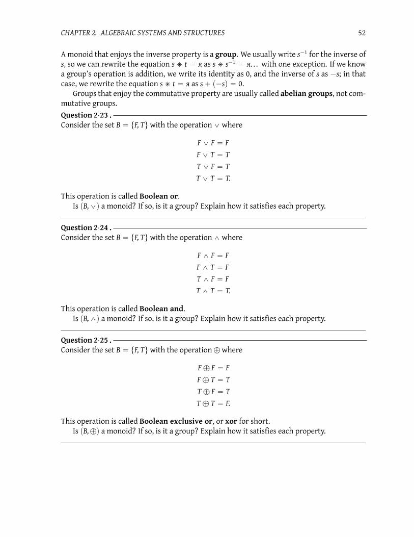
CHAPTER 2. ALGEBRAIC SYSTEMS AND STRUCTURES 52
A monoid that enjoys the inverse property is a group. We usually write s´1
for the inverse of
s, so we can rewrite the equation s˙ t “ я as s˙ s´1 “ я. . . with one exception. If we know
a group’s operation is addition, we write its identity as 0, and the inverse of s as ´s; in that
case, we rewrite the equation s˙ t “ я as s` p´sq “ 0.
Groups that enjoy the commutative property are usually called abelian groups, not com-
mutative groups.
Question 2¨23 .Consider the set B “ tF, Tu with the operation_ where
F _ F “ F
F _ T “ T
T _ F “ T
T _ T “ T.
This operation is called Boolean or.Is pB,_q a monoid? If so, is it a group? Explain how it satisfies each property.
Question 2¨24 .Consider the set B “ tF, Tu with the operation^ where
F ^ F “ F
F ^ T “ F
T ^ F “ F
T ^ T “ T.
This operation is called Boolean and.
Is pB,^q a monoid? If so, is it a group? Explain how it satisfies each property.
Question 2¨25 .Consider the set B “ tF, Tu with the operation‘ where
F ‘ F “ F
F ‘ T “ T
T ‘ F “ T
T ‘ T “ F.
This operation is called Boolean exclusive or, or xor for short.
Is pB,‘q a monoid? If so, is it a group? Explain how it satisfies each property.

CHAPTER 2. ALGEBRAIC SYSTEMS AND STRUCTURES 53
Question 2¨26 .Which of the sets N`, N, and Q are
(a) commutative monoids under addition?
(b) commutative monoids under multiplication?
(c) abelian groups under addition?
(d) abelian groups under multiplication?
Question 2¨27 .Recall that if S is a set, then P pSq is the power set of S; that is, the set of all subsets of S.
(a) Suppose S “ ta, bu. Compute P pSq, and show that it is a monoid under Y (union). Is it
also a group?
(b) Let S be any set. Show that P pSq is a monoid underY (union). Is it also a group?
Question 2¨28 .
(a) Suppose S “ ta, bu. Compute P pSq, and show that it is a monoid under X (intersection).
Is it also a group?
(b) Let S be any set. Show that P pSq is a monoid underX (intersection). Is it also a group?
Definition 2¨29. Let G be any group.
1. For all x, y P G, define the commutator of x and y to be x´1y´1xy. We write rx, ys for the
commutator of x and y.
2. For all z, g P G, define the conjugation of g by z to be zgz´1
. We write gz
for the conju-
gation of g by z.
Question 2¨30 .
(a) Explain why rx, ys “ e iff x and y commute.
(b) Show that rx, ys´1“ ry, xs; that is, the inverse of rx, ys is ry, xs.
(c) Show that pgzq´1“ pg´1q
z; that is, the inverse of conjugation of g by z is the conjugation
of the inverse of g by z.
(d) Fill in each blank of Figure 2.30 with the appropriate justification or statement.

CHAPTER 2. ALGEBRAIC SYSTEMS AND STRUCTURES 54
Claim: rx, ysz “ rxz, yzs for all x, y, z P G.
Proof:
1. Let _____.
2. By _____, rxz, yzs “ rzxz´1, zyz´1s.
3. By _____, rzxz´1, zyz´1s “ pzxz´1q´1pzyz´1q
´1pzxz´1q pzyz´1q.
4. By Question _____,
`
zxz´1˘´1 `
zyz´1˘´1 `
zxz´1˘ `
zyz´1˘
“
“`
zx´1z´1˘ `
zy´1z´1˘ `
zxz´1˘ `
zyz´1˘
.
5. By _____,
`
zx´1z´1˘ `
zy´1z´1˘ `
zxz´1˘ `
zyz´1˘
“`
zx´1˘ `
z´1z˘
y´1
`
z´1z˘
x`
z´1z˘ `
yz´1˘
.
6. By _____,
`
zx´1˘ `
z´1z˘
y´1
`
z´1z˘
x`
z´1z˘ `
yz´1˘
“
“`
zx´1˘
ey´1exe
`
yz´1˘
.
7. By _____, pzx´1q ey´1exe pyz´1q “ pzx´1q y´1x pyz´1q.
8. By _____, pzx´1q y´1x pyz´1q “ z px´1y´1xyq z´1.
9. By _____, z px´1y´1xyq z´1 “ z rx, ys z´1.
10. By _____, z rx, ys z´1 “ rx, ysz.
11. By _____, rxz, yzs “ rx, ysz.
Figure 2¨1: Material for Question 2.30(c)

CHAPTER 2. ALGEBRAIC SYSTEMS AND STRUCTURES 55
So does addition of remainders form a monoid, or even a group?
To answer this question, we first have to make precise what sort of addition we mean. We
have to fix a divisor, so let’s go ahead and use d in general, and d “ 4 for examples, just as
before.
Remainders aren’t closed under ordinary addition (Example 2¨16), but clockwork addition
is closed (Theorem 2¨17), so let’s try that. We’ll use the symbol‘d to make it clear that we’re
thinking about the result of clockwork addition, or just plain ‘ when no one is looking and
it’s clear which d we mean, which is pretty much all the time. That is, r “ a‘ bmeans that r
is the remainder from division of a` b by d.
Is clockwork addition associative? Let a, b, c P Zd. Suppose that r “ a‘ b and s “ pa‘ bq‘ c.
By definition, r ” a ` b, so by substitution, s ” r ` c. Use Theorem 2¨19 to choose p, q P Zsuch that dp “ pa` bq ´ r, and dq “ pr ` cq ´ s. We need to show that s “ a ‘ pb‘ cq, or
equivalently, r` c ” a`pb` cq. The definition of congruence impels us to consider whether
d | rpa` pb` cqq ´ pr ` cqs .
This is true if and only if d | pa` b´ rq. We have already stated that dp “ pa` bq ´ r, which
by definition means d | pa` b´ rq.
Does clockwork addition have an identity element? It makes sense to guess that 0 is the identity
of clockwork addition. Let a P Zd; a` 0 “ a, a remainder, so a‘ 0 “ a and 0‘ a “ a, as well.
We have shown that Zd is a monoid under addition! It is commutative since a` b “ b` a,
so a‘ b “ b‘ a, as well. Let’s see if it is also a group.
Does clockwork addition satisfy the inverse property? Let a P Zd; we showed that 0 is the
identity, so we need to find b P Zd such that a ` b “ 0 and b ` a “ 0. We claim that d ´ a
is the inverse. To see why, let b “ d ´ a. Notice that a ` b “ 0 and b ` a “ 0, as desired.
However, it’s not enough for an inverse to exist somewhere; it must exist in the same set! We
have to check that b is an actual element of Zd.The elements of Zd are t0, 1, 2, . . . , d´ 1u. If we can show that d´ a is one of those num-
bers, we’re done. We know b P N because b “ d´ a, and a ă d, so that’s fine. However, we do
not have b P Zd when a “ 0, because d ´ a “ d R Zd! This is a mistake, but it’s an important
mistake to point out, because it can be easy to overlook. Fortunately, we can fix this.
Most values of awork fine with the formula b “ d´ a; the only one that fails is a “ 0. It’s
easy to verify that 0 is its own inverse: 0 ` 0 “ 0, done. So, one way to bridge the gap is to
define b “ a for a “ 0, and b “ d´ a otherwise. A second, equivalent, way to bridge the gap:
define b as the remainder of d´ awhen you divide by d; we leave it to you to explain why this
resolves the matter.
Question 2¨31 .Show that defining b as the remainder of d´awhen we divide by d always obtains the additive
inverse of a in Zd.
We have now encountered finite groups, and we will encounter more. It’s useful to think
in terms of their size, for which we use a special term.
Definition 2¨32. If a group has a finite number of elements, we say its order is that number
of elements. If a group has an infinite number of elements, we say its order is infinite.

CHAPTER 2. ALGEBRAIC SYSTEMS AND STRUCTURES 56
Question 2¨33 .The smallest group has order 1. What properties does that only element have?
Question 2¨34 .We did not indicate whether Zd was a commutative monoid, and thus an abelian group. Is it?
What about structures with two operations?
So far, we’ve dealt only with structures that have one operation; we considered addition
of numbers, clockwork addition, and monomial multiplication. You may be wondering how
we classify two operations that interact. For example, how might addition and multiplication
interact? You may recall the following property.
distributive if s, t, u P S, then sˆ pt ` uq “ sˆ t ` sˆ u.
A ring is a set Swhereˆ satisfies the properties of a monoid, addition satisfies the properties
of an abelian group, and the two interact via the distributive property.2
If the multiplication
is also commutative, we call S a commutative ring. We always write a generic ring’s additive
identity as 0, and a generic ring’s multiplicative identity as 1.
What about division? A unit is an element of a ring with a multiplicative inverse. A fieldis a commutative ring where you can “divide” by non-zero elements, because they all have
multiplicative inverses. The integers are not a field; after all, 23 R Z, in part because the
multiplicative inverse of 3 is not in Z. We fix that in the following way.
• The set of rational numbers is the set of all well-defined fractions of integers; in set-
builder notation, we’d write,
Q “
ab : a P Z and b P N`(
.
Just as the integers “enable” subtraction, the rationals “enable” division. That is, while you
can subtract naturals, you aren’t guaranteed a natural, but when you expand your horizon
to include integers, you are always guaranteed an integer. Likewise, while you can divide
integers, you aren’t guaranteed an integer, but when you expand your horizon to include
rationals, you are always guaranteed a rational. — With one exception: a number with 0
in the denominator has issues that only a nonstandard analyst can handle. This is why we
qualify our fractions as “well-defined” for the same reason that the set-builder notation puts
b P N`.3
2Many texts do not assume a ring has a multiplicative identity, but others do. We side with the latter for the
sake of simpler exposition and theorems.3Why can’t we divide by zero? Basically, it doesn’t make sense. Suppose that we could find a number c such
that 1˜ 0 “ c. The very idea of division means that if 1˜ 0 “ c, then 1 “ 0 ¨ c, but 0 ¨ c “ 0 for any integer c, so
we can’t have 1 “ 0 ¨ c. We could replace 1 by any nonzero integer a, and achieve the same result. Admittedly,
this reasoning doesn’t apply to 0˜0, but even that offends our notion of an operation! If we were to assign some
c “ 0˜0, we would not be able to decide between 0˜0 “ 1 (since 0 “ 0 ¨1), 0˜0 “ 2 (since 0 “ 0 ¨2), 0˜0 “ 3
(since 0 “ 0 ¨ 3), and so forth. Then there is the matter of the grouping model of division; dividing 4 ˜ 0 “ c
implies that there are exactly c groups of 0 in 4, but no finite c satisfies this assertion.

CHAPTER 2. ALGEBRAIC SYSTEMS AND STRUCTURES 57
Question 2¨35 .Which of the sets N`, N, and Q are
(a) commutative rings under ordinary addition and multiplication?
(b) fields under ordinary addition and multiplication?
Question 2¨36 .Is pB,_,^q a ring? Is it a field? (Here we are saying that_ stands in for the addition, while^
stands in for the multiplication.)
Question 2¨37 .Is pB,‘,^q a ring? Is it a field? (Here we are saying that‘ stands in for the addition, while^
stands in for the multiplication.)
Question 2¨38 .Let’s return to the discussion of cardinality in Question 1¨18. We had concluded with the weird
result that the cardinalities of N and Z are the same.
Speaking of weird results, show that N and Q have the same cardinality. This is a little
harder, so we’re going to cheat. First, explain why Q “obviously” has cardinality no smaller
than N’s, by showing that you can match every element of N to an element of Q, and have
infinitely many elements of Q left over. Then, show that N “obviously” has cardinality no
smaller than Q’s, because if we arrange the elements of Q according to the following table:
01 02 03 04 ¨ ¨ ¨11 12 13 14 ¨ ¨ ¨21 22 23 24 ¨ ¨ ¨31 32 33 34 ¨ ¨ ¨...
......
.... . .
then you can match every element ofQ to an element ofN, and have infinitely many elements
of N left over. (Think diagonally. — No, the other diagonally.) Since neither’s cardinality is
smaller than the other’s, it seems reasonable to conclude they have equal cardinality.
Cayley tables
A useful tool for analyzing operations on small sets is an abstract multiplication table,
sometimes called the Cayley table. For instance, the Cayley tables for addition and multipli-
cation in Z4 look like this:
‘ 0 1 2 3
0 0 1 2 3
1 1 2 3 0
2 2 3 0 1
3 3 0 1 2
b 0 1 2 3
0 0 0 0 0
1 0 1 2 3
2 0 2 0 2
3 0 3 2 1

CHAPTER 2. ALGEBRAIC SYSTEMS AND STRUCTURES 58
You may notice some interesting properties: every element of Z4 appears exactly once in
each row or column of the first table, but not the second. Another strange phenomenon is
that 2b 3 “ 2b 1 even though 3 ‰ 1.
Question 2¨39 .List the elements of Z2, and write its Cayley table. Notice how this starts to justify our notion
of a self-canceling arithmetic.
Question 2¨40 .We observed that every element appears exactly once in each row or column of the Cayley
tables above. We can write this mathematically as, if a˙ c “ d and b˙ c “ d, then a “ b.
(a) To see that the statement might not be true in a monoid, build the Cayley table of Z6under multiplication. Show that it satisfies the properties of a monoid, but not of a group.
Then identify elements x, y, z P Z6 such that xb z “ yb z, even though x ‰ y. Isn’t that
weird?
(b) A phenomenon related to this one is that with natural numbers, if ab “ 0, then a “ 0
or b “ 0. That’s not true in an arbitrary monoid! Identify elements a, b P Z6 such that
ab b “ 0, but a, b ‰ 0. How are these elements related to the result in (a)? Hint: You’ve
already done this problem; it’s just phrased differently. See Question 4.72.
(c) Prove that, in a group G, if a, b, c, d P G, a˙ c “ d and b˙ c “ d, then a “ b. Hint: Since it’s
true in a group, but not in a monoid, you should use a property that is special to groups,
but not monoids.
(d) Use (c) to explain why every element d of a group G appears exactly once in each row or
column of a group’s Cayley table. Hint: If it appears in two rows, what equation does that
imply?
In a ring, multiplication by zero behaves exactly as you’d expect.
Fact 2¨41. If R is a ring and a P R, then aˆ 0 “ 0 and 0ˆ a “ 0.
Why? By the identity and distributive properties, a ˆ 0 “ a ˆ p0` 0q “ a ˆ 0 ` a ˆ 0. Let
b “ aˆ 0 and condense the chain to
b “ b` b.
Add´b to both sides, and apply some properties of rings, and we have
´b` b “ ´b` pb` bq
0 “ p´b` bq ` b
0 “ 0` b
0 “ b.
By substitution, aˆ 0 “ 0.

CHAPTER 2. ALGEBRAIC SYSTEMS AND STRUCTURES 59
On the other hand, multiplication to zero is a bit funny — not so much “ha ha funny” so
much as “strange funny.”
Definition 2¨42. Let R be a ring, and a, b P R. If ab “ 0 and neither a “ 0 nor b “ 0, then we
call a and b zero divisors. A ring without zero divisors satisfies the zero product property;
that is, if ab “ 0, then a “ 0 or b “ 0. (“If the product is zero, a factor is zero.”) A ring that
satisfies the zero product rule is an integral domain.
Example 2¨43. • The integers Z are an integral domain.
As you have just seen, Zd is not always an integral domain, but sometimes it is. When?
Question 2¨44 .Carry out enough computations in Z3, Z4, Z5, and Z6 to answer the following: For which
values of d will Zd have zero divisors, and for which values of d is Zd an integral domain?
What property do the rings with zero divisors share, as opposed to the integral domains?
Question 2¨45 .Show that every field is an integral domain. Conversely, name an integral domain that is not
a field.
2¨3 Isomorphism
Plus ca change, plus c’est la meme chose.
(The more things change, the more they stay the same.)
— French proverb
We’ve seen several important algebraic systems that share the same structure. For instance,
pN,`q, pZd,`q, and pM,ˆq are all monoids. When looking at two algebraic systems that share
a basic structure, mathematicians sometimes ask themselves, How similar are they? Is the sim-
ilarity more than superficial? Could it be that their Cayley tables are essentially identical, so
that one of the systems are, from an algebraic view, exactly the same?
You might also look at it a different way. Two algebraic systems can have an initially
different appearance, but while working with both you notice that certain behaviors are the
same. It’s easier to work with one system than the other; in particular, it’s easier to show
that a pleasant property holds for one system than for the other. If their Cayley tables are
essentially identical, then you know the “difficult” system does in fact share that pleasant
property, as well.
The technical word for this is isomorphism, and we can rephrase our question this way:
How can we decide whether two algebraic systems are isomorphic?
In general, we replace “algebraic system” with the particular structure that interests us:
How can we decide whether two monoids are isomorphic?

CHAPTER 2. ALGEBRAIC SYSTEMS AND STRUCTURES 60
How can we decide whether two groups are isomorphic?
How can we decide whether two rings are isomorphic?
How can we decide whether two fields are isomorphic?
This section considers how to do this.
Question 2¨46 .Recall the structures Boolean or pB,_q, Boolean and pB,^q, and Boolean xor pB,‘q (Ques-
tions 2.23, 2.24, and 2.25).
All three are monoids, but inspection of the Cayley tables will show that two are more
or less the same (hence, “isomorphic” in our intuitive notion of the term), but the third is
different from the others. Which two are isomorphic? Why isn’t the third isomorphic?
Be careful on this problem — superficially, none of their Cayley tables look the same. You
have to look closely at the layout of the Cayley table before you notice the pattern.
The idea
Imagine two offices. How would you decide if the offices were equally suitable for a certain
job? You first need to know what tasks have to be completed, and what materials you need.
If the tasks require reference books, you would want a bookshelf in the office. If they require
writing, you would want a desk, perhaps a computer. If they require communication, you
might need a phone.
With such a list in hand, you can make an educated comparison between the offices. If
both offer the needed equipment, you’d consider both suitable for the job at hand. The precise
manner in which the offices satisfy these requirements doesn’t matter; if one’s desk is wood,
and the other’s is steel, that makes an aesthetic difference, but they’re functionally the same.
If one office lacked a desk, however, it wouldn’t be up to the required job.
Deciding whether two algebraic systems are isomorphic is similar. First, you decide what
structure you want to analyze. Next, you compare how the sets satisfy those structural prop-
erties. If you’re looking at finite monoids, an exhaustive comparison of their Cayley tables
might work, but the method is called “exhaustive” for a reason. Besides, we deal with infi-
nite sets like N often enough that we need a non-exhaustive way to compare their structure.
Functions turn out to be just the tool we need.
How so? Let S and T be any two sets. Recall that a function f : S Ñ T is a relation that
sends every input s P S to precisely one value in T, the output f psq. You have probably heard
the geometric interpretation of this: f passes the “vertical line test.” You might suspect at this
point that we are going to generalize the notion of function to something more general, just
as we generalized from the lattice and monomials to monoids. To the contrary, we specialize
the notion of a function in a way that tells us important information about a monoid.
SupposeM and N are monoids. If they are isomorphic, their monoid structure is identical,
so we ought to be able to build a function that maps elements with a certain behavior in M
to elements with the same behavior in N. (Table to table, phone to phone.) What does that
mean? Let a, b, c P M and x, y, z P N. If M and N have the same structure as monoids, with x
filling in for a, y filling in for b, and z filling in for c, we would expect that

CHAPTER 2. ALGEBRAIC SYSTEMS AND STRUCTURES 61
• if ab “ c, then
• xy “ z.
Question 2¨47 .Suppose you know only two facts about an algebraic system pG,˙q: it forms a group, and G
holds exactly two elements, я (the identity) and g. You know neither the elements’ internal
structure, nor how the operation ˙ works. You know only that G is a group of two elements.
Show that, regardless of this profound ignorance, the group properties force exactly one Cay-
ley table on G. In other words, all groups of order 2 are isomorphic!Hint: Try to build the Cayley table of G. You will encounter no ambiguity in the process,
forcing the conclusion that only one possible table exists.
Question 2¨48 .Suppose you know only two facts about an algebraic system pG,˙q: it forms a group, and
G holds exactly three elements, я (the identity), g, and h. As before, you know neither the
elements’ internal structure, nor how the operation ˙ works. Show that, regardless of this
profound ignorance, the group properties force exactly one Cayley table on G. In other words,
all groups of order 3 are isomorphic!
Question 2¨49 .Suppose you know only two facts about an algebraic system pG,˙q: it forms a group, and G
holds exactly four elements, я (the identity), g, h, and gh. As before, you know neither the
elements’ internal structure, nor how the operation ˙ works. Show that, regardless of this
profound ignorance, the group properties force exactly. . . two Cayley tables on G. (More than
one!) In other words, (a) not all groups of order 4 are isomorphic, and (b) there are exactly
two groups of order 4, “up to isomorphism!”
Definition 2¨50. In Question 2.49, you should have encountered exactly one ambiguity while
completing the Cayley table: what value can we assign a˙ a? The case where a2 “ я is called
the Klein 4-group. The case where a2 ‰ я should look like another system you’ve played
with.
The definition
Recall that our idea of isomorphism in monoids works as follows. For every a, b, c P M and
every x, y, z P N,
• if a corresponds to x, b corresponds to y, and c corresponds to z, and
• if ab “ c, then xy “ z.
In mathematics, we can say that “a corresponds to x” using function notation, f paq “ x. That
principle allows us to rewrite the equation xy “ z as
f paq f pbq “ f pcq .

CHAPTER 2. ALGEBRAIC SYSTEMS AND STRUCTURES 62
But remember, ab “ c, so substitution tells us the operation corresponds if
f paq f pbq “ f pabq . (2.2)
The identity ofM should also correspond to the identity of N, so we need to add the condition
f pяMq “ яN . (2.3)
When dealing with a group, the inverse of an element should correspond to the inverse its
corresponding element, which gives us a third condition, f px´1q “ a´1, which we rewrite as
f`
x´1˘
“ f pxq´1. (2.4)
If we can pull off both (2.2) and (2.3) (as well as (2.4) in a group), we say that f is a ho-momorphism, from the Greek words “homo” and “morphos”, meaning “same shape”. The
existence of a homomorphism tells us that the Cayley table of M has the same shape as a
subset of the Cayley table of N.
That’s not enough to answer the question. We don’t want to know merely whether some-
thing akin to M appears in N; we want M and N to be essentially identical. Just as we only need
one table in any office, we want the correspondence between the elements of the monoids to
be unique: in other words,
f should be one-to-one.
Finally, everything in N should correspond to something in M; if the offices are identical, we
shouldn’t find something useful in the second that doesn’t appear in the first. In terms of f ,
that means
f should be onto.
We summarize our discussion up to this point with the following definition:
Definition 2¨51. Let pS,˙q and pT, ‹q be monoids. If there exists a function f : S Ñ T such
that
• f pяSq “ яT (f preserves the identity)
and
• f pa˙ bq “ f paq ‹ f pbq for all a, b P S, (f preserves the operation)
then we call f amonoid homomorphism.
Now suppose pS,˙q and pT, ‹q are groups. If there exists a function f : SÑ T such that
• f pяSq “ яT, (f preserves the identity)
• f pa˙ bq “ f paq ‹ f pbq for all a, b P S, (f preserves the operation)
and

CHAPTER 2. ALGEBRAIC SYSTEMS AND STRUCTURES 63
• f pa´1q “ f paq´1 for all a P S, (f preserves inverses)
then we call f a group homomorphism.
Finally, suppose pR,ˆ,`q and pS,ˆ,`q are rings. If there exists a function f : RÑ S such
that
• f is a group homomorphism with respect to addition, and
• f is a monoid homomorphism with respect to multiplication,
then we call f a ring homomorphism.
If f is also a bijection, then we say M is isomorphic to N, write M – N, and call f an
isomorphism. (A bijection is a function that is both one-to-one and onto.)
We used pS,˙q and pT, ‹q in the definition to emphasize that they could stand for any two
algebraic systems, regardless of the operations involved.
An immediate goal, of course, is to show that the natural numbers under addition are
isomorphic (as monoids) to the monomials under multiplication. We’ll write X for the set
of all natural powers of x; that is, X “ t1, x, x2, . . . u. We have noticed already that monoid
multiplication works like the addition of natural numbers.
Example 2¨52. We claim that pX,ˆq is isomorphic to pN,`q. To see why, map f : XÑ N via
f pxaq “ a. First we show that f is a bijection.
To see that it is one-to-one, let t, u P X, and assume that f ptq “ f puq. By definition of X,
we can find a, b P N such that t “ xa
and u “ xb. Substituting this into f ptq “ f puq, we find
that f pxaq “ f`
xb˘
. The definition of f allows us to rewrite this as a “ b. However, if a “ b,
then xa “ xb, and t “ u. We assumed that f ptq “ f puq for arbitrary t, u P X, and showed that
t “ u; that proves f is one-to-one.
To see that f is onto, let a P N. We need to find t P X such that f ptq “ a. Which t should
we choose? We want f`
xsomething
˘
“ a. We know that f`
xsomething
˘
“ something. We are
looking for a t that makes f ptq “ a, so the “natural” choice seems to be something “ a, or
t “ xa. That would certainly guarantee f ptq “ a, but can we actually find such an object t in
X? Since xa P X, we can in fact make this choice! We took an arbitrary element a P N, and
showed that f maps some element of X to a; that proves f is onto.
So f is a bijection. Is it also an isomorphism? First we check that f preserves the operation.
Let4t, u P X. By definition of X, t “ x
aand u “ x
bfor a, b P N. We now manipulate f ptuq
using definitions and substitutions to show that the operation is preserved:
f ptuq “ f`
xaxb˘
“ f`
xa`b
˘
“ a` b
“ f pxaq ` f
`
xb˘
“ f ptq ` f puq .
4The definition uses the variables x and y, but those are just letters that stand for arbitrary elements of M.
HereM “ X and we can likewise choose any two letters we want to stand in place of x and y. It would be a very
bad idea to use xwhen talking about an arbitrary element of X, because there is an element of X called x. So we
choose t and u instead.

CHAPTER 2. ALGEBRAIC SYSTEMS AND STRUCTURES 64
The operation inX is multiplication; the operation inN is addition, so we should expect f ptq`
f puq at the end; the operations is indeed preserved.
Does f also preserve the identity? We usually write the identity of M “ X as 1, but this
just stands in for x0. On the other hand, the identity (under addition) of N “ N is the number
0. We use this fact to verify that f preserves the identity:
f pяMq “ f p1q “ f`
x0˘
“ 0 “ яN .
(We won’t usually write яM and яN, but I’m doing it here to show explicitly how this relates to
the definition.)
We have shown that there exists a bijection f : X ÝÑ N that preserves the operation and
the identity. We conclude that X – N.
Question 2¨53 .Earlier, you inspected the Cayley tables of pB,^q, pB,_q, and pB,‘q, and found that two were
isomorphic. Define an isomorphism f from one monoid to its isomorphic counterpart.
On the other hand, is pN,`q – pN,ˆq? You might think this easy to verify, since the sets
are the same. Let’s see what happens.
Example 2¨54. Suppose there does exist an isomorphism f : pN,`q Ñ pN,ˆq. What would
have to be true about f ? Let a P N such that f p1q “ a; after all, f has to map 1 to something!
An isomorphism must preserve the operation, so
f p2q “ f p1` 1q “ f p1q ˆ f p1q “ a2
and
f p3q “ f p1` p1` 1qq “ f p1q ˆ f p1` 1q “ a3, so that
f pnq “ ¨ ¨ ¨ “ an
for any n P N.
So f sends every integer in pN,`q to a power of a.
Think about what this implies. For f to be a bijection, it would have to be onto, so every
element of pN,ˆq would have to be an integer power of a. This is false! After all, 2 is not an
integer power of 3, and 3 is not an integer power of 2. We have found that pN,`q fl pN,ˆq.Question 2¨55 .Both Z and 2Z are groups under addition.
(a) Show that f : ZÑ 2Z by f pzq “ 2z is a group isomorphism. Hence Z – 2Z.
(b) Show that Z – nZ, as groups, for every nonzero integer n.
Question 2¨56 .Let d ě 1. Both Z and Zd are rings, though Z is a ring under ordinary addition and multi-
plication, while Zd is a ring under modular addition and multiplication. Let f : Z Ñ Zd by
f paq “ rasd, where ras
dmeans “the remainder of a after division by d.”
(a) Show that f is a ring homomorphism.
(b) Explain why f cannot possibly be a ring isomorphism. You don’t need any symbols here;
the best explanation uses only a few words.

CHAPTER 2. ALGEBRAIC SYSTEMS AND STRUCTURES 65
Question 2¨57 .LetM “ ttu , tauu.
(a) Show thatM is a monoid under the operationY (set union).
(b) Show that pM,Yq is isomorphic to the monoid “Boolean or”.
(c) CanM be isomorphic to the monoid “Boolean xor”?
Question 2¨58 .Let
M “
"ˆ
1 0
0 1
˙
,
ˆ
0 1
1 0
˙*
.
(a) Show thatM is a monoid under matrix multiplication.
(b) Show thatM is isomorphic to the monoid “Boolean xor”.
(c) CanM be isomorphic to the monoid “Boolean or”?
Sometimes, less is more
As defined, a group homomorphism is a function that preserves
• the operation (f pxyq “ f pxq f pyq),
• the identity (f pяq “ я), and
• inverses (f px´1q “ f pxq´1
).
Amazingly, we can define a group homomorphism using only one of these three!
Theorem 2¨59. Let G and H be groups, and suppose f : G Ñ H is a function that preserves the
operation; that is, f pxyq “ f pxq f pyq for all x, y P G. In this case, f automatically preserves the
identity and all inverses.
The upshot is that to show a function is a group homomorphism, you need not check all
three properties! You need check only that the operation is preserved.
Proof. We need to show that f preserves the identity and all inverses.
For the identity, let h P H. Let g P G, and h “ f pgq. By hypothesis, f preserves the
operation, so f pgяGq “ f pgq f pяGq. By definition of an identity, gяG “ g, so we can rewrite the
previous equation as f pgq “ f pgq f pяGq. By substitution, h “ h ¨ f pяGq. Since H is a group, h
has an inverse in H, so we can multiply both sides by the inverse of h, obtaining яH “ f pяGq.
In other words, f preserves the identity.

CHAPTER 2. ALGEBRAIC SYSTEMS AND STRUCTURES 66
For inverses, let g P G, and let h “ f pgq. Since G is a group, g has an inverse in G. By
hypothesis, f preserves the operation, so f pg ¨ g´1q “ f pgq ¨ f pg´1q. By substitution, f pяGq “
hf pg´1q. We just showed that f preserves the identity, so we can rewrite the equation as яH “
hf pg´1q. Since H is a group, h has an inverse in H, so we can multiply both sides by the inverse
of h, obtaining h´1 “ f pg´1q. By substitution, f pgq
´1“ f pg´1q. In other words, f preserves
the inverse of g. Since g was an arbitrary element of G, f must preserve all inverses.
This shortcut does not work for monoid homomorphisms!
Question 2¨60 .What aspect of the proof suggests that this shortcut does not work for monoid homomor-
phisms?
Question 2¨61 .Consider the monoidsM “ pN,ˆq and N “ pN,`q. Let f : MÑ N by f pxq “ 0. Explain why:
(a) f preserves the operation, but
(b) f does not preserve the identity.
Question 2¨62 .Let M “ tя, au, and consider the operation where я is the identity and a
2 “ я. Let N “ t1, bu
and consider the operation where 1 is the identity and b2 “ b.
(a) Show thatM and N are both monoids under this operation. Which one is not a group?
(b) Show that the map f : MÑ N defined by f pяq “ b and f paq “ b preserves the operation,
despite not preserving the identity.
(c) How does this show that there is no parallel to Theorem 2¨59 for monoids?
Direct Products
It is easy to build new algebraic systems using a Cartesian product of algebraic systems.
Let S1, S2, . . . be a sequence of groups, a sequence of monoids, or a sequence of rings. Let
T “ S1 ˆ S2 ˆ ¨ ¨ ¨ . (We proceed as if we have infinitely many S, but it works just as well if
there are finitely many, and the example below will have finitely many.) Define an operation
˙ on T as follows:
• for any t, u P T,
• we can write t “ pt1, t2, . . . q, pu1, u2, . . . q where
– t1, u1 P S1, t2, u2 P S2, . . .

CHAPTER 2. ALGEBRAIC SYSTEMS AND STRUCTURES 67
so define
t˙ u “ ps1t1, s2t2, . . . q .
We say that the operation in T is componentwise: we apply the operation of S1 to elements in
the first component; the operation of S2 to elements in the second component; and so forth.
Example 2¨63. Consider Z2 and Z3 as rings under addition and multiplication, modulo 2 or 3
as appropriate. Then
Z2 ˆ Z3 “ tp02, 03q , p02, 13q , p02, 23q , p12, 03q , p12, 13q , p12, 23qu .
(Henceforth we leave off the 2’s and 3’s, since the first component is only ever in Z2 and the
second only ever in Z3.) Given the operation defined above, sums of elements in Z2 ˆ Z3 are
p0, 2q ` p1, 1q “ p1, 0q
p1, 1q ` p1, 1q “ p0, 2q
while products of elements in Z2 ˆ Z3 are
p0, 2q ˆ p1, 1q “ p0, 2q
p1, 1q ˆ p1, 1q “ p1, 1q .
Fact 2¨64. Let S1, S2, . . . be a sequence (possibly finite) of algebraic systems, and T their cartesian
product, with componentwise operation(s) defined as above.
(A) T is a monoid under the componentwise operation if all the Si are monoids.
(B) T is a group under the componentwise operation if all the Si are groups.
(C) T is a ring under componentwise addition and multiplication if all the Si are rings under their
respective addition and multiplication.
However, T is never an integral domain, even if all the Si are integral domains, unless every Si “ t0u.
Why? We show (A) and (B), since that also covers (C). We leave the question of why T is not
an integral domain to the reader. To see why, let t, u P T.
(A) Suppose each Si is a group. By definition, t˙u “ pt1u1, t2u2, . . . q. By hypothesis, each Si
is a monoid, hence closed, so each tiui P Si, so t˙ u P T. That shows closure. For associativity,
let v P T; again, each Si is associative, so
t˙ pu˙ vq “ t˙ pu1v1, u2v2, . . . q pdef of ˙q
“ pt1 pu1v1q , t2 pu2v2q , . . . q pdef of ˙q
“ ppt1u1q v1, pt2u2q v2, . . . q peach Si assocq
“ pt1u1, t2u2, . . . q˙ v pdef of ˙q
“ pt˙ uq˙ v. pdef of ˙q

CHAPTER 2. ALGEBRAIC SYSTEMS AND STRUCTURES 68
Finally, write яi for the identity of Si, and observe that pя1, я2, . . . q P T. We claim that this is
the identity; indeed,
t˙ pя1, я2, . . . q “ pt1я1, t2я2, . . . q “ pt1, t2, . . . q “ t
and likewise if we multiply by t on the right. So pя1, я2, . . . q really does act as the identity for
T, and we abbreviate it as яT.
We have show that T is closed and associative under the componentwise operation, and
that it has an identity; hence, T is a monoid.
(B) For the group property, we need merely show that every element of T has an inverse.
Each component ti of t is an element of Si, which by hypothesis is a group, so t´1iP Si. By
definition of T,`
t´11 , t
´12 , . . .
˘
P T. Consider its product with t:
t˙`
t´11, t´12, . . .
˘
“`
t1t´11, t2t
´12, . . .
˘
“ pя1, я2, . . . q “ яT.
Hence`
t´11 , t
´12 , . . .
˘
is an inverse of t in T.
Question 2¨65 .Construct Cayley tables for addition and multiplication in Z2ˆZ3. Indicate the zero divisors.
Question 2¨66 .The group Z2 ˆ Z2 has four elements. We already know that, up to isomorphism, there are
only two groups: Z4 and the Klein 4-group. To which of these is Z2 ˆ Z2 isomorphic?
Question 2¨67 .Let f : Z6 Ñ Z2ˆZ3 by the rule f paq “ pras
2, ras
3q. For instance, f p4q “ pr4s
2, r4s
3q “ p0, 1q.
(a) Compute all the images of f .
(b) How do you know f is one-to-one and onto?
(c) Show that f is a homomorphism.
Hint: You could show this exhaustively (only 36 pairs!) but need not do so. Instead, use a
previous result on products of Zn.
(d) Why is Z6 – Z2 ˆ Z3?
Question 2¨68 .Show that even if S1, S2, . . . are all integral domains, T “ S1 ˆ S2 ˆ ¨ ¨ ¨ is not an integral
domain, unless every Si “ t0u.

Chapter 3
Common and important algebraicsystems
The previous chapter introduced you to monoids, groups, rings, and fields, emphasizing pri-
marily remainders. This chapter aims to show that these structures’ elegant properties apply
to other mathematical objects. These objects are of fundamental important in advanced al-
gebra, so it seems appropriate to introduce them here.
3¨1 Polynomials, real and complex numbers
God created the integers. All else is the work of man.
— Leopold Kronecker
Let R be any commutative ring. We say that x is indeterminate over R if x has no specific
value, but we can substitute any value of R for x. Naturally, ax “ xa. A polynomial in x overR is any finite sum of the form
f “ a0 ` a1x` a2x2` ¨ ¨ ¨ ` anx
n,
where each ai P R and an ‰ 0. We call each ai the coefficient of the corresponding xi, and call
an the leading coefficient.If we’re feeling lazy, which we often are, we just say f is polynomial over R, since the
indeterminate is obvious. If we’re feeling especially lazy, which we sometimes are, we just say
f is polynomial, since the ring is clear from context.
We need not restrain ourselves to x; any symbol will do, as long as the meaning is clear.
For instance, if t is indeterminate over Z4, then 2t ` 3 is a polynomial in t over Z4. If y is
indeterminate over Q, then2
3x2 ´ 1
5x is a polynomial in y over Q.
Let f be a polynomial in x whose coefficients are elements of R. We say that f is a poly-nomial over R, and we write R rxs for the set of all polynomials over R. We call R the groundring of R rxs. Addition and multiplication of polynomials over R behaves the same as addition
and multiplication of polynomials over Z; the only difference is the ground ring.
Example 3¨1. Polynomials with integer coefficients are elements of Z rxs. Polynomials with
rational coefficients are elements of Q rxs. Polynomials with coefficients modulo d ą 0 are
elements of Zd rxs.
69

CHAPTER 3. COMMON AND IMPORTANT ALGEBRAIC SYSTEMS 70
Question 3¨2 .Suppose R is a commutative ring, with additive identity 0 and multiplicative identity 1. Show
that R rxs is also a commutative ring, with the same identities as R.
Fact 3¨3. It is also the case that if R is an integral domain, then so is R rxs.
Why? If f, g P R rxs are nonzero but fg “ 0, then the leading term of fg is zero; this leading
term is the product of the leading terms of f and g. If we write at for the leading term of f
and bu for the leading term of g (where c, d P R and t, u P X) then, by definition, pctq pduq “ 0.
This is possible only if cd “ 0. As they come from the leading terms of f and g, the leading
coefficients must be nonzero; that is, c, d ‰ 0. But c, d ‰ 0 and cd “ 0means c and d are zero
divisors, so R cannot be an integral domain. We have shown the contrapositive of the claim,
and the contrapositive is equivalent to the claim itself.
The Division Theorem for Polynomials (p. 34) tells us that we can use monic divisors to
compute quotients and remainders in Z rxs. We can actually do this with polynomials over
any commutative ring!
On the one hand, it makes sense that a similar argument should apply for polynomials with
rational, or even real coefficients, but it might not be so clear for stranger rings which you
have yet to meet. Stranger yet, we decline to write a proof generalizing the Division Theorem
for Polynomials to these other rings. Why? Sometimes, generalizing a result like this is quite
hard, but in this case it does not require much convincing; go back and examine the proof.
Does anything in the argument depend on the coefficients’ being integers? Nothing does; the
argument would have worked for any ringR. We do need a monic divisor, and we do need a ring
of coefficients, since the proof required both subtraction and multiplication of coefficients.
This hints that there is a larger, more interesting structure we have not named yet, but we
pass over that for the time being.
Question 3¨4 .Rewrite the proof of the Division Theorem for Polynomials, replacing any instance of Z or
“integer” with R or “ring element”. Convince yourself that, yes, this is a wonderfully general
result.
You will recall that we developed a class of rings, calledZd, by building an algebraic system
on remainders of integer division. A natural question to ask is,
Can we build a consistent algebraic system on remainders of polynomial division?
Indeed, we can! We will also find that this gives us a concrete way of building an “imaginary”
algebraic system.
Polynomial remainders
Let’s look at how remainder arithmetic modulo a polynomial might work.

CHAPTER 3. COMMON AND IMPORTANT ALGEBRAIC SYSTEMS 71
Example 3¨5. Let g “ x2 ´ 1. Any remainder r after division by g has degree smaller than 2
(after all, deg g “ 2), so we can write
r “ ax` b,
where a and b are integers. That’s it! There are no other restrictions on r, and none on a and
b, aside from their being integers.
We have already encountered one difference with integer remainders: there can be in-
finitely many polynomial remainders! (After all, you can choose a and b arbitrarily from the
ground ring.) At least the degree of the divisor constrains them.
Will the arithmetic of polynomial remainders exhibit a “clockwork” behavior, as with in-
teger remainders? Not with addition, since
pax` bq ` pcx` dq “ pa` cq x` pb` dq ,
and no matter what the values of a, b, c, and d, that sum has degree 1. With multiplication,
however,
pax` bq pcx` dq “ acx2` pad` bcq x` bd
ventures into forbidden territory, with degree 2. We have to reduce this polynomial modulo
x2 ´ 1.
Example 3¨6. Consider the remainders 2x` 3 and´5x` 12, modulo x2 ´ 1. Their sum is
p2x` 3q ` p´5x` 12q “ ´3x` 15,
another remainder. Their product is
p2x` 3q p´5x` 12q “ ´10x2` 9x` 36,
which is not a remainder, but we can reduce it modulo x2 ´ 1 to 9x` 26. In other words,
p2x` 3q p´5x` 12q ” 9x` 26.
Theorem 3¨7. Let R be a commutative ring, and R rxs a polynomial ring. Let g be a monic polynomial
of R rxs. The set of remainders modulo g also forms a ring under addition and multiplication, modulo g.
Proof. Question 3.2 tells us that R rxs is a commutative ring, and hence an abelian group under
addition. Addition of polynomials does not change the degree, so as we saw above, the prop-
erties of R rxs are preserved in the set of remainders; the sums are, in fact, identical, so the
identity of addition of remainders remains the zero polynomial, which is itself a remainder,
and the additive inverse of a remainder is also present. So the set of remainders preserves
the abelian group property of R rxs.
On the other hand, multiplication of remainders risks raising the degree, so the product of
two remainders might not itself be a remainder, as we saw above. However, our multiplication
is modulo g, and when we divide the product by g, we obtain a remainder. This guarantees clo-
sure. The multiplicative identity of polynomial multiplication is the constant polynomial 1,
which is itself a remainder. The commutative property is likewise preserved, so if the set of
remainders is a ring, it is a commutative ring. There remain two properties to check.
What of the associative property of multiplication? Let r, s, and t be remainders. We know
that prsq t “ r pstq as polynomials; since the remainder of division is unique, we must also have
prsq t ” r pstq. Distribution follows similarly.

CHAPTER 3. COMMON AND IMPORTANT ALGEBRAIC SYSTEMS 72
So far, we have observed nothing strange with these remainders, but the next example
does exhibit a very unusual behavior.
Example 3¨8. Consider the remainders x` 1 and x´ 1modulo x2 ´ 1. Their sum is
px` 1q ` px´ 1q “ 2x,
another remainder. No surprise. Their product is
px` 1q px´ 1q “ x2´ 1,
which is not a remainder, but we can reduce it modulo x2 ´ 1 to. . . 0?!?
Zero divisors have returned!
Ordinary multiplication of two nonzero polynomials over an integral domain gives you a
nonzero polynomial (Fact 3¨3). After all, multiplication increases the degree, so you can’t get
0 as a product of nonzero polynomials.
With the modular product of remainders, those guarantees vanish! Upon reflection, this
makes sense, because x2 ´ 1 factors into x` 1 and x´ 1 precisely — just as 6 “ 2ˆ 3. Just as
with Zd, this has consequences for solving equations; until now, you usually solved equations
under the assumption that a product of zero has a factor of zero.
Example 3¨9. When we try to find integer solutions of equations such as x3 ´ 1 “ 0, we
typically factor first, obtaining
px´ 1q`
x2` x` 1
˘
“ 0.
As integer polynomials, we know that if the product is zero, a factor must be zero, helping us to
find the solution x “ 1. We enjoy no such guarantee from remainder arithmetic.
The introduction of zero divisors doesn’t happen modulo every polynomial. With some,
we get a different phenomenon.
Real numbers
The set of real numbers is the set of all possible distances one can move along a line, with
“positive length” indicating we moved in one direction, and “negative length” indicating we
moved in the opposite direction. Its shorthand isR. There are ways to write this in set-builder
notation, but I’ll pass over that for now.
You may wonder if R “ Q. If you don’t wonder it, that’s okay; someone else has already
wondered it, and we know the answer: no.
Fact 3¨10.?2 is real, but not rational.
Why? We know that?2 is real because the Pythagorean Theorem tells us that it is the length
of the hypotenuse of an isosceles right triangle whose legs have length 1.

CHAPTER 3. COMMON AND IMPORTANT ALGEBRAIC SYSTEMS 73
1
1?
The length of the red line is?2, so
?2 is real.
However,?2 is not rational. To see why, let a, b P N, with b ‰ 0, and suppose
?2 “ ab. (We
can assume a is natural because?2 is positive.) Suppose further that a and b have no common
divisors; after all, if they do, we can simplify the fraction. (The well-ordering principle means
simplification can’t continue indefinitely.) Rewrite?2 “ ab as b
?2 “ a; square both sides
to obtain 2b2 “ a
2. Notice that a
2is an even number; this is possible only if a is even, so
a “ 2c for some integer c. Rewrite as 2b2 “ p2cq
2, so 2b
2 “ 4c2, so b
2 “ 2c2. The argument
above implies that b is even. So a and b are both even, giving them a common divisor. But
this contradicts the reasonable assumption above that they have no common divisors! Our
assumption that we could write?2 “ ab, where a and b are natural, is false:
?2 is real, but
not rational.
We call lengths like?2 irrational numbers. You’ll meet some of these in the exercises.
Despite the unfortunate name, they are not unreasonable, and have some very important
uses. Thus, we not only have
N` Ď N Ď Z Ď Q Ď R,
we also have
N` Ĺ N Ĺ Z Ĺ Q Ĺ R.
We can describe three-dimensional real space as
R3“ Rˆ Rˆ R “ tpa, b, cq : a, b, c P Ru ;
people use this notation a lot in multivariate calculus.
As with the rationals, we can divide real numbers, and end up with a real number. Also
with the rational, we can’t divide by zero.
Question 3¨11 .We return to the question of cardinality again. We had shown thatN, Z, andQ have the same
cardinality. They do not have the same cardinality as R. To see why, suppose the contrary,
that we have a matching of distinct real numbers to natural numbers, so that we can list all
the real numbers in a row, a1, a2, . . . .

CHAPTER 3. COMMON AND IMPORTANT ALGEBRAIC SYSTEMS 74
Consider a real number b built by taking as its first digit after the decimal point a digit
that is not the first digit after the decimal point of a1, as its second digit after the decimal
point a digit that is not the second digit after the decimal point of a2, as its third digit after
the decimal point a digit that is not the third digit after the decimal point of a3, and so forth.
(a) How do we know that b does not appear in the list a1, a2, . . . ?
(b) You need not show that b is a real number, but it is. How does this show that N and Rmust have different cardinality?
(c) Why does that mean that Z and Q likewise have different cardinality from R?
Complex numbers
The real numbers make for a lovely field, but they retain an important defect.
Fact 3¨12. There is no real solution to x2 ` 1 “ 0; that is,
?´1 R R.
Proof. Let a P R. By the definitions of real arithmetic, a2
is positive. That means a2 ` 1 is also
positive, so a2 ` 1 ą 0 for any real number a. Thus, no real number a can serve as a solution
to x2 ` 1 “ 0.
Historically, we introduce a new symbol, i, to stand in for the solution to x2 ` 1 “ 0, and
say that i possesses the property that i2 “ ´1. This is not especially appealing; small wonder
mathematicians refer to it as “the imaginary number”. Aside from our desire to introduce a
solution to this polynomial, can we identify a concrete representation of such a number? Yes!
LetC be the set of all remainders when you divide a polynomial inR rxs by x2`1. In other
words,
C “ tax` b : a, b P Ru .
We can show without much effort that C is a field, where the arithmetic is addition and mul-
tiplication modulo x2 ` 1.
Fact 3¨13. C is a field.
Proof. Theorem 3¨7 tells us that C is a commutative ring, so we need merely show that every
nonzero element of C has an inverse. To see this, let z P C be nonzero. By definition, we can
find real numbers a and b such that z “ ax ` b, and at least one of a and b is nonzero. That
means a2 ` b2 ‰ 0. Let
w “ ´a
a2 ` b2¨ x`
b
a2 ` b2.
Notice that w has the proper form to be an element of C. In addition,
zw “
ˆ
´a2
a2 ` b2
˙
¨ x2`
b2
a2 ` b2.

CHAPTER 3. COMMON AND IMPORTANT ALGEBRAIC SYSTEMS 75
Reducing this modulo x2 ` 1, we have
zw ”
„ˆ
´a2
a2 ` b2
˙
¨ x2`
b2
a2 ` b2
´
„ˆ
´a2
a2 ` b2
˙
¨ x2´
a2
a2 ` b2
“b2 ` a2
a2 ` b2“ 1,
so w is the multiplicative inverse of z, and C is a field.
In the example of the previous section, we encountered zero divisors via px` 1q px´ 1q ”
0. Can this happen in C? In fact, it cannot, precisely because C is a field.
Question 3¨14 .Suppose that f and g are nonzero polynomials over a field. Why must fg ‰ 0? Hint: Ques-
tion 2.45 would be helpful.
You should notice that R Ď C, since constants are a special kind of polynomial. One
element of C has a very special property.
Fact 3¨15. C contains exactly two elements that satisfy x2 ` 1 ” 0.
Why? Let i “ 1x`0. We claim that i satisfies the equation. Notice that i is, in fact, an element
of C, since it has the proper form. Substituting x “ 1x` 0 into x2 ` 1 shows that
x2` 1 “ p1x` 0q p1x` 0q ` 1 ” 0
The other root is ´i “ ´1x ` 0. We leave it to the reader to see that no other element of Csatisfies the equation.
Question 3¨16 .Why can no other element of C satisfy the equation x
2 ` 1 “ 0?
Let’s summarize our accomplishment. We created a new field C, which contains the real
numbers as a subfield, and possesses a well-defined arithmetic that is consistent with the
arithmetic of the real numbers: after all, multiplication of real numbers does not increase
the degree, let alone invoke modular reduction. This new field also contains two elements
that satisfy the equation given. We have constructed a number that has the properties of the
imaginary number, but by its construction is clearly concrete!
Question 3¨17 .A real number a has a polynomial representation inC as 0x`a. Use this to explain why “mul-
tiplication of real numbers does not increase the degree, let alone invoke modular reduction.”
Although we have introduced the complex numbers using polynomial notation and con-
gruence of remainders, we can write them in the more natural form, a ` bi where a, b P R.
Question 3¨18 .Show that there is a ring isomorphism between C as we have defined them, and C as tradi-
tionally defined. That is, show that
ax` b : a, b P R, x2 ` 1 ” 0(
–
a` bi : a, b P R, i2 “ ´1(
.
We rely on the traditional representation for future sections.

CHAPTER 3. COMMON AND IMPORTANT ALGEBRAIC SYSTEMS 76
Question 3¨19 .We don’t have to build C to obtain a ring containing the roots of x
2 ` 1. Show that we can
build such a ring using remainders of Z rxs, modulo x2 ` 1.
We were able to construct a field containing the roots of x2 ` 1 using x
2 ` 1 itself, but
we cannot do this with x2 ´ 1, because x
2 ´ 1 “ px´ 1q px` 1q, creating zero divisors. So
x2 ` 1 is special, in that we can’t rewrite it as the product of two smaller polynomials over Z,
or even over R. That’s an important property; let’s give them a name. Recall that a unit is any
element of a ring with a multiplicative inverse.
Definition 3¨20. Suppose r P R is an element of a commutative ring, and r is not a unit. We
say that r factors over R if we can find s, t P R such that r “ st and neither s nor t has a
multiplicative inverse. Otherwise, r is irreducible.
Remark. If you are familiar with the notion of a “prime number”, then you are likely wonder-
ing why we call r “irreducible” rather than “prime”. The reason is that the algebraic meaning
of “prime” is different. The two notions are compatible in the integers, but not in some other
rings that you have studied, and will study later.
The definition assumes only that R is a commutative ring. That includes polynomial rings,
so we’ve taken care of x2 ` 1 P Z rxs, and in fact of all irreducible polynomials over Z.
The requirement that neither snor t have a multiplicative inverse is important; otherwise,
some smart aleck will point out that, in the integers, 2 “ p´1q ˆ p´2q is a factorization of 2.
Don’t write off the smart aleck too quickly, though; we will see in Chapter 6 that this has
important implications for factorization.
Question 3¨21 .Suppose that f is a polynomial with integer coefficients that factors into two polynomials of
smaller degree, g and h, so that f “ gh. Explain why we cannot use f to construct a field
containing its own roots.
However, we can still build the roots of non-irreducible polynomials; it just takes a few
steps.
Question 3¨22 .Suppose f P Z rxs is not irreducible. How could you construct a field that contains at least one
root of f , if not all of them? Hint: If f factors, the factors have lower degree. If they factor. . .
Question 3¨23 .Earlier, we constructed
?2 as the length of the hypotenuse of a right triangle with legs of
length 1. We can also construct it in the same way that we constructed the imaginary number
i, using an irreducible polynomial with integer coefficients. Find such an irreducible polyno-
mial, and show which remainder behaves the same as?2.
Irreducible polynomials play a major role in Chapter 6 on Factorization.

CHAPTER 3. COMMON AND IMPORTANT ALGEBRAIC SYSTEMS 77
3¨2 The roots of unity
The imaginary number is a fine and wonderful recourse of the divine spirit, almost
an amphibian between being and not being.
— Gottfried Wilhelm Leibniz
Recall from Question 1.69 that a root of a polynomial f pxq is any element a of the domain
which, when substituted into f , gives us zero; that is, f paq “ 0. The example that motivated
us to define the complex numbers was the polynomial f pxq “ x2 ` 1, which has two roots,
˘i, where i2 “ ´1.
Any root of the polynomial f pxq “ xn ´ 1 is called a root of unity. These are very impor-
tant in the study of polynomial roots, in part because of their elegant form.
Example 3¨24. The roots of x2 ´ 1 are called the square roots of unity; they are x “ ˘1.
The roots of x3 ´ 1 are called the cube roots of unity. It is clear that x “ 1 is one such
root, and the polynomial factors as
px´ 1q`
x2` x` 1
˘
.
The quadratic factor contains the other cube roots of unity; by the quadratic formula, they
are
x “´1˘
?1´ 4
2“ ´
1
2˘ i ¨
?3
2.
The roots of x4´1 are called the fourth roots of unity. Since x
4´1 factors as px2 ´ 1q px2 ` 1q,
we already know these roots; they are x “ ˘1,˘i.
A geometric pattern
It’s often instructive to study the geometric behavior of a phenomenon, and this is no
exception, but how shall we visualize complex numbers? Write z “ a ` bi P C, and refer
to a as the real part of z, and b as the imaginary part. We’ll abbreviate this in the future
as real pzq “ a and imag pzq “ b. Let’s agree to plot z on the x-y plane using real pzq for the
x-coordinate, and imag pzq for the y-coordinate. The graphs of the square, cube, and fourth
roots of unity are as follows:
We’ve added the outline of a circle of radius 1 at the origin to illustrate a few interesting
patterns:

CHAPTER 3. COMMON AND IMPORTANT ALGEBRAIC SYSTEMS 78
• x “ 1 is always a root.
• All the roots lie on the circle.
• The roots are, in fact, equidistant around the circle: they split the circumference of 2π
into equal-sized arcs.
Question 3¨25 .Use the pattern above to sketch where the sixth roots of unity should like on the complex
plane. Use that graph and some basic trigonometry to find their actual values as complex
numbers. Verify that the values are correct by substituting them into the polynomial x6 ´ 1.
If you recall your trigonometry, especially the parametric representation of the unit circle as
cos2t ` sin
2t “ 1, the observations above suggest the following.
Theorem 3¨26. Let n P N`. The complex number
ω “ cos
ˆ
2π
n
˙
` i sin
ˆ
2π
n
˙
is a root of f pxq “ xn ´ 1.
To prove Theorem 3¨26, we need a different property of ω. We could insert it into the
proof of Theorem 3¨26, but it’s useful enough on its own that we separate it as:
Lemma 3¨27 (Powers of ω). Ifω is defined as in Theorem 3¨26, then
ωm“ cos
ˆ
2πm
n
˙
` i sin
ˆ
2πm
n
˙
for everym P N`.
Proof. We proceed by induction onm. For the inductive base, the definition of ω shows that ω1
has the desired form. For the inductive hypothesis, assume thatωm
has the desired form. In the
inductive step, we need to show that
ωm`1
“ cos
ˆ
2π pm` 1q
n
˙
` i sin
ˆ
2π pm` 1q
n
˙
.
To see why this is true, use the inductive hypothesis to rewrite ωm`1
as,
ωm`1
“ ωm¨ ω “
ind.
hyp.
„
cos
ˆ
2πm
n
˙
` i sin
ˆ
2π
n
˙
¨
„
cos
ˆ
2π
n
˙
` i sin
ˆ
2π
n
˙
.
Distribution gives us
ωm`1
“ cos
ˆ
2πm
n
˙
cos
ˆ
2π
n
˙
` i sin
ˆ
2π
n
˙
cos
ˆ
2πm
n
˙
` i sin
ˆ
2πm
n
˙
cos
ˆ
2π
n
˙
´ sin
ˆ
2πm
n
˙
sin
ˆ
2π
n
˙
.
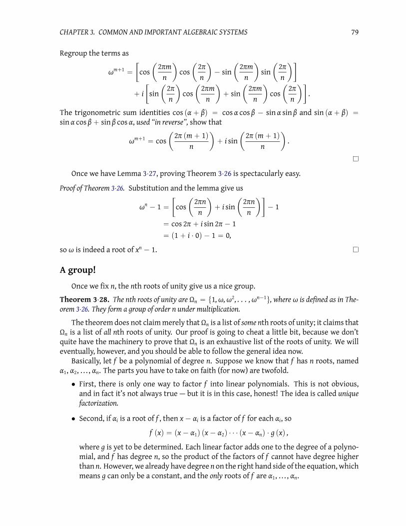
CHAPTER 3. COMMON AND IMPORTANT ALGEBRAIC SYSTEMS 79
Regroup the terms as
ωm`1
“
„
cos
ˆ
2πm
n
˙
cos
ˆ
2π
n
˙
´ sin
ˆ
2πm
n
˙
sin
ˆ
2π
n
˙
` i
„
sin
ˆ
2π
n
˙
cos
ˆ
2πm
n
˙
` sin
ˆ
2πm
n
˙
cos
ˆ
2π
n
˙
.
The trigonometric sum identities cos pα` βq “ cos α cos β ´ sin α sin β and sin pα` βq “
sin α cos β` sin β cos α, used “in reverse”, show that
ωm`1
“ cos
ˆ
2π pm` 1q
n
˙
` i sin
ˆ
2π pm` 1q
n
˙
.
Once we have Lemma 3¨27, proving Theorem 3¨26 is spectacularly easy.
Proof of Theorem 3¨26. Substitution and the lemma give us
ωn´ 1 “
„
cos
ˆ
2πn
n
˙
` i sin
ˆ
2πn
n
˙
´ 1
“ cos 2π ` i sin 2π ´ 1
“ p1` i ¨ 0q ´ 1 “ 0,
so ω is indeed a root of xn ´ 1.
A group!
Once we fix n, the nth roots of unity give us a nice group.
Theorem 3¨28. The nth roots of unity are Ωn “ t1,ω,ω2, . . . ,ω
n´1u, where ω is defined as in The-
orem 3¨26. They form a group of order n under multiplication.
The theorem does not claim merely thatΩn is a list of some nth roots of unity; it claims that
Ωn is a list of all nth roots of unity. Our proof is going to cheat a little bit, because we don’t
quite have the machinery to prove that Ωn is an exhaustive list of the roots of unity. We will
eventually, however, and you should be able to follow the general idea now.
Basically, let f be a polynomial of degree n. Suppose we know that f has n roots, named
α1, α2, . . . , αn. The parts you have to take on faith (for now) are twofold.
• First, there is only one way to factor f into linear polynomials. This is not obvious,
and in fact it’s not always true — but it is in this case, honest! The idea is called unique
factorization.
• Second, if αi is a root of f , then x´ αi is a factor of f for each αi, so
f pxq “ px´ α1q px´ α2q ¨ ¨ ¨ px´ αnq ¨ g pxq ,
where g is yet to be determined. Each linear factor adds one to the degree of a polyno-
mial, and f has degree n, so the product of the factors of f cannot have degree higher
than n. However, we already have degree n on the right hand side of the equation, which
means g can only be a constant, and the only roots of f are α1, . . . , αn.

CHAPTER 3. COMMON AND IMPORTANT ALGEBRAIC SYSTEMS 80
(You can see this in the example above with x4´1, but the Factor Theorem will have the details
(Question 1.69). You should have encountered that theorem in your precalculus studies, and
since it doesn’t depend on anything in this section, the reasoning is not circular.)
If you’re okay with that, then you’re okay with everything else.
Proof. For m P N`, we use the associative property of multiplication in C and the commuta-
tive property of multiplication in N`:
pωmqn´ 1 “ ω
mn´ 1 “ ω
nm´ 1 “ pω
nqm´ 1 “ 1
m´ 1 “ 0.
This shows that every positive power of ω is a root of unity. Most of these overlap, just as
p´1q2“ p´1q
4“ p´1q
6“ ¨ ¨ ¨ . If ω
m “ ω`, then
cos
ˆ
2πm
n
˙
“ cos
ˆ
2π`
n
˙
and sin
ˆ
2πm
m
˙
“ sin
ˆ
2π`
n
˙
,
and we know from trigonometry that this is possible only if
2πm
n“2π`
n` 2πk
2π
npm´ `q “ 2πk
m´ ` “ kn.
That is, m ´ ` is a multiple of n. Since Ωn lists only those powers from 0 to n ´ 1, the powers
must be distinct, so Ωn contains n distinct roots of unity. (See also Question 3¨26.) As there
can be at most n distinct roots, Ωn is a complete list of nth roots of unity.
Now we show that Ωn is a cyclic group.
(closure) Let x, y P Ωn; you will show in Question 3.29 that xy P Ωn.
Question 3¨29 .Let n P N`, and suppose that a and b are both positive powers of ω. Show that ab P Ωn.
Proof of Theorem 3¨28, continued. (associativity) The complex numbers are associative under
multiplication; since Ωn Ď C, the elements of Ωn are also associative under
multiplication.
(identity) The multiplicative identity in C is 1. This is certainly an element of Ωn, since
1n “ 1 for any n P N`.
(inverses) Let x P Ωn; you will show in Question 3.33 that x´1 P Ωn.
(cyclic) Theorem 3¨26 tells us that ω P Ωn; the remaining elements are powers of ω.
Hence Ωn “ xωy.

CHAPTER 3. COMMON AND IMPORTANT ALGEBRAIC SYSTEMS 81
i
ω2
ω3
ω4
ω5 ω6
ω
1
Figure 3¨1: The seventh roots of unity, on the complex plane
Combined with the explanation we gave earlier of the complex plane, Theorem 3¨28 gives
us a wonderful symmetry for the roots of unity.
Example 3¨30. Consider the case where n “ 7. According to the theorem, the 7th roots of
unity are Ω7 “ t1,ω,ω2, . . . ,ω
6u where
ω “ cos
ˆ
2π
7
˙
` i sin
ˆ
2π
7
˙
.
According to Lemma 3¨27,
ωm“ cos
ˆ
2πm
7
˙
` i sin
ˆ
2πm
7
˙
,
where m “ 0, 1, . . . , 6. By substitution, the angles we are looking at are
0,2π
7,4π
7,6π
7,8π
7,10π
7,12π
7.
See Figure 3¨30.
Although we used n “ 7 in this example, we used no special properties of that number in
the argument. That tells us that this property is true for any n: the nth roots of unity divide
the unit circle of the complex plane into n equal arcs!
Here’s an interesting question: is ω is the only element of Ωn whose powers “generate”
the other elements of the group? In fact, no. A natural follow-up: are all the elements of Ωn
generators of the group? Likewise, no. Well, which ones are? We are not yet ready to give a
precise criterion that signals which elements generate Ωn, but they do have a special name.
Definition 3¨31. We call any element of Ωn whose powers gives us all other elements of Ωn a
primitive nth root of unity.

CHAPTER 3. COMMON AND IMPORTANT ALGEBRAIC SYSTEMS 82
Question 3¨32 .Show that Ωn is isomorphic to Zn.
Question 3¨33 .
(a) Let ω be a 14th root of unity; let α “ ω5, and β “ ω14´5 “ ω9. Show that αβ “ 1.
(b) More generally, letω be a primitive nth root of unity, Let α “ ωa, where a P N and a ă n.
Show that β “ ωn´a satisfies αβ “ 1.
(c) Explain why this shows that every element of Ωn has an inverse.
Question 3¨34 .Suppose β is a root of x
n ´ b.
(a) Show that ωβ is also a root of xn ´ b, where ω is any nth root of unity.
(b) Use (a) and the idea of unique factorization that we described right before the proof of
Theorem 3¨28 to explain how we can use β and Ωn to list all n roots of xn ´ b.
Definition 3¨35. Given a field F, a vector space over F is an abelian group pV,`q with an
additional property called scalar multiplication that satisfies the following additional prop-
erties:
• Scalar multiplication maps Fˆ V to V, with pa, uq ÞÑ v abbreviated as au “ v.
• Closure: for all a P F and all v P V, av P V.
• Compatibility: for all a, b P F and all v P V, pabq v “ a pbvq.
• Scalar identity: for all v P V, 1Fv “ v.
• Scalar distribution: for all a P F and all u, v P V, a pu` vq “ au` av.
• Vectors distribution: for all a, b P F and all v P V, pa` bq v “ av` bv.
Question 3¨36 .Show that this section’s construction of C satisfies the requirements of a vector space over
R.

CHAPTER 3. COMMON AND IMPORTANT ALGEBRAIC SYSTEMS 83
3¨3 Cyclic groups; the order of an element
“Well, in our country,” said Alice, still panting a little, “you’d generally get to some-
where else—if you run very fast for a long time, as we’ve been doing.”
“A slow sort of country!” said the Queen. “Now, here, you see, it takes all the run-
ning you can do, to keep in the same place. If you want to get somewhere else, you
must run at least twice as fast as that!”
— Lewis Carroll
This section builds on a phenomenon we observed in a group of roots of unity to describe an
important class of groups. Recall that the nth roots of unity can all be written as powers of
ω “ cos
ˆ
2π
n
˙
` i sin
ˆ
2π
n
˙
;
that is,
Ωn “
ω,ω2, . . . ,ω
n“ 1
(
.
Because of this, we spoke of ω as “generating” Ωn. As you will see, we can write many other
groups in this form. In addition, it will be of interest to look at groups generated by an ele-
ment. Since we’re dealing with repeating the operation of a group on one element, we’d best
shore up some properties of exponents first.
Exponents
In essence, we claim that the usual arithmetic holds for exponents and multiples, regard-
less of the underlying group or ring; that is:
• for any integers a, b P Z, we define gagb “ ga`b;
• if the set has an identity, then we define g0 “ я;
• if the set has multiplicative inverses, then we define g´a “ pg´1q
a“ pgaq
´1.
We have to make sure these definitions are reasonably well defined in any group or ring.
Question 3¨37 .We’re going to start off deciding that g
0is just shorthand for the group identity, я. If the
operation of the group is addition, we’ll usually write 0 ˆ g “ 0. Why do these notations
make sense? Hint: я “ gg´1.
Question 3¨38 .Suppose a P N`. Why can we say g
´a “ pg´1qa“ pgaq
´1? Are we sure that pg´1q
aand pgaq
´1
are always the same? Hint: Think about the definitions. The meaning of pgaq´1
is, “the inverse
of ga.” What, then, has to be true for us to be able to say that pg´1q
a“ pgaq
´1? Show that that
is true.
Lemma 3¨39. Let G be a group, g P G, andm, n P Z. Each of the following holds:

CHAPTER 3. COMMON AND IMPORTANT ALGEBRAIC SYSTEMS 84
(A) gmg´m “ я; that is, g
´m “ pgmq´1
.
(B) pgmqn“ gmn.
(C) gmgn “ gm`n.
The proof of Lemma 3¨39 is not especially hard, but it does involve tedious notation. Orig-
inally, I included it here, but decided to remove it, on the grounds that (a) it distracts from
the point of this section, which is to introduce you to cyclic groups, and (b) you really ought
to be able to show it on your own (especially if your plan is to teach one day). So:
Question 3¨40 .Suppose m P Z (not just a P N` as before). Why can we say g
´m “ pgmq´1
? Hint: What makes
this different from before is that we’re now dealing with negative exponents. Try considering
different cases when m P N` (which we’ve already discussed, actually) and n ă 0.
Question 3¨41 .Building on the previous question: let n P Z. Why can we say pgmq
n“ g
mn? Hint: As before,
you need to consider separate cases for m or n negative.
Cyclic groups and generators
Some groups enjoy the special property that every element is a power of one, special ele-
ment.
Definition 3¨42. Let G be a group. If there exists g P G such that every element x P G has
the form x “ gn
for some n P Z, then G is a cyclic group and we write G “ xgy. We call g a
generator of G.
The idea of a cyclic group is that it has the form
. . . , g´2, g´1, я, g
1, g2, . . .
(
.
If the group’s operation is addition, we would of course write
t. . . ,´2g,´g, 0, g, 2g, . . . u .
Example 3¨43. Let’s look atZfirst. Any n P Zhas the form n¨1, such as 2 “ 2¨1,´5 “ p´5q¨1,
and so forth. We see that Z is cyclic, and write Z “ x1y.In addition, n has the form p´nq ¨ p´1q, soZ “ x´1y as well. Both 1 and´1 are generators
of Z.
Question 3¨44 .Show that any group of 3 elements is cyclic.
Question 3¨45 .Is the Klein 4-group (Question 2.49 on page 61) cyclic? What about the cyclic group of order
4?

CHAPTER 3. COMMON AND IMPORTANT ALGEBRAIC SYSTEMS 85
Question 3¨46 .Show that Q is not cyclic as an additive group. Hint: Suppose it were; then you could find a
rational number q such that Q “ t. . . ,´2q,´q, 0, q, 2q, . . . u. Surely you can find some r P Qthat isn’t listed.
Question 3¨47 .Let n P Z, and consider the ring Zn.
(a) Show that its additive group is cyclic.
(b) Show that if n “ 7, the subset t1, 2, . . . , 6u is a cyclic group under multiplication.
Hint: It’s not enough to show that all the elements are generated by one element, though
you do have to start there. You also have to check the properties of a group, especially
that every element has an inverse.
(c) Show that if n “ 6, the subset t1, 2, . . . , 5u is not a cyclic group under multiplication.
(d) Look at the subsets t1, 2, . . . , n´ 1u in some other finite rings Zn, where n ě 5. Try at
least two more and determine whether they are cyclic groups under multiplication.
(e) Do you notice a pattern to which values of n work and which don’t?
Question 3¨48 .Suppose that G and H are groups, and G – H. Show that if G is cyclic, then so is H, because the
generator of G is a generator of H.
In Definition 3¨42 we referred to g as a generator of G, not as the generator. There could
in fact be more than one generator; we see this in Example 3¨43 from the fact that Z “ x1y “x´1y. Another example is Ω3, where ω and ω
2both generate the group.
An important question arises here. Given a group G and an element g P G, define xgy as
the set of all integer powers of g. That is,
xgy “
. . . , g´2, g´1, я, g, g
2, . . .
(
.
We call this the group generated by g, and call g the generator of this group. When we’re
feeling a little lazy, which is actually pretty common, we simply say the group generated byg. Every cyclic group has the form xgy for some g P G. Is the converse also true that xgy is a
group for any g P G? As a matter of fact, yes!
Theorem 3¨49. For every group G and for every g P G, xgy is an abelian group.
Proof. We show that xgy satisfies the properties of an abelian group. Let x, y, z P xgy. By defini-
tion of xgy, there exist a, b, c P Z such that x “ ga, y “ gb, and z “ gc. We will use Lemma 3¨39
implicitly.
• By substitution, xy “ gagb “ ga`b P xgy. So xgy is closed.

CHAPTER 3. COMMON AND IMPORTANT ALGEBRAIC SYSTEMS 86
• By substitution, x pyzq “ ga`
gbgc˘
. These are elements of G by inclusion (that is, xgy Ď G
so x, y, z P G), so the associative property in G gives us
x pyzq “ ga`
gbgc˘
“`
gagb˘
gc“ pxyq z.
• By definition, я “ g0 P xgy.
• By definition, g´a P xgy, and x ¨ g´a “ gag´a “ e. Hence x
´1 “ g´a P xgy.
• Using the fact that Z is commutative under addition,
xy “ gagb“ g
a`b“ g
b`a“ g
bga“ yx.
Question 3¨50 .Find all the generators of Ω8. Hint: In Question 3.32 you showed that Ωn – Zn, so the genera-
tors ofZ8 must correspond to the generators ofΩ8. The mapping you used in the isomorphism
will tell you which ones.
The order of an element
Given an element and an operation, Theorem 3¨49 links them to a group. It makes sense,
therefore, to link an element to the order of the group that it generates.
Definition 3¨51. Let G be a group, and g P G. We say that the order of g is the order of the
group it generates; ord pgq “ |xgy|. If ord pgq “ 8, we say that g has infinite order.
We can write an element in different ways when its order is finite.
Example 3¨52. Consider Z4 “ t0, 1, 2, 3u. Since 4 ”4 0, we can write 1 as 1ˆ 4` 1, 2ˆ 4` 1,
3ˆ 4` 1, etc.
Example 3¨53. Recall Ω7 “ t1,ω,ω2, . . . ,ω
6u. Since ω7 “ 1, we can write ω
2as ω
2, ω
9, ω
16,
etc.
The example suggests that if the order of an element G is n P N, then we can write
xgy “
я, g, g2, . . . , g
n´1(
.
This explains why we call xgy a cyclic group: once they reach ord pgq, the powers of g “cycle”.
To prove this in general, we have to show that for a finite cyclic group xgy with ord pgq “ n,
• n is the smallest positive power that gives us the identity; that is, gn “ я, and
• for any two integers between 0 and n, the powers of g are different; that is, if 0 ď a ă
b ă n, then ga ‰ gb.
Theorem 3¨54 accomplishes that, and a bit more as well.

CHAPTER 3. COMMON AND IMPORTANT ALGEBRAIC SYSTEMS 87
Theorem 3¨54. Let G be a finite group, g P G, and ord pgq “ n.
(A) я, g, g2, . . . , g
n´1are all distinct.
(B) gn “ я;
(C) n is the smallest positive integer d such that gd “ я; and
(D) For any a, b P Z, n | pa´ bq if and only if ga “ gb.
Proof. The meat of the theorem is (A). The remaining assertions are consequences.
(A) By way of contradiction, suppose that there exist a, b P N such that 0 ď a ă b ă n and
ga “ gb; then я “ pgaq
´1gb. By Lemma 3¨39, we can write
я “ g´agb“ g
´a`b“ g
b´a.
Let d “ b ´ a. Recall that a ă b, so d “ b ´ a P N`. By the Division Theorem, for any
integermwe can find q, r P Z such thatm “ qd` r and 0 ď r ă d. Applying Lemma 3¨39
again, we have
gm“ g
qd`r“`
gd˘q
gr“ я
qgr“ g
r,
so any power of g can be written as a remainder after division by d. In other words,
xgy “
я, g, g2, . . . , g
d´1(
.
This implies that |xgy| “ d, which contradicts the assumption that n “ ord pgq “ |xdy|.
(B) We know that ord pgq “ n, so there are n distinct elements of xgy. By part (a), the n
powers g0, g1, . . . , g
n´1are all distinct, so
xgy “
g0, g1, . . . , g
n´1(
.
This implies that gn “ gd for some d “ 0, 1, . . . , n´ 1. Which one?
Using Lemma 3¨39, we find that gn´d “ я. Recall that 0 ď d ă n, so 0 ă n´d ď n. By (A),
ga ‰ я for a “ 1, 2, . . . , n´ 1, so n´ d “ n, so d “ 0. By substitution, g
n “ gd “ g0 “ я.
(C) let S is the set of all positive integers m such that gm “ я; this is a subset of N, so it has a
smallest element. Let the smallest element be d; by (B), gn “ я, so n P S. Hence d ď n. On
the other hand, (A) tells us that we cannot have d ă n; otherwise, gd “ g
0 “ я. Hence,
n ď d. We already had d ď n, so the two must be equal.
(D) Let a, b P Z. Assume that n | pa´ bq. Let q P Z such that nq “ a ´ b. Substitution,
Lemma 3¨39 and some arithmetic tell us that
gb“ g
b¨ я “ g
b¨ я
q
“ gb¨ pg
nqq“ g
b¨ g
nq
“ gb¨ g
a´b“ g
b`pa´bq“ g
a.

CHAPTER 3. COMMON AND IMPORTANT ALGEBRAIC SYSTEMS 88
Conversely, if we assume that gb “ g
a, then Lemma 3¨39 implies that g
b´a “ я. Use
the Division Theorem to choose q, r P Z such that b ´ a “ nq ` r and 0 ď r ă n. By
substitution and Lemma 3¨39,
я “ gb´a“ g
qn`r“ pg
nqqgr“ я
qgr“ g
r.
Recall that 0 ď r ă n. By (C), r cannot be positive, so r “ 0. By substitution, b´ a “ qn,
so n | pb´ aq.
We conclude that, at least when they are finite, cyclic groups are aptly named: increasing
powers of g generate new elements until the power reaches n, in which case gn “ я and we
“cycle around.”
Question 3¨55 .Complete the proof of Lemma 3¨39(C).
Question 3¨56 .Fill in each blank of Figure 3.56 with the justification or statement.
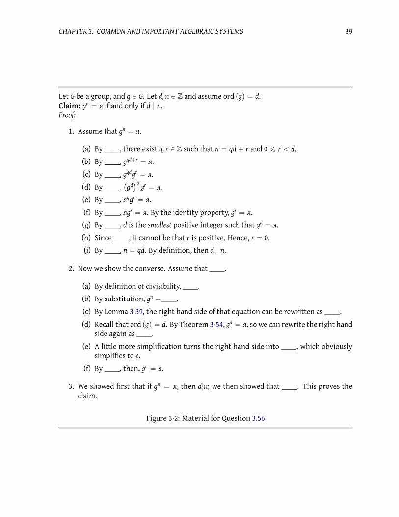
CHAPTER 3. COMMON AND IMPORTANT ALGEBRAIC SYSTEMS 89
Let G be a group, and g P G. Let d, n P Z and assume ord pgq “ d.
Claim: gn “ я if and only if d | n.
Proof:
1. Assume that gn “ я.
(a) By _____, there exist q, r P Z such that n “ qd` r and 0 ď r ă d.
(b) By _____, gqd`r “ я.
(c) By _____, gqdgr “ я.
(d) By _____,`
gd˘q
gr “ я.
(e) By _____, яqgr “ я.
(f) By _____, яgr “ я. By the identity property, g
r “ я.
(g) By _____, d is the smallest positive integer such that gd “ я.
(h) Since _____, it cannot be that r is positive. Hence, r “ 0.
(i) By _____, n “ qd. By definition, then d | n.
2. Now we show the converse. Assume that _____.
(a) By definition of divisibility, _____.
(b) By substitution, gn “_____.
(c) By Lemma 3¨39, the right hand side of that equation can be rewritten as _____.
(d) Recall that ord pgq “ d. By Theorem 3¨54, gd “ я, so we can rewrite the right hand
side again as _____.
(e) A little more simplification turns the right hand side into _____, which obviously
simplifies to e.
(f) By _____, then, gn “ я.
3. We showed first that if gn “ я, then d|n; we then showed that _____. This proves the
claim.
Figure 3¨2: Material for Question 3.56

CHAPTER 3. COMMON AND IMPORTANT ALGEBRAIC SYSTEMS 90
3¨4 An introduction to finite rings and fields
Our minds are finite, and yet even in these circumstances of finitude we are sur-
rounded by possibilities that are infinite, and the purpose of life is to grasp as much
as we can out of that infinitude.
— Alfred North Whitehead
The rings and fields you’re most familiar with are infinite: Q, R, C. A natural question to ask
is, “Do finite rings or fields exist?”
We’ll look at rings first. You saw in Section 2¨2 that Zd is an abelian group under addition,
one of the requirements of a ring.
Theorem 3¨57. For any nonzero integer d, the set Zd is a commutative ring under modular addition
and multiplication.
Proof. Let d P Z be nonzero, and let a, b, c P Zd. We already know that Zd makes an abelian
group under modular addition, so we need merely show that modular multiplication satis-
fies the requirements of a commutative monoid. Closure is guaranteed by property (D2) of
the Division Theorem. The multiplicative identity is 1, itself a remainder and thus an ele-
ment of Zn. The associative property follows from multiplication of the integers and from
the uniqueness of remainders: since a pbcq “ pabq c as integers, the unique remainders of
a pbcq and pabq cmust also be equal, so a pbcq ” pabq c.
So Zd is a finite ring for every nonzero value of d.
As for finite fields, ah, uhm. . . well! You already met zero divisors of finite rings in Ques-
tion 2.40, so at least one of our finite rings are not good candidates for finite fields. Other
finite rings work dandily.
Example 3¨58. Recall Z7 “ t0, 1, 2, . . . , 6u. We can see that this is a field by verifying that
every nonzero element has a multiplicative inverse: 1b1 “ 1, 2b4 “ 8 ” 1, 3b5 “ 15 ” 1,
and 6b 6 “ 36 ” 1.
So Z7 is a field, but Z6 is not.
Question 3¨59 .What difference between Z6 and Z7 makes the latter a field, while the former is not?
Don’t draw too hasty a conclusion! You might be tempted to think that the only finite field
are those of the Zd, where d has the “correct” form. In fact, there can be other fields of size d!
Example 3¨60. Consider g “ x2`1, in the ringZ3 rxs. LetF9 be the set of remainders possible
when dividing by g. Arithmetic is modulo both 3 and x2 ` 1, so its elements are
F9 “ t0, 1, 2, x, x` 1, x` 2, 2x, 2x` 1, 2x` 2u .
This set is not the same as Z9!

CHAPTER 3. COMMON AND IMPORTANT ALGEBRAIC SYSTEMS 91
You already know from Theorem 3¨7 that F9 forms a ring. It is routine to verify that:
1´1 “ 1 px` 1q
´1“ x` 2
2´1 “ 2 p2x` 1q´1 “ 2x` 2
x´1 “ 2x
For example,
p2x` 1q p2x` 2q “ 4x2`>
06x` 2 ” x
2` 2 ” 1.
So all its nonzero elements have inverses.
Even though it has nine elements,F9 is a field! So we can’t just look at whether the number
of elements in a set factors. That said, it’s not completely unrelated.
Characteristics of finite rings
Definition 3¨61. Let R be a ring. The characteristic of R is the smallest positive integer n
such that
0 ” nr “ r ` r ` ¨ ¨ ¨ ` rlooooooomooooooon
n times
for every r P R. If there is no such number, we say that R has characteristic 0.
If n is the characteristic of R, we write charR “ n.
Example 3¨62. In Z7, the characteristic of 1 is 7, since 7 ˆ 1 ” 0, and any smaller multiple
of 1 is non-zero. In fact, 7ˆ r ” 0 for any nonzero element r, and no smaller value of n gives
n ˆ r ” 0. The one exception is r “ 0, in which case 1 ˆ 0 ” 0, but 1 doesn’t work for the
other elements (1 ˆ 2 ı 0), whereas 7 works for 0 (7 ˆ 0 ” 0), so the characteristic of Z7 is
indeed 7.
In Z6, the relationship 2 ˆ 3 ” 0 suggests that the characteristic could be 2 or 3, but
neither number is the characteristic of every element, since 2ˆ1 ” 2 ı 0 and 3ˆ5 ” 3 ı 0.
We have to try something larger, and in fact neither 4ˆ5 ” 0 nor 5ˆ5 ” 0; we find 6ˆ5 ” 0.
Similarly, 6ˆ 1 ” 0, so the characteristic of Z6 is 6.
Don’t jump too quickly into thinking the characteristic of a ring is simply the number of
elements! In F9, we get a different answer, because everything is modulo 3, so 3 ˆ r ” 0 for
every r P F9. Smaller numbers won’t work as 1 ˆ 1 ı 0, and 2 ˆ 1 ı 0, so the characteristic
must in fact be 3.
While the characteristic of a ring is defined in terms of every element, it actually depends
on only one element!
Theorem 3¨63. The characteristic of a ring is either zero or the smallest positive number n such that
nˆ 1 “ 0, where 1 is the multiplicative identity of R.
Proof. LetRbe a ring, and r P R. If nˆ1 ‰ 0 for any n P N`, then by definition of characteristic,
charR “ 0. Otherwise, R has positive characteristic, and there exists n P N` such that nˆ1 “

CHAPTER 3. COMMON AND IMPORTANT ALGEBRAIC SYSTEMS 92
0; use the Well-Ordering Principle to choose the smallest such n. By closure, n P R, so we can
apply the associative property to see that
nˆ r “ nˆ p1ˆ rq “ pnˆ 1q ˆ r “ 0ˆ r “ 0.
(Notice the use of Fact 2¨41 in the last step.) Thus, any n P N` satisfying n ˆ 1 “ 0 also
satisfies nˆ r “ 0. By choice of n, no smaller positivem satisfiesmˆ1 “ 0, so nˆ r “ 0 for all
r P R, and is the smallest such. The characteristic of R depends entirely on its multiplicative
identity.
It turns out that the characteristic is the key property distinguishing fields from mere rings.
Theorem 3¨64. The characteristic of a field is either zero or irreducible.
Proof. Let F be a field of characteristic n. Suppose to the contrary that n “ pq, where p and q
are integers, but neither is 1. Notice that 1 ă p, q ă n. Let S “ t0, 1, 2ˆ 1, . . . , pn´ 1q ˆ 1u.
By closure of multiplication, S Ď F. In addition, S is a set with n distinct elements; otherwise,
we would contradict Theorem 3¨63. (Keep in mind that 2ˆ 1means 1` 1, 3ˆ 1 “ 1` 1` 1,
etc.)
Of course, 1 is the multiplicative identity, so S “ t0, 1, 2, . . . , n´ 1u. Recall that p, q ă n.
That means p, q P S; by inclusion, p, q P F. Closure of multiplication forces p ˆ q P F. By
the definition of characteristic, p ˆ q “ n ” 0, so that F has zero divisors. This contradicts
Question 2.45 and the hypothesis that F is a field!
The only questionable assumption we have made is that neither p nor q is 1, so it must be
that one of them is 1, and n is irreducible.
But what if n is irreducible?
Fact 3¨65. If n is irreducible, then Zn is a field of characteristic n.
Proof. Certainly Zn is a ring of characteristic n, since i ˆ 1 ı 0 for any i “ 1, . . . , n ´ 1. Why
must it be a field? We claim that for any nonzero r P Zn we can find s P Zn such that rs ” 1.
To see why, we need the following lemma.
Bézout’s Lemma. If d is the largest integer that divides two integers m and n, then we can find
integers x and y such that mx ` ny “ d. In fact, d is the smallest positive integer for which we can
find such an expression.
The equationmx`ny “ d is sometimes calledBézout’s Identity. The integer d of Bezout’s
Lemma is the greatest common divisor of m and n, and is abbreviated gcd pm, nq.
Proof of Bezout’s Lemma. Let S “ tmx` ny : x, y P Zu, and let L “ SXN`. By the Well-Ordering
Principle, L has a smallest element; call it `, and choose x and y such that mx ` ny “ `. By
hypothesis, d divides both m and n; say m “ ad and n “ bd. By substitution,
padq x` pbdq y “ `.
We can rewrite this as
d pax` byq “ `,

CHAPTER 3. COMMON AND IMPORTANT ALGEBRAIC SYSTEMS 93
so d | `. We know that this means d ď `.On the other hand, choose a quotient q and remainder r such thatm “ q`` r satisfies the
Division Theorem. Rewrite this equation as
r “ m´ q` “ m´ q pmx` nyq “ m p1´ qxq ` n p´qyq .
With r “ m p1´ qxq ` n p´qyq, we see that r P S. As a remainder, r P N, so either r “ 0 or
r P S X N “ L. If r ‰ 0, the choice of ` as the smallest element of L implies ` ď r. But r is a
remainder from division by d, so r ă d, and we saw above that d ď `; it doesn’t make sense
to have ` ď r ă d ď `! The only way to avoid a contradiction is if r “ 0, so ` divides m. A
similar argument shows that ` divides n. We now have ` dividing both m and n; recall that d
is the largest integer that divides both m and n, so ` ď d.We are now finished: the first paragraph concluded that d ď `, and the second paragraph
concluded that ` ď d. This is only possible if ` “ d, and we have shown the claim.
Question 3¨66 .The first paragraph of the proof of Bezout’s Theorem concludes with the assertion that if d, `are both positive integers, and d divides `, then d ď `. Why must this be true?
We return to our main question.
Proof of Fact 3¨64 (continued). Let m P Zn. By hypothesis, n is irreducible, so the greatest com-
mon divisor of m and n is 1. Well, then, Bezout’s Lemma gives us integers x, y such that
mx ` ny “ 1. Rewrite this as ny “ 1 ´ mx, and Theorem 2¨19 shows that 1 ”n mx. In
other words, x is the multiplicative inverse we sought for m.
Evaluating positions in the game
We return to the question of evaluating the value of a position in Nim and Ideal Nim. One
way to do this is to count the number of possible moves remaining. For instance, if we have
only a single row of m boxes, we would call that a row of value m. How can we model this?
Let’s start with these first two principles to keep in mind:
Principle the first: A choice’s value must satisfy 0 ď m.
Principle the second: Any choice is its own inverse, so m‘ m “ 0.
To a seasoned mathematician, the self-inverse property indicates that we’re working in a ring
of characteristic 2. We’ll aim for a field, if we can get it. Unfortunately, the basic field of
characteristic 2 is Z2, which has only two values. By themselves, 0 and 1 won’t model our
game, so we’ll have to extend our ring. Nothing stops us from extending it in a fashion similar
to the one we used to build the complex numbers, so let’s try that.
Fact 3¨67. The polynomial f “ x px´ 1q px´ a1q ¨ ¨ ¨ px´ an´2q ` 1 has no roots in the finite field
Fn “ t0, 1, a1, . . . , an´2u.
Why? We can see this by simple substitution; f pbq ” 1 for any element b of Fn.

CHAPTER 3. COMMON AND IMPORTANT ALGEBRAIC SYSTEMS 94
Fact 3¨68. Any factorization of f that uses coefficients only in Fn has no linear components.
Why? The alternative would set up a contradiction between the Division Theorem for Poly-
nomials and the previous fact: for any hypothetical linear factor of f , the definition of f would
have a remainder of 1, while the factorization would have a remainder of 0.
In other words, while f may factor, its irreducible factors are not linear.
Fact 3¨69. Defining a ring E as Fn rxsmodulo an irreducible factor of f actually gives us a field.
Why? If not, there must be some nonzero element a of E that does not have a multiplicative
inverse. SinceE is finite, we can list all products ax for x P E. The fact that ax ‰ 1means there
must be distinct elements x, y P E whose products give ax “ ay. Rewrite this as a px´ yq “ 0.
Let z “ x ´ y; with distinct x and y, we must have z ‰ 0. That means az “ 0 even though
a, z ‰ 0; we have found zero divisors.
This is a contradiction! To see why, let g be the irreducible factor of f . Both a and z are
polynomials with degree smaller than deg g. The statement “az “ 0 inE” translates to “az ” 0
in Fn rxsmodulo g,” but since 0 ” g, we have found a factorization of an irreducible polyno-
mial!
Satisfied that E is in fact a field, we can now build successively larger fields
t0, 1u Ĺ t0, 1, 2, 3u Ĺ t0, 1, 2, 3, 4, 5, 6, 7u Ĺ ¨ ¨ ¨
where 2n
represents xn
in the corresponding extension, 2n ` 1 represents x
n ` 1, 2n ` 2 rep-
resents xn ` x, etc. These are not your ordinary 2, 3, . . . because here, 1 ` 1 ı 2; after all,
1` 1 ” 0. The addition of the remainders, modulus the irreducible polynomial, corresponds
precisely to integer addition using powers of 2, also called binary notation. This allows us to
model the Nim and Ideal Nim.
It is not enough to form a winning strategy for Ideal Nim, because a winning strategy for
this game is currently unknown! However, we can still evaluate the values of many games using
the implication of symmetry that x` x ” 0.
Example 3¨70. Suppose a game of Ideal Nim has led to the following configuration:

CHAPTER 3. COMMON AND IMPORTANT ALGEBRAIC SYSTEMS 95
Suppose it is Emmy’s turn. As this is visually non-symmetric, you might conclude that the
Emmy has an advantage. Upon further inspection, you’d discover that if David has any sense
at all, then no, Emmy will in fact lose. For instance, if Emmy chooses p0, 3q, David could choose
p1, 1q, leaving a visually symmetric game; if Emmy chooses p0, 2q instead, David could choose
p2, 1q, again leaving a visually symmetric game. Either choice is a win for David! The remaining
choices for the next player are similarly parried.
Our conclusion from this is that the value of the upside-down L on the right is equivalent
to the value of the two blocks in a line on the left; both blocks have value 2.
Question 3¨71 .Operating under the assumption that a line ofm blocks has valuem, use a technique analogous
to the one in the previous example to show that the values of the following configurations
are 1, 3, 4, 1 (again!), and 5.
3¨5 Matricesmatrix, n. 1. (Latin) the womb. 2. (mathematics) A rectangular array of numeric
or algebraic quantities subject to mathematical operations.
— from The American Heritage Dictionary of the English Language
(4th edition)
Let R be a commutative ring, and m, n P N`. An m ˆ n matrix M over R is a list of m lists
(rows) of n elements of R. We say the dimension of the matrix is m ˆ n. We call R the basering of M. If m “ n, we call the matrix square, and say that the dimension of the matrix is
m. The set of all mˆ nmatrices over R is Rmˆn
.
Notation 3¨72. We write the jth element of row i of the matrix A as aij. We often omit 0’s from
the matrix, not so much from laziness as from a desire to improve readability. (It really does
help to omit the 0’s when there are a lot of them.) If the dimension of A is m ˆ n, then we
write dimA “ mˆ n.
Example 3¨73. If
A “
¨
˝
1 1
1
5 1
˛
‚,
then a21 “ 0 while a32 “ 5. Notice that A is a 3 ˆ 3 matrix; or, dimA “ 3 ˆ 3. As a square
matrix, we say its dimension is 3.
Definition 3¨74. The transpose of a matrix A is the matrix B satisfying bij “ aji. In other
words, the jth element of row i of B is the ith element of row j of A. A column of a matrix is a
row of its transpose.

CHAPTER 3. COMMON AND IMPORTANT ALGEBRAIC SYSTEMS 96
Notation 3¨75. We often write AT
for the transpose of A.
Example 3¨76. If A is the matrix of the previous example, then
AT“
¨
˝
1
1 5
1 1
˛
‚.
We focus mostly on square matrices, with the exception of m ˆ 1 matrices, also called
column vectors, or just plain “vectors” if we feel lazy, as we often do. The dimension of an
m ˆ 1 vector is m. We write Rm
for the set of all column vectors of dimension n with entries
from a ringR. This looks the same as the Cartesian productRˆRˆ¨ ¨ ¨¨R, because it is: a column
vector pr1 ¨ ¨ ¨ rmqT
is merely a different representation of writing the tuple pr1, . . . , rmq.
Matrix arithmetic
The two major operations for matrices are addition and multiplication. Addition is com-
ponentwise; we add matrices by adding entries in the same row and column. Multiplication
is not componentwise.
• If A and B are mˆ nmatrices and C “ A` B, then cij “ aij ` bij for all 1 ď i ď m and all
1 ď j ď n. Notice that C is also an mˆ nmatrix.
• If A is anmˆ rmatrix, B is an rˆnmatrix, and C “ AB, then C is themˆnmatrix whose
entries satisfy
cij “
rÿ
k“1
aikbkj ;
that is, the jth element in row i of C is the sum of the products of corresponding elements
of row i of A and column j of B.
This definition of multiplication, while odd, satisfies certain useful properties: in particular,
relating matrix equations to systems of linear equations.
Example 3¨77. If A is the matrix of the previous example and
B “
¨
˝
1 5 ´1
1
´5 1
˛
‚,
then
AB “
¨
˝
1 ¨ 1` 0 ¨ 0` 1 ¨ 0 1 ¨ 5` 0 ¨ 1` 1 ¨ ´5 1 ¨ ´1` 0 ¨ 0` 1 ¨ 1
0 ¨ 1` 1 ¨ 0` 0 ¨ 0 0 ¨ 5` 1 ¨ 1` 0 ¨ ´5 0 ¨ ´1` 1 ¨ 0` 0 ¨ 1
0 ¨ 1` 5 ¨ 0` 1 ¨ 0 0 ¨ 5` 5 ¨ 1` 1 ¨ ´5 0 ¨ ´1` 5 ¨ 0` 1 ¨ 1
˛
‚
“
¨
˝
1
1
1
˛
‚.

CHAPTER 3. COMMON AND IMPORTANT ALGEBRAIC SYSTEMS 97
On the other hand, if x “ px y zqT and b “ p0 0 2qT, the matrix equation
Ax “ b
simplifies to¨
˝
x z
y
5y z
˛
‚“
¨
˝
0
0
2
˛
‚,
which corresponds to the system of equations
$
’
&
’
%
x ` z “ 0
y “ 0
5y` z “ 2
.
Question 3¨78 .Recall the definition of zero divisors from Definition 2¨42. Show that matrix multiplication
has zero divisors by finding two square matrices A and B such that A ‰ 0 and B ‰ 0, but
AB “ 0. You can start with 2ˆ 2matrices, but try to make it a general formula, and describe
how one could build such matrix zero divisors regardless of their size. Hint: Don’t overthink
this; there is a very, very simple answer.
Question 3¨79 .In this problem, pay careful attention to which symbols are thickened, as they represent
matrices.
Let i denote the imaginary number, so that i2 “ ´1, and let Q8 be the set of quaternions,
defined by the matrices t˘1,˘i,˘j,˘ku where
1 “ˆ
1 0
0 1
˙
, i “ˆ
i 0
0 ´i
˙
,
j “ˆ
0 1
´1 0
˙
, k “ˆ
0 i
i 0
˙
.
(a) Show that i2 “ j2 “ k2 “ ´1.
(b) Show that ij “ k, jk “ i, and ik “ ´j.
(c) Show that ij “ ´ji, ik “ ´ki, and jk “ ´kj.
(d) Use these properties to construct the Cayley table of Q8. Hint: If you use the properties
carefully, along with what you know of linear algebra, you can fill in the remaining spaces
without performing a single matrix multiplication.
(e) Show that Q8 is a group under matrix multiplication.
(f) Explain why Q8 is not an abelian group.

CHAPTER 3. COMMON AND IMPORTANT ALGEBRAIC SYSTEMS 98
Question 3¨80 .The following exercises refer to elements of the quaternions (Question 3.79).
(a) Determine the elements of x´1y and xjy in Q8.
(b) Verify that H “ t1,´1, i,´iu is a cyclic group. Which elements actually generate H?
(c) Show that Q8 is not cyclic.
Question 3¨81 .In each of the following, compute the order of the element a P Q8.
(a) a “ i
(b) a “ ´1
(c) a “ 1
Question 3¨82 .We sometimes allow matrices which proceed indefinitely in two directions. Here are two such
matrices which are mostly zero, though we highlight the zeros on the main diagonal:
D “
¨
˚
˚
˚
˚
˚
˝
0 1
0 2
0 3
0 4
. . .. . .
˛
‹
‹
‹
‹
‹
‚
S “
¨
˚
˚
˚
˚
˚
˚
˚
˝
01
201
301
401
50
. . .. . .
˛
‹
‹
‹
‹
‹
‹
‹
‚
.
Let R be a ring. A polynomial in R rxs corresponds to a coefficient vector via the map
rnxn` ¨ ¨ ¨ r1x` r0 ÞÑ
¨
˚
˚
˚
˚
˚
˚
˚
˚
˚
˝
r0
r1...
rn
0
0
...
˛
‹
‹
‹
‹
‹
‹
‹
‹
‹
‚
.
Choose several random polynomials p, write their coefficient vectors p, then compute Dp and
Sp for each. What are the results? How would you characterize the effect of multiplying D
and S to a “polynomial vector”?

CHAPTER 3. COMMON AND IMPORTANT ALGEBRAIC SYSTEMS 99
Definition 3¨83. The kernel of a matrix M is the set of vectors v such that Mv “ 0. In other
words, the kernel is the set of vectors whose product withM is the zero matrix.
Notation 3¨84. We write kerM for the kernel ofM.
Example 3¨85. Let R “ Z, and
M “
¨
˝
1 0 5
0 1 0
0 0 0
˛
‚.
Let
x “
¨
˝
1
2
1
˛
‚ and y “
¨
˝
´5
0
1
˛
‚.
Since
Mx “
¨
˝
6
2
0
˛
‚ and My “
¨
˝
0
0
0
˛
‚“ 0,
we see that x is not in the kernel of M, but y is. In fact, it can be shown (you will do so in a
moment) that
kerM “
$
&
%
v P R3: v “
¨
˝
´5c
0
c
˛
‚ Dc P F
,
.
-
.
The kernel has important and fascinating properties, which we explore later on.
Question 3¨86 .Let R “ Z, and
M “
¨
˝
1 1
1
5 ´1
˛
‚ and N “
¨
˝
1 0 5
0 1 0
0 0 0
˛
‚.
Show that
kerM “ t0u ,
and
kerN “
$
&
%
v P R3: v “
¨
˝
´5c
0
c
˛
‚ Dc P R
,
.
-
.
Question 3¨87 .What are the kernels of the matrices D and I of Question 3.82? Hint: In that problem, we asked
you to “characterize the effect” of D and S on a “polynomial vector.” If you know the effect,
you can use that to make an educated guess at what appears in the kernel, then prove it.
Properties of matrix arithmetic
We now explore some properties of arithmetic of square matrices, so as to find a structure
that describes them.

CHAPTER 3. COMMON AND IMPORTANT ALGEBRAIC SYSTEMS 100
Fact 3¨88. For a fixed dimension of square matrices, matrix addition and multiplication are closed.
Why? The hypothesis is that we have a fixed dimension of square matrices, say n ˆ n. From
the definition of the operations, you see immediately that both addition and multiplication of
matrices result in an nˆnmatrix. Thus, anyA, B P Rmˆn satisfyA`B P Rmˆn andAB P Rmˆn.
Recall A and B from Examples 3¨73 and 3¨77. If we write I3 for a 3 ˆ 3 matrix of three 1’s
on the diagonal (and zeroes elsewhere), something interesting happens:
AI3 “ I3A “ A and BI3 “ I3B “ B.
The pattern of this matrix ensures that the property remains true for any matrix, as long as
you’re working in the correct dimension. That is, I3 is an “identity” matrix. In particular, it’s
the identity ofmultiplication. Is there a second identity matrix?
Don’t confuse “the identity matrix” with a matrix filled with zeros; that is the identity ma-
trix for addition. Can there be another second matrix for multiplication? In fact, there cannot.
You will see why in a moment.
Notation 3¨89.
• We write 0 (that’s a bold zero) for any matrix whose entries are all zero.
• We write In for the nˆ nmatrix satisfying
– aii “ 1 for any i “ 1, 2, . . . , n; and
– aij “ 0 for any i ‰ j.
Theorem 3¨90. The zero matrix 0 is an identity for matrix addition. The matrix In is an identity for
multiplication of nˆ nmatrices.
When reading theorems, you sometimes have to read between the lines. Here, you have
to infer that n P N` and 0 is a matrix whose dimension is appropriate to the other matrix.
We should not take it to mean anmˆ 4matrix with zero entries is an identity for matrices of
dimensionmˆ 2, as the addition would be undefined. Similarly, you have to infer that In is an
identity for square matrices of dimension n; it wouldn’t make sense to multiply In to a 3 ˆ 5
matrix.
Question 3¨91 .Can you find a multiplicative identity for 3ˆ 5matrices? If so, what it is? If not, why not?
Proof of Theorem 3¨90. Let A be a square matrix of dimension m ˆ n. By definition, the jth el-
ement in row i of A ` 0 is aij ` 0 “ aij. This is true regardless of the values of i and j, so if
we choose 0 to be an m ˆ n matrix with zero entries, A ` 0 “ A. A similar argument shows
0` A “ A. Since A is arbitrary, 0 really is an additive identity.

CHAPTER 3. COMMON AND IMPORTANT ALGEBRAIC SYSTEMS 101
As for In, we point out that the jth element of row i ofAIn is (by definition of multiplication)
¨
˚
˚
˚
˚
˚
˚
˚
˝
col j
.
.
.
row i ¨ ¨ ¨ this element? ¨ ¨ ¨
.
.
.
˛
‹
‹
‹
‹
‹
‹
‹
‚
“
¨
˚
˚
˚
˝
row i a1 ¨ ¨ ¨ aij ¨ ¨ ¨ ain
˛
‹
‹
‹
‚
¨
˚
˚
˚
˚
˚
˚
˚
˚
˚
˝
col j
1
...
1
...
1
˛
‹
‹
‹
‹
‹
‹
‹
‹
‹
‚
“ aij ¨ 1`ÿ
k“1,. . . ,m
k‰j
aik ¨ 0.
Simplifying this gives us aij. This is true regardless of the values of i and j, so AIn “ A. A similar
argument shows that InA “ A. Since A is arbitrary, In really is a multiplicative identity.
Given a matrix A, an additive inverse of A is any matrix B such that A ` B “ 0. A
multiplicative inverse of A is any matrix B such that AB “ In. Additive inverses always exist,
and it is easy to construct them. Multiplicative inverses do not exist for some matrices, even
when the matrix is square. Because of this we call a matrix invertible if it has a multiplicative
matrix, and if we merely speak of the “inverse” of a matrix, we mean its multiplicative inverse.
Notation 3¨92. We write the additive inverse of a matrix A and ´A, and the multiplicative
inverse of A as A´1
.
Example 3¨93. The matrices A and B of the previous example are inverses; that is, A “ B´1
and B “ A´1. The non-zero matrixˆ
1 0
2 0
˙
is not invertible, because any matrix satisfying
ˆ
1 0
2 0
˙ˆ
a b
c d
˙
“ I2
must satisfy the system of equations
$
’
’
’
&
’
’
’
%
a “ 1
b “ 0
2a “ 0
2b “ 1
,
an impossible task.
Question 3¨94 .A matrix A is orthogonal if its transpose is also its inverse. Let n P N` and O pnq be the set of
all orthogonal nˆ nmatrices.
(a) Show that this matrix is orthogonal, regardless of the value of α:
ˆ
cos α sin α
´ sin α cos α
˙
.
(b) Find some other orthogonal matrices. (Their entries can consist of numbers alone.)
Compute their determinant. Do you notice a pattern? See if you can prove it.

CHAPTER 3. COMMON AND IMPORTANT ALGEBRAIC SYSTEMS 102
Hint: The easiest way to show this requires some properties of determinants. Since you
may not remember them, or may not even have seen them (it could depend on the class,
on the teacher, on which universe you existed in the day they were presented. . . ) here
are the ones you need: for any matrix that has an inverse, detA “ detAT, det pABq “
pdetAq pdet Bq, and det In “ 1 for every n P N`.
We want one more property.
Theorem 3¨95. Matrix multiplication is associative. That is, ifA, B, and C are matrices, thenA pBCq “
pABq C.
Proof. Let A be anmˆ rmatrix, B an rˆ smatrix, and C an sˆ nmatrix. By definition, the `thelement in row i of AB is
pABqi` “
rÿ
k“1
aikbk`.
Likewise, the jth element in row i of pABq C is
ppABq Cqij“
sÿ
`“1
pABqi` c`j “
sÿ
`“1
«˜
rÿ
k“1
aikbk`
¸
c`j
ff
.
Notice that c`j is multiplied to a sum; we can distribute it and obtain
ppABq Cqij“
sÿ
`“1
rÿ
k“1
paikbk`q c`j. (3.1)
We turn to the other side of the equation. By definition, the jth element in row k of BC is
pBCqkj“
sÿ
`“1
bk`c`j.
Likewise, the jth element in row i of A pBCq is
pA pBCqqij“
rÿ
k“1
˜
aik
sÿ
`“1
bk`c`j
¸
.
This time, aik is multiplied to a sum; we can distribute it and obtain
pA pBCqqij“
rÿ
k“1
sÿ
`“1
aik
`
bk`c`j
˘
.
By the associative property of the entries,
pA pBCqqij“
rÿ
k“1
sÿ
`“1
paikbk`q c`j. (3.2)

CHAPTER 3. COMMON AND IMPORTANT ALGEBRAIC SYSTEMS 103
The only difference between equations (3.1) and (3.2) is in the order of the summations:
whether we add up the k’s first or the `’s first. That is, the sums have the same terms, but
those terms appear in different orders! We assumed the entries of the matrices were com-
mutative under addition, so the order of the terms does not matter; we have
ppABq Cqij“ pA pBCqq
ij.
We chose arbitrary i and j, so this is true for all entries of the matrices. The matrices are equal,
which means pABq C “ A pBCq.
We now have enough information to classify two useful and important structures of square
matrices. First, suppose the entries come from a general ring.
Theorem 3¨96. For any commutative ringR, the setRnˆn
ofnˆnmatrices overR is a noncommutative
ring.
Proof. We have shown that matrix addition satisfies most of the properties of an abelian group;
the only one we have not shown is the commutative property of addition, which is easy to
show.
Question 3¨97 .Why is matrix addition commutative?
Proof of Theorem 3¨96 (continued). We have also shown that matrix multiplication satisfies the
properties of a monoid; see Fact 3¨88 and Theorems 3¨90 and 3¨95. So we need merely show
that matrix multiplication distributes over addition. Let n P N` and A, B, C P Rnˆn.
rA pB` Cqsij“
nÿ
k“1
“
aik
`
bkj ` ckj˘‰
“
nÿ
k“1
`
aikbkj ` aikckj˘
“
nÿ
k“1
aikbkj `
nÿ
k“1
aikckj
“ pABqij` pACq
ij.
This shows the elements in row i and column j are equal whenever we fix i and j between 1 and
n. All the entries of A pB` Cq and AB` AC are equal, so A pB` Cq “ AB` AC; the distributive
property holds.
Usually the multiplication does not commute.
Question 3¨98 .Look back at Question 3.79. Find two quaternion matrices A and B such that AB ‰ BA.

CHAPTER 3. COMMON AND IMPORTANT ALGEBRAIC SYSTEMS 104
Question 3¨99 .Suppose n ą 1 and R
nˆnis the set of all n ˆ nmatrices whose entries are elements of R. Find
matrices A and B such that AB ‰ BA.
Hint: Since the ring R is arbitrary, it has to work even when R “ Z2, which limits your
options in a way that is surprisingly useful. So, try finding two 2ˆ 2matrices A and B whose
entries are elements of Z2, and AB ‰ BA. Once you find them, generalize your answer to any
dimension n ě 2.
So if the entries of our matrices merely come from a ring, the set of square matrices forms
another ring, though most sets of matrices form a noncommutative ring. Nice!
Suppose we go further, using a field for our base ring. Except for the additive identity,
multiplication in a field satisfies the inverse property. Will this be true of the matrices over
that field? We’ve already seen this isn’t true: Question 3.78 shows that zero divisor matrices
exist over every ground ring R, which includes fields, and Question 2.45 tells us that fields
cannot have zero divisors. So most rings of matrices will not be fields.
Can we build a field using invertible matrices? We need closure of multiplication.
Fact 3¨100. The product of two invertible matrices is also invertible.
Question 3¨101 .Why is Fact 3¨100 true? In other words, ifA and B are invertible matrices, why is AB invertible?
Hint: Try to construct an inverse using the inverses of A and B.
We already know that matrix multiplication has an identity, which is invertible, and is
associative. That’s all we need; the set of invertible matrices forms a group!
Definition 3¨102. Let F be a field. We call the set of invertible nˆ nmatrices with elements
in F the general linear group over F of dimension n, abbreviated GLn pFq. The operation
is multiplication. Ordinarily we work with F “ R and fixed degree n, so when the meaning
is clear and we’re feeling somewhat lazy (which we usually are), we will refer simply to the
general linear group.
Unfortunately, the set of invertible matrices still won’t form a field, for several reasons.
Question 3¨103 .Find at least three properties of a field that GLn pFq does not satisfy.
Question 3¨104 .Recall from Question 3.94 the orthogonal matrices O pnq.
(a) Show that if A and B are orthogonal matrices, then AB is also orthogonal.
Hint: You will need the additional matrix properties pABqT“ BTAT.
(b) Show that O pnq is a group under matrix multiplication.

CHAPTER 3. COMMON AND IMPORTANT ALGEBRAIC SYSTEMS 105
We now return to the question we first posed above: why can’t there be a different identity,
either for addition or multiplication?
Fact 3¨105. The identity of a monoid is unique.
Notice the claim: we don’t say merely that the identity matrix is unique, whether that be
the identity of addition or multiplication. We say that the identity of any monoid is unique.
This covers matrices, whether under addition or multiplication, and every other monoid possible.
We don’t need even the full monoid structure! Pay attention to the explanation, and see if
you can identify which properties aren’t required.
Why? Let M be a monoid, and я P M an identity. Suppose that e P M is also an identity;
perhaps я “ e, but perhaps я ‰ e; we are not sure. (Merely having a different name does not
imply a different substance.) By the fact that я is an identity, we know that яe “ e. On the
other hand, the fact that e is an identity tells us that яe “ я. By substitution, я “ e. Since our
choice of identities was arbitrary, and they turned out equal, it must be that the identity of a
monoid is unique.
Question 3¨106 .Which property (-ies) of a monoid did we not use in the explanation above?
Question 3¨107 .Suppose G is a group, and x P G. We know that x has an inverse; call it y P z. Can x have
another inverse, z P G? Hint: As in the explanation for Fact 3¨105, it helps to show that y “ z,
but the trick is a little different.
Question 3¨108 .Use a fact from linear algebra to explain why GLm pRq is not cyclic.
Example 3¨109. Let
G “
$
’
’
’
’
&
’
’
’
’
%
ˆ
1 0
0 1
˙
,
ˆ
0 ´1
1 0
˙
,
ˆ
0 1
´1 0
˙
,
ˆ
´1 0
0 ´1
˙
,
/
/
/
/
.
/
/
/
/
-
Ĺ GLm pRq .
It turns out that G is a group; both the second and third matrices generate it. For example,
ˆ
0 ´1
1 0
˙2
“
ˆ
´1 0
0 ´1
˙
ˆ
0 ´1
1 0
˙3
“
ˆ
0 1
´1 0
˙
ˆ
0 ´1
1 0
˙4
“
ˆ
1 0
0 1
˙
.

CHAPTER 3. COMMON AND IMPORTANT ALGEBRAIC SYSTEMS 106
Question 3¨110 .For the matrices in Example 3¨109, let
A “
ˆ
´1 0
0 ´1
˙
.
Express A as a power of the other non-identity matrices of the group.
Example 3¨111. Recall Example 3¨109; we can write
ˆ
1 0
0 1
˙
“
ˆ
0 ´1
1 0
˙0
“
ˆ
0 ´1
1 0
˙4
“
ˆ
0 ´1
1 0
˙8
“ ¨ ¨ ¨ .
Since multiples of 4 give the identity, let’s take any power of the matrix, and divide it by 4.
The Division Theorem allows us to write any power of the matrix as 4q` r, where 0 ď r ă 4.
Since there are only four possible remainders, and multiples of 4 give the identity, positive
powers of this matrix can generate only four possible matrices:
ˆ
0 ´1
1 0
˙4q
“
ˆ
1 0
0 1
˙
,
ˆ
0 ´1
1 0
˙4q`1
“
ˆ
1 0
0 1
˙ˆ
0 ´1
1 0
˙
“
ˆ
0 ´1
1 0
˙
,
ˆ
0 ´1
1 0
˙4q`2
“
ˆ
1 0
0 1
˙ˆ
´1 0
0 ´1
˙
“
ˆ
´1 0
0 ´1
˙
,
ˆ
0 ´1
1 0
˙4q`3
“
ˆ
1 0
0 1
˙ˆ
0 1
´1 0
˙
“
ˆ
0 1
´1 0
˙
.
We can do the same with negative powers; the Division Theorem still gives us only four
possible remainders. Let’s write
g “
ˆ
0 ´1
1 0
˙
.
Thus
xgy “
I2, g, g2, g3(
.
3¨6 Symmetry in polygons
What is it indeed that gives us the feeling of elegance in a solution, in a demonstra-
tion? It is the harmony of the diverse parts, their symmetry, their happy balance;
in a word it is all that introduces order, all that gives unity, that permits us to see
clearly and to comprehend at once both the ensemble and the details.
— Henri Poincare

CHAPTER 3. COMMON AND IMPORTANT ALGEBRAIC SYSTEMS 107
32
1
ρ
(a)
32
1
ϕ
π
(b)
Figure 3¨3: Rotation and reflection of the triangle
A geometric phenomenon with mathematical structure is called “the symmetries of a regular
polygon.” This mouthful of words requires some explanation. For the sake of simplicity, we
stick with a triangle, but the basic ideas here work with any number of sides, and we touch
on this briefly at the end of the section.
In general, the set of symmetries of a regular polygon with n sides is called Dn, so we will
be looking at D3, but you should pause from time to time and think of D4 or D5, because you’re
going to face them sooner or later, too.
Intuitive development of D3
To describe D3, start with an equilateral triangle in R2, with its center at the origin. A
“symmetry” is a transformation of the plane that leaves the triangle in the same location,
even if its points are in different locations. For instance, if you rotate the triangle 120˝
over
its center, the triangle ends up in the same location, even thought all the points have moved;
this is not true if you rotate by 30˝
or 60˝. Likewise, if you reflect the triangle about the y-axis,
the triangle ends up in the same location, even though most of the points have moved. We’ll
call that rotation ρ, and that reflection φ. See Figure 3¨6.
“Transformations” include actions like rotation, reflection (flip), and translation (shift).
Translating the plane in some direction certainly won’t leave the triangle intact, but rotation
and reflection can.
It is helpful to observe two important properties.
Theorem 3¨112. If φ and ρ are as specified, then φρ “ ρ2φ.
For now, we consider intuitive proofs only. Detailed proofs appear later in the section. It’ll
help if you sketch the arguments.
Intuitive proof. The expression φρmeans to apply ρ first, then φ; after all, these are functions,
so pφρq pxq “ φ pρ pxqq. Rotating 120˝
moves vertex 1 to vertex 2, vertex 2 to vertex 3, and
vertex 3 to vertex 1. Flipping through the y-axis leaves the top vertex in place; since we
performed the rotation first, the top vertex is now vertex 3, so vertices 1 and 2 are the ones
swapped. Thus, vertex 1 has moved to vertex 3, vertex 3 has moved to vertex 1, and vertex 2
is in its original location.

CHAPTER 3. COMMON AND IMPORTANT ALGEBRAIC SYSTEMS 108
On the other hand, ρ2φ means to apply φ first, then apply ρ twice. Again, it will help to
sketch what follows. Flipping through the y-axis swaps vertices 2 and 3, leaving vertex 1 in
the same place. Rotating twice then moves vertex 1 to the lower right position, vertex 3 to
the top position, and vertex 2 to the lower left position. This is the same arrangement of the
vertices as we had for φρ, which means that φρ “ ρ2φ.
You might notice a gap in the reasoning: we showed that each vertex of the triangle moved
to a position that previously held a vertex, but said nothing of the points in between. That
requires a little more work, which is why we provide detailed proofs later.
By the way, did you notice what Theorem 3¨112 did not claim?
Question 3¨113 .Show that D3 is non-commutative: φρ ‰ ρφ.
Another “obvious” symmetry of the triangle is the transformation where you do nothing –
or, if you prefer, where you effectively move every point back to itself, as in a 360˝
rotation. We’ll
call this symmetry ι. It gives us the last property we need to specify the group, D3.
Question 3¨114 .Compute the cyclic group generated by a in D3.
(a) a “ φ
(b) a “ ρ2
(c) a “ ρφ
Theorem 3¨115. In D3, ρ3 “ φ2 “ ι.
Intuitive proof. Rotating 120˝
three times is the same as rotating 360˝, which leaves points in
the same position as if they had not rotated at all. Likewise,φmoves any point px, yq to px,´yq,
and applying φ again moves px,´yq back to px, yq, which is the same as not flipping at all.
We are now ready to specify D3.
Theorem 3¨116. The set of symmetries of a regular triangle, D3 “ tι,φ, ρ, ρ2, ρφ, ρ2φu, is a group
under composition of functions.
We can prove most of these by mere inspection of the Cayley table, will you will compute
in Question 3.117. However, we can also give geometric reasoning. As long as that isn’t too
complicated, we add a geometric argument, as well.
Proof. We prove this by showing that all the properties of a group are satisfied. We only start
the proof, leaving it you to finish in Question 3.117.
Closure: In Question 3.117, you will compute the Cayley table of D3. There, you will see that
every composition is also an element of D3.
Associative: In Section 7¨1, we show that composition of functions is associative. Symme-
tries are functions that map any point in R2to another point in R2
, with no ambiguity about

CHAPTER 3. COMMON AND IMPORTANT ALGEBRAIC SYSTEMS 109
where the point goes. Proving the associative property once for an arbitrary function over an
arbitrary set takes care of particular functions (D3) over a particular set (R2).
Identity: In Question 3.117, you will compute the Cayley table of D3. There, you will find
that ισ “ σι “ σ for every σ P D3.
(Alternately, let σ P D3 be any symmetry. Apply σ to the triangle. Then apply ι. Since ι
leaves everything in place, all the points are in the same place they were after we applied σ.
In other words, ισ “ σ. The proof that σι “ σ is similar.)
Inverse: In Question 3.117, you will compute the Cayley table of D3. There, you will find
that for every σ P D3, the row labeled σ contains ι in exactly one column. The element at the
top of that row is σ´1
by definition.
(Alternately, it is clear that rotation and reflection are one-to-one-functions; after all, if
a point P is mapped to a point R by either, it doesn’t make sense that another point Q would
also be mapped to R. Since one-to-one functions have inverses, every element σ of D3 must
have an inverse function σ´1
, which undoes whatever σ did. But is σ´1 P D3 — that is, is σ
´1a
symmetry? Since σmaps every point of the triangle onto the triangle, σ´1
will undo that map:
every point of the triangle will be mapped back onto another point of the triangle, as well.
So, yes, σ´1 P D3.)
Question 3¨117 .The multiplication table for D3 has at least this structure:
˝ ι φ ρ ρ2
ρφ ρ2φ
ι ι φ ρ ρ2
ρφ ρ2φ
φ φ ρ2φ
ρ ρ ρφ
ρ2
ρ2
ρφ ρφ
ρ2φ ρ
2φ
Complete the multiplication table, writing every element in the form ρmφn, never with φ be-
fore ρ. Do not use matrix multiplication; instead, use Theorems 3¨112 and 3¨115.
Question 3¨118 .The set D4 of symmetries of a square is also a group, though it has 8 elements. It, too, can be
built using only a rotation and a reflection. Choose such a rotation and reflection that allow
you to list all 8 elements as products of them, in a manner similar to what we did with D3.
Identify properties of its elements that resemble the properties found for the rotation and
reflection of D3, and use them to build a Cayley table for D4
Question 3¨119 .Find a geometric figure (not a polygon) that is preserved by at least one rotation, at least
one reflection, and at least one translation. Keep in mind that, when we say “preserved”, we
mean that the points of the figure end up on the figure itself — just as a 120˝
rotation leaves
the triangle on itself.

CHAPTER 3. COMMON AND IMPORTANT ALGEBRAIC SYSTEMS 110
Detailed proof that D3 contains all symmetries of the triangle
To prove that D3 contains all symmetries of the triangle, we need to make some notions
more precise. First, what is a symmetry? A symmetry of any polygon is a distance-preserving
function on R2that maps points of the polygon back onto itself. Notice the careful wording:
the points of the polygon can change places, but since they have to be mapped back onto the
polygon, the polygon itself has to remain in the same place.
Let’s look at the specifics for our triangle. What functions are symmetries of the triangle?
To answer this question, we divide it into two parts.
1. What are the distance-preserving functions that map R2to itself, and leave the origin
undisturbed? Here, distance is measured by the usual metric,
d “
b
px2 ´ x1q2` py2 ´ y1q
2.
(You might wonder why we don’t want the origin to move. Basically, if a function α
preserves both distances between points and a figure centered at the origin, then the
origin cannot move, since its distance to points on the figure would change.)
2. Not all of the functions identified by question (1) map points on the triangle back onto
the triangle; for example, a 45˝
degree rotation does not. Which ones do?
Lemma 3¨120 answers the first question.
Lemma 3¨120. Let α : R2 Ñ R2. If
• α does not move the origin; that is, α p0, 0q “ p0, 0q, and
• the distance between α pPq and α pRq is the same as the distance between P and R for every P, R P
R2,
then α has one of the following two forms:
ρ “
ˆ
cos t ´ sin t
sin t cos t
˙
Dt P R
or
φ “
ˆ
cos t sin t
sin t ´ cos t
˙
Dt P R.
The two values of tmay be different.
Proof. Assume that α p0, 0q “ p0, 0q and for every P, R P R2the distance between α pPq and
α pRq is the same as the distance between P and R. We can determine α precisely merely from
how it moves two points in the plane! We’ll choose two “easy” points to manipulate.
Consider P “ p1, 0q as the first point. Let Q “ α pPq; that is, Q is P’s destination when α
moves it. Write Q “ pq1, q2q. The distance between P and the origin is 1. By hypothesis α, does
not move the origin, so the distance between Q and the origin will also be 1. In other words,
1 “a
q21 ` q
22,

CHAPTER 3. COMMON AND IMPORTANT ALGEBRAIC SYSTEMS 111
or
q2
1` q
2
2“ 1.
The only values for Q that satisfy this equation are those points that lie on the circle whose
center is the origin. We can describe any point on this circle as
pcos t, sin tq
where t P r0, 2πq represents an angle. Hence, α pPq “ pcos t, sin tq.
Consider R “ p0, 1q as the second point. Let S “ α pRq; that is, S is R’s destination when α
moves it. Write S “ ps1, s2q. An argument similar to the one above shows that S also lies on
the circle whose center is the origin. Moreover, the distance between P and R is?2, so the
distance between Q and S is also?2. That is,
b
pcos t ´ s1q2` psin t ´ s2q
2“?2,
or
pcos t ´ s1q2` psin t ´ s2q
2“ 2. (3.3)
Recall that cos2t ` sin
2t “ 1. That means we can rewrite (3.3) as
´ 2 ps1 cos t ` s2 sin tq ``
s2
1` s
2
2
˘
“ 1. (3.4)
To solve this, recall that the distance from S to the origin must be the same as the distance
from R to the origin, which is 1. Hence
a
s21 ` s
22 “ 1
s2
1` s
2
2“ 1.
Substituting this into (3.4), we find that
´2 ps1 cos t ` s2 sin tq ` s2
1` s
2
2“ 1
´2 ps1 cos t ` s2 sin tq ` 1 “ 1
´2 ps1 cos t ` s2 sin tq “ 0
s1 cos t “ ´s2 sin t. (3.5)
You can guess two solutions to this equation: S “ psin t,´ cos tq and S “ p´ sin t, cos tq is
another. Are there more?
Recall that s2
1` s2
2“ 1, so s2 “ ˘
a
1´ s21. Likewise sin t “ ˘?1´ cos2 t. Substituting
into equation (3.5) and squaring (so as to remove the radicals), we find that
s1 cos t “ ´a
1´ s21 ¨?1´ cos2 t
s2
1cos
2t “
`
1´ s2
1
˘ `
1´ cos2t˘
s2
1cos
2t “ 1´ cos
2t ´ s
2
1` s
2
1cos
2t
s2
1“ 1´ cos
2t
s2
1“ sin
2t
6 s1 “ ˘ sin t.

CHAPTER 3. COMMON AND IMPORTANT ALGEBRAIC SYSTEMS 112
Along with equation (3.5), this implies that s2 “ ¯ cos t. We already found theses solutions,
so we’re done.
It can be shown (see Question 3.124) that α satisfies a property called “linear transforma-
tion”; that is, for all P, Q P R2and for all a, b P R, α paP` bQq “ aα pPq`bα pQq.. Linear algebra
tells us that we can describe any linear transformation over a finite-dimensional vector space
as a matrix. If S “ psin t,´ cos tq then
α “
ˆ
cos t sin t
sin t ´ cos t
˙
;
otherwise
α “
ˆ
cos t ´ sin t
sin t cos t
˙
.
The lemma names the first of these forms φ and the second ρ.
How do these matrices affect points in the plane?
Example 3¨121. Consider the set of points
S “ tp0, 2q , p˘2, 1q , p˘1,´2qu ;
these form the vertices of a (non-regular) pentagon in the plane. Let t “ π4; then
ρ “
˜ ?2
2´?2
2?2
2
?2
2
¸
and φ “
˜ ?2
2
?2
2?2
2´?2
2
¸
.
If we apply ρ to every point in the plane, then the points of S move to
ρ pSq “ tρ p0, 2q , ρ p´2, 1q , ρ p2, 1q , ρ p´1,´2q , ρ p1,´2qu
“
"
`
´?2,?2˘
,
ˆ
´?2´
?2
2,´?2`
?2
2
˙
,
ˆ
?2´
?2
2,?2`
?2
2
˙
,
ˆ
´
?2
2`?2,´
?2
2´?2
˙
,
ˆ?2
2`?2,
?2
2´?2
˙*
« tp´1. 4, 1. 4q , p´2. 1,´0. 7q , p0. 7, 2. 1q ,
p0. 7,´2. 1q , p2. 1,´0. 7qu .
This is a 45˝
(π4) counterclockwise rotation in the plane.
If we apply φ to every point in the plane, then the points of S move to
φ pSq “ tφ p0, 2q ,φ p´2, 1q ,φ p2, 1q ,φ p´1,´2q ,φ p1,´2qu« tp1. 4,´1. 4q , p´0. 7,´2. 1q , p2. 1, 0. 7q ,
p´2. 1, 0. 7q , p´0. 7, 2. 1qu .
This is shown in Figure 3¨121 . The line of reflection for φ has slope`
1´ cos π4
˘
sin π
4. (You
will show this in Question 3.126.)

CHAPTER 3. COMMON AND IMPORTANT ALGEBRAIC SYSTEMS 113
ρ φ
Figure 3¨4: Actions of ρ and φ on a pentagon, with t “ π4
The second questions asks which of the matrices described by Lemma 3¨120 also preserve
the triangle.
• The first solution (ρ) corresponds to a rotation of degree t of the plane. To preserve the
triangle, we can only have t “ 0, 2π3, 4π3 (0˝, 120
˝, 240
˝). (See Figure 3¨6(a).) Let ι
correspond to t “ 0, the identity rotation, as that gives us
ι “
ˆ
cos 0 ´ sin 0
sin 0 cos 0
˙
“
ˆ
1 0
0 1
˙
,
which is what we would expect for the identity. Let ρ correspond to a counterclockwise
rotation of 120˝, or
ρ “
ˆ
cos2π
3´ sin 2π
3
sin2π
3cos
2π
3
˙
“
˜
´ 1
2´?3
2?3
2´ 1
2
¸
.
A rotation of 240˝
is the same as rotating 120˝
twice. We can write that as ρ ˝ ρ or ρ2;
matrix multiplication gives us
ρ2“
˜
´ 1
2´?3
2?3
2´ 1
2
¸˜
´ 1
2´?3
2?3
2´ 1
2
¸
“
˜
´ 1
2
?3
2
´?3
2´ 1
2
¸
.
• The second solution (φ) corresponds to a flip along the line whose slope is
m “ p1´ cos tq sin t.

CHAPTER 3. COMMON AND IMPORTANT ALGEBRAIC SYSTEMS 114
One way to do this would be to flip across the y-axis (see Figure 3¨6(b)). For this we
need the slope to be undefined, so the denominator needs to be zero and the numerator
needs to be non-zero. One possibility is t “ π. So
φ “
ˆ
cos π sin π
sin π ´ cos π
˙
“
ˆ
´1 0
0 1
˙
.
There are two other flips, but we can actually ignore them, because they are combina-
tions of φ and ρ. (Why? See Question 3.123.)
We can now give more detailed proofs of Theorems 3¨112 and 3¨115. We’ll prove the first here,
and you’ll prove the second in a moment.
Detailed proof of Theorem 3¨112. Compare
φρ “
ˆ
´1 0
0 1
˙
˜
´ 1
2´?3
2?3
2´ 1
2
¸
“
˜
1
2
?3
2?3
2´ 1
2
¸
and
ρ2φ “
˜
´ 1
2´?3
2?3
2´ 1
2
¸˜
´ 1
2´?3
2?3
2´ 1
2
¸
ˆ
´1 0
0 1
˙
“
˜
´ 1
2
?3
2
´?3
2´ 1
2
¸
ˆ
´1 0
0 1
˙
“
˜
1
2
?3
2?3
2´ 1
2
¸
.
Question 3¨122 .Show explicitly (by matrix multiplication) that ρ
3 “ φ2 “ ι.
Question 3¨123 .Two other values of t allow us to define flips for the triangle. Find these values of t, and explain
why their matrices are equivalent to the matrices ρφ and ρ2φ.

CHAPTER 3. COMMON AND IMPORTANT ALGEBRAIC SYSTEMS 115
Question 3¨124 .Show that any function α satisfying the requirements of Theorem 3¨120 is a linear transfor-
mation; that is, for all P, Q P R2and for all a, b P R, α paP` bQq “ aα pPq ` bα pQq. Use the
following steps.
(a) Prove that α pPq ¨ α pQq “ P ¨ Q, where ¨ denotes the usual dot product (or inner product)
on R2.
(b) Show that α p1, 0q ¨ α p0, 1q “ 0.
(c) Show that α ppa, 0q ` p0, bqq “ aα p1, 0q ` bα p0, 1q.
(d) Show that α paPq “ aα pPq.
(e) Show that α pP` Qq “ α pPq ` α pQq.
Question 3¨125 .Show that the only stationary point in R2
for the general ρ is the origin. That is, if ρ pPq “ P,
then P “ p0, 0q. (By “general”, we mean any ρ, not just the one in D3.)
Question 3¨126 .Fill in each blank of Figure 3¨6 with the appropriate justification.
Question 3¨127 .Let
φ “
ˆ
´1 0
0 1
˙
, and Φ “
φ,φ2(
.
(a) Simplify φ2.
(b) Is Φ a monoid under multiplication? if so, is it commutative?
(c) Is Φ a monoid under addition? if so, is it commutative?
(d) Is Φ a group under addition? if so, is it abelian?
(e) Is Φ a group under multiplication? if so, is it abelian?
(f) Show that Φ has the formˆ
cos α sin α
sin α ´ cos α
˙
by identifying the value of α.
(g) Explain why a matrix φ endowed with the form described in part (f) can serve as the
“basis” for a set tφ,φ2u that satisfies or fails the structures you determined in parts (a)–(e).
Hint: You should be able to do this using induction and properties of the ‘trigonometric
functions involved.

CHAPTER 3. COMMON AND IMPORTANT ALGEBRAIC SYSTEMS 116
Claim: The only stationary points of φ lie along the line whose slope is p1´ cos tq sin t,
where t P r0, 2πq and t ‰ 0, π. If t “ 0, only the x-axis is stationary, and for t “ π, only the
y-axis.
Proof:
1. Let P P R2. By _____, there exist x, y P R such that P “ px, yq.
2. Assume φ leaves P stationary. By _____,ˆ
cos t sin t
sin t ´ cos t
˙ˆ
x
y
˙
“
ˆ
x
y
˙
.
3. By linear algebra,ˆ
_____
_____
˙
“
ˆ
x
y
˙
.
4. By the principle of linear independence, _____“ x and _____“ y.
5. For each equation, collect x on the left hand side, and y on the right, to obtain#
x p_____q “ ´y p_____q
x p_____q “ y p_____q.
6. If we solve the first equation for y, we find that y “_____.
(a) This, of course, requires us to assume that _____‰ 0.
(b) If that was in fact zero, then t “_____, _____ (remembering that t P r0, 2πq).
7. Put these values of t aside. If we solve the second equation for y, we find that y “_____.
(a) Again, this requires us to assume that _____‰ 0.
(b) If that was in fact zero, then t “_____. We already put this value aside, so ignore it.
8. Let’s look at what happens when t ‰_____ and _____.
(a) Multiply numerator and denominator of the right hand side of the first solution
by the denominator of the second to obtain y “_____.
(b) Multiply right hand side of the second with denominator of the first: y “_____.
(c) By _____, sin2t “ 1´ cos2 t. Substitution into the second solution gives the first!
(d) That is, points that lie along the line y “_____ are left stationary by φ.
9. Now consider the values of t we excluded.
(a) If t “_____, then the matrix simplifies to φ “_____.
(b) To satisfy φ pPq “ P, we must have _____“ 0, and _____ free. The points that satisfy
this are precisely the _____-axis.
(c) If t “_____, then the matrix simplifies to φ “_____.
(d) To satisfy φ pPq “ P, we must have _____“ 0, and _____ free. The points that satisfy
this are precisely the _____-axis.
Figure 3¨5: Material for Question 3.126

CHAPTER 3. COMMON AND IMPORTANT ALGEBRAIC SYSTEMS 117
Question 3¨128 .Let
$ “
˜
´ 1
2´?3
2?3
2´ 1
2
¸
, and P “
$, $2, $3(
.
If you’ve not seen the symbol that looks like a backwards g, we call it “rho”. How does it
differ from ρ? It’s fancier. (There’s no other difference.) Likewise, the symbol that looks like
a capital P is actually a capital rho.
(a) Simplify $2 and $3.
(b) Is P a monoid under multiplication? if so, is it commutative?
(c) Is P a monoid under addition? if so, is it commutative?
(d) Is P a group under addition? if so, is it abelian?
(e) Is P a group under multiplication? if so, is it abelian?
(f) Show that P has the formˆ
cos α ´ sin α
sin α cos α
˙
by identifying the value of α.
(g) Explain why a matrix $ with the form described in part (f), and the condition α “ πn,
can serve as the “basis” for a set t$, $2, . . . , $nu that satisfies or fails the structures you
determined in parts (a)–(d). Hint: First show that for any k $k has almost the same form
as $, but with a “ kπn. You should be able to do this using induction and properties of the
trigonometric functions involved.

Chapter 4
Subgroups and Ideals, Cosets andQuotients
A subset of a group is not necessarily a group; for example, t2, 4u Ĺ Z, but t2, 4u doesn’t
satisfy the same group properties as Z unless we change the operation. On the other hand, if
we do change the operation, it doesn’t make sense to call t2, 4u a subgroup of Z, because the
group property depends not only on the elements, but on the operation, as well.
Some subsets of groups are groups, and one key to algebra consists in understanding the
relationship between subgroups and groups. We start this chapter by describing the prop-
erties that guarantee that a subset is a “subgroup” of a group (Section 4¨1). In a ring, we are
more interested in a special sort of subgroup called an ideal. Ideals are related to roots of poly-
nomial equations (Section 4¨2) and generalize a number of ideas you have seen, including the
bases of vector spaces (Section 4¨3). We then explore how equivalence relations and classes
related to Zd (Section 4¨5) lead to a more general relationship between subgroups and ideals,
which generalizes the idea of division and modular arithmetic via cosets (Section 4¨6). In fi-
nite groups and rings, we can count the number of cosets quite easily (Section 4¨7). Cosets
open the door to a special class of groups called quotient groups, (Sections 4¨8) which form an
important foundation of the second half of these notes.
4¨1 Subgroups
Definition 4¨1. Let G be a group and H Ď G be nonempty. If H is also a group under the same
operation as G, then H is a subgroup of G. We call H a proper subgroup if tяu Ĺ H Ĺ G.
Notation 4¨2. If H is a subgroup of G, then we write H ă G.
118

CHAPTER 4. SUBGROUPS AND IDEALS, COSETS AND QUOTIENTS 119
Question 4¨3 .Verify the following statements by checking that the properties of a group are satisfied.
(a) Z is a subgroup of Q.
(b) Let 4Z :“ t4m : m P Zu “ t. . . ,´4, 0, 4, 8, . . . u. Then 4Z is a subgroup of Z.
(c) Let d P Z and dZ :“ tdm : m P Zu. Then dZ is a subgroup of Z.
(d) The set of multiples of the quaternion i is a subgroup of Q8.
Checking all four properties of a group is cumbersome. It would be convenient to verify
that a set is a subgroup by checking fewer properties. Which properties can we skip when
checking whether a subset is a subgroup?
Intuitively, we can skip a property if it is “inheritable.” For instance, if the operation is
commutative on a set, then it remains commutative any subset; after all, the elements of the
subset are elements of the original set.
Lemma 4¨4. Let G be a group and H Ď G. Then H satisfies the associative property of a group. In
addition, if G is abelian, then H satisfies the commutative property of an abelian group. So, we only
need to check the closure, identity, and inverse properties to ensure that G is a group.
Be careful: Lemma 4¨4 neither assumes nor concludes that H is a subgroup. The other
three properties may not be satisfied: H may not be closed; it may lack an identity; or some
element may lack an inverse. The lemma merely states that any subset automatically satisfies
two important properties of a group.
Proof. If H “ H, then the lemma is true trivially.
Otherwise, H ‰ H. Let a, b, c P H. Since H Ď G, we have a, b, c P G. Since the operation is
associative in G, a pbcq “ pabq c; that is, the operation remains associative for H. Likewise, if G
is abelian, then ab “ ba; that is, the operation also remains commutative for H.
Lemma 4¨4 has reduced the number of requirements for a subgroup from four to three.
Amazingly, we can simplify this further, to one criterion alone!
The Subgroup Theorem. Let A Ď G be nonempty. The following are equivalent:
(A) A ă G;
(B) for every a, b P A, we have a´1b P A.
(C) for every a, b P A, we have ab´1 P A.
Notation 4¨5. If the operation governing Gwere addition, we would write´a`b or a´b instead
of a´1b or ab
´1.
Characterization (C) of the Subgroup Theorem gives us a nice, intuitive guideline: “A
nonempty subset is a subgroup iff it closed under division (or subtraction).” We will typi-
cally go by this characterization.

CHAPTER 4. SUBGROUPS AND IDEALS, COSETS AND QUOTIENTS 120
Proof. Assume (A). Let a, b P A. By the inverse property, a´1 P A; by closure, a
´1b P A. We
chose a and b arbitrarily, so this holds for all a, b P A.
Conversely, assume (B). By Lemma 4¨4, we need to show only that A satisfies the closure,
identity, and inverse properties. We do this slightly out of order:
identity: Let a P A. By (B), я “ a´1a P A.1
inverse: Let a P A. We just showed A satisfies the identity property, so я P A. By (B), a´1 “
a´1 ¨ я P A.
closure: Let a, b P A. We just showed A satisfies the inverse property, so a´1 P H. By (B),
ab “ pa´1q´1b P A.
Since H satisfies the closure, identity, and inverse properties, A ă B.
We have show that (A) is equivalent to (B). We leave the proof that (A) is equivalent to
(C)
Question 4¨6 .Show that item (C) of the Subgroup Theorem is equivalent to item (A): that is, A ă G if and
only if A is closed under division (or subtraction).
Let’s take a look at the Subgroup Theorem in action.
Example 4¨7. Let d P Z. We claim that dZ ă Z. (Recall that dZ, defined in Example 4.3, is
the set of integer multiples of d.) Why? Let’s use the Subgroup Theorem.
Let x, y P dZ. If we can show that x´y P dZ, or in other words, x´y is an integer multiple
of d, then we will satisfy part (B) of the Subgroup Theorem. The theorem states that (B) is
equivalent to (A); that is, dZ is a group.
Since x and y are by definition integer multiples of d, we can write x “ dm and y “ dn for
some m, n P Z. Note that´y “ ´pdnq “ d p´nq. Then
x´ y “ x` p´yq “ dm` d p´nq
“ d pm` p´nqq “ d pm´ nq .
Now, m´ n P Z, so x´ y “ d pm´ nq P dZ.
We did it! We took two integer multiples of d, and showed that their difference is also an
integer multiple of d. By the Subgroup Theorem, dZ ă Z.
Example 4¨7 gives us an example of how the Subgroup Theorem verifies subgroups of
abelian groups. Two interesting examples of subgroups of a nonabelian group appear in D3.
Example 4¨8. Recall D3 from Section 3¨6. Both H “ tι,φu and K “ tι, ρ, ρ2u are subgroups of
D3. Why? Certainly H, K Ĺ G, and Theorem 3¨49 on page 85 tells us that H and K are groups,
since H “ xφy, and K “ xρy.
1Notice that here we are replacing the b in (B) with a. This is fine, since nothing in (B) requires a and b to be
distinct.

CHAPTER 4. SUBGROUPS AND IDEALS, COSETS AND QUOTIENTS 121
Let G be a group and A1, A2, . . . , Am subgroups of G. Let
B “ A1 X A2 X ¨ ¨ ¨ X Am.
Claim: B ă G.
Proof:
1. Let x, y P_____.
2. By _____, x, y P Ai for all i “ 1, . . . , m.
3. By _____, xy´1 P Ai for all i “ 1, . . . , m.
4. By _____, xy´1 P B.
5. By _____, B ă G.
Figure 4¨1: Material for Question 4.10
Sometimes we can build new subgroups from old ones. The following questions consider
these possibilities.
Question 4¨9 .Will the union of two subgroups form a subgroup? Not usually. Find a group G and subgroups
H, K of G such that A “ H Y K is not a subgroup of G.
Question 4¨10 .Will the intersection of two subgroups form a subgroup? Yes! To see why, fill each blank of
Figure 4¨1 with the appropriate justification or expression.
Question 4¨11 .Will a subset formed by applying the operation to elements of two subgroups form a sub-
group? We consider two cases.
(a) If G is an abelian group and H, K are subgroups of G, let
H ` K “ tx` y : x P H, y P Ku .
Show that H ` K ă G.
(b) If G is a nonabelian group and H, K are subgroups of G, let
HK “ txy : x P H, y P Ku .
Find G, H, K such that HK is not a subgroup of G.

CHAPTER 4. SUBGROUPS AND IDEALS, COSETS AND QUOTIENTS 122
Question 4¨12 .Let H “ tι,φu ă D3.
(a) Find a different subgroup K of D3 with only two elements.
(b) Let HK “ txy : x P H, y P Ku. Confirm that HK ă D3.
The following geometric example gives a visual image of what a subgroup “looks” like.
Example 4¨13. Recall thatR is a group under addition, and let G be the direct productRˆ R.
Geometrically, this is the set of points in the x-y plane. As is usual with a direct product, we
define an addition for elements of G in the natural way: for P1 “ px1, y1q and P2 “ px2, y2q,
define
P1 ` P2 “ px1 ` x2, y1 ` y2q .
Let H be the x-axis; a set definition would be, H “ tx P G : x “ pa, 0q Da P Ru. We claim
that H ă G. Why? Use the Subgroup Theorem! Let P, Q P H. By the definition of H, we can
write P “ pp, 0q and Q “ pq, 0q where p, q P R. Then
P´ Q “ P` p´Qq “ pp, 0q ` p´q, 0q “ pp´ q, 0q .
Membership in H requires the first ordinate to be real, and the second to be zero. As P ´ Q
satisfies these requirements, P´ Q P H. The Subgroup Theorem implies that H ă G.
Let K be the line y “ 1; a set definition would be, K “ tx P G : x “ pa, 1q Da P Ru. We
claim that K ă G. Why not? Again, use the Subgroup Theorem! Let P, Q P K. By the definition
of K, we can write P “ pp, 1q and Q “ pq, 1q where p, q P R. Then
P´ Q “ P` p´Qq “ pp, 1q ` p´q,´1q “ pp´ q, 0q .
Membership in K requires the second ordinate to be one, but the second ordinate of P ´ Q is
zero, not one. Since P´ Q R K, the Subgroup Theorem tells us that K is not a subgroup of G.
There’s a more direct explanation as to why K is not a subgroup; it doesn’t contain the ori-
gin. In a direct product of groups, the identity is formed using the identities of the component
groups. In this case, the identity is p0, 0q, which is not in K.
Figure 4¨13 gives a visualization of H and K. You will diagram another subgroup of G in
Question 4.14.

CHAPTER 4. SUBGROUPS AND IDEALS, COSETS AND QUOTIENTS 123
H
K
K4 4
K4
4
Figure 4¨2: H and K from Example 4¨13
Question 4¨14 .Let G “ R2
, with addition defined as in Example 4¨13. Let
L “ tx P G : x “ pa, aq Da P Ru .
(a) Describe L geometrically.
(b) Show that L ă G.
(c) Suppose ` Ď G is any line. Identify the simplest criterion possible that decides whether
` ă G. Justify your answer.
(d) Show that any subgroup ` you identify in part (c), which includes our original L, is iso-
morphic to R as an additive group.
Hint: Use a isomorphism f that maps R to `, then the symmetry of isomorphism (Ques-
tion 4.74 on page 144).
Aside from the basic group properties, what other properties can a subgroup inherit from
a group? The answer is not always obvious. Cyclic groups are a good example: is every sub-
group of a cyclic group also cyclic? The answer relies on the Division Theorem.
Theorem 4¨15. Subgroups of cyclic groups are also cyclic.
Proof. Let G be a cyclic group, and H ă G. From the fact that G is cyclic, choose g P G such that
G “ xgy.
First we must find a candidate generator of H. Every element of H is an element of G, and
every element of G is a power of g, so we will work strictly in terms of powers of g. If H “ tяu,

CHAPTER 4. SUBGROUPS AND IDEALS, COSETS AND QUOTIENTS 124
then H “ xяy “ xg0y, and we are done. So assume there exists x P H such that x ‰ e. By
inclusion, every element x P H is also an element of G, which is generated by g, so x “ gn
for
some n P Z. Without loss of generality, we may assume that n P N`; after all, we just showed
that we can choose x ‰ я, so n ‰ 0, and if n R N, then closure of H implies that x´1 “ g´n P H,
so choose x´1
instead.
Now, if you were to take all the positive powers of g that appear in H, which would you
expect to generate H? Certainly not the larger ones! The ideal candidate for the generator
would be the smallest positive power of g in H, if it exists. Let S be the set of positive natural
numbers i such that gi P H; in other words, S “ ti P N` : gi P Hu. The Well-Ordering Principle
means that S has a smallest element; call it d, and assign h “ gd.
We claim that H “ xhy. Let x P H; then x P G. By hypothesis, G is cyclic, so x “ ga for some
a P Z. By the Division Theorem, we know that there exist unique q, r P Z such that
• a “ qd` r, and
• 0 ď r ă d.
Let y “ gr; by Question 3.55, we can rewrite this as
y “ gr“ g
a´qd“ g
ag´pqdq
“ x ¨`
gd˘´q
“ x ¨ h´q.
Now, x P H by definition, and h´q P H by closure and the existence of inverses, so by closure
y “ x ¨h´q P H as well. We chose d as the smallest positive power of g in H, and we just showed
that gr P H. Recall that 0 ď r ă d. If 0 ă r; then g
r P H, so r P S. But r ă d, which contradicts
the choice of d as the smallest element of S. Hence r cannot be positive; instead, r “ 0 and
x “ ga “ gqd “ hq P xhy.
Since x was arbitrary in H, every element of H is in xhy; that is, H Ď xhy. Since h P H and
H is a group, closure implies that H Ě xhy, so H “ xhy. In other words, H is cyclic.
We again look to Z for an example.
Question 4¨16 .Recall from Example 3¨43 on page 84 that Z is cyclic; in fact Z “ x1y. By Theorem 4¨15, dZ is
cyclic. In fact, dZ “ xdy. Can you find another generator of dZ?
Question 4¨17 .Recall that Ωn, the nth roots of unity, is the cyclic group xωy.
(a) List the elements of Ω2 and Ω4, and explain why Ω2 ă Ω4.
(b) List the elements of Ω8, and explain why both Ω2 ă Ω8 and Ω4 ă Ω8.
(c) Explain why, if d | n, then Ωd ă Ωn.
Question 4¨18 .Show that even though the Klein 4-group is not cyclic, each of its proper subgroups is cyclic
(see Definition 2¨50 on page 61 and Questions 2.49 on page 61 and 3.45 on page 84).

CHAPTER 4. SUBGROUPS AND IDEALS, COSETS AND QUOTIENTS 125
Let G be any group and g P G.
Claim: 〈g〉 ă G.
Proof:
1. Let x, y P_____.
2. By definition of _____, there exist m, n P Z such that x “ gm and y “ gn.
3. By _____, y´1 “ g´n.
4. By _____, xy´1 “ gm`p´nq “ gm´n.
5. By _____, xy´1 P xgy.
6. By _____, xgy ă G.
Figure 4¨3: Material for Question 4.19
Question 4¨19 .Fill in each blank of Figure 4.19 with the appropriate justification or expression to show that
the set of powers of an element g of a group G forms a subgroup of G.
Question 4¨20 .Explain why R cannot be cyclic. Hint: You already showed that one of its subgroups is not
cyclic. Which one, and why does this make the difference?
Question 4¨21 .Recall that the ring of matrices Rnˆn
is a ring, and therefore a group under addition, while
the general linear group GLn pRq is a group under multiplication.
(a) Let Dn pRq “ taIn : a P Ru; that is, Dn pRq is the set of all diagonal matrices whose values
along the diagonal is constant. Show that Dn pRq ă Rnˆn.
(b) Let D˚npRq “ taIn : a P Rz t0uu; that is, D
˚npRq is the set of all non-zero diagonal matrices
whose values along the diagonal is constant. Show that D˚npRq ă GLn pRq.

CHAPTER 4. SUBGROUPS AND IDEALS, COSETS AND QUOTIENTS 126
Question 4¨22 .Recall the set of orthogonal matrices from Question 3.94.
(a) Show that O pnq ă GL pnq. We call O pnq the orthogonal group.
Let SO pnq be the set of all orthogonal n ˆ nmatrices whose determinant is 1. We call SO pnq
the special orthogonal group.
(b) Show that SO pnq ă O pnq.
Hint: The easiest way to show this requires some properties of determinants. Since you
may not remember them, or may not even have seen them (it could depend on the class,
on the teacher, on which universe you existed in the day they were presented. . . ) here
are the ones you need: for any matrix that has an inverse, detA “ detAT, det pABq “
pdetAq pdet Bq, and detA´1 “ pdetAq
´1.
In keeping with with the analogy of matrices, we say that the kernel of a group homo-
morphism is the subset of the domain that is sent to the identity of the range. That is, for a
group homomorphism f : GÑ H, we
g P ker f iff f pgq “ яH.
A ring homomorphism is a group homomorphism on the additive group of the ring, so the
kernel of a ring homomorphism is the subset of the domain that is sent to the additive identity
of the range, 0.
The kernel of a monoid is somewhat more complicated; we omit that for now.
Question 4¨23 .This question builds on Question 4.22. Let φ : O pnq Ñ Ω2 by φ pAq “ detA.
(a) Show that φ is a homomorphism, but not an isomorphism.
(b) Explain why kerφ “ SO pnq.
4¨2 Ideals
A major reason for the study of rings and fields is to analyze polynomial roots. How do the
roots of a polynomial behave with respect to basic arithmetic on the polynomials? Start with
a ring R, an element a P R, and two univariate polynomials f and g over R.
Example 4¨24. Consider R “ Z rxs. Two polynomials with a root at a “ 3 are f pxq “ x2 ´ 9
and g pxq “ x2´ 7x` 12. Their sum is h pxq “ 2x2´ 7x` 3, and h p3q “ 2ˆ 9´ 7ˆ 3` 3 “ 0.

CHAPTER 4. SUBGROUPS AND IDEALS, COSETS AND QUOTIENTS 127
Adding f and g gave us a new polynomial, h, that also had a root at a “ 3. This is true in
general; if a is a root of two polynomials f and g, then a is also a root of both their sum and
their difference h “ f ´ g, since
h paq “ pf ´ gq paq “ f paq ´ g paq “ 0.
Closure of subtraction means the Subgroup Theorem applies, giving us the following result.
Fact 4¨25. Let R be a ring, and a P R. The set of polynomials with a root at a forms a subgroup of R rxs
under addition.
We can do better. If a is a root of f , then it is a root of any polynomial multiple of f , such as
h “ fp. After all,
h paq “ pfpq paq “ f paq p paq “ 0 ¨ p paq “ 0.
Example 4¨26. Consider R “ R rxs and f “ x2 ´ 1. The roots of f are˘1. Let p “ x4 ` x2 ` 1;
the roots of p do not include ˘1; after all, 0 ‰ 3 “ p p1q “ p p´1q. On the other hand, let
h “ fp “ x6 ´ 1; we see quickly that˘1 are indeed roots of h.
Even though p does not have a root at x “ ˘1, h does!
Let’s put this together. Let a P R and A be the set of polynomials that have a root at a. Let
f and g be any such polynomials; we saw above that their difference f ´ g is also in A; that
makes A a subgroup of R. In addition, any multiple of f is also in A, so there’s something special
about A: its element “absorbs” the products of its polynomials with others.
This property is not true within a group and its usual operation; even within the polyno-
mial ring, adding a polynomial outside a subgroup to one within the subgroup always results
in a polynomial outside the subgroup.
Question 4¨27 .Continuing the previous example, show that adding p to f gives you a polynomial that, like p,
does not have a root at˘1.
The phenomenon of absorption is quite simple. You will see that it appears in a number
of important contexts. Here’s an example.
Question 4¨28 .Let A be the set of all integers that are a sum of multiples of 4 and 6; that is,
A “ t4m` 6n : m, n P Zu .
(a) Show that A is in fact a subgroup of Z.
(b) Show that A absorbs multiplication by nonmembers; that is, 3a P A for all a P A.
Definition and examples
As usual, R is a ring.

CHAPTER 4. SUBGROUPS AND IDEALS, COSETS AND QUOTIENTS 128
Definition 4¨29. Let A Ď R. If A
• is a subgroup of R under addition, and
• satisfies the absorption property:
@r P R @a P A ra P A and ar P A,
then A is an ideal of R, and we write A Ÿ R. An ideal A is proper if it is a proper subgroup
under addition; that is, t0u ‰ A ‰ R.
Recall that we work in commutative rings unless otherwise specified, so if ra P A then
usually ar P A is free.
Example 4¨30. Recall the subring 2Z of the ring Z. We claim that 2Z Ÿ Z. Why? Let r P Z,
and a P 2Z. By definition of 2Z, there exists q P Z such that a “ 2q. Substitution gives us
ra “ r ¨ 2q “ 2 prqq P 2Z,
so 2Z “absorbs” multiplication by Z. We know from Example 4¨7 that 2Z was a subgroup of Z(use d “ 2), so 2Z is an ideal of Z.
We can generalize this example to arbitrary d P Z, so let’s do that. Remember that you
already know dZ is a subgroup of Z; you need merely show that dZ absorbs multiplication.
Question 4¨31 .Show that for any d P N, dZ is an ideal of Z.
Our original example of an ideal came from roots of univariate polynomials. What about
multivariate polynomials? If a1, . . . , an P R, f P R rx1, . . . , xns, and f pa1, . . . , anq “ 0, then we
call pa1, . . . , anq a root of f .
Example 4¨32. Let f “ x2 ` y2 ´ 4, g “ xy ´ 1, and S “ thf ` kg : h, k P R rx, ysu. As in the
univariate case, the common roots of f and g are roots of any element of S. To see this, let pα, βq be
a common root of f and g; that is, f pα, βq “ g pα, βq “ 0. Figure 4¨4 depicts the root
pα, βq “
ˆb
2`?3, 2
b
2`?3´
b
6` 3?3
˙
.
Do all the elements of S have pα, βq as a root? Let s P S; by definition, we can write s “
hf ` kg for some h, k P R rx, ys. By substitution,
s pα, βq “ phf ` kgq pα, βq
“ h pα, βq ¨ f pα, βq ` k pα, βq ¨ g pα, βq
“ h pα, βq ¨ 0` k pα, βq ¨ 0
“ 0;
that is, pα, βq is a root of s. In fact, S is an ideal. To show this, we must show that S is a subring
of R rx, ys that absorbs multiplication.

CHAPTER 4. SUBGROUPS AND IDEALS, COSETS AND QUOTIENTS 129
Figure 4¨4: A common root of x2 ` y2 ´ 4 and xy´ 1
• Is S a subgroup under addition? Let s, r P S. By definition, we can find h, k, p, q P R rx, yssuch that s “ hf ` kg and r “ pf ` qg. A little arithmetic gives us
s´ r “ phf ` kgq ´ ppf ` qgq
“ ph´ pq f ` pk´ qq g P S.
A ring is an abelian group under addition, so the Subgroup Theorem implies S is a sub-
group of C rx, ys.
• Does S absorb multiplication? Let s P S, and p P R rx, ys. As above, we can write s “
hf ` kg. A little arithmetic gives us
ps “ p phf ` kgq “ p phf q ` p pkgq
“ pphq f ` ppkq g P S.
Let
h1“ ph and k
1“ pk;
then ps “ h1f ` k
1g. By closure, h
1, k1 P R rx, ys, so by definition, ps P S, as well. By
definition, S satisfies the absorption property.
We have shown that S satisfies the subgroup and absorption properties; thus, SŸ R rx, ys.
You will show in Question 4.59 that the ideal of Example 4¨32 can be generalized to other
rings and larger numbers of variables.
Important properties of ideals
An ideal inherits the associative, commutative, and distributive properties of the ring. It
also inherits closure of multiplication, though you might not notice why at first:

CHAPTER 4. SUBGROUPS AND IDEALS, COSETS AND QUOTIENTS 130
Fact 4¨33. An ideal is closed under multiplication.
Why? Let A be an ideal of a ring R. Let a, b P A. By absorption, ab P A.
An ideal might not contain the multiplicative identity. Proper ideals never contain the
multiplicative identity.
Question 4¨34 .Let AŸ R. Show that A is proper if and only if A ‰ t0u and 1 R A.
Also, proper ideals never contain elements with multiplicative inverses.
Question 4¨35 .Let r be any nonzero element of a ring. Show that r has a multiplicative inverse if and only if
any ideal that contains r also contains unity, and thus is not proper.
Since an ideal is really a special sort of subgroup, an analog of the Subgroup Theorem
determines whether a subset of a ring is an ideal, with only one or two criteria.
The Ideal Theorem. Let R be a ring and A Ď R with A nonempty. The following are equivalent:
(A) A is an ideal of R.
(B) A is closed under subtraction and absorption. That is,
(I1) for all a, b P A, a´ b P A; and
(I2) for all a P A and r P R, we have ar, ra P A.
Question 4¨36 .Prove the Ideal Theorem.
Question 4¨37 .We can take Question 4.31 further. Fill in the blanks of Figure 4¨5 to show that every ideal of
Z has the form dZ, for some d P N.
Question 4¨38 .Suppose A is an ideal of R and B is an ideal of S. Is Aˆ B an ideal of Rˆ S?
Question 4¨39 .Let R be a ring and A, B two ideals of R. Decide whether the following subsets of R are also
ideals, and explain your reasoning:
(a) AX B
(b) AY B
(c) A` B “ ta` b : a P A, b P Bu
(d) AB “ tř
n
i“1aib : n P N, ai P A, bi P Bu

CHAPTER 4. SUBGROUPS AND IDEALS, COSETS AND QUOTIENTS 131
Claim: Every ideal of Z has the form dZ, for some d P Z.
Proof:
1. Let A be an ideal of Z.
2. Let D “ AX N`.
3. By ____, we can find a smallest element of D, which we call d.
4. We claim that A “ dZ. To see why, first let b P dZ. By definition of dZ, b “____.
(a) By ____, b P A.
(b) By ____, dZ Ď A.
5. We now claim A Ď dZ. To see why, let a P____.
(a) By ____, we can find q, r P Z such that a “ qd` r and 0 ď r ă d.
(b) Rewrite the equation as r “____.
(c) By ____, qd P A.
(d) By ____, a´ qd P A.
(e) By ____, r P A.
(f) If r ą 0, then r P D, since ____.
(g) However, we cannot have r ą 0, since ____.
(h) That forces r “____.
(i) Hence d divides a, since ____.
(j) By ____, A Ď dZ.
6. We have shown A Ď dZ and dZ Ď A. Hence ____.
7. ____ means that every ideal of Z has the form dZ, for some d P Z.
Figure 4¨5: Material for Question 4.37

CHAPTER 4. SUBGROUPS AND IDEALS, COSETS AND QUOTIENTS 132
Question 4¨40 .Let A, B be two ideals of a ring R. The definition of AB appears in Question 4.39.
(a) Show that AB Ď AX B.
(b) Show that sometimesAB ‰ AXB; that is, find a ring R and idealsA, B such thatAB ‰ AXB.
Hint: A good example is related to Bezout’s Identity. Look at ideals generated by integers
with a common divisor.
4¨3 The basis of an ideal
The ideals of Questions 4.31 and 4.37 are cyclic subgroups of the additive group of Z, so it
makes sense to write
〈d〉 “ dZ,
just as we write 〈d〉 for the cyclic group generated by d. This works in general, too.
Fact 4¨41. Let R be a ring, and a P R. The set
〈a〉 “ tar : r P Ru
is an ideal of R.
(Some authors use paq, and some use aR. We will stick with 〈a〉, but you are likely to see
these other notations from time to time.)
Why? First we check that 〈a〉 is a subgroup of R under addition. Let x, y P 〈a〉; by definition,
there exist r, s P R such that x “ ar and y “ as. Substitution and the distributive property
show us that
x´ y “ ar ´ as “ a pr ´ sq P 〈a〉 .
Let r P R and b P 〈a〉. By definition, we can find x P R such that b “ ax. Then rb “ r paxq “
r pxaq “ prxq a; that is, rb is also a multiple of a. The arbitrary choice of r and b show that 〈a〉absorbs multiplication; 〈a〉 is indeed an ideal of R.
We call these ideals principal ideals. Principal ideals of the integers have a nice property
that we will use in future examples.
Example 4¨42. Certainly 3 | 6 since 3 ¨ 2 “ 6. Look at the ideals generated by 3 and 6:
〈3〉 “ 3Z “ t. . . ,´12,´9,´6,´3, 0, 3, 6, 9, 12, . . . u〈6〉 “ 6Z “ t. . . ,´12,´6, 0, 6, 12, . . . u .
Inspection suggests that 〈6〉 Ď 〈3〉. Is it? Let x P 〈6〉. By definition, x “ 6q for some q P Z. By
substitution, x “ p3 ¨ 2q q “ 3 p2 ¨ qq P 〈3〉. Since x was arbitrary in 〈6〉, we have 〈6〉 Ď 〈3〉.

CHAPTER 4. SUBGROUPS AND IDEALS, COSETS AND QUOTIENTS 133
This property holds both in the integers and in every ring, using more or less the same
reasoning. It will prove useful in subsequent sections.
Lemma 4¨43. Let R be a ring and a, b P R. The following are equivalent:
(A) a | b;
(B) 〈b〉 Ď 〈a〉.
Question 4¨44 .Prove Lemma 4¨43.
Ideals generated by more than one element
One way to look at xdy Ĺ Z is that xdy is the smallest ideal that contains d: any other ideal
must contain all its multiples. Extending this line of thinking, define the set 〈a1, a2, . . . , am〉as the intersection of all the ideals of R that contain all of a1, a2, . . . , am.
Theorem 4¨45. For any choice ofm P N` and a1, a2, . . . , am P R, 〈a1, a2, . . . , am〉 is an ideal.
We will not prove this directly, as it follows immediately from:
Lemma 4¨46. For every set S of ideals of a ring R,Ş
IPSI is also an ideal.
Proof. Let J “Ş
IPSI. We are protected from J ‰ H by the fact that the additive identity 0 is
an element of every ideal. Let a, b P J and r P R. Let I P S. Since J contains only those elements
that appear in every element of S, and a, b P J, we know that a, b P I. By the Ideal Theorem,
a´ b P I, and also ra P I. Since I was an arbitrary ideal in S, every element of S contains a´ b
and ra. Thus a´ b and every ra are in the intersection of these sets, which is J; in other words,
a´ b, ra P J. By the Ideal Theorem, J is an ideal.
Since 〈a1, a2, . . . , am〉 is defined as the intersection of ideals containing a1, a2, . . . , am, The-
orem 4¨46 implies that 〈a1, a2, . . . , am〉 is an ideal. This ideal is closely related to Example 4¨32,
making it important enough to identify by a special name.
Definition 4¨47. We call 〈a1, a2, . . . , am〉 the ideal generated by a1, a2, . . . , am, and ta1, a2, . . . , amu
a basis of 〈a1, a2, . . . , am〉.
Theorem 4¨48. For any commutative ring R, 〈a1, a2, . . . , am〉 is precisely the set
A “ tr1a1 ` r2a2 ` ¨ ¨ ¨ ` rmam : ri P Ru .
Proof. First, we show that A Ď 〈a1, a2, . . . , am〉. Let b P A; by definition, there exist r1, . . . , rm P
R such that b “ř
m
i“1riai. Let I be any ideal that contains all of a1, . . . , am. By absorption,
riai P I for each i. By closure, b “ř
m
i“1riai P I. Since I was an arbitrary ideal containing all
of a1, . . . , am, we infer that all the ideals containing all of a1, . . . , am contain b. Since b is an
arbitrary element of A, A is a subset of all the ideals containing all of a1, . . . , am. By definition,
A Ď 〈a1, a2, . . . , am〉.

CHAPTER 4. SUBGROUPS AND IDEALS, COSETS AND QUOTIENTS 134
Now we show that A Ě 〈a1, a2, . . . , am〉. We claim that A is (a) an ideal that (b) contains all
of a1, . . . , am. If true, the definition of 〈a1, a2, . . . , am〉 does the rest, as it consists of elements
common to every ideal that contains a1, . . . , am.
(a) But why is A an ideal? Consider the absorption property. By definition of A, we can
identify for any b P A ring elements r1, . . . , rm P R such that
b “ r1a1 ` ¨ ¨ ¨ ` rmam.
Let p P R; by the distributive and associative properties,
pb “ ppr1q a1 ` ¨ ¨ ¨ ` pprmq am.
By closure, pri P R for each i “ 1, . . . , m. We have written pb in a form that satisfies the
definition of A, so ps P A. We still need subtraction, so let b, c P A, and choose pi, qi P R such
that
b “ p1a1 ` ¨ ¨ ¨ ` pmam and
c “ q1a1 ` ¨ ¨ ¨ ` qmam.
Using the associative property, the commutative property of addition, the commutative prop-
erty of multiplication, distribution, and the closure of subtraction, we see that
b´ c “ pp1a1 ` ¨ ¨ ¨ ` pmamq ´ pq1a1 ` ¨ ¨ ¨ ` qmamq
“ pp1a1 ´ q1a1q ` ¨ ¨ ¨ ` ppmam ´ qmamq
“ pp1 ´ q1q a1 ` ¨ ¨ ¨ ` ppm ´ qmq am.
By closure, pi ´ qi P R for each i “ 1, . . . , m, so b´ c has a form that satisfies the definition of
A, so b´ c P A. By the Ideal Theorem, A is an ideal.
(b) But, is ai P A for each i “ 1, 2, . . . , m? Well,
ai “ 1 ¨ ai `ÿ
j‰i
`
0 ¨ aj˘
P A.
Since R has unity, this expression of ai satisfies the definition of A, so ai P A.
Hence A is an ideal containing all of a1, . . . , am. By definition of 〈a1, a2, . . . , am〉, A Ě
〈a1, a2, . . . , am〉.We have shown that A Ď 〈a1, a2, . . . , am〉 Ď A. Hence A “ 〈a1, a2, . . . , am〉 as claimed.
Remark 4¨49. The structure and properties of ideals should remind you of vector spaces from
linear algebra. In linear algebra, we analyze systems of linear equations. By manipulating a
matrix, we obtain a triangular basis of a system of linear polynomials, with which we analyze
the system’s solutions.
Example 4¨32 illustrates that ideals are an important analog for non-linear polynomial
equations. As with linear systems, a “triangular basis” of a polynomial ideal allows us to
analyze its solutions in a systematic method. We take up this task in due course. . . but not
just yet.

CHAPTER 4. SUBGROUPS AND IDEALS, COSETS AND QUOTIENTS 135
Question 4¨50 .Let’s explore how 〈a1, a2, . . . , am〉 behaves inZ. Keep in mind that the results do not necessar-
ily generalize to other rings.
(a) For the following values of a, b P Z, list a few elements of 〈a, b〉. Then verify that 〈a, b〉 “〈c〉 for a certain c P Z.
(i) a “ 3, b “ 6
(ii) a “ 4, b “ 6
(iii) a “ 5, b “ 6
(iv) a “ 6, b “ 6
(b) Can you identify a relationship between a, b, and c in part (a)?
(c) Prove your observation in part (b).
Hint: Bezout’s Identity can be useful.
Principal ideal domains
The basis of an ideal need not be unique!
Example 4¨51. Consider the ring Z, and let I “ 〈6, 8〉. Proposition 4¨48 claims that
I “ t6m` 8n : m, n P Zu .
Choosing concrete values of m and n, we see that
6 “ 6 ¨ 1` 8 ¨ 0 P I
0 “ 6 ¨ 0` 8 ¨ 0 P I
´24 “ 6 ¨ p´4q ` 8 ¨ 0 P I
´24 “ 6 ¨ 0` 8 ¨ p´3q P I.
Notice that for some elements of I, we can provide more than one representation in terms
of 6 and 8.
While we’re at it, we claim that we can simplify I as I “ 2Z. Why? For starters, it’s pretty
easy to see that 2 “ 6 ¨ p´1q ` 8 ¨ 1, so 2 P I. Now that we have 2 P I, let x P 2Z; then x “ 2q
for some q P Z. By substitution and distribution,
x “ 2q “ r6 ¨ p´1q ` 8 ¨ 1s ¨ q “ 6 ¨ p´qq ` 8 ¨ q P I.
Since x was arbitrary, I Ě 2Z. On the other hand, let x P I. By definition, there exist m, n P Zsuch that
x “ 6m` 8n “ 2 p3m` 4nq P 2Z.
Since x was arbitrary, I Ď 2Z. We already showed that I Ď 2Z, so we conclude that I “ 2Z.

CHAPTER 4. SUBGROUPS AND IDEALS, COSETS AND QUOTIENTS 136
So I “ 〈6, 8〉 “ 〈2〉 “ 2Z. If we think of r1, . . . , rm as a “basis” for 〈r1, . . . , rm〉, then the
example above shows that any given ideal can have bases of different sizes.
You might wonder if every ideal can be written as 〈a〉, the same way that I “ 〈4, 6〉 “ 〈2〉.As you will see in due course, “Not always.” However, the statement is true for ideals of Z(as you saw above), as well as a number of other rings. Rings where every ideal is principal,
are called principal ideal rings. If the ring is an integral domain, we call it a principal idealdomain. Alas, not all integral domains are principal ideal domains.
Example 4¨52. Let R be a ring, and R rx, ys the ring of polynomials over R. Let A “ 〈x, y〉. Can
we find f P A such that A “ 〈f 〉?We cannot. Suppose to the contrary that we could; in that case, both x and y would be
multiples of f . This is not possible, because only 1 divides both x and y. If f “ 1, then 1 P A,
and A “ R. That means A is not principal, and R rx, ys is not a principal domain.
Theorem 4¨53. The following rings are principal ideal domains.
(A) Z is a principal ideal domain.
(B) Any field is a principal ideal domain (so Q, R, C, and finite fields Fn are principal ideal domains).
(C) Any univariate polynomial ring over a field is a principal ideal domain.
Proof. (A) You proved this when you answered Question 4.37, since 〈d〉 “ dZ.
(B) Let A be an ideal in a field. If A “ t0u, then A “ 〈0〉. Otherwise, let a be a non-zero
element ofA. As an element of a field, it has a multiplicative inverse a´1
; by absorption, a´1a P
A. By Question 4.35, A is not proper. Every improper ideal is generated by the multiplicative
identity; that is, A “ 〈1〉.
Question 4¨54 .How do we know that if A “ R, then A “ 〈1〉?
Proof of Theorem 4¨53 (continued). (C) Let F be any field, R “ F rxs, and A an ideal of R. Let
D “ tdeg f : f P Au; that is, D is the set of all degrees of polynomials in A.
Example 4¨55. Suppose that f “ 2x3 ´ 3x, g “ 5x
7 ´ 12, and h “ 128x2 ´ 2x ` 13 are all
elements of A. Then 3, 7, 2 P D.
Proof of Theorem 4¨53 (continued). Degrees are nonnegative integers, so D Ď N. By the Well-
Ordering Principle, there is a least element of D; call it d. By definition of D, there exists f P A
such that deg f “ d. Let c be the leading coefficient of f , and let g “ c´1f . By absorption,
g P A; by polynomial arithmetic, deg g “ d and the leading coefficient of g is now 1.
Let h be any element of A. Use Polynomial Division to identify q, r P R such that h “ qg` r
and r ‰ 0 or deg r ă deg g. If r “ 0, then h is a multiple of g, as claimed, and we’re done.
Otherwise, rewrite the division equation as
r “ h´ qg.

CHAPTER 4. SUBGROUPS AND IDEALS, COSETS AND QUOTIENTS 137
By absorption, qg P A. By definition, h P A. By the Ideal Theorem, h ´ qg P A, so r P A itself.
If r ‰ 0, then deg r ă deg g “ d, contradicting the choice of d as the smallest element of D,
the degrees of polynomials in A. Hence r “ 0, and g divides h. We chose h arbitrarily in A,
and found that g has to divide h. That makes every element of a a multiple of g, so A “ 〈g〉.We chose A as an arbitrary ideal of R, and found it was principal. That makes every ideal of R
principal, as claimed.
Question 4¨56 .Show that in any field F, the only two distinct ideals are the zero ideal and F itself.
Hint: Consider Question 4.54.
Question 4¨57 .Let R be any ring and P “ R rx, ys. Let A “ 〈x` 1, xy〉, B “ 〈x, y〉, and C “ 〈x, y` 1〉.
(a) Show that A “ P.
Hint: Use the result of Question 4.34.
(b) Show that B ‰ P and C ‰ P.
Hint: Proceed by contradiction. We need 1 P B (why?) so there must be polynomials
f, g P P such that xf ` yg “ 1. The right side is constant, so x and y must cancel on the
left. That forces f and g to have a certain form — what form is it? Following this to its
conclusion leads to a contradiction.
Question 4¨58 .Let A and B be ideals of R. Define A ¨B “ tab : a P A, b P Bu. (This is not the same as AB, defined
in Question 4.39.)
(a) Show that A ¨ B need not be an ideal.
Hint: Two ideals of Question 4.57 do the trick.
(b) Show that if R is a commutative, principal ideal ring, then A ¨ B is an ideal.
Question 4¨59 .LetR be any commutative ring. Recall the polynomial ring P “ R rx1, x2, . . . , xns, whose ground
ring is R. Let
xf1, . . . , fmy “ th1f1 ` ¨ ¨ ¨ ` hmfm : h1, h2, . . . , hm P Pu .
Show that the common roots of f1, f2, . . . , fm are common roots of all polynomials in this ideal.

CHAPTER 4. SUBGROUPS AND IDEALS, COSETS AND QUOTIENTS 138
Question 4¨60 .Let A be an ideal of a ring R. Define its radical to be
?A “
r P R : rnP A Dn P N`
(
.
(a) Suppose R “ Z. Compute?A for
(i) A “ 4Z(ii) A “ 5Z(iii) A “ 12Z
Hint: Every element of 12Z is a multiple of 12, so it will help to look at how 12 factors.
How could you simplify those factors so that some power of the simplification is a
multiple of 12?
(b) Suppose R “ Q rxs. Compute?A for
(i) A “ xx2 ` 1y
(ii) A “ xx2 ` 2x` 1y
(iii) A “ xx3 ` x2 ´ x´ 1y
(c) Show that?A is an ideal.
Hint: You need to show that if a, b P?A, then ab, a ` b P
?A. The hypothesis implies
that you can find m and n such that am P A and b
n P A. Use m and n to build an expo-
nent e such that pa` bqeP A. As a further hint, a very big e is probably easier than the
smallest possible e. As a final hint, don’t forget that you already know elements of A absorb
multiplication — you only have to show that this is also true of elements of?A.
4¨4 Equivalence relations and classes
I remember one occasion when I tried to add a little seasoning to a review . . . The
domains of the underlying measures were not sets but elements of more general
Boolean algebras, and their range consisted not of positive numbers but of certain
abstract equivalence classes. My proposed first sentence was: “The author dis-
cusses valueless measures in pointless spaces.”
— Paul Halmos
At this point we can tie together two topics that share a relationship you likely haven’t noticed
yet. In the following section, we tie it to a third phenomenon. At the end of the chapter, these
will come together in a very beautiful relationship.
Throughout this section, d P N`. We’ve written a ”d b using a symbol ” that looks like
an equals sign, but does it behave like an equals sign? Don’t rush into an answer; just because
I use a symbol that looks like an equals sign, that doesn’t mean it is. Three important and
useful properties of an equals sign are the reflexive, symmetric, and transitive properties.

CHAPTER 4. SUBGROUPS AND IDEALS, COSETS AND QUOTIENTS 139
Definition 4¨61. An equivalence relation on S is a subset R of S ˆ S that satisfies the prop-
erties
reflexive: a „ a for all a P S;
symmetric: for all a, b P S, if a „ b, then b „ a; and
transitive: for all a, b, c P S, if a „ b and b „ c, then a „ c.
Does the”d relationship of clockwork arithmetic satisfy these three properties?
Fact 4¨62. For any integer a, a ”d a .
Why? The statement a ”d a translates to, “a and a have the same remainder after division
by d.” Even if we divide different ways, the Division Theorem guarantees that remainders
are unique! So our clockwork equivalence is “reflexive”, in that any integer is equivalent to
itself.
Fact 4¨63. For any integers a and b, a ”d b implies b ”d a.
Why? The statement that “a and b have the same remainder after division by d” surely means
(thanks in part to uniqueness of remainder) that “b and a have the same remainder after
division by d,” so our clockwork equivalence is symmetric.
Is it also transitive? This is a big deal, because substitution is a powerful tool, and substitu-
tion requires the transitive property; that is,
If a ”d b and b ”d c, then is a ”d c ?
What we’re asking translates to,
• if a and b have the same remainder after division by d, and
• b and c have the same remainder after division by d, then
• do a and c have the same remainder after division by d?
Fact 4¨64. For any integers a, b, and c, a ”d b and b ”d c imply that a ”d c.
Why? Let r be the remainder of division of a by d. This remainder is unique, so a ”d bmeans
it’s the same as the remainder of division of b by d. Likewise, b ”d c tells us that r is the
remainder of division of c by d. We have a ”d c.
There are plenty of relations that aren’t equivalence relations.
Example 4¨65. Define a relation „ on Z such that a „ b if ab P N. Is this an equivalence
relation?
Reflexive? Let a P Z. By properties of arithmetic, a2 P N. By definition, a „ a, and the
relation is reflexive.
Symmetric? Let a, b P Z. Assume that a „ b; by definition, ab P N. By the commutative
property of multiplication, ba P N also, so b „ a, and the relation is symmetric.

CHAPTER 4. SUBGROUPS AND IDEALS, COSETS AND QUOTIENTS 140
Transitive? Let a, b, c P Z. Assume that a „ b and b „ c. By definition, ab P N and bc P N.
I could argue that ac P N using the trick
ac “pabq pbcq
b2,
and pointing out that ab, bc, and b2
are all natural, which suggests that ac is also natural.
However, this argument contains a fatal flaw. Do you see it?
It lies in the fact that we don’t know whether b “ 0. If b ‰ 0, then the argument above
works just fine, but if b “ 0, then we encounter division by 0, which you surely know is not
allowed! (If you’re not sure why it is not allowed, fret not. We explain this in a moment.)
This apparent failure should not discourage you; in fact, it gives us the answer to our origi-
nal question. We asked if„was an equivalence relation. It is not! This illustrates an important
principle of mathematical study. Failures like this typically suggested an unexpected avenue
to answer a question. In this case, the fact that a ¨ 0 “ 0 P N for any a P Z implies that 1 „ 0
and ´1 „ 0. However, 1 ´1! The relation is not transitive, so it cannot be an equivalence
relation on this set!
In the context of an equivalence relation, related elements of a set are considered “equiv-
alent”.
Example 4¨66. Let „ be a relation on Z such that a „ b if and only if a and b have the same
remainder after division by 4. Then 7 „ 3 and 7 „ 19 but 7 6.
We will find it very useful to group elements that are equivalent under a certain relation.
Definition 4¨67. Let„ be an equivalence relation on a set A, and let a P A. The equivalenceclass of a in A with respect to „ is ras “ tb P S : a „ bu, the set of all elements equivalent to
a.
Example 4¨68. Continuing our example above, 3, 19 P r7s but 6 R r7s.
Normally, we think of the division of n by d as dividing a set of n objects into q groups,
where each group contains d elements, and r elements are left over. For example, n “ 23
apples divided among d “ 6 bags gives q “ 3 apples per bag and r “ 5 apples left over.
Another way to look at division by d is that it sorts every integer into one of d sets, ac-
cording to its remainder after division. An illustration using d “ 4:
Z: . . . -2 -1 0 1 2 3 4 5 6 . . .
Ó Ó Ó Ó Ó Ó Ó Ó Ó
division by 4: . . . 2 3 0 1 2 3 0 1 2 . . .
In other words, division by 4 “divides” Z into the sets
A “ t. . . ,´4, 0, 4, 8, . . . u “ r0s
B “ t. . . ,´3, 1, 5, 9, . . . u “ r1s
C “ t. . . ,´2, 2, 6, 10, . . . u “ r2s
D “ t. . . ,´1, 3, 7, 11, . . . u “ r3s .
(4.1)
Observe that

CHAPTER 4. SUBGROUPS AND IDEALS, COSETS AND QUOTIENTS 141
Z =
A
B
C
D
which means to say that
• the sets A, B, C, and D cover Z; that is,
Z “ AY BY C Y D;
and
• the sets A, B, C, and D are disjoint; that is,
AX B “ AX C “ AX D “ BX C “ BX D “ C X D “ H.
When a collection B of subsets of a set S form a disjoint cover, we call that collection a parti-tion.
Example 4¨69. In the example above, S “ Z and the collection B “ tA, B, C, Du where A, B,
C, and D are defined as in (4.1). Since the elements of B are disjoint, and they cover Z, we
conclude that B is a partition of Z.
There is nothing special about the number “4” in this discussion; clockwork arithmetic
always induces a partition. Is this true of every equivalence relation?
Surprisingly, yes! Actually, it isn’t so surprising if you just think about the meaning of an
equivalence relation:
• the reflexive property implies that every element is in relation with itself, and
• the symmetric and transitive properties help ensure that no element can be related to
two elements that are not themselves related.
Theorem 4¨70. An equivalence relation partitions a set, and any partition of a set defines an equiva-
lence relation.
Proof. Does any partition of any set define an equivalence relation? Let S be a set, and B a partition
of S. Define a relation„ on S in the following way: x „ y if and only if x and y are in the same
element of B. That is, if X P B is the set such that x P X, then y P X as well.
We claim that „ is an equivalence relation. It is reflexive because a partition covers the
set; that is, S “Ť
BPB, so for any x P S, we can find B P B such that x P B, which means the
statement that “x is in the same element of B as itself” (x „ x) actually makes sense. The
relation is symmetric because x „ ymeans that x and y are in the same element of B, which
is equivalent to saying that y and x are in the same element of B; after all, set membership
is not affected by which element we list first. So, if x „ y, then y „ x. Finally, the relation
is transitive because distinct elements of a partition are disjoint. Let x, y, z P S, and assume
x „ y and y „ z. Choose X, Z P B such that x P X and z P Z. The symmetric property tells us
that z „ y, and the definition of the relation implies that y P X and y P Z. The fact that they

CHAPTER 4. SUBGROUPS AND IDEALS, COSETS AND QUOTIENTS 142
share a common element tells us that X and Z are not disjoint (XX Z ‰ H). By the definition
of a partition, X and Z are not distinct, or, X “ Z. That shows x and z are in the same element
of the partition, so x „ z.
Does an equivalence relation partition a set? Let S be a set, and „ an equivalence relation on
S. If S is empty, the claim is “vacuously true;”that is, nothing about S can make it false. So
assume S is non-empty. Let s P S. Notice that rss ‰ H, since the reflexive property of an
equivalence relation guarantees that s „ s, which implies that s P rss.
Let B be the set of all equivalence classes of elements of S; that is, B “ trss : s P Su. We
have already seen that every s P S appears in its own equivalence class, so B covers S. Are
distinct equivalence classes also disjoint?
Let X, Y P B and assume that assume that X X Y ‰ H; this means that we can choose
z P X X Y. By definition, X “ rxs and Y “ rys for some x, y P S. By definition of X “ rxs and
Y “ rys, we know that x „ z and y „ z. Now let w P X be arbitrary; by definition, x „ w;
by the symmetric property of an equivalence relation, w „ x and z „ y; by the transitive
property of an equivalence relation, w „ z, and by the same reasoning, w „ y. Since w was
an arbitrary element of X, every element of X is related to y; in other words, every element of
X is in rys “ Y, so X Ď Y. A similar argument shows that X Ě Y. By definition of set equality,
X “ Y.
We took two arbitrary equivalence classes of S, and showed that if they were not disjoint,
then they were not distinct. The contrapositive states that if they are distinct, then they
are disjoint. Since the elements of B are equivalence classes of S, we conclude that distinct
elements of B are disjoint. They also cover S, so as claimed, B is a partition of S induced by
the equivalence relation.
Question 4¨71 .
(a) Show that divisibility is transitive for the natural numbers; that is, if a, b, c P N, a | b, and
b | c, then a | c.
(b) However, divisibility is not an equivalence relation. Show that it is not symmetric.
(c) In fact, divisibility is a partial ordering for the natural numbers. Show why.
(d) Can a partial ordering ever be an equivalence relation? Explain.

CHAPTER 4. SUBGROUPS AND IDEALS, COSETS AND QUOTIENTS 143
Question 4¨72 .
(a) Explain why 2 ¨ 3 ”6 0.
(b) Integer equations such as
px` 1q px` 2q “ 0
rely on the equivalence relation properties of equality. In this case, we can solve the
equation by rewriting it as
x` 1 “ 0 or x` 2 “ 0.
Explain how part (a) shows that we cannot do this for
px` 1q px` 2q ”6 0.
We observe, then, that integer equations really are a special kind of equivalence relation;
that is, they enjoy a property that not all equivalence relations enjoy, even when they
look similar.
Question 4¨73 .Define a relation ’ on Q, the set of rational numbers, in the following way:
a ’ b if and only if a´ b P Z.
(a) Give some examples of rational numbers that are related. Include examples where a and
b are not themselves integers.
(b) Show that that a ’ b if they have the same sign and the same fractional part. That is, if we
write a and b in decimal form, we see exactly the same numbers on the right hand side
of the decimal point, in exactly the same order. (You may assume, without proof, that
we can write any rational number in decimal form.)
(c) Is ’ an equivalence relation?
For any a P Q, let Sa be the set of all rational numbers b such that a ’ b. We’ll call these new
sets classes.
(d) Is every a P Q an element of some class? If so, which? If not, why not?
(e) Show that if Sa ‰ Sb, then Sa X Sb “ H.
(f) Does ’ partition Q?
So far, we’ve restricted ourselves to talking about clockwork groups, but here’s the sur-
prise: these are intimately related to isomorphism. We tease you with your first hint here,
another hint in the next section, and the full glory later on.

CHAPTER 4. SUBGROUPS AND IDEALS, COSETS AND QUOTIENTS 144
Question 4¨74 .Let pM,ˆq, pN,`q, and pP,[q be monoids.
(a) Show that the identity function I pmq “ m is an isomorphism onM.
(b) Suppose that we know pM,ˆq – pN,`q. That means there is an isomorphism f : MÑ N.
One of the requirements of isomorphism is that f be a bijection. Recall from previous
classes that this means f has an inverse function, f´1
: N Ñ M. Show that f´1
is an
isomorphism.
Hint: You need to show that f´1 pxyq “ f
´1 pxq f ´1 pyq for every x, y P N. You already
know f is an isomorphism, so you can find a, b P M such that f paq “ x and f pbq “ y. The
fact that f is a homomorphism will help you a lot with showing f´1
is a homomorphism.
(c) Suppose that we know pM,ˆq – pN,`q and pN,`q – pP,[q. As above, we know there
exist isomorphisms f : M Ñ N and g : N Ñ P. Let h “ g ˝ f ; that is, h is the composition
of the functions g and f . Explain why h : MÑ P, and show that h is also an isomorphism.
(d) Explain how (a), (b), and (c) prove that isomorphism is an equivalence relation.
4¨5 Clockwork rings and ideals
In this section, we combine our work using remainders to create a consistent “clockwork
arithmetic” (Sections 2¨1, 4¨4, and 3¨4) with our observation that the multiples of an integer
form an ideal of a ring, and thus a subgroup of a group (Section 4¨2). We highlight some re-
lationships between these two phenomena, which the following sections generalize to other
situations.
Recall that we defined Zd as the set of remainders t0, 1, . . . , d´ 1u and that this forms a
ring under addition and multiplication, modulo d. This congruence relationship (modulo d) is
an equivalence relation, and we saw that this means it partitions the integers via the elements
of dZ.
Example 4¨75. In Section 4¨4 we considered the case where d “ 4. We’ll rename those equiv-
alence classes from A, B, C, and D to
4Z “ t. . . ,´4, 0, 4, 8, . . . u1` 4Z “ t. . . ,´3, 1, 5, 9, . . . u2` 4Z “ t. . . ,´2, 2, 6, 10, . . . u3` 4Z “ t. . . ,´1, 3, 7, 11, . . . u .

CHAPTER 4. SUBGROUPS AND IDEALS, COSETS AND QUOTIENTS 145
We will see in a moment that we can write them differently, using any element of that equiv-
alence class:
4` 4Z “ t. . . ,´4, 0, 4, 8, . . . u´3` 4Z “ t. . . ,´3, 1, 5, 9, . . . u10` 4Z “ t. . . ,´2, 2, 6, 10, . . . u7` 4Z “ t. . . ,´1, 3, 7, 11, . . . u .
However, it’s typical to use the remainder, and we call that way of writing these equivalence
classes the canonical representation for each equivalence class.
In general, if X is an equivalence class of the remainder after division by d, we write X “
x ` dZ for any x P X. This notation causes no confusion, since the equivalence class is a
partition, and forces every element of Z into a unique class. We can actually make a stronger
statement:
Fact 4¨76. Two such equivalence classes X and Y d are equal if and only if any representations X “
x` dZ and Y “ y` dZ satisfy the relationship d | px´ yq.
Why? The equivalence classes partition Z, so X “ Y if and only if x ” ymodulo d. By defini-
tion, d | px´ yq.
For instance, our example above shows that 1 ` 4Z “ ´3 ` 4Z. Here we have x “ 1 and
y “ ´3, and indeed 4 | p1´ p´3qq.
Henceforth we write ZdZ for the set of equivalence classes of the remainders after divi-
sion by d. Another observation:
Fact 4¨77. The setZdZ of equivalence classes of the remainders after division by d forms a ring under
the following arithmetic:
pa` dZq ` pb` dZq “ pa` bq ` dZ and pa` dZq pb` dZq “ pabq ` dZ.
In fact, this ring is isomorphic to Zd.
Example 4¨78. Recall that Z4Z “ t4Z, 1` 4Z, 2` 4Z, 3` 4Zu. Addition in this group will
always give us one of those four representations of the classes:
p2` 4Zq ` p1` 4Zq “ 3` 4Z;p1` 4Zq ` p3` 4Zq “ 4` 4Z “ 4Z;p2` 4Zq ` p3` 4Zq “ 5` 4Z “ 1` 4Z;
and so forth. Likewise, multiplication will give us one of those four representations of classes:
p0` 4Zq p2` 4Zq “ 0` 4Z;p1` 4Zq p3` 4Zq “ 3` 4Z;p2` 4Zq p3` 4Zq “ 6` 4Z “ 2` 4Z;
and so forth.
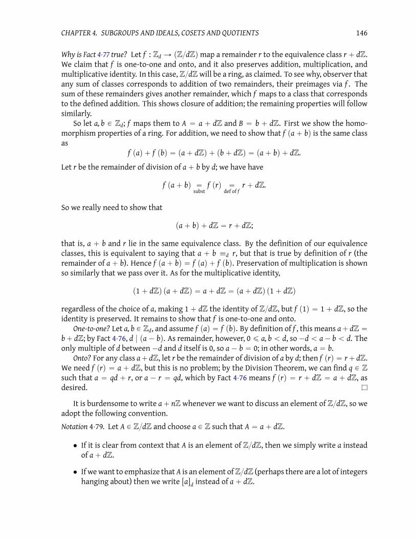
CHAPTER 4. SUBGROUPS AND IDEALS, COSETS AND QUOTIENTS 146
Why is Fact 4¨77 true? Let f : Zd Ñ pZdZqmap a remainder r to the equivalence class r ` dZ.
We claim that f is one-to-one and onto, and it also preserves addition, multiplication, and
multiplicative identity. In this case, ZdZ will be a ring, as claimed. To see why, observer that
any sum of classes corresponds to addition of two remainders, their preimages via f . The
sum of these remainders gives another remainder, which f maps to a class that corresponds
to the defined addition. This shows closure of addition; the remaining properties will follow
similarly.
So let a, b P Zd; f maps them to A “ a ` dZ and B “ b ` dZ. First we show the homo-
morphism properties of a ring. For addition, we need to show that f pa` bq is the same class
as
f paq ` f pbq “ pa` dZq ` pb` dZq “ pa` bq ` dZ.
Let r be the remainder of division of a` b by d; we have have
f pa` bq “subst
f prq “def of f
r ` dZ.
So we really need to show that
pa` bq ` dZ “ r ` dZ;
that is, a ` b and r lie in the same equivalence class. By the definition of our equivalence
classes, this is equivalent to saying that a ` b ”d r, but that is true by definition of r (the
remainder of a` b). Hence f pa` bq “ f paq ` f pbq. Preservation of multiplication is shown
so similarly that we pass over it. As for the multiplicative identity,
p1` dZq pa` dZq “ a` dZ “ pa` dZq p1` dZq
regardless of the choice of a, making 1 ` dZ the identity of ZdZ, but f p1q “ 1 ` dZ, so the
identity is preserved. It remains to show that f is one-to-one and onto.
One-to-one? Let a, b P Zd, and assume f paq “ f pbq. By definition of f , this means a` dZ “b` dZ; by Fact 4¨76, d | pa´ bq. As remainder, however, 0 ď a, b ă d, so´d ă a´ b ă d. The
only multiple of d between´d and d itself is 0, so a´ b “ 0; in other words, a “ b.
Onto? For any class a` dZ, let r be the remainder of division of a by d; then f prq “ r` dZ.
We need f prq “ a ` dZ, but this is no problem; by the Division Theorem, we can find q P Zsuch that a “ qd ` r, or a ´ r “ qd, which by Fact 4¨76 means f prq “ r ` dZ “ a ` dZ, as
desired.
It is burdensome to write a` nZ whenever we want to discuss an element of ZdZ, so we
adopt the following convention.
Notation 4¨79. Let A P ZdZ and choose a P Z such that A “ a` dZ.
• If it is clear from context that A is an element of ZdZ, then we simply write a instead
of a` dZ.
• If we want to emphasize that A is an element ofZdZ (perhaps there are a lot of integers
hanging about) then we write rasd
instead of a` dZ.

CHAPTER 4. SUBGROUPS AND IDEALS, COSETS AND QUOTIENTS 147
• If the value of d is obvious from context, we simply write ras.
To help you grow accustomed to the notation rasd, we use it for the rest of this chapter, even
when d is mindbogglingly obvious.
Definition 4¨80. On account of Fact 4¨77, we can designate the remainder of division of a by
d, whose value is between 0 and |d| ´ 1, inclusive, as the canonical representation of rasd
in
ZdZ.
Question 4¨81 .Write out the Cayley tables for Z2Z and Z3Z (both addition and multiplication).
Question 4¨82 .Write out the Cayley table for Z5Z (both addition and multiplication). Which elements gen-
erate Z5Z?
Question 4¨83 .Write down the Cayley table for Z6Z (both addition and multiplication). Which elements
generate Z6Z?
We now present two more properties. Both properties follow immediately from the iso-
morphism between ZdZ and Zd, so we do not provide any further proof.
Theorem 4¨84. ZdZ is finite for every nonzero d P Z. In fact, if d ‰ 0 then ZdZ has |d| elements
corresponding to the remainders from division by d: 0, 1, 2, . . . , d´ 1.
Question 4¨85 .What if d “ 0? How many elements would ZdZ have? You can’t use division here, so you
have to rely on the equivalence classes, not the isomorphism. Illustrate a few additions and
subtractions, and indicate whether you think that Z0Z is an interesting or useful group.
Question 4¨86 .In the future, we won’t considerZdZwhen d ă 0. Show that this is becauseZdZ “ Z |d|Z.
(Notice that this asks for equality, not merely isomorphism.)
Questions 2.47 on page 61 and 2.48 on page 61 tell us that there is only one group of order 2
(up to isomorphism) and only one group of order 3 (up to isomorphism). So the structure of
Z2Z and Z3Z was determined well before you ever looked at Question 4.81. On the other
hand, there are two possible structures for a group of order 4: the Klein 4-group, and a cyclic
group. (See Question 2.49 on page 61.) Which of these structures does Z4Z have? Again,
isomorphism gives it away.
Theorem 4¨87. ZdZ is cyclic for every d P Z.
This theorem has a more general version, which you will prove in the homework.
A natural and interesting followup question is, which non-zero elements do generateZdZ?
You need a bit more background in number theory before you can answer that question, but
you can still formulate a hypothesis.

CHAPTER 4. SUBGROUPS AND IDEALS, COSETS AND QUOTIENTS 148
Question 4¨88 .Write out a Cayley table for Z4, and compare it to the results of Questions 4.81, 4.82, and 4.83.
Formulate a conjecture as to which elements generate Zn, for arbitrary n.
Question 4¨89 .Use Bezout’s Lemma to prove your conjecture in Question 4.88. Hint: If a P Zn generates Zn,then ab “ 1 for some b P Z. Bezout’s Lemma should help you find b. On the other hand, if 1
is a multiple of a, then so is every other element of Zn — why?
The following important lemma gives an “easy” test for whether two integers are in the
same class of ZdZ, and summarizes what we have done in this section.
Lemma 4¨90. Let a, b, d P Z and assume that d ‰ 0. The following are equivalent.
(A) a` dZ “ b` dZ.
(B) rasd“ rbs
d.
(C) d | pa´ bq.
Proof. (A) is equivalent to (B) by definition of the notation rasd
(see above), and (A) is equiva-
lent to (C) by Fact 4¨76.
4¨6 Partitioning groups and rings
We saw in Section 4¨4 how clockwork arithmetic uses division to partition the integers ac-
cording to their remainder. We also found that this partition has group and ring structures;
for instance, it’s pretty clear that 3` 5 ”6 2, but a few additions and subtractions show that
3 ” ´3, 5 ” 11, and 2 ” 62; the equivalence classes thus tell us that ´3 ` 11 ” 62. We also
saw in Section 3¨1 that working with division of polynomials gave us a way to model roots and
build complex numbers.
Can we do this with other groups and rings? Indeed we can, using a tool called cosets.
Students often have a hard time wrapping their minds around cosets, so we’ll start with an
introductory example that should give you an idea of how cosets “look” in a group. Then we’ll
define cosets, and finally look at some of their properties.
The idea
Two aspects of division were critical for making clockwork arithmetic an equivalence re-
lation, and thus a way to partition of Z:
• existence of a remainder, which implies that every integer belongs to at least one class,
which in turn implies that the union of the classes covers Z; and
• uniqueness of the remainder, which implies that every integer ends up in only one set, so
that the classes are disjoint.

CHAPTER 4. SUBGROUPS AND IDEALS, COSETS AND QUOTIENTS 149
Using the vocabulary of groups, recall from Section 138 the sets
A “ t. . . ,´4, 0, 4, 8, . . . u “ r0s
B “ t. . . ,´3, 1, 5, 9, . . . u “ r1s
C “ t. . . ,´2, 2, 6, 10, . . . u “ r2s
D “ t. . . ,´1, 3, 7, 11, . . . u “ r3s .
Recall from Section 118 that A “ 4Z ă Z, so it is a group under addition. The other sets are
not groups; after all, they lack the additive identity.
What interests us is how the equivalence classes relate to the subgroup. All elements of B
have the form 1` a for some a P A. For example,´3 “ 1` p´4q. Likewise, all elements of C
have the form 2` a for some a P A, and all elements of D have the form 3` a for some a P A.
So if we define
1` A :“ t1` a : a P Au ,
then
1` A “ t. . . , 1` p´4q , 1` 0, 1` 4, 1` 8, . . . u
“ t. . . ,´3, 1, 5, 9, . . . u
“ B.
Likewise, we can write A “ 0` A and C “ 2` A, D “ 3` A.
Pursuing this further, you can check that
¨ ¨ ¨ “ ´3` A “ 1` A “ 5` A “ 9` A “ ¨ ¨ ¨
and so forth. Interestingly, all the sets in the previous line are the same as B! In addition,
1`A “ 5`A, and 1´5 “ ´4 P A. The same holds for C: 2`A “ 10`A, and 2´10 “ ´8 P A.
This relationship will prove important at the end of the section.
So the partition by remainders of division by four is related to the subgroup A of multiples
of 4. How can we generalize this phenomenon to other groups, even nonabelian ones?
Definition 4¨91. Let G be a group and A ă G. Let g P G. We define the left coset of A with gas
gA “ tga : a P Au
and the right coset of A with g as
Ag “ tag : a P Au .
In general, left cosets and right cosets are not equal, partly because the operation might
not commute. If we speak of “cosets” without specifying “left” or “right”, we mean “left
cosets”.
Example 4¨92. Recall the group D3 from Section 3¨6 and the subgroup H “ xφy “ tι,φu from
Example 4¨8. In this case,
ρH “ tρ, ρφu and Hρ “ tρ,φρu .
Since φρ “ ρ2φ ‰ ρφ, we see that ρH ‰ Hρ.

CHAPTER 4. SUBGROUPS AND IDEALS, COSETS AND QUOTIENTS 150
Question 4¨93 .In Question 4.17, you showed that Ω2 ă Ω8. Compute the left and right cosets of Ω2 in Ω8.
Question 4¨94 .Let tя, a, b, a` bu be the Klein 4-group. (See Questions 2.49 on page 61, 3.45 on page 84,
and 4.18 on page 124.) Compute the left and right cosets of xay.
Question 4¨95 .Compute the left and right cosets of xjy in Q8.
For some subgroups, left and right cosets are always equal. This is always true in abelian
groups, as illustrated by Example 4¨97.
Question 4¨96 .Show explicitly why left and right cosets are equal in abelian groups.
If A is an additive subgroup, we write the left and right cosets of Awith g as g`A and A`g.
Rings are abelian groups under addition, with ideals as subgroups, so if R is a ring, AŸ R, and
r P R, then we write the coset of Awith r is r` A. For now we focus on the theory of cosets in
the context of groups, as this applies equally to cosets of ideals of rings.
Example 4¨97. Consider the subgroup H “ tpa, 0q : a P Ru of R2from Question 4.14. Let
p “ p3,´1q P R2. The coset of H with p is
p` H “ tp3,´1q ` q : q P Hu
“ tp3,´1q ` pa, 0q : a P Ru“ tp3` a,´1q : a P Ru .
Sketch some of the points in p ` H, and compare them to your sketch of H in Question 4.14.
How does the coset compare to the subgroup?
Generalizing this further, every coset of H has the form p ` H where p P R2. Elements of
R2are points, so p “ px, yq for some x, y P R. The coset of H with p is
p` H “ tpx` a, yq : a P Ru .
Sketch several more cosets. How would you describe the set of all cosets of H in R2?
Question 4¨98 .Recall the subgroup L of R2
from Question 4.14 on page 123.
(a) Give a geometric interpretation of the coset p3,´1q ` L.
(b) Give an algebraic expression that describes p` L, for arbitrary p P R2.
(c) Give a geometric interpretation of the cosets of L in R2.
(d) Use your answers to (a) and (c) give a geometric description of how cosets of L partition
R2.

CHAPTER 4. SUBGROUPS AND IDEALS, COSETS AND QUOTIENTS 151
A group does not have to be abelian for the left and right cosets to be equal. When deciding
if gA “ Ag, we are not deciding whether elements of G commute, but whether subsets of G are equal.
Returning to D3, we can find a subgroup whose left and right cosets are equal even though
the group is not abelian and the operation is not commutative.
Example 4¨99. Let K “ tι, ρ, ρ2u; certainly K ă D3, after all, K “ xρy. In this case, αK “ Kα for
all α P D3:
α αK Kα
ι K K
φ tφ,φρ,φρ2u tφ, ρφ, ρ2φu
ρ K K
ρ2
K K
ρφ tρφ, pρφq ρ, pρφq ρ2u tρφ,φ, ρ2φu
ρ2φ tρ2φ, pρ2φq ρ, pρ2φq ρ2u tρ2φ, ρφ,φu
In each case, the sets φK and Kφ are equal, even though φ does not commute with ρ. (You
should verify these computations by hand.)
Question 4¨100 .In Question 4.12 on page 122, you found another subgroup K of order 2 in D3. Does K satisfy
the property αK “ Kα for all α P D3?
When a subgroup’s left and right cosets are always equal, we call it a normal subgroupof its group. Normal subgroups play a critical role in later sections, but we won’t worry too
much about them at the moment.
You might notice a few things. In each case, every element appears in a coset: a subgroup
A always contains the identity, so any g appears in “its own” coset gA. On the other hand, g
seems to appear only in gA, and in no other other coset! After all, φK and pρφq K differ only
superficially; when you consider their contents, you find that they are equal. This sounds
an awful lot like the partition we were aiming for. Does it hold true in general? What other
properties might cosets contain?
Properties of Cosets
We present some properties of cosets that illustrate further their similarities to division.
Theorem 4¨101. The cosets of a subgroup partition the group.
Before proving this, we pause to point out that combining Theorems 4¨101 and 4¨70 implies
another nice result.
Corollary 4¨102. Let A ă G. Define a relation„ on x, y P G by
x „ y ðñ x is in the same coset of A as y.
This relation is an equivalence relation.

CHAPTER 4. SUBGROUPS AND IDEALS, COSETS AND QUOTIENTS 152
We will make repeated use of this equivalence relation.
Proof of Theorem 4¨101. Let G be a group, and A ă G. We have to show two things:
(CP1) the cosets of A cover G, and
(CP2) distinct cosets of A are disjoint.
We show (CP1) first. Let g P G. The definition of a group tells us that g “ gя. Since я P A by
definition of subgroup, g “ gя P gA. Since gwas arbitrary, every element of G is in some coset
of A. Hence the union of all the cosets is G.
For (CP2), let X and Y be arbitrary cosets of A. Assume that X and Y are distinct; that
is, X ‰ Y. We need to show that they are disjoint; that is, X X Y “ H. We will show the
contrapositive instead; that is, we will assume XX Y ‰ H, and show X “ Y. A contrapositive
is logically equivalent to the original statement, so we will have accomplished our goal.
To prove the contrapositive, assume XXY ‰ H. By definition of intersection, we can find
z P X X Y. By definition of a coset, there exist x, y P G such that X “ xA and Y “ yA; we can
write z “ xa and z “ yb for some a, b P A. By substitution, xa “ yb, so x “ pybq a´1, or
x “ y`
ba´1˘
. (4.2)
We still have to show that X “ Y. We show this by showing that X Ď Y and X Ě Y. For
the former, let w P X; by definition of X, w “ xa for some a P A. Applying our conversion
mechanism,
w “ xa ““
y`
ba´1˘
a‰
“ y“`
ba´1˘
a‰
P yA.
We chose w as an arbitrary element of X, so X Ď Y. The proof that X Ě Y is so similar that we
omit it. By definition of set equality, X “ Y. Inasmuch as X and Y were arbitrary, this holds
for all cosets of A: if two cosets of A are not disjoint, then they are not distinct.
Having shown (CP2) and (CP1), we have shown that the cosets of A partition G.
We conclude this section with three facts that allow us to decide when cosets are equal.
Lemma 4¨103 (Equality of cosets). Let G be a group and A ă G. All of the following hold:
(CE1) яA “ A.
(CE2) For all g P G, gA “ A if and only if g P A.
(CE3) For all g, h P G, gA “ hA if and only if g P hA.
(CE4) For all g, h P G, gA “ hA if and only if g´1h P A.
As usual, you should keep in mind that in additive groups (and thus in rings) the first three
conditions translate to
(CE1) 0` A “ A.
(CE2) For all g P G, g P A if and only if g` A “ A.
(CE3) For all g, h P G, g` A “ h` A if and only if g P h` A.
(CE4) For all g, h P G, g` A “ h` A if and only if g´ h P A.

CHAPTER 4. SUBGROUPS AND IDEALS, COSETS AND QUOTIENTS 153
Notice also that characterization (CE4) resembles the third criterion of the Subgroup The-
orem. The resemblance is mostly superficial; in the Subgroup Theorem, a´1b refers to elements
of A, while (CE4) refers to elements of G that are not always in A. That said, if it is the case that
g, h P A then the Subgroup Theorem tells us that g´1h P A, so gA “ hA — though we already
knew that from (CE2), since gA “ A “ hA.
Proof. (CE1) is “obvious” (but you will fill in the details in Question 4.105.).
We jump to (CE3) for the moment. Let g, h P G. We know that я P A, so g “ gя P gA.
Corollary 4¨102 tells us that membership in a coset is an equivalence relation, where the cosets
are the equivalence classes. By substitution, gA “ hA if and only if g P hA.
We turn to (CE2). Let g P G. By (CE3), gA “ яA if and only if g P яA. By (CE1), яA “ A, so
by substitution, g P A if and only if gA “ A.
We finally turn to (CE4). Let g, h P G. By (CE3), gA “ hA if and only if g P hA. By definition
of a coset, g P hA if and only if g “ ha for some a P A. Applying the inverse property twice, we
rewrite this equation first as я “ g´1 phaq, then (after an associative property) as a´1 “ g´1h.
Since a´1 P A, we have g
´1h P A. Every step used an equivalence, so we can connect the chain
into the one equivalence, gA “ hA if and only if g´1h P A.
Property (CE4) does little more than restate the partition property, with the added knowl-
edge that any elements lies in its own coset. However, it emphasizes that, when computing
cosets of a subgroup A, you can skip hA whenever h appears in gA.
Question 4¨104 .Consider the ideal A “ 〈x2 ` 1〉 in R rxs. Why can we write every coset of A as pax` bq ` A,
where a, b P R? Hint: This is related to the isomorphism of Section 3¨1.
Question 4¨105 .Fill in each blank of Figure 4.105 with the appropriate justification or statement.
4¨7 Lagrange’s Theorem and the order of an element of agroup
How many cosets can a subgroup have? This section answers this question, as well as some
related questions about the size of a subgroup and the order of an element. Throughout this
section, we assume |G| is finite, even if we don’t say so explicitly.
Notation 4¨106. Let G be a group, and A ă G. We write GA for the set of all left cosets of A.
That is,
GA “ tgA : g P Gu .
We also write AzG for the set of all right cosets of A:
AzG “ tAg : g P Gu .

CHAPTER 4. SUBGROUPS AND IDEALS, COSETS AND QUOTIENTS 154
Let G be a group and H ă G.
Claim: яH “ H.
1. First we show that _____. Let x P яH.
(a) By definition of яH, x “_____.
(b) By the identity property, _____.
(c) By substitution, x P_____.
(d) We had chosen an arbitrary element of яH , so by inclusion, _____.
2. Now we show the converse, that яH Ě H. Let x P_____.
(a) By the identity property, _____.
(b) By definition of яH, _____P яH.
(c) We had chosen an arbitrary element, so by inclusion, _____.
Figure 4¨6: Material for Question 4.105
Example 4¨107. Let G “ Z and A “ 4Z. We saw in Example 4¨69 that
GA “ Z4Z “ tA, 1` A, 2` A, 3` Au .
We actually “waved our hands” in Example 4¨69. That means that we did not provide a very
detailed argument, so let’s show the details here. Recall that 4Z is the set of multiples of Z,
so x P A iff x is a multiple of 4. What about the remaining elements of Z?
Let x P Z; then
x` A “ tx` z : z P Au “ tx` 4n : n P Zu .
Use the Division Theorem to write
x “ 4q` r
for unique q, r P Z, where 0 ď r ă 4. Then
x` A “ tp4q` rq ` 4n : n P Zu “ tr ` 4 pq` nq : n P Zu .
By closure, q` n P Z. If we write m in place of 4 pq` nq, then m P 4Z. So
x` A “ tr ` m : m P 4Zu “ r ` 4Z.
The distinct cosets of A are thus determined by the distinct remainders from division by 4.
Since the remainders from division by 4 are 0, 1, 2, and 3, we conclude that
ZA “ tA, 1` A, 2` A, 3` Au
as claimed above.

CHAPTER 4. SUBGROUPS AND IDEALS, COSETS AND QUOTIENTS 155
Example 4¨108. Let G “ D3 and K “ tι, ρ, ρ2u as in Example 4¨99, then
GK “ D3 xρy “ tK,φKu .
Example 4¨109. Let H ă R2be as in Example 4¨13 on page 122; that is,
H “
pa, 0q P R2: a P R
(
.
Then
R2H “
r ` H : r P R2(
.
It is not possible to list all the elements of GH, but some examples would be
p1, 1q ` H, p4,´2q ` H.
Question 4¨110 .Speaking geometrically, what do the elements of R2H look like? This question is similar to
Question 4.98.
Keep in mind that GA is a set whose elements are also sets. Showing equality of two
elements of GA requires one to show that two sets are equal.
Remember our assumption that G is finite. In this case, a simple formula gives us the size
of GA.
Lagrange’s Theorem. Let A ă G. The size of GA is the ratio of the number of elements of G to the
number of elements of A. That is,
|GA| “|G|
|A|.
While the notation of cosets is somewhat suggestive of the relationship between cosets
and division, Lagrange’s Theorem is not as obvious as the notation might imply: we can’t
“divide” the sets G and A. We are not moving the absolute value bars “inside” the fraction;
nor can we, as GA is not a number. Rather, we are partitioning the group G by the cosets of
its subgroup A, and counting the number of sets that result.
Proof. We know from Theorem 4¨101 that the cosets of A partition G. How many such cosets
are there? |GA|, by definition! Each coset has the same size, |A|. Suppose there are n cosets;
we can visualize the partition in this fashion:
|G| elements in the entire grouphkkkkkkkkkkkkkkkkkkkkkkkkkkkkkkkkkkkkkkkkkkkkikkkkkkkkkkkkkkkkkkkkkkkkkkkkkkkkkkkkkkkkkkkkj
partition яA partition g1A partition g2A ¨ ¨ ¨ partition gnA
loooooomoooooon loooooomoooooon loooooomoooooon loooooomoooooon
|A| elements |A| elements |A| elements |A| elements
A basic principle of counting tells us that the number of elements of G is thus the product
of the number of elements in each coset and the number of cosets. That is, |GA| ¨ |A| “ |G|.
This implies the theorem.

CHAPTER 4. SUBGROUPS AND IDEALS, COSETS AND QUOTIENTS 156
The next-to-last sentence of the proof contains the statement |GA| ¨ |A| “ |G|. Since |A|
is the order of the group A, and |GA| is an integer, we conclude that:
Corollary 4¨111. The order of any subgroup of G divides the order of the group.
Example 4¨112. Let G be the Klein 4-group (see Questions 2.49 on page 61, 3.45 on page 84,
and 4.18 on page 124). Every subgroup of the Klein 4-group has order 1, 2, or 4. As predicted
by Corollary 4¨111, the orders of the subgroups divide the order of the group.
Likewise, the order of tι,φu divides the order of D3.
By contrast, the subset HK of D3 that you computed in Question 4.12 on page 122 has four
elements. Since 4 - 6, the contrapositive of Lagrange’s Theorem implies that HK cannot be a
subgroup of D3.
From the fact that every element g generates a cyclic subgroup xgy ă G, Lagrange’s The-
orem also implies an important consequence about the order of any element of any finite
group.
Corollary 4¨113. The order of any element of a group divides the order of a group.
Proof. You do it! See Question 4.115.
Question 4¨114 .Recall from Question 4.17 that if d | n, then Ωd ă Ωn. How many cosets of Ωd are there in Ωn?
Question 4¨115 .Fill in each blank of Figure 4.115 with the appropriate justification or expression.
Question 4¨116 .Suppose that a group G has order 8, but is not cyclic. Why must g
4 “ я for all g P G?
Question 4¨117 .Let G be a finite group, and g P G. Why is g
|G| “ я?
Question 4¨118 .Suppose that a group has five elements. Why must it be abelian?
Question 4¨119 .Find a criterion on the order of a group that guarantees the group is cyclic.

CHAPTER 4. SUBGROUPS AND IDEALS, COSETS AND QUOTIENTS 157
Claim: The order of an element of a group divides the order of a group.
Proof:
1. Let G _____.
2. Let x _____.
3. Let H “ x_____y.
4. By _____, every integer power of x is in G.
5. By _____, H is the set of integer powers of x.
6. By _____, H ă G.
7. By _____, |H| divides |G|.
8. By _____, ord pxq divides |H|.
9. By definition, there exist m, n P_____ such that |H| “ mord pxq and |G| “ n |H|.
10. By substitution, |G| “_____.
11. _____.
(This last statement must include a justification.)
Figure 4¨7: Material for Question 4.115

CHAPTER 4. SUBGROUPS AND IDEALS, COSETS AND QUOTIENTS 158
Question 4¨120 .Let p be an irreducible number, and recall thatZp is a field, so that its non-zero elements form
a group under multiplication. For instance, in Z7, the set t1, 2, 3, 4, 5, 6u forms a group under
multiplication. Explain why, for every a P Zp,
(a) ap´1 “ 1, and
(b) ap “ a, and
(c) ap´2 “ a´1.
This fact is called Fermat’s Little Theorem. We explore it in a general context later.
4¨8 Quotient Rings and Groups
Consider the polynomial ring R rxs. Looking at remainders from division by x2 ` 1 gave us a
way to model complex numbers as
C “ tax` b : a, b P Ru ,
where 1x ` 0 stood in for the imaginary number. An isomorphism (Question 3.18) showed
that this was equivalent to the traditional model of the complex numbers, with 1x` 0 ÞÑ i.
Since then, we pointed out that every multiple of x2 ` 1 has the imaginary number i as
a root. Multiples of x2 ` 1 have two things in common. First, dividing such polynomials by
x2 ` 1 gives a remainder of 0. Second, and equivalently, they are in the ideal A “ 〈x2 ` 1〉.
Question 4.104 showed us that the cosets of 〈x2 ` 1〉 correspond to remainders from division
by x2 ` 1. As noted, those remainders formed a field isomorphic to C. In other words, the
cosets of 〈x2 ` 1〉 give us another model of the field C.
Can we do this for cosets of general groups? To make the question precise, let A ă G.
Can we find a natural generalization of the operation(s) of G that makes GA a group? By a
“natural” generalization, we mean something like
pgAq˙ phAq “ pghqA.
Quotient rings
The first order of business it to make sure that the operation even makes sense. The tech-
nical word for this is that the operation is well-defined. What does that mean? A coset can
have different representations. An operation must be a function: for every pair of elements,
it must produce exactly one result. The relation above would not be an operation if differ-
ent representations of a coset gave us different answers. Example 4¨121 shows how it can go
wrong.

CHAPTER 4. SUBGROUPS AND IDEALS, COSETS AND QUOTIENTS 159
Example 4¨121. Recall H “ xφy ă D3 from Example 4¨92. Let X “ ρH and Y “ ρ2H. Notice
that pρφqH “ tρφ, ιu “ ρH, so X has two representations, ρH and pρφqH.
Were the operation well-defined, XY would have the same value, regardless of the represen-
tation of X. That is not the case! When we use the the first representation,
XY “ pρHq`
ρ2H˘
“`
ρ ˝ ρ2˘
H “ ρ3H “ ιH “ H.
When we use the second representation,
XY “ ppρφqHq`
ρ2H˘
“`
pρφq ρ2˘
H “`
ρ`
φρ2˘˘
H
“ pρ pρφqqH “`
ρ2φ˘
H ‰ H.
On the other hand, sometimes the operation is well-defined.
Example 4¨122. Recall the subgroup A “ 4Z ofZ. Let B, C, D P ZA, so B “ b`4Z, C “ c`4Z,
and D “ d` 4Z for some b, c, d P Z.
We have to make sure that we cannot have B “ D and B ` C ‰ D ` C. For example, if
B “ 1` 4Z and D “ 5` 4Z, B “ D. Does it follow that B` C “ D` C?
From Lemma 4¨103, we know that B “ D iff b´ d P A “ 4Z. That is, b´ d “ 4m for some
m P Z. Let x P B` C; then x “ pb` cq ` 4n for some n P Z. By substitution,
x “ ppd` 4mq ` cq ` 4n “ pd` cq ` 4 pm` nq P D` C.
Since x was arbitrary in B ` C , we have B ` C Ď D ` C. A similar argument shows that
B` C Ě D` C, so the two are, in fact, equal.
The operation was well-defined in the second example, but not the first. What made for
the difference? In the second example, we rewrote
ppd` 4mq ` cq ` 4n “ pd` cq ` 4 pm` nq ,
but that relies on the fact that addition commutes in an abelian group. Without that fact, we
could not have swapped c and 4m.
Right away we see that we can always do this for cosets of ideals: after all, ideals are sub-
groups of rings under addition. Indeed, we can say something more.
Fact 4¨123. Let R be a commutative ring. The cosets of an ideal A of R form a new ring, whose addition
and multiplication are natural generalizations of the addition and multiplication of R. That is, for any
r, s P R,
pr ` Aq ` ps` Aq “ pr ` sq ` A and pr ` Aq ps` Aq “ rs` A.
Why? Let AŸ R, and let X, Y, Z P RA.
Our first task is to show that addition and multiplication are well-defined. To do this,
we need to show that the definitions of X ` Y and XY give us the same result, regardless of
the representation we choose for X and Y. To this end, suppose there exist r, s, x, y P A such that
X “ x` A “ r ` A and Y “ y` A “ s` A.

CHAPTER 4. SUBGROUPS AND IDEALS, COSETS AND QUOTIENTS 160
addition? We need to show that px` yq`A “ pr ` sq`A. The lemma on Coset Equality
tells us that this is true if and only if ´px` yq ` pr ` sq P A, so we’ll aim to
show this latter expression is true. By hypothesis, x ` A “ r ` A, so by
Coset Equality,´x` r P A. Similarly,´y` s P A. By closure of addition and
properties of ring addition,
´px` yq ` pr ` sq “ p´x` rq ` p´y` sq P A.
As we explained earlier, this shows that px` yq ` A “ pr ` sq ` A; in short,
the addition is well-defined.
multiplication? We need to show that xy` A “ rs` A. The lemma on Coset Equality tells us
that this is true if and only if´pxyq ` rs P A, so we’ll aim to show this latter
expression is true. Recall from the previous paragraph that´x`r,´y`s P A.
To get from these to ´pxyq ` rs, we’ll use a fairly standard trick of adding
zero in “the right form”,
´pxyq ` rs “ ´pxyq ` ry´ ry` rs “ y p´x` rq ` r p´y` sq .
Absorption implies that y p´x` rq , r p´y` sq P A. Closure implies their sum
is also in A. By substitution, ´pxyq ` rs P A. As we explained earlier, this
shows that xy` A “ rs` A; in short, the multiplication is well-defined.
The remaining properties of addition are relatively straightforward. Choose x, y, z P R such
that X “ x` A, Y “ y` A, Z “ z` A.
associative? pX ` Yq ` Z “ rpx` Aq ` py` Aqs ` pz` Aq “ rpx` yq ` As ` pz` Aq “
rpx` yq ` zs`A. Apply the associative property of addition inR to obtain pX ` Yq`
Z “ rx` py` zqs ` A. Now reverse the simplification to obtain pX ` Yq ` Z “
px` Aq`rpy` zq ` As “ px` Aq`rpy` Aq ` pz` Aqs “ X`pY ` Zq. The ends
of this latter chain of equalities show the associative property is satisfied.
identity? We want a cosetW such that X`W “ X andW`X “ X. Letw P R such thatW “
w` A; by substitution, our first desired equation becomes px` Aq ` pw` Aq “
x ` A, or px` wq ` A “ x ` A. By coset equality, we need px` wq ´ x P A; by
simplification, w P A. From coset equality (Theorem 4¨103(CE2)) that choosing
any a P A gives us A itself, soW “ Amust be the identity.
inverse? We want an “inverse” coset of X “ x`A. The natural suspect would be p´xq`A;
that is, the coset of A with ´x. Indeed, it works great: px` Aq ` rp´xq ` As “
0 ` A “ A, and likewise rp´xq ` As ` px` Aq “ A. We just showed A is the
identity of RA, so we have found the inverse of X.
abelian? X ` Y “ px` Aq ` py` Aq “ px` yq ` A. Apply the commutative property of
addition in R to obtain X ` Y “ py` xq ` A “ py` Aq ` px` Aq “ Y ` X. The
ends of this latter chain of equalities show the addition is abelian.

CHAPTER 4. SUBGROUPS AND IDEALS, COSETS AND QUOTIENTS 161
We’ve found that RA is an abelian group under the proposed addition, the first step towards
showing it’s a ring. We still need to show that multiplication satisfies the properties of a
monoid, along with distribution.
We leave the remaining, multiplicative properties of a ring to you, the reader.
Question 4¨124 .Show the remaining properties of a ring for RA: closure, associative, identity, and distribu-
tive.
“Normal” subgroups
What about the cosets of nonabelian groups? Given the example above, you might be
inclined to dismiss them, but that would be too hasty.
The key in Example 4¨122 was not thatZ is abelian, but that we could rewrite p4m` cq`4n
as c ` p4m` 4nq, then simplify 4m ` 4n to 4 pm` nq. The abelian property makes it easy to
do that, but we don’t need the group G to be abelian; we need the subgroup A to satisfy it. If
A were not abelian, we could still make it work if, after we move c left, we get some element
of A to its right, so that it can be combined with the other one. That is, we have to be able
to rewrite any ac as ca1, where a
1is also in A. We need not have a “ a
1! Let’s emphasize that,
changing c to g for an arbitrary group G:
The operation defined above is well-defined
iff
for every g P G and for every a P A
there exists a1 P A such that ga “ a1g.
In terms of sets, for every g P G and every a P A, there exists a1 P A such that ga “ a
1g. Here
ga P gA is arbitrary, so gA Ď Ag. The other direction must also be true, so gA Ě Ag. In other
words,
The operation defined above is well-defined
iff gA “ Ag for all g P G.
Definition 4¨125. Let A ă G. If
gA “ Ag
for every g P G, then A is a normal subgroup of G.
Since normal subgroups partition a group into a new group, the same way ideals partition a
ring into a new ring, let’s “promote” them to having the same notation.
Notation 4¨126. We write AŸ G to indicate that A is a normal subgroup of G.
Question 4¨127 .Show that for any group G, tяu Ÿ G and GŸ G.

CHAPTER 4. SUBGROUPS AND IDEALS, COSETS AND QUOTIENTS 162
Although we have outlined the argument above, we should show explicitly that if A is a
normal subgroup, then the operation proposed for GA is indeed well-defined.
Lemma 4¨128. Let A ă G. Then (CO1) implies (CO2).
(CO1) AŸ G.
(CO2) Let X, Y P GA and x, y P G such that X “ xA and Y “ yA. The operation ˙ on GA defined by
X ˙ Y “ pxyqA
is well-defined for all x, y P G.
Proof. Let W, X, Y, Z P GA and choose w, x, y, z P G such that W “ wA, X “ xA, Y “ yA, and
Z “ zA. To show that the operation is well-defined, we must show that if W “ X and Y “ Z,
then WY “ XZ regardless of the values of w, x, y, or z. Assume therefore that W “ X and
Y “ Z. By substitution, wA “ xA and yA “ zA. By Lemma 4¨103(CE3), w´1x P A and y
´1z P A.
Since WY and XZ are sets, showing that they are equal requires us to show that each is
a subset of the other. First we show that WY Ď XZ. To do this, let t P WY “ pwyqA. By
definition of a coset, t “ pwyq a for some a P A. What we will do now is rewrite t by
• using the fact that A is normal to move some element of a left, then right, through the
representation of t; and
• using the fact thatW “ X and Y “ Z to rewrite products of the form wα as xα and y 9α as
z:α, where α, α, 9α, :α P A.
How, precisely? By the associative property, t “ w pyaq. By definition of a coset, ya P yA. By
hypothesis, A is normal, so yA “ Ay; thus, ya P Ay. By definition of a coset, there exists α P A
such that ya “ »ay. By substitution, t “ w pαyq. By the associative property, t “ pwαq y. By
definition of a coset, wα P wA. By hypothesis, A is normal, so wA “ Aw. Thus wα P Aw. By
hypothesis, W “ X; that is, wA “ xA. Thus wα P xA, and by definition of a coset, wα “ xa for
some a P A. By substitution, t “ pxaq y. The associative property again gives us t “ x payq;
since A is normal we can write ay “ y 9a for some 9a P A. Hence t “ x py 9aq. Now,
y 9a P yA “ Y “ Z “ zA,
so we can write y 9a “ z:a for some :a P A. By substitution and the definition of coset arithmetic,
t “ x pz:aq “ pxzq:a P pxzqA “ pxAq pzAq “ XZ.
Since twas arbitrary inWY, we have shown thatWY Ď XZ. A similar argument shows that
WY Ě XZ; thusWY “ XZ and the operation is well-defined.
An easy generalization of the argument of Example 4¨122 shows the following Theorem.
Theorem 4¨129. Let G be an abelian group, and H ă G. Then H Ÿ G.

CHAPTER 4. SUBGROUPS AND IDEALS, COSETS AND QUOTIENTS 163
Question 4¨130 .Prove Theorem 4¨129.
Question 4¨131 .Explain why every subgroup of Dm pRq is normal.
Question 4¨132 .Show that Q8 is not a normal subgroup of GLm pCq.
Question 4¨133 .Let G be a group, and A ă G. Suppose that |GA| “ 2; that is, the subgroup A partitions G into
precisely two left cosets. Show that:
• AŸ G; and
• GA is abelian.
We said before that we don’t need an abelian group to have a normal subgroup. Here’s a
great example.
Example 4¨134. Let
A3 “
ι, ρ, ρ2(
ă D3.
We call A3 the alternating group on three elements. We claim that A3 Ÿ D3. Indeed,
σ σA3 A3σ
ι A3 A3
ρ A3 A3
ρ2
A3 A3
φ φA3 “ tφ,φρ,φρ2u “ A3φ A3φ “ φA3
ρφ tρφ, pρφq ρ, pρφq ρ2u “ φA3 φA3
ρ2φ tρ2φ, pρ2φq ρ, pρ2φq ρ2u “ φA3 φA3
We have left out some details, though we also computed this table in Example 4¨99, calling
the subgroup K instead of A3. Check the computation carefully, using extensively the fact
that φρ “ ρ2φ.
Quotient groups
The set of cosets of a normal subgroup is, as desired, a group.
Theorem 4¨135. Let G be a group. If AŸ G, then GA is a group.
Proof. Assume A Ÿ G. By Lemma 4¨128, the operation is well-defined, so it remains to show
that GA satisfies the properties of a group.

CHAPTER 4. SUBGROUPS AND IDEALS, COSETS AND QUOTIENTS 164
(closure) Closure follows from the fact that multiplication of cosets is well-defined when AŸ
G, as shown in Lemma 4¨128: Let X, Y P GA, and choose g1, g2 P G such that X “ g1A and
Y “ g2A. By definition of coset multiplication, XY “ pg1Aq pg2Aq “ pg1g2qA P GA. Since
X, Y were arbitrary in GA, coset multiplication is closed.
(associativity) The associative property of GA follows from the associative property of G. Let
X, Y, Z P GA; choose g1, g2, g3 P G such that X “ g1A, Y “ g2A, and Z “ g3A. Then
pXYq Z “ rpg1Aq pg2Aqs pg3Aq .
By definition of coset multiplication,
pXYq Z “ ppg1g2qAq pg3Aq .
By the definition of coset multiplication,
pXYq Z “ ppg1g2q g3qA.
(Note the parentheses grouping g1g2.) Now apply the associative property of G and reverse
the previous steps to obtain
pXYq Z “ pg1 pg2g3qqA
“ pg1Aq ppg2g3qAq
“ pg1Aq rpg2Aq pg3Aqs
“ X pYZq .
Since X, Y, Z were arbitrary in GA, coset multiplication is associative.
(identity) We claim that the identity of GA is A itself. Let X P GA, and choose g P G such
that X “ gA. Since я P A, Lemma 4¨103 on page 152 implies that A “ яA, so
XA “ pgAq pяAq “ pgяqA “ gA “ X.
Since X was arbitrary in GA and XA “ X, A is the identity of GA.
(inverse) Let X P GA. Choose g P G such that X “ gA, and let Y “ g´1A. We claim that
Y “ X´1. By applying substitution and the operation on cosets,
XY “ pgAq`
g´1A˘
“`
gg´1˘
A “ яA “ A.
Hence X has an inverse in GA. Since X was arbitrary in GA, every element of GA has an
inverse.
We have shown that GA satisfies the properties of a group.
Definition 4¨136. Let G be a group, and A Ÿ G. Then GA is the quotient group of G withrespect to A, also called Gmod A.
Normally we say “the quotient group” rather than “the quotient group of G with respect to
A.”

CHAPTER 4. SUBGROUPS AND IDEALS, COSETS AND QUOTIENTS 165
Example 4¨137. SinceA3 is a normal subgroup of D3, D3A3 is a group. By Lagrange’s Theorem,
it has 63 “ 2 elements. The Cayley table is
˝ A3 φA3
A3 A3 φA3
φA3 φA3 A3
We meet an important quotient group in Section 4¨5.
Question 4¨138 .Prove the following generalization of Theorem 4¨87: If G is a cyclic group and AŸ G, then GA
is cyclic.
Question 4¨139 .Recall from Question 4.17 that if d | n, then Ωd ă Ωn.
(a) Explain how we know that, in fact, Ωd Ÿ Ωn.
(b) Does the quotient group Ω8Ω2 have the same structure as the Klein 4-group, or as the
Cyclic group of order 4?
Question 4¨140 .In Question 4.95, you computed the left and right cosets of xjy in Q8. Is xjy a normal subgroup
of Q8? If so, compute the Cayley table of Q8 xjy.
Question 4¨141 .Let H “ xiy ă Q8.
(a) Show that H Ÿ Q8 by computing all the cosets of H.
(b) Compute the Cayley table of Q8H.
Question 4¨142 .Recall the subgroup L of R2
from Questions 4.14 on page 123 and 4.98 on page 150.
(a) Explain how we know that LŸ R2without checking p` L “ L` p for any p P R2
.
(b) Sketch two elements of R2L and show their sum.
Conjugation
Another way to show a subgroup is normal involves rephrasing the idea of equality be-
tween left and right cosets. This is tied into an important operation, called conjugation.

CHAPTER 4. SUBGROUPS AND IDEALS, COSETS AND QUOTIENTS 166
Definition 4¨143. Let G be a group, g P G, and H ă G. Define the conjugation of H by g as
gHg´1“
ghg´1: h P H
(
.
Theorem 4¨144. H Ÿ G if and only if H “ gHg´1 for all g P G.

CHAPTER 4. SUBGROUPS AND IDEALS, COSETS AND QUOTIENTS 167
Let G be a group, and H ă G. Claim: H Ÿ G if and only if H “ gHg´1 for all g P G.
Proof:
1. First, we show that if H Ÿ G, then _____.
(a) Assume _____.
(b) By definition of normal, _____.
(c) Let g_____.
(d) We first show that H Ď gHg´1.
i. Let h_____.
ii. By 1b, hg P_____.
iii. By definition, there exists h1 P H such that hg “_____.
iv. Multiply both sides on the right by g´1
to see that h “_____.
v. By _____, h P gHg´1.
vi. Since h was arbitrary, _____.
(e) Now we show that H Ě gHg´1.
i. Let x P_____.
ii. By _____, x “ ghg´1 for some h P H.
iii. By _____, gh P Hg.
iv. By _____, there exists h1 P H such that gh “ h1g.
v. By _____, x “ ph1gq g´1.
vi. By _____, x “ h1.
vii. By _____, x P H.
viii. Since x was arbitrary, _____.
(f) We have shown that H Ď gHg´1 and H Ě gHg´1. Thus, _____.
2. Now, we show _____: that is, if H “ gHg´1 for all g P G, then H Ÿ G.
(a) Assume _____.
(b) First, we show that gH Ď Hg.
i. Let x P_____.
ii. By _____, there exists h P H such that x “ gh.
iii. By _____, g´1x “ h.
iv. By _____, there exists h1 P H such that h “ g´1h1g. (This holds for all g P G.)
v. By _____, g´1x “ g´1h1g.
vi. By _____, x “ g pg´1h1gq.
vii. By _____, x “ h1g.
viii. By _____, x P Hg.
ix. Since x was arbitrary, _____.
(c) The proof that _____ is similar.
(d) We have show that _____. Thus, gH “ Hg.
Figure 4¨8: Material for Question 4.145

CHAPTER 4. SUBGROUPS AND IDEALS, COSETS AND QUOTIENTS 168
Question 4¨145 .Prove Theorem 4¨144 by filling in each blank of Figure 4¨8 with the appropriate justification
or statement.2
Example 4¨146. We posed the question of whether SOn pRq Ÿ On pRq. We claim that it is. To
see why, letM P SOn pRq and A P On pRq. By properties of determinants,
det`
AMA´1˘
“ detA ¨ detM ¨ detA´1“ detA ¨ 1 ¨ pdetAq
´1“ 1.
By definition, AMA´1 P SOn pRq, regardless of the choice of A andM. Hence, A ¨SOn pRq ¨A´1 Ď
SOn pRq for all A P On pRq.Conversely, let B “ A´1MA; an argument similar to the one above shows that B P SOn pRq,
and substitution gives us M “ ABA´1
, so that M P A ¨ SOn pRq ¨ A´1, regardless of the choice
of A and M. Hence, A ¨ SOn pRq ¨ A´1 Ě SOn pRq, and the two are equal. By Theorem 4¨144,
SOn pRq Ÿ On pRq.
Example 4¨147. On the other hand, we can also use conjugation to show easily that O2 pRq is
not a normal subgroup of GL2 pRq. Why not? Let
A “
ˆ
1 1
0 1
˙
P GL2 pRq and M “
ˆ
0 1
1 0
˙
O2 pRq ; notice that A´1“
ˆ
1 ´1
0 1
˙
.
If we can show that AMA´1 R O2 pRq, then we would know that A ¨ O2 pRq ¨ A´1 Ę O2 pRq,
showing that O2 pRq is not normal. In fact,
AMA´1“
ˆ
1 0
1 ´1
˙
,
and its inverse is itself, not its transpose, so in fact AMA´1 R O2 pRq.
Question 4¨148 .In Question 4.95, you computed the left cosets of x´1y in Q8.
(a) Show that x´1y is normal.
(b) Compute the Cayley table of Q8 x´1y.
(c) The quotient group of Q8 x´1y is isomorphic to a group with which you are familiar.
Which one?
Question 4¨149 .Fill in every blank of Figure 4.149 with the appropriate justification or statement.
2Certain texts define a normal subgroup this way; that is, a subgroup H is normal if every conjugate of H is
precisely H. They then prove that in this case, any left coset equals the corresponding right coset.

CHAPTER 4. SUBGROUPS AND IDEALS, COSETS AND QUOTIENTS 169
Let G be a group. The centralizer of G is
Z pGq “ tg P G : xg “ gx @x P Gu .
Claim: Z pGq Ÿ G.
Proof:
1. First, we must show that Z pGq ă G.
(a) Let g, h, x_____.
(b) By _____, xg “ gx and xh “ hx.
(c) By _____, xh´1 “ h´1x.
(d) By _____, h´1 P Z pGq.
(e) By the associative property and the definition of Z pGq, pgh´1q x “_____=_____=. . .“
x pgh´1q.
(Fill in more blanks as needed.)
(f) By _____, gh´1 P Z pGq.
(g) By _____, Z pGq ă G.
2. Now, we show that Z pGq is normal.
(a) Let x_____.
(b) First we show that xZ pGq Ď Z pGq x.
i. Let y_____.
ii. By definition of cosets, there exists g P Z pGq such that y “_____.
iii. By definition of z pGq, _____.
iv. By definition of _____, y P Z pGq x.
v. By _____, xZ pGq Ď Z pGq x.
(c) A similar argument shows that _____.
(d) By definition, _____. That is, Z pGq is normal.
Figure 4¨9: Material for Question 4.149

CHAPTER 4. SUBGROUPS AND IDEALS, COSETS AND QUOTIENTS 170
Question 4¨150 .Let G be a group, and H ă G. Define the normalizer of H as
NG pHq “ tg P G : gH “ Hgu .
Show that H Ÿ NG pHq.
Question 4¨151 .Recall from Question 2.30 on page 53 the commutator of two elements of a group. Let rG, Gs
denote the intersection of all subgroups of G that contain rx, ys for all x, y P G.
(a) Compute rD3, D3s.
(b) Compute rQ8, Q8s.
(c) Show that rG, Gs ă G.
(d) Fill in each blank of Figure 4¨8 with the appropriate justification or statement.
Definition 4¨152. We call rG, Gs the commutator subgroup of G, and make use of it later.

CHAPTER 4. SUBGROUPS AND IDEALS, COSETS AND QUOTIENTS 171
Claim: For any group G, rG, Gs is a normal subgroup of G.
Proof:
1. Let _____.
2. We will use Question 4.145 to show that rG, Gs is normal. Let g P_____.
3. First we show that rG, Gs Ď g rG, Gs g´1. Let h P rG, Gs.
(a) We need to show that h P g rG, Gs g´1. It will suffice to show that this is true if h has
the simpler form h “ rx, ys, since _____. Thus, choose x, y P G such that h “ rx, ys.
(b) By _____, h “ x´1y´1xy.
(c) By _____, h “ яx´1
яy´1
яxяyя.
(d) By _____, h “ pgg´1q x´1 pgg´1q y´1 pgg´1q x pgg´1q y pgg´1q.
(e) By _____, h “ g pg´1x´1gq pg´1y´1gq pg´1xgq pg´1ygq g´1.
(f) By _____, h “ g px´1qg
´1
py´1qg
´1´
xg
´1
¯´
yg
´1
¯
g´1
.
(g) By Question 2.30 on page 53(c), h “_____.
(h) By definition of the commutator, h “_____.
(i) By _____, h P g rG, Gs g´1.
(j) Since _____, rG, Gs Ď g rG, Gs g´1.
4. Conversely, we show that rG, Gs Ě g rG, Gs g´1. Let h P g rG, Gs g´1.
(a) We need to show that h P rG, Gs. It will suffice to show this is true if h has the
simpler form h “ g rx, ys g´1, since _____. Thus, choose x, y P G such that h “
g rx, ys g´1.
(b) By _____, h “ rx, ysg.
(c) By _____, h “ rxg, ygs.
(d) By _____, h P rG, Gs.
(e) Since _____, rG, Gs Ě g rG, Gs g´1.
5. We have shown that rG, Gs Ď g rG, Gs g´1 and rG, Gs Ě g rG, Gs g´1. By _____, rG, Gs “
g rG, Gs g´1.
Figure 4¨10: Material for Question 4.151

CHAPTER 4. SUBGROUPS AND IDEALS, COSETS AND QUOTIENTS 172
4¨9 The Isomorphism Theorem
This section describes an important relationship between a subgroup A ă G that has a special
relationship to a homomorphism, and the image of the quotient group f pGAq. It builds on
an important property of the kernel of a group or ring homomorphism.
Fact 4¨153. (A) Let f : GÑ H be a homomorphism of groups. Then ker f is a normal subgroup of G.
(B) Let φ : RÑ S be a homomorphism of rings. Then kerφ is an ideal of R.
Why? (A) First we show that ker f is a subgroup of G. Let x, y P ker f ; by definition, f pxq “
яH “ f pyq. Multiply both sides by f pyq´1
and we have f pxq f pyq´1“ яH. Properties of
homomorphisms show us that f pxy´1q “ яH. By definition of the kernel, xy´1 P ker f .
We still have to show that K “ ker f is a normal subgroup of G. We do this by conjugation
(Theorem 4¨144); that is, we show that for any g P G, gKg´1 “ K. To see why, let x P gKg´1; by
definition, x “ gkg´1
for some k P K and f pkq “ яH. Apply properties of homomorphisms to
see that
f pxq “ f`
gkg´1˘
“ f pgq f pkq f`
g´1˘
“ f pgq яHf pgq´1“ яH.
So x P ker f “ K; it was arbitrary in gKg´1
, so gKg´1 Ď K. We also have to show that gKg
´1 Ě K,
so let k P K. Let x “ g´1kg; by an argument similar to that of the previous paragraph, x P K.
Hence
k “ яGkяG “`
gg´1˘
k`
gg´1˘
“ g`
g´1kg˘
g´1“ gxg P gKg
´1,
as claimed. Since kwas arbitrary in K, gKg´1 Ě K, as claimed. We have shown that each set is a
subset of the other, so gKg´1 “ K. Since gwas arbitrary in G, Theorem 4¨144 tells us K “ ker f
is a normal subgroup of G.
(B) To show that kerφ is an ideal, we need only show that it absorbs multiplication, since
(A) has already shown that it is a subgroup for the additive group of R. To that end, let r P R
and k P kerφ. By properties of a homomorphism, φ prkq “ φ prqφ pkq “ φ prq ¨ 0 “ 0, so
rk P kerφ. Since r was arbitrary in R, kerφ absorbs multiplication by all elements of R; it is
thus an ideal.
First, an example.
Motivating example
Example 4¨154. Recall A3 “ tι, ρ, ρ2u Ÿ D3 from Example 4¨134. We saw that D3A3 has only
two elements, so it must be isomorphic to any group of two elements. First we show this
explicitly: Let µ : D3A3 Ñ Z2 by
µ pXq “
#
0, X “ A3;
1, otherwise.
Is µ a homomorphism? Recall that A3 is the identity element of D3A3, so for any X P D3A3
µ pX ¨ A3q “ µ pXq “ µ pXq ` 0 “ µ pXq ` µ pA3q .

CHAPTER 4. SUBGROUPS AND IDEALS, COSETS AND QUOTIENTS 173
This verifies the homomorphism property for all products in the Cayley table of D3A3 except
pφA3q ¨ pφA3q, which is easy to check:
µ ppφA3q ¨ pφA3qq “ µ pA3q “ 0 “ 1` 1 “ µ pφA3q ` µ pφA3q .
Hence µ is a homomorphism. The property of isomorphism follows from the facts that
• µ pA3q ‰ µ pφA3q, so µ is one-to-one, and
• both 0 and 1 have preimages, so µ is onto.
Notice further that ker µ “ A3.
Something subtle is at work here. Let f : D3 Ñ Z2 by
f pxq “
#
0, x P A3;
1, otherwise.
Is f a homomorphism? The elements of A3 are ι, ρ, and ρ2; f maps these elements to zero, and
the other three elements of D3 to 1. Let x, y P D3 and consider the various cases:
Case 1. Suppose first that x, y P A3. Since A3 is a group, closure implies that xy P A3. Thus
f pxyq “ 0 “ 0` 0 “ f pxq ` f pyq .
Case 2. Next, suppose that x P A3 and y R A3. SinceA3 is a group, closure implies that xy R A3.
(Otherwise xy “ z for some z P A3, and multiplication by the inverse implies that
y “ x´1z P A3, a contradiction.) Thus
f pxyq “ 1 “ 0` 1 “ f pxq ` f pyq .
Case 3. If x R A3 and y P A3, then a similar argument shows that f pxyq “ f pxq ` f pyq.
Case 4. Finally, suppose x, y R A3. Inspection of the Cayley table of D3 (Question 3.117 on
page 109) shows that xy P A3. Hence
f pxyq “ 0 “ 1` 1 “ f pxq ` f pyq .
We have shown that f is a homomorphism from D3 to Z2. Again, ker f “ A3.
In addition, consider the function η : D3 Ñ D3A3 by
η pxq “
#
A3, x P A3;
φA3, otherwise.
It is easy to show that this is a homomorphism; we do so presently.

CHAPTER 4. SUBGROUPS AND IDEALS, COSETS AND QUOTIENTS 174
Now comes the important observation: Look at the composition function η ˝ µ whose
domain is D3 and whose range is Z2:
pµ ˝ ηq pιq “ µ pη pιqq “ µ pA3q “ 0;
pµ ˝ ηq pρq “ µ pη pρqq “ µ pA3q “ 0;
pµ ˝ ηq`
ρ2˘
“ µ`
η`
ρ2˘˘
“ µ pA3q “ 0;
pµ ˝ ηq pφq “ µ pη pφqq “ µ pφA3q “ 1;
pµ ˝ ηq pρφq “ µ pη pρφqq “ µ pφA3q “ 1;
pµ ˝ ηq`
ρ2φ˘
“ µ`
η`
ρ2φ˘˘
“ µ pφA3q “ 1.
We have
pµ ˝ ηq pxq “
#
0, x P A3;
1, otherwise,
or in other words
µ ˝ η “ f.
In words, f is the composition of a “natural” mapping between D3 and D3A3, and the isomor-
phism fromD3A3 toZ2. But another way of looking at this is that the isomorphism µ is related
to f and the “natural” homomorphism.
The Isomorphism Theorem
This remarkable correspondence can make it easier to study quotient groups GA:
• find a group H that is “easy” to work with; and
• find a homomorphism f : GÑ H such that
– f pgq “ яH for all g P A, and
– f pgq ‰ яH for all g R A.
If we can do this, then H – GA and studying GA is equivalent to studying H.
The reverse is also true: suppose that a group G and its quotient groups are relatively easy
to study, whereas another group H is difficult. The isomorphism theorem helps us identify a
quotient group GA that is isomorphic to H, making it easier to study.
Another advantage, which we use later in the course, is that computation in G can be
difficult or even impossible, while computation in GA can be quite easy. This turns out to be
the case with Z when the coefficients grow too large; we will work in Zp for several values of
p, and reconstruct the correct answers.
We need to formalize this observation in a theorem, but first we have to confirm some-
thing that we claimed earlier:
Lemma 4¨155. Let G be a group and AŸ G. The function η : GÑ GA by
η pgq “ gA
is a homomorphism.

CHAPTER 4. SUBGROUPS AND IDEALS, COSETS AND QUOTIENTS 175
Question 4¨156 .Prove Lemma 4¨155.
Question 4¨157 .Use Question 4.23 to explain why Ω2 – O pnq SO pnq.
Definition 4¨158. We call the homomorphism η of Lemma 4¨155 the natural homomor-phism from G to GA.
What’s special about A3 in the example that began this section? Of course, A3 is a normal
subgroup of D3, but something you might not have noticed is that f sent all its elements to
the identity of Z2.We use this to formalize the observation of Example 4¨154.
Theorem 4¨159 (The IsomorphismTheorem). LetG andH be groups, f : GÑ H a homomorphism
that is onto, and ker f “ A. Then GA – H, and the isomorphism µ : GA Ñ H satisfies f “ µ ˝ η,
where η : GÑ GA is the natural homomorphism.
We can illustrate Theorem 4¨159 by the following diagram:
Gf //
η
H
GA
µ
>>
The idea is that “the diagram commutes”, or f “ µ ˝ η.
Proof. We are given G, H, f and A. Define µ : GAÑ H in the following way:
µ pXq “ f pgq , where X “ gA.
We claim that µ is an isomorphism from GA to H, and moreover that f “ µ ˝ η.
Since the domain of µ consists of cosets which may have different representations, we
must show first that µ is well-defined. Suppose that X P GA has two representations X “
gA “ g1Awhere g, g1 P G and g ‰ g1. We need to show thatµ pgAq “ µ pg1Aq. From Lemma 4¨103(CE3),
we know that g´1g1 P A, so there exists a P A such that g
´1g1 “ a, so g
1 “ ga. Applying the
definition of µ and the homomorphism property,
µ pg1Aq “ f pg
1q “ f pgaq “ f pgq f paq .
Recall that a P A “ ker f , so f paq “ яH. Substitution gives
µ pg1Aq “ f pgq ¨ яH “ f pgq “ µ pgAq .
Hence µ pg1Aq “ µ pgAq and µ pXq is well-defined.

CHAPTER 4. SUBGROUPS AND IDEALS, COSETS AND QUOTIENTS 176
Is µ a homomorphism? Let X, Y P GA; we can represent X “ gA and Y “ g1A for some
g, g1 P G. We see that
µ pXYq “ µ ppgAq pg1Aqq (substitution)
“ µ ppgg1qAq (coset multiplication)
“ f pgg1q (definition of µ)
“ f pgq f pg1q (homomorphism)
“ µ pgAq µ pg1Aq . (definiition of µ)
Thus µ is a homomorphism.
Is µ one-to-one? Let X, Y P GA and assume that µ pXq “ µ pYq. Represent X “ gA and
Y “ g1A for some g, g1 P G; we see that
f`
g´1g1˘
“ f`
g´1˘
f pg1q (homomorphism)
“ f pgq´1f pg
1q (homomorphism)
“ µ pgAq´1µ pg
1Aq (definition of µ)
“ µ pXq´1µ pYq (substitution)
“ µ pYq´1µ pYq (substitution)
“ яH, (inverses)
so g´1g1 P ker f . By hypothesis, ker f “ A, so g
´1g1 P A. Lemma 4¨103(CE3) now tells us that
gA “ g1A, so X “ Y. Thus µ is one-to-one.
Is µ onto? Let h P H; we need to find an element X P GA such that µ pXq “ h. By hypoth-
esis, f is onto, so there exists g P G such that f pgq “ h. By definition of µ and substitution,
µ pgAq “ f pgq “ h,
so µ is onto.
We have shown that µ is an isomorphism; we still have to show that f “ µ ˝ η, but the
definition of µmakes this trivial: for any g P G,
pµ ˝ ηq pgq “ µ pη pgqq “ µ pgAq “ f pgq .
Question 4¨160 .Recall the normal subgroup L ofR2
from Questions 4.14, 4.98, and 4.142 on pages 123, 150, and
165, respectively. In Question 4.14 on page 123 you found an explicit isomorphism L – R.
(a) Use the Isomorphism Theorem to find an isomorphism R2L – R.
(b) Argue from this that R2R – R.
(c) Describe geometrically how the cosets of R2L are mapped to elements of R.

CHAPTER 4. SUBGROUPS AND IDEALS, COSETS AND QUOTIENTS 177
Question 4¨161 .Recall the normal subgroup x´1y of Q8 from Question 4.148 on page 168.
(a) Use Lagrange’s Theorem to explain why Q8 x´1y has order 4.
(b) We know from Question 2.49 on page 61 that there are only two groups of order 4, the
Klein 4-group and the cyclic group of order 4, which we can represent by Z4. Use the
Isomorphism Theorem to determine which of these groups is isomorphic to Q8 x´1y.
Question 4¨162 .Recall the kernel of a homomorphism, and that group homomorphisms are also monoid ho-
momorphisms. These two definitions do not look the same, but in fact, one generalizes the
other.
(a) Show that if x P G is in the kernel of a group homomorphism f : G Ñ H if and only
px, eq P ker f when we view f as a monoid homomorphism.
(b) Show that x P G is in the kernel of a group homomorphism f : G Ñ H if and only if we
can find y, z P G such that f pyq “ f pzq and y´1z “ x.
Question 4¨163 .Fill in each blank of Figure 4¨11 with the appropriate justification or statement.

CHAPTER 4. SUBGROUPS AND IDEALS, COSETS AND QUOTIENTS 178
Let G and H be groups, and AŸ G.
Claim: If GA – H, then there exists a homomorphism φ : GÑ H such that kerφ “ A.
1. Assume _____.
2. By hypothesis, there exists f _____.
3. Let η : GÑ GA be the natural homomorphism. Define φ : GÑ H by φ pgq “_____.
4. By _____, φ is a homomorphism.
5. We claim that A Ď kerφ. To see why,
(a) By _____, the identity of GA is A.
(b) By _____, f pAq “ яH.
(c) Let a P A. By definition of the natural homomorphism, η paq “_____.
(d) By _____, f pη paqq “ яH.
(e) By _____, φ paq “ яH.
(f) Since _____, A Ď kerφ.
6. We further claim that A Ě kerφ. To see why,
(a) Let g P GzA. By definition of the natural homomorphism, φ pgq ‰_____.
(b) By _____, f pη pgqq ‰ яH.
(c) By _____, φ pgq ‰ яH.
(d) By _____, g R kerφ.
(e) Since g was arbitrary in GzA, _____.
7. We have shown that A Ď kerφ and A Ě kerφ. By _____, A “ kerφ.
Figure 4¨11: Material for Question 4.163

Chapter 5
Applications to elementary numbertheory
This text tends to focus on algebra as a study of polynomials, but algebra exhibits an impor-
tant mark of a profound subject, in that its ideas pop up in many other places. One of these is
number theory, which is closely intertwined with algebra; each can explain results and mo-
tivate new questions in the other. They also share a common spirit of exploration; it is not
uncommon to find them grouped together in departments conferences, or research agencies.
This chapter introduces several of these relationships. Section 5¨1 fills some background
with two of the most important tools in computational algebra and number theory. The first
is a fundamental definition; the second, a fundamental algorithm. Both recur throughout
the chapter, and later in the notes. Section 5¨2 moves us to our first application of group
theory, the Chinese Remainder Theorem, used thousands of years ago for the task of counting
the number of soldiers who survived a battle. We will use it to explain a neat card trick that
you can teach to grade-school children (though they may not understand why it works).
The rest of the chapter moves us toward Section 5¨6, the RSA cryptographic scheme, a
major component of internet communication and commerce. In Section 4¨5 you learned of
additive clockwork groups; in Section 5¨4 you will learn of multiplicative clockwork groups.
These allows us to describe in Section 5¨5 the theoretical foundation of RSA, Euler’s number
and Euler’s Theorem.
5¨1 The Euclidean Algorithm
Until now, we’ve focused on division with remainder, extending its notion even to cosets of
subgroups. Many problems care about divisibility; that is, division with remainder 0.
Common divisors
Recall that we say the integer a divides the integer b when we can find another integer x
such that ax “ b. Recall that a common divisor of m and n is an integer d that divides both
numbers, and that d P N is a greatest common divisor of m and n if d is a common divisor
and any other common divisor d1satisfies d
1 ă d.
179

CHAPTER 5. NUMBER THEORY 180
Example 5¨1. Common divisors of 36 and´210 are 1, 2, 3, and 6. The greatest common divisor
is 6.
Do greatest common divisors always exist? We already know from Bezout’s Lemma that
they do, but we can prove something a little deeper, too.
Theorem 5¨2. Letm, n P Z, not both zero. There exists a unique greatest common divisor ofm, n.
Proof. Let D be the set of common divisors of m, n that are also in N`. Since 1 divides both m
and n, we know that D ‰ H. We also know that any d P D must satisfy d ď min p|m| , |n|q;
otherwise, the remainder from the Division Algorithm would be nonzero for at least one of
m, n. Hence, D is finite. Let d be the largest element of D. By definition of D, d is a common
divisor; we claim that it is also the only greatest common divisor. After all, the integers are a
linear ordering, so every other common divisor d1of m and n is either
• negative, so that by definition of subtraction, d´d1 P N`, or (by definition ofă) d1 ă d;
or,
• in D, so that (by definition of d) d1 ď d, and d ‰ d1 implies d
1 ă d.
Question 5¨3 .Show that any common divisor of any two integers divides the integers’ greatest common
divisor.
How can we compute the greatest common divisor? Common divisors are important
enough that they appear in grade school, where you likely learned one way to compute the
greatest common divisor of two integers: list all the divisors of each, and pick the largest one
in both lists. In practice, this takes a Very Long TimeTM
, so we need a different method. One
such method was described by the ancient Greek mathematician, Euclid.
The Euclidean Algorithm
The Euclidean Algorithm. Letm, n P Z. We can compute the greatest common divisor ofm, n in
the following way:
1. Let s “ m and t “ n.
2. Repeat the following steps until t “ 0:
(a) Let q be the quotient and r the remainder after dividing s by t.
(b) Assign s the current value of t.
(c) Assign t the current value of r.
The final value of s is gcd pm, nq.

CHAPTER 5. NUMBER THEORY 181
Algorithm 5.1 The Euclidean algorithm
inputsm, n P Z
outputsgcd pm, nq
doLet s “ m
Let t “ n
while t ‰ 0 doLet q, r P Z be the result of dividing s by t
Let s “ t
Let t “ r
return s
It is common to write algorithms in a form called pseudocode, and from this point we will
make increasing use of this format. Algorithm 5.1 shows the Euclidean Algorithm in pseu-
docode. If you’ve seen computer programs, you’ll notice that pseudocode is formatted much
like most computer programs, in that it specifies inputs, outputs, and indents subtasks. Unlike
computer code, pseudocode uses “ordinary” English and mathematical statements to com-
municate the necessary tasks. This provides two benefits:
• It is usually more intuitive to read and analyze pseudocode than computer code.
• Pseudocode is more easily “translated” into different computer languages.
Pseudocode appears often in texts on mathematical computation, so it’s something you need
to accustom yourself to reading and thinking about. We will use pseudocode a great deal in
the remainder of these notes.
Before proving that the Euclidean algorithm gives us a correct answer, let’s do an example.
Example 5¨4. We compute gcd p36, 210q. At the outset, let s “ 210 and t “ 36. Subsequently:
1. Dividing 210 by 36 gives q “ 5 and r “ 30. Let s “ 36 and t “ 30.
2. Dividing 36 by 30 gives q “ 1 and r “ 6. Let s “ 30 and t “ 6.
3. Dividing 30 by 6 gives q “ 5 and r “ 0. Let s “ 6 and t “ 0.
Now that t “ 0, we stop, and conclude that gcd p36, 210q “ s “ 6. This agrees with Exam-
ple 5¨1.
Question 5¨5 .Compute the greatest common divisor of 100 and 140 by (a) listing all divisors, then identify-
ing the largest; and (b) the Euclidean Algorithm.

CHAPTER 5. NUMBER THEORY 182
Question 5¨6 .Compute the greatest common divisor of 100 and 82 by (a) listing all divisors, then identifying
the largest; and (b) the Euclidean Algorithm.
Question 5¨7 .Show that gcd pn, n´ 1q “ 1 for any integer n. The argument when n “ 0 might be a little
different.
To prove that the Euclidean algorithm generates a correct answer, we will number each
remainder that we compute; so, the first remainder is r1, the second, r2, and so forth. We will
then show that the remainders give us a chain of equalities,
gcd pm, nq “ gcd pm, r1q “ gcd pr1, r2q “ ¨ ¨ ¨ “ gcd prk´1, 0q ,
where ri is the remainder from division of the previous two integers in the chain, and rk´1 is
the final non-zero remainder from division.
Lemma 5¨8. Let s, t P Z. Let q and r be the quotient and remainder, respectively, of division of s by t,
as per the Division Theorem. Then gcd ps, tq “ gcd pt, rq.
Example 5¨9. We can verify Lemma 5¨8 using the numbers from Example 5¨4. We know that
gcd p210, 36q “ 6. The remainder from division of 210 by 36 is r “ 30. The lemma claims that
gcd p210, 36q “ gcd p36, 30q, and indeed gcd p36, 30q “ 6.
Question 5¨10 .In Lemma 5¨8 we showed that gcd pm, nq “ gcd pm, rq where r is the remainder after divi-
sion of m by n. Prove the following more general statement: for all m, n, q P Z gcd pm, nq “gcd pn, m´ qnq.
We turn to the proof.
Proof of Lemma 5¨8. Let d “ gcd ps, tq. First we show that d is a divisor of r. By definition, there
exist a, b P Z such that s “ ad and t “ bd. By hypothesis, s “ qt ` r and 0 ď r ă |t|.
Substitution gives us ad “ q pbdq ` r; rewriting the equation, we have
r “ pa´ qbq d.
By definition of divisibility, d | r.
Since d is a common divisor of s, t, and r, it is a common divisor of t and r. We claim that
d “ gcd pt, rq. Let d1 “ gcd pt, rq; since d is also a common divisor of t and r, the definition
of greatest common divisor implies that d ď d1. Since d
1is a common divisor of t and r, the
definition of divisibility again implies that there exist x, y P Z such that t “ d1x and r “ d
1y.
Substituting into the equation s “ qt ` r, we have s “ q pd1xq ` d1y; rewriting the equation,
we have
s “ pqx` yq d1.
So d1 | s. We already knew that d
1 | t, so d1is a common divisor of s and t.

CHAPTER 5. NUMBER THEORY 183
Recall that d “ gcd ps, tq; since d1
is also a common divisor of t and r, the definition of
greatest common divisor implies that d1 ď d. Earlier, we showed that d ď d1. Hence d ď d1 ď d,
which implies that d “ d1.
Substitution gives the desired conclusion: gcd ps, tq “ gcd pt, rq.
We can finally prove that the Euclidean algorithm gives us a correct answer. This requires
two stages, necessary for any algorithm.
1. Correctness. If the algorithm terminates, we show it has computed the correct output
(result).
2. Termination. We show the algorithm concludes its computation in finite time.
If an algorithm has finitely many instructions, how could it go continue running without end?
The Euclidean algorithm holds a clue: an instruction asks us to repeat some steps “while t ‰0.” What if t never attains the value of zero? It’s conceivable that its values remain positive at
all times, or jump from positive to negative, skipping zero. In that case, the algorithm would
continue without end.
In computation, the repetition of tasks is called a loop. Loops save us an enormous amount
of time, but not all algorithms contain loops.
A proof of termination is needed if and only if an algorithm contains a loop.
These notes use only two kinds of loops: for loops and while loops.
• A while loop repeats every subtask as long as the expression that immediately follows
it remains true. As soon as it completes a pass through the subtasks and the expression
becomes false, the loop ends.
• A for loop works exactly like logical quantification: it applies all subtasks to each ele-
ment of the set specified immediately after the word for. The statement “for s P S”means to apply the subtasks to each element of the set S, and “for n P N such that
n ă 10” means to apply the subtasks to each natural number less than 10. You will see
examples of for loops later.
The proof of the Euclidean algorithm will identify clearly both the Correctness and Termina-
tion stages. As it depends on the Division Theorem and the Well-Ordering Principle, you may
wish to review those.
Proof of The Euclidean Algorithm. We start with termination. The only repetition in the algo-
rithm occurs in line 8. The first time we compute line 9, we compute the quotient q and
remainder r of division of s by t. By the Division Theorem,
0 ď r ă |t| . (5.1)
Denote this value of r by r1. In the next lines we set s to t, then t to r1 “ r. Thanks to equation
(5.1), the size of tnew “ r is smaller than that of |snew| “ |told|. (We measure “size” using

CHAPTER 5. NUMBER THEORY 184
absolute value.) If t ‰ 0, then we return to line 9 and divide s by t, again obtaining a new
remainder r. Denote this value of r by r2; by the Division Theorem, r2 “ r ă t, so
0 ď r2 ă r1.
Proceeding in this fashion, we generate a strictly decreasing sequence of elements,
r1 ą r2 ą r3 ą ¨ ¨ ¨ .
By Fact 1¨51, this sequence is finite. In other words, the algorithm terminates.
We now show that the algorithm terminates with the correct answer. If line 9 of the algo-
rithm repeated a total of k times, then rk “ 0. Apply Lemma 5¨8 repeatedly to the remainders
to obtain the chain of equalities
rk´1 “ gcd p0, rk´1q “ gcd prk, rk´1q (definition of gcd, substitution)
“ gcd prk´1, rk´2q (Lemma 5¨8)
“ gcd prk´2, rk´3q (Lemma 5¨8)
...
“ gcd pr2, r1q (Lemma 5¨8)
“ gcd pr1, sq (substitution)
“ gcd pt, sq (substitution)
“ gcd pm, nq . (substitution)
The Euclidean Algorithm terminates with the correct answer.
The Euclidean Algorithm and Bezout’s Lemma
Recall Bezout’s Lemma, which tells us that for any integers m and n we can find integers
x and y such that
gcd pm, nq “ mx` ny.
You may have noticed that Bezout’s Lemma gives us no advice on how to do find this expres-
sion; it merely states that we can do it. The proof of Bezout’s Lemma isn’t very helpful, either;
it says to look at all the elements of a certain set, and choose the smallest. That set contains
infinitely many elements; how would we know when we’ve found the smallest?
The Euclidean Algorithm turns out to be just the tool for the job.
The Extended Euclidean Algorithm. Let m, n P Z. There exist a, b P Z such that am ` bn “
gcd pm, nq. Both a and b can be found by adapting the results from the Euclidean algorithm, using the
following steps:
• Isolate the remainder of the penultimate division of the Euclidean Algorithm; that is, rk´1 “
rk´3 ´ qk´1rk´2.
• The proof of the Euclidean Algorithm tells us that rk´1 “ gcd pm, nq, so in fact gcd pm, nq “
rk´3 ´ qk´1rk´2. We call this theworking equation.

CHAPTER 5. NUMBER THEORY 185
Algorithm 5.2 Extended Euclidean Algorithm
inputsm, n P N such that m ą n
outputsgcd pm, nq and a, b P Z such that gcd pm, nq “ am` bn
doif n “ 0 then
Let d “ m, a “ 1, b “ 0
elseLet r0 “ m and r1 “ n
Let k “ 1
First apply the Euclidean Algorithm
while rk ‰ 0 doIncrement k by 1
Let qk, rk be the quotient and remainder from division of rk´2 by rk´1
Now reverse it
Let d “ rk´1 and p “ rk´3 ´ qk´1rk´2 (do not simplify p)
Decrement k by 2
while k ě 2 doSubstitute rk “ rk´2 ´ qkrk´1 into p
Decrement k by 1
Let a be the coefficient of r0 in p, and b be the coefficient of r1 in p
return d, a, b
• Working backwards from the previous division, until we arrive at the first,
– Isolate the remainder of this division; that is, r` “ r`´2 ´ q`r`´1.
– Find r` in the working equation, and replace it by r`´2 ´ q`r`´1.
Pseudocode appears in Algorithm 5.2.
Example 5¨11. Recall from Example 5¨4 the computation of gcd p210, 36q. The divisions gave
us a series of equations:
210 “ 5 ¨ 36` 30 (5.2)
36 “ 1 ¨ 30` 6 (5.3)
30 “ 5 ¨ 6` 0.
We concluded from the Euclidean Algorithm that gcd p210, 36q “ 6. The Extended Euclidean
Algorithm gives us a way to find a, b P Z such that 6 “ 210a`36b. Start by rewriting equation
(5.3):
36´ 1 ¨ 30 “ 6. (5.4)
This looks a little like what we want, but we need 210 instead of 30. Equation (5.2) allows us
to rewrite 30 in terms of 210 and 36:
30 “ 210´ 5 ¨ 36. (5.5)
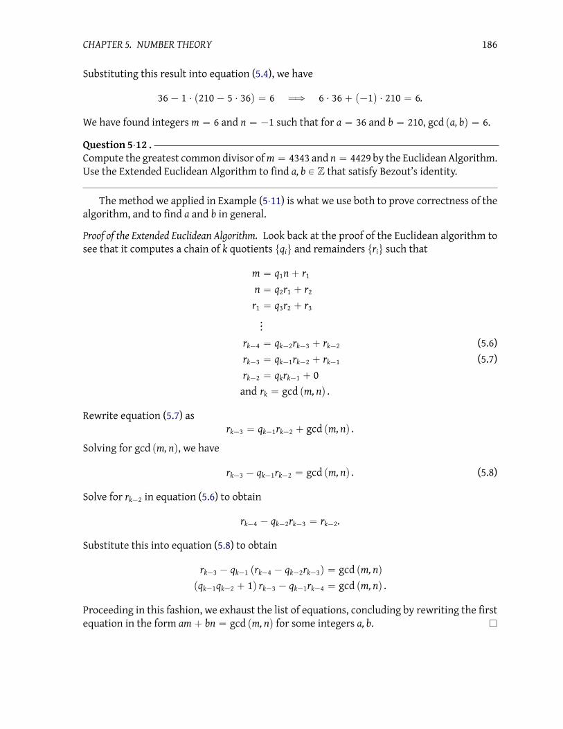
CHAPTER 5. NUMBER THEORY 186
Substituting this result into equation (5.4), we have
36´ 1 ¨ p210´ 5 ¨ 36q “ 6 ùñ 6 ¨ 36` p´1q ¨ 210 “ 6.
We have found integers m “ 6 and n “ ´1 such that for a “ 36 and b “ 210, gcd pa, bq “ 6.
Question 5¨12 .Compute the greatest common divisor ofm “ 4343 and n “ 4429 by the Euclidean Algorithm.
Use the Extended Euclidean Algorithm to find a, b P Z that satisfy Bezout’s identity.
The method we applied in Example (5¨11) is what we use both to prove correctness of the
algorithm, and to find a and b in general.
Proof of the Extended Euclidean Algorithm. Look back at the proof of the Euclidean algorithm to
see that it computes a chain of k quotients tqiu and remainders triu such that
m “ q1n` r1
n “ q2r1 ` r2
r1 “ q3r2 ` r3
...
rk´4 “ qk´2rk´3 ` rk´2 (5.6)
rk´3 “ qk´1rk´2 ` rk´1 (5.7)
rk´2 “ qkrk´1 ` 0
and rk “ gcd pm, nq .
Rewrite equation (5.7) as
rk´3 “ qk´1rk´2 ` gcd pm, nq .
Solving for gcd pm, nq, we have
rk´3 ´ qk´1rk´2 “ gcd pm, nq . (5.8)
Solve for rk´2 in equation (5.6) to obtain
rk´4 ´ qk´2rk´3 “ rk´2.
Substitute this into equation (5.8) to obtain
rk´3 ´ qk´1 prk´4 ´ qk´2rk´3q “ gcd pm, nq
pqk´1qk´2 ` 1q rk´3 ´ qk´1rk´4 “ gcd pm, nq .
Proceeding in this fashion, we exhaust the list of equations, concluding by rewriting the first
equation in the form am` bn “ gcd pm, nq for some integers a, b.

CHAPTER 5. NUMBER THEORY 187
Let m, n P Z, S “ tam` bn : a, b P Zu, and M “ S X N. Since M is a subset of N, the Well-
Ordering Principle implies that it has a smallest element; call it d.
Claim: d “ gcd pm, nq.Proof:
1. We first claim that gcd pm, nq divides d.
(a) By _____, we can find a, b P Z such that d “ am` bn.
(b) By _____, gcd pm, nq divides m and n.
(c) By _____, there exist x, y P Z such that m “ x gcd pm, nq and n “ y gcd pm, nq.
(d) By susbtitution, _____.
(e) Collect the common term to obtain _____.
(f) By _____, gcd pm, nq divides d.
2. A similar argument shows that d divides gcd pm, nq.
3. By _____, d ď gcd pm, nq and gcd pm, nq ď d.
4. By _____, d “ gcd pm, nq.
Figure 5¨1: Material for Question 5.13
Question 5¨13 .Bezout’s Identity states that for any m, n P Z, we can find a, b P Z such that am ` bn “
gcd pm, nq.
(a) Show that the existence of a, b, d P Z such that am`bn “ d does not imply d “ gcd pm, nq.
(b) However, not only does the converse of Bezout’s Identity hold, we can specify the rela-
tionship more carefully. Fill in each blank of Figure 5¨1 with the appropriate justification
or statement.
5¨2 A card trick
This section describes and explains a card trick based on an old Chinese observation.1
Recall
from Sections 2¨1 and 4¨5 that for any positive m we can perform clockwork addition in the
groupZm. We often write rxs for the elements ofZm to emphasize that its elements are cosets.
The simple Chinese Remainder Theorem
1I asked Dr. Ding what the Chinese call this theorem. He looked it up in one of his books, and told me that
they call it Sun Tzu’s Theorem. This is not the same as the author of The Art of War.

CHAPTER 5. NUMBER THEORY 188
The Chinese Remainder Theorem, simple version. Let m, n P Z such that gcd pm, nq “ 1.
Let α, β P Z. There exists a solution x P Z to the system of linear congruences
#
rxs “ rαs in Zm;rxs “ rβs in Zn;
and rxs is unique in ZN where N “ mn.
Before giving a proof, let’s look at an example of how this works in practice.
Example 5¨14. Take twelve cards and ask a friend to pick one, then shuffle them. Do the
following:
• Lay the cards out in three columns (from left to right), and ask your friend to identify
which column contains the card. Remember the answer as 1, 2, or 3. (Use 1 as leftmost, 3
as rightmost.)
• Collect the cards in such a way that their order is preserved!
• Lay the cards out again in four columns (from left to right), and ask your friend to iden-
tify which column contains the card. Remember the answer as 1, 2, 3, or 4. (Again, 1 is
leftmost, 4 rightmost.)
• If α is the first number and β the second, compute γ “ 4α´ 3β. If the result is negative,
add 12.
• Starting from the first card, in the same order you laid out the cards, count to the γ’th card.
This is your friend’s card.
How does this trick work? Each time, your friend identified the column in which the mys-
tery card lay. Laying out the cards in rows of three and four corresponds to division by three
and four, so that α and β are the remainders from division by three and by four. This corre-
sponds to a system of linear congruences,
#
rxs “ rαs in Z3rxs “ rβs in Z4
,
where x is the location of the mystery card. The simple version of the Chinese Remainder
Theorem guarantees that the value of x is unique in Z12. Since there are only twelve cards,
the solution is unique in the game: as long as the dealer can compute x, s/he can identify the
card infallibly.
“Well, and good,” you think, “but knowing only the existence of a solution seems rather
pointless. I also need to know how to compute x, so that I can pinpoint the location of the
card.” Bezout’s identity is the key to unlocking the Chinese Remainder Theorem. Before
doing so, we need an important lemma about numbers whose gcd is 1.
Lemma 5¨15. Let d, m, n P Z. Ifm | nd and gcd pm, nq “ 1, thenm | d.
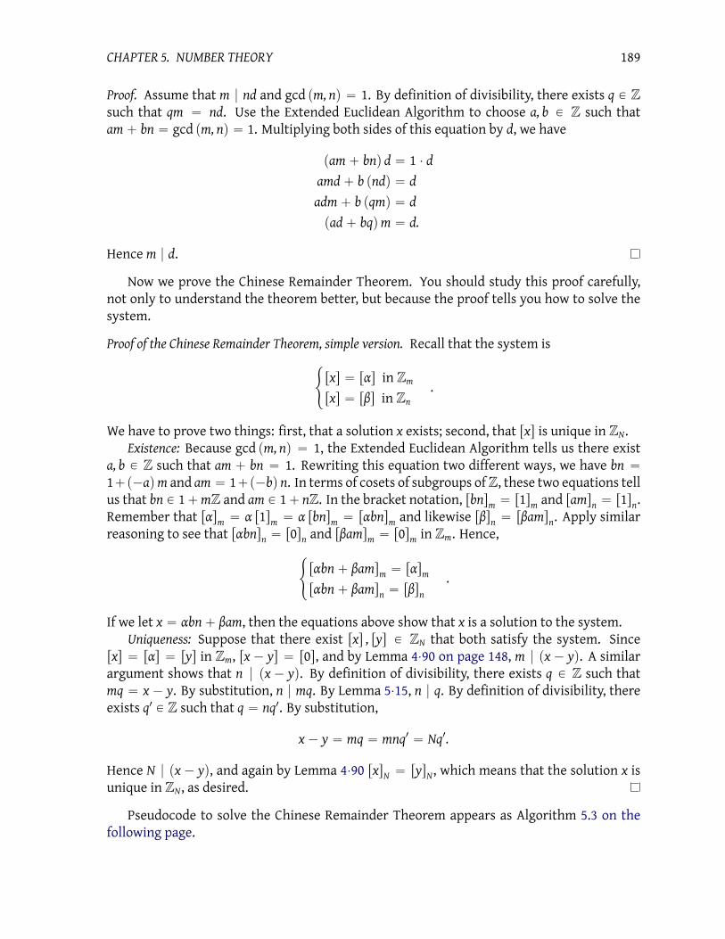
CHAPTER 5. NUMBER THEORY 189
Proof. Assume that m | nd and gcd pm, nq “ 1. By definition of divisibility, there exists q P Zsuch that qm “ nd. Use the Extended Euclidean Algorithm to choose a, b P Z such that
am` bn “ gcd pm, nq “ 1. Multiplying both sides of this equation by d, we have
pam` bnq d “ 1 ¨ d
amd` b pndq “ d
adm` b pqmq “ d
pad` bqqm “ d.
Hence m | d.
Now we prove the Chinese Remainder Theorem. You should study this proof carefully,
not only to understand the theorem better, but because the proof tells you how to solve the
system.
Proof of the Chinese Remainder Theorem, simple version. Recall that the system is
#
rxs “ rαs in Zmrxs “ rβs in Zn
.
We have to prove two things: first, that a solution x exists; second, that rxs is unique in ZN.
Existence: Because gcd pm, nq “ 1, the Extended Euclidean Algorithm tells us there exist
a, b P Z such that am ` bn “ 1. Rewriting this equation two different ways, we have bn “
1`p´aqm and am “ 1`p´bq n. In terms of cosets of subgroups ofZ, these two equations tell
us that bn P 1`mZ and am P 1` nZ. In the bracket notation, rbnsm“ r1s
mand rams
n“ r1s
n.
Remember that rαsm“ α r1s
m“ α rbns
m“ rαbns
mand likewise rβs
n“ rβams
n. Apply similar
reasoning to see that rαbnsn“ r0s
nand rβams
m“ r0s
min Zm. Hence,
#
rαbn` βamsm“ rαs
m
rαbn` βamsn“ rβs
n
.
If we let x “ αbn` βam, then the equations above show that x is a solution to the system.
Uniqueness: Suppose that there exist rxs , rys P ZN that both satisfy the system. Since
rxs “ rαs “ rys in Zm, rx´ ys “ r0s, and by Lemma 4¨90 on page 148, m | px´ yq. A similar
argument shows that n | px´ yq. By definition of divisibility, there exists q P Z such that
mq “ x ´ y. By substitution, n | mq. By Lemma 5¨15, n | q. By definition of divisibility, there
exists q1 P Z such that q “ nq1. By substitution,
x´ y “ mq “ mnq1“ Nq
1.
Hence N | px´ yq, and again by Lemma 4¨90 rxsN“ rys
N, which means that the solution x is
unique in ZN, as desired.
Pseudocode to solve the Chinese Remainder Theorem appears as Algorithm 5.3 on the
following page.

CHAPTER 5. NUMBER THEORY 190
Algorithm 5.3 Solution to Chinese Remainder Theorem, simple version
inputsm, n P Z such that gcd pm, nq “ 1
α, β P Zoutputsx P Z satisfying the Chinese Remainder Theorem
doUse the Extended Euclidean Algorithm to find a, b P Z such that am` bn “ 1
return rαbn` βamsN
Example 5¨16. The algorithm of Corollary 5.3 finally explains the method of the card trick.
We have m “ 3, n “ 4, and N “ 12. Suppose that the player indicates that his card is in
the first column when they are grouped by threes, and in the third column when they are
grouped by fours; then α “ 1 and β “ 3.
Using the Extended Euclidean Algorithm, we find that a “ ´1 and b “ 1 satisfy am`bn “
1; hence am “ ´3 and bn “ 4. We can therefore find the mystery card by computing
x “ 1 ¨ 4` 3 ¨ p´3q “ ´5.
Its canonical representation in Z12 is
rxs “ r´5` 12s “ r7s ,
which implies that the player chose the 7th card. In fact, r7s “ r1s in Z3, and r7s “ r3s in Z4,which agrees with the information given.
Question 5¨17 .Solve the system of linear congruences
#
rxs “ r2s in Z4rxs “ r3s in Z9
.
Express your answer so that 0 ď x ă 36.
Question 5¨18 .Explain why you can modify the card trick to use 24 cards by doing everything the same, with
one exception: if the γ’th card isn’t the one your friend chose, then you can add or subtract 12
to find the right one.
Question 5¨19 .Give directions for a similar card trick on all 52 cards, where the cards are grouped first by
4’s, then by 13’s. Do you think this would be a practical card trick?
Question 5¨20 .Is it possible to modify the card trick to work with only ten cards instead of 12? If so, how; if
not, why not?

CHAPTER 5. NUMBER THEORY 191
The Chinese Remainder Theorem can be generalized to larger systems with more than
two equations under certain circumstances.
A generalized Chinese Remainder Theorem
What if you have more than just two ways to arrange the cards? You might like to arrange
the cards into rows of 3, 4, and 5, for instance. What about other arrangements?
Chinese Remainder Theorem on Z. Let m1, m2, . . . , mn P Z and assume gcd`
mi, mj
˘
“ 1
for all 1 ď i ă j ď n. Let α1, α2, . . . αn P Z. There exists a solution x P Z to the system of linear
congruences$
’
’
’
’
&
’
’
’
’
%
rxs “ rα1s in Zm1 ;rxs “ rα2s in Zm2 ;
...
rxs “ rαns in Zmn ;
and rxs is unique in ZN where N “ m1m2 ¨ ¨ ¨mn.
Before we can prove this version of the Chinese Remainder Theorem, we need to make an
observation of m1, m2, . . . , mn.
Lemma 5¨21. Let m1, m2, . . . , mn P Z such that gcd`
mi, mj
˘
“ 1 for all 1 ď i ă j ď n. For each
i “ 1, 2, . . . , n define Ni “ Nmi where N “ m1m2 ¨ ¨ ¨mn; that is, Ni is the product of all the m’s
exceptmi. Then gcd pmi, Niq “ 1.
Proof. We show that gcd pm1, N1q “ 1; for i “ 2, . . . , n the proof is similar.
Use the Extended Euclidean Algorithm to choose a, b P Z such that am1 ` bm2 “ 1. Use it
again to choose c, d P Z such that cm1 ` dm3 “ 1. Then
1 “ pam1 ` bm2q pcm1 ` dm3q
“ pacm1 ` adm3 ` bcm2qm1 ` pbdq pm2m3q .
Let x “ gcd pm1, m2m3q; since x divides both m1 and m2m3, it divides each term of the right
hand side above. That right hand side equals 1, so x also divides 1. The only divisors of 1
are˘1, so x “ 1. We have shown that gcd pm1, m2m3q “ 1.
Rewrite the equation above as 1 “ a1m1` b1m2m3; notice that a
1, b1 P Z. Use the Extended
Euclidean Algorithm to choose e, f P Z such that em1 ` fm4 “ 1. Then
1 “ pa1m1 ` b
1m2m3q pem1 ` fm4q
“ pa1em1 ` a
1fm4 ` b
1em2meqm1 ` pb
1f q pm2m3m4q .
An argument similar to the one above shows that gcd pm1, m2m3m4q “ 1.
Repeating this process with each mi, we obtain gcd pm1, m2m3 ¨ ¨ ¨mnq “ 1. Since N1 “
m2m3 ¨ ¨ ¨mn, we have gcd pm1, N1q “ 1.
We can now prove the Chinese Remainder Theorem on Z.
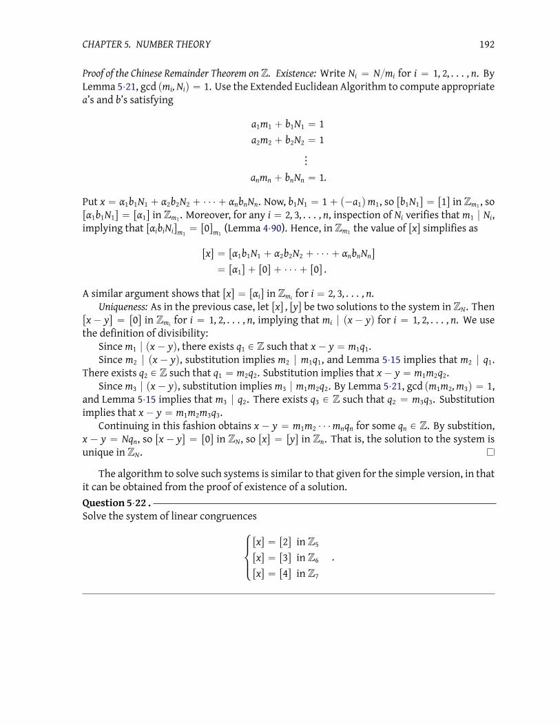
CHAPTER 5. NUMBER THEORY 192
Proof of the Chinese Remainder Theorem on Z. Existence: Write Ni “ Nmi for i “ 1, 2, . . . , n. By
Lemma 5¨21, gcd pmi, Niq “ 1. Use the Extended Euclidean Algorithm to compute appropriate
a’s and b’s satisfying
a1m1 ` b1N1 “ 1
a2m2 ` b2N2 “ 1
...
anmn ` bnNn “ 1.
Put x “ α1b1N1 ` α2b2N2 ` ¨ ¨ ¨ ` αnbnNn. Now, b1N1 “ 1` p´a1qm1, so rb1N1s “ r1s in Zm1 , so
rα1b1N1s “ rα1s in Zm1 . Moreover, for any i “ 2, 3, . . . , n, inspection of Ni verifies that m1 | Ni,
implying that rαibiNism1 “ r0sm1 (Lemma 4¨90). Hence, in Zm1 the value of rxs simplifies as
rxs “ rα1b1N1 ` α2b2N2 ` ¨ ¨ ¨ ` αnbnNns
“ rα1s ` r0s ` ¨ ¨ ¨ ` r0s .
A similar argument shows that rxs “ rαis in Zmi for i “ 2, 3, . . . , n.
Uniqueness: As in the previous case, let rxs , rys be two solutions to the system in ZN. Then
rx´ ys “ r0s in Zmi for i “ 1, 2, . . . , n, implying that mi | px´ yq for i “ 1, 2, . . . , n. We use
the definition of divisibility:
Since m1 | px´ yq, there exists q1 P Z such that x´ y “ m1q1.
Since m2 | px´ yq, substitution implies m2 | m1q1, and Lemma 5¨15 implies that m2 | q1.
There exists q2 P Z such that q1 “ m2q2. Substitution implies that x´ y “ m1m2q2.
Since m3 | px´ yq, substitution implies m3 | m1m2q2. By Lemma 5¨21, gcd pm1m2, m3q “ 1,
and Lemma 5¨15 implies that m3 | q2. There exists q3 P Z such that q2 “ m3q3. Substitution
implies that x´ y “ m1m2m3q3.
Continuing in this fashion obtains x ´ y “ m1m2 ¨ ¨ ¨mnqn for some qn P Z. By substition,
x ´ y “ Nqn, so rx´ ys “ r0s in ZN, so rxs “ rys in Zn. That is, the solution to the system is
unique in ZN.
The algorithm to solve such systems is similar to that given for the simple version, in that
it can be obtained from the proof of existence of a solution.
Question 5¨22 .Solve the system of linear congruences
$
’
&
’
%
rxs “ r2s in Z5rxs “ r3s in Z6rxs “ r4s in Z7
.

CHAPTER 5. NUMBER THEORY 193
Question 5¨23 .Solve the system of linear congruences
$
’
&
’
%
rxs “ r33s in Z16rxs “ r´4s in Z33rxs “ r17s in Z504
.
This problem is a little tougher than the previous, since gcd p16, 504q ‰ 1 and gcd p33, 504q ‰
1. Since you can’t use either of the Chinese Remainder Theorems presented here, you’ll have
to generalize their approaches to get a method for this one.
Question 5¨24 .Is it possible to modify the card trick to work with only eight cards instead of 12? If so, how;
if not, why not?
5¨3 The Fundamental Theorem of Arithmetic
In this section, we address a fundamental result of number theory with algebraic implications.
Let’s recall what Definition 3¨20 means in the context of natural numbers.
Definition 5¨25. Let n P N` and n ‰ 1. We say that n is irreducible if the only integers that
divide n are˘1 and˘n.
(We may sometimes refer to certain negative numbers as irreducible. While certain neg-
ative numbers do satisfy the property of irreducibility, there are reasons that only natural
numbers are properly called prime.)
You may be wondering why we call these integers irreducible instead of prime, the custom-
ary term in earlier classes. We’ll say more about that in a moment.
Example 5¨26. The integer 36 is not irreducible, because 36 “ 6 ˆ 6. The integer 7 is irre-
ducible, because the only integers that divide 7 are˘1 and˘7.
One useful aspect to irreducible integers is that, aside from˘1, any integer is divisible by
at least one irreducible integer.
Theorem 5¨27. Let n be any integer besides˘1. There exists at least one irreducible integer p such
that p | n.
Proof. Case 1: If n “ 0, then 2 is a divisor of n, and we are done.
Case 2: Assume that n P N` and n ‰ 1. Let a0 “ n. If a0 is not irreducible, then by
definition a0 “ a1b1 such that a1, b1 P Z and a1, b1 ‰ ˘1. Without loss of generality, we may
assume that a1, b1 P N` (otherwise both are negative and we can replace them with their
opposites). Observe further that a1 ă a0 (this is a consequence of Question 1.28 on page 13).
If a1 is irreducible, then we are done; otherwise, we can write a1 “ a2b2 where a2, b2 P N` and
a2 ă a1. Continuing in this fashion, as long as ai is not irreducible, we can find ai`1, bi`1 P N`

CHAPTER 5. NUMBER THEORY 194
such that ai “ ai`1bi`1, with ai ą ai`1 for each i. We have a strictly decreasing sequence of
elements,
a0 ą a1 ą a2 ą ¨ ¨ ¨ .
By Question 1¨51, this sequence must be finite. Let am be the final element in the sequence.
We claim that am is irreducible; after all, were it not irreducible, then we could extend the
sequence further, which we cannot. By substitution,
n “ a1b1 “ a2 pb2b1q “ ¨ ¨ ¨ “ am pbm´1 ¨ ¨ ¨ b1q .
That is, am is an irreducible integer that divides n.
Case 3: Assume that n is negative, but not´1. Letm “ ´n. Case 2 implies that there exists
an irreducible integer p such that p | m. By definition,m “ qp for some q P Z. By substitution
and properties of arithmetic, n “ ´pqpq “ p´qq p, so p | n.
Question 5¨28 .Show that there are infinitely many irreducible numbers. Hint: Proceed by contradiction:
suppose there is a finite list of irreducible numbers, then exploit the Division Theorem to
construct a remainder whose division by each of those irreducible numbers is nonzero. The-
orem 5¨27 does the rest.
Let’s turn now to the term you might have expected for the definition given above: a prime
number. We actually associate a different notion with this term.
Definition 5¨29. Let R be a ring, and suppose p P R is not a unit. We say that p is prime if,
whenever we find a, b P R such that p | ab, then p | a or p | b. Consistent with this definition,
a natural number p is a prime number if p ‰ 1 and for any two integers a, b we have
p | ab ùñ p | a or p | b.
(We may sometimes refer to certain negative numbers as prime. While certain negative
numbers do satisfy the property of being prime, called primality, there are reasons that only
natural numbers are properly called prime.)
Example 5¨30. Let a “ 68 and b “ 25. It is easy to recognize that 10 divides ab “ 1700.
However, 10 divides neither a nor b, so 10 is not a prime number.
It is also easy to recognize that 17 divides ab “ 1700. Unlike 10, 17 divides one of a or b; in
fact, it divides a. Were we to look at every possible product ab divisible by 17, we would find
that 17 always divides one of the factors a or b. Thus, 17 is prime.
If the next-to-last sentence in the example, bothers you, good. I’ve claimed something
about every product divisible by 17, but haven’t explained why that is true. That’s cheating!
If I’m going to claim that 17 is prime, I need a better explanation than, “look at every possible
product ab.” After all, there are infinitely many products possible, and we can’t do that in
finite time. We need a finite criterion.
To this end, let’s return to the notion of an irreducible number. It’s fairly easy to tell if
an integer a is irreducible; Question 1.28 tells us to look for factors among natural numbers
smaller than |a|. If we knew that prime numbers were irreducible, then we could simply test
for irreducibility. Could it be that the definitions are distinctions without a difference?

CHAPTER 5. NUMBER THEORY 195
Theorem 5¨31. An integer is prime if and only if it is irreducible.
Proof. This proof has two parts. You will show in Question 5.32 that if an integer is prime,
then it is irreducible. Here, we show the converse.
Let n P N`z t1u and assume that n is irreducible. To show that n is prime, we must take
arbitrary a, b P Z and show that if n | ab, then n | a or n | b. Therefore, let a, b P Z and assume
that n | ab. If n | a, then we would be done, so assume that n - a. We must show that n | b.
By definition, the common factors of n and a are a subset of the factors of n. Since n is
irreducible, its factors are˘1 and˘n. By hypothesis, n - a, so˘n cannot be common factors
of n and a. Thus, the only common factors of n and a are˘1, which means that gcd pn, aq “ 1.
By Lemma 5¨15, n | b.
We assumed that if n is irreducible and divides ab, then n must divide one of a or b. By
definition, n is prime.
Question 5¨32 .Show that any prime integer p is irreducible.
If the two definitions are equivalent, why would we give a different definition? It turns
out that the concepts are equivalent for the integers, but not for other sets; you will see this in
detail in Section 6¨2.
The following theorem is a cornerstone of Number Theory.
The Fundamental Theorem of Arithmetic. Let n P N` but n ‰ 1. We can factor n intoirreducibles; that is, we can write
n “ pα1
1pα2
2¨ ¨ ¨ p
αr
r
where p1, p2, . . . , pr are irreducible and α1, α2, . . . , αr P N. The representation is unique if we order
p1 ă p2 ă. . . ă pn.
Since prime integers are irreducible and vice versa, you can replace “irreducible” by “prime”
and obtain the expression of this theorem found more commonly in number theory text-
books.
Proof. The proof has two parts: a proof of existence and a proof of uniqueness.
Existence: We proceed by induction on positive integers.
Inductive base: If n “ 2, then n is irreducible, and we are finished.
Inductive hypothesis: Assume that the integers 2, 3, . . . , n´ 1 have a factorization into irre-
ducibles.
Inductive step: If n is irreducible, then we are finished. Otherwise, n is not irreducible. By
Lemma 5¨27, there exists an irreducible integer p1 such that p1 | n. By definition, there exists
q P N` such that n “ qp1. Since p1 ‰ 1, Question 1.58 tells us that q ă n. By the inductive
hypothesis, q has a factorization into irreducibles; say
q “ pα1
1pα2
2¨ ¨ ¨ p
αr
r.
Thus n “ qp “ pα1`11 p
α22 ¨ ¨ ¨ p
αrr
; that is, n factors into irreducibles.
Uniqueness: Here we use the fact that irreducible numbers are also prime (Lemma 5¨31).
Assume that p1 ă p2 ă ¨ ¨ ¨ ă pr and we can factor n as
n “ pα1
1pα2
2¨ ¨ ¨ p
αr
r“ p
β1
1 pβ2
2 ¨ ¨ ¨ pβr
r.

CHAPTER 5. NUMBER THEORY 196
Without loss of generality, we may assume that α1 ď β1. It follows that
pα2
2pα3
3¨ ¨ ¨ p
αr
r“ p
β1´α11 p
β2
2 pβ3
3 ¨ ¨ ¨ pβr
r.
This equation implies that pβ1´α11 divides the expression on the left hand side of the equation.
Since p1 is irreducible, hence prime, β1 ´ α1 ‰ 0 implies that p1 divides one of p2, p3, . . . , pr.
This contradicts the irreducibility of p2, p3, . . . , pr. Hence β1 ´ α1 “ 0. A similar argument
shows that βi “ αi for all i “ 1, 2, . . . , r; hence the representation of n as a product of irre-
ducible integers is unique.
Question 5¨33 .Fill in each blank of Figure 5¨2 with the justification.
Question 5¨34 .Let n P N`. Modify the proof in Figure 5¨2 to show that if p is irreducible, then n
?p is irrational.
Question 5¨35 .Let n P N`. Modify the proof in Figure 5¨2 to show that if there exists an irreducible integer
p such that p | n but p2 - n, then
?n is irrational.
5¨4 Multiplicative clockwork groups
Throughout this section, n P N`z t1u, unless otherwise stated.
Clockwork multiplication
Recall that Zn is an additive group, but not multiplicative. In this section we find for each
eligible n a subset of Zn that we can turn into a multiplicative group.
Example 5¨36. Recall thatZ5 – Z x5y. We saw that it was a ring; that is, it is an abelian group
under addition, a monoid under multiplication, and multiplication distributes over addition.
Can we turn a subset of it into a multiplicative group? We need to identify an identity, and
inverses. Certainly r0s won’t have a multiplicative inverse, but what about Z5z tr0su? This
generates a multiplication table that satisfies the properties of an abelian (but non-additive)
group:
ˆ 1 2 3 4
1 1 2 3 4
2 2 4 1 3
3 3 1 4 2
4 4 3 2 1
That is a group! We’ll call it Z˚5.
In fact, Z˚5– Z4; they are both cyclic groups of four elements, and inspection shows that
Z5 “ x2y “ x3y “ x4y. In Z˚5, however, the nominal operation is multiplication, whereas in
Z4 the nominal operation is addition.

CHAPTER 5. NUMBER THEORY 197
Claim: If p is irreducible, then?p is not rational.
Proof:
1. Assume that p is irreducible.
2. By way of contradiction, assume that?p is rational.
3. By _____, there exist a, b P N such that?p “ ab.
4. Without loss of generality, we may assume that gcd pa, bq “ 1.
(After all, we could otherwise rewrite?p “ padq pbdq, where d “ gcd pa, bq.)
5. By _____, p “ a2b2.
6. By _____, pb2 “ a2.
7. By _____, p | a2.
8. By _____, p is prime.
9. By _____, p | a.
10. By _____, a “ pq for some q P Z.
11. By _____ and _____, pb2 “ ppqq
2“ p2q2.
12. By _____, b2 “ pq2.
13. By _____, p | b2.
14. By _____, p | b.
15. This contradicts step _____. Our assumption that?p is rational must have been wrong.
Hence,?p is irrational.
Figure 5¨2: Material for Question 5.33

CHAPTER 5. NUMBER THEORY 198
You might think that this trick of dropping zero and building a multiplication table always
works, but it doesn’t.
Example 5¨37. Recall that Z4 “ Z x4y “ tr0s , r1s , r2s , r3su. Consider the set Z4z tr0su “tr1s , r2s , r3su. The multiplication table for this set is not closed because
r2s ¨ r2s “ r4s “ r0s R Z4z tr0su .
We obviously can’t fix this by including zero, as well: zero has no inverse. So, we must exclude
zero; our mistake seems to have been that we included 2 Excluding 2 finally works out:
ˆ 1 3
1 1 3
3 3 1
That is a group! We’ll call it Z˚4.
In fact, Z˚4– Z2; they are both the cyclic group of two elements. In Z˚
4, however, the
operation is multiplication, whereas in Z2, the operation is addition.
You can determine for yourself that Z2z tr0su “ tr1su and Z3z tr0su “ tr1s , r2su are also
multiplicative groups. In this case, as in Z˚5, we need remove only 0. For Z6, however, we
have to remove nearly all the elements! We only get a group from Z6z tr0s , r2s , r3s , r4su “tr1s , r5su.
Why do we need to remove more elements of Zn for some values of n than others? Aside
from zero, which clearly has no inverse under the operation specified, the elements we’ve
had to remove are those whose multiplication would re-introduce zero. We’re observing zero
divisors again.
Can we find a criterion to detect this? You should have done this in Question 2.44; to be
safe, let’s flesh it out here.
Lemma 5¨38. Let x P Zn be nonzero. The following are equivalent:
(A) x is a zero divisor.
(B) x and n have a common divisor besides˘1.
Proof. That (B) implies (A): Assume that x and n share a common divisor d ‰ 0, 1. Use the
definition of divisibility to choose t, q P Zz t0u such that n “ qd and x “ td. Let y be the
remainder of dividing q by n. Substitution implies that
xy ”n xq “ ptdq q “ t pdqq “ tn ” 0.
Since d ‰ 0, 1, ´n ă q ă n, so 0 ‰ q ”n y. This shows that y is also nonzero, so x is a zero
divisor.
Question 5¨39 .You can also prove that (B) implies (A) using Bezout’s Lemma. Try it that way.

CHAPTER 5. NUMBER THEORY 199
Proof of Lemma 5¨38, continued. That (A) implies (B): Assume that x is a zero divisor. By definition,
we can find nonzero y P Zn such that xy ”n 0. There are two points to recall here: first,
0 ď y ă n, and second, n | xy. By definition, we can find q P Z such that nq “ xy. Use
the Fundamental Theorem of Arithmetic to factor n “ pa11 ¨ ¨ ¨ p
ak
k, where the pi’s are distinct
irreducibles and the ai’s are natural. By substitution,
`
pa1
1¨ ¨ ¨ p
ak
k
˘
q “ xy.
Not every pai
ican appear in y; otherwise, n | y, and by Question 1.58, we would have n ď y,
contradicting y ă n. Hence at least one pi divides x, so that n and x have a common divisor
that is not 1.
A multiplicative clockwork group
We can thus construct a multiplicative clockwork group using the elements of Zn that are
not zero divisors.
Definition 5¨40. Define the set Z˚n
to be the set of elements of Zn that are not zero divisors.
In set builder notation,
Z˚n:“ tx P Znz t0u : @y P Znz t0u xy ‰ 0u .
We claim that Z˚n
is a group under multiplication. Keep in mind that, while it is a subset
of Zn, it is not a subgroup, as the operations are different.
Theorem 5¨41. Z˚n
is an abelian group under its multiplication.
Proof. We check each requirement of a group, slightly out of order. Let a, b, c P Z˚n.
(associative) From Question 2.20, clockwork multiplication is consistent with integer multi-
plication. Since pabq c “ a pbcq, then, pabq c ” a pbcq. Notice that this applies for
elements of Zn as well as elements of Z˚n.
(closed) Assume to the contrary that ab R Z˚n. We have defined ab to give us an element
of Zn, so the only way ab R Z˚n
is if ab ” 0 or ab is a zero divisor. By definition of
Z˚n, neither a nor b is a zero divisor, so ab ı 0, which forces us to conclude that ab
is a zero divisor. Choose c P Zn such that pabq c ” 0. By the associative property,
a pbcq ” 0; that is, a is a zero divisor, contradicting the choice of a! Thus, ab cannot
be a zero divisor, either; the assumption that ab R Z˚n
must have been wrong.
(identity) We claim that 1 is the identity. Since gcd p1, nq “ 1, we have 1 P Z˚n
by definition.
It is then trivial that 1 ¨ a “ a “ a ¨ 1.
(inverse) We need to find an inverse of a. By definition, a and n have no common divisors
except˘1; hence gcd pa, nq “ 1. Bezout’s Lemma tells us we can find b, m P Z such
that ab` mn “ 1. We deduce that
ab´ 1 “ n p´mq
6 ab´ 1 P nZ6 ab ” 1.

CHAPTER 5. NUMBER THEORY 200
But is b P Z˚n? It might not be. To start with, we could have b ě n or b ă 0. In this
case, let q and r be the quotient and remainder of division of b by n; then ar ” 1.
But what if r is a zero divisor? Recall the equation above:
ab` mn “ 1 ñ a pnq` rq ` mn “ 1 ñ ar ` pm` aqq n “ 1.
This is a form of the identity in Bezout’s Lemma not just for a, but also for r! Bezout’s
Lemma tells us that gcd pr, nq is the smallest positive number that can be written in
that form, so gcd pr, nq “ 1, so r is in fact a zero divisor by Lemma 5¨38, so a´1 “ r P
Z˚n
.
(commutative) Use the definition of multiplication in Z˚n
and the commutative property of
integer multiplication to see that ab “ ba.
By removing elements that share non-trivial common divisors with n, we have managed to
eliminate those elements that do not satisfy the zero-product rule, and would break closure by
trying to re-introduce zero in the multiplication table. We have thereby created a clockwork
group for multiplication, Z˚n.
Example 5¨42. Consider Z˚10
. To find its elements, collect the elements of Z10 that are not
zero divisors. Lemma 5¨38 tells us that these are the elements a such that gcd pa, nq ‰ 1. Thus
Z˚10“ t1, 3, 7, 9u .
Theorem 5¨41 tells us that Z˚10
is a group. Since it has four elements, it must be isomorphic to
either the Klein 4-group, or to Z4. Which is it? In this case, it’s probably easiest to decide the
question with a glance at its multiplication table:
ˆ 1 3 7 91 1 3 7 9
3 3 9 1 7
7 7 1 9 3
9 9 7 3 1
Notice that 3´1 ‰ 3. In the Klein 4-group, every element is its own inverse, so Z˚
10cannot
be isomorphic to the Klein 4-group. Instead, it must be isomorphic to Z4.
Question 5¨43 .List the elements ofZ˚
7using their canonical representations, and construct its multiplication
table. Use the table to identify the inverse of each element.
Question 5¨44 .List the elements of Z˚
15using their canonical representations, and construct its multiplica-
tion table. Use the table to identify the inverse of each element.
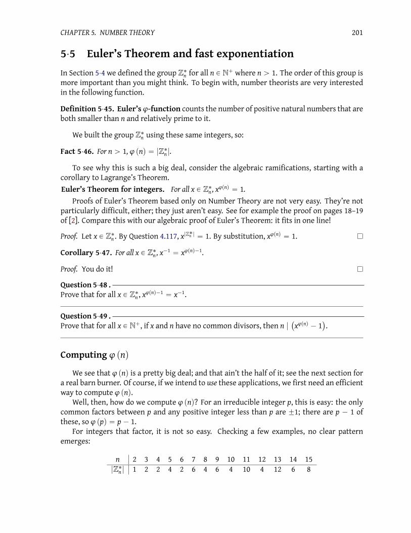
CHAPTER 5. NUMBER THEORY 201
5¨5 Euler’s Theorem and fast exponentiation
In Section 5¨4 we defined the group Z˚n
for all n P N` where n ą 1. The order of this group is
more important than you might think. To begin with, number theorists are very interested
in the following function.
Definition 5¨45. Euler’s φ-function counts the number of positive natural numbers that are
both smaller than n and relatively prime to it.
We built the group Z˚n
using these same integers, so:
Fact 5¨46. For n ą 1, φ pnq “ |Z˚n|.
To see why this is such a big deal, consider the algebraic ramifications, starting with a
corollary to Lagrange’s Theorem.
Euler’s Theorem for integers. For all x P Z˚n, xφpnq “ 1.
Proofs of Euler’s Theorem based only on Number Theory are not very easy. They’re not
particularly difficult, either; they just aren’t easy. See for example the proof on pages 18–19
of [2]. Compare this with our algebraic proof of Euler’s Theorem: it fits in one line!
Proof. Let x P Z˚n. By Question 4.117, x
|Z˚n | “ 1. By substitution, x
φpnq “ 1.
Corollary 5¨47. For all x P Z˚n, x´1 “ xφpnq´1.
Proof. You do it!
Question 5¨48 .Prove that for all x P Z˚
n, xφpnq´1 “ x´1.
Question 5¨49 .Prove that for all x P N`, if x and n have no common divisors, then n |
`
xφpnq ´ 1
˘
.
Computing φ pnq
We see that φ pnq is a pretty big deal; and that ain’t the half of it; see the next section for
a real barn burner. Of course, if we intend to use these applications, we first need an efficient
way to compute φ pnq.
Well, then, how do we compute φ pnq? For an irreducible integer p, this is easy: the only
common factors between p and any positive integer less than p are ˘1; there are p ´ 1 of
these, so φ ppq “ p´ 1.
For integers that factor, it is not so easy. Checking a few examples, no clear pattern
emerges:
n 2 3 4 5 6 7 8 9 10 11 12 13 14 15
|Z˚n| 1 2 2 4 2 6 4 6 4 10 4 12 6 8

CHAPTER 5. NUMBER THEORY 202
Computingφ pnq turns out to be hard in practice. It is a major research topic in number theory,
and its difficulty makes the RSA algorithm secure (see Section 5¨6). One approach, of course,
is to factor n and count the integers that do not share any common factors. For example,
28 “ 22¨ 7,
so to compute φ p28q, we could look at all the positive integers smaller than 28 that do not
have 2 or 7 as factors. Try this on your own, though, and you’ll discover how tedious it is.
We’d like an efficient way to compute φ pnq.
Another way would be to computeφ pmq for each factorm of n, then recombine them. But,
how? Lemma 5¨50 gives us a first step.
Lemma 5¨50. Let a, b, n P N`. If n “ ab and gcd pa, bq “ 1, then φ pnq “ φ paqφ pbq.
Example 5¨51. In the table above, we have φ p15q “ 8. Notice that this satisfies
φ p15q “ φ p5ˆ 3q “ φ p5qφ p3q “ 4ˆ 2 “ 8.
Proof of Lemma 5¨50. Assume n “ ab. Recall that direct products are groups, so that Z˚aˆ Z˚
b
is a group; the size of this group is |Z˚a| ˆ
ˇ
ˇZ˚b
ˇ
ˇ “ φ paqφ pbq. We claim that Z˚n– Z˚
aˆ Z˚
b. If
true, this would prove the lemma, since
φ pnq “ |Z˚n| “ |Z˚
aˆ Z˚
b| “ |Z˚
a| ˆ |Z˚
b| “ φ paqφ pbq .
To show that they are indeed isomorphic, let f : Z˚nÑ Z˚
aˆ Z˚
bby f prxs
nq “ prxs
a, rxs
bq.
First we show that f is a homomorphism: Let y, z P Z˚n; then
f prysnrzs
nq “ f pryzs
nq (arithm. in Z˚
n)
“ pryzsa, ryzs
bq (def. of f )
“ prysarzs
a, rys
brzs
bq (arithm. in Z˚
a,Z˚
b)
“ prysa, rys
bq przs
a, rzs
bq (arithm. in Z˚
aˆ Z˚
b)
“ f prysnq f przs
nq . (def. of f )
It remains to show that f is one-to-one and onto. It is both surprising and delightful that
the Chinese Remainder Theorem will do most of the work for us. To show that f is onto, let
prysa, rzs
bq P Z˚
aˆ Z˚
b. We need to find x P Z such that f prxs
nq “ prys
a, rzs
bq. Consider the
system of linear congruences
rxs “ rys in Za;rxs “ rzs in Zb.
The Chinese Remainder Theorem tells us not only that such x exists inZn, but that x is unique
in Zn.We are not quite done; we have shown that a solution rxs exists in Zn, but what we really
need is that rxs P Z˚n. To see that rxs P Z˚
n, let d be any common divisor of x and n. By way of
contradiction, assume d ‰ ˘1; by Theorem 5¨27, we can find an irreducible divisor r of d; by
Question 4.71 on page 142, r | n and r | x. Recall that n “ ab, so r | ab. Since r is irreducible,

CHAPTER 5. NUMBER THEORY 203
hence prime, r | a or r | b. Without loss of generality, we may assume that r | a. Recall that
rxsa“ rys
a; Lemma 4¨90 on page 148 tells us that a | px´ yq. Let w P Z such that wa “ x ´ y.
Rewrite this equation as x ´ wa “ y. Recall that r | x and r | a; we can factor r from the
left-hand side of x´ wa “ y to see that r | y.
What have we done? We showed that if x and n have a common factor besides ˘1, then
y and a also have a common, irreducible factor r. The definition of irreducible implies that
r ‰ 1.
Do you see the contradiction? We originally chose rys P Z˚a. By definition, rys cannot be
a zero divisor in Za, so by Lemma 5¨38, gcd py, aq “ 1. But the definition of greatest common
divisor means that
gcd py, aq ě r ą 1 “ gcd py, aq ,
a contradiction! Our assumption that d ‰ 1must have been false; we conclude that the only
common divisors of x and n are˘1. Hence, x P Z˚n.
Lemma 5¨50 gives us a more efficient way to compute φ pnq, but it’s still not that great,
since first you have to find factors a and b of n. This turns out to be quite difficult to do in
practice; to see how mathematicians made lemonade of this mathematical lemon, see the
next chapter.
Fast exponentiation
Corollary 5¨47 gives us an “easy” way to compute the inverse of any x P Z˚n. Even suppos-
ing we could compute φ pnq in reasonable time, it can still take a long time to compute xφpnq
,
as it could be a very large number. We take a moment to explain how to compute canonical
forms of exponents more quickly. There are two main considerations.
Lemma 5¨52. For any n P N`, rxas “ rxsa
in Z˚n.
(In other words, don’t compute xa, and then the remainder. Compute the remainder while
computing xa.)
Proof. This follows from the fact that multiplication is well-defined, and there are finitely
many products. You can prove it by induction if you want more detail than that.
Example 5¨53. In Z˚15
we can determine easily that r420s “ r4s20“
`
r4s2˘10
“ r16s10“
r1s10“ r1s. This is a lot faster than computing 4
20 “ 1099511627776, then dividing to find the
canonical form.
Do you see what we did? The trick is to break the exponent down into “manageable”
powers. How exactly can we do that?
Fast Exponentiation. Let a P N and x P Z. We can compute xa
in the following way:
1. Let b be the largest integer such that 2b ď a.
2. Let q0, q1, . . . , qb be the bits of the binary representation of a.
3. Let y “ 1, z “ x and i “ 0.

CHAPTER 5. NUMBER THEORY 204
4. Repeat the following until i ą b:
(a) If qi ‰ 0, replace y with the product of y and z.
(b) Replace z with z2.
(c) Replace i with i` 1.
This ends with xa “ y.
Fast Exponentiation effectively computes the binary representation of a and uses this to
square x repeatedly, multiplying the result only by those powers that matter for the repre-
sentation. Its algorithm is especially effective on computers, whose mathematics is based on
binary arithmetic. Combining it with Lemma 5¨52 gives an added bonus in Z˚n, which is what
we care about most.
Example 5¨54. Since 10 “ 23 ` 2
1, we can compute r410s
7following the algorithm of Fast
Exponentiation:
1. We have q3 “ 1, q2 “ 0, q1 “ 1, q0 “ 0.
2. Let y “ 1, z “ 4 and i “ 0.
3. When i “ 0:
(a) We do not change y because q0 “ 0.
(b) Put z “ 42 “ 16 “ 2. (We’re in Z˚7, remember.)
(c) Put i “ 1.
4. When i “ 1:
(a) Put y “ 1 ¨ 2 “ 2.
(b) Put z “ 22 “ 4.
(c) Put i “ 2.
5. When i “ 2:
(a) We do not change y because q2 “ 0.
(b) Put z “ 42 “ 16 “ 2.
(c) Put i “ 3.
6. When i “ 3:
(a) Put y “ 2 ¨ 2 “ 4.
(b) Put z “ 42 “ 2.
(c) Put i “ 4.

CHAPTER 5. NUMBER THEORY 205
We conclude that r410s7“ r4s
7. Hand computation the long way, or a half-decent calculator,
will verify this.
Proof of Fast Exponentiation.
Termination: Termination is due to the fact that b is a finite number, and the algorithm
assigns to i the values 0, 1, . . . , b` 1 in succession, stopping when i ą b.
Correctness: First, the theorem claims that qb, . . . , q0 are the bits of the binary represen-
tation of xa, but do we actually know that the binary representation of x
ahas b ` 1 bits? By
hypothesis, b is the largest integer such that 2b ď a; if we need one more bit, then the defini-
tion of binary representation means that 2b`1 ď x
a, which contradicts the choice of b. Thus,
qb, . . . , q0 are indeed the bits of the binary representation of xa. By definition, qi P t0, 1u for
each i “ 0, 1, . . . , b. The algorithm multiplies z “ x2i
to y only if qi ‰ 0, so that the algorithm
computes
xqb2
b`qb´12b´1`¨¨¨`q12
1`q020
,
which is precisely the binary representation of xa.
Question 5¨55 .Compute 3
28in Z using fast exponentiation. Show each step.
Question 5¨56 .Compute 24
28in Z˚
7using fast exponentiation. Show each step.
5¨6 The RSA encryption algorithm
Whenever you buy a product online, you submit private information: at the very least, a credit
card or bank account number, and usually more. There is no guarantee that this information
will pass only through servers run by disinterested persons. It is quite possible for the infor-
mation to pass through a computer run by at least one ill-intentioned hacker, and possibly
even organized crime. You probably don’t want criminals looking at your credit card num-
ber. And not just you – many organizations desire a reliable and efficient method to disguise
private information so that snoopers cannot understand it.
This problem provides a surprisingly useful application of group theory, via number the-
ory. A number of approaches exist, and a method in common use is the RSA encryption al-
gorithm.2
First we describe the algorithms for encryption and decryption; then we explain
the ideas behind each stage, illustrating with an example; finally we prove that it succesfully
encrypts and decrypts messages.
Description and example
The RSA algorithm. Let M be a list of positive integers. Let p, q be two irreducible integers such
that:
2RSA stands for Rivest (of MIT), Shamir (of the Weizmann Institute in Israel), and Adleman (of USC).
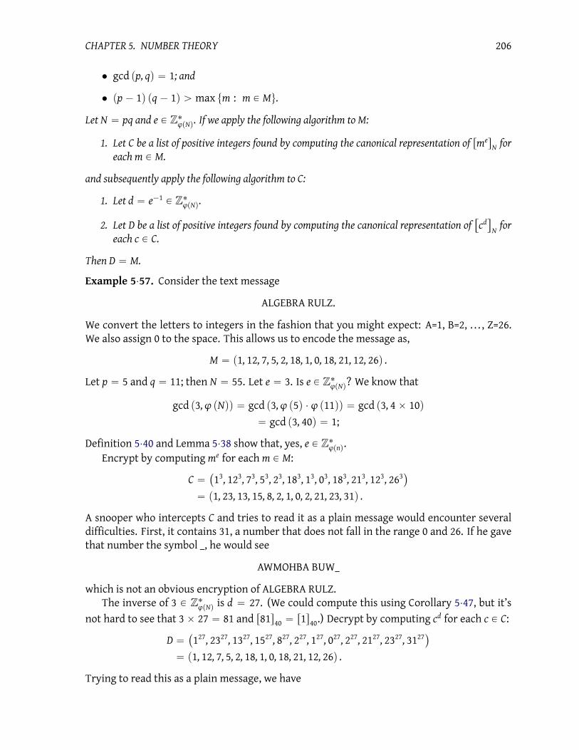
CHAPTER 5. NUMBER THEORY 206
• gcd pp, qq “ 1; and
• pp´ 1q pq´ 1q ą max tm : m P Mu.
Let N “ pq and e P Z˚φpNq
. If we apply the following algorithm toM:
1. Let C be a list of positive integers found by computing the canonical representation of rmesN
for
eachm P M.
and subsequently apply the following algorithm to C:
1. Let d “ e´1 P Z˚φpNq
.
2. Let D be a list of positive integers found by computing the canonical representation of“
cd‰
Nfor
each c P C.
Then D “ M.
Example 5¨57. Consider the text message
ALGEBRA RULZ.
We convert the letters to integers in the fashion that you might expect: A=1, B=2, . . . , Z=26.
We also assign 0 to the space. This allows us to encode the message as,
M “ p1, 12, 7, 5, 2, 18, 1, 0, 18, 21, 12, 26q .
Let p “ 5 and q “ 11; then N “ 55. Let e “ 3. Is e P Z˚φpNq
? We know that
gcd p3,φ pNqq “ gcd p3,φ p5q ¨ φ p11qq “ gcd p3, 4ˆ 10q
“ gcd p3, 40q “ 1;
Definition 5¨40 and Lemma 5¨38 show that, yes, e P Z˚φpnq
.
Encrypt by computing me
for each m P M:
C “`
13, 12
3, 73, 53, 23, 18
3, 13, 03, 18
3, 21
3, 12
3, 26
3˘
“ p1, 23, 13, 15, 8, 2, 1, 0, 2, 21, 23, 31q .
A snooper who intercepts C and tries to read it as a plain message would encounter several
difficulties. First, it contains 31, a number that does not fall in the range 0 and 26. If he gave
that number the symbol _, he would see
AWMOHBA BUW_
which is not an obvious encryption of ALGEBRA RULZ.
The inverse of 3 P Z˚φpNq
is d “ 27. (We could compute this using Corollary 5¨47, but it’s
not hard to see that 3ˆ 27 “ 81 and r81s40“ r1s
40.) Decrypt by computing c
dfor each c P C:
D “`
127, 23
27, 13
27, 15
27, 827, 227, 127, 027, 227, 21
27, 23
27, 31
27˘
“ p1, 12, 7, 5, 2, 18, 1, 0, 18, 21, 12, 26q .
Trying to read this as a plain message, we have

CHAPTER 5. NUMBER THEORY 207
ALGEBRA RULZ.
Doesn’t it?
Encrypting messages letter-by-letter is absolutely unacceptable for security. For a stronger
approach, letters should be grouped together and converted to integers. For example, the
first four letters of the secret message above are
ALGE
and we can convert this to a number using any of several methods; for example
ALGE Ñ 1ˆ 263` 12ˆ 26
2` 7ˆ 26` 5 “ 25, 785.
The integers to encrypt here are larger than 55, so we need larger values for p and q. This is
too burdensome to compute by hand, so you want a computer to help. We give an example
in the exercises.
RSA is an example of a public-key cryptosystem. That means that person A broadcasts to the
world, “Anyone who wants to send me a secret message can use the RSA algorithm with values
N “. . . and e “. . . .” So a snooper knows the method, the modulus, N, and the encryption
key, e!
If the snooper knows the method, N, and e, how can RSA be safe? To decrypt, the snooper
needs to compute d “ e´1 P Z˚φpNq
. Corollary 5¨47 tells us that computing d is merely a matter
of computing eφpNq´1
, which is easy if you know φ pNq. The snooper also knows that N “ pq,
where p and q are prime. So, decryption should be a simple matter of factoring N “ pq and
applying Lemma 5¨50 to obtain φ pNq “ pp´ 1q pq´ 1q. Right?
Well, yes and no. Typical implementations choose very large numbers for p and q, many
digits long, and there is no known method of factoring a large integer “quickly” — even when
you know that it factors as the product of two primes! In addition, a careful science to choosing p
and qmakes it hard to determine their values from N and e.
As it is too time-consuming to perform even easy examples by hand, a computer algebra
system becomes necessary to work with examples. The end of this section lists programs to
help you perform these computations in the Sage and Maple computer algebra systems. The
programs are:
• scramble, which accepts as input a plaintext message like “ALGEBRA RULZ” and turns
it into a list of integers;
• descramble, which accepts as input a list of integers and turns it into plaintext;
• en_de_crypt, which encrypts or decrypts a message, depending on whether you feed
it the encryption or decryption exponent.
Examples of usage:
• in Sage:
– to determine the list of integersM, type M = scramble("ALGEBRA RULZ")

CHAPTER 5. NUMBER THEORY 208
– to encryptM, type
C = en_de_crypt(M,3,55)
– to decrypt C, type
en_de_crypt(C,27,55)
• in Maple:
– to determine the list of integersM, type M := scramble("ALGEBRA RULZ");
– to encryptM, type
C := en_de_crypt(M,3,55);
– to decrypt C, type
en_de_crypt(C,27,55);
Question 5¨58 .The phrase
r574, 1, 144, 1060, 1490, 0, 32, 1001, 574, 243, 533s
is the encryption of a message using the RSA algorithm with the numbersN “ 1535 and e “ 5.
You will decrypt this message.
(a) Factor N.
(b) Compute φ pNq.
(c) Find the appropriate decryption exponent.
(d) Decrypt the message.
Question 5¨59 .In this exercise, we encrypt a phrase using more than one letter in a number.
(a) Rewrite the phrase GOLDEN EAGLES as a list M of three positive integers, each of which
combines four consecutive letters of the phrase.
(b) Find two prime numbers whose product is larger than the largest number you would get
from four letters.
(c) Use those two prime numbers to compute an appropriateN and e to encryptM using RSA.
(d) Find an appropriate d that will decryptM using RSA.
(e) Decrypt the message to verify that you did this correctly.

CHAPTER 5. NUMBER THEORY 209
Theory
Now, why does the RSA algorithm work?
Proof of the RSA algorithm. Let c P C. By definition of C, c “ me P Z˚
Nfor some m P M. We need
to show that cd “ pmeq
d“ m.
Since res P Z˚φpNq
, which is a group under multiplication, we know that it has an inverse
element, rds. That is, rdes “ rds res “ r1s. By Lemma 4¨90, φ pNq | p1´ deq, so we can find
b P Z such that b ¨ φ pNq “ 1´ de, or de “ 1´ bφ pNq.
We claim that rmsde“ rms P ZN. To do this, we will show two subclaims about the behavior
of the exponentiation in Zp and Zq.Claim 5¨1. rms
de“ rms P Zp.
If p | m, then rms “ r0s P Zp. Without loss of generality, d, e P N`, so
rmsde“ r0s
de“ r0s “ rms P Zp.
Otherwise, p - m. Recall that p is irreducible, so gcd pm, pq “ 1. By Euler’s Theorem,
rmsφppq
“ r1s P Z˚p.
Recall that φ pNq “ φ ppqφ pqq; thus,
rmsφpNq
“ rmsφppqφpqq
“
´
rmsφppq
¯
φpqq
“ r1s .
Thus, in Z˚p,
rmsde“ rms
1´bφpNq“ rms ¨ rms
´bφpNq
“ rms
´
rmsφpNq
¯´b
“ rms ¨ r1s´b“ rms .
As p is irreducible, Any element of Zp is either zero or in Z˚p. We have considered both cases;
hence,
rmsde“ rms P Zp.
Claim 5¨2. rms1´bφpNq
“ rms P Zq.The argument is similar to that of the first claim.
Since rmsde“ rms in both Zp and Zq, properties of the quotient groups Zp and Zq tell us
that“
mde ´ m
‰
“ r0s in both Zp and Zq as well. In other words, both p and q divide mde ´ m.
You will show in Question 5.3 that this implies that N divides mde ´ m.
From the fact that N divides mde ´ m, we have rms
ed
N“ rms
N. Thus, computing pmeq
din
ZφpNq gives us m.
Question 5¨3 .Let m, p, q P Z and suppose that gcd pp, qq “ 1.
(a) Show that if p | m and q | m, then pq | m.
(b) Explain why this completes the proof of the RSA algorithm; that is, since p and q both
divide mde ´ m, then so does N.

CHAPTER 5. NUMBER THEORY 210
Sage programs
The following programs can be used in Sage to help make the amount of computation
involved in the exercises less burdensome:
def scramble(s):result = []for each in s:
if ord(each) >= ord("A") \and ord(each) <= ord("Z"):
result.append(ord(each)-ord("A")+1)else:
result.append(0)return result
def descramble(M):result = ""for each in M:
if each == 0:result = result + " "
else:result = result + chr(each+ord("A") - 1)
return result
def en_de_crypt(M,p,N):result = []for each in M:
result.append((each^p).mod(N))return result
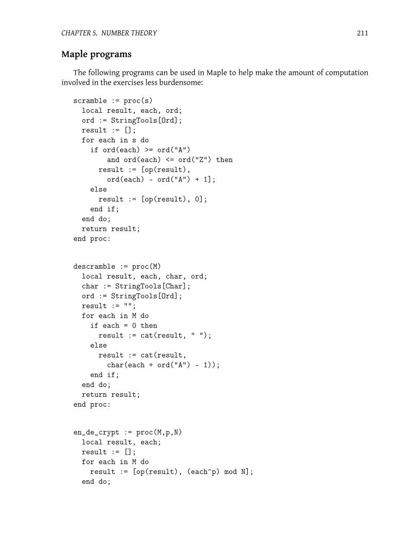
CHAPTER 5. NUMBER THEORY 211
Maple programs
The following programs can be used in Maple to help make the amount of computation
involved in the exercises less burdensome:
scramble := proc(s)local result, each, ord;ord := StringTools[Ord];result := [];for each in s do
if ord(each) >= ord("A")and ord(each) <= ord("Z") then
result := [op(result),ord(each) - ord("A") + 1];
elseresult := [op(result), 0];
end if;end do;return result;
end proc:
descramble := proc(M)local result, each, char, ord;char := StringTools[Char];ord := StringTools[Ord];result := "";for each in M do
if each = 0 thenresult := cat(result, " ");
elseresult := cat(result,
char(each + ord("A") - 1));end if;
end do;return result;
end proc:
en_de_crypt := proc(M,p,N)local result, each;result := [];for each in M do
result := [op(result), (each^p) mod N];end do;

CHAPTER 5. NUMBER THEORY 212
return result;end proc:

Chapter 6
Factorization
This chapter builds up some basic algorithms for factoring polynomials. This is actually a
tricky subject, so we focus first on some theory before discussing the practice. We will see in
Sections 6¨1 and 6¨2 that factorization is tied to ideals. To keep things simple, we focus on a
special kind of ring where factorization is deterministic; Section 6¨3 introduces the relevant
structure.
The typical trick is to factorize modulo a prime, then reconstruct the integer factorization;
this prequires a deeper study of finite fields than the one we had in Section 3¨4, which we
address in Sections 6¨5 and 6¨6. That finally gets us to the point where Section 6¨7 can describe
algorithms for factorization over a field field and Section 6¨8 can outline how to approach
factorization in Z rxs.Remark 6¨1. In this chapter, every “generic” ring is an integral domain, unless otherwise spec-
ified. Thus, it is commutative, has a multiplicative identity, and lacks zero divisors.
Before proceeding, it will be very useful to observe that we make heavy use of Lemma 4¨43.
Please review that.
6¨1 A wrinkle in “prime”
We said earlier that even though the properties of being “prime” and “irreducible” coincide
for integers, this is not true in a general ring. This section shows why.
Prime and irreducible: a distinction
Recall Definition 3¨20,
Suppose r P R is an element of a commutative ring, and r is not a unit. We say
that r factors over R if we can find s, t P R such that r “ st and neither s nor t is
a unit. Otherwise, r is irreducible.
Example 6¨2. Consider the ring Q rxs.
• The only units are the rational numbers, since no polynomial of degree at least one has
a multiplicative inverse that is also a polynomial.
213

CHAPTER 6. FACTORIZATION 214
• x` q is irreducible for every q P Q.
• x2 is not irreducible, since x2 “ x ¨ x.
• x2 ` q is irreducible for every positive q P Q.
Recall now the definition of “prime” in Definition 5¨29,
A positive integer p is prime if p ‰ 1 and for any two integers a, b we have p |
ab ùñ p | a or p | b.
Fact 5¨31 told us that
An integer is prime if and only if it is irreducible.
This coincidence is because the integers are a special sort of ring. In this section we explore
rings where the two definitions do not coincide. We start by generalizing the definition of
prime:
Definition 6¨3. Suppose p P R is not a unit. We say that p is prime if, whenever we find
a, b P R such that p | ab, then p | a or p | b.
Prime and irreducible: a difference
Unexpected things happen when you look at rings that involve i. For instance, the set of
Gaussian integers is
Z ris “ ta` bi : a, b P Zu .
Question 6¨4 .Show that Z ris is a ring and an integral domain, but not a field.
Question 6¨5 .Show that Z ris is isomorphic to the lattice structure of Section 1¨5. Explain why this means
we can divide with quotient and remainder in Z ris, so it makes sense to speak of divisibility,
irreducible elements, and so forth in Z ris.
The number 2 is no longer irreducible in Z ris:
2 “ p1` iq p1´ iq .
Let’s see if it will factor further. Suppose 1` i factors as pa` biq pc ` diq. Expand the product
to obtain the equation
1` i “ pac ´ bdq ` i pad` bcq .
The real and complex parts must be equal, giving us the system of equations
ac ´ bd “ 1
ad` bc “ 1.

CHAPTER 6. FACTORIZATION 215
Let’s refine this relationship between a, b, c, d. Eliminate b by multiplying the first equation
by c and the second equation by d, then subtracting:
ac2 ´ bcd “ c
ad2 ` bcd “ d
*
ùñ a`
c2` d
2˘
“ c ` d ùñ a “c ` d
c2 ` d2.
By definition, a is an integer, so c2`d2 must divide c`d, so either c`d “ 0 or c
2`d2 ď |c ` d|.
If c`d “ 0, then c “ ´d. Reconsider the first equation in the original system: substitution
gives ac ` bc “ 1, so c pa` bq “ 1. These are integers, so c “ ˘1 and d “ ¯1, giving us the
factorization we already had.
On the other hand, suppose c` d ‰ 0; then c2 ` d2 ď |c ` d|. As c and d are also integers,
which are less than their squares, we have |c ` d| ď |c2 ` d2| “ c2`d2. These two inequalities
imply c ` d “ c2 ` d2, which is possible only if c, d P t0,˘1u; any other integers give c
2 ą c
or d2 ą d.
Consider the following cases.
• We cannot have c “ d “ 0, as that would make the original equation false: 1 ` i “
pa` biq pc ` diq “ 0.
• Suppose c “ ˘1.
– If d “ 0, then c`di “ ˘1, so 1`i “ pa` biq¨˘1. This factorization of 1`i involves
a unit, called a “trivial factorization”. Those don’t count against the definition of
a prime element. (If you doubt me, reread the definition.)
– If d “ 1, then either c ` di “ 1 ` i and a ` bi “ 1, a trivial factorization, or
c ` di “ ´1 ` i and a ` bi “ ´i. This only looks non-trivial, since ´i has a
multiplicative inverse in Z ris. (See Question 6.6.)
– If d “ ´1, then either c ` di “ ´1 ´ i “ ´p1` iq and a ` bi “ ´1, a trivial
factorization, or c ` di “ 1 ´ i and a ` bi “ i. This only looks non-trivial, since i
has a multiplicative inverse in Z ris.
Question 6¨6 .What are the inverses of i and´i in Z ris?
Recall what we wrote after Definition 3¨20: units don’t count in factorization, because every-
thing factors with units. We don’t consider 2 “ p´1qˆp´2q to be different factorizations, be-
cause, after all,´1ˆ´1 “ 1. In the same way, we won’t consider 1`i “ i p1´ iq “ ´i p´1` iq
to be different factorizations, because after all iˆp´iq “ 1. To call to mind this point, we add
a new term to our growing vocabulary:
Definition 6¨7. Let R be a commutative ring with unity, not necessarily an integral domain,
and a, b P Rz t0u. We say that a and b are associates if a | b and b | a.
Example 6¨8. In Q rxs, 4x2 ` 6 and 6x2 ` 9 are associates, since 4x
2 ` 6 “ 2
3p6x2 ` 9q, and
2
3
is a unit. They are not associates in Z rxs.

CHAPTER 6. FACTORIZATION 216
Question 6¨9 .
(a) Explain why 2 and 7 are not associates in Z.
(b) Explain why the only associate of 7 in Z is´7.
(c) Show that, in an integral domain, a and b are associates if and only if a “ bu, where u is
a unit.
(d) Explain why 2 and 4 are not associates in Z, but they are in Z6.
Remember that in this chapter, a generic ring is an integral domain, so we will typically
treat the characterization of Question 6.9 as if it were the definition of an associate.
Question 6¨10 .
(a) Show that 23 and 1117 are associates in Q.
(b) Show that 2 and 5 are associates in Z7.
(c) Show that a ring R is a field if and only if every non-zero element is an associate of every
other non-zero element.
In the Gaussian integers, i is a unit, so 1 ` i and 1 ´ i “ i p1` iq are associates. The only
factorizations of 1` i involve associates, so 1` i is irreducible.
Question 6¨11 .Show that 1´ i is also irreducible.
On the other hand, consider the ring
Z“
i?5‰
“
a` bi?5 : a, b P Z
(
.
It isn’t hard to verify that Z“
i?5‰
is also a ring, and additionally that
6 “ 2ˆ 3 “`
1` i?5˘ `
1´ i?5˘
.
Question 6¨12 .Verify that Z
“
i?5‰
is a ring and an integral domain.
Question 6¨13 .Show that 2, 3, 1` i
?5, and 1´ i
?5 are irreducible in Z
“
i?5‰
.
This has an amazing consequence:

CHAPTER 6. FACTORIZATION 217
Integers factor uniquely into irreducibles in Z, but not in Z“
i?5‰
!
Why is factorization unique in Z, but not in Z“
i?5‰
? If you look back at the proof of unique
factorization of integers, you’ll notice that we used the equivlance of “irreducible” and “prime”
to infer that the irreducible p1 divided q1. In the equation above,
2ˆ 3 “`
1` i?5˘ `
1´ i?5˘
,
all four factors are irreducible, but clearly not prime! After all, if 2 |`
1` i?5˘
, we could find
a` bi?5 such that
2`
a` bi?5˘
“ 1` i?5,
or,
2a “ 1 and 2b “ 1,
neither of which is possible if a and b are integers, which they must be in Z“
i?5‰
. So the
property of prime ring elements must be distinguished from that of irreducible ring elements.
So irreducible elements of integral domains need not be prime. On the other hand, prime
elements of integral domains are irreducible.
Question 6¨14 .Let R be an integral domain. Show that if p P R is prime, then it is also irreducible.
Question 6¨15 .Show that:
• For any n P N`, the ring Zn has no irreducible or prime elements unless n is a power of
a prime.
• If n is a power of a prime p, then multiples of p that are not multiples of p2
are both
irreducible and prime; moreover, they are associates.
Definition 6¨16. The norm of a Gaussian integer a` bi is a2 ` b2.
Question 6¨17 .Show that:
(a) irreducible elements of Z ris are prime;
(b) if z “ xy in Z ris is a nontrivial factorization of z, then the norms of x and y are each
smaller than the norm of z;
(c) every element of Z ris factors into irreducibles; and
(d) these factorizations are unique up to units.
Hint: For (a), you will need a Bezout-like identity, and then you can imitate the proof for in-
tegers. You are helped in your quest for a Bezout-like identity by the fact that Question 6.5
gives you division of Gaussian integers. For (b), show also that the norm of z is the product
of the norm of x and the norm of y. For (c), use (b) and the Well-Ordering Principle. For (d),
imitate the proof for uniqueness of factorization of integers.

CHAPTER 6. FACTORIZATION 218
Factors are divisors, and greatest common divisors will prove useful in our search for fac-
tors. However, we have to define this term a little differently, since not all rings have a linear
ordering.
Definition 6¨18. Let R be a ring, and a, b P R. Suppose we can find d P R such that d divides
both a and b, and for any r P R that divides both a and b, we also have r | d. We call d a greatestcommon divisor of a and b.
What makes d “greatest” is that it sits at the top of a tree of divisibilities. Don’t get the
wrong idea; dmight not be alone! At the very least, its associates will sit next to it at the top
of the tree.
Example 6¨19. To see how you need to be careful with these ideas, consider Z14. Certainly
2 | 6 and 2 | 8, so 2 is a common divisor of 6 and 8. Is it the greatest such? Looking just at 6,
by congruence we know that 6 ” 20 ” 34 ” ¨ ¨ ¨ . Notice that 5 | 20, so 5 | 6. We can likewise
show 5 | 8. Is 5 a “greater” common divisor than 2? No, 5 is actually a unit: 5ˆ3 ” 1. Because
of that, we automatically get 5 | 2; for instance,
2 ” 1ˆ 2 ” p5ˆ 3q ˆ 2 “ 5ˆ p3ˆ 2q “ 5ˆ 6.
So 6 actually divides 2, as well. . . which means 6 divides 8! Likewise, 8ˆ 2 “ 16 ” 2, so 8 | 2.
Question 6¨20 .Show that in a principal ideal domain R:
(a) 〈d〉 “ 〈a, b〉, making d a greatest common divisor of a and b;
(b) there exist r, s P R such that d “ ra` sb; and
(c) if both c and d are greatest common divisors of a and b, then c and d are associates.
6¨2 The ideals of factoring
The link between divisibility and principal ideals in Lemma 4¨43 implies that we can rewrite
Definition 6¨7 in terms of ideals. We start with the facts that (a) it’s trivial to obtain the iden-
tity from a unit, and hence obtain the entire ring; and (b) since associates differ only by a
unit, their ideals shouldn’t differ at all.
Theorem 6¨21. Let R be an integral domain, and let a, b P Rz t0u.
(A) a is a unit if and only if 〈a〉 “ R.
(B) a and b are associates if and only if 〈a〉 “ 〈b〉.
Example 6¨22. This theorem gives us an alternate route to showing that some ring elements
are units or associates (or not). In the Gaussian integers, 3 R 〈1` i〉, so 1` i is not a unit.
It likewise allows us to decide when two ideals are equal. Since ´i p1` iq “ p1´ iq, and
´i is a unit, 〈1` i〉 “ 〈1´ i〉.

CHAPTER 6. FACTORIZATION 219
Proof of Theorem 6¨21 on the preceding page. (A) This is a straightforward chain: a is a unit if and
only if there exists b P R such that ab “ 1R, which is true if and only if 1R P 〈a〉, which is true
if and only if R “ 〈a〉 (Questions 4.34 and 4.35).
(B) Assume that a and b are associates. Let c P R be a unit such that a “ bc. By definition,
a P 〈b〉. Since any x P 〈a〉 satisfies x “ ar “ pbcq r “ b pcrq P 〈b〉, we see that 〈a〉 Ď 〈b〉. In
addition, we can rewrite a “ bc as ac´1 “ b, so a similar argument yields 〈b〉 Ď 〈a〉.
Conversely, assume 〈a〉 “ 〈b〉. By definition, a P 〈b〉, so there exists c P R such that a “ bc.
Likewise, b P 〈a〉, so there exists d P R such that b “ ad. By substitution, a “ bc “ padq c. Use
the associative and distributive properties to rewrite this as a p1´ dcq “ 0. By hypothesis,
a ‰ 0; since we are in an integral domain, 1 ´ dc “ 0. Rewrite this as 1 “ dc; we see that c
and d are units, which implies that a and b are associates.
Remark. The proof requires R to be an integral domain in order to show (B). For a counterex-
ample, consider R “ Z6; we have 〈2〉 “ 〈4〉, but 2 ¨ 2 “ 4 and 4 ¨ 2 “ 2. Neither 2 nor 4 is a
unit, so 2 and 4 are not associates. Strange things happen with zero divisors!
Question 6¨23 .Show that in an integral domain, factorization terminates iff every ascending sequence of
principal ideals 〈a1〉 Ď 〈a2〉 Ď ¨ ¨ ¨ is eventually stationary; that is, for some n P N`, 〈ai〉 “〈ai`1〉 for all i ě n.
Ideals of irreducible and prime elements
What about prime or irreducible elements of a ring? We’ll preface the result with an ex-
ample that leads to two new definitions.
Start with an irreducible element; for instance, 2 P Z. Let A “ 〈2〉. What can we say about
it? No other integer divides it, so Lemma 4¨43 suggests that no other ideal can contain it —
aside from Z itself, naturally. By definition, 〈2〉 is the smallest ideal that contains 2, but it is
also the largest proper ideal that contains 2.
Definition 6¨24. Let I be an ideal in an integral domain R. If I Ĺ R and no other ideal of R
contains I, we call I amaximal ideal.
For prime elements, it might be more instructive to consider first an integer that is not
prime, 6 P Z. The fact that it is not prime means we can find two integers a and b such that
6 | ab but 6 - a and 6 - b . For instance, if a “ 3 and b “ 4, we see that 6 | p3ˆ 4q but 6 - 3 and
6 - 4. Applying Lemma 4¨43 again, we see that 〈3ˆ 4〉 Ď 〈6〉, while 〈3〉 Ę 〈6〉 and 〈4〉 Ę 〈6〉.On the other hand, when an integer p is prime, we know that if p | ab, then p | a or p | b; in
terms of Lemma 4¨43, we would say that if 〈ab〉 Ď 〈p〉, then 〈a〉 Ď 〈p〉 or 〈b〉 Ď 〈p〉.This is not especially remarkable, butwe can say something stronger! Recall from Ques-
tion 4.39 that if A and B are ideals, then
AB “
#
nÿ
i“1
aibi : n P N`, ai P A, bi P B
+

CHAPTER 6. FACTORIZATION 220
is also an ideal. A moment ago, we looked at 〈ab〉 when referring to a prime element p. What
of 〈a〉 〈b〉? This is actually a larger ideal; for instance, you could have solved Question 4.40 by
looking at
〈6〉 〈9〉 “ 〈3〉 ;
after all, 〈6〉 Ď 〈3〉 and 〈9〉 Ď 〈3〉 just by using Lemma 4¨43, which easily gives us 〈6〉 〈9〉 Ď 〈3〉,whereas
3 “ ´1ˆ 6` 1ˆ 9 P 〈6〉 〈9〉 ,
which easily gives us 〈6〉 〈9〉 Ě 〈3〉. So 〈6〉 〈9〉 “ 〈3〉, but 〈6ˆ 9〉 “ 〈54〉, period, full stop, etc.
In fact, in the integers we can say that 〈a〉 〈b〉 “ 〈gcd pa, bq〉.Question 6¨25 .Why can we say that:
(a) 〈6〉 Ď 〈3〉 and 〈9〉 Ď 〈3〉 gives us 〈6〉 〈9〉 Ď 〈3〉? (perhaps not as “easily” as I claim above)
(b) In the integers, 〈a〉 〈b〉 “ 〈gcd pa, bq〉?Hint: As with Question 4.40, think about Bezout’s Identity.
We will carry this stronger property of primes with us from Z to any integral domain.
Definition 6¨26. Let P be a proper ideal of an integral domain R. If, for any two ideals A and
B of R, we find that AB Ď P implies A Ď P or B Ď P, we call P a prime ideal.
Here’s another example.
Example 6¨27. Let R “ Z rx, ys and P “ 〈x〉. Let A, B Ÿ R such that A Ę P but AB Ď P. By
definition, any f P AB has the form f “ř
n
i“1gihi where each gi P A and hi P B. By inclusion,
f P P, as well, so x | f . This means x divides every term of f , as well. (That’s true for monomials,
but not for arbitrary polynomials; for instance, this would not be true of x` 1.)
Let g P AzP and h P B. By definition, x - g, so g has at least one term t such that x - t. Let
u be any term of h; by polynomial multiplication, a ctu is a term of f “ gh for some c P Z.
By definition of AB, f P AB, so, as pointed out a moment ago, x | tu. By hypothesis, x - t, so
deg xt “ 0, so
deg xu “ deg xtu´ deg xt “ deg xtu ě 1.
By definition of divisibility, x | u. Now, u was an arbitrary term of h, so x divides every term
of h, which means x | h, so h P P. We chose h arbitrarily from B, so every polynomial of B is
also in P. By definition, B Ď P.
We have shown that if A, B Ÿ R, AB Ď P, and A Ę P, then B Ď P. Hence P “ 〈x〉 is a prime
ideal.
Theorem 6¨28. Let R be an integral domain, and let a, b P Rz t0u.
(A) In a principal ideal domain, a is irreducible if and only if 〈a〉 is maximal.
(B) In a principal ideal domain, a is prime if and only if 〈a〉 is prime.

CHAPTER 6. FACTORIZATION 221
Proof. (A) Assume that R is a principal ideal domain, and suppose first that a is irreducible.
Let B be an ideal of R such that 〈a〉 Ď B Ď R. Since R is a principal ideal domain, B “ 〈b〉 for
some b P R. Since a P B “ 〈b〉, a “ rb for some r P R. By definition of irreducible, r or b is a
unit. If r is a unit, then by definition, a and b are associates, and by part (B) of Theorem 6¨21,
〈a〉 “ 〈b〉 “ B. Otherwise, b is a unit, and by part (A) of the same Theorem, B “ 〈b〉 “ R.
Since 〈a〉 Ď B Ď R implies 〈a〉 “ B or B “ R, we can conclude that 〈a〉 is maximal.
For the converse, we show the contrapositive. Assume that a is not irreducible; then there
exist r, b P R such that a “ rb and neither r nor b is a unit. Thus a P 〈b〉 and by Lemma 4¨43
and part (B) of Theorem 6¨21, 〈a〉 Ĺ 〈b〉 Ĺ R. In other words, 〈a〉 is not maximal. By the
contrapositive, then, if 〈a〉 is maximal, then a is irreducible.
Question 6¨29 .Show part (B) of the theorem.
The discussion above did not require that R be a principal ideal domain to show that if
〈a〉 is maximal, then a is irreducible. This remains true even when R is not a principal ideal
domain.
On the other hand, it can happen that a is irreducible when R is not a principal ideal do-
main, but 〈a〉 is not maximal. To see why, consider any ring R, and its bivariate polynomial
ring R rx, ys. Example 4¨52 on page 136 shows that this is not a principal ideal domain, even if
R is! The element x is irreducible, but 〈x〉 Ĺ 〈x, y〉 Ĺ R rx, ys, so 〈x〉 is not maximal.
In a similar way, your proof of part (B) should have shown that if 〈a〉 is prime, then a is
prime even if R is not a principal ideal domain. The converse, however, need not be true.
In any case, we have the following result.
Theorem 6¨30. Let R be an integral domain, and let p P R. If 〈p〉 is maximal, then p is irreducible,
and if 〈p〉 is prime, then p is prime.
We can take this a little further.
Theorem 6¨31. Maximal ideals are always prime, even if you are not in an integral domain.
Proof. Let R be a ring,M a maximal ideal of R, and A, B ideals of R. Suppose that AB Ď M.
By way of contradiction, suppose further that A, B Ę M. That means we can choose a P
AzM and b P BzM; do so. Note that ab P AB Ď M.
For any r P R we can write 〈r, M〉 for the smallest ideal that contains both r and the ele-
ments of M. As a and b are not elements of M, we infer M Ĺ 〈a, M〉 , 〈b, M〉. By maximality of
M, we infer 〈a, M〉 “ 〈b, M〉 “ R.
Let C be the product ideal of 〈a, M〉 and 〈b, M〉. Let x P C; by definition of a product ideal,
x “ř
n
i“1yizi where n P N`, yi P 〈a` M〉, and zi P 〈b` M〉 . For any term yizi of this sum,
choose t, u P M such that yi “ a` t and zi “ b` u. We have
yizi “ pa` tq pb` uq “ ab` au` bt ` tu.
We noted above that ab P M, and absorption guarantees au, bt, tu P M. So yizi P M. Closure of
ideals under addition means x P M. As x was arbitrary in C, C Ď M.

CHAPTER 6. FACTORIZATION 222
On the other hand, recall that 〈a, M〉 , 〈b, M〉 “ R. Let r P R; by inclusion, r P 〈a, M〉; by
definition of a product ideal, r “ 1 ¨ r P 〈a, M〉 〈b, M〉 “ C. The arbitrary choice of r P R implies
that R Ď C Ď M Ĺ R, a contradiction!
The only assumption not forced by the hypotheses was the one that both A, B Ę M. We
are forced to conclude that A Ď M or B Ď M. By definition,M is a prime ideal.
Amazingly, this is true even when the ring is not an integral domain! Combined with
Theorem 6¨30, we have the following diagram for integral domains:
〈p〉 maximal +3
p irreducible
〈p〉 prime +3 p prime
Do the arrows also point in the other directions? We can make a start on answering that.
Question 6¨32 .Show that if p is prime, then 〈p〉 is also prime. Hint: Suppose A, B are ideals of a ring and
AB Ď 〈p〉, but A Ę 〈p〉. Use an element of Az 〈p〉 to show that every element of B lies in 〈p〉.
How are prime and irreducible elements related?
The relationships we have discussed have many useful consequences. Ideals are a pow-
erful enough tool that we can prove quite a few properties about both elements and rings
through their ideals.
One question that comes to mind is, what is so special about Z, that irreducible elements
are prime? After all, it was not true about Z“
i?5‰
! The answer is not obvious if we think
only about the properties of the elements per se, but it becomes easier if we think about their
ideals. Your eyes should dart immediately to the different hypotheses in the theorems above:
to prove one direction, we needed only an integral domain; to prove the other, we needed a
principal ideal domain.
We have already shown thatZ is a principal ideal domain (Theorem 4¨53). Could it be that
Z“
i?5‰
is not? In the case we studied before, we had 2 ˆ 3 “`
1` i?5˘ `
1´ i?5˘
. These
elements are all irreducible. InZ, joining two elements in a ring gives us an ideal generated by
one element, their gcd (see Question 4.37, where you hopefully used Bezout’s Identity); since
gcd p2, 3q “ 1, we have 〈2, 3〉 “ 〈1〉 in Z, so 〈2, 3〉 “ Z.
It’s another story entirely inZ“
i?5‰
. Consider the ideal I “⟨2, 1` i
?5⟩. Both generators
are irreducible, and they are not associates, but 1 R I! Hence I ‰ Z“
i?5‰
, and we now have a
chain
2 Ĺ I Ĺ Z“
i?5‰
.
Interestingly, 2 is irreducible, but its ideal is not maximal! On the other hand, the fact that 2
and 1` i?5 are irreducible but not associates means no one element can generate I. SoZ
“
i?5‰
is not a principal ideal domain!
Question 6¨33 .What are the units of Z
“
i?5‰
? Explain how this shows 2 and 1` i?5 are not associates.

CHAPTER 6. FACTORIZATION 223
Question 6¨34 .We wrote in the discussion above that 1 R I. How do we know this?
We have our criterion for an irreducible element to be prime! Prove it for the general case.
Question 6¨35 .Suppose that R is a principal ideal domain, and r P R. Show that if r is irreducible, then it is
prime.
The converse is true even if we are not in a principal ideal domain; see Question 6.14.
You may be wondering why we worked with prime and irreducible elements in the context
of integral domains. It may seem intuitive that zero divisors would throw off the properties
we expect, but even if not, an ideal you already know provides a direct answer.
Example 6¨36. Consider the ring Z6. This is not an integral domain, so our definition of a
“prime” element doesn’t apply, but it is not hard to verify that 2 satisfies the requirements of
a prime element of Z6, if such a thing existed:
〈2〉 “ t0, 2, 4u ,
and if 2 - a, 2 - b then 2 - ab:
1ˆ 1, 1ˆ 3, 1ˆ 5, 3ˆ 3, 3ˆ 5, 5ˆ 5 R 〈2〉 .
Alas, 2 is not irreducible; after all, 2 “ 8 “ 2 ˆ 2 ˆ 2, so 2 factors itself, even though it isn’t a
unit!
We have now answered one question posed at the beginning of the chapter:
• If R is an integral domain, then prime elements are irreducible.
• If R is a principal ideal domain, then irreducible elements are prime.
Because we are generally interested in factoring only for integral domains, many authors
restrict the definition of prime so that it is defined only in an integral domain. In this case, a
prime element is always irreducible, although the converse might not be true, since not all
integral domains are principal ideal domains. We went beyond this in order to show, as we
did above, why it is defined in this way. Since we maintain throughout most of this chapter
the assumption that all rings are integral domains, one could shorten this to,
Fact 6¨37 (Prime and irreducible elements in integral domains.). A prime element is always
irreducible, but an irreducible element is not always prime.
To sum up what we have found:
• We saw in Example 6¨27 that in Z rx, ys, the ideal 〈x〉 is prime, but 〈x〉 Ĺ 〈x, y〉 Ĺ 〈1〉, so
a prime ideal need not be maximal, even in an integral domain.

CHAPTER 6. FACTORIZATION 224
• Likewise, inZ rx, ys, the element x is irreducible, but 〈x〉 Ĺ 〈x, y〉 Ĺ 〈1〉, so an irreducible
element need not generate a maximal ideal, even in an integral domain.
• We saw in Z“
i?5‰
that an irreducible element need not be prime, even in an integral
domain.
• You will see below that if p is prime, then 〈p〉 is also prime.
We can, therefore, revise our diagram for integral domains as follows:
〈p〉 maximal
any ring +3
any ring
p irreduciblePID
ks
PID
〈p〉 prime
any ring +3
PID
KS
p primePID
ks
integral domain
KS
Question 6¨38 .Use the theory developed in this section to describe how prime ideals and maximal ideals are
related in:
• an integral domain, and
• a principal ideal domain.
6¨3 Time to expand our domains
This section considers two ideas essential to factorization: unique factorization and divi-
sion. You might think that the ability to divide would give you a unique factorization, but
on the other hand, the distinction between prime and irreducible elements might also give
you pause. Indeed, the ability to divide and the ability to obtain a unique factorization are
not quite identical, a fact reflected in the structures of rings with these properties.
Unique factorization domains
The Fundamental Theorem of Arithmetic tells us that every integer factors uniquely into
a product of irreducible elements. This is not true in every ring; in Z“
´?5‰
, we factored
6 “ 2 ¨3 and 6 “`
1`?´5
˘ `
1´?´5
˘
. Since 2, 3, 1`?´5, and 1´
?´5 are all irreducible
in Z?´5, 6 factors two different ways as a product of irreducibles.
Definition 6¨39. A ring is a unique factorization domain if every nonzero, non-unit r P R
factors into irreducibles r “ pa11 p
a22 ¨ ¨ ¨ p
amm
, and if this factorization is unique up to order and
associates.
Another way of saying this is that if r also factors into irreducibles r “ qb11 q
b22 ¨ ¨ ¨ q
bnn
, then
m “ n and each p corresponds to a unique q via an associate c, according to the relationship
p “ cq, and the corresponding exponents are also the same, with ai “ bj.

CHAPTER 6. FACTORIZATION 225
Aside from Z, what are some other unique factorization domains?
Example 6¨40. You showed in Question 6.17 that Z ris is a unique factorization domain.
Example 6¨41. Z rxs is a unique factorization domain. To see this requires two major steps.
(Existence) Let f P Z rxs. If the coefficients of f have a common factor, we can factor that out
easily; for example, 2x2`4x “ 2 px2 ` 2xq. We know that integers have a unique factorization,
so we may assume, without loss of generality, that the terms of f have no common factor.
If f is irreducible, then we are done; it has a factorization into irreducibles. Otherwise,
we claim it factors into two polynomials of smaller degree. After all, if f factors as ag where
deg g “ deg f , then we must have deg a “ 0. That implies a P Z, so a is a common factor of f ’s
coefficients, a possibility we excluded! So if f factors, it factors as f “ gh, where deg g, deg h ă
deg f . Degrees are natural numbers, and they decrease each time we factor a polynomial
further, so Fact 1¨51 tells us this process must eventually end with polynomials that do not
factor; that is, with irreducibles. Hence f factors into irreducibles; say f “ p1 ¨ ¨ ¨ pm. Without
loss of generality, we may assume that none of the p’s are associates.
Of course, having a factorization into irreducibles doesn’t exclude the possibility of having
more than one factorization into irreducibles, so we turn our attention to. . .
(Uniqueness) Suppose we can also factor f into irreducibles as f “ q1 ¨ ¨ ¨ qn. The coefficients
of f are integers, and any integer a corresponds to a rational number a1, so we can consider
f as an element of Q rxs. Why would we do this? By Theorem 4¨53(C) we know that Q rxs is a
principal ideal domain. You showed in Question 6.35 that irreducible elements of a principal
ideal domain are prime. Hence p1 divides qj for some j “ 1, . . . , n. Without loss of generality,
p1 | q1. Since q1 is also irreducible, p1 and q1 are associates; say p1 “ a1q1 for some unit a1.
The units of Q rxs are the nonzero elements of Q, so a1 P Qz t0u. And so forth; each pi is an
associate of a unique qj in the product. Without loss of generality, we may assume that pi is
an associate of qi. This forces m “ n.
Right now we have pi and qi as associates in Q rxs. If we can show that each ai “ ˘1, then
we will have shown that the corresponding pi and qj are associates inZ rxs as well, so thatZ rxsis a unique factorization domain. Write a1 “ bc where gcd pb, cq “ 1; we have p1 “ bc ¨ q1.
Rewrite this as cp1 “ bq1. Remember that p1 and q1 are integer polynomials. What’s more, the
fact that gcd pb, cq “ 1means we can infer b | p1 and c | q1 (see below). However, p1 and q1 are
irreducible, integer polynomials, so b and c must be integer units. The only integer units are
˘1, so p1 and q1 are associates.
The same argument can be applied to the remaining irreducible factors. Thus, the factor-
ization of f is unique up to order and associates.
This result generalizes to an important class of rings.
Theorem 6¨42. Every principal ideal domain is a unique factorization domain.
Proof. Let R be a principal ideal domain, and f P R.
(Existence) First we show that f has a factorization. Suppose f is not irreducible; then there
exist r1, r2 P R such that f “ r1r2 and f is an associate of neither. By Theorem 6¨21, 〈f 〉 Ĺ 〈r1〉and 〈f 〉 Ĺ 〈r2〉. If r1 is not irreducible, then there exist r3, r4 P R such that r1 “ r3r4 and r1 is an
associate of neither. Again, 〈r1〉 Ĺ 〈r3〉 and 〈r1〉 Ĺ 〈r4〉. Continuing in this fashion, we obtain
an ascending chain of ideals
〈f 〉 Ĺ 〈r1〉 Ĺ 〈r3〉 Ĺ ¨ ¨ ¨ .

CHAPTER 6. FACTORIZATION 226
We step out of this proof a moment to show that such a chain cannot continue indefinitely:
Lemma 6¨43. In any principal ideal domain R, an ascending chain of ideals A1 Ď A2 Ď A3 Ď ¨ ¨ ¨
eventually stabilizes at an ideal B.
Proof of Lemma 6¨43. Let B “ A1 Y A2 Y A3 Y ¨ ¨ ¨ . We claim B is an ideal of R. For any b P B and
r P R, we know b P Ai for some i P N`, and since Ai is an ideal of R, br P Ai; by inclusion, br P B.
On the other hand, let c P B; we know c P Aj for some j P N`. Let k “ max pi, jq; by inclusion,
b, c P Ak, which is an ideal, so b´ c P Ak, and by inclusion b´ c P B. We have shown that B is
closed under subtraction, and that it absorbs multiplication from R.
We have established that B is an ideal. By hypothesis, R is a principal ideal domain, so
B “ 〈b〉 for some b P B. By definition, b P Ai for some i P t1, 2, . . . u. Every element in B is a
multiple of b, so every element in B is also in Ai; that is, B Ď Ai. But Ai Ď B by definition of B.
The two sets are therefore equal. Likewise, Aj “ B for every j “ i ` 1, i ` 12, . . . . The chain
has become
A1 Ď A2 Ď ¨ ¨ ¨ Ď Ai´1 Ď Ai “ B “ Ai`1 “ Ai`1 “ ¨ ¨ ¨ .
As claimed, the ascending chain of ideals stabilized at B.
This property of ascending chains of ideals is similar to the Noetherian behavior we ob-
served inZ and other rings. Indeed, an ascending chain of ideals inZ corresponds to divisibil-
ity and factorization (Lemma 4¨43). The Well-Ordering Principle means that integer divisors
must eventually end with irreducible factors; thus, an ascending chain of integer ideals must
eventually end with a maximal ideal.
Question 6¨44 .Consider the ideal 〈180〉 Ă Z. Use unique factorization to build a chain of ideals 〈180〉 “〈a1〉 Ĺ 〈a2〉 Ĺ ¨ ¨ ¨ Ĺ 〈an〉 “ Z such that there are no ideals between 〈ai〉 and 〈ai`1〉. Identify
a1, a2, . . . clearly.
This property is sufficiently important that we give it a special name. Any ring where an
ascending chain of ideals eventually stabilizes is said to satisfy the ascending chain condi-tion. We can also say it is a Noetherian ring.
Proof of Theorem 6¨42, continued: (Still on existence) By Theorem 6¨43, a principal ideal domain
satisfies the ascending chain condition; thus, the chain
〈f 〉 Ĺ 〈r1〉 Ĺ 〈r3〉 Ĺ ¨ ¨ ¨
must stabilize eventually. We have already explained that if ri factors, the chain continues
further, so it can stabilize only if we reach an irreducible polynomial. This holds for each
chain, regardless of whether it starts with r1, r2, r3, r4, . . . . All must terminate with irreducible
elements of the ring, which gives us f “ p1 ¨ ¨ ¨ pm where each pi is irreducible.
(Uniqueness) Now we show the factorization is unique. Suppose f also factors as f “
q1 ¨ ¨ ¨ qn where each qj is irreducible. Without loss of generality, m ď n. Recall that irre-
ducible elements are prime in a principal ideal domain (Corollary 6.35). Hence p1 divides one
of the qi; without loss of generality, p1 | q1. However, q1 is irreducible, so p1 and q1 must be

CHAPTER 6. FACTORIZATION 227
associates; say c1p1 “ q1 for some unit c1 P R. Since we are in an integral domain, we can
cancel p1 and q1 from f “ f , obtaining
c1p2 ¨ ¨ ¨ pm “ q2 ¨ ¨ ¨ qn.
Since p2 is irreducible, hence prime, we can continue this process until we conclude with
c1c2 ¨ ¨ ¨ cm “ qm`1 ¨ ¨ ¨ qn. Now, the left hand side is a unit. By definition, irreducible elements
are not units, so the right hand side must also be a unit, but that is possible only if there are
no more irreducibles on the right hand side; that is, m “ n. Thus the factorization is unique
up to ordering and associates.
We chose an arbitrary element of an arbitrary principal ideal domain R, and showed that
it had only one factorization into irreducibles. Thus every principal ideal domain is a unique
factorization domain.
We can likewise extend a result from a previous section.
Question 6¨45 .Show that in a unique factorization domain, irreducible elements are prime.
Corollary 6¨46. In a unique factorization domain:
• an element is irreducible iff it is prime; and
• an ideal is maximal iff it is prime.
Euclidean domains
We’d like to define a Euclidean domain as a ring with a valid division with quotient and
remainder. Once we have a precise notion of such division, we can use the Euclidean algo-rithm to find greatest common divisors — so long as the remainder “shrinks.” But how can
we decide that the remainder “shrinks”, when not all rings have natural orderings?
What we will do is define a valuation function v from the nonzero elements of a ring to
the naturals, N, satisfying the desirable property
v prsq “ v prq v psq for all r, s P R.
Definition 6¨47. If R is an integral domain and v is a valuation function on R such that for
any a P R and any d P Rz t0u, we can find q, r P R such that a “ qd ` r and either r “ 0 or
v prq ă v pdq, then we call R a Euclidean domain.
Example 6¨48. In Z, the valuation function is the absolute value: v prq “ |r|. Observe that
v prsq “ |rs| “ |r| ¨ |s| “ v prq v psq, and for any a P Z and any d P Zz t0u we can find q, r P Zsuch that a “ qd` r and r “ 0 or v prq “ |r| ă |d| “ v pdq.
Example 6¨49. We can also see this in Z ris. We defined division using the lattice; the valu-
ation function is effectively the norm. We have a “ qd ` r with r “ 0 or the norm of r less
than the norm of d.

CHAPTER 6. FACTORIZATION 228
Question 6¨50 .We can adapt the Euclidean algorithm (Theorem ) to any Euclidean domain by making just
one change: in step 1, replace
1. Let s “ max pm, nq and t “ min pm, nq.
by
1. If v pmq ě v pnq, let s “ m and t “ n; otherwise, let s “ n and t “ m.
Adapt the original proof of the Euclidean Algorithm to show that this one change does indeed
give us an algorithm that terminates correctly in any Euclidean domain.
Question 6¨51 .Building on Question 6.50, explain why Bezout’s Lemma also applies in Euclidean domains: if
R is a Euclidean domain with valuation function v, r, s P R, and d is a gcd of r and s, then we
can find a, b P R such that ar` bs “ d, and v pdq ě v pd1q for any other common divisor d1 P R
of x and y.
Question 6¨52 .Use Bezout’s Lemma to show that if gcd pb, cq “ 1 and b | ac, then b | a. This argument should
apply in any Euclidean domain.
Polynomials in one variable also have a division. What is the valuation function when
dividing these polynomials? That is, what aspect of polynomials is guaranteed to decrease
when you divide them correctly? We use v prq “ deg r .
Question 6¨53 .Use x
3`x`1 and x2´1 as an example of polynomial division: find a quotient and a remainder
r with deg r ă deg px2 ´ 1q “ 2.
However, Z rxs is not a Euclidean domain if the valuation function is v prq “ deg r. After
all, if f “ 2 and g “ x, we cannot find q, r P Z rxs such that g “ qf ` r and deg r ă deg f . The
best we can do is x “ 0 ¨ 2` x, but deg x ą deg 2.
Question 6¨54 .Use Z rxs to show that even if R is a unique factorization domain but not a principal ideal
domain, then we cannot always find r, s P R such that gcd pa, bq “ ra` sb for every a, b P R.
Over a ground field F, however, it’s another matter.
Fact 6¨55. If F is a field, then F rxs is a Euclidean domain with valuation function v pf q “ deg f for
all nonzero f P F rxs.
Why? The difference in the success of F rxs and the failure Z rxs is precisely in that fields
contain their multiplicative inverses, whereas in the example above Z was unable to provide
a multiplicative inverse for 2.

CHAPTER 6. FACTORIZATION 229
To be precise, let f, g P F rxs. We claim that we can divide f by g using degree for the
valuation. If deg g ą deg f , let q “ 0 and r “ f , and we have f “ qg ` r with v prq ă v pgq,
as claimed. Suppose, then, that deg g ď deg f . Let a1 be the leading coefficient of f , b the
leading coefficient of g, m “ deg f , and n “ deg g. Let c1 “ a1b´1
, ` “ m ´ n, and q1 “ c1x`.
Define
r1 “ f ´ q1g.
By construction, the leading term of q1g is
`
a1b´1˘
x`¨ bx
m“ a1x
pm´nq`n“ a1x
m,
the same as the leading term of f . So the leading terms cancel, and deg r1 ă deg f .
If deg r1 ă deg g, then let q “ q1 and r “ r1 , and we are done. Otherwise, for i “ 1, 2, . . .
let ai`1 be the leading coefficient of ri, ci`1 “ ai`1b´1
, `i “ deg ri ´ deg g, and qi`1 “ ci`1x`.
Define ri`1 “ ri ´ qi`1g, and in each case the leading terms will cancel, as above. We obtain
a sequence of polynomials f , r1, r2, . . . whose degrees constitute a decreasing sequence of
nonnegative integers. By Fact 1¨51, this sequence must eventually stabilize, but the only way
it stabilizes is if we can no longer divide by g. That happens only if the remainder eventually
is either zero or has a degree smaller than that of g.
This fact plugs a hole at which we’ve mostly hinted in the past, without explaining rig-
orously. In the past, we’ve pointed out that the Factor Theorem allows us to associate every
root α of a polynomial f with a factor x´α of f . That strongly suggests that a polynomial has at
most n roots (and exactly n roots, if you count multiplicities) but it doesn’t guarantee it; after
all, irreducibles need not be prime.
Question 6¨56 .Let f P F rxs of degree n. Use Fact 6¨55 and the Factor Theorem to show that f has at most n
roots in F.
Fact 6¨57. If R is a Euclidean domain with valuation function v, r and s are nonzero elements of R, and
r | s, then v prq ď v psq.
Proof. Given the hypotheses, we can find q P R such that s “ qr. By substitution, v psq “
v pqrq “ v pqq v prq. These are all positive integers, so v prq ď v psq.
Theorem 6¨58. Every Euclidean domain is a principal ideal domain.
Proof. Let R be a Euclidean domain with respect to v, and let A be any non-zero ideal of R. Let
a1 P A. As long as A ‰ 〈ai〉, do the following:
• find bi P Az 〈ai〉;
• let ri be the remainder of dividing bi by ai;
– notice v priq ă v paiq;
• use the Euclidean algorithm to compute a gcd ai`1 of ai and ri;

CHAPTER 6. FACTORIZATION 230
– notice v pai`1q ď v priq ă v paiq;
• this means 〈ai〉 Ĺ 〈ai`1〉; after all,
– as a gcd, ai`1 | ai, but
– ai - ai`1, lest ai | ai`1 imply v paiq ď v pai`1q ă v paiq;
• hence, 〈ai〉 Ĺ 〈ai`1〉 and v pai`1q ă v paiq.
By Fact 1¨51, the sequence v pa1q ą v pa2q ą ¨ ¨ ¨ cannot continue indefinitely, which means
that we cannot compute ai’s indefinitely. Let d be the final ai computed. If A ‰ 〈d〉, we could
certainly compute another ai, so it must be that A “ 〈d〉.
Corollary 6¨59. Every Euclidean domain is a unique factorization domain.
Proof. This is a consequence of Theorem 6¨42 and Theorem 6¨58.
The converse is false: Z rxs is a unique factorization domain, but we saw above that it is not
a Euclidean domain. On the other hand, its deficiencies do not extend to Q rxs, or polynomial
rings over other fields.
Corollary 6¨60. If F is a field, then F rxs is both a principal ideal domain and a unique factorization
domain.
However, the definition of a greatest common divisor that we introduced with Euclidean
domains certainly generalizes to unique factorization domains.
Theorem 6¨61. In a unique factorization domain, greatest common divisors are unique up to asso-
ciates.
Proof. LetR be a unique factorization domain, and let f, g P R. Let d,pdbe two gcds of f, g. Let d “
pa11 ¨ ¨ ¨ p
amm
be an irreducible factorization of d, andpd “ qb11 ¨ ¨ ¨ q
bnn
be an irreducible factorization
of pd. Since d and pd are both gcds, d | pd and pd | d. So p1 |pd. By Theorem 6.45, irreducible
elements are prime in a unique factorization domain, so p1 | qi for some i “ 1, . . . , n. Without
loss of generality, p1 | q1. Since q1 is irreducible, p1 and q1 must be associates.
We can continue this argument withd
p1and
pd
p1, so that d “ apd for some unit a P R. Since d
and pd are unique up to associates, greatest common divisors are unique up to associates.
Question 6¨62 .Theorem 6¨61 says that gcd’s are unique up to associate in every unique factorization domain.
Suppose that P “ F rxs for some field F. Since P is a Euclidean domain (Question 6¨60), it is a
unique factorization domain, and gcd’s are unique up to associates (Theorem 6¨61). The fact
that the base ring is a field allows us some leeway that we do not have in an ordinary unique
factorization domain. For any two f, g P P, use the properties of a field to describe a method
to define a “canonical” gcd of f and g, and show that this canonical gcd is unique.

CHAPTER 6. FACTORIZATION 231
Question 6¨63 .Generalize the argument of Example 6¨41 to show that for any unique factorization domain
R, the polynomial ring R rxs is a unique factorization domain. Explain why this shows that for
any unique factorization domain R, the polynomial ring R rx1, . . . , xns is a unique factorization
domain. On the other hand, give an example that shows that if R is not a unique factorization
domain, then neither is R rxs.
6¨4 Field extensions
This section explores the relationship between polynomials, roots, and fields. Let F be any
field.
Extending a ring
Let R and S be rings, with R Ď S and s P S.
Question 6¨64 .We define R rss as the smallest ring containing both R and s. Show that:
(a) R Ď R rss Ď S;
(b) R “ R rss if and only if s P R; and
(c) R rss “
!
ř
k
i“0risi: k P N, ri P R
)
.
We call R rss a ring extension of R. Sometimes, this is isomorphic to a polynomial ring
over R; in this case, s is transcendental over R. We won’t prove it, but it is fairly well known
that e and π are transcendental over Q, so Q res – Q rπs – Q rxs.We are not interestined in transcendental extensions. We are interested in the case where
R rss is not isomorphic to R rxs; in that case, we call s algebraic, as it is the root of a polynomial
over R. (This may not be obvious, but we prove it in Theorem 6¨66 below.)
Example 6¨65. Let R “ R, S “ C, and s “ i “?´1. Then R ris is a ring extension of C.
Moreover, R ris is not isomorphic to a polynomial ring over R, since i2` 1 “ 0, but x
2` 1 ‰ 0
in R rxs. Every element of R ris has the form a ` bi for some a, b P R, so we can view R ris as
a vector space of dimension 2 over R! The basis elements are u “ 1 and v “ i, and a ` bi “
au` bv.
We made a rather bold claim here about the isomorphism, so let’s pause to verify it before
proceeding.
Theorem 6¨66. With R, S, and s defined as above, R rss – R rxs if and only if s is not the root of a
polynomial over R rxs.

CHAPTER 6. FACTORIZATION 232
Proof. Let φ : R rxs Ñ R rss by φ př
rixiq “
ř
risi. We claim this is a homomorphism of rings:
addition is fairly obvious, and multiplication is harder only because it’s a notational disgrace:
φ
´´
ÿ
rixi
¯´
ÿ
aixi
¯¯
“ φ
¨
˝
ÿ
i`j“k
`
ri ` aj˘
xk
˛
‚“ÿ
i`j“k
`
ri ` aj˘
sk“
´
ÿ
risi
¯´
ÿ
aisi
¯
.
That leaves the question of isomorphism. Suppose thatφ is an isomorphism. An isomorphism
is one-to-one, so we have φ p0q “ 0 “ř
risi “ φ prix
iq only if ri “ 0 for each i. By definition, s
is not a root of a polynomial over R rxs. On the other hand, suppose s is the root of a nonzero
polynomial over R rxs; call it f pxq, and suppose f pxq “ř
rixi. By definition of a root,
φ pf q “ φ
´
ÿ
rixi
¯
“ÿ
risi“ f psq “ 0 “ φ p0q ,
which shows that φ is not one-to-one.
Let’s see if this result generalizes, at least for fields. For the rest of this section, we let Fand E be fields, with α P E. It’s helpful to look at polynomials whose leading coefficient is 1.
Extending a field to include a root
Notation 6¨67. We write F pαq for the smallest field containing both F and α.
Example 6¨68. We prove later, in the Fundamental Theorem of Algebra, thatR ris “ C, which
is a field. So, R ris “ R piq “ C. On the other hand, Q“?2‰
Ĺ Q`?2˘
Ĺ C.
Question 6¨69 .Explain why Q
“?2‰
Ĺ Q`?2˘
Ĺ C.
Theorem 6¨72 below generalizes the construction of complex numbers in Section 3¨1.
When we built the complex numbers, we worked modulo the polynomial x2 ` 1 P R rxs.
That polynomial is irreducible over R, and by Theorem 6¨28 you now know that irreducible
ring elements generate maximal ideals. Really, then, you were building the quotient ring
R rxs 〈x2 ` 1〉, which is modulo a maximal ideal.
Do quotient rings formed by maximal ideals always result in a field? Indeed they do.
Fact 6¨70. Let R be a ring with unity, andM a maximal ideal of R. Then RM is a field.
Why? Let X P RM be any nonzero coset; choose x P R such that X “ x` I. As a nonzero coset,
X ‰ M, so x R M (Lemma 4¨103). We claim that we can find Y P RM such that XY ” 1 ` M.
Since Y has the form y`M, that means we can find y P R such that px` Mq py` Mq “ 1`M;
also by coset equality, xy ´ 1 P M. Written another way, we claim that we can find y P R and
m P M such that xy´ 1 “ m, or xy´ m “ 1.
To see why the claim is true, observe that xy P 〈x〉 , so xy ´ m P 〈x〉 ` M. This is the sum
of two ideals, which is also an ideal (Question 4.39). Let’s call it N “ 〈x〉` M. Now, x P N and
x R M implies that M Ĺ N; by hypothesis, M is maximal, giving us N “ R. As R is a ring with
unity, 1 P N. The definition of a sum of ideals tells us that 1 “ a`m for some a P 〈x〉 and some
m P M. By definition, we can find y P R such that a “ xy. Rewrite the equation 1 “ a ` m as
xy ´ 1 “ ´m, and we have xy ´ 1 P M, as desired. We finish the proof by reversing the first
paragraph: let Y “ y` M, and XY ” 1` M in RM.

CHAPTER 6. FACTORIZATION 233
Question 6¨71 .The converse is also true: if R is a ring with unity, M is an ideal, and RM is a field, then M
is a maximal ideal. Show why. Hint: You should just be able to reverse the main ideas of the
explanation above.
Theorem 6¨72. Suppose f P F rxs is irreducible.
(A) E “ F rxs 〈f 〉 is a field.
(B) F is isomorphic to a subfield F1 of E.
(C) Letpf P E rys such that the coefficient of yiis ai ` 〈f 〉, where ai is the coefficient of x
iin f . There
exists α P E such thatpf pαq “ 0.
In other words, E contains a root ofpf .
We call E an extension field of F. The isomorphism between F and F1 implies that we
can always assume that an irreducible polynomial over a field F has a root in another field
containing F. We will, in the future, think of E as a field containing F, rather than containing
a field isomorphic to F.
Proof. Denote I “ 〈f 〉.(A) Let E “ F rxs I. By Corollary 4¨53, F rxs is a principal ideal domain. Theorem 6¨28
states that if f is irreducible inF rxs, then I is maximal inF rxs. Fact 6¨70 states thatE “ F rxs Iis a field.
(B) To see that F is isomorphic to
F1 “ ta` I : a P Fu Ď E,
use the function φ : F Ñ F1 by φ paq “ a ` I. You will show in Question 6.73 that φ is a ring
isomorphism.
(C) Let α “ y` I. Let a0, a1, . . . , an P F such that
f “ a0 ` a1x` ¨ ¨ ¨ ` anxn.
As defined in this Theorem,
pf “ pa0 ` Iq ` pa1 ` Iq y` ¨ ¨ ¨ ` pan ` Iq yn.
By substitution and the arithmetic of ideals,
pf pαq “ pa0 ` Iq ` pa1 ` Iq px` Iq ` ¨ ¨ ¨ ` pan ` Iq px` Iqn
“ pa0 ` Iq ` pa1x` Iq ` ¨ ¨ ¨ ` panxn` Iq
“ pa0 ` a1x` ¨ ¨ ¨ ` anxnq ` I
“ f ` I.
By Theorem 4¨103, f`I “ I, sopf pαq “ I. Recall thatE “ F rxs I; it follows thatpf pαq “ 0E.

CHAPTER 6. FACTORIZATION 234
Question 6¨73 .Show that the function φ defined in part (B) of the proof of Theorem 6¨72 is an isomorphism
between F and F1.
The result of this is that, given any irreducible polynomial over a field, we can factor it
symbolically as follows:
• let f0 “ f , E0 “ F, and i “0;
• repeat while fi ‰ 1:
– let Ei`1 “ Ei rxs Ii;– let αi “ x` Ii P Ei`1, where Ii “ 〈fi〉;– by Theorem 6¨72, fi pαiq “ 0, so by the Factor Theorem, x´ αi is a factor of fi;
– let fi`1 P Ei`1 rxs such that fi “ px´ αiq fi`1;
– increment i.
Each pass through the loop generates a new root αi, and a new polynomial fi whose degree
satisfies the equation
deg fi “ deg fi`1 ´ 1.
Since we have a strictly decreasing sequence of natural numbers, the algorithm terminates
after deg f steps (Question 1¨51). We have thus described a way to factor irreducible polyno-
mials.
Corollary 6¨74 (Kronecker’s Theorem). Let f P F rxs and n “ deg f . There exists a field E such
that F Ď E, and f factors into linear polynomials over E.
Proof. We proceed by induction on deg f .
Inductive base: If deg f “ 1, then f “ ax ` b for some a, b P F with a ‰ 0. In this case, let
E “ F; then´a´1b P E is a root of f .
Inductive hypothesis: Assume that for any polynomial of degree n, there exists a fieldE such
that F Ď E, and f factors into linear polynomials in E.
Inductive step: Assume deg f “ n ` 1. By Question 6.63, F rxs is a unique factorization
domain, so let p be an irreducible factor of f . Let g P F rxs such that f “ pg. By Theorem 6¨72,
there exists a field D such that F Ĺ D and D contains a root α of p. Of course, if α is a root of
p, then it is a root of f : f pαq “ p pαq g pαq “ 0 ¨ g pαq “ 0. By the Factor Theorem, we can write
f “ px´ αq q pxq P D rxs. We now have deg q “ deg f ´ 1 “ n. By the inductive hypothesis,
there exists a field E such that D Ď E, and q factors into linear polynomials in E. But then
F Ĺ D Ď E, and f factors into linear polynomials over F.
Remember that we can write elements of R ris and Q“?2‰
in the form ax ` b, where a
and b come from the underlying field. We have two free variables a and b to choose any ring
element we want as coefficients. There are infinitely many such polynomials, but with respect
to the field elements they behave a little like vectors. Is that always the case?

CHAPTER 6. FACTORIZATION 235
Theorem 6¨75. Let f be an irreducible polynomial over the field F, and E “ F rxs 〈f 〉. Then E is a
vector space over F of dimension d “ deg f .
Proof. Let I “ 〈f 〉. By Theorem 6¨72, we can consider F Ď E. Since f is irreducible, 〈f 〉 is
maximal, and E is a field. Any element of E has the form g` I where g P F rxs; we can use the
fact that F rxs is a Euclidean Domain to write
g “ qf ` r
where q, r P F rxs and deg r ă deg f “ d. Notice g ´ r P 〈f 〉 “ I, so coset equality assures us
that g` I “ r ` I. In other words, every element of E has the form
`
ad´1xd´1` ¨ ¨ ¨ ` a1x
1` a0x
0˘
` I
where ad´1, . . . , a1, a0 P F.
Finally, view each coset written in this form as the vector pad´1, . . . , a1, a0q over the field
F; define vector addition as the component-wise addition of the coset representatives and
scalar multiplication by b P F aspbad´1, . . . , ba1, ba0q. The vector and scalar properties of a
vector space are fairly straightforward; we leave them to you as an exercise. Once done, we
have proved that E is a vector space over F with basis
B “
x0` I, x
1` I, . . . , x
d´1` I
(
.
Question 6¨76 .Show the remaining details that E is indeed a vector space over F.
Definition 6¨77. Let f , α, and E be as in Theorem 6¨72. Theorem 6¨75 tells us that deg f “
dimE. We call this number the degree of α.
It is sensible to say that deg f “ deg α since we showed in Theorem 6¨75 that deg f “
dim pF rxs 〈f 〉q.
Example 6¨78. Let f pxq “ x4 ` 1 P Q rxs. We can construct a field D with a root α of f ; using
the proofs above,
D “ Q rxs 〈f 〉 and α “ x` 〈f 〉 .
Notice that´α is also a root of f , so in fact, D contains two roots of f . If we repeat the proce-
dure, we obtain two more roots of f in a field E.
What if we extend a field more than once?
Theorem 6¨79. Suppose F is a field, E “ F pαq, and D “ E pβq. Then E is a vector space over F of
dimension deg α ¨ deg β, and in fact D “ F pγq for some root γ of a polynomial over F.

CHAPTER 6. FACTORIZATION 236
Proof. By Theorem 6¨75, B1 “
α0, . . . , α
d1´1(
and B2 “
β0, . . . , β
d2´1(
are bases of E over
F and D over E, respectively, where d1 and d2 are the respective degrees of the irreducible
polynomials of which α and β are roots. We claim that B3 “
αpiqβpjq: 0 ď i ă d1, 0 ď j ă d2
(
is a basis of D over F. To see this, we must show that it is both a spanning set — that is, every
element of D can be written as a linear combination of elements of B3 over F — and that its
elements are linearly independent.
To show that B3 is a spanning set, let γ P D. By definition of basis, there exist b0, . . . ,
bd2´1 P E such that
γ “ b0β0` ¨ ¨ ¨ ` bd2´1β
d2´1.
Likewise, for each j “ 0, . . . , d2 ´ 1 there exist apjq
0 , . . . , apjq
d1´1P F such that
bj “ apjq
0 α0` ¨ ¨ ¨ ` a
pjq
d1´1αd1´1.
By substitution,
γ “
d2´1ÿ
j“0
bjβj
“
d2´1ÿ
j“0
˜
d1´1ÿ
i“0
apjq
iαi
¸
βj
“
d´1ÿ
i“0
d´1ÿ
j“0
apjq
i
`
αiβj˘
.
Hence, B3 is a spanning set of D over F.
To show that it is a basis, we must show that its elements are linearly independent. For
that, assume we can find cpjq
iP F such that
d1´1ÿ
i“0
d2´1ÿ
j“0
cpjq
i
`
αiβj˘
“ 0.
We can rewrite this as an element of D over F by rearranging the sum:
d2´1ÿ
j“0
˜
d1´1ÿ
i“0
cpjq
iαi
¸
βj“ 0.
Since B2 is a basis, its elements are linearly independent, so the coefficient of each βjmust be
zero. In other words, for each j, we have
d1´1ÿ
i“0
cpjq
iαi“ 0.
Of course, B1 is also a basis, so its elements are also linearly independent, so the coefficient of
each αimust be zero. In other words, for each j and each i,
cpjq
i“ 0.

CHAPTER 6. FACTORIZATION 237
We took an arbitrary linear combination of elements of B3 over F, and showed that it is zero
only if each of the coefficients are zero. Thus, the elements of B3 are linearly independent.
Since the elements of B3 are a linearly independent spanning set, B3 is a basis of D over F.
If we count the number of elements of B3, we find that there are d1 ¨ d2 elements of the basis.
Hence,
dimFD “ |B3| “ d1 ¨ d2 “ deg α ¨ deg β.
We still have to show that D “ F pγq for some root γ P D of a polynomial f P F rxs. If
α P F pβq, then D “ F pβq, and we are done. Likewise if β P F pαq, then D “ F pαq. Otherwise,
we claim that γ “ α`β does the job. Why? By closure of addition, γ “ α`β P D, soD Ě F pγqrather easily. For the reverse inclusion, we point out that if the the sequence
γ, γ2, γ
3, . . .
consists entirely of elements that are linearly independent over F, then D cannot be finite
dimensional over F, as closure of multiplication means D must contain all these powers of γ.
We have just seen thatD is finite dimensional, so there must be elements c0, c1, . . . , cd1d2´1 P Fsatisfying
c0 ` c1γ ` ¨ ¨ ¨ ` cd1d2´1γd1d2´1 “ 0.
Let f pxq “ c0`c1x`¨ ¨ ¨`cd1d2´1xd1d2´1; we have f P F rxs and f pγq “ 0. We claim that cd1d2´1 ‰
0; if it were, then we could substitute x “ α ` y and obtain a polynomial g pyq “ f pα` yq P
rF pαqs rys “ E rys with β as a root, but of smaller degree than d2. This is a contradiction;
hence, the smallest degree possible for f is d1d2´1, which means (using what we just proved)
that
dimF pα` βq “ d1d2 “ pdimF Eq pdimEDq “ dimFD.
We have two vector spaces of identical dimension over F, one contained in the other; this is
possible if and only if the two are identical. Hence D “ F pα` βq.
Question 6¨80 .Let F “ Q
`?2˘ `?
3˘
.
(a) Find an polynomial f P Q rxs that is irreducible over Q but factors over F.
(b) What is dimQ F?
Question 6¨81 .Factor x
3` 2 over Q using the techniques described in this section. You may use the fact that
if a “ bn, then xn ` a “ px` bq pxn´1 ´ bxn´2 ` ¨ ¨ ¨ ` bn´1q.

CHAPTER 6. FACTORIZATION 238
6¨5 Finite Fields I
We saw in Section 3¨4 that the characteristic of a finite ring or field tells us a great deal; for
instance, Zn is a field when n is irreducible. The finite fields that we have worked with so far
are of the form Zp , where p is irreducible.
Don’t jump to the conclusion that the size of a finite field is the same as the number of
elements! After all, in Example 3¨60 on page 90 we encountered a finite field, generated by
polynomials, that had characteristic 3 but 9 elements.
You might notice that 9 is a power of 3. This is no mere coincidence; the goal of this section
is to establish that every finite field has pn
elements where p, n P N and p is irreducible.
Quick review
In a ring R without zero divisors, cr ‰ 0 for every c P N` and every r “ 0. Not all rings
satisfy this property; the characteristic of a ring is therefore 0 when the first property holds,
otherwise the smallest integer c satisfying c ¨ 1 “ 0, and c was the smallest positive integer
satisfying this property.
Example 6¨82. The rings Z,Q,R,C have characteristic zero.
The ringZ8 has characteristic 8. Why? Certainly 8¨r1s “ r8s “ r0s, and no smaller integer
n gives us n ¨ r1s “ r0s. In fact, the characteristic of Zn is n for any n P N`.
Let p P Z be irreducible. We know from Fact 3¨65 that Zp is a field. The same argument
we used in Example 6¨82 shows that the characteristic of Zp is p.
In the previous example, the characteristic of a finite ring turned out to be the number of
elements in the ring. This is not always the case.
Example 6¨83. Let R “ Z2 ˆ Z4 “ tpa, bq : a P Z2, b P Z4u, with addition and multiplication
defined in the natural way:
pa, bq ` pc, dq “ pa` c, b` dq
pa, bq ¨ pc, dq “ pac, bdq .
From Fact 2¨64 on page 67, R is a ring. It has eight elements,
R “ tpr0s2, r0s
4q , pr0s
2, r1s
4q , pr0s
2, r2s
4q , pr0s
2, r3s
4q ,
pr1s2, r0s
4q , pr1s
2, r1s
4q , pr1s
2, r2s
4q , pr1s
2, r3s
4qu .
However, the characteristic of R is not eight, but four:
• for any a P Z2, we know that 2a “ r0s2
, so 4a “ 2 r0s2“ r0s
2; and
• for any b P Z4, we know that 4b “ r0s4; thus
• for any pa, bq P R, we see that 4 pa, bq “ p4a, 4bq “ pr0s2, r0s
4q “ 0R.
Since the characteristic of Z4 is 4, we cannot go smaller than that.

CHAPTER 6. FACTORIZATION 239
Building finite fields
The standard method of building a finite field is different from what we will do here, but
the method used here is an interesting application of quotient rings.
Notation 6¨84. Our notation for a finite field with n elements is Fn.
Example 6¨85. You have already seen a finite field with nine elements (Example 3¨60); here
we build a finite field with sixteen elements.
To build F16, start with the polynomial ring Z2 rxs. We claim that f pxq “ x4 ` x ` 1 does
not factor in Z2 rxs; if it did, it would have to factor as a product of either a linear and cubic
polynomial, or as a product of two quadratic polynomials. The former is impossible, since
neither 0 nor 1 is a root of f . As for the second, suppose that f “ px2 ` ax` bq px2 ` cx` dq,
where a, b, c, d P Z2. Expanding the product, we have
x4` x` 1 “ x
4` pa` cq x
3` pac ` b` dq x
2
` pad` bcq x` db.
Equal polynomials have the same coefficients for like terms, giving us a system of linear equa-
tions,
a` c “ 0
ac ` b` d “ 0
ad` bc “ 1
bd “ 1. (6.1)
Recall that b, d P Z2, so (6.1) means that b “ d “ 1; after all, the only other choice would be 0,
which would contradict bd “ 1. The system now simplifies to
a` c “ 0 (6.2)
ac ` 1` 1 “ ac “ 0
a` c “ 1 (6.3)
Equations 6.2 and 6.3 contradict! That shows f is irreducible, and Fact 3¨69 tells us that we
can build a field by taking Z2 rxsmodulo f .
How many elements does this field have? Let X P RI; choose a representation g ` I of X
where g P R. Without loss of generality, we can assume that deg g ă 4, since if deg g ě 4 then
we can divide and use the remainder, instead. There are thus four terms in g: c3x3, c2x
2, c1x
1,
and c0x0. Each term’s coefficient is either r0s or r1s. This gives us 2
4 “ 16 distinct possibilities
for X, and so 16 elements of RI,
I, 1` I,
x` I, x` 1` I,
x2 ` I, x
2 ` 1` I,
x2 ` x` I, x
2 ` x` 1` I,
x3 ` I, x
3 ` 1` I,
x3 ` x` I, x
3 ` x` 1` I,
x3 ` x2 ` I, x
3 ` x2 ` 1` I,
x3 ` x2 ` x` I, x
3 ` x2 ` x` 1` I.

CHAPTER 6. FACTORIZATION 240
Question 6¨86 .Construct a field with 27 elements, and list them all.
Recalling the link between irreducible elements and ideals, we point out that
• Z2 is a field, so
• Z2 rxs is a principal ideal domain (Theorem 4¨53(C)), so
• Z2 rxs is a unique factorization domain (Theorem 6¨42), so
• I “ xf y is a maximal ideal in R “ Z2 rxs (Theorem 6¨28(A)), and it just so happened that
• RI turned out to be a field.
This illustrates Fact 6¨70.
You may have noticed that we obtained F9 by starting in Z3 rxs and using an irreducible
element of degree 2; we obtained F16 by starting in Z2 rxs and using an irreducible element of
degree 4; you (hopefully) obtainedF27 by starting inZ3 rxs and using a polynomial of degree 3.
In turn, each gave us 32, 2
4, and 3
3elements; that is, p
nelements where p is the characteristic
and n is the degree.
You might wonder if this also generalizes to arbitrary finite fields: that is,
• start with Zp rxs,
• find a polynomial of degree n that does not factor in that ring, then
• build a quotient ring such that
• the field has pn
elements.
Yes and no. We do start with Zp, and all finite fields have pn
elements.
Theorem 6¨87. Suppose that Fn is a finite field with n elements. Then n is a power of an irreducible
integer p, and the characteristic of Fn is p.
Proof of Theorem 6¨87: Let p be the characteristic of Fn; by Theorem 6¨75 on page 235, Fn is a
vector space over Zp. The space has finitely many elements, so it has finite dimension over
Zp. Let m “ dimFn. Let tu1, . . . ,umu be a basis of Fn over Zp; every linearly independent
element of Fn has the form a1u1` ¨ ¨ ¨` amum, where ai P Zp is arbitrary. As we have p choices
for each ai, there are pm
possible vectors, so n “ |Fn| “ pm.
To construct Fpn for every irreducible p and every n P N`, however, we would need to find
a polynomial of degree n that is irreducible over Fp. It is not obvious that such polynomials
exist for every possible p and n. That is the subject of Section 6¨6.

CHAPTER 6. FACTORIZATION 241
Question 6¨88 .Does every infinite field have characteristic 0? To see why not, consider the set of all “rational
functions” over Z2,
R2 pxq “
"
f pxq
g pxq: f, g P Z2 rxs and g ‰ 0
*
.
For instance,
0, x2, ,
1
x` 1,
x` 1
x2 ` 1P R2 pxq .
As you might expect, we consider two rational functions fg and pq equivalent if fq “ pg as
polynomials, so in fact
1
x` 1“x` 1
x2 ` 1because x
2` 1 “ px` 1q px` 1q .
(Don’t forget that in Z2 rxs we have 2x “ 0.)
(a) Show that the relation described above is in fact an equivalence relation.
(b) Show that the set of equivalence classes of this relation forms a field. We call this field
Z2 pxq.
(c) Explain why the characteristic of this field is 2.
(d) Explain why this means we can create an infinite field of characteristic p for any irre-
ducible integer p.
6¨6 Finite fields II
We saw in Section 6¨5 that if a field is finite, then its size is pn
for some n P N` and some
irreducible integer p. In this section, we show the converse: for every irreducible integer p
and for every n P N`, there exists a field with pn
elements. In this section, we show that for
any polynomial f P F rxs, where F is a field of characteristic p,
• there exists a field E containing one root of f ;
• there exists a field E where f factors into linear polynomials; and
• we can use this fact to build a finite field with pn
elements for any irreducible integer p,
and for any n P N`.
Before we proceed to the main topic of this section, we need a concept that we borrow from
Calculus.
Definition 6¨89. Let f P F rxs, and write f “ a0`a1x`a2x2`¨ ¨ ¨`anx
n. The formal derivative
of f is
f1“ a1 ` 2a2x` ¨ ¨ ¨ ` nanx
n´1.
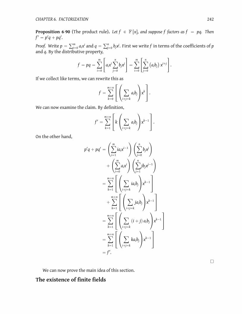
CHAPTER 6. FACTORIZATION 242
Proposition 6¨90 (The product rule). Let f P F rxs, and suppose f factors as f “ pq. Then
f1 “ p1q` pq1.
Proof. Write p “ř
m
i“0aix
iand q “
ř
n
j“0bjx
j. First we write f in terms of the coefficients of p
and q. By the distributive property,
f “ pq “
mÿ
i“0
«
aixi
nÿ
j“0
bjxj
ff
“
mÿ
i“0
«
nÿ
j“0
`
aibj
˘
xi`j
ff
.
If we collect like terms, we can rewrite this as
f “
m`nÿ
k“0
»
–
¨
˝
ÿ
i`j“k
aibj
˛
‚xk
fi
fl .
We can now examine the claim. By definition,
f1“
m`nÿ
k“1
»
–k
¨
˝
ÿ
i`j“k
aibj
˛
‚xk´1
fi
fl .
On the other hand,
p1q` pq
1“
˜
mÿ
i“1
iaixi´1
¸˜
nÿ
j“0
bjxj
¸
`
˜
mÿ
i“0
aixi
¸˜
nÿ
j“1
jbjxj´1
¸
“
m`nÿ
k“1
»
–
¨
˝
ÿ
i`j“k
iaibj
˛
‚xk´1
fi
fl
`
m`nÿ
k“1
»
–
¨
˝
ÿ
i`j“k
jaibj
˛
‚xk´1
fi
fl
“
m`nÿ
k“1
»
–
¨
˝
ÿ
i`j“k
pi` jq aibj
˛
‚xk´1
fi
fl
“
m`nÿ
k“1
»
–
¨
˝
ÿ
i`j“k
kaibj
˛
‚xk´1
fi
fl
“ f1.
We can now prove the main idea of this section.
The existence of finite fields

CHAPTER 6. FACTORIZATION 243
Theorem 6¨91. For any irreducible integer p, and for any n P N`, there exists a field with pn
elements.
Proof. First, suppose p “ 2. If n “ 1, the field Z2 proves the theorem. If n “ 2, the field
Z2 〈x2 ` x` 1〉 proves the theorem. We may therefore assume that p ‰ 2 or n ‰ 1, 2.
Let f “ xpn
´ x P Zp rxs. By Kronecker’s Theorem, there exists a field D such that Zp Ď D,
and f factors into linear polynomials over D. Let E “ tα P D : f pαq “ 0u. We claim that Ehas p
nelements, and that E is a field.
To see that E has pn
elements, it suffices to show that f has no repeated linear factors.
Recall that f “ xpn
´ x. The definition of a formal derivative tells us that
f1“ p
nxpn´1´ 1.
In Zp, pn “ 0, so we can simplify f1as
f1“ 0´ 1 “ ´1.
When we assumed that f had a repeated linear factor, we concluded that x ´ a divides f1.
However, we see now that f1 “ ´1, and x´a certainly does not divide´1, since deg px´ aq “
1 ą 0 “ deg p´1q. That assumption leads to a contradiction; so, f has no repeated linear
factors.
We now show that E is a field. By its very definition, E consists of elements of D; thus,
E Ď D. We know that D is a field, and thus a ring; we can therefore use the Subring Theorem
to show thatE is a ring. Once we have that, we have to find an inverse for any nonzero element
of E.
For the Subring Theorem, let a, b P E. We must show that ab and a´ b are both roots of f ;
they would then be elements ofE by definition of the latter. You will show in Question 6.93(a)
that ab is a root of f . For subtraction, we claim that
pa´ bqpn
“ apn
´ bpn
.
We proceed by induction.
Inductive base: Assume n “ 1. Observe that
pa´ bqp“ a
p`
p´1ÿ
i“1
p´1qi
ˆ
p
i
˙
aibp´i` p´1q
pbp.
By assumption, p is an irreducible integer, so its only divisors in N are itself and 1. For any
i P N`, then, the integerˆ
p
i
˙
“p!
i! pp´ iq!
can be factored into the two integers
ˆ
p
i
˙
“ p ¨pp´ 1q!
i! pp´ iq!;

CHAPTER 6. FACTORIZATION 244
the fractionpp´1q!
i!pp´iq!is an integer precisely because no element of the denominator can divide
p. Using Question 6.93(b), we can rewrite pa´ bqp
as
pa´ bqp“ a
p`
p´1ÿ
i“1
p´1qi p!
i! pp´ iq!aibp´i` p´1q
pbp
“ ap` p ¨
p´1ÿ
i“1
p´1qi pp´ 1q!
i! pp´ iq!aibp´i` p´1q
pbp
“ ap` 0` p´1q
pbp
“ ap` p´1q
pbp.
If p “ 2, then´1 “ 1, so either way we have ap ´ bp, as desired.
Inductive hypothesis: Assume that pa´ bqpn
“ apn
´ bpn
.
Inductive step: Applying the properties of exponents,
pa´ bqpn`1
“
”
pa´ bqpnı
p
“`
apn
´ bpn˘p
“ apn`1
´ bpn`1
,
where the final step uses the base case. Thus
pa´ bqpn
´ pa´ bq “`
apn
´ bpn˘
´ pa´ bq .
Again, a and b are roots of f , so apn
“ a and bpn
“ b, so
pa´ bqpn
´ pa´ bq “ pa´ bq ´ pa´ bq “ 0.
We see that a´ b is a root of f , and therefore a´ b P E.
Finally, we show that every nonzero element of E has an inverse in E. Let a P Ez t0u; by
definition, a P D. Since D is a field, there exists an inverse of a in D; call it b. By definition of
E, a is a root of f ; that is, apn
´ a “ 0. Multiply both sides of this equation by b2, and rewrite
to obtain apn´2 “ b. Using the substitutions b “ ap
n´2and a
pn
“ a in f pbq shows that:
f pbq “ bpn
´ b
“`
apn´2
˘pn
´ apn´2
“`
apn
¨ a´2˘p
n
´ apn´2
“`
apn˘p
n `
apn˘´2
´ apn´2
“ apn
¨ a´2´ a
pn´2
“ apn´2´ a
pn´2
“ 0.
We have shown that b is a root of f . By definition, b P E. Since b “ a´1 and awas an arbitrary
element of Ez t0u, every nonzero element of E has its inverse in E.
We have shown that

CHAPTER 6. FACTORIZATION 245
• E has pn
elements;
• it is a ring, since it is closed under multiplication and subtraction; and
• it is a field, since every nonzero element has a multiplicative inverse in E.
In other words, E is a field with pn
elements.
Euler’s theorems
The existence of finite fields means affords us some nice theorems that generalize Euler’s
Theorem.
Euler’s Theorem for arbitrary finite fields. If p is irreducible and f pxq “ xpn
´x, then f paq “
0 for all a P Zp.The proof is an exercise:
Question 6¨92 .Let Fn be a finite field of size n. (We now know such critters exist.)
(a) Use a corollary to Lagrange’s Theorem to explain why an´1 “ 1 for every nonzero a P Fn.
(b) Explain how we know n “ pk for some k P N`.
(c) Combine (a) and (b) to show Euler’s Theorem for arbitrary finite fields.
We can view this result a different way, too.
Euler’s Theorem for polynomials. Let p be an irreducible integer. For all a P Fp and for all
n P N`, apn
´ a “ 0, and thus apn
“ a and in Zp rxs, we have
xp´ x “
ź
aPZp
px´ aq .
Proof. Recall the F rxs is a unique factorization domain for any field F; Zp is a field, so xp ´ x
has a unique factorization. By Euler’s Theorem for arbitrary finite fields, a is a root of xp ´ x
for every a P Zp – Fp. Apply the Factor Theorem to complete the proof.
We can generalize Euler’s Theorem a little further.
Fermat’s Little Theorem on polynomials. Let k P N`. In Fpk rxs, we have
xpk
´ x “ź
aPFpk
px´ aq .
Proof. We first claim that every a P Fpk is a root of xpk
´ x. This is obvious when a “ 0,
so assume a lies in Fpkz t0u. By definition, the nonzero elements of Fpk form a group under
multiplication. By Corollary 4¨113 to Lagrange’s Theorem, the order of a dividesˇ
ˇFpkz t0uˇ
ˇ “
pk ´ 1, so a
pk´1 “ 1. Multiplying both sides by a, we have a
pk
“ a, which we can rewrite as
apk
´ a “ 0. By definition, a is a root of xpd
´ x. The Factor Theorem implies that x ´ a is a
factor of xpk
´ x. If a, b P Fpk are distinct, so are x´ a, x´ b P Fpk , so there are at least pk
such
factors. The fact that Fpk rxs is a unique factorization domain completes the proof.

CHAPTER 6. FACTORIZATION 246
Question 6¨93 .Let p be an irreducible integer and f pxq “ xp
n
´ x P Zp rxs. Define E “ Zp rxs 〈f 〉.
(a) Show that pa “ 0 for all a P E.
(b) Show that if f paq “ f pbq “ 0, then f pabq “ 0.
6¨7 Polynomial factorization in finite fields
We now turn to the question of factoring polynomials in R rxs. This material comes primarily
from [3]. Keep in mind that the goal of these notes is merely to show you how the ideas studied
so far combine into this problem, so the algorithms we study won’t be cutting-edge practice,
though they’re not bad, either.
This section factors polynomials whose coefficients come from finite fields, as that is
somewhat easier than factoring polynomials whose coefficients come from the integers. We
put that off to the next section.
Factorization of f P R rxs requires the following steps.
• Squarefree factorization is the process of removing multiples of factors of f ; that is,
if ga | f , then we want to work with
f
ga´1 , of which only g is a factor.
• Distinct degree factorization is the process of factoring a squarefree polynomial f into
polynomials g1, . . . , gm such that if gi factors as gi “ h1 ¨ ¨ ¨ hn, then deg h1 “ ¨ ¨ ¨ deg hn.
• Equal degree factorization is the process of factoring each distinct degree factor gi
into its equal degree factors h1, . . . , hn.
Example 6¨94. Suppose R “ Z2. Let
f pxq “ x16` x
13` x
11` x
10` x
9` x
8` x
7` x
5` x
2.
You can see that g pxq “ x2
is a factor of f , so f is not squarefree. (It is not typically this
easy.) Squarefree factorization identifies this factor and removes it, reducing the problem to
factoring
g pxq “ x2
and h pxq “ x14` x
11` x
9` x
8` x
7` x
6` x
5` x
3` 1.
Distinct degree factorization factors h as
`
x6` x
5` x
4` x
3` x
2` x` 1
˘ `
x8` x
7` x
5` x
4` x
3` x` 1
˘
. (6.4)
Equal degree factorization focuses on the second two factors, giving us
“`
x3` x` 1
˘ `
x3` x
2` 1
˘‰ “`
x4` x` 1
˘ `
x4` x
2` 1
˘‰
. (6.5)
Notice how the second and third factors in (6.5), which come from the second factor of (6.4),
have the same degree. Likewise, the second and third factors of (6.5), which have the same
degree, come from the third factor of (6.4).

CHAPTER 6. FACTORIZATION 247
For the rest of this section, we assume that p P N is irreducible and f P Zp rxs.
It would be nice to proceed in order, but the approach we take requires us to perform
distinct- and equal-degree factorization first.
Distinct degree factorization.
We accomplish distinct-degree factorization via Fermat’s Little Theorem on polyomials.
Example 6¨95. Suppose p “ 5. You already know from basic algebra that
x5´ x “ x
`
x4´ 1
˘
“ x`
x2´ 1
˘ `
x2` 1
˘
“ x px´ 1q px` 1q`
x2` 1
˘
.
We are working in Z5, so 1 “ ´4. Thus x ` 1 “ x ´ 4, and px´ 2q px´ 3q “ px2 ´ 5x` 6q “
px2 ` 1q. This means that we can write
x5´ x “ x px´ 1q px´ 2q px´ 3q px´ 4q “
ź
aPZ5
px´ aq ,
as claimed.
Generalization of Fermat’s Little Theorem for polynomials. Let k, q P N`, and a “ qk.
Then xpa
´ x is the product of all monic irreducible polynomials in Fpk rxs whose degree divides q.
Proof. Let f P Fpk rxs be monic and irreducible of degree n. We will show that
f |`
xpa
´ x˘
ðñ n | a.
Assume first that f divides xpa
´ x. By unique factorization and Fermat’s Little Theorem on
polynomials, f factors into linear polynomials x ´ c, where c P Fpa . Let α be any one of the
corresponding roots, and let E “ Fpk pαq. Using the basis B of Theorem 6¨75, we see that
|E| “`
pk˘n
“ pkn
, since it has |B| “ n basis elements, and pk
choices for each coefficient of a
basis element.
Now, Fpa is the extension of E by the remaining roots of xpa
´ x, one after the other. By
reasoning similar to that for E, we see that pa “
ˇ
ˇFpaˇ
ˇ “ |E|b “ pbkn
for some b P N`.
Rewriting the extreme sides of that equation, we have pbkn “ p
a “ pqk
, whence bkn “ qk and
n | q.
Conversely, assume n | q. A straightforward computation verifies that
pq´ 1 “ pp
n´ 1q
`
pq´n` p
q´2n` ¨ ¨ ¨ ` p
n` 1
˘
.
Let r “ pq´n ` pq´2n ` ¨ ¨ ¨ ` pn ` 1; a straightforward computation verifies that
xpq´1´ 1 “
`
xpn´1´ 1
˘ `
xppn´1qpr´1q
` xppn´1qpr´2q
` ¨ ¨ ¨ ` xpn´1` 1
˘
.

CHAPTER 6. FACTORIZATION 248
Algorithm 6.1 Distinct degree factorization
inputsf P Zp rxs, squarefree and monic, of degree n ą 0
outputsp1, . . . , pm P Zp rxs, a distinct-degree factorization of f
doLet h0 “ x
Let f0 “ f
Let i “ 0
while fi ‰ 1 doIncrement i
Let hi be the remainder of division of hp
i´1 by f
Let pi “ gcd phi ´ x, fi´1q
Let fi “fi´1
pi
Let m “ i
return p1, . . . , pm
Rewrite this as
xpq
´ x “`
xpn
´ x˘ `
xppn´1qpr´1q
` xppn´1qpr´2q
` ¨ ¨ ¨ ` xpn´1` 1
˘
. (6.6)
Construct Fpkn “ Fpk rxs 〈f 〉, and let α be the corresponding root x` 〈f 〉 of f . Fermat’s Little
Theorem tells us αpn
“ α. Equation (6.6) tells us xpn
´ x divides xpq
´ x, so x ´ α is also a
root of xpq
´ x. Similar reasoning implies xpq
´ x divides xpa
´ x, so α is also a root of xpa
´ x.
Thus, px´ αq | gcd`
f, xpa
´ x˘
in Fpn . By hypothesis, f is irreducible; the only divisors it has
are 1 and f itself. But x´ α divides the gcd, implying that gcd`
f, xpa
´ x˘
“ f ; in other words,
f |`
xpa
´ x˘
, as claimed.
The Generalization of Fermat’s Little Theorem for polynomials suggests an “easy” algo-
rithm to compute the distinct degree factorization of f P Zp rxs. See algorithm 6.1.
Theorem 6¨96. Algorithm 6.1 terminates with each pi the product of the factors of f that are all of
degree i.
Proof. Note that the second and third steps of the loop are an optimization of the computation
of gcd
´
xpi
´ x, f
¯
; you can see this by thinking about how the Euclidean algorithm would
compute the gcd. So termination is guaranteed by the fact that eventually deg hp
ią deg fi:
the generalization of Fermat’s Little Theorem for polynomials implies that at this point, all
distinct degree factors of f have been removed. Correctness is guaranteed by the fact that in
each step we are computing gcd
´
xpi
´ x, f
¯
.
Example 6¨97. Returning to Z5 rxs, let’s look at
f “ x px` 3q`
x3` 4
˘
.
Do not assume whether this factorization is into irreducible elements. Expanded, f “ x5 `
3x4 ` 4x2 ` 2x. When we plug it into algorithm 6.1, the following occurs:

CHAPTER 6. FACTORIZATION 249
• For i “ 1,
– the remainder of division of h5
0“ x5 by f is h1 “ 2x
4 ` x2 ` 3x;
– p1 “ x3 ` 2x2 ` 2x;
– f1 “ x2 ` x` 1.
• For i “ 2,
– the remainder of division of h5
1“ 2x20 ` x10 ` 3x5 by f is h2 “ x;
– p2 “ gcd p0, f1q “ f1;
– f2 “ 1.
Thus the distinct degree factorization of f is
f “`
x3` 2x
2` 2x
˘ `
x2` x` 1
˘
.
This demonstrates that the original factorization was not into irreducible elements, since
x px` 3q is not equal to either of the two new factors, so that x3 ` 4must have a linear factor
as well.
Question 6¨98 .Compute the distinct degree factorization of f “ x
5 ` x4 ` 2x3 ` 2x2 ` 2x ` 1 in Z5 rxs. This
factorization is in irreducible elements; explain how we know this.
Question 6¨99 .Suppose that we don’t want the factors of f , but only its roots. Explain how we can use
gcd pxp ´ x, f q to give us the maximum number of roots of f in Zp. Use the polynomial from
Example 6.98 to illustrate your argument.
Equal degree factorization
Once we have a distinct degree factorization of f P Zp rxs as f “ p1 ¨ ¨ ¨ pm, where each pi is
the product of the factors of degree i of a squarefree polynomial f , we need to factor each pi
into its irreducible factors. Here we consider the case that p is an odd prime; the case where
p “ 2 requires different methods.
Take any pi, and let its factorization into irreducible polynomials of degree i be pi “
q1 ¨ ¨ ¨ qn. Suppose we select at random some h P Zp rxs with deg h ă n. If pi and h share a
common factor, then gcd ppi, hq ‰ 1, and we have found a factor of pi. Otherwise, we will try
the following. Since each qj is irreducible and of degree i,⟨qj
⟩is a maximal ideal in Zp rxs, so
Zp rxs ⟨qj
⟩is a field with p
ielements. Denote it by F.
Lemma 6¨100. Let G be the multiplicative group of nonzero elements of F; that is, G “ Fz t0u. Let
a “pi´1
2, and let φ : GÑ G by φ pgq “ ga.
(A) φ is a group homomorphism of G.

CHAPTER 6. FACTORIZATION 250
(B) Its image, φ pGq, consists of the square roots of unity.
(C) |kerφ| “ a.
Proof. From the definition of a field, G is an abelian group under multiplication.
(A) Let g, h P G. Since G is abelian,
φ pghq “ pghqa“ pghq pghq ¨ ¨ ¨ pghqloooooooomoooooooon
a copies
“ pg ¨ g ¨ ¨ ¨ gqloooomoooon
a copies
¨ ph ¨ h ¨ ¨ ¨ hqloooomoooon
a copies
“ gaha“ φ pgqφ phq .
(B) Let y P φ pGq; by definition, there exists g P G such that
y “ φ pgq “ ga.
Corollary 4¨113 to Lagrange’s Theorem, with the fact that |G| “ pi ´ 1, implies that
y2“ pg
aq2“
ˆ
gpi´1
2
˙
2
“ gpi´1“ 1.
We see that y is a square root of unity. We chose y P φ pGq arbitrarily, so every element of φ pGq
is a square root of unity.
(C) Observe that g P kerφ implies ga “ 1, or g
a ´ 1 “ 0. That makes g an ath root of
unity. Since g P kerφwas chosen arbitrarily, kerφ consists of ath roots of unity. By the Factor
Theorem, each g P kerφ corresponds to a linear factor x ´ g of xa ´ 1. There can be at most
a such factors, so there can be at most a distinct elements of kerφ; that is, |kerφ| ď a. Since
φ pGq consists of the square roots of unity, similar reasoning implies that there are at most
two elements in φ pGq. Since G has pi ´ 1 elements, the Isomorphism Theorem tells us that
Gkerφ – φ pGq, so |Gkerφ| “ |φ pGq|. That gives us
pi´ 1 “ |G| “ |kerφ| |φ pGq| ď a ¨ 2 “
pi ´ 1
2¨ 2 “ p
i´ 1.
The inequality is actually an equality, forcing |kerφ| “ a.
To see how Lemma 6¨100 is useful, consider a nonzero coset in F,
rhs “ h`⟨qj
⟩P F.
As a field, F can have no zero divisors, so h can have no common factor with qj. As qj is irre-
ducible, this gives us h R⟨qj
⟩, so rhs ‰ 0F, so rhs P G. Raising rhs to the ath power gives us an
element of φ pGq. Part (B) of the lemma tells us that φ pGq consists of the square roots of unity
in G, so rhsa
is a square root of 1F, either 1F or ´1F. If rhsa“ 1F, then rhs
a´ 1F “ 0F. Recall
that F is a quotient ring, and rhs “ h`⟨qj
⟩. Thus
pha´ 1q `
⟨qj
⟩“ rhs
a´ 1F “ 0F P
⟨qj
⟩.
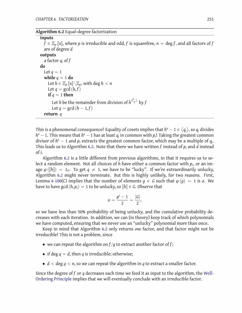
CHAPTER 6. FACTORIZATION 251
Algorithm 6.2 Equal-degree factorization
inputsf P Zp rxs, where p is irreducible and odd, f is squarefree, n “ deg f , and all factors of f
are of degree d
outputsa factor qi of f
doLet q “ 1
while q “ 1 doLet h P Zp rxs zZp, with deg h ă n
Let q “ gcd ph, f q
if q “ 1 then
Let h be the remainder from division of hpd´1
2 by f
Let q “ gcd ph´ 1, f q
return q
This is a phenomenal consequence! Equality of cosets implies that ha ´ 1 P
⟨qj
⟩, so qj divides
ha´ 1. This means that h
a´ 1 has at least qj in common with pi! Taking the greatest common
divisor of ha ´ 1 and pi extracts the greatest common factor, which may be a multiple of qj.
This leads us to Algorithm 6.2. Note that there we have written f instead of pi and d instead
of i.
Algorithm 6.2 is a little different from previous algorithms, in that it requires us to se-
lect a random element. Not all choices of h have either a common factor with pi, or an im-
age φ prhsq “ 1F. To get q ‰ 1, we have to be “lucky”. If we’re extraordinarily unlucky,
Algorithm 6.2 might never terminate. But this is highly unlikely, for two reasons. First,
Lemma 6¨100(C) implies that the number of elements g P G such that φ pgq “ 1 is a. We
have to have gcd ph, piq “ 1 to be unlucky, so rhs P G. Observe that
a “pi ´ 1
2“|G|
2,
so we have less than 50% probability of being unlucky, and the cumulative probability de-
creases with each iteration. In addition, we can (in theory) keep track of which polynomials
we have computed, ensuring that we never use an “unlucky” polynomial more than once.
Keep in mind that Algorithm 6.2 only returns one factor, and that factor might not be
irreducible! This is not a problem, since
• we can repeat the algorithm on f g to extract another factor of f ;
• if deg q “ d, then q is irreducible; otherwise;
• d ă deg q ă n, so we can repeat the algorithm in q to extract a smaller factor.
Since the degree of f or q decreases each time we feed it as input to the algorithm, the Well-
Ordering Principle implies that we will eventually conclude with an irreducible factor.

CHAPTER 6. FACTORIZATION 252
Example 6¨101. Recall from Example 6¨97 that
f “ x px` 3q`
x3` 4
˘
P Z5 rxs
gave us the distinct degree factorization
f “`
x3` 2x
2` 2x
˘ `
x2` x` 1
˘
.
The second polynomial is in fact the one irreducible quadratic factor of f ; the first polynomial,
p1 “ x3 ` 2x2 ` 2x, is the product of the irreducible linear factors of f . We use algorithm 6.2
to factor the linear factors.
• We have to pick h P Z5 rxs with deg h ă deg p1 “ 3. Let h “ x2 ` 3.
– Using the Euclidean algorithm, we find that h and f are relatively prime. (In par-
ticular, r1 “ f ´ px` 2q h “ 4x` 4, r2 “ h´ p4x` 1q r1 “ 4.)
– The remainder of division of h51´1
2 by f is 3x2 ` 4x` 4.
– Now q “ gcd pp3x2 ` 4x` 4q ´ 1, p1q “ x` 4.
– Return x` 4 as a factor of p1.
We did not know this factor from the outset! In fact, f “ x px` 3q px` 4q px2 ` x` 1q.
As with Algorithm 6.1, we need efficient algorithms to compute gcd’s and exponents in
order to perform Algorithm 6.2. Doing these as efficiently as possible is beyond the scope of
these notes, but we do in fact have relatively efficient algorithms to do both: the Euclidean
algorithm (Algorithm 5.1 on page 181) and fast exponentiation (Section 5¨5).
Question 6¨102 .Use the distinct degree factorization of Example 6¨97 and the fact that f “ x px` 3q px3 ` 4q
to find a complete factorization of f , using only the fact that you now know three irreducible
factors f (two linear, one quadratic).
Squarefree factorization over a field of nonzero characteristic
Another approach to squarefree factorization is to combine the previous two algorithms
in such a way as to guarantee that, once we identify an irreducible factor, we remove all pow-
ers of that factor from f before proceeding to the next factor. See Algorithm 6.3.
Example 6¨103. In Question 6.104 you will try (and fail) to perform a distinct degree factor-
ization on f “ x5 ` x3 using only Algorithm 6.1. Suppose that we use algorithm 6.3 to factor
f instead.
• Since f is monic, b “ 1.
• With i “ 1, distinct-degree factorization gives us h1 “ 4x3, q1 “ x
3 ` x, f1 “ x2.

CHAPTER 6. FACTORIZATION 253
Algorithm 6.3 Squarefree factorization in Zp rxsinputsf P Zp rxs
outputsAn irreducible factorization f “ bp
α11 ¨ ¨ ¨ p
αmm
doLet b “ lc pf q
Let h0 “ x
Let f0 “ b´1 ¨ f After this step, f is monic
Let i “ j “ 0
while fi ‰ 1 doOne step of distinct degree factorization
Increment i
Let hi be the remainder of division of hp
i´1 by f
Let qi “ gcd phi ´ x, fi´1q
Let fi “fi´1
qi
Find the equal degree factors of qi
while qi ‰ 1 doIncrement j
Find a degree-i factor pj of qi using algorithm 6.2
Let qi “qi
pj
Divide out all copies of pj from fi
Let αj “ 1
while pj divides fi doIncrement αj
Let fi “fi
pj
Let m “ j
return b, p1, . . . , pm, α1, . . . , αm

CHAPTER 6. FACTORIZATION 254
– Suppose that the first factor that Algorithm 6.2 gives us is x. We can then divide
f1 twice by x, so αj “ 3 and we conclude the innermost loop with f1 “ 1.
– Algorithm 6.2 subsequently gives us the remaining factors x ` 2 and x ` 3, none
of which divides f1 more than once..
The algorithm thus terminates with b “ 1, p1 “ x, p2 “ x`2, p3 “ x3, α1 “ 3, and α2 “ α3 “ 1.
Question 6¨104 .Explain why Algorithm 6.1 might not work for f “ x
5 ` x3. Then try the algorithm on f in
Z5 rxs, and explain why the result is incorrect.
6¨8 Factoring integer polynomials
We conclude, at the end of this chapter, with factorization in Z rxs. The previous section
showed how to factor a polynomial in an arbitrary finite field whose characteristic is an odd
irreducible integer. We can use this technique to factor a polynomial f P Z rxs. As in the
previous section, this method is not necessarily the most efficient, but it does illustrate tech-
niques that are used in practice.
We show this using the example
f “ x4` 8x
3´ 33x
2` 120x´ 720.
Suppose f factors as
f “ pα1
1¨ ¨ ¨ p
αm
m.
Now let p P N` be odd and irreducible, and considerpf P Zp rxs such that the coefficients ofpf
are the coefficients of f mapped to their cosets in Zp. That is,
pf “ r1spx4` r8s
px3` r´33s
px2` r120s
px` r´720s
p.
By the properties of arithmetic in Zp, we know thatpf will factor as
pf “ ppα1
1¨ ¨ ¨pp
αm
m,
where the coefficients of eachppi are the coefficients of pi mapped to their cosets in Zp. As we
will see, these ppi might not be irreducible for each choice of p; we might have instead
pf “ pqβ1
1 ¨ ¨ ¨pqβn
n
where eachpqi divides someppj. Nevertheless, we will be able to recover the irreducible factors
of f even from these factors; it will simply be more complicated. There are two possible so-
lutions to this issue: using one big irreducible p, or several small irreducibles along with the
Chinese Remainder Theorem.
Squarefree factorization over a field of characteristic zero
We first pause to discuss squarefree factorization in this context. When our ground field
has characteristic 0, we can compute the formal derivative f1of f , then g “ gcd pf, f 1q. The
quotientf
gis then squarefree.

CHAPTER 6. FACTORIZATION 255
Example 6¨105. Recall the polynomial of Example 6¨94,
f pxq “ x16` x
13` x
11` x
10` x
9` x
8` x
7` x
5` x
2.
Its formal derivative is
f1pxq “ 16x
15` 13x
12` 11x
10` 10x
9` 9x
8` 8x
7` 7x
6` 5x
4` 2x.
The Euclidean algorithm tells us g “ gcd pf, f 1q “ x, so f is not squarefree; as indicated earlier,
we can continue by factoring both g (which in this case is trivial) and h “ fg.
This example also explains why we didn’t use the formal derivative in the previous section:
over Z2 a lot of terms in the derivative become zero! Which ones? the terms derived from
those with even powers:
f1pxq ” x
12` x
10` x
8` x
6` x
4.
In this case, the gcd is x2, and while we can factor that out of f , we cannot reduce x
2itself to
squarefree form, because its derivative is 2x ” 0.
Question 6¨106 .Show that
f
gis squarefree if f P C rxs, f 1 is the usual derivative from Calculus, and g “
gcd pf, f 1q.
One big irreducible.
One approach is to choose an odd, irreducible p P N` sufficiently large that, once we
factorpf , the coefficient ai of any pi is either the corresponding coefficient inppi or (on account
of the modulus) the largest negative integer corresponding to it. Sophisticated methods to
obtain a good p exist, but for our purposes it suffices to choose p approximately twice the size
of the maximum coefficient of f .
Example 6¨107. The maximum coefficient in the example f given above is 720. There are
several irreducible integers larger than 1440 and “close” to it. We’ll try the closest one, 1447.
Using the techniques of the previous section, we obtain the factorization in Z1447 rxs
pf “ px` 12q px` 1443q`
x2` 15
˘
P Z1447 rxs .
It is “obvious” that this cannot be the correct factorization in Z rxs, because 1443 is too large.
On the other hand, properties of modular arithmetic tell us that
pf “ px` 12q px´ 4q`
x2` 15
˘
P Z1447 rxs .
In fact,
f “ px` 12q px´ 4q`
x2` 15
˘
P Z rxs .
This is why we chose an irreducible number that is approximately twice the largest coefficient
of f : it will recover negative factors as integers that are “too large”.
We mentioned above that we can get “false positives” in the finite field.

CHAPTER 6. FACTORIZATION 256
Example 6¨108. Let f “ x2 ` 1. In Z5 rxs, this factors as x
2 ` r1s5“ px` r2s
5q px` r3s
5q, but
certainly f ‰ px` 2q px` 3q in Z rxs.
Avoiding this problem requires techniques that are beyond the scope of these notes. How-
ever, it is certainly easy enough to verify whether a factor of f is a factor of f using division;
once we find all the factors pqj ofpf that do not give us factors pi of f , we can try combinations
of them until they give us the correct factor. Unfortunately, this can be very time-consuming,
which is why in general one would want to avoid this problem entirely.
Several small primes.
For various reasons, we may not want to try factorization modulo one large prime; in
this case, it would be possible to factor using several small primes, then recover f using the
Chinese Remainder Theorem. Recall that the Chinese Remainder Theorem tells us that if
gcd`
mi, mj
˘
“ 1 for each 1 ď i ă j ď n, then we can find x satisfying
$
’
’
’
’
&
’
’
’
’
%
rxs “ rα1s in Zm1 ;rxs “ rα2s in Zm2 ;
...
rxs “ rαns in Zmn ;
and rxs is unique in ZN where N “ m1 ¨ ¨ ¨mn. If we choose m1, . . . , mn to be all irreducible,
they will certainly satisfy gcd`
mi, mj
˘
“ 1; if we factor f in each Zmi , we can use the Chinese
Remainder Theorem to recover the coefficients of each pi from the correspondingpqj.
Example 6¨109. Returning to the polynomial given previously; we would like a unique solu-
tion in Z720 (or so). Unfortunately, the factorization 720 “ 24 ¨ 32 ¨ 5 is not very convenient
for factorization. We can, however, use 3 ¨ 5 ¨ 7 ¨ 11 “ 1155:
• in Z3 rxs,pf “ x3 px` 2q;
• in Z5 rxs,pf “ px` 1q px` 2q x2;
• in Z7 rxs,pf “ px` 3q px` 5q px2 ` 1q; and
• in Z11 rxs,pf “ px` 1q px` 7q px2 ` 4q.
If we examine all these factorizations, we can see that there appears to be a “false positive”
in Z3 rxs; we should have
f “ px` aq px` bq`
x2` c
˘
.
The easiest of the coefficients to recover will be c, since it is unambiguous that
$
’
’
&
’
’
%
c “ r0s3
c “ r0s5
c “ r1s7
c “ r4s11

CHAPTER 6. FACTORIZATION 257
In fact, the Chinese Remainder Theorem tells us that c “ r15s P Z1155.Recovering a and b is more difficult, as we have to guess “correctly” which arrangement of
the coefficients in the finite fields gives us the arrangement corresponding toZ. For example,
the system$
’
’
&
’
’
%
b “ r0s3
b “ r1s5
b “ r3s7
b “ r1s11
gives us b “ r276s1155
, which turns out to be wrong, but the system
$
’
’
&
’
’
%
b “ r0s3
b “ r2s5
b “ r5s7
b “ r1s11
gives us b “ r12s1155
, the correct coefficient in Z.
The drawback to this approach is that, in the worst case, we would try 24 “ 16 combi-
nations before we can know whether we have found the correct one. In practice, therefore,
sophisticated criteria and techniques are used to reassemble f .
Question 6¨110 .Factor x
7`8x6`5x5`53x4´26x3`93x2´96x`18 using each of the two approaches described
here.
Question 6¨111 .Let f pxq “ x
8 ` 5x7 ` 9x5 ` 53x4 ` 40x3 ` 72x ` 360. We want to factor f over Z by first
factoring over Zp for some “good” values of p.
(a) Suppose we try to factor f over Z3. Someone might argue that this is actually a bad idea,
because it gives false positives; that is, it allows too much factorization. Why?
Hint: Think about an “obvious” factorization of f when you write its coefficients mod-
ulo 3, and whether this “obvious” factorization also occurs over Z.
(b) Based on the answer to part (a), what would be bad values of p?
(c) If we wanted to factor f overZp for several irreducibles p, then reconstruct the factoriza-
tion overZ using the Chinese Remainder Theorem, without using for p any of the moduli
you identified in (b), and you wanted to use
(i) the smallest p possible, how many such p would you want to use, and what are they?
(ii) the fewest p possible, how many such p would you want to use, and what are they?

Chapter 7
Some important, noncommutativegroups and rings
We’ve identified a number of common structures shared by certain systems. Most of the
systems we’ve studied have enjoyed commutative operations, but we generally worked with-
out that assumption, when possible. We now consider systems that are built with a non-
commutative operation. These appear in many interesting situations.
7¨1 Functions
The systems we will consider in this chapter are organized primarily around functions. We’ve
already defined a function, but we haven’t made much use of the definition, so it can’t hurt
to remind ourselves what they are.
A function is any relation F Ĺ S ˆ T such that every s P S corresponds
to exactly one ps, tq P F. If F is a function, we write F : S Ñ T instead of
F Ď S ˆ T, and F psq “ t instead of ps, tq P F. When F psq “ t, we call t the
image of s, and s the preimage of t. Notice that we can never have F psq “ t
and F psq “ u whenever t ‰ u.
The domain of F in the definition above is S; the range of F is T in the definition above; and
the image of F, or Img pFq, is the subset of T whose elements actually have a preimage. More
precisely,
Img pFq “ tt P T : f psq “ t for some s P Su .
In this chapter, we generally assume the domain and range of a function are the same; in such
cases, we say that F is a function on S.Two functions are equalwhen they map every element of the same domain to the same
image. That is, if f : SÑ T and g : SÑ T, then f “ g if and only if f psq “ g psq for every s P S.
Remark 7¨1. A subtle difference distinguishes our definition of a function from the one you’ve
encountered before: F psqmust be defined for every s P S. Thus, the following relations are not
functions according to our definition:
258

CHAPTER 7. SOME IMPORTANT, NONCOMMUTATIVE GROUPS AND RINGS 259
• F : NÑ N by F pnq “?n, because
?2 R N;
• F : RÑ R by F prq “ 1r, because 10 is undefined.
We never use the word “function” unless we know it is defined for every element of its domain.
The usual convention is to use lower-case letters for function names, but try not to forget
that functions are really a special subset of a Cartesian product.
Addition and multiplication of functions
Let S and T be sets where addition or multiplication is defined, though S and T need not
be rings or groups. Let f, g : SÑ T. We “add” two functions f and g and obtain a new function
f ` g by identifying pf ` gq psq with the sum of the images of s. That is,
pf ` gq psq “ f psq ` g psq .
We “multiply” two functions f and g in a similar way. That is,
pfgq psq “ f psq ¨ g psq .
Since f and g are both defined for all s P S, the sum and product of f and g is also a function.
Example 7¨2. Let S “ Z, and let f and g be functions on S such that f psq “ s2 and f psq “ s´2.
Then f ` g : SÑ S according to the rule
pf ` gq psq “ f psq ` g psq “ s2` ps´ 2q ,
while fg : SÑ S according to the rule
pfgq psq “ f psq ¨ g psq “ s2ps´ 2q .
Fact 7¨3. If T is a ring under addition and multiplication of its elements, then the setF of all functions
mapping S to T is a ring under addition and multiplication of functions.
Notice that S need not be a ring itself.
Why is this true? We already showed closure above. We now show some of the other proper-
ties, leaving the rest as an exercise. Assume that S is a ring under addition and multiplication
of its elements.
associativity of addition? Let f, g, h P F . We need to show that f ` pg` hq “ pf ` gq ` h.
This is true if the two functions f ` pg` hq and pf ` gq ` hmap every element of S to
the same image. So, let s P S. We use the fact that S is a ring to show that the associative
property carries over to F . For the left-hand sum,
pf ` pg` hqq psq “ f psq ` pg` hq psq “ f psq ` rg psq ` h psqs .
For the right-hand sum,
ppf ` gq ` hq psq “ pf ` gq psq ` h psq “ rf psq ` g psqs ` h psq .

CHAPTER 7. SOME IMPORTANT, NONCOMMUTATIVE GROUPS AND RINGS 260
We have translated from a problem about functions f , g, and h to one about f psq, g psq,
and h psq, which are elements of the ring T. Ring addition is associative, so
f psq ` rg psq ` h psqs “ rf psq ` g psqs ` h psq .
Substitution gives us
pf ` pg` hqq psq “ ppf ` gq ` hq psq .
Recall that s is an arbitrary element of S, so the above equation is true for every element
of S, showing that the functions f ` pg` hq and pf ` gq ` h are equal. Addition of
functions is associative.
additive identity? Since T is a ring, it has an additive identity, 0. We claim that the additive
identity of F is the zero function, z : S Ñ S by z psq “ 0 for all s P S. (We usually
write this function simply as 0, but for the sake of pedantry, we use more function-like
notation. Pedantry has its uses sometimes.) To show that this is indeed the additive
identity, we must show that z ` f “ f and f ` z “ f for all f P F . So, let f P F . We
must show that show that z` f , f ` z, and f map every element of S to the same image.
So, let s P S. By substitution,
pz` f q psq “ z psq ` f psq “ 0` f psq “ f psq
and
pf ` zq psq “ f psq ` z psq “ f psq ` 0 “ f psq .
Substitution gives us
pf ` zq psq “ f psq “ pz` f q psq .
Recall that s is an arbitrary element of S, so the above equation is true for every element
of S, showing that the functions f ` z, z` f , and f are equal. This shows that z really is
the additive identity of addition of functions.
Question 7¨4 .Show that the remaining properties of a commutative ring are true; that is, addition of func-
tions is commutative; every element has an additive inverse; multiplication of functions is
associative; there is a multiplicative identity function; and multiplication of functions dis-
tributes over addition of functions. Show also that multiplication of functions is commutative
if and only if T is a commutative ring.
Question 7¨5 .Show that F is almost never a field, even if T is a field! (To answer this question fully, you
should give a very specific criterion that determines when F is a field, and that also shows
there are “very few” F that can satisfy this requirement.)

CHAPTER 7. SOME IMPORTANT, NONCOMMUTATIVE GROUPS AND RINGS 261
Functions under composition
It is not uncommon to compose functions, yet even if students do it routinely, they often
forget the term. Let S and T be sets (neither necessarily a ring) and suppose f : S Ñ T and
g : T Ñ U. The composition g ˝ f of functions f and g is a function that maps any s P S to
g pf psqq.
Example 7¨6. Suppose S “ N and f, g : S Ñ S by f psq “ s2, g ptq “ t ´ 2. Then g ˝ f : S Ñ S
according to the rule
pg ˝ f q psq “ g pf psqq “ g`
s2˘
“ s2´ 2,
while f ˝ g : SÑ S according to the rule
pf ˝ gq psq “ f pg psqq “ f ps´ 2q “ ps´ 2q2.
Under certain conditions, composition of functions can also be an operation on functions.
The main point is that g needs to be defined on the image of f . This is easy to satisfy if the
domain and range of both functions are the same, as in the example above.
So, let S be an arbitrary set, and letF be the set of all functions on S. Which properties of
an operation does composition satisfy?
closure? Let f, g P F . Is g ˝ f P F also? Well, yes: g is defined for all t P S, so for any s P S, we
know that pg ˝ f q psq P S regardless of the value of f psq “ t. Hence, g ˝ f will be defined
for all s P S, and is a function on S, so an element of F .
associative? Let f, g, h P F . Is h ˝ pg ˝ f q “ ph ˝ gq ˝ f ? To find out, we have to make sure
that every s P S has the same destination, regardless of which path it takes. So let s P S.
The left path, h ˝ pg ˝ f q, asks us to evaluate pg ˝ f q psq first, and then evaluate h on the
result. Let u “ pg ˝ f q psq and v “ h puq. The right path, ph ˝ gq ˝ f , asks us to evaluate
f psq first, and then evaluate h ˝ g on the result. Let t “ f psq.
The question comes down to checking whether v “ ph ˝ gq ptq. By definition, ph ˝ gq psq “
h pg ptqq. What is g ptq? Recall that u “ pg ˝ f q psq “ g pf psqq “ g ptq. So, g ptq “ u, which
means h pg ptqq “ h puq “ v. We have now verified that v “ ph ˝ gq ptq, so indeed
ph ˝ pg ˝ f qq psq “ pph ˝ gq ˝ f q psq .
Recall that swas chosen arbitrarily, so h˝pg ˝ f q “ ph ˝ gq˝ f regardless of the preimage
s P S. The two functions are equal, and composition is associative.
What about the identity property? Define ι : SÑ S by ι psq “ s. As this is defined for all s P S,
ι P F .
Question 7¨7 .Show that the function ι is also an identity for composition; that is, ι ˝ f “ f and f ˝ ι “ f for
all f P F .

CHAPTER 7. SOME IMPORTANT, NONCOMMUTATIVE GROUPS AND RINGS 262
Question 7¨8 .On the other hand, show that not all functions have inverse elements. That is, find a set S and
a function f on S such that the inverse of f , if it exists, is not a function on S. Hint: One such
function appears earlier in this section.
Question 7¨9 .Also, show that composition of functions is not always commutative. That is, find a set S and
two functions f and g on S such that f ˝ g ‰ g ˝ f .
We have just shown the following important fact.
Fact 7¨10. The set of all functions on a set S is a monoid under the operation of composition. In general,
it is not a group.
Having said that, some sets of functions on a set S are a group; one has to choose the right
subset of F . Most of this chapter considers such special sets, but we first turn to an example
you may not have expected.
Differentiation and integration
In Calculus, you learned about differentiation and integration. In some cases, we can con-
sider them to be functions of functions! For now, we’ll make life easy and work (mostly) with
polynomials, which are functions. Let R be any ring.
Fact 7¨11. Differentiation with respect to x is a function on R rxs; that is,d
dx: R rxs Ñ R rxs. If R is a
field of characteristic zero, then integration with respect to x is a function on R rxs.
Why? Keeping in mind that elements of R are constant, this becomes straightforward with
the familiar rules of differentiation and integration:
d
dxprnx
n` ¨ ¨ ¨ ` r1x` r0q “ nrnx
n´1` ¨ ¨ ¨ ` 2r2x` r1 P R rxs
and, if R is a field,
ż
rnxn` ¨ ¨ ¨ ` r1x` r0 dx “ pn` 1q
´1rn ¨ x
n`1` ¨ ¨ ¨ ` 2
´1r1 ¨ x
2` r0x P R rxs .
Either way, the result is an element ofR rxs, and the formula is deterministic, so differentiation
and integration are defined for every element of the polynomial ring, showing that they are
functions.
(Notice that we do not tack on an arbitrary constant of integration, but use zero, instead.
This is okay for our purposes.)
The upshot of this is that if you take the set of all functions of R rxs, thend
dxand
ş
dx are
included. Building on what we wrote above, then, expressions such as 0 `ş
dx and ι ˝ d
dx
actually make sense.
Question 7¨12 .Why must the field have characteristic zero for
ş
dx to be a function?

CHAPTER 7. SOME IMPORTANT, NONCOMMUTATIVE GROUPS AND RINGS 263
7¨2 Permutations
Certain applications of mathematics involve the rearrangement of a list of n elements. It is
common to refer to such rearrangements as permutations.
Definition 7¨13. A list is a sequence. Let V be any finite list. A permutation is a one-to-one,
onto function whose domain and range are both V.
Throughout this section, V is a list of n elements, unless we say otherwise.
Example 7¨14. If V is a list of all the elements in a finite group or ring, an isomorphism on V
is a permutation.
The order of the elements matters in a permutation: the lists pa, d, k, rq ‰ pa, k, d, rq even
though ta, d, k, ru “ ta, k, d, ru. For the sake of convenience, we usually write V as a list of
natural numbers between 1 and |V|, but it can be any finite list.
Example 7¨15. The permutation of the list pred, green, blueq to pgreen, red, blueq is equivalent
to the permutation of the list p1, 2, 3q to p2, 1, 3q. We care only about the change in the entries’
positions, not in the values of those entries.
The importance of permutations is twofold. First, group theory is a pretty neat and useful
thing in itself, and we will see eventually that all finite groups can be modeled by groups of
permutations. Anything that can model every possible group is by that very fact important.
Besides that, permutations relate to the factorization of polynomials. The polynomial
x4 ´ 1 can be factored over C as
px` 1q px´ 1q px` iq px´ iq ,
and
px´ 1q px` 1q px´ iq px` iq .
On account of the commutative property, it doesn’t matter what order we list the factors;
this corresponds to a permutation, and is related to another idea that we will study, called
field extensions. Field extensions can be used to solve polynomials equations, and since the
order of the extensions doesn’t really matter, permutations are important to determining the
structure of the extension that solves a polynomial.
Permutations as functions
Example 7¨16. Let S “ pa, d, k, rq. Define a permutation on the elements of S by
f pxq “
$
’
’
’
&
’
’
’
%
r, x “ a;
a, x “ d;
k, x “ k;
d, x “ r.
Notice that f is one-to-one, and f pSq “ pr, a, k, dq.

CHAPTER 7. SOME IMPORTANT, NONCOMMUTATIVE GROUPS AND RINGS 264
We can represent the same permutation on V “ p1, 2, 3, 4q, a generic list of four elements.
Define a permutation on the elements of V by
π piq “
$
’
’
’
&
’
’
’
%
2, i “ 1;
4, i “ 2;
3, i “ 3;
1, i “ 4.
Here π is one-to-one, and π piq “ j is interpreted as “the jth element of the permuted list is
the ith element of the original list.” You could visualize this as
position i in original list position j in permuted list
1 Ñ 2
2 Ñ 4
3 Ñ 3
4 Ñ 1
Thus π pVq “ p4, 1, 3, 2q. If you look back at f pSq, you will see that in fact the first element of
the permuted list, f pSq, is the fourth element of the original list, S.
It should not surprise you that the identity function is a “do-nothing” permutation, just
as it was a “do-nothing” symmetry of the triangle in Section 3¨6.
Proposition 7¨17. LetV be a set of n elements. The function I : V Ñ V by I pxq “ x is a permutation
on V. In addition, for any permutation α on V, I ˝ α “ α and α ˝ I “ α.
Question 7¨18 .Why is Proposition 7¨17 true?
As functions, the composition of two permutations is also a function. It gets a little bet-
ter. . .
Lemma 7¨19. The composition of two permutations on a list of n elements is a permutation on the
same list.
Proof. Let V be a set of n elements, and α, β permutations of V. Let γ “ α ˝ β. We claim that γ
is a permutation. To show this, we must show that γ is a one-to-one function whose domain
and range are both V. By definition, the domain and range of γ are both V; it remains to show
that γ is one-to-one. Let x, y P V and assume that γ pxq “ γ pyq; substituting the definition of
γ,
α pβ pxqq “ α pβ pyqq .
Because they are permutations, α and β are one-to-one functions. Since α is one-to-one, we
can simplify the above equation to
β pxq “ β pyq ;
and since β is one-to-one, we can simplify the above equation to
x “ y.

CHAPTER 7. SOME IMPORTANT, NONCOMMUTATIVE GROUPS AND RINGS 265
We assumed that γ pxq “ γ pyq, and found that this forced x “ y. By definition, γ is a one-to-
one function. We already explained why its domain and range are both V, so γ is a permuta-
tion.
In Example 7¨16, we wrote a permutation as a piecewise function. This is burdensome; we
would like a more efficient way to denote permutations.
Notation 7¨20. The tabular notation for a permutation on a list of n elements is a 2ˆnmatrix
α “
ˆ
1 2 ¨ ¨ ¨ n
α1 α2 ¨ ¨ ¨ αn
˙
indicating that α p1q “ α1, α p2q “ α2, . . . , α pnq “ αn. Again, α piq “ j indicates that the jth
element of the permuted list is the ith element of the original list.
Example 7¨21. Recall V and π from Example 7¨16. In tabular notation,
π “
ˆ
1 2 3 4
2 4 3 1
˙
because π moves
• the element in the first position to the second;
• the element in the second position to the fourth;
• the element in the third position nowhere; and
• the element in the fourth position to the first.
Then
π p1, 2, 3, 4q “ p4, 1, 3, 2q .
Notice that the tabular notation for π looks similar to the table in Example 7¨16.
We can also use π to permute different lists, so long as the new lists have four elements:
π p3, 2, 1, 4q “ p4, 3, 1, 2q ;
π p2, 4, 3, 1q “ p1, 2, 3, 4q ;
π pa, b, c, dq “ pd, a, c, bq .
Question 7¨22 .For the permutation
α “
ˆ
1 2 3 4 5 6
1 5 2 4 6 3
˙
,
(a) Evaluate α p1, 2, 3, 4, 5, 6q.
(b) Evaluate α p1, 5, 2, 4, 6, 3q.
(c) Evaluate α p6, 3, 5, 2, 1, 4q.

CHAPTER 7. SOME IMPORTANT, NONCOMMUTATIVE GROUPS AND RINGS 266
Groups of permutations
Permutations form groups in a very natural way.
Definition 7¨23. For n ě 2, denote by Sn the set of all permutations of a list of n elements.
Example 7¨24. For n “ 2, 3 we have
S2 “
"ˆ
1 2
1 2
˙
,
ˆ
1 2
2 1
˙*
S3 “
"ˆ
1 2 3
1 2 3
˙
,
ˆ
1 2 3
2 1 3
˙
,
ˆ
1 2 3
3 2 1
˙
,
ˆ
1 2 3
1 3 2
˙
,
ˆ
1 2 3
2 3 1
˙
,
ˆ
1 2 3
3 1 2
˙*
.
Is there some structure to Sn? By definition, a permutation is a one-to-one function.
Fact 7¨10 on page 262 tells us that the set of functions on a set is a monoid under compo-
sition of functions. The identity function is one-to-one, and the composition of one-to-one
functions is also one-to-one, so Sn has an identity and is closed under composition. In addi-
tion, Sn inherits the associative property from the larger set of functions. Already, then, we
can conclude that Sn is a monoid. However, one-to-one functions have inverses, which leads
us to ask whether Sn is also a group.
Theorem 7¨25. For all n ě 2 pSn, ˝q is a group.
Notation 7¨26. Normally we just write Sn, assuming that the operation is composition of func-
tions. It is common to refer to Sn as the symmetric group of n elements.
Proof. Let n ě 2. We have to show that Sn satisfies the properties of a group under the oper-
ation of composition of functions. Proposition 7¨17 tells us that the identity function acts as
an identity in Sn, and Lemma 7¨19 tells us that Sn is closed under composition. We showed in
Section 7¨1 that functions are associative; as a subset of functions, Sn satisfies the associative
property.
We still have to show that Sn satisfies the inverse property. Let V be a list of n elements.
Let α P Sn. By definition of a permutation, α is one-to-one; since V is finite, α is onto. Since α
is one-to-one, it has an inverse function α´1
, which satisfies the relationship that, for every
v P V,
α´1pα pvqq “ v and α
`
α´1pvq
˘
“ v.
Since I pvq “ v for every v P V, we have shown that α´1 ˝ α “ α ˝ α´1 “ I. The function α
´1
is also a one-to-one, onto function on V, so α´1 P Sn! We chose α as an arbitrary permutation
of n elements, so Sn satisfies the inverse property.
As claimed, Sn satisfies all four properties of a group.
Question 7¨27 .Compute the order of
α “
ˆ
1 2 3 4
3 1 4 2
˙
.

CHAPTER 7. SOME IMPORTANT, NONCOMMUTATIVE GROUPS AND RINGS 267
A final question: how large is each Sn? In other words, “how many permutations are there
of n elements?” A counting argument called the multiplication principle shows that there are
n! “ n ¨ pn´ 1q ¨ pn´ 2q ¨ ¨ ¨ 3 ¨ 2 ¨ 1
such permutations. Why? Given any list of n elements,
• we have n positions to move the first element, including its current position;
• we have n´1 positions to move the second element, since the first element has already
taken one spot;
• we have n´ 2 positions to move the third element, since the first and second elements
have already take two spots;
• etc.
We have shown the following.
Lemma 7¨28. For each n P N`, |Sn| “ n!
Question 7¨29 .How many elements are in S4 and S5? Try listing all the elements of S4.
A hint of things to come.
You won’t work extensively with groups of permutations just yet, but we mentioned ear-
lier that all finite groups are really groups of permutations, and it’s convenient to close here
with an example of this.
Fact 7¨30. S3 – D3 as groups.
Why? We map D3 to S3 by considering how each symmetry of the triangle permutes the three
vertices. As long as this new point of view preserves the operation, the fact that D3 and S3
have six elements shows that such a map is a bijection, and we are done.
We take as our guide the labeling of the triangle’s vertices from Section 3¨6. For any sym-

CHAPTER 7. SOME IMPORTANT, NONCOMMUTATIVE GROUPS AND RINGS 268
metry σ P S3 map
f pσq “
$
’
’
’
’
’
’
’
’
’
’
’
’
’
’
’
’
’
’
’
’
’
’
’
’
&
’
’
’
’
’
’
’
’
’
’
’
’
’
’
’
’
’
’
’
’
’
’
’
’
%
˜
1 2 3
1 2 3
¸
, if σ “ ι;
˜
1 2 3
1 3 2
¸
, if σ “ φ;
˜
1 2 3
2 3 1
¸
, if σ “ ρ;
˜
1 2 3
3 1 2
¸
, if σ “ ρ2;
˜
1 2 3
3 2 1
¸
, if σ “ ρφ;
˜
1 2 3
2 1 3
¸
, if σ “ ρ2φ.
This map is clearly a bijection.
Question 7¨31 .Verify that f pφ2q “ rf pφqs
2, f pρ2q “ rf pρqs
2, f pρ3q “ rf pρqs
3. (This will be a big deal in a
moment.)
Explanation of Fact 7¨30, continued: We must verify that f preserves the operation. We have
thirty-six products to check, but with a little cleverness we can reduce this significantly. For
instance, regardless of the value of σ,0
f pσιq “subst
f pσq “ f pσq ˝ I,
and the same can be shown easily for f pισq, giving us 11 products more or less for free. That
leaves twenty-five products to check. This quickly becomes a bit tedious, but remember that
D3 enjoys the property φρ “ ρ2φ. If this map is an isomorphism, we should expect a corre-
sponding relationship in their images. To help us out, let’s name α “ f pφq and β “ f pρq.
Indeed,
f pφq f pρq “ αβ “
ˆ
1 2 3
1 3 2
˙
˝
ˆ
1 2 3
2 3 1
˙
“
ˆ
1 2 3
3 2 1
˙
and by Question 7.31,
f`
ρ2˘
f pφq “ β2α “
ˆ
1 2 3
3 1 2
˙
˝
ˆ
1 2 3
1 3 2
˙
“
ˆ
1 2 3
3 2 1
˙
.
This allows us to rewrite all products of S3 where f pφq appears before f pρq exactly the same
way we rewrite all products of D3 where φ appears before ρ. We can verify the remaining
twenty operations by mere substitution and application of these properties. For instance,
f`
φρ2˘
“ f`
ρ4φ˘
“ f``
ρ3ρ˘
φ˘
“ f pρφq “ βα

CHAPTER 7. SOME IMPORTANT, NONCOMMUTATIVE GROUPS AND RINGS 269
while
f pφq f`
ρ2˘
“ αβ2“ pαβq β “
`
β2α˘
β “ β2pαβq “ β
2`
β2α˘
“ β4α “
`
β3β˘
α “ βα,
so the two are equal, as desired.
Question 7¨32 .Find an explicit isomorphism from S2 to Z2. (It’s not nearly as involved as Fact 7¨30.)
7¨3 Morphisms
We saw earlier that the set of all functions on a set S is a monoid under composition, even
when S is not. What of the set F of all homomorphisms on a monoid S, or the set of all
isomorphisms on S? Remember that “on S” means the domain and range are both S.
Homomorphisms
Theorem 7¨33. F is a monoid under composition.
Proof. The proof of every property is identical to that of Fact 7¨10, except for the closure and
identity properties. The challenge with the identity property is easy to dispose of, as Ques-
tion 4.74 shows the identity homomorphism I acts as an identity under composition. The
challenge with the closure property is that the operation is composition of functions; so, we
have to show that the set is closed under composition.
We begin with closure; we need to show that for any homomorphisms f and g on S, f ˝ g
is also a homomorphism on S. To that end, let f, g P F , and define h “ f ˝ g. We need to show
that h P F ; in other words, h pstq “ h psq h ptq for any s, t P S. So, let s, t P S. By substitution,
h pstq “ pf ˝ gq pstq “ f pg pstqq .
By definition, g pstq “ g psq g ptq , so we can rewrite the equation above as
h pstq “ f pg psq g ptqq .
Let x “ g psq and y “ g ptq. By definition, f pxyq “ f pxq f pyq, so we can rewrite the equation
above as
h pstq “ f pxyq “ f pxq f pyq “ rf pg psqqs rf pg ptqqs “ rpf ˝ gq psqs rpf ˝ gq ptqs “ h psq h ptq .
Recall that s and t were arbitrary in S; the ends of this equation show that h satisfies the ho-
momorphism property. Since h “ f ˝ g, we have shown that the composition of f and g, two
homomorphisms on S, is itself a homomorphism S. Since f and g were arbitrary homomor-
phisms on S, we have shown that composition of homomorphisms satisfies closure in the set
of all homomorphisms on S. That is, F is closed.
We have shown that the set of all homomorphisms on a set S satisfies the associative,
closure, and identity properties. This set forms a monoid.

CHAPTER 7. SOME IMPORTANT, NONCOMMUTATIVE GROUPS AND RINGS 270
Is it also a group?
Fact 7¨34. If S is a monoid with more than one element, the set of homomorphisms on S is not a group.
Why not? Suppose S has more than one element. Define a function f on S as f psq “ я; that
is, f maps every element of S to the identity. We claim that f is a homomorphism: It clearly
preserves the identity, since f pяq “ я. As for preserving the operation: for any s, t P S we
have
f pstq “ я and f psq f ptq “ яя “ я,
so f pstq “ f psq f ptq. On the other hand, f is not one-to-one; to see why, let s, t P S be distinct
elements of S; that is, s ‰ t. By definition, f psq “ я and f ptq “ я. As f is not one-to-one,
its inverse cannot be a function, let alone a homomorphism. Thus, f´1
is not in the set F of
homomorphisms on S. We have an element f of F with no inverse in F ; by definition, F is
not a group.
Question 7¨35 .The only monoid with one element is the set tяu, whose only element is the identity under
whatever the operation may be. It is not a very interesting monoid, except that it sometimes
serves as an exception to what would otherwise be a rule. Is this one of those cases? Is the
set F of homomorphisms on tяu a group?
Isomorphisms
We saw that the set F of homomorphisms on a monoid of at least two elements did not
form a group, effectively because at least one homomorphism was not one-to-one. What if
we looked only at one-to-one homomorphisms? For convenience, write G for this set.
Fact 7¨36. The set of one-to-one homomorphisms is also not a group under composition of functions.
Why not? Consider the monoid of integers under addition. You found in Question 2.55(a) that
the doubling function is an isomorphism between Z and 2Z. Since 2Z Ĺ Z, the doubling
function is a homomorphism on Z.
This has big implications. The doubling function is a one-to-one homomorphism on Z,
so it is in G. If G is to be a group, the doubling function must have an inverse function in G.
What would that inverse function be? Let’s call it g; to be an element of G, gmust be defined
for every element of Z. Sometimes, this is obvious: . . . , g p´2q “ ´1, g p0q “ 0, g p2q “ 1,
g p4q “ 2, . . . . But what is g p1q? It has to be an integer, but we just saw g covers every integer
by some even integer. That means g p1q cannot exist, because no possible images are left! But
if g p1q does not exist, g is not defined on all elements of S, so g R G!
Now, g is the only possible inverse for the doubling function; since g R G, the doubling
function has no inverse inG, despite being an element ofG itself. The only possible conclusion
is that G cannot be a group.
The problem, of course, is that the doubling function is not onto. In Fact 7¨34, the problem
was that not all homomorphisms are one-to-one; in Fact 7¨36, the problem was that not all
one-to-one homomorphisms are onto. In a last-ditch attempt to obtain a group, we’ll look at

CHAPTER 7. SOME IMPORTANT, NONCOMMUTATIVE GROUPS AND RINGS 271
the set of homomorphisms on S that are both one-to-one and onto. That is, we’ll look at the
set of isomorphisms.
(This may look like an act of desperation, and from a certain point of view, it is. However,
it is also how a lot of research works. You ask a question about a set, and when you find that
it doesn’t work for all elements of that set, you identify a subset for which you hope it does
work. Unless you’re completely off-base, this eventually leads to an interesting result. Along
the way, you get additional interesting results, namely, why it does not work in other subsets.)
Theorem 7¨37. The setH of isomorphisms on a monoid is a group under composition of functions.
Notice that we get a group, even though the underlying set is a monoid.
Proof. As with Theorem 7¨33, we need only worry about that which is not covered by Fact 7¨10:
closure and inverse proprerties.
For closure, we need to show that composition of isomorphisms is still an isomorphism.
Let f, g P H; that is, let f and g be any two isomorphisms on S. Let h “ f ˝ g; we need to show
that h P H; in other words, that h is an isomorphism. We have already showed that it is a
homomorphism in the proof of Theorem 7¨33, so we need only show that it is one-to-one and
onto. We show first that it is onto; let s P S. We need to find an element of S whose image
under h is s; we’ll try to use the structure of h to do this. Composition means that we can
calculate h by going through g and f :
?
f
&&s
? h
;;g
AA
Because f is onto, we can find t P S such that f ptq “ s; because g is onto, we can find u P S
such that g puq “ t. By definition,
h puq “ pf ˝ gq puq “ f pg puqq “ f ptq “ s,
so we have found an element of S that hmaps to s. Since s was arbitrary in S, h is onto.
To show that h is one-to-one, let s, t P S, and suppose
h psq “ h ptq .
We need to show that s “ t. By definition, h psq “ pf ˝ gq psq “ f pg psqq, and likewise h ptq “
f pg ptqq, so by substitution into our supposition we know
f pg psqq “ f pg ptqq .
To make the next steps a little easier, write y “ g psq and z “ g ptq. The equation immediately
above becomes f pyq “ f pzq. By hypothesis, f is one-to-one; by definition, y “ z. We now
have
g psq “ g ptq .
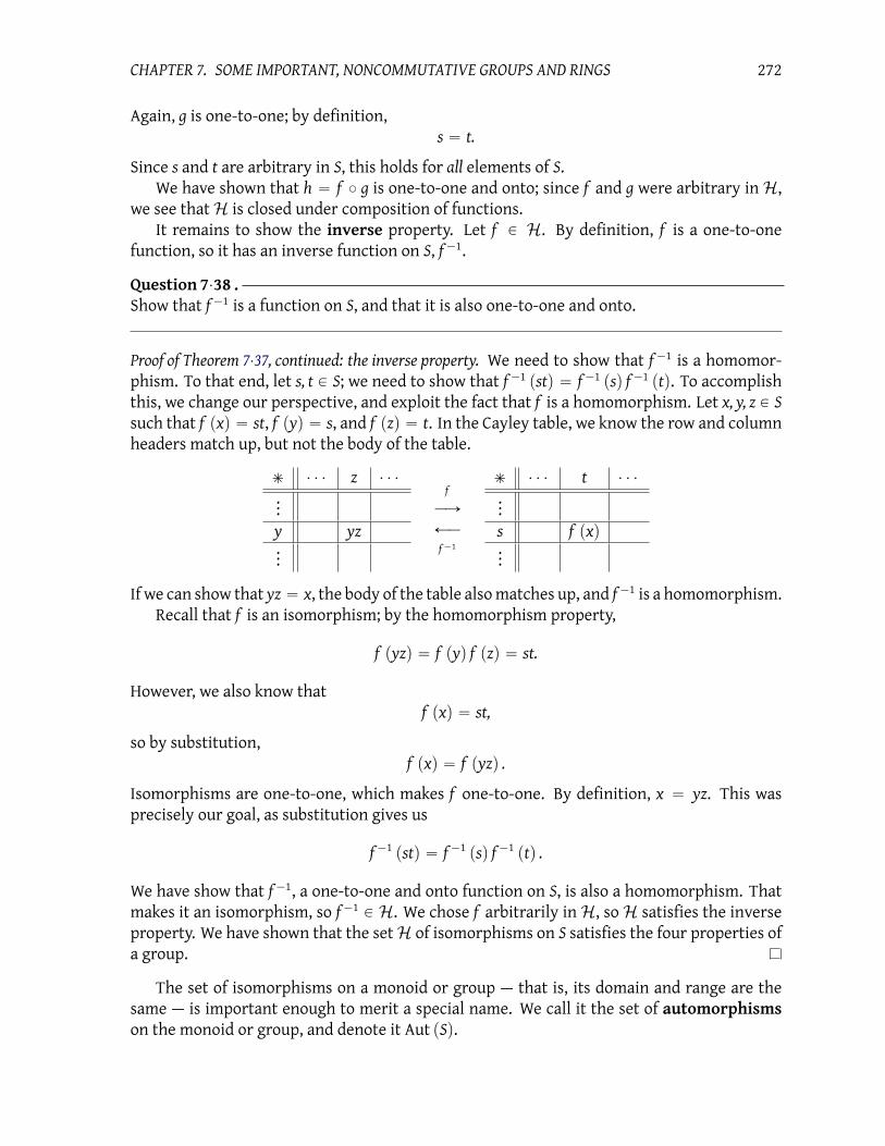
CHAPTER 7. SOME IMPORTANT, NONCOMMUTATIVE GROUPS AND RINGS 272
Again, g is one-to-one; by definition,
s “ t.
Since s and t are arbitrary in S, this holds for all elements of S.
We have shown that h “ f ˝ g is one-to-one and onto; since f and g were arbitrary inH,
we see thatH is closed under composition of functions.
It remains to show the inverse property. Let f P H. By definition, f is a one-to-one
function, so it has an inverse function on S, f´1
.
Question 7¨38 .Show that f
´1is a function on S, and that it is also one-to-one and onto.
Proof of Theorem 7¨37, continued: the inverse property. We need to show that f´1
is a homomor-
phism. To that end, let s, t P S; we need to show that f´1 pstq “ f
´1 psq f ´1 ptq. To accomplish
this, we change our perspective, and exploit the fact that f is a homomorphism. Let x, y, z P S
such that f pxq “ st, f pyq “ s, and f pzq “ t. In the Cayley table, we know the row and column
headers match up, but not the body of the table.
˙ ¨ ¨ ¨ z ¨ ¨ ¨
...
y yz
...
f
ÝÑ
ÐÝ
f´1
˙ ¨ ¨ ¨ t ¨ ¨ ¨
...
s f pxq...
If we can show that yz “ x, the body of the table also matches up, and f´1
is a homomorphism.
Recall that f is an isomorphism; by the homomorphism property,
f pyzq “ f pyq f pzq “ st.
However, we also know that
f pxq “ st,
so by substitution,
f pxq “ f pyzq .
Isomorphisms are one-to-one, which makes f one-to-one. By definition, x “ yz. This was
precisely our goal, as substitution gives us
f´1pstq “ f
´1psq f
´1ptq .
We have show that f´1
, a one-to-one and onto function on S, is also a homomorphism. That
makes it an isomorphism, so f´1 P H. We chose f arbitrarily inH, soH satisfies the inverse
property. We have shown that the setH of isomorphisms on S satisfies the four properties of
a group.
The set of isomorphisms on a monoid or group — that is, its domain and range are the
same — is important enough to merit a special name. We call it the set of automorphismson the monoid or group, and denote it Aut pSq.

CHAPTER 7. SOME IMPORTANT, NONCOMMUTATIVE GROUPS AND RINGS 273
Question 7¨39 .Recall from Question that f : ZÑ Zd is a homomorphism of rings, but not an isomorphism.
(a) Determine ker f . (It might help to use a specific value of n first.)
(b) Indicate how we know that Z ker f – Zn. (Eventually, we will show that G ker f – H
for any homomorphism f : G ÝÑ H that is onto.)

Chapter 8
Groups of permutations
You met permutations in Section 7¨2. The main goal of this chapter is to show that groups of
permutations are, in some sense, “all there is” to group theory, so in some sense, Section 8¨2 is
the point. Section 8¨1 develops a convenient way to denote permutations, and 8¨3 introduce
you to two special classes of groups of permutation. We conclude with a great example of an
application of symmetry groups in Section 8¨4.
8¨1 Cycle notation
Tabular notation of permutations is rather burdensome; a simpler and more compact nota-
tion is possible.
Cycles
Definition 8¨1. A cycle is a vector
α “ pα1 α2 ¨ ¨ ¨ αnq
that corresponds to the permutation where the entry in position α1 is moved to position α2;
the entry in position α2 is moved to position α3, . . . and the element in position αn is moved to
position α1. If a position is not listed in α, then the entry in that position is not moved. We call
such positions stationary. For the identity permutation where no entry is moved, we write
я “ I “ p1q .
The fact that the permutation αmoves the entry in position αn to position α1 is the reason
we call it a cycle; applying it repeatedly cycles the list of elements around, and on the nth
application the list returns to its original order.
Example 8¨2. Example 7¨21 considered the following permutation in tabular notation,
π “
ˆ
1 2 3 4
2 4 3 1
˙
.
274

CHAPTER 8. GROUPS OF PERMUTATIONS 275
To write it as a cycle, we can start with any position of the list we like. However, the conven-
tion is to start with the smallest position affected by the permutation. Since πmoves elements
out of position 1, we start with
π “ p1 ?q .
The second entry in the cycle tells us where πmoves the element in the position indicated by
the first entry, 1. From the tabular notation, we see that πmoves the element in position 1 to
position 2, so
π “ p1 2 ?q .
The third entry of cycle notation tells us where πmoves the element in the position indicated
by the second entry. The second entry indicates position 2. From the tabular notation, we see
that π moves the element in position 2 to position 4, so
π “ p1 2 4 ?q .
The fourth entry of cycle notation tells us where πmoves the element in the position indicated
by the third entry. The third element indicates position 4. From the tabular notation, we see
that πmoves the element in position 4 to position 1, so you might feel the temptation to write
π “ p1 2 4 1 ?q ,
but that misses the entire point of cycle notation: we have now returned to the position in-
dicated by the first entry, so we close the cycle:
π “ p1 2 4q .
The cycle p1 2 4q, indicates that
• the element in position 1 of a list moves to position 2;
• the element in position 2 of a list moves to position 4;
• the element in position 4 of a list moves to position 1.
What about the element in position 3? Since it doesn’t appear in the cycle notation, it must
be stationary. This agrees with what we wrote in the piecewise and tabular notations for π.
Question 8¨3 .Write every element of S3 in cycle notation.
Question 8¨4 .Let α “ p1 2 3q and β “ p2 3q. In this problem, you will verify two things about α and β.
(a) Verify that they are the same as the permutations designated α and β in the proof of
Fact 7¨30 on page 267.
(b) All elements of S3 can be written as compositions of α and β; that is, every element of S3
(in cycle form) has the form αiβjwhere 0 ď i ă 3 and 0 ď j ă 2.

CHAPTER 8. GROUPS OF PERMUTATIONS 276
Question 8¨5 .For α and β as defined in Question 8.4, show that β ˝ α “ α
2 ˝ β. (Notice that α, β P Sn for all
n ą 2, so as a consequence of this exercise Sn is not abelian for n ą 2.)
Question 8¨6 .Write the Cayley table for S3, with every element in the form α
iβj
where 0 ď i ă 3 and
0 ď j ă 2. Question 8.5 will make your life easier.
Question 8¨7 .In Fact 7¨30, we showed D3 – S3 by mapping ρ and φ of D3 to elements α and β of S3. We used
tabular notation at that time. Work through the proof again, this time using cycle notation
instead of tabular notation.
Not all permutations can be written as one cycle.
Example 8¨8. Consider the permutation in tabular notation
α “
ˆ
1 2 3 4
2 1 4 3
˙
.
We can easily start the cycle with α “ p1 2q, and this captures the behavior on the elements
in the first and second positions of a list, but what about the third and fourth positions? We
cannot write p1 2 3 4q; that would imply that the element in the second position is moved to
the third, and the element in the fourth position is moved to the first.
To solve this difficulty, we develop a simple arithmetic of cycles.
Cycle arithmetic
What operation should we apply to cycles? Cycles represent permutations; permutations
are functions; functions can be composed. Hence, the appropriate operation is composition.
Example 8¨9. Consider the cycles
β “ p2 3 4q and γ “ p1 2 4q .
What is the cycle notation for
β ˝ γ “ p2 3 4q ˝ p1 2 4q?
Cycles represent permutations, and permutations are closed under composition, tellingus
β ˝ γ is also a permutation. With any luck, it will be a permutation that we can write as a
cycle. What we need to do, then, is determine how the permutation β ˝ γmoves a list of four
elements around. If that permutation can be represented as a cycle, then we’ve answered the
question.
Since an element in the first position is moved, we should be able to write
β ˝ γ “ p1 ?q .

CHAPTER 8. GROUPS OF PERMUTATIONS 277
3 2β
oo 1γ
oo
β˝γ
2 4oo 2oo
4 3oo 3oo
1 1oo 4oo
Figure 8¨1: Diagram of how β˝γmodifies a list of four elements, for β “ p2 3 4q and γ “ p1 2 4q.
Where is this first element moved? Let’s apply the definition of composition: β˝γmeans, “first
apply γ; then apply β.” Figure 8¨1 show the basic idea; we refer to it throughout the example.
The first cycle entry considers the first element of the list, or the top row of Figure 8¨1; γ
moves the first element to the second position, and β then moves it to the third. It must be
that β ˝ γmoves an element from the first position to the third. We now know that
β ˝ γ “ p1 3 ?q .
The second cycle entry should tell us where β ˝ γ moves an element that starts in the third
position (not the second), illustrated by the third row of Figure 8¨1. Applying the definition
of composition again, we know that γ moves an element from the third position to. . . well,
nowhere, actually. So an element in the third position doesn’t move under γ; if we then apply
β, however, it moves to the fourth position. It must be that β ˝ γ moves an element from the
third position to the fourth. We now know that
β ˝ γ “ p1 3 4 ?q .
The third cycle entry should tell tell us where β˝γmoves and element that starts in the fourth
position, illustrated by the fourth row of Figure 8¨1. We know that γmoves an element in the
fourth position to the first position (4 is at the end of the cycle, so it moves to the beginning),
and βmoves elements in the first position. . . well, nowhere, actually. So β˝ γmoves elements
from the fourth position to the first position. This completes the cycle, so we now know that
β ˝ γ “ p1 3 4q .
Haven’t we missed something? What about an element that starts in the second position?
Since γmoves elements in the second position to the fourth, and βmoves elements from the
fourth position to the second, they undo each other, and the second position is stationary. It
is, therefore, absolutely correct that 2 does not appear in the cycle notation of β ˝ γ, and we see
this in the second row of Figure 8¨1.
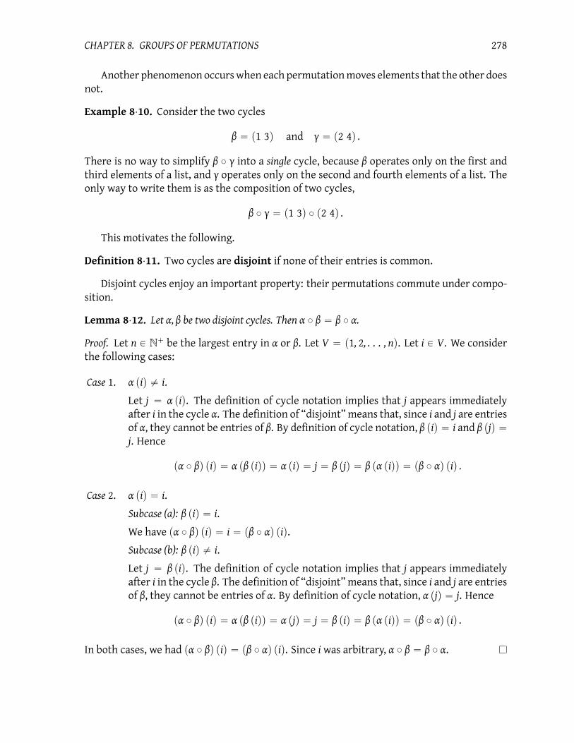
CHAPTER 8. GROUPS OF PERMUTATIONS 278
Another phenomenon occurs when each permutation moves elements that the other does
not.
Example 8¨10. Consider the two cycles
β “ p1 3q and γ “ p2 4q .
There is no way to simplify β ˝ γ into a single cycle, because β operates only on the first and
third elements of a list, and γ operates only on the second and fourth elements of a list. The
only way to write them is as the composition of two cycles,
β ˝ γ “ p1 3q ˝ p2 4q .
This motivates the following.
Definition 8¨11. Two cycles are disjoint if none of their entries is common.
Disjoint cycles enjoy an important property: their permutations commute under compo-
sition.
Lemma 8¨12. Let α, β be two disjoint cycles. Then α ˝ β “ β ˝ α.
Proof. Let n P N` be the largest entry in α or β. Let V “ p1, 2, . . . , nq. Let i P V. We consider
the following cases:
Case 1. α piq ‰ i.
Let j “ α piq. The definition of cycle notation implies that j appears immediately
after i in the cycle α. The definition of “disjoint” means that, since i and j are entries
of α, they cannot be entries of β. By definition of cycle notation, β piq “ i and β pjq “
j. Hence
pα ˝ βq piq “ α pβ piqq “ α piq “ j “ β pjq “ β pα piqq “ pβ ˝ αq piq .
Case 2. α piq “ i.
Subcase (a): β piq “ i.
We have pα ˝ βq piq “ i “ pβ ˝ αq piq.
Subcase (b): β piq ‰ i.
Let j “ β piq. The definition of cycle notation implies that j appears immediately
after i in the cycle β. The definition of “disjoint” means that, since i and j are entries
of β, they cannot be entries of α. By definition of cycle notation, α pjq “ j. Hence
pα ˝ βq piq “ α pβ piqq “ α pjq “ j “ β piq “ β pα piqq “ pβ ˝ αq piq .
In both cases, we had pα ˝ βq piq “ pβ ˝ αq piq. Since i was arbitrary, α ˝ β “ β ˝ α.
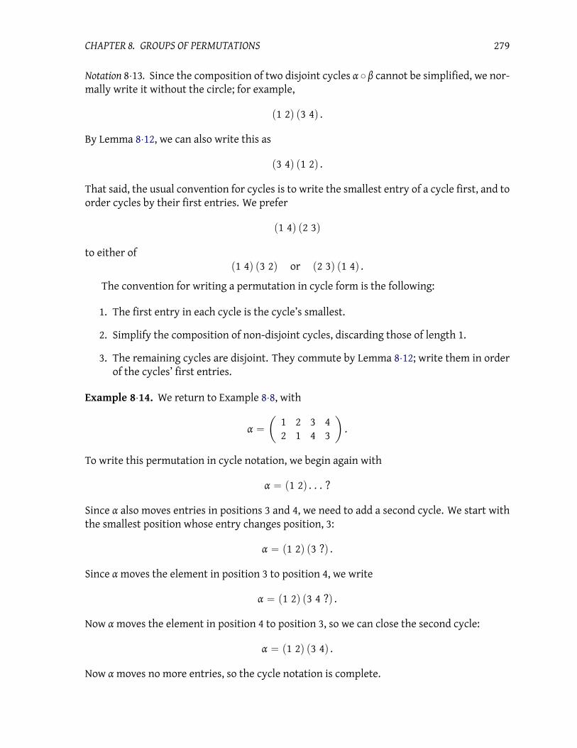
CHAPTER 8. GROUPS OF PERMUTATIONS 279
Notation 8¨13. Since the composition of two disjoint cycles α ˝ β cannot be simplified, we nor-
mally write it without the circle; for example,
p1 2q p3 4q .
By Lemma 8¨12, we can also write this as
p3 4q p1 2q .
That said, the usual convention for cycles is to write the smallest entry of a cycle first, and to
order cycles by their first entries. We prefer
p1 4q p2 3q
to either of
p1 4q p3 2q or p2 3q p1 4q .
The convention for writing a permutation in cycle form is the following:
1. The first entry in each cycle is the cycle’s smallest.
2. Simplify the composition of non-disjoint cycles, discarding those of length 1.
3. The remaining cycles are disjoint. They commute by Lemma 8¨12; write them in order
of the cycles’ first entries.
Example 8¨14. We return to Example 8¨8, with
α “
ˆ
1 2 3 4
2 1 4 3
˙
.
To write this permutation in cycle notation, we begin again with
α “ p1 2q . . . ?
Since α also moves entries in positions 3 and 4, we need to add a second cycle. We start with
the smallest position whose entry changes position, 3:
α “ p1 2q p3 ?q .
Since αmoves the element in position 3 to position 4, we write
α “ p1 2q p3 4 ?q .
Now αmoves the element in position 4 to position 3, so we can close the second cycle:
α “ p1 2q p3 4q .
Now αmoves no more entries, so the cycle notation is complete.

CHAPTER 8. GROUPS OF PERMUTATIONS 280
Permutations as cycles
We have come to the main result of this section.
Theorem 8¨15. Every permutation can be written as a composition of disjoint cycles.
The proof is constructive; we build the cycle notation for the permutation.
Proof. Let π P Sn. If π piq “ i for all i “ 1, . . . , n, then we can write π “ p1q. Otherwise, we can
find i1 P t1, . . . , nu such that π pi1q ‰ i1. Let i1 be the smallest such number. As Sn is finite, we
know πk “ p1q “ I for some k P t2, . . . , nu, and then π
k pi1q “ I pi1q “ i1. Let
αp1q“`
i1 π pi1q π pπ pi1qq ¨ ¨ ¨ πk´1pi1q
˘
.
By construction, αp1q
correctly describes how π moves elements in positions i1, π pi1q, . . . ,
πk´1 pi1q.
Ifπ “ αp1q, then we are done. Otherwise, we can find i2 P t1, . . . , nu z
i1, π pi1q , . . . , πk´1 pi1q
(
such thatπ pi2q ‰ i2. Choose the smallest such i2, and letαp2q “
`
i2 π pi2q π pπ pi2qq ¨ ¨ ¨ π`´1 pi2q
˘
,
where, as before π` pi2q “ i2.
Repeat this process until every non-stationary element of V appears in a cycle, gener-
ating αp3q
, . . . , αpmq
for non-stationary i3 R αp1q, αp2q
, i4 R αp1q, αp2q, αp3q
, and so on until im R
αp1q, . . . , α
pm´1q. There are only finitely many numbers π can move, so this process will not
continue indefinitely, and concludes with a finite list of cycles.
The remainder of the proof consists of two claims.
Claim 1: Each cycles is disjoint from any other.
By way of contradiction, assume that two cycles αpiq
and αpjq
are not disjoint. Without
loss of generality, assume i ă j. Let c be the first entry in αpjq
that also appears in αpiq
; by
construction, it is not the first element of αpjq
, so let a be the entry that precedes c in αpiq
,
and b the entry that precedes c in αpjq
. By construction, π paq “ c “ π pbq. Permutations are
one-to-one, so a “ b, but then b appears in αpiq
, contradicting our choice of c as the first entry
of αpjq
that appears in αpiq
. Hence, αpiq
and αpjq
are disjoint.
Claim 2: π “ αp1qαp2q ¨ ¨ ¨ αpmq.
Let i P V. We consider two cases.
If π piq “ i, then i could not have been used to begin construction of an α. Since π is a one-
to-one function, we cannot have π pkq “ i for any k ‰ i, either. By construction, i appears in
none of the αpjq
. By substitution, the expression`
αp1qαp2q ¨ ¨ ¨ αpmq
˘
piq simplifies to
`
αp1qαp2q¨ ¨ ¨ α
pmq˘
piq “ αp1q
`
αp2q
`
¨ ¨ ¨ αpmqpiq˘˘
“ i “ π piq .
So far, so good.
Assume, then, that π piq ‰ i. By construction, i appears in αpjq
for some j “ 1, 2, . . . , m. By
definition, αpjq piq “ π piq, so both i and π piq appear in α
pjq. By Claim 1, i and π piq do not appear
in αpkq
whenever k ‰ j. That guarantees αpkq piq “ i and α
pkq pπ piqq “ π piq. By substitution,

CHAPTER 8. GROUPS OF PERMUTATIONS 281
the expression`
αp1qαp2q ¨ ¨ ¨ αpmq
˘
piq simplifies to
`
αp1qαp2q¨ ¨ ¨ α
pmq˘
piq “ αp1q
`
αp2q
`
¨ ¨ ¨ αpm´1q
`
αpmqpiq˘˘˘
...
“ αp1q
`
αp2q
`
¨ ¨ ¨ αpj´1q
`
αpjqpiq˘˘˘
“ αp1q
`
αp2q
`
¨ ¨ ¨ αpj´1q
pπ piqq˘˘
...
“ π piq .
We have shown that`
αp1qαp2q¨ ¨ ¨ α
pmq˘
piq “ π piq .
Since i is arbitrary, π “ αp1q ˝ αp2q ˝ ¨ ¨ ¨ ˝ αpmq. That is, π is a composition of cycles. Since π was
arbitrary, every permutation is a composition of cycles.
Example 8¨16. Consider the following permutation written in tabular notation,
π “
ˆ
1 2 3 4 5 6 7 8
7 5 3 2 4 8 1 6
˙
.
The proof of Theorem 8¨15 constructs the cycles
αp1q“ p1 7q
αp2q“ p2 5 4q
αp3q“ p6 8q .
Notice that αp1q
, αp2q
, and αp3q
are disjoint. In addition, the only element of V “ p1, 2, . . . , 8q
that does not appear in an α is 3, because π p3q “ 3. Inspection verifies that
π “ αp1qαp2qαp3q.
We conclude with some examples of simplifying the composition of permutations.
Example 8¨17. Let α “ p1 3q p2 4q and β “ p1 3 2 4q. Notice that α ‰ β; check this on
V “ p1, 2, 3, 4q if this isn’t clear. In addition, α and β are not disjoint.
1. We compute the cycle notation for γ “ α ˝ β. We start with the smallest entry moved
by either α or β:
γ “`
1 ?˘
.
The notation α ˝ β means to apply β first, then α. What does β do with the entry in
position 1? It moves it to position 3. Subsequently, αmoves the entry in position 3 back
to the entry in position 1. The next entry in the first cycle of γ should thus be 1, but
that’s also the first entry in the cycle, so we close the cycle. So far, we have
γ “ p1q . . . ?

CHAPTER 8. GROUPS OF PERMUTATIONS 282
We aren’t finished, since α and β also move other entries around. The next smallest
entry moved by either α or β is 2, so
γ “ p1q p2 ?q .
Now β moves the entry in position 2 to the entry in position 4, and α moves the entry
in position 4 to the entry in position 2. The next entry in the second cycle of γ should
thus be 2, but that’s also the first entry in the second cycle, so we close the cycle. So far,
we have
γ “ p1q p2q . . . ?
Next, βmoves the entry in position 3, so
γ “ p1q p2q p3 ?q .
Where does βmove the entry in position 3? To the entry in position 2. Subsequently, α
moves the entry in position 2 to the entry in position 4. We now have
γ “ p1q p2q p3 4 ?q .
You can probably guess that 4, as the largest possible entry, will close the cycle, but to
be safe we’ll check: β moves the entry in position 4 to the entry in position 1, and α
moves the entry in position 1 to the entry in position 3. The next entry of the third
cycle will be 3, but this is also the first entry of the third cycle, so we close the third
cycle and
γ “ p1q p2q p3 4q .
Finally, we simplify γ by not writing cycles of length 1, so
γ “ p3 4q .
Hence
pp1 3q p2 4qq ˝ p1 3 2 4q “ p3 4q .
2. Now we compute the cycle notation for β˝α, but with less detail. Again we start with 1,
which αmoves to 3, and β then moves to 2. So we start with
β ˝ α “ p1 2 ?q .
Next, αmoves 2 to 4, and βmoves 4 to 1. This closes the first cycle:
β ˝ α “ p1 2q . . . ?
We start the next cycle with position 3: α moves it to position 1, which β moves back
to position 3. This generates a length-one cycle, so there is no need to add anything.
Likewise, the element in position 4 is also stable under β ˝ α. Hence we need write no
more cycles;
β ˝ α “ p1 2q .
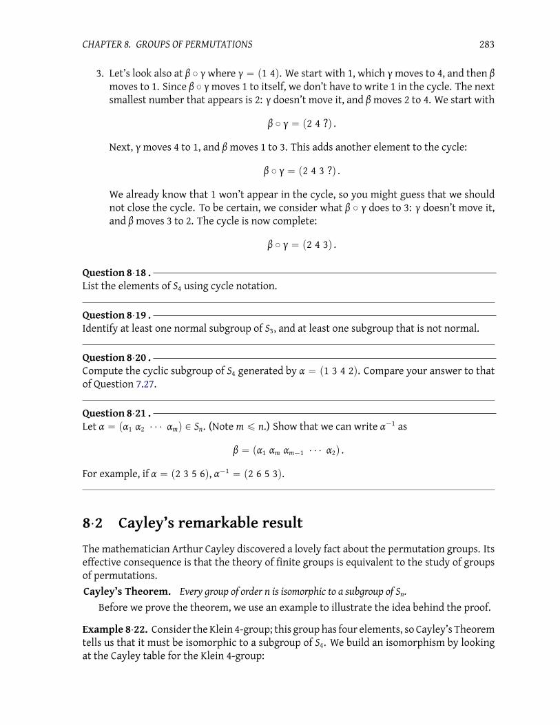
CHAPTER 8. GROUPS OF PERMUTATIONS 283
3. Let’s look also at β ˝ γ where γ “ p1 4q. We start with 1, which γmoves to 4, and then β
moves to 1. Since β ˝ γmoves 1 to itself, we don’t have to write 1 in the cycle. The next
smallest number that appears is 2: γ doesn’t move it, and βmoves 2 to 4. We start with
β ˝ γ “ p2 4 ?q .
Next, γmoves 4 to 1, and βmoves 1 to 3. This adds another element to the cycle:
β ˝ γ “ p2 4 3 ?q .
We already know that 1 won’t appear in the cycle, so you might guess that we should
not close the cycle. To be certain, we consider what β ˝ γ does to 3: γ doesn’t move it,
and βmoves 3 to 2. The cycle is now complete:
β ˝ γ “ p2 4 3q .
Question 8¨18 .List the elements of S4 using cycle notation.
Question 8¨19 .Identify at least one normal subgroup of S3, and at least one subgroup that is not normal.
Question 8¨20 .Compute the cyclic subgroup of S4 generated by α “ p1 3 4 2q. Compare your answer to that
of Question 7.27.
Question 8¨21 .Let α “ pα1 α2 ¨ ¨ ¨ αmq P Sn. (Note m ď n.) Show that we can write α
´1as
β “ pα1 αm αm´1 ¨ ¨ ¨ α2q .
For example, if α “ p2 3 5 6q, α´1 “ p2 6 5 3q.
8¨2 Cayley’s remarkable result
The mathematician Arthur Cayley discovered a lovely fact about the permutation groups. Its
effective consequence is that the theory of finite groups is equivalent to the study of groups
of permutations.
Cayley’s Theorem. Every group of order n is isomorphic to a subgroup of Sn.
Before we prove the theorem, we use an example to illustrate the idea behind the proof.
Example 8¨22. Consider the Klein 4-group; this group has four elements, so Cayley’s Theorem
tells us that it must be isomorphic to a subgroup of S4. We build an isomorphism by looking
at the Cayley table for the Klein 4-group:

CHAPTER 8. GROUPS OF PERMUTATIONS 284
ˆ я a b ab
я я a b ab
a a я ab b
b b ab я a
ab ab b a я
To find a permutation appropriate to each element, we first label the elements:
я ú 1,
aú 2,
bú 3,
abú 4.
Using tabular notation for permutations, we define a map f from the Klein 4-group to S4 by
f pxq “
ˆ
1 2 3 4
` px ¨ яq ` px ¨ aq ` px ¨ bq ` px ¨ abq
˙
, (8.1)
where ` pyq is the label that corresponds to y.
This notation affords us a powerful means of expression, but can be hard to read. Suppose
f maps an element x of the Klein 4-group to the permutation σ “ p1 2q p3 4q of S4 Any per-
mutation of S4 is a one-to-one function on a list of 4 elements, say p1, 2, 3, 4q. By definition,
σ p2q “ 1. Since σ “ f pxq, we can likewise write, pf pxqq p2q “ 1. This double-evaluation can
be hard to look at; it does not say “f pxq times 2,” but rather, “f pxq of 2”? To avoid confusion,
we adopt the following notation to emphasize that f pxq is a permutation, and thus a function:
f pxq “ fx.
It’s much easier to look at fx p2q and understand we want fx p2q “ σ p1q.
Let’s compute fa:
fa “
ˆ
1 2 3 4
` pa ¨ яq ` pa ¨ aq ` pa ¨ bq ` pa ¨ abq
˙
.
The first entry has the value ` pa ¨ eq “ ` paq “ 2, telling us that
fa “
ˆ
1 2 3 4
2 ` pa ¨ aq ` pa ¨ bq ` pa ¨ abq
˙
.
The next entry has the value ` pa ¨ aq “ ` pa2q “ ` pяq “ 1, telling us that
fa “
ˆ
1 2 3 4
2 1 ` pa ¨ bq ` pa ¨ abq
˙
.
The third entry has the value ` pa ¨ bq “ ` pabq “ 4, telling us that
fa “
ˆ
1 2 3 4
2 1 4 ` pa ¨ abq
˙
.

CHAPTER 8. GROUPS OF PERMUTATIONS 285
The final entry has the value ` pa ¨ abq “ ` pa2bq “ ` pbq “ 3, telling us that
fa “
ˆ
1 2 3 4
2 1 4 3
˙
“`
1 2˘ `
3 4˘
.
So applying the formula in equation (8.1) definitely gives us a permutation.
Look closely. We could have filled out the bottom row of the permutation by looking above
at the Klein 4-group’s Cayley table, locating the row for the multiples of a (the second row of
the multiplication table), and filling in the labels for the entries in that row! After all,
the row corresponding to a is precisely
the row of products a ¨ y for all elements y of the group!
Doing this or applying equation (8.1) to the other elements of the Klein 4-group tells us
fя “
ˆ
1 2 3 4
1 2 3 4
˙
“ p1q
fb “
ˆ
1 2 3 4
3 4 1 2
˙
“`
1 3˘ `
2 4˘
fab “
ˆ
1 2 3 4
4 3 2 1
˙
“`
1 4˘ `
2 3˘
.
The result is a subset of S4; or, in cycle notation,
W “ tfя, fa, fb, fabu
“ tp1q , p1 2q p3 4q , p1 3q p2 4q , p1 4q p2 3qu .
Verifying that W is a group, and therefore a subgroup of S4, is straightforward; you will
do so in the homework. In fact, it is a consequence of the fact that f is a homomorphism.
Strictly speaking, f is really an isomorphism. Inspection shows that f is one-to-one and onto;
the hard part is the homomorphism property. We will use a little cleverness for this. Let x, y
in the Klein 4-group.
• Recall that fx, fy, and fxy are permutations, and by definition one-to-one, onto functions
on a list of four elements.
• Notice that ` is also a one-to-one function, and it has an inverse. Just as ` pzq is the label
of z, `´1 pmq is the group element labeled by the number m. For instance, `´1 p3q “ b.
• Since fx is a permutation of a list of four elements, we can look at fx pmq as the position
where fx moves the list element in the mth position.
• By definition, fx movesm to ` pzqwhere z is the product of x and the element in themth
position. Written differently, z “ x ¨ `´1 pmq, so
fx pmq “ ``
x`´1 pmq˘
. (8.2)
Similar statements hold for fy and fxy.

CHAPTER 8. GROUPS OF PERMUTATIONS 286
• Applying these facts, we observe that
`
fx ˝ fy˘
pmq “ fx`
fy pmq˘
(def. of comp.)
“ fx`
``
y ¨ `´1 pmq˘˘
(def. of fy)
“ ``
x ¨ `´1`
``
y ¨ `´1 pmq˘˘˘
(def. of fx)
“ ``
x ¨`
y ¨ `´1 pmq˘˘
(`´1, ` inverses)
“ ``
xy ¨ `´1 pmq˘
(assoc. prop.)
“ fxy pmq . (def. of fxy)
• Since m was arbitrary in t1, 2, 3, 4u, fxy and fx ˝ fy are identical functions.
• Since fxfy “ fx ˝ fy, we have fxy “ fxfy.
• Since x, y were arbitrary in the Klein 4-group, this holds for the entire group.
We conclude that f is a homomorphism; since it is one-to-one and onto, f is an isomorphism.
You should read through Example 8¨22 carefully two or three times, and make sure you
understand it, since in the homework you will construct a similar isomorphism for a different
group, and also because we do the same thing now in the proof of Cayley’s Theorem.
Proof of Cayley’s Theorem. Let G be a finite group of n elements. Label the elements in any order
G “ tg1, g2, . . . , gnu and denote ` pgiq “ i. Define a relation
f : GÑ Sn by f pgq “
ˆ
1 2 ¨ ¨ ¨ n
` pg ¨ g1q ` pg ¨ g2q ¨ ¨ ¨ ` pg ¨ gnq
˙
.
By definition, this assigns to each g P G the permutation whose second row of the tabular
notation contains, in order, the labels for each entry in the row of the Cayley table corre-
sponding to g. By this fact, we know that f is one-to-one and onto (see also Question 2.40
on page 58). The proof that f is a homomorphism is identical to the proof for Example 8¨22:
nothing in that argument required x, y, or z to be elements of the Klein 4-group; the proof was
for a general group! Hence f is an isomorphism, and G – f pGq ă Sn.
What’s so remarkable about this result? One way of looking at it is the following: since
every finite group is isomorphic to a subgroup of a group of permutations, you can learn every-
thing you need to know about finite groups by studying the groups of permutations!
In theory, I could go back and rewrite these notes, introducing the reader first to lists, then
to permutations, then to S2, to S3, to the subgroups of S4 that correspond to the cyclic group
of order 4 and the Klein 4-group, and so forth, making no reference to these other groups,
nor to the dihedral group, nor to any other finite group that we have studied. But it is more
natural to think in terms other than permutations (geometry for Dn is helpful); and it can
be tedious to work only with permutations. While Cayley’s Theorem has its uses, it does not
suggest that we should always consider groups of permutations in place of the more natural
representations.
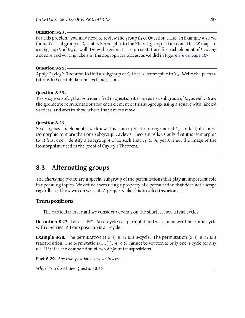
CHAPTER 8. GROUPS OF PERMUTATIONS 287
Question 8¨23 .For this problem, you may need to review the group D4 of Question 3.118. In Example 8¨22 we
foundW, a subgroup of S4 that is isomorphic to the Klein 4-group. It turns out thatW maps to
a subgroup V of D4, as well. Draw the geometric representations for each element of V, using
a square and writing labels in the appropriate places, as we did in Figure 3¨6 on page 107.
Question 8¨24 .Apply Cayley’s Theorem to find a subgroup of S4 that is isomorphic to Z4. Write the permu-
tations in both tabular and cycle notations.
Question 8¨25 .The subgroup of S4 that you identified in Question 8.24 maps to a subgroup of D4, as well. Draw
the geometric representations for each element of this subgroup, using a square with labeled
vertices, and arcs to show where the vertices move.
Question 8¨26 .Since S3 has six elements, we know it is isomorphic to a subgroup of S6. In fact, it can be
isomorphic to more than one subgroup; Cayley’s Theorem tells us only that it is isomorphic
to at least one. Identify a subgroup A of S6 such that S3 – A, yet A is not the image of the
isomorphism used in the proof of Cayley’s Theorem.
8¨3 Alternating groups
The alternating groups are a special subgroup of the permutations that play an important role
in upcoming topics. We define them using a property of a permutation that does not change
regardless of how we can write it. A property like this is called invariant.
Transpositions
The particular invariant we consider depends on the shortest non-trivial cycles.
Definition 8¨27. Let n P N`. An n-cycle is a permutation that can be written as one cycle
with n entries. A transposition is a 2-cycle.
Example 8¨28. The permutation p1 2 3q P S3 is a 3-cycle. The permutation p2 3q P S3 is a
transposition. The permutation p1 3q p2 4q P S4 cannot be written as only one n-cycle for any
n P N`: it is the composition of two disjoint transpositions.
Fact 8¨29. Any transposition is its own inverse.
Why? You do it! See Question 8.30

CHAPTER 8. GROUPS OF PERMUTATIONS 288
Question 8¨30 .Show that:
(a) the inverse of any transposition is a transposition; and
(b) if we can write the permutation π as π “ τ1τ2 ¨ ¨ ¨ τk, where each τi is a transposition, then
π´1 “ τkτk´1 ¨ ¨ ¨ τ1.
Any permutation can be written with many different numbers of cycles; after all, any
one-cycle is the identity:
p1 2 3q “ p1 2 3q p1q “ p1 2 3q p1q p3q “ p1 2 3q p1q p3q p1q “ ¨ ¨ ¨ .
A neat trick allows us to write every permutation as a composition of transpositions.
Example 8¨31. Verify that
• p1 2 3q “ p1 3q p1 2q;
• p1 4 8 2 3q “ p1 3q p1 2q p1 8q p1 4q; and
• p1q “ p1 2q p1 2q.
Do you see the relationship between the n-cycle and the corresponding transpositions?
Lemma 8¨32. Any permutation can be written as a composition of transpositions.
Proof. You do it! See Question 8.33.
Question 8¨33 .Show that any permutation can be written as a product of transpositions.
Remark 8¨34. Given an expression of σ as a product of transpositions, say σ “ τ1 ¨ ¨ ¨ τn, it is
clear from Fact 8¨29 that we can write σ´1 “ τn ¨ ¨ ¨ τ1, as an application of the associative
property yields
pτ1 ¨ ¨ ¨ τnq pτn ¨ ¨ ¨ τ1q “ pτ1 ¨ ¨ ¨ τn´1q pτnτnq pτn´1 ¨ ¨ ¨ τ1q
“ pτ1 ¨ ¨ ¨ τn´1q`
1˘
pτn´1 ¨ ¨ ¨ τ1q
...
“ p1q .
At this point it is worth revisiting Example 8¨31. Can we write`
1 2 3˘
with many
different numbers of transpositions? Yes:
p1 2 3q “ p1 3q p1 2q
“ p1 3q p1 2q p2 3q p2 3q
“ p1 3q p1 2q p1 3q p1 3q
“ ¨ ¨ ¨ .

CHAPTER 8. GROUPS OF PERMUTATIONS 289
Nevertheless, there is a difference to writing p1 2 3q as any number of cycles: no matter how
we try, we seem able to write it only as an even number of transpositions. Similarly,
p2 3q “ p2 3q p2 3q p2 3q
“ p2 3q p1 2q p1 3q p1 3q p1 2q “ ¨ ¨ ¨ .
No matter how we try, we seem able to write it only as an odd number of transpositions.
Is this always the case?
Even and odd permutations
Theorem 8¨35. Let α P Sn.
• If α can be written as the composition of an even number of transpositions, then it cannot be
written as the composition of an odd number of transpositions.
• If α can be written as the composition of an odd number of transpositions, then it cannot be
written as the composition of an even number of transpositions.
Proof. Define the polynomials
g “ź
1ďiăjďn
`
xi ´ xj˘
and gα “ź
1ďiăjďn
`
xαpiq ´ xαpjq˘
.
The value of gα depends on the permutation α; in particular, it depends only on what α does
to each pair i and j. That makes gα invariant under the representation of α. Its value does not
depend on how we write α in terms of transpositions!
How is gα related to g? Sometimes they agree; for example, if α “`
1 3 2˘
then
g “ px1 ´ x2q px1 ´ x3q px2 ´ x3q
and
gα “ px3 ´ x1q px3 ´ x2q px1 ´ x2q
“ rp´1q px1 ´ x3qs rp´1q px2 ´ x3qs px1 ´ x2q
“ g.
Is it always the case that gα “ g? Not necessarily: if α “`
1 2˘
then g “ x1 ´ x2 and
gα “ x2 ´ x1 ‰ g. In this case , gα “ ´g.
Question 8¨36 .We pause the proof a moment to ask you a question. Compute gα for the permutations p1 3q p2 4q
and p1 3 2 4q. Use the value of gα to determine which of the two permutations is odd, and
which is even?

CHAPTER 8. GROUPS OF PERMUTATIONS 290
Proof of Theorem 8¨35 (continued). We cannot guarantee gα “ g, but can we write gα in terms of
g? Try the following. Lemma 8¨32 tells us α is a composition of transpositions, so let’s think
about what happens when we compute gτ for any transposition τ “`
i j˘
. Without loss of
generality, we may assume that i ă j. Let k be another positive integer.
• We know that xi ´ xj is a factor of g. After applying τ, xi ´ xj is no longer a factor of gτ;
rather, xj ´ xi. Observe that xj ´ xi “ ´`
xi ´ xj˘
.
• If i ă j ă k, then xi ´ xk and xj ´ xk are factors of g. After applying τ, xj ´ xk and xi ´ xk
are factors of gτ. While the order has changed, the factors have not.
• If k ă i ă j, then xk ´ xi and xk ´ xj are factors of g. After applying τ, xk ´ xj and xk ´ xi
are factors of gτ. Again, the order has changed, but the factors have not.
• If i ă k ă j, then xi ´ xk and xk ´ xj are factors of g. After applying τ, xj ´ xk and xk ´ xi
are factors of gτ. The factors have changed, but the changes cancel:
`
xj ´ xk˘
pxk ´ xiq ““
´`
xk ´ xj˘‰
r´ pxi ´ xkqs “ pxi ´ xkq`
xk ´ xj˘
.
To summarize: xi ´ xj is the only factor whose change of sign makes a difference in g and gτ.
We see that gτ “ ´g.
Excellent! We have characterized the relationship between gα and gwhenever α is a trans-
position! Return to the general case, whereα is an arbitrary permutation. From Lemma 8¨32, α
is a composition of transpositions. Choose transpositions τ1, τ2, . . . , τm such thatα “ τ1τ2 ¨ ¨ ¨ τm.
Using substitution and the observation we just made,
gα “ gτ1¨¨¨τm “ ´gτ1¨¨¨τm´1“ p´1q
2gτ1¨¨¨τm´2
“ ¨ ¨ ¨ “ p´1qmg.
In short,
gα “ p´1qmg. (8.3)
Recall that gα depends only on α, and not on its representation. Assume α can be written as an
even number of transpositions; say, α “ τ1 ¨ ¨ ¨ τ2m. Formula (8.3) tells us that gα “ p´1q2mg “
g. If we could also write α as an odd number of transpositions, say, α “ µ1 ¨ ¨ ¨ µ2m`1, then
gα “ p´1q2k`1
g. Substitution gives us p´1q2mg “ p´1q
2k`1g “
“
p´1q2‰k
p´gq “ ´g, a
contradiction. Hence, α cannot be written as an odd number of transpositions.
A similar argument shows that if α can be written as an odd number of transpositions,
then it cannot be written as an even number of transpositions. Since α P Sn was arbitrary, the
claim holds.
Lemma 8¨32 tells us any permutation can be written as a composition of transpositions,
and Theorem 8¨35 tells us that for any given permutation, this number is always either an
even or odd number of transpositions. The number itself is invariant, but whether it is even
or odd (its parity) is not.
Definition 8¨37. If a permutation can be written with an even number of permutations, then
we say the permutation is even. Otherwise, we say the permutation is odd.

CHAPTER 8. GROUPS OF PERMUTATIONS 291
Example 8¨38. The permutation ρ “ p1 2 3q P S3 is even, since as we saw earlier ρ “
p1 3q p1 2q. So is the permutation ι “ p1q “ p1 2q p1 2q. The permutation φ “ p2 3q is odd.
Question 8¨39 .Recall the polynomials g and gα defined in the proof of Theorem 8¨35. The sign functionsgn pαq indicates the relationship,
g “ sgn pαq ¨ gα.
Another way of saying this is that
sgn pαq “
#
1, α P An;
´1, α R An.
Show that for any two cycles α, β,
p´1qsgnpαβq
“ p´1qsgnpαq
p´1qsgnpβq
.
Explain why sgn is a homomorphism from Sn to the group under multiplication t˘1u. What
is its kernel?
The alternating groups
The invariance of a permutation’s parity allows us to identify a new kind of group.
Definition 8¨40. Let n P N` and n ě 2. Let An “ tα P Sn : α is evenu. We call An the set ofalternating permutations.
Remark 8¨41. While this A3 is not the “A3” of Example 4¨134 on page 163, the isomorphism
between D3 and S3 maps one to the other, so they are isomorphic.
Question 8¨42 .List the elements of A2, A3, and A4 in cycle notation.
This set is, in fact, a subgroup of the symmetric group.
Theorem 8¨43. For all n ě 2, An ă Sn.
We prove this two different ways.
First proof: directly. Let n ě 2. By Lemma 4¨4, the elements of An are associative under compo-
sition. Observe that p1q “ p1 2q p1 2q P An, so An has an identity. For any π P An, write it as an
even number of transpositions, say π “ τ1τ2 ¨ ¨ ¨ τ2k; by Question 8.30, τ´1 “ τ2kτ2k´1 ¨ ¨ ¨ τ1 P
An, so An satisfies the inverse property. Finally, for any π, σ P An, write them as an even
number of transpositions, say π “ τ1τ2 ¨ ¨ ¨ τ2k and σ “ υ1υ2 ¨ ¨ ¨ υ2`. Their product is πσ “
pτ1 ¨ ¨ ¨ τ2kq pυ1 ¨ ¨ ¨ υ2`q, which is clearly an even number of transpositions, so An is closed under
composition of function. Since it satisfies the four properties of a group, An ă Sn.

CHAPTER 8. GROUPS OF PERMUTATIONS 292
Second proof: using the Subgroup Theorem. Let n ě 2. Observe that p1q “ p1 2q p1 2q, so An ‰ H.
Let x, y P An. By definition, we can write x “ σ1 ¨ ¨ ¨ σ2m and y “ τ1 ¨ ¨ ¨ τ2n, where m, n P Z and
each σi or τj is a transposition. From Remark 8¨34,
y´1“ τ2n ¨ ¨ ¨ τ1,
so
xy´1“ pσ1 ¨ ¨ ¨ σ2mq pτ2n ¨ ¨ ¨ τ1q .
This is a composition of 2m ` 2n “ 2 pm` nq transpositions, which shows xy´1 P An. By the
Subgroup Theorem, An ă Sn.
How large is An, relative to Sn?
Theorem 8¨44. For any n ě 2, there are half as many even permutations as there are permutations.
That is, |An| “ |Sn| 2.
Proof. We show that there are two cosets of An ă Sn, then apply Lagrange’s Theorem.
Let X P SnAn. Let α P Sn such that X “ αAn. If α is an even permutation, then Lemma 4¨103
on page 152 implies that X “ An. Otherwise, α is odd. Let β be any other odd permutation.
Write out the odd number of transpositions of α´1
, followed by the odd number of transpo-
sitions of β, to see that α´1β is an even permutation. Hence, α
´1β P An, and by Lemma 4¨103,
αAn “ βAn.
We have shown that even permutations lie in one coset (An itself) while odd permutations
lie in one different coset (we can write it as p1 2qAn). From Lemma 8¨32, any permutation is
either even or odd. These two cosets of An thus partition Sn. By Lagrange’s Theorem,
|Sn|
|An|“ |SnAn| “ 2,
and a little algebra rewrites this equation as |An| “ |Sn| 2.
Corollary 8¨45. For any n ě 2, An Ÿ Sn.
Proof. You do it! See Question 8.46.
Question 8¨46 .Show that for any n ě 2, An Ÿ Sn.
8¨4 The 15-puzzle
The 15-puzzle resembles a 4 ˆ 4 square, with all the squares numbered, except one. The
numbering starts in the upper left and proceeds consecutively until the lower right; the only
squares that aren’t in order are the last two, which are swapped:
1 2 3 4
5 6 7 8
9 10 11 12
13 15 14

CHAPTER 8. GROUPS OF PERMUTATIONS 293
The only permissible moves are those where one “slides” a square left, right, above, or below
the empty square. The following moves are permissible from the starting position above:
1 2 3 4
5 6 7 8
9 10 11 12
13 15 14
or
1 2 3 4
5 6 7 8
9 10 11
13 15 14 12
.
The following moves are not:
1 2 3 4
5 6 7 8
9 10 12
13 15 14 11
or
1 2 3 4
5 6 7 8
9 10 11 12
13 14 15
.
(You may have played with a similar toy as a child.) The challenge is to find a way to rearrange
the squares so that they are in order, like so:
1 2 3 4
5 6 7 8
9 10 11 12
13 14 15
This section shows the challenge to be impossible.
How? Since the problem is one of rearranging a list of elements, it is a problem of permu-
tations. Every permissible move consists of transpositions τ “ px yq in S16 where:
• x ă y;
• one of x or y is the position of the empty square in the current list; and
• legal moves imply that either
– y “ x` 1 and 4 - x; or
– y “ x` 4.
Example 8¨47. The legal moves illustrated above correspond to the transpositions
• p15 16q, because square 14 was in position 15, and the empty space was in position 16:
notice that 16 “ 15` 1; and
• p12 16q, because square 12 was in position 12, and the empty space was in position 16:
notice that 16 “ 12` 4.
The illegal moves illustrated above correspond to the transpositions
• p11 16q, because square 11 was in position 11, and the empty space was in position 16:
notice that 16 “ 11` 5; and

CHAPTER 8. GROUPS OF PERMUTATIONS 294
• p13 14q, because neither 13 nor 14 contains the empty square.
Likewise p12 13qwould be an illegal move in any configuration, because it crosses rows: even
though y “ 13 “ 12` 1 “ x` 1, x “ 12 “ 3ˆ 4.
How can we use this to show that it is impossible to solve 15-puzzle? We take two steps. The
first shows that if there is a solution, it must belong to a particular group.
Lemma 8¨48. Any solution to the 15-puzzle is a permutation σ P A16.
Proof. Any permissible move corresponds to a transposition τ as described above. Any solu-
tion contains the empty square in the lower right hand corner. As a consequence,
• if px yq is a move left, then the empty square must eventually return to the rightmost
row, so there must eventually be a corresponding move right, px1 y1q; and
• if px yq is a move up, the empty square must eventually return to the bottom row, so
there must eventually be a corresponding move down, px1 y1q.
Thus, moves come in pairs. The upshot is that any solution to the 15-puzzle must be a permu-
tation σ defined by an even number of transpositions. By Theorem 8¨35 and Definitions 8¨37
and 8¨40, σ P A16.
The second step is to explain why the initial configuration makes this impossible.
Theorem 8¨49. The 15-puzzle has no solution.
Proof. By way of contradiction, assume that it has a solution σ. By Lemma 8¨48, σ P A16.
BecauseA16 is a subgroup of S16, and hence a group in its own right, σ´1 P A16. Notice σ
´1σ “ ι,
the permutation which corresponds to the configuration of the solution.
Now σ´1
is a permutation corresponding to the moves that change the arrangement
1 2 3 4
5 6 7 8
9 10 11 12
13 14 15
into the arrangement
1 2 3 4
5 6 7 8
9 10 11 12
13 15 14
which corresponds to p14 15q. Remember that a permutation’s parity is invariant; you will
show below that a permutation and its inverse have the same parity. We conclude that sgnσ “
sgn pσ´1q “ sgn p14 15q, contradicting Lemma 8¨48.

CHAPTER 8. GROUPS OF PERMUTATIONS 295
Question 8¨50 .Let σ P Sn. How do we know that sgnσ “ sgn pσ´1q?
As a historical note, the 15-puzzle was developed in 1878 by an American puzzle maker,
who promised a $1,000 reward to the first person to solve it. Most probably, the puzzle maker
knew that no one would ever solve it: if we account for inflation, the reward would correspond
to $22,265 in 2008 dollars.1
The textbook [2] contains a more general discussions of solving puzzles of this sort using
algebra.
Question 8¨51 .Determine which of these configurations, if any, is solvable by the same rules as the 15-puzzle:
1 2 3 4
5 6 7 8
9 10 12 11
13 14 15
,
1 2 3 4
5 10 6 8
13 9 7 11
14 15 12
,
3 6 4 7
1 2 12 8
5 15 10 14
9 13 11
.
1According to the website www.measuringworth.com/ppowerus/result.php.
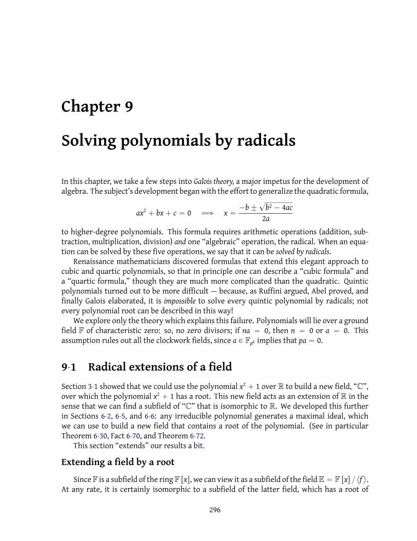
Chapter 9
Solving polynomials by radicals
In this chapter, we take a few steps into Galois theory, a major impetus for the development of
algebra. The subject’s development began with the effort to generalize the quadratic formula,
ax2` bx` c “ 0 ùñ x “
´b˘?b2 ´ 4ac
2a
to higher-degree polynomials. This formula requires arithmetic operations (addition, sub-
traction, multiplication, division) and one “algebraic” operation, the radical. When an equa-
tion can be solved by these five operations, we say that it can be solved by radicals.
Renaissance mathematicians discovered formulas that extend this elegant approach to
cubic and quartic polynomials, so that in principle one can describe a “cubic formula” and
a “quartic formula,” though they are much more complicated than the quadratic. Quintic
polynomials turned out to be more difficult — because, as Ruffini argued, Abel proved, and
finally Galois elaborated, it is impossible to solve every quintic polynomial by radicals; not
every polynomial root can be described in this way!
We explore only the theory which explains this failure. Polynomials will lie over a ground
field F of characteristic zero: so, no zero divisors; if na “ 0, then n “ 0 or a “ 0. This
assumption rules out all the clockwork fields, since a P Fpk implies that pa “ 0.
9¨1 Radical extensions of a field
Section 3¨1 showed that we could use the polynomial x2 ` 1 over R to build a new field, “C”,
over which the polynomial x2 ` 1 has a root. This new field acts as an extension of R in the
sense that we can find a subfield of “C” that is isomorphic to R. We developed this further
in Sections 6¨2, 6¨5, and 6¨6: any irreducible polynomial generates a maximal ideal, which
we can use to build a new field that contains a root of the polynomial. (See in particular
Theorem 6¨30, Fact 6¨70, and Theorem 6¨72.
This section “extends” our results a bit.
Extending a field by a root
SinceF is a subfield of the ringF rxs, we can view it as a subfield of the fieldE “ F rxs 〈f 〉.At any rate, it is certainly isomorphic to a subfield of the latter field, which has a root of
296

CHAPTER 9. SOLVING POLYNOMIALS BY RADICALS 297
f , which means we are not unreasonable in stating that there exists a superfield of F that
contains a root α of f .
Definition 9¨1. Let f be an irreducible polynomial over a field F, and let α be a root of f that
is not in F. We call the field E “ F pαq an algebraic extension of F, and say that we obtain
E from F by adjoining α. If f is irreducible and d “ deg f , we say that E is an extensionof degree d (over F). If there exists m P N` such that α
m P F, then we say that E is a
radical extension of F. We will also relax our precision sometimes to say that a sequence of
field extensions is an algebraic (or radical) extension if every extension in the sequence is
algebraic (or radical).
This terminology allows us to give our main question more precision:
Is an algebraic extension always radical?
Were the answer “Yes,” then we could always solve polynomials by radicals; we would simply
construct a finite sequence of radical extensions
E1 “ Q pα1q , E2 “ Q pα1q pα2q , ¨ ¨ ¨ Ek “ Q pα1q ¨ ¨ ¨ pαkq
where each αi has the form
αi “n
a
β for some β P Ei´1,
and every root of the polynomial would appear in Ek.
The purpose of this chapter is to show that the answer is, in fact, “No.”
Question 9¨2 .Let α be a root of an irreducible polynomial f P F rxs, with deg f ě 2. Explain how we know
that F pαq satisfies both the properties of a field and F Ĺ F pαq Ď E, where E is any field that
contains both F and α.
You may wonder whether the degree of an algebraic extension is well-defined; after all, α
could be the root of two different irreducible polynomials of different degree. In fact, this
cannot happen.
Fact 9¨3. Let f, g P F rxs be two irreducible polynomials with a common root α R F. Then deg f “
deg g.
Why? Recall that F rxs is a Euclidean domain, and compute a gcd p of f and g. Since f is ir-
reducible and p | f , p is either a unit or an associate of f . By Question 6.51 and Fact 6¨55 we
know that Bezout’s Lemma applies, so we can find h1, h2 P F rxs such that p “ h1f ` h2g. By
substitution,
p pαq “ h1 pαq f pαq ` h2 pαq g pαq “ h1 pαq ¨ 0` h2 pαq ¨ 0 “ 0.
You will show in Question 9.4 that a polynomial cannot both have a root and be a unit, so p is
not a unit; it must be an associate of f ; say p “ af where a P F rxs is a unit. Since g is irreducible

CHAPTER 9. SOLVING POLYNOMIALS BY RADICALS 298
and p | g, by substitution af | g, so f | a´1g. Recall that F rxs is a unique factorization domain,
so the irreducible f is prime, so f | a´1 or f | g. You will show in Question that only a unit can
divide a unit, and an irreducible is by definition not a unit, so f | g. Since g is irreducible, f
must be an associate of g. You will also show in Question 9.4 that the degree of a unit is zero,
so deg f “ deg g.
Question 9¨4 .The explanation for all three properties hinted at in the proof above is nearly identical.
(a) Let f P F rxs. Show that if f has a root α P F, then f cannot be a unit. Hint: Proceed by
contradiction. Think about the value of f and its inverse at α.
(b) Let R be a ring and a, r P R, where a is a unit. Show that if r | a then r is also a unit.
(c) Let F rxs be the ring of polynomials over the field F, and a P F rxs a unit. Show that
deg a “ 0.
Question 9¨5 .An alternate approach to defining the degree of an extension is as follows. Let α be the root
of an irreducible polynomial f over F.
(a) Show that F pαq is a vector space over F.
(b) Show that the vector space is finite dimensional. Hint: Use f to show that only finitely
many powers of α are linearly independent.
Define deg F pαq to be the dimension of F pαq over F.
(c) Explain why the value of deg F pαq computed this way gives the identical result as the
value indicated above.
Example 9¨6. Let f “ x5 ´ 2x
3 ´ 3x2 ` 6. This factors over Q as px2 ´ 2q px3 ´ 3q. Both
factors are irreducible over Q. From what we wrote above, there exists a radical extension
of degree 2 of Q that contains a root of x2 ´ 2; call the corresponding root α “
?2, so that
instead of writing Q pαq, we can write Q`?2˘
, instead.
What do elements of Q pαq “look” like? By the definition of a ring extension, we know
that elements of this field have the form a ` b?2 ` c
?22
` ¨ ¨ ¨ . Now,?2 is a root of x
2 ´ 2,
which means that?22
´ 2 “ 0, which we can rewrite as?22
“ 2. Hence, we can assume that
elements of Q“?2‰
really have the form a` b?2, since we just saw how higher powers of
?2
reduce either to an element of Q, or to a rational multiple of?2 itself.
It might not be obvious that such elements have multiplicative inverses, but they do. You
can see this either by working with the isomorphic quotient field Q rxs 〈x2 ´ 2〉, or in this
case solving a straightforward linear equation. For the nonzero element a ` b?2 to have an
inverse c ` d?2, we need
1 “`
a` b?2˘ `
c ` d?2˘
“ pac ` 2bdq ` pad` bcq?2.

CHAPTER 9. SOLVING POLYNOMIALS BY RADICALS 299
Since 1 “ 1` 0?2, we know we can find an inverse if
ac ` 2bd “ 1 and ad` bc “ 0.
Since a` b?2 is nonzero, we can assume that a ‰ 0 or b ‰ 0. If a ‰ 0, then we can solve the
two equations to see that
c “1´ 2bd
aand d “ ´
bc
a.
Notice that this solution satisfies c, d P Q, since the rationals are a field. If a “ 0, on the other
hand, those equations simplify to
2bd “ 1 and bc “ 0,
so that d “ 1 p2bq and c “ 0. To make sure you understand that, use this principle to find
the inverses of 1´ 2?2 and 3
?2.
Does x3 ´ 3 factor over this extension field? If so, then it has at least one linear factor,
x´ β. This makes β a root of x3´ 3, so we can resolve the question by asking, does x
3´ 3 have
a root in Q`?2˘
? If so, it has the form x “ a` b?2, and we can rewrite the polynomial as
0 “ x3´ 3 “
`
a` b?2˘3
´ 3
“ a3` 3a
2b?2` 6ab
2` 2b
3?2´ 3
“`
a3` 6ab
2´ 3
˘
``
3a2b` 2b
3˘?2.
In other words,?2 “
´a3 ´ 6ab2 ` 3
3a2b` 2b3.
Remember that a, b P Q, so addition, subtraction, and multiplication, are closed, and division
is closed so long as the divisor is nonzero. If the divisor in this expression is in fact nonzero
— that is, 3a2b` 2b3 ‰ 0— then the equation above tells us that
?2 P Q. We know that this
is false! The divisor must, therefore, be zero, which means that
b`
3a2` 2b
2˘
“ 3a2b` 2b
3“ 0 ùñ b “ 0 or 3a
2` 2b
2“ 0.
If b “ 0, then x P Q. That is, x3 ´ 3 has a rational root. We know that this is false! If b ‰ 0,
on the other hand, then 3a2` 2b2 “ 0, which we can rewrite as ab “
a
´23. Since a, b P Q,
we conclude thata
´23 P Q. Again,we know that this is false! All the possibilities lead us
to a contradiction, so we conclude that x3´3 does not factor over the extension fieldQ
`?2˘
.
As before, we can extendQ`?2˘
by a root of x3´2; call it
3?3. We now have the extension
fieldE “ Q`?2˘ `
3?3˘
. Have we found all the roots f now? For the factor x2´2, we certainly
have, since x2´2 “
`
x´?2˘ `
x`?2˘
. For the other factor, we are not quite done; we have,
x3´ 3 “
`
x´3?3˘ `
x2` x
3?3`
3?9˘
,

CHAPTER 9. SOLVING POLYNOMIALS BY RADICALS 300
and this latter polynomial does not factor. To see why not, let’s use the quadratic equation to
find what the roots should be:
x2` x
3?3`
3?9 “ 0
x “´
3?3˘
b
`
3?3˘2
´ 4 3?9
2
“´
3?3˘
a
´3 3?9
2
“´
3?3˘ i
?3
3?3
2
“ ´3?3
ˆ
1
2˘ i
?3
2
˙
.
So we are still missing the cube roots of unity.
Question 9¨7 .Find the smallest extension field of Q where f pxq “ x7´2x4´ x3`2 factors completely. Hint:
f is not irreducible overQ, so try to factor it completely overQ before working on extensions.
In the example, we construct Q`?2˘
, whose degree over Q is 2, and Q`?2,
3?3˘
, whose
degree over Q`?2˘
is 3. How should we determine the degree of Q`?2,
3?3˘
over Q? You
might think to add the degrees, but then you would lose an important relationship between
the degree of an extension and the dimension of the extension as a vector space over the base
field. Elements of Q`?2,
3?3˘
can be written as
a` b?2` c
3?3` d
3?9` e
?2
3?3` f
?2
3?9;
each term is linearly independent of the others, so that Q`?2,
3?3˘
is a vector space of di-
mension 6 over Q. In the same way, Q`?2˘
was a vector space of dimension 2 over Q, and
Q`?2,
3?3˘
was a vector space of dimension 3 over Q`?2˘
. Given that link, it makes better
sense to define the degree of Q`?2,
3?3˘
over Q as 6.
Definition 9¨8. Let F be a field, and
F “ E0 Ĺ E1 Ĺ E2 Ĺ ¨ ¨ ¨ Ĺ Em
a chain of algebraic extensions. Denote the degree ofEi overEi´1 as rEi : Ei´1s; we define the
degree of Em over F as
rEm : Em´1s rEm´1 : Em´2s ¨ ¨ ¨ rE2 : E1s rE1 : E0s .

CHAPTER 9. SOLVING POLYNOMIALS BY RADICALS 301
Question 9¨9 .Show that Definition 9¨8 is well-defined; that is, if there is more than one way to fill in the
dots of the chain of algebraic extensions E0 Ĺ ¨ ¨ ¨ Ĺ Em (for instance,
Q Ĺ Q`?2˘
Ĺ Q`?2,?5˘
Ĺ Q`?2,?5,?7˘
or
Q Ĺ Q`?5˘
Ĺ Q`?5,?7˘
Ĺ Q`?2,?5,?7˘
,
then we do not obtain different degrees by considering different chains. Hint: Use the alter-
nate definition of the degree of an extension, given in Question 9.5.
Remark. The usual study of Galois theory considers field extensions in a more general case;
that is, not just as the roots of irreducible polynomials. Our restriction tries to keep the affair
in a very concrete setting; this allows us some latitude with the degree of an extension that
the more general case does not enjoy.
Complex roots
As a cube root of unity popped up in the example above, you would be wise to conjecture
that the roots of unity play a fundamental role here. In fact, we can obtain radical roots by
adjoining both a “principal” root, and a sensible “root of unity.”
Recall from Theorems 3¨26 and 3¨28 that 1,ω,ω2, . . . ,ω
n´1are all n-th roots of unity, where
ω has the form
ω “ cos
ˆ
2π
n
˙
` i sin
ˆ
2π
n
˙
,
and from Lemma 3¨27 we see further that
ωm“ cos
ˆ
2πm
n
˙
` i sin
ˆ
2πm
n
˙
.
This pattern extends beyond the roots of unity.
Theorem 9¨10. If α is a root of an irreducible polynomial xn´ a P Q rxs, then all other roots of x
n´ a
have the form α ¨ ωm, whereω is a primitive n-th root of unity andm P t1, . . . , n´ 1u.
Proof. Assume that α is a root of an irreducible polynomial xn´ a P Q rxs. By substitution and
definition of the primitive n-th root,
pαωmqn´ a “ α
npω
nqm´ a “ α
n¨ 1
m´ a.
By hypothesis, αn ´ a “ 0, so
pαωmqn´ a “ 0.
By definition, αωm
is a root of xn ´ a.
Very well, but why must this form characterize all the roots of xn ´ a? Using the Factor
Theorem, we see that xn´ a can have no more than n roots, and we just found n such distinct
roots,
α, αω, αω2, . . . , αω
n´1.

CHAPTER 9. SOLVING POLYNOMIALS BY RADICALS 302
α
αω
αω2
Figure 9¨1: The roots of x3 ´ 3, obtained using one root and the cube roots of unity.
Example 9¨11. Returning to the question of the roots of x3´ 3, we defined one root to be
3?3.
The other roots are, therefore,
3?3
„
cos
ˆ
2π
3
˙
` i sin
ˆ
2π
3
˙
and3?3
„
cos
ˆ
4π
3
˙
` i sin
ˆ
4π
3
˙
or, after evaluating these trigonometric functions,
3?3
ˆ
´1
2` i
?3
2
˙
and3?3
ˆ
´1
2´ i
?3
2
˙
.
If you look back at the result of the quadratic equation, you will find that this does indeed
describe the missing roots. Figure 9¨1 shows how the primitive cube roots of unity “scale
out” to give us the roots of x3 ´ 3.
Thus, the extension of Q to a field containing all the roots of x5´ 2x3´ 3x2` 6 is the field
Q`?2˘ `
3?3˘
pωq , where ω is any primitive cube root of unity.
(You may wonder: have we actually captured all the roots? After all, we didn’t extend
by a primitive square root of unity. This is because there is only one primitive square root of
unity, -1, and it appears in Q already.)
At this point, we encounter a problem: what if we had proceeded in a different order? In
the example given, we adjoined?2 first, then
3?3, and finally ω. Suppose we were to adjoin
them in a different order — say,3?3 first, then ω, and finally
?2? How would that work out?
As long as we adjoin all the roots, we arrive at the same field. For this reason, we write
Q pα1, . . . , αnq “ Q pα1q pα2q ¨ ¨ ¨ pαnq as a shorthand. However, Theorem 9¨10 implies that
Q`
3?3˘
by itself does not contain all the roots of x3 ´ 3; it contains only
3?3. We could adjoin
the other roots, Q`
3?3,ω
3?3,ω
2 3?3˘
, but there is another, simpler way. To obtain all the roots
of x3 ´ 3, we can first adjoin a primitive cube root of unity, then
3?3. Typically, we adjoin a
primitive cube root of unity first, obtaining Q pωq`
3?3˘
, or Q`
ω,3?3˘
. This certainly gives us3?3, ω
3?3, and ω
2 3?3.
You might wonder if this doesn’t give us too much. After all, ω P Q`
ω,3?3˘
, but it isn’t
obviously an element of Q`
3?3,ω
3?3,ω
2 3?3˘
. You will show in the exercises that, in fact,

CHAPTER 9. SOLVING POLYNOMIALS BY RADICALS 303
Q`
ω,3?3˘
“ Q`
3?3,ω
3?3,ω
2 3?3˘
, and the more general notion also holds: if we adjoin a prim-
itive n-th root of unity ω and n?a, we end up with exactly the field Q p n
?a,ω n?a, . . . ,ω
n´1 n?aq
— nothing more, nothing less.
Question 9¨12 .Suppose that α
n P Q, αi R Q for 1 ď i ă n, and ω is a primitive n-th root of unity. Show that
Q pα,ωα, . . . ,ωn´1αq “ Q pω, αq.
9¨2 The symmetries of the roots of a polynomial
Let F be a field, and f P F rxs of degree 2. We can show by the Factor Theorem that f has
at most 2 roots in F. (See Exercise 6.56.) Suppose that f does have 2 roots in F; we can
then write f pxq “ px´ α1q px´ α2q. If we expand this product, we obtain f pxq “ x2 ´
pα1 ` α2q x ` α1α2. Likewise, if f is of degree 3, it can have at most 3 roots in F; we can write
f pxq “ px´ α1q px´ α2q px´ α3q, which expands to
f pxq “ x3´ pα1 ` α2 ` α3q x` pα1α2 ` α1α3 ` α2α3q x´ α1α2α3.
In general, if f is of degree n and has n roots in F, we can write
f pxq “ px´ α1q px´ α2q ¨ ¨ ¨ px´ αnq ,
which expands to
f pxq “ xn`
˜
nÿ
i“1
αi
¸
xn´1
`
˜
ÿ
iăj
αiαj
¸
xn´2
` ¨ ¨ ¨ ` α1α2 ¨ ¨ ¨ αn.
Every coefficient is a sum of terms that are products of roots. Permuting the roots does not change
the sum.
Example 9¨13. Look at the coefficient of x in the cubic polynomial above. One of the terms
is α1α3. If we permute by p123q, α1 changes to α2 and α3 changes α1. The result is α2α1 “ α1α2,
which also appears in that coefficient. Another term is α2α3; applying the same permutation
gives us α3α1 “ α1α3.
This gives rise to a special class of polynomial.
Definition 9¨14. Let R be a ring and f P R rx1, . . . , xns. For any σ P Sn, write σf for the poly-
nomial g P R rx1, . . . , xns obtained by replacing xi by xσpiq. We say that f is a symmetric poly-nomial if f “ σf for all σ P Sn.
Example 9¨15. Let f pxq “ x1x2´x1x3. This is not a symmetric polynomial, since for σ “ p1 3q
we obtain
σf “ x2x3 ´ x1x3 ‰ f.

CHAPTER 9. SOLVING POLYNOMIALS BY RADICALS 304
Example 9¨16. On the other hand, if f pxq “ x1x2x3 ` x2x3x4 ` x1x3x4 ` x1x2x4, every σ P S4
satisfies σf “ f . For example, if σ “ p1 4q,
σf “ x2x3x4 ` x1x2x3 ` x1x3x4 ` x1x2x4 “ f.
Here, f is symmetric.
Question 9¨17 .The polynomial f pxq “ x4´ 7x2` 10 factors over Q as px2 ´ 2q px2 ´ 5q, and over Q
`?2,?5˘
as`
x˘?2˘ `
x˘?5˘
.
(a) Compute the symmetric polynomials of the coefficients of a generic fourth-degree poly-
nomial.
(b) Substitute the roots of f into the symmetric polynomials. Show that they simplify to the
coefficients of f .
Theorem 9¨18. Let f P F rxs. The coefficient of any term of f is a symmetric polynomial of the roots
of f . In particular, if deg f “ n, then the coefficient of xiis the sum of all squarefree products of exactly
n´ i roots.
Proof. We proceed by induction on n “ deg f . Write α1, . . . , αn for the roots of f .
Inductive base: If n “ 2, then f pxq “ px´ α1q px´ α2q “ x2 ´ pα1 ` α2q x ` α1α2. The
coefficient of x2
is the sum of all products of 2´ 2 “ 0 roots; the coefficient of x is the sum of
all squarefree products of 2´1 “ 1 roots, and the coefficient of x0
is the sum of all squarefree
products of 2´ 0 “ 2 roots.
Inductive hypothesis: Assume that the coefficients of the terms of any pn´ 1q-th degree
polynomial have the form specified.
Inductive step: Let g P F pα1q ¨ ¨ ¨ pαn´1q such that f pxq “ g pxq px´ αnq. Since deg g “ n´ 1,
the inductive hypothesis tells us that its terms are symmetric polynomials of its roots, in
precisely the form specified. With that in mind, write
g pxq “ xn´1` βn´2x
n´2` ¨ ¨ ¨ ` β0
where βi is the sum of all squarefree products of pn´ 1q ´ i roots α1, . . . , αn´1. Expand the
product f pxq “ g pxq px´ αnq to see that
f pxq “`
xn` βn´2x
n´1` ¨ ¨ ¨ ` β0x
˘
``
αnxn´1` αnβn´2x
n´2` ¨ ¨ ¨ ` αnβ0
˘
“ xn` pβn´2 ` αnq x
n´1``
βn´3 ` αnβn´2xn´2
˘
` ¨ ¨ ¨ ` αnβ0.
• Since βn´2 is the sum of all squarefree products of pn´ 1q ´ pn´ 2q “ 1 roots α1, . . . ,
αn´1, we indeed have βn´2 ` αn as the sum of all products of 1 root in α1, . . . , αn.
• Let i P t2, 3, . . . , n´ 1u. Since βn´i is the sum of all squarefree products of pn´ 1q ´
pn´ iq “ i´ 1 roots α1, . . . , αn´1, we see that αnβn´i is the sum of all squarefree products
of i roots α1, . . . , αn that contain precisely one αn. Since βn´i´1 is the sum of all squarefree
products of pn´ 1q ´ pn´ i´ 1q “ i roots α1, . . . , αn´1, and αnβn´i is the sum of all
squarefree products of i roots α1, . . . , αn that contain precisely one αn, we indeed have
βn´i´1 ` αnβn´i as the sum of all squarefree products of i roots in α1, . . . , αn.

CHAPTER 9. SOLVING POLYNOMIALS BY RADICALS 305
• Since β0 is the sum of all squarefree products of pn´ 1q ´ 0 “ n´ 1 roots α1, . . . , αn, we
have β0 “ α1 ¨ ¨ ¨ αn´1. By substitution, αnβ0 “ α1 ¨ ¨ ¨ αn. This is precisely the sum of all
squarefree products of n´ 0 “ n roots α1, . . . , αn.
Another way to read Theorem 9¨18 is that we can study the roots of polynomials by looking
at permutations of them. In particular, the functions defined on E “ Q pα1, . . . , αnq that
permute the roots but leave elements of Q fixed must be of paramount importance. We are
especially interested in those functions that are isomorphisms on E itself; in other words,
automorphisms on E.
Example 9¨19. Let f “ x2 ` 1; we have f P Q rxs, but its roots are not in Q. Let i be a root
of f , and let E “ Q piq. By Exercise 9.5, E is a vector space over Q, with basis t1, iu, so every
element of E can be written as a` bi where a, b P Q.
We are interested in the automorphisms ofE that fixQ. Let φ be any such automorphism;
by definition, φ pqq “ q for any q P Q, while for any w, z P EzQ, φ pwqφ pzq “ φ pwzq.
Let z P E, and choose a, b P Q such that z “ a`bi. The properties of a ring homomorphism
imply that
φ pzq “ φ pa` biq “ φ paq ` φ pbiq “ φ paq ` φ pbqφ piq .
As stated, φ fixes Q, so φ paq “ a and φ pbq “ b. By substitution,
φ pzq “ a` bφ piq .
In other words, φ is determined completely by what it does to i.
What are the possible destinations of φ piq? First notice that φ cannot map i to a rational
number q, because φ is an automorphism, hence one-to-one, and φ fixes Q, so φ pqq “ q: we
would have φ piq “ φ pqq, but i ‰ q. The only thing we can choose for φ piq to satisfy this
requirement is some w “ c ` di P E where c, d P Q and d ‰ 0. On the other hand, the
homomorphism property means that we must have
w2“ φ piq
2“ φ
`
i2˘
“ φ p´1q “ ´1.
(Again, φ fixes Q, and´1 P Q.) That forces w “ ˘i.
Can we use both? If w “ i, then φ is the identity map, since φ pzq “ a ` bi “ z. That
certainly works. If w “ ´i, then φ pzq “ a ´ bi, the conjugation map. You will show in the
exercises that this is indeed a ring automorphism.
Question 9¨20 .Show that the conjugation map φ pa` biq “ a´ bi is a ring isomorphism in C.

CHAPTER 9. SOLVING POLYNOMIALS BY RADICALS 306
Question 9¨21 .Find all the automorphisms on E that fix F.
(a) F “ Q; E “ Q`?2˘
(b) F “ Q; E “ Q p2q
(c) F “ Q; E “ Q`?2,?5˘
(d) F “ Q; E “ Q`
i,?2˘
9¨3 Galois groups
In the previous section, we observed that permuting a polynomials’ roots does not change its
coefficients, and that suggests a connection with permutations.
Isomorphisms of field extensions that permute the roots
Let’s look, therefore, at formulating functions that combine these two. Let f P Q rxs have
degree n, and let E be a field that extends Q by all the roots of f . For any permutation σ P Sn,
define a function φ : E ÝÑ E such that φ acts as the identity on elements of Q (we say
that φ fixes Q), but permutes the roots of f . We place one condition on φ: it must be an
isomorphism; after all, we want the same field structure. This imposes a condition on σ, as well.
Example 9¨22. In the previous section, we used f pxq “ x5 ´ 2x
3 ´ 3x2 ` 6. That gave us
E “ Q`?2,ω,
3?3˘
, where ω is a primitive cube root of unity. The roots of f are α1 “?2,
α2 “ ´?2, α3 “
3?3, α4 “ ω
3?3, and α5 “ ω
2 3?3. Which permutations of the roots will we
allow?
One example to try is p1 2q; this would switch?2 and ´
?2 in any element of E. Does it
extend to an isomorphism? Any expression that does not contain ˘?2 is left untouched, so
let’s look at expressions that contain ˘?2. As a simple case, consider two elements of the
elements of Q`?2˘
Ĺ E. By Exercise 9.5, we can write any x, y P Q`?2˘
as x “ a` b?2 and
y “ c ` d?2 for some a, b, c, d P Q. For addition, we have
φ px` yq “ φ`
pa` cq ` pb` dq?2˘
“ pa` cq ´ pb` eq?2
“`
a´ b?2˘
``
c ´ d?2˘
“ φ pxq ` φ pyq .
For multiplication, we have
φ pxyq “ φ`
pac ` 2bdq ` pad` bcq?2˘
“ pac ` 2bdq ´ pad` bcq?2

CHAPTER 9. SOLVING POLYNOMIALS BY RADICALS 307
and
φ pxqφ pyq “`
a´ b?2˘ `
c ´ d?2˘
“ pac ` 2bdq ´ pad` bcq?2
“ φ pxyq .
We have show that φ is a homomorphism; it should be clear that it is one-to-one and onto
from the fact that all we did was switch ˘?2. Thus, φ is a field isomorphism on E that fixes
Q.
On the other hand, consider the permutation p1 3q, which would exchange?2 and
3?3.
This cannot be turned into an isomorphism on E that fixes Q, since fixing Q implies
φ`?2 ¨?2˘
“ φ p2q “ 2,
while the homomorphism property implies
φ`?2 ¨?2˘
“ φ`?2˘
φ`?2˘
“3?3 ¨
3?3 ‰ 2,
a contradiction.
This example illustrates an important property.
Theorem 9¨23. If E is a radical extension of F, and α, β P E such that αm, βn P F but α
m ‰ βm, then
no isomorphism over E both fixes F and exchanges α and β.
Proof. By way of contradiction, suppose there is such an isomorphism φ. Let q P F such that
αm “ q. By substitution and the homomorphism property,
φ pβmq “ rφ pβqs
m“ α
m“ q “ φ pqq “ φ pα
mq .
We chose φ to be an isomorphism, hence one-to-one. By definition of one-to-one, we infer
that αm “ βm, which contradicts the hypothesis that α
m ‰ βm.
Question 9¨24 .Let f P F rxs be irreducible over F, and E an extension of F. Show that if φ : E Ñ E is an
automorphism that fixes F, and α P E is a root of f , then φ pαq is also a root of f .
In short, we can obtain an isomorphism by permuting3?3 with other cube roots of three
(ω3?3, ω
2 3?3), and we can obtain an isomorphism by permuting
?2 with other square roots
of 2 (´?2 only), but we cannot obtain an isomorphism by permuting
3?3 with
?2. We have
shown that
Isomorphisms in the extension field that fix the base field isolate roots of the base field.
Such a fundamental relationship deserves a special name.
Definition 9¨25. Let E be an extension of F. The set of field automorphisms of E that fixes Fis the Galois set of E over F. We write Gal pEFq.

CHAPTER 9. SOLVING POLYNOMIALS BY RADICALS 308
Our first observation of the Galois set is that it’s actually a group.
Theorem 9¨26. The Galois set of an extension is a group.
Proof. LetE be any extension of a fieldF, and let G be its Galois set. We wish to show that G is a
group. Since G consists of automorphisms, which are functions, which satisfy the associative
property, the elements of G satisfy the associative property. The identity automorphism ι over
E fixes elements of E, so it likewise fixes elements of F, so ι P G.
To show that G is closed, let φ,ψ P G. Let a P F; by definition, φ paq “ a and ψ paq “ a,
so pφ ˝ ψq paq “ φ pψ paqq “ a. We know from before that the composition of one-to-one,
onto functions is one-to-one and onto, and the composition of homomorphisms is a homo-
morphism. Thus, φ ˝ ψ P G.
It remains to show that G contains the inverses of its elements. Let φ P G. Since φ is
an automorphism, it has an inverse, ψ, which is also a field automorphism. Let a P F; by
definition, φ paq “ a, so ψ paq “ φ´1 paq “ a. Hence, ψ fixes F, so that by definition, ψ P G.
Since φ was an arbitrary element of G, every element of G has an inverse in G itself.
We have shown that G satisfies the definition of a group. By definition, Gal pEFq “ G is a
group.
Our second observation is that the Galois group of a radical extension has a wonderfully
simple form.
Theorem 9¨27. Let p P N` be irreducible, and F a field that contains a primitive p-th root of unity.
If αp P F, then Gal pF pαq Fq – Zp.
One reason we first adjoin a primitive p-th root of unity is the discussion at the end of
Section 9¨1, where we saw that in order to obtain all the roots of xp ´ a we must adjoin not
only p?a, but a primitive p-th root of unity, as well. We will talk about the Galois group of an
extension by a primitive p-th root of unity in Exercise 9.30. (See also Exercise 9.12.)
Proof. Assume αp P F. For convenience, write E “ F pαq and q “ α
p. Let G “ Gal pEFq. By
Theorem 9¨23, anyφ P G satisfiesφ pαq “ β only if β is another pth root of αp. By Theorem 9¨10,
β “ ωmα where ω is a primitive p-th root of unity and m lies between 0 and p ´ 1, inclusive.
Thus, any φ P G has p choices for where to map.
Can we have that many, though? In other words, do all such choices lead to an isomor-
phism that fixes F? We claim that they do. To see why, let 0 ď i ă p ´ 1 and define, for
any m P N`, φ
´
ř
m
j“0bjα
j
¯
“ř
m
j“0bj pω
iαqj. It is clear that φ fixes F, since any a P F can
be written as a ` 0 ¨ α, and by definition φ pa` 0 ¨ αq “ a ` 0 pωiαq “ α. To see why φ is a
homomorphism, observe that for any a, b, c, d P F, we have
φ
˜˜
p´1ÿ
j“0
bjαj
¸˜
p´1ÿ
k“0
ckαk
¸¸
“ φ
¨
˝
2p´2ÿ
j“0
»
–
ÿ
k``“j
pbkc`q
fi
fl αj
˛
‚
“
2p´2ÿ
j“0
»
–
ÿ
k``“j
pbkc`q
fi
fl
`
ωiα˘
j

CHAPTER 9. SOLVING POLYNOMIALS BY RADICALS 309
and
φ
˜
p´1ÿ
j“0
bjαj
¸
φ
˜
p´1ÿ
k“0
ckαk
¸
“
«
p´1ÿ
j“0
bj
`
ωiα˘
j
ff«
p´1ÿ
k“0
ck
`
ωiα˘
k
ff
“
p´1ÿ
j“0
p´1ÿ
k“0
bjck
`
ωiα˘
j`k
“
2p´2ÿ
j“0
»
–
ÿ
k``“j
pbkc`q
fi
fl
`
ωiα˘
j
.
(The j and k in the last line are not the same as the j and k in the one before it.)
Is φ one-to-one? The definition of φ guarantees that φ paxq “ aφ pxq for any a P F and any
x P E, so a problem can arise only if φ pωjαq “ φ`
ωkα˘
for some 0 ď j, k ă p. Recall that Fcontains a primitive pth root of unityω, soφ pωjαq “ φ pωq
jφ pαq “ ωj pωiαq “ ωijα. Likewise,
φ`
ωkα˘
“ ωikα. By substitution,ωijα “ ωikα; multiply both sides byω
´iα´1
to obtainωj “ ωk.
In other words, φ remains one-to-one.
Is φ onto? As before, we need merely ensure that for any k “ 0, . . . , p ´ 1 we can find
j P t0, . . . , p´ 1u such thatφ pωjαq “ ωkα. To that end, let k P t0, . . . , p´ 1u. By substitution,
φ`
ωk´iα˘
“ ωiωk´iα “ ωkα. Since k was arbitrary, φ is onto.
Since i was arbitrary, we conclude that, for any choice of i “ 0, . . . , p ´ 1, the choice of
φ pωαq “ ωiα is an isomorphism, and so there are at least p isomorphisms in G.
We had already found that there are at most p isomorphisms in G; we have now found that
there are at least that many. Together, this means |G| “ p. Recall that p is irreducible; up to
isomorphism, there is only one group of order p, Zp (see below). Hence, Gal pEFq – Zp.
Question 9¨28 .Let p be irreducible. Explain why Zp is the only group of order p, up to isomorphism. (Hint:
Use a corollary to Langrange’s Theorem to determine the group’s structure. It then becomes
straightforward to describe an isomorphism from any group of order p to Zp.)
Question 9¨29 .Show that when p is irreducible, every non-identity element of Ωp is a primitive root of unity.
Question 9¨30 .Suppose that ω is a primitive p-th root of unity, where p ą 2 and p is irreducible. Show that
if ω R F, then Gal pF pωq Fq – Zp´1.
Solving polynomials by radicals
We want to know whether we can solve a polynomial over Q by radicals; that is, if for any
f P Q rxswe can construct a radical extensionE “ Q pα1, . . . , αnq containing all the roots of f .
We can certainly construct some extension field E containing all the roots of f using quotient
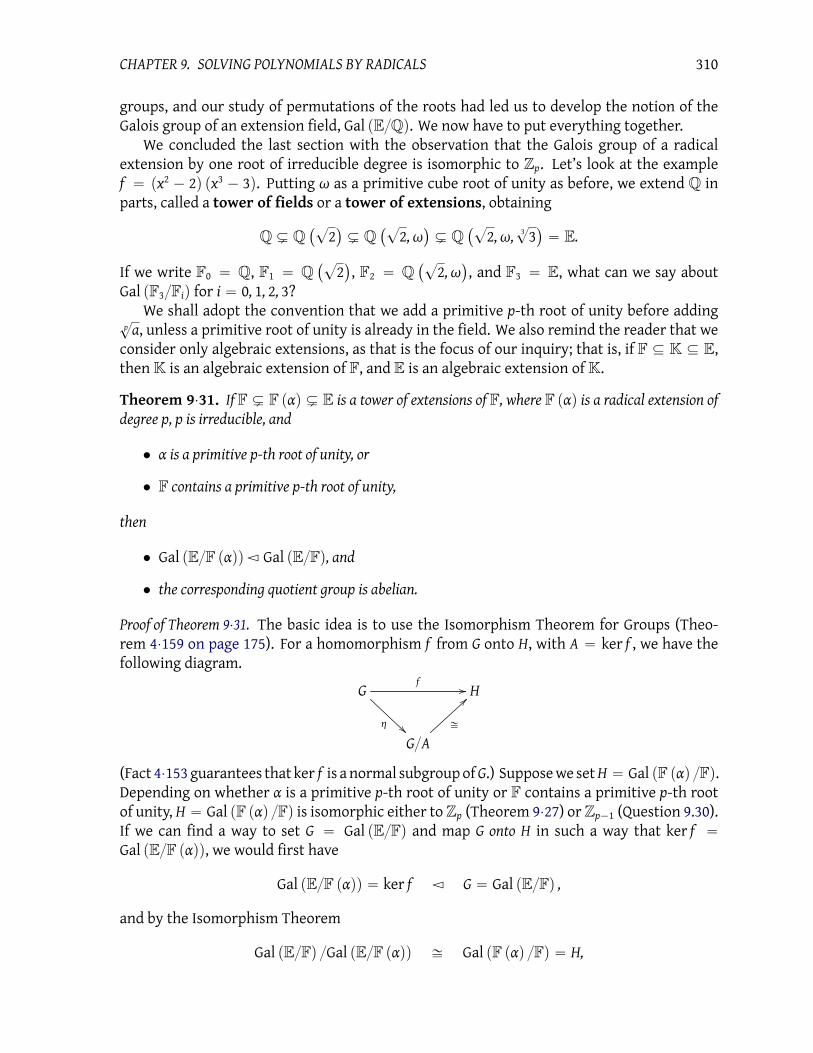
CHAPTER 9. SOLVING POLYNOMIALS BY RADICALS 310
groups, and our study of permutations of the roots had led us to develop the notion of the
Galois group of an extension field, Gal pEQq. We now have to put everything together.
We concluded the last section with the observation that the Galois group of a radical
extension by one root of irreducible degree is isomorphic to Zp. Let’s look at the example
f “ px2 ´ 2q px3 ´ 3q. Putting ω as a primitive cube root of unity as before, we extend Q in
parts, called a tower of fields or a tower of extensions, obtaining
Q Ĺ Q`?2˘
Ĺ Q`?2,ω
˘
Ĺ Q`?2,ω,
3?3˘
“ E.
If we write F0 “ Q, F1 “ Q`?2˘
, F2 “ Q`?2,ω
˘
, and F3 “ E, what can we say about
Gal pF3Fiq for i “ 0, 1, 2, 3?
We shall adopt the convention that we add a primitive p-th root of unity before adding
p?a, unless a primitive root of unity is already in the field. We also remind the reader that we
consider only algebraic extensions, as that is the focus of our inquiry; that is, if F Ď K Ď E,
then K is an algebraic extension of F, and E is an algebraic extension of K.
Theorem 9¨31. If F Ĺ F pαq Ĺ E is a tower of extensions of F, where F pαq is a radical extension of
degree p, p is irreducible, and
• α is a primitive p-th root of unity, or
• F contains a primitive p-th root of unity,
then
• Gal pEF pαqq Ÿ Gal pEFq, and
• the corresponding quotient group is abelian.
Proof of Theorem 9¨31. The basic idea is to use the Isomorphism Theorem for Groups (Theo-
rem 4¨159 on page 175). For a homomorphism f from G onto H, with A “ ker f , we have the
following diagram.
Gf //
η
H
GA
–
>>
(Fact 4¨153 guarantees that ker f is a normal subgroup ofG.) Suppose we setH “ Gal pF pαq Fq.Depending on whether α is a primitive p-th root of unity or F contains a primitive p-th root
of unity, H “ Gal pF pαq Fq is isomorphic either to Zp (Theorem 9¨27) or Zp´1 (Question 9.30).
If we can find a way to set G “ Gal pEFq and map G onto H in such a way that ker f “
Gal pEF pαqq, we would first have
Gal pEF pαqq “ ker f Ÿ G “ Gal pEFq ,
and by the Isomorphism Theorem
Gal pEFq Gal pEF pαqq – Gal pF pαq Fq “ H,

CHAPTER 9. SOLVING POLYNOMIALS BY RADICALS 311
so that, since H is abelian, the quotient group is abelian, as desired.
To this end, define f : Gal pEFq Ñ Gal pF pαq Fq by restriction to F pαq, which means that
f assigns each σ P Gal pEFq to τ P Gal pF pαq Fq so long as τ pxq “ σ pxq for every x P F pαq.Is fwell-defined? Assume that f can map σ to either τ or pτ. By definition, τ pxq “ σ pxq “
pτ pxq for every x P F pαq. However, the domain of τ andpτ is precisely F pαq, so τ “ pτ. Hence, f
is indeed well-defined.
Is f a homomorphism? Let σ,pσ P Gal pEFq, τ “ f pσq, pτ “ f ppσq, and µ “ f pσpσq. To show
that f is a homomorphism, we have to show that pτpτq pxq “ µ pxq for each x P F pαq. So, let
x P F pαq. By definition, pτ pxq “ pσ pxq, so substitution gives us pτpτq pxq “ τ ppτ pxqq “ τ ppσ pxqq.
Since pσ is an automorphism, pσ pxq P F pαq, so by definition, τ ppσ pxqq “ σ ppσ pxqq. On the other
hand, the definition of µ tells us that µ pxq “ pσpσq pxq “ σ ppσ pxqq. We just saw that this was
the same as pτpτq pxq, and x was arbitrary in F pαq; thus, f pσq f ppσq “ τpτ “ µ “ f pσpσq, and we
are indeed dealing with a homomorphism.
Is f onto? Let τ P Gal pF pαq Fq, and define
σ pxq “
#
τ pxq , x P F pαq ;x, otherwise.
You will show in Question 9.33 that σ P Gal pEFq, and it is clear from the definition of σ that
f pσq “ τ. Thus, f is indeed onto.
So, what is ker f ? By definition, σ P ker f if and only if f pσq is the identity homomorphism
ι of Gal pF pαq Fq. An identity homomorphism maps every element to itself; in this case,
ι pxq “ x for all x P F pαq. Thus, σ P ker f if and only if σ pxq “ x for all x P F pαq. This
implies that σ is an automorphism of E that fixes not only F, but F pαq, as well! In other
words, σ P Gal pEF pαqq! Since σ was arbitrary, ker f “ Gal pEF pαqq.We have shown that f is a function from Gal pEFq onto Gal pF pαq Fq whose kernel is
Gal pEF pαqq. As explained in the first paragraph of the proof, this completes the theorem.
We rely on the following corollary in subsequent sections.
Corollary 9¨32. LetF Ĺ F pα1q Ĺ F pα1, α2q Ĺ ¨ ¨ ¨F pα1, . . . , αnq be a tower of radical extensions of
irreducible degree, where we always add a primitive p-th root of unity before any other p-th root. There
exist subgroups G1, . . . , Gn of Gal pF pα1, . . . , αnq Fq such that
tяu “ G0 Ÿ G1
G1 Ÿ G2
...
Gn´1 Ÿ Gn “ Gal pF pα1, . . . , αnq Fq
and the corresponding quotient groups are abelian.
Proof. Apply repeatedly the preceding theorem with E “ F pα1, . . . , αnq, αtheorem “ αk, and

CHAPTER 9. SOLVING POLYNOMIALS BY RADICALS 312
Ftheorem “ F pα1, . . . , αk´1q to build the abelian quotient groups
Gal pF pα1, . . . , αnq Fq Gal pF pα1, . . . , αnq F pα1qqGal pF pα1, . . . , αnq F pα1qq Gal pF pα1, . . . , αnq F pα1, α2qq
...
Gal pF pα1, . . . , αnq F pα1, . . . , αn´1qq Gal pF pα1, . . . , αnq F pα1, . . . αnqq .
From these groups, the following assignments satisfy the claim:
G0 “ Gal pF pα1, . . . , αnq F pα1, . . . , αnqqG1 “ Gal pF pα1, . . . , αnq F pα1, . . . , αn´1qq
...
Gn´1 “ Gal pF pα1, . . . , αnq F pα1qq .
Question 9¨33 .Suppose E Ľ K Ľ F is a tower of fields. Let τ P Gal pKFq. Define σ : EÑ E by
#
σ pxq “ τ pxq , x P K;σ pxq “ x, otherwise.
Show that σ P Gal pEFq.
9¨4 “Solvable” groups
We found in the previous section that the Galois groups corresponding to each step of a tower
of radical extensions form abelian quotient groups. We study this property in some detail in
this section, and start by generalizing the property to arbitrary groups.
Definition 9¨34. If a group G contains subgroups G0, G1, . . . , Gn such that
• G0 “ tяu;
• Gn “ G;
• Gi´1 Ÿ Gi; and
• GiGi´1 is abelian,
then G is a solvable group. The chain of subgroups G0, . . . , Gn is called a normal series.
Example 9¨35. Any finite abelian group G is solvable: let G0 “ tяu and G1 “ G. Subgroups of
an abelian group are always normal, so G0ŸG1. In addition, X, Y P G1G0 implies that X “ x tяu
and Y “ y tяu for some x, y P G1 “ G. Since G is abelian,
XY “ pxyq tяu “ pyxq tяu “ YX.

CHAPTER 9. SOLVING POLYNOMIALS BY RADICALS 313
Example 9¨36. The group D3 is solvable. To see this, let n “ 2 and G1 “ xρy:
• By Exercise 4.127 on page 161, tιu Ÿ G1. To see that G1 tιu is abelian, note that for any
X, Y P G1 tιu, we can write X “ x tιu and Y “ y tιu for some x, y P G1. By definition
of G1, we can write x “ ρa
and y “ ρb
for some a, b P Z. We can then fall back on the
commutative property of addition in Z to show that
XY “ pxyq tιu “ ρa`btιu
“ ρb`atιu “ pyxq tιu “ YX.
• By Exercise 4.133 and the fact that |G1| “ 3 and |G2| “ 6, we know that G1 Ÿ G2. The
same exercise tells us that G2G1 is abelian.
Question 9¨37 .Explain why Ωn is solvable for any n P N`.
Question 9¨38 .Show that Q8 is solvable.
A rather surprising property of solvable groups is that their subgroups and quotient groups
are also solvable. Showing that quotient groups are solvable is a little easier, so we start with
that first.
Theorem 9¨39. Every quotient group of a solvable group is solvable.
Proof. Let G be a solvable group and A Ÿ G. We need to show that GA is solvable. Since G is
solvable, choose a normal series G0, . . . , Gn. For each i “ 0, . . . , n, put
Ai “ tgA : g P Giu .
We claim that the chain A0, A1, . . . , An likewise satisfies the definition of a solvable group.
First, we show that Ai´1 Ÿ Ai for each i “ 1, . . . , n. First we must show that Ai´1 ă Ai. It is
a subset because any X P Ai´1 has the form xA where x P Gi´1 Ď Gi, so x P Gi and thus xA P Ai.
To show that it is a subgroup, let X, Y P Ai´1, and x, y P Gi´1 such that X “ xA and Y “ yA.
By substitution and coset arithmetic, XY´1 “ pxAq pyAq
´1“ pxy´1qA. Recall that Gi´1 is a
subgroup of Gi; by the Subgroup Theorem, xy´1 P Gi´1, so XY
´1 “ pxy´1qA P Ai´1
Now we show that Ai´1 is a normal subgroup. Let X P Ai; by definition, X “ xA for some
x P Gi. We have to show that XAi´1 “ Ai´1X. Let Y P Ai´1; by definition, Y “ yA for some
y P Gi´1. Recall that Gi´1 Ÿ Gi, so there exists py P Gi´1 such that xy “ pyx. Let pY “ pyA; since
py P Gi´1, pY P Ai´1. Using substitution and the definition of coset arithmetic, we have
XY “ pxyqA “ ppyxqA “ pYX P Ai´1X.
Since Y was arbitrary in Ai´1, XAi´1 Ď Ai´1X. A similar argument shows that XAi´1 Ě Ai´1X,
so the two are equal. Since X is an arbitrary coset of Ai´1 in Ai, we conclude that Ai´1 Ÿ Ai.

CHAPTER 9. SOLVING POLYNOMIALS BY RADICALS 314
Second, we show that AiAi´1 is abelian. Let X, Y P AiAi´1. By definition, we can write
X “ SAi´1 and Y “ TAi´1 for some S, T P Ai. Again by definition, there exist s, t P Gi such that
S “ sA and T “ tA. We know that
XY “ YX ô pSAi´1q pTAi´1q “ pTAi´1q pSAi´1q
ô pSTqAi´1 “ pTSqAi´1
ô pSTq´1pTSq P Ai´1
ô T´1S´1TS P Ai´1.
By substitution and coset arithmetic,
T´1S´1TS “
`
t´1A˘ `
s´1A˘
ptAq psAq “`
t´1s´1ts˘
A.
Recall that Gi´1 Ÿ Gi and GiGi´1 is abelian, so
ptGi´1q psGi´1q “ psGi´1q ptGi´1q ô ptsq Gi´1 “ pstq Gi´1 ô t´1s´1ts P Gi´1.
By substitution,
T´1S´1TS P Ai´1.
Following the above chain of equivalences back to their beginning, we have XY “ YX. Since
X and Y were arbitrary in the quotient group AiAi´1, we conclude that it is abelian.
We have constructed a normal series in GA; it follows that GA is solvable.
Question 9¨40 .In Question 9.38 you showed that Q8 is solvable. From Theorem 9¨39 you know the quotient
group Q8 x´1y is also solvable. List a normal series.
The following result is also true:
Theorem 9¨41. Every subgroup of a solvable group is solvable.
To prove Theorem 9¨41, we need the definition of the commutator from Questions 2.30 on
page 53 and 4.151 on page 170, and a few properties of commutator subgroups. If you skipped
those before, you should go back and do them now, to familiarize yourself with the idea.
Definition 9¨42. Let G be a group. The commutator subgroup G1 of G is the intersection of
all subgroups of G that contain rx, ys for all x, y P G.
Notice that G1 ă G by Question 4.10.
Notation 9¨43. We wrote G1as rG, Gs in Question 4.151.
Question 9¨44 .Compute G
1for Q8. Then compute pG1q
1(we call this G
p2qfurther below) and
`
pG1q1˘1
. Keep
going until you can go no further; how do you know you can go no further?
Lemma 9¨45. For any group G, G1 Ÿ G. In addition, GG1 is abelian.

CHAPTER 9. SOLVING POLYNOMIALS BY RADICALS 315
Proof. You showed that G1 Ÿ G in Question 4.151. To show that GG1 is abelian, let X, Y P GG1.
Write X “ xG1 and Y “ yG1 for appropriate x, y P G. By definition, XY “ pxyq G1. Let g1 P G1; by
definition, g1is in every group that contains all the commutators of G. Closure ensures that
the product of g1with another element of G
1is also in G
1; certainly the commutator rx, ys is in
G1, so rx, ys g1 P G1. Write z “ rx, ys g1. Substitution and properties of groups allows to infer
rx, ys g1“ z ùñ
`
x´1y´1xy˘
g1“ z ùñ pxyq g
1“ pyxq z.
Thus, pxyq g1 P pyxq G1. Since g1was arbitrary, pxyq G1 Ď pyxq G1. Similar reasoning shows that
pxyq G1 Ě pyxq G1, which gives us equality. Substitution gives us
XY “ pxyq G1“ pyxq G
1“ YX.
We conclude that GG1 is abelian.
Lemma 9¨46. If H Ď G, then H1 Ď G1.
Proof. You do it! See Question 9.47.
Question 9¨47 .Show that if H Ď G, then H
1 Ď G1.
Notation 9¨48. Define Gp0q “ G and G
piq “`
Gpi´1q
˘1; that is, G
piqis the commutator subgroup of
Gpi´1q
.
Lemma 9¨49. A group is solvable if and only if Gpnq “ tяu for some n P N.
Proof. (ðù) Suppose that Gpnq “ tяu for some n P N. By Lemma 9¨45, the subgroups form a
normal series; that is,
tяu “ GpnqŸ G
pn´1qŸ ¨ ¨ ¨ Ÿ G
p0q“ G
and Gpn´iqGpn´pi´1qq is abelian for each i “ 0, . . . , n ´ 1. As this is a normal series, we have
shown that G is solvable.
(ùñ) Suppose that G is solvable. Let G0, . . . , Gn be a normal series for G. We claim that
Gpn´iq Ď Gi. If this claim were true, then G
pn´0q Ď G0 “ tяu, and we would be done. We
proceed by induction on n´ i P N.
Inductive base: If n ´ i “ 0, then Gpn´iq “ G “ Gn. Also, i “ n, so G
pn´iq “ Gn “ Gi, as
claimed.
Inductive hypothesis: Assume that the assertion holds for n´ i.
Inductive step: By definition, Gpn´i`1q “
`
Gpn´iq
˘1. By the inductive hypothesis, G
pn´iq Ď Gi;
by Lemma 9¨46,`
Gpn´iq
˘1Ď G1
i. Hence
Gpn´i`1q
Ď G1i. (9.1)
We now show that G1iĎ Gi´1. Recall from the properties of a normal series that GiGi´1 is
abelian; for any x, y P Gi, we have
pxyq Gi´1 “ pxGi´1q pyGi´1q
“ pyGi´1q pxGi´1q “ pyxq Gi´1.

CHAPTER 9. SOLVING POLYNOMIALS BY RADICALS 316
By equality of cosets, pyxq´1pxyq P Gi´1 (Lemma 4¨103 on page 152); in other words, rx, ys “
x´1y´1xy P Gi´1. Since x and y were arbitrary in Gi, we have G
1iĎ Gi´1. Along with (9.1), this
implies that Gpn´pi´1qq “ Gpn´i`1q Ď Gi´1.
We have shown the claim; thus, Gpnq “ tяu for some n P N.
We can now prove Theorem 9¨41.
Proof of Theorem 9¨41. LetH ă G. AssumeG is solvable; by Lemma 9¨49, Gpnq “ tяu. By Lemma 9¨46,
Hpiq Ď G
piqfor all n P N, so H
pnq Ď tяu. By the definition of a group, Hpnq Ě tяu, so the two are
equal. By the same lemma, H is solvable.
Question 9¨50 .In the textbook God Created the Integers. . . the theoretical physicist Stephen Hawking collects
reprints of some of the greatest mathematical results in history, adding some commentary.
For an excerpt from Evariste Galois’ Memoirs, Hawking sums up the main result this way.
To be brief, Galois demonstrated that the general polynomial of degree n could be
solved by radicals if and only if every subgroup N of the group of permutations Sn
is a normal subgroup. Then he demonstrated that every subgroup of Sn is normal
for all n ď 4 but not for any n ą 5. —p. 105
Unfortunately, Hawking’s explanation is completely wrong, and this exercise leads you to-
wards an explanation as to why.1
Recall from Fact 7¨30 on page 267 that S3 is isomorphic to
D3; you can work with whichever group is more comfortable for you.
(a) Find all six subgroups of S3.
(b) It is known that the general polynomial of degree 3 can be solved by radicals. According
to the quote above, what must be true about all the subgroups of S3?
(c) Why is Hawking’s explanation of Galois’ result “obviously” wrong?
Question 9¨51 .Show that S4 is solvable, and explain why this means any degree-four polynomial can be
solved by radicals.
9¨5 The Theorem of Abel and Ruffini
In this section, we use the characterization of solution by radicals in Theorem 9¨31 and Defi-
nition 9¨34 to show that some polynomials cannot be solved by radicals. The basic idea is that
1Perhaps Hawking was trying to simplify what Galois actually showed, and went too far. (I’ve done much
worse, on occasion.) You will see the actual result in the next section.

CHAPTER 9. SOLVING POLYNOMIALS BY RADICALS 317
S5 is not a solvable group, and we can find a degree-5 polynomial whose Galois group is S5.
Before we dive into that, though, we need an important fact about the order of a group.
A “reverse-Lagrange” Theorem
Lagrange’s Theorem tells us that the order of any element g of a group Gmust divide the
order of a group; that is, ord pgq | |G|. You might wonder whether the reverse is true; that is,
if m is an integer that divides |G|, can we always find g P G such that ord pgq “ m? The easy
answer is, “Of course not;” after all, we could find g P G such that ord pgq “ |G|, and every
group would be cyclic. Nevertheless, some interesting properties do hold, and one of them is
critical to the result we want.
Cauchy’s Theorem. Let p P N` be irreducible, and let G be a group. If p | |G|, then we can find
g P G such that ord pgq “ p.
The property is not true in general, as you can show:
Question 9¨52 .Find a finite group G where m “ |G|, m is not irreducible, and no g P G has ord pgq “ m.
We start with the case where G is abelian, as this is a special case of the more general
problem.
Lemma 9¨53. Cauchy’s Theorem is true if G is abelian.
Proof. Suppose that G is an abelian group, p P N` is irreducible, and p | |G|. We proceed by
induction on |G|.
Inductive base: If |G| “ 1, then no irreducible number divides |G|, and the theorem is “vac-
uously” true.
Inductive hypothesis: Let n P N`, and suppose that any abelian group whose size is n ă |G|,
and where p | n, contain at least one element whose order is p.
Inductive step: Let g P Gz tяu. If p | ord pgq, then let d “ ord pgq p, and the group
@
gdD
“
!
gd,`
gd˘2
, . . . ,`
gd˘p´1
,`
gd˘p
“ gordpgq
“ я
)
will have order p. Otherwise, p - ord pgq. Let Q “ G xgy; the size of Q is, by definition, the
number of cosets of xgy, which is |G| ord pgq. Since p | |G| but p - xgy, an application of
Lagrange’s Theorem shows that p | |Q|. By hypothesis, G is abelian, so all its subgroups are
normal; specifically, xgy is normal. Thus, Q is also a group; since g ‰ я, the size of Q is less
than the size of G, so the inductive hypothesis applies; Q contains an element of order p; call
this element X. Let x P G such that X “ x xgy. Let m “ ord pxq in G. By definition, xm “ я, so
Xm“ x
mxgy “ я xgy “ xgy .
Hence Xm
is the identity in Q. The order of X is p, so by Exercise 3.56, p | m. Choose d P N`such that pd “ m, and then x
dwill have order p, just as g
dhad order p above.
We now prove the general case.

CHAPTER 9. SOLVING POLYNOMIALS BY RADICALS 318
Proof of Cauchy’s Theorem. As with the abelian case, we proceed by induction, with the induc-
tive base using the same reasoning. We proceed directly to the inductive step.
If G is abelian, then Lemma 9¨53 gives us the result, so assume that G is not abelian. Let
Z pGq denote the center of G,
Z pGq “ tg P G : xg “ gx @x P Gu .
You will show in Question 9.54 that Z pGq is a subgroup of G. Notice that Z pGq is abelian by
definition, so if p | |Z pGq|, then Lemma 9¨53 gives us an element of order p, and we are done.
Assume, therefore, that p - |Z pGq|. For each x P G, define Cx “ tg P G : gx “ xgu. We
call Cx the centralizer of x; you will show in Exercise 9.55 that this is a subgroup of G. Since
p - |Z pGq|, Z pGq ‰ G, so we can find x P GzZ pGq that does not commute with every element of
G, and |Cx| ă |G|. If p | |Cx|, the inductive hypothesis applies.
Assume, therefore, that p does not divide the size of any centralizer. Consider GCx; since
p | |G| but p - |Cx|, Lagrange’s Theorem tells us that p | |GCx|. At this point, we meet up with
our old friend conjugation (Definitions 2¨29 and 4¨143); let xG
be the set of all conjugations of
x by some g P G; that is,
xG“
gxg´1: g P G
(
.
We claim that the set of all these xG
partition G. They certainly cover G, since x “ exe´1 P xG,
so x P xG always. To see that distinct subsets are disjoint, let x, y P G, and suppose y P xG. By
definition, there exists g P G such that y “ gxg´1. We can rewrite this expression as x “ g´1yg,
so x P yG, as well. Moreover, let z P xG; by definition, we can find h P G such that
z “ hxh´1“ h
`
g´1yg˘
h´1“`
hg´1˘
y`
gh´1˘
“`
hg´1˘
y`
hg´1˘´1
,
so z P yG. Since z was arbitrary in xG, x
G Ď yG. A similar argument shows that x
G Ě yG, so
the two must be equal. We have shown that if two subsets are not disjoint, then they are not
distinct; thus, if they are distinct, then they are also disjoint. As claimed, the xG
partition G.
Use this partition to defineP Ď G such thatYxPPxG “ G, and for any distinct x, y P P , x
G ‰ yG,
so xG X yG “ H. From the partition we can see that
ř
xPP |xG| “ |G|.
We also claim that each xG
satisfies |xG| “ |GCx|. Why? Let x P G; by definition, for any
y P xG, we can find g P G such that gxg´1 “ y. Let φ : x
G Ñ GCx by φ pyq “ gCx. We claim
that φ is a one-to-one, onto function. We first check that it is a function, since it is possible
that more than one g P G gives us gxg´1 “ y. So, let g, h P G such that gxg
´1 “ y “ hxh´1
.
Rewrite this as ph´1gq x pg´1hq “ x, or ph´1gq x ph´1gq´1“ x, so h
´1g P Cx. The Lemma on
coset equality then gives us hCx “ gCx, as needed; φ is, indeed, a function. Is it one-to-one?
Suppose φ pyq “ φ pzq; let g P G such that φ pyq “ φ pzq “ gCx. By definition of φ, gxg´1 “ y
and gxg´1 “ z; substitution shows us that y “ z. So, φ is, indeed, one-to-one. Is it onto? For
any gCx P GCx, simply let y “ gxg´1
, and by definition, both y P xG and φ pyq “ gCx. So, φ
is, indeed, onto. We have found a one-to-one, onto function from xG
to GCx; this implies that
the two have the same size.
We can finally show what we set out to show. We have constructed P Ď G such thatř
xPP |xG| “ |G|. For any x P Z pGq, we have
xG“
gxg´1: g P G
(
“
gg´1x : g P G
(
“ txu .

CHAPTER 9. SOLVING POLYNOMIALS BY RADICALS 319
In other words, each element of Z pGq has its own set in the partition. That means we can
rewrite the sum as
|G| “ |Z pGq| `ÿ
xPPzZpGq
ˇ
ˇxGˇ
ˇ .
We have also seen that |xG| “ |GCx| for all x P G, so by substitution,
|G| “ |Z pGq| `ÿ
xPPzZpGq
|GCx| . (9.2)
(This important fact is called the class equation.) Rewrite this as
|G| ´ÿ
xPPzZpGq
|GCx| “ |Z pGq| . (9.3)
Recall that if p - |Cx| for each x P PzZ pGq, then p | |GCx| for the same x. We have assumed
that p does not divide the size of any centralizer, so p must divide the size of every GCx. By
hypothesis, p | |G|, so p divides the left hand side of 9.3. It must divide the right hand side, as
well, which means p | |Z pGq|, a contradiction.
The only assumptions we made that were not required by the hypothesis were that p -|Z pGq| and p - |Cx| for any x. One of these assumptions must be false, but if so, the fact that
their size is smaller than that of Gmeans that the induction hypothesis holds, and we can find
g P G such that ord pgq “ p.
Question 9¨54 .Show that the center Z pGq of a group G is a subgroup of G.
Question 9¨55 .Show that the centralizer Cx of an element x in a group G is a subgroup of G.
Question 9¨56 .Is either Z pGq or Cx pGq guaranteed to be a normal subgroup? Either show why they are, or
provide a counterexample.
Question 9¨57 .Compute the class equation for D3.
Question 9¨58 .Compute the class equation for Q8.
We cannot solve the quintic by radicals
To show that some polynomials cannot be solved by radicals, we begin with a general-
ization of the fact that the purely radical roots of a polynomial can only be mapped to other
roots of the same radical; that is, we can map4?3 ÝÑ ´
4?3, but not to
?2.
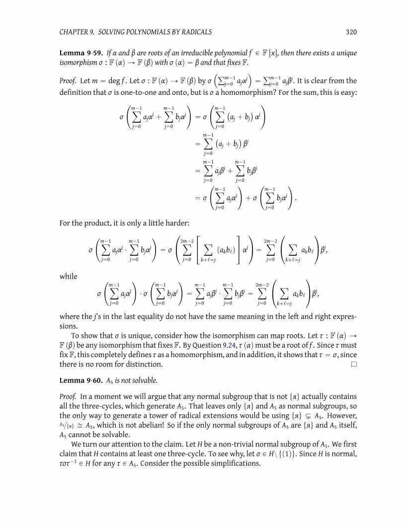
CHAPTER 9. SOLVING POLYNOMIALS BY RADICALS 320
Lemma 9¨59. If α and β are roots of an irreducible polynomial f P F rxs, then there exists a unique
isomorphism σ : F pαq Ñ F pβq with σ pαq “ β and that fixes F.
Proof. Let m “ deg f . Let σ : F pαq Ñ F pβq by σ
´
ř
m´1
j“0ajα
j
¯
“ř
m´1
j“0ajβ
j. It is clear from the
definition that σ is one-to-one and onto, but is σ a homomorphism? For the sum, this is easy:
σ
˜
m´1ÿ
j“0
ajαj`
m´1ÿ
j“0
bjαj
¸
“ σ
˜
m´1ÿ
j“0
`
aj ` bj˘
αj
¸
“
m´1ÿ
j“0
`
aj ` bj˘
βj
“
m´1ÿ
j“0
ajβj`
m´1ÿ
j“0
bjβj
“ σ
˜
m´1ÿ
j“0
ajαj
¸
` σ
˜
m´1ÿ
j“0
bjαj
¸
.
For the product, it is only a little harder:
σ
˜
m´1ÿ
j“0
ajαj¨
m´1ÿ
j“0
bjαj
¸
“ σ
¨
˝
2m´2ÿ
j“0
»
–
ÿ
k``“j
pakb`q
fi
fl αj
˛
‚“
2m´2ÿ
j“0
¨
˝
ÿ
k``“j
akb`
˛
‚βj,
while
σ
˜
m´1ÿ
j“0
ajαj
¸
¨ σ
˜
m´1ÿ
j“0
bjαj
¸
“
m´1ÿ
j“0
ajβj¨
m´1ÿ
j“0
bjβj“
2m´2ÿ
j“0
¨
˝
ÿ
k``“j
akb`
˛
‚βj,
where the j’s in the last equality do not have the same meaning in the left and right expres-
sions.
To show that σ is unique, consider how the isomorphism can map roots. Let τ : F pαq ÑF pβq be any isomorphism that fixesF. By Question 9.24, τ pαqmust be a root of f . Since τmust
fixF, this completely defines τ as a homomorphism, and in addition, it shows that τ “ σ, since
there is no room for distinction.
Lemma 9¨60. A5 is not solvable.
Proof. In a moment we will argue that any normal subgroup that is not tяu actually contains
all the three-cycles, which generate A5. That leaves only tяu and A5 as normal subgroups, so
the only way to generate a tower of radical extensions would be using tяu Ĺ A5. However,
A5tяu – A5, which is not abelian! So if the only normal subgroups of A5 are tяu and A5 itself,
A5 cannot be solvable.
We turn our attention to the claim. Let H be a non-trivial normal subgroup of A5. We first
claim that H contains at least one three-cycle. To see why, let σ P Hz tp1qu. Since H is normal,
τστ´1 P H for any τ P A5. Consider the possible simplifications.

CHAPTER 9. SOLVING POLYNOMIALS BY RADICALS 321
• You will show in Question that if H contains a two-cycle or a four-cycle, then it also
contains a three-cycle. The argument is very similar to the next two.
• If σ “ pa bq pc dq, let τ “ pa bq pc eq. Notice that τ “ τ´1. The conjugation tells us that
rpa bq pc eqs rpa bq pc dqs rpa bq pc eqs “ pa bq pd eq P H.
The closure of H implies that it must also contain pa bq pc dq pa bq pd eq “ pc d eq.
• If σ “ pa b c d eq, let τ “ pa b cq. Notice that τ´1 “ pa c bq. The conjugation tells us
that
pa b cq pa b c d eq pa c bq “ pa d e b cq P H.
The closure of H implies that it must also contain pa b c d eq2pa d e b cq “ pb e dq.
Either way, H contains a three-cycle.
Now we claim that H contains all the three-cycles. Suppose H contains pa b cq. By conju-
gation, it also contains
• pb c dq pa b cq pb d cq “ pa c dq,
• pb c eq pa b cq pb e cq “ pa c eq,
• pb d cq pa b cq pb c dq “ pa d bq,
• pb dq pc eq pa b cq pb dq pc eq “ pa d eq,
• pb e cq pa b cq pb c eq “ pa e bq,
• pa c dq pa b cq pa d cq “ pb d cq,
• pa dq pc eq pa b cq pa dq pc eq “ pb e dq,
• pa c eq pa b cq pa e cq “ pb e cq, and
• pa dq pb eq pa b cq pa dq pb eq “ pc d eq.
Since H is closed, it also contains the inverses of these elements, so H contains at least twenty
three-cycles. A counting argument tells us that there are in fact 5!3! “ 20 three-cycles, so H
contains all the three-cycles.
We leave it to the reader to show that A5 is generated by all the three-cycles; see Ques-
tion 9.61.
Question 9¨61 .Show that if a subgroup H of A5 contains all the three-cycles, then in fact H “ A5.

CHAPTER 9. SOLVING POLYNOMIALS BY RADICALS 322
Question 9¨62 .We can also show that A5 is not solvable by considering its commutators. As usual, let A
15
denote the commutator subgroup of A5.
(a) Show that pa b cq P A15
for any distinct a, b, c P t1, 2, 3, 4, 5u.
(b) Show that pa bq pc dq P A15
for any distinct a, b, c, d P t1, 2, 3, 4, 5u.
(c) Show that pa b c d eq P A15
for any distinct a, b, c, d, e P t1, 2, 3, 4, 5u.
(d) Explain why this shows that A15“ A5.
(e) Explain why this shows that A5 is not solvable.
Corollary 9¨63. S5 is not solvable.
Proof. If S5 were solvable, then Theorem 9¨41 would imply that A5 is solvable. We just saw that
A5 is not solvable, so S5 cannot be solvable, either.
We turn our attention to finding a polynomial whose Galois group is S5.
Lemma 9¨64 (Eisenstein’s Criterion). Let f “ amxm` ¨ ¨ ¨` a1x` a0 P Z rxs, and p an irreducible
integer. If
• p | ai for each i “ 0, . . . , m´ 1,
• p - am, and
• p2 - a0,
then f is irreducible, even when viewed in Q rxs.
Proof. Suppose f factors inZ rxs as f “ gh. It will also factor when considered as a polynomial
of Zp rxs, with the same gh. Assume that p divides every coefficient of f except the leading
coefficient, so f “ amxm
as a polynomial in Zp rxs, so g “ bxβ
and h “ cxγ. Observe that p
divides the constant terms of g and h, which means that p2 | a0. This contradicts the third
criterion, so if f factors in Z rxs, then we cannot satisfy all three criteria.
To complete the proof, we need to show that if f factors in Q rxs, then it also factors in
Z rxs. Suppose f “ gh is a factorization of f in Q rxs. Rewrite this factorization as f “ dpgph,
where d P N` is the least common denominator of the coefficients of, g and h, obtaining an
integer factorization of an integer polynomial. Rewrite the factorization again as f “ d1g1h1,
where d1
is the product of d and the greatest common divisors of the coefficients of pg and
of ph. Notice that d1must be an integer, as d cannot divide g
1or h
1. We have thus obtained a
factorization of f into integer polynomials.
Question 9¨65 .Use the product rule of Calculus to show that x “ a is a repeated root of a polynomial f if and
only f1 paq “ 0.

CHAPTER 9. SOLVING POLYNOMIALS BY RADICALS 323
Theorem 9¨66. There exists a quintic polynomial over Q that is not solvable by radicals.
Proof. Let f pxq “ x5 ´ 4x` 2. Using Eisenstein’s Criterion and the irreducible integer p “ 2,
we see that f is irreducible over Q. Extend Q to a field E that contains all the roots of f .
Since we are working over the real numbers, we resort briefly to calculus. The maxima
and minima of f pxq “ x5 ´ 4x` 2 occur when 0 “ f
1 pxq “ 5x4 ´ 4; these are x “ ˘ 4
a
45. If
we substitute these values of x into f , we find that
f
˜
´4
c
4
5
¸
« ´1` 4` 2 ą 0 and f
˜
4
c
4
5
¸
« 1´ 4` 2 ă 0.
Since neither critical point is also a root, there are no repeated roots (see Question 9.65), so f
makes exactly two turns on the real plane, so it can have exactly three roots α1, α2, α3 P RzQ.
Once we extend Q with those roots, f factors as
f pxq “ px´ α1q px´ α2q px´ α3q`
x2` ax` b
˘
,
where a, b P R. Since f has no more real roots, the quadratic polynomial has complex roots;
call them β1 and β2. We know from the quadratic formula that if β1 “ c` di, then β2 “ c´ di.
Now consider the automorphisms of the final extension field E.
• One automorphism is defined homomorphically by φ piq “ ´i; this corresponds to an
exchange of the complex roots, or, a transposition in S5. Of course, it’s not enough to
claim it’s an automorphism that fixes Q; we must actually show this. It is clear that φ
fixes not onlyQ, but non-complex elements ofE, as well, as mapping˘iÑ ¯i does not
affect them in the slightest. You showed in Question 9.20 that φ is a ring isomorphism
in C; the same argument applies to E, as well.
• We claim that when Gal pEQq is viewed as a subgroup of S5, there must also be a 5-
cycle. To see why, consider how we can extend the identity isomorphism ι : Q Ñ Qto an automorphism on Q pαq, where α is any one of the roots of f . The elements of
F “ Q rxs 〈f 〉 can be written using the basis t1, x` I, . . . , x4 ` Iu, and Q pαq – F, so
when we view E as an extension of Q pαq, each element that we adjoin can be seen as
having a coefficient in F, which has dimension 5. Using similar reasoning, elements
of E can be seen as an extension of Q with a basis containing 5m elements, for some
m P N`. By Lemma 9¨59, there are 5m unique isomorphisms extending ι to E, one for
each element of the basis of E. Hence, |Gal pEFq| “ 5m. What matters here is that
the size of the group is divisible by 5; we can now apply Cauchy’s Theorem to show that
Gal pEFq has an element of order 5; in other words, a 5-cycle.
Once we have a two-cycle and a five-cycle in Gal pEQq, we can show that Gal pEQq – S5
(Question 9.67). We know from Corollary 9¨63 that S5 is not solvable. Apply the contrapositive
of Theorem 9¨31 to see that f cannot be solved by radicals.
Question 9¨67 .Suppose a subgroup H of S5 has a two-cycle and a five-cycle. Show that H “ S5.

CHAPTER 9. SOLVING POLYNOMIALS BY RADICALS 324
9¨6 The Fundamental Theorem of Algebra
Carl Friedrich Gauß proved the Fundamental Theorem of Algebra in his doctoral thesis.
The Fundamental Theorem of Algebra. Every f P C rxs has a root in C.
Although it deals with an algebraic topic (the roots of univariate polynomial equations),
proving it requires at least a few non-trivial results from analysis, and it can be proved without
any algebraic ideas at all. This has led some to joke that the theorem is neither fundamental
nor algebraic.
We will describe an algebraic proof of the Fundamental Theorem, based on ideas from
Galois theory; this argument is basically found in Chapter 7 of [1]. Of course, Galois would
not have made the argument we produce below. Since we need some analytical ideas first, we
turn to them, without dwelling on why they are true — you can consult a text on calculus or
analysis.
Background from Calculus
Every first-semester calculus student encounters the following fact.
The Intermediate Value Theorem. Let f be a continuous function on ra, bs. For every y-value
between f paq and f pbq, we can find c P pa, bq such that f pcq “ y.
Intuitively speaking, continuity means that f has no holes or asymptotes, so of course it
would pass through y. However, this is not so easy to prove; the precise definition of continu-
ity is that you can evaluate the limit at every point by substitution (limxÑa f pxq “ f paq), so it
takes a little more work than you would imagine at first glance. This is a class in algebra, not
analysis, so we move on.
Theorem 9¨68. Polynomials over C are continuous.
This one is not quite so intuitive, unless you have worked extensively with polynomials
whose coefficients are complex. It is not difficult, but again, it is analytical in nature, so we
move on.
Corollary 9¨69. Let f P R rxs. If deg f is odd, then f has a root in R.
This one is worth considering briefly; again, we rely on ideas from calculus.
Proof. Let n “ deg f , and consider
limxÑ8
f pxq
xn“ lim
xÑ8
anxn ` an´1x
n´1 ` ¨ ¨ ¨ ` a1x` a0
xn“ lim
xÑ8
´
an `an´1
x` ¨ ¨ ¨ `
a1
xn´1`a0
xn
¯
“ an.
Let ε ą 0. By definition, there exists N P R such that for all x ą N,
ˇ
ˇ
ˇan ´
f pxq
x
ˇ
ˇ
ˇă ε. Thus, for
all these x, we have
´ε ă an ´f pxq
xă ε ùñ x pan ` εq ą f pxq ą x pan ´ εq .
In other words, for all x ą N, f pxq has the same sign as an. A similar argument shows that we
can findM P R such that for all x ă M, f pxq has the same sign as´an. By definition of degree,
an ‰ 0, so f has at least one positive value, and at least one negative value. Apply continuity
and the Intermediate Value Theorem to see that f has a root between these two points.

CHAPTER 9. SOLVING POLYNOMIALS BY RADICALS 325
Some more algebra
Now for two algebraic ideas. The first is separability, which has to do with how a polynomial
factors in its extension field. The second is the first of the famous Sylow Theorems.
Definition 9¨70. Suppose E “ F pαq is an extension field. Let f be an irreducible polyno-
mial over F such that α is a root of f . We say that α is separable over F if f factors in E as
px´ αq g pxq, and g pαq ‰ 0.
Theorem 9¨71. Extensions of C are separable.
Proof. This is a consequence of Calculus. If f “ px´ aqm¨ g, then f
1 “ m px´ aqm´1
g `
px´ aqmg1. The derivative of a complex polynomial is also a complex polynomial, and the
Euclidean algorithm gives us a gcd which has p “ px´ aqm´1
as a factor. If f is irreducible,
the gcd of f and f1must be a constant, so m “ 1.
(The proof above can fail in a field of nonzero characteristic, but in this chapter we have
assumed that this is not the case.)
Theorem 9¨72. Let E be an algebraic extension of C. The degree of E over C is |Gal pECq|.
Proof. We proceed by induction on rE : Cs (the degree of E over C).
Inductive base: If rE : Cs “ 1, then E “ C, so the only element of Gal pECq is the identity.
Hence rE : Cs “ |Gal pECq|.Inductive hypothesis: Let n P N`, and assume that if rE : Cs ď n, then Gal pECq “ n.Inductive step: Let f P C rxs such that E is the algebraic extension by the roots of f , and
rE : Cs “ n`1. Let q be an irreducible factor of f , and choose g such that f “ qg; if deg q “ 1,
then the root of q is already in C. Hence, we may assume without loss of generality that
deg q ą 1. Let α be any root of q, and φ P Gal pECq. In Question 9.24 you showed that φ pαq is
another root of q. By Theorem 9¨71, extensions of C are separable, so the choice of mappings
for φ is determined entirely by q. Hence, |Gal pC pαq Cq| “ deg q “ rC pαq : Cs. Apply the
inductive hypothesis to rE : C pαqs to obtain
rE : Cs “ rE : C pαqs rC pαq : Cs “ |Gal pEC pαqq| ¨ |Gal pC pαq Cq| .
At this point we define a homomorphism that maps elements of Gal pECq to elements of
Gal pC pαq Cq by restriction, similar to the proof of Theorem 9¨31. (The difference here is
that we are not working with radical extensions, so we cannot guarantee Gal pC pαq Cq is
abelian.) As before, the kernel will be Gal pEC pαqq. The kernel is a normal subgroup, so
Lagrange’s Theorem tells us
|Gal pEC pαqq| ¨ |Gal pC pαq Cq| “ |Gal pECq| ,
which completes the proof.
We now turn to the First Sylow Theorem, which generalizes Cauchy’s Theorem that if an
irreducible p divides |G|, then G contains an element of order p.
First Sylow Theorem. Let G be a group, and p P N` be irreducible. If |G| “ pmqwhere p - q, then
G has a subgroup of size pifor each i P t1, . . . , mu.

CHAPTER 9. SOLVING POLYNOMIALS BY RADICALS 326
Proof. We proceed by induction on the size of G. The inductive basis follows from Cauchy’s
Theorem, so for the inductive hypothesis, assume that for any group H of order smaller than
|G|, such that |H| “ pmr and p - r, we can find a subgroup A of size p
m. We need to show that
we can also find a subgroup of size pm`1
.
Recall the class equation (9.3),
|G| ´ÿ
xPPzZpGq
|GCx| “ |Z pGq| .
We consider two cases.
Case 1: If p divides |Z pGq|, then Cauchy’s Theorem tells us that Z pGq has a normal subgroup
A of size p. Elements of Z pGq commute with all elements of G, so A is a normal subgroup of G.
Hence, GA is a quotient group. By Lagrange’s Theorem,
|GA| “|G|
|A|“pmq
p“ p
m´1q,
and since m ą 1, p divides |GA|. By hypothesis, GA has a subgroup of size pm´1
. Call it B.
Recall the natural homomorphism µ : G Ñ GA by µ pgq “ gA. This homomorphism is
onto GA, so let
H “ tg P G : µ pgq P Bu .
We claim that H ă G; to see why, let x, y P H. A property of homomorphisms is that µ py´1q “
µ pyq´1P B, so now closure and properties of homomorphisms guarantee that µ pxy´1q “
µ pxq µ pyq´1P B.
We claim that |H| “ pm
. Why? An argument similar to that of the Isomorphism Theorem
shows that B – H ker µ, so |B| “ |H| |ker µ|, and |ker µ| “ |A|, so |H| “ |A| |B| “ p¨pm´1 “ pm,
as desired.
Case 2: Suppose p - |Z pGq|. We claim that p - |GCx| for some x P G. To see why, assume by
way of contradiction that it divides all of them. By hypothesis, p divides |G|; p then divides
the left-hand side of the class equation above, so p must divide the right hand side, |Z pGq|, a
contradiction.
The centralizer of an element is a subgroup ofG. By Lagrange’s Theorem, |GCx| “ |G| |Cx|.
Rewrite this as |GCx| |Cx| “ |G|. By hypothesis, pm
divides the right hand side, but p - |GCx|,so the definition of a prime number forces p
m | |Cx|.
On the other hand, x R Z pGq, so Cx ‰ G, so |Cx| ă |G|. The inductive hypothesis applies,
and we can find a subgroup A of Cx of size pm
. A subgroup of Cx is also a subgroup of G, so A is
a desired subgroup of G whose order is pm
.
Proof of the Fundamental Theorem
Let f P C rxs. Let E be the field that contains all the roots of f . We claim that E “ C.
By unique factorization and the Factor Theorem, f can have only finitely many roots, so
E is a finite extension of C, itself a finite extension of R. Hence, E is also a finite extension of
R. We claim that E is an odd-degree extension of R; if not, we would be able to find an odd-
degree polynomial f P R rxs that is irreducible. By the corollary to the Intermediate Value
Theorem, however, odd-degree polynomials over R must have a root in R, a contradiction.

CHAPTER 9. SOLVING POLYNOMIALS BY RADICALS 327
Hence, E must be an even extension of R. If it is a degree-2 extension, then the quadratic
formula suggests that C Ě E Ě C, so C “ E. The remaining possibilities fall into two cases:
rE : Rs “ 2m (a pure power of 2) or rE : Rs “ 2mq for some odd q.
We consider the second possibility first. Suppose the degree of E over R is 2mq, where
m, q P N` and 2 - q. Let G “ Gal pERq be its Galois group; notice that |G| “ 2mq. By the
First Sylow Theorem, G has a subgroup H of size 2m
. By Lagrange’s Theorem, |GH| “ q. This
corresponds to an intermediate field pE such that
• the degree of E over pE is 2m
, and
• the degree of pE over R is q.
Since 2 - q, pE is an odd-degree extension of R, and we already dealt with that. Hence q “ 1,
and the only possibility that remains is|G| “ 2m, a pure power of 2.
Of course, C “ R“?´1
‰
is an intermediate field between E and R. Its degree over R is
2, so the degree of E over C is 2m´1
. Let f be an irreducible polynomial of degree m ´ 1 over
C. We claim that m “ 1; to see why, assume the contrary, and proceed by induction on m. If
m “ 2, then the quadratic formula shows us that the roots of f “ ax2 ` bx` c are
x “´b˘
?b2 ´ 4ac
2a.
We claim that the square roots of complex numbers are also complex. To see why, consider
z “ a`bi, where a, b P R. Let α “ arctan pbaq and r “ a2`b2. You will show in Question 9.73
that z “ r pcos α` i sin αq. Let
w “?r
´
cosα
2` i sin
α
2
¯
;
notice that
w2“`?r˘
2”´
cos2α
2´ sin
2α
2
¯
` 2i sinα
2cos
α
2
ı
.
Apply the double-angle formulas to get
w2“ r
”
cos
´
2 ¨α
2
¯
` i sin
´
2 ¨α
2
¯ı
“ r pcos α` i sin αq “ z.
Since z was arbitrary in C, we see that square roots of complex numbers are also complex.
Assume, therefore, that for some n P N`, if the degree of an extension field over C is 2n,
then the extension field is C. Let F be an extension of C of degree 2n`1
. As before, we can
construct an extension field pF of C of degree 2n, so that the degree of F over pF is 2. By the
inductive hypothesis, pF “ C. Hence the degree of F over C is 2, which the inductive base
tells us means F “ C.
By induction, then, E “ C.
Question 9¨73 .Let z P C, and choose a, b P R such that z “ a`bi. Let α “ arctan pbaq and r “ a2`b2. Show
that z “ r pcos α` i sin αq.

Chapter 10
Roots of polynomial systems
This chapter is about the roots of systems of polynomial equations, such as
"
x2 ` y3 “ 4
xy “ 1.
Rather than investigate the computation of roots, we consider the analysis of roots we have not
enumerated explicitly, and the tools used to compute that analysis. In particular, we want to
know when the roots to a multivariate system of polynomial equations exists. Techniques
described here allow us to answer the following questions:
1. Does the system have any solutions in C?
2. If so,
(a) Are there infinitely many, or finitely many?
i. If finitely many, exactly how many?
ii. If infinitely many, what is the “dimension” of the solution set?
(b) Are any of the solutions in R?
We refer to these as five natural questions about the roots of a polynomial system. We start off
reviewing them for linear systems, but you should already have seen that in linear algebra,
so we emphasize “review.” We then analyze how the nature of a non-linear, multivariate
monomial hampers this strategy with non-linear, multivariate polynomials, before concluding
with a foray into Hilbert’s Nullstellensatz and Grobner bases, fundamental results and tools
of commutative algebra and algebraic geometry.
It shouldn’t surprise you that polynomial systems appear in many contexts. A chemist
once emailed me about a problem he was studying that involved microarrays. Microarrays
measure gene expression, and he was trying to model them using this system of equations:
axy´ b1x´ cy` d1 “ 0
axy´ b2x´ cy` d2 “ 0 (10.1)
axy´ b2x´ b1y` d3 “ 0
328

CHAPTER 10. ROOTS OF POLYNOMIAL SYSTEMS 329
where a, b1, b2, c, d1, d2, d3 P N are known constants and x, y P R were unknown. The chemist
wanted to find values for x and y that made all the equations true.
This already is an interesting, well-studied problem, but the chemist’s fancy software
didn’t always solve the system. He didn’t understand whether it was because there was some-
thing wrong with his numbers, or with the system itself. All he knew is that for some values
of the coefficients, the system gave him a solution, but for other values the system found no
solution. The reason turned out to be the software’s reliance on numerical techniques to look
for a solution, which can fail even when a solution exists.
Techniques described in this chapter showed that no real solution existed; all solutions
were complex. The software’s numerical techniques wasn’t designed to discover such solu-
tions, and this is why it failed.
10¨1 Gaussian elimination
A generic system of m linear equations in n variables looks like
a11x1 ` a12x2 ` ¨ ¨ ¨ ` a1nxn “ b1
a21x1 ` a22x2 ` ¨ ¨ ¨ ` a2nxn “ b2
......
am1x1 ` am2x2 ` ¨ ¨ ¨ ` amnxn “ bm
where the aij and bi are elements of a fieldF. Although it is typically taught withF “ R, linear
algebra can be done over any field F, such as a finite field!
Example 10¨1. A linear system with m “ 3, n “ 5, and coefficients in Z13 is
5x1 ` x2 ` 7x5 “ 7
x3 ` 11x4 ` 2x5 “ 1
3x1 ` 7x2 ` 8x3 “ 2.
An equivalent system, with the same solutions, is
5x1 ` x2 ` 7x5 ` 6 “ 0
x3 ` 11x4 ` 2x5 ` 12 “ 0
3x1 ` 7x2 ` 8x3 ` 11 “ 0.
Our standard formwill typically describe a system as a list or sequence of the left-hand sides
of the second form above,$
&
%
5x1 ` x2 ` 7x5 ` 6,
x3 ` 11x4 ` 2x5 ` 12,
3x1 ` 7x2 ` 8x3 ` 11
,
.
-
.
Gaussian eliminationobtains a “triangular system” equivalent to the original. By “equiv-
alent”, we mean that pa1, . . . , anq P Fn is a solution to the triangular system if and only if it
is a solution to the original system as well. Algorithm 10.1 describes one way to apply the
method.

CHAPTER 10. ROOTS OF POLYNOMIAL SYSTEMS 330
Algorithm 10.1 Gaussian elimination
1: inputs2: F “ pf1, f2, . . . , fmq, a list of linear polynomials in n variables, with coefficients from a
field F.
3: outputs4: G “ pg1, g2, . . . , gmq, a list of linear polynomials in n variables, in triangular form, whose
roots are precisely the roots of F.
5: do6: Let G :“ F
7: for i “ 1, 2, . . . , m´ 1 do8: Rearrange gi, gi`1, . . . , gm so that for each k ă `, g` “ 0, or lv pgkq ě lv pg`q
9: if gi ‰ 0 then10: Denote the coefficient of lv pgiq by a
11: for j “ i` 1, i` 2, . . . m do12: if lv
`
gj
˘
“ lv pgiq then13: Denote the coefficient of lv
`
gj
˘
by b
14: Replace gj with agj ´ bgi
15: return G
Definition 10¨2. Let G “ pg1, g2, . . . , gmq be a list of linear polynomials in n variables. For
each i “ 1, 2, . . . , m designate the leading variable of gi, as the smallest-indexed variable of
non-zero coefficient. Write lv pgiq for this variable.
Remark. The leading variable of the zero polynomial, lv p0q, is undefined.
The ordering for leading variables guarantees x1 ą x2 ą. . . ą xn, something like a dictio-
nary. We refer to it as the lexicographic term ordering. In the same way, we order x ą y ą z;
if other variables appear, we state the ordering explicitly.
Example 10¨3. Using the example from 10¨1,
lv p5x1 ` x2 ` 7x5 ` 6q “ x1,
lv px3 ` 11x4 ` 2x5 ` 12q “ x3.
Definition 10¨4. A list of linear polynomials F is in triangular form if for each i ă j,
• fi “ 0 implies fj “ 0, while
• fi, fj ‰ 0 implies lv pfiq ą lv`
fj
˘
.
Example 10¨5. Using the example from 10¨1,the list
F “ p 5x1 ` x2 ` 7x5 ` 6, x3 ` 11x4 ` 2x5 ` 12, 3x1 ` 7x2 ` 8x3 ` 11 q
is not in triangular form, since lv pf1q “ lv pf3q “ x1, whereas we want lv pf1q ą lv pf3q.
The list
G “ p x1 ` 6, 0, x2 ` 3x4 q

CHAPTER 10. ROOTS OF POLYNOMIAL SYSTEMS 331
is also not in triangular form, because g2 is zero while g3 ‰ 0.
However, the list
H “ p x1 ` 6, x2 ` 3x4, 0 q
is in triangular form, because h3 “ 0 and lv ph1q ą lv ph2q.
Theorem 10¨6. Algorithm 10.1 terminates correctly.
Proof. All the loops of the algorithm are explicitly finite, so the algorithm terminates. To show
that it terminates correctly, we must show both that G is triangular and that its roots are the
roots of F.
That G is triangular: We first claim that the ith iteration of the outer loop terminates with
G in i-subtriangular form; by this we mean that
• the list pg1, . . . , giq is in triangular form; and
• for each j “ 1, . . . , i if gj ‰ 0 then the coefficient of lv`
gj
˘
in gi`1, . . . , gm is 0.
For example, a system in 2-subtriangular form looks like this, where a “*” indicates a non-zero
coefficient of a variable:
˚ ˚ ˚ ˚ ˚
˚ ˚ ˚ ˚
˚ ˚ ˚
˚ ˚ ˚
˚ ˚ ˚
Proving this first subclaim is straightforward; after all, line 8 ensures that all the zero poly-
nomials occur at the end of the list, and lv pgiq ě lv`
gi`j
˘
for any j ě 1, while lines 13 and 14
ensure that if gi ‰ 0 then lv pgiq ą lv`
gi`j
˘
for any j ě 1.
Having established that subclaim, we now observe that G is in triangular form if and only
if G is in i-subtriangular form for all i “ 1, 2, . . . , m. Again, this is straightforward, and estab-
lishes that G is in triangular form after at most m iterations.
Showing that G is equivalent to F is only a little harder. The combinations of F that produce
G are all linear; that is, for each j “ 1, . . . , m there exist ci,j P F such that
gj “ c1,jf1 ` c2,jf2 ` ¨ ¨ ¨ ` cm,jfm.
Hence if pα1, . . . , αnq P Fn is a common root of F, it is also a common root ofG. For the converse,
observe from the algorithm that there exists some i such that fi “ g1; then there exists some
j P t1, . . . , mu z tiu and some a, b P F such that fj “ ag1´bg2; and so forth. Hence the elements
of F are also a linear combination of the elements of G, and a similar argument shows that the
common roots of G are common roots of F.
Remark 10¨7. There are other ways to define both triangular form and Gaussian elimination.
The approach we have taken assists us in the development of later ideas.
Example 10¨8. We illustrate Gaussian elimination for the system of equations described in
Example 10¨1.
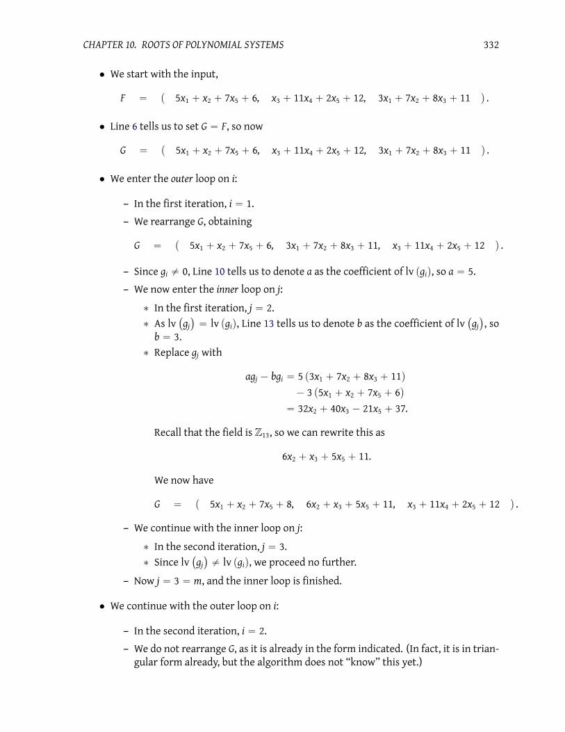
CHAPTER 10. ROOTS OF POLYNOMIAL SYSTEMS 332
• We start with the input,
F “ p 5x1 ` x2 ` 7x5 ` 6, x3 ` 11x4 ` 2x5 ` 12, 3x1 ` 7x2 ` 8x3 ` 11 q .
• Line 6 tells us to set G “ F, so now
G “ p 5x1 ` x2 ` 7x5 ` 6, x3 ` 11x4 ` 2x5 ` 12, 3x1 ` 7x2 ` 8x3 ` 11 q .
• We enter the outer loop on i:
– In the first iteration, i “ 1.
– We rearrange G, obtaining
G “ p 5x1 ` x2 ` 7x5 ` 6, 3x1 ` 7x2 ` 8x3 ` 11, x3 ` 11x4 ` 2x5 ` 12 q .
– Since gi ‰ 0, Line 10 tells us to denote a as the coefficient of lv pgiq, so a “ 5.
– We now enter the inner loop on j:
∗ In the first iteration, j “ 2.
∗ As lv`
gj
˘
“ lv pgiq, Line 13 tells us to denote b as the coefficient of lv`
gj
˘
, so
b “ 3.
∗ Replace gj with
agj ´ bgi “ 5 p3x1 ` 7x2 ` 8x3 ` 11q
´ 3 p5x1 ` x2 ` 7x5 ` 6q
“ 32x2 ` 40x3 ´ 21x5 ` 37.
Recall that the field is Z13, so we can rewrite this as
6x2 ` x3 ` 5x5 ` 11.
We now have
G “ p 5x1 ` x2 ` 7x5 ` 8, 6x2 ` x3 ` 5x5 ` 11, x3 ` 11x4 ` 2x5 ` 12 q .
– We continue with the inner loop on j:
∗ In the second iteration, j “ 3.
∗ Since lv`
gj
˘
‰ lv pgiq, we proceed no further.
– Now j “ 3 “ m, and the inner loop is finished.
• We continue with the outer loop on i:
– In the second iteration, i “ 2.
– We do not rearrange G, as it is already in the form indicated. (In fact, it is in trian-
gular form already, but the algorithm does not “know” this yet.)

CHAPTER 10. ROOTS OF POLYNOMIAL SYSTEMS 333
– Since gi ‰ 0, Line 10 tells us to denote a as the coefficient of lv pgiq; since lv pgiq “
x2, a “ 6.
– We now enter the inner loop on j:
∗ In the first iteration, j “ 2.
∗ Since lv`
gj
˘
‰ lv pgiq, we do not proceed with this iteration.
– Now j “ 3 “ m, and the inner loop is finished.
• Now i “ 2 “ m´ 1, and the outer loop is finished.
• We return G, which is in triangular form!
Once we have the triangular form of a linear system, it is easy to answer the five natural
questions.
Theorem 10¨9. Let G “ pg1, g2, . . . , gmq is a list of nonzero linear polynomials in n variables over a
field F. If G is in triangular form, then each of the following holds.
(A) G has common solutions if and only if none of the gi is a nonzero constant.
(B) G has finitely many common solutions if and only if F has nonzero characteristic, G has common
solutions, andm “ n. In this case, there is exactly one solution.
(C) G has common solutions of dimension d ą 1 if and only ifF has characteristic zero, G has common
solutions, and d “ n´ m.
A proof of Theorem 10¨9 can be found in any textbook on linear algebra, although probably
not in one place.
Example 10¨10. Continuing with the system that we have used in this section, we found that
a triangular form of
F “ p 5x1 ` x2 ` 7x5 ` 6, x3 ` 11x4 ` 2x5 ` 12, 3x1 ` 7x2 ` 8x3 ` 11 q
is
G “ p 5x1 ` x2 ` 7x5 ` 6, 6x2 ` x3 ` 5x5 ` 11, x3 ` 11x4 ` 2x5 ` 12 q .
Theorem 10¨9 implies that
(A) G has a solution, because none of the gi is a constant.
(B) G has finitely many solutions, because the characteristic (13) is nonzero.
(C) If the characteristic were zero, it would have infinitely many solutions of dimension d “
n ´ m “ 2, as the number of polynomials (m “ 3) is not the same as the number of
variables (n “ 5). (A field of characteristic zero always has infinitely many elements.)

CHAPTER 10. ROOTS OF POLYNOMIAL SYSTEMS 334
Lexicographic order allows us to parametrize the solution set easily. Let s, t P Z13 be arbitrary,
and let x4 “ s and x5 “ t. Back-substituting in S, we have:
• From g3 “ 0, x3 “ 2s` 11t ` 1.
• From g2 “ 0,
6x2 “ 12x3 ` 8t ` 12. (10.2)
The Euclidean algorithm helps us derive the multiplicative inverse of 6 in Z13; we get
11. Multiplying both sides of (10.2) by 11, we have
x2 “ 2x3 ` 10t ` 9.
Recall that we found x3 “ 2s` 11t ` 1, so
x2 “ 2 p2s` 11t ` 1q ` 10t ` 9 “ 4s` 6t ` 11.
• From g1 “ 0,
5x1 “ 12x2 ` 6x5 ` 7.
Repeating the process that we carried out in the previous step, we find that
x1 “ 7s` 7.
We can verify this solution by substituting it into the original system:
f1 : 5 p7s` 7q ` p4s` 6t ` 11q ` 7t ` 6
“ 39s` 13t ` 52
“ 0
f2 : p2s` 11t ` 1q ` 11s` 2t ` 12
“ 0
f3 : 3 p7s` 7q ` 7 p4s` 6t ` 11q ` 8 p2s` 11t ` 1q ` 11
“ p8s` 8q ` p2s` 3t ` 12q ` p3s` 10t ` 8q ` 11
“ 0.
Before proceeding to the next section, study the proof of Theorem 10¨6 carefully. Think
about how we might relate these ideas to non-linear polynomials.
Question 10¨11 .A homogeneous linear system is one where none of the polynomials has a constant term: that is,
bi “ 0 for i “ 1, . . . , m. Explain why homogeneous systems always have at least one solution.
Question 10¨12 .Find the triangular form of the following linear systems, and use it to find the common solu-
tions of the corresponding system of equations (if any).
(a) f1 “ 3x` 2y´ z´ 1, f2 “ 8x` 3y´ 2z, and f3 “ 2x` z´ 3; over the field Z7.
(b) f1 “ 5a` b´ c ` 1, f2 “ 3a` 2b´ 1, f3 “ 2a´ b´ c ` 1; over the same field.
(c) The same system as (a), over the field Q.

CHAPTER 10. ROOTS OF POLYNOMIAL SYSTEMS 335
Question 10¨13 .In linear algebra you also used matrices to solve linear systems, by rewriting them in echelon
(or triangular) form. Do the same with system (a) of the Question 10.12.
Question 10¨14 .Does Algorithm 10.1 also terminate correctly if the coefficients of F are not from a field, but
from an integral domain? If so, and if m “ n, can we then solve the resulting triangular
system G for the roots of F as easily as if the coefficients were from a field? Why or why not?
10¨2 Monomial orderings
As in the linear case, we would like to find a triangular form for non-linear polynomial sys-
tems. We expect that we shall have to cancel monomials. Consider the example we mentioned
at the beginning of the chapter,"
x2 ` y3 “ 4
xy “ 1.
This translates to F “ px2 ` y3 ´ 4, xy´ 1q. We will need to cancel the leading monomials of
multiples of these polynomials. (We explain why later.) But, which monomial is the “leading”
monomial of f1 “ x2 ` y3 ´ 4?
• If the leading monomial is x2, then the smallest multiples that cancel leading terms
1
give us
y`
x2` y
3´ 4
˘
´ x pxy´ 1q “ y4´ 4y` x.
• If the leading monomial is y3, then the smallest multiples that cancel leading terms give
us
x`
x2` y
3´ 4
˘
´ y pxy´ 1q “ xy3´ 4x` y.
These different results lead to different bases!
Before proceeding, we must ask ourselves how to identify the “most important” monomial
in this more general setting. With linear polynomials, it was relatively easy; we picked the
variable with the smallest index. You could rearrange the variables if you wanted (choose y
as the leading variable, rather than x) and you’d still end up with the same basis. That doesn’t
work in the polynomial case; there are different options for ordering terms, and we consider
them now.
Remark. We assume variables to be both prime and irreducible, so that every term of X has
a unique factorization into variables. For instance, xy - z and x2y3 ‰ yz
2. When you do want
these relations to be true, build an ideal containing xyq´ z and x2y3 ´ yz2.
The lexicographic ordering
Our first ordering generalizes the lexicographic ordering described in Definition 1¨29 on
page 13.
1We explain the whys and wherefores of “smallest multiples that cancel leading terms” in the next section.

CHAPTER 10. ROOTS OF POLYNOMIAL SYSTEMS 336
Definition 10¨15. Let t, u P X. The lexicographic ordering orders t ą u if
• deg x1t ą deg x1
u, or
• deg x1t “ deg x1
u and deg x2t ą deg x2
u, or
• . . .
• deg xit “ deg xi
u for i “ 1, 2, . . . , n´ 1 and deg xnt ą deg xn
u.
Another way of saying this is that t ą u iff there exists i such that
• deg xjt “ deg xj
u for all j “ 1, 2, . . . , i´ 1, and
• deg xit ą deg xi
u.
The leading monomial of a non-zero polynomial p is any monomial t such that t ą u for all
other terms u of p. The leading monomial of 0 is left undefined.
Notation 10¨16. We denote the leading monomial of a polynomial p as lm ppq.
Example 10¨17. Using the lexicographic ordering over x, y,
lm`
x2` y
3´ 4
˘
“ x2
lm pxy´ 1q “ xy
lm`
y4´ 4y` x
˘
“ x.
Recall that X is the set of all monomials in the variables x1, . . . , xn.
Fact 10¨18. The lexicographic ordering on X
(A) is a linear ordering;
(B) is compatible with divisibility: for any t, u P X, if t | u, then t ď u;
(C) is compatible with multiplication: for any t, u, v P X, if t ă u, then for any monomial v over
X, tv ă uv;
(D) orders 1 ď t for any t P X; and
(E) is a well ordering.
Proof. For (A), suppose that t ‰ u. Then there exists i such that deg xit ‰ deg xi
u. Pick the
smallest i for which this is true. We now have deg xjt “ deg xj
u for j “ 1, 2, . . . , i ´ 1. If
deg xit ă deg xi
u, then t ă u; otherwise, deg xit ą deg xi
u, so t ą u.
For (B), t | u iff deg xit ď deg xi
u for all i “ 1, 2, . . . , m. Hence t ď u.

CHAPTER 10. ROOTS OF POLYNOMIAL SYSTEMS 337
For (C), assume that t ă u. Let i be such that deg xjt “ deg xj
u for all j “ 1, 2, . . . , i´ 1 and
deg xit ă deg xi
u. For any @j “ 1, 2, . . . , i´ 1, we have
deg xjptvq “ deg xj
t ` deg xjv
“ deg xju` deg xj
v
“ deg xjuv
and
deg xiptvq “ deg xi
t ` deg xiv
ă deg xiu` deg xi
v “ deg xiuv.
Hence tv ă uv.
(D) is a special case of (B).
For (E), letM Ď X. We proceed by induction on the number of variables n.
For the inductive base, if n “ 1 then the monomials are ordered according to the exponent
on x1, which is a natural number. Let E be the set of all exponents of the monomials inM; then
E Ď N. By the Well-Ordering Principle, E has a least element; call it e. By definition of E, e is
the exponent of some monomial m of M. Since e ď α for any other exponent xα P M, m is a
least element ofM.
For the inductive hypothesis, assume that for all i ă n, the set of monomials in i variables is
well-ordered.
For the inductive step, let N be the set of all monomials in n´ 1 variables such that for each
t P N, there exists m P M such that m “ t ¨ xen
for some e P N. By the inductive hypothesis, N
has a least element; call it t. Let
P “ tt ¨ xe
n: t ¨ x
e
nP M De P Nu .
All the elements of P are equal in the first n´ 1 variables: their exponents are the exponents
of t. Let E be the set of all exponents of xn for any monomial u P P. As before, E Ď N. Hence
E has a least element; call it e. By definition of E, there exists u P P such that u “ t ¨ xen; since
e ď α for all α P E, u is a least element of P.
Finally, let v P M. Since t is minimal in N, either there exists i such that
deg xju “ deg xj
t “ deg xjv @j “ 1, . . . , i´ 1
and
deg xiu “ deg xi
t ă deg xiv,
or
deg xju “ deg xj
t “ deg xjv @j “ 1, 2, . . . , n´ 1
In the first case, u ă v by definition. In the second case, e is minimal in E, and
deg xnu “ e ď deg xn
v,
in which case u ď v. Hence u is a least element ofM.
Since M is arbitrary in X, every subset of X has a least element. Hence X is well-ordered
by the lexicographic order.

CHAPTER 10. ROOTS OF POLYNOMIAL SYSTEMS 338
Monomial diagrams
Monomial diagrams, essentially lattices, can only represent phenomena surrounding
monomials in a bivariate polynomial ring F rx, ys. We can however infer properties that hold
true with an arbitrary number of variables, as well.
Definition 10¨19. Let t P X. Its exponent vector pα1, . . . , αnq P Nnsatisfies αi “ deg xi
t.
Let t P F rx, ys be a monomial, and pα, βq its exponent vector. That is,
t “ xαyβ.
If we consider pα, βq as a point in the x-y plane, the set of all monomials in two variables forms
a lattice:
1 2 3 4
1
2
3
4
If t | u, then the point corresponding to u lies above and/or to the right of the point corre-
sponding to t, but never below or to the left of it. The points corresponding to monomials
divisible by xy2
lie within the shaded region of the following diagram:
1 2 3 4
1
2
3
4
These diagrams come in handy when visualizing certain features of an ideal. For instance, we
can sketch vectors on a monomial diagram that show the ordering of the monomials.
Example 10¨20. In the lex ordering, the smallest monomial is 1. The next smallest is always y.
Lex ordering ensures x ą y, y2, y3, . . . , so the next monomial after y is y
2, followed by y
3, etc.
Once we have marked every pure power of y, the next monomial is x. Lex ordering ensures
x2 ą xy, xy
2, xy
3, . . . , so the next monomial after x is xy, followed by xy
2, etc. The following
diagram illustrates this with each arrow pointing from one term to the next-smaller, or else
to the “top” of a column of infinitely many monomials smaller than it:
1 2 3 4
1
2
3
4
This diagram illustrates an important and useful fact.

CHAPTER 10. ROOTS OF POLYNOMIAL SYSTEMS 339
Fact 10¨21. Unless t “ xan, the lexicographic order places infinitely many monomials smaller than t.
That’s bad news in a computational sense, as it makes it impossible to guarantee from a
leading monomial how many monomials a polynomial has: even if lm pf q “ x, f could have 1,
10, 100, 1000, or even more monomials. No one likes to work with polynomials that large, not
even computers!
The graded reverse lexicographic ordering
Let’s try ordering the monomials in a way that allows us to cap the size of a polynomial. For
instance, given a monomial t, we might like to guarantee that all monomials have the same
degree or smaller.
Definition 10¨22. For a monomial t, the total degree of t is the sum of the exponents, denoted
tdeg ptq. For two monomials t, u, a total-degree ordering orders t ă u whenever tdeg ptq ă
tdeg puq.
Example 10¨23. The total degrees of x3y2
and xy5
are 5 and 6, respectively, so x3y2 ă xy5. How-
ever, we cannot order x3y2
and x2y3
by total degree alone, because tdeg px3y2q “ tdeg px2y3q
but x3y2 ‰ x2y3.
Ties in the total degree force us to refine this approach. One way is the following.
Definition 10¨24. For monomials t, u thegraded reverse lexicographic ordering, orgrevlex,
orders t ă u whenever
• tdeg ptq ă tdeg puq, or
• tdeg ptq “ tdeg puq and there exists i P t1, . . . , nu such that for all j “ i` 1, . . . , n
– deg xjt “ deg xj
u, and
– deg xit ą deg xi
u.
To break a total-degree tie, grevlex reverses the lexicographic ordering in a double way: it
searches backwards for the smallest degree, and designates the winner as the larger monomial.
Example 10¨25. Under grevlex, x3y2 ą x2y3 because the total degrees are both 5 and y
2 ă y3.
Question 10¨26 .Define πďi as the map fromX to itself that “projects” a monomial in n variables to a monomial
in i variables. For example,
πď3
`
x5
1x4
2x4x
2
5
˘
“ x5
1x4
2.
Think of πďi as “chopping” variables xi`1, xi`2, . . . , xn off the monomial. More formally, if
0 ă i ď n, then
πďi : Xrms Ñ Xris by πďi pxa1
1¨ ¨ ¨ x
an
nq “ x
a1
1¨ ¨ ¨ x
ai
i.
Show that the definition of the grevlex ordering is equivalent to the following:
Definition 10¨27 (Alternate definition of grevlex). We say that t ă u if there exists i such
that tdeg pπďk ptqq “ tdeg pπďk puqq for k “ 1, 2, . . . , i´ 1 but tdeg pπďi ptqq ă tdeg pπďi puqq.

CHAPTER 10. ROOTS OF POLYNOMIAL SYSTEMS 340
Fact 10¨28. The graded reverse lexicographic ordering
(A) is a linear ordering;
(B) is compatible with divisibility;
(C) is compatible with multiplication;
(D) orders 1 ď t for any t P X; and
(E) is a well ordering.
Proof. Let t, u P X.
Linear ordering? Assume t ‰ u; by definition, there exists i P N` such that deg xit ‰ deg xi
u.
Choose the largest such i, so that deg xjt “ deg xj
u for all j “ i ` 1, . . . , n. Then t ă u if
deg xit ă deg xi
u; otherwise u ă t.
Compatible with divisibility? Assume t | u. If t “ u, then we’re done. Otherwise, t ‰ u.
We can’t have tdeg ptq ą tdeg puq, as that would contradict the hypothesis that t | u! Hence
tdeg ptq ď tdeg puq. If tdeg ptq ă tdeg puq, then t ă u, and we’re done. Otherwise, t ‰ u
implies there exists i P t1, . . . , nu such that deg xit ‰ deg xi
u. Choose the largest such i, so that
deg xjt “ deg xj
u for j “ i` 1, . . . , n. By definition, t ă u.
Question 10¨29 .Why is it that if t | u, then tdeg ptq ď tdeg puq? Show the details that I’ve glossed over in the
paragraph above.
Proof of Theorem 10¨28 (continued). Compatible with multiplication? Assume t ă u, and let v P X.
By definition, tdeg ptq ă tdeg puq or there exists i P t1, 2, . . . , nu such that deg xit ą deg xi
u
and deg xjt “ deg xj
u for all j “ i` 1, . . . , n. In the first case,
tdeg ptvq “ tdeg ptq ` tdeg pvq
ă tdeg puq ` tdeg pvq “ tdeg puvq .
In the second case,
deg xitv “ deg xi
t ` deg xiv ą deg xi
u` deg xiv “ deg xi
uv
while for j “ i` 1, . . . , n
deg xjtv “ deg xj
t ` deg xjv “ deg xj
u` deg xjv “ deg xj
uv.
In either case, tv ă uv as needed.
Question 10¨30 .In the first case above, why is tdeg ptvq “ tdeg ptq ` tdeg pvq? We skipped over that detail.

CHAPTER 10. ROOTS OF POLYNOMIAL SYSTEMS 341
Proof of Theorem 10¨28 (continued). (D) is again a special case of (B), but we can also argue from
the fact that tdeg p1q “ 0 while tdeg ptq ą 0 for any non-constant monomial t P X.
We defer the proof of (E) until Fact 10¨35.
Example 10¨31. Let’s diagram the grevlex ordering. Again, the smallest monomial is 1, fol-
lowed by y. Here’s where things change; in the grevlex order, the monomial after y is x, not
y2; after all, tdeg pxq ă tdeg py2q. Following x is y
2, then xy, then x
2, in that order, rounding
out the degree-two monomials. We then have the degree-three monomials y2, xy
2, x
2y, and
x3, again in that order. This leads to the following monomial diagram:
1 2 3 4
1
2
3
4
Fact 10¨32. Let t P X. In the grevlex order, there are finitely many monomials smaller than t.
Question 10¨33 .Explain why Fact 10¨32 is true.
Admissible orderings
Propositions 10¨18 and 10¨28 show that lex and grevlex share some common properties
that are both convenient to the multiplication of monomials, and consistent with monomials
in only one variable. We can distill these properties and identify the ones from which the
others flow.
Definition 10¨34. An admissible ordering ă on X is a linear ordering which is compatible
with divisibility and multiplication.
By definition, properties (A), (B), and (C) of Proposition 10¨18 hold for an admissible or-
dering. What of the others?
Fact 10¨35. The following properties of an admissible ordering all hold.
(A) 1 ď t for all t P X.
(B) The setX of all monomials in n variables is well-ordered by any admissible ordering. That is, every
subsetM of X has a least element.
Proof. Letă be any admissible ordering. For (A), you do it!
Question 10¨36 .Show that for any admissible ordering and any t P X, 1 ď t.

CHAPTER 10. ROOTS OF POLYNOMIAL SYSTEMS 342
Proof of Fact 10¨35 (continued). For (B), let M Ď X and let A be the smallest absorbing subset of
X that contains M. (Recall from Section 4¨2 that the absorption property means that for any
t P X and any u P A, tu P A also.)
We claim that A has finitely many monomials that are not divisible by another element
of A. Why? Hark back to Ideal Nim. Let F (the Forbidden Frontier) be defined as the set of
monomials not in A, F “ XzA. If A had an infinite set S of monomials not divisible by other
elements of A, then two player of Ideal Nim could play a game defined by F where they chose
elements of S, playing for ever. Dickson’s Lemma tells us this cannot happen!
So A has a finite set of monomials not divisible by other elements of A; call this set T.
Since A is the smallest absorbing subset of X that contains M, T Ď M; otherwise, we’d have a
monomial t P TzM that we could remove from T, and the resulting absorbing subset would
still contain M. A linear ordering can always sort finitely many elements, so the admissible
ordering allows us to identify a smallest element of T; call it t. Let u P M; by definition, u P A,
so we can find v P T such that v divides u. Since t ď v, we use compatibility with divisibility
to see that t ď v ď u. We chose u as an arbitrary element ofM, so t is minimal inM. We chose
M as an arbitrary subset of X, so X is well-ordered byă.
Question 10¨37 .The graded lexicographic order, which we will denote by gralex, orders t ă u if
• tdeg ptq ă tdeg puq, or
• tdeg ptq “ tdeg puq and the lexicographic ordering would place t ă u.
(a) Order x2y, xy
2, and z
5by gralex.
(b) Show that gralex is an admissible order.
(d) Sketch a monomial diagram that shows how gralex orders X.
We conclude this section by showing two properties of admissible orderings that we need
for polynomial arithmetic.
Fact 10¨38. Let f, g P F rx1, x2, . . . , xns. Each of the following holds:
(A) lm pfgq “ lm pf q ¨ lm pgq
(B) lm pf ˘ gq ď max plm pf q , lm pgqq
Proof. For convenience, write t “ lm pf q and u “ lm pgq.
(A) Any monomial of fg can be written as the product of two monomials vw, where v is
a monomial of f and w is a monomial of g. If v ‰ lm pf q, then the definition of a leading
monomial implies that v ă t. Proposition 10¨18 implies that
vw ď tw,

CHAPTER 10. ROOTS OF POLYNOMIAL SYSTEMS 343
-4 -2 0 2 4
-4
-2
0
2
4
Figure 10¨1: Plots of x2 ` y3 “ 4 and xy “ 1
with equality only if v “ t. The same reasoning implies that
vw ď tw ď tu,
with equality only if w “ u. Hence
lm pfgq “ tu “ lm pf q lm pgq .
(B) Any monomial of f ˘g is a monomial of f or of g. Hence lm pf ˘ gq is a monomial of f or
of g. The maximum of these ismax plm pf q , lm pgqq. Hence lm pf ˘ gq ď max plm pf q , lm pgqq.
We typically use Fact (10¨38) without explicitly referencing it, since familiarity with poly-
nomial arithmetic typically allows one to recognize it through experience.
10¨3 A triangular form for polynomial systems
Throughout this section, assume an admissible ordering of monomials.
Consider the following system of equations:
x2` y
3“ 4
xy “ 1.
A picture can help us analyze the roots; Figure 10¨1 shows the curves that correspond to these
equations. Common solutions occur at the curves’ intersections. We see three intersections
in the real plane: two in the first quadrant, one in the fourth.
Unfortunately, the graph does not show whether complex solutions exist. (In fact, there
are two.) In any case, plotting graphs for three variables is difficult; plotting more than three,
effectively impossible. While it’s relatively easy to solve the system above, it isn’t “triangular”
system in the sense that the last equation is only in one variable. So we can’t solve for one
variable immediately and then go backwards. We can solve for y in terms of x, but not for an
exact value of y.

CHAPTER 10. ROOTS OF POLYNOMIAL SYSTEMS 344
Question 10¨39 .Manipulate the given equations until one of them is in terms of one variable alone y. Use a
computer algebra system to try to find an exact value of y.
A matrix point of view
Another way of seeing that the system isn’t triangular is to consider a matrix whose rows
are degree-one multiples of f1 “ x2`y3´4 and f2 “ xy´1, and whose columns are coefficients
of monomials. If we order the monomials according to lex, we have the following matrix:
¨
˚
˚
˚
˚
˚
˚
˚
˚
˝
x3x2y x
2xy3xy2xy x y
4y3
y 1
1 ´1 xf21 ´1 yf2
1 ´1 f2
1 1 ´4 xf1
1 1 ´4 yf11 1 ´4 f1
˛
‹
‹
‹
‹
‹
‹
‹
‹
‚
.
Look at the rows labeled by yf1 and xf2; the leading terms’ coefficients appear in the same
column (x2y). Triangularize those rows to get a new polynomial:
f3 “ y`
x2` y
3´ 4
˘
´ x pxy´ 1q “ x` y4´ 4y. (10.3)
We have transformed the matrix into a new form:
¨
˚
˚
˚
˚
˚
˚
˚
˚
˝
x3x2y x
2xy3xy2xy x y
4y3
y 1
1 1 ´4 yf1 ´ xf21 ´1 yf2
1 ´1 f2
1 1 ´4 xf1
1 1 ´4 yf11 1 ´4 f1
˛
‹
‹
‹
‹
‹
‹
‹
‹
‚
.
The leading monomials no longer cancel — in this matrix! With degree-one multiples of f3,
however, we find ourselves in another pickle:
¨
˚
˚
˚
˚
˚
˚
˚
˚
˝
x2xy4
xy x y5y4
y3
y2
y 1
1 1 ´4 xf31 1 ´4 yf31 1 ´4 f3
1 ´1 y3f2
1 ´1 f21 1 ´4 f1
˛
‹
‹
‹
‹
‹
‹
‹
‹
‚
.

CHAPTER 10. ROOTS OF POLYNOMIAL SYSTEMS 345
(You will see why we included y4f2 in a moment.) This matrix has two cancellations. Their
triangularization gives us
¨
˚
˚
˚
˚
˚
˚
˚
˚
˝
x2xy4xy x y
5y4
y3y2
y 1
´1 4 1 ´4 f1 ´ xf3´1 4 ´1 f2 ´ yf3
1 1 ´4 f3
1 ´1 y3f21 ´1 f2
1 1 ´4 f1
˛
‹
‹
‹
‹
‹
‹
‹
‹
‚
,
which through cancellation in column xy4
reduces to
¨
˚
˚
˚
˚
˚
˚
˚
˚
˝
x2xy4xy x y
5y4y3y2
y 1
4 ´4 f1 ´ xf3 ` y4f2´1 4 ´1 f2 ´ yf3
1 1 ´4 f3
1 ´1 y4f2
1 ´1 f21 1 ´4 f1
˛
‹
‹
‹
‹
‹
‹
‹
‹
‚
,
and through cancellation in column xy to
¨
˚
˚
˚
˚
˚
˚
˚
˚
˝
x2xy4xy x y
5y4y3y2
y 1
0 f1 ´ xf3 ` y4f2 ` 4f2´1 4 ´1 f2 ´ yf3
1 1 ´4 f3
1 ´1 y4f2
1 ´1 f2
1 1 ´4 f1
˛
‹
‹
‹
‹
‹
‹
‹
‹
‚
,
This gives us two new polynomials,
f4 “ ´y5` 4y
2´ 1
f5 “ 0,
but the latter is irrelevant. However, it is apparent that cancellation will continue, since the
leading monomials of yf4, xf4, and x2f4 cancel with the leading monomials of multiples of f2, f3,
and f1, respectively. For that matter, the leading monomials of x2f2 and xyf1 also cancel, as do
others.
Will this ever end?
An ideal point of view
Recall that all elements of a polynomial ideal share the generators’ roots. The operations
we perform by subtracting multiples of rows of the matrix above produce elements of the
ideal, so they share those roots. Under the lex ordering, every non-constant monomial is
new (x, y5, y4, y2, y); none appears in the original polynomials (x
2, y3, xy)! Contrast this to the
linear case; cancelling leading variables always gives a monomial that appears in one or both
of the originals! This difference is largely due to the facts that

CHAPTER 10. ROOTS OF POLYNOMIAL SYSTEMS 346
• we cancel variables using scalar multiplication; but
• we cancel monomials using monomial multiplication.
Thus, standard Gaussian elimination won’t work here, inasmuch as we need to reconsider
what “triangular form” means in this case.
The primary issue to resolve is the one we observed immediately after computing the
subtraction polynomial of equation (10.3): we built a polynomial f3 whose leading term xwas
not divisible by the leading term of either f1 or f2. We built f3 as
f3 “ yf1 ´ xf2;
by the Ideal Theorem, ideals absorb multiplication and are closed under subtraction, so
f3 P@
x2` y
3´ 4, xy´ 1
D
.
While f3 is in the ideal, we wouldn’t have guessed that from its leading monomial , which is
not divisible by the leading monomials of the ideal’s basis. We’d like a basis for the ideal that
does not suffer from this problem.
Definition 10¨40. Let G be a basis of an ideal I. We call it a Gröbner basis of I if for every
p P I, we can find g P G such that lm pgq | lm ppq.
It isn’t obvious at the moment that a finite basis of this kind exists, let alone how we could
decide whether a basis has that form. On the other hand, we can certainly conclude that
`
x2` y
3´ 4, xy´ 1
˘
is not a Grobner basis, because f3 “ x` y4 ´ 4y violates the definition of a Grobner basis, and
f3 P 〈x2 ` y3 ´ 4, xy´ 1〉.
Buchberger’s algorithm
How did we find f3, f4, and f5? The matrices directed our attention to subtraction poly-
nomials, using the smallest multiples whose leading monomials cancel. Let t, u P X. Write
t “ xα11 x
α22 ¨ ¨ ¨ x
αnn
and u “ xβ1
1 xβ2
2 ¨ ¨ ¨ xβnn . Any common multiple of t and umust have the form
v “ xγ1
1 xγ2
2 ¨ ¨ ¨ xγn
n
where γi ě αi and γi ě βi for each i “ 1, 2, . . . , n. We can thus identify a least commonmultiple
lcm pt, uq “ xγ1
1 xγ2
2 ¨ ¨ ¨ xγn
n
where γi “ max pαi, βiq for each i “ 1, 2, . . . , n. It really is the least because no common mul-
tiple can have a smaller degree in any of the variables, and so it is smallest by the definition
of the lexicographic ordering.
Lemma 10¨41. Let f, g P F rx1, x2, . . . , xns, with lm pf q “ t and lm pgq “ u. The smallest multiples
of f and g whose leading terms cancel have lcm pt, uq as their leading terms.

CHAPTER 10. ROOTS OF POLYNOMIAL SYSTEMS 347
Proof. Since lcm pt, uq is defined to have exponents no smaller than those of t andu, it is straight-
forward to find monomials v and w such that tv “ uw “ lcm pt, uq. Hence, lm pvf q “
lm pwgq “ lcm pt, uq; we need merely multiply vf and wg by appropriate field elements to
get cancellation. For instance, if c “ lc pf q and d “ lc pgq, then c´1vf ´ d´1wg does the job.
It remains to show that the smallest multiples that cancel have leading term lcm pt, uq. Let
vf andwg be any multiples such that c´1vf´d´1wg cancels the leading terms. For each variable
x P tx1, . . . , xnu,
deg x plm pvf qq “ deg xv` deg xt and deg x plm pwgqq “ deg xw` deg xu;
cancellation implies lm pvf q “ lm pwgq, so deg x plm pvf qq “ deg x plm pwgqq, giving us
deg xv` deg xt “ deg xw` deg xu.
Suppose deg xt ă deg xu; the degree of a monomial is nonnegative, so
deg xv “ deg xw` pdeg xu´ deg xtq ě deg xu´ deg xt.
By substitution,
deg xv` deg xt ě pdeg xu´ deg xtq ` deg xt “ deg xu “ deg xlcm pt, uq .
Similarly, if deg xt ą deg xu, we would find
deg xw` deg xu ě deg xt “ deg xlcm pt, uq .
Recall that x was arbitrary in tx1, . . . , xnu, so in fact deg xv ` deg xt ě deg xlcm pt, uq for each
variable x, guaranteeing that
lcm pt, uq divides vt,
and similarly lcm pt, uq divides wu. As an admissible ordering is compatible with divisibility,
lcm pt, uq ď vt, wu.
This shows that any multiples of f, gwhose leading terms cancel have leading terms no smaller
than lcm pt, uq, as claimed.
Definition 10¨42. Let f, g be two polynomials, and v, w P X such that lm pvf q “ lm pwgq “
lcm plm pf q , lm pgqq. Choose c, d such that cvf ´ dwg cancels the leading terms. We call cvf ´
dwg an S-polynomial of f and g, and write spol pf, gq “ cvf ´ dwg.
(The S stands for “subtraction.”) Some S-polynomials occur after a row of the matrix
has already had its first cancellation, as in the computation of f4 and f5 above. We want to
distinguish those from the first cancellation, so we reserve the term S-polynomial for the
initial cancellation in a row, and refer to subsequent cancellations as top-reductions.

CHAPTER 10. ROOTS OF POLYNOMIAL SYSTEMS 348
Question 10¨43 .Let f “ x5 ` 2x4 ` 2x2y` 3y3 ´ 4x` 2 and g “ y6 ´ 4y4 ` 3y3 ´ 2y2 ` y. We use the grevlex
order in this example.
(a) Show that spol pf, gq reduces to zero.
(b) Pay attention to the quotients you used when reducing f and g to zero. What do you notice
about them?
(c) Notice that lm pf q “ x5 and lm pgq “ y6 have no common divisors aside from 1. Suppose
that f and g are any two polynomials whose leading monomials have no common divisors.
Show that spol pf, gq reduces to zero.
We now have the machinery we need to identify and compute a Grobner basis.
Buchberger’s Characterization and Buchberger’s Algorithm. Let F “ tf1, f2, . . . , fmu Ĺ
F rx1, x2, . . . , xns, and I “ 〈f1, f2, . . . , fm〉 the ideal generated by F.
(A) (Buchberger’s Characterization) F is a Grobner basis of I if and only if all the S-polynomials of F
reduce to zero.
(B) (Buchberger’s Algorithm) If F is not a Grobner basis of I, we can compute a Grobner basis G, by
setting G “ F initially, then constructing and top-reducing S-polynomials, adding to G the reduced
forms of those that do not reduce to zero, until all the S-polynomials ofG reduce to zero. This process
takes finitely many S-polynomials.
Example 10¨44. Recall
F “`
x2` y
3´ 4, xy´ 1
˘
.
We already know it is not a Grobner basis, as its one S-polynomial is
S “ spol pf1, f2q
“ y`
x2` y
3´ 4
˘
´ x pxy´ 1q
“ x` y4´ 4y,
and if we adopt the lex order, lm pSq “ x, which neither leading term of F divides.
Buchberger’s Algorithm tells us to compute and top-reduce S-polynomials, adding the
reduced forms to G. We start with G “ tf1, f2u and add f3, f4, as computed earlier. At this point,
something interesting happens; most of the remaining S-polynomials top-reduce to zero. We
already saw that spol pf1, f3q reduced to zero; while we do not show it, spol pf1, f4q also reduces
to zero, as does spol pf3, f4q. One reason we skip them is that we can actually detect this without
computing those S-polynomials; see Question 10.43. As for spol pf2, f4q, we get
spol pf2, f4q “ y4pxy´ 1q ` x
`
´y5` 4y
2´ 1
˘
“ 4xy2´ x´ y
4.

CHAPTER 10. ROOTS OF POLYNOMIAL SYSTEMS 349
We first reduce this via f2:
spol pf2, f4q ` 4yf2 “ ´x´ y4` 4y,
then via f3:
spol pf2, f4q ` 4yf2 ` f3 “ 0.
We have reached the point where all of G’s S-polynomials top-reduce to zero. Buchberger’s
characterization states that we have a Grobner basis, so Buchberger’s Algorithm can termi-
nate safely.
Question 10¨45 .Show that
G “`
xy´ 1, x` y3´ 4y, y
4´ 4y
2` 1
˘
is a Grobner basis with respect to the lexicographic ordering.
Question 10¨46 .Show that G of Question 10.45 is not a Grobner basis with respect to the grevlex ordering. The
Grobner basis property depends on the choice of term ordering!
Question 10¨47 .Show that for any non-constant polynomial f , F “ pf, f ` 1q is not a Grobner basis.
Question 10¨48 .Show that every list of monomials is a Grobner basis.
It remains to prove Buchberger’s Characterization and Buchberger’s Algorithm. We need
the following lemma, which allows us to replace polynomials that are “too large” with smaller
polynomials.
Lemma 10¨49. Let p, f1, f2, . . . , fm P F rx1, x2, . . . , xns. Let F “ pf1, f2, . . . , fmq. If p top-reduces to
zero with respect to F, then there exist q1, q2, . . . , qm P F rx1, x2, . . . , xns such that each of the following
holds:
(A) p “ q1f1 ` q2f2 ` ¨ ¨ ¨ ` qmfm; and
(B) for each k “ 1, 2, . . . , m, qk “ 0 or lm pqkq lm pgkq ď lm ppq.
Question 10¨50 .Let
p “ 4x4´ 3x
3´ 3x
2y4` 4x
2y2´ 16x
2` 3xy
3´ 3xy
2` 12x
and F “ px2 ` y2 ´ 4, xy´ 1q.
(a) Show that p reduces to zero with respect to F.
(b) Show that there exist q1, q2 P F rx, ys such that p “ q1f1 ` q2f2.
(c) Generalize the argument of (b) to prove Lemma 10¨49.

CHAPTER 10. ROOTS OF POLYNOMIAL SYSTEMS 350
By rewriting polynomials that are “too large” as smaller polynomials, Lemma 10¨49 leads
us to the desired form.
Proof of Buchberger’s Characterization and Buchberger’s Algorithm. Assume first that F is a Grobner
basis, and let f, g P F. Then
spol pf, gq P xf, gy Ď xf1, f2, . . . , fmy .
The definition of a Grobner basis implies that there exists k1 P t1, 2, . . . , mu such that fk1 top-
reduces spol pf, gq to a new polynomial, say r1. If r1 is not zero, then by definition we can find
k2 P t1, 2, . . . , mu such that fk2 top-reduces r1 to a new polynomial, say r2. Repeating this
iteratively, we obtain a chain of polynomials r1, r2, . . . such that r` top-reduces to r``1 for each
` P N. From Proposition 10¨38, we see that
lm pr1q ą lm pr2q ą ¨ ¨ ¨ .
Recall that the monomials are well-ordered under an admissible ordering, so any set of mono-
mials has a least element, including the set R “ tlm pr1q , lm pr2q , . . . u. The chain of top-
reductions cannot continue indefinitely. It cannot conclude with a non-zero polynomial rlast,
since:
• top-reduction keeps each r` in the ideal:
– multiplication by the absorption property, and
– subtraction by the subring property; hence
• by definition of a Grobner basis, a non-zero rlast must be top-reducible by some element
of G.
It must be that rlast “ 0 so spol`
fi, fj
˘
top-reduces to zero.
Now assume every S-polynomial top-reduces to zero modulo F. We want to show any ele-
ment of I is top-reducible by an element of F. So let p P I; by definition, there exist polynomials
h1, . . . , hm P F rx1, x2, . . . , xns such that
p “ h1f1 ` ¨ ¨ ¨ ` hmfm.
For each i, write ti “ lm pfiq and ui “ lm phiq. Let T “ maxi“1,2,. . . ,m puitiq. We call T themaximalterm of the representation h1, h2, . . . , hm. If lm ppq “ T, we are done, since
lm ppq “ T “ uktk “ lm phkq lm pfkq Dk P t1, 2, . . . , mu
and we can top-reduce p by fk. Otherwise, there must be some cancellation among the leading
monomials of each polynomial in the sum on the right hand side. That is,
T “ lm ph`1 f`1q “ lm ph`2 f`2q “ ¨ ¨ ¨ “ lm ph`s f`sq

CHAPTER 10. ROOTS OF POLYNOMIAL SYSTEMS 351
for some `1, `2, . . . , `s P t1, 2, . . . , mu. From Lemma 10¨41, we know that these leading terms
are multiples of lcm pt`1 , t`2q, etc. That means we can rewrite the cancellations as multiples of
S-polynomials,
lc ph`1q lm ph`1q f`1 ` ¨ ¨ ¨ ` lc ph`sq lm ph`sq f`s “
“ÿ
1ďaăbďs
ca,bua,bspol`
f`a , f`b
˘
where for each a, b we have ca,b P F and ua,b PM. Let
S “ÿ
1ďaăbďs
ca,bua,bspol`
f`a , f`b
˘
.
Observe that
rlm ph`1q f`1 ` lm ph`2q f`2 ` ¨ ¨ ¨ ` lm ph`sq f`ss ´ S “ 0. (10.4)
By hypothesis, each S-polynomial of S top-reduces to zero. This fact, Lemma 10¨49, and Fact 10¨38
imply that for each a, b we can find qpa,bq
λP F rx1, x2, . . . , xns such that
spol`
f`a , f`b
˘
“ qpa,bq
1 f1 ` ¨ ¨ ¨ ` qpa,bqmfm
and for each λ “ 1, 2, . . . , m we have qpa,bq
λ“ 0 or
lm
´
qpa,bq
λ
¯
lm pfλq ď lm`
spol`
f`a , f`b
˘˘
ă lcm`
lm pf`aq , lm`
f`b
˘˘
. (10.5)
Let Q1, Q2, . . . , Qm P F rx1, x2, . . . , xns such that
Qk “
#
ř
1ďaăbďsca,bua,bq
pa,bq
k, k P t`1, . . . , `su ;
0, otherwise.
By substitution,
S “ Q1f1 ` Q2f2 ` ¨ ¨ ¨ ` Qmfm.
In other words,
S´ pQ1f1 ` Q2f2 ` ¨ ¨ ¨ ` Qmfmq “ 0.
By equation (10.5) and Proposition 10¨38, for each k “ 1, 2, . . . , m we have Qk “ 0 or
lm pQkq lm pfkq ď max1ďaăbďs
!”
ua,blm
´
qpa,bq
k
¯ı
lm pfkq
)
“ max1ďaăbďs
!
ua,b
”
lm
´
qpa,bq
k
¯
lm pfkq
ı)
ď max1ďaăbďs
ua,blm`
spol`
f`a , f`b
˘˘(
ă ua,blcm`
lm pf`aq , lm`
f`b
˘˘
“ T. (10.6)

CHAPTER 10. ROOTS OF POLYNOMIAL SYSTEMS 352
By substitution,
p “ ph1f1 ` h2f2 ` ¨ ¨ ¨ ` hmfmq ´
¨
˝S´ÿ
kPt`1 ,. . . ,`su
Qkfk
˛
‚
“
»
–
ÿ
kRt`1 ,. . . ,`su
hkfk `ÿ
kPt`1 ,. . . ,`su
phk ´ lc phkq lm phkqq fk
fi
fl
`
:0»
–
ÿ
kPt`1 ,. . . ,`su
lc phkq lm phkq fk ´ S
fi
fl
`ÿ
kPt`1 ,. . . ,`su
Qkfk.
LetQ1, . . . ,Qm P F rx1, . . . , xns such that
Qk pxq “
#
hk, k R t`1, . . . , `su ;
hk ´ lc phkq lm phkq ` Qk, otherwise.
By substitution,
p “ Q1f1 ` ¨ ¨ ¨ `Qmfm.
If k R t`1, . . . , `su, then the choice of T as the maximal term of the representation implies that
lm pQkq lm pfkq “ lm phkq lm pfkq ă T.
Otherwise, Proposition 10¨38 and equation (10.6) imply that
lm pQkq lm pfkq ď max pplm phk ´ lc phkq lm phkqq , lm pQkqq lm pfkqq
ă lm phkq lm pfkq
“ T.
What have we done? We have rewritten the original representation of p over the ideal,
which had maximal term T, with another representation, which has maximal term smaller
than T. This was possible because all the S-polynomials reduced to zero; S-polynomials ap-
peared because T ą lm ppq, implying cancellation in the representation of p over the ideal.
We can repeat this as long as T ą lm ppq, generating a list of monomials
T1 ą T2 ą ¨ ¨ ¨ .
The well-ordering of X implies that this cannot continue indefinitely! Hence there must be a
representation
p “ H1f1 ` ¨ ¨ ¨ ` Hmfm
such that for each k “ 1, 2, . . . , m Hk “ 0 or lm pHkq lm pfkq ď lm ppq. Both sides of the
equation must simplify to the same polynomial, with the same leading variable, so at least

CHAPTER 10. ROOTS OF POLYNOMIAL SYSTEMS 353
one k has lm pHkq lm pfkq “ lm ppq; that is, lm pfkq | lm ppq. Since pwas arbitrary, F satisfies the
definition of a Grobner basis.
(B) If F is not a Grobner basis, then Buchberger’s Algorithm instructs us to continue adding
the non-zero top-reductions of S-polynomials in G until all S-polynomials reduce to zero. Can
this process continue indefinitely? No! To see why not, let r be an element we have just added
to G. It completed top-reduction, so lm pgq - lm prq for all g P G. Remember that monomials
correspond to moves in Ideal Nim, so adding r to G corresponds to a legal move of Ideal Nim:
lm prq is not in the set of points Gone from Gameplay! We know from Dickson’s Lemma that
this cannot continue indefinitely, so Buchberger’s Algorithm likewise cannot continue indef-
initely. The algorithm ends only if every S-polynomial reduces to zero, so the algorithm ends
with a Grobner basis, as claimed.
Question 10¨51 .Using G of Question 10.45, compute a Grobner basis with respect to the grevlex ordering.
Question 10¨52 .It is usually “faster” to compute a Grobner basis in a total degree ordering than it is in the
lexicographic ordering; monomial diagrams can help explain why.
(a) On a monomial diagram, shade the region containing monomials smaller than x2y3
with
respect to lex.
(b) On a monomial diagram, shade the region containing monomials smaller than x2y3
with
respect to grevlex.
(c) Explain how the diagram implies top-reduction of a polynomial with leading monomial
x2y3
will probably take less effort with grevlex than with lex.
Question 10¨53 .For G to be a Grobner basis, Definition 10¨40 requires that every polynomial in the ideal gener-
ated by G be top-reducible by some element of G. If polynomials in the basis are top-reducible
by other polynomials in the basis, we call them redundant elements of the basis.
(a) The Grobner basis of Question 10.45 has redundant elements. Find a subset Gmin of G that
contains no redundant elements, but is still a Grobner basis.
(b) Describe the method you used to find Gmin.
(c) Explain why redundant polynomials are not required to satisfy Definition 10¨40. That is,
if we know that G is a Grobner basis, then we could remove redundant elements to obtain
a smaller list, Gmin, which is also a Grobner basis of the same ideal.
Definition 10¨54. We call the basis obtained by the process you describe in Question 10.53 a
minimal Gröbner basis of the ideal.

CHAPTER 10. ROOTS OF POLYNOMIAL SYSTEMS 354
10¨4 Nullstellensatz
In order to apply our triangular form to the solution of zeros, we need a theorem of Hilbert.
The theorem goes by its German name, Nullstellensatz, which translates roughly as “Theorem
(satz) on the locations (stellen) of zero (null).” There are two versions, a weak Nullstellensatz,
and a “not-so-weak” Nullstellensatz. We consider only the weak version. Throughout this
section,
• F is an algebraically closed field—that is, the roots of every nonconstant polynomial over
F appear in F;
• R “ F rx1, x2, . . . , xns is a polynomial ring;
• F Ď R;
• VF Ď Fn is the set of common roots of elements of F;2
and
• I “ 〈F〉.
For example, C is algebraically closed by the Fundamental Theorem of Algebra, but R is not,
since the roots of x2 ` 1 P R rxs are not in R. An interesting and useful consequence of
algebraic closure is the following.
Lemma 10¨55. F is infinite.
Proof. Let n P N`, and a1, . . . , an P F. Let A “ ta1, . . . , anu Ď F be any list of elements of
F. Let f “ px´ a1q ¨ ¨ ¨ px´ anq; this is a polynomial in F rx1, . . . , xns. While it is not the zero
polynomial, it is equal to zero at every point used to build f .
Now let g “ f ` 1; it, too, is a polynomial of F rx1, . . . , xns. However, g has no common
roots with f , since
g paq “ f paq ` 1 “ 0` 1 “ 1 for all a P F.
Because F is algebraically closed, we can find a root b P FzA of g. In other words, every
finite set A of elements of F lacks at least one element b of f , showing that no finite subset
enumerates F, which must be infinite.
Hilbert’s Weak Nullstellensatz. If VF “ H, then I “ R.
Proof. We proceed by induction on n, the number of variables.
Inductive base: Let n “ 1. In this case,R “ F rxs. By Theorem 4¨53,R is a principal ideal
domain. Thus I “ 〈f 〉 for some f P R. If VF “ H, then f has no roots in F. Theorem 6¨42
tells us that every principal ideal domain is a unique factorization domain, so if f is non-
constant, it has a unique factorization into irreducible polynomials. Fact 3¨69 tells us that
any irreducible factor p of f transformsR to a field E “ R 〈p〉 containing both F and a root
α of p. Since F is algebraically closed, α P F itself; that is, E – F. But then α P F, which
means both p and, therefore, f have a root in F, contradicting the hypothesis that VF “ H.
Our only questionable assumption was that p is an irreducible factor of f ; we conclude that f
2The notation VF comes from the term variety in algebraic geometry.

CHAPTER 10. ROOTS OF POLYNOMIAL SYSTEMS 355
has no irreducible factors, which (since we are in a unique factorization domain) means that
f is a nonzero constant; that is, f P F. By the inverse property of fields, f´1 P F Ď F rxs, and
absorption implies that 1 “ f ¨ f ´1 P I.
Inductive hypothesis: Let k P N`, and suppose that in any polynomial ring over a closed
field with k variables, VF “ H implies I “ R.
Inductive step: Let n “ k`1. Assume VF “ H. If F contains a constant polynomial, then we
are done; thus, let f P F. Let d be the maximum degree of a term of f . Rewrite f by substituting
x1 “ y1,
x2 “ y2 ` a2y1,
...
xn “ yn ` any1,
with a1, . . . , an P F specificied below. This can be a little confusing, so let’s take an example.
Example 10¨56. Suppose f “ x1 ` x2
2x3. We rewrite f as
y1 ` py2 ` a2y1q2py3 ` a3y1q
3“
y1 ``
y2
2` 2a2y1y2 ` a
2
2y2
1
˘ `
y3
3` 3a3y1y
2
3` 3a
2
3y2
1y3 ` a
3
3y3
1
˘
.
Take note of the forms within the parentheses.
Proof of the Weak Nullstellensatz, continued. Observe that if i ‰ 1, then we rewrite xd
ias y
d
i`
a2y1yd´1i¨ ¨ ¨ ` ad
iyd
1, so if both 1 ă i ă j and b` c “ d, then
xb
ixc
j“`
yb
i` ¨ ¨ ¨ ` a
b
iyb
1
˘ `
yc
j` ¨ ¨ ¨ ` a
c
jyc
1
˘
“ ab
iac
jyb`c1` g
`
y1, yi, yj
˘
“ ab
iac
jyd
1` g
`
y1, yi, yj
˘
,
where deg y1g ă d. Thus, we can collect the terms of f as
f “ cyd
1` g py1, . . . , ynq
where c P F, d is the maximal degree of y1, and deg y1g ă d. Since F is infinite, we can find
a2, . . . , an such that c ‰ 0.
Let φ : R ÝÑ F ry1, . . . , yns by
φ pf px1, . . . , xnqq “ f py1, y2 ` a2y1, . . . , yn ` any1q ;
that is, φ substitutes every element of R with the values that we obtained so that f1 would
have the special form above. This is a ring isomorphism (Question 10.59), so J “ φ pIq is an
ideal of F ry1, . . . , yns. If VJ ‰ H, then any b P VJ can be transformed into an element of VF
(see Question 10.60); hence VJ “ H as well.
Now let η : F ry1, . . . , yns ÝÑ F ry2, . . . , yns by η pgq “ g p0, y2, . . . , ynq.

CHAPTER 10. ROOTS OF POLYNOMIAL SYSTEMS 356
Example 10¨57. For instance, η px31` x1x
2
3` x2
2x3 ` x4q “ x
2
2x3 ` x4.
Proof of the Weak Nullstellensatz, continued. Again, K “ η pJq is an ideal, though the proof is dif-
ferent (Question 10.62). We claim that if VK ‰ H, then likewise VJ ‰ H. To see why, let
h P η pF ry1, . . . , ynsq, and suppose b P Fn´1 satisfies h pbq “ 0. Let g be any element of
F ry1, . . . , yns such that η pgq “ h; then
g p0, b1, . . . , bn´1q “ h pb1, . . . , bn´1q “ 0,
so that we can prepend 0 to any element of VK and obtain an element of VJ. Since VJ “ H,
this is impossible, so VK “ H.
Since VK “ H and K Ď F ry2, . . . , yns, the inductive hypothesis finally helps us see that
K “ F ry2, . . . , yns. In other words, 1 P K. Since K Ď J (see Question 10.62), 1 P J. Since
φ pf q P F if and only if f P F (Question 10.61), there exists some f P 〈F〉 such that f P F.
Question 10¨58 .Show that the intersection of two radical ideals is also radical.
Question 10¨59 .Show that φ in the proof of Hilbert’s Weak Nullstellensatz is a ring isomorphism.
Question 10¨60 .Show that in the proof of Hilbert’s Weak Nullstellensatz, any b P VφpFq can be rewritten to
obtain an element of VF. Hint: Reverse the translation that defines φ.
Question 10¨61 .Show that in the proof of Hilbert’s Weak Nullstellensatz, φ pf q P F if and only if f P F.
Question 10¨62 .Show that if J is an ideal of F ry1, . . . , yns, then η in the proof of Hilbert’s Weak Nullstellensatz
maps J to an ideal η pJq of F ry2, . . . , yns. Hint: F ry2, . . . , yns Ĺ F ry1, . . . , yns and η pJq “ J X
F ry2, . . . , yns is an ideal of F ry2, . . . , yns.
10¨5 Elementary applications of Gröbner bases
We turn our attention to posing, and answering, questions that make Grobner bases interest-
ing. As in Section 10¨4,
• F is an algebraically closed field—that is, all polynomials over F have their roots in F;
• R “ F rx1, x2, . . . , xns is a polynomial ring;
• F Ď R;
• VF Ď Fn is the set of common roots of elements of F;

CHAPTER 10. ROOTS OF POLYNOMIAL SYSTEMS 357
• I “ 〈F〉; and
• G “ pg1, g2, . . . , gmq is a Grobner basis of I with respect to an admissible ordering.
Note that C is algebraically closed, but R is not, since the roots of x2 ` 1 P R rxs are not in R.
A Gröbner basis of an ideal
Our first questions regards the relationship of a Grobner basis to its ideal.
Theorem 10¨63 (The Ideal Membership Problem). Let p P R. The following are equivalent:
(A) p P I, and
(B) p top-reduces to zero with respect to G.
Proof. That (A)ñ (B): Assume that p P I. If p “ 0, then we are done. Otherwise, the definition
of a Grobner basis implies that lm ppq is top-reducible by some element of G; let r be the result
of this top-reduction. By Fact 10¨38, lm pr1q ă lm ppq. By the definition of an ideal, r1 P I. If
r1 “ 0, then we are done; otherwise the definition of a Grobner basis implies that lm ppq is
top-reducible by some element of G. Continuing as above, we generate a list of polynomials
p, r1, r2, . . . such that
lm ppq ą lm pr1q ą lm pr2q ą ¨ ¨ ¨ .
By the well-ordering of X, this list cannot continue indefinitely, so eventually top-reduction
must be impossible. As long as ri ‰ 0, we can continue this indefinitely, so the chain must
terminate with ri “ 0.
That (B) ñ (A): Assume that p top-reduces to zero with respect to G “ tg1, . . . , gmu. By
Lemma 10¨49, we can find q1, . . . , qm such that p “ q1g1 ` ¨ ¨ ¨ ` qmgm. A Grobner basis is a
subset of its ideal, so g P I for each g P G. By absorption, qigi P I for i “ 1, . . . , m. By closure
of addition in subgroups, p “ q1g1 ` ¨ ¨ ¨ ` qmgm P I, as claimed.
Up to this point, we’ve considered a Grobner basis to be a basis of an ideal in the mere
sense of divisibility of leading monomials. Is it also a basis in the sense of Definition 4¨47; that
is, can we write every element of I in terms of the Grobner basis?
Question 10¨64 .Why do Question 10¨49 and Theorem 10¨63 show that a Grobner basis of I is a basis of I in the
traditional sense? That is, for every element f P I we can find q1, q2, . . . , qm P F rx1, . . . , xmssuch that f “ q1g1 ` q2g2 ` ¨ ¨ ¨ ` qmgm?
A Gröbner basis and a variety
In Question 4.59 you showed that
. . . the common roots of f1, f2, . . . , fm are common roots of all polynomials in the
ideal I.

CHAPTER 10. ROOTS OF POLYNOMIAL SYSTEMS 358
In Question 10.64, you showed that I “ 〈G〉. So the common roots of g1, g2, . . . , gm are common
roots of all polynomials in I. Similarly, the common roots of f1, f2, . . . , fm are common roots of
g1, g2, . . . , gm. So we can analyze the roots of a polynomial system F by analyzing the roots of
any Grobner basis G of 〈F〉. This might seem unremarkable, except that like triangular linear
systems, it is easy to analyze the roots of Grobner bases! Our next result gives an easy test for the
existence of common roots.
Theorem 10¨65. The following both hold.
(A) VF “ VG; that is, common roots of F are common roots of G, and vice versa.
(B) F has no common roots if and only if G contains a nonzero constant polynomial.
Proof. (A) Let α P VF. By definition, fi pα1, . . . , αnq “ 0 for each i “ 1, . . . , m. By construction,
G Ď 〈F〉, so g P G implies that g “ h1f1`¨ ¨ ¨`hmfm for certain h1, . . . , hm P R. By substitution,
g pα1, . . . , αnq “
mÿ
i“1
hi pα1, . . . , αnq fi pα1, . . . , αnq
“
mÿ
i“1
hi pα1, . . . , αnq ¨ 0
“ 0.
That is, α is also a common root of G. In other words, VF Ď VG.
On the other hand, F Ď 〈F〉 “ 〈G〉 by Question 10.64, so a similar argument shows that
VF Ě VG. We conclude that VF “ VG.
(B) From (A), F has common roots if and only ifGhas common roots. IfG contains a nonzero
constant polynomial g, then no element of F is a root of g, so VG “ H, and we conflude that
VF “ H; or, F has no common roots.
For the converse, we need the Weak Nullstellensatz. If F has no common roots, then VF “
H, and by the Weak Nullstellensatz, I “ R. By Question 4.34, 1 P I. By definition of a Grobner
basis, there is some g P G such that lm pgq | lm p1q. This is possible only if g is a constant.
Once we know common solutions exist, we want to know how many there are.
Theorem 10¨66. There are finitely many complex solutions if and only if for each i “ 1, . . . , n we
can find g P G and a P N such that lm pgq “ xai.
Remark 10¨67. Theorem 10¨66 is related to the strong Nullstellensatz.
Proof. We can find g P G and α P N such that lm pgq “ xa
ifor each i “ 1, 2, . . . , n if and only
ifRI is finite; see Figure 10¨2. So the trick is to show a relationship between the residues of
RI and the common roots of I. The definitionRI is independent of any monomial ordering,
so we can assume the ordering is lexicographic without loss of generality.
Assume first that for each i “ 1, . . . , n we can find g P G and a P N such that lm pgq “ xa
i.
Since xn is the smallest variable, even xn´1 ą xn, so g must be a polynomial in xn alone; any
other variable in a non-leading monomial would contradict the assumption that lm pgq “ xan.
The Fundamental Theorem of Algebra implies that g has a complex solution. We can back-
substitute these solutions into the remaining polynomials, using similar logic. Each back-
substitution yields only finitely many solutions. There are finitely many polynomials, so G
has finitely many complex solutions.

CHAPTER 10. ROOTS OF POLYNOMIAL SYSTEMS 359
Figure 10¨2: This monomial diagram shades the monomials divisible by the leading monomi-
als of a Grobner basis of I. IfRI is finite, then we cannot find infinitely many polynomials in
R and outside I. This includes the axes of the monomial diagram, which consist of the mono-
mials x, x2, x
3, . . . and y, y
2, y
3, . . . . They must reduce into a finite RI, so the Grobner basis
must have polynomials whose leading monomials divide them: in this case, x2
and y3.
Conversely, assume G has finitely many solutions; call them αp1q, . . . , α
p`q P Fn. Let
J “
⟨x1 ´ α
p1q
1 , . . . , xn ´ αp1qn
⟩č
¨ ¨ ¨č
⟨x1 ´ α
p`q1 , . . . , xn ´ α
p`qn
⟩.
By Lemma 4¨46, J is an ideal. The roots of I and J are related:
Question 10¨68 .Suppose A, B are ideals ofR.
(a) Show that VAXB “ V pAq Y V pBq; that is, the variety of an intersection of ideals is the
union of the ideals’ varieties.
(b) Explain why this shows that for I and J defined above, VI “ VJ.
Proof of Theorem 10¨66 (continued). Recall from Question 4.60 the radical of an ideal. Recall from
Question 3.14 thatR has no zero divisors, so for any f P?I,
f pαq “ 0 ðñ fapαq “ 0 Da P N`.
The roots of an ideal and its radical are thus identical; VI “ V?I.
Let K be the ideal of polynomials that vanish on VI. By definition, I Ď?I Ď K. We claim
that?I Ě K as well. Why? Let p P K be a nonzero polynomial. Consider the polynomial
ring F rx1, . . . , xn, ys where y is a new variable. Let A “ 〈f1, . . . , fm, 1´ yp〉. Does A have any
common roots? We claim that it does not; to see why not, let a “`
a1, . . . , an, ay
˘
be a hypo-
thetical common root. By definition, f1 paq “ ¨ ¨ ¨ “ fm paq “ 0, so that a is a common root of
I, or a P VI. Elements of K vanish at a, so p paq “ 0, so by substitution into 1 ´ yp, we have
1 ´ ayp paq “ 1 ´ ay ¨ 0 “ 1. This contradicts the hypothesis that a is a common root of the
f ’s and of 1´ yp, so A has no common roots.

CHAPTER 10. ROOTS OF POLYNOMIAL SYSTEMS 360
By the Weak Nullstellensatz, any Grobner basis of A has a nonconstant polynomial, call it
c. By definition of A, there exist H1, . . . , Hm`1 P F rx1, . . . , xn, ys such that
c “ H1f1 ` ¨ ¨ ¨ ` Hmfm ` Hm`1 p1´ ypq .
Let hi “ c´1Hi and
1 “ h1f1 ` ¨ ¨ ¨ ` hmfm ` hm`1 p1´ ypq .
Put y “ 1
pand we have
1 “ h1f1 ` ¨ ¨ ¨ ` hmfm ` hm`1 ¨ 0
where each hi is now in terms of x1, . . . , xn and 1p. Clear the denominators by multiplying
both sides by a suitable power a of p, and we have
pa“ h
11f1 ` ¨ ¨ ¨ ` h
1mfm
where each h1iP R. Since I “ 〈f1, . . . , fm〉, we see that p
a P I. Thus p P?I. Since p was
arbitrary in K, we have?I Ě K, as claimed.
We have shown3
that K “?I. Since K is the ideal of polynomials that vanish on VI, VK “
VI; by substitution, V?I“ VI; by Question 10.68, we can substitute to V?
I“ VJ. In fact,
V?I“ V?J.
Question 10¨69 .Why can we claim that V?
I“ V?J? Hint: If you can show that J “
?J, it’s a matter of substi-
tution.
Proof of Theorem 10¨66 (continued). If two radical ideals have identical varieties, then the radical
ideals themselves must be identical. Hence?I “
?J “ J. Define qj “
ś`i“1
´
xj ´ apiq
j
¯
for
j “ 1, . . . , n. By definition of J, each qj P J. Since?I “ J, suitable choices of a1, . . . , an P N`
give us
q1 “ź
i“1
´
x1 ´ αpiq
1
¯
a1
, . . . , qn “ź
i“1
`
xn ´ αpiqn
˘anP I.
Notice that lm pqiq “ xai
ifor each i. Since G is a Grobner basis of I, the definition of a Grobner
basis implies that for each i there exists g P G such that lm pgq | lm pqiq. In other words, for
each i there exists g P G and a P N such that lm pgq “ xai.
Example 10¨70. Recall the system from Example 10¨44,
F “`
x2` y
2´ 4, xy´ 1
˘
.
In Question 10.45 you computed a Grobner basis in the lexicographic ordering. You probably
obtained a superset of
G “`
x` y3´ 4y, y
4´ 4y
2` 1
˘
.
G is also a Grobner basis of 〈F〉. Since G contains no constants, we know that F has common
roots. Since x “ lm pg1q and y4 “ lm pg2q, we know that there are finitely many common
roots.
3This, incidentally, is the “full” Nullstellensatz: any f whose roots are the common roots of I appears in
?I.

CHAPTER 10. ROOTS OF POLYNOMIAL SYSTEMS 361
We conclude by pointing in the direction of how to find the common roots of a system.
The Elimination Theorem. Suppose the ordering is lexicographic with x1 ą x2 ą ¨ ¨ ¨ ą xn. For
all i “ 1, 2, . . . , n, each of the following holds.
(A) pI “ I X F rxi, xi`1, . . . , xns is an ideal of F rxi, xi`1, . . . , xns. (If i “ n, thenpI “ I X F.)
(B) pG “ GX F rxi, xi`1, . . . , xns is a Grobner basis of the idealpI.
Proof. For (A), let f, g P pI and h P F rxi, xi`1, . . . , xns. Now f, g P I as well, we know that
f ´ g P I, and subtraction does not add any terms with factors from x1, . . . , xi´1, so f ´ g P
F rxi, xi`1, . . . , xns as well. By definition of pI, f ´ g P pI. Similarly, h P F rx1, x2, . . . , xns as
well, so fh P I, and multiplication does not add any terms with factors from x1, . . . , xi´1, so
fh P F rxi, xi`1, . . . , xns as well. By definition ofpI, fh PpI.
For (B), let p P pI. Again, p P I, so there exists g P G such that lm pgq divides lm ppq. The
ordering is lexicographic, so g cannot have any terms with factors from x1, . . . , xi´1. Thus
g P F rxi, xi`1, . . . , xns. By definition of pG, g P pG. Thus pG satisfies the definition of a Grobner
basis ofpI.
The idealpI is important enough to merit its own terminology.
Definition 10¨71. For i “ 1, 2, . . . , n the ideal pI “ I X F rxi, xi`1, . . . , xns is called the ithelimination ideal of I.
The Elimination Theorem suggests that we can find the common roots of F by computing
a Grobner basis G of F with respect to the lexicographic ordering, then:
• find common roots of GX F rxns;
• back-substitute to find common roots of GX F rxn´1, xns;
• . . .
• back-substitute to find common roots of GX F rx1, x2, . . . , xns.
This is exactly how Gaussian elimination worked: reducing a matrix to row-echelon form
gives us a polynomial in the bottom row whose solutions we can calculate easily, then back-
substitute into previous rows.
Example 10¨72. We can find the common solutions of the circle and the hyperbola in Fig-
ure 10¨1 on page 343 using the Grobner basis computed in Example 10¨70. Since
G “`
x` y3´ 4y, y
4´ 4y
2` 1
˘
,
we have
pG “ GX C rys “
y4´ 4y
2` 1
(
.
It isn’t hard to find the roots of this polynomial. Let u “ y2; the resulting substitution gives
us the quadratic equation u2 ´ 4u` 1 whose roots are
u “4˘
b
p´4q2´ 4 ¨ 1 ¨ 1
2“ 2˘
?3.

CHAPTER 10. ROOTS OF POLYNOMIAL SYSTEMS 362
Back-substituting u into pG,
y “ ˘?u “ ˘
b
2˘?3.
We can now back-substitute y into G to find that
x “ ´y3` 4y
“ ¯
ˆb
2˘?3
˙
3
˘ 4
b
2˘?3.
Thus there are four common roots, all of them real, illustrated by the four intersections of
the circle and the hyperbola.
Question 10¨73 .Determine whether x
6`x4`5y´2x`3xy2`xy`1 is an element of the ideal 〈x2 ` 1, xy` 1〉.
Question 10¨74 .How many solutions does this system have?
w` x` y` z, wx` xy` yz` zw, wxy` xyz` yzw` zwx, wxyz´ 1.
If infinitely many, what is the dimension? (This system is commonly known as the Cyclic-4system.)
Question 10¨75 .Consider the system
F “ p xyz` xz` 3y` 3,
x2yz2` x
2z2´ y´ 1
˘
.

Bibliography
[1] Benjamin Fine and Gerhard Rosenberger. The Fundamental Theorem of Algebra. Undergrad-
uate Texts in Mathematics. Springer-Verlag New York, Inc., 1997.
[2] Niels Lauritzen. Concrete Abstract Algebra: From Numbers to Grobner Bases. Cambridge Uni-
versity Press, Cambridge, 2003.
[3] Joachim von zur Gathen and Jurgen Gerhard. Modern Computer Algebra. Cambridge Uni-
versity Press, Cambridge, 1999.
363