agile multi-phy wireless networking - tel archives ouvertes
TRANSCRIPT
HAL Id: tel-03723918https://tel.archives-ouvertes.fr/tel-03723918v2
Submitted on 15 Jul 2022
HAL is a multi-disciplinary open accessarchive for the deposit and dissemination of sci-entific research documents, whether they are pub-lished or not. The documents may come fromteaching and research institutions in France orabroad, or from public or private research centers.
L’archive ouverte pluridisciplinaire HAL, estdestinée au dépôt et à la diffusion de documentsscientifiques de niveau recherche, publiés ou non,émanant des établissements d’enseignement et derecherche français ou étrangers, des laboratoirespublics ou privés.
Agile Multi-PHY Wireless NetworkingMina Rady Abdelshahid Mouawad
To cite this version:Mina Rady Abdelshahid Mouawad. Agile Multi-PHY Wireless Networking. Networking and InternetArchitecture [cs.NI]. Sorbonne Université, 2021. English. �NNT : 2021SORUS462�. �tel-03723918v2�
Thesis
of the
École Doctorale Informatique, Télécommunicationset Électronique (Paris)
Agile Multi-PHY Wireless Networking
presented by
Mina Rady Abdelshahid Mouawad
A dissertation submitted in partial satisfaction of therequirements for the degree of
Doctor of Philosophyin
Computer Scienceat
Sorbonne Université
Presented on 9 December 2021.
Jury:
Xavier Vilajosana Universitat Oberta de Catalunya, Barcelona, Spain ReviewerBernard Tourancheau Université Grenoble Alpes, Grenoble, France ReviewerNathalie Mitton Inria, Lille , France ExaminerFabrice Theoleyre Université de Strasbourg, Strasbourg, France ExaminerOana Iova INSA, Lyon, France ExaminerGeorgios Papadopoulos IMT Atlantique, Rennes, France ExaminerPaul Muhlethaler Inria, Paris, France PhD AdviserThomas Watteyne Inria, Paris, France PhD co-AdviserDominique Barthel Orange Labs, Meylan, France Industrial AdvisorQuentin Lampin Orange Labs, Meylan, France Industrial Advisor
Summary 1
Acronyms 3
Acknowledgements 6
1 Introduction 81.1 Agility: A Story . . . . . . . . . . . . . . . . . . . . . . . . . . . . . . . . 81.2 The Internet of Things . . . . . . . . . . . . . . . . . . . . . . . . . . . . . 91.3 Why Multi-hopping Still Makes Sense for Long-Range PHYs? . . . . . . . 141.4 The Vision: Agile IoT Networking . . . . . . . . . . . . . . . . . . . . . . 151.5 Organization of the Thesis . . . . . . . . . . . . . . . . . . . . . . . . . . . 16
2 State of the Art 192.1 Evaluation of IEEE802.15.4g PHYs . . . . . . . . . . . . . . . . . . . . . . 192.2 IETF 6TiSCH Protocol Stack . . . . . . . . . . . . . . . . . . . . . . . . . 20
2.2.1 6TiSCH Overview . . . . . . . . . . . . . . . . . . . . . . . . . . . 202.2.2 Scheduling in 6TiSCH . . . . . . . . . . . . . . . . . . . . . . . . . 212.2.3 6TiSCH Performance Evaluation . . . . . . . . . . . . . . . . . . . 23
2.3 Unlicensed Band Considerations . . . . . . . . . . . . . . . . . . . . . . . . 242.4 TSCH Schedule Compactness . . . . . . . . . . . . . . . . . . . . . . . . . 252.5 IETF RPL Protocol . . . . . . . . . . . . . . . . . . . . . . . . . . . . . . 25
2.5.1 RPL Standardization . . . . . . . . . . . . . . . . . . . . . . . . . . 262.5.2 OFs for a Hybrid RPL Topology . . . . . . . . . . . . . . . . . . . 26
2.6 Multi-PHY Integration . . . . . . . . . . . . . . . . . . . . . . . . . . . . . 282.7 Summary and Contributions . . . . . . . . . . . . . . . . . . . . . . . . . . 30
3 Methodology 313.1 OpenTestbed . . . . . . . . . . . . . . . . . . . . . . . . . . . . . . . . . . 31
3.1.1 Setup . . . . . . . . . . . . . . . . . . . . . . . . . . . . . . . . . . 323.1.2 Methodology . . . . . . . . . . . . . . . . . . . . . . . . . . . . . . 33
3.2 Local Experiment Setup . . . . . . . . . . . . . . . . . . . . . . . . . . . . 363.3 RPLSim . . . . . . . . . . . . . . . . . . . . . . . . . . . . . . . . . . . . . 36
3.3.1 Architecture . . . . . . . . . . . . . . . . . . . . . . . . . . . . . . . 383.3.2 Methodology . . . . . . . . . . . . . . . . . . . . . . . . . . . . . . 39
3.4 Summary . . . . . . . . . . . . . . . . . . . . . . . . . . . . . . . . . . . . 41
4 6TiSCH Performance Evaluation using Different PHYs 424.1 Introduction . . . . . . . . . . . . . . . . . . . . . . . . . . . . . . . . . . . 434.2 Problem Statement and Contributions . . . . . . . . . . . . . . . . . . . . 434.3 A PHY-layer Agile Extension of OpenWSN . . . . . . . . . . . . . . . . . 444.4 Experimental Results . . . . . . . . . . . . . . . . . . . . . . . . . . . . . . 47
4.4.1 Network Formation Time . . . . . . . . . . . . . . . . . . . . . . . 47
4.4.2 End-to-End Reliability . . . . . . . . . . . . . . . . . . . . . . . . . 504.4.3 End-to-End Latency . . . . . . . . . . . . . . . . . . . . . . . . . . 524.4.4 Battery Lifetime . . . . . . . . . . . . . . . . . . . . . . . . . . . . 53
4.5 Conclusions . . . . . . . . . . . . . . . . . . . . . . . . . . . . . . . . . . . 54
5 Generalizing 6TiSCH for an Agile Multi-PHY Networking 565.1 Problem Statement and Contributions . . . . . . . . . . . . . . . . . . . . 575.2 Adapting 6TiSCH for a Generalized Multi-PHY Support . . . . . . . . . . 58
5.2.1 Time Slotted Physical-layer Hopping . . . . . . . . . . . . . . . . . 585.2.2 Generalized Neighbor Discovery and Network Join . . . . . . . . . 595.2.3 Generalized Parent Selection and Link Negotiation . . . . . . . . . 61
5.3 Experimental Setup and Methodology . . . . . . . . . . . . . . . . . . . . 655.4 Experimental Results . . . . . . . . . . . . . . . . . . . . . . . . . . . . . . 68
5.4.1 Network Formation . . . . . . . . . . . . . . . . . . . . . . . . . . . 685.4.2 End-to-end Latency . . . . . . . . . . . . . . . . . . . . . . . . . . 685.4.3 End-to-end reliability . . . . . . . . . . . . . . . . . . . . . . . . . 705.4.4 Battery lifetime . . . . . . . . . . . . . . . . . . . . . . . . . . . . . 72
5.5 Conclusions . . . . . . . . . . . . . . . . . . . . . . . . . . . . . . . . . . . 75
6 Heterogeneous Slot Frames in 6TiSCH 766.1 Problem Statement and Contributions . . . . . . . . . . . . . . . . . . . . 776.2 6DYN: A TSCH Network with Heterogeneous Slot Durations . . . . . . . 78
6.2.1 Timeslot Templates . . . . . . . . . . . . . . . . . . . . . . . . . . 796.2.2 Heterogeneous Slot Durations . . . . . . . . . . . . . . . . . . . . . 796.2.3 Neighbor Discovery . . . . . . . . . . . . . . . . . . . . . . . . . . . 806.2.4 Timeslot Allocation . . . . . . . . . . . . . . . . . . . . . . . . . . 80
6.3 Extending 6TiSCH with 6DYN . . . . . . . . . . . . . . . . . . . . . . . . 806.4 Implementing 6DYN in OpenWSN . . . . . . . . . . . . . . . . . . . . . . 82
6.4.1 Implementing 6DYN . . . . . . . . . . . . . . . . . . . . . . . . . . 826.4.2 Running 6DYN . . . . . . . . . . . . . . . . . . . . . . . . . . . . . 83
6.5 Conclusions . . . . . . . . . . . . . . . . . . . . . . . . . . . . . . . . . . . 83
7 Multi-PHY Routing in RPL for Extending Network Lifetime 887.1 Problem Statement and Contributions . . . . . . . . . . . . . . . . . . . . 897.2 The Routing Algorithm . . . . . . . . . . . . . . . . . . . . . . . . . . . . 90
7.2.1 Path Evaluation . . . . . . . . . . . . . . . . . . . . . . . . . . . . 917.2.2 Node Lifetime Estimation . . . . . . . . . . . . . . . . . . . . . . . 937.2.3 Node Rank Calculation . . . . . . . . . . . . . . . . . . . . . . . . 947.2.4 RPL Protocol Elements . . . . . . . . . . . . . . . . . . . . . . . . 95
7.3 Results . . . . . . . . . . . . . . . . . . . . . . . . . . . . . . . . . . . . . . 967.3.1 Example Topology . . . . . . . . . . . . . . . . . . . . . . . . . . . 967.3.2 Single PHY networks . . . . . . . . . . . . . . . . . . . . . . . . . . 967.3.3 Multi-PHY networks . . . . . . . . . . . . . . . . . . . . . . . . . . 997.3.4 Combined Results . . . . . . . . . . . . . . . . . . . . . . . . . . . 101
7.4 Conclusion . . . . . . . . . . . . . . . . . . . . . . . . . . . . . . . . . . . . 104
8 Conclusions and Future Work 1058.1 Conclusions . . . . . . . . . . . . . . . . . . . . . . . . . . . . . . . . . . . 1058.2 Future Work . . . . . . . . . . . . . . . . . . . . . . . . . . . . . . . . . . 107
8.2.1 Open Multi-PHY Architectures . . . . . . . . . . . . . . . . . . . . 1078.2.2 Scheduling in Multi-PHY networks . . . . . . . . . . . . . . . . . . 1088.2.3 Multi-PHY Gateways . . . . . . . . . . . . . . . . . . . . . . . . . 1088.2.4 Multi-PHY Cellular Networks . . . . . . . . . . . . . . . . . . . . . 1098.2.5 Security in Multi-PHY Networks . . . . . . . . . . . . . . . . . . . 1108.2.6 Agile Spectrum Access . . . . . . . . . . . . . . . . . . . . . . . . . 1118.2.7 Routing Metrics for Improving Network Costs . . . . . . . . . . . . 111
9 Publications Resulting from this Work 113
Bibliography 115

Résumé
Cette thèse contribue au domaine émergent des réseaux sans-fil agiles utilisant plusieurscouches physiques. Traditionnellement, les réseaux sans-fil industriels n’emploient qu’uneseule interface radio, à l’instar des implémentations de la pile protocolaire réseau IETF6TiSCH qui s’appuient sur la radio IEEE 802.15.4 O-QPSK opérant dans la bandede fréquence à 2,4 GHz. Des progrès dans l’intégration de plusieurs schémas demodulation/codage au sein d’un même circuit radio et capable d’opérer dans différentesbandes de fréquence permettent aujourd’hui l’exploitation au sein d’un même réseaud’une diversité de configurations radios. Nous utilisons le terme “PHY” pour désignertoute combinaison de : modulation, bande de fréquence et schéma de codage. Dans cetterecherche, nous soutenons que la combinaison de PHY longue portée et courte portéepeut offrir des performances de bout en bout de réseau équilibrées qu’aucun PHY uniquen’atteint. Nous démontrons comment un ensemble de PHY courte et longue portée peutêtre intégré sous une architecture 6TiSCH généralisée (“g6TiSCH”) et nous évaluonsexpérimentalement ses performances dans un banc d’essai de 36 nœuds à Inria-Paris. Deplus, nous montrons, expérimentalement, comment un slotframe TSCH peut adapter ladurée du slot, slot par slot, en fonction du débit du PHY utilisé (“6DYN”). Enfin, nousconcevons et évaluons, par simulation, une fonction d’objectif pour RPL qui optimise ladurée de vie du réseau (“Life-OF”). Nous démontrons comment Life-OF combine diversPHYs pour augmenter la durée de vie du réseau de jusqu’à 470% par rapport à la fonctiond’objectif MRHOF du staandard IETF actuel.
1
Summary
This thesis contributes to the emerging field of agile multi-PHY wireless networking.Industrial wireless networks have relied on a single physical layer for their operation.One example is the standardized IETF 6TiSCH protocol stack for industrial wirelessnetworking, which uses IEEE 802.15.4 O-QPSK radio in the 2.4 GHz band as its physicallayer. Advances in radio chip manufacturing have resulted in chips that support adiverse set of long range and short range PHYs. We use the term “PHY” to refer toany combination of: modulation, frequency band, and coding scheme. In this research,we argue that combining long-range and short-range PHYs can offer balanced networkend-to-end performance that no single PHY achieves. We demonstrate how a set ofshort-range and long-range PHYs can be integrated under one generalized 6TiSCH(“g6TiSCH”) architecture and we evaluate its performance experimentally in a testbed of36 motes at Inria-Paris. We further demonstrate, experimentally, how a TSCH slotframecan adapt the slot duration on a slot-by-slot basis, as a function of the bitrate of theused PHY (“6DYN”). Finally, we design and evaluate, through simulation, an objectivefunction for RPL that optimizes for network lifetime (“Life-OF”). We demonstrate howLife-OF combines diverse PHYs to boost network lifetime to be up to 470% compared tothe IETF standard MRHOF.
2
Acronyms
6LoWPAN IPv6 over Low-Power Wireless Personal Area Networks6P 6top Protocol6top 6TiSCH Operation Sublayer6TiSCH IPv6 over TSCHASN Absolute Slot NumberDIO Destination Information ObjectDMC DAG Metric ContainerDODAG Destination-Oriented Directed Acyclic GraphETSI European Telecommunications Standards InstituteFSK Frequency Shift-KeyingGFSK Gaussian Frequency Shift-KeyingGW GatewayHART Highway Addressable Remote TransducerIEEE Institute of Electrical and Electronics EngineersIETF Internet Engineering Task ForceIIoT Industrial Internet of ThingsIoT Internet of ThingsIPv6 Internet Protocol version 6JSON JavaScript Object NotationKPI Key Performance IndicatorsLLN Low-power and Lossy Network
3
MAC Medium Access ControlMCS Modulation and Coding SchemeMQTT Message Queuing Telemetry TransportO-QPSK Offset quadrature phase-shift keyingOF Objective FunctionOFDM Orthogonal frequency division multiplexingPDR Packet Delivery RatioPHY Physical layerPLC Power Line CommunicationsQoS Quality of ServiceRFC Request For CommentsRPL Routing Protocol for Low-Power and Lossy NetworksRSSI Received Signal Strength IndicatorSPI Serial Peripheral InterfaceTSCH Time Slotted Channel HoppingUDP User Datagram Protocol

To the man who taught me how to walk.
Until we meet again.
“the thought that makes me smile now,
even as the tears fall down
is that the only scars in heaven
are on the hands that hold you now”
In memory of my father Rady Abdelshahid
9 November 1953 - 22 December 2020.

Acknowledgements
I have been blessed with a wonderful family: no words or actions of gratitude canoutweigh how each and every one of you supported and guided me during tough anddry seasons: My Mom and my sisters Mariana and Merna, Nahamia Nathan and LydiaHanna, Pierre-Alain and Viviane Brunel, Jean-Luc and Jeannie Tabailloux, Blaine andOlivia Vorster, Roy and Jennifer Nagelkirk, Jean-Pierre and Ruth Hoonakker, Fadia andFawwaz Dalloul, Kathryn and Kamal Loudiyi. I am grateful from all my heart. Thiswork would not have been even nearly possible without your wholehearted presence inmy life.
If I ever happen to seem tall, it is only because I stood on the shoulders of giants.Dominique Barthel, Quentin Lampin and Thomas Watteyne are true giants that heldme up during incredibly turbulent times and who did not cease to give me their absolutebest, in time, effort, and sincere unfiltered advice. I could not wish for stronger ormore supportive supervisors. Thank you for everything and for bearing every time I,unintentionally, tested your patience. A good sailor is known in the storm and you arethe best sailors I know. No words can suffice to serve you due honor.
I would not have been here without my role model: Professor Nazli Choucri, MITFaculty of Political Science, who was the first to teach me how to think like researcherand how to remain human during a work that can get cold and tough. I could not bemore grateful to everything you taught me. To this day, I still have no clue why youpicked me to work with you.
If I know anything today about networks, it is thanks to Professor Francis Lepageand Professor Jean-Philippe Georges in Université de Lorraine in Nancy and to the wholeErasmus Mundus PERCCOM Program. They had me as their student when I had nottouched a network in my life and when I was still googling: "what is a protocol stack".Again, to this day, I still have no clue why you picked me to work with you.
I would like to thank my undergraduate supervisors when I was at the AmericanUniversity in Cairo: Professor Awad Khalil and Professor Ahmed Rafea as you madecomputer science seem so easy.
Thank you all for being the role models you are.I would like to express my special gratitude for my team in Orange and in Inria for
this wonderful time. I specially thank my boss Nadège Favre: thank you for all yourhard efforts to help me have my life as smooth as possible. I feel incredibly fortunate(and a bit spoiled) to have you as my boss!

I thank my comrades in the Inria AIO team who helped me patiently andunswervingly as I was figuring out my way around this work. Tengfei Chang: thank youfor your incredible effort and patience in walking me around OpenWSN and 6TiSCH.Jonathan Muñoz: you know this work is only possible thanks to the fruit of your hardwork in your PhD titled “km-scale industrial networking”. I am truly grateful for yoursupport and your friendship.
I specially thank my Comité de Suivi: Marcelo Amorim and Samia Bouzefrane fortheir precious advice at both meetings. It was an eye opening advice that made a realdifference to my thesis and to my thinking as a researcher.
Chapter 1
Introduction
This thesis contributes to the growing research topic of low-power wireless networking andIoT. Specifically, it focuses on exploring the potential for multi-PHY wireless networkingfor increasing the agility of network architectures. This chapter is organized as follows.Section 1.1 introduces a historical perspective on the concept of “agility” in computersystems. Section 1.2 provides an introduction on the IoT use cases and main technologiesusing both short-range and long-range PHYs. Section 1.3 presents why multi-hoppingis still needed even with use of long-range PHYs. Section 1.4 introduces the vision ofthis thesis for an agile IoT networking. Finally, Section 1.5, introduces the outline of thethesis manuscript.
1.1 Agility: A Story
Agility can be defined by its french root agilité as “the ability to move and adaptlightly, fast, and smoothly”. It has historically marked the technical epochs in softwareengineering and systems development.
In 1880, the United States experienced a large wave of immigration. The U.S.Census Bureau had a challenge to process the paper records of all U.S. residents. Ittook employees of the bureau full eight years of work to complete the census processing.Herman Hollerith, an engineer of mines and a clerk at the bureau, proposed a solutionto accelerate the census processing. He proposed to store the records in the form ofpunched cards and he proposed an electro-mechanical machine that can translate thelocations of holes on the cards to mechanical rotations of counting gears. In 1890 theU.S. Census Bureau adopted those machines which led to reducing census processingtime down to two years only instead of eight. The first card format had 22 columns,specifically designed for the census application.
Later, Hollerith generalized the solution under his new company: InternationalBusiness Machines (IBM). It was used in banking, commercial, and even police recordkeeping and processing. As the use cases became more diverse, different punched cardswere needed with more columns and different hole shape. In 1928, IBM adopted a new80-column punched card that was designed to allow as versatile applications as possible.
8
Chapter 1 9
However, as the use cases increased in diversity, it became clear that the punched cardswere not able to keep up with the diverse requirements. IBM researched several options tothe best design of its punched cards. A grand challenge was ahead: adopting new/largercards meant to customize the mechanical design of the equipment for each potential card(let alone backward-compatibility).
In 1952, instead of attempting to find “the best” configuration of a punched card,IBM introduced the magnetic tape storage with IBM 701 computer. This storage systemwas large, fast, and cost-effective enough that it was able to be generalized to diverseuse cases via the IBM 701, the IBM’s first released scientific computer. Magnetic tapestorage paved the road later for the magnetic disk storage (i.e. hard disk storage).
One can observe a factor behind the evolution of modern storage systems: there wasno single design of punched cards that was best fit for all use cases.
Later technological developments followed suite with a similar pattern. Networkswere developed with different MAC protocols and physical mediums that varied betweenfocus on reliability, delay, and simplicity. Examples of these networks were ARCNET,Ethernet, and Token Ring. Each network was advanced in the market by industrialplayers behind them. The networking market did not converge on one solution thatseemed “the best”. Instead, the Internet Protocol was introduced to allow harnessingthe advantages of diverse networks by integrating them into one larger network: theInternet. This way, a network solution can be adapted to diverse use cases by integratingthe different networks under one larger logical network.
Therefore, a key factor behind the evolution of both modern storage systems as wellas the Internet Protocol is this: how to adapt as quickly as possible to changing anddiverse requirements when no single solution seems to be always the best?
1.2 The Internet of Things
In the recent two decades, the world witnessed a renaissance in industrial wirelessnetworking with the advent of the IoT. This was motivated by industrial interest inremote monitoring of huge and complex machinery in industrial plants (i.e. the fourthindustrial revolution). Wireless is preferred in such a case since it can be easily deployedand maintained without invasion to the plant infrastructure [1]. It was also motivatedby a need to automate monitoring for utility metering in remote or dense areas.
In 2003, the IEEE standardized a physical layer for IoT applications in theIEEE802.15.4 standard. It is the O-QPSK modulation at 2.4 GHz with 250 kbps rawbitrate. There has been one major limitation of this configuration: its usual physicalrange is considerably small. It may not exceed a dozen meters in a typical office building.To overcome this limitation, IoT networks using this physical layer rely on multi-hoppingwithin the network: a node uses its neighbors to route its traffic to the gateway. Ithas been adopted at the base of several commercial solutions such as Zigbee [2] andSmartMeshIP [3].
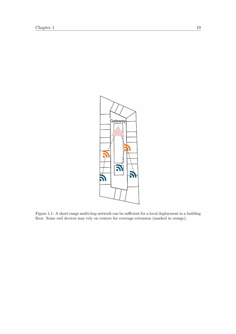
Therefore, a typical “short range” IoT network using the O-QPSK 2.4 GHz PHYis depicted in Fig. 1.1. It consists of a number of embedded nodes where each node
Chapter 1 10
Gateway
Figure 1.1: A short-range multi-hop network can be sufficient for a local deployment in a buildingfloor. Some end devices may rely on routers for coverage extension (marked in orange).
Chapter 1 11
contains a low-power micro-controller, attached sensors to monitor physical phenomena(e.g. temperature, gas concentration, vibration intensity), and a radio chip that is usedto transmit the sensor readings using a communication protocol. Nodes can send theirreadings periodically or based on alarm event triggers.
Applications of IoT began spanning a growing number of use cases. These usecases covered areas such as environmental monitoring [4], smart building [5], [6],precision agriculture [7], automated meter reading [8], indoor localization [9], micro-robotconnectivity [10], smart grid management [11] and predictive maintenance [1]. Eachapplication poses its own requirements for the QoS expected from the network. Theaverage current draw is often a key performance factor as devices are typicallybattery-powered and deployed in hard-to-reach areas. For some applications, the abilityto communicate over a long distance is important as the network is deployed over a largearea, or an area with poor propagation conditions. Other important network performancemetrics include end-to-end reliability and latency.
A short-range radio such as O-QPSK 2.4 GHz can be sufficient in meeting therequirements for some applications where energy saving has higher priority than latencyand reliability. But since it relies on routers for multi-hopping, this made it less suitablefor wide area coverage (such as a 2× 2 km2 industrial plant). In this case, more routersare needed to bridge the link between the nodes and the gateway, which means moremaintenance overhead and therefore less financial and practical feasibility.
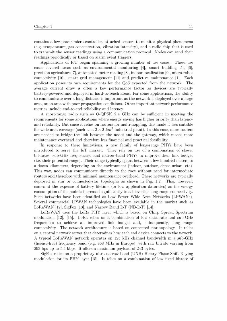
In response to these limitations, a new family of long-range PHYs have beenintroduced to serve the IoT market. They rely on use of a combination of slowerbit-rates, sub-GHz frequencies, and narrow-band PHYs to improve their link budget(i.e. their potential range). Their range typically spans between a few hundred meters toa dozen kilometers, depending on the environment (indoor, outdoor, dense urban, etc).This way, nodes can communicate directly to the root without need for intermediaterouters and therefore with minimal maintenance overhead. These networks are typicallydeployed in star or connected-star topologies as shown in Fig. 1.2. This, however,comes at the expense of battery lifetime (or low application datarates) as the energyconsumption of the node is increased significantly to achieve this long-range connectivity.Such networks have been identified as Low Power Wide Area Networks (LPWANs).Several commercial LPWAN technologies have been available in the market such asLoRaWAN [12], SigFox [13], and Narrow Band IoT (NB-IoT) [14].
LoRaWAN uses the LoRa PHY layer which is based on Chirp Spread Spectrummodulation [12], [15]. LoRa relies on a combination of low data rate and sub-GHzfrequencies to achieve an improved link budget and, subsequently, long rangeconnectivity. The network architecture is based on connected-star topology. It relieson a central network server that determines how each end device connects to the nework.A typical LoRaWAN network operates on 125 kHz channel bandwidth in a sub-GHz(license-free) frequency band (e.g. 868 MHz in Europe), with raw bitrate varying from293 bps up to 5.4 kbps. It offers a maximum payload of 243 bytes.
SigFox relies on a proprietary ultra narrow band (UNB) Binary Phase Shift Keyingmodulation for its PHY layer [15]. It relies on a combination of low fixed bitrate of
Chapter 1 12
Gateway
Figure 1.2: A long-range star network can serve metropolitan area deployments. End devicesrely on the robust modulations to communicate directly with the gateway.
100 bps, UNB channel width of 100 Hz, and use of sub-GHz (license-free) frequencies. Itsarchitecture is also based on multiple-antenna sites and a cloud-based network server [13].It limits the available data payload to 12 bytes with an allowance of 140 up-link messagesper device per day [15].
NB-IoT uses narrow-band Quadrature Phase Shift Keying and Frequency DivisionMultiple Access as uplink PHY layer. It further uses Orthogonal Frequency DivisionMultiple Access at its downlink PHY layer [14], [15]. It relies on a combination ofnarrow-band channel width of 200 kHz and use of licensed sub-GHz frequency. It offersa maximum throughput of 20 kbps and 200 kbps for uplink and downlink, respectively,with a maximum allowed payload of 1600 bytes [15]. Its architecture is also based oncellular topology with cellular coverage.
There are three common factors among the three technologies. First, eachtechnology is developed as a full protocol stack backed by an industrial body or alliance(e.g. LoRaWAN Alliance and 3rd Generation Partnership Project – 3GPP). Second, thesetechnologies rely on base stations for cellular coverage which can cost anywhere between1 k and up to 15 k euros in capital expenditure (excluding operational expenditure) [15].Third, the protocol stack of each technology is packaged with pre-specified PHY layerthat is often proprietary.
In 2012, the IEEE introduced the 802.15.4g amendment to include a family of31 modulations in the sub-GHz band as well as 2.4 GHz band [5], [16]. They varyin performance, from long range to high bit-rate, to serve the requirements for diverseuse cases. The advent of these standardized PHYs paves the way for more open networkarchitectures as it allows the network solution architect more diverse set of standardPHYs that can be supplied from multiple vendors.
The diversity in use case requirements opens pathways where either short- orlong-range approaches are beneficial. Short-range radios generally run at faster dataratesleading to shorter air time. This leads to an improved battery lifetime and can offer
Chapter 1 13
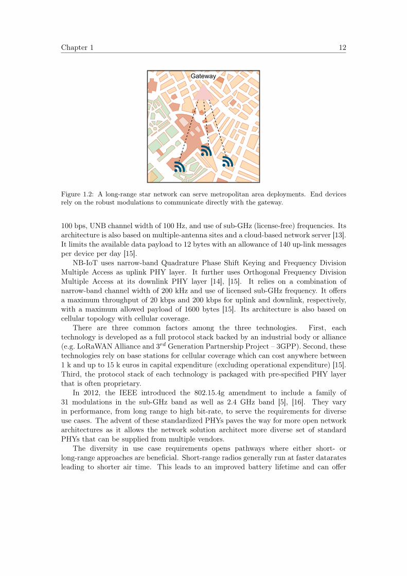
Figure 1.3: A typical TSCH slotframe for Motes A–D, using a uniform slot duration andsingle PHY at a fixed bitrate. Each node allocates a specific slot offset and channel offsetfor transmissions to its parent.
satisfying coverage for some applications involving few nodes within a building-floor [5],[6], a peach orchard [7], [9], or a few single-chip micro-motes [10]. Conversely, long-rangeradios can offer the necessary coverage for deployments spanning multiple km2 such as alarge factory [1] or a power grid [11], at an acceptable compromise in battery lifetime [16].
Battery lifetime has been a key performance indicator in IoT networks. In manyuse cases, an area is covered with a wireless network of battery-powered devices wheremains power is not available. Even when mains power is available, a none-invasivedeployment is often inevitable in sensitive infrastructures (e.g. hospitals [9], complexindustrial plants [1]). This creates a need to manage the network protocol in such as wayas to result in the longest battery lifetime possible. IoT network protocols have beenintroduced to save the average battery lifetime by using MAC techniques that allow theradios to go into sleep mode when they are not needed.
One of these MAC techniques is the class of protocols under the TSCH paradigm [17],[18]. While early low-power wireless networks used contention-based MAC approach,TSCH, initially developed for industrial applications, is now supported by manycommercial products and open-source implementations [19]. In a TSCH network, timeis cut into timeslots and a schedule orchestrates all communication; it indicates to everynode what to do in each timeslot: transmit, listen or sleep. An example of a TSCHslot-frame is presented in Fig. 1.3. TSCH is the key principle of the IEEE802.15.4estandard which is the standard MAC layer for several industrial protocol stacks such asWirelessHART, ISA100.11a, and more recently, 6TiSCH. In today’s TSCH networks, foreach cell, the schedule indicates the frequency to communicate on, resulting in “channelhopping”, a technique known to efficiently combat external narrowband interference andmulti-path fading.
Within this context, the IETF standardized the 6TiSCH protocol stack, whichcombines the high reliability of TSCH and the low power operation of the IEEE 802.15.4PHY [20] (e.g. 24 mA current draw for transmission [21]). It is a fully distributed protocolstack for mesh networking (i.e. no central controller). Specifically, 6TiSCH combines IPv6with the TSCH mode of IEEE802.15.4e standard.
Chapter 1 14
1.3 Why Multi-hopping Still Makes Sense for Long-RangePHYs?
A common question is raised when discussing specifically the use of long-range PHYs ina multi-hop network: multi-hopping was useful with short-range PHYs, but now if allnodes are equipped with long-range PHYs such as LoRa, do we still need multi-hopping?There is at least two reasons why multi-hopping makes sense even with long-range PHYs:extreme connectivity barriers and budget barriers.
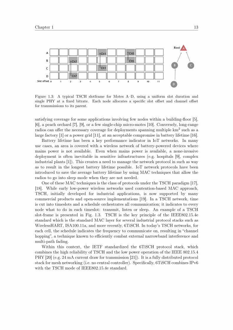
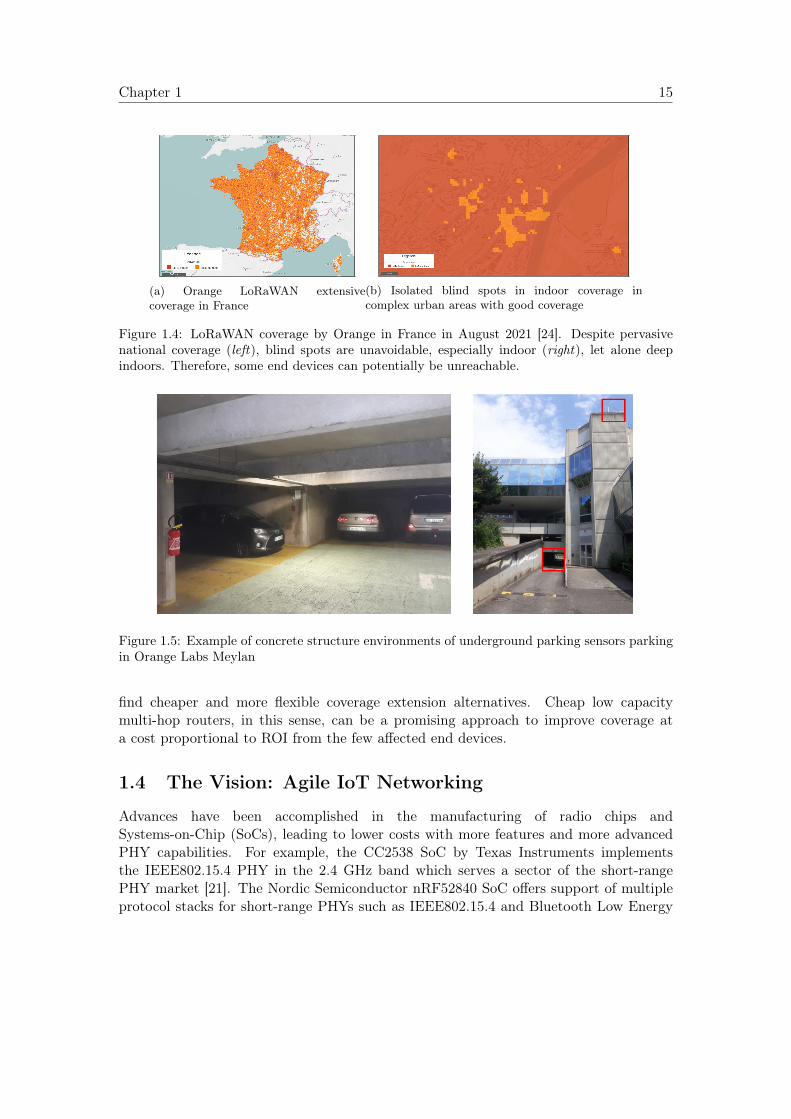
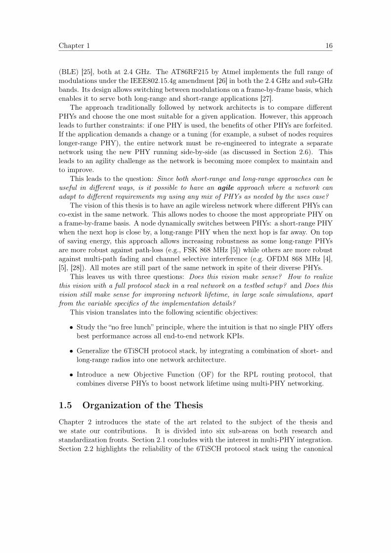
Even with long-rang PHYs, connectivity barriers are still unavoidable. Orangeprovides extensive LoRaWAN coverage of France, as illustrated in Fig. 1.4a. Blind spotsare unavoidable in deep indoor locations where utility meters or parking sensors aredeployed, as shown in Fig. 1.4b. From the point of view of a network operator suchas Orange, the LoRaWAN network is deployed in a way similar to a cellular network.Users cannot add gateways on their own to improve the coverage in areas where theconnectivity is not sufficient. An example of this scenario can be seen at Orange Labssite in Meylan, France in Fig. 1.5. The gateway is placed right on top of the garagebuilding, yet the LoRaWAN network is inaccessible in this garage because of the layersof concrete walls and ceilings. Consumer interest or regulatory requirements normallynecessitate pervasive coverage of end devices in different contexts. For instance, theEuropean Commission (EC) mandate M/441 draws the regulatory requirements for openbidirectional communications interfacing of metering instruments [22]. This is in orderto comply with utility monitoring standards outlined in several EC directives such asdirective 2006/32/EC (Article 13) [23]. Also, an owner of an underground deploymentof sensors (e.g. parking sensors) requires all sensors to be covered.
In a long-range star topology (Fig. 1.2), this connectivity gap is addressed todayby adding more GWs, thereby creating more stars. However, this is challenged by abudget barrier. GWs provide hot spots for end devices and then forward the traffic viaa high-throughput link such as Ethernet or cellular network. However, GWs come withsignificant financial costs for their installation. Mainly, the main cost element is thatoperator has to dispatch employees to access mobile towers to install these GWs (oftenin remote areas). In addition, the cost of a GW ranges between a few hundred eurosto a few thousand euros depending on its capacity, antenna, and network interfaces.Furthermore, GWs need to be constantly powered, and mounted to an infrastructurewith a grid power and a high throughput connection. This is the normal setting of acellular tower, and it is where a network operator would usually mount their LPWANGWs.
Network operators want to provide an affordable subscription cost to their users,typically in the order of one euro per end-device per month. Therefore, efficient capacityutilization of the network, to enable reasonable subscription costs, is a common interest.Maybe in some situations, the number of poorly covered devices are numerous enoughto justify the cost of adding a GW. But what if this is not the case? For instance,the area of the indoor blind-spots observed in Fig. 1.4b is likely to contain too fewdevices/subscriptions to offset the cost of adding another GW. This invites efforts to
Chapter 1 15
(a) Orange LoRaWAN extensivecoverage in France
(b) Isolated blind spots in indoor coverage incomplex urban areas with good coverage
Figure 1.4: LoRaWAN coverage by Orange in France in August 2021 [24]. Despite pervasivenational coverage (left), blind spots are unavoidable, especially indoor (right), let alone deepindoors. Therefore, some end devices can potentially be unreachable.
Figure 1.5: Example of concrete structure environments of underground parking sensors parkingin Orange Labs Meylan
find cheaper and more flexible coverage extension alternatives. Cheap low capacitymulti-hop routers, in this sense, can be a promising approach to improve coverage ata cost proportional to ROI from the few affected end devices.
1.4 The Vision: Agile IoT Networking
Advances have been accomplished in the manufacturing of radio chips andSystems-on-Chip (SoCs), leading to lower costs with more features and more advancedPHY capabilities. For example, the CC2538 SoC by Texas Instruments implementsthe IEEE802.15.4 PHY in the 2.4 GHz band which serves a sector of the short-rangePHY market [21]. The Nordic Semiconductor nRF52840 SoC offers support of multipleprotocol stacks for short-range PHYs such as IEEE802.15.4 and Bluetooth Low Energy
Chapter 1 16
(BLE) [25], both at 2.4 GHz. The AT86RF215 by Atmel implements the full range ofmodulations under the IEEE802.15.4g amendment [26] in both the 2.4 GHz and sub-GHzbands. Its design allows switching between modulations on a frame-by-frame basis, whichenables it to serve both long-range and short-range applications [27].
The approach traditionally followed by network architects is to compare differentPHYs and choose the one most suitable for a given application. However, this approachleads to further constraints: if one PHY is used, the benefits of other PHYs are forfeited.If the application demands a change or a tuning (for example, a subset of nodes requireslonger-range PHY), the entire network must be re-engineered to integrate a separatenetwork using the new PHY running side-by-side (as discussed in Section 2.6). Thisleads to an agility challenge as the network is becoming more complex to maintain andto improve.
This leads to the question: Since both short-range and long-range approaches can beuseful in different ways, is it possible to have an agile approach where a network canadapt to different requirements my using any mix of PHYs as needed by the uses case?
The vision of this thesis is to have an agile wireless network where different PHYs canco-exist in the same network. This allows nodes to choose the most appropriate PHY ona frame-by-frame basis. A node dynamically switches between PHYs: a short-range PHYwhen the next hop is close by, a long-range PHY when the next hop is far away. On topof saving energy, this approach allows increasing robustness as some long-range PHYsare more robust against path-loss (e.g., FSK 868 MHz [5]) while others are more robustagainst multi-path fading and channel selective interference (e.g. OFDM 868 MHz [4],[5], [28]). All motes are still part of the same network in spite of their diverse PHYs.
This leaves us with three questions: Does this vision make sense? How to realizethis vision with a full protocol stack in a real network on a testbed setup? and Does thisvision still make sense for improving network lifetime, in large scale simulations, apartfrom the variable specifics of the implementation details?
This vision translates into the following scientific objectives:
• Study the “no free lunch” principle, where the intuition is that no single PHY offersbest performance across all end-to-end network KPIs.
• Generalize the 6TiSCH protocol stack, by integrating a combination of short- andlong-range radios into one network architecture.
• Introduce a new Objective Function (OF) for the RPL routing protocol, thatcombines diverse PHYs to boost network lifetime using multi-PHY networking.
1.5 Organization of the Thesis
Chapter 2 introduces the state of the art related to the subject of the thesis andwe state our contributions. It is divided into six sub-areas on both research andstandardization fronts. Section 2.1 concludes with the interest in multi-PHY integration.Section 2.2 highlights the reliability of the 6TiSCH protocol stack using the canonical
Chapter 1 17
O-QPSK 2.4 GHz PHY. Section 2.3 highlights the regulation constraints to mediumaccess in the ISM band. Section 2.4 highlights related work that improves TSCHschedule compactness using a centralized controller in a single-PHY network. Section 2.5highlights related work on improving RPL performance either by improving networklifetime or by improving network stability in hybrid RF-PLC networks. Section 2.6highlights the state of the art in multi-PHY industrial networks which confirms theintuition of the potential benefits of multi-PHY integration. Chapter 2 concludes withthe key contributions of this thesis.
Chapter 3 describes the experimental and evaluation methodologies used throughoutthe thesis. We deploy three different setups to investigate the different research questionsaddressed. First, we describe a floor-scale testbed for network-wide evaluation protocolstack performance evaluation, used in Chapter 4 and Chapter 5. Second, we describe alocal experimental setup for real-time performance demonstration using hardware probes,used in Chapter 6. Third, we describe the RPL simulator for high-level performanceevaluation of RPL OFs, used in Chapter 7.
Chapter 4 addresses the question of why multi-PHY integration makes sense.Low-power wireless applications require different trade-off points between latency,reliability, data rate and power consumption. Given such a set of constraints, whichPHY should I be using? We study this question in the context of 6TiSCH, astate-of-the-art recently standardized protocol stack developed for harsh industrialapplications. Specifically, we augment OpenWSN, the reference 6TiSCH open-sourceimplementation of our choice, to support one of three PHYs from the IEEE802.15.4gstandard: FSK 868 MHz which offers long range, OFDM 868 MHz which offers highdata rate, and O-QPSK 2.4 GHz which offers more balanced performance. We run theresulting firmware on the 42-mote OpenTestbed deployed in an office environment, oncefor each PHY. Performance results show that, indeed, no PHY outperforms the otherfor all metrics. The long range FSK 868 MHz radio leads to fastest network formationand lowest latency at the expense of battery lifetime. The short range O-QPSK 2.4 GHzradio leads to best network lifetime at the expense of latency and reliability, and networkformation time. Chapter 4 proposes a principle of “no free lunch”: advantages gainedfrom one PHY will lead to forfeiting advantages of another PHY in terms of industrialKPIs. Subsequently, it argues for combining the PHYs, rather than choosing one, ina generalized 6TiSCH architecture. This is possible with technology-agile radio chips(of which there are now many), driven by a protocol stack which chooses the mostappropriate PHY on a link-by-link basis.
Chapter 5 generalizes the 6TiSCH protocol stack with multi-PHY integration. We callthe resulting protocol “g6TiSCH”, which we evaluate on a real testbed setup. Wirelessnetworks traditionally use a single PHY for communication: some use high bit-rateshort-range radios, others low bit-rate long-range radios. g6TiSCH allows nodes equippedwith multiple radios to dynamically switch between them on a link-by-link basis, as afunction of link-quality. This approach results in a dynamic trade-off between latencyand power consumption. We evaluate the performance of the approach experimentally onan indoor office testbed of 36 OpenMote B boards. Each OpenMote B can communicate
Chapter 1 18
using FSK 868 MHz, O-QPSK 2.4 GHz or OFDM 868 MHz, a combination of long-rangeand short-range PHYs. We measure network formation time, end-to-end reliability,end-to-end latency, and battery lifetime. We compare the performance of g6TiSCHagainst that of a traditional 6TiSCH stack running on each of the three PHYs. Resultsshow that g6TiSCH yields lower latency and network formation time than any of theindividual PHYs, while maintaining a similar battery lifetime.
Ch. 6 goes a step further by showing how a multi-PHY TSCH slot frame can haveheterogeneous slot-durations that vary by the bit rate of the each PHY. This chapterintroduces 6DYN, an extension to the g6TiSCH multi-PHY protocol stack. In a 6DYNnetwork, nodes switch PHYs dynamically on a link-by-link basis, in order to exploit thediversity offered by this new technology agility. To offer low latency and high networkcapacity, 6DYN uses heterogeneous slot durations: the length of a slot in the 6TiSCHschedule depends on the PHY used. This chapter shows how reserved bits in 6TiSCHheaders can be used to standardize 6DYN and details its implementation in OpenWSN,a reference implementation of 6TiSCH.
Chapter 7 addresses the question of whether multi-PHY integration makes sense forimproving network lifetime within high-level simulation setup. We propose a routingmechanism based on the RPL protocol in a wireless network that is equipped with a mixof short-range and long-range radios. We introduce Life-OF, an objective function forRPL which uses a combination of metrics and the diverse PHYs to boost the network’slifetime. We evaluate the performance of Life-OF compared to the standardized MRHOFobjective function in simulations. Two KPIs are reported: network lifetime and networklatency. Results demonstrate that MRHOF tends to converge to a pure long-rangenetwork, leading to short network lifetime. However, Life-OF improves network lifetimeby continuously adapting the routing topology to favor routing over nodes with longestremaining lifetime. Life-OF combines diverse radios and balances power consumption inthe network. This way, nodes switch between using their short-range radio to improvetheir own battery lifetime and using their long-range radio to avoid routers that are closeto depletion. Results show that using Life-OF improves the lifetime of the network byup to 470% compared to MRHOF, while maintaining similar latency.
Chapter 8 concludes this manuscript and discusses the avenues for future work itopens. The list of publications and software contributions made as part of this work arelisted in Chapter 9.
Chapter 2
State of the Art
Key Takeaways: This chapter surveys the research and standards related tothis thesis. We introduce in Section 2.1 related work on performance evaluation ofIEEE802.15.4g PHYs and we present why multi-PHY integration can be of interest.We then introduce in Section 2.2 an overview of the IETF 6TiSCH protocol stackfor a reader without former knowledge on 6TiSCH and we present how it achieveshigh reliability. We introduce in Section 2.3 the regulation constraints to mediumaccess in the unlicensed band and we present why multi-PHY integration canhelp relax these constraints. Furthermore, in Section 2.4, we present related workon schedule compactness in TSCH networks and we highlight that it only existsin centralized networks. We then provide an overview on RPL in Section 2.5and we introduce related work on improving network lifetime in RPL or use ofhybrid interface networks. Section 2.6 presents related work on state of the art inmulti-PHY industrial networks. Finally, Section 2.7 summarizes the related work,and lists the key contributions of this thesis.
2.1 Evaluation of IEEE802.15.4g PHYs
As previously discussed in the introduction, the IEEE adopted a standard and diverseset of 31 PHYs in the IEEEE802.15.4g amendment [26]. The set consists of 31 PHYs forSUNs and their advantages vary to serve a wide array of use cases. Some PHYs are moresuitable for long-range applications such as the family of FSK PHYs. The OFDM familyof PHYs are more robust against multi-path fading in urban or indoor environmentswhile offering high bitrates up to 800 kbps. Therefore, we consider this standard as areference for our PHY selection because of its wide diversity.
This section introduces the related work on the performance evaluation of theIEEE802.15.4g PHYs (without the 6TiSCH stack).
Kojima et al.[28] examine the impact of interference between multi regional
19
Chapter 2 20
FSK mode 2 and multi regional OFDM option 4 MCS 3. FSK mode 2 offers 100 kbpsraw datarate at 400 kHz channel spacing whereas OFDM option 4 MCS 3 offers thesame datrate but at only 200 kHz channel spacing. Generally, FSK requires less circuitrythan OFDM and it is less immune against multi-path fading. Conversely, OFDM iscapable of withstanding multi-path fading in complex environments at higher bit-ratethan FSK at the expense of complex circuitry. The authors deploy IEEE802.15.4e MACwith multi-hop capability on top of each PHY layer and measure the impact of theinterference between two networks, each running one PHY. Results are reported in termsof the degradation of throughput of each network in the presence of the other interferingnetwork. Kojima et al.demonstrates that, since the OFDM modulation scheme usesmultiple sub-carriers, it performs better than FSK in the presence of frequency selectiveinterference.
Muñoz et al. [5] run an experimental campaign to compare the performance ofIEEE802.15.4 O-QPSK 2.4 GHz at 250 kbps, and IEEE802.15.4g OFDM. They showa higher robustness of OFDM, even though it operates at a higher bit rate (800 kbps).They show that, although a radio draws less current when running O-QPSK 2.4 GHz,using OFDM 868 MHz leads to an overall lower power budget as transmission happensmuch faster.
The same authors also evaluate the performance of all IEEE802.15.4g PHYs [4]. Theyconduct a complete range-testing campaign for the 31 PHYs on the four scenarios theyconsider the most prevalent in outdoor applications: line of sight, smart agriculture,urban canyon, smart metering. Their results of the range-tests are reported in terms ofPDR measurements, throughput, and electric charge consumption. They demonstratethe longer range of FSK and O-QPSK in the sub-GHz band compared to OFDM optionsdue to their higher receiver sensitivity. Muñoz et al.provide interesting results as to whichradio could be better in certain scenarios.
My thesis goes one step further to address the end-to-end performance of a full6TiSCH stack using these PHY layers. We show in Chapter 4 the performance of 6TiSCHstack using each PHY. We demonstrate that there is not a single PHY that offers the bestperformance across all relevant network KPIs. This is the key motivation for generalizingthe 6TiSCH architecture so it offers a balanced performance by integrating diverse PHYs.
2.2 IETF 6TiSCH Protocol Stack
This section provides an overview of standards and research related to the 6TiSCHprotocol stack. It presents an overview of the standards of the protocol stack(Section 2.2.1), related work on the schedule management in 6TiSCH (Section 2.2.2),and related work on performance evaluation of 6TiSCH (Section 2.2.3).
2.2.1 6TiSCH Overview
The IETF is organized in Working Groups, some of which standardize IoT protocols. Oneof these Working Groups formalized a set of standards for Industrial IoT applications,
Chapter 2 21
which require high reliability: the IPv6 over the Time Slotted Channel Hopping modeof IEEE802.15.4e (6TiSCH) Working Group. At the MAC layer, 6TiSCH uses theIEEE802.15.4e TSCH mode, which is also at the root of industrial wireless protocolssuch as WirelessHART and ISA100.11a. In TSCH, a node cuts time into slots. Acommunication schedule orchestrates all communication, indicating to each node whatto do in each slot: transmit, receive or sleep. Combined with channel hopping, this leadsto high end-to-end reliability, and can be used in networks with a high traffic rate. Atthe PHY layer, 6TiSCH only supports a single PHY for the entire network. Currently,the chosen PHY for the standard stack is IEEE802.15.4 O-QPSK at 2.4 GHz [29].
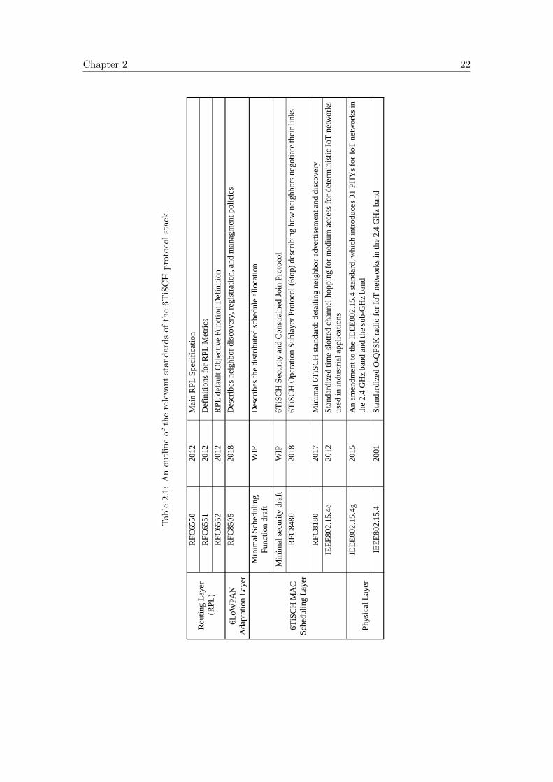
Several articles shed light on 6TiSCH evolution and state of the art. Vilajosana etal. [30] provide a detailed tutorial on the stack of protocols adopted by the IETF 6TiSCHworking group. For the purpose of this thesis, we focus on the basic overview of theprotocol stack for a reader without previous knowledge of 6TiSCH. An outline of therelevant 6TiSCH standards is presented in Table 2.1.
The main vision of 6TiSCH is to benefit from the industrial reliability ofIEEE802.15.4e TSCH under a generic IP routing layer [31]. To achieve such integration,an adaptation layer called 6LoWPAN has been introduced to enable IP operation on overIEEE 802.15.4 PHY. Furthermore, the Minimal 6TiSCH standard RFC8180 [29] describeshow neighbor advertisement and discovery should take place using the “minimal” sharedcells. These advertisements are carried in 802.15.4 TSCH Enhanced Beacons (EBs) [18].As neighbors are being discovered, the RPL routing algorithm chooses one or moreneighbors to be routing parents, according to an objective function [32]–[34]. Theobjective function can consider one or more parameters for link cost estimations [34].When a parent is selected, a node negotiates with its parent to add dedicated cellsfor uplink traffic using the 6TiSCH Operation Sublayer Protocol (6top) [35]. 6topnegotiations occur via autonomous cells: each node allocates a default cell to receivenegotiation requests, the index of this cell is calculated by a hashing function based onthe slotframe length and the mote’s MAC address [36]. After cells are allocated, the nodebroadcasts its routing information and the cost of the path between the node and the root(i.e. rank). These RPL broadcasts are called Destination-oriented directed acyclic graphInformation Objects (DIOs). This information allows neighboring nodes to calculate thebest route (according to some objective) to use for their traffic.
2.2.2 Scheduling in 6TiSCH
This section takes a closer look into the scheduling mechanisms in 6TiSCH. The 6TiSCHprotocol stack [19], [31] combines the ease of use of IPv6 with the industrial performanceof TSCH. A 6TiSCH schedule is a matrix of cells, each identified by its slot offset andchannel offset(a cell is the combination of a location of a time-slot in the schedule and afrequency setting). There are three types of cells:
• A dedicated cell is negotiated between neighbor nodes. A TX cell is allocated atthe source mote and an RX cell is allocated at the destination motes.
Chapter 2 22
Tab
le2.1:
Anou
tlineof
therelevant
stan
dardsof
the6T
iSCH
protocol
stack.
RF
C6550
2012
Mai
n R
PL
Spec
ific
atio
n
RF
C6551
2012
Def
init
ions
for
RP
L M
etri
cs
RF
C6552
2012
RP
L d
efau
lt O
bje
ctiv
e F
unct
ion D
efin
itio
n
6L
oW
PA
N
Adap
tati
on L
ayer
RF
C8505
2018
Des
crib
es n
eighbor
dis
cover
y, re
gis
trat
ion, an
d m
anag
men
t poli
cies
Min
imal
Sch
eduli
ng
Funct
ion d
raft
WIP
Des
crib
es t
he
dis
trib
ute
d s
ched
ule
all
oca
tion
Min
imal
sec
uri
ty d
raft
WIP
6T
iSC
H S
ecuri
ty a
nd C
onst
rain
ed J
oin
Pro
toco
l
RF
C8480
2018
6T
iSC
H O
per
atio
n S
ubla
yer
Pro
toco
l (6
top)
des
crib
ing h
ow
nei
ghbors
neg
oti
ate
thei
r li
nks
RF
C8180
2017
Min
imal
6T
iSC
H s
tandar
d:
det
aili
ng n
eighbor
adver
tise
men
t an
d d
isco
ver
y
IEE
E802.1
5.4
e2012
Sta
ndar
diz
ed t
ime-
slott
ed c
han
nel
hoppin
g f
or
med
ium
acc
ess
for
det
erm
inis
tic
IoT
net
work
s
use
d i
n i
ndust
rial
appli
cati
ons
IEE
E802.1
5.4
g2015
An a
men
dm
ent
to t
he
IEE
E802.1
5.4
sta
ndar
d, w
hic
h i
ntr
oduce
s 31 P
HY
s fo
r Io
T n
etw
ork
s in
the
2.4
GH
z ban
d a
nd t
he
sub-G
Hz
ban
d
IEE
E802.1
5.4
2001
Sta
ndar
diz
ed O
-QP
SK
rad
io f
or
IoT
net
work
s in
the
2.4
GH
z ban
d
Physi
cal
Lay
er
Routi
ng L
ayer
(R
PL
)
6T
iSC
H M
AC
Sch
eduli
ng L
ayer
Chapter 2 23
• A broadcast cell (also called “Minimal cell”) is used for network-wide broadcastmessages and network routing information. This allows a mote to synchronize tothe network, discover its neighbors and the network routing details.
• Each node allocates an autonomous cell in its schedule where it can receivenegotiation requests for cell allocations from its neighbors.
6top coordinates a mote’s negotiations with its neighbors to allocate cells [35].It further defines a default scheduling algorithm, called Minimal Scheduling Function(MSF) [36], which defines how cells are allocated for unicast or broadcast activities.6TiSCH uses the 6LoWPAN adaptation layer [37] to transport IPv6 packets over IEEE802.15.4e MAC layer, and the IPv6 Routing Protocol for Low-Power and Lossy Networks(RPL) [32] routing protocol. Chang et al.provided a comprehensive overview of the6TiSCH protocol stack [10].
Schedule management can be done in a centralized or distributed manner. In acentralized approach [3], [9], a central entity manages the schedule based on a completeview of the network. In a distributed approach, nodes manage their resources locally.6TiSCH uses the latter.
2.2.3 6TiSCH Performance Evaluation
Related research provides performance evaluation of 6TiSCH in different situations.Yang et al. [38] evaluate the performance of the full 6TiSCH stack on the OpenWSN
reference architecture in terms of responsiveness to time critical event triggers. Theyvary the number of active slots in a frame of length 11 slots and measure how packetend-to-end latency is affected.
Theoleyre et al. [39] evaluate the performance of the 6TiSCH stack with thedeployment of traffic isolation mechanisms that allow reservation of dedicated slotsfor certain applications and reservation of shared slots for alarm events. They reportend-to-end latency and PDR under various schedule management strategies, includingusing uniformly distributed shared cells instead of contiguous (adjacent) shared cells inthe slot-frame.
Teles Hermeto et al. [40] execute a performance evaluation of the 6TiSCH protocolstack in an indoor environment with a focus on the stability of the stack performance.They report the end-to-end reliability and the number of parent changes as the networkis converging. They also propose a stable link quality metric and a simplified method forschedule inconsistency management.
Ben Yaala et al.[41] evaluate the performance of the 6TiSCH stack in co-locatednetworks. They consider both cases where the coexisting 6TiSCH networks are eithersynchronized or un-synchronized.
In all of related works listed above, the PHY used is IEEE802.15.4 O-QPSK 2.4 GHz.Sum et al. [8] use different approach: they provide an experimental evaluation ofIEEE802.15.4e TSCH MAC based on IEEE802.15.4g FSK 868 MHz radio. Theexperiments report range and performance testing results in terms of PDR and Packet
Chapter 2 24
Error Rate in four situations: Line-of-Sight conditions, Non-line-of-sight conditions, treetopology in corridor setting and line topology across buildings.
This thesis goes a step further by conducting performance evaluation of 6TiSCH ontop of three different PHYs (Chapter 4). We report the end-to-end performance based onindustrial KPIs [42]: network formation time, end-to-end reliability, end-to-end latency,and battery lifetime. We further propose a generalized 6TiSCH architecture (Chapter 5)where a node can use a short-range PHY to communicate with nearby neighbors andlong-range PHY to communicate with neighbors further away. g6TiSCH is configuredto include the following PHYs: FSK 868 MHz as low bitrate PHY, OFDM 868 MHzas high bitrate PHY, and O-QPSK 2.4 GHz as an in-between option. We compare theperformance of g6TiSCH against that of a traditional 6TiSCH stack running on each ofthe three physical layers.
2.3 Unlicensed Band Considerations
This section details practical limitations on network performance when operating inpublicly shared spectrum. When the wireless network is operating in an unlicensedband, it faces constraints by regulations or by medium scarcity. There are two mainconsiderations to take into account related to the frequency band used: co-existencewith other technologies in unlicensed band, and duty cycle limits on sub-GHz unlicensedbands.
Hermeto et al.indicated that the articles they surveyed [43]–[46] do not consider packetloss due to interference from IEEE802.11 WiFi networks [47]. Since the IEEE802.15.4PHY operates using O-QPSK 2.4 GHz, it has classically suffered interference fromco-existing Wi-Fi networks. Musaloiu et al.showed how IEEE802.15.4 networks exhibitpacket losses ranging 22–58% when WiFi networks are operating in the same area [48].Gonga et al.showed that up to 95% of the links in a IEEE802.15.4 channel hoppingnetwork can suffer independent packet losses due to WiFi interference [49].
Furthermore, Liu et al. [50] proposed an IIoT architecture that integrates satelliteIIoT with ground cellular IIoT to extend coverage in satellite-blocked areas. Thisintegration leads to co-channel interference from both networks operating on the samefrequencies. The authors therefore propose a mechanism to optimize the satellite powerresource allocation to mitigate the interference and guarantee a QoS level.
In Europe, ETSI is the regulatory body which governs frequency bands. Section 7.2.3of ETSI 300-220 [51] limits the transmit duty cycle (the portion of the time a radio isactively transmitting) in the 868 MHz band between 0.1% and 1% depending on thesub-band. Similar regulation is in place in the U.S. (under the guidance of the FCC)and other parts of the world. Such regulations must be taken into account by schedulingpolicy using these frequencies.
g6TiSCH proposed in Chapter 5 uses both the 2.4 GHz and sub-GHz bands. Byincreasing the available frequency resources, it reduces the probability of interference fromco-existing networks. Furthermore, it reduces the impact of the duty-cycle regulation bysplitting the amount of traffic between the two bands.
Chapter 2 25
2.4 TSCH Schedule Compactness
This section presents articles that focused on improving TSCH schedule compactness.Schedule compactness can be defined as “[the maximization of] the number of channeloffsets and timeslots not used by any transmitter” [47]. A schedule that is compact allowsto accept new flows as there is enough space available to allocate more bandwidth.This permits the improvement of end-to-end throughput by allocating more slotsand by increasing the number of available channels for hopping, which increases linkrobustness [52], [53].
Hermeto et al.focus on scheduling in IEEE802.15.4-TSCH industrial networks,surveying both centralized and distributed approaches [47]. They indicate that researchon improving schedule compactness has been done exclusively for centralized networks.
Palattella et al.propose the Traffic Aware Scheduling Algorithm (TASA) for scheduleoptimization [43]. TASA relies on a central manager to reserve slots as early as possiblein the schedule. It relies on minimizing the maximum offset of used slots in theschedule. The authors port TASA to the 6TiSCH architecture in combination withthe IEEE802.15.4e MAC, and provide a simulation of its performance [44]. They showthat TASA-based IEEE802.15.4e MAC shows 80% improvement in the power efficiencycompared to the legacy IEEE802.15.4 MAC.
Soua et al.propose MODESA, a centralized slot allocation algorithm which relies ona root node having multiple radio interfaces [45]. MODESA reduces the slotframe lengthby optimizing slot and channel allocation across a tree-topology network. The authorsprovide a linear programming model that runs on the central controller and optimizesslot and channel assignment. They show how this approach reduces slotframe length by13% in a 100-node network.
The related work surveyed in this section is based on a centralized controller, and itall assumes the same PHY is used across the network (hence, a uniform slot duration).This thesis proposes 6DYN (Chapter 6), a distributed mechanism for increasing schedulecompactness, combined with a multi-PHY approach and heterogeneous slot durations.6DYN allows nodes to allocate shorter slots for faster transmissions and longer slots whennecessary for slower transmissions. This allows for better packing of the schedule, whichreduces latency and increases network capacity.
2.5 IETF RPL Protocol
Another IETF working group is the Routing Over Low power and Lossy networks (ROLL)group focused on the routing layer in IoT applications. The group standardized RPL,the IPv6 Routing Protocol for LLNs [32]. An LLN can be defined as different namefor IoT low-power wireless mesh networks. This section presents previous work relatedto routing with RPL. We present the work in two sections. Section 2.5.1 gives the abackground on the RPL standard and related RFCs. Section 2.5.2 introduces relatedwork on RPL Objective Functions (OFs) that intersect with this work.
Chapter 2 26
2.5.1 RPL Standardization
RPL was first standardized in 2012 as a proactive, distance-vector, distributed algorithm,aligned on Destination Oriented DAGs rooted at the internet border routers [32]. It wasextended later with options to do point-to-point proactive routing, and to do reactiverouting. It is currently being extended to enable centralized routing.
RPL provides an elaborate framework with a wide range of features that allow itto address simple as well as complex use cases. A key advantage of RPL is that it isa distributed protocol: decisions are taken independently by each node. This way, itminimizes the risk of having a single point of failure, which occurs when the networkis using a centralized controller (i.e. Path Computation Element). It also reduces thenetwork control overhead as nodes do not send all their state information to the controller.The core routing decision in RPL is taken by the OF which evaluates each available pathaccording to “an objective”, and decides which path best meets that objective. There arecurrently two IETF-adopted OFs that aim to improve latency and energy by choosingpaths with the least possible number of hops or transmissions.
The Root advertises metrics [33] that are used by intermediate nodes to select routesaccording to the OF. Standardized OFs include route selection by hop-count (calledOF0 [34]) or by minimum end-to-end ETX with hysteresis (called MRHOF [54]). Thenetwork DODAG is guaranteed to be acyclic (in steady state) by having each nodeassign itself and advertise a rank that is strictly monotonic along any path to the Root.In addition to defining how routes are selected, the OF also specifies how the rank iscalculated. The RPL protocol is extensible with other objective functions, yet to bedefined. The currently defined metrics include node metrics such as: node remainingenergy, node workload, or hop-count. Link metrics are also defined such as: linkthroughput, latency, reliability, or link color.
Metrics are shared in the network via Destination Information Object (DIO)multicasts among router nodes. DIOs contain DAG Metric Containers (DMCs) whichdescribe the utilized metrics and how they are shared in the network. We note twoparticular control points in the routing metric flag field that define how metrics areshared (which will be referred to later in the Chapter 7).
• “R-Flag”: if set, the metric is recorded by separate entry for each node along thepath. Otherwise, the metric is aggregated along the path in one entry.
• “A-Field”: in case an aggregate metric is defined (i.e. R-Flag set to 0). It allowschoosing the mode of aggregation: additive, minimum, maximum, or multiplicative.
This way, metrics can be combined in different ways to optimize the routing topologyfor different use cases.
2.5.2 OFs for a Hybrid RPL Topology
The main RPL standard RFC6550 [32] does not specify an OF for a RPL implementation.Specification of the OF is left to the architects of each network since the criteria of
Chapter 2 27
optimization can vary by use case. Some applications using alarms may prioritize delayover energy savings. Other applications for utility metering in remote areas may prioritizeenergy saving over delay.
Extensions to the standard have proposed OFs that can serve as reference points forRPL implementations. RFC6552 [34] introduces OF0 which serves as a minimal OF thatcan allow basic interoperation of RPL implementations in simple use cases. It uses thehop-count as an additive aggregate metric along the path. This way, nodes closer to theroot in the routing tree will be favored, irrespective of the link quality.
RFC6719 [54] introduces the Minimum Rank with Hysteresis Objective Function(MRHOF). It goes one step further than OF0 by expressing the link quality across thepath using Expected Transmission Count (ETX) as a path metric. This way, it can besensitive to temporary fluctuations in link quality across the path due to interference ormulti-path fading. For instance, a link between a node and the root can suffer temporaryinterference that leads to degrading the link quality from 99% down to 75% PDR. Thenode may choose an alternative route through a neighbor where each hop has 95% PDR.In this case, 2-hop route has a higher PDR (90%) than the one hop route. When theinterference ends, the node can return to the one-hop route of 99% PDR.
Ben Saad et al. [55] propose a heterogeneous infrastructure for IPv6 using acombination of diverse PHYs: PLC interface, Sub-GHz radio at 250 kbps, and 2.4 GHzradio at 250 kbps. The authors propose an infrastructure where PLC-RF routers areintroduced to improve lifetime of an RF network. They emulate a testbed of 25 motesin a 50 × 50 m2 area, with a fixed RF range of 10 m and placed in a grid topology.They place mains-powered RF-PLC routers in optimal points and show how it leads toimprovement of network lifetime.
Lemercier et al. [56], [57] address the challenge of routing when each node is equippedwith heterogeneous interfaces, namely IEEE 802.15.4g RF and PLC. The authorscompare three approaches for multi-PHY routing in RPL: (1) a multi-instance RPLwhere RPL maintains a separate DODAG per each PHY, (2) a parent-oriented designwhere switching between PHYs is more favorable for interfaces of the same neighbornode, and (3) an interface-oriented design where each combination of node/interfaceis considered as an independent neighbor. The objective of the study is to arrive ata solution that yields the best network reliability in case of interface failure. This isexpressed as the number of parent changes and degree of connectivity of the resultingtopologies. The authors propose an OF that aims at optimizing the link quality andexpected transmission time. They show that the parent-oriented design yields networkwith the best reliability performance in terms of number of parent-changes and linkquality in the DODAG.
Iova et al. [58] propose an OF for RPL that optimizes for network lifetime (i.e. thetime until the first battery depletion of a node in the network). They propose that therouting algorithm avoids nodes that appear as energy bottlenecks. They also proposeto use multi-parent routing to balance the load across the network. Their OF definesexpected lifetime node metric that is based on: node energy consumption, remainingbattery energy, ETX, and estimated node traffic rate. They simulate the performance
Chapter 2 28
of the proposed multi-path routing technique in a single-PHY topologies of 30–90 nodesin a 300× 300 m2. They show that the hybrid OF with probabilistic multi-path routingis able to improve network lifetime by several orders of magnitude (depending on thenetwork’s density) compared to MRHOF.
The related work presented in this section demonstrates significant advances inadapting RPL for multi-PHY integration or network lifetime. Both OF0 and MRHOFoffer a basic PHY-agnostic routing approach that leaves room for improvement in the caseof multi-PHY networks or specialized use cases. Ben Saad et al. [55] demonstrate howintroducing heterogeneous mains-powered routers can improve network lifetime. Thisconfirms out intuition about the benefit of having heterogeneous network for improvinglifetime. Lemercier et al. [56], [57] demonstrate that having a heterogeneous networkwith mix of wired/wireless interfaces can improve network reliability and stability.
My work goes a step further by demonstrating in Chapter 7 how heterogeneousnodes that are fully wireless and fully battery-powered can improve network lifetime byintegrating a mix of long-range and short-range PHYs. Iova et al. [58] demonstrate thebenefit of optimizing for a node’s estimated lifetime to yield an energy balanced networkwith improved lifetime. This confirms the intuition behind using combined metricsfor network lifetime optimization and how that path diversity can allow improving thenetwork lifetime. This thesis designs in Chapter 7 an OF that makes use of heterogeneousPHYs to improve the network lifetime and how the characteristics of each PHY canbe taken into account by the routing layer. Finally, this work simulates the resultingnetworks in a setting of 100 nodes in 2 × 2 km2. This is to demonstrate the potentialimpact of this function in wide area coverage.
2.6 Multi-PHY Integration
This section presents recent related work that uses hybrid PHYs in an integrated network.The study by Brachmann et al. [59] demonstrates enabling multi-PHY capability in
the 6TiSCH stack. The authors run link performance testing campaigns using multiplePHYs: 2-GFSK (at 1.2 kbps, 8 kbps, 50 kbps, 250 kbps), 4-GFSK (at 1000 kbps),O-QPSK 2.4 GHz (at 250 kbps). The authors choose two PHYs in the sub-GHz band forintegration in the 6TiSCH MAC layer: 2-GFSK at 1.2 kbps for transmitting EnhancedBeacons (EB), 4-GFSK at 1000 kbps for data traffic. The slot templates for the PHYlayers are defined in accordance with the IEEE802.15.4 standard, and used in Contiki-NG.They demonstrate that the faster bit-rate of 4-GFSK at 1000 kbps for data packetsreduces the collision probability and leads to less than 0.1% channel utilization despitethe higher re-transmission rate. Furthermore, the slower bit-rate of 2-GFSK at 1.2 kbpsleads to higher channel occupancy, at 2% duty cycle.
The proposal by Van Leemput et al. [60] is the state-of-the-art in multi-PHYintegration in TSCH networking. The authors propose using slower PHYs for unicastlinks in case the RSSI is persistently below a certain threshold. PHY switching occurs atthe MAC layer by continuously assessing the link’s RSSI, using an Exponentially MovingAverage filter. The timeslot is long enough for a single packet when using a low bit-rate
Chapter 2 29
radio, or multiple back-to-back packets when using a high bit-rate radio. The authorsdemonstrate that a link’s throughput can be increased by 153 % with only 84 % powerconsumption. This is achieved by using single acknowledgment for multiple packets inthe same slot.
Garrido-Hidalgo et al. [61] develop a body-area network (BAN) using BLE mesh inthe 2.4 GHz band. The mesh connects BLE wrist-bands worn by factory workers alongwith BLE-based machine sensors. The devices capture data relevant for safety in a realindustrial setting. Collected data is forwarded to a BLE gateway which has a LoRaWANinterface that relays the data over long-range PHY in the sub-GHz band to a LoRaWANgateway connected to the cloud.
Al-Saadi et al. [62] propose a hybrid network architecture integrating Long TermEvolution (LTE) “eNodeB” base stations with a WiFi mesh based on an IEEE802.11stack. The architecture enables relaying traffic among nodes with multiple interfaces:LTE, WiFi, and Ethernet. This enables the utilization of unlicensed band of WiFi toimprove LTE coverage via WiFi mesh networks, without having to buy more of thelicensed spectrum of LTE. The authors make use of the multi-rate feature of WiFi tocombat interference and use a re-enforcement learning algorithm that determines for eachnode which technology to use for forwarding. They use simulations to demonstrate thatthe overall network throughput is increased.
These papers provide insightful performance evaluation of three kinds of multi-PHYnetworks.
First, Brachmann et al. [59] integrate two PHYs under one protocol stack; however,only one PHY is used as a default setting for data packets. Our proposed g6TiSCHarchitecture (Chapter 5) introduces a fully generalized stack where nodes can use hybridPHYs for different neighbors for data transmission or reception and a node can switchits PHY dynamically depending on the neighbor.
Second, the architecture proposed by Van Leemput et al. [60] also integrates twosub-GHz PHYs under one protocol stack; however, the link switching mechanism occursat the MAC layer. The authors show significant throughput improvement and energysavings using their multi-PHY architecture at the MAC layer. This confirms the intuitionbehind using multiple PHYs in the same TSCH-network. g6TiSCH goes a step furtherby allowing the integration of any number of (multi-band) PHYs. g6TiSCH also allowsexposing the different costs associated with each PHY to the routing layer. The latterbecomes aware of such costs and can improve the network energy footprint by selectingless costly PHYs when possible. This way, the routing layer cooperates with the lowerlayers. Furthermore, they demonstrate how the PHY-switching mechanism adapts theused PHY in case of switching to another PHY of the same parent node. g6TiSCH goesa step further by proposing a PHY-switching mechanism that is demonstrated in caseof switching to a PHY of the same parent node or of a different parent node, since bothcases are treated the same way. We further demonstrate the end-to-end performanceof the resulting architecture for a holistic performance evaluation and we compare it tosingle-PHY architectures.
Third, Garrido-Hidalgo et al. [61] integrate two full stack networks side-by-side:
Chapter 2 30
LoRaWAN and BLE mesh to benefit from long-range and short-range PHYs. Sincethe g6TiSCH architecture proposed in this paper allows for the co-existence of multiplePHYs under one protocol stack, it allows less network management overhead and easierintegration than multiple independent full-stacks.
Finally, Al-Saadi et al.propose running WiFi and LTE side-by-side on relay nodes.My thesis goes a step further by introducing a unified multi-PHY protocol stack andproviding experimental evaluation of its performance.
2.7 Summary and Contributions
This section describes related work on both research and standardization fronts. Wedemonstrate the potential of multi-PHY integration and we provide an overview ofthe 6TiSCH protocol stack and its related work that we later extend with multi-PHYcapabilities. We further present how multi-PHY integration can help in relaxing MACconstraints in the unlicensed band. We then show that TSCH schedule compactnessis currently addressed only in the context of centralized single-PHY network, whichleaves room for contribution in the context of a distributed multi-PHY network. Wegive an overview of RPL and related RPL OFs that address either improving networklifetime or improving network stability in hybrid RF-PLC networks. This leaves room forcontribution with an OF that improves network lifetime by use of multi-PHY network.Finally, we highlight the state of the art in multi-PHY industrial networks which showsthe growing intuition in the research community for the potential benefits of multi-PHYintegration.
My works builds upon this related work, and bring the following key contributions:
1. Instead of trying to find the best PHY from those surveyed in Section 2.1, we arguefor a “no free lunch” principle: that no single PHY can offer best performance acrossall end-to-end network KPIs. This is developed in Chapter 4.
2. We generalize the 6TiSCH architecture (surveyed in Section 2.2): we demonstratehow a set of short-range and long-range radios can be integrated under onegeneralized 6TiSCH architecture and we evaluate its performance experimentallyin a testbed of 36 motes at Inria-Paris. This is developed in Chapter 5.
3. While related work in Section 2.4 improves schedule compactness in centralizedsingle-PHY networks, we demonstrate in Chapter 6 how to enable compactscheduling in a TSCH slot-frame in a decentralized multi-PHY network. Theschedule can adapt slot-duration on a slot-by-slot basis depending on the bit-rateof the used PHY (“6DYN”) and we show how this can help mitigate the unlicensedband limitations surveyed in Section 2.3.
4. We extend RPL based on the work in Section 2.5 and we demonstrate, usingsimulation, a RPL OF that optimizes for network lifetime (“Life-OF”). We show howit combines diverse PHYs to boost network lifetime using multi-PHY networking.
Chapter 3
Methodology
Key Takeaways: This chapter surveys the methodology followed for conductingthe experiments in this thesis. We employ three different setups to investigate thedifferent research questions addressed.
• Section 3.1 details the OpenTestbed [63], a set of nodes deployed acrossan office building. We use the OpenTestbed to test end-to-end networkperformance. The OpenTestbed is used in Chapters 4 and 5.
• Section 3.2 describes a lab-bench setup of 4 motes connected to labequipment. This allows us to get an in-depth look into the real-timeperformance of the protocol stack using hardware probes. This setup isused in Chapter 6.
• Section 3.3 presents RPLSim, a RPL simulator that we built to examine theperformance of the proposed OF for multi-PHY routing. The RPLSim isused in Chapter 7.
3.1 OpenTestbed
We are interested in the end-to-end performance of the 6TiSCH protocol stack(Chapter 4) as well as the g6TiSCH stack (Chapter 5) at in a realistic setting. Forthis reason, we use the OpenTestbed which is a real deployment in Inria Paris, which is atypical indoor office building setting. We outline the physical setup of the OpenTestbed inSection 3.1.1. We describe the methodology for experiment and measurement collectionin Section 3.1.2.
31
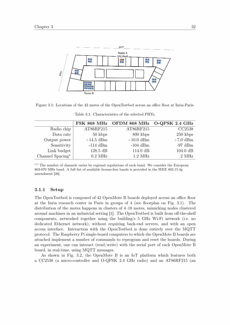
Chapter 3 32
Figure 3.1: Locations of the 42 motes of the OpenTestbed across an office floor at Inria-Paris.
Table 3.1: Characteristics of the selected PHYs.
FSK 868 MHz OFDM 868 MHz O-QPSK 2.4 GHzRadio chip AT86RF215 AT86RF215 CC2538Data rate 50 kbps 800 kbps 250 kbps
Output power +14.5 dBm +10.0 dBm +7.0 dBmSensitivity -114 dBm -104 dBm -97 dBm
Link budget 128.5 dB 114.0 dB 104.0 dBChannel Spacing∗ 0.2 MHz 1.2 MHz 2 MHz
(∗) The number of channels varies by regional regulations of each band. We consider the European863-870 MHz band. A full list of available license-free bands is provided in the IEEE 802.15.4gamendment [26].
3.1.1 Setup
The OpenTestbed is composed of 42 OpenMote B boards deployed across an office floorat the Inria research center in Paris in groups of 4 (see floorplan on Fig. 3.1). Thedistribution of the motes happens in clusters of 4–18 motes, mimicking nodes clusteredaround machines in an industrial setting [1]. The OpenTestbed is built from off-the-shelfcomponents, networked together using the building’s 5 GHz Wi-Fi network (i.e. nodedicated Ethernet network), without requiring back-end servers, and with an openaccess interface. Interaction with the OpenTestbed is done entirely over the MQTTprotocol. The Raspberry Pi single-board computers to which the OpenMote B boards areattached implement a number of commands to reprogram and reset the boards. Duringan experiment, one can interact (read/write) with the serial port of each OpenMote Bboard, in real-time, using MQTT messages.
As shown in Fig. 3.2, the OpenMote B is an IoT platform which features botha CC2538 (a micro-controller and O-QPSK 2.4 GHz radio) and an AT86RF215 (an
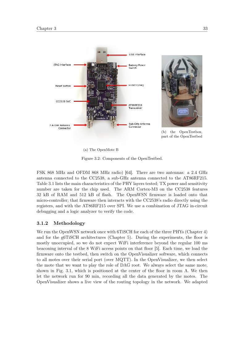
Chapter 3 33
(a) The OpenMote B
(b) the OpenTestbox,part of the OpenTestbed
Figure 3.2: Components of the OpenTestbed.
FSK 868 MHz and OFDM 868 MHz radio) [64]. There are two antennas: a 2.4 GHzantenna connected to the CC2538, a sub-GHz antenna connected to the AT86RF215.Table 3.1 lists the main characteristics of the PHY layers tested; TX power and sensitivitynumber are taken for the chip used. The ARM Cortex-M3 on the CC2538 features32 kB of RAM and 512 kB of flash. The OpenWSN firmware is loaded onto thatmicro-controller; that firmware then interacts with the CC2538’s radio directly using theregisters, and with the AT86RF215 over SPI. We use a combination of JTAG in-circuitdebugging and a logic analyzer to verify the code.
3.1.2 Methodology
We run the OpenWSN network once with 6TiSCH for each of the three PHYs (Chapter 4)and for the g6TiSCH architectures (Chapter 5). During the experiments, the floor ismostly unoccupied, so we do not expect WiFi interference beyond the regular 100 msbeaconing interval of the 8 WiFi access points on that floor [5]. Each time, we load thefirmware onto the testbed, then switch on the OpenVisualizer software, which connectsto all motes over their serial port (over MQTT). In the OpenVisualizer, we then selectthe mote that we want to play the role of DAG root. We always select the same mote,shown in Fig. 3.1, which is positioned at the center of the floor in room A. We thenlet the network run for 90 min, recording all the data generated by the motes. TheOpenVisualizer shows a live view of the routing topology in the network. We adapted
Chapter 3 34
this live view to show the multi-PHY routing topology as shown in Fig. 3.3 (furtherdetails in Chapter 5).
We developed a custom application which runs at the application layer of each mote.That application sends a data packet every minute containing the following fields:
• a counter, which we use to detect lost data packets,
• the time at which the data packet is generated (ASN),
• the DAG rank of the sender,
• the size of the neighbor table of the sender,
• Ton, how long the sender’s radio has been on since the previous data packettransmission,
• TTX , how long the sender’s radio has been on and transmitting since the previousdata packet transmission,
• Ttotal, the amount of time since the previous data packet transmission,
• the maximum and minimum number of packets in the packet buffer since theprevious packet.
After the experiment is done, we use that information to compute the following KPIs(recommended by Reference [42]):
• Network Formation Time: how much time elapses between the moment the root isselected and that root has received at least one packet from each mote.
• End-to-End Reliability: what portion of all packet generated in the network arereceived by the root.
• End-to-End latency: how much time elapses between the generation of the packetat the sender, and reception at the root.
• Radio duty cycle: what portion of the time a node’s radio is on; a good indicationfor its power consumption.
We display the results in three forms:
• Time series. We show the mean and the inter-quartile range of the KPI, with a3 min sliding window and a 1 s time resolution.
• Cumulative Distribution Function (CDF). We show the cumulative distributionof all data samples at steady state (starting 30 min into the experiment), using100 bins. This allows for efficiently visualizing key performance indicators such asoutages.
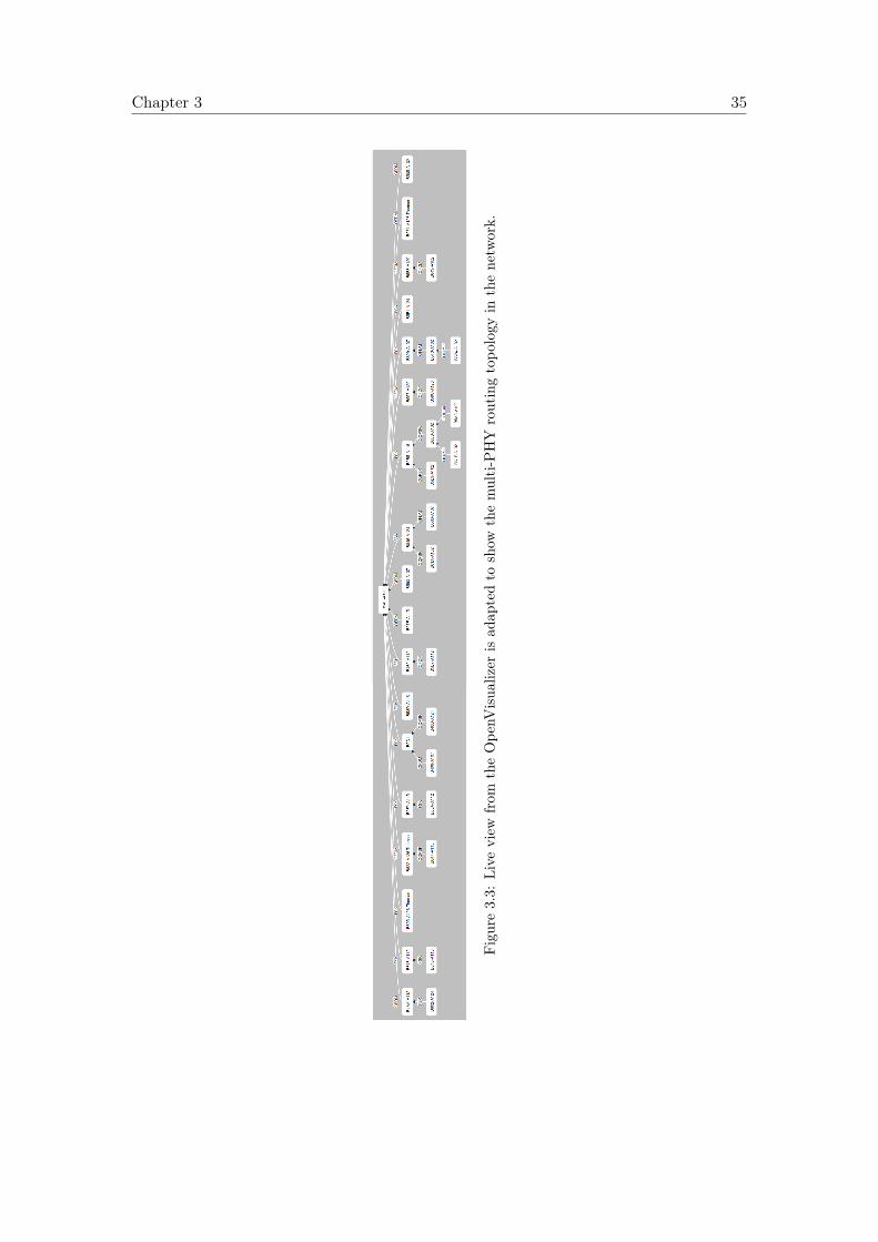
Chapter 3 35
Figure3.3:
Live
view
from
theOpe
nVisua
lizer
isad
aptedto
show
themulti-P
HY
routingtopo
logy
inthenetw
ork.
Chapter 3 36
• Probability Distribution Function (PDF). We show the probability distribution ofall data samples at steady state using 100 bins. This allows for a more detailedassessment of the distribution of each data set.
We developed a data logging and processing tool for the OpenTestbed known as theKPI monitor (Chapter 9). The tool allows logging bulk measurements by experimentID in distributed JSON files. This allows post-experiment analytics. Doing so allowyou to extract new insights or KPIs without re-running experiments. For instance, plotscan be reproduced by modifying the width or the time resolution of the sliding window.Similarly, CDFs and PDFs can be reproduced for the whole or a portion of the experimentdataset.
3.2 Local Experiment Setup
We are interested to show the real-time performance of 6DYN, 6TiSCH withheterogeneous slot-frames. For this purpose, we create a lab-bench experimental setupwith 4 nodes connected to lab equipment, to inspect the real-time performance of theMAC layer. OpenMote B (Fig. 3.2a) is used as the development platform. A logicanalyzer is used to capture the event-triggers from the different MAC layer componentsat real-time. We use a JTAG interface for in-circuit debugging and the IAR EmbeddedWorkbench as the Integrated Development Environment.
The OpenMote B routes six general purpose input/output pins from the CC2538 toextension headers. We use those to follow the execution of the firmware using the logicanalyzer. This setup is outlined in Fig. 3.4. We instrument the firmware to toggle thefollowing pins:
• The slot pin is toggled at the start of each timeslot.
• The radio is set high when the radio is on, either in transmit or receive mode.
• The fsm pin toggles at each transition of the Finite State Machine of theimplementation of the TSCH MAC layer. This pin allows us to identify transmitand receive slots and the timing inside the slot, defined in the timeslot template(see Section 4.3).
Fig. 3.5 shows the resulting real-time capture of MAC-layer events on both nodesduring a ping session from the root to the node. This setup is expanded to fournodes as illustrated in Fig. 3.6 to enable capturing the real-time multi-hop/multi-PHYperformance of 6DYN. The output of this setup is shown in Fig. 6.5 and the contentdetails will be explained in Chapter 6.
3.3 RPLSim
We are interested in measuring the impact of the used RPL OF on network lifetime andlatency. For this purpose, we have developed a high level RPL discrete-time simulator
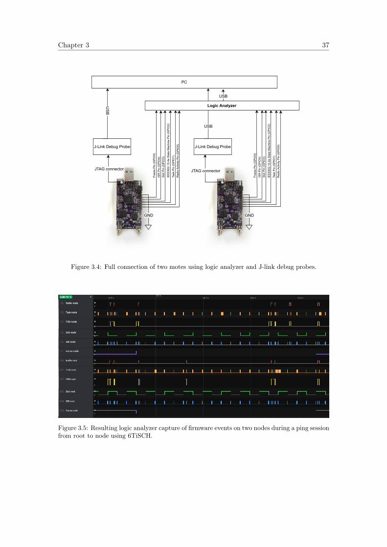
Chapter 3 37
USB
Slot
Pin
(GPI
O3)
IEEE
802.
15.4
e St
ate
Mac
hine
Pin
(GPI
O2)
PC
USB
J-Link Debug Probe
JTAG connector
USB
Logic Analyzer
Rad
io A
ctiv
ity P
in (G
PIO
0)Ta
sk P
in (G
PIO
1)
ISR
Pin
(GPI
O4)
Fram
e Pi
n (G
PIO
5)
GND
Slot
Pin
(GPI
O3)
IEEE
802.
15.4
e St
ate
Mac
hine
Pin
(GPI
O2)
J-Link Debug Probe
JTAG connector
Rad
io A
ctiv
ity P
in (G
PIO
0)Ta
sk P
in (G
PIO
1)
ISR
Pin
(GPI
O4)
Fram
e Pi
n (G
PIO
5)
GND
Figure 3.4: Full connection of two motes using logic analyzer and J-link debug probes.
Figure 3.5: Resulting logic analyzer capture of firmware events on two nodes during a ping sessionfrom root to node using 6TiSCH.
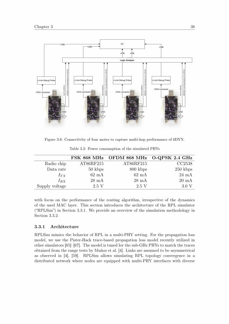
Chapter 3 38
GND
Slot
Pin
(GPI
O3)
IEEE
802.
15.4
e St
ate
Mac
hine
Pin
(GPI
O2)
PCUSB
J-Link Debug Probe
JTAG connector
Slot
Pin
(GPI
O3)
IEEE
802.
15.4
e St
ate
Mac
hine
Pin
(GPI
O2)
USB
J-Link Debug Probe
JTAG connector
Slot
Pin
(GPI
O3)
IEEE
802.
15.4
e St
ate
Mac
hine
Pin
(GPI
O2)
USB
J-Link Debug Probe
JTAG connector
Slot
Pin
(GPI
O3)
IEEE
802.
15.4
e St
ate
Mac
hine
Pin
(GPI
O2)
USB
USB
J-Link Debug Probe
JTAG connector
Logic Analyzer
GND GND GND
Figure 3.6: Connectivity of four motes to capture multi-hop performance of 6DYN.
Table 3.2: Power consumption of the simulated PHYs
FSK 868 MHz OFDM 868 MHz O-QPSK 2.4 GHzRadio chip AT86RF215 AT86RF215 CC2538Data rate 50 kbps 800 kbps 250 kbps
ITX 62 mA 62 mA 24 mAIRX 28 mA 28 mA 20 mA
Supply voltage 2.5 V 2.5 V 3.0 V
with focus on the performance of the routing algorithm, irrespective of the dynamicsof the used MAC layer. This section introduces the architecture of the RPL simulator(“RPLSim”) in Section 3.3.1. We provide an overview of the simulation methodology inSection 3.3.2.
3.3.1 Architecture
RPLSim mimics the behavior of RPL in a multi-PHY setting. For the propagation lossmodel, we use the Pister-Hack trace-based propagation loss model recently utilized inother simulators [65]–[67]. The model is tuned for the sub-GHz PHYs to match the tracesobtained from the range tests by Muñoz et al. [4]. Links are assumed to be asymmetricalas observed in [4], [59]. RPLSim allows simulating RPL topology convergence in adistributed network where nodes are equipped with multi-PHY interfaces with diverse
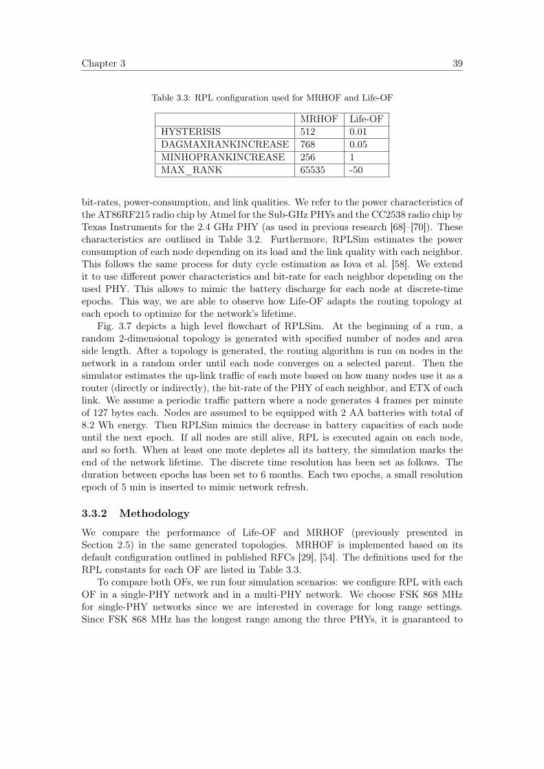
Chapter 3 39
Table 3.3: RPL configuration used for MRHOF and Life-OF
MRHOF Life-OFHYSTERISIS 512 0.01DAGMAXRANKINCREASE 768 0.05MINHOPRANKINCREASE 256 1MAX_RANK 65535 -50
bit-rates, power-consumption, and link qualities. We refer to the power characteristics ofthe AT86RF215 radio chip by Atmel for the Sub-GHz PHYs and the CC2538 radio chip byTexas Instruments for the 2.4 GHz PHY (as used in previous research [68]–[70]). Thesecharacteristics are outlined in Table 3.2. Furthermore, RPLSim estimates the powerconsumption of each node depending on its load and the link quality with each neighbor.This follows the same process for duty cycle estimation as Iova et al. [58]. We extendit to use different power characteristics and bit-rate for each neighbor depending on theused PHY. This allows to mimic the battery discharge for each node at discrete-timeepochs. This way, we are able to observe how Life-OF adapts the routing topology ateach epoch to optimize for the network’s lifetime.
Fig. 3.7 depicts a high level flowchart of RPLSim. At the beginning of a run, arandom 2-dimensional topology is generated with specified number of nodes and areaside length. After a topology is generated, the routing algorithm is run on nodes in thenetwork in a random order until each node converges on a selected parent. Then thesimulator estimates the up-link traffic of each mote based on how many nodes use it as arouter (directly or indirectly), the bit-rate of the PHY of each neighbor, and ETX of eachlink. We assume a periodic traffic pattern where a node generates 4 frames per minuteof 127 bytes each. Nodes are assumed to be equipped with 2 AA batteries with total of8.2 Wh energy. Then RPLSim mimics the decrease in battery capacities of each nodeuntil the next epoch. If all nodes are still alive, RPL is executed again on each node,and so forth. When at least one mote depletes all its battery, the simulation marks theend of the network lifetime. The discrete time resolution has been set as follows. Theduration between epochs has been set to 6 months. Each two epochs, a small resolutionepoch of 5 min is inserted to mimic network refresh.
3.3.2 Methodology
We compare the performance of Life-OF and MRHOF (previously presented inSection 2.5) in the same generated topologies. MRHOF is implemented based on itsdefault configuration outlined in published RFCs [29], [54]. The definitions used for theRPL constants for each OF are listed in Table 3.3.
To compare both OFs, we run four simulation scenarios: we configure RPL with eachOF in a single-PHY network and in a multi-PHY network. We choose FSK 868 MHzfor single-PHY networks since we are interested in coverage for long range settings.Since FSK 868 MHz has the longest range among the three PHYs, it is guaranteed to
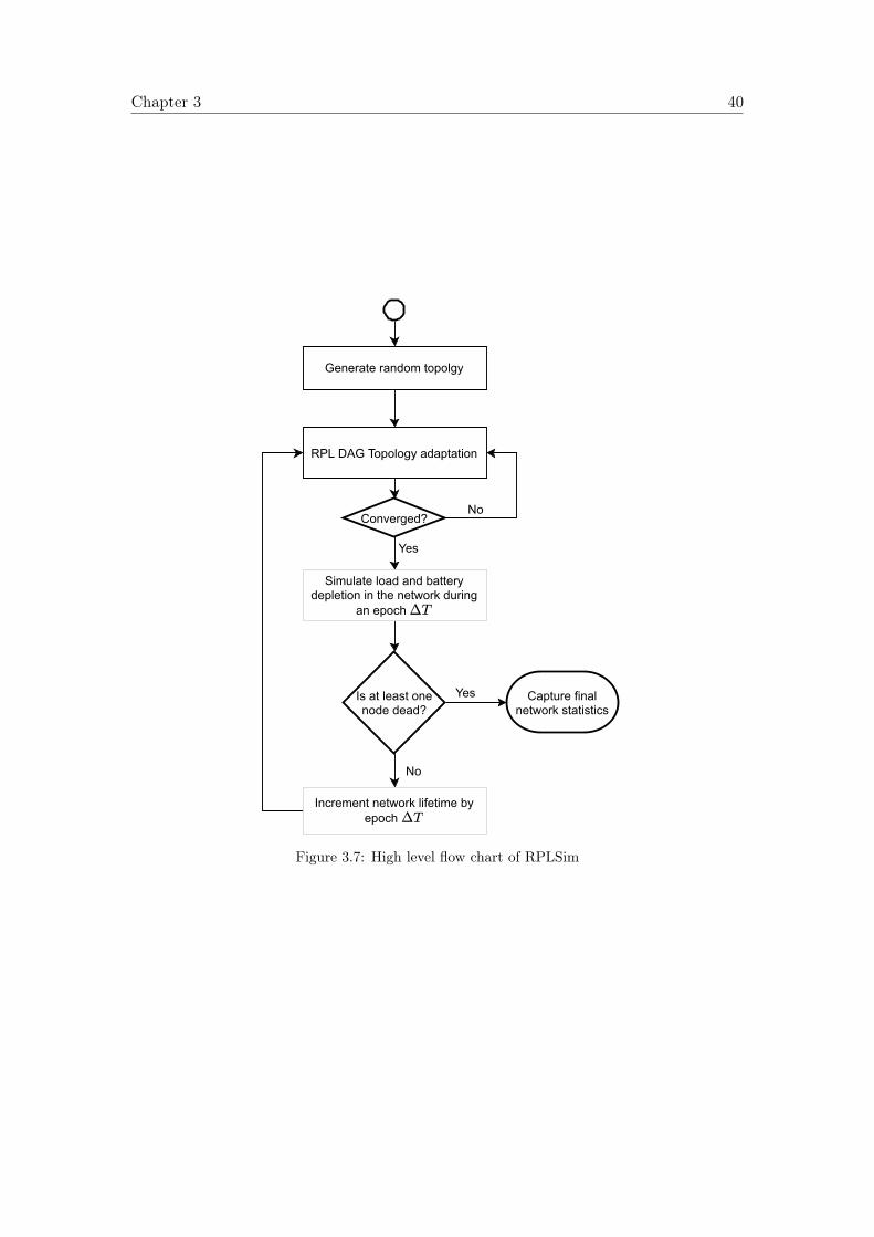
Chapter 3 40
RPL DAG Topology adaptation
Is at least onenode dead?
Simulate load and batterydepletion in the network during
an epoch
Increment network lifetime byepoch
Yes
Converged?
Capture finalnetwork statistics
Generate random topolgy
No
Yes
No
Figure 3.7: High level flow chart of RPLSim
Chapter 3 41
provide the same coverage range as a multi-PHY network. This allows to have a faircomparison between both OFs since the resulting networks will cover the same territory.Each scenario is run 50 times with random topologies generated in each run. We use atopology configuration with the area size of 2 × 2 km2, mimicking a typical industrialplant. We use a network size of 100 nodes which is an average size of an industrialnetwork according to the IETF-defined use cases [71].
At the end of each run, two KPIs are captured: network lifetime and networkETX. Network lifetime is calculated based on the simulated duration until the first nodedepleted all its battery energy. This KPI is essential to estimate a real cost of operatingthe network in many industrial use cases. Network ETX is calculated for each node bysumming the ETX of each link on the path from that node to the root. This KPI reflectsthe end-to-end latency which is necessary to observe how each OF impacts the upperbounds of latency in the network.
To report the results across runs for each KPI, we plot a statistical description ofthe distribution of measurements using box plots. Box boundaries represent the firstand third quartiles of the distribution. A red horizontal line represents the median.Individual outliers are plotted as individual data point.
3.4 Summary
This chapter presents three experimental setups used for the research conducted in thisthesis. First, the OpenTesbed, which consists of 42 nodes deployed across an officebuilding, is used for network-wide evaluation of the protocol stack performance. We usethe OpenTestbed in Chapters 4 and 5. Second, a local experimental setup for real-timeperformance demonstration using hardware probes, which we use in Chapter 6. Finally,RPLSim, a RPL simulator for high-level performance evaluation of RPL OFs, which weuse in Chapter 7.
Chapter 4
6TiSCH Performance Evaluationusing Different PHYs
Parts of this chapter were published as part of the following article: No FreeLunch—Characterizing the Performance of 6TiSCH When Using Different PhysicalLayers. Mina Rady, Quentin Lampin, Dominique Barthel, Thomas Watteyne. MDPISensors, vol. 20, no. 17, p. 4989, September 2020.
Key Takeaways: Low-power wireless applications require different trade-offpoints between latency, reliability, data rate and power consumption. Given sucha set of constraints, which physical layer should we be using? In this chapter,we study this question in the context of 6TiSCH, a state-of-the-art protocol stackdeveloped for harsh industrial applications and recently standardized. Specifically,we augment OpenWSN, the reference 6TiSCH open-source implementation,to support one of three physical layers from the IEEE802.15.4g standard:FSK 868 MHz which offers long range, OFDM 868 MHz which offers high datarate, and O-QPSK 2.4 GHz which offers more balanced performance. We run theresulting firmware on the 42-mote OpenTestbed deployed in an office environment,once for each physical layer. Performance results show that, indeed, no physicallayer outperforms the other for all metrics. The long range FSK 868 MHz radioyields the fastest network formation and lowest latency at the expense of batterylifetime. The short range O-QPSK 2.4 GHz radio yields the best network lifetimeat the expense of latency, reliability, and network formation time. This chapterargues for combining the physical layers, rather than choosing one, in a generalized6TiSCH architecture in which technology-agile radio chips (of which there are nowmany) are driven by a protocol stack which chooses the most appropriate physicallayer on a link-by-link basis.
42
Chapter 4 43
4.1 Introduction
The goal of this chapter is to provide a base for the vision of a generalized 6TiSCHprotocol stack by comparing the performance of a 6TiSCH network for different PHYlayers. Here, we try to address the question: does multi-PHY integration make sense?This is a necessary first step towards dynamically changing the PHY layer, the object ofthe thesis. Specifically, we augment the OpenWSN reference 6TiSCH implementation tosupport the following three PHYs: O-QPSK 2.4 GHz at 250 kbps, FSK 868 MHz option1 at 50 kbps, OFDM 868 MHz option 1 Modulation and Coding Scheme (MCS) 3 at800 kbps. The literature indicates that these three PHYs cover the range of possibilitiesof IEEE802.15.4g: very high data rate with OFDM 868 MHz, very long range withFSK 868 MHz, O-QPSK 2.4 GHz being a balance between range and data rate [16], [59],[72]. We then conduct a comprehensive experimental campaign, using the OpenTestbedwhich was introduced in Section 3.1. We compare the performance of the network interms of network formation time, battery lifetime, end-to-end latency and end-to-endreliability.
The remainder of this chapter is organized as follows. Section 4.2 states the problemsand lists the contributions of this chapter. Section 4.3 introduces the agile extensionto the OpenWSN PHY-layer that enabled this research. Section 4.4 demonstrates theexperiment results and KPI evaluations. Finally, Section 4.5 provides insights andconclusions based on the results.
4.2 Problem Statement and Contributions
While active research proposed various enhancements in 6TiSCH for achieving wire-likereliability and low power consumption, one common assumption is that it usesthe IEEE802.15.4 O-QPSK at 2.4 GHz, as concluded in Section 2.2. WhileO-QPSK 2.4 GHz is appropriate for many applications, the increasing demand forlong range (including for environmental monitoring and automated meter reading) hastriggered the standardization of longer range PHYs [4]. A problem statement hasbeen proposed within the IETF detailing the theoretical challenges or side-effects ofaugmenting 6TiSCH to include different PHYs [72]. Using a different PHY will cause thenetwork to behave differently, leading to different overall performance. For example, adifferent energy consumption and link cost changes how links to neighbors are evaluatedat the link-layer, hence which multi-hop paths are picked by the routing protocol. Adifferent PHY also impacts the number of re-transmissions, the level of interferenceand the amount of contention in shared cells [73]. Changing the PHY layer triggerssubtle changes in the behavior of the protocol stack, resulting in different performance.We believe measuring this difference is best done through a real-world system levelevaluation [74]. We show that there are significant benefits for each of the radio options:FSK 868 MHz, OFDM 868 MHz, and O-QPSK 2.4 GHz, yet they all come at a certaincost.
The contribution of this chapter is three-fold:

Chapter 4 44
• We augment the OpenWSN reference implementation of 6TiSCH to support thethree PHY layers∗.
• We conduct an experimental performance evaluation campaign of the resultingcode on the 42-node OpenTestbed described in Chapter 3. For each PHY, wemeasure the network formation time, the end-to-end reliability, the end-to-endlatency, the estimated battery lifetime of each node, and the memory footprint ofthe implementation.
• We highlight the advantages and disadvantages of each PHY layer, specifically:
– Using FSK 868 MHz yields the fastest network formation, the highestend-to-end reliability, and the lowest end-to-end latency, at the cost of a 75%decrease in battery lifetime, on average, compared to O-QPSK 2.4 GHz.
– Using O-QPSK 2.4 GHz yields the longest battery lifetime, at the cost of theslowest network formation, the lowest end-to-end reliability, and the highestend-to-end latency.
– Using OFDM 868 MHz yields an intermediate network formation timeend-to-end reliability, and end-to-end latency at the cost of a 30% decrease inbattery lifetime compared to O-QPSK 2.4 GHz. In line with Muñoz et al. [4],a node using OFDM 868 MHz discovers a number of neighbors close to thatof FSK 868 MHz despite having the highest data rate. This is because it ismore robust against frequency selective interference than FSK 868 MHz [28]and more immune to WiFi interference than O-QPSK 2.4 GHz [5].
This shows there is no PHY among our candidates that is best across all metrics.
4.3 A PHY-layer Agile Extension of OpenWSN
As presented in Section 2.2, the IETF 6TiSCH working group has standardized how tocombine TSCH and IPv6 [30]. The 6TiSCH protocol stack has been ported to all mainopen-source IoT protocol stacks: OpenWSN, Contiki-NG, RIOT and TinyOS [19].
Since it is the reference implementation, and since it is ported to the OpenMote B,we use the OpenWSN implementation in this thesis. Prior to this work, OpenWSNonly supported the IEEE802.15.4 O-QPSK 2.4 GHz PHY. Although initial rangemeasurements were conducted using the OpenMote’s AT86RF215 radio [4], [5], thefull 6TiSCH stack had never been ported. We therefore extend OpenWSN to supportthe following PHYs: FSK 868 MHz, OFDM 868 MHz, and O-QPSK 2.4 GHz. Thisextension consists of three steps: writing the low-level drivers to configure the radio chipsappropriately, tuning the durations within the timeslots to each PHY, and providing aclean software abstraction to allow the TSCH implementation to switch between them.
∗As an online addition to this chapter, these extensions have been merged into the main codebase ofOpenWSN at https://github.com/openwsn-berkeley and published under an open-source license.

Chapter 4 45
Tab
le4.1:
Definition
oftimingvariab
lesthat
compo
sean
IEEE
802.15.4etime-slot
template
Rad
io-specificvariab
les
TsT
xOffset
The
timebe
tweenslot
startan
dda
tatran
smission
TsL
ongG
TThe
max
imum
duration
forradioto
listenforthebe
ginn
ingof
data
packet
TsT
xAckDelay
The
timebe
tweenpa
cket
receptionan
dackn
owledg
mentstartof
tran
smission
TsSho
rtGT
The
max
imum
duration
forradioto
listenforthebe
ginn
ingof
ackn
owledg
mentpa
cket
wdR
adioTx
The
max
imum
timeforaradiochip
tostartfram
etran
smission
wdD
ataD
uration
The
max
imum
timeto
completeatran
smission
ofada
tafram
ewdA
ckDuration
The
max
imum
timeto
completeatran
smission
ofan
ackn
owledg
mentfram
eBoard-specificvariab
les
max
TxD
ataP
repa
reThe
max
imum
timeto
retrieve
andprepareada
tafram
eon
tran
smitterside.
max
RxA
ckPrepa
reThe
max
imum
timeto
retrieve
andpreparean
ackn
owledg
ementfram
eon
receiver
side.
max
RxD
ataP
repa
reThe
max
imum
timeto
prepareforda
tafram
ereceptionon
receiver
side.
max
TxA
ckPrepa
reThe
max
imum
timeto
prepareforackn
owledg
ementfram
ereceptionon
tran
smitterside.
delayT
xThe
expe
cted
delaybe
tweenissuingatran
smit
comman
dby
themicro-con
trolleran
ditsexecutionon
theradio-chip
delayR
xThe
expe
cted
delaybe
tweenissuingareceivecomman
dby
themicro-con
trolleran
ditsexecutionon
theradio-chip
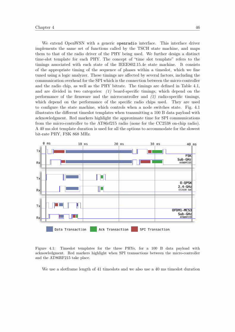
Chapter 4 46
We extend OpenWSN with a generic openradio interface. This interface driverimplements the same set of functions called by the TSCH state machine, and mapsthem to that of the radio driver of the PHY being used. We further design a distincttime-slot template for each PHY. The concept of “time slot template” refers to thetimings associated with each state of the IEEE802.15.4e state machine. It consistsof the appropriate timing of the sequence of phases within a timeslot, which we finetuned using a logic analyzer. These timings are affected by several factors, including thecommunication overhead for the SPI which is the connection between the micro-controllerand the radio chip, as well as the PHY bitrate. The timings are defined in Table 4.1,and are divided in two categories: (1) board-specific timings, which depend on theperformance of the firmware and the microcontroller and (2) radio-specific timings,which depend on the performance of the specific radio chips used. They are usedto configure the state machine, which controls when a node switches state. Fig. 4.1illustrates the different timeslot templates when transmitting a 100 B data payload withacknowledgment. Red markers highlight the approximate time for SPI communicationsfrom the micro-controller to the AT86rf215 radio (none for the CC2538 on-chip radio).A 40 ms slot template duration is used for all the options to accommodate for the slowestbit-rate PHY, FSK 868 MHz.
Figure 4.1: Timeslot templates for the three PHYs, for a 100 B data payload withacknowledgment. Red markers highlight when SPI transactions between the micro-controllerand the AT86RF215 take place.
We use a slotframe length of 41 timeslots and we also use a 40 ms timeslot duration
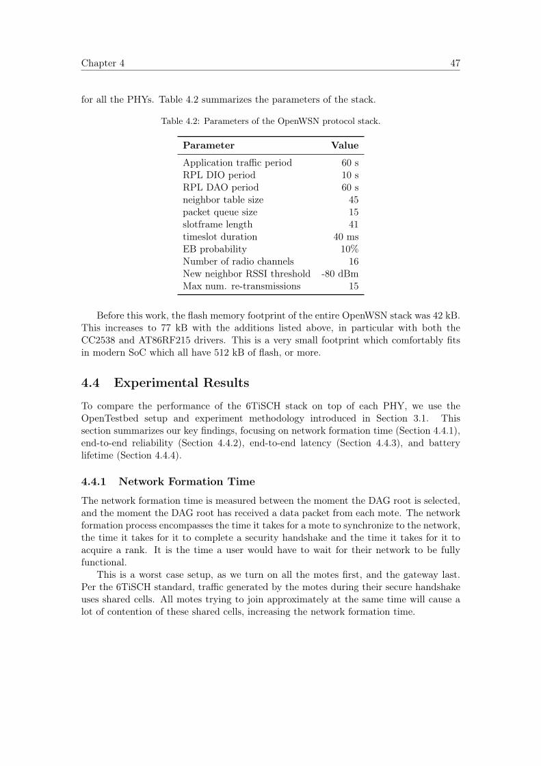
Chapter 4 47
for all the PHYs. Table 4.2 summarizes the parameters of the stack.
Table 4.2: Parameters of the OpenWSN protocol stack.
Parameter Value
Application traffic period 60 sRPL DIO period 10 sRPL DAO period 60 sneighbor table size 45packet queue size 15slotframe length 41timeslot duration 40 msEB probability 10%Number of radio channels 16New neighbor RSSI threshold -80 dBmMax num. re-transmissions 15
Before this work, the flash memory footprint of the entire OpenWSN stack was 42 kB.This increases to 77 kB with the additions listed above, in particular with both theCC2538 and AT86RF215 drivers. This is a very small footprint which comfortably fitsin modern SoC which all have 512 kB of flash, or more.
4.4 Experimental Results
To compare the performance of the 6TiSCH stack on top of each PHY, we use theOpenTestbed setup and experiment methodology introduced in Section 3.1. Thissection summarizes our key findings, focusing on network formation time (Section 4.4.1),end-to-end reliability (Section 4.4.2), end-to-end latency (Section 4.4.3), and batterylifetime (Section 4.4.4).
4.4.1 Network Formation Time
The network formation time is measured between the moment the DAG root is selected,and the moment the DAG root has received a data packet from each mote. The networkformation process encompasses the time it takes for a mote to synchronize to the network,the time it takes for it to complete a security handshake and the time it takes for it toacquire a rank. It is the time a user would have to wait for their network to be fullyfunctional.
This is a worst case setup, as we turn on all the motes first, and the gateway last.Per the 6TiSCH standard, traffic generated by the motes during their secure handshakeuses shared cells. All motes trying to join approximately at the same time will cause alot of contention of these shared cells, increasing the network formation time.
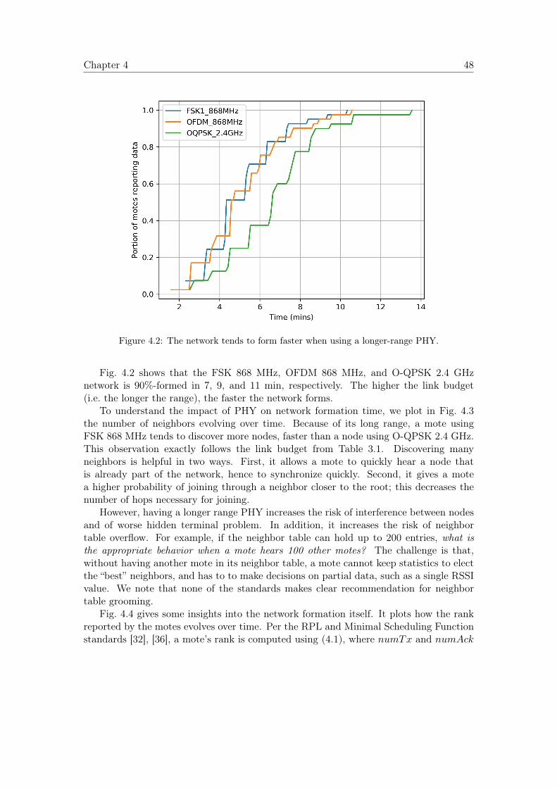
Chapter 4 48
Figure 4.2: The network tends to form faster when using a longer-range PHY.
Fig. 4.2 shows that the FSK 868 MHz, OFDM 868 MHz, and O-QPSK 2.4 GHznetwork is 90%-formed in 7, 9, and 11 min, respectively. The higher the link budget(i.e. the longer the range), the faster the network forms.
To understand the impact of PHY on network formation time, we plot in Fig. 4.3the number of neighbors evolving over time. Because of its long range, a mote usingFSK 868 MHz tends to discover more nodes, faster than a node using O-QPSK 2.4 GHz.This observation exactly follows the link budget from Table 3.1. Discovering manyneighbors is helpful in two ways. First, it allows a mote to quickly hear a node thatis already part of the network, hence to synchronize quickly. Second, it gives a motea higher probability of joining through a neighbor closer to the root; this decreases thenumber of hops necessary for joining.
However, having a longer range PHY increases the risk of interference between nodesand of worse hidden terminal problem. In addition, it increases the risk of neighbortable overflow. For example, if the neighbor table can hold up to 200 entries, what isthe appropriate behavior when a mote hears 100 other motes? The challenge is that,without having another mote in its neighbor table, a mote cannot keep statistics to electthe “best” neighbors, and has to to make decisions on partial data, such as a single RSSIvalue. We note that none of the standards makes clear recommendation for neighbortable grooming.
Fig. 4.4 gives some insights into the network formation itself. It plots how the rankreported by the motes evolves over time. Per the RPL and Minimal Scheduling Functionstandards [32], [36], a mote’s rank is computed using (4.1), where numTx and numAck
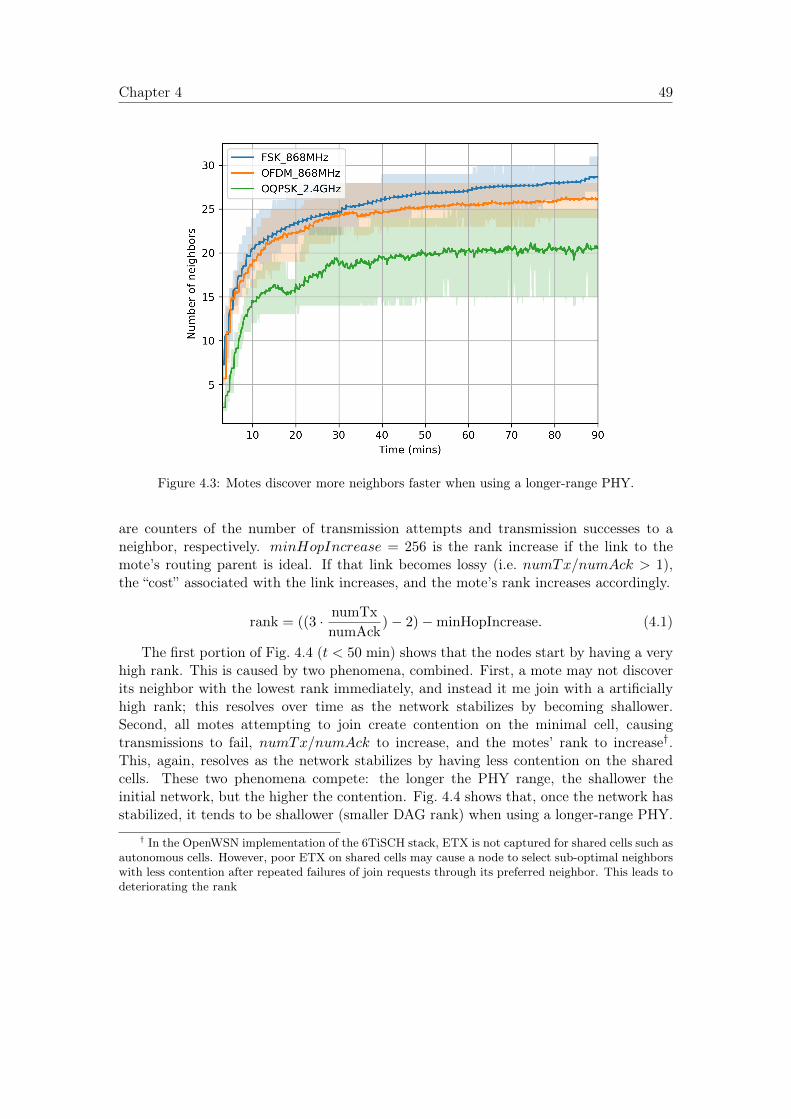
Chapter 4 49
Figure 4.3: Motes discover more neighbors faster when using a longer-range PHY.
are counters of the number of transmission attempts and transmission successes to aneighbor, respectively. minHopIncrease = 256 is the rank increase if the link to themote’s routing parent is ideal. If that link becomes lossy (i.e. numTx/numAck > 1),the “cost” associated with the link increases, and the mote’s rank increases accordingly.
rank = ((3 · numTx
numAck)− 2)−minHopIncrease. (4.1)
The first portion of Fig. 4.4 (t < 50 min) shows that the nodes start by having a veryhigh rank. This is caused by two phenomena, combined. First, a mote may not discoverits neighbor with the lowest rank immediately, and instead it me join with a artificiallyhigh rank; this resolves over time as the network stabilizes by becoming shallower.Second, all motes attempting to join create contention on the minimal cell, causingtransmissions to fail, numTx/numAck to increase, and the motes’ rank to increase†.This, again, resolves as the network stabilizes by having less contention on the sharedcells. These two phenomena compete: the longer the PHY range, the shallower theinitial network, but the higher the contention. Fig. 4.4 shows that, once the network hasstabilized, it tends to be shallower (smaller DAG rank) when using a longer-range PHY.
† In the OpenWSN implementation of the 6TiSCH stack, ETX is not captured for shared cells such asautonomous cells. However, poor ETX on shared cells may cause a node to select sub-optimal neighborswith less contention after repeated failures of join requests through its preferred neighbor. This leads todeteriorating the rank
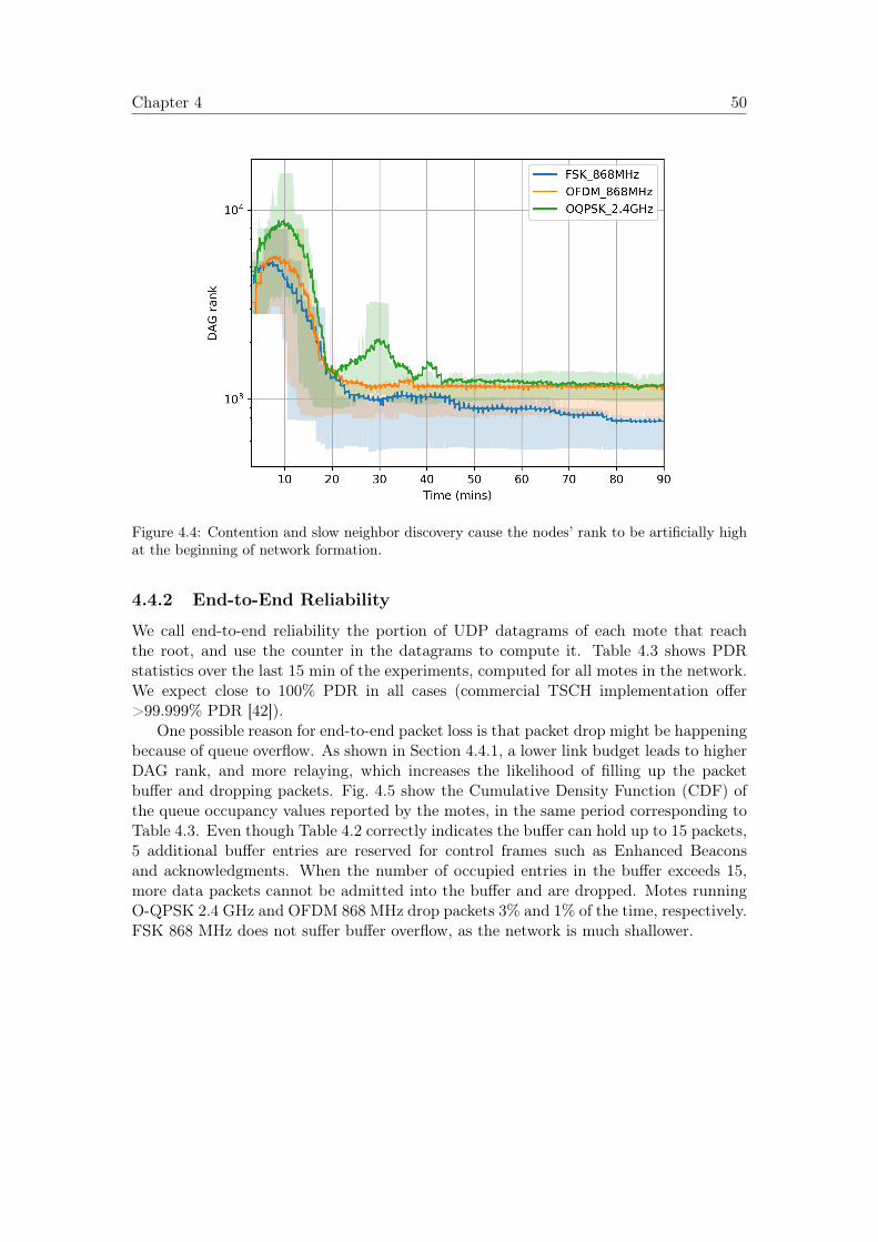
Chapter 4 50
Figure 4.4: Contention and slow neighbor discovery cause the nodes’ rank to be artificially highat the beginning of network formation.
4.4.2 End-to-End Reliability
We call end-to-end reliability the portion of UDP datagrams of each mote that reachthe root, and use the counter in the datagrams to compute it. Table 4.3 shows PDRstatistics over the last 15 min of the experiments, computed for all motes in the network.We expect close to 100% PDR in all cases (commercial TSCH implementation offer>99.999% PDR [42]).
One possible reason for end-to-end packet loss is that packet drop might be happeningbecause of queue overflow. As shown in Section 4.4.1, a lower link budget leads to higherDAG rank, and more relaying, which increases the likelihood of filling up the packetbuffer and dropping packets. Fig. 4.5 show the Cumulative Density Function (CDF) ofthe queue occupancy values reported by the motes, in the same period corresponding toTable 4.3. Even though Table 4.2 correctly indicates the buffer can hold up to 15 packets,5 additional buffer entries are reserved for control frames such as Enhanced Beaconsand acknowledgments. When the number of occupied entries in the buffer exceeds 15,more data packets cannot be admitted into the buffer and are dropped. Motes runningO-QPSK 2.4 GHz and OFDM 868 MHz drop packets 3% and 1% of the time, respectively.FSK 868 MHz does not suffer buffer overflow, as the network is much shallower.
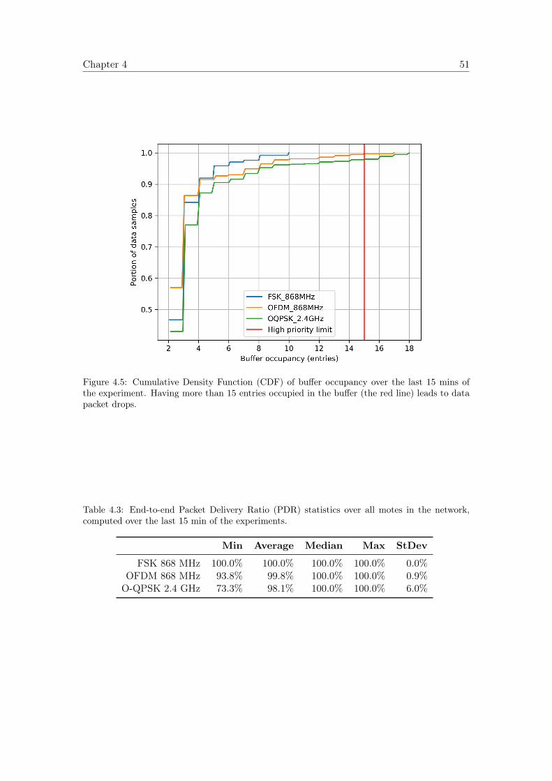
Chapter 4 51
Figure 4.5: Cumulative Density Function (CDF) of buffer occupancy over the last 15 mins ofthe experiment. Having more than 15 entries occupied in the buffer (the red line) leads to datapacket drops.
Table 4.3: End-to-end Packet Delivery Ratio (PDR) statistics over all motes in the network,computed over the last 15 min of the experiments.
Min Average Median Max StDev
FSK 868 MHz 100.0% 100.0% 100.0% 100.0% 0.0%OFDM 868 MHz 93.8% 99.8% 100.0% 100.0% 0.9%O-QPSK 2.4 GHz 73.3% 98.1% 100.0% 100.0% 6.0%
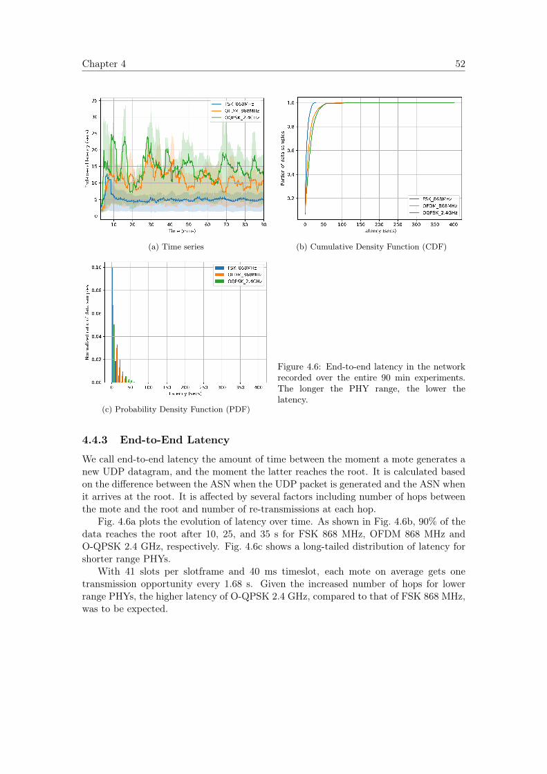
Chapter 4 52
(a) Time series (b) Cumulative Density Function (CDF)
(c) Probability Density Function (PDF)
Figure 4.6: End-to-end latency in the networkrecorded over the entire 90 min experiments.The longer the PHY range, the lower thelatency.
4.4.3 End-to-End Latency
We call end-to-end latency the amount of time between the moment a mote generates anew UDP datagram, and the moment the latter reaches the root. It is calculated basedon the difference between the ASN when the UDP packet is generated and the ASN whenit arrives at the root. It is affected by several factors including number of hops betweenthe mote and the root and number of re-transmissions at each hop.
Fig. 4.6a plots the evolution of latency over time. As shown in Fig. 4.6b, 90% of thedata reaches the root after 10, 25, and 35 s for FSK 868 MHz, OFDM 868 MHz andO-QPSK 2.4 GHz, respectively. Fig. 4.6c shows a long-tailed distribution of latency forshorter range PHYs.
With 41 slots per slotframe and 40 ms timeslot, each mote on average gets onetransmission opportunity every 1.68 s. Given the increased number of hops for lowerrange PHYs, the higher latency of O-QPSK 2.4 GHz, compared to that of FSK 868 MHz,was to be expected.
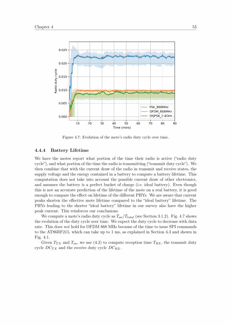
Chapter 4 53
Figure 4.7: Evolution of the mote’s radio duty cycle over time.
4.4.4 Battery Lifetime
We have the motes report what portion of the time their radio is active (“radio dutycycle”), and what portion of the time the radio is transmitting (“transmit duty cycle”). Wethen combine that with the current draw of the radio in transmit and receive states, thesupply voltage and the energy contained in a battery to compute a battery lifetime. Thiscomputation does not take into account the possible current draw of other electronics,and assumes the battery is a perfect bucket of charge (i.e. ideal battery). Even thoughthis is not an accurate prediction of the lifetime of the mote on a real battery, it is goodenough to compare the effect on lifetime of the different PHYs. We are aware that currentpeaks shorten the effective mote lifetime compared to the “ideal battery” lifetime. ThePHYs leading to the shorter “ideal battery” lifetime in our survey also have the higherpeak current. This reinforces our conclusions.
We compute a mote’s radio duty cycle as Ton/Ttotal (see Section 3.1.2). Fig. 4.7 showsthe evolution of the duty cycle over time. We expect the duty cycle to decrease with datarate. This does not hold for OFDM 868 MHz because of the time to issue SPI commandsto the AT86RF215, which can take up to 1 ms, as explained in Section 4.3 and shown inFig. 4.1.
Given TTX and Ton, we use (4.2) to compute reception time TRX , the transmit dutycycle DCTX and the receive duty cycle DCRX .
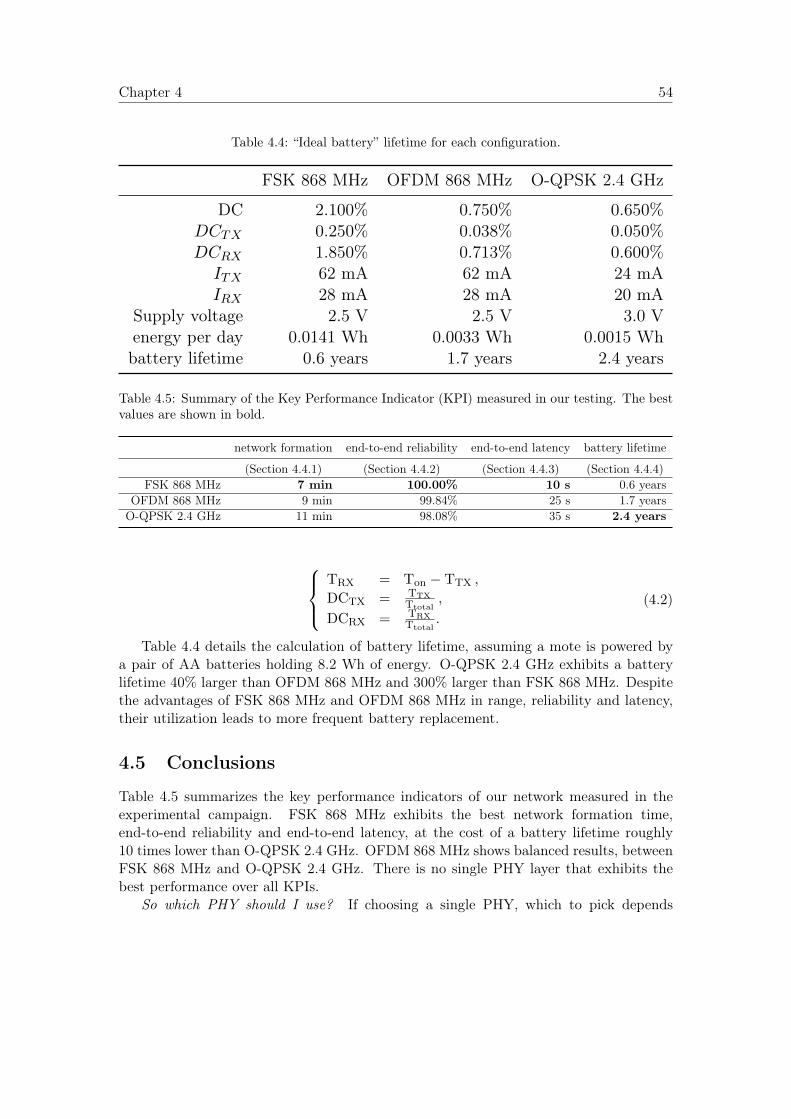
Chapter 4 54
Table 4.4: “Ideal battery” lifetime for each configuration.
FSK 868 MHz OFDM 868 MHz O-QPSK 2.4 GHz
DC 2.100% 0.750% 0.650%DCTX 0.250% 0.038% 0.050%DCRX 1.850% 0.713% 0.600%ITX 62 mA 62 mA 24 mAIRX 28 mA 28 mA 20 mA
Supply voltage 2.5 V 2.5 V 3.0 Venergy per day 0.0141 Wh 0.0033 Wh 0.0015 Whbattery lifetime 0.6 years 1.7 years 2.4 years
Table 4.5: Summary of the Key Performance Indicator (KPI) measured in our testing. The bestvalues are shown in bold.
network formation end-to-end reliability end-to-end latency battery lifetime
(Section 4.4.1) (Section 4.4.2) (Section 4.4.3) (Section 4.4.4)FSK 868 MHz 7 min 100.00% 10 s 0.6 years
OFDM 868 MHz 9 min 99.84% 25 s 1.7 yearsO-QPSK 2.4 GHz 11 min 98.08% 35 s 2.4 years
TRX = Ton − TTX ,
DCTX = TTXTtotal
,
DCRX = TRXTtotal
.
(4.2)
Table 4.4 details the calculation of battery lifetime, assuming a mote is powered bya pair of AA batteries holding 8.2 Wh of energy. O-QPSK 2.4 GHz exhibits a batterylifetime 40% larger than OFDM 868 MHz and 300% larger than FSK 868 MHz. Despitethe advantages of FSK 868 MHz and OFDM 868 MHz in range, reliability and latency,their utilization leads to more frequent battery replacement.
4.5 Conclusions
Table 4.5 summarizes the key performance indicators of our network measured in theexperimental campaign. FSK 868 MHz exhibits the best network formation time,end-to-end reliability and end-to-end latency, at the cost of a battery lifetime roughly10 times lower than O-QPSK 2.4 GHz. OFDM 868 MHz shows balanced results, betweenFSK 868 MHz and O-QPSK 2.4 GHz. There is no single PHY layer that exhibits thebest performance over all KPIs.
So which PHY should I use? If choosing a single PHY, which to pick depends
Chapter 4 55
on the application. If it is acceptable to change batteries every half a year or so,FSK 868 MHz appears to be the most appropriate. If battery lifetime is of utmostimportance, Table 4.5 suggests O-QPSK 2.4 GHz is the most appropriate. Finally, foran “in between” performance, choose OFDM 868 MHz.
Of course, it is important to note that the results depend on the use case and theKPIs and their respective importance. This can lead to a different answer to this questionand we develop a rationale to illustrate this claim. First, the results presented in thischapter, while conducted and presented in a rigorous fashion, only hold for use cases verysimilar to the deployment shown in Fig. 3.1. There are undoubtedly cases (deeply sparsenetwork, heavily unbalanced deployment, . . . ) where our results do not hold, and wherethe “ranking” of the different PHYs is different. Second, even if every precaution is takento pick the right PHY during the design phase of the network, it is entirely possible thatconditions or requirements change during the operation of the network. This could leadto operating with the “wrong” PHY layer, leading to sub-optimal performance.
It is interesting for future work to revisit the KPIs used as reference points in theseexperiments and to see the tradeoffs could look like if different KPIs are used. To confirmthis view: network deployment cost as a KPI can create interest in long range PHYs (sincelower densities are favored by industrialists). However, if we introduce another KPI suchas network operation costs (including the cost of battery replacement), then the havingshort range PHYs can allow improved battery lifetime and therefore lower operationalcosts.
The real outcome of this paper is not the absolute numbers presented in Table 4.5.What that table does indicate is that no PHY is the best for all metrics, and that bestperformance is achieved when combining the PHY layers, rather than picking one. Thisresult holds when contemplating additional PHY layer, one obvious candidate beingLoRa [12]. As alluded to in Section 4.1, we are at an exciting stage where we haveboth radio chips which are able to switch PHY on a frame-by-frame basis, and wehave the scheduling technology to orchestrate this PHY-layer agility. We argue for atechnology-agile network, in which each mote keeps track of the quality of its link to itsneighbors for each PHY layer, and uses the PHY layer most appropriate for each frame.This means a mote may use a different PHY to communicate with different neighborsor to send frames belonging to different classes of traffic. This also means that, in amulti-hop scenario, a packet can travel from source to destination using a different PHYat each hop. In that context, energy efficient neighbor discovery and network consistencyare the main challenges, elements we addressed in this research.
Chapter 5
Generalizing 6TiSCH for an AgileMulti-PHY Networking
Parts of this chapter were published as part of the following article: g6TiSCH:Generalized 6TiSCH for Agile Multi-PHY Wireless Networking. Mina Rady, QuentinLampin, Dominique Barthel, Thomas Watteyne. IEEE Access, vol. 9, pp. 84465-84479,2021.
Key Takeaways: Wireless networks traditionally use a single physical layer forcommunication: some use high bit-rate short-range radios, others low bit-ratelong-range radios. This chapter introduces g6TiSCH, a generalization of thestandards-based IETF 6TiSCH protocol stack. g6TiSCH allows nodes equippedwith multiple radios to dynamically switch between them on a link-by-link basis,as a function of link-quality. This approach results in a dynamic trade-off betweenlatency and power consumption. We evaluate the performance of the approachexperimentally on the OpenTestBed. Each OpenMote B can communicate usingFSK 868 MHz, O-QPSK 2.4 GHz or OFDM 868 MHz, a combination of long-rangeand short-range physical layers. We measure network formation time, end-to-endreliability, end-to-end latency, and battery lifetime. We compare the performanceof g6TiSCH against that of a traditional 6TiSCH stack running on each of the threephysical layers. Results show that g6TiSCH yields lower latency and networkformation time than any of the individual PHYs, while maintaining a similarbattery lifetime.
In Chapter 4, we demonstrated that no single PHY performs best across allKPIs. The main contribution of this chapter is generalizing 6TiSCH to support amulti-PHY approach; we call this “g6TiSCH”. In g6TiSCH, nodes dynamically switchbetween using low bit-rate and high bit-rate PHYs, based on the link quality to each
56
Chapter 5 57
neighbor. We implement g6TiSCH in OpenWSN∗, the reference 6TiSCH open-sourceimplementation [75]. In this implementation, we use three PHYs: FSK 868 MHzoption 1 at 50 kbps (offering the lowest bit-rate), OFDM 868 MHz option 1 MCS 3at 800 kbps (offering the highest bit-rate), and O-QPSK 2.4 GHz at 250 kbps as anintermediate option. We experimentally compare the performance of g6TiSCH againstthe performance of the 6TiSCH architecture with each PHY individually (as previouslystudied [68]). The comparison is based on the KPIs recommended by Vucinic et al. [42]:network formation time, end-to-end latency, end-to-end reliability, and battery lifetime.
The remainder of this chapter is organized as follows. Section 5.1 presents the problemstatement and lists the specific contributions of this chapter. Section 5.2 shows how the6TiSCH stack is adapted to provide multi-PHY support. Section 5.3 introduces theexperimental testbed we used and the methodology we followed to generate the KPIs.Section 5.4 discusses experimental results. Finally, Section 4.5 concludes this chapter.
5.1 Problem Statement and Contributions
As noted in Section 2.6, several studies have explored comparing and integrating multiplePHYs in hybrid architectures [59]–[62]. These studies indicate the significance of hybridnetworks. However, the challenge remains for a fully wireless, single-stack architecturethat can accommodate a set of PHYs and yet offer wire-like reliability, especially forlow-power and lossy applications.
The 6TiSCH protocol stack combines low-power operation and high reliability butit only uses one PHY, which is IEEE802.15.4 O-QPSK 2.4 GHz. Muñoz et al.haveoutlined the challenges and opportunities for a generalized 6TiSCH architecture [72].One challenge is that the difference in energy consumption between the PHYs changeshow the cost of communication to different neighbors is measured at the link-layer.This also affects how multi-hop paths are formed by the routing protocol. PHYsdiffer in their expected number of re-transmissions, resulting level of interference andresulting contention in shared cells [73]. Furthermore, previous experiments in [68]show system-level side-effects of each PHY. That is, a short-range PHY such asO-QPSK 2.4 GHz leads to a higher probability of packet queue overflow for increasedre-transmissions and forwarding, which leads to packet drop. A long-range PHY suchas FSK 868 MHz increases the risk of interference between nodes and of worsening thehidden terminal problem. In addition, it leads to a higher probability of neighbor tableoverflow due to an increased number of discovered neighbors, which leads to denial ofservice to possibly good neighbors.
This chapter goes one step further by demonstrating a generalized 6TiSCH stack formulti-PHY wireless networking. The contributions of this chapter are three-fold:
• We detail the minimal adaptations we had to do on some layers of the 6TiSCHprotocol stack to support the g6TiCH architecture.
∗ As an online addition to this chapter, the source code is available under an open-source license athttp://github.com/openwsn-berkeley/.
Chapter 5 58
• We augment the OpenWSN reference implementation of 6TiSCH withg6TiSCH support, and compare its performance to single-PHY networks usingO-QPSK 2.4 GHz, OFDM 868 MHz, and FSK 868 MHz.
• We evaluate end-to-end performance using industrial KPIs, and show how g6TiSCHprovides a more balanced performance compared to single-PHY networks.
The following section gives an overview of the 6TiSCH adaptation to g6TiSCH for ageneralized multi-PHY support.
5.2 Adapting 6TiSCH for a Generalized Multi-PHYSupport
In our generalized architecture, the following adaptations have been introduced to the6iTSCH protocol stack:
• In Section 5.2.1, we show how TSCH is combined with Time-Slotted Physical-layerHopping. This allows a mote to choose a different physical layer at each slot: radiochannel, frequency band, radio modulation and the radio chip used (in case ofmultiple radio interfaces).
• In Section 5.2.2, we show how minimal cells are used to broadcast EBs and DIOson each PHY. This enables nodes to synchronize and then discover neighbors oneach PHY.
• In Section 5.2.3, we show how the objective function used by the routing algorithmis adapted to favor parents with energy efficient PHYs. The 6P is then adapted sothat nodes can determine the type of PHY they need in their requested cells. Thelongest range radio, FSK 868 MHz, is also used as a default for autonomous cells.
The remainder of this section will go over each adaptation in more detail.
5.2.1 Time Slotted Physical-layer Hopping
The IEEE802.15.4 (2015) standard defines the notion of a “PHY” as the combination of“the radio frequency (RF) transceiver and its low-level control mechanisms” (see [20],Section 5.6). It also defines the “channel” as the RF used by the transceiver fortransmissions and receptions (Sections 10.1 and 11.3). The IEEE802.15.4e MAC layer of6TiSCH uses channel hopping over 16 channels for O-QPSK 2.4 GHz.
In g6TiSCH, we introduce Time Slotted PHY Hopping for medium access: for amote, time is divided into slots and in each time slot, the mote selects a specific PHYlayer independent from the one used in the previous slot. The mote selects the mostappropriate PHY at each slot depending on the negotiated links and protocol stackconfiguration. In our implementation, we use the OpenMote which features two radiochips: Atmel AT86RF215 which implements FSK 868 MHz and OFDM 868 MHz in the
Chapter 5 59
sub-GHz band, Texas Instruments CC2538 which implements O-QPSK in the 2.4 GHzband. FSK 868 MHz offers the lowest bit-rate at 50 kbps, OFDM 868 MHz offers thehighest bit-rate at 800 kbps, and O-QPSK 2.4 GHz offers an intermediate bit-rate at250 kbps. Their physical properties are outlined in Table 3.1 [21], [27].
To use a different PHY at each slot, we extend the OpenWSN implementation withthe openradio extension that allows a generic interface to the drivers of different chipsfrom the MAC layer, as described in Section 4.3.
Timings are tuned with a logic analyzer; resulting templates are depicted in Fig. 4.1.We use a 40 ms timeslot duration in all slot templates in g6TiSCH to accommodate forthe lowest bit-rate PHY, FSK 868 MHz. This decision is to allow for comparison withthe results from the single-PHY networks previous research in Chapter 4.
5.2.2 Generalized Neighbor Discovery and Network Join
In a traditional 6TiSCH network, when a new node is switched on, it keeps its radioon in receive mode, on the O-QPSK 2.4 GHz PHY. The radio switches from channel tochannel, “scanning” the medium until it receives an EB broadcast from a synchronizednode [18]. All synchronized motes transmit an EB with a given probability in the minimalshared cell. The EB contains details on the source mote, in addition to the specificationof the slot-frame and the offset(s) of minimal cells that are used for EB broadcasts [29].Once the new mote receives an EB, it synchronizes to the common slotframe shared bythe network and starts aggressively duty-cycling its radio for energy-saving. The nodekeeps listening on minimal cells for more neighbors and then chooses one neighbor as aproxy for joining the network. It establishes a secure join procedure using ConstrainedJoin Protocol (CoJP) [76] with the proxy mote using its autonomous cell.
In this g6TiSCH amendment, a minimal cell is allocated for each PHY for EBtransmission. In this architecture, un-synchronized motes need to know which cells touse for EB broadcast and which PHY to use in each cell. To address this, we use the mostsignificant byte in the linkOptions field to determine the PHY used for each minimalcell (Appendix A.1 in RFC8180 [29]). This way, when an un-synchronized mote processesan EB, it populates its schedule accordingly. As demonstrated in the sequence diagramin Fig. 5.1, the root transmits EBs on the 3 minimal cells. Mote B uses FSK 868 MHzfor medium scanning since previous experiments in [59], [68] show that it leads to fastestsynchronization (thanks to its longest range). Fast synchronization is important becauseit allows the mote to turn its radio off and save energy. When new mote B receives theEB transmitted from the root on the FSK 868 MHz minimal cell, it synchronizes to thenetwork and registers the root in its neighbor table.
Other approaches could be used for neighbor discovery; for example, only one minimalcell can be allocated using the longest range PHY (e.g., FSK 868 MHz). This may leadto saving the energy for the two extra minimal cells. The benefit of using one minimalcell for each PHY is its simplicity as motes do not have to agree on a pre-specified PHYto synchronize into the network. Furthermore, increased contention is expected on thesub-GHz band because of its long range and on the 2.4 GHz band due to common Wi-Fiinterference. Therefore, combining both bands improves discovery performance.
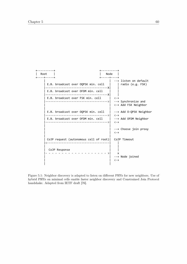
Chapter 5 60
1 2 +----------+ +----------+3 | Root | | Node |4 +----+-----+ +-----+----+5 | | --+ listen on default6 | E.B. broadcast over OQPSK min. cell | | radio (e.g. FSK)7 |--------------------------------------X| |8 | E.B. broadcast over OFDM min. cell | |9 |--------------------------------------X| |
10 | E.B. broadcast over FSK min. cell | <-+11 |-------------------------------------->| --+ Synchronize and12 | | <-+ Add FSK Neighbor13 | |14 | E.B. broadcast over OQPSK min. cell | --+ Add O-QPSK Neighbor15 |-------------------------------------->| <-+16 | E.B. broadcast over OFDM min. cell | --+ Add OFDM Neighbor17 |-------------------------------------->| <-+18 | |19 | | --+ Choose join proxy20 | | <-+21 | |22 | CoJP request (autonomous cell of root)| CoJP Timeout23 |<--------------------------------------| | 24 | | | 25 | CoJP Response | | 26 |- - - - - - - - - - - - - - - - - - - >| x 27 | | --+ Node joined28 | | <-+ 29 | | 30 31 32 33 Figure 5.1: Neighbor discovery is adapted to listen on different PHYs for new neighbors. Use of
hybrid PHYs on minimal cells enable faster neighbor discovery and Constrained Join Protocolhandshake. Adapted from IETF draft [76].
Chapter 5 61
Then node B starts the neighbor discovery as it begins scanning the medium onthe minimal cell of each PHY for more EBs from the neighboring PHYs. The use ofmultiple minimal cells allows the mote to discover available neighbors on each PHY. Inthis adaptation, PHYs of a neighboring mote are considered as different neighbors. Inclassical 6TiSCH, the minimal cells are used in either transmit or receive modes; that is,in case there are no packets queued for transmission, the mote goes to receive mode bydefault. Since g6TiSCH uses n times more PHYs than classical 6TiSCH, it also uses ntimes more minimal cells for neighbor discovery. This can cause it to consume, roughly,n times more power for broadcast cells. One way to mitigate this is as follows. In casethere are no packets queued for transmission, each cell goes to receive mode with a givenprobability; otherwise, the PHY remains powered off for energy saving. We use Prx = 1
n ,where Prx is the probability to go in receive mode. This allows the mote to balancethe energy spent in listening according to the number of used PHYs. For example,a network that uses three PHYs would consume approximately 200% more power inminimal cells than a single-PHY network if the radios were never switched off in any ofthese cells. So, in a configuration with three PHYs, we use Prx = 1
3 . Therefore, if thereare no packets queued for transmission, the radio will turn on for reception in all cellsapproximately 100% instead of 300% of the time compared to single-PHY network. Thisway, the multi-PHY network will remain approximately at the same power consumptionat minimal cells as the single-PHY network.
Node B starts the procedure to join the network according to the join protocol [76].The procedure selects the neighbor with the best join priority as proxy (the closer to theroot, the lower the energy cost of the join procedure). It then sends the join requeston the autonomous cell of the proxy (e.g. the root in this case). In this g6TiSCHamendment, FSK 868 MHz is used for communication on autonomous cells since itis the most robust PHY. When the request is authenticated and acknowledged by theroot, the join procedure is successful, and B can proceed with parent selection and cellnegotiation.
We note that security is an integral part of the 6TiSCH framework as defined inIEEE 802.15.4e (Section 7) [18] and the IETF 6TiSCH Minimal Security draft [76]. Allthe security features 6TiSCH carry over to g6TiSCH, including packet encryption andsecure join.
5.2.3 Generalized Parent Selection and Link Negotiation
The IETF RPL-related standards define mechanisms for neighbor evaluation and parentselection [32], [34]. In the IPv6 RPL routing layer of 6TiSCH, a node selects a parent moteby evaluating the expected path cost through each neighbor to the root and it chooses theparent with the least expected path cost. The cost of a single link is estimated based onthe expected transmission count (ETX) ratio as in (5.1), where: numTx is the numberof transmissions on the link and numAck is the number of acknowledgments received.This full path cost through neighbor i to the root is evaluated by the objective functionbased on (5.2) (as defined in the 6TiSCH minimal configuration [29]), where: Ranki isthe advertised rank of the neighbor, minHopIncrease is the minimal cost to use for a one
Chapter 5 62
hop link. For example, the root has a default rank of 256. If a mote has a link to the rootwith perfect ETX ratio of 1, the expected path cost is 512. After a parent is selected, therouting algorithm can later decide to change the parent to new neighbor i if the conditionin (5.3) evaluates to true. The factor P is the parent switch threshold so that the motedoes not change parent unless it expects significant improvement (i.e. hysteresis). Thisway, the network avoids too frequent parent changes, which would lead to instability.The recommended configuration for this threshold is 2×minHopIncrease, as proposedin the minimal 6TiSCH configuration [29].
ETXi =numTxi
numAcki(5.1)
Cost(Neighbori) = Ranki + ((3 · ETXi)− 2)×minHopIncrease. (5.2)
f(Parent,Neighbori) =
{true, if Cost(Parent)− Cost(Neighbori) ≥ P
false, otherwise(5.3)
In g6TiSCH, a combination of neighbor IPv6 address and a PHY link is consideredan independent neighbor. The use of multiple PHYs poses the need for a metric toevaluate and compare different PHYs. There can be different ways to build this metric;for example, based on power consumption, latency, or time-on-air. We use a simpleconfiguration for the routing layer that is sufficient to demonstrate the advantage of theg6TiSCH architecture.
Therefore, for the purposes of the experiment, we choose to evaluate the differentPHYs based on energy consumption in order to extend the battery lifetime as much aspossible. The objective function is adapted as in (5.4) to compute the link cost of acertain “neighbor” by giving weight to the expected energy per bit Ebit for the PHY ofthat neighbor. Therefore, in case neighboring links have similar ETX ratios, the motewould favor PHYs with lower Ebit for energy saving.
Cost(Neighbori) = Ranki + ((3 · ETXi)− 2)
×minHopIncrease× Factor(PHYi).(5.4)
To derive an ordering of the PHYs based on power consumption, we estimate theEbit for each PHY as a function of its power consumption for transmission and receptionand its bitrate. The function is expressed in (5.5), where Iitx and Iirx are the currentdraw for transmission and reception for PHYi, V i
s is the voltage supply for the radiochip of PHYi, and Ri
b is the bit rate. Table 5.1 shows the Ebit for each PHY. Therefore,the least power consuming PHY is OFDM 868 MHz, followed by O-QPSK 2.4 GHz andFSK 868 MHz. We assign Factor(OFDM) = 1, and Factor(OQPSK) = 2. However,we assign Factor(FSK) = 5 just to make the switch to an FSK 868 MHz PHY harderthan the switch to O-QPSK 2.4 GHz PHY, to account for its energy hungry footprint.Different configurations of the OF can be used to tune the performance depending on theapplication criteria, exercising different tradeoffs between datarate and range. Chapter 7
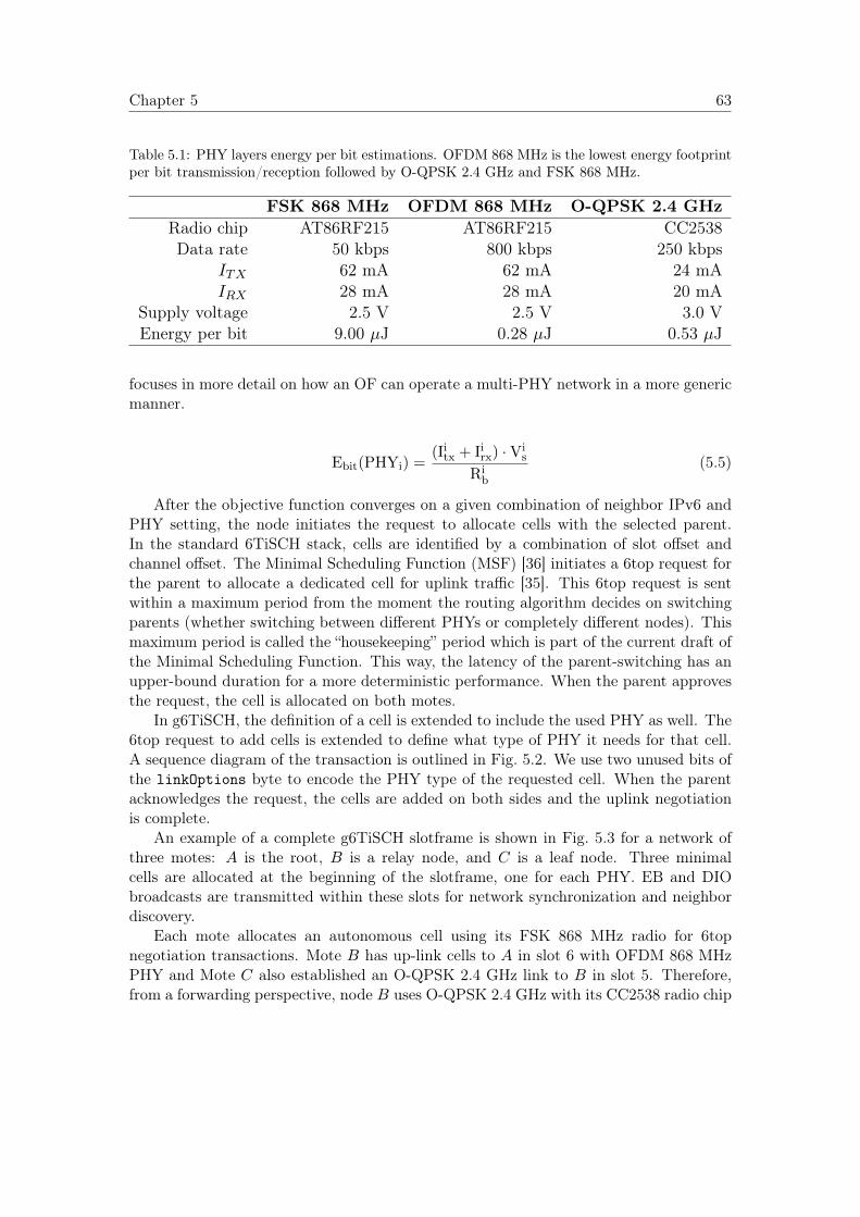
Chapter 5 63
Table 5.1: PHY layers energy per bit estimations. OFDM 868 MHz is the lowest energy footprintper bit transmission/reception followed by O-QPSK 2.4 GHz and FSK 868 MHz.
FSK 868 MHz OFDM 868 MHz O-QPSK 2.4 GHzRadio chip AT86RF215 AT86RF215 CC2538Data rate 50 kbps 800 kbps 250 kbps
ITX 62 mA 62 mA 24 mAIRX 28 mA 28 mA 20 mA
Supply voltage 2.5 V 2.5 V 3.0 VEnergy per bit 9.00 µJ 0.28 µJ 0.53 µJ
focuses in more detail on how an OF can operate a multi-PHY network in a more genericmanner.
Ebit(PHYi) =(Iitx + Iirx) ·Vi
s
Rib
(5.5)
After the objective function converges on a given combination of neighbor IPv6 andPHY setting, the node initiates the request to allocate cells with the selected parent.In the standard 6TiSCH stack, cells are identified by a combination of slot offset andchannel offset. The Minimal Scheduling Function (MSF) [36] initiates a 6top request forthe parent to allocate a dedicated cell for uplink traffic [35]. This 6top request is sentwithin a maximum period from the moment the routing algorithm decides on switchingparents (whether switching between different PHYs or completely different nodes). Thismaximum period is called the “housekeeping” period which is part of the current draft ofthe Minimal Scheduling Function. This way, the latency of the parent-switching has anupper-bound duration for a more deterministic performance. When the parent approvesthe request, the cell is allocated on both motes.
In g6TiSCH, the definition of a cell is extended to include the used PHY as well. The6top request to add cells is extended to define what type of PHY it needs for that cell.A sequence diagram of the transaction is outlined in Fig. 5.2. We use two unused bits ofthe linkOptions byte to encode the PHY type of the requested cell. When the parentacknowledges the request, the cells are added on both sides and the uplink negotiationis complete.
An example of a complete g6TiSCH slotframe is shown in Fig. 5.3 for a network ofthree motes: A is the root, B is a relay node, and C is a leaf node. Three minimalcells are allocated at the beginning of the slotframe, one for each PHY. EB and DIObroadcasts are transmitted within these slots for network synchronization and neighbordiscovery.
Each mote allocates an autonomous cell using its FSK 868 MHz radio for 6topnegotiation transactions. Mote B has up-link cells to A in slot 6 with OFDM 868 MHzPHY and Mote C also established an O-QPSK 2.4 GHz link to B in slot 5. Therefore,from a forwarding perspective, node B uses O-QPSK 2.4 GHz with its CC2538 radio chip
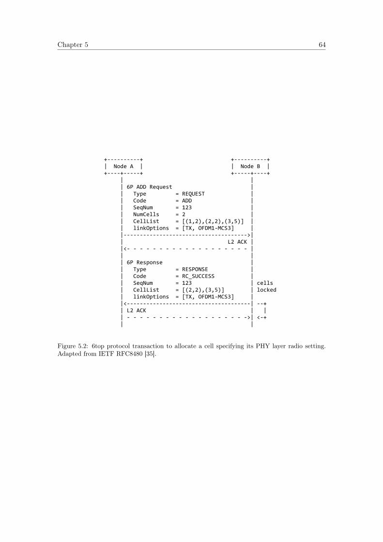
Chapter 5 64
1 2 +----------+ +----------+3 | Node A | | Node B |4 +----+-----+ +-----+----+5 | |6 | 6P ADD Request |7 | Type = REQUEST |8 | Code = ADD |9 | SeqNum = 123 |
10 | NumCells = 2 |11 | CellList = [(1,2),(2,2),(3,5)] |12 | linkOptions = [TX, OFDM1-MCS3] |13 |-------------------------------------->|14 | L2 ACK |15 |<- - - - - - - - - - - - - - - - - - - |16 | |17 | 6P Response |18 | Type = RESPONSE |19 | Code = RC_SUCCESS |20 | SeqNum = 123 | cells21 | CellList = [(2,2),(3,5)] | locked22 | linkOptions = [TX, OFDM1-MCS3] | 23 |<--------------------------------------| --+24 | L2 ACK | |25 | - - - - - - - - - - - - - - - - - - ->| <-+26 | |
Figure 5.2: 6top protocol transaction to allocate a cell specifying its PHY layer radio setting.Adapted from IETF RFC8480 [35].
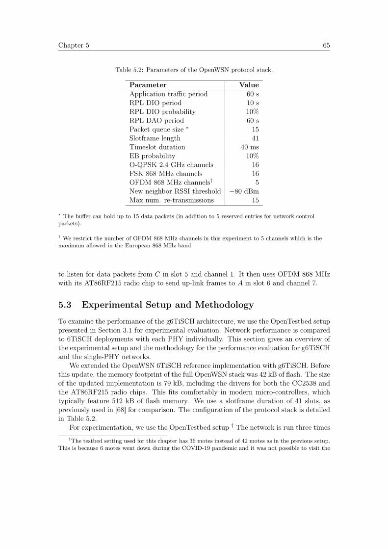
Chapter 5 65
Table 5.2: Parameters of the OpenWSN protocol stack.
Parameter ValueApplication traffic period 60 sRPL DIO period 10 sRPL DIO probability 10%RPL DAO period 60 sPacket queue size ∗ 15Slotframe length 41Timeslot duration 40 msEB probability 10%O-QPSK 2.4 GHz channels 16FSK 868 MHz channels 16OFDM 868 MHz channels† 5New neighbor RSSI threshold −80 dBmMax num. re-transmissions 15
∗ The buffer can hold up to 15 data packets (in addition to 5 reserved entries for network controlpackets).
† We restrict the number of OFDM 868 MHz channels in this experiment to 5 channels which is themaximum allowed in the European 868 MHz band.
to listen for data packets from C in slot 5 and channel 1. It then uses OFDM 868 MHzwith its AT86RF215 radio chip to send up-link frames to A in slot 6 and channel 7.
5.3 Experimental Setup and Methodology
To examine the performance of the g6TiSCH architecture, we use the OpenTestbed setuppresented in Section 3.1 for experimental evaluation. Network performance is comparedto 6TiSCH deployments with each PHY individually. This section gives an overview ofthe experimental setup and the methodology for the performance evaluation for g6TiSCHand the single-PHY networks.
We extended the OpenWSN 6TiSCH reference implementation with g6TiSCH. Beforethis update, the memory footprint of the full OpenWSN stack was 42 kB of flash. The sizeof the updated implementation is 79 kB, including the drivers for both the CC2538 andthe AT86RF215 radio chips. This fits comfortably in modern micro-controllers, whichtypically feature 512 kB of flash memory. We use a slotframe duration of 41 slots, aspreviously used in [68] for comparison. The configuration of the protocol stack is detailedin Table 5.2.
For experimentation, we use the OpenTestbed setup † The network is run three times†The testbed setting used for this chapter has 36 motes instead of 42 motes as in the previous setup.
This is because 6 motes went down during the COVID-19 pandemic and it was not possible to visit the
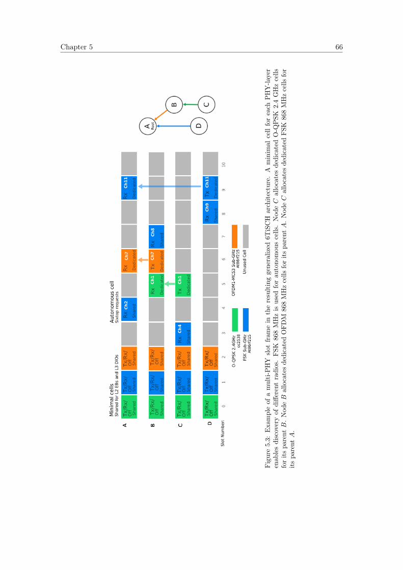
Chapter 5 66
Figure5.3:
Exa
mpleof
amulti-P
HY
slot
fram
ein
theresultinggeneralized
6TiSCH
architecture.A
minim
alcellforeach
PHY-la
yer
enab
lesdiscoveryof
diffe
rent
radios.FSK
868MHzis
used
forau
tono
mou
scells.Nod
eC
allocatesdedicatedO-Q
PSK
2.4GHzcells
foritspa
rentB.Nod
eB
allocatesdedicatedOFDM
868MHzcells
foritspa
rentA.Nod
eC
allocatesdedicatedFSK
868MHzcells
for
itspa
rentA.
Chapter 5 67
with each PHY individually. For short, the single PHY networks will be referred to bytheir PHY names hereafter (i.e. O-QPSK 2.4 GHz, FSK 868 MHz, and OFDM 868 MHz).It is then run a fourth time with the generalized multi-PHY architecture. This is todemonstrate that the generalized architecture is capable of providing a more balancedperformance than each PHY individually. For each experiment, a mote placed in themiddle of the floor is set as the DAG root (see Fig. 3.1) and the network is run for90 min.
The following measurements are captured and sent every 60 s from each mote:
• a counter, that is used to detect loss of data packets.
• the time at which the data packet was created (expressed as ASN),
• the DAG rank of the sender,
• Ton: how long the sender’s radio has been on since the previous data packettransmission,
• TTX : how long the sender’s radio has been on and transmitting since the previousdata packet transmission,
• TFSKon , TOFDM
on , and TOQPSKon : the breakdown of Ton for each PHY ,
• TFSKTX , TOFDM
TX , and TOQPSKTX : the breakdown of TTX for each PHY,
• Ttotal: the amount of time since the previous data packet transmission,
• the maximum and minimum number of packets in the packet buffer since theprevious packet.
As previously described, we use the logged data to compute Network Formation Time,End-to-End Reliability, End-to-End latency, and Network lifetime.
We are aware that end-to-end latency for OFDM 868 MHz and O-QPSK 2.4 GHz canbe improved by using smaller slot durations (instead of the 40 ms timeslot). However,to maintain consistency across experiments, we choose to change one parameter only,the network PHY, in order to measure its impact on end-to-end KPIs. Therefore, wefix the slot-duration at 40 ms for all networks in order to isolate any possible effects ofsmaller slot durations (such as increased duty cycle). This way, we can ensure that ourobservations are strictly due to change of PHYs. We are also aware that use of differentslot durations in the same slotframe for g6TiSCH can improve latency performance.However, we are interested in demonstrating the baseline performance of g6TiSCH inthis study. Furthermore, we address this in a separate study in Chapter 6 since ittouches on a separate research context of “Schedule Compactness” in TSCH networks.
We display the results in Time Series form and CDF form (as introduced inSection 3.1.2.
center physically to resolve the problem due to confinement conditions.
Chapter 5 68
5.4 Experimental Results
This section details the findings from the experimental campaigns. We show theperformance of the networks in terms of: Network formation time (Section 5.4.1),end-to-end latency (Section 5.4.2), end-to-end reliability (Section 5.4.3), and batterylifetime (Section 5.4.4).
5.4.1 Network Formation
Network formation time is influenced by the duration of a full join process, which includesthe time a mote needs to synchronize to the network, establish a secure join hand-shake,and successfully negotiate a link to a parent (as outlined in Sections 5.2.2 and 5.2.3). Asin the previous chapter, we assume a worst-case scenario as all motes are flashed at onceand begin the network join procedure at the same time. This increases contention sinceneighbor discovery and link negotiations occur on shared cells. So this helps us observethe behavior of the network under stress.
We plot in Fig. 5.4 the cumulative density of the time-to-first-data-packet fromeach of the 36 motes in the network. For 90% of the motes, network formationtime is 5, 5, 7, and 18 min for g6TiSCH, FSK 868 MHz, O-QPSK 2.4 GHz, andOFDM 868 MHz, respectively. Among the single PHY networks, the OFDM 868 MHznetwork is the slowest to form. This is because the low number of available channels(5) for OFDM 868 MHz Option 1 increases the probability of collision in shared cells,slowing down neighbor discovery. The g6TiSCH formation time is in the same orderof magnitude as FSK 868 MHz and O-QPSK 2.4 GHz networks in spite of the largernumber of available links. This is because the g6TiSCH network dynamically improvesits selected PHYs, its formation time remains within the same efficiency.
This can be observed in Fig. 5.5, which shows the number of PHYs selected for routingas the g6TiSCH network is forming. The multi-PHY neighbor discovery enables thenetwork to combine the advantages of each PHY. On minimal cells of long-range PHYssuch as FSK 868 MHz, a mote can hear a larger portion of the network with an increasedrisk of contention. On minimal cells of short-range PHYs such as O-QPSK 2.4 GHz, amote can hear a smaller portion of the network with less risk of contention. Therefore,this leads to an overall robust network formation.
5.4.2 End-to-end Latency
We show in Fig. 5.6 a time-domain plot of the end-to-end latency in the network. Thecumulative density of all the packets, during the steady state phase, is shown in Fig. 5.7.The longer range of OFDM 868 MHz and FSK 868 MHz (due to the sub-GHz band)leads to lower latency because of decreased re-transmissions and decreased number ofhops. This is because motes are able to reach closer to the root thanks to the low ETX.
The g6TiSCH architecture exhibits a lower latency than each single-PHY network,although the best PHY for up-link is selected with respect to power consumption.Interestingly, it even demonstrates better latency than both the OFDM 868 MHz and
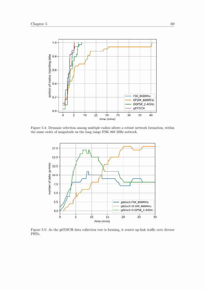
Chapter 5 69
Figure 5.4: Dynamic selection among multiple radios allows a robust network formation, withinthe same order of magnitude as the long range FSK 868 MHz network.
Figure 5.5: As the g6TiSCH data collection tree is forming, it routes up-link traffic over diversePHYs.
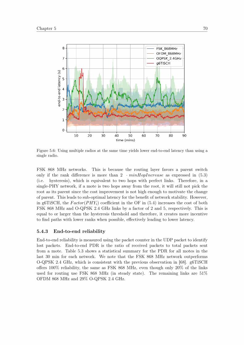
Chapter 5 70
Figure 5.6: Using multiple radios at the same time yields lower end-to-end latency than using asingle radio.
FSK 868 MHz networks. This is because the routing layer favors a parent switchonly if the rank difference is more than 2 · minHopIncrease as expressed in (5.3)(i.e. hysteresis), which is equivalent to two hops with perfect links. Therefore, in asingle-PHY network, if a mote is two hops away from the root, it will still not pick theroot as its parent since the cost improvement is not high enough to motivate the changeof parent. This leads to sub-optimal latency for the benefit of network stability. However,in g6TiSCH, the Factor(PHYi) coefficient in the OF in (5.4) increases the cost of bothFSK 868 MHz and O-QPSK 2.4 GHz links by a factor of 2 and 5, respectively. This isequal to or larger than the hysteresis threshold and therefore, it creates more incentiveto find paths with lower ranks when possible, effectively leading to lower latency.
5.4.3 End-to-end reliability
End-to-end reliability is measured using the packet counter in the UDP packet to identifylost packets. End-to-end PDR is the ratio of received packets to total packets sentfrom a mote. Table 5.3 shows a statistical summary for the PDR for all motes in thelast 30 min for each network. We note that the FSK 868 MHz network outperformsO-QPSK 2.4 GHz, which is consistent with the previous observation in [68]. g6TiSCHoffers 100% reliability, the same as FSK 868 MHz, even though only 20% of the linksused for routing use FSK 868 MHz (in steady state). The remaining links are 51%OFDM 868 MHz and 29% O-QPSK 2.4 GHz.
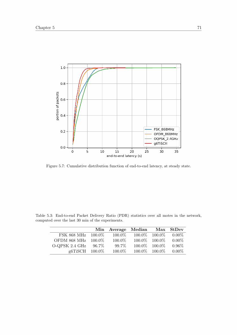
Chapter 5 71
Figure 5.7: Cumulative distribution function of end-to-end latency, at steady state.
Table 5.3: End-to-end Packet Delivery Ratio (PDR) statistics over all motes in the network,computed over the last 30 min of the experiments.
Min Average Median Max StDevFSK 868 MHz 100.0% 100.0% 100.0% 100.0% 0.00%
OFDM 868 MHz 100.0% 100.0% 100.0% 100.0% 0.00%O-QPSK 2.4 GHz 96.7% 99.7% 100.0% 100.0% 0.96%
g6TiSCH 100.0% 100.0% 100.0% 100.0% 0.00%
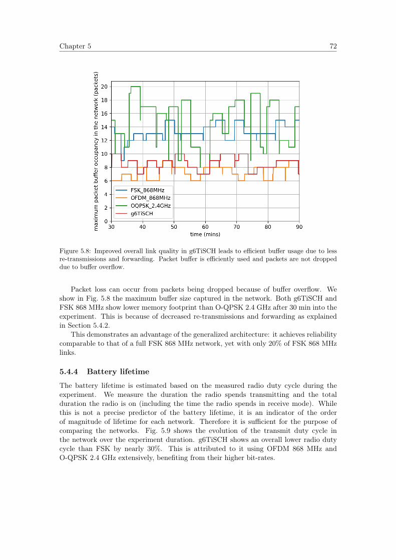
Chapter 5 72
Figure 5.8: Improved overall link quality in g6TiSCH leads to efficient buffer usage due to lessre-transmissions and forwarding. Packet buffer is efficiently used and packets are not droppeddue to buffer overflow.
Packet loss can occur from packets being dropped because of buffer overflow. Weshow in Fig. 5.8 the maximum buffer size captured in the network. Both g6TiSCH andFSK 868 MHz show lower memory footprint than O-QPSK 2.4 GHz after 30 min into theexperiment. This is because of decreased re-transmissions and forwarding as explainedin Section 5.4.2.
This demonstrates an advantage of the generalized architecture: it achieves reliabilitycomparable to that of a full FSK 868 MHz network, yet with only 20% of FSK 868 MHzlinks.
5.4.4 Battery lifetime
The battery lifetime is estimated based on the measured radio duty cycle during theexperiment. We measure the duration the radio spends transmitting and the totalduration the radio is on (including the time the radio spends in receive mode). Whilethis is not a precise predictor of the battery lifetime, it is an indicator of the orderof magnitude of lifetime for each network. Therefore it is sufficient for the purpose ofcomparing the networks. Fig. 5.9 shows the evolution of the transmit duty cycle inthe network over the experiment duration. g6TiSCH shows an overall lower radio dutycycle than FSK by nearly 30%. This is attributed to it using OFDM 868 MHz andO-QPSK 2.4 GHz extensively, benefiting from their higher bit-rates.
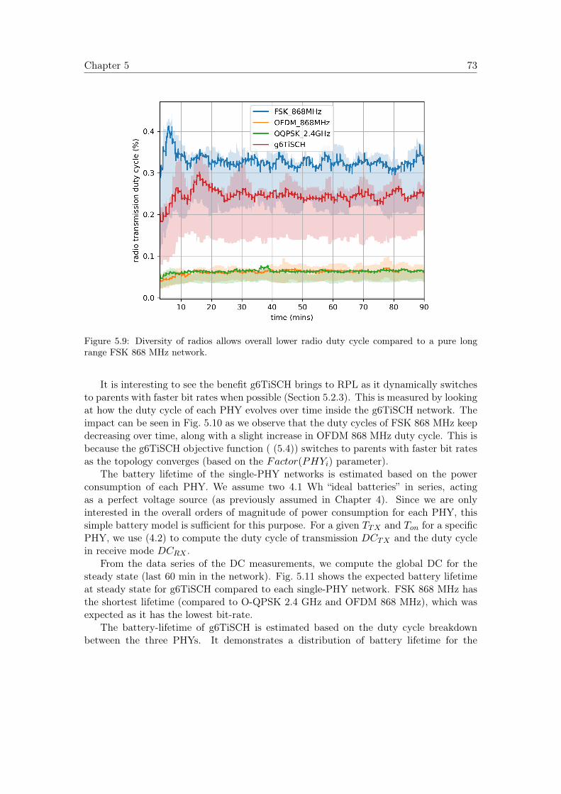
Chapter 5 73
Figure 5.9: Diversity of radios allows overall lower radio duty cycle compared to a pure longrange FSK 868 MHz network.
It is interesting to see the benefit g6TiSCH brings to RPL as it dynamically switchesto parents with faster bit rates when possible (Section 5.2.3). This is measured by lookingat how the duty cycle of each PHY evolves over time inside the g6TiSCH network. Theimpact can be seen in Fig. 5.10 as we observe that the duty cycles of FSK 868 MHz keepdecreasing over time, along with a slight increase in OFDM 868 MHz duty cycle. This isbecause the g6TiSCH objective function ( (5.4)) switches to parents with faster bit ratesas the topology converges (based on the Factor(PHYi) parameter).
The battery lifetime of the single-PHY networks is estimated based on the powerconsumption of each PHY. We assume two 4.1 Wh “ideal batteries” in series, actingas a perfect voltage source (as previously assumed in Chapter 4). Since we are onlyinterested in the overall orders of magnitude of power consumption for each PHY, thissimple battery model is sufficient for this purpose. For a given TTX and Ton for a specificPHY, we use (4.2) to compute the duty cycle of transmission DCTX and the duty cyclein receive mode DCRX .
From the data series of the DC measurements, we compute the global DC for thesteady state (last 60 min in the network). Fig. 5.11 shows the expected battery lifetimeat steady state for g6TiSCH compared to each single-PHY network. FSK 868 MHz hasthe shortest lifetime (compared to O-QPSK 2.4 GHz and OFDM 868 MHz), which wasexpected as it has the lowest bit-rate.
The battery-lifetime of g6TiSCH is estimated based on the duty cycle breakdownbetween the three PHYs. It demonstrates a distribution of battery lifetime for the
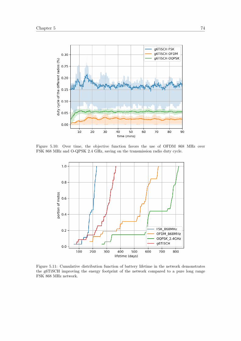
Chapter 5 74
Figure 5.10: Over time, the objective function favors the use of OFDM 868 MHz overFSK 868 MHz and O-QPSK 2.4 GHz, saving on the transmission radio duty cycle.
Figure 5.11: Cumulative distribution function of battery lifetime in the network demonstratesthe g6TiSCH improving the energy footprint of the network compared to a pure long rangeFSK 868 MHz network.
Chapter 5 75
nodes with a median that is 100 day higher than the FSK 868 MHz network thanksto the overall lower duty cycle. However, it has on overall the same network lifetime asFSK 868 MHz (i.e. time to first battery depletion). Therefore, there is an interestingroom for improvement on this aspect by exploring a routing algorithm to optimize fornetwork lifetime (which is a key focus of Chapter 7).
5.5 Conclusions
This chapter presents g6TiSCH, a generalized 6TiSCH architecture for multi-PHYwireless networking. g6TiSCH adds agility to the protocol stack: nodes can use diversephysical layers within the same network and adapt their links depending on theirconditions, while maintaining wire-like reliability.
To introduce this agility, we augment the 6TiSCH protocol stack in different ways.At the MAC layer, we add the physical layer to use for each timeslot. At the 6LoWPANadaptation layer, we demonstrate a generalized neighbor discovery mechanism wheremotes discover the network over different PHYs. At the RPL layer, we adapt the routingobjective function with weighted link costs.
The resulting architecture is evaluated experimentally on the OpenTestbed to provethe soundness of the approach on a real-life scenario. We extract KPIs important forindustrial applications. Experiments with g6TiSCH show fastest network formation,lowest latency, wire-like end-to-end reliability, and improved energy footprint comparedto a pure long-range network. Furthermore, our proposed objective function for IPv6RPL successfully steers the network topology, over time, towards energy efficiency. Thisis achieved by dynamically switching to faster bit-rates when possible, while maintaininglatency and reliability performance.
While the quantitative results are specific to this experiment, the key findings hold.First, g6TiSCH provides more controls that help achieving a more balanced performancethan single-PHY networks. Second, by combining long-range and short-range radios,g6TiSCH yields lower latency and network formation time than any of the individualPHYs, while maintaining a similar battery lifetime. Third, the routing layer in g6TiSCHimproves the network’s energy footprint over time by selecting faster links for routing.This balances performance and energy consumption of the network for deployments wherethere are both long and short distances between nodes. This provides an incentiveto exploit the characteristics specific to each PHY and drive the network to build uptrade-offs between energy consumption and performance in diverse use cases instead ofhaving to choose one PHY over the other ones.
Chapter 6 introduces extending g6TiSCH with the use of slots with variable durationin the same slot frame in order to further lower latency. This way, a faster PHY can usea slot with smaller duration. This enables the network to have more compact schedulewith both long and short duration slots. Furthermore, Chapter 7 explores, using RPLsimulations, how to improve the battery lifetime of the network using multi-PHY routing.The RPL objective function relies on different metrics to improve the battery lifetime.
Chapter 6
Heterogeneous Slot Frames in6TiSCH
Parts of this chapter were published as part of the following article: 6DYN: 6TiSCHwith Heterogeneous Slot Durations. Mina Rady, Quentin Lampin, Dominique Barthel,Thomas Watteyne. MDPI Sensors, special issue on Dependable IoT Networking vol.21, no. 5, p. 1611, February 2021.
Key Takeaways: In the previous chapters, we demonstrated that new radiochips implement different physical layers, allowing firmware to change modulation,datarate and frequency dynamically. This technological development is anopportunity for industrial low-power wireless networks to offer even higherdeterminism, including latency predictability. This chapter introduces 6DYN,an extension to the IETF 6TiSCH standards-based protocol stack. In a 6DYNnetwork, nodes switch physical layer dynamically on a link-by-link basis, in orderto exploit the diversity offered by this new technology agility. To offer low latencyand high network capacity, 6DYN uses heterogeneous slot durations: the length ofa slot in the 6TiSCH schedule depends on the physical layer used. This chaptershows how reserved bits in 6TiSCH headers can be used to standardize 6DYN anddetails its implementation in OpenWSN, a reference implementation of 6TiSCH.
In Chapter 5 we introduced a generalization of the 6TiSCH protocol for agilemulti-PHY networking but using a slot-frame with the same slot duration. This chaptergoes a step further by introducing 6DYN, a g6TiSCH extension in which a nodedynamically changes its PHY and the slot duration at each time slot, depending onthe bitrate of the used PHY.
Since 6TiSCH was designed on a fixed PHY, in today’s 6TiSCH standard, all slots areof the same duration. The slot duration is tuned so there is time to transmit the longestsupported frame and receive an acknowledgment. When using the IEEE802.15.4 2.4 GHz
76
Chapter 6 77
PHY at 250 kbps, a slot is typically 10 ms long. When using multiple PHYs, we can havetwo approaches. The first is to settle for using the longest slot duration among all PHYs.This is the approach we previously took in Chapter 5. While this makes schedulingsimple, it makes most slots artificially long, wasting latency and network capacity. Amore complete approach is to vary the slot duration on a slot-by-slot basis, based on thePHY used. This is the approach 6DYN uses.
This chapter answers the following questions:
• How can we build a g6TiSCH schedule with different slot durations?
• What are the minimal changes we need to make to the 6TiSCH standard to achievethis network agility?
• What are the benefits of 6DYN over using the longest duration?
The remainder of this chapter is organized as follows. Section 6.1 states the problemand lists this chapter’s contributions. Section 6.2 presents the design of 6DYN, includingslot duration management, neighbor discovery and timeslot allocation. Section 6.3 liststhe two small changes needed to the 6TiSCH standard to support 6DYN. Section 6.4describes our implementation of 6DYN in OpenWSN, the reference implementation of6TiSCH. Finally, Section 4.5 concludes this chapter.
6.1 Problem Statement and Contributions
In their IETF problem statement, Muñoz et al.discuss the challenges of integratingheterogeneous PHYs in 6TiSCH [72], including multi-PHY discovery of neighbors androuting.
6DYN is one answer to those challenges, with a particular focus on schedulecompactness. In a 6TiSCH network today, a communication opportunity betweenneighbor nodes is identified by a timeslot and a channel offset. 6DYN adds one dimensionto this, the PHY, as illustrated in Fig. 6.1. The result is that, when neighbor nodescommunicate, they previously agree on the frequency band, modulation and bit-ratethat make their communication most efficient.
The contribution of this chapter is three-fold:
1. 6DYN, a TSCH approach in which nodes use multiple PHYs in an efficient mannerby managing a communication schedule with multiple slot durations
2. A draft standardization of 6DYN by crafting it as an extension of 6TiSCH
3. An implementation of 6DYN in OpenWSN, a reference open-source implementationof 6TiSCH
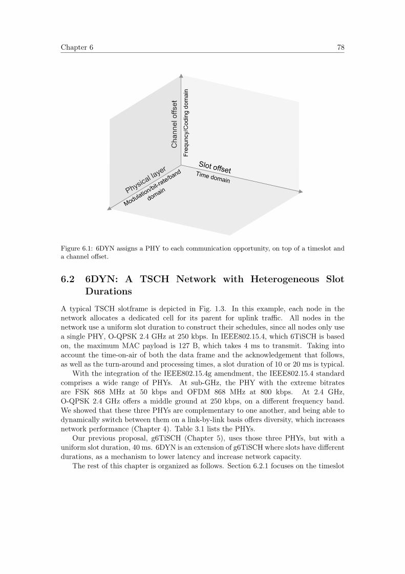
Chapter 6 78
Figure 6.1: 6DYN assigns a PHY to each communication opportunity, on top of a timeslot anda channel offset.
6.2 6DYN: A TSCH Network with Heterogeneous SlotDurations
A typical TSCH slotframe is depicted in Fig. 1.3. In this example, each node in thenetwork allocates a dedicated cell for its parent for uplink traffic. All nodes in thenetwork use a uniform slot duration to construct their schedules, since all nodes only usea single PHY, O-QPSK 2.4 GHz at 250 kbps. In IEEE802.15.4, which 6TiSCH is basedon, the maximum MAC payload is 127 B, which takes 4 ms to transmit. Taking intoaccount the time-on-air of both the data frame and the acknowledgement that follows,as well as the turn-around and processing times, a slot duration of 10 or 20 ms is typical.
With the integration of the IEEE802.15.4g amendment, the IEEE802.15.4 standardcomprises a wide range of PHYs. At sub-GHz, the PHY with the extreme bitratesare FSK 868 MHz at 50 kbps and OFDM 868 MHz at 800 kbps. At 2.4 GHz,O-QPSK 2.4 GHz offers a middle ground at 250 kbps, on a different frequency band.We showed that these three PHYs are complementary to one another, and being able todynamically switch between them on a link-by-link basis offers diversity, which increasesnetwork performance (Chapter 4). Table 3.1 lists the PHYs.
Our previous proposal, g6TiSCH (Chapter 5), uses those three PHYs, but with auniform slot duration, 40 ms. 6DYN is an extension of g6TiSCH where slots have differentdurations, as a mechanism to lower latency and increase network capacity.
The rest of this chapter is organized as follows. Section 6.2.1 focuses on the timeslot
Chapter 6 79
templates for each PHY. Section 6.2.2 describes how slots with different durations canbe combined in a single schedule. Section 6.2.3 details how neighbor nodes discover oneanother, on each PHY. Section 6.2.4 details how cells of different durations are allocated.
6.2.1 Timeslot Templates
To support each PHY in the same schedule, we first need to design their timeslottemplates in accordance with IEEE 802.15.4e standard. We refer to the templatesdesigned in Section 4.3. A full list of the factors that are considered in the design ofa time-slot template is presented in Table 4.1. Fig. 4.1 is a capture of the logic analyzer,showing when the motes exchange a 127 B data frame (the maximum length), exchangean acknowledgment frame and communicate over SPI. As much as possible, we condensethe activity at the beginning of the slot, in order to terminate the sequence as soon aspossible within a slot.
We note that the FSK 868 MHz and OFDM 868 MHz PHYs require time for SPItransactions between the radio chip (AT86RF215) and the micro-controller (CC2538).For O-QPSK 2.4 GHz, the radio front-end is part of the CC2538 in a system-on-chipdesign. Fig. 4.1 shows that OFDM 868 MHz, O-QPSK 2.4 GHz and FSK 868 MHztransactions are over in roughly 10, 20 and 40 ms, respectively. We choose these “round”numbers because they make the slot lengths multiples of one another, significantlysimplifying scheduling, as demonstrated in the following section.
6.2.2 Heterogeneous Slot Durations
How then can the different slot durations be integrated in the same slotframe? Theapproach by Brachmann et al. [59], inspired by IEEE802.11 WiFi networks, is to use theslowest bit rate PHY with a specific slot duration for control packets, and the highestbitrate PHY for data packets and grouping multiple slots for it. While this approachimproves schedule compactness, it does not give the node the flexibility to use lowerbit-rates for data transmissions in case the quality is poor.
Another approach in g6TiSCH is to use a uniform slot duration based on the slowestPHY (40 ms) as presented in Chapter 5, while allowing the node to switch between thethree PHYs for data packet depending on link quality. This gives the mote flexibility totune its performance by switching to faster bit-rates when possible or to slower bit-rateswhen necessary. It is also easier to manage the schedule using the existing schedulingpolicies that are designed to manage slots with a uniform slot duration. This doeslead to schedule compactness and capacity problems: in each OFDM 868 MHz andO-QPSK 2.4 GHz slot, the mote wastes 30 or 20 ms, respectively.
We extend the approach of g6TiSCH by allowing for slots of different durations. Weset the slot duration to that of the fastest PHY, 10 ms, and group consecutive slotswhen using slower PHYs, resulting in some longer “virtual” slots. Given the durationslisted in Section 6.2.1, an O-QPSK 2.4 GHz slot occupies two consecutive slots, whilean FSK 868 MHz slot occupies four consecutive slots. We use this approach for anydedicated cell that is dynamically negotiated between neighbors and use the slowest
Chapter 6 80
bit-rate (FSK 868 MHz) for autonomous cells. Autonomous cells are used to “bootstrap”the negotiation.
Fig. 6.2 depicts the resulting heterogeneous slotframe for a multi-hop network ofthree motes and one root. On top of the 16 frequencies for O-QPSK 2.4 GHz, thisschedule also includes 16 FSK 868 MHz frequencies with 200 kHz channel spacing and5 OFDM 868 MHz frequencies with 1.2 MHz channel spacing. We use a slotframe lengthof 163 timeslots, resulting in a duration of 1.63 s, comparable to the 1.64 s used ing6TiSCH. A separate minimal cell is allocated at the beginning of the slotframe for eachof the PHYs, for network-wide communication. Autonomous cells are allocated using thelongest range FSK 868 MHz PHY.
6.2.3 Neighbor Discovery
Given that 6TiSCH is a multi-hop mesh network, nodes need to discover one another,on different PHYs. Among other things, this allows each node to pick the most suitableneighbor and the most suitable PHY, for up-link communication. In traditional 6TiSCH,all nodes that are part of a network send enhanced beacons on the schedule’s minimalcell at a slow rate. By listening on that cell when not sending, a node eventually buildsup a list of all the other nodes it can hear, i.e. its neighbors.
We adapt this discovery mechanism to multi-PHY discovery by having three distinctminimal cells, one for each PHY. Fig. 6.2 shows these cells. Since 6DYN is based ong6TiSCH, it follows the same generalized neighbor discovery mechanism introduced inSection 5.2.2 If a node has not joined the network yet, it listens for beacons using itsFSK 868 MHz radio. After it hears an enhanced beacon, the node synchronizes to thenetwork and continues listening for enhanced beacons only on the minimal cell. A mote’sneighbor table contains one row per tuple (MAC address, PHY). This allows keeping theupper layers unchanged, notably the routing layer.
6.2.4 Timeslot Allocation
In a distributed network, neighbor nodes negotiate with one another to add/deletededicated cells in their schedule to communicate. This mechanism is augmented tosupport multi-PHY operation: schedule a single cell to add an OFDM 868 MHz cell,schedule two consecutive cells to add an O-QPSK 2.4 GHz cell and schedule fourconsecutive cells to add an FSK 868 MHz cell. The node issuing the transaction proposesgroups of contiguous cells that are unused in its schedule; the other node selects a groupit is not using itself.
6.3 Extending 6TiSCH with 6DYN
As a path towards standardization, this section details how the 6TiSCH standard can beamended to support 6DYN. The goal is to make only small adjustments to the standard tosimplify implementation and favor adoption. Implementing 6DYN does not require moreadjustments to the frame formats other than what was already proposed for g6TiSCH
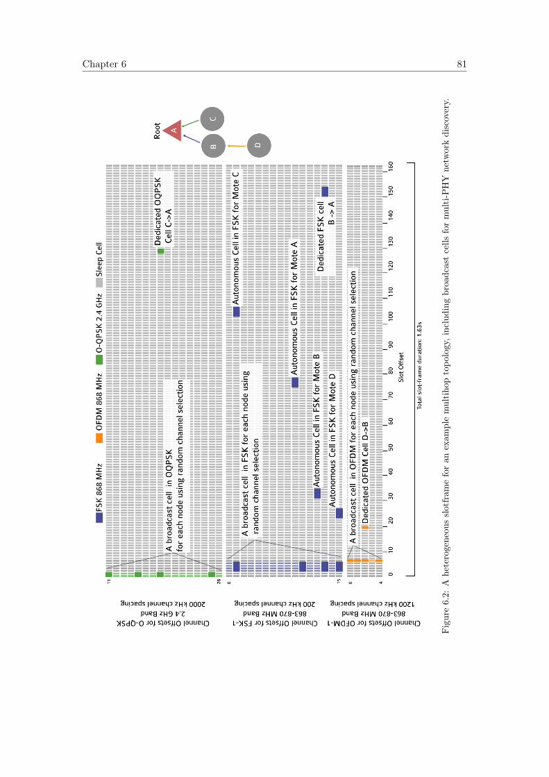
Chapter 6 81
Figure6.2:
Aheterogeneou
sslotfram
eforan
exam
plemultiho
ptopo
logy,including
broadcastcells
formulti-P
HY
netw
orkdiscovery.
Chapter 6 82
outlined in Section 5.2. However, the cell reservation algorithm is adapted to detectpartial conflicts between cells that consist of slot groups as detailed in Section6.4
The first change is to encode the PHYs used in the network in the Enhanced Beacon(EB) [29]. Per the IEEE802.15.4 standard, the EB encodes the slot offsets of each minimalcell in the TSCH slot frame, and Link Information Elements [29]. In the Link InformationElements for each minimal cell, we use the left-most 3 bits of the Link Options byte toencode the type of PHY associated with each minimal cell. These bits are currently“reserved for future use” in the IEEE802.15.4 standard. This allows a mote that hears anEB during the joining process to bootstrap its schedule correctly. This mechanism furtherallows a network to use only a subset of the PHYs listed in Table 3.1. The remaining stepsof the secure joining procedure of a node is carried out by the Constrained Join Protocol(CoJP) [76] and is unmodified. The resulting join process is illustrated in Fig. 5.1.
6P is used by neighbor nodes to negotiate when adding/deleting cells with oneanother [35]. The second change is to extend 6P for an ADD request to indicate whichPHY to use. We use the left-most 3 bits of the Cell Options byte in the 6P header toencode the PHY index of the requested cells. These bits are currently “reserved for futureuse” in the 6P standard. The resulting 6P ADD transaction is illustrated in Fig. 5.2.
These two changes, while requiring a rigorous definition through an official standard,remain small changes to the standard. The remaining of the 6TiSCH standardremains unmodified.
6.4 Implementing 6DYN in OpenWSN
We extend OpenWSN, the 6TiSCH reference open-source implementation, with 6DYN.We demonstrate the running stack in the local hardware setup detailed in Section 3.2,including the debugging infrastructure. Section 6.4.1 highlights the key elements in theimplementation of 6DYN. Section 6.4.2 shows 6DYN running on the OpenMote B board.
6.4.1 Implementing 6DYN
We implemented 6DYN in OpenWSN∗, following the architecture indicated in Section 6.2and the frame defined in Section 6.3. The implementation extends the openradiointerface introduced in Section 5.2.1, by allowing variable slot durations for aslot-template. While the implementation is relatively straightforward, we believe thefollowing details to be particularly important.
In our implementation, we encode the communication schedule as a circular linkedlist of cells, in increasing slot offset order. We only use a single entry in that linkedlist to represent a cell, regardless of the PHY used. This means that an FSK 868 MHztimeslot, which spans 40 ms (i.e. four cells), occupies the same memory footprint as a10 ms OFDM 868 MHz timeslot. The fact that timeslots are ordered in a circular linked
∗ As an online addition to this chapter, all of the source code used is available at https://github.com/openwsn-berkeley/
Chapter 6 83
list allows the implementation to iterate to the next slot without a time-consuming searchoperation.
The default implementation of MSF in OpenWSN allocates multiple entries inthe same timeslot (i.e. backup slots). This is done so that, if there are no packetsassociated with this timeslot, the MAC layer executes a lower-priority slot entry [36],[77]. This implementation does not carry over directly to 6DYN, as slots can be partiallyoverlapping. In our implementation, backup slots are allowed only for slots of the samesize.
The flash memory footprint of g6TiSCH without the 6DYN extension is 79 kB.Implementing 6DYN increases that footprint to 84 kB, still very far from filling up the512 kB of flash memory available on the OpenMote B.
6.4.2 Running 6DYN
To “witness” the execution of 6DYN, we use OpenMote B boards to form a link betweentwo motes and a multi-hop network of four motes. On top of the 6DYN-enabled 6TiSCHprotocol stack, on each mote, we run an application which periodically reports anincrementing counter (used to compute end-to-end reliability) and the radio duty cycleof each PHYs.
Fig. 6.3 shows the resulting real-time capture of MAC-layer events on both nodes(left) during a ping session from the root to the node (right) using 6DYN.
Fig. 6.4 shows the annotated activity of both nodes. Slot are 10 ms long, the slotframeis 163 slots long. On the left, per the neighbor discovery detailed in Section 6.3, we seethe three minimal cells: a 20 ms O-QPSK 2.4 GHz cell, a 40 ms FSK 868 MHz celland a 10 ms OFDM 868 MHz cell. Fig. 6.4 shows a dedicated cell using FSK 868 MHz,which the nodes negotiated using 6P, as detailed in Section 6.3. Finally, we see each nodeswitching on its radio during its autonomous cell; each node listens for a short periodand turns off its radio as no frame is received.
Fig. 6.5 shows the activity of four motes implementing 6DYN and forming a multi-hopnetwork. It shows how different pairs of nodes establish different links (D→B, B→A andC→A), incidentally each using a different PHY.
6.5 Conclusions
New radio chips implement multiple PHY layers, offering different trade-offs betweenrange, data rate and power consumption. Because a low-power wireless network iscomposed of many links, each with different characteristics, being able to dynamicallychange between PHYs on a link-by-link basis yields higher network performance thanlocking the entire network to a single PHY. Recent proposals, such as a g6TiSCH(Chapter 5), propose a networking approach which allows for this technology agility,in a time slotted and scheduled manner. They do so, however, by aligning the durationof a timeslot to the slowest PHY layer. While this simplifies the implementation, the
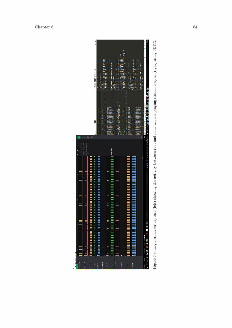
Chapter 6 84
Figure6.3:
LogicAna
lyzercapture(left)
show
ingtheactivity
betw
eenroot
andno
dewhile
aping
ingsessionisop
en(right)using6D
YN.
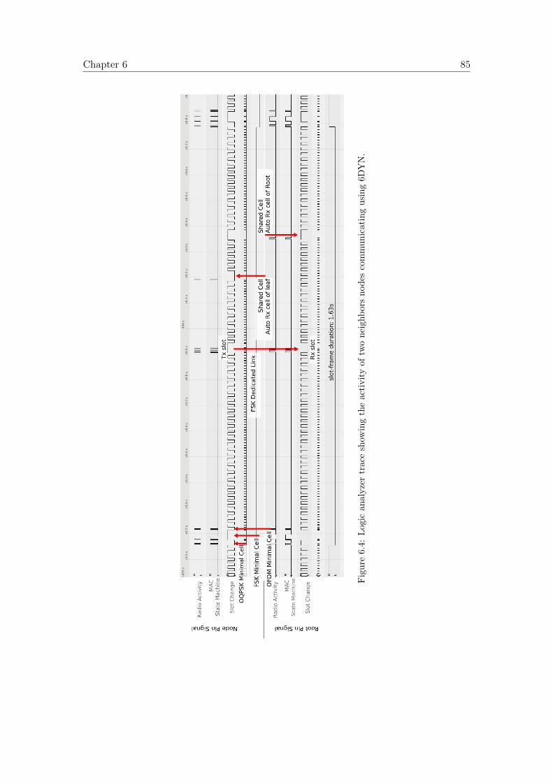
Chapter 6 85
Figure6.4:
Logican
alyzer
traceshow
ingtheactivity
oftw
oneighb
orsno
descommun
icatingusing6D
YN.
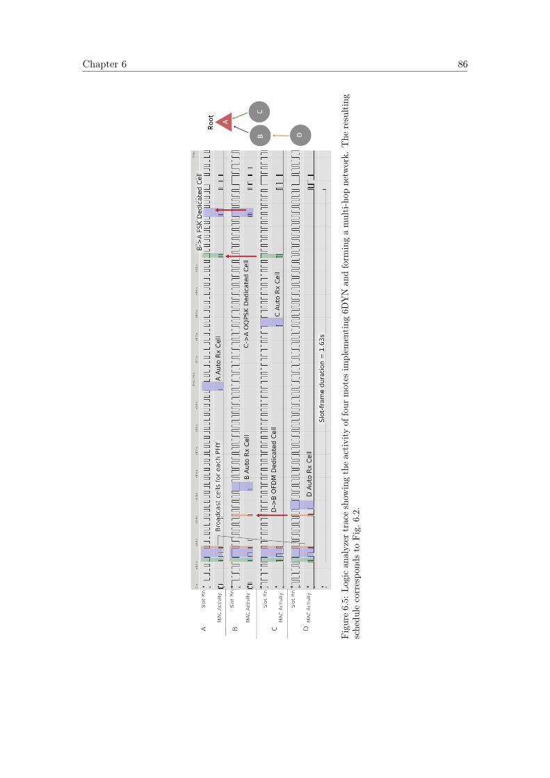
Chapter 6 86
Figure6.5:
Logican
alyzer
traceshow
ingtheactivity
offour
motes
implem
enting
6DYN
andform
ingamulti-hop
netw
ork.
The
resulting
schedu
lecorrespo
ndsto
Fig.6
.2.
Chapter 6 87
time “wasted” when using faster PHYs results in increase latency and reduces networkcapacity.
This chapter introduces 6DYN, a time-synchronized channel hopping protocol whichuses heterogeneous timeslot durations. 6DYN defines different timeslot durations: 10 mswhen using OFDM 868 MHz, 20 ms when using O-QPSK 2.4 GHz and 40 ms whenusing FSK 868 MHz. 6DYN offers diversity across modulations, data rate and frequencybands. We detail how 6DYN achieves multi-PHY neighbor discovery and how timeslotsare allocated. We also show how reusing two sets of reserved bits in packet headersmakes 6DYN easy to standardize as an extension to 6TiSCH. We implemented 6DYNin OpenWSN, the reference implementation of 6TiSCH, an extension that is available tothe community.
We see 6DYN as a step towards deterministic networks in industrial applications(e.g., control loops), made possible by multi-PHY chips. In the next chapter, we moveup to the routing layer. We address how routing metrics can be adapted to improve thenetwork lifetime by making good use of diverse PHYs in the network.
Chapter 7
Multi-PHY Routing in RPL forExtending Network Lifetime
Parts of this chapter were published as part of the following article: Bringing Life outof Diversity: Boosting Network Lifetime using Multi-PHY Routing in RPL. Mina Rady,Quentin Lampin, Dominique Barthel, Thomas Watteyne. Wiley Transactions onEmerging Telecommunications (ETT), under review.
Key Takeaways: In this chapter, we propose a routing mechanism based on theRPL protocol in a wireless network that is equipped with a mix of short-range andlong-range radios. We introduce Life-OF, an objective function for RPL which usesa combination of metrics and the diverse physical layers to boost the network’slifetime. We evaluate the performance of Life-OF compared to the classicalMRHOF objective function through simulation. Two Key Performance Indicators(KPIs) are reported: network lifetime, network latency. Results demonstrate thatMRHOF tends to converge to a pure long-range network, leading to short networklifetime. In contrast, Life-OF improves network lifetime by continuously adaptingthe routing topology to favor routing over nodes with longest remaining lifetime.Life-OF combines diverse radios and balances power consumption in the network.This way, nodes switch between using their short-range radio to improve their ownbattery lifetime and using their long-range radio to avoid routers that are close todepletion. Results show that using Life-OF improves the lifetime of the networkby up to 300% compared to MRHOF, while maintaining similar latency.
In the previous chapters we demonstrated mechanisms for multi-PHY integrationunder a generalized 6TiSCH protocol stack. This chapter goes a step further by exploringhow can multi-PHY integration improve network lifetime.
Why, then, does it make sense to optimize for network lifetime as opposed to simplyselecting links with the least power consumption? The reason is that, in many cases,
88
Chapter 7 89
optimizing for energy saving alone does not necessarily mean optimizing for networkcost [78]. Network cost can be defined by the hours spent by employees for replacing thebatteries and the salaries involved. In those cases, network devices are maintained bydispatching employees, either to nearby or to remote locations, to replace the depletedbatteries of nodes. This leads to a situation where the cost of the actual batteries isnegligible compared to the cost of battery replacement. In this case, the real cost ofrunning the network can be expressed as the number of times employees are mobilized toreplace a battery (regardless whether it is for one device or all the devices). For instance,a network can have 90% of its motes living for 5 years with 10% of the motes that dieafter 6 months. In this case, the real cost of running the network is the cost of one batteryreplacement mission per six months. However, if 100% of the nodes have a 2-year batterylifetime, the effective cost of running the network is one battery replacement mission everytwo years. The latter scenario is more budget-efficient, even if it has an overall loweraverage battery lifetime. Therefore, it becomes desirable to improve the time for the firstbattery to deplete and have all nodes reach the end of their batteries at approximatelythe same time.
In this chapter, we propose an OF that improves network lifetime using dynamicallycalculated metrics and using a heterogeneous physical layer. We call it the LifetimeObjective Function, “Life-OF”. When using this OF, the network alternates between twokinds of connectivity are: (1) a node uses short-range PHYs to save its own energy(while having its neighbors consume more energy); (2) it uses long-range PHYs, therebysaving the energy of its neighbors. The result is that the network re-routes traffic toavoid relay nodes that are close to full depletion. We demonstrate the performance ofthis OF by simulating nodes that are equipped with radios that vary in link-budget,bit-rate, frequency band, and power consumption. Specifically, we use the followingPHYs: FSK 868 MHz as a the slowest bit-rate PHY, OFDM 868 MHz as the fastestbit-rate PHY, the canonical O-QPSK 2.4 GHz as an in-between option.
The remainder of this chapter is organized as follows. Section 7.1 defines the problemstatement and presents the specific contributions of the chapter. Section 7.2 outlinesthe components of the routing algorithm for Life-OF. Section 7.3 presents the simulationresults. Finally, Section 7.4 presents the conclusions of the chapter.
7.1 Problem Statement and Contributions
Previous research on the optimization of LPWAN architectures has demonstrated thatoptimizing for energy consumption in the network may not necessarily result in lowernetwork costs [78]. An example of this is the case where the cost of battery replacement isfixed whether it is for one mote or for the entire network. This cost reflects the paid-timeof staff members to collect all the nodes and have all their batteries replaced. Therefore,this cost is incurred once the first mote has died, regardless how much energy was stillremaining in the other motes.
Availability of radio chips that support changing PHYs on a frame by frame basiscan offer a chance to improve network lifetime. First, if a node has remaining lifetime
Chapter 7 90
less than its surrounding routers, it can extend its own lifetime by switching to route itstraffic using a more energy efficient PHY (i.e. a short-range PHY). Second, if a node hasremaining lifetime that is higher than its surrounding routers, it can relieve the routersby using a longer range PHY to bypass them and reach the root directly (or to reach theclosest point to the root).
Achieving this multi-PHY integration in RPL was identified in an IETF problemstatement by Muñoz et al. [72]. We demonstrate in the g6TiSCH architecture inChapter 5 how a simple adaptation to RPL for multi-PHY integration can providea balanced network performance. This research aims at going one step further byproposing an OF that optimizes for network lifetime while harnessing the advantagesof heterogeneous PHYs.
Specifically, the contribution of this chapter is three-fold:
• We propose Life-OF: an OF for RPL that improves network lifetime using aheterogeneous physical layer.
• We evaluate the performance of Life-OF by simulation in long-range industrialscenarios, and compare its performance against MRHOF in a single-PHY settingand in a multi-PHY setting.
• We demonstrate that using Life-OF in a multi-PHY network leads to the bestnetwork lifetime at the expense of increasing latency of only 10% of the nodes byup to 300%.
7.2 The Routing Algorithm
This section outlines the adaptations necessary for RPL to optimize for network lifetime.The adaptations to RPL to integrate Life-OF consist of four main components:
• Path evaluation and selection (i.e. the objective function).
• Calculation of remaining battery lifetime by each node.
• Calculation of the node’s new rank.
• Identifying the RPL protocol elements required by Life-OF.
Fig. 7.1 is a high-level diagram that shows how the components interact with eachother in a closed loop. The component for evaluating the node’s remaining lifetime keepstrack of the duty cycles for the different PHYs for a certain period.
The “path evaluation and selection” component keeps track of the current node’s rankand the advertised ranks of each neighbor. Based on Life-OF, it selects the path withthe best estimated path metric. At the beginning of a defined period (i.e. an epoch),the “Node remaining lifetime evaluation” component estimates the node’s lifetime basedon the usage of each PHY, its power consumption, and the remaining battery energy.
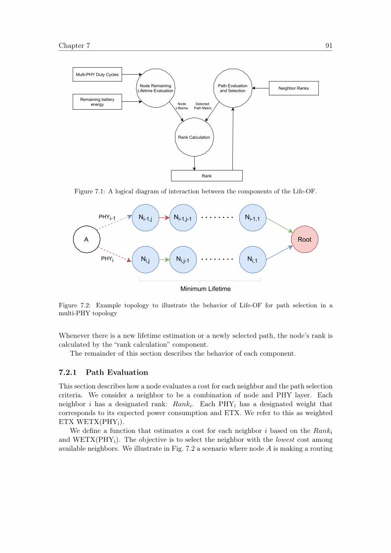
Chapter 7 91
Node RemainingLifetime Evaluation
Path Evaluationand Selection
Rank
Rank Calculation
Multi-PHY Duty Cycles
Remaining batteryenergy
Neighbor Ranks
Selected Path Metric
NodeLifteime
Figure 7.1: A logical diagram of interaction between the components of the Life-OF.
A Root
Ni,j Ni,j-1 Ni,1
Minimum Lifetime
Ni-1,j Ni-1,j-1 Ni-1,1PHYi-1
PHYi
Figure 7.2: Example topology to illustrate the behavior of Life-OF for path selection in amulti-PHY topology
Whenever there is a new lifetime estimation or a newly selected path, the node’s rank iscalculated by the “rank calculation” component.
The remainder of this section describes the behavior of each component.
7.2.1 Path Evaluation
This section describes how a node evaluates a cost for each neighbor and the path selectioncriteria. We consider a neighbor to be a combination of node and PHY layer. Eachneighbor i has a designated rank: Ranki. Each PHYi has a designated weight thatcorresponds to its expected power consumption and ETX. We refer to this as weightedETX WETX(PHYi).
We define a function that estimates a cost for each neighbor i based on the Rankiand WETX(PHYi). The objective is to select the neighbor with the lowest cost amongavailable neighbors. We illustrate in Fig. 7.2 a scenario where node A is making a routing

Chapter 7 92
decision between paths through Ni and Ni−1. Let the whole network agree on a commonset of PHYs: Φ = {PHY 1, . . . , PHY L}. Let node A have K neighbors and use PHYi
with neighbor i, with PHYi ∈ Φ.To obtain the cost, WETX(PHYi) has to be derived at first as follows:
• Energy per bit (Eb) for all PHYs is obtained through (7.1), where Ii is the currentconsumption of the radio chip of PHYi in amps, Vi is the voltage in volts, and thebitrate is in bps.
• EnergyWeight(PHYi) is obtained by normalizing the Eb of all the PHYs withrespect to the PHY with the lowest Eb according to (7.2).
• ETX(PHYi) is obtained using (7.3) where numTxi is the number of transmissionsto neighbor i, numAcki is the number of received acknowledgments.
• WETX(PHYi) is obtained as a function of EnergyWeight(PHYi) and ETX(PHYi),per (7.4)
Energy Per Bit(PHYi) =Ii ×Vi
Bitratei(7.1)
Energy Weight(PHYi) =Energy Per Bit(PHYi)
Min(Energy Per Bit(PHY1, . . . ,PHYL))(7.2)
ETXi =numTxi
numAcki(7.3)
WETX(PHYi) = EnergyWeight(PHYi)× ETX(PHYi) (7.4)
The cost of the path through a neighbor Ni is per (7.5).
Cost(Ni) =Rank(i)
WETX(PHYi)+ MinHopRankIncrease (7.5)
Where:
• We define Ranki using a range of values from [−50,−105], where −50 is the highestpossible rank (i.e. least preferable), and −105 is the best possible rank (i.e. theadvertised rank of the root)
• MinHopRankIncrease is a constant value to guarantee loop avoidance by ensuringthat the rank decreases monotonically across a given path.
The reasoning behind the formulation in (7.5) is as follows. Ranki expresses the rankof the neighbor, and therefore, the lower, the better. If both neighbor Ni and Ni−1 havethe same rank, then the neighbor with the PHY of lower energy weight will result into alower rank, and therefore will be favored as per (7.4), (7.2), and (7.1). If both neighborsshare the same rank and the same PHY, then the neighbor with the lower ETX – asper (7.4) and (7.3) – will be favored.
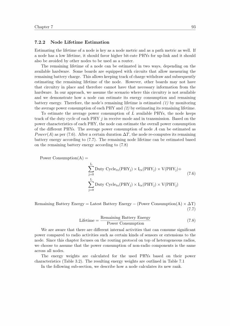
Chapter 7 93
7.2.2 Node Lifetime Estimation
Estimating the lifetime of a node is key as a node metric and as a path metric as well. Ifa node has a low lifetime, it should favor higher bit-rate PHYs for up-link and it shouldalso be avoided by other nodes to be used as a router.
The remaining lifetime of a node can be estimated in two ways, depending on theavailable hardware. Some boards are equipped with circuits that allow measuring theremaining battery charge. This allows keeping track of charge withdraw and subsequentlyestimating the remaining lifetime of the node. However, other boards may not havethat circuitry in place and therefore cannot have that necessary information from thehardware. In our approach, we assume the scenario where this circuitry is not availableand we demonstrate how a node can estimate its energy consumption and remainingbattery energy. Therefore, the node’s remaining lifetime is estimated (1) by monitoringthe average power consumption of each PHY and (2) by estimating its remaining lifetime.
To estimate the average power consumption of L available PHYs, the node keepstrack of the duty cycle of each PHY j in receive mode and in transmission. Based on thepower characteristics of each PHY, the node can estimate the overall power consumptionof the different PHYs. The average power consumption of node A can be estimated asPower(A) as per (7.6). After a certain duration ∆T , the node re-computes its remainingbattery energy according to (7.7). The remaining node lifetime can be estimated basedon the remaining battery energy according to (7.8)
Power Consumption(A) =
L∑j=0
Duty Cyclerx(PHYj)× Irx(PHYj)×V(PHYj)+
L∑j=0
Duty Cycletx(PHYj)× Itx(PHYj)×V(PHYj)
(7.6)
Remaining Battery Energy = Latest Battery Energy − (Power Consumption(A)×∆T)(7.7)
Lifetime =Remaining Battery Energy
Power Consumption(7.8)
We are aware that there are different internal activities that can consume significantpower compared to radio activities such as certain kinds of sensors or extensions to thenode. Since this chapter focuses on the routing protocol on top of heterogeneous radios,we choose to assume that the power consumption of non-radio components is the sameacross all nodes.
The energy weights are calculated for the used PHYs based on their powercharacteristics (Table 3.2). The resulting energy weights are outlined in Table 7.1
In the following sub-section, we describe how a node calculates its new rank.
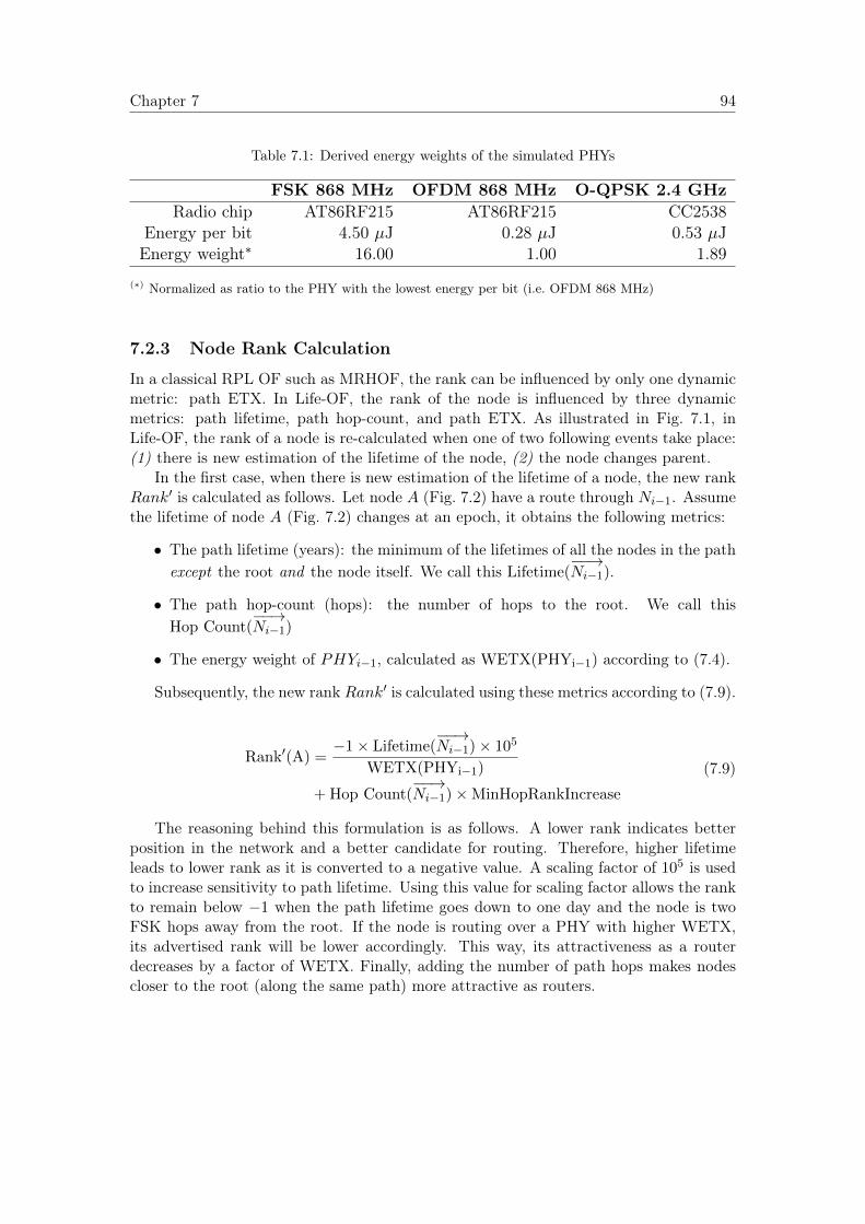
Chapter 7 94
Table 7.1: Derived energy weights of the simulated PHYs
FSK 868 MHz OFDM 868 MHz O-QPSK 2.4 GHzRadio chip AT86RF215 AT86RF215 CC2538
Energy per bit 4.50 µJ 0.28 µJ 0.53 µJEnergy weight∗ 16.00 1.00 1.89
(∗) Normalized as ratio to the PHY with the lowest energy per bit (i.e. OFDM 868 MHz)
7.2.3 Node Rank Calculation
In a classical RPL OF such as MRHOF, the rank can be influenced by only one dynamicmetric: path ETX. In Life-OF, the rank of the node is influenced by three dynamicmetrics: path lifetime, path hop-count, and path ETX. As illustrated in Fig. 7.1, inLife-OF, the rank of a node is re-calculated when one of two following events take place:(1) there is new estimation of the lifetime of the node, (2) the node changes parent.
In the first case, when there is new estimation of the lifetime of a node, the new rankRank′ is calculated as follows. Let node A (Fig. 7.2) have a route through Ni−1. Assumethe lifetime of node A (Fig. 7.2) changes at an epoch, it obtains the following metrics:
• The path lifetime (years): the minimum of the lifetimes of all the nodes in the pathexcept the root and the node itself. We call this Lifetime(
−−→Ni−1).
• The path hop-count (hops): the number of hops to the root. We call thisHop Count(
−−→Ni−1)
• The energy weight of PHYi−1, calculated as WETX(PHYi−1) according to (7.4).
Subsequently, the new rank Rank′ is calculated using these metrics according to (7.9).
Rank′(A) =−1× Lifetime(
−−→Ni−1)× 105
WETX(PHYi−1)
+ Hop Count(−−→Ni−1)×MinHopRankIncrease
(7.9)
The reasoning behind this formulation is as follows. A lower rank indicates betterposition in the network and a better candidate for routing. Therefore, higher lifetimeleads to lower rank as it is converted to a negative value. A scaling factor of 105 is usedto increase sensitivity to path lifetime. Using this value for scaling factor allows the rankto remain below −1 when the path lifetime goes down to one day and the node is twoFSK hops away from the root. If the node is routing over a PHY with higher WETX,its advertised rank will be lower accordingly. This way, its attractiveness as a routerdecreases by a factor of WETX. Finally, adding the number of path hops makes nodescloser to the root (along the same path) more attractive as routers.
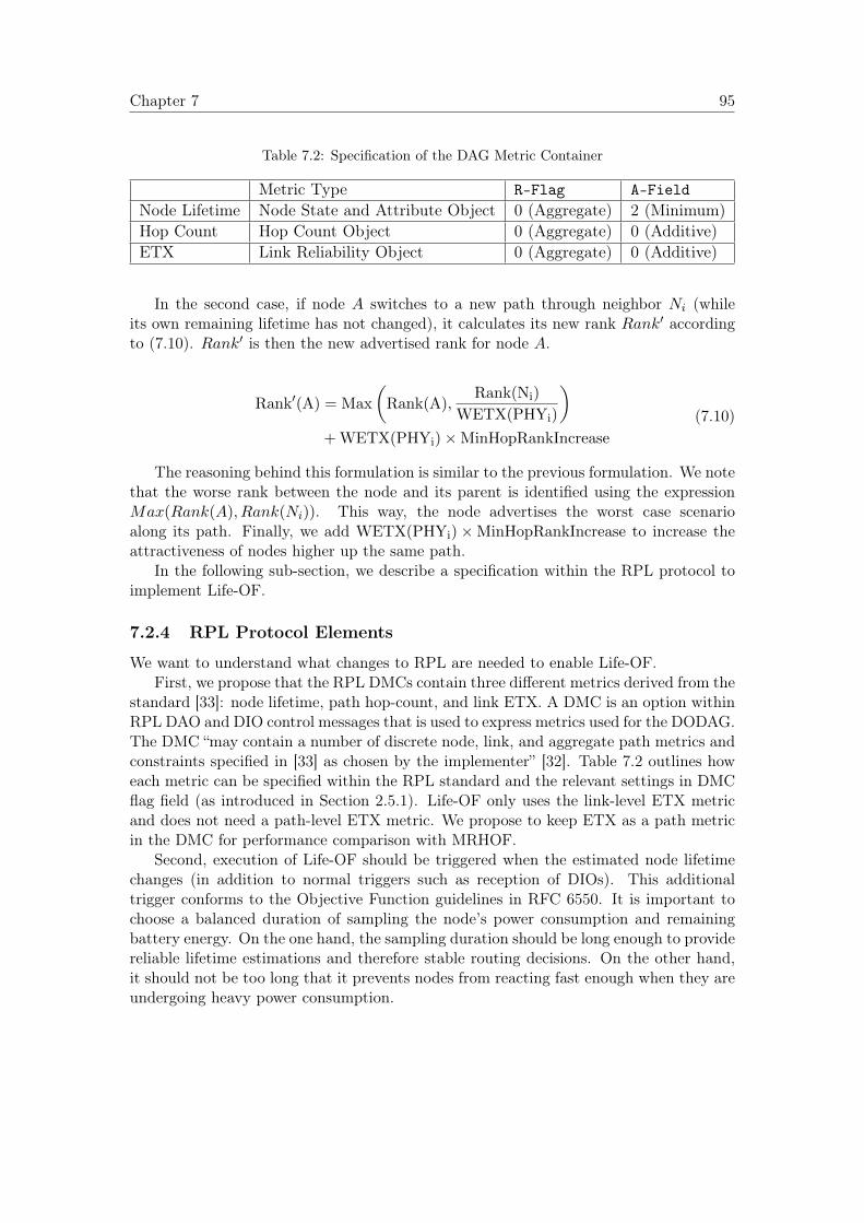
Chapter 7 95
Table 7.2: Specification of the DAG Metric Container
Metric Type R-Flag A-FieldNode Lifetime Node State and Attribute Object 0 (Aggregate) 2 (Minimum)Hop Count Hop Count Object 0 (Aggregate) 0 (Additive)ETX Link Reliability Object 0 (Aggregate) 0 (Additive)
In the second case, if node A switches to a new path through neighbor Ni (whileits own remaining lifetime has not changed), it calculates its new rank Rank′ accordingto (7.10). Rank′ is then the new advertised rank for node A.
Rank′(A) = Max
(Rank(A),
Rank(Ni)
WETX(PHYi)
)+ WETX(PHYi)×MinHopRankIncrease
(7.10)
The reasoning behind this formulation is similar to the previous formulation. We notethat the worse rank between the node and its parent is identified using the expressionMax(Rank(A), Rank(Ni)). This way, the node advertises the worst case scenarioalong its path. Finally, we add WETX(PHYi)×MinHopRankIncrease to increase theattractiveness of nodes higher up the same path.
In the following sub-section, we describe a specification within the RPL protocol toimplement Life-OF.
7.2.4 RPL Protocol Elements
We want to understand what changes to RPL are needed to enable Life-OF.First, we propose that the RPL DMCs contain three different metrics derived from the
standard [33]: node lifetime, path hop-count, and link ETX. A DMC is an option withinRPL DAO and DIO control messages that is used to express metrics used for the DODAG.The DMC “may contain a number of discrete node, link, and aggregate path metrics andconstraints specified in [33] as chosen by the implementer” [32]. Table 7.2 outlines howeach metric can be specified within the RPL standard and the relevant settings in DMCflag field (as introduced in Section 2.5.1). Life-OF only uses the link-level ETX metricand does not need a path-level ETX metric. We propose to keep ETX as a path metricin the DMC for performance comparison with MRHOF.
Second, execution of Life-OF should be triggered when the estimated node lifetimechanges (in addition to normal triggers such as reception of DIOs). This additionaltrigger conforms to the Objective Function guidelines in RFC 6550. It is important tochoose a balanced duration of sampling the node’s power consumption and remainingbattery energy. On the one hand, the sampling duration should be long enough to providereliable lifetime estimations and therefore stable routing decisions. On the other hand,it should not be too long that it prevents nodes from reacting fast enough when they areundergoing heavy power consumption.
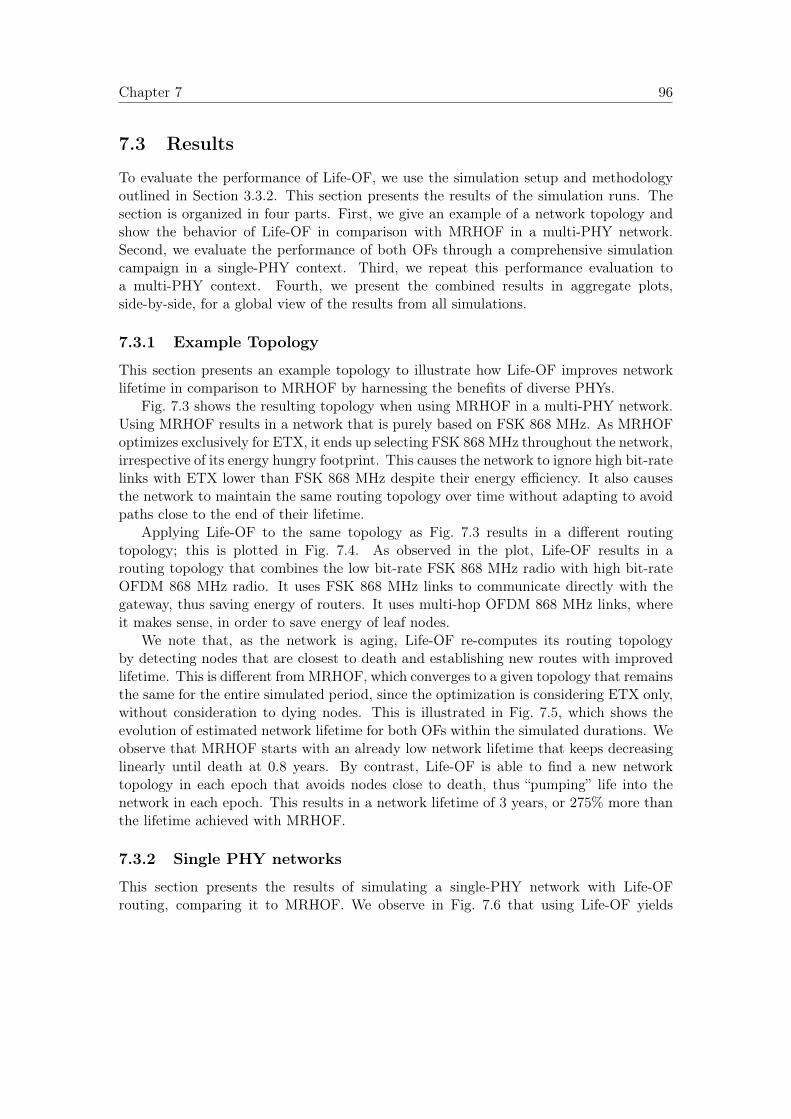
Chapter 7 96
7.3 Results
To evaluate the performance of Life-OF, we use the simulation setup and methodologyoutlined in Section 3.3.2. This section presents the results of the simulation runs. Thesection is organized in four parts. First, we give an example of a network topology andshow the behavior of Life-OF in comparison with MRHOF in a multi-PHY network.Second, we evaluate the performance of both OFs through a comprehensive simulationcampaign in a single-PHY context. Third, we repeat this performance evaluation toa multi-PHY context. Fourth, we present the combined results in aggregate plots,side-by-side, for a global view of the results from all simulations.
7.3.1 Example Topology
This section presents an example topology to illustrate how Life-OF improves networklifetime in comparison to MRHOF by harnessing the benefits of diverse PHYs.
Fig. 7.3 shows the resulting topology when using MRHOF in a multi-PHY network.Using MRHOF results in a network that is purely based on FSK 868 MHz. As MRHOFoptimizes exclusively for ETX, it ends up selecting FSK 868 MHz throughout the network,irrespective of its energy hungry footprint. This causes the network to ignore high bit-ratelinks with ETX lower than FSK 868 MHz despite their energy efficiency. It also causesthe network to maintain the same routing topology over time without adapting to avoidpaths close to the end of their lifetime.
Applying Life-OF to the same topology as Fig. 7.3 results in a different routingtopology; this is plotted in Fig. 7.4. As observed in the plot, Life-OF results in arouting topology that combines the low bit-rate FSK 868 MHz radio with high bit-rateOFDM 868 MHz radio. It uses FSK 868 MHz links to communicate directly with thegateway, thus saving energy of routers. It uses multi-hop OFDM 868 MHz links, whereit makes sense, in order to save energy of leaf nodes.
We note that, as the network is aging, Life-OF re-computes its routing topologyby detecting nodes that are closest to death and establishing new routes with improvedlifetime. This is different fromMRHOF, which converges to a given topology that remainsthe same for the entire simulated period, since the optimization is considering ETX only,without consideration to dying nodes. This is illustrated in Fig. 7.5, which shows theevolution of estimated network lifetime for both OFs within the simulated durations. Weobserve that MRHOF starts with an already low network lifetime that keeps decreasinglinearly until death at 0.8 years. By contrast, Life-OF is able to find a new networktopology in each epoch that avoids nodes close to death, thus “pumping” life into thenetwork in each epoch. This results in a network lifetime of 3 years, or 275% more thanthe lifetime achieved with MRHOF.
7.3.2 Single PHY networks
This section presents the results of simulating a single-PHY network with Life-OFrouting, comparing it to MRHOF. We observe in Fig. 7.6 that using Life-OF yields
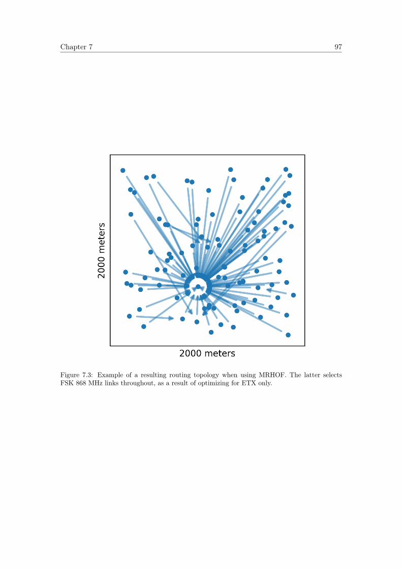
Chapter 7 97
Figure 7.3: Example of a resulting routing topology when using MRHOF. The latter selectsFSK 868 MHz links throughout, as a result of optimizing for ETX only.
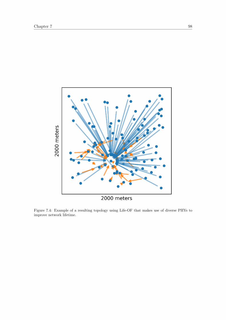
Chapter 7 98
Figure 7.4: Example of a resulting topology using Life-OF that makes use of diverse PHYs toimprove network lifetime.
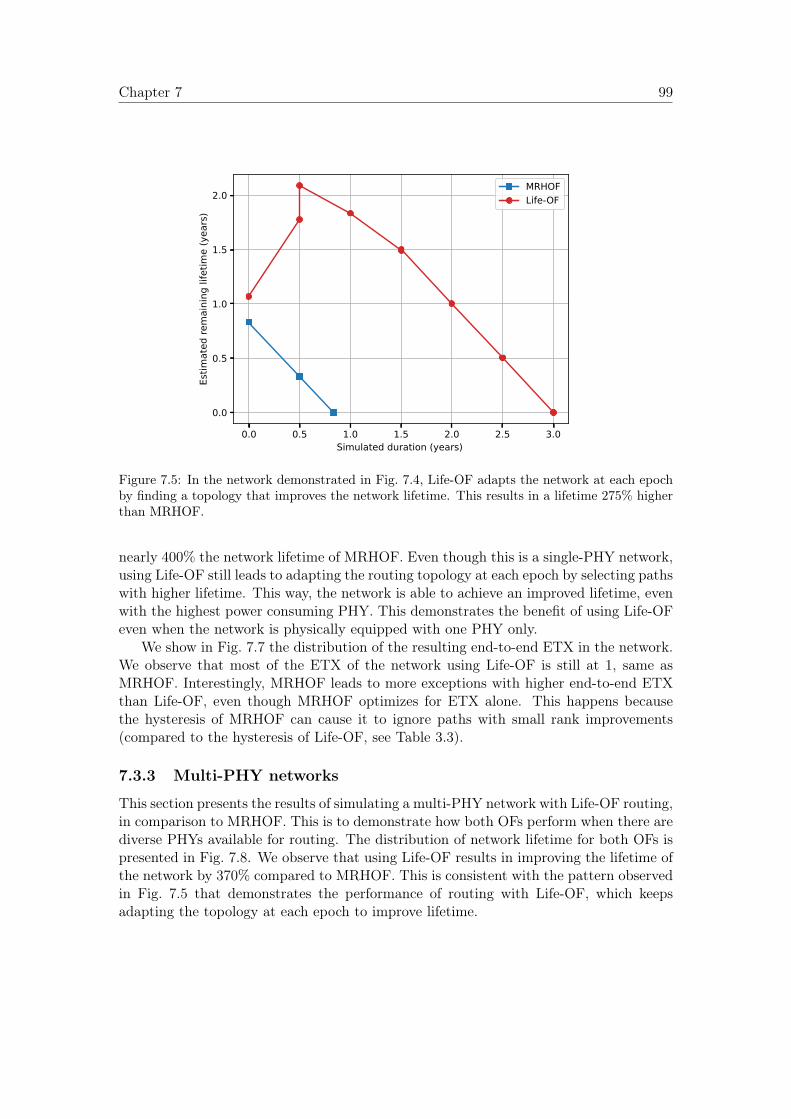
Chapter 7 99
0.0 0.5 1.0 1.5 2.0 2.5 3.0Simulated duration (years)
0.0
0.5
1.0
1.5
2.0Es
timat
ed re
mai
ning
life
time
(yea
rs)
MRHOFLife-OF
Figure 7.5: In the network demonstrated in Fig. 7.4, Life-OF adapts the network at each epochby finding a topology that improves the network lifetime. This results in a lifetime 275% higherthan MRHOF.
nearly 400% the network lifetime of MRHOF. Even though this is a single-PHY network,using Life-OF still leads to adapting the routing topology at each epoch by selecting pathswith higher lifetime. This way, the network is able to achieve an improved lifetime, evenwith the highest power consuming PHY. This demonstrates the benefit of using Life-OFeven when the network is physically equipped with one PHY only.
We show in Fig. 7.7 the distribution of the resulting end-to-end ETX in the network.We observe that most of the ETX of the network using Life-OF is still at 1, same asMRHOF. Interestingly, MRHOF leads to more exceptions with higher end-to-end ETXthan Life-OF, even though MRHOF optimizes for ETX alone. This happens becausethe hysteresis of MRHOF can cause it to ignore paths with small rank improvements(compared to the hysteresis of Life-OF, see Table 3.3).
7.3.3 Multi-PHY networks
This section presents the results of simulating a multi-PHY network with Life-OF routing,in comparison to MRHOF. This is to demonstrate how both OFs perform when there arediverse PHYs available for routing. The distribution of network lifetime for both OFs ispresented in Fig. 7.8. We observe that using Life-OF results in improving the lifetime ofthe network by 370% compared to MRHOF. This is consistent with the pattern observedin Fig. 7.5 that demonstrates the performance of routing with Life-OF, which keepsadapting the topology at each epoch to improve lifetime.
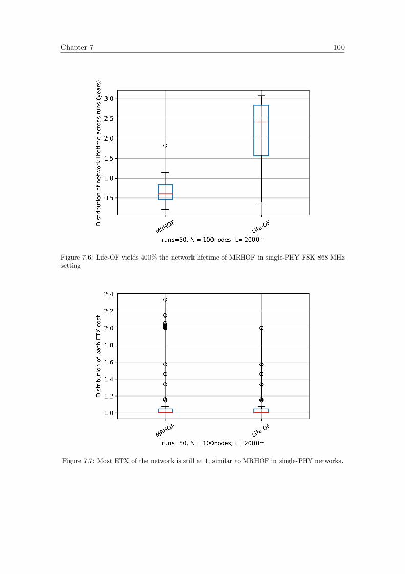
Chapter 7 100
Figure 7.6: Life-OF yields 400% the network lifetime of MRHOF in single-PHY FSK 868 MHzsetting
Figure 7.7: Most ETX of the network is still at 1, similar to MRHOF in single-PHY networks.
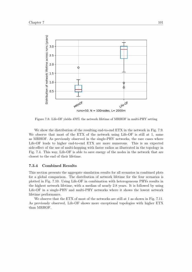
Chapter 7 101
Figure 7.8: Life-OF yields 470% the network lifetime of MRHOF in multi-PHY setting
We show the distribution of the resulting end-to-end ETX in the network in Fig. 7.9.We observe that most of the ETX of the network using Life-OF is still at 1, sameas MRHOF. As previously observed in the single-PHY networks, the rare cases whereLife-OF leads to higher end-to-end ETX are more numerous. This is an expectedside-effect of the use of multi-hopping with faster radios as illustrated in the topology inFig. 7.4. This way, Life-OF is able to save energy of the nodes in the network that areclosest to the end of their lifetime.
7.3.4 Combined Results
This section presents the aggregate simulation results for all scenarios in combined plotsfor a global comparison. The distribution of network lifetime for the four scenarios isplotted in Fig. 7.10. Using Life-OF in combination with heterogeneous PHYs results inthe highest network lifetime, with a median of nearly 2.8 years. It is followed by usingLife-OF in a single-PHY and multi-PHY networks where it shows the lowest networklifetime performance.
We observe that the ETX of most of the networks are still at 1 as shown in Fig. 7.11.As previously observed, Life-OF shows more exceptional topologies with higher ETXthan MRHOF.
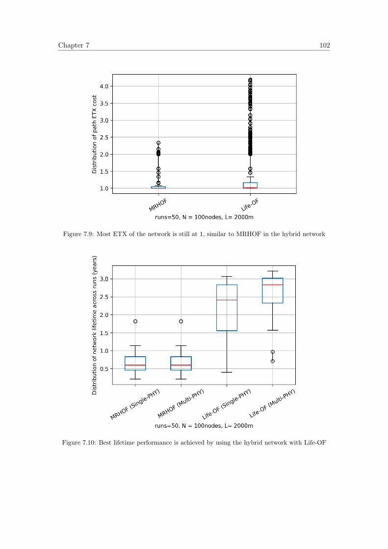
Chapter 7 102
Figure 7.9: Most ETX of the network is still at 1, similar to MRHOF in the hybrid network
Figure 7.10: Best lifetime performance is achieved by using the hybrid network with Life-OF
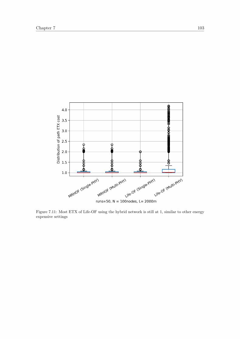
Chapter 7 103
Figure 7.11: Most ETX of Life-OF using the hybrid network is still at 1, similar to other energyexpensive settings
Chapter 7 104
7.4 Conclusion
In this chapter, we propose Life-OF, an OF that uses a combination of metrics in orderto improve network lifetime using diverse PHYs. We demonstrated how the routing layercan consider the link quality, node’s remaining lifetime, hop-count, and the characteristicsof each available PHY to make routing decisions that improve the network’s lifetime. Wedemonstrate how Life-OF can be defined using RPL protocol specifications.
The performance of Life-OF is compared to classical MRHOF using simulations insingle-PHY and multi-PHY settings. The simulations consider a scenario in a 2× 2 km2
area. Simulation results demonstrate that MRHOF converges to a pure long-rangeFSK 868 MHz network, leading to lowest network lifetime. However, Life-OF is able toimprove network lifetime by continuously adapting the routing topology to favor routingover nodes with relatively high remaining lifetime. It combines diverse PHYs in a waythat balances power consumption in the network. This way, nodes can switch betweenusing short-range PHYs to improve their own battery lifetime or using long-range PHYsto avoid routers that are close to depletion. Results show that using Life-OF yields 400%the network lifetime of MRHOF in a single-PHY setting. Furthermore, using Life-OFyields 470% the network lifetime of MRHOF in a multi-PHY setting.
Chapter 8
Conclusions and Future Work
This chapter concludes this manuscript by summarizing the work and listing its maincontributions (Section 8.1), and discussing the avenues for future research that this workopens (Section 8.2).
8.1 Conclusions
This thesis contributes to the research field of low power IoT. Such networks arecharacterized by the use of battery-powered sensor nodes which relay their readingsusing wireless PHYs. The IoT use cases cover a wide range of applications, includingpredictive industrial maintenance, precision agriculture, environmental monitoring, andsmart utility metering. Early IoT technologies that were introduced in the market relyon short-range PHYs that operate in the 2.4 GHz band. Examples of these technologiesare BLE, Zigbee, SmartMesh IP, and WirelessHART; they can create indoor coverageor reach for tens of meters. Longer range connectivity could only be achieved viamulti-hopping. A later family of technologies was introduced in the market that relyon long-range PHYs, which rely on lower bitrates, sub-GHz frequencies, and/or narrowband channels, to improve link robustness. Some examples of such technologies areLoRaWAN, Sigfox, and NB-IoT; their coverage span anywhere from hundreds of metersto several kilometers. Many of these technologies rely on proprietary PHYs. In 2012,the IEEE adopted a standard set of 31 PHYs serving both long-range and short-rangeapplications under the IEEE802.015.4g amendment.
Both short-range and long-range PHYs have different physical characteristics. Forexample, long-range PHYs offer link robustness at the expense of higher energyconsumption per bit and increased interference in dense networks. Short-range PHYs,however, offer lower energy consumption per bit at the expense of link robustness.Therefore, this leads to the first question we address in this thesis: does it makesense to integrate multiple PHYs in a network for improved QoS? Second, how can wegeneralize the standard IETF 6TiSCH protocol stack to support multi-PHY networking(i.e. g6TiSCH), and how does it compare to a single-PHY 6TiSCH network with respectto QoS? Third, how can the g6TiSCH protocol stack support variable-duration slots to
105
Chapter 8 106
improve schedule compactness by using shorter slots for fast bitrate PHYs? Finally, howcan a routing protocol make use of multi-PHY integration to improve network lifetime?
We organize this manuscript in seven core chapters, including four with technicalcontributions.
Chapter 1 provides a historical perspective on the concept of agility in computersystems. It gives background on emergent families of IoT technologies prevailing themarket and the research: short-range multi-hop networks and long-range star networks.Then we discuss why multi-hop topologies are still relevant even with long-range PHYsbefore we conclude with the organization of this manuscript.
Chapter 2 presents related work in several research and standardization tracks.We outline related work on the evaluation of IEEE 802.15.4g PHYs and we concludewith the need for an end-to-end evaluation of 6TiSCH protocol stack using differentIEEE 802.15.4g PHYs. We introduce an overview of the 6TiSCH protocol stack andrelated research on its performance improvement. We discuss challenges in operatingnetworks in the unlicensed bands. We then discuss related work on improving TSCHschedule compactness. This is followed by an overview of RPL and related work inmulti-PHY routing and network lifetime optimization. Finally, we present the state ofthe art on multi-PHY integration.
Chapter 3 introduces the three technical setups used for the experiments conductedthroughout this thesis. We introduce the OpenTestbed of 42 OpenMote B nodes deployedin a real office setting at Inria-Paris, which we use for the experiments in Chapters 4 and 5.We then introduce the local setup of four OpenMote B nodes using hardware probes.This is used to demonstrate the real-time performance of 6TiSCH with a heterogeneousslot-frame in Chapter 6. Finally, we introduce the RPLSim, a high-level discrete-timeRPL simulator that we use for the multi-PHY routing simulations in Chapter 7.
Chapter 4 discusses the question of whether multi-PHY integration makes sense. Weargue for a positive answer: instead of finding the best PHY for a network, we argue fora “no free lunch” principle. That is, no single PHY can offer best performance across allend-to-end network KPIs.
Chapter 5 adapts the 6TiSCH protocol stack for multi-PHY networking. Itdemonstrates how a set of short-range and long-range radios can be integrated under onegeneralized 6TiSCH architecture using Time Slotted PHY Hopping for medium access.The performance of g6TiSCH is evaluated experimentally on the OpenTestbed.
Chapter 6 demonstrates how to enable compact scheduling in a TSCH slot-frame in adecentralized multi-PHY network. The schedule can adapt slot-duration on a slot-by-slotbasis depending on the bit-rate of the used PHY (“6DYN”) and we show how this can helpmitigate the unlicensed band limitations. Finally we demonstrate the real-time behaviorof 6DYN using local hardware probes.
Chapter 7 introduces how multi-PHY networking can improve network lifetime. Wepropose“Life-OF”, a RPL OF that optimizes for network lifetime and we describe how toadapt RPL control messages to support this OF. Finally, both Life-OF and the standardMRHOF are evaluated using RPLSim and we demonstrate how Life-OF combines diversePHYs to boost network lifetime.
Chapter 8 107
In summary, this works makes the following three contributions to the field of lowpower IoT:
• On a conceptual front, the thesis argues for a “no free lunch” principle: nosingle PHYs outperforms other PHYs across all industrial KPIs. We advance howmulti-PHY radio chips can be used to enable multi-PHY integration, so that a nodecan change PHYs on a link-by-link basis using Time Slotted PHY Hopping. Weintroduce compact scheduling for industrial multi-PHY networking and we furthermake the case for boosting network lifetime using multi-PHY routing.
• We propose a generalization of the standard IETF 6TiSCH protocol stackfor multi-PHY networking. We show how to adapt the 6TiSCH architecturefor multi-PHY integration: IEEE 802.154e MAC layer, Sixtop sub-layer, MSFsub-layer, 6LoWPAN layer, and RPL routing layer. We demonstrate how RPLcan improve network lifetime by proposing an OF that combines different PHYs toachieve this objective.
• This thesis has resulted in technical developments in embedded firmware, software,and simulation to evaluate our proposals for multi-PHY integration. We extendOpenWSN – an RTOS and a reference implementation of 6TiSCH – withmulti-PHY support with the OpenMote B board, and develop a KPI monitor toextract industrial KPIs out of our experiments on the OpenTestbed. We furtherdevelop a high level discrete-time RPL simulator that mimics the evolution ofnetwork lifetime as a function of RPL configuration.
8.2 Future Work
This work has opened up several avenues for future work on agile multi-PHY networking.Section 8.2.1 discusses building open and flexible multi-PHY network architectures.Section 8.2.2 discusses challenges for scheduling in multi-PHY networks.
Section 8.2.3 discusses open challenges on multi-PHY gateways. Section 8.2.4discusses the possibility to extend this multi-PHY approach to cellular networks.Section 8.2.5 discusses open research challenges related to security in multi-PHYnetworks. Section 8.2.6 discusses the QoS degradation in the unlicensed band andhow multi-band support can yield improved QoS. Section 8.2.7 discusses future workon routing metrics for reducing network costs.
8.2.1 Open Multi-PHY Architectures
Throughout this thesis, we used only three PHYs from the IEEE 802.15.4g amendment,where each PHY has a specifically interesting feature: FSK 868 MHz as a long rangePHY, OFDM 868 MHz as a fast bit-rate PHY, and O-QPSK 2.4 GHz as a canonicalin-between option. But, as noted in Section 2.1, there is a total of 31 available PHYsin the IEEE802.15.4g amendment. Furthermore, there are other proprietary PHYs with
Chapter 8 108
different characteristics such as the LoRa PHY which is used for long-range coverage.It is configurable with 6 spreading factor indexes and tunable bandwidth ranging from7.8 kHz up to 500 kHz (subject to regional regulation) [79].
Therefore, future work can explore how to keep an open network architecture thatallows flexible additions of new PHYs to improve the QoS for different use cases. Thiscan be illustrated by two examples.
The first example is of an industrial site that spans tens of square kilometers. Inthat case, the network may combine a LoRa PHY with high spreading factor index forlong-range hops (e.g. SF = 12), a faster bitrate LoRa configuration for nearby nodessuch as (e.g. SF = 7), and an in-between option (e.g. SF = 10)
The second example is of a network deployed in deep-indoor environment such asinside a residential complex. In that case, the network may benefit from a configurationthat is fully based on an OFDM family of PHYs such as OFDM Option 1 which offersa bitrate from 100 kbps up to 800 kbps depending on the MCS. This can be interestingbecause OFDM is particularly robust against multi-path fading in indoor or urbansettings [5].
Future work can therefore explore how the architecture of the network can acceptnew PHYs. One challenge is how slot-templates can be conceived quickly (if notautomatically) for each PHY. Slot-templates were designed manually for this thesiswith the aid of hardware probes which can be impractical to do every time a PHYis introduced.
8.2.2 Scheduling in Multi-PHY networks
Future work can compare the performance of 6DYN to g6TiSCH using same slotdurations in large scale networks. This could be interesting when adaptive MSF is usedby allowing motes with high bit-rate up-links to increase their throughput by allocatingmore slots. Moreover, there is a whole diversity of different combinations that would beinteresting to evaluate. For instance a network can use a combination of PHYs on the5kbps-250kbps range to fit more sparse deployment or 250kbps to 800kbps to fit moredense deployments.
It can also be interesting to explore how parallel transmissions can take place within6DYN to improve reliability. At this point, g6TiSCH and 6DYN are designed to use onlyone transmission per slot. Since the mote has two different chips, it seems feasible thatmultiple chips can be sent commands at the same time. However, this requires morecareful design of time slot templates since the time for each state in the radio varies bythe design of each chip and how it is connected to the micro-controller (e.g., in an SoCor through SPI).
8.2.3 Multi-PHY Gateways
There is growing industrial interest in efficient use of the fixed infrastructure byminimizing wasted RF resources. For example, recent development in cellular5G networks have focused on “network slicing” which is the ability to divide
Chapter 8 109
the infrastructure among different use cases (e.g. human-type communications andmachine-type communications) [80].
The g6TiSCH architecture put forward in this thesis can be used to provisionmulti-PHY GWs where each connecting end device can negotiate a PHY depending onits own configuration. This does not come at extra cost for the GWs if they are equippedwith PHY-agile radio chips which support PHY changing on a frame-by-frame basis.
A challenge for this research is how to define an upper limit for the resources allocatedfor each PHY? Assuming the GW is using 6DYN to improve schedule compactness,should the upper limit on each PHY be expressed in number of slots or total time on air?Furthermore, can the GW dynamically expand the slot-frame to admit more flows? or isit better to request some devices to use faster bitrates when possible? In addition, howdoes increasing the number of supported PHYs impact the network performance in termsof signaling overhead? Finally, this track can address the different scheduling strategiesto improve network QoS. For example, if a poorly covered end device is generating highpacket rate, should it resort to use slower bit-rate or reserving more slots with higherbit-rate?. One way to address these challenges is by using heuristic search methods atrun-time to find better slot-frame configuration for improved QoS for connecting devices.
8.2.4 Multi-PHY Cellular Networks
Future work can consider the potential for deployment of multi-PHY base stations(Section 8.2.3) in a cellular topology. This can lower the Total Cost of Ownership (TCO)of the network infrastructure in three ways. First, since cellular base stations are majorcost elements because of the cost of manual labor to maintain them, it is not feasibleto add stations to improve coverage in remote areas with few users. Using a g6TiSCHarchitecture enables end users to deploy cheap, possibly battery-powered, routers forcoverage extension in hard to reach areas. This way, network QoS may be improved forextensive coverage for the users at no additional cost to the operators. Second, since basestations costs are fixed, using a multi-PHY gateway allows a device to switch to fasterbitrates when possible. Although existing cellular architectures such as NB-IoT [15] usedifferent PHYs for different activities, the set of used PHYs is pre-determined by therelevant standard. However, use of an open multi-PHY architecture allows admittingmore diverse use cases at the same cost. Therefore, it allows more efficient use of thebase station resources. Third, since the g6TiSCH architecture is fully wireless, it ispossible to have a cellular-like network spanning dozens of kilometers without the needfor wired infrastructure. This can enable low-cost and pervasive coverage in challengingwide areas such as mountains or hilly landscapes.
We identify three challenges for this research focus. The first challenge is how tomeasure the monetary cost of multi-PHY management (resulting from energy spent onsignaling overhead) and the possible side-effects on other performance aspects of thenetwork. This way, we can explore the possible side-effects of increasing the number ofsupported PHYs in the network and weigh them against the benefits in reducing TCOor QoS improvement.
The second challenge is to explore how the network can support human-type
Chapter 8 110
communications that are significantly different in their requirements from IoT (e.g. voicecalls). g6TiSCH uses low power radios that are designed to fit LLNs in general (assumedto be stationary and with low per device packet rates). However, the concepts developedin 6DYN (specially use of Time Slotted PHY Hopping) can be applied to higherthroughput radios, such as commonly used for human-type communications.
For example:
• a high bitrate PHY can be sufficient for a nearby stationary device and vice versa,
• a node can negotiate slots to nearby stations during mobility for a smooth handoff,and
• a node can negotiate cells with different PHYs to use for different applications(e.g. low bitrate PHY for alarms and high-bitrate PHY for applications with regularnon-critical transmission).
Finally, how can multi-PHY base stations be deployed in complex terrain for improvedcoverage? One way to address this is by referring to existing machine learning methodsthat use Light Detection and Ranging (LIDAR) data for coverage improvement incomplex terrain [81], [82] and adapting them for multi-PHY architectures.
8.2.5 Security in Multi-PHY Networks
Security is a fundamental aspect of networked computer systems and it is an integralelement of the 6TiSCH protocol stack [76]. Future work can explore how multi-PHYcapabilities can be used to enhance network security against different threat models. Wepresent two examples for this track.
First, a network that is deployed in a hostile zone can possibly increase the difficultyof jamming or sniffing of its communication channels by adopting what can be called“PHY-Anonymity”. The network can use two sets of PHYs: a statically defined set fornetwork discovery and a dynamically configured set for communication. A device thatjoins the network has a priori knowledge only of the first set of PHYs. If it successfullyauthenticates, it receives specific set of PHYs to be used by this for communication (eitherfrom a neighbor in a distributed network or form the gateway in a centralized network).This set may vary from one device to another. This way, it is harder for unauthenticatednodes to know which PHYs are used for communication. Also, in case of an unauthorizedjoin to the network, only a part of the network is compromised since not all the devicesuse the same set of PHYs. This mechanism is inspired by the “bridge” access mode forthe The Onion Routing network that enables it to survive hostile blocking attempts [83].
Second, multi-PHY integration can improve network protection against sniffing orjamming by “random” hopping over a diverse set of PHYs (e.g. modulation, band, codingrate etc.). Future work can explore different hopping schemes that can mitigate therisk of sniffing of a multi-hop TSCH network, such as the sniffing approach proposed byKovac et al. [84]. For example, Kovac et al.perform sniffing on 16 channels in the 2.4 GHzband. How can the diversity in band (e.g., sub-GHz band) or modulations mitigate thisrisk of sniffing?.
Chapter 8 111
8.2.6 Agile Spectrum Access
Future work can explore the potential of multi-band support within the network toimprove network QoS in industrial applications. This track is important since networkQoS can be degraded as a side-effect of the interference in the unlicensed band.
As discussed in Section 2.3, the use of the unlicensed band introduces throughputlimitations due to interference, specially with the use of long-range PHYs. This is becausein highly industrialized or urbanized zones, hundreds or thousands of wireless devices areexpected to co-exist, yet without any coordination among them on the use of the sharedspectrum. This can lead to degraded QoS of the network because of external interference.
This research track can be interesting in three focus points. First, it can helpnetworks develop more resilience against external interference by simply changing anyPHY that seems to suffer low PDR (especially if it is combined with high RSSIs). Second,network operators may choose to offload some traffic using licensed bands or using TVwhite-spaces for an improved reliability. This way, the network operators can createQoS trade-offs for each end device depending on the use case. Existing proposals, suchas the proposal of Labib et al. [85], have introduced off-loading Long Term Evolution(LTE) traffic to the unlicensed spectrum. This confirms the intuition behind integrationof the licensed and unlicensed bands. Therefore, future work can explore the off-loadingfrom the unlicensed band into the licensed band. For example, alarms messages canbe off-loaded to the licensed band for improved latency and reliability. Less criticaluse-cases, such as smart utility meter readings, can be transmitted in the unlicensedband with higher latency. Third, there is an existing interest in dynamic spectrumsharing for efficient utilization of the licensed spectrum [86]. The reason is that licensedbands usually have the fixed costs of their purchase, yet they are not always in use bythe end customers, which means a waste of bandwidth resources. Since the spectrum isalready a scarce resource, there is interest in its commoditization: operators can “rentout” licensed bands temporarily for efficient utilization. Renters can be operators in theunlicensed bands who may benefit from partial access to licensed bands for improvedQoS. This can be subject to pricing dynamics based on supply and demand [87].
Since g6TiSCH in combination with 6DYN enables multi-PHY support, it canincrease the spectral agility of the network by allowing the network to dynamically switchbands or PHYs (fully or partially). This way, there is more space for QoS trade-offs inthe network. The challenge in this focus track is how should the network scan anddiscover the available spectral options during its running? Finally, how should a routebe selected in this setting when the route is a mixture of free and rented bands? Thiscan be addressed through cost-aware routing which is discussed in the following section.
8.2.7 Routing Metrics for Improving Network Costs
In Chapter 7, we introduced a RPL OF that improves network lifetime. This wasmotivated by the need to improve network cost by reducing the number of employeehours and trips to replace the batteries of all the devices. However, there can be morecost elements involved, other than the factory trips. For example, as mentioned in
Chapter 8 112
Section 8.2.6, some links can be more costly than others if they use licensed bands (incase of mixing license-free and licensed PHYs). Furthermore, some devices may be in aharder to reach areas than others or may be more critical than others such that removingthem can incur excessive labor costs or halting production lines.
Future work can then consider routing metrics to improve the overall network cost,which can follow an LPWAN budget model such as in previous research [78]. Thechallenge in this work is how to extend RPL DMCs to include cost-related metrics suchas cost of licensed bands (when in use), battery replacement cost, and battery capacity.Furthermore, consumption of battery energy can be computed more systematically toinclude power consumption of the radios as well as non-radio components such as attachedsensing modules or local storage such as flash memory as introduced in [88]. This way, therouting topology is more aware of the budget-consuming factors and is more intentionalabout optimizing for budget saving.
Chapter 9
Publications Resulting from thisWork
Journal Articles
1. No Free Lunch—Characterizing the Performance of 6TiSCH When Using DifferentPhysical Layers. Mina Rady, Quentin Lampin, Dominique Barthel, ThomasWatteyne. MDPI Sensors, vol. 20, no. 17, p. 4989, September 2020.
2. g6TiSCH: Generalized 6TiSCH for Agile Multi-PHY Wireless Networking.Mina Rady, Quentin Lampin, Dominique Barthel, Thomas Watteyne. IEEEAccess, vol. 9, pp. 84465-84479, 2021.
3. 6DYN: 6TiSCH with Heterogeneous Slot Durations. Mina Rady, Quentin Lampin,Dominique Barthel, Thomas Watteyne. MDPI Sensors, special issue onDependable IoT Networking vol. 21, no. 5, p. 1611, February 2021.
4. Bringing Life out of Diversity: Boosting Network Lifetime using Multi-PHYRouting in RPL. Mina Rady, Quentin Lampin, Dominique Barthel, ThomasWatteyne. Wiley Transactions on Emerging Telecommunications (ETT),under review.
Conference Paper and Demonstration
1. Demo: Blink - Room-Level Localization Using SmartMesh IP. Yasuyuki Tanaka,Hai Le, Victor Kobayashi, Camilo Lopez, Thomas Watteyne, Mina Rady. IEEEINFOCOM, CNERT workshop, Paris, France, 29 April 2019.
Conference Poster
1. Extending LPWANs with Heterogeneous Mesh Networks. Mina Rady, QuentinLampin, Dominique Barthel, Thomas Watteyne. Journées thématiques GDRRSD ResCom Low-Power Wide Area Networks (LPWAN),Lyon, France, July2019.
113
Chapter 9 114
Research Report
1. Initial Design of a Generalization of the 6TiSCH Standard to Support Multiple PHYLayers. Mina Rady, Quentin Lampin, Dominique Barthel, Thomas Watteyne.Inria Research Report RR-9392, 2021.
Software Contributions
1. to the OpenWSN project (http://www.openwsn.org), the reference open-sourceimplementation of the 6TiSCH protocol stack. Specifically, I lead the developmentof:
• the openradio interface (https://github.com/minarady1/openwsn-fw/tree/develop_FW-866_v2),
• the g6TiSCH OpenWSN implementation (https://github.com/minarady1/openwsn-fw/tree/develop_FW-877),
• the OpenVisualizer support for the multi-PHY network (https://github.com/minarady1/openvisualizer/tree/develop_FW-877),
• the 6DYN OpenWSN implementation (https://github.com/minarady1/openwsn-fw/tree/develop_FW-877).
My contributions are published under an open-source BSD license.
2. to the OpenTestbed Project (http://testbed.openwsn.org/), an open-sourcelow-power wireless testbed solution based on off-the-shelf hardware. Specifically, Ilead the development of the KPI Monitor (https://github.com/minarady1/kpi_monitor). My contribution is published under an open-source BSD license.
3. RPLSim a discrete-event high-level RPL Simulator written in Python. RPLSimhas allowed us to mimic the evolution of network lifetime as a function of RPL OFconfiguration. I am the lead developer on this project.
Bibliography
[1] F. Civerchia, S. Bocchino, C. Salvadori, E. Rossi, L. Maggiani, and M. Petracca,“Industrial Internet of Things Monitoring Solution for Advanced PredictiveMaintenance Applications,” Elsevier Journal of Industrial Information Integration,vol. 7, pp. 4–12, Sep. 2017. doi: 10.1016/j.jii.2017.02.003.
[2] Waht is Zigbee? https://zigbeealliance.org/solution/zigbee/, Accessed: 31August, 2021.
[3] T. Watteyne, L. Doherty, J. Simon, and K. Pister, “Technical Overview ofSmartMesh IP,” in Seventh International Conference on Innovative Mobile andInternet Services in Ubiquitous Computing, Taichung, Taiwan: IEEE, Jul. 2013,pp. 547–551. doi: 10.1109/IMIS.2013.97.
[4] J. Muñoz, T. Chang, X. Vilajosana, and T. Watteyne, “Evaluation ofIEEE802.15.4g for Environmental Observations,” MDPI Sensors, vol. 18, no. 10,p. 3468, Oct. 2018. doi: 10.3390/s18103468.
[5] J. Muñoz, E. Riou, X. Vilajosana, P. Muhlethaler, and T. Watteyne, “Overview ofIEEE802.15.4g OFDM and Its Applicability to Smart Building Applications,” inWireless Days (WD), IEEE, Dubai, UAE, Apr. 2018, pp. 123–130. doi: 10.1109/WD.2018.8361707.
[6] A. H. Kazmi, M. J. O’grady, D. T. Delaney, A. G. Ruzzelli, and G. M. P. O’hare,“A Review of Wireless-Sensor-Network-Enabled Building Energy ManagementSystems,” ACM Transactions on Sensor Networks, vol. 10, no. 4, pp. 1–43, Jun.2014. doi: 10.1145/2532644.
[7] T. Watteyne, A. Laura Diedrichs, K. Brun-Laguna, J. Emilio Chaar, D. Dujovne,J. Carlos Taffernaberry, and G. Mercado, “PEACH: Predicting Frost Events inPeach Orchards Using IoT Technology,” EAI Endorsed Transactions on Internetof Things, vol. 2, no. 5, Dec. 2016. doi: 10.4108/eai.1-12-2016.151711.
[8] C.-S. Sum, M.-T. Zhou, F. Kojima, and H. Harada, “Experimental PerformanceEvaluation of Multihop IEEE 802.15.4/4g/4e Smart Utility Networks in OutdoorEnvironment,” Wireless Communications and Mobile Computing, vol. 2017,pp. 1–13, 2017. doi: 10.1155/2017/7137406.
115
Chapter 9 116
[9] Y. Tanaka, H. Le, V. Kobayashi, C. Lopez, T. Watteyne, and M. Rady,“Demo: Blink – Room-Level Localization Using SmartMesh IP,” in InternationalConference on Embedded Wireless Systems and Networks (EWSN), ACM, Lyon,France, Feb. 2020, pp. 198–199.
[10] T. Chang, T. Watteyne, B. Wheeler, F. Maksimovic, O. Khan, S. Mesri, L. Lee,I. Suciu, D. Burnett, X. Vilajosana, and K. Pister, “6TiSCH on SCµM: Runninga Synchronized Protocol Stack without Crystals,” Sensors, vol. 20, p. 1912, Mar.2020. doi: 10.3390/s20071912.
[11] E. Fadel, V. Gungor, L. Nassef, N. Akkari, M. A. Malik, S. Almasri, and I. F.Akyildiz, “A Survey on Wireless Sensor Networks for Smart Grid,” IEEE ComputerCommunications, vol. 71, pp. 22–33, Nov. 2015. doi: 10.1016/j.comcom.2015.09.006.
[12] F. Adelantado, X. Vilajosana, P. Tuset-Peiró, B. Martinez, J. Melia-Segui, andT. Watteyne, “Understanding the Limits of LoRaWAN,” IEEE CommunicationsMagazine, vol. 55, no. 9, pp. 34–40, 2017. doi: 10.1109/mcom.2017.1600613.
[13] Sigfox Technology, https://www.sigfox.com/en/what- sigfox/technology,Accessed: 04 August, 2021.
[14] Y.-P. E. Wang, X. Lin, A. Adhikary, A. Grovlen, Y. Sui, Y. Blankenship, J.Bergman, and H. S. Razaghi, “A Primer on 3GPP Narrowband Internet of Things,”IEEE Communications Magazine, vol. 55, no. 3, pp. 117–123, Mar. 2017. doi:10.1109/mcom.2017.1600510cm.
[15] K. Mekki, E. Bajic, F. Chaxel, and F. Meyer, “Overview of Cellular LPWANTechnologies for IoT Deployment: Sigfox, LoRaWAN, and NB-IoT,” Mar. 2018.doi: 10.1109/PERCOMW.2018.8480255.
[16] J. Muñoz, “km-Scale Industrial Networking,” Ph.D. dissertation, SorbonneUniversity, Paris, France, 2019.
[17] T. Watteyne, J. Weiss, L. Doherty, and J. Simon, “Industrial IEEE802.15.4eNetworks: Performance and Trade-Offs,” in IEEE International Conference onCommunications (ICC), London: IEEE, Jun. 2015, pp. 604–609. doi: 10.1109/ICC.2015.7248388.
[18] IEEE, 802.15.4e-2012 - IEEE Standard for Local and metropolitan areanetworks–Part 15.4: Low-Rate Wireless Personal Area Networks (LR-WPANs)Amendment 1: MAC sublayer, IEEE, Apr. 2012.
[19] T. Watteyne, V. Handziski, X. Vilajosana, S. Duquennoy, O. Hahm, E. Baccelli,and A. Wolisz, “Industrial Wireless IP-based Cyber Physical Systems,” Proceedingof the IEEE, vol. PP, no. 99, pp. 1–14, Mar. 2016.
[20] IEEE, IEEE Standard for Local and Metropolitan Area Networks–Part 15.4:Low-Rate Wireless Personal Area Networks (LR-WPANs), Piscataway, NJ: IEEE,2016.
Chapter 9 117
[21] Texas Instruments, Datasheet: CC2538 Powerful Wireless MicrocontrollerSystem-On-Chip for 2.4-GHz IEEE 802.15.4, 6LoWPAN, and ZigBee Applications,Red. D, 2015.
[22] The European Commission, M/441 Standardisation Mandate to CEN, CENELECAnd ETSI in the field of Measuring Instruments for the Development of anOpen Architecture for Utility Meters Involving Communication Protocols EnablingInteroperability, Brussels, Apr. 2009.
[23] The European Council, “Directive 2006/32/EC of the European Parliament andof the Council on Energy End-Use Efficiency and Energy Services and RepealingCouncil Directive 93/76/EEC,” OJ, vol. L 114, pp. 64–85, Apr. 2006.
[24] Couverture LoRa® Orange, https://www.orange-business.com/fr/reseau-iot, Accessed: 20 August, 2021.
[25] Nordic Semiconductor, nRF52840 Product Specification, v1.1, 2019.
[26] IEEE, IEEE Standard for Local and metropolitan area networks–Part 15.4:Low-Rate Wireless Personal Area Networks (LR-WPANs) Amendment 3: PhysicalLayer (PHY) Specifications for Low-Data-Rate, Wireless, Smart Metering UtilityNetworks, IEEE, Apr. 2012.
[27] Atmel, Atmel AT86RF215 Device Family Datasheet, 42415E, 2016.
[28] F. Kojima, C.-S. Sum, M.-T. Zhou, L. Lu, and H. Harada, “System Evaluationof a Practical IEEE 802.15.4/4e/4g Multi-Physical and Multi-Hop Smart UtilityNetwork,” IET Communications, vol. 9, no. 5, pp. 665–673, Mar. 2015. doi: 10.1049/iet-com.2014.0240.
[29] X. Vilajosana, K. Pister, and T. Watteyne, Minimal IPv6 over the TSCH Modeof IEEE 802.15.4e (6TiSCH) Configuration, RFC8180, Internet Engineering TaskForce (IETF), May 2017. [Online]. Available: https://datatracker.ietf.org/doc/html/rfc8180.
[30] X. Vilajosana, T. Watteyne, T. Chang, M. Vucinic, S. Duquennoy, and P. Thubert,“IETF 6TiSCH: a Tutorial,” IEEE Communications Surveys & Tutorials, vol. 22,no. 1, pp. 595–615, 2019. doi: 10.1109/COMST.2019.2939407.
[31] D. Dujovne, T. Watteyne, X. Vilajosana, and P. Thubert, “6TiSCH: DeterministicIP-Enabled Industrial Internet (of Things),” IEEE Communications Magazine,vol. 52, no. 12, pp. 36–41, Dec. 2014. doi: 10.1109/MCOM.2014.6979984.
[32] T. Winter, P. Thubert, A. Brandt, J. Hui, R. Kelsey, P. Levis, K. Pister, R. Struik,J. Vasseur, and R. Alexander, RPL: IPv6 Routing Protocol for Low-Power andLossy Networks, RFC6550, Internet Engineering Task Force (IETF), Mar. 2012.[Online]. Available: https://datatracker.ietf.org/doc/html/rfc6550.
[33] J. Vasseur, M. Kim, K. Pister, N. Dejean, and D. Barthel, Routing MetricsUsed for Path Calculation in Low-Power and Lossy Networks, RFC6551, InternetEngineering Task Force (IETF), Mar. 2012. [Online]. Available: https : / /datatracker.ietf.org/doc/html/rfc6551.
Chapter 9 118
[34] P. Thubert, Objective Function Zero for the Routing Protocol for Low-Power andLossy Networks (RPL), RFC6552, Internet Engineering Task Force (IETF), Mar.2012. [Online]. Available: https://datatracker.ietf.org/doc/html/rfc6552.
[35] Q. Wang, X. Vilajosana, and T. Watteyne, 6TiSCH Operation Sublayer (6top)Protocol (6P), RFC8480, Internet Engineering Task Force (IETF), Nov. 2018.[Online]. Available: https://datatracker.ietf.org/doc/html/rfc6719.
[36] T. Chang, M. Vucinic, X. Vilajosana, S. Duquennoy, and D. Dujovne, 6TiSCHMinimal Scheduling Function (MSF), RFC9033, Internet Engineering Task Force(IETF), May 2021. [Online]. Available: https://datatracker.ietf.org/doc/html/rfc9033.
[37] J. Hui and P. Thubert, Compression Format for IPv6 Datagrams over IEEE802.15.4-Based Networks, RFC6282, Internet Engineering Task Force (IETF), Sep.2011. [Online]. Available: https://datatracker.ietf.org/doc/html/rfc6282.
[38] A. Yang, A. Sundararajan, C. B. Schindler, and K. Pister, “Analysis of Low LatencyTSCH Networks for Physical Event Detection,” in Wireless Communicationsand Networking Conference Workshops (WCNCW), Barcelona, Catalunya, Spain:IEEE, Apr. 2018, pp. 167–172.
[39] F. Theoleyre and G. Z. Papadopoulos, “Experimental Validation of a DistributedSelf-Configured 6TiSCH with Traffic Isolation in Low Power Lossy Networks,” inInternational Conference on Modeling, Analysis and Simulation of Wireless andMobile Systems (MSWIM), Malta, Malta: ACM, 2016, pp. 102–110.
[40] R. Teles Hermeto, A. Gallais, and F. Theoleyre, “On the (over)-Reactions andthe Stability of a 6TiSCH Network in an Indoor Environment,” in InternationalConference on Modeling, Analysis and Simulation of Wireless and Mobile Systems(MSWIM), Montreal, QC, Canada: ACM, 2018, pp. 83–90.
[41] S. Ben Yaala, F. Theoleyre, and R. Bouallegue, “Performance Study of Co-LocatedIEEE 802.15.4-TSCH Networks: Interference and Coexistence,” in Symposiumon Computers and Communication (ISCC), Messina, Italy: IEEE, Jun. 2016,pp. 513–518.
[42] M. Vucinic, T. Chang, B. Skrbic, E. Kocan, M. Pejanovic-Djurisic, and T.Watteyne, “Key Performance Indicators of the Reference 6TiSCH Implementationin Internet-of-Things Scenarios,” IEEE Access, vol. 8, pp. 79 147–79 157, 2020. doi:10.1109/ACCESS.2020.2990278.
[43] M. R. Palattella, N. Accettura, M. Dohler, L. A. Grieco, and G. Boggia, “TrafficAware Scheduling Algorithm for Reliable Low-Power Multi-Hop IEEE 802.15.4eNetworks,” in IEEE 23rd International Symposium on Personal, Indoor and MobileRadio Communications - (PIMRC), 2012, pp. 327–332. doi: 10.1109/PIMRC.2012.6362805.
Chapter 9 119
[44] M. R. Palattella, N. Accettura, L. A. Grieco, G. Boggia, M. Dohler, and T. Engel,“On Optimal Scheduling in Duty-Cycled Industrial IoT Applications Using IEEE802.15.4e TSCH,” IEEE Sensors Journal, vol. 13, no. 10, pp. 3655–3666, Oct. 2013.doi: 10.1109/jsen.2013.2266417.
[45] S. Ridha, P. Minet, and E. Livolant, “MODESA: an Optimized Multichannel SlotAssignment for Raw Data Convergecast in Wireless Sensor Networks,” in IEEE 31stInternational Performance Computing and Communications Conference (IPCCC),Dec. 2012, pp. 91–100. doi: 10.1109/PCCC.2012.6407742.
[46] Y. Kim and M. Lee, “Scheduling Multi-Channel and Multi-Timeslot inTime Constrained Wireless Sensor Networks via Simulated Annealing andParticle Swarm Optimization,” IEEE Communications Magazine, vol. 52, no. 1,pp. 122–129, Jan. 2014. doi: 10.1109/mcom.2014.6710073.
[47] R. T. Hermeto, A. Gallais, and F. Theoleyre, “Scheduling for IEEE802.15.4-TSCHand Slow Channel Hopping MAC in Low Power Industrial Wireless Networks: Asurvey,” Computer Communications, vol. 114, pp. 84–105, Dec. 2017. doi: 10.1016/j.comcom.2017.10.004.
[48] R. Musaloiu-E and A. Terzis, “Minimising the Effect of WiFi Interference in802.15.4 Wireless Sensor Networks,” International Journal of Sensor Networks,vol. 3, no. 1, p. 43, 2008. doi: 10.1504/ijsnet.2008.016461.
[49] A. Gonga, O. Landsiedel, P. Soldati, and M. Johansson, “Revisiting Multi-channelCommunication to Mitigate Interference and Link Dynamics in Wireless SensorNetworks,” in IEEE 8th International Conference on Distributed Computing inSensor Systems, IEEE, May 2012. doi: 10.1109/dcoss.2012.15.
[50] X. Liu, X. Zhai, W. Lu, and C. Wu, “QoS-guarantee Resource Allocation forMultibeam Satellite Industrial Internet of Things with NOMA,” IEEE Transactionson Industrial Informatics, pp. 2052–2061, 2019. doi: 10.1109/tii.2019.2951728.
[51] ETSI, Electromagnetic Compatibility and Radio Spectrum Matters (ERM); ShortRange Devices (SRD); Radio Equipment to be Used in the 25 MHz to 1000 MHzFrequency Range with Power Levels Ranging up to 500 mW; Part 1: TechnicalCharacteristics and Test Methods, Sophia Antipolis Cedex - FRANCE: ETSI, 2012.
[52] T. Watteyne, A. Mehta, and K. Pister, “Reliability through Frequency Diversity,”in Proceedings of the 6th ACM Symposium on Performance Evaluation of WirelessAd Hoc, Sensor, and Ubiquitous Networks - PE-WASUN, ACM Press, 2009. doi:10.1145/1641876.1641898.
[53] J. Munoz, P. Muhlethaler, X. Vilajosana, and T. Watteyne, “Why Channel HoppingMakes Sense, even with IEEE 802.15.4 OFDM at 2.4 GHz,” in Global Internet ofThings Summit (GIoTS), IEEE, Jun. 2018. doi: 10.1109/giots.2018.8534544.
[54] O. Gnawali and P. Levis, The Minimum Rank with Hysteresis Objective Function,RFC6719, Internet Engineering Task Force (IETF), Sep. 2012. [Online]. Available:https://datatracker.ietf.org/doc/html/rfc6719.

Chapter 9 120
[55] L. Ben Saad, C. Chauvenet, and B. Tourancheau, “IPv6 (Internet Protocol Version6) Heterogeneous Networking Infrastructure for Energy Efficient Building,” Energy,vol. 44, no. 1, pp. 447–457, Aug. 2012. doi: 10.1016/j.energy.2012.06.008.
[56] F. Lemercier, N. Montavont, L. Toutain, K. Vijayasankar, R. Vedantham, C.Pissard-Gibollet, and C. Philippe, “Support for hybrid network in RPL,” in IEEEInternational Conference on Smart Grid Communications (SmartGridComm),IEEE, Sydney, Australia, Dec. 2016, pp. 527–532. doi: 10.1109/SmartGridComm.2016.7778815.
[57] F. Lemercier, N. Montavont, L. Toutain, and P. Chiummiento, “A NewObjective Function for Hybrid Network in the Smart Grid,” in IEEE 19thInternational Symposium on “A World of Wireless, Mobile and MultimediaNetworks” (WoWMoM), IEEE, Chania, Greece, Jun. 2018, pp. 14–16. doi: 10.1109/WoWMoM.2018.8449744.
[58] O. Iova, F. Theoleyre, and T. Noel, “Using Multiparent Routing in RPL to Increasethe Stability and the Lifetime of the Network,” Ad Hoc Networks, vol. 29, pp. 45–62,Jun. 2015. doi: 10.1016/j.adhoc.2015.01.020.
[59] M. Brachmann, S. Duquennoy, N. Tsiftes, and T. Voigt, “IEEE 802.15.4 TSCHin Sub-GHz: Design Considerations and Multi-Band Support,” in Conferenceon Local Computer Networks (LCN), IEEE, Osnabrueck, Germany, Oct. 2019,pp. 2169–3536. doi: 10.1109/LCN44214.2019.8990806.
[60] Van Leemput, Dries and Bauwens, Jan and Elsas, Robbe and Hoebeke, Jeroen andJoseph, Wout and De Poorter, Eli, “Adaptive Multi-PHY IEEE802.15.4 TSCH inSub-GHz Industrial Wireless Networks,” Ad Hoc Networks, vol. 111, p. 102 330,2021. doi: https://doi.org/10.1016/j.adhoc.2020.102330.
[61] C. Garrido-Hidalgo, D. Hortelano, L. Roda-Sanchez, T. Olivares, C. Ruiz, andV. Lopez, “IoT Heterogeneous Mesh Network Deployment for Human-in-the-LoopChallenges Towards a Social and Sustainable Industry 4.0,” IEEE Access, vol. 6,pp. 2169–3536, May 2018. doi: 10.1109/ACCESS.2018.2836677.
[62] A. Al-Saadi, R. Setchi, Y. Hicks, and S. M. Allen, “Routing Protocol forHeterogeneous Wireless Mesh Networks,” IEEE Transactions on VehicularTechnology, vol. 65, no. 12, pp. 9773–9786, Feb. 2016. doi: 10.1109/TVT.2016.2518931.
[63] J. Muñoz, F. Rincon, T. Chang, X. Vilajosana, B. Vermeulen, T. Walcarius, W. vande Meerssche, and T. Watteyne, “OpenTestBed: Poor Man’s IoT Testbed,” in IEEEConference on Computer Communications (INFOCOM), CNERT Workshop, Paris,France: IEEE, Apr. 2019, pp. 467–471. doi: 10.1109/INFCOMW.2019.8845269.
[64] P. Tuset, X. Vilajosana, and T. Watteyne, “OpenMote+: a Range-AgileMulti-Radio Mote,” in International Conference on Embedded Wireless Systemsand Networks (EWSN), ACM, 2016, pp. 333–334.
Chapter 9 121
[65] Esteban, Municio and Glenn, Daneels and Vucinic, Malisa and Latré, Steven andFamaey, Jeroen and Tanaka, Yasuyuki and Brun-Laguna, Keoma and Vilajosana,Xavier and Muraoka, Kazushi and Watteyne, Thomas, “Simulating 6TiSCHNetworks,” Transactions on emerging telecommunications technologies, Aug. 2018.[Online]. Available: https://hal.inria.fr/hal-01838566.
[66] G. Daneels, E. Municio, B. Van de Velde, G. Ergeerts, M. Weyn, S. Latré, and J.Famaey, “Accurate Energy Consumption Modeling of IEEE 802.15.4e TSCH UsingDual-Band OpenMote Hardware,” Sensors, vol. 18, no. 2, 2018, issn: 1424-8220.[Online]. Available: https://www.mdpi.com/1424-8220/18/2/437.
[67] A. Elsts, “TSCH-Sim: Scaling Up Simulations of TSCH and 6TiSCH Networks,”Sensors, vol. 20, no. 19, 2020, issn: 1424-8220. doi: 10.3390/s20195663. [Online].Available: https://www.mdpi.com/1424-8220/20/19/5663.
[68] M. Rady, Q. Lampin, D. Barthel, and T. Watteyne, “No FreeLunch—Characterizing the Performance of 6TiSCH When Using DifferentPhysical Layers,” MDPI Sensors, vol. 20, no. 17, p. 4989, Sep. 2020. doi:10.3390/s20174989.
[69] M. Rady, Q. Lampin, D. Barthel, and T. Watteyne, “g6TiSCH: Generalized6TiSCH for Agile Multi-PHY Wireless Networking,” IEEE Access, vol. 1, no. 1,2021. doi: 10.1109/ACCESS.2021.3085967.
[70] M. Rady, Q. Lampin, D. Barthel, and T. Watteyne, “6DYN : 6TiSCH withHeterogeneous Slot Durations,” Sensors, vol. 21, no. 5, 2021. doi: 10 . 3390 /s21051611.
[71] K. Pister, T. Phinney, P. Thubert, and S. Thubert, Industrial Routing Requirementsin Low-Power and Lossy Networks, RFC 5673, Oct. 2009. doi: 10.17487/RFC5673.[Online]. Available: https://rfc-editor.org/rfc/rfc5673.txt.
[72] J. Muñoz, X. Vilajosana, and T. Chang, Problem Statement for Generalizing6TiSCH to Multiple PHYs, Internet Engineering Task Force (IETF), Jul. 2018.[Online]. Available: https://datatracker.ietf.org/doc/html/draft-munoz-6tisch-multi-phy-nodes-00.
[73] A. Kim, J. Han, T. Yu, and D. S. Kim, “Hybrid Wireless Sensor Network forBuilding Energy Management Systems Based on the 2.4GHz and 400MHz Bands,”Information Systems, vol. 48, pp. 320–326, Mar. 2015. doi: 10.1016/j.is.2014.06.005.
[74] J. H. Saltzer, D. P. Reed, and D. D. Clark, “End-to-End Arguments in SystemDesign,” ACM Transactions on Computer Systems (TOCS), vol. 2, no. 4,pp. 277–288, Nov. 1984.
[75] T. Watteyne, X. Vilajosana, B. Kerkez, F. Chraim, K. Weekly, Q. Wang, S. Glaser,and K. Pister, “OpenWSN: a standards-based low-power wireless developmentenvironment,” Transactions on Emerging Telecommunications Technologies, vol. 23,no. 5, pp. 480–493, 2012. doi: 10.1002/ett.2558.
Chapter 9 1
[76] M. Vucinic, J. Simon, K. Pister, and M. Richardson, Constrained Join Protocol(CoJP) for 6TiSCH, RFC9031, Internet Engineering Task Force (IETF), May 2021.[Online]. Available: https://datatracker.ietf.org/doc/html/rfc9031.
[77] S. Duquennoy, B. Al Nahas, O. Landsiedel, and T. Watteyne, “Orchestra: RobustMesh Networks Through Autonomously Scheduled TSCH,” in Proceedings of the13th ACM Conference on Embedded Networked Sensor Systems - SenSys, NewYork, NY, USA: ACM Press, 2015, pp. 337–350. doi: 10.1145/2809695.2809714.
[78] M. Rady, J.-P. Georges, and F. Lepage, “Can Energy Optimization Lead toEconomic and Environmental Waste in LPWAN Architectures?” ETRI Journal,pp. 1–14, Sep. 2020. doi: 10.4218/etrij.2019-0524.
[79] SX1276/77/78/79 - 137 MHz to 1020 MHz Low Power Long Range Transceiver,Accessed: 07 September, 2021.
[80] X. Foukas, G. Patounas, A. Elmokashfi, and M. K. Marina, “Network Slicing in5G: Survey and Challenges,” IEEE Communications Magazine, vol. 55, no. 5,pp. 94–100, May 2017. doi: 10.1109/mcom.2017.1600951.
[81] C. A. Oroza, J. Giraldo, M. Parvania, and T. Watteyne, “Wireless-Sensor NetworkTopology Optimization in Complex Terrain: A Bayesian Approach,” IEEE Internetof Things Journal, pp. 1–1, 2021. doi: 10.1109/jiot.2021.3082168.
[82] M. Rady, M. Hafeez, and S. A. R. Zaidi, “Computational Methods forNetwork-Aware and Network-Agnostic IoT Low Power Wide Area Networks(LPWANs),” IEEE Internet of Things Journal, vol. 6, no. 3, pp. 5732–5744, Jun.2019. doi: 10.1109/jiot.2019.2905134.
[83] M. Rady, “Anonymity Networks: New Platforms for Conflict and Contention,”SSRN Electronic Journal, 2013. doi: 10.2139/ssrn.2241536.
[84] J. Kovac, J. Crnogorac, E. Kocan, and M. Vucinic, “Sniffing Multi-hopMulti-channel Wireless Sensor Networks,” in 28th Telecommunications Forum(TELFOR), IEEE, Nov. 2020. doi: 10.1109/telfor51502.2020.9306544.
[85] M. Labib, V. Marojevic, J. H. Reed, and A. I. Zaghloul, “Extending LTE intothe Unlicensed Spectrum: Technical Analysis of the Proposed Variants,” IEEECommunications Standards Magazine, vol. 1, no. 4, pp. 31–39, Dec. 2017. doi:10.1109/mcomstd.2017.1700040.
[86] Y. Xing, R. Chandramouli, S. Mangold, and S. S. N., “Dynamic SpectrumAccess in Open Spectrum Wireless Networks,” IEEE Journal on Selected Areasin Communications, vol. 24, no. 3, pp. 626–637, Mar. 2006. doi: 10.1109/jsac.2005.862415.
[87] Y. Xing, R. Chandramouli, and C. Cordeiro, “Price Dynamics in Competitive AgileSpectrum Access Markets,” IEEE Journal on Selected Areas in Communications,vol. 25, no. 3, pp. 613–621, Apr. 2007. doi: 10.1109/jsac.2007.070411.
[88] M. Rady, “Budget of IoT Low Power Wide Area Networks,” M.S. thesis,Lappeenranta University of Technology, Lappeenranta, Finland, Sep. 2018.