aggregate and particle size distribution of the soil sediment
TRANSCRIPT
applied sciences
Article
Aggregate and Particle Size Distribution of the Soil SedimentEroded on Steep Artificial Slopes
Romana Kubínová * , Martin Neumann and Petr Kavka
�����������������
Citation: Kubínová, R.; Neumann,
M.; Kavka, P. Aggregate and Particle
Size Distribution of the Soil Sediment
Eroded on Steep Artificial Slopes.
Appl. Sci. 2021, 11, 4427. https://
doi.org/10.3390/app11104427
Academic Editors: Gema Guzmán
and David Zumr
Received: 13 April 2021
Accepted: 8 May 2021
Published: 13 May 2021
Publisher’s Note: MDPI stays neutral
with regard to jurisdictional claims in
published maps and institutional affil-
iations.
Copyright: © 2021 by the authors.
Licensee MDPI, Basel, Switzerland.
This article is an open access article
distributed under the terms and
conditions of the Creative Commons
Attribution (CC BY) license (https://
creativecommons.org/licenses/by/
4.0/).
Department of Landscape Water Conservation, Faculty of Civil Engineering, Czech Technical University inPrague, 160 00 Prague, Czech Republic; [email protected] (M.N.); [email protected] (P.K.)* Correspondence: [email protected]
Abstract: In this study, the particle size distribution (PSD) of the soil sediment from topsoil obtainedfrom soil erosion experiments under different conditions was measured. Rainfall simulators wereused for rain generation on the soil erosion plots with slopes 22◦, 30◦, 34◦ and length 4.25 m.The influence of the external factors (slope and initial state) on the particle and aggregate sizedistribution were evaluated by laser diffractometer (LD). The aggregate representation percentagein the eroded sediment was also investigated. It has been found that when the erosion processesare intensive (steep slope or long duration of the raining), the eroded sediment contains coarserparticles and lower amounts of aggregates. Three methods for the soil particle analyses were tested:(i) conventional–sieving and hydrometer method; (ii) PARIO Soil Particle Analyzer combined withsieving; and (iii) laser diffraction (LD) using Mastersizer 3000. These methods were evaluated interms of reproducibility of the results, time demands, and usability. It was verified that the LD hassignificant advantages compared to other two methods, especially the short measurement time forone sample (only 15 min per sample for LD) and the possibility to destroy soil aggregates usingultrasound which is much easier than using hexametaphosphate.
Keywords: water erosion; rainfall simulator; slope; laser diffraction; hydrometer method; PARIO
1. Introduction
Soil erosion by water is commonly mentioned as a worldwide environmental problem.During a rainfall, the soil surface is disturbed by rain drops and surface runoff, the soilparticles get mobilized and washed out of the surface [1]. The particle and aggregatesize distribution of the eroded soil sediment could give us information about the erosionprocess and formation of the rills [2].
Topsoil is a non-renewable resource and a valuable asset of every country. Watererosion has very negative effect on the productivity of agricultural land and also on theservice life of soil structure. It removes the most fertile topsoil, reduces the thickness ofthe soil profile and decreases the content of nutrients and soil organic matter. It causessignificant degradation of agricultural soils and reduces the quality of surface water inwhich the eroded sediment is transported [3–12]. Therefore, the soil must be protectedas much as possible from degradation and the negative effects of water erosion must bereduced. The processes of water erosion must be thoroughly researched and understood inorder to protect soil and reduce soil erosion effectively.
The particle size distribution of the soil is given by the representation of individualmineral particles of different sizes. The soil is divided into fine soil and skeleton. Finesoil is formed by particles smaller than 2000 µm and affects the basic soil properties [12].There are many classification systems for classifying soils according to their particle size.In the Czech Republic, Novak’s classification system is used which divides soils intoseven soil categories, from sandy soils to the finest soils marked as clay, according to therepresentation of fine particles smaller than 10 µm [13]. The classification system USDA
Appl. Sci. 2021, 11, 4427. https://doi.org/10.3390/app11104427 https://www.mdpi.com/journal/applsci
Appl. Sci. 2021, 11, 4427 2 of 16
NRCS classifies soils using a triangular diagram for which the representation of the threebasic fractions must be known: sand (50 µm–2000 µm), silt (2 µm–50 µm), and clay (smallerthan 2 µm) [14]. Furthermore, ASTM Unified Soil Classification System (USCS) can beapplied. The combination of two letters to classify the soil is used, the first letter representsPSD (gravel, sand, silt, clay, organic) and the second letter represents the texture (poorlygraded, well-graded, high plasticity, low plasticity) [15].
The soil aggregates are formed by cementing soil particles with organic matter andother cementing agents, thus increasing the stability of the soil structure, which makesthe soil more resistant to the erosion. The aggregate’s formation is influenced by manyfactors, like swelling pressure, capillary action, and biological and chemical cementingagents [16]. The organic matter increases the soil’s ability to retain water [17]. Pores formedbetween the aggregates may contain air or may be filled with a loose material and allowwater to infiltrate through the soil. The infiltration of water through the soil aggregatesis influenced by their spatial arrangement. The destruction of soil aggregates by rainfallleads to soil degradation and increased soil erosion [18]. The aggregate size distributioncan be determined by using a laser diffractometer [19,20].
Recently, the popularity of laser diffraction for analyzing particle size distribution hasincreased. This method is faster than sedimentation methods, thus it is possible to analyzegreater number of samples within the same time [21,22]. In previous studies comparingparticle size analysis methods based on different physical principles, it was found that theusability of the methods to obtain particle size distribution differ in the type of soil thatis measured, mainly in the particle shape characteristics [23–28]. The studies where thesedimentation methods and laser diffraction were compared conclude that the volumerepresentation of the clay fraction obtained by laser diffraction was generally lower thanthe mass representation of the clay fraction derived by the pipette or hydrometer method,while an opposite trend was determined for the silt fraction [21,23,27–31]. Conclusionsfrom the study of comparison of laser diffractometer and sieving method are that thesieving method underestimates particles which contain non-equant grain types comparedto the laser diffraction, because grains with a width to length ratio of 0.5 can pass throughsmaller mesh size of the sieve [31]. Durner et al. [32] who presented an integral suspensionpressure (ISP) method—this method is based on the temporal change of the pressuremeasured with high accuracy at a certain depth within the suspension to derive the particlesize distribution—concluded that the results from the pipette method and the ISP methodare in a very good agreement.
In previous studies, the impact of slope to the erosion processes was investigated.Shanshan et al. [33] found that if the slope is lower than 18◦, the intensity of erosionprocesses increases equally to the degree of the slope. For slopes from 18◦ to 25◦ therelationship between the erosion and the degree of the slope is exponential. On the otherhand, the erosion processes decrease for slopes higher than 25◦. The higher the slope,the greater the influence of the rainfall intensity. The slopes of the experimental plotsinvestigated by Jing et al. [34] were 35◦, 40◦, and 45◦, and rainfall intensity was 102 mm/h.They concluded that with higher slope less water percolate to the soil which causes greaterrunoff and erosion effect.
Erosion processes are influenced by the aggregate stability (AGS) and possibilitiesof their disintegration [35]. Kasmerchak et al. [36] conclude the possibilities of the laserdiffraction method in the studies of AGS. In most of the soil erosion studies, and in general,the size-selection of the sediment is recognized as a common natural process [37–39]. Inanother study, it was found that the fine particles were washed out during sheet flow andsplash erosion, while the coarser particles were eroded during rill and interrill erosion [40].
The goal of this contribution was to achieve more detailed monitoring of the percent-age representation of eroded aggregates and their distribution in individual soil fractionsin relation to the slope gradient, precipitation duration, and the initial state. The researchwas focused on the bare soil on the steep slopes that are situated along linear engineer-ing structures (road, railways, embankments). Many of recent studies have mainly been
Appl. Sci. 2021, 11, 4427 3 of 16
focused on soil erosion on cropland [33] where the slope is usually small. This studyaims to investigate soil erosion processes on steep slope land, which has not been studiedthoroughly before. Also, our study benefits from the large sizes of the experimental plots,which ensures good reliability of the results.
In this study, three different methods to determine particle size distribution werecompared to find the best suitable method for this research.
2. Materials and Methods
In this contribution, the particle size distribution of the soil sediment eroded fromexperimental plots during rainfall experiments was analyzed and three different methodsto determine particle size distribution were compared, i.e., hydrometer (GECO, Bochum,Germany), PARIO Soil Particle Analyzer (METER Group, München, Germany) and laserdiffractometer Mastersizer 3000 (Malvern Instruments, Malvern, UK).
2.1. Experimental Setup
The data for this research were obtained from outdoor experimental plots in the STRIXChomutov a.s. company (Jirkov, Chomutov, Czech Republic). Three experimental plotswere sprinkled with rainfall simulators. The dimensions of the plots were 4.25 × 1 × 1.6 m.The setup of experiments differed in the slope of the soil containers during experiment andin the initial condition. The sediment transported due to the surface runoff and rill erosionwas collected from the discharge of the inclined soil erosion plots. The eroded sedimentwas collected into 2 L sample tube. The soil samples were referred as a dry variant (labelledD), when the initial soil condition is dry and the soil is not fully saturated by the rain, andas a wet variant (labelled W) when the initial soil condition is wet and the soil is fullysaturated from the previous rain.
The soil material for the 20 cm deep upper layer was an arable topsoil taken froma realized construction as an overburden. This soil was analyzed by hydrometer andwas classified as clay loam, and the sand, silt, and clay fractions were 30.1%, 31.5%, and38.4% respectively (USDA NRCS triangle diagram). The particle density of the soil was2.83 g/cm3.
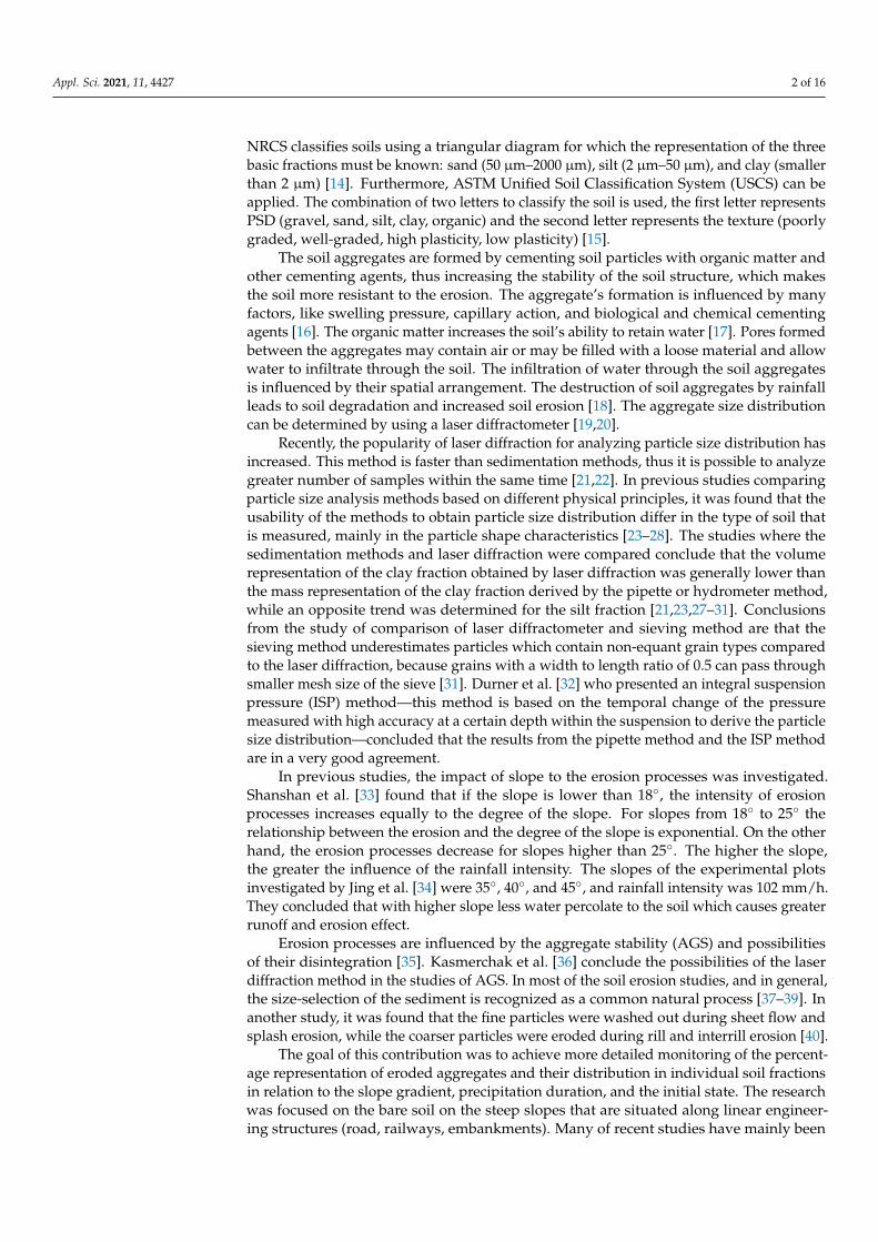
Three experimental containers were created, on which a rainfall simulator (detaileddescription in Vanícek et al. [41]) with pulse nozzle system type WSQ 40 was installed thatenabled us to sprinkle them with artificial heavy rain with an intensity of 113 mm/h. Theheight of the raindrop falling head was 2.5 m. The control unit was capable of fixing thewater pressure to ensure required rainfall characteristics [42]. The drop size resemblednatural rain [41,43]. The slopes of the containers with the soil were set according to the limitslopes for the embankment and notch constructions according to Czech Technical Standard,namely 1:1.5 (34◦), 1:1.75 (30◦), and 1:2.5 (22◦) [44]. From the experimental plots (Figure 1),each one of them measuring 4.25 × 1 m, and overall 156 soil samples were collected.
2.2. Sampling Procedure
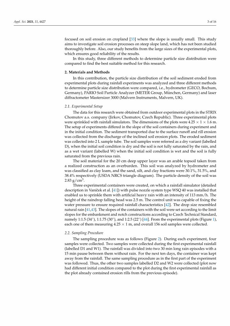
The sampling procedure was as follows (Figure 2). During each experiment, foursamples were collected. Two samples were collected during the first experimental rainfall(labelled D1 and W1). The rainfall was divided into two 30 min long rain episodes with a15 min pause between them without rain. For the next ten days, the container was keptaway from the rainfall. The same sampling procedure as in the first part of the experimentwas followed. Thus, the other two samples labelled D2 and W2 were collected (plot nowhad different initial condition compared to the plot during the first experimental rainfall asthe plot already contained erosion rills from the previous episode).
Appl. Sci. 2021, 11, 4427 4 of 16Appl. Sci. 2021, 11, x FOR PEER REVIEW 4 of 16
Figure 1. Experimental plots. Slope 34°, 30° and 22°. Dimensions 4.25 × 1 × 1.6 m. Rainfall simula-tor pulse nozzle system type WSQ 40. Location–Jirkov.
2.2. Sampling Procedure The sampling procedure was as follows (Figure 2). During each experiment, four
samples were collected. Two samples were collected during the first experimental rainfall (labelled D1 and W1). The rainfall was divided into two 30 min long rain episodes with a 15 min pause between them without rain. For the next ten days, the container was kept away from the rainfall. The same sampling procedure as in the first part of the experiment was followed. Thus, the other two samples labelled D2 and W2 were collected (plot now had different initial condition compared to the plot during the first experimental rainfall as the plot already contained erosion rills from the previous episode).
The first initial state D1 corresponds to the conditions when the structure is finished. W1 is the state when the soil profile is fully saturated. After 10 days, the soil in the con-tainer dried out to the field capacity. The initial states D2 and W2 represent a repeated event. Erosion rills had occurred already after the first part of the experiment (D1). For each slope, at least 35 soil samples were collected.
Figure 2. Scheme of the sampling procedure at the experimental plots.
2.3. Evaluation of Soil Samples—Particle Size Distribution To find an optimal method for the particle size distribution measurement for our re-
search, three methods were compared: hydrometer, PARIO Soil Particle Analyzer (ME-TER Group, München, Germany), and laser diffractometer Mastersizer 3000 (Malvern In-struments, Malvern, UK). The hydrometer and the PARIO are indirect gravitational sedi-mentation methods based on Stokes’ law [45] to determine particle size distribution.
Figure 1. Experimental plots. Slope 34◦, 30◦ and 22◦. Dimensions 4.25 × 1 × 1.6 m. Rainfall simulatorpulse nozzle system type WSQ 40. Location–Jirkov.
Appl. Sci. 2021, 11, x FOR PEER REVIEW 4 of 16
Figure 1. Experimental plots. Slope 34°, 30° and 22°. Dimensions 4.25 × 1 × 1.6 m. Rainfall simula-tor pulse nozzle system type WSQ 40. Location–Jirkov.
2.2. Sampling Procedure The sampling procedure was as follows (Figure 2). During each experiment, four
samples were collected. Two samples were collected during the first experimental rainfall (labelled D1 and W1). The rainfall was divided into two 30 min long rain episodes with a 15 min pause between them without rain. For the next ten days, the container was kept away from the rainfall. The same sampling procedure as in the first part of the experiment was followed. Thus, the other two samples labelled D2 and W2 were collected (plot now had different initial condition compared to the plot during the first experimental rainfall as the plot already contained erosion rills from the previous episode).
The first initial state D1 corresponds to the conditions when the structure is finished. W1 is the state when the soil profile is fully saturated. After 10 days, the soil in the con-tainer dried out to the field capacity. The initial states D2 and W2 represent a repeated event. Erosion rills had occurred already after the first part of the experiment (D1). For each slope, at least 35 soil samples were collected.
Figure 2. Scheme of the sampling procedure at the experimental plots.
2.3. Evaluation of Soil Samples—Particle Size Distribution To find an optimal method for the particle size distribution measurement for our re-
search, three methods were compared: hydrometer, PARIO Soil Particle Analyzer (ME-TER Group, München, Germany), and laser diffractometer Mastersizer 3000 (Malvern In-struments, Malvern, UK). The hydrometer and the PARIO are indirect gravitational sedi-mentation methods based on Stokes’ law [45] to determine particle size distribution.
Figure 2. Scheme of the sampling procedure at the experimental plots.
The first initial state D1 corresponds to the conditions when the structure is finished.W1 is the state when the soil profile is fully saturated. After 10 days, the soil in the containerdried out to the field capacity. The initial states D2 and W2 represent a repeated event.Erosion rills had occurred already after the first part of the experiment (D1). For each slope,at least 35 soil samples were collected.
2.3. Evaluation of Soil Samples—Particle Size Distribution
To find an optimal method for the particle size distribution measurement for ourresearch, three methods were compared: hydrometer, PARIO Soil Particle Analyzer (ME-TER Group, München, Germany), and laser diffractometer Mastersizer 3000 (MalvernInstruments, Malvern, UK). The hydrometer and the PARIO are indirect gravitationalsedimentation methods based on Stokes’ law [45] to determine particle size distribution.PARIO is an automated system which uses ISP method [32,46]. Laser diffractometer Mas-tersizer 3000 provided by Malvern Panalytical allows an exact evaluation of the samplescontaining soil aggregates and also samples without soil aggregates. The aggregates weredestroyed during the measurement by ultrasound [47–49]. The hydrometer and PARIOmeasurements were supplemented by a sieving method. The methods were tested onfive samples. From the comparison of the methods, the laser diffraction was found as themost suitable method for our further research, thus all remaining samples were analyzedonly by the LD. By the comparison of the particle and aggregate size distribution, theinfluence of the following external factors was investigated: initial state and slope of theexperimental plots.
Appl. Sci. 2021, 11, 4427 5 of 16
2.3.1. Sedimentation Methods
The preparation of the soil samples for the particle size analysis by the hydrometerand the PARIO was identical. In a bosh, 40 g of air-dried soil sediment together with40 mL of sodium hexametaphosphate was boiled for 15 min. Thus, the soil aggregateswere destroyed and the fraction content greater than 100 µm was separated. This fractionwas oven dried at 105 ◦C, sieved, and weighed. Mesh sizes of the sieves were 2000 µm,1250 µm, 1000 µm, 800 µm, 500 µm, 250 µm, and 100 µm. The suspension of fine particlessmaller than 100 µm was filled with distilled water in graduated cylinder to reach thevolume of 1000 mL [23,50]. Suspension was analyzed by hydrometer and after that, thesame suspension was analyzed by the PARIO.
Analysis by the hydrometer continued with suspension mixing and registering ofits temperature. The end of the mixing determined the beginning of the sedimentationprocess, and the hydrometer was put into the suspension. Hydrometer readings wererecorded at intervals of 30 s, 1 min, 2 min, 5 min, 10 min, 25 min, 50 min, 75 min, 2.5 h,24 h, and 48 h from the beginning of the sedimentation process. Finally, the particle sizedistribution curves were manually calculated using the hydrometer readings and sieveanalysis data [50].
Before the measurement by PARIO, the duration parameter—8 h—and timer forhomogenization parameter—60 s—were set in the PARIO Control software. Besides thesuspension with the soil sample, the graduated cylinder with distilled water was needed.In both of them, the room temperature was the same. The PARIO device was immersed intothe distilled water for ten minutes calibrate to temperature. The suspension with the soilsample was mixed for 60 s and the PARIO device was then moved from the distilled waterto the suspension. Automated measurement was begun. It took 8 h, and the temperatureand the pressure were recorded every 10 s. While the results from the sieving analysis weremanually entered to the software, the particle size distribution curves were automaticallycalculated [46].
2.3.2. Laser Diffractometer—Mastersizer 3000
The Mastersizer 3000 uses optical model Mie theory, which is recommended by ISO13320 for particles smaller than 50 µm. Mie theory is based on Maxwell’s electromagneticfield equations and provides solution for the calculation of particle size distribution fromlight scattering data. To obtain accurate results, which the Malvern software calculatesbased on the data from the laser diffractometer, information about the analyzed materialand dispersion medium (refractive and absorption indices which characterize the passageof light through) must be entered before the measurement starts [49].
Silica (SiO2), which has the most similar properties to soil, was selected as a referentialmaterial from the software database. Based on the selected material, the software assignedvalues for the refractive index, 1.457 [22], and the absorption index, 0.010. Water wasselected as a dispersion medium with a refractive index value of 1.33. Adjusted valueswere in agreement with the user manual [49].
The air dried soil sediment was and thoroughly mixed before the measurement toensure its representativeness. For 40 s, the background data of distilled water was measured.To a beaker of 550 mL distilled water, the amount of the soil sample (approximatelyone gram) was added in order to achieve the concentration required by the software(obscuration 10–30%).
The analysis of each sample was set up to run 25 records for 20 s each. Laser beamscattering information was recorded during these measurements. During the first fiverecords, the soil sample with aggregates was analyzed. Then, the ultrasound was manuallystarted. Ryzak et al. [20] adduced that 4 min of ultrasound application is enough to destroyall soil aggregates, and that there is no upper limit whose exceeding could cause breakingof the particles themselves. Accordingly, the time of active ultrasound was set to 320 s. Bythis time soil aggregates had been destroyed, and the five records after ultrasound werecarried out on the soil sample, already without aggregates.
Appl. Sci. 2021, 11, 4427 6 of 16
Faé et al. [51] found that only one reading per sample is sufficient. Therefore, forfurther comparison of the particle size analysis, two curves from analysis of each soilsample were used—the average of the first five (soil with aggregates) and the average ofthe last five records (soil with already destroyed aggregates).
3. Results
The results obtained by measuring the particle and aggregate size distribution of thesoil sediment are represented by the dependency graphs of cumulative volume on particlesize distribution. The x-axes of these graphs are displayed in a logarithmic scale.
Three particle size values to evaluate the data were selected: <2 µm, <10 µm, and<50 µm. These boundaries were chosen on the basis of the commonly used soil classificationsystems according to their particle size. The 2 µm value determined the boundaries of thetriangular diagram fractions—NRCS USDA [15]. The 10 µm value is used in the Novak’sclassification system to classify the soil type [14]. The 50 µm value is again the boundaryof the triangular diagram. The numerical representation of the PSD curves is shown inthe tables where the median and standard deviation (SD) values for particles smaller than2 µm, 10 µm, and 50 µm are presented.
3.1. Comparison of Three Tested Methods
The PSD curves of five randomly selected samples (Samples 1–5) obtained by all threemethods are shown in Figure 3. In Appendix A, Tables A1–A3 show the representationof the particles smaller than 2, 10, and 50 µm for all particle size curves obtained by thecompared methods. The representation of particles smaller than 2, 10, and 50 µm wereaveraged and compared in Table 1. Overall, the least differences are between the resultsfrom the laser diffractometer and the PARIO, especially the results for the fraction contentsmaller than 2 µm are very similar (difference 6%). Sedimentation methods are close toeach other in fraction content smaller than 50 µm (difference 4%), but comparing bothof them to the laser diffractometer there were large differences (18% and 14%) for thisfraction. Results for the fraction content smaller than 2 µm obtained by the hydrometerdiffer significantly compared to those from the laser diffractometer (by 22%) and PARIO(by 16%). The comparison showed that the volume representation of the fraction smallerthan 2 µm measured by the laser diffractometer was generally lower than the volumerepresentation analyzed by hydrometer (by 22%) and PARIO (by 6%). On the other hand,the fraction content smaller than 50 µm s lower for the sedimentation methods (by 18%and 14%).
Table 1. Comparison of average differences of representation of particles smaller than 2, 10 and50 µm between three tested methods (±SD), differences between the results for methods in the firstand the last column.
Method <2 µm <10 µm <50 µm Method
LD −22 ± 9% −4 ± 7% 18 ± 2% HydrometerLD −6 ± 9% 11 ± 10% 14 ± 5% PARIO
PARIO 16 ± 8% 15 ± 9% −4 ± 4% Hydrometer

Appl. Sci. 2021, 11, 4427 7 of 16Appl. Sci. 2021, 11, x FOR PEER REVIEW 7 of 16
Figure 3. Comparison of PSD curves of soil samples measured by three tested methods–LD (black, solid), hydrometer (red, dashed) and PARIO (blue, dotted): (a) Sample 1; (b) Sample 2; (c) Sample; (d) Sample 4; (e) Sample 5.
Table 1. Comparison of average differences of representation of particles smaller than 2, 10 and 50 μm between three tested methods (±SD), differences between the results for methods in the first and the last column.
Method <2 μm <10 μm <50 μm Method LD −22 ± 9% −4 ± 7% 18 ± 2% Hydrometer LD −6 ± 9% 11 ± 10% 14 ± 5% PARIO
PARIO 16 ± 8% 15 ± 9% −4 ± 4% Hydrometer
3.2. Samples with and without Soil Aggregates At the beginning, all data were first analyzed in terms of the number of particles that
form soil aggregates, independently of other variables. Graphical representation of statis-tical analysis of PSD of all 156 collected samples is shown in Appendix A in Figure A1.
Table 2 shows all measured particle and aggregate size distribution analysis of 156 soil samples collected from experimental location with and without aggregates. The table shows that the samples, after destruction of the soil aggregates, contain finer particles compared to the samples before destruction of the aggregates, and that the particle size distribution curves after destroying aggregates for particles smaller than 10 and 50 μm have smaller standard deviation than those before its destruction —the SD for particles smaller than 10 and 50 μm was 8.4 and 3.4 for samples without soil aggregates and 13.1 and 16.7 for samples with aggregates, respectively. Graphical representation of statistical analysis of PSD of all 156 collected samples is shown in Appendix A in Figure A1.
Figure 3. Comparison of PSD curves of soil samples measured by three tested methods–LD (black, solid), hydrometer (red,dashed) and PARIO (blue, dotted): (a) Sample 1; (b) Sample 2; (c) Sample; (d) Sample 4; (e) Sample 5.
3.2. Samples with and without Soil Aggregates
At the beginning, all data were first analyzed in terms of the number of particlesthat form soil aggregates, independently of other variables. Graphical representation ofstatistical analysis of PSD of all 156 collected samples is shown in Appendix A in Figure A1.
Table 2 shows all measured particle and aggregate size distribution analysis of 156 soilsamples collected from experimental location with and without aggregates. The tableshows that the samples, after destruction of the soil aggregates, contain finer particlescompared to the samples before destruction of the aggregates, and that the particle sizedistribution curves after destroying aggregates for particles smaller than 10 and 50 µmhave smaller standard deviation than those before its destruction—the SD for particlessmaller than 10 and 50 µm was 8.4 and 3.4 for samples without soil aggregates and 13.1and 16.7 for samples with aggregates, respectively. Graphical representation of statisticalanalysis of PSD of all 156 collected samples is shown in Appendix A in Figure A1.
Table 2. LD method. Statistical analysis (median and standard deviation) of PSD of all 156 collectedsamples [%].
With Aggregates Without Aggregates
Median ± SD<2 µm 4.3 ± 3.5 18.2 ± 6.9
<10 µm 21.7 ± 13.1 50.5 ± 8.4
<50 µm 52.0 ± 16.7 91.3 ± 3.4
Appl. Sci. 2021, 11, 4427 8 of 16
3.3. Influence of Initial Condition and Slopes of the Experimental Plots
Tables 3–5 show statistical analysis of particle size distribution curves for each slopeseparately. Graphical representation of these tables is shown in Appendix A in Figure A1.A table representing average statistical analysis of all three slopes is shown in Appendix A(Table A4). The SD of the particle size distribution curves before destroying aggregates wasgenerally higher—the highest for the particles with aggregates smaller than 50 µm (SD ofthe particles smaller than 50 µm from the slope of 22◦—5.8, 9.3, 6.8, and 6.9 for samples D1,W1, D2, and W2, respectively) compared to the curves without aggregates.
Table 3. Statistical analysis (median and standard deviation) of influence of initial conditions to the particle size distribution(obtained by LD) for the samples from the plot with slope 22◦ [%].
With Aggregates Without AggregatesD1 W1 D2 W2 D1 W1 D2 W2
Median ± SD
<2 µm 5.2 ± 1.5 3.5 ± 1.7 5.0 ± 2.5 3.0 ± 1.3 17.9 ± 1.9 16.2 ± 7.7 18.0 ± 3.8 17.3 ± 7.0
<10 µm 22.4 ± 4.0 20.1 ± 4.3 22.0 ± 5.4 19.3 ± 4.5 49.6 ± 1.3 48.4 ± 5.0 50.5 ± 2.9 49.1 ± 4.6
<50 µm 50.5 ± 5.8 51.7 ± 9.3 52.4 ± 6.8 47.8 ± 6.9 91.3 ± 1.1 91.3 ± 1.9 90.9 ± 1.2 91.1 ± 1.0
Table 4. Statistical analysis (median and standard deviation) of influence of initial conditions to the particle size distribution(obtained by LD) for the samples from the plot with slope 30◦ [%].
With Aggregates Without AggregatesD1 W1 D2 W2 D1 W1 D2 W2
Median ± SD
<2 µm 4.0 ± 1.8 3.5 ± 0.9 5.5 ± 1.9 3.9 ± 1.7 22.8 ± 4.2 17.5 ± 6.6 19.0 ± 3.7 16.9 ± 4.0
<10 µm 20.3 ± 2.3 19.5 ± 3.0 22.4 ± 4.7 20.0 ± 3.6 54.2 ± 3.0 48.6 ± 4.7 49.7 ± 2.2 48.2 ± 2.6
<50 µm 46.9 ± 4.6 47.5 ± 6.9 47.5 ± 6.7 49.0 ± 4.5 92.4 ± 1.2 90.6 ± 1.5 91.2 ± 0.9 90.9 ± 2.1
Table 5. Statistical analysis (median and standard deviation) of influence of initial conditions to the particle size distribution(obtained by LD) for the samples from the plot with slope 34◦ [%].
With Aggregates Without AggregatesD1 W1 D2 W2 D1 W1 D2 W2
Median ± SD
<2 µm 5.3 ± 1.6 4.0 ± 2.9 4.3 ± 2.1 3.9 ± 1.1 19.5 ± 6.8 15.9 ± 2.4 15.4 ± 6.4 14.9 ± 4.6
<10 µm 23.0 ± 3.5 20.4 ± 6.5 21.9 ± 4.6 21.2 ± 3.1 52.0 ± 4.8 48.3 ± 3.1 46.5 ± 4.7 46.7 ± 3.8
<50 µm 52.7 ± 4.2 52.7 ± 9.8 55.4 ± 5.8 53.4 ± 5.2 90.7 ± 2.1 89.8 ± 1.8 90.3 ± 1.5 89.5 ± 2.2
For the samples with aggregates from all three slopes, samples D1 and D2 had moreparticles smaller than 2 µm compared to the samples W1 and W2. The representationof the particles smaller than 10 µm had the same trend. At slopes of 22◦ and 30◦, therepresentation of particles smaller than 50 µm for samples with aggregates became higherwith later sampling time, with the exception of the samples eroded last, W2.
For the samples without aggregates from the slopes of 22◦ and 30◦, samples D1 and D2had more particles smaller than 2 µm compared to the samples W1 and W2; representationof the particles smaller than 10 µm had also the same trend. For the samples withoutaggregates eroded from the 34◦ slope, the representation of the particles smaller than 2and 10 µm became lower with later sampling time. For the slopes of 30◦ and 34◦, samplesD1 and D2 without aggregates had more particles smaller than 50 µm compared to thesamples W1 and W2.
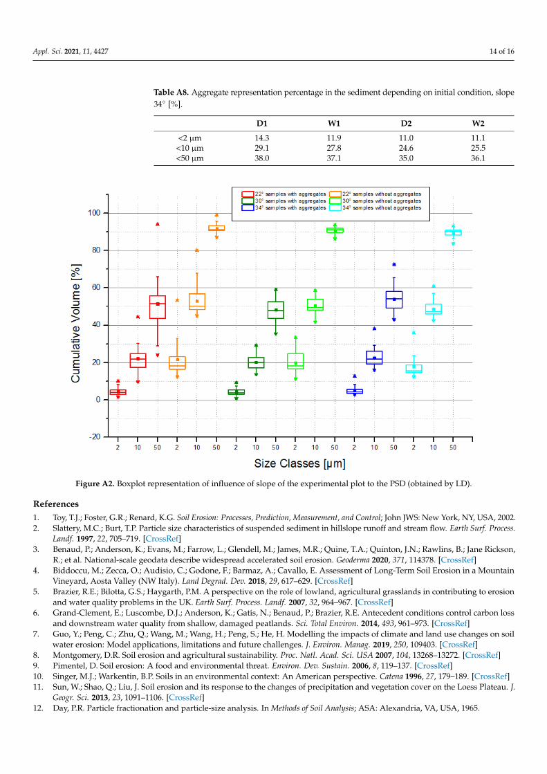
The influence of the slope of the soil container on the aggregate representation percent-age in the soil sediment was examined. Graphical representation of statistical analysis ofPSD of samples collected from each slope is shown in Appendix A in Figure A2. Tables 3–5,the tables representing difference of the median values with and without aggregates for
Appl. Sci. 2021, 11, 4427 9 of 16
each fraction size were created (Tables A6–A8). The difference shows aggregate represen-tation percentage in the sample. It is shown that with a later sampling time the medianvalues of aggregate representation decreased on the 30◦and 34◦ slopes and increased onthe 22◦ slope. Furthermore, for particles smaller than 2 and 10 µm, the largest differencesduring the first part of the experiments (D1 and W1) had samples eroded from the slope30◦ (18.8%, 14.1%, 34.0%, and 29.1%, respectively), while during the second part (D2 andW2) it was the samples from the 22◦ slope (13.0%, 14.3% and 28.4%, 29.8%, respectively).For the particles smaller than 50 µm, the samples from the slope 34◦ exhibited the leastdifferences (38.0%, 37.1%, 35.0%, and 36.1% for samples D1, W1, D2, and W2, respectively)and the samples from the slope 30◦ the largest differences (45.5%, 43.1%, 43.7%, and 42.0%for samples D1, W1, D2, and W2, respectively).
4. Discussion
The research presented here had two main goals. The first one was to determinethe limits of using the methods to analyze PSD for estimation the intensity of the erosionprocess on artificial slopes. The second goal was the actual analysis of the PSD andaggregate percentage representation of eroded soil samples in relation to external factors(slope, initial soil water content).
4.1. Comparison of Three Tested Methods
From the mutual comparison of the three methods tested, it is obvious that the resultsfrom the hydrometer are overestimated compared to the other two methods and suggestthat the number of particles finer than 1 µm is almost 40% in all tested soil samples,which corresponds to the PSD analysis of the original soil. The shape of the particle sizedistribution curves obtained by the PARIO is similar to those from laser diffractometer,while the curves with a linear trend obtained from the hydrometer differ; see Figure 3.
The representation of particles smaller than 2, 10, and 50 µm were compared in Table 1.It was found that the fraction smaller than 2 µm obtained by the LD was lower comparedto the sedimentation method, and the fraction smaller than 50 µm had an opposite result.This confirms the conclusions from the previous studies [21,23,27–31] which state that thelaser diffraction underestimates the clay fraction content and overestimates the silt fractioncontent. Furthermore, it was found that LD and hydrometer gave very similar results forparticle size <10 µm. Note that this value is a boundary used in the Novak’s classificationsystem [14].
The time required for the methods tested varies greatly. To determine the PSD usingboth the hydrometer and the PARIO, the standard sample preparation is required beforethe measurement to destroy soil aggregates and separate the fine fraction from the sandfraction. This preparation takes about 25 min per sample. In addition, a sieve analysisrequired for the sand fraction of each sample takes another 10 min. The hydrometermeasurement takes 48 h and the PARIO measurement takes 8 h for one sample. However,in 2021 the METER Group developed the innovative device PARIO Plus which can reducethe analysis time to 2.5 h [46]. The PSD analysis by the LD requires no prior preparation ofthe soil sample except for thorough mixing. The particle size distribution is analyzed for15 min per sample. Evaluation of the PSD of all 156 samples by LD took 39 h. If the PARIOwas used for the particle size analysis of all samples, the total measurement time wouldbe 340 h and the hydrometer evaluation would take 1590 h, i.e., more than 66 days (if fivePARIO devices and five hydrometers were used).
The main advantage of using of the laser diffractometer is that the soil aggregates aredestroyed during the measurement by ultrasound which is sufficient and a very time anduser-friendly method [20]. Also, the particle size can be analyzed before the aggregatesare destroyed. Such results are satisfying thanks to the principles of laser diffraction. Onthe other hand, the sample preparation for the hydrometer and PARIO measurementsis demanding and analysis of the soil samples with aggregates using sedimentationsprinciples (Stokes’ law) has physical imperfections.
Appl. Sci. 2021, 11, 4427 10 of 16
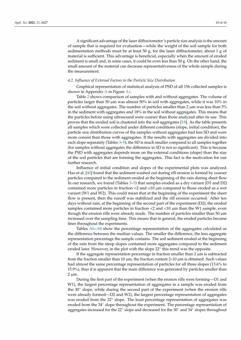
A significant advantage of the laser diffractometer’s particle size analysis is the amountof sample that is required for evaluation—while the weight of the soil sample for bothsedimentation methods must be at least 50 g, for the laser diffractometer, about 1 g ofmaterial is sufficient. This advantage is beneficial, especially when the amount of erodedsediment is small and, in some cases, it could be even less than 50 g. On the other hand, thesmall amount of the material can decrease representativeness of the whole sample duringthe measurement.
4.2. Influence of External Factors to the Particle Size Distribution
Graphical representation of statistical analysis of PSD of all 156 collected samples isshown in Appendix A in Figure A1.
Table 2 shows comparison of samples with and without aggregates. The volume ofparticles larger than 50 µm was almost 50% in soil with aggregates, while it was 10% inthe soil without aggregates. The number of particles smaller than 2 µm was less than 5%in the sediment with aggregates and 18% in the soil without aggregates. This means thatthe particles before using ultrasound were coarser than those analyzed after its use. Thisproves that the eroded soil is clustered into the soil aggregates [18]. As the table presentsall samples which were collected under different conditions (slope, initial condition), theparticle size distribution curves of the samples without aggregates had less SD and weremore consist than those with aggregates. If the results with aggregates are divided intoeach slope separately (Tables 3–5), the SD is much smaller compared to all samples together(for samples without aggregates the difference in SD is not so significant). This is becausethe PSD with aggregates depends more on the external conditions (slope) than the sizeof the soil particles that are forming the aggregates. This fact is the motivation for ourfurther research.
Influence of initial condition and slopes of the experimental plots was analyzed.Hao et al. [40] found that the sediment washed out during rill erosion is formed by coarserparticles compared to the sediment eroded at the beginning of the rain during sheet flow.In our research, we found (Tables 3–5) that samples eroded as a dry variant (D1 and D2)contained more particles in fraction <2 and <10 µm compared to those eroded as a wetvariant (W1 and W2). This could mean that at the beginning of the experiment the sheetflow is present, then the runoff was stabilized and the rill erosion occurred. After tendays without rain, at the beginning of the second part of the experiment (D2), the erodedsamples contained more particles in fraction <2 and <10 µm than the W1 sample, eventhough the erosion rills were already made. The number of particles smaller than 50 µmincreased over the sampling time. This means that in general, the eroded particles becamefiner throughout the experiments.
Tables A6–A8 show the percentage representation of the aggregates calculated asthe difference between the median values. The smaller the difference, the less aggregaterepresentation percentage the sample contains. The soil sediment eroded at the beginningof the rain from the steep slopes contained more aggregates compared to the sedimenteroded later. However, in the plot with the slope 22◦ this trend was the opposite.
If the aggregate representation percentage in fraction smaller than 2 µm is subtractedfrom the fraction smaller than 10 µm, the fraction content 2–10 µm is obtained. Such valueshad almost the same percentage representation of particles for all three slopes (13.6% to15.9%), thus it is apparent that the main difference was generated by particles smaller than2 µm.
During the first part of the experiment (when the erosion rills were forming—D1 andW1), the largest percentage representation of aggregates in a sample was eroded fromthe 30◦ slope, while during the second part of the experiment (when the erosion rillswere already formed—D2 and W2), the largest percentage representation of aggregateswas eroded from the 22◦ slope. The least percentage representation of aggregates waseroded from the 34◦ slope throughout the experiment. The percentage representation ofaggregates increased for the 22◦ slope and decreased for the 30◦ and 34◦ slopes throughout
Appl. Sci. 2021, 11, 4427 11 of 16
the experiment. This means that for steep slopes, the rill erosion was present and onlysmaller percentage representation of aggregates was eroded.
Samples without soil aggregates contained smaller particles from the 30◦ slope com-pared to the 22◦ slope. However, the particles eroded from the extreme 34◦ slope gradientused in our research was the finest compared to the less steep slopes. This result agreeswith Shanshan et al. [33], who concluded that on the steep slopes (higher than 25◦) theerosion processes decrease.
5. Conclusions
During our research, it was found that the method that uses the rainfall simulatorswhere the eroded sediment is collected and then analyzed by laser diffraction to obtain theparticle size distribution data is a suitable method to evaluate the impact of the externalfactors to the particle size distribution of the eroded soil sediment.
The main advantages of the laser diffractometer Mastersizer 3000 compared to thehydrometer and the PARIO are the very short evaluating time of 15 min per sample, thesmall amount of required sample at 1 g, and its ability to comfortably and relevantlyanalyze soil samples both with and without soil aggregates.
When the soil is fully saturated and the erosion rills are made, the samples containedcoarser particles than the samples eroded during the sheet flow. Also, in general, theeroded particles had become finer throughout the experiments.
Generally, when the erosion processes were intensive (steep slope or long durationof the raining), the eroded sediment contained coarser particles and lower amounts ofthe aggregates.
For further research, it would be interesting to study aggregates content on moresamples obtained from plots with different soil types or with different rainfall intensities,and also to analyze PSD results in the context of volume of the surface runoff and theformation of the rills.
Author Contributions: Conceptualization, R.K. and P.K.; Data curation, M.N. and P.K.; Formalanalysis, R.K.; Investigation, R.K.; Methodology, R.K., M.N. and P.K.; Software, M.N.; Supervision,P.K.; Writing—original draft, R.K.; Writing—review & editing, M.N. and P.K. All authors have readand agreed to the published version of the manuscript.
Funding: This research was funded by the TH02030428—“Design of technical measures for slopes sta-bilization and soil erosion prevention”. And by the international CTU grant SGS20/156/OHK1/3T/11.
Institutional Review Board Statement: The study was conducted according to the guidelines of theDeclaration of Helsinki, and approved by the Institutional Review Board (or Ethics Committee) ofCTU in Prague.
Informed Consent Statement: Informed consent was obtained from all subjects involved in the study.
Data Availability Statement: The data that support the findings of this study are available on requestfrom the corresponding author.
Conflicts of Interest: The authors declare no conflict of interest and the funders had no role inthe design of the study; in the collection, analyses, or interpretation of data; in the writing of themanuscript, or in the decision to publish the results.
Appl. Sci. 2021, 11, 4427 12 of 16
Appendix A
Table A1. Representation of the particles smaller than 2 µm obtained by three tested methods.
LD Hydrometer PARIO
Sample 1 26% 40% 16%Sample 2 10% 42% 19%Sample 3 12% 41% 29%Sample 4 16% 43% 22%Sample 5 33% 42% 40%
Table A2. Representation of the particles smaller than 10 µm obtained by three tested methods.
LD Hydrometer PARIO
Sample 1 56% 51% 29%Sample 2 42% 53% 32%Sample 3 42% 53% 41%Sample 4 50% 56% 34%Sample 5 59% 57% 57%
Table A3. Representation of the particles smaller than 50 µm obtained by three tested methods.
LD Hydrometer PARIO
Sample 1 91% 70% 70%Sample 2 88% 70% 75%Sample 3 86% 71% 79%Sample 4 92% 72% 80%Sample 5 91% 74% 73%
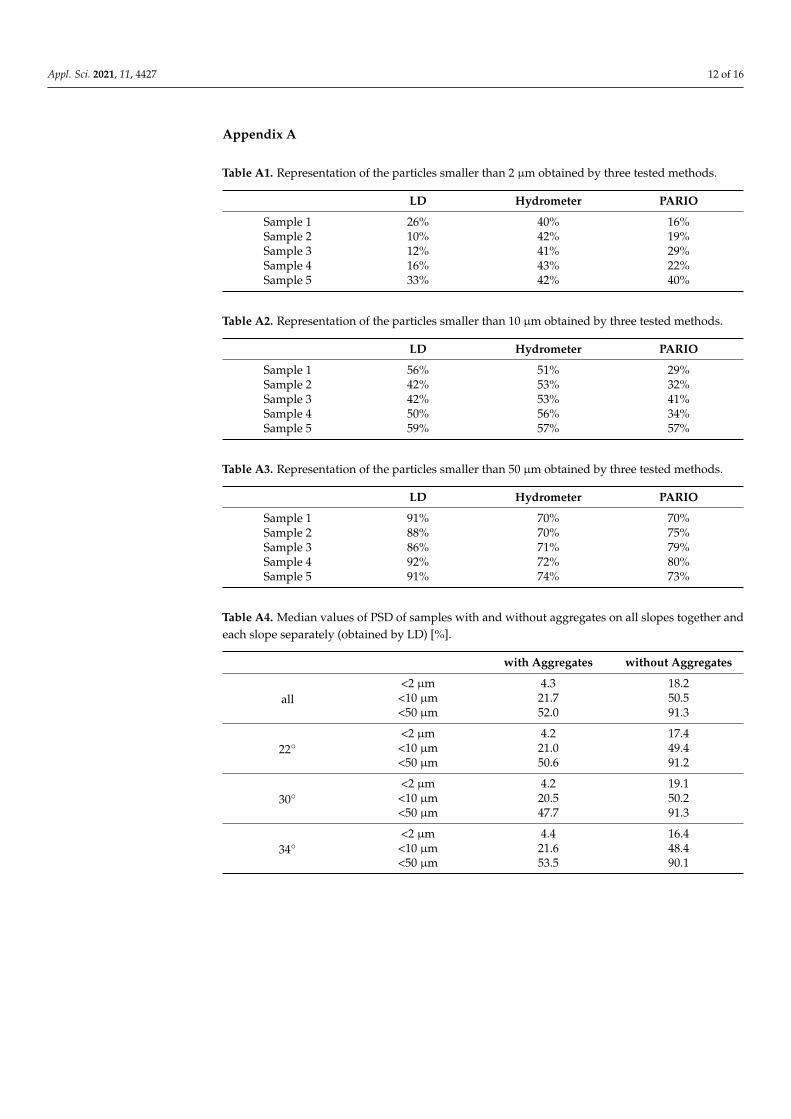
Table A4. Median values of PSD of samples with and without aggregates on all slopes together andeach slope separately (obtained by LD) [%].
with Aggregates without Aggregates
all<2 µm 4.3 18.2
<10 µm 21.7 50.5<50 µm 52.0 91.3
22◦<2 µm 4.2 17.4
<10 µm 21.0 49.4<50 µm 50.6 91.2
30◦<2 µm 4.2 19.1
<10 µm 20.5 50.2<50 µm 47.7 91.3
34◦<2 µm 4.4 16.4
<10 µm 21.6 48.4<50 µm 53.5 90.1
Appl. Sci. 2021, 11, 4427 13 of 16
Appl. Sci. 2021, 11, x FOR PEER REVIEW 13 of 16
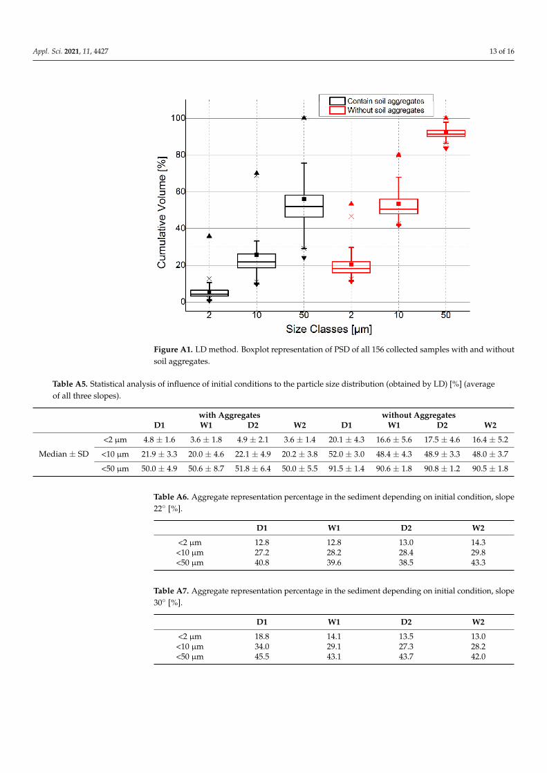
Figure A1. LD method. Boxplot representation of PSD of all 156 collected samples with and without soil aggregates.
Table A5. Statistical analysis of influence of initial conditions to the particle size distribution (obtained by LD) [%] (average of all three slopes).
with Aggregates without Aggregates D1 W1 D2 W2 D1 W1 D2 W2
Median ± SD <2 μm 4.8 ± 1.6 3.6 ± 1.8 4.9 ± 2.1 3.6 ± 1.4 20.1 ± 4.3 16.6 ± 5.6 17.5 ± 4.6 16.4 ± 5.2
<10 μm 21.9 ± 3.3 20.0 ± 4.6 22.1 ± 4.9 20.2 ± 3.8 52.0 ± 3.0 48.4 ± 4.3 48.9 ± 3.3 48.0 ± 3.7 <50 μm 50.0 ± 4.9 50.6 ± 8.7 51.8 ± 6.4 50.0 ± 5.5 91.5 ± 1.4 90.6 ± 1.8 90.8 ± 1.2 90.5 ± 1.8
Table A6. Aggregate representation percentage in the sediment depending on initial condition, slope 22° [%].
D1 W1 D2 W2 <2 μm 12.8 12.8 13.0 14.3
<10 μm 27.2 28.2 28.4 29.8 <50 μm 40.8 39.6 38.5 43.3
Table A7. Aggregate representation percentage in the sediment depending on initial condition, slope 30° [%].
D1 W1 D2 W2 <2 μm 18.8 14.1 13.5 13.0
<10 μm 34.0 29.1 27.3 28.2 <50 μm 45.5 43.1 43.7 42.0
Figure A1. LD method. Boxplot representation of PSD of all 156 collected samples with and withoutsoil aggregates.
Table A5. Statistical analysis of influence of initial conditions to the particle size distribution (obtained by LD) [%] (averageof all three slopes).
with Aggregates without AggregatesD1 W1 D2 W2 D1 W1 D2 W2
Median ± SD
<2 µm 4.8 ± 1.6 3.6 ± 1.8 4.9 ± 2.1 3.6 ± 1.4 20.1 ± 4.3 16.6 ± 5.6 17.5 ± 4.6 16.4 ± 5.2
<10 µm 21.9 ± 3.3 20.0 ± 4.6 22.1 ± 4.9 20.2 ± 3.8 52.0 ± 3.0 48.4 ± 4.3 48.9 ± 3.3 48.0 ± 3.7
<50 µm 50.0 ± 4.9 50.6 ± 8.7 51.8 ± 6.4 50.0 ± 5.5 91.5 ± 1.4 90.6 ± 1.8 90.8 ± 1.2 90.5 ± 1.8
Table A6. Aggregate representation percentage in the sediment depending on initial condition, slope22◦ [%].
D1 W1 D2 W2
<2 µm 12.8 12.8 13.0 14.3<10 µm 27.2 28.2 28.4 29.8<50 µm 40.8 39.6 38.5 43.3
Table A7. Aggregate representation percentage in the sediment depending on initial condition, slope30◦ [%].
D1 W1 D2 W2
<2 µm 18.8 14.1 13.5 13.0<10 µm 34.0 29.1 27.3 28.2<50 µm 45.5 43.1 43.7 42.0
Appl. Sci. 2021, 11, 4427 14 of 16
Table A8. Aggregate representation percentage in the sediment depending on initial condition, slope34◦ [%].
D1 W1 D2 W2
<2 µm 14.3 11.9 11.0 11.1<10 µm 29.1 27.8 24.6 25.5<50 µm 38.0 37.1 35.0 36.1
Appl. Sci. 2021, 11, x FOR PEER REVIEW 14 of 16
Table A8. Aggregate representation percentage in the sediment depending on initial condition, slope 34° [%].
D1 W1 D2 W2 <2 μm 14.3 11.9 11.0 11.1
<10 μm 29.1 27.8 24.6 25.5 <50 μm 38.0 37.1 35.0 36.1
Figure A2. Boxplot representation of influence of slope of the experimental plot to the PSD (obtained by LD).
References 1. Toy, T.J.; Foster, G.R.; Renard, K.G. Soil Erosion: Processes, Prediction, Measurement, and Control; John JWS: New York, NY, USA,
2002. 2. Slattery, M.C.; Burt, T.P. Particle size characteristics of suspended sediment in hillslope runoff and stream flow. Earth Surf.
Process. Landf. 1997, 22, 705–719. 3. Benaud, P.; Anderson, K.; Evans, M.; Farrow, L.; Glendell, M.; James, M.R.; Quine, T.A.; Quinton, J.N.; Rawlins, B.; Jane Rickson,
R.; et al. National-scale geodata describe widespread accelerated soil erosion. Geoderma 2020, 371, 114378. 4. Biddoccu, M.; Zecca, O.; Audisio, C.; Godone, F.; Barmaz, A.; Cavallo, E. Assessment of Long-Term Soil Erosion in a Mountain
Vineyard, Aosta Valley (NW Italy). Land Degrad. Dev. 2018, 29, 617–629. 5. Brazier, R.E.; Bilotta, G.S.; Haygarth, P.M. A perspective on the role of lowland, agricultural grasslands in contributing to ero-
sion and water quality problems in the UK. Earth Surf. Process. Landf. 2007, 32, 964–967. 6. Grand-Clement, E.; Luscombe, D.J.; Anderson, K.; Gatis, N.; Benaud, P.; Brazier, R.E. Antecedent conditions control carbon loss
and downstream water quality from shallow, damaged peatlands. Sci. Total Environ. 2014, 493, 961–973. 7. Guo, Y.; Peng, C.; Zhu, Q.; Wang, M.; Wang, H.; Peng, S.; He, H. Modelling the impacts of climate and land use changes on soil
water erosion: Model applications, limitations and future challenges. J. Environ. Manag. 2019, 250, 109403. 8. Montgomery, D.R. Soil erosion and agricultural sustainability. Proc. Natl. Acad. Sci. USA 2007, 104, 13268–13272. 9. Pimentel, D. Soil erosion: A food and environmental threat. Environ. Dev. Sustain. 2006, 8, 119–137. 10. Singer, M.J.; Warkentin, B.P. Soils in an environmental context: An American perspective. Catena 1996, 27, 179–189. 11. Sun, W.; Shao, Q.; Liu, J. Soil erosion and its response to the changes of precipitation and vegetation cover on the Loess Plateau.
J. Geogr. Sci. 2013, 23, 1091–1106. 12. Day, P.R. Particle fractionation and particle-size analysis. In Methods of Soil Analysis; ASA: Alexandria, VA, USA, 1965.
Figure A2. Boxplot representation of influence of slope of the experimental plot to the PSD (obtained by LD).
References1. Toy, T.J.; Foster, G.R.; Renard, K.G. Soil Erosion: Processes, Prediction, Measurement, and Control; John JWS: New York, NY, USA, 2002.2. Slattery, M.C.; Burt, T.P. Particle size characteristics of suspended sediment in hillslope runoff and stream flow. Earth Surf. Process.
Landf. 1997, 22, 705–719. [CrossRef]3. Benaud, P.; Anderson, K.; Evans, M.; Farrow, L.; Glendell, M.; James, M.R.; Quine, T.A.; Quinton, J.N.; Rawlins, B.; Jane Rickson,
R.; et al. National-scale geodata describe widespread accelerated soil erosion. Geoderma 2020, 371, 114378. [CrossRef]4. Biddoccu, M.; Zecca, O.; Audisio, C.; Godone, F.; Barmaz, A.; Cavallo, E. Assessment of Long-Term Soil Erosion in a Mountain
Vineyard, Aosta Valley (NW Italy). Land Degrad. Dev. 2018, 29, 617–629. [CrossRef]5. Brazier, R.E.; Bilotta, G.S.; Haygarth, P.M. A perspective on the role of lowland, agricultural grasslands in contributing to erosion
and water quality problems in the UK. Earth Surf. Process. Landf. 2007, 32, 964–967. [CrossRef]6. Grand-Clement, E.; Luscombe, D.J.; Anderson, K.; Gatis, N.; Benaud, P.; Brazier, R.E. Antecedent conditions control carbon loss
and downstream water quality from shallow, damaged peatlands. Sci. Total Environ. 2014, 493, 961–973. [CrossRef]7. Guo, Y.; Peng, C.; Zhu, Q.; Wang, M.; Wang, H.; Peng, S.; He, H. Modelling the impacts of climate and land use changes on soil
water erosion: Model applications, limitations and future challenges. J. Environ. Manag. 2019, 250, 109403. [CrossRef]8. Montgomery, D.R. Soil erosion and agricultural sustainability. Proc. Natl. Acad. Sci. USA 2007, 104, 13268–13272. [CrossRef]9. Pimentel, D. Soil erosion: A food and environmental threat. Environ. Dev. Sustain. 2006, 8, 119–137. [CrossRef]10. Singer, M.J.; Warkentin, B.P. Soils in an environmental context: An American perspective. Catena 1996, 27, 179–189. [CrossRef]11. Sun, W.; Shao, Q.; Liu, J. Soil erosion and its response to the changes of precipitation and vegetation cover on the Loess Plateau. J.
Geogr. Sci. 2013, 23, 1091–1106. [CrossRef]12. Day, P.R. Particle fractionation and particle-size analysis. In Methods of Soil Analysis; ASA: Alexandria, VA, USA, 1965.

Appl. Sci. 2021, 11, 4427 15 of 16
13. Zádorová, T.; Penížek, V. Problems in correlation of Czech national soil classification and World Reference Base 2006. Geoderma2011, 167–168, 54–60. [CrossRef]
14. Soil Survey Staff. Keys to Soil Taxonomy, 12th ed.; USDA-Natural Resources Conservation Service: Washington, DC, USA, 2014.15. American Society for Testing and Materials. Classification of Soils for Engineering Purposes: Annual Book of ASTM Standards, D
2487-83, 04; American Society for Testing and Materials: West Conshohocken, PA, USA, 1985; pp. 395–408.16. Carminati, A.; Kaestner, A.; Hassanein, R.; Ippisch, O.; Vontobel, P.; Flühler, H. Infiltration through series of soil aggregates:
Neutron radiography and modeling. Adv. Water Resour. 2007, 30, 1168–1178. [CrossRef]17. Zemedelci, V. Prírucka Ochrany Proti Vodní Erozi; Ministerstvo zemedelství: Praha, Czech Republic, 2014.18. Zumr, D.; Jerábek, J.; Klípa, V.; Dohnal, M.; Snehota, M. Estimates of tillage and rainfall effects on unsaturated hydraulic
conductivity in a small central european agricultural catchment. Water 2019, 11, 740. [CrossRef]19. Bieganowski, A.; Zaleski, T.; Kajdas, B.; Sochan, A.; Józefowska, A.; Beczek, M.; Lipiec, J.; Turski, M.; Ryzak, M. An improved
method for determination of aggregate stability using laser diffraction. Land Degrad. Dev. 2018, 29, 1376–1384. [CrossRef]20. Ryzak, M.; Bieganowski, A. Methodological aspects of determining soil particle-size distribution using the laser diffraction
method. J. Plant Nutr. Soil Sci. 2011, 174, 624–633. [CrossRef]21. Eshel, G.; Levy, G.J.; Mingelgrin, U.; Singer, M.J. Critical evaluation of the use of laser diffraction for particle-size distribution
analysis. Soil Sci. Soc. Am. J. 2004, 68, 736–743. [CrossRef]22. Arriaga, F.J.; Lowery, B.; Mays, D.W. A fast method for determining soil particle size distribution using a laser instruments. Soil
Sci. 2006, 171, 663–674. [CrossRef]23. Beuselinck, L.; Govers, G.; Poesen, J.; Degraer, G.; Froyen, L. Grain-size analysis by laser diffractometry: Comparison with the
sieve-pipette method. Catena 1998, 32, 193–208. [CrossRef]24. Kimura, S.; Ito, T.; Minagawa, H. Grain-size analysis of fine and coarse non-plastic grains: Comparison of different analysis
methods. Granul. Matter 2018, 20, 1–15. [CrossRef]25. Konert, M.; Vandenberghe, J. Comparison of laser grain size analysis with pipette and sieve analysis: A solution for the
underestimation of the clay fraction. Sedimentology 1997, 44, 523–535. [CrossRef]26. Lamorski, K.; Bieganowski, A.; Ryzak, M.; Sochan, A.; Sławinski, C.; Stelmach, W. Assessment of the usefulness of particle size
distribution measured by laser diffraction for soil water retention modelling. J. Plant Nutr. Soil Sci. 2014, 177, 803–813. [CrossRef]27. Pieri, L.; Bittelli, M.; Pisa, P.R. Laser diffraction, transmission electron microscopy and image analysis to evaluate a bimodal
Gaussian model for particle size distribution in soils. Geoderma 2006, 135, 118–132. [CrossRef]28. Vdovic, N.; Obhodaš, J.; Pikelj, K. Revisiting the particle-size distribution of soils: Comparison of different methods and sample
pre-treatments. Eur. J. Soil Sci. 2010, 61, 854–864. [CrossRef]29. Di Stefano, C.; Ferro, V.; Mirabile, S. Comparison between grain-size analyses using laser diffraction and sedimentation methods.
Biosyst. Eng. 2010, 106, 205–215. [CrossRef]30. Igaz, D.; Aydin, E.; Šinkovicová, M.; Šimanský, V.; Tall, A.; Horák, J. Laser diffraction as an innovative alternative to standard
pipette method for determination of soil texture classes in central europe. Water 2020, 12, 1232. [CrossRef]31. Mattheus, C.R.; Diggins, T.P.; Santoro, J.A. Issues with integrating carbonate sand texture data generated by different analytical
approaches: A comparison of standard sieve and laser-diffraction methods. Sediment. Geol. 2020, 401, 105635. [CrossRef]32. Durner, W.; Iden, S.C.; von Unold, G. The integral suspension pressure method (ISP) for precise particle-size analysis by
gravitational sedimentation. Water Resour. Res. 2017, 53, 33–48. [CrossRef]33. Shanshan, W.; Baoyang, S.; Chaodong, L.; Zhanbin, L.; Bo, M. Runoff and Soil Erosion on Slope Cropland: A Review. JRE 2018,
12, 461–470. [CrossRef]34. Jing, X.; Chen, Y.; Pan, C.; Yin, T.; Wang, W.; Fan, X. Erosion failure of a soil slope by heavy rain: Laboratory investigation and
modified GA model of soil slope failure. Int. J. Environ. Res. Public Health 2019, 16, 1075. [CrossRef]35. Bissonnais, Y. Aggregate stability and assessment of soil crustability and erodibility: I. Theory and methodology. Eur. J. Soil Sci.
1996, 47, 425–437. [CrossRef]36. Kasmerchaka, C.S.; Mason, J.A.; Liang, M. Laser diffraction analysis of aggregate stability and disintegration in forest and
grassland soils of northern Minnesota, USA. Geoderma 2019, 338, 430–444. [CrossRef]37. Asadi, H.; Moussavi, A.; Ghadiri, H.; Rose, C.W. Flow-driven soil erosion processes and the size selectivity of sediment. J. Hydrol.
2011, 406, 73–81. [CrossRef]38. Quan, X.; He, J.; Cai, Q.; Sun, L.; Li, X.; Wang, S. Soil erosion and deposition characteristics of slope surfaces for two loess soils
using indoor simulated rainfall experiment. Soil Tillage Res. 2020, 204, 104714. [CrossRef]39. Wei, S.; Zhang, X.; McLaughlin, N.B.; Chen, X.; Jia, S.; Liang, A. Impact of soil water erosion processes on catchment export of soil
aggregates and associated SOC. Geoderma 2017, 294, 63–69. [CrossRef]40. Hao, H.; Wang, X.; Guang, J.; Guo, Z.; Hua, L. Water erosion processes and dynamic changes of sediment size distribution under
the combined effects of rainfall and overland flow. Catena 2019, 173, 494–504. [CrossRef]41. Vanícek, M.; Vanícek, J.; Kavka, P.; Zumr, D.; Marek, O. Efficiency of erosion prevention geosynthetics for non-vegetated slopes
during extreme artificial rainfalls testing. In Proceedings of the XVII European Conference on Soil Mechanics and GeotechnicalEngineering, Reykjavik, Iceland, 1–6 September 2019.

Appl. Sci. 2021, 11, 4427 16 of 16
42. Kavka, P.; Neumann, M.; Laburda, T.; Zumr, D. Developing of the laboratory rainfall simulator for testing the technical soilsurface protection measures and droplets impact. In Proceedings of the XVII European Conference on Soil Mechanics andGeotechnical Engineering, Reykjavik, Iceland, 1–6 September 2019.
43. Kavka, P.; Neumann, M. Swinging-Pulse Sprinkling Head for Rain Simulators. Hydrology 2021, 8, 74. [CrossRef]44. Úrad Pro Technickou Normalizaci, Metrologii a Státní Zkušebnictví. CSN 73 6133. Návrh a Provádení Zemního Telesa Pozemních
Komunikací: Road Earthwork—Design and Execution; Úrad Pro Technickou Normalizaci, Metrologii a Státní Zkušebnictví: Praha,Czech Republic, 2010.
45. Stokes, G.G. On the effect of the internal friction of fluids on the motion of pendulums. Trans. Camb. Philos. Soc. 1850, IX, 1–86.46. METER Group. PARIO Soil Particle Analyzer—Manual; METER Group: München, Germany, 2018.47. Ghasemy, A.; Rahimi, E.; Malekzadeh, A. Introduction of a new method for determining the particle-size distribution of
fine-grained soils. Meas. J. Int. Meas. Confed. 2019, 132, 79–86. [CrossRef]48. Malvern Instruments Ltd. Mastersizer 2000 User Manual; Malvern Instruments Ltd.: Malvern, UK, 2007.49. Malvern Instruments Ltd. Mastersizer 3000 User Manual; Malvern Instruments Ltd.: Malvern, UK, 2017.50. Motsara, M.R.; Roy, R.N. Guide to Laboratory Establishment for Plant Nutrient Analysis; Food and Agriculture Organization of the
United Nations: Rome, Italy, 2008.51. Faé, G.S.; Montes, F.; Bazilevskaya, E.; Añó, R.M.; Kemanian, A.R. Making Soil Particle Size Analysis by Laser Diffraction
Compatible with Standard Soil Texture Determination Methods. Soil Sci. Soc. Am. J. 2019, 83, 1244–1252. [CrossRef]