Advances in

manufacturing technology

Dr Xun Chen

Professor of Manufacturing

Advanced Manufacturing Technology Research Laboratory

General Engineering Research Institute

Liverpool John Moores University

Liverpool L3 3AF, UK

27 January 2012

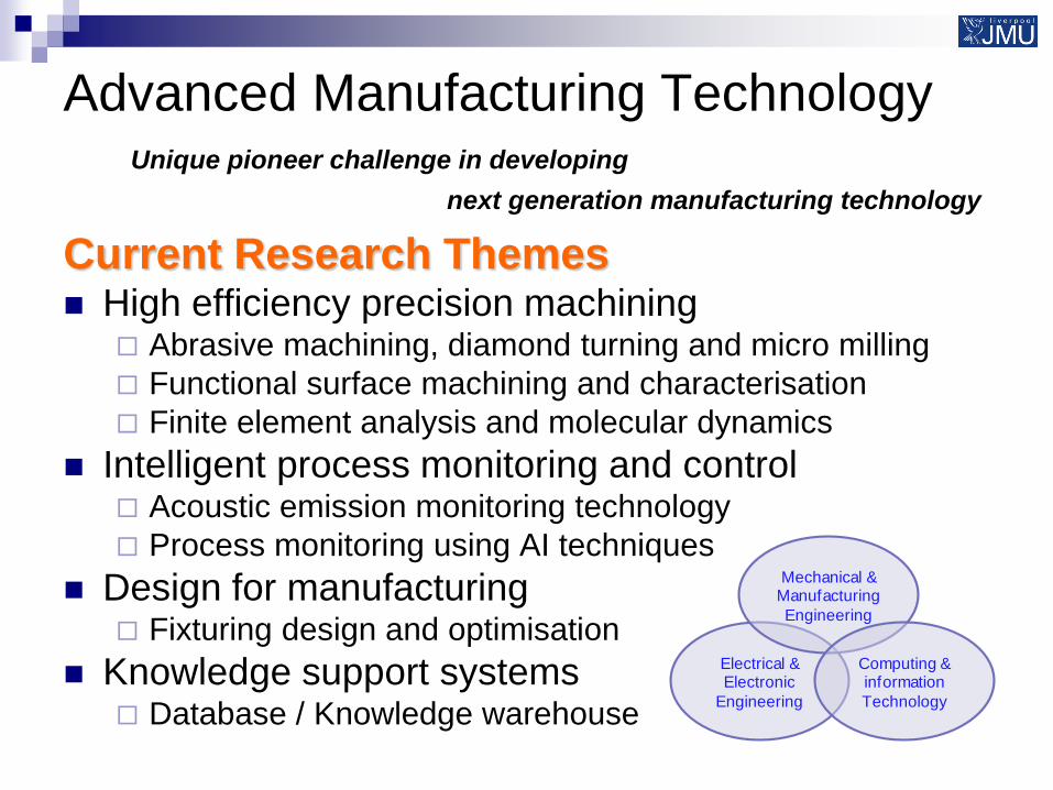
Advanced Manufacturing Technology

Current Research Themes High efficiency precision machining

Abrasive machining, diamond turning and micro milling

Functional surface machining and characterisation

Finite element analysis and molecular dynamics

Intelligent process monitoring and control Acoustic emission monitoring technology

Process monitoring using AI techniques

Design for manufacturing Fixturing design and optimisation

Knowledge support systems Database / Knowledge warehouse

Unique pioneer challenge in developing

next generation manufacturing technology

Electrical & Electronic

Engineering

Mechanical & Manufacturing

Engineering

Computing & information

Technology

Scope

Precision corrective machining

Fundamental investigation on abrasive machining

Acoustic emission monitoring technology

Intelligent process monitoring

Laser cleaning technique for grinding

Fixturing design and optimisation

Functional surface machining and characterisation

Knowledge warehouse development

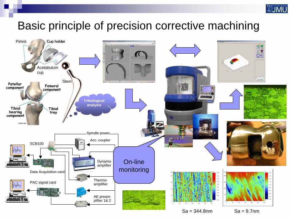
Basic principle of precision corrective machining

Sa = 344.8nm Sa = 9.7nm

Pelvis

Acetabulum

cup

Cup holder

Stem

Tribological

analysis

AE pream - plifier 1& 2

Acc. coupler

Dynamo - amplifier

Thermo - amplifier

Data Acquisition card

SCB100

Spindle power

PAC signal card

On-line

monitoring

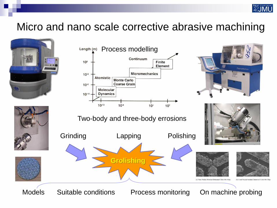
Micro and nano scale corrective abrasive machining

Process modelling

Two-body and three-body errosions

Grinding Lapping Polishing

Models Suitable conditions On machine probing

Grolishing

Process monitoring

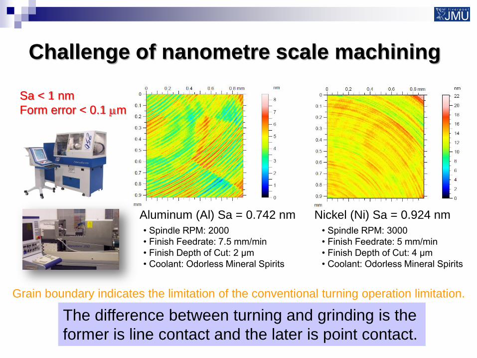
Challenge of nanometre scale machining

Grain boundary indicates the limitation of the conventional turning operation limitation.

What can be done?

Aluminum (Al) Sa = 0.742 nm Nickel (Ni) Sa = 0.924 nm

• Spindle RPM: 2000

• Finish Feedrate: 7.5 mm/min

• Finish Depth of Cut: 2 μm

• Coolant: Odorless Mineral Spirits

• Spindle RPM: 3000

• Finish Feedrate: 5 mm/min

• Finish Depth of Cut: 4 μm

• Coolant: Odorless Mineral Spirits

Sa < 1 nm

Form error < 0.1 mm

It was claimed that grinding has no minimum depth of cut.

The difference between turning and grinding is the

former is line contact and the later is point contact.

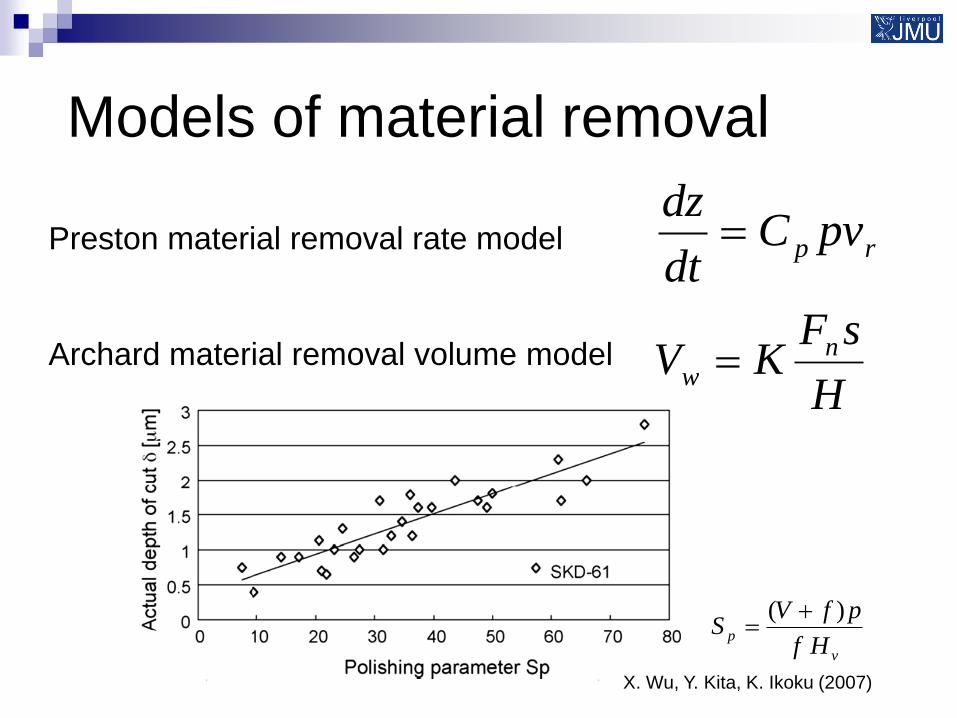
Models of material removal

rp pvCdt

dzPreston material removal rate model

Archard material removal volume model

H

sFKV n

w

v

pHf

pfVS

)(

X. Wu, Y. Kita, K. Ikoku (2007)

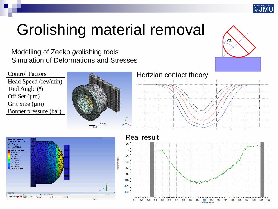
Grolishing material removal a

Hertzian contact theory

Real result

Modelling of Zeeko grolishing tools

Simulation of Deformations and Stresses

Control Factors

Head Speed (rev/min)

Tool Angle (o)

Off Set (µm)

Grit Size (µm)

Bonnet pressure (bar)

9

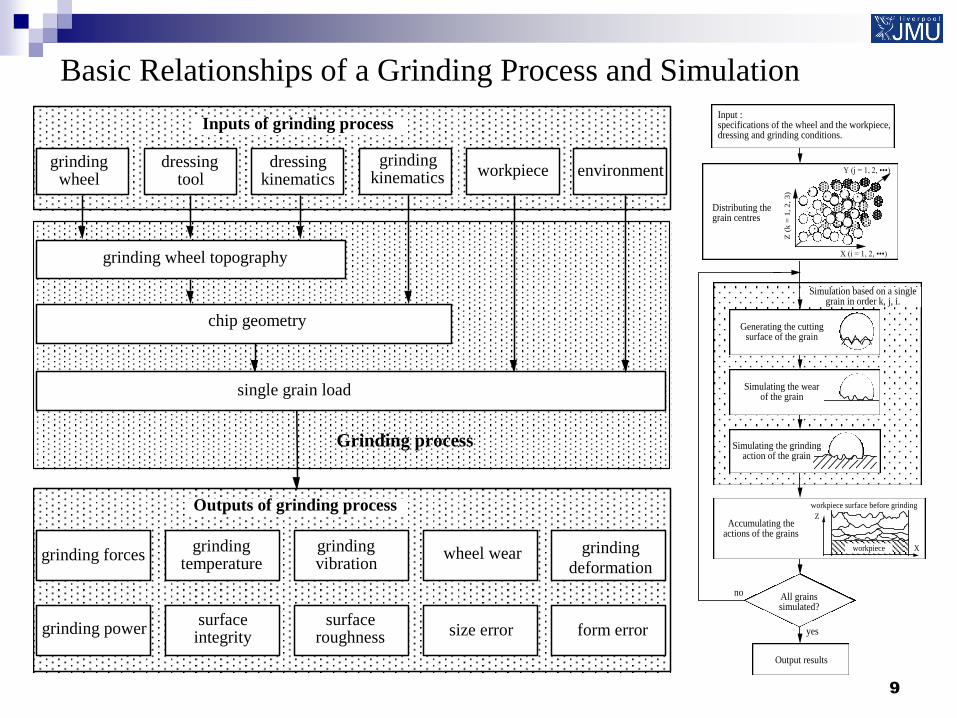
grinding forces wheel wear

grinding wheel topography

surfaceintegrity

surfaceroughness

grindingtemperature

grindingvibration

size error

Outputs of grinding process

grinding power

grindingwheel

workpiecedressing

tooldressing

kinematicsgrinding

kinematics

Inputs of grinding process

chip geometry

Grinding process

single grain load

environment

grinding

deformation

form error

Basic Relationships of a Grinding Process and Simulation

Input : specifications of the wheel and the workpiece, dressing and grinding conditions.

Generating the cutting surface of the grain

Simulation based on a single grain in order k, j, i.

Distributing the grain centres

X (i = 1, 2, •••)

Y (j = 1, 2, •••)

Z (

k =

1,

2,

3)

Simulating the grinding action of the grain

All grains simulated?

no

Output results

yes

Accumulating the actions of the grains

workpiece surface before grinding

workpiece

Z

X

Simulating the wear of the grain

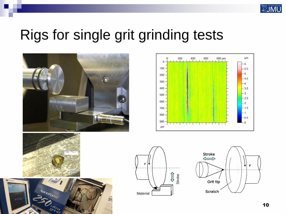
10

Rigs for single grit grinding tests

Material

v

Str

oke

v

Grit tip

Scratch

Stroke

v

Grit tip

Scratch

Stroke

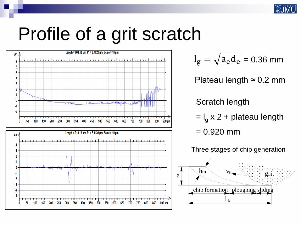
Profile of a grit scratch

= 0.36 mm

Plateau length ≈ 0.2 mm

Scratch length

= lg x 2 + plateau length

= 0.920 mm

a

chip formation ploughing sliding

grit h m

l k

v s

Three stages of chip generation

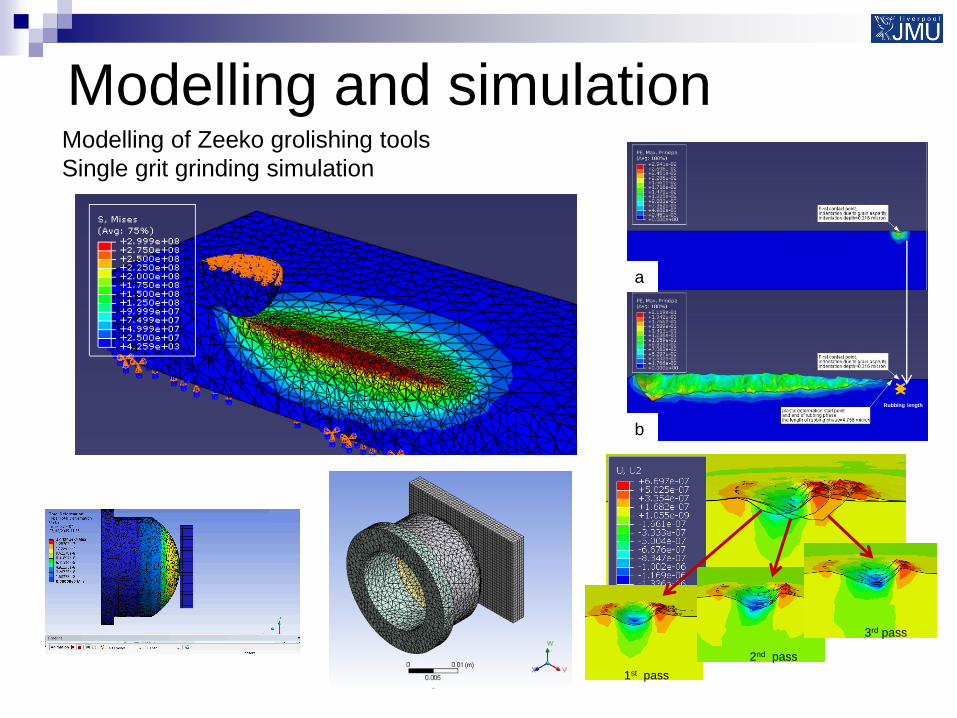
Modelling and simulation Modelling of Zeeko grolishing tools

Single grit grinding simulation

1st pass

2nd pass

3rd pass

Rubbing length

a

b

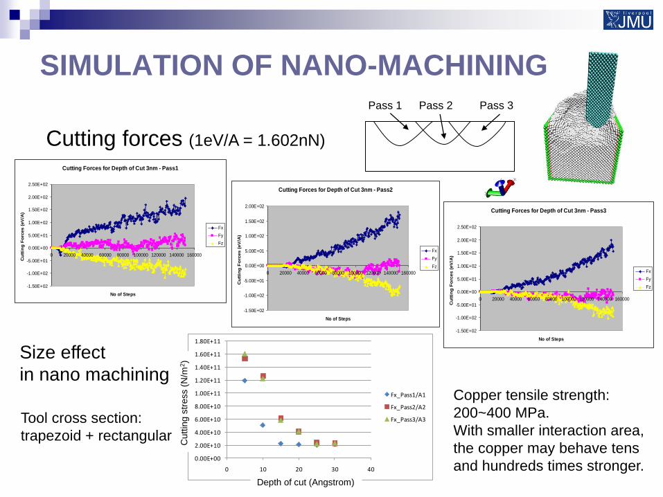
SIMULATION OF NANO-MACHINING Pass 1 Pass 2 Pass 3

Cutting Forces for Depth of Cut 3nm - Pass1

-1.50E+02

-1.00E+02

-5.00E+01

0.00E+00

5.00E+01

1.00E+02

1.50E+02

2.00E+02

2.50E+02

0 20000 40000 60000 80000 100000 120000 140000 160000

No of Steps

Cu

ttin

g F

orc

es (

eV

/A)

Fx

Fy

Fz

Cutting Forces for Depth of Cut 3nm - Pass2

-1.50E+02

-1.00E+02

-5.00E+01

0.00E+00

5.00E+01

1.00E+02

1.50E+02

2.00E+02

0 20000 40000 60000 80000 100000 120000 140000 160000

No of Steps

Cu

ttin

g F

orc

es (

eV

/A)

Fx

Fy

Fz

Cutting Forces for Depth of Cut 3nm - Pass3

-1.50E+02

-1.00E+02

-5.00E+01

0.00E+00

5.00E+01

1.00E+02

1.50E+02

2.00E+02

2.50E+02

0 20000 40000 60000 80000 100000 120000 140000 160000

No of Steps

Cu

ttin

g F

orc

es (

eV

/A)

Fx

Fy

Fz

Cutting forces (1eV/A = 1.602nN)

0.00E+00

2.00E+10

4.00E+10

6.00E+10

8.00E+10

1.00E+11

1.20E+11

1.40E+11

1.60E+11

1.80E+11

0 10 20 30 40

Fx_Pass1/A1

Fx_Pass2/A2

Fx_Pass3/A3

Depth of cut (Angstrom)

Cuttin

g s

tress (

N/m

2)

Size effect

in nano machining Copper tensile strength:

200~400 MPa.

With smaller interaction area,

the copper may behave tens

and hundreds times stronger.

Tool cross section:

trapezoid + rectangular

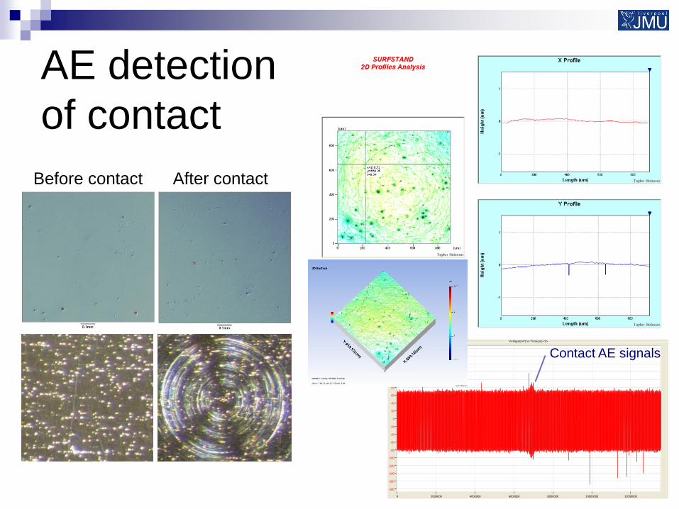
AE detection

of contact

Voltage(mV) vs Time(us) <2>

0 2000000 4000000 6000000 8000000 10000000 12000000

-180

-160

-140

-120

-100

-80

-60

-40

-20

0

20

40

60

80

100

120

140

160

180

Before contact After contact

Contact AE signals

15

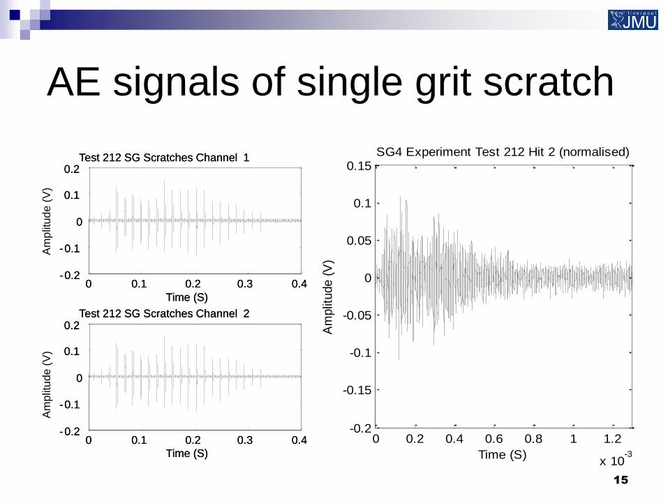
AE signals of single grit scratch

0 0.1 0.2 0.3 0.4 - 0.2

- 0.1

0

0.1

0.2 Test 212 SG Scratches Channel 1

Time (S)

0 0.1 0.2 0.3 0.4 - 0.2

- 0.1

0

0.1

0.2 Test 212 SG Scratches Channel 2

Time (S)

Am

plit

ude

(V

)

0 0.1 0.2 0.3 0.4 - 0.2

- 0.1

0

0.1

0.2 Test 212 SG Scratches Channel 1

Time (S)

Am

plit

ud

e (

V)

0 0.1 0.2 0.3 0.4 - 0.2

- 0.1

0

0.1

0.2 Test 212 SG Scratches Channel 2

Time (S)

0 0.2 0.4 0.6 0.8 1 1.2

x 10-3

-0.2

-0.15

-0.1

-0.05

0

0.05

0.1

0.15

Time (S)

Am

plit

ude (

V)

SG4 Experiment Test 212 Hit 2 (normalised)

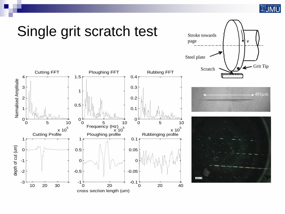
Single grit scratch test

v v

Scratch

Stroke towards

page

Grit Tip

Steel plate

0 5 10

x 105

0

1

2

3

4 Cutting FFT

Nor

mal

ised

Am

plitu

de

0 5 10

x 105

0

0.5

1

1.5 Ploughing FFT

Frequency (Hz)0 5 10

x 105

0

0.1

0.2

0.3

0.4 Rubbing FFT

10 20 30-3

-2

-1

0

1Cutting Profile

dept

h of

cut

(um

)

0 20-1

-0.5

0

0.5

1 Ploughing profile

cross section length (um)

0 20 40-0.1

-0.05

0

0.05

0.1 Rubbinging profile

401mm

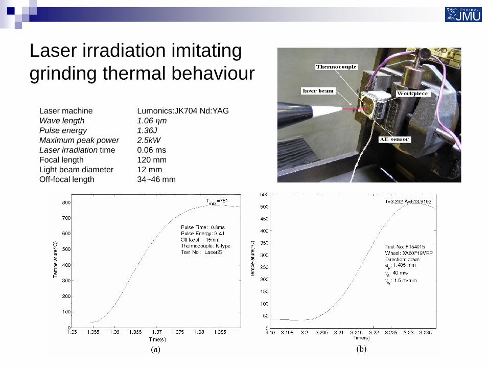
Laser irradiation imitating

grinding thermal behaviour

Laser machine Lumonics:JK704 Nd:YAG

Wave length 1.06 ηm

Pulse energy 1.36J

Maximum peak power 2.5kW

Laser irradiation time 0.06 ms

Focal length 120 mm

Light beam diameter 12 mm

Off-focal length 34~46 mm

18

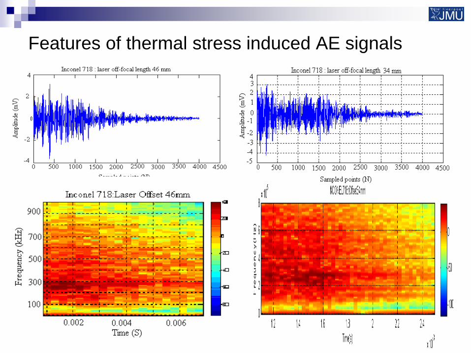
Features of thermal stress induced AE signals

Comparison of AE signals generated by laser and grinding

0 1 2 3 4 5 6 7 8 9 10

x 105

0

0.1

0.2

0.3

0.4

0.5

Frequency(Hz)

Norm

aliz

ed E

nerg

y

Test No.: Laser23H8

Pulse Time: 0.6ms

Pulse Energy: 3.4J

Off-focal: 15mmTm=781C

Thermocouple: K-type

867KHz

835KHz

820KHz

508KHz

461KHz

336KHz

0 1 2 3 4 5 6 7 8 9 10

x 105

0

0.1

0.2

0.3

0.4

0.5

0.6

Frequency(Hz)

Norm

alized E

nerg

y

Pulse Time: 0.6ms

Pulse Energy: 3.5J

Temperature: 108COff-focal: 30mm

Thermocouple: K-type

Test No.: Laser37

F1=266KHz

F2=258KHz

F3=141KHz

F4=391KHz

F5=836KHz

0 1 2 3 4 5 6 7 8 9 10

x 105

0

0.05

0.1

0.15

0.2

0.25

0.3

0.35

Frequency(Hz)

Norm

alized E

ne

rgy

Test No:Fd2-4

Wheel: XA60F13VRP

Material:CMSX4vs=40 m/s

vw

=0.5 m/min

ap=0.074

Direction: down

Coolant: NoT

m=784C

258

141

391 766

0 1 2 3 4 5 6 7 8 9 10

x 105

0

0.05

0.1

0.15

0.2

0.25

0.3

0.35

0.4

Frequency(Hz)

Norm

alis

ed e

nerg

y

Test No:F155010

Wheel:XA60F13VRP

Material:CMSX4vs=50 m/s

vw

=1 m/min

ap=1.3 mm

Direction: down

Coolant:48barT

m=611C

391 141

406

156

438

Laser

Grinding

Low temperature High temperature

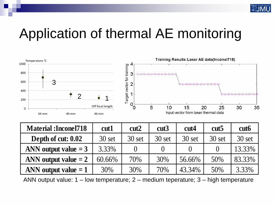
Application of thermal AE monitoring

Material :Inconel718 cut1 cut2 cut3 cut4 cut5 cut6

Depth of cut: 0.02 30 set 30 set 30 set 30 set 30 set 30 set

ANN output value = 3 3.33% 0 0 0 0 13.33%

ANN output value = 2 60.66% 70% 30% 56.66% 50% 83.33%

ANN output value = 1 30% 30% 70% 43.34% 50% 3.33%

0

200

400

600

800

1000

34 mm 40 mm 46 mm

Temperature °C

Off focal length

1 2

3

ANN output value: 1 – low temperature; 2 – medium teperature; 3 – high temperature

21

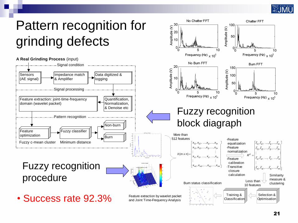
Pattern recognition for

grinding defects

A Real Grinding Process (input)

Sensors (AE signal)

Impedance match & Amplifier

Data digitized & logging

Quantification, Normalization, & Denoise etc

Feature extraction: joint-time-frequency domain (wavelet packet)

Feature optimization

Non-burn

Burn

Signal condition

Signal processing

Pattern recognition

Fuzzy classifier

Minimum distance Fuzzy c-mean cluster

Feature extraction by wavelet packet

and Joint Time-Frequency Analysis

-Feature

calibration

-Transitive

closure

calculation

-Feature

equalization

-Feature

normalization

More than

512 features

Similarity

measure &

clusteringLess than

10 features

mnmjm2m1

iniji2i1

2n2j22

n1j12

x ..., x ..., x x

x ..., x ..., x x

x ..., x x x

x x..., ,x x

n x mX

,,,

,,,

,...,,,

...,,,

)(

21

111

nnnjn2n1

iniji2i1

2n2j22

n1j12

K

r ..., r ..., r r

r ..., r ..., r r

r ..., r r r

r r..., ,r r

R

~,~,~,~

~,~,~,~

~,~...,,~,~

~...,,~~,~

21

111

Selection &

Optimisation

Training &

Classification

0

1

2

3

4

5

6

0 5 10 15 20 25 30 35

Burn status classification

Fuzzy recognition

procedure

Fuzzy recognition

block diagraph

• Success rate 92.3%

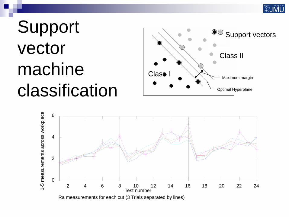
Support

vector

machine

classification Maximum margin

Optimal Hyperplane

Class I

Class II

Support vectors 1

-5 m

ea

su

rem

ents

acro

ss w

ork

pie

ce

2 4 6 8 10 12 14 16 18 20 22 24

0

2

4

6

Ra measurements for each cut (3 Trials separated by lines)

Test number

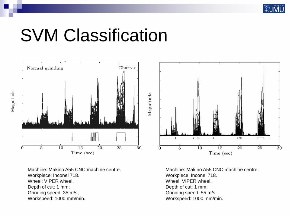
SVM Classification

Machine: Makino A55 CNC machine centre.

Workpiece: Inconel 718.

Wheel: VIPER wheel.

Depth of cut: 1 mm;

Grinding speed: 35 m/s;

Workspeed: 1000 mm/min.

Machine: Makino A55 CNC machine centre.

Workpiece: Inconel 718.

Wheel: VIPER wheel.

Depth of cut: 1 mm;

Grinding speed: 55 m/s;

Workspeed: 1000 mm/min.

+

+ *

Y X 0.707 1.5

*

+ *

Y Y

0.121

* X

X 0.707Y + X – 1.5 XY (Y+0.121X)

+

+

X 1.5

*

*

Y X

Y+0.121X+ X + 1.5 XY(0.707Y)

*

Y 0.70

7

+

Y

0.121

*

X

5A

7

A 6A

1

A 5B

7B

9

B

8

B

6B

1B

2B

3B 4B

2

A 3A 4A

X20

X8

X10

X14

X8

X10

X8

X10

X14

X14

X8

X13 X20

mydivide

plus

mydivide

mydivide

plus

plus

plusX20

mydivide

plus

mydivide

plus

plus

mydivide

-400 -350 -300 -250 -200 -150 -100 -50 0 50 100 -100

-50

0

50

100

150

200

250

300

350

400

Distance

Dis

tan

ce

Burn data & cluster centre

Chatter data & cluster centre

Normal grinding data & cluster centre

-400 -350 -300 -250 -200 -150 -100 -50 0 50 100 -150

-100

-50

0

50

100

150

Distance

Dis

tan

ce

Burn data & cluster centre

Chatter data & cluster centre

Normal grinding data & cluster centre

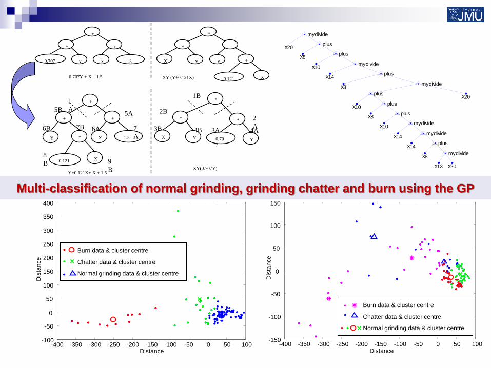
Multi-classification of normal grinding, grinding chatter and burn using the GP

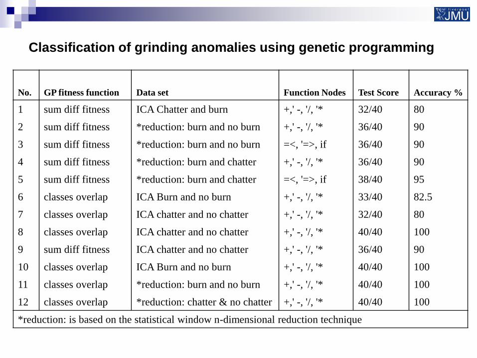
Classification of grinding anomalies using genetic programming

No. GP fitness function Data set Function Nodes Test Score Accuracy %

1 sum diff fitness ICA Chatter and burn +,' -, '/, '* 32/40 80

2 sum diff fitness *reduction: burn and no burn +,' -, '/, '* 36/40 90

3 sum diff fitness *reduction: burn and no burn =<, '=>, if 36/40 90

4 sum diff fitness *reduction: burn and chatter +,' -, '/, '* 36/40 90

5 sum diff fitness *reduction: burn and chatter =<, '=>, if 38/40 95

6 classes overlap ICA Burn and no burn +,' -, '/, '* 33/40 82.5

7 classes overlap ICA chatter and no chatter +,' -, '/, '* 32/40 80

8 classes overlap ICA chatter and no chatter +,' -, '/, '* 40/40 100

9 sum diff fitness ICA chatter and no chatter +,' -, '/, '* 36/40 90

10 classes overlap ICA Burn and no burn +,' -, '/, '* 40/40 100

11 classes overlap *reduction: burn and no burn +,' -, '/, '* 40/40 100

12 classes overlap *reduction: chatter & no chatter +,' -, '/, '* 40/40 100

*reduction: is based on the statistical window n-dimensional reduction technique

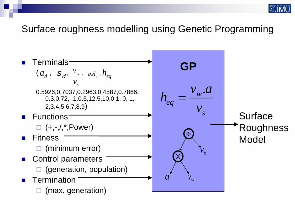
Surface roughness modelling using Genetic Programming

Terminals

( , , , ,

0.5926,0.7037,0.2963,0.4587,0.7866,

0.3,0.72, -1,0.5,12.5,10,0.1, 0, 1,

2,3,4,5,6,7,8,9)

Functions

(+,-,/,*,Power)

Fitness

(minimum error)

Control parameters

(generation, population)

Termination

(max. generation)

GP

Surface

Roughness

Model

da dss

w

v

veda. eqh

X

÷

wva

sv

s

weq

v

avh

.

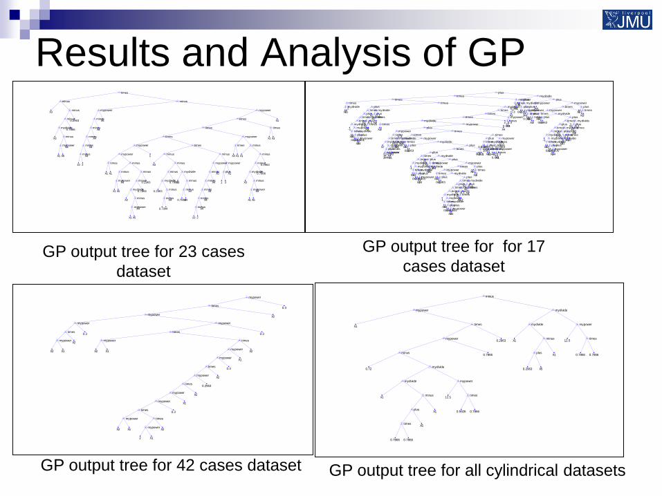
Results and Analysis of GP X3

X3

X1 X5

mypowerX4

minus

mydivide0.7866

minus0.2963

minus

minus

10 2

minusX4

minusX4

minusX4

minusX4

minusX5

mypower

X1 X1

times

X1 X5

mypowerX4

minus

X3

X1 X5

mypowerX4

minus

mydivide0.7866

minus0.2963

minus

minus

mypower1

mypower

X3

0.2963

0.72X4

minusX4

minus

mydivide0.7866

minus

X3

0.7866X4

minusX4

minus

mydivide

minus

minus

10 2

minusX4

minusX4

minusX4

minusX4

minusX5

mypower

1 3

plusX1

mypower

minus

times

times

X3 X1

times

X1

X3

X1 X5

mypowerX4

minus

mydivide0.7866

minus0.2963

minus

minus

mypower

times

X1 X3

times

timesX1

mypower

minus

times

GP output tree for 23 cases

dataset

X2X1

mydivide2

times

-1

X3X3

times

X10.2963

plus

X2X4

mypower0.001

plus

mydivide

mypower

mydivide2

timesX1

times

X2

X22

times

plus0.1

mydivide

plusX2

times

X2

X22

times

plus0.1

mydivide

plus

X22

times

X2

2X4

mypower0.001

plus

X2X1

timesX3

times

mypower

mydivideX3

times

0.001X3

times0.3

mypower

times0.3

mypower

X2X1

mydivide

X3X3

times

X10.2963

plus

-1

X3X3

times

X10.2963

plus

X2X4

mypower0.001

plus

mydivide

mypower

mydivide2

timesX1

times

X2

X2X1

mydivide0.3

times

plus

2X4

mypower

X3X3

times

X10.2963

plus

-1

X3X3

times

X10.2963

plus

X2X4

mypower0.001

plus

mydivide

mypower

mydivide2

timesX1

times

X2

X20.3

times

plus0.1

mydivide

plusX2

times

X2

X22

times

plus0.1

mydivide

plus

mydivide

mypowerX3

times

0.1

X22

times

plus

mypower

plus

mydivide

plusX2

times

0.0010.1

mydivide

plus

mydivide

mypower

times

0.29630.487

times

1000

X2X1

times

plus0.1

mydivide

plus

0.4872

times

0.001X3

times0.3

mypower

times0.2963

times0.3

mypower

times

times

plusX4

mypower

mydivide2

times

0.001X3

times0.3

mypower

timesX3

times0.3

mypower

times

times

0.001X3

times0.3

mypower

times

X1

X10.2963

plus

2X4

mypower

0.001X3

times

0.1

X22

times

plus

mypower

plus

mydivide

plus

2X4

mypower

X3X3

times

X10.2963

plus

-1

X3X3

times

X10.2963

plus

X2X4

mypower0.001

plus

mydivide

mypower

mydivide2

timesX1

times

X2

X2X1

mydivide0.3

times

plus

0.1

X110

times

plus

mydivide

plusX2

times

X2

X22

times

plus0.1

mydivide

plus

mydivide

mypowerX3

times

0.1

X22

times

plus

mypower

plus

mydivide

plus

GP output tree for for 17

cases dataset

X2 X1

mypowerX2

times0.3

mypower

X2 X1

mypower

X2 X1

mypower

2 X1

mypowerX2

times

times0.3

mypowerX1

mypowerX2

times0.2963

mypowerX2

times0.3

mypowerX1

mypowerX2

times

times0.3

mypower

mypowerX2

times0.3

mypower

X1

0.72

X1

0.7866 0.7866

timesX5

plusX1

minus

mydivide

12.5

0.5926 0.7866

times

mypower

mydivide

minus0.7866

mypower0.2963

times

mypower

X1

0.2963 X5

plusX1

minus

mydivide

12.5

0.7866 0.7866

times

mypower

mydivide

minus

GP output tree for 42 cases dataset GP output tree for all cylindrical datasets

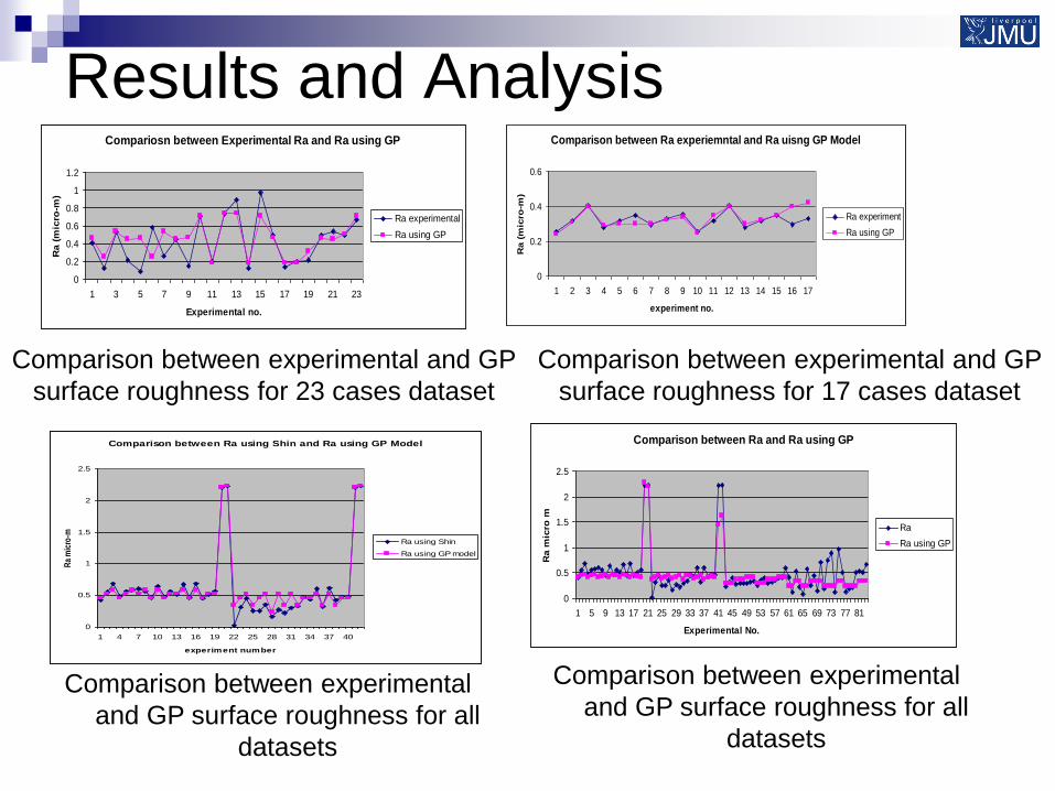
Results and Analysis Compariosn between Experimental Ra and Ra using GP

0

0.2

0.4

0.6

0.8

1

1.2

1 3 5 7 9 11 13 15 17 19 21 23

Experimental no.

Ra (

mic

ro-m

)

Ra experimental

Ra using GP

Comparison between experimental and GP

surface roughness for 23 cases dataset

Comparison between Ra experiemntal and Ra uisng GP Model

0

0.2

0.4

0.6

1 2 3 4 5 6 7 8 9 10 11 12 13 14 15 16 17

experiment no.

Ra (

mic

ro-m

)

Ra experiment

Ra using GP

Comparison between experimental and GP

surface roughness for 17 cases dataset

Comparison between Ra using Shin and Ra using GP Model

0

0.5

1

1.5

2

2.5

1 4 7 10 13 16 19 22 25 28 31 34 37 40

experiment number

Ra

mic

ro-m

Ra using Shin

Ra using GP model

Comparison between Ra and Ra using GP

0

0.5

1

1.5

2

2.5

1 5 9 13 17 21 25 29 33 37 41 45 49 53 57 61 65 69 73 77 81

Experimental No.

Ra m

icro

m

Ra

Ra using GP

Comparison between experimental

and GP surface roughness for all

datasets

Comparison between experimental

and GP surface roughness for all

datasets

29

T800 HP turbine blade fixture development

CUTTER PATHS SPACE REMAINING FOR FIXTURE

Cutting strategy and available space

Industrial Benefits

• Labour time saving: 3min/blade

• Cost saving:

Fixture saving: 25k/part number,

Marginal cost : 2.5pound/blade

30

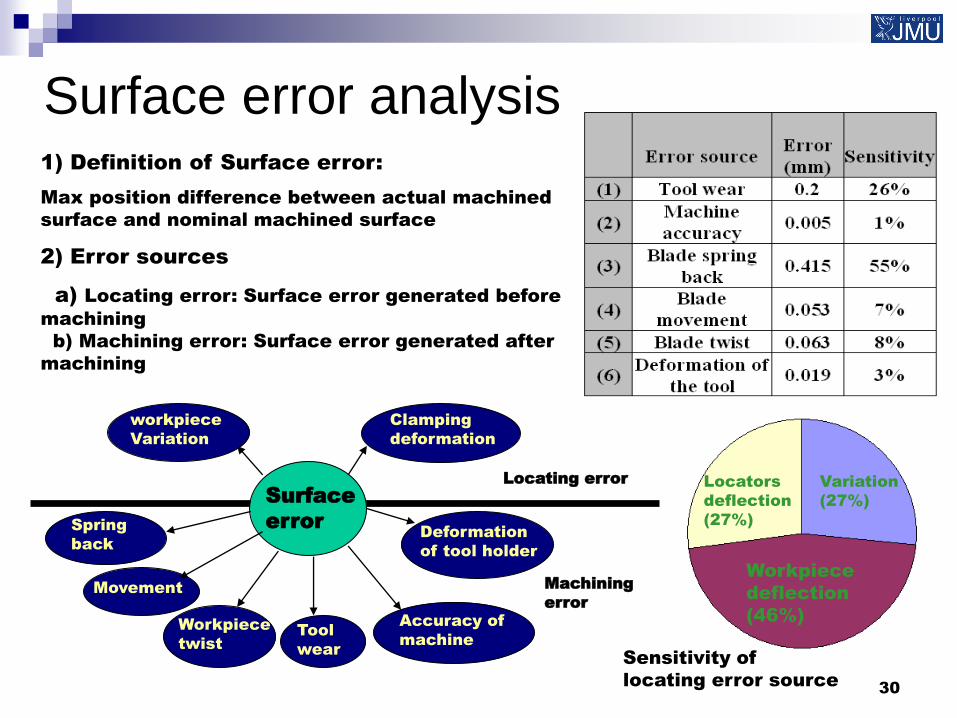
Surface error analysis

Surface

error

Locating error

Clamping

deformation

workpiece

Variation

Spring

back

Movement

Workpiece

twist

Tool

wear

Accuracy of

machine

Deformation

of tool holder

Machining

error

1) Definition of Surface error:

Max position difference between actual machined

surface and nominal machined surface

2) Error sources

a) Locating error: Surface error generated before

machining

b) Machining error: Surface error generated after

machining

Variation

(27%)

Workpiece

deflection

(46%)

Locators

deflection

(27%)

Sensitivity of

locating error source

31

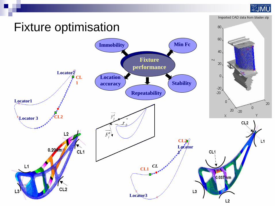
Fixture optimisation

CL2

Locator1

Locator2 CL

1

Locator 3

CL1

CL2

CL

Locator

1

Locator3

Fixture

performance

Repeatability

Min Fc

Stability

Immobility

Location

accuracy

32

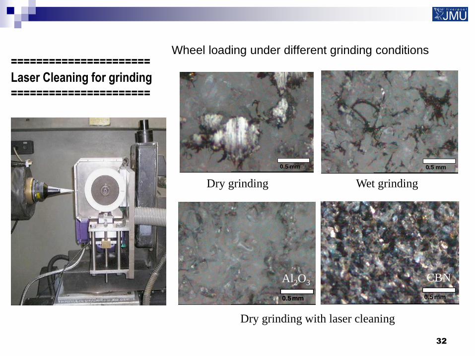
Wheel loading under different grinding conditions

0.5 mm

0.5 mm

Dry grinding Wet grinding

0.5 mm 0.5 mm

Dry grinding with laser cleaning

CBN

0.5 mm 0.5 mm

Al2O3

======================

Laser Cleaning for grinding

======================

33

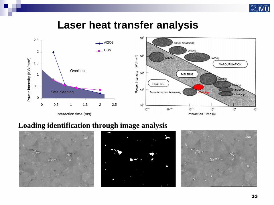
Laser heat transfer analysis

0

0.5

1

1.5

2

2.5

0 0.5 1 1.5 2 2.5

Al2O3

CBN

Interaction time (ms)

Pow

er

inte

nsity (

KW

/mm

2)

Safe cleaning

Overheat

Loading identification through image analysis

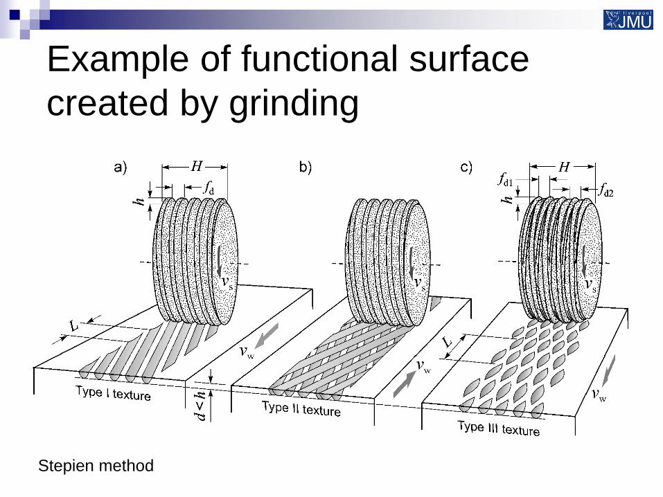
Example of functional surface

created by grinding

Stepien method

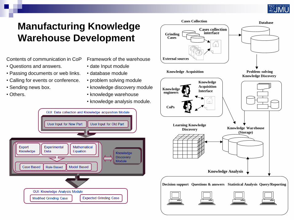
Manufacturing Knowledge

Warehouse Development

Framework of the warehouse

• date Input module

• database module

• problem solving module

• knowledge discovery module

• knowledge warehouse

• knowledge analysis module.

Database

Decision support Questions & answers Statistical Analysis Query/Reporting

Knowledge Acquisition

Knowledge Analysis

Cases Collection

Knowledge War e house (Storage)

Learning Knowledge Discovery

External sources

Grinding Cases

Cases collection interface

Knowledge engineers

CoPs

Knowledge

Acquisition

Interface

Problem - solving Knowledge Discovery

Contents of communication in CoP

• Questions and answers.

• Passing documents or web links.

• Calling for events or conference.

• Sending news box.

• Others.

Opportunities of further development

Ultra precision corrective machining at

nanometre scale

Structured functional surface machining

Intelligent machining monitoring and optimisation.

Precision machining knowledge support system

Design for precision manufacture

Thanks for listening