adaptive depth estimation for pyramid multi-view stereo
TRANSCRIPT
Computers & Graphics 0 0 0 (2021) 1–11
Contents lists available at ScienceDirect
Computers & Graphics
journal homepage: www.elsevier.com/locate/cag
Special Section on CAD & Graphics 2021
Adaptive depth estimation for pyramid multi-view stereo
Jie Liao
a , Yanping Fu
b , Qingan Yan
c , Fei Luo
a , ∗∗, Chunxia Xiao
a , ∗
a School of Computer Science, Wuhan University, Wuhan, China b School of Computer Science and Technology, Anhui University, Hefei, China c Silicon Valley Research Center for Multimedia Software, JD.com, Beijing, China
a r t i c l e i n f o
Article history:
Received 5 February 2021
Revised 7 April 2021
Accepted 13 April 2021
Available online xxx
Keywords:
3D Reconstruction
Multi-View Stereo
Deep Learning
a b s t r a c t
In this paper, we propose a Multi-View Stereo (MVS) network which can perform efficient high-resolution
depth estimation with low memory consumption. Classical learning-based MVS approaches typically con-
struct 3D cost volumes to regress depth information, making the output resolution rather limited as the
memory consumption grows cubically with the input resolution. Although recent approaches have made
significant progress in scalability by introducing the coarse-to-fine fashion or sequential cost map reg-
ularization, the memory consumption still grows quadratically with input resolution and is not friendly
for commodity GPU. Observing that the surfaces of most objects in real world are locally smooth, we
assume that most of the depth hypotheses upsampled from a well-estimated depth map are accurate.
Based on the assumption, we propose a pyramid MVS network based on the adaptive depth estimation,
which gradually refines and upsamples the depth map to the desired resolution. Instead of estimating
depth hypotheses for all pixels in the depth map, our method only performs prediction at adaptively
selected locations, alleviating excessive computation on well-estimated positions. To estimate depth hy-
potheses for sparse selected locations, we propose the lightweight pixelwise depth estimation network,
which can estimate depth value for each selected location independently. Experiments demonstrate that
our method can generate results comparable with the state-of-the-art learning-based methods while re-
constructing more geometric details and consuming less GPU memory.
© 2021 Elsevier Ltd. All rights reserved.
1
M
a
r
t
i
l
fi
l
l
c
t
r
q
c
t
m
i
a
w
i
i
b
p
R
t
t
P
w
o
h
0
. Introduction
Given images calibrated manually or through Structure-From-
otion (SFM) algorithms [2–6,34] , Multi-View Stereo reconstructs
dense representation of the target scenes. The reconstruction
esults can be applied in automatic geometry, scene classifica-
ion, image-based rendering, and robot navigation. The publish-
ng of the MVS training dataset [7,8] facilitates the design of
earning-based MVS algorithms and boosts the progress in this
eld.
Currently, learning-based MVS methods have achieved excel-
ent performance on the MVS benchmarks [8–10] . Instead of uti-
izing handcrafted similarity measuring metrics and engineered
ost volume regularization, learning-based MVS methods learn
o extract features, measure the similarity across images, and
egularize the cost volumes. The learned ones have larger per-
∗ Corresponding author. ∗∗ Co-corresponding author.
E-mail addresses: [email protected] (J. Liao), [email protected] (Y. Fu),
[email protected] (Q. Yan), [email protected] (F. Luo), [email protected]
(C. Xiao).
a
t
m
l
p
o
ttps://doi.org/10.1016/j.cag.2021.04.016
097-8493/© 2021 Elsevier Ltd. All rights reserved.
eption domains and can utilize high-level semantic informa-
ion. Therefore, learning-based depth estimation is relatively im-
une to specular, low-textured, and reflective regions that are
ntractable for traditional methods. Classical learning-based MVS
lgorithms [11,12] build 3D cost volumes and regularize them
ith 3D CNNs. Although the 3D cost volume and 3DCNNs are
nherently suitable for handling 3D information, the correspond-
ng GPU memory consumption is large, leading to the methods
ased on them limited to low-resolution input images and out-
ut results. To improve the scalability of the network for MVS,
-MVSNet [1] sequentially regularizes the 2D cost maps along
he depth direction via the gated recurrent unit (GRU), leading
o only quadratic GPU memory growth with volume resolution.
oint-MVSNet [13] introduces a point-based deep iterative frame-
ork and reduces the computational cost by concentrating only
n depth range near the output point cloud from the last iter-
tion. Although both [1] and [13] make a great contribution to
he scalability improvement of learning-based MVS methods, their
ethods still only generate down-sampled depth maps due to
imited GPU memory. Yang et al. [14] and Gu et al. [15] pro-
ose to estimate depth maps in the coarse-to-fine manner. Instead
f constructing a cost volume at a fixed resolution, their meth-
J. Liao, Y. Fu, Q. Yan et al. Computers & Graphics 0 0 0 (2021) 1–11
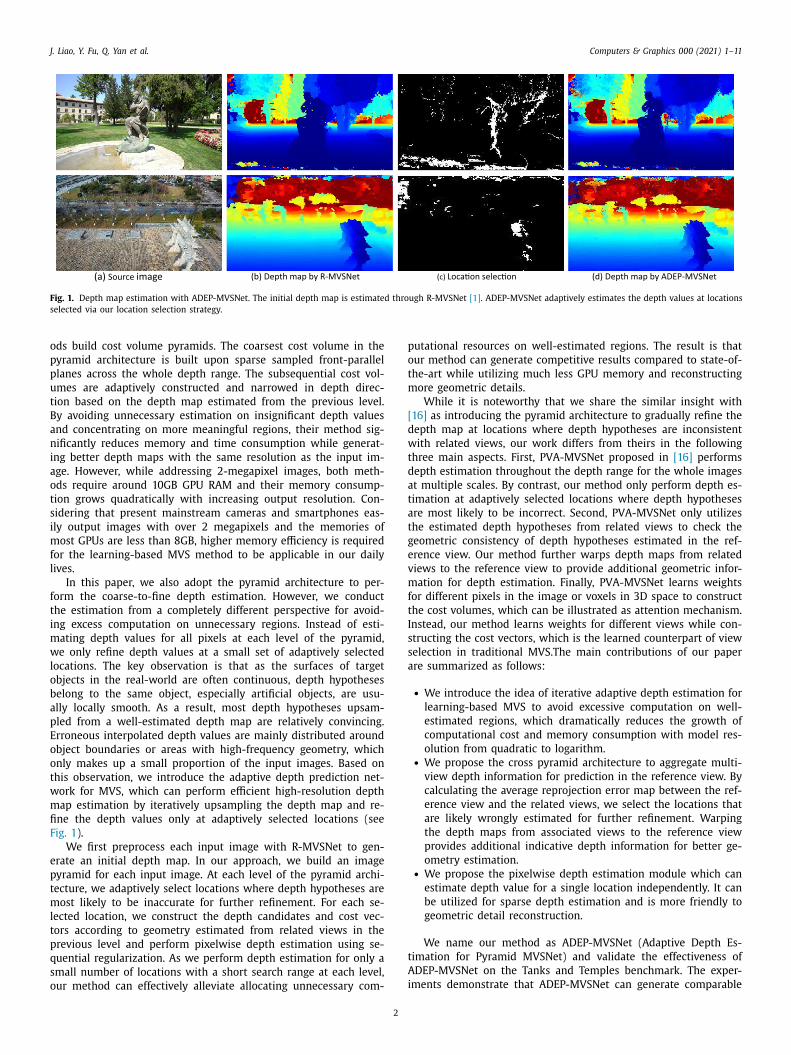
Fig. 1. Depth map estimation with ADEP-MVSNet. The initial depth map is estimated through R-MVSNet [1] . ADEP-MVSNet adaptively estimates the depth values at locations
selected via our location selection strategy.
o
p
p
u
t
B
a
n
i
a
o
t
s
i
m
f
l
f
t
i
m
w
l
o
b
a
p
E
o
o
t
w
m
fi
F
e
p
t
m
l
t
p
q
s
o
p
o
t
m
[
d
w
t
d
a
t
a
t
g
e
v
m
f
t
I
s
s
a
t
A
i
ds build cost volume pyramids. The coarsest cost volume in the
yramid architecture is built upon sparse sampled front-parallel
lanes across the whole depth range. The subsequential cost vol-
mes are adaptively constructed and narrowed in depth direc-
ion based on the depth map estimated from the previous level.
y avoiding unnecessary estimation on insignificant depth values
nd concentrating on more meaningful regions, their method sig-
ificantly reduces memory and time consumption while generat-
ng better depth maps with the same resolution as the input im-
ge. However, while addressing 2-megapixel images, both meth-
ds require around 10GB GPU RAM and their memory consump-
ion grows quadratically with increasing output resolution. Con-
idering that present mainstream cameras and smartphones eas-
ly output images with over 2 megapixels and the memories of
ost GPUs are less than 8GB, higher memory efficiency is required
or the learning-based MVS method to be applicable in our daily
ives.
In this paper, we also adopt the pyramid architecture to per-
orm the coarse-to-fine depth estimation. However, we conduct
he estimation from a completely different perspective for avoid-
ng excess computation on unnecessary regions. Instead of esti-
ating depth values for all pixels at each level of the pyramid,
e only refine depth values at a small set of adaptively selected
ocations. The key observation is that as the surfaces of target
bjects in the real-world are often continuous, depth hypotheses
elong to the same object, especially artificial objects, are usu-
lly locally smooth. As a result, most depth hypotheses upsam-
led from a well-estimated depth map are relatively convincing.
rroneous interpolated depth values are mainly distributed around
bject boundaries or areas with high-frequency geometry, which
nly makes up a small proportion of the input images. Based on
his observation, we introduce the adaptive depth prediction net-
ork for MVS, which can perform efficient high-resolution depth
ap estimation by iteratively upsampling the depth map and re-
ne the depth values only at adaptively selected locations (see
ig. 1 ).
We first preprocess each input image with R-MVSNet to gen-
rate an initial depth map. In our approach, we build an image
yramid for each input image. At each level of the pyramid archi-
ecture, we adaptively select locations where depth hypotheses are
ost likely to be inaccurate for further refinement. For each se-
ected location, we construct the depth candidates and cost vec-
ors according to geometry estimated from related views in the
revious level and perform pixelwise depth estimation using se-
uential regularization. As we perform depth estimation for only a
mall number of locations with a short search range at each level,
ur method can effectively alleviate allocating unnecessary com-
2
utational resources on well-estimated regions. The result is that
ur method can generate competitive results compared to state-of-
he-art while utilizing much less GPU memory and reconstructing
ore geometric details.
While it is noteworthy that we share the similar insight with
16] as introducing the pyramid architecture to gradually refine the
epth map at locations where depth hypotheses are inconsistent
ith related views, our work differs from theirs in the following
hree main aspects. First, PVA-MVSNet proposed in [16] performs
epth estimation throughout the depth range for the whole images
t multiple scales. By contrast, our method only perform depth es-
imation at adaptively selected locations where depth hypotheses
re most likely to be incorrect. Second, PVA-MVSNet only utilizes
he estimated depth hypotheses from related views to check the
eometric consistency of depth hypotheses estimated in the ref-
rence view. Our method further warps depth maps from related
iews to the reference view to provide additional geometric infor-
ation for depth estimation. Finally, PVA-MVSNet learns weights
or different pixels in the image or voxels in 3D space to construct
he cost volumes, which can be illustrated as attention mechanism.
nstead, our method learns weights for different views while con-
tructing the cost vectors, which is the learned counterpart of view
election in traditional MVS.The main contributions of our paper
re summarized as follows:
• We introduce the idea of iterative adaptive depth estimation for
learning-based MVS to avoid excessive computation on well-
estimated regions, which dramatically reduces the growth of
computational cost and memory consumption with model res-
olution from quadratic to logarithm. • We propose the cross pyramid architecture to aggregate multi-
view depth information for prediction in the reference view. By
calculating the average reprojection error map between the ref-
erence view and the related views, we select the locations that
are likely wrongly estimated for further refinement. Warping
the depth maps from associated views to the reference view
provides additional indicative depth information for better ge-
ometry estimation. • We propose the pixelwise depth estimation module which can
estimate depth value for a single location independently. It can
be utilized for sparse depth estimation and is more friendly to
geometric detail reconstruction.
We name our method as ADEP-MVSNet (Adaptive Depth Es-
imation for Pyramid MVSNet) and validate the effectiveness of
DEP-MVSNet on the Tanks and Temples benchmark. The exper-
ments demonstrate that ADEP-MVSNet can generate comparable
J. Liao, Y. Fu, Q. Yan et al. Computers & Graphics 0 0 0 (2021) 1–11
r
s
2
2
c
c
d
c
p
n
i
p
s
i
i
t
m
M
m
m
s
H
p
T
v
t
a
i
o
b
i
t
2
g
h
l
f
d
s
v
s
[
L
t
a
u
B
l
m
t
[
n
t
u
q
b
a
b
o
p
t
a
c
e
c
N
t
e
o
a
w
t
w
c
o
[
N
p
3
t
t
t
f
a
t
f
l
e
c
i
a
t
i
e
b
l
a
v
t
i
d
o
t
d
fi
s
p
i
c
d
o
t
u
d
i
esults with the state-of-the-art learning-based MVS while recon-
tructing more geometric details with less GPU memory.
. Related work
.1. Traditional MVS
According to output representations, traditional MVS methods
an be classified into three categories: 1) direct point cloud re-
onstructions [17,18] , 2) volumetric reconstructions [19–21] and 3)
epth map reconstructions [22–28] .
Point-based methods directly operate on and output point
louds. To densify the point cloud, these methods usually adopt
ropagation strategies to propagate a well-optimized point to
earby 3D space. The drawback is that the propagation procedure
s performed in a sequence, which is not friendly to parallel com-
utation and takes a long time. Volumetric methods divide 3D
pace into regular grids and reconstruct the target scene by judg-
ng whether the voxels adhere to the target scene surface. The lim-
tation of volumetric presentation is the inherent space discretiza-
ion error and high memory consumption. In contrast, the depth
ap presentation is much more flexible. It breaks the complex
VS problem into relatively more tractable per-view depth esti-
ation problems and can be easily fused into point cloud or volu-
etric presentation. According to MVS benchmarks [9,10] , current
tate-of-the-art MVS methods [26–29] are all depth-map based.
owever, although the depth map estimation procedure can be
arallelized, depth map based methods usually take a longer time.
he reason is that the depth map estimation is performed for each
iew, which is analogous to estimating geometry as many times as
he number of input images. Besides, most of the traditional MVS
lgorithms mainly estimate geometry by maximizing the Normal-
zed Cross-Correlation (NCC) between the projections of the patch
n the reference and related views. The photometric consistency
ased on NCC is fragile to textureless and specular surfaces, mak-
ng the reconstruction of the corresponding regions hard work for
raditional MVS algorithms.
.2. Learning-based MVS
Recently, learning-based MVS approaches have demonstrated
reat potentials on various MVS benchmarks [8–10] . Instead of
andcrafted feature extraction and engineered matching metrics,
earning-based methods utilize learned ones that are more robust
or illumination change and non-Lambertian surface. Similar to tra-
itional MVS methods, learning-based methods can also be clas-
ified into three categories according to output representations:1)
olumetric reconstructions [11,30] , 2) depth (disparity) map recon-
tructions [1,12,14,15,31] and 3) direct point cloud reconstruction
13] .
Earlier learning-based MVS methods like SurfaceNet [30] and
SM [11] are volumetric based methods. SurfaceNet [30] learns
he probability of voxels lying on the surface. LSM [11] presents
learnable system to back-project pixel features to the 3D vol-
me and classify whether a voxel is occupied or not by the surface.
oth SurfaceNet and LSM made a groundbreaking contribution to
earning-based MVS. However, the volumetric representations are
emory expensive, making the algorithms based on them limited
o small-scale scenes.
[1,12,14–16,31] estimate the depth map for each view. DeepMVS
31] pre-warps the multi-view images to 3D space and uses deep
etworks for regularization and aggregation. MVSNet [12] proposes
o learn the depth map for each view by constructing a cost vol-
me followed by 3D CNN regularization. As the 3D cost volume re-
uires GPU memory that is cubic to the input resolution, the scala-
ility of MVSNet is rather limited. R-MVSNet [1] improves the scal-
3
bility of MVSNet by sequentially regularizing the 2D cost maps,
ut the memory consumption still restricts the method to only
utput downsampled depth maps. PVA-MVSNet [16] constructs the
yramid architecture to aggregate the reliable depth estimation at
he coarser scale to fill in the mismatched regions at the finer scale
nd utilizes the self-adaptive view aggregation to improve the re-
onstruction quality. However, the memory cost of PVA-MVSNet is
ven larger than the seminal MVSNet [12] . Instead of building 3D
ost volumes at fixed resolution, CVP-MVSNet [14] and CasMVS-
et [15] construct the cost volume pyramid. By gradually narrow
he cost volumes according to depth estimation from previous lev-
ls, both two methods avoid unnecessary computation and mem-
ry consumption on insignificant regions. As a result, CVP-MVSNet
nd CasMVSNet are able to output the full-resolution depth map
ith high-quality. However, the memory requirement is quadratic
o the input resolution.
Point-MVSNet [13] introduces a novel point-based deep frame-
ork that estimates the 3D flow for each point to refine the point
loud. The idea of concentrating only on depth range near the
utput point cloud comes from the last iteration inspired both
15] and [14] . Although Point-MVSNet is more scalable than MVS-
et, it still can not estimate full-resolution depth maps for images
rovided by the Tanks and Temples benchmark.
. Methodology
The surfaces of objects in the real world are generally con-
inuous, and most of them are smooth. This phenomenon is par-
icularly evident in artificial scenes. Taking the desk as example,
he majority of the desk surface is made up of planes and high-
requency geometry basically occurs at edges or some decorative
ccessories. Based on this observation, we assume that most of
he depth values upsampled from a well-estimated depth map are
undamentally accurate, except for those near high-frequency areas
ike object boundaries. We validate our assumption on the Blend-
dMVS [7] as shown in Section 4.1 .
The overview of our method is depicted in Fig. 2 . The input
alibrated images are first processed with R-MVSNet to generate
nitial low-resolution depth maps. Then we iteratively upsample
nd refine the depth maps. The refinement mainly consists of
hree steps: 1) selecting the locations to be refined, 2) construct-
ng depth candidates for selected locations, and 3) performing pix-
lwise depth estimation and updating the upsampled depth maps.
We first introduce the cross pyramid architecture, which
ridges the depth estimation across the related views. Current
earning-based MVS algorithms perform depth estimation mainly
ccording to the feature (photometric) information across multiple
iews. However, the geometric consistency, which is equally impor-
ant in MVS and widely considered in traditional MVS algorithms,
s ignored. We construct the cross pyramid architecture to allow
epth refinement at the current level to utilize depth hypotheses
f related views at the previous level. The cross pyramid architec-
ure is the foundation of our location selection and depth candi-
ate construction procedure.
Then we illustrate our location selection strategy, which aims to
nd falsely estimated or upsampled depth values. One direct and
traightforward way to select locations to be refined is to upsam-
le the probability map and pick the locations with low probabil-
ty values. However, as we only refine part of the locations in the
urrent depth map and adopt different numbers of depth candi-
ate at each level, the denominators for probability normalization
f refined locations are different from that of other locations. On
he other hand, depth maps estimated at the previous level enable
s to check the geometric consistency. The geometric consistency
irectly relates to the depth map fusion procedure and the qual-
ty of the output point cloud. Therefore, we propose the location
J. Liao, Y. Fu, Q. Yan et al. Computers & Graphics 0 0 0 (2021) 1–11
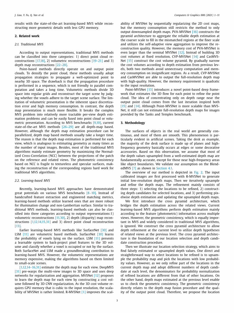
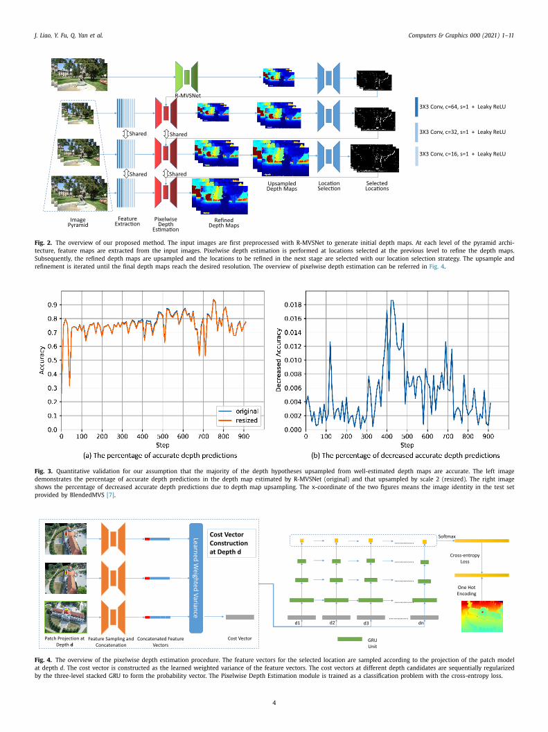
Fig. 2. The overview of our proposed method. The input images are first preprocessed with R-MVSNet to generate initial depth maps. At each level of the pyramid archi-
tecture, feature maps are extracted from the input images. Pixelwise depth estimation is performed at locations selected at the previous level to refine the depth maps.
Subsequently, the refined depth maps are upsampled and the locations to be refined in the next stage are selected with our location selection strategy. The upsample and
refinement is iterated until the final depth maps reach the desired resolution. The overview of pixelwise depth estimation can be referred in Fig. 4 .
Fig. 3. Quantitative validation for our assumption that the majority of the depth hypotheses upsampled from well-estimated depth maps are accurate. The left image
demonstrates the percentage of accurate depth predictions in the depth map estimated by R-MVSNet (original) and that upsampled by scale 2 (resized). The right image
shows the percentage of decreased accurate depth predictions due to depth map upsampling. The x-coordinate of the two figures means the image identity in the test set
provided by BlendedMVS [7] .
Fig. 4. The overview of the pixelwise depth estimation procedure. The feature vectors for the selected location are sampled according to the projection of the patch model
at depth d. The cost vector is constructed as the learned weighted variance of the feature vectors. The cost vectors at different depth candidates are sequentially regularized
by the three-level stacked GRU to form the probability vector. The Pixelwise Depth Estimation module is trained as a classification problem with the cross-entropy loss.
4
J. Liao, Y. Fu, Q. Yan et al. Computers & Graphics 0 0 0 (2021) 1–11
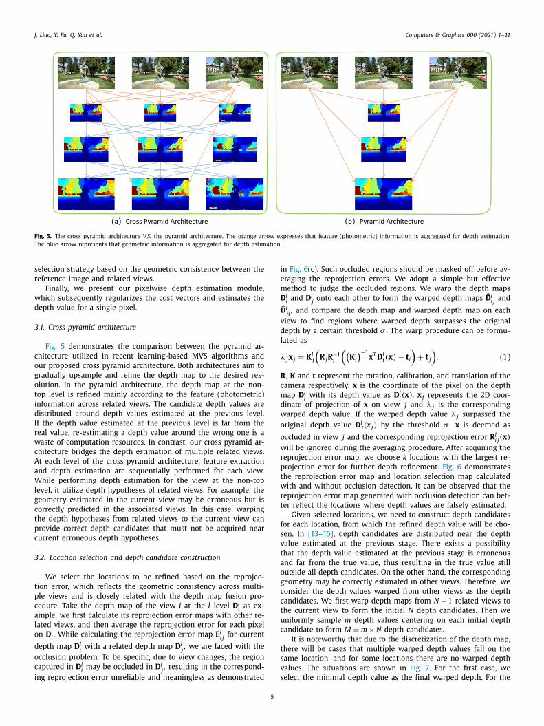
Fig. 5. The cross pyramid architecture V.S. the pyramid architecture. The orange arrow expresses that feature (photometric) information is aggregated for depth estimation.
The blue arrow represents that geometric information is aggregated for depth estimation.
s
r
w
d
3
c
o
g
o
t
i
d
I
r
w
c
A
a
W
l
g
c
t
p
c
3
t
p
c
a
l
o
d
o
c
i
i
e
m
D
D
v
d
l
λ
R
c
m
d
w
o
o
w
r
p
t
w
r
t
f
s
v
t
a
o
g
c
c
t
u
c
t
s
v
s
election strategy based on the geometric consistency between the
eference image and related views.
Finally, we present our pixelwise depth estimation module,
hich subsequently regularizes the cost vectors and estimates the
epth value for a single pixel.
.1. Cross pyramid architecture
Fig. 5 demonstrates the comparison between the pyramid ar-
hitecture utilized in recent learning-based MVS algorithms and
ur proposed cross pyramid architecture. Both architectures aim to
radually upsample and refine the depth map to the desired res-
lution. In the pyramid architecture, the depth map at the non-
op level is refined mainly according to the feature (photometric)
nformation across related views. The candidate depth values are
istributed around depth values estimated at the previous level.
f the depth value estimated at the previous level is far from the
eal value, re-estimating a depth value around the wrong one is a
aste of computation resources. In contrast, our cross pyramid ar-
hitecture bridges the depth estimation of multiple related views.
t each level of the cross pyramid architecture, feature extraction
nd depth estimation are sequentially performed for each view.
hile performing depth estimation for the view at the non-top
evel, it utilize depth hypotheses of related views. For example, the
eometry estimated in the current view may be erroneous but is
orrectly predicted in the associated views. In this case, warping
he depth hypotheses from related views to the current view can
rovide correct depth candidates that must not be acquired near
urrent erroneous depth hypotheses.
.2. Location selection and depth candidate construction
We select the locations to be refined based on the reprojec-
ion error, which reflects the geometric consistency across multi-
le views and is closely related with the depth map fusion pro-
edure. Take the depth map of the view i at the l level D
l i
as ex-
mple, we first calculate its reprojection error maps with other re-
ated views, and then average the reprojection error for each pixel
n D
l i . While calculating the reprojection error map E
l i j
for current
epth map D
l i
with a related depth map D
l j , we are faced with the
cclusion problem. To be specific, due to view changes, the region
aptured in D
l i
may be occluded in D
l j , resulting in the correspond-
ng reprojection error unreliable and meaningless as demonstrated
5
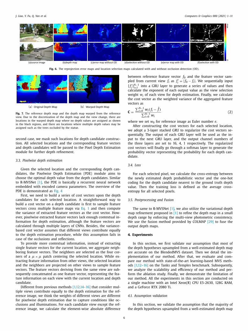
n Fig. 6 (c). Such occluded regions should be masked off before av-
raging the reprojection errors. We adopt a simple but effective
ethod to judge the occluded regions. We warp the depth maps
l i
and D
l j
onto each other to form the warped depth maps ˆ D
l i j
and
ˆ
l ji , and compare the depth map and warped depth map on each
iew to find regions where warped depth surpasses the original
epth by a certain threshold σ . The warp procedure can be formu-
ated as
j x j = K
l j
(R j R
−1 i
((K
l i
)−1 x
T D
l i (x ) − t i
)+ t j
). (1)
, K and t represent the rotation, calibration, and translation of the
amera respectively. x is the coordinate of the pixel on the depth
ap D
l i
with its depth value as D
l i (x ) . x j represents the 2D coor-
inate of projection of x on view j and λ j is the corresponding
arped depth value. If the warped depth value λ j surpassed the
riginal depth value D
l j (x j ) by the threshold σ, x is deemed as
ccluded in view j and the corresponding reprojection error R
l i j (x )
ill be ignored during the averaging procedure. After acquiring the
eprojection error map, we choose k locations with the largest re-
rojection error for further depth refinement. Fig. 6 demonstrates
he reprojection error map and location selection map calculated
ith and without occlusion detection. It can be observed that the
eprojection error map generated with occlusion detection can bet-
er reflect the locations where depth values are falsely estimated.
Given selected locations, we need to construct depth candidates
or each location, from which the refined depth value will be cho-
en. In [13–15] , depth candidates are distributed near the depth
alue estimated at the previous stage. There exists a possibility
hat the depth value estimated at the previous stage is erroneous
nd far from the true value, thus resulting in the true value still
utside all depth candidates. On the other hand, the corresponding
eometry may be correctly estimated in other views. Therefore, we
onsider the depth values warped from other views as the depth
andidates. We first warp depth maps from N − 1 related views to
he current view to form the initial N depth candidates. Then we
niformly sample m depth values centering on each initial depth
andidate to form M = m × N depth candidates.
It is noteworthy that due to the discretization of the depth map,
here will be cases that multiple warped depth values fall on the
ame location, and for some locations there are no warped depth
alues. The situations are shown in Fig. 7 . For the first case, we
elect the minimal depth value as the final warped depth. For the
J. Liao, Y. Fu, Q. Yan et al. Computers & Graphics 0 0 0 (2021) 1–11
Fig. 6. The reprojection error maps and location selection maps calculated with and without occlusion detection (OD).
Fig. 7. The reference depth map and the depth map warped from the reference
view. Due to the discretization of the depth map and the view change, there are
locations in the warped depth map where no depth values are assigned as shown
in the black regions, and there are locations where multiple depth values may be
assigned such as the trees occluded by the statue.
s
t
a
m
3
d
c
t
e
P
c
b
v
t
e
f
c
b
t
c
s
b
n
t
a
v
s
t
c
t
e
f
c
e
b
p
{c
w
t
v
C
w
w
q
p
t
c
p
d
3
t
c
v
e
3
m
d
W
o
4
t
a
p
p
o
w
f
o
a
a
4
t
econd case, we mask such locations for depth candidate construc-
ion. All selected locations and the corresponding feature vectors
nd depth candidates will be passed to the Pixel Depth Estimation
odule for further depth refinement.
.3. Pixelwise depth estimation
Given the selected location and the corresponding depth can-
idates, the Pixelwise Depth Estimation (PDE) module aims to
hoose the optimal depth value from the depth candidates. Similar
o R-MVSNet [1] , the PDE is basically a recurrent neural network
mbedded with encoded camera parameters. The overview of the
DE is demonstrated as Fig. 4
First, we need to build a series of cost vectors upon the depth
andidates for each selected location. A straightforward way to
uild a cost vector on a depth candidate is first to sample feature
ectors cross multiple feature maps via Eq. 1 and then compute
he variance of extracted feature vectors as the cost vector. How-
ver, pixelwise extracted feature vectors lack enough contextual in-
ormation for depth estimation, although the feature vectors are
alculated through multiple layers of CNNs. Besides, the variance-
ased cost vector assumes that different views contribute equally
o the depth estimation procedure, while this assumption fails in
ase of the occlusions and reflections.
To provide more contextual information, instead of extracting
ingle feature vectors for the current location, we aggregate neigh-
oring feature vectors. The neighbors are selected as the four cor-
ers of a μ × μ patch centering the selected location. While ex-
racting feature information from other views, the selected location
nd the neighbors are projected on other views to sample feature
ectors. The feature vectors deriving from the same view are sub-
equently concatenated as one feature vector, representing the fea-
ure information on each view with the current location and depth
andidate.
Different from previous methods [1,12,14–16] that consider mul-
iple views contribute equally to the depth estimation for the ref-
rence image, we think the weights of different views are different
or pixelwise depth estimation due to capture conditions like oc-
lusions and illuminations. For each candidate view except the ref-
rence image, we calculate the element-wise absolute difference
6
etween reference feature vector f 0 and the feature vector sam-
led from current view f i as f ′ i
= | f 0 − f i | . We sequentially input
f ′ i } N−1
i =1 into a GRU layer to generate a series of values and then
alculate the exponent of each output value as the view selection
eight w i of each view for depth estimation. Finally, we calculate
he cost vector as the weighted variance of the aggregated feature
ectors as
=
∑ N−1 i =0 w i ( f i − f̄ ) ∑ N−1
i =0 w i
(2)
here we set w 0 for reference image as Euler number e .
After constructing the cost vectors for each selected location,
e adopt a 3-layer stacked GRU to regularize the cost vectors se-
uentially. The output of each GRU layer will be used as the in-
ut to the next GRU layer, and the output channel numbers of
he three layers are set to 16, 4, 1 respectively. The regularized
ost vectors will finally go through a softmax layer to generate the
robability vector representing the probability for each depth can-
idate.
.4. Loss
For each selected pixel, we calculate the cross-entropy between
he newly estimated depth probabilistic vector and the one-hot
oding for the depth candidate nearest to the ground truth depth
alue. Then the training loss is defined as the average cross-
ntropy for all selected pixels.
.5. Postprocessing and Fusion
The same to R-MVSNet [1] , we also utilize the variational depth
ap refinement proposed in [1] to refine the depth map in a small
epth range by enforcing the multi-view photometric consistency.
e use the fusion method provided by COLMAP [29] to fuse the
utput depth maps.
. Experiments
In this section, we first validate our assumption that most of
he depth hypotheses upsampled from a well-estimated depth map
re accurate on the BlendedMVS dataset. Then we detail the im-
lementation of our method. After that, we evaluate and com-
are our method with state-of-the-art learning-based MVS meth-
ds [1,12–16] on the Tanks and Temples benchmark. Subsequently,
e analyze the scalability and efficiency of our method and per-
orm the ablation study. Finally, we demonstrate the limitation of
ur method. All the experiments in this section are conducted on
single machine with an Intel Xeon(R) CPU E5-2630, 128G RAM,
nd a GeForce RTX 2080 Ti.
.1. Assumption validation
In this section, we validate the assumption that the majority of
he depth hypotheses upsampled from a well-estimated depth map
J. Liao, Y. Fu, Q. Yan et al. Computers & Graphics 0 0 0 (2021) 1–11
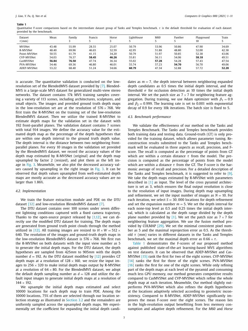
Table 1
Quantitative F-score comparisons based on the intermediate dataset group of Tanks and Temples benchmark. τ is the default threshold for evaluation of each dataset
provided by the benchmark.
Dataset Mean Family Francis Horse LightHouse M60 Panther Playground Train
τ (mm) 3 5 3 5 5 5 10 5
MVSNet 43.48 55.99 28.55 25.07 50.79 53.96 50.86 47.90 34.69
R-MVSNet 48.40 69.96 46.65 32.59 42.95 51.88 48.80 52.00 42.38
Point-MVSNet 50.55 61.79 41.15 34.20 50.79 51.97 50.85 52.38 43.06
CVP-MVSNet 54.03 76.37 58.45 46.26 55.81 56.11 54.06 58.18 49.51
CasMVSNet 56.84 76.50 47.74 36.34 55.02 57.28 54.28 57.43 47.54
PVA-MVSNet 54.46 69.36 46.80 46.01 55.74 57.23 54.70 56.70 49.06
ADEP-MVSNet 53.22 68.40 51.24 34.66 60.79 47.34 52.88 57.72 52.28
i
r
M
n
i
s
i
fi
B
e
1
w
m
a
T
p
b
d
u
a
u
o
m
l
4
d
e
T
r
a
u
6
t
t
t
h
n
d
a
a
t
f
1
1
1
l
u
m
d
d
t
i
g
a
d
4
T
b
v
c
m
s
w
c
w
m
t
W
d
t
t
a
e
a
e
v
p
n
v
b
o
b
a
o
M
[
[
p
m
c
d
p
a
s
p
i
s
s accurate. The quantitative validation is conducted on the low-
esolution set of the BlendedMVS dataset provided by [7] . Blended-
VS is a large-scale MVS dataset for generalized multi-view stereo
etworks. The dataset contains 17k MVS training samples cover-
ng a variety of 113 scenes, including architectures, sculptures, and
mall objects. The images and provided ground truth depth maps
n the low-resolution set are at the resolution of 576 × 768 . We
rst train the R-MVSNet on the training set of the low-resolution
lendedMVS dataset. Then we utilize the trained R-MVSNet to
stimate depth maps for the validation set in the dataset with
92 front-parallel planes. The validation dataset contains 7 scenes
ith total 914 images. We define the accuracy value for the esti-
ated depth map as the percentage of the depth hypotheses that
re within one depth interval to the ground truth depth value.
he depth interval is the distance between two neighboring front-
arallel planes. For every 10 images in the validation set provided
y the BlendedMVS dataset, we record the accuracy values of the
epth map estimated by R-MVSNet (original) and the depth map
psampled by factor 2 (resized), and plot them as the left im-
ge in Fig. 3 . Meanwhile, we also plot the decreased accuracy val-
es caused by upsampling in the right image in Fig. 3 . It can be
bserved that depth values upsampled from well-estimated depth
aps are mostly accurate as the decreased accuracy values are no
arger than 1 . 86% .
.2. Implementation
We train the feature extraction module and PDE on the DTU
ataset [32] and low-resolution BlendedMVS dataset [7] .
The DTU dataset contains over 100 scenes under seven differ-
nt lightning conditions captured with a fixed camera trajectory.
hanks to the open-source project released by [1,12] , we can di-
ectly use the modified DTU dataset for training. The depth maps
re generated from ground truth point clouds through the method
tilized in [12] . All training images are resized to H × W = 512 ×40 . The resolution of the images and ground-truth depth maps in
he low-resolution BlendedMVS dataset is 576 × 768 . We first run
he R-MVSNet on both datasets with the input view number as 5
o generate the initial depth maps. For the DTU dataset, the depth
ypotheses are sampled from 425 mm to 905 mm with the depth
umber d = 192 . As the DTU dataset modified by [12] provides GT
epth maps at a resolution of 128 × 160 , we resize the input im-
ges to 256 × 320 to make initial depth maps output by R-MVSNet
t a resolution of 64 × 80 . For the BlendedMVS dataset, we adopt
he default depth sampling number as d = 128 and utilize the de-
ault input images to generate initial depth maps at a resolution of
44 × 192 .
We upsample the initial depth maps estimated and select
0 0 0 0 locations for each depth map to train PDE. Among the
0 0 0 0 locations, 75% of them are selected through our location se-
ection strategy as illustrated in Section 3.2 and the remainders are
niformly sampled across the upsampled depth maps. We experi-
entally set the coefficient for expanding the initial depth candi-
7
ates as m = 7 , the depth interval between neighboring expanded
epth candidates as 0.5 times the initial depth interval, and the
hreshold σ for occlusion detection as 10 times the initial depth
nterval. We set the patch size as 7 × 7 for neighboring feature ag-
regation. During training, we use Adam optimizer with β1 = 0 . 9
nd β2 = 0 . 999 . The learning rate is set to 0.001 with exponential
ecay of 0.9 for every 10k iterations. The batch size is fixed to 5.
.3. Benchmark performance
We validate the effectiveness of our method on the Tanks and
emples Benchmark. The Tanks and Temples benchmark provides
oth training data and testing data. Ground-truth (GT) is only pro-
ided for the training dataset, which allows parameter tuning. Re-
onstruction results submitted to the Tanks and Temples bench-
ark will be evaluated in three aspects as recall, precision, and F-
core. The recall is computed as the percentage of points from GT
hich are within a certain distance τ from the model. The pre-
ision is computed as the percentage of points from the model
hich are within a distance τ from the GT. The F-score is the har-
onic average of recall and precision. For a detailed description of
he Tanks and Temples benchmark, it is suggested to refer to [9] .
e take the depth maps estimated by R-MVSNet with parameters
escribed in [1] as input. The level of the cross pyramid architec-
ure is set as 3, which ensures the final output resolution is close
o the resolution of input images. During depth map upsampling
nd refinement, we set the input number of images as N = 10 . For
ach iteration, we select S = 30 , 0 0 0 locations for depth refinement
nd set the expansion number m = 5 . We set the depth interval for
ach none-top level as 0.5 and 0.25 times the initial depth inter-
al, which is calculated as the depth range divided by the depth
lane number provided by [1] . We set the patch size as 7 × 7 for
eighboring feature aggregation. We use the fusion method pro-
ided by COLMAP [29] . We set the minimal consistent pixel num-
er as 5 and the maximal reprojection error as 0.5. As the thresh-
ld τ (mm) varies in different datasets in the Tanks and Temples
enchmark, we set the maximal depth error as 0 . 66 × τ .
Table 1 demonstrates the F-scores of our proposed method
gainst published state-of-the-art learning-based MVS algorithms
n test datasets. It can be observed that ADEP-MVSNet and Cas-
VSNet [15] rank the first for two of the eight scenes. CVP-MVSNet
14] ranks the first for three of the eight scenes. PVA-MVSNet
16] ranks the first for one of the eight scenes. While only refining
art of the depth maps at each level of the pyramid and consuming
uch less GPU memory, our method generates competitive results
ompared to CasMVSNet and CVP-MVSNet which refine the whole
epth map at each iteration. Meanwhile, Our method slightly out-
erforms PVA-MVSNet which also refines the depth hypotheses
t the locations adaptively selected according to geometric incon-
istency. Compared to R-MVSNet, ADEP-MVSNet significantly im-
roves the mean F-score over the eight scenes. The reason lies
n the high-resolution output benefitting from less memory con-
umption and adaptive depth refinement. For the M60 and Horse
J. Liao, Y. Fu, Q. Yan et al. Computers & Graphics 0 0 0 (2021) 1–11
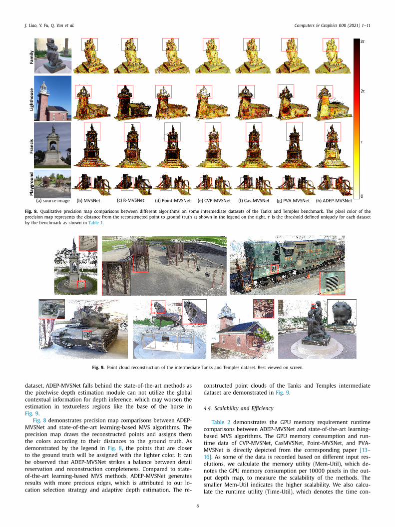
Fig. 8. Qualitative precision map comparisons between different algorithms on some intermediate datasets of the Tanks and Temples benchmark. The pixel color of the
precision map represents the distance from the reconstructed point to ground truth as shown in the legend on the right. τ is the threshold defined uniquely for each dataset
by the benchmark as shown in Table 1 .
Fig. 9. Point cloud reconstruction of the intermediate Tanks and Temples dataset. Best viewed on screen.
d
t
c
e
F
M
p
t
d
t
b
r
o
r
c
c
d
4
c
b
t
M
1
o
n
p
s
ataset, ADEP-MVSNet falls behind the state-of-the-art methods as
he pixelwise depth estimation module can not utilize the global
ontextual information for depth inference, which may worsen the
stimation in textureless regions like the base of the horse in
ig. 9 .
Fig. 8 demonstrates precision map comparisons between ADEP-
VSNet and state-of-the-art learning-based MVS algorithms. The
recision map draws the reconstructed points and assigns them
he colors according to their distances to the ground truth. As
emonstrated by the legend in Fig. 8 , the points that are closer
o the ground truth will be assigned with the lighter color. It can
e observed that ADEP-MVSNet strikes a balance between detail
eservation and reconstruction completeness. Compared to state-
f-the-art learning-based MVS methods, ADEP-MVSNet generates
esults with more precious edges, which is attributed to our lo-
ation selection strategy and adaptive depth estimation. The re-
l8
onstructed point clouds of the Tanks and Temples intermediate
ataset are demonstrated in Fig. 9 .
.4. Scalability and Efficiency
Table 2 demonstrates the GPU memory requirement runtime
omparisons between ADEP-MVSNet and state-of-the-art learning-
ased MVS algorithms. The GPU memory consumption and run-
ime data of CVP-MVSNet, CasMVSNet, Point-MVSNet, and PVA-
VSNet is directly depicted from the corresponding paper [13–
6] . As some of the data is recorded based on different input res-
lutions, we calculate the memory utility (Mem-Util), which de-
otes the GPU memory consumption per 10 0 0 0 pixels in the out-
ut depth map, to measure the scalability of the methods. The
maller Mem-Util indicates the higher scalability. We also calcu-
ate the runtime utility (Time-Util), which denotes the time con-
J. Liao, Y. Fu, Q. Yan et al. Computers & Graphics 0 0 0 (2021) 1–11
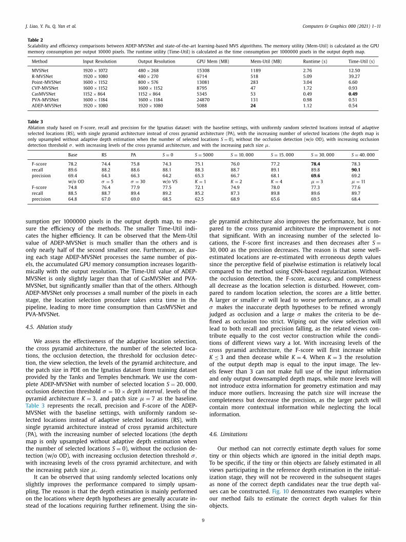
Table 2
Scalability and efficiency comparisons between ADEP-MVSNet and state-of-the-art learning-based MVS algorithms. The memory utility (Mem-Util) is calculated as the GPU
memory consumption per output 10 0 0 0 pixels. The runtime utility (Time-Util) is calculated as the time consumption per 10 0 0 0 0 0 pixels in the output depth map.
Method Input Resolution Output Resolution GPU Mem (MB) Mem-Util (MB) Runtime (s) Time-Util (s)
MVSNet 1920 × 1072 480 × 268 15308 1189 2.76 12.50
R-MVSNet 1920 × 1080 480 × 270 6714 518 5.09 39.27
Point-MVSNet 1600 × 1152 800 × 576 13081 283 3.04 6.60
CVP-MVSNet 1600 × 1152 1600 × 1152 8795 47 1.72 0.93
CasMVSNet 1152 × 864 1152 × 864 5345 53 0.49 0.49
PVA-MVSNet 1600 × 1184 1600 × 1184 24870 131 0.98 0.51
ADEP-MVSNet 1920 × 1080 1920 × 1080 5088 24 1.12 0.54
Table 3
Ablation study based on F-score, recall and precision for the Ignatius dataset: with the baseline settings, with uniformly random selected locations instead of adaptive
selected locations (RS), with single pyramid architecture instead of cross pyramid architecture (PA), with the increasing number of selected locations (the depth map is
only upsampled without adaptive depth estimation when the number of selected locations S = 0 ), without the occlusion detection (w/o OD), with increasing occlusion
detection threshold σ, with increasing levels of the cross pyramid architecture, and with the increasing patch size μ.
Base RS PA S = 0 S = 50 0 0 S = 10 , 0 0 0 S = 15 , 0 0 0 S = 30 , 0 0 0 S = 40 , 0 0 0
F-score 78.2 74.4 75.8 74.3 75.1 76.0 77.2 78.4 78.3
recall 89.6 88.2 88.6 88.1 88.3 88.7 89.1 89.8 90.1
precision 69.4 64.3 66.3 64.2 65.3 66.7 68.1 69.6 69.2
w/o OD σ = 5 σ = 30 w/o VS K = 1 K = 2 K = 4 μ = 3 μ = 11
F-score 74.8 76.4 77.9 77.5 72.1 74.9 78.0 77.3 77.6
recall 88.5 88.7 89.4 89.2 85.2 87.3 89.8 89.6 89.7
precision 64.8 67.0 69.0 68.5 62.5 68.9 65.6 69.5 68.4
s
s
c
v
o
i
e
m
M
M
A
s
p
P
4
t
t
t
t
p
p
o
p
T
M
l
s
(
m
t
t
w
t
s
p
o
s
g
p
t
c
3
e
s
c
t
a
p
A
σj
fi
l
t
t
c
K
o
e
a
n
i
c
c
i
4
t
T
v
i
a
u
o
o
umption per 10 0 0 0 0 0 pixels in the output depth map, to mea-
ure the efficiency of the methods. The smaller Time-Util indi-
ates the higher efficiency. It can be observed that the Mem-Util
alue of ADEP-MVSNet is much smaller than the others and is
nly nearly half of the second smallest one. Furthermore, as dur-
ng each stage ADEP-MVSNet processes the same number of pix-
ls, the accumulated GPU memory consumption increases logarith-
ically with the output resolution. The Time-Util value of ADEP-
VSNet is only slightly larger than that of CasMVSNet and PVA-
VSNet, but significantly smaller than that of the others. Although
DEP-MVSNet only processes a small number of the pixels in each
tage, the location selection procedure takes extra time in the
ipeline, leading to more time consumption than CasMVSNet and
VA-MVSNet.
.5. Ablation study
We assess the effectiveness of the adaptive location selection,
he cross pyramid architecture, the number of the selected loca-
ions, the occlusion detection, the threshold for occlusion detec-
ion, the view selection, the levels of the pyramid architecture, and
he patch size in PDE on the Ignatius dataset from training dataset
rovided by the Tanks and Temples benchmark. We use the com-
lete ADEP-MVSNet with number of selected location S = 20 , 0 0 0 ,
cclusion detection threshold σ = 10 × depth interv al, levels of the
yramid architecture K = 3 , and patch size μ = 7 as the baseline.
able 3 represents the recall, precision and F-score of the ADEP-
VSNet with the baseline settings, with uniformly random se-
ected locations instead of adaptive selected locations (RS), with
ingle pyramid architecture instead of cross pyramid architecture
PA), with the increasing number of selected locations (the depth
ap is only upsampled without adaptive depth estimation when
he number of selected locations S = 0 ), without the occlusion de-
ection (w/o OD), with increasing occlusion detection threshold σ,
ith increasing levels of the cross pyramid architecture, and with
he increasing patch size μ.
It can be observed that using randomly selected locations only
lightly improves the performance compared to simply upsam-
ling. The reason is that the depth estimation is mainly performed
n the locations where depth hypotheses are generally accurate in-
tead of the locations requiring further refinement. Using the sin-
9
le pyramid architecture also improves the performance, but com-
ared to the cross pyramid architecture the improvement is not
hat significant. With an increasing number of the selected lo-
ations, the F-score first increases and then decreases after S =
0 , 0 0 0 as the precision decreases. The reason is that some well-
stimated locations are re-estimated with erroneous depth values
ince the perceptive field of pixelwise estimation is relatively local
ompared to the method using CNN-based regularization. Without
he occlusion detection, the F-score, accuracy, and completeness
ll decrease as the location selection is disturbed. However, com-
ared to random location selection, the scores are a little better.
larger or smaller σ will lead to worse performance, as a small
makes the inaccurate depth hypotheses to be refined wrongly
udged as occlusion and a large σ makes the criteria to be de-
ned as occlusion too strict. Wiping out the view selection will
ead to both recall and precision falling, as the related views con-
ribute equally to the cost vector construction while the condi-
ions of different views vary a lot. With increasing levels of the
ross pyramid architecture, the F-score will first increase while
≤ 3 and then decease while K = 4 . When K = 3 the resolution
f the output depth map is equal to the input image. The lev-
ls fewer than 3 can not make full use of the input information
nd only output downsampled depth maps, while more levels will
ot introduce extra information for geometry estimation and may
nduce more outliers. Increasing the patch size will increase the
ompleteness but decrease the precision, as the larger patch will
ontain more contextual information while neglecting the local
nformation.
.6. Limitations
Our method can not correctly estimate depth values for some
iny or thin objects which are ignored in the initial depth maps.
o be specific, if the tiny or thin objects are falsely estimated in all
iews participating in the reference depth estimation in the initial-
zation stage, they will not be recovered in the subsequent stages
s none of the correct depth candidates near the true depth val-
es can be constructed. Fig. 10 demonstrates two examples where
ur method fails to estimate the correct depth values for thin
bjects.
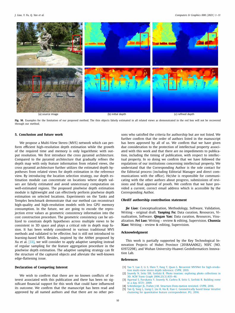
J. Liao, Y. Fu, Q. Yan et al. Computers & Graphics 0 0 0 (2021) 1–11
Fig. 10. Examples for the limitation of our proposed method. The thin objects falsely estimated in all related views as demonstrated in the red box will not be recovered
through our method.
5
f
o
p
C
d
c
p
v
t
u
w
m
e
T
h
c
j
c
l
c
s
m
l
X
o
p
t
e
D
t
n
i
a
s
f
h
d
a
t
t
r
u
t
m
c
s
v
C
C
W
s
a
X
A
n
6
t
R
. Conclusion and future work
We propose a Multi-View Stereo (MVS) network which can per-
orm efficient high-resolution depth estimation while the growth
f the required time and memory is only logarithmic with out-
ut resolution. We first introduce the cross pyramid architecture.
ompared to the pyramid architecture that gradually refines the
epth map with only feature information from related views, the
ross pyramid architecture further utilizes the estimated depth hy-
otheses from related views for depth estimation in the reference
iew. By introducing the location selection strategy, our depth es-
imation module can concentrate on locations where depth val-
es are falsely estimated and avoid unnecessary computation on
ell-estimated regions. The proposed pixelwise depth estimation
odule is lightweight and can effectively perform pixelwise depth
stimation on selected locations. Experiments on the Tanks and
emples benchmark demonstrate that our method can reconstruct
igh-quality and high-resolution models with less GPU memory
onsumption. In the future, we are going to encode the repro-
ection error values as geometric consistency information into the
ost construction procedure. The geometric consistency can be uti-
ized to constrain depth hypotheses across multiple views to be
onsistent in 3D space and plays a critical role in depth map fu-
ion. It has been widely considered in various traditional MVS
ethods and validated to be effective, but is still not introduced to
earning-based MVS. Besides, inspired by the AANet proposed by
u et al. [33] , we will consider to apply adaptive sampling instead
f regular sampling for the feature aggregation procedure in the
ixelwise depth estimation. The adaptive sampling strategy can fit
he structure of the captured objects and alleviate the well-known
dge-flattening issue.
eclaration of Competing Interest
We wish to confirm that there are no known conflicts of in-
erest associated with this publication and there has been no sig-
ificant financial support for this work that could have influenced
ts outcome. We confirm that the manuscript has been read and
pproved by all named authors and that there are no other per-
10
ons who satisfied the criteria for authorship but are not listed. We
urther confirm that the order of authors listed in the manuscript
as been approved by all of us. We confirm that we have given
ue consideration to the protection of intellectual property associ-
ted with this work and that there are no impediments to publica-
ion, including the timing of publication, with respect to intellec-
ual property. In so doing we confirm that we have followed the
egulations of our institutions concerning intellectual property. We
nderstand that the Corresponding Author is the sole contact for
he Editorial process (including Editorial Manager and direct com-
unications with the office). He/she is responsible for communi-
ating with the other authors about progress, submissions of revi-
ions and final approval of proofs. We confirm that we have pro-
ided a current, correct email address which is accessible by the
orresponding Author.
RediT authorship contribution statement
Jie Liao: Conceptualization, Methodology, Software, Validation,
riting - original draft. Yanping Fu: Data curation, Resources, Vi-
ualization, Software. Qingan Yan: Data curation, Resources, Visu-
lization. Fei Luo: Writing - review & editing, Supervision. Chunxia
iao: Writing - review & editing, Supervision.
cknowledgment
This work is partially supported by the Key Technological In-
ovation Projects of Hubei Province (2018AAA062), NSFC (NO.
1972298), and Wuhan University-Huawei GeoInformatices Innova-
ion Lab.
eferences
[1] Yao Y , Luo Z , Li S , Shen T , Fang T , Quan L . Recurrent MVSNet for high-resolu-
tion multi-view stereo depth inference. CVPR; 2019 . [2] Snavely N , Seitz SM , Szeliski R . Photo tourism: exploring photo collections in
3D. ACM Trans Graph 2006;25(3):835–46 .
[3] Agarwal S , Furukawa Y , Snavely N , Curless B , Seitz S , Szeliski R . Building romein a day. ICCV; 2009 .
[4] Schönberger JL , Frahm J-M . Structure-from-motion revisited. CVPR; 2016 . [5] Yan Q , Yang L , Liang C , Liu H , Hu R , Xiao C . Geometrically based linear iterative
clustering for quantitative feature correspondence. PG; 2016 .
J. Liao, Y. Fu, Q. Yan et al. Computers & Graphics 0 0 0 (2021) 1–11
[
[
[
[
[
[
[
[
[
[
[
[
[
[
[
[
[6] Yan Q , Yang L , Zhang L , Xiao C . Distinguishing the indistinguishable: exploringstructural ambiguities via geodesic context. CVPR; 2017 .
[7] Yao Y , Luo Z , Li S , Zhang J , Ren Y , Zhou L , et al. Blendedmvs: a large-scaledataset for generalized multi-view stereo networks CVPR; 2020 .
[8] Jensen RR , Dahl AL , Vogiatzis G , Tola E , Aanaes H . Large scale multi-view stere-opsis evaluation. CVPR; 2014 .
[9] Knapitsch A , Park J , Zhou Q-Y , Koltun V . Tanks and temples: benchmarkinglarge-scale scene reconstruction. ACM Trans Graph 2017;36(4) .
[10] Schöps T , Schönberger JL , Galliani S , Sattler T , Schindler K , Pollefeys M , et al. A
multi-view stereo benchmark with high-resolution images and multi-camera videos CVPR; 2017 .
[11] Kar A , Hane C , Malik J . Learning a multi-view stereo machine. NIPS; 2017 . 12] Yao Y , Luo Z , Li S , Fang T , Quan L . MVSNet: depth inference for unstructured
multi-view stereo. ECCV; 2018 . [13] Chen R , Han S , Xu J , Su H . Point-based multi-view stereo network. ICCV; 2019 .
[14] Yang J , Mao W , Alvarez JM , Liu M . Cost volume pyramid based depth inference
for multi-view stereo. CVPR; 2020 . [15] Gu X , Fan Z , Zhu S , Dai Z , Tan F , Tan P . Cascade cost volume for high-resolution
multi-view stereo and stereo matching. CVPR; 2020 . [16] Yi H , Wei Z , Ding M , Zhang R , Chen Y , Wang G , et al. Pyramid multi-view
stereo net with self-adaptive view aggregation ECCV; 2020 . [17] Furukawa Y , Ponce J . Accurate, dense, and robust multiview stereopsis. PAMI
2010;32(8):1362–76 .
[18] Lhuillier M , Quan L . A quasi-dense approach to surface reconstruction from
uncalibrated images. IEEE Trans Pattern Anal Mach Intell 2005;27(3):418–33 .
[19] Collins RT . A space-sweep approach to true multi-image matching. CVPR. IEEE; 1996 .
20] Kutulakos KN , Seitz SM . A theory of shape by space carving. Int J Comput Vis20 0 0;38(3):199–218 .
11
21] Seitz SM , Dyer CR . Photorealistic scene reconstruction by voxel coloring. Int J Comput Vis 1999;35(2):151–73 .
22] Campbell ND , Vogiatzis G , Hernández C , Cipolla R . Using multiple hypothesesto improve depth-maps for multi-view stereo. ECCV. Springer; 2008 .
23] Galliani S , Lasinger K , Schindler K . Massively parallel multiview stereopsis by surface normal diffusion. ICCV; 2015 .
24] Schönberger JL , Zheng E , Frahm J-M , Pollefeys M . Pixelwise view selection forunstructured multi-view stereo. In: ECCV. Springer; 2016. p. 501–18 .
25] Yao Y , Li S , Zhu S , Deng H , Fang T , Quan L . Relative camera refinement for
accurate dense reconstruction. 3DV. IEEE; 2017 . 26] Liao J , Fu Y , Yan Q , Xiao C . Pyramid multiview stereo with local consistency.
Comput Graph Forum 2019;38(7):335–46 . 27] Romanoni A , Matteucci M . TAPA-MVS: textureless-aware patchMatch multi-
-view stereo.. CVPR; 2019 . 28] Xu Q , Tao W . Multi-scale geometric consistency guided multi-view stereo..
CVPR; 2019 .
29] Schönberger JL , Zheng E , Pollefeys M , Frahm J-M . Pixelwise view selection forunstructured multi-view stereo. ECCV; 2016 .
30] Ji M , Gall J , Zheng H , Liu Y , Fang L . Surfacenet: an end-to-end 3d neural net-work for multiview stereopsis. ICCV; 2017 .
31] Huang P , Matzen K , Kopf J , Ahuja N , Huang J . DeepMVS: learning multi-viewstereopsis. CVPR; 2018 .
32] Aanæs H , Jensen RR , Vogiatzis G , Tola E , Dahl AB . Large-scale data for multi-
ple-view stereopsis. Int J Comput Vis 2016;120(2):153–68 . 33] Xu H , Zhang J . Aanet: adaptive aggregation network for efficient stereo match-
ing. In: Proceedings of the IEEE/CVF conference on computer vision and pat- tern recognition; 2020. p. 1959–68 .
34] Yan Q , Xu Z , Xiao C . Fast feature-oriented visual connection for large imagecollections. Computer Graphics Forum 2014;33(7):339–48. Wiley .