adaptability factors for open-field tomato production in east and west of malaysia

2015 ASABE Annual International Meeting Paper

An ASABE Meeting Presentation

Paper Number: 2188185

Adaptability Factors for Open-field Tomato Production in East and West of Malaysia

Ramin Shamshiri, PhD, ASABE member1,2

[email protected]

Wan Ishak Wan Ismail, PhD, Professor. Ir3

[email protected]

Desa Ahmad, PhD, Professor. Ir2

[email protected] 1Department of Agricultural and Biological Engineering, University of Florida, Gainesville, FL 32611, USA

2Department of Electrical and Electronic Engineering,

3Department of Biological and Agricultural Engineering,

Universiti Putra Malaysia, 43400, Serdang, Selangor, Malaysia

Written for presentation at the

2015 ASABE Annual International Meeting

Sponsored by ASABE

New Orleans, Louisiana

July 26 – 29, 2015

Abstract. This study concerns with climate resource management to improve open-field production of tomato in tropical lowlands of Malaysia. The objective was to use a model based approach for identifying optimum combination of growing season and location that is most adapted with different reference borders of temperature, relative humidity and vapor pressure deficit. Data were continuously collected every 60 seconds and for 12 months (January to December, 2014), from two major crop production sites in Seremban and Kota Kinabalu, respectively located in East and West of Malaysia. Interactions between simulated environment and growth responses of tomato were determined by means of an adaptability factor model for the purpose of comparing two locations at different months of year. Results of hypotheses testing that in each location, raw data does not vary with different months were rejected at any significant level, concluding that daily-averaged temperature, relative humidity and vapor pressure deficit were affected by different months. To identify the optimum group of days to be recommended as the best candidate growing seasons in each location, raw data were processed by an iterative algorithm that incremented desired growth response values in a tomato-growth model and calculated responses for each environment. Results showed that data from Kota Kinabalu had higher adaptabilities compared to Seremban. In addition, results of simulation indicated that for an open-field tomato production, the highest evapotranspiration rate will occur in the growing season that begins in March.

The authors are solely responsible for the content of this meeting presentation. The presentation does not necessarily reflect the official position of the American Society of Agricultural and Biological Engineers (ASABE), and its printing and distribution does not constitute an

endorsement of views which may be expressed. Meeting presentations are not subject to the formal peer review process by ASABE editorial committees; therefore, they are not to be presented as refereed publications. Citation of this work should state that it is from an ASABE meeting paper. EXAMPLE: Author’s Last Name, Initials. 2015. Title of Presentation. ASABE Paper No. ---. St. Joseph, Mich.:

ASABE. For information about securing permission to reprint or reproduce a meeting presentation, please contact ASABE at [email protected] or 269-932-7004 (2950 Niles Road, St. Joseph, MI 49085-9659 USA).


Keywords. Adaptability, Tomato; Growth response, Temperature, Relative humidity, Vapor Pressure deficit, Malaysia, Tropical lowland, Open-field production.

Introduction

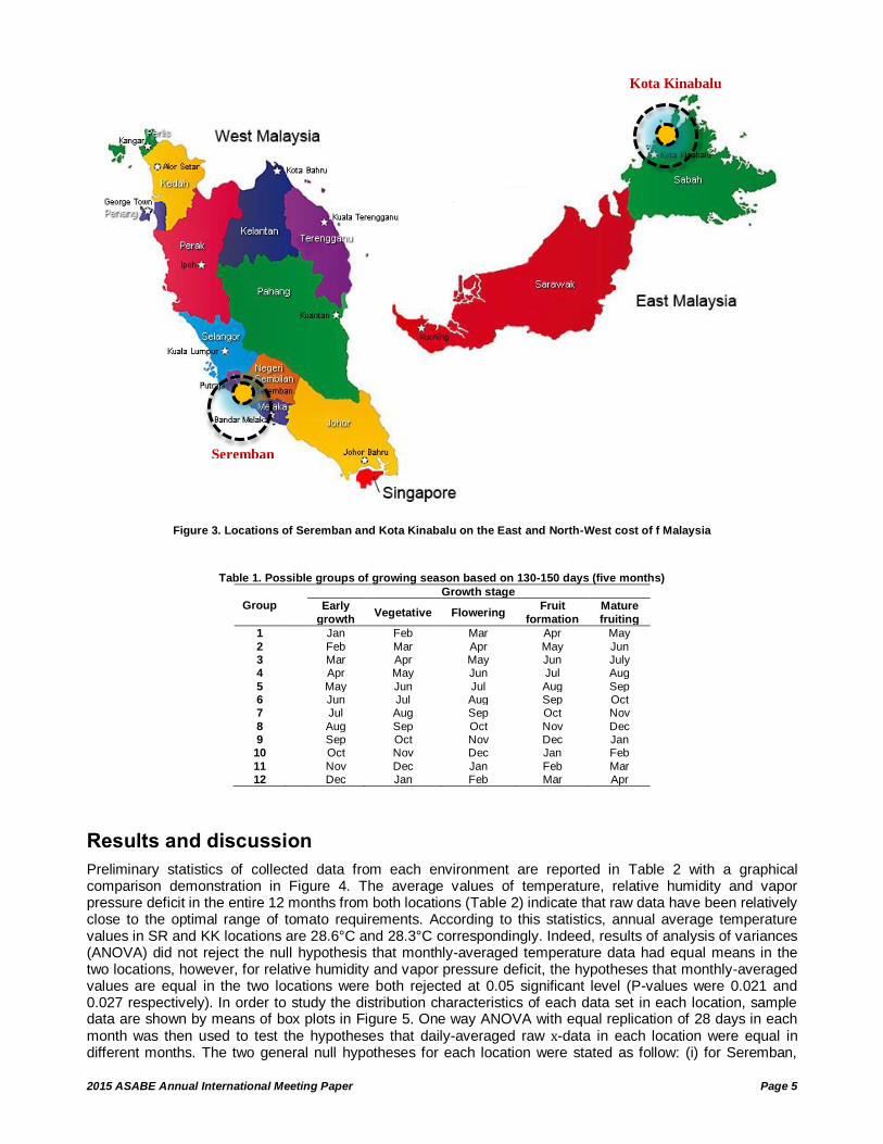
Malaysia is located in the center of South East Asia, and is composed of Peninsular Malaysia on the East and the states of Sabah and Sarawak on the North coast of the Island of Borneo. Malaysia’s climate is identified as tropical and uniform, generally with light winds, high air temperature, humidity, and ample rain throughout the year. Seremban (SR) is the agricultural center for the state of Negeri Sembilan and is located in west Malaysia, about 60 kilometers south from Kuala Lumpur, about 30 kilometers inland from the coast. It has tropical climate (hot and humid) with average temperature of 27-30°C, and peak rainfalls experienced during April to October. Kota Kinabalu (KK) is the capital of the state of Sabah and is located on the northwest coast of Malaysia, facing the South China Sea. It features a distinctive equatorial climate with constant temperature, abundant rainfalls and high humidity. The average temperature ranges from 26-28 °C, with April and May the hottest and January the coolest months respectively. The average annual rainfall in KK is around 2400 millimeters and varies remarkably throughout the year. February and March are typically the driest months. The wind speed ranges from 5.5 to 7.9 m/s during the Northeast Monsoon but is significantly lower to 0.3 to 3.3 m/s during the Southwest Monsoon (Russel, 2006). Sabah Agriculture Park (Taman Pertanian Sabah), is located in KK, it is situated on a 200 hectare site and was developed and maintained by the Agriculture Department. The park offers native Orchids, crops museum, ornamental garden, model garden, plant evolution and plant adaptation garden that has potential for both open-field and closed-field plant production environments. Protected open-field plant production (Shamshiri, 2014) has been practiced as alternative for greenhouse cultivation in hot and humid regions due to their contributions to natural resources and management. Reports indicate that under humid tropical climatic conditions, increase in air temperature and relative humidity can exceed 35ºC and 99% respectively, leading to air vapor pressure deficit (VPD) of 4kPa (Shamshiri et al., 2014a), that causes high transpiration rates with significantly increases in evapotranspiration (ET) demands and stomatal closure. For tropical and subtropical conditions, the strategy in open-field crop cultivation and management in terms of production location and selection of growing season are important in improving resource efficiency.

Tomato (Lycopersicon Esculentum) is one of the most popular vegetables in the world that can grow all year round with available modern cultivation technology. While expected greenhouse yield for tomato is between 300 to 500 tons/ha, traditional greenhouse techniques with fully-closed controlled environment for production of tomato in tropical lowlands of Malaysia causes extreme microclimate condition (Shamshiri and Ismail, 2012; Shamshiri and Ismail, 2014b) with average yield of 80 tons/ha (Shamshiri and Ismail, 2013). It has been reported that by using sheltered open-field production (without side cover and without any environmental control), air temperature and relative humidity under the shelter remain similar with outside (Shamshiri and Ismail, 2014a), which is potentially favored by tomato requirements. Green energy strategies for sustainable development of protected open-field plant production require accurate determination of interactions between climate parameters and growth responses. Requirements of air temperature, relative humidity and vapor pressure deficit for production of tomato depends on specific growth stages (GS) and light condition (sun, cloud, night). Tomato plants are sensitive to temperature and humidity. Temperatures outside the borders of 15-35°C (and night temperatures above 21°C) are harmful for the plant and unflavored to fruit setting. Optimal temperature is in the range of 23-27°C, with exact values depending on crop varieties and growth stages. Tomatoes are either produced for processing purposes (i.e., tomato paste, pulp, sauce and ketchups) or for fresh fruit consumption. They grow best in warm temperatures with a lot of light. Tomato production for processing is cultivated in open-fields, with expected yield of 100-120 ton/ha. Fresh fruit production is cultivated both in greenhouses or open-fields. Average greenhouse yields are around 300-500 tons/ha (FAO, 2012). Different qualities are demanded by the market from each tomato type. For example, processing tomato, the brix (measure of the carbohydrate level in the fruit juices) is counted. For fresh-fruit tomato, the consumer test and shelf life are important. Growth cycle for processing tomato in open-fields is between 120-135 days, according to variety, and for fresh-fruit production in greenhouses is between 150 to 270 days. For tomato farmers, the main criteria for crop management are deciding when to grow, and whether to grow for quantity or quality (with maximum tonnage). Insufficient production of tomato in the scarce highlands of Malaysia has motivated additional development of horticulture facilities to move into lowlands. This research addresses the potential ability of two environments in East and West Malaysia by means of adaptability factors. Specific objectives included identifying optimum combination of growing season and location that is most adapted with different reference borders of temperature, relative humidity and vapor pressure deficit.


Materials and Methods

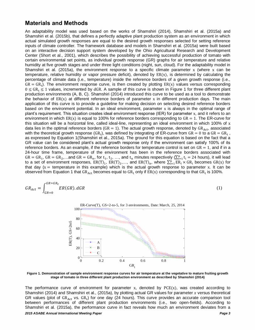
An adaptability model was used based on the works of Shamshiri (2014), Shamshiri et al. (2015a) and Shamshiri et al. (2015b), that defines a perfectly adaptive plant production system as an environment in which actual simulated growth responses are equal to the desired growth responses selected for setting reference inputs of climate controller. The framework database and models in Shamshiri et al. (2015a) were built based on an interactive decision support system developed by the Ohio Agricultural Research and Development Center (Short et al., 2001), which describes the possibility of achieving successful production of tomato with certain environmental set points, as individual growth response (GR) graphs for air temperature and relative humidity at five growth stages and under three light conditions (night, sun, cloud). For the adaptability model in Shamshiri et al. (2015a), the environment response to a specific climate parameter x (where x can be temperature, relative humidity or vapor pressure deficit), denoted by ER(x), is determined by calculating the percentage of climate data (i.e., temperature) inside the reference borders of a given growth response (i.e., GR = GRt). The environment response curve, is then created by plotting ER(x) values versus corresponding

0 ≤ GRt ≤ 1 values, incremented by dGR. A sample of this curve is shown in Figure 1 for three different plant production environments (A, B, C). Shamshiri (2014) introduced this curve to be used as a tool to demonstrate the behavior of ER(x) at different reference borders of parameter x in different production days. The main application of this curve is to provide a guideline for making decision on selecting desired reference borders based on the environment potential. In an ideal environment, parameter x is always in the optimal range of plant’s requirement. This situation creates ideal environment response (IER) for parameter x, and it refers to an environment in which ER(x) is equal to 100% for reference borders corresponding to GR = 1. The ER-curve for

this situation will be a horizontal line, called ideal-line, representing an ideal environment in which 100% of x data lies in the optimal reference borders (GR = 1). The actual growth response, denoted by GRAct, associated with the theoretical growth response (GRt), was defined by integrating of ER-curve from GR = 0 to a GR = GRt , as expressed by Equation 1(Shamshiri et al., 2015a). The ground for this equation is based on the fact that a GR value can be considered plant’s actual growth response only if the environment can satisfy 100% of its reference borders. As an example, if the reference borders for temperature control is set on GR = 1, and if in a 24-hour time frame, temperature of the environment has been in the reference borders associated with GR = GR1, GR = GR2,…and GR = GRn, for t1, t2, …, and tn minutes respectively (∑ ti

ni=1 = 24 hours), it will lead

to a set of environment responses, ER(T)1, ER(T)2,…, and ER(T)n, where ∑ ERini=1 × GRi becomes GR(x) for

that day (x = temperature in this example) which is the actual growth response to parameter x. It can be observed from Equation 1 that GRAct becomes equal to GRt only if ER(x) corresponding to that GRt is 100%.

𝐺𝑅𝐴𝑐𝑡 = ∫ 𝐸𝑅(𝐺𝑅). 𝑑𝐺𝑅𝐺𝑅=𝐺𝑅𝑡

𝐺𝑅=0

(1)

Figure 1. Demonstration of sample environment response curves for air temperature at the vegetative to mature fruiting growth stage of tomato in three different plant production environment as described by Shamshiri (2014)

The performance curve of environment for parameter x, denoted by PCE(x), was created according to

Shamshiri (2014) and Shamshiri et al., (2015a), by plotting actual GR values for parameter 𝑥 versus theoretical GR values (plot of GRAct vs. GRt) for one day (24 hours). This curve provides an accurate comparison tool between performances of different plant production environments (i.e., two open-fields). According to Shamshiri et al. (2015a), the performance curve in fact reveals how much an environment deviates from a

0 0.2 0.4 0.6 0.8 10

20

40

60

80

100ER-Curve(T), GS=2-to-5, for 3 environments, Date: March, 25, 2014

GRt

ER

(T),

GS

=2to

5

A

B

C


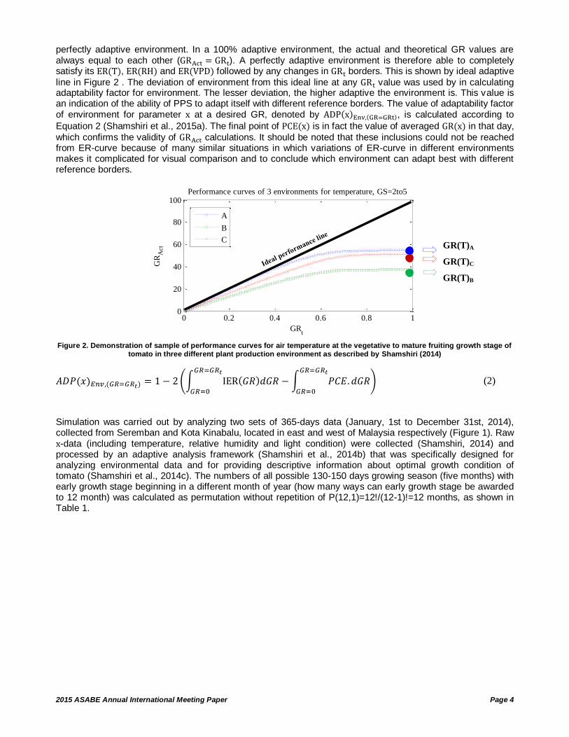
perfectly adaptive environment. In a 100% adaptive environment, the actual and theoretical GR values are always equal to each other (GRAct = GRt). A perfectly adaptive environment is therefore able to completely satisfy its ER(T), ER(RH) and ER(VPD) followed by any changes in GRt borders. This is shown by ideal adaptive

line in Figure 2 . The deviation of environment from this ideal line at any GRt value was used by in calculating adaptability factor for environment. The lesser deviation, the higher adaptive the environment is. This value is an indication of the ability of PPS to adapt itself with different reference borders. The value of adaptability factor of environment for parameter x at a desired GR, denoted by ADP(x)Env,(GR=GRt), is calculated according to

Equation 2 (Shamshiri et al., 2015a). The final point of PCE(x) is in fact the value of averaged GR(x) in that day,

which confirms the validity of GRAct calculations. It should be noted that these inclusions could not be reached from ER-curve because of many similar situations in which variations of ER-curve in different environments makes it complicated for visual comparison and to conclude which environment can adapt best with different reference borders.

Figure 2. Demonstration of sample of performance curves for air temperature at the vegetative to mature fruiting growth stage of tomato in three different plant production environment as described by Shamshiri (2014)

𝐴𝐷𝑃(𝑥)𝐸𝑛𝑣,(𝐺𝑅=𝐺𝑅𝑡) = 1 − 2 (∫ IER(𝐺𝑅)𝑑𝐺𝑅𝐺𝑅=𝐺𝑅𝑡

𝐺𝑅=0

− ∫ 𝑃𝐶𝐸. 𝑑𝐺𝑅𝐺𝑅=𝐺𝑅𝑡

𝐺𝑅=0

) (2)

Simulation was carried out by analyzing two sets of 365-days data (January, 1st to December 31st, 2014), collected from Seremban and Kota Kinabalu, located in east and west of Malaysia respectively (Figure 1). Raw x-data (including temperature, relative humidity and light condition) were collected (Shamshiri, 2014) and processed by an adaptive analysis framework (Shamshiri et al., 2014b) that was specifically designed for analyzing environmental data and for providing descriptive information about optimal growth condition of tomato (Shamshiri et al., 2014c). The numbers of all possible 130-150 days growing season (five months) with early growth stage beginning in a different month of year (how many ways can early growth stage be awarded to 12 month) was calculated as permutation without repetition of P(12,1)=12!/(12-1)!=12 months, as shown in Table 1.

0 0.2 0.4 0.6 0.8 10

20

40

60

80

100Performance curves of 3 environments for temperature, GS=2to5

GRt

GR

Act

A

B

CGR(T)A

GR(T)C

GR(T)B


Figure 3. Locations of Seremban and Kota Kinabalu on the East and North-West cost of f Malaysia

Table 1. Possible groups of growing season based on 130-150 days (five months)

Group

Growth stage

Early

growth Vegetative Flowering

Fruit

formation

Mature

fruiting

1

Jan Feb Mar Apr May

2

Feb Mar Apr May Jun 3

Mar Apr May Jun July

4

Apr May Jun Jul Aug

5

May Jun Jul Aug Sep 6

Jun Jul Aug Sep Oct

7

Jul Aug Sep Oct Nov

8

Aug Sep Oct Nov Dec 9

Sep Oct Nov Dec Jan

10

Oct Nov Dec Jan Feb

11

Nov Dec Jan Feb Mar 12

Dec Jan Feb Mar Apr

Results and discussion

Preliminary statistics of collected data from each environment are reported in Table 2 with a graphical comparison demonstration in Figure 4. The average values of temperature, relative humidity and vapor pressure deficit in the entire 12 months from both locations (Table 2) indicate that raw data have been relatively close to the optimal range of tomato requirements. According to this statistics, annual average temperature values in SR and KK locations are 28.6°C and 28.3°C correspondingly. Indeed, results of analysis of variances (ANOVA) did not reject the null hypothesis that monthly-averaged temperature data had equal means in the two locations, however, for relative humidity and vapor pressure deficit, the hypotheses that monthly-averaged values are equal in the two locations were both rejected at 0.05 significant level (P-values were 0.021 and 0.027 respectively). In order to study the distribution characteristics of each data set in each location, sample data are shown by means of box plots in Figure 5. One way ANOVA with equal replication of 28 days in each month was then used to test the hypotheses that daily-averaged raw x-data in each location were equal in different months. The two general null hypotheses for each location were stated as follow: (i) for Seremban,

Kota Kinabalu

Seremban


H0: μ(xJan)SR

= ⋯ = μ(xDec)SR = 0 and (ii) for Kota Kinabalu, H0: μ(xJan)KK

= ⋯ = μ(xDec)KK = 0, where x refers

to temperature, relative humidity, or VPD. A total of 6 null hypotheses (three parameters and two locations) were tested. Associated P-values resulted from each test were by far smaller than any significant level (almost equal to zero), leading to rejection decision for all null hypotheses. It was then concluded that daily averaged x-data for both locations were affected by months of the year. In the other words, open-field production of tomato can be affected by different selection of growing season.

Table 2. Monthly average temperature, relative humidity and vapor pressure deficit for SR and KK in year 2014

Month Temperature (°C) RH (%) VPD (kPa)

SR KK SR KK SR KK

Jan 27.6 26.4 74.9 85.6 0.994 0.549 Feb 29.3 27.2 67.8 82.6 1.429 0.685 Mar 29.3 28.0 72.2 82.0 1.255 0.730

Apr 28.5 29.3 82.4 80.2 0.758 0.876 May 28.9 29.4 82.5 82.2 0.760 0.802 Jun 30.0 29.6 74.8 78.1 1.142 0.977

Jul 29.5 29.0 74.6 79.4 1.133 0.892 Aug 28.5 28.1 79.1 82.9 0.882 0.717 Sep 28.5 28.8 79.8 80.0 0.848 0.856

Oct 28.3 27.9 81.3 86.8 0.793 0.552 Nov 27.9 28.6 84.5 85.1 0.648 0.644 Dec 27.5 28.0 85.2 86.6 0.598 0.559

Avg 28.7 28.4 78.2 82.6 0.937 0.737 Std 0.8 0.9 5.4 2.9 0.256 0.145

Min 27.5 26.4 67.8 78.1 0.598 0.549 Max 30.0 29.6 85.2 86.8 1.429 0.977

Figure 4. Graphical comparison between monthly-averaged raw data in SR and KK

Jan Feb Mar Apr May Jun Jul Aug Sep Oct Nov Dec25

26

27

28

29

30

31

32

Months

Tem

per

atu

re (

C)

Seremban

Kota Kinabalu

Jan Feb Mar Apr May Jun Jul Aug Sep Oct Nov Dec60

65

70

75

80

85

90

Months

RH

(%

)

Seremban

Kota Kinabalu

Jan Feb Mar Apr May Jun Jul Aug Sep Oct Nov Dec0.4

0.6

0.8

1

1.2

1.4

1.6

Months

VP

D (

kP

a)

Seremban

Kota Kinabalu


Seremban Kota Kinabalu

Figure 5. Distribution characteristics of daily-averaged raw data in SR and KK

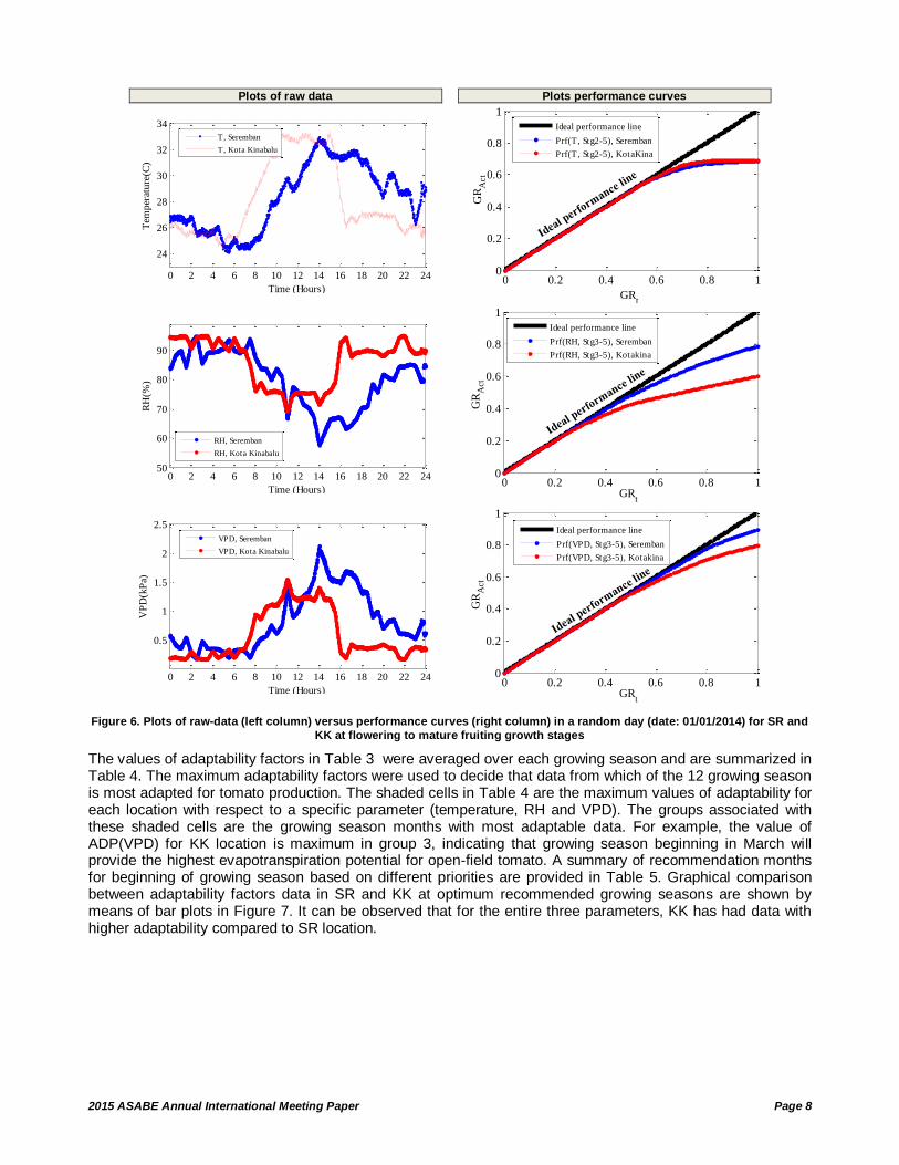
A sample of data collected on a random day (date: 01/01/2014) has been selected for demonstration purpose of the raw-data (Figure 6), and their associations with performance curves at the flowering to mature fruiting growth stages (Figure 6). According to the performance curves for each parameter (temperature, RH, and VPD), a lesser deviation from ideal performance line indicates a higher adaptability of environment with that parameter. In this regards, temperature from both environments in the randomly selected day has similar impact on tomato production at the flowering to mature fruiting growth stage (Figure 6, first row). Raw temperature data for SR and KK locations in Figure 6 have been shown by blue and red color respectively. It can be observed from plots of raw data (Figure 6) that approximately in the first 6 hours, temperature, relative humidity and vapor pressure deficit in both locations have been relatively similar; however in the rest of 18 hours, these plots do not provide an inclusive method for immediate conclusion that climate from which location is more favored at a specific growth stage of tomato. While temperature has been different for 18 hours in the two locations, the overlapped performance curves of temperature (Figure 6, first row) show that this difference does not affect growth response of tomato at flowering to mature fruiting growth stages. It can also be observed that the difference in relative humidity and vapor pressure deficit in SR and KK is translated by performance curves that both data from Seremban are more favored and are closer the ideal performance line (higher adaptability). It should be noted that similar results can be generated for each specific data collection day at different growth responses. The analysis framework developed by Shamshiri et al., (2014b), was used to process the entire raw data and to determine response values for adaptability factor calculations as summarized in Table 3.

Jan Feb Mar Apr May Jun Jul Aug Sep Oct Nov Dec

26

27

28

29

30

31

Tem

per

atu

re (

C)


24

26

28

30

32

Tem

per

atu

re (

C)


50

60

70

80

90

RH

(%

)


70

75

80

85

90

95

RH

(%

)


0.5

1

1.5

2

VP

D (

kP

a)


0.2

0.4

0.6

0.8

1

1.2

1.4

VP

D (

kP

a)


Plots of raw data Plots performance curves

Figure 6. Plots of raw-data (left column) versus performance curves (right column) in a random day (date: 01/01/2014) for SR and

KK at flowering to mature fruiting growth stages

The values of adaptability factors in Table 3 were averaged over each growing season and are summarized in Table 4. The maximum adaptability factors were used to decide that data from which of the 12 growing season is most adapted for tomato production. The shaded cells in Table 4 are the maximum values of adaptability for each location with respect to a specific parameter (temperature, RH and VPD). The groups associated with these shaded cells are the growing season months with most adaptable data. For example, the value of ADP(VPD) for KK location is maximum in group 3, indicating that growing season beginning in March will provide the highest evapotranspiration potential for open-field tomato. A summary of recommendation months for beginning of growing season based on different priorities are provided in Table 5. Graphical comparison between adaptability factors data in SR and KK at optimum recommended growing seasons are shown by means of bar plots in Figure 7. It can be observed that for the entire three parameters, KK has had data with higher adaptability compared to SR location.

0 2 4 6 8 10 12 14 16 18 20 22 24

24

26

28

30

32

34

Time (Hours)

Tem

per

ature

(C)

T, Seremban

T, Kota Kinabalu

0 0.2 0.4 0.6 0.8 10

0.2

0.4

0.6

0.8

1

GRt

GR

Act

Ideal performance line

Prf(T , Stg2-5), Seremban

Prf(T , Stg2-5), KotaKina

0 2 4 6 8 10 12 14 16 18 20 22 2450

60

70

80

90

Time (Hours)

RH

(%)

RH, Seremban

RH, Kota Kinabalu

0 0.2 0.4 0.6 0.8 10

0.2

0.4

0.6

0.8

1

GRt

GR

Act


Prf(RH, Stg3-5), Seremban

Prf(RH, Stg3-5), Kotakina

0 2 4 6 8 10 12 14 16 18 20 22 24

0.5

1

1.5

2

2.5

Time (Hours)

VP

D(k

Pa)

VPD, Seremban

VPD, Kota Kinabalu

0 0.2 0.4 0.6 0.8 10

0.2

0.4

0.6

0.8

1

GRt

GR

Act


Prf(VPD, Stg3-5), Seremban

Prf(VPD, Stg3-5), Kotakina


Table 3. Monthly adaptability factors of climate in different growth stages and growing season groups

Group

ADP(Temperature)


Early growth Vegetative to mature fruiting Early growth Vegetative to mature fruiting

1 0.9 0.83 0.83 0.87 0.86 0.94 0.92 0.9 0.84 0.83 2 0.75 0.83 0.87 0.86 0.81 0.91 0.9 0.84 0.83 0.83 3 0.76 0.87 0.86 0.81 0.83 0.88 0.84 0.83 0.83 0.85

4 0.84 0.86 0.81 0.83 0.88 0.77 0.83 0.83 0.85 0.89 5 0.83 0.81 0.83 0.88 0.88 0.75 0.83 0.85 0.89 0.86 6 0.74 0.83 0.88 0.88 0.88 0.74 0.85 0.89 0.86 0.9

7 0.77 0.88 0.88 0.88 0.9 0.78 0.89 0.86 0.9 0.88 8 0.86 0.88 0.88 0.9 0.91 0.84 0.86 0.9 0.88 0.9 9 0.86 0.88 0.9 0.91 0.91 0.81 0.9 0.88 0.9 0.94

10 0.85 0.9 0.91 0.91 0.83 0.87 0.88 0.9 0.94 0.92 11 0.88 0.91 0.91 0.83 0.83 0.82 0.9 0.94 0.92 0.9 12 0.91 0.91 0.83 0.83 0.87 0.87 0.94 0.92 0.9 0.84

Group

ADP(RH)


Early growth Flowering to mature fruiting Early growth Flowering to mature fruiting

1 0.76 0.83 0.86 0.8 0.81 0.96 0.78 0.84 0.88 0.83 2 0.61 0.79 0.8 0.81 0.93 0.93 0.84 0.88 0.83 0.91

3 0.68 0.79 0.81 0.93 0.9 0.95 0.88 0.83 0.91 0.9 4 0.9 0.8 0.93 0.9 0.87 0.93 0.83 0.91 0.9 0.81 5 0.91 0.89 0.9 0.87 0.87 0.95 0.9 0.9 0.81 0.88

6 0.78 0.85 0.87 0.87 0.81 0.89 0.9 0.81 0.88 0.68 7 0.74 0.84 0.87 0.81 0.72 0.91 0.8 0.88 0.68 0.74 8 0.85 0.86 0.81 0.72 0.72 0.95 0.87 0.68 0.74 0.69 9 0.88 0.79 0.72 0.72 0.88 0.9 0.68 0.74 0.69 0.7

10 0.88 0.71 0.72 0.88 0.93 0.99 0.74 0.69 0.7 0.79 11 0.92 0.71 0.88 0.93 0.86 0.98 0.68 0.7 0.79 0.84 12 0.93 0.84 0.93 0.86 0.8 0.98 0.69 0.79 0.84 0.88

Group

ADP(VPD)


Early growth Flowering to mature fruiting Early growth Flowering to mature fruiting

1 0.83 0.87 0.9 0.92 0.93 0.96 0.88 0.94 0.96 0.94 2 0.66 0.85 0.92 0.93 0.96 0.94 0.93 0.96 0.94 0.96

3 0.71 0.91 0.93 0.96 0.94 0.94 0.95 0.94 0.96 0.96 4 0.89 0.91 0.96 0.94 0.94 0.88 0.93 0.96 0.96 0.92 5 0.89 0.92 0.94 0.94 0.95 0.89 0.93 0.96 0.92 0.95

6 0.77 0.9 0.94 0.95 0.92 0.84 0.95 0.92 0.95 0.84 7 0.76 0.92 0.95 0.92 0.86 0.87 0.9 0.95 0.84 0.88 8 0.86 0.93 0.92 0.86 0.87 0.92 0.93 0.84 0.88 0.83

9 0.88 0.9 0.86 0.87 0.94 0.88 0.83 0.88 0.83 0.82 10 0.88 0.85 0.87 0.94 0.93 0.96 0.88 0.83 0.82 0.89 11 0.91 0.86 0.94 0.93 0.9 0.94 0.83 0.82 0.89 0.94

12 0.93 0.91 0.93 0.9 0.92 0.96 0.82 0.89 0.94 0.96

Table 4. Overall adaptability factors in SR and KK for each growing season. Shaded cells are maximum values

Group ADP(T) ADP(RH) ADP(VPD)

SR KK SR KK S KK

1 0.859 0.888 0.812 0.859 0.890 0.938

2 0.826 0.863 0.787 0.878 0.863 0.947 3 0.828 0.846 0.823 0.894 0.889 0.950 4 0.846 0.832 0.880 0.875 0.927 0.928

5 0.846 0.836 0.888 0.886 0.928 0.931 6 0.842 0.847 0.834 0.830 0.895 0.898 7 0.862 0.862 0.797 0.803 0.880 0.890

8 0.886 0.876 0.791 0.785 0.887 0.882 9 0.892 0.885 0.798 0.742 0.888 0.851 10 0.881 0.902 0.824 0.779 0.891 0.877

11 0.873 0.898 0.860 0.797 0.907 0.884 12 0.872 0.897 0.872 0.837 0.918 0.915

Max 0.892 0.902 0.888 0.894 0.928 0.95 Min 0.826 0.832 0.787 0.742 0.863 0.851


Table 5. Recommended starting months for open-field tomato production in SR and KK based on climate priorities

Preference Seremban Kota Kinabalu

Temperature September October RH May March VPD May March

Figure 7. Graphical comparison between adaptability factors of SR and KK at optimum recommended growing seasons

Conclusion

This paper provided a better understanding of climate condition in two tropical lowland environments in East and West of Malaysia, by addressing relatively long-term trends in temperature, relative humidity and vapor pressure deficit. The objective was to evaluate potential of climate data two locations in tropical lowlands of Malaysia in satisfying different input references of growing condition. A systematic approach with an adaptability model was used for management decision in terms of scheduling efficiencies and site-selection for open-field production of tomato. It was shown that daily-averaged raw data for both locations are affected by different months, concluding that open-field tomato production will experience different climate based on different selection of growing season. Raw data were collected and analyzed by an adaptive analysis framework for instant simulation of growth and environment responses to air-temperature, RH and VPD at specific days, growth stages and location. Performance curves were used as a graphical tool to demonstrate the differences in data of a random day for the two locations. Overall result showed that data from Kota Kinabalu were more favored compared to Seremban. In addition, results of simulation indicated that an open-field tomato production beginning in the month of May (for Seremban) and in March (for Kota Kinabalu) will have the highest evapotranspiration rate due to the highest adaptability factors of vapor pressure deficit.

Acknowledgements

The second author would like to express his appreciations and acknowledge Professor. Ray Buckling, Professor. Tomas Burks, Professor. John K. Schuller and Professor. Reza Ehsani at the University of Florida for their insightful advices and valuable suggestions during his graduate studies.

References FAO world data for 2012 (FAO Statistical Yearbook, FAO, Rome, Italy). Database results (http://faostat.fao.org/)) Russel, Andy Immit Mojiol, (2006). Ecological Landuse Planning and Sustainable Management of Urban and Sub-urban Green

Areas in Kota Kinabalu, Malaysia. Cuvillier Verlag. p. 23. ISBN 978-3-86727-081-6 Shamshiri, R. and W.I.W. Ismail, (2012). Performance evaluation of ventilation and pad-and-fan systems for greenhouse

production of tomato in lowland Malaysia. World Research Journal of Agricultural & Biosystems Engineering. 1(1):1-5. Shamshiri, R. and W.I.W. Ismail, (2013). A Review of Greenhouse Climate Control and Automation Systems in Tropical

Regions. J. Agric. Sci. Appl. 2(3):176-183. Shamshiri, R. 2014. Adaptive Management Framework for Growth Response Analysis of Tomato in Controlled Environment

Plant Production Systems. PhD diss. Universiti Putra Malaysia, Faculty of Engineering. Shamshiri, R. & Wan Ishak Wan Ismail, (2014a). Data Acquisition for Monitoring Vapor Pressure Deficit in a Tropical Lowland

Shelter-house Plant Production. Research Journal of Applied Sciences, Engineering and Technology. 7(20): 4175-4181. Shamshiri, R. & W.I.W. Ismail, (2014b). Investigation of climate control techniques for tropical lowland greenhouses in

Malaysia. J. Applied Sci., 14(1): 60-65.

0.84

0.86

0.88

0.9

0.92

0.94

0.96

0.98

1

ADP(T) ADP(RH) ADP(VPD)

Adap

tabil

ity

fact

or

Adaptability factor based on five months (130-150 days)



Shamshiri, R., Wan Ismail, W.I., & Ahmad, D.B. (2014a). Experimental evaluation of air temperature, relative humidity and vapor pressure deficit in Tropical Lowland Plant Production Environments. Advances in Environmental Biology. 8(22):5-13.

Shamshiri, R., Wan Ismail, W.I., & Ahmad, D.B. (2014b). Adaptive Analysis Framework for Controlled Environments Plant Production, Case Study in Tropical Lowland Malaysia. Paper Number: 1855835. DOI: 10.13031/aim.20141855835. In proceeding of: 2014 ASABE and CSBE/SCGAB Annual International Meeting, At Montreal, Quebec Canada, Page 62-79

Shamshiri, R., Wan Ismail, W.I., & Ahmad, D.B. (2014c). Determining Tomato’s Growth Response to air Temperature, Relative Humidity and Vapor Pressure Deficit in Tropical Lowland Conditions. Paper Number: 1894987. DOI: 10.13031/aim.20141894987. In proceeding of: 2014 ASABE and CSBE/SCGAB Annual International Meeting, At Montreal, Quebec Canada, Page 1107-1124

Shamshiri, R., Wan Ismail, W.I., & Ahmad, D.B. (2015a). Determining Adaptability Factor in Modern Controlled Plant Production Systems. Paper Number: 152108109. In proceeding of ASABE 1st Climate Change Symposium: Adaptation and Mitigation Conference, May 3-5, 2015. Chicago, Illinois USA. (doi:10.13031/cc.20152108109)

Shamshiri, R., Wan Ismail, W.I., Che Man, B. H., & Ahmad, D. B. (2015b). Light Condition Based Analysis of Microclimate Parameters for Improvement of Closed-Field Tomato Production in Tropical lowlands. ASABE Paper No. 2143549. New Orleans, Louisiana.: ASABE.

Short, T.H., Ivey, J. Keener, H.M., 2001. Development of an Interactive Hydroponic Tomato Production Model for Internet Users. ASAE, St. Joseph, U.S.A, paper number 018014

adaptability factors for open-field tomato production in east and west of malaysia

Documents