arX

iv:0

809.

0309

v1 [

astr

o-ph

] 1

Sep

200

8Draft version September 1, 2008Preprint typeset using LATEX style emulateapj v. 03/07/07

AGN HOST GALAXY MORPHOLOGIES IN COSMOS ⋆

J. M. Gabor1, C. D. Impey1, K. Jahnke2, B. D. Simmons3, J. R. Trump1, A. M. Koekemoer4, M. Brusa5, N.Cappelluti5, E. Schinnerer2, V. Smolcic6, M. Salvato6, J. D. Rhodes6,7, B. Mobasher8, P. Capak6, R. Massey6, A.

Leauthaud9, N. Scoville6

Draft version September 1, 2008

ABSTRACT

We use HST/ACS images and a photometric catalog of the COSMOS field to analyze morphologiesof the host galaxies of ∼400 AGN candidates at redshifts 0.3 < z < 1.0. We compare the AGN hostswith a sample of non-active galaxies drawn from the COSMOS field to match the magnitude andredshift distribution of the AGN hosts. We perform 2-D surface brightness modeling with GALFIT toyield host galaxy and nuclear point source magnitudes. X-ray selected AGN host galaxy morphologiesspan a substantial range that peaks between those of early-type, bulge-dominated and late-type,disk-dominated systems. We also measure the asymmetry and concentration of the host galaxies.Unaccounted for, the nuclear point source can significantly bias results of these measured structuralparameters, so we subtract the best-fit point source component to obtain images of the underlying hostgalaxies. Our concentration measurements reinforce the findings of our 2-D morphology fits, placingX-ray AGN hosts between early- and late-type inactive galaxies. AGN host asymmetry distributionsare consistent with those of control galaxies. Combined with a lack of excess companion galaxiesaround AGN, the asymmetry distributions indicate that strong interactions are no more prevalentamong AGN than normal galaxies. In light of recent work, these results suggest that the host galaxiesof AGN at these X-ray luminosities may be in a transition from disk-dominated to bulge-dominated,but that this transition is not typically triggered by major mergers.Subject headings: galaxies: active — galaxies: evolution — galaxies: interactions — galaxies: structure

1. INTRODUCTION

Studies over the past decade suggest fundamen-tal links between galaxies and their central super-

⋆ Based on observations with the NASA/ESA Hubble Space Tele-scope, obtained at the Space Telescope Science Institute, whichis operated by AURA Inc, under NASA contract NAS 5-26555;also based on data collected at : the Subaru Telescope, whichis operated by the National Astronomical Observatory of Japan;the XMM-Newton, an ESA science mission with instruments andcontributions directly funded by ESA Member States and NASA;the European Southern Observatory under Large Program 175.A-0839, Chile; Kitt Peak National Observatory, Cerro Tololo Inter-American Observatory, and the National Optical Astronomy Ob-servatory, which are operated by the Association of Universitiesfor Research in Astronomy, Inc. (AURA) under cooperative agree-ment with the National Science Foundation; the National RadioAstronomy Observatory which is a facility of the National ScienceFoundation operated under cooperative agreement by AssociatedUniversities, Inc ; and and the Canada-France-Hawaii Telescopewith MegaPrime/MegaCam operated as a joint project by theCFHT Corporation, CEA/DAPNIA, the National Research Coun-cil of Canada, the Canadian Astronomy Data Centre, the CentreNational de la Recherche Scientifique de France, TERAPIX andthe University of Hawaii.

1 Steward Observatory, University of Arizona, 933 North CherryAvenue, Tucson, AZ 85721; jgabor@as.arizona.edu

2 Max-Planck-Institut fur Astronomie, Konigstuhl 17, Heidel-berg, D-69117, Germany

3 Department of Astronomy, Yale University, P.O. Box 208101,New Haven, CT 06520-8101

4 Space Telescope Science Institute, 3700 San Martin Drive, Bal-timore, MD 21218

5 Max-Planck-Institut fur extraterrestrische Physik, Giessen-bachstrasse 1, D-85478 Garching, Germany

6 California Institute of Technology, MC 105-24, 1200 East Cal-ifornia Boulevard, Pasadena, CA 91125

7 Jet Propulsion Laboratory, California Institute of Technology,Pasadena, CA 91109

8 Physics and Astronomy Department, University of California,Riverside, Ca 92521

9 BNL & BCCP, University of California, Berkeley, CA 94720

massive black holes (SMBHs). The masses of thecentral SMBHs in nearby galaxies correlate withseveral host bulge properties, including luminos-ity (Kormendy & Richstone 1995; McLure & Dunlop2001; Marconi & Hunt 2003), velocity dispersion(Ferrarese & Merritt 2000; Gebhardt et al. 2000), andmass (Magorrian et al. 1998, for a review of these re-lations, see Ferrarese 2004). More recent studies extendthese relationships to galaxies and quasars at redshiftsfrom z = 0.37 (Treu et al. 2004) to as high as z ∼ 4(Peng et al. 2006a,b).

These observations indicate co-evolution of SMBHmass accretion and host bulge formation processes,perhaps through interactions such as AGN feedback.Galaxy merger simulations that include a prescription forSMBH feedback (Springel et al. 2005) and reproduce theMBH-σbulge relation can recover several observed prop-erties of quasar host descendants, including the stellarmass function of local elliptical galaxies, and the redgalaxy luminosity function and its variation with red-shift (Hopkins et al. 2006). In these models, gas-richmergers drive material toward the central black holes,leading to intense star formation and SMBH accretion.The nuclear SMBH begins its active phase obscured, butfeedback energy during the peak accretion phase blowsaway the obscuring material and results in a brief quasarphase. The blowout phase coincides with a rapid trun-cation of star formation throughout the host galaxy. Re-cent observational studies lend credibility to this pictureby hinting that star-formation quenching coincides withAGN activity (Bundy et al. 2007; Silverman et al. 2008;Tremonti et al. 2007).

This picture of SMBH-host co-evolution relies on a hy-pothesized merger mechanism for fueling active black

2 Gabor et al.

holes, and incorporates predictions that gas-rich diskgalaxies merge to form luminous starbursts, eventuallyevolving into massive elliptical galaxies. Other possi-ble fueling mechanisms include less-direct tidal inter-actions with nearby galaxies (Menci et al. 2004) andinstabilities in a quiescent galaxy’s gaseous disk (e.g.Hopkins & Hernquist 2006). In this study, we explorethe interaction mechanism for intermediate-luminosityAGN in the COSMOS field by analyzing their environ-ments and host galaxies.

Previous similar work employing HST survey data hasfound conflicting evidence. Grogin et al. (2005) analyzed∼100 X-ray selected AGN at redshifts up to ∼1.3 inthe GOODS fields and found no significant differencesbetween their host structural properties and companionfractions and those measured for matched control samplegalaxies. Pierce et al. (2007), on the other hand, exam-ined ∼60 X-ray and IR-selected AGN with 0.2 < z < 1.2in the Extended Groth Strip and found that AGN aremarginally more likely than control galaxies to havenearby companions. In both studies X-ray selected AGNare found to reside predominantly in host galaxies withbulge-dominated morphologies, generally in agreementwith work at low and high redshift quasar host stud-ies (Jahnke et al. 2004b; Sanchez et al. 2004). Inves-tigating larger-scale environments of 52 quasars fromthe DEEP2 redshift survey, Coil et al. (2007) showedthat the quasar-galaxy cross-correlation function at z ∼1closely resembles the galaxy auto-correlation function atall scales, and that the relative quasar bias traces thatof blue galaxies better than red galaxies. This mightsuggest that high luminosity AGN reside in blue bulges(Jahnke et al. 2004b; Silverman et al. 2008) that havenot yet migrated to the high-density environments typi-cally found for massive red galaxies.

In the nearby universe, where precise techniques al-low detailed studies of tens of thousands of AGN hosts(with, e.g., the Sloan Digital Sky Survey), active nu-clei reside in the most massive galaxies, with structuralproperties similar to early-type galaxies but with rela-tively young stellar populations (Kauffmann et al. 2003).Examining images of ∼100 of the most luminous AGNwithin z < 0.1, Kauffmann et al. found that they oc-cupy roughly equal fractions of blue spheroids, single diskgalaxies, and disturbed/interacting galaxies. Further-more, low-redshift close galaxy pairs that exhibit strongindications of interaction are more likely to include AGNthan pairs without interaction indicators (Alonso et al.2007). At the same time, black hole accretion activity issignificantly larger for AGN with bright companions thanotherwise (Alonso et al. 2007), and quasars are found tohave local galaxy overdensities within 100 kpc in excessof that seen in non-active galaxies (Serber et al. 2006)and lower-luminosity AGN (Strand et al. 2008). Com-bined with earlier imaging studies showing that a mi-nority of local Type 1 AGN are undergoing interactions(e.g. De Robertis et al. 1998), these studies suggest thatmergers and interactions play some role in fueling AGN,but not necessarily a dominant one.

These low-redshift AGN may represent a different pop-ulation than that found closer to the peak of AGN ac-tivity, z ≃ 2, with different fueling mechanisms in play.The typical AGN in a local survey like the SDSS is lessluminous and possibly hosted by a galaxy in a differ-

ent evolutionary state than AGN selected at higher red-shift. Intermediate- and high-redshift AGN (z > 0.5)are typically found in bluer, more extended, and more ir-regular galaxies than their low-redshift counterparts (cf.Jahnke et al. 2004b; Sanchez et al. 2004). By using sam-ples with a wider redshift range we can constrain thedominant mechanism in the history of AGN fueling, andpotentially uncover its evolution over cosmic time. Sam-ples at z > 0.3, however, remain limited to a few dozenobjects selected through a variety of methods (see stud-ies mentioned above). In the present study, we extendthis moderate-redshift sample and compare the effects ofdifferent selection techniques.

Using the extensive data of the Cosmic EvolutionSurvey (COSMOS), we determine basic properties of asample of AGN hosts to probe their co-evolution withSMBHs. Selection of the AGN sample and data usedfor the analysis is described in §2. The analyses of thehost galaxies are presented in §§3 and 4, followed by abrief discussion and conclusions. For cosmological cal-culations, we adopt h = 0.75, (where H0 = 100h kms−1 Mpc−1 is the Hubble parameter), ΩM = 0.3 (matterdensity parameter), and ΩΛ = 0.7 (cosmological constantdensity parameter).

2. DATA AND SAMPLE

COSMOS (Scoville et al. 2007), a Hubble Space Tele-scope Treasury project, includes coverage of a 2 squaredegree field from X-ray wavelengths to UV, optical, IR,and radio. The cornerstone data set, which we use forthe bulk of our analysis, consists of 583 orbits takenwith Hubble’s Advanced Camera for Surveys (ACS) withthe F814W filter (see Koekemoer et al. 2007, for a com-plete description). Ancillary observations include XMM-Newton X-ray imaging (Hasinger et al. 2007), VLA ra-dio maps (Schinnerer et al. 2007), and VLT/VIMOS(Lilly et al. 2007) and Magellan/IMACS optical spec-troscopy (Trump et al. 2007, Trump et al. 2008, inpreparation).

Our sample selection focuses on AGN candidates inthe COSMOS field with spectroscopic redshifts. An ob-ject is identified as an AGN candidate through detec-tion as an X-ray point source above the ∼ 10−15 ergcm−2 s−1 flux limit in the 0.5-2 keV or 2-10 keV fluxbands (Cappelluti et al. 2007; Brusa et al. 2007), or aradio source above the 0.1 mJy flux limit at 1.4 GHz(Schinnerer et al. 2007). Optical counterparts to thesecandidates with IAB < 24 are followed up in the Mag-ellan/IMACS spectroscopic survey, whose first season ofobservations is detailed in Trump et al. (2007), includingemission line identification and redshift determination for∼350 objects. We include additional sources from thesecond season of IMACS observations, as well as compan-ion observations using MMT/Hectospec (Trump et al.,in preparation). Targets with successful redshift deter-minations are separated into 4 primary spectral classes:1) broad emission line AGN; 2) narrow emission line ob-jects; 3) red galaxies, with detectable continua but noemission lines; and 4) hybrids showing narrow emissionlines superposed on a red galaxy continuum.

From the spectroscopically-confirmed AGN candi-dates, we restrict our redshift range of interest to 0.3 <z < 1.0. The upper limit arises from our limited abil-ity to adequately analyze targets at high redshift us-

AGN Morphologies 3

TABLE 1Numbers of AGN in the samples.

AGN sample No. of objects a w/ ACS images Successful 2-D fits

AGN candidates w/ spectra ∼1300 *** ***Spec. redshifts 0.3 < z < 1.0 459 391 314Type 1 48 36 19X-ray Class 2 83 (95) 73 57X-ray Class 3 48 (62) 44 36Radio Class 2 40 (120) 32 30Radio Class 3 82 (134) 71 62

a Numbers in parentheses include those objects in the X-ray sample with log(LX ) < 42,and those objects in the radio sample not classified as AGN. Objects failing to satisfythese AGN classifications are excluded from the other columns, as well as the analysesin this work.

ing single-orbit ACS data, and because the ACS F814Wbandpass shifts into the rest-frame UV at z > 1, bias-ing morphological characterization. Based on our sim-ulations described in section 3.1, typical AGN hosts atthis redshift have recovered magnitude uncertainties of∼0.4 magnitudes. The lower redshift limit is a practi-cal one, applied to limit ourselves to objects which havea large number of corresponding inactive galaxies andwhose environments can be analyzed adequately withina 2 square degree field. Additionally, some of the ancil-lary survey boundaries extend beyond those of the ACSobservations, so ∼60 AGN candidates were identified forwhich we have no Hubble data for host analysis. Theseobjects are excluded from the sample.

Determining which candidates truly host an AGN isnon-trivial. Those objects with broad emission lines arethe easiest to classify as AGN, but we treat them sepa-rately due to the uncertainties in analysis of their hosts(see below). A significant fraction of the narrow-line ob-jects may be star-forming galaxies rather than genuineAGN (Trump, private communication), and the IMACSspectra lack sufficient signal-to-noise and spectral rangeto make such a distinction using line-ratio diagnostic di-agrams (cf. Baldwin et al. 1981; Veilleux & Osterbrock1987; Kewley et al. 2001; Kauffmann et al. 2003). Fur-thermore, many X-ray selected candidates, which are ex-pected to be AGN (Mushotzky 2004), exhibit no emis-sion lines, falling into the red galaxy spectral classifica-tion. This might occur due to obscuration of the regionsemitting optical spectral lines, misidentification of theoptical counterparts, or misplacement of the slit whenperforming optical spectroscopy.

With these complications in mind, we present our find-ings separately for various sub-samples, and we use thefollowing terms to describe them. “AGN candidates”refers to the full sample of candidate AGN with spec-troscopic redshifts, and includes 459 objects. “Class 1”or Type 1 “broad line” AGN refers to those candidateswith broad optical emission lines, easily distinguishableas AGN or quasars, and including 48 objects. “Class2” or “narrow emission line” objects refers to AGN can-didates with narrow emission lines in their spectra, in-cluding 120 radio-selected objects and 95 X-ray-selectedobjects. This category generally includes both Type 2AGN as well as star-forming galaxies. “Class 3” or “non-emission line” candidates are those whose spectra looklike red galaxies with no emission lines, including 134radio-selected and 62 X-ray selected objects. In cases

where an object has been detected both in radio and X-ray emission, we include it in the X-ray category. Thesesub-samples are summarized in Table 1.

As in previous AGN studies with similar red-shift ranges (Pierce et al. 2007; Silverman et al. 2008;Bundy et al. 2007), we adopt a cutoff in X-ray luminos-ity above which objects are likely to be AGN-dominated(Bauer et al. 2004). After excluding broad-line AGN, wetake those candidates with L2−10keV > 1042 ergs s−1 asthe most likely to harbor accreting black holes. Here,L2−10keV is the X-ray luminosity in the 2-10 keV band.We estimate this luminosity for all X-ray sources by con-verting the observed XMM-Newton X-ray fluxes via ak-correction. To do so, we assume an X-ray power lawslope of Γ = 1.9 and perform the k-corrections usingspectroscopic redshifts. Of the 95 X-ray-selected Class 2objects, 83 satisfy the luminosity cut given above, andwe refer to them as “X-ray Class 2” AGN. Of the 62X-ray-selected class 3 objects, 48 satisfy the luminositycut, and we refer to them as “X-ray Class 3” objects. Insome parts of our analysis, we combine these two sam-ples together, and generally refer to them as X-ray AGN.Those objects which do not satisfy the luminosity cutare excluded from the following analyses. We note herethat some X-ray point sources have more than one possi-ble optical counterpart, with the most likely counterpartchosen. This ambiguity applies only to three objects inour final sample, so we suspect it has little effect.

For the radio-selected AGN candidates, we use thenovel technique for separating AGN and star-forminggalaxies described in (Smolcic et al. 2008). Briefly, thetechnique uses a combination of morphology and rest-frame colors of optical counterparts to the radio sourcesto classify them as QSOs, stars, star-forming galax-ies, AGN or high-redshift galaxies. From the modi-fied Stromgren photometric system (Odell et al. 2002),Smolcic et al. (2006) derive two principle-componentcombinations of rest-frame colors which “optimally quan-tify the distribution of galaxies in the rest-frame color-color space” (Smolcic et al. 2008). Because the emis-sion line strengths correlate with galaxy spectral en-ergy distributions, these color parameters can mimic linediagnostic diagrams’ ability to separate emission linegalaxies into AGN, composite, and star-forming objects.Smolcic et al. (2008) calibrate this color classificationscheme using galaxies from SDSS matched to the NRAOVLA Sky Survey at 1.4 GHz (Condon et al. 1998), andapply it to the COSMOS radio sources (Schinnerer et al.

4 Gabor et al.

2007). The low-redshift calibration suggests that thesample classified as AGN contatins ∼5% star-forminggalaxies, ∼15% composite objects, and ∼80% AGN, andthese AGN comprise ∼90% of the total population of ra-dio AGN. When we apply the classification scheme tothe radio-selected objects in our sample, we find that122 are identified as AGN, including 40 Class 2 objectsand 82 Class 3 objects. We refer to these as radio AGNthroughout the paper. Roughly 30% of our radio-selectedAGN candidates are not classified either as AGN or star-forming because Smolcic et al. (2008) a) use a conserva-tive search radius of 0.5 arcseconds when identifying opti-cal counterparts, whereas the spectroscopic follow-up in-cluded objects as far as 1 arcsecond from the peak radioemission, and b) they exclude from their radio–opticalsample a fraction of objects (15%) that are photometri-cally flagged in the COSMOS photometric redshift cat-alog Capak et al. (2007, ∼ 30% of which have availablespectroscopic redshifts; see Tab. 1 in Smolcic et al. 2008).The remaining objects, mostly Class 2, are classified asstar-forming galaxies.

We include the broad line AGN for comparison only.Because the redshift distribution of broad line AGNpeaks at higher redshift than the Type 2 distribution,the Type 1 sample includes only ∼50 objects. Further-more, the nuclear component in broad-line AGN tendsto dominate the total optical flux more than in narrow-line AGN, so some of the host-fitting techniques that weapply suffer from more serious systematic uncertainties.These factors hamper our ability to compare with confi-dence the structural parameters and interaction indica-tors between Type 1 and Type 2 AGN hosts. We applythe present analyses to all objects for completeness.

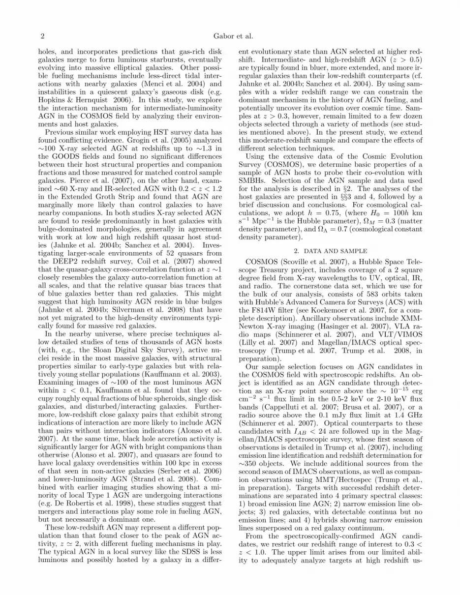
Fig. 1.— Top panel: redshift distributions of narrow-line (solidline) and broad-line (dotted line) AGN cadidates, along with can-didates with no emission lines (dashed line), from seasons 1 and2 of IMACS observations. Bottom panel: redshift distributions ofnarrow line AGN candidates selected using radio emission (dashedline) and X-ray emission (solid line).

Our AGN sample thus includes ∼200 objects withspectroscopically confirmed redshifts in the range 0.3 <z < 1.0, narrow emission line identifications, and ACSimaging. Figure 1 shows the redshift distributions ofAGN in our samples, extending to lower redshift for ref-erence. We suspect the redshift peaks near z = 0.3and z = 0.7 are associated with large scale structuresin the COSMOS field (Scoville et al. 2007). Broad-lineobjects are plotted for comparison, and the distributions

of radio-selected and X-ray-selected narrow-line objectsare compared.

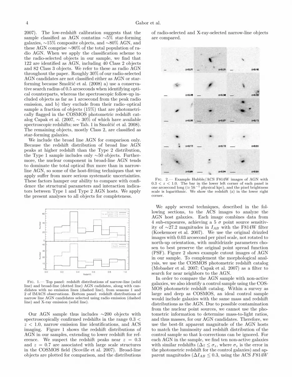
Fig. 2.— Example Hubble/ACS F814W images of AGN with0.3 < z < 1.0. The bar in the lower left corner of each panel isone arcsecond long (≃ 5h−1 physical kpc), and the pixel brightnessscale is logarithmic. We show the redshift (z) in the lower rightcorner.

We apply several techniques, described in the fol-lowing sections, to the ACS images to analyze theAGN host galaxies. Each image combines data from4 sub-exposures, achieving a 5 σ point source sensitiv-ity of ∼27.2 magnitudes in IAB with the F814W filter(Koekemoer et al. 2007). We use the original drizzledimages with 0.03 arcsecond per pixel scale, not rotated tonorth-up orientation, with multidrizzle parameters cho-sen to best preserve the original point spread function(PSF). Figure 2 shows example cutout images of AGNin our sample. To complement the morphological anal-ysis, we use the COSMOS photometric redshift catalog(Mobasher et al. 2007; Capak et al. 2007) as a filter tosearch for near neighbors to the AGN.

In order to compare the AGN sample with non-activegalaxies, we also identify a control sample using the COS-MOS photometric redshift catalog. Within a survey aslarge and deep as COSMOS, an ideal control samplewould include galaxies with the same mass and redshiftdistributions as the AGN. Due to possible contaminationfrom the nuclear point sources, we cannot use the pho-tometric information to determine mass-to-light ratios,and thus masses, for our AGN candidates. Therefore, weuse the best-fit apparent magnitude of the AGN hoststo match the luminosity and redshift distribution of thecontrol sample so that k-corrections can be ignored. Foreach AGN in the sample, we find ten non-active galaxieswith similar redshifts (∆z ≤ σz , where σz is the error inthe photometric redshift for the control galaxies) and ap-parent magnitudes (∆IAB ≤ 0.3, using the ACS F814W

AGN Morphologies 5

detections) to those of the AGN host. We perform anal-yses on the control galaxies in a comparable fashion tothe hosts, as described in the following sections. Forsome comparisons, we find it illustrative to separate thecontrol sample into early and late spectral types usingthe photometric redshift catalog Tphot parameter, whichclassifies galaxies on a scale from 1.0 (red elliptical) to6.0 (starburst) using photometric fits to the galaxy spec-tral energy distributions. We divide the control sampleat Tphot = 2.0, corresponding to an Sa/Sb spectral type.

3. MORPHOLOGICAL ANALYSIS

Using the deep, high-resolution ACS COSMOS imageswe attempt to determine properties of the host galax-ies of our AGN sample. The high angular resolution ofHubble’s diffraction-limited imaging allows us to sepa-rate host galaxy light from that of the nucleus. Usingonly the I-band images, we can constrain the magni-tude, scale, radial light profile, and orientation of thehost galaxy.

In this work we use 2-dimensional surface bright-ness fitting (with GALFIT, Peng et al. 2002) to mea-sure AGN host properties. To understand systematicuncertainties in the surface brightness fitting, we simu-late AGN images and apply identical fitting techniques.After decomposing the images into AGN point sourceand galaxy light, we measure the asymmetry and con-centration of the underlying host galaxies and comparethem directly with the non-active control galaxies. Wefirst describe our simulated AGN images, then explainthe techniques we use for 2-D surface brightness fitting,and describe the results of our 2-D fits. Finally, we dis-cuss the asymmetry and concentration measurements.

3.1. Simulations

We performed two types of simulations to help under-stand systematic uncertainties in our analysis. One suiteof simulations aims to quantify our ability to reliably re-cover parameters in 2-D surface brightness models. Theother suite examines the effect of point-spread function(PSF) variation and mis-application on the analysis. Inthis way we isolate the impacts of the two most impor-tant problems with 2-D fitting.

3.1.1. PSF Variations

In performing 2-D fits to galaxy images, a PSF mustbe supplied to convolve with the galaxy model image.Fits of AGN images are especially sensitive to the PSFdue to the sometimes bright, nuclear point source whoselight is superimposed on that of the host galaxy. TheACS instrument’s PSF ellipticity and size are known tovary both temporally and across the CCD at the levelof a few percent (Rhodes et al. 2007). Our solution, de-scribed in §3.2, includes sets of model PSF grids. Be-cause systematic uncertainties in the PSF can dominatethe morphological classification of compact AGN hosts,we have performed a series of simulations to test how ourability to recover host properties varies with PSF.

We simulate AGN images by superimposing a real starextracted from an ACS image onto sets of simple modelgalaxy images with varying parameters whose ranges aresimilar to those of the AGN sample. The model galaxyimages are created using GALFIT, with effective radius

and magnitude randomly chosen from uniform distribu-tions in the ranges 0.15′′ < reff < 2.5′′ and 19 < m <24, respectively. GALFIT convolves the specified galaxymodel with chosen stellar PSF to yield the model galaxyimage. The star image is then scaled to a random mag-nitude with 16 < m < 25 and added to the galaxy modelimage. We create 2000 such simulated images with expo-nential disk profiles, and an additional 2000 with deVau-couleurs profiles. We use four different real star imagesfor the PSFs, with 500 simulated images per star. Oneof the four stars was chosen to be near the limit of satu-ration, and results for the corresponding 500 simulationsare obviously skewed and thus ignored in later discussion.We refer to the simulations as “PSF simulations,” andwe use them below to characterize the systematic effectsof PSF variation on the results of 2-D surface brightnessfits. To check whether the simulations created with thesefour stars adequately encompass the full range of PSFvariations, we also created 500 simulated AGN imagesusing 50 different stars (10 simulated images per star),each taken from a different ACS tile and a different de-tector position. As the results of fits to these imagesclosely mimic the results obtained with the original fourstars, we leave them out of the discussion below.

3.1.2. Parameter Recovery

Even if we have applied a perfect PSF, signal-to-noiselimits our ability to recover fit parameters accurately, andparameter uncertainties are dominated by systematic ef-fects. To gauge the robustness of recovered parametersand assign appropriate uncertainties, we have performeda set of simulations where the PSF remains constant.

We simulate 2000 AGN images with exponential diskhosts, and another 2000 with deVaucouleurs hosts, withthe same range of parameters as for the PSF simulations.To better represent the background sky noise, which isthe dominant noise component in our images, we ran-domly add cutouts from COSMOS images. While thesebackground images will sometimes include contaminat-ing galaxies, the same is true for our real AGN imagesand the overall effect of the galaxies is minimal. We referto these simulations as “Recovery Simulations,” and byperforming 2-D fits on them we characterize the uncer-tainties in our best-fit AGN parameters due to noise.

3.2. 2-D Surface Brightness Fitting

We use GALFIT (Peng et al. 2002) to fit models toAGN images in the sample. For each image, we modelthe nuclear point source as a point spread function, andthe host galaxy as a single Sersic function (see Peng et al.2002, for details of the functional forms of different mod-els in GALFIT; Sersic 1968). In short, the Sersic func-tion is a general galaxy model which encompasses a rangeof more specific models through the variation of an in-dex, n. The Sersic function with n = 1 is equivalentto an exponential disk model, whereas a Sersic func-tion with n = 4 is equivalent to the de Vaucouleurs(r1/4; de Vaucouleurs & Capaccioli 1979) profile, whichdescribes typical galactic bulges and early-type galaxies.The fit results include point source position and magni-tude (mp), along with the host galaxy magnitude (mh),effective radius (rh), Sersic index (n), axis ratio (b/a),and position angle in the image. Because some of ourAGN candidates may not have a nuclear point source,

6 Gabor et al.

we also performed fits which excluded the point sourcecomponent and used just a single Sersic galaxy model.

Running GALFIT requires an initial guess of each ofthe best-fit parameters, an input image, a point-spreadfunction image, and a sigma image. Input AGN imagesare cut directly from the original ACS images, with acutout image size corresponding to 35 h−1 kpc comov-ing (∼17” for z = 0.3 and 6” for z = 1.0; larger andsmaller image sizes were attempted, with no impact onthe resulting best-fit parameters). In order to generateinitial guesses in an automated way, we developed a pro-cedure similar to that used in GALAPAGOS, describedby Haußler et al. (2007). First we run Source Extractor(Bertin & Arnouts 1996) on the cutout image. For everyextracted source, we generate an elliptical mask imageusing the Source Extractor FLUX_RADIUS, ELONGATION,and THETA_IMAGE output parameters for that source. Toensure conservative estimates of galaxy boundaries, weset the mask semi-major axis to 2×FLUX_RADIUS. Sincethe cutouts are centered on the AGN coordinates (whichare taken as the optical counterparts of X-ray sources),we select the extracted source nearest the center of theimage as the target AGN. For each additional source inthe image, we include it in the 2-D fit if and only if itsmask overlaps the mask of the AGN, and otherwise wesimply mask it out of the image. All added objects aremodeled as single Sersic function profiles. Finally, weidentify the brightest pixel within the AGN mask as aninitial guess for the location of the point-spread functioncomponent.

For Sersic function profiles included in a fit, weestimate the initial parameters using results fromSource Extractor. The effective radius is set torh = 0.162×FLUX_RADIUS based on the simulation re-sults of Haußler et al. (2007). Magnitude guesses areset to MAG_BEST, the axis ratio determined from theELONGATION parameter, and the position angle computedfrom THETA_IMAGE. We constrain the Sersic index to liebetween 0.5 and 8, the magnitude to stray no furtherthan 5 magnitudes from the initial guess, and the effec-tive radius to be less than 500 pixels (15 arcseconds). Forthe AGN host Sersic component, we constrain the effec-tive radius to be less than half the image width. For thePSF component, we set the initial magnitude to 3 mag-nitudes fainter than the AGN host component (based ontypical previous fits of the AGN sample). We constrainthe PSF magnitude to within 10 magnitudes of its initialvalue, and the position to lie within 5 pixels of its initiallocation. The sky value for the image is held constantbased on the sky subtraction of the original COSMOSACS images. We tested several methods for comput-ing the sigma image, including conversion of the weightimages output by MultiDrizzle which correspond to theACS tiles, as well as an empirical determination of thenoise based on the rms signal of regions of sky aroundeach AGN candidate. Differences in the choice of sigmaimages lead to uncertainties which are small comparedto those introduced by PSF mismatch and other effectsdescribed below.

We choose the parameter constraints largely by con-vention, but also to ensure that they fully encompass thereasonable ranges of the parameters. As described be-low, we exclude from further analysis those fits which runinto constraints, since these did not find a true best-fit

and the parameters are likely unphysical. We attemptedsome variations on the fitting constraints; notably, weperformed fits without constraints and fits where we re-stricted the Sersic index to n < 5 rather than 8. Fitswithout constraints fail to converge with a higher fre-quency than those with constraints, although this oc-curs mostly because our model poorly matches the reallight distribution in cases of failure. Fits with a morerestricted Sersic index yield comparable results to thoseobtained with the original n < 8 constraint. A vast ma-jority of fits with n > 5 in the original fits (∼80 objects,including 25 which run into the n = 8 constraint) run intothe constraint when we restrict n < 5. Placing the con-straint at n < 5 would effectively eliminate those objectsfrom our further analysis. However, other parametersof the fits (e.g. host magnitude) may yield reasonableand useful estimates even when a fit runs into the con-straints, and these other parameters can be sensitive tothe constraints chosen. We find that the more restric-tive Sersic index constraint yields host magnitude esti-mates systematically 0.13 magnitudes higher (dimmer)than the original constraint, with a scatter ∼0.5 mag-nitudes. This systematic offset differs from the resultsof Kim et al. (2008) because the objects here are heavilyskewed toward host galaxy-dominated images. Further-more, radius estimates in the restrictive Sersic index caseare a median of 15 pixels (0.45 arcseconds) smaller thanin the original case. These relatively minor differencesdo not affect our main conclusions.

Fig. 3.— Normalized radial point spread function profiles. Theshaded region (upper panel) and dashed lines (both panels) showthe variation from the 10th percentile to the 90th percentile ofprofiles for 50 stars extracted from ACS images. Thick solid linesshow the profiles for three TinyTim PSF models. In the lowerpanel, we divide each profile by the median profile (dotted straightline at 1.0) of the 50 real stars.

For the point-spread function (PSF) solution to theACS imaging, we adopt the PSF grids described inRhodes et al. (2007). These authors were motivated bythe demands of detecting weak lensing signals, which re-quire characterization of image ellipticities at the ∼1%level. Briefly, they use TinyTim software (Krist 2003) tocreate a PSF model at each of ∼4000 points in a regulargrid, and develop several such grids corresponding to dif-ferent focus offsets of the Hubble Space Telescope duringexposure. For each COSMOS ACS image, the best-fit fo-cus position is obtained by simultaneously matching theshapes of model PSFs to ∼10 bright stars chosen from

AGN Morphologies 7

the image. This process is found to be repeatable toan accuracy of ∼1 µm in focus position. Figure 3 ex-hibits the variation in the PSF profiles for 50 real starsselected from different ACS images at different detectorpositions, along with three TinyTim PSF profiles. TheTinyTim PSFs can generally encompass the variationsof the real PSFs, although at large radii they system-atically underestimate the flux level of real PSFs. Foran AGN at any position in an image we use the nearestmodel PSF from the best-fit grid. The results of 2-D fit-ting of simulations described above exhibit some of theresulting systematic effects of inappropriate PSF choice.These effects are described below in §3.3.

After initially fitting all the AGN candidates withGALFIT, we determined whether the results had runinto the boundaries set by the parameter constraints.Many of those objects for which this is the case havecompact light profiles, so we adjusted the initial guessfile such that the point source magnitude equals the hostgalaxy magnitude and the host radius is double the orig-inal guess, and ran GALFIT once again on those objects.Finally, we visually inspected all of the resulting modelimages and residual images, subjectively assessing thequality of the fit, and in some cases attempting to rem-edy a failed fit. This typically entailed masking out anearby star or galaxy whose light was contaminating theimage beyond its original mask. We discuss fit results inthe following section.

In order to place constraints on those objects for whichthe fits failed altogether, we used a simple point sourcesubtraction method. First, we fit each AGN with a sin-gle point source component and no galaxy component inGALFIT. Then we subtracted the best-fit point sourcefrom the image. On the residual image, we identifiedpixels whose flux values changed from positive on theoriginal image to negative after subtraction (indicatingover-subtraction), and set those pixels to zero flux. Thenwe estimated a lower limit for the host galaxy magnitudeby using aperture photometry to measure the residualflux in an aperture with a two arcsecond diameter.

We followed similar procedures with the sample of con-trol galaxies as with the AGN candidates themselves. Wefirst fit the galaxies without a central point source com-ponent. To mimic the process of fitting AGN, we thensuperimposed a point source and applied a fit procedureidentical to the one used for the AGN candidates. Sinceeach AGN candidate has ten matched control galaxies,each control galaxy is matched to a particular AGN can-didate. We thus determined the brightness of the super-imposed point source by using the best-fit point sourcemagnitude from the AGN candidate fit. Thus, the fittingperformed on the control galaxies is well-matched to thatperformed on the AGN candidates.

3.3. 2-D Fitting Results

Since the formal statistical uncertainties output byGALFIT tend to underestimate the true uncertainties,we follow Haußler et al. (2007) and use the mean sur-face brightness as a proxy for image signal-to-noise todiagnose the reliability of recovered fit parameters. Themean surface brightness is defined here as µ = mh +2.5 log(2πr2

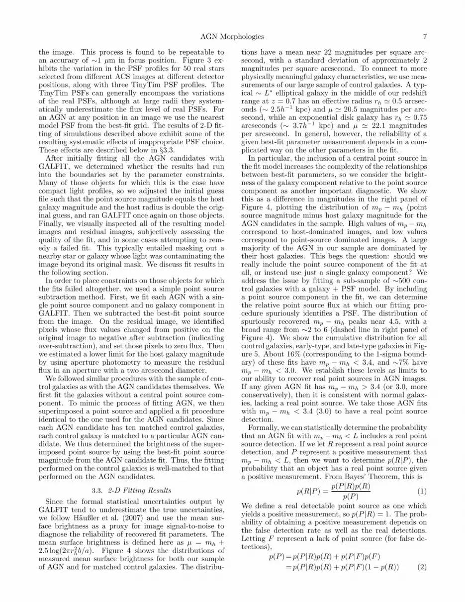
hb/a). Figure 4 shows the distributions ofmeasured mean surface brightness for both our sampleof AGN and for matched control galaxies. The distribu-

tions have a mean near 22 magnitudes per square arc-second, with a standard deviation of approximately 2magnitudes per square arcsecond. To connect to morephysically meaningful galaxy characteristics, we use mea-surements of our large sample of control galaxies. A typ-ical ∼ L∗ elliptical galaxy in the middle of our redshiftrange at z = 0.7 has an effective radius rh ≃ 0.5 arcsec-onds (∼ 2.5h−1 kpc) and µ ≃ 20.5 magnitudes per arc-second, while an exponential disk galaxy has rh ≃ 0.75arcseconds (∼ 3.7h−1 kpc) and µ ≃ 22.1 magnitudesper arcsecond. In general, however, the reliability of agiven best-fit parameter measurement depends in a com-plicated way on the other parameters in the fit.

In particular, the inclusion of a central point source inthe fit model increases the complexity of the relationshipsbetween best-fit parameters, so we consider the bright-ness of the galaxy component relative to the point sourcecomponent as another important diagnostic. We showthis as a difference in magnitudes in the right panel ofFigure 4, plotting the distribution of mp − mh (pointsource magnitude minus host galaxy magnitude for theAGN candidates in the sample. High values of mp −mh

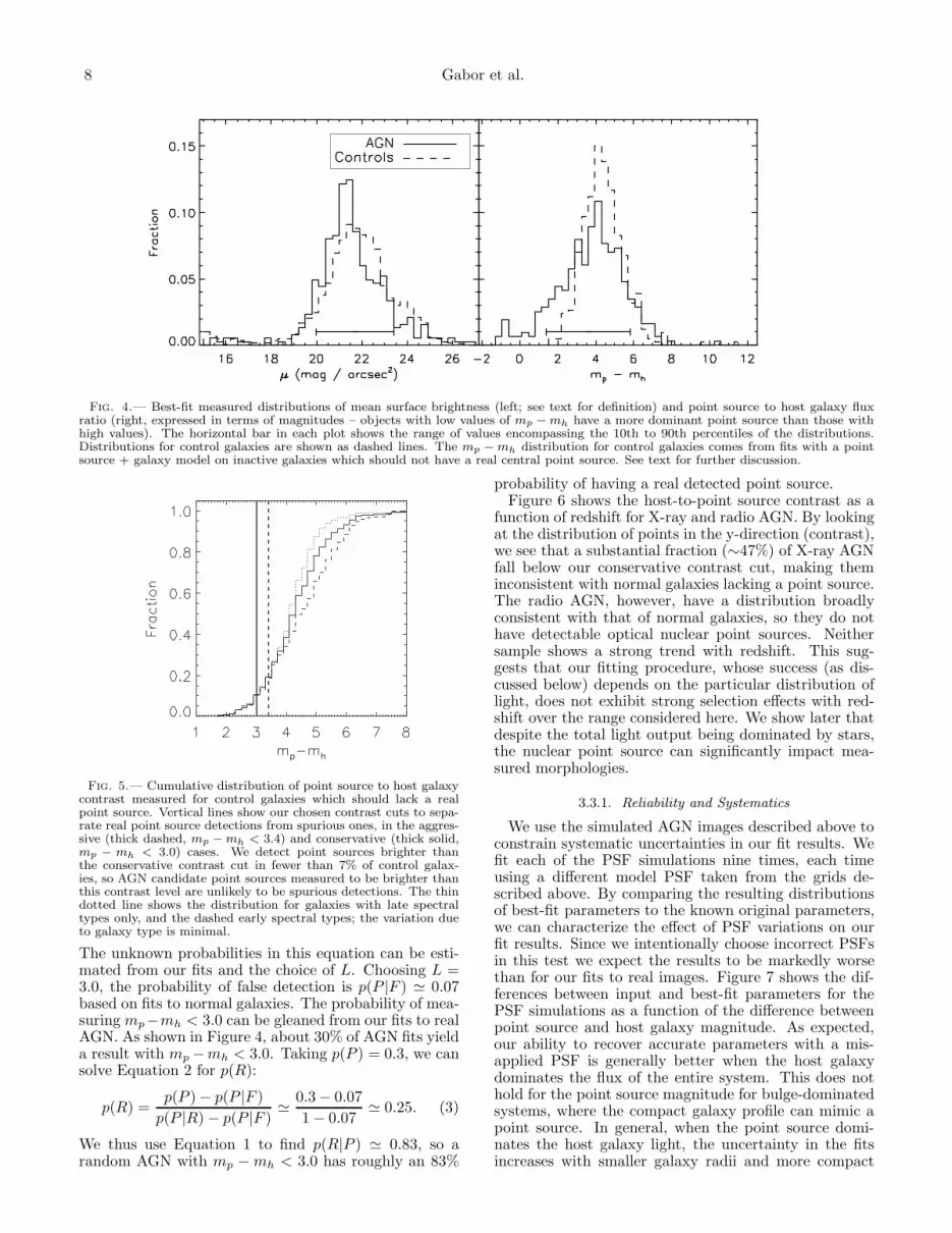
correspond to host-dominated images, and low valuescorrespond to point-source dominated images. A largemajority of the AGN in our sample are dominated bytheir host galaxies. This begs the question: should wereally include the point source component of the fit atall, or instead use just a single galaxy component? Weaddress the issue by fitting a sub-sample of ∼500 con-trol galaxies with a galaxy + PSF model. By includinga point source component in the fit, we can determinethe relative point source flux at which our fitting pro-cedure spuriously identifies a PSF. The distribution ofspuriously recovered mp − mh peaks near 4.5, with abroad range from ∼2 to 6 (dashed line in right panel ofFigure 4). We show the cumulative distribution for allcontrol galaxies, early-type, and late-type galaxies in Fig-ure 5. About 16% (corresponding to the 1-sigma bound-ary) of these fits have mp − mh < 3.4, and ∼7% havemp − mh < 3.0. We establish these levels as limits toour ability to recover real point sources in AGN images.If any given AGN fit has mp − mh > 3.4 (or 3.0, moreconservatively), then it is consistent with normal galax-ies, lacking a real point source. We take those AGN fitswith mp − mh < 3.4 (3.0) to have a real point sourcedetection.

Formally, we can statistically determine the probabilitythat an AGN fit with mp −mh < L includes a real pointsource detection. If we let R represent a real point sourcedetection, and P represent a positive measurement thatmp − mh < L, then we want to determine p(R|P ), theprobability that an object has a real point source givena positive measurement. From Bayes’ Theorem, this is

p(R|P ) =p(P |R)p(R)

p(P )(1)

We define a real detectable point source as one whichyields a positive measurement, so p(P |R) = 1. The prob-ability of obtaining a positive measurement depends onthe false detection rate as well as the real detections.Letting F represent a lack of point source (for false de-tections),

p(P )=p(P |R)p(R) + p(P |F )p(F )

=p(P |R)p(R) + p(P |F )(1 − p(R)) (2)

8 Gabor et al.

Fig. 4.— Best-fit measured distributions of mean surface brightness (left; see text for definition) and point source to host galaxy fluxratio (right, expressed in terms of magnitudes – objects with low values of mp − mh have a more dominant point source than those withhigh values). The horizontal bar in each plot shows the range of values encompassing the 10th to 90th percentiles of the distributions.Distributions for control galaxies are shown as dashed lines. The mp − mh distribution for control galaxies comes from fits with a pointsource + galaxy model on inactive galaxies which should not have a real central point source. See text for further discussion.

Fig. 5.— Cumulative distribution of point source to host galaxycontrast measured for control galaxies which should lack a realpoint source. Vertical lines show our chosen contrast cuts to sepa-rate real point source detections from spurious ones, in the aggres-sive (thick dashed, mp − mh < 3.4) and conservative (thick solid,mp − mh < 3.0) cases. We detect point sources brighter thanthe conservative contrast cut in fewer than 7% of control galax-ies, so AGN candidate point sources measured to be brighter thanthis contrast level are unlikely to be spurious detections. The thindotted line shows the distribution for galaxies with late spectraltypes only, and the dashed early spectral types; the variation dueto galaxy type is minimal.

The unknown probabilities in this equation can be esti-mated from our fits and the choice of L. Choosing L =3.0, the probability of false detection is p(P |F ) ≃ 0.07based on fits to normal galaxies. The probability of mea-suring mp−mh < 3.0 can be gleaned from our fits to realAGN. As shown in Figure 4, about 30% of AGN fits yielda result with mp −mh < 3.0. Taking p(P ) = 0.3, we cansolve Equation 2 for p(R):

p(R) =p(P ) − p(P |F )

p(P |R) − p(P |F )≃

0.3 − 0.07

1 − 0.07≃ 0.25. (3)

We thus use Equation 1 to find p(R|P ) ≃ 0.83, so arandom AGN with mp − mh < 3.0 has roughly an 83%

probability of having a real detected point source.Figure 6 shows the host-to-point source contrast as a

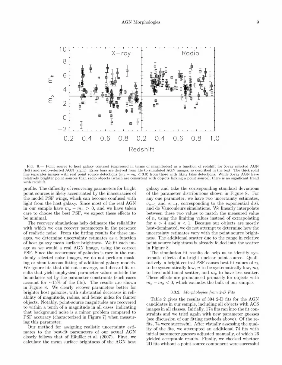
function of redshift for X-ray and radio AGN. By lookingat the distribution of points in the y-direction (contrast),we see that a substantial fraction (∼47%) of X-ray AGNfall below our conservative contrast cut, making theminconsistent with normal galaxies lacking a point source.The radio AGN, however, have a distribution broadlyconsistent with that of normal galaxies, so they do nothave detectable optical nuclear point sources. Neithersample shows a strong trend with redshift. This sug-gests that our fitting procedure, whose success (as dis-cussed below) depends on the particular distribution oflight, does not exhibit strong selection effects with red-shift over the range considered here. We show later thatdespite the total light output being dominated by stars,the nuclear point source can significantly impact mea-sured morphologies.

3.3.1. Reliability and Systematics

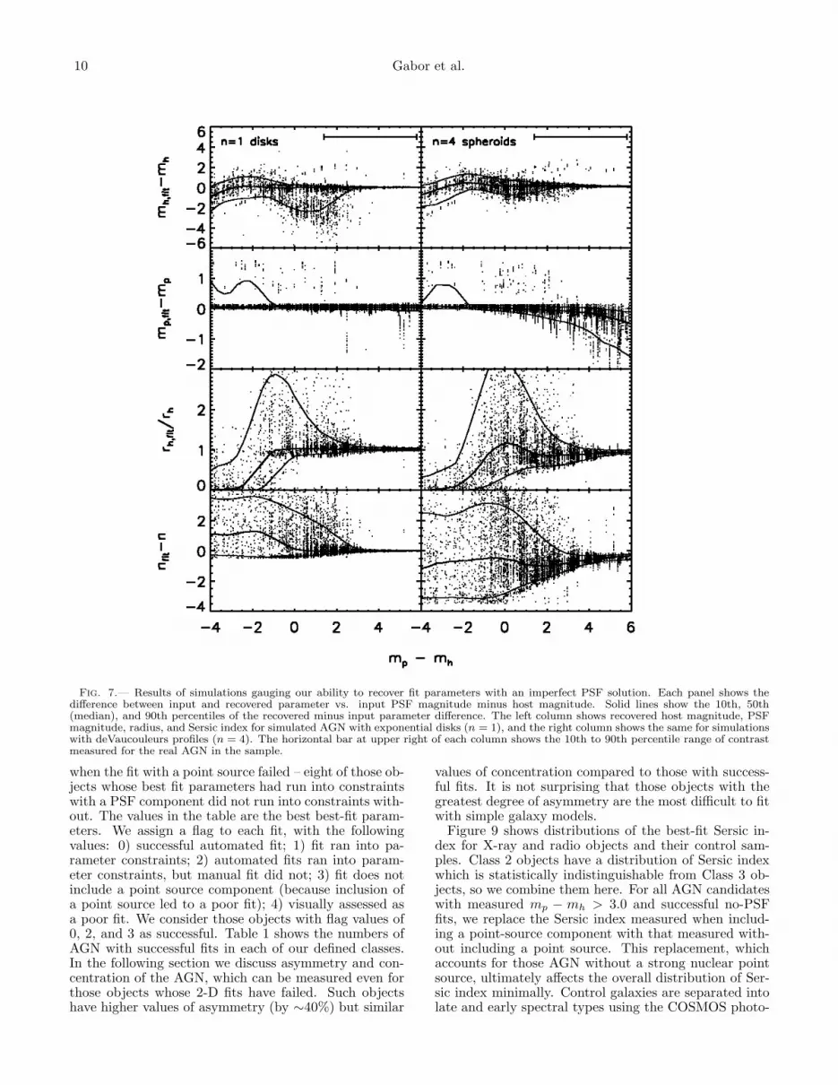
We use the simulated AGN images described above toconstrain systematic uncertainties in our fit results. Wefit each of the PSF simulations nine times, each timeusing a different model PSF taken from the grids de-scribed above. By comparing the resulting distributionsof best-fit parameters to the known original parameters,we can characterize the effect of PSF variations on ourfit results. Since we intentionally choose incorrect PSFsin this test we expect the results to be markedly worsethan for our fits to real images. Figure 7 shows the dif-ferences between input and best-fit parameters for thePSF simulations as a function of the difference betweenpoint source and host galaxy magnitude. As expected,our ability to recover accurate parameters with a mis-applied PSF is generally better when the host galaxydominates the flux of the entire system. This does nothold for the point source magnitude for bulge-dominatedsystems, where the compact galaxy profile can mimic apoint source. In general, when the point source domi-nates the host galaxy light, the uncertainty in the fitsincreases with smaller galaxy radii and more compact

AGN Morphologies 9

Fig. 6.— Point source to host galaxy contrast (expressed in terms of magnitudes) as a function of redshift for X-ray selected AGN(left) and radio-selected AGN (right). Error bars are derived from fits to simulated AGN images, as described in the text. The thick solidline separates images with real point source detections (mp − mh < 3.0) from those with likely false detections. While X-ray AGN haverelatively brighter point sources than radio objects (which are consistent with objects lacking a point source), there is no significant trendwith redshift.

profile. The difficulty of recovering parameters for brightpoint sources is likely accentuated by the inaccuracies ofthe model PSF wings, which can become confused withlight from the host galaxy. Since most of the real AGNin our sample have mp − mh > 0, and we have takencare to choose the best PSF, we expect these effects tobe minimal.

The recovery simulations help delineate the reliabilitywith which we can recover parameters in the presenceof realistic noise. From the fitting results for these im-ages, we determine uncertainty estimates as a functionof host galaxy mean surface brightness. We fit each im-age as we would a real AGN image, using the correctPSF. Since the occurrence of galaxies is rare in the ran-domly selected noise images, we do not perform mask-ing or simultaneous fitting of additional galaxy models.We ignore fits that did not converge, and discard fit re-sults that yield unphysical parameter values outside theboundaries set by the parameter constraints (such casesaccount for ∼15% of the fits). The results are shownin Figure 8. We clearly recover parameters better forbrighter host galaxies, with substantial decreases in reli-ability of magnitude, radius, and Sersic index for fainterobjects. Notably, point-source magnitudes are recoveredto within a tenth of a magnitude in all cases, indicatingthat background noise is a minor problem compared toPSF accuracy (characterized in Figure 7) when measur-ing this parameter.

Our method for assigning realistic uncertainty esti-mates to the best-fit parameters of our actual AGNclosely follows that of Haußler et al. (2007). First, wecalculate the mean surface brightness of the AGN host

galaxy and take the corresponding standard deviationsof the parameter distributions shown in Figure 8. Forany one parameter, we have two uncertainty estimates,σn=1 and σn=4, corresponding to the exponential diskand de Vaucouleurs simulations. We linearly interpolatebetween these two values to match the measured valueof n, using the limiting values instead of extrapolatingfor n > 4 and n < 1. Because our objects are mostlyhost-dominated, we do not attempt to determine how theuncertainty estimates vary with the point source bright-ness. The additional scatter due to the range in relativepoint source brightness is already folded into the scatterin Figure 8.

The simulation fit results do help us to identify sys-tematic effects of a bright nuclear point source. Quali-tatively, a bright central PSF causes best-fit values of rh

to be systematically low, n to be systematically low, mh

to have additional scatter, and mp to have less scatter.These effects are pronounced primarily for objects withmp − mh < 0, which excludes the bulk of our sample.

3.3.2. Morphologies from 2-D Fits

Table 2 gives the results of 394 2-D fits for the AGNcandidates in our sample, including all objects with ACSimages in all classes. Initially, 174 fits ran into the fit con-straints and we tried again with new parameter guesses(see discussion of our fitting methods above). Of the re-fits, 74 were successful. After visually assessing the qual-ity of the fits, we attempted an additional 74 fits withinitial parameter guesses adjusted manually, of which 26yielded acceptable results. Finally, we checked whether2D fits without a point source component were successful

10 Gabor et al.

Fig. 7.— Results of simulations gauging our ability to recover fit parameters with an imperfect PSF solution. Each panel shows thedifference between input and recovered parameter vs. input PSF magnitude minus host magnitude. Solid lines show the 10th, 50th(median), and 90th percentiles of the recovered minus input parameter difference. The left column shows recovered host magnitude, PSFmagnitude, radius, and Sersic index for simulated AGN with exponential disks (n = 1), and the right column shows the same for simulationswith deVaucouleurs profiles (n = 4). The horizontal bar at upper right of each column shows the 10th to 90th percentile range of contrastmeasured for the real AGN in the sample.

when the fit with a point source failed – eight of those ob-jects whose best fit parameters had run into constraintswith a PSF component did not run into constraints with-out. The values in the table are the best best-fit param-eters. We assign a flag to each fit, with the followingvalues: 0) successful automated fit; 1) fit ran into pa-rameter constraints; 2) automated fits ran into param-eter constraints, but manual fit did not; 3) fit does notinclude a point source component (because inclusion ofa point source led to a poor fit); 4) visually assessed asa poor fit. We consider those objects with flag values of0, 2, and 3 as successful. Table 1 shows the numbers ofAGN with successful fits in each of our defined classes.In the following section we discuss asymmetry and con-centration of the AGN, which can be measured even forthose objects whose 2-D fits have failed. Such objectshave higher values of asymmetry (by ∼40%) but similar

values of concentration compared to those with success-ful fits. It is not surprising that those objects with thegreatest degree of asymmetry are the most difficult to fitwith simple galaxy models.

Figure 9 shows distributions of the best-fit Sersic in-dex for X-ray and radio objects and their control sam-ples. Class 2 objects have a distribution of Sersic indexwhich is statistically indistinguishable from Class 3 ob-jects, so we combine them here. For all AGN candidateswith measured mp − mh > 3.0 and successful no-PSFfits, we replace the Sersic index measured when includ-ing a point-source component with that measured with-out including a point source. This replacement, whichaccounts for those AGN without a strong nuclear pointsource, ultimately affects the overall distribution of Ser-sic index minimally. Control galaxies are separated intolate and early spectral types using the COSMOS photo-

AGN Morphologies 11

Fig. 8.— Results of simulations gauging our ability to recover fit parameters in the presence of noise. Each panel shows the differencebetween initial and recovered parameters vs. host galaxy mean surface brightness. Solid lines trace the 10th, 50th (median), and 90thpercentiles of the parameter difference. The left column shows recovered host magnitude, PSF magnitude, host radius, and Sersic index forsimulated images with exponential disk (n = 1) profiles, and the right column shows the same for simulations with deVaucouleurs profiles(n = 4). The horizontal bar in top panel of each column shows the 10th to 90th percentile range of µ measured for the real AGN in thesample.

metric redshift catalog (Mobasher et al. 2007) Tphot pa-rameter, and we find a good corresponding separationof morphologies into disk- and bulge-dominated. Early-type control galaxies are clustered around n = 4, al-though with significant scatter, and late-type galaxiesaround n = 1. With this division, approximately 60% ofall the control galaxies have late-type morphologies andspectral types, and the remaining 40% have early-typemorphologies and spectral types.

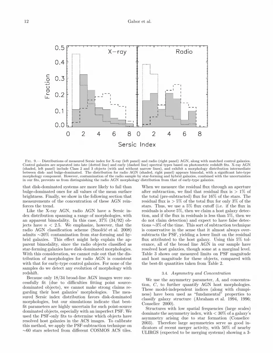
X-ray AGN have a Sersic index distribution interme-diate between the late- and early-type control galaxies,including a broad range of morphologies. When the con-trol galaxies are not separated by spectral type, a KStest rejects the hypothesis that the X-ray AGN distribu-tion is consistent with that of the controls at the 97%level. This result, which conflicts with some previousfindings (Grogin et al. 2005; Pierce et al. 2007), deserves

a fair amount of scrutiny. In particular, our simula-tions show (cf. Figure 8) that a substantial number ofbulge-dominated AGN will have a recovered Sersic in-dex with n < 2.5, the typically used cutoff between disk-and bulge-dominated. Quantitatively, .30% of recov-ered Sersic indices will incorrectly have n < 2.5. Onthe other hand, 43% (40/93) of the AGN in our mea-sured distribution have n < 2.5, indicating a significantdisk-dominated population. Furthermore, systematicallylow values of measured Sersic index are more prevalentfor point-source dominated images included in our sim-ulations, but most of our X-ray AGN are actually host-dominated. Another possible effect emerges from the factthat 20% of our X-ray AGN did not yield successful 2-D fits. Perhaps the objects with failed fits are exactlythe ones which would fill in the bulge-dominated por-tion of the distribution. Our simulations show, however,

12 Gabor et al.

Fig. 9.— Distributions of measured Sersic index for X-ray (left panel) and radio (right panel) AGN, along with matched control galaxies.Control galaxies are separated into late (dotted line) and early (dashed line) spectral types based on photometric redshift fits. X-ray AGN(shaded, left panel) include Class 2 and 3 objects (with and without narrow lines), and exhibit a morphology distribution intermediatebetween disk- and bulge-dominated. The distribution for radio AGN (shaded, right panel) appears bimodal, with a significant late-typemorphology component. However, contamination of the radio sample by star-forming and hybrid galaxies, combined with the uncertaintiesin our fits, prevents us from distinguishing the radio AGN morphology distribution from that of early-type galaxies.

that disk-dominated systems are more likely to fail thanbulge-dominated ones for all values of the mean surfacebrightness. Finally, we show in the following section thatmeasurements of the concentration of these AGN rein-forces the trend.

Like the X-ray AGN, radio AGN have a Sersic in-dex distribution spanning a range of morphologies, withan apparent bimodality. In this case, 37% (34/92) ob-jects have n < 2.5. We emphasize, however, that theradio AGN classification scheme (Smolcic et al. 2008)admits ∼20% contamination from star-forming and hy-brid galaxies. This effect might help explain the ap-parent bimodality, since the radio objects classified asstar-forming galaxies have disk-dominated morphologies.With this consideration, we cannot rule out that the dis-tribution of morphologies for radio AGN is consistentwith that for early-type control galaxies. For none of thesamples do we detect any evolution of morphology withredshift.

Because only 18/34 broad-line AGN images were suc-cessfully fit (due to difficulties fitting point source-dominated objects), we cannot make strong claims re-garding their host galaxies’ morphologies. The mea-sured Sersic index distribution favors disk-dominatedmorphologies, but our simulations indicate that best-fit parameters are highly uncertain for such point-sourcedominated objects, especially with an imperfect PSF. Weused the PSF-only fits to determine which objects haveresolved host galaxies in the ACS images. To calibratethis method, we apply the PSF-subtraction technique on∼60 stars selected from different COSMOS ACS tiles.

When we measure the residual flux through an apertureafter subtraction, we find that residual flux is > 1% ofthe total (pre-subtracted) flux for 16% of the stars. Theresidual flux is > 5% of the total flux for only 3% of thestars. Thus, we use a 5% flux cutoff (i.e. if the flux inresiduals is above 5%, then we claim a host galaxy detec-tion, and if the flux in residuals is less than 5%, then wedo not claim detection) and expect to have false detec-tions ∼3% of the time. This sort of subtraction techniqueis conservative in the sense that it almost always over-subtracts the PSF, yielding a lower limit on the residualflux attributed to the host galaxy. Using this 5% tol-erance, all of the broad line AGN in our sample haveresolved host galaxies, though some at a marginal level.Table 3 shows our measured limits on PSF magnitudeand host magnitude for these objects, compared withthe best-fit quantities taken from Table 2.

3.4. Asymmetry and Concentration

We use the asymmetry parameter, A, and concentra-tion, C, to further quantify AGN host morphologies.These model-independent indices (along with clumpi-ness) have been used as “fundamental” properties toclassify galaxy structure (Abraham et al. 1994, 1996;Conselice 2000).

Structures with low spatial frequencies (large scales)dominate the asymmetry index, with < 30% of a galaxy’sasymmetry arising due to star formation (Conselice2003). Therefore large asymmetries serve as good in-dicators of recent merger activity, with 50% of nearbyULIRGS (expected to be merging systems) showing a 3-

AGN Morphologies 13

sigma deviation from the asymmetry trend with colorsfor normal galaxies (Conselice 2003). A conservativeminimum asymmetry for merging systems is A = 0.35,but we do not apply this limit here because we are inter-ested only in a difference in asymmetry between activeand non-active galaxies.

In this study, we compare asymmetries measured forAGN hosts to those measured for control galaxies to de-termine whether AGN activity is more likely to be as-sociated with mergers and interactions. Grogin et al.(2005) use similar logic in applying asymmetry measure-ments. Because only one filter of ACS data is avail-able for most objects in our sample, we probe differentrest wavelengths as a function of redshift. Capak et al.(2007), using COSMOS ACS images in both the F814Wband as well as the F475W band (which was used to im-age ∼81 square arcminutes), find that asymmetries aresystematically different when the F475W band samplesrest frame UV and the F814W band samples rest-frameoptical light. Measured values are consistent, however,when both bands sample optical light or both sampleUV light. The authors illustrate that the shift in mea-sured asymmetry values for the F814W filter occurs nearz ≃1, where rest-frame UV begins to dominate. Simi-larly, Sanchez et al. (2004), using Sersic index to classifyquasar host galaxy morphologies at z ≃1, found thatmost objects’ optical and UV classifications were thesame. We therefore expect only small systematic effectsdue to band shifting in the present study.

We follow the method of defining and measuring asym-metry given in Conselice (2000). Starting with an imagecutout with flux distribution S, we rotate the image by180 degrees to get a new image, S180, and define asym-metry as A = min(

∑|S − S180| /

∑|S|) − A0. The sum

is over all pixels, and we take the minimum asymme-try value from a grid of central pixels near the centercoordinate of the image. A0 is the asymmetry of thebackground, estimated by taking a median of 25 imagessurrounding the primary target. The images used in con-structing the background are taken from the same ACStile as the primary, and each has the same size as the pri-mary cutout image. For primary targets near the edgeof a tile, we shift the grid of 25 images so that all imagesfall within the tile’s field of view.

To measure galaxy asymmetry meaningfully for arange of redshifts, we must carefully choose the size ofthe image cutout which we rotate and subtract. A simplechoice would be a constant physical radius, which trans-lates directly to an angular size given a chosen cosmol-ogy. Since galaxies come in many sizes, perhaps a betterchoice is to use a Petrosian radius (Petrosian 1976), ora multiple thereof, as in Conselice (2000). The Pet-rosian η-function, η(r), is defined as the ratio of surfacebrightness at radius r (from the galaxy centroid) to theaverage surface brightness within r. We then denote thePetrosian radius as rη0 , the radius at which η(r) = η0.We choose η0 = 0.2 and measure asymmetries for im-age cutouts with this half-width. Because the Petrosianradius can give unphysical values for unusual light dis-tributions or for images with multiple objects, we seta minimum cutout size of 1 arcsecond and a maximumcutout size corresponding to a physical radius of 15 h−1

kpc (∼ 3 arcseconds at z = 0.7). These restrictions pre-vent unrealistically small (e.g., less than the PSF full

width at half max) or large choices of cutout radius.We measure asymmetries for both the AGN host galax-

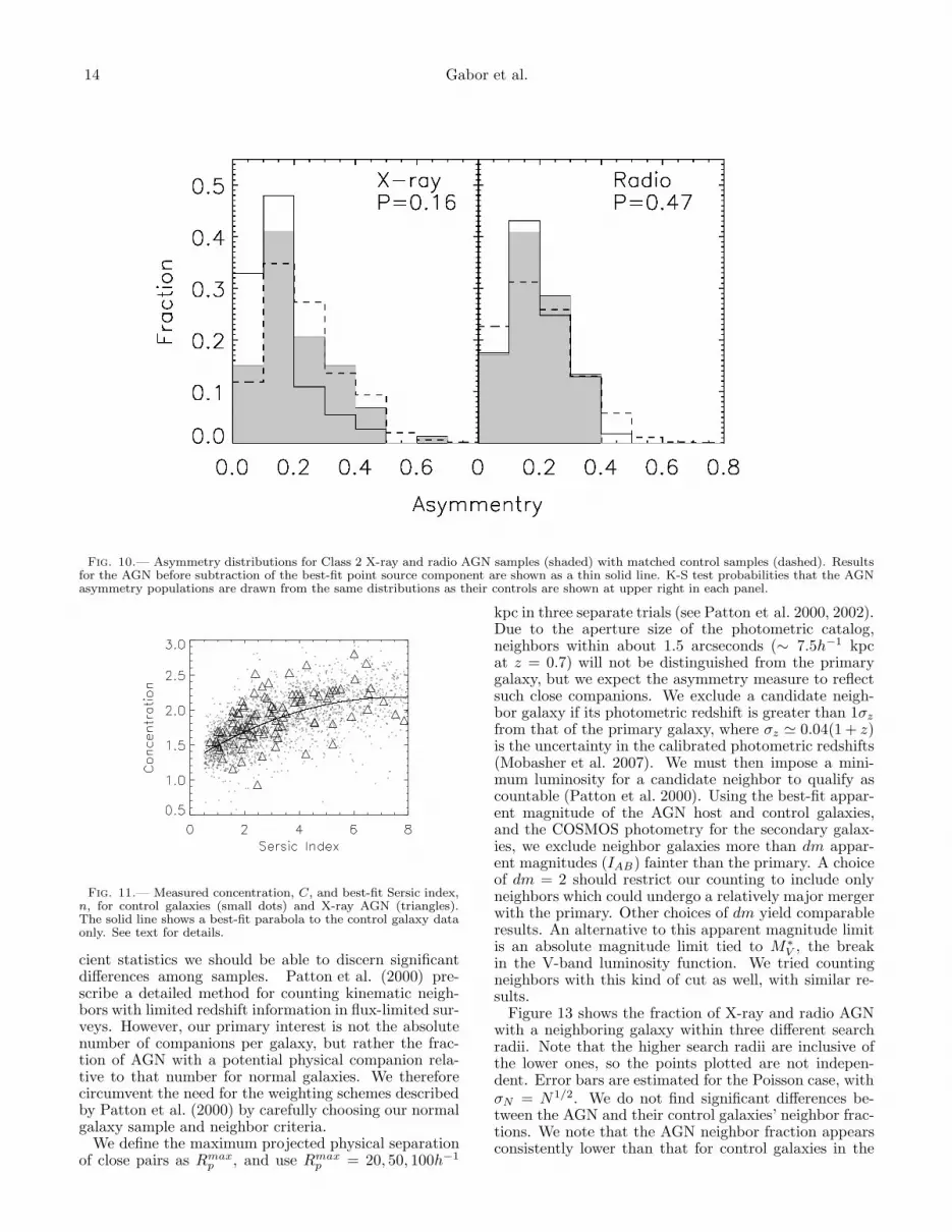
ies and the sample of control galaxies. Because the highlysymmetric central point source of an AGN biases theasymmetry toward low values, we measure asymmetryfor images with the point source component subtracted.We subtract the best-fit model nuclear point source fromeach AGN image. For objects without successful fits, weuse residual images from our PSF-only-fit subtraction.The resulting A distributions for X-ray and radio AGNare shown in Figure 10, including measurements bothbefore and after subtraction of the point source. Pointsource subtraction clearly biases the results for the X-ray objects toward lower asymmetry, but very little forthe radio objects. We perform a two-sided K-S test todetermine whether the AGN and control sample popu-lations are consistent with the same underlying distri-bution. We find no evidence that AGN have differentasymmetry distributions from non-active galaxies, withK-S test probabilities of 16% and 47% (where a typicaltolerance of 5% is used to claim the distributions dif-fer). The asymmetries for AGN are generally consistentwith those of non-active galaxies. We find no correlationbetween X-ray luminosity and asymmetry.

The concentration parameter serves as an alternativeto the Sersic index to determine whether a galaxy is dom-inated by a highly concentrated central bulge component.Here we define the concentration as C = 5 log(r>/r<),with r> = 0.9rη0 and r< = 0.5rη0 . Figure 11 shows therelationship between concentration and Sersic index forthose control galaxies with successful 2D fits. Despite thesubstantial scatter, the overall correlation is clear. Be-cause the relationship appears to flatten out for n > 4,we fit a parabola to the control galaxy data, with thebest-fit equation yielding C = 1.262+0.244n−0.0163n2.For comparison, we plot the X-ray AGN in our sample,showing that the trend is comparable. A parabolic fitto just the X-ray AGN data yields fit parameters consis-tent with those given above. With our definition of C,our best-fit parameters show that a delineation betweenlate- and early-type of n = 2.5 corresponds to C = 1.8.

Figure 12 shows the concentration distributions for X-ray and radio AGN. As in our Sersic index analysis,we separate control galaxies into early and late spectraltypes. Both X-ray and radio samples include objectsboth with and without emission lines combined into one.We also show the distribution of C values before (thinsolid) and after (shaded) point-source subtraction for theX-ray AGN. The presence of the point source signifi-cantly biases concentration measurements to high valuesfor these objects. X-ray AGN have intermediate values ofC between those of late and early type control galaxies.Radio AGN also include objects with values of C lowerthan that measured for early-type galaxies, but again wecaution that the radio AGN sample includes substantialcontamination. These results support those of the Sersicindex distributions discussed above.

4. COMPANION GALAXIES

Kinematically associated neighboring galaxies provideevidence for ongoing galaxy interactions. Without de-tailed spectral information, we are limited to countingneighbors that are within long cylinders seen in projec-tion, but with photometric redshift estimates and suffi-

14 Gabor et al.

Fig. 10.— Asymmetry distributions for Class 2 X-ray and radio AGN samples (shaded) with matched control samples (dashed). Resultsfor the AGN before subtraction of the best-fit point source component are shown as a thin solid line. K-S test probabilities that the AGNasymmetry populations are drawn from the same distributions as their controls are shown at upper right in each panel.

Fig. 11.— Measured concentration, C, and best-fit Sersic index,n, for control galaxies (small dots) and X-ray AGN (triangles).The solid line shows a best-fit parabola to the control galaxy dataonly. See text for details.

cient statistics we should be able to discern significantdifferences among samples. Patton et al. (2000) pre-scribe a detailed method for counting kinematic neigh-bors with limited redshift information in flux-limited sur-veys. However, our primary interest is not the absolutenumber of companions per galaxy, but rather the frac-tion of AGN with a potential physical companion rela-tive to that number for normal galaxies. We thereforecircumvent the need for the weighting schemes describedby Patton et al. (2000) by carefully choosing our normalgalaxy sample and neighbor criteria.

We define the maximum projected physical separationof close pairs as Rmax

p , and use Rmaxp = 20, 50, 100h−1

kpc in three separate trials (see Patton et al. 2000, 2002).Due to the aperture size of the photometric catalog,neighbors within about 1.5 arcseconds (∼ 7.5h−1 kpcat z = 0.7) will not be distinguished from the primarygalaxy, but we expect the asymmetry measure to reflectsuch close companions. We exclude a candidate neigh-bor galaxy if its photometric redshift is greater than 1σz

from that of the primary galaxy, where σz ≃ 0.04(1 + z)is the uncertainty in the calibrated photometric redshifts(Mobasher et al. 2007). We must then impose a mini-mum luminosity for a candidate neighbor to qualify ascountable (Patton et al. 2000). Using the best-fit appar-ent magnitude of the AGN host and control galaxies,and the COSMOS photometry for the secondary galax-ies, we exclude neighbor galaxies more than dm appar-ent magnitudes (IAB) fainter than the primary. A choiceof dm = 2 should restrict our counting to include onlyneighbors which could undergo a relatively major mergerwith the primary. Other choices of dm yield comparableresults. An alternative to this apparent magnitude limitis an absolute magnitude limit tied to M∗

V , the breakin the V-band luminosity function. We tried countingneighbors with this kind of cut as well, with similar re-sults.

Figure 13 shows the fraction of X-ray and radio AGNwith a neighboring galaxy within three different searchradii. Note that the higher search radii are inclusive ofthe lower ones, so the points plotted are not indepen-dent. Error bars are estimated for the Poisson case, withσN = N1/2. We do not find significant differences be-tween the AGN and their control galaxies’ neighbor frac-tions. We note that the AGN neighbor fraction appearsconsistently lower than that for control galaxies in the

AGN Morphologies 15

Fig. 12.— Distributions of measured concentration, C, for X-ray and Radio AGN, along with control samples. Control galaxies areseparated into late (dotted line) and early (dashed line) types. For comparison, we show the concentration distribution of X-ray AGNbefore point-source subtraction (thin solid). Since the radio AGN are all host dominated, we do not show results for measurements beforepoint-source subtraction in the right panel. These results mimic those of our 2-D fits, as shown in Figure 9.

Fig. 13.— Fraction of AGN (triangles) with at least one neighborwithin a physical separation of Rmax

p , as a function Rmaxp . Control

galaxy neighbor fractions are shown as boxes connected by dashedlines.

figure, but changes in the redshift tolerance and mag-nitude cut can reverse this effect. No significant trendswith morphology or luminosity can be discerned withthe sample size used here. We conclude that AGN areno more likely than non-active galaxies to have a nearneighbor. With spectroscopic redshifts from the COS-MOS VLT survey (Lilly et al. 2007), future work willmore accurately identify kinematic neighbors.

5. DISCUSSION

Recent evidence suggests that galaxies hosting AGNrepresent a transitional population, passing from theblue cloud to the red sequence in galaxy color-magnitude space at redshifts z . 1 (Jahnke et al. 2004b;Sanchez et al. 2004; Silverman et al. 2008; Bundy et al.2007). AGN host galaxies at both low and high red-

Fig. 14.— Measured host galaxy Sersic index as a function of X-ray luminosity for X-ray AGN. No significant trend is discernible.

shift are found to be bluer than quiescent ellipticalgalaxies (Kauffmann et al. 2003; Jahnke et al. 2004a,b;Sanchez et al. 2004), indicating recent or ongoing starformation. Contrary to the findings of some previ-ous authors studying morphologies of moderate-redshiftX-ray selected AGN (Grogin et al. 2005; Pierce et al.2007) and quasars at low redshifts (Dunlop et al. 2003;McLeod & McLeod 2001), our results indicate that X-ray AGN hosts may be undergoing a morphological tran-sition concurrent with a transition from blue to red col-ors. Peng et al. (2006c) came to a similar conclusionwhen studying the host galaxies of gravitationally lensedquasars – 30-50% of quasar hosts in their z > 1 sam-ple have disk-dominated morphologies. Further, our re-sults qualitatively agree with those of Kauffmann et al.(2003), whose AGN sample had a distribution of con-centration index intermediate between that of early-

16 Gabor et al.

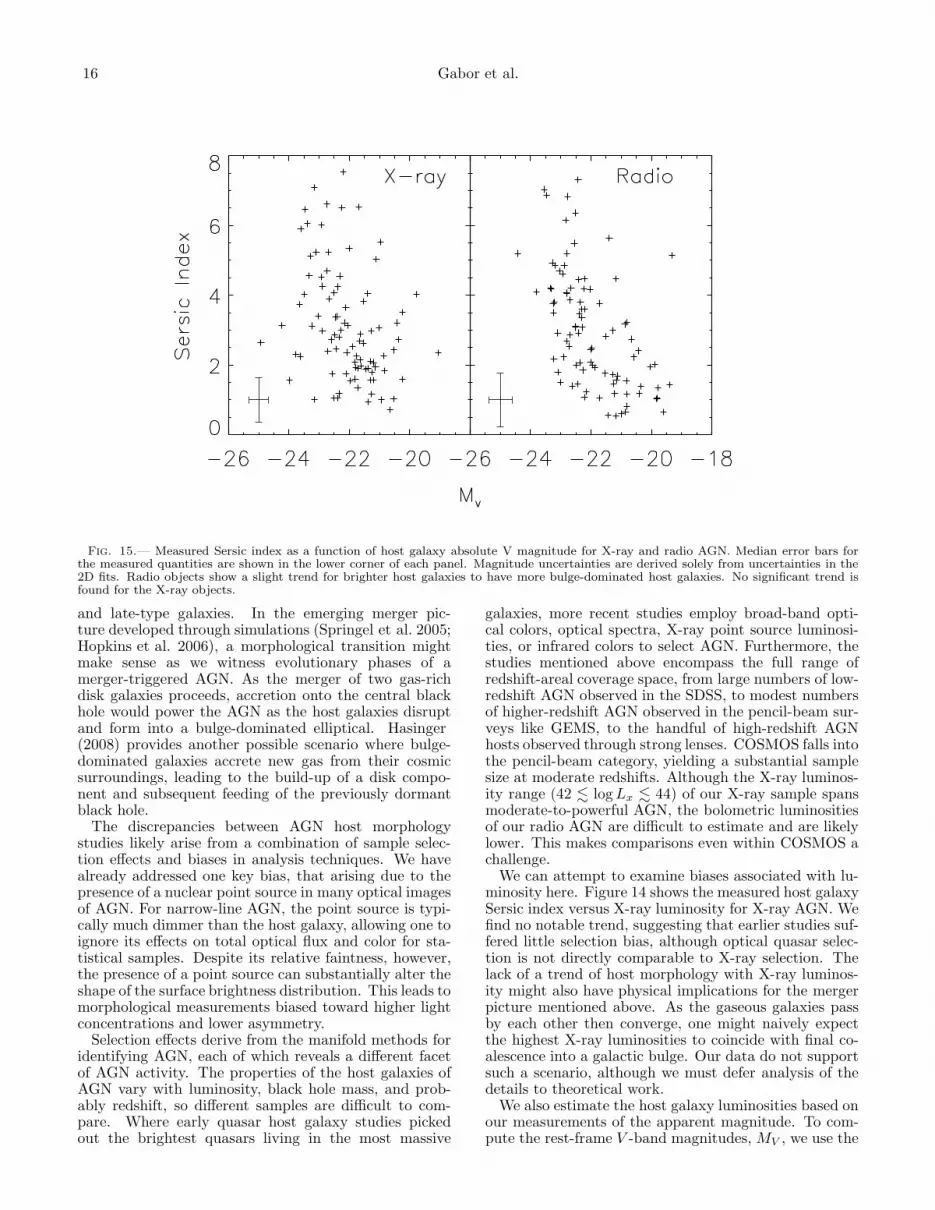
Fig. 15.— Measured Sersic index as a function of host galaxy absolute V magnitude for X-ray and radio AGN. Median error bars forthe measured quantities are shown in the lower corner of each panel. Magnitude uncertainties are derived solely from uncertainties in the2D fits. Radio objects show a slight trend for brighter host galaxies to have more bulge-dominated host galaxies. No significant trend isfound for the X-ray objects.

and late-type galaxies. In the emerging merger pic-ture developed through simulations (Springel et al. 2005;Hopkins et al. 2006), a morphological transition mightmake sense as we witness evolutionary phases of amerger-triggered AGN. As the merger of two gas-richdisk galaxies proceeds, accretion onto the central blackhole would power the AGN as the host galaxies disruptand form into a bulge-dominated elliptical. Hasinger(2008) provides another possible scenario where bulge-dominated galaxies accrete new gas from their cosmicsurroundings, leading to the build-up of a disk compo-nent and subsequent feeding of the previously dormantblack hole.

The discrepancies between AGN host morphologystudies likely arise from a combination of sample selec-tion effects and biases in analysis techniques. We havealready addressed one key bias, that arising due to thepresence of a nuclear point source in many optical imagesof AGN. For narrow-line AGN, the point source is typi-cally much dimmer than the host galaxy, allowing one toignore its effects on total optical flux and color for sta-tistical samples. Despite its relative faintness, however,the presence of a point source can substantially alter theshape of the surface brightness distribution. This leads tomorphological measurements biased toward higher lightconcentrations and lower asymmetry.

Selection effects derive from the manifold methods foridentifying AGN, each of which reveals a different facetof AGN activity. The properties of the host galaxies ofAGN vary with luminosity, black hole mass, and prob-ably redshift, so different samples are difficult to com-pare. Where early quasar host galaxy studies pickedout the brightest quasars living in the most massive

galaxies, more recent studies employ broad-band opti-cal colors, optical spectra, X-ray point source luminosi-ties, or infrared colors to select AGN. Furthermore, thestudies mentioned above encompass the full range ofredshift-areal coverage space, from large numbers of low-redshift AGN observed in the SDSS, to modest numbersof higher-redshift AGN observed in the pencil-beam sur-veys like GEMS, to the handful of high-redshift AGNhosts observed through strong lenses. COSMOS falls intothe pencil-beam category, yielding a substantial samplesize at moderate redshifts. Although the X-ray luminos-ity range (42 . log Lx . 44) of our X-ray sample spansmoderate-to-powerful AGN, the bolometric luminositiesof our radio AGN are difficult to estimate and are likelylower. This makes comparisons even within COSMOS achallenge.

We can attempt to examine biases associated with lu-minosity here. Figure 14 shows the measured host galaxySersic index versus X-ray luminosity for X-ray AGN. Wefind no notable trend, suggesting that earlier studies suf-fered little selection bias, although optical quasar selec-tion is not directly comparable to X-ray selection. Thelack of a trend of host morphology with X-ray luminos-ity might also have physical implications for the mergerpicture mentioned above. As the gaseous galaxies passby each other then converge, one might naively expectthe highest X-ray luminosities to coincide with final co-alescence into a galactic bulge. Our data do not supportsuch a scenario, although we must defer analysis of thedetails to theoretical work.

We also estimate the host galaxy luminosities based onour measurements of the apparent magnitude. To com-pute the rest-frame V -band magnitudes, MV , we use the

AGN Morphologies 17

spectroscopic redshifts and assume spectral energy distri-butions for the AGN host galaxies. We choose the rest-frame V -band because it shifts into the observed I-bandnear the median redshift of our sample, and because itserves as a convenient reference to the absolute V -bandmagnitudes derived for all galaxies in the COSMOS pho-tometric redshift catalog. Following Hogg et al. (2002),we calculate the K-corrections by applying filter curvesfor the F814W filter of HST and the Subaru V filterused for COSMOS observations. We calculate the cor-rections with both an elliptical galaxy and an Sb galaxytemplate optical SED from Kinney et al. (1996), and wedisplay results from the early-type template. Given thatAGN host galaxies have blue colors and recent star for-mation, the true SED lies somewhere between the twotemplates considered here. However, at all redshifts con-sidered here, the K-correction differs by .0.2 magnitudesbetween the two templates, so the choice of templatedoes not strongly affect the results. Figure 15 showsmeasured Sersic index versus these derived host galaxyabsolute magnitudes. We note that for both X-ray AGNand radio AGN hosts, the distribution of absolute mag-nitudes peaks around MV = −22, so these galaxies havesimilar luminosities to M∗

V ≃ −22 (for z = 1, computedby starting from the local value of Brown et al. 2001 andfollowing Capak et al. 2007 and Smith et al. 2005 in al-lowing 1 magnitude of passive evolution to z = 1). Wesee a weak trend (with correlation coefficient ≈ −0.2 forX-ray and ≈ −0.4 for radio AGN) of morphology withhost galaxy luminosity in both samples, where brighterhost galaxies have bulge-dominated morphologies. Thistrend is not redshift-dependent, and may reflect the gen-eral galaxy population.

Although the major merger picture is elegant and en-ticing, none of our AGN samples shows enhancementof the merger and interaction indicators applied. Thisroughly agrees with previous studies (Grogin et al. 2005;Pierce et al. 2007). Furthermore, differences in this re-sult between subsamples are not significant: radio andX-ray AGN candidates all follow the same trends as non-active galaxies. These results suggest that major galaxymergers do not play the dominant role in triggering AGNactivity, with the likely alternatives being minor merg-ers and interactions, and dynamical instabilities withingalaxies (Hasinger 2008, cf/).

We caution, however, that the tools we apply here maybe too blunt to cut to the heart of the question. The keyuncertainty in drawing conclusions from tests like theseis the timescale – for any given merger event, how longit takes to go from interaction to merger to coalescenceto relaxation, when and how long an AGN fueling eventmight occur, and how long interaction indicators will beobservable. While galaxy counts in AGN environmentsmay be connected to the likelihood for mergers, theyserve as an indirect probe at best. By counting neighborswe are finding systems that are likely to merge in thefuture, rather than those that have already merged andmight be in the midst of AGN fueling.

Like galaxy counts, the morphological measures usedin this work may not trace galaxy mergers as sensitivelyas necessary to distinguish recently merged systems fromnormal galaxies at moderate redshifts. Certainly we canbe confident that high-A galaxies are undergoing merg-ers, but not all recent mergers necessarily have large val-

ues of asymmetry. As Conselice (2003) suggests, per-haps only systems in certain phases of the merger processexhibit the large-scale asymmetries to which A is sensi-tive. If major mergers are indeed the trigger of AGN,the triggering lags the merger in such a way that thedominant light distribution of the host galaxy appearsessentially as relaxed as a normal galaxy. This presentsdifficulties becauses the typical AGN duty cycle of 108

years is much shorter than a typical galaxy’s relaxationtime, and similar to the free-fall time on which violent re-laxation is expected to occur. Another possibility is thatlarge scale disruptions such as tidal tails are present, butat such a low surface brightness that they are too diffi-cult to see and measure with such crude techniques athigher redshifts.

Perhaps minor mergers are the answer. These inter-actions may disrupt a gaseous galaxy enough to causecentral inflow of gas onto a black hole without signifi-cantly altering the observed distribution of light. As em-phasized in the review by Jogee (2006), for most AGNthe amount of fuel available is not the problem per se,but rather decreasing the specific angular momentum ofthat fuel by 99.99% to feed the central black hole. Mi-nor mergers could potentially disrupt the inner regionsof a gas-rich galaxy enough to initiate fueling, althoughthis is not seen in simulations. Such an interaction wouldbe difficult to detect using the techniques described here.However, Canalizo et al. (2007) find faint shell structuresindicative of a merger in deep HST images of the hostgalaxy of a low-redshift quasar whose morphology hadpreviously been considered quiescent. Detecting similarstructures in larger samples of AGN could help reveal amerger-driven fueling mechanism, but such work will bechallenging at moderate and high redshifts.

These considerations make clear the need for morework in understanding the relationships among dynam-ics, timescales, and observable properties of galaxy merg-ers and AGN. As the resolution and scale of simulationsimproves, we expect new constraints on the merger massratios necessary to trigger black hole accretion to emerge.In future work, we hope to develop new techniques fordetecting and measuring low surface brightness featuresthat may betray recent merger activity.

6. SUMMARY AND CONCLUSION

We explored the host morphologies and environmentsof AGN in the COSMOS field. Using X-ray- and radio-selected AGN candidates with confirmed spectroscopicredshifts, we analyzed host galaxy structural propertiesas well as merger indicators, probing the connection be-tween AGN activity and galaxy interactions. The follow-ing summarizes our main points:

• The central point source in optical images of X-rayselected AGN has substantial impact on measuredstructural parameters such as asymmetry and con-centration. Insufficient accounting for the pointsource can lead to systematically low asymmetryand systematically high concentration.

• Full 2-D fits and concentration measurementswhich account for the central point source in X-rayAGN show that their host galaxies have a broadrange of morphologies whose distribution is inter-

18 Gabor et al.

mediate between the bulge- and disk-dominatedregimes.

• Although radio AGN hosts also appear to have awide range of morphologies, contamination by star-forming galaxies prevents us from distinguishingthem from early-type normal galaxies.

• Measurements of AGN host galaxy asymmetry donot differ significantly from those of matched con-trol galaxies.

• Neighbor counts around AGN are indistinguishablefrom those around matched control galaxies usingphotometric redshifts.

These findings do not support the hypothesis that ma-jor mergers drive black hole activity, but they do suggestthat the host galaxies of AGN at these luminosities maybe in a state of morphological transition. Future workby members of the COSMOS collaboration will addressthis possibility in more detail by examing the colors and

star formation rates of AGN hosts and their relationshipswith environment (Silverman et al. in preparation).

We gratefully acknowledge the contributions of the en-tire COSMOS colaboration consisting of more than 70scientists. More information on the COSMOS survey isavailable at http://www.astro.caltech.edu/cosmos.We also thank the anonymous, thorough referee forcontributing to the quality of this work. JG wouldlike to thank Romeel Dave, Rodger Thompson, andAnn Zabludoff for guidance and useful discussion, andStephanie Juneau for help with K-corrections. JDRwas supported by internal funding at the Jet Propul-sion Laboratory, California Institute of Technology, op-erated under a contract with NASA. KJ acknowledgessupport by the German DFG under grant SCHI 536/3-1 andthrough the DFG Emmy Noether-Program undergrant JA 1114/3-1.

Facilities: HST (ACS), Magellan:Baade (IMACS),XMM (), VLA (), MMT (Hectospec).

REFERENCES

Abraham, R. G., Valdes, F., Yee, H. K. C., & van den Bergh, S.1994, ApJ, 432, 75.

Abraham, R. G., van den Bergh, S., Glazebrook, K., Ellis, R.,Santiago, B. X., Surma, P., & Griffiths, R. E. 1996, ApJS, 107,1.

Alonso, M. S., Lambas, D. G., Tissera, P., & Coldwell, G. 2007,MNRAS, 375, 1017.

Baldwin, J. A., Phillips, M. M., & Terlevich, R. 1981, PASP, 93, 5.Bauer, F. E., Alexander, D. M., Brandt, W. N., Schneider, D. P.,

Treister, E., Hornschemeier, A. E., Garmire, G.P. 2004, AJ, 128,2048.

Bertin, E. and Arnouts, S. 1996. A&AS, 117, 393.Brown, W. R., Geller, M. J., Fabricant, D. G., Kurtz, M. J. 2001,

AJ 122, 714.Brusa, M., et al.2007. ApJS, 172, 353.Bundy, K. et al. 2007, ApJ, submitted (arXiv:0710.2105).Canalizo, G., Bennert, N., Jungwiert, B., Stockton, A., Schweizer,

F., Lacy, M., & Peng, C. 2007, ApJ, 669, 801.Capak, P., Abraham, R. G., Ellis, R. S., Mobasher, B., Scoville,

N., Sheth, K., & Koekemoer, A. 2007, ApJS, 172, 284.Capak, P. et al.2007b, ApJS, 172, 99.Cappelluti, N. et al.2007, ApJS, 172, 341.Coil, A. L., Hennawi, J. F., Newman, J. A., Cooper, M. C., &

Davis, M. 2007, ApJ, 654, 115.Condon, J. J., Cotton, W. D., Greisen, E. W., Yin, Q. F., Perley,

R. A., Taylor, G. B., & Broderick, J. J. 1998, AJ, 115, 1693.Conselice, C. J., Bershady, M. A., & Jangren, A. 2000, ApJ, 529,

886.Conselice, C. J. 2003, ApJS, 147, 1.De Robertis, M. M., Yee, H. K. C., & Hayhoe, K. 1998. ApJ, 496,

93D.de Vaucouleurs, G. & Capaccioli, M. 1979. ApJS, 40, 699.Dunlop, J. S., McLure, R. J., Kukula, M. J., Baum, S. A., O’Dea,

C. P., & Hughes, D. H. 2003, MNRAS, 340, 1095.Ferrarese, L. 2004, in Supermassive Black Holes in the Distant

Universe, ed. Barger, A. (Netherlands: Kluwer AcademicPublishers), 1.

Ferrarese, L. & Merritt, D. 2000. ApJ, 539, L9.Gebhardt, K., et al. 2000, ApJ, 539, 13.Grogin, N. A. et al. 2005, ApJ, 627L, 97.Hasinger, G. et al. 2007, ApJS, 172, 29.Hasinger, G. 2008, A&A, submitted.Haußler, B. et al. 2007, ApJS, 172, 615.Hogg, D. W., Baldry, I. K., Blanton, M. R., Eisenstein, D. J. 2002,

preprint (astro-ph/0210394)Hopkins, P. F., Hernquist, L., Cox, T. J., Robertson, B., Springel,

V. 2006, ApJS, 163, 50.Hopkins, P. F. & Hernquist, L. 2006. ApJS, 166, 1H.Jahnke, K., Kuhlbrodt, B., & Wisotzki, L. 2004, MNRAS, 352, 399.Jahnke, K. et al. 2004. ApJ, 614, 568.

Jogee, S. 2006. LNP, 693, 143.Kauffmann, G. et al. 2003, MNRAS, 346, 1055.Kewley, L. J., Dopita, M. A., Sutherland, R. S., Heisler, C. A., &

Trevena, J. 2001, ApJ, 556, 121.Kim, M., Ho, L. C., Peng, C. Y., Barth, A. J., & Im, M. 2008,

ApJS, in press (arXiv:0807.1334)Kinney, A. L., Calzetti, D., Bohlin, R. C., McQuade, K., Storchi-

Bergmann, T., & Schmitt, H. R. 1996, ApJ, 467, 38.Koekemoer, A. M. et al. 2007, ApJS, 172, 196.Kormendy, J. & Richstone, D. 1995, ARA&A, 581.Krist, J. Instrument Science Rep. ACS 2003-06 (Baltimore: STScI)Lilly, S. J. et al.2007, ApJS, 172, 70.Magorrian, J., et al. 1998, AJ, 115, 2285.Marconi, A. & Hunt, L.K. 2003, ApJ, 589, L21.McLure, R.J. & Dunlop, J.S. 2001, MNRAS, 327, 199.McLeod, K. K. & McLeod, B. A. 2001, ApJ, 546, 782.Menci, N., Cavaliere, A., Fontana, A., Giallongo, E., Poli, F., &

Vittorini, V. 2004, ApJ, 604, 12M.Mobasher, B. et al. 2007, ApJS, 172, 117.Mushotzky, R. 2004, in Supermassive Black Holes in the Distant

Universe, ed. Barger, A. (Netherlands: Kluwer AcademicPublishers), 53.

Odell, A. P., Schombert, J., & Rakos, K. 2002, AJ, 124, 3061.Patton, D. R., Carlberge, R. G., Marzke, R. O., Pritchet, C. J., da

Costa, L. N., & Pellegrini, P. S. 2000, ApJ, 536, 153.Patton, D. R. et al. 2002. ApJ, 565, 208.Peng, C. Y., Ho, L. C., Impey, C. D., & Rix, H-W. 2002, AJ, 124,

266.Peng, C. Y., Impey, C. D., Ho, L. C., Barton, E. J., & Rix, H-W.

2006a, ApJ, 640, 114.Peng, C. Y., Impey, C. D., Rix, H-W., Kochanek, C. S., Keeton, C.

R., Falco, E. E., Lehar, J., & McLeod, B. A., 2006b, ApJ, 649,616.

Peng, C. Y., Impey, C. D., Rix, H-W., Falco, E. E., Keeton, C. R.,Kochanek, C. S., Lehar, J., & McLeod, B. A. 2006c, NewAR, 50,689.

Petrosian, V., 1976. ApJ, 209, L1.Pierce, C. M. et al. 2007, ApJL, 660L, 19.Rhodes, J. et al. 2007. ApJS, 172, 203.Sanchez, S. F. et al. 2004. ApJ, 614, 586.Schinnerer, E. et al. 2007, ApJS, 172, 46.Scoville, N. et al. 2007, ApJS, 172, 1.Scoville, N. et al. 2007, ApJS, 172, 150.Serber, W., Bahcall, N., Menard, B., & Richards, G. 2006, ApJ,

643, 68.Sersic, J. L. Atlas de Galaxias Australes. (Cordoba: Obbs. Astron.

Univ. Nacional Cordoba).Silverman, J. D. et al. 2007, ApJ, 675, 1025.Smith, G. P., Treu, T., Ellis, R. S., Moran, S. M., & Dressler, A.

2005, ApJ, 620, 78.

AGN Morphologies 19

Smolcic, V. et al. 2006, MNRAS, 371, 121.Smolcic, V. et al. 2008, ApJS, in press (arXiv:0803.0997)Springel, V., Di Matteo, T., & Hernquist, L. 2005, MNRAS, 361,

776.Strand, N. E., Brunner, R. J., & Myers, A. D. 2008, preprint

(arXiv:0712.2474).Tremonti, C. A., Moustaka, J., & Diamond-Stanic, A. M. 2007,

ApJ, 663, 77.

Treu, T., Malkan, M. A., & Blandford, R. D. 2004, ApJ, 615L, 97.Trump, J. R. et al. 2007, ApJS, 172, 383.Veilleux, S. & Osterbrock, D. E. 1987. ApJS, 63, 295.

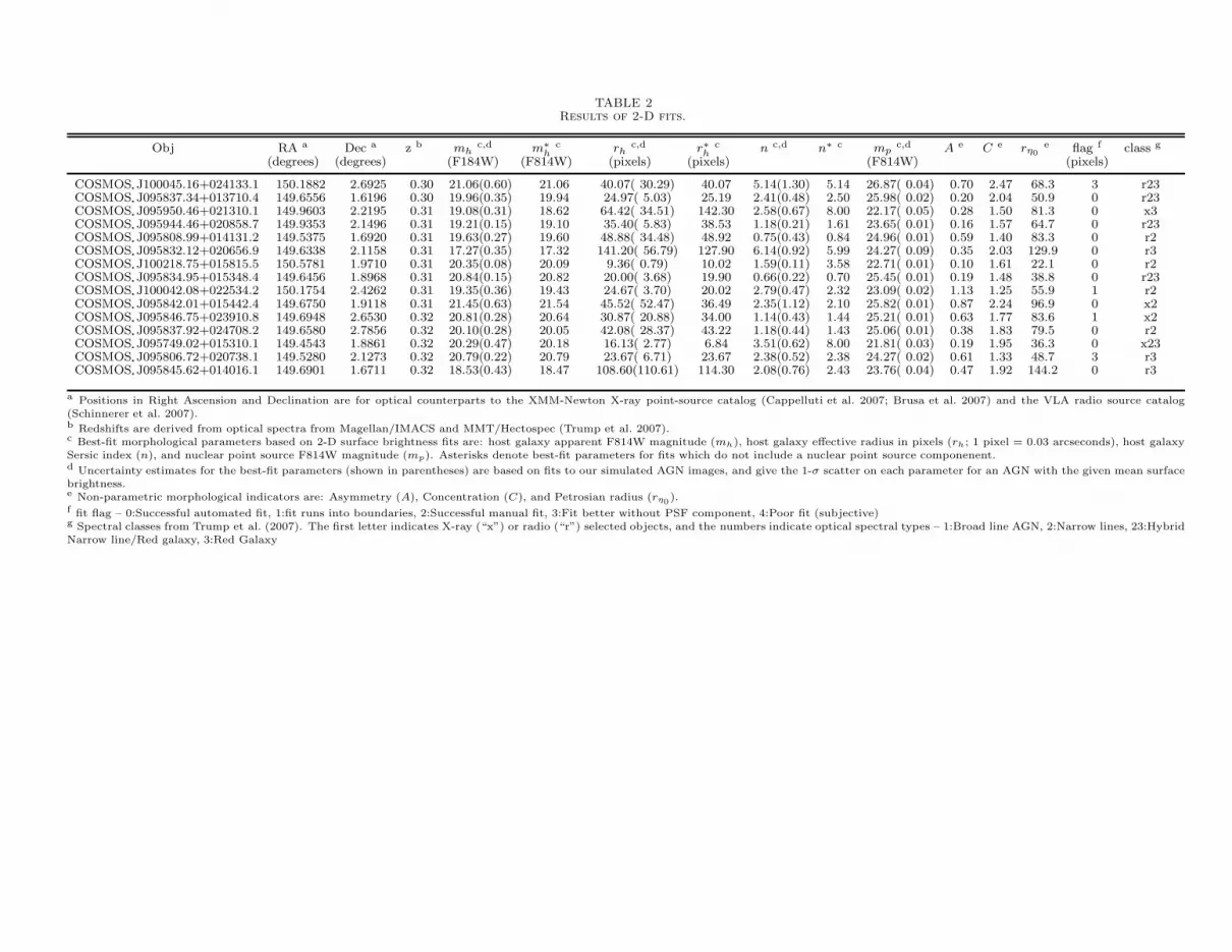
TABLE 2Results of 2-D fits.

Obj RA a Dec a z b mhc,d m∗

hc rh

c,d r∗h

c n c,d n∗ c mpc,d A e C e rη0

e flag f class g

(degrees) (degrees) (F184W) (F814W) (pixels) (pixels) (F814W) (pixels)

COSMOS J100045.16+024133.1 150.1882 2.6925 0.30 21.06(0.60) 21.06 40.07( 30.29) 40.07 5.14(1.30) 5.14 26.87( 0.04) 0.70 2.47 68.3 3 r23COSMOS J095837.34+013710.4 149.6556 1.6196 0.30 19.96(0.35) 19.94 24.97( 5.03) 25.19 2.41(0.48) 2.50 25.98( 0.02) 0.20 2.04 50.9 0 r23COSMOS J095950.46+021310.1 149.9603 2.2195 0.31 19.08(0.31) 18.62 64.42( 34.51) 142.30 2.58(0.67) 8.00 22.17( 0.05) 0.28 1.50 81.3 0 x3COSMOS J095944.46+020858.7 149.9353 2.1496 0.31 19.21(0.15) 19.10 35.40( 5.83) 38.53 1.18(0.21) 1.61 23.65( 0.01) 0.16 1.57 64.7 0 r23COSMOS J095808.99+014131.2 149.5375 1.6920 0.31 19.63(0.27) 19.60 48.88( 34.48) 48.92 0.75(0.43) 0.84 24.96( 0.01) 0.59 1.40 83.3 0 r2COSMOS J095832.12+020656.9 149.6338 2.1158 0.31 17.27(0.35) 17.32 141.20( 56.79) 127.90 6.14(0.92) 5.99 24.27( 0.09) 0.35 2.03 129.9 0 r3COSMOS J100218.75+015815.5 150.5781 1.9710 0.31 20.35(0.08) 20.09 9.36( 0.79) 10.02 1.59(0.11) 3.58 22.71( 0.01) 0.10 1.61 22.1 0 r2COSMOS J095834.95+015348.4 149.6456 1.8968 0.31 20.84(0.15) 20.82 20.00( 3.68) 19.90 0.66(0.22) 0.70 25.45( 0.01) 0.19 1.48 38.8 0 r23COSMOS J100042.08+022534.2 150.1754 2.4262 0.31 19.35(0.36) 19.43 24.67( 3.70) 20.02 2.79(0.47) 2.32 23.09( 0.02) 1.13 1.25 55.9 1 r2COSMOS J095842.01+015442.4 149.6750 1.9118 0.31 21.45(0.63) 21.54 45.52( 52.47) 36.49 2.35(1.12) 2.10 25.82( 0.01) 0.87 2.24 96.9 0 x2COSMOS J095846.75+023910.8 149.6948 2.6530 0.32 20.81(0.28) 20.64 30.87( 20.88) 34.00 1.14(0.43) 1.44 25.21( 0.01) 0.63 1.77 83.6 1 x2COSMOS J095837.92+024708.2 149.6580 2.7856 0.32 20.10(0.28) 20.05 42.08( 28.37) 43.22 1.18(0.44) 1.43 25.06( 0.01) 0.38 1.83 79.5 0 r2COSMOS J095749.02+015310.1 149.4543 1.8861 0.32 20.29(0.47) 20.18 16.13( 2.77) 6.84 3.51(0.62) 8.00 21.81( 0.03) 0.19 1.95 36.3 0 x23COSMOS J095806.72+020738.1 149.5280 2.1273 0.32 20.79(0.22) 20.79 23.67( 6.71) 23.67 2.38(0.52) 2.38 24.27( 0.02) 0.61 1.33 48.7 3 r3COSMOS J095845.62+014016.1 149.6901 1.6711 0.32 18.53(0.43) 18.47 108.60(110.61) 114.30 2.08(0.76) 2.43 23.76( 0.04) 0.47 1.92 144.2 0 r3

a Positions in Right Ascension and Declination are for optical counterparts to the XMM-Newton X-ray point-source catalog (Cappelluti et al. 2007; Brusa et al. 2007) and the VLA radio source catalog(Schinnerer et al. 2007).b Redshifts are derived from optical spectra from Magellan/IMACS and MMT/Hectospec (Trump et al. 2007).c Best-fit morphological parameters based on 2-D surface brightness fits are: host galaxy apparent F814W magnitude (mh), host galaxy effective radius in pixels (rh; 1 pixel = 0.03 arcseconds), host galaxySersic index (n), and nuclear point source F814W magnitude (mp). Asterisks denote best-fit parameters for fits which do not include a nuclear point source componenent.d Uncertainty estimates for the best-fit parameters (shown in parentheses) are based on fits to our simulated AGN images, and give the 1-σ scatter on each parameter for an AGN with the given mean surfacebrightness.e Non-parametric morphological indicators are: Asymmetry (A), Concentration (C), and Petrosian radius (rη0).f fit flag – 0:Successful automated fit, 1:fit runs into boundaries, 2:Successful manual fit, 3:Fit better without PSF component, 4:Poor fit (subjective)g Spectral classes from Trump et al. (2007). The first letter indicates X-ray (“x”) or radio (“r”) selected objects, and the numbers indicate optical spectral types – 1:Broad line AGN, 2:Narrow lines, 23:HybridNarrow line/Red galaxy, 3:Red Galaxy

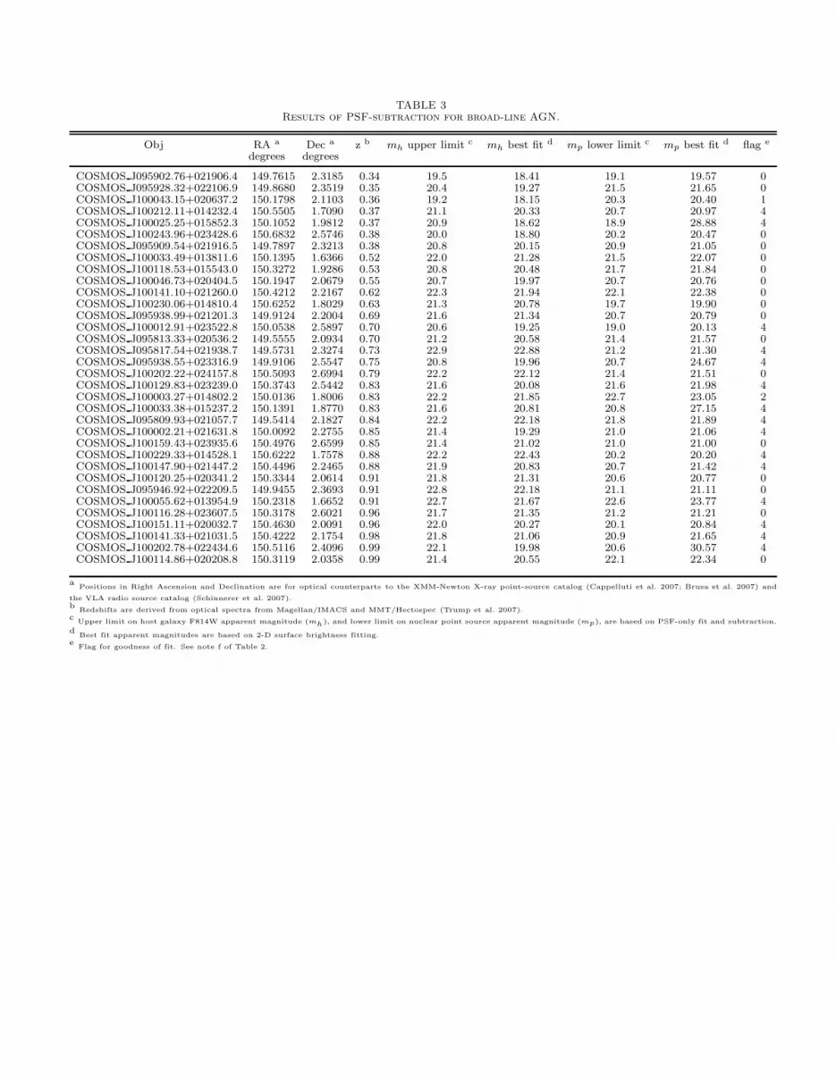
TABLE 3Results of PSF-subtraction for broad-line AGN.

Obj RA a Dec a z b mh upper limit c mh best fit d mp lower limit c mp best fit d flag e

degrees degrees

COSMOS J095902.76+021906.4 149.7615 2.3185 0.34 19.5 18.41 19.1 19.57 0COSMOS J095928.32+022106.9 149.8680 2.3519 0.35 20.4 19.27 21.5 21.65 0COSMOS J100043.15+020637.2 150.1798 2.1103 0.36 19.2 18.15 20.3 20.40 1COSMOS J100212.11+014232.4 150.5505 1.7090 0.37 21.1 20.33 20.7 20.97 4COSMOS J100025.25+015852.3 150.1052 1.9812 0.37 20.9 18.62 18.9 28.88 4COSMOS J100243.96+023428.6 150.6832 2.5746 0.38 20.0 18.80 20.2 20.47 0COSMOS J095909.54+021916.5 149.7897 2.3213 0.38 20.8 20.15 20.9 21.05 0COSMOS J100033.49+013811.6 150.1395 1.6366 0.52 22.0 21.28 21.5 22.07 0COSMOS J100118.53+015543.0 150.3272 1.9286 0.53 20.8 20.48 21.7 21.84 0COSMOS J100046.73+020404.5 150.1947 2.0679 0.55 20.7 19.97 20.7 20.76 0COSMOS J100141.10+021260.0 150.4212 2.2167 0.62 22.3 21.94 22.1 22.38 0COSMOS J100230.06+014810.4 150.6252 1.8029 0.63 21.3 20.78 19.7 19.90 0COSMOS J095938.99+021201.3 149.9124 2.2004 0.69 21.6 21.34 20.7 20.79 0COSMOS J100012.91+023522.8 150.0538 2.5897 0.70 20.6 19.25 19.0 20.13 4COSMOS J095813.33+020536.2 149.5555 2.0934 0.70 21.2 20.58 21.4 21.57 0COSMOS J095817.54+021938.7 149.5731 2.3274 0.73 22.9 22.88 21.2 21.30 4COSMOS J095938.55+023316.9 149.9106 2.5547 0.75 20.8 19.96 20.7 24.67 4COSMOS J100202.22+024157.8 150.5093 2.6994 0.79 22.2 22.12 21.4 21.51 0COSMOS J100129.83+023239.0 150.3743 2.5442 0.83 21.6 20.08 21.6 21.98 4COSMOS J100003.27+014802.2 150.0136 1.8006 0.83 22.2 21.85 22.7 23.05 2COSMOS J100033.38+015237.2 150.1391 1.8770 0.83 21.6 20.81 20.8 27.15 4COSMOS J095809.93+021057.7 149.5414 2.1827 0.84 22.2 22.18 21.8 21.89 4COSMOS J100002.21+021631.8 150.0092 2.2755 0.85 21.4 19.29 21.0 21.06 4COSMOS J100159.43+023935.6 150.4976 2.6599 0.85 21.4 21.02 21.0 21.00 0COSMOS J100229.33+014528.1 150.6222 1.7578 0.88 22.2 22.43 20.2 20.20 4COSMOS J100147.90+021447.2 150.4496 2.2465 0.88 21.9 20.83 20.7 21.42 4COSMOS J100120.25+020341.2 150.3344 2.0614 0.91 21.8 21.31 20.6 20.77 0COSMOS J095946.92+022209.5 149.9455 2.3693 0.91 22.8 22.18 21.1 21.11 0COSMOS J100055.62+013954.9 150.2318 1.6652 0.91 22.7 21.67 22.6 23.77 4COSMOS J100116.28+023607.5 150.3178 2.6021 0.96 21.7 21.35 21.2 21.21 0COSMOS J100151.11+020032.7 150.4630 2.0091 0.96 22.0 20.27 20.1 20.84 4COSMOS J100141.33+021031.5 150.4222 2.1754 0.98 21.8 21.06 20.9 21.65 4COSMOS J100202.78+022434.6 150.5116 2.4096 0.99 22.1 19.98 20.6 30.57 4COSMOS J100114.86+020208.8 150.3119 2.0358 0.99 21.4 20.55 22.1 22.34 0

aPositions in Right Ascension and Declination are for optical counterparts to the XMM-Newton X-ray point-source catalog (Cappelluti et al. 2007; Brusa et al. 2007) and

the VLA radio source catalog (Schinnerer et al. 2007).b

Redshifts are derived from optical spectra from Magellan/IMACS and MMT/Hectospec (Trump et al. 2007).c

Upper limit on host galaxy F814W apparent magnitude (mh), and lower limit on nuclear point source apparent magnitude (mp), are based on PSF-only fit and subtraction.

dBest fit apparent magnitudes are based on 2-D surface brightness fitting.

eFlag for goodness of fit. See note f of Table 2.