Auton Robot (2008) 24: 401–417DOI 10.1007/s10514-008-9084-9

Active audition using the parameter-less self-organising map

Erik Berglund · Joaquin Sitte · Gordon Wyeth

Received: 18 November 2005 / Accepted: 3 January 2008 / Published online: 31 January 2008© Springer Science+Business Media, LLC 2008

Abstract This paper presents a novel method for enablinga robot to determine the position of a sound source in threedimensions using just two microphones and interaction withits environment. The method uses the Parameter-Less Self-Organising Map (PLSOM) algorithm and ReinforcementLearning (RL) to achieve rapid, accurate response. We alsointroduce a method for directional filtering using the PL-SOM. The presented system is compared to a similar systemto evaluate its performance.

Keywords Active audition · Self-organisation

1 Introduction

For a robot communicating with humans or navigating thephysical world, hearing is important. In communication, itcontains a large portion of the information. In navigation,it informs of landmarks and warns of dangers which maybe outside the field of view. Merely detecting sound is notenough, however—the direction of the source of the soundis also important. This is clear in the case of navigation but

E. Berglund (�) · G. WyethSchool of Information Technology and Electrical Engineering,University of Queensland, Brisbane, Australiae-mail: berglund@itee.uq.edu.au

G. Wyethe-mail: wyeth@itee.uq.edu.au

J. SitteSchool of Software Engineering and Data Communication,Queensland University of Technology, Brisbane, Australiae-mail: sitte@qut.edu.au

equally true for communication where for example a mes-sage such as “come here” has no meaningful content un-less the direction and distance to the source is, at the veryleast, estimated. Sound information is also relatively cheapin terms of computing power. Unlike vision, which uses sen-sors producing two-dimensional data, audition relies on sen-sors producing one-dimensional data. While vision offersgreat angular resolution, audition offers superior temporalresolution. One problem with audition is the microphoneswhich, along with their associated circuitry, draw power, addweight and add a possible point of failure. Therefore, it is de-sirable to have as few microphones as possible. The systemdescribed in this paper uses two—this is the number used innature and the smallest with which one can expect to detectdirection.

Since the direction sensitivity of a two-microphone sys-tem is greatest along the plane perpendicular to the axis be-tween the microphones (Bregman 1990), we can increaseaccuracy by moving this plane towards a sound source. Thisis the central idea of active audition (Reid and Milios 1999,2003); to arrange the articulated microphone platform (suchas a robot head) so that one maximises the information con-tent available from sound.

This paper presents a method which solves the active au-dition task using the Parameter-Less Self-Organising Map(PLSOM) algorithm (Berglund and Sitte 2006) to find pat-terns in the high-dimensional features extracted from sounddata, and associate these patterns with an appropriate mo-tor action. This makes it unnecessary to have an explicitmodel or any a priori knowledge of the robot or environmentacoustics. The presented method also utilises the short-termmovement of the robot to achieve localisation of the soundsource in three dimensions, a first for two-channel roboticsystems. In order to do so the system incorporates a larger

402 Auton Robot (2008) 24: 401–417

number of sound features than previous systems, includingthe new Relative Interaural Intensity Difference (RIID).

A system for separating sound signals from noise usingtwo microphones based on direction is presented, imple-mented, tested, and compared to existing methods.

Section 2 will examine earlier works in the field of activeaudition and robot audition. Section 3 gives a brief systemoverview, before Sect. 4 deals with the system in more detailand Sect. 5 gives implementation details, experimental re-sults and evaluation. Section 6 summarises the findings andSect. 7 concludes the paper.

2 Earlier works

It is important to separate passive audition and active audi-tion.

2.1 Passive audition

Passive audition is well understood, and has roots datingback to the works of Lord Rayleigh (J. W. Strutt 3rd BaronRayleigh 1896) on human audition and the properties ofsound. Since sound is a wave phenomenon many of thesame principles are employed in radio transmission, radar,and sonar research. We will here give a brief overview ofhow it applies to robotic audition. Robotic audition, whichis concerned with detecting sound and inferring the locationand nature of the sound source, is distinguished from speechrecognition, which is about retrieving the message encodedin the signal.

Most passive audition systems rely on three or more mi-crophones. For example (Huang et al. 1995, 1997) presentsa system for sound source localisation and separation basedon three microphones. The system uses event detection andtime delay calculations to provide a direction in the hori-zontal plane and can separate sources based on direction.Other examples are Rabinkin et al. (1996a) or Guentchevand Weng (1998). The latter is interesting in that it usesfour microphones arranged as vertices in a tetrahedron toachieve three-dimensional localisation. Numerous other ap-proaches to the direction detection problem have been pro-posed. Some examples are mask diffraction (Ge et al. 2003),formant frequencies (Obata et al. 2003), and support vectormachines (Yamamoto et al. 2003). Use of passive audition todetect snipers during warfare has been suggested (Rabinkinet al. 1996b).

Some methods use integration of vision and audition incombination with Self-Organising Maps (SOMs). Promi-nent examples are those of Rucci et al. (1999) andNakashima et al. (2002), which both rely on time delays andvisual feedback to train the auditory system and pinpoint thelocation of the target.

The works of Rucci et al., Konishi (1993), and Day(2001) are inspired by the auditory system of the Barn Owl(Tyto alba). Rucci et al. recreated the brain pathways of theowl computationally with a high degree of fidelity. The re-sulting framework was connected to a robot which, assistedby visual cues, learned to orient towards the sound sourcewith an error of approximately 1°. This work relied on vi-sual feedback to train its motor response; the visual feed-back was provided in the shape of a clearly distinguishabletarget (a small electric lamp that was always associated withthe active speaker) and image processing software that de-termines whether the target was in front of the robot or offto the sides, issuing a ‘reward’ to the system based on this.Rucci et al. focus on the Interaural Time Difference (ITD)only, employing a relatively large distance between the mi-crophones (300 mm) and pre-determined static networks.The mapping between the central nucleus of the inferior col-liculus to the external nucleus of the inferior colliculus canbe changed during training, but is partially pre-determined.

Elevation detection has long been the exclusive domainof multi-microphone systems. Detecting elevation by twomicrophones has long been assumed to be dependent onspectral cues produced by diffraction in the pinna (Blauert1983; Shaw 1997; Kuhn 1987) and several studies in mod-elling these cues have been performed based on Head-Related Transfer Functions. Later research (Avendano et al.1999) has identified elevation cues related to low-frequencyreverberation in the human torso. These studies have in com-mon that they focus on recreating a realistic spatial listeningexperience for humans, not on source location detection forrobots.

Robotic work in this field has mainly concentrated on us-ing multiple microphones with good results (for example,Tamai et al. 2004). Some recent applications (for example,Kumon et al. 2005) have created artificial pinnae with well-understood acoustics in order to use two microphones andspectral cues for elevation detection. This is thought to beanalogous to how many animals, including humans, detectelevation.

2.2 Active audition

Active audition aims at using the movement of the listeningplatform to pinpoint the location of a sound source in thesame way biological systems do. Active audition is there-fore an intrinsically robotic solution to the problem of sounddirection detection.

The term active audition appears to have originated in1999 with Reid et al. (Reid and Milios 1999, 2003), who de-scribed a system using two omnidirectional microphones ona pan and tiltable microphone assembly. Two sets of possi-ble directions to the sound source were computed using timedelay and two different positions of the platform. The cor-rect source direction was then the intersection of the two

Auton Robot (2008) 24: 401–417 403

sets; the system used its own movement to detect direc-tion. Reid et al.’s approach was therefore different from ap-proaches that only used the bearing to the sound source todirect movement. Apart from this early example there havebeen few instances of active audition research. One impor-tant exception was the SIG group, which started researchinto the topic around 2000 (Nakadai et al. 2000a).

The SIG method also relied on synergy of visual and au-ditory cues for direction detection (Nakatani et al. 1994;Nakadai et al. 2000a, 2000b, 2001, 2002a, 2002b, 2003a,2003b, 2003c; Kitano et al. 2002). The output of this grouprepresents the main body of active audition research to date,most of which has been conducted in the last five years. TheSIG Humanoid project was (it has now been supplanted bythe SIG 2 project) a large multidisciplinary cross-institutionproject aimed at creating a robotic receptionist capable ofinteracting with several humans at once in a realistic (noisy)office environment. The system used the Fast Fourier Trans-form (FFT) to extract interaural phase and intensity differ-ence (IPD and IID, respectively) from a stereo signal.

Combinations of SOMs and Reinforcement Learninghave been explored by (Sitte et al. 2000; Iske et al. 2000).

3 Overview of presented system

A robotic audition system should have the following quali-ties:

• Effective with just two microphones placed relativelyclose together; this reduces weight, power consumption,cost, and the risk of hardware failure. It also places fewerconstraints on the size and shape of the robot, and theplacement of the microphones.

• Distance estimation capabilities without relying on famil-iarity with the signal; so that the robot can determine thedistance to a sound source it has not encountered before.

• Elevation estimation capabilities; in order that the robotcan determine the elevation of a sound source.

• Robust to environmental changes; so that post-processingto compensate for environment is not necessary, thus re-ducing complexity and increasing flexibility.

• Flexible and easily adaptable to diverse architectures; sothat the same software and/or hardware can be used onmultiple platforms, thus reducing development time andcost.

This section gives a brief overview of such a system and dis-cusses some of the obstacles that must be overcome in orderto implement it. The system includes as many features aspossible to maximise the available information and coun-teract the frequency-limited range of the Interaural PhaseDifference (IPD) and Interaural Intensity Difference (IID).Therefore, both IPD and IID, as well as ITD and RIID, are

included. The calculation of the IPD, IID, and RIID featuresare extracted by the aid of the FFT. The ITD is calculatedby cross-correlation of time-shifted copies of the right andleft sound buffers. The IID, RIID, IPD, and ITD will be dis-cussed in detail in Sect. 4.2.

The pre-processed features are combined into one featurevector which the data association strategy can use in orderto make a decision about how to move the robot or convertinto information about the location of the sound source.

By calculating the direction for each subband of the FFT,one can filter the entire signal based on the direction.

3.1 Feature selection rationale

Some of the features selected seem to duplicate the sameinformation, yet on closer examination they are quite differ-ent.

ITD and IPD seem identical on a cursory examination, butit is important to realise that ITD gives only one value pertimestep where the IPD gives one value per timestep andsubband. This is especially important because the profile ofhow the IPD changes relative to the frequency contains im-portant clues to the direction. The ITD, on the other hand, isnot limited to ±π radians, and gives a more robust yet lessaccurate value. In short, the ITD is frequency-independent;the IPD is frequency-dependent. The ITD is also better atlocalising transient sounds, while the IPD requires a soundto last the entire duration of the FFT input buffer to be re-liably and accurately detected.

IID and RIID also seem identical at first glance but thereader should note that the RIID is necessary for distancedetection but, since it is an absolute value, does not dis-tinguish between left and right. The RIID must be an ab-solute value to prevent the distance resolution from invert-ing around the central axis.

Overall the aim is not to constrain or minimise the amount ofdata extracted from the sound signal but to provide sufficientdata for the system to work with.

3.2 Data association strategy and possible obstacles toimplementation

Once the features are extracted the task is to extract thesalient information from them. In other words: how can thedata be categorised into practical groups that can be usedfor decision making? This is a complicated task since theinput contains large amounts of irrelevant data such as fre-quency distribution, intensity and intensity distribution. Anideal learning system will focus on those properties in thetraining examples that change between training examplesand ignore those that stay constant. In that way it becomeseasy to train the system by simply providing training data

404 Auton Robot (2008) 24: 401–417

that exemplifies change in the property the system shouldlearn.

The learning system for this task must deal with the com-plexity of the data. Even at low sample rates and small FFTsizes, there will be hundreds of variables to be evaluated andcorrelated with each other. There is also the problem of pro-viding sufficient training examples. In order to avoid record-ing samples from every possible location and every possibleenvironmental condition, an ideal system would be able togeneralise from few training examples. Although systemsbased on theoretical models have achieved good results, itwould be preferable to have a model-less system or a systemthat develops its own model based on experience to avoid theneed for a detailed analysis of the implementation platform’sacoustics for each new implementation.

This leads in the direction of neural network basedsolutions. Traditional neural network algorithms (such asbackpropagation) and architectures (multilayer perceptrons,feedforward networks) are very good at learning similarproblems, but here the added constraint on the number oftraining examples must be taken into account. Training net-works by using backpropagation also requires the trainingdata to be correctly labelled.

It would therefore be a good idea to use a system thatcan self-organise, such as the Self-Organising Map (SOM).The SOM can reduce the dimensionality of a data set byfinding low-dimensional manifolds embedded in the high-dimensional input space, which is exactly what is requiredhere. The position of the sound source (three dimensions) isembedded in the input space (hundreds of dimensions). Theinput space is the set of all possible input combinations to asystem. The data in a feature vector represents one point inthe input space, the key to understanding the input space isunderstanding the feature vector. The contents of the featurevector is described in Sect. 4.2.

The problem with the SOM is that there is no firm theo-retical basis for selecting the training parameters, so that the

search for the correct values becomes an empirical searchthrough a four-dimensional space. The SOM also requiresa large number of iterations to achieve a good mapping,which is a problem in this case since the preprocessing ofeach training example requires computation time. The com-bination of time-consuming training and the need for severaltraining sessions in search for the optimal parameters meansthat the SOM-based approach will be slow.

Finally, the size of the input space and the relatively fewtraining examples makes it unlikely that there is an even dis-tribution of training examples, which will make the SOMclump weights in certain areas. This is undesirable since thesystem needs a continuous generalisation that covers the en-tire possible input space.

4 Active audition with PLSOM

This section describes a general active audition system ca-pable of using any robot with two audio input channels forsound source localisation. To emphasise that the system isnot tied to one specific robot architecture, the implemen-tation details and experiments are discussed separately, inSect. 5.

4.1 Brief system overview

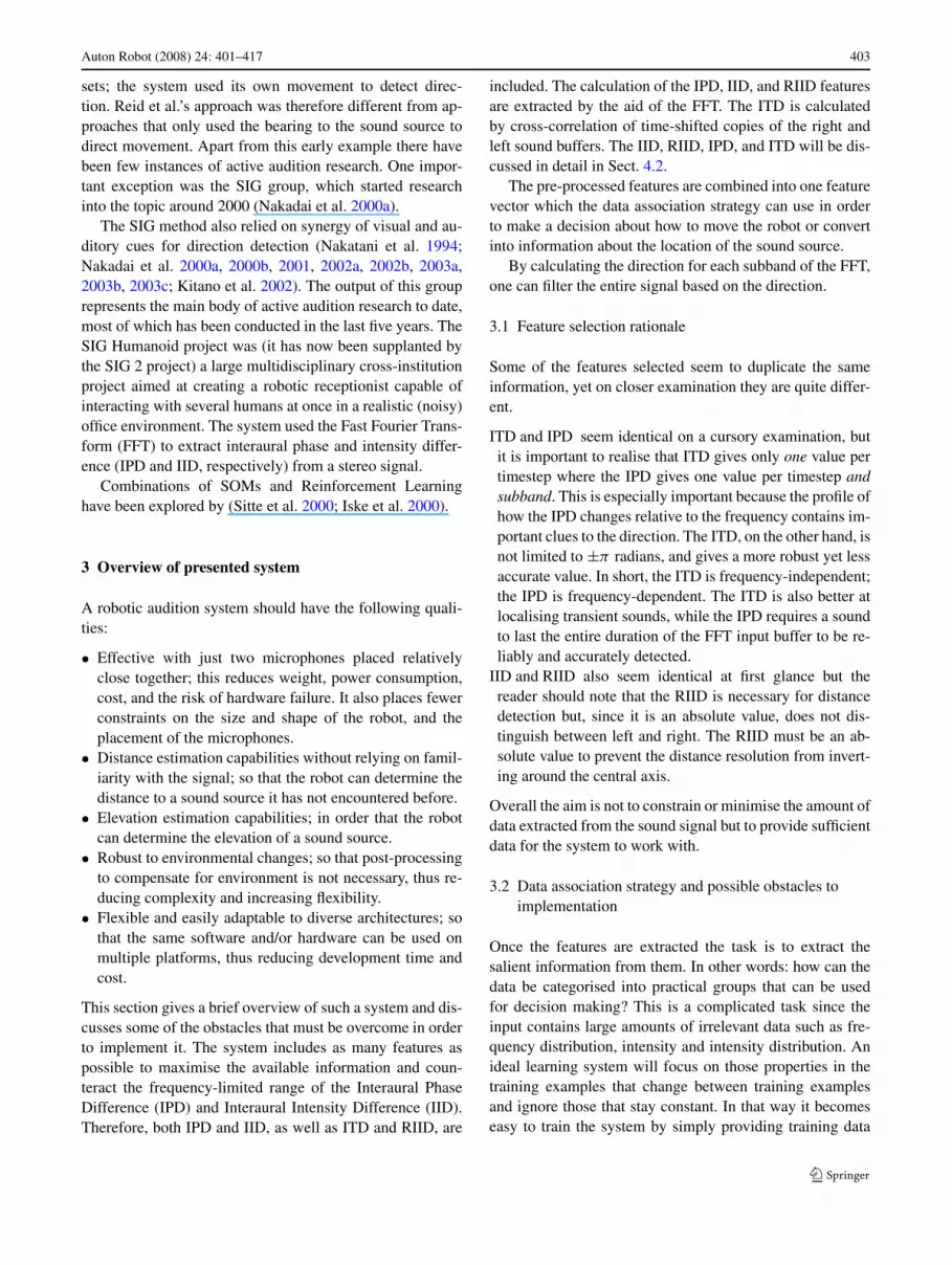
The system needs an articulated robot platform with twomicrophones to function, subsystem A in Fig. 1. The sig-nals are processed and sound features indicating the rela-tionship between the stereo channels are extracted, see sub-system B in Fig. 1. These features are the IID, RIID, IPD,ITD, and volume, which will be discussed in more detail inthe next section. These features are combined into a featurevector and used to train a Parameter-Less Self-OrganisingMap (PLSOM), see subsystem C in Fig. 1. The PLSOMlearns to extract the low-dimensional manifold embedded in

Fig. 1 Active audition systemlayout. Sound information flowsalong the direction of the arrows

Auton Robot (2008) 24: 401–417 405

the high-dimensional feature vector, which corresponds tothe position of the sound source. Once trained, the PLSOMstarts passing the position information to a ReinforcementLearning (RL) algorithm, see subsystem D in Fig. 1. TheRL subsystem uses the input from the PLSOM as feedbackto learn to orient the robot towards the sound source.

4.2 Preprocessing

Four features are extracted from the sound signal, describingthe difference in time, phase, intensity, and relative intensityof the two channels. In addition, the overall intensity is cal-culated.

For each sampling window, which is Υ samples long, thesystem computes the FFT of the signal. The FFT dividesthe signal into its constituent frequency components, givingΥ/2 components that approximately represent the originalsignal in the frequency domain. Each frequency componentin the FFT output is here termed a subband—the FFT givesΥ/2 subbands which can be averaged to fewer subbands toenable us to work with a smaller feature vector.

For each sampling window the system computes the ITDby simple offset matching on the original input signal in ac-cordance with (1)

itd(L,R) = arg mind

√∑Υ −2dt=0 (L(t + d) − R(t))2

(Υ − 2d)(1)

where Υ is the size of the FFT input buffer, L and R arearray representations of Υ samples of stereo sound, leftand right channels respectively. d has a range that reflectsthe maximum possible time delay, measured in number ofsamples. The ITD could also be computed through cross-correlation.

For robots with low sample rates or small heads, andtherefore small distances between the microphones, the ITDdoes not offer usable accuracy. As an example, consider asmall robot with 70 mm between the microphones that usesa sample rate of 16000 Hz (an example of such a robot isgiven in Sect. 5). Since the speed of sound is 340 m/s, thisgives a maximal time difference of only 200 μs, this occurswhen the sound source is at 90° to either side. At 16000 sam-ples per second this is less than 3.3 samples difference be-tween 0° and 90°, so the optimal theoretical accuracy avail-able from ITD alone is roughly 30°.

As is well known, the FFT gives an array of complexnumbers, one complex number re(s) + i im(s) for each sub-band s. The real and imaginary parts are denoted rel (s) andiml (s) for the left channel, rer (s) and imr (s) for the rightchannel of subband s. The IID is computed according to (2).

ild(s) =√

rel (s)2 + iml(s)2 −√

rer (s)2 + imr (s)2. (2)

The IPD is computed according to (3)

ipd(s) ={

a − b, if |a − b| ≤ π ,a − b + 2π, if |a − b| > π and a < b,a − b − 2π, otherwise

(3)

where a and b are given by (4) and (5), respectively

a = arctanimr (s)

rer (s), (4)

b = arctaniml (s)

rel (s)(5)

and RIID according to (6):

rild(s) = ild(s)

v(s)(6)

where v(s) is the averaged volume of the left and right chan-nel for subband s, computed according to (7):

v(s) =√

rel (s)2 + iml(s)2 + √rer (s)2 + imr (s)2

2. (7)

IPD, IID, and RIID are based on the FFT so that thereis one value for each of the Υ/2 subbands. The ITD valueis copied Υ/2 times in order to lend it the same importanceas the IPD, IID, and RIID in the PLSOM. Finally the ITD,IID, RIID, and IPD vectors are concatenated into one 2 · Υ -element feature vector x which, in addition to the volume v,is passed to the PLSOM.

4.3 PLSOM

The Parameter-Less Self-Organising Map has already beenpublished independently (Berglund and Sitte 2003, 2006),therefore this section will only point out one modificationthat was applied relative to the standard PLSOM for the sakeof improving sound processing performance. The PLSOMand other SOM algorithms depend on a distance measure tocalculate the distance between each node and a given input;one example is the commonly used Euclidean norm. Un-fortunately the Euclidean norm assigns equal importance toall parts of the input, which will be detrimental where sub-bands with low intensity have a high phase difference. Toavoid this problem a slightly modified Euclidean norm wasselected. When computing the distance between input andweight vectors, a weight based on the subband intensity isapplied, substituting the Euclidean distance in the standardPLSOM algorithm with the norm:

‖x(t) − wi(t)‖v

=√√√√2·Υ∑

s=1

(xs(t) − wi,s(t))2vmod(s,Υ/2)(t). (8)

406 Auton Robot (2008) 24: 401–417

In (8) wi,s(t) is the weight of node i at time t in subband s,xs(t) is the input in subband s at time t . vmod(s,Υ/2)(t) is thenormalised (divided by the loudest volume up until time t)average volume of both channels in subband mod(s,Υ/2) attime t .

Notice that since x is the 2 ·Υ -dimensional concatenationof the Υ/2-dimensional ITD, IID, RIID, and ILD vectors themod(s,Υ/2) operator must be applied to the subband indexs. Thus, subbands with high volume influence the winningnode more than subbands with a low volume, and there is noneed for discrete volume based thresholding.

4.4 Reinforcement learning

The output of the PLSOM (the position of the winning node)is used by the RL subsystem to turn the robot head towardsthe sound source, based on the hypothesis (which will betested in Sect. 5.2) that a node in the centre of the map is thewinning node when the sound source is directly ahead of therobot.

Reinforcement Learning (RL) (Sutton 1992; Mitchell1997; Sutton and Barto 1998; Gosavi 2003) is a machinelearning paradigm based on the concept of an agent, whichlearns through interaction with its environment.

RL is particularly well suited to applications where astrategy balancing long-term and short-term gains (reflectedin the value and reward functions) must be developed with-out any predetermined model of how the environment willrespond to actions.

5 Experiments and results

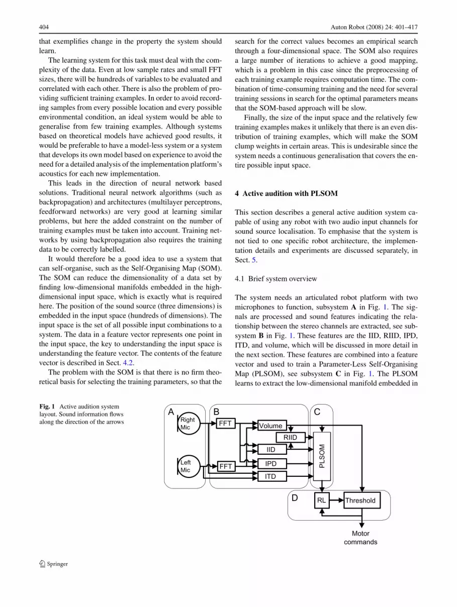
To test the system described in Sect. 4 it was implementedusing Sony Aibo ERS-210 robots (known simply as ‘Aibo’hereafter) (Fig. 2). This section describes the details of theimplementation, the experimental setup and the results. TheAibo robots used in the experiments were standard exceptfor the addition of a wireless networking card.

The physical system consists of two parts:

1. The SONY Aibo robot—a dog-like quadruped robot withstereo recording capabilities. Several models exist, theexperiments described in this paper were all carried outon ERS-210 models.

2. An ordinary desktop PC.

This robot was connected via a wireless link to the PC.Sound samples were transferred from the Aibo to the PC, onwhich the sound processing took place. Motor commandsfrom the system were passed back to the Aibo.

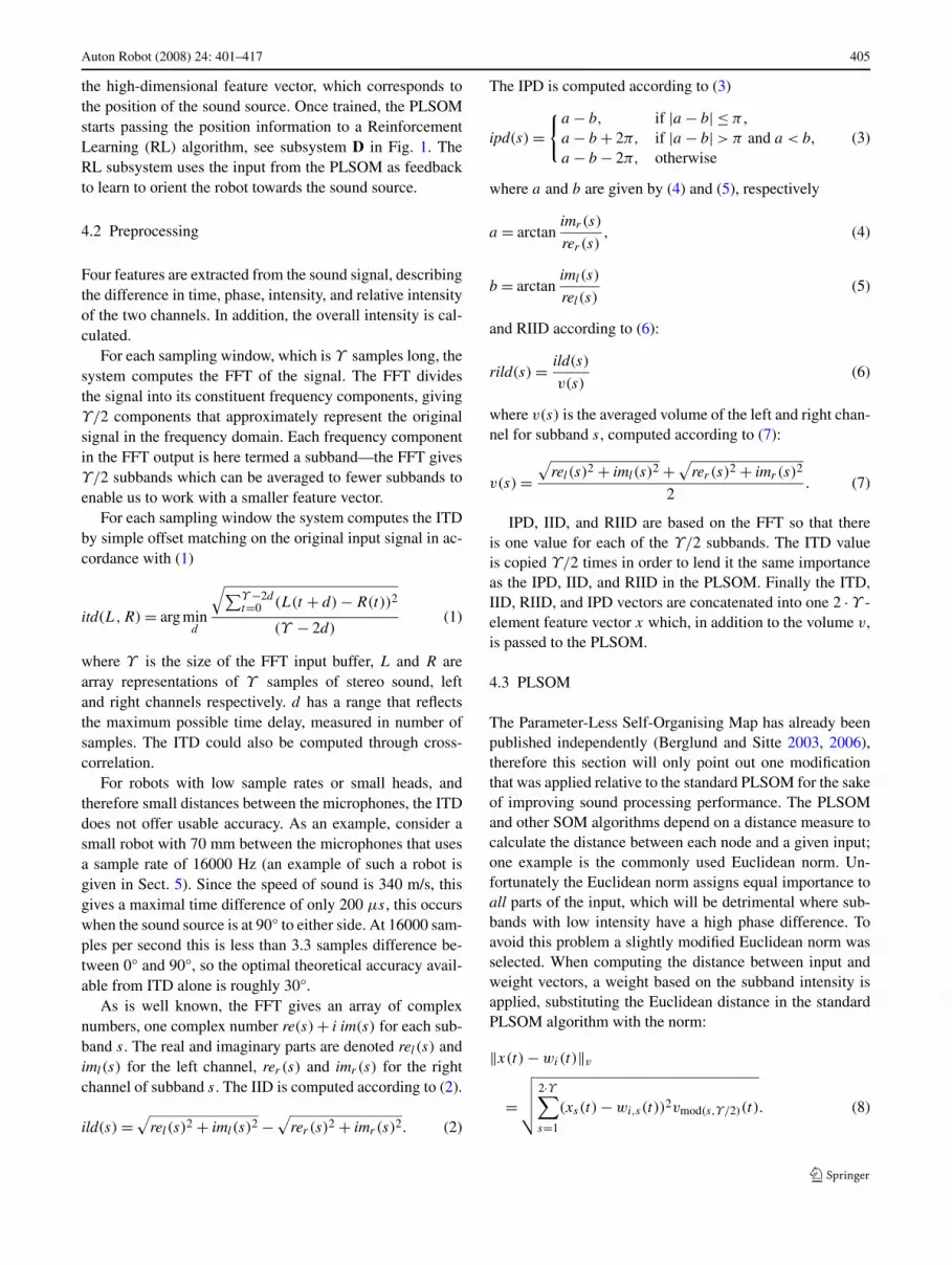
The sound was transmitted as 16 bit/channel, 16000samples/second linear Pulse Code Modulated (PCM) stereodata. The directional response of the Aibo can be seen in

Fig. 2 One of the Sony Aibo ERS-210 robots used in the experiments.Note that the artificial auricles are mounted separately from the micro-phones (the three horizontal slits)

Fig. 3 Directional response of the Aibo microphones. The graphshows sensitivity as distance from the robot head; greater distancemeans greater sensitivity. Test conducted with speaker playing 79 dBwhite noise at 0.1 m in a room with a background noise of 50 dB andreverberation time (T60) = 0.4 seconds. Note the increased sensitivityaround ±60–70°

Fig. 3. It is interesting to note that the directional responsewas not the same for all frequencies. At 800 Hz the direc-tional sensitivity was almost completely opposite of that forwhite noise, as can be seen in Fig. 4. This would pose a se-rious problem for direction detection systems only based onintensity difference.

5.1 Experimental setup

During the experiments described below a PLSOM with18 × 5 nodes and a neighbourhood size of 11 was used. TheFFT input buffer size, Υ , was equal to 512.

The 256-dimensional output was averaged to 64 dimen-sions to give us a smaller data vector and therefore smallerSOM. It was decided to not simply use a smaller Υ sincethat would have constrained the frequency range of the sys-tem too much. Furthermore, the Aibo sends samples to the

Auton Robot (2008) 24: 401–417 407

Fig. 4 Aibo sensitivity response to 800 Hz sine wave under the sameconditions as in Fig. 3. Note that the sensitivity is switched along thecentral axis compared with that for white noise. This is caused by thesound source interfering with itself in the near field

PC in 512-sample packets. The maximum range of d in (1)was limited to 12.

Before application of the FFT the input signal was nor-malised over each 512-sample window. After application ofthe FFT the first subband was discarded, since it was almostpure noise. The signal was then downsampled before com-puting the IPD, IID, and RIID.

The logarithm of the ITD values was normalised by di-viding by the largest ITD so far and then multiplied by 0.25.The IPD was normalised. The IID was normalised and mul-tiplied by the volume of each subband. The RIID was nor-malised. The volume (defined in (7)) was normalised. TheITD, IPD, IID, RIID, and volume was combined into onefeature vector, which was not normalised.

In order to train the PLSOM a number of sound sam-ples were recorded; white noise samples from 38 locationsin front of the robot were used. The samples were recordedwith the speaker at 0.5 and 3 m distance from the robot,with 10° horizontal spacing, ranging from −90° to 90°. Foreach training step the PLSOM training algorithm presented1.984 seconds of a randomly selected sample to the system,off-line. This was repeated for 10000 training steps. Thissensitised each node to sound from one direction and dis-tance, as shown in Fig. 5, and typically completed in lessthan eight hours on an entry-level (in 2005) desktop PC.The sound environment was a quiet office setting, noisesources included air-conditioning and traffic noises but nohuman voices. The floors were carpeted and the ceiling wasordinary office noise-absorbing tile. The two closest wallswere hard concrete and glass. Reverberation time (T60) wasapproximately 400 ms and background noise was close to50 dB. This corresponds to data set A, to be discussed inSect. 5.1.1. The physical setup was similar for all data sets,see Fig. 6 for an example.

The reinforcement learning was done online, with the ro-bot responding to actual sound from a stationary speakerplaying white noise in front of it. Initially the robot head was

Fig. 5 Plot showing the input position each node was most sensitiveto on average, relative to the head. Each line intersection represents anode. The semi-circle represents 3 m, the circle represents 0.5 m. Notehow the largest PLSOM dimension was allocated to the most promi-nent feature of the sound

Fig. 6 A typical recording setup. The tape measure was extended toone meter for scale. This particular picture shows the recording of dataset H, see Sect. 5.1.1

pointed in a randomly selected direction, and the RL trainingprogressed until the robot kept its head steadily pointed to-wards the speaker, at which time a new direction was pickedby random and the RL training continues. The RL train-ing reached usable results in 2000 iterations, which typicallytook less than 20 minutes.

5.1.1 Data sets used throughout this paper

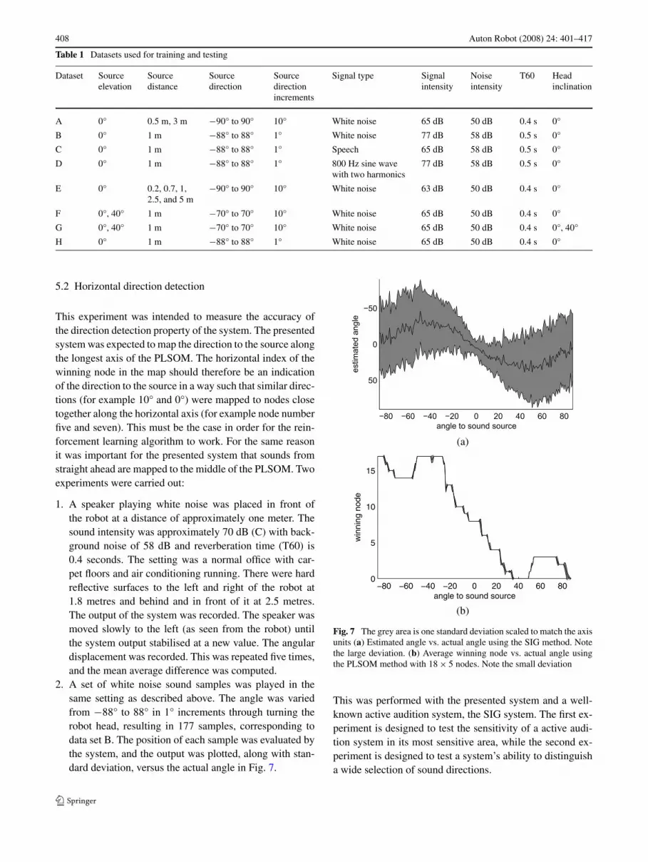
In Table 1 the reverberation time is given as T60, whichrefers to the time it takes the reverberations of a sound todiminish by 60 dB. Data set A was used in all training, theother data sets were only used for testing.

408 Auton Robot (2008) 24: 401–417

Table 1 Datasets used for training and testing

Dataset Sourceelevation

Sourcedistance

Sourcedirection

Sourcedirectionincrements

Signal type Signalintensity

Noiseintensity

T60 Headinclination

A 0° 0.5 m, 3 m −90° to 90° 10° White noise 65 dB 50 dB 0.4 s 0°

B 0° 1 m −88° to 88° 1° White noise 77 dB 58 dB 0.5 s 0°

C 0° 1 m −88° to 88° 1° Speech 65 dB 58 dB 0.5 s 0°

D 0° 1 m −88° to 88° 1° 800 Hz sine wavewith two harmonics

77 dB 58 dB 0.5 s 0°

E 0° 0.2, 0.7, 1,2.5, and 5 m

−90° to 90° 10° White noise 63 dB 50 dB 0.4 s 0°

F 0°, 40° 1 m −70° to 70° 10° White noise 65 dB 50 dB 0.4 s 0°

G 0°, 40° 1 m −70° to 70° 10° White noise 65 dB 50 dB 0.4 s 0°, 40°

H 0° 1 m −88° to 88° 1° White noise 65 dB 50 dB 0.4 s 0°

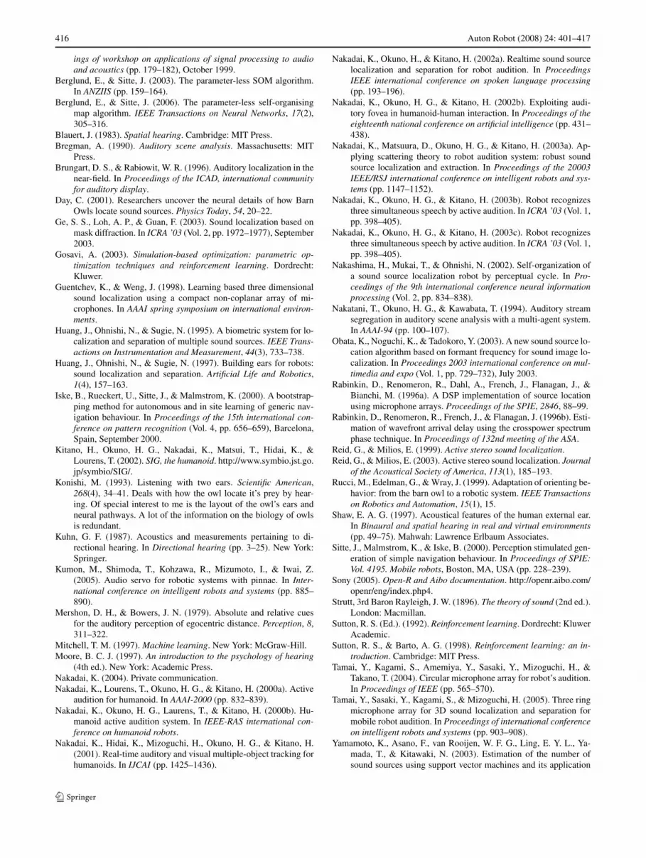
5.2 Horizontal direction detection

This experiment was intended to measure the accuracy ofthe direction detection property of the system. The presentedsystem was expected to map the direction to the source alongthe longest axis of the PLSOM. The horizontal index of thewinning node in the map should therefore be an indicationof the direction to the source in a way such that similar direc-tions (for example 10° and 0°) were mapped to nodes closetogether along the horizontal axis (for example node numberfive and seven). This must be the case in order for the rein-forcement learning algorithm to work. For the same reasonit was important for the presented system that sounds fromstraight ahead are mapped to the middle of the PLSOM. Twoexperiments were carried out:

1. A speaker playing white noise was placed in front ofthe robot at a distance of approximately one meter. Thesound intensity was approximately 70 dB (C) with back-ground noise of 58 dB and reverberation time (T60) is0.4 seconds. The setting was a normal office with car-pet floors and air conditioning running. There were hardreflective surfaces to the left and right of the robot at1.8 metres and behind and in front of it at 2.5 metres.The output of the system was recorded. The speaker wasmoved slowly to the left (as seen from the robot) untilthe system output stabilised at a new value. The angulardisplacement was recorded. This was repeated five times,and the mean average difference was computed.

2. A set of white noise sound samples was played in thesame setting as described above. The angle was variedfrom −88° to 88° in 1° increments through turning therobot head, resulting in 177 samples, corresponding todata set B. The position of each sample was evaluated bythe system, and the output was plotted, along with stan-dard deviation, versus the actual angle in Fig. 7.

(a)

(b)

Fig. 7 The grey area is one standard deviation scaled to match the axisunits (a) Estimated angle vs. actual angle using the SIG method. Notethe large deviation. (b) Average winning node vs. actual angle usingthe PLSOM method with 18 × 5 nodes. Note the small deviation

This was performed with the presented system and a well-known active audition system, the SIG system. The first ex-periment is designed to test the sensitivity of a active audi-tion system in its most sensitive area, while the second ex-periment is designed to test a system’s ability to distinguisha wide selection of sound directions.

Auton Robot (2008) 24: 401–417 409

5.2.1 SIG system

In order to provide a performance baseline for system eval-uation, a version of the SIG system as described by Nakadaiet al. (2002a) was implemented. The SIG group reported anaccuracy of 5° but when the published method was imple-mented on an Aibo robot a somewhat lower accuracy of 10°was achieved in experiment one. It was hard to measure thisaccuracy exactly given the large standard deviation of theestimated angle, which made it hard to note when the sys-tem settled on a new stable value. This discrepancy can haveseveral explanations:

• The SIG Humanoid robot had high resolution input; theAibo used a low resolution sampling rate of 16 kHz.

• The shape of the head of the Aibo robot was highly non-spherical, making calculating time delays (and thereforethe idealised IPD) between the ears difficult (Nakadai2004).

In experiment two the SIG system performed as indicatedby Fig. 7(a), note the large standard deviation.

5.2.2 PLSOM system

The PLSOM system was trained with data set A, and con-sistently managed an accuracy of approximately 5° in ex-periment one. This is comparable to human acuity (Moore1997), especially when considering the low resolution dataavailable. The results of experiment two are displayed inFig. 7(b). The system showed a clear correspondence be-tween winning node and source direction.

These results indicate that in the −20° to 20° window, thePLSOM goes through eight different winning nodes, givingabout 5° per node.

5.2.3 Comparison of SIG and PLSOM systems

The PLSOM was almost free of deviation. This enabled thesystem to estimate the direction using a small number ofsamples, in other words; quickly. The SIG method on theother hand had to average over a larger number of samplesto achieve a reliable estimate, thus increasing response time.This occurs despite both systems measuring angle in dis-crete steps.

5.2.4 Further tests with the PLSOM system and discussion

Labelling the PLSOM nodes in order to give an estimateddirection in human-readable terms (angles or radians) is notnecessary and indeed not desirable for robotic applications.Nevertheless, in order to give an intuitive idea of the perfor-mance of the direction finding algorithm a labelling step was

Fig. 8 The estimated angle of a labelled PLSOM vs. the actual an-gle. An idealised straight line has been inserted for reference. The greyareas (barely visible) represent one standard deviation

performed in which each node in the PLSOM was associ-ated with the direction it was most sensitive to, as describedbelow. The result can be seen in Fig. 8.

The sound data set used in the labelling was the same asthe training set, which was different from the test set. Thelabelling was performed in the following way. The PLSOMwas trained as in previous experiments, using data set A,and training was then disabled. Each of the samples in dataset A was then played to the system in turn. For each sam-ple the winning node was noted. At the end of the sessionthe nodes were labelled with the mean average of the anglesfor which it was the winning node. Since the training setonly contains samples for every 10°, some nodes were neverwinning nodes. These nodes were given labels formed frominterpolating between the two closest nodes with labels. Theaccuracy was then tested as before, using data set B.

Note that while it seemed like the labelling resolved theambiguity around large angles seen in Fig. 7(b), this wasonly because some of the horizontal displacement of thesource is mapped along the vertical axis in the PLSOM. In-deed, the labelling introduced a new inaccuracy around 30°since there were not enough labelling examples to label allnodes correctly (there were 90 nodes, but only 38 labellingexamples).

The PLSOM was also tested with speech signals (dataset C) and generated sine waves (data set D) to see whateffect sound type has on accuracy. As can be seen fromFig. 9 the PLSOM performed only marginally worse withthe speech signal despite the speech signal’s intermittent na-ture and lower volume (65 dB instead of 77 dB).

With the generated sine wave, on the other hand, the re-sults were not so good. This is not surprising on a largelyfrequency-domain based method, as the spectrum of a nearlypure tone contains little information. It should also be notedthat the recording distance (one meter) was very close tothe near field (depending on which definition one uses). The

410 Auton Robot (2008) 24: 401–417

(a)

(b)

Fig. 9 The grey area was one standard deviation, scaled to match theaxis units. (a) Average winning node vs. actual angle using the samePLSOM as in Fig. 7(b). Here the test data was speech, the sentence“She had your dark suit in greasy wash water all year” from the TIMITdatabase. (b) Average winning node vs. actual angle using the samePLSOM as in Fig. 7(b). Here the test data was a sine wave with twoharmonic overtones. Base frequency is 800 Hz, intensity circa 77 dBat one meter

near field is the area close to a sound source where con-structive and destructive interference can give rise to differ-ences in amplitude not consistent with the inverse squarelaw, especially when the signal consists of only one or a fewfrequencies. One factor in estimating the extent of the nearfield is the size of the transducer, which in this case was aCDSONIC JC-999 speaker with a maximum dimension of210 mm. No clear consensus of the correct estimate of theextent of the near field seems to exist, with estimates rangingfrom 0.2 m to 1.28 m at 800 Hz. Some authors (e.g. Brungartand Rabiowit 1996) give the near field as the region of spacewithin a fraction of a wavelength away from a sound source.This would give a near field boundary at less than 0.425 m at800 Hz. The measurements (see Fig. 3 and Fig. 4) indicatedsignificant interference at this distance and frequency, whichwould go a long way towards explaining the relatively poorperformance displayed in Fig. 9(b).

Still, comparing the plots for the three different record-ings, as in Fig. 10, it was clear that the difference was small,especially in the most sensitive areas.

Fig. 10 The direction detection results for the three different soundspresented above overlaid in one graph. The PLSOM used was trainedwith white noise only

Fig. 11 Average winning node vs. actual angle using the PLSOMmethod with 36 × 10 nodes. The grey area is one standard deviation

The experiments show that the PLSOM system achievesgreater levels of accuracy and speed than a well researchedand documented method, the SIG group algorithm. The ex-periment was also run with larger networks to see the ef-fect of size. Networks up to 36 nodes wide were trainedwithout problems, as seen in Fig. 11. This gives a theoret-ical accuracy of 2.2°, although one should note the addeddeviation around large angles. One important observationfrom Fig. 7(b) and Fig. 11 was the area of great inaccuracywhere the sound source is at approximately ±60° angle tothe sagittal plane. These areas of low directional sensitivitycoincided with the areas of highest distance sensitivity, seeSect. 5.5. The reason was that the PLSOM allocated mostweights along the dimension that contained the most infor-mation. This hypothesis was supported by the arrangementof the weights in Fig. 5. Unfortunately, changing the shapeof the PLSOM grid did not appear to alleviate the problem.Another cause for this deviation was the shape of the Aibohead. The microphones were placed relatively close to therear of the head, so that when the angle between the head

Auton Robot (2008) 24: 401–417 411

roll axis and the direction to the sound source increased to±45° the IID started decreasing instead of increasing be-cause sound waves passed more easily behind the head thanin front of it, see Fig. 3.

5.3 Horizontal source localisation

Since there is a correspondence between the winning nodeand the direction to the sound source, a reinforcement learn-ing system should be able to orient towards the soundsource. The system was expected to learn to orient the robothead towards the sound source using only the output fromthe PLSOM as feedback.

To determine how well the system outlined in Sect. 4.4was able to orient the robot head towards the sound sourcethe following experiment was conducted. The PLSOM wastrained in the same way as described in Sect. 5.1. Then PL-SOM training was switched off and the RL subsystem wasturned on. A speaker is placed one meter in front of the robotplaying white noise at approximately 77 dB. The RL sub-system was allowed to move the robot head. Whenever thePLSOM winning node stabilised in the middle for more thanfive iterations, the robot head was rotated to a randomly se-lected horizontal angle and the learning continued. The ab-solute difference between the direction of the robot head andthe direction of the sound source was termed the directionalerror in the following. The directional error was recordedfor each iteration only when the robot was not facing di-rectly towards the sound source (as indicated by the outputof the PLSOM). The rewards were as follows:

• 0.5 for when the output (the location of the winning node)of the PLSOM moved towards the centre.

• 0.1 for when the output of the PLSOM remained in thecentre.

• −0.1 for output of the PLSOM did not change.• −0.5 for all other cases.

These reward were designed to be positive for actions thatwere desirable (contributing to correct head orientation) andnegative otherwise. The exact values were arrived at throughtrial and error. The robot had 14 actions to choose from;turning the head 70, 40, 30, 20, 15, 10 or 5 degrees to eitherside. The robot could also choose to keep its head still. Thistest was carried out off-line using data set B. In the off-lineexperiment, the system was running as it would in a real-world application, but instead of controlling a real robot itcontrolled a virtual robot that returned sound samples drawnfrom data set B based on the direction of the sound sourceand the position of the virtual robot.

The total averaged error of the learning algorithm wasless than 0.26 radians and it was able to orient the head towithin ±5°.

Fig. 12 The cone of confusion can be seen as a cone with its vertexbetween the microphones obtained by rotating the vector to the soundsource around the tilt axis. The actual position of the sound source maylie anywhere on the cone

5.4 The cone of confusion

Since IID, IPD, RIID or ITD with two microphones can onlygive an angle relative to the median plane,1 the actual posi-tion of the sound source could lie on a cone with its ver-tex between the microphones, see Fig. 12. Humans solvethis through spectral cues, caused by our asymmetric headand ears, and through active audition. The Aibo, being com-pletely symmetric, must rely on active audition alone. Bytilting the robot head the system was able to work out theelevation, thus eliminating the cone of confusion in caseswhere the source was in front of the robot but elevated. Thealgorithm for doing this is outlined below:

1. Pan the Aibo head left/right until the PLSOM winningnode is in the middle.

2. Roll the head to one side. The head is rolled 23°, or asclose to 23° as permitted by the safety limits described in(Sony 2005).

3. Use the same RL system as used to pan the head, but in-stead of connecting the output to the pan motor, connectit to the tilt motor.

4. Tilt the head up/down until the PLSOM winning node isin the middle.

5. Roll the head back.

1The median plane is the plane perpendicular to the line through bothmicrophones and equidistant to them.

412 Auton Robot (2008) 24: 401–417

6. If the PLSOM winning node is not in the middle, go to 1.

It was expected that vertical detection is less accuratethan horizontal direction detection since the PLSOM wastrained for horizontal, not vertical, directions. The restric-tions on how much the neck joint of the Aibo could movemight also make this approach difficult to use in some cases.

In order to test the algorithm the system was subjected tothe following test. A speaker playing white noise at 68 dBwas placed 30° to the right of the robot at one meter distanceand 0° elevation. The Aibo head started out pointing straightahead with 0° elevation. The system was then left to run untilit did not alter the head position any more. The horizontaldeviation was then noted. This was repeated 10 times eachfor three elevations: 20°, 30°, and 40°.

The system determined the correct tilt within ±10°. Thesystem was not very useful because of the limited mobil-ity of the Aibo’s neck joints which restricts how much it ispossible to tilt and roll the head without damaging the ro-bot, as described in the Aibo ERS-210 manual (Sony 2005).The cone of confusion can also be advantageous for three-dimensional sound source localisation, as will be discussedin Sect. 5.7.

5.5 Distance resolution

Distance detection of sound, as horizontal direction detec-tion, is a composite task. Humans do this mainly throughtwo cues (Mershon and Bowers 1979):

1. Level of familiar sounds. This is of limited usefulnessunder some applications, but in speech applications it ishighly useful since human speech falls into a narrow levelrange.

2. Ratio of reverberation to direct sound levels. This is onlyapplicable to intermittent sounds, and requires a familiar-ity with the reverberation characteristics of the room.

Instead of trying to reproduce these two heuristics we se-lected a metric that is robust and works for both intermittentand continuous sounds as well as unfamiliar sounds of un-known source intensity; the RIID. See (6) for details. Thecentral idea behind the RIID, discussed in Sect. 4.2, is thatsound, being a wave phenomenon, decreases in intensity inaccordance with the inverse square law, see (Brungart andRabiowit 1996). Thus, one can get an idea of the distanceby comparing the intensity falloff between the two micro-phones to the absolute intensity recorded at one of the mi-crophones, which is exactly what the RIID does. Theoreti-cally this should give a metric which is independent of theintensity of the sound source.

Since the RIID is part of the input of the PLSOM, thedistance to the sound source should map to one of the outputdimensions of the PLSOM.

(a)

(b)

Fig. 13 Average winning node vs. source distance with one standarddeviation for various angle ranges. The stronger the correlation be-tween distance and winning node, the better. Note that this map hadonly been trained with inputs from a distance of 0.5–3 m, which ex-plains the poor correspondence over three meters. (a) −90° to 90° an-gle between sound source and median plane. (b) ±60–70° angle be-tween sound source and median plane

In order to test this hypothesis the following experimentwas carried out. The system was trained with the standardtraining set, data set A. Then a speaker playing white noisewas placed at five different distances from the robot; 0.2, 0.7,1, 2.5, and 5 m. The volume of the transmitted signal was ad-justed so that it gave the same intensity of 63 dB measuredat the robot to prevent the algorithm from simply estimatingthe distance based on intensity. For each distance, the robot’shead was turned from −90° to 90° in 10° increments. Theresult was recorded in data set E. For each angle/distance po-sition the system recorded the position of the winning nodeof the PLSOM (along the shortest axis of the PLSOM out-put space). The average winning node was plotted with stan-dard deviation in Fig. 13(a). Clearly, this did not provide agreat deal of accuracy. Upon examination of the data it be-came evident that the distance sensitivity was virtually zeroclose to the median plane, which corresponds well with whatone would expect from a distance metric based on the RIID,

Auton Robot (2008) 24: 401–417 413

Fig. 14 Estimated source-robot distance vs. actual source-robot dis-tance with one standard deviation. These points represent cases wherethe source was located 60–70° to the left or right of the median planeof the robot head. A linear fit has been inserted for reference

since the IID (and hence the RIID) decreases with decreas-ing angle to the median plane.

Theoretically one would be able to discern distance bet-ter when the sound source is at greater angles to the me-dian plane. This was supported by the experimental data,which showed good correspondence between winning nodeand source distance for ±60–70° angle between the medianplane and the sound source, see Fig. 13(b). One would ex-pect the distance sensitivity to be at a maximum at ±90°,but because of the shape of the Aibo head sound passes eas-ily around the back, altering the RIID at angles greater than±70°. Also, note that the area of high distance sensitivitylargely coincided with the areas of lowest directional sen-sitivity and vice versa. Although labelling the output of thesystem to provide human-readable distance estimates is notalways practical for robotic applications this step was per-formed to give the reader a more intuitive impression of thesystem’s accuracy, shown in Fig. 14.

This experiment showed that within the range it wastrained in the system performed remarkably well. It shouldbe noted that the distances of 0.7, 1, and 2.5 m were accu-rately labelled despite the system never having encounteredsounds from these distances before, since the training set(data set A) only contained samples recorded at 0.5 and 3m.

5.6 Limits to response time

In order to test the response time of the system, the followingtwo experiments were conducted:

1. The robot was filmed with a digital camera. A set of fourkeys were dropped onto a wood surface one meter infront of the robot from a height of 150 mm. This was re-peated 20 times. The video recording was analysed withvideo editing software, and the time from the keys hit thewood surface to the robot begins turning was measured.

2. Three sounds of different durations were played to theleft and right of the robot: keys dropping (duration 60ms), hands clapping (20 ms), and fingers snapping (20ms). This was repeated 10 times for each sound. Thenumber of times the robot turns in the correct directionwas noted, and a success rate calculated.

The first experiment gave a mean response time of 0.5seconds. The second experiment gave a success rate of 80%for the 60 ms sound but only 50% for the 20 ms sounds.

5.7 Taking advantage of the cone of confusion forelevation estimation

The cone of confusion might seem like a problem at first, butthe principles of active audition can be used to turn it intoan advantage. Consider the following scenario: the systemdetects a sound source at 60° to the right of the sagittal plane.It can be deduced that the actual position of the sound sourceis on a cone with axis parallel to the head tilt axis and vertexbetween the microphones with an opening angle of 60°.

Now the system turns the head 45° to the right in responseto the stimuli. This changes the angle between the soundsource and the sagittal plane but the change depends on theelevation of the sound source. If the source is in the horizon-tal plane, the new angle is (60°−45°) = 15°. If, on the otherhand, the source is above or below the horizontal plane, thenew angle will be greater than 15°. The relationship betweenthe change in sagittal/source angle, the pan movement of thehead and elevation of the source is shown in (9)–(11)

� = ψ − ψ ′, (9)

η = (sin(ν))2(cos(�))2 − 2 sin(ν) cos(�) sin(ν′)

+ (sin(ν′))2 + (sin(ν))2(sin(�))2, (10)

μ = arccos

( √η

sin(�)

). (11)

Here, μ is the elevation angle of the source, seen as rota-tion around the tilt axis. ν is the apparent angle between thesource and the sagittal plane, ψ is the angle the head is atbefore movement, and ψ ′ is the angle after movement. ν′ isthe apparent angle between source and sagittal plane afterthe pan movement. This is clearly independent of distance,but is unable to distinguish between negative and positive μ.Therefore the following experiments will be conducted withonly negative μ, which is to say the source is in or abovethe horizontal plane. It might be feasible to implement theexplicit algorithm as described in (9)–(11), but it requiresknowing the explicit values of ν and ν′.

Instead, the existing implicit representation of the soundsource position can be re-used. This can be done withoutconverting the sound source position to explicit coordinates:

414 Auton Robot (2008) 24: 401–417

Fig. 15 Elevation each node was sensitive to vs. node index with onestandard deviation. The map was five by two nodes and the neighbour-hood size was 4.27

The processing is done using the implicit position represen-tation by utilising the dimension-reducing properties of thePLSOM. Therefore, the system was extended with a secondPLSOM, which took a two-dimensional input vector:

1. The current estimated position in the form of the hori-zontal index of the winning node divided by the width ofthe entire map.

2. The difference in head direction since the last input di-vided by the difference in winning node since the last in-put. The head direction was given by the neck joint anglein this application, in a mobile implementation it wouldneed to be calculated from inertial sensors or similar inorder to get the change in direction of the head relative tothe source.

This second PLSOM was also of two output dimensions,giving a representation of horizontal angle along one axisand elevation along the other axis.

Training took place in two stages. First, the PLSOM wastrained with data set A, as before. Then, the RL was trainedwith data set B. During training of the RL subsystem the ele-vation of the sound source was simulated by altering the an-gle of the sound source in accordance with (9)–(11) solvedfor the apparent angle, ν. The elevation was varied from 0to 63°. The RL subsystem was trained in this way for 1000weight updates. During this training the output of the di-rection detecting PLSOM was fed to the elevation detectingPLSOM, as outlined above. The elevation detecting PLSOMwas five by two nodes and the neighbourhood size was setto 4.27, settings that were arrived at empirically.

As can be seen in Fig. 15, the elevation detection PLSOMbecame sensitive to different elevations along its longestaxis. The system was tested by selecting 100 source posi-tions at elevations ranging from 0° to 63° in 6.3° incrementsand horizontal positions ranging from −88° to 88° in 17.7°

Fig. 16 Estimated elevation vs. actual elevation with one standard de-viation. A linear fit has been added for reference. The map was five bytwo nodes and the neighbourhood size was 4.27

Fig. 17 Elevation each node was sensitive to vs. node index with onestandard deviation. The map was 20 × 8 nodes and the neighbourhoodsize was nine

increments and letting the robot orient towards them whilerecording the output of the elevation PLSOM. The nodes ofthe PLSOM were then labelled with the elevation in the testdata set which they were most sensitive to, and the experi-ment was run again with a different data set (data set H). Themean estimated elevation and standard deviation was notedfor each elevation and plotted in Fig. 16 As can clearly beseen, this was not particularly sensitive at all. Increasing themap size to 20 × 8 nodes with a neighbourhood size of ninegives a better result, see Fig. 18.

Unfortunately, the larger map size meant there were in-sufficient numbers of training examples to label all nodes,so some nodes simply never got selected as winning nodesand it was not possible to calculate the mean elevation theywere sensitive to, as seen in Fig. 17.

For the large map, the Pearson correlation coefficient r

was 0.62, which compares favourably, given the difference

Auton Robot (2008) 24: 401–417 415

Fig. 18 Estimated elevation vs. actual elevation with one standard de-viation. A linear fit has been added for reference. The map was 20 × 8nodes and the neighbourhood size was nine. Pearson correlation coef-ficient r = 0.62

in sampling rate and resolution, with human accuracy insimulated tests by Avendano et al. (1999) where r up to 0.77was achieved. Most of the inaccuracy was around low eleva-tions, where the granularity of the horizontal angle detectionmap should become more evident. The method of approxi-mating the elevated sound should also give more inaccura-cies around small elevations because of the 1° granularity ofthe samples used for approximation. It should be noted thatAvendano’s experiments were performed using headphones,so the subjects did not have the option of using active headmovements to locate the sound.

Although this result was less impressive than the 6° ac-curacy exhibited by multi-microphone systems (Tamai et al.2005), this should be seen in relation to the number of mi-crophones and consequently amount of processing required.

6 Discussion

This paper has analysed the problem of sound direction de-tection and active audition for robots using two-channel au-dio. The goal was to create a system that can detect the po-sition of a sound source in three dimensions and orient to-wards it. The system should also be robust to changes, learnfrom experience without the need for supervision and reactquickly. The system should be able to react to both transientand continuous sounds, as well as sounds with both broadand narrow spectra. Finally the system should be able to fil-ter sound from noise based on direction without having torely on assumptions about the nature of the sound or thenoise.

The presented system uses unsupervised learning exclu-sively. The system was compared with the SIG humanoidsystem and human hearing for horizontal localisation and

human hearing for elevation detection. Human hearing candetect changes in source position down to 1° with absolutepositional error approximately 5°, the SIG system has a re-ported accuracy of approximately 5°, but on the test plat-form the accuracy was approximately 10° in the best areaswith a standard deviation of ±40° in some areas. The pre-sented system achieves an accuracy of 5° with negligible de-viation on this platform. Correlation between elevation andestimated elevation is r = 0.62, when humans have achievedup to r = 0.77 in simulated tests and up to r = 0.98 in testswhere the test subjects can move their heads freely. Soundsource distance estimation approaches generally apply morethan two sound channels and are not directly comparableto the presented system, which achieves an estimation errorof less than 150 mm and a standard deviation of less than±0.1 m. The orienting behaviour is accurate to within ±5°and responds in 0.5 s, even when network lag is factored in.

The system has been tested with white noise, humanspeech and pure frequencies with two harmonics. Its re-sponse has been tested with continuous sounds and transientsounds such as keys dropping, hands clapping and fingerssnapping, giving 80% success rate for sounds of 60 ms du-ration and 50% success rate for 20 ms duration.

7 Conclusion

We have described a system for letting a robot determinethe direction, distance and elevation of a sound source andlearn to orient towards a sound source without supervision.The system performs well compared to other approaches wehave implemented. The system determines a model of theacoustic properties of the robot using a PLSOM, and auto-matically associates the output of the PLSOM with the cor-rect motor actions. Interestingly, this is done without anyexplicit theoretical model of the environment; there is no in-formation built into the system about the shape of the robothead, the distance between the robot ears or the physics ofsound. All these constants and their internal relationships areimplicitly worked out by the system. This makes the systemflexible since it can be implemented on any robot with stereomicrophones without alteration.

Acknowledgements The authors would like to thank Dr. KazuhiroNakadai of the Japan Science and Technology Corporation and Dr.Frederic Maire of the Smart Devices Lab at the Queensland Univer-sity of Technology for their valuable input. This project is supported,in part, by a grant from the Australian Government Department of thePrime Minister and Cabinet. NICTA is funded by the Australian Gov-ernment’s Backing Australia’s Ability initiative, in part through theAustralian Research Council.

References

Avendano, C., Algazi, V. R., & Duda, R. O. (1999). A head-and-torsomodel for low-frequency binaural elevation effects. In Proceed-

416 Auton Robot (2008) 24: 401–417

ings of workshop on applications of signal processing to audioand acoustics (pp. 179–182), October 1999.

Berglund, E., & Sitte, J. (2003). The parameter-less SOM algorithm.In ANZIIS (pp. 159–164).

Berglund, E., & Sitte, J. (2006). The parameter-less self-organisingmap algorithm. IEEE Transactions on Neural Networks, 17(2),305–316.

Blauert, J. (1983). Spatial hearing. Cambridge: MIT Press.Bregman, A. (1990). Auditory scene analysis. Massachusetts: MIT

Press.Brungart, D. S., & Rabiowit, W. R. (1996). Auditory localization in the

near-field. In Proceedings of the ICAD, international communityfor auditory display.

Day, C. (2001). Researchers uncover the neural details of how BarnOwls locate sound sources. Physics Today, 54, 20–22.

Ge, S. S., Loh, A. P., & Guan, F. (2003). Sound localization based onmask diffraction. In ICRA ’03 (Vol. 2, pp. 1972–1977), September2003.

Gosavi, A. (2003). Simulation-based optimization: parametric op-timization techniques and reinforcement learning. Dordrecht:Kluwer.

Guentchev, K., & Weng, J. (1998). Learning based three dimensionalsound localization using a compact non-coplanar array of mi-crophones. In AAAI spring symposium on international environ-ments.

Huang, J., Ohnishi, N., & Sugie, N. (1995). A biometric system for lo-calization and separation of multiple sound sources. IEEE Trans-actions on Instrumentation and Measurement, 44(3), 733–738.

Huang, J., Ohnishi, N., & Sugie, N. (1997). Building ears for robots:sound localization and separation. Artificial Life and Robotics,1(4), 157–163.

Iske, B., Rueckert, U., Sitte, J., & Malmstrom, K. (2000). A bootstrap-ping method for autonomous and in site learning of generic nav-igation behaviour. In Proceedings of the 15th international con-ference on pattern recognition (Vol. 4, pp. 656–659), Barcelona,Spain, September 2000.

Kitano, H., Okuno, H. G., Nakadai, K., Matsui, T., Hidai, K., &Lourens, T. (2002). SIG, the humanoid. http://www.symbio.jst.go.jp/symbio/SIG/.

Konishi, M. (1993). Listening with two ears. Scientific American,268(4), 34–41. Deals with how the owl locate it’s prey by hear-ing. Of special interest to me is the layout of the owl’s ears andneural pathways. A lot of the information on the biology of owlsis redundant.

Kuhn, G. F. (1987). Acoustics and measurements pertaining to di-rectional hearing. In Directional hearing (pp. 3–25). New York:Springer.

Kumon, M., Shimoda, T., Kohzawa, R., Mizumoto, I., & Iwai, Z.(2005). Audio servo for robotic systems with pinnae. In Inter-national conference on intelligent robots and systems (pp. 885–890).

Mershon, D. H., & Bowers, J. N. (1979). Absolute and relative cuesfor the auditory perception of egocentric distance. Perception, 8,311–322.

Mitchell, T. M. (1997). Machine learning. New York: McGraw-Hill.Moore, B. C. J. (1997). An introduction to the psychology of hearing

(4th ed.). New York: Academic Press.Nakadai, K. (2004). Private communication.Nakadai, K., Lourens, T., Okuno, H. G., & Kitano, H. (2000a). Active

audition for humanoid. In AAAI-2000 (pp. 832–839).Nakadai, K., Okuno, H. G., Laurens, T., & Kitano, H. (2000b). Hu-

manoid active audition system. In IEEE-RAS international con-ference on humanoid robots.

Nakadai, K., Hidai, K., Mizoguchi, H., Okuno, H. G., & Kitano, H.(2001). Real-time auditory and visual multiple-object tracking forhumanoids. In IJCAI (pp. 1425–1436).

Nakadai, K., Okuno, H., & Kitano, H. (2002a). Realtime sound sourcelocalization and separation for robot audition. In ProceedingsIEEE international conference on spoken language processing(pp. 193–196).

Nakadai, K., Okuno, H. G., & Kitano, H. (2002b). Exploiting audi-tory fovea in humanoid-human interaction. In Proceedings of theeighteenth national conference on artificial intelligence (pp. 431–438).

Nakadai, K., Matsuura, D., Okuno, H. G., & Kitano, H. (2003a). Ap-plying scattering theory to robot audition system: robust soundsource localization and extraction. In Proceedings of the 20003IEEE/RSJ international conference on intelligent robots and sys-tems (pp. 1147–1152).

Nakadai, K., Okuno, H. G., & Kitano, H. (2003b). Robot recognizesthree simultaneous speech by active audition. In ICRA ’03 (Vol. 1,pp. 398–405).

Nakadai, K., Okuno, H. G., & Kitano, H. (2003c). Robot recognizesthree simultaneous speech by active audition. In ICRA ’03 (Vol. 1,pp. 398–405).

Nakashima, H., Mukai, T., & Ohnishi, N. (2002). Self-organization ofa sound source localization robot by perceptual cycle. In Pro-ceedings of the 9th international conference neural informationprocessing (Vol. 2, pp. 834–838).

Nakatani, T., Okuno, H. G., & Kawabata, T. (1994). Auditory streamsegregation in auditory scene analysis with a multi-agent system.In AAAI-94 (pp. 100–107).

Obata, K., Noguchi, K., & Tadokoro, Y. (2003). A new sound source lo-cation algorithm based on formant frequency for sound image lo-calization. In Proceedings 2003 international conference on mul-timedia and expo (Vol. 1, pp. 729–732), July 2003.

Rabinkin, D., Renomeron, R., Dahl, A., French, J., Flanagan, J., &Bianchi, M. (1996a). A DSP implementation of source locationusing microphone arrays. Proceedings of the SPIE, 2846, 88–99.

Rabinkin, D., Renomeron, R., French, J., & Flanagan, J. (1996b). Esti-mation of wavefront arrival delay using the crosspower spectrumphase technique. In Proceedings of 132nd meeting of the ASA.

Reid, G., & Milios, E. (1999). Active stereo sound localization.Reid, G., & Milios, E. (2003). Active stereo sound localization. Journal

of the Acoustical Society of America, 113(1), 185–193.Rucci, M., Edelman, G., & Wray, J. (1999). Adaptation of orienting be-

havior: from the barn owl to a robotic system. IEEE Transactionson Robotics and Automation, 15(1), 15.

Shaw, E. A. G. (1997). Acoustical features of the human external ear.In Binaural and spatial hearing in real and virtual environments(pp. 49–75). Mahwah: Lawrence Erlbaum Associates.

Sitte, J., Malmstrom, K., & Iske, B. (2000). Perception stimulated gen-eration of simple navigation behaviour. In Proceedings of SPIE:Vol. 4195. Mobile robots, Boston, MA, USA (pp. 228–239).

Sony (2005). Open-R and Aibo documentation. http://openr.aibo.com/openr/eng/index.php4.

Strutt, 3rd Baron Rayleigh, J. W. (1896). The theory of sound (2nd ed.).London: Macmillan.

Sutton, R. S. (Ed.). (1992). Reinforcement learning. Dordrecht: KluwerAcademic.

Sutton, R. S., & Barto, A. G. (1998). Reinforcement learning: an in-troduction. Cambridge: MIT Press.

Tamai, Y., Kagami, S., Amemiya, Y., Sasaki, Y., Mizoguchi, H., &Takano, T. (2004). Circular microphone array for robot’s audition.In Proceedings of IEEE (pp. 565–570).

Tamai, Y., Sasaki, Y., Kagami, S., & Mizoguchi, H. (2005). Three ringmicrophone array for 3D sound localization and separation formobile robot audition. In Proceedings of international conferenceon intelligent robots and systems (pp. 903–908).

Yamamoto, K., Asano, F., van Rooijen, W. F. G., Ling, E. Y. L., Ya-mada, T., & Kitawaki, N. (2003). Estimation of the number ofsound sources using support vector machines and its application

Auton Robot (2008) 24: 401–417 417

to sound source separation. In ICASSP ’03 (Vol. 5, pp. 485–488),April 2003.

Erik Berglund received the equivalent of aBachelor’s degree in Computer Engineeringfrom Østfold University College in 2000 anda Ph.D from the University of Queensland in2006. He is currently a senior research fellow atUQ. Research interests include neural networks,face recognition and implicit data processing.

Joaquin Sitte is an Associate Professor at theSchool of Software Engineering and Data Com-munications, Queensland University of Tech-nology, Australia, where he leads the Smart De-vices Lab. Joaquin received his Licenciado de-gree in physics from the Universidad Centralde Venezuela in 1968 and his Ph.D. degree inquantum chemistry from Uppsala University,Sweden, in 1974. Until 1985 he was an Asso-ciate Professor at the Universidad de Los An-

des, Merida, Venezuela, where he also headed the Surface Physics Re-search Group. Since 1986 he is on the faculty of Queensland Universityof Technology. He has a special interest in the use of neural networksfor sensing, thinking, learning and actuation in autonomous robots.

Gordon Wyeth is a senior lecturer in roboticsat the University of Queensland, Australia. Hereceived his Bachelor in Engineering (Honours)from the same university in 1989, and his PhDfrom the same university in 1997. He is Pres-ident of the Australian Robotics and Automa-tion Association. His research centres on the de-velopment of robotic systems based on neuro-ethological data. This research is being appliedin humanoid robotics, consumer robot applica-tions and robot soccer.