acoustic source identification using a generalized weighted inverse beamforming technique
TRANSCRIPT

Contents lists available at SciVerse ScienceDirect
Mechanical Systems and Signal Processing
Mechanical Systems and Signal Processing 32 (2012) 349–358
0888-32
http://d
n Corr
E-m
journal homepage: www.elsevier.com/locate/ymssp
Acoustic source identification using a Generalized Weighted InverseBeamforming technique
Flavio Presezniak a,f,n, Paulo A.G. Zavala b,c, Gunther Steenackers a,e, Karl Janssens d,Jose R.F. Arruda c, Wim Desmet b, Patrick Guillaume a
a Vrije Universiteit Brussels, Pleinlaan 2, 1050 Brussels, Belgiumb K.U. Leuven, Department of Mechanical Engineering, Celestijnenlaan 300b, 3001 Leuven, Belgiumc Faculty of Mechanical Engineering, State University of Campinas (UNICAMP), Campinas, SP, Brazild LMS International, Interleuvenlaan 68, 3001 Leuven, Belgiume Artesis Hogeschool Antwerpen, Paardenmarkt 92, B-2000 Antwerpen, Belgiumf Volvo do Brasil, 3P-PD, Av. Juscelino K de Oliveira, 2600, 81260-900 Curitiba, Brazil
a r t i c l e i n f o
Article history:
Received 24 August 2010
Received in revised form
23 November 2011
Accepted 15 June 2012Available online 11 July 2012
Keywords:
Acoustic
Inverse problem
Optimization
Source identification
70/$ - see front matter & 2012 Elsevier Ltd. A
x.doi.org/10.1016/j.ymssp.2012.06.019
esponding author. Tel.: þ55 4133174276.
ail address: [email protected] (F. Presez
a b s t r a c t
In the last years, acoustic source identification has gained special attention, mainly due
to new environmental norms, urbanization problems and more demanding acoustic
comfort expectation of consumers. From the current methods, beamforming techniques
are of common use, since normally demands affordable data acquisition effort, while
producing clear source identification in most of the applications. In order to improve
the source identification quality, this work presents a method, based on the Generalized
Inverse Beamforming, that uses a weighted pseudo-inverse approach and an optimiza-
tion procedure, called Weighted Generalized Inverse Beamforming. To validate this
method, a simple case of two compact sources in close vicinity in coherent radiation
was investigated by numerical and experimental assessment. Weighted generalized
inverse results are compared to the ones obtained by the conventional beamforming,
MUltiple Signal Classification, and Generalized Inverse Beamforming. At the end, the
advantages of the proposed method are outlined together with the computational effort
increase compared to the Generalized Inverse Beamforming.
& 2012 Elsevier Ltd. All rights reserved.
1. Introduction
In the past years the reduction in the noise pollution has received special attention, due to, among else, newenvironmental regulations, urbanization problems and more demanding acoustic comfort expectation of consumers(transportation, housing, houseware, etc.). For this purpose, the identification of acoustic source characteristics, such assource location and amplitude, has an important role.
The acoustic source identification can be obtained using several methods, such as acoustic holography, acousticbeamforming and also by the solution of the inverse problem. Those methods start with the definition of a target grid, thatcorresponds to the locations where the sources will be searched. A model for the transfer function between the target gridand the measurement grid is then defined, based on the adopted reference source type.
ll rights reserved.
niak).

Nomenclature
H transfer functionI identity matrixW weighting matrixok discrete angular frequencyq source pressureP source pressure vectorU matrix containing the left singular valuesV matrix containing the right singular valuesS diagonal matrix containing the singular
valuess singular valuesb regularization parametero angular frequencyk conditional numberK cost functionCSM cross spectral matrixJ � Jp p-norm
Ue eigenvector matrixL eigenvalue matrixPi ith eigenmodeui ith eigenvectorli ith eigenvalueqi ith source amplitude vectori
ffiffiffiffiffiffiffi�1p
Superscripts
þ pseudo-inverseH Hermitian transpose
Subscripts
W weighted matrixk relative to the kth natural frequencyR regularized matrix
F. Presezniak et al. / Mechanical Systems and Signal Processing 32 (2012) 349–358350
The main problem of the classical techniques is the low spatial resolution. Methods such as CLEAN [1] and DAMAS [2]have been proposed to improve this map resolution. The CLEAN method proved to be sensitive to noisy signals, especiallycoherent noise. To avoid this problem, deconvolution techniques treating coherent sources have been proposed such asDAMAS. In this method, the uncorrelated source distribution is extracted by iteratively deconvolving the map generated byconventional beamforming with the point spread function, which represents a monopole source at the target grid. Thistechnique has a substantial computational cost, even though it has improved in the past years.
A method called Generalized Inverse Beamforming is proposed by Suzuki [3]. In this method, the cross spectral matrixis decomposed into its eigenstructure, and the response is represented by eigenmodes, each one related to a coherentsource distribution. This source distribution is calculated by the inversion of the transfer function matrix, built based on acandidate source type. In the case that this transfer function matrix is ill-conditioned, regularization techniques, such asTikhonov’s regularization, can be used. Recently, the regularization strategy was optimized and an automated process forthe definition of the regularization factor developed [4].
To improve solution of general inverse problems, the weighted pseudo-inverse technique [5] is widely adopted. Thismethod pre- and post-multiply the transfer function matrix by a diagonal weight matrix. The weight values are thenoptimized in order to minimize the number of relevant sources.
In this paper, a new technique is proposed to increase the resolution on the GIB, the Generalized Weighted InverseBeamforming (GWIB). This technique can put more emphasis on some transfer function matrix columns, or sources,increasing the dynamic range of the identification.
In the following sections, the weighted pseudo-inverse will be presented, as well as the proposed Generalized WeightedInverse Beamforming technique.
A simple example is used to illustrate the advantages of this method to perform source identification on closely spacedcompact source. Numerical and experimental assessment are presented and the results with GWIB are compared to theconventional beamforming, MUltiple Signal Classification (MUSIC) and GIB results. The conclusion and remarks arepresented at the end.
2. General principles
2.1. Generalized Inverse Beamforming
The Generalized Inverse Beamforming (GIB) [3] similarly as the conventional beamforming technique, starts with thecross spectral matrix (CSM), which, in this case is decomposed as
C¼/P � PHS¼UeLUHe , ð1Þ
where Ue and L are, respectively, the eigenvector and the diagonal eigenvalue matrix, P is the matrix of measured acousticpressure spectra, the superscript H indicates the Hermitian transpose and / �S indicates an average signal. The ith‘eigenmode’ is defined as [3]
Pi ¼ffiffiffiffili
pui, ð2Þ

F. Presezniak et al. / Mechanical Systems and Signal Processing 32 (2012) 349–358 351
where li is the ith eigenvalue and ui is the ith eigenvector. Each eigenmode represent a coherent response, and theobjective is to recover the source distribution that produce each eigenmode.
Similar to the other techniques, it is necessary to define a target grid, in which the sources are searched. The result atthe microphones is a combination of the sources present at each grid point. This is necessary to identify the transferfunction H between the target grid points and the measurement points. Considering that the microphone signal is given bythe eigenmode, Eq. (2), the source estimator will be given by
Pi ¼Hqi, ð3Þ
where qi is a vector representing the source amplitude over the target domain, Pi is the ith ‘eigenmode’ and H is thetransfer function matrix. The total source amplitude q is related by the qi amplitude by
q¼X
qi ð4Þ
and the acoustic pressure P related by the Pi by
P¼X
Pi: ð5Þ
To solve Eq. (3), for an underdetermined (more possible source positions then measurements) and overdeterminedsystem of equations, with the Generalized Inverse Beamforming, the following equations are used [3]:
qi ¼HHðHHH
Þ�1Pi ð6Þ
and
qi ¼ ðHHHÞ�1HHPi: ð7Þ
The Generalized Inverse Beamforming considers that the target grid can be reduced iteratively by discarding thelocations with lower magnitude on each iteration. This is an interesting approach, focusing on the locations with a higherprobability to find the sources. However, the grid points close to the true source location will also have a participation onthe mapping.
2.2. The weighted pseudo-inverse
Because HðokÞ is rank deficient, it is not possible to find a unique solution for the source, but, an infinite amount ofsolutions exist. By using a weighted pseudo-inverse, an infinite set of source vectors are obtained, depending on W. Thus,the weighted version of a rectangular N0 � Ni complex valued matrix H is defined. The following definition is used:
ðHÞþW ¼WðHWÞþ , ð8Þ
where W 2 RN0�N0 is a regular square weighting matrix and ‘þ ’ indicates the pseudo-inverse. In the sequel, only diagonalweighting matrices, W ¼ diagðw1,w2, . . . ,wN0
Þ, will be considered. So, according to the definition in Eq. (8), every column ofH is first weighted with a w-factor before being pseudo-inverted. In that way, it is possible to put more emphasis on somecolumns (inputs) of H. Note that if W equals the identity matrix I
ðHÞþI ¼ IðHIÞþ ¼Hþ ð9Þ
or, if H (and W) is of full rank (i.e., rankðHÞ ¼minðNi,N0ÞÞ
ðHÞþw ¼WðHWÞþ ¼WW þHþ ¼Hþ ð10Þ
the weighted pseudo-inverse reduces to a classical pseudo-inverse. Hence, it only makes sense to use a weighted pseudo-inverse when H is rank deficient (i.e., when rankðHÞ ¼minðNi,N0Þ). In that case, the weighted pseudo-inverse, ðHÞþW , differsfrom Hþ and depends on the weighting matrix W as well as on the truncation level used (i.e., the number of singularvalues considered during the computation of the pseudo-inverse).
This weighting matrix right-multiplies the Frequency Response Function (FRF) matrix, HðokÞW , allowing to put moreemphasis (or weight) on some locations (inputs) while other locations, corresponding with zero (or small) w values, areminimized.
In the procedure used in this paper, a Tikhonov regularization will be applied to calculate the pseudo-inverseðHðokÞWÞ
þ . This is done with the objective to reduce the ratio between largest, smax, and the smallest, smin, singular value,called the condition number. Therefore, the condition number is defined as
kðHÞ ¼ smax=smin: ð11Þ
Following Nelson and Yoon [6], let us assume that small deviations dP in P produce small deviations dq in the solution q,and then
HðqþdqÞ ¼ ðPþdPÞ: ð12Þ
For two matrices A and B, a property of the 2-norm states that JABJrJAJJBJ. Applying this property to the smalldeviations, dq¼HþdP, it is possible to verify that JdqJrJHþ JJdPJ and that JPJrJHJJqJ. Therefore, it is possible to write
JdqJJPJrJHJJHþ JJdPJJqJ, ð13Þ

F. Presezniak et al. / Mechanical Systems and Signal Processing 32 (2012) 349–358352
with the definition of the condition number
dq
qrkðHÞ JdPJ
P: ð14Þ
The above equation shows the importance of the condition number k in the solution. It is possible to verify that smallperturbations in P, dP, will be amplified if the H matrix has a large condition number. In practice, extraneous noiseintroduced into the measurements of the acoustic pressure will have a large impact on the solution for the acoustic sourcestrength if the matrix is badly conditioned, with a large condition number k. Thus, the Tikhonov regularization starts in theform
ðHðokÞWÞþ¼ VS�1Uþ , ð15Þ
where V and U are the matrices containing the right and left singular vectors and S is a diagonal matrix containing thesingular values.
Applying the regularization technique to Eq. (17), one can write the inverse weighted matrix as
ðHðokÞWÞþR ¼ VS�1
R Uþ , ð16Þ
where the subscript R denotes the regularized matrix and where the regularized singular value matrix is given by
S�1R ¼
s1=ðs21þbÞ 0 � � � 0
0 s2=ðs22þbÞ � � � 0
^ ^ ^ ^
0 0 � � � sN=ðs2NþbÞ
266664
377775: ð17Þ
2.3. Optimization procedure
The diagonal weighting matrix W is determined in such a way that the ‘p-norm of the source is minimized
KðWÞ ¼XNf
k ¼ 1
Jqðok,WÞJpp, ð18Þ
with a p value close to zero (e.g., 0.01) and JPJpp ¼ ð
PN0
i ¼ 1 9Pi9pÞð1=pÞ.
Note that for p-0, the K(W) converges to the number of entries in Pðok,WÞ that are different from zero. Hence,minimizing Eq. (18) corresponds to making as many as possible entries of Pðok,WÞ equal to zero, i.e., finding the solutionrequiring the lowest possible amount of locations.
It can be remembered that all these solutions must satisfy the input–output relationship
PðokÞ ¼HðokÞ � qðokÞ ð19Þ
very well (depends on the used tolerance, which is related to the amount of disturbing noise on the responsemeasurement). Indeed
HðokÞqðok,WÞ ¼HðokÞWðHðokÞWÞþPðokÞ � PðokÞ: ð20Þ
This means that the weighting matrix W cannot be a zero matrix, in order to be coherent to this condition.Because the ‘p-norm is differentiable w.r.t. W, the cost function, Eq. (18), can be minimized by means of classical
optimization algorithm (e.g., Gauss–Newton, Levenberg–Marquardt). Note that cost function, Eq. (18), can be written as aquadratic cost function
KðWÞ ¼1
p
XNf
k ¼ 1
XN0
i ¼ 1
9Riðok,WÞ92, ð21Þ
with
Riðok,WÞ ¼ 9qiðok,WÞ9p=2: ð22Þ
This quadratic cost function can be minimized using the Gauss–Newton optimization algorithm. Furthermore, ananalytical expression for the Jacobian matrix J¼ @R=@w, i.e., the derivative of the residue vector R¼ ½R1, . . . ,RN0
�T w.r.t. theweighting vector, w¼ ½w1, . . . ,wN0
�T , is available.One can show that the entries Jij ¼ @Ri=@wj of the Jacobian matrix equal
@Ri
@wj¼
P
29qi9
P=2�2ReðqiÞ Re
@qi
@wj
� �þ ImðqiÞ Im
@qi
@wj
� �� �ð23Þ
and that the derivatives @qi=@wj ¼ ½@q=@w�ij are given by
@q
@w¼ ðI�WðHWÞþHÞW þ
½q�, ð24Þ
with ½q� ¼ diagðqÞ.

F. Presezniak et al. / Mechanical Systems and Signal Processing 32 (2012) 349–358 353
Since the Jacobian matrix can be computed analytically using Eqs. (23) and (24) (instead of using time-consuming finitedifference approximations), a significant reduction in the computation time is obtained.
3. Generalized Weighted Inverse Beamforming
The introduction of the weighted pseudo-inverse can increase the dynamic range of the Generalized InverseBeamforming (GIB). With this, the solution of Eq. (3) is given by
qi ¼ ðHÞþW Pi, ð25Þ
where qi represents a source amplitude vector, H represents the transfer function matrix, Pi represents the ith eigenmodeand the subscript W represents the weight matrix, minimizing the possible source locations.
The proposed technique, weighted pseudo-inverse applied to the Generalized Inverse Beamforming, increases thesource identification resolution while the reduced target grid over the algorithm iterations also reduces the weightoptimization effort per iteration.
Thus, the GWIB method can be summarized as follows:
1.
Generate the cross spectral matrix, according to Eq. (1). 2. Select the number of modes to be used. 3. Generate the corresponding eigenmodes Pi. 4. Select a target grid and calculate the transfer function matrix H. 5. Calculate the amplitude distribution according to Eq. (25). 6. Eliminate the locations with the smallest amplitudes and calculate a new transfer function matrix H. 7. Repeat items 3–5 until the size of the target grid is reduced to a specific value that guarantee a clear source region oruntil when some convergence criteria is reached.
4. Numerical example
In this section a numerical example will be presented to show the advantages of this method. The example consists oftwo monopole sources radiating at 1 kHz and separated by 1.5 wavelength distance. The array is adopted with 30microphones distributed over a 6-arm spiral configuration and 2 m aperture. The array distance to the source plane is2.5 m. The target grid region is chosen as three wavelengths from the target center, with a rectangular grid with 1=4 of awavelength spacing and 25 points, as indicated in Fig. 1.
A source model in the frequency domain is used and the transfer function is given by
P¼f
4p9r9e�ik9r9, ð26Þ
where f represents the acoustic source amplitude.In this paper, four identification methods are compared: conventional beamforming, MUltiple SIgnal Classification
(MUSIC), Generalized Inverse Beamforming (GIB) and the proposed Generalized Weighted Inverse Beamforming (GWIB).The GIB result is shown after 32 iterations using 10% truncation, this means that after each iteration, 10% of the possible
-1 -0.5 0 0.5 1-1
-0.5
0
0.5
1
x
y
Target Grid Sources Measurement Grid
Fig. 1. Target and measurement grids and source locations.

x[m]
y[m
]
-1 -0.5 0 0.5 1-1
-0.8-0.6-0.4-0.2
00.20.40.60.8
1
x[m]
y[m
]
-1 -0.5 0 0.5 1-1
-0.8-0.6-0.4-0.2
00.20.40.60.8
1
x[m]
y[m
]
-1 -0.5 0 0.5 1-1
-0.8-0.6-0.4-0.2
00.20.40.60.8
1
x[m]
y[m
]
-1 -0.5 0 0.5 1-1
-0.8-0.6-0.4-0.2
00.20.40.60.8
1
Fig. 2. Source identification for: (a) conventional beamforming, (b) MUSIC, (c) Generalized Inverse Beamforming (GIB) and (d) Generalized Weighted
Inverse Beamforming.
F. Presezniak et al. / Mechanical Systems and Signal Processing 32 (2012) 349–358354
source locations are discarded. In the GWIB method, the optimal result is obtained after 15 iterations. The results for all theidentification methods are shown in Fig. 2.
All the plots are shown in a 10 dB range. From Fig. 2 it is possible to draw the following conclusions:
�
All the methods converged to the source areas. � The conventional beamforming technique correctly identified the zone, but was not able to identify both sourcesseparately.
� The MUSIC method presented results comparable to the conventional beamforming method but with a betterdynamic range.
� The Generalized Inverse Beamforming (GIB) showed a better result, identifying both sources. � The Generalized Weighted Inverse Beamforming (GWIB) improved the GIB results, especially when it refers to thedynamic range.
4.1. Influence of noise
In order to verify the noise influence in the GWIB method, simulations with a noisy signal were performed. For this, theacoustic pressure was corrupted with a Gaussian noise with zero mean and variance s2 obtained by [7]
S
N¼ 20 log10
1
J
9P92
s2
" #1=2
: ð27Þ
Since for this case J represents the number of measurement points, the S/N ratio is related to an average acousticpressure value at a specific frequency. For example, for a 0 dB S/N ratio, the noise will have the same amplitude as theaverage pressure value. Thus, the S/N will increase for points closer to the source and decrease for points further the sourcewhere the signal level is lower, as is possible to visualize in Fig. 3.

Fig. 3. Signal and applied noise.
X[m]
Y[m
]
Generalized Weighted Inverse Beamforming - 2Monopoles S/N ratio=0dB
-1 -0.5 0 0.5 1-1
-0.8-0.6-0.4-0.2
00.20.40.60.8
1
X[m]
Y[m
]
Generalized Inverse Beamforming - 2Monopoles in phase - with noise
-1 -0.5 0 0.5 1-1
-0.8-0.6-0.4-0.2
00.20.40.60.8
1
Fig. 4. Numerical results with 0 dB SNR for (a) GWIB and (b) GIB.
F. Presezniak et al. / Mechanical Systems and Signal Processing 32 (2012) 349–358 355
This figure was generated for a source placed at the center. Is possible to observe that at the center, where the signalstrength is more important its level is higher then the noise information, while for the points in the edge the noiseamplitude is more important then the signal. The results is shown in Fig. 4.
From these figures one can conclude that, even with highly noisy signal, the GWIB still can separate both sources, whilethe GIB method focus only in one source and other ghost sources are also visualized.
5. Experimental results
To validate the proposed methodology, an experiment was performed using the same configuration as the numericalexample. A picture from the setup is shown in Fig. 5.
As adopted in the numerical example, two compact sources radiate an in-phase sine wave at 1 kHz with a distance of1.5 of a wavelength from each other. The measurements used a simultaneous acquisition with 20.48 kHz samplingfrequency. Blocks with 1024 time samples per microphone are used for each acquisition. The target grid region is chosen asthree wavelengths from the target center, with a grid spacing of 1/4 of wavelength. The results are shown in Fig. 6.
The Generalized Inverse Beamforming (GIB) result is obtained after 32 iterations using 10% truncation. In theGeneralized Weighted Inverse Beamforming (GWIB) method, the optimal results are obtained after 15 iterations, butwith the optimization procedure, the computational time is still almost the same, 1.526 s for the GIB versus 2.081 s forthe GWIB.
Experimental results using GIB are very similar to the numerical prediction, and the method was able to capture theindividual source locations, in contrast to the conventional beamforming and the MUltiple SIgnal Classification (MUSIC)that presented one single source center. The beamforming and the MUSIC results are almost the same but the MUSICalgorithm indicates a source center more to the right, possibly steered to a slightly louder speaker.
The maps indicate some level differences in the source radiations which led the GIB to keep more source grid terms onthe side of the higher emission. The GWIB was able to capture individual source locations with substantial increase indynamic range and no clear influence of the higher level of one loudspeaker.
To better show the convergence of the proposed method, Fig. 7 shows the results for 1, 5, 10 and 15 iterations.
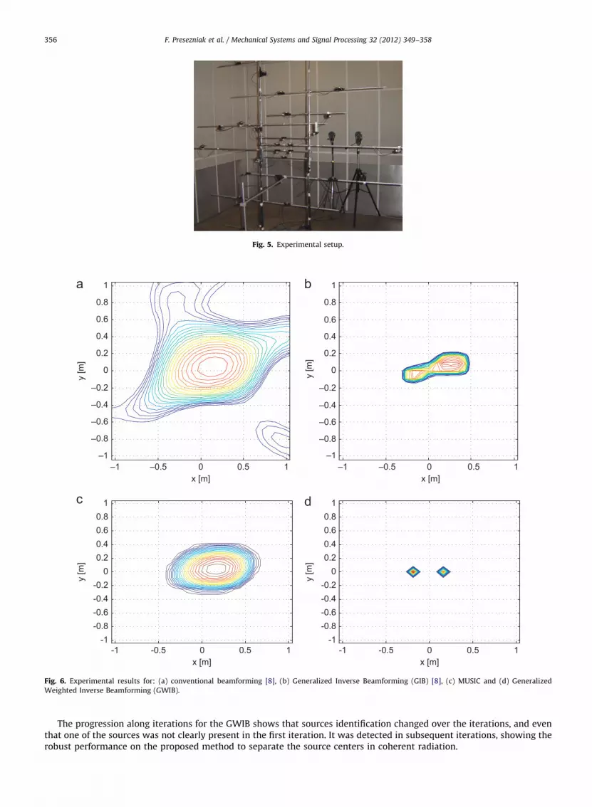
Fig. 5. Experimental setup.
x [m]
y [m
]
-1 -0.5 0 0.5 1
x [m]–1 –0.5 0 0.5 1
x [m]–1 –0.5 0 0.5 1
-1-0.8-0.6-0.4-0.2
00.20.40.60.8
1
y [m
]
–1
–0.8
–0.6
–0.4
–0.2
0
0.2
0.4
0.6
0.8
1
y [m
]
–1
–0.8
–0.6
–0.4
–0.2
0
0.2
0.4
0.6
0.8
1
x [m]
y [m
]
-1 -0.5 0 0.5 1-1
-0.8-0.6-0.4-0.2
00.20.40.60.8
1
Fig. 6. Experimental results for: (a) conventional beamforming [8], (b) Generalized Inverse Beamforming (GIB) [8], (c) MUSIC and (d) Generalized
Weighted Inverse Beamforming (GWIB).
F. Presezniak et al. / Mechanical Systems and Signal Processing 32 (2012) 349–358356
The progression along iterations for the GWIB shows that sources identification changed over the iterations, and eventhat one of the sources was not clearly present in the first iteration. It was detected in subsequent iterations, showing therobust performance on the proposed method to separate the source centers in coherent radiation.

x [m]
y [m
]
-1 -0.5 0 0.5 1-1
-0.8-0.6-0.4-0.2
00.20.40.60.8
1
x [m]
y [m
]
-1 -0.5 0 0.5 1-1
-0.8-0.6-0.4-0.2
00.20.40.60.8
1
x [m]
y [m
]
-1 -0.5 0 0.5 1-1
-0.8-0.6-0.4-0.2
00.20.40.60.8
1
x [m]
y[m
]
-1 -0.5 0 0.5 1-1
-0.8-0.6-0.4-0.2
00.20.40.60.8
1
Fig. 7. Generalized Weighted Inverse Beamforming (GWIB) after: (a) 1 iteration, (b) 5 iterations, (c) 10 iterations and (d) 15 iterations.
F. Presezniak et al. / Mechanical Systems and Signal Processing 32 (2012) 349–358 357
6. Conclusions
This paper presents a new beamforming technique based on the Generalized Inverse Beamforming but using aweighted pseudo-inverse approach and an optimization procedure for the weight definition. The objective of thisoptimization is to minimize the number of sources with a higher sensitivity to generate the response. This method, calledGeneralized Weighted Inverse Beamforming (GWIB), increases the dynamic range of the GIB, making it possible to identifyclosely spaced sources, as close as 1.5 wavelength in the example treated, supported by numerical and experimentalinvestigation.
The results show that this new method converges faster than the Generalized Inverse Beamforming, but thecomputational effort is somewhat equivalent, since an optimization procedure is required for the weight definition ateach iteration.
Thus, considering the computational effort and the obtained results, the advantage of this proposed method, GWIB, isevident, since it improves significantly the dynamic range on the identification with approximately the same processingeffort as the GIB.
References
[1] T. Hogbom, Aperture synthesis with a non-regular distribution of interferometer baselines, Astron. Astrophys. (Suppl. 15) (1974) 417–426.[2] T. Brooks, W. Humphereys, A deconvolution approach for the mapping of acoustic sources (damas) determined from phased microphone arrays,
J. Sound Vib. 294 (2006) 856–879.[3] T. Suzuki, Generalized inverse beam-forming algorithm resolving coherent/incoherent, distributed and multipole sources, in: 14th AIAA/CEAS
Aeroacoustics Conference, 2008.[4] P.A.G. Zavala, W. De Roeck, K. Janssens, J.R.F. Arruda, P. Sas, W. Desmet, Generalized inverse beamforming with optimized regularization strategy,
Mech. Syst. Signal Process., http://dx.doi.org/10.1016/j.ymssp.2010.09.012.[5] P. Guillaume, E. Parloo, G. De Sitter, Source identification from noisy response measurements using an iterative weighted pseudo-inverse approach,
in: ISMA Conference on Advanced Acoustics and Vibration Engineering, 2002.

F. Presezniak et al. / Mechanical Systems and Signal Processing 32 (2012) 349–358358
[6] P.A. Nelson, S.H. Yoon, Estimation of acoustic source strength by inverse methods: Part I, conditioning of the inverse problem, J. Sound Vib. 233 (2000)643–688.
[7] A. Gerard, A. Berry, P. Masson, Control of tonal noise from subsonic axial fan. Part 1: reconstruction of aeroacoustic sources from far-field soundpressure, J. Sound Vib. 288 (2005) 1049–1075.
[8] P.A.G. Zavala, W. De Roeck, K. Janssens, J.R.F. Arruda, P. Sas, W. Desmet, Monopole and dipole identification using generalized inverse beamforming,in: 16th AIAA/CEAS Aeroacoustic Conference, 2010.