Accurate Modeling of Weak Lensing with the sGL Method

Kimmo Kainulainen∗ and Valerio Marra†

Department of Physics, University of Jyvaskyla, PL 35 (YFL), FIN-40014 Jyvaskyla, Finland andHelsinki Institute of Physics, University of Helsinki, PL 64, FIN-00014 Helsinki, Finland

We revise and extend the stochastic approach to cumulative weak lensing (hereafter the sGLmethod) first introduced in Ref. [1]. Here we include a realistic halo mass function and densityprofiles to model the distribution of mass between and within galaxies, galaxy groups and galaxyclusters. We also introduce a modeling of the filamentary large-scale structures and a methodto embed halos into these structures. We show that the sGL method naturally reproduces theweak lensing results for the Millennium Simulation. The strength of the sGL method is that anumerical code based on it can compute the lensing probability distribution function for a giveninhomogeneous model universe in a few seconds. This makes it a useful tool to study how lensingdepends on cosmological parameters and its impact on observations. The method can also be usedto simulate the effect of a wide array of systematic biases on the observable PDF. As an example weshow how simple selection effects may reduce the variance of observed PDF, which could possiblymask opposite effects from very large scale structures. We also show how a JDEM-like survey couldconstrain the lensing PDF relative to a given cosmological model. The updated turboGL code isavailable at turboGL.org.

PACS numbers: 98.62.Sb, 98.65.Dx, 98.80.Es

I. INTRODUCTION

Inhomogeneities in the large-scale matter distributioncan in many ways affect the light signals coming fromvery distant objects. These effects need to be understoodwell if we want to map the expansion history and deter-mine the composition of the universe to a high precisionfrom cosmolgical observations. In particular the evidencefor dark energy in the current cosmological concordancemodel is heavily based on the analysis of the apparentmagnitudes of distant type Ia supernovae (SNe) [2, 3].Inhomogeneities can affect the observed SNe magnitude-redshift relation for example through gravitational lens-ing, in a way which essentially depends on size and com-position of the structures through which light passes onits way from source to observer.

The fundamental quantity describing this statisticalmagnification is the lensing probability distribution func-tion (PDF). It is not currently possible to extract thelensing PDF from the observational data and we have toresort to theoretical models. Two possible alternativeshave been followed in the literature. A first approach(e.g. Ref. [4–7]) relates a “universal” form of the lens-ing PDF to the variance of the convergence, which inturn is fixed by the amplitude of the power spectrum,σ8. Moreover the coefficients of the proposed PDF aretrained on some specific N-body simulations. A secondapproach (e.g. Ref. [8, 9]) is to build ab-initio a modelfor the inhomogeneous universe and directly compute therelative lensing PDF, usually through time-consumingray-tracing techniques. The flexibility of this method is

∗Electronic address: kimmo.kainulainen@jyu.fi†Electronic address: valerio.marra@jyu.fi

therefore penalized by the increased computational time.

In Ref. [1] we introduced a stochastic approach tocumulative weak lensing (hereafter sGL method) whichcombines the flexibility in modeling with a fast perfor-mance in obtaining the lensing PDF. The speed gainis actually a sine-qua-non for likelihood approaches, inwhich one needs to scan many thousands different mod-els (see Ref. [10]). The sGL method is based on the weaklensing approximation and generating stochastic config-urations of inhomogeneities along the line of sight. Themajor improvements introduced here are the use of a real-istic halo mass function to determine the halo mass spec-trum and the incorporation of large-scale structures inthe form of filaments. The improved modeling togetherwith the flexibility to include a wide array of system-atic biases and selection effects makes the sGL method apowerful and comprehensive tool to study the impact oflensing on observations.

We show in particular that the sGL method, endowedwith the new array of inhomogeneities, naturally and ac-curately reproduces the lensing PDF of the MilleniumSimulation [11, 12]. We also study a simple selection ef-fect model and show that selection biases can reduce thevariance of the observable PDF. Such reduction couldat least partly cancel the opposite effect coming fromlarge scale inhomogeneities, masking their effect on theobservable PDF. We also show how a JDEM-like sur-vey could constrain the lensing PDF relative to a givencosmological model. Along with this paper, we releasean updated version of the turboGL package, which is asimple and very fast Mathematica implementation of thesGL method [13].

This paper is organized as follows. In Section II weintroduce the cosmological background, the generic lay-out of inhomogeneities and review the basic formalismneeded to compute the weak lensing convergence. In Sec-

arX

iv:1

011.

0732

v2 [

astr

o-ph

.CO

] 2

7 D

ec 2

010

2

tion III we derive the halo mass function and the halodensity profiles and define the precise modeling of fila-ments. In Section IV we present the revised and extendedsGL method. The exact discretization of the model pa-rameters, which is a crucial step in the sGL model build-ing, is explained in Section V and in Section VI we ex-plain how the realistic structures where halos are confinedin filaments are modelled in the sGL method. Section VIIcontains our numerical results including the comparisonwith the cosmology of the Millennium Simulation [14]and, finally, in Section VIII we will give our conclusions.

II. SETUP

A. Cosmological Background

We consider homogeneous and isotropic Friedmann-Lemaıtre-Robertson-Walker (FLRW) background solu-tions to Einstein’s equations, whose metric can be writtenas:

ds2 = −c2dt2 + a2(t)[dr2 + f2

K(r)dΩ2], (1)

where dΩ2 = dθ2 + sin2 θdφ2 and

fK(r) =

K−1/2 sin(K1/2r) K > 0r K = 0(−K)−1/2 sinh[(−K)1/2r] K < 0

, (2)

where K/a2(t) is the spatial curvature of any t−slice.In particular we will focus on wCDM models whose

Hubble expansion rate depends on redshift according to:

H2(z)

H20

≡ E2(z) = ΩQ0 (1 + z)3q(z) (3)

+ ΩK0 (1 + z)2 + ΩM0 (1 + z)3 + ΩR0 (1 + z)4 ,

where q(z) is given by:

q(z) =1

ln(1 + z)

∫ z

0

1 + w(z′)

1 + z′dz′ . (4)

Here w(z) could be taken to follow e.g. the parameteri-zation [15]:

w(z) = w0 + waz

1 + z, (5)

for which:

q(z) = 1 + w0 + wa −wa z

(1 + z) ln(1 + z). (6)

For a constant equation of state w(z) = w0, the latterreduces to q(z) = 1 + w0.

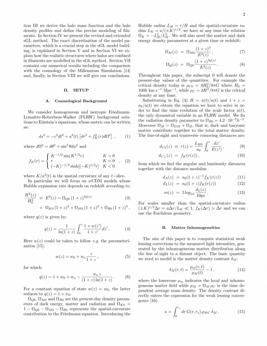
ΩQ0, ΩM0 and ΩR0 are the present-day density param-eters of dark energy, matter and radiation and ΩK0 =1 − ΩQ0 − ΩM0 − ΩR0 represents the spatial-curvaturecontribution to the Friedmann equation. Introducing the

Hubble radius LH = c/H and the spatial-curvature ra-dius LK = a/(±K)1/2, we have at any time the relationΩK = −L2

H/L2K . We will also need the matter and dark

energy density parameters at a given time or redshift:

ΩM (z) = ΩM0(1 + z)3

E2(z), (7)

ΩQ(z) = ΩQ0(1 + z)3q(z)

E2(z). (8)

Throughout this paper, the subscript 0 will denote thepresent-day values of the quantities. For example thecritical density today is ρC0 = 3H2

0/8πG where H0 =100h km s−1 Mpc−1, while ρC = 3H2/8πG is the criticaldensity at any time.

Substituting in Eq. (3) H = a(t)/a(t) and 1 + z =a0/a(t) we obtain the equation we have to solve in or-der to find the time evolution of the scale factor a(t),the only dynamical variable in an FLRW model. We fixthe radiation density parameter to ΩR0 = 4.2 · 10−5h−2.Moreover ΩM = ΩDM + ΩB , that is, dark and baryonicmatter contribute together to the total matter density.The line-of-sight and transverse comoving distances are:

dC‖(z) ≡ r(z) =LH0

a0

∫ z

0

dz′

E(z′), (9)

dC⊥(z) = fK(r(z)) , (10)

from which we find the angular and luminosity distancestogether with the distance modulus:

dA(z) = a0(1 + z)−1fK(r(z)) (11)

dL(z) = a0(1 + z)fK(r(z)) (12)

m(z) = 5 log10

dL(z)

10pc. (13)

For scales smaller than the spatial-curvature radius(±K)1/2∆r = a∆r/LK 1, fK(∆r) ' ∆r and we canuse the Euclidean geometry.

B. Matter Inhomogeneities

The aim of this paper is to compute statistical weaklensing corrections to the measured light intensities, gen-erated by the inhomogeneous matter distribution alongthe line of sight to a distant object. The basic quantitywe need to model is the matter density contrast δM :

δM (r, t) =ρm(r, t)

ρM (t)− 1 , (14)

where the lowercase ρm indicates the local and inhomo-geneous matter field while ρM = ΩM ρC is the time de-pendent average mass density. The density contrast di-rectly enters the expression for the weak lensing conver-gence [16]:

κ =

∫ rs

0

dr G(r, rs) ρMC δM , (15)

3

where rs is the co-moving position of the source and theintegral is along an unperturbed light geodesic. The den-sity ρMC ≡ a3

0 ρM0 is the constant matter density in aco-moving volume and we defined the auxiliary function1

G(r, rs) =4πG

c2fK(r)fK(rs − r)

fK(rs)

1

a, (16)

which gives the optical weight of an inhomogeneity atthe comoving radius r. The convergence is related to theshift in the distance modulus by:

∆m = 5 log10 µ−1/2 ' 5 log10(1− κ) , (17)

where µ is the net magnification and the second-ordercontribution of the shear has been neglected [1, 16]. Itis obvious that an accurate statistical modeling of themagnification PDF calls for a detailed description of theinhomogeneous mass distribution.

In this paper we will significantly improve the modelingof the inhomogeneities from our previous work [1], whereonly single-mass spherical overdensities were considered.First of all, we improve the modeling of these “halos”by using a realistic halo mass function f(M, z), whichgives the fraction of the total mass in halos of mass Mat the redshift z. The function f(M, z) is related to the(comoving) number density n(M, z) by:

dn(M, z) ≡ n(M, z)dM =ρMC

Mf(M, z)dM , (18)

where we defined dn as the number density of halos inthe mass range dM . The halo function is by definitionnormalized to unity∫

f(M, z)dM = 1 . (19)

The idea is of course that halos describe large virializedmass concentrations such as large galaxies, galaxy clus-ters and superclusters. Not all matter is confined intovirialized halos however. Moreover, only very large massconcentrations play a significant role in our weak lensinganalysis: for example the stellar mass in galaxies affectsthe lensing PDF only at very large magnifications [11, 12]where the PDF is close to zero. Therefore the fraction ofmass ∆fH concentrated in large virialized halos can bedefined by introducing a lower limit to the integral (19):

∆fH(z) ≡∫Mcut

f(M, z)dM < 1 . (20)

Only mass concentrations with M > Mcut are treatedas halos. The remaining mass is divided into a familyof large mass, but low density contrast objects with a

1 Note that this definition slightly differs from the one of Ref. [1].

fraction ∆fL and a uniform component with a fraction∆fU = ρMU/ρM , such that

∆fH + ∆fL + ∆fU = 1 . (21)

The low contrast objects are introduced to account forthe filamentary structures observed in the large scalestructures of the universe. In our analysis they will bemodeled by elongated objects with random positions andorientations. The mass in these objects can consist of asmooth unvirialized (dark) matter field and/or of a fine“dust” of small virialized objects with M < Mcut. Inweak lensing this distinction does not matter becausesmall halos act effectively as a mean field, with a size-able contribution only at very large magnifications (seecomment above about stellar mass).

For later use we define ∆fLU ≡ ∆fL+∆fU = 1−∆fHwhich gives the total mass fraction not in large virializedhalos. If we only consider virialized masses larger thancompanion galaxies (Mcut ∼ 1010 h−1M), then typicalvalues for the concordance model are ∆fLU ∼ 0.5 atz = 0[14] and ∆fLU ∼ 0.7 at z = 1.5, with a weak depen-dence on the particular f(M, z) used. Although ∆fLU issensitive on Mcut, the lensing PDF depends only weaklyon the cut mass. Moreover, halo functions obtained fromN-body simulations are valid above a mass value imposedby the numerical resolution of the simulation itself andso the use of Mcut is also necessary in this case [17].

To obtain an as accurate modeling as possible, wewill use realistic mass functions and spatial density pro-files for the halo distribution. There is less theoreticaland observational input to constrain the mass distribu-tion of the filamentary structures or their internal den-sity profiles. We will therefore parametrize the filamentswith reasonable assumptions for their lengths and widthsand by employing cylindrical nonuniform density pro-files. Our modeling allows treating the two families ofinhomogeneities independently. Both can be given ran-dom spatial distributions, or alternatively all halos canbe confined to have random positions in the interiors ofrandomly distributed cylinders. The latter configurationmore closely resembles the observed large scale struc-tures, and an illustration created by a numerical sim-ulation using the turboGL package is shown in Fig. 1. InSection VI A we will discuss the power spectrum and thelarge-scale correlations of our model universe.

We can now formally rewrite Eq. (14) for our modeluniverse in which the density distribution is givenby ρm =

∑j ρj + ρMU :

δM =

∑jMjϕj

ρMC+ ∆fU − 1 , (22)

where the index j labels all the inhomogeneities, we usedEq. (21) and we defined ρj ≡ a−3Mj ϕj , so that bothvirialized halos and the unvirialized objects are describedby a generic reduced density profile ϕj which satisfies the

4

0 15 30 45 60 750

20

40

60

80

100

h-1Mpc

h-1 M

pc

FIG. 1: Shown is an illustrative-only projection of the randommatter density within a 100h−1 Mpc thick slice generated byour stochastic model. The shaded disks represent clusters andthe shaded cylinders the filamentary dark matter structures.Only large clusters are displayed.

normalization∫VϕdV = 1.2 The lensing convergence we

are interested in can now be written as

κ ≡ κHL + κU + κE , (23)

where the positive contribution due to the inhomo-geneities (halos and low contrast objects) is

κHL =

∫ rs

0

dr G(r, rs)∑j

Mjϕj , (24)

the also positive contribution due to the uniformly dis-tributed matter is

κU = ρMC

∫ rs

0

dr G(r, rs) ∆fU (z(r)) , (25)

and the negative empty beam convergence is:

κE = −ρMC

∫ rs

0

dr G(r, rs) . (26)

2 Note that this definition slightly differs from the one of Ref. [1].

A light ray that misses all the inhomogeneities ϕj willexperience a negative total convergence κUE = κU + κE ,which gives the maximum possible demagnification in agiven model universe. In an exactly homogeneous FLRWmodel the two contributions κHL and κUE cancel andthere is no net lensing. In an inhomogeneous universe,on the other hand, a light ray encounters positive or neg-ative density contrasts, and its intensity will be magni-fied or demagnified, respectively. The essence of the sGLmethod is finding a simple statistical expression for theprobability distribution of the quantity κHL in the inho-mogeneous universe described above.

For a discussion about the validity of the weak lens-ing approximation within our setup see Ref. [1], where itwas shown that the error introduced is . 5%. We stressagain that the lensing caused by stellar mass in galaxiesis negligible in the weak lensing regime [11, 12] and so wecan focus on just modeling the dark matter distributionin the universe. Also, we will treat the inhomogeneitiesas perturbations over the background metric of Eq. (1).In particular we will assume that redshifts can be relatedto comoving distances through the latter metric. SeeRef. [18–21] for a discussion of redshift effects.

In the next section we will give the accurate model-ing of the inhomogeneities. We begin by introducing thehalo mass function and the detailed halo profiles, andthen move on to describe the precise modeling of thecylindrical filaments.

III. HALO AND FILAMENT PROPERTIES

We begin by explaining our dark matter halo modeling.The two main concepts here are the halo mass functionf(M, z) giving the normalized distribution of the halosas a function of their mass and redshift, and the darkmatter density profile within each individual halo. Bothquantities are essential for an accurate modeling of theweak lensing effects by inhomogeneities. We shall beginwith the halo mass function introduced above in Eq. (18).

A. Halo Mass Function

The halo mass function acquires an approximate uni-versality when expressed with respect to the variance ofthe mass fluctuations on a comoving scale r at a giventime or redshift, ∆(r, z). Relating the comoving scale r tothe mass scale by M = 4π

3 r3 ρMC , we can define the vari-

ance in a given mass scale by ∆2(M, z) ≡ ∆2(r(M), z).The variance ∆(r, z) can be computed from the powerspectrum:

∆2(r, z) ≡(δM

M

)2

=

∫ ∞0

dk

k∆2(k, z)W 2(kr) , (27)

where W (kr) is the Fourier transform of the chosen (top-hat in this work) window function and the dimensionless

5

power spectrum extrapolated using linear theory to theredshift z is:

∆2(k, z) ≡ k3

2π2P (k, z) (28)

= δ2H0

(ck

a0H0

)3+ns

T 2(k/a0)D2(z) .

Here ns is the spectral index and δH0 is the amplitudeof perturbations on the horizon scale today, which we fixby requiring:

∆(r = 8/a0h Mpc, z = 0) = σ8 , (29)

where the value of σ8 is estimated by cluster abundanceconstraints [22]. D(z) is the linear growth function whichdescribes the growth speed of the linear perturbations inthe universe. Fit functions for D could be found, e.g.,in Ref. [23], but it can also be easily solved numericallyfrom the equation:

D′′(z) +1

2

D′(z)

1 + z[ΩM (z) + (3w(z) + 1)ΩQ(z)]

− 3

2

D(z)

(1 + z)2ΩM (z) = 0 , (30)

where we have neglected the radiation. As usual, we nor-malize D to unity at the present time, D(0) = 1. Finally,for the transfer function T (k) we use the fit provided bythe Equations (28-31) of Ref. [24], which accurately re-produces the baryon-induced suppression on the interme-diate scales but ignores the acoustic oscillations, whichare not relevant for us here.

With ∆(M, z) given, we can now define our halo massfunction. Several different mass functions have been in-troduced in the literature, but here we will consider themass function given in Eq. (B3) of Ref. [17]:

fJ(M, z) = 0.301 exp(−| ln ∆(M, z)−1+0.64|3.82) , (31)

which is valid in the range −0.5 ≤ ln ∆−1 ≤ 1.0. Becauseof the change of variable, fJ is related to our originaldefinition of f by:

f(M, z) = fJ(M, z)d ln ∆(M, z)−1

dM. (32)

The mass function of Eq. (31) is defined relative toa spherical-overdensity (SO) halo finder, and the over-density used to identify a halo of mass M at redshift zis ∆SO = 180 with respect to the mean matter densityρM (z). The SO finder allows therefore a direct relationbetween halo mass M and the radius Rp:

M =4π

3R3p ρM (z) ∆SO . (33)

The subscript p will denote the proper values of otherwisecomoving quantities throughout this paper. For example,the comoving halo radius R is related to the proper valueby Rp = aR.

A direct relation between the mass and the radius ofa cluster is necessary for our sGL method. This is whywe prefer mass functions based on SO finders over massfunctions based on friends-of-friends halo finders; for thelatter an appropriate ∆SO to be used in Eq. (33) is not di-rectly available. Moreover, as shown in Ref. [17, 25], theSO(180) halo finder gives a good degree of universalityto the mass function. Another mass function which man-ifests approximate universality with the SO(180) halofinder [25] is provided by Sheth & Tormen in Ref. [26].

B. Halo Profile

With the halo mass function given the only missingingredient is the halo profile which, as said after Eq. (22),we describe by means of the reduced halo profile ϕh. Westress that our halo of a given mass M and redshift zis an avererage representative of the total ensemble ofhalos, which in reality have some scatter in the densityprofiles.

We will focus on the Navarro-Frenk-White (NFW) pro-file [27]:

ρhρM

=δc

(rp/Rs)(1 + rp/Rs)2. (34)

Here the scale radius is related to the halo radius byRp = cRs, where c is the concentration parameter tobe defined below. By integrating equation (34) one findsthe total mass M = 4π δc ρM (Rp/c)

3[ln(1+c)−c/(1+c)]which, when combined with Eq. (33), gives:

δc =∆SO

3

c3

ln(1 + c)− c/(1 + c). (35)

This relation fixes δc once the concentration parameteris given. The reduced halo profile ϕh in comoving coor-dinates is then:

ϕh(r, t) =

[4πr

(R

c+ r

)2(ln(1 + c)− c

1 + c

)]−1

,

(36)where the t-dependence (as well as M -dependence) arisesthrough the redshift dependence of R (Eq. (33)) and c(Eq. (37)).

The last ingredient needed to fully specify the NFWprofile is a relation between the concentration parameterand the halo mass at a given redshift. For the ΛCDMmodel we will use the following fit obtained from numer-ical simulations [28] satisfying WMAP5 cosmology [29]:

c(M, z) = 10.14

(M

MR

)−0.081

(1 + z)−1.01 , (37)

where the pivot mass scale is MR = 2 · 1012h−1M.

6

Apart from the NFW profile, alternative simple densityprofiles of interest include:

ϕh =3

4πR3Uniform, (38)

ϕh = 0.97−1 exp[−r2/2(R/3)2]

(2π)3/2(R/3)3Gaussian, (39)

ϕh =1

4πr2RSIS, (40)

where R is again given by Eq. (33). The normalizationfactor in (39) is necessary to have the correct volumeintegral of unity and is due to the restriction of the profilebetween 0 and R. In these cases there are no furtherparameters to be fixed.

C. Filaments

We will model dark matter filaments by cylindrical,non-uniform low density objects. Let us stress thatthroughout this chapter by a “filament” we refer onlyto the smoothly distributed dark matter component of areal filament; we shall later explain how virialized haloscan be embedded within these objects to form a morerealistic model of the true filamentary structures in thefull sGL framework. Keeping the low contrast compo-nent and the halos as separate entities in our evaluationis convenient for the modeling and explicitly avoids dou-ble counting.

Using Eqs. (18) and (21) we can obtain the follow-ing equation which relates the comoving filament density∆nf and the filament mass Mf to the fraction ∆fLU ofmass not confined in virialized halos:

Mf ∆nf ≡ ρMC βf ∆fLU , (41)

where the quantity βf defines the fraction of the totalunvirialized mass which is confined in filaments: ∆fL =βf ∆fLU . Because of the ongoing halo formation ∆fLUdecreases with time and we shall simply assume that βfis a constant.

We will assume that all filaments have the same mass,but this assumption can easily be relaxed later by intro-ducing a filament mass function [30]. We are also neglect-ing merging of smaller filaments into larger ones, wherebythe comoving number density of filaments ∆nf remainsa constant. This assumption seems to be supported bynumerical simulations [14] at least at low redshifts. FromEq. (41) it then follows that the filament mass Mf is notconstant, but it gradually decreases as more and morehalos virialize. (The total mass of the full filamentarystructure which includes the halos remains on averageconstant.)

Now we need to specify the precise geometry, dimen-sions and time-dependent density profile ϕf for our fil-aments. First, we will relate the filament mass to itslength and radius at present day according to:

Mf0 = πR2p0Lp0 ρM0 ∆f0 ≡ Vfp0 ρM0 ∆f0 , (42)

where Rp0 and Lp0 are the present-day filament properradius and length and ∆f0 is the average overdensity ofthe filament with respect to the FLRW matter density.Consistent with our assumptions of neglecting filamentmergers and using a constant comoving filament density,we will assume that filaments have a constant comovinglength. This is again in accordance with the generic pic-ture of a web of filaments of constant comoving lengthcondensing with time seen in numerical simulations. Fi-nally, for simplicity, we will choose our filaments to havea constant proper radius. Summarizing, we will use:

L = Lp0/a0 ,

R(t) = Rp0/a(t) . (43)

The simplest assumption would be to take filaments tohave uniform density. In this case the reduced densityprofile is simply ϕf = V −1

f . However, we will also con-sider a profile which is uniform along the length of thefilament L, but which has a gaussian profile in the radialdirection. In this case

ϕf (r, t) = 0.989−1 exp[−r2/2(R/3)2]

L 2π(R/3)2, (44)

where 0 ≤ r ≤ R and 0 ≤ l ≤ L, and ϕf = 0 otherwise.Finally, let us compute the mass of the “dressed” fil-

aments which comprises the “bare” filaments until nowdiscussed together with the halos (to be embedded inSection VI). It is easy to find that:

MDf0 = Vfp0 ρM0

[∆f0

(1 +

∆fH∆fL

)+ ∆fU

], (45)

where also the contribution from the uniformly dis-tributed matter is included. Eq. (45) is valid if all halosare embedded within the filaments and has to be slightlymodified if different levels of confinement are considered.

This completes our description of the objects in ourmodel. Next we shall have to understand how to simulatetheir effect on the weak lensing properties of the completeinhomogeneous model universe.

IV. THE sGL METHOD

In this section we will review and extend the stochasticgravitational lensing (sGL) method of Ref. [1] for com-puting the probability distribution function of the lensconvergence κ in the presence of inhomogeneities. Thebasic quantity to evaluate is the inhomogeneity-inducedpart κHL in Eq. (24):

κHL(zs) =

∫ rs

0

dr G(r, rs)∑j

Mj ϕj(|r − rj |, tj) , (46)

where rs = r(zs). We wish to obtain a probabilistic pre-diction for this quantity along a line of sight to a sourcelocated at rs, through a random distribution of halos and

7

filaments. The problem could be solved by constructing alarge comoving volume of statistically distributed objectssuch as the one shown in Fig. 1, and then computing thedistribution of κHL along random directions in this space.However, an equivalent and computationally much moreefficient approach is to construct random realizations ofobject locations along a fixed geodesic and compute thelensing PDF from a large sample of such realizations.

Let θ refer to a particular realization of the integral inEq. (46) and denote the resulting convergence by κ(θ, zs).Because of the finite size of the halos and filaments, onlya finite number Nθ of objects intercept the geodesic andcontribute to the sum. Moreover, because all objects aresmall compared to a typical comoving distance to thesource rs R,L, the functionG is, to a good approxima-tion, a constant G(r, rs) ≈ G(rj , rs) for each individualobject. Similarly, one can assume that ϕ(x, t) ≈ ϕ(x, tj)with tj = t(rj), and so one finds:

κHL(θ, zs) 'Nθ∑j=1

G(rj , rs) Σj(tj) , (47)

where Σj is the surface mass density of the j-th in-tercepting object in the realization. Next divide thegeodesic into NS subintervals with centers at ri andwith (possibly variable) length ∆ri rs, such thatG(r, rs) ≈ G(ri, rs) ≡ Gi(rs) = ∆r−1

i

∫∆ri

G(r, rs)dr

holds within each interval. In this way we can write

κHL(θ, zs) 'NS∑i=1

Ni∑ji=1

Gi(rs)Σji(ti) , (48)

where ji labels all objects encountered by the geodesic

within the comoving length bin ∆ri, such that∑NSi=1Ni =

Nθ. At this level Eq. (48) still consists of a sum over allobjects along a given path. Next we categorize these ob-jects into different classes depending on the parametersthat define the surface density Σji . For spherical halosof a given ϕ-profile Σ depends only on the mass of thehalo and the impact parameter, and for filaments therelevant parameters are the angle between the main fil-ament axis and the geodesic and the impact parameterin the cylindrical radius. Now assume all these variablesare discretized into finite-length bins.3 The precise wayof the discretization will be discussed in detail in SectionV, but for now we simply let a generic index u label theset of independent parameter cells created by the bin-ning. If we now let kθiu denote the number of objectsthat fall into the cell labeled by indices i and u in therealization θ, we can replace the sum over the individual

3 All other parameters, such as filament length, radius and massare kept fixed. In a more accurate modeling the fixed parameters(for example the filament mass) could be let vary, in which casethey should also be discretized.

objects in Eq. (48) by a weighted sum over the discreteparameter cells:

κHL(θ, zs) 'NS∑i=1

Gi(rs)

NC∑u=1

kθiu Σiu(ti)

≡NS∑i=1

NC∑u=1

kθiu κ1iu(zs) , (49)

where NC is the total number of independent parameter

cells4 used in the binning,∑NSi=1

∑NCu=1 k

θiu = Nθ and κ1iu

is the convergence due to one object in the bin iu:

κ1iu(zs) ≡ Gi(rs) Σiu(ti) . (50)

Note that the quantity κ1iu is a function of the distanceand internal variables, it is universal for arbitrary real-izations: all the information specific to a particular real-ization θ is contained in the set of integers kθiu.

Equation (49) is the starting point of the sGL analy-sis, because it can be easily turned into a probabilisticquantity. Indeed, instead of thinking of realizations θalong arbitrary lines of sight through a pre-created modeluniverse, we can define a statistical distribution of con-vergences through Eq. (49). Indeed, we have shown inRef. [1] that, for random initial and final points of thegeodesics, the integers kθiu are distributed as Poisson ran-dom variables:

Pkiu =(∆Niu)kiu

kiu!e−∆Niu , (51)

where the parameter ∆Niu is the expected number of ob-jects in the bin volume ∆Viu:

∆Niu = ∆niu ∆Viu = ∆niu ∆ri ∆Aiu . (52)

Here ∆niu is the comoving density of objects correspond-ing to the parameters in the bin iu and ∆Aiu is the cor-responding cross sectional area of these objects in co-moving units. We shall specify these quantities preciselyin Section V. Physically, the statistical distribution ofconvergences is equivalent to our original set of realiza-tions θ averaged over the position of the observer. Thisis a welcome feature because the statistical model explic-itly incorporates the Copernican Principle. The originalrealization θ has now been replaced by a configurationof random integers kiu and the convergence equationEq. (49) by a statistical convergence:

κHL(kiu, zs) =∑iu

kiu κ1iu(zs) , (53)

4 The binning of internal variables could depend on r, and so theindexing u and the number of different parameter cells NC couldin fact depend on i, but we suppress this notation for simplicity.

8

where the probability for a particular configuration tooccur is just

Pkiu =

NS∏i=1

NC∏u=1

Pkiu . (54)

It is easy to show that this probability distribution is cor-rectly normalized. Moreover, including the convergenceκUE due to the uniformly distributed matter and theempty space (see Eq. (26) and below), one can show thatthe total convergence corresponding to the configurationkiu becomes [1]:

κ(kiu, zs) =∑iu

κ1iu(zs)(kiu −∆Niu

). (55)

For a configuration without any inhomogeneities we cor-rectly recover κ(kiu = 0, zs) = κUE(zs), see SectionV. Moreover, Eq. (55) shows explicitly that the expectedconvergence vanishes consistently with the photon con-servation in weak lensing, because 〈kiu〉 = ∆Niu for arandom variable following Eq. (51). The final conver-gence PDF can now be formally written as

Pwl(κ, zs) = lim∆→01

∆

∫ κ+ ∆2

κ−∆2

dκ′Pwl(κ′, zs) , (56)

where

Pwl(κ, zs) ≡∑kiu

Pkiuδ(κ− κ(kiu, zs)) , (57)

is a discrete probability distribution. Note that the mostlikely configuration which maximises Pkiu correspondsto the mode of the Poisson distribution, which is thefloor of its parameter: kiu → b∆Niuc. Moreover, fora large ∆Niu the Poisson distribution approximates agaussian with mean and variance equal to ∆Niu and themost likely configuration therefore approaches the mean:kiu → ∆Niu. When this is the case the mode of thelensing PDF vanishes even for a single observation andthe PDF tends to a gaussian. One can similarly createthe PDF in the shift in the distance modulus ∆m orin the magnification µ, using Eq. (17) to compute thesequantities for a given configuration5 and then replacingκ by the desired quantity in equations (56-57).

In practice, equations (56-57) are not useful for a directevaluation of the PDF. Indeed, the configuration spacesare infinite and a direct evaluation of the sum of configu-rations would not be feasible even for relatively roughlydiscretized systems. Instead, we compute an approxima-tion for Pwl by statistically creating a large set of ran-dom configurations kiu from the probability distribu-tion Pkiu, and by forming a discrete normalized his-togram out from the corresponding set of convergences

5 This is true assuming that nonlinear effects can be neglected,i.e., in the weak lensing limit.

(or distance moduli or magnifications). That is, we definea histogram PDF using the function:

Pwl(κi, zs)∆i ≈Nsim,i

Nsim, (58)

where Nsim is the total number of realizations and Nsim,i

is the number of convergences in the sample falling inthe bin ∆i centered around the mean value κi. It iseasy to check that Eq. (58) is correctly normalized tounity. Moreover, the more configurations one creates inthe simulation step, the more fine-detailed and accurateapproximation for Pwl(κ, zs) can be constructed.6

To summarize, the sGL method consists of two steps:first the internal variables specifying the inhomogeneitiesare binned, reducing them to a finite number of differentobject classes labeled by the cell index u, for which uni-versal convergence functions κ1iu can be computed. Sec-ond the occupation numbers kiu of these objects within agiven co-moving distance bin are shown to be Poisson dis-tributed with parameter ∆Niu. The lensing PDF is thencomputed statistically, binning the convergence distribu-tion obtained from a large set of random configurationskiu on a given geodesic. Computing the lensing PDFthis way is very efficient. Finding the PDF for a givenmodel universe using the turboGL package [13] typicallytakes a few seconds in an ordinary desktop computer. Seethe Appendix A for more details about its performance.

Let us point out that Eq. (58) treats all objects on thesame footing. That is, all object families are indepen-dently randomly distributed throughout the space. Con-fining the halos to within filaments will require slightmodifications which we will explain in the section VI.For now, we shall study the effects that may cause theactual observed PDF deviate from the fundamental weaklensing PDF.

A. Observable PDF

The lensing PDF (58) is the fundamental quantity in-herent to a given background model and a set of inho-mogeneities. However, in reality there are interferencesthat prevent us from observing Pwl directly. Firstly, theintrinsic magnitudes of the sources are not known witharbitrary accuracy, and so the observed lensing PDF isat best a convolution:

P1(∆m, zs) =

∫dy Pwl(y, zs)Pin(∆m− y) , (59)

where Pin describes the source magnitude dispersion foran imperfect standard candle. Clearly the fundamental

6 One could also define a smooth Pwl(κ, zs) from the simulateddata as a moving average weighted by some window function, butthat would not give any advantage in the analysis with respectto using the simple histogram of Eq. (58).

9

lensing PDF is recovered in the limit that Pin becomes adelta function. If there were no other sources of errors,the distribution P1 could be used to contrast observationsagainst different cosmological background models, sets ofinhomogeneities and the models for the source magni-tude distributions. However, there can be several differ-ent types of selection effects caused by matter betweenthe source and the observer or by the search strategies,that may bias the observed PDF from the one predictedby Eq. (59). One of the strengths of the sGL method isthat it can be easily extended to model the effects of awide range of selection biases on the observable PDF.

Observational Biases

Let us begin with a simple class of biases that mightaffect the observed distance modulus beyond the weaklensing correction; an obvious example would be an errormade in the estimate of reddening. What makes suchcorrection nontrivial, is that one would expect the errorto be correlated with the types of mass concentrationsencountered by the photon beam on its way from thesource to the observer. The effects should thus be differ-ent along different lines of sight, affecting mostly thosedirections where light has to travel through volumes withhigher mass densities. In the sGL method such correlatedbiases are very easily modelled, as one needs merely toreplace

∆m → ∆m(kiu, zs) + δm(kiu, zs)≡ ∆meff(kiu, zs) , (60)

where the first part ∆m(kiu, zs) is the usual weak lens-ing correction and the second part the object-specific cor-rection. Indeed, the bias function δm(kiu, zs) can becorrelated with the redshifts zs and zi, and with all theinternal characteristics of the objects, such as the haloand filament masses and impact parameters. A quantita-tive analysis of the possible magnitude of the function δmwould require detailed astrophysical information and it isbeyond the scope of this paper. However, once properlymodelled, the sGL allows a very easy way of evaluatingthe outcome of biases on the observations.

Other types of selection biases might not directly af-fect the magnitudes, but rather the relative likelihoodof observing particular events, in a way that is corre-lated with the mass density. This includes, for exam-ple, all sources leading to obscuration of the light beam,either alone or in combination with restrictions comingfrom imperfect search efficiencies and strategies. For ex-ample selection by extinction effects or by outlier rejec-tion mainly relate to high-magnification events which areclearly correlated with having high intervening mass con-centrations (halos with large M and/or small b) along thelight geodesic. Similarly, short duration events might bemissed by search telescopes or be rejected from the datadue to poor quality of the light curve, for example in

cases where a supernova is not separable from the im-age of a bright foreground galaxy. Probability of suchevents would obviously be correlated with the brightnessof the source (zs and source dependent parameters), withthe density and redshift of the intervening matter and ofcourse with the search efficiencies.

The selection biases can be studied in the sGL frame-work by introducing a new, object-dependent survivalprobability function. That is, we replace

Pkiu → P effkiu ≡ K P sur

kiuPkiu (61)

in the probability distribution for the magnificationPDF (57). Here K is a normalization constant thatmakes sure that the final PDF is normalized to unity.The most generic form of the survival probability func-tion is

P surkiu =

∏iu

(P suriu )

kiu . (62)

This allows the survival function to depend on the ar-bitrary local properties along the photon geodesic. Thephysical interpretation of P sur

iu is of course clear: it givesthe relative probability that an event whose signal inter-cepts an object with characteristics given by internal pa-rameters u at redshift zi would make it to the acceptedobservational sample. Given the form (62) the propernormalization is easily seen to be:

P effkiu =

∏iu

(∆N effiu )kiu

kiu!e−∆Neff

iu , (63)

where

∆N effiu = P sur

iu ∆Niu . (64)

The correct expression for the convergence is still givenby Eq. (55), with the important difference that the ran-dom integers kiu used to evaluate Eq. (58) are now drawnfrom the Poisson distribution of Eq. (63) with parameterthe effective expected number of objects ∆N eff

iu .As mentioned above, modeling P sur

iu quantitativelywould need detailed input of the astrophysical proper-ties of the intervening matter distributions and of theobservational apparatus, which is beyond the scope ofthis work. See Ref [1] for an analytical example giv-ing 〈κ(zs)〉 = (1 − α)κE , where α is the effective fillingfactor of a partially-filled beam [18] (see [31] for an ex-tension of the partially-filled beam formalism). We willdiscuss an illustrative numerical example in Section VIIwhere we will consider as survival probability a simplestep-function in the impact parameter.

To summarise, let us note that it is easy to combineboth types of observational biases discussed in this sec-tion. The true observational PDF can be defined as

Pobs(∆m, zs) =

∫dy P eff

wl (y, zs)Pin(∆m− y) , (65)

where Pin again is the intrinsic source magnitude dis-persion and the effective lensing probability distribution

10

function P effwl (y, zs) is computed from Eq. (58) using the

effective probability distribution of Eq. (63), and com-puting the effective magnitudes for configurations fromequations (60) and (17). This setting clearly allows mod-eling a very complex structure of observational biases.

Finally note that the generic trend among all the ef-fects discussed above is to suppress events with highermagnifications. It could then be that a non-negligibleoverestimate of the observed magnitudes follows from ne-glecting the selection biases, even if the individual effectswere relatively small. Moreover, while the present datacannot yet constrain the lensing PDF itself, it can putbounds on its variance. Since the observational biases aresuppressing the high magnification tail, they give Pobs asmaller effective variance which may open the possibilityfor a comparison with the experiments. We will furtherdiscuss these topics in Section VII.

B. Binned Data Samples

We conclude this section by deriving an effective distri-bution PNO for a data sample NO, where the set NOrefers to a given binning of the original data. PNO couldbe computed directly from the fundamental PDF [1], butit is much faster to create it directly during the initialsimulation, bypassing the calculation of the fundamen-tal Pwl altogether. Indeed, if we label the configurationswithin a given sample of observations by s, the meanconvergence after NO observations is:

κNO (kiu) =1

NO

NO∑s=1

κ(kius) (66)

=∑iu

κ1iu

(∑NOs=1 kiu,sNO

−∆Niu

)

=∑iu

κ1iu

(kiu,NONO

−∆Niu

),

where in the second line we have used the fact that thequantities κ1iu are independent of s and in the last linewe have used the property that the independent Poissonvariables kiu,s (with the same weight) sum exactly (ina statistical sense) into the Poisson variable kiu,NO ofparameter given by the sum of the individual parameters,which is NO ∆Niu. PNO is then given by an expressionsimilar to Eqs. (56-57) or Eq. (58).

Note, however, that including the selection effects (seeSection IV A) in general does not commute with takingan average over the observations. In other words, if theNO measurements are correlated, we cannot use Eq. (66),but we have to start from the fundamental PDF. On theother hand, Eq. (66) displays explicitly the effect of thesize of the data sample: even if κ had a skewed PDF anda nonzero mode for NO = 1, for large NO the distributionapproaches a gaussian and eventually converges to a δ-function with a zero convergence, as it is clear from theproperties of Poisson variables.

C. Integral Formulas for Expected Value andVariance of the Lensing Convergence

From the general expression Eq. (66), including a non-trivial survival probability, it follows that the expectedvalue and variance of the convergence are:

〈κ〉 =∑iu

κ1iu (P suriu − 1)∆Niu , (67)

and

σ2κ =

1

NO

∑iu

κ21iu P

suriu ∆Niu , (68)

where we assumed that the survival probability for a lightray going through the uniformly distributed matter den-sity ρMU equals unity and that the random variables kiuare uncorrelated. Eqs. (67-68) can then be put back inintegral form giving the following exact results:

〈κ〉 =

∫ rs

0

dr G(r, rs)

∫ ∞Mcut

dn(M, z(r))× (69)

×∫ R(M,z(r))

0

dA(b,M) (Psur − 1) Σ(b,M, z(r))) ,

and

σ2κ =

1

NO

∫ rs

0

dr G2(r, rs)

∫ ∞Mcut

dn(M, z(r))× (70)

×∫ R(M,z(r))

0

dA(b,M)Psur Σ2(b,M, z(r))) ,

where the integral limits for the last two integrals areimplicitly defined and the explicit form of surface areaelement dA depends on the geometrical properties of theobject of mass M . For example, for spherical halos it isdA = 2πb db. We again stress that the quantity Psur =Psur(b,M, z, zs) is a generic function that describes theprobability that a light ray is observed when it hits a haloof mass M at the redshift z and impact parameter b fora source at redshift zs.

Eqs. (69-70) are a simple and direct prediction of thesGL method and allow to draw some general considera-tions. First, if Psur = 1, the expected value of the conver-gence is correctly zero, showing the “benevolent” natureof weak lensing corrections for unbiased observations. Ifhowever the survival probability is not trivial, selectionbiases persist even in very large datasets so that the av-erage convergence over a large number of observationsapproaches a nonvanishing value. Second, Eq. (70) is aproduct of positive quantities and so a nontrivial survivalprobability always reduces the observed variance.

We would like to stress that it is easy to numericallyevaluate the integrals of Eqs. (69-70), and their predic-tions can be straightforwardly implemented in χ2 analy-ses based on gaussian likelihoods, which may be a reason-able approximation if the observable PDF is not stronglyskewed.

11

V. DISCRETIZING THE MODELPARAMETERS

The key role played by the discretization of the modelparameters in the sGL method is now quite obvious. Ofcourse, the final lensing PDF should not depend on thediscretization. Indeed, as the numerical value of a Rie-mann integral does not depend on the binning chosen ifthe integrand does not significantly vary within the bins,the resulting PDF will not depend on the specific binningif the cosmological functions κ1iu are approximately con-stant within the bin cells iu. Once this condition is wellmet a further refinement of binning does not increase theaccuracy. This statement can be proved formally as fol-lows: imagine that we have a valid binning prescriptionA and we want to move to a new prescription B whichis N times finer. Because A is valid, the convergencesκB1iu are approximately constant within each A-bin. Therelative Poisson variables can then be resummed as donein Eq. (66), and we obtain the same formal expression interms of A-bins we started from.

This theorem also explains why we do not need to binany variable in which the surface mass density Σ of agiven object is constant, such as the rotational anglealong the center of a spherical halo in the lens plane. Asthe convergences κ1iu are constants within angular bins,their contributions can be resummed to give a modelwithout any angular binning. That is, the fundamentalhalo objects are actually finite-width rings in the conver-gence plane.

The first quantity to be binned is the co-moving dis-tance to the source. Here the basic quantity that needsto be accurately modelled is the function G(r, rs), whichgives the optical weight of a given convergence plane.This is a rather smooth function with a shallow peak,and only slightly dependent on rs when expressed in thescaled variable r/rs. Simple linear bins ri have beenfound to give accurate results, with only 10− 15 redshiftslices. This turns out to be the typical number of binsneeded for an accurate modeling of most of the internalvariables as well.

A. Discretizing the Halo Parameters

We begin by discretizing the halo parameters, whichare the mass and the impact parameter in the lens plane.Binning the halo masses involves two main considera-tions. First, the halo mass function only carries informa-tion about high-contrast virialized halos within a specificmass range (see Eq. (31)). Moreover, as explained in Sec-tion II B, only very large mass concentrations play a sig-nificant role in our weak lensing analysis. Consequently,we introduced the lower cut Mcut to the mass distribu-tion so that only mass concentrations with M > Mcut aretreated as halos, while the remaining mass has been di-vided into low contrast objects and uniform matter den-sity (see Eq. (21)). Second, the fact that the concentra-

geodesic

Rb

FIG. 2: Shown is a comoving segment of a photon geodesicintercepting a number of halos represented by shaded discs.

tion parameter of Eq. (37) follows a power law suggeststhe use of a logarithmic binning in mass. The mass func-tion drops quickly at very large masses, so that we cancombine all masses above a certain limit to a single bin.We found it reasonable to define at any redshift7 the cellboundaries by Mn = 10n h−1M and the cell centersby Mn = 10n+1/2 h−1M, with Mcut = M10. Becausef(M > M16, z) ' 0 to a very good approximation, it issufficient to bin with an integer n between 10 and 15:

M10 < M ≤M11 “companion galaxies”,

M11 < M ≤M12 “spiral galaxies”,

M12 < M ≤M13 “elliptical galaxies”,

M13 < M ≤M14 “groups”,

M14 < M ≤M15 “clusters”,

M15 < M ≤ ∞ “superclusters”. (71)

The fraction of total mass in a bin is then

∆fn =

∫ Mn+1

Mn

f dM , (72)

which correctly gives the total halo mass fraction (seeEq. (20)) when summed over all the halo bins:∑

n

∆fn = ∆fH . (73)

Finally, the binned comoving halo densities are

∆nn ≡ρMC

Mn∆fn , (74)

which also allows to relate the mass Mn to the interhalo

scale λn ≡ ∆n−1/3n .

7 A more efficient binning may be obtained by adopting redshift-dependent mass bins Mn(z). One could, for example, use binssuch that ∆fLU has always the present-day value. See SectionII B for a discussion about ∆fLU .

12

geo

des

ic

LR

!

L! = L sin(!)

FIG. 3: This illustration shows how we project the cylindricalfilaments on the plane perpendicular to the geodesic. Thetriangular section on the right is moved to the left end of thefilament so that the projected profile is independent of lθ.

The halo impact parameter bh in the lens plane is re-stricted to the range bh ∈ [0, R], where R is the comovinghalo radius. It should be noted that through Eq. (33) theradius depends both on the halo mass and the redshift.See Fig. 2 for an illustrative sketch. It is efficient to dis-cretize b into bins of constant integrated surface density(constant equal mass):∫ bhinm+1

bhinm

db 2πbΣh(b, Mn, ti) ≡Mn

NhB

, (75)

where NhB is the number of b-bins used and the surface

density is given by (see Fig. 2):

Σh(bh,M, t) = M

∫ R

bh

2xdx√x2 − b2h

ϕh(x, t) . (76)

After the redshift and the halo mass is specified,the bin boundaries bhinm and the weighted centers ofgravity bhinm can be computed using Eq. (75). Af-ter these are defined, the corresponding area functions∆Ahinm = π bh 2

inm+1 − π bh 2inm, needed for the Poisson pa-

rameters ∆Nhinm and the binned surface densities Σhinm =

Σh(bhinm, Mn, ti) ≡ Mn/(NhB∆Ahinm), can be computed.

Overall, our halo model is described by the redshift in-dex and two internal indices for the discretized mass andimpact parameter. In terms of the generic parameter uwe can formally express this as: h, inm ∈ iu, wherethe label h refers to the “halo” family of the inhomo-geneities.

B. Discretizing the Filament Parameters

The position and the orientation of a generic objectin the three dimensional space is described by three po-sition and three orientation degrees of freedom. Since

geod

esic

l! = 0

l! = L!

bf

R

FIG. 4: Sketch of a cylindrical filament projected on a planeperpendicular to the geodesic. The effective length of thecylinder is Lθ of Eq. (77) as shown in Fig. 3.

our filaments objects are confined to within a given ∆rislice, they generically have only five degrees of freedom.Special symmetries of a sphere reduced the number ofrelevant parameters for halos to a sigle one, the impactparameter bh. For filaments the situation is slightly morecomplicated because a cylinder is invariant only for rota-tions around one symmetry axis. This leaves us with fourdegrees of freedom. The relevant parameters, however,are reduced by the symmetries to only two: the angle θ ofthe filament main axes with respect to the geodesic andthe impact parameter bf . For illustration see Figs. 3-4.This can be understood by the fact that all the possiblefilament configurations with the same θ and bf have thesame surface density Σf and so can be resummed usingthe theorem given above. In particular, the projectedsurface density of our filaments does not depend on thecoordinate lθ along the projected main axes8 allowing toresum the lθ-bins into a single effective bin of the totalθ-dependent length of the projection:

Lθ = L sin θ . (77)

The angle θ is physically important because objects seenwith a smaller θ have a smaller cross section and a highersurface density. Accounting for this geometrical effectleads to a more strongly skewed lensing PDF.

8 In order to have the projected profile independent of lθ we“move” the triangular section as shown in Fig. 3. Strictly speak-ing our filaments do not have a cylindrical symmetry, but a θ-dependent “tilted” rotation symmetry, such that the projectedsurface densities follow equation (78) for all lθ. This approxima-tion should be good for long filaments with L R.

13

The expression for the surface density is given by

Σf (bf , θ, t) =Mf

sin θ

∫ R

bf

2xdx√x2 − b2f

ϕf (x, t) . (78)

For the uniform filament profile this gives simply Σf =

2 ρfθ√R2 − b2f , where ρfθ ≡Mf/(πR

2Lθ). For the gaus-sian profile (44) one instead finds

Σf = 0.997−1ρfθ R

√9π

2exp[−b2f/2(R/3)2] . (79)

The angle θ can be restricted by symmetry to the inter-val θ ∈ [0, π/2], which we divide into NT uniform lengthbins around centers θt = π(t − 1)/(2NT ). The impactparameter is restricted to bf ∈ [0, R], and it will be dis-

cretized into NfB bins using the equal mass criteria, as in

the halo case defined in Eq. (75). That is, our filamentswill be represented by a family of “bars” of different sur-face densities Σf

itm and length Lt ≡ L sin θt. The surfacearea of these bars to be used in the Poisson parametersis ∆Af

itm = 2Lt ∆bfitm.

Overall, our filament model is described by the redshiftindex, and two internal indices for the discretized angleand impact parameter. In terms of the generic parameteru we can again formally express this as: f, itm ∈ iu,where the family label f refers to the “filament” familyof the inhomogeneity. Of course adding, e.g., a massdistribution for filaments and/or an l-dependent densityprofile would increase the necessary number of indices inthe discrete model.

VI. CONFINING HALOS TO FILAMENTS

Until now we have implicitly assumed that the haloand the filament families are independent. We will nowshow how a more realistic model with halos confined tothe filaments can be set up in the sGL approach. Thecentral observation is that the exact positions of halosand filaments within the co-moving distance bins are ir-relevant in Eq. (55) for the convergence. It then does notmatter if we really confine the halos to filaments; for thesame effect it is sufficient to merely confine them into theequivalent volume occupied by the filaments in a givenbin.

We can actually do even better than imposing a simplevolume confinement. Indeed, it is natural to assume thatthe halo distribution follows the smooth density profilethat defines the filament, which can be accounted for byweighting the volume elements by their reduced densityprofiles. Because only the projected matter density isrelevant for lensing, this weighting is accounted for bythe effective surface densities of the objects. We thenintroduce the effective co-moving thickness for the low

density objects as:9

∆rfiv ≡1

ρfiΣf

iv , (80)

where ρfi ≡ Mf/Vfi is the average mass density of thefilament with volume Vfi. The total effective length of aconfiguration of filaments kfiv along the line of sight isthen:

∆rfi (kf

iv) =∑v

kfiv∆rf

iv ≡ ∆ri qfi . (81)

It is easy to show that the statistical average of ∆rfiover the configuration space is just the expected distancecovered by filaments:

〈∆rfi 〉 =∑v

∆N f

iv ∆rfiv = ∆ri qfi , (82)

where we defined the comoving average filament volumefraction:

qfi = Vfi ∆nfi . (83)

The confining simulation can now be performed in twosteps: in the first step a random configuration of fila-ments is generated and Eq. (81) is used to compute theeffective lengths ∆rfi at different co-moving slices. Theselengths define then the Poisson parameters for the halosthrough Eq. (52):

∆N fh

iu (kfiv) = ∆nfhiu ∆rfi ∆Ahiu . (84)

Note that the halo densities ∆nfhiu are corrected to ac-count for the reduced volume available due to confine-ment:

∆nfhiu ≡∆nhiuqfi

, (85)

where ∆nhiu are the usual halo densities of Eq. (74) whenthe halos are uniformly distributed through all space. In-serting Eq. (85) back to (84) and using Eqs. (81-82) wecan rewrite Eq. (84) simply as

∆N fh

iu =qfiqfi

∆Nhiu ≡ Xfi ∆Nh

iu , (86)

where ∆Nhiu are the usual configuration independent

Poisson parameters computed without confinement.Note that the central quantities needed in the evalu-

ation of Eq. (86) are the filamentary weights ∆N f

iv and

9 Note that this discussion is again general, and applies to all typesof low density objects, not necessarily with cylindrical geometry.To distinguish filaments from halos we use v to refer to genericinternal filamentary degrees of freedom.

14

surface densities Σf

iv. With these given, all the infor-mation about the specific low contrast objects used iscondensed into the single stochastic variable:

Xfi =

∑v k

f

ivΣf

iv∑v ∆N f

ivΣf

iv

, (87)

which has an expectation value of unity and a modesmaller than unity. The lensing effects due to large-scalestructures are thus tied to the probability distribution ofXf : its added skewness is the effect coming from confin-ing halos within filaments. This opens the possibility toinvestigate and compare different filamentary geometriesby means of the Xf -PDF. We will develop these thoughtsfurther in a forthcoming paper [32].

We can further generalize the picture given in this Sec-tion by considering different levels of confinement for ha-los of different masses. Indeed, because halos of differentmass are treated independently in Eq. (86), one couldhave small halos populate also the voids and massive ha-los only the filamentary structure.

Let us finally point out that in practical computationsthe convergence PDF is obtained by creating a large num-ber of independent halo configurations for each “master”filament configuration. Typically we use simulations withfew hundred master configurations with a few hundredhalo configurations each.

A. Power Spectrum

In this Section we will discuss the power spectrum ofour model universe and the importance of large-scale cor-relations for the lensing PDF. We start by making a con-nection between the sGL method and the so-called “halomodel” (see, for example, [33–39] and [40] for a review),where inhomogeneities are approximated by a collectionof different kinds of halos whose spatial distributions sat-isfies the linear power spectrum. The idea behind thehalo model is that on small scales (large wavenumbersk) the statistics of matter correlations are dominated bythe internal halo density profiles, while on large scales thehalos are assumed to cluster according to linear theory.The two components are then combined together.

The sGL modeling of the inhomogeneities can bethought as a two-step halo model where we first createthe random filamentary structures and then place thehalos randomly within these structures. Similarly to thehalo model, one can then combine the linearly-evolvedpower spectrum with the nonlinear one coming from thefilaments and the halos they contain. In this sense ourfilamentary structures extend the halo model by intro-ducing correlations in the intermediate scales betweenthe halo substructures and the cosmological scale con-trolled by the linear power spectrum. In the halo modelthe power spectrum can be computed analytically, buthere the calculation has to be done numerically. Weare currently extending the sGL method such that thesimulation will produce also the power spectrum [32] in

addition to the lensing PDF. The power spectrum canindeed place useful constraints on the filament parame-ters which, as remarked in Section II B, are not tightlyconstrained by observations.

While the power spectrum is relevant for understand-ing the correlations at the largest observable scales, thelensing PDF depends mainly on the much stronger in-homogeneities at smaller scales. This can be understoodfrom Eq. (15) which shows the direct dependence of thelensing convergence on the density contrast. The smalllensing variance from the large-scale correlations inducedby the linear power spectrum was numerically computed,for example, in [41]. Moreover, weak lensing and thepower spectrum probe somewhat different aspects of theinhomogeneities. The web-like structures of filamentsand voids that affect weak lensing are mainly describedby higher order correlation terms beyond the power spec-trum, and so special care has to be put in designing thefilamentary structure. This is indeed the goal of the sGLmethod: to give an accurate and flexible modeling of theuniverse as far as its lensing properties are concerned.

VII. RESULTS

Our main goal in this Section is to compare the sGLapproach with the convergence PDF computed from largescale simulations. The idea is that by achieving a goodagreement with numerical simulations we are provingthat the sGL method does provide a good and accuratedescription of the weak lensing phenomena. As we shallsee, this is indeed the case, as we can naturally reproducethe lensing PDF of the Millenium Simulation.10

Let us stress that while a comparison to simulations isa good benchmark test for the sGL approach, the simu-lations and underlying ΛCDM model do not necessarilydescribe Nature. Indeed observations do not yet providestrong constraints to the lensing PDF, which leaves roomfor very different types of large scale structures, examplesof which have been studied for example in Ref. [1, 10, 42].

With the accuracy of the method tested, one can re-liably compute the effects of selection biases using sGL.While we lack the necessary expertise to quantitativelyestimate the possible bias parameters, we will study asimple toy model for the survival probability functionP suriu to show qualitatively how selection effets might bias

the observable PDF. Finally, we will also show how aJDEM-like survey could constrain the lensing PDF rel-ative to a given cosmological model. We shall begin,however, by the comparison with the simulations.

10 We plan to compare the sGL model with other simulations inorder to check its accuracy for different cosmological parameters.

15

TABLE I: Filament parameterizations.

Parameters I II

∆f0 4.5 9

Rp0 (h−1Mpc) 2 4

Lp0 (h−1Mpc) 20 25

profile uniform gaussian

MDf0 (h−1ΩM0M) 9.3 × 1014 9.3 × 1015

A. Comparison with the Millennium Simulation

We shall now confront the sGL method with thecosmology described by the Millennium Simulation(MS) [14]. Accordingly, we will fix the cosmological pa-rameters to h = 0.73, ΩM0 = 0.25, ΩQ0 = 0.75, w = −1,ΩB0 = 0.045 σ8 = 0.9 and ns = 1. Moreover, the massfunction of Eq. (31) agrees with the MS results. Theseparameters completely fix the background cosmology andthe halos.

We are then left with the filament parameters to spec-ify. First, we fix βf = 0.5, which means that half ofthe unvirialized mass forms filaments, while the otherhalf is uniformly distributed. This value determines themaximum possible demagnification ∆mUE in the lensingPDF, corresponding to light that misses all the inhomo-geneities. For the background model described above thisimplies ∆mUE ' 0.17 mag.

The next parameter to set is the present-day filamentmass Mf0. Since βf was taken a constant, a lower Mf0

implies a higher comoving filament density (see Eq. (41)),a more homogeneous universe and hence less pronouncedlensing effects. In order to connect with the literaturewe actually have to use the dressed filament mass ofEq. (45) which, because of the chosen βf , is roughlyMDf0 ≈ 3Mf0. To choose the parameters defining Mf0,

we follow Ref. [43], according to which it is reasonableto fix the average filament overdensity to ∆f0 = 4.5and the filament radius to Rp0 = 2h−1Mpc. Notethat the overdensity of the dressed filament is roughly3∆f0 and that our filaments include also the large ha-los at the filament ends. Moreover the density profileseems rather uniform within Rp0 according to [43] andso we use the simple uniform density profile. The dis-tribution of filament lengths is quite wide (see Fig. 7 ofRef. [43]) and we choose to use a representative value ofLp0 = 20h−1Mpc. With these choices the bare filamentmass becomes Mf0 = 3.1 × 1014 h−1ΩM0M. We havesummarized in Table I this first filament parameteriza-tion (I). We can now compare the properties of the lens-ing PDF from the sGL method to the one from the Mil-lenium Simulation, which is a courtesy of Refs. [11, 12].

The four histograms in Fig. 5 show the four steps inbuilding the model universe in the sGL method. Thefirst (orange) histogram from the top corresponds to auniverse endowed only with the halos specified by themass function. The second (green) histogram from the

!0.3 !0.2 !0.1 0.0 0.10

2

4

6

8

10

"m

Lensing PDF

FIG. 5: Shown are the lensing PDFs for a source at z = 1.5for the ΛCDM model of the Millennium Simulation [14]. Thedashed line is the lensing PDF generated by shooting raysthrough the MS [11, 12], while the histograms are obtainedwith the sGL method. The first (orange) histogram fromthe top corresponds to a model universe with halos but nofilaments, the second (green) is relative to a universe with ha-los and cylindrical filaments randomly placed and the third(blue) to the case in which the halos are confined within mass-less filaments. The fourth (red) histogram is the most realis-tic case with halos confined within randomly placed massivefilaments. The filaments are modelled according to Table I(parameterization I). See Section VII A for details.

top-left represents a model in which half of the uniformmatter density (βf = 0.5) is condensed into filaments,but halos are not confined to them. The third (blue)histogram from the top-left represents a model in whichthe halos are confined within the filaments but these aremassless. Finally, the lowest (red) histogram representsthe case where the halos are confined within massive fil-aments.

For these parameters the lensing PDF seems domi-nated by the halo contribution due to the NFW densityprofiles and the effect of the large scale clustering seemsto increase the dispersion. In particular, the clustering ofhalos and of smooth mass within filaments seems to give asimilar contribution as the two corresponding histogramsare close to each other, with a slightly more skewed PDFfor the former as compared to the latter. In other words,the nonlinear clustering of halos at the filament scalesappears to increase the dispersion similarly to the distri-bution of smooth matter in low density filamentary struc-tures. The results relative to the Millennium Simulationfrom Ref. [11, 12] are shown with a dashed line. Theagreement becomes very good when the large scale struc-tures are fully included, showing that the lensing PDF isa sensitive probe of the large scale structures. We canconclude that the halos have to be confined within mas-sive filaments if we are to reproduce the MS results, atleast for the parameters chosen. Moreover, by fixing theother parameters one could place an upper bound on fila-

16

0 0.2 0.4 0.6 0.8 1 1.2 1.4 1.6

0

0.01

0.02

0.03

0.04m

ode

(mag

)

Millennium SimulationsGL (par. I)

0 0.2 0.4 0.6 0.8 1 1.2 1.4 1.60

0.01

0.02

0.03

0.04

0.05

v (m

ag)

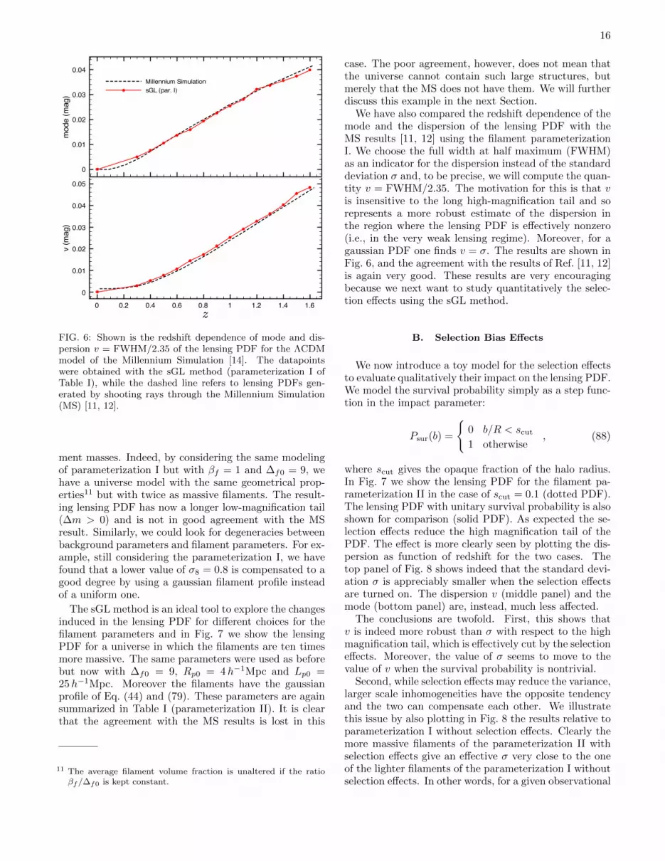
FIG. 6: Shown is the redshift dependence of mode and dis-persion v = FWHM/2.35 of the lensing PDF for the ΛCDMmodel of the Millennium Simulation [14]. The datapointswere obtained with the sGL method (parameterization I ofTable I), while the dashed line refers to lensing PDFs gen-erated by shooting rays through the Millennium Simulation(MS) [11, 12].

ment masses. Indeed, by considering the same modelingof parameterization I but with βf = 1 and ∆f0 = 9, wehave a universe model with the same geometrical prop-erties11 but with twice as massive filaments. The result-ing lensing PDF has now a longer low-magnification tail(∆m > 0) and is not in good agreement with the MSresult. Similarly, we could look for degeneracies betweenbackground parameters and filament parameters. For ex-ample, still considering the parameterization I, we havefound that a lower value of σ8 = 0.8 is compensated to agood degree by using a gaussian filament profile insteadof a uniform one.

The sGL method is an ideal tool to explore the changesinduced in the lensing PDF for different choices for thefilament parameters and in Fig. 7 we show the lensingPDF for a universe in which the filaments are ten timesmore massive. The same parameters were used as beforebut now with ∆f0 = 9, Rp0 = 4h−1Mpc and Lp0 =25h−1Mpc. Moreover the filaments have the gaussianprofile of Eq. (44) and (79). These parameters are againsummarized in Table I (parameterization II). It is clearthat the agreement with the MS results is lost in this

11 The average filament volume fraction is unaltered if the ratioβf/∆f0 is kept constant.

case. The poor agreement, however, does not mean thatthe universe cannot contain such large structures, butmerely that the MS does not have them. We will furtherdiscuss this example in the next Section.

We have also compared the redshift dependence of themode and the dispersion of the lensing PDF with theMS results [11, 12] using the filament parameterizationI. We choose the full width at half maximum (FWHM)as an indicator for the dispersion instead of the standarddeviation σ and, to be precise, we will compute the quan-tity v = FWHM/2.35. The motivation for this is that vis insensitive to the long high-magnification tail and sorepresents a more robust estimate of the dispersion inthe region where the lensing PDF is effectively nonzero(i.e., in the very weak lensing regime). Moreover, for agaussian PDF one finds v = σ. The results are shown inFig. 6, and the agreement with the results of Ref. [11, 12]is again very good. These results are very encouragingbecause we next want to study quantitatively the selec-tion effects using the sGL method.

B. Selection Bias Effects

We now introduce a toy model for the selection effectsto evaluate qualitatively their impact on the lensing PDF.We model the survival probability simply as a step func-tion in the impact parameter:

Psur(b) =

0 b/R < scut

1 otherwise, (88)

where scut gives the opaque fraction of the halo radius.In Fig. 7 we show the lensing PDF for the filament pa-rameterization II in the case of scut = 0.1 (dotted PDF).The lensing PDF with unitary survival probability is alsoshown for comparison (solid PDF). As expected the se-lection effects reduce the high magnification tail of thePDF. The effect is more clearly seen by plotting the dis-persion as function of redshift for the two cases. Thetop panel of Fig. 8 shows indeed that the standard devi-ation σ is appreciably smaller when the selection effectsare turned on. The dispersion v (middle panel) and themode (bottom panel) are, instead, much less affected.

The conclusions are twofold. First, this shows thatv is indeed more robust than σ with respect to the highmagnification tail, which is effectively cut by the selectioneffects. Moreover, the value of σ seems to move to thevalue of v when the survival probability is nontrivial.

Second, while selection effects may reduce the variance,larger scale inhomogeneities have the opposite tendencyand the two can compensate each other. We illustratethis issue by also plotting in Fig. 8 the results relative toparameterization I without selection effects. Clearly themore massive filaments of the parameterization II withselection effects give an effective σ very close to the oneof the lighter filaments of the parameterization I withoutselection effects. In other words, for a given observational

17

!0.3 !0.2 !0.1 0.0 0.10

2

4

6

8

"m

Lensing PDF

FIG. 7: Lensing PDF for a source at z = 1.5 for the filamentparameterization II of Table I. The solid (green) histogramis without selection effects, while the dotted (blue) histogramis with the selection effects toy-modelled by Eq. (88). Forcomparison with Fig. 5, the lensing PDF relative to the Mil-lennium Simulation is plotted again as a dashed line. SeeSection VII for details.

bound on the lensing variance, there may be some degen-eracy between observational biases and weak lensing bylarge scale structures. This clearly shows the importanceof correctly modeling selection effects. The above degen-eracy, however, is broken by the redshift dependence ofv and mode, showing that a precise measurement of thelensing PDF (beyond the variance) can yield importantcosmological information. We will discuss in the nextSection the possibility of observing the lensing PDF.

C. Measuring the Lensing PDF

We will now discuss the possibility of measuring thelensing PDF for the universe of the Millennium Simu-lation. We will perform a simplified analysis in whichwe assume that we are observing perfect standard can-dles and we are thus neglecting the intrinsic dispersionin the SNe absolute luminosity. Moreover, we will alsoneglect any observational uncertainties. We refer to sub-sequent work for a more comprehensive analysis, whilehere we give an illustrative picture for the prospects ofobservationally constraining the lensing PDF. We will inparticular consider a dataset of a JDEM-like survey withone thousand high redshift SNe. With this in mind, weshow in Figs. 9-10 the lensing PDFs for sets of 200 and1000 perfect standard candles at a given target redshiftof z = 1.5. Also plotted are the 2σ errors, where the stan-dard deviation was computed with turboGL in a MonteCarlo fashion by generating many of such histograms andcalculating the σ for each bin height.

The two figures represent two possible comparisons ofthe data with a given cosmological model, the difference

0 0.2 0.4 0.6 0.8 1 1.2 1.4 1.6

0

0.02

0.04

0.06

0.08

v (m

ag)

0 0.2 0.4 0.6 0.8 1 1.2 1.4 1.6

0

0.01

0.02

0.03

0.04

0.05

mod

e (m

ag)

0 0.2 0.4 0.6 0.8 1 1.2 1.4 1.6

0

0.02

0.04

0.06

0.08

0.1

sigm

a (m

ag)

par. II without selectionpar. II with selectionpar. I without selection

FIG. 8: Shown is the redshift dependence of σ (top panel),v = FWHM/2.35 (middle panel) and mode (bottom panel) forthe filament parameterization II of Table I with (dotted line)and without (dashed line) the selection effects of Eq. (88).The solid line is relative to the filament parameterization Iwithout selection effects.

being the amount of prior cosmological information as-sumed. Indeed, since the observational data is heteroge-nous it must be binned to some redshift intervals ∆zand the SNe luminosities have to be normalized to thesame bin redshift. If ∆z is small the implicit dependenceof the above correction on the background cosmology issmall and one finds a direct constraint on the cosmo-logical model. This situation is displayed in Fig. 9 fora JDEM-type dataset with 200 SNe in the redshift bin∆z = [1.45, 1.55]. It is clear that this single redshift bincannot put very tight constraints on a generic lensingPDF and one has to use all the high-redshift dataset.

One way to proceed is to compare per bin the predictedlensing PDF with the observed one, that is, by treatingdifferent bins independently. Another way could be tocombine all the 1000 SNe at z & 1 to one bin. Fig. 10 dis-plays the relative histogram, which now has much smallererror bars as compared to Fig. 9. The normalization ofthe dataset to the same target redshift, however, usedheavily the prior assumptions about the cosmologicalmodel. That is, the comparison shown in Fig. 10 pro-vides only a consistency check for the assumed cosmolog-ical model, and it should be noted that the reconstructed

18

!0.3 !0.2 !0.1 0.0 0.1

0

2

4

6

8

10

"m

Lensing PDF

FIG. 9: Lensing PDF for a source at z = 1.5 for the filamentparameterization I of Table I (without selection effects). Thehistogram simulates a possible PDF obtained with a datasetof 200 perfect standard candles. The 2σ errors are representedas rectangles. The PDF relative to the Millennium Simulationis plotted as a dashed line. See Section VII C for details.

!0.3 !0.2 !0.1 0.0 0.10

2

4

6

8

"m

Lensing PDF

FIG. 10: Same as in Fig. 9 but for a dataset of 1000 perfectstandard candles.

lensing PDF might hide a high degree of degeneracy onthe cosmological parameters.

VIII. CONCLUSIONS

In this paper we have revised and extended the stochas-tic approach to cumulative weak lensing first introducedin Ref. [1]. The (sGL) method is based on the weaklensing approximation and on generating stochastic con-figurations of halos and large-scale structures along theline of sight to cosmological objects, such as supernovae.The halos are intended to model the virialized structures,such as galaxies and clusters of galaxies. We model these

structures accurately by means of realistic mass distri-bution functions and by NFW density profiles (with ap-propriate z and M dependent concentration parameter).The filamentary structures were modelled with (possibly)non-uniform cylindrical objects.

This modeling incorporates the essential fact thatmost of the spatial volume is occupied by underdensities(voids), while most of the mass lies in overdense regions ofmuch smaller total volume, in the form of virialized clus-ters and large filamentary structures. As a consequencethe column mass density along a random single geodesicis likely to be lower than the average, which gives rise tothe skewness of the lensing PDF. A skewed PDF is of po-tential importance in particular for the interpretation ofthe supernova observations, which are still probing muchsmaller angular scales than the scale at which the homo-geneity is recovered. The sGL method with its excellentperformance provides a useful tool to investigate the im-pact of lensing, especially on analyses based on likelihoodapproaches as done in Ref. [10].

We confronted our sGL modeling with the lensing re-sults [11, 12] from the Millennium Simulation [14]. Eventhough the MS does not necessarily represent the actualuniverse, this comparison provides a very useful bench-mark test, because here the results are exactly known, aswell as the main characteristics of the inhomogeneitiesinvolved. The sGL-generated PDF agreed with the MSresults very well and naturally without any fine tuning,when all model parameters were chosen to match thetypical structures seen in numerical simulations. In theMS cosmology most of the lensing was found to be dueto the halos, with a smaller, but clearly distinguishablecontribution coming from filaments. We conclude that itis necessary to embed the halos along massive filamentsto reproduce the MS results.

Moreover, the sGL method can easily incorporate ob-servational biases such as selection effects or any othermechanisms that can obscure lines of sight. We believethis to be an appealing feature of the sGL method, es-pecially with the growing size of SNe datasets: a largenumber of observations indeed reduces the statistical biasdue to the skewed lensing PDF, but does not eliminatethe systematic ones possibly caused by selection effects.One can alleviate such problems with a good understand-ing and modeling of the biases, which is also needed ifone wants to observationally constrain the lensing PDF.Indeed, we have shown by a simple toy-model examplethat selection effects can potentially alter the observablePDF in such a way as to cancel the opposing modificationcoming from very large scale structures. Assuming no se-lection effects might then lead to a premature exclusionof such structures.

Finally, we have also shown how a JDEM-like surveycould constrain the lensing PDF relative to the cosmol-ogy of the Millennium Simulation. Our results suggestthat such a survey might be able to give important in-formation about the PDF and thus about the large-scalestructure of the universe.

19

Along with this paper, we release an updated versionof the turboGL package, a simple and very fast Mathe-matica implementation of the sGL method, which can befound at turboGL.org.

Acknowledgments

It is a pleasure to thank Stefan Hilbert for providingthe results of Ref. [11, 12] accompanied by helpful expla-nations and Gerard Lemson for help in exploring the MSdatabase. The authors benefited from discussions withLuca Amendola, Pierre Astier, Matthias Bartelmann,Stefano Borgani, Julien Guy, Miguel Quartin, EduardoRozzo, Barbara Sartoris and Esra Tigrak.

Appendix A: Performance of the sGL Method

In order to estimate the performance of the sGLmethod we have to calculate the total number Nbinsof iu-bins. It is easy to find that Nbins/NSNB =NH + NFNT , where NH is the number of halo-massbins, NF is the number of filaments, NT is the num-ber of θ-bins and we have used for simplicity the same

number of impact-parameter bins NB for both halos andfilaments. We remind that NT is the effective numberof θ-bins, while the actual number of configurations is2NT . For each Nbins the sGL method evaluates the cor-

TABLE II: Performance of the sGL method.

Model type NH NF CPU time

Single-mass halo model 1 0 0.2 s

Mass function f(M) 6 0 1.1 s

f(M) + filaments 6 1 1.8 s

responding occupational number from the Poisson statis-tics. The program Mathematica using one core of a CPUat 2.5− 3 GHz takes a time tbin ' 10−3 s to produce anarray of Nstat = 104 Poisson numbers. Other programswill likely have similar performances. Nstat determinesthe statistics with which the lensing PDF is generated.Using this information we can then estimate the perfor-mance of the sGL method by evaluating tbinNbins. Theresults are shown in Table II where we fixed NS = 12,NB = 15 and NT = 4. Confining halos within filamentstypically makes calculations about ten times longer.

[1] K. Kainulainen and V. Marra, Phys. Rev. D 80, 123020(2009).

[2] A. G. Kim, E. V. Linder, R. Miquel and N. Mostek, Mon.Not. Roy. Astron. Soc. 347, 909 (2004).

[3] M. Kowalski et al., Astrophys. J. 686, 749 (2008).[4] P. Valageas, Astron. Astrophys. 356, 771 (2000).[5] D. Munshi and B. Jain, Mon. Not. Roy. Astron. Soc. 318,

109 (2000).[6] Y. Wang, D. E. Holz and D. Munshi, Astrophys. J. 572,

L15 (2002).[7] S. Das and J. P. Ostriker, Astrophys. J. 645, 1 (2006).[8] D. E. Holz, R. M. Wald, Phys. Rev. D 58, 063501 (1998).[9] D. E. Holz, E. V. Linder, Astrophys. J. 631, 678 (2005).

[10] L. Amendola, K. Kainulainen, V. Marra and M. Quartin,Phys. Rev. Lett. 105, 121302 (2010).

[11] S. Hilbert, S. D. M. White, J. Hartlap and P. Schneider,Mon. Not. Roy. Astron. Soc. 382, 121 (2007).

[12] S. Hilbert, S. D. M. White, J. Hartlap and P. Schneider,Mon. Not. Roy. Astron. Soc. 386, 1845 (2008).

[13] turboGL is available at: http://www.turbogl.org[14] V. Springel et al., Nature 435, 629 (2005).[15] M. Chevallier and D. Polarski, Int. J. Mod. Phys. D 10,

213 (2001); E. V. Linder, Phys. Rev. Lett. 90, 091301(2003).

[16] M. Bartelmann and P. Schneider, Phys. Rept. 340, 291(2001).

[17] A. Jenkins et al., Mon. Not. Roy. Astron. Soc. 321, 372(2001).

[18] R. Kantowski, Astrophys. J. 155, 89 (1969).[19] V. Marra, E. W. Kolb, S. Matarrese and A. Riotto, Phys.

Rev. D 76, 123004 (2007); V. Marra, E. W. Kolb andS. Matarrese, Phys. Rev. D 77, 023003 (2008); V. Marra,

arXiv:0803.3152 [astro-ph]; E. W. Kolb, V. Marra andS. Matarrese, Gen. Rel. Grav. 42, 1399 (2010).

[20] T. Biswas and A. Notari, JCAP 0806, 021 (2008).[21] N. Brouzakis and N. Tetradis, Phys. Lett. B 665, 344

(2008).[22] E. Rozo et al., Astrophys. J. 708, 645 (2010).[23] W. J. Percival, Astron. Astrophys. 443, 819 (2005); see

also: S. Basilakos, Astrophys. J. 590, 636 (2003).[24] D. J. Eisenstein and W. Hu, Astrophys. J. 496, 605

(1998).[25] M. J. . White, Astrophys. J. Suppl. 143, 241 (2002).[26] R. K. Sheth and G. Tormen, Mon. Not. Roy. Astron. Soc.

308 (1999) 119.[27] J. F. Navarro, C. S. Frenk and S. D. M. White, Astrophys.

J. 462, 563 (1996).[28] A. R. Duffy, J. Schaye, S. T. Kay and C. Dalla Vecchia,

Mon. Not. Roy. Astron. Soc. 390, L64 (2008).[29] E. Komatsu et al. [WMAP Collaboration], Astrophys. J.

Suppl. 180, 330 (2009).[30] J. Shen, T. Abel, H. Mo and R. K. Sheth, Astrophys. J.

645, 783 (2006).[31] T. Mattsson, Gen. Rel. Grav. 42, 567 (2010).[32] K. Kainulainen and V. Marra, “Weak lensing and fila-

mentary geometries,” in preparation.[33] J. Neyman and E. L. Scott, Astrophys. J. 116, 144

(1952).[34] P. J. E. Peebles, A&A 32, 197 (1974).[35] R. J. Scherrer, E. Bertschinger, Astrophys. J. 381, 349

(1991).[36] U. Seljak, Mon. Not. Roy. Astron. Soc. 318, 203 (2000).[37] C. P. Ma and J. N. Fry, Astrophys. J. 543, 503 (2000).[38] J. A. Peacock and R. E. Smith, Mon. Not. Roy. Astron.

20

Soc. 318, 1144 (2000).[39] R. Scoccimarro, R. K. Sheth, L. Hui and B. Jain, Astro-

phys. J. 546, 20 (2001).[40] A. Cooray, R. K. Sheth, Phys. Rept. 372, 1-129 (2002).[41] F. Bernardeau, L. Van Waerbeke, Y. Mellier, Astron. As-

trophys. 322, 1-18 (1997).

[42] K. Kainulainen and V. Marra, Phys. Rev. D 80, 127301(2009);

[43] J. M. Colberg, K. S. Krughoff and A. J. Connolly, Mon.Not. Roy. Astron. Soc. 359, 272 (2005).