ABSTRACT

PADMANABHAN, KANCHANA. Hierarchical Modularity-driven Discovery and Characterizationof Network Biomarkers: Application to Bioenergy Production and Prognostics of NeurologicalDisorders.(Under the direction of Dr. Nagiza F. Samatova.)

Biomarkers, short for biological markers are ubiquitous and help distinguish organisms that

exhibit certain characteristics. Characteristics could refer to bioenergy related processes such as

bioethanol production or biohydrogen production by microorganisms, or could refer to neurolog-

ical disorders such as Alzheimer’s or schizophrenia. These characteristics are termed phenotypes

in biological literature.

Biomarker discovery and characterization have gained a lot of attention in the recent past

and have many uses including improving the efficiency of bioengineering processes or increasing

the skill of disease prognostics. Traditionally, these biomarkers are defined as individual genes

or sets of genes correlated with the presence of a phenotype. However, genes do not function

individually but cooperate with other genes to carry out various functions in an organism. These

inter-gene relationships are captured using a network structure, where the nodes are genes and

the edges represent some functional associations between the genes (e.g., genetic interaction

networks). Recently, the focus has been shifting towards utilizing these biological networks for

unearthing biomarkers. Such biomarkers are coined as network biomarkers.

In this thesis, we argue that the performance of biomarker identification could be improved

by explicit consideration of hierarchical modularity—the inherent design and organization prin-

ciple of cellular systems. According to this principle, individual genes combine in a hierarchical

manner into larger, functionally less cohesive subsystems. The hierarchy can be broadly di-

vided into three major levels: (1) the gene level, (2) the subsystem level, and (3) the subsystem

crosstalk level.

The subsystem crosstalk level captures the interactions between the subsystems. The area

of identifying phenotype-related network biomarker crosstalks is in its infancy. To the best of

our knowledge, this thesis is the first systematic approach to identify crosstalk biomarkers by

utilizing the power of multiple existing clues. The method has been empirically validated using

Alzheimer’s disease as a use-case. The method not only verified previously known Alzheimer’s

related crosstalks but also suggested hypothesis for further investigation. In addition, the iden-

tified crosstalks improve the accuracy of Alzheimer’s prognosis by 15.9% in comparison to the

current state-of-the-art methodologies.

At the subsystem level, our in silico identification of phenotype-related network biomarker

subsystems offers an efficient solution to the contrast-based comparative analysis of multiple

biological networks. The method is robust to noise in and incompleteness of biological data, and

is also parameter free. It has been validated against subsystem biomarkers reported in literature

for phenotypes such as biohydrogen production, motility, respiration, and gram stain.

At the gene level, the information about the functional roles of individual genes is utilized

to assess significance of the network biomarkers in a biological context. Ignoring hierarchical

modularity leads to high false negative rates, namely biologically significant results are termed

insignificant. By explicitly incorporating the hierarchical modularity principle into evaluation

of the biological significance of network biomarkers improved the accuracy by 15% on average

when compared to state-of-the-art methods.

Hierarchical Modularity-driven Discovery and Characterization of Network Biomarkers: Application to Bioenergy Production and Prognostics of Neurological Disorders

byKanchana Padmanabhan

A dissertation submitted to the Graduate Faculty ofNorth Carolina State University

in partial fulfillment of therequirements for the Degree of

Doctor of Philosophy

Computer Science

Raleigh, North Carolina

2013

APPROVED BY:

Dr. Steffen Heber Dr. Donald L. Bitzer

Dr. Kemafor Ogan Dr. Nagiza F. SamatovaChair of Advisory Committee

DEDICATION

To my parents for their unconditional love and to my husband for his unflinching support

ii

BIOGRAPHY

Kanchana Padmanabhan received her Bachelor of Technology in Information Technology from

Madras Institute of Technology, Anna University, India in 2007. She enrolled into North Carolina

State University in Fall 2009 in pursuit of a Master’s degree in Computer Science. Towards the

end of Spring 2010, she transferred from the Master’s to the Ph.D program. Kanchana passed

her Written Qualifier Examination in Spring 2011. She obtained her “en-route” Master’s degree

in Spring 2012. She then spent Summer of 2012 at the Lawrence Berkeley National Laboratory.

Kanchana defended her Oral Preliminary Examination in Fall 2012. During the course of her

graduate studies, she was inducted into The Honor Society of Phi Kappa Phi and Golden

Key International Honor Society. She was also given the opportunity to co-edit a book titled

“Practical Graph Mining with R,” that was published by the CRC Press and came to the

marketplace in July 2013.

Publications

Book

Editors. N. F. Samatova, W. Hendrix, J. Jenkins, K. Padmanabhan, and A. Chakraborty.

Practical Graph Mining with R: Students Series. Chapman & Hall/CRC Data Mining and

Knowledge Discovery Series, CRC Press, 2013

Book Chapters

1. K. Padmanabhan, W. Hendrix, and N. F. Samatova, Introduction, Practical Graph

Mining with R. Editors. N. F. Samatova, W. Hendrix, J. Jenkins, K. Padmanabhan, and

A. Chakraborty. Practical Graph Mining with R: Students Series. Chapman & Hall/CRC

Data Mining and Knowledge Discovery Series, CRC Press, 2013

2. K. Padmanabhan, B. Harrison, K. Wilson, M. L. Warren, K. Bright, J. Mosiman,

J. Kancherla, H. Phung, B. Miller, and S. Shamseldin, Cluster analysis, Practical Graph

Mining with R. Editors. N. F. Samatova, W. Hendrix, J. Jenkins, K. Padmanabhan, and

A. Chakraborty. Practical Graph Mining with R: Students Series. Chapman & Hall/CRC

Data Mining and Knowledge Discovery Series, CRC Press, 2013

3. K. Padmanabhan, Z. Chen, Sriram Lakshminarasimhan, S. Shankar Ramaswamy, and

B. T. Richardson, Graph-based anomaly detection, Practical Graph Mining with R. Edi-

tors. N. F. Samatova, W. Hendrix, J. Jenkins, K. Padmanabhan, and A. Chakraborty.

iii

Practical Graph Mining with R: Students Series. Chapman & Hall/CRC Data Mining

and Knowledge Discovery Series, CRC Press, 2013

4. K. Padmanabhan and J. Jenkins, Performance metrics for graph mining Tasks, Practi-

cal Graph Mining with R. Editors. N. F. Samatova, W. Hendrix, J. Jenkins, K. Padman-

abhan, and A. Chakraborty. Practical Graph Mining with R: Students Series. Chapman

& Hall/CRC Data Mining and Knowledge Discovery Series, CRC Press, 2013

5. K. Padmanabhan, S. Lakshminarasimhan, Z. Gong, J. Jenkins, N. Shah, E. Schendel,

I. Arkatkar, R. Ross, S. Klasky, and N. F. Samatova, In situ analysis in support of ex-

ploratory scientific discovery in data intensive science, Data Intensive Science, Editors.

Terence Critchlow and Kerstin Kleese Van Dam. Chapman & Hall/CRC Computational

Science, CRC Press, 2013

Journal

1. K. Padmanabhan, K. Wang, and N. F. Samatova, Functional annotation of hierarchical

modularity, 2012, PLoS ONE, 10.1371/journal.pone.0033744

2. K. Padmanabhan, K. Wilson, A. Rocha, J. R. Mihelcic, and N. F. Samatova, In situ

identification of phenotype related modules, 2012, Proteome Science, 10(1):S2, 10.1186/1477-

5956-10-S1-S2

3. G. Atluri, K. Padmanabhan, M. Steinbach, J. R. Petrella, K. Lim, A. McDonald III,

N. F. Samatova, M. Doraiswamy, and V. Kumar, Complex biomarker discovery in neu-

roimaging data: Finding a needle in a haystack, NeuroImage: Clinical, 2013, 3:123-131,

4. Z. Chen, K. Padmanabhan, A. Rocha, Y. Shpanskaya, J. R. Mihelcic, and N. F. Sam-

atova, SPICE: Discovery of phenotype-determining component interplays, 2012, BMC

Systems Biology, 6:40

5. M. C Schmidt, A. Rocha, K. Padmanabhan, Z. Chen, K. Scott, J. R Mihelcic, and

N. F Samatova, Efficient alpha,beta-motif finder for identification of phenotype-related

functional modules, 2011, BMC Bioinformatics, 12:440

6. W. Hendrix*, A. Rocha*, K. Padmanabhan, A. Choudhary, K. Scott, J. R. Mihelcic, and

N. F. Samatova, DENSE: Efficient and prior knowledge-driven discovery of phenotype-

associated protein functional modules, 2011, BMC Systems Biology, 5:172

7. M. C. Schmidt*, A. Rocha*, K. Padmanabhan, Y. Shpanskaya, J. Banfield, K. Scott,

J. R. Mihelcic, and N. F. Samatova, NIBBS-Search for fast and accurate prediction of

iv

phenotype-biased metabolic systems, 2012, PLoS Computational Biology, 10.1371/jour-

nal.pcbi.1002490

8. P. Varalakshmi, S. T. Selvi, K. Padmanabhan, and J. Ramesh, Fuzzy based resource

management in broker architecture using trust and credentials, 2007, International Jour-

nal of Soft Computing, 2: 494

Conference

1. D.Gonzalez II, S. Pendse, K. Padmanabhan, M. Angus, I. Tetteh, S. Srinivas, A. Vil-

lanes, F. Semazzi, V. Kumar, and N. Samatova, Coupled Heterogeneous Association Rule

Mining (CHARM): Application toward Inference of Modulatory Climate Relationships,

2013, IEEE International Conference on Data Mining, Dallas, TX, USA.

2. P. Varalakshmi, S. T. Selvi, K. Padmanabhan, and S. Wazirah, Three-tier grid archi-

tecture with policy-based resource selection in grid, 2008, International Conference on

Signal Processing, Communications, and Networking, Chennai, Tamil Nadu, India

3. P. Varalakshmi, S. T. Selvi, K. Padmanabhan, and S. Wazirah, A robust trust model

with rated genuine feedbacks in a grid environment, 2007, International Conference on

Computational Intelligence and Multimedia Applications, Sivakasi, Tamil Nadu, India

4. K. Wilson, A. Rocha, K. Padmanabhan, K. Wang, Z. Chen, Y. Jin, J. R. Mihelcic, and

N. F. Samatova, Detecting pathway cross-talks by analyzing conserved functional modules

across multiple phenotype-expressing organisms, 2011, IEEE International Conference

Bioinformatics and Biomedicine, Atlanta, GA, USA

Submission

� K. Padmanabhan, K. Holohan, G. B. Lander*, S. Harenberg*, L. Gjeltema*, G. Atluri,

A. Saykin, M. Doraiswamy, V. Kumar and N. F. Samatova, Pathway Crosstalks as

Biomarkers for Conversion from Mild Cognitive Impairment to Alzheimers Disease, 2013,

PLoS Computational Biology

� S. Harenberg, K. Holohan, K. Padmanabhan, L. Gjeltema, G. B. Lander, A. Saykin,

M. Doraiswamy, V. Kumar and N. F. Samatova, Inferring Complex Disease Relationships

with Manually Curated Knowledge Priors, 2013, PLoS Computational Biology

* - contributed equally

v

ACKNOWLEDGEMENTS

It is my belief that a person needs excellent mentors, a good working environment, and a strong

support system to successfully complete his/her doctoral dissertation. I was fortunate to have

all of those things. I would like to take this opportunity to thank all the people without whom

this journey would not have been possible.

First and foremost, I will always be grateful and deeply indebted to my advisor, mentor,

and guide, Dr. Nagiza F. Samatova. I can safely say that I could not have completed this

dissertation without her constant encouragement and belief in my abilities. There are no words

sufficient to express the magnitude of her contribution to my growth both as a person and as a

researcher. I feel truly blessed that she decided to take me on as her student. The opportunity

to continue working under her was one of the main reasons that pushed me to switch from the

Master’s to the Ph.D. program. She is a mentor who is always available to her students—I have

had 4 AM conversations with her regarding my research. Her enthusiasm towards her work, be

it research or teaching, never ceases to impress me. She backs it up with a tremendous amount

of hard work, determination, ability to multi-task, and a drive to succeed. She set a benchmark

that I constantly strive towards. She provided me opportunities to teach, work on proposals,

be involved in meetings with collaborators, co-develop a course, and even edit a book. These

experiences have helped transform me into a professional who can function independently and

at the same time know what it means to be a team player. I am glad I have someone like her

to count on for excellent professional guidance throughout my life.

I would like to thank my committee members Dr. Steffen Heber, Dr. Donald Bitzer, and Dr.

Kemafor Ogan for offering their invaluable time, support, and guidance during the course of

my doctoral studies. I am thankful to Dr. David Thuente for helping me with the transfer from

the Master’s to the Ph.D. program. I also thank Dr. Douglas Reeves for helping me with all the

admistrative processes associated with the degree. I would also like to thank Ms. Margery Page,

Ms. Carol Allen, Mr. Andrew Sleeth, and Mr. Ron Hartis, who have been of tremendous help in

various capacities. I am thankful to several professors in the department specifically Dr.Thomas

Honeycutt, Dr. Rada Chirkova, Dr. Munindar Singh, and Dr. Ting Yu. I am thankful to Dr.

Chirkova, Dr. Ogan, and Dr. Honeycutt for also graciously agreeing to act as my professional

references. I am thankful to Dr. Heber for also giving me a recommendation to transfer from

the Master’s to the Ph.D. program. I would also like to thank Dr. Anatoli Melechko for offering

kind words of support on many occasions.

I have had the privilege of working in a lab where team work and camaraderie are part of

the culture. Nobody hesitated to jump in and help out another. Many of the current and former

lab members and some external student collaborators have contributed to the completion of

vi

my thesis. I would like to begin by thanking former student Dr. Andrea Rocha for her support

in finishing several of my publications and for also agreeing serve as one of my professional

references. Specifically, I would like to thank her for the biological insights she provided for

my second thesis component. I am grateful to (in no specific order) Lucia Gjeltema, Steven

Harenberg, and Gonzalo Bello Lander, without whom the timely completion of my first thesis

component would not have been possible. I would also like to thank Kelly Holohan (Indiana

University) for the detailed biological analysis she provided for my first thesis component. I

want to thank Yekaterina Shpanskaya for the biological analysis she provided for two of the

publications I co-authored (NIBBS and SPICE). I am thankful to Kuangyu Wang, a former

student, for the biological insights he provided for both my first and third thesis components.

I am thankful to Dr. Mathew Schmidt and Dr. William Hendrix, who have acted both in

the capacity of mentors and co-authors. I am grateful to John Jenkins for his comments and

suggestions that tremendously improved the book chapters I was lead author for. I would also

like to thank Gowtham Atluri (University Of Minnesota), Dr. Zhengzhang Chen, Kevin Wilson,

and Doel Gonzalez for giving me the opportunity to co-author with them.

I have been lucky to have external collaborators who in spite of their hectic schedules have

never hesitated to offer help, advice, and suggestions. I would like to begin by thanking Dr.

Murali Doraiswamy (Duke University) for providing me the Alzheimer’s disease use-case and

access to the corresponding datasets. I am grateful to Dr. Andrew Saykin (Indiana University)

in addition to Dr. Doraiswamy for reviewing and providing suggestions and insights that added

incredible value to my first thesis component. I would also like to thank Dr. Saykin for connecting

me to his student Kelly Hoholan who ended up being a valued co-author. I would like to

thank Dr. Vipin Kumar (University of Minnesota) for giving me with opportunity to co-author

a journal publication with his student Gowtham Atluri. I spent the summer of 2012 at the

Lawrence Berkeley National Lab in Dr. Inna Dubchak’s group. I am thankful to her for taking

me in. I am also deeply grateful to Dr. Pavel Novichkov and Dr. Alexey Kazakov for taking me

under their wings and mentoring me for the duration of the internship.

Sriram Lakshmininarasimhan has been my best friend, confidante, and sounding board for

the past four years. He has been an integral part of the support system that has propelled

me to successfully complete my dissertation. His confidence in me has on many occasions been

overwhelming and provided inspiration to better myself. He has always offered a patient listening

ear and his sound advice has often helped me navigate situations. Graduate school among other

things has given me a friend for life.

I would also like to thank (in no particular order) my friends Veda, Vishnu, Sarah, Uthra,

TC, Sai, and PK, for always being excited and happy for me in all my endeavors. I also thank

Padmashree for getting me involved in the STARS USCRI Refugee Outreach project that gave

me an opportunity to contribute to the society in some tiny capacity.

vii

The acknowledgments would be incomplete without thanking my family. My parents Usha

and Padmanabhan have instilled in me the confidence to achieve all my goals. I would be never

be able to thank them enough for all the sacrifices they made to ensure a good life for me. I am

lucky to have them as my parents. My sister Vidhya and brother-in-law Mukundh have been two

of the biggest supporters of my intent to pursue this doctoral degree. I am indebted to them for

their consistent backing. I am thankful to my sister Nandhini and brother-in-law Vishwanath

who have always been there for me and my parents-in-law Bhanumathi and Vasudevan who

have always offered their support, when needed.

I will always consider myself fortunate to have Srinivasan for my husband. My decision to

go into graduate school resulted in us living many thousand miles apart for over four years but

that never stopped him from supporting or encouraging my decision. I am unable to find the

right words to express my gratitude except to say that he has been my rock through all these

years of graduate school.

Last but not the least, I would like to thank my funding sources U.S. Department of Energy

(Office of Advanced Scientific Computing Research and Office of Biological and Environmental

Research, Office of Science) and North Carolina State University, Department of Computer

Science for their financial support.

viii

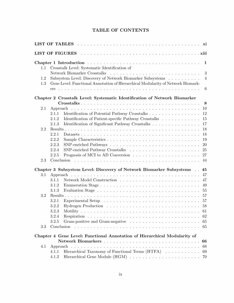
TABLE OF CONTENTS

LIST OF TABLES . . . . . . . . . . . . . . . . . . . . . . . . . . . . . . . . . . . . . . xi

LIST OF FIGURES . . . . . . . . . . . . . . . . . . . . . . . . . . . . . . . . . . . . . xiii

Chapter 1 Introduction . . . . . . . . . . . . . . . . . . . . . . . . . . . . . . . . . . . 11.1 Crosstalk Level: Systematic Identification of

Network Biomarker Crosstalks . . . . . . . . . . . . . . . . . . . . . . . . . . . . 31.2 Subsystem Level: Discovery of Network Biomarker Subsystems . . . . . . . . . . 41.3 Gene Level: Functional Annotation of Hierarchical Modularity of Network Biomark-

ers . . . . . . . . . . . . . . . . . . . . . . . . . . . . . . . . . . . . . . . . . . . . 6

Chapter 2 Crosstalk Level: Systematic Identification of Network BiomarkerCrosstalks . . . . . . . . . . . . . . . . . . . . . . . . . . . . . . . . . . . . . 8

2.1 Approach . . . . . . . . . . . . . . . . . . . . . . . . . . . . . . . . . . . . . . . . 102.1.1 Identification of Potential Pathway Crosstalks . . . . . . . . . . . . . . . . 122.1.2 Identification of Patient-specific Pathway Crosstalks . . . . . . . . . . . . 152.1.3 Identification of Significant Pathway Crosstalks . . . . . . . . . . . . . . . 17

2.2 Results . . . . . . . . . . . . . . . . . . . . . . . . . . . . . . . . . . . . . . . . . . 182.2.1 Datasets . . . . . . . . . . . . . . . . . . . . . . . . . . . . . . . . . . . . . 182.2.2 Sample Characteristics . . . . . . . . . . . . . . . . . . . . . . . . . . . . . 192.2.3 SNP-enriched Pathways . . . . . . . . . . . . . . . . . . . . . . . . . . . . 202.2.4 SNP-enriched Pathway Crosstalks . . . . . . . . . . . . . . . . . . . . . . 252.2.5 Prognosis of MCI to AD Conversion . . . . . . . . . . . . . . . . . . . . . 27

2.3 Conclusion . . . . . . . . . . . . . . . . . . . . . . . . . . . . . . . . . . . . . . . 44

Chapter 3 Subsystem Level: Discovery of Network Biomarker Subsystems . . 453.1 Approach . . . . . . . . . . . . . . . . . . . . . . . . . . . . . . . . . . . . . . . . 47

3.1.1 Network Model Construction . . . . . . . . . . . . . . . . . . . . . . . . . 473.1.2 Enumeration Stage . . . . . . . . . . . . . . . . . . . . . . . . . . . . . . . 493.1.3 Evaluation Stage . . . . . . . . . . . . . . . . . . . . . . . . . . . . . . . . 55

3.2 Results . . . . . . . . . . . . . . . . . . . . . . . . . . . . . . . . . . . . . . . . . . 573.2.1 Experimental Setup . . . . . . . . . . . . . . . . . . . . . . . . . . . . . . 573.2.2 Hydrogen Production . . . . . . . . . . . . . . . . . . . . . . . . . . . . . 583.2.3 Motility . . . . . . . . . . . . . . . . . . . . . . . . . . . . . . . . . . . . . 613.2.4 Respiration . . . . . . . . . . . . . . . . . . . . . . . . . . . . . . . . . . . 623.2.5 Gram-positive and Gram-negative . . . . . . . . . . . . . . . . . . . . . . 65

3.3 Conclusion . . . . . . . . . . . . . . . . . . . . . . . . . . . . . . . . . . . . . . . 65

Chapter 4 Gene Level: Functional Annotation of Hierarchical Modularity ofNetwork Biomarkers . . . . . . . . . . . . . . . . . . . . . . . . . . . . . . 66

4.1 Approach . . . . . . . . . . . . . . . . . . . . . . . . . . . . . . . . . . . . . . . . 684.1.1 Hierarchical Taxonomy of Functional Terms (HTFA) . . . . . . . . . . . 694.1.2 Hierarchical Gene Module (HGM) . . . . . . . . . . . . . . . . . . . . . . 70

ix

4.1.3 Assessing Statistical Significance . . . . . . . . . . . . . . . . . . . . . . . 734.1.4 Fuzzy Reconstruction of Hierarchical Modularity . . . . . . . . . . . . . . 74

4.2 Results . . . . . . . . . . . . . . . . . . . . . . . . . . . . . . . . . . . . . . . . . . 764.2.1 Benchmark Data and Tools . . . . . . . . . . . . . . . . . . . . . . . . . . 764.2.2 Functional Coherency of Protein Functional Modules . . . . . . . . . . . . 774.2.3 Functional Coherency of Protein Pairs . . . . . . . . . . . . . . . . . . . . 814.2.4 Inferred Hierarchy of Functional Modules . . . . . . . . . . . . . . . . . . 834.2.5 Effect of Fuzziness . . . . . . . . . . . . . . . . . . . . . . . . . . . . . . . 854.2.6 Choosing ωλ Value . . . . . . . . . . . . . . . . . . . . . . . . . . . . . . . 87

4.3 Conclusion . . . . . . . . . . . . . . . . . . . . . . . . . . . . . . . . . . . . . . . 87

Chapter 5 Conclusion and Future Work . . . . . . . . . . . . . . . . . . . . . . . . 895.1 Causative Network Biomarkers . . . . . . . . . . . . . . . . . . . . . . . . . . . . 905.2 Dynamic Network Biomarkers . . . . . . . . . . . . . . . . . . . . . . . . . . . . 905.3 Multi-phenotype Network Biomarkers . . . . . . . . . . . . . . . . . . . . . . . . 915.4 Prediction of Missing Values . . . . . . . . . . . . . . . . . . . . . . . . . . . . . . 91

References . . . . . . . . . . . . . . . . . . . . . . . . . . . . . . . . . . . . . . . . . . . . 92

x

LIST OF TABLES

Table 2.1 Subset of genes from CTD [30] and their association to Alzheimer’s disease 19Table 2.2 Baseline characteristics of MCI study sample . . . . . . . . . . . . . . . . 20Table 2.3 List of literature verified the pathways found in the study [139] . . . . . . . 22Table 2.4 Performance of models with baseline clinical parameters . . . . . . . . . . 31Table 2.5 Performance of models with baseline clinical parameters with ApoE . . . . 33Table 2.6 Performance of models with baseline clinical parameters and all imaging

(MRI, PET) and bio-specimen (CSF) biomarkers . . . . . . . . . . . . . . 35Table 2.7 Performance of models with baseline clinical parameters and PET biomarkers 35Table 2.8 Performance of models with baseline clinical parameters, PET, and CSF

biomarkers . . . . . . . . . . . . . . . . . . . . . . . . . . . . . . . . . . . . 37Table 2.9 Performance of models with baseline clinical parameters and ApoE with

all imaging (MRI, PET) and bio-specimen (CSF) biomarkers . . . . . . . . 38Table 2.10 Performance of models with clinical parameters and ApoE with PET

biomarker . . . . . . . . . . . . . . . . . . . . . . . . . . . . . . . . . . . . 39Table 2.11 Performance of models with clinical parameters and ApoE with PET and

CSF biomarkers . . . . . . . . . . . . . . . . . . . . . . . . . . . . . . . . . 39Table 2.12 Performance of Shaffer et al [158] model in comparison with 97 patients in

comparison to our model with 91 patients . . . . . . . . . . . . . . . . . . 41Table 2.13 Performance of Shaffer et al [158] model in comparison with 91 patients in

comparison to our model with 91 patients . . . . . . . . . . . . . . . . . . 42Table 2.14 Performance of models with randomized pathway crosstalk features . . . . 44

Table 3.1 Subsystem associated with light fermentation . . . . . . . . . . . . . . . . . 59Table 3.2 Subsystem associated with dark fermentation . . . . . . . . . . . . . . . . . 60Table 3.3 Subsystem associated with motility . . . . . . . . . . . . . . . . . . . . . . 62Table 3.4 Subsystem associated with aerobic respiration . . . . . . . . . . . . . . . . 63Table 3.5 Subsystem associated with anaerobic respiration . . . . . . . . . . . . . . . 63Table 3.6 Subsystem associated with gram-negativity . . . . . . . . . . . . . . . . . . 64Table 3.7 Subsystem associated with gram-positivity . . . . . . . . . . . . . . . . . . 65

Table 4.1 Statistical significance of protein pairs’ functional coherence in Saccha-romyces cerevisiae . . . . . . . . . . . . . . . . . . . . . . . . . . . . . . . . 67

Table 4.2 Functional modules evaluated using existing enrichment analysis tools incomparison with HMS. The first two rows show two homogeneous func-tional modules and the next two rows of the table show heterogeneousfunctional modules that have coherent submodules. Functional moduleshave been obtained from Chen and Yuan [22] of the Saccharomyces cere-visiae PPI network . . . . . . . . . . . . . . . . . . . . . . . . . . . . . . . 78

Table 4.3 Percentage of significant (p-value≤ 0.05) and highly significant (p-value≤0.001) functionally coherent modules from Chen and Yuan [22] and CYS2008[137] . . . . . . . . . . . . . . . . . . . . . . . . . . . . . . . . . . . . . . . 81

xi

Table 4.4 HMS results for some KEGG metabolic pathways and MIPS protein com-plexes [21] classified as insignificant by Chagoyen et al. [21] . . . . . . . . . 81

Table 4.5 Comparison of pair-wise semantic similarity metrics using functionally-associated and non-functional protein pairs . . . . . . . . . . . . . . . . . . 82

Table 4.6 Skill metrics for Saccharomyces cerevisiae KEGG experiments . . . . . . . 84Table 4.7 Skill metrics for Saccharomyces cerevisiae MIPS experiments . . . . . . . . 85Table 4.8 Consistency of multi-pathway genes across clusters that enrich the cor-

ressponding pathways . . . . . . . . . . . . . . . . . . . . . . . . . . . . . . 86

xii

LIST OF FIGURES

Figure 1.1 Hierarchical modularity of phenotype-related network biomarkers . . . . . 2

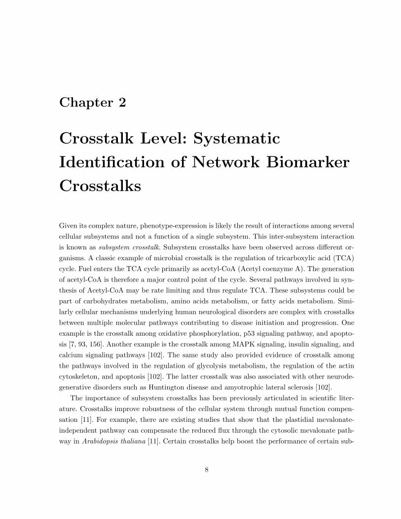
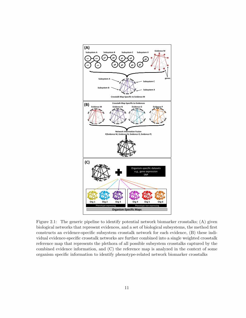
Figure 2.1 The generic pipeline to identify potential network biomarker crosstalks;(A) given biological networks that represent evidences, and a set of biolog-ical subsystems, the method first constructs an evidence-specific subsys-tem crosstalk network for each evidence, (B) these individual evidence-specific crosstalk networks are further combined into a single weightedcrosstalk reference map that represents the plethora of all possible sub-system crosstalks captured by the combined evidence information, and(C) the reference map is analyzed in the context of some organism spe-cific information to identify phenotype-related network biomarker crosstalks 11

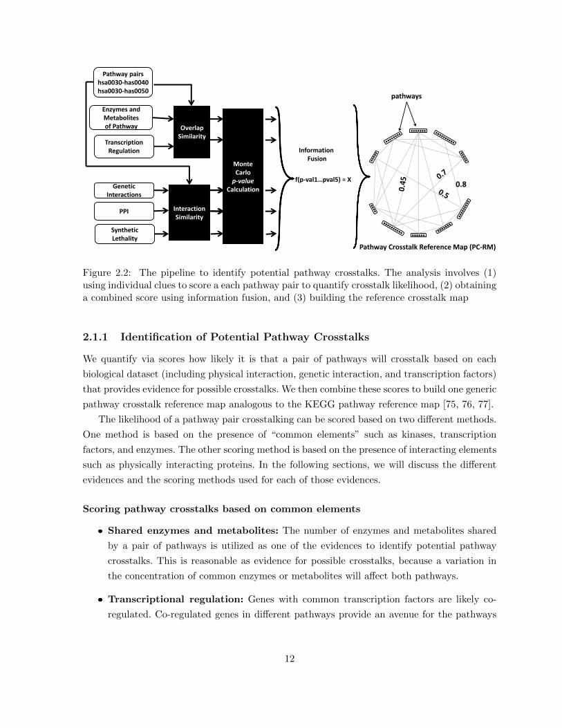
Figure 2.2 The pipeline to identify potential pathway crosstalks. The analysis in-volves (1) using individual clues to score a each pathway pair to quantifycrosstalk likelihood, (2) obtaining a combined score using informationfusion, and (3) building the reference crosstalk map . . . . . . . . . . . . . 12

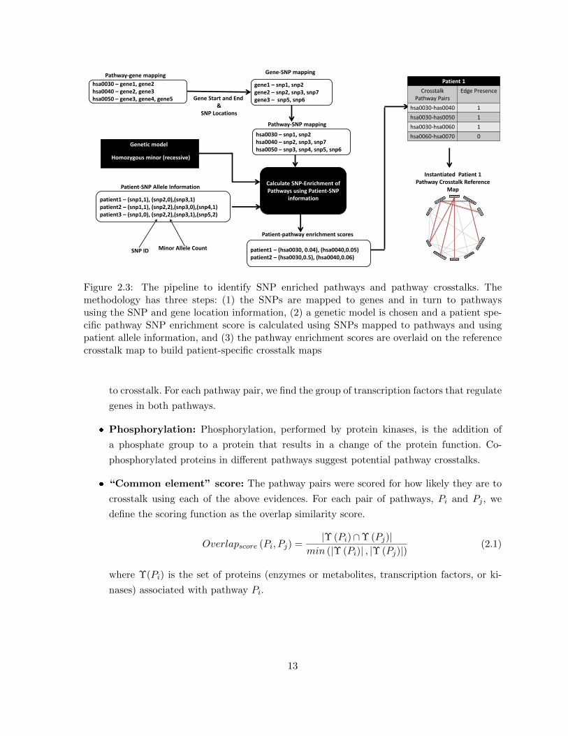
Figure 2.3 The pipeline to identify SNP enriched pathways and pathway crosstalks.The methodology has three steps: (1) the SNPs are mapped to genes andin turn to pathways using the SNP and gene location information, (2) agenetic model is chosen and a patient specific pathway SNP enrichmentscore is calculated using SNPs mapped to pathways and using patientallele information, and (3) the pathway enrichment scores are overlaid onthe reference crosstalk map to build patient-specific crosstalk maps . . . . 13

Figure 2.4 Pie chart showing the distribution of types of SNP-enriched pathwaysidentified in the study and comparison to KEGG pathway distribution . . 21

Figure 2.5 Alzheimer’s disease pathway crosstalk: pathways found to have signifi-cant crosstalk with the AD pathway fall into KEGG categories includingHuman Diseases, Environmental Information Processing, Genetic Infor-mation Processing, Cellular Processes, Metabolism, and Organismal Sys-tems. Specific KEGG pathway types are listed below each category, andthe number of occurrences is listed in parentheses. . . . . . . . . . . . . . 27

Figure 3.1 Methdology overview to identify and evaluate phenotype-related networkbiomarker subsystems . . . . . . . . . . . . . . . . . . . . . . . . . . . . . 47

Figure 3.2 Three step building of the orthologous-group organism bipartite network . 49Figure 3.3 Enumeration of conserved edge-sets using maximal biclique subgraph model 50Figure 3.4 Parameter-free biclique enumerator. (A) An example graph, (B) Repre-

sentative selection, and (C) The search tree for the example graph . . . . 53Figure 3.5 Extracting the potential phenotype-related modules from the enumerated

maximal bicliques . . . . . . . . . . . . . . . . . . . . . . . . . . . . . . . 56

Figure 4.1 Overview of the methodology to assess functional coherence and assignannotation to hierarchical functional modules . . . . . . . . . . . . . . . . 68

Figure 4.2 Overview of fuzzy reconstruction of hierarchical modularity . . . . . . . . 69

xiii

Figure 4.3 Hierarchical functional annotation of a gene module M for a gene setG = {g1, g2, g3, g4} given the taxonomy T in Figure 4.4. (A) Functionalannotation of genes in G by unrelated term sets in T , (B) A hierarchicalgene module M , and (C) The resulting annotation of the internal (non-leaf) nodes in V (M) . . . . . . . . . . . . . . . . . . . . . . . . . . . . . . 71

Figure 4.4 An illustration of a hierarchical taxonomy T over the set of functionalannotation terms A = {t0, t1, t2, t3, t4, t5}. (A) A DAG view and (B) Alevel set view . . . . . . . . . . . . . . . . . . . . . . . . . . . . . . . . . . 72

Figure 4.5 llustration of penalization factor calculation. (A) Hierarchical annotationof the functional module defined in Figure 7 and (B) Dissimilarity scoreψ(p, c) for a parent p = v and a child c = g1 . . . . . . . . . . . . . . . . . 73

Figure 4.6 Comparison between the three penalization factor functions considered . . 74Figure 4.7 Functionally coherent modules from the Chen and Yuan [22] study. (A)

Module ID M1 and (B) Module ID M3 . . . . . . . . . . . . . . . . . . . . 77Figure 4.8 Functional coherence analysis of protein complexes from MIPS-curated

[52], Ho [62], Gavin [41], and Krogan [91] as well as metabolic pathwaysfrom KEGG. Comparison between our HMS scoring, cosine similaritywith different -value methods from [21], Jaccard similarity with differentvalue methods from [21] and GS2 [146] methods. (A) Significant Modules(p-value ≤ 0.05 and (B) Highly Significant Modules (p-value≤ 0.001) . . . 80

Figure 4.9 Effect of different values of ωλ on the SHMS() score . . . . . . . . . . . . . 87

xiv

Chapter 1

Introduction

Biomarker discovery and characterization have been an important area of research in the re-

cent past. Biomarkers help differentiate organisms that possess certain characteristics from the

organisms that do not exhibit the characteristics. Examples of characteristics include bioenergy

related characteristics, such as bioethanol production, biohydrogen production, and acid toler-

ance. Examples of characteristics also include human diseases, such as Alzheimer’s, cancer, or

diabetes. The term for these biological characteristics is phenotypes.

Biomarker discovery is extremely important in many areas of research. Biomarkers related to

phenotypes such as bioethanol production and biohydrogen production are useful in improving

the efficiency of many industrial processes. Similarly, biomarkers related to uranium reduction

phenotype can assist in uranium decontamination of soil and water, because uranium takes

hundreds of millions of years to decay radioactively. Biomarkers can also improve the accuracy

of disease prognostics and support development of more effective drugs.

Traditionally, biomarker discovery has revolved around searching for individual genes or

gene sets that are linked to phenotype presence [46, 72, 89, 163, 172] (see also [4], our review

of biomarker discovery for neurological disorder phenotypes). However, genes do not function

individually but work together with other genes to carry out various functions in an organism.

Biological networks (e.g., genetic interaction networks) capture inter-gene relationships,

where the nodes are genes (or gene sets) and the edges represent some functional associa-

tion between the genes (or gene sets). Hence, the biomarker discovery space is moving towards

utilizing these networks for unearthing biomarkers. These biomarkers are known as network

biomarkers.

Network biomarkers are discovered in an unsupervised fashion, where the problem is to

discover discriminatory subnetworks between biological networks for organisms that exhibit the

target phenotype and those biological networks for organisms that do not exhibit the phenotype

[26, 46, 47, 60, 61, 72, 89, 97, 152, 153, 163, 172, 198]. Such signature subnetworks are assumed

1

to be functionally coherent, or forming functional modules, with respect to the function that

is critical to the target phenotype. Moreover, these functionally coherent modules combine in

a hierarchical manner into larger, less cohesive subsystems, thus revealing one of the essential

design principles of system-level cellular organization and function—hierarchical modularity

[58, 108, 140, 164].

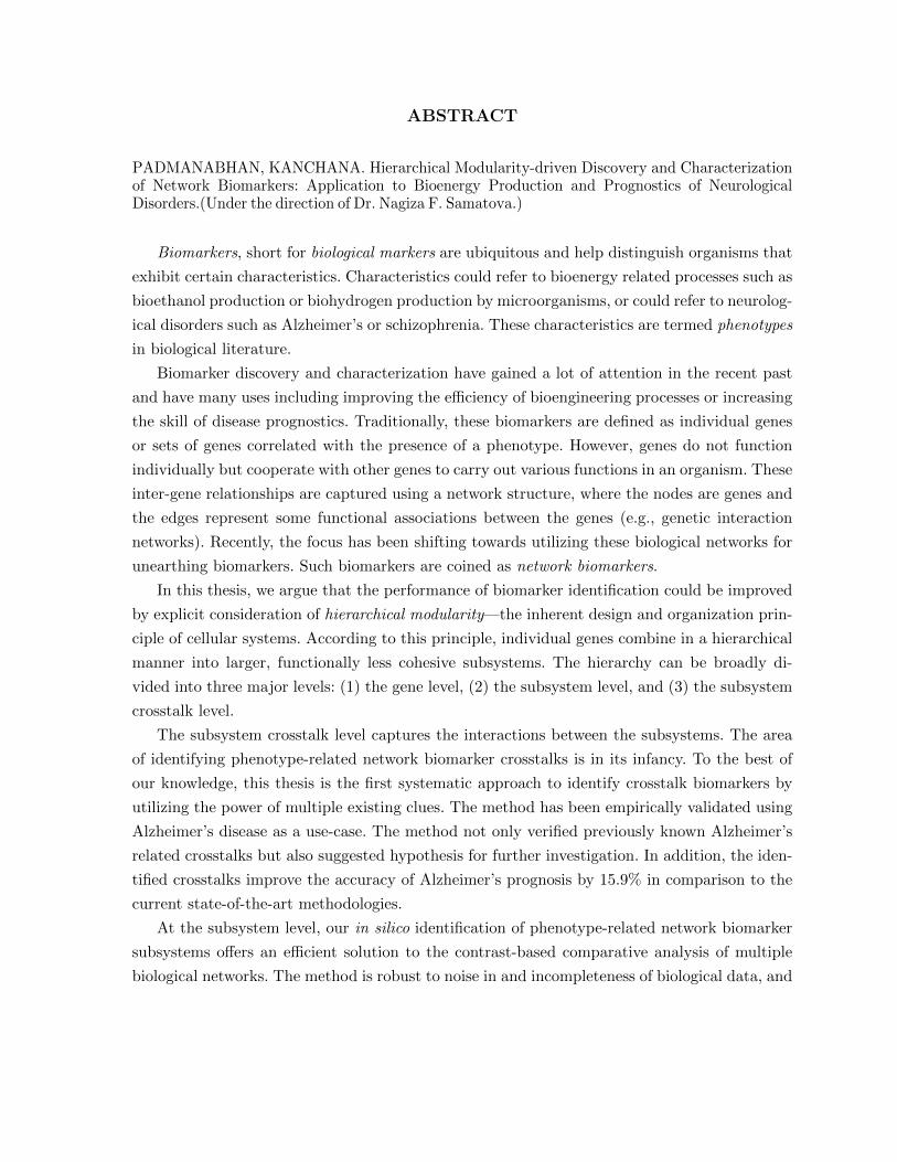
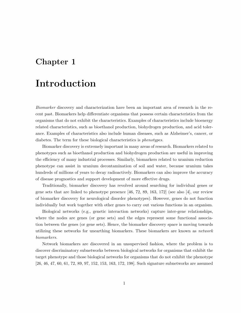
Figure 1.1 illustrates this concept of hierarchical modularity in cellular systems, using three

major levels of abstraction: (1) the gene level, (2) the subsystem level, and (3) the subsystem

crosstalk level. Such hierarchical modularity of complex systems has several benefits especially

from the evolutionary adaptation point of view [108]. Examples of such hierarchical organization

with respect to biohydrogen production phenotype include functionally coherent modules de-

rived from transcriptome data related to electron transport (fixX, fixC, fixB, fixA, ferN, fer1 ),

co-factor synthesis (nifB, nifV, nifQ, nifN, nifE, nifX ), assembly or stability (nifW, nifS2,

nifU ), and regulation (nifA) in Rhodopseudomonas palustris [142]. Likewise, the CD4+ T-cell

modules involved in human immune protection and regulation are hierarchically organized and

are made up of polarizing cues, lineage-specifying transcription factors, homing receptors, and

effector molecules [148].

g3 g4 g5 g6 g1 g2

g3

g4

g1

g2 g5

g6

g3

g4

g1

g2 g5

g6

Individual Gene Level

Subsystem Level

Crosstalk Level

Network Biomarker Functional Annotation (using individual genes & their functional roles)

Network Biomarker Subsystems (functionally associated genes)

Network Biomarker Crosstalks (interacting subsystems)

Figure 1.1: Hierarchical modularity of phenotype-related network biomarkers

With this perspective of phenotype-centric hierarchical modularity, the central hypothesis of

this thesis is the following:

Phenotype-centric hierarchical-modularity driven network biomarker discovery and analysis

will enhance the performance of phenotype-related biomarker identification and improve

phenotype diagnostics and prognostics using such biomarkers

2

Motivated by this hypothesis we focus each component of this thesis towards one level of the

hierarchical modularity, depicted in Fig 1.1.

1.1 Crosstalk Level: Systematic Identification of

Network Biomarker Crosstalks

Phenotype-expression in an organism is extremely complex and it is likely that not a single

cellular subsystem such as the ones identified at the subsystem level, but a group of subsystems

interact to help express a particular phenotype. This inter-subsystem interaction has been

coined as subsystem crosstalk. Crosstalks useful in improving our understanding of phenotype

expression are termed crosstalk biomarkers. For example, the human neurological disorders are

complex and characterized by crosstalks among multiple molecular pathways contributing to

disease initiation and progression. One example is the crosstalk among AD pathway, oxidative

phosphorylation, p53 signaling pathway, and apoptosis [7, 93, 156]. Drug developers are now

focusing on understanding the interactions between the multiple key pathways that are affected

as a result of these diseases [101], because the previous one-target, one-drug approach is not

successful for diseases, such as Alzheimer’s and cancer.

To the best of our knowledge, there has been no systematic computational study of crosstalk

biomarkers. There are several different “clues” for crosstalk prediction including synthetic lethal-

ity, phosphorylation, genetic interaction, genes common between subsystems, etc. Incorporating

different clues will likely improve the confidence of crosstalk predictions. However, the computa-

tional methodologies developed so far [102, 122] make use of only one kind of “clue” to identify

crosstalks between phenotype related subsystems identified at the subsystem level. A method-

ology that includes multiple clues simultaneously will likely help identify crosstalks that are

biologically more meaningful.

Besides contributing to mechanistic understanding, crosstalks could likely be important

features for phenotype prediction as well. However, to the best of our knowledge, crosstalk

biomarkers as features for phenotype prediction, especially, for disease prognosis has not be

investigated in-depth.

Approach

We propose a methodology to identify subsystem crosstalk biomarkers and show their utility in

phenotype prediction. Given biological networks that represent evidences such as protein inter-

action and genetic interaction, and a set of biological subsystems, the method first constructs

an evidence-specific subsystem crosstalk network for each evidence. These individual evidence-

specific crosstalk networks are then combined into a single weighted crosstalk reference map

3

that represents the plethora of all possible subsystem crosstalks captured by the combined

evidence information.

In order to identify phenotype related crosstalks, these reference maps have to be analyzed in

the context of some organism specific information. This is done by choosing a target phenotype

and a set of organisms and instantiating the crosstalk reference map with information specific

to each organism (e.g., gene expression datasets, single nucleotide polymorphism datasets).

These instantiated organism-specific crosstalk maps are then comparatively analyzed to identify

crosstalk network biomarkers. These biomarkers are then further utlized as additional features

in phenotype prediction or disease prognosis.

Results and Impact

In this study, we utilize biological subsystems that model biological pathways, i.e., the nodes of

the crosstalk reference map are pathways. We have developed a methodology to build a pathway

crosstalk reference map using the combined power of several protein/gene level evidences. We

also identified pathway crosstalks that are potential features for phenotype prediction.

Our methodology was tested on the human disease phenotype, Alzheimer’s disease. Specif-

ically, the problem of interest is to predict which of the patients with condition known as mild

cognitive impairement (MCI) will progress to Alzheimer’s disease (AD).

The method captured the well documented crosstalks associated with oxidative damage and

insulin resistance cause metabolic dysfunction in AD. A temporal three-part sequence occurs

with changes in glycolysis, the tricarboxylic acid cycle (TCA) and oxidative phosphorylation

pathways [160]. The method also found several neural cell adhesion pathways supported by

previous research indicating that these pathways might be involved in this disease process [139].

Since AD is a neurodegenerative disease, we also observed nervous system related pathways; in

particular, enrichment of long-term potentiation and depression and neurotransmitter signaling

pathways all support our process given that these pathways have been previously associated

with cognitive impairment and AD [24, 37, 96, 171].

Pathway crosstalks incorporated as additional features for MCI to AD conversion prediction,

improved the accuracy by 15.9% in comparison to the best predictive model of the current state-

of-the-art [158].

1.2 Subsystem Level: Discovery of Network Biomarker Subsys-

tems

Information about the cellular system of an organism can be represented as a network. For

example, gene functional association networks model the cellular system using genes as nodes

4

and edges representing a functional association between the genes. These organismal networks

are comparatively analyzed to identify subsystems that could be potentially associated with a

phenotype, also known as subsystem network biomarkers or simply subsystem biomarkers.

The current state of the art α, β−motif finder [152] algorithm identifies subsystem biomark-

ers modeled as cliques (completely connected subgraphs) that are present in at least α-phenotype

expressing organisms and no more than β phenotype non-expressing organisms (where α is cho-

sen to be greater than β). However, due to the noise and missing information inherent to real

world networks, cellular subsystems are not always cliques (cliques have a density of 1.0—

where density ratio of the number of edges in the subnetwork to the total number of edges the

subnetwork would have if every pair of vertices in the subnetwork were connected)[54].

Additionally, selecting α and β parameters that will produce biologically meaningful results

could be a hard problem to solve. Hence, several runs of the algorithm with varying parameters

would be required to identify all the potential phenotype-related subsystem biomarkers.

Comparative analysis methods to identify phenotype-related subsystem biomarkers typically

work under the assumption that subsystems more likely to be present in phenotype-expressing

organisms are responsible for phenotype-expression. However, it is possible that the absence

of a subsystem causes the phenotype. For example, it was shown that the “couched potato”

syndrome could be potentially caused by the result of a person missing some key genes related

to the MP-activated protein kinase (AMPK) [179]. For α, β-motif finder to identify this kind of

information would require reruns of the algorithms by reversing the phenotype-expressing and

non-expressing organisms and once again the choice of parameters would come into play.

A straightforward approach of enumerating subsystem biomarkers of all densities (0.1−1.0)

present in all subsets of organisms and determining which of those are specifically present or ab-

sent in the networks of phenotype-expressing organisms would be computationally intractable

due to the potential number of subsystems in each network. The goal of this study is to enu-

merate phenotype-related subsystem biomarkers placing no restriction on the density or size of

the enumerated subgraphs. The method also does not place any restriction on the number of

networks the resulting biomarker should be present in.

Approach

Given functional association networks of the target organisms for the phenotype of interest,

our method first combines these networks into the proposed orthologous group-pair, organism

bi-partite network. This network model is utilized for enumerating the phenotype-related net-

work biomarkers at the subsystem level. Unlike our earlier work, the current-state-of-the-art

α, β-motif finder that needs the α and β parameters to identify the subsystem level network

biomarkers, our method is parameter free. In addition, the method can identify biomarkers

5

biased towards both phenotype-expressing organisms and phenotype non-expressing organisms

using a single run of the method in contrast to the existing method that requires two passes.

Moreover, an identified network biomarkers corresponds to a more relaxed representation of a

cellular subsystem in comparison to the highly rigid clique representation used by α, β-motif

finder. These subsystems, as subgraphs, have topological density ranging from 0.1 to 1.0, unlike

cliques. Hence, the method is more robust at handling the inherent noise and missing infor-

mation in the input networks. We use a statistical method to calculate for each biomarker a

p−value quantifying its bias towards both the phenotype-expressing organisms and phenotype

non-expressing organisms.

Results and Impact

We developed a method to enumerate phenotype-related subsystem biomarkers taking into

consideration lessons learned from our earlier α, β-motif finder method, which is the current-

state-of-the-art. The methodology was tested on data for a number of phenotypes including

hydrogen production, gram stain, motility, and respiration. The results show that in each case

the method identified subsystems associated with the phenotypes that can be verified by lit-

erature. For example, for dark fermentation, we identified literature verified subsystems either

directly or indirectly responsible for the uptake or production of hydrogen; subsystems that in-

clude proteins associated with to the synthesis or expression of [NiFe]-hydrogenase, an enzyme

that catalyzes the reversible oxidation of molecular hydrogen, and plays a vital role in anaer-

obic metabolism [159]; the others are involved in nitrogen and iron metabolic pathways that

include proteins like nitrogenase, iron uptake proteins, ammonia assimilation proteins, such as

glutamine synthetase, and proteins involved in electron transfer.

The methodology is not confined to the biology domain alone but has applications in other

areas. For example, we adopted this methodology for anomaly detection is time-evolving climate

networks [25].

This work is published in [129].

1.3 Gene Level: Functional Annotation of Hierarchical Modu-

larity of Network Biomarkers

Computationally enumerated phenotype-related network biomarkers are further evaluated for

biological significance. This analysis helps identify results that are biologically meaningful. Bi-

ological significance analysis includes assigning a functional coherence score to quantify the

significance and a functional annotation denoting the biological function of the gene set con-

stituent of the network biomarker. Functional annotation methods assign a set of functional

6

terms to the gene set. The terms come from a semantic functional taxonomy that documents all

possible functions of genes in a cell. Arguably, hierarchical modularity has not been explicitly

taken into consideration by most, if not all, current methodologies. As a result, the existing

methods would often fail to assign a statistically significant coherence score to biologically

relevant molecular machines. The goal of this study is to develop a methodology to analyze

gene sets for functional coherence and assign functional annotation by explicitly taking into

consideration the hierarchical modularity principle.

Approach

Given the hierarchical taxonomy of functional concepts (e.g., Gene Ontology) and the associa-

tion of individual genes to these concepts (e.g., GO terms), our method will assign a proposed

Hierarchical Modularity Score (HMS) to each node in the hierarchical structure of the gene set;

the HMS score and its p−value measure functional coherence. While existing methods annotate

each network biomarker with a set of “enriched” functional terms in a bag of genes, our com-

plementary method provides the hierarchical functional annotation of the modules and their

hierarchically organized components. A hierarchical organization of the gene set often comes as

a bi-product of cluster analysis of gene expression data or protein interaction data. Otherwise,

our method will automatically build such a hierarchy by directly incorporating the functional

taxonomy information into the hierarchy search process and by allowing multi-functional genes

to be part of more than one component in the hierarchy. In addition, the underlying HMS scoring

metric ensures that functional specificity of the terms across different levels of the hierarchical

taxonomy is properly treated.

Results and Impact

We developed a method to assess biological significance (functional coherence and annotation)

of gene sets taking into consideration their hierarchical modularity. The method shows an

improved performance (on average 15%) in comparison to the current state-of-the-art functional

coherence and annotation analysis methods when evaluated on known functionally coherent

gene sets from KEGG [75, 76, 77] and MIPS [52] and several other computationally derived

and curated datasets [22, 41, 62, 91, 137]. The use of this methodology is not confined to

the biology domain alone but is useful in other areas where such hierarchical annotations are

required. For example, semantic text analysis uses hierarchical taxonomies (e.g., WordNet) to

annotate and analyze text for topical similarity of its components.

This work has been published in [128].

7

Chapter 2

Crosstalk Level: Systematic

Identification of Network Biomarker

Crosstalks

Given its complex nature, phenotype-expression is likely the result of interactions among several

cellular subsystems and not a function of a single subsystem. This inter-subsystem interaction

is known as subsystem crosstalk. Subsystem crosstalks have been observed across different or-

ganisms. A classic example of microbial crosstalk is the regulation of tricarboxylic acid (TCA)

cycle. Fuel enters the TCA cycle primarily as acetyl-CoA (Acetyl coenzyme A). The generation

of acetyl-CoA is therefore a major control point of the cycle. Several pathways involved in syn-

thesis of Acetyl-CoA may be rate limiting and thus regulate TCA. These subsystems could be

part of carbohydrates metabolism, amino acids metabolism, or fatty acids metabolism. Simi-

larly cellular mechanisms underlying human neurological disorders are complex with crosstalks

between multiple molecular pathways contributing to disease initiation and progression. One

example is the crosstalk among oxidative phosphorylation, p53 signaling pathway, and apopto-

sis [7, 93, 156]. Another example is the crosstalk among MAPK signaling, insulin signaling, and

calcium signaling pathways [102]. The same study also provided evidence of crosstalk among

the pathways involved in the regulation of glycolysis metabolism, the regulation of the actin

cytoskeleton, and apoptosis [102]. The latter crosstalk was also associated with other neurode-

generative disorders such as Huntington disease and amyotrophic lateral sclerosis [102].

The importance of subsystem crosstalks has been previously articulated in scientific liter-

ature. Crosstalks improve robustness of the cellular system through mutual function compen-

sation [11]. For example, there are existing studies that show that the plastidial mevalonate-

independent pathway can compensate the reduced flux through the cytosolic mevalonate path-

way in Arabidopsis thaliana [11]. Certain crosstalks help boost the performance of certain sub-

8

systems. The Mitogen-activated protein kinase (MAPK) pathway enhances the signaling in the

Integrin pathway by increasing the activation rate of key proteins in the Integrin pathway [155].

MAPK also alters transcription of genes that are important to other metabolic pathways by

altering the levels and activities of transcription factors.

There is no universal categorization of biological mechanisms that are responsible for crosstalks

but some attempts have been made to model certain pathway crosstalks. Mathematical mod-

els have been developed to study signaling pathway crosstalks [32]. The different models are

the signal flow, substrate availability, receptor function, gene expression, and intracellular com-

munication. Signal flow crosstalk between two pathways occurs when the molecules of one

pathway affect the rate of protein activation in another pathway. For example, MAPK pathway

enhances the signaling in the Integrin pathway by increasing the activation rate of key pro-

teins in the Integrin pathway [155]. Substrate availability crosstalk occurs when two pathways

compete for proteins that perform the same function. For example, the hyperosmolar pathway

and pheromone mitogen-activated protein (MAP) kinase pathway in Saccharomyces cerevisiae

share the STE11 protein [111]. Receptor function crosstalk occurs when the pathway receptor

can be activated by factors other than its target ligands. For example, in the absence of the es-

trogen ligand, other signaling pathways can activate the estrogen receptor [80]. Gene expression

crosstalk occurs when a transcription factor (TF) contained in one pathway represses another

TF activated through a second pathway. For example, the transcription factor NR3C1 relocates

to the nucleus upon activation and represses the transcription factor NF-kB that is present in

multiple pathways. Intracellular communication crosstalk occurs when a ligand released by a

pathway activates another pathway. For example, the Bone morphogenetic proteins (BMP) and

WNT pathways reciprocally regulate the production of their ligands [12]. There has also been

a study on the interactions between different biological processes defined by the Gene Ontology

taxonomy in Saccharomyces cerevisiae [33].

Crosstalks can also be potential biomarkers for phenotype prediction or disease prognosis,

also called network biomarker crosstalks. Diseases such as cancer, diabetes, obesity, and asthma

are caused by defects in multiple pathways [69, 23, 99]. Drug developers are focusing on the

interactions between multiple key pathways that are affected as a result of these diseases [102],

because the previous one-target, one-drug approach has not been particularly successful for

diseases such as cancer.

For phenotypes such as Alzheimers disease (AD), a variety of features have been tested for

disease prognosis: imaging data such as structural magnetic resonance imaging (MRI), fluorine

18 flurodeoxyglucose positron emission tomography (PET), and bio-specimen samples such

as cerebrospinal fluid (CSF). Clinical parameters including neurological cognitive tests such

as the Alzheimer’s disease Assessment Scale-Cognitive subscale with 70-point scale (ADAS-

cog) and age, gender, education, etc., have been tested as well. However, to the best of our

9

knowledge, utilizing biomarker crosstalks as potential features for disease prognostics has not

be investigated in-depth. (In the following sections the MRI, PET, and CSF features may also

be referred together as AD biomarkers.)

From the computational methodology standpoint we find that the area of network biomarker

crosstalks is still in its infancy. Molecular level interactions (functional associations between

genes or interactions between proteins) can act as “clues” to predict potential crosstalks [33].

Molecular level interactions are better studied in comparison to inter-subsystem crosstalks that

are ubiquitous, yet poorly understood. There are several documented mechanisms for molec-

ular interactions. These mechanisms (clues) include physical evidences such as direct binding,

biochemical evidences such as phosphorylation, and functional evidences such as transcrip-

tional regulation [101]. However, we find that existing computational methods that attempt to

predict crosstalks do not take advantage of the different “clues” available. Existing methods

predicts crosstalk between known metabolic pathways using physical protein interaction data

[102, 122, 192]. Besides improving mechanistic understanding, biomarker crosstalks are likely

to worth investigating as features for phenotype diagnostics and prognostics.

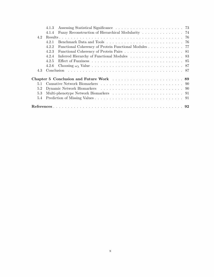
In this chapter, we provide a three-part methodology for network biomarker crosstalks dis-

covery. The methodology (see Figure 2.1) performs the following steps; (A) Given biological

networks that represent evidences and a set of biological subsystems, the method first con-

structs an evidence-specific subsystem crosstalk network for each evidence, (B) These individ-

ual evidence-specific crosstalk networks are further combined into a single weighted crosstalk

reference map that represents the plethora of all possible subsystem crosstalks captured by the

combined evidence information, and (C) The reference map is analyzed in the context of some

organism specific information to identify phenotype-related network biomarker crosstalks that

are further incorporated in prognostic models.

2.1 Approach

In this study, we utilize cellular subsystems that model biological pathways. Henceforth in

this chapter we will refer to a cellular subsystem as a pathway. We utilize the human disease

phenotype Alzheimer’s disease, as our use-case. The pipeline specific to our use-case are shown

in Figures 2.2 and 2.3.

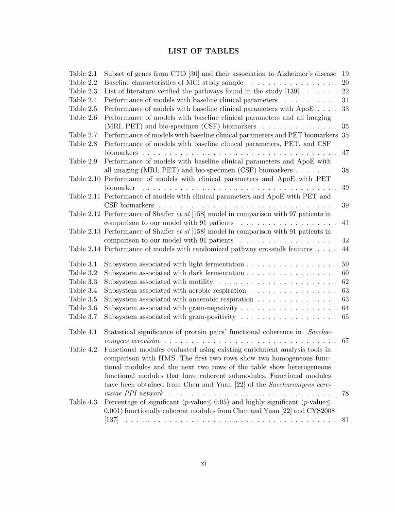
Specifically, our methodology consists of the following steps: (A) identify the potential path-

way crosstalks by using existing gene/protein level data (see Figure 2.2), (B) identify per-patient

pathway crosstalks via SNP information (see Figure 2.3), and (C) identify the significant path-

way crosstalks that will be combined with other imaging (MRI, PET) and bio-specimen (CSF)

biomarkers and clinical parameters for AD prognosis.

10

g8

g9

g7

g5

g6

Subsystem A Subsystem B

g3

g4

g1

g2

g12

g14

g11

g13

Subsystem C Subsystem X

Subsystem A

Subsystem B

Subsystem C

Subsystem X

genes

Evidence M

Crosstalk Map Specific to Evidence M

(A)

Organism-Specific Maps

Phenotype-expressing Phenotype non-expressing

Organism-specific datasets e.g., gene expression

SNP

Org 1 Org 2 Org 3 Org 4 Org 5 Org 6

(C)

Crosstalk Map Specific to Evidences

Network Information Fusion F(Evidence M, Evidence N, Evidence O, Evidence P)

(B) Evidence M Evidence N Evidence O Evidence P

Figure 2.1: The generic pipeline to identify potential network biomarker crosstalks; (A) givenbiological networks that represent evidences, and a set of biological subsystems, the method firstconstructs an evidence-specific subsystem crosstalk network for each evidence, (B) these indi-vidual evidence-specific crosstalk networks are further combined into a single weighted crosstalkreference map that represents the plethora of all possible subsystem crosstalks captured by thecombined evidence information, and (C) the reference map is analyzed in the context of someorganism specific information to identify phenotype-related network biomarker crosstalks

11

Enzymes and Metabolites of Pathway

Transcription Regulation Information

Fusion

Synthetic Lethality

f(p-val1…pval5) = X

Pathway pairs hsa0030-has0040 hsa0030-has0050

Genetic Interactions

PPI

Overlap Similarity

Interaction Similarity

Monte Carlo

p-value Calculation

pathways

Pathway Crosstalk Reference Map (PC-RM)

0.8

Figure 2.2: The pipeline to identify potential pathway crosstalks. The analysis involves (1)using individual clues to score a each pathway pair to quantify crosstalk likelihood, (2) obtaininga combined score using information fusion, and (3) building the reference crosstalk map

2.1.1 Identification of Potential Pathway Crosstalks

We quantify via scores how likely it is that a pair of pathways will crosstalk based on each

biological dataset (including physical interaction, genetic interaction, and transcription factors)

that provides evidence for possible crosstalks. We then combine these scores to build one generic

pathway crosstalk reference map analogous to the KEGG pathway reference map [75, 76, 77].

The likelihood of a pathway pair crosstalking can be scored based on two different methods.

One method is based on the presence of “common elements” such as kinases, transcription

factors, and enzymes. The other scoring method is based on the presence of interacting elements

such as physically interacting proteins. In the following sections, we will discuss the different

evidences and the scoring methods used for each of those evidences.

Scoring pathway crosstalks based on common elements

� Shared enzymes and metabolites: The number of enzymes and metabolites shared

by a pair of pathways is utilized as one of the evidences to identify potential pathway

crosstalks. This is reasonable as evidence for possible crosstalks, because a variation in

the concentration of common enzymes or metabolites will affect both pathways.

� Transcriptional regulation: Genes with common transcription factors are likely co-

regulated. Co-regulated genes in different pathways provide an avenue for the pathways

12

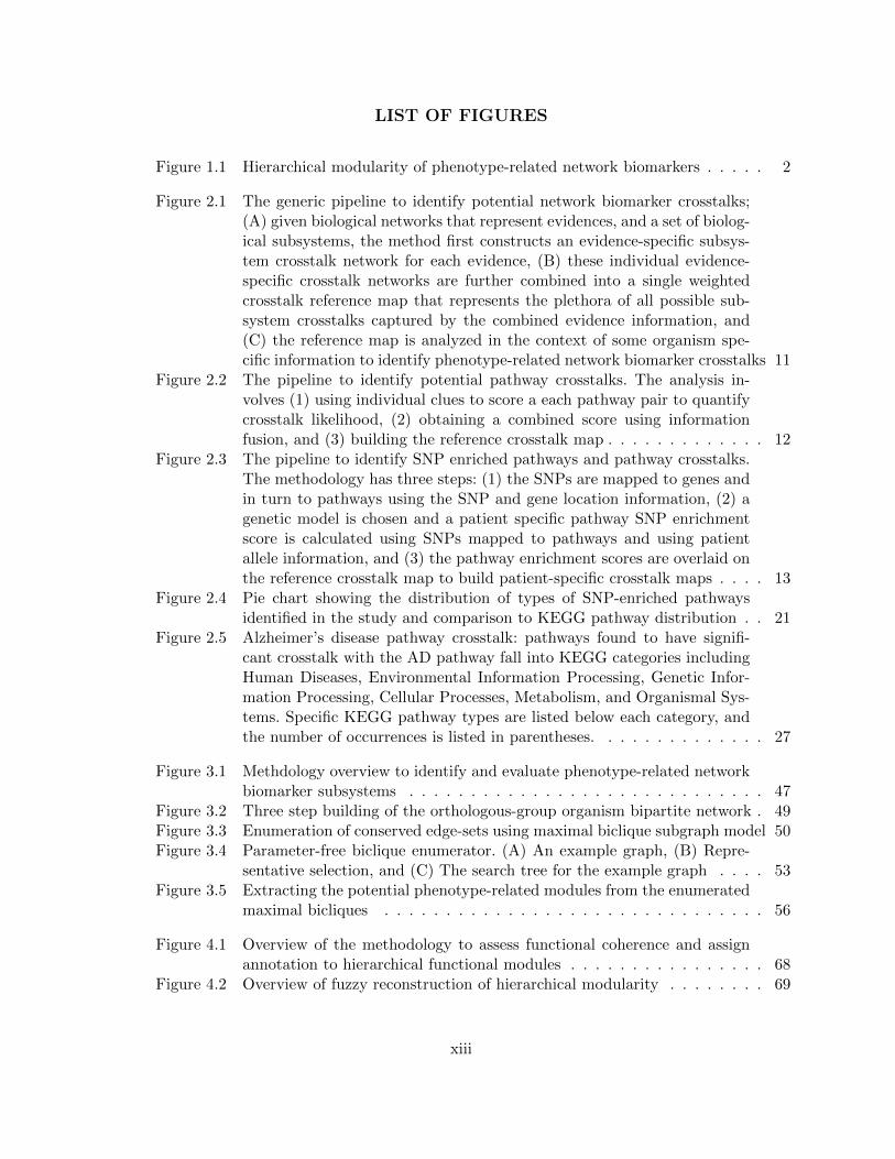
hsa0030 – gene1, gene2 hsa0040 – gene2, gene3 hsa0050 – gene3, gene4, gene5 Gene Start and End

& SNP Locations

hsa0030 – snp1, snp2 hsa0040 – snp2, snp3, snp7 hsa0050 – snp3, snp4, snp5, snp6

patient1 – (snp1,1), (snp2,0),(snp3,1) patient2 – (snp1,1), (snp2,2),(snp3,0),(snp4,1) patient3 – (snp1,0), (snp2,2),(snp3,1),(snp5,2)

Pathway-gene mapping

Pathway-SNP mapping

Patient-SNP Allele Information

SNP ID Minor Allele Count

Calculate SNP-Enrichment of Pathways using Patient-SNP

information

patient1 – (hsa0030, 0.04), (hsa0040,0.05) patient2 – (hsa0030,0.5), (hsa0040,0.06)

Patient-pathway enrichment scores

gene1 – snp1, snp2 gene2 – snp2, snp3, snp7 gene3 – snp5, snp6

Gene-SNP mapping

Homozygous minor (recessive)

Genetic model

Instantiated Patient 1 Pathway Crosstalk Reference

Map

Patient 1

Crosstalk Pathway Pairs

Edge Presence

hsa0030-has0040 1

hsa0030-has0050 1

hsa0030-hsa0060 1

hsa0060-hsa0070 0

Figure 2.3: The pipeline to identify SNP enriched pathways and pathway crosstalks. Themethodology has three steps: (1) the SNPs are mapped to genes and in turn to pathwaysusing the SNP and gene location information, (2) a genetic model is chosen and a patient spe-cific pathway SNP enrichment score is calculated using SNPs mapped to pathways and usingpatient allele information, and (3) the pathway enrichment scores are overlaid on the referencecrosstalk map to build patient-specific crosstalk maps

to crosstalk. For each pathway pair, we find the group of transcription factors that regulate

genes in both pathways.

� Phosphorylation: Phosphorylation, performed by protein kinases, is the addition of

a phosphate group to a protein that results in a change of the protein function. Co-

phosphorylated proteins in different pathways suggest potential pathway crosstalks.

� “Common element” score: The pathway pairs were scored for how likely they are to

crosstalk using each of the above evidences. For each pair of pathways, Pi and Pj , we

define the scoring function as the overlap similarity score.

Overlapscore (Pi, Pj) =|Υ (Pi)∩Υ (Pj)|

min (|Υ (Pi)| , |Υ (Pj)|)(2.1)

where Υ(Pi) is the set of proteins (enzymes or metabolites, transcription factors, or ki-

nases) associated with pathway Pi.

13

Scoring pathway crosstalks based on interacting elements

� Physical interaction: Protein interaction has previously been used to identify crosstalks

[102, 101] in yeast. The physical interaction between the proteins belonging to different

pathways provides a way for pathways to crosstalk.

� Genetic interactions: The use of genetic interactions for identifying pathway crosstalk

stems from the concept of “between-pathway” interactions. This essentially states that if

there is a genetic interaction between pathways, one pathway covers for the defects in the

other pathway.

� Protein domain: Protein function is closely related to fundamental units of protein

structure called “domains.” In the domain interaction network, a pair of proteins has an

edge if they are associated with the same set of protein domains. These edges are taken

into consideration to assess for potential pathway crosstalks.

� Synthetically lethal gene pairs: Gene pairs whose simultaneous low- or non-expression

can cause the organism to die are called synthetically lethal pairs [57, 168]. The presence

of synthetically lethal pairs of genes across two pathways is a possible sign of pathway

crosstalk.

� “Interaction-based” score: For each pair of pathways, Pi and Pj , we define the scoring

function as follows

Interactionscore (Pi, Pj) =Ninter (Pi, Pj)

|Υ (Pi)| ∗ |Υ (Pj)|(2.2)

where Ninter(Pi, Pj) is the number of interactions (genetic, physical, domain, syntheti-

cally lethal) that exist among the proteins associated with pathway Pi and the proteins

associated with pathway Pj .

Significance estimation of pathway crosstalk scores

We use Monte Carlo p−value estimation to normalize and assess the significance of the scores

obtained for the pathway crosstalks using different evidences. The Monte Carlo method [125] is

a robust statistical significance assessment method. Each pathway is randomized by replacing

a protein from that pathway with a randomly chosen protein from the set of all proteins in

the organism. This pathway randomization step is repeated W times (W ≈ 1000), i.e., we

obtain W sets of randomized pathways. For each of the evidences and each set of randomized

pathways, the evidence-specific score is recalculated for all distinct pathway pairs. We estimate

an empirical evidence-specific p−value as R/W for each pathway pair, where R is the number

14

of randomized versions of the pathway pair that produce an evidence-specific score greater than

or equal to the original score obtained.

Combining the scores for each pathway crosstalk

For each pathway pair, we combine the p−values obtained from each of the individual evidences.

This gives us a combined estimation for crosstalk likelihood between the pathway pair. To

combine the p−values, we use the q−fast information fusion methodology derived by Bailey

and Gribskov[6], which is based on a theorem defined by Feller [36]. q−fast uses the product

of the individual p−values as a test statistic to calculate the combined p−value. Usage of the

product of p−values as a test statistic has been shown to be a desirable method for information

fusion [6]. One issue to consider is that some pathway pairs may not be scored by some of

the evidences due to missing data. For those cases, we assign a p−value of 1 to denote that

that particular evidence offers no information about those pathways crosstalking. The q−fast

formula to calculate the combined p−value for the n evidences is(n∏i=1

pi

)n−1∑i=0

− ln (∏ni=1 pi)

i!(2.3)

where pi is the p-value obtained for evidence i. This combined p-value is obtained for each

pathway pair. The generic pathway crosstalk reference map is built with nodes as pathways and

edges representing a statistically significant (threshold α = 0.01) crosstalk between a pathway

pair.

2.1.2 Identification of Patient-specific Pathway Crosstalks

The crosstalks identified so far are generic, however, in order to analyze their effect on a specific

phenotype, in this case our use-case of Alzheimers, we need to identify those crosstalks that are

active in individual patients. For that purpose, we make use of an additional data source called

the SNP (Single nucleotide polymorphism) data. SNPs are variations in the DNA sequence at

particular locations. SNPs can generate biological variation between people by causing differ-

ences in the genetic codes for proteins that are written in genes. These variations can in turn

influence phenotypes such as disease proneness or reaction to different drugs. DNA is inherited

by a child from both parents and this leads to inheriting SNP versions from your parents. Ini-

tiatives such as the Alzheimer’s disease Neuroimaging Initiative (ADNI) collect patient specific

information for a large number of SNPs (620901 SNPs) and this information is incorporated

to transform the generic pathway crosstalk signatures into patient specific pathway crosstalk

signatures.

The pathway-crosstalks for a patient are obtained using the following four steps.

15

1. Obtain a mapping of SNPs to pathways using genes.

2. Identify the list of SNPs that are active (or present) in a patient.

3. Use the mapping obtained in Step 1 and the patient-specific SNP list in Step 2 to obtain

the pathways that are “SNP-enriched” in the patient.

4. Utilize the “SNP-enriched” pathways from Step 3 to obtain patient-specific pathway

crosstalks.

Obtain a mapping of SNPs to pathways

Every SNP is assigned a chromosome number and a location on the genome, which can be used

to map SNPs to genes and in turn to pathways. Starting with a list of all genes that map to at

least one pathway, we assign a SNP to a gene if it is present within 10 kilo base pairs distance

of that gene. This method has been previously used by Silver et al [160, 161]. Note that since

SNPs are mapped to all genes within a range of 10 kbp, the same SNP may map to more than

one gene. The set of SNPs assigned to a pathway is the union of all SNPs assigned to the genes

in the pathway.

Identify patient-specific lists of SNPs that are active

A genetic model decides the minor allele count required for a SNP to be active (or present) in

a person. In the current study we fix our genetic model to be the homozygous minor (recessive)

model. This genetic model requires a minor allele count of 2 for a SNP to be considered active,

i.e., the minor allele is inherited from both parents. For each patient, we decide whether each

SNP is active or not. This gives us a per-patient list of SNPs that are active.

Identify patient-specific SNP-enriched pathways

We define the notion of SNP-enriched pathways based on a new scoring function. We first

identify a set of SNPs of interest, SNP interest. SNP interest can be the union of all SNPs found

on the human genome or a list of SNPs from other sources such as scientific literature. Given

the set of SNPs assigned to a pathway, SNP pathway, and the set of SNPs active (or present) in a

patient, SNP patient, the enrichment score for this pathway and patient taking into consideration

the SNPs of interest is calculated as

Enrichment(patient, pathway) =SNP patient ∩ SNP pathway ∩ SNP interest

SNPinterest(2.4)

16

A p-value for the enrichment is calculated using the Monte Carlo method discussed previ-

ously. The pathways with a p-value below a certain threshold for a patient are referred to as

“SNP-enriched” for that patient.

Identify patient-specific pathway crosstalks that are active

A crosstalking pathway pair is considered active in a patient if both pathways are SNP-enriched,

i.e. they both have a significant SNP-enrichment score with respect to the patient. The stringent

condition is to ensure we do not incorporate noise. Identifying the crosstalking pathway pairs

that are active is equal to identifying those edges of the pathway crosstalk reference map that

are present in this patient. This translates to creating a patient-specific pathway crosstalk map

from the generic pathway crosstalk reference map, synonymous with obtaining an organism-

specific pathway map from the KEGG pathway reference map.

2.1.3 Identification of Significant Pathway Crosstalks

We calculate the bias for each SNP-enriched pathway and for each active pathway crosstalk to-

wards AD converters and non-converters. A SNP-enriched pathway or active pathway crosstalk

is considered statistically significant if its bias is below 0.01. The significant pathways and

significant pathway crosstalks are incorporated as features for disease prognosis. The bias is

quantified by using the hypergeometric test. The bias of an active pathway crosstalk towards

converters is calculated as:

φ (n, x, v, w) =

∑vi=w

(v

w

)(n− vx− w

)(n

x

) (2.5)

where we define

� Population: n is the total number of patients

� Success in population: x is the total number of converters and y is the number non-

converters

� Sample: v is the total number of patients (both converters and non-converters) a pathway

crosstalk is enriched in

� Success in sample: w is the number of converters and z is the number of non-converters

the pathway crosstalk is enriched in

17

Similarly, the bias of an active pathway crosstalk towards non-converters can be calculated via

φ (n, y, v, z) .

2.2 Results

2.2.1 Datasets

Datasets used were primarily obtained from the Alzheimer’s Disease (AD) Neuroimaging Ini-

tiative (ADNI) database [187] (adni.loni.ucla.edu, www.adni-info.org). ADNI launched in 2004

as a multi-site study with the goal of collecting a wide range of longitudinal data in 200 healthy

elderly control subjects, 400 subjects with MCI, and 200 subjects with AD. The data included a

wide array of neuropsychological tests, genetic data (including SNPs), CSF biomarkers, MRIs,

and PET scans, and subjects were followed up every 6 months for up to 4 years. The measured

outcome of the ADNI study was whether or not a patient converted to AD during this time

period.

In this retrospective study, we look into the specific prognosis problem of patients progressing

from Mild Cognitive Impairment to Alzheimer’s disease. Patients with the specific condition

called Mild Cognitive Impairment (MCI) have an increased risk of progressing to Alzheimer’s

disease (AD). Thus, it is important to establish the predictive power of conversion to AD once

MCI is detected. Thus we look into the prognosis problem of MCI to AD conversion.

We utilized the dataset from an earlier study [158] based on ADNI. That particular study

identified 97 MCI patients and predicted conversion to AD based on their clinical parameters,

MRI results, PET scans, CSF markers (tau, p-tau181P, and -amyloid1-42), apolipoprotein E

(ApoE) genotype, and results from at least one follow-up clinical examination as of October

19, 2010. The data preprocessing has been detailed in the publication[158] pertaining to this

previous study. Out of the 97 patients from the earlier study, only 91 patients have corresponding

SNP data in the ADNI database. Hence, for the current study we only utilized these 91 patients.

However, this reduction in the number of patients did not much affect the ratio of converters

to non-converters. The original study had 43 converters and 54 non-converters and the reduced

dataset has 41 converters and 50 non-converters. Thus, there is still sufficient representation of

the two classes of patients. According to the Shaffer et al [158] paper, the Four MR imaging and

nine FDG PET components were extracted using ICA analysis from the raw imaging dataset.

Notably, the components were not extracted on the basis of the known outcome of the study;

rather, they were extracted to account for variance across the entire MCI study population

without regard to future conversion status. The MRI and PET components from the [158] were

not recalculated on the basis of each fold of cross-validation. Due to the lack of the original

data, we were unable to perform ICA for each fold. We suggest the results that include these

18

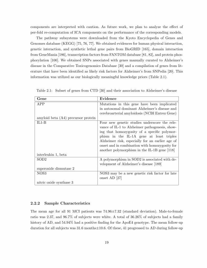
components are interpreted with caution. As future work, we plan to analyze the effect of

per-fold re-computation of ICA components on the performance of the corresponding models.

The pathway subsystems were downloaded from the Kyoto Encyclopedia of Genes and

Genomes database (KEGG) [75, 76, 77]. We obtained evidences for human physical interaction,

genetic interaction, and synthetic lethal gene pairs from BioGRID [165], domain interaction

from GeneMania [186], transcription factors from FANTOM database [81, 82], and protein phos-

phorylation [100]. We obtained SNPs associated with genes manually curated to Alzheimer’s

disease in the Comparative Toxicogenomics Database [30] and a compilation of genes from lit-

erature that have been identified as likely risk factors for Alzheimer’s from SNPedia [20]. This

information was utilized as our biologically meaningful knowledge priors (Table 2.1).

Table 2.1: Subset of genes from CTD [30] and their association to Alzheimer’s disease

Gene Evidence

APP Mutations in this gene have been implicatedin autosomal dominant Alzheimer’s disease andcerebroarterial amyloidosis (NCBI Entrez Gene)

amyloid beta (A4) precursor protein

IL1-B Four new genetic studies underscore the rele-vance of IL-1 to Alzheimer pathogenesis, show-ing that homozygosity of a specific polymor-phism in the IL-1A gene at least triplesAlzheimer risk, especially for an earlier age ofonset and in combination with homozygosity foranother polymorphism in the IL-1B gene [118]

interleukin 1, beta

SOD2 A polymorphism in SOD2 is associated with de-velopment of Alzheimer’s disease [189]

superoxide dismutase 2

NOS3 NOS3 may be a new genetic risk factor for lateonset AD [27]

nitric oxide synthase 3

2.2.2 Sample Characteristics

The mean age for all 91 MCI patients was 74.96±7.32 (standard deviation). Male-to-female

ratio was 2.37, and 96.7% of subjects were white. A total of 36.26% of subjects had a family

history of AD, and 54.94% had a positive finding for the ApoE4 genotype. The mean follow-up

duration for all subjects was 31.6 months±10.6. Of these, 41 progressed to AD during follow-up

19

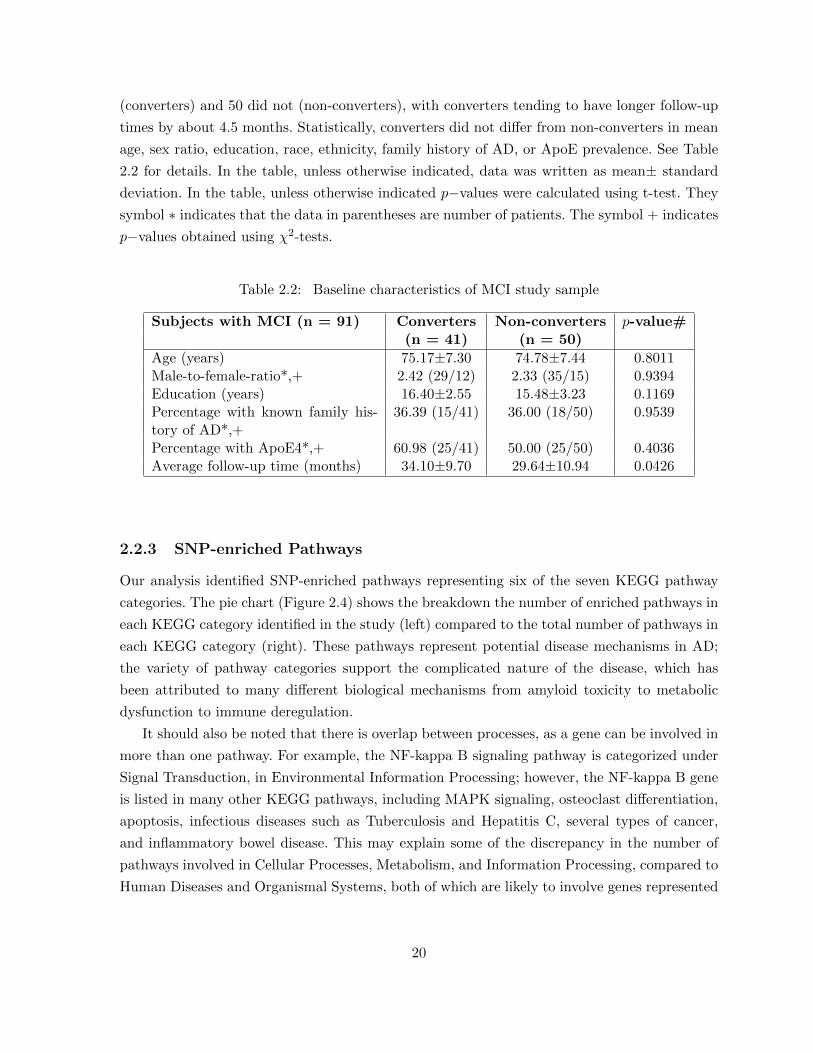
(converters) and 50 did not (non-converters), with converters tending to have longer follow-up

times by about 4.5 months. Statistically, converters did not differ from non-converters in mean

age, sex ratio, education, race, ethnicity, family history of AD, or ApoE prevalence. See Table

2.2 for details. In the table, unless otherwise indicated, data was written as mean± standard

deviation. In the table, unless otherwise indicated p−values were calculated using t-test. They

symbol ∗ indicates that the data in parentheses are number of patients. The symbol + indicates

p−values obtained using χ2-tests.

Table 2.2: Baseline characteristics of MCI study sample

Subjects with MCI (n = 91) Converters Non-converters p-value#(n = 41) (n = 50)

Age (years) 75.17±7.30 74.78±7.44 0.8011Male-to-female-ratio*,+ 2.42 (29/12) 2.33 (35/15) 0.9394Education (years) 16.40±2.55 15.48±3.23 0.1169Percentage with known family his-tory of AD*,+

36.39 (15/41) 36.00 (18/50) 0.9539

Percentage with ApoE4*,+ 60.98 (25/41) 50.00 (25/50) 0.4036Average follow-up time (months) 34.10±9.70 29.64±10.94 0.0426

2.2.3 SNP-enriched Pathways

Our analysis identified SNP-enriched pathways representing six of the seven KEGG pathway

categories. The pie chart (Figure 2.4) shows the breakdown the number of enriched pathways in

each KEGG category identified in the study (left) compared to the total number of pathways in

each KEGG category (right). These pathways represent potential disease mechanisms in AD;

the variety of pathway categories support the complicated nature of the disease, which has

been attributed to many different biological mechanisms from amyloid toxicity to metabolic

dysfunction to immune deregulation.

It should also be noted that there is overlap between processes, as a gene can be involved in

more than one pathway. For example, the NF-kappa B signaling pathway is categorized under

Signal Transduction, in Environmental Information Processing; however, the NF-kappa B gene

is listed in many other KEGG pathways, including MAPK signaling, osteoclast differentiation,

apoptosis, infectious diseases such as Tuberculosis and Hepatitis C, several types of cancer,

and inflammatory bowel disease. This may explain some of the discrepancy in the number of

pathways involved in Cellular Processes, Metabolism, and Information Processing, compared to

Human Diseases and Organismal Systems, both of which are likely to involve genes represented

20

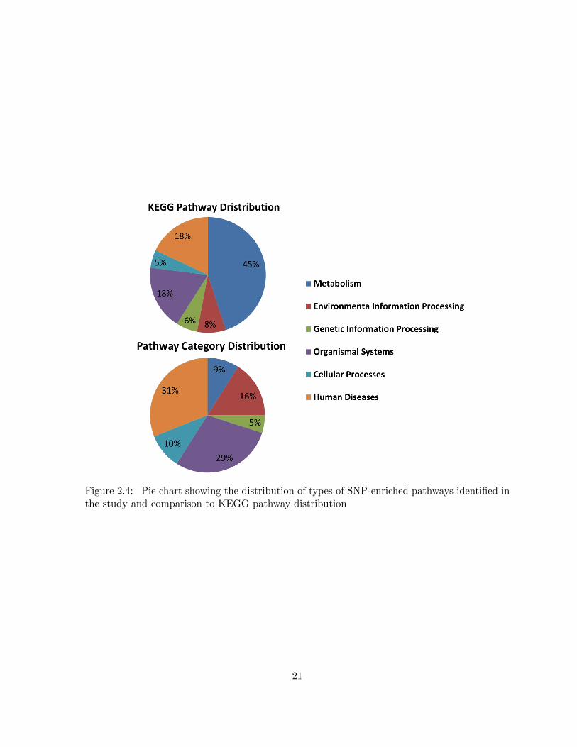
Figure 2.4: Pie chart showing the distribution of types of SNP-enriched pathways identified inthe study and comparison to KEGG pathway distribution

21

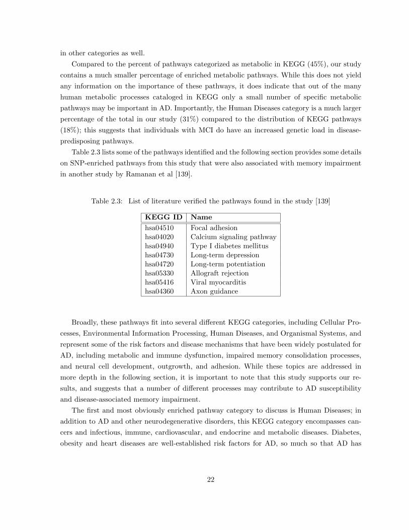
in other categories as well.

Compared to the percent of pathways categorized as metabolic in KEGG (45%), our study

contains a much smaller percentage of enriched metabolic pathways. While this does not yield

any information on the importance of these pathways, it does indicate that out of the many

human metabolic processes cataloged in KEGG only a small number of specific metabolic

pathways may be important in AD. Importantly, the Human Diseases category is a much larger

percentage of the total in our study (31%) compared to the distribution of KEGG pathways

(18%); this suggests that individuals with MCI do have an increased genetic load in disease-

predisposing pathways.

Table 2.3 lists some of the pathways identified and the following section provides some details

on SNP-enriched pathways from this study that were also associated with memory impairment

in another study by Ramanan et al [139].

Table 2.3: List of literature verified the pathways found in the study [139]

KEGG ID Name

hsa04510 Focal adhesionhsa04020 Calcium signaling pathwayhsa04940 Type I diabetes mellitushsa04730 Long-term depressionhsa04720 Long-term potentiationhsa05330 Allograft rejectionhsa05416 Viral myocarditishsa04360 Axon guidance

Broadly, these pathways fit into several different KEGG categories, including Cellular Pro-

cesses, Environmental Information Processing, Human Diseases, and Organismal Systems, and

represent some of the risk factors and disease mechanisms that have been widely postulated for

AD, including metabolic and immune dysfunction, impaired memory consolidation processes,

and neural cell development, outgrowth, and adhesion. While these topics are addressed in

more depth in the following section, it is important to note that this study supports our re-

sults, and suggests that a number of different processes may contribute to AD susceptibility

and disease-associated memory impairment.

The first and most obviously enriched pathway category to discuss is Human Diseases; in

addition to AD and other neurodegenerative disorders, this KEGG category encompasses can-

cers and infectious, immune, cardiovascular, and endocrine and metabolic diseases. Diabetes,

obesity and heart diseases are well-established risk factors for AD, so much so that AD has

22

been referred to as type 3 diabetes; so finding SNP-enriched pathways for cardiovascular and

endocrine and metabolic diseases in individuals with MCI is not unexpected [181]. Evidence

has supported an inverse association of the development of cancer and AD, and it is postu-

lated that this may be due to differential regulation of common signaling pathways [63, 144].

Autoimmune pathways have also previously been implicated in AD, particularly the idea that

a compromised blood brain barrier may allow entry of serum proteins, which lead to neuronal

death via autoimmune mechanisms [28, 149]. Chronic infection with pathogens including herpes

simplex virus type 1, Chlamydia pneumonia, Helicobacter pylori, and spirochete [64] has been

implicated in AD and cognitive change, and mouse model research suggests that Toxoplasma

gondii infection may be neuroprotective [74], further linking immune and inflammatory pro-

cesses to AD. Finally, certain molecular markers such as alpha-synuclein protein have linked

AD to other neurodegenerative diseases including Parkinson disease and dementia with Lewy

bodies [2]. These disparate pieces of evidence support the identification in this study of enriched

pathways in human diseases in patients with MCI.

Enriched metabolic pathways in this population include metabolism of carbohydrates, lipids,

amino acids, cofactors and vitamins, energy, and xenobiotics. Glycolysis and gluconeogenesis

are pathways involved in glucose metabolism. One of the hallmarks of early AD is deficits in

glucose metabolism in the brain, which can be clinically detected using FDG-PET. One theory

is that this simply reflects neuronal injury and loss, whereas another theory proposes that there

is a primary metabolic energy deficit in the AD brain. The AD brain has been also called “the

starving brain.” The pentose phosphate pathway generates NADH which is an anti-oxidant,

and oxidative stress is one of the postulated neurodegenerative mechanisms in AD; pentose

phosphate activity is increased in the brains of AD patients in response to oxidative stress.

The pentose phosphate pathway is also involved as an alternate to glycolysis. It has been well

documented that oxidative damage and insulin resistance cause metabolic dysfunction in AD;

a temporal three-part sequence occurs with changes in glycolysis, the tricarboxylic acid cycle

(TCA) and oxidative phosphorylation pathways[160]. Given that apolipoprotein E is the largest

genetic risk factor for AD identified to date, we would expect to find an enrichment of lipid

metabolic pathways. Finally, the xenobiotic cytochrome-P450 gene pathway identified, while

most commonly tied to drug metabolism, has also been implicated in neurodegeneration. For

example, variations in CYP17 P450 gene have been linked to increased AD risk. Studies have

also found alterations in constituent cytochrome enzymes in mouse models of AD. Lastly, NADH

CYP450 reductase is induced by the amyloid peptide, which has been identified as mutated in

familial AD, and such a response could be a possible mechanism whereby amyloid beta causes

oxidative stress. Thus, the identification of enriched metabolic pathways in patients with MCI

is also logical.

Organismal systems enriched in this population include the endocrine, excretory, digestive,

23

immune, nervous, and sensory systems, as well as development processes. The first and most

obvious link here is the identification of the insulin and adipocytokine signaling pathways, which

are logical given that diabetes is a risk factor for AD. Other pathways in the endocrine system

include the PPAR signaling pathway [110], which is known to interact with the apolipoprotein E

functional pathway, as well as several hormone signaling pathways including the gonadotropin-

releasing hormone signaling pathway, which has been shown to play a potential role in diabetes

[9]. As previously discussed, metabolism has been shown to play an important role in AD, so it

is unsurprising that we observe enrichment in digestive and excretory pathways, as malfunction

could presumably result in unbalanced energy metabolism and compromised metabolic function.

Both up and downregulation of inflammatory processes have been associated with AD, and some

research has suggested that a combination of inflammation and aging, or inflammaging, may

be a prodromal stage of AD, potentially accompanied by age-related immune dysregulation.

This supports the identification of SNP-enriched immune and inflammatory pathways [45, 106,

112]. Since AD is a neurodegenerative disease, we would expect to observe nervous system

pathway enrichment; in particular, enrichment of long-term potentiation and depression and

neurotransmitter signaling pathways all support our process given that these pathways have

been previously associated with cognitive impairment and AD [24, 37, 96, 171].

Cell processes include a number of pathways linked to neurodegeneration via their involve-

ment in cell growth and death, including p53 signaling, autophagy, apoptosis, and cell cycle

regulation. There are also several neural cell adhesion pathways that are enriched in individuals

with MCI, which is supported by previous research indicating that these pathways might be

involved in this disease process [139]. Interestingly, there were also a number of enriched ge-

netic information processing pathways, including DNA replication, transcription, translation,

and protein processing. Enriched pathways in cell cycle regulation and DNA replication are

particularly interesting given that previous research has found that neurons in the brains of AD

patients exhibit markers indicating reentry into the cell cycle, and that neuronal cell death may

be preceded by DNA replication [117, 194, 197]. It has been proposed that DNA replication

resulting in tetraploid cells that do not undergo mitosis may be resulting in neuronal cell death.

Furthermore, there is some evidence that cells from AD patients have a DNA repair deficiency

after treatment with alkylating agents [14]. Genetic variants increasing risk for cell cycle and/or

transcription/translation misregulation could thus play an important part in AD pathology.

The final category of enriched pathways identified in our study is Environmental Information

Processing; all of these pathways involve signal transduction or cell trafficking, and most could

be predicted based on pathways identified in other categories. For example, the TGF-beta,

NF-kappa B, VEGF, HIF-1, PI3K-Akt, Wnt, Notch, mTOR, MAPK, and Hedgehog signaling

pathways are all annotated in the KEGG Pathways in Cancer, as well as their normal functions

in growth and development. Notch is known to interact with the presenilin genes, in which

24

mutations have been identified in individuals with familial AD, linking this signaling pathway

to the disease. Calcium signaling is important in a number of mechanisms that have been

discussed as important in AD, including long-term potentiation and depression, as well as

apoptosis and metabolism. Several cell receptor interaction pathways are also enriched, which

might be expected given that AD has been posited to have an environmental risk component

[44]. These common signaling pathways are responsible for normal growth and development,

and many have previously been linked to abnormal processes in disease, so it is not surprising

that differential genetic load in these pathways could impact risk of development of AD as well.

All six categories of enriched pathways identified in our study can be linked to AD through

various mechanisms, and support the complex etiology behind this disease. This systematic

investigation of pathways in individuals with MCI provides evidence that many risk factors and

biological mechanisms are potentially important for disease development; the identification of

many pathways that could be impacted by environment, such as memory processes that could

be impacted by education and occupation, also help to explain the incomplete penetrance of

disease.

2.2.4 SNP-enriched Pathway Crosstalks

The categories with the greatest numbers of crosstalks are Human Diseases and Organismal

Systems, which we would expect given that these categories also contain the greatest numbers of

pathways; however, it is interesting to note that although the two categories contain an approxi-

mately equal percentage of the total number of pathways tested (31% for Human Diseases, 29%

for Organismal Systems), Human Diseases generated almost twice as many crosstalks as Organ-

ismal Systems. This is most likely attributable to the complex etiology of many diseases within

this category, which could potentially involve many different pathways, but also demonstrates

the potential utility of this type of analysis for prioritizing pathways.

The largest category of interactions appear to be Human Diseases with Environmental In-

formation Processing, other Human Diseases, and Organismal Systems, most likely indicating

process interactions for disease risk and development (Environmental Information Processing),

risk factors predisposing to multiple disease (Human Disease crosstalks such as AD and dia-

betes), and disease development, immunity, and pathology (Organismal Systems). Interestingly,

Organismal Systems crosstalks form primarily between Environmental Information Processing

and other Organismal Systems, perhaps representing less pathological genetic factors and mech-

anisms.

Metabolism and Genetic Information Processing show an unexpected dearth of crosstalks

compared to that expected based strictly on percentage of total enriched pathways in the cohort,

suggesting that genetic load in these processes may be less important or have less overall impact

25

than other types of biological mechanisms in this particular cohort. All but one of the enriched

pathways had at least one significant crosstalk; the one carbon pool by folate pathway did not

have any significant crosstalks. This maybe because the pathway is small and specific; it is only

linked to rare, serious diseases in KEGG, including several metabolic disorders and spina bifida.

Because our aim was to investigate the genetic load specifically in regards to AD, we also

examined enriched pathway crosstalk specifically relating to this disease process. Sorting out

interactions involving the KEGG AD pathway, we identified 97 AD-related crosstalks. Identified

pathways were grouped according to category; all six KEGG categories were represented (Figure

2.4).

Given the overall findings of crosstalk enrichment, it is not surprising that the largest cat-

egories are once again Human Diseases and Organismal Systems. These categories are equally

represented in AD crosstalk, echoing the percentage of enriched pathways in these categories

and supporting the importance of both processes in AD genetic load. Interestingly, although

the crosstalks in the broad search did not match the percentages of enriched pathways, for

AD-specific crosstalks the percentages do largely reflect the percentages of enriched pathways;

Human Diseases and Organismal Systems are the largest categories (33% each), followed by

Environmental Information Processing (19%), Cellular Processes (10%), Metabolism (3%), and

Genetic Information Processing (2%). As seen in the broad crosstalk analysis, Metabolism and

Genetic Information Processing have fewer crosstalks than might be expected given the per-

centage of pathways involved, suggesting that genetic load in these processes is not as important

to the disease process, at least in this particular cohort.

Investigation of pathway crosstalk revealed the presence of a large number of SNP-enriched

pathway interactions. These pathway crosstalks were observed to be particularly common for

human disease and organismal system KEGG pathways, which makes sense given that these

pathways are known to involve many biological mechanisms. Interestingly, the large number

of enriched disease and organismal system pathway crosstalks present in the dataset might

suggest a core set of biological mechanisms are central to many different disorders including

infectious diseases, nervous disorders, and cancer. One example of this is the calcium signaling

pathway; this SNP-enriched pathway shows crosstalk with AD, as expected given the method

of identification, but also crosstalks with other nervous system disorders including Huntington’s

disease and Amyotrophic lateral sclerosis (ALS), infectious disease pathways and a number of

different types of cancers among others indicating that this pathway is an important signaling

hub, and that increased SNP load in this pathway could have wide-ranging systemic effects.

Focal cell adhesion is another interesting example of a signaling pathway with wide-ranging

effects; in addition to AD, this pathway shows crosstalk with immune pathways and infectious,

immune, and cardiomyopathic diseases, many types of cancer, nervous system pathways and

diseases such as ALS, diabetes and insulin signaling, and cell growth, development, and signal

26

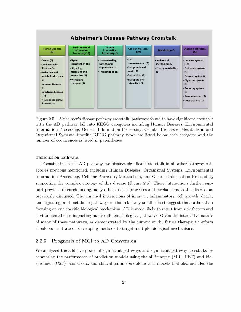
•Cancer (9)

•Cardiovascular

diseases (3)

•Endocrine and

metabolic diseases

(3)

•Immune diseases

(3)

•Infectious diseases

(11)

•Neurodegenerative

diseases (3)

•Signal

Transduction (14)

• Signaling

molecules and

interaction (3)

•Membrane

transport (1)

•Protein folding,

sorting, and

degradation (1)

•Transcription (1)

•Cell

communication (2)

•Cell growth and

death (4)

•Cell motility (1)

•Transport and

catabolism (3)

•Amino acid

metabolism (2)

•Energy metabolism

(1)

•Immune system

(12)

•Endocrine system

(6)

•Nervous system (6)

•Digestive system

(2)

•Excretory system

(2)

•Sensory system (2)

•Development (2)

Human Diseases (32)

Environmental Information

Processing (18)

Genetic Information

Processing (2)

Cellular Processes (10)

Metabolism (3) Organismal Systems

(32)

Alzheimer’s Disease Pathway Crosstalk

Figure 2.5: Alzheimer’s disease pathway crosstalk: pathways found to have significant crosstalkwith the AD pathway fall into KEGG categories including Human Diseases, EnvironmentalInformation Processing, Genetic Information Processing, Cellular Processes, Metabolism, andOrganismal Systems. Specific KEGG pathway types are listed below each category, and thenumber of occurrences is listed in parentheses.

transduction pathways.

Focusing in on the AD pathway, we observe significant crosstalk in all other pathway cat-

egories previous mentioned, including Human Diseases, Organismal Systems, Environmental

Information Processing, Cellular Processes, Metabolism, and Genetic Information Processing,

supporting the complex etiology of this disease (Figure 2.5). These interactions further sup-

port previous research linking many other disease processes and mechanisms to this disease, as

previously discussed. The enriched interactions of immune, inflammatory, cell growth, death,

and signaling, and metabolic pathways in this relatively small cohort suggest that rather than

focusing on one specific biological mechanism, AD is more likely to result from risk factors and

environmental cues impacting many different biological pathways. Given the interactive nature

of many of these pathways, as demonstrated by the current study, future therapeutic efforts

should concentrate on developing methods to target multiple biological mechanisms.

2.2.5 Prognosis of MCI to AD Conversion

We analyzed the additive power of significant pathways and significant pathway crosstalks by

comparing the performance of prediction models using the all imaging (MRI, PET) and bio-

specimen (CSF) biomarkers, and clinical parameters alone with models that also included the

27

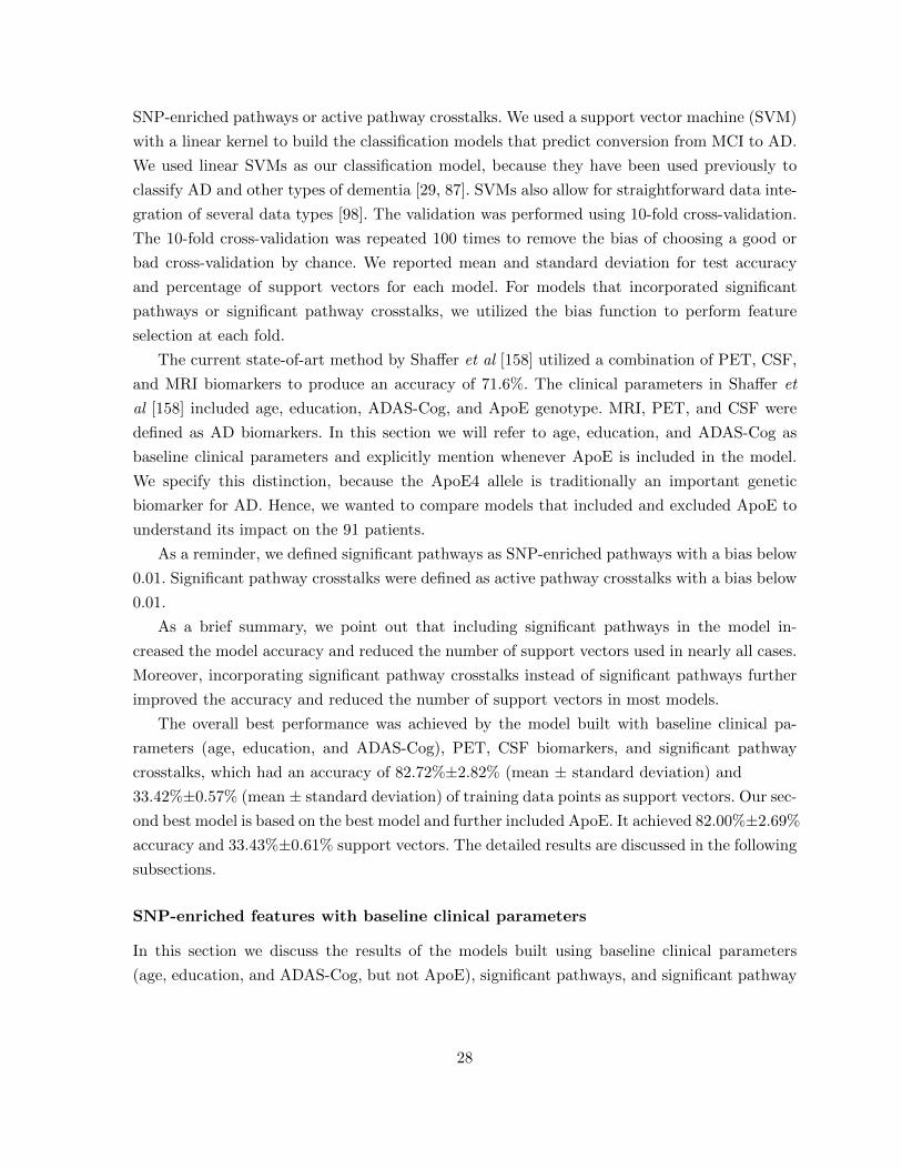
SNP-enriched pathways or active pathway crosstalks. We used a support vector machine (SVM)

with a linear kernel to build the classification models that predict conversion from MCI to AD.

We used linear SVMs as our classification model, because they have been used previously to

classify AD and other types of dementia [29, 87]. SVMs also allow for straightforward data inte-

gration of several data types [98]. The validation was performed using 10-fold cross-validation.

The 10-fold cross-validation was repeated 100 times to remove the bias of choosing a good or

bad cross-validation by chance. We reported mean and standard deviation for test accuracy

and percentage of support vectors for each model. For models that incorporated significant

pathways or significant pathway crosstalks, we utilized the bias function to perform feature

selection at each fold.

The current state-of-art method by Shaffer et al [158] utilized a combination of PET, CSF,

and MRI biomarkers to produce an accuracy of 71.6%. The clinical parameters in Shaffer et

al [158] included age, education, ADAS-Cog, and ApoE genotype. MRI, PET, and CSF were

defined as AD biomarkers. In this section we will refer to age, education, and ADAS-Cog as

baseline clinical parameters and explicitly mention whenever ApoE is included in the model.

We specify this distinction, because the ApoE4 allele is traditionally an important genetic

biomarker for AD. Hence, we wanted to compare models that included and excluded ApoE to

understand its impact on the 91 patients.

As a reminder, we defined significant pathways as SNP-enriched pathways with a bias below

0.01. Significant pathway crosstalks were defined as active pathway crosstalks with a bias below

0.01.

As a brief summary, we point out that including significant pathways in the model in-

creased the model accuracy and reduced the number of support vectors used in nearly all cases.

Moreover, incorporating significant pathway crosstalks instead of significant pathways further

improved the accuracy and reduced the number of support vectors in most models.

The overall best performance was achieved by the model built with baseline clinical pa-

rameters (age, education, and ADAS-Cog), PET, CSF biomarkers, and significant pathway

crosstalks, which had an accuracy of 82.72%±2.82% (mean ± standard deviation) and

33.42%±0.57% (mean ± standard deviation) of training data points as support vectors. Our sec-

ond best model is based on the best model and further included ApoE. It achieved 82.00%±2.69%

accuracy and 33.43%±0.61% support vectors. The detailed results are discussed in the following

subsections.

SNP-enriched features with baseline clinical parameters

In this section we discuss the results of the models built using baseline clinical parameters

(age, education, and ADAS-Cog, but not ApoE), significant pathways, and significant pathway

28

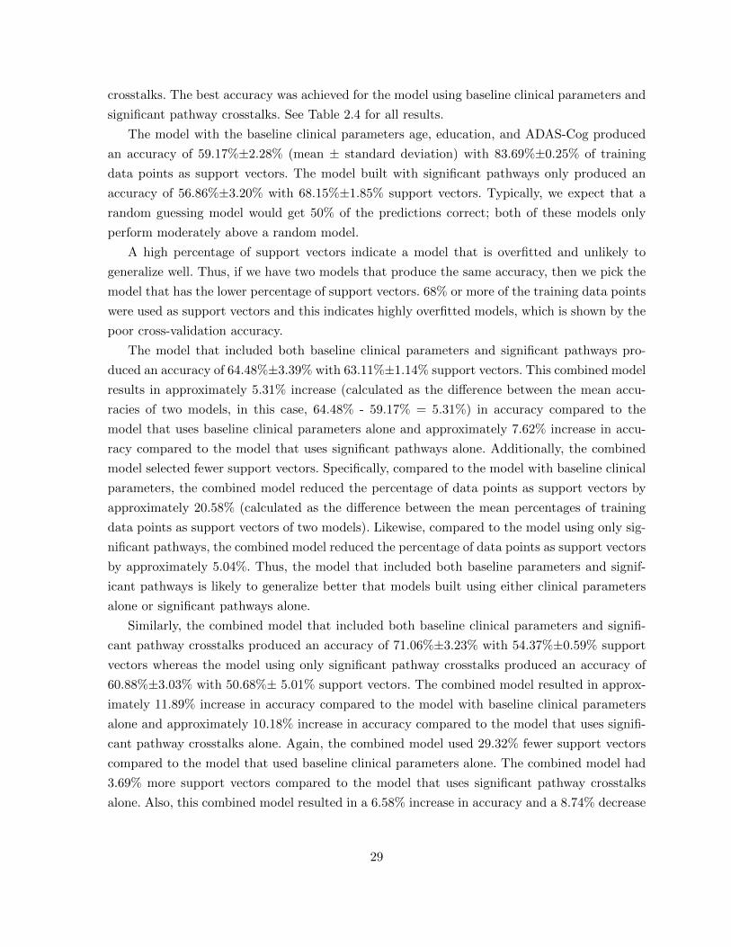
crosstalks. The best accuracy was achieved for the model using baseline clinical parameters and

significant pathway crosstalks. See Table 2.4 for all results.

The model with the baseline clinical parameters age, education, and ADAS-Cog produced

an accuracy of 59.17%±2.28% (mean ± standard deviation) with 83.69%±0.25% of training

data points as support vectors. The model built with significant pathways only produced an

accuracy of 56.86%±3.20% with 68.15%±1.85% support vectors. Typically, we expect that a

random guessing model would get 50% of the predictions correct; both of these models only

perform moderately above a random model.

A high percentage of support vectors indicate a model that is overfitted and unlikely to

generalize well. Thus, if we have two models that produce the same accuracy, then we pick the

model that has the lower percentage of support vectors. 68% or more of the training data points

were used as support vectors and this indicates highly overfitted models, which is shown by the

poor cross-validation accuracy.

The model that included both baseline clinical parameters and significant pathways pro-

duced an accuracy of 64.48%±3.39% with 63.11%±1.14% support vectors. This combined model

results in approximately 5.31% increase (calculated as the difference between the mean accu-

racies of two models, in this case, 64.48% - 59.17% = 5.31%) in accuracy compared to the

model that uses baseline clinical parameters alone and approximately 7.62% increase in accu-

racy compared to the model that uses significant pathways alone. Additionally, the combined

model selected fewer support vectors. Specifically, compared to the model with baseline clinical

parameters, the combined model reduced the percentage of data points as support vectors by

approximately 20.58% (calculated as the difference between the mean percentages of training

data points as support vectors of two models). Likewise, compared to the model using only sig-

nificant pathways, the combined model reduced the percentage of data points as support vectors

by approximately 5.04%. Thus, the model that included both baseline parameters and signif-

icant pathways is likely to generalize better that models built using either clinical parameters

alone or significant pathways alone.

Similarly, the combined model that included both baseline clinical parameters and signifi-

cant pathway crosstalks produced an accuracy of 71.06%±3.23% with 54.37%±0.59% support

vectors whereas the model using only significant pathway crosstalks produced an accuracy of

60.88%±3.03% with 50.68%± 5.01% support vectors. The combined model resulted in approx-

imately 11.89% increase in accuracy compared to the model with baseline clinical parameters

alone and approximately 10.18% increase in accuracy compared to the model that uses signifi-

cant pathway crosstalks alone. Again, the combined model used 29.32% fewer support vectors

compared to the model that used baseline clinical parameters alone. The combined model had

3.69% more support vectors compared to the model that uses significant pathway crosstalks

alone. Also, this combined model resulted in a 6.58% increase in accuracy and a 8.74% decrease

29

in support vectors when compared to the model that uses both baseline parameters and signif-

icant pathways. Thus, including significant pathway crosstalks, instead of significant pathways,

in a model that also contains baseline clinical parameters produced an improved model.

In all tables of the Results section, unless otherwise noted, support vector machines with

linear kernel functions were used as classification method for MCI to AD conversion; mean and

standard deviation of 100 iterations of 10-fold cross-validation results are shown.

30

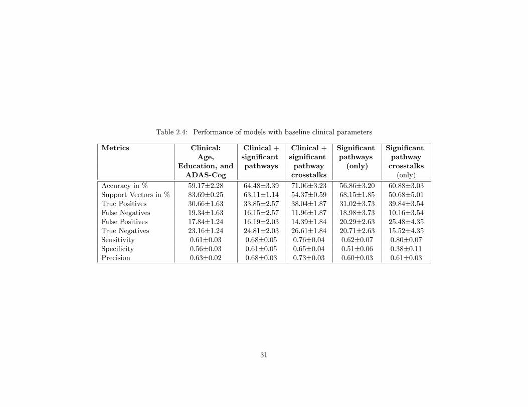
Table 2.4: Performance of models with baseline clinical parameters

Metrics Clinical: Clinical + Clinical + Significant SignificantAge, significant significant pathways pathway

Education, and pathways pathway (only) crosstalksADAS-Cog crosstalks (only)

Accuracy in % 59.17±2.28 64.48±3.39 71.06±3.23 56.86±3.20 60.88±3.03Support Vectors in % 83.69±0.25 63.11±1.14 54.37±0.59 68.15±1.85 50.68±5.01True Positives 30.66±1.63 33.85±2.57 38.04±1.87 31.02±3.73 39.84±3.54False Negatives 19.34±1.63 16.15±2.57 11.96±1.87 18.98±3.73 10.16±3.54False Positives 17.84±1.24 16.19±2.03 14.39±1.84 20.29±2.63 25.48±4.35True Negatives 23.16±1.24 24.81±2.03 26.61±1.84 20.71±2.63 15.52±4.35Sensitivity 0.61±0.03 0.68±0.05 0.76±0.04 0.62±0.07 0.80±0.07Specificity 0.56±0.03 0.61±0.05 0.65±0.04 0.51±0.06 0.38±0.11Precision 0.63±0.02 0.68±0.03 0.73±0.03 0.60±0.03 0.61±0.03

31

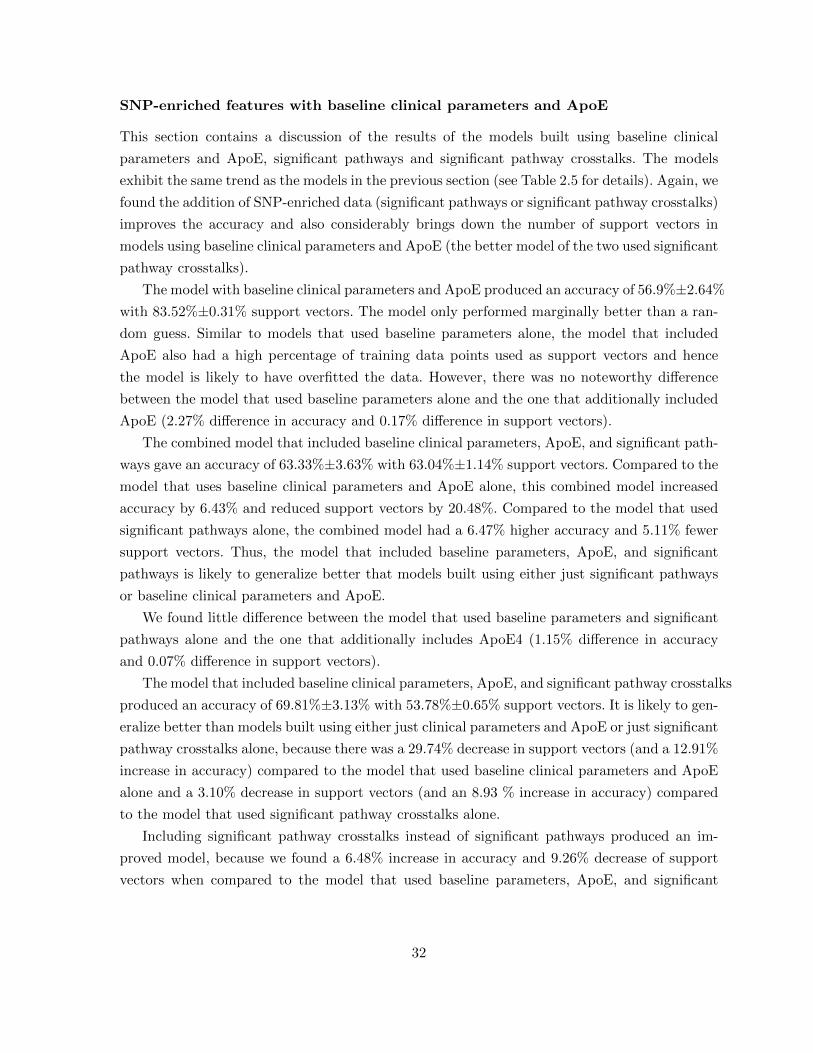
SNP-enriched features with baseline clinical parameters and ApoE

This section contains a discussion of the results of the models built using baseline clinical

parameters and ApoE, significant pathways and significant pathway crosstalks. The models

exhibit the same trend as the models in the previous section (see Table 2.5 for details). Again, we

found the addition of SNP-enriched data (significant pathways or significant pathway crosstalks)

improves the accuracy and also considerably brings down the number of support vectors in

models using baseline clinical parameters and ApoE (the better model of the two used significant

pathway crosstalks).

The model with baseline clinical parameters and ApoE produced an accuracy of 56.9%±2.64%

with 83.52%±0.31% support vectors. The model only performed marginally better than a ran-

dom guess. Similar to models that used baseline parameters alone, the model that included

ApoE also had a high percentage of training data points used as support vectors and hence

the model is likely to have overfitted the data. However, there was no noteworthy difference

between the model that used baseline parameters alone and the one that additionally included

ApoE (2.27% difference in accuracy and 0.17% difference in support vectors).

The combined model that included baseline clinical parameters, ApoE, and significant path-

ways gave an accuracy of 63.33%±3.63% with 63.04%±1.14% support vectors. Compared to the

model that uses baseline clinical parameters and ApoE alone, this combined model increased

accuracy by 6.43% and reduced support vectors by 20.48%. Compared to the model that used

significant pathways alone, the combined model had a 6.47% higher accuracy and 5.11% fewer

support vectors. Thus, the model that included baseline parameters, ApoE, and significant

pathways is likely to generalize better that models built using either just significant pathways

or baseline clinical parameters and ApoE.

We found little difference between the model that used baseline parameters and significant

pathways alone and the one that additionally includes ApoE4 (1.15% difference in accuracy

and 0.07% difference in support vectors).

The model that included baseline clinical parameters, ApoE, and significant pathway crosstalks

produced an accuracy of 69.81%±3.13% with 53.78%±0.65% support vectors. It is likely to gen-

eralize better than models built using either just clinical parameters and ApoE or just significant

pathway crosstalks alone, because there was a 29.74% decrease in support vectors (and a 12.91%

increase in accuracy) compared to the model that used baseline clinical parameters and ApoE

alone and a 3.10% decrease in support vectors (and an 8.93 % increase in accuracy) compared

to the model that used significant pathway crosstalks alone.

Including significant pathway crosstalks instead of significant pathways produced an im-

proved model, because we found a 6.48% increase in accuracy and 9.26% decrease of support

vectors when compared to the model that used baseline parameters, ApoE, and significant

32

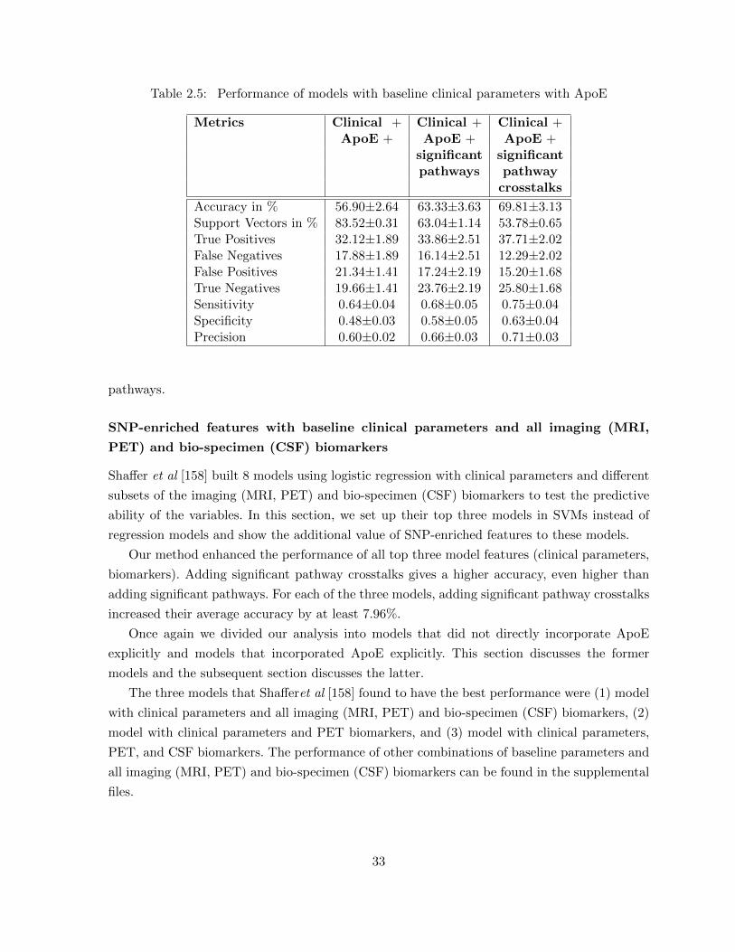
Table 2.5: Performance of models with baseline clinical parameters with ApoE

Metrics Clinical + Clinical + Clinical +ApoE + ApoE + ApoE +

significant significantpathways pathway

crosstalks

Accuracy in % 56.90±2.64 63.33±3.63 69.81±3.13Support Vectors in % 83.52±0.31 63.04±1.14 53.78±0.65True Positives 32.12±1.89 33.86±2.51 37.71±2.02False Negatives 17.88±1.89 16.14±2.51 12.29±2.02False Positives 21.34±1.41 17.24±2.19 15.20±1.68True Negatives 19.66±1.41 23.76±2.19 25.80±1.68Sensitivity 0.64±0.04 0.68±0.05 0.75±0.04Specificity 0.48±0.03 0.58±0.05 0.63±0.04Precision 0.60±0.02 0.66±0.03 0.71±0.03

pathways.

SNP-enriched features with baseline clinical parameters and all imaging (MRI,

PET) and bio-specimen (CSF) biomarkers

Shaffer et al [158] built 8 models using logistic regression with clinical parameters and different

subsets of the imaging (MRI, PET) and bio-specimen (CSF) biomarkers to test the predictive

ability of the variables. In this section, we set up their top three models in SVMs instead of

regression models and show the additional value of SNP-enriched features to these models.

Our method enhanced the performance of all top three model features (clinical parameters,

biomarkers). Adding significant pathway crosstalks gives a higher accuracy, even higher than

adding significant pathways. For each of the three models, adding significant pathway crosstalks

increased their average accuracy by at least 7.96%.

Once again we divided our analysis into models that did not directly incorporate ApoE

explicitly and models that incorporated ApoE explicitly. This section discusses the former

models and the subsequent section discusses the latter.

The three models that Shafferet al [158] found to have the best performance were (1) model

with clinical parameters and all imaging (MRI, PET) and bio-specimen (CSF) biomarkers, (2)

model with clinical parameters and PET biomarkers, and (3) model with clinical parameters,

PET, and CSF biomarkers. The performance of other combinations of baseline parameters and

all imaging (MRI, PET) and bio-specimen (CSF) biomarkers can be found in the supplemental

files.

33

Model performance with baseline clinical parameters and all imaging (MRI,

PET) and bio-specimen (CSF) biomarkers: We analyzed the model that included all

imaging (MRI, PET) and bio-specimen (CSF) biomarkers along with baseline clinical parame-

ters. The model had an accuracy of 65.48%±2.40% with 54.85%±0.45% support vectors. This

model resulted in a 6.31% increase in accuracy and a 28.84% reduction in support vectors in

comparison to the model that used only the baseline clinical parameters alone.

The model that included significant pathways along with all imaging (MRI, PET), bio-

specimen (CSF) biomarkers and baseline clinical parameters (Table 2.6) resulted in an accuracy

of 72.66%±4.04% with 41.17%±0.72% support vectors. Dropping either all imaging (MRI,

PET) and bio-specimen (CSF) biomarkers or significant pathways from this model gave a worse

performance (8.18% decrease in accuracy and 21.94% increase in support vectors when removing

all imaging (MRI, PET) and bio-specimen (CSF) biomarkers; 7.18% decrease in accuracy and

13.68% more support vectors when removing significant pathways).

Similarly, the model built on all imaging (MRI, PET), bio-specimen (CSF) biomarkers and

baseline clinical parameters along with significant pathway crosstalks led to 81.38%±2.79%

accuracy with 35.31%±0.62% support vectors. Removing either all imaging (MRI, PET)and

bio-specimen (CSF) biomarkers or significant pathway crosstalks from the model decreased

performance (10.32% less accuracy and 19.06% more support vectors when dropping all imaging

(MRI, PET) and bio-specimen (CSF) biomarkers; 15.90% less accurate and 19.54% increase in

support vectors when dropping significant pathway crosstalks).

Including significant pathway crosstalks, instead of significant pathways, in a model that also

contained baseline clinical parameters and all imaging (MRI, PET) and bio-specimen (CSF)

biomarkers improved model accuracy by 8.72% and reduced the support vectors by 5.86%.

Model performance with baseline clinical parameters and PET biomarkers: The

model built using PET biomarkers and baseline clinical parameters (Table 2.7) had

68.58%±2.32% accuracy and 57.59%±0.42% support vectors, which was 9.41% more accurate

and had 25.93% fewer support vectors than the model that used only baseline clinical parame-

ters.

The model that included significant pathways along with PET biomarkers and baseline clin-

ical parameters gave an accuracy of 74.26%±2.71% with 43.91%±0.79% support vectors. Elim-

inating either the PET biomarkers or the significant pathways decreased performance (9.78%

less accurate and 19.13% more support vectors in the model without PET biomarkers; 5.68%

decrease in accuracy and 13.68% more support vectors when removing significant pathways

from our model instead).

The model based on significant pathway crosstalks, PET biomarkers, and baseline clinical

parameters reported an accuracy of 76.54%±2.76% with 38.99%±0.56% support vectors. When

we exclude either PET biomarkers or significant pathway crosstalks, the performance dropped

34

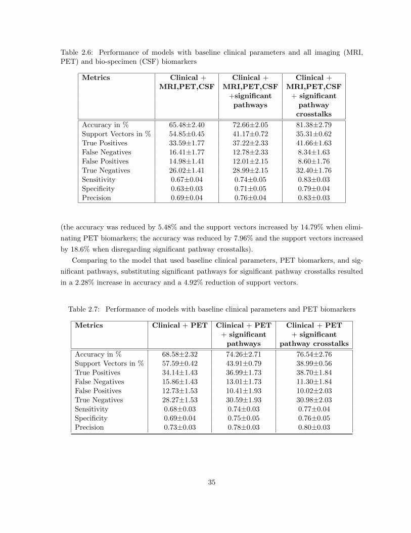
Table 2.6: Performance of models with baseline clinical parameters and all imaging (MRI,PET) and bio-specimen (CSF) biomarkers

Metrics Clinical + Clinical + Clinical +MRI,PET,CSF MRI,PET,CSF MRI,PET,CSF

+significant + significantpathways pathway

crosstalks

Accuracy in % 65.48±2.40 72.66±2.05 81.38±2.79Support Vectors in % 54.85±0.45 41.17±0.72 35.31±0.62True Positives 33.59±1.77 37.22±2.33 41.66±1.63False Negatives 16.41±1.77 12.78±2.33 8.34±1.63False Positives 14.98±1.41 12.01±2.15 8.60±1.76True Negatives 26.02±1.41 28.99±2.15 32.40±1.76Sensitivity 0.67±0.04 0.74±0.05 0.83±0.03Specificity 0.63±0.03 0.71±0.05 0.79±0.04Precision 0.69±0.04 0.76±0.04 0.83±0.03

(the accuracy was reduced by 5.48% and the support vectors increased by 14.79% when elimi-

nating PET biomarkers; the accuracy was reduced by 7.96% and the support vectors increased

by 18.6% when disregarding significant pathway crosstalks).

Comparing to the model that used baseline clinical parameters, PET biomarkers, and sig-

nificant pathways, substituting significant pathways for significant pathway crosstalks resulted

in a 2.28% increase in accuracy and a 4.92% reduction of support vectors.

Table 2.7: Performance of models with baseline clinical parameters and PET biomarkers

Metrics Clinical + PET Clinical + PET Clinical + PET+ significant + significant

pathways pathway crosstalks

Accuracy in % 68.58±2.32 74.26±2.71 76.54±2.76Support Vectors in % 57.59±0.42 43.91±0.79 38.99±0.56True Positives 34.14±1.43 36.99±1.73 38.70±1.84False Negatives 15.86±1.43 13.01±1.73 11.30±1.84False Positives 12.73±1.53 10.41±1.93 10.02±2.03True Negatives 28.27±1.53 30.59±1.93 30.98±2.03Sensitivity 0.68±0.03 0.74±0.03 0.77±0.04Specificity 0.69±0.04 0.75±0.05 0.76±0.05Precision 0.73±0.03 0.78±0.03 0.80±0.03

35

Model performance with baseline clinical parameters, PET, and CSF biomark-

ers: The model based on baseline clinical parameters, PET, and CSF biomarkers (Table 2.8)

yielded an accuracy of 67.19%±2.75% with 56.19%±0.47% support vectors. This model had a

slightly lower (1.30%) accuracy but a 27.33% reduction of support vectors in comparison to the

model that used only the baseline clinical parameters and PET. Moreover, this model yielded

10.74% more accuracy and 25.02% fewer support vectors in comparison to the model that used

only the baseline clinical parameters and CSF.

The model incorporating significant pathways along with PET and CSF biomarkers and

baseline clinical parameters resulted in 75.27%±2.82% accuracy and 41.06%±0.76% support

vectors. Comparing to models without either CSF biomarkers or PET biomarkers we were

better off keeping both in the model (1.01% decrease in accuracy and 21.98% increase in support

vectors for the model without CSF biomarkers; 11.96% decrease in accuracy and 19.33% more

support vectors for the model excluding PET biomarkers).

Similarly, the model that included significant pathway crosstalks, baseline clinical param-

eters, PET, and CSF biomarkers gave us an accuracy of 82.72%±2.82% and 33.42%±0.57%

support vectors. Omitting either CSF biomarkers or PET biomarkers gave worse results (6.18%

less accurate and 5.57% more support vectors when dropping CSF biomarkers; 10.61% reduction

in accuracy and 15.49% increase of support vectors when omitting PET biomarkers).

Including significant pathway crosstalks instead of significant pathways in a model that also

contained baseline clinical parameters, PET, and CSF biomarkers produced an improved model

(7.45% increase in accuracy and 7.64% decrease in support vectors).

SNP-enriched features with baseline clinical parameters, ApoE, and all imaging

(MRI, PET) and bio-specimen (CSF) biomarkers

This section contains the top three models from the previous section, extended by ApoE. Again,

we contrast and compare those models with models that also include significant pathways or

significant pathway crosstalks.

Model performance with baseline clinical parameters, ApoE, and all imaging

(MRI, PET) and bio-specimen (CSF) biomarkers: The model built using baseline clinical

parameters, ApoE, and all imaging (MRI, PET) and bio-specimen (CSF) biomarkers (Table

2.9), produced an accuracy of 67.08%±2.78% with 54.05%±0.48% support vectors. This model

had only a slightly higher (1.60%) accuracy and just 0.80% fewer support vectors compared to

dropping ApoE from the model. The addition of significant pathway crosstalks produced the

best accuracy (see Table 2.9 for details).

Similarly, the model containing significant pathways, all imaging (MRI, PET) and bio-

specimen (CSF) biomarkers, baseline clinical parameters, and ApoE yielded an accuracy of

36

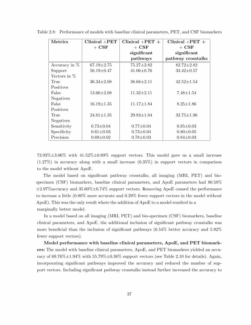
Table 2.8: Performance of models with baseline clinical parameters, PET, and CSF biomarkers

Metrics Clinical +PET Clinical +PET + Clinical +PET ++ CSF + CSF + CSF

significant significantpathways pathway crosstalks

Accuracy in % 67.19±2.75 75.27±2.82 82.72±2.82Support 56.19±0.47 41.06±0.76 33.42±0.57Vectors in %True 36.34±2.08 38.68±2.11 42.52±1.54PositivesFalse 13.66±2.08 11.32±2.11 7.48±1.54NegativesFalse 16.19±1.35 11.17±1.84 8.25±1.86PositivesTrue 24.81±1.35 29.83±1.84 32.75±1.86NegativesSensitivity 0.73±0.04 0.77±0.04 0.85±0.03Specificity 0.61±0.03 0.73±0.04 0.80±0.05Precision 0.69±0.02 0.78±0.03 0.84±0.03

73.93%±3.06% with 41.52%±0.69% support vectors. This model gave us a small increase

(1.27%) in accuracy along with a small increase (0.35%) in support vectors in comparison

to the model without ApoE.

The model based on significant pathway crosstalks, all imaging (MRI, PET) and bio-

specimen (CSF) biomarkers, baseline clinical parameters, and ApoE parameters had 80.58%

±2.97%accuracy and 35.60%±0.74% support vectors. Removing ApoE caused the performance to increase a little (0.80% more accurate and 0.29% fewer support vectors in the model without

ApoE). This was the only result where the addition of ApoE to a model resulted in amarginally better model.

In a model based on all imaging (MRI, PET) and bio-specimen (CSF) biomarkers, baseline

clinical parameters, and ApoE, the additional inclusion of significant pathway crosstalks was

more beneficial than the inclusion of significant pathways (6.54% better accuracy and 5.92%

fewer support vectors).

Model performance with baseline clinical parameters, ApoE, and PET biomark-

ers: The model with baseline clinical parameters, ApoE, and PET biomarkers yielded an accu-

racy of 69.76%±1.94% with 55.79%±0.38% support vectors (see Table 2.10 for details). Again,

incorporating significant pathways improved the accuracy and reduced the number of sup-

port vectors. Including significant pathway crosstalks instead further increased the accuracy to

37

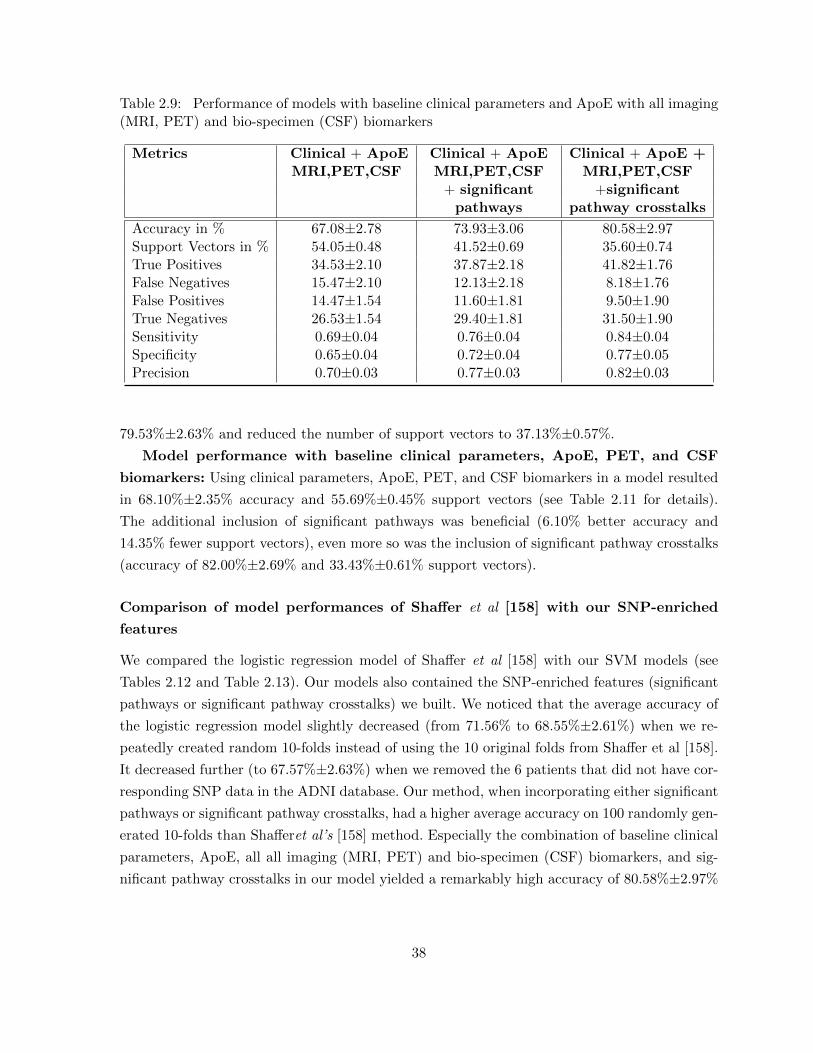
Table 2.9: Performance of models with baseline clinical parameters and ApoE with all imaging(MRI, PET) and bio-specimen (CSF) biomarkers

Metrics Clinical + ApoE Clinical + ApoE Clinical + ApoE +MRI,PET,CSF MRI,PET,CSF MRI,PET,CSF

+ significant +significantpathways pathway crosstalks

Accuracy in % 67.08±2.78 73.93±3.06 80.58±2.97Support Vectors in % 54.05±0.48 41.52±0.69 35.60±0.74True Positives 34.53±2.10 37.87±2.18 41.82±1.76False Negatives 15.47±2.10 12.13±2.18 8.18±1.76False Positives 14.47±1.54 11.60±1.81 9.50±1.90True Negatives 26.53±1.54 29.40±1.81 31.50±1.90Sensitivity 0.69±0.04 0.76±0.04 0.84±0.04Specificity 0.65±0.04 0.72±0.04 0.77±0.05Precision 0.70±0.03 0.77±0.03 0.82±0.03

79.53%±2.63% and reduced the number of support vectors to 37.13%±0.57%.

Model performance with baseline clinical parameters, ApoE, PET, and CSF

biomarkers: Using clinical parameters, ApoE, PET, and CSF biomarkers in a model resulted

in 68.10%±2.35% accuracy and 55.69%±0.45% support vectors (see Table 2.11 for details).

The additional inclusion of significant pathways was beneficial (6.10% better accuracy and

14.35% fewer support vectors), even more so was the inclusion of significant pathway crosstalks

(accuracy of 82.00%±2.69% and 33.43%±0.61% support vectors).

Comparison of model performances of Shaffer et al [158] with our SNP-enriched

features

We compared the logistic regression model of Shaffer et al [158] with our SVM models (see

Tables 2.12 and Table 2.13). Our models also contained the SNP-enriched features (significant

pathways or significant pathway crosstalks) we built. We noticed that the average accuracy of

the logistic regression model slightly decreased (from 71.56% to 68.55%±2.61%) when we re-

peatedly created random 10-folds instead of using the 10 original folds from Shaffer et al [158].

It decreased further (to 67.57%±2.63%) when we removed the 6 patients that did not have cor-

responding SNP data in the ADNI database. Our method, when incorporating either significant

pathways or significant pathway crosstalks, had a higher average accuracy on 100 randomly gen-

erated 10-folds than Shafferet al’s [158] method. Especially the combination of baseline clinical

parameters, ApoE, all all imaging (MRI, PET) and bio-specimen (CSF) biomarkers, and sig-

nificant pathway crosstalks in our model yielded a remarkably high accuracy of 80.58%±2.97%

38

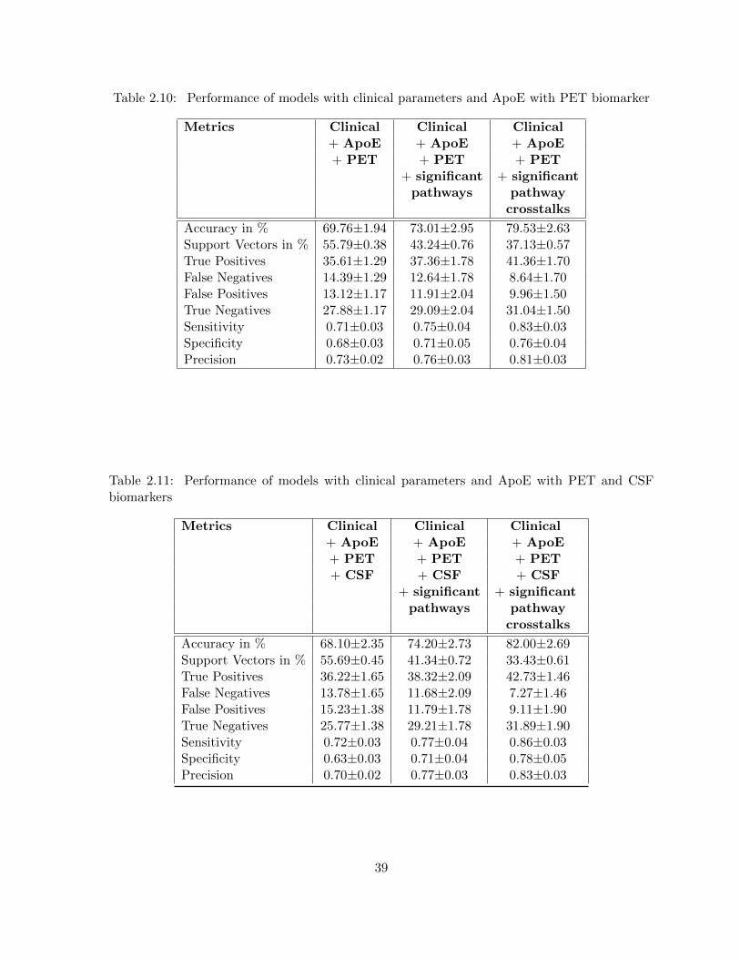
Table 2.10: Performance of models with clinical parameters and ApoE with PET biomarker

Metrics Clinical Clinical Clinical+ ApoE + ApoE + ApoE+ PET + PET + PET

+ significant + significantpathways pathway

crosstalks

Accuracy in % 69.76±1.94 73.01±2.95 79.53±2.63Support Vectors in % 55.79±0.38 43.24±0.76 37.13±0.57True Positives 35.61±1.29 37.36±1.78 41.36±1.70False Negatives 14.39±1.29 12.64±1.78 8.64±1.70False Positives 13.12±1.17 11.91±2.04 9.96±1.50True Negatives 27.88±1.17 29.09±2.04 31.04±1.50Sensitivity 0.71±0.03 0.75±0.04 0.83±0.03Specificity 0.68±0.03 0.71±0.05 0.76±0.04Precision 0.73±0.02 0.76±0.03 0.81±0.03

Table 2.11: Performance of models with clinical parameters and ApoE with PET and CSFbiomarkers

Metrics Clinical Clinical Clinical+ ApoE + ApoE + ApoE+ PET + PET + PET+ CSF + CSF + CSF

+ significant + significantpathways pathway

crosstalks

Accuracy in % 68.10±2.35 74.20±2.73 82.00±2.69Support Vectors in % 55.69±0.45 41.34±0.72 33.43±0.61True Positives 36.22±1.65 38.32±2.09 42.73±1.46False Negatives 13.78±1.65 11.68±2.09 7.27±1.46False Positives 15.23±1.38 11.79±1.78 9.11±1.90True Negatives 25.77±1.38 29.21±1.78 31.89±1.90Sensitivity 0.72±0.03 0.77±0.04 0.86±0.03Specificity 0.63±0.03 0.71±0.04 0.78±0.05Precision 0.70±0.02 0.77±0.03 0.83±0.03

39

with 35.60%±0.74% support vectors. The original data set of 97 patients from the logistic re-

gression by Shaffer et al [158] was obtained. Table 2.12 provides the result details for. The

results of the original 10-fold cross-validation on 97 patients are shown in column 2. The mean

and standard deviation of 100 iterations of random 10-fold cross-validation on 97 patients are

shown in column 3. Columns 4-5 show mean and standard deviation of 100 iterations of 10-fold

cross-validation on 91 patients, performed with our method. Table 2.13 provides the result de-

tails for the reduced 91 patient dataset. The mean and standard deviation of 100 iterations of

random 10-fold cross-validation on 91 patients are shown in column 2. Columns 3-4 show mean

and standard deviation of 100 iterations of 10-fold cross-validation on 91 patients, performed

with our method.

40

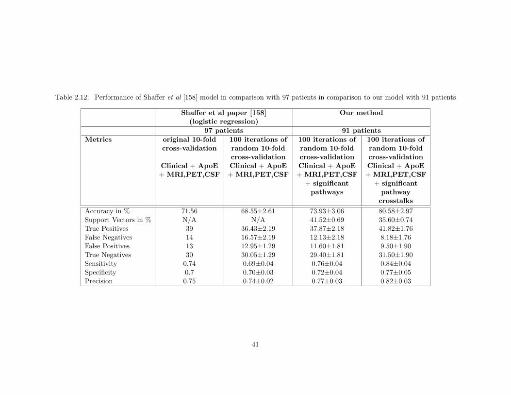
Table 2.12: Performance of Shaffer et al [158] model in comparison with 97 patients in comparison to our model with 91 patients

Shaffer et al paper [158] Our method(logistic regression)

97 patients 91 patients

Metrics original 10-fold 100 iterations of 100 iterations of 100 iterations ofcross-validation random 10-fold random 10-fold random 10-fold

cross-validation cross-validation cross-validationClinical + ApoE Clinical + ApoE Clinical + ApoE Clinical + ApoE+ MRI,PET,CSF + MRI,PET,CSF + MRI,PET,CSF + MRI,PET,CSF

+ significant + significantpathways pathway

crosstalks

Accuracy in % 71.56 68.55±2.61 73.93±3.06 80.58±2.97Support Vectors in % N/A N/A 41.52±0.69 35.60±0.74True Positives 39 36.43±2.19 37.87±2.18 41.82±1.76False Negatives 14 16.57±2.19 12.13±2.18 8.18±1.76False Positives 13 12.95±1.29 11.60±1.81 9.50±1.90True Negatives 30 30.05±1.29 29.40±1.81 31.50±1.90Sensitivity 0.74 0.69±0.04 0.76±0.04 0.84±0.04Specificity 0.7 0.70±0.03 0.72±0.04 0.77±0.05Precision 0.75 0.74±0.02 0.77±0.03 0.82±0.03

41

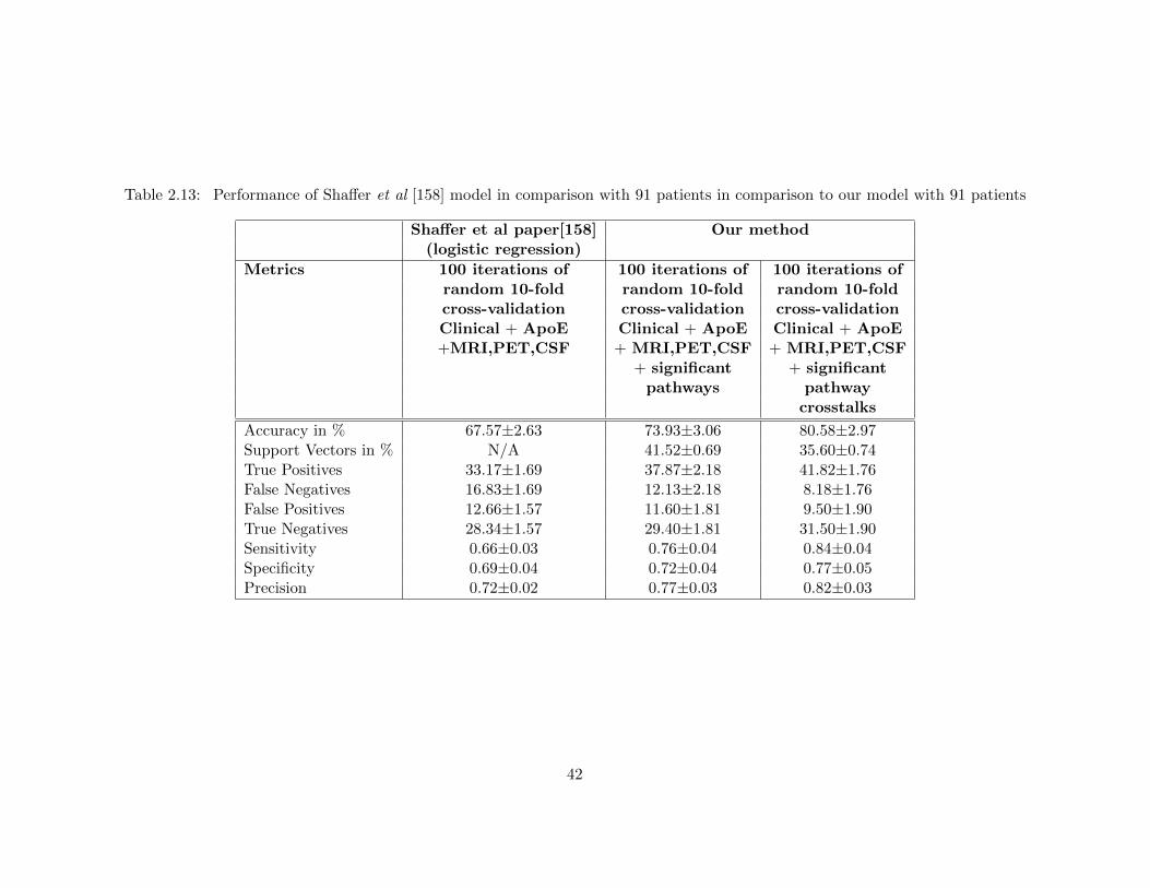
Table 2.13: Performance of Shaffer et al [158] model in comparison with 91 patients in comparison to our model with 91 patients

Shaffer et al paper[158] Our method(logistic regression)

Metrics 100 iterations of 100 iterations of 100 iterations ofrandom 10-fold random 10-fold random 10-foldcross-validation cross-validation cross-validationClinical + ApoE Clinical + ApoE Clinical + ApoE+MRI,PET,CSF + MRI,PET,CSF + MRI,PET,CSF

+ significant + significantpathways pathway

crosstalks

Accuracy in % 67.57±2.63 73.93±3.06 80.58±2.97Support Vectors in % N/A 41.52±0.69 35.60±0.74True Positives 33.17±1.69 37.87±2.18 41.82±1.76False Negatives 16.83±1.69 12.13±2.18 8.18±1.76False Positives 12.66±1.57 11.60±1.81 9.50±1.90True Negatives 28.34±1.57 29.40±1.81 31.50±1.90Sensitivity 0.66±0.03 0.76±0.04 0.84±0.04Specificity 0.69±0.04 0.72±0.04 0.77±0.05Precision 0.72±0.02 0.77±0.03 0.82±0.03

42

Randomized SNP-enriched features

We wanted to ensure that the choice of knowledge priors utilized in this study has true additive

power and the results are not a random occurrence. To do so, we generated 25 random samples

knowledge priors with no prior association to Alzheimer’s. This translates to creating random-

ized significant pathway crosstalks. We performed 100 iterations of 10-fold cross-validation for

each of the 25 samples and reported mean and standard deviation. The results clearly show that

the knowledge priors are truly effective in building better models for MCI to AD conversion

(see Table 2.14).

We analyzed models based on this randomized SNP-enriched data and: (1) baseline clinical

parameters, and (2) baseline clinical parameters and all imaging (MRI, PET) and bio-specimen

(CSF) biomarkers.

The model with baseline clinical parameters and randomized significant pathway crosstalks

gave an accuracy of 59.27%±3.66% with 83.47%±1.84% support vectors. This model yields 12%

less accuracy and 29.1% increase in support vectors, in comparison to the original model that

uses baseline parameters and significant pathway crosstalks (instead of randomized significant

pathway crosstalks). As expected, our randomly generated knowledge priors (randomized sig-

nificant pathway crosstalks) give us worse performance than significant pathway crosstalks. The

model accuracy is still moderately above a random guessing model, only due to the presence of

the clinical parameters.

Similarly, the model with baseline clinical parameters, all imaging (MRI, PET) and bio-

specimen (CSF) biomarkers, and randomized significant pathway crosstalks gave an accuracy

of 65.62%±3.53% with 54.73%±1.46% support vectors. This model yields nearly 15% less accu-

racy and almost 19% increase in support vectors, in comparison to the original model that uses

baseline parameters, all imaging (MRI, PET) and bio-specimen (CSF) biomarkers, and signif-

icant pathway crosstalks (instead of randomized significant pathway crosstalks). As expected,

our randomly generated knowledge priors (randomized significant pathway crosstalks) give us

worse performance than significant pathway crosstalks. The model accuracy is still above a

random guessing model, only due to the presence of the clinical parameters and all imaging

(MRI, PET) and bio-specimen (CSF) biomarkers. Again, for models using pathway crosstalks

only, no features were being selected as significant to build the model and hence the runs could

not be completed.

A similar trend was seen when investigating models with baseline clinical parameters and all

imaging (MRI, PET) and bio-specimen (CSF) biomarkers to determine the effects of randomized

pathways.

43

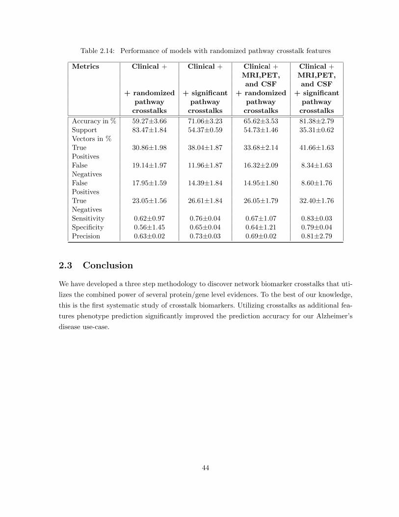
Table 2.14: Performance of models with randomized pathway crosstalk features

Metrics Clinical + Clinical + Clinical + Clinical +MRI,PET, MRI,PET,and CSF and CSF

+ randomized + significant + randomized + significantpathway pathway pathway pathway

crosstalks crosstalks crosstalks crosstalks

Accuracy in % 59.27±3.66 71.06±3.23 65.62±3.53 81.38±2.79Support 83.47±1.84 54.37±0.59 54.73±1.46 35.31±0.62Vectors in %True 30.86±1.98 38.04±1.87 33.68±2.14 41.66±1.63PositivesFalse 19.14±1.97 11.96±1.87 16.32±2.09 8.34±1.63NegativesFalse 17.95±1.59 14.39±1.84 14.95±1.80 8.60±1.76PositivesTrue 23.05±1.56 26.61±1.84 26.05±1.79 32.40±1.76NegativesSensitivity 0.62±0.97 0.76±0.04 0.67±1.07 0.83±0.03Specificity 0.56±1.45 0.65±0.04 0.64±1.21 0.79±0.04Precision 0.63±0.02 0.73±0.03 0.69±0.02 0.81±2.79

2.3 Conclusion

We have developed a three step methodology to discover network biomarker crosstalks that uti-

lizes the combined power of several protein/gene level evidences. To the best of our knowledge,

this is the first systematic study of crosstalk biomarkers. Utilizing crosstalks as additional fea-

tures phenotype prediction significantly improved the prediction accuracy for our Alzheimer’s

disease use-case.

44

Chapter 3

Subsystem Level: Discovery of

Network Biomarker Subsystems

At the subsystem level, the phenotype-related subsytem biomarkers are discovered and char-

acterized. Biological relationships (e.g., protein functional associations) between proteins are

often modeled as networks (protein functional association networks [70]), where each node is

a protein and every pair of functionally associated proteins is connected with an edge. Func-

tional association between proteins is derived from a number of clues like experimental data [5],

gene-fusion [167], co-occurrence of the corresponding genes on the same operon [31], etc. The

subgraphs of these networks can model the cellular subsystems.

Evolutionary conservation of cellular subsystems across multiple organisms with similar

phenotype can be used as one clue to identify the phenotype-related cellular subsystems [152].

Namely, the cellular subsystems associated with a phenotype are more likely to be conserved

across phenotype-expressing organisms and are less likely to be conserved across phenotype

non-expressing organisms [152].

Our earlier work, the α, β-motif finder [152] algorithm, which is the current state-of-the-art,

identifies phenotype-related subsystems that are modeled as cliques in the organismal functional

association networks. A clique is a subgraph with an edge between every pair of vertices in the

subgraph, i.e., every pair of proteins in the subsystem has to be functionally associated. Density,

the ratio of the number of edges in the subgraph to the total number of possible edges in the

subgraph is 1.0 for subgraphs modeled as cliques.

The clique model is too stringent to model all potential phenotype-related cellular subsys-

tems. There are existing studies that show that cellular subsystems can have different topolo-

gies [54]. A detailed study of the densities of existing protein complexes from various sources

[40, 41, 62, 91, 165] has revealed that the density of complexes varies from 0.1 to 1.0 [54]. This is

likely due to the fact that real world biological networks are prone to noise and missing informa-

45

tion (like missing edges) [127, 193]. Other studies [61, 164] have shown that non-clique clusters

form biologically relevant cellular subsystems. An example of a non-clique subsystem is the

cell-cycle regulation consisting of cyclins (CLB1-4 and CLN2), cyclin-dependent kinases (CKS1

and CDC28), and a nuclear import protein NIP29 identified from Saccharomyces cerevisiae

network [164]. Additionally, Hwang et al [68] showed that maximal clique enumeration based

methods discard over 90% of network nodes when applied to the protein interaction network of

Saccharomyces cerevisiae. Hence, α, β-motif finder method may not cover the entire spectrum

of phenotype-related cellular subsystems.

As a post processing step, each subsystem identified by the α, β-motif finder can be fed into

methods like our DENSE algorithm [61], a knowledge prior-driven quasi clique enumeration

algorithm to identify the subsystems missed by α, β-motif finder. However, DENSE can extract

subsystems from only a single organismal network and these subsystems may or may not be

related towards the target phenotype. DENSE also requires an input parameter to fix the density

of the subgraphs to be identified. This post processing amounts to running a compute-intensive

quasi-clique enumeration algorithm for every subsystem identified by the α, β-motif finder.

Our previous α, β-motif finder method requires two inputs: the parameter α−the least num-

ber of phenotype-expressing organisms the identified clique has to be present in and the pa-

rameter β−the number of phenotype non-expressing organisms the identified clique can be

present in. These parameters may be hard to estimate beforehand and, hence, multiple runs

with different parameter values may be required.

The α, β-motif finder works under the assumption that a subsystem’s presence can alone

cause a phenotype. Hence, the method only aims to identify the subsystems that are more

prevalent in phenotype-expressing organismal networks and less prevalent in phenotype non-

expressing organismal networks. However, a subsystem’s absence could also cause a phenotype-

expression. It was shown that the “couched potato” syndrome could be potentially caused

by the result of a person missing some key genes related to the MP-activated protein kinase

(AMPK) [179]. It was also shown that one out of every 4 cases of breast cancer is associated

with the absence of the NF1, a gene that negatively regulates an oncogene called RAS. RAS,

when mutated or highly expressed, contributes to a normal cell turning cancerous [183].

We propose to develop a methodology to enumerate phenotype-related cellular subsystems

(functional modules) placing no restriction on the density or size of the enumerated subgraphs.

The method also does not place any restriction on the number of networks the resulting sub-

graph should be present in. Additionally, the method identifies subsystems biased towards the

phenotype expressing organisms and towards phenotype non-expressing organisms from the

results of a single run of the methodology.

46

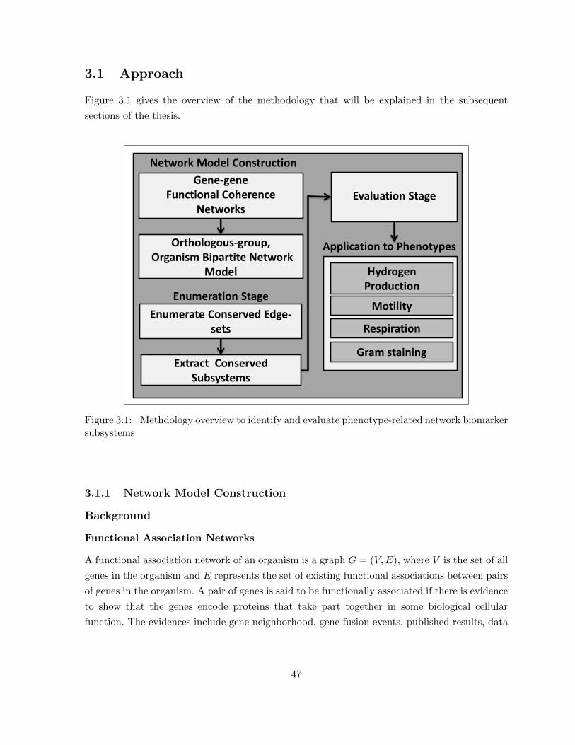
3.1 Approach

Figure 3.1 gives the overview of the methodology that will be explained in the subsequent

sections of the thesis.

Gene-gene Functional Coherence

Networks

Orthologous-group, Organism Bipartite Network

Model

Enumerate Conserved Edge-sets

Extract ConservedSubsystems

Hydrogen Production

Motility

Respiration

Gram staining

Evaluation Stage

Network Model Construction

Enumeration Stage

Application to Phenotypes

Figure 3.1: Methdology overview to identify and evaluate phenotype-related network biomarkersubsystems

3.1.1 Network Model Construction

Background

Functional Association Networks

A functional association network of an organism is a graph G = (V,E), where V is the set of all

genes in the organism and E represents the set of existing functional associations between pairs

of genes in the organism. A pair of genes is said to be functionally associated if there is evidence

to show that the genes encode proteins that take part together in some biological cellular

function. The evidences include gene neighborhood, gene fusion events, published results, data

47

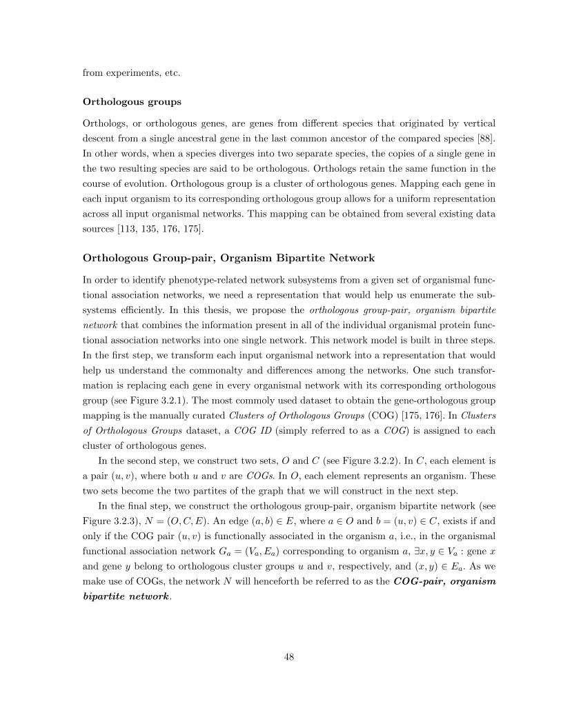
from experiments, etc.

Orthologous groups

Orthologs, or orthologous genes, are genes from different species that originated by vertical

descent from a single ancestral gene in the last common ancestor of the compared species [88].

In other words, when a species diverges into two separate species, the copies of a single gene in

the two resulting species are said to be orthologous. Orthologs retain the same function in the

course of evolution. Orthologous group is a cluster of orthologous genes. Mapping each gene in

each input organism to its corresponding orthologous group allows for a uniform representation

across all input organismal networks. This mapping can be obtained from several existing data

sources [113, 135, 176, 175].

Orthologous Group-pair, Organism Bipartite Network

In order to identify phenotype-related network subsystems from a given set of organismal func-

tional association networks, we need a representation that would help us enumerate the sub-

systems efficiently. In this thesis, we propose the orthologous group-pair, organism bipartite

network that combines the information present in all of the individual organismal protein func-

tional association networks into one single network. This network model is built in three steps.

In the first step, we transform each input organismal network into a representation that would

help us understand the commonalty and differences among the networks. One such transfor-

mation is replacing each gene in every organismal network with its corresponding orthologous

group (see Figure 3.2.1). The most commoly used dataset to obtain the gene-orthologous group

mapping is the manually curated Clusters of Orthologous Groups (COG) [175, 176]. In Clusters

of Orthologous Groups dataset, a COG ID (simply referred to as a COG) is assigned to each

cluster of orthologous genes.

In the second step, we construct two sets, O and C (see Figure 3.2.2). In C, each element is

a pair (u, v), where both u and v are COGs. In O, each element represents an organism. These

two sets become the two partites of the graph that we will construct in the next step.

In the final step, we construct the orthologous group-pair, organism bipartite network (see

Figure 3.2.3), N = (O,C,E). An edge (a, b) ∈ E, where a ∈ O and b = (u, v) ∈ C, exists if and

only if the COG pair (u, v) is functionally associated in the organism a, i.e., in the organismal

functional association network Ga = (Va, Ea) corresponding to organism a, ∃x, y ∈ Va : gene x

and gene y belong to orthologous cluster groups u and v, respectively, and (x, y) ∈ Ea. As we

make use of COGs, the network N will henceforth be referred to as the COG-pair, organism

bipartite network .

48

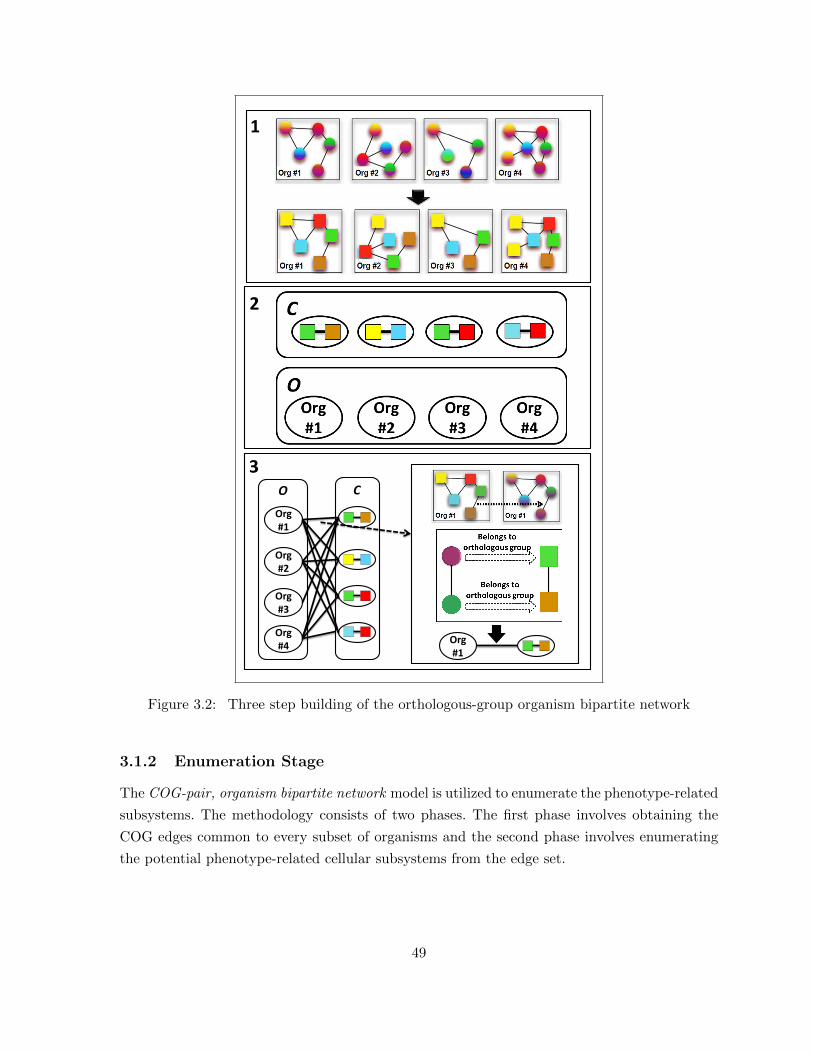
1

Org #4

Org #3

Org #2

Org #1

C O

Org #1

3

2

Figure 3.2: Three step building of the orthologous-group organism bipartite network

3.1.2 Enumeration Stage

The COG-pair, organism bipartite network model is utilized to enumerate the phenotype-related

subsystems. The methodology consists of two phases. The first phase involves obtaining the

COG edges common to every subset of organisms and the second phase involves enumerating

the potential phenotype-related cellular subsystems from the edge set.

49

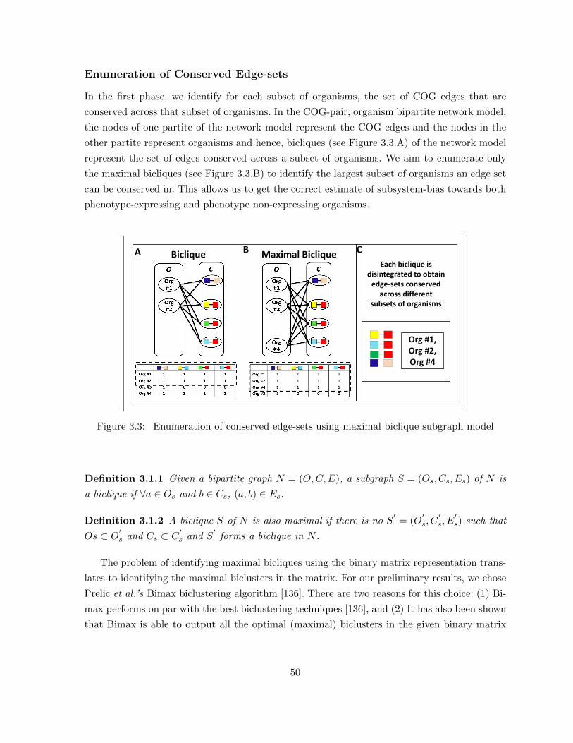
Enumeration of Conserved Edge-sets

In the first phase, we identify for each subset of organisms, the set of COG edges that are

conserved across that subset of organisms. In the COG-pair, organism bipartite network model,

the nodes of one partite of the network model represent the COG edges and the nodes in the

other partite represent organisms and hence, bicliques (see Figure 3.3.A) of the network model

represent the set of edges conserved across a subset of organisms. We aim to enumerate only

the maximal bicliques (see Figure 3.3.B) to identify the largest subset of organisms an edge set

can be conserved in. This allows us to get the correct estimate of subsystem-bias towards both

phenotype-expressing and phenotype non-expressing organisms.

Biclique Maximal Biclique Each biclique is

disintegrated to obtain edge-sets conserved

across different subsets of organisms

Org #1,Org #2,Org #4

A B C

Figure 3.3: Enumeration of conserved edge-sets using maximal biclique subgraph model

Definition 3.1.1 Given a bipartite graph N = (O,C,E), a subgraph S = (Os, Cs, Es) of N is

a biclique if ∀a ∈ Os and b ∈ Cs, (a, b) ∈ Es.

Definition 3.1.2 A biclique S of N is also maximal if there is no S′

= (O′s, C

′s, E

′s) such that

Os ⊂ O′s and Cs ⊂ C′s and S

′forms a biclique in N .

The problem of identifying maximal bicliques using the binary matrix representation trans-

lates to identifying the maximal biclusters in the matrix. For our preliminary results, we chose

Prelic et al.’s Bimax biclustering algorithm [136]. There are two reasons for this choice: (1) Bi-

max performs on par with the best biclustering techniques [136], and (2) It has also been shown

that Bimax is able to output all the optimal (maximal) biclusters in the given binary matrix

50

[136]. The algorithm uses a divide-and-conquer approach to enumerate maximal biclusters in

the COG-pair, organism bipartite network.

However, the methodology should be scalable for large number of organisms because, as we

increase the size of the organism set (O), the corresponding number of COG-edges (vertices

of partite C) could increase, and a significant number of edges will be added to the edge set

E. Thus, the underlying algorithm to mine the bicliques should be scalable and complete its

execution in a practical amount of time.To meet this goal, we consider another representation

of the problem—enumerating maximal bicliques in bipartite graphs.

Most existing methods solve the biclique mining problem by introducing restrictions to im-

prove algorithm efficiency. These include bounding the maximum input degree [174], bounding

the maximum biclique degree [51], bounding the minimum biclique size [103, 114, 184], bound-

ing an inputs arboricity [35], solving the problem for graphs that satisfy certain conditions

[126], even assigning weights to the vertices of the graph and identifying the “high confidence”

bicliques [123]. However, algorithms that depend for its efficiency on such restrictions cannot

solve arbitrary bipartite instances. Additionally, if we do utilize existing methods, we would

have to then perform a seperate analysis to determine the right parameter values. An existing

algorithm to solving the general bipartite biclique problem is serial [200]. The existing parallel

algorithm for the biclique mining in general graphs [147] places restrictions on the bicliques

mined.

Another approach relies on graph inflation. It is easily observed (see, for example, [109]) that

maximal biclique enumeration on bipartite graphs can be turned into a maximal clique enu-

meration on general graphs, by adding edges between all pairs of vertices belonging to the same

partite. This approach is neither practical nor scalable due to the enormous number of edges

that may be needed and the accompanying increase in problem difficulty that is incurred. How-

ever, it has been suggested in literature [1], that it is worthwhile adapting existing algorithms

for the general clique problem to mine bicliques.

We developed a parallel parameter-free heuristic algorithm to generate all maximal bicliques

in bipartite graphs. The algorithm is a modified version from the widely-used, efficient, back-

tacking method of enumerating maximal cliques of Bron and Kerbosch (BK) [17]. The parallel

framework from our earlier work on maximal clique enumeration [154] has been adopted and

modified to provide a parallel implementation our algorithm.

The main difference between a clique mining in a general graph and biclique mining in a

bipartite graph is the relationship that can exist between a pair of vertices (a, b). In general

graphs, a and b, can either be connected or disconnected and that condition can be checked to

decide if a vertex can be added to a current clique to form a larger clique. A pair of discon-

nected vertices cannot be part of the same clique. In case of bipartite graphs, the concept of

disconnection is more profound. A pair of vertices can be disconnected and belong to the same

51

clique, if they are part of the same partite. This means, that checking a pair of vertices from

the same partite to tell if they can or cannot be part of the same clique without additional

information cannot be done. This extremely basic but important concept was kept in mind

while developing the algorithm.

In generic BK, for every clique three lists get maintained, the compsub—the vertices cur-

rently part of the clique, the cand—vertices that are connected to all vertices in compsub, and

not—the set of vertices connected to all vertices in compsub, but would form cliques that have

been previously enumerated. The basic idea is that, a vertex a is selected from cand and added

to the set compsub and subsequently the sets cand and not are updated to only contain vertices

adjacent to a. However, in the modified algorithm, we not only keep vertices adjacent to a but

also vertices in the same partite as a (see Algorithm 3.2 - Line 10 and Line 11), since these

vertices could also be potentially added to the current clique.

The modified definitions of cand and not require a more sophisticated approach when it

comes to selecting a vertex to be added to the clique. In the general BK algorithm, any vertex

from the set cand could be selected, but for a bipartite graph, we need to make sure that the

selected vertex is connected to every vertex that is in compsub and not in the same partite

as a. The brute force way would for every vertex in cand, loop through the vertices in the

compsub to check for a’s connectivity. This solution would be an significant addition to the

clique enumeration time as the clique sizes increase and would defy the purpose of utilizing an

algorithm like the BK.

Thus, we introduce the concept of partite-representatives. Partite-representatives (partc and

parto) are elements that belong to compsub that belong to different partites. A potential candi-

date a is added to compsub if it is connected to either one of the representatives (see Algorithm

3.2 - Line 6 ). Each time a vertex x is added to compsub, the cand is updated to only con-

tain vertices that are connected or in the same partite as x. The update at the current step

is performed over the updates performed the previous steps, hence, if the current candidate a

is connected to a vertex x from compsub, we know that a is also connected to every vertex in

the same partite as x, and all other vertices in compsub would belong to the same partite as

a. The first candidate added to an empty compsub becomes the first representative, and the

second representative is the second candidate chosen because it will have to satisfy the criteria

of being connected the one existing representative.

In the generic BK algorithm, once the selected candidate a was added to compsub, the

algorithm looks for other vertices in cand that is not connected to a and this would signify

a new branch being added to the search tree. We modify the search condition to check that

vertices that are not connected to a are also not in the same partite as a (see Algorithm 3.2

- Line 16). The BK algorithm with all the modifications is shown in Algorithm 3.2 and an

example is shown in Figure 3.4. The algorithm had been fitted into the parallel framework from

52

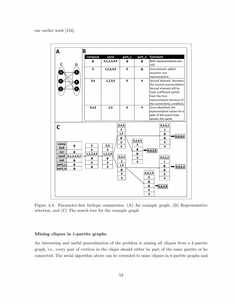
our earlier work [154].

Figure 3.4: Parameter-free biclique enumerator. (A) An example graph, (B) Representativeselection, and (C) The search tree for the example graph

Mining cliques in k-partite graphs

An interesting and useful generalization of the problem is mining all cliques from a k-partite

graph, i.e., every pair of vertices in the clique should either be part of the same partite or be

connected. The serial algorithm above can be extended to mine cliques in k-partite graphs and

53

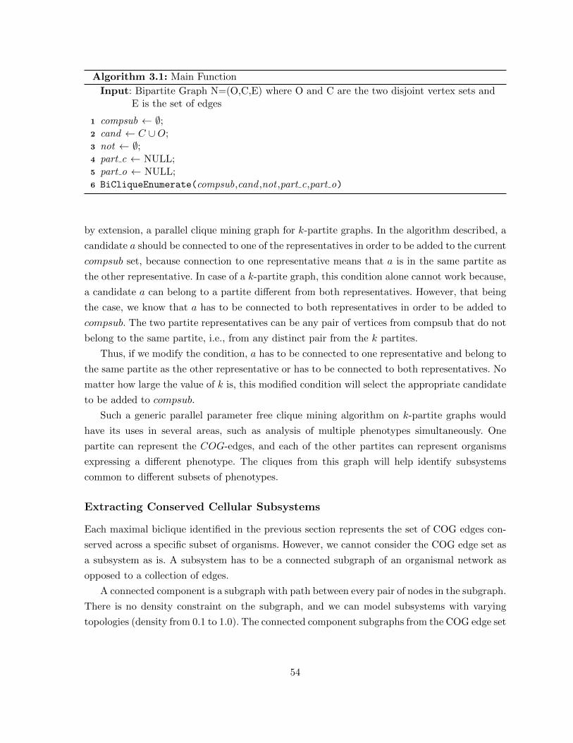
Algorithm 3.1: Main Function

Input: Bipartite Graph N=(O,C,E) where O and C are the two disjoint vertex sets andE is the set of edges

1 compsub ← ∅;2 cand ← C ∪O;3 not ← ∅;4 part c ← NULL;5 part o ← NULL;6 BiCliqueEnumerate(compsub,cand ,not ,part c,part o)

by extension, a parallel clique mining graph for k-partite graphs. In the algorithm described, a

candidate a should be connected to one of the representatives in order to be added to the current

compsub set, because connection to one representative means that a is in the same partite as

the other representative. In case of a k-partite graph, this condition alone cannot work because,

a candidate a can belong to a partite different from both representatives. However, that being

the case, we know that a has to be connected to both representatives in order to be added to

compsub. The two partite representatives can be any pair of vertices from compsub that do not

belong to the same partite, i.e., from any distinct pair from the k partites.

Thus, if we modify the condition, a has to be connected to one representative and belong to

the same partite as the other representative or has to be connected to both representatives. No

matter how large the value of k is, this modified condition will select the appropriate candidate

to be added to compsub.

Such a generic parallel parameter free clique mining algorithm on k-partite graphs would

have its uses in several areas, such as analysis of multiple phenotypes simultaneously. One

partite can represent the COG-edges, and each of the other partites can represent organisms

expressing a different phenotype. The cliques from this graph will help identify subsystems

common to different subsets of phenotypes.

Extracting Conserved Cellular Subsystems

Each maximal biclique identified in the previous section represents the set of COG edges con-

served across a specific subset of organisms. However, we cannot consider the COG edge set as

a subsystem as is. A subsystem has to be a connected subgraph of an organismal network as

opposed to a collection of edges.

A connected component is a subgraph with path between every pair of nodes in the subgraph.

There is no density constraint on the subgraph, and we can model subsystems with varying

topologies (density from 0.1 to 1.0). The connected component subgraphs from the COG edge set

54

of each maximal bicluster are enumerated (see Figure 3.5). The enumeration can be performed

using depth-or-breadth-first-search, both of which are linear time algorithms in terms of the

number of edges.

Algorithm 3.2: Parameter-free biclique enumerator

1 BiCliqueEnumerate(compsub,cand ,not ,part c,part o)

2 if cand = ∅ then3 if not = ∅ then4 Output compsub;

5 else6 fixp ← The vertex in cand that is connected to the greatest number of other vertices

in cand and connected to either part c or part o;7 cur v ← fixp;8 if cur v 6= NULL then9 while cur v 6= NULL do

10 new not ← All vertices in not that are connected to cur v or in the samepartite as cur v ;

11 new cand ← All vertices in cand that are connected to or in the same partiteas cur v ;

12 new cs ← compsub + cur v ;13 BiCliqueEnumerate(new cs, new cand , new not ,part o,part c);14 not ← not + cur v ;15 cand ← cand − cur v ;16 if there is a vertex v in cand that is not connected to fixp and not in the

same partite as fixp then17 cur v ← v;

18 else19 cur v ← NULL;

20 return

3.1.3 Evaluation Stage

Statistical Significance Assessment

The results of the method only guarantee that the subgraphs output are connected components

but there is no clear indication whether the subgraphs could represent subsystems or if their

occurrence was purely random. To determine this statistical significance the topological density

of each subgraph is compared with a density of randomly obtained subgraphs with the same

number of nodes.

55

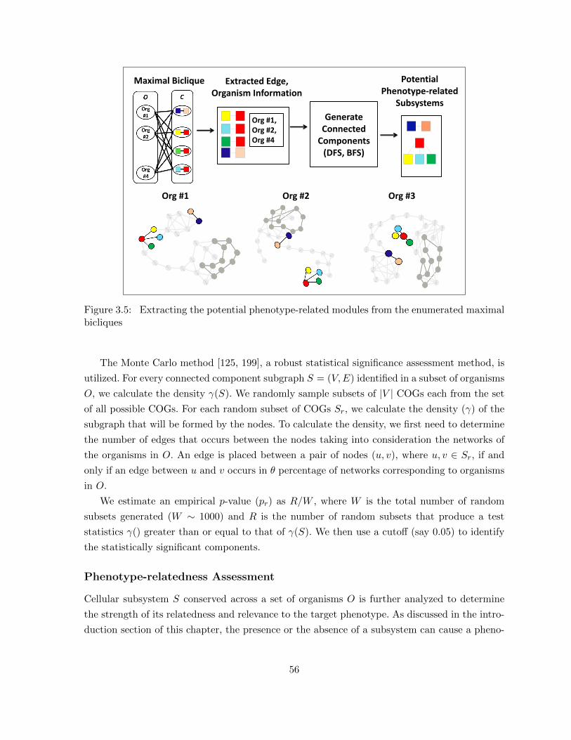
GenerateConnected

Components (DFS, BFS)

Org #1, Org #2, Org #4

Org #1 Org #2 Org #3

Maximal Biclique Extracted Edge, Organism Information

Potential Phenotype-related

Subsystems

Figure 3.5: Extracting the potential phenotype-related modules from the enumerated maximalbicliques

The Monte Carlo method [125, 199], a robust statistical significance assessment method, is

utilized. For every connected component subgraph S = (V,E) identified in a subset of organisms

O, we calculate the density γ(S). We randomly sample subsets of |V | COGs each from the set

of all possible COGs. For each random subset of COGs Sr, we calculate the density (γ) of the

subgraph that will be formed by the nodes. To calculate the density, we first need to determine

the number of edges that occurs between the nodes taking into consideration the networks of

the organisms in O. An edge is placed between a pair of nodes (u, v), where u, v ∈ Sr, if and

only if an edge between u and v occurs in θ percentage of networks corresponding to organisms

in O.

We estimate an empirical p-value (pr) as R/W , where W is the total number of random

subsets generated (W ∼ 1000) and R is the number of random subsets that produce a test

statistics γ() greater than or equal to that of γ(S). We then use a cutoff (say 0.05) to identify

the statistically significant components.

Phenotype-relatedness Assessment

Cellular subsystem S conserved across a set of organisms O is further analyzed to determine

the strength of its relatedness and relevance to the target phenotype. As discussed in the intro-

duction section of this chapter, the presence or the absence of a subsystem can cause a pheno-

56

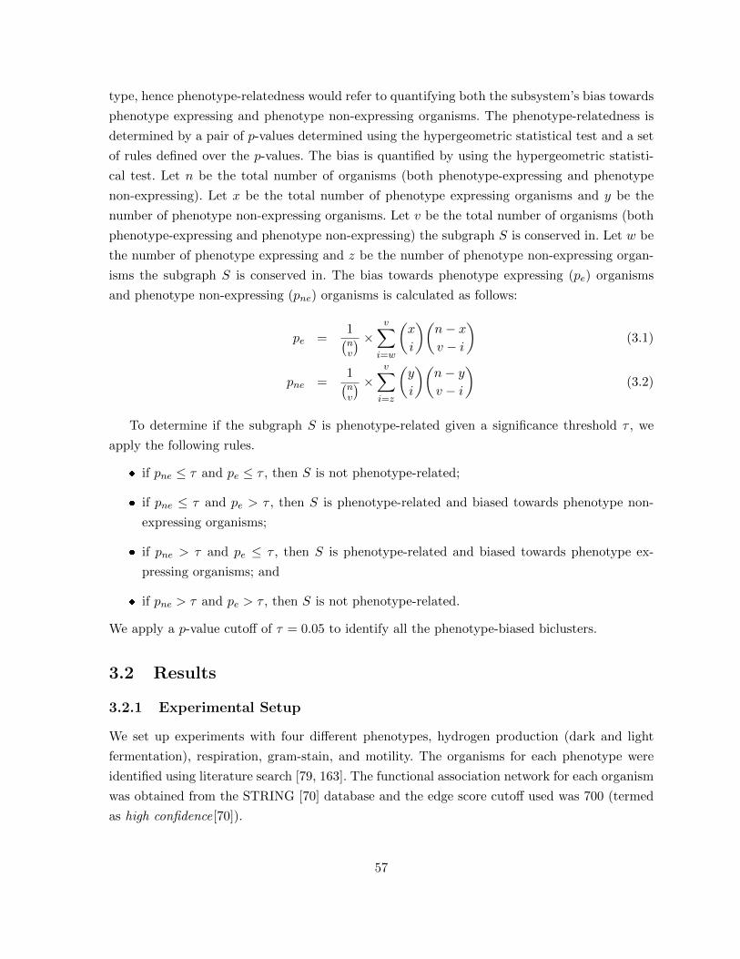
type, hence phenotype-relatedness would refer to quantifying both the subsystem’s bias towards

phenotype expressing and phenotype non-expressing organisms. The phenotype-relatedness is

determined by a pair of p-values determined using the hypergeometric statistical test and a set

of rules defined over the p-values. The bias is quantified by using the hypergeometric statisti-

cal test. Let n be the total number of organisms (both phenotype-expressing and phenotype

non-expressing). Let x be the total number of phenotype expressing organisms and y be the

number of phenotype non-expressing organisms. Let v be the total number of organisms (both

phenotype-expressing and phenotype non-expressing) the subgraph S is conserved in. Let w be

the number of phenotype expressing and z be the number of phenotype non-expressing organ-

isms the subgraph S is conserved in. The bias towards phenotype expressing (pe) organisms

and phenotype non-expressing (pne) organisms is calculated as follows:

pe =1(nv

) × v∑i=w

(x

i

)(n− xv − i

)(3.1)

pne =1(nv

) × v∑i=z

(y

i

)(n− yv − i

)(3.2)

To determine if the subgraph S is phenotype-related given a significance threshold τ , we

apply the following rules.

� if pne ≤ τ and pe ≤ τ , then S is not phenotype-related;

� if pne ≤ τ and pe > τ , then S is phenotype-related and biased towards phenotype non-

expressing organisms;

� if pne > τ and pe ≤ τ , then S is phenotype-related and biased towards phenotype ex-

pressing organisms; and

� if pne > τ and pe > τ , then S is not phenotype-related.

We apply a p-value cutoff of τ = 0.05 to identify all the phenotype-biased biclusters.

3.2 Results

3.2.1 Experimental Setup

We set up experiments with four different phenotypes, hydrogen production (dark and light

fermentation), respiration, gram-stain, and motility. The organisms for each phenotype were

identified using literature search [79, 163]. The functional association network for each organism

was obtained from the STRING [70] database and the edge score cutoff used was 700 (termed

as high confidence[70]).

57

3.2.2 Hydrogen Production

Biological hydrogen production is being looked at as a source of alternate energy and there are

a number of microorganisms that can utilize different organic substrates to produce hydrogen.

This makes it a useful alternative energy option to explore [15, 78, 124]. Identifying cellular

subsystems related to hydrogen production will be extremely useful to genetic engineers aiming

to make the process of biological hydrogen production more efficient. The light and dark fer-

mentation are two important sub-phenotypes of hydrogen production, and experiments based

on these phenotypes will be discussed in this section.

Light fermentation

Initial review of the light fermentation clusters shows the presence of a set of 13 identical COGs

found across all 8 COG clusters. These “core” COGs include genes necessary for synthesis of

hydrogenase complex(es).

Nitrogen-fixation is the process, in which nitrogenase catalyzes the conversion of nitrogen

gas to ammonia and inadvertently results in the production of hydrogen gas as a byproduct

[142, 143]. Two COGs (COG2710 and COG1348), which are associated with the expression

of two key proteins, nitrogenase iron protein (NifH) and molybdenum iron protein [142], were

present across all the clusters. Although, the presence of these two proteins is essential for

nitrogen-fixation to be carried out by light fermenting microorganisms, expression of various

genes in other metabolic pathways plays important roles in either directly or indirectly regulat-

ing the expression of genes encoding NifH proteins. These proteins include ferric iron regulation

proteins (sigK, clpB, and fur-related), ammonia ligase (glnA), and nitrogenase [94]. In this

study, glutamate ammonia ligase (glnA), a key gene for nitrogenase (NifH), and genes encoding

proteins for iron uptake, are assembled in the same cluster. In Anabaena, iron uptake proteins

and some nitrogen proteins (e.g., Ntc) have been shown to regulate genes encoding glutamate

synthetase (glnA) [107]. Review of the role of glutamine synthetase in Anabaena indicates that

this enzyme is responsible for regulating nitrogenase activity, thus impacting hydrogen produc-

tion [107]. The indirect regulation of nitrogenase by iron uptake proteins provides an example

of crosstalk between iron and nitrogen-related metabolic pathways.

In addition to nitrogenase, proteins associated with the synthesis of uptake or expression

of hydrogenase, were identified in 11 of the 19 COGs present in Table 3.1. Hydrogen uptake

proteins help with removing excess hydrogen to maintain the reducing environment in cells [90].

We also identified a number of proteins (e.g., Hyd and Hyp) involved in formation of [NiFe]-

uptake hydrogenases. The presence of maturation hydrogenase factors (COG0068, COG0298,

COG0309) and accessory proteins for uptake of nickel (COG0378) are consistent with literature

reports describing the structure of hydrogenase complexes. Inclusion of hydrogenase proteins

58

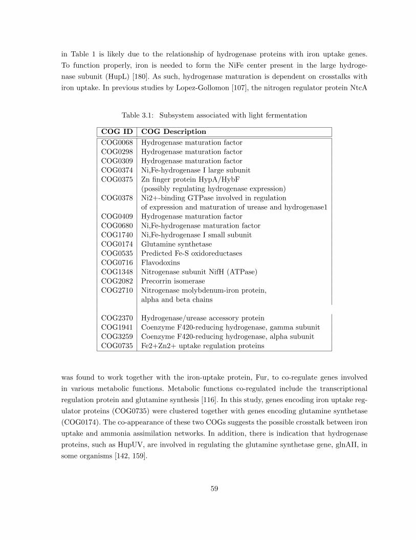
in Table 1 is likely due to the relationship of hydrogenase proteins with iron uptake genes.

To function properly, iron is needed to form the NiFe center present in the large hydroge-

nase subunit (HupL) [180]. As such, hydrogenase maturation is dependent on crosstalks with

iron uptake. In previous studies by Lopez-Gollomon [107], the nitrogen regulator protein NtcA

Table 3.1: Subsystem associated with light fermentation

COG ID COG Description

COG0068 Hydrogenase maturation factorCOG0298 Hydrogenase maturation factorCOG0309 Hydrogenase maturation factorCOG0374 Ni,Fe-hydrogenase I large subunitCOG0375 Zn finger protein HypA/HybF

(possibly regulating hydrogenase expression)COG0378 Ni2+-binding GTPase involved in regulation

of expression and maturation of urease and hydrogenase1COG0409 Hydrogenase maturation factorCOG0680 Ni,Fe-hydrogenase maturation factorCOG1740 Ni,Fe-hydrogenase I small subunitCOG0174 Glutamine synthetaseCOG0535 Predicted Fe-S oxidoreductasesCOG0716 FlavodoxinsCOG1348 Nitrogenase subunit NifH (ATPase)COG2082 Precorrin isomeraseCOG2710 Nitrogenase molybdenum-iron protein,

alpha and beta chains

COG2370 Hydrogenase/urease accessory proteinCOG1941 Coenzyme F420-reducing hydrogenase, gamma subunitCOG3259 Coenzyme F420-reducing hydrogenase, alpha subunitCOG0735 Fe2+Zn2+ uptake regulation proteins

was found to work together with the iron-uptake protein, Fur, to co-regulate genes involved

in various metabolic functions. Metabolic functions co-regulated include the transcriptional

regulation protein and glutamine synthesis [116]. In this study, genes encoding iron uptake reg-

ulator proteins (COG0735) were clustered together with genes encoding glutamine synthetase

(COG0174). The co-appearance of these two COGs suggests the possible crosstalk between iron

uptake and ammonia assimilation networks. In addition, there is indication that hydrogenase

proteins, such as HupUV, are involved in regulating the glutamine synthetase gene, glnAII, in

some organisms [142, 159].

59

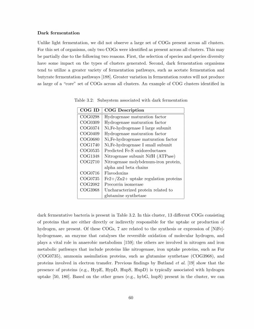
Dark fermentation

Unlike light fermentation, we did not observe a large set of COGs present across all clusters.

For this set of organisms, only two COGs were identified as present across all clusters. This may

be partially due to the following two reasons. First, the selection of species and species diversity

have some impact on the types of clusters generated. Second, dark fermentation organisms

tend to utilize a greater variety of fermentation pathways, such as acetate fermentation and

butyrate fermentation pathways [188]. Greater variation in fermentation routes will not produce

as large of a “core” set of COGs across all clusters. An example of COG clusters identified in

Table 3.2: Subsystem associated with dark fermentation

COG ID COG Description

COG0298 Hydrogenase maturation factorCOG0309 Hydrogenase maturation factorCOG0374 Ni,Fe-hydrogenase I large subunitCOG0409 Hydrogenase maturation factorCOG0680 Ni,Fe-hydrogenase maturation factorCOG1740 Ni,Fe-hydrogenase I small subunitCOG0535 Predicted Fe-S oxidoreductasesCOG1348 Nitrogenase subunit NifH (ATPase)COG2710 Nitrogenase molybdenum-iron protein,

alpha and beta chainsCOG0716 FlavodoxinsCOG0735 Fe2+/Zn2+ uptake regulation proteinsCOG2082 Precorrin isomeraseCOG3968 Uncharacterized protein related to

glutamine synthetase

dark fermentative bacteria is present in Table 3.2. In this cluster, 13 different COGs consisting

of proteins that are either directly or indirectly responsible for the uptake or production of

hydrogen, are present. Of these COGs, 7 are related to the synthesis or expression of [NiFe]-

hydrogenase, an enzyme that catalyses the reversible oxidation of molecular hydrogen, and

plays a vital role in anaerobic metabolism [159]; the others are involved in nitrogen and iron

metabolic pathways that include proteins like nitrogenase, iron uptake proteins, such as Fur

(COG0735), ammonia assimilation proteins, such as glutamine synthetase (COG3968), and

proteins involved in electron transfer. Previous findings by Butland et al. [19] show that the

presence of proteins (e.g., HypE, HypD, HupS, HupD) is typically associated with hydrogen

uptake [50, 180]. Based on the other genes (e.g., hybG, hupS) present in the cluster, we can

60

predict that [NiFe]-hydrogenase is associated with hydrogen uptake in this group of organisms.

In addition to hydrogenase maturation and expression proteins, Fe-S oxidoreductases were

identified. As part of the structure of [NiFe]-hydrogenase, Fe-S metal centers are located on

the small subunit of the hydrogenase complex [159, 180]. Thus, it is expected that iron uptake

pathway would crosstalk with hydrogenase-related pathways. Furthermore, the iron uptake

pathway also crosstalks with nitrogen metabolism, in a sense that iron uptake proteins can be

involved indirectly in nitrogen metabolism through regulation of nitrogenase and maintaining

the reducing environment in the cell through hydrogen uptake (hydrogenase) [116, 195].

It has been shown that crosstalk between iron uptake and nitrogen metabolism enables reg-

ulation of ammonia assimilation [143]; it may be possible that the uncharacterized glutamine

synthetase protein in Table 2 is subject to such regulation. In our results, the gene encoding

the uncharacterized glutamine synthetase proteins was only present in a few species, includ-

ing Clostridium acetobutylicum and Clostridium beijerinckii, which both contained nitrogenase

and hydrogenase enzymes. It has been demonstrated that, in light fermenting organisms, such

as Rhodopseudomonas palustris, glutamine synthetase is regulated by hydrogenase accessory

proteins (HupUV) [143]. However, to the best of our knowledge, this relationship has not been

described in dark fermentation organisms. This knowledge increases the probability that the

uncharacterized glutamine synthetase protein maybe present in the COG cluster oweing to its

association with nitrogenase proteins, which may further indicate a possible crosstalk between

ammonia assimilation and nitrogen metabolism.

3.2.3 Motility

The motility experiment was set up with a set of 85 motile and 56 non-motile organisms chosen

from Slonim et al [163]. The method identified clusters that contained COG1360, COG1558,

COG1157, COG1684, and COG1536 (Table 3.3). All these COGS are related to flagella pro-

teins. The flagella proteins are those that enable the organisms to move. The method also found

COG0643, COG0835, and COG0784 that are related to bacterial chemotaxis. It is well known

that chemotaxis controls an organism’s movement with respect to the chemical composition

of its environment. For example, it helps the organism moves to the areas where there is very

high concentration of food [177]. COGS related to the Type III secretion system (COG1766,

COG1684, COG1987, COG1338, and COG1886) were also identified. It has been shown that

Type III secretion proteins share similarities with flagella proteins in structure and func-

tion [105]. Additionally, we identified COG0835, COG0643, COG1344, COG1291,COG0784,

COG1508, and COG1191 associated with the two-component systems. This is a signaling path-

way that regulates motility [48].

61

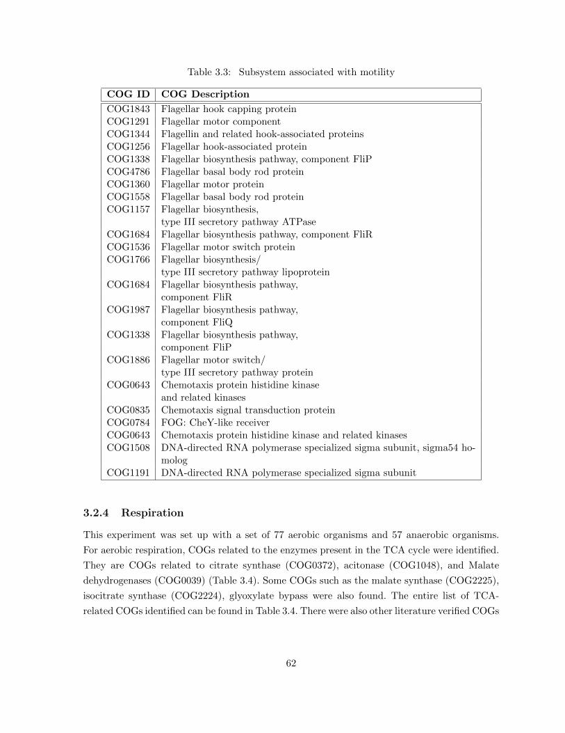
Table 3.3: Subsystem associated with motility

COG ID COG Description

COG1843 Flagellar hook capping proteinCOG1291 Flagellar motor componentCOG1344 Flagellin and related hook-associated proteinsCOG1256 Flagellar hook-associated proteinCOG1338 Flagellar biosynthesis pathway, component FliPCOG4786 Flagellar basal body rod proteinCOG1360 Flagellar motor proteinCOG1558 Flagellar basal body rod proteinCOG1157 Flagellar biosynthesis,

type III secretory pathway ATPaseCOG1684 Flagellar biosynthesis pathway, component FliRCOG1536 Flagellar motor switch proteinCOG1766 Flagellar biosynthesis/

type III secretory pathway lipoproteinCOG1684 Flagellar biosynthesis pathway,

component FliRCOG1987 Flagellar biosynthesis pathway,

component FliQCOG1338 Flagellar biosynthesis pathway,

component FliPCOG1886 Flagellar motor switch/

type III secretory pathway proteinCOG0643 Chemotaxis protein histidine kinase

and related kinasesCOG0835 Chemotaxis signal transduction proteinCOG0784 FOG: CheY-like receiverCOG0643 Chemotaxis protein histidine kinase and related kinasesCOG1508 DNA-directed RNA polymerase specialized sigma subunit, sigma54 ho-

mologCOG1191 DNA-directed RNA polymerase specialized sigma subunit

3.2.4 Respiration

This experiment was set up with a set of 77 aerobic organisms and 57 anaerobic organisms.

For aerobic respiration, COGs related to the enzymes present in the TCA cycle were identified.

They are COGs related to citrate synthase (COG0372), acitonase (COG1048), and Malate

dehydrogenases (COG0039) (Table 3.4). Some COGs such as the malate synthase (COG2225),

isocitrate synthase (COG2224), glyoxylate bypass were also found. The entire list of TCA-

related COGs identified can be found in Table 3.4. There were also other literature verified COGs

62

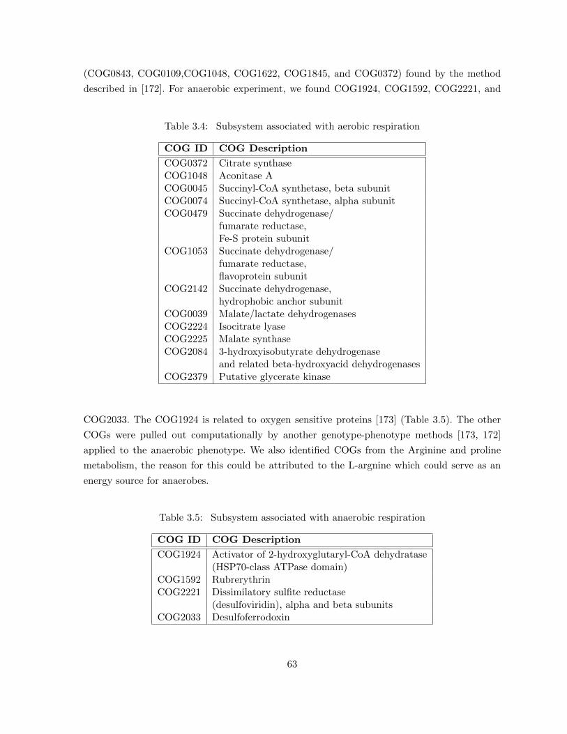
(COG0843, COG0109,COG1048, COG1622, COG1845, and COG0372) found by the method

described in [172]. For anaerobic experiment, we found COG1924, COG1592, COG2221, and

Table 3.4: Subsystem associated with aerobic respiration

COG ID COG Description

COG0372 Citrate synthaseCOG1048 Aconitase ACOG0045 Succinyl-CoA synthetase, beta subunitCOG0074 Succinyl-CoA synthetase, alpha subunitCOG0479 Succinate dehydrogenase/

fumarate reductase,Fe-S protein subunit

COG1053 Succinate dehydrogenase/fumarate reductase,flavoprotein subunit

COG2142 Succinate dehydrogenase,hydrophobic anchor subunit

COG0039 Malate/lactate dehydrogenasesCOG2224 Isocitrate lyaseCOG2225 Malate synthaseCOG2084 3-hydroxyisobutyrate dehydrogenase

and related beta-hydroxyacid dehydrogenasesCOG2379 Putative glycerate kinase

COG2033. The COG1924 is related to oxygen sensitive proteins [173] (Table 3.5). The other

COGs were pulled out computationally by another genotype-phenotype methods [173, 172]

applied to the anaerobic phenotype. We also identified COGs from the Arginine and proline

metabolism, the reason for this could be attributed to the L-argnine which could serve as an

energy source for anaerobes.

Table 3.5: Subsystem associated with anaerobic respiration

COG ID COG Description

COG1924 Activator of 2-hydroxyglutaryl-CoA dehydratase(HSP70-class ATPase domain)

COG1592 RubrerythrinCOG2221 Dissimilatory sulfite reductase

(desulfoviridin), alpha and beta subunitsCOG2033 Desulfoferrodoxin

63

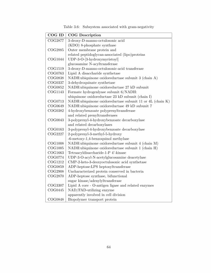
Table 3.6: Subsystem associated with gram-negativity

COG ID COG Description

COG2877 3-deoxy-D-manno-octulosonic acid(KDO) 8-phosphate synthase

COG2885 Outer membrane protein andrelated peptidoglycan-associated (lipo)proteins

COG1044 UDP-3-O-[3-hydroxymyristoyl]glucosamine N-acyltransferase

COG1519 3-deoxy-D-manno-octulosonic-acid transferaseCOG0763 Lipid A disaccharide synthetaseCOG0838 NADH:ubiquinone oxidoreductase subunit 3 (chain A)COG0337 3-dehydroquinate synthetaseCOG0852 NADH:ubiquinone oxidoreductase 27 kD subunitCOG1143 Formate hydrogenlyase subunit 6/NADH:

ubiquinone oxidoreductase 23 kD subunit (chain I)COG0713 NADH:ubiquinone oxidoreductase subunit 11 or 4L (chain K)COG0649 NADH:ubiquinone oxidoreductase 49 kD subunit 7COG0382 4-hydroxybenzoate polyprenyltransferase

and related prenyltransferasesCOG0043 3-polyprenyl-4-hydroxybenzoate decarboxylase

and related decarboxylasesCOG0163 3-polyprenyl-4-hydroxybenzoate decarboxylaseCOG2227 2-polyprenyl-3-methyl-5-hydroxy

-6-metoxy-1,4-benzoquinol methylaseCOG1008 NADH:ubiquinone oxidoreductase subunit 4 (chain M)COG1005 NADH:ubiquinone oxidoreductase subunit 1 (chain H)COG1663 Tetraacyldisaccharide-1-P 4’-kinaseCOG0774 UDP-3-O-acyl-N-acetylglucosamine deacetylaseCOG1212 CMP-2-keto-3-deoxyoctulosonic acid synthetaseCOG0859 ADP-heptose:LPS heptosyltransferaseCOG2908 Uncharacterized protein conserved in bacteriaCOG2870 ADP-heptose synthase, bifunctional

sugar kinase/adenylyltransferaseCOG3307 Lipid A core - O-antigen ligase and related enzymesCOG0445 NAD/FAD-utilizing enzyme

apparently involved in cell divisionCOG0848 Biopolymer transport protein

64

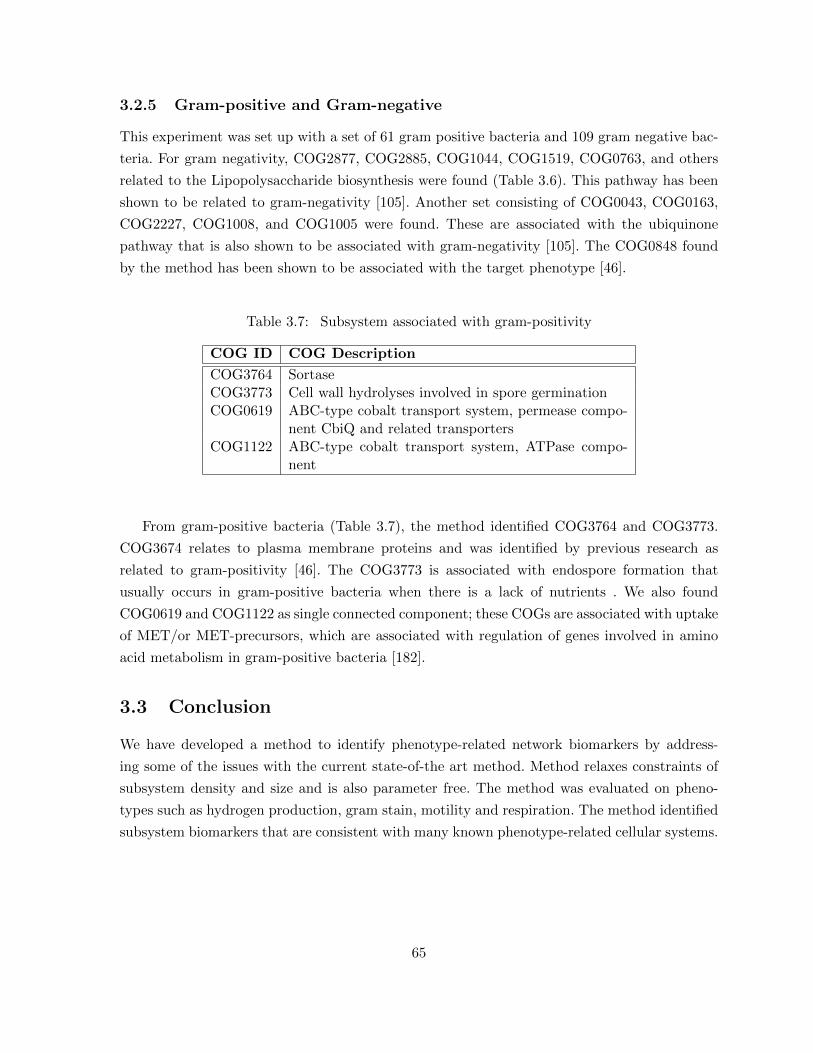
3.2.5 Gram-positive and Gram-negative

This experiment was set up with a set of 61 gram positive bacteria and 109 gram negative bac-

teria. For gram negativity, COG2877, COG2885, COG1044, COG1519, COG0763, and others

related to the Lipopolysaccharide biosynthesis were found (Table 3.6). This pathway has been

shown to be related to gram-negativity [105]. Another set consisting of COG0043, COG0163,

COG2227, COG1008, and COG1005 were found. These are associated with the ubiquinone

pathway that is also shown to be associated with gram-negativity [105]. The COG0848 found

by the method has been shown to be associated with the target phenotype [46].

Table 3.7: Subsystem associated with gram-positivity

COG ID COG Description

COG3764 SortaseCOG3773 Cell wall hydrolyses involved in spore germinationCOG0619 ABC-type cobalt transport system, permease compo-

nent CbiQ and related transportersCOG1122 ABC-type cobalt transport system, ATPase compo-

nent

From gram-positive bacteria (Table 3.7), the method identified COG3764 and COG3773.

COG3674 relates to plasma membrane proteins and was identified by previous research as

related to gram-positivity [46]. The COG3773 is associated with endospore formation that

usually occurs in gram-positive bacteria when there is a lack of nutrients . We also found

COG0619 and COG1122 as single connected component; these COGs are associated with uptake

of MET/or MET-precursors, which are associated with regulation of genes involved in amino

acid metabolism in gram-positive bacteria [182].

3.3 Conclusion

We have developed a method to identify phenotype-related network biomarkers by address-

ing some of the issues with the current state-of-the art method. Method relaxes constraints of

subsystem density and size and is also parameter free. The method was evaluated on pheno-

types such as hydrogen production, gram stain, motility and respiration. The method identified

subsystem biomarkers that are consistent with many known phenotype-related cellular systems.

65

Chapter 4

Gene Level: Functional Annotation

of Hierarchical Modularity of

Network Biomarkers

The identified network biomarkers are analyzed for biological significance. Biological significance

analysis identifies gene sets that are meaningful in a biological context. Biological significance

can be computationally determined by analyzing the gene set for functional coherence and as-

signing functional annotations. Functional coherence analysis assigns a score quantifying the

gene set’s biological significance. Functional annotation methods identify the possible biolog-

ical functions of the gene set. Biological significance analysis should take into consideration

the principle of hierarchical modularity, i.e., consider the gene set as hierarchically organized

entities.

Hierarchical modularity as a generic principle of system-level cellular organization and func-

tion is supported by existing literature [22, 140, 148, 201]. Hierarchical taxonomies of functional

terms manifested by GO ontology or by KEGG knowledgebase further suggest a possible hier-

archical functional organization of the gene set. This kind of functional organization could help

with understanding the functioning of the gene set at various levels of functional specificity. For

example, the overall function of the target gene set could be chromosome segregation, but at

lower level of the hierarchy, we could find a subset of genes responsible for proper alignment and

attachment of chromosomes and another subset responsible for translating the force generated

by microtubule depolarization into movement to facilitate chromosome segregation [22].

Arguably, hierarchical modularity has not been explicitly taken into consideration by most, if

not all, functional annotation systems [3, 145]. As a result, the existing methods would often fail

to assign a statistically significant functional coherence score to biologically relevant molecular

machines (see Table 4.1).

66

Table 4.1: Statistical significance of protein pairs’ functional coherence in Saccharomycescerevisiae

Protein pair p-value (pair/ module/ module size) Ref.

ID Description ID Description HMS [130,

131]

[13] [8] [66,

67]

SNU13 RNA binding

protein

DIB1 17-kDa com-

ponent of the

U4/ U6aU5

tri-snRNP

0.0/0.0/2

0.23 0.01/0.01/2

0.1/0.1/2

0.42/0.42/2

[166]

HAP1Zinc finger

transcription

factor involved

in the complex

regulation of

gene expression

in response to

levels of heme

and oxygen

RPM2 Protein

subunit of

mitochondrial

RNase P

0.0/0.01/3

0.214 0.1/0.337/3

0.02/1.0/3

0.51/1.0∗/3

[55]

SRB2 Subunit of

the RNA

polymerase

II mediator

complex

RPB9 RNA poly-

merase II

subunit B12.6

0.0/0.01/58

0.48 0.12/1.0∗/58

0.333/1.0/58

0.98/1.0∗/58

[121]

NSR1 Nucleolar

protein that

binds nuclear

localization

sequences

DBP2 Essential ATP-

dependent

RNA helicase

of the DEAD-

box protein

family

0.0/0.0/2

0.44 0.1/0.1/2

0.13/0.13/2

0.74/0.74/2

[170]

∗assigned a p-value of 1 because the tool was unable to find a score for the entire module

To address this gap, we developed a methodology for hierarchical functional annotation of

gene sets. Given the hierarchical taxonomy of functional concepts (e.g., Gene Ontology) and the

association of individual genes or proteins with these concepts (e.g., GO terms), our method

will assign a Hierarchical Modularity Score (HMS); the HMS score and its p−value measure

functional coherence of the gene set. While existing methods annotate the gene set with a set

of “enriched” functional terms, our complementary method provides the hierarchical functional

annotation of the gene set.

A hierarchical organization of gene set often comes as a bi-product of cluster analysis of gene

expression data or protein interaction data. Otherwise, our method will automatically build such

a hierarchy by directly incorporating the functional taxonomy information into the hierarchy

search process and by allowing multi-functional genes to be part of more than one component in

67

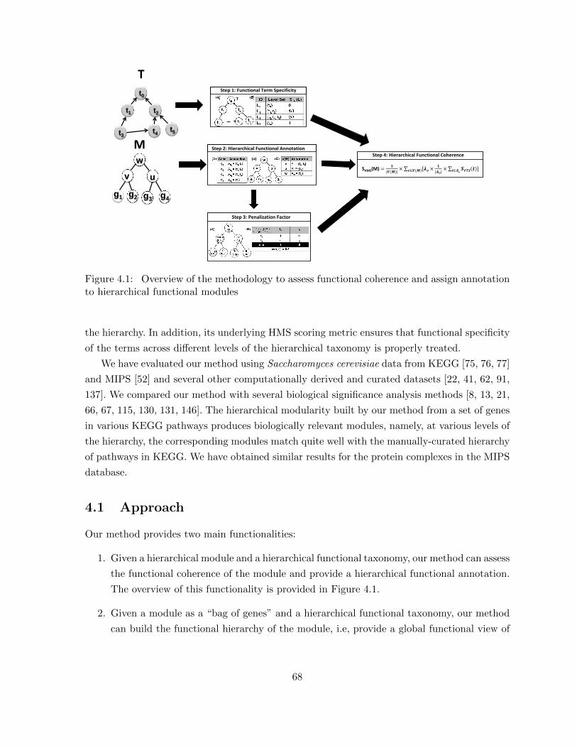
SHMS(M) =𝟏

|𝑽(𝑴)|× [𝝀𝒗 ×

𝟏

|𝑨𝒗|× 𝑺𝑭𝑻𝑺(𝒕)𝒕∈𝑨

𝒗]𝒗∈𝑽(𝑴)

Step 4: Hierarchical Functional Coherence

Step 1: Functional Term Specificity

Step 2: Hierarchical Functional Annotation

Step 3: Penalization Factor

t0

t4

t1

t5

t2

t3

T

w

g3

v

g4

u

g1 g2

M

Figure 4.1: Overview of the methodology to assess functional coherence and assign annotationto hierarchical functional modules

the hierarchy. In addition, its underlying HMS scoring metric ensures that functional specificity

of the terms across different levels of the hierarchical taxonomy is properly treated.

We have evaluated our method using Saccharomyces cerevisiae data from KEGG [75, 76, 77]

and MIPS [52] and several other computationally derived and curated datasets [22, 41, 62, 91,

137]. We compared our method with several biological significance analysis methods [8, 13, 21,

66, 67, 115, 130, 131, 146]. The hierarchical modularity built by our method from a set of genes

in various KEGG pathways produces biologically relevant modules, namely, at various levels of

the hierarchy, the corresponding modules match quite well with the manually-curated hierarchy

of pathways in KEGG. We have obtained similar results for the protein complexes in the MIPS

database.

4.1 Approach

Our method provides two main functionalities:

1. Given a hierarchical module and a hierarchical functional taxonomy, our method can assess

the functional coherence of the module and provide a hierarchical functional annotation.

The overview of this functionality is provided in Figure 4.1.

2. Given a module as a “bag of genes” and a hierarchical functional taxonomy, our method

can build the functional hierarchy of the module, i.e, provide a global functional view of

68

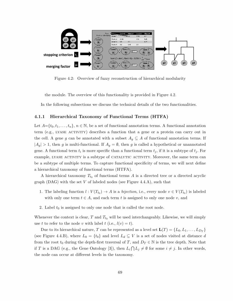
g1 g2

g3 g4

τs

μ g1 g2 g3 g4

stopping criterion

merging factor

Figure 4.2: Overview of fuzzy reconstruction of hierarchical modularity

the module. The overview of this functionality is provided in Figure 4.2.

In the following subsections we discuss the technical details of the two functionalities.

4.1.1 Hierarchical Taxonomy of Functional Terms (HTFA)

Let A={t0, t1, . . . , tn}, n ∈ N, be a set of functional annotation terms. A functional annotation

term (e.g., lyase activity) describes a function that a gene or a protein can carry out in

the cell. A gene g can be annotated with a subset Ag ⊆ A of functional annotation terms. If

|Ag| > 1, then g is multi-functional. If Ag = ∅, then g is called a hypothetical or unannotated

gene. A functional term ti is more specific than a functional term tj , if it is a subtype of tj . For

example, lyase activity is a subtype of catalytic activity. Moreover, the same term can

be a subtype of multiple terms. To capture functional specificity of terms, we will next define

a hierarchical taxonomy of functional terms (HTFA).

A hierarchical taxonomy Tt0 of functional terms A is a directed tree or a directed acyclic

graph (DAG) with the set V of labeled nodes (see Figure 4.4.A), such that

1. The labeling function l : V (Tt0)→ A is a bijection, i.e., every node v ∈ V (Tt0) is labeled

with only one term t ∈ A, and each term t is assigned to only one node v, and

2. Label t0 is assigned to only one node that is called the root node.

Whenever the context is clear, T and Tt0 will be used interchangeably. Likewise, we will simply

use t to refer to the node v with label t (i.e., l(v) = t).

Due to its hierarchical nature, T can be represented as a level set L(T ) = {L0, L1, . . . , LDT}

(see Figure 4.4.B), where L0 = {t0} and level Ld ⊆ V is a set of nodes visited at distance d

from the root t0 during the depth-first traversal of T , and DT ∈ N is the tree depth. Note that

if T is a DAG (e.g., the Gene Ontology [3]), then Li⋂Lj 6= ∅ for some i 6= j. In other words,

the node can occur at different levels in the taxonomy.

69

A pair of nodes ti and tj in Tt0 forms an ancestor relationship (ti ≺ tj), if there is a simple

directed path from ti to tj in Tt0 . An ancestor relationship between a pair of nodes ti and tj in

Tt0 represents a functional specificity relationship, namely, a functional term of the child node

is a subtype of the functional term of its parent, grandparent, grandgrandparent, and so on.

This relationship is transitive, i.e, ti ≺ tj and tj ≺ tk imply ti ≺ tk. Also, a child can have

multiple parents, as in a DAG.

Given this fact, we next introduce the functional term specificity score SFTS(t) for a node

t ∈ T as follows:

SFTS(t) =

∑t∈L SLS(L)∑L∈L δ(t, L)

, (4.1)

where SLS(L) (see Figure 6.B) is the level specificity score associated with level L ∈ L and

defined as

SLS(Ld) =d

DT, (4.2)

and δ() is a term characteristic function that specifies whether the term t occurs at level L:

δ(t, L) =

1, if t ∈ L

0, if t /∈ L(4.3)

A distinct pair (ti, tj) ∈ A × A of functional terms is called related, if the corresponding

nodes in T form an ancestor relationship, i.e., ti ≺ tj . More generally, a set of terms U ⊆ A is

called an unrelated set, or an unrelated term set in T , if no distinct pair (ti, tj), s.t. ti, tj ∈ U ,

is related in T .

Let U be an unrelated functional term set in T . Then, as defined by Equation 4.4, the

ancestor functional term set U of U is the set of all the functional terms t ∈ T on any simple

path from any node t ∈ U to the root node t0 ∈ T :

U = U ∪ P ∪ {t0},

P = {∀t, t ∈ T : ∃t ∈ U : t ≺ t ≺ t0} (4.4)

For example, consider an unrelated functional term set Au = {t4, t6} in Figure 6. According to

Equation 4.4, its ancestor functional term set is Au = Au ∪ {t0, t2, t3}.

4.1.2 Hierarchical Gene Module (HGM)

Given a set of genesG = {g1, g2, . . . , gm}, a hierarchical gene module (HGM)M is an undirected

tree over the set G of leaf nodes. Given the hierarchical taxonomy T of functional terms A, let

an unrelated term set Ag, Ag ⊂ A, denote the functional annotation of gene g.

70

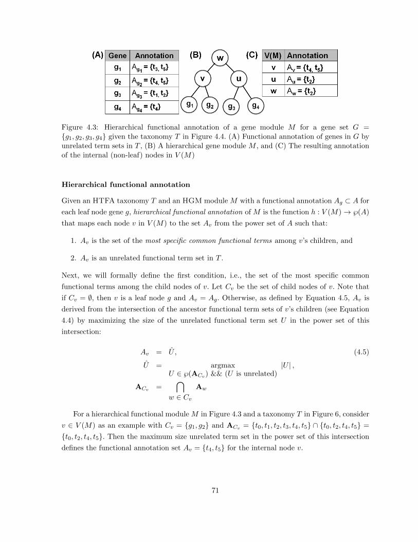
Figure 4.3: Hierarchical functional annotation of a gene module M for a gene set G ={g1, g2, g3, g4} given the taxonomy T in Figure 4.4. (A) Functional annotation of genes in G byunrelated term sets in T , (B) A hierarchical gene module M , and (C) The resulting annotationof the internal (non-leaf) nodes in V (M)

Hierarchical functional annotation

Given an HTFA taxonomy T and an HGM module M with a functional annotation Ag ⊂ A for

each leaf node gene g, hierarchical functional annotation of M is the function h : V (M)→ ℘(A)

that maps each node v in V (M) to the set Av from the power set of A such that:

1. Av is the set of the most specific common functional terms among v’s children, and

2. Av is an unrelated functional term set in T .

Next, we will formally define the first condition, i.e., the set of the most specific common

functional terms among the child nodes of v. Let Cv be the set of child nodes of v. Note that

if Cv = ∅, then v is a leaf node g and Av = Ag. Otherwise, as defined by Equation 4.5, Av is

derived from the intersection of the ancestor functional term sets of v’s children (see Equation

4.4) by maximizing the size of the unrelated functional term set U in the power set of this

intersection:

Av = U , (4.5)

U = argmaxU ∈ ℘(ACv) && (U is unrelated)

|U | ,

ACv =⋂

w ∈ CvAw

For a hierarchical functional module M in Figure 4.3 and a taxonomy T in Figure 6, consider

v ∈ V (M) as an example with Cv = {g1, g2} and ACv = {t0, t1, t2, t3, t4, t5} ∩ {t0, t2, t4, t5} =

{t0, t2, t4, t5}. Then the maximum size unrelated term set in the power set of this intersection

defines the functional annotation set Av = {t4, t5} for the internal node v.

71

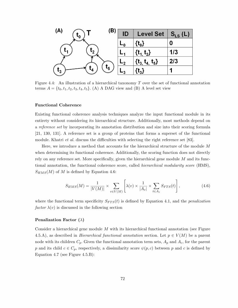
Figure 4.4: An illustration of a hierarchical taxonomy T over the set of functional annotationterms A = {t0, t1, t2, t3, t4, t5}. (A) A DAG view and (B) A level set view

Functional Coherence

Existing functional coherence analysis techniques analyze the input functional module in its

entirety without considering its hierarchical structure. Additionally, most methods depend on

a reference set by incorporating its annotation distribution and size into their scoring formula

[21, 130, 131]. A reference set is a group of proteins that forms a superset of the functional

module. Khatri et al. discuss the difficulties with selecting the right reference set [83].

Here, we introduce a method that accounts for the hierarchical structure of the module M

when determining its functional coherence. Additionally, the scoring function does not directly

rely on any reference set. More specifically, given the hierarchical gene module M and its func-

tional annotation, the functional coherence score, called hierarchical modularity score (HMS),

SHMS(M) of M is defined by Equation 4.6:

SHMS(M) =1

|V (M)|×

∑v∈V (M)

[λ(v)× 1

|Av|×∑t∈Av

SFTS(t)

], (4.6)

where the functional term specificity SFTS(t) is defined by Equation 4.1, and the penalization

factor λ(v) is discussed in the following section

Penalization Factor (λ)

Consider a hierarchical gene module M with its hierarchical functional annotation (see Figure

4.5.A), as described in Hierarchical functional annotation section. Let p ∈ V (M) be a parent

node with its children Cp. Given the functional annotation term sets, Ap and Ac, for the parent

p and its child c ∈ Cp, respectively, a dissimilarity score ψ(p, c) between p and c is defined by

Equation 4.7 (see Figure 4.5.B):

72

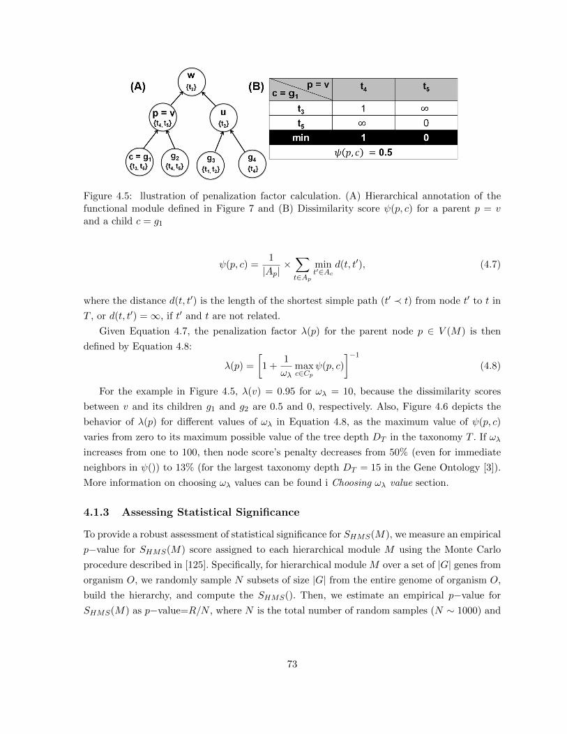
Figure 4.5: llustration of penalization factor calculation. (A) Hierarchical annotation of thefunctional module defined in Figure 7 and (B) Dissimilarity score ψ(p, c) for a parent p = vand a child c = g1

ψ(p, c) =1

|Ap|×∑t∈Ap

mint′∈Ac

d(t, t′), (4.7)

where the distance d(t, t′) is the length of the shortest simple path (t′ ≺ t) from node t′ to t in

T , or d(t, t′) =∞, if t′ and t are not related.

Given Equation 4.7, the penalization factor λ(p) for the parent node p ∈ V (M) is then

defined by Equation 4.8:

λ(p) =

[1 +

1

ωλmaxc∈Cp

ψ(p, c)

]−1

(4.8)

For the example in Figure 4.5, λ(v) = 0.95 for ωλ = 10, because the dissimilarity scores

between v and its children g1 and g2 are 0.5 and 0, respectively. Also, Figure 4.6 depicts the

behavior of λ(p) for different values of ωλ in Equation 4.8, as the maximum value of ψ(p, c)

varies from zero to its maximum possible value of the tree depth DT in the taxonomy T . If ωλ

increases from one to 100, then node score’s penalty decreases from 50% (even for immediate

neighbors in ψ()) to 13% (for the largest taxonomy depth DT = 15 in the Gene Ontology [3]).

More information on choosing ωλ values can be found i Choosing ωλ value section.

4.1.3 Assessing Statistical Significance

To provide a robust assessment of statistical significance for SHMS(M), we measure an empirical

p−value for SHMS(M) score assigned to each hierarchical module M using the Monte Carlo

procedure described in [125]. Specifically, for hierarchical module M over a set of |G| genes from

organism O, we randomly sample N subsets of size |G| from the entire genome of organism O,

build the hierarchy, and compute the SHMS(). Then, we estimate an empirical p−value for

SHMS(M) as p−value=R/N , where N is the total number of random samples (N ∼ 1000) and

73

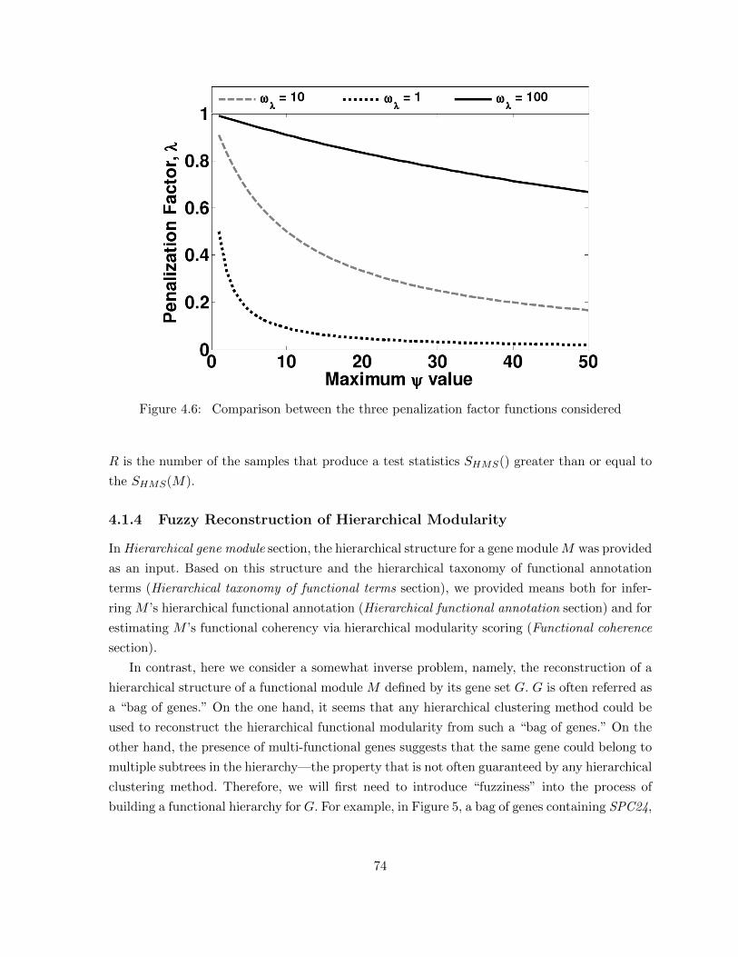
Figure 4.6: Comparison between the three penalization factor functions considered

R is the number of the samples that produce a test statistics SHMS() greater than or equal to

the SHMS(M).

4.1.4 Fuzzy Reconstruction of Hierarchical Modularity

In Hierarchical gene module section, the hierarchical structure for a gene moduleM was provided

as an input. Based on this structure and the hierarchical taxonomy of functional annotation

terms (Hierarchical taxonomy of functional terms section), we provided means both for infer-

ring M ’s hierarchical functional annotation (Hierarchical functional annotation section) and for

estimating M ’s functional coherency via hierarchical modularity scoring (Functional coherence

section).

In contrast, here we consider a somewhat inverse problem, namely, the reconstruction of a

hierarchical structure of a functional module M defined by its gene set G. G is often referred as

a “bag of genes.” On the one hand, it seems that any hierarchical clustering method could be

used to reconstruct the hierarchical functional modularity from such a “bag of genes.” On the

other hand, the presence of multi-functional genes suggests that the same gene could belong to

multiple subtrees in the hierarchy—the property that is not often guaranteed by any hierarchical

clustering method. Therefore, we will first need to introduce “fuzziness” into the process of

building a functional hierarchy for G. For example, in Figure 5, a bag of genes containing SPC24,

74

TID3, NUF2, and FHL1 and a functional annotation taxonomy T are provided as input to the

method. It is known that SPC24, TID3, and NUF2 are functionally related because they are

part of the Ndc80 protein complex but SPC24 is also trnascriptionally regulated by FHL1 [95]

and so SPC24 is part of multiple subtress and, hence, fuzziness is introduced.

Existing fuzzy clustering schemes typically introduce some fuzziness into some known clus-

tering algorithm. C-means [10, 178] is a typical example of this kind. Others are typically

partitional by nature [43, 66, 67]. Agglomerative fuzzy clustering algorithms are not common,

because agglomerative techniques are considered “hard clustering,” i.e., it becomes difficult to

move an element from an existing cluster to a new cluster. Ideally, any fuzziness in a clustering

procedure should be introduced, while the hierarchy is being built and not as a post-processing

step.

To meet these requirements, we propose a taxonomy-based, agglomerative, fuzzy inference

(TAFI) of the hierarchical gene module M from a gene set G, provided each gene g ∈ G

is annotated with an unrelated functional term set Ag ⊂ A in a hierarchical taxonomy T of

functional annotation terms A (see Hierarchical taxonomy of functional terms section). The

overview of this method is provided in Figure 5.

Similar to an agglomerative hierarchical clustering (AHC) process, TAFI starts with assign-

ing each gene to its own cluster and proceeds building the hierarchy in an iterative, bottom-up

manner, but it introduces fuzziness by allowing multiple cluster pairs to merge simultaneously

at each iteration. The two user-defined parameters control this fuzziness process at each itera-

tion: (a) the merging factor µ and (b) the stopping criterion τs. The former defines what cluster

pairs get merged at a given iteration it. Namely, unlike traditional AHC that merge the pair

of clusters with the maximum similarity Smax(it), TAFI allows for clusters with suboptimal

similarity to be merged as well. Suboptimality is defined by the percentage µ of Smax(it). In ad-

dition, TAFI prevents the formation of unrelated clustering modules by stopping the bottom-up

cluster merging process at iteration it as soon as Smax(it) value falls below τs.

Note that Horng et al. [65] proposed to merge the cluster pairs whose similarity is greater

than Smax(i) −∆ unlike TAFI’s way of restricting to µ100 × Smax(i) similarity threshold. The

reason behind our choice of multiplicative factor rather than additive/subtractive factor is the

following. If ∆ = 0.1 and Smax(i) = 0.5, then any cluster pair with inter-cluster similarity

greater than 0.4 would be merged. The value of 0.4 is 80% of 0.5. However, if Smax(i) = 0.2,

then any cluster pair with inter-cluster similarity greater than 0.1 would be merged, but the

value of 0.1 is only 50% of 0.2. The criterion becomes more stringent with a larger value of

Smax() and, conversely, it becomes more lenient, as Smax() gets smaller. In contrast, our choice

of the merging factor allows for resolving this inconsistency issue.

Also, observe that multiple merges at each iteration can sometimes result in the same subtree

being formed repeatedly. This leads to redundancy. Thus, TAFI employs pruning, where a

75

merge is allowed only if the merge results in a subtree that has not been already formed.

In addition, we need to make two important decisions in order to apply TAFI: (1) the

inter-cluster similarity measure and (2) the linkage algorithm. For the inter-cluster similarity

measure, we use Equation 4.6 that calculates the hierarchical modularity score SHMS(M) for a

hypothetical module M that could be formed if the two clusters, or hierarchical tree modules M1

and M2, were merged by adding a new root node vnew and making the root nodes v1 ∈ V (M1)

and v2 ∈ V (M2) to be the children of vnew.

It is worth noticing that SHMS(M) is a semi-metric, and this property has direct implications

on our choice of the base clustering algorithm. Since semi-metrics do not adhere to the triangle

inequality principle, we can resort to an average, single, complete, or centroid linkage algorithm

as our base clustering technique. Therefore, the effective clustering techniques, such as Ward’s

method cannot be used in conjunction with semi-metrics [92].

4.2 Results

4.2.1 Benchmark Data and Tools

To evaluate the performance of our method, we first need to define (1) the model organism;

(2) the benchmark data of known functional annotations for this organism; (3) the hierarchical

taxonomy of functional terms, and (4) the state-of-the-art methods that are most suitable for

our comparative analysis.

Saccharomyces cerevisiae is our model organism. The reason is that its genome annotation

is mostly complete and manually curated by human experts [21]. Apart from annotation qual-

ity, the availability of functional module datasets, both manually curated and experimentally

generated, for S. cerevisiae is advantageous for our method validation purposes.

For benchmark data, we plan to use both metabolic pathways from KEGG database [75,

76, 77] and protein complexes in MIPS database [52] including experimental protein-protein

interaction data and protein complexes derived from this data [22, 41, 62, 91, 137].

For the hierarchical taxonomy of functional terms, we will rely on the commonly-used func-

tional annotation taxonomy provided by the Gene Ontology consortium [3]. As such, we will

limit ourselves to the existing methods that are also based on GO ontology. Namely, we will

compare our method with the ones by Pandey et al. [130, 131], Chen et al. [21], and GS2 [146]

methods. The former makes use of the lowest common ancestor principle to score functional

coherence for a protein pair; it is based on Jiang and Conrath’s scoring method [71], which is a

normalized version of the scoring method in Resnik et al. [141]. It has been shown that Jiang

and Conrath’s method is the best measure to capture semantic relatedness [18]. The method by

Chen et al. is based on a widely used cosine similarity measure to assess functional coherence

76

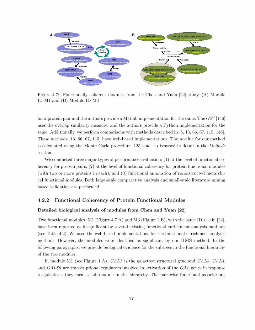
Figure 4.7: Functionally coherent modules from the Chen and Yuan [22] study. (A) ModuleID M1 and (B) Module ID M3

for a protein pair and the authors provide a Matlab implementation for the same. The GS2 [146]

uses the overlap similarity measure, and the authors provide a Python implementation for the

same. Additionally, we perform comparisons with methods described in [8, 13, 66, 67, 115, 146].

These methods [13, 66, 67, 115] have web-based implementations. The p-value for our method

is calculated using the Monte Carlo procedure [125] and is discussed in detail in the Methods

section.

We conducted three major types of performance evaluation: (1) at the level of functional co-

herency for protein pairs; (2) at the level of functional coherency for protein functional modules

(with two or more proteins in each); and (3) functional annotation of reconstructed hierarchi-

cal functional modules. Both large-scale comparative analysis and small-scale literature mining

based validation are performed.

4.2.2 Functional Coherency of Protein Functional Modules

Detailed biological analysis of modules from Chen and Yuan [22]

Two functional modules, M1 (Figure 4.7.A) and M3 (Figure 1.B), with the same ID’s as in [22],

have been reported as insignificant by several existing functional enrichment analysis methods

(see Table 4.2). We used the web-based implementations for the functional enrichment analysis

methods. However, the modules were identified as significant by our HMS method. In the

following paragraphs, we provide biological evidence for the subtrees in the functional hierarchy

of the two modules.

In module M1 (see Figure 1.A), GAL1 is the galactose structural gene and GAL3, GAL4,

and GAL80 are transcriptional regulators involved in activation of the GAL genes in response

to galactose; they form a sub-module in the hierarchy. The pair-wise functional associations

77

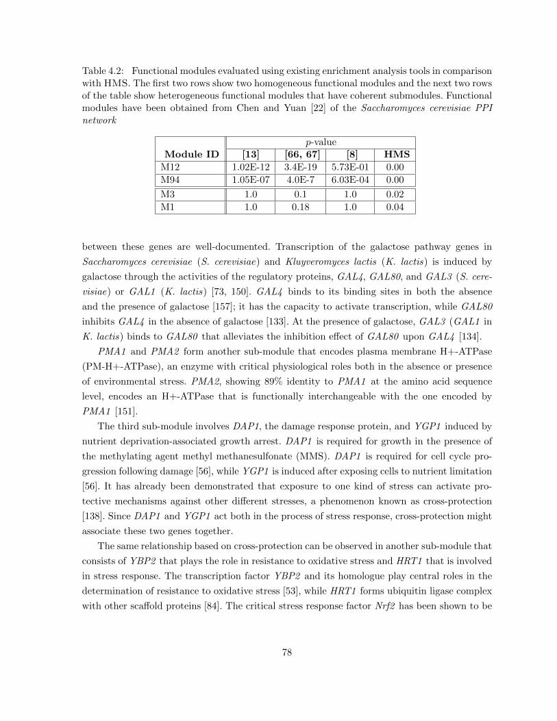
Table 4.2: Functional modules evaluated using existing enrichment analysis tools in comparisonwith HMS. The first two rows show two homogeneous functional modules and the next two rowsof the table show heterogeneous functional modules that have coherent submodules. Functionalmodules have been obtained from Chen and Yuan [22] of the Saccharomyces cerevisiae PPInetwork

p-valueModule ID [13] [66, 67] [8] HMS

M12 1.02E-12 3.4E-19 5.73E-01 0.00

M94 1.05E-07 4.0E-7 6.03E-04 0.00

M3 1.0 0.1 1.0 0.02

M1 1.0 0.18 1.0 0.04

between these genes are well-documented. Transcription of the galactose pathway genes in

Saccharomyces cerevisiae (S. cerevisiae) and Kluyveromyces lactis (K. lactis) is induced by

galactose through the activities of the regulatory proteins, GAL4, GAL80, and GAL3 (S. cere-

visiae) or GAL1 (K. lactis) [73, 150]. GAL4 binds to its binding sites in both the absence

and the presence of galactose [157]; it has the capacity to activate transcription, while GAL80

inhibits GAL4 in the absence of galactose [133]. At the presence of galactose, GAL3 (GAL1 in

K. lactis) binds to GAL80 that alleviates the inhibition effect of GAL80 upon GAL4 [134].

PMA1 and PMA2 form another sub-module that encodes plasma membrane H+-ATPase

(PM-H+-ATPase), an enzyme with critical physiological roles both in the absence or presence

of environmental stress. PMA2, showing 89% identity to PMA1 at the amino acid sequence

level, encodes an H+-ATPase that is functionally interchangeable with the one encoded by

PMA1 [151].

The third sub-module involves DAP1, the damage response protein, and YGP1 induced by

nutrient deprivation-associated growth arrest. DAP1 is required for growth in the presence of

the methylating agent methyl methanesulfonate (MMS). DAP1 is required for cell cycle pro-

gression following damage [56], while YGP1 is induced after exposing cells to nutrient limitation

[56]. It has already been demonstrated that exposure to one kind of stress can activate pro-

tective mechanisms against other different stresses, a phenomenon known as cross-protection

[138]. Since DAP1 and YGP1 act both in the process of stress response, cross-protection might

associate these two genes together.

The same relationship based on cross-protection can be observed in another sub-module that

consists of YBP2 that plays the role in resistance to oxidative stress and HRT1 that is involved

in stress response. The transcription factor YBP2 and its homologue play central roles in the

determination of resistance to oxidative stress [53], while HRT1 forms ubiquitin ligase complex

with other scaffold proteins [84]. The critical stress response factor Nrf2 has been shown to be

78

repressed by the ubiquitin-proteasome system under normal, unstressed conditions, with Nrf2

exploiting ubiquitin ligase complexes [86].

The next module is made up of PMA1 and TPO5 that are involved in excretion of putrescine

and spermidine. TPO5 functions as a suppressor of cell growth by excreting polyamines [169].

PMA1 is a polytopic membrane protein, whose essential physiological function is to pump

protons out of the cell. Both the excretion of putrescine by TPO5 and the delivery of PMA1

to cell surface rely on secretory pathway. Furthermore, small portions of TPO5 are co-localized

with PMA1 in plasma membrane, which indicates possible interactions between these two

proteins [184].

PMA1 also forms a sub-module together with RVS161 that regulates polarization of the

actin cytoskeleton. RVS161 regulates secretory vesicle trafficking [16] as well as cell polarity

[34], actin cytoskeleton polarization [162], and endocytosis [119]. It is already known that the

efficient delivery of PMA1 to cell surface relies on secretory pathway[184]. Thus, RVS161 has

a regulatory effect upon PMA1.

Genes in this module have coherent functions, namely more than half of the proteins in this

module are related to stress response, five out of 20 total have regulatory roles in cell cycle,

four out of 20 total are evolved in endocytosis. Stress conditions are likely to cause cell cycle

arrest, as well as endocytosis induction.

For module M3 (see Figure 1.B), the vast majority of the genes in the module enjoy oxidative

stress response as the common theme. SOD2 protects cells against oxygen toxicity and TSA2,

responsible for the removal of reactive oxygen, directly protects cells against oxidative stress,

while PXR1 plays the role in negative regulation of telomerase, and YKU80, a subunit of the

telomeric Ku complex, contributes to the maintenance of telomere stability, since oxidative

stress is likely to induce telomere attrition [104].

Meanwhile, proteolysis could also be the result of oxidative stress: YNL311C is part of

an ubiquitin protease complex, DEF1 enables ubiquitination, DMA1 is involved in ubiquitin

ligation, and DMA2 is involved in ubiquitination [49]. Since proteolysis involves many protein

transportation processes, the signal recognition particles are essential to enable transportation:

SRP14, SRP21, SRP54, SRP68, SRP72, and SEC65 are all part of the signal recognition

particle (SRP) subunit, and appear in module M3.

Furthermore, Wu et al. [190] showed that repression of sulfate assimilation is an adap-

tive response of yeast to the oxidative stress of zinc deficiency, while we notice that MET1,

MET10, MET14, MET16, and YPR003C are basic proteins or protein subunits that are re-

quired for sulfate assimilation. Finally, oxidative phosphorylation produces ATP by utilizing

electron transport trains. As a result, the inhibition of electron transport chain will lead to

oxidative stress [39]. That is probably why ATP3, ATP5, and ATP7 are all part of the enzyme

complex required for ATP synthesis. Also, STI1, ATPase inhibitor activity, and YBT1, ATPase

79

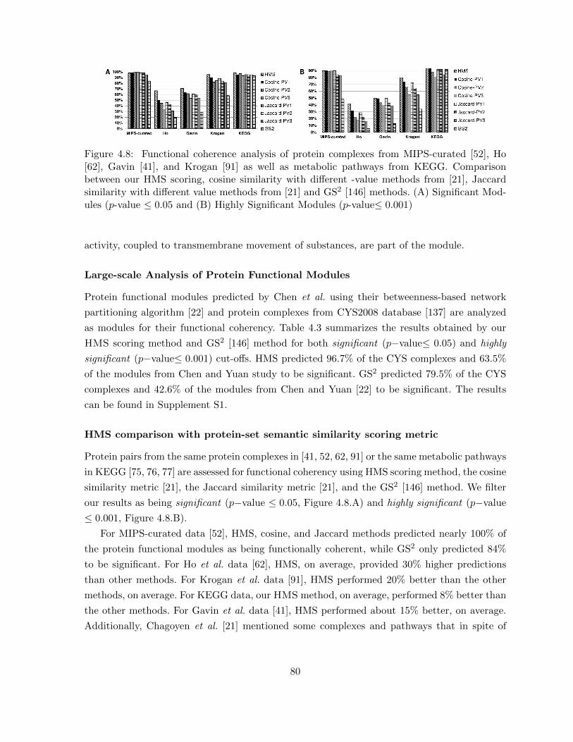
Figure 4.8: Functional coherence analysis of protein complexes from MIPS-curated [52], Ho[62], Gavin [41], and Krogan [91] as well as metabolic pathways from KEGG. Comparisonbetween our HMS scoring, cosine similarity with different -value methods from [21], Jaccardsimilarity with different value methods from [21] and GS2 [146] methods. (A) Significant Mod-ules (p-value ≤ 0.05 and (B) Highly Significant Modules (p-value≤ 0.001)

activity, coupled to transmembrane movement of substances, are part of the module.

Large-scale Analysis of Protein Functional Modules

Protein functional modules predicted by Chen et al. using their betweenness-based network

partitioning algorithm [22] and protein complexes from CYS2008 database [137] are analyzed

as modules for their functional coherency. Table 4.3 summarizes the results obtained by our

HMS scoring method and GS2 [146] method for both significant (p−value≤ 0.05) and highly

significant (p−value≤ 0.001) cut-offs. HMS predicted 96.7% of the CYS complexes and 63.5%

of the modules from Chen and Yuan study to be significant. GS2 predicted 79.5% of the CYS

complexes and 42.6% of the modules from Chen and Yuan [22] to be significant. The results

can be found in Supplement S1.

HMS comparison with protein-set semantic similarity scoring metric

Protein pairs from the same protein complexes in [41, 52, 62, 91] or the same metabolic pathways

in KEGG [75, 76, 77] are assessed for functional coherency using HMS scoring method, the cosine

similarity metric [21], the Jaccard similarity metric [21], and the GS2 [146] method. We filter

our results as being significant (p−value ≤ 0.05, Figure 4.8.A) and highly significant (p−value

≤ 0.001, Figure 4.8.B).

For MIPS-curated data [52], HMS, cosine, and Jaccard methods predicted nearly 100% of

the protein functional modules as being functionally coherent, while GS2 only predicted 84%

to be significant. For Ho et al. data [62], HMS, on average, provided 30% higher predictions

than other methods. For Krogan et al. data [91], HMS performed 20% better than the other

methods, on average. For KEGG data, our HMS method, on average, performed 8% better than

the other methods. For Gavin et al. data [41], HMS performed about 15% better, on average.

Additionally, Chagoyen et al. [21] mentioned some complexes and pathways that in spite of

80

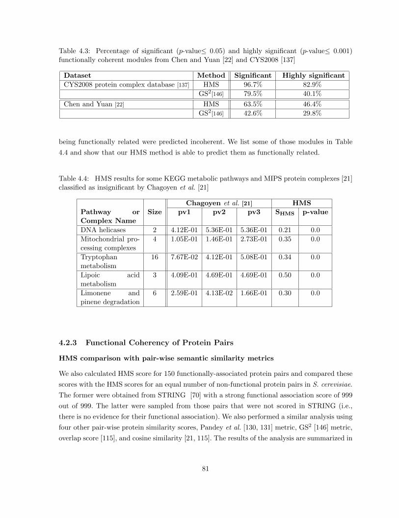
Table 4.3: Percentage of significant (p-value≤ 0.05) and highly significant (p-value≤ 0.001)functionally coherent modules from Chen and Yuan [22] and CYS2008 [137]

Dataset Method Significant Highly significant

CYS2008 protein complex database [137] HMS 96.7% 82.9%

GS2[146] 79.5% 40.1%

Chen and Yuan [22] HMS 63.5% 46.4%

GS2[146] 42.6% 29.8%

being functionally related were predicted incoherent. We list some of those modules in Table

4.4 and show that our HMS method is able to predict them as functionally related.

Table 4.4: HMS results for some KEGG metabolic pathways and MIPS protein complexes [21]classified as insignificant by Chagoyen et al. [21]

Chagoyen et al. [21] HMSPathway orComplex Name

Size pv1 pv2 pv3 SHMS p-value

DNA helicases 2 4.12E-01 5.36E-01 5.36E-01 0.21 0.0

Mitochondrial pro-cessing complexes

4 1.05E-01 1.46E-01 2.73E-01 0.35 0.0

Tryptophanmetabolism

16 7.67E-02 4.12E-01 5.08E-01 0.34 0.0

Lipoic acidmetabolism

3 4.09E-01 4.69E-01 4.69E-01 0.50 0.0

Limonene andpinene degradation

6 2.59E-01 4.13E-02 1.66E-01 0.30 0.0

4.2.3 Functional Coherency of Protein Pairs

HMS comparison with pair-wise semantic similarity metrics

We also calculated HMS score for 150 functionally-associated protein pairs and compared these

scores with the HMS scores for an equal number of non-functional protein pairs in S. cerevisiae.

The former were obtained from STRING [70] with a strong functional association score of 999

out of 999. The latter were sampled from those pairs that were not scored in STRING (i.e.,

there is no evidence for their functional association). We also performed a similar analysis using

four other pair-wise protein similarity scores, Pandey et al. [130, 131] metric, GS2 [146] metric,

overlap score [115], and cosine similarity [21, 115]. The results of the analysis are summarized in

81

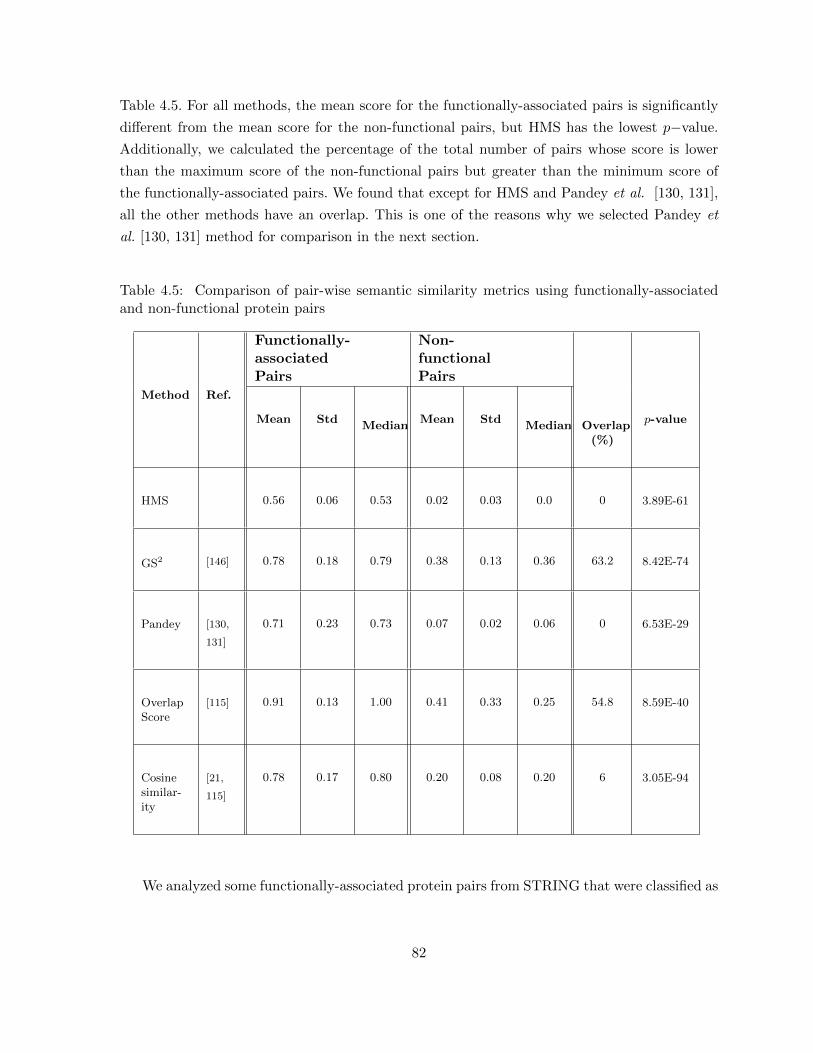
Table 4.5. For all methods, the mean score for the functionally-associated pairs is significantly

different from the mean score for the non-functional pairs, but HMS has the lowest p−value.

Additionally, we calculated the percentage of the total number of pairs whose score is lower

than the maximum score of the non-functional pairs but greater than the minimum score of

the functionally-associated pairs. We found that except for HMS and Pandey et al. [130, 131],

all the other methods have an overlap. This is one of the reasons why we selected Pandey et

al. [130, 131] method for comparison in the next section.

Table 4.5: Comparison of pair-wise semantic similarity metrics using functionally-associatedand non-functional protein pairs

Functionally-associatedPairs

Non-functionalPairs

Method Ref.

Mean StdMedian

Mean StdMedian Overlap

(%)

p-value

HMS 0.56 0.06 0.53 0.02 0.03 0.0 0 3.89E-61

GS2 [146] 0.78 0.18 0.79 0.38 0.13 0.36 63.2 8.42E-74

Pandey [130,

131]

0.71 0.23 0.73 0.07 0.02 0.06 0 6.53E-29

OverlapScore

[115] 0.91 0.13 1.00 0.41 0.33 0.25 54.8 8.59E-40

Cosinesimilar-ity

[21,

115]

0.78 0.17 0.80 0.20 0.08 0.20 6 3.05E-94

We analyzed some functionally-associated protein pairs from STRING that were classified as

82

functionally coherent and thus biologically relevant (p−value ≤ 0.05) by our method, yet were

assessed as incoherent by Pandey’s et al. We found literature support for biological relevance of

these protein pairs. The results are summarized in Table 1. RPB9 and SRB2 proteins are part

of RNA polymerase II holoenzyme in S. cerevisiae [121]. SNU13 and DIB1 proteins have been

shown to be associated with the U4/U6U5 pre-mRNA splicing small nuclear ribonucleoprotein

(snRNP) complex [166]. HAP1 and RPM2 are related by the fact that RPM2 is required for

repression of the heme activator protein HAP2 in the absense of heme [55]. When NSR1 was

used as a bait in the protein-fragment complementation assay (PCA), the experiment pulled

out DBP2 as one of its prey proteins [170].

4.2.4 Inferred Hierarchy of Functional Modules

To assess the quality of the hierarchy of functional modules derived from a given “bag of

genes” using our HMS scoring metric and the hierarchical modularity inference methodology

described in the Methods section, we assess the consistency between the predicted hierarchy

and the hierarchy of known functional concepts in KEGG and MIPS databases. Remind that

HMS, by default, uses GO ontology as its hierarchical taxonomy of functional terms.

Consistency Analysis for KEGG Metabolic Pathways

Note that each metabolic pathway is a functional module. We consider the genes from several

metabolic pathways as one “bag of genes” to build the hierarchy of functional modules. If the

constructed hierarchy of functional modularity is biologically relevant, then the genes in each

pathway should form a subtree in the hierarchy and not be “contaminated” by the genes from

the other pathways. We set the fuzziness to null before running the algorithm in order to be

able to use standard clustering validation metrics like the Heidke Score [59], Gerrity Score [42],

and Peirce Score [132].

Since KEGG is organized into a three level hierarchy, the pathways at the lower levels of

the hierarchy are functionally more coherent. Hence, they should be harder to separate into

different subtrees. This hierarchical specificity of the KEGG knowledgebase provides us with

an opportunity to check both the specificity and the sensitivity of our hierarchical modularity

inference method.

We build contingency tables to provide a mathematically and statistically sound way for

assessing the performance at large-scale. To construct a contingency table, the inferred hierarchy

is first cut at the level that produces s subtrees that are then compared with s pathways used

as input to the algorithm. In the ideal scenario, all the genes in a given pathway (or row in the

contingency table) will end up in the corresponding subtree (or the column in the contingency

table) and vice versa; or the contingency table will form a diagonal matrix with the number

83

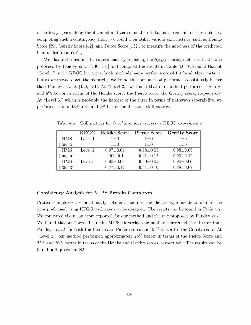
of pathway genes along the diagonal and zero’s on the off-diagonal elements of the table. By

completing such a contingency table, we could then utilize various skill metrics, such as Heidke

Score [59], Gerrity Score [42], and Peirce Score [132], to measure the goodness of the predicted

hierarchical modularity.

We also performed all the experiments by replacing the SHMS scoring metric with the one

proposed by Pandey et al. [130, 131] and compiled the results in Table 4.6. We found that at

“Level 1” in the KEGG hierarchy, both methods had a perfect score of 1.0 for all three metrics,

but as we moved down the hierarchy, we found that our method performed consistantly better

than Pandey’s et al. [130, 131]. At “Level 2,” we found that our method performed 6%, 7%,

and 8% better in terms of the Heidke score, the Pierce score, the Gerrity score, respectively.

At “Level 3,” which is probably the hardest of the three in terms of pathways seperability, we

performed about 13%, 6%, and 2% better for the same skill metrics.

Table 4.6: Skill metrics for Saccharomyces cerevisiae KEGG experiments

KEGG Heidke Score Pierce Score Gerrity Score

HMS Level 1 1±0 1±0 1±0

[130, 131] 1±0 1±0 1±0

HMS Level 2 0.97±0.04 0.98±0.05 0.98±0.05

[130, 131] 0.91±0.1 0.91±0.12 0.90±0.12

HMS Level 3 0.90±0.03 0.90±0.05 0.90±0.06

[130, 131] 0.77±0.14 0.84±0.10 0.88±0.07

Consistency Analysis for MIPS Protein Complexes

Protein complexes are functionally coherent modules, and hence experiments similar to the

ones preformed using KEGG pathways can be designed. The results can be found in Table 4.7.

We compared the mean score reported for our method and the one proposed by Pandey et al.

We found that at “Level 1” in the MIPS hierarchy, our method performed 12% better than

Pandey’s et al. for both the Heidke and Pierce scores and 13% better for the Gerrity score. At

“Level 2,” our method performed approximately 26% better in terms of the Pierce Score and

35% and 26% better in terms of the Heidke and Gerrity scores, respectively. The results can be

found in Supplement S2.

84

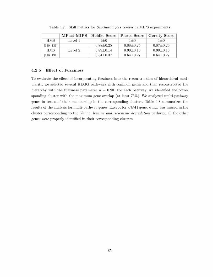
Table 4.7: Skill metrics for Saccharomyces cerevisiae MIPS experiments

MPact-MIPS Heidke Score Pierce Score Gerrity Score

HMS Level 1 1±0 1±0 1±0

[130, 131] 0.88±0.25 0.88±0.25 0.87±0.26

HMS Level 2 0.89±0.14 0.90±0.13 0.90±0.13

[130, 131] 0.54±0.37 0.64±0.27 0.64±0.27

4.2.5 Effect of Fuzziness

To evaluate the effect of incorporating fuzziness into the reconstruction of hierarchical mod-

ularity, we selected several KEGG pathways with common genes and then reconstructed the

hierarchy with the fuzziness parameter µ = 0.90. For each pathway, we identified the corre-

sponding cluster with the maximum gene overlap (at least 75%). We analyzed multi-pathway

genes in terms of their membership in the corresponding clusters. Table 4.8 summarizes the

results of the analysis for multi-pathway genes. Except for UGA1 gene, which was missed in the

cluster corresponding to the Valine, leucine and isoleucine degradation pathway, all the other

genes were properly identified in their corresponding clusters.

85

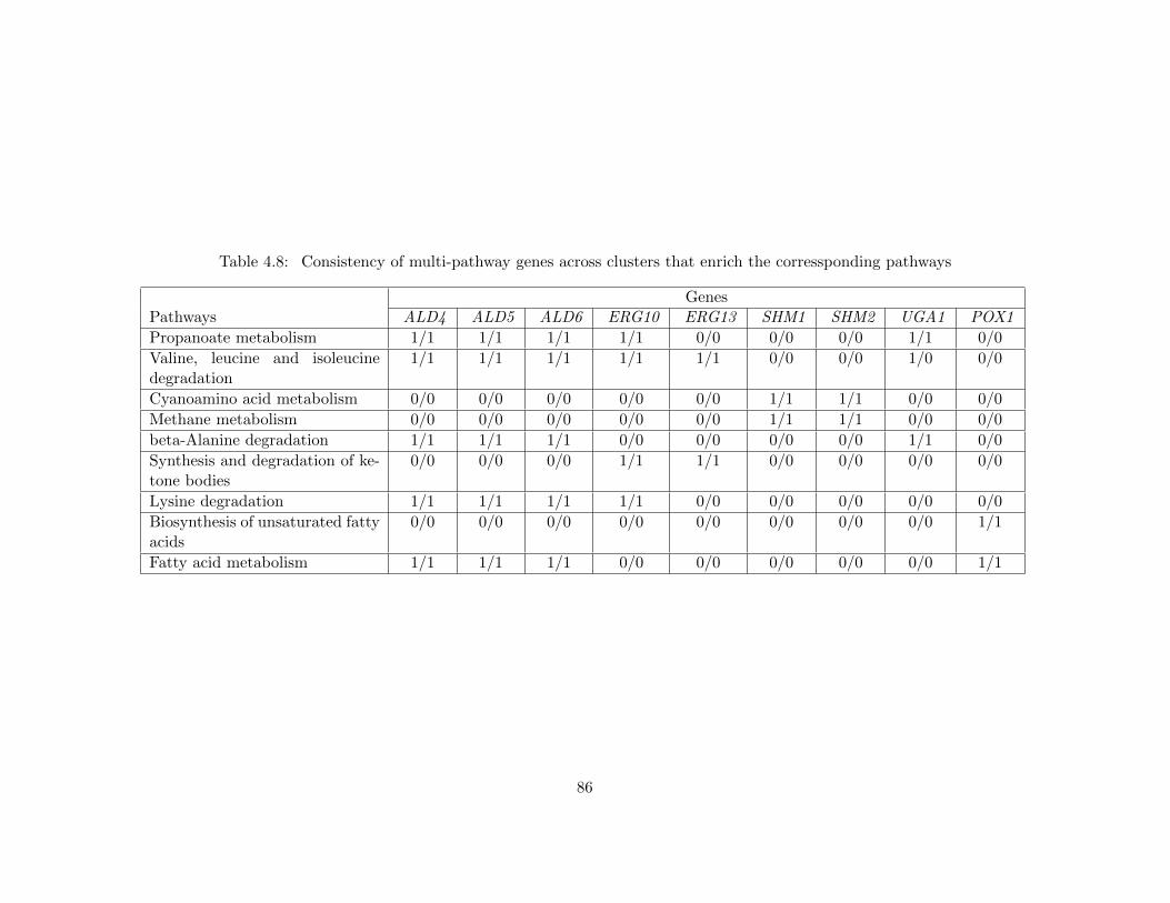
Table 4.8: Consistency of multi-pathway genes across clusters that enrich the corressponding pathways

GenesPathways ALD4 ALD5 ALD6 ERG10 ERG13 SHM1 SHM2 UGA1 POX1

Propanoate metabolism 1/1 1/1 1/1 1/1 0/0 0/0 0/0 1/1 0/0

Valine, leucine and isoleucinedegradation

1/1 1/1 1/1 1/1 1/1 0/0 0/0 1/0 0/0

Cyanoamino acid metabolism 0/0 0/0 0/0 0/0 0/0 1/1 1/1 0/0 0/0

Methane metabolism 0/0 0/0 0/0 0/0 0/0 1/1 1/1 0/0 0/0

beta-Alanine degradation 1/1 1/1 1/1 0/0 0/0 0/0 0/0 1/1 0/0

Synthesis and degradation of ke-tone bodies

0/0 0/0 0/0 1/1 1/1 0/0 0/0 0/0 0/0

Lysine degradation 1/1 1/1 1/1 1/1 0/0 0/0 0/0 0/0 0/0

Biosynthesis of unsaturated fattyacids

0/0 0/0 0/0 0/0 0/0 0/0 0/0 0/0 1/1

Fatty acid metabolism 1/1 1/1 1/1 0/0 0/0 0/0 0/0 0/0 1/1

86

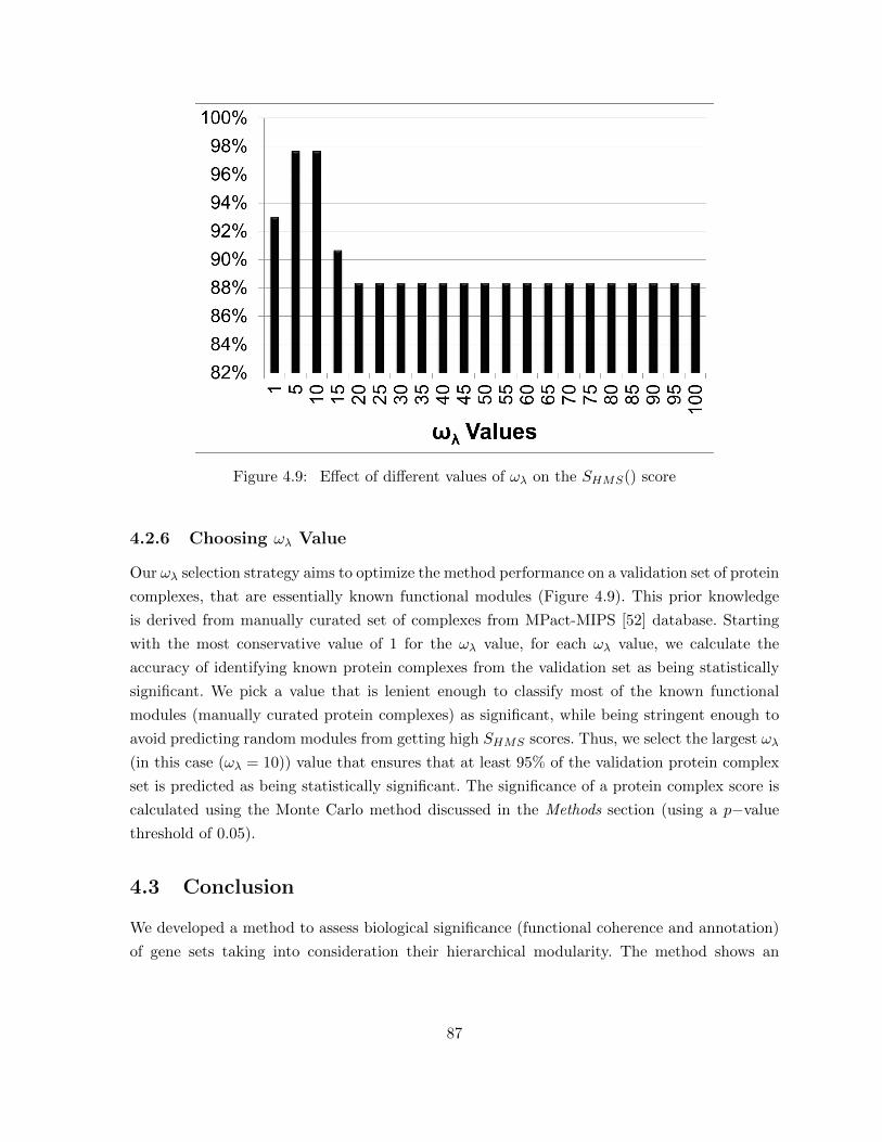
Figure 4.9: Effect of different values of ωλ on the SHMS() score

4.2.6 Choosing ωλ Value

Our ωλ selection strategy aims to optimize the method performance on a validation set of protein

complexes, that are essentially known functional modules (Figure 4.9). This prior knowledge

is derived from manually curated set of complexes from MPact-MIPS [52] database. Starting

with the most conservative value of 1 for the ωλ value, for each ωλ value, we calculate the

accuracy of identifying known protein complexes from the validation set as being statistically

significant. We pick a value that is lenient enough to classify most of the known functional

modules (manually curated protein complexes) as significant, while being stringent enough to

avoid predicting random modules from getting high SHMS scores. Thus, we select the largest ωλ

(in this case (ωλ = 10)) value that ensures that at least 95% of the validation protein complex

set is predicted as being statistically significant. The significance of a protein complex score is

calculated using the Monte Carlo method discussed in the Methods section (using a p−value

threshold of 0.05).

4.3 Conclusion

We developed a method to assess biological significance (functional coherence and annotation)

of gene sets taking into consideration their hierarchical modularity. The method shows an

87

improved performance in comparison to the current state-of-the-art functional coherence and

annotation analysis methods when evaluated on several known functionally coherent gene sets.

88

Chapter 5

Conclusion and Future Work

The central hypothesis of this thesis is Phenotype-centric hierarchical-modularity driven network

biomarker discovery and analysis will enhance the performance of phenotype-related biomarker

identification and improve phenotype diagnostics and prognostics using such biomarkers. The

thesis proposed three methodologies towards this hypothesis. We have presented empirical re-

sults showing the efficacy and applicability of our methods.

The subsystem crosstalk level methodology is to the best of our knowledge the first to sys-

tematically identify network biomarker crosstalks, taking into account the multiple biological

clues. The method when applied to the Alzheimer’s disease phenotype, identifies crosstalks

that are expected to be found and novel crosstalks that require further investigation. Further-

more, empirical results demonstrate the value of crosstalk biomarkers in Alzheimer’s disease

prognosis—improving prognosis accuracy by 15.9% compared to current state-of-the-art.

The subsystem level methodology analyzes hundreds of organismal networks to enumerate

the phenotype-related network biomarker subsystems avoiding several of the pitfalls of the

current state-of-the art methodology. The method has been applied to microbial phenotypes

such as acid tolerance, motility, gram stain, and biohydrogen production. The method captures

biomarkers verified by existing literature as well as novel subsystems whose relationship with

the phenotype can be biologically explained.

The individual gene level methodology evaluates network biomarkers for functional coher-

ence and assigns a hierarchy functional annotations by considering the constituent gene sets

as hierarchically organized components. The method demonstrates a 15%-30% improvement in

performance compared to the current state-of-the art methods.

However, the thesis does not purport to represent the fully comprehensive closure of all

valid or effective approaches to the problem of hierarchical modularity driven phenotype-related

network biomarker identification and analysis. The following sections describe major directions

for future work.

89

5.1 Causative Network Biomarkers

The network biomarkers identified so far have an “associative” relationship with the pheno-

type. Moving towards “causal” relationships is a natural progression. Causal relationships can

be looked at from two perspectives. The first perspective looks into causality between the

biomarker and the phenotype, to decide if the variations in the network biomarker (A) such

as missing edges human brain network biomarker, caused the phenotype (B) such as dementia

or vice versa. The second perspective looks into causal crosstalks to help understand if the

structural and functional variations in a subsystem A caused a variation in subsystem B, A→B, or vice-versa. The methodology can use the reference map built earlier and evaluate the

edges for directionality, i.e., decide if the undirected associative edges can be converted into

directed causal edges. Causal relationships are of significant value because the (A→B)-type

causal relationship would provide more specific targets for clinical interference.

The existing methods [38, 85] in this space primarily look at causality between genes or gene

sets not taking into consideration the network biomarker structure. There are several computa-

tional challenges in this space. The causality relationships between a pair of biomarkers and be-

tween biomarker-phenotype pairs are likely non-linear. Identifying causal relationships between

overlapping subsystems is non-trivial. Hierarchical-modularity adds a layer of complexity; it is

imperative to understand how causality at one level of the hierarchy (say, at the individual gene

level) can be translated into the next level in the hierarchy (say, at the subsystem level). The

final challenge lies in identifying causal relationships that are conserved across organisms—to

analyze if strategies used for “associative” relationships would suffice for “causal” relationships.

5.2 Dynamic Network Biomarkers

This thesis discussed methods for comparative network analysis of static biological networks,

i.e, networks without a temporal component. However, the trend in the recent past has been to

collect longitudinal patient-specific data (e.g., ADNI Initiative), i.e., to collect patient variables

at regular time intervals, over several years. Dynamic network biomarkers are biomarkers that

are identified at a given timestamp, and then monitored and evaluated at different stages and

time points during development of disease. Dynamic network biomarkers will likely demon-

strate changes at various stages of the disease and improve phenotype specificity of identified

biomarkers[185].

Dynamic biomarkers will help in further understanding not only disease progression but also

identifying certain other factors (e.g., environmental factors) that maybe contributing to faster

(or slower) disease progression. This kind of analysis when performed on normal patients can

help cancel out effects/changes that are not related to a specific-disease but related to normal

90

“wear and tear” of the human body. Dynamic network biomarkers can be utilized to compare

patients in different cohorts even if the actual timelines of data collection is different, since the

trajectory of the biomarker rather than the actual measurements are compared.

There are several computational challenges in this space. Matching network biomarkers

across two time stamps is non-trivial. The network could have undergone perturbation across

two timepoints. Tracking all network biomarkers across all timepoints is computationally in-

tensive. In addition, the method should take into consideration that at each time-stamp, new

biomarkers may appear and some existing ones may disappear, several biomarkers may combine

and a single biomarker may split and so on. The methodology should handle updates, i.e., data

collected at future timepoints should not require complete reruns of the method.

5.3 Multi-phenotype Network Biomarkers

The current methodologies look at phenotypes one-at-a-time; however, in the real-world, pheno-

types do not occur independently but as a combination. It is necessary to explore and develop

methodologies that can find network biomarkers that are biased towards two or more traits

simultaneously. For example, diseases such as Alzheimer’s, hypertension, heart problems, and

diabetes often co-occur [120]. These diseases, if analyzed together, may provide useful informa-

tion that can be utilized in effective drug discovery.

5.4 Prediction of Missing Values

Prediction of missing values is an important area of research that will complement all the meth-

ods developed in the network biomarker space. Solutions to this problem will likely improve the

stability, utility, and robustness of methods developed in the research areas discussed previously.

In disease prognostics, missing data often leads to omitting patients from the analysis since the

usual strategies of using the mean or mode values are not sufficient. We need more intelligent

and domain-specific techniques to fill in missing values. The most recent papers [191, 196] on

the topic build different prediction models for different subsets of patients and then use the

features with known values for a patient to predict values of missing variables. However, it

would be worthwhile investigating this problem more systematically by addressing the follow-

ing challenges. Different features follow different patterns and a “one glove fits all” strategy

might not necessarily work. For example, the missing value solution for the PET data would

likely be different from the MRI data. Another challenge is to decide when to use a methodology

to fill in missing values and when to omit the data point. There is also a need to estimate an

error margin for the predicted missing values. This would also help calculate a confidence to

prognosis performed incorporating the predicted missing values.

91

REFERENCES

[1] C.E. Acuna, V.and Ferreira, A.S. Freire, and E. Moreno. Solving the maximum edgebiclique packing problem on unbalanced bipartite graphs. Discrete Appl. Math. in press,2011.

[2] K. Al-Mansoori, M. Hasan, A. Al-Hayani, and O. El-Agnaf. The role of α-synuclein in neu-rodegenerative diseases: From molecular pathways in disease to therapeutic approaches.Curr Alzheimer Res., 10(6):559–568, 2013.

[3] M. Ashburner, C.A. Ball, J.A. Blake, D. Botstein, H. Butler, J.M. Cherry, A.P. Davis,K. Dolinski, S.S. Dwight, J.T. Eppig, M.A. Harris, D.P. Hill, L. Issel-Tarver, A. Kasarskis,S. Lewis, J.C. Matese, J.E. Richardson, M. Ringwald, G.M. Rubin, and G. Sherlock. GeneOntology: A tool for the unification of biology. Nat. Genet., 25(1):25–29, 2000.

[4] G. Atluri, K. Padmanabhan, G. Fang, M. Steinbach, J. Petrella, K. Lim, A. MacDon-ald III, N. Samatova, M. Doraiswamy, and V. Kumar. Complex biomarker discovery inneuroimaging data: Finding a needle in a haystack. NeuroImage: Clinical, 3(0):123 – 131,2013.

[5] G.D. Bader, D. Betel, and C.W.V. Hogue. BIND: The biomolecular interaction networkdatabase. Nucleic Acids Res., 31(1):248–250, 2003.

[6] T. Bailey and M. Gribskov. Combining evidence using p-values: Application to sequencehomology searches. Bioinformatics, 14(1):48–54, January 1998.

[7] C. Ballatore, V. Lee, and J. Trojanowski. Tau-mediated neurodegeneration in Alzheimer’sdisease and related disorders. Nat Rev Neurosci., 8:663–672, 2007.

[8] S. Bauer, S. Grossmann, M. Vingron, and P.N. Robinson. Ontologizer 2.0-a multi-functional tool for GO term enrichment analysis and data exploration. Bioinformatics,24(14):1650 –1651, 2008.

[9] K. Berntorp, A. Frid, R. Alm, G. Fredrikson, K. Sjoberg, and B. Ohlsson. Antibodiesagainst gonadotropin-releasing hormone (GnRH) in patients with diabetes mellitus isassociated with lower body weight and autonomic neuropathy. BMC Res Notes., 6:329,2013.

[10] J.C. Bezdek, R. Ehrlich, and W. Full. FCM: The fuzzy c-means clustering algorithm.Comput. Geosci., 10(2-3):191–203, 1984.

[11] J. Bick and B. Lange. Metabolic cross talk between cytosolic and plastidial pathways ofisoprenoid biosynthesis: Unidirectional transport of intermediates across the chloroplastenvelope membrane. Mol. Syst. Biol., 415(2):146–154, 2010.

[12] K. Bosscher, W.V. Berghe, and G. Haegeman. Cross-talk between nuclear receptors andnuclear factor kappaB. Oncogene, 25(51):6868–86, 2006.

92

[13] E.I. Boyle, S. Weng, J. Gollub, H. Jin, D. Botstein, J.M. Cherry, and G. Sherlock.GO::termfinder-open source software for accessing gene ontology information and findingsignificantly enriched gene ontology terms associated with a list of genes. Bioinformatics,20(18):3710 –3715, 2004.

[14] W. Bradley, R. Polinsky, W. Pendlebury, S. Jones, L. Nee, J. Bartlett, J. Hartshorn,R. Tandan, L. Sweet, and G. Magin. DNA repair deficiency for alkylation damage in cellsfrom Alzheimer’s disease patients. Prog Clin Biol Res., 317:715–732, 1989.

[15] L. Brentner, J. Peccia, and J. Zimmerman. Challenges in developing biohydrogen as asustainable energy source: Implications for a research agenda. Environ. Sci. Technol.,44:2243–2254, 2010.

[16] A. M. Breton, J. Schaeffer, and M. Aigle. The yeast rvs161 and rvs167 proteins areinvolved in secretory vesicles targeting the plasma membrane and in cell integrity. Yeast,18(11):1053–1068, 2001.

[17] C. Bron and J. Kerbosch. Algorithm 457: Finding all cliques of an undirected graph.Commun. ACM, 16(9):575–577, 1973.

[18] A. Budanitsky. Semantic distance in WordNet: An experimental, application-orientedevaluation of five measures. In Proceedings of the North American Conference on ChineseLinguistics Workshop on WordNet and other lexical resources: Applications, extensions,and customizations, 2001.

[19] G. Butland, J. Zhang, W. Yang, A. Sheung, P. Wong, J. Greenbalt, A. Emili, and D. Zam-ble. Interactions of the Escherichia coli hydrogenase biosynthetic proteins: HybG complexformation. FEBS Lett., 580:677–681, 2006.

[20] M. Cariaso and G. Lennon. SNPedia: A wiki supporting personal genome annotation,interpretation and analysis. Nucleic Acids Res, 40:1308–1312, 2012.

[21] M. Chagoyen, J. Carazo, and A. Pascual-Montano. Assessment of protein set coherenceusing functional annotations. BMC Bioinformatics, 9:444, 2008.

[22] J. Chen and B. Yuan. Detecting functional modules in the yeast protein-protein interac-tion network. Bioinformatics, 22(18):2283 –2290, 2006.

[23] J.Z. Chen. Targeted therapy of obesity-associated colon cancer. Transl. Gastrointest.Cancer, 1(1):44–57, 2012.

[24] Q. Chen, W. Wei, T. Shimahara, and C. Xie. Alzheimer amyloid beta-peptide inhibitsthe late phase of long-term potentiation through calcineurin-dependent mechanisms inthe hippocampal dentate gyrus. Neurobiol Learn Mem., 77(3):354–371, 2002.

[25] Z. Chen, W. Hendrix, and N.F. Samatova. Community-based anomaly detection in evo-lutionary networks. J. Intell. Inf. Syst., 39(1):59–85, 2012.

93

[26] Z. Chen, K. Padmanabhan, A. Rocha, Y. Shpanskaya, J. Mihelcic, K. Scott, and N. Sam-atova. SPICE: Discovery of phenotype-determining component interplays. BMC Sys Biol,6(1):40, 2012.

[27] M. Dahiyat, A. Cumming, C. Harrington, C. Wischik, J. Xuereb, F. Corrigan, G. Breen,D. Shaw, and D. St Clair. Association between Alzheimer’s disease and the NOS3 gene.Ann Neurol, 46(4):664–667, 1999.

[28] M. D’Andrea. Evidence linking neuronal cell death to autoimmunity in Alzheimer’s dis-ease. Brain Res., 982(1):19–30, 2003.

[29] C. Davatzikos, P. Bhatt, L. Shaw, K. Batmanghelich, and J. Trojanowski. Prediction ofMCI to AD conversion, via MRI, CSF biomarkers, and pattern classification. NeurobiolAging., 32:2322.e19–27, 2011.

[30] A. Davis, C. Murphy, R. Johnson, J. Lay, K. Lennon-Hopkins, C. Saraceni-Richards,D. Sciaky, B. King, M. Rosenstein, T. Wiegers, and C. Mattingly. The comparativetoxicogenomics database: Update 2013. Nucleic Acids Res., 41(1):1104–1114, 2013.

[31] P.S. Dehal, M.P. Joachimiak, M.N. Price, J.T. Bates, J.K. Baumohl, D. Chivian, G.D.Friedland, K.H. Huang, K. Keller, P.S. Novichkov, I. Dubchak, E.J. Alm, and A.P. Arkin.MicrobesOnline: An integrated portal for comparative and functional genomics. NucleicAcids Res, 38:396–400, 2009.

[32] R. Donaldson and M. Calder. Modelling and analysis of biochemical signalling pathwaycross-talk. EPTCS, 19:40–54, 2010.

[33] D. Dotan-Cohen and S. Letovsky. Biological process linkage networks. PLoS One,4(4):e5313, 2009.

[34] P. Durrens, E. Revardel, M. Bonneu, and M. Aigle. Evidence for a branched pathwayin the polarized cell division of Saccharomyces cerevisiae. Curr. Genet., 27(3):213–216,1995.

[35] D. Eppstein. Arboricity and bipartite subgraph listing algorithms. Inform. Process. Lett.,51(4):207–211, 1994.

[36] W. Feller. An introduction to probability theory and its applications. Wiley, New York,1957.

[37] U. Freo, G. Pizzolato, M. Dam, C. Ori, and L. Battistin. A short review of cognitiveand functional neuroimaging studies of cholinergic drugs: Implications for therapeuticpotentials. J Neural Transm., 109(5-6):857–870, 2002.

[38] A. Fujita, K. Kojima, A. Patriota, J. Sato, P. Severino, and S. Miyano. A fast androbust statistical test based on likelihood ratio with bartlett correction to identify grangercausality between gene sets. Bioinformatics, 26(18):2349–2351, 2010.

94

[39] C. Garcia-Ruiz, A. Colell, A. Morales, N. Kaplowitz, and J.C. Fernandez-Checa. Role ofoxidative stress generated from the mitochondrial electron transport chain and mitochon-drial glutathione status in loss of mitochondrial function and activation of transcriptionfactor nuclear factor-kappaB: Studies with isolated mitochondria and rat hepatocytes.Mol. Pharmacol., 48:825–834, 1995.

[40] A. Gavin, P. Aloy, P. Grandi, R. Krause, M. Boesche, M. Marzioch, C. Rau, L. Jensen,S. Bastuck, B. Dumpelfeld, A. Edelmann, M. Heurtier, V. Hoffman, C. Hoefert, K. Klein,M. Hudak, A. Michon, M. Schelder, M. Schirle, M. Remor, T. Rudi, S. Hooper, A. Bauer,T. Bouwmeester, G. Casari, G. Drewes, G. Neubauer, J. Rick, B. Kuster, P. Bork, R. Rus-sell, and G. Superti-Furga. Proteome survey reveals modularity of the yeast cell machin-ery. Nature, 440(7084):631–636, 2006.

[41] A. Gavin, M. Bosche, R. Krause, P. Grandi, M. Marzioch, A. Bauer, J. Schultz, J.M. Rick,A. Michon, C. Cruciat, M. Remor, C. Hofert, M. Schelder, M. Brajenovic, H. Ruffner,A. Merino, K. Klein, M. Hudak, D. Dickson, T. Rudi, V. Gnau, A. Bauch, S. Bastuck,B. Huhse, C. Leutwein, M. Heurtier, R.R. Copley, A. Edelmann, E. Querfurth, V. Rybin,G. Drewes, M. Raida, T. Bouwmeester, P. Bork, B. Seraphin, B. Kuster, G. Neubauer, andG. Superti-Furga. Functional organization of the yeast proteome by systematic analysisof protein complexes. Nature, 415(6868):141–147, 2002.

[42] J.P. Gerrity. A note on Gandin and Murphy’s equitable skill score. Mon. Weather. Rev.,120:2709–2712, 1992.

[43] A.B. Geva. Hierarchical unsupervised fuzzy clustering. IEEE Trans. Fuzzy Syst., 7(6):723–733, 1999.

[44] N. Ghebranious, B. Mukesh, P. Giampietro, I. Glurich, S. Mickel, S. Waring, and C. Mc-Carty. A pilot study of gene/gene and gene/environment interactions in Alzheimer disease.Clin Med Res., 9(1):17–25, 2011.

[45] B. Giunta, F. Fernandez, W. Nikolic, D. Obregon, E. Rrapo, T. Town, and J. Tan. In-flammaging as a prodrome to Alzheimer’s disease. J Neuroinflammation., 5:51, 2008.

[46] C. Goh, T. Gianoulis, J. Liu, Y.and Li, A. Paccanaro, Y. Lussier, and M. Gerstein. Integra-tion of curated databases to identify genotype-phenotype associations. BMC Genomics,7:257, 2006.

[47] O. Gonzalez and R. Zimmer. Assigning functional linkages to proteins using phylogeneticprofiles and continuous phenotypes. Bioinformatics, 24(10):1257–1263, 2008.

[48] R. Gross and D. Beier, editors. Two-Component Systems in Bacteria. Caister AcademicPress, Norwich,U.K., 2011.

[49] T. Grune, T. Reinheckel, M. Joshi, and K.J. Davies. Proteolysis in cultured liver epithelialcells during oxidative stress. Role of the multicatalytic proteinase complex, proteasome.J. Biol. Chem., 270:2344–2351, 1995.

95

[50] O. Guerrini, P. Soucaille, L. Girbal, B. Guigliarelli, C. Leger, B. Burlat, and C. Lger.Characterization of two 2[4Fe4S] ferredoxins from Clostridium acetobutylicum. Curr.Microbiol., 56:261–267, 2008.

[51] L. Guimei, K. Sim, and J. Li. Efficient mining of large maximal bicliques. In Proceedingsof the International Conference on Data Warehousing and Knowledge Discovery, 2006.

[52] U. Guldener, M. Munsterkotter, M. Oesterheld, P. Pagel, A. Ruepp, H. Mewes, andV. Stumpflen. MPact: The MIPS protein interaction resource on yeast. Nucleic AcidsRes., 34(1):436–441, 2005.

[53] K. Gulshan, S.A. Rovinsky, and W.S Moye-Rowley. YBP1 and its homologueYBP2 /YBH1 influence oxidative-stress tolerance by nonidentical mechanisms in Sac-charomyces cerevisiae. Eukaryot. Cell, 3:318–330, 2004.

[54] M. Habibi, C. Eslahchi, and L. Wong. Protein complex prediction based on k-connectedsubgraphs in protein interaction network. BMC Syst. Biol., 4:129, 2010.

[55] A. Hach, T. Hon, and L. Zhang. A new class of repression modules is critical for hemeregulation of the yeast transcriptional activator HAP1. Mol. Cell Biol., 19(6):4324–4333,1999.

[56] R.A. Hand, N. Jia, M. Bard, and R.J. Craven. Saccharomyces cerevisiae Dap1p, a novelDNA damage response protein related to the mammalian membrane-associated proges-terone receptor. Eukaryot. Cell, 2:306–317, 2003.

[57] J. Hartman, B. Garvik, and L. Hartwell. Principles for the buffering of genetic variation.Science, 291:1001–1004, 2001.

[58] L.H. Hartwell, J.J. Hopfield, S. Leibler, and A.W. Murray. From molecular to modularcell biology. Nature, 402(6761):47–52, 1999.

[59] P. Heidke. Berechnung des erfolges und der gte der windstrkevorhersagen im sturmwar-nungsdienst. Geogr. Ann., 8:301–349, 1926.

[60] W. Hendrix, A. Rocha, M. Elmore, J. Trien, and N. Samatova. Discovery of enrichedbiological motifs using knowledge priors with application to biohydrogen production. InProceedings of the International Conference on Bioinformatics & Computational Biology,pages 17–23, 2010.

[61] W. Hendrix, A. Rocha, K. Padmanabhan, A. Choudhary, K. Scott, J. Mihelcic, andN.F. Samatova. DENSE: Efficient and prior knowledge-driven discovery of phenotype-associated protein functional modules. BMC Syst. Biol., 5:172, 2011.

[62] Y. Ho, A. Gruhler, A. Heilbut, G. Bader, L. Moore, S. Adams, A. Millar, P. Taylor, K. Ben-nett, K. Boutilier, L. Yang, C. Wolting, I. Donaldson, S. Schandorff, Shewnarane J., M. Vo,J. Taggart, M. Goudreault, B. Muskat, C. Alfarano, D. Dewar, Z. Lin, K. Michalickova,A. Willems, H. Sassi, P. Nielsen, K. Rasmussen, J. Andersen, L. Johansen, L. Hansen,H. Jespersen, A. Podtelejnikov, E. Nielsen, J. Crawford, V. Poulsen, B. Sorensen,

96

J. Matthiesen, R. Hendrickson, F. Gleeson, T. Pawson, M. Moran, D. Durocher, M. Mann,C. Hogue, D. Figeys, and M. Tyers. Systematic identification of protein complexes in Sac-charomyces cerevisiae by mass spectrometry. Nature, 415(6868):180–183, 2002.

[63] K. Holohan, D. Lahiri, B. Schneider, T. Foroud, and A. Saykin. Functional microRNAsin Alzheimer’s disease and cancer: Differential regulation of common mechanisms andpathways. Front Genet., 3:323, 2012.

[64] K. Honjo, R. van Reekum, and N. Verhoeff. Alzheimer’s disease and infection: Do in-fectious agents contribute to progression of Alzheimer’s disease? Alzheimers Dement.,5(4):348–360, 2009.

[65] Y. Horng, S. Chen, Y. Chang, and C. Lee. A new method for fuzzy information retrievalbased on fuzzy hierarchical clustering and fuzzy inference techniques. IEEE Trans. FuzzySyst., 13(2):216–228, 2005.

[66] D.W. Huang, B.T. Sherman, and R.A. Lempicki. Systematic and integrative analysis oflarge gene lists using DAVID bioinformatics resources. Nat. Protoc., 4(1):44–57, 2008.

[67] D.W. Huang, B.T. Sherman, and R.A. Lempicki. Bioinformatics enrichment tools: Pathstoward the comprehensive functional analysis of large gene lists. Nucleic Acids Res.,37(1):1–13, 2009.

[68] W. Hwang, Y. Cho, A. Zhang, and M. Ramanathan. A novel functional module detectionalgorithm for protein-protein interaction networks. Algorithms Mol. Biol., 1:24, 2006.

[69] T.L. Jackson. A mathematical investigation of the multiple pathways to recurrent prostatecancer: Comparison with experimental data. Neoplasia, 6(6):697–704, 2004.

[70] L. J. Jensen, M. Kuhn, M. Stark, S. Chaffron, C. Creevey, J. Muller, T. Doerks, P. Julien,A. Roth, M. Simonovic, P. Bork, and C. von Mering. String 8: A global view on proteinsand their functional interactions in 630 organisms. 37:412–416, 2009.

[71] J.J. Jiang and D.W. Conrath. Semantic similarity based on corpus statistics and lexicaltaxonomy. In Proceedings of the International Conference on Research in ComputationalLinguistics, 1997.

[72] K. Jim, K. Parmar, M. Singh, and S. Tavazoie. A cross-genomic approach for systematicmapping of phenotypic traits to genes. Genome Res., 14(1):109–115, 2004.

[73] M. Johnston. A model fungal gene regulatory mechanism: the GAL genes of Saccha-romyces cerevisiae. Microbiol Rev., 51(4):458–476, 1987.

[74] B. Jung, K. Pyo, K. Shin, Y. Hwang, H. Lim, S. Lee, J. Moon, S. Lee, Y. Suh, J. Chai,and E. Shin. Toxoplasma gondii infection in the brain inhibits neuronal degeneration andlearning and memory impairments in a murine model of Alzheimer’s disease. PLoS ONE,7(3):e33312, 2012.

[75] M. Kanehisa and S. Goto. KEGG: Kyoto encyclopedia of genes and genomes. NucleicAcids Res., 28(1):27–30, 2000.

97

[76] M. Kanehisa, S. Goto, M. Furumichi, M. Tanabe, and M. Hirakawa. KEGG for repre-sentation and analysis of molecular networks involving diseases and drugs. Nucleic AcidsRes., 38(1):355–360, 2010.

[77] M. Kanehisa, S. Goto, M. Hattori, K.F. Aoki-Kinoshita, M. Itoh, S. Kawashima,T. Katayama, M. Araki, and M. Hirakawa. From genomics to chemical genomics: Newdevelopments in KEGG. Nucleic Acids Res., 34(1):354–357, 2006.

[78] I. Kapdan and F. Kargi. Bio-hydrogen production from waste materials. Enzyme Microb.Technol., 38(5):569–582, 2006.

[79] G. Kastenmuller, M. Schenk, J. Gasteiger, and H. Mewes. Uncovering metabolic pathwaysrelevant to phenotypic traits of microbial genomes. Gen. Biol., 10(3):28, 2009.

[80] B.S. Katzenellenbogen. Estrogen receptors: Bioactivities and interactions with cell sig-naling pathways. Biol. Reprod., 54(2):287–293, 1996.

[81] H. Kawaji, J. Severin, M. Lizio, A. Forrest, E. van Nimwegen, M. Rehli, K. Schroder,K. Irvine, H. Suzuki, P. Carninci, Y. Hayashizaki, and C. Daub. Update of the FANTOMweb resource: From mammalian transcriptional landscape to its dynamic regulation. Nu-cleic Acids Res., 39:856–860, 2010.

[82] H. Kawaji, J. Severin, M. Lizio, A. Waterhouse, S. Katayama, K. Irvine, D. Hume, A. For-rest, H. Suzuki, P. Carninci, Y. Hayashizaki, and C. Daub. The FANTOM web resource:From mammalian transcriptional landscape to its dynamic regulation. Genome Biol.,10(4):R40, 2009.

[83] P. Khatri and S. Draghici. Ontological analysis of gene expression data: Current tools,limitations, and open problems. Bioinformatics, 21(18):3587 –3595, 2005.

[84] Y. Kikuchi, Y. Oka, M. Kobayashi, Y. Uesono, A. Tohe, and A. Kikuchi. A new yeastgene, HTR1, required for growth at high-temperature, is needed for recovery from matingpheromone-induced G1 arrest. Mol. Gen. Genet., 245:107–116, 1994.

[85] Y. Kim, S. Wuchty, and T. Przytycka. Identifying causal genes and dysregulated pathwaysin complex diseases. PLoS Comput Biol, 7(3), 2011.

[86] A. Kobayashi, M. Kang, Y. Watai, K.I. Tong, T. Shibata, K. Uchida, and M. Yamamoto.Oxidative and electrophilic stresses activate Nrf2 through inhibition of ubiquitinationactivity of Keap1. Mol. Cell. Biol., 26(1):221–229, 2006.

[87] O. Kohannim, X. Hua, D. Hibar, S. Lee, Y. Chou, A.. Toga, C.. Jack, M. Weiner,and P. Thompson. Boosting power for clinical trials using classifiers based on multiplebiomarkers. Neurobiol Aging, 31(8):1429–1442, August 2010.

[88] E.V. Koonin. Orthologs, paralogs, and evolutionary genomics. Annu. Rev. Genet., 39:309–338, 2005.

98

[89] J. Korbel, T. Doerks, L. Jensen, C. Perez-Iratxeta, S. Kaczanowski, S. Hooper, M. An-drade, and P. Bork. Systematic association of genes to phenotypes by genome and liter-ature mining. PLoS Biol., 3:e134, 2005.

[90] K.L. Kovacs, Z. Bagi, B. Balint, B.D. Fodor, G. Scnadi, R. Csaki, T. Hanczar, A.T. Ko-vacs, G. Maroti, K. Perei, A. Toth, and G. Rakhely. Novel approaches to exploit microbialhydrogen metabolism. In J. Miyake, Y Igarashi, and M Rogner, editors, Biohydrogen III.Elsevier Inc, New York, USA, 2004.

[91] N. Krogan, W. Peng, G. Cagney, M. Robinson, R. Haw, G. Zhong, X. Guo, X. Zhang,V. Canadien, D. Richards, B. Beattie, A. Lalev, W. Zhang, A. Davierwala, S. Mnaimneh,A. Starostine, A. Tikuisis, J. Grigull, N. Datta, J. Bray, T. Hughes, A. Emili, and J. Green-blatt. High-definition macromolecular composition of yeast RNA-processing complexes.Mol. Cell., 13(2):225–239, 2004.

[92] G.N. Lance and W.T. Williams. A general theory of classificatory sorting strategies.Comput. J., 9(4):373–380, 1967.

[93] C. Lanni, D. Uberti, M. Racchi, S. Govoni, and M. Memo. Unfolded p53: A potentialbiomarker for Alzheimer’s disease. J Alzheimers Dis., 12:93–99, 2007.

[94] W. Lathe, J. Williams, M. Mangan, and D. Karolchik. Genomic data resources: Challengesand promises. Nature Edu., 1(3), 2008.

[95] H. Lavoie, H. Hogues, J. Mallick, A. Sellam, A. Nantel, and M. Whiteway. Evolutionarytinkering with conserved components of a transcriptional regulatory network. PLoS Biol.,8:e1000329, 2010.

[96] A. Lawrence and B. Sahakian. Alzheimer disease, attention, and the cholinergic system.Alzheimer Dis Assoc Disord, 9 Suppl 2:43–49, 1995.

[97] M. Levesque, D. Shasha, W. Kim, M.G. Surette, and P.N. Benfey. Trait-to-Gene: Acomputational method for predicting the function of uncharacterized genes. Curr. Biol.,13(2):129–133, 2003.

[98] L. Li, B. Rakitsch, and K. Borgwardt. ccSVM: Correcting support vector machines forconfounding factors in biological data classification. Bioinformatics, 27(13):i342–i348,2011.

[99] S. Li and X. Li. Multiple pathways contribute to the pathogenesis of huntington disease.Mol. Neurodegener., 16:1–19, 2006.

[100] T. Li, P. Du, and N. Xu. Identifying human kinase-specific protein phosphorylation sitesby integrating heterogeneous information from various sources. PLoS ONE, 5(11):e15411,2010.

[101] Y. Li. Pathway crosstalk network. In S. Choi, editor, Syst Biol Sig Net. Springer, NewYork, USA, 2010.

99

[102] Y. Li, P. Agarwal, and D. Rajagopalan. A global pathway crosstalk network. Bioinfor-matics, 24(12):1442–1447, 2008.

[103] J. Liu and W. Wang. OP-cluster: Clustering by tendency in high dimensional space. InProceedings of the International Conference on Data Mining, 2003.

[104] L. Liu, J.R. Trimarchi, P. Navarro, M.A. Blasco, and D.L. Keefe. Oxidative stress con-tributes to arsenic-induced telomere attrition, chromosome instability, and apoptosis. J.Biol. Chem., 278(34):31998–32004, 2003.

[105] Y. Liu, J. Li, L. Sam, C. Goh, M. Gerstein, and Y. Lussier. An integrative genomicapproach to uncover molecular mechanisms of prokaryotic traits. PLoS Comput. Biol.,2(11):e159, 2006.

[106] Y. Liu, F. Zeng, Y. Wang, H. Zhou, B. Giunta, J. Tan, and Y. Wang. Immunity andAlzheimer’s disease: Immunological perspectives on the development of novel therapies.Drug Discov Today., 2013.

[107] S. Lopez-Gomollon, J. Hernandez, S. Pellicer, V. Angarica, M. Peleato, and M. Fil-lat. Cross-talk between iron and nitrogen regulatory networks in Anabaena (Nostoc)sp. PCC 7120: Identification of overlapping genes in FurA and NtcA regulons. J. Mol.Biol, 374(1):267–281, 2007.

[108] D.M. Lorenz, A. Jeng, and M.W. Deem. The emergence of modularity in biologicalsystems. Phys. Life Rev., 8(2):129–160, 2011.

[109] K. Makino and T. Uno. New algorithms for enumerating all maximal cliques. In Proceed-ings of the Scandinavian Workshop Algorithm Theory, 2004.

[110] S. Mandrekar-Colucci, C. Karlo, and G. Landreth. Mechanisms underlying the rapidperoxisome proliferator-activated receptor-γ-mediated amyloid clearance and reversal ofcognitive deficits in a murine model of Alzheimer’s disease. J Neurosci., 32(30):10117–10128, 2012.

[111] M.N. McClean, A. Mody, J.R. Broach, and S. Ramanathan. Cross-talk and decisionmaking in MAP kinase pathways. Nat. Genet., 39(3):409–414, 2007.

[112] D. Meraz-Rıos, M.and Toral-Rios, Di. Franco-Bocanegra, J. Villeda-Hernandez, andV. Campos-Pena. Inflammatory process in Alzheimer’s disease. Front Integr Neurosci.,7:59, 2013.

[113] C. Mering, M. Huynen, D. Jaeggi, S. Schmidt, P. Bork, and B. Snel. STRING: A databaseof predicted functional associations between proteins. Nucleic Acids Res., 31(1):258–261,2003.

[114] M. Mirghorbani and P. Krokhmal. On finding k-cliques in k-partite graphs. OptimizationLett., pages 1–11, 2012.

[115] M. Mistry and P. Pavlidis. Gene Ontology term overlap as a measure of gene functionalsimilarity. BMC Bioinformatics, 9(1):327, 2008.

100

[116] J. Miyake. Biohydrogen. Plenum Press, New York, USA, 1998.

[117] B. Mosch, M. Morawski, A. Mittag, D. Lenz, A. Tarnok, and T. Arendt. Aneuploidyand DNA replication in the normal human brain and Alzheimer’s disease. J Neurosci.,27(26):6859–6867, 2007.

[118] R. Mrak and S. Griffin. Interleukin-1, neuroinflammation, and Alzheimer’s disease. Neu-robiol Aging, 22(6):903–908, 2001.

[119] A. L. Munn, B. J. Stevenson, M. I. Geli, and H. Riezman. END5, END6, and END7 :Mutations that cause actin delocalization and block the internalization step of endocytosisin Saccharomyces cerevisiae. Mol. Biol. Cell, 6(12):1721–1742, 1995.

[120] J. Murray, I.and Proza, F. Sohrabji, and J. Lawler. Vascular and metabolic dysfunctionin alzheimer’s disease: a review. Exp Biol Med (Maywood), 236(7):772–782, 2011.

[121] V.E. Myer and R.A. Young. RNA polymerase II holoenzymes and subcomplexes. J. Biol.Chem., 273(43):27757–27760, 1998.

[122] C.L. Myers, D. Robson, A. Wible, M.A. Hibbs, C. Chiriac, C.L. Theesfeld, K. Dolinski,and O.G. Troyanskaya. Discovery of biological networks from diverse functional genomicdata. Genome Biol., 6(13):114, 2005.

[123] N. Nagarajan and C. Kingsford. GiRaF: Robust, computational identification of influenzareassortments via graph mining. Nucleic Acids Res, 39(6), 2011.

[124] K. Nath and D. Das. Improvement of fermentative hydrogen production: Various ap-proaches. Appl. Microbiol. Biotechnol., 65(5):520–529, 2004.

[125] B. North, D. Curtis, and P. Sham. A note on the calculation of empirical p-values fromMonte Carlo procedures. Am. J. Hum. Genet., 71(2):439–441, 2002.

[126] D. Nussbaum, S. Pu, J. Sack, T. Uno, and H. Zarrabi-Zadeh. Finding maximum edgebicliques in convex bipartite graphs. Algorithmica, 64(2), 2012.

[127] A. Paccanaro, V. Trifonov, H. Yu, and M. Gerstein. Inferring protein-protein interactionsusing interaction network topologies. In Proceedings of the International Joint Conferenceon Neural Networks, 2005.

[128] K. Padmanabhan, K. Wang, and N. Samatova. Functional annotation of hierarchicalmodularity. PLoS ONE, 7(4):e33744, 04 2012.

[129] K. Padmanabhan, K. Wilson, A. Rocha, K. Wang, J. Mihelcic, and N. Samatova. In-silicoidentification of phenotype-biased functional modules. Proteome Sci, 10(1):2, 2012.

[130] J. Pandey, M. Koyuturk, and A. Grama. Functional characterization and topologicalmodularity of molecular interaction networks. BMC Bioinformatics, 11(1):35, 2010.

[131] J. Pandey, M. Koyuturk, S. Subramaniam, and A. Grama. Functional coherence in domaininteraction networks. Bioinformatics, 24(16):28–34, 2008.

101

[132] C.S. Peirce. The numerical measure of the success of predictions. Science, 4(93):453–454,1884.

[133] V. Pilauri, M. Bewley, C. Diep, and J. Hopper. Gal80 dimerization and the yeast GALgene switch. Genetics, 169(4):1903–1914, 2005.

[134] A. Platt and R.J. Reece. The yeast galactose genetic switch is mediated by the formationof a Gal4p-Gal80p-Gal3p complex. Embo. J., 17(14):4086–4091, 1998.

[135] S. Powell, D. Szklarczyk, K. Trachana, A. Roth, M. Kuhn, J. Muller, R. Arnold, T. Rattei,I. Letunic, T. Doerks, L.J. Jensen, C. von Mering, and P. Bork. eggNOG v3.0: Orthologousgroups covering 1133 organisms at 41 different taxonomic ranges. Nucleic Acids Res.,40(1):284–289, 2012.

[136] A. Prelic, S. Bleuler, P. Zimmermann, A. Wille, P. Buhlmann, W. Gruissem, L. Hennig,L. Thiele, and E. Zitzler. A systematic comparison and evaluation of biclustering methodsfor gene expression data. Bioinformatics, 22(9):1122–1129, 2006.

[137] S. Pu, J. Wong, B. Turner, E. Cho, and S.J. Wodak. Up-to-date catalogues of yeastprotein complexes. Nucleic Acids Res., 37(3):825–831, 2009.

[138] J. Quinn. Different stress response between model and pathogenic fungi. In S. Avery,M. Stratford, and P. West, editors, Stress in yeasts and filamentous fungi. Academic Press,Massachusetts, USA, 2008.

[139] V. Ramanan, S. Kim, K. Holohan, L. Shen, K. Nho, S. Risacher, T. Foroud, S. Mukherjee,P. Crane, P. Aisen, R. Petersen, M. Weiner, and A. Saykin. Genome-wide pathway analysisof memory impairment in the Alzheimer’s disease neuroimaging initiative (ADNI) cohortimplicates gene candidates, canonical pathways, and networks. Brain Imaging Behav.,6(4):634–648, 2012.

[140] E. Ravasz, A.L. Somera, D.A. Mongru, Z.N. Oltvai, and A.L. Barabasi. Hierarchicalorganization of modularity in metabolic networks. Science, 297(5586):1551–1555, 2002.

[141] P. Resnik. Semantic similarity in a taxonomy: An information based measure and itsapplication to problems of ambiguity in natural language. J. Artif. Intell. Res., 11(1):95–130, 1999.

[142] F. Rey, E.. Heiniger, and C. Harwood. Redirection of metabolism for biological hydrogenproduction. Appl. Environ. Microbiol., 73(5):1665–1671, 2007.

[143] F. Rey, Y. Oda, and C. Harwood. Regulation of uptake hydrogenase and effects ofhydrogen utilization on gene expression in Rhodopseudomonas palustris. J. Bacteriol.,188(17):6143–6152, 2006.

[144] C. Roe, M. Behrens, C. Xiong, J. Miller, and J. Morris. Alzheimer disease and cancer.Neurology, 64(5):895–898, 2005.

102

[145] A. Ruepp, A. Zollner, D. Maier, K. Albermann, J. Hani, M. Mokrejs, I. Tetko,U. Guldener, G. Mannhaupt, M. Munsterkotter, and H.W. Mewes. The FunCat, a func-tional annotation scheme for systematic classification of proteins from whole genomes.Nucleic Acids Res., 32(18):5539 –5545, 2004.

[146] T. Ruths, D. Ruths, and L. Nakhleh. GS2: An efficiently computable measure of GO-basedsimilarity of gene sets. Bioinformatics, 25(9):1178–1184, 2009.

[147] Nataraj R.V and S. Selvan. Parallel mining of large maximal bicliques using order pre-serving generators. Int. J. Comput., 8(3):105–113, 2009.

[148] F. Sallusto and A. Lanzavecchia. Heterogeneity of CD4+ memory T cells: Functionalmodules for tailored immunity. Eur. J. Immunol., 39(8):2076–2082, 2009.

[149] F. Sardi, L. Fassina, L. Venturini, M. Inguscio, F. Guerriero, E. Rolfo, and G. Ricevuti.Alzheimer’s disease, autoimmunity and inflammation. The good, the bad and the ugly.Autoimmun Rev., 11(2):149–153, 2011.

[150] R. Schaffrath and K.D. Breunig. Genetics and molecular physiology of the yeastKluyveromyces lactis. Fungal Genet. Biol., 30:173–190, 2000.

[151] A. Schlesser, S. Ulaszewski, M. Ghislain, and A. Goffeau. A second transport ATPasegene in Saccharomyces cerevisiae. J. Biol. Chem., 263:19480–19487, 1988.

[152] M. Schmidt, A. Rocha, K. Padmanabhan, Z. Chen, K. Scott, J. Mihelcic, and N.F. Sama-tova. Efficient α, β-motif finder for identification of phenotype-related functional modules.BMC Bioinformatics, 12:440, 2011.

[153] M. Schmidt, A. Rocha, K. Padmanabhan, Y. Shpanskaya, J. Banfield, K. Scott, J. Mihel-cic, and N. Samatova. NIBBS-Search for fast and accurate prediction of phenotype-biasedmetabolic systems. PLoS Comput Biol, 8(5):e1002490, 2012.

[154] M.C Schmidt, N.F. Samatova, K. Thomas, and B. Park. A scalable, parallel algorithmfor maximal clique enumeration. J. Parallel. Distr. Com., 69(4):417–428, 2009.

[155] M.A. Schwartz and V. Baron. Interactions between mitogenic stimuli, or, a thousand andone connections. Curr. Opin. Cell Biol., 11(2):197–202, 1999.

[156] D. Selkoe. Alzheimer’s disease: Genes, proteins, and therapy. Physiol Rev., 81:741–766,2001.

[157] S.B. Selleck and J.E. Majors. In vivo DNA-binding properties of a yeast transcriptionactivator protein. Mol. Cell Biol., 7(9):3260–3267, 1987.

[158] J. Shaffer, J. Petrella, F. Sheldon, K. Choudhury, V. Calhoun, E. Coleman, and M. Do-raiswamy. Predicting cognitive decline in subjects at risk for Alzheimer disease by usingcombined cerebrospinal fluid, MR imaging, and PET biomarkers. Radiology, 266(2):583–591, 2013.

103

[159] S. Shima and R. Thauer. A third type of hydrogenase catalyzing H2 activation. Chem.Rec., 7(1):37–46, 2007.

[160] M. Silver, E. Janousova, X. Hua, P. Thompson, and G. Montana. Identification of genepathways implicated in Alzheimer’s disease using longitudinal imaging phenotypes withsparse regression. NeuroImage., 63(3):1681–1694, 2012.

[161] M. Silver and G. Montana. Fast identification of biological pathways associated with aquantitative trait using group lasso with overlaps. Stat Appl Genet Mol Biol., 11(1):Article7, 2012.

[162] P. Sivadon, F. Bauer, M. Aigle, and M. Crouzet. Actin cytoskeleton and budding patternare altered in the yeast RVS161 mutant: The RVS161 protein shares common domainswith the brain protein amphiphysin. Mol. Gen. Genet., 246(4):485–495, 1995.

[163] N. Slonim, O. Elemento, and S. Tavazoie. Ab initio genotype-phenotype associationreveals intrinsic modularity in genetic networks. Mol. Syst. Biol., 2:2006.0005, 2006.

[164] V. Spirin and L. Mirny. Protein complexes and functional modules in molecular networks.Proc. Natl. Acad. Sci., 100(21):12123–12128, 2003.

[165] C. Stark, B. Breitkreutz, T. Reguly, L. Boucher, A. Breitkreutz, and M. Tyers. BioGRID:A general repository for interaction datasets. Nucleic Acids Res., 34:535–539, 2005.

[166] S.W. Stevens and J. Abelson. Purification of the yeast U4/U6-U5 small nuclear ribonu-cleoprotein particle and identification of its proteins. Proc. Natl. Acad. Sci., 96(13):7226–7231, 1999.

[167] K. Suhre and J. Claverie. FusionDB: A database for in-depth analysis of prokaryotic genefusion events. Nucleic Acids Res., 32(1):273–276, 2004.

[168] P. Suthers, A. Zomorrodi, and C. Maranas. Genome-scale gene/reaction essentiality andsynthetic lethality analysis. Mol Syst Biol., 5, 2009.

[169] K. Tachihara, T. Uemura, K. Kashiwagi, and K. Igarashi. Excretion of putrescine andspermidine by the protein encoded by YKL174C (TPO5 ) in Saccharomyces cerevisiae. J.Biol. Chem., 280(13):12637–12642, 2005.

[170] S.L. Tai, P. Daran-Lapujade, M.C. Walsh, J.T. Pronk, and J. Daran. Acclimation ofSaccharomyces cerevisiae to low temperature: A chemostat-based transcriptome analysis.Mol. Biol. Cell., 18(12):5100–5112, 2007.

[171] A. Tamburri, A. Dudilot, S. Licea, C. Bourgeois, and J. Boehm. NMDA-Receptor acti-vation but not ion flux is required for amyloid-beta induced synaptic depression. PLoSONE, 8(6):e65350, 2013.

[172] M. Tamura and P. D’haeseleer. Microbial genotype-phenotype mapping by class associa-tion rule mining. Bioinformatics, 24(13):1523–1529, 2008.

104

[173] M. Tamura and P. D’haeseler. Comparative genome content analysis with respect to basicmicrobial phenotypes by class association rule mining? In Proceedings of the InternationalConference on Systems Biology, 2007.

[174] A. Tanay, R. Sharan, and R. Shamir. Discovering statistically significant biclusters ingene expression data. Bioinformatics, 18(1):136–144, 2002.

[175] R.L. Tatusov, Koonin E.V., and Lipman D.J. A genomic perspective on protein families.Science, 278(5338):631–637, 1997.

[176] R.L. Tatusov, M. Galperin, D. Natale, and E.V. Koonin. The COG database: A tool forgenome-scale analysis of protein functions and evolution. Nucleic Acids Res., 28(1):33–36,2000.

[177] A. Thomaz, L. Pozzo, A. Fontes, D. Almeida, C. Stahl, J. Santos-Mallet, S. Gomes,D. Feder, D. Ayres, S. Giorgio, and C. Cesar. Optical tweezers force measurements tostudy parasites chemotaxis. In Proceedings of the European Conference on BiomedicalOptics, 2009.

[178] G. Tsekouras, H. Sarimveis, E. Kavakli, and G. Bafas. A hierarchical fuzzy-clusteringapproach to fuzzy modeling. Fuzzy Set. Syst., 150(2):245–266, 2005.

[179] McMaster University. Couch potatoes explained? missing key genesmay be cause for lack of resolve to exercise, researchers find.http://www.sciencedaily.com/releases/2011/09/110905160904.htm, 2011. Accessed:11/26/2012.

[180] P. Vignais, B. Billoud, and J. Meyer. Classification and phylogeny of hydrogenases. FEMSMicrobiol. Rev., 25(4):455–501, 2001.

[181] A. Vignini, A. Giulietti, L. Nanetti, F. Raffaelli, L. Giusti, L. Mazzanti, and L. Provinciali.Alzheimer’s disease and diabetes: New insights and unifying therapies. Curr DiabetesRev., 9(3):218–227, 2013.

[182] A.G. Vitreschak, A. Mironov, V.A. Lyubetsky, and M. Gelfand. Comparative genomicanalysis of T-box regulatory systems in bacteria. RNA, 14(4):717–735, 2008.

[183] M.D. Wallace, A.D. Pfefferle, L. Shen, A.J. McNairn, E.G. Cerami, B.L. Fallon, V.D.Rinaldi, T.L. Southard, C.M. Perou, and J.C. Schimenti. Comparative oncogenomics im-plicates the Neurofibromin 1 Gene (NF1) as a breast cancer driver. Genetics, 192(2):385–396, 2012.

[184] Q.Q. Wang and A. Chang. Sphingoid base synthesis is required for oligomerization andcell surface stability of the yeast plasma membrane ATPase, PMA1. Proc. Natl. Acad.Sci., 99(20):12853–12858, 2002.

[185] X. Wang and P. Ward. Opportunities and challenges of disease biomarkers: a new sectionin the journal of translational medicine. J Transl Med, 10(1):220, 2012.

105

[186] D. Warde-Farley, S. Donaldson, O. Comes, K. Zuberi, R. Badrawi, P. Chao, M. Franz,C. Grouios, F. Kazi, C. Lopes, A. Maitland, S. Mostafavi, J. Montojo, Q. Shao, G. Wright,G. Bader, and Q. Morris. The GeneMANIA prediction server: Biological network integra-tion for gene prioritization and predicting gene function. Nucleic Acids Res., 38(2):W214–W220, 2010.

[187] M. Weiner, D. Veitch, P. Aisen, L. Beckett, N. Cairns, R. Green, D. Harvey, C. Jack,W. Jagust, E. Liu, J. Morris, R. Petersen, A. Saykin, M. Schmidt, L. Shaw, J. Siuciak,H. Soares, A. Toga, and J. Trojanowski. The Alzheimer’s disease neuroimaging initiative:A review of papers published since its inception. Alzheimers Dement, 8(1):1 –68, 2012.

[188] D. White. The physiology and biochemistry of prokaryotes. Oxford University Press, Inc.,Oxford, UK, 2000.

[189] H. Wiener, R. Perry, Z. Chen, L. Harrell, and R. Go. A polymorphism in SOD2 isassociated with development of Alzheimer’s disease. Genes Brain Behav, 6(8):770–776,2007.

[190] C.Y. Wu, S. Roje, F.J. Sandoval, A.J. Bird, D.R. Winge, and D.J. Eide. Repressionof sulfate assimilation is an adaptive response of yeast to the oxidative stress of zincdeficiency. J. Biol. Chem., 284(40):27544–27556, 2009.

[191] S. Xiang, L. Yuan, W. Fan, Y. Wang, P. Thompson, and J. Ye. Bi-level multi-sourcelearning for heterogeneous block-wise missing data. NeuroImage, 13:S1053–8119, 2013.

[192] Y. Xu, W. Hu, Z. Chang, H. DuanMu, S. Zhang, Z. Li, Z. Li, L. Yu, and X. Li. Predictionof human proteinprotein interaction by a mixed Bayesian model and its application toexploring underlying cancer-related pathway crosstalk. J. Royal Soc. Interface, 8(57):555–567, 2011.

[193] B. Yan and S. Gregory. Finding missing edges and communities in incomplete networks.J. Phys. A., 44(49):5102, 2011.

[194] Y. Yang, D. Geldmacher, and K. Herrup. DNA replication precedes neuronal cell deathin Alzheimer’s disease. J Neurosci., 21(8):2661–2668, April 2001.

[195] J. Yu and P. Takahashi. Biophotolysis-based hydrogen production by cyanobacteria andgreen microalgae. In A. Mendez-Vilas, editor, Communicating Current Research and Edu-cational Topics and Trends in Applied Microbiology. Formatex Research Center, Badajoz,Spain, 2007.

[196] L. Yuan, Y. Wang, P. Thompson, V. Narayan, and J. Ye. Multi-source learning forjoint analysis of incomplete multi-modality neuroimaging data. In Proceedings of theInternational Conference on Knowledge Discovery and Data Mining, pages 1149–1157,2012.

[197] Y. Yurov, S. Vorsanova, and I. Iourov. The DNA replication stress hypothesis ofAlzheimer’s disease. ScientificWorldJournal., 11:11, 2011.

106

[198] A. Zalesky, A. Fornito, and E. Bullmore. Network-based statistic: Identifying differencesin brain networks. NeuroImage, 53(4):1197 – 1207, 2010.

[199] B. Zhang, B. Park, T. Karpinets, and N.F. Samatova. From pull-down data to proteininteraction networks and complexes with biological relevance. Bioinformatics, 24(7):979–986, 2008.

[200] Y Zhang, E.J Chesler, and M.A Langston. On finding bicliques in bipartite graphs: Anovel algorithm with application to the integration of diverse biological data types. InProceedings of the International Conference on System Sciences, 2008.

[201] H. Zhou and R. Lipowsky. The yeast protein-protein interaction map is a highly modularnetwork with a staircase community structure. in press, 2005.

107