about word length counting in serbian
TRANSCRIPT

CONTRIBUTIONS TOTHE SCIENCE OF LANGUAGE


CONTRIBUTIONS TOTHE SCIENCE OF LANGUAGEWord Length Studies and Related Issues
Edited byPETER GRZYBEKUniversity of Graz
Kluwer Academic PublishersBoston/Dordrecht/London

Preface
The studies represented in this volume have been collected in the interest ofbringing together contributions from three fields which are all important fora comprehensive approach to the quantitative study of text and language, ingeneral, and of word length studies, in particular: first, scholars from linguisticsand text analysis, second, mathematicians and statisticians working on relatedissues, and third, experts in text corpus and text data bank design.
A scientific research project initiated in spring 2002 provided the perfectopportunity for this endeavor. Financially supported by the Austrian ResearchFund (FWF), this three-year project, headed by Peter Grzybek (Graz Univer-sity) and Ernst Stadlober (Technical University Graz) concentrates on the studyof word length and word length frequencies, with particular emphasis on Slaviclanguages. Specifically, factors influencing word length are systematically stud-ied.
The majority of contributions to be found in this volume go back to a con-ference held in Austria at the very beginning of the project, at Graz Universityand the nearby Schloss Seggau in June, 2002.1 Experts from all over Europewere invited to contribute, with a particular emphasis on the participation ofscholars from East European countries whose valuable work continues to re-main ignored, be it due to language barriers, or to difficulties in the accessibilityof their publications. It is the aim of this volume to contribute to a better mutualexchange of ideas.
Generally speaking, the aim of the conference was to diagnose and to discussthe state of the art in word length studies, with experts from the above-mentioneddisciplines. Moreover, the above-mentioned project and the guiding ideas be-hind it should be presented to renowned experts from the scientific community,with three major intentions: first, to present the basic ideas as to the problemoutlined, and to have them discussed from an external perspective in order to
1 For a conference report see Grzybek/Stadlober (2003), for further details see http://www-gewi.
uni-graz.at/quanta.

vi CONTRIBUTIONS TO THE SCIENCE OF LANGUAGE
profit from differing approaches; second, to raise possible critical points as tothe envisioned methodology, and to discuss foreseeable problems which mightarise during the project; and third, to discuss, at the very beginning, optionsto prepare data, and analytical procedures, in such a way that they might bepublicly useful and available not only during the project, but afterwards, aswell.
Since, with the exception of the introductory essay, the articles appear inalphabetical order, they shall be briefly commented upon here in relation totheir thematic relevance.
The introductory contribution by Peter Grzybek on the History and Method-ology of Word Length Studies attempts to offer a general starting point and, infact, provides an extensive survey on the state of the art. This contribution con-centrates on theoretical approaches to the question, from the 19th century up tothe present, and it offers an extensive overview not only of the development ofword length studies, but of contemporary approaches, as well.
The contributions by Gejza Wimmer from Slovakia and Gabriel Altmannfrom Germany, as well as the one by Victor Kromer from Russia, follow thisline of research, in so far as they are predominantly theory-oriented. WhereasWimmer and Altmann try to achieve an all-encompassing Unified Derivation ofSome Linguistic Laws, Kromer’s contribution About Word Length Distributionis more specific, concentrating on a particular model of word length frequencydistribution.
As compared to such theory-oriented studies, a number of contributions arelocated at the other end of the research spectrum: concentrating less on meretheoretical aspects of word length, they are related to the authors’ work ontext corpora. Whereas Reinhard Kohler from Germany, understanding a TextCorpus As an Abstract Data Structure, tries to generally outline The ArchitectureOf a Universal Corpus Interface, the contributions by Primoz Jakopin fromSlovenia, Marko Tadic from Croatia, and Dusko Vitas, Gordana Pavlovic-Lazetic, & Cvetana Krstev from Belgrade concentrate on the specifics ofCroatian, Serbian, and Slovenian corpora, with particular reference to word-length studies. Jakopin’s contribution On Text Corpora, Word Lengths, andWord Frequencies in Slovenian, Tadic’s report on Developing the CroatianNational Corpus and Beyond, as well as the study About Word Length Countingin Serbian by Vitas, Pavlovic-Lazetic, and Krstev primarily intend to discussthe availability and form of linguistic material from different text corpora, andthe usefulness of the underlying data structure of their corpora for quantitativeanalyses. From this point of view their publications show the efficiency of co-operations between the different fields.
Another block of contributions represent concrete analyses, though fromdiffering perspectives, and with different objectives. The first of these is theanalysis by Andrew Wilson from Great Britain of Word-Length Distribution

PREFACE vii
in Present-Day Lower Sorbian. Applying the theoretical framework outlinedby Altmann, Wimmer, and their colleagues, this is one example of theoreticallymodelling word length frequencies in a number of texts of a given language,Lower Sorbian in this case. Gordana Antic, Emmerich Kelih, & Peter Grzy-bek from Austria, discuss methodological problems of word length studies,concentrating on Zero-syllable Words in Determining Word Length. Whereasthis problem, which is not only relevant for Slavic studies, usually is “solved”by way of an authoritative decision, the authors attempt to describe the concreteconsequences arising from such linguistic decisions. Two further contributionsby Ernst Stadlober & Mario Djuzelic from Graz, and by Otto A. Rottmannfrom Germany, attempt to apply word length analysis for typological purposes:thus, Stadlober & Djuzelic, in their article on Multivariate Statistical Methodsin Quantitative Text Analyses, reflect their results with regard to quantitativetext typology, whereas Rottmann discusses Aspects of the Typology of SlavicLanguages Exemplified on Word Length.
A number of further contributions discuss the relevance of word length stud-ies within a broader linguistic context. Thus, Simone Andersen & Gabriel Alt-mann (Germany) analyze Information Content of Words in Texts, and AugustFenk & Gertraud Fenk-Oczlon (Austria), study Within-Sentence Distributionand Retention of Content Words and Function Words.
The remaining three contributions have the common aim of shedding light onthe interdependence between word length and other linguistic units. Thus, bothWerner Lehfeldt from Germany, and Anatolij A. Polikarpov from Russia,place their word length studies within a Menzerathian framework: in doing so,Lehfeldt, in his analysis of The Fall of the Jers in the Light of Menzerath’s Law,introduces a diachronic perspective, Polikarpov, in his attempt at ExplainingBasic Menzerathian Regularity, focuses the Dependence of Affix Length on theOrdinal Number of their Positions within Words. Finally, Udo Strauss, PeterGrzybek, & Gabriel Altmann re-analyze the well-known problem of WordLength and Word Frequency; on the basis of their study, the authors arrive at theconclusion that sometimes, in describing linguistic phenomena, less complexmodels are sufficient, as long as the principle of data homogeneity is obeyed.
The volume thus offering a broad spectrum of word length studies, shouldbe of interest not only to experts in general linguistics and text scholarship, butin related fields as well. Only a closer co-operation between experts from theabove-mentioned fields will provide an adequate basis for further insight intowhat is actually going on in language(s) and text(s), and it is the hope of thisvolume to make a significant contribution to these efforts.
This volume would not have seen the light of day without the invaluable helpand support of many individuals and institutions. First and foremost, my thanksgoes to Gabriel Altmann, who has accompanied the whole project from itsvery beginnings, and who has nurtured it with his competence and enthusiasm

viii CONTRIBUTIONS TO THE SCIENCE OF LANGUAGE
throughout the duration. Also, without the help of the Graz team, mainly myfriends and colleagues Gordana Antic, Emmerich Kelih, Rudi Schlatte, and ofcourse Ernst Stadlober, this book could not have taken its present shape.
Furthermore, it is my pleasure and duty to express my gratitude to the follow-ing for their financial support: first of all, thanks goes to the Austrian ScienceFund (FWF) in Vienna for funding both research project # P15485 (¿WordLength Frequencies in Slavic Language TextsÀ), and the present volume. Sin-cere thanks as well goes to various institutions which have repeatedly sponsoredacademic meetings related to this volume, among others: Graz University (ViceRector for Research and Knowledge Transfer, Vice Rector and Office for Inter-national Relations, Faculty for Cultural Studies, Department for Slavic Studies),Technical University Graz (Department for Statistics), Office for the Govern-ment of the Province of Styria (Department for Science), Office of the Mayorof the City of Graz.
Finally, my thanks goes to Wolfgang Eismann for his help in interpretingsome Polish texts, and to Brıd Nı Mhaoileoin for her careful editing of the textsin this volume.
Preparing the layout of this volume myself, using TEXor LATEX 2ε, respec-tively, I have done what I could to put all articles into an atrtractive shape; anyremaining flaws are my responsibility.
Peter Grzybek

Contents
Preface v
1On The Science of Language In Light of The Language of Science 1Peter Grzybek
2History and Methodology of Word Length Studies 15Peter Grzybek
3Information Content of Words in Texts 91Simone Andersen, Gabriel Altmann
4Zero-syllable Words in Determining Word Length 117Gordana Antic, Emmerich Kelih, Peter Grzybek
5Within-Sentence Distribution and Retention of
Content Words and Function Words157
August Fenk, Gertraud Fenk-Oczlon
6On Text Corpora, Word Lengths, and Word Frequencies in Slovenian 171Primoz Jakopin
7Text Corpus As an Abstract Data Structure 187Reinhard Kohler
8About Word Length Distribution 199Victor V. Kromer
9The Fall of the Jers in the Light of Menzerath’s Law 211Werner Lehfeldt

x CONTRIBUTIONS TO THE SCIENCE OF LANGUAGE
10Towards the Foundations of Menzerath’s Law 215Anatolij A. Polikarpov
11Aspects of the Typology of Slavic Languages 241Otto A. Rottmann
12Multivariate Statistical Methods in Quantitative Text Analyses 259Ernst Stadlober, Mario Djuzelic
13Word Length and Word Frequency 277Udo Strauss, Peter Grzybek, Gabriel Altmann
14Developing the Croatian National Corpus and Beyond 295Marko Tadic
15About Word Length Counting in Serbian 301Dusko Vitas, Gordana Pavlovic-Lazetic, Cvetana Krstev
16Word-Length Distribution in Present-Day Lower Sorbian Newspaper Texts 319Andrew Wilson
17Towards a Unified Derivation of Some Linguistic Laws 329Gejza Wimmer, Gabriel Altmann
Contributing Authors 339
Author Index 342
Subject Index 345

xi
Dedicated to all those pioneers in the field of quantitative linguis-tics and text analysis, who have understood that quantifying isnot the aim, but a means to understanding the structures andprocesses of text and language, and who have thus paved the wayfor a theory and science of language


INTRODUCTORY REMARKS:ON THE SCIENCE OF LANGUAGEIN LIGHT OF THE LANGUAGE OF SCIENCE
Peter Grzybek
The seemingly innocent formulation as to a science of language in light ofthe language of science is more than a mere play on words: rather, this for-mulation may turn out to be relatively demanding, depending on the concreteunderstanding of the terms involved – particularly, placing the term ‘science’into a framework of a general theory of science. No doubt, there is more thanone theory of science, and it is not the place here to discuss the philosophicalimplications of this field in detail. Furthermore, it has become commonplaceto refuse the concept of a unique theory of science, and to distinguish betweena general theory of science and specific theories of science, relevant for indi-vidual sciences (or branches of science). This tendency is particularly strongin the humanities, where 19th century ideas as to the irreconcilable antagonyof human and natural, of weak and hard sciences, etc., are perpetuated, thoughsophisticatedly updated in one way or another.
The basic problem thus is that the understanding of ’science’ (and, conse-quently, the far-reaching implications of the understanding of the term) is notthe same all across the disciplines. As far as linguistics, which is at stake here,is concerned, the self-evaluation of this discipline clearly is that it fulfills therequirements of being a science, as Smith (1989: 26) correctly puts it:
Linguistics likes to think of itself as a science in the sense that it makes testable,i.e. potentially falsifiable, statements or predictions.
The relevant question is not, however, to which extent linguistics considersitself to be a science; rather, the question must be, to which extent does lin-guistics satisfy the needs of a general theory of science. And the same holdstrue, of course, for related disciplines focusing on specific language productsand processes, starting from subfields such as psycholinguistics, up to the areaof text scholarship, in general.
Generally speaking, it is commonplace to say that there can be no sciencewithout theory, or theories. And there will be no doubt that theories are usually

2 CONTRIBUTIONS TO THE SCIENCE OF LANGUAGE
conceived of as models for the interpretation or explanation of the phenom-ena to be understood or explained. More often than not, however, linguisticunderstandings of the term ‘theory’ are less “ambitious” than postulates fromthe philosophy of science: linguistic “theories” rather tend to confine them-selves to being conceptual systems covering a particular aspect of language.Terms like ‘word formation theory’ (understood as a set of rules with whichwords are composed from morphemes), ‘syntax theory’ (understood as a setof rules with which sentences are formed), or ‘text theory’ (understood as aset of rules with which sentences are combined) are quite characteristic in thisrespect (cf. Altmann 1985: 1). In each of these cases, we are concerned with notmore and not less than a system of concepts whose function it is to provide aconsistent description of the object under study. ‘Theory’ thus is understood inthe descriptive meaning; ultimately, it boils down to an intrinsically plausible,coherent descriptive system, cf. Smith (1989: 14)
But the hallmark of a (scientific) theory is that it gives rise to hypotheses whichcan be the object of rational argumentation.
Now, it goes without saying that the existence of a system of concepts isnecessary for the construction of a theory: yet, it is a necessary, but not sufficientcondition (cf. Altmann 1985: 2):
One should not have the illusion that one constructs a theory when one clas-sifies linguistic phenomena and develops sophisticated conceptual systems, ordiscovers universals, or formulates linguistic rules. Though this predominantlydescriptive work is essential and stands at the beginning of any research, nothingmore can be gained but the definition of the research object [. . . ]
What is necessary then, for science, is the existence of a theory, or of theories,which are systems of specific hypotheses, which are not only plausible, butmust be both deduced or deducible from the theory, and tested, or in principlebe testable (cf. Altmann 1978: 3):
The main part of a theory consists of a system of hypotheses. Some of them areempirical (= tenable), i.e. they are corroborated by data; others are theoretical or(deductively) valid, i.e. they are derived from the axioms or theorems of a (notnecessarily identical) theory with the aid of permitted operations. A scientifictheory is a system in which some valid hypotheses are tenable and (almost) nohypotheses untenable.
Thus, theories pre-suppose the existence of specific hypotheses the formula-tion of which, following Bunge (1967: 229), implies the three main requisites:
(i) the hypothesis must be well formed (formally correct) and meaningful(semantically nonempty) in some scientific context;
(ii) the hypothesis must be grounded to some extent on previous knowledge,i.e. it must be related to definite grounds other than the data it covers; ifentirely novel it must be compatible with the bulk of scientific knowledge;

On The Science of Language In Light of The Language of Science 3
(iii) the hypothesis must be empirically testable by the objective proceduresof science, i.e. by confrontation with empirical data controlled in turn byscientific techniques and theories.
In a next step, therefore, different levels in conjecture making may thusbe distinguished, depending on the relation between hypothesis (h), antecedentknowledge (A), and empirical evidence (e); Figure1.1 illustrates the four levels.
(i) Guesses are unfounded and untested hypotheses, which characterize spec-ulation, pseudoscience, and possibly the earlier stages of theoretical work.
(ii) Empirical hypotheses are ungrounded but empirically corroborated con-jectures; they are rather isolated and lack empirical validation, since theyhave no support other than the one offered by the fact(s) they cover.
(iii) Plausible hypotheses are founded but untested hypotheses; they lack anempirical justification but are, in principle, testable.
(iv) Corroborated hypotheses are well-grounded and empirically confirmed;ultimately, only hypotheses of this level characterize theoretical knowl-edge and are the hallmark of mature science.
Figure 1.1: Levels of Conjecture Making and Validation
If, and only if, a corroborated hypothesis is, in addition to being well-grounded and empirically confirmed, general and systemic, then it may betermed a ‘law’. Now, given that the “chief goal of scientific research is the dis-covery of patterns” (Bunge 1967: 305), a law is a confirmed hypothesis that issupposed to depict such a pattern.

4 CONTRIBUTIONS TO THE SCIENCE OF LANGUAGE
Without a doubt, use of the term ‘law’ will arouse skepticism and refusal inlinguists’ ears and hearts.1 In a way, this is no wonder, since the term ‘law’ has aspecific connotation in the linguistic tradition (cf. Kovacs 1971, Collinge 1985):basically, this tradition refers to 19th century studies of sound laws, attempts todescribe sound changes in the history of (a) language.
In the beginnings of this tradition, predominantly in the Neogrammarianapproach to Indo-European language history, these laws – though of descriptiverather than explanative nature – allowed no exceptions to the rules, and theywere indeed understood as deterministic laws. It goes without saying that up tothat time, determinism in nature had hardly ever been called into question, andthe formation of the concept of ‘law’ still stood in the tradition of Newtonianclassical physics, even in Darwin’s time, he himself largely ignoring probabilityas an important category in science.
The term ‘sound law’, or ‘phonetic law’ [Lautgesetz] had been originallycoined as a technical term by German linguist Franz Bopp (1791–1867) in the1820s. Interestingly enough, his view on language included a natural-scientificperspective, understanding language as an organic physical body [organischerNaturkorper]. At this stage, the phonetic law was not considered to be a law ofnature [Naturgesetz], as yet; rather, we are concerned with metaphorical com-parisons, which nonetheless signify a clear tendency towards scientific exact-ness in linguistics. The first militant “naturalist-linguist” was August Schleicher(1821–1868). Deeply influenced by evolutionary theorists, mainly Charles Dar-win and Ernst Hackel, he understood languages to be a ‘product of nature’ in thestrict sense of this word, i.e., as a ‘natural organism’ [Naturorganismus] which,according to his opinion, came into being and developed according to specificlaws, as he claimed in the 1860s. Consequently, for Schleicher, the science oflanguage must be a natural science, and its method must by and large be the sameas that of the other natural sciences. Many a scholar in the second half of the 19thcentury would elaborate on these ideas: if linguistics belonged to the natural sci-ences, or at least worked with equivalent methods, then linguistic laws should beidentical with the natural laws. Natural laws, however, were considered mech-anistic and deterministic, and partly continue to be even today. Consequently,in the mid-1870s, scholars such as August Leskien (1840–1916), Hermann Os-thoff (1847–1909), and Karl Brugmann (1849–1919) repeatedly emphasizedthe sound laws they studied to be exceptionless. Every scholar admitting ex-ceptions was condemned to be addicted to subjectivism and arbitrariness. Therigor of these claims began to be heavily discussed from the 1880s on, mainlyby scholars such as Berthold G.G. Delbruck (1842–1922), MikoÃlai Kruszewski
1 Quite characteristically, Collinge (1985), for example, though listing some dozens of Laws of Indo-European, avoids the discussion of what ‘law’ actually means; for him, these “are issues better left tophilosophers of language history” (ibd., 1)

On The Science of Language In Light of The Language of Science 5
(1851–87), and Hugo Schuchardt (1842–1927). Now, ‘laws’ first began to bedistinguished from ‘regularities’ (the latter even being sub-divided into ‘ab-solute’ and ‘relative’ regularities), and they were soon reduced to analogies oruniformities [Gleichmaßigkeiten]. Finally, it was generally doubted whether theterm ‘law’ is applicable to language; specifically, linguistic laws were refutedas natural laws, allegedly having no similarity at all with chemical or physicallaws.
If irregularities were observed, linguists would attempt to find a “regula-tion for the irregularity”, as linguist Karl A. Verner (1846–96) put it in 1876.Curiously enough, this was almost the very same year that Austrian physicistLudwig Boltzmann (1844–1906) re-defined one of the established natural laws,the second law of thermodynamics, in terms of probability.
As will be remembered, the first law of thermodynamics implies the statementthat the energy of a given system remains constant without external influence.No claim is made as to the question, which of various possible states, all havingthe same energy, is at stake, i.e. which of them is the most probable one. As to thispoint, the term ‘entropy’ had been introduced as a specific measure of systemicdisorder, and the claim was that entropy cannot decrease in case processestaking place in closed systems. Now, Boltzmann’s statistical re-definition ofthe concept of entropy implies the postulate that entropy is, after all, a functionof a system’s state. In fact, this idea may be regarded to be the foundation ofstatistical mechanics, as it was later called, describing thermodynamic systemsby reference to the statistical behavior of their constituents.
What Boltzmann thus succeeded to do was in fact not less than deliver proofthat the second law of thermodynamics is not a natural law in the deterministicunderstanding of the term, as was believed in his time, and is still often mis-takenly believed, even today. Ultimately, the notion of ‘law’ thus generally wassupplied with a completely different meaning: it was no longer to be understoodas a deterministic law, allowing for no exceptions for individual singularities;rather, the behavior of some totality was to be described in terms of statisticalprobability. In fact, Boltzmann’s ideas were so radically innovative and impor-tant that almost half a century later, in the 1920s, physicist Erwin Schrodinger(1922) would raise the question, whether not all natural laws might generallybe statistical in nature. In fact, this question is of utmost relevance in theoret-ical physics, still today (or, perhaps, more than ever before). John ArchibaldWheeler (1994: 293) for example, a leading researcher in the development ofgeneral relativity and quantum gravity, recently suspected, “that every law ofphysics, pushed to the extreme, will be found to be statistical and approximate,not mathematically perfect and precise.”
However, the statistical or probabilistic re-definition of ‘law’ escaped atten-tion of linguists of that time. And, generally speaking, one may say it remainedunnoticed till today, which explains the aversion of linguists to the concept of

6 CONTRIBUTIONS TO THE SCIENCE OF LANGUAGE
law, at the end of the 19th century as well as today. . . Historically speaking, thisaversion has been supported by the spirit of the time, when scholars like Dilthey(1883: 27) established the hermeneutic tradition in the humanities and declaredsingularities and individualities of socio-historical reality to be the objective ofthe humanities. It was the time when ‘nature itself’, as a research object, wasopposed to ‘nature ad hominem’, when ‘explanation’ was increasingly juxta-posed to ‘interpretation’, and when “nomothetic law sciences” [nomothetischeGesetzeswissenschaften] were distinguished from “idiographic event sciences”[idiographische Ereigniswissenschaften], as Neokantian scholars such as Hein-rich Windelband and Wilhelm Rickert put it in the 1890s. Ultimately, this wouldresult in what Snow should term the distinction of Two Cultures, in the 1960s –a myth strategically upheld even today. This myth is well prone to perpetuatingthe overall skepticism as to mathematical methods in the field of the humanities.Mathematics, in this context, tends to be discarded since it allegedly neglectsthe individuality of the object under study. However, mathematics can neverbe a substitute for theory, it can only be a tool for theory construction (Bunge1967: 467).
Ultimately, in science as well as in everyday life, any conclusion as to thequestion, whether observed or assumed differences, relations, or changes areessential, are merely chance or not, must involve a decision. In everyday life,this decision may remain a matter of individual choice; in science, however,it should obey conventional rules. More often than not, in the realm of thehumanities, the empirical test of a given hypothesis has been replaced by theacceptance of the scientific community; this is only possible, of course, because,more often than not, we are concerned with specific hypotheses, as comparedto the above Figure 1.1, i.e., with plausible hypotheses.
As soon as we are concerned with empirical tests of a hypothesis, we facethe moment where statistics necessarily comes into play: after all, for morethan two hundred years, chance has been statistically “tamed” and (re-)definedin terms of probability. Actually, this is the reason why mathematics in gen-eral, and particularly statistics as a special field of it, is so essential to science:ultimately, the crucial function of mathematics in science is its role in the ex-pression of scientific models. Observing and collecting measurements, as wellas hypothesizing and predicting, typically require mathematical models.
In this context, it is important to note that the formation of a theory is notidentical to the simple transformation of intuitive assumptions into the languageof formal logic or mathematics; not each attempt to describe (!) particular phe-nomena by recourse to mathematics or statistics, is building a theory, at leastnot in the understanding of this term as outlined above. Rather, it is importantthat there be a model which allows for formulating the statistical hypotheses interms of probabilities.

On The Science of Language In Light of The Language of Science 7
At this moment, human sciences in general, and linguistics in particular, tendto bring forth a number of objections, which should be discussed here in brief(cf. Altmann 1985: 5ff.):
a. The most frequent objection is: ¿We are concerned not with quantities, butwith qualities.À – The simple answer would be that there is a profound epis-temological error behind this ‘objection’, which ultimately is of ontologicalnature: actually, neither qualities nor quantities are inherent in an objectitself; rather they are part of the concepts with which we interpret nature,language, etc.
b. A second well-known objection says: ¿Not everything in nature, language,etc. can be submitted to quantification.À – Again, the answer is trivial, sinceit is not language, nature, etc., which is quantified, but our concepts of them.
In principle, there are therefore no obstacles to formulate statistical hypothe-ses concerning language in order to arrive at an explanatory model of it; thetransformation into statistical meta-language does not depend so much on theobject, as on the status of the concrete discipline, or the individual scholar’seducation (cf. Bunge 1967: 469).
A science of language, understood in the manner outlined above, must there-fore be based on statistical hypotheses and theorems, leading to a completeset of laws and/or law-like regularities, ultimately being described and/or ex-plained by a theory. Thus, although linguistics, text scholarship, etc., in thecourse of their development, have developed specific approaches, measures,and methods, the application of statistical testing procedures must correspondto the following general schema (cf. Altmann 1973: 218ff.):
1. The formulation of a linguistic hypothesis, usually of qualitative kind.
2. The linguistic hypothesis must be translated into the language of statistics;qualitative concepts contained in the hypothesis must be transformed intoquantitative ones, so that the statistical models can be applied to them. Thismay lead to a re-formulation of the hypothesis itself, which must have theform of a statistical hypotheses. Furthermore, a mathematical model mustbe chosen which allows the probability to be calculated with which thehypothesis may be valid with regard to the data under study.
3. Data have to be collected, prepared, evaluated, and calculated according tothe model chosen. (It goes without saying that, in practice, data may standat the beginning of research – but this should not prevent anyone from going“back” to step one within the course of scientific research.)
4. The result obtained is represented by one or more digits, by a particularfunction, or the like. Its statistical evaluation leads to an acceptance or refusalof the hypothesis, and to a statement as to the significance of the results.

8 CONTRIBUTIONS TO THE SCIENCE OF LANGUAGE
Ultimately, this decision is not given a priori in the data, but the result ofdisciplinary conventions.
5. The result must be linguistically interpreted, i.e., re-translated into the lin-guistic (meta-)language; conclusions must be linguistically drawn, whichare based on the confirmed or rejected hypothesis.
Now what does it mean, concretely, if one wants to construct a theory oflanguage in the scientific understanding of this term? According to Altmann(1978: 5), designing a theory of language must start as follows:
When constructing a theory of language we proceed on the basic assumptionthat language is a self-regulating system all of whose entities and properties arebrought into line with one another in some way or other.
From this perspective, general systems theory and synergetics provide ageneral framework for a science of language; the statistical formulation of thetheoretical model thus can be regarded to represent a meta-linguistic interfaceto other branches of sciences. As a consequence, language is by no means un-derstood as a natural product in the 19th century understanding of this term;neither is it understood as something extraordinary within culture. Most rea-sonably, language lends itself to being seen as a specific cultural sign system.Culture, in turn, offers itself to be interpreted in the framework of an evolu-tionary theory of cognition, or of evolutionary cultural semiotics, respectively.Culture thus is defined as the cognitive and semiotic device for the adaption ofhuman beings to nature. In this sense, culture is a continuation of nature on theone hand, and simultaneously a reflection of nature on the other – consequently,culture stands in an isologic relation to nature, and it can be studied as such.
Therefore culture, understood as the functional correlation of sign systems,must not be seen in ontological opposition to nature: after all, we know at leastsince Heisenberg’s times, that nature cannot be directly observed as a scientificobject, but only by way of our culturally biased models and perspectives. Both‘culture’ and ‘nature’ thus turn out to be two specific cultural constructs. Oneconsequence of this view is that the definitions of ‘culture’ and ‘nature’ neces-sarily are subject to historical changes; another consequence is that there canonly be a unique theory of ‘culture’ and ‘nature’, if one accepts the assumptionsabove. As Koch (1986: 161) phrases it: “ ‘Nature’ can only be understood via‘Culture’; and ‘Culture’ can only be comprehended via ‘Nature’.”
Thus language, as one special case of cultural sign systems, is not – anddefinitely not per se, and not a priori – understood as an abstract system of rulesor representations. Primarily, language is understood as a sign system serving asa vehicle of cognition and communication. Based on the further assumption thatcommunicative processes are characterized by some kind of economy betweenthe participants, language, regarded as an abstract sign system, is understoodas the economic result of communicative processes.

On The Science of Language In Light of The Language of Science 9
Talking about economy of communication, or of language, any exclusivefocus on the production aspect must result in deceptive illusions, since dueattention has to be paid to the overall complexity of communicative processes:In any individual speech act, the producer’s creativity, his or her principallyunlimited freedom to produce whatever s/he wants in whatever form s/he wants,is controlled by the recipient’s limited capacities to follow the producer in whats/he is trying to communicate. Any producer being interested in remainingunderstood (even in the most extreme forms of avantgarde poetry), consequentlyhas to take into consideration the recipient’s limitations, and s/he has to makeconcessions with regard to the recipient.
As a result, a communicative act involves a circular process, providing some-thing like an economic equilibrium between producer’s and recipient’s interests,which by no means must be a symmetric balance. Rather, we are concernedwith a permanent process of mutual adaptation, and of a specific interrelationof (partly contradictory) forces at work, leading to a specific dynamics of an-tagonistic interest forces in communicative processes. Communicative acts, aswell as the sign system serving communication, thus represent something likea dynamic equilibrium.
In principle, this view has been delineated by G.K. Zipf as early as in the1930s and 40s (cf. Zipf 1949). Today, Zipf is mostly known for his frequencystudies, mainly on the word level; however, his ideas have been applied tomany other levels of language too, and have been successfully transferred toother disciplines as well.
Most importantly, his ideas as to word length and word frequency have beenintegrated into a synergetic concept of language, as envisioned by Altmann(1978: 5), and as outlined by Kohler (1985) and Kohler/Altmann (1986). Itwould be going too far to discuss the relevant ideas in detail here; still, thebasic implications of this approach should be presented in order to show thatthe focus on word length chosen in this book is far from accidental.
Word Length in a Synergetic ContextWord length is, of course, only one linguistic trait of texts, among others. In thissense, word length studies cannot be but a modest contribution to an overallscience of language. However, a focus on the word is not accidental, and thelinguistic unit of the word itself is far from trivial.
Rather, word length is an important factor in a synergetic approach to lan-guage and text, and it is by no means an isolated linguistic phenomenon withinthe structure of language. Given one accepts the distinction of linguistic levels,such as (1) phoneme/grapheme, (2) syllable/morpheme, (3) word/lexeme, (4)clause, and (5) sentence, structurally speaking, the word turns out to be hier-archically located in the center of linguistic units: it is formed by lower-level

10 CONTRIBUTIONS TO THE SCIENCE OF LANGUAGE
units, and itself is part of the higher-level units. The question here cannot be,of course, in how far each of the units mentioned are equally adequate for lin-guistic models, in how far their definitions should be modified, or in how farthere may be further levels, particularly with regard to specific text types (suchas poems, for example, where verses and stanzas may be more suitable units).
At closer inspection (cf. Table 1.1), at least the first three levels are concernedwith recurrent units. Consequently, on each of these levels, the re-occurrenceof units results in particular frequencies, which may be modelled with recourseto specific frequency distribution models. To give but one example, the fa-mous Zipf-Mandelbrot distribution has become a generally accepted model forword frequencies. Models for letter and phoneme frequencies have recentlybeen discussed in detail. It turns out that the Zipf-Mandelbrot distribution isno adequate model, on this linguistic level (cf. Grzybek/Kelih/Altmann 2004).Yet, grapheme and phoneme frequencies seem to display a similar rankingbehavior, which, in both cases depends on the relevant inventory sizes and theresulting frequencies with which the relevant units are realized in a given text(Grzybek/Kelih/Altmann 2005).
Moreover, the units of all levels are characterized by length; and again, thelength of the units on one level is directly interrelated with those of the neigh-boring levels, and, probably, indirectly with those of all others. This is whereMenzerath’s law comes into play (cf. Altmann 1980, Altmann/Schwibbe 1989),and Arens’s law as a special case of it (cf. Altmann 1983).
Finally, systematic dependencies cannot only be observed on the level oflength; rather, each of the length categories displays regularities in its ownright. Thus, particular frequency length distributions may be modelled on alllevels distinguished.
Table 1.1, illustrating the basic interrelations, may be, cum grano salis, re-garded to represent something like the synergetics of linguistics in a nutshell.
Table 1.1: Word Length in a Synergetic Circuit
SENTENCE Length Frequencyl
CLAUSE Length Frequency Á l
Frequency WORD / LEXEME Length Frequencyl  Á l
Frequency SYLLABLE / MORPHEME Length Frequencyl  Á l
Frequency PHONEME / GRAPHEME Length Frequency

On The Science of Language In Light of The Language of Science 11
Much progress has been made in recent years, regarding all the issues men-tioned above; and many questions have been answered. Yet, many a problemstill begs a solution; in fact, even many a question remains to be asked, at leastin a systematic way. Thus, the descriptive apparatus has been excellently devel-oped by structuralist linguistics; yet, structuralism has never made the decisivenext step, and has never asked the crucial question as to explanatory models.Also, the methodological apparatus for hypothesis testing has been elaborated,along with the formation of a great amount of valuable hypotheses.
Still, much work remains to be done. From one perspective, this work maybe regarded as some kind of “refinement” of existing insight, as some kind ofdetail analysis of boundary conditions, etc. From another perspective, this workwill throw us back to the very basics of empirical study. Last but not least, thequality of scientific research depends on the quality of the questions asked, andany modification of the question, or of the basic definitions, will lead to differentresults.
As long as we do not know, for example, what a word is, i.e., how to definea word, we must test the consequences of different definitions: do we obtainidentical, or similar, or different results, when defining a word as a graphemic,an orthographic, a phonetic, phonological, a morphological, a syntactic, a psy-chological, or other kind of unit? And how, or in how far, do the results change –and if so, do they systematically change? – depending on the decision, in whichunits a word is measured: in the number of letters, or graphemes, or of sounds,phones, phonemes, of morphs, morphemes, of syllables, or other units? Thesequestions have never been systematically studied, and it is a problem sui generis,to ask for regularities (such as frequency distributions) on each of the levelsmentioned. But ultimately, these questions concern only the first degree of un-certainty, involving the qualitative decision as to the measuring units: given,we clearly distinguish these factors, and study them systematically, the nextquestions concern the quality of our data material: will the results be the same,and how, or in how far, will they (systematically?) change, depending on thedecision as to whether we submit individual texts, text segments, text mixtures,whole corpora, or dictionary material to our analyses? At this point, the im-portant distinction of types and tokens comes into play, and again the questionmust be, how, or in how far, the results depend upon a decision as to this point.
Thus far, only language-intrinsic factors have been named, which possiblyinfluence word length; and this enumeration is not even complete; other factorsas the phoneme inventory size, the position in the sentence, the existence ofsuprasegmentals, etc., may come into play, as well. And, finally, word lengthdoes of course not only depend on language-intrinsic factors, according to thesynergetic schema represented in Table 1.1. There is also abundant evidence thatexternal factors may strongly influence word length, and word length frequency

12 CONTRIBUTIONS TO THE SCIENCE OF LANGUAGE
distributions, factors such as authorship, text type, or the linguo-historical periodwhen the text was produced.
More questions than answers, it seems. And this may well be the case. Askinga question is a linguistic process; asking a scientific question, is a also linguisticprocess, – and a scientific process at the same time. The crucial point, thus, isthat if one wants to arrive at a science of language, one must ask questions insuch a way that they can be answered in the language of science.

On The Science of Language In Light of The Language of Science 13
ReferencesAltmann, Gabriel
1973 “Mathematische Linguistik.” In: W.A. Koch (ed.), Perspektiven der Linguistik. Stuttgart.(208–232).
Altmann, Gabriel1978 “Towards a theory of language.” In: Glottometrika 1. Bochum. (1–25).
Altmann, Gabriel1980 “Prolegomena to Menzerath’s Law.” In: Glottometrika 2. Bochum. (1–10).
Altmann, Gabriel1983 “H. Arens’ ÀVerborgene Ordnung¿ und das Menzerathsche Gesetz.” In: M. Faust; R.
Harweg; W. Lehfeldt; G. Wienold (eds.), Allgemeine Sprachwissenschaft, Sprachtypologieund Textlinguistik. Tubingen. (31–39).
Altmann, Gabriel1985 “Sprachtheorie und mathematische Modelle.” In: SAIS Arbeitsberichte aus dem Seminar
fur Allgemeine und Indogermanische Sprachwissenschaft 8. Kiel. (1–13).Altmann, Gabriel; Schwibbe, Michael H.
1989 Das Menzerathsche Gesetz in informationsverarbeitenden Systemen. Mit Beitragen vonWerner Kaumanns, Reinhard Kohler und Joachim Wilde. Hildesheim etc.
Bunge, Mario1967 Scientific Research I. The Search for Systems. Berlin etc.
Collinge, Neville E.1985 The Laws of Indo-European. Amsterdam/Philadelphia.
Dilthey, Wilhelm1883 Versuch einer Grundlegung fur das Studium der Gesellschaft und Geschichte. Stuttgart,
1973.Grzybek, Peter; Kelih, Emmerich; Altmann, Gabriel
2004 Graphemhaufigkeiten (Am Beispiel des Russischen) Teil II: Theoretische Modelle.In: Anzeiger fur Slavische Philologie, 32; 25–54.
Grzybek, Peter; Kelih, Emmerich; Altmann, Gabriel2005 “Haufigkeiten von Buchstaben / Graphemen / Phonemen: Konvergenzen des Rangierungsver-
haltens.” In: Glottometrics, 9; 62–73.Koch, Walter A.
Evolutionary Cultural Semiotics. Bochum.Kohler, Reinhard
1985 Linguistische Synergetik. Struktur und Dynamik der Lexik. Bochum.Kohler, Reinhard; Altmann, Gabriel
1986 “Synergetische Aspekte der Linguistik”, in: Zeitschrift fur Sprachwissenschaft, 5; 253-265.Kovacs, Ferenc
1971 Linguistic Structures and Linguistic Laws. Budapest.Rickert, Heinrich
1899 Kulturwissenschaft und Naturwissenschaft. Stuttgart, 1986.Schrodinger, Erwin
1922 “Was ist ein Naturgesetz?” In: Ibd., Was ist ein Naturgesetz? Beitrage zum naturwis-senschaftlichen Weltbild. Munchen/Wien, 1962. (9–17).
Smith, Neilson Y.1989 The Twitter Machine. Oxford.
Snow, Charles P.1964 The Two Cultures: And a Second Look. Cambridge, 1969.
Wheeler, John Archibald1994 At Home in the Universe. Woodbury, NY.
Windelband, Wilhelm1894 Geschichte und Naturwissenschaft. Strassburg.
Zipf, George K.1935 The Psycho-Biology of Language: An Introduction to Dynamic Philology. Cambridge,
Mass., 21965.

14 CONTRIBUTIONS TO THE SCIENCE OF LANGUAGE
Zipf, George K.1949 Human behavior and the principle of least effort. An introduction to human ecology. Cam-
bridge, Mass.

Peter Grzybek (ed.): Contributions to the Science of Language.Dordrecht: Springer, 2005, pp. 15–90
HISTORY AND METHODOLOGY OFWORD LENGTH STUDIES
The State of the Art
Peter Grzybek
1. Historical rootsThe study of word length has an almost 150-year long history: it was on August18, 1851, when Augustus de Morgan, the well-known English mathematicianand logician (1806–1871), in a letter to a friend of his, brought forth the idea ofstudying word length as an indicator of individual style, and as a possible factorin determining authorship. Specifically, de Morgan concentrated on the numberof letters per word and suspected that the average length of words in differ-ent Epistles by St. Paul might shed some light on the question of authorship;generalizing his ideas, he assumed that the average word lengths in two texts,written by one and the same author, though on different subjects, should bemore similar to each other than in two texts written by two different individualson one and the same subject (cf. Lord 1958).
Some decades later, Thomas Corwin Mendenhall (1841–1924), an Ameri-can physicist and metereologist, provided the first empirical evidence in favorof de Morgan’s assumptions. In two subsequent studies, Mendenhall (1887,1901) elaborated on de Morgan’s ideas, suggesting that in addition to analy-ses “based simply on mean word-length” (1887: 239), one should attempt tographically exhibit the peculiarities of style in composition: in order to arriveat such graphics, Mendenhall counted the frequency with which words of agiven length occur in 1000-word samples from different authors, among themFrancis Bacon, Charles Dickens, William M. Thackerey, and John Stuart Mill.Mendenhall’s (1887: 241) ultimate aim was the description of the “normal curveof the writer”, as he called it:
[. . . ] it is proposed to analyze a composition by forming what may be called a’word spectrum’ or ’characteristic curve’, which shall be a graphic representationof the arrangement of words according to their length and to the relative frequencyof their occurrence.

16 CONTRIBUTIONS TO THE SCIENCE OF LANGUAGE
Figure 2.1, taken from Mendenhall (1887: 237), illustrates, by way of anexample, Mendenhall’s achievements, showing the result of two 1000-wordsamples from Dickens’ Oliver Twist: quite convincingly, the two curves con-verge to an astonishing degree.
Figure 2.1: Word Length Frequencies in Dickens’ Oliver Twist(Mendenhall 1887)
Mendenhall (1887: 244) clearly saw the possibility of further applications ofhis approach:
It is hardly necessary to say that the method is not necessarily confined to theanalysis of a composition by means of its mean word-length: it may equally wellbe applied to the study of syllables, of words in sentences, and in various otherways.
Still, Mendenhall concentrated on solely on word length, as he did in hisfollow-up study of 1901, when he continued his earlier line of research, extend-ing it also to include selected passages from French, German, Italian, Latin, andSpanish texts.
As compared to the mere study of mean length, Mendenhall’s work meant anenormous step forward in the study of word length, since we know that a givenmean may be achieved on the basis of quite different frequency distributions.In fact, what Mendenhall basically did, was what would nowadays rather becalled a frequency analysis, or frequency distribution analysis. It should bementioned, therefore, that the mathematics of the comparison of frequencydistributions was very little understood in Mendenhall’s time. He personallywas mainly attracted to the frequency distribution technique by its resemblanceto spectroscopic analysis.
Figure 2.2, taken from Mendenhall (1901: 104) illustrates the curves fromtwo passages by Bacon and Shakespeare. Quite characteristically, Mendenhall’sconclusion was a suggestion to the reader: “The reader is at liberty to draw anyconclusions he pleases from this diagram.”

History and Methodology of Word Length Studies 17
Figure 2.2: Word Length Frequencies in Bacon’s and Shake-speare’s Texts (Mendenhall 1901)
On the one hand, one may attribute this statement to the author’s ‘scientificcaution’, as Williams (1967: 89) put it, discussing Mendenhall’s work. On theother hand, the desire for calculation of error or significance becomes obvious,techniques not yet well developed in Mendenhall’s time.
Finally, there is another methodological flaw in Mendenhall’s work, whichhas been pointed out by Williams (1976). Particularly as to the question of au-thorship, Williams (1976: 208) emphasized that before discussing the possiblesignificance of the Shakespeare–Bacon and the Shakespeare–Marlowe contro-versies, it is important to ask whether any differences, other than authorship,were involved in the calculations. In fact, Williams correctly noted that the textswritten by Shakespeare and Marlowe (which Mendenhall found to be very sim-ilar) were primarily written in blank verse, while all Bacon’s works were inprose (and were clearly different). By way of additionally analyzing works bySir Philip Sidney (1554–1586), a poet of the Elizabethan Age, Williams (1976:211) arrived at an important conclusion:
There is no doubt, as far as the criterion of word-length distribution is concerned,that Sidney’s prose more closely resembles prose of Bacon than it does his ownverse, and that Sidney’s verse more closely resembles the verse plays of Shake-speare than it does his own prose. On the other hand, the pattern of differencebetween Shakespeare’s verse and Bacon’s prose is almost exactly comparablewith the difference between Sidney’s prose and his own verse.
Williams, too, did not submit his observations to statistical testing; yet, hemade one point very clear: word length need not, or not only, or perhaps noteven primarily, be characteristic of an individual author’s style; rather wordlength, and word length frequencies, may be dependent on a number of otherfactors, genre being one of them (cf. Grzybek et al. 2005, Kelih et al. 2005).
Coming back to Mendenhall, his approach should thus, from a contemporarypoint of view, be submitted to cautious criticism in various aspects:

18 CONTRIBUTIONS TO THE SCIENCE OF LANGUAGE
(a) Word length is defined by the number of letters per word.– Still today, manycontemporary approaches (mainly in the domain of computer sciences),measure word length in the number of letters per word, not paying dueattention to the arbitrariness of writing systems. Thus, the least one wouldexpect would be to count the number of sounds, or phonemes, per word;as a matter of fact, it would seem much more reasonable to measure wordlength in more immediate constituents of the word, such as syllables, ormorphemes. Yet, even today, there are no reliable systematic studies onthe influence of the measuring unit chosen, nor on possible interrelationsbetween them (and if they exist, they are likely to be extremely language-specific).
(b) The frequency distribution of word length is studied on the basis of arbitrar-ily chosen samples of 1000 words.– This procedure, too, is often applied,still today. More often than not, the reason for this procedure is based on thestatistical assumption that, from a well-defined sample, one can, with anequally well-defined degree of probability, make reliable inferences aboutsome totality, usually termed population. Yet, as has been repeatedly shown,studies along this line do not pay attention to a text’s homogeneity (andconsequently, to data homogeneity). Now, for some linguistic questions,samples of 1000 words may be homogeneous – for example, this seems tobe the case with letter frequencies (cf. Grzybek/Kelih/Altmann 2004). Forother questions, particularly those concerning word length, this does notseem to be the case – here, any selection of text segments, as well as anycombination of different texts, turns out to be a “quasi text” destroying theinternal rules of textual self-regulation. The very same, of course, has tobe said about corpus analyses, since a corpus, from this point of view, isnothing but a quasi text.
(c) Analyses and interpretations are made on a merely graphical basis.– Ashas been said above, the most important drawback of this method is thelack of objectivity: no procedure is provided to compare two frequencydistributions, be it the comparison of two empirical distributions, or thecomparison of an empirical distribution to a theoretical one.
(d) Similarities (homogeneities) and differences (heterogeneities) are unidimen-sionally interpreted.– In the case of intralingual studies, word length fre-quency distributions are interpreted in terms of authorship, and in the caseof interlingual comparisons in terms of language-specific factors, only; thepossible influence of further influencing factors thus is not taken into con-sideration.
However, much of this criticism must then be directed towards contemporaryresearch, too. Therefore, Mendenhall should be credited for having establishedan empirical basis for word length research, and for having initiated a line of

History and Methodology of Word Length Studies 19
research which continues to be relevant still today. Particularly the last pointmentioned above, leads to the next period in the history of word length studies.As can be seen, no attempt was made by Mendenhall to find a formal (mathe-matical) model, which might be able to describe (or rather, theoretically model)the frequency distribution. As a consequence, no objective comparison betweenempirical and theoretical distributions has been possible.
In this respect, the work of a number of researchers whose work has onlyrecently and, in fact, only partially been appreciated adequately, is of utmost im-portance. These scholars have proposed particular frequency distribution mod-els, on the one hand, and they have developed methods to test the goodnessof the results obtained. Initially, most scholars have (implicitly or explicitly)shared the assumption that there might be one overall model which is able torepresent a general theory of word length; more recently, ideas have been devel-oped assuming that there might rather be some kind of general organizationalprinciple, on the basis of which various specific models may be derived.
The present treatment concentrates on the rise and development of suchmodels. It goes without saying that without empirical data, such a discussionwould be as useless as the development of theoretical models. Consequently, thefollowing presentation, in addition to discussing relevant theoretical models,will also try to present the results of empirical research. Studies of merelyempirical orientation, without any attempt to arrive at some generalization, willnot be mentioned, however – this deliberate concentration on theory may bean important explanation as to why some quite important studies of empiricalorientation will be absent from the following discussion.
The first models were discussed as early as in the late 1940s. Research thenconcentrated on two models: the Poisson distribution, and the geometric dis-tribution, on the other. Later, from the mid-1950s onwards, in particular thePoisson distribution was submitted to a number of modifications and gener-alizations, and this shall be discussed in detail below. The first model to bediscussed at some length, here, is the geometric distribution which was sug-gested to be an adequate model by Elderton in 1949.
2. The Geometric Distribution (Elderton 1949)In his article “A Few Statistics on the Length of English Words” (1949), Englishstatistician Sir William P. Elderton (1877–1962), who had published a bookon Frequency-Curves and Correlation some decades before (London 1906),studied the frequency of word lengths in passages from English writers, amongthem Gray, Macaulay, Shakespeare, and others.
As opposed to Mendenhall, Elderton measured word length in the numberof syllables, not letters, per word. Furthermore, in addition to merely countingthe frequencies of the individual word length classes, and representing them in

20 CONTRIBUTIONS TO THE SCIENCE OF LANGUAGE
graphical form, Elderton undertook an attempt to find a statistical model fortheoretically describing the distributions under investigation. His assumptionwas that the frequency distributions might follow the geometric distribution.
It seems reasonable to take a closer look at this suggestion, since, histori-cally speaking, this was the first attempt ever made to arrive at a mathematicaldescription of a word length frequency distribution. Where are zero-syllablewords, i.e., if class x = 0 is not empty (P0 6= 0), the geometric distributiontakes the following form (2.1):
Px = p · qx x = 0, 1, 2, . . . 0 < q < 1 p = 1− q (2.1)
If class x = 0 is empty, however (i.e., if P0 = 0), and the first class areone-syllable words (i.e., P1 6= 0) – then the geometric distribution looks asfollows (2.2):
Px = p · qx−1 x = 1, 2, 3, . . . (2.2)
Thus, generally speaking, for r-displaced distributions we may say:
Px = p · qx−r x = r, r + 1, r + 2, . . . (2.3)
Data given by Elderton (1949: 438) on the basis of letters by Gray, may serveas material to demonstrate the author’s approach. Table 2.1 contains for eachword length (xi) the absolute frequencies (fi), as given by Elderton, as well asthe corresponding relative frequencies (pi).1
There are various possibilities for estimating the parameter p of the geometricdistribution when fitting the theoretical model to the empirical data. Eldertonchose one of the standard options (at least of his times), which is based on themean of the distribution:
x =1
N
n∑
i=1
xi · fi =7063
5237= 1.3487
Since, by way of the maximum likelihood method (or the log-likelihoodmethod, respectively), it can be shown that, for P1 6= 0 (x = 1, 2, 3, . . .), p isthe reciprocal of the mean, i.e. p = 1/x; therefore, the calculation is as follows:
p = 1/x = 1/1.3487 = 0.7415
and
q = 1− p = 1− 0.7415 = 0.2585.
1 In his tables, Elderton added the data for these frequencies in per mille, and on this basis he then calculatedthe theoretical frequencies by fitting the geometric distribution to them. For reasons of exactness, onlythe raw data will be used in the following presentation and discussion of Elderton’s data.

History and Methodology of Word Length Studies 21
Table 2.1: Word Length Frequencies for English Letters by Th.Gray (Elderton 1949)
Number of Frequency ofsyllables x-syllable words
(xi) (fi) (pi)
1 3987 0.76132 831 0.15873 281 0.05374 121 0.02315 15 0.00296 2 0.0004
In Elderton’s English data, which are represented in Table 2.1, there areno zero-syllable words (P0 = 0); we are thus concerned with a 1-displaceddistribution. Therefore, formula (2.2) is to be applied. We thus obtain:
P1 =P (X = 1) = 0.7415 · 0.25851−1 = 0.7415
P2 =P (X = 2) = 0.7415 · 0.25852−1 = 0.1917 etc.
Based on these probabilities, the theoretical frequencies can easily be calcu-lated:
NP1 =5237 · 0.7415 = 3883.08
NP2 =5237 · 0.1917 = 1003.89 etc.
The theoretical data, obtained by fitting the geometric distribution2 to theempirical data from Table 2.1, are represented in Table 2.2 (cf. p. 22).
According to Elderton (1949: 442), the results obtained show that “the dis-tributions [. . . ] are not sufficiently near to geometrical progressions to be sodescribed”. Figure 2.3 (cf. p. 22) presents a comparison between the empiricaldata and the theoretical results, obtained by fitting the geometrical distribu-tion to them (given in percentages). An inspection of this figure shows thatElderton’s intuitive impression that the geometrical distribution is no adequatemodel to be fitted to the empirical data in a convincing manner, cannot clearlybe corroborated.
2 As compared to the calculations above, the theoretical frequencies slightly differ, due to rounding effects;additionally, for reasons not known, the results provided by Elderton (1949: 442) himself slightly differfrom the results presented here, obtained by the method described by him.

22 CONTRIBUTIONS TO THE SCIENCE OF LANGUAGE
Table 2.2: Fitting the Geometric Distribution to English WordLength Frequencies (Elderton 1949)
xi NPi Pi
1 3883.08 0.74152 1003.89 0.19173 259.54 0.04964 67.10 0.01285 17.35 0.00336 4.48 0.0009
As was rather usual in his time, Elderton did not run any statistical procedureto confirm his intuitive impression, i.e., to test the goodness of fit. Later, it wouldbecome a standard procedure to at least calculate a Pearson χ2-goodness-of-fitvalue in order to test the adequacy of the theoretical model. Given this laterdevelopment, it seems reasonable to re-analyze the result for Elderton’s data inthis respect.
Pearson’s χ2 is calculated by way of formula (2.4):
χ2 =k∑
i=1
(fi −NPi)2Ei
(2.4)
In formula (2.4), k is number of classes, fi is the observed frequency of agiven class, and NPi is the absolute theoretical frequency. For the data repre-sented above, with k = 6 classes, we thus obtain χ2 = 79.33. The statisticalsignificance of this χ2 value depends on the degrees of freedom (d.f.), which
1 2 3 4 5 6
Syllables per word
0
20
40
60
80Frequency
emp irical
geometric d.
Figure 2.3: Empirical and Theoretical Word Length Frequencies(Elderton 1949)

History and Methodology of Word Length Studies 23
in turn, are calculated with regard to the number of classes (k) minus 1, and thenumber of parameters (a) involved in the theoretical estimation:d.f. = k−a−1.Thus, with d.f. = 6 − 2 = 4 the χ2 value obtained for Elderton’s data can beinterpreted in terms of a very poor fit indeed, since p(χ2) < 0.001.
However, it is a well-known fact that the value ofχ2 grows in a linear fashionwith an increase of the sample size. Therefore, the larger a sample, the morelikely the deviations tend to be statistically significant. Since linguistic samplestend to be rather larger, various suggestions have been brought forth as to astandardization ofχ2 scores. Thus, in contemporary linguistics, the discrepancycoefficient (C), which is easily calculated as C = χ2/N , has met generalacceptance. The discrepancy coefficient, has the additional advantage that it isnot dependent on degrees of freedom: in related studies, one speaks of a goodfit for C < 0.02, and of a very good fit for C < 0.01.
In case of Elderton’s data, we thus obtain a discrepancy coefficient of C =79.33/5237 = 0.015; ultimately, this can be regarded to be an acceptable fit.Historically speaking, one should very much appreciate Elderton’s early attemptto find an overall model for word length frequencies. What is problematic abouthis approach is not so much that his attempt was only partly successful for someEnglish texts; rather, it is the fact that the geometrical distribution is adequate todescribe monotonously decreasing distributions only. And although Elderton’sdata are exactly of this kind, word length frequencies from many other languagesusually do not tend to display this specific shape.
Nevertheless, the geometric distribution has always attracted researchers’attention. Some decades later, Merkyte (1972), for example, discussed the geo-metric distribution with regard to its possible relevance for word length frequen-cies. Analyzing randomly chosen lexical material from a Lithuanian dictionary,he found differences as to the distribution of root words and words with affixes.As a first result, Merkyte (1972: 131) argued in favor of the notion “that the dis-tribution of syllables in the roots is described by a geometric law”, as a simplespecial case of the negative binomial distribution (for k = 1).
As an empirical test shows, the geometric distribution indeed turns out tobe a good model. Since the data for the root words are given completely, theresults given by Merkyte (1972: 128) are presented in Table 2.3 (p. 24).
As opposed to the root words, Merkyte found empirical evidence in agree-ment with the assumption that words with affixes follow a binomial distribution,i.e.
Px =
(nx
)pxqn−x x = 0, 1, . . . n; 0 < p < 1, q = 1− p (2.5)
Unfortunately, no data are given for the words with affixes; rather, the authorconfines himself to theoretical ruminations on why the binomial distributionmight be an adequate model. As a result, Merkyte (1972: 131) arrives at the

24 CONTRIBUTIONS TO THE SCIENCE OF LANGUAGE
Table 2.3: Fitting the Geometric Distribution to Word LengthFrequencies of Lithuanian Root Words (Merkyte1972)
xi fi NPi
1 525 5182 116 1353 48 344 9 95 2 2
hypothesis that the distribution of words is likely to be characterized as a “com-position of geometrical and binomial laws”.
In order to test his hypothesis, he gives, by way of an example, the relativefrequencies of a list of dictionary words taken from a Lithuanian-French dic-tionary, represented in Table 2.4. Since the absolute sample size (N = 25036)is given as well, the absolute frequencies can easily be reconstructed as inTable 2.4.
Merkyte’s combination of these two distributions results in the convolutionof both for x = 1, . . . n, and the geometric alone for x = n+ 1, n+ 2, . . .; witha slight correction of Merkyte’s presentation, it can be written as represented informula (2.6):
Px =
x−1∑i=0
(ni
)αiβn−ipqx−i−1 for x ≤ n
(1−
n∑j=1
Pj
)pqx−n−1 for x > n
(2.6)
Here, q is estimated as q = 1/x2, where x2 is the mean word length of thesample’s second part, i.e. its tail (x > n), and p = 1− q. Parameter β, in turn,is estimated as β = (x− x2)/n, with α = 1− β.
The whole sample is thus arbitrarily divided into two portions, assuming thatat a particular point of the data, there is a rupture in the material. With regardto the data presented in Table 2.4, Merkyte suggests n = 3 to be the crucialpoint. The approach as a whole thus implies that word length frequency wouldnot be explained as an organic process, regulated by one overall mechanism,but as being organized by two different, overlapping mechanisms.
In fact, this is a major theoretical problem: Given one accepts the suggestedseparation of different word types – i.e., words with and without affixes – asa relevant explanation, the combination of both word types (i.e., the complete

History and Methodology of Word Length Studies 25
Table 2.4: Theoretical Word Length Frequencies for LithuanianWords: Merkyte-geometric, Binomial and Conway-Maxwell-Poisson Distributions
(Merkyte) (Binomial) (CMP)xi fi NPi
1 3609 3734.09 3966.55 3346.982 9398 9147.28 8836.30 9544.323 7969 8144.84 7873.87 7965.804 3183 3232.87 3508.13 3240.215 752 651.59 781.51 791.506 125 125.31 69.64 147.19
C 0.0012 0.0058 0.0012
material) does not, however, necessarily need to follow a composition of bothindividual distributions. Yet, the fitting of the Merkyte geometric distributionleads to convincing results: although the χ2 value of χ2 = 31.05 is not reallygood (p < 0.001 for d.f. = 3), the corresponding discrepancy coefficientC = 0.0012 proves the fit to be excellent.3 The results are represented in thefirst two columns of Table 2.4.
As a re-analysis of Merkyte’s data shows, the geometric distribution cannot,of course, be a good model due to the lack of monotonous decrease in the data.However, the standard binomial distribution can be fitted to the data with quitesome success: although the χ2 value of χ2 = 144, 34 is far from being satis-factory, resulting in p < 0.001 (with d.f. = 3), the corresponding discrepancycoefficient C = 0.0058 turns out be extremely good and proves the binomialdistribution to be a possible model as well. The fact that the Merkyte geometricdistribution turns out to be a better model as compared to the ordinary binomialdistribution, is no wonder since after all, with its three parameters (α, p, n), theMerkyte geometric distribution has one parameter more than the latter.
Yet, this raises the question whether a unique, common model might not beable to model the Lithuanian data from Table 2.4. In fact, as the re-analysisshows, there is such a model which may very well be fitted to the data; weare concerned, here, with the Conway-Maxwell-Poisson (cf. Wimmer/Altmann1999: 103), a standard model for word length frequencies, which, in its 1-
3 In fact, the re-analysis led to slightly different results; most likely, this is due to the fact that the datareconstruction on the basis of the relative frequencies implies minor deviations from the original raw data.

26 CONTRIBUTIONS TO THE SCIENCE OF LANGUAGE
displaced form, has the following shape:
Px =ax−1
(x− 1)!bT1
, x = 1, 2, 3, . . . , T1 =∞∑
j=1
aj
(j!)b(2.7)
Since this model will be discussed in detail below, and embedded in a broadertheoretical framework (cf. p. 77), we will confine ourselves here to a demonstra-tion of its good fitting results, represented in Table 2.4. As can be seen, the fittingresults are almost identical as compared to Merkytes specific convolution of thegeometric and binomial distributions, although the Conway-Maxwell-Poissondistribution has only two, not three parameters. What is more important, how-ever, is the fact that, in the case of the Conway-Maxwell-Poisson distribution,no separate treatment of two more or less arbitrarily divided parts of the wholesample is necessary, so that in this case, the generation of word length followsone common mechanism.
With this in mind, it seems worthwhile to turn back to the historical back-ground of the 1940s, and to discuss the work of Cebanov (1947), who, inde-pendent of and almost simultaneously with Elderton, discussed an alternativemodel of word length frequency distributions, suggesting the 1-displaced Pois-son distribution to be of relevance.
3. The 1-Displaced Poisson Distribution (Cebanov 1947)Sergej Grigor’evic Cebanov (1897–1966) was a Russian military doctor fromSankt Petersburg.4 His linguistic interests, to our knowledge, mainly concen-trated on the process of language development. He considered “the distributionof words according to the number of syllables” to be “one of the fundamen-tal statistical characteristics of language structures”, which, according to him,exhibits “considerable stability throughout a single text, or in several closelyrelated texts, and even within a given language group” (Cebanov 1947: 99).
As Cebanov reports, he investigated as many as 127 different languages andvulgar dialects of the Indo-European family, over a period of 20 years. In hisabove-mentioned article – as far as we know, no other work of his on this topichas ever been published – Cebanov presented selected data from these studies,e.g., from High German, Iranian, Sanskrit, Old Irish, Old French, Russian,Greek, etc.
Searching a general model for the distribution of word length frequencies,Cebanov’s starting expectation was a specific relation between the mean wordlength x of the text under consideration, and the relative frequencies pi ofthe individual word length classes. In the next step, given the mean of the
4 For a short biographical sketch of Cebanov see Best/Cebanov (2001)

History and Methodology of Word Length Studies 27
distribution, Cebanov assumed the 1-displaced Poisson distribution to be anadequate model for his data. The Poisson distribution can be described as
Px =e−a · axx!
x = 0, 1, 2, . . . (2.8)
Since the support of (2.8) isx = 0, 1, 2, . . .with a ≥ 0, and since there are nozero-syllable words in Cebanov’s data, we are concerned with the 1-displacedPoisson distribution, which consequently takes the following shape:
Px =e−a · ax−1
(x− 1)!x = 1, 2, 3, . . . (2.9)
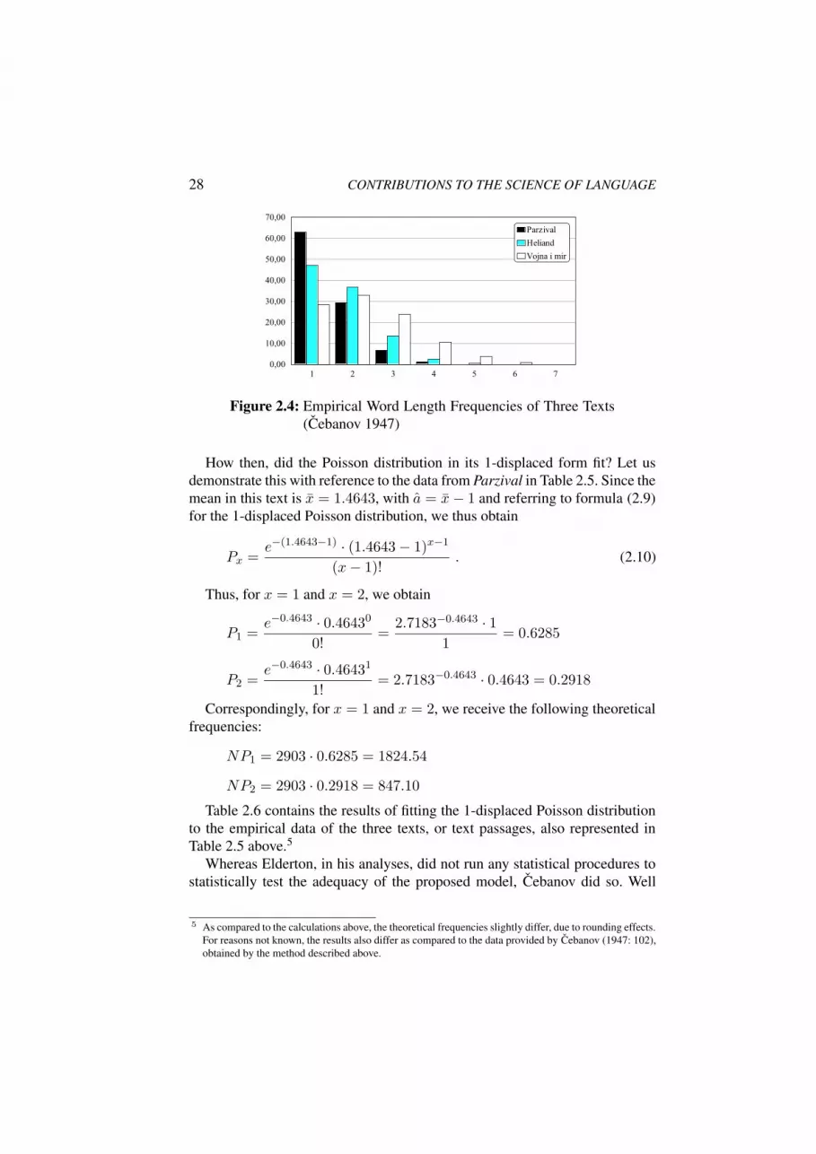
Cebanov (1947: 101) presented the data of twelve texts from different lan-guages (or dialects). By way of an example, his approach will be demonstratedhere, with reference to three texts. Two of these texts were studied in detailby Cebanov (1947: 102) himself: the High German text Parzival, and the LowFrankish text Heliand; the third text chosen here, by way of example, is a pas-sage from Lev N. Tolstoj’s Vojna i mir [War and Peace]. These data shall beadditionally analyzed here because they are a good example for showing thatword length frequencies do not necessarily imply a monotonously decreasingprofile (cf. class x = 2) – it will be remembered that this was a major problemfor the geometric distribution which failed be an adequate overall model (seeabove). The absolute frequencies (fi), as presented by Cebanov (1947: 101), aswell as the corresponding relative frequencies (pi), are represented in Table 2.5for all three texts.
Table 2.5: Relative Word Length Frequencies of Three DifferentTexts (Cebanov 1947)
Number of Parzival Heliand Vojna i mirsyllables (xi) fi pi fi pi fi pi
1 1823 0.6280 1572 0.4693 466 0.28262 849 0.2925 1229 0.3669 541 0.32813 194 0.0668 452 0.1349 391 0.23714 37 0.0127 83 0.0248 172 0.10435 14 0.0042 64 0.03886 15 0.0091∑
2903 3350 1698
As can be seen from Figure 2.4, all three distributions clearly seem to differfrom each other in their shape; particularly the Vojna i mir passage, displayinga peak at two-syllable words, differs from the two others.
28 CONTRIBUTIONS TO THE SCIENCE OF LANGUAGE
1 2 3 4 5 6 70,00
10,00
20,00
30,00
40,00
50,00
60,00
70,00
Parzival
Heliand
Vojna i mir
Figure 2.4: Empirical Word Length Frequencies of Three Texts(Cebanov 1947)
How then, did the Poisson distribution in its 1-displaced form fit? Let usdemonstrate this with reference to the data from Parzival in Table 2.5. Since themean in this text is x = 1.4643, with a = x− 1 and referring to formula (2.9)for the 1-displaced Poisson distribution, we thus obtain
Px =e−(1.4643−1) · (1.4643− 1)x−1
(x− 1)!. (2.10)
Thus, for x = 1 and x = 2, we obtain
P1 =e−0.4643 · 0.46430
0!=
2.7183−0.4643 · 11
= 0.6285
P2 =e−0.4643 · 0.46431
1!= 2.7183−0.4643 · 0.4643 = 0.2918
Correspondingly, for x = 1 and x = 2, we receive the following theoreticalfrequencies:
NP1 = 2903 · 0.6285 = 1824.54
NP2 = 2903 · 0.2918 = 847.10
Table 2.6 contains the results of fitting the 1-displaced Poisson distributionto the empirical data of the three texts, or text passages, also represented inTable 2.5 above.5
Whereas Elderton, in his analyses, did not run any statistical procedures tostatistically test the adequacy of the proposed model, Cebanov did so. Well
5 As compared to the calculations above, the theoretical frequencies slightly differ, due to rounding effects.For reasons not known, the results also differ as compared to the data provided by Cebanov (1947: 102),obtained by the method described above.

History and Methodology of Word Length Studies 29
Table 2.6: Fitting the 1-Displaced Poisson Distribution to WordLength Frequencies (Cebanov 1947)
Number of Parzival Heliand Vojna i mirsyllables (xi) fi NPi fi NPi fi NPi
1 1823 1824.67 1572 1618.01 466 442.292 849 847.28 1229 1177.53 541 582.043 194 196.72 452 428.48 391 382.974 37 30.45 83 103.94 172 167.995 14 18.91 64 55.276 15 14.55∑
2903 3350 1698
aware of A.A. Markov’s (1924) caveat, that “complete coincidence of figurescannot be expected in investigations of this kind, where theory is associated withexperiment”, Cebanov (1947: 101) calculated χ2 goodness-of-fit values. As aresult, Cebanov (ibd.) arrived at the conclusion that the χ2 values “show goodagreement in some cases and considerable departure in others.” Let us followhis argumentation step by step, based on the three texts mentioned above.
For Parzival, with k = 4 classes, we obtain χ2 = 1.45. This χ2 value canbe interpreted in terms of a very good fit, since p(χ2) = 0.48 (d.f. = 2).6
Whereas the 1-displaced Poisson distribution thus turns out to be a good modelfor Parzival, Cebanov interprets the results for Heliand not to be: here, the valueis χ2 = 10.35, which, indeed, is a significantly worse, though still acceptableresult (p = 0.016 for d.f. = 3).7
Interestingly enough, the 1-displaced Poisson distribution would also turnout to be a good model for the passage from Tolstoj’s Vojna i mir (not analyzedin detail by Cebanov himself), with a value of χ2 = 5.82 (p = 0.213 ford.f. = 4).
On the whole, Cebanov (1947: 101) arrives at the conclusion that the theoret-ical results “show good agreement in some cases and considerable departure inothers.” This partly pessimistic estimation has to be corrected however. In fact,Cebanov’s (1947: 102) interpretation clearly contradicts the intuitive impres-sion one gets from an optical inspection of Figure 2.5: as can be seen, Pi(a),represented for i = 1, 2, 3, indeed seems to be “determined all but completely”
6 Cebanov (1947: 102) himself reports a value of χ2 = 0.43 which he interprets to be a good result.7 Cebanov (1947: 102) reports a value ofχ2 = 13.32 and, not indicating any degrees of freedom, interprets
this result to be a clear deviation from expectation.

30 CONTRIBUTIONS TO THE SCIENCE OF LANGUAGE
Figure 2.5: The 1-Displaced Poisson Distribution as a WordLength Frequency Distribution Model (Cebanov1947)
by the mean of the text under consideration (ibd., 101). In Figure 2.5, Poisson’sPi(a) can be seen on the horizontal, the relative frequencies for pi on the verticalaxis).
The good fit of the 1-displaced Poisson distribution may also be provenby way of a re-analysis of Cebanov’s data, calculating the discrepancy valuesC (see above). Given that in case of all three texts mentioned and analyzedabove, we are concerned with relatively large samples (N = 2903 for Parzival,N = 1649 for Heliand, and N = 1698 for the Vojna i mir passage). In fact,the result is C < 0.01 in all three cases.8 In other words: what we have hereare excellent fits, in all three cases, which can be clearly seen in the graphicalillustration of Figure 2.6 (p. 31).
Unfortunately, Cebanov’s work was consigned to oblivion for a long time.If at all, reference to his work was mainly made by some Soviet scholars,who, terming the 1-displaced Poisson distribution “Cebanov-Fucks distribu-tion”, would later place him on a par with German physician Wilhelm Fucks.As is well known, Fucks and his followers would also, and independently of
8 As a corresponding re-analysis of the twelve data sets given by Cebanov (1947: 101) shows, C valuesare C < 0.02 in all cases, and they are even C < 0.01 in two thirds of the cases.

History and Methodology of Word Length Studies 31
Figure 2.6: Fitting the 1-Displaced Poisson Distribution to ThreeText Segments (Cebanov 1947)
Cebanov’s work, favor the 1-displaced Poisson distribution to be an importantmodel, in the late 1950s. Before presenting Fucks’ work in detail, it is necessaryto discuss another approach, which also has its roots in the 1940s.
4. The Lognormal DistributionA different approach to theoretically model word length distributions was pur-sued mainly in the late 1950s and early 1960s by scholars such as Gustav Herdan(1958, 1966), Rene Moreau (1963), and others.
As opposed to the approaches thus far discussed, these authors did not try tofind a discrete distribution model; rather, they worked with continuous models,mainly the so-called lognormal model.
Herdan was not the first to promote this idea with regard to language. Beforehim, Williams (1939, 1956) had applied it to the study of sentence length fre-quencies, arguing in favor of the notion that the frequency with which sentencesof a particular length occur, are lognormally distributed. This assumption wasbrought forth, based on the observation that sentence length or word lengthfrequencies do not seem to follow a normal distribution; hence, the idea oflognormality was promoted. Later, the idea of word length frequencies beinglognormally distributed was only rarely picked up, such as for example by Rus-sian scholar Piotrovskij and colleagues (Piotrovskij et al. 1977: 202ff.; cf. 1985:278ff.).
Generally speaking, the theoretical background of this assumption can becharacterized as follows: the frequency distribution of linguistic units (as ofother units occurring in nature and culture) often tends to display a right-sidedasymmetry, i.e., the corresponding frequency distribution displays a positive

32 CONTRIBUTIONS TO THE SCIENCE OF LANGUAGE
skewness. One of the theoretical reasons for this can be seen in the fact that thevariable in question cannot go beyond (or remain below) a particular limit; sinceit is thus characterized by a one-sided limitation in variation, the distributioncannot be adequately approximated by the normal distribution.
Particularly when a distribution is limited by the value 0 to the left side, onesuspects to obtain fairly normally distributed variables by logarithmic transfor-mations: as a result, the interval between 0 and 1 is transformed into −∞ to0. In other words: the left part of the distribution is stretched, and at the sametime, the right part is compressed.
The crucial idea of lognormality thus implies that a given random variableXfollows a lognormal distribution if the random variableY = log(X) is normallydistributed.
Given the probability density function for the normal distribution as in (2.11),
y = f(x) =1
σ ·√
2π· e− 1
2(x−µσ )2
, −∞ < x <∞ (2.11)
one thus obtains the probability density function for the lognormal distributionin equation (2.12):
y = f(x) =1
σ · x ·√
2π· e− 1
2( ln x−µσ )
2
, 0 < x <∞ (2.12)
Herdan based his first analyses of word length studies on data by Dewey(1923) and French et al. (1930). These two studies contain data on word lengthfrequencies, the former 78,633 words of written English, the latter 76,054 wordsof spoken English. Thus, Herdan had the opportunity to do comparative analysesof word length frequencies measured in letters and phonemes. In order to test hishypothesis as to the lognormality of the frequency distribution, Herdan (1966:224) confined himself to graphical techniques only. The most widely appliedmethod in his time was the use of probability grids, with a logarithmicallydivided abscissa (x-axis) and the cumulative frequencies on the ordinate (y-axis). If the resulting graph showed a more or less straight line, one regarded alognormal distribution to be proven.
As can be seen from Figure 2.7, the result seems to be quite convincing,both for letters and phonemes. In his later monograph on The Advanced Theoryof Language as Choice and Chance, Herdan (1966: 201ff.) similarly analyzedFrench data samples, taken from analyses by Moreau (1963). The latter hadanalyzed several French samples, among them the three picked up by Herdanin Figure 2.7:
1. 3,204 vocabulary entries from George Gougenheim’s Dictionnaire fonda-mental de la langue francaise,
2. 76,918 entries from Emile Littre’s Dictionnaire de la langue francaise
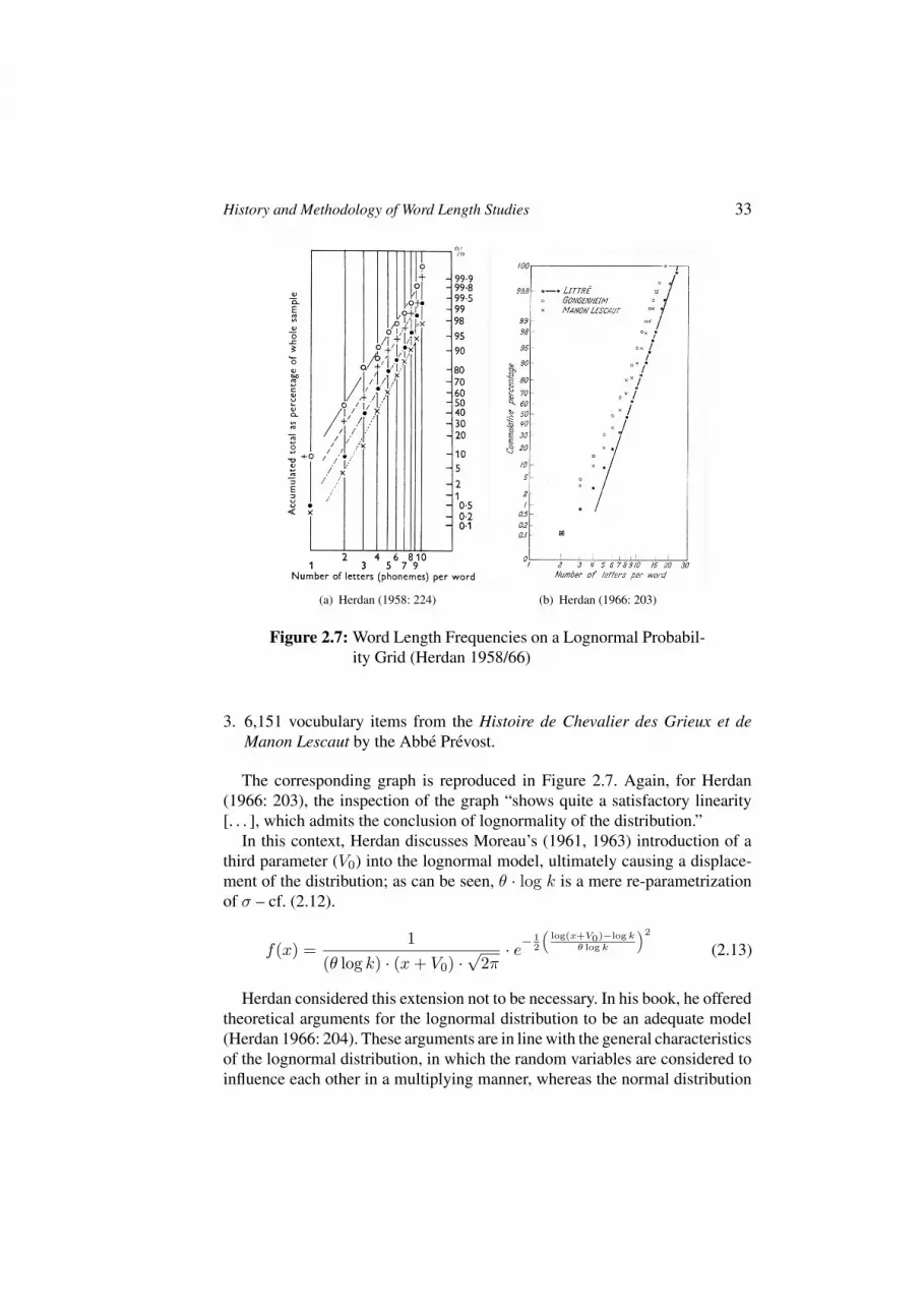
History and Methodology of Word Length Studies 33
(a) Herdan (1958: 224) (b) Herdan (1966: 203)
Figure 2.7: Word Length Frequencies on a Lognormal Probabil-ity Grid (Herdan 1958/66)
3. 6,151 vocubulary items from the Histoire de Chevalier des Grieux et deManon Lescaut by the Abbe Prevost.
The corresponding graph is reproduced in Figure 2.7. Again, for Herdan(1966: 203), the inspection of the graph “shows quite a satisfactory linearity[. . . ], which admits the conclusion of lognormality of the distribution.”
In this context, Herdan discusses Moreau’s (1961, 1963) introduction of athird parameter (V0) into the lognormal model, ultimately causing a displace-ment of the distribution; as can be seen, θ · log k is a mere re-parametrizationof σ – cf. (2.12).
f(x) =1
(θ log k) · (x+ V0) ·√
2π· e−
12
(log(x+V0)−log k
θ log k
)2
(2.13)
Herdan considered this extension not to be necessary. In his book, he offeredtheoretical arguments for the lognormal distribution to be an adequate model(Herdan 1966: 204). These arguments are in line with the general characteristicsof the lognormal distribution, in which the random variables are considered toinfluence each other in a multiplying manner, whereas the normal distribution

34 CONTRIBUTIONS TO THE SCIENCE OF LANGUAGE
Observed cumulative probabilities
1,0,8,5,30,0
Exp
ecte
d c
um
ula
tive
pro
ba
bili
tie
s
1,0
,8
,5
,3
0,0
(a) Normal distribution
Observed cumulative probabilities
1,0,8,5,30,0
Exp
ecte
d c
um
ula
tive
pro
ba
bili
tie
s
1,0
,8
,5
,3
0,0
(b) Lognormal distribution)
Figure 2.8: P-P Plots for Fitting the Normal and LognormalDistributions to Word Length Frequencies in AbbePrevost’s Manon Lescaut
is characterized by the additive interplay of the variables (the variables thusbeing considered to be independent of one another).
However, Herdan did not do any comparative analyses as to the efficiency ofthe normal or the lognormal distribution, neither graphically nor statistically.Therefore, both procedures shall be presented here, by way of a re-analysis ofthe original data.
As far as graphical procedures are concerned, probability grids have beenreplaced by so-called P-P plots, today, which also show the cumulative pro-portions of a given variable and should result in a linear rise in case of normaldistribution. By way of an example, Figure 2.8 represents the P-P plots forManon Lescaut, tested for normal and lognormal distribution.
It can clearly be seen that there are quite some deviations for the lognor-mal distribution (cf. Figure2.8(b)). What is even more important, however, isthe fact that the deviations are clearly less expressed for the normal distribu-tion (cf. Figure2.8(a)). Although this can, in fact, be shown for all three datasamples mentioned above, we will concentrate on a statistical analysis of theseobservations.
Table 2.7 contains the relevant Kolmogorov-Smirnov values (KS) and thecorresponding p-values with the given degrees of freedom (d.f.) for all threesamples, both for the normal and the logarithmized values. Additionally, valuesfor skewness (γ1) and kurtosis (γ2) are given, so that the effect of the logarithmicmanipulation of the data can easily be seen.

History and Methodology of Word Length Studies 35
Table 2.7: Statistical Comparison of Normal and Lognormal Dis-tributions for Three French Texts (Herdan 1966)
KS df p γ1 γ2
Manon Lescaut normal distr. 0.105 6151 < 0.00010.30 0.22
lognormal d. 0.135 −0.89 1.83
Littre normal distr. 0.108 76917 < 0.00010.53 0.49
lognormal d. 0.103 −0.47 0.68
Gougenheim normal distr. 0.121 3204 < 0.00010.80 2.06
lognormal d. 0.126 −0.55 1.12
As can clearly be seen, the deviations both from the normal and the lognor-mal distributions are highly significant in all cases. Furthermore, differencesbetween normal and lognormal are minimal; in case of Manon Lescaut, thelognormal distribution is even worse than the normal distribution.
The same holds true, by the way, for the above-mentioned data presented byPiotrovskij et al. (1985: 283). The authors analyzed a German technical textof 1,000 words and found, as they claimed, “a clear concordance between theempirical distribution and the lognormal distribution of the random variable”.As a justification of their claim they referred to a graphical representation ofempirical and theoretical values, only; however, they additionally maintainedthat the assumed concordance may easily and strongly be proven by way ofKolmogorov’s criterium (ibd., 281).
As a re-analysis of the data shows, this claim may not be upheld, however(cf. table 2.8). As in the case of Herdan’s analyses, the effect of the logarithmic
Table 2.8: Statistical Comparison of Normal and Lognormal Dis-tribution for German data (Piotrovskij 1985)
KS df p γ1 γ2
normal distr. 0.12 1000 0.00010.81 0.20
lognormal d. 0.08 −0.25 −0.52
transformation can easily be deduced from the values for γ1 and γ2 (i.e., forskewness and kurtosis). Also, the deviation from the normal distribution ishighly significant (p < 0.001). However, as can be seen the deviation from thelognormal distribution is highly significant as well, and, strictly speaking, evengreater compared to the normal distribution.

36 CONTRIBUTIONS TO THE SCIENCE OF LANGUAGE
In summary, one can thus say that neither the normal distribution nor thelognormal distribution model turns out to be adequate in praxis. With regard tothis negative finding, one may add the result of a further re-analysis, saying thatin case of all three data samples discussed by Herdan, the binomial distributioncan very well be fitted to the empirical data, with 0.006 ≤ C ≤ 0.009. No suchfit is possible in the case of Piotrovskij’s data, however, which may be due tothe fact that the space was considered to be part of a word.
Incidently, Michel (1982) arrived at the very same conclusion, in an exten-sive study on Old and New Bulgarian, as well as Old and new Greek material.He tested the adequacy of the lognormal distribution for the word length fre-quencies of the above-mentioned material on two different premises, basing hiscalculation of word length both on the number of letters per word, and on thenumber of syllables per word. As a result, Michel (1982: 198) arrived at theconclusion “that the fitting fails completely”.9
One can thus say that there is overwhelming negative empirical evidencewhich proves that the lognormal distribution is no adequate model for wordlength frequencies of various languages. Additionally, and this is even moreimportant in the given context, one must state that there are also major theoreticalproblems which arise in the context of the (log-)normal distribution as a possiblemodel for word length frequencies:
a. the approximation of continuous models to discrete data;
b. the doubtful dependence of the variables, due to the multiplying effect ofvariables within the lognormal model;
c. the manipulation of the initial data by way of logarithmic transformations.
With this in mind, let us return to discrete models. The next historical step inthe history of word length studies were the important theoretical and empiricalanalyses by Wilhelm Fucks, a German physician, whose theoretical modelsturned out to be of utmost importance in the 1950s and 1960s.
5. The Fucks Generalized Poisson Distribution5.1 The BackgroundAs mentioned previously, the 1-displaced Poisson distribution had been sug-gested by S.G. Cebanov in the late 1940s. Interestingly enough, some yearslater the very same model – i.e., the 1-displaced Poisson distribution – was alsofavored by German physicist Wilhelm Fucks (1955a,b, 1956b). Completelyindependent of Cebanov, without knowing the latter’s work, and based on com-pletely different theoretical assumptions, Fucks arrived at similar conclusions to
9 Michel also tested the adequacy of the 1-displaced Poisson distribution (see below, p. 46).

History and Methodology of Word Length Studies 37
those of Cebanov some years before. However, Fucks’ work was much more in-fluential than was Cebanov’s, and it was Fucks rather than Cebanov, who wouldlater be credited for having established the 1-displaced Poisson distribution asa standard model for word length frequency distributions.
When Fucks described the 1-displaced Poisson distribution and applied itto his linguistic data, he considered it to be “a mathematical law, thus far notknown in mathematical statistics” (Fucks 1957: 34). In fact, he initially derivedit from a merely mathematical perspective (Fucks 1955c); in his application ofit to the study of language(s) and language style(s), he then considered it to bethe “general law of word-formation” (1955a: 88, 1957: 34), or, more exactly, asthe “mathematical law of the process of word-formation from syllables for allthose languages, which form their words from syllables” (Fucks 1955b: 209).
In fact, Fucks’ suggestion was the most important model discussed from the1950s until the late 1970s; having the 1-displaced Poisson distribution in mind,one used to refer to it as “the Fucks model”. Only in Russia, one should laterspeak of the “Cebanov-Fucks distribution” (e.g., Piotrovskij et al. 1977: 190ff.;cf. Piotrowski et al. 1985: 256ff.), thus adequately honoring the pioneering workof Cebanov, too.
There was one major difference between Cebanov’s and Fucks’ approaches,however: this difference has to be seen in the fact that Fucks’ approach wasbased on a more general theoretical model, the 1-displaced Poisson distributionbeing only one of its special cases (see below). Furthermore, Fucks, in a numberof studies, developed many important ideas on the general functioning not onlyof language, but of other human sign systems, too. This general perspective asto the “mathematical analysis of language, music, or other results of humancultural activity” (Fucks 1960: 452), which is best expressed in Fucks’ (1968)monograph Nach allen Regeln der Kunst, cannot be dealt with in detail, here,where our focus is on the history of word length studies.
5.2 The General ApproachUltimately, Fucks’ general model can be considered to be an extension of thePoisson distribution; specifically, we are concerned with a particularly weightedPoisson distribution. These weights are termed εk − εk+1, k indicating thenumber of components to be analyzed.
In its most general form, this weighting generalization results in the followingformula (2.14):
pi = P (X = i) = e−λ∞∑
k=0
(εk − εk+1) · λi−k
(i− k)!(2.14)
Here, the random variable X denotes the number of syllables per word, i.e.X = i, i = 0, 1, 2, 3, . . . , I . The probability that a given word has i syllables,

38 CONTRIBUTIONS TO THE SCIENCE OF LANGUAGE
is pi = P (X = i), withI∑i=0
pi = 0, λ = µ − ε′, ε′ =∞∑k=1
εk and µ = E(X).
The parameters of the distribution {εk} are called the ε-spectrum. For (2.14),there are a number of conditions postulated by Fucks which must be fulfilled:
(a) From the necessity that εk − εk+1 ≥ 0 it follows that εk+1 ≤ εk;
(b) Since the sum of all weights equals 1, we have
1 =∞∑k=0
(εk − εk+1) =∞∑k=0
εk −∞∑k=0
εk+1 = ε0; it follows that ε0 = 1.
Finally, from (a) and (b) it follows
(c) 1 = ε0 ≥ ε1 ≥ ε2 ≥ ε3 ≥ . . . ≥ εk ≥ εk+1 . . .
As can be seen from equation (2.14), the so-called “generalized Fucks distri-bution” includes both the standard Poisson distribution (2.8) and the 1-displacedPoisson distribution (2.9) as two of its special cases. Assuming that ε0 = 1, andε1 = ε2 = . . . = εk = 0 – one obtains the standard Poisson distribution (2.8):
pi = e−λ · λi
i!i = 0, 1, 2, . . .
Likewise, for ε0 = ε1 = 1, and ε2 = ε3 = . . . = εk = 0, one obtains the1-displaced Poisson distribution (2.9) (cf. p. 27):
pi = e−λ · λi−1
(i− 1)!, i = 1, 2, . . .
As was already mentioned above, the only model which met general ac-ceptance was the 1-displaced Poisson distribution. More often than not, Fuckshimself applied the 1-displaced Poisson distribution without referring to hisgeneral model, and this may be one more reason why it has often (though ratherincorrectly) been assumed to be “the Fucks distribution”. In other words: Inspite of the overwhelming number of analyses presented by Fucks in the 1950sand 1960s, and irrespective of the broad acceptance of the 1-displaced Poissondistribution as an important model for word length studies, Fucks’ generaliza-tion as described above can only be found in very few of his works (e.g., Fucks1956a,b).
It is no wonder, then, that the generalized model has practically not beendiscussed. Interestingly enough, however, several scholars of East Europeanbackground became familiar with Fucks’ concept, and they not only discussedit at some length, but also applied it to specific data. It seems most reasonableto assume that this rather strange circumstance is due to the Russian translationof Fucks’ 1956b paper (cf. Fucks 1957).

History and Methodology of Word Length Studies 39
Before turning to the East European reception of Fucks’ model, resulting notonly in its application, but also in some modification of it, let us first discusssome of the results obtained by Fucks in his own application of the 1-displacedPoisson distribution to linguistic data.
5.3 The 1-Displaced Poisson Distribution as a Special Caseof Fucks’ Generalization of the Poisson Distribution
In his inspiring works, Fucks applied the 1-displaced Poisson distribution ondifferent levels of linguistic and textual analysis: on the one hand, he analyzedsingle texts, but he also studied word length frequency distribution in text cor-pora, both from one and the same language and across languages. Thus, hisapplication of the 1-displaced Poisson distribution included studies on (1) theindividual style of single authors, as well as on (2) texts from different authorseither (2.1) of one and the same language or (2.2) of different languages.
As an example of the study of individual texts, Figure 2.9(a) from Fucks(1956b: 208) may serve. It shows the results of Fucks’ analysis of Goethe’sWilhelm Meister: on the horizontal x-axis, the number of syllables per word(termed i by Fucks) are indicated, on the vertical y-axis the relative frequencyof each word length class (pi) can be seen. As can be seen from the dotted line inFigure 2.9(a), the fitting of the 1-displaced Poisson distribution seems to resultin extremely good theoretical values.
As to a comparison of two German authors, Rilke and Goethe, on the onehand, and two Latin authors, Sallust and Caesar, on the other, Figure 2.9(b)may serve. It gives rise to the impression that word length frequency may becharacteristic of a specific author’s style, rather than of specific texts. Again,the fitting of the 1-displaced Poisson distribution seems to be convincing.
There can be no doubt about the value of Fucks’ studies, and still today,they contain many inspiring ideas which deserve to be further pursued. Yet, inre-analyzing his works, there remains at least one major problem: Fucks givesmany characteristics of the specific distributions, starting from mean values andstandard deviations up to the central moments, entropy etc. Yet, there are hardlyever any raw data given in his texts, a fact which makes it impossible to checkthe results at which he arrived. Thus, one is forced to believe in the goodness ofhis fittings on the basis of his graphical impressions, only; and this drawback isfurther enhanced by the fact that there are no procedures which are applied totest the goodness of his fitting the 1-displaced Poisson distribution. Ultimately,therefore, Fucks’ works cannot but serve as a starting point for new studieswhich would have to replicate his results.
There is only one instance where Fucks presents at least the relative, thoughnot the absolute frequencies of particular distributions in detail. This is when hepresents the results of a comparison of texts from nine different languages – eight

40 CONTRIBUTIONS TO THE SCIENCE OF LANGUAGE
(a) Goethe’s Wilhelm Meister (b) German and Latin authors
Figure 2.9: Fitting the 1-Displaced Poisson Distribution to Ger-man and Latin Text Segments (Fucks 1956)
natural languages, and one artificial (cf. Fucks 1955a: 85ff.). The results for eachlanguage are based on what Fucks (1955a: 84) considered to be “representativecross-sections of written documents” of the given languages.
The relative frequencies are reproduced in Table 2.9 which, in addition to therelative frequency of each word length class (measured in syllables per word),also contains the mean (x), as well as the entropy (H) for each language, thelatter being calculated by way of formula (2.15):
H = −n∑
i=1
pi ln pi (2.15)
Unfortunately, quite a number of errors can be found in Fuck’ original table,both as to the calculated values of x and H; therefore, the data in Table 2.9represent the corrected results which one obtains on the basis of the relativefrequencies given by Fucks and formula (2.15). We will come back to thesedata throughout the following discussion, using them as exemplifying material.Being well aware of the fact that for each of the languages we are concernedwith mixed data, we can ignore this fact, and see the data as a representation ofa maximally broad spectrum of different empirical distributions which may besubjected to empirical testing.
Figure 2.10 illustrates the frequency distributions, based on the relative fre-quencies of the word length classes for each language. The figure is taken fromFucks (1955a: 85), since the errors in the calculation concern only x andH andare not relevant here. According to Fucks’ interpretation, all shapes fall into oneand the same profile, except for Arabic; as a reason for this, Fucks assumed thatthe number of texts analyzed in this language might not have been sufficient.

History and Methodology of Word Length Studies 41
Table 2.9: Relative Frequencies, Mean Word Length, and En-tropy for Different Languages (Fucks 1955)
English German Esperanto Arabic Greek
1 0.7152 0.5560 0.4040 0.2270 0.37602 0.1940 0.3080 0.3610 0.4970 0.32103 0.0680 0.0938 0.1770 0.2239 0.16804 0.0160 0.0335 0.0476 0.0506 0.08895 0.0056 0.0071 0.0082 0.0017 0.03466 0.0012 0.0014 0.0011 – 0.00837 – 0.0002 – – 0.00078 – 0.0001 – – –
x 1.4064 1.6333 1.8971 2.1106 2.1053H 0.3665 0.4655 0.5352 0.5129 0.6118
Japanese Russian Latin Turkish
1 0.3620 0.3390 0.2420 0.18802 0.3440 0.3030 0.3210 0.37843 0.1780 0.2140 0.2870 0.27044 0.0868 0.0975 0.1168 0.12085 0.0232 0.0358 0.0282 0.03606 0.0124 0.0101 0.0055 0.00567 0.0040 0.0015 0.0007 0.00048 0.0004 0.0003 0.0002 0.00049 0.0004 – – –
x 2.1325 2.2268 2.3894 2.4588H 0.6172 0.6355 0.6311 0.6279

42 CONTRIBUTIONS TO THE SCIENCE OF LANGUAGE
Figure 2.10: Relative Frequencies of Word Lengths in Eight Nat-ural and One Artificial Languages (Fucks 1955)
As was mentioned above, Fucks did not, as was not unusual at his time,calculate any tests as to the significance of the goodness of his fits. It seemsthat Fucks (1955a: 101) was very well aware of the problems using the χ2-goodness-of-fit test for this purpose, since he explicitly emphasized that, “forparticular mathematical reasons”, his data are “not particularly adequate” forthe application of the χ2test.
The problem behind Fucks’ assumption might be the fact that the χ2 valueincreases in a linear way with an increase of sample size; therefore, resultsare more likely to display significant differences for larger samples, which isalmost always the case in linguistic studies. As was mentioned above (cf. p. 23),the problem is nowadays avoided by calculating the discrepancy coefficientC = χ2/N , which is not dependent on the degrees of freedom. We may thuseasily, by way of a re-analysis, calculateC for the data given by Fucks, in orderto statistically test the goodness-of-fit of the 1-displaced Poisson distribution;in order to do so, we simply have to create “artificial” samples of ca. 10,000each, by multiplying the relative frequencies with 10,000.
Remembering that fitting is considered to be good in case of 0.01 < C <0.02 and very good in case of C < 0.01, one has to admit that fitting the 1-displaced Poisson distribution to Fucks’ data from different languages is notreally convincing (see Table 2.10): strictly speaking, it turns out to be adequateonly for an artificial language, Esperanto, and must be discarded as an overallvalid model.
It is difficult to say whether the observed failure is due to the fact that thedata for each of the languages originated from text mixtures (and not from

History and Methodology of Word Length Studies 43
Table 2.10: Discrepancy Coefficient C as a Result of Fitting the1-Displaced Poisson Distribution to Different Lan-guages (Fucks 1955)
English German Esperanto Arabic Greek
C (1-par.) 0.0903 0.0186 0.0023 0.1071 0.0328
Japanese Russian Latin Turkish
C (1-par.) 0.0380 0.0208 0.0181 0.0231
&(
'+
,
-#$
"
1 1,2 1,4 1,6 1,8 2 2,2 2,4 2,6
Average word length
0
0,1
0,2
0,3
0,4
0,5
0,6
0,7
0,8Entropy
Poisson German Greek Japanese Latin
English Esperanto Arabic Russian Turkish
" $ # -
, + ' ( &
Figure 2.11: Entropy as a Function of Mean Word Length (Fucks1955a)
individual texts), or if there are other reasons. Still, Fucks and many followersof his pursued the idea of the 1-displaced Poisson distribution as the mostadequate model for word length frequencies.
Although Fucks did not calculate any statistics to test the goodness of fit(which in fact many people would not do still today), one must do him justiceand point out that he tried to go another way to empirically prove the adequacy ofhis findings: knowing the values of x andH for each language, Fucks graphicallyillustrated their relationship and interdependency. Figure 2.11 (p. 43) shows theresults, with x on the horizontal x-axis, and H on the vertical y-axis; the dataare based on the corrected values from Table 2.9.
Additionally, Fucks calculated the entropy of the theoretical distribution,estimating a as x; these values can easily be obtained by formula (2.8) (cf.p. 27), and they are reproduced below in Table 2.11. Thus, one arrives at thecurve in Figure 2.11, representing the Poisson distribution (cf. Fucks 1955a:85).
As can be seen with Fucks (1955a: 88, 1960: 458f.), the theoretical distri-bution “represents the values found in natural texts very well”. In other words:

44 CONTRIBUTIONS TO THE SCIENCE OF LANGUAGE
Table 2.11: Empirical and Theoretical Entropy for Nine WordLength Frequency Distributions (Fucks)
x H [y] H [y]
1.4064 0.3665 0.35901.6333 0.4655 0.45631.8971 0.5352 0.53922.1032 0.5129 0.59132.1106 0.6118 0.59172.1325 0.6172 0.60302.2268 0.6355 0.61842.3894 0.6311 0.64982.4588 0.6279 0.6614
evaluating his results, Fucks once again confined himself to merely visual im-pressions, as he did in the case of the frequency probability distribution. Andagain, it would have been easy to run such a statistical test, calculating the co-efficient of determination (R2) in order to test the adequacy of the theoreticalcurve obtained.
Let us shortly discuss this procedure: in a nonlinear regression model, R2
represents that part of the variance of the variable y, which can be explainedby variable x. There are quite a number of more or less divergent formulae tocalculate R2 (cf. Grotjahn 1982), which result in partly significant differences.Usually, the following formula (2.16) is taken:
R2 = 1−
n∑
i=1
(yi − yi)2
n∑
i=1
(yi − y)2(2.16)
With 0 ≤ R2 ≤ 1, one can say that the greater R2, the better the theoreticalfit. In order to calculateR2, we thus consider x to be the independent variable x,andH to be the dependent variable y. Thus, for each empirical xi, we need boththe empirical values (yi) and the theoretical values (yi) which can be obtained byformula (2.8), and which are represented in Table 2.11. Based on these results,we can now easily calculate R2, with y = H[y] (cf. Table 2.11), as
R2 = 1− 0.0097
0.0704= 0.8768 (2.17)
History and Methodology of Word Length Studies 45
As can be seen, the fit can be regarded to be relatively good.10 This resultis not particularly influenced by the fit for Arabic, which, according to Fucks,deviates from the other languages. In fact, the value for R2 hardly changes ifone, following Fucks’ argumentation, eliminates the data for Arabic: under thiscondition, the determination coefficient would result in R2 = 0.8763.
Still, there remains a major theoretical problem with the specific methodchosen by Fucks in trying to prove the adequacy of the 1-displaced Poissondistribution: this problem is related to the method itself, i.e., in establishing arelation between x and H . Taking a second look at formula (2.15), one caneasily see that the entropy of a frequency distribution is ultimately based on pi,only; pi, however, in case of the Poisson distribution, is based on parameter ain formula (2.8), which is nothing but the mean x of the distribution! In otherwords, due to the fact that the Poisson distribution is mainly shaped by the meanof the distribution, Fucks arrives at a tautological statement, relating the meanx of the Poisson distribution to its entropy H .
To summarize, one has thus to draw an important conclusion: Due to the factthat Fucks did not apply any suitable statistics to test the goodness of fit for the1-displaced Poisson distribution, he could not come to the point of explicitlystating that this model may be adequate in some cases, but is not acceptable asa general standard model. Still, Fucks’ suggestions had an enormous influenceon the study of word length frequencies, particularly in the 1960’s. Most ofthese subsequent studies concentrated on the 1-displaced Poisson distribution,as suggested by Fucks.
In fact, work on the Poisson distribution is by no means a matter of the past.Rather, subsequent to Fucks’ (and of course Cebanov’s) pioneering work onthe Poisson distribution, there have been frequent studies discussing and tryingto fit the 1-displaced Poisson distribution to linguistic data, with and withoutreference to the previous achievements.
No reference to Fucks (or Cebanov) is made, for example, by Rothschild(1986) in his study on English dictionary material. Rothschild’s initial discus-sion of previous approaches to word length frequencies, both continuous anddiscrete, was particularly stimulated by his disapproval of Bagnold’s (1983) as-sumption that word length distributions are not Gaussian, but skew (hyperbolicor double exponential) distributions. Discussing and testing various distributionmodels, Rothschild did not find any one of the models he tested to be adequate.This holds true for the (1-displaced) Poisson distribution, as well, which, ac-cording to Rothschild (1986: 317), “fails on a formal χ2-test”. Nevertheless, heconsidered it to be “the most promising candidate” (ibd., 321) – quite obviously,faute de mieux. . .
10 Calculating the determination coefficient with the data given by Fucks himself results in R2=0.8569.

46 CONTRIBUTIONS TO THE SCIENCE OF LANGUAGE
As opposed to Rothschild, Michel (1982), in his above-mentioned studyof Old and New Bulgarian and Greek material (cf. p. 36), explicitly referredto Fucks’ work on the Poisson distribution. As was said above, Michel firstfound the lognormal distribution to be a completely inadequate model. He thentested the 1-displaced Poisson distribution and obtained negative results as well:although fitting the Poisson distribution led to better results as compared to thelognormal distribution, word length in his data turned out not to be Poissondistributed, either (Michel 1982: 199f.)
Finally, Grotjahn (1982) whose work will be discussed in more detail below(cf. p. 61ff.), explicitly discussed Fucks’ work on the 1-displaced Poisson dis-tribution, being able to show under which empirical conditions it is likely to bean adequate model, and when it is prone to fail. He too, however, did not dis-cuss the 1-displaced Poisson distribution as a special case of Fucks’ generalizedPoisson model.
It seems reasonable, therefore, to follow Fucks’ own line of thinking. Indoing so, let us first direct our attention to the 2-parameter model suggested byhim, and then to his 3-parameter model.
5.4 The (1-Displaced) Dacey-Poisson Distribution as a2-Parameter Special Case of Fucks’ Generalization ofthe Poisson Distribution
It has been pointed out in the preceding section that for ε0 = 1, and ε1 =ε2 = . . . = εk = 0 the standard Poisson distribution (2.8) is obtained fromformula (2.14). Likewise, for ε0 = ε1 = 1, and ε2 = ε3 = . . . = εk = 0, oneobtains the 1-displaced Poisson distribution (2.9), which has been discussedabove (cf. p. 27). In either case, the result is a 1-parameter model in which onlyλ has to be estimated.
In a similar way, two related 2-parameter distributions can be derived fromthe general model (2.14) under the following circumstances: In case of ε0 =1, ε1 6= 0, and εk = 0 for k ≥ 2, one obtains the so-called Dacey-Poissondistribution (cf. Wimmer/Altmann 1999: 111), replacing ε1 by α:
pi = (1− α) · e−λλi
i!+ α · e
−λλi−1
(i− 1)!, i = 0, 1, 2, . . . (2.18)
with λ = µ− α. Here, in addition to λ, a second parameter (ε1 = α) has to beestimated, e.g., as α =
√x−m2.
Similarly, for ε0 = ε1 = 1, ε2 6= 0, and εk = 0 for k ≥ 3, one obtainsa model which has become known as the 1-displaced Dacey-Poisson distribu-tion (2.19), replacing ε2 by α:
pi = (1− α) · e−λλi−1
(i− 1)!+ α · e
−λλi−2
(i− 2)!, i = 1, 2, . . . (2.19)

History and Methodology of Word Length Studies 47
with λ = (µ− α)− 1; in this case, α can be estimated as α =√x− 1−m2.
It is exactly the latter distribution (2.19) which has been discussed by Fucksas another special case of his generalized Poisson model, though not underthis name. Fucks has not systematically studied its relevance; still, it might betempting to see what kind of results are yielded by this distribution for the dataalready analyzed above (cf. Table 2.10).
Table 2.12 (which additionally contains the dispersion quotient d to be ex-plained below) represents the values of the discrepancy coefficientC as a resultof a corresponding re-analysis.
Table 2.12: Discrepancy Coefficient C as a Result of Fitting the1-displaced Dacey-Poisson Distribution to DifferentLanguages (Fucks 1955)
English German Esperanto Arabic Greek
C (2-par.) — — 0.0019 0.0077 —d 1.3890 1.1751 0.9511 0.5964 1.2179
Japanese Russian Latin Turkish
C (2-par.) — — 0.0149 0.0021d 1.2319 1.1591 0.8704 0.8015
As can be seen from Table 2.12, in some cases, the results are slightly betteras compared to the results obtained from fitting the 1-displaced Poisson distri-bution (cf. Table 2.10). However, in some cases no results can be obtained. Thereason for this failure is the fact that the estimation of α as α =
√x− 1−m2
(see above) results in a negative root, obviously due to the fact that the estimateα is not defined if x− 1 ≤ m2.
Recently, Stadlober (2003) gave an explanation for this finding. Referring toGrotjahn’s (1982) work, which will be discussed below (cf. p. 61ff.), Stadloberanalyzed the theoretical scope of Fucks’ 2-parameter model. Grotjahn’s interesthad been to find out under what conditions the 1-displaced Poisson distributioncan be an adequate model for word length frequencies. Therefore, Grotjahn(1982) had suggested to calculate the quotient of dispersion δ, based on thetheoretical values for a sample’s mean (µ) and its variance (σ2):
δ =σ2
µ(2.20)
For r-displaced distributions, the corresponding equation is
δ =σ2
µ− r , (2.21)
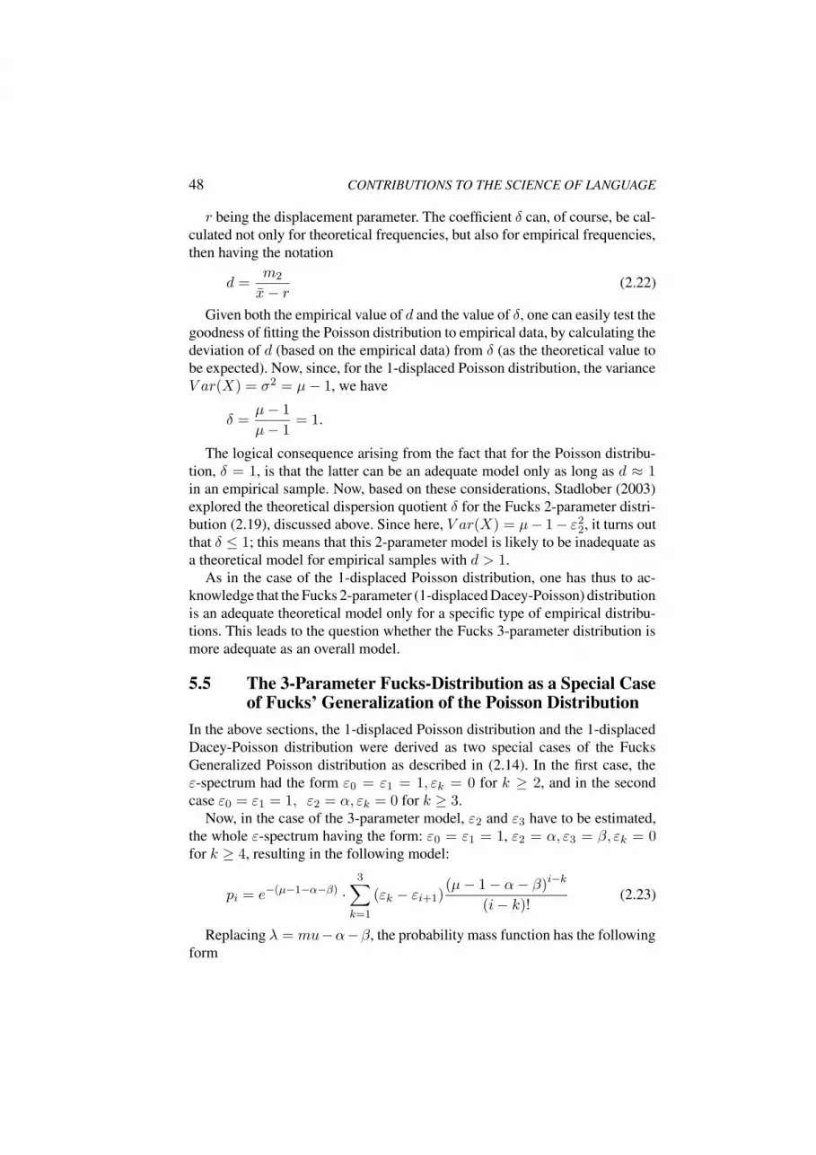
48 CONTRIBUTIONS TO THE SCIENCE OF LANGUAGE
r being the displacement parameter. The coefficient δ can, of course, be cal-culated not only for theoretical frequencies, but also for empirical frequencies,then having the notation
d =m2
x− r (2.22)
Given both the empirical value of d and the value of δ, one can easily test thegoodness of fitting the Poisson distribution to empirical data, by calculating thedeviation of d (based on the empirical data) from δ (as the theoretical value tobe expected). Now, since, for the 1-displaced Poisson distribution, the varianceV ar(X) = σ2 = µ− 1, we have
δ =µ− 1
µ− 1= 1.
The logical consequence arising from the fact that for the Poisson distribu-tion, δ = 1, is that the latter can be an adequate model only as long as d ≈ 1in an empirical sample. Now, based on these considerations, Stadlober (2003)explored the theoretical dispersion quotient δ for the Fucks 2-parameter distri-bution (2.19), discussed above. Since here, V ar(X) = µ− 1− ε2
2, it turns outthat δ ≤ 1; this means that this 2-parameter model is likely to be inadequate asa theoretical model for empirical samples with d > 1.
As in the case of the 1-displaced Poisson distribution, one has thus to ac-knowledge that the Fucks 2-parameter (1-displaced Dacey-Poisson) distributionis an adequate theoretical model only for a specific type of empirical distribu-tions. This leads to the question whether the Fucks 3-parameter distribution ismore adequate as an overall model.
5.5 The 3-Parameter Fucks-Distribution as a Special Caseof Fucks’ Generalization of the Poisson Distribution
In the above sections, the 1-displaced Poisson distribution and the 1-displacedDacey-Poisson distribution were derived as two special cases of the FucksGeneralized Poisson distribution as described in (2.14). In the first case, theε-spectrum had the form ε0 = ε1 = 1, εk = 0 for k ≥ 2, and in the secondcase ε0 = ε1 = 1, ε2 = α, εk = 0 for k ≥ 3.
Now, in the case of the 3-parameter model, ε2 and ε3 have to be estimated,the whole ε-spectrum having the form: ε0 = ε1 = 1, ε2 = α, ε3 = β, εk = 0for k ≥ 4, resulting in the following model:
pi = e−(µ−1−α−β) ·3∑
k=1
(εk − εi+1)(µ− 1− α− β)i−k
(i− k)!(2.23)
Replacing λ = mu−α−β, the probability mass function has the followingform

History and Methodology of Word Length Studies 49
p1 = e−λ · (1− α)
p2 = e−λ · [(1− α) · λ+ (α− β)]
pi = e−λ[(1− α) λi−1
(i−1)! + (α− β) λi−2
(i− 2)!+ β λi−3
(i− 3)!
], i ≥ 3
As to the estimation of ε2 = α and ε3 = β, Fucks (1956a: 13) suggestedcalculating them by reference to the second and third central moments (µ2 andµ3). It would lead too far, here, to go into details, as far as their derivation isconcerned. Still, the resulting 2× 2-system of equations shall be quoted:
(a) µ2 = µ1 − 1− (α+ β)2 + 2β
(b)µ3 = µ3 = µ1+2(1+α+β)3−3(1+α+β)2−6(α+β)(α+2β)+6β
As can be seen, the solution of this equation system – which can be math-ematically simplified (cf. Antic/Grzybek/Stadlober 2005a) – involves a cubicequation. Consequently, three solutions are obtained, not all of which mustnecessarily be real solutions. For each real solution the values for ε2 = α andε3 = β have to be estimated (which is easily done by computer programs today,as opposed to in Fucks’ time).11
Before further going into details of this estimation, let us remember that thereare two important conditions as to the two parameters:
(a) ε2 = α ≤ 1 and ε3 = β ≤ 1,
(b) ε2 = α ≥ β = ε3.
With this in mind, let us once again analyze the data of Table 2.9, this timefitting Fucks’ 3-parameter model. The results obtained can be seen in Table 2.13;results not meeting the two conditions mentioned above, are marked as ∅.
It can clearly be seen that in some cases, quite reasonably, the results for the3-parameter model are better, as compared to those of the two models discussedabove. One can also see that the 3-parameter model may be an appropriate modelfor empirical distributions in which d > 1 (which was the decisive problem forthe two models described above): thus, in the Russian sample, for example,where d = 1.1591, the discrepancy coefficient is C = 0.0005. However, asthe results for German and Japanese data (with d = 1.1751 and d = 1.2319,respectively) show, D does not seem to play the crucial role in case of the3-parameter model.
11 In addition to a detailed mathematical reconstruction of Fucks’ ¿Theory of Word FormationÀ,Antic/Grzybek/Stadlober (2005b) have tested the efficiency of Fucks’ model in empirical research.

50 CONTRIBUTIONS TO THE SCIENCE OF LANGUAGE
Table 2.13: Discrepancy Coefficient C as a Result of Fitting theFucks 3-Parameter Poisson Distribution to DifferentLanguages (Fucks 1955)
English German Esperanto Arabic Greek
C ∅ ∅ 0.00004 0.0021 ∅
ε2 — — 0.3933 0.5463 —ε3 — — 0.0995 -0.1402 —d 1.3890 1.1751 0.9511 0.5964 1.2179
Japanese Russian Latin Turkish
C ∅ 0.0005 0.0003 0.0023ε2 — 0.2083 0.5728 0.6164ε3 — 0.1686 0.2416 0.1452d 1.2319 1.1591 0.8704 0.8015
In fact, as Antic/Grzybek/Stadlober (2005a) show, the conditions for theFucks 3-parameter model to be appropriate are slightly different. The detailsneed not be discussed here; it may suffice to say that it is ultimately the differenceM = x−m2, i.e. the difference between the mean of the empirical distribution(x) and its variance (m2). One thus obtains the following two conditions:
1. The sum a = ε2 + ε3 = α+ β must be in a particular interval:
ai ∈[
1−√
4M − 3
2,1 +
√4M − 3
2
]i = 1, 2, 3
Thus, there are two interval limits a1 and a2:
ai1 =1−
√4M − 3
2and ai2 =
1 +√
4M − 3
2
2. In order to be a ∈ R, the root 4M − 3 must be positive, i.e. 4M − 3 ≥ 0;therefore, M = x−m2 ≥ 0.75.
From the results represented in Table 2.14 (p. 51) it can clearly be seen why,in four of the nine cases, the results are not as desired: there are a number ofviolations, which are responsible for the failure of Fucks’ 3-parameter model.These violations can be of two kinds:
a. As soon as M < 0.75, the definition of the interval limits of a1 and a2
involves a negative root – this is the case with the Japanese data, for example;

History and Methodology of Word Length Studies 51
Table 2.14: Violations of the conditions for Fucks’ 3-parametermodel
English German Esperanto Arabic Greek
C ∅ ∅ < 0.01 < 0.01 ∅
ε2 — — 0.3933 0.5463 —ε3 — — 0.0995 -0.1402 —
a = ε2 + ε3 -0.0882 -0.1037 0.4929 0.4061 0.2799ai1 0.1968 0.1270 -0.0421 -0.3338 0.4108ai2 0.8032 0.8730 1.0421 1.3338 0.5892
ai1 < a < ai2 − − X X −x 1.4064 1.6333 1.8971 2.1032 2.1106m2 0.5645 0.7442 0.8532 0.6579 1.3526
M = x−m2 0.8420 0.8891 1.0438 1.4453 0.7580M ≥ 0.75 X X X X X
Japanese Russian Latin Turkish
C ∅ < 0.01 < 0.01 < 0.01ε2 — 0.2083 0.5728 0.6164ε3 — 0.1686 0.2416 0.1452
a = ε2 + ε3 -0.1798 0.3769 0.8144 0.7616ai1 C 0.2659 -0.1558 -0.2346ai1 C 0.7341 1.1558 1.2346
ai1 < a < ai2 − X X X
x 2.1325 2.2268 2.3894 2.4588m2 1.3952 1.4220 1.2093 1.1692
M = x−m2 0.7374 0.8048 1.1800 1.2896M ≥ 0.75 − X X X

52 CONTRIBUTIONS TO THE SCIENCE OF LANGUAGE
b. Even if the first condition is met with M ≥ 0.75, fitting the Fucks 3-parameter model may fail, if the condition ai1 < a < ai2 is not fulfilled –this can be seen in the case of the English, German, and Greek data.
Fucks’ 3-parameter model thus is adequate only for particular types of em-pirical distributions, and it can not serve as an overall model for language, noteven for syllabic languages, as Fucks himself claimed. However, some of theproblems met might be related to the specific way of estimating the parameterssuggested by him, and this might be the reason why other authors followinghim tried to find alternative ways.
5.6 The Georgian Line: Cercvadze, Cikoidze, Cilosani,Gaceciladze
Quite early, three Georgian scholars, G.N. Cercvadze, G.B. Cikoidze, andT.G. Gaceciladze (1959), applied Fucks’ ideas to Georgian linguistic mate-rial, mainly to phoneme frequencies and word length frequencies. Their study,which was translated into German as early as 1962, and which was later ex-tended by Gaceciladze/Cilosani (1971), was originally inspired by the Russiantranslation of Fucks’ English-language article ¿Mathematical Theory of WordFormationÀ. Fucks’ article, originally a contribution to the 1956 London Con-ference on Information Theory, had been published in England in 1956, and itwas translated into Russian only one year later, in 1957. As opposed to mostof his German papers, Fucks had discussed his generalization at some lengthin this English synopsis of his work, and this is likely to be the reason why hisapproach received much more attention among Russian-speaking scholars.
In fact, Cercvadze, Cikoidze, and Gaceciladze (1959) based their analyseson Fucks’ generalization; the only thing different from Fucks’ approach istheir estimation of the two parameters ε2 and ε3 of Fucks 3-parameter model:as opposed to Fucks, they estimated ε2 and ε3 not with recourse to the centralmoments, but to the initial moments of the empirical distribution. The empiricalcentral moment of the order r
mr =1
(N − 1)
∑
x
(x− x)rfx
is an estimate of the r-th theoretical moment defined as
µr =∑
x
(x− µ)rPx
.As estimate for the theoretical initial moment of the order r
µ′r =∑
x
xrPx

History and Methodology of Word Length Studies 53
serves the empirical r-th initial moment given as:
m′r =1
N
∑
x
xrfx
Since it can be shown that central moments and initial moments can betransformed into each other, the results can be expected to be identical; still, theprocedure of estimating is different.
We need not go into details, here, as far as the derivation of the Fucks dis-tribution and its generating function is concerned (cf. Antic/Grzybek/Stadlober2005a). Rather, it may suffice to name its first three initial moments, which arenecessary for the equation system to be established, which, in turn, is neededfor the estimation of ε2 and ε3. Thus, with
∞∑
k=1
εk = ε′ (2.24)
we have the first three initial moments of Fucks’ distribution:
µ′1 = µ
µ′2 = µ2 + µ− ε′2 − 2ε′ + 2
∞∑
k=1
kεk
µ′3 = µ3 + 3µ2 + µ+ 2ε′3
+ 3ε′2 − ε′ − 3µε′
2 − 6µε′+
+∞∑
k=0
k3 (εk − εk+1) + 6(µ− ε′
) ∞∑
k=1
kεk
(2.25)
Now, replacing ε2 with α, and ε3 with β, we obtain the following system ofequations:
(a) µ′2 = µ2 + µ− (1 + α+ β)2 − 2 (1 + α+ β) + 2 (1 + 2α+ 3β)
(b) µ′3 = µ3 + 3µ2 + µ+ 2 (1 + α+ β)3 + 3 (1− µ) (1 + α+ β)2 + 6α++18β − 6µ (1 + α+ β) + 6 (µ− 1− α− β) (1 + 2α+ 3β) .
After the solution for α and β, we thus have the following probabilities:
p1 = e−λ · (1− α)
p2 = e−λ · [(1− α) · λ+ (α− β)]
pi = e−λ[(1− α) λi−1
(i− 1)!+ (α− β) λi−2
(i− 2)!+ β λi−3
(i− 3)!
], i ≥ 3

54 CONTRIBUTIONS TO THE SCIENCE OF LANGUAGE
with λ = µ− 1− α− β
As was said above, the results are identical as compared to those obtainedby recourse to the central moments. Unfortunately, there are several mistakesin the authors’ own formula; therefore, there is no sense in reproducing theirresults on their Georgian sample, here.12
Almost twenty years later, Russian scholars Piotrovskij, Bektaev, and Pio-trovskja (1977: 193; cf. 1985: 261), would again refer to Fucks’ generalizedmodel. These authors quite rightly termed the above-mentioned 1-displacedPoisson distribution (2.9) the “Cebanov-Fucks distribution” (cf. p. 27). In ad-dition to this, they mentioned the so-called “generalized Gaceciladze-Fucksdistribution”, which deserves some more attention here.
As was seen above, the 1959 paper by Cercvadze, Cikoidze, and Gaceciladzewas based on Fuck’s generalization of the Poisson distribution. Obviously,these authors indeed once again generalized the Fucks model, which is notinherent in the 1959 paper mentioned, but represented in an extension of it byGaceciladze/Cilosani (1971). This extension contains an additional factor ϕnu,which is dependent on three parameters:
(a) the mean of the sample (i),
(b) the relevant class i,
(c) the sum of all εν , A =∞∑ν=1
εν (termed ε′ by Fucks).
As a result, the individual weights of the generalized Fucks distribution,defined as (εk − εk+1), are multiplied by the function ϕν . Unfortunately,Gaceciladze/Cilosoni (1971: 114) do not explain the process by which ϕnumay be theoretically derived; they only present the final formula (2.26):
Pi = e−(i−A
) ∞∑
ν=0
(εν − εν+1)(λ−A)i−ν
(i− ν)!ϕν (A, i, i) (2.26)
Here, i is the mean of the sample, and (εk − εk+1) are the weighting fac-tors. Unfortunately, Piotrovskij et al. (1977: 195), who term formula (2.26)the “Fucks-Gaceciladze distribution”, also give no derivation for φν . Assumingthat ϕν takes account of the contextual environment, they only refer to Fucks’1955 Mathematische Analyse von Sprachelementen, Sprachstil und Sprachen.However, neither Fucks’ generalization nor ϕ are mentioned in this work.Thus, as to the theoretical derivation of ϕν , there are only sparse references
12 In fact, in spite of, or rather due to their obvious calculation errors, the authors arrived at a solution for ε2and ε3, which yields a good theoretical result; these values cannot be derived from the correct formula,however, and therefore must be considered to be a casual and accidental ad hoc solution.

History and Methodology of Word Length Studies 55
by Gaceciladze/Cilosani (1971: 114) who mentioned some of their Georgianpublications, which are scarcely available.
Still, it can easily be seen that for φν → 1, one obtains the generalized Fucksdistribution, which has also been discussed by some Polish authors.
5.7 Estimating the Fucks Distribution With First-ClassFrequency (Bartkowiakowa/Gleichgewicht 1964/65)
Two Polish authors, Anna Bartkowiakowa and BolesÃlaw Gleichgewicht (1964,1965), also suggested an alternative way to estimate the two parameters ε2 and ε3of Fucks’ 3-parameter distribution. Based on the standard Poisson distribution,as represented in (2.27),
gk =λk
k!e−λ k = 0, 1, 2, . . . (2.27)
and referring to Fucks’ (2.14) generalization of it, the authors reformulated thelatter as seen in (2.28):
pi =∞∑
k=0
(εk − εk+1)e−λλi−k
(i− k)!
=∞∑
k=0
(εk − εk+1) · gi−k(2.28)
Determining ε0 = ε1 = 1, and εk = 0 for k > 3, the two parameters ε2 6= 0and ε3 6= 0 remain to be estimated on the basis of the empirical distribution.Based on these assumptions, the following special cases are obtained for (2.28):
p1 = (1− ε2) · g0p2 = (1− ε2) · g1 + (ε2 − ε3) · g0pi = (1− ε2) · gi−1 + (ε2 − ε3) · gi−2 + ε3 · gi−3 for i ≥ 3
with λ = µ− (1 + ε2 + ε3)As to the estimation of ε2 and ε3, the authors did not set up an equation
system on the basis of the second and third central moments (µ2 and µ3), as didFucks, thus arriving at a cubic equation; rather, they first defined the portionof one-syllable words (p1), and then modelled the whole distribution on thatproportion. Thus, by way of a logarithmic transformation of p1 = (1− ε2) · g0
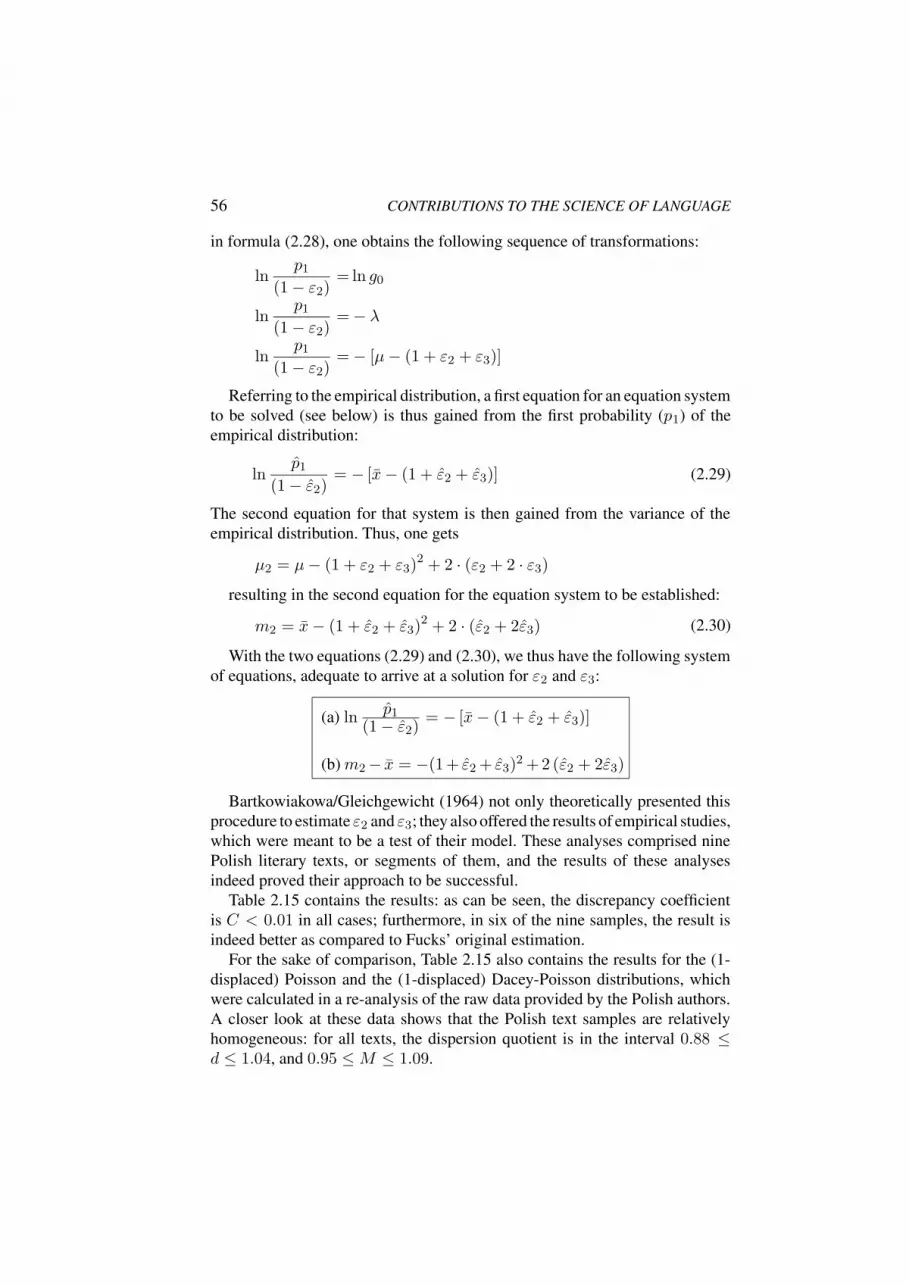
56 CONTRIBUTIONS TO THE SCIENCE OF LANGUAGE
in formula (2.28), one obtains the following sequence of transformations:
lnp1
(1− ε2)= ln g0
lnp1
(1− ε2)=− λ
lnp1
(1− ε2)=− [µ− (1 + ε2 + ε3)]
Referring to the empirical distribution, a first equation for an equation systemto be solved (see below) is thus gained from the first probability (p1) of theempirical distribution:
lnp1
(1− ε2)= − [x− (1 + ε2 + ε3)] (2.29)
The second equation for that system is then gained from the variance of theempirical distribution. Thus, one gets
µ2 = µ− (1 + ε2 + ε3)2 + 2 · (ε2 + 2 · ε3)
resulting in the second equation for the equation system to be established:
m2 = x− (1 + ε2 + ε3)2 + 2 · (ε2 + 2ε3) (2.30)
With the two equations (2.29) and (2.30), we thus have the following systemof equations, adequate to arrive at a solution for ε2 and ε3:
(a) lnp1
(1− ε2)= − [x− (1 + ε2 + ε3)]
(b)m2− x = −(1 + ε2 + ε3)2 + 2 (ε2 + 2ε3)
Bartkowiakowa/Gleichgewicht (1964) not only theoretically presented thisprocedure to estimate ε2 and ε3; they also offered the results of empirical studies,which were meant to be a test of their model. These analyses comprised ninePolish literary texts, or segments of them, and the results of these analysesindeed proved their approach to be successful.
Table 2.15 contains the results: as can be seen, the discrepancy coefficientis C < 0.01 in all cases; furthermore, in six of the nine samples, the result isindeed better as compared to Fucks’ original estimation.
For the sake of comparison, Table 2.15 also contains the results for the (1-displaced) Poisson and the (1-displaced) Dacey-Poisson distributions, whichwere calculated in a re-analysis of the raw data provided by the Polish authors.A closer look at these data shows that the Polish text samples are relativelyhomogeneous: for all texts, the dispersion quotient is in the interval 0.88 ≤d ≤ 1.04, and 0.95 ≤M ≤ 1.09.

History and Methodology of Word Length Studies 57
Table 2.15: Fitting the Fucks 3-Parameter Model to Polish Data,with Parameter Estimation Based on First-Class Fre-quency
1 2 3 4 5
x 1.81 1.82 1.96 1.93 2.07m2 0.76 0.73 0.87 0.94 1.07d 0.93 0.88 0.91 1.00 0.99M 1.05 1.09 1.09 0.99 1.00
C (Poisson) 0.00420 0.00540 0.00370 0.00170 0.00520C (Dacey-Poisson) 0.00250 0.00060 0.00200 ∅ 0.00531
C (m2,m3) 0.00240 0.00017 0.00226 0.00125 0.00085C (p1,m2) 0.00197 0.00043 0.00260 0.00194 0.00032
6 7 8 9
x 2.12 2.05 2.18 2.16m2 1.10 0.98 1.21 1.21d 0.98 0.94 1.03 1.04M 1.02 1.07 0.97 0.95
C (Poisson) 0.00810 0.00220 0.01360 0.00940C (Dacey-Poisson) 0.00862 0.00145 ∅ ∅
C (m2,m3) 0.00084 0.00120 0.00344 0.00383C (p1,m2) 0.00030 0.00077 0.00216 0.00271
This raises the question in how far the procedure suggested by Bartkowia-kowa/Gleichgewicht (1964) is able to improve the results for the nine differentlanguages analyzed by Fucks himself (cf. Table 2.9, p. 41). Table ?? representsthe corresponding results.
In summary, one may thus say that the procedure to estimate the two param-eters ε2 and ε3, as suggested by Bartkowiakowa/Gleichgewicht (1964), mayindeed, for particular samples, result in better fittings. However, they cannotovercome the overall limitations of Fucks’ 3-parameter model, which havebeen discussed above.

58 CONTRIBUTIONS TO THE SCIENCE OF LANGUAGE
Table 2.16: Fucks’ 3-parameter Model, with Parameter Estima-tion
Esperanto Arabic Russian Latin Turkish
m2,m3
ε2 0.3933 0.5463 0.2083 0.5728 0.6164ε3 0.0995 -0.1402 0.1686 0.2416 0.1452C 0.00004 0.0021 0.0005 0.0003 0.0023
p1,m2
ε2 0.3893 0.7148 0.2098 0.5744 0.6034ε3 0.0957 0.1599 0.1695 0.2490 0.1090C 0.00001 0.0042 0.0005 0.0003 0.0018
6. The Doubly Modified Poisson Distribution(Vranic/Matkovic 1965)
A different approach to modify the standard Poisson distribution has been sug-gested by Vranic/Matkovic (1965a,b). The authors analyzed Croatian data fromtwo corpora, each consisting of several literary works and a number of news-paper articles. The data of one of the two samples are represented in Table 2.17
Table 2.17: Word Length Frequencies for Croato-Serbian TextSegments (Vranic/Matkovic 1965)
i fi pi
1 13738 0.34202 12000 0.29883 8776 0.21854 4234 0.10545 1103 0.02756 253 0.00637 47 0.00128 13 0.00039 3 0.0001
In Table 2.17, fi denotes the absolute and pi the relative frequencies of i-syllable words..

History and Methodology of Word Length Studies 59
Referring to the work of Fucks, and testing if their data follow a 1-displacedPoisson distribution, as suggested by Fucks, Vranic/Matkovic (1965b: 187)observed a clear “discrepancy from the Poisson distribution in monosyllabicand disyllabic words”, at the same time seeing “indications of conformity inthe distribution of three-syllable, four-syllable, and polysyllabic words.” Thecorresponding data are represented in Figure 2.12.
1 2 3 4 5 6 7 8
Syllables per word
0
2000
4000
6000
8000
10000
12000
14000
16000Frequency
observed
Poisson
Figure 2.12: Fitting the 1-Displaced Poisson Distribution toCroato-Serbian Text Segments (Vranic/Matkovic1965a,b)
We need not concentrate here on questions of the particular data structure.Rather, it is of methodological interest to see how the authors dealt with thedata. Guided by the conclusion (supported by the graphical representation ofFigure 2.12), the authors tested if the words of length i ≥ 3, taken as a separatesample, follow the Poisson distribution. Calculating the corresponding χ2 val-ues, they reduced the whole sample of the remaining 14429 items to an artificialsample of 1000 items, retaining the proportions of the original data set. The rea-son for this reduction is likely to be the linear rise of χ2 values with increasingsample size (see above, p. 23). As a result, the authors conclude “that three- andpolysyllabic words in Croato-Serbian roughly follow the Poisson distribution”(ibd., 189).
In fact, a re-analysis shows that for fitting the Poisson distribution to theoriginal sample (N = 40167), one obtains a rather bad discrepancy coefficientofC = 0.0206, whereas for that portion of words with length i ≥ 3 one obtainsC = 0.0085. Though convincing at first sight, the question remains why thegoodness of the Poisson distribution has not been tested for that portion ofwords with length i ≥ 2; curiously enough, the result is even better with C =0.0047. Yet, obviously (mis-)led by the optical impression, Vranic/Matkovic(1965b: 194) concentrate on a modification of the first two classes, suggestinga procedure which basically implies a double modified Poisson distribution.Referring to the approaches discussed by Fucks and Bartkowiakowa/Gleich-

60 CONTRIBUTIONS TO THE SCIENCE OF LANGUAGE
gewicht (see above), Vranic/Matkovic suggest the introduction of particularweights, which, according to their proposal, are obtained by way of the followingmethod.
Taking the relative frequency of p1 = 0.342, one obtains λ = 1.079 as thatparameter of the standard (i.e., unweighted) Poisson distribution, from whichv1 = 0.340 results as the theoretical relative frequency:
vi =λi−1e−λ
(i− 1)!i = 1, 2, . . . (2.31)
Furthermore, for λ = 1.079, one obtains v2 = 0.367, and the correspondingvalues for the remaining frequencies (v3 . . . vn). Given the observation that theempirical values follow a Poisson distribution for i ≥ 3, the authors consider itto be necessary and sufficient to represent monosyllabic and disyllabic wordsthrough superposition by way of introducing two weighting parameters a1 anda2 modifying the theoretical frequencies of v1 and v2, as obtained from (2.31),thus arriving at the weighted theoretical frequencies p′1 and p′2 by assuming:
p′1 = a1 · v1 p′2 = a1 · v2 + a2 · v1
Given the condition that p′1 + p′2 = p1 + p2 = 0.3420 + 0.2988 = 0.6408,one has to seek the minimum for formula (2.32):
F (a1, a2) = (p′1 − a1 · v1)2 + (p′2 − a1 · v2 − a2 · v1)−− 2β · (v1 + v2 − 0.6408)
(2.32)
Solving the resulting set of equations, one thus obtains the two weightsa1 = 1.006 and a2 = −0.2066; consequently,
p′1 = 1.006 · v1 = 1.006 · 0.340 = 0.342p′2 = 1.006 · v2 + a2 · v1 = 1.006 · 0.367− 0.2066 · 0.340 = 0.2988
We thus obtain the weighted theoretical values NPi of the doubly modifiedPoisson distribution, represented in Table 2.18.
As a re-analysis shows, the results must be regarded to be excellent, statis-tically confirmed by a discrepancy coefficient value of C = 0.0030 (χ2
df=5 =122.18). Still, there remain at least two major theoretical problems:
1. No interpretation is given as to why the weighting modification is necessary:is this a matter of the specific data structure, is this specific for Croatianlanguage products?
2. Is it reasonable to stick to the Poisson distribution, though in a modifiedversion of it, as a theoretical model, if almost two thirds of the data sample(f1 + f2 ≈ 64%) do not seem to follow it?
3. As was mentioned above, the whole sample follows a Poisson distributionnot only for i ≥ 3, but already for i ≥ 2: Consequently, in this case, onlythe first class would have to be modified, if it all.

History and Methodology of Word Length Studies 61
Table 2.18: Fitting the Doubly Modified Poisson Distributionto Croato-Serbian Text Segments (Vranic/Matkovic1965a,b)
i fi NPi
1 13738 13738.002 12000 12000.003 8776 8599.814 4234 4450.405 1103 1151.546 253 198.647 47 25.708 13 2.669 3 0.23
7. The Negative Binomial Distribution (Grotjahn 1982)An important step in the discussion of possibly adequate distribution modelsfor word length frequencies was Grotjahn’s (1982) contribution. As can be seenabove, apart from Elderton’s early attempt to favor the geometric distribution,the whole discussion had focused for almost three decades on the Poisson dis-tribution; various attempts had been undertaken to modify the Poisson distribu-tion, due to the fact that the linguistic data under study could not be theoreticallymodelled by recourse to it. As the re-analyses presented in the preceding chap-ters have shown, neither the standard Poisson distribution nor any of its straightforward modifications can be considered to be an adequate model. Still, all theattempts discussed above, from the late 1950s until the 1980s, in one way oranother, stuck to the conviction that the Poisson distribution is the one relevantmodel which “only” has to be modified, depending on the specific structure oflinguistic data.
Grotjahn, in his attempt, opened the way for new perspectives: he not onlyshowed that the Poisson model per se might not be an adequate model; fur-thermore, he initiated a discussion concentrating on the question whether oneoverall model could be sufficient when dealing with word length frequenciesof different origin.
Taking into consideration that the 1-displaced Poisson model, basically sug-gested by Fucks and often, though mistakenly, called the “Fucks distribution”,was still considered to be the standard model, it seems to be necessary to putsome of Grotjahn’s introductory remarks into the right light.

62 CONTRIBUTIONS TO THE SCIENCE OF LANGUAGE
As most scholars at that time would do – and, in fact, as most scholars woulddo still today –, Grotjahn (1982: 46ff.), at the beginning of his ruminations,referred to the so-called “Fucks distribution”. According to him, “the Fucksdistribution has to be regarded a special case of a displaced Poisson distribution”(ibd., 46). As was shown above, this statement is correct only if one considers the1-displaced Poisson distribution to be the “Fucks distribution”; in fact, however,as was shown above, the 1-displaced Fucks distribution is not more and not lessthan a special case of the generalized Fucks-Poisson distribution.
With this in mind, Grotjahn’s own suggestions appear in a somewhat moreadequate light. Given a random variableY , representing the number of syllablesper word (which may have the values k = a, a+ 1, . . ., with a ∈ N0), we haveformula (2.33) for the displaced Poisson distribution, resulting in the standardPoisson distribution for a = 0:
P (Y = k) =e−λλk−a
(k − a)!, k = a, a+ 1, ... a ∈ N
0 (2.33)
As a starting point, Grotjahn analyzed seven letters by Goethe, written in 1782,and tested in how far the (1-displaced) Poisson distribution would prove to be anadequate model. As to the statistical testing of the findings, Grotjahn (1982: 52)suggested calculating not only χ2 values, or their transformation into z values,but also the deviation of the empirical dispersion index (d) from its theoreticalexpectation (δ). As was pointed out above (cf. p. 48), the Poisson distributioncan be an adequate model only in case d ≈ 1.
However, of the concrete data analyzed by Grotjahn, only some satisfiedthis condition; others clearly did not, the value of d ranging from 1.01 ≤ d ≤1.32 for the seven Goethe letters under study. Given this observation, Grotjahnarrived at two important conclusions: the first consequence is that “the displacedPoisson distribution hardly can be regarded to be an adequate model for the wordlength frequency distribution in German” (ibd., 55). And his second conclusionis even more important, generally stating that the Poisson model “cannot be ageneral law for the formation of words from syllables” (ibd., 47).
In a way, this conclusion paved the way for a new line of research. Afterdecades of concentration on the Poisson distribution, Grotjahn was able toprove that this model alone cannot be adequate for a general theory of wordlength distribution. On the basis of this insight, Grotjahn further elaboratedhis ruminations. Replacing the Poisson parameter λ in (2.33) by θ − a, andobtaining (2.34)
P (Y = k) =e−(θ−a)(θ − a)k−a
(k − a)!, k = a, a+ 1, ... a ∈ N0, (2.34)
Grotjahn’s (1982: 55) reason for this modification was as follows: a crucialimplication of the Poisson distribution is the independence of individual occur-

History and Methodology of Word Length Studies 63
rences. Although every single word thus may well follow a Poisson distribution,this assumption does not necessarily imply the premise that the probability isone and the same for all words; rather, it depends on factors such as (linguistic)context, theme, etc. In other words, Grotjahn further assumed that parameter θitself is likely to be a random variable.
Now, given one follows this (reasonable) assumption, the next question iswhich theoretical model might be relevant for θ. Grotjahn (1982: 56ff.) ten-tatively assumed the gamma distribution to be adequate. Thus, the so-callednegative binomial distribution (2.35) (also known as ‘composed Poisson’ or‘multiple Poisson’ distribution) in its a-displaced form is obtained, as a resultof this super-imposition of two distributions:
f(x; k; p) =
(k + x− a− 1
x− a
)pkqx−a, x = a, a+ 1, ... a ∈ N0
(2.35)
As can be seen, for k = 1 and a = 1, one obtains the 1-displaced geometricdistribution (2.2), earlier discussed by Elderton (1949) as a possible model (seeabove, p. 20).
f(x) = p · qx−1, x = 1, 2, . . . (2.36)
In fact, the negative binomial distribution had been discussed before by Brain-erd (1971, 1975: 240ff.). Analyzing samples from various literary works writtenin English, Brainerd first tested the 1-displaced Poisson distribution and foundthat it “yields a poor fit in general for the works considered” (Brainerd 1975:241). The 1-displaced Poisson distribution turned out to be an acceptable modelonly in the case of short passages, whereas in general, his data indicated “thata reasonable case can be made for the hypothesis that the frequencies of syl-lables per word follow the negative binomial distribution” (ibd., 248). In somecases, however (in fact those with k → 1), also the geometric distribution (2.2)suggested by Elderton (1949) turned out to be adequate.
The negative binomial distribution does not only converge to the geometricdistribution, however; under particular circumstances, it converges to the Pois-son distribution: namely, if k → ∞, q → 0, k · q → a (cf. Wimmer/Altmann(1999: 454). Therefore, as Grotjahn (1982: 71f.) rightly stated, the negativebinomial distribution, too, is apt to model frequency distributions with d ≈ 1.
With his approach, Grotjahn thus additionally succeeded in integrating earlierresearch, both on the geometric and the Poisson distributions, which had failed tobe adequate as an overall valid model. In this context, it is of particular interest,therefore, that the negative binomial distribution is a theoretically adequate

64 CONTRIBUTIONS TO THE SCIENCE OF LANGUAGE
model also for data with d > 1. Given the theoretical values for σ2 and µ
σ2 =k · q2p2 +
k · pp
µ =k · qp
it can easily be shown that for the negative binomial distribution,
δ = 1 +1− pp
> 1 (2.37)
As Grotjahn (1982: 61) concludes, the negative binomial distribution there-fore should be taken into account for empirical distributions with d > 1. A com-parison of German corpus data from Meier’s (1967) Deutsche Sprachstatistikclearly proves Grotjahn’s argument to be reasonable. The data are reproducedin Table 2.19, which contains the theoretical values both for the Poisson and thenegative binomial distributions. In addition to the χ2 values, given by Grotjahn,Table 2.19 also contains the values of the discrepancy coefficient C discussedabove (cf. p. 23), which are calculated anew, here.
Table 2.19: Fitting the Negative Binomial and Poisson Distribu-tions to German Data from Meier’s corpus (Grotjahn1982)
neg. binom. d. Poisson d.x fx NPx NPx
1 25940 25827.1 22357.12 14113 14174.9 17994.83 5567 6144.5 7241.84 2973 2427.2 1942.95 1057 912.1 391.06 264 332.2 62.97 74 118.5 8.48 10 41.6 1.0≥ 9 2 21.9 0.1
N = 50000 χ2 = 273.72 χ2 = 4752.17C = 0.005 C = 0.095
As can be seen, the negative binomial distribution yields significantly betterresults as compared to the Poisson model. The results are graphically repre-sented in Figure 2.13.

History and Methodology of Word Length Studies 65
1 2 3 4 5 6 7 8 90
5000
10000
15000
20000
25000
30000
f(x)
neg.bin.
Poisson
Figure 2.13: Observed and Expected Word Length Frequenciesfor Meier’s German Corpus (Grotjahn 1982)
Concluding, it seems important to emphasize that Grotjahn’s (1982: 74)overall advice was that the negative binomial distribution should be taken intoaccount as one possible model for word length frequencies, not as the onlygeneral model. Still, it is tempting to see in how far the negative binomialdistribution is able to model the data of nine languages, given by Fucks (cf.Table 2.9, p. 41). Table 2.20 represents the corresponding results, including theestimated values for the parameters k and p.
Table 2.20: Fitting the Negative Binomial Distribution to Fucks’Data From Nine Languages
English German Esperanto Arabic Greek
k 1.04 3.62 597.59 9.89 5.09p 0.72 0.85 0.99 0.90 0.82
C 0.0026 0.0019 0.0026 0.1503 0.0078
Japanese Russian Latin Turkish
k 4.79 7.71 12.47 13.11p 0.81 0.86 0.90 0.90
C 0.0036 0.0078 0.0330 0.0440
From Table 2.20, two things can be nicely seen:
1. first, for Esperanto – the only ‘language’ with a really convincing fittingresult of the Poisson distribution (cf. Table 2.10, p. 43) – both parametersbehave as predicted: k →∞, and q = (1− p) → 0.

66 CONTRIBUTIONS TO THE SCIENCE OF LANGUAGE
2. second, particularly from the results for Arabian, Latin, and Turkish (all withC > 0.02), it is evident that the negative binomial distribution indeed cannotbe an overall adequate model.
In so far, historically speaking, Grotjahn’s (1982: 73) final conclusion that forGerman texts, the negative binomial distribution leads to better results almostwithout exception, is not as important as the general insight of his study: namely,that instead of looking for one general model one should rather try to concentrateon a variety of distributions which are able to represent a valid “law of wordformation from syllables”.
8. The Poisson-Uniform Distribution:Kromer (2001/2002)
Based on Grotjahn’s (1982) observation as to frequent discrepancies betweenempirical data and theoretical models thereof, Grotjahn/Altmann (1993) gen-eralized the importance of this finding by methodologically reflecting principalproblems of word length studies. Their discussion is of unchanged importance,still today, since many more recent studies in this field do not seem to paysufficient attention to the ideas expressed almost a decade ago.
Before discussing these important reflections, one more model should bediscussed, however, to which attention has recently been directed by Kromer(2001a,b,c; 2002). In this case, we are concerned with the Poisson-uniformdistribution, also called Poisson-rectangular distribution (cf. Wimmer/Altmann1999: 524f.). Whereas Grotjahn’s combination of the Poisson distribution witha second model (i.e., the gamma distribution), resulted in a specific distributionin its own right (namely, the negative binomial distribution), this is not the casewith Kromer’s combination of the Poisson distribution (2.8) with the uniform(rectangular) distribution:
f(x) =1
b− a, a ≤ x ≤ b (2.38)
As a result of combining the rectangular distribution (2.38) with the Poissondistribution (2.8), one obtains the Poisson uniform distribution:
Px = (b− a)−1
e−a
x∑
j=0
aj
j!− e−b
x∑
j=0
bj
j!
, x = 0, 1, 2, . . . (2.39)
Here, a necessary condition is that b > a ≥ 0. In his approach, Kromer(2001a) derived the Poisson-uniform distribution along a different theoreticalway, which need not be discussed here in detail. With regard to formula (2.39),this results in a replacement of parameters a and b by (λ1− 1) and (λ2-1), thus

History and Methodology of Word Length Studies 67
leading to the following 1-displaced form (with the support x = 1, 2, 3, . . .):
Px =1
λ2 − λ1
e−(λ1−1)
x∑
j=1
(λ1 − 1)j−1
(j − 1)!− e−(λ2−1)
x∑
j=1
(λ2 − 1)j−1
(j − 1)!
.
(2.39a)
Kromer then defined the mean of the distribution to be
λ0 =λ1 + λ2
2. (2.40)
A simple transformation of this equation leads to λ2 = 2 · λ0 − λ1. As aresult, one thus obtains λ2 as depending on λ1 which remains to be estimated.With regard to this question, Kromer (2001a: 95) discusses two methods: themethod of moments, and the method of χ2 minimization.
Since, as a result, Kromer does not favor the method of moments, he unfor-tunately does not deem the system of equations necessary to arrive at a solutionfor λ1. It would be too much, here, to completely derive the two relevant equa-tions anew. It may suffice therefore to say that the first equation can easily bederived from (2.40); as to the second necessary equation, Kromer (2001a: 95)refers to the second initial moments of the empirical (m′2) and the theoretical(µ′2) distributions (cf. page 52):
m′2 =1
N
∑
x
x2 · fx
µ′2 =∑
x
x2 · Px
One thus obtains the following system of equations:
(a) 0 = λ1 + λ2 − 2x
(b) 0 = 6m′2 − 2λ21 − 3λ1 − 2λ2
2 − 3λ2 − 2λ1λ2 + 6
In empirically testing the appropriateness of his model, Kromer (2001a) useddata from Best’s (1997) study on German-language journalistic texts from anAustrian journal. Best, in turn, had argued in favor of the negative binomialdistribution discussed above, as an adequate model.
The results obtained for these data need not be presented here, since theycan easily be taken from the table given by Kromer (2001a: 93). It is moreimportant to state that Kromer (2001a: 95), as a result of his analyses, found“that the method of moments leads to an unsatisfactory approximation of theempirical distribution by the theoretical one owing to the strong dependence of

68 CONTRIBUTIONS TO THE SCIENCE OF LANGUAGE
the second moment of the distribution on random factors”. Kromer thereforesuggested not to use this procedure, and to prefer the method ofχ2 minimization.
In the case of this method, we are concerned with a merely numerical so-lution, fitting λ1 by minimizing the χ2 value. Instead of presenting the resultsof Kromer’s fittings, it might be tempting to re-analyze once again Fucks’ data(cf. Table 2.9). These data have been repeatedly analyzed above, among otherswith regard to the negative binomial distribution (cf. Table 2.20, p. 65). Sincethe negative binomial distribution had proven not to be an adequate model forLatin, Arabic, and Turkish, it is interesting to see the results one obtains withKromer’s model.
Table 2.21 presents the corresponding results. In addition to the valuesfor λ1 and λ2, obtained according to the two methods described above, Ta-ble 2.21 also contains the results one obtains for the 1-displaced Poisson-uniform distribution, using iterative methods incorporating relevant special soft-ware (Altmann-Fitter, version 2.1, 2000).
It can clearly be seen that for the 1-displaced Poisson-uniform distribution(with b > a ≥ 0), there are solutions for all data sets, although for four ofthe nine languages, the results cannot be called satisfying (C > 0.02): thesefour languages are English, Arabic, Latin, and Turkish. As compared to this, theresults for Kromer’s modification are better in all cases. Additionally, they proveto be interesting in a different aspect, depending on the manner of estimatingλ1 (and, consequently, of λ2). Using the method of moments, it turns out thatin four of the nine cases (Esperanto, Arabic, Latin, and Turkish), no acceptablesolutions are obtained. However, for these four cases, too, acceptable resultsare obtained with the χ2 minimization method. Interestingly the values for λ1
and λ2, obtained with this method, are almost identical, differing only after thefifth or higher decimal (thus, λ1 ≈ λ2 ≈ λ0).
Now, what is the reason for no satisfying results being obtained, accordingto the method of moments? Let us once again try to explain this referringto the dispersion quotient δ discussed above (cf. p. 47). As can be seen above,δ = V ar(X)/[E(X)−1]. Now, given that, for Kromer’s version of the Poisson-uniform distribution in its 1-displaced form, we have the theoretical first andsecond moments:
µ1 =(λ1 − 1) + (λ2 − 1)
2+ 1 =
λ1 + λ2
2
µ2 =[(λ1 − 1)− (λ2 − 1)]2
12+
(λ1 − 1) + (λ2 − 1)
2
=(λ1 − λ2)2
12+λ1 + λ2 − 2
2

History and Methodology of Word Length Studies 69
Table 2.21: Fitting the 1-Displaced Poisson-Uniform Distribu-tion to Fucks’ Data From Nine Languages
English German Esperanto Arabic Greek
b > a ≥ 0
a 0.0497 0.1497 0.4675 0.6101 0.3197b 0.8148 1.1235 1.3432 1.6686 1.9199
C 0.0288 0.0029 0.0068 0.1409 0.0065
x,m′2
λ1 0.7178 1.0567 ∅ ∅ 1.2587λ2 2.0950 2.2100 ∅ ∅ 2.9625
C 0.0028 0.0027 – – 0.0047
χ2-min.
λ1 0.7528 1.0904 1.8971 2.1032 1.1556λ2 2.0600 2.1763 1.8971 2.1032 3.0656
C 0.0021 0.0024 0.0023 0.1071 0.0023
d > 1 X X – – X
Japanese Russian Latin Turkish
b > a ≥ 0
a 0.3457 0.3720 0.8373 0.8635b 1.9401 2,0900 1.9942 2.0859
C 0.0054 0.0054 0.0282 0.0391
x,m′2
λ1 1.2451 1.4619 ∅ ∅
λ2 3.0199 2.9918 ∅ ∅
C 0.0053 0.0060 – –
χ2-min.
λ1 1.3122 1.3088 2.3894 2.4588λ2 2.9528 3.1449 2.3894 2.4588
C 0.0037 0.0037 0.0166 0.0207
d > 1 X X – –

70 CONTRIBUTIONS TO THE SCIENCE OF LANGUAGE
As to the theoretical dispersion quotient δ, we thus obtain the followingequation:
δ =V ar(X)
E(X)− 1=
(λ1 − λ2)2
12+λ1 + λ2 − 2
2λ1 + λ2
2− 1
=
(λ1 − λ2)2 + 6λ1 + 6λ2 − 12
12λ1 + λ2 − 2
2
=(λ1 − λ2)2 + 6(λ1 + λ2 − 2)
6(λ1 + λ2 − 2)
=(λ1 − λ2)2
6 (λ1 + λ2 − 2)+ 1
Because (λ1−λ2)2 is positive, and because λ1 > 1 and λ2 > 1 by definition,(λ1 + λ2 − 2) must be positive, as well; therefore, the quotient
Qδ =(λ1 − λ2)2
6 (λ1 + λ2 − 2)> 0 (2.41)
must be positive as well. Consequently, for the 1-displaced Poisson-uniformdistribution to be fitted with the method of moments, a necessary condition isthat the dispersion quotient is d > 1. Empirically, this is proven by the resultsrepresented in Table 2.21: here, for those cases with d ≤ 1, fitting Kromer’smodification of the Poisson-uniform distribution with the method of momentsfails.
Additionally, this circumstance explains why in these cases, we have almostidentical values for λ1 and λ2 (i.e., λ1 ≈ λ2): As can be shown, the dispersionquotient of the 1-displaced Poisson-uniform distribution is δ = 1, only in thecase that the quotientQδ = 0 – cf. equation (2.41), as to this point. This however,is the case only if λ1 = λ2. Actually, this explains Kromer’s assumption thatfor λ1 = λ2, the 1-displaced Poisson-uniform “degenerates” to the 1-displacedPoisson distribution, where, by definition, δ = 1.13
According to Kromer (2001a: 96, 2001b: 74), the model proposed by him“degenerates” into the Poisson (Cebanov-Fucks) distribution with λ1 = λ0
(and correspondingly λ2 = λ0). In principle, this assumption is correct; strictlyspeaking, however, it would be more correct to say that for λ1
∼= λ2, the1-displaced Poisson-uniform distribution can be approximated by the Pois-son distribution. For the sake of clarity, the approximation of the 1-displaced
13 From this perspective, it is no wonder that the C values obtained for the Poisson-uniform distributionby way of the χ2 minimization method are almost the same, or even identical to those obtained for thePoisson distribution (cf. Table 2.10, p. 43).

History and Methodology of Word Length Studies 71
Poisson-uniform distribution suggested by Kromer (personal communication)shall be demonstrated here; it is relevant for those cases when parameter a con-verges with parameter b in equation (2.39). In these cases, when b = a + εwith ε → 0, we first replace b with a + ε in equation (2.39), thus obtainingformula (2.39’):
Px =1
ε
e−a
x∑
j=0
aj
j!− e−a−ε
x∑
j=0
(a+ ε)j
j!
(2.39’)
In the next step, the binomial expression (a + ε)j from equation (2.39’) isreplaced with its first two terms, i.e.,
(a+ ε)j =(a(
1 +ε
a
))j= aj
(1 +
ε
a
)j= aj
(1 +
ε
a· j + . . .
)≈
≈ aj(1 + ε · j · a−1
)= aj
(1 +
ε · ja
)= aj + aj−1ε · j,
thus obtaining (2.39”)
Px =1
ε
e
−ax∑
j=0
aj
j!− e−a · e−ε
x∑
j=0
aj
j!+
x∑
j=0
aj−1εj
j!
(2.39”)
Finally, function e−ε in equation (2.39”) is approximated by the first twoterms of the Taylor series of this function, resulting in 1 − ε, thus stepwisereceiving the ordinary Poisson distribution:
Px = e−a
x∑
j=0
aj
j!−
x∑
j=0
j · aj−1
j!
= e−a
ax
x!(2.39”’)
Yet, we are concerned here with an approximation of the Poisson-uniformdistribution, not with its convergence to the Poisson distribution, since λ1 = λ2
would result in zero for the first part of equation (2.39a), and the second partof (2.39a) would make no sense either, also resulting in 0.
Anyway, Kromer’s (2001c) further observation – based on the results ob-tained by the χ2 minimization – saying that there seems to be a direct depen-dence of λ1 on λ0, is of utmost importance and deserves further attention. Infact, in addition to his assumption that this is the case for homogeneous textsof a given genre only, a re-analysis of Fucks’ data (cf. p. 41) as to this questioncorroborates and extends Kromer’s findings; although these data are based onmixed corpora of the languages under study, there is a clear linear dependenceof λ1 on λ0, for these data as well (R2 = 0.91).

72 CONTRIBUTIONS TO THE SCIENCE OF LANGUAGE
In this respect, another assumption of Kromer’s might turn out to be impor-tant, here. This assumption is as plausible and as far-reaching, since Kromerpostulates two invariant parameters (I and α, in his terminology) to be atwork in the generation of word length frequencies. According to Kromer,the first of these two parameters (I) is supposed to be an invariant parame-ter for the given language, being defined as I = (λ0 − 1) · (λ1 − λ1min).It is important to note that parameter λ1min should not be confounded herewith the result of the χ2 minimization described above; rather, it is the lowerlimit of λ1. On the basis of his analyses, Kromer (2001b,c, 2002) assumesλ1min to be 0.5, approximately. The second parameter α can be derived fromthe equation λ1 = α · λ1min + (1 − α) · λ0. Consequently, it is defined asα = (λ0 − λ1)/(λ0 − λ1min).
According to Kromer, both parameters (I and α) allow for a direct lin-guistic interpretation. Parameter I , according to him, expresses something likethe specifics of a given language (i.e., the degree of a language’s syntheticity(Kromer 2001c). As opposed to this, parameter α characterizes the degree ofcompletion of synergetic processes optimizing the code of the given language.According to Kromer (2001c), α ∈ (0, 1) for real texts, with α ≈ 0.3− 0.6 forsimple genres (such as letters or children’s literature), and α ≈ 0.8 for morecomplex genres (such as journalistic or scientific texts).
Unfortunately, most of the above-mentioned papers (Kromer 2001b,c; 2002)have the status of abstracts, rather than of complete papers; as a consequence,only scarce empirical data are presented which might prove the claims broughtforth on a broader empirical basis. In summary, one can thus first of all saythat Kromer’s modification of the Poisson-uniform distribution, as well as theoriginal Poisson-uniform distribution, turns out to be a model which has thusproven its adequacy for linguistic material from various languages. ParticularlyKromer’s further hope to find language- and text-specific invariants deservesfurther study. If his assumption should bear closer examination on a broaderempirical basis, this might as well explain why we are concerned here witha mixture of two distributions. However, one must ask the question, why it isonly the rectangular distribution which comes into play here, as one of twocomponents. In other words: Wouldn’t it be more reasonable to look for amodel which by way of additional parameters, or by way of parameters takingextreme values (such as 0, 1, or ∞) allows for transitions between differentdistribution models, some of them being special cases, or generalizations, ofsome superordinate model? Strangely enough, it is just the Poisson-uniformdistribution, which converges to almost no other distribution, not even to thePoisson distribution, as can be seen above (for details, cf. Wimmer/Altmann1999: 524).
Ultimately, this observation leads us back to the conclusion drawn at the endof the last chapter, when the necessity to discuss the problems of word length

History and Methodology of Word Length Studies 73
studies from a methodological point of view was mentioned. This discussionwas initiated by Grotjahn and Altmann as early as in 1993, and it seems impor-tant to call to mind the most important arguments brought forth some ten yearsago.
9. Theoretical and Methodological Reflections:Grotjahn/Altmann (1993)
This is not to say that no attention has been paid to the individual points raisedby Grotjahn and Altmann. Yet, only recently systematic studies have been un-dertaken to solve just the methodological problems by way of empirical studies.It would lead too far, and in fact be redundant, to repeat the authors’ centralarguments here. Nevertheless, most of the ideas discussed – Grotjahn and Alt-mann combined them in six groups of practical and theoretical problems – areof unchanged importance for contemporary word length studies, which makesit reasonable to summarize at least the most important points, and comment onthem from a contemporary point of view.
a. The problem of the unit of measurement.– As to this question, it turns outto be of importance what Ferdinand de Saussure stated about a century ago,namely, that there are no positive facts in language. In other words: Therecan be no a priori decision as to what a word is, or in what units wordlength can be measured. Meanwhile, in contemporary theories of science,linguistics is no exception to the rule: there is hardly any science which wouldnot acknowledge, to one degree or another, that it has to define its object,first, and that constructive processes are at work in doing so. The relevantthing here is that measuring is (made) possible, as an important thing in theconstruction of theory. As Grotjahn/Altmann (1993: 142) state with regardto word length, there are three basic types of measurement which can bedistinguished: graphic (e.g. letters), phonetic (sounds, phonemes, syllables,etc.), and semantic (morphemes). And, as a consequence, it is obvious “thatthe choice of the unit of measurement strongly effects the model of wordlength to be constructed” (ibd., 143).What has not yet been studied is whether there are particular dependenciesbetween the results obtained on the basis of different measurement units; itgoes without saying that, if they exist, they are highly likely to be language-specific.Also, it should be noted that this problem does not only concern the unitof measurement, but also the object under study: the word. It is not eventhe problem of compound words, abbreviation and acronyms, or numbersand digits, which comes into play here, or the distinction between wordforms and lexemes (lemmas) – rather it is the decision whether a word is tobe defined on a graphemic, orthographic-graphemic, or phonological level.

74 CONTRIBUTIONS TO THE SCIENCE OF LANGUAGE
Defining not only the measurement unit, but the unit under investigationitself, we are thus faced with the very same problems, only on a different(linguistic, or meta-linguistic) level.
b. The population problem.– As Grotjahn/Altmann (1993: 143ff.) rightly state,the result can be expected to be different, depending on whether the materialunder study is taken from a dictionary, from a frequency dictionary, or fromtexts. On the one hand, when one is concerned with “ordinary” dictionaries,one has to be aware of the fact that attention is paid neither to frequency norto the frequency of particular word forms; on the other hand, in the case offrequency dictionaries, the question is what kind of linguistics material hasbeen used to establish the frequencies. And, as far as a text is considered tobe the basic unit of study, one must ask what a ‘text’ is: is it a chapter of anovel, or a book composed of several chapters, or the complete novel?Again, as to these questions, there are hardly any systematic studies whichwould aim at a comparison of results obtained on an empirical basis. Moreoften than not, letters as a specific text type have been considered to be “pro-totypical” texts, optimally representing language due to the interweaving oforal and written components. However, there are some dozens of differenttypes of letters, which can be proven to follow different rules, and whicheven more clearly differ from other text types.One is thus concerned, in one way or another, with the problem of datahomogeneity: therefore, one should not only keep apart dictionaries (of var-ious kinds) on the one hand, and texts, on the other – rather, one shouldalso make clear distinctions between complete ‘texts’, text segments (i.e.,randomly chosen parts of texts), text mixtures (i.e., combinations of texts,from the combination of two texts up to the level of complete corpora), andtext cumulations (i.e., that type of text, which is deliberately composed ofsubsequent units).
c. The goodness-of-fit problem.– Whereas Grotjahn/Altmann (1993: 147ff.)present an extensive discussion of this problem, it has become usual, by now,to base any kind of test on Pearson’s χ2 test. And, since it is well-knownthat differences are more likely to be significant for large samples (since theχ2 value increases linearly with sample sizes), it has become the norm tocalculating the discrepancy coefficient C = χ2/N , with two conventionaldeviation boundaries: 0.01 < C < 0.02 (“good fit”), and C < 0.01 (“verygood fit”). The crucial unsolved question, in this field, is not so much if theseboundaries are reasonable – in fact, there are some studies which use theC < 0.05 boundary, otherwise not obtaining acceptable results. Rather, thequestion is, what is a small text, and where does a large text start? And whydo we, in some cases, obtain significant C values when p(χ2) is significant,too, but in other cases do not?

History and Methodology of Word Length Studies 75
d. The problem of the interrelationship of linguistic properties.– Under thisheading, Grotjahn/Altmann (1993: 150) analyzed a number of linguisticproperties interrelated with word length. What they have in mind are in-tralinguistic factors which concern the synergetic organization of language,and thus the interrelationship between word length factors such as size of thedictionary, or the phoneme inventory of the given language, word frequency,or sentence length in a given text (to name but a few examples).The factors enumerated by Grotjahn/Altmann all contribute to what may becalled the boundary conditions of the scientific study of language. As soonas the interest shifts from language, as a more or less abstract system, to theobject of some (real, fictitious, imagined, or even virtual) communicativeact, between some producer and some recipient, we are not concerned withlanguage, any more, but with text. Consequently, there are more factors to betaken into account forming the boundary conditions, factors such as author-specific, or genre-dependent conditions. Ultimately, we are on the borderlinehere, between quantitative linguistics and quantitative text analysis, and theadditional factors are, indeed, more language-related than intralinguistic inthe strict sense of the word. However, these factors cannot be ignored, as soonas running texts are taken as material; it might be useful, therefore, to extendthe problem area outlined by Grotjahn/Altmann and term it the problem oflanguage-related and text-related influence factors. It should be mentioned,however, that very little is known about such factors, and systematic workon this problem has only just begun.
e. The modelling problem.– As Grotjahn/Altmann (1993: 146f.) state, it isvery unlikely that one single model should be sufficient for the various typesof data involved. Rather one would, as they claim, “expect one specificmodel for each data type” (ibd., 146). Grotjahn/Altmann mainly had in mindthe distinctions of different populations, as they were discussed above (i.e.dictionary vs. frequency dictionary, vs. text, etc.); the expectation broughtforth by them, however, ultimately results in the possibility that there mightbe single models for specific boundary conditions (i.e. for specific languages,for texts of a given author written in a particular language, or for specifictext types in a given language, etc.).The options discussed by Grotjahn/Altmann (1993) are relevant, still today,and they can be categorized as follows: (i) find a single model for the dataunder study; (ii) find a compound model, a convolution, or a mixture ofmodels, for the data under study. As can be seen, the aim may be different withregard to the particular research object, and it may change from case to case;what is of crucial relevance, then, is rather the question of interpretabilityand explanation of data and their theoretical modelling.

76 CONTRIBUTIONS TO THE SCIENCE OF LANGUAGE
f. The problem of explanation.– As Grotjahn/Altmann (1993: 150f.) correctlystate, striving for explanation is the primary and ultimate aim of science.Consequently, in order to obtain an explanation of the nature of word length,one must discover the mechanism generating it, hereby taking into accountthe necessary boundary conditions. Thus far, we cannot directly concentrateon the study of particular boundary conditions, since we do not know enoughabout the general system mechanism at work. Consequently, contemporaryresearch involves three different kinds of orientation: first, we have manybottom-up oriented, partly in the form of ad-hoc solutions for particularproblems, partly in the form of inductive research; second, we have top-downoriented, deductive research, aiming at the formulation of general laws andmodels; and finally, we have much exploratory work, which may be calledabductive by nature, since it is characterized by constant hypothesis testing,possibly resulting in a modification of higher-level hypotheses.As to a possible way of achieving these goals, Grotjahn/Altmann (1993:147) have suggested to pursue the “synergetic” approach of modelling. Inthis framework, it is not necessary to know the probabilities of all individualfrequency classes; rather, it is sufficient to know the (relative) differencebetween two neighboring classes, e.g.
D =Px − Px−1
Px−1, or D = Px − Px−1
and set up theories about D. Ultimately, this line of research has in factprovided the most important research impulses in the 1990s, which shall bediscussed in detail below.
10. From the Synergetic Approach To A Unified Theoryof Linguistic Laws(Altmann/Grotjahn/Kohler/Wimmer)
In their 1994 contribution “Towards a theory of word length distribution”, Wim-mer et al. regarded word length as a “part of several control cycles which main-tain the self-organization in language” (ibd., 101). Generally assuming that thedistribution of word length in the lexicon and in texts follows a law, the authorsfurther claim that the “empirical distributions actually observed can be repre-sented as specifications of this law according to the boundary and subsidiaryconditions which they are subject to in spite of the all-pervasive creativity ofspeakers/writers” (ibd., 101).
In their search for relevant regularities in the organization of word length,Wimmer et al. (1994: 101) then assume that the various word length classesdo not evolve independently of each other, thus obtaining the following basic

History and Methodology of Word Length Studies 77
mechanism:
Px = g(x)Px−1 (2.42)
With regard to previous results from synergetic linguistics, particular re-search on the so-called “Menzerath law”, modelling the regulation of the sizeof (sub)systems by the size of the corresponding supersystems, Wimmer et al.state that in elementary cases the function g(x) in (2.42) has the form
g(x) = ax−b (2.43)
Based on these assumptions, Wimmer et al. (1994: 101ff.) distinguish threelevels, if one wants, as to the synergetic modelling of word length distribution:(a) elementary form, (b) modification, and (c) complication.
(a) The most elementary, basic organization of a word length distributionwould follow the difference equation
Px+1 =a
(x+ 1)bPx, x = 0, 1, 2, . . . a, b > 0 (2.44)
Depending on whether there are 0-syllable words or not (i.e., P0 = 0 orP0 6= 0), one obtains one of the two following formulas (2.45) or (2.45a),which are identical except for translation, i.e. either:
Px =ax
(x!)bP0, x = 0, 1, 2, . . . a, b > 0 (2.45)
or, in 1-displaced form:
Px =ax−1
(x− 1)!bP1, x = 1, 2, 3, . . . a, b > 0 (2.45a)
This finally results in the so-called Conway-Maxwell-Poisson distribution(cf. Wimmer et al. 1994: 102; Wimmer/Altmann 1999: 103), i.e.:
Px =ax
(x!)b T0
, x = 0, 1, 2, . . . , a ≥ 0, b > 0, T0 =∞∑
j=0
aj
(j!)b(2.46)
with T0 as norming constant. This model was already discussed above, in its1-displaced form (2.7), when discussing the Merkyte geometric distribution(cf. p. 26). It has also been found to be an adequate model for word lengthfrequencies from a Slovenian frequency dictionary (Grzybek 2001).
(b) As to the second level of modelling (“first order extensions”), Wimmeret al. (1994: 102) suggested to set parameter b = 1 in equation (2.43) and to

78 CONTRIBUTIONS TO THE SCIENCE OF LANGUAGE
modify the proportionality function. After corresponding re-parametrizations,these modifications result in well-known distribution models. In 1994, Wimmeret al. wrote that g(x)-functions like the following had been found:
Hyper-Poisson: g(x) =a
(c+ x)
Hyper-Pascal: g(x) =(a+ bx)
(c+ dx)
negative binomial: g(x) =(a+ bx)
cx
This system of modifications was further elaborated by Wimmer/Altmann in1996, and shall be presented in detail, below (cf. p. 81ff.).
(c) The third level of modelling is more complex: as Wimmer et al. (1994:102f.) say, in these more complex models “it is not appropriate to take intoaccount only the neighboring class (x − 1). The set of word length classes isorganized as a whole, i.e. the class of length x is proportional to all other classesof smaller length j(j = 1, 2, . . . , x).” This can be written as
Px =x∑
j=1
h(j)Px−j
Inserting the original proportionality function g(x) thus yields (2.47), ren-dering (2.42) a special case of this more complex form:
Px = g(x)x∑
j=1
h(j)Px−j (2.47)
If one again chooses g(x) = a · x−b with b = 1, as in the case of the firstorder extensions (b), this results in g(x) = a/x; if one furthermore definesh(j) = j
∏j – where
∏j itself is a probability function of a variable J –, then
the probability Px fulfills the necessary conditions Px ≥ 0 and∑
x Px = 1.Now, different distributions may be inserted for
∏j . Thus, inserting the Borel
distribution (cf. Wimmer/Altmann 1999: 50f.)
Px =e−ax · xx−1 · xx−2
(x− 1)!, x = 1, 2, 3, . . . 0 ≤ a < 1 (2.48)
for∏j in h(j) = j
∏j , yields
Px =a
x
x∑
j=1
e−bj (bj)j−1
(j − 1)!Px−j (2.49)

History and Methodology of Word Length Studies 79
The solution of this is a specific generalized Poisson distribution (GPD),usually called Consul-Jain-Poisson distribution (cf. Wimmer/Altmann 1999:93ff.):
P0 = e−a ,
Px =a (a+ bx)x−1 e−(a+bx)
x!, x = 1, 2, 3, . . .
(2.50)
It can easily be seen that for b = 0, the standard Poisson is a special case of theGPD. The parametersa and b of the GPD are independent of each other; there area number of theoretical restrictions for them, which need not be discussed here indetail (cf. Antic/Grzybek/Stadlober 2005a,b). Irrespective of these restrictions,already Wimmer et al. (1994: 103) stated that the application of the GPD hasturned out to be especially promising, and, by way of an example, they referredto the results of fitting the generalized Poisson distribution to the data of aTurkish poem. These observations are supported by recent studies in whichStadlober (2003) analyzed this distribution in detail and tested its adequacy forlinguistic data. Comparing the GPD with Fucks’ generalization of the Poissondistribution (and its special cases), Stadlober demonstrated that the GPD isextremely flexible, and therefore able to model heterogeneous linguistic data.The flexibility is due to specific properties of the mean and the variance of theGPD, which, in its one-displaced form, are:
µ = E(X) =a+ 1− b
1− b and
σ2 = V ar(X) =a
(1− b)3
Given these characteristics, we may easily compute δ, as was done in thecase of the generalized Fucks distribution and its special cases (see above):
δ =V ar(X)
E(X)− 1=
1
(1− b)2≥ 1
4
Thus, whereas the Poisson distribution turned out to be an adequate model forempirical distributions with d ≈ 1, the 2-parameter Dacey-Poisson distributionwith d < 1, and the 3-parameter Fucks distribution with d ≥ 0.75, the GPDproves to be an alternative model for empirical distributions withD ≥ 0.25 (cf.Stadlober 2004). It is interesting to see, therefore, in how far the GPD is ableto model Fucks’ data from nine languages, represented in Table 2.9, repeatedlyanalyzed above; the results taken from Stadlober (2003) are given in Table 2.22.
As can be seen, the results are good or even excellent in all cases; in fact, asopposed to all other distributions discussed above, the Consul-Jain GPD is ableto model all data samples given by Fucks. It can also be seen from Table 2.22

80 CONTRIBUTIONS TO THE SCIENCE OF LANGUAGE
Table 2.22: Fitting the Generalized Poisson Distribution (GPD)to Fucks’ Data From Nine Languages
English German Esperanto Arabic Greek
a 0.3448 0.5842 0.9198 1.4285 1.0063
b 0.1515 0.0775 −0.0254 −0.2949 0.0939
C 0.0030 0.0019 0.0014 0.0121 0.0072
Japanese Russian Latin Turkish
a 1.0204 1.1395 1.4892 1.6295
b 0.0990 0.0712 0.0719 −0.1170
C 0.0037 0.0078 0.0092 0.0053
that the empirical findings confirm the theoretical assumption that there is nodependence between the parameters a and b – this makes it rather unlikelythat it might be possible to arrive at a direct interpretation of the results. In thisrespect, i.e. as to an interpretation of the results, an even more important questionremains to be answered, already raised by Wimmer et al. (1994: 103), namelywhat might be a linguistic justification for the use of the Borel distribution.
As to this problem, it seems however important to state that this is not aproblem specifically related to the GPD; rather, any mixture of distributions willcause the very same problems. From this perspective, the crucial question as topossible interpretation remains open for Fucks’ generalization too, however, aswell as for any other distribution implying weights, as long as no reason can begiven for the amount of the specific weights of the elements in the ε-spectrum.
In this respect, it is important that other distributions which imply no mixturescan also be derived from (2.47). Thus, as Wimmer/Altmann (1996: 126ff.) haveshown in detail, the probability generating function of X in (2.47) is
G(t) = ea[H(t)−1], (2.51)
which leads to the so-called generalized Poisson distributions; the specific sol-ution merely depends on the choice of H(t). Now, if one sets, for example,H(t) = t, which is the probability generating function of the deterministicdistribution (Px = 1, Pc ∈ R), one obtains the Poisson distribution. And ifone sets a = −k ·ln p andH(t) = ln(1−qt)/ ln(1−q), which is the probabilitygenerating function of the logarithmic distribution, then one obtains the negativebinomial distribution applied by Grotjahn. However, both distributions can also

History and Methodology of Word Length Studies 81
Figure 2.14: Modifications of Frequency Distributions(Wimmer/Altmann 1996)
(and more easily) be derived directly from (2.42), as was already mentionedabove.
In their subsequent article on “The Theory of Word Length”, Wimmer/Alt-mann (1996) then elaborated on their idea of different-order extensions andmodifications of the postulated basic mechanism and the basic organizationform resulting from it. Figure 2.14, taken from Wimmer/Altmann (1996: 114),illustrates the complete schema.
It would go beyond the frame of the present article to discuss the variousextensions and modifications in detail here. In fact, Wimmer/Altmann (1996)have not only discussed the various extensions, as shown in Figure 2.14; theyhave also shown which concrete distributions result from these modifications.

82 CONTRIBUTIONS TO THE SCIENCE OF LANGUAGE
Furthermore, they have provided empirical evidence for them from variousanalyses, involving different languages, authors, and texts, etc.
As a result, there seems to be increasing reason to assume that there is in-deed no unique overall distribution which might cover all linguistic phenom-ena; rather, different distributions may be adequate with regard to the materialstudied. This assumption has been corroborated by a lot of empirical work onword length studies from the second half of the 1990s onwards. This workis best documented in the ongoing ÀGottingen Project¿, managed by Best(cf. http://wwwuser.gwdg.de/~kbest/projekt.htm), and his bibliogra-phy (cf. Best 2001).
More often than not, the relevant analyses have been made with specializedsoftware, usually the Altmann Fitter. This is an interactive computer pro-gram for fitting theoretical univariate discrete probability functions to empiricalfrequency distributions; fitting starts with the common point estimates and isoptimized by way of iterative procedures.
There can be no doubt about the merits of such a program. Previous, deductiveapproaches with particular a priori assumptions dominated studies on wordlength, beginning with Elderton’s work. Now, the door is open for inductiveresearch, too, and the danger of arriving at ad-hoc solutions is more virulent thanever before. What is important, therefore, at present, is an abductive approachwhich, on the one hand, has theory-driven hypotheses at its background, butwhich is open for empirical findings which might make it necessary to modifythe theoretical assumptions.
With this in mind, it seems worthwhile to apply this procedure once againto the Fucks’ data from Table 2.9. Now, as opposed to previous approaches,we will not only go the inductive way, but we will also see how the result(s)obtained related to Wimmer/Altmann’s (1994, 1996) theoretical assumptionsoutlined above.
Table 2.23 represents the results for that distribution which was able to modelthe data of all nine languages, and which, in this sense, yielded the best fittingvalues: we are concerned with the so-called hyper-Poisson distribution, whichhas two parameters (a and b). In addition to the C values of the discrepancycoefficient, the values for parameters a and b (as a result of the fitting) are given.
As can be seen, fitting results are really good in all cases. As to the dataanalyzed, at least, the hyper-Poisson distribution should be taken into accountas an alternative model, in addition to the GDP, suggested by Stadlober (2003).Comparing these two models, a great advantage of the GPD is the fact thatits reference value can be very easily calculated – this is not so convenient inthe case of the hyper-Poisson distribution. On the other hand, the generationof the hyper-Poisson distribution does not involve any secondary distributionto come into play; rather, it can be directly derived from equation (2.42). Letus therefore discuss the hyper-Poisson distribution in terms of the suggestions

History and Methodology of Word Length Studies 83
Table 2.23: Fitting the Hyper-Poisson Distribution to Fucks’Data From Nine Languages
English German Esperanto Arabic Greek
a 60.7124 1.1619 0.8462 0.5215 1.9095
b 207.8074 2.1928 0.9115 0.2382 2.2565
C 0.0024 0.0028 0.0022 0.0068 0.0047
Japanese Russian Latin Turkish
a 1.8581 1.8461 1.2360 1.0875
b 2.1247 1.9269 0.7904 0.5403
C 0.0069 0.0029 0.0152 0.0023
made by Wimmer et al. (1994), and Wimmer/Altmann (1996), respectively. Aswas mentioned above, the hyper-Poisson distribution can be understood to bea “first-order extension” of the basic organization form g(x) = a/xb: Settingb = 1, in (2.43), the corresponding extension has the form g(x) = a/(c+ x),which, after re-parametrization, leads to the hyper-Poisson distribution:
Px =ax
1F1(1; b; a) · b(x), x = 0, 1, 2, ... a ≥ 0, b > 0 (2.52)
Here, 1F1(1; b; a) is the confluent hypergeometric function
1F1(1; b; a) =∞∑
j=0
aj
b(j)= 1 +
a1
b(1)+
a2
b(2)+ . . .
and
b(0) = 1 ,
b(j) = b (b+ 1) (b+ 2) . . . (b+ j − 1).
In its 1-displaced form, equation (2.52) takes the following shape:
Px =ax−1
1F1(1; b; a) · b(x−1), x = 1, 2, 3, ... a ≥ 0, b > 0 (2.52a)
As can be seen, if b = 1 in equation (2.52) or (2.52a), respectively, weobtain the ordinary Poisson distribution (2.8); also, what is relevant for the

84 CONTRIBUTIONS TO THE SCIENCE OF LANGUAGE
English data, if a → ∞, b → ∞, and a/b → q, one obtains the geometricdistribution (2.1), or (2.2), respectively.
To summarize, we can thus state that the synergetic approach as developedby Wimmer et al. (1994) and Wimmer/Altmann (1996), has turned out to be ex-tremely fruitful over the last years, and it continues to be so still today. Much em-pirical research has thus been provided which is in agreement with the authors’hypothesis as to a basic organization form from which, by way of extension andmodification14, further distribution models can be derived.
Most recently, Wimmer/Altmann (2005) have presented an approach whichprovides an overall unification of linguistic hypotheses. Generally speaking, theauthors understand their contribution to be a logical extension of their synergeticapproach, unifying previous assumptions and empirical findings. The individualhypotheses belonging to the proposed system have been set up earlier; they arewell-known from empirical research of the last decades, and they are partlyderived from different approaches.
In this approach, Wimmer/Altmann start by setting up a relative rate of changesaying what should be the first step when dealing with discrete variables. Ac-cording to their suggestions, this rate of change should be based on the difference∆x = x− (x− 1) = 1, and consequently has the general form
∆Px−1
Px−1=Px − Px−1
Px−1. (2.53)
According to Wimmer/Altmann (2005), this results in the open equation
∆Px−1
Px−1= a0 +
k1∑
i=1
a1i
(x− b1i)c1+
k2∑
i=1
a2i
(x− b2i)c2+ ... (2.54)
Now, from this general formula (2.54), different families of distributions maybe derived, representing an overall model depending on the (linguistic) materialto be modelled, or, mathematically speaking, depending on the definition of theparameters involved. If, for example, k1 = k2 = . . . = 1, b11 = b21 = . . . =0, ci = i, ai1 = ai, i = 1, 2, . . ., then one obtains formula (2.55), given byWimmer/Altmann (2005):
Px =
(1 + a0 +
a1
x+a2
x2 + . . .
)Px−1 (2.55)
As to concrete linguistic analyses, particularly relevant for word length stud-ies, the most widely used form at present seems to be (2.56). As can be seen,
14 The authors have discussed further so-called “local” modifications, which need not be discussed here.Specifically, Wimmer et al. (1999) have discussed the modification of probability distributions, appliedto Word Length Research, at some length.

History and Methodology of Word Length Studies 85
it is confined to the first four terms of formula (2.54), with k1 = k2 = . . . =1, ci = 1, ai1 = ai, bi1 = bi, i = 1, 2, . . .. Many distributions can be derivedfrom (2.54), which have frequently been used in linguistics studies, and whichare thus united under one common roof:
Px =
(1 + a0 +
a1
x− b1+
a2
x− b2
)Px−1 (2.56)
Let us, in order to arrive at an end of the history and methodology of wordlength studies, discuss the relevant distributions discussed before, on the back-ground of these theoretical assumptions.
Thus, for example, with −1 < a0 < 0, ai = 0 for i = 1, 2, . . ., one obtainsfrom (2.56)
Px = (1 + a0)Px−1 (2.57)
resulting in the geometric distribution (with 1 + a0 = q, 0 < q < 1, p = 1− q)in the form
Px = p · qx x = 0, 1, 2, . . . (2.58)
Or, for −1 < a0 < 0, −a1 < 1 + a0 and a2 = b1 = b2 = 0, one obtainsfrom (2.56)
Px+1 =1 + a0 + a1 + (1 + a0)x
x+ 1Px (2.59)
With k = (1 + a0 + a1)/(1 + a0), p = −a0, and q = 1− p this leads to thenegative binomial distribution:
Px =
(k + x− 1
x
)pkqx x = 0, 1, 2, . . . (2.60)
Finally, inserting a2 = 0 in (2.56), one obtains
Px =(1 + a0)(x− b1) + a1
x− b1Px−1 (2.61)
from which the hyper-Poisson distribution (2.52) can be derived, with a0 =−1, b1 = 1− b, a1 = a ≥ 0, and b > 0.
It can thus be said that the general theoretical assumptions implied in thesynergetic approach has experienced strong empirical support. One may objectthat this is only one of possible alternative models, only one theory amongothers. However, thus far, we do not have any other, which is as theoreticallysound, and as empirically supported, as the one presented.
It seems to be a historical absurdity, therefore, that the methodological discus-sion on word length studies, which was initiated by Grotjahn/Altmann (1993)

86 CONTRIBUTIONS TO THE SCIENCE OF LANGUAGE
about a decade ago, has often not been sufficiently taken account of in the rel-evant research: more often than not, research has concentrated on word lengthmodels for particular languages, not taking notice of the fact that boundary andsubsidiary conditions of individual text productions may be so strong that nooverall model is adequate, not even within a given language. On the other hand,hardly any systematic studies have been undertaken to empirically study pos-sible influencing factors, neither as to the data basis in general (i.e., text, textsegments, mixtures, etc.), nor as to specific questions such as authorship, texttype, etc.
Ultimately, the question, what may influence word length frequencies, maybe a bottomless pit – after all, any text production is an historically uniqueevent, the boundary conditions of which may never be reproduced, at leastnot completely. Still, the question remains open if particular factors may bedetected, the relevance of which for the distribution of word length frequenciesmay be proven.
This point definitely goes beyond a historical survey of word length studies;rather, it directs our attention to research desires, as a result of the methodolog-ical discussion above. As can be seen, the situation has remained unchanged:in this respect, it will always be a matter of orientation, or of object definition,if one attempts to find “local” solutions (on the basis of a clearly defined databasis), or general solutions, attempting a general explanation of language ortext processing.

History and Methodology of Word Length Studies 87
ReferencesAltmann, Gabriel; Hammer, Rolf
1989 Diskrete Wahrscheinlichkeitsverteilungen I. Bochum.Antic, Gordana; Grzybek, Peter; Stadlober, Ernst
2005a “Mathematical Aspects and Modifications of Fucks’ Generalized Poisson Distribution.” In:Kohler, R.; Altmann, G.; Piotrovskij, R.G. (eds.), Handbook of Quantitative Linguistics.[In print]
Antic, Gordana; Grzybek, Peter; Stadlober, Ernst2005b “50 Years of Fucks’ ÀTheory of Word Formation¿: The Fucks Generalized Poisson
Distribution in Theory and Praxis.” In: Journal of Quantitative Linguistics. [In print]Bagnold, R.A.
1983 “The nature and correlation of random distributions”, in: Proceedings of the Royal Societyof London, ser. A, 388; 273–291.
Bartkowiakowa, Anna; Gleichgewicht, BolesÃlaw1962 “O dÃlugosci sylabicznej wyrazow w tekstach autorow polskich”, in: Zastosowania mate-
matyki, 6; 309–319. [= On the syllable length of words in texts by Polish authors]Bartkowiakowa, Anna; Gleichgewicht, BolesÃlaw
1964 “Zastosowanie dwuparametrowych rozkÃladow Fucksa do opisu dÃlugosci sylabicznej wyra-zow w roznych utworach prozaicznych autorow polskich”, in: Zastosowania matematyki,7; 345–352. [= Application of two-parameter Fucks distributions to the description ofsyllable length of words in various prose texts by Polish authors]
Bartkowiakowa, Anna; Gleichgewicht, BolesÃlaw1965 “O rozkÃladach dÃlugosci sylabicznej wyrazow w roznych tekstach.” In: Mayenowa, M.R.
(ed.), Poetyka i matematyka. Warszwawa. (164–173). [ = On the distribution of syllablelength of words in various texts.]
Best, Karl-Heinz1997 “Zur Wortlangenhaufigkeit in deutschsprachigen Pressetexten.” In: Best, K.-H. (ed.), Glot-
tometrika 16: The Distribution of Word and Sentence Length. Trier. (1–15).Best, Karl-Heinz; Cebanov, Sergej G.
2001 “Biographische Notiz: Sergej Grigor’evic Cebanov (1897–1966).” In: Best (ed.) (2001);281–283.
Best, Karl-Heinz2001 “Kommentierte Bibliographie zum Gottinger Projekt.” In: Best, K.-H. (ed.) (2001); 284–
310.Best, Karl-Heinz (ed.)
2001 Haufigkeitsverteilungen in Texten. Gottingen.Brainerd, Barron
1971 “On the distribution of syllables per word”, in: Mathematical Linguistics [Keiryo Koku-gogaku], 57; 1–18.
Brainerd, Barron1975 Weighing evidence in language and literature: A statistical approach. Toronto.
Cercvadze, G.N./Cikoidze, G.B./Gaceciladze, T.G.1959 Primenenie matematiceskoj teorii slovoobrazovanija k gruzinskomu jazyku. In: Soobscenija
akademii nauk Gruzinskoj SSR, t. 22/6, 705–710.Cercvadze, G.N./Cikoidze, G.B./Gaceciladze, T.G.
1962 see: Zerzwadse et al. (1962)Cebanov s. ChebanowChebanow, S.G.
1947 “On Conformity of Language Structures within the Indo-European Familiy to Poisson’sLaw”, in: Comptes Rendus (Doklady) de l’Adademie des Sciences de l’URS, vol. 55, no.2; 99–102.
Dewey, G.1923 Relative Frequencies of English Speech Sounds. Cambridge; Mass.
Elderton, William P.1949 “A Few Statistics on the Length of English Words”, in: Journal of the Royal Statistical
Society, series A (general), vol. 112; 436–445.

88 CONTRIBUTIONS TO THE SCIENCE OF LANGUAGE
French, N.R.; Carter, C.W.; Koenig, W.1930 “Words and Sounds of Telephone Communications”, in: Bell System Technical Journal,
9; 290–325.Fucks, Wilhelm
1955a Mathematische Analyse von Sprachelementen, Sprachstil und Sprachen. Koln/Opladen.[= Arbeitsgemeinschaft fur Forschung des Landes Nordrhein-Westfalen; 34a]
Fucks, Wilhelm1955b “Theorie der Wortbildung”, in: Mathematisch-Physikalische Semesterberichte zur Pflege
des Zusammenhangs von Schule und Universitat, 4; 195–212.Fucks, Wilhelm
1955c “Eine statistische Verteilung mit Vorbelegung. Anwendung auf mathematische Sprach-analyse”, in: Die Naturwissenschaften, 421; 10.
Fucks, Wilhelm1956a “Die mathematischen Gesetze der Bildung von Sprachelementen aus ihren Bestandteilen”,
in: Nachrichtentechnische Fachberichte, 3 [= Beiheft zu Nachrichtentechnische Fachzeit-schrift]; 7–21.
Fucks, Wilhelm1956b “Mathematische Analyse von Werken der Sprache und der Musik”, in: Physikalische
Blatter, 16; 452–459 & 545.Fucks, Wilhelm
1956c “Statistische Verteilungen mit gebundenen Anteilen’, in: Zeitschrift fur Physik, 145; 520–533.
Fucks, Wilhelm1956d “Mathematical theory of word formation.” In: Cherry, Colin (ed.), Information theory.
London, 1955. (154–170).Fucks, Wilhelm
1957 “Gibt es allgemeine Gesetze in Sprache und Musik?”, in: Umschau, 572; 33–37.Fucks, Wilhelm
1960 “Mathematische Analyse von Werken der Sprache und der Musik”, in: PhysikalischeBlatter, 16; 452–459.
Fucks, Wilhelm; Lauter, Josef1968 “Mathematische Analyse des literarischen Stils.” In: Kreuzer, H.; Gunzenhauser, R. (eds.),
Mathematik und Dichtung. Munchen, 41971.Fucks, Wilhelm
1968 Nach allen Regeln der Kunst. Diagnosen uber Literatur, Musik, bildende Kunst – die Werke,ihre Autoren und Schopfer. Stuttgart.
Gaceciladze, T.G./Cilosani, T.P.1971 Ob odnom metode izucenija statisticeskoj struktury teksta. In: Statistika reci i avtomaticeskij
analiz teksta. Leningrad, Nauka: 113–133.Grotjahn, Rudiger
1982 “Ein statistisches Modell fur die Verteilung der Wortlange”, in: Zeitschrift fur Sprachwis-senschaft, 1; 44–75.
Grotjahn, Rudiger; Altmann, Gabriel1993 “Modelling the Distribution of Word Length: Some Methodological Problems.” In: Kohler,
R.; Rieger, B. (eds.), Contributions to Quantitative Linguistics. Dordrecht, NL. (141–153).Grzybek, Peter
2001 “Pogostnostna analiza besed iz elektronskego korpusa slovenskih besedel”, in: SlavisticnaRevija, 48(2) 2000 [2001]; 141–157.
Grzybek, Peter (ed.)2004 Studies on the Generalized Fucks Model of Word Length. [In prep.]
Grzybek, Peter; Kelih, Emmerich; Altmann, Gabriel2004 Graphemhaufigkeiten (Am Beispiel des Russischen) Teil II: Theoretische Modelle.
In: Anzeiger fur Slavische Philologie, (32); 25–54.Grzybek, Peter; Kelih, Emmerich
2005 “Texttypologie in/aus empirischer Perspektive.” In: Bernard, J.; Fikfak, J.; Grzybek, P.(eds.), Text und Realitat – Text and Reality. Ljubljana etc. [In print]

History and Methodology of Word Length Studies 89
Grzybek, Peter; Stadlober, Ernst2003 “Zur Prosa Karel Capeks – Einige quantitative Bemerkungen.” In: Kempgen, S.; Schweier,
U.; Berger, T. (eds.), Rusistika • Slavistika • Lingvistika. Munchen. (474–488).Grzybek, Peter; Stadlober, Ernst; Antic, Gordana; Kelih, Emmerich
2005 “Quantitative Text Typology: The Impact of Word Length.” In: Weihs, C. (ed.), Classifi-cation – The Ubiquitous Challenge. Heidelberg/Berlin. [In print]
Herdan, Gustav1958 “The relation between the dictionary distribution and the occurrence distribution of word
length and its importance for the study of quantitative linguistics”, in: Biometrika, 45;222–228.
Herdan, Gustav1966 The Advanced Theory of Language as Choice and Chance. Berlin etc.
Kelih, Emmerich; Antic, Gordana; Grzybek, Peter; Stadlober, Ernst2005 “Classification of Author and/or Genre? The Impact of Word Length.” In: Weihs, C. (ed.),
Classification – The Ubiquitous Challenge. Heidelberg/Berlin. [In print]Kromer, Victor V.
2001a “Word length model based on the one-displaced Poisson-uniform distribution”, in: Glot-tometrics, 1; 87–96.
Kromer, Victor V.2001b “Dvuchparametriceskaja model’ dliny slova ‘jazyk –zanr’ . [= A Two-Parameter Model of
Word Length: ¿Language – GenreÀ.]” In: Electronic archive Computer Science, March8, 2001 [http://arxiv.org/abs/cs.CL/0103007.
Kromer, Victor V.2001c “Matematiceskaja model’ dliny slova na osnove raspredelenija Cebanova-Fuksa s ravno-
mernym raspredeleniem parametra. [= A Mathematical Model of Word Length on theBasis of the Cebanov-Fucks Distribution with Uniform Distribution of the Parameter.]”In: Informatika i problemy telekommunikacij: mezdunarodnaja naucno-tekhniceskaja kon-ferencija SibGUTI, 26-27 aprelja 2001 g. Materialy konferencii. Novosibirsk. (74–75).[http://kromer.newmail.ru/kvv_c_18.pdf]
Kromer, Victor V.2002 “Ob odnoj vozmoznosti obobscenija matematiceskoj modeli dliny slova. [= On A Possible
Generalization of the Word Length Model.]” In: Informatika i problemy telekommunikacij:mezdunarodnaja naucno-tekhniceskaja konferencija SibGUTI, 25-26 aprelja 2002 g. Ma-terialy konferencii. Novosibirsk. (139–140). [http://kromer.newmail.ru/kvv_c_23.pdf]
Lord, R.D.1958 “Studies in the history of probability and statistics. VIII: De Morgan and the statistical
study of literary style”, in: Biometrika, 45; 282.Markov, Andrej A.
1924 Iscislenie verojatnostej. Moskva.Mendenhall, Thomas C.
1887 “The characteristic curves of composition”, in: Science, supplement, vol. 214, pt. 9; 237–249.
Mendenhall, Thomas C.1901 “A mechanical solution of a literary problem”, in: Popular Science Monthly, vol. 60, pt. 7;
97–105.Merkyte, R.Ju.
1972 “Zakon, opisyvajuscij raspredelenie slogov v slovach slovarej”, in: Lietuvos matematikosrinkinys, 12/4; 125–131.
Michel, Gunther1982 “Zur Haufigkeitsverteilung der Wortlange im Bulgarischen und im Griechischen.” In: 1300
Jahre Bulgarien. Studien zum 1. Internationalen Bulgaristikkongress Sofia 1981. Neuried.(143–208).
Moreau, Rene1961 “Linguistique quantitative. Sur la distribution des unites lexicales dans le francais ecrit”,
in: Comptes rendus hebdomaires des seances de l’academie des sciences, 253; 2626–2628.

90 CONTRIBUTIONS TO THE SCIENCE OF LANGUAGE
Moreau, Rene1963 “Sur la distribution des formes verbales dans le francais ecrit”, in: Etudes de linguistique
appliquee, 2; 65–88.Piotrovskij, Rajmond G.; Bektaev, Kaldybaj B.; Piotrovskaja, Anna A.
1977 Matematiceskaja lingvistika. Moskva. [German translation: Piotrowski, R.G.; Bektaev,K.B.; Piotrowskaja, A.A.: Mathematische Linguistik. Bochum, 1985]
Rothschild, Lord1986 “The Distribution of English Dictionary Word Lengths”, in: Journal of Statistical Planning
and Inference, 14; 311–322.Stadlober, Ernst
2003 “Poissonmodelle und Wortlangenhaufigkeiten.” [Ms.]Vranic, V.
1965a “Statisticko istrazivanje hrvatskosrpskog jezika”, in: Statisticka revija, 15(2-3); 174–185.Vranic, V.; Matkovic, V.
1965b “Mathematic Theory of the Syllabic Structure of Croato-Serbian”, in: Rad JAZU (odjel zamatematicke, fizicke i tehnicke nauke; 10) (331); 181–199.
Williams, Carrington B.1939 “A note on the statistical analysis of sentence-length as a criterion of literary style”, in:
Biometrika, 31; 356–361.Williams, Carrington B.
1956 “Studies in the history of probability and statistics. IV: A note on an early statistical studyof literary style”, in: Biometrika, 43; 248–256.
Williams, Carrington B.1967 “Writers, readers and arithmetic”, in: New Scientist, 13; 88–91.
Williams, Carrington B.1976 “Mendenhall’s studies of word-length distribution in the works of Shakespeare and Bacon”,
in: Biometrika, 62; 207–212.Wimmer, Gejza; Altmann, Gabriel
1996 “The Theory of Word Length: Some Results and Generalizations.” In: Schmidt, P. (ed.),Glottometrika 15: Issues in General Linguistic Theory and the Theory of Word Length.Trier. (112–133).
Wimmer, Gejza; Altmann, Gabriel1999 Thesaurus of univariate discrete probability distributions. Essen.
Wimmer, Gejza; Altmann, Gabriel2005 “Unified derivation of some linguistic laws.” In: Kohler, R.; Altmann, G.; Piotrovskij, R.G.
(eds.), Handbook of Quantitative Linguistics. [In print]Wimmer, Gejza; Kohler, Reinhard; Grotjahn, Rudiger; Altmann, Gabriel
1994 “Towards a Theory of Word Length Distribution”, in: Journal of Quantitative Linguistics,1/1; 98–106.
Wimmer, Gejza; Witkovsky, Viktor; Altmann, Gabriel1999 “Modification of Probability Distributions Applied to Word Length Research”, in: Journal
of Quantitative Linguistics, 6/3; 257–268.Zerzwadse, G./Tschikoidse, G./Gatschetschiladse, Th.
1962 Die Anwendung der mathematischen Theorie der Wortbildung auf die georgische Sprache.In: Grundlagenstudien aus Kybernetik und Geisteswissenschaft 4, 110–118.
Ziegler, Arne1996 “Word Length Distribution in Brazilian-Portuguese Texts”, in: Journal of Quantitative
Linguistics, 31; 73–79.Ziegler, Arne
1996 ”Word Length in Portuguese Texts”, in: Journal of Quantitative Linguistics, 51−2; 115–120.

Peter Grzybek (ed.): Contributions to the Science of Language.Dordrecht: Springer, 2005, pp. 91–115
INFORMATION CONTENT OF WORDS IN TEXTS
Simone Andersen, Gabriel Altmann
1. IntroductionIn a previous study, Andersen (2002a) postulated that information of wordsin texts has to be examined from two aspects yielding two distinct measurescalled “speaker’s information content” (SIC) and “hearer’s information con-tent” (HIC) which may differ in amount, i.e. SIC 6= HIC, and cannot alwaysbe mechanically evaluated from the frequencies of words in the text. The ideais derived from the Fitts–Garner controversy in mathematical psychology (cf.Fitts et al. 1956; Garner 1962, 1970; Garner, Hake 1951; Coombs, Dawes, Tver-sky 1970; Evans 1967; Attneave 1959, 1968). Obviously, the problem is quiteold but has not penetrated into linguistics as yet.
A word in a text can be thought of as a realization of a number of differentalternative possibilities, see Fig. 3.1, in which for each word in the sequencethe probability distribution of its alternatives is shown.
1 2 3 4 5 6 ...nth word 0
20
40
60
80
100
Figure 3.1: Probability Distributions of Word Alternatives in aSequence
The number of alternatives is varying for different words, and the proba-bilities for the alternatives are distributed in varying ways (in detail: Andersen2002b). They can even be understood in different ways, e.g. they can be usedwhen counting the number of cases in which an alternative can be found as anadmitted substitute for the word or the number of cases of a given alternative ina corpus (without considering its ability as substitute). For greater simplicity,only the number of alternatives is taken into account, regardless of their dif-

92 CONTRIBUTIONS TO THE SCIENCE OF LANGUAGE
fering probability distributions, treating them as being equal. So the classicalconcept of “uncertainty” can be used here, according to Hartley (1928), where“information” is interpreted in terms of freedom of choice or decision contentand where the alternatives are supposed to be equal.
For every word in the text the degree of uncertainty can be determined byentering for p = 1/s into the information content formula
h(xi) = −ld p(xi)
yielding the uncertainty U or h(xi) as
h(xi) = ld s
which is a function of the number of alternatives s.The p that is replaced by 1/s here, is not the p denoting the relative fre-
quency in the total text. Neither is it the conditional probability resulting fromhearer’s/reader’s guessings depending on the preceding words. It is the p relatedto the possible occurrence a specific word has at a specific place: here definedas either zero or 1/s, where s is not the total sum of words in the entire text, butthe set of words conceivable at the specific place. So speaker’s p and hearer’s pneed not to be equal.
As Attneave (1959, 1968) already remarked, the amount of information con-tent and redundancy in metric figures depends on whether they are calculatedfrom construction or from reception perspective; correspondingly, the proba-bility of a word occuring at a specific place in a text also depends on whetherit is evaluated from the hearer’s or from the speaker’s perspective.
The conditions for determining HIC (hearer’s information content or:h fromhearer’s perspective) for a specific word are the possibilities of inferencing itin case of missing (“surprise potential”, Berlyne 1960; cf. also Andersen 1985;Piotrowski, Lesohin, Lukjanenkov 1990). On the other hand, determining SIC(speaker’s information content or: h from speaker’s perspective) depends onthe decision content of the special place in the text: the freedom of choice. Theconstraints for the speaker’s uncertainty h are in his intentions of transmission,not in the predictability of the message. What is neglected when correlating thelengths and the frequencies of words in real texts is the fact that for the textproducer there is not at all free choice of all existing words at every moment.
An example for SIC 6= HIC: In the sentence “Tomorrow he will be inCologne” the word ‘Cologne’ is being deleted, replaced by a blank. Trying tofill in the blank is a model for determining the uncertainty of the missing word.From the hearer’s perspective, trying to anticipate what could be intended to besaid, the word ‘Cologne’ stands in a “hearer’s distribution” with a nearly infinitenumber of alternatives – presumed, there is no prior pragmatic knowledge – itsinformation (HIC) is extremely high. However, when p is defined from thespeaker’s distributions, other values result. Provided he wants to transmit the

Information Content of Words in Texts 93
message that a certain person will be in Cologne tomorrow, then there is noalternative for ‘Cologne’, so s = 1 and SIC = 0.
According to Andersen’s (2002) conjecture, SIC is a variable which issimultaneously correlated with frequency (F ) and length (L) of words in text.It must be noted that SIC or HIC are associated not only with words butalso with whole phrases or clauses, so that they represent rather polystraticstructures and sequences. The present approach is the first approximation at theword level.
2. PreparationIn order to illustrate the variables which will be treated later on, let us first definesome quantities. The cardinality of the set X will be symbolized as |X|.P the set of positions in a text, whatever the counting unit. The elements
of this set are natural numbers k ∈ N|P | the length of the textW the set of all different types (or word forms) in the text|W | the number of different types (word forms) in the textwi type i, i = 1, 2, . . . , |W | (element of set W )Ji the number of tokens of the type iT the set of all tokens in the text, i.e. the set of realizations of the types.
The elements of this set are tokens tijk , i.e. tijk is the jth realizationof the ith type at position k (i. = 1, 2, . . . , |W |, j = 1, 2, . . . , Ji, k =1, 2, . . . , |P |). If the type and its token are known, the indices i and jcan be left out. |T | = |P |
Aij the set of latent entities which can be substituted for the token j oftype i at position k without changing the sense of the sentence. Theelements of this set, aij , are not necessarily synonyms but in the givencontext they are admissible alternatives of the given token. That isAij ={aij1 , aij2 , aiJi}. The index k can be omitted
|Aij | the number of elements in the set Aij , i.e. the number of latent elementsof token j of type i
aiJi∑j=1|Aij |, i.e. the number of all latent entities of type i
Mij the set consisting of a token and the specific set of alternatives at aspecific position, i.e.Mij = tij ∪Aij . This entity can be called tokeme.By defining Mij , we are able to distinguish between tokens of the sametype but with different alternatives and different number ai – so they aredifferent tokemes. If two tokens of a type i differ in kind and number ofalternatives, they are two different tokemes
|Mij | size of the tokeme = |Aij |+ 1

94 CONTRIBUTIONS TO THE SCIENCE OF LANGUAGE
si = ai + Ji, i.e. the number of all latent entities of type i + the number oftokens of i, i.e.
si =
Ji∑
j=1
|Mij |
si =1
Ji(ai + Ji) =
1
Ji
Ji∑
j=1
|Mij | (3.1)
i.e., the number of all latent entities of type i+ the number of tokens of i. Thisis the mean of the size of all tokemes of type i
SICi = ld (si), i = 1, 2, . . . , |W | (3.2)
i.e., speaker’s information content is the dual logarithm of the mean tokeme size.Thus, as a matter of fact, SIC is a new variable which should be embedded inKohler’s control cycles of synergetic linguistics.
ExampleUsing Table 9 (cf. appendix, p. 108ff.) representing the analysis of the text takenfrom a German newspaper (Hamburger Morgenpost, 24.04.2002) we can illus-trate these concepts. The text is reproduced word for word in the second columnof Table 9 (p. 108ff.).There are |P | = 128 positions in the text.The set W = {ein, Taschenbuch, ist, das, . . . }|W | = 102 i.e. there are 102 different types (word forms) in the text, realized by|T | = 128 tokens in the text: |P | = |T |The type ‘die’ is realized by five tokens in the text (Jdie = 5): At positions 31,120, 126 it is used in a tokeme of size |Mdie,31| = |Mdie,120| = |Mdie,126| = 1(only word ‘die’ is possible in this context, adie = 0); at positions 64 and 81 itis used in a tokeme of size |Mdie,64| = |Mdie,81| = 2 (‘die’ and also ‘diese’are possible alternatives in this context, adie = 1 every time); so the type ‘die’is used here three times with |M | = 1 and two times with |M | = 2, or withsdie = (1 + 1 + 1 + 2 + 2)/5 = 7/5 = 1.4 alternatives per mean in this text.The SIC for the type ‘die’ results as SICdie = ld (sdie) = ld (1.4) = 0.48.Thus, the mean decision content or uncertainty for the word ‘die’ in this textis 0.48, which is not very much; in contrast, the word/type ‘Taschenbuch’ isused in one tokeme with size |M | = 16 and SIC = 4 (it is used here once: 1token, position 2, so the SIC(s) is also 4), so this type has a far greater decisioncontent – or speaker’s information content – in this text. The type ‘die’ here ismuch nearer to the “forced choice” situation than ‘Taschenbuch’, for which thereis much more freedom.
The uncertainty cannot be infinite: there is no infinite number of alternativewords for any token, and for psychological reasons we can determine about 30

Information Content of Words in Texts 95
alternatives with SIC ≈ 5 as an upper limit: speakers will hardly handle morethan 50 or 100 alternative words; if we take into respect Miller’s magical number7±2 as a kind of short term memory capacity, we even could determine a realisticupper limit of SIC ≈ 3 resulting from ≈ 8 alternatives), the uncertainty liesin an interval which is specific for every text. In the given text it lies within< 0.4 >.
3. Latent Length (LL)We define further Lk = L(word) the length of a word in text. The length ismeasured in terms of the number of syllables of the word. Thus, e.g. the lengthof “Taschenbuch” is L(Taschenbuch) = L2 = 3.
LLk =1
|Mk|
|Mk|∑
m=1
L(Mkm) ; (3.3)
i.e., the mean length of all possible alternatives at this specific position k in-cluding the realized token j. We can define it for types too: then it is the meanof all LLs of all tokens of this type in the text. LL is usually a positive realnumber.
We consider for every token in the text its length L as a random variablewhich is realized out of the distribution of possible alternatives at the specificposition (for many of the tokens the local variance is σ2 = 0). The deviation ofL from LL can be considered as “error” in terms of classical test theory. Theerrors compensate each other in the long run, so the distribution of L equalsthat of LL. The distribution of LL is the “real” distribution of lengths in texts.It can be ascertained for any text. We can set up the hypothesis that
Hypothesis 1The longer the token, the longer the tokeme at the given position.
This hypothesis can be tested in different ways.1. As an empirical consequence of hypothesis (1) it can be expected that the
distribution of L and LL is approximately equal. A token of length L hasalternatives which are on average the same length, i.e. L ≈ LL yieldingthe most elementary linear regression. Since LL is a positive real number(it is an average) we divide the range of lengths in the text in continuousintervals and ascertain the number of cases (the frequency) in the particularintervals. This can easily be made using the third and the sixth column ofTable 9 (p. 108ff.). The result is presented in Table 3.1.It can easily be shown that the frequencies differ non-significantly. For ex-ample, the chi-square test for homogeneity – after pooling the three highestclasses – yields χ2
4 = 4.93, P = 0.29, signalizing non-significant differ-ence.

96 CONTRIBUTIONS TO THE SCIENCE OF LANGUAGE
Table 3.1: The Frequencies of Token Lengths (L) and TokemeLengths (Latent Lengths) (LL) From Table 9
Length interval x f(Lx) f(LLx)
≤ 1.5 59 61(1.5, 2.5 > 42 36(2.5, 3.5 > 15 22(3.5, 4.5 > 5 7(4.5, 5.5 > 6 1(5.5, 6.5 > 0 0> 6.51 1 1
2. Since the distributions are equal, they must abide by the same theoreticaldistribution. Using the well corroborated theory of word length (cf. Wim-mer et al. 1994; Wimmer/Altmann 1996) we choose one of the simplestdistributions resulting from the theory, namely the 1-displaced geometricdistribution
Px = pqx−1, x = 1, 2, . . . (3.4)
and assume that the parameter pwill be equal for both distributions. As a matterof fact, for the distribution ofLLwe take the middles of the intervals as variable.It would, perhaps, be more correct to use for both data the continuous equivalentof the geometric distribution, namely the exponential distribution – however,again not quite correct. Thus we adhere to discreteness without loss of validity.The result of fitting the geometric distribution to the data from Table 3.1 areshown in Table 3.2.
1 2 3 4 5 6 7 0 5
10 15 20 25 30 35 40 45 50 55 60 65
1 2 3 4 5 6 7 0 5
10 15 20 25 30 35 40 45 50 55 60 65 70
Figure 3.2: Fitting the Geometric Distribution to Token Length /Tokeme Length (Latent Length)

Information Content of Words in Texts 97
Table 3.2: Fitting the Geometric Distribution to the Data FromTable 3.1
Length x f(Lx) NP (Lx) f(LLx) NP (LLx)
1 59 64.60 61 65.932 42 32 36 31.973 15 15.85 22 15.504 5 7.85 7 7.525 6 3.89 1 3.656 0 1.93 0 1.777 1 1.89 1 1.66
p = 0.5047, χ25 = 8.18;P = 0.15 p = 0.5151, χ2
5 = 7.59, P = 0.18
Any other test would yield the same result, namely the equality of lengthdistributions of tokens and tokemes.
4. Length range in tokemesIn each tokeme the lengths of words (local latent lengths) are distributed them-selves in a special way. It is not fertile to study them individually since themajority of them is deterministic (i.e. one-point) or two-point distribution, e.g.zero-one. It is more prolific to consider the ranges of latent lengths for the wholetext. For this phenomenon we set up the hypothesis
Hypothesis 2The range of latent lengths within the tokemes is geometric-Poisson.
Since the latent length distribution (LLx) is geometric and each LLx is al-most identical on average with that ofLx (the alternatives tend to keep the lengthof the token), the range of the latent lengths in the tokeme is very restricted.The deviations seem to be distributed at random, i.e. without any trend. If wetake the range of latent lengths
Rgx = LLx(aijmax)− LLx(aijmin) (3.5)
i.e., the length of the longest elements of the tokeme minus that of the shortestone (excluding the case of ∅ = “saying nothing”), as a measure of this deviation,then we must simply note that for each separate token length they follow thePoisson distribution with parameter a < 1
Px =axe−a
x!, x = 0, 1, 2, . . . (3.6)

98 CONTRIBUTIONS TO THE SCIENCE OF LANGUAGE
Since LLx follows the geometric distribution – for the sake of simplicitywe consider the not-displaced form of (3.4) which is a question of convention –and the ranges within a length class are Poissonian, the distribution of rangesof latent lengths in the text must consequently be geometric-Poisson. In orderto obtain this result we replace t in the probability generating function of thegeometric distribution
G(t) = p(1− qt)−1 (3.7)
by that of the Poisson distribution
H(t) = ea(t−1) (3.8)
resulting in
G(t) = p[1− qea(t−1)]−1 (3.9)
From (3.9) we obtain the probability mass function as
Px =1
x!
[dxG(t)
dtx
]
t=0
(3.10)
yielding in our case
Px =∞∑
j=0
e−aj(aj)xpqj
x!, x = 0, 1, 2, . . . (3.11)
The fitting of (3.11) to the empirical distribution of latent length rangesyields results presented in Table 3.3 and Fig. 3.3. Evidently, the fitting is verygood and corroborates in addition hypothesis 1, too.
0 1 2 3 4 length range rg 0
20
40
60
80
100 f[x] NP[x]
Figure 3.3: Fitting (3.11) to the Length Range of Tokeme Ele-ments
The interpretation of this is that there is a very small chance for the lengthL of a word to differ from its latent length LL. Thus latent length is a kindof latent mechanism controlling the token length at the given position. Latentlength is not directly measurable, it is an invisible result of the complex flow ofinformation. Nevertheless, it can be made visible – as we tried to do above – orit can be approximately deduced on the basis of token lengths.

Information Content of Words in Texts 99
Table 3.3: Fitting the Geometric-Poisson Distribution (3.11) tothe Length Ranges of Tokeme Elements
Length range of Frequency NPx (3.11)tokeme elements x f(x)
0 87 81.161 17 17.682 13 11.573 6 6.374 7 7.22
a = 0.9029, p = 0.4525,χ2
2 = 0.23, P = 0.89
5. Stable latent lengthConsider the deviations of the individual token lengths from those of the re-spective tokeme lengths as shown in Table 9 (p. 108ff.), symbolized by
dx = Lx − LLx. (3.12)
One can see that the deviations are small and very regular up and down – asfar as the text is sufficiently long. This encourages us to set up the hypothesisthat
Hypothesis 3There is no tendency to choose the smallest possible alternative at thegiven position in text.
The hypothesis can easily be tested. Let the mean deviation be defined as
d =1
|P |
|P |∑
x=1
dx ; (3.13)
then for our data we obtain 0, 15/128 = 0.0018. Let E(d) = 0. Since thevariance of the deviations is σ2
d = 0, 26 and there are 128 positions, we obtain
z =|d− E(d)|
σ√|P |
=|0.0018|
0.51√128
= 0.04 (3.14)
which is not significant.

100 CONTRIBUTIONS TO THE SCIENCE OF LANGUAGE
6. SIC of the textAbove, we defined SIC of a type as the dual logarithm of the mean size of alltokeme sizes of the given type, as shown in formula (3.2). Now, the speaker’sinformation content for the whole text can again be characterized by an indexby means of which texts can be compared. Two possibilities can be proposed.
(i) Since SICi = ld (si), i = 1, 2, . . . , |W |, we can construct an index:
SIC1 =1
|W |
|W |∑
i=1
ld (si) (3.15)
where one must first compute the SICs for individual types i, a procedure thatis the more tedious the longer the text.
(ii) Another procedure is to take simply the local sizes of tokemes and define
SIC2 =1
|T |
|T |∑
k=1
ld |Mk|. (3.16)
The difference between (3.15) and (3.16) consists merely in weighting:(3.16) is a weighted measure considering each local alternation separately,while (3.15) takes a mean of means into account. We shall use here (3.16).
For the given text it can be computed directly using the fifth column ofTable 9 (p. 108ff.) where one finds the tokeme sizes. Here we obtain
SIC2 = (1/128)[ld 1 + ld 16 + ld 3 + . . .+ ld 1 + ld 1 + ld 3]
or, if we collect the frequencies
SIC2 = (1/128)[70ld 1 + 21ld 2 + 6ld 3 + 9ld 4 + 15ld 8 + 7ld 16]
= (1/128)[0 + 21 + 9.5097 + 18 + 45 + 28] = 0.9493
SIC is a content – informational characteristic of the text seen from thespeaker’s perspective. We suppose that it is the smaller the more formal thetext. Thus for scientific or juridical texts SIC2 → 0 because the number ofalternatives is very restricted, while for poetic texts it will be much higher. Wecan build about it a confidence interval. We easily compute the variance
σ2SIC
=σ2
ld |M |
|T | = 0.0124
Using our result as a first estimation for journalistic texts we obtain a 95%confidence interval as
|SIC2| < 0.9493± 1.96√
0.0124 = 0.9493± 0.2183

Information Content of Words in Texts 101
The variance of (3.16) can approximatively be computed directly fromtokeme sizes |Mk|, i.e. without first taking their logarithms. Using Taylor ex-pansion we obtain
σSIC
2 =(log2 e)
2σ2|M |
|T ||M |2(3.17)
7. The sequences of SICsConsider again the fifth column of Table 9 (p. 108ff.). Here the tokeme sizesbuild a sequence of
(a) 1, 16, 3, 2, 1, 8, 2, 1,. . .
Taking the dual logarithms we obtain a new sequence
(b) 0, 4, 1.585, 1, 0, 3, 1, 0,. . .
The zeroes in this sequence signalize content rigidity restricting speaker’sselection possibilities, numbers greater than 0 signalize greater or smaller stylis-tic freedom. In order to control the information flow and at the same time toallow licentia poetica, zeros and non-zeroes must display some pattern whichis characteristic of different text types. In the first approximation we leave thezeroes as they are and symbolize all other numbers (> 0) as 1. Thus we obtainthe two state sequence
(c) 0, 1, 1, 1, 0, 1, 1, 0,. . .
which can be analyzed in different ways. We begin with the examination of runsof 0 and 1 and set up the hypothesis that
Hypothesis 4The building of text blocks with zero uncertainty (0) and those withselection possibilities (1) is random
i.e., there is no tendency either to enlarge or to reduce passages with the same(dichotomized) information content. In practice it means that the runs of zeroesand ones are distributed at random.
For testing the hypothesis on great samples one usually applies the normaldistribution and computes the quantity
z =n(r − 1)− n0n1[
2n0n1(2n0n1 − n)
n− 1
]1/2(3.18)

102 CONTRIBUTIONS TO THE SCIENCE OF LANGUAGE
where r = number of runs, n0 = number of zeroes, n1 = number of ones,n = n0 + n1 = |T |. In our text (see Table (9), p. 108ff.) we find r = 58 runs,n0 = 70, n1 = 58, n = |T | = 128 thus
z =128(57)− 2(70)58
[2(70)58[2(70)58− 128]
128− 1
]1/2= −1.15
which is conform with the hypothesis at the α = 0.05 level (the critical value is±1.96). Another possibility is to consider sequence (c) as a two-state Markovchain or sequences (a) and (b) as multi-state Markov chains. In the first approx-imation we consider case (c) as a dynamical system and compute the transitionmatrix between zeroes and ones. Thus we obtain the raw numbers
0 1
0 41 29 701 28 29 57
Dividing the numbers in the cells by the marginal sums we obtain the tran-sition probability matrix as
P =
[0.5857 0.41430.4912 0.5088
]
We are interested in the limiting behavior of transitions which is a charac-teristic of tokemic sequences, i.e. of patterns of content information sequencingor of the sequences between choice and non-choice, in cognitive psychologyterms: between possibly controlled and automatic application. The limiting ma-trix can be obtained simply as P∞, i.e. as the infinite power of the transitionprobability matrix. Taking the powers of the above matrix we can easily see thatthe probabilities are stable to four decimal places withP 4 yielding a matrix withequal rows [0.5425, 0.4575]. Since P n represents the n-step transition prob-ability matrix, the exponent n is also a characteristic of the text. The limitingstate probability vector of P itself, π = [π1 π2], can be computed from
π = πP
under the condition that π1 + π2 = 1, or writing P as
P =
[1− p01 p01
p10 1− p10
](3.19)
from which[
p10
p10 + p01
p01
p10 + p01
](3.20)

Information Content of Words in Texts 103
yielding again
π1 =0.4912
0.4912 + 0.4143= 0.5425
π1 =0.4143
0.4912 + 0.4143= 0.4575
i.e., π = [0.5425 0.4575] as above.
8. Alternatives, length and frequencySince SIC has not been imbedded in the network of synergetic linguisticsas yet, it is quite natural to ask whether it is somehow associated with basiclanguage properties such as length and frequency. In the present paper all otherproperties (e.g. polysemy of types, polytexty of types, degree of synonymywithin the tokeme, word class, etc.) must be left out, but they are worth beingstudied on a wider material basis. Here we merely set up the hypothesis that
Hypothesis 5The mean number of alternatives sL,F of a token depends on its lengthand frequency.
That is, we have the hypothesis sL,F = f(L,F ). The data for testing caneasily be prepared using Table 9 (p. 108ff.). Below we show merely lengths 4and 5 because the full Table is very extensive (cf. Table 3.4).
Table 3.4: Tokens of Lengths 4 and 5 of the Text
Token Length Frequency number of∑A/∑F
L F alternatives (A) = sL,F
250 5 1 1 45/6 = 7.5Kinderbuchautor 5 1 4
Gemeinschaftswerkes 5 1 8Prasentation 5 1 8
Nachwuchsautoren 5 1 16geheimnisvolle 5 1 8
aufgerufen 4 1 4 14/5 = 2.818000 4 1 1
aufgenommen 4 1 4Bahnhofshalle 4 1 4
Detektive 4 1 1

104 CONTRIBUTIONS TO THE SCIENCE OF LANGUAGE
Considering all tokens, we obtain the results in Table 3.5 in which the num-bers designate sL,F .
Table 3.5: sL,F for Individual Lengths L and Frequencies F
Frequency
Length 1 2 3 4 5 6
1 1.83 1.88 1.33 – 1.30 1.172 3.64 4.673 6.08 1.504 2.805 7.507 1.00
Since some classes are not representative (e.g. L = 7, F = 1 and someother classes contain merely 1 token), they were pooled in order to obtainrather smooth data. This results in Table 3.6.
Table 3.6: The Raw Data After Pooling Non-RepresentativeClasses
Frequency
Length 1 2 3
1 1.83 1.88 1.262 3.64 4.673 5.464 5.00
In order to find the theoretical link between the three above mentionedvariables we use the conjecture of Wimmer and Altmann (2002) that the usualsimple relationship between linked linguistic variables is
dy
ydx= a0 +
a1
x+a2
x2 + . . . (3.21)
i.e., the relative rate of change of a variable y is a function of x represented byan infinite series in which x is the main variable braking the effect of all otherones – represented by constants – by its higher powers (x2, x3, . . .). Unfortu-nately, other variables intervene in many cases very intensively and cannot be

Information Content of Words in Texts 105
considered as ceteris paribus. In such cases they must be taken into accountexplicitly. In our case this leads to partial differential equations.
Consider the dependence of sL,F symbolized as s on length L in the aboveform as
ds
(s−m)dL= a0 +
a1
L+a2
L2 + . . . (3.22)
and the dependence on frequency F in the form
ds
(s−m)dF= b0 +
b1F
+b2
F 2 + . . . (3.23)
The constant m is here necessary because s ≥ 1. Let us assume that lengthhas a constant effect, i.e.
ds
(s−m)dL= a
and frequency has the effectds
(s−m)dF=
b
F(3.24)
Putting them together and solving we obtain
s = CeaLF b +m (3.25)
where C is a constant. Fitting this curve to the data in Table 3.6 we obtain theresults in Table 3.7.
Table 3.7: Fitting (3.26) to the Data in Table 3.6
Frequency
Length 1 2 3
1 1.82 1.62 1.502 4.29 4.223 5.034 5.25
The values in Table 3.7 can be obtained from the curve (3.25) as
s = −11.8286 exp(−1.2117L)F 0.0795 + 5.3407 (3.26)
with R = 0.94. This is, of course, merely the first approximation using datasmoothing because the text was rather a short one. In any case it shows thatspeaker’s selection, i.e. his information content, is a latent variable integratedin the interplay of text properties.

106 CONTRIBUTIONS TO THE SCIENCE OF LANGUAGE
9. Interpretation and outlookLooking at Tables 3.6 and 3.7 we observe a strong influence of word lengthon SIC. Actually, we would rather expect a strong influence of frequency:if there are few alternatives or no alternatives at all for a special word, theprobability for being “preferred” will be increased, and so will be its frequency.But we recognize that the influence of frequency is considerably weaker thanthat of length. If we regard (3.26), the term containing F is playing only therole of nearly a constant with ≈ 1, so roughly speaking, it has not the powerto change a lot of the value. On the other hand, the term containing L showsthat word length is the interesting “factor” here. The direction of this influenceis even more astonishing: with increasing length the number of alternatives isincreasing too, longer words are more often freely chosen, while one perhapswould expect a preference for choosing shorter words. Since the e-function playsan important role in psychology, for example in cognitive tasks like decisionmaking, we suppose that word length is a variable which is connected withsome basic cognitive psychological processes.

Information Content of Words in Texts 107
References
Andersen, S.1985 Sprachliche Verstandlichkeit und Wahrscheinlichkeit. [= Quantitative Linguistics; 29].
Bochum.Andersen, S.
2002a “Speaker’s information content: the frequency-length correlation as partial correlation”,in: Glottometrics, 3; 90–109.
Andersen, S.2002b “Freedom of choice and the psychological interpretation of word frequencies in texts”, in:
Glottometrics, 2; 45–52.Attneave, F.
1959 Application of information theory to psychology. New York.Attneave, F.
1968 “Triangles of ambiguous figures”, in: American Journal of Psychology, 81; 447–453.Berlyne, D.E.
1960 Conflict, arousal and curiosity. New York.Coombs, C.H.; Dawes, R.M.; Tversky, A.
1970 Mathematical psychology: an elementary introduction. Englewood Cliffs, N.J.Evans, T.G.
1967 “A program for the solution of a class of geometric-analogy intelligence-test questions.”In: Minsky, M. (ed.), Semantic Information Processing. Cambridge, Mass. (271–353).
Fitts, P.M.; Weinstein, M.; Rappaport, M.; Anderson, N.; Leonard, J.A.1956 “Stimulus correlates of visual pattern recognition – a probability approach”, in: Journal of
Experimental Psychology, 51; 1–11.Garner, W.R.
1962 Uncertainty and structure as psychological concepts. New York.Garner, W.R.
1970 “Good patterns have few alternatives”, in: American Scientist, 58; 34–42.Garner, W.R.; Hake, H.
1951 “The amount of information in absolute judgements”, in: Psychological Review, 58; 446–459.
Hartley, R.V.L.1928 “Transmission of information”, in: Bell System Technical Journal, 7; 535–563.
Piotrowski, R.G.; Lesohin, M.; Lukjanenkov, K.1990 Introduction to elements of mathematics in linguistics. Bochum.
Wimmer, G.; Altmann, G.2002 “Unified derivation of some linguistic laws.” Paper presented at the International Sympo-
sium on Quantitative Text Analysis. June 21–23, 2002, Graz University. [Text publishedin the present volume]
Wimmer, G.; Altmann, G.1996 “The theory of word length: some results and generalizations”, in: Glottometrika, 15;
112–133.Wimmer, G.; Kohler, R.; Grotjahn, R.; Altmann, G.
1994 “Towards a theory of word length distribution”, in: Journal of Quantitative Linguistics, 1;98–106.

108 CONTRIBUTIONS TO THE SCIENCE OF LANGUAGE
Appendix
Analyzed text from German newspaper“Hamburger Morgenpost” (24.04.2002)

Information
ContentofW
ordsin
Texts109
Pos. Text word Length Alternatives Aijk Tokeme LLk Range dLk size |Mk| rg
1. Ein 1 - 1 1.00 0.00 0.002. Taschenbuch 3 Leichtgewicht, Buchlein, Federgewicht, Fliegengewicht, Pappenstiel,
Kleinformat, Geschenkbuch, Reisebuch, Reisebegleiter, Kinderspiel,Minigewicht, Federball, Papierflieger, Kinderspielzeug, Spielzeug
16 3.31 3.00 -0.31
3. ist 1 war, schien 3 1.00 0.00 0.004. das 1 es 2 1.00 0.00 0.005. nicht 1 - 1 1.00 0.00 0.006. gerade 3 eben, wirklich, unbedingt, direkt, ∅, tatsachlich, ganz 8 2.00 2.00 1.007. was 1 das 2 1.00 0.00 0.008. gestern 2 - 1 2.00 0.00 0.009. auf 1 in 2 1.00 0.00 0.00
10. dem 1 - 1 1.00 0.00 0.0011. Bahnhof 2 - 1 2.00 0.00 0.0012. Altona 3 - 1 3.00 0.00 0.0013. als 1 - 1 1.00 0.00 0.0014. “dickstes 2 großtes, umfangreichstes, gewaltigstes, schwerstes, riesigstes, seiten-
reichstes, gigantischstes8 3.13 2.00 -1.13
15. Kinderbuch 3 - 1 3.00 0.00 0.0016. der 1 - 1 1.00 0.00 0.0017. Welt” 1 - 1 1.00 0.00 0.0018. vorgestellt 3 prasentiert, vorgefuhrt, aufgeschlagen, aufgebaut, vorgelegt, bewundert,
gezeigt, dargeboten, ausgestellt, enthullt, bestaunt, begutachtet, ange-staunt, vorgezeigt, geboten
16 3.00 2.00 0.00

110C
ON
TRIB
UTIO
NS
TOTH
ESC
IEN
CE
OF
LAN
GU
AGE
Pos. Text word Length Alternatives Aijk Tokeme LLk Range dLk size |Mk| rg
19. wurde: 2 - 1 2.00 0.00 0.0020. Funf 1 - 1 1.00 0.00 0.0021. Meter 2 - 1 2.00 0.00 0.0022. dick 1 breit, tief 3 1.00 0.00 0.0023. ist 1 war 2 1.00 0.00 0.0024. der 1 dieser 2 1.50 1.00 -0.5025. Monster- 2 Mammut-, Riesen-, Morder-, Mega-, Super-, Wahnsinns-, ∅ 8 1.75 0.2526. Walzer 2 Schmoker, Schinken, Roman 4 2.00 0.00 0.0027. und 1 - 1 1.00 0.00 0.0028. wiegt 1 - 1 1.00 0.00 0.0029. 250 5 - 1 5.00 0.00 0.0030. Kilo. 2 Kilogramm 2 2.50 1.00 -0.5031. Die 1 - 1 1.00 0.00 0.0032. Stiftung 2 - 1 2.00 0.00 0.0033. Lesen 2 - 1 2.00 0.00 0.0034. hatte 2 - 1 2.00 0.00 0.0035. zum 1 - 1 1.00 0.00 0.0036. “Welttag 2 - 1 2.00 0.00 0.0037. des 1 - 1 1.00 0.00 0.0038. Buches” 2 - 1 2.00 0.00 0.0039. Schuler 2 Kinder, Schulkinder, Leseratten 4 2.75 2.00 -0.7540. in 1 aus 2 1.00 0.00 0.0041. ganz 1 ∅ 2 0.50 0.00 0.5042. Deutschland 2 - 1 2.00 0.00 0.0043. aufgerufen 4 aufgefordert, gebeten, angeregt 4 3.50 1.00 0.50

Information
ContentofW
ordsin
Texts111
Pos. Text word Length Alternatives Aijk Tokeme LLk Range dLk size |Mk| rg
44. einen 2 - 1 2.00 0.00 0.0045. spannenden 3 ∅, aufregenden, spannungsreichen, tollen, interessanten, fesselnden,
packenden8 3.00 3.00 0.00
46. Kinder- 2 - 1 2.00 0.00 0.0047. Krimi 2 Kriminalroman, Thriller 3 3.00 3.00 -1.0048. zu 1 - 1 1.00 0.00 0.0049. schreiben 2 dichten, erfinden, verfassen, erstellen, erzahlen, texten, erdenken 8 2.63 1.00 -0.6350. Kinderbuchautor 5 Autor, Schriftsteller, Kinderbuchschriftsteller 4 4.00 4.00 1.0051. Andreas 3 - 1 3.00 0.00 0.0052. Steinhofel 3 - 1 3.00 0.00 0.0053. dachte 2 - 1 2.00 0.00 0.0054. sich 1 ∅, lediglich 3 1.33 2.00 -0.3355. den 1 einen 2 1.50 1.00 -0.5056. Anfang 2 Beginn, Start 3 1.67 1.00 0.3357. aus 1 - 1 1.00 0.00 0.0058. und 1 - 1 1.00 0.00 0.0059. 18000 4 - 1 4.00 0.00 0.0060. Jungen 2 - 1 2.00 0.00 0.0061. und 1 sowie 2 1.50 1.00 -0.5062. Madchen 2 - 1 2.00 0.00 0.063. “strickten” 2 bastelten, schrieben, dichteten, fuhrten, erdachten, texteten, brachten,
dachten, erfanden, sponnen, hakelten, erganzten, erarbeiteten, webten,erzahlten
16 2.69 3.00 -0.69
64 die 1 diese 2 1.50 1.00 -0.50

112C
ON
TRIB
UTIO
NS
TOTH
ESC
IEN
CE
OF
LAN
GU
AGE
Pos. Text word Length Alternatives Aijk Tokeme LLk Range dLk size |Mk| rg
65. Geschichte 3 Story, Erzahlung, Handlung 4 2.50 1.00 0.5066. rund 1 ∅ 2 0.50 0.00 0.5067. um 1 - 1 1.00 0.00 0.0068. eine 2 - 1 2.00 0.00 0.0069. geheimnisvolle 5 mysteriose, seltsame, merkwurdige, eigenartige, unheimliche, ratsel-
hafte, zwielichtige8 4.25 2.00 0.75
70. Weltuhr 2 Uhr 2 1.50 1.00 0.5071. und 1 - 1 1.00 0.00 0.0072. einen 2 - 1 2.00 0.00 0.0073. bosen 2 fiesen, verbrecherischen, finsteren, schlimmen, gemeinen, gefahrlichen,
ublen, schurkigen, hinterhaltigen, miesen, arglistigen, tuckischen, be-drohlichen, durchtriebenen, ∅
16 3.00 3.00 -1.00
74. Gauner 2 Gangster, Verbrecher, Schurken, Kriminellen, Dunkelmann, Bosewicht,Spitzbuben
8 2.75 2.00 -0.75
75. zu 1 - 1 1.00 0.00 0.0076. Ende 2 - 1 2.00 0.00 0.0077. 47000 7 - 1 7.00 0.00 0.0078. Seiten 2 - 1 2.00 0.00 0.0079 kamen 2 - 1 2.00 0.00 0.00
80. zusammen 3 - 1 3.00 0.00 0.0081. die 1 diese 2 1.50 1.00 -0.5082. Aktion 3 Leistung, Tat, Sache 4 2.00 2.00 1.0083. soll 1 wird 2 1.00 0.00 0.0084. ins 1 - 1 1.00 0.00 0.0085. Guinness 2 - 1 2.00 0.00 0.00

Information
ContentofW
ordsin
Texts113
Pos. Text word Length Alternatives Aijk Tokeme LLk Range dLk size |Mk| rg
86. Buch 1 - 1 1.00 0.00 0.0087. der 1 - 1 1.00 0.00 0.0088. Rekorde 3 - 1 3.00 0.00 0.0089. aufgenommen 4 eingetragen, ubernommen, geschrieben 4 3.75 1.00 0.2590. werden 2 - 1 2.00 0.00 0.0091. Zur 1 - 1 1.00 0.00 0.0092. Prasentation 5 Vorfuhrung, Vorstellung, Ausstellung, Enthullung, Darbietung,
Musterung, Begutachtung8 3.38 2.00 1.63
93. des 1 dieses 2 1.50 1.00 -0.5094. Gemeinschafts-
werkes5 Werkes, Buches, Krimis, Riesenbuchs, Walzers, Mammutwerks, Pro-
jekts8 2.88 3.00 2.13
95. kamen 2 reisten, fuhren, eilten, zogen, pilgerten, drangten, sausten 8 2.13 1.00 -0.1396. viele 2 Dutzende, einige, etliche, zahlreiche, zahllose, scharenweise, Unmengen 8 3.00 2.00 -1.0097. der 1 - 1 1.00 0.00 0.0098. Nachwuchs-
autoren5 Schuler, Kinder, Autoren, Schreiber, Krimiautoren, Nachwuchs-
schreiber, Starschreiber, Kinderautoren, Teilnehmer, Beteiligten, Schul-kinder, Kriminalautoren, Krimischreiber, Schreiberlinge, Jungschrift-steller
16 3.69 4.00 1.31
99. nach 1 - 1 1.00 0.00 0.00100. Altona 3 Hamburg 2 2.50 1.00 0.50101. Und 1 - 1 1.00 0.00 0.00102. weil 1 da 2 1.00 0.00 0.00

114C
ON
TRIB
UTIO
NS
TOTH
ESC
IEN
CE
OF
LAN
GU
AGE
Pos. Text word Length Alternatives Aijk Tokeme LLk Range dLk size |Mk| rg
103. es 1 - 1 1.00 0.00 0.00104. in 1 - 1 1.00 0.00 0.00105. dem 1 diesem 2 1.50 1.00 -0.50106. Buch 1 Werk, Krimi, Walzer, Roman, Schmoker, Plot, Kriminalroman 8 2.00 4.00 -1.00107. um 1 - 1 1.00 0.00 0.00108. zwei 1 ∅ 1 0.50 0.00 0.50109. junge 2 ∅, jugendliche, kleine, eifrige, begabte, echte, richtige 8 2.38 2.00 -0.38110. Spurnasen 3 Detektive, Schnuffler, Ermittler, Spurensucher, Privatdetektive,
Auskundschafter, Spaher, Beobachter, Lauscher, Beschatter, Aufpasser,Schlauberger, Schlaukopfe, Derricks
16 3.19 4.00 -0.19
111. geht 1 - 1 1.00 0.00 0.00112. spielten 2 stellten, empfanden, sangen, tanzten, mimten, machten, agierten 8 2.25 1.00 -0.25113. Stella- 2 ∅ 2 1.00 0.00 1.00114. Musical 3 ∅ 2 1.50 0.00 1.50115. Stars 1 Schauspieler, Sanger, Akteure, Mitglieder, Leute, Darsteller, Kunstler 8 2.38 2.00 -1.38116. in 1 - 1 1.00 0.00 0.00117. der 1 - 1 1.00 0.00 0.00118. Bahnhofshalle 4 Halle, Vorhalle, Wandelhalle 4 3.25 2.00 0.75119. fur 1 - 1 1.00 0.00 0.00120. die 1 - 1 1.00 0.00 0.00

Information
ContentofW
ordsin
Texts115
Pos. Text word Length Alternatives Aijk Tokeme LLk Range dLk size |Mk| rg
121. Kinder 2 Schuler, Autoren, Schreiber, Krimiautoren, Nachwuchsautoren, Nach-wuchsschreiber, Starschreiber, Kinderautoren, Teilnehmer, Beteiligten,Schulkinder, Kriminalautoren, Krimischreiber, Schreiberlinge,Jungschriftsteller
16 3.69 4.00 -1.69
122. Szenen 2 Bilder, Teile, Partien 4 2.00 0.00 0.00123. aus 1 - 1 1.00 0.00 0.00124. Emil 2 - 1 2.00 0.00 0.00125. und 1 - 1 1.00 0.00 0.00126. die 1 - 1 1.00 0.00 0.00127. Detektive 4 - 1 4.00 0.00 0.00128. nach 1 vor, ∅ 3 0.67 0.00 0.33


Peter Grzybek (ed.): Contributions to the Science of Language.Dordrecht: Springer, 2005, pp. 117–156
ZERO-SYLLABLE WORDSIN DETERMINING WORD LENGTH∗
Gordana Antic, Emmerich Kelih, Peter Grzybek
1. IntroductionThis paper concentrates on the question of zero-syllable words (i.e. words with-out vowels) in Slavic languages. By way of an example, special emphasis willbe laid on Slovenian, subsequent to general introductory remarks on the quan-titative study of word length, which focus on the basic definition of ‘word’ and‘syllable’ as linguistic units.The problem of zero-syllable words has become evident in a number of studieson word length in Slavic languages, dealing with the theoretical modelling offrequency distributions of x-syllable words (as for example Best/Zinenko 1998,1999, 2001; Girzig 1997; Grzybek 2000; Nemcova/Altmann 1994; Uhlırova1996, 1997, 1999, 2001). As an essential result of these studies it turned outthat, due to the specific structure of syllable and word in Slavic languages (a)several probability distribution models have to be taken into account, and thisdepends (b) on the fact if zero-syllable words are considered as a separate wordclass in its own right or not.Apart from the question how specific explanatory factors may be submitted tolinguistic interpretations with regard to the parameters given by the relevantmodel(s), we are faced with the even more basic question, to what extent thespecific definition of the underlying linguistic units (as, in the given case, thedefinition of ‘syllable’ as the measure unit), causes the necessity to introducedifferent models.Instead of looking for an adequate model for the frequency distribution of x-syllable words, as is done in works theoretically modelling word length in asynergetic framework, as developed by Grotjahn/Altmann (1993), Wimmer etal. (1994), Wimmer/Altmann (1996), Altmann et al. (1997), Wimmer/Altmann(in this volume), we rather suggest to first follow a different line in this study:
∗ This study was conducted in the context of the Graz Project “Word Length (Frequencies) in SlavicLanguage Texts”, financially supported by the Austrian Fund for Scientific Research (FWF, P-15485).

118 CONTRIBUTIONS TO THE SCIENCE OF LANGUAGE
our interest will be to find out, which empirical effects result from the choice(or definition) of the observed units ‘word’ or ‘syllable’. Predominantly puttinga particular accent on zero-syllable words, we examine if and how the majorstatistical measures are influenced by the theoretical definition of the above-mentioned units. We do not, of course, generally neglect the question if andhow the choice of an adequate frequency model is modified depending on thesepre-conditions – it is simply not pursued in this paper which has a differentaccent.Basing our analysis on 152 Slovenian texts, we are mainly concerned with thefollowing two questions:
(a) How can word length reasonably be defined for automatical analyses, and
(b) what influence has the determination of the measure unit (i.e. the syllable)on the given problem?
Thus, subsequent to the discussion of (a), it will be necessary to test how thedecision to consider zero-syllable words as a specific word length class in itsown right influences the major statistical measures.Any answer to the problem outlined should lead to the solution of specific prob-lems: among others, it should be possible to see to what extent the proportion ofx-syllable words can be interpreted as a discriminating factor in text typology –to give but one example. Also, it is our hope that by analyzing the influence thedefinition of ‘word’ and ‘syllable’ (as the two basic linguistic units) have, andfurther testing the consequences of considering zero-syllable words as a separateword class in its own right, we can contribute to current word length-researchat least of Slavic languages (and other languages with similar problems).In a way, the scope of this study may be understood to be more far-reaching,however, insofar as it focuses relevant pre-conditions which are of generalmethodological importance.In order to arrive at answers to at least some of these questions, it seems rea-sonable to test the operationality of different definitions of the units ‘word’ and‘syllable’. For these ends, we will empirically test, on a basis of 152 Sloveniantexts, which effects can be observed in dependence of diverging definitions ofthese units.
2. Word DefinitionWithout a doubt, a consistent definition of the basic linguistic units is of utmostimportance for the study of word length. It seems that, in an everyday under-standing of the relevant terms, one easily has a notion of what the term ‘word’implies. Yet, as has already been said in the introduction, there is no generallyaccepted definition of this term, not even in linguistics; thus the ‘word’ has tobe operationally defined according to the objective of the research in question.

Zero-syllable Words in Determining Word Length 119
Irrespective of the theoretical problems of defining the word, there can be nodoubt that the latter is one of the main formal textual and perceptive units inlinguistics, which has to be determined in one way or another.Knowing that there is no uniquely accepted, general definition, which we canaccept as a standardized definition and use for our purposes, it seems reasonableto discuss relevant available definitions. As a result, we should then choose oneintersubjectively acceptable definition, adequate for dealing with the concretequestions we are pursuing.With the framework of quantitative linguistics and computer linguistics, onecan distinguish, among others, the following alternatives:
(a) The ‘word’ is defined as a so-called “rhythm group”, a definition related tothe realm of phonetics, which is, among others, postulated in the work byLehfeldt (1999: 34ff.) and Lehfeldt/Altmann (2002: 38). This conception,which is methodologically based on Mel’cuk’s (1997) theoretical works,strictly distinguishes between ‘slovoforma’ [словоформа] and ‘lexema’[лексема]: whereas ‘slovoforma’ is the individual occurrence of the lin-guistic sign (частный случай языкового знака), the ‘lexema’ is a mul-titude of word forms [slovoforms] or word fusions, which are different fromeach other only by inflectional forms.
In our context, only the concept of ‘slovoforma’ is of relevance; in furtherspecifying it, one can see that it is defined by a number of further qualities,first and foremost by suprasegmental marks, i.e. by the presence of anaccent (accentogene word forms vs. clitics). Based on this phonematiccriterium, phonotactical, morphophonological and morphological (“wordend signals”) criteria will have to be pursued additionally.
(b) In a number of works by Rottmann (1997, 1999), the word is, withoutfurther specification, defined as a semantic unit. Taking into considerationsyntactic qualities, and differentiating autosemantic vs. synsemantic words,a more or less autonomous role is attributed to prepositions as a class intheir own right.
(c) The definition of the word according to orthographic criteria can be foundthroughout the literature, and it is also used in quantitative linguistics.According to this definition, “words are units of speech which appear assequences of written letters between spaces” (cf. Buhler et al. 1972, Bun-ting/Bergenholtz 1995). Such a definition has been fundamentally criticizedby many linguists, as, for example, by Wurzel (2000: 30): “With this cri-terium, we arrive at a concept of word, which is not morphological, butorthographic and thus, from the perspective of theoretical grammar, irrele-vant: it reflects the morphological aspects of a word only insufficiently andincoherently.” – Similar arguments are brought forth by Mel’cuk (1997:198 ff.), who objects that the orthographical criterium can have no linguis-

120 CONTRIBUTIONS TO THE SCIENCE OF LANGUAGE
tic meaning because (i) some languages have never been alphabetized, (ii)the space (and other punctuation marks) does not have a word-separatingfunction in all languages, and (iii) the space must not be generally consid-ered to be a reliable and consistent means of separating words.
Subsequent to this discussion of three different theoretical definitions, we willtry to work with one of these definitions, of which we demand that it is acceptableon an intersubjective level. The decisive criterium in this next step will be asufficient degree of formalization, allowing for an automatic text processingand analysis.
2.1 Towards the choice of definitionGiven the contradictory situation of arguments outlined above, it is self-evidentthat the present article cannot offer a solution to the discussion outlined above.Rather, what can be realized, is an attempt to show which consequences ariseif one makes a decision in favor of one of the described options. Since this,too, cannot be done in detail for all of the above-mentioned alternatives, withinthe framework of this article, there remains only one reasonable way to go: Wewill tentatively make a decision for one of the options, and then, in a numberof comparative studies, empirically test which consequences result from thisdecision as compared to the theoretical alternatives.By way of pragmatic solution, we will therefore tentatively adopt the graphem-atic-orthographic word definition; accordingly, a ‘word’ is understood as a “per-ceptible unit of written text”, which can be recognized according to the spacesor some additional special marks” (Bunting/Bergenholtz 1995: 39).In accepting this procedure, it seems reasonable, however, to side with Jach-now’s (1974: 66) warning that a word – irrespective of its universal character –should be described as a language-specific phenomenon. This will be brieflyanalyzed in the following work and only in the Slovenian language, but underspecial circumstances, and with specific modifications.In the previous discussion, we already pointed out the weaknesses of this defini-tion; therefore, we will now have to explain that we regard it to be reasonable totake just the graphematic-orthographic definition as a starting point. Basically,there are three arguments in favor of this decision:
(a) First, there seems to be general agreement that the orthographic-graphem-atic criterium is the less complex definition of the word, the ‘least commondenominator’ of definitions, in a way. This is the reason why this definitioncan be and is used in an almost identical manner by many researchers,though with a number of “local modifications” (cf. Best/Zinenko 1980: 10).It can therefore be expected that the results allow for some intersubjectivecomparability, at least to a particular degree.

Zero-syllable Words in Determining Word Length 121
(b) Second, since the definition of the units involves complex problems ofquantifying linguistic data, this question can be solved only by way of theassumption that any quantification is some kind of a process which needs tobe operationally defined. Thus, any kind of clear-cut definition guaranteesthat the claim of possible reproduction of the experiment can be fulfilled,which guarantees the control over the precision and reliability of the appliedmeasures (see Altmann/Lehfeldt 1980).
(c) Third, it must be emphasized that when studying the length of particularlinguistic units, we are not so much concerned with the phonetic, morpho-logical and syntactic structure of langauge, or of a given language, but withthe question of regularities, which underly language(s) and text(s).
The word thus being defined according to purely formal criteria – i.e., as a unitdelimited by spaces and, eventually, additional special marks – finds well itsplace and approval in pragmatically and empirically oriented linguistics. Witha number of additional modifications, this concept can easily be integrated inthe following model:
TEXT ————— WORD FORM ————— WORD(LEXEME)
MORPHE —————————— MORPHEME(Schaeder/Willee 1989: 189)
This scheme makes it clear that the determination of word forms is an importantfirst step in the analysis of (electronically coded) texts. This, in turn, can serve asa guarantee that an analysis on all other levels of language (i.e., word, lexeme,morpheme) remains open for further research.In summary, we will thus understand by ‘word’ that kind of ‘word form’ which,in corpus linguistics and computer linguistics, uses to be termed ‘token’ (or‘running word’), i.e., that particular unit which can be obtained by the formalsegmentation of concrete texts (Schaeder/Willee 1989: 191).The definition chosen above is, of course, of relevance for the automatic pro-cessing and quantitative analysis of text(s). In detail, a number of concretetextual modifications result from the above-mentioned definition.1
(a) Acronyms – being realized as a sequence of capitals from the words’ ini-tial letters, or as letters separated by punctuation marks – have to be trans-formed into a textual form corresponding to their unabbreviated pronunci-ation. Therefore, vowelless acronyms often have to be supplemented by anadditional ‘vowel’ to guarantee the underlying syllabic structure, as, e.g.:
1 The “Principles of Word Length Counting” applied in the Graz Project (see fn. 1) can be found under:http://www-gewi.uni-graz.at/quanta

122 CONTRIBUTIONS TO THE SCIENCE OF LANGUAGE
SMS Slovenska mladinska stranka → EsEmEsSDS Socialdemokratska stranka Slovenije → EsDeEsNK Nogometni klub → EnKaJLA Jugoslovanska ljudska armada → JeLeA
In all these cases, the acronyms are counted as words with two or threesyllables respectively.
(b) Abbreviations are completely transformed, in correspondence with theorthographical norm, and in congruence with the relevant grammatical andsyntactical rules.
c.k. → cesarsko-kraljevisv. → sveti, svetegag. → gospod
(c) Numerals (numeralia, cardinalia, ordinalia, distributiva) in the form ofArabic or Latin figures (year, date, etc.) will be processed homogeneously:figures will be written in their complete, graphemic realization:
Example: Bilo je leta 1907→ Bilo je leta tisoc devetsto sedem. In this case,‘1907’ will be counted as three words consisting of seven syllables.
(d) Foreign language passages will be eliminated in case of longer passages.In case of single elements, they are processed according to their syllabicstructure. For example, the name “Wiener Neustadt”, occurring in a Slove-nian text, will be “transliterated” as Viner Nejstadt, in order to guarantee theunderlying syllabic structure. Particularly with regard to foreign languageelements and passages, attention must be paid to syllabic and non-syllabicelements which, for the two languages under consideration, differ in func-tion: cf. the letter “Y” in lorry→ lori vs. New York→ Nju Jork.
(e) Hyphenated words, including hyphenated adjective and noun compositessuch as “Benezi-Najstati”, etc., will be counted as two words.
It should be noted here that irrespective of these secondary manipulations theoriginal text structure remains fully recognizable to a researcher; in other words,the text remains open for further examinations (e.g., on the phonemic, syllabic,or morphemic level).
2.2 On the Definition of ‘Syllable’ as the Unit ofMeasurement
In quantitative analyses of word length in texts, a word usually is measuredby the number of syllables (cf. Altmann et al. 1997: 2), since the syllable isconsidered as a direct constituent of the word.The syllable can be regarded as a central syntagmatic-paradigmatic, phonotacticand phonetic-rhythmic unit of the word, which is characterized by increased

Zero-syllable Words in Determining Word Length 123
sonority, and which is the carrier of all suprasegmental qualities of a language(cf. Unuk 2001: 3). In order to automatically measure word length it is thereforenot primarily necessary to define the syllable boundaries; rather, it is sufficientto determine all those units (phonemes) which are characterized by an increasedsonority and thus have syllabic function.Analyzing the Slovenian phoneme inventory in this respect, the following vow-els and sonants can potentially have syllabic function:
(i) vowels [ /a/, /E/, /e/, /i/, /O/, /o/. /u/, /@/]
(ii) sonants [/v/, /j/, /r/, /l/, /m/, /n/] (cf. Unuk 2001: 29)
The phonemes listed under (i) are graphemically realized as [a, e, i, o, u]; they all,including the half-vowel /@/ – which is not represented by a separate grapheme,but realized as [e] (Toporisic 2000: 72) – have syllabic function.The sonants /m/, /n/, /l/, /j/ – except for some special cases in codified Slovenian(cf. Toporisic 2000: 87) – can not occur in syllabic position, and are thus notregarded to be syllabic in the automatic counting of syllables.The sonant /r/ can be regarded to be syllabic only within a word, between twoconsonants: [‘smrt’, ‘grlo’, ‘prt’].As to the phoneme /v/, there has been a long discussion in (Slovenian) lin-guistics, predominantly concerning its orthographic realization and phonematicvalence. On the one hand (see Toporisic 2000: 74), it has been classified as asonant with three different consonantal variants, namely as
1) /u“
/ in siv, sivka – a non-syllabic bilabial sound, a short /u/ from a quantitativeperspective
2) /w/ in vzeti, vreti – a voiced bilabial fricative, and
3) /û/ in vsak, vsebina – a voiceless bilabial fricative.
On the other hand, empirical sonographic studies show that there are no bilabialfricatives in Slovenian standard language (cf. Srebot-Rejec 1981). Instead, itis an unaccentuated /u/ which occurs in this position and which, in the initialposition, is shortened so significantly that it occurs in a non-syllabic position.We can thus conclude that a consistent picture of the syllabic valence of /v/cannot be derived either from normative Slovenian grammar or from any othersources.2
Once again, it appears that it is necessary to define an operational, clearly definedinventory, as far as the measurement of word length is concerned. Of course,
2 For further discussions on this topic see: Tivadar (1999), Srebot Rejec (2000), Slovenski pravopis (2001);cf. also Lekomceva (1968), where the sonants /r/, /l/, /w/, /j/, /v/ are both as vowels and as consonants,depending on the position they take.

124 CONTRIBUTIONS TO THE SCIENCE OF LANGUAGE
this question is also relevant regarding the Slovenian inventory of zero-syllablewords, as e.g., the non-vocalic valence of the sonant /v/ as a preposition: partly –in particular when slowly spoken (see Toporisic 2000: 86) – /v/ is pronouncedas a short /u/ in non-vocalic surrounding, whereas the preposition “v”, whenpreceding vowels, can be phonetically realized as either /u
“/, /w/, or /u/.
In spite of these ambiguities, it is necessary to exactly define the syllabic unitsof the phoneme as well as of the grapheme inventory, if an automatic analysis ofword length is desired. Since the valence of the phoneme /v/ cannot be clearlydefined, we will, in the following analyses, proceed as follows: both the vowelslisted above under (i) and the sonant /r/, in combination with the half vowel /@/(in the positions mentioned), will be regarded to be syllabic, and consequentlywill be treated as the basic measuring unit.
3. On the Question of zero-syllabic WordsThe question whether there is a class of zero-syllabic words in its own right,is of utmost importance for any quantitative study on word length. With regardto this question, two different approaches can be found in the research on thefrequency of x-syllabic words.On the one hand, in correspondence with the orthographic-graphematic paradigm,zero-syllabic words have been analyzed as a separate category in the followingworks:
Slowak Nemcova/Altmann (1994)Czech Uhlırova (1996, 1997, 1999)Russian Girzig (1997)Slovenian Grzybek (2000)Bulgarian Uhlırova (2001)
On the other hand, there are studies in which scholars have not treated zero-syllabic as a category in its own right: Best/Zinenko (1998: 10), for example,who analyzed Russian texts, argued in favor of the notion that zero-syllabicwords can be regarded to be words in the usual understanding of this term,but that they are not words in a phonetic and phonological sense. Instead ofdiscussing the partly contradictory results in detail, here (see Best/Zinenko1999, 2001), we shall rather describe and analyze the Slovenian inventory ofzero-syllable words: subsequent to a description of the historical development ofthis word class, we will shift our attention to a statistical-descriptive analysis.In this context, it will be important to see if consideration or neglect of thisspecial word class results in statistical differences, and how much informationconsideration of them offers for quantitative studies.

Zero-syllable Words in Determining Word Length 125
Inventory of Slovenian zero-syllable Words. In addition to interjections3
not containing a syllable, there are two words in Slovenian, which are to beconsidered as zero-syllable words (provided, one regards the preposition ‘v’ tobe consonantal, according to its graphematic-orthographical realization). Bothwords may be realized in two graphematic variants, depending on their specificposition:
¦ the preposition k, or h;
¦ the preposition s, or z.
As can be seen, we are concerned with two zero-syllable prepositions and withcorresponding orthographical-graphematic variants for their phonetic realiza-tions. In Slovenian, as in other Slavic languages as well, these words, whichoriginally had one syllable, were shortened to zero-syllable words after the lossof /ż/ in weak positions. Whereas in Old Church Slavonic only the preposi-tion /kż/ is documented, in Slovenian, according to Bajec (1959), only the formwithout vowels, /k/, occurs. According to contemporary Slovenian orthography,the preposition “k” tends to be modified as follows: preceding the consonants‘g’ or ’k’, the preposition ‘k’ is transformed to “h”.The situation is similar in the case of the prepositions s, or z respectively:(s precedes the graphemes “p, f, t, s, c, c, s”), which are documented as one-syllable “sż” in Old Church Slavonic as well as in the Brizinski spomeniki (Bajec1959: 106ff.). As opposed to this, these prepositions are treated as zero-syllablewords in modern Slovenian; they thus exemplify the following general trend:original one-syllable words have been transformed into zero-syllable words.Obviously, there are economic reasons for this reduction tendency. From aphonematic point of view, one might add the argument that these prepositionsdo not display any suprasegmental properties, i.e., they are not stressed, andtherefore are proclitically attached to the subsequent word (cf. Toporisic 2000:112). Following this (diachronic) line of thinking might lead one to assume thatzero-syllable words should (or need) not be considered as a specific class inlinguo-statistic studies.Incidently, the depicted trend (i.e., that zero-syllable prepositions are procliti-cally attached to the subsequent word) can also be observed in the case of someadverbs: according to Bajec (1959: 88), expressions such as kmalu, kvecjemu,hkrati can be regarded as frozen prepositional fusions. Adverbs with the prepo-sition “s/z” can be dealt with accordingly: zdavnaj, zdrda, zlahko, skupa, zgoraj,etc. Yet, due to modern Slovenian vowel reduction, it is not always clear whetherthese fusions originate from the preposition “s/z” or from “iz”.
3 A list of interjections without syllable can be found in Toporisic (2000: 450 ff.); here, one can also finda suggestion how to deal with this inventory.

126 CONTRIBUTIONS TO THE SCIENCE OF LANGUAGE
Once again it turns out that diverging concepts and definitions run parallelto each other. Yet, as was said above, it is not our aim to provide a theo-retical solution to this open question. Nor do we have to make a decision,here, whether zero-syllable words should or should not be treated as a specificclass, i.e., whether they should or should not, in accordance with the phonetic-phonological argument, be defined as independent words. Rather, we will leavethis question open and shift our attention to the empirical part of our study,testing what importance such a decision might have for particular statisticalmodels.
4. Descriptive StatisticsThe statistical analyses are based on 152 Slovenian texts, which are consideredto represent the text corpus of the present study. The whole number of textsis divided into the following groups4: literary prose, poetry, journalism. Thedetailed reference for the prose and poetic texts are given in Tables 4.8 and 4.9(pp. 144ff.); the sources of the journalistic texts are given in Table 4.1.
Table 4.1: Sources of Journalistic Prose Texts
Text # Source Text sort Year
104-120 www.delo.si Essays, News 2001121-129 www.mladina.si Reports 2001130-139 www.delo.si News 2001140-152 www.dnevnik.si News 2001
Homogeneous texts (or parts of texts) were chosen as analytical units, i.e.,complete poetic and journalistic texts. Furthermore, based on Orlov’s (1982:6) suggestions, chapters of longer prose text (such as novels) are treated asseparate analytical units.Based on these considerations, and taking into account that the text data basis isheterogeneous both with regard to content and text types, statistical measures,such as mean, standard deviation, skewness, kurtosis, etc., can be calculated ondifferent analytical levels, illustrated in Figure 4.1 (p. 128).
Level IThe whole corpus is analyzed under two conditions, once considering zero-syllable words to be a separate class in their own right, and once not doing so.One can thus, for example, calculate relevant statistical measures or analyzethe distribution of word length within one of the two corpora. Alternatively,
4 For our purposes, we do note really need a theoretical text typology, as would usually be the case

Zero-syllable Words in Determining Word Length 127
one can compare both corpora with each other; one can thus, for example,measure the correlation between the average word length of corpus withzero-syllable words (WC(0)) and average word length of corpus withoutzero-syllable words (WC).
Level IICorresponding groups of texts in each of the two corpora can be comparedto each other: one can, for example, compare the poetic texts, taken as agroup, in the corpus with zero-syllable words, with the corresponding textgroup in corpus without zero-syllable words.
Level IIIIndividual texts are compared to each other. Here, one has to distinguishdifferent possibilities: the two texts under consideration may be from oneand the same text group, or from different text groups; additionally, theymay be part of the corpus with zero-syllable words or the corpus withoutzero-syllable words.
Level IVAn individual text is studied without comparison to any other text.
By way of an introductory example, let us analyze a literary prose text, chapter6 of Ivan Cankar’s Hlapec Jernej in njegova pravica. The text is analyzed twice:In the first analysis, zero-syllable words are treated as a separate class, whereasin the second analysis, zero-syllable words are “ignored”. Table 4.2 representscharacteristic statistical measures (mean word length, standard deviation, skew-ness, kurtosis) for the analyses under both conditions: with (0) and without (∅)considering zero-syllable words as a separate category.
Table 4.2: Characteristic Statistical Measures of Chapter 6 ofIvan Cankar’s (Hlapec Jernej in njegova pravica(With/Without Zero-Syllable Words)
TL Mean Standard Skewness Kurtosisin words word length deviation
0 890 1.8101 0.9915 0.9555 0.2182∅ 882 1.8265 0.9808 1.0029 0.2170
It is self-evident that text length (TL) varies according to the decision as to thispoint; furthermore, it can clearly be seen that the values differ in the secondor the third decimal place. A larger positive skewness implies a right skeweddistribution. In the next step, we analyze which percentage of the whole textcorpus is represented by x-syllable words. The results of the same analysis,

128C
ON
TRIB
UTIO
NS
TOTH
ESC
IEN
CE
OF
LAN
GU
AGE
Prose (0) Poetry (0) Journal. Texts (0)
Corpus (0)
Text no. 1Text no. 2
.
.
.Text no. 52
Text no. 53Text no. 54
.
.
.Text no. 103
Text no. 104Text no. 105
.
.
.Text no. 152
Prose (
��
Poetry (Ø) Journal. Texts (Ø)
Corpus (Ø)
Text no. 1Text no. 2
.
.
.Text no. 52
Text no. 53Text no. 54
.
.
.Text no. 103
Text no. 104Text no. 105
.
.
.Text no. 152
Level 1
Level 2
Level 2
Le
ve
l 3
Le
vel 4
Figure4.1:D
ifferentLevels
ofStatisticalAnalysis

Zero-syllable Words in Determining Word Length 129
but separate for each of the three text types, are represented in Figure 4.2; thecorresponding data can be found below Figure 4.2.
0 1 2 3 4 5 6 7 8 90
10
20
30
40
50
text corpus 1,19 42,87 30,37 17,71 6,38 1,23 0,19 0,05 0,006 0,0007
L 1,17 44,26 31,21 16,91 5,55 0,79 0,1 0,01 0 0
P 0,71 46,38 36,26 14,73 1,79 0,13 0 0 0 0
J 1,42 35,16 24,45 22,47 11,82 3,67 0,72 0,25 0,034 0,004
Figure 4.2: Percentage of x-syllable Words: Corpus vs. ThreeText Types
Figure 4.2 convincingly shows that the percentage of zero-syllable words isvery small, both as compared to the whole text corpus, and to isolated samplesof the three text types mentioned above. It should be noted that many poetictexts do not contain any 0-syllable words at all. Of the 51 poetic texts, only 26contain such words.
5. Analysis of Mean Word Length in TextsThe statistical analysis is carried out twice, once considering the class of zero-syllable words as a separate category, and once considering them to be proclitics.Our aim is to answer the question, whether the influence of the zero-syllablewords on the mean word length is significant. In the next step concentrating onthe mean word length value of all 152 texts (Level I), two vector variables areintroduced, each of them with 152 components: W C(0) and WC .The i-th component of the vector variableWC(0) defines the mean word lengthof the i-th text including zero-syllable words. In analogy to this, the i-th com-ponent of the vector variable WC gives the mean word length of the i-th textexcluding zero-syllable words (see Table 4.10, column 5 and 6; p. 147). In orderto obtain a more precise structure of the word length mean values, the analyseswill be run both over all 152 texts of the whole corpus (Level I), and over thegiven number of texts belonging to one of the following three text types, only(Level II):
(i) literary prose (L),
(ii) poetry (P ),
(iii) journalistic prose (J).

130 CONTRIBUTIONS TO THE SCIENCE OF LANGUAGE
Separate analyses for each of these groups requires six new vector variables,given in Table 4.3:
Table 4.3: Description of Vector Variables
Mean Word Length Vector Variable Number of Components
Literary prosewith zero-syllable words WL(0) 52without zero-syllable words WL 52
Poetrywith zero-syllable words WP (0) 51without zero-syllable words W P 51
Journalistic prosewith zero-syllable words W J(0) 49without zero-syllable words W J 49
5.1 CorrelationSince we are interested in the relation between the pairs of these variables, itseems reasonable to start with an inspection of the scatterplots. A scatterplot is agraph which uses a coordinate plane to show the relation (correlation) betweentwo variables X and Y . Each point in the scatterplot represents one case of thedata set. In such a graph, one can see if the data follow a particular trend: If bothvariables tend in the same direction (that is, if one variable increases as the otherincreases, or if one variable decreases as the other decreases), the relation ispositive. There is a negative relationship, if one variable increases, whereas theother decreases. The more tightly data points are arranged around a negatively orpositively sloped line, the stronger is the relation. If the data points appear to be acloud, there is no relation between the two variables. In the following graphicalrepresentations of Figure 4.3, the horizontal x-axis represents the variablesWC(0),WL(0),WP (0), andW J(0), respectively, whereas on the vertical y-axis,the variables WC , WL,WP , and W J are located.In our case, the scatterplot shows a clear positive, linear dependence betweenmean word length in the texts (both with and without zero-syllable words), foreach pair of variables. This result is corroborated by a correlation analysis. Themost common measure of correlation is the Pearson Product Moment Correla-tion (called Pearson’s correlation). Pearson’s correlation coefficient reflects thedegree of linear relationship between two variables. It ranges from −1 (a per-fect negative linear relationship between two variables) to +1 (a perfect positivelinear relationship between the variables); 0 means a random relationship.

Zero-syllable Words in Determining Word Length 131
2,62,42,22,01,81,61,4
2,6
2,4
2,2
2,0
1,8
1,6
1,4
W C( )0
WC
(a) Scatterplot WC vs. WC(0)
2,01,91,81,71,6
2,0
1,9
1,8
1,7
1,6
W L( )0
WL
(b) Scatterplot WL vs. WL(0)
2,01,91,81,71,61,51,4
2,0
1,9
1,8
1,7
1,6
1,5
1,4
W P( )0
WP
(c) Scatterplot WP vs. WP (0)
2,52,42,32,22,12,01,9
2,6
2,5
2,4
2,3
2,2
2,1
2,0
W J ( )0
WJ
(d) Scatterplot W J vs. WJ(0)
Figure 4.3: Relationship Between Mean Word Length For theText Corpus and the Three Text Types (With/WithoutZero-Syllable Words)

132 CONTRIBUTIONS TO THE SCIENCE OF LANGUAGE
Alternatively, if the data do not originate from a normal distribution, Kendall’sor Spearman’s correlation coefficient can be used. As to our data, a strongdependence (at the 0.01 significance level, 2-sided) for all pairs of variables canbe observed (see Table 4.4).
Table 4.4: Kendall and Spearman Correlations Between MeanWord Lengths in Texts With and Without Zero-syllableWords
WC(0) WL(0) WP (0) W J(0)
& WC & WL & WP & W J
Kendall 0.964 0.927 0.940 0.937Spearman 0.997 0.986 0.991 0.992
5.2 Test of Normal DistributionIn the next step, we have to examine whether the variables are normally dis-tributed, since this is a necessary condition for further investigations. Let ustherefore take a look at the histograms of each of the eight new variables. Thefirst pair of histograms (cf. Figure 4.4) represents the distribution of mean wordlength for the whole text corpus, with and without zero-syllable words (Level I).
2,472,362,252,142,021,911,801,691,571,46
Frequency
50
40
30
20
10
0
Std.abw. = ,25
Mittel = 1,92
N = 152,00
W C( )0
(a) Corpus With Zero-Syllable Words
2,532,422,302,182,061,941,821,701,581,47
Freq
uenc
y
50
40
30
20
10
0
Std.abw. = ,26
Mittel = 1,94
N = 152,00
W C
(b) Corpus Without Zero-Syllable Words
Figure 4.4: Distribution of Mean Word Length
The subsequent three pairs of histograms (Figures 4.5(a)–4.5(f)) represent thecorresponding distributions for each of the three text types:L,P , andJ (Level II).

Zero-syllable Words in Determining Word Length 133
Whereas the first pair of histograms (Figure 4.4) gives reason to assume that themean word lengths of the whole text corpus (with and without zero-syllable)are not normally distributed, the other three pairs of histograms (Figure 4.5)seem to indicate a normal distribution. Still, we have to test these assumptions.Usually, either the Kolmogorov-Smirnov test or the Shapiro-Wilk test are ap-plied in order to test if the data follow the normal distribution. However, theKolmogorov-Smirnov test is rather conservative (and thus loses power), if themean and/or variance (parameters of the normal distribution) are not specifiedbeforehand; therefore, it tends not to reject the null hypothesis.Since, in our case, the parameters of the distribution must be estimated fromthe sample data, we use the Shapiro-Wilk test, instead. This test is specificallydesigned to detect deviations from normality, without requiring that the meanor variance of the hypothesized normal distribution are specified in advance.We thus test the null hypothesis (H0) against the alternative hypothesis (H1):H0 : The mean word length of texts with (without) zero-syllable words
is normally distributed
H1 : The mean word length of texts with (without) zero-syllable wordsis not normally distributed
The Shapiro-Wilk test statistic (W ) is calculated as follows:
W =
(n∑
i=1
ai · x(i)
)2
n∑
i=1
(xi − x)2
where x = 1n
n∑i=1
xi is the sample mean of the data.
x(i) are the ordered sample values, and ai (for i = 1, 2, . . . , n) are a set of“weights” whose values depend on the sample size n only. For n ≤ 50, exacttables are available for ai (Royston 1982); for 50 < n ≤ 2000, the coefficientscan be determined by way of an approximation to the normal distribution. Todetermine whether the null hypothesis of normality has to be rejected, the prob-ability associated with the test statistic (i.e., the p-value), has to be examined.If this value is less than the chosen level of significance (such as 0.05 for 95%),then the null hypothesis is rejected, and we can conclude that the data do notoriginate from a normal distribution.Table 4.5 (p. 135) shows the results of the Shapiro-Wilk test (as obtained bySPSS). The obtained p-values support our assumptions, i.e., the mean wordlength of the text types ‘literary prose’, ‘poetry’, and ‘journalistic prose’ (Level II)are normally distributed, though the mean word lengths (with and without zero-syllable words) in the whole text corpus (Level I) are not normally distributed.

134 CONTRIBUTIONS TO THE SCIENCE OF LANGUAGE
1,9471,9171,8861,8561,8251,7941,7641,7331,703
Frequency
16
14
12
10
8
6
4
2
0
Std.abw. = ,06
Mittel = 1,824
N = 52,00
W L( )0
(a) L With Zero-Syllable Words
1,9711,9371,9041,8711,8371,8041,7711,7371,704
Frequency
14
12
10
8
6
4
2
0
Std.abw. = ,07
Mittel = 1,847
N = 52,00
W L
(b) L Without Zero-Syllable Words
1,9131,8631,8131,7631,7131,6631,6131,5631,5131,463
Frequency
12
10
8
6
4
2
0
Std.abw. = ,10
Mittel = 1,707
N = 51,00
W P( )0
(c) P With Zero-Syllable Words
1,9131,8631,8131,7631,7131,6631,6131,5631,5131,463
Frequency
12
10
8
6
4
2
0
Std.abw. = ,11
Mittel = 1,716
N = 51,00
W P
(d) P Without Zero-Syllable Words
2,502,442,392,332,282,222,172,112,062,00
Frequency
12
10
8
6
4
2
0
Std.abw. = ,12
Mittel = 2,24
N = 49,00
W J ( )0
(e) J With Zero-Syllable Words
2,552,492,432,372,312,252,192,132,072,01
Frequency
12
10
8
6
4
2
0
Std.abw. = ,12
Mittel = 2,28
N = 49,00
W J
(f) J Without Zero-Syllable Words
Figure 4.5: Distribution of Mean Word Length For Literary Prose(L), Poetry (P ), and Journalistic Prose (J), With andWithout Zero-Syllable Words

Zero-syllable Words in Determining Word Length 135
Table 4.5: Results of the Shapiro-Wilk Test For the Three TextTypes
Text type variable p value
Literary prosewith zero-syllable words WL(0) 0.140without zero-syllable words WL 0.267
Poetrywith zero-syllable words W P (0) 0.864without zero-syllable words W P 0.620
Journalistic prosewith zero-syllable words W J(0) 0.859without zero-syllable words W J 0.640
Corpuswith zero-syllable words WC(0) 3.213·10−7
without zero-syllable words WC 5.020 ·10−7
Given this finding, we will now concentrate on the six normally distributedvariables. In the following analyses, we shall focus on the second analyticallevel, i.e., between-group comparisons within a given corpus.
5.3 Analysis of Paired ObservationsIn this section, we will investigate whether the mean values of these new vari-ables differ significantly from each other, within each of the three text types. Inorder to test this, we can apply the t-test for paired samples. This test comparesthe means of two variables; it computes the difference between the two vari-ables for each case, and tests if the average difference is significantly differentfrom zero. Since we have already shown that the necessary conditions for theapplication of t-test are satisfied (normal distribution and correlation of vari-ables), we can proceed with the test; therefore, we form the differences betweencorresponding pairs of variables:
dL = WL −WL(0) dP = WP −WP (0) dJ = W J −W J(0)
For each text type, we consider one selected example (text #1, #53, and #104,respectively); these three texts are characterized by the values represented inTable 4.6 (for all texts see appendix, p. 147ff., Table 4.10).

136 CONTRIBUTIONS TO THE SCIENCE OF LANGUAGE
Table 4.6: Differences (d) Between Mean Word Length of TwoVariables
mean word length of texts Differencewithout zero-syllable with zero-syllable (d)
Text # 1 1.8409 1.8073 0.0336Text # 53 1.8000 1.7895 0.0105Text #104 2.2745 2.2431 0.0314
Instead of a t-test for paired samples, we now have a one-sample t-test for thenew variables dL, dP , dJ . This means that we test the following hypothesis:
H0 : There is no significant difference between the theoretical means(i.e., expected values) of the two variables:E(di) = 0
(E(W i) = E(W i(0))
), i = L,P, J
H1 : There is a significant difference between the theoretical means ofthe two variables: E(di) 6= 0
We thus test for each text type, whether the mean value of the difference equalszero or not. In other words, we test if the mean values of the variables ‘meanword length with zero-syllables’ and ‘mean word length without zero-syllables’differ. Before applying the t-test, we have to test if the variables dL, dP , dJ arealso normally distributed. As they are linear combinations of normally dis-tributed variables, there is sound reason to assume that this is the case. TheShapiro-Wilk test yields the p-values given in Table 4.7.
Table 4.7: Results of the Shapiro-Wilk Tests For Differences (d)For the Three Text Types
Differences p value
Literary prose dL 0,084Poetry dP 3, 776 · 10−7
Journalistic prose dJ 0,059
According to the Shapiro-Wilk test, we may conclude that the variables dL anddJ are normally distributed at the 5% level of significance, whereas the variabledP does not seem to be normally distributed. Once more checking our data,we can see that 25 of the poetic texts (almost 50% of this text type) containno zero-syllable words at all; it is obvious that this is the reason why the meanword lengths of those 25 texts are exactly the same for both conditions, and why

Zero-syllable Words in Determining Word Length 137
the corresponding differences are equal to zero. The histogram of the variabledP shows the same result (cf. Figure 4.6).
,044,038,032,026,019,013,007,001
Frequency
30
20
10
0
dP
Figure 4.6: Histogram of dP
We may thus conclude that the variable dP is not normally distributed becauseof this exceptional situation in our data set. In spite of the result of the Shapiro-Wilk test, we therefore apply a one sample t-test assuming that dP is normallydistributed.The t-test statistic is given as:
t =di
sdi/√n
for i = L,P, J.
The t-test yields p-values close to zero for all three text types; therefore, wereject the null hypothesis, and conclude that the mean values of the mean wordlengths with and without zero-syllable words differ significantly. All six vari-ables (W i(0) and W i, i = L,P, J) are thus normally distributed with differentexpected values. Two distribution functions (for variables which denote meanword length of texts with and without zero-syllable words) have the same shape,but they are shifted, since their expected values differ.The following Figures 4.7(a)– 4.7(c) show the density functions of the pairs ofvariables for the three text typesL,P , J , where the black line always representsthe variable “mean word length with zero-syllables”, and the dot line representsthe variable “mean word length without zero-syllables” in each text type.It should be noted that this conclusion can not be generalized. As long asthe variables dL, dP , dJ are normally distributed, our statement is true. Yet,normality has to be tested in advance and we can not generally assume normallydistributed variables.In the next step we show the box plots and error bars of the variables dL, dP ,dJ . A box plot is a graphical display which shows a measure of location (themedian-center of the data), a measure of dispersion (the interquartile range, i.e.iqr = q0.75 − q0.25), and possible outliers; it also gives an indication of the

138 CONTRIBUTIONS TO THE SCIENCE OF LANGUAGE
(a) Literary Prose (b) Poetry
(c) Journalistic Prose
Figure 4.7: Density of Mean Word Length of the Pairs of Vari-ables (With/Without Zero-Syllable Words) for theThree Text Types
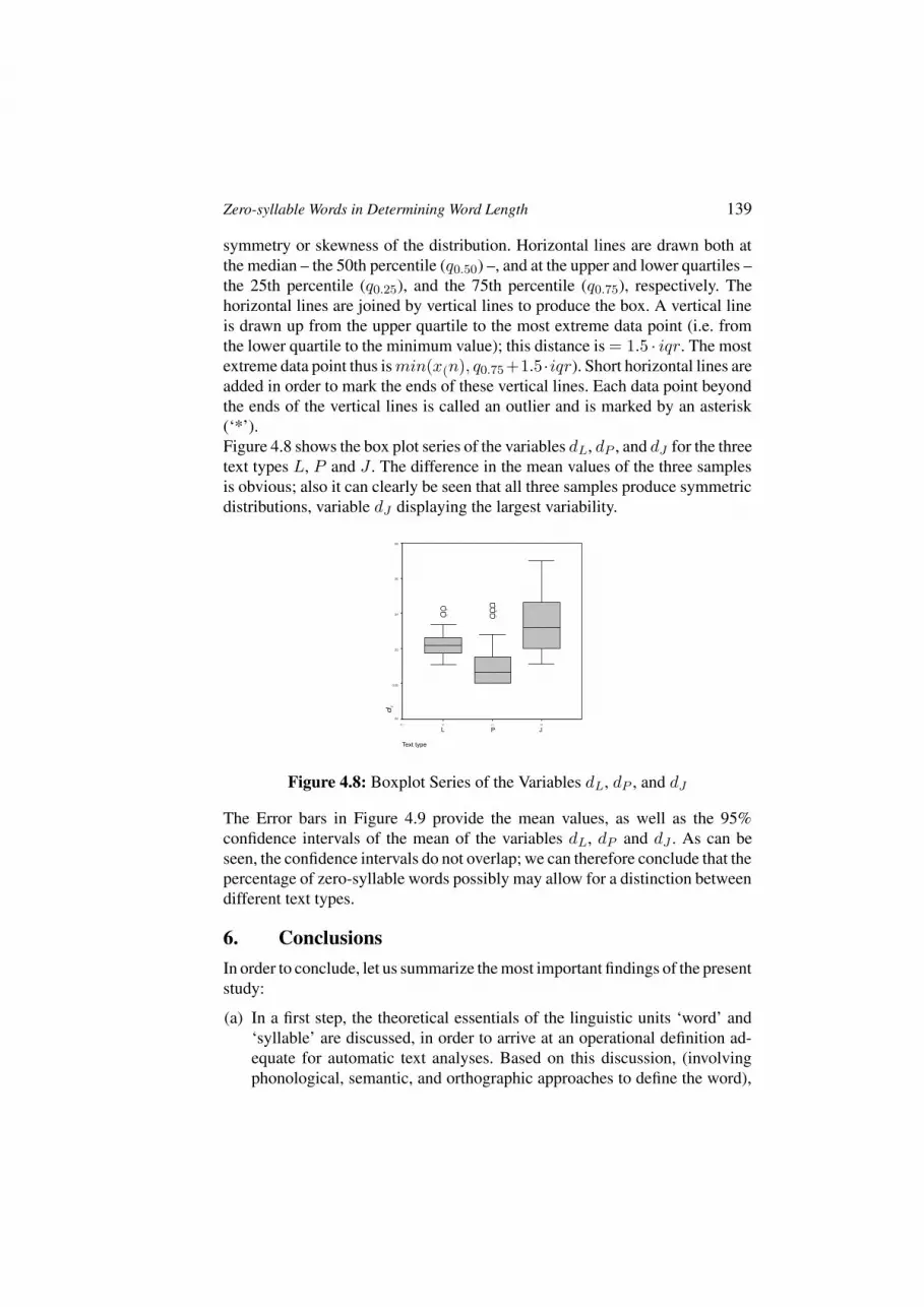
Zero-syllable Words in Determining Word Length 139
symmetry or skewness of the distribution. Horizontal lines are drawn both atthe median – the 50th percentile (q0.50) –, and at the upper and lower quartiles –the 25th percentile (q0.25), and the 75th percentile (q0.75), respectively. Thehorizontal lines are joined by vertical lines to produce the box. A vertical lineis drawn up from the upper quartile to the most extreme data point (i.e. fromthe lower quartile to the minimum value); this distance is = 1.5 · iqr. The mostextreme data point thus ismin(x(n), q0.75+1.5 ·iqr). Short horizontal lines areadded in order to mark the ends of these vertical lines. Each data point beyondthe ends of the vertical lines is called an outlier and is marked by an asterisk(‘*’).Figure 4.8 shows the box plot series of the variables dL, dP , and dJ for the threetext types L, P and J . The difference in the mean values of the three samplesis obvious; also it can clearly be seen that all three samples produce symmetricdistributions, variable dJ displaying the largest variability.
495152N =
Text type
JPL
,08
,06
,04
,02
0,00
-,02
74
60
57
38
18
di
Figure 4.8: Boxplot Series of the Variables dL, dP , and dJ
The Error bars in Figure 4.9 provide the mean values, as well as the 95%confidence intervals of the mean of the variables dL, dP and dJ . As can beseen, the confidence intervals do not overlap; we can therefore conclude that thepercentage of zero-syllable words possibly may allow for a distinction betweendifferent text types.
6. ConclusionsIn order to conclude, let us summarize the most important findings of the presentstudy:
(a) In a first step, the theoretical essentials of the linguistic units ‘word’ and‘syllable’ are discussed, in order to arrive at an operational definition ad-equate for automatic text analyses. Based on this discussion, (involvingphonological, semantic, and orthographic approaches to define the word),
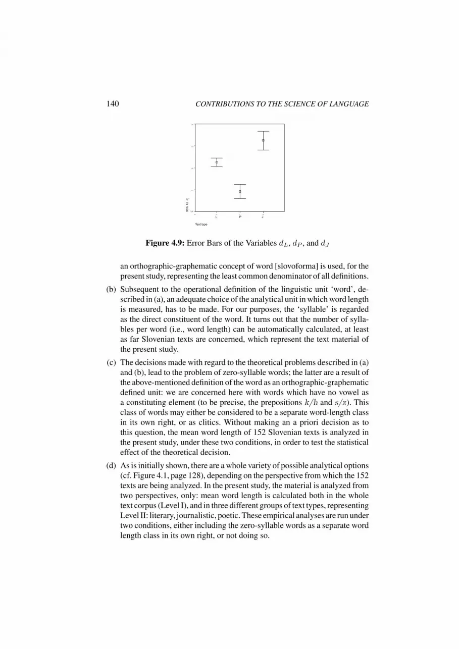
140 CONTRIBUTIONS TO THE SCIENCE OF LANGUAGE
495152N =
Text type
JPL
95%
CI
,04
,03
,02
,01
0,00
di
Figure 4.9: Error Bars of the Variables dL, dP , and dJ
an orthographic-graphematic concept of word [slovoforma] is used, for thepresent study, representing the least common denominator of all definitions.
(b) Subsequent to the operational definition of the linguistic unit ‘word’, de-scribed in (a), an adequate choice of the analytical unit in which word lengthis measured, has to be made. For our purposes, the ‘syllable’ is regardedas the direct constituent of the word. It turns out that the number of sylla-bles per word (i.e., word length) can be automatically calculated, at leastas far Slovenian texts are concerned, which represent the text material ofthe present study.
(c) The decisions made with regard to the theoretical problems described in (a)and (b), lead to the problem of zero-syllable words; the latter are a result ofthe above-mentioned definition of the word as an orthographic-graphematicdefined unit: we are concerned here with words which have no vowel asa constituting element (to be precise, the prepositions k/h and s/z). Thisclass of words may either be considered to be a separate word-length classin its own right, or as clitics. Without making an a priori decision as tothis question, the mean word length of 152 Slovenian texts is analyzed inthe present study, under these two conditions, in order to test the statisticaleffect of the theoretical decision.
(d) As is initially shown, there are a whole variety of possible analytical options(cf. Figure 4.1, page 128), depending on the perspective from which the 152texts are being analyzed. In the present study, the material is analyzed fromtwo perspectives, only: mean word length is calculated both in the wholetext corpus (Level I), and in three different groups of text types, representingLevel II: literary, journalistic, poetic. These empirical analyses are run undertwo conditions, either including the zero-syllable words as a separate wordlength class in its own right, or not doing so.

Zero-syllable Words in Determining Word Length 141
Based on these definitions and conditions, the major results of the present studymay be summarized as follows:
(1) As a first result, the proportion of zero-syllable words turned out to berelatively small (i.e., less than 2%).
(2) Generally speaking, mean values differ only slightly, at first sight, underboth conditions. Furthermore, it can be shown that the mean word lengthin texts under both conditions are highly correlated with each other; thepositive linear trend, which is statistically tested in the form of a correlationanalysis and graphically represented in Figure 4.3, (p. 131).
(3) In order to test if the expected values significantly differ or not, underboth conditions, data have to be checked for their normal distribution. Asa result, it turns out that mean word length is normally distributed in thethree text groups analyzed (Level II), but, interestingly enough, not in thewhole corpus (Level II). Based on this finding, further analyses concentrateon Level II, only. Therefore, t-tests are run, in order to compare the meanlengths between the three groups of texts on the basis of the differencesbetween the mean lengths under both conditions. As a result, the expectedvalues of mean word length significantly differ between all three groups.
(4) As can be clearly seen from Figure 4.7 (p. 138), representing the probabil-ity density function of mean word length (with and without zero-syllablewords as a separate category) there is reason to assume that the choice ofa particular word definition results in a systematic displacement of wordlengths.
To summarize, we thus obtain a further hint at the well-organized structure ofword length in texts.

142 CONTRIBUTIONS TO THE SCIENCE OF LANGUAGE
References
Altmann, G.1988 “Verteilungen der Satzlange.” In: Schulz, K.-P. (Hrsg.): Glottometrika, 9. [= Quantitative
Linguistics, Vol. 35]. (147–171).Altmann, G.; Best, K.H.; Wimmer, G.
1997 “Wortlange in romanischen Sprachen.” In: Gather, A.; Werner, H. (Hrsg.): SemiotischeProzesse und naturliche Sprache. Festschrift fur Udo L. Figge zum 60. Geburtstag. Stutt-gart. (1–13).
Altmann, G.; Lehfeldt, W.1980 Einfuhrung in die Quantitative Phonologie. [= Quantitative Linguistics, Vol. 7].
Bajec, A.1959 Besedotovorje slovenskega jezika, IV. Predlogi in predpone. Ljubljana. [= SAZU, Razred
za filoloske in literarne vede, Dela 14.]Best, K.H.; Zinenko, S.
1998 “Wortlangenverteilung in Briefen A.T. Twardowskis,” in: Gottinger Beitrage zur Sprach-wissenschaft, 1; 7–19.
Best, K.-H.; Zinenko, S.1999 “Wortlangen in Gedichten des ukrainischen Autors Ivan Franko.” In: J. Genzor; S. On-
drejovic (eds.): Pange lingua. Zbornık na pocest’ Viktora Krupu. Bratislava. (201–213).Best, K.-H.; Zinenko, S.
2001 “Wortlangen in Gedichten A.T. Twardowskis.” In: L. Uhlırova; G. Wimmer; G. Altmann; R.Kohler (eds.), Text as a Linguistic Paradigm: Levels, Constituents, Constructs. Festschriftin honour of Ludek Hrebıcek. Trier. (21–28).
Buhler, H.; Fritz, G., Herlitz, W.31972 Linguistik I. Lehr- und Ubungsbuch zur Einfuhrung in die Sprachwissenschaft. Tubingen.
Bunting, K.D.; Bergenholtz, H.31995 Einfuhrung in die Syntax. Stuttgart.
Girzig, P.1997 “Untersuchungen zur Haufigkeit von Wortlangen in russischen Texten.” In: Best, K.H.
(ed.): The Distribution of Word and Sentence Length. [= Glottometrika 16.] (152–162).Grotjahn, R.; Altmann, G.
1993 “Modelling the Distribution of Word Length: Some Methodological Problems.” In: Kohler,R.; Rieger, B. (eds.): Contributions to Quantitative Linguistics: Proceedings of the FirstInternational Conference on Quantitative Linguistics, QUALICO, Trier; 1991. Dordrecht.(141–153).
Grzybek, P.2000 “Pogostnostna analiza besed iz elektronskega korpusa slovenskih besedil”, in: Slavisticna
revija, 482; 141–157.Jachnow, H.
1974 “Versuch einer Klassifikation der wortabgrenzenden Mittel in gesprochenen russischenTexten”, in: Die Welt der Slaven, 19; 64–79.
Lehfeldt, W.1999 “Akzent.” In: H. Jachnow (ed.), Handbuch der sprachwissenschaftlichen Russistik und
ihrer Grenzdisziplinen. Wiesbaden. (34–48).Lehfeldt, W.; Altmann, G.
2002 “Der altrussische Jerwandel”, in: Glottometrics, 2; 34–44.Lekomceva, M.I.
1968 Tipologija struktur sloga v slavjanskich jazykach. Moskva.Mel’ cuk, I.A.
1999 Kurs obscej morfologii. Tom 1. Vvedenie. Cast’ pervaja. Slovo. Wien. [= Wiener Slawis-tischer Almanach, Sonderband 38/1).
Nemcova, E., Altmann, G.1994 “Zur Wortlange in slowakischen Texten”. In: Zeitschrift fur Empirische Textforschung,
1994 (1); 40–44.

Zero-syllable Words in Determining Word Length 143
Rottmann, Otto A.1997 “Word–Length Counting in Old Church Slavonic.” In: Altmann, G.; Mikk, J.; Saukkonen,
P.; Wimmer. G. (eds.), Festschrift in honour of Juhan Tuldava. [= Special issue of: Journalof Quantitative Linguistics, 4,1−3; 252–256.
Rottmann, Otto A.1999 “Word and Syllable Lengths in East Slavonic”, in: Journal of Quantitative Linguistics, 63;
235–238.Royston, P.
1982 “An Extension of Shapiro and Wilk’sW Test for Normality to Large Samples”, in: AppliedStatistics, 31; 115–124.
Schaeder, B.; Willee, G.1989 “Computergestutzte Verfahren morphologischer Beschreibung.” In: Batori, I.S.; Lenders,
W.; Putschke,W. (eds.), Computerlinguistik. An International Handbook on ComputerOriented Language Research and Applications. Berlin/New York. (188–203).
Srebot-Rejec, T.1981 “On the Allophones of /v/ in Standard Slovene”, in: Scando-Slavica, 27; 233–241.
Srebot-Rejec, T.2000 “Se o fonemu /v/ in njegovih alofonih”, in: Slavisticna revija, 481; 41–54.
2001 Slovenski pravopis. Ljubljana.Tivadar, H.
1999 “Fonem /v/ v slovenskem govorjenem knjiznem jeziku”, in: Slavisticna revija, 473; 341–361.
Toporisic, J.2000 Slovenska slovnica. Maribor.
Uhlırova, L.1996 “How long are words in Czech?” In: Schmidt, P. (ed.), Issues in General Linguistic Theory
and The Theory of Word Length. [= Glottometrika 15]. (134–146).Uhlırova, L.
1997 “Word length Distribution in Czech: On the Generality of Linguistic Laws and Individ-uality of Texts.” In: Best, K.-H. (ed.), The Distribution of Word and Sentence Length.[= Glottometrika 16.] (163–174).
Uhlırova, L.1999 “Word Length Modelling: Intertextuality as a Relevant Factor?”, in: Journal of Quantitative
Linguistics, 6; 252–256.Uhlırova, L.
2001 “On Word length, clause length and sentence length in Bulgarian”, In: Uhlırova, L.; Wim-mer, G.; Altmann, G.; Kohler, R. (eds.), Text as a Linguistic Paradigm: Levels, Constituents,Constructs. Festschrift in honour of Ludek Hrebıcek. Trier. (266–282).
Unuk, D.2001 Zlog v slovenskem jeziku. Doktorska disertacija. Maribor.
Wimmer, G.; Kohler, R.; Grotjahn, R.; Altmann, G.1994 “Towards a Theory of Word Length Distribution”, in: Journal of Quantitative Linguistics,
1; 98–106.Wimmer, G.; Altmann, G.
1996 “The Theory of Word Length: Some Results and Generalizations.” In: Schmidt, P. (ed.),Issues in General Linguistic Theory and The Theory of Word Length. [= Glottometrika15.] Trier. (112–133).
Wimmer, G.; Altmann, G.2005 “Towards a Unified derivation of Some Linguistic Laws.” [In this volume]
Wurzel, W.U.2000 “Was ist ein Wort?” In: Thieroff, R. et al. (eds.), Deutsche Grammatik in Theorie und
Praxis. Tubingen. (29–42).

144 CONTRIBUTIONS TO THE SCIENCE OF LANGUAGE
Appendix
Table 4.8: Sources of the Literary Prose Texts
Text # Author Title ch. Year
1-18 Cankar, Ivan Hlapec Jernej in njegova pravica 1-18 190719-27 Hisa Marije pomocnice 1-9 190428 Mimo zivljenja 1 192029 O prescah 1 192030 Brez doma 1 190331-33 Greh 1-3 190334 V temi 1-3 190335-40 Tinica 1-6 1903
41 Kocevar, Matija Izgubljene stvari 1 200142 Ko je vsega konec 1 200143 Ko se vrnem v postelju 1 200144 Moja vloga 1 200145 Nevidni svet 1 200146 Noc 1 2001
47 Kocevar, Ferdo Papezev poslanec 1 189248 Stiriperesna deteljica 1 189249 Suznost 1 189250 Vbeznik vjetnik 1 189251 Volitev nacelnika 1 189252 Grof in menih 1 1892

Zero-syllable Words in Determining Word Length 145
Table 4.9: Source of the Poetic Texts
Text # Author Title Year
53 Gregorcic, Simon Cas 188854 Cloveka nikar! 187755 Cvete, cvete pomlad 190156 Daritev 188257 Domovini 188058 Izgubljeni raj 188259 Izgubljeni cvet 188260 Kako srcno sva se ljubila 190161 Kesanje 188262 Klubuj usodi 190863 Kropiti te ne smem 190264 Kupa zivljenja 187265 Moj crni plasc 187966 Mojo srcno kri skropite 186467 Na bregu 190868 Na potujceni zemlji 188069 Na sveti vecer 188270 Nasa zvezda 188271 Njega ni! 187972 O nevihti 187873 Oj zbogom, ti planinski svet! 187974 Oljki 188275 Pogled v nedolzno oko 188276 Pozabljenim 188177 Pri zibelki 188278 Primula 188279 Sam 187280 Samostanski vratar 188281 Siroti 188282 Srce sirota 188283 Sveta odkletev 188284 Ti veselo poj! 187985 Tri lipe 187886 Ujetega ptica tozba 187887 V mraku 187088 Veseli pastir 1871
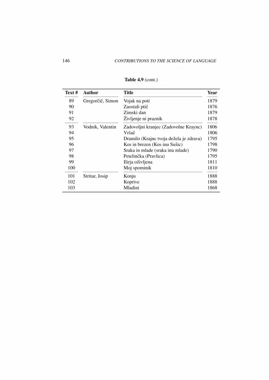
146 CONTRIBUTIONS TO THE SCIENCE OF LANGUAGE
Table 4.9 (cont.)
Text # Author Title Year
89 Gregorcic, Simon Vojak na poti 187990 Zaostali ptic 187691 Zimski dan 187992 Zivljenje ni praznik 1878
93 Vodnik, Valentin Zadovoljni kranjec (Zadovolne Kraync) 180694 Vrsac 180695 Dramilo (Krajnc tvoja dezela je zdrava) 179596 Kos in brezen (Kos inu Susic) 179897 Sraka in mlade (sraka inu mlade) 179098 Petelincka (Pravlica) 179599 Ilirja ozivljena 1811
100 Moj spominik 1810
101 Stritar, Josip Konju 1888102 Koprive 1888103 Mladini 1868

Zero-syllable Words in Determining Word Length 147
Table 4.10: Characteristic Statistical Measures of the Texts
Text TL in words TL in Difference# 0 ∅ syllables W i W i(0) d
1 591 602 1088 1.8409 1.8073 0.03362 969 977 1665 1.7183 1.7042 0.01413 1029 1038 1807 1.7561 1.7408 0.01534 790 796 1403 1.7759 1.7626 0.01335 803 809 1395 1.7372 1.7244 0.01286 882 890 1611 1.8265 1.8101 0.01647 957 973 1743 1.8213 1.7914 0.02998 1447 1473 2608 1.8023 1.7705 0.03189 922 939 1679 1.8210 1.7881 0.0329
10 1121 1134 1956 1.7449 1.7249 0.020011 925 937 1675 1.8108 1.7876 0.023212 1191 1203 2177 1.8279 1.8096 0.018313 1558 1583 2828 1.8151 1.7865 0.028614 942 956 1691 1.7951 1.7688 0.026315 1376 1388 2502 1.8183 1.8026 0.015716 1188 1203 2138 1.7997 1.7772 0.022517 1186 1203 2127 1.7934 1.7681 0.025318 296 303 546 1.8446 1.8020 0.042619 2793 2836 5437 1.9467 1.9171 0.029620 2733 2775 5400 1.9759 1.9459 0.030021 3240 3271 6107 1.8849 1.8670 0.017922 3548 3588 6418 1.8089 1.7887 0.020223 4485 4547 8442 1.8823 1.8566 0.025724 3698 3761 6760 1.8280 1.7974 0.030625 3054 3090 5922 1.9391 1.9165 0.022626 3172 3220 5806 1.8304 1.8031 0.027327 2592 2616 4899 1.8900 1.8727 0.017328 1425 1448 2765 1.9404 1.9095 0.030929 4411 4452 7993 1.8121 1.7954 0.016730 970 978 1786 1.8412 1.8262 0.015031 2906 2944 5239 1.8028 1.7796 0.023232 2874 2902 4897 1.7039 1.6875 0.016433 2872 2890 4981 1.7343 1.7235 0.010834 3416 3458 6260 1.8326 1.8103 0.022335 1104 1115 2089 1.8922 1.8735 0.0187

148 CONTRIBUTIONS TO THE SCIENCE OF LANGUAGE
Table 4.10 (cont.)
Text TL in words TL in Difference# 0 ∅ syllables W i W i(0) d
36 910 922 1665 1.8297 1.8059 0.023837 1086 1101 1987 1.8297 1.8047 0.025038 716 732 1290 1.8017 1.7623 0.039439 971 984 1841 1.8960 1.8709 0.025140 686 694 1288 1.8776 1.8559 0.021741 2337 2361 4380 1.8742 1.8551 0.019142 1563 1578 2982 1.9079 1.8897 0.018243 1493 1513 2748 1.8406 1.8163 0.024344 1458 1473 2852 1.9561 1.9362 0.019945 1999 2023 3763 1.8824 1.8601 0.022346 916 926 1750 1.9105 1.8898 0.020747 2388 2406 4601 1.9267 1.9123 0.014448 4899 4944 9346 1.9077 1.8904 0.017349 4120 4157 8009 1.9439 1.9266 0.017350 7380 7477 14188 1.9225 1.8976 0.024951 5018 5075 9707 1.9344 1.9127 0.021752 5528 5588 10524 1.9038 1.8833 0.020553 170 171 306 1.8000 1.7895 0.010554 228 228 393 1.7237 1.7237 0.000055 101 101 165 1.6337 1.6337 0.000056 81 81 151 1.8642 1.8642 0.000057 150 154 257 1.7133 1.6688 0.044558 48 48 92 1.9167 1.9167 0.000059 69 69 110 1.5942 1.5942 0.000060 121 124 208 1.7190 1.6774 0.041661 186 188 345 1.8548 1.8351 0.019762 37 37 54 1.4595 1.4595 0.000063 81 81 125 1.5432 1.5432 0.000064 62 62 110 1.7742 1.7742 0.000065 164 166 258 1.5732 1.5542 0.019066 69 69 121 1.7536 1.7536 0.000067 68 68 124 1.8235 1.8235 0.000068 193 193 307 1.5907 1.5907 0.000069 121 123 209 1.7273 1.6992 0.028170 70 71 121 1.7286 1.7042 0.0244

Zero-syllable Words in Determining Word Length 149
Table 4.10 (cont.)
Text TL in words TL in Difference# 0 ∅ syllables W i W i(0) d
71 109 110 183 1.6789 1.6636 0.015372 225 226 385 1.7111 1.7035 0.007673 167 167 259 1.5509 1.5509 0.000074 640 654 1151 1.7984 1.7599 0.038575 141 142 222 1.5745 1.5634 0.011176 131 131 216 1.6489 1.6489 0.000077 119 120 209 1.7563 1.7417 0.014678 129 129 209 1.6202 1.6202 0.000079 59 59 105 1.7797 1.7797 0.000080 246 247 445 1.8089 1.8016 0.007381 95 96 158 1.6632 1.6458 0.017482 70 70 120 1.7143 1.7143 0.000083 196 198 314 1.6020 1.5859 0.016184 181 181 266 1.4696 1.4696 0.000085 333 336 586 1.7598 1.7440 0.015886 248 252 414 1.6694 1.6429 0.026587 94 94 162 1.7234 1.7234 0.000088 134 135 240 1.7910 1.7778 0.013289 50 50 83 1.6600 1.6600 0.000090 137 138 242 1.7664 1.7536 0.012891 256 257 417 1.6289 1.6226 0.006392 176 177 311 1.7670 1.7571 0.009993 154 156 282 1.8312 1.8077 0.023594 165 166 308 1.8667 1.8554 0.011395 60 60 108 1.8000 1.8000 0.000096 126 127 211 1.6746 1.6614 0.013297 72 72 120 1.6667 1.6667 0.000098 23 23 44 1.9130 1.9130 0.000099 265 267 492 1.8566 1.8427 0.0139
100 87 87 155 1.7816 1.7816 0.0000101 158 158 272 1.7215 1.7215 0.0000102 411 413 725 1.7640 1.7554 0.0086103 306 306 522 1.7059 1.7059 0.0000104 714 724 1624 2.2745 2.2431 0.0314105 510 519 1195 2,3431 2,3025 0,0406

150 CONTRIBUTIONS TO THE SCIENCE OF LANGUAGE
Table 4.10 (cont.)
Text TL in words TL in Difference# 0 ∅ syllables W i W i(0) d
106 1932 1966 4344 2.2484 2.2096 0.0388107 775 781 1659 2.1406 2.1242 0.0164108 386 390 886 2.2953 2.2718 0.0235109 314 319 658 2.0955 2.0627 0.0328110 490 495 1144 2.3347 2.3111 0.0236111 441 450 1118 2.5351 2.4844 0.0507112 584 593 1251 2.1421 2.1096 0.0325113 1560 1582 3533 2.2647 2.2332 0.0315114 785 800 1772 2.2573 2.2150 0.0423115 341 343 799 2.3431 2.3294 0.0137116 681 687 1468 2.1557 2.1368 0.0189117 573 590 1391 2.4276 2.3576 0.0700118 312 319 750 2.4038 2.3511 0.0527119 936 942 2008 2.1453 2.1316 0.0137120 976 981 2217 2.2715 2.2599 0.0116121 141 143 283 2.0071 1.9790 0.0281122 460 463 1004 2.1826 2.1685 0.0141123 291 295 688 2.3643 2.3322 0.0321124 438 441 945 2.1575 2.1429 0.0146125 254 256 582 2.2913 2.2734 0.0179126 777 793 1853 2.3848 2.3367 0.0481127 826 837 1878 2.2736 2.2437 0.0299128 219 224 458 2.0913 2.0446 0.0467129 202 203 474 2.3465 2.3350 0.0115130 422 433 939 2.2251 2.1686 0.0565131 394 402 843 2.1396 2.0970 0.0426132 606 612 1357 2.2393 2.2173 0.0220133 406 412 887 2.1847 2.1529 0.0318134 397 406 825 2.0781 2.0320 0.0461135 682 698 1646 2.4135 2.3582 0.0553136 439 448 1009 2.2984 2.2522 0.0462137 430 439 1007 2.3419 2.2938 0.0481138 191 194 429 2.2461 2.2113 0.0348139 200 170 484 2.4556 2.4412 0.0144140 215 219 546 2.5395 2.4932 0.0463

Zero-syllable Words in Determining Word Length 151
Table 4.10 (cont.)
Text TL in words TL in Difference# 0 ∅ syllables W i W i(0) d
141 334 337 766 2.2934 2.2730 0.0204142 138 139 302 2.1884 2.1727 0.0157143 236 239 510 2.1610 2.1339 0.0271144 214 218 461 2.1542 2.1147 0.0395145 325 330 793 2.4400 2.4030 0.0370146 827 836 1847 2.2334 2.2093 0.0241147 114 117 269 2.3596 2.2991 0.0605148 299 302 687 2.2977 2.2748 0.0229149 200 201 484 2.4200 2.4080 0.0120150 201 203 448 2.2289 2.2069 0.0220151 162 164 372 2.2963 2.2683 0.0280152 159 162 403 2.5346 2.4877 0.0469

152 CONTRIBUTIONS TO THE SCIENCE OF LANGUAGE
Table 4.11: Proportion of x-syllable Words
Syllables per word
Text # 0 1 2 3 4 5 6 7 8 9
1 11 266 194 93 35 32 8 478 325 130 33 33 9 507 315 164 37 64 6 376 250 131 32 15 6 381 280 119 19 3 16 8 434 237 151 50 107 16 441 306 157 46 78 26 672 449 270 52 49 17 423 288 169 37 5
10 13 560 336 181 39 511 12 441 269 165 49 112 12 566 339 213 71 213 25 726 477 283 61 1114 14 466 265 156 48 715 12 645 423 230 69 916 15 573 361 185 58 10 117 17 585 340 188 67 618 7 136 94 46 16 419 43 1126 944 500 197 22 3 120 42 1099 872 527 203 29 2 121 31 1397 1057 579 180 23 422 40 1669 1104 581 174 18 223 62 1961 1444 780 252 43 524 63 1675 1223 592 180 25 325 36 1326 895 573 218 37 526 48 1472 1005 497 165 25 827 24 1131 832 439 168 17 528 23 581 477 255 96 15 129 41 1993 1524 658 208 22 630 8 452 313 130 59 14 231 38 1386 886 474 143 15 232 28 1460 918 389 101 633 18 1424 924 406 99 1934 42 1540 1131 554 162 26 335 11 474 353 214 51 10 1 136 12 430 272 150 49 9

Zero-syllable Words in Determining Word Length 153
Table 4.11 (cont.)
Syllables per word
Text # 0 1 2 3 4 5 6 7 8 9
37 15 508 315 210 46 738 16 336 226 118 32 439 13 434 288 177 62 8 240 8 302 216 128 32 7 141 24 1067 695 404 148 20 2 142 15 692 462 289 102 17 143 20 691 446 270 76 9 144 15 643 399 278 115 21 245 24 890 615 360 110 21 346 10 400 271 182 53 1047 18 1021 744 433 159 29 248 45 2102 1599 805 340 47 649 37 1724 1282 784 283 45 250 97 3101 2398 1327 473 68 1351 57 2117 1589 917 327 56 11 152 60 2381 1770 974 344 50 8 153 1 72 62 34 254 119 66 33 7 355 50 39 11 156 27 38 1657 4 75 48 22 558 21 14 9 459 35 27 760 3 58 42 18 361 2 77 63 42 462 26 5 663 42 34 564 26 25 10 165 2 98 44 16 666 29 29 10 167 27 26 1568 106 63 21 369 2 59 37 24 170 1 29 33 6 2

154 CONTRIBUTIONS TO THE SCIENCE OF LANGUAGE
Table 4.11 (cont.)
Syllables per word
Text # 0 1 2 3 4 5 6 7 8 9
71 1 45 55 8 172 1 104 84 35 273 99 50 12 674 14 278 226 125 9 275 1 78 47 14 276 65 49 15 277 1 50 48 2178 65 49 14 179 25 23 10 180 1 104 91 45 681 1 48 34 11 382 30 33 4 383 2 103 69 23 184 107 63 1185 3 151 117 59 686 4 123 89 32 3 187 40 41 12 188 1 57 53 24 289 22 23 590 1 61 49 25 291 1 131 93 28 492 1 81 58 34 393 2 64 55 32 394 1 55 84 19 795 23 27 9 196 1 53 62 10 197 36 25 10 198 10 6 6 199 2 115 85 54 10 1100 38 31 17 1101 69 67 19 3102 2 187 145 70 7 2103 144 117 37 7 1104 10 267 167 145 96 32 5 2105 9 167 127 122 68 20 6

Zero-syllable Words in Determining Word Length 155
Table 4.11 (cont.)
Syllables per word
Text # 0 1 2 3 4 5 6 7 8 9
106 34 699 484 443 210 75 15 5 1107 6 278 236 163 77 15 5 1108 4 142 82 99 38 19 6109 5 124 76 82 25 6 1110 5 170 113 120 54 27 5 1111 9 132 94 110 72 23 5 5112 9 220 155 134 60 12 2 1113 22 564 359 368 209 52 5 3114 15 280 201 174 87 38 5115 2 121 69 90 45 9 5 1 1116 6 259 185 147 58 27 4 1117 17 179 139 128 94 26 5 2118 7 87 81 95 36 7 5 1119 6 362 256 182 99 30 7120 5 326 269 216 134 24 7121 2 54 47 26 13 1122 3 187 108 85 62 10 8123 4 103 61 76 29 14 7 1124 3 178 112 77 46 23 1 1 0125 2 97 60 48 31 13 3 2126 16 254 174 191 127 19 9 3127 11 295 200 201 80 41 8 1128 5 74 80 43 17 3 2129 1 65 61 33 30 10 3130 11 150 118 86 49 17 1 1131 8 164 89 88 37 11 2 2 1132 6 227 137 149 62 27 2 2133 6 156 104 79 51 14 2134 9 170 103 68 43 8 2 3135 16 202 174 174 98 26 4 4136 9 141 121 105 57 10 2 3137 9 148 104 96 54 22 5 1138 3 66 50 45 24 4 2139 1 54 38 39 25 11 1 1140 4 71 38 43 45 18

156 CONTRIBUTIONS TO THE SCIENCE OF LANGUAGE
Table 4.11 (cont.)
Syllables per word
Text # 0 1 2 3 4 5 6 7 8 9
141 3 108 94 84 31 13 1 1 2142 1 54 30 32 19 2 1143 3 95 52 58 21 7 3144 4 86 49 50 22 5 2145 5 101 72 90 40 16 4 2146 9 307 200 189 90 35 4 2147 3 42 23 24 16 9148 3 107 73 61 39 19149 1 69 36 53 32 7 2 1150 2 73 49 52 16 9 2151 2 52 41 40 27 2152 3 46 33 49 20 6 3 2

Peter Grzybek (ed.): Contributions to the Science of Language.Dordrecht: Springer, 2005, pp. 157–170
WITHIN-SENTENCE DISTRIBUTIONAND RETENTION OF CONTENT WORDSAND FUNCTION WORDS
August Fenk, Gertraud Fenk-Oczlon
1. Serial position effects in the recall of sentencesExperiments with free immediate recall of lists of unconnected words usuallyreveal a saddle-shaped ‘serial position curve’: high frequency of recall in theitems obtaining the first positions (‘primacy effect’) of the list and those obtain-ing the last positions (‘recency effect’), and, in the words of Murdock Jr., “ahorizontal asymptote spanning the primacy and recency effect” (cf. Figure 5.1).
Figure 5.1: A “Typical” Serial Position Curve Resulting FromImmediate Free Recall of Unconnected Words (Mur-dock Jr. 1962: 484, modified)
Murdock Jr. (1962: 488) suggested “that the shape of the curve may well resultfrom proactive and retroactive inhibition effects occurring within the list itself.”Assumptions regarding the underlying mechanisms became more differentiated

158 CONTRIBUTIONS TO THE SCIENCE OF LANGUAGE
in later experiments introducing – in addition to input-order – sense-modalityof list presentation as a second independent variable (Murdock & Walker 1969)and evaluating – in addition to frequency of recall – output-order in recall asa second dependent variable (Fenk 1979). Many of the relevant psychologicalfindings seem to be interesting for linguistics as well: the results reported e.g.by Murdock Jr. (1962) suggesting that the recency effect extends over the last7 plus minus 2 words; the observation of Murdock & Walker (1969) that inauditory presentation the recency effect is higher and more extensive than invisual presentation (‘modality effect’); the observation that ‘sequential clusters’,i.e. word groups with the words recalled in the same order as represented, arein the recency part of auditorily presented word strings significantly larger andsignificantly more frequent than in the recency part of visually presented wordstrings – in series of unconnected nouns as well as in real sentences, and despitethe tendency to start the recall of auditorily presented word strings with wordsand word groups from the end of the string (Fenk 1979: 14). Of particularlinguistic interest is the question whether the serial position effects shown inthe recall of lists of unconnected words show in the recall of real sentences aswell. Are the underlying processes also efficient in real sentence processing andin connected discourse?Indications reported so far (Jarvella 1971; Fenk 1979, 1981; Rummler 2003)are not fully convincing: In Jarvella’s study, subjects were presented sentenceslike “. . . Having failed to disprove the charges, Taylor was later fired by thepresident" (p. 410). The fragment starting with “Taylor. . . ” is not only localizedin the ‘recency part’ of the sentence but also represents the main constituentof this sentence, so that one has to suspect a confusion of the effects of theseconditions. The marked and plateau-shaped ‘recency effect’ in the serial positioncurves (p. 411) might suggest some additive effects on the performance of recall(see Figure 5.2).Rummler (2003: 96) states that the so-called “subordination effect” (subor-dinating conjunctions achieve a better verbatim recall than coordinating con-junctions) mainly comes off by better retention of the second clause. This betterrecall of the second clause might again be a consequence of the restricted “span”of the recency effect and/or of the fact that in the subordinating conjunction theinternal redundancy is higher and the informational content (and cognitive load)of the second clause lower than in the coordinating conjunction.The serial position curve reported by Fenk (1981: 25) shows a marked recencyeffect (only) in auditory presentation of the sentence. (And, in addition, an‘inverse modality effect’, i.e. a superiority of visual presentation in the primacypart.) But these results originate from only two different sentences presentedsimultaneously in two different sense modalities.For a more systematic approach, the subjects in an experiment by Auer, Bacik &Fenk (2001) were presented a text by Glasersfeld (1998). Speech was interrupted

Content Words and Function Words 159
Figure 5.2: One of the Serial Position Curves For Free Recall ofSentences (Jarvella 1971: 414, modified)
after some of the sentences by a certain signal. Subjects were instructed to writedown as much as they could remember from the last sentence before the testpause. Since the position of a word is by far not the only factor determining itschance to be recalled, the serial position curves obtained differ not only fromthe “ideal” curve (Figure 5.1) that approximately shows when different groupsof subjects are presented different lists with the single items changing theirpositions in systematic rotation. They differed also from sentence to sentence,since these individual sentences (n = 10) differed in all possible respects –lexemes, syntactic structure, length. Nevertheless the family of curves showsa (rather weak) primacy effect and a marked recency effect. Data from thisexperiment were re-analyzed in order to investigate further questions.
2. Wordclass-specific effects on the serial position curve?2.1 Two hypothesesThe aim of our statistical reanalysis was to test the following assumptions:
Hypothesis 1In content words the likelihood of recalling is higher than in functionwords.

160 CONTRIBUTIONS TO THE SCIENCE OF LANGUAGE
Hypothesis 2In the recency part the difference predicted in assumption I will besmaller than in earlier parts of the serial position curve.
The basic consideration leading to these assumptions was that the fundamentaldifference between content words and function words (a) should be in someway reflected in sentence processing, especially in our ‘semantic memory’ (b).
Ad (a):
Within linguistics, content words are often characterized as ‘open class words’opposed to function words as ‘closed class words’. Rather relevant with re-spect to our hypotheses is the fact that content words are more significantfor the specific topic, just for the particular and concrete ‘content’ of textsand sentences, while the function of function words is to bring about certainreferences between more or less exchangeable contents and content words.In brief: The relevant division here is between context-specific content wordsand rather context-independent function words. Function words are, more-over, rather short, very frequent, and ‘multifunctional’ in the sense of Zipf(1949).
Ad (b):
A widely accepted model concerning our memory says: After having ex-tracted the meaning of an actual clause, its verbatim form (words and syntax)is rapidly lost from memory, while the meaning is preserved (and affects e.g.our interpretation of the following clauses). This conception is strongly influ-enced by Sachs (1967). Her findings could be reproduced in later experimentsby Luther & Fenk (1984) which showed moreover that this outcome is notgrounded in the nature and incapability of our long term memory but is theresult of a cognitive strategy which is successful under ‘normal’ conditions,i.e. in the absence of the instruction and motivation to concentrate on otheraspects of sentences.
This principle – rapid loss of the form after the meaning has been extracted – isactually also supported by two findings already mentioned in the present paper:
(i) The tendency to repeat some of the words in the ‘input order’ especiallyfrom the recency part of auditorily presented word strings (Fenk 1979:14) indicates that verbatim representation is a speciality of immediateacoustic memory.
(ii) The plateau at the end of Jarvella’s (1971) serial position curves. Jarvella’scomment on his findings:

Content Words and Function Words 161
“Various verbatim measures of recall support only the immediate sentenceand immediately heard clause as retrievable units in memory” (p. 409). “Ap-parently only these immediate sentences hold a retrievable form in memory;this form also leads to superior recall of their most recent clause. On theother hand, recall of previous sentences indicates that they had received arelatively thorough semantic interpretation. It appears that the propositionalmeaning of sentences was remembered shortly after they were heard, al-though, as measured by verbatim recall, the form of sentences was quicklyforgotten” (p. 415).
2.2 MethodIn order to test our assumptions, each of the test-sentences used in the Auer,Bacik & Fenk experiment was divided into four quarters, rounding off wherenecessary. The first quarter (I) was defined as the primacy part of the sentence, IIand III taken together as the medium part, and the last 25 percent of the words(IV) as the recency part. Then we determined, separately for the three parts(I, II+III, IV) of each sentence, the number of content words – nouns, verbs,adjectives, manner adverbs – and the number of function words such as articles,prepositions, pronouns, conjunctions, negations, particles, auxiliary verbs.Our operationalization of ‘primacy part’ (first 25% of words) and ‘recency part’(last 25% of words) might, at a first glance, appear as a rather arbitrary and roughmethod, since a ‘quarter’ means different things in sentences of differing length:e.g. five words in a 20-word sentence or ten words in a 40-word sentence. Butthe alternative – to define the primacy part and the recency part in terms of afixed number of words – would again be arbitrary: How many words should befixed? And it would restrict the application to rather long sentences: A fixednumber of, let us say, six words for the primacy part and six words for therecency part would, in the case of a 12-word sentence, reduce the ‘mediumpart’ to zero, and would exclude shorter sentences altogether.Our operationalization, however, offers a wide range of applications and es-tablishes a firm proportion between, on the one hand, the primacy and recencypart, and, on the other hand, the part in between and the sentence as a whole.And it has proved to bring about significant results.
2.3 ResultsA problem for the quantification of a primacy and recency effect in our two wordclasses was the unexpected observation that the proportion of content words tofunction words showed a considerable variation between the interesting partsof the sentences. Thus, a quantification in absolute terms did not make muchsense, and the recall scores had to be related to the number of words presented.Table 5.1 lists the results – number of words occurring, number of words re-called, and the ‘relative’ recall scores R/O.

162 CONTRIBUTIONS TO THE SCIENCE OF LANGUAGE
Table 5.1: Number of Words Occurring (O) in and Recalled (R)from the First Quarter (I), the Medium Part (II + III),and the Last Quarter (IV) of a Total of 10 Sentences;R/O = Mean Frequency of Recall Per Word Given
I II + III IV
Wordclasses O R R/O O R R/O O R R/O
Content 22 55 2.5000 75 152 2.0267 37 132 3.5676Words (C)
Function 37 68 1.8378 68 98 1.4412 25 75 3.0000Words (F )
Total (C + F ) 59 123 2.0847 143 250 1.7483 62 207 3.3387
Difference(C − F ) 0.6622 0.5855 0.5676
Level of signi-ficance (p) < 5% < 5% < 1%
The results of the statistical evaluation (Wilcoxon tests) in words:
– The primacy effect – the gradient we can see in Figure 5.3 between middlepart and primacy part – was not significant.
– The recency effect, i.e. the gradient between middle part and recency part,was more marked (Figure 5.3) and was significant in all possible evaluations:in the content words (p < 1%), in the function words (p < 2%), and whenboth word classes were taken together (p < 1%).
– Hypothesis 1 was clearly confirmed: Level of relative recall scores was sig-nificantly higher in content words than in function words throughout thesentences. (Table 5.1 presents in its lowest line the error probabilities forparts I, II+III, and IV).
– Hypothesis 2 would predict a convergence between the recall curves forcontent words and function words at least between the middle part and therecency part (Figure 5.3). Actually there is, as can be seen from the valuesin Table 5.1, a slight convergence from I to II+III and from II+III to IV. Butin both cases this convergence is far from significant.
3. Three more or less hypothetical regularitiesThe formulation of the first of the following assumptions is motivated by theoccasional observation that our test sentences taken from a Glasersfeld textshowed a tendency of an increase of content words and a decrease of functionwords during a sentence. As to this tendency we carried out a little follow-up

Content Words and Function Words 163
Figure 5.3: Differences Between Content and Function Words ina Serial Position Curve For Free Recall of Sentencesof Different Length (I = first quarter, IV = last quarter)
study (3.1). Results strongly indicate that this is a general tendency at leastin German texts. And if our tentative explanation (section 4) of this regularityholds, its scope should not be restricted to German texts.Regularities 3.2 and 3.3 have the status of as yet unexamined lawlike hypotheses.Regularity 3.2 proceeds from the assumption that the token frequency of func-tion words is higher than the token frequency of content words. If these functionwords tend to occupy initial positions of sentences, this should contribute to theregularity “the more frequent before the less frequent”. This statistical regular-ity has proven to be the most powerful one in the explanation of word order infrozen conjoined expressions (Fenk-Oczlon 1989), and it seems that its rangeof validity can be extended on clauses in general. In this present paper we willstate this generalized rule mainly as an inferential step to our third regularity(3.3) which perfectly fits with the topic of this volume on “word length”.
3.1 Decrease of function words and increase of contentwords within sentences
As Table 5.1 shows, function words tend to decrease and content words toincrease in the course of a sentence. Figure 5.4 illustrates these tendencies.Despite the small sample of only ten sentences, the relevant differences provedto be significant in the Wilcoxon test (Table 5.2).These differences in the distribution of the instances of the two word classeswere, as already mentioned in section 2.3, a problem for a simple evaluationof the recall scores. But we suspected that it might indicate an interesting phe-

164 CONTRIBUTIONS TO THE SCIENCE OF LANGUAGE
Figure 5.4: Differences Found in the Within-Sentence Distribu-tion of Content and Function Words
nomenon within the scope of quantitative linguistics – provided, that these ten-dencies are not a special feature of a certain text of a certain author. A pilot studywas conducted in order to find some indications of possible generalizations ofthis tendency. The sample of authors was increased – nine more German textpassages, four of them from scientific books, five from literary books. Taken to-gether with the already analysed text passages from Glasersfeld this is a sampleof ten (five scientific, five literary) text passages, and a sample of ten sentencesfrom each of these passages, i.e. a total of 10 × 10 = 100 sentences. (Sourcetexts are listed at the end of the paper.)
Table 5.2: Differences Between the Frequency of FunctionWords and Content Words Occurring in the PrimacyPart (I) and in the Recency Part (IV) of 10 Sentencesfrom a Text by Glasersfeld (1998)
difference quarter I – quarter IV error probability
function words 12 p < 1%content words −15 p < 1%
difference function w. – content w.
quarter I 15 p < 1%quarter IV −12 p < 5%

Content Words and Function Words 165
The evaluation was carried out by a student who did not know our assumptions.She was instructed not to collect ten successive sentences from each passage intothe sample, but – where possible – each third sentence. Sometimes she had tooverleap more than two sentences, e.g. when one of the intervening ‘sentences’was too short (less than four words) or the heading of a new section. As alreadysuggested by Niehaus (1997: 221), a colon was accepted as the end of thesentence when the following word started with a capital letter. The results:The gradient of the decrease of function words and increase of content wordsfrom the first quarter to the last quarter is not as steep as in Glasersfeld, but stillsignificant (Fenk-Oczlon & Fenk 2002). These results suggest that the tendencyof function words to decrease and of content words to increase in the course ofa sentence is a general tendency at least in German texts. And the provisionalresults of Muller (in preparation) indicate that this tendency is not restricted toGerman texts.
3.2 The more frequent before the less frequentThis regularity was originally stated in order to explain and predict the order ofthe two main elements forming a frozen conjoined expression such as knife andfork, salt and pepper, peak and valley. From all the rules examined (e.g. “shortbefore long”, “the first word has fewer initial consonants than the second”), therule “the more frequent before the less frequent” showed the highest explanatorypower as to the word order in 400 freezes (Fenk-Oczlon 1989). Our regularity3.1 should establish or enhance such a tendency in sentences as well to theeffect that regularity 3.2 is not restricted to freezes.If the tendency “the more frequent before the less frequent” fits to sentences aswell – as a consequence of 3.1 or for whatever reason – then it is plausible toassume a further regularity:
3.3 Increase of word length in the course of a sentenceA more general regularity of this sort was already postulated in Behaghel (1909):“Das Gesetz der wachsenden Glieder”, i.e. “the law of increasing elements,parts, links, constituents. . . ”. Behaghel illustrates this law with many examplesfrom classical texts in a variety of languages such as ancient Greek, Latin, OldHigh German and German. In most of his examples the comparison was betweenword groups of different size or between single words and word groups: aufder Turbank und im dunklen Gang (p. 110), ih inti father min (p. 111). Ina little experiment by Behaghel the subjects got four sheets of paper with thefollowing words and word groups: Gold / edles Geschmeide / und / sie besitzt.They were instructed to form a sentence from these fragments, and the resultwas always the same: sie besitzt Gold und edles Geschmeide. (Behaghel 1909:137). He offers the following interpretation:

166 CONTRIBUTIONS TO THE SCIENCE OF LANGUAGE
Man wird nicht nur die langer dauernde Arbeit auf den Zeitraum verlegen, wo manden Abschluß leichter hinausschieben kann; man wird auch, wenn man sich Zeitlassen kann, die Arbeit grundlicher tun, mehr ins Einzelne gehen, oder, sprachlichausgedruckt: man wird nicht nur fur den umfangreicheren Ausdruck die spatereStelle wahlen, sondern auch fur die spatere Stelle den umfangreicheren Ausdrucksich zubereiten. So bildet sich unbewußt in den Sprachen ein eigenartiges rhyth-misches Gefuhl, die Neigung, vom kurzeren zum langeren Glied uberzugehen; soentwickelt sich das, was ich, um einen ganz knappen Ausdruck zu gewinnen, alsdas Gesetz der wachsenden Glieder bezeichnen mochte. (Behaghel 1909: 138f.)
Our regularity “increase of word length during a sentence” is similar to Be-haghel’s law but more specific in that it is localized at the single word level. Aspecial case of Behaghel’s law, so to speak! At present we cannot offer resultsof empirical tests of this lawlike assumption. (But see Muller, in preparation.)But we can contribute two new perspectives:
1. An operationalization that allows for a statistical examination of the law:Define words as the relevant ‘Glieder’ or ‘constituents’, determine their‘size’ in terms of ‘number of syllables’, and compare the mean size of wordsin the early and late parts of sentences.
2. An interpretation specifying a concrete factor that might at least contribute tothe rhythmic pattern described by Behaghel. This factor is the concentrationor accumulation of function words in the first parts of clauses (sentences,subordinate clauses). And since function words are generally extremely fre-quent and frequent words tend – for economic reasons – to be rather short(Zipf 1929, 1949), the concentration of these rather short units in the firstpart of clauses results in an increase of the mean word length in the courseof a sentence. This hypothesized tendency will of course depend on the re-spective language type and is expected to be more pronounced in languageswith a tendency to agglutinative morphology and a tendency to OV order.
4. ConclusionsA possible explanation for our regularity “decrease of function words and in-crease of content words”: In a running text, almost any clause has to refer towhat was said in the clauses before (“old before new”, “topic before comment”,“theme before rheme”). This reference is – most probably not only in Germantexts – first of all brought about by function words (e.g. anaphoric pronouns,conjunctions) right at the beginning of the new clause. If this is an appropriateexplanation of our regularity 3.1, then it is – indirectly – also relevant for thehypothesized regularities 3.2 “the more frequent before the less frequent” and3.3 “within-sentence increase of word length”. The last steps of the argumentsin other words: Function words accumulate at the beginning of clauses; theyare very frequent and ‘therefore’ very short in terms of number of syllables;members of our second word class ‘content words’ are, on average, composed

Content Words and Function Words 167
of a higher number of syllables, and the number of these content words tendsto increase during the sentence. This means, first of all: The regularity “themore frequent before the less frequent” found in frozen binomials holds truefor sentences as well. As a consequence, one may expect an increase of wordlength in the course of a sentence. All the regularities outlined above (“the morefrequent before the less frequent”, “short before long”) fit to and contribute tothe more general law (Fenk-Oczlon 2001) of an economic and rather ‘constant’flow of linguistic information.

168 CONTRIBUTIONS TO THE SCIENCE OF LANGUAGE
5. Appendix: Sources of the Test Sentences
Bachmann, I. (1980 [1971]). Malina. Frankfurt: Suhrkamp Verlag (suhrkamptaschenbuch 641).B pp. 200–202, beginning with section “Malina ist . . . ”
Frisch, M. (1975). Montauk. Gutersloh: Bertelsmann Reinhard Mohn OHG.B pp. 157–159, beginning with section “Money”
Gigerenzer, G., Swijtink, Z., Porter, Th., Daston, L., Beatty, J., Kruger, L.(1999). Das Reich des Zufalls. Heidelberg/Berlin: Spektrum AkademischerVerlag.B pp. 212–213, beginning with section “5.8 Diskontinuitat, eine Grundlagealler Veranderung”
Glasersfeld, E. von (1998). Konstruktivismus statt Erkenntnistheorie. In: W.Dorfler & J. Mitterer (eds.), Ernst von Glasersfeld – Konstruktivismus stattErkenntnistheorie. Klagenfurt: Drava Verlag.B pp. 11–17
Hesse, H. (1972). Der Steppenwolf. Gutersloh: Bertelsmann Reinhard MohnOHGB pp. 269–271, beginning with section “Die Fremdenstadt im Suden”
Mann, Th. (5. Aufl. 1997 [1947]). Doktor Faustus. Frankfurt a. M.: FischerTaschenbuch Verlag.B pp. 47–50, beginning with section “VI”
Musil, R. (1960; A. Frise, ed.). Der Mann ohne Eigenschaften. Stuttgart: Deut-scher Bucherbund.B pp. 445–447, beginning with section “98. Aus einem Staat, der an einemSprachfehler zugrundegegangen ist”
Niehaus, B. (1997). Untersuchung zur Satzlangenhaufigkeit im Deutschen. In:Best, K.-H. (ed.), The Distribution of Word and Sentence Length. Glot-tometrika 16, Quantitative Linguistics 58, 213–275. Trier: WVT Wissen-schaftlicher Verlag Trier.B pp. 263–264, beginning with section “6. Ausblick”
Spies, M. (1993). Unsicheres Wissen. Heidelberg/Berlin/Oxford: SpektrumAkademischer Verlag.B pp. 20–21, beginning with section “3. Perspektive: Kognitive Modelle derInformationsverarbeitung”

Content Words and Function Words 169
Stegmuller, W. (1957). Das Wahrheitsproblem und die Idee der Semantik. Wien:Springer-Verlag.B pp. 38–40, beginning with section “III. Die Trennung von Objekt- undMetasprache als Weg zur Losung und die Idee der Semantik als exakterWissenschaft. Semantische Systeme von elementarer Struktur”
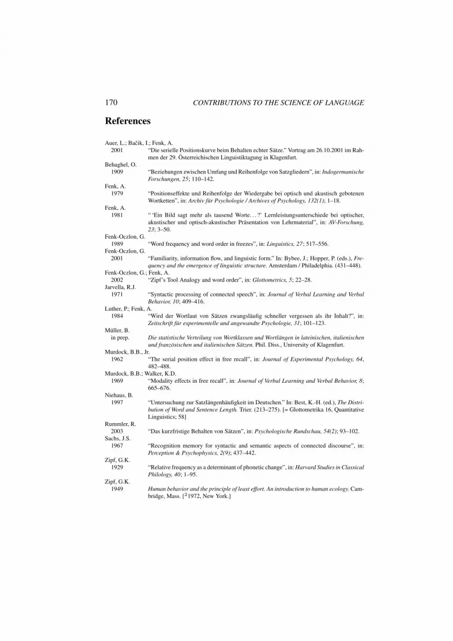
170 CONTRIBUTIONS TO THE SCIENCE OF LANGUAGE
References
Auer, L.; Bacik, I.; Fenk, A.2001 “Die serielle Positionskurve beim Behalten echter Satze.” Vortrag am 26.10.2001 im Rah-
men der 29. Osterreichischen Linguistiktagung in Klagenfurt.Behaghel, O.
1909 “Beziehungen zwischen Umfang und Reihenfolge von Satzgliedern”, in: IndogermanischeForschungen, 25; 110–142.
Fenk, A.1979 “Positionseffekte und Reihenfolge der Wiedergabe bei optisch und akustisch gebotenen
Wortketten”, in: Archiv fur Psychologie / Archives of Psychology, 132(1); 1–18.Fenk, A.
1981 “ ‘Ein Bild sagt mehr als tausend Worte. . . ?’ Lernleistungsunterschiede bei optischer,akustischer und optisch-akustischer Prasentation von Lehrmaterial”, in: AV-Forschung,23; 3–50.
Fenk-Oczlon, G.1989 “Word frequency and word order in freezes”, in: Linguistics, 27; 517–556.
Fenk-Oczlon, G.2001 “Familiarity, information flow, and linguistic form.” In: Bybee, J.; Hopper, P. (eds.), Fre-
quency and the emergence of linguistic structure. Amsterdam / Philadelphia. (431–448).Fenk-Oczlon, G.; Fenk, A.
2002 “Zipf’s Tool Analogy and word order”, in: Glottometrics, 5; 22–28.Jarvella, R.J.
1971 “Syntactic processing of connected speech”, in: Journal of Verbal Learning and VerbalBehavior, 10; 409–416.
Luther, P.; Fenk, A.1984 “Wird der Wortlaut von Satzen zwangslaufig schneller vergessen als ihr Inhalt?”, in:
Zeitschrift fur experimentelle und angewandte Psychologie, 31; 101–123.Muller, B.
in prep. Die statistische Verteilung von Wortklassen und Wortlangen in lateinischen, italienischenund franzosischen und italienischen Satzen. Phil. Diss., University of Klagenfurt.
Murdock, B.B., Jr.1962 “The serial position effect in free recall”, in: Journal of Experimental Psychology, 64,
482–488.Murdock, B.B.; Walker, K.D.
1969 “Modality effects in free recall”, in: Journal of Verbal Learning and Verbal Behavior, 8;665–676.
Niehaus, B.1997 “Untersuchung zur Satzlangenhaufigkeit im Deutschen.” In: Best, K.-H. (ed.), The Distri-
bution of Word and Sentence Length. Trier. (213–275). [= Glottometrika 16, QuantitativeLinguistics; 58]
Rummler, R.2003 “Das kurzfristige Behalten von Satzen”, in: Psychologische Rundschau, 54(2); 93–102.
Sachs, J.S.1967 “Recognition memory for syntactic and semantic aspects of connected discourse”, in:
Perception & Psychophysics, 2(9); 437–442.Zipf, G.K.
1929 “Relative frequency as a determinant of phonetic change”, in: Harvard Studies in ClassicalPhilology, 40; 1–95.
Zipf, G.K.1949 Human behavior and the principle of least effort. An introduction to human ecology. Cam-
bridge, Mass. [21972, New York.]

Peter Grzybek (ed.): Contributions to the Science of Language.Dordrecht: Springer, 2005, pp. 171–185
ON TEXT CORPORA, WORD LENGTHS,AND WORD FREQUENCIES IN SLOVENIAN
Primoz Jakopin
1. IntroductionFrom the first beginnings in the mid-1990s, availability of electronic text corporain Slovenian, all with an Internet user interface, has grown to a level compara-ble to many European languages with a long history of quantitative linguisticresearch. There are two established corpora with 100 million running words,an academic one which is freely accessible and a commercial one, preparedby industrial and academic partners. The two are complemented by a sizeablecollection of works of fiction, available for reading in a free virtual library andseveral specialized corpora, compiled for the needs of particular institutions.The majority of Slovenian newspapers are also accessible online, at least in theform of selected articles.
Lists of word forms with frequencies can be downloaded in chunks of 1000from the Nova beseda corpus, and a lemmatization service is also available fromthe companion page (http://bos.zrc-sazu.si/dol_lem.html). Onlinetranslation from Slovenian into English for short texts (up to 500 characters) isalready at hand (http://presis.amebis.si/prevajanje), with English-Slovenian in preparation.
The basic infrastructure for word-length analysis is in place and in the fol-lowing chapters these topics are discussed in some more detail.
2. Online Text CorporaThere are two online text corpora in the narrow sense of this word, each 100million running words in size and each equipped with an Internet user interfaceincluding a concordancer and some other searching facilities. Other text col-lections have been built with different uses in mind and they complement theSlovenian corpus scene.

172 CONTRIBUTIONS TO THE SCIENCE OF LANGUAGE
2.1 Nova besedaNova beseda is a text corpus, built and run by the Corpus Laboratory of theFran Ramovs Institute of Slovenian Language ZRC SAZU. It is availableto everyone, together with three monolingual dictionaries developed at theInstitute, with word lemmatisation and word-frequency service, at the URLhttp://bos.zrc-sazu.si. The corpus was online in November 1999 withthree million running words of fiction from the author’s doctoral thesis, on theserver of his then home university, Faculty of Arts, University of Ljubljanaat the URL http://www.ff.uni-lj.si/cortes, under the name CORTES(CORpus of TExts in Slovenian). In April 2000 it was expanded with newspapertexts to 28 million words, and in May 2000 it was moved to the current server(in unforgettable circumstances) and given two more modest names: Beseda(‘word’ in Slovenian) for the fiction subcorpus and Nova beseda (‘new word’)for the complete corpus. Nova beseda was upgraded to 48 million words inSeptember 2000, to 76 million words in October 2002, to 93 million words inApril 2003 and to 100 million words of text in Slovenian in July 2003.
The current corpus contents can be classified as: DELO daily newspaper1998–2003 – 88.5 million words, fiction – 5.6 million words (it includes thecomplete works of Drago Jancar, Ciril Kosmac and Ivan Cankar), non-fiction(essays, correspondence) – 1.0 million words, scientific and technical publica-tions – 1.6 million words, Monitor computer magazine 1999–2001 – 3.2 millionwords and Viva healthy living magazine 2002–2003 – 0.5 million words. Alltexts have undergone an extensive word form check-up and correction processand so the level of noise is kept to a minimum (over 45,000 errors, mostly typ-ing errors, but also other errors which usually appear during the preparation ofelectronic publications or its transfer from one format or platform to another,have been detected and corrected). The corpus web pages are accessed over 500times a day and an overview of the referring URLs in the first three months of2003 are shown in Table 6.1 (Jakopin 2003).
The domain .net is mostly used by Slovenian users from home (siol.net 12.155, volja.net 2.969, slon.net 237, telemach.net 227, k2.net192, amis.net190), domain .si by in-house users, academic and office use,(zrc-sazu.si 8.642, arnes.si 2.411, uni-lj.si 873, uni-mb.si 631,select-tech.si 587, delo.si 424, rtvslo.si 370, ijs.si 183); there isalso quite a sizeable amount of use from Italy (interbusiness.it 2.365) andPoland (edu.pl 1.747).
2.2 FIDAFIDA is a text corpus (URL http://www.fida.net), compiled by four part-ners; two academic – the Faculty of Arts of the University of Ljubljana (whencethe F at the beginning of the acronym FIDA, and the Jozef Stefan Institute pro-

On Text Corpora, Word Lengths, and Word Frequencies in Slovenian 173
Table 6.1: Identifiable Web Domains of the Nova beseda Users,January–March 2003
net 16.514 uk 165 dk 18 es 6 ch 2si 15.058 edu 81 au 17 fr 6 il 2it 2.435 hr 66 ca 16 mil 6 int 2pl 1.792 de 56 bg 11 tw 6 mx 2com 1.388 hu 56 be 9 lu 5 pt 2yu 453 org 42 jp 9 sk 5 cn 1cz 276 nl 27 lt 8 tr 5 info 1at 203 ru 21 se 8 us 3 ro 1
viding the I in it) – and two commercial partner: DZS, a publishing house witha long history of lexical publications, including dictionaries (cf. the D. DZSwas also the coordinator and leading partner. Amebis, the main Slovenian en-terprise in the field of language resources, mostly spell-checkers, provides theA in FIDA). Publications about FIDA are in Slovenian (e.g. Gorjanc 1999), thecorpus contains 100 million running words of mostly newspaper text, it wentoperational in 1999 and was completed in the first half of 2000; the corpus hasremained unchanged since that time. The project, aiming at a reference corpusof modern Slovenian, has been financed by the two commercial partners and sois not freely available. Free use is restricted to 10 concordance lines per searchand the number of concurrent free users is also limited; full use requires thesigning of a contract which regulates eventual publications based on the use ofthe FIDA corpus and a yearly fee in the vicinity of 500e per user.
2.3 Web index NAJDI.SIIn the past two years NAJDI.SI (http://www.najdi.si), owned and op-erated by Noviforum from Ljubljana, has become the main Slovenian searchengine with over 100,000 unique users per day (400,000 searches per day).Words from around 1.5 million web pages are included in its index, the amountof words in Slovenian can be estimated at around 500 million. An automatic pro-cedure based on n-gram frequencies, is used to identify the page language – it isusually successful after two or three lines of text. The distribution of languagesrepresented in March 2002 can be seen in Table 6.2 (Jakopin 2002).
The search engine’s word index, as can be expected for such a source, con-tains a considerable amount of noise, which is reflected in a very large numberof different tokens – close to 7,500,000. Nevertheless, it is an excellent source ofnew words in Slovenian. The search engine does not yet include a lemmatizer;a simple stemmer is used instead and it usually performs remarkably well. To
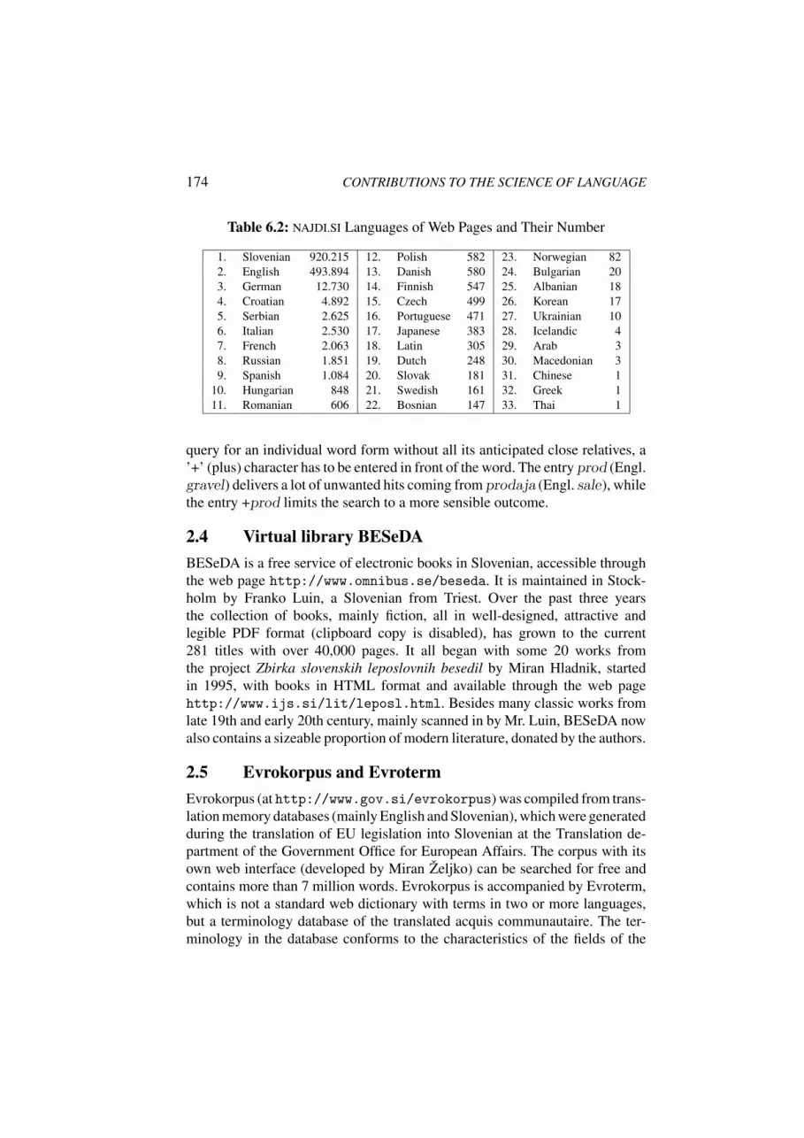
174 CONTRIBUTIONS TO THE SCIENCE OF LANGUAGE
Table 6.2: NAJDI.SI Languages of Web Pages and Their Number
1. Slovenian 920.215 12. Polish 582 23. Norwegian 822. English 493.894 13. Danish 580 24. Bulgarian 203. German 12.730 14. Finnish 547 25. Albanian 184. Croatian 4.892 15. Czech 499 26. Korean 175. Serbian 2.625 16. Portuguese 471 27. Ukrainian 106. Italian 2.530 17. Japanese 383 28. Icelandic 47. French 2.063 18. Latin 305 29. Arab 38. Russian 1.851 19. Dutch 248 30. Macedonian 39. Spanish 1.084 20. Slovak 181 31. Chinese 1
10. Hungarian 848 21. Swedish 161 32. Greek 111. Romanian 606 22. Bosnian 147 33. Thai 1
query for an individual word form without all its anticipated close relatives, a’+’ (plus) character has to be entered in front of the word. The entry prod (Engl.gravel) delivers a lot of unwanted hits coming from prodaja (Engl. sale), whilethe entry +prod limits the search to a more sensible outcome.
2.4 Virtual library BESeDABESeDA is a free service of electronic books in Slovenian, accessible throughthe web page http://www.omnibus.se/beseda. It is maintained in Stock-holm by Franko Luin, a Slovenian from Triest. Over the past three yearsthe collection of books, mainly fiction, all in well-designed, attractive andlegible PDF format (clipboard copy is disabled), has grown to the current281 titles with over 40,000 pages. It all began with some 20 works fromthe project Zbirka slovenskih leposlovnih besedil by Miran Hladnik, startedin 1995, with books in HTML format and available through the web pagehttp://www.ijs.si/lit/leposl.html. Besides many classic works fromlate 19th and early 20th century, mainly scanned in by Mr. Luin, BESeDA nowalso contains a sizeable proportion of modern literature, donated by the authors.
2.5 Evrokorpus and EvrotermEvrokorpus (at http://www.gov.si/evrokorpus) was compiled from trans-lation memory databases (mainly English and Slovenian), which were generatedduring the translation of EU legislation into Slovenian at the Translation de-partment of the Government Office for European Affairs. The corpus with itsown web interface (developed by Miran Zeljko) can be searched for free andcontains more than 7 million words. Evrokorpus is accompanied by Evroterm,which is not a standard web dictionary with terms in two or more languages,but a terminology database of the translated acquis communautaire. The ter-minology in the database conforms to the characteristics of the fields of the

On Text Corpora, Word Lengths, and Word Frequencies in Slovenian 175
EU activities, the purpose of the database and the needs of users, mainly thetranslators. It contains more than 40,000 entries and in April 2003 alone therewere 316,000 queries, which makes Evroterm the second most popular webpage on the Slovenian government server (www.gov.si).
2.6 Electronic Theses and DissertationsThere have been several initiatives to make available, in full text, the academictheses, produced at the end of graduate, master’s and doctoral studies. An ex-ample is an extensive collection at the Faculty of Economics at the Universityof Ljubljana (http://www.cek.ef.uni-lj.si/dela, 1107 titles, it does notinclude doctoral dissertations) with search on meta data and with full text ac-cessible in PDF format. An inter-faculty project with much wider ambitions,involving electronic theses and dissertations, supported by a grant from theMinistry of Information Society, was initiated at the end of 2002 and at thebeginning of 2003. It aimed at establishing the required logistical and softwareinfrastructure for inclusion of all new master’s and doctoral theses in a commondata base with a corpus-like full text search engine and entire texts download-able in PDF format. There are three participating faculties of the Universityof Ljubljana: the Faculty of Medicine, the Faculty of Arts and the Faculty ofMathemathics and Physics. Currently 51 theses are online (44 + 1 + 6); for theFaculty of Medicine the URL is http://pelin.mf.uni-lj.si/ETD-mf.
The awareness that academic production should be readily accessible is gain-ing momentum and probably the best path to take would be to open a way for theauthors to publish their articles and monographs on the web themselves, withoutthe intervention of a librarian and using the existing Co-operative Online Biblio-graphic System & Services (COBISS at the URL http://cobiss.izum.si).The idea has been suggested by Ziga Turk (Turk 2003) and though it is fearedby many it is worth a shot. Democracy can be chaos but it is, however, also themost effective way of doing things.
2.7 NewspapersThere are eight daily newspapers in the Slovenian language, seven publishedin Slovenia and one in Italy. The more important five have a free online pres-ence – not with complete coverage but with a selection of articles availablein full text. DELO is the standard daily with wide reader coverage, it is pub-lished in Ljubljana and a selection of articles is available at the address http://www.delo.si/delofax.php. Dnevnik is the second daily from Ljubljana, aselection of the articles is available at http://www.dnevnik.si; its machine-translated English version, not what one would want, but nevertheless a start, canbe found at http://www.dnevnik.si/eng. Finance, the Slovenian versionof the Wall Street Journal also comes from Ljubljana, has a very neat inter-

176 CONTRIBUTIONS TO THE SCIENCE OF LANGUAGE
net interface and can be checked at http://www.finance-on.net. Vecer ispublished in Maribor, covers the northeastern part of Slovenia and is avail-able at http://www.vecer.si. Primorski dnevnik is published in Triest andcovers the Slovenian readership in Italy; the newspaper is online at http://www.primorski.it.
There are many more weekly (103), biweekly and monthly (587) magazinesin Slovenian and every year a larger number is available online, at least with aselection of articles. One of them is Monitor, a computer magazine with goodcoverage of modern technology, at http://www.monitor.si.
2.8 Other InitiativesThe idea of a complete text corpus which would contain everything publishedin Slovenian, has become technically feasible in the past several years (Jakopin2002). Yearly growth has been estimated to roughly 1.5 billion words (Jakopin2002: serial publications 1.0 billion, monographs 315 million and Internet pagesat 150 million), an amount that could now be processed even on ordinary desk-top computers. A copy of every printed publication is collected and storedby the national and university library (NUK), under an instrument of legaldeposit. As virtually every publication nowadays is printed from a computerfile, i.e. from electronic form, it would only make sense that the NUK wouldalso act as a collector and guardian of those files. An initiative of the NUKfor preservation of texts found on the web has come in the past two years(contribution of Alenka Kavcic-Colic at the Digital library conference – athttp://www.zbds-zveza.si/eng_referati2001.html) and recently alsofor storing the electronic layouts of printed material.
Besides all of the above mentioned text corpora or text collections there arealso a few other, usually much smaller resources gathered by other centers ofresearch in language technology, such as the web concordance service of theDepartment of Intelligent Systems at the Jozef Stefan Institute in Ljubljana,available at the URL http://nl2.ijs.si/index-mono.html.
3. Words, Word LengthsMore often than not, words are the basic units of linguistic research, and wordlengths in particular are a very welcome object in quantitative linguistics (Grzy-bek 2000, 2002). The definition of a word was of no particular importance inclassic works, such as grammars, but in corpus construction, for instance, itcan be a real problem. How far to go, what to treat as a basic (word) token ofa frequency dictionary? The following definitions of the term word representsome standard definitions and/or relevant references:
• “speech, utterance, verbal expression” – The Oxford English Dictionary,1989, pp. 526–531.

On Text Corpora, Word Lengths, and Word Frequencies in Slovenian 177
• “six characters including spaces” – standard use by an editor in a publish-ing house, Rothman, C. 2001: What is a word – http://www.sfwa.org/
writing/wordcount.htm
• “a single unit of language which has meaning and can be spoken or written” –Cambridge International Dictionary of English – http://dictionary.
cambridge.org
• “a group of letters or sounds that mean something” – Cambridge Learner’sDictionary – http://dictionary.cambridge.org
• “a collection of letters indicating a concept” – Goldstein, D. L. (2001): Hy-perflow, hypertextual dictionary –http://www.haileris.com/cgi-bin/dict
• “any segment of written or printed discourse ordinarily appearing betweenspaces or between a space and a punctuation mark, a number of bytes pro-cessed as a unit and conveying a quantum of information in communicationand computer work” – Merriam-Webster 1997
• Di Sciullo, A.; Williams, E. (1987): On the definition of word. Cambridge,Mass.: MIT Press.
Most definitions are close to what one would intuitively expect – a sequenceof letters that can be pronounced and has meaning. In corpus construction, largegroups of tokens also emerge which do not fulfill the above criterion but whichdefinitely have a meaning and which obviously should not be wasted. Usuallythese tokens amount to about 1–2% of the entire lot. The author of these linesdescribed them as wordlike terms and as nonwords; they could be classifiedaccording to the following schemas (examples and frequencies, where given,are taken from the DELO 1998–2000 subcorpus, 47 million running words).
Wordlike terms from DELO 1998–20001. Hyphen-connected termsTop 10:le-ta, crno-bel, slovensko-hrvaski, hrvasko-slovenski, obvescevalno-varno-sten, kmetijsko-gozdarski, cestno-hitrosten, operativno-komunikacijski,ekonomsko-socialen, hat-trick
10 longest:
plesem-v-sandalcih-in-pisanih-hlacah-in-mam-rada-Krizanke-juhu, povelj-nisko-nadzorno-racunalnisko-komunikacijsko-obvescevalen, ta-gospa-pa-ze-mora-znati-nemsko-saj-je-hodila-v-slovensko-gimnazijo, bio-psiho-so-cialno-kulturno-zgodovinsko-ekonomsko-filozofski, gorenjsko-ljubljansko-dolenjsko-notranjsko-belokranjski, sportno-poslovno-loterijsko-medijsko-

178 CONTRIBUTIONS TO THE SCIENCE OF LANGUAGE
oglasevalski, francosko-amerisko-slovensko-judovsko-madzarski, vlada-o-tem-se-ni-razpravljala-bo-pa-v-kratkem, glicidilmetalkrilaten-etilen-dime-takrilaten, mi-si-balkansko-politiko-ze-lahko-privoscimo
2. Words with Parenthesestotal(itar)ne, T(usar), uradni(c)ki, (tragi)komicne, T(wist), U(rbancic),varne(jse)m, T(rakl), (u)branila, urednik(ca), var(ov)al, (trans)estetsko,ucitelja(e), U(ros), V(asja), T(renet), (u)lov, U(senicnik), (vec)vrednosti,T(ul), upa(j)mo, V(alentin), (vele)mestnega, T(urner), (u)porabi, V(alic),velik(a)
3. Incomplete Words.afukala, .aterna, .izda, j..i, k..c, pizd...ije, prapraprapra....predniki, pra-pra... vnuk, p...da, r..i, ...ski, slo...nske, sr...nje, s....a, .urba, zaje...vati..
Hyphen-connected terms can be quite long, the longest is 68 characters long,and in the ten longest there are five writer-invented multiword expressions, fouradjectives, one noun, and a chemical formula. Words with parentheses are eitherexplained abbreviations of names or two words written as one. Incomplete wordswould often look very strange if written without dots, and besides terms such asprapra. . . vnuk (Engl. great-great. . . grandson) they are all part of obscenespeech.
Nonwords from DELO 1998–20001. numbers
1. simple numbers5,400 instances (284,000 total frequency): 0, 1, 2, . . . , 99, 100, . . .33455432112332233455432112321 – Ode to Joy by Ludwig van Beet-hoven (as keyed in for Ericsson GF 768 mobile phone)
2. ordinal numbers1,100 instances (284,000 total frequency): 1., 2., 3., . . .
3. composite numbers 250 instances (cumulative frequency 161.100):6,5, 6:2, 7:5, 2:4, 50.000, 1,3, 1:0, 2:1, 4:6, 0:3, 1:4, 15.000,the longest: 2.235.197.406.895.366.368.301.599.999 – about a groupfrom Ipswich, playing whist
4. number-prefixed adjectives and nouns6,000 instances (total frequency 42.000): -leten (25800), -milijonski(195), -litrski (80), -sekunden (25), -lukenjski (12), -odstoten (8237),-kilometrski (189), -kilovolten (76), -megahercen (25), -obletnica(12), -letnica (1499), -kraten (169), -kilogramski (75), -milijarden(24), -tisocglavi (11), -krat (1150), -minuten (159), -glavi (71), -palcen (24), -km (11), -clanski (692), -oktanski (149), -tonski (62),

On Text Corpora, Word Lengths, and Word Frequencies in Slovenian 179
-tedenski (20), -stranski (11), -metrski (528), -milimetrski (122), -l(45), -megavaten (19), -mesten (10), -m (452), -ti (110), -let (43),-gramski (18), -hektarski (10), -letnik (420), -metrovka (104), -centimetrski (41), -nadstropen (17), -kratnik (10), -dneven (373),-mesecen (103), -biten (32), -karaten (14), -mikronski (8), -urni(304), -kubicen (86), -sedezen (28), -vaten (12), -dolarski (8).
5. times and dates 2,010 instances (total frequency 108.500): 1999, 2000,2000-2006, 15.5.2001
6. ISBN, ISSN, ISO numbers: ISBN 892, ISSN 19, ISO 27 (total frequency1394)
7. UDC (Universal Decimal Classification) classifiers550 instances (total frequency 860): 663.2(035), 666.1/.2 (497.4 Novomesto) (091), 681.3.06(075.2), 681.816.61(497.4):929 Skrabl A.
8. car license plate numbers1000 instances (total frequency 1030): NM 94-83J, LJ LAZE
2. URLs, file names, dotted names2,183 instances (total frequency 2,661): offline@online = Festival of mod-ern electronic art, b.ALT.ica Modern gallery (Ljubljana) project, Mar-cel.li Catalan artist Antunez Roca.
3. e-mail addresses121 instances (total frequency 262):[email protected], [email protected],[email protected], [email protected], [email protected]
4. measures and weights130 instances (total frequency 42,863):m (17885), km (5926), cm (5661),kg (3475), h (2516), Mb (1200), g (774), km/h (716), min (671), l(644).
Nonwords, especially numbers, represent the bulk of what in corpus doesnot fit the standard definition for word and if not treated properly they wouldseriously pollute the word form dictionary; each full URL, for instance, containsat least four strings of letters.
In Table 6.3, the most frequent word forms from three subcorpora of the Novabeseda corpus are shown, the complete works of Ciril Kosmac, probably mostprominent mid-twentieth century writer (0.4 million running words, not muchbut delicately composed, he knew all his works by heart), the complete worksof Ivan Cankar, the paramount master of Slovenian, from the early twentiethcentury (2 million words) and DELO, the main Slovenian newspaper 1998–2000 (47 million words).

180 CONTRIBUTIONS TO THE SCIENCE OF LANGUAGE
Table 6.3: Top 20 Word Forms With Frequencies – C. Kosmac,I. Cankar, DELO
Ciril Kosmac Ivan Cankar DELO 1998–2000
1. je 25.798 je 123.281 je 1 570.4042. in 18.471 in 78.807 v 1 350.6803. se 13.330 se 56.101 in 1 171.3704. v 7.809 v 38.931 na 759.1285. da 5.412 da 34.552 za 656.8146. na 5.124 na 25.983 se 604.6427. pa 4.625 ne 24.117 da 583.3478. so 4.243 so 22.109 so 561.0739. ne 3.695 bi 21.678 ki 510.010
10. bi 3.221 sem 19.675 pa 472.05611. z 3.181 ni 14.182 z 344.91712. ga 3.039 pa 13.796 tudi 332.18713. ki 2.995 kakor 13.528 bi 314.82814. po 2.948 ki 12.741 po 287.91115. sem 2.812 bil 12.469 s 281.80516. ni 2.636 z 12.107 ne 271.77717. s 2.441 se 11.754 bo 251.95118. se 2.410 mi 11.116 se 241.06319. za 2.327 za 10.719 kot 234.45720. tako 2.155 bilo 10.010 ni 190.827

On Text Corpora, Word Lengths, and Word Frequencies in Slovenian 181
As can be expected, no open class word, such as noun, adjective or verb,can be found in any of the above lists, the only exception being je (Engl. is)in the role of auxiliary verb (je bil – he was). There is a remarkable matchbetween the two fiction corpora in the top six places (je, in, se, v, da and na –Engl. is, and, pertaining to oneself, in, that and on). In general there arefour words from the first list which do not show in the DELO column (five fromthe second) and only three words (ga, sem, tako) from the C. Kosmac columnwhich cannot be found in the DELO list.
How various corpora can really be quite different and how it shows in thetop list of nouns can be seen from the Table 6.4. The list of top nouns fromthe British National Corpus has been taken from the standard source (Leech,Rayson & Wilson 2001) and the frequencies are normalized; they are givenper million running words. In the lists of the two fiction subcorpora wordsfrom ordinary life, of communication in romantic circumstances, such as eyes,heart, head, hand or cheek are to be found, while in the newspaper subcorpuswords related to politics, economy and sports are easily recognized. In the BNCcorpus and in the NAJDI.SI web index the origin of top nouns is more difficultto explain. From the table it is also clear that fiction operates with a smallernoun apparatus of higher frequency than is the case in other corpora.
Figure 6.1 presents a distribution of word forms, where every occurrence isaccounted for, for three different units: fiction (white), composed of the Besedasubcorpus (3 million words, includes the complete works of Ciril Kosmac) andthe complete works of Ivan Cankar (2 million words), DELO 1998–2000 (tiledpattern, 47 million words) and NAJDI.SI (black, from the index of March 2002,460 million Slovenian words).
1 2 3 4 5 6 7 8 9 10 11 12 13 14 15 16 17 18 19 20
L
0
5
10
15
20
25
30p(L)%
Fiction
DELO
NAJDI.SI
Figure 6.1: All word forms (Length Frequency Distribution):Fiction, DELO, NAJDI.SI
It is clearly evident that fiction has a much more fluent language, the shareof function class words, most of them two letters long (also see Table 6.3), is29% as opposed to 23% for the newspaper language and 19% for texts from

182C
ON
TRIB
UTIO
NS
TOTH
ESC
IEN
CE
OF
LAN
GU
AGE
Table6.4:Top
20N
ounsFrom
DifferentC
orporaCiril Kosmac Ivan Cankar DELO 1998–2000 BNC NAJDI.SI
1. hand 3, 866 eyes 3, 153 state 1, 906 time 1, 833 article 2, 1072. head 2, 415 heart 2, 739 year 1, 824 year 1, 639 page 1, 6663. eyes 2, 042 face 2, 675 time 1, 394 people 1, 256 day 1, 5264. child 2, 013 hand 2, 620 city, place 1, 309 way 1, 108 year 1, 2675. day 1, 836 man 2, 351 president 1, 167 man 1, 003 work 1, 2526. house 1, 716 word 1, 646 law 1, 022 day 940 world 1, 0737. year 1, 539 life 1, 570 percent 1, 021 thing 776 time 8278. door 1, 314 day 1, 435 day 989 child 710 law 7999. word 1, 258 head 1, 335 end 973 Mr. 673 group 790
10. father 1, 191 people 1, 153 people 921 government 670 contribution 77611. man 1, 110 way, path 1, 134 tolar 860 work 653 system 77312. voice 1, 074 night 1, 123 party (pol.) 796 life 645 city, place 71713. heart 1, 039 Mr. 1, 113 million 789 woman 631 connection 69014. village 1, 015 time 1, 081 group 774 system 619 data item 68015. face 971 cheek 1, 055 minister 744 case 613 school 63816. table 961 road 1, 036 enterprise 737 part 612 community 60817. leg 941 window 1, 023 government 732 group 607 right 60018. life 914 voice 995 case 694 number 606 use 55919. people 905 mother 959 question 694 world 600 court 55820. water 887 table 938 sport match 669 house 598 change 556

On Text Corpora, Word Lengths, and Word Frequencies in Slovenian 183
web pages. It is also interesting that the curve tail peaks at 5-letter words forfiction, 6-letter words for DELO and 4-letter words for the web index. The shareof long words, 14 letters or more, is negligible.
1 2 3 4 5 6 7 8 9 10 11 12 13 14 15 16 17 18 19 20
L
0
5
10
15
20p(L)%
Fiction
DELO
NAJDI.SI
Figure 6.2: Different word forms (Length Frequency Distribu-tion): Fiction, DELO, NAJDI.SI
These trends are further illustrated in Figure 6.2, where word form lengthsare shown with every word form accounted for only once. For fiction the distri-bution curve is fairly regular and peaks at 8-letter words, with 17% share, andtails off quickly to the length of 16. In newspaper texts the shares of 7-letter(peak at 14%), 8-letter and 9-letter words are close enough. This fact may beattributed to the large share of names; the tail diminishes much more slowlyto the length of 20. In the web index the peak is very broad, it stretches from5-letter to 8-letter words, and it remains to be further explored in the future.
In Table 6.5, finally, a brief history of quantitative research, at least in thesize of texts analyzed, is shown.
Table 6.5: Size of Statistically Evaluated Slovenian Texts in Time
year words publication
1962 4.000 Gyergyek (1962)1973 6.000 Gyergyek (1973)1974 60.000 Gyergyek et al. (1974)1980 100.000 Vasle (1980)1994 650.000 Kristan et al. (1994)1995 1.600.000 Jakopin (1995)1998 3.100.000 Jakopin (2002a)2002 512.000.000 this paper

184 CONTRIBUTIONS TO THE SCIENCE OF LANGUAGE
Computers did not really exist in Slovenia before Gyergyek initiated the firstresearch (students counted the letters by hand) with publication in April 1962;the first computer, Zuse Z 23, was installed at the Institute for Mathematics,Physics and Mechanics on November 15, 1962. In the early seventies a quantumleap was achieved with the installation of the CYBER mainframe computer(1971) at the Republic Computing Centre (RRC) and everything seemed withinreach. The disappointment which followed lasted nearly two decades, until themid-nineties when desktop (personal) computers grew to a scale suitable forserious quantitative linguistic research. The adequate system needed to providea detailed analysis of immense text collections such as Slovenian online texts,incorporating a robust part-of-speech tagger and lemmatizer combined witha guesser familiar with an encyclopaedia of names and words in all relevantlanguages besides Slovenian (from English to C++), still does not exist.
4. ConclusionIn this paper a brief overview of what is currently available in the domain ofelectronic text corpora has been given. The situation has moved from very littleto two 100-million-word corpora in the past five years, and further prospectsare open.
The infrastructure which would push word- and word-length studies to theabsolute levels we all strive for is slowly emerging. With the combined effortsof all players and with the wide availability of quantitative resources from majorEuropean languages, such high goals could be achieved in this generation.

On Text Corpora, Word Lengths, and Word Frequencies in Slovenian 185
5. References
Gorjanc, Vojko1999 “Kaj in kako v korpus FIDA?”, in: Razgledi, 13, 23.6.1999; 7–8.
Grzybek, Peter2002 Einflussfaktoren auf die Wortlange und ihre Haufigkeitsverteilung in Texten slawischer
Sprachen. Projekt-Skizze 2002. (29.10.2003)[http://www-gewi.uni-graz.at/quanta/projects/wol/wol_descr.htm]
Grzybek, Peter2000 “Pogostnostna analiza besed iz elektronskega korpusa slovenskih besedil”, in: Slavisticna
revija, 48(2); 141–157.Gyergyek, Ludvik
1962 “Nekateri stavki iz teorije o informacijah in srednja vrednost informacije na crko slovenskeabecede”, in: Avtomatika, III/april; 74–80.
Gyergyek, Ludvik1973 “Prispevek k statisticni obdelavi slovenskega pisanega besedila”, in: Elektrotehniski vest-
nik, 40/11-12; 247–252.Gyergyek, Ludvik et al.
1974 “Prispevek k statisticni obdelavi slovenskega jezika”, in: Raziskovalna naloga 122; Fakul-teta za elektrotehniko, Ljubljana.
Jakopin, Primoz2003 “O spletnih virih slovenskega jezika, tretjic”, in: DELO, 19.5.2003; 14.
Jakopin, Primoz2002 “The feasibility of a complete text corpus.” In: Proceedings of LREC 2002 International
Conference, Vol. II. Las Palmas. (437-440).Jakopin, Primoz
2002a Entropija v slovenskih leposlovnih besedilih. Ljubljana.Jakopin, Primoz
2000 “Beseda: a Slovenian text corpus.” In: Fraser, M.; Williamson, N.; Deegan, M. (eds.),Digital Evidence: selected papers from DRH2000, Digital Resources for the HumanitiesConference. University of Sheffield, September 2000. (229–241).
Jakopin, Primoz1995 “Nekaj stevilk iz Slovarja slovenskega knjiznega jezika”, in: Slavisticna revija, 43/3; 341–
375.Kristan, Blaz et al.
1994 “Entropija slovenskih besedil”, in: Elektrotehniski vestnik, 61/4; 171–179.Leech, Geoffrey; Rayson, Paul; Wilson, Andrew
2001 Word Frequencies in Written and Spoken English: based on the British National Corpus.London.
Turk, Ziga2003 “Zalozniki postajajo ovira”, in: DELO, 5.5.2003; 12.
Vasle, Tomaz1980 Statisticna obdelava slovenskega besedila. Diplomska naloga. Fakulteta za elektrotehniko,
Ljubljana.


Peter Grzybek (ed.): Contributions to the Science of Language.Dordrecht: Springer, 2005, pp. 187–197
TEXT CORPUS AS AN ABSTRACTDATA STRUCTURE
The Architecture Of a Universal Corpus Interface
Reinhard Kohler
1. IntroductionLinguistic corpora have become one of the most important sources of evidencefor empirical scientists in a number of disciplines connected with the study oflanguage, language behaviour and text. Consequently, the methods of compilingand analysing text corpora play a central role for data acquisition, observation,and the testing of hypotheses, as well as for inductive, heuristic attempts suchas data or text mining. In linguistics, corpus linguistics has become establishedas an academic branch and many researchers consider themselves, in the firstline, as corpus linguists. The number of publications in this field is increasingcontinuously, their topics varying from purely notational questions about the useof mark-up languages over corpus classifications, directives for the compilationof corpora, and individual empirical studies using corpora, to methodologicaland mathematical text books on quantitative text analysis. However, there is onevery practical, technical aspect which has not yet been approached until know(to my best knowledge) although is bears far-reaching consequences for thework with corpora. The following considerations, which deal with this aspect,are based on theoretical work and practical experience in the field of softwareengineering in computational, quantitative, and corpus linguistics.
The compilation of a linguistic corpus is connected with a large amount ofpreparational thought and work, depending on the purpose of the corpus. Wecan distinguish three types of corpus compilers:
1. The researcher who needs the corpus for a specific investigation and cannotfind another suitable data source;
2. the researcher who needs appropriate data for empirical studies and thinksthat other scientists will probably need similar data;
3. the academic who considers corpus compilation as a good idea and hopesthat other colleagues will find his corpus useful for this or that purpose.

188 CONTRIBUTIONS TO THE SCIENCE OF LANGUAGE
The effort involved in the task of corpus compilation justifies some additionalthought and work in order to guarantee that as much use as possible can be madeof the result:
(a) The use of a corpus which has been set up by others is also connected witha lot of thought and work, and this effort should be minimized if possible;
(b) it would be a shame if someone had to redo all the work because of a tinydetail of a given corpus preventing him from using it for his own purpose.
A frequently found problem is the less-than-optimal conservation of originaldata (in short: annihilation of information). An illustrative example is a corpuscompiled by, say, a linguist who has access to data he receives from a newspaperpublisher in the form of the daily typeset tapes. These tapes contain all the textincluding some ‘strange’ control characters for positioning and layouting thetext portions. As a rule, our linguist will remove all these strange and ‘useless’control characters from the data stream when forming his corpus. As a con-sequence, a researcher interested in problems of content analysis, who wouldneed information about position and size of the newspaper articles – exactlythe information which was, among others, hidden in the ‘strange’ characterstrings – cannot use our linguist’s corpus.
From an a posteriori point of view of a potential user of the corpus, theabove method of preparing a corpus is hardly comprehensible – a lot of workhas been done with the result that valuable data have been destroyed. On theother hand, we would have to admit two things:
(1) Our linguist did not have the faintest idea that what he removed could havebeen of any interest to anyone, and if he did, he would never know whetheranyone would ever want to use it.
(2) The simplified version of the corpus is much more transparent and moreefficient with respect to his own purposes because corpus inspection be-comes easier, and the computer programs for analysing the data do not haveto cope with possibly complicated technical details which do not contributein any way to the solution of the problem under consideration.
However, the more optimized a corpus is with respect to a given task (notonly in a purely technical sense) the harder it is to use for purposes other thanfrom the original one.
Clearly, there are much more less extreme technical questions to be con-sidered before setting up a corpus, and a lot of these questions are discussedat length in the literature: Which of the currently popular mark-up languages(such as SGML, HTML, XML,. . . ) should be used (if any), the choice of one of themost prominent morphological tag sets, the pros and cons of document repre-sentation systems (PDF), and many others. Moreover, there is a large variety of

Text Corpus As an Abstract Data Structure 189
formats (document structures) in which the texts can be presented: Plain textwith marks to separate individual texts, text with annotations (such as part ofspeech information assigned to the words, syntactic trees in form of labelledbrackets or in form of indented lines, files with a line structure where each linecontains just one running word together with annotated data, files which con-tain plain texts accompanied by annotation files, referenced by position or withpointers from the annotations to the linguistic items). There are always goodreasons to select among the possibilities, depending on the given circumstancesand on the purposes.
Furthermore, every corpus has certain technical characteristics which are,in general, not at the disposal of the persons that compile the corpus: operationsystems, file systems, character codes (such as ASCII, EBCDIC, Unicode, to namea few of the contemporarily most common ones), place of storage and accessmethods (the corpus may consist of one large file or of thousands of files, itmay be distributed over several computers in a network or reside on a singleCD-ROM. The technical representation may even change dynamically).
What is rarely seen is the fact that virtually every possible feature becomesrealized with a number of corpora and, as a consequence, users who want to use,and authors of analytical software meant to work with, more than one specificcorpus are confronted with a wide spectrum of structures and technical details –every corpus is a special case. To make things even worse, whenever a designfeature or a technical detail of a corpus has to be changed, all the computerprograms which are supposed to work on the data have to be changed, too.
Surprisingly, not much attention is paid to these kinds of problems althoughstandard solutions are available. It is the purpose of the present paper to proposesuch a solution.
2. Abstract data types and abstract data structuresLet us consider a much simpler example: the programming task of calculatingthe sum of two numbers. To perform this task, in the early days of computertechnology, a programmer had to know where the corresponding numbers werestored in the computer’s storage (in which register or index cell, or the addressin the core memory or elsewhere), and how it was represented on the givencomputer (e.g. four bytes for the mantissa and one for the exponent in a certainsequence, where two specific bits represent the signs of mantissa and exponent,others care for error detection etc.; which nibble (half-byte) counts as high andwhich as low; how many bytes make a machine word; which is the high/lowsequence of the bytes in a word; which access methods to bytes and/or machinewords are available etc.). Only with this information was it possible to write aprogram for adding the corresponding numbers. Later, programming languagessimplified this task considerably. Operators such as addition (symbolized in

190 CONTRIBUTIONS TO THE SCIENCE OF LANGUAGE
most cases by the ‘+’ sign) were introduced, which could be used withoutknowing any details of the machine representation of the operands. It is a gooddesign principle of a programming language if it prevents programmers fromknowing how the operands are represented on the given machine and howthe algorithm which realizes the operator works. In software engineering, thisprinciple is called information hiding, and many good reasons support thisprinciple. The two most important ones are:
1. If you do not have to know the details when formulating your program,because the programming language takes care of these details, then yourprogram will run on every computer hardware and with all existing and futureoperating and file systems in the world where the programming languageyou used is available.
2. Information hiding prevents the programmer from making assumptions onspecific representations and other technical details, which – if used in analgorithm – would cause errors in a different environment.
A further improvement is the introduction of data types in programminglanguages, which make sure that a programmer does not compare apples withpears or multiply a number with a character. Each operator is defined withrespect to its possible operands (arguments) and with respect to the propertiesof its result. Modern programming languages enable the programmer to definehis own operators in the form of functions or procedures.
Teachers of programming style emphasize that one should use proceduresand functions also in order to improve program structure (readability, change-ability, and other software quality criteria) and to write code that is re-usable.A procedure that has been written for, say, finding the maximum value in a listof numbers or for sorting a list according to a given criterion can be used notonly for the program it has been written for originally, but also for numerousother programs where a similar task occurs – if the corresponding procedurehas been designed in a general enough way.
Re-usability is the main concern of abstract data structures (ADS) and ab-stract data types (ADT), which go a step further: They enable the programmerto define not only operators on the basis of predefined data types but even tocreate their own data types together with possible operations. What is specialabout ADS and ADT is that the implementation details are hidden: They consistof an object together with the corresponding access procedures in the case ofan ADS and of a class of objects in the case of an ADT. The latter allows to cre-ate more than one data item of the given type during runtime. Let us considerthe following example. Many complex data structures are rather common butin the framework of traditional programming techniques, every programmerwrites his own code for, say, a matrix, a stack, or a tree each time he needs one
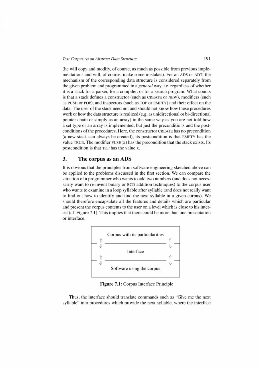
Text Corpus As an Abstract Data Structure 191
(he will copy and modify, of course, as much as possible from previous imple-mentations and will, of course, make some mistakes). For an ADS or ADT, themechanism of the corresponding data structure is considered separately fromthe given problem and programmed in a general way, i.e. regardless of whetherit is a stack for a parser, for a compiler, or for a search program. What countsis that a stack defines a constructor (such as CREATE or NEW), modifiers (suchas PUSH or POP), and inspectors (such as TOP or EMPTY) and their effect on thedata. The user of the stack need not and should not know how these procedureswork or how the data structure is realized (e.g. as unidirectional or bi-directionalpointer chain or simply as an array) in the same way as you are not told howa set type or an array is implemented, but just the preconditions and the post-conditions of the procedures. Here, the constructor CREATE has no precondition(a new stack can always be created); its postcondition is that EMPTY has thevalue TRUE. The modifier PUSH(x) has the precondition that the stack exists. Itspostcondition is that TOP has the value x.
3. The corpus as an ADSIt is obvious that the principles from software engineering sketched above canbe applied to the problems discussed in the first section. We can compare thesituation of a programmer who wants to add two numbers (and does not neces-sarily want to re-invent binary or BCD addition techniques) to the corpus userwho wants to examine in a loop syllable after syllable (and does not really wantto find out how to identify and find the next syllable in a given corpus). Weshould therefore encapsulate all the features and details which are particularand present the corpus contents to the user on a level which is close to his inter-est (cf. Figure 7.1). This implies that there could be more than one presentationor interface.
Corpus with its particularities⇑ ⇑⇓ ⇓
Interface⇑ ⇑⇓ ⇓
Software using the corpus
Figure 7.1: Corpus Interface Principle
Thus, the interface should translate commands such as “Give me the nextsyllable” into procedures which provide the next syllable, where the interface

192 CONTRIBUTIONS TO THE SCIENCE OF LANGUAGE
has the knowledge of how to find and identify the next syllable in the givencorpus whereas the software using it has not. In general, the interface shouldoffer access procedures which can pass all the items the corpus contains to theusing program, i.e. units and categories, together with annotations if available.On the string level, character strings (separated by spaces or interpunction)should be accompanied by information on the separators, on the characters(upper/lower case), font, size, and style (bold, italics, . . . ), position of the string(relative to sentence, paragraph, text) etc. – everything that is either explicitlyannotated in the corpus or can easily be inferred by the interface software.Similarly, on the syllable, morph(eme), word, phrase, sentence etc. levels, alllinguistic or typographical (or other) information should be passed as a valueof a complex procedure parameter.
The corpus interface should be made bi-directional, i.e. there should also beprocedures that allow to write annotations (provided the linguistic applicationprogram has the corresponding rights). In this way, the linguistic applicationprogram (which could be, e.g. an interactive editor for manual/intellectual an-notations as well as an automatic tagger or parser) would not have any informa-tion about the way in which the annotations are stored (in analogy to the lackof knowledge when reading from the corpus).
A basic function of the interface is the procedure which tells the linguisticapplication program which facilities, categories, items, annotations are availablein the given corpus version, the alphabet used, special symbols, limitations etc.
Finally, the question remains where the interface gets all that informationfrom. Clearly, the information should not be hard coded in the interface software.The disadvantages are obvious: The interface software would have to be changedand re-compiled for every corpus it is used with, and for every change whichis made to a corpus. Moreover, numerous versions of the interface softwarewould result, of which only one would work with the corresponding corpuswhile others would yield errors or, worse, provide incorrect data.
Therefore, an independent corpus description is needed: a file which containsthe information about the corpus, including which files it consists of, wherethey can be found, and how accessed. The best way to describe the corpusfor the interface module is to use a formal language, which should be a LL(1)language. Such languages possess properties which make them particularly easyto parse (cf. Aho et al. 1988; Mossenbock/Rechenberg 1985; Wirth 1986). Thedescription must be set up together with the corpus by the corpus compiler.The overall architecture of the interface technique proposed here is shown inFigure 7.2.
In the appendix (cf. p. 195ff.), an example of a formal description of a corpuscan be found – in this case, a dictionary of Maori with data for quantitativeanalysis.

Text Corpus As an Abstract Data Structure 193
Corpus description
(formal grammar)Corpus
interface
software
managesdescribes
interprets
Access procedures
Corpus analysing software
imports and uses
File 8
File 2
File 1 File 6
File 4
File 3
File 7
File 5
Computer 1
Computer 84
Computer 5 Computer 91
Corpus
provides
Figure 7.2: The Architecture of a Corpus Interface

194 CONTRIBUTIONS TO THE SCIENCE OF LANGUAGE
References
Aho, Alfred; Sethi, Ravi; Ullman, Jeffrey D.21988 Compilers. Principles, Techniques, and Tools. Reading.
Mossenbock, Hanspeter; Rechenberg, Peter1985 Ein Compiler-Generator fur Mikrocomputer: Grundlagen, Anwendung, Programmierung
in Modula-2. Munchen.Wirth, Niklas
41986 Compilerbau. Stuttgart.

Text Corpus As an Abstract Data Structure 195
AppendixA Maori dictionary descriptionusing a formal LL(1) language
&Language = "maori"
&Columns
&Separator = ';'
&Column 1
&Name = "Phonological transliteration of the lemma"
&Characters = {'a','e','h','i',chr(231),'k','m','n','o','p','r',
't','u','w','A','E','H','I','K','M','N','O','P','R','T','U','V',
'W','X','#','(',')','-','=','/','.','1','2','3','4','7','9','0'}
&Value range = {"a","e","h","i","k","m","n","o","p","r","t","u",
"w","A","E","H","I","K","M","N","O","P","R","T","U","V","W","X",
"#","(",")","-","=","/",".","1","2","3","4","7","9","0","II","III",
"IV","VI","VII","VIII","IX","(1)","(2)","(3)","(4)","(7)","(9)",
"(0)"}
&Column 2
&Name = "part of speech"
&Character = {'a','c','d','e','g','i','j','l','m','n','o','p','r',
's','t','u','v',','}
&List separator = ','
&Value range = {"a","ad","adv","c","conj","int","l","loc","m","n",
"num","pe","pr","pron","pt","ptg","ptm","ptmod","ptv","rp","st",
"u","v"}
&Column 3
&Name = "Inflectional paradigm"
&Characters = {'0','1','2','3','4','5','6','7','8','9'}
&List separator = ','
&Value range = [0..12]
&Column 4
&Name = "Morphological status"
&Characters = 'c','d','e','f','i','n','o','q','r','s','t','u','z'
&Value range = {"c","cd","cdr","ced","cr","crd","crqint","ct","d",
"dc","dcr","de","dr","drc","drd","dt","f","n","o","r","rc","rcd",
"rd","ru","rz","s","se","sr","t","u","uc","ur"}

196 CONTRIBUTIONS TO THE SCIENCE OF LANGUAGE
&Column 5
&Name = "Function"
&Characters = 'a','b','c','d','e','f','g','i','l','m','n','o','p',
'q','r','s', 't','u','v','x','-','+','2'
&Value range =
{"an","al","crint+","dem","dempl","demplur","detplur","dur","ex",
"fr","freg","ftu-","fut","fut+","gn","gnfut","gnplur","gu",
"inr+","int","int+","int-","intfr","intfreg","intr","intr+2",
"intchr(374)","n","ndet","neg","nom","nposal","nprep","pers",
"persposs","perssing","plur","plurposs","posalpl","poss",
"possalpl","possalplur","possplural","prep","q","qu","rec",
"recfreg","recint+","red","rep","restr","s","sim","simint-",
"st","tr","ubt+","v","vb","verb","vimp"}
&Column 6
&Name = "Number of meanings"
&Characters = '-','0','1','2','3','4','5','6','7','8','9'
&Value range = [1..23]
&Column 7
&Name = "Style characteristics"
&Characters = {'a','c','d','g','h','i','l','m','n','o','p','r',
's','t','u','w','z','(',')','/'}
&Value range = {"a","c","col","d","d(po)","d(tahu)","d(tu)",
"d/rau/","d/si/","d/tah/","d/tahu/","d/whang/","dngi","doz",
"dpo","drar","dtahu","dtai","dtu","dwha","l","m","mod","p"}
&Column 8
&Name = "Lemma length"
&Characters = {'0','1','2','3','4','5','6','7','8','9'}
&Column 9
&Name = "Syllable number"
&Characters = '0', '1', '2', '3', '4', '5', '6', '7', '8', '9'
&Column 10
&Name = "Mean syllable number"
&Characters = '.','+','e','0','1','2','3','4','5','6','7','8','9'
&Column 11
&Name = "Morpheme number"
&Characters = '0','1','2','3','4','5','6','7','8','9'
&Column 12
&Name = "Mean morpheme number"
&Characters = '.','+','e','0','1','2','3','4','5','6','7','8','9'

Text Corpus As an Abstract Data Structure 197
&Files = "D:\dictionaries\maori\"
"maori11k.lex"
"maori11t.lex"
"maori1k.lex"
"maoria1.lex"
"maorif1.lex"
"maorig1.lex"
"maorih1.lex"
"maorii1.lex"
"maorip1.lex"
"maorir1.lex"


Peter Grzybek (ed.): Contributions to the Science of Language.Dordrecht: Springer, 2005, pp. 199–210
ABOUT WORD LENGTH DISTRIBUTION
Victor V. Kromer
The author of the present paper earlier proposed a mathematical model of wordlength based on the Cebanov-Fucks distribution with equal distributions ofthe parameter (Kromer 2001). The Cebanov-Fucks distribution is the knownPoisson distribution when the obligatory (first) syllable is not taken into account:
px =(λ0 − 1)x−1
(x− 1)!e−(λ0−1) x = 1, 2, 3, . . . (8.1)
The parameter λ0 of the model is the average word length in the text, whichis determined by the formula:
λ0 =1
N
N∑
i=1
xi =1
N
∞∑
x=1
nxx , (8.2)
where N is the text size measured by the number of word occurrences, xi isthe word length of the i-th word, measured in syllables, and nx is the numberof words having length x. In Fucks’ model the only parameter λ0 is strictlydetermined by the text, i.e., the Fucks model does not contain fitting parameters.
It has been suggested, that Fucks’ model would be more flexible, if thetext would be parted into groups of words with equal mathematical expectationof word length, and word length distribution would be calculated separatelyfor each word group in accordance with formula (8.1) and subsequent addingof separate particular distributions based on their weights. The text might beparted, for example, into groups of words with equal frequency, polysemy,age etc. To construct a model, it is nessary to know the dependence of wordlength on the chosen group characteristic in the text. The most investigatedare the frequency distributions (in the form of the frequency spectrum andrank-frequency distribution) and the dependence of the word length from thefrequency or rank. Let us construct a model on the base of these dependencies.The model construction has been detailed in (Kromer 2001).
Let us repeat in brief the main course of considerations. Let us order textwords according to the decreasing frequency, giving each word a number i from

200 CONTRIBUTIONS TO THE SCIENCE OF LANGUAGE
1 to N , where N stands for text size in running words. Supposing that Zipf’slaw (8.3) holds true
Fr =kN
r, (8.3)
whereFr is frequency of the word with rank r, and k is parameter, the followingrelation holds:
i =r∑
m=1
Fm = kNr∑
m=1
1
m= kN(ψ(r + 1) + C) ≈ kN(ln r + C) , (8.4)
where m are the numbers of natural order, and C = 0.5772 . . . is Euler’sconstant. An average word length dependence in function from the rank isknown:
x = d1 + d2 ln r , (8.5)
where d1 and d2 are coefficients. This dependence has been verified empiricallymore than once. Some authors deduce it from theoretical considerations. Ara-pov (1998: 123) deduces this formula for written Russian from the followinghypothesis:
i) the number of places in the word structure is directly proportional to thecubic root of the word rank;
ii) the probability of filling the place in the word structure with a unit-syllableis related to the number of the place (the number of the place is not relatedto the spatial orientation in the unity-word).
The mentioned probabilities, arranged in a non-increasing order, are inverseto the numbers of natural order. Substituting the member ln r in (8.5) by the samemember from (8.4), and designating the coefficient of word coverage of the textin word successive appearance in the word frequency list asQi = i
N , we obtain(after some transformations) that there exists a linear dependence between xandQi. The parameter λ0 in (8.1) should be replaced by the variable parameterλ = λ1 + (λ2 − λ1)Qi , where Qi is uniformly distributed on [0, 1], and λ1
and λ2 are the mathematical expectations of word length correspondingly at thebeginning and the end of the rank frequency list. By integrating the obtainedexpression in limits of 0 to 1 on dQi, and after replacing the variables for thesought for expression for px, we obtain
px =1
λ2 − λ1
(e−(λ1−1)
x∑
t=1
(λ1 − 1)t−1
(t− 1)!−e−(λ2−1)
x∑
t=1
(λ2 − 1)t−1
(t− 1)!
)
(8.6)

About Word Length Distribution 201
with the support x = 1, 2, 3, . . ..The obtained expression is the known Poisson uniform or Bhattacharya-
Holla distribution (Wimmer/Altmann 1999: 524f.). Since the average wordlength throughout the text λ0 is equal to λ0 = (λ1 + λ2)/2, the values λ2
and λ1 are related by the dependence λ2 = 2λ0−λ1. The value of λ0 is strictlydetermined by the text (formula 8.2), and there exists only one fitting parameter(λ1), fitted in order to obtain better agreement between theoretical and empiri-cal data. The monotonically increasing x(r) dependence reflects the synergeticregulation of language. Ideally, the word length dependence from word rank isconsistent with a language without redundancy:
Gr ≈ logG r =1
lnGln r
where G stands for the number of letters in the alphabet (cited from Leopold1998: 225); there are no restrictions on letter combinability, all possible lettercombinations are realized in the language lexicon. We are thus concerned witha language with equal probabilities of all letters and language optimal organi-zation, which means that the shortest words are the most frequent ones and viceversa.
Let us make the supposition that the synergetic organization of the languageis carried out on a certain abstract “language as a whole”. The frequency dic-tionaries, on the base of which theoretical dependencies are constructed andverified, are representative of a concrete sublanguage (language of a particulartext corpus, author or text). The optimum relations between word length andword rank are broken on such dictionaries, as word ranks in the dictionariesof the sublanguage and the language as whole do not match, which leads toretaining the value of λ0 to λ1-value increasing and λ2-value decreasing. In thecase λ1 = λ0 = λ2, the dependence (8.6) degenerates into dependence (8.1).This case corresponds to the assumption (used as the base for dependence (8.1))that the word has a certain average length in the given language, not dependingon its frequency. It seems that a language (sublanguage) with such a degenerateword distribution is synergetically chaotic to a larger extent. However, there ex-ist languages with larger degrees of chaos. Such languages can be described bythe dependence (8.6), with parameter values λ1 and λ2, equal to λ1 = λ0 − igand λ2 = λ0 + ig, where g is a certain positive real number, and i =
√−1 is
the imaginary unit. With such conjugate complex values of parameters λ1 andλ2, the values of px are nevertheless real, and the range of the model feasibilityextends.
The question arises about lower limit of λ1-value. If the ideal Mandelbrot’sdistribution x(r) of the word length in the dependence of word rank is realized,which means stepped distribution with step height of unity and equal stepslength (in log scale), the graph of linear dependence of type (8.5), approximating

202 CONTRIBUTIONS TO THE SCIENCE OF LANGUAGE
stepped distribution, cuts the middles of horizontal steps, which results in λ1 =0.5. Considering that the text with the minimum value with λ1min
is totallysynergetically regulated, and the text withλ1 = λ0 value is totally synergeticallydisordered, a possibility occurs to introduce the parameter
α =λ0 − λ1
λ0 − λ1 min, (8.7)
which is the coefficient of completeness of synergetic processes of linguisticcode optimization. For real values of parameter λ1, the values of α are in therange of 0 ≤ α ≤ 1, for complex values of λ1, the values of α are imaginary.
There exists another variant of describing the empirical distribution in theway of composition of two distributions of type (8.6) with α = 1 (with corre-sponding λ1 = 0.5) and α = 0 (with corresponding λ2 = λ1), which meanspx(β) = βpx|α = 1|+ (1−β)px|α = 0|. The model parameter β ∈ (−∞, 1).Now find out, in which way the parametersα andβ of a mixed text are dependentof the same parameters of constituent texts.
We took data from two newspaper texts in Austrian-German from the paperby Best (1997a). Texts #2 and #4, as the most diverging ones according tothe results of parameterization done by Best (1997), are chosen. The results ofthe parameterization of the original texts and the mixed texts are given in theTable 8.1.
Table 8.1: Parameters of the Original Texts #2, #4, and of themixed text #2+4
Text N λ0 λ1 α α∗ β β∗
Text 2 770 1.996 1.211 0.515 – 0.223 –Text 4 621 2.222 0.794 0.829 – 0.668 –Text 2+4 1391 2.081 0.990 0.690 0.655 0.448 0.422
The defined values of parameter λ1 for texts #2 and #4 slightly differ fromthose for the same texts, defined by Kromer (2001: 93). The difference can beassigned to use of a different (modified) χ2-criterion.
As α∗ and β∗ are designated weighted (in accordance with the sizes ofconstituent texts) average parameters of the corresponding parameters, so
α∗2+4 =α2N2 + α4N4
N2 +N4,
where α2 and α4 are values of parameter α for texts correspondingly #2 and#4, and N2 and N4 are the sizes of corresponding texts in running words.Comparison of α2+4 with α∗2+4 and β2+4 with β∗2+4 reveals that the measured

About Word Length Distribution 203
values are greater than the weighted means for both parameters. With the aimof revealing the possible reason for this let us switch from real texts to modelledtexts with controlled values of parameters.
Let us model four texts A, B, C and D of equal size N with given values ofparameters λ0 and β (Table 8.2), where nx stands for number of words in themodelled texts of the given size x (measured in syllables).
Table 8.2: Data on modelled texts A, B, C and D
Text N λ0 β x
1 2 3 4 5 6 7 8 9
nx
A 1000 2.000 0.100 383 349 182 63 17 4 1 0 0B 1000 2.000 0.900 507 198 164 78 34 13 4 1 0C 1000 1.500 0.500 660 218 93 22 6 1 0 0 0D 1000 2.500 0.500 314 253 214 120 58 25 11 4 1
The results of parameterization of all four modelled texts and two mixedtexts (A+B) and (C+D) in the context of the investigated model are given inTable 8.3.
Table 8.3: Parameters of modelled texts A, B, C and D and mixedtexts (A+B) and (C+D)
Text N λ0 λ1 α α∗ β β∗
A 1000 2.000 1.529 0.314 – 0.100 –B 1000 2.000 0.562 0.959 – 0.900 –C 1000 1.500 0.778 0.722 – 0.500 –D 1000 2.500 1.026 0.737 – 0.500 –
A + B 2000 2.000 0.906 0.729 0.637 0.500 0.500C + D 2000 2.000 0.688 0.875 0.730 0.740 0.500
The comparison of weighted parameters α∗ and β∗ with measured parame-ters α and β for the mixed text (A + B) allows us to come to the conclusion thatparameter β unlike parameter α normally has an additive function on texts withthe same word length. The same comparison for mixed text (C + D) reveals theviolation of parameter β additivity on texts with different average word lengthin the direction of parameter β increasing.

204 CONTRIBUTIONS TO THE SCIENCE OF LANGUAGE
Considering that parameterλ0 depends on text topic, the increase of parame-ter β for the mixed text, composed from model texts with different average wordlength λ0 can be explained by increasing thematic variety of mixed texts, whichcounts in favor of defining β as a parameter, reflecting the degree of synergeticregularity in the text (the mixed text is closer to the “language as a whole”, assingle texts). Earlier, Polikarpov (personal communication, november 2001);suggested in the course of model discussion that parameter α expresses genrediversity of the text. As parameters α and β are directly related, this suggestionis supported.
Parameter α, calculated using formula (8.7), is an imaginary number withcomplex values of λ1 and real value of λ0. For the same texts β is a realnegative number. If α is positive (for real values of λ0), β is positive too. Afteranalyzing many pairs of values of parameters α and β, a statistical relationbetween parameters α ≈ √β is revealed, which is valid both for positive andfor negative values of β.
Data on 28 typologically different ancient and modern languages were pro-cessed in order to test the model checking and to reveal possible regularities.For some languages, data were processed for texts of different genres (styles).It was revealed that there exists a direct dependence between parameters λ1
and λ0 for single-genre texts. The dependence λ1(λ0) for six European lan-guages, and the most consistently represented in the available data genre ofletters, is reflected in the graph Figure 8.1 (points 1–16). The correspondingdata concerning processed mixed samples are given in the Table 8.4 (p. 205).
The trend line, described by the equation λ1 = 0.40 + 0.35λ0, is drawnthrough the points 1–16 (excluding point 7). The processed material does notinclude Luther’s letters. The Latin phrases occurring in them lead to sharpdeviation of the word structure from the general tendency, in particular the λ1-value is overstated. The determination coefficient is equal toR2 = 0.38. Let uscalculate coefficient α for the points of the trend line (we consider λ1min
to beequal to 0.5).
α =λ0 − λ1
λ0 − 0.5=λ0 − 0.40− 0.35λ0
λ0 − 0.5= 0.65− 0.075
λ0 − 0.5
The analysis of the obtained expression permits to conclude thatα is constantfor the chosen genre of letters, at least for the processed six modern languages.At the same time this simple relation breaks for languages of the synthetic type,not belonging to German or Roman language groups, as well as for other Indo-European languages, where α-values tend to be zero or to become imaginary.
A dependence between the values of the parameters λ1 and λ0, as reflectedby the formula I = (λ0 − 1)(λ1 − 0.5) – where I is a certain constant, equalto 0.36 – is determined for the German language: here exists an inversely pro-portional dependence between the values of λ0 and λ1, shifted at 1 and 0.5

AboutW
ordLength
Distribution
205
Table8.4:Param
etersof26
mixed
textsin
sixlanguages
Point number Language Sample N λ0 λ1 α β
1 English Letters 6480 1.368 0.753 0.709 0.4772 English Sidney’s letters 4459 1.370 0.845 0.604 0.3383 English Austin’s letters 5610 1.383 0.824 0.633 0.3744 German Durer’s letters 7255 1.467 1.077 0.403 0.1525 French Letters 9572 1.484 0.874 0.620 0.3636 German Tucholsky’s letters 12531 1.605 1.003 0.544 0.2607 German Luther’s letters 8471 1.618 1.618− 0.189i −0.019
0.211i8 Swedish Ekelof’s letters 6876 1.685 0.968 0.605 0.3259 German Lichtenberg’s letters 4028 1.687 1.161 0.443 0.18310 German Lessing’s letters 7215 1.693 1.148 0.456 0.19111 German Letters 10031 1.757 0.946 0.645 0.38312 German Hoffmann’s letters 5014 1.770 0.925 0.665 0.41613 German Behaim’s letters 5163 1.901 1.100 0.572 0.30514 Spanish Mistral’s letters 10444 1.901 1.168 0.523 0.25215 Spanish Lorca’s letters 5503 1.993 1.042 0.637 0.37916 Italian Pasolini’s letters 5848 2.045 1.003 0.674 0.426
17 German Low German texts 7121 1.391 0.829 0.630 0.37318 German Luther’s songs and fables 6016 1.420 1.241 0.195 −0.00119 German Middle High German texts 13728 1.448 1.358 0.095 −0.00720 German Baroque Poetry 12638 1.454 1.273 0.190 0.03121 German Children’s textbooks 7286 1.524 1.209 0.307 0.05722 German Children’s textbooks 8517 1.679 1.052 0.532 0.24723 German Old High German Poetry 2159 1.708 1.708− 0.275i −0.115
0.332i24 German Texts 18425 1.914 0.877 0.733 0.51325 German Biology 19174 1.995 0.851 0.765 0.55626 German Press texts 9583 2.080 0.825 0.795 0.617

206 CONTRIBUTIONS TO THE SCIENCE OF LANGUAGE
correspondingly, i.e. counted off from their lowest possible values. Hence I isan invariant of the German language and does not depend on the text genre.The points of this dependence and the line of hyperbolic trend are also plottedin Figure 8.1.
Figure 8.1: The dependencies λ1(λ0) and I(λ0)
The trend line is drawn through all points, related to German texts (Table 8.4,p. 205), excluding Luther’s letters (point 7), Low German texts (point 17) andOld High German texts (point 23). Points 7 and 23 with complex values of λ1
do not belong to the graph of Figure 8.1 (one more coordinate axis is neededfor adequate mapping). The coefficient of determination is equal to 0.95. Forother languages from the six listed, the value of I changes from 0.11 (Englishlanguage) to 0.53 (Italian language) and reflects the degree of language syn-theticity. The invariance of I-value, i.e., its independence of the genre, needsto be verified for those languages on the basis of additional material.
Of special interest is the comparison of α (or β) values for texts of differentgenres of the same language. A general rule can be observed: the values ofthose parameters increase when passing from simple genres to sophisticatedones. So, for the genre of Children’s textbooks in German α ≈ 0.30 − 0.53,for the genre of letters α ≈ 0.60, for scientific and journalistic texts α ≈ 0.80.At the same time low and zero values of α (sometimes even imaginary ones)are characteristic for ancient texts. Old High German and Middle High Germantexts are satisfactorily described by Poisson’s distribution (Best 1997b), whichis a special case of the distribution under consideration at α = 0.
The historical dynamics of structural reorganization of modern languages areof special interest. Such reorganization could be represented as the movementof a point in a multi-dimensional space with time and language parametersas coordinates. In the contest of the model under consideration, a coordinate

About Word Length Distribution 207
system βλ0, where parameter β is plotted on the abscissa axis, and parameterλ0 on the ordinates axis, is very illustrative. The results are given in Table 8.5and in Figure 8.2.
Table 8.5: Data on the Structural Reorganization of the GermanLanguage
Language Old Middle Modern High German
High High Early Modern ContemporaryGerman German High German Standard German
Point no. 1 2 3 4
λ0 1.708 1.448 1.450 1.812λ1 1.708− 0.332i 1.358 1.183 0.907α 0.275i 0.095 0.281 0.690β −0.115 −0.007 0.065 0.446
Old High German is represented by poetry. Middle High German is rep-resented by songs by Walter von der Vogelweide and other authors from theminnesang collection Deutscher Minnesang, by texts from the Codex Karls-ruhe, and from the Sachsenspiegel. Early Modern High German is representedby letters and poetic works (songs and fables) by Luther, letters by Durer, andbaroque poetry. Among Modern Standard German texts were selected: 18th-20th century letters, texts from schoolbooks, newspaper texts, texts with naturalscience topics. Parameter β is characterized by a direct chronological depen-dence, while parameter λ0 has a local minimum. The decrease of λ0 from Old
Figure 8.2: The Dependenceλ0(β), Reflecting the Structural Re-organization of German Language

208 CONTRIBUTIONS TO THE SCIENCE OF LANGUAGE
High German to Middle High German is explained by the development to-wards relative analyticity of the language, in particular, by the formation ofthe article as a new category (Arsen’eva et al. 1998: 267). The increase of λ0
from Early Modern High German on is due to the rise of compounding and theappearance of numerous derived verbs with prefixes and suffixes, and also ofderived and complex adjectives (Arsen’eva et al. 1998: 274). The Results of theparameterization of mixed texts on 23 languages are given in Table 8.6 (p. 209).
The quality of adaptation is estimated by the discrepancy coefficient C,which is somehow different from the coefficient, used by the research groupof Gottingen Quantitative Linguistics Project (Best 1998). The adaptation oftheoretical data to the empirical ones is considered as acceptable if C ≤ 0.02.Three languages (Icelandic, Mordvinian and Korean), on which the adaptationis unsatisfactory (0.02 ≤ C ≤ 0.04), are marked with a star (?) in Table 8.6(p. 209). Nevertheless, the data are given owing to their significance.
The fit in accordance with the proposed model in its current state is notsufficient for Arabic, Old Hebrew and Sami. It is worth mentioning that wordstructure in Mao Zedong’s letters in Chinese could not be described satisfacto-rily, whereas mixed Chinese texts are described as very satisfactory.
AcknowledgmentsThe author of the present paper processed data on word length distributionsin different languages, given in papers of S. Abbe, A. Ahlers, G. Altmann, S.Ammermann, C. Balschun, S. Barbaro, O. Bartels, H.-H. Bartens, C. Becker,G. Behrmann, M. Bengtson, K.-H. Best, B. Christiansen, S. Dieckmann, H.Dittrich, J. Drechsler, E. Erat, S. Feldt, J. Frischen, P. Girzig, A. Hasse, M.Hein, C. Hollberg, L. Hrebıcek, M. Janssen, B. Judt, I. Kaspar, I. Kim, S. Kuhr,S. Kuleisa, F. Laass, P. Medrano, B. Muller, H. G. Riedemann, W. Rottger,O.A. Rottman, A. Schweers, M. Strehlow, L. Uhlırova, M. Weinbrenner, J.Zhu, A. Ziegler, S. Zinenko, T. Zobelin and M. Zuse, written in the frames ofthe Gottingen Quantitative Linguistics Project on word length (Best, 1998).
The author is personally grateful to Dr. K.-H. Best for supporting the presentinvestigation.

About Word Length Distribution 209
Table 8.6: Parameters of mixed texts in 23 languages
Language Genre N λ0 λ1 α β
1 Chinese Mixed sample 14917 1.187 0.872 0.458 0.1852 Gaelic Mixed sample 23333 1.494 1.091 0.405 0.1683 French Fiction 1888 1.513 1.016 0.491 0.2434 Icelandic? Old Songs & 17818 1.547 1.547− 0.445i −0.264
Prose Texts 0.466i5 Faeroe Letters 5044 1.557 1.457 0.094 −0.0376 French Press 4276 1.611 0.896 0.644 0.3897 French Press 9918 1.650 0.753 0.780 0.5818 English Press 15188 1.666 0.739 0.795 0.6099 English Biology 5441 1.810 0.616 0.912 0.834
10 Czech Fiction 40936 1.917 1.680 0.167 0.06111 Ukrainian Poems 2426 1.940 1.940− 0.221i −0.020
(Franko) 0.318i12 Czech Stories for 10919 1.949 1.949− 0.282i −0.063
Children 0.408i13 Russian Poems 2630 1.976 1.976− 0.292i −0.055
(Tvardovskij) 0.431i14 Polish Mixed Sample 4956 1.983 1.983− 0.162i −0.035
0.240i15 Swedish Press 4292 1.988 0.732 0.844 0.69816 East Slavonic Old Russian 5298 1.995 0.809 0.793 0.592
Reader17 Russian Poems 3801 2.017 2.017− 0.257i −0.028
0.390i18 Portuguese European P. 8686 2.086 0.974 0.701 0.45819 Portuguese Brazilian P. 20263 2.087 1.100 0.622 0.35220 Japan Press 2796 2.117 1.080 0.641 0.39421 Mordvinian? Mixed sample 9134 2.176 2.176− 0.573i −0.392
0.961i22 Estonian Mixed sample 6998 2.181 2.181− 0.167i −0.100
0.280i23 Czech Press 2870 2.208 1.010 0.116 0.03524 Italian Press 8027 2.212 1.377 0.488 0.23725 Russian Fiction 6096 2.220 1.994 0.131 0.02026 Hungarian Mixed sample 12615 2.236 1.213 0.589 0.33027 Latin Letters 6092 2.312 1.636 0.373 0.150
(Cicero)28 Czech Letters 2895 2.371 2.371− 0.339i −0.084
(Answers) 0.634i29 Czech Letters 2546 2.372 2.372− 0.323i −0.047
(Questions) 0.605i30 Old Church OCS Holy 9118 2.575 1.694 0.424 0.171
Slavonic texts31 Turkish Mixed sample 11655 2.720 2.720− 0.320i −0.085
0.711i32 Korean? Mixed sample 25384 2.894 2.894− 0.475i −0.200
1.138i33 Kechua Poems & 3057 3.420 3.420− 0.267i −0.124
Fairy tales 0.781i

210 CONTRIBUTIONS TO THE SCIENCE OF LANGUAGE
References
Arapov, M.V.1988 Kvantitativnaja lingvistika. Moskva.
Arsen’eva, M.G. et al.1998 Vvedenie v germanskuju filologiju: Ucebnik dlja filologiceskich fakul’tetov. Moskva.
Best, K.-H.1997a “Zur Wortlangenhaufigkeit in deutschsprachigen Pressetexten.” In: Best, K.-H. (ed.), The
Distribution of Word and Sentence Length. [= Glottometrika 16.] Trier. (1–15).Best, K.-H.
1997b “Wortlangen in mittelhochdeutschen Texten.” In: Best, K.-H. (ed.), The Distribution ofWord and Sentence Length. [= Glottometrika 16.] Trier. (40–54).
Best, K.-H.1998 “Results and perspectives of the Gottingen project on quantitative linguistics”, in: Journal
of Quantitative Linguistics, 5; 155–162.Kromer, V.V.
2001 “Word length model based on the one-displaced Poisson-uniform distribution”, in: Glot-tometrics, 1; 87–96.
Kromer, V.V.2002 “Ob odnoj vozmoznosti obobscenija matematiceskoj modeli dliny slova.” In: Informatika i
problemy telekommunikacii: Mezdunarodnaja naucno-techniceskaja konferencija (SibGUTI,25–26 aprelja 2002 g.). Materialy konferencii. Novosibirsk. (139–140).
Leopold, E.1998 “Frequency spectra within word length classes”, in: Journal of Quantitative Linguistics,
5; 224–231.Wimmer, G.; Altmann, G.
1996 “The theory of word length: Some results and generalizations.” In: Glottometrika 15. (112–133).
Wimmer, G.; Altmann, G.1999 Thesaurus of univariate discrete probability distributions. Essen.

Peter Grzybek (ed.): Contributions to the Science of Language.Dordrecht: Springer, 2005, pp. 211–213
THE FALL OF THE JERSIN THE LIGHT OF MENZERATH’S LAW
Resumee
Werner Lehfeldt
It was the aim of the lecture on which this paper is based to model one of themost important sound changes in Slavic on the basis of Menzerath’s law inorder to establish an explanation for this process. The sound change in questionis the fall of the “reduced” vowels ь and ъ – the jers – in “weak” position; cf.in Russian otьcь > otec, pъtica > ptica, sъnъ > son. The fall of the jers had farreaching consequences for the phonological systems of all Slavic languages.In Russian, for instance, the whole vowel and consonantal system was restruc-tured, one result being the development of the correlation of palatalization, socharacteristic for the Russian consonantal system. Another consequence of thefall of the jers was the restructuring of syllable structure: Before the soundchange there had only been open syllables in Slavic, i.e. syllables ending in avowel, but as a result of the fall of the jers closed syllables also became possible.There also developed consonantal sequences “forbidden” in the period beforethe fall of the jers. The fall, i.e. the elimination of a jer automatically led to thereduction of the number of syllables in the word in question. At the same timelonger and more complex syllables emerged. So, for instance, the three-syllableword otьcь became the two-syllable word otec, the second syllable of whichnow comprises three instead of two phonemes, the three-syllable word pъticaresulted in the two- syllable word ptica. The onset of the first syllable of thisnew word comprises three instead of two phonemes, with a sequence of twoplosives, formerly “forbidden” in Slavic.
Such observations and speculations led to the hypothesis that it should bepossible to model the fall of the jers with the help of Menzerath’s law. In its mostgeneral form, this law states that the increase of a linguistic construct results ina decrease of its constituents, and vice versa. Gabriel Altmann (1980) gave thelaw the following mathematical form:
y = a · x−b · e−cx

212 CONTRIBUTIONS TO THE SCIENCE OF LANGUAGE
In this formula, y represents constituent size – e.g., mean syllable length,measured as the number of phonemes –, x represents the size of the linguisticconstruct in question – e.g. the mean number of syllables per word –, whereasa, b and c are parameters.
In the research program reported in the lecture, the following hypothesishad to be tested: As a consequence of the fall of the jers, the mean syllablelength of words comprising i (i = 1, 2, 3, . . .) syllables increased significantlyin principal accordance with Menzerath’s law. In order to test this hypothesistwo text samples were analyzed: The first sample was taken from the earliestsurviving dated East Slavic manuscript book, the famous Ostromir Gospel of1056-57, which represents the situation before the fall of the jers. This samplewas compared with a corresponding sample taken from the Gennadius Biblewritten in the 15th century and representing the situation after the fall of the jers.For both samples the mean syllable length for words comprising one to six syl-lables was determined. As expected, curve fitting with the help of Menzerath’slaw led to an unsatisfactory result for the Ostromir Gospel sample, whereas forthe Gennadius Bible sample a theoretical curve in excellent accordance withMenzerath’s law resulted.
In order to put our research on a broader basis and to reexamine the reportedresult, the following experiment was carried out in a second step: The PoucenieVladimira Monomakha, a text written in the 12th century and thus representingthe situation after the fall of the jers was artificially archaized by restitutingall eliminated jers and by reversing all sound contractions. As expected, curvefitting on the basis of Menzerath’s law gave an extremely unsatisfactory resultfor this artificial text, whereas curve fitting for the original Poucenie led to anexcellent result. It can thus be assumed that before the fall of the jers some factorexisted which distorted the mechanism of Menzerath’s law, a factor which waseliminated by the sound change in question. Examination of a number of textsranging from the 15th to the 20th century showed that, apparently, Menzerath’slaw never again lost its effect after the fall of the jers. In the meantime severalSerbian and Polish texts were also analyzed. In all these cases curve fitting onthe basis of Menzerath’s law gave very good results.
We plan to found our research on an ever broadening basis, i.e. to analyze allSlavic languages, taking into account texts from all periods of language history.It is the aim of this research program to test the hypothesis according to whichby the fall of the jers, Menzerath’s law became effective in the whole Slaviclanguage area. This is meant to further underline the great significance of thesound change in question.
The results reached so far have been published in the following articles:Lehfeldt/Altmann (2002a,b; 2003).

The Fall of the Jers in the Light of Menzerath’s Law 213
References
Altmann, G.1980 “Prolegomena to Menzerath’s law”, in: Glottometrika 2; 1–10.
Lehfeldt, W.; Altmann, G.2002a “Der altrussische Jerwandel”, in: Glottometrics, 2; 34–44.
Lehfeldt, W.; Altmann, G.2000b “Padenie reducirovannykh v svete zakona P. Mencerata”, in: Russian Linguistics, 26; 327–
344.Lehfeldt, W.; Altmann, G.
2003 “The Process of the Fall of the Reduced Vowels in Old Russian in the Light of the PiotrovskiiLaw”, in: Russian Linguistics, 27; 141–149.


Peter Grzybek (ed.): Contributions to the Science of Language.New York: Springer, 2005, pp. 215–240
TOWARDS THE FOUNDATIONS OF MENZERATH’SLAW
On the Functional Dependence of Affix LengthOn their Positional Number Within Words
Anatolij A. Polikarpov
Introductory RemarkBased on the suggestions of the Model of a sign’s life cycle, this article of-fers a foundation of the logics of the word formation process, from whichgeneral regularities are derived concerning the length relation of words and ofmorphemes. Furthermore, a representative sample of Russian language data isanalyzed (50787 Russian root words and affixal-derivational words) for a pre-liminary test of the suggested model. Primary attention is paid to one of themost fundamental regularities in the organization of language – the negativedependence of the length of affixes and the magnitudes of the ordered numbersof their sequence within a word. The conclusion is drawn that this dependencecan be formalized in the form of a logarithmic dependence: y = a·ln(x+c)+b,where y is the mean length of affixes in position x in some numbered positionin their word forms, a the coefficient of proportionality; b the average length ofaffixes in the initial (−3rd) position within word forms present in the analyzeddictionary; and c – the coefficient for converting a negative-positive scale intoa purely positive one.
Also, an attempt is made to explain the empirically observed oscillationof the values of suffix length, depending on their even or odd position in aword. Finally, observations are made as to the specific characteristics of Menz-erathian regularities for morphemes of various quality (root, prefix, suffix) andfor all kinds of morphemes combined within the limits of words of differentage categories.

216 CONTRIBUTIONS TO THE SCIENCE OF LANGUAGE
1. The Unexplained State of the “Menzerath’s Law”Phenomenon
“Menzerath’s Law” is widely accepted to be one of the most fundamental reg-ularities in human language organization. In its initial form (Menzerath 1954)it described the negative correlation between the length of words (measuredaccording to the number of syllables), and the length of syllables (measuredaccording to the numbers of letters or phonemes). Later on this “law” was ex-tended to the description of word length, measured not only in syllables, butalso in morphemes, and even extended to the description of collocation and thesentence level and the like. Finally the law has been applied for describing someother phenomena such as semiotic, biologic, astrologic etc. In the most generalformulation, Menzerathian regularity has been defined by Altmann and his fol-lowers (cf. Altmann/Schwibbe 1989; Hrebıcek 1995) as follows: the longer alanguage “construct” (the whole) the shorter its “constituents” (parts).
Nevertheless, Menzerath’s law has not been theoretically substantiated, ei-ther in linguistics or in any other relevant science.1 Moreover, not much empir-ical research has been carried out on this phenomenon up to the present in thearea in which it was discovered, namely linguistics.
What is most striking is that the Menzerathian regularity has not been ade-quately studied empirically even on the basic semiotic level of the organizationof human language, the level of its morphemic units in word boundaries. Up tonow only sporadic word/morphemic studies exist on the relation between wordlength and morpheme length, and these in only three languages – German (Ger-lach 1982), Turkish (Hrebıcek 1995), and Russian (Polikarpov 2000, 2000a).Meanwhile, it would be natural to expect that regularities of the most basic unitsof human language should determine to some significant extent regularities forunits on any other upper levels of language.
So, in principle, it is not possible to elaborate a relatively complete linguistictheory (including a quantitatively-oriented theory of the length of syntactic andsuprasyntactic units) without a deep understanding of the regularities of theformation of the most elementary sign-units of a language, namely words andmorphemes. Therefore, there is a vital need first and foremost for a substantiatedtheory of a possibly ontological mechanism which would lead to “Menzerath’sLaw”, in relation to words and morphemes. Further, in order to test this theory,it is necessary to gather and analyse extensive and systematically characteriseddata of a multi-aspectual nature on morphemic structures of words in variouslanguages.
1 The most interesting attempts at a theoretical study of the “Law” are presented in the works of Altmann(1980), Altmann/Schwibbe (1989), Kohler (1989), Fenk/Fenk-Oczlon (1993), Hrebıcek (1995).

Towards the Foundations of Menzerath’s Law 217
This paper is a step towards building a theory of word/morpheme relationshipand a step towards widening the empirical basis for testing a model of word/mor-pheme length regularities using Russian language data.
2. An Evolutionary Model as a Basis for Revealing theStructure of Word-Formational Regularities
2.1 Directionality of Word-Formational Process as aDerivative of Directionality of Basic Semantic Drift
According to the Model of sign life cycle (Polikarpov 1993, 1998, 2000, 2000a,2000b, 2001, 2001a; Khmelev/Polikarpov 2000), it is natural to expect that themost probable (statistically dominant) direction for the categorial order withinthe branches of any nest of derivationally related words will be the movementfrom more objective words at the beginning of the word-building chain towardstheir derivatives of gradually more abstract, subjectively oriented and functionalquality, i.e. towards words of gradually more grammatical parts of speech. So,there should be a tendency to begin a word-formational tree mainly with nouns,to continue it with adjectives, verbs, adverbs, pronouns, etc., and to end ittypically with words of pure syntactic (functional) quality like conjunctionsand prepositions. This general direction of the categorial development of wordswithin any nest is predetermined most fundamentally by two basic semanticprocesses acting together in the same direction in the history of any given word(as well as in the history of morphemic, phrasemic or other linguistic signs):
(1) by the inescapable gradual drift in character of any lexical item’s meaningin time (word, morpheme, phraseme), during each speech act, mainly inthe direction of its gradually greater abstractness and subjectivity,
(2) by the predominant relative change of new word meanings (also of mor-phemes, phrasemes etc.) in the direction of their relatively greater abstract-ness as compared to their maternal meanings.
Such a tendency of a lexical item’s meaning to change over time, points to ageneral tendency towards the semantic abstractness and subjectivity of words,morphemes, phrasemes, etc., with increasing age.
According to the principle of necessity for close correspondence betweenlexical and categorial semantics of words (Polikarpov 1998), increasingly moreabstract lexical units “seek” their correspondingly more abstract categorial(part-of-speech) form to achieve the closer correspondence. This “seeking” and“finding” of a more organic categorial form results in acts of word-formation,in the production of word derivatives of a relatively more abstract categorialnature. A basic way of modifying the character of the categorial form of words,including the character of the lexical content, is what is called the “syntactic

218 CONTRIBUTIONS TO THE SCIENCE OF LANGUAGE
derivation” (a term introduced by Kurylowicz). In other words, from a givenword, a more grammatical derivative is formed, which transparently demon-strates the exact semantic inheritance, even if only in relation to one of themeanings of a maternal word. For example, in such a correlation of syntacticderivation, there are many relative adjectives which are derived from nouns.
Naturally, acts of word formation involve not only the syntactical type ofderivation, but also the lexical type which differs from various kinds of thesyntactical type by the noticeable changes in the lexical semantics of a derivedword as compared to the basic word. But according to our data, about 40 percent of new words are formed by way of “syntactic derivation”. This means thatthis type of derivative has a significant impact on the general pattern of changein the categorial semantics of words, for each following step of derivation – inincreasing their relative categorial abstractness.
The production of derivatives of more grammatical word categories at eachnext step of word formation is reached usually by means of adding relativelymore abstract, more grammatical suffixes to corresponding word-bases. Withtime, a formerly derived “new word” becomes “old” and semantically moreabstract than it was initially. Therefore it loses semantic-grammatical concordobtained initially, and correspondingly tends to give birth to a new, categoricallymore abstract derivative than it is now itself. Repeated acts of word formation,though gradually retarded in time and intensity, eventually can lead in somenests to the formation of pure grammatical (functional) words.
2.2 Prefixes vs. Suffixes: Principle Difference in FunctionPrefixes added step by step to the left of a root during the word-formational pro-cess, on the contrary, are usually relatively more semantically specific, moreconcrete than those prefixes which were put into the word form before them.This significant difference in semantic quality direction of relative changes be-tween prefixes and suffixes within their growing chains, is explained by theprinciple difference in function of these two different kinds of affixes. Thefunction of prefixes is not confined to establishing new grammar categories ofwords (as is the case for suffixes), but to varying aspectually already establishedcategories (with the help of suffixes) by way of “multiplying” categorial mean-ing of suffixes by different aspectual meanings of prefixes. Thus the relativemodification of lexical and categorial meaning of derived words with the helpof prefixes, begins in each chain of prefixes from the most general categoriesto the more specific prefixes, in meaning and function.

Towards the Foundations of Menzerath’s Law 219
2.3 Correlation of Categorial, Age, Frequency andLength Ordering of Morphemes within Word-Formswith their Positional Ordering
More grammatical affixes usually are the result of some longer history in lan-guage. Therefore, they should be more aged and more frequent than less gram-matical ones. Greater frequency of use of more grammatical affixes determinestheir corresponding shortening. Growing in two opposite directions (to the rightand to the left of a root), chains of affixes correspondingly change their age,grammar, frequency and length features also in two opposite directions.
The above mentioned issue of functional difference between prefixes andsuffixes predetermines significant difference (even opposition) in the directionof the positional dependence of semantic quality, frequency and length of suf-fixes and prefixes in any word form, subject to their distance from the root, tothe right or to the left of the root.
The most remarkable consequence of the above mentioned processes is thecorrelation between categorial-, age-, frequency- and length related character-istics of all type of affixes and their corresponding position in a word.
This correlation can be seen as follows:
(i) suffixal units which are further away from their root should be propor-tionally more grammatical, more frequent, and, finally, shorter than lessdistant ones;
(ii) prefixal units which are further away from their root, on the contrary,should be proportionally less grammatical, less frequent, and, finally,longer than less distant ones;
(iii) in the process of the functioning of roots in a language, they tend not onlyto become more semantically abstract and more frequent and thereforeshorter with time, but also tend to be “packed” by “chains” of a growingnumber of affixes, cumulated during the word-formational process.
So, in general, morpheme length change brought about by the gradual in-crease of the number of all morphemes in word formation, is determined bythree interrelated but different process regularities. Prefixes and suffixes followtwo different, even opposite tendencies of the development of their functionaland structural characteristics depending on the positional number of their plac-ing in relation to the root. Roots follow yet another specific law of length- andfunction changes over time, including of course the growing affixal chain to theright and the left of the root.
In sum, our ontological model predicts a negative correlation of suffix lengthand a positive correlation of prefix length with their growing positional numberwithin their word forms. Correspondingly, we predict a positive correlationbetween prefix length and their overall quantity, and a negative correlation of

220 CONTRIBUTIONS TO THE SCIENCE OF LANGUAGE
suffix length and their overall quantity within word forms. So, dealing withthe dependence of average affix length on overall number of affixes (suffixesand prefixes together) we, seemingly, do not obtain a homogeneous dependence.This fact has not yet been mentioned in any Menzerathian study to date, becausetoo often the problem has been dealt with in too abstract a manner, not taking intoaccount the regularities of real mechanisms of the word-formational process.
The specific role and dynamics of roots within lengthening word formshave not yet been examined either. Therefore the positional numbers of pre-fixes and suffixes are of primary interest in the model being elaborated. Thepositional numbers are oriented to a root as a center of word-formational pro-cess and a zero point in word-formational static structure. Positional featuresof morphemes constitute a basic system of coordinates which have to be takeninto account, especially when examining the correlation between length of mor-phemes and word structure. The overall number of morphemes in a word (whichis usually taken as the main determinant of “Menzerath’s Law”) is not more thana combined (mixed) parameter. The exact form of this parameter’s influenceon average morpheme length can only be analytically considered, taking intoaccount the three more fundamental dependencies mentioned previously.
If however the growth of number of prefixes in any word form is correlatedwith the growth of number of suffixes, and if the degree of corresponding gradualchanges for the average length of suffixes and prefixes is correlated, this couldpresent an opportunity to come to a more reasonable conclusion as to a lesssophisticated dependence of affix length on the overall number of affixes (andcorrespondingly on the overall number of morphemes in a word form, whichmeans including the morpheme units and roots in the total). The question ofthe integration of regularities of length change of roots and affix morphemes,requires separate study which is still ahead. Especially the change of root lengthwith the increasing affix length, follow a certain regularity.
All in all it can be said that the “Menzerath’s Law” for word/morphemicrelations is a mixed result of three different independent fundamental laws(each affecting prefixal, root, and suffixal length respectively), which should beconsidered one by one in order to be able to arrive at a conclusion as to theirintegration in the form of some complex law.
Below we will firstly characterize the sources of the data on which webase our experimental investigation to confirm our prediction of two types ofpositional dependence of affix length.
Further we will undertake an initial attempt to formally integrate the twotypes of dependence on the basis of the prognosis of a logarithmic dependence,the correlation between average affix length and positional number of affixeson a uniform position scale of morphemes in an affix-derived word.

Towards the Foundations of Menzerath’s Law 221
3. Source of Data and Analytical ToolsIn the submitted paper, data were analysed which concerns morphemic struc-tures of root and affix-derived Russian words (50,747 different words). Thesedata were taken from the Chronological Morphemic and Word-FormationalDictionary of Russian Language – a database containing more than 180,000words, prepared at the Laboratory for General and Computational Lexicologyand Lexicography of Moscow State Lomonosov University. The data from thisdictionary were previously characterized and analyzed (Polikarpov / Bogdanov /Krjukova 1998; Polikarpov 2000, 2000a). The data were presented and analyzedwith the help of Access97 and Excel97 DB shells.
4. A Possible Mathematical Form for the Law of AffixLength Dependence on their Positional Number
4.1 From a Three-Factor-Model to a Two-Factor ModelOur experimental investigation of the material from the above-mentioned Chrono-logical Dictionary shows that this three-factor model of morpheme length de-pendence can be simplified, or reduced to a two-factor one, if we take intoaccount that prefixal and suffixal tendencies of change are really correlated andcan be considered as components of the integral construction – as different, butclosely correlated results of some unified process. On this basis it is possible toestablish a unified distant scale for prefixes and suffixes, where a root “center”is symbolized by a zero ordinal number of its position – suffixes by increasingpositive numbers and prefixes by increasing (in absolute value) negative ones.It is possible to see (table 10.1 and figures 10.1, 10.2 below) that this statementis valid, except for the oscillative nature of the positional dynamics of suffixes(discussed below, cf. point 4.4). Yet there is a necessity to examine these depen-dencies independently, and to explain the close correlation between them byfurther investigation into the quality nature of word-formational process. In themeantime, we will attempt here to develop a general mathematical form whichwill show the correlation between affix length dependence and their positionalnumber.
4.2 An attempt at Revealing the General Form for thePositional Dependence of Affix Length
Based on the theoretical positions described above, we have considered differentpossible mathematical forms of defining the positional effect of affix placementwithin word forms. We have arrived at the conclusion that this can best beformalized by a logarithmic dependence:
y = a · ln(x+ c) + b, (10.1)

222 CONTRIBUTIONS TO THE SCIENCE OF LANGUAGE
wherey – the average length of affixes being in some numbered position in their word-
forms;x– the positional number of affixes;a – the coefficient of proportionality;b – the average length of affixes in the initial (−3rd) position within word forms
present in the analyzed dictionary;c – the coefficient for converting a negative-positive scale into a purely positive
one (c is here maximum ordinal number of prefixes plus one in words ofany given dictionary).
4.3 Parameters of the Positional Dependence for Lengthof Affixes in Russian Words from the “ChronologicalDictionary”
The results obtained on the basis of analysis of the above-mentioned “Chrono-logical Dictionary” clearly show the validity of the theoretically derived de-pendence. Besides, we revealed significant oscillations of the dependence (seepoint 4.4 below) and stable variations in the positional dependence for affixialword structures of differing age and categorial form as well as significant dif-ferences in the parameters of average root length, and of the affixes in words ofdifferent grammar and age categories.
The empirical values achieved from the study of the chronological dictio-nary, for parameters a b and c in the proposed positional dependence of affixlength are presented as follows
a = −0.3953
b = 2.5473
c = 4
The equation for the dependence of the average length of Russian affixmorphemes on their positional numbers therefore is as follows:
y = −0.3953 · ln(x+ 4) + 2.5473 (10.2)
The parameters of the above equation have been calculated on the basisof the data presented in Table 10.1 (for a detailed presentation of the data seeTable 10.4 in the Appendix below (cf. pp. 234ff.). The graphical projection of theresults which are presented in Table 10.4 may be seen in Figures 10.1 and 10.2below.
The primary data, regarding the correlation of length of different type andage words, to the length of morphemes of different quality (roots, prefixesand suffixes), forming the words, are represented in Table 10.4 (see Appendixbelow), separately for each single position within the word.

Towards
theFoundations
ofMenzerath’s
Law223
Table10.1:D
ependenceof
Lengths
ofM
orphemes
ofD
ifferentType
onthe
OrdinalN
umber
oftheir
Positionsin
aW
ordSuffixes in words 0 1 2 3 4 5 6 7 total
Pos. of mor- Average letter lengthphemes in words of morphemes
-3 2.00 1.83 2.93 2.55 2.50 2.75 2.56-2 1.89 2.18 2.33 2.20 2.28 2.25 1.73 1.5 2.25-1 2.22 2.11 2.10 2.05 1.97 1.94 1.98 1.60 2.080 4.15 3.70 3.63 3.45 3.37 3.17 2.91 2.70 3.591 1.95 1.71 1.66 1.48 1.42 1.23 1.00 1.702 1.93 1.87 2.03 2.14 2.27 2.80 1.923 1.84 1.80 1.72 2.27 2.50 1.834 1.85 1.90 1.54 2.50 1.855 1.70 1.77 1.10 1.706 1.76 1.90 1.787 1.40 1.40
All morphemes 3.47 2.69 2.37 2.18 2.09 2.01 1.96 1.92 2.31
All prefixes 2.19 2.12 2.12 2.06 2.00 1.98 1.94 1.57 2.09
All suffixes 1.70 1.92 1.83 1.85 1.70 1.78 1.40 1.81

224 CONTRIBUTIONS TO THE SCIENCE OF LANGUAGE
&
&
&&
&
&& &
&&
-3 -2 -1 0 1 2 3 4 5 6 7
Position of morphemes in words
0
0,5
1
1,5
2
2,5
3
Av
erag
e le
tter
leng
th
Figure 10.1: Dependence of Average Letter Length of Mor-phemes of Different Types on Their Positional Fea-tures
Length of morphemes is measured by the number of letters in them. Accord-ing to the specific features of the Russian alphabet there is a very close (almostone-to-one) correspondence between Russian letters and phonemes. So, it ispossible to use both kinds of units without any noticeable difference.
+
+
++
+
++ + +
+ +# #
#
#
#
## #
#
#& &
&
&
&
& &
&&
)
)
)
)
)
)
)
))
*
*
**
*
*
**
)
)
))
)
))
"
"
""
"
"$
$
$
$
-3 -2 -1 0 1 2 3 4 5 6 7
Position of morphemes in words
0
1
2
3
4
5
Ave
rag
e le
tte
r le
ng
th
0 1 2 3 4 5 6 7 total$ " ) * ) & # +
Figure 10.2: Dependence of Average Morpheme Length on theOrdinal Number of Their Position Within a Word(separately for words of different number of suf-fixes)
Towards the Foundations of Menzerath’s Law 225
4.4 Oscillations in the Dependence of Suffix Length onTheir Positional Features
On analyzing the data presented in Table 10.1 and figures 10.1 and 10.2, onecan easily notice, in addition to the expected correlation between positional andlength features of suffixes, a lesser phenomena of oscillations, local rhythmic de-viations of average suffix length from the theoretically drawn general tendency.The phenomena of oscillation of word length features (as well as frequency andother range of other word features) have already been noticed (see, for instance,Kohler 1986). Apparently, however, it was not evaluated fully and was not de-clared as one of the most remarkable features of the word-formational process inlanguage. A proper evaluation of the oscillation phenomenon can only be madeon the basis of the present evolutionary model of the word-formational processdescribed above. We suppose that these oscillations represent small rhythmicdeviations from a general tendency of change of affix length according to theirposition, which could be interpreted as a basic rhythm of the word-formationalprocess.
For modelling this phenomenon it is enough to make two assumptions. Thefirst and main assumption (already explained above) is that there is a propor-tionally greater probability to produce at each next step of the word-formationalprocess, a relatively more grammatical affix, than at each previous step. The sec-ond assumption is that acts of production of more and less categorially abstractaffixes should take turns for the whole chain of derivatives in any nest.
Despite the seemingly contradictory nature of these two statements, thereis no real inconsistency. The first assumption concerns only the summarizedpicture of the whole chain of all derivatives on average, without taking intoaccount their closer pair relations. The second assumption, on the contrary,takes into account only relations of contiguous derivatives in successions ofMarkovian-like pairs. The real interaction between the two tendencies is presentin the form of modulations of the general tendency (of diminishing affix lengthfrom left to right within a word) by some rhythmic, auto-correlative “plus” and“minus” deviations of real length values from those values which are determinedby the main tendency. It should be admitted, however, that, due to the brevity ofthe prefixal part of the affixal structure of the word, it is still uncertain, whetheroscillations also concern prefixes or not.
The backward tendency within derivational pairs (like the derivational move-ment from an adjective back to a noun) is explained by the necessity to producethose derivatives which could be used for expressing almost the same mean-ings, but in greater variety of syntactic conditions than was possible for theirimmediate derivational predecessor. For instance, substantivation of the formof expressing various static and dynamic features of objects (expressed usuallyby adjectives and verbs) is one means of using the substantivized name of a

226 CONTRIBUTIONS TO THE SCIENCE OF LANGUAGE
feature (a feature itself is characterising some set of objects in nature) in themost syntactically open and flexible – object – position. This syntactic positionprovides some additional opportunities for the specification of the denoted fea-ture (if necessary), by the possible additional use of attributes and predicates,and object determinants (circumstantial).
If we take for granted that in the majority of cases, a word of the initial, zerodegree of derivation within a word-formational nest is represented by a noun(usually having physical object reference and not having any affixal “clothes”,i.e. being represented by a pure root), this means that the first step of suffixation(at suffixal position # 1, just after a root) would most suitably be taken up by anadjectival or verbal affix with a movement mainly in the direction of a relativelygreater categorial abstractness using a relatively shorter suffix. The second stepof suffixation can be in either of two directions – (1) towards greater or (2) lowercategorial abstractness. But in a substantial number of cases it is realized intothe second – categorially more concrete, direction and, correspondingly, witha relative increase of suffix average length. This is because of the strong nega-tive correlation between quality of contiguous derivation steps within any nest,mentioned above. But this substantivizing “revenge” prepares some additionalabstractivizing opportunities for those words which have undergone substan-tivizing at the previous step. So, the third word-formation step – according to theglobal abstractivizing tendency together with the minor tendency of negativecorrelation between the direction of quality changes for contiguous derivationsteps – should be towards the relatively greater categorial abstractness as com-pared to that of their word-bases and, and correspondingly in the direction of arelative shortening of the third suffix in comparison to the second one.
This, in turn, gives additional opportunities in the next step for relativesubstantivization of derivatives of it (as compared to word bases), for relativecategorial and semantic specification of suffixes and, correspondingly, to therelative increase in their length. As can be seen, the third step will repeat therelative logic of the first step, the fourth step will repeat the relative logic ofthe second one, and so on. But each next odd and even step is made from thehigher level of abstractness of suffixal semantics than a previous one, leadingeventually to the shaping of a global abstractivizing tendency.
All in all, on the basis of the correlation between the two recorded tendencies,one should be able to notice a strong negative correlation between the qualityof each next step of derivation and the previous one, whereas a strong positivecorrelation between each previous and each next odd and even step. So, thegeneral pattern of suffix length dynamics is determined by a process of globalshortening of suffix length. The process is modulated by rhythmic (“plus” and“minus”) deviations from the general pattern as a result of negative correlationbetween contiguous steps of derivation. The phenomenon of specific progres-sion of characteristic and nominative derivatives, during the word-formational

Towards the Foundations of Menzerath’s Law 227
process, with a global movement towards the increasingly abstract quality ofword lexical and categorial semantics is now being experimentally examinedand analysed on the basis of data from the “Chronological Dictionary” andprepared for publishing.
5. The Specifics of Menzerathian Regularities Separatelyfor Roots, Prefixes and Suffixes
For a deeper understanding of this process and a more differentiated analysisof morphemes of different quality, we have obtained a series of projections ofroot-, prefix- and suffix length dependence on length features of words. Herewe present the dependence of length features of the above-mentioned kinds ofmorpheme units on the number of suffixes in words (see Figure 10.3).
An initial consideration shows significant differences in dependence formorphemes of different quality. It is most important to note, firstly, that rootsare opposed to affixes on the whole and, secondly, that prefixes on the wholespectrum of word-lengths are, on average, considerably longer than suffixes,which also means that according to their function and length, that they arenearest to the roots after the affix. This is obviously produced by the oscillationin the above examined positional dependence. Thirdly, the general pattern ofdependence of length of all morphemes together, on the number of suffixes inthe words studied, is most smooth. As we now understand, this is the resultof a mixture of the three types of dependence (for prefixes, roots and suffixes)which are represented in Figure 10.3).
)
)
) )) )
))
' '' ' ' ' '
#
#
# # # # # #
$
$
$
$$ $ $ $
0 1 2 3 4 5 6 7
Number of suffixes in word
1
2
3
4
5
Av
erag
e l
ength
of
mo
rph
em
es
of
dif
fere
nt typ
es
morphemes
prefixes
suffixes
roots
$
#
'
)
Figure 10.3: Dependence of Average Letter Length of Mor-phemes of Different Types on the Number of Suf-fixes in Words

228 CONTRIBUTIONS TO THE SCIENCE OF LANGUAGE
Table 10.2: Dependence of Average Letter Length of Morphemeson the Number of Morphemes
Qmrf age 1 age2 age 3 age 4 age 5 age 6 age 7 all ages
1 3.28 4.35 4.87 4.96 4.75 4.86 4.34 4.582 2.15 2.68 2.92 3.08 3.11 3.18 3.50 3.013 1.88 2.25 2.39 2.45 2.58 2.66 2.74 2.534 2.02 2.15 2.21 2.29 2.34 2.43 2.275 1.84 2.04 2.07 2.17 2.22 2.23 2.176 1.58 1.94 1.98 2.08 2.10 2.19 2.107 1.87 1.88 2.02 2.08 2.06 2.048 1.84 1.88 1.98 2.01 1.97 1.989 2.11 2.00 1.83 1.99 2.04 2.01
10 2.10 1.95 2.00 2.00
Total 2.52 2.36 2.19 2.30 2.30 2.33 2.37 2.31
6. Menzerathian Regularity for Morphemes of Words ofDifferent Age
According to our data collected from the Chronological Dictionary, there areseven grades of ages – from the 1st, most ancient words of Indo-European (andolder) origin, to gradually younger words of the 2nd (Common Slavic) period,3rd (Old Russian), 4th (15-17th centuries of origin), 5th (18th century), 6th(19th century) up to 7th age period (words of the origin in 20th century).
It can be seen from the data that words of different age follow the sameMenzerathian law of correlation with the specification that words of older agebut of the same length (i.e., with the same number of morphemes) are builtwith the use of gradually shorter morphemes (see table 10.2 and 10.3 – cf.figures 10.4 and 10.5).
This can presumably be explained by the fact that, on average, younger,and therefore less semantically abstract and less grammatical words (whichcan be seen in the relationship of words within each of the age categories, cf.table 10.4) are usually built by relatively younger (and, correspondingly, byless grammatical, less frequent, and, therefore – longer) morphemes than, onaverage, older words.
One of the reasons for this is that new morphemic material, for example rootmaterial, will be required to form new signs (for example through borrowingfrom other languages), when new concepts emerge in reality. Another reasonis that morphemic units entering the language earlier – both root- and suffixunits – in time become too empty, less effective in denoting and therefore less

Towards the Foundations of Menzerath’s Law 229
,
,
,
,,
, , , ,
&
&
&
&
& & & & & &
#
#
#
## # # # #
#
)
)
)
))
) ) ) ) )
'
'
'
'' ' ' ' '
"
"
"
""
"
$
$$
1 2 3 4 5 6 7 8 9 10
Number of morphemes in word
1
2
3
4
5
6
Av
erag
e lett
er l
ength
of
mo
rph
emes age 1 age2 age 3 age 4
age 5 age 6 age 7 all ages
$ " ' )
# & ,
Figure 10.4: Dependence of Average Letter Length of Mor-phemes of Different Types on the Number of Mor-phemes in Words of Different Age Periods
used and eventually obsolete, which means that they gradually rid themselvesof the word-forming process.
Thus the need arises to find and use relatively new, relatively more specificmorphemes to signify the lexical content of new words. This brings about thenecessity to discriminate between the influence of the length of words andtheir age on the average length of affixes. Presumably, length and age of wordsare correlated, albeit separately-acting factors, in the complex process of affixlength formation.
It is necessary to develop a further formal apparatus of modelling positionaland Menzerathian-like dependencies, which would include not only positionalfeatures of words as well as average number of morphemes, but also age prop-erties, for an independent calculation of the influence of both of these factors.
One more projection of word age↔morphemic length relations is presentedin Figure 10.5 below. It shows even more clearly the fact of the dependence ofthe average length of morphemes of any kind on age of words containing thosemorphemes.
7. ConclusionIn this study, we demonstrated the predicted phenomenon of the correlationbetween average affix length and their positional number on the unified ordi-nal scale of affixes within a word, on the basis of the model of life cycle of asign, as a natural effect of the word-formational process. “Menzerath’s Law”from this point of view, turns out to be a regularity which is produced fromthe fundamental dependence of morpheme units on their positional number in

230 CONTRIBUTIONS TO THE SCIENCE OF LANGUAGE
Table 10.3: Dependence of Average Letter Length of Morphemeson the Number of Morphemes in Words (for wordsof different age periods)
Age Average Letter Length
period Prefixes Suffixes Affixes Roots
1 1.0000 1.3678 1.3556 3.12792 2.0365 1.5926 1.6314 3.59613 2.0575 1.6741 1.7721 3.43284 2.1935 1.7053 1.8289 3.50425 2.0579 1.8358 1.8873 3.57516 2.0970 1.8567 1.9113 3.66997 2.0868 1.9417 1.9726 3.6809
the word structure, and correspondingly on their function in each position. Wepredicted and demonstrated a general growth in the degree of semantic andcategorial abstractness of suffixes, in increasing distance rightwards of the root,and conversely a decrease in the degree of semantic and categorial abstract-ness of prefixes, in increasing distance leftwards of the root. The harmonisedpositional dynamics is expressed by the equation elaborated in this study of alogarithmical dependency of the average length of affixes on their positionalnumber on the unified ordinal scale within the word morphemic structure.
)
))
) ) ))
'
'
'' ' ' '
%
%
%% %
% %
$
$$ $$
$ $
1 2 3 4 5 6 7
Age Period
1
1,5
2
2,5
3
3,5
4
Av
erag
e lett
er l
ength
of m
orph
emes
Prefixes Suffixes Affixes Roots$ % ' )
Figure 10.5: Dependence of Average Letter Length of Mor-phemes on the Number of Morphemes in Words(for words of different age periods)

Towards the Foundations of Menzerath’s Law 231
For a deeper understanding of the observed features it is necessary to alsotake into account age features of words and morphemes.
The phenomenon of oscillation of suffix length within a word is of primaryimportance for further studies of Menzerathian regularities. As already shown,the general tendency for relative greater categorial abstractness of derivativesof each next step on the word-formational chain is modified by oscillations as aresult of collaboration of two tendencies – the main tendency of the productionof new words of relatively greater abstractness (for instance, in the course ofderivational movement from nouns to adjectives), with a minor tendency ofnegative correlation between contiguous steps of derivation in relative quality(more abstract and more specific) of derivatives.
So, if at the zero step of the process we usually have an almost pure concreteword category (semantically objective nouns), the next (first) step of deriva-tion should result in an overwhelming majority of non-nouns. The second step,according to the above-mentioned negative correlation of steps, should restoreto some degree the categorial quality lost during the previous step of deriva-tion (like the derivation of abstract nouns from adjectives: ‘friendliness’ from‘friendly’). Nevertheless, these backward and forward movements are realizedwithin a more general tendency to the eventual relative abstractivization of wordand morpheme categories. Seemingly, there is a general tendency present bya block consisting of every next pair of derivational steps. Each new block,on the average contains a more abstract word category and, correspondingly,a shorter suffix, than each previous block. Oscillations in this case may beconsidered as inner processes inside each such block. “Menzerath’s Law” forword/morphemic relations is a mixed result of the action of three different,more elementary, local laws (affecting prefixal, root, and suffixal length differ-ently), which can be integrated into a more complex dependence only takinginto account each of them one-by-one. In the current study, we have attemptedto integrate these regularities, in relation to suffixes and prefixes in the generalpattern of positional dependence of their length. Roots still need a similar inte-grative effort. On this point, one important empirical observation has been madeby Victor Kromer in 2002 (personal communication), which states that the rootlength may be organically integrated into the general morpheme sequence inthe zero position of a word in the case where only half of an empirically givenlength of it is taken.
We would hope that the above considerations would ultimately lead to ageneral ontological and quantitative theory of length dependencies in humanlanguage, for the explanation of the specific shape of length distributions forunits of various linguistic levels.

232 CONTRIBUTIONS TO THE SCIENCE OF LANGUAGE
References
Altmann, G.1980 “Prolegomena to Menzerath’s Law.” In: Glottometrika 2. Bochum. (1–10).
Altmann, G.; Schwibbe, M.H.1989 Das Menzerathsche Gesetz in informationsverarbeitenden Systemen. Mit Beitragen von
Werner Kaumanns, Reinchard Kohler und Joachim Wilde. Hildesheim etc.Fenk, A.; Fenk-Oczlon, G.
1993 “Menzerath’s Law and the Constant Flow of Linguistic Information.” In: R. Kohler; B.B.Rieger (eds.), Contributions to Quantitative Linguistics. Dordrecht (NL) etc. (11–32).
Gerlach, R.1982 “Zur Uberprufung des Menzerath’schen Gesetzes im Bereich der Morphologie.” In: Glot-
tometrika 4. Bochum. (95–102).Hrebıcek, L.
1995 Text Levels. Language Constructs, Constituents and the Menzerath-Altmann Law. Trier.Khmelev, D.V.; Polikarpov, A.A.
2000 “Regularities of Sign’s Life Cycle as a Basis for System Modelling of Human LanguageEvolution.” In: Abstracts of papers for Qualico-2000. Praha.[http://www.philol.msu.ru/~lex/khmelev/proceedings/qualico2000.html].
Kohler, R.1986 Zur linguistischen Synergetik: Struktur und Dynamik der Lexik. Bochum.
Kohler, R.1989 “Das Menzerathsche Gesetz als Resultat des Sprachverarbeitungs-Mechanismus.” In: G.
Altmann; M.H. Schwibbe (eds.), Das Menzerathsche Gesetz in informationsverarbeiten-den Systemen. Hildesheim etc. (108–112).
Menzerath, P.1954 Die Architektonik des deutschen Wortschatzes. Bonn.
Polikarpov, A.A.1993 “On the Model of Word Life Cycle.” In: R. Kohler, R.; B. Rieger (eds.), Contributions to
Quantitative Linguistics. Dordrecht (NL). (53–66).Polikarpov, A.A.
1998 Cikliceskie processy v stanovlenii leksiceskoj sistemy jazyka. Modelirovanie i eksperiment.[ =Cyclic Processes in the Emergence of Lexical System: Modelling and Experiments.Moscow, Doctoral Thesis.
Polikarpov, A.A.2000 “Menzerath’s Law for Morphemic Structures of Words: A Hypothesis for the Evolutionary
Mechanism of its Arising and its Testing.” In: Abstracts of papers for Qualico-2000. Praha.Polikarpov, A.A.
2000a “Chronological Morphemic and Word-Formational Dictionary of Russian: Some Sys-tem Regularities for Morphemic Structures and Units.” In: Linguistische Arbeitsberichte;75. [Institut fur Linguistik der Universitat Leipzig. 3. Europaische Konferenz ÀFormaleBeschreibung slavischer Sprachen, Leipzig 1999¿. Leipzig. (201–212).[http://www.philol.msu.ru/~lex/articles/fdsl.htm]
Polikarpov, A.A.2000b “Zakonomernosti obrazovanija novykh slov. [= Regularities of New Word Formation].” In:
Jazyk. Glagol. Predlozenie. Sbornik v cest’ 70-letija G.G. Cil’nitskogo. Smolensk. (211–226).[http://www.philol.msu.ru/~lex/articles/words_ex.htm].
Polikarpov, A.A.2001 Kognitivnoe modelirovanie cikliceskich processov v stanovlenii leksiceskoj sistemy jazyka.
[= Cognitive Modelling of Cyclic Processes in the Emergence of Lexical System]. Kazan’.[= Trudy Kazanskoj skoly po komp’juternoj i kognitivnoj lingvistike. TEL-2001.[http://www.philol.msu.ru/~lex/kogn/kogn_cont.htm].
Polikarpov, A.A.2001a “Cognitive Model of Lexical System Evolution and its Verification.” In: Site of the Lab-
oratory for General and Computer Lexicology and Lexicography (Faculty of Philology,

Towards the Foundations of Menzerath’s Law 233
Lomonosov Moscow State University).[http://www.philol.msu.ru/~lex/articles/cogn_ev.htm].
Polikarpov, A.A.; Bogdanov, V.V.; Krjukova, O.S.1998 “Khronologiceskij morfemno-slovoobrazovatel’nyj slovar’ russkogo jazyka: Sozdanie bazy
dannykh i ee sistemno-kvantitativnyj analiz. [ =Chronological Morphemic-Word-FormationalDictionary of Russian Language: Creation of a Database and its Systemic-QuantitativeAnalysis.” In: Questions of General, Historical and Comparative Linguistics. Issue 2.Moskva. (172–184).

Appendix
M-Pos. = Morpheme positions, i.e. ordinal numbers of morphemes (pref3,2,1, root, suf1,2,3,4,5,6,7)in a wordform
L = Length of morphemes in a given position (for words with a given number of suffixes)m.s = absolute number of morphemesl.s = absolute number of letters
Table 10.4: Dependence of Lengths of Morphemes of DifferentType on the Ordinal Number of their Positions in aWord (for words with a given number of suffixes)
M-Pos. Word length (in number of suffixes in them)
PREF 0 1 2 3
3 L m.s l.s m.s l.s m.s l.s m.s l.s
0 2815 0 5402 22728 155041 0 2 2 1 1 4 42 5 10 3 6 9 18 5 103 0 1 3 8 24 10 304 0 9 36 3 12∑
5 10 6 11 27 79 22 56x 2.00 1.83 2.93 2.55
4 5 6 7
L m.s l.s m.s l.s m.s l.s m.s l.s
0 3655 531 70 101 12 2 4 1 23 5 15 3 94∑
8 19 4 11x 2.38 2.75

Towards the Foundations of Menzerath’s Law 235
Table 10.4 (cont.)
PREF 0 1 2 3
2 L m.s l.s m.s l.s m.s l.s m.s l.s
0 2697 5241 21502 147611 44 44 35 35 221 221 153 1532 53 106 71 142 475 950 345 6903 22 66 57 171 485 1455 229 6874 4 16 4 16 72 288 38 152∑
123 232 167 364 1253 2914 765 1682x 1.89 2.18 2.33 2.20
4 5 6 7
L m.s l.s m.s l.s m.s l.s m.s l.s
0 3430 499 59 61 53 53 10 10 5 5 2 22 77 154 11 22 4 8 2 43 87 261 11 33 2 6 04 16 64 4 16 0 0∑
233 532 36 81 11 19 4 6x 2.28 2.25 1.73 1.50
M-Pos. Word length (in number of suffixes in them)
PREF 0 1 2 3
1 L m.s l.s m.s l.s m.s l.s m.s l.s
0 1463 3115 8122 50851 265 265 481 481 3041 3041 2421 24212 624 1248 1125 2250 7200 14400 5215 104303 372 1116 630 1890 4208 12624 2699 80974 95 380 55 220 179 716 101 404∑
1356 3009 2291 4841 14628 30781 10436 21352x 2.22 2.11 2.10 2.05
4 5 6 7
L m.s l.s m.s l.s m.s l.s m.s l.s
0 1455 220 161 613 613 96 96 20 20 7 72 1072 2144 151 302 20 40 1 23 500 1500 60 180 9 27 1 34 20 80 8 32 5 20 1 4∑
2205 4337 315 610 54 107 10 16x 1.97 1.94 1.98 1.60

236 CONTRIBUTIONS TO THE SCIENCE OF LANGUAGE
Table 10.4 (cont.)
Word length (in number of suffixes in them)
ROOT 0 1 2 3
L m.s l.s m.s l.s m.s l.s m.s l.s
1 10 10 70 70 87 87 78 782 89 178 608 1216 1821 3642 1866 37323 976 2928 1977 5931 10171 30513 7262 217864 793 3172 1511 6044 6527 26108 4245 169805 531 2655 821 4105 3017 15085 1649 82456 279 1674 310 1860 780 4680 321 19267 92 644 82 574 288 2016 87 6098 32 256 26 208 62 496 16 1289 13 117 2 18 2 18 2 1810 3 30 1 1012 1 1215 1 15∑
2820 11691 5408 20036 22755 82645 15526 53502x 4.15 3.70 3.63 3.45
4 5 6 7
L m.s l.s m.s l.s m.s l.s m.s l.s
1 16 16 10 10 4 4 1 12 530 1060 103 206 16 32 1 23 1748 5244 271 813 32 96 8 244 985 3940 111 444 18 725 273 1365 18 906 75 450 20 1207 29 203 2 148 7 569101215∑
3663 12334 535 1697 70 204 10 27x 3.37 3.17 2.91 2.70

Towards the Foundations of Menzerath’s Law 237
Table 10.4 (cont.)
M-Pos. Word length (in number of suffixes in them)
SUF 0 1 2 3
1 L m.s l.s m.s l.s m.s l.s m.s l.s
0 28201 1764 1764 12766 12766 8463 84632 2545 5090 4427 8854 4195 83903 783 2349 5041 15123 2639 79174 268 1072 401 1604 171 6845 37 185 51 255 46 2306 11 66 68 408 12 727 1 7∑
5408 10526 22755 39017 15526 25756x 1.95 1.71 1.66
4 5 6 7
L m.s l.s m.s l.s m.s l.s m.s l.s
1 2257 2257 374 374 57 57 10 102 1187 2374 118 236 11 223 126 378 23 69 1 34 73 292 17 68 1 45 15 75 3 156 5 30∑
3663 5406 535 762 70 86 10 10x 1.48 1.42 1.23 1.00
SUF 0 1 2 3
2 L m.s l.s m.s l.s m.s l.s m.s l.s
0 2820 54081 4786 4786 4495 44952 16256 32512 9153 183063 313 939 1491 44734 1294 5176 209 8365 100 500 147 7356 6 36 31 186∑
22755 43949 15526 29031x 1.93 1.87

238 CONTRIBUTIONS TO THE SCIENCE OF LANGUAGE
Table 10.4 (cont.)
M-Pos. Word length (in number of suffixes in them)
SUF 4 5 6 7
2 L m.s l.s m.s l.s m.s l.s m.s l.s
(cont.) 01 1575 1575 191 191 17 17 2 22 1015 2030 190 380 28 56 3 63 480 1440 49 147 14 424 583 2332 99 396 11 44 5 205 6 30 3 156 3 18 3 18∑
3662 7425 535 1147 70 159 10 28x 2.03 2.14 2.27 2.80
SUF 0 1 2 3
3 L m.s l.s m.s l.s m.s l.s m.s l.s
0 2820 5408 227551 3778 37782 11075 221503 91 2734 567 22685 15 75∑
15526 28544x 1.84
4 5 6 7
L m.s l.s m.s l.s m.s l.s m.s l.s
01 1373 1373 297 297 18 18 3 32 1767 3534 150 300 25 503 418 1254 37 111 19 57 6 184 76 304 45 180 7 28 1 45 27 135 3 156 1 6 3 18 1 67 1 7∑
3663 6613 535 921 70 159 10 25x 1.80 1.72 2.27 2.50

Towards the Foundations of Menzerath’s Law 239
Table 10.4 (cont.)
M-Pos. Word length (in number of suffixes in them)
SUF 0 1 2 3
4 L m.s l.s m.s l.s m.s l.s m.s l.s
0 2820 5408 22755 1552612∑
x
4 5 6 7
L m.s l.s m.s l.s m.s l.s m.s l.s
01 941 941 171 171 43 432 2530 5060 278 556 18 36 7 143 4 12 58 174 7 21 1 34 188 752 23 92 2 8 2 85 4 206 1 6∑
3662 7425 535 1147 70 159 10 28x 1.85 1.90 1.54 2.50
SUF 0 1 2 3
5 L m.s l.s m.s l.s m.s l.s m.s l.s
0 2820 5408 22755 1552612∑
x
4 5 6 7
L m.s l.s m.s l.s m.s l.s m.s l.s
0 36631 196 196 17 17 9 92 321 642 52 104 1 23 0 1 3 04 18 72 0 0∑
535 910 70 124 10 11x 1.70 1.77 1.10
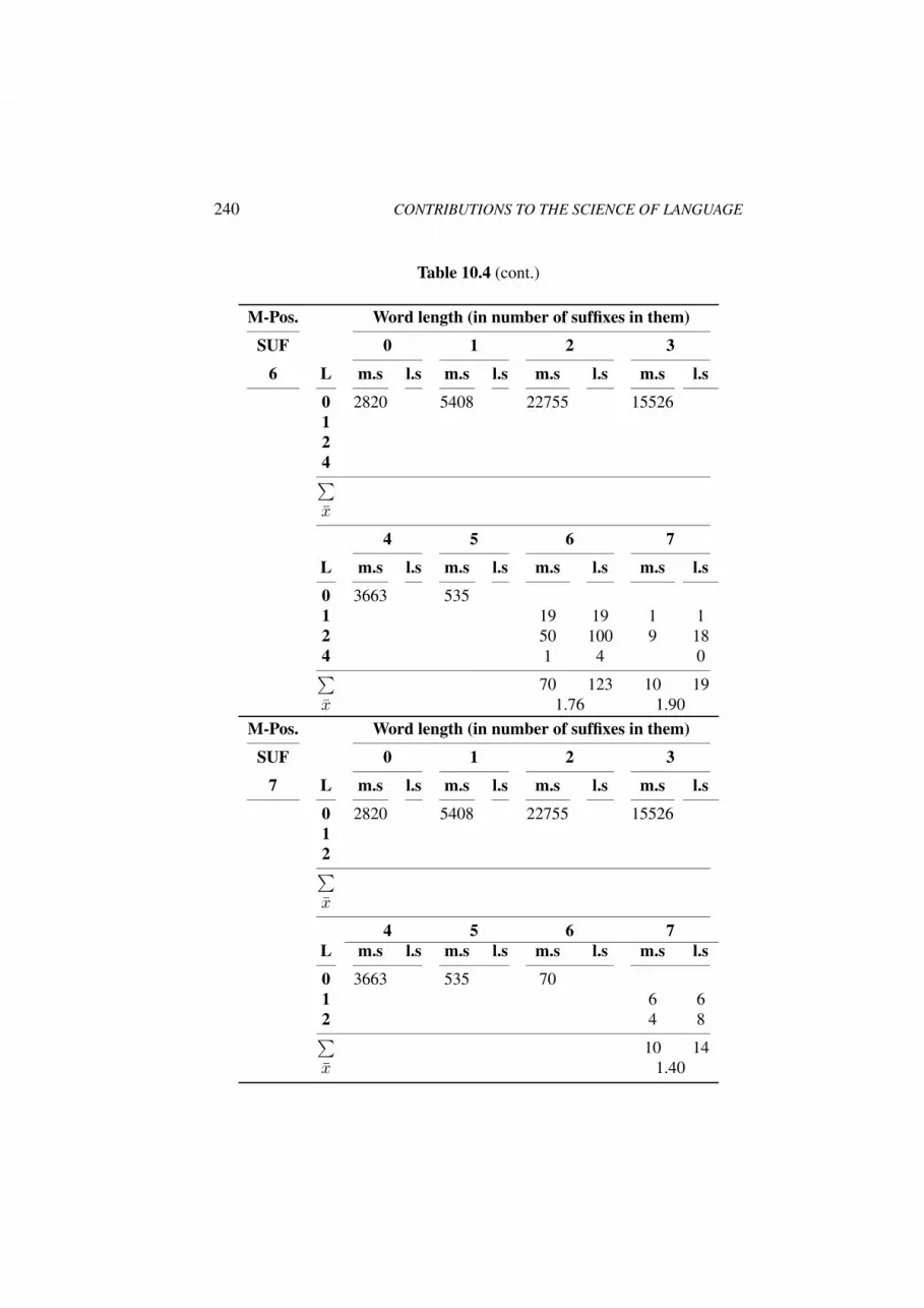
240 CONTRIBUTIONS TO THE SCIENCE OF LANGUAGE
Table 10.4 (cont.)
M-Pos. Word length (in number of suffixes in them)
SUF 0 1 2 3
6 L m.s l.s m.s l.s m.s l.s m.s l.s
0 2820 5408 22755 15526124∑
x
4 5 6 7
L m.s l.s m.s l.s m.s l.s m.s l.s
0 3663 5351 19 19 1 12 50 100 9 184 1 4 0∑
70 123 10 19x 1.76 1.90
M-Pos. Word length (in number of suffixes in them)
SUF 0 1 2 3
7 L m.s l.s m.s l.s m.s l.s m.s l.s
0 2820 5408 22755 1552612∑
x
4 5 6 7L m.s l.s m.s l.s m.s l.s m.s l.s
0 3663 535 701 6 62 4 8∑
10 14x 1.40

Peter Grzybek (ed.): Contributions to the Science of Language.Dordrecht: Springer, 2005, pp. 241–258
ASPECTS OF THE TYPOLOGYOF SLAVIC LANGUAGES
Exemplified on Word Length
Otto A. Rottmann
Traditional linguistic approaches are characterized by a generous use of theterms ‘classification’ and ‘typology’; this can for example be found with Haar-mann (1976: 13), who calls the classification of natural languages the aim ofgeneral language typology, Lehmann (1969: 58), who says that the classifica-tion of languages is the main target of each typology, as do Horne (1966: 4)and Serebrennikov (1972), where we find the term of ‘typological classifica-tion’). So it seems the two terms are used as synonyms. Linguistic dictionariespublished in the second half of the 20th century also reflect a state which canalready be found in the 19th century. A good example of this is the dictionaryby Rozental’/Telenkova; in their dictionary the entry¿typological classificationof languagesÀ is followed by the definition: “morphological classification oflanguages” (1976: 487). The same holds for quite modern works, e.g. Siemund(2000), in which several contributors identify typology with plain classification.This definition can already be found at the beginning of any interest in typology.For the purpose of our study we have separated both terms. We call the traditionalmethod of grouping languages a classification and reserve the term ‘typology’for the study of mechanisms generating types, i.e. in our conception typologyis identical with Hempel’s ideal typology or theory. We would like to take awell-known example to show the reach of classification and thus demonstratethe differences.The genealogical approach groups languages according to their developmentand their ancestors, so it is oriented merely diachronically and its main criterionfor the allocation of languages to a class is their common, historically foundedroot. According to Schleicher’s family tree, the Slavic languages form a bigbranch which in turn ramifies into three smaller branches: the West, East andSouth Slavic languages. The group of East Slavic languages comprises theRussian, Ukrainian and Belorussian languages. All three of them are in this

242 CONTRIBUTIONS TO THE SCIENCE OF LANGUAGE
group due to their common origin, not because of linguistic similarities, andcertainly not because of linguistic laws governing mechanisms according towhich certain phenomena, e.g. word length, arise. It is as easy as that. The pureclassificatory approach leads to classes like inflectional, agglutinating, isolatingetc., touching merely one unique morphological feature, i.e., it is monothetic.Practically all languages belong to all classes, the classes do not abide by theprinciples of classification (cf. Bunge 1983: 324), they are not even predictive –the only exception is Skalicka (1979).This example clearly shows that classification is a mere ordering method, butexplains nothing with respect to the question: Why does it work that way?If explanation is what we are after, we have to turn to theory. What is thedifference between an order creating classification and a theory?The basic idea to set up a classification is the desire to have order and handlelanguage practically. But order alone does not necessarily explain much.
(a) The selection criterion for a classification is a property considered importantby the scientist. For a theory all properties are equally important.
(b) Therefore the selection criterion in classification is extremely arbitrary, itis the result of an impression, the impression that a specific phenomenonoccurs frequently or is more important than others.
(c) Subjective relevance means that the scientist already has acquired an overviewof the material to be classified, he studies the material to find important dis-criminating (= classifying) properties which are then taken as the basis forthe study and subsequent classification. For a theory it is not the discrim-inating properties, but the mechanisms creating the phenomena that arerelevant.
(d) Due to differing properties considered important, a language or one of itssubsystems can be classified differently. A theory entails a unique classifi-cation.
(e) A class is static, a property considered important once prohibits an alterationto the class; the class can only be expanded, but its limits cannot be overcomedue to the characteristic property. A theory is dynamic, it presents the objectas a dynamic system.
(f) Classification results in rules conditioning language-related behavior. Rules,however, are not synonyms for inherent laws.
(g) Classification has a descriptive character and therefore supports structuraldescription. A theory has an explanative character and supports the deriva-tion of laws.
Certainly, this list is not complete, but sufficiently long to show why a classifi-cation is not the desirable aim. The aim to come to an answer to the question

Aspects of the Typology of Slavic Languages 243
‘Why does it work that way?’ can merely be approached by a theory whichautomatically gives rise to a typology (see below).In order to avoid the deficiencies linked with classifications, we must avoidthe specific elements on which a classification is based: the names of concretelinguistic elements or the names of classes. So we have to exploit properties ofdifferent character.Properties of objects are neither qualitative nor quantitative – also see: Carnap(1969: 66), Essler(1971: 65). Both are features attributed to our concepts whichwe use to order the world. Or, seen from the other point of view, ‘All factualitems are at the same time qualitative and quantitative: All properties of concreteentities, except for existence, belong to some (natural or artificial) kind or other,and they all come in definite degrees.’ Quality merely precedes quantity inconcept formation (Bunge 1995: 3). If we for example speak of ¿morphemeÀ,this term is qualitative until we quantify it operationally. If we speak of ¿wordlengthÀ, this term happens to be more quantitative, but only because we areused to express length in specific dimensions and secondly, because it expressesa property of form (not of meaning). However, it is not more quantitative thanthat of ¿morphemeÀ; it can only be quantitative by definition. Then it can bemeasured, i.e. assigned to words and used for the description, classification andtesting of theories.The aim of this paper is to report on a study of word length in the living Slaviclanguages as well as Old Church Slavonic as the oldest Slavic written languageknown to us. The study was performed on the basis of randomly chosen texts inthe individual Slavic languages; the results were intended to be the foundationfor a typology of Slavic languages with the progress meant not only to elaboratean order of entities which were the object of papers on classification in the past,but also assign an explanatory character to this order apart from inevitablydescriptive ones.The idea for this study originated from two sources being independent of eachother: On the one hand the Petersburg resident Bunjakovskij, a mathematician,inspired quantitative studies in the middle of the 19th century (1847: passim),on the other hand a lot of articles have been published in Germany in thepast twenty years, especially under the influence of Gabriel Altmann. Specialreference should be made to works in the series Glottometrika, Glottometrics,Quantitative Linguistics, Journal of Quantitative Linguistics etc. and paperspublished under the charge of Karl-Heinz Best in Gottingen. With respect toBunjakovskij’s ideas we only know that he conducted such studies; however,we do not know anything about the methods or the results obtained, since therelevant publications cannot be found any more (also see Papp 1966).The key term for the understanding of how language works is ¿attractorÀ,which by the way is a term which reflects a controlling function not only withinthe scope of language, but also in other sciences as well. Just imagine that an

244 CONTRIBUTIONS TO THE SCIENCE OF LANGUAGE
attractor is a basin, e.g. an ocean into which all rivers flow. You can also imagineattractors to be accumulation points, means, real forms, abstract forms and manyother objects or entities. Biological species are attractors for the organization ofindividuals, geometrical forms attractors for artifacts. In language all ‘-eme’-s,e.g. phoneme, morpheme, lexeme etc., are attractors. Of course, we know that‘-eme’-s stand for theoretical objects, but those terms reflect – more or lessvaguely – an attractor. For example, in a human being’s mouth there is the areaof the palate exploited by the tongue for the production of sounds. The areafor a specific sound, however, is slightly different with every individual, andit is always slightly different in each speech act, but as long as articulation iseffected in the same area, i.e. attractor, the sound is identified as identical. Anattractor permits variability – it depends on how it is shaped.At the semantic level each term is an attractor. The term ‘tree’ or ‘bird’ evokescertain ideas; in psychology and psycholinguistics such ideas are called ‘proto-types’. A semantic attractor is the special constellation of specific neurones inthe brains which can permanently alter their shape by learning or communica-tion. The traditional classification was characterized by the search for attractors,for example as they were called, classes, a search which was based on the as-sumption that fixed forms existed in the frames of which languages could formthemselves. This is in no way different to biology, where just a limited num-ber of species is found despite an endless combining capability of genes. Noteverything is combined with everything, the number of known fit-for-life com-binations is not infinite, however, it is high. Today we know that a languageis just a combination of states of linguistic entities with entities just taking thevalues in a state space; those states are interlinked by self-regulation. Theoreti-cally, all states are possible, but not all their combinations seem to be preferredor even allowed. Self-regulation depends on the human being’s different needs(e.g. minimization of the work of the brain, minimization of the extent of cod-ing, minimization of the extent of decoding etc., cf. Kohler 1986), a large partof which is governed by Zipf’s principle of least effort. A linguistic type is aspecial case of an efficient attractor, however we define it. It is a state vector,whose elements represent the properties of data interlinked by control cycles.For classical typology it was important that the elements of that vector repre-sented some less preferred values; the numerical taxonomy (as represented bySilnickij) already permitted an arbitrary number of combinations, because theymultiplied due to the inductive approach. In our point of view we do not onlylook for linguistic attractors, because the theoretically most important job isto find self-regulation cycles interlinking all linguistic levels. As already said,an attractor then, is just a state vector of all linked properties. The two graphi-cal depictions elucidate this: Figure 11.1 shows a controlled circuit of the fourproperties E1–E4, as they occur in synergetic linguistics. The arrows representfunctions connecting the properties.

Aspects of the Typology of Slavic Languages 245
E1 E2
E4 E3
Figure 11.1: A Simple Control Cycle
If the relevant (observed) values of a property are inserted in a function, then theresult is the values of all other properties linked with the initial one (elementsof the vector). This is the way to build up a theory of language.Our typological view, however, only considers the intrinsic shaping of a prop-erty, i.e. we examine the loops in control circuits (an example can be seen inFigure 11.2) and thus a branch of synergetic linguistics. A loop in the graphmeans that property E2 is controlled by an inherent dynamics having its ownattractor.
E1 E2
E4 E3
Figure 11.2: A Control Cycle With a Loop
To find such attractors, e.g. for word length, it is necessary to deductively setup (hypothetical) models and put individual languages to the test. Our modelsreflect the attractors. If a model is confirmed we say that an attractor is about tobecome or has already become dominant. The existence of attractors, in otherwords, the modelling capability of a property, is assumed automatically. Thus,it is not only possible to set up a theory of word length, but also group thelanguages according to the relevant attractor by which they are governed. Thisis a classification resulting from theory, i.e. an ideal typology as designed byHempel. Just think of Mendeleev’s classification of elements based on weight,

246 CONTRIBUTIONS TO THE SCIENCE OF LANGUAGE
which has turned out to be a proven one, but today is based on fully differentarguments. In analogy to that, linguists do not compare word length means,but search for common attractors. Thus, our view changes. We do not neces-sarily have a unique law (mechanism) moulding word length in the same wayany more, but we can expect a mechanism sensitive to initial conditions andcreating an attractor landscape. The initial conditions (genre, state of the au-thor, audience, etc.) may decide which special attractor will be headed for. Thismeans that we can expect several attractors for the given property. ¿We canexpectÀ also includes the possibility that we find one attractor only, however,such a result would be surprising.This immediately results in interesting questions like for example:
(a) How many attractors (models) exist in the Slavic languages for word length?Do Slavic languages even happen to have the same attractors?
(b) Does a historical development exist, i.e. a change from one attractor toanother? We know that changes are set in motion on different grounds, e.g.contacts with other languages or socio-economic influences, tendenciesto facilitate pronunciation to keep articulation efforts low or the tendencyto limit the complex character of utterances, seemingly unexpected self-organization etc.
(c) How does this change materialize? Gradual change of parameters, modifi-cation of length classes (i.e. maintaining a model by adding ad hoc param-eters), precipitous changes?
(d) Is the theory adequate or does it have to be modified?
Let’s follow Hempel and thus his approach to modern scientific theory, we haveto meet the following steps:
(1) Find hypotheses on the shaping of certain properties (e.g. word length). Itis only of secondary character how these hypotheses come into being (cf.Bunge 1967: 243ff.), because the inception need not be identical with thereasoning, i.e. in the end those hypotheses must be deducible, testable andcapable of being integrated into a system of hypotheses.
(2) Test the hypothesis/hypotheses given on many data. Observe that the datamay incorporate other boundary conditions. Should a model not be suitable,provide for the following actions:
(3) (a) Check the data.(b) Check the computation.(c) Vary the parameters of the hypothesis either by using different point
estimation or by iterative optimization.(d) Modify the hypothesis locally.

Aspects of the Typology of Slavic Languages 247
(e) Modify the hypothesis globally.(f) Alter the basic assumptions of the hypothesis and derive a new model
including minimum alterations to the basic assumptions.(g) Generalize the basic model such that all its variants obtained so far
become special cases.(h) If all these measures do not help, search for other plausible hypotheses
explaining most anomalies.
A warning has to be issued with respect to theories and models which attempt toexplain everything, because a theory trying to explain everything undergoes therisk of explaining nothing. Just think that variability in languages is enormous,and even when we accept that everything in language is based on laws, we knowthat mechanisms only work in the same way when boundary conditions areidentical and the ceteris paribus conditions are met. Thus we have to concludethat we have to derive a variety of models for one and the same phenomenonunless we are able to comprise all boundary conditions. This variety of modelscan be used for diachronic as well as synchronic purposes.The reason for setting up a hypothesis and testing it in the area of word lengthis to obtain a theory in the form of an attractor landscape and, following there-from, a typology in the Slavic languages. With respect to the construction ofword length hypotheses, works by Grotjahn (1982), Wimmer et al. (1994),Wimmer/Altmann (1996, 2002) were taken as the sources for basic reflections.To come to a hypothesis on word length let us start with the general idea thatthe proportionality Px Px−1 applies to the relationship between length classes.This proportionality is expressed by a function g(x) which results in the basicassumption
Px = g(x)Px−1 (11.1)
g(x) has an ordering function in the self-regulating system warranting redun-dancy, meeting different requirements (cf. Kohler 1986), braking excessivefluctuations etc.A first hypothesis on word length distribution is found with Cebanov (1947)and independently with Fucks (1955). It is the 1–displaced Poisson distribution.Grotjahn (1982) adopts this model and gives evidence that it cannot be seenas an adequate model in general, which he shows by means of a word andsyllable counting of German texts. Since Grotjahn assumes that the probabilityof word length also depends on influencing factors like context, change ofsubject etc., and therefore the probability of x syllables is not identical foreach word, he generalizes the distribution by randomizing the parameter ofthe Poisson distribution. Using the gamma distribution, he obtains the negativebinomial distribution which he proposes to be a good model after relevant testsin various languages.

248 CONTRIBUTIONS TO THE SCIENCE OF LANGUAGE
In a later study, Altmann (1994) defines further g(x) functions and adds someother distributions to Grotjahn’s hypothesis on word length. Comprehensivestudies in the course of the project at Gottingen University extended thoseresults considerably. In order to obtain a general model comprising all Slaviclanguages, the proportionality function in (11.1) must be defined as
g(x) = 1 + a0 +a1
(x+ b1)c1(11.2)
which is a special case of the “Unified Theory” presented by Wimmer andAltmann (2002). Inserting (11.2) into (11.1) we obtain
Px =
(1 + a0 +
a1
(x+ b1)c1
)Px−1 (11.3)
representing the preliminary landscape of distributions of word length in Slaviclanguages. It has some pronounced centers with peripheries which signal thewandering from one center to another.The basis for the testing performed were the living Slavic languages and thefirst known written Slavic language, Old Church Slavonic or Old Bulgarian. Thedecision as to what is to be considered a Slavic language was based on Panzer’sclassification (21996) despite the fact that it is for example vehemently differentto the one presented by Rehder (31998), but Panzer’s classification is next tothe traditional one.The number of texts analyzed was not identical in all languages; usually itamounted to thirty with the individual texts being randomly chosen. Half ofthem were fictional prose texts, half of them non-fictional texts with the actualkind of text being irrelevant. It was the aim of our work to come to statementson Russian, Polish, etc., and not on Russian press texts, Serbo-Croatian novelexcerpts etc. It is, of course, self-evident that the Old Bulgarian language –due to its character – does not show any non-fictional texts. A number of textsslightly below or above 30 is as accidental as the choice of the texts itself.Of course, we are conscious of the fact that an arbitrary number of texts wouldnot be sufficient to characterize a language globally. Samples are used to drawconclusions representing the possibilities in a language. With respect to cer-tain properties, texts could be assigned to a number of attractors which do notresemble a clearly limited landscape, but a jagged one, which, however, per-mits creativity and evolution and grants full adaptation to growing informationneeds.We assume that the principle of randomly chosen texts applied to the choice oftexts strengthens expressiveness. It is exactly this almost unlimited principle ofrandomly chosen objects (almost unlimited because of the only restriction bythe division 50% fictional, 50% non-fictional texts) which is standard in othersciences as well. The metallurgical ASTM standard E112 (a text in a series of

Aspects of the Typology of Slavic Languages 249
standards where quantitative examinations are used to assure quality) says insection 11.3:
Fields should be chosen at random and without preference. Do not try to choosefields which look typical. Choose fields blindly and there choose different positionon the polished surface.
We proceeded analogously when choosing the texts. Word length data wereprocessed by means of the software Fitter. Word length was analyzed on the basisof syllables. The evaluation of the test results is mainly based on the criterion ofP : If P ≥ 0.01, the result can at least be called “satisfactory”. Surely, this valuedoes not have the character of a statistical law, but just a conventional decision.In many sciences, e.g. in the social sciences or in metallurgy, the threshold takenas the basis for decision isP ≥ 0.05. In linguistics, however, the criterion couldeven be lowered, since the number of data processed is considerably high: it isa known fact that the χ2 grows with the size of the sample. We will stick withthe above convention. In those cases in which the value of P is not acceptable –e.g. the sample size is too great or the number of degrees of freedom is zero(d.f. = 0) –, another discrepancy criterion is used. In the software Fitter onefinds C = χ2/N . C is satisfactory, if its value is C ≤ 0.01. Values in the range0.01 ≤ C ≤ 0.02 are weak, but tolerable. C does not depend on degrees offreedom, it merely relativizes the observed discrepancy.Word length, as it occurs in individual Slavic languages, has been the objectof studies before and works we could refer to have been on word length inthe Russian, Czech, Slovak, Slovene, modern Bulgarian and Old Bulgarianlanguages.In our study counting was based on the following criteria:
(a) ‘Word’ is defined as an entity whose end is indicated orthographically bya subsequent blank or punctuation.
(b) Abbreviations occurring in the texts were dissolved and counted as if thetext included the non-abbreviated form.
(c) Words were taken as we found them in the texts, not evaluated accordingto any differing correct spelling (a criterion which is especially importantfor Old Bulgarian where the written language reflects phonetic changes inthe spoken language).
(d) Numbers, decimal numbers, years written in figures were counted as ifwritten in full words in the texts.
(e) Headings and captions were counted, as in the case of word length, it isirrelevant if words are part of a full sentence, an ellipsis or a word combi-nation.

250 CONTRIBUTIONS TO THE SCIENCE OF LANGUAGE
(f) Quotations were only taken into consideration if they were worded in thesame language as the text itself (e.g. an Old Russian quotation in a modernRussian text was not taken into consideration).
(g) Proper names were counted, if they were part of the language of the text.
(h) Initials of first names and patronymics were counted as one syllable.
(i) Abbreviated words were counted in compliance with the inflected word(e.g. ГУМ consists of one syllable, ГУМе comprises two and колхозе
three syllables).
(j) Prepositions which like the modern Russian с do not include a vowel them-selves were counted as one-syllable words.
As already mentioned, it was one of the aims of the study to find attractors(= types, frequently occupied states) which in the field of word length allowa typology of the Slavic languages. Within the scope of synergetic linguisticswe only analyzed the internal dynamics (i.e. distributions) of lengths (i.e. theloops in the control circuit) and did not tackle the relation of length to otherproperties.Those results are the boundary condition related realizations of a model withinthe meaning of the ideal typology when being systemized deductively. Theallocation of attractors to languages, however, can be evaluated within the scopeof classification. The first kind of evaluation is a theoretically constructed pointof view, which under favorable conditions can also be understood as part ofan evolution. Within the scope of ideal typology the entire range of models ispresented as special cases, limiting cases or modifications of a general model,i.e. the movement is “from the top to the bottom”. In case of a historical pointof view the movement is “from the bottom to the top”, i.e. analysis beginswith the simplest models and is expanded gradually. It should be difficult togive evidence of the correspondence of the evolution based view with the realevolution, since multitudes and multitudes of data – and this includes a historicalsequence – will have to be analyzed. The classificatory view is simply a statusquo. The concrete form of this process is shown hereinafter with the partialresults.At first glance, the studies of the word lengths in the Slavic languages generallydid not corroborate the hypothesis that word length is controlled by the 0-truncated negative binomial distribution, introduced by Grotjahn (1982); theevaluation of the control mechanism turned out to be a more complex problem.With respect to Old Church Slavonic – and this underlines a former result(Rottmann 1997) – the 1-displaced hyper-Poisson distribution turned out to be
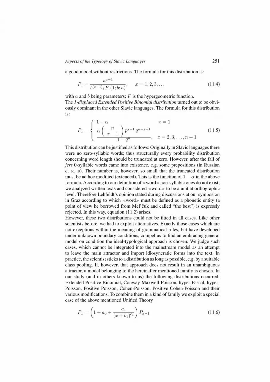
Aspects of the Typology of Slavic Languages 251
a good model without restrictions. The formula for this distribution is:
Px =ax−1
b(x−1)1F1(1; b; a)
, x = 1, 2, 3, . . . (11.4)
with a and b being parameters; F is the hypergeometric function.The 1-displaced Extended Positive Binomial distribution turned out to be obvi-ously dominant in the other Slavic languages. The formula for this distributionis:
Px =
1− α, x = 1
α
(n
x− 1
)px−1 qn−x+1
1− qn , x = 2, 3, . . . , n+ 1
(11.5)
This distribution can be justified as follows: Originally in Slavic languages therewere no zero-syllabic words; thus structurally every probability distributionconcerning word length should be truncated at zero. However, after the fall ofjers 0-syllabic words came into existence, e.g. some prepositions (in Russianс, к, в). Their number is, however, so small that the truncated distributionmust be ad hoc modified (extended). This is the function of 1− α in the aboveformula. According to our definition of ¿wordÀ non-syllabic ones do not exist;we analyzed written texts and considered ¿wordÀ to be a unit at orthographiclevel. Therefore Lehfeldt’s opinion stated during discussions at our symposionin Graz according to which ¿wordÀ must be defined as a phonetic entity (apoint of view he borrowed from Mel’cuk and called “the best”) is expresslyrejected. In this way, equation (11.2) arises.However, these two distributions could not be fitted in all cases. Like otherscientists before, we had to exploit alternatives. Exactly those cases which arenot exceptions within the meaning of grammatical rules, but have developedunder unknown boundary conditions, compel us to find an embracing generalmodel on condition the ideal-typological approach is chosen. We judge suchcases, which cannot be integrated into the mainstream model as an attemptto leave the main attractor and import idiosyncratic forms into the text. Inpractice, the scientist sticks to a distribution as long as possible, e.g. by a suitableclass pooling. If, however, that approach does not result in an unambiguousattractor, a model belonging to the hereinafter mentioned family is chosen. Inour study (and in others known to us) the following distributions occurred:Extended Positive Binomial, Conway-Maxwell-Poisson, hyper-Pascal, hyper-Poisson, Positive Poisson, Cohen-Poisson, Positive Cohen-Poisson and theirvarious modifications. To combine them in a kind of family we exploit a specialcase of the above mentioned Unified Theory
Px =
(1 + a0 +
a1
(x+ b1)c1
)Px−1 (11.6)

252 CONTRIBUTIONS TO THE SCIENCE OF LANGUAGE
whose solution leads to the main attractors (Binomial, Conway-Maxwell-Pois-son, hyper-Pascal, hyper-Poisson, Poisson), which in turn by an a-posteriorimodification lead to the remaining cases (Extended Positive Binomial, Posi-tive Poisson, Cohen-Poisson, Positive Cohen-Poisson), and all cases found byUhlırova (2001).The basic reparametrizing operations of (11.1) are as follows:
Table 11.1: Reparametrizations of (11.1)
Binomial: 1 + a0 = −p/q, a1 = (n+ 1)p/q, b1 = 0, c1 = 1Conway-Max- a0 = −1, a1 = a, b1 = 0, c1 = bwell-Poisson:Hyper-Pascal: −1 < a0 < 0, 1 + a0 = q,
a1 = q(k −m), b1 = m− 1, c1 = 1Hyper-Poisson: a0 = −1, a1 = a, b1 = b− 1, c1 = 1Poisson: a0 = −1, a1 = a, b1 = 0, c1 = 1.
For example, if we insert the reparametrization concerning the hyper-Pascaldistribution into (11.3), we obtain
Px =
(q +
q(k −m)
x+m− 1
)Px−1 (11.7)
and by ordering the expression in the brackets, we obtain
Px =q(x+m− 1) + q(k −m)
m+ x− 1Px−1 =
k + x− 1
m+ x− 1qPx−1 (11.8)
in which we recognize the recurrence formula of the hyper-Pascal distribution.Convergencies and special cases can be ascertained directly in the recurrenceformulas. For example, if in the hyper-Pascal distributionm = 1, k →∞, q →0, kq → a, then we obtain Px = a
xPx−1, i.e. the Poisson distribution, etc.The interpretation of (11.3) is simple and elucidating (cf. Wimmer/Altmann2002. The majority of linguistic laws have been derived on the assumption thatthe relative rate of change of the dependent variable is proportional to that ofthe independent one, i.e. the first step undertaken with continuous variables was
dy
y=
(a+
b
x
)dx (11.9)
which in discrete form is
∆Px−1
Px−1= a+
b
x(11.10)

Aspects of the Typology of Slavic Languages 253
Since the right hand side is, as a matter of fact, the beginning of an infinite series,it is sufficient to expand it to the necessary number of members and solve thepertinent equations. The further coefficients represent those factors which exertan influence only via the first independent variable and are relativized by certainpowers of it. Thus different kinds of generalizations are obtained, from whichit is sufficient (“sufficient” for our purposes) to take
∆Px−1
Px−1= a0 +
a1
(x+ b1)c1+
a2
(x+ b2)c2+ . . . (11.11)
Letting a2 = a3 = . . . = 0 and by reordering, we obtain formula (11.3). Alldistributions mentioned above are shown in Table 11.2.
Table 11.2: Special Cases of (11.3)
Name g(x) Px Modifications
Poisson ax
e−aax
x!Cohen-Poisson
Positive Poisson ax
e−aax
x!(1− e−a)Pos. Cohen-Poisson
hyper-Poisson ab+ x− 1
ax
b(x)1F1(1; b; a)
Conway-Max- axb
ax
(x!)bP0
well-Poisson
Binomial n− x+ 1x
pq
(n
x
)pxqn−x Ext. Pos. Binomial
hyper-Pascal k + x− 1m+ x− 1q
(k + x− 1
x
)
(m+ x− 1
x
)qxP0
All others used for modelling word length in Slavic languages originate frommodifications of the binomial distribution [Extended Positive Binomial, Uhlırova’scases (Uhlırova 2001)] and the Poisson distribution (Positive Poisson, PositiveCohen-Poisson, Cohen-Poisson).All “plain” distributions are used in their 1-displaced forms, P0 is the normal-izing factor. The entire hierarchy then looks as follows (see Figure 11.3).The hierarchy includes the basic distribution, i.e. we do not make any differencebetween standard and displaced distributions; truncated distributions (calledpositive) are listed separately. The hierarchy in Figure 11.3 is not based onthe number of parameters (simplicity), since modifications usually have more

254 CONTRIBUTIONS TO THE SCIENCE OF LANGUAGE
Conway-Maxwell-Poisson Binomial Hyperpascal
Poisson
Hyperpoisson
Extended Positive Binomial
Other modifications
Positive Poisson
Positive Cohen-Poisson
Cohen-Poisson
Modifikation
Convergency
Special case
Figure 11.3: Hierarchy of word length distributions
parameters than the parent distribution. It is obvious that the range of Slaviclanguages is a rather narrow one and their positions are very close together.The allocation of the languages to those attractors is shown in Table 11.3 (thefigures in brackets indicate the number of texts in our study).1
Table 11.3: Classification According to Evolutionary Tendencies
OCS HYP(14) EPB(1) PCP(1)BG EPB(31)MC EPB(30)POL EPB (30)RS HYP(1) EPB(30)SCR EPB(59) CP(1)SOR EPB(21) HPa(2)SK HYP(1) EPB(28) HPa(1) CMP (1) PP(1)SLO EPB(29) CMP(1)CZ EPB(28) ModBin (1)UK HYP(3) EPB(26)BR HYP(2) EPB(28)
1 Abbreviations for distributions discussed in this paper: CMP = Conway–Maxwell–Poisson, CP = Cohen–Poisson, EPB = Extended Positive Binomial, HPa = Hyper-Pascal, HYP = Hyper-Poisson, ModBin =Modified Binomial, PCP = Positive Cohen–Poisson, PP = Positive Poisson

Aspects of the Typology of Slavic Languages 255
Table 11.3 is self-explaining. It shows the weight of an attractor (number inbrackets) and the variation of the attractors, and it shows that the Slavic lan-guages are all members of one word length family. Though the attractors giveevidence of a strong gravitation, we find secondary attractors in nine out oftwelve languages. This may be due to the evolutionary movement in the givenlanguage, other causes are: number of analyzed texts, size of the samples, kindsof texts etc.A possibility to order languages and obtain a traditional, though not explanatoryclassification is a list including the number of attractors as the relevant criterion.Thus we obtain Table 11.4.2
Table 11.4: Classification According to Evolutionary Tendencies
Number of LanguagesAttractors
1 BG, MC, POL2 RS, SCR, SOR, SLO, CZ, UK, BR3 OCS5 SK
It can be assumed that studies on further texts in each Slavic language – mostprobably with the exception of the Old Church Slavonic language – will resultin new attractors, the current representation, however, suggests the followinginterpretation: a language showing many attractors seems to be one governedby movement, i.e. alterations can be expected. With respect to the Old ChurchSlavonic language we can confirm that assumption: It was subjected to a move-ment evoking the jer modification and loss; the modern languages already sta-bilized after that modification. From a historical point of view those attractorsare maintained, as the texts exist, but stabilization can be concluded from theiroccurrences.With respect to history, Figure 11.3 can be turned around, and it can be assumedthat evolutionary development starts with the simplest distribution, i.e. the Pois-son distribution, and continues either by adding further parameters or extendingthe proportionality g(x) or (after the solution of the difference equation, thatis to say after the attractor comes into being) by local modifications of alreadyexisting distributions.
2 Abbreviations for languages analyzed in this paper: BG = Bulgarian, BR = Belorussian, CZ = Czech, MC= Macedonian, OCS = Old Church Slavonic, POL = Polish, RS = Russian, SCR = Serbo–Croatian, SOR= Sorbian, SK = Slovak, SLO = Slovene, UK = Ukrainian
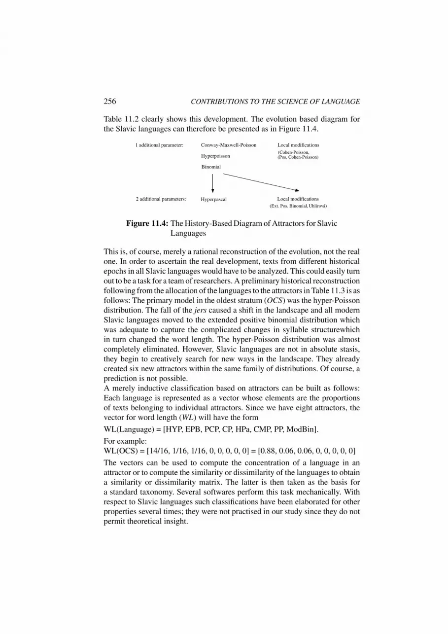
256 CONTRIBUTIONS TO THE SCIENCE OF LANGUAGE
Table 11.2 clearly shows this development. The evolution based diagram forthe Slavic languages can therefore be presented as in Figure 11.4.
1 additional parameter: Conway-Maxwell-Poisson
2 additional parameters:
Hyperpoisson(Cohen-Poisson,
Local modifications
(Pos. Cohen-Poisson)
Binomial
Local modifications(Ext. Pos. Binomial, Uhlírová)
Hyperpascal
Figure 11.4: The History-Based Diagram of Attractors for SlavicLanguages
This is, of course, merely a rational reconstruction of the evolution, not the realone. In order to ascertain the real development, texts from different historicalepochs in all Slavic languages would have to be analyzed. This could easily turnout to be a task for a team of researchers. A preliminary historical reconstructionfollowing from the allocation of the languages to the attractors in Table 11.3 is asfollows: The primary model in the oldest stratum (OCS) was the hyper-Poissondistribution. The fall of the jers caused a shift in the landscape and all modernSlavic languages moved to the extended positive binomial distribution whichwas adequate to capture the complicated changes in syllable structurewhichin turn changed the word length. The hyper-Poisson distribution was almostcompletely eliminated. However, Slavic languages are not in absolute stasis,they begin to creatively search for new ways in the landscape. They alreadycreated six new attractors within the same family of distributions. Of course, aprediction is not possible.A merely inductive classification based on attractors can be built as follows:Each language is represented as a vector whose elements are the proportionsof texts belonging to individual attractors. Since we have eight attractors, thevector for word length (WL) will have the formWL(Language) = [HYP, EPB, PCP, CP, HPa, CMP, PP, ModBin].For example:WL(OCS) = [14/16, 1/16, 1/16, 0, 0, 0, 0, 0] = [0.88, 0.06, 0.06, 0, 0, 0, 0, 0]The vectors can be used to compute the concentration of a language in anattractor or to compute the similarity or dissimilarity of the languages to obtaina similarity or dissimilarity matrix. The latter is then taken as the basis fora standard taxonomy. Several softwares perform this task mechanically. Withrespect to Slavic languages such classifications have been elaborated for otherproperties several times; they were not practised in our study since they do notpermit theoretical insight.

Aspects of the Typology of Slavic Languages 257
References
American Society for Testing and Materials (ASTM).1996 ASTM Standard E112: Standard Test Methods for Determining Average Grain Size. West
Conshocken.Bunge, M.
1967 Scientific research I. The search for system. New York.Bunge, M.
1983 Treatise on basic philosophy. Vol. 5: Epistemology & Methodology I: Exploring the World.Dordrecht.
Bunge, M.1995 “Quality, quantity, pseudoquantity and measurement”, in: Journal of Quantitative Linguis-
tics, 2; 1–10.Bunjakovskij, V.Ja.
1847 “O vozmonosti vvedenija opredelitel’nych mer” doverija k” rezul’tatam” nekotorych”nauk” nabljudatel’nych”, i preimuscestvenno statistiki.” In: Sovremennik, tom 3. Sankt-peterburg. (36–49).
Carnap, R.1969 Einfuhrung in die Philosophie der Naturwissenschaft. Munchen.
Cebanov, S.G.1947 “O podcinenii recevych ukladov indoevropejskoj gruppy zakonu Puassona.” In: Doklady
Akademii Nauk SSSR, 55/2; 103–106.Essler, W.
1971 Wissenschaftstheorie I–III. Freiburg, 1971.Fucks, W.
1955 Mathematische Analyse von Sprachelementen, Sprachstil und Sprachen. Koln.Grotjahn, R.
1982 “Ein statistisches Modell fur die Verteilung der Wortlange”, in: Zeitschrift fur Sprachwis-senschaft, 1; 44–75.
Haarmann, H.1976 Grundzuge der Sprachtypologie. Stuttgart.
Horne, K.M.1966 Language Typology – 19th and 20th Century Views. Washington.
Kohler, R.1986 Zur linguistischen Synergetik. Struktur und Dynamik der Lexik. Bochum.
Lehmann, W.1969 Einfuhrung in die historische Linguistik. Heidelberg.
Nemcova, E.; Altmann, G.1994 “Zur Wortlange in slovakischen Texten”, in: Zeitschrift fur empirische Textforschung, 1;
40–43.Panzer, B.
1996 Die slavischen Sprachen in Gegenwart und Geschichte. Frankfurt.Papp, F.
1966 Mathematical Linguistics in the Soviet Union. The Hague.Rehder, P.
1998 Einfuhrung in die slavischen Sprachen. Darmstadt.Rottmann, O.A.
1997 “Word Length Counting in Old Church Slavonic”, in: Journal of Quantitative Linguistics,4; 252–256.
Rozental’, D.; Telenkova, M.1972 Spravocnik lingvisticeskich terminov. Moskva.
Serebrennikov, B.A.1972 Obscee jazykoznanie. Vnutrennjaja struktura jazyka. Moskva.
Siemund, P. (ed.)2000 Methodology in Linguistic Typology. Sprachtypologie und Universalienforschung. Bd. 53,
1.

258 CONTRIBUTIONS TO THE SCIENCE OF LANGUAGE
Silnitzky, G.1993 “Typological Indices and Language Classes: A Quantitative Study”, in: Glottometrika 14.
Bochum. (139–160).Skalicka, V.
1979 Typologische Studien. Braunschweig.Uhlırova, L.
2001 “On Word Length, Clause Length and Sentence Length in Bulgarian”, in: QuantitativeLinguistics 6; 266–282.
Wimmer, G.; Kohler, R.; Grotjahn, R.; Altmann, G.1994 “Towards a theory of word length distribution”, in: Journal of Quantitative Linguistics, 1;
98–106.Wimmer, G.; Altmann, G.
1996 “The theory of word length: some results and generalizations”, in: Glottometrika 15.Bochum. (112–133).
Wimmer, G.; Altmann, G.2002 “Unified derivation of some linguistic laws.” Paper read out at the International Symposium
ÀWord Lengths in Texts. International Symposium on Quantitative Text Analysis¿ (June21–23, 2002, Graz University). [Text published in the present volume]
SoftwareAltmann, G. (1997): FITTER. Ludenscheid.

Peter Grzybek (ed.): Contributions to the Science of Language.Dordrecht: Springer, 2005, pp. 259–275
MULTIVARIATE STATISTICAL METHODSIN QUANTITATIVE TEXT ANALYSES∗
Ernst Stadlober, Mario Djuzelic
1. IntroductionQuantitative text studies characterize scholarly disciplines such as, for example,quantitative linguistics or stylometry. Although there are methodological over-lappings between these two approaches, their orientation is essentially different,at least in some important aspects: in general, quantitative linguistics strives forthe detection, description, and explanation of particular linguistic rules, or laws;as compared to this, the ‘classical’ objectives of stylometry usually concentrate,in addition to mere style-oriented research, on problems such as authorship de-termination of given texts, or text classification. The characterization of theseapproaches and their major orientation is admittedly rather sketchy and polar-izing; still, generally speaking, one may say that quantitative linguistics tendsto concentrate on general aspects of a language’s linguistic system, whereasstylometry rather focuses on individually based aspects of texts.With regard to word length studies, it may be sufficient to give but one exampleto demonstrate the differences at stake. Quantitative linguists such as Wimmeret al. (1994), or Wimmer/Altmann (1996), recently have suggested a generaltheory of word length distribution. The adequacy of this theory has repeatedlybeen tested with regard to many different languages – cf. the results of the‘Gottingen Project’ headed by Karl-Heinz Best. As to the concrete analyses,rather than in their theoretical foundation, quantitative linguists tend to haveconcentrated on languages as a whole, thus neglecting language-internal factorspossibly influencing word length – at least, these factors have not been controlledsystematically.In the tradition of stylometry, as compared to this, word length has alwaysbeen an important factor as well; yet, stylometric studies rather have followed adifferent track, laid by Mendenhall, as early as in the 19th century: here, wordlength is considered to be one factor characterizing an individual author’s style.
∗ This work was financially supported by the Austrian Science Foundation (FWF), contract # P-15485

260 CONTRIBUTIONS TO THE SCIENCE OF LANGUAGE
More recent stylometric studies, however, usually have not concentrated on thespecific impact of word length; rather, more than one textual characteristic hasbeen included at a time – thus, observations as to various parameters (suchas sentence length, word frequency, etc.) have been simultaneously combined,in the hope that this combination would lead to a maximum of informationabout the text under study; and to a certain degree, the same holds true forstylometric attempts as for text classification (not taking into account content-based approaches, here).The systematic study of word length, along with the careful control of language-internal factors – such as authorship, or text type – possibly influencing wordlength, thus would yield precious insights for both quantitative linguistics andstylometry. Quantitative linguistics would not gain insight as to the questionin how far its methodological apparatus is useful for the study of individualtexts, too; also, it would learn in how far it is necessary to pay attention tosuch language-internal factors. Stylometry, in turn, would profit from realizingwhich linguistic factors contribute to what degree in analyzing questions ofauthorship, text attribution, etc.In a way, the present case study attempts to combine both approaches: on thebasis of word length analyses, multivariate analyses will be applied in order totest to what extent each individual text can be classified in one of three cate-gories: literary prose, journalistic prose, and poetry. The study is based on 153Slovenian texts: 51 of these texts are of a poetic nature, 102 texts are writtenin prose (52 of them represent literary prose, 50 journalistic prose).1 Each textwill be quantitatively described by a number of measures reflecting the mo-ments of the distribution of its word length (mean valuem1, variancem2, thirdmoment m3, and the quotients I = m2/m1 and S = m3/m2). Additionally,the number of syllables of the text will be defined as the text length. Our studywas done within the framework of the Graz Project on Word Length (Frequen-cies) as described in Grzybek/Stadlober (2002) and is specifically based on theundergraduate thesis of Djuzelic (2002) considering the following approach.A collection of three categories of texts (literary prose, journalistic prose, andpoetry) will be analyzed by means of discriminant analysis to give answers tothe following questions. Is it possible to discriminate between the texts withthe help of the measures mentioned above such that most of the texts can beassigned to the original category? Which measures are the most important onesfor suitable discrimination and classification?
1 Note that we use the same text base as the paper Antic et al. (2005), except one additional journalistic textin our data collection. The appendix of the paper mentioned contains details of these texts as to author,title, chapter, and year, as well as to statistical measures.

Multivariate Statistical Methods in Quantitative Text Analyses 261
2. Quantitative Measures for the Analysis of TextsThe distribution of the word length of the texts are described by the four variablesm1,m2, I and S, and the text length is characterized by the two variables TLSwhich is the length of text in syllables and its logarithm log(TLS). These twovariables will act as control variables for our statistical procedures, becausethe texts were chosen from three groups which differ remarkably accordingtheir text length; e.g. the mean text length of literary texts is four times longerthan the mean text length of journalistic texts, which again is four times longerthan the mean text length of poetic texts (see Table 12.2). The definition of thevariables used in our analysis are listed in Table 12.1.
Table 12.1: Six Statistical Measures Characterizing SlovenianTexts
m1 average word length where word length isthe number of syllables per word
m2 empirical variance of the word lengthI = m1/m2 first criterion of Ord (see Ord, 1967)S = m3/m2 second criterion of Ord with m3 the third momentTLS text length as number of syllableslog(TLS) natural logarithm of text length
Every text in our context is a statistical object carrying its information on p = 6variables. In this way the quantitative description of text j from group i is givenby an observation vector of dimension 6.
xij = (TLS(i, j),m1(i, j),m2(i, j), log(TLS)(i, j), I(i, j), S(i, j))
where j = 1, . . . , ni ; i = 1, 2, 3.(12.1)
For each group i the mean values of the six variables are collected to a meanvector of same dimension:
xi =(TLS(i),m1(i),m2(i), log(TLS)(i), I(i), S(i)
), i = 1, 2, 3 . (12.2)
An outline of the data with two texts of each category is given in Table 12.2.
2.1 Variance-Covariance Structure of the VariablesThe variability of the data is measured by the symmetric variance-covariancematrix S of dimension 6 × 6. The diagonal elements sjj of this matrix arethe empirical variances of the variables and the non-diagonal elements sjk,j 6= k, constitute the empirical co-variances between the variables j and k.

262 CONTRIBUTIONS TO THE SCIENCE OF LANGUAGE
Table 12.2: Statistical Values of Two Slovenian Texts For EachGroup
Text category TLS m1 m2 log(TLS) I S
1 literary prose 4943 1.89 1.02 8.51 0.54 0.952 2791 1.93 1.06 7.93 0.55 0.86
n1 = 52,x1 = ( 4000 1.84 0.96 8.05 0.52 0.90)
1 journalistic prose 1537 2.21 1.75 7.34 0.79 1.092 1200 2.31 1.62 7.09 0.70 0.74
n2 = 50,x2 = ( 1084 2.25 1.59 6.78 0.71 0.85)
1 poetry 312 1.81 0.72 5.74 0.40 0.502 402 1.75 0.91 6.00 0.52 1.27
n3 = 51,x3 = ( 270 1.74 0.68 5.41 0.39 0.69)
The elements rjk of the correlation matrix R are obtained from the variance–covariance matrix by the standardization rjk = sjk/
√sjjskk. It follows that
−1 ≤ rjk ≤ 1 where values near±1 (high negative or high positive correlation)indicate a nearly linear relationship between the two variables, and values rjk ≈0 signify that the variables are uncorrelated. The variance-covariance matrix S1
and the correlation matrixR1 of the texts in group 1 (literary prose) are listed inTable 12.3. There are high correlations between the pairs average word lengthm1 and quotient I = m2/m1 (r = 0.98), and momentsm1 andm2 (r = 0.92).Rather low correlations appear between the second criterion of Ord (1967),S = m3/m2 and all other variables.
2.2 Statistical Distance and Linear Discriminant FunctionUnivariate Statistical Distance. The univariate statistical distance is an im-portant measure for separating data of two different groups of text. It will be as-sumed that the texts are independent samples (x11, . . . , x1n1) and (x21, . . . , x2n2)of two distributions having possibly different theoretical means µi, but the samevariance σ2. The theoretical means are estimated by the arithmetic means xi ofthe samples and the common variance can be estimated by pooling together thetwo empirical variances s2i of the samples as
s2pool =1
n1 + n2 − 2
((n1 − 1)s21 + (n2 − 1)s22
). (12.3)

Multivariate Statistical Methods in Quantitative Text Analyses 263
Table 12.3: Variance-Covariance and Correlation Matrix ForText Category 1: Literary Prose
S1 =
TLS log(TLS) m1 m2 I STLS 8664007.55 1961.689 80.350 75.170 18.007 27.434
log(TLS) 1961.69 0.504 0.019 0.017 0.004 0.005m1 80.35 0.019 0.004 0.006 0.002 0.001m2 75.17 0.017 0.006 0.009 0.003 0.003I 18.01 0.004 0.002 0.003 0.001 0.001S 27.43 0.005 0.001 0.003 0.001 0.007
R1 =
TLS log(TLS) m1 m2 I STLS 1 0.94 0.41 0.27 0.17 0.11
log(TLS) 0.94 1 0.41 0.25 0.14 0.09m1 0.41 0.41 1 0.92 0.82 0.17m2 0.27 0.25 0.92 1 0.98 0.33I 0.17 0.14 0.82 0.98 1 0.39S 0.11 0.09 0.17 0.33 0.39 1
The univariate statistical distance D and the t-value |t| are given as
D(x1, x2) =|x1 − x2|spool
, |t| =
√n1 n2
n1 + n2D(x1, x2) . (12.4)
Tables 12.4, 12.5 and 12.6 contain the mean values, standard deviations and uni-variate statistical distances for all six variables giving the results of all pairwisecomparisons according to the three categories of text.The comparison of literary prose and journalistic prose in Table 12.4 shows thehighest distance values D ≥ 3.6 according the variables m1 and I which arealso highly correlated. However, the mean values of TLS differ at most, butthe large empirical standard deviations keep the statistical distance between thetwo categories at a lower level.The scatter plot in Figure 12.1(a) shows a very high correlation between m1
and I for texts of type literary prose (lower part on the left) and also a highcorrelation for journalistic texts (upper part, right). However, the combinationof these two variables results in a good discrimination of the two categoriesbased on the larger values of both m1 and I for journalistic texts.Literary prose and poetry are discriminated best by the variable log(TLS)resulting in D ≈ 3.9. Here a large difference of the mean values is combinedwith similar standard deviations having low order of magnitude compared tothe means (see Table 12.5). Because of its better distributional properties, thevariable log(TLS) is a more significant measure for discrimination than the un-transformed text length TLS. According to this, the only possible discriminator

264 CONTRIBUTIONS TO THE SCIENCE OF LANGUAGE
Table 12.4: Literary Prose and Journalistic Prose: Mean Values,Standard Deviations, Univariate Statistical Distances
Variable Text type x(1)j |x
(2)k s
(1)j |s
(2)k D(x
(1)j , x
(2)k )
TLS literary prose 4000.00 2943.47 1.342journalistic prose 1084.20 784.47
log(TLS) literary prose 8.05 0.71 1.869journalistic prose 6.78 0.64
m1 literary prose 1.84 0.07 3.994journalistic prose 2.25 0.13
m2 literary prose 0.96 0.96 0.900journalistic prose 1.59 0.20
I literary prose 0.52 0.04 3.606journalistic prose 0.71 0.06
S literary prose 0.90 0.09 0.328journalistic prose 0.85 0.22
with respect to word length is the first criterion of Ord I = m1/m2 yieldingD ≈ 2.1.The scatter plot of log(TLS) and I in Figure 12.1(b) illustrates the situationdescribed above: the categories literary prose and poetry can be discriminatedby log(TLS), but looking at the distribution of the variable I one can observesimilar values in both text categories corresponding to a lower value of thestatistical distance.The most interesting results appear in the comparison of journalistic prose andpoetry. Table 12.6 lists three measures of similar performance (4.1 ≤ D ≤ 4.8)for univariate discrimination where all three are based on word length variables:the variance m2, the first criterion of Ord I = m1/m2 and the mean valuem1. For our comparison in Figure 12.1(c) we selected the most discriminatingvariablesm2 and I . The perfect linear relationship between these two variablesis combined with a good discriminating power for the categories journalisticprose and poetry.
Multivariate Statistical Distance and Discriminant Function. In the fol-lowing we will study multivariate observations looking at all p = 6 variablessimultaneously. The theoretical background of discriminant analysis may befound in the books of Flury (1997) and Hand (1981). A distance measure be-

Multivariate Statistical Methods in Quantitative Text Analyses 265
1.7 1.9 2.1 2.3 2.5
m1
0.4
0.5
0.6
0.7
0.8
I
literary prose
journalistic prose
(a) Scatter Plot of the Pair (m1, I) for Literary Proseand Journalistic Prose
3 4 5 6 7 8 9 10
log(TLS)
0.2
0.3
0.4
0.5
0.6
0.7
I
poetry
literary prose
(b) Scatter Plot of the Pair (log(TLS), I) for Lit-erary Prose and Poetry
0.25 0.50 0.75 1.00 1.25 1.50 1.75 2.00
m2
0.2
0.4
0.6
0.8
I
poetry
journalistic prose
(c) Scatter Plot of the Pair (m2, I) for JournalisticProse and Poetry
Figure 12.1: Scatterplots
tween two groups of texts based on multivariate observations is a generalizationof the univariate case given in (12.4). It will be assumed that the texts are in-dependent samples of observation vectors (xj1, . . . ,xjnj ) and (xk1, . . . ,xknk)of two p–dimensional distributions having possibly different theoretical meanvectorsµj andµk and the same p×p variance-covariance matrix Σ. The meanvectors are estimated by the vectors of the arithmetic means xj and xk. Thevariance-covariance matrix Σ is estimated by the common empirical variance-covariance matrixSjk obtained by pooling together the two variance-covariancematrices Sk and Sj of the groups as
Sjk =1
nj + nk − 2· ((nj − 1) · Sj + (nk − 1) · Sk) . (12.5)

266 CONTRIBUTIONS TO THE SCIENCE OF LANGUAGE
Table 12.5: Literary Prose and Poetry: Mean Values, StandardDeviations, Univariate Statistical Distances
Variable Text type x(1)j |x
(2)k s
(1)j |s
(2)k D(x
(1)j , x
(2)k )
TLS literary prose 4000.0 2943.47 1.780poetry 269.86 1917.46
log(TLS) literary prose 8.05 0.71 3.943poetry 5.41 0.62
m1 literary prose 1.84 0.07 1.045poetry 1.74 0.12
m2 literary prose 0.96 0.96 0.403poetry 0.68 0.17
I literary prose 0.52 0.04 2.147poetry 0.39 0.08
S literary prose 0.90 0.09 1.126poetry 0.69 0.25
The multivariate statistical distance D(xj ,xk) between the mean vectors xj
and xk is defined as
Djk = D (xj ,xk) =√
(xj − xk)′S−1jk (xj − xk) , (12.6)
where S−1jk is the inverse of matrix Sjk and x
′ the transposed vector of x. So, thedistance Djk between two groups is defined as the distance between the groupcenters (means) standardized by the pooled variance-covariance structure. Asnumerical values of the distances we get
D12 = 5.5167 , D13 = 4.7661 D23 = 5.4022 (12.7)
which are remarkably higher than the maximal values 3.99, 3.94 and 4.80 ofthe corresponding univariate distances given in Tables 12.4–12.6. The variance-covariance matrices Sj , j = 1, 2, 3, and the pooled variance-covariance matri-ces Sjk may be found in Djuzelic (2002). The discrimination function Yjk isintroduced as a linear combination of the p-variables and can be calculated foreach p-dimensional observation xlm of the two groups as
Yjk(xlm) = b′ijxlm with vector of coefficients bij = S−1
jk (xj −xk) .
(12.8)

Multivariate Statistical Methods in Quantitative Text Analyses 267
Table 12.6: Journalistic Prose and Poetry: Mean Values, StandardDeviations, Univariate Statistical Distances
Variable Text type x(1)j |x
(2)k s
(1)j |s
(2)k D(x
(1)j , x
(2)k )
TLS journalistic prose 1084.16 784.47 1.432poetry 269.86 191.75
log(TLS) journalistic prose 6.78 0.64 2.173poetry 5.41 0.62
m1 journalistic prose 2.25 0.13 4.149poetry 1.74 0.12
m2 journalistic prose 1.59 0.20 4.795poetry 0.68 0.17
I journalistic prose 0.71 0.06 4.417poetry 0.39 0.08
S journalistic prose 0.85 0.22 0.660poetry 0.69 0.25
The mean values Y jjk, Y k
jk of the groups, the centermjk of the two groups, andthe standardized discriminant function Zjk are defined as
Yjjk =Yjk(xj) , Y
kjk = Yjk(xk) ,
mjk =1
2
(Yjjk + Y
kjk
), Zjk(xlm) = (Yjk(xlm)−mjk) /Djk .
(12.9)
Now each observation vector xlm can be classified according to its value ofZjk. For our data we get the following classification rules:
1. A text is classified as literary prose if Z12 > 0 and Z13 > 0.
2. A text is classified as journalistic prose if Z12 < 0 and Z23 > 0.
3. A text is classified as poetry if Z13 < 0 and Z23 < 0.
The specific situation is best explained by the histograms of the standardizeddiscriminating variables Z12, Z13 and Z23 exhibited as Figures 12.2(a), 12.2(b)and 12.2(c). With these graphical displays it is possible to judge the separationpower of the discriminant functions. The cut point between two groups is zeroas given above. The largest statistical distance D12 = 5.5167 appears betweenjournalistic prose and literary prose resulting in a good discrimination bythe variable Z12 (see Figure 12.2(a)). The lowest statistical distance of D13 =
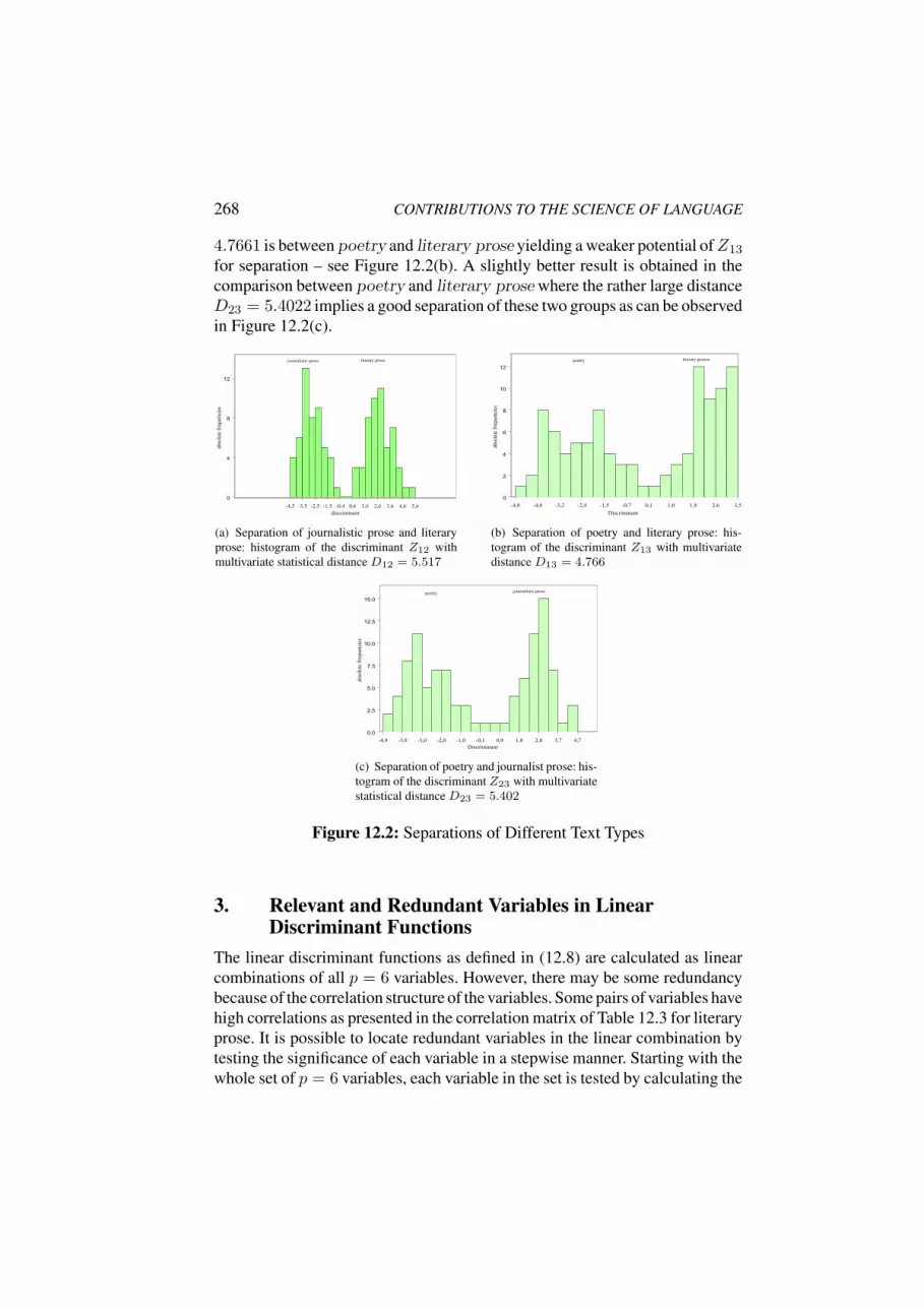
268 CONTRIBUTIONS TO THE SCIENCE OF LANGUAGE
4.7661 is between poetry and literary prose yielding a weaker potential ofZ13
for separation – see Figure 12.2(b). A slightly better result is obtained in thecomparison between poetry and literary prose where the rather large distanceD23 = 5.4022 implies a good separation of these two groups as can be observedin Figure 12.2(c).
-4,5 -3,5 -2,5 -1,5 -0,4 0,6 1,6 2,6 3,6 4,6 5,6
discriminant
0
4
8
12
abso
lute
fre
quenci
es
literary prosejournalistic prose
(a) Separation of journalistic prose and literaryprose: histogram of the discriminant Z12 withmultivariate statistical distance D12 = 5.517
-4,8 -4,0 -3,2 -2,4 -1,5 -0,7 0,1 1,0 1,8 2,6 3,5
Discriminant
0
2
4
6
8
10
12
abso
lute
fre
quenci
es
literary proseapoetry
(b) Separation of poetry and literary prose: his-togram of the discriminant Z13 with multivariatedistance D13 = 4.766
-4,9 -3,9 -3,0 -2,0 -1,0 -0,1 0,9 1,8 2,8 3,7 4,7
Discriminant
0.0
2.5
5.0
7.5
10.0
12.5
15.0
abso
lute
fre
quenci
es
poetry journalistic prose
(c) Separation of poetry and journalist prose: his-togram of the discriminant Z23 with multivariatestatistical distance D23 = 5.402
Figure 12.2: Separations of Different Text Types
3. Relevant and Redundant Variables in LinearDiscriminant Functions
The linear discriminant functions as defined in (12.8) are calculated as linearcombinations of all p = 6 variables. However, there may be some redundancybecause of the correlation structure of the variables. Some pairs of variables havehigh correlations as presented in the correlation matrix of Table 12.3 for literaryprose. It is possible to locate redundant variables in the linear combination bytesting the significance of each variable in a stepwise manner. Starting with thewhole set of p = 6 variables, each variable in the set is tested by calculating the

Multivariate Statistical Methods in Quantitative Text Analyses 269
corresponding test statistic which is a Student t statistic with nk + nj − p− 1degrees of freedom. If there is at least one redundant variable in the set, i.e.having value |t| < 2, then the variable with the smallest |t| value (this is alsothe variable with the smallest reduction of the statistical distance) is removedfrom the set. In the next stage the same procedure is carried out on the reducedset with p′ = p − 1 variables. The procedure terminates when all variables inthe remaining set are relevant. This test procedure is demonstrated in Table 12.7comparing literary prose with journalistic prose where the variables S andTLS are identified as redundant variables. Hence the set of 6 variables is reducedto a set of four relevant variables, and this reduction has no impact on the distancefunction (marginal reduction from 5.5167 to 5.5131).
Table 12.7: Redundant VariablesS andTLS inY12 (First Block),Redundant Variable TLS in Y −{S}12 (Second Block)and No Redundant Variable in Y
−{S,TLS}12 (Third
Block)
Variable coeff. std.error t-statistic red.distanceb12(k) se(b12(k)) t12(k)-values D12(−k)
TLS 0.0002 0.0005 0.3897 5.513log(TLS) 4.0731 1.5774 2.5822 5.309
m1 −117.3995 22.2230 −5.2828 4.757m2 129.0193 32.5310 3.9660 5.055I −314.3848 68.9248 −4.5613 4.926S 0.6883 4.7043 0.1463 5.516
TLS 0.0002 0.0005 0.3135 5.513log(TLS) 4.1049 1.5533 2.6427 5.301
m1 −118.0241 21.6579 −5.4495 4.724m2 128.8789 32.3504 3.9838 5.055I −312.4976 67.4393 −4.6338 4.914
log(TLS) 4.5291 0.7755 5.8405 4.633m1 −116.3618 20.9648 −5.5759 4.697m2 126.8984 31.6495 4.0095 5.051I −308.8842 66.2722 −4.6608 4.911
In the following the reduced linear discriminant functions for all three pair-wise combinations are listed. Each combination contains log(TLS) as relevantvariable which was to be expected.

270 CONTRIBUTIONS TO THE SCIENCE OF LANGUAGE
Literary Prose and Journalistic Prose:Reduced Linear Discriminant Function With 4 Variables
Y red12 = 4.5291 · log(TLS)− 116.3617 ·m1 + 126.8984 ·m2−
− 308.8842 · ID12(red) = 5.5131 vs. D12 = 5.5167
Literary Prose and Poetry:Reduced linear discriminant function with 3 variables
Y red13 = − 0.0014 · TLS + 9.0437 · log(TLS) + 13.6011 ·m2
D13(red) = 4.7311 vs. D13 = 4.7661
Journalistic Prose and Poetry:Reduced linear discriminant function with 3 variables
Y red23 = 3.0937 · log(TLS) + 22.9766 ·m1 + 39.6065 · I
D23(red) = 5.3366 vs. D23 = 5.4022
Figures 12.3(a), 12.3(b) and 12.3(c) demonstrate the importance of relevantvariables for all pairs of categories by comparing the multivariate distancesbefore and after removing the respective variable.
4,00
4,20
4,40
4,60
4,80
5,00
5,20
5,40
5,60
distance without log(TLS) distance without m1
distance without m2 distance without I
(a) Distances for Literary Prose and Journal-istic Prose
2,20
2,50
2,80
3,10
3,40
3,70
4,00
4,30
4,60
4,90
5,20
5,50
without TLS without log(TLS) without m2
(b) Distances for Literary Prose and Poetry
4,40
4,60
4,80
5,00
5,20
5,40
5,60
without log(TLS) without m1 without I
(c) Distances for Journalistic Prose and Po-etry
Figure 12.3: Distances for Different Text Types
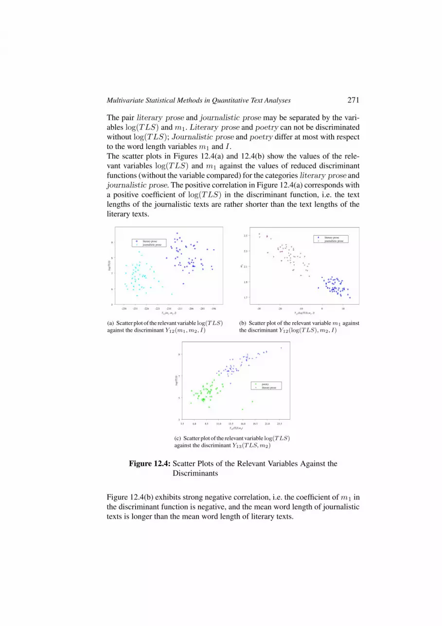
Multivariate Statistical Methods in Quantitative Text Analyses 271
The pair literary prose and journalistic prose may be separated by the vari-ables log(TLS) and m1. Literary prose and poetry can not be discriminatedwithout log(TLS); Journalistic prose and poetry differ at most with respectto the word length variables m1 and I .The scatter plots in Figures 12.4(a) and 12.4(b) show the values of the rele-vant variables log(TLS) and m1 against the values of reduced discriminantfunctions (without the variable compared) for the categories literary prose andjournalistic prose. The positive correlation in Figure 12.4(a) corresponds witha positive coefficient of log(TLS) in the discriminant function, i.e. the textlengths of the journalistic texts are rather shorter than the text lengths of theliterary texts.
-236 -231 -226 -221 -216 -211 -206 -201 -196
Y12(m1 ,m2 ,I)
5
6
7
8
9
log(TLS)
literary prose
journalistic prose
(a) Scatter plot of the relevant variable log(TLS)against the discriminant Y12(m1,m2, I)
-30 -20 -10 0 10
Y12(log(TLS),m2 ,I)
1.7
1.9
2.1
2.3
2.5
m1
literary prose
journalistic prose
(b) Scatter plot of the relevant variable m1 againstthe discriminant Y12(log(TLS),m2, I)
3.5 6.0 8.5 11.0 13.5 16.0 18.5 21.0 23.5
Y13(TLS,m2)
3
5
7
9
log(TLS)
poetry
literary prose
(c) Scatter plot of the relevant variable log(TLS)against the discriminant Y13(TLS,m2)
Figure 12.4: Scatter Plots of the Relevant Variables Against theDiscriminants
Figure 12.4(b) exhibits strong negative correlation, i.e. the coefficient of m1 inthe discriminant function is negative, and the mean word length of journalistictexts is longer than the mean word length of literary texts.

272 CONTRIBUTIONS TO THE SCIENCE OF LANGUAGE
The categories poetry and literary prose are compared in Figure 12.4(c) wherelog(TLS) is plotted against the reduced discriminant function. The positive cor-relation implies a positive coefficient for log(TLS) in the discriminant function.The scatter plot expresses the obvious fact that the poetic texts are shorter thanthe literary texts.Figures 12.5(a) and 12.5(b) display the values of the relevant variables log(TLS)andm1 against the values of the reduced discriminant functions in terms of jour-nalistic prose and poetry. Positive correlation in Figure 12.5(a) is connectedwith a positive coefficient for log(TLS) in the discriminant function. However,more than 50% of the texts in both categories do not differ regarding text length.The effect of m1 is also positive with a much better separation than before: allbut two poetic texts have smaller values of m1 than journalistic texts.
40 50 60 70 80 90
Y23(m1 ,I)
4
5
6
7
8
log(TLS
)
poetry
journalistic prose
(a) Scatter plot of the relevant variable log(TLS)against the discriminant Y23(m1, I)
30 40 50 60 70
Y23(log(TLS) ,I)
1.4
1.6
1.8
2.0
2.2
2.4
m1
poetry
journalistic prose
(b) Scatter plot of the relevant variable m1 againstthe discriminant Y23(log(TLS), I)
Figure 12.5: Scatter Plots of the Relevant Variables Against theDiscriminants
3.1 Canonical DiscriminationOur approach of comparing two categories of text can be generalized to asimultaneous comparison of all three categories of text. For this we used aso-called canonical discriminant analysis with the three variables log(TLS),m1 and I establishing canonical discriminant functions Z1 and Z2. Details ofthis procedure, together with an SPlus program may be found in Djuzelic(2002). For a description of statistics with SPlus we refer to the book ofVenables/Ripley (1999).The first block in Table 12.8 lists the coefficients of the discriminant functionswhich are also the components of the eigenvectors of Z1 and Z2. The secondblock contains the mean values and variances of the discriminants Z1 and Z2
for each text category.

Multivariate Statistical Methods in Quantitative Text Analyses 273
Table 12.8: Canonical Coefficients For Discriminants Z1 and Z2
Variable Z1 Z2
log(TLS) 0.33752 −1.40306m1 4.66734 4.47832I 9.51989 −1.82010
text category group means | variances of Z1 and Z2
literary prose 16.25733 | 0.52973 −4.02454 | 0.83067journalistic prose 19.49542 | 1.20942 −0.74287 | 1.09144poetry 13.64796 | 1.27444 −0.51754 | 1.08310
The eigenvalues λ1 = 5.77386 ofZ1 and λ2 = 2.64693 ofZ2 express quotientsof variances, i.e. the variance between the groups is 5.8 times, respectively 2.6times higher than the variance within the groups. Hence, both variables Z1 andZ2 are good measures for the separation of the categories as can be observedin the scatter plot of Z1 against Z2 in Figure 12.6.
10 12 14 16 18 20 22
-6-4
-20
2
5.99
10 12 14 16 18 20 22
-6-4
-20
2
5.99
10 12 14 16 18 20 22
-6-4
-20
2
5.99
10 12 14 16 18 20 22
-6-4
-20
2
2
2 2
22 22
2
2
2222
2222
2
2 22
2 22
22
2
2
2
2
22 2 2
222
2 2
2
2
2
222
2
2
2
22
2
2
1
1
1
1
1
1
1
1 1
1
1
1
1
11
1
1
1
1
11
1
11
1
1
1
1
1
1
11 11
11
1
1
1
111
1
1
1
1
1
1
1
11 3
3
3
3
33
3
3
3
3
3
3
3
3
3
33
3
3
3
3
3
3
33
3
3
33 33
3
33 3
3
33
3
3
33
3
3
3
3
3
3
33
10 12 14 16 18 20 22
Z1
-6-4
-20
2
Z2
10 12 14 16 18 20 22
-6-4
-20
2
10 12 14 16 18 20 22
-6-4
-20
2
10 12 14 16 18 20 22
-6-4
-20
2
1 poetry
2 literary prose
3 journalistic prose
Figure 12.6: Canonical Discriminant Functions With Regions ofClassification for the Three Text Types
The imposed lines partition the (Z1, Z2)-plane into the three regions of clas-sification resulting in an excellent discrimination of the text categories: 150 of153 texts (i.e., 98%) are classified correctly.In detail we have the following. All 52 literary texts are classified correctly (cat-egory 3). One of the 50 journalistic texts (category 2) is assigned to category 1(poetry). Only two of the 53 poetic texts are misclassified: one text is classifiedas journalistic text and one as literary text.

274 CONTRIBUTIONS TO THE SCIENCE OF LANGUAGE
Figure 12.6 contains also three ellipses of concentration each defined by aquadratic distance of 5.99 from the corresponding group means given in Ta-ble 12.8.
4. ConclusionsOur case study on three categories of Slovenian texts was a first attempt to studythe usefulness of discriminant analysis for the problem of text classification.The major results of our analysis may be summarized as follows.
1. In the univariate setting we calculated for all three pairwise comparisons theunivariate statistical distances of six variables: two variables based on textlength and four variables based on word length. This gave us the first hintsof the overall order of discrimination and the order of influence of specificvariables.
2. The corresponding analysis of multivariate distances and discriminationfunctions demonstrated that the correlation structure of the variables maychange the role of the variables, e.g. comparing literary prose and poetry theunivariate analysis listed variable I as important, but variable m2 as unim-portant. In the multivariate analysis we ended up with m2 as relevant andI as redundant. (This special effect is caused by the high correlation of thevariables.)
3. We established a linear discriminant function for the pair (literary prose| jour-nalistic prose) with four relevant variables. For the two other pairs (literaryprose| poetry) and (journalistic prose| poetry) only three relevant variablesappear in each discriminant function.
4. Both types of variables were relevant for discrimination: variables for textlength as well as variables for word length.
5. Canonical discrimination of all three text categories with the three variableslog(TLS), m1 and I was able to classify 98% of the texts correctly.
6. Our future research will be concentrated on the following considerations.Different categories of texts from various Slavic languages will be studied byclassification methods to find combinations of discriminating variables basedon word length only. For this we prepared a large collection of variables,i.e. statistical parameters describing word length. Our hope is to establishsuitable classification rules for at least some interesting categories of texts.

Multivariate Statistical Methods in Quantitative Text Analyses 275
References
Antic, G.; Kelih, E.; Grzybek, P.2005 “Zero-syllable Words in Determining Word Length”. [In the present volume]
Djuzelic, M.2002 Einflussfaktoren auf die Wortlange und ihre Haufigkeitsverteilung am Beispiel von Tex-
ten slowenischer Sprache. Diplomarbeit, Institut fur Statistik, Technical University Graz.[http://www.stat.tugraz.at/dthesis/djuz02.zip]
Flury, B.1997 A First Course in Multivariate Statistics. New York.
Grotjahn, R.; Altmann, G.1993 “Modelling the Distribution of Word Length: Some Methodological Problems.” In: Kohler,
R.; Rieger, B. (eds.), Contributions to Quantitative Linguistics. Dordrecht, NL.Grzybek, P.; Stadlober, E.
2002 “The Graz Project on Word Length (Frequencies)”, in: Journal of Quantitative Linguistics,9(2); 187–192.
Hand, D.1981 Discrimination and Classification. New York.
Ord, J.K.1967 “On a System of Discrete Distributions”, in: Biometrika, 54, 649–659.
Venables, W.N.; Ripley, B.D.1999 Modern Applied Statistics with S-Plus. 3rd Edition, New York.
Wimmer, G.; Kohler, R.; Grotjahn, R.; Altmann, G.1994 “Towards a theory of word length distribution”, in: Journal of Quantitative Linguistics, 1;
98–106.Wimmer, G.; Altmann, G.
1996 “The theory of word length: Some results and generalizations.” In: Glottometrika 15. (112–133).


Peter Grzybek (ed.): Contributions to the Science of Language.Dordrecht: Springer, 2005, pp. 277–294
WORD LENGTH AND WORD FREQUENCY
Udo Strauss, Peter Grzybek, Gabriel Altmann
1. Stating the ProblemSince the appearance of Zipf’s works, (esp. Zipf 1932, 1935), his hypothesis“that the magnitude of words tends, on the whole, to stand in an inverse (notnecessarily proportionate) relationship to the number of occurrences” (1935: 25)has been generally accepted. Zipf illustrated the relation between word lengthand frequency of word occurrence using German data, namely the frequencydictionary of Kaeding (1897–98).In the past century, Zipf’s idea has been repeatedly taken up and examined withregard to specific problems. Surveying the pertinent work associated with thishypothesis, one cannot avoid the impression that there are quite a number ofproblems which have not been solved to date. Mainly, this seems to be due to thefact that the fundamentals of the different approaches involved have not beensystematically scrutinized. Some of these unsolved problems can be capturedin the following points:
i. The direction of dependence. Zipf himself discussed the relation betweenlength and frequency of a word or word form – which in itself representsan insufficiently clarified problem – only in one direction, namely as thedependence of frequency on length. However, the question is whether fre-quency depends on length or vice versa. While scholars such as Miller,Newman, & Friedman (1958) favored the first direction, others, as for ex-ample, Kohler (1986), Arapov (1988) or Hammerl (1990), preferred thelatter. As to a solution of this question, it seems reasonable to assume thatit depends on the manner of embedding these variables in Kohler’s controlcycle.
ii. Unit of measurement. While some researchers – as, e.g., Hammerl (1990) –measured word length in terms of syllable numbers, others – as for exam-ple Baker (1951) or Miller, Newman & Friedman (1958) – used letters asthe basic units to measure word length. Irrespective of the fact that a highcorrelation between these two units should seem likely be found, a sys-tematic study of this basic pre-condition would be important with regardto different languages and writing systems.

278 CONTRIBUTIONS TO THE SCIENCE OF LANGUAGE
iii. Rank or frequency. Again, while some researchers, as e.g., Kohler (1986),based his analysis on the absolute occurrence of words, others, such asGuiraud (1959), Belonogov (1962), Arapov (1988), or Hammerl (1990)who, in fact, examined both alternatives, considered the frequency rankof word forms. In principle, it might turn out to be irrelevant whetherone examines the frequency or the rank, as long as the basic dependenceremains the same, and one obtains the same function type with differentparameters; still, relevant systematic examinations are missing.
iv. The linguistic data. A further decisive point is the fact that Zipf and hisfollowers did not concentrate on individual texts, but on corpus data orfrequency dictionaries. The general idea behind this approach has been theassumption, that assembling a broader text basis should result in more rep-resentative results, reflecting an alleged norm to be discovered by adequateanalyses. However, this assumption raises a crucial question, as far as thequality of the data is concerned. Specifically, it is the problem of data ho-mogeneity, which comes into play (cf. Altmann 1992), and it seems mostobvious that any corpus, by principle, is inherently inhomogeneous. More-over, it should be reasonable to assume that oscillations as observed byKohler (1986), are the outcome of mixing heterogeneous texts: examiningthe German LIMAS corpus, Kohler (1986) and Zornig et al. (1990) foundnot a monotonously decreasing relationship, but an oscillating course. Thereason for this has not been found until today; additionally, no oscillationhas been discovered in the corpus data examined by Hammerl (1990).
v. Hypotheses and immanent aspects. Finally, it should be noted that Zipf’soriginal hypothesis implies four different aspects; these aspects should,theoretically speaking, be held apart, but, in practice, they tend to be inter-mingled:
(a) The textual aspect. Within a given text, longer words tend to be usedmore rarely, short words more frequently. If word frequency is not takeninto account, one obtains the well-known word length distribution.If, however, word frequency is additionally taken into account, thenone can either study the dependence of length from frequency, or thetwo-dimensional length-frequency distribution. Ultimately, the lengthdistribution is a marginal distribution of the two-dimensional one. Ingeneral, one accepts the dependence L = f(F ) or L = f(R) [L =length, F = frequency, R = rank].
(b) The lexematic aspect. The construction of words, i.e. their length in agiven lexicon, depends both on the lexicon size in question and on thephoneme inventory, as well as on the frequential load of other poly-semic words. Frequency here is a secondary factor, since it does notplay any role in the generation of new words, but will only later result

Word Length and Word Frequency 279
from the load of other words. This aspect cannot easily be embedded inthe modeling process because the size of the lexicon is merely an em-pirical constant whose estimation is associated with great difficulties.It can at best play the role of ceteris paribus.
(c) Shortening through usage. This aspect, which concerns the shorteningof frequently used words or phrases, has nothing to do with wordconstruction or with the usage of words in texts; rather, the process ofshortening, or shortening substitution, is concerned (e.g., references→ refs).
(d) The paradigmatic aspect. The best examined aspect is the frequency offorms in a paradigm where the shorter forms are more frequent than thelonger ones, or where the frequent forms are shorter. The results of thisresearch can be found under headings such as ‘markedness’, ‘iconismvs. economy’, ‘naturalness’, etc. (cf. Fenk-Oczlon 1986, 1990, Haiman1983, Manczak 1980). If the paradigmatic aspect is left apart, aspect(d) becomes a special case of aspect (a).
2. The Theoretical ApproachIn this domain, quite a number of adequate and theoretically sound formulaehave been proposed and empirically confirmed: more often than not, one hasadhered to the “Zipfian relationship” also used in synergetic linguistics (cf.Herdan 1966, Guiter 1974, Kohler 1986, Hammerl 1990; Zornig et al. 1990):consequently, one has started from a differential equation, in which the relativerate of change of mean word length (y) decreases proportionally to the relativerate of change of the frequency (Kohler 1986).Since in most languages, zero-syllabic words either do not exist, or can beregarded as clitics, the mean length cannot take a value of less than 1. This isthe reason why the corresponding function must have the asymptote 1. Finally,the equations get the form (13.1).
dy
y − 1= −bdx
x(13.1)
from which the well-known formula (13.2)
y = a · x−b + 1 (13.2)
follows, with a = eC (C being the integration constant). Here, y is the meanlength of words occurring x times in a given text. If one also counts words withlength zero, the constant 1 must be eliminated, of course, and as a result, atleast some of the values (depending on the number of 0-syllabic words) will belower.As compared to other approaches, the hypothesis represented by (13.2) has theadvantage that the inverse relation yields the same formula, only with different

280 CONTRIBUTIONS TO THE SCIENCE OF LANGUAGE
parameters, i.e.
x = A · (y − 1)−B (13.3)
where A = a1/b, B = 1/b. This means that the dependence of frequency onlength can be captured in the same way as can that of length on frequency, onlywith transformed parameters.In the present paper, we want to test hypothesis (13.2). We restrict ourselvesexclusively to the textual aspect of the problem, assuming that, in a given text,word length is a variable depending on word frequency. Therefore, we con-centrate on testing this relationship with regard to individual texts and not –as is usually done – with regard to corpus or (frequency) dictionary material.Though this kind of examination does not, at first sight, seem to yield newtheoretical insights with regard to the original hypothesis itself, the focus onthe variable text, which, thus far, has not been systematically studied, promisesthe clarification of at least some of the above-mentioned problems. Particularly,the phenomenon of oscillation as observed by Kohler (1986), might find anadequate solution when this variable is systematically controlled; yet, this par-ticular issue will have to be the special object of a separate follow-up analysis(cf. Grzybek/Altmann 2003).For the present study, word length has been counted in terms of the numbers ofsyllables per word, in order to submit the text under study to as few transfor-mations as possible; further, every word form has been considered as a separatetype, i.e., the text has not been lemmatized. Since our main objective is to testthe validity of Zipf’s approach for individual texts, we have chosen exclusivelysingle texts
a) by different authors,
b) in different languages, and
c) of different text types.
Additionally, attention has been paid to the fact that the definition of ‘text’ itselfpossibly influences the results. Pragmatically speaking, a ‘text’ may easily bedefined as the result of a unique production and/or reception process. Still,this rather vague definition allows for a relatively broad spectrum of what aconcrete text might look like. Therefore, we have analyzed ‘texts’ of ratherdifferent profiles, in order to gain a more thorough insight into the homogeneityof the textual entity examined:
i. a complete novel, composed of chapters
ii. one complete book of a novel, consisting of several chapters
iii. individual chapters, either (a) as part of a book of a novel, or (b) of a wholenovel

Word Length and Word Frequency 281
iv. dialogical vs. narrative sequences within a text.
It is immediately evident that our study primarily focuses the problem of ho-mogeneity of data, inhomogeneity being the possible result of mixing varioustexts, different text types, heterogeneous parts of a complex text, etc. Thus,theoretically speaking, there are two possible kinds of data inhomogeneity:
(a) intertextual inhomogeneity
(b) intratextual inhomogeneity.
Whereas intertextual inhomogeneity thus can be understood as the result ofcombining (“mixing”) different texts, intratextual inhomogeneity is due to thefact that a given text in itself does not consist of homogeneous elements. Thisaspect, which is of utmost importance for any kind of quantitative text analysis,has hardly ever been systematically studied. In addition to the above-mentionedfact that any text corpus is necessarily characterized by data inhomogeneity,one can now state that there is absolutely no reason to a priori assume that atext (in particular, a long text) is characterized by data homogeneity, per se. Thecrucial question thus is, under which conditions can we speak of a homogeneous‘text’, when do we have to speak of mixed texts, and what may empirical studiescontribute to a solution of these question?
3. Text Analyses in Different LanguagesThe results of our analyses are represented according to the scheme in Ta-ble 13.1, which contains exemplary data illustrating the procedure: The first col-umn shows the absolute occurrence frequencies (x); the second, the number ofwords f(x) with the given frequency x; the third, the mean lengthL(x) of thesewords in syllables per word. Length classes were pooled, in case of f(x) < 10:in the example, classesx = 8 andx = 9 were pooled because they contain fewerthan 10 cases per class. Since the mean values were not weighted, we obtainedthe new values x = (8+9)/2 = 8.5 andL(x) = (1.5714+1.6667)/2 = 1.62.This kind of smoothing yields more representative classes. In how far othersmoothing procedures can lead to diverging results, will have to be analyzed ina separate study.The following texts have been used for the analyses:
1. L.N. Tolstoj: Anna Karenina – This Russian novel appeared first in 1875;in 1877, Tolstoj prepared it for a separate edition, which was published in1878. The novel consists of eight parts, subdivided into several chapters.Our analysis comprises (a) the first chapter of Part I, and (b) the whole ofPart I consisting of 34 chapters.

282 CONTRIBUTIONS TO THE SCIENCE OF LANGUAGE
Table 13.1: An illustrative example of data pooling
x f(x) L(x) x′ L′
1 2301 27.432 1 27.4322 354 22.090 2 22.0903 93 20.645 3 20.6454 39 19.487 4 19.4875 29 13.793 5 13.7936 23 16.087 6 16.0877 11 11.818 7 11.8188 7 15.714 e e9 6 16.667 8.5 c 1.62 c10 9 12.222 e e11 2 10.000 10.5 c 1.11 c. . . . . . . . . . . . . . .
2. A.S. Puskin: Evgenij Onegin – This Russian verse-novel consists of eightchapters. Chapter I first was published in 1825, periodically followed byfurther individual chapters; the novel as a whole appeared in 1833.
3. F. Mora: Diobel kiralykisasszony [“Nut kernel princess”] – This shortHungarian children’s story is taken from a children book, published in 1965.
4. K.S. Gjalski: Na badnjak [“On Christmas Evening”] – This Croatianstory was first published in 1886, in the volume Pod starimi krovovi. Forour purposes, we have analyzed both the complete text, and dialogical andnarrative parts separately.
5. Karel & Josef Capek: Zarive hlubiny [“Shining depths”] – This Czechstory is a co-authored work by the two brothers Karel and Josef Capek. Thetext appeared in 1913, for the first time, and was then published togetherwith other stories in 1916, in a volume bearing the same title.
6. Ivan Cankar: Hisa Marije Pomocnice [“The House of Charity”] – ThisSlovenian novel was published in 1904. For our purposes, we analyzed thefirst chapter only.
7. Janko Kral: Zakliata panna vo Vahu a divny Janko [“The EnchantedVirgin in Vah and the Strange Janko”] – This text is a Slovak poem, whichwas published in 1844.
8. Hansel und Gretel – This is a famous German fairy tale, which was includedin the well-known Kinder- und Hausmarchen by Jacob and Wilhelm Grimm(1812), under the title of “Little brother and little sister”.

Word Length and Word Frequency 283
9. Sjarif Amin: Di lembur kuring [“In my Village”] – This story is writtenin Sundanese, a minority language of West Java; it was published in 1964.We have analyzed the first chapter of the story.
10. Pak Ojik: Burung api [“The Fire Bird”] – This fairy tale from Indonesia (inBahasa Indonesia), which was published in 1971, is written in the traditionalorthography (the preposition di being written separately).
11. Henry James: Portrait of a lady – This novel, written in 1881, consists of55 individual chapters. We have analyzed both the whole novel, and the firstchapter, only.
Table 13.2 represents the results of the analyses.1 The first column containsthe occurrence frequencies of word forms (x); the next two columns presentthe observed (y) and the computed (y) mean lengths of word forms havingthe corresponding frequency in the given individual texts. As described above,words having zero-length - such as for example the Russian preposition k, s, v,or the Hungarian s (from es) – have not been counted as a separate category,and have been considered as proclitics instead. In the last row of Table 13.2 onefinds the values for the parameters a and b of (13.2), the text length N , and thedetermination coefficient R2.As can be seen from Table 13.2, hypothesis (13.2) can be accepted in all cases,since the fits yield R2 values between 0.84 and 0.96, which can be consideredvery good – independently of language, author, text type, or text length.
1 The English data for Portrait of a Lady have kindly been provided by John Constable; we would like toexpress our sincere gratitude for his co-operative generosity.– All other texts were analyzed in co-operationwith the FWF research project #15485ÀWord Length Frequency Distributions in Slavic Texts¿ at GrazUniversity (cf. Grzybek/Stadlober 2002).

284 CONTRIBUTIONS TO THE SCIENCE OF LANGUAGE
Table 13.2: Dependence of Word Form Length on Word Fre-quency
Russian Russian HungarianAnna Karenina (ch. I) Evgenij Onegin (ch. I) Diobel kiralykisasszony
x y y x y y x y y
1 2.92 3.03 1 2.66 2.70 1 2.52 2.572 2.14 2.04 2 2.13 1.99 2 2.00 1.883 2.05 1.70 3 1.78 1.71 3 1.56 1.624 1.50 1.53 4 1.42 1.57 4 1.57 1.495 1.33 1.43 5.50 1.36 1.45 6 1.33 1.356 1.50 1.36 7.50 1.30 1.35 14.66 1 1.177 1.67 1.31 11.50 1.35 1.258 1 1.27 39.64 1.09 1.099 1 1.24
10 1 1.2213 1 1.1719 1 1.1220 1 1.1137 1 1.06
a = 2.0261, b = 0.9690 a = 1.7029, b = 0.7861 a = 1.5668, b = 0.8379R2 = 0.88, N = 3970 R2 = 0.96, N = 1871 R2 = 0.96, N = 234
Croatian Czech SlovenianNa badnjak Zarive hlubiny Hisa Marije P. (ch. I)
x y y x y y x y y
1 2.83 2.95 1 2.69 2.76 1 2.71 2.802 2.44 2.37 2 2.20 2.17 2 2.35 2.363 2.22 2.12 3 2.15 1.92 3 2.23 2.164 2.18 1.96 4 1.74 1.77 4 2 2.035 1.63 1.86 5 1.74 1.68 5 2 1.946 1.76 1.79 6 1.58 1.61 6 2 1.877 1.87 1.73 7 1.33 1.55 7 1.86 1.828 1.69 1.68 9 1.51 1.48 8 2.14 1.789 1.57 1.64 36.23 1.16 1.21 9.5 1.50 1.73
10 1.67 1.61 18.25 1.22 1.5616.11 1.49 1.48 89.13 1.25 1.3032.91 1.14 1.33
127 1 1.17
a = 1.9454, b = 0.5064 a = 1.7603, b = 0.5921 a = 1.7969, b = 0.4023R2 = 0.93, N = 2450 R2 = 0.94, N = 1363 R2 = 0.84, N = 1147

Word Length and Word Frequency 285
Table 13.2 (cont.)
Slovak German SundaneseZakliata panna Hansel & Gretel Di lembur kuring
x y y x y y x y y
1 2.41 2.48 1 2.12 2.17 1 2.79 2.862 2.05 1.92 2 1.79 1.82 2 2.38 2.313 1.55 1.69 3 1.73 1.67 3 2.05 2.064 1.85 1.57 4 1.71 1.58 4.5 1.13 1.865 1.50 1.49 5 1.55 1.52 6.5 1.58 1.726.50 1.39 1.41 6.5 1.56 1.45 13.29 1.33 1.50
10 1.07 1.30 8.5 1.49 1.4024.67 1.11 1.16 10.5 1.08 1.36
13.5 1.21 1.3119.67 1.25 1.2650.46 1.15 1.16
a = 1.1476, b = 0.675 a = 1.1688, b = 0.5062 a = 1.8609, b = 0.5110R2 = 0.88, N = 926 R2 = 0.87, N = 803 R2 = 0.91, N = 431
Indonesian EnglishBurung api Portrait of a Lady (ch. I)
x y y x y y
1 3.34 3.44 1 2.17 2.232 3.03 3.04 2 1.78 1.693 2.93 2.83 3 1.56 1.494 2.78 2.70 4 1.5 1.395 2.33 2.61 5 1.37 1.326 2.68 2.53 6 1 1.287 2.57 2.47 7 1.33 1.248 2.53 2.42 8.50 1.28 1.209 2.38 2.38 11 1 1.17
10 2.50 2.34 14.50 1.06 1.1311 2.36 2.31 19.83 1.06 1.1013 2.17 2.25 27.50 1.13 1.0817 2 2.17 73.43 1 1.03
a = 2.4353, b = 0.2587 a = 1.2293, b = 0.8314R2 = 0.92, N = 1393 R2 = 0.89, N = 1104

286 CONTRIBUTIONS TO THE SCIENCE OF LANGUAGE
By way of an example, Figure 13.1 illustrates the results of the first chapter ofTolstoj’s Anna Karenina: the courses both of the observed data and the datacomputed according to (13.2), can be seen. On the abscissa, the occurrencefrequencies from x = 1 to x = 40 are given, on the ordinate, the mean wordlengths, measured in the average number of syllables per word. With a deter-mination coefficient of R2 = 0.88, the fit can be accepted to be satisfactory.
1 11 21 31
Frequency
0
0,5
1
1,5
2
2,5
3
3,5
Me
an
Word
Len
gth
observed
theoretical
Figure 13.1: Observed and Computed Mean Lengths in AnnaKarenina (I,1)
4. The ParametersSince all results can be regarded to be good (R2 > .85), or even very good(R2 > .95), the question of a synthetical interpretation of these results quitenaturally arises. First and foremost, a qualitative interpretation of the parametersa and b, as well as a possible relation between them, would be desirable.Figure 13.2 represents the course of all theoretical curves, based on the param-eters a and b given in Table 13.3.Since the curves representing the individual texts intersect, it is to be assumedthat no general judgment, holding true for all texts in all languages, is possible.In Table 13.3 the parameters and the length of the individual texts are summa-rized.From Figure 13.3(a) it can easily be seen that there is no clear-cut relationshipbetween the two parameters a and b.The next question to be asked, quite logically concerns a possible relationbetween the parameters a and b, and the text length N ; yet, the answer isnegative, again. As can be seen in Figure 13.3(b), the relation rather seems tobe relatively constant with a great dispersion; consequently, no interpretablecurve can capture it.It is evident that the fact of a missing relationship between the parameters aand b, and text lengthN , respectively, can be accounted for by the obvious datainhomogeneity: since the texts come from different languages and various text

Word Length and Word Frequency 287
1 2 3 4 5 6 7 8 9 101
1,5
2
2,5
3
3,5
41 2 3 4 5 6 7 8 9 10 11
Figure 13.2: The Course of the Theoretical Curves (Dependenceof Word Form Length on Frequency; cf. Table 13.2
)
Table 13.3: Parameters and Text Length of Individual Texts
Text Language a b N
Anna Karenina (I,1) Russian 2.03 0.97 397Evgenij Onegin (I) Russian 1.70 0.79 1871Na badnjak Croatian 1.95 0.51 2450Zarive hlubiny Czech 1.76 0.59 1363Hisa Marije Pomocnice (I) Slovenian 1.80 0.40 1147Zakliata panna Slovak 1.48 0.69 926Hansel und Gretel German 1.16 0.51 803Fairy Tale by Mora Hungarian 1.57 0.84 234Di lembung kuring Sundanese 1.86 0.51 431Burung api Indonesian 2.44 0.26 1393Portrait of a Lady (I) English 1.23 0.83 1104
types, the ceteris paribus condition is strongly violated, and the data in thismixture are not adequate for testing the hypothesis at stake.
5. The Homogeneity of a ‘Text’In order to avoid the encroachment caused by the different provenience of thetexts, we will next examine the problem using texts whose linguistic and textualhomogeneity can, at least hypothetically, a priori be taken for granted. However,even here, the problem of homogeneity is not ultimately solved.

288 CONTRIBUTIONS TO THE SCIENCE OF LANGUAGE
$
$
$
$
$$
$
$
$ $
$
1 1,1 1,2 1,3 1,4 1,5 1,6 1,7 1,8 1,9 2 2,1 2,2 2,3 2,4 2,5
Parameter a
0
0,2
0,4
0,6
0,8
1
1,2
Pa
ram
ete
r b
(a) Parameters a and b (
&
&&&
&
&
&
& &
&
&
0 50 100 150 200 250
Text Length (N)
0
0,5
1
1,5
2
2,5
3
Param
eter a
(b) Text Length N and Parameter a
Figure 13.3: Relationship Between Parameters a and b and TextLength N (cf. Table 13.3)
Let us therefore compare the results for Chapter I of Tolstoj’s Anna Kareninawith those for the complete Book I, consisting of 34 chapters, as represented inTable 13.4.
Table 13.4: The Length-Frequency Curves for Chapter I and theComplete Text of Anna Karenina
Chapter 1 Complete text
x y y x y y x y y
1 2.92 3.03 1 3.38 3.60 22 2.20 2.132 2.14 2.04 2 3.04 3.16 23 1.94 2.123 2.05 1.70 3 2.84 2.94 24.50 2.27 2.104 1.50 1.53 4 2.76 2.79 26.50 2.04 2.085 1.33 1.43 5 2.84 2.69 28.50 2.27 2.056 1.50 1.36 6 2.65 2.61 30.50 2.07 2.047 1.67 1.31 7 2.45 2.54 33.50 2.29 2.018 1 1.27 8 2.57 2.49 38 1.70 1.989 1 1.24 9 2.47 2.44 42.50 2.13 1.95
10 1 1.22 10 2.64 2.40 51.50 1.67 1.9013 1 1.17 11 2.59 2.36 57.50 1.83 1.8719 1 1.12 12 2.41 2.33 62 1.64 1.8520 1 1.11 13 2.50 2.30 73.25 1.88 1.8237 1 1.06 14 2.20 2.28 91.71 1.43 1.77
15 2.43 2.25 106.86 1.33 1.7416.50 2.11 2.22 137.70 1.70 1.6918 2.35 2.19 229.11 1.28 1.6019.50 2.32 2.17 458.75 1.38 1.5021 2.20 2.14
In Figure 13.4, the empirical data and the theoretical curve are presented forthe sake of a graphical comparison. One can observe two facts:

Word Length and Word Frequency 289
1 11 21 31
Word Frequency
0,00
1,00
2,00
3,00
4,00
Mea
n W
ord
Length
A.K. (I,1) - emp.
A.K. (I,1,) - th.
A.K. (I) - emp.
A.K. (I) - th.
Figure 13.4: Comparison of Anna Karenina, chap. I and Book I
1. The empirical and, consequently, the theoretical values of the larger sample(i.e., Book I, 1-34), are located distinctly higher. For the theoretical curvethis results in an increase of a and a decrease of b.
2. The fitting for the greater sample is still acceptable, but clearly worse (R2 =0.86) as compared to the smaller sample (R2 = 0.97).
A.K. (I,1) A.K. (I)
Tokens 702 38226Types 397 8661
a 2.03 2.60b 0.97 0.27
R2 0.97 0.86
The important finding, that a more comprehensive text unit leads to a worseresult than a particular part of this ‘text’, can be demonstrated even more clearly,comparing the single chapter of a novel with the whole novel. Testing thecomplete novel Portrait of a Lady to this end, one obtains a determinationcoefficient of merely R2 = 0.58, even after smoothing the data as describedabove. As compared to the first chapter of this novel taken separately, yieldinga determination coefficient of R2 = 0.89, (cf. Table 13.2), this is a dramaticdecrease. In fact, an extremely drastic smoothing procedure is necessary inorder to obtain an acceptable result (with a = 1.34, b = 0.47;R2 = 0.92), asshown in Table 13.5 and Figure 13.5.Thus, appropriate smoothing of the data turns out to be an additional problem.On the one hand, some kind of smoothing is necessary because the frequencyclass size should be “representative” enough, and on the other hand, the partic-ular kind of smoothing is a further factor influencing the results.

290 CONTRIBUTIONS TO THE SCIENCE OF LANGUAGE
Table 13.5: Results of Fitting Equation (13.2) to Portrait of aLady, Using the Given Pooling of Values
Class Class
lower upper lower upperlimit limit x′ y y limit limit x′ y y
1 10 1 2.22 2.34 601 700 70 1 1.1811 20 2 1.92 1.97 701 800 80 1 1.1721 30 3 1.84 1.80 801 900 90 1 1.1631 40 4 1.81 1.70 901 1000 100 1 1.1541 50 5 1.71 1.63 1001 2000 200 1.17 1.1151 60 6 1.71 1.57 2001 4000 400 1 1.0861 70 7 1.66 1.53 4001 5000 500 1 1.0771 80 8 1.49 1.50 5001 6000 600 1 1.0681 90 9 1.55 1.47 6001 7000 700 1 1.0691 100 10 1.30 1.45 7001 8000 800 1 1.06101 200 20 1.40 1.32 8001 9000 900 1 1.05201 300 30 1.25 1.27301 400 40 1.40 1.23401 500 50 1.25 1.21501 600 60 1.18 1.19
However, there is a clear tendency according to which the individual chapters ofa novel abide by their own individual regimes organizing the length-frequencyrelation. This boils down to the assessment that even a seemingly homogeneousnovel-text is an inhomogeneous text mixture, composed of diverging superposi-tions. As to an interpretation of this phenomenon, it seems most likely that afterthe end of a given chapter, a given ruling order ends, and a new order (of the
Word Frequency0,00
0,50
1,00
1,50
2,00
2,50
Mea
n W
ord
Le
ngth
Figure 13.5: Fitting Equation (13.2) to Portrait of a Lady (cf.Table 13.5)

Word Length and Word Frequency 291
same organization principle) begins. The new order superposes the preceding,balances or destroys it. Theoretically speaking, one should start with as manycomponents of y = a1x
b1 + a2xb2 + a3x
b3 + . . ., as there are chapters in thetext. Whether this is, in fact, a reasonable procedure, will have to be examinedseparately).As a further consequence, one must even ask if one individual chapter of a novel,or a short story, etc. is a homogeneous text, or if we are concerned with textmixtures due to the combination of heterogeneous components. In order to atleast draw attention to this problem, we have separately analyzed the narrativeand the dialogical sequences in the Croatian story “Na badnjak”. As a result,it turned out that the outcome is relatively similar under all circumstances: forthe dialogue sequences we obtain the values a = 1.61, b = 0.84, R2 = 0.96,for the narrative sequences a = 1.93, b = 0.54, and R2 = 0.91 (as comparedto a = 1.95, b = 0.51, R2 = 0.93 for the story as a whole). It goes withoutsaying, that more systematic examination is necessary to attain more reliableresults.While on the one hand, it turns out that a longer text does not necessarily yieldbetter results, on the other hand, increasing text length need not necessarilyyield worse results. By way of an example, this can be shown on the basis ofcumulative processing of Evgenij Onegin and its eight chapters (i.e., chapter1, then chapter 1+2, 1+2+3, etc.). In this way, one obtains the results shownin Table 13.6; the curves corresponding to the particular parts are displayed inFigure 13.6.
Table 13.6: Parameters of the Frequency-Length Relation in Ev-genij Onegin
Parameters Types Tokens Fit
Chapter a b N M R2
1 1.703 0.786 1871 3209 0.961-2 1.838 0.691 2918 5546 0.881-3 1.921 0.574 3951 8359 0.881-4 1.967 0.525 4851 10936 0.921-5 1.954 0.476 5737 13376 0.941-6 1.968 0.52 6509 15978 0.941-7 2.031 0.425 7476 19061 0.861-8 2.049 0.399 8329 22482 0.88
As can be seen, the curves do not intersect under these circumstances. Thedisplacement of the curve position with increasing text size can be explained

292 CONTRIBUTIONS TO THE SCIENCE OF LANGUAGE
1 2 3 4 5 6 7 8 9 101,00
1,50
2,00
2,50
3,00
3,50
1 1-2 1-3 1-4 1-5 1-6 1-7 total
Figure 13.6: Fitting (13.2) to the text cumulation of Evgenij One-gin
by the fact that words from classes with low frequency wander to higher classesand are substituted by ever longer words. In Figure 13.7(a) the dependencybetween the parameters a and b is shown for the cumulative processing (b beingrepresented by its absolute value).
1,6 1,7 1,8 1,9 2 2,1
Parameter a
0,00
0,20
0,40
0,60
0,80
1,00
Pa
ram
ete
r b
(a) Parameters a and b
#
#
#
#
##
#
#
1 101 201 301 401 501 601 701 801 901
Text Length (Word Forms - Types)
1,50
1,60
1,70
1,80
1,90
2,00
2,10
Pa
ram
ete
r a
(b) Text Length N and Parameter a
Figure 13.7: Relationship Between Parameters a and b and TextLength N in Evgenij Onegin (cf. Table 13.6)
Evidently, b depends on a. Although there seems to be a linear decline, therelation between a and b cannot, however, be linear, since bmust remain greaterthan 0. The power curve b = 4.9615a−3.3885 yields a good fit with R2 = 0.92.In the same way, b depends on text length N . The same relationship yields b =21.4405N−0.4360 withR2 = 0.96. The dependence of a onN can be computedby mere substitution in the second formula, yielding a = 0.6493N 0.1286 whosevalues are almost identical with the observed ones. It is irrelevant whetherone considers types or tokens since they are strongly correlated (r = 0.997).Fig. 13.7(b) shows the relationship between text length N and parameter a.It can thus be concluded that, in a homogeneous text, i.e., in a text in whichone can reasonably assume the ceteris paribus condition to be fulfilled, the

Word Length and Word Frequency 293
relationship between frequency and length remains intact: with an increasingtext length, the curve is shifted upwards and becomes flatter. The parametersare joined in form of a = f(N), b = g(a) or b = h(N), respectively, f, g, hbeing functions of the same type.
6. ConclusionLet us summarize the basic results of the present study. With regard to theleading question as to the relationship between frequency and length of wordsin texts, we have come to the following conclusions:
I. The above hypothesis (2) is corroborated in the given form by our data;
II. A homogeneous text does not interfere with linguistic laws, an inhomo-geneous one can distort the textual reality;
III. Text mixtures can evoke phenomena which do not exist as such in in-dividual texts: In text mixtures, the ceteris paribus condition does nothold; short texts have the disadvantage of not allowing a property to takeappropriate shape; without smoothing, the dispersion can be too strong.Long texts contain mixed generating regimes superposing different lay-ers. In text corpora, this may lead to “artificial” phenomena as, probably,oscillation. Since these phenomena do not occur in all corpora, it seemsreasonable to consider them as a result of mixing.
IV. With increasing text size, the resulting curve of frequency-length relationis shifted upwards; this is caused by the fact that the number of wordsoccurring only once increases up to a certain text length. If this assumptionis correct, then b converges to zero, yielding the limit y = a.

294 CONTRIBUTIONS TO THE SCIENCE OF LANGUAGE
ReferencesAltmann, G.
1992 “Das Problem der Datenhomogenitat.” In: Glottometrika 13. Bochum. (287–298).Arapov, M.V.
1988 Kvantitativnaja lingvistika. Moskva.Baker, S.J.
1951 “A linguistic law of constancy: II”, in: The Journal of General Psychology, 44; 113–120.Belonogov, G.G.
1962 “O nekotorych statisticeskich zakonomernostjach v russkoj pis’mennoj reci”, in: Voprosyjazykoznanija, 11(1); 100–101.
Fenk-Oczlon, G.1990 “Ikonismus versus Okonomieprinzip. Am Beispiel russischer Aspekt- und Kasusbildun-
gen”, in: Papiere zur Linguistik, 42; 49–68Fenk-Oczlon, G.
1986 “Morphologische Naturlichkeit und Frequenz.” Paper presented at the 19th Annual Meetingof Societas Linguistica Europae, Ohrid.
Grzybek, P.; Altmann, G.2003 “Oscillation in the frequency-length relationship”, in: Glottometrics, 5; 97–107.
Grzybek, P.; Stadlober, E.2003 “The Graz Project on Word Length Frequency (Distributions)”, in: Journal of Quantitative
Linguistics, 9(2); 187–192.Guiraud, P.
1954 Les caracteres statistiques du vocabulaire. Essai de methodologie. Paris.Guiter, H.
1977 “Les relations /frequence – longueur – sens/ des mots (langues romanes et anglais).” In: XIVCongresso Internazionale di linguistica e filologia romanza, Napoli, 15-20 aprile 1974.Napoli/Amsterdam. (373–381).
Haiman, J.1983 “Iconic and economic motivation”, in: Language, 59; 781–819.
Hammerl, R.1990 “Lange – Frequenz, Lange – Rangnummer: Uberprufung von zwei lexikalischen Model-
len.” In: Glottometrika 12. Bochum. (1–24).Herdan, G.
1966 The advanced theory of language as choice and chance. Berlin.Kaeding, F.W.
1897–98 Haufigkeitsworterbuch der deutschen Sprache. Steglitz.Kohler, R.
1986 Zur linguistischen Synergetik. Struktur und Dynamik der Lexik. Bochum.Manczak, W.
1980 “Frequenz und Sprachwandel.” In: Ludtke, H. (ed.), Kommunikationstheoretische Grund-lagen des Sprachwandels. Berlin/New York. (37–79).
Miller, G.A.; Newman, E.B.; Friedman, E.A.1958 “Length-frequency statistics for written English”, in: Information and Control, 1; 370–389.
Zipf, G.K.1932 Selected studies of the principle of relative frequency in language. Cambridge, Mass.
Zipf, G.K.1935 The psycho-biology of language: An introduction to dynamic philology. Boston.
Zornig, P.; Kohler, R.; Brinkmoller, R.1990 “Differential equation models for the oscillation of the word length as a function of the
frequency.” In: Glottometrika 12. Bochum. (25–40).

Peter Grzybek (ed.): Contributions to the Science of Language.Dordrecht: Springer, 2005, pp. 295–300
DEVELOPING THE CROATIANNATIONAL CORPUS AND BEYOND
Marko Tadic
1. The Croatian National Corpus – a Case StudyThe Croatian National Corpus (HNK) has been collected since 1998 undergrant # 130718 by the Ministry of Science and Technology of the Republic ofCroatia. The theoretical foundations for such a corpus was laid down in Tadic(1996, 1998), where the need for a Croatian reference corpus (both synchronicand diachronic) was expressed. The tentative solution for its structure was sug-gested, its time-span and size as well as its availability over the WWW furtherelaborated. The overall structure of the HNK was divided on two constituents:
1. 30m: a 30-million corpus of contemporary Croatian2. HETA: Croatian Electronic Textual Archive
The 30m is collected with the purpose of representing a reference corpus forcontemporary Croatian language. It encompasses texts from 1990 until today,from different domains and genres and tries to be balanced in that respect.The HETA is, according to the blurred border between text-collections and thirdgeneration of corpora, intended to be a vast collection of texts older than 1990,or a complete series (sub-corpora) of publications which would mis-balance the30m.Since for Croatian there has been no research on text production/reception orsystematized data on text-flow in society, we were forced to use figures frombook-stores about the most selling books, from libraries about books whichare the most borrowed ones, and overall circulation figures for newspapers andmagazines in order to select the text sources for the HNK. The literary critic’spanoramic surveys on Croatian fiction were also consulted for the fictional typesof texts.The overall structure of 30m consists of:74% Informative texts (Faction): newspaper, magazines, books (journalism,
crafts, sciences, . . . )23% Imaginative texts (Fiction): prose (novels, stories, essays, diaries, . . . )3% Mixed texts

296 CONTRIBUTIONS TO THE SCIENCE OF LANGUAGE
Several technical decisions were made at the beginning of corpus collecting:we wanted to avoid any typing and/or OCR-input of texts. This narrowed oursources to texts in the format of e-text, i.e. already digitally stored documents.On the grounds of these decisions we had no problems with the text quantity fornewspapers, fiction, textbooks from social sciences and/or humanities, but weexperienced severe lack of sources from the natural and technical sciences. Untilnow, more than 100 million words have been collected but it is not included in thecorpus because it would disturb the planned balance. The copyright problem isanother problem, which emerges in the process of corpus compilation since thecopyrights have to be preserved. We are making agreements with text-supplierson that issue.The corpus is encoded in Corpus Encoding Standard (Ide, Bonhomme & Ro-mary 2000), more precisely, its XML version called XCES. The idea to stickto standard data formats is very important because it allows us (and others aswell) to apply different tools to the different data sets while maintaining thesame data-format. The choice of XML as mark-up language in 1998 turned tobe right as nowadays the majority of new corpora are being encoded with XML.Since XML is Unicode compatible, there are no problems with different scrip-tures (i.e., code-pages). The level of mark-up is XCES level 1, which includesthe division on the level of document structure and on the level of individualparagraphs. For the mark-up at level 2, we have developed the tokenizer but ithas been applied only experimentally on limited amounts of texts. The sentencedelimitation is also being done with the system we have developed but the se-rious problem in Croatian are ordinal numbers written with Arabic numbers.The Croatian orthography prescribes the obligatory punctuation (a dot) whichdiscerns between cardinal and ordinal numbers. The problem is that on average28% of all ordinal numbers written with Arabic numbers and dot are at thesame time the sentence endings. In those cases, the dot can also be a fullstop.For the moment this can not be solved in any other way other than with humaninspection.The tool 2XML was developed in order to speed the process of conversion fromthe original text format (RTF, HTML, DOC, QXD, WP, TXT etc.) to XML. Thetool has a two-step procedure of conversion with the ability to apply user-definedscript for fine-tuning the XML mark-up in the output. The conversion can bedone in batch mode as well.The HNK is available at the address http://www.hnk.ffzg.hr where a testversion is freely available for searching. The results of the search are KWICconcordances with frequency information and possibility to turn each keywordin KWAL format.The POS tagging of HNK is currently in its experimental phase right now. SinceCroatian is an inflectionally rich language (7 cases, 2 numbers for nouns; 3 gen-ders, 2 forms (definite/indefinite), 3 grades for adjectives; 7 cases, 2 numbers,

Developing the Croatian National Corpus and Beyond 297
3 persons for pronouns; 7 cases for numbers; 2 numbers, 3 persons, 3 simpleand 3 complex tenses etc. for verbs) there exists a serious complexity in thatprocess. Bearing in mind that Croatian, like all other Slavic languages, is arelatively free-order language, it is obvious that the computational processingof inflection is a prerequisite for any computational syntactic analysis sincethe majority of intra-sentential relations is encoded by inflectional word-formsinstead of word-order (like for example English).Since there are no automatic inflectional analysers for Croatian, we took adifferent approach. Based on a Croatian word-forms generator (Tadic 1994),a Croatian Morphological Lexicon (HML) has been developed. It includesgenerated word-forms for 12,000 nouns, 7,700 verbs and 5,500 adjectivesfor now. It is fully conformant to the MULTEXT-East recommendations v2.0(http://nl.ijs.si/et/MTE). The HML is freely searchable at http://www.hnk.ffzg.hr/hml and allows queries on lemmas as well as word-forms.The POS (and MSD) tagging of HNK will be performed by matching the corpuswith the word-forms from HML thus giving us the opportunity to attach to eachtoken in the corpus all possible morphosyntactical descriptions on unigramlevel. The reason for this is that we do not have any data on “morphosyntacticalor POS homographical weight” of Croatian words and this presents a way ofgetting it. We will do the matching on a carefully selected 1 million corpus.After that we will disambiguate between all possible MSDs and select the rightone for each token in the corpus. This will be done with the help of local regulargrammars that will process the contexts of tokens, and with human inspection.What we expect is a large amount of “internal” homography (where all possibledifferent MSDs of the same token belong to the same lemma) and relativelysmall amount of “external” homography (where possible different MSDs ofthe same token belong to different lemmas). The manually disambiguated 1million corpus will be used as a training data for the POS-tagger. The thustrained POS-tagger will be used to tag the whole HNK with expected precisionabove 90%.The new project proposals have been submitted recently to our Ministry of Sci-ence and Technology and we have proposed a new project: Developing CroatianLanguage Resources (2003-2005). Its primary goals would be the completionof the 30m corpus and its enlargement to 100m. The inclusion of some kindof spoken corpus would be highly preferable as well as development of severalparallel corpora with Croatian being one side of the pair. The new corpus man-ager (Manatee coupled with its client Bonito) is being considered as a basiccorpus software platform.

298 CONTRIBUTIONS TO THE SCIENCE OF LANGUAGE
2. Some Methodological RemarksWe have to look upon the corpora as the sources of our primary linguistic data.But what kind of data do we get from corpora exactly? We can assume that onthe first level there are three basic types of data:
1. evidence: is the linguistic unit we are looking for there?
2. frequency: if it is there, how often?
3. relation: if it is there more than once, is there any recognizable relationshipwith other units? Are there different relationships or only one?
What do we count in corpora? This question should be spread over differentlinguistic levels:
– phonemes/graphemes (and their combinations, syllables)
– morphemes (and their combinations: words)
– words (and their combinations: syntagms)
– syntagms (and their combinations: clauses and sentences)
– meanings (?)
Let us concentrate on the level of words only. If we get the “bag of words”containing (zenom, zene, zenu, zenom), we can say that in it there are fourtokens, three types, two lemmas and one lemma (two lemmas in the case ofword-form zene, which is “externally” homographic). When we say “words”,we must be precise and define to which possible types of words we are referring.Corpora start with tokens.But in the case of Croatian even such a straightforward concept as the word canbe is not always easy to grasp in real texts (corpora). Consider the examples:
(a) nikoji, pron. adjective = nijedan, nikakav (no one)
(b) Ni u kojem se slucaju ne smijes okrenuti
(c) oligo- i polisaharidi
(d) Ivan je Sikic radosno krenuo nizbrdo.
where (a) is a citation from the Anic (1990) dictionary, (b) is a case of dividedpronominal adjective, (c) a case of text compression, (d) a very frequent case ofanalytical (or complex) verbal tense where auxiliary can be almost anywhere inthe clause. How many words do we have here? Is it a trivial question? How doesthe opposition between “graphic words”, phonetic words, types and lemmasstand?Measuring of word length implies (1) a definition of the word “word”, and (2)a definition of the unit of measurement.

Developing the Croatian National Corpus and Beyond 299
(1) Words can be defined as a graphic, phonetic, morphotactic, lexical (= lis-teme), syntactic or semantic word. Each of these possible definitions con-centrates on different features of words.
(2) Units of measurement can be graphemes, phonemes, syllables, morphemes.It would be really interesting to see a whole corpus with words measuredin all possible units of measurement.
What is the nature of linguistic investigation? It is always about the two sidesof the same “piece of paper”: form and meaning. Form is there to convey themeaning. Our meaning motivates the choice of the form on the level of lexicalchoice and syntactic constructions. What we do in a normal situation is that wechoose the best forms we have at our disposal in the language we speak to conveythe meaning. If we try to compare forms of different languages, we should havemeaning under controlled conditions; meaning should be a neutral factor in ourexperiment. It would be best to have (more-or-less) the same meaning in bothlanguages. Therefore, I plea for the use of parallel corpora for any purpose ofthis kind. The parallel corpora are original texts paired with their translations.This is the closest we can get in our attempt to keep the “same” meaning intwo or more languages. This is the situation in which our comparison of formsbetween languages will yield the methodologically cleanest results.Regarding purely quantitative approaches to language, there is a lot of ground forfruitful cooperation with corpus linguistics. Quantitative and corpus linguisticapproaches are complementary. Corpus linguistics gives quantitative linguis-tics large amounts of systematized data, far more variables and the possibilityto test and define parameters in quantitative approaches. On the other hand,quantitative linguistics gives corpus linguistics tools to discrete segmentationof text continuum which results in discrete classes and/or units. Quantitativeand corpus linguistics should work in synergy.

300 CONTRIBUTIONS TO THE SCIENCE OF LANGUAGE
ReferencesAnic, V.
1990 Rjecnik hrvatskoga jezika. Zagreb.Ide, N.; Bonhomme, P.; Romary, L.
2000 “An XML-based Encoding Standard for Linguistic Corpora.” In: Proceedings of the SecondInternational Language Resources and Evaluation Conference, vol. 2. Athens. (825–830).
Rychly, P.2000 Korpusove manazery a jejich efektivnı implementace. [= Corpus Managers and their ef-
fective implementation). Ph.D. thesis, University of Brno. [http://www.fi.muni.cz/~pary/disert.ps]
Tadic, M.1994 Racunalna obradba morfologije hrvatskoga knjievnoga jezika. Ph.D. thesis, University of
Zagreb. [http://www.hnk.ffzg.hr/txts/mt_dr.pdf].Tadic, M.
1996 “Racunalna obradba hrvatskoga i nacionalni korpus,” in: Suvremena lingvistika, 41-42;603–611. [English: http://www.hnk.ffzg.hr/txts/mt4hnk_e.pdf].
Tadic, M.1997 “Racunalna obradba hrvatskih korpusa: povijest, stanje i perspektive,” in: Suvremena
lingvistika, 43-44; 387–394. [English: http://www.hnk.ffzg.hr/txts/mt4hnk3_e.pdf].
Tadic, M.1998 “Raspon, opseg i sastav korpusa hrvatskoga suvremenog jezika,” in: Filologija, 30-31;
337–347. [English: http://www.hnk.ffzg.hr/txts/mt4hnk2_e.pdf].Tadic, M.
2002 “Building the Croatian National Corpus.” In: Proceedings of the Third International Lan-guage Resources and Evaluation Conference, vol. 2. Paris. (441–446).

Peter Grzybek (ed.): Contributions to the Science of Language.Dordrecht: Springer, 2005, pp. 301–317
ABOUT WORD LENGTH COUNTING IN SERBIAN
Dusko Vitas, Gordana Pavlovic-Lazetic, Cvetana Krstev
1. IntroductionText elements can be counted in several ways. Depending on the counting unit,different views of the structure of a text as well as of the structure of its parts suchas words, may be obtained. In this paper, we present different distributions incounting words in Serbian, applied to samples chosen from a corpus developedby the Natural Language Processing Group at the Faculty of Mathematics,University of Belgrade.This presentation is organized in four parts. The first part presents formal ap-proximations of a word. These approximations partially normalize text in sucha way that the influence of orthographic variations is neutralized in measuringspecific parameters of texts. Text elements will be counted with respect to suchapproximations. The second part of the paper describes in brief some of theexisting resources for Serbian language processing such as corpora and textarchives. Part three presents the results of analysis of structure of word lengthin Serbian, while in part four, distributions of word frequencies in chosen textsare analyzed, as well as the role morphological, syntactic and lexical relationsplay in a revision of the results obtained in counting single words.
1.1 The Formal wordThe digital form of a text is an approximation of the text as an object orga-nized in a natural language. Text registered in such a way, as a raw material,appears in the form of character sequences. The first step in recognizing its nat-ural language organizations consists of the identification of words as potentiallinguistic units. In order to identify words, it is necessary to notice the differ-ence between a character sequence potentially representing a word, and theword itself, represented by the character sequence, and belonging to a specificlanguage system.Let Σ be a finite alphabet used for writing in a specific language system, and ∆a finite alphabet of separators used for separating records of words (alphabetsΣ and ∆ do not have to be disjointed in a natural language). Then a formalword is any contingent character string over the alphabet Σ. For example, if

302 CONTRIBUTIONS TO THE SCIENCE OF LANGUAGE
Σ = {a, b}, then aaabbb and ababab are formal words over Σ, but the first onebelongs to the language
L = {anbn|n ≥ 0}
while the second does not. If ∆={c, d} is an alphabet of separators, then in thestring aaabbbcabababdaabb there are three formal words over Σ, the first andthe third of which being words from the language L, while the formal wordababab, enclosed with the separators c, d, is not a word from the language L.If, on the other side, the alphabet of separators is ∆ = {b, c}, i.e., Σ ∩∆ 6= ∅,then the segmentation of the sequence abacab into formal words is ambiguous.The necessity to differentiate a formal word from a word as a linguistic unitarises from the following example: let Σ be the Serbian language alphabet (nomatter how it is defined). Even if we limit the contents of Σ so as to containalphabet symbols only, the problem of identifying formal word is nontrivial.For example, in the string PETAR I PETROVIC, I has twofold interpretation(either as a Roman numeral or as a conjunction). Similarly, in the course oftransliteration from Latin to Cyrillic and vice versa, formal words occur ina Serbian text that do not belong to Serbian language, or that have twofoldinterpretation. String VILJEM has two Cyrillic interpretations, string PC hasdifferent interpretations in Latin and Cyrillic, and the string Xorx in the Latinalphabet is a formal word resulting in transliteration from the Cyrillic alphabet(in the so-called yuscii-ordering) of the word Dzordz etc.Ambiguity may originate in orthographic rules. For example, the name of theflower daninoc (Latin viola tricolor) has, according to different orthographicvariants, the following forms:
(1a) daninoc (cf. Jovanovic/Atanackovic (1980)(1b) dan-i-noc (cf. Pesikan et al. (1993)(1c) dan i noc (cf. Pesikan et al.(1993)
It is obvious that segmentation into formal words depends on whether the hy-phen is an element of the separator set or not. Let us look at the followingexamples of strings over the Serbian language alphabet:
(2) 1%-procentni versus jednopostotni3,5 miliona evra versus tri i po miliona evra
or tri miliona i pet stotina hiljada evra21.06.2003. versus 21. juni ove godine
If we constrain Σ to the alphabet character set, it is not possible to establishformal equality between the former strings. Extending the set Σ to digits, punc-tuation or special characters leads to ambiguity in interpreting and recognizingformal words.For a more thorough discussion on the problem of defining and recognizingformal words, see Vitas (1993), Silberztein (1993).

About Word Length Counting in Serbian 303
1.2 The Simple and compound wordIf we assume that Σ ∩ ∆ = ∅, then it is possible to reduce the concept of aformal word to the concept of a simple word. By a simple word we assumea contingent string of alphabet characters (characters from the Σ set) betweentwo consecutive separators. Then in example (1) only the form daninoc is asimple word. The other two forms are sequences of three simple words, sincethey contain separators. Simple words represent better approximation of lexicalwords (words as elements of a written text), than formal words. Still, a simpleword does not have to be a word from the language, either. For example, indziju-dzica (Pesikan et al. (1993: t. 59a), segmentation to simple words givestwo strings dziju and dzica which by themselves do not exist in the Serbianlanguage.In some cases, simple words participating in a compound word cannot standby themselves. For example, in contemporary Serbian the noun kostac occursonly in the phrase uhvatiti se u kostac.Based on the notion of a simple word, a notion of a compound word is defined,as a sequence of simple words. The notion of a compound word has beenintroduced in Silberztein (1993), including different constraints necessary inorder for a compound word to be differentiated from an arbitrary sequence ofsimple words. Let us compare the following sentences:
(3a) Radi dan i noc(3b) Cveta dan i noc
At the level of automatic morphological analysis, segmentation to simple wordsis unambiguous and both examples contain four simple words, and in both sen-tences the same grammatical structure is recognized: V N Conj N . But, if anotion of a compound word is applied to the segmentation level, the segmen-tation becomes ambiguous. The string dan i noc in (3a) is a compound word(an adverbial), and the sentence (3a) then may consist of one simple and onecompound word and have a form of V Adv. In example (3b), considering themeaning of the verb cvetati (to bloom), a twofold segmentation of the com-pound word dan i noc is possible: as an adverbial compound or as the name ofa flower.It follows that the notion of a word as a syntactic-semantic unit can be ap-proximated in a written text in several different ways: as a formal or a simpleword, including correction by means of a compound word. The way wordsare counted as well as the result of such a counting certainly depends on theaccepted definition of a word. Ambiguity occurring in examples (3a) and (3b)offers an example of possibly different results in counting words as well as incounting morpho-syntactic categories.

304 CONTRIBUTIONS TO THE SCIENCE OF LANGUAGE
1.3 Serbian language corporaOne of the resources for empirical investigation of the Serbian language areSerbianlanguage corpora in digital form.In the broadest sense, significant resources of Serbian language are collectionsof texts collected without explicit linguistic criteria. One such collection is rep-resented by the project Rastko (www.rastko.org.yu). This website containsseveral hundred integral texts. A different source is thewebsite of Danko Sipka(main.amu.edu.pl/\~{}sipkadan/), which is a corpus of Serbo-Croatianlanguage, representing a portal to collections of texts available through theweb,regardless of the way texts are encoded and tagged. Pages of daily or weeklynewspapers, as well as CD editions, can be considered as relevant material forquantitative language investigations.If the notion of a corpus is constrained so that explicit criteria of structuringresources have to be applied in its construction, two corpora then exist: thediachronic corpus of Serbian / Serbo-Croatian language compiled by DordeKostic, and the corpus of contemporary Serbian language developed at theFaculty of Mathematics, University of Belgrade.The diachronic corpus compiled by Dorde Kostic originated in the 1950s asa result of manual processing of samples of texts. It encompasses the periodfrom the 12th century to the beginning of the 1950s. During the 1990s, thismaterial was transformed into digital form, and insights into its structure andexamples can be found at the URL:www.serbian-corpus.edu.yu/. This corpuscontains about 11 million words and it is manually lemmatized and tagged.Although significant in size, it does not make explicit relationships betweentextual and lexical words, and the process of manual lemmatization appliedcannot be reproduced on new texts.1
The corpus developed at the Faculty of Mathematics, University of Belgrade,contains Serbian literature of the 20th century, including translations publishedafter 1960, different genres of newspaper texts (after 1995), textbooks and othertypes of texts (published after 1980), in integral form. Some parts of the cor-pus are publicly available through the web at www.korpus.matf.bg.ac.yu/korpus/. The total size of the corpus is over 100 million words, and only asmaller portion of it is available through theweb for on-line retrieval. The corpusat the Faculty of mathematics has been partly automatically tagged and disam-biguated using the electronic morphological dictionary system and the systemIntex (Vitas 2001). Besides, parallel French-Serbian and English-Serbian cor-pora have been partially developed, consisting of literary and newspaper texts.
1 For inconsistencies in traditional lexicography, see Vitas (2000).

About Word Length Counting in Serbian 305
1.4 Description of textsFor the analysis of word length in Serbian, texts were chosen from the corpus ofthe contemporary Serbian language, developed at the Faculty of Mathematicsin Belgrade. Texts are in ekavian, except for rare fragments. The sample consistsof the following texts:
i. The web-editions of daily newspapers Politika (www.politika.co.yu)in the period from 5th to 10th of October 2000 (further referred to asPoli). These texts are a portion of a broader sample of the same newspaper(period from the 10th of September to the 20th of October 2000, referredto as Politika).
ii. The web-edition of the Serbian Orthodox Church journal Pravoslavlje[Orthodoxy](www.spc.org.yu) – numbers 741 to 828 from the period1998–2001. This sub-sample will be referred to as SPC.
iii. Collection of tales entitled Partija karata [Card game], written by RadeKuzmanovic (Nolit, Belgrade, 1982). The text will be referred to as Radek.
iv. The novel Treci sektor ili zena sama u tranziciji [Third sector or a womanalone in transition] by Mirjana Durdevic (Zagor, Belgrade, 2001). This textwill be referred to as Romi.
v. Translation of the novel Bouvard and Pecuchet by Gustave Flaubert (Nolit,Belgrade, 1964). The text will be referred to as Buvar.
Table 15.1 represents the way characters from the Serbian alphabet are encoded.
Table 15.1: Serbian Alphabet-Specific Characters Encoding
c c d dz z s lj njcx cy dx dy zx sx lx,lj nx,nj
The length of the texts, in terms of total number of tokens (and different tokens),after initial preprocessing by Intex, is given in Table 15.2. Any of the followingthree types of formal words are considered to be tokens: simple word, numeral(digits) and delimiters (string of separators).
2. Word length in text and dictionary of SerbianConsidering the sub-samples described in table 15.2, let us examine word lengthdistributions in Serbian, using different criteria for expressing word length.

306 CONTRIBUTIONS TO THE SCIENCE OF LANGUAGE
Table 15.2: Length of Texts Expressed by the Total Number ofTokens and Different Tokens
source tokens (diff.) simple words digits delimiters
Politika 1736094 1355785 82135 298172(107919) (107867) (10) (42)
Poli 190664 147913 9079 33672(26921) (26884) (10) (27)
SPC 369541 293460 15505 60576(48987) (48940) (10) (37)
Romi 68389 53271 120 14998(11131) (11101) (10) (20)
Radek 101231 88105 67 13059(16438) (16420) (10) (8)
Buvar 96170 79176 129 16865(21272) (21245) (10) (17)
2.1 Word length in terms of number of charactersThe length of a simple word may be expressed by the number of characters itconsists of. In this sense, word length may be calculated by a function suchas, for example, strlen in the programming language C, modified by the factthat characters have to be alphabetical (from the class [A–Z a–z]). Consideringthe method of encoding, since diacritic characters are encoded as digraphs(Table 15.1), the function for calculating simple word length treats digraphsfrom Table 15.1 as single characters. Results of such a calculation are given inTable 15.3, and graphically represented by Figure 15.1.The local peak on the length 21 in the SPC sub-sample comes from the highfrequency of different forms of the noun Visokopreosvesxtenstvo (71) and theinstrumental singular of the adjective zahumskohercegovacyki (1). With thisapproach to calculating the length of a formal word, the word foto-reporter (inRadek) or rasko-prizrenski (in SPC) are considered as two separate words.
2.2 Word length in terms of number of syllablesThe length of a simple word may also be expressed by the number of sylla-bles also. Calculation is based on the occurrence of characters correspondingto vowels and syllabic ‘r’ (where it is possible to automatically recognize its

About Word Length Counting in Serbian 307
Figure 15.1: Differences Found in the Within-Sentence Distribu-tion of Content and Function Words
occurrence). Word length in terms of the number of syllables is represented inTable 15.4, and graphically by Figure 15.2.
Figure 15.2: Word Length in Terms of Number of Syllables
Prepositions such as ‘s’ [with], ‘k’ [toward], abbreviation such as ‘g.’ [Mr],‘sl.’ [similar], etc., are considered as words with 0 syllables. As a side effect incalculating word length by the number of syllables, the vowel-consonant wordstructure in Serbian has been obtained. If we denote the position of a vowel in aword by v, and position of a consonant by c, then Tables 15.5 and 15.6 present

308 CONTRIBUTIONS TO THE SCIENCE OF LANGUAGE
Table 15.3: Word Length in Terms of Number of Characters
length in number of simple wordscharacters Poli SPC Romi Radek
1 13509 29496 3511 76302 25509 44756 13201 171423 9389 19813 6519 96024 14335 33926 8946 122425 14092 33766 6963 116386 16155 35554 4754 104357 14779 28093 3472 78468 13262 23235 2689 55359 10593 17218 1508 3197
10 6545 11022 834 163411 5223 8013 481 74712 2131 5025 228 28513 1307 1715 95 8914 734 846 34 3315 192 525 19 2716 73 201 12 1917 43 106 3 118 28 44 1 319 7 13 120 4 721 2 7822 1 723 1
∑147913 293460 53271 88105
frequencies of vowel-consonant structure for two literary texts analyzed, andrespectively for newspaper texts. Along with each structure, the first occurrenceof a simple word corresponding to the structure is given. Simple words consist-ing of open syllables have high frequencies. It can be seen that newspaper andliterary texts show different distributions regarding vowel-consonant orderingsin a simple word, although data about length of words in terms of number ofcharacters or syllables do not show such differences. A detailed analysis of theconsonant group structure in Serbo-Croatian is given in Krstev (1991).The texts analyzed, both literary texts and newspapers, have an identical setof eight most frequent vowel-consonant word structures. It is rather interestingthat among the literary as well as among the newspaper texts, the ordering of

About Word Length Counting in Serbian 309
Table 15.4: Word Length in Terms of Number of Syllables
length in number of simple wordssyllables Poli SPC Romi Radek
0 2295 3331 278 6331 45570 88496 21708 322692 34215 82796 18112 273583 34196 64513 8544 185034 22660 38648 3519 77255 7277 12411 925 13786 1413 2618 152 2177 229 471 24 188 52 163 9 49 5 12 0 010 1 1 0 0∑
147913 293460 53271 88105
these structures by frequency is identical too; between literary and newspapertexts there is, however, a noticeable difference in this ordering (consecutivestructures in one are permuted in another), cf. Figure 15.3.
Figure 15.3: Top Frequencies of Vowel-Consonant Structures inLiterary and Newspaper Texts

310 CONTRIBUTIONS TO THE SCIENCE OF LANGUAGE
Table 15.5: Top Frequencies of Vowel-Consonant Structures ForTwo Literary Texts
Radek Romi
group frequ. example group frequ. example
cv 15745 je cv 12349 Necvcv 9147 nebu cvcv 6942 radav 6999 i v 3260 Icvc 5357 sam cvc 3019 Josxcvcvcv 4342 kucxice cvcvcv 2315 dodusxecvcvc 3391 Taman cvcvc 2152 jedancvccv 3097 Tesxko cvccv 2127 Jesteccvcv 2587 svoje ccv 1583 gdevcv 1852 Ona ccvcv 1577 vremeccv 1638 dva vcv 1559 oneccvcvcv 1621 sparina vc 817 odvc 1394 ih cvcvcvcv 762 Terazijecvcvcvcv 1374 nekoliko ccvcvcv 721 primiticvccvcv 1337 putnika cvccvcv 636 najmanxecvccvc 1260 zadnxem vcvc 618 opet
2.3 Word length in a dictionaryLet us further examine the length of simple words in a dictionary, e.g., theSistematski recnik srpskohrvatskog jezika by Jovanovic/Atanackovic (1980).Simple words are reduced here to their lemma form, i.e., verbs to infinitive,nouns to nominative singular, etc. There are 7773 verbs and 38287 other simplewords (nouns, adjectives, adverbs) in the dictionary. The distribution of theirlength in terms of number of characters (calculated in the manner describedabove) is depicted by the diagram in Figure 15.4. It is substantially differentfrom the word distribution in a running text.This distribution may be proved to be Gaussian normal distribution with param-eters (8.58; 2.65), established by Kolmogorov χ2-test with significance levelα=0.01, number of intervals n = 8 and interval endpoints
5 < a1 < 6 < a2 < 7 < a3 < 8 < a4 < 9 < a5 < 10 < a6 < 11 < a7 < 12.
2.4 Word frequency in textThe results of calculating simple word frequencies in samples from 1.4 confirmwell-known results about the participation of functional words in a text. The

About Word Length Counting in Serbian 311
Table 15.6: Top Frequencies of Vowel-Consonant Structures ForTwo Newspaper Texts
Poli SPC
group frequ. example group frequ. example
cv 23053 da cv 39408 SAv 12583 i v 28304 Ucvcv 10717 SUDA cvcv 25328 SAVAcvcvcv 6330 godine cvcvcv 16788 godineccvcv 3910 sceni ccvcv 10676 SVETIcvcvc 3635 danas cvcvc 8164 kojojcvccv 3310 posle cvccv 7826 CENTUcvc 3294 sud cvc 7773 nxihcvcvcvcv 3140 politika cvcvcvcv 6132 delovanxacvccvcv 2809 Tanjugu cvccvcv 5259 poznateccvcvcv 2484 gradxana ccvcvcv 5100 dvoranivc 2209 od ccv 4410 svevccvcv 2162 odnosi vcv 4403 ovecvcvccv 2133 ponisxti vc 4254 odccv 1888 svi ccvcvc 3859 Dragan
most frequent ten words coincide in all of the chosen samples (a, da, i, je,na, ne, se, u, za), with some insignificant deviations (the form su – ‘are’ in the
Figure 15.4: Word Length Distribution in a Dictionary

312C
ON
TRIB
UTIO
NS
TOTH
ESC
IEN
CE
OF
LAN
GU
AGE
newspapersam
pleversusthe
formsam
–‘am
’inthe
literarysam
ple),asshown
inTable
15.7.Thus,underlined
arew
ordsoccurring
infouroutoffive
samples
(e.g.,od ,sa),inunderlined
italicare
thoseoccurring
inthree
samples
(e.g.,iz,koji,su),in
italic–
two
(e.g.,cxe,kao,mi,o,sam
,sxto,to),inbold
face–
thoseoccurring
inone
sample
only,e.g.,ja,nije,s,ti.
Table15.7:M
ostFrequentWords
Politika Poli SPC Radek Romi
frequ. word frequ. word frequ. word frequ. word frequ. word
1. 53215 i 5507 i 15163 i 3838 i 2326 da2. 46338 u 5077 je 9656 u 3202 da 1658 je3. 43778 je 5174 u 8675 je 2643 se 1230 se4. 34875 da 4196 da 5525 da 2392 u 1431 i5. 20689 se 2340 se 4913 se 1906 je 1006 u6. 19875 na 2087 na 3831 na 1569 sam 915 ne7. 16093 za 1726 su 3138 su 1493 na 752 sam8. 15596 su 1456 za 2167 za 807 ne 651 na9. 8854 a 1070 a 1779 od 610 mi 470 a
10. 8263 od 1002 sa 1733 sa 598 s 422 ja11. 8208 sa 844 od 1718 a 579 od 422 mi12. 7200 koji 768 cxe 1544 koji 532 sxto 414 to13. 6013 cxe 723 koji 1406 ne 515 za 384 sa14. 5730 iz 599 o 1397 kao 498 to 383 za15. 5480 o 592 iz 1131 iz 474 kao 361 ti16. 5197 ne 566 ne 1016 sxto 422 a 326 nije

AboutW
ordLength
Counting
inSerbian
313
Table15.8:Top
FrequenciesofW
ordB
igrams
Radek Romi Politika SPC
frequ. bigram frequ. bigram frequ. bigram frequ. bigram
1. 286 da se 124 da se 297 da se 455 da se2. 114 kao da 81 da je 274 da je 310 kao i3. 90 da je 43 Ne znam 185 rekao je 279 da je4. 29 i onda 37 da ne 181 da cxe 252 koji je5. 28 ja sam 37 da mi 159 kao i 235 koji su6. 28 i ja 33 ja sam 140 i da 158 je u7. 28 da bih 32 Ja sam 135 koji je 152 Sxto je8. 27 sxto se 32 i da 120 koji su 147 i u9. 27 mislim da 31 a ne 109 u Beogradu 126 i da
10. 26 je u 29 ne znam 95 On je 120 koja je11. 26 je bilo 27 to je 91 sxto je 118 To je12. 25 mogu da 26 mi je 90 kako je 112 da bi13. 24 mogao da 26 I sxta 90 rekao da 110 Nxegova Svetost14. 24 da cxu 26 a ja 79 da su 109 pravoslavne crkve15. 24 bih se 25 A i 73 izjavio je 102 da cxe
Still,apictureofthemostfrequentw
ordswillbesignificantly
changedif,instead
ofcalculating
frequenciesof
singlesim
plew
ords,frequenciesof
contingentsequences
oftwo
orthreesim
plew
ordsare
calculated(Table
15.8).

314 CONTRIBUTIONS TO THE SCIENCE OF LANGUAGE
Except for the strings da je and da se, the first 15 combinations of two simplewords do not include any other common element. On the other hand, meaning-ful words such as verbs, nouns, adjectives, emerge in highly frequent levels.Frequency of the most frequent word bigrams is significantly lower than thefrequency of single simple words, which points out the influence of syntacticconditions in combining simple words. When the same comparison with wordtrigrams is performed, the results represented in table 15.9 is obtained.Among the high frequent combinations of three simple words, in our sub-samples there is no more common element. Participation of functional words ineach of the sub-samples depends on a type of a sentence construction, or theyare parts of compounds.

AboutW
ordLength
Counting
inSerbian
315
Table15.9:Top
FrequenciesofW
ordTrigram
s
Radek Romi Politika SPC
frequ. trigram frequ. trigram frequ. trigram frequ. trigram
1. 28 kao da sam 17 ne mogu da 34 od nasxeg 41 Nxegova Svetoststalnog patrijarh
2. 27 u neku ruku 8 ne znam da 30 Demokratske 38 Kosovuopozicije Srbije i Metohiji
3. 25 cyinilo mi 8 a ne samo 30 kako je rekao 34 Srpskese pravoslavne crkve
4. 23 kao da je 7 sxta ti je 29 kazxe se u 28 na Kosovu i5. 18 znao sam da 7 da mi je 29 navodi se u 27 Kao sxto je6. 17 da tako 7 bojim se 25 da cxe se 21 a to je
kazxem da7. 16 po svoj 6 da je to 22 kako bi se 20 i da se
prilici8. 15 Tacyno je da 5 Ti si 22 kao i da 19 da bi se
stvarno9. 15 kao da se 5 Otkud ti 20 i da se 18 Nxegova Svetost
znasx je10. 14 u svakom 5 Ne znam ni 18 i da je 17 bracxo i sestre
slucyaju

316 CONTRIBUTIONS TO THE SCIENCE OF LANGUAGE
2.5 Morphological problem in counting wordsResults presented naturally raise questions about results that will be obtained ifa simple word from text is substituted by its lemma and further on, by its part ofspeech. Results of such a substitution over texts Radek and Romi, consideringthe verb znati (to know) which occurred in both texts, are given in Table 15.10.
Table 15.10: Lemma Frequency – Example of the Verb znati
<znati> Total Present tense Participle Infinitive
Radek 121 80 40 1Romi 218 186 29 3Poli 77 62 8 3
In the Poli sample, <znati> appears in adverbial form (znajuci, 2) and passiveparticiple form (znan, 2). This suggests the conclusion that the distribution ofword length will further change if lemmatization of word forms is performed.Note that among the word trigrams, phrases po svoj prilici (probably) and usvakom slucaju (anyway) can be found (Radek), representing adverbial com-pounds, as well as noun toponym Kosovo i Metohija (SPC).The problem becomes more evident if a parallelized text is analyzed, as theexample of the Buvar sample shows: in the original text string Bouvard oc-curs 635 times in total; in the Serbian translation, this string is separated intodifferent forms of the proper name Buvar and its possessive adjective. Furtherconsiderations in this direction are given in Senellart (1999).

About Word Length Counting in Serbian 317
ReferencesJovanovic, Ranko; Atanackovic, Laza
1980 Sistematski recnik srpskohrvatskog jezika. Novi Sad.Krstev, Cvetana
1991 “Serbo-Croatian Hyphenation: a TEX point of view”, in: TUGboat, 122; 215–223.Pesikan, Mitar; Pizurica, Mato; Jerkovic, Jovan
1993 Pravopis srpskoga jezika. Novi Sad.Senellart, Jean
1999 Outils de reconnaissance d’expresions linguistiques complexes dans des grands corpus.Universite Paris VII: These de doctorat.
Silberztein, Max D.1993 Le dictionnaire electronique et analyse automatique de textes: Le systeme INTEX. Paris.
Vitas, Dusko1993 Matematicki model morfologije srpskohrvatskog jezika (imenska fleksija). University of
Belgrade: PhD. Thesis, Faculty of Mathematics.Vitas, Dusko; Krstev, Cvetana; Pavlovic-Lazetic, Gordana
2000 “Recent Results in Serbian Computational Lexicography.” In: Bokan, Neda (ed.), Proceed-ings of the Symposium¿Contemporary MathematicsÀ. Belgrade: University of Belgrade,Faculty of Mathematics. (113–130).
Vitas, Dusko; Krstev, Cvetana; Pavlovic-Lazetic, Gordana2002 “The Flexible Entry.” In: Zybatow, Gerhild; Junghanns, Uwe; Mehlhorn, Grit; Szucsich,
Luka (eds.), Current Issues in Formal Slavic Linguistics. Frankfurt/M. (461–468).


Peter Grzybek (ed.): Contributions to the Science of Language.Dordrecht: Springer, 2005, pp. 319–327
WORD-LENGTH DISTRIBUTIONIN PRESENT-DAY LOWER SORBIANNEWSPAPER TEXTS
Andrew Wilson
1. IntroductionLower Sorbian is a West Slavic language, spoken primarily in the south-easterncorner of the eastern German federal state of Brandenburg; the speech area alsoextends slightly further south into the state of Saxony.Although the dialect geography of Sorbian is rather complex, Lower Sorbianis one of the two standard varieties of Sorbian, the other being Upper Sorbian,which is mainly used in Saxony.1
As a whole, Sorbian has fewer than 70,000 speakers, of whom only about 28%are speakers of Lower Sorbian. However, an understanding of both varietiesof Sorbian is a key element in understanding the structure and history of theWest Slavic language group as a whole, since Sorbian is generally recognizedas constituting a separate sub-branch of West Slavic, alongside Lechithic (i.e.Polish and Cassubian) and Czecho-Slovak.2
This study is the first attempt to investigate word-length distribution in Sorbiantexts, with a view to comparison with similar studies on other Slavic languages.
2. BackgroundThe main task of quantitative linguistics is to attempt to explain, and expressas general language laws, the underlying regularities of linguistic structure andusage. Until recently, this task has tended to be approached by way of normallyunrelated individual studies, which has hindered the comparison of languagesand language varieties owing to variations in methodology and data typology.Since 1993, however, Karl-Heinz Best at the University of Gottingen has beencoordinating a systematic collaborative project, which, by means of comparable
1 For an overview of both varieties of Sorbian, see Stone (1993).2 For a brief review of the arguments for this and for other, previously proposed groupings, see Stone (1972).
It is, of course, important to analyse Sorbian for its own sake and not just for comparative purposes.

320 CONTRIBUTIONS TO THE SCIENCE OF LANGUAGE
methodologies, makes it possible to obtain an overview of many languages andlanguage varieties. The present investigation is a contribution to the Gottingenproject.The Gottingen project has so far been concerned especially with the distributionof word lengths in texts. The background to the project is discussed in detailby Best (1998, 1999), hence only the most important aspects are summarizedhere.Proceeding from the suggestions of Wimmer and Altmann (1996), the projectseeks to investigate the following general approach for the distribution of wordlengths in texts:
Px = g(x)Px−1 (16.1)
where Px is the probability of the word length x and Px−1 is the probabilityof the word length x − 1. It is thus conjectured that the frequency of wordswith length x is proportional to the frequency of words with length x − 1. Itis, however, clear that this relationship is not constant, hence the element g(x)must be a variable proportion. Wimmer and Altmann have proposed 21 specificvariants of the above equation, depending on the nature of the element g(x).The goal of the Gottingen project is thus, first of all, to test the conformanceof different languages, dialects, language periods, and text types to this generalequation, and, second, to identify the appropriate specific equation for eachdata type according to the nature of the element g(x). Up to now, data fromapproximately 40 languages have been processed, which have shown that, sofar, all languages support Wimmer and Altmann’s theory, and, furthermore,that only a relatively small number of theoretical probability distributions arerequired to account for these (see, for example, Best 2001).
3. Data and methodology3.1 DataIn accordance with the principles of the Gottingen project3, a study such asthis needs to be carried out using homogeneous text, ideally between 100 and2,000 words in length. It was therefore decided to use newspaper editorials(section “tak to wizimy”) from the Lower Sorbian weekly newspaper NowyCasnik. These were available in sufficient quantity and were of an ideal length.Similar text types have also been used for investigations on other languages (cf.Riedemann 1996).The following ten texts were analyzed, all dating from 2001:
3 http://www.gwdg.de/∼kbest/principl.htm

Word-Length Distribution in Present-Day Lower Sorbian Newspaper Texts 321
1 March, 3 Dolnoserbsko–engelski sÃlownik – to jo wjelgin zajmnawec
2 March, 31 Na skodu nimskeje recy?3 April, 7 Tenraz ‘olympiada’ mimo Casnika4 April, 14 Rednje tak, Picanski amt!5 April, 21 PDS jo psasaÃla – z poÃlnym psawom6 April, 28 Serbski powedas – to jo za nas wazne7 May, 5 Sud piwa za nejwusu maju8 May, 26 Nic jano pla WITAJ serbski9 June, 2 Psawje tak, sakski a bramborski ministar
10 June, 16 Ga buzo skoncnje zgromadna konferenca soÃltow?
3.2 Count principlesFor each text analyzed, the number of words falling into each word-lengthclass was counted. The word lengths were determined in accordance with theusual principles of the Gottingen project, i.e., in terms of the number of spokensyllables per orthographic word.In counting word lengths, there are a number of special cases, which are regu-lated by the general guidelines of the project:
1. Abbreviations are counted as instances of the appropriate full form; thus, forexample, dr. is counted as a two-syllable word (doktor).
2. Acronyms are counted as they are pronounced, e.g. PDS is counted as a singlethree-syllable word.
3. Numerals are counted according to the appropriate spelt-out (written) forms,e.g. 70 is treated as sedymzaset (a word with four syllables).
There is no general guideline for the treatment of hyphenated forms. In thisstudy, hyphens are disregarded and treated as inter-word spaces, so that, forexample WITAJ-projektoju is treated as two separate words.A special problem in Lower Sorbian, as also in the other West Slavic languages,is the class of zero-syllabic prepositions. Previously, these have been treated asspecial cases within the Slavic language group and have been included in thefrequency statistics (cf. the work of Uhlırova 1995). However, if one counts theseprepositions as independent words, it is then necessary to fit rarer probabilitymodels to the data. Current practice is therefore to treat these zero-syllabic wordsas parts of the neighbouring words (i.e. as clitics), and, since they do not containany vowels, they are thus simply disregarded (Best, personal communication).If treated in this way, then more regular probability distributions can normallybe fitted.

322 CONTRIBUTIONS TO THE SCIENCE OF LANGUAGE
The word-length frequency statistics for each text were run through the AltmannFitter software4 at Gottingen to determine which probability distribution wasthe most appropriate model. 5
3.3 StatisticsThe Altmann Fitter compares the empirical frequencies obtained in the dataanalysis with the theoretical frequencies generated by the various probabilitydistributions (Wimmer and Altmann 1996; 1999). The degree of differencebetween the two sets of frequencies is measured by the chi-squared test andalso by the discrepancy coefficient C; the latter is given by χ2/N (where Nis the total number of words counted) and is used especially where there is nodegree of freedom.A probability distribution is considered an appropriate model for the data if thedifference between the empirical and theoretical frequencies is not significant,i.e., if P (χ2) > 0.05 and/or C < 0.02. The best distribution is that whichshows the highest P and/or lowest C.
4. ResultsIn all cases, the 1-displaced hyper-Poisson distribution could be fitted to thetexts with good P and/or C values. In some cases, however, it was necessary tocombine length classes in order to obtain a good fit; this is indicated by verticallines linking length classes in the individual results tables.The 1-displaced hyper-Poisson distribution is given by equation (16.2), in whicha and b are parameters and F is the hypergeometric function:
Px =a(x−1)
b(x−1)1F1(1; b; a)
, x = 1, 2, ... (16.2)
The following tables present the individual results for the ten texts, where:x[i] number of syllablesf [i] observed frequency of i-syllable words
NP [i] theoretical frequency of i-syllable wordsχ2 chi-squared.f. degrees of freedom
P [χ2] probability of the chi-squareC discrepancy coefficient (χ2/N )a parameter a in the above formula (16.2)b parameter b in the above formula (16.2)
4 RST Rechner- und Softwaretechnik GmbH, Essen5 I am grateful to Karl-Heinz Best for running the data through the Altmann Fitter.

Word-Length Distribution in Present-Day Lower Sorbian Newspaper Texts 323
Text # 1 March, 3 Text # 2 March, 31
x[i] f [i] NP [i] x[i] f [i] NP [i]
1 61 61.01 1 71 75.172 67 67.01 2 76 66.643 19 29.20 e 3 25 32.614 18 7.94 | 4 13 11.025 2 1.85 c 5 2 2.84 e
6 1 0.59 |7 1 0.12 c
a 0.7223 a 1.0920b 0.6576 b 1.2317χ2 0.0001 χ2 3.73d.f. 0 d.f. 2
P [χ2] 0.15C < 0.0001 C 0.0197
Text # 3 April, 7 Text # 4 April, 14
x[i] f [i] NP [i] x[i] f [i] NP [i]
1 68 67.58 1 56 55.422 54 51.74 2 49 52.703 23 27.82 3 32 33.684 14 11.53 4 25 16.21 e5 4 3.88 5 5 9.00 c6 1 1.45
a 1.8059 a 1.9492b 2.3588 b 2.0500χ2 1.61 χ2 1.26d.f. 3 d.f. 1P [χ2] 0.66 P [χ2] 0.26C 0.0098 C 0.0075
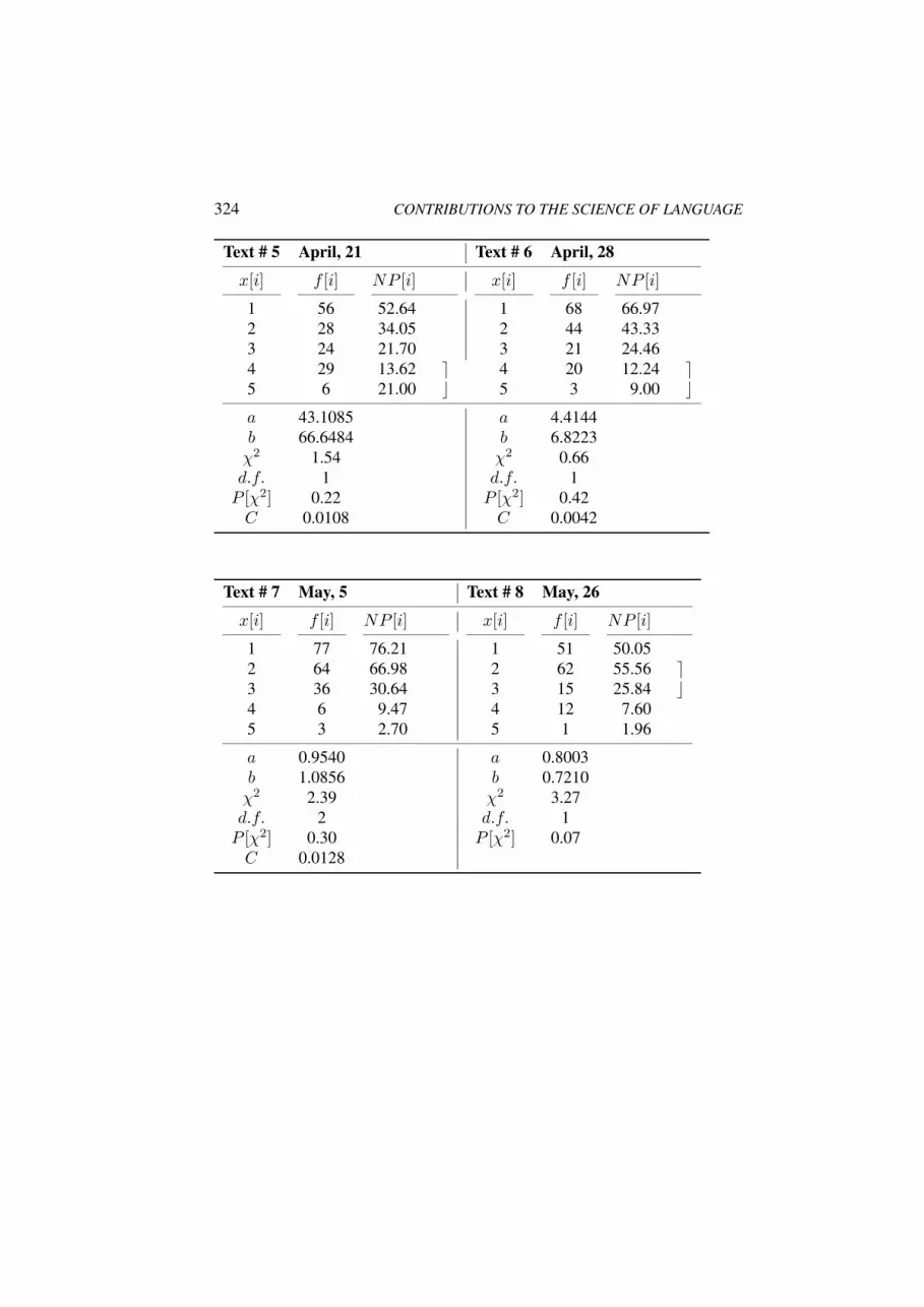
324 CONTRIBUTIONS TO THE SCIENCE OF LANGUAGE
Text # 5 April, 21 Text # 6 April, 28
x[i] f [i] NP [i] x[i] f [i] NP [i]
1 56 52.64 1 68 66.972 28 34.05 2 44 43.333 24 21.70 3 21 24.464 29 13.62 e 4 20 12.24 e5 6 21.00 c 5 3 9.00 ca 43.1085 a 4.4144b 66.6484 b 6.8223χ2 1.54 χ2 0.66d.f. 1 d.f. 1P [χ2] 0.22 P [χ2] 0.42C 0.0108 C 0.0042
Text # 7 May, 5 Text # 8 May, 26
x[i] f [i] NP [i] x[i] f [i] NP [i]
1 77 76.21 1 51 50.052 64 66.98 2 62 55.56 e3 36 30.64 3 15 25.84 c4 6 9.47 4 12 7.605 3 2.70 5 1 1.96
a 0.9540 a 0.8003b 1.0856 b 0.7210χ2 2.39 χ2 3.27d.f. 2 d.f. 1P [χ2] 0.30 P [χ2] 0.07C 0.0128

Word-Length Distribution in Present-Day Lower Sorbian Newspaper Texts 325
Text # 9 June, 2 Text # 10 June, 16
x[i] f [i] NP [i] x[i] f [i] NP [i]
1 60 59.65 1 48 47.022 52 54.89 2 44 42.553 30 26.33 3 19 23.044 9 8.54 4 13 8.905 0 2.09 5 0 2.676 1 0.49
a 1.0024 a 1.3479b 1.0893 b 1.4895χ2 1.66 χ2 4.45d.f. 2 d.f. 2P [χ2] 0.44 P [χ2] 0.11C 0.0109 C 0.0356
5. ConclusionsSince one of the theoretical distributions suggested by Wimmer and Altmanncan be fitted to the empirical data with a good degree of confidence, we mayconclude that the Lower Sorbian language is no exception to the Wimmer-Altmann theory for the distribution of word lengths in texts.It has also been found that the 1-displaced hyper-Poisson distribution is the mostappropriate theoretical distribution to account for word lengths in present-dayLower Sorbian newspaper texts. However, this cannot yet be considered as ageneral distribution for the Lower Sorbian language as a whole, since text typeand period can have an effect on word-length distribution.6 Further studies aretherefore necessary to investigate these variables for Lower Sorbian.Direct comparisons with all the other Slavic languages are not yet possible, sincemost of the existing data were processed under earlier counting guidelines,i.e., with the inclusion of zero-syllabic words. Rarer variants of word-lengthprobability distributions thus had to be fitted in these cases. However, Best(personal communication) has re-processed the data for a West Slavic language(Polish) and an East Slavic language (Russian) without zero-syllabic words. Inboth cases, the 1-displaced hyper-Poisson distribution gave the best results. Itis thus possible that the 1-displaced hyper-Poisson distribution may prove to be
6 For example, Wilson (2001) found that quantitative Latin verse showed a different distribution to thatpreviously demonstrated for Latin prose and rhythmic verse; and Zuse (1996) demonstrated a differentdistribution for a genre of Early Modern English prose to that shown by Riedemann (1996) for a genreof present-day English prose.

326 CONTRIBUTIONS TO THE SCIENCE OF LANGUAGE
a generally applicable distribution for the Slavic language group. However, thiscannot yet be said with certainty: the processing of data without zero-syllabicwords from the other West, East and South Slavic languages (including UpperSorbian) is a pre-condition for such a claim. Different text types and periods ineach language must also be examined.

Word-Length Distribution in Present-Day Lower Sorbian Newspaper Texts 327
ReferencesBest, K.-H.
1998 “Results and perspectives of the Gottingen project on quantitative linguistics”, in: Journalof Quantitative Linguistics, 5; 155–162.
Best, K.-H.1999 “Quantitative Linguistik: Entwicklung, Stand und Perspektive”, in: Gottinger Beitrage zur
Sprachwissenschaft, 2; 7–23.Best, K.-H. (ed.)
2001 Haufigkeitsverteilungen in Texten. Gottingen.Riedemann, H.
1996 “Word-length distribution in English press texts”, in: Journal of Quantitative Linguistics,3; 265–271.
Stone, G.1972 The smallest Slavonic nation: the Sorbs of Lusatia. London.
Stone, G.1993 “Sorbian (Upper and Lower).” In: Comrie, B.; Corbett, G. (eds.), The Slavonic languages.
London. (593–685).Uhlırova, L.
1995 “On the generality of statistical laws and individuality of texts. A case of syllables, wordforms, their length and frequencies”, in: Journal of Quantitative Linguistics, 2; 238–247.
Wilson, A.2001 “Word length distributions in classical Latin verse”, in: Prague Bulletin of Mathematical
Linguistics, 75; 69–84.Wimmer, G.; Altmann, G.
1996 “The theory of word length: Some results and generalizations.” In: Glottometrika 15. (112–133).
Wimmer G.; Altmann, G.1999 Thesaurus of univariate discrete probability distributions. Essen.
Zuse, M.1996 “Distribution of word length in Early Modern English letters of Sir Philip Sidney”, in:
Journal of Quantitative Linguistics, 3; 272–276.


Peter Grzybek (ed.): Contributions to the Science of Language.Dordrecht: Springer, 2005, pp. 329–337
TOWARDS A UNIFIED DERIVATIONOF SOME LINGUISTIC LAWS∗
Gejza Wimmer, Gabriel Altmann
1. IntroductionIn any scientific discipline the research usually begins in the form of membradisiecta because there is no theory which would systematize the knowledgeand from which hypotheses could be derived. The researchers themselves havedifferent interests and observe at first narrow sectors of reality. Later on, oneconnects step by step disparate domains (cf., for example, the unified represen-tation of all kinds of motion of the macro world by Newton’s theory) and theold theories usually become special cases of the new one. One speaks aboutepistemic integration (Bunge 1983: 42):
The integration of approaches, data, hypotheses, theories, and even entire fieldsof research is needed not only to account for things that interact strongly withtheir environment. Epistemic integration is needed everywhere because there areno perfectly isolated things, because every property is related to other properties,and because every thing is a system or a component of some system. . . Thus, justas the variety of reality requires a multitude of disciplines, so the integration ofthe latter is necessitated by the unity of reality.
In quantitative linguistics we stand at the beginning of such a development.There are already two “grand” integrating cross-border approaches like lan-guage synergetics (cf. Kohler 1986) or Hrebıcek’s (1997) text theory as well as“smaller” ones, joining fewer disparate phenomena out of which some can bementioned as examples:
(a) Baayen (1989), Chitashvili and Baayen (1993), Zornig and Boroda (1992),Balasubrahmanyan/Naranan (1997) show that rank distributions can betransformed in frequency distributions, announced already by Rapoport(1982) in a non-formal way.
(b) Altmann (1990) shows that Buhler’s “theory” is merely a special case ofZipf’s theory who saw the “principle of least effort” behind all humanactivities (1949).
∗ Supported by a grant from the Scientific Grant Agency of the Slovak Republic VEGA 1/7295/20

330 CONTRIBUTIONS TO THE SCIENCE OF LANGUAGE
(c) More integrating is Menzerath’s law whose effects can be noticed not onlyin different domains of language but also in molecular biology, sociologyand psychology (Altmann/Schwibbe 1989); it is a parallel to the allometriclaw and can be found also in chaos theory (Hrebıcek’s 1997, Schroeder1990), in self-organized criticality (Bak 1996), in music (Boroda/Altmann1991) etc.
(d) Orlov, Boroda and Nadarejsvili (1982) searched for commonalities in lan-guage, music and fine arts where they found the effect of Zipf-Mandelbrot’slaw.
(e) Krylov, Naranan and Balasubrahmanyan, all physicists, came indepen-dently to the conclusion that the maximization of entropy results in a lawfitting excellently frequency distributions of language entities.
One could continue this enumeration of unification of domains from a certainpoint of view ad libitum – here we have brought merely examples. In all casesone can see the common background that in the end leads to systems theory. Allthings are systems. We join two domains if we find isomorphies, parallelities,similarities between the respective systems or if we ascertain that they are specialcases of a still more general system. From time to time one must perform suchan integration in order to obtain ever more unified theories and to organize theknowledge about the object of investigation.In this contribution we want to present an approach that unifies several wellknown linguistic hypotheses, is easy to be generalized and is very simple –even if simplicity does not belong to the necessary virtues of science (cf. Bunge1963). It is a logical extension of the “synergetic” approach (cf. Wimmer etal. 1994; Wimmer/Altmann 1996; Altmann/Kohler 1996). The individual hy-potheses belonging to this system have been set up earlier as empirical, wellfitting curves or derived from different approaches.
2. Continuous ApproachIn linguistics, continuous variables can be met mostly in phonetics but weare aware that “variable” is merely a construct of our mathematical apparatuswith which we strive for capturing the grades of real properties transformingthem from discrete to continuous (e.g., average) or vice versa (e.g., splitting acontinuous range in intervals) as the need arises, which is nothing unusual inthe sciences. Thus there is nothing wrong in modelling continuous phenomenausing discrete models or the other way round. “Continuous” and “discrete” areproperties of our concepts, the first approximations of our epistemic endeavor.Here we start from two assumptions which are widespread and accepted inlinguistics, treating first the continuous case:

Towards a Unified Derivation of Some Linguistic Laws 331
(i.) Let y be a continuous variable. The change of any linguistic variable, dy,is controlled directly by its actual size because every linguistic variableis finite and part of a self-regulating system, i.e., we can always use inmodelling the relative rate of change dy/y.
(ii.) Every linguistic variable y is linked with at least one other variable (x)which shapes the behavior of y and that can be considered in the givencase as independent. The independent variable influences the dependentvariable y also by its rate of change, dx, which is itself in turn controlledby different powers of its own values that are associated with differentfactors, “forces” etc. We consider x, y as differently scaled and so thesetwo assumptions can be expressed formally as
dy
y − d =
(a0 +
k1∑
i=1
a1i
(x− b1i)c1+
k2∑
i=1
a2i
(x− b2i)c2+ . . .
)dx (17.1)
with ci 6= cj , i 6= j. (We note that for ks = 0 isks∑i=1
asi(x−bsi)cs
= 0.)
The constants aij must be interpreted in every case differently; they representproperties, “forces”, order parameters, system requirements etc. which activelyparticipate in the linkage between x and y (cf. Kohler 1986, 1987, 1989, 1990)but remain constant because of the ceteris paribus condition. In the differentialequation (17.1) the variables are already separated. The solution of (17.1) is (ifc1 = 1)
y = Cea0xk1∏
i=1
(x− b1i)a1ie
∑j≥2
kj∑i=1
aji(1− cj)(x− bji)cj−1
+ d (17.2)
The most common solutions of this approach result in
(a) type-token curves
(b) Menzerath’s law
(c) Piotrovskij-Bektaev-Piotrovskaja’s law of vocabulary growth
(d) Naranan-Balasubrahmanyan’s word frequency models
(e) Gersic-Altmann’s distribution of vowel duration
(f) Job-Altmann’s model of change compulsion of phonemes
(g) Tuldava’s law of polysemy
(h) Uhlırova’s dependence of nouns in a given position in sentence
(i) The continuous variant of Zipf-Mandelbrot’s law and its special cases(Good, Woronczak, Orlov, Zornig-Altmann)

332 CONTRIBUTIONS TO THE SCIENCE OF LANGUAGE
3. Two-Dimensional ApproachThis is of course not sufficient. In synergetic linguistics there is a number ofinterrelations that cannot be captured with the aid of only one variable, conceal-ing the other ones under the “ceteris paribus” condition. They are frequently sostrong that they must be explicitly taken into account.Consider first a simple special case of formula (17.1)
dy
y=(a0 +
a1
x+a2
x2
)dx (17.3)
whose solution yiels
y = Cea0xxa1e−a2/x (17.4)
which represents e.g. Gersic-Altmann’s model of vowel duration. In (17.3)we assume that all other factors (besides x) are weaker than x and can beconsidered as constants relativized by powers of x (e.g., a2/x
2, a3/x3 etc.). But
in synergetic linguistics this is not usual. In many models, the researchers (e.g.Kohler, Krott, Prun) show that a variable depends at the same time on severalother variables which have a considerable influence. Now, we assume – as isusual in synergetic linguistics – that the dependent variable has the same relationto other variables as shown in (17.3). Thus we combine several approaches andobtain in the first step
∂y
∂x= y
(a0 +
a1
x+a2
x2+ . . .
);
∂y
∂z= y
(b0 +
b1z
+b2z2
+ . . .
)(17.5)
which results in
y = Cea0x+b0zxa1zb1e
(−∞∑i=1
ai+1
ixi−∞∑i=1
bi+1
izi
)
(17.6)
The special cases of (17.6) are often found in synergetic linguistics wheremore than two variables are involved. This system can be generalized to anynumber of variables, can, as a matter of fact, encompass the whole synergeticlinguistics and is applicable to very complex systems. Some well known casesfrom synergetic linguistics are
y = Cxazb (17.7)
y = Ceax+bz (17.8)
y = Ceax+bzxazb (17.9)
etc.

Towards a Unified Derivation of Some Linguistic Laws 333
4. Discrete ApproachIf X is a discrete variable – being the usual case in linguistics – then we useinstead of dx the difference ∆x = x − (x − 1) = 1. Since here one has todo mostly with (nonnegative discrete) probability distributions with probabilitymass functions {P0, P1, . . .} we set up the relative rate of change as
∆Px−1
Px−1=Px−Px−1
Px−1(17.10)
and obtain the discrete analog to (17.1) as
∆Px−1
Px−1= a0 +
k1∑
i=1
a1i
(x− b1i)ci+
k2∑
i=1
a2i
(x− b2i)c2+ . . . (17.11)
If k1 = k2 = . . . = 1, d = b11 = b21 = . . . = 0, ci = i, ai1 = ai, i = 1, 2, . . .the equivalent form of (17.11) is
Px =
(1 + a0 +
a1
x+a2
x2 + . . .
)Px−1 . (17.12)
The system most used in linguistics is
Px =
(1 + a0 +
a1
x− b1+
a2
x− b2
)Px−1, (17.13)
whose solution for x = 0, 1, 2, . . . yields
Px =
(1 + a0)x(C −B + x
x
)(D −B + x
x
)
(−b1 + x
x
)(−b2 + x
x
) ×
× 3F−12 (1, C −B + 1, D −B + 1;− b1 +1,− b2 +1; 1 + ao)
(17.14)
where
B = b1 + b22
C =a1 + a2−
√2(1 + a0)2(b1 − b2)2 − 2(1 + a0)(a1 − a2)(b1 − b2) + (a1 + a2)2
2(1 + a0)
D =a1 + a2 +
√2(1 + a0)2(b1 − b2)2 − 2(1 + a0)(a1 − a2)(b1 − b2) + (a1 + a2)2
2(1 + a0)
From the recurrence formulas (17.12) and (17.13) one can obtain many wellknown distributions used frequently in linguistics, e.g., the geometric distri-bution, the Katz family of distributions, different diversification distributions,

334 CONTRIBUTIONS TO THE SCIENCE OF LANGUAGE
rank-frequency distributions,, distribution of distances, the Poisson, negative bi-nomial, binomial, hyper-Poisson, hyper-Pascal, Yule, Simon, Waring, Johnson-Kotz, negative hypergeometric, Conway-Maxwell-Poisson distributions etc.etc.The laws contained in this system are e.g. Frumkina’s law, different syllable,word and sentence length laws, some forms of Zipf’s law, ranking laws, distri-butions of syntactic properties, Krylov’s semantic law, etc. etc.
5. Discrete Two-Dimensional ApproachIn the same way as with the continuous approach one can generalize the discreteapproach to several variables. Since the number of examined cases in linguisticsup to now is very small (an unyet published article by Wimmer and Uhlırova, anarticle on syllable structure by Zornig/Altmann1993, and an article on semanticdiversification by Beothy/Altmann 1984), we merely show the method.In the one-dimensional discrete approach we had a recurrence formula – e.g.,(17.12) or (17.13) – that can be written as
Px = g(x)Px−1 (17.15)
where g(x) was (a part of) an infinite series. Since now we have two variables,we can set up the model as follows
Pi,j = g(i, j)Pi,j−1
Pi,j = h(i, j)Pi−1,j
(17.16)
where g(i, j) andh(i, j) are different functions of i and j. The equations must besolved simultaneously. The result depends on the given functions. Thus Wim-mer and Uhlırova obtained the two dimensional binomial distribution, Zornigand Altmann obtained the two-dimensional Conway-Maxwell-Poisson distribu-tion and Beothy and Altmann obtained the two-dimensional negative binomialdistribution.
6. ConclusionThe fact that in this way one can systematize different hypotheses has severalconsequences:
(1) It shows that there is a unique mechanism – represented by (17.1), (17.5),(17.11), (17.16) – behind many language processes in which one can com-bine variables and “forces”.
(2) Formulas (17.1), (17.5), (17.11), (17.16) represent systems in which alsoextra-systemic factors can be inserted.

Towards a Unified Derivation of Some Linguistic Laws 335
(3) This approach allows to test inductively new, up to now unknown relationsand systematize them in a theory by a correct interpretation of factors; thisis usually not possible if one proceeds inductively. The explorative part ofthe work could therefore be speeded up with the appropriate software. Oneshould not assume that one can explain everything in language using thisapproach but one can comfortably unify and interpret a posteriori manydisparate phenomena.

336 CONTRIBUTIONS TO THE SCIENCE OF LANGUAGE
ReferencesAltmann, G.
1990 “Buhler or Zipf? A re-interpretation.” In: Koch, W.A. (ed.), Aspekte einer Kultursemiotik.Bochum. (1–6).
Altmann, G.; Kohler, R.1996 “ ‘Language Forces’ and synergetic modelling of language phenomena”, in: Glottometrika,
15; 62–76.Altmann, G.; Schwibbe, M.H.
1989 Das Menzerathsche Gesetz in informationsverarbeitenden Systemen. Hildesheim.Baayen, R.H.
1989 A corpus-based approach to morphological productivity. Amsterdam: Centrum voor Wis-kunde en Informatica.
Bak, P.1996 How nature works. The science of self-organized criticality. New York.
Balasubrahmanyan, V.K.; Naranan, S.1997 “Quantitative linguistics and complex system studies”, in: Journal of Quantitative Lin-
guistics, 3; 177–228.Beothy, E.; Altmann, G.
1984 “Semantic diversification of Hungarian verbal prefices. III. ‘fol-’, ‘el-’, ‘be-’.” In: Glot-tometrika 7. (73–100).
Boroda, M.G.; Altmann, G.1991 “Menzerath’s law in musical texts.” In: Musikometrika 3. (1–13).
Bunge, M.1963 The myth of simplicity. Englewood Cliffs, N.J.
Bunge, M.1983 Understanding the world. Dordrecht, NL.
Chitashvili, R.J.; Baayen, R.H.1993 “Word frequency distributions of texts and corpora as large number of rare event distribu-
tions.” In: Hrebıcek, L.; Altmann, G. (eds.), Quantitative Text Analysis. Trier. (54–135).Gersic, S.; Altmann, G.
1988 “Ein Modell fur die Variabilitat der Vokaldauer.” In: Glottometrika 9. (49–58).Hrebıcek, L.
1997 Lectures on text theory. Prague: Oriental Institute.Kohler, R.
1986 Zur linguistischen Synergetik. Struktur und Dynamik der Lexik. Bochum.Kohler, R.
1987 “Systems theoretical linguistics”, in: Theoretical Linguistics, 14; 241–257.Kohler, R.
1989 “Linguistische Analyseebenen, Hierarchisierung und Erklarung im Modell der sprach-lichen Selbstregulation.” In: Glottometrika 11. (1–18).
Kohler, R.1990 “Elemente der synergetischen Linguistik.” In: Glottometrika 12. (179–187).
Orlov, Ju.K.; Boroda, M.G.; Nadarejsvili, I.S.1982 Sprache, Text, Kunst. Quantitative Analysen. Bochum.
Rapoport, A.1982 “Zipf’s law re-visited.” In: Guiter, H.; Arapov, M.V. (eds.), Studies on Zipf’s Law. Bochum.
(1–28).Schroeder, M.
1990 Fractals, chaos, power laws. Minutes from an infinite paradise. New York.Wimmer, G.; Kohler, R.; Grotjahn, R.; Altmann, G.
1994 “Towards a theory of word length distribution”, in: Journal of Quantitative Linguistics, 1;98–106.
Wimmer, G.; Altmann, G.1996 “The theory of word length: Some results and generalizations.” In: Glottometrika 15. (112–
133).

Towards a Unified Derivation of Some Linguistic Laws 337
Zipf, G.K.1949 Human behavior and the principle of least effort. Reading, Mass.
Zornig, P.; Altmann, G.1993 “A model for the distribution of syllable types.” In: Glottometrika 14. (190-196).
Zornig, P.; Boroda, M.G.1992 “The Zipf-Mandelbrot law and the interdependencies between frequency structure and
frequency distribution in coherent texts.” In: Glottometrika 13. (205–218).


Contributing Authors
Gabriel Altmann, Stuttinghauer Ringstraße 44, D-58515 Ludenscheid,Germany.k [email protected]
Simone Andersen, Textpsychologisches Institut, Graf-Recke-Straße 38,D-40239 Dusseldorf, Germany.k [email protected]
Gordana Antic, Technische Universitat Graz, Institut fur Statistik, Stey-rergasse 17/IV , A-8010 Graz, Austria.k [email protected]
Mario Djuzelic, Atronic International, Seering 13-14, A-8141 Unter-premstatten, Austria.k [email protected]
August Fenk, Universitat Klagenfurt, Institut fur Medien- und Kom-munikationswissenschaft, Universitatsstraße 65-67, A-9020 Klagenfurt,Austria.k [email protected]
Gertraud Fenk-Oczlon, Universitat Klagenfurt, Institut fur Sprach-wissenschaft und Computerlinguistik, Universitatsstraße 65-67, A-9020Klagenfurt, Austria.k [email protected]

340 CONTRIBUTIONS TO THE SCIENCE OF LANGUAGE
Peter Grzybek, Karl-Franzens-Universitat Graz, Institut fur Slawistik,Merangasse 70, A-8010 Graz, Austria.k [email protected]
Primoz Jakopin, Laboratorij za korpus slovenskega jezika, Institut zaslovenski jezik Frana Ramovsa ZRC SAZU Gosposka 13, SLO-1000Ljubljana, Slovenia.k [email protected]
Emmerich Kelih, Karl-Franzens-Universitat Graz, Institut fur Slawis-tik, Merangasse 70, A-8010 Graz, Austria.k [email protected]
Reinhard Kohler, Universitat Trier, Linguistische Datenverarbeitung /Computerlinguistik, Universitatsring 15, D-54286 Trier.k [email protected]
Victor V. Kromer, Novosibirskij gosudarstvennyj pedagogiceskij uni-versitet, fakul’tet inostrannych jazykov, ul. Vilujskaja 28, RUS-630126Novosibirsk-126, Russia.k [email protected]
Cvetana Krstev, Filoloski fakultet, Studentski trg 3, CS-11000 Beograd,Serbia and Montenegro.k [email protected]
Werner Lehfeldt, Georg-August Universitat, Seminar fur Slavische Phi-lologie, Humboldtallee 19, D-37073 Gottingen, Germany.k [email protected]
Gordana Pavlovic-Lazetic, Matematicki fakultet, Studentski trg 16,CS-11000 Beograd, Serbia and Montenegro.k [email protected]
Anatolij A. Polikarpov, Proezd Karamzina, kv. 204, dom 9-1, RUS-117463 Moskva, Russia.k [email protected]

Contributing Authors 341
Otto A. Rottmann, Behrensstraße 19, D-58099 Hagen, Germany.k [email protected]
Ernst Stadlober, Technische Universitat, Institut fur Statistik, Steyrer-gasse 17/IV, A-8010 Graz, Austria.k [email protected]
Udo Strauss, AIS, Schuckerstraße 25-27, D-48712 Gescher, Germany.k [email protected]
Marko Tadic, Odsjek za lingvistiku, Filozofski fakultet Sveucilista uZagrebu. Ivana Lucica 3, HR-10000 Zagreb, Croatia.k [email protected]
Dusko Vitas, Matematicki fakultet, Studentski trg 16, CS-11000 Beo-grad, Serbia and Montenegro.k [email protected]
Andrew Wilson, Lancaster University, Linguistics Department, Lan-caster LA1 4YT, Great Britain.k [email protected]
Gejza Wimmer, Slovenska akademia vied, Matematicky ustav Stefani-kova 49, SK-81438 Bratislava, Slovakia.k [email protected]

Author Index
AAho, A. . . . . . . . . . . . . . . . . . . . . . . . . . . . . . . . . 192Altmann, G. . . . . . . . . . . . . . . 2, 7–10, 18, 25, 63,
66, 72–85, 91–115, 117, 119, 121,124, 201, 212, 216, 247, 248, 259,277–294, 320, 322, 325, 329–337
Andersen, S. . . . . . . . . . . . . . . . . . . . . . . . . 91–115Anderson, N. . . . . . . . . . . . . . . . . . . . . . . . . . . . . 91Anic, V. . . . . . . . . . . . . . . . . . . . . . . . . . . . . . . . . 298Antic, G. . . . . . . . . 17, 50, 53, 79, 117–156, 260Arapov, M.V. . . . . . . . . . . . . . . . . . . . . . . 200, 278Arsen’eva, A.G. . . . . . . . . . . . . . . . . . . . . . . . . 208Atanackovic, L. . . . . . . . . . . . . . . . . . . . . 302, 310Attneave, F. . . . . . . . . . . . . . . . . . . . . . . . . . . 91, 92Auer, L. . . . . . . . . . . . . . . . . . . . . . . . . . . . 158, 161
BBaayen, R.H. . . . . . . . . . . . . . . . . . . . . . . . . . . . 329Bacik, I. . . . . . . . . . . . . . . . . . . . . . . . . . . . 158, 161Bacon, F. . . . . . . . . . . . . . . . . . . . . . . . . . . . . . . . . 15Bagnold, R.A. . . . . . . . . . . . . . . . . . . . . . . . . . . . 45Bajec, A. . . . . . . . . . . . . . . . . . . . . . . . . . . . . . . . 125Bak, P. . . . . . . . . . . . . . . . . . . . . . . . . . . . . . . . . . 330Baker, S.J. . . . . . . . . . . . . . . . . . . . . . . . . . . . . . 277Balasubrahmanyan, V.K. . . . . . . . . . . . . 329, 330Bartkowiakowa, A. . . . . . . . . . . . . . . . . 55–57, 60Beothy, E. . . . . . . . . . . . . . . . . . . . . . . . . . . . . . . 334Behaghel, O. . . . . . . . . . . . . . . . . . . . . . . . 165, 166Bektaev, K.B. . . . . . . . . . . . . . . . . . 31, 35, 37, 54Belonogov, G.G. . . . . . . . . . . . . . . . . . . . . . . . . 278Bergenholtz, H. . . . . . . . . . . . . . . . . . . . . 119, 120Berlyne, D.E. . . . . . . . . . . . . . . . . . . . . . . . . . . . . 92Best, K.-H. . . . 67, 82, 117, 202, 206, 208, 259,
320–322Bogdanov, V.V. . . . . . . . . . . . . . . . . . . . . . . . . . 221Boltzmann, L. . . . . . . . . . . . . . . . . . . . . . . . . . . . . 5Bonhomme, P. . . . . . . . . . . . . . . . . . . . . . . . . . . 296Bopp, F. . . . . . . . . . . . . . . . . . . . . . . . . . . . . . . . . . . 4Boroda, M.G. . . . . . . . . . . . . . . . . . . . . . . 329, 330Brainerd, B. . . . . . . . . . . . . . . . . . . . . . . . . . . . . . 63Brinkmoller, R. . . . . . . . . . . . . . . . . . . . . 278, 279Brugmann, K. . . . . . . . . . . . . . . . . . . . . . . . . . . . . 4Buhler, H. . . . . . . . . . . . . . . . . . . . . . . . . . . . . . . 119Buhler, K. . . . . . . . . . . . . . . . . . . . . . . . . . . . . . . 329Bunting, K.D. . . . . . . . . . . . . . . . . . . . . . . 119, 120Bunge, M. . . . . 3, 6, 7, 242, 243, 246, 329, 330Bunjakovskij, V.Ja. . . . . . . . . . . . . . . . . . . . . . .243
CCankar, I. . . . . . . . . . . . . . . . . . . . . . 127, 172, 181Carnap, R. . . . . . . . . . . . . . . . . . . . . . . . . . . . . . 243Carter, C.W. . . . . . . . . . . . . . . . . . . . . . . . . . . . . . 32Cercvadze, G.N. . . . . . . . . . . . . . . . . . . . . . . 52, 54Chitashvili, R.J. . . . . . . . . . . . . . . . . . . . . . . . . 329
Collinge, N.E. . . . . . . . . . . . . . . . . . . . . . . . . . . . . 4Coombs, C.H. . . . . . . . . . . . . . . . . . . . . . . . . . . . 91Cikoidze, G.B. . . . . . . . . . . . . . . . . . . . . . . . 52, 54Cebanov, S.G. . . . . . . . . . 26–30, 36, 37, 45, 247
DDarwin, Ch. . . . . . . . . . . . . . . . . . . . . . . . . . . . . . . 4Dawes, R.M. . . . . . . . . . . . . . . . . . . . . . . . . . . . . 91Delbruck, B.G.G. . . . . . . . . . . . . . . . . . . . . . . . . . 4Dewey, G. . . . . . . . . . . . . . . . . . . . . . . . . . . . . . . . 32Dickens, Ch. . . . . . . . . . . . . . . . . . . . . . . . . . 15, 16Dilthey, W. . . . . . . . . . . . . . . . . . . . . . . . . . . . . . . . 6Djuzelic, M. . . . . . . . . . . . . . . . . . . . . . . . 259–275
EElderton, W.P. . . . . . . . . . . 19–23, 26, 28, 61, 63Evans, T.G. . . . . . . . . . . . . . . . . . . . . . . . . . . . . . . 91
FFenk, A. . . . . . . . . . . . . . . . . . . . . . . 157–170, 216Fenk, G. . . . . . . . . . . . . . . . . . . . . . . . . . . . 157–170Fenk-Oczlon, G. . . . . . . . . . . . . . . . . . . . 216, 279Fitts, P.M. . . . . . . . . . . . . . . . . . . . . . . . . . . . . . . . 91Flury, B. . . . . . . . . . . . . . . . . . . . . . . . . . . . . . . . 264French, N.R. . . . . . . . . . . . . . . . . . . . . . . . . . . . . .32Friedman, E.A. . . . . . . . . . . . . . . . . . . . . . . . . . 277Fritz, G. . . . . . . . . . . . . . . . . . . . . . . . . . . . . . . . 119Fucks, W. 30, 36–40, 42–50, 52–56, 61, 65, 68,
79, 199, 247
GGaceciladze, T.G. . . . . . . . . . . . . . . . . . . . . . 52, 54Garner, W.R. . . . . . . . . . . . . . . . . . . . . . . . . . . . . 91Gerlach, R. . . . . . . . . . . . . . . . . . . . . . . . . . . . . . 216Girzig, P. . . . . . . . . . . . . . . . . . . . . . . . . . . 117, 124Gleichgewicht, B. . . . . . . . . . . . . . . . . . 55–57, 60Gorjanc, V. . . . . . . . . . . . . . . . . . . . . . . . . . . . . . 173Gray, Th. . . . . . . . . . . . . . . . . . . . . . . . . . . . . . . . . 19Grotjahn, G. . . . . . . . . . . . . . . . . . . . . . . . . . . . . 117Grotjahn, R. . 44, 46, 47, 61–66, 73–80, 83–85,
247, 248, 250, 259, 330Grzybek, P. . . v–viii, xii, 14–90, 117–156, 176,
260, 277–294Guiraud, P. . . . . . . . . . . . . . . . . . . . . . . . . . . . . . 278Guiter, R. . . . . . . . . . . . . . . . . . . . . . . . . . . . . . . 279Gyergyek, L. . . . . . . . . . . . . . . . . . . . . . . .183, 184
HHaarmann, H. . . . . . . . . . . . . . . . . . . . . . . . . . . 241Hackel, E. . . . . . . . . . . . . . . . . . . . . . . . . . . . . . . . . 4Haiman, J. . . . . . . . . . . . . . . . . . . . . . . . . . . . . . 279Hake, H. . . . . . . . . . . . . . . . . . . . . . . . . . . . . . . . . 91Hammerl, R. . . . . . . . . . . . . . . . . . . . . . . . 277–279Hand, D. . . . . . . . . . . . . . . . . . . . . . . . . . . . . . . . 264

AUTHOR INDEX 343
Hartley, R.V.L. . . . . . . . . . . . . . . . . . . . . . . . . . . .92Hempel, C.G. . . . . . . . . . . . . . . . . . 241, 245, 246Herdan, G. . . . . . . . . . . . . . . . . . . . . . . 31–36, 279Herrlitz, W. . . . . . . . . . . . . . . . . . . . . . . . . . . . . 119Horne, K.M. . . . . . . . . . . . . . . . . . . . . . . . . . . . .241Hrebıcek, L. . . . . . . . . . . . . . . . . . . . 216, 329, 330
IIde, N. . . . . . . . . . . . . . . . . . . . . . . . . . . . . . . . . . 296
JJachnow, H. . . . . . . . . . . . . . . . . . . . . . . . . . . . . 120Jakopin, P. . . . . . . . . . . . . . . . . . . . . . . . . . 171–185Jancar, D. . . . . . . . . . . . . . . . . . . . . . . . . . . . . . . 172Jarvella, R.J. . . . . . . . . . . . . . . . . . . . . . . . 158–160Jerkovic, J. . . . . . . . . . . . . . . . . . . . . . . . . 302, 303Jovanovic, R. . . . . . . . . . . . . . . . . . . . . . . 302, 310
KKaeding, F.W. . . . . . . . . . . . . . . . . . . . . . . . . . . 277Kelih, E. . . . . . . . . . . . . 10, 17, 18, 117–156, 260Khmelev, D.V. . . . . . . . . . . . . . . . . . . . . . . . . . . 217Koch, W.A. . . . . . . . . . . . . . . . . . . . . . . . . . . . . . . . 8Kohler, R. 9, 76–80, 83, 84, 117, 187–197, 225,
244, 247, 259, 277–280, 329–332Koenig, W. . . . . . . . . . . . . . . . . . . . . . . . . . . . . . . 32Kosmac, C. . . . . . . . . . . . . . . . . . . . . . . . . 172, 181Kovacs, F. . . . . . . . . . . . . . . . . . . . . . . . . . . . . . . . . 4Kristan, B. . . . . . . . . . . . . . . . . . . . . . . . . . . . . . 183Krjukova, O.S. . . . . . . . . . . . . . . . . . . . . . . . . . 221Kromer, V.V. . . . . . . . . . 66–68, 70–72, 199–210Krott, A. . . . . . . . . . . . . . . . . . . . . . . . . . . . . . . . 332Krstev, C. . . . . . . . . . . . . . . . . . . . . . . . . . .301–317Kruszweski, M. . . . . . . . . . . . . . . . . . . . . . . . . . . . 4Krylov, Ju.K. . . . . . . . . . . . . . . . . . . . . . . . . . . . 330Kurylowicz, J. . . . . . . . . . . . . . . . . . . . . . . . . . . 218
LLeech, G. . . . . . . . . . . . . . . . . . . . . . . . . . . . . . . 181Lehfeldt, W. . . . . . . . . . . 119, 121, 211–213, 251Lehmann, W. . . . . . . . . . . . . . . . . . . . . . . . . . . . 241Lekomceva, M.I. . . . . . . . . . . . . . . . . . . . . . . . . 123Leonard, J.A. . . . . . . . . . . . . . . . . . . . . . . . . . . . . 91Leskien, A. . . . . . . . . . . . . . . . . . . . . . . . . . . . . . . . 4Lesohin, M. . . . . . . . . . . . . . . . . . . . . . . . . . . . . . 92Lord, R.D. . . . . . . . . . . . . . . . . . . . . . . . . . . . . . . 15Lukjanenkov, K. . . . . . . . . . . . . . . . . . . . . . . . . . 92Luther, P. . . . . . . . . . . . . . . . . . . . . . . . . . . . . . . 160
MMacaulay, Th.B. . . . . . . . . . . . . . . . . . . . . . . . . . 19Manczak, W. . . . . . . . . . . . . . . . . . . . . . . . . . . . 279Mandelbrot, B. . . . . . . . . . . . . . . . . . . . . . . . . . 330Markov, A.A. . . . . . . . . . . . . . . . . . . . . . . . . . . . . 29Matkovic, V. . . . . . . . . . . . . . . . . . . . . . . . . . 58–60Mel’cuk, I.A. . . . . . . . . . . . . . . . . . . . . . . 119, 251Mendeleev, D.I. . . . . . . . . . . . . . . . . . . . . . . . . .245
Mendenhall, T.G. . . . . . . . . . . . . . . . . 15–19, 259Menzerath, P. 211, 212, 216, 220, 229, 231, 330Merkyte, R.Ju. . . . . . . . . . . . . . . . . . . . . . . . 23–25Michel, G. . . . . . . . . . . . . . . . . . . . . . . . . . . . 36, 46Mill, J.S. . . . . . . . . . . . . . . . . . . . . . . . . . . . . . . . . 15Miller, G.A. . . . . . . . . . . . . . . . . . . . . . . . . . . . . 277Mossenbock, H. . . . . . . . . . . . . . . . . . . . . . . . . 192Moreau, R. . . . . . . . . . . . . . . . . . . . . . . . . . . .31, 33Morgan, A. de . . . . . . . . . . . . . . . . . . . . . . . . . . . 15Muller, B. . . . . . . . . . . . . . . . . . . . . . . . . . 165, 166Murdock, B.B. . . . . . . . . . . . . . . . . . . . . . 157, 158
NNadarejsvili, I.S. . . . . . . . . . . . . . . . . . . . . . . . . 330Naranan, S. . . . . . . . . . . . . . . . . . . . . . . . . 329, 330Nemcova, E. . . . . . . . . . . . . . . . . . . . . . . . 117, 124Newman, E.B. . . . . . . . . . . . . . . . . . . . . . . . . . . 277Niehaus, B. . . . . . . . . . . . . . . . . . . . . . . . . . . . . 165
OOrd, J.K. . . . . . . . . . . . . . . . . . . . . . . 261, 262, 264Orlov, Ju.K. . . . . . . . . . . . . . . . . . . . . . . . .126, 330Osthoff, H. . . . . . . . . . . . . . . . . . . . . . . . . . . . . . . . 4
PPanzer, B. . . . . . . . . . . . . . . . . . . . . . . . . . . . . . . 248Papp, F. . . . . . . . . . . . . . . . . . . . . . . . . . . . . . . . . 243Pavlovic-Lazetic, G. . . . . . . . . . . . . . . . . 301–317Pesikan, M. . . . . . . . . . . . . . . . . . . . . . . . . 302, 303Piotrovskaja, A.A. . . . . . . . . . . . . . 31, 35, 37, 54Piotrovskij, R.G. . . . . . . . . . . . 31, 35, 37, 54, 92Pizurica, M. . . . . . . . . . . . . . . . . . . . . . . . 302, 303Polikarpov, A.A. . . . . . . . . . . . . . . . 204, 215–240Prun, C. . . . . . . . . . . . . . . . . . . . . . . . . . . . . . . . . 332
RRapoport, A. . . . . . . . . . . . . . . . . . . . . . . . . . . . 329Rappaport, M. . . . . . . . . . . . . . . . . . . . . . . . . . . . 91Rayson, P. . . . . . . . . . . . . . . . . . . . . . . . . . . . . . . 181Rechenberg, P. . . . . . . . . . . . . . . . . . . . . . . . . . . 192Rehder, P. . . . . . . . . . . . . . . . . . . . . . . . . . . . . . . 248Rickert, W. . . . . . . . . . . . . . . . . . . . . . . . . . . . . . . . 6Riedemann, H. . . . . . . . . . . . . . . . . . . . . . 320, 325Ripley, B.D. . . . . . . . . . . . . . . . . . . . . . . . . . . . . 272Romary, L. . . . . . . . . . . . . . . . . . . . . . . . . . . . . . 296Rothschild, L. . . . . . . . . . . . . . . . . . . . . . . . . 45, 46Rottmann, O.A. . . . . . . . . . . . . . . . .119, 241–258Royston, P. . . . . . . . . . . . . . . . . . . . . . . . . . . . . . 133Rummler, R. . . . . . . . . . . . . . . . . . . . . . . . . . . . 158
SSachs, J.S. . . . . . . . . . . . . . . . . . . . . . . . . . . . . . 160Saussure, F. de . . . . . . . . . . . . . . . . . . . . . . . . . . . 73Schaeder, B. . . . . . . . . . . . . . . . . . . . . . . . . . . . . 121Schleicher, A. . . . . . . . . . . . . . . . . . . . . . . . . 4, 241Schrodinger, E. . . . . . . . . . . . . . . . . . . . . . . . . . . . 5Schroeder, M. . . . . . . . . . . . . . . . . . . . . . . . . . . 330

344 CONTRIBUTIONS TO THE SCIENCE OF LANGUAGE
Schuchardt, H. . . . . . . . . . . . . . . . . . . . . . . . . . . . . 5Schwibbe, M. . . . . . . . . . . . . . . . . . . 10, 216, 330Senellart, J. . . . . . . . . . . . . . . . . . . . . . . . . . . . . 316Serebrennikov, B.A. . . . . . . . . . . . . . . . . . . . . . 241Sethi, R. . . . . . . . . . . . . . . . . . . . . . . . . . . . . . . . 192Shakespeare, W. . . . . . . . . . . . . . . . . . . . . . . . . . 19Siemund, P. . . . . . . . . . . . . . . . . . . . . . . . . . . . . 241Silberztein, M.D. . . . . . . . . . . . . . . . . . . . 302, 303Silnickij, G. . . . . . . . . . . . . . . . . . . . . . . . . . . . . 244Skalicka, P. . . . . . . . . . . . . . . . . . . . . . . . . . . . . . 242Smith, N.Y. . . . . . . . . . . . . . . . . . . . . . . . . . . . . 1, 2Srebot-Rejec, T. . . . . . . . . . . . . . . . . . . . . . . . . 123Stadlober, E. . . 17, 47, 50, 53, 79, 82, 259–275Stone, G. . . . . . . . . . . . . . . . . . . . . . . . . . . . . . . . 319Strauss, U. . . . . . . . . . . . . . . . . . . . . . . . . . 277–294
TTadic, M. . . . . . . . . . . . . . . . . . . . . . . . . . . 295–300Thackerey, W.M. . . . . . . . . . . . . . . . . . . . . . . . . . 15Tivardar, H. . . . . . . . . . . . . . . . . . . . . . . . . . . . . 123Tolstoj, L.N. . . . . . . . . . . . . . . . . . . . . . . . . . . . . . 27Toporisic, J. . . . . . . . . . . . . . . . . . . . . . . . 123, 125Turk, Z. . . . . . . . . . . . . . . . . . . . . . . . . . . . . . . . . 175Tversky, A. . . . . . . . . . . . . . . . . . . . . . . . . . . . . . . 91
UUhlırova, L. . . . . . . . . . . 117, 124, 252, 321, 334Ullman, J. . . . . . . . . . . . . . . . . . . . . . . . . . . . . . . 192Unuk, D. . . . . . . . . . . . . . . . . . . . . . . . . . . . . . . . 123
VVasle, T. . . . . . . . . . . . . . . . . . . . . . . . . . . . . . . . 183Venables, W.N. . . . . . . . . . . . . . . . . . . . . . . . . . 272Verner, K.A. . . . . . . . . . . . . . . . . . . . . . . . . . . . . . . 5Vitas, D. . . . . . . . . . . . . . . . . . . . . . . . . . . . 301–317Vranic, V. . . . . . . . . . . . . . . . . . . . . . . . . . . . . 58–60
WWalker, K.D. . . . . . . . . . . . . . . . . . . . . . . . . . . . 158Weinstein, M. . . . . . . . . . . . . . . . . . . . . . . . . . . . .91Wheeler, J.A. . . . . . . . . . . . . . . . . . . . . . . . . . . . . . 5Willee, G. . . . . . . . . . . . . . . . . . . . . . . . . . . . . . . 121Williams, C.B. . . . . . . . . . . . . . . . . . . . . . . . 17, 31Wilson, A. . . . . . . . . . . . . . . . . . . . . 181, 319–327Wimmer, G. . 25, 63, 72, 76–84, 117, 201, 247,
252, 259, 320, 322, 325, 329–337Windelband, H. . . . . . . . . . . . . . . . . . . . . . . . . . . . 6Wirth, N. . . . . . . . . . . . . . . . . . . . . . . . . . . . . . . .192Wurzel, W.U. . . . . . . . . . . . . . . . . . . . . . . . . . . . 119
ZZinenko, S. . . . . . . . . . . . . . . . . . . . . . . . . . . . . . 117Zipf, G.K. 9, 160, 166, 244, 277–280, 329, 330Zornig, P. . . . . . . . . . . . . . . . . . 278, 279, 329, 334Zuse, M. . . . . . . . . . . . . . . . . . . . . . . . . . . . . . . . 325

Subject Index
Aaffix . . . . . . . . . . . . . . . . . . . . . . . . . . . . . . 215–240Arabic . . . 40, 41, 43, 45, 47, 65, 68, 69, 80, 83,
122, 208Arens’ law . . . . . . . . . . . . . . . . . . . . . . . . . . . . . . 10authorship . . . . . . . . 12, 15, 17, 18, 86, 259, 260
BBehaghel’s law . . . . . . . . . . . . . . . . . . . . . 165, 166Belorussian . . . . . . . . . . . . . . . . . . . . . . . . 241, 255Bhattacharya-Holla
distribution . . . . . . . . . . . . . . . . . 201binomial distribution . . 23, 25, 26, 36, 252, 334Borel distribution . . . . . . . . . . . . . . . . . . . . . 78, 80Bulgarian . . . . . . . . . . . . . . . . . . . . . . . . . . 124, 255
Ccanonical discriminant
analysis . . . . . . . . . . . . . . . . 272–274chemical law . . . . . . . . . . . . . . . . . . . . . . . . . . . . . 5χ2-goodness-of-fit test . . . . . . 22, 29, 39, 42, 43χ2-test . . . . . . . . . . . . . . . . . . . . . . . . . . . . . 45, 310Chinese . . . . . . . . . . . . . . . . . . . . . . . . . . . 208, 209classification
explanatory classification, 255inductive classification, 256text classification, 259, 260, 274typological classification, 241
coefficientcorrelation coefficient, 130, 132determination coefficient, 44, 45, 204, 206,
283, 286, 289discrepancy coefficient, 23, 25, 42, 43, 47,
49, 56, 59, 60, 64, 74, 82, 322Cohen-Poisson distribution . . . . . . . . . . 251–254computer linguistics . . . . . . . . . . . . . . . . 119, 121Consul-Jain-Poisson
distribution . . . . . . . . . . . . . . . . . . 79Conway-Maxwell-Poisson
distribution . 25, 26, 251, 252, 254,334
corpuscorpus compilation, 187, 188, 296corpus interface, 187–197corpus linguistics, 121, 187, 299diachronic corpus, 304reference corpus, 173, 295spoken corpus, 297subcorpus, 172, 177, 181text corpus, v, 126, 129, 131–133, 140,
172, 176, 187–197, 201, 281correlation
correlation coefficient, 130, 132
correlation matrix, 262, 263Kendall correlation, 132Pearson product moment
correlation, 130Spearman correlation, 132
Croatian . . . vi, 58, 60, 174, 282, 284, 287, 291,295–298
Czech . . 124, 174, 209, 249, 255, 282, 284, 287Cebanov-Fucks distribution . . . . 30, 37, 70, 199
DDacey-Poisson distribution . . . . . 46, 48, 56, 79determination coefficient 44, 45, 204, 206, 283,
286, 289deterministic distribution . . . . . . . . . . . . . . 80, 97deterministic law . . . . . . . . . . . . . . . . . . . . . . . 4, 5diachronic corpus . . . . . . . . . . . . . . . . . . . . . . . 304dictionary
frequency dictionary, 74, 75, 176, 277discrepancy coefficient . . 23, 25, 42, 43, 47, 49,
56, 59, 60, 64, 74, 82, 322discriminant analysis
canonical discriminantanalysis, 272–274
linear discriminantanalysis, 262, 268, 270
discriminant function . . . . . . . . . . . . . . . 267–274dispersion
quotient of dispersion, 47distance
distance function, 269distance value, 263distribution of distances, 334multivariate distance, 270statistical distance, 262–264, 266, 267, 269,
274univariate distance, 266
distributionBhattacharya-Holla
distribution, 201binomial distribution, 23, 25, 26, 36, 252,
334Borel distribution, 78, 80Cohen-Poisson distribution, 251–254Consul-Jain-Poisson
distribution, 79Conway-Maxwell-Poisson
distribution, 25, 26, 251, 252, 254,334
Cebanov-Fucks distribution, 30, 37, 70, 199Dacey-Poisson distribution, 46, 48, 56, 79deterministic distribution, 80, 97exponential distribution, 45, 96

346 CONTRIBUTIONS TO THE SCIENCE OF LANGUAGE
Fucks distribution, 38, 54, 61, 62, 79Fucks-Gaceciladze
distribution, 54gamma distribution, 63, 66, 247generalized Poisson distribution, 79, 80,
82geometric distribution, 19–21, 23, 25, 27,
61, 63, 84, 85, 96, 98, 333hyper-Pascal distribution, 78, 251, 252, 254,
334hyper-Poisson distribution, 78, 82, 83, 85,
250–252, 254, 256, 322, 325, 334Johnson-Kotz distribution, 334latent length distribution, 97logarithmic distribution, 80lognormal distribution, 31–36, 46modified binomial distribution, 254negative binomial distribution, 23, 61, 63,
64, 66, 67, 78, 80, 85, 250, 334negative hypergeometric distribution, 334normal distribution, 31, 32, 34–36, 101,
133, 135, 141Poisson distribution, 19, 26–31, 36–39, 42,
43, 45–48, 58–64, 79, 80, 97, 98,199, 206, 247, 252, 253, 334
Poisson-rectangulardistribution, 66
Poisson-uniformdistribution, 66–73
positive binomial distribution, 251–254, 256probability distribution, 91, 92, 251, 320–
322, 333rank-frequency distribution, 199, 334Simon distribution, 334symmetric distribution, 139two-point distribution, 97Waring distribution, 334word length distribution, 45, 247, 278Yule distribution, 334
diversitytext genre diversity, 204
EEast Slavic . . . . . . . . . . . . . . . . . . . . 241, 325, 326East Slavonic . . . . . . . . . . . . . . . . . . . . . . . . . . . 209English . . . . . 19, 21–23, 32, 41, 43, 45, 47, 52,
63, 65, 68, 69, 80, 83, 84, 171, 174,175, 184, 205, 206, 209, 283, 285,287, 297, 304, 325
equilibriumdynamic, 9
Esperanto . . . . . . . 41–43, 47, 65, 68, 69, 80, 83Estonian . . . . . . . . . . . . . . . . . . . . . . . . . . . . . . . 209European languages . . . . . . . . . . . . . . . . 171, 184explanatory classification . . . . . . . . . . . . . . . . 255exponential distribution . . . . . . . . . . . . . . . 45, 96
FFaeroe . . . . . . . . . . . . . . . . . . . . . . . . . . . . . . . . . 209French . . 16, 24, 26, 32, 35, 174, 205, 209, 304frequency
frequency dictionary, 74, 75, 176, 277frequency distribution, vi, 10–12, 16, 18,
19, 26, 30–32, 39, 45, 62, 63, 117,181, 183, 199, 330, 334
frequency spectrum, 15, 199frequency statistics, 322frequency-length
relation, 277–294grapheme frequency, 10letter frequency, 18, 21phoneme frequency, 10, 52rank frequency, 200token frequency, 103, 163word frequency, 9, 10, 75, 106, 171, 172,
199, 200, 260, 277–294, 310, 314,331
word length frequency, v, vii, 11, 16, 18,20–28, 31–34, 36, 37, 39, 44, 47, 58,61, 62, 65, 72, 77, 86
Frumkina’s law . . . . . . . . . . . . . . . . . . . . . . . . . 334Fucks distribution . . . . . . . . . . 38, 54, 61, 62, 79Fucks-Gaceciladze
distribution . . . . . . . . . . . . . . . . . . 54
GGaelic . . . . . . . . . . . . . . . . . . . . . . . . . . . . . . . . . 209gamma distribution . . . . . . . . . . . . . . . 63, 66, 247Generalized Poisson distribution (GPD) 79, 80,
82geometric distribution . . .19–21, 23, 25, 27, 61,
63, 84, 85, 96, 98, 333German . . . . . . . . . . . . 16, 26, 27, 39, 41, 49, 52,
62, 64–67, 69, 80, 83, 94, 163–166,174, 202, 204–208, 247, 277, 278,282, 285, 287
grapheme . . . . . . . . . . . 9, 11, 123, 125, 298, 299grapheme inventory, 124
Greek . . . 26, 36, 41, 43, 47, 52, 65, 69, 80, 83,165, 174
Hhearer’s information . . . . . . . . . . . . . . . . . . 91, 92Hebrew . . . . . . . . . . . . . . . . . . . . . . . . . . . . . . . . 208Hungarian . . . . . . . . . . . 174, 209, 282–284, 287hyper-Pascal distribution 78, 251, 252, 254, 334hyper-Poisson distribution . . . . . .78, 82, 83, 85,
250–252, 254, 256, 322, 325, 334
IIcelandic . . . . . . . . . . . . . . . . . . . . . . 174, 208, 209Indo-European languages . . . . . . . . . . 4, 26, 204Indonesian . . . . . . . . . . . . . . . . . . . . . . . . . . . . . 283inductive classification . . . . . . . . . . . . . . . . . . 256information

SUBJECT INDEX 347
hearer’s information, 91, 92information content, 91, 92, 94, 100, 101,
105information flow, 101speaker’s information, 94, 100
Iranian . . . . . . . . . . . . . . . . . . . . . . . . . . . . . . . . . . 26Irish . . . . . . . . . . . . . . . . . . . . . . . . . . . . . . . . . . . . 26Italian . . . . . . . . . . . . . . . . 16, 174, 205, 206, 209
JJapanese 41, 43, 47, 49, 50, 65, 69, 80, 83, 174,
209Johnson-Kotz distribution . . . . . . . . . . . . . . . . 334journalistic prose . . . . . . . 67, 72, 100, 126, 129,
133, 140, 206, 260–264, 267, 269,271–274
KKechua . . . . . . . . . . . . . . . . . . . . . . . . . . . . . . . . 209Kendall correlation . . . . . . . . . . . . . . . . . . . . . . 132Kolmogorov-Smirnov test . . . . . . . . . . . . 34, 133Korean . . . . . . . . . . . . . . . . . . . . . . . 174, 208, 209Krylov’s law . . . . . . . . . . . . . . . . . . . . . . . . . . . 334
Llanguage
language behavior, 187, 242language group, 26, 319language properties, 75, 103, 192language syntheticity, 72, 204, 206language system, 301language technology, 176language type, 166, 241mark-up language, 187, 188, 296meta-language, 7natural language, 241, 301newspaper language, 181programming language, 189, 190, 306spoken language, 32, 249
language groupsEast Slavic, 241, 325, 326East Slavonic, 209European languages, 171, 184German language, 204Indo-European languages, 4, 26, 204Roman language, 204Slavic languages, v, 117, 118, 125, 211,
212, 241–258, 274, 297, 319, 321,325, 326
South Slavic, 241, 326West Slavic, 241, 319, 321, 325, 326West Slavonic, 319
languagesArabic, 40, 41, 43, 45, 47, 65, 68, 69, 80,
83, 122, 208Belorussian, 241, 255Bulgarian, 124, 255
New Bulgarian, 36, 46, 249Old Bulgarian, 36, 46, 248, 249
Chinese, 208, 209Croatian, vi, 58, 60, 174, 282, 284, 287,
291, 295–298Czech, 124, 174, 209, 249, 255, 282, 284,
287English, 19, 21–23, 32, 41, 43, 45, 47, 52,
63, 65, 68, 69, 80, 83, 84, 171, 174,175, 184, 205, 206, 209, 283, 285,287, 297, 304, 325
Esperanto, 41–43, 47, 65, 68, 69, 80, 83Estonian, 209Faero, 209French, 16, 24, 32, 35, 174, 205, 209, 304
Old French, 26Gaelic, 209German, 16, 26, 27, 39, 41, 49, 52, 62, 64–
66, 69, 80, 83, 94, 163–166, 174,204–208, 247, 277, 278, 282, 285,287
Austrian-German, 67, 202High German, 206Low German, 206Middle High German, 206, 207Old High German, 165, 206, 207
Greek, 26, 36, 41, 43, 47, 52, 65, 69, 80,83, 165, 174
Hebrew, 208Hungarian, 174, 209, 282–284, 287Icelandic, 174, 208, 209Indonesian, 283Iranian, 26Irish
Old Irish, 26Italian, 16, 174, 205, 206, 209Japanese, 41, 43, 47, 49, 50, 65, 69, 80, 83,
174, 209Kechua, 209Korean, 174, 208, 209Latin, 16, 39–41, 43, 47, 65, 66, 68, 69,
80, 83, 122, 165, 174, 204, 209, 325Lower Sorbian, vii, 255, 319–327Mordvinian, 208, 209Old Church Slavonic, 125, 209, 243, 248,
250, 255Old Russian, 209Polish, 56, 87, 174, 209, 212, 248, 255,
319, 325Portuguese, 174, 209Russian, 26, 41, 43, 47, 49, 65, 69, 80, 83,
124, 174, 200, 209, 211, 241, 248–251, 255, 281–284, 287, 325
Sami, 208Sanskrit, 26Serbian, 174, 212, 301–305, 307Serbo-Croatian, 248, 304, 308

348 CONTRIBUTIONS TO THE SCIENCE OF LANGUAGE
Slovak, 282Slovene, 249, 255Slovenian, vi, 77, 117, 118, 120, 122–126,
140, 171–185, 260, 274, 282, 284,287
Slowak, 124Sundanese, 283Swedish, 174, 205, 209Turkish, 41, 43, 47, 65, 66, 68, 69, 79, 80,
83, 209Ukrainian, 174, 209, 241, 255
latent length . . . . . . . . . . . . . . . . . . . . . . . . . .97, 98Latin . 16, 39–41, 43, 47, 65, 66, 68, 69, 80, 83,
122, 165, 174, 204, 209, 325law
Arens’ law, 10Behaghel’s law, 165, 166chemical law, 5deterministic law, 4, 5Frumkina’s law, 334Krylov’s law, 334linguistic law, 4, 242, 252, 293Menzerath’s law, vii, 10, 77, 211, 212, 216,
220, 228, 229, 231, 330, 331natural law, 4, 5phonetic law, 4physical law, 5Piotrovskij-Bektaev-
Piotrovskaja’s law, 331ranking law, 334sound law, 4thermodynamic law, 5Zipf’s law, 334Zipf-Mandelbrot law, 330, 331
lemma . . . . . . . . . . . 73, 195, 297, 298, 310, 316lemmatization . . . 171, 173, 184, 280, 304, 316length
affix length, 215–240frequency-length
relation, 290, 293latent length, 97, 98morpheme length, 215–240sentence length, 31, 75, 260, 334suffix length, 215–240syllable length, 87, 212text length, 127, 261, 271, 272, 274, 283,
286, 291–293token length, 97–99, 103word length, v–viii, 9–12, 15–90, 96, 106,
117–156, 163, 165–167, 176, 199–210, 241–275, 277–294, 298, 301–317, 334
lexicon size . . . . . . . . . . . . . . . . . . . . 75, 278, 279linear discriminant
analysis . . . . . . . . . . . 262, 268, 270linguistic law . . . . . . . . . . . . . . . 4, 242, 252, 293linguistics
computational linguistics, 187computer linguistics, 119, 121corpus linguistics, 121, 187, 299quantitative linguistics, 75, 119, 164, 171,
176, 184, 187, 259, 260, 299, 319,329
synergetic linguistics, 8–11, 72, 76, 77, 84,85, 94, 103, 117, 201, 202, 244, 245,250, 279, 329, 330, 332
literary prose . . . . . . . . . . . . . . . . . . . . . 56, 58, 63,127, 129, 133, 140, 164, 260–264,266–269, 271–274, 304, 308, 309
logarithmic distribution . . . . . . . . . . . . . . . . . . . 80lognormal distribution . . . . . . . . . . . . . 31–36, 46Lower Sorbian . . . . . . . . . . . . . vii, 255, 319, 327
Mmark-up language . . . . . . . . . . . . . .187, 188, 296matrix
correlation matrix, 262, 263transition matrix, 102variance-covariance matrix, 261, 262, 265,
266Menzerath’s law vii, 10, 77, 211, 212, 216, 220,
228, 229, 231, 330, 331meta-language . . . . . . . . . . . . . . . . . . . . . . . . . . . . 7modified binomial distribution . . . . . . . . . . . 254Mordvinian . . . . . . . . . . . . . . . . . . . . . . . . 208, 209morpheme 2, 9, 11, 18, 73, 121, 196, 215–240,
243, 244, 298morphology 119, 121, 166, 188, 242, 297, 303,
304, 316multivariate distance . . . . . . . . . . . . . . . . . . . . 270
Nnatural language . . . . . . . . . . . . . . . . . . . .241, 301natural law . . . . . . . . . . . . . . . . . . . . . . . . . . . . . 4, 5negative binomial distribution . . 23, 61, 63, 64,
66, 67, 78, 80, 85, 250, 334negative hypergeometric distribution . . . . . . 334New Bulgarian . . . . . . . . . . . . . . . . . . .36, 46, 249newspaper language . . . . . . . . . . . . . . . . . . . . . 181normal distribution . . . 31, 32, 34–36, 101, 133,
135, 141
OOld Bulgarian . . . . . . . . . . . . . . . 36, 46, 248, 249Old Church Slavonic . 125, 209, 243, 248, 250,
255Old Russian . . . . . . . . . . . . . . . . . . . . . . . . . . . . 209
PPearson product moment
correlation . . . . . . . . . . . . . . . . . . 130phoneme . 9, 11, 18, 32, 73, 123, 124, 211, 212,
244, 298, 331phoneme frequency, 10, 52

SUBJECT INDEX 349
phoneme inventory, 11, 75, 123, 124, 278phonetic law . . . . . . . . . . . . . . . . . . . . . . . . . . . . . . 4physical law . . . . . . . . . . . . . . . . . . . . . . . . . . . . . . 5Piotrovskij-Bektaev-
Piotrovskaja’s law . . . . . . . . . . . 331poetry 9, 100, 101, 126, 127, 129, 133, 136, 140,
207, 260–264, 266–268, 271–274Poisson distribution . 19, 26–31, 36–39, 42, 43,
45–48, 58–64, 79, 80, 97, 98, 199,206, 247, 252, 253, 334
Poisson-rectangulardistribution . . . . . . . . . . . . . . . . . . 66
Poisson-uniformdistribution . . . . . . . . . . . . . . . 66–73
Polish 56, 87, 174, 209, 212, 248, 255, 319, 325polysemy . . . . . . . . . . . . . . . . . . . . . 103, 199, 331Portuguese . . . . . . . . . . . . . . . . . . . . . . . . 174, 209positive binomial distribution . . . 251–254, 256probability distribution . . 91, 92, 251, 320–322,
333programming language . . . . . . . . . 189, 190, 306prose
journalistic prose, 67, 72, 100, 126, 129,133, 140, 206, 260–264, 267, 269,271–274
literary prose, 56, 58, 63, 127, 129, 133,140, 164, 260–264, 266–269, 271–274, 304, 308, 309
psycholinguistics . . . . . . . . . . . . . . . . . . . . . 1, 244
Qquantitative linguistics . 75, 119, 164, 171, 176,
184, 187, 259, 260, 299, 319, 329quantitative text analysis . . . . . . . . . . . v, 75, 187
Rrank frequency . . . . . . . . . . . . . . . . . . . . . . . . . 200rank-frequency distribution . . . . . . . . . . 199, 334ranking law . . . . . . . . . . . . . . . . . . . . . . . . . . . . 334recall of sentences . . . . . . . . . . . . . . . . . . 157, 161reference corpus . . . . . . . . . . . . . . . . . . . .173, 295Russian . 26, 41, 43, 47, 49, 65, 69, 80, 83, 124,
174, 200, 209, 211, 241, 248–251,255, 281–284, 287, 325
SSami . . . . . . . . . . . . . . . . . . . . . . . . . . . . . . . . . . 208Sanskrit . . . . . . . . . . . . . . . . . . . . . . . . . . . . . . . . . 26sentence
recall of sentences, 157, 161sentence length, 31, 75, 260, 334
Serbian . . . . . . . . . . . . . . 174, 212, 301–305, 307Serbo-Croatian . . . . . . . . . . . . . . . . 248, 304, 308Shapiro-Wilk test . . . . . . . . . . . . . . 133, 136, 137Simon distribution . . . . . . . . . . . . . . . . . . . . . . 334Slovak . . . . . . . . . . . . . . . . . . . . . . . . . . . . . . . . . 282Slovene . . . . . . . . . . . . . . . . . . . . . . . . . . . 249, 255
Slovenian vi, 77, 117, 118, 120, 122–126, 140,171–174, 179, 181, 185, 260, 274,282, 284, 287
Slowak . . . . . . . . . . . . . . . . . . . . . . . . . . . . . . . . 124sound change . . . . . . . . . . . . . . . . . . . . 4, 211, 212sound law . . . . . . . . . . . . . . . . . . . . . . . . . . . . . . . . 4South Slavic . . . . . . . . . . . . . . . . . . . . . . . 241, 326speaker’s information . . . . . . . . . . . . . . . . 94, 100Spearman correlation . . . . . . . . . . . . . . . . . . . . 132spoken corpus . . . . . . . . . . . . . . . . . . . . . . . . . . 297spoken language . . . . . . . . . . . . . . . . . . . . .32, 249statistical distance 262–264, 266, 267, 269, 274stylometry . . . . . . . . . . . . . . . . . . . . . . . . . 259, 260subcorpus . . . . . . . . . . . . . . . . . . . . . 172, 177, 181suffix . . . . . . . . . . . . . . . . . . . . . . . . . . . . . 215–240Sundanese . . . . . . . . . . . . . . . . . . . . . . . . . . . . . 283Swedish . . . . . . . . . . . . . . . . . . . . . . 174, 205, 209syllable . . . . . . 9, 16, 18, 19, 39, 40, 55, 58, 59,
62, 63, 66, 73, 77, 87, 95, 117–156,211–213, 247, 249, 250, 260, 261,277, 280, 281, 286, 298, 299, 321,322, 334
syllable definition, 117, 118, 122–124syllable length, 87, 212syllable structure, 20, 23, 26, 27, 36, 37,
117, 166, 167, 191, 192, 199, 200,203, 211–213, 256
symmetric distribution . . . . . . . . . . . . . . . . . . .139synergetic linguistics . . . . . . . . 8–11, 72, 76, 77,
84, 85, 94, 103, 117, 201, 202, 244,245, 250, 279, 329, 330, 332
synergeticssynergetic linguistics, 8–11, 72, 76, 77, 84,
85, 94, 103, 117, 201, 202, 244, 245,250, 279, 329, 330, 332
synergetic organization, 75, 76, 201synergetic regulation, 18, 77, 201
synonymy . . . . . . . . . . . . . . . . . . . . . . . . . . . . . . 103syntax . . . . . . . . . . . . . . . . . . . . . . 2, 122, 160, 297
Ttest
χ2-goodness-of-fit test, 22, 29, 39, 42, 43χ2-test, 310Kolmogorov-Smirnov test, 34, 133Shapiro-Wilk test, 133, 136, 137t-test, 135–137, 141Wilcoxon test, 163
textquantitative text analysis, v, 75, 187text classification, 259, 260, 272, 273text corpus, v, 126, 129, 132, 133, 140,
172, 176, 187–197, 201, 281text definition, 280text genre diversity, 204text length, 127, 261, 271, 272, 274, 283,
286, 291–293

350 CONTRIBUTIONS TO THE SCIENCE OF LANGUAGE
text theory, 2text typology, vii, 10, 74, 75, 86, 101, 117–
156, 260, 280, 281, 287, 320, 326thermodynamic law . . . . . . . . . . . . . . . . . . . . . . . 5tokeme . . . . . . . . . . . . . . 93–95, 97, 99–101, 103token . . 11, 93–95, 97, 103, 104, 121, 173, 176,
177, 292, 297, 298, 305token length, 97–99type-token relation, 11, 95, 100, 331
Turkish . . 41, 43, 47, 65, 66, 68, 69, 79, 80, 83,209
two-point distribution . . . . . . . . . . . . . . . . . . . . 97type . . . . . . . . . . . 11, 93, 95, 100, 292, 298, 331
language type, 166, 241type-token relation, 11, 95, 100, 331
typologytext typology, vii, 10, 74, 75, 86, 101, 117–
156, 260, 280, 281, 287, 320, 326typological classification, 241
UUkrainian . . . . . . . . . . . . . . . . 174, 209, 241, 255univariate distance . . . . . . . . . . . . . . . . . . . . . . 266
WWaring distribution . . . . . . . . . . . . . . . . . . . . . 334West Slavic . . . . . . . . . . 241, 319, 321, 325, 326Wilcoxon test . . . . . . . . . . . . . . . . . . . . . . . . . . .163word
word construction, 278, 279word definition, 117–122, 139–141, 176,
177, 179, 251, 298, 299, 303word form, 73, 74, 93, 94, 119, 121, 171,
172, 174, 179–181, 183, 218–222,277, 278, 280, 283, 284, 316
word formation, 2, 37, 52, 66, 215, 217–222, 225, 226, 229, 231
word frequency, 9, 10, 106, 171, 172, 199,200, 260, 277–294, 310, 314
word length, v–viii, 9–12, 15–90, 96, 106,117–156, 163, 165–167, 176, 199–210, 241–275, 277–294, 298, 301–317, 334
in corpora, 11in dictionary, 11, 23, 24, 45, 74, 75, 77,
277, 280, 305–306, 310in text, 11, 75, 122, 129–130, 141, 293,
305–306, 320, 325in text segments, 11of compounds, 73, 303of simple words, 308, 310
word length distribution, 45, 247, 278word length frequency, v, vii, 11, 16, 18,
20–28, 31–34, 36, 37, 39, 44, 47, 58,61, 62, 65, 72, 77, 86
word structure, 200, 204, 208, 307, 308
YYule distribution . . . . . . . . . . . . . . . . . . . . . . . . 334
ZZipf’s law . . . . . . . . . . . . . . . . . . . . . . . . . . . . . . 334Zipf-Mandelbrot law . . . . . . . . . . . . . . . 330, 331