a z_ 04 - /o&7 - dtic

UNITED STATES AIR FORCE

SUMMER RESEARCH PROGRAM - 1996

SUMMER RESEARCH EXTENSION PROGRAM FINAL REPORTS

VOLUME 4B WRIGHT LABORATORY

RESEARCH & DEVELOPMENT LABORATORIES

5800 Upiander Way

Culver City, CA 90230-6608

Program Director, RDL Program Manager, AFOSR Gary Moore Major Linda Steel-Goodwin

Program Manager, RDL Program Administrator, RDL Scott Licoscos Johnetta Thompson

Program Administrator Rebecca Kelly-Clemmons

Submitted to:

AIR FORCE OFFICE OF SCIENTIFIC RESEARCH

Boiling Air Force Base

Washington, D.C.

December 1996

20010319 012 a z_ 04 - /o&7

REPORT DOCUMENTATION PAGE

Public reporting burden for this collection of information is estimated to average 1 hour per response, including the time for reviewing instructions, s the collection of informetion Send comments regarding this burden estimate or any other aspect of this collection of information, including si Operations and Reports, 1215 Jefferson Davis Highway, Suite 1204, Arlington, VA 222024302, and to the Office of Management and Budget, ft

1. AGENCY USE ONLY (Leave blank) 2. REPORT DATE

December, 1996

_ AFRL-SR-BL-TR- 00- i reviewing Information

3. REPORT TYPE AND DAItsuu

4. TITLE AND SUBTITLE

1996 Summer Research Program (SRP), Summer Research Extension Program (SREP), Final Report, Volume 4B, Wright Laboratory

6. AUTHOR(S)

Gary Moore

7. PERFORMING ORGANIZATION NAME(S) AND ADDRESS(ES)

Research & Development Laboratories (RDL)

5800 Uplander Way Culver City, CA 90230-6608

9. SPONSORING/MONITORING AGENCY NAME(S) AND ADDRESS(ES)

Air Force Office of Scientific Research (AFOSR) 801 N. Randolph St. Arlington, VA 22203-1977

5. FUNDING NUMBERS

F49620-93-C-0063

8. PERFORMING ORGANIZATION REPORT NUMBER

10. SPONSORING/MONITORING AGENCY REPORT NUMBER

11. SUPPLEMENTARY NOTES

12a. DISTRIBUTION AVAILABILITY STATEMENT

Approved for Public Release

12b. DISTRIBUTION CODE

13. ABSTRACT (Maximum 200 words) The United States Air Force Summer Research Program (SRP) is designed to introduce university, college, and technical institute faculty members to Air Force research. This is accomplished by the faculty members, graduate students, and high school students being selected on a nationally advertised competitive basis during the summer intersession period to perfora research at Air Force Research Laboratory (AFRL) Technical Directorates and Air Force Air Logistics Centers (ALC). AFOSR also offers its research associates (faculty only) an opportunity, under the Summer Research Extension Program (SREP), to continue their AFOSR-sponsored research at their home institutions through the award of research grants. This volume consists of a listing of the participants for the SREP and the technical report from each participant working at the AI Wright Laboratory.

14. SUBJECT TERMS

Air Force Research, Air Force, Engineering, Laboratories, Reports, Summer, Universities, Faculty, Graduate Student, High School Student

17. SECURITY CLASSIFICATION OF REPORT

Unclassified

18. SECURITY CLASSIFICATION OF THIS PAGE

Unclassified

19. SECURITY CLASSIFICATION OF ABSTRACT

Unclassified

15. NUMBER OF PAGES

16. PRICE CODE

20. LIMITATION OF ABSTRACT

UL Standard Form 298 (Rev. 2-89) (EG) Prescribed by ANSI Std. 239.18 Designed using Perform Pro, WHS/DIOR, Oct 94

GENERAL INSTRUCTIONS FOR COMPLETING SF 298

The Report Documentation Page (RDP) is used in announcing and cataloging reports. It is important that this information be consistent with

the rest of the report, particularly the cover and title page. Instructions for filling in each block of the form follow. It is important to stay within the lines to meet optical scanning requirements.

Block 1. Agency Use Only (Leave blank).

Block 2. Report Date. Full publication date including day, month, and year, if available (e.g. 1 Jan 88). Must cite at least the year.

Block 3. Type of Report and Dates Covered. State whether report is interim, final, etc. If applicable, enter inclusive report dates (e.g. 10Jun87-30Jun88).

Block 4. Title and Subtitle. A title is taken from the part of the report that provides the most meaningful and complete information. When a report is prepared in more than one volume, repeat the primary title, add volume number, and include subtitle for the specific volume. On classified documents enter the title classification in parentheses.

Block 5. Funding Numbers. To include contract and grant numbers; may include program element number(s), project number(s), task number(s), and work unit number(s). Use the following labels:

C - Contract G - Grant PE- Program

Element

PR ■ Project TA ■ Task WU - Work Unit

Accession No.

Block 6. Author(s). Name(s) of person(s) responsible for writing the report, performing the research, or credited with the content of the report. If editor or compiler, this should follow the name(s).

Block 7. Performing Organization Name(s) and Address(es). Self-explanatory.

Block 8. Performing Organization Report Number. Enter the unique alphanumeric report number(s) assigned by the organization performing the report.

Block 9. Sponsoring/Monitoring Agency Name(s) and Address(es). Self-explanatory.

Block 10. Sponsoring/Monitoring Agency Report Number. (If known)

Block 11. Supplementary Notes. Enter information not included elsewhere such as: Prepared in cooperation with....; Trans, of....; To be published in.... When a report is revised, include a statement whether the new report supersedes or supplements the older report.

Block 12a. Distribution/Availability Statement. Denotes public

availability or limitations. Cite any availability to the public. Enter

additional limitations or special markings in all capitals (e.g. NOFORN,

REL, ITAR).

DOD - See DoDD 5230.24, "Distribution Statements on

Technical Documents."

DOE - See authorities.

NASA - See Handbook NHB 2200.2.

NTIS - Leave blank.

Block 12b. Distribution Code.

DOD

DOE

NASA

NTIS

Leave blank.

Enter DOE distribution categories from the Standard

Distribution for Unclassified Scientific and Technical

Reports.

Leave blank.

Leave blank.

Block 13. Abstract. Include a brief (Maximum 200 words) factual

summary of the most significant information contained in the report.

Block 14. Subject Terms. Keywords or phrases identifying major

subjects in the report.

Block 15. Number of Pages. Enter the total number of pages.

Block 16. Price Code. Enter appropriate price code (NTIS only).

Blocks 17.-19. Security Classifications. Self-explanatory. Enter

U.S. Security Classification in accordance with U.S. Security

Regulations (i.e., UNCLASSIFIED). If form contains classified

information, stamp classification on the top and bottom of the page.

Block 20. Limitation of Abstract. This block must be completed to

assign a limitation to the abstract. Enter either UL (unlimited) or SAR

(same as report). An entry in this block is necessary if the abstract is

to be limited. If blank, the abstract is assumed to be unlimited.

Standard Form 298 Back (Rev. 2-89)

PREFACE

This volume is part of a five-volume set that summarizes the research of participants in the 1996 AFOSR Summer Research Extension Program (SREP.) The current volume, Volume 1 of 5, presents the final reports of SREP participants at Armstrong Laboratory. Volume 1 also includes the Management Report.

Reports presented in this volume are arranged alphabetically by author and are numbered consecutively - e.g., 1-1, 1-2, 1-3; 2-1, 2-2, 2-3, with each series of reports preceded by a 35 page management summary. Reports in the five-volume set are organized as follows:

VOLUME TITLE

1 Armstrong Laboratory

2 Phillips Laboratory

3 Rome Laboratory

4A Wright Laboratory

4B Wright Laboratory

5 Arnold Engineering Development Center Air Logistics Centers

1996 SREP FINAL REPORTS

Armstrong Laboratory

VOLUME 1

Report Title Report # Author's University

Chlorinated Ethene Transformation, Sorption & Product Distr in Metallic Iron/Water Systems: Effect of Iron Properties Washington State University, Pullman, WA

Dynamically Adaptive Interfaces: A Preliminary Investigation Wright State University, Dayton, OH

Geographically Distributed Collaborative Work Environment California State University, Hayward, CA

Development of Fluorescence Post Labeling Assay for DNA Adducts: Chloroacetaldeh New York Univ Dental/Medical School, New York, NY

The Checkmark Pattern & Regression to the Mean in Dioxin Half Life Studies University of South Alabama, Mobile, AL

Determination of the Enzymatic Constraints Limiting the Growth of Pseudomonas University of Dayton, Dayton, OH

Tuned Selectivity Solid Phase Microextraction Clarkson University, Potsdam, NY

A Cognitive Engineering Approach to Distributed Team Decision Making During University of Georgia, Athens, GA

Report Author

Dr. Richelle M Allen-King Dept. of Geology AL/EQ

Dr. Kevin B Bennett Dept. of Psychology AL/CF

Dr. Alexander B Bordetsky Dept. Decesion Sciences AL/HR

Dr. Joseph B Guttenplan Dept. of Chemistry AL/OE

Dr. Pandurang M Kulkarni Dept. of Statistics AL/AO

Dr. Michael P Labare Dept. of Marine Sciences AL/HR

Dr. Barry K Lavine Dept. of Chemistry AL/EQ

Dr. Robert P Mahan Dept. of Psychology AL/CF

Repetative Sequence Based PCR: An Epidemiological Study of a Streptococcus Stonehill College, North Easton, MA

10 An Investigation into the Efficacy of Headphone Listening for Localization of Middle Tennessee State University, Murfreesbord, TN

11 The Neck Models to Predict Human Tolerance in a G-Y CUNY-City College, New York, NY

Dr. Sandra McAlister Dept. of Biology AL/CF

Dr. Alan D. Musicant Dept. of Psychology AL/CF

Dr. Ali M. Sadegh Dept. of Mech Engineering AL/CF


Armstrong Laboratory

VOLUME 1 (cont.)

Report # Report Title Author's University

12 Tracer Methodology Development for Enhanced Passive Ventilation for Soil University of Florida, Gainesville, FL

13 Application of a Distribution-Based Assessment of Mission Readiness System for the Evaluation of Personnel Training Texas A&M University, College Station, TX

14 Electrophysiological, Behaviorial, and Subjective Indexes of Workload when Performing Multiple Tasks Washington State University, Pullman, WA

Report Author

Dr. William R. Wise Dept. of Civil Engineering AL/EQ

Dr. David J. Woehr Dept. of Psychology AL/HR

Ms. Lisa Fournier Dept. of Psychology AL/CF

15 Methods for Establishing Design Limits to Ensure Accomodation for Ergonomie Design Miami University, Oxford, OH

Ms. Kristie Nemeth Dept. of Psychology AL/HR

111


Phillips Laboratory

VOLUME 2

Report Title Report # Author's University

Experimental Study of the Tilt Angular Anisopalantaic Correlation & the Effect Georgia Tech Research Institute, Atlanta, GA

Performance Evaluations & Computer Simulations of Synchronous & Asynchronous California State University, Fresno, CA

MM4 Model Experiments on the Effects of Cloud Shading Texas Tech University, Lubbock, TX

Miniature Laser Gyro consisting in a Pair of Unidirectional Ring Lasers University of New Mexico, Albuquerque, NM

Simulations & Theoretical Studies of Ultrafast Silicon Avalanche Old Dominion University, Norfolk, VA

Theory of Wave Propagation in a Time-Varying Magnetoplasma Medium & Applications to Geophysical Phenomena University of Massachusetts Lowell, Lowell, MA

Thermal Analysis for the Applications of High Power Lasers in Large-Area Materials Processing University of Central Florida, Orlando, FL

Analytical Noise Modeling and Optimization of a Phasor-Based Phase Texas Tech University, Lubbock, TX

Mathematical Modeling of Thermionic-AMTEC Cascade System for Space Power Texas Tech University, Lubbock, TX

Report Author

10 Preparation & characterization of Polymer Blends Ohio State University, Columbus, OH

11 Evaluation of Particle & Energy Transport to Anode, Cathode University of Texas-Denton, Denton, TX

12 Analysis of the Structure & Motion of Equatorial Emission Depletion Bands Using Optical All-Sky Images University of Massachusetts Lowell, Lowell, MA

Dr. Mikhail Belen'kii Dept. of Electro Optics PL/LI

Dr. Daniel C. Bukofzer Dept. of Elec Engineering PL/VT

Dr. Chia-Bo Chang Dept. of Geosciences PL/GP

Dr. Jean-Claude M. Diels Dept. of Physics PL/LI

Dr. Ravindra P. Joshi Dept. of Elec Engineering PL/WS

Dr. Dikshitulu K. Kalluri Dept. of Elec Engineering PL/GP

Dr. Arvinda Kar Dept. of Engineering PL/LI

Dr. Thomas F. Krile Dept. of Elec Engineering PL/LI

Dr. M. Arfin K. Lodhi Dept. of Physics PL/VT

Dr. Charles J. Noel Dept. of Chemistry PL/RK

Dr. Carlos A. Ordonez Dept. of Physics PL/WS

Dr. Ronald M. Pickett Dept. of Psychology PL/GP


Phillips Laboratory

VOLUME 2 (cont.)

Report # Author's University

13. On the Fluid Dynamics of High Pressure Atomization in Rocket Propulsion University of Blinois-Chicago, Chicago, IL

Report Author

Dr. Dimos Poulikakos Dept. of Mech Engineering PL/RK

14 Gigahertz Modulation & Ultrafast Gain Build-up in Iodine Lasers University of New Mexico, Albuquerque, NM

15 Inversion of Hyperspectral Atmospheric Radiance Images for the Measurement of Temperature, Turbulence, and Velocity University of New Mexico, Albuquerque, NM

Dr. W. Rudolph Dept. of Physics PL/LI

Dr. David Watt Dept. of Mech Engineering PL/GP


Rome Laboratory

VOLUME 3

Report # Author's University Report Author

1 Performance Analysis of an ATM-Satellite System Florida Atlantic University, Boca Raton, FL

Reformulatiang Domain Theories to Improve their Computational Usefulness Oklahoma State University, Stillwater, OK

An Analysis of the Adaptive Displaced Phase Centered Antenna Lehigh University, Bethlehem, PA

Effect of Concatenated Codes on the Transport of ATM-Based Traffic California Polytechnic State, San Luis Obispo, CA

Development of Efficient Algorithms & Software Codes for Lossless and Near-Lossless Compression of Digitized Images Oakland University, Rochester, MI

Mode-Locked Fiber Lasers Rensselaer Polytechnic Institution, Troy, NY

7 Magnitude & Phase Measurements of Electromagnetic Fields Using Infrared University of Colorado, Colorado Springs, CO

8 Image Multiresolution Decomposition & Progressive Transmision Using Wavelets New Jersey Institute of Technology, Newark, NJ

Investigation of Si-Based Quantum Well Intersubband Lasers University of Massachusetts-Boston, Boston, MA

10 Numerical Study of Bistatic Scattering from Land Surfaces at Grazing Incidence Oklahoma State University, Stillwater, OK

Dr. Valentine Aalo Dept. of Elec Engineering RL/C3

Dr. David P. Benjamin Dept. of Comp Engineering RL/C3

Dr. Rick S. Blum Dept. Elec Engineering RL/OC

Dr. Mostafa Chinichian Dept. of Engineering RL/C3

Dr. Manohar K. Das Dept. Elec Engineering RL/IR

Dr. Joseph W. Haus Dept. of Physics RL/OC

Dr. John D. Norgard Dept. Elec Engineering RL/ER

Dr. Frank Y. Shih Dept. of Comp Science RL/IR

Dr. Gang Sun Dept. of Physics RL/ER

Dr. James C. West Dept. of Elec Engineering RL/ER

VI


Wright Laboratory

VOLUME 4A


1 Barrel-Launched Adaptive Munition Experimental Round Research Auburn University, Auburn, AL

Report Author

Dr. Ronald M. Barrett Dept. of Aerospace Eng WL/MN

Modeling & Design of New Cold Cathode Emitters & Photocathodes University of Cincinnati, Cincinnati, OH

Unsteady Aerodynamics University of California-Berkeley, Berkeley, CA

Dr. Marc M. Cahay Dept. of Elec Engineering WL/EL

Dr. Gary Chapman Dept. of Aerospace Eng WL/MN

Characteristics of the Texture Formed During the Annealing of Copper Plate University of Nebraska-Lincoln, Lincoln, NE

Dr. Robert J. DeAngelis Dept. of Mech Engineering WL/MN

Development of Perturbed Photoretlectance, Implementation of Nonlinear Optical Parametric Devices Bowling Green State University

Computations of Drag Reduction & Boundary Layer Structure on a Turbine Blade with an Oscillating Bleed Flow University of Dayton, Dayton, OH

Low Signal to Noise Signal Processor for Laser Doppler Velocimetry North Carolina State University, Raleigh, NC

Modeling & Control for Rotating Stall in Aeroengines Louisiana State University, Baton Rouge, LA

Dr. Yujie J. Ding Dept. of Physics WL/EL

Dr. Elizabeth A. Ervin Dept. of Mech Engineering WL/PO

Dr. Richarad D. Gould Dept. of Mech Engineering WL/PO

Dr. Guoxiang Gu Dept. of Elec Engineering WL/FI

Scaleable Parallel Processing for Real-time Rule-Based Decision Aids University of Missouri-Columbia, Columbia, MO

Dr. Chun-Shin Lin Dept. of Elec Engineering WL/FI

10 Quantitative Image Location & Processing in Ballistic Holograms University of West Florida, Pensacola, FL

Dr. James S. Marsh Dept. of Physics WL/MN

11 Experimental & Computational Investigation of Flame Suppression University of North Texas, Denton, TX

Dr. Paul Marshall Dept. of Chemistry WL/ML

12 Investigations of Shear Localization in Energetic Materials Systems University of Notre Dame, Notre Dame, IN

Dr. James J. Mason Dept. of Aerospace Eng WL/MN

VI1


Wright Laboratory

VOLUME 4A (cont.)


13 A Time Slotted Approach to Real-Time Message Scheduling on SCI University of Nebraska-Lincoln, Lincoln, NE

14 Dielectric Resonator Measurements on High Temperature Superconductor (HTS) Wright State University, Dayton, OH

15 Modeling of Initiation & Propagation of Detonation Energetic Solids University of Notre Dame, Notre Dame, IN

16 Robust control Design for Nonlinear Uncertain Systems by Merging University of Central Florida, Orlando, FL

Report Author

Dr. Sarit Mukherjee Dept. of Comp Engineering WL/AA

Dr. Krishna Naishadham Dept. Elec Engineering WL/ML

Dr. Joseph M. Powers Dept. of Aerospace WL/MN

Dr. Zhihua Qu Dept. of Elec Engineering WL/MN

vni


Wright Laboratory

VOLUME 4B


17 HELPR: A Hybrid Evolutionary Learning System Wright State University, Dayton, OH

Report Author

Dr. Mateen M. Rizki Dept. of Comp Engineering WL/AA

18 Virtual Materials Processing: automated Fixture Design for Materials Southern Illinois University-Carbondale, IL

Dr. Yiming K. Rong Dept. of Technology WL/ML

19 A Flexible Architecture for Communication Systems (FACS): Software AM Radio Wright State University, Dayton, OH

20 A Design Strategy for Preventing High Cycle Fatigue by Minimizing Sensitivity of Bladed Disks to Mistuning Wright State University, Dayton, OH

21 Growth of Silicon Carbide Thin Films by Molecular Beam Epitaxy University of Cincinnati, Cincinnati, OH

22 Performance of Iterative & Noniterative Schemes for Image Restoration University of Arizona, Tucson, AZ

23 Improving the Tribological Properties of Hard TiC Coatings University of New Orleans, New Orleans, IA

24 Development of Massively Parallel Epic Hydrocode in Cray T3D Using PVM Florida Atlantic University, Boca Raton, FL

Dr. John L. Schmalzel Dept. of Engineering WL/AA

Dr. Joseph C. Slater Dept. of Mech Engineering WL/FI

Dr. Andrew J. Steckl Dept. of Elec Engineering WL/FI

Dr. Malur K. Sundareshan Dept. of Elec Engineering WL/MN

Dr. Jinke Tang Dept. of Physics WL/ML

Dr. Chi-Tay Tsai Dept. of Mech Engineering WL/MN

25 Supramolecular Multilayer Assemblies w/Periodicities in a Submicron Range Western Michigan University, Kalamazoo, MI

26 Distributed Control of Nonlinear Flexible Beams & Plates w/Mechanical & Temperature Excitations University of Kentucky, Lexington, KY

27 A Progressive Refinement Approach to Planning & Scheduling University of Colorado-Denver, Denver, CO

Dr. Vladimir V. Tsukruk Dept. of Physics WL/ML

Dr. Horn-Sen Tzou Dept. of Mech Engineering WL/FI

Dr. William J. Wolfe Dept. of Comp Engineering WL/MT

28 Development of a New Numerical Boundary condition for Perfect Conductors University of Idaho, Moscow, OH

Dr. Jeffrey L. Young Dept. of Elec Engineering WL/FI

IX


Wright Laboratory

VOLUME 4B (cont.)


29 Eigenstructure Assignment in Missile Autopilot Design Using a Unified Spectral Louisiana State University, Baton Rouge, LA

30 Design & Implementation of a GNSS Software Radio Receiver Ohio University, Athens, OH

31 Experimental & Numerical Study of Localized Shear as an Initiation Mechanism University of Notre Dame, Notre Dame, IN

32

33

A Molecular-Level view of Solvation in Supercritical Fluid Systems State University of New York - Buffalo, Buffalo, NY

Initiation of Explosives by High Shear Strain Rate Impact University of Notre Dame, Notre Dame, IN

Dr. Jianchao Zhu Dept. of Elec Engineering WL/FI

Dr. Dennis M. Akos Dept. of Elec Engineering

Mr. Richard J. Caspar Dept. of Aero Engineering WL/MN

Ms. Emily D. Niemeyer Dept. of Chemistry WL/PO

Mr. Keith M. Roessig Dept. of Aero Engineering WL/MN


VOLUME 5


Arnold Engineering Development Center

Facility Health Monitoring & Diagnosis Vanderbilt University, Nashville, TN

Dr. Theodore Bapty Dept. of Elec Engineering AEDC

Air Logistic Centers

Fatigue Crack Growth Rates in Naturally-Coroded Aircraft Aluminum University of Oklahome, Norman, OK

Dr. James D. Baldwin Dept. of Mech Engineering OCALC

A Novel Artificial Neural Network Classifier for Multi-Modal University of Toledo, Toledo, OH

Dr. Gursel Serpen Dept. of Elec Engineering OOALC

Development of a Cost-Effective Organizational Information System West Virginia University, Morgantown, WV

Dr. Michael D. Wolfe Dept. Mgmt Science SAALC

Implementation of a Scheduling Software w/Shop Floor Parts Tracking Sys University of Wisconsin-Stout, Menomonie, WI

Dr. Norman D. Zhou Dept. of Technology SMALC

Development of a High Performance Electric Vehicle Actuator System Clarkson University, Potsdam, NY

Dr. James J. Carroll Dept. Elec Engineering WRALC

XI

Hybrid Evolutionary Learning System

Mateen M. Rizki Associate Professor

Department of Computer Science and Engineering

College of Engineering and Computer Science Wright State University

Dayton, Ohio 45435

Final Report for: Summer Research Extension Program

Avionics Laboratory (WL/AA)

Sponsored by: Air Force Office of Scientific Research

Boiling Air Force Base, DC

and

Avionics Laboratory Wright-Patterson Air Force Base, Dayton Ohio

December 1996

17-1

Hybrid Evolutionary Learning System


Department of Computer Science and Engineering Wright State University

Abstract

E-MORPH is a multi-phase evolutionary learning system that evolves cooperative sets of feature detectors and

combines their response using a simple nearest neighbor classifier to form a complete pattern recognition system.

The learning system evolves registered sets of primitive morphological detectors that directly measure normalized

radar signatures. Special convolution kernels are evolved to extract information from the output of the primitive

transforms to form real valued feature vectors. Starting with a population of trivial randomly generated transforms,

EMORPH uses a novel combination of three evolutionary learning techniques, genetic programming (GP),

evolutionary programming (EP), and genetic algorithms (GA) to evolve complete pattern recognition systems. The

GP grows complex mathematical expressions that perform signal-to-signal transformations, EP optimizes

convolution templates to process the results of these transformations, and the GA combines sets of feature detectors

to form orthogonal features. A simple nearest neighbor classifier is used to classify the resulting features forming a

complete pattern recognition system. This report provides a brief description of E-MORPH and presents recognition

results for the problem of classifying high range resolution radar signatures. This problem is challenging because the

data sets exhibit a large within class variation and poor separation between classes. The specific data set used in this

experiment consists of 60 signatures of six airborne targets drawn from a 1° x 10° (azimuth x elevation) view

window. The best recognition system evolved using EMORPH accurately classified 100% of the training signatures

(6 targets x 5 samples = 30 signatures) and 90.0% of the signatures in an independent test set (6 targets x 5 samples =

30 signatures). This result is based on a preliminary experiment that did not involve tuning EMORPH's control

parameters for this specific problem. This suggests that even better performance can be achieved in future

experiments. The techniques used in E-MORPH are not tied to radar signals. The approach is generic and readily

transitions to many different problems in automatic target recognition.

17-2

HYBRID EVOLUTIONARY LEARNING SYSTEM


Department of Computer Science and Engineering Wright State University

INTRODUCTION

The foundation of a robust pattern recognition system is the set of features used to distinguish among the given

patterns. In many problems, the features are predetermined and the task is to build a system to extract the selected

features and then classify the resultant measurements. In automatic target recognition problems, the identification of

a set of robust, invariant features is complicated because the shape and orientation of the objects of interest are often

not known a priori. As a result, a human expert is responsible of examining each problem to formulate an effective

set of features and then build a system to perform the recognition task. An alternative to this labor intensive approach

of building recognition systems has emerged in the past ten years that uses learning algorithms such as neural

networks and genetic algorithms to automate the process of feature extraction. There are many advantages to the

automated construction of recognition systems over techniques that rely solely on human expertise. Automated

approaches are not problem specific. Consequently, once an automated system is developed, it can be readily applied

to similar problems greatly reducing the time needed to solve new recognition problems. Automated systems are

capable of producing solutions that are comparable to the customized solutions created by human experts, but the

solutions formed by these systems are often non-intuitive and quite different from the solutions formed by human

experts. In many applications, this is a drawback because it is not possible to describe how the solution is obtained.

This is also a strength of the automated approach. Automated techniques are unbiased. The features selected to solve

problems represent alternative designs based on the structural and statistical attributes of the data. The fact that

different features are selected suggests that automated systems are capable of exploring different regions of the space

of potential solutions.

Several automated target recognition systems exist that use evolutionary learning to extract features from raw data

and perform classification [Rizki et al. 1993, 1994]. Early experiments with EMORPH, a system developed to

evolve morphological algorithms, demonstrated that hybrid evolutionary learning systems are capable of generating

pattern recognition systems to automatically perform feature extraction and classification from grey-scale images. In

this system, a robust set of features is identified using a population of pattern recognition systems. Each system is

composed of a collection of cooperative feature detectors and a classifier that evolves under the control of a user

provided performance measure. The performance measure is tied to recognition accuracy, but additional constraints

are included such as complexity measures to sculpt specific types of solutions. The recognition systems compete for

survival based on their performance. Successful systems have a higher probability of survival and contribute more

17-3

information to future generations. The structural and statistical information gathered by each recognition system

during the evolutionary process is passed to the next generation through a process of reproduction with variation.

The most successful recognition systems are combined to form new recognition systems that are often superior to

either parental unit. Two opposing forces operate in the evolutionary process: exploration and exploitation. By

recombining successful solutions during reproduction, each generation contains recognition systems that are more

capable of exploiting the performance measure and solving the recognition task. The reproductive process is

imperfect, variations in the new recognition systems are created by mutating the structure of the feature detectors.

Each new recognition system contains pieces of past successful designs with variations that explore alternative

designs. The process of reproduction with variation and selection continues until the best recognition system in the

population achieves a satisfactory level of performance.

This report describes experiments conducted using a modified version of EMORPH to evolve pattern recognition

systems to classify high range resolution radar cross sections. This version of EMORPH blends three evolutionary

learning paradigms: evolutionary programming [Fogel et el., 1966; Fogel, 1991], genetic algorithms [Holland, 1975;

Goldberg, 1989], and genetic programming [Koza, 1992] to form a hybrid learning system. The system extracts

features from a training set of radar cross sections, assembles cooperative sets of features, and forms a nearest

neighbor classifier to label targets. A minimum amount of effort was devoted to tuning the EMORPH for the specific

problem of classifying radar target, yet the evolved pattern recognition systems accurately classify an independent

test set of radar cross sections.

THE EVOLUTIONARY T.F.ARNTNfi SVSTFM

The overall design of the EMORPH generated recognition system is shown in Figure 1. A recognition system is

composed of a feature extraction module and a classification module. The feature extraction module applies a set of

feature detectors to each radar cross section to form a feature vector. The classifier then assigns a target label to each

feature vector. A feature detector is composed of two components, a transformation and a cap. Transformations are

networks of morphological and arithmetic operations that alter the signal in an attempt to enhance the most

discriminating regions of the radar cross sections while suppressing noise. Caps are convolution kernels or templates

composed of a collection of positive and negative Gaussian probes that are used to explore both the geometrical

structure and contrast variation of the transformed signal. The convolution operator produces its strongest response

when all of the positive and negative probe points align with similar regions in the signal. Consequently, when a cap

produces a strong response, it indicates that geometry and contrast variation embodied in the cap also exists in the

transformed signal. By adjusting the positions, values, and spread of the probe points, complex structural

relationships are readily identified. The output of a detector set is a registered stack of processed radar cross sections.

The set of caps present in a single recognition system is a registered set of convolution templates that serves as a 3D

probe. This probe allows the recognition system to explore relationships within a single stack-plane (transformed

17-4

Raw Input Signals

T«fJ»l» A1 t A2 T»g«t» B1 A BZ ssrära.

A A B B <■ Labalad Targtts

Evolved Pattern Recognition System Feature

Extraction

Cappad Tranatormad Signal» T« fl«u A1A A3 Tfqli B1 * B2

i i

I l I

F1 r •* 1SI 0J1 oja 0J3

/-U» D.U 0.40 0J2 0.25 r » 0.62 0.4S 0.09 0.11

F4 0.21J |_0^0_ Al« A2

0.93J lo.96 B1*B2

Faatura Vaetora

Figure 1. Overview of an evolved pattern recognition system.

view of the input signal) or across several stack-planes. By varying the parameters of each transform, the feature

extraction module can decompose a signal into different spatial frequencies creating a pseudo-wavelet

transformation. When this occurs, the 3D probe can exploit multiple resolution levels to selectively mask noisy high

frequency spikes leaving only the most prominent structures for further analysis. When the full set of detectors is

applied to a radar signal, a real valued feature vector is produced. Each detector contributes one component to the

vector. By repeating this process for all the signals, a feature matrix is created that is used to form a nearest neighbor

classifier for target classification.

The E-MORPH system forms feature detectors by creating a pool of signal transformation as shown in Figure 2.

These transformations are evaluated using local performance measures that attempt to evaluate the information

content of each transformed signal. The results of these transforms are capped using convolution templates and the

results of the capped transforms are evaluated using a second local performance measure. Finally, capped transforms

are selected to form a cooperative set of feature detectors that are evaluated by forming a nearest neighbor classifier

to evaluate recognition accuracy. After each recognition system is assigned a performance measure, is competes for

survival with other members of the population. The competition is organized as a tournament that ranks each

recognition system based on its performance relative to the performance of other systems in the population. The size

17-5

Data

Feature Extraction

Genetic Programming

Transform Generation

Evolutionary Programming

Genetic Algorithm

Readout Cap Generation

Transforms

Feature Selection

Feature Detectors

Classification

Nearest Neighbor Classifier

Label

Figure 2. Overview of the EMORPH system.

of the tournament changes throughout the evolutionary process and is based on the average performance of the

population as shown in Equation 1.

/

NC = max

N

t w HPmi l,M-,-=1

N Equation 1

In this Equation, NC is the number of competitors in each tournament, N is the population size, and M is a user

imposed upper limit on the number of competitions (M <= N). Each recognition system must win as many conflicts

as possible to increase its chance for survival. The number of competitions won or lost is calculated using Equation 2.

Pmi \ "I <U(0, 1)J

NC

win i [U™, + pm2.N. £/(0> j) Equation 2

In these local competitions, the chance of winning is proportional to the ratio of the performance measure of the

recognition system and its competitor. For example, if a recognition system's performance (pm;) is high and a

randomly selected competitor's performance (pm2*N*U(0ii)) is low, then the probability that the ratio is greater than a

value drawn from a uniformly distributed random variable U(0, 1) is also high. When the relationship shown in

Equation 2 is satisfied, the recognition system wins the pairwise competition. Limiting the tournaments to a subset of

the population reduces the possibility of premature convergence of the evolutionary process. When the average

performance of the population is poor, the number of individuals in each tournament is small and a marginally better

recognition system does not have the opportunity to dominate the population. The pairwise competition used within

17-6

each tournament tends to maintain a diverse population of recognition systems because marginal individuals always

have a small probability of survival. The final selection for survival is based on a ranking of the number of conflicts

won by each recognition system. The sets with the greatest number of victories survive to the next learning cycle.

E-MORPH uses three different techniques to alter the structure of the detector set contained in each recognition

system. The position of the Gaussian points in the convolution templates within a detector set are varied using

evolutionary programming [Fogel, 1991], the functional form of the transformation is modified using genetic

programming [Koza, 1992], and the collection of detectors that form the basis of the feature extraction module are

selected using a genetic algorithm [Holland, 1975]. These techniques are combined to exploit the strengths of each

paradigm.

EMORPH uses genetic programming (GP) to grow signal transformations. Transformations are networks of

morphological, arithmetic, and special operators that are represented as expression trees. Each expression performs a

mathematical transformation of the input signal. The performance of a transformation is evaluated using a local

performance measure that consists of a weighted sum of the total energy of the transformed signal, the number of

peaks in the signal, the magnitude of the strongest peaks, and the distance between the strongest peaks. In addition,

the performance is adjusted so that transforms producing similar effects receive a diminished score. The GP

algorithm operates on a population of transformation. Parental units are selected from the base population using

roulette wheel sampling where the probability of selection is proportional to the transform's performance measure.

The transformations are represented as expression trees. The input patterns flow from the leaves of the tree through

the operators to the root of the tree. The GP algorithm exchanges sub-trees between pairs of transformations. In

Figure 3, transform one (dark grey) contains a root and two sub-trees labeled SI and S2 while transform two (stippled

grey) consists of a root and two different sub-trees labeled Tl and T2. Recombination forms two new

transformations where the sub-trees SI and Tl are exchanged in the offspring. In addition to exchanging information

by recombination, sub-trees can be added, deleted, or replaced. Mixing the structure of expressions produces radical

changes in the operation of the offspring transform. This disruptive process facilitates the search for new functions.

The probability of each type of action is defined by the user. Usually, the probability of mutation (addition, deletion,

replacement) is lower than the probability of recombination because recombination preserves larger pieces of the

structure and therefore is slightly less disruptive than mutation.

EMORPH uses a combination of morphological and arithmetic operators as a basis for its functional transformations.

Mathematical morphology is a technique for probing the structure of signals or images using set theoretic operations

[Serra, 1982; Haralick et. al. 1987]. Each morphological operation is a signal-to-signal transformation that applies a

probe-like pattern, referred to as a structuring element, to an input signal to produce an output signal. By selecting

the correct algebraic form and structuring elements, specific objects can be isolated or enhanced, but finding the

combination of operators and probes to perform a given task is difficult even for an experienced morphological

17-7

Transform 2

Transform 1 Transform 2'

Figure 3. The GP process applied to transformation. Parental transformations are defined as expression trees. Sub-trees are recombined to form new transformations. During this process, some new operators are introduced (addition), some are removed (deletion), and some sub-trees are replaced with randomly generated sub-trees.

analyst. EMORPH solves this problem using GP to generate, evaluate, and select suitable morphological

transformations to accomplish the desired classification. To begin the evolutionary process, the transformations that

form the basis for the population of recognition systems are initialized with small randomly generated expression

trees. Each node in the trees contains an operator drawn from the set: erosion, dilation, opening, closing, band-

opening, band-closing, complement, addition, subtraction, minimum, maximum, and threshold. Most of the

operators require some type of parameter. The morphological operators (erosion, dilation, opening, closing, band-

opening, band-closing) use structuring elements that are selected at random from a standard library consisting of

three basic shapes (e.g. 1-D cross section of a cone, a bar, a ball). A scale factor is also included to alter the size of

the structuring element. Some of the arithmetic operators (minimum, maximum, threshold) also use a parameter to

control the behavior of the operation. These parameters are selected from a uniformly distributed random variable

(U(0,1)). Detailed examples of morphological operations, library structuring elements, and the process of generating

expressions are described by Zmuda et al. [1992]. When each expression is generated, it is applied to the input

signals. If it produces an extreme effect (e.g., the output of the operation is a constant value), it is considered a lethal

form and discarded. Transforms are generated until an acceptable pool is formed for the second stage of the process.

Two sample transformations are shown in Figure 4, and the process of generating transformations is summarized in

Figure 5.

The purpose of the EP algorithm is to systematically improve the position, type, and number of probe points in the

17-8

~\f\ ~iy~\ s&/r\ «l/TV »l/V »l/H.

S|/V =1/^ q*x »l/A »I/O. =1/^

~iru »i^ m^\ r»[y°\ -L^V »i/n

»IAs =l^r\ ~iyx "!IA^ ™[AA\ »l/^

=i/\ Î^V D 32 «4

»l/N =IAA\. »i^

=iru »l^V «lyn^ »1/^ »IW mpr\

=I/"M -1^ »IX\ "ii/â Sj|/^ »i/n

=I/V =IJ-\ =|yr\ "il^V »[/^ »irv =l/A_. ~I^JX »l^n\ =i/-\ "IA^L =ir\ »l/v. -IJ^ "|[X\ î/A =W ;

»IJ^Y

Transform = (Sum (Close ( Sum ( Union (Close Identity SE4 ) Identity ) ( Sum ( Band-Dila te ( Dilate Identity SE14 ) SEI 1 2 3 ) (Dilate Identity SE20 ))) SEI7 ) ( Dilate Identity SEI ))

=1 A, "11 Ä

=.IJWi

»liHV

»IJUPS

"JljÄ

-1IÄ

-lljJk.

"11 ^\

"1I.#V

-HA,

"II/«i

"11Ä

-if JK

";|/H\

"■[JPA,

"•IJIK

-11 Ä_ ■1IXV

=1 A.

"11 A,

-11/»

»LA. -•I An,

"11 flX

•lllWK.

■»IJWK

=LJ*

=U**

"flJV

-;Iä_.

~;Iä

«JA/V

"il.jWU =W*. "iliWA.

Transfonn = ( Union (Sum (Sum ( Dilate Identity SE14 ) ( Band-Dilate (Close ( Union ( Band-Dilate Identity SE18 2 3 )(Band-Erode Identity SE17 2 3 ))SE8 )SE12 2 3 ))(Union (Band-Dilate (Close Identity SE6 )SE1123 )( Scale (Union (Threshold Identity TL46 TU132 ) Identity )))) Identity )

Figure 4. Sample transformations. The result of applying the transform to the training set is shown each bottom. The actual form of the transform is shown at the bottom of each box. The columns represent the radar signatures for six different targets. The row are variation in target elevation(-20, -18, ...,-12 degrees).

17-9

Tran* (arm 2

Figure 5. Overview of process used to evolve transformations.

convolution templates. This is accomplished using a controlled vibration of the position of the Gaussian points in

each template followed by a series of random mutations that add and/or delete points (see Figure 6). The EP phase

manipulate each recognition system independently. To begin, a member of the population of capped transformations

is cloned to form an extended clonal population of C capped transformations. Each member of the clonal population

then reproduces form an extended population. The caps in the extended population are subjected to random

variations. The amount of variation is inversely proportional to the performance of the parental capped

transformation and controlled by Equation 3. The value xjk is the central position of the kth Gaussian point in the jth

' "'"" " ' Equation 3 Xjk = max (min[(xlk + (-P • 1 -pm^ . tf(0> l))^),XmfaJ

convolution template, Xsize is the size of the template, Xmin is the location of the left side of the template, Xmax is the

location of the right side of the template, (l-puij) is the complement of the performance measure of the ith detector set,

and N(0,1) is a normally distributed random variable with a mean of zero and a variance of one. To update a probe

point's position, the mean of the random variable is set to the value of the initial position of the probe point and the

CAP BEFORE

CAP AFTER

Figure 6. Evolving a convolution template.

17-10

variance is scaled to fall into the range from zero to half the template size. Using this technique, when the

performance measure is low, the potential extent of variation in the position of a probe point is high. The potential

for variation is reduced as the performance increases. If the performance reaches one, the potential for variation is

zero and the template's point configuration is frozen. This approach to adjusting the structure of a template is similar

to the process of simulated annealing where gradual improvements in the population performance shut down the

process of random variation as a solution is formed.

The vibration process is only capable of adjusting the position of existing probe points. The second step of the EP

phase is mutation that adds and/or deletes probe points to alter the complexity of the templates. Point mutation

occurs immediately after the template points are vibrated. The amount of each type of mutation is controlled by a

user selected probability. As a rule, if the detector set is initialized with a limited number of probe points, the

probability of addition should be larger than the probability of deletion. This will bias the mutation rate toward

addition and cause the detectors to grow in complexity.

In addition to the type and placement of the Gaussian points in a template, the variance (spread) of Gaussian probes

change during the evolutionary process. The extent of each probe point is determined using an Equation 4. The

° = °min + (! -Pmi) ■ (cmax ~ Gmin) Equation 4

limits on the spread of a single Gaussian point are set by the user to (cmjn, (Tmax). The actual size of the probe point

is then adjusted relative to the performance of the ith capped transform (prnj). If the resulting cap exhibits poor

performance, the points increase in size to become less sensitive to the environment. If the cap is very accurate, the

points become smaller and more sensitive to variations in the signals.

The decision to accept a mutated cap is based on a local performance measure. A value for the Fisher's Discriminant

[Fisher, 1936] is calculated for the original capped detector and the mutated detector. This is a measure of the

detector's ability to increase the separation between the means of the response for each class of target while

simultaneously reducing the variance in the response for each class. If the mutated detector is more discriminating

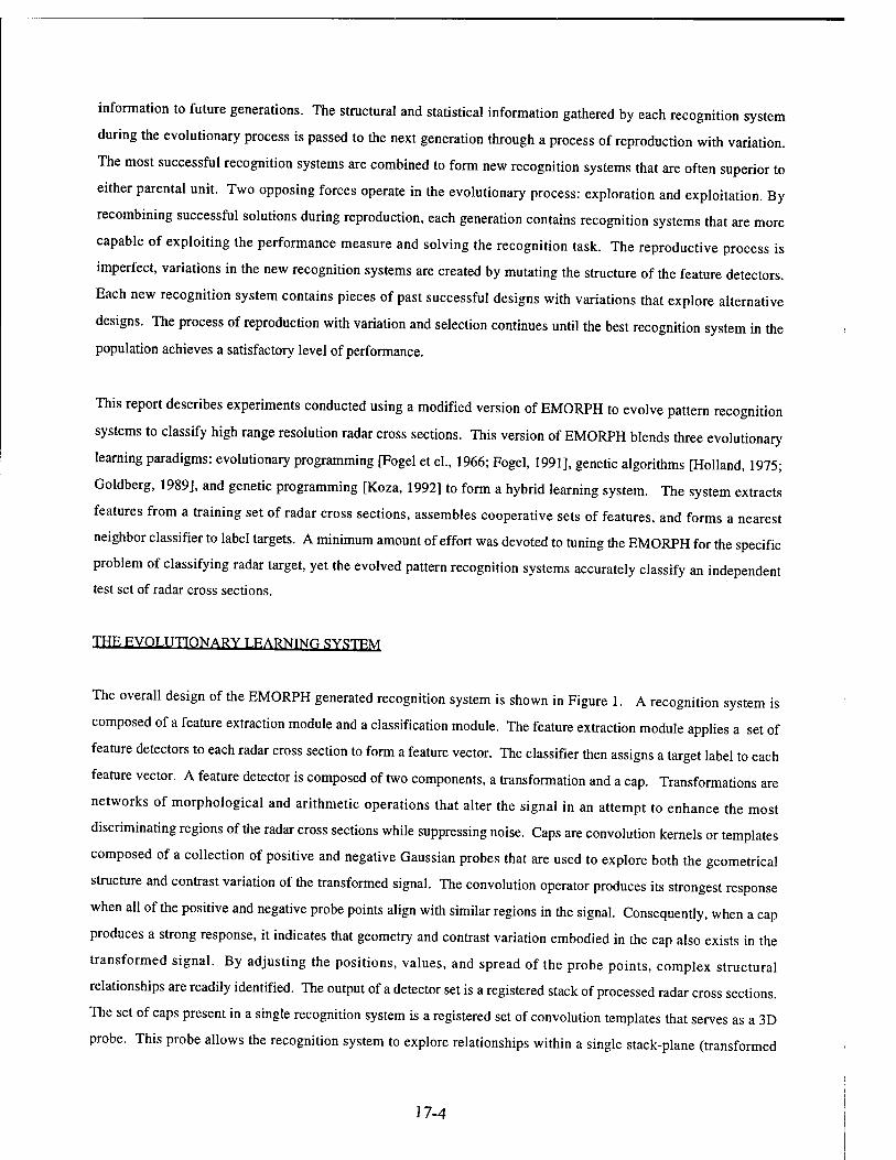
than the original detector, it replaces the parental unit. A few sample caps are shown in Figure 7 and the result of

applying these caps to the transforms are shown in Figure 8.

After all the member of the clonal population reproduce, the C parental capped transform competes with the C

offspring capped transforms for survival in a tournament. The top ranked C detectors are preserved and the

evolutionary programming cycle begins again. After a fixed number of EP cycles, the performance of the best

capped transform evolved during the EP phase is compare to the original parental capped transform. If the best

evolved capped transform is more accurate than its parent, it replaces its parent in the base population. This process

17-11

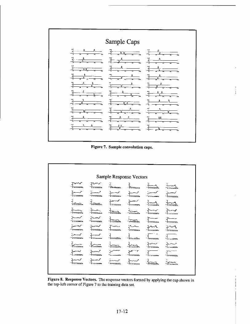
Figure 7. Sample convolution caps

Sample Response Vectors

;L,—_A

KJ-"^ 1. 1——^ DL-~r—~irS"

l, n. ;p—uJ-

h— °p»^-^r^

U-*~J~ .?h~-^

U_^^*v/~ :p— U^-^r il „ Lr*—p*-j -!U*->JT.

Lu-r-i-^j/" ;L^-~^

L_-~j-" '{—

I .:(-—'T

.Lw-vj1 'L*^-™!'^

nL»_p~»'<jJ,~ :h-~A.

'k^«-^. lh~—a'

'k^-^ lh —

p-_—«^-_ :p-i--<*L

L"~^ ^Lwi-^-T-^

IjJl -v

|~W" .'1~~---L

ip^-a

jL^n-s/*

.!tcü

Figure 8. Response Vectors. The response vectors formed by applying the cap shown in the top-left corner of Figure 7 to the training data set.

17-12

EP Algorithm

for each tranform Ti do Generate N random caps for Ti Evaluate capped version of the transform using Fisher's Discriminant for 1 to maxCycles do

for each cap Cj do Produce an offspring cap by vibrating the point Mutate offspring (add/delete) points Evaluate the offspring

endfor Perform tournament selection to rank the full population of caps Reduce population size to N based on ranking

endfor Save the best cap for Ti

endfor

Figure 9. EP Process used to generate convolution caps for transformations.

is repeated for each member of the base population. When the EP phase terminates, the base population contains

optimized sets of feature detectors consisting of convolution caps specifically tuned to the transforms produced by the

GP phase. The process of evolving capped transformations is summarized in Figure 9.

EMORPH uses a genetic algorithm (GA) to form detector sets. The GA is responsible for recombining detector sets

(see Figure 10). Parental units are selected from the base population using roulette wheel sampling where the

probability of selection is proportional to the recognition system's accuracy. Once a pair of parents is selected, their

detectors are exchanged using a uniform crossover. The detector set is analogous to a biological chromosome and the

individual detectors are similar to genes. During crossover, each detector position in the parental set contributes

some portion of each of its detectors to a pair of offspring detector sets. There is a 0.5 probability that the first parent

places its information in the first offspring and the second parent places its detector in the second offspring.

Similarly, there is a 0.5 probability that the first parent places its information in the second offspring and the second

parent places its detector in the first offspring. As shown in Figure 10, a parental unit simply copies its whole

detector (cap plus transform) into the selected offspring.

The GA phase begins with N detector sets and combines N/2 pairs of parental sets to form an extend population of 2N

sets. Each member of the extended population is evaluated using the same procedure described for the EP phase. A

tournament selection process is applied to rank the entire population and the N top-ranked detector sets are preserved

17-13

Detector

Set1 Set 2

Parental Detector Set 1 & 2

Offspring Detector Sets 1' & 2

Detector Copy

Detector Exchange

Transform Exchange

'^'Transform:

Figure 10. Action of the GA process. The GA takes pairs of detector sets and recombines components of each parental set to form pairs of offspring. This process can result in combinations of different caps on transforms whole detectors being exchanged between sets.

or

for the next cycle of the GA algorithm. When the GA phase is complete, each detector set consists of combinations

of transforms and caps that proved useful in the recognition process. A sample response matrix is shown in Figure

11. The rows represent the response of individual detectors. The x-axis is organized by target classes (1-5 is target

one, 6-10 is target two, etc.). Notice how some detectors respond consistently to subsets of targets. The features

defined by these detector readily form prototypes for a nearest neighbor classifier. The overall flow of the GA ph

is outlined in Figure 12. ase

To summarize, EMORPH consist of four distinct stages: transform generation (form expression trees - GP phase),

detector formation (capping expressions - EP phase), feature selection (forming response matrices - GA phase), and

finally, creating a nearest neighbor classifier to form the complete pattern recognition system. The user can set

parameters to control the duration of each phase as well as control parameters to influence the behavior of each step

of the process. For example, the user can increase the sensitivity of the individual detectors by increasing the number

of passes through the EP phase relative to the number of passes through the GA phase. Alternatively, the user may

elect to spend more computational resources adjusting the average complexity of the detector sets by increasing the

number of passes through the GP phase. It is difficult to select an appropriate mixture of passes because the

evolutionary learning process is dynamic. During the early stages of evolution, it is not likely that the complexity and

number of detectors in the population is suitable for the recognition task. If the user arbitrarily increases the number

of EP passes, the probe point density will increase to compensate for the lack of complexity in the transforms and

17-14

Figure 11. Sample response matrix.

GA Algorithm

Form N random sets of detectors by sampling the pool produced by the EP process Evaluate each detector set by forming the response matrix and classifying the training set for 1 to maxCycles do

Generate a selection vector based on classification accuracy for 1 to maxMatings do

Select pairs of detector sets Perform uniform crossover on detector sets to form two offspring Muatate offspring by adding/deleting detectors Evaluate offspring detector sets

endfor Perform tournament selection to rank the full population Reduce population size to N based on ranking

endfor

Figure 12. GA Process used to select cooperative sets of feature detectors.

17-15

limited number of detectors. This will produce customized solutions that tend to perform well on training sets and

poorly on test sets. If the number of GP cycles is too large, the transform can become too complex to compensate for

the inadequate distribution of probe points within each cap. A good compromise would be to implement an adaptive

feedback mechanism to control the duration of each phase and adjust parameters relative to the contribution of each

phase throughout the evolutionary process.

EXPERIMENTAL DESTfiN

To demonstrate how EMORPH generates pattern recognition systems, the results of a target recognition task in high

range resolution radar are presented. Specifically, the problem is to classify a set of airborne targets from their radar

cross sections. For this experiment, a sample of 60 radar signatures were extract from a large database of signals.

Each radar signature is one view of a target at a specific azimuth and elevation. The selected data set contains six

targets at azimuth 25° and elevations that range from -20° to -11° in increments of 1°. Thus, there are one ten

samples of each target in the data set. These were divided into a training set of 30 radar signatures that contain 5

samples of each target and a test set of 30 cross sections that also contain 5 samples of each target. The data was not

placed in the sets at random. The training set contains all targets with odd values of azimuth while the test set

contains the remaining signatures. This amounts to placing every other signature in the view volume (azimuths x

elevations) into one set and the remaining signatures into the other. Notice the signatures have been normalized into

Training Set Test Set

1L_ LL

»I A J-Ä .

11X II

JL .LiL JJL IJL LL

LL "LL 11 H " ■Jl LL

:UL i JL LL

LL .L|_ LL. ÜL .LL LL

LLLILLLLLL ILIL1L LL LL L LL 11. IL. LL LL 11 LL JJL JJL LL JJL LL

• Data set consists of 60 signals

• Six targets at AZ=[-25,-16] at EL=-20

• 30 targets for training and 30 target for testing

Figure 13. Training and Test Data Sets.

17-16

128 range bins with the maximum value (255) placed in bin 63. Looking down the column of data it is easy to see

there are characteristic features in each target that persist through a few degrees of change in elevation, but then

rapidly disappear. Also note the similarity in the signatures between targets making the classification task quite

difficult.

An E-MORPH learning cycle consists of thirty-five GP sub-cycles, followed by 35 EP sub-cycles, followed by 150

GA sub-cycles. To begin the GP phase, a population of 100 transforms was generated at random. Each transform

was initialized with one to three operators. Each pass through the GP algorithm produced 100 offspring that were

evaluated using the local performance measure. Then tournament selection was used to reduce the population back to

100 transforms. The EP phase was then applied to form a pool of feature detectors. The initial caps were generated

with one or two randomly placed Gaussian points. The performance of each capped transform was evaluated by

computing the Fisher discriminant for the response vector produced by applying the detector to the training set. A

pass through the EP phase consists of processing each member of the base population of 100 transforms. Each

member of the base population was used to produce 10 clones that are then mutated to produce an additional 10

recognition systems. This extended population of 20 caps was pruned back to 10 individual using tournament

selection. The process was repeated five times and the best recognition system found competed to replace its

ancestor in the base population. The GA phase started with the base population of 10 recognition systems. Copies

of these base systems are mutated and recombined to create an extended population of 20 systems (10 parents + 10

offspring). The extended population was ranked using tournament selection and the top 10 systems were saved to

start the next GA sub-cycle.

For the EP phase, the probabilities of vibration, addition, and deletion are 0.6, 0.3,0.1 respectively. When a Gaussian

point is added to a cap, there is a 0.67 probability that the point is positive and a 0.33 probability that the point is

negative. The range of a Gaussian probe point is 4 to 12 range bins (i.e. pixels) and the maximum weight of a point is

limited to the range of 1 to 3. In the GP phase there is a 0.3 probability that a transform is mutated and a 0.7

probability that a pair of transforms is recombined. If a set is selected to undergo mutation, there is a 0.2 probability

that an individual transform passes to the offspring unchanged; a 0.7 probability that the transform is extended with a

randomly selected operator, and a 0.1 probability that a random tree is added to the transform.

The average recognition accuracy for the population produced during the evolutionary learning process is shown in

Figure 14. The performance is displayed at the end of each GA cycle. The average training set recognition accuracy

rises from a low of 38% in generation 0 to 69% in generation 150. Notice, the curve is not monotonically increasing.

This is because the uniform crossover used in the GA algorithm can extend and/or shrink detector sets producing

disruptive effects. Also, tournament selection does not guarantee that the most accurate recognition systems will

survive. The overall trend shown in this graph suggests that the selection process is locating increasingly accurate

sets of features. Notice there is more variation in the test set performance than the training set performance. This is

17-17

Average Accuracy

50 75 100

Generation

125 150

Figure 14. Average recognition accuracy for the training and test set

Maximum Accuracy

90% or 27/30

77% or 23/30

75 100 125 150

Generation

Figure 15. Recognition accuracy of the best pattern recognition system for the training and test data sets.

17-18

unfortunate, because it suggests that the features selected for the recognition systems are not generalizing. The

performance of the best recognition system in each generation is shown in Figure 15. The accuracy of the best

system rises from approximately 57% accuracy on the training and 22% accuracy on test data sets using 3 detectors to

a maximum level of 100% on the training set and 90% on the independent test set. The best recognition system uses 9

detectors (Figure 16). The system appears to converge to rapidly producing a best training set score of 100% in

generation 50. This sharply reduces the amount of exploration that can occur in future generations. This is partly due

to the same population size used in this experiment. It is interesting to note that several recognition systems appear

with test set accuracies approaching 100%, but these systems do not produce the top training scores. This suggests

that a two-level training set might improve performance. One set would be used to form the recognition system and a

second set would then be used to determine survival based on how well the system classified the secondary training

set.

DISCUSSION

E-MORPH successfully generated a pattern recognition system to classify high range resolution radar signatures.

The evolved recognition system achieved a classification accuracy of 100% when applied to a training data set

consisting of 30 radar signatures (5 samples of six targets) and 90% accuracy on an independent set of 30 additional

signatures. The best recognition system contained nine feature detectors composed of primitive morphological and

Number of Feature Detectors

12

10

(2 8 -

r 6

4 -

2 - Best Recognition System Average Recognition System

25 50 75 100

Generation

125 150

Figure 16. Number of feature detector used in the average and most accurate recognition systems.

17-19

arithmetic operators capped by a special convolution template containing an evolved distribution of Gaussian-shaped

probe points. The response of these detectors are processed by a simple nearest neighbor classifier that labels each

signature. The use of morphological operators in the construction of primitive feature detectors allows EMORPH to

evolve wavelet-like transformations that eliminate noise from the signatures and suppress information at various

spatial frequencies to facilitate the process of classifying targets.

Although EMORPH achieves excellent recognition results, its performance can be improved. Inspection of the

evolved feature detectors suggests that various redundant sub-expressions within the detector transformations can be

eliminated to accelerate the evolutionary search process. This also implies that adjusting the library of operators and

parameters used to grow feature detectors may improve both accuracy and the robustness of the evolved recognition

systems. In addition, EMORPH's control parameters were not carefully tuned for this specific problem.

Consequently, even better performance can be achieved in future experiments by adjusting the library of

morphological operators, structuring elements, and distribution of the computation resource among the different

phases of the evolutionary process.

The techniques used in EMORPH are not tied to radar signal processing. The approach is generic and can readily

transition to many different problems in automatic target recognition. No single approach solves all problems in

automatic target recognition, EMORPH represents one viable alternative. The solutions generated using our

evolutionary learning algorithm are quite different than the solutions produced by human experts. This indicates that

human experts may not be using all of the available information to develop robust pattern recognition systems. In

future work, we hope to tune EMORPH, perform a more definitive set of experiments, and explore the possibility of

combining human expertise with the evolutionary search process to access alternative designs. This hybrid approach

to design may ultimately produce recognition systems with performance superior to any in use today.

ACKNOWT.F.nrTMF.NT

I would like to express my appreciation to Dr. Louis Tamburino for serving as my laboratory focal point for the

Summer Faculty Research Program. His total commitment to this research made my stay at Wright-Patterson Air

Force Base a pleasure. I enjoyed his many helpful ideas and stimulating discussions over the years. I would also like

to thank Dale Nelson and Jerry Covert for again allowing me the opportunity to participate in the summer program

and providing a stimulating environment in which to work.

17-20

REFERENCES

Fisher, R. A., (1936). "The use of multiple measurements in taxonomic problems," Ann. Eugenics, 7, Part II, 179- 188.

Fogel, D. B. (1991). Sxstem Identification Through Simulated Evolution: A Machine Learning Approach to Modeline. Needham, MA: Ginn Press.

Fogel, L. J., A. J. Owens, and M. J. Walsh (1966). Artificial Intelligence Through Simulated Evolution. New York, NY: John Wiley & Sons.

Goldberg, D. E. (1989). Genetic Algorithms in Search. Optimization, and Machine Learning. Reading, MA: Addison-Wesley.

Haralick, R. M., S. R. Sternburg, and X. Zhuang, (1987). "Image Analysis Using Mathematical Morphology", IEEE Trans, on Pattern Analysis and Machine Intelligence, PAMI-9:532-550.

Holland, J. H. (1975). Adaptation in Natural and Artificial Systems. Ann Arbor, MI: The University of Michigan Press.

Koza, J. R. (1992). Genetic Programming: On the Programming of Computers B\ Means of Natural Selection. Cambridge, MA: The MIT Press.

Rizki, M. M., L. A. Tamburino, and M. A. Zmuda (1993) Evolving multi-resolution feature detectors. In Proceedings of the Second Annual Conference on Evolutionary Learning, eds. D.B. Fogel and W. Atmar, La Jolla, CA: Evolutionary Programming Society, 57-66.

Rizki, M. M., L. A. Tamburino, and M. A. Zmuda (1994) E-MORPH: A two-phased learning system for evolving morphological classification systems. In Proceedings of the Third Annual Conference on Evolutionary Learning, eds. A. V. Sebald and L. J. Fogel, River Edge, NJ: World Scientific, 60-67.

Serra, J., (1982). Image Analysis and Mathematical Morphology. London: Academic Press.

Zmuda, M. A., M. M. Rizki, and L. A. Tamburino, (1992). Automatic generation of morphological sequences, In SPIE Conference on Image Algebra and Morphological Image Processing III, pp. 106- 118.

17-21

AUTOMATED MODULAR FIXTURE PLANNING FOR VIRTUAL MATERIALS PROCESSING: GEOMETRIC ANALYSIS

Yiming (Kevin) Rong Associate Professor

Manufacturing Systems Program

Southern Illinois University at Carbondale Carbondale, IL 62901-6603

Final Report for: Summer Faculty Research Extension Program

Wright-Patterson Laboratory



and

Wright-Patterson Laboratory

December 1996

18-1


Yiming (Kevin) Rong Associate Professor

Manufacturing Systems Program Southern Illinois University at Carbondale

Afcsttacj

Attendant Processes such as fixture and die design are often a necessary but time

consuming and expensive component of a production cycle. Coupling such attendant

processes to product design via feature-based CAD will lead to more responsive and

affordable product design and redesign. In the context of on-going research in automating

fixture configuration design, this report presents a fundamental study of automated fixture

planning with a focus on geometric analysis. The initial conditions for modular fixture

assembly are established together with needed relationships between fixture components

and the workpiece to be analyzed. Of particular focus is the design of alternative locating

points and components, together with example 3-D fixture designs.

18-2


Yiming (Kevin) Rong

1. Introduction

Global competition has forced U.S. manufacturers to reduce production cycles and

Product design agility. Generally, a manufacturing process is uncoupled and divided into:

product design, process design (selection, routing and tooling), and assembly. Obvious

and continual advances in computer-aided design (CAD), computer-aided process

planning (CAPP) and computer-aided manufacturing (CAM) are enabling more multi-

disciplinary design. However, computer-aided tooling (CAT), which is a critical part of

process design and a bridge between CAD and CAM together with CAPP, has been least

addressed and remains a missing link.

As a consequence of evolving CNC technology, specifically re-usable objects

called features coupling shape and process (milling, drilling, etc.) to generate machine

specific NC code, workpiece setup and associated fixturing has become the process

bottleneck. To address this bottleneck, research and development of flexible fixturing,

including modular fixturing technology, has received continued support. Modular fixture

components enable a large number of configurations to be derived, disassembled and re-

used. However, modular fixture design is a geometrically complex task and such

complexity impedes widespread application of modular fixtures. Development of an

automated modular fixture design system is needed to simplify process design of more

affordable products. This research focuses on a geometric analysis for automated modular

fixture planning which is inspired by several previous research in this area, especially a

modular fixture synthesis algorithm [1] and an automated fixture configuration design

methodology [2].

18-3

Previous Rp^r^ h

Fixture design involves three steps: setup ptating, tour« plaming, mi fKtore

configuration design [2], Setup planning research has been address to the context of

CAPP t3,4,5]. Seminal work to computer-aided fixture design (CAFD) focused on fixture planning:

* a method for automating fixture location and clamping [6];

* an algorithm for selection of locating/clamping positions providing maximum mechanical leverage [7];

* kinematic analysis based fixture planning [8,9]; and

* rule-based systems to design modular fixtures for prismatic workpieces [10 11]

But with respect to previous work on automating the configuration of workpiece

fixtures, ,.e., automated fixture configuration design (AFCD), liffle can be found Fixture

design depends upon critical locating and clamping poitos on workpiece surfaces for

whtch fixtore components can be selected to hold toe workpiece based on CAD graphic

funcons [12]. A 2-D modular fixture component placemen, algorithms has been

developed [13]. In addition, a method for automating design of toe configuration of T-

slot based modular fixturing components has been developed[14]. A prototype AFCD

system has been developed, including tor* core modules: fixture unit generation and

selection module, fixture unit mount module, and interference checking module [2]

Assembly relationships between fixture components have also been defined and automatically established [15].

Nearly all toe CAFD researchers admit that workpiece geometry is toe pivotal

factor in a successful CAFD system. Since toe geometry of workpieces may vary greatly

many researchers in CAFD consider only regular workpieces, i.e., workpieces suiteble for

3-2-1 locating method. There have been some attempt, toward handling more

complicated workpiece geometries as in reference [16]. However, their results are only

apphcable to some specific geometry, i.e. regular polygonal prisms.

18-4

Review of Brost-Goldherp Algorithm

Recenüy, research in modular assembly based on geometric access and assembly

analysis has gained considerable attention. Reference [1] presented a "complete"

algorithm for synthesizing modular fixtures for polygonal workpieces and reference [17]

explored the existence of modular fixture design solutions for a given fixture configuration

model and a workpiece. Fixture foolproofing for polygonal workpieces was studied [18],

and partially employed the approach in reference [1]. Reference [19] presented a

framework on automatic design of 3-D fixtures and assembly pallets, but no detailed

design methodology, procedure and results were provided.

In reference [1], an algorithm which is called the Brost-Goldberg algorithm was

presented for synthesizing planar modular fixtures for polygonal workpieces. The basic

assumptions were that a workpiece can be represented with a simple polygon, locators can

be represented as circles with identical radius less than half the grid spacing, the fixturing

configuration will be three circular locators and a clamp, the base plate is infinite, and all

the contacts are frictionless. In addition to polygonal workpiece boundaries a set of

geometric access constraints are provided as a list of polygons with clamp descriptions

and a quality metric. The output of the algorithm includes the coordinates of the three

locators, the clamp, and the translation and rotation of the workpiece relative to the base

plate. The implementation of the algorithm is as follows per step 1:

1. The polygonal workpiece and geometric access constraints are transformed by

extending the workpiece by the radius of the locators which are treated as ideal points

(Figure 1) [1].

2. All candidate fixture designs are synthesized by enumerating the set of possible

locator setups. The possible clamp locations are also found with each locator setup and

clamp location specifies a unique fixture.

3. The set of candidate fixtures are then filtered to remove those that cause

problems, i.e., collision. The survivors are then scored according to the quality metric.

In step 2 placement of three circular locators on the base plate are evaluated while

translating and rotating the workpiece relative to the base plate. An algorithm was also

presented to find all combinations of the three edges, where two of them may be identical,

18-5

on the polygon with a satisfaction of hole-alignment conditions with the base plate (Figure

2) [1]. For each set of locators and associated contact edges, consistent workpiece

configurations or workpiece positions are calculated. All the possible clamp positions are

then enumerated based upon the constraint analysis of the constructed force sphere.

The algorithm is called a "complete» algorithm for planer modular fixture design

because it guarantees finding all possible planner fixture designs for a specific polygonal

workpiece if they do exist. However, the major limitations of the method are:

1. Only polygonal workpieces are considered, i.e., no curved surfaces are allowed

in the workpiece geometry. In reality, many fixture design cases include cylindrical

surfaces, or circular arcs in 2-D representations.

2. Only circular locating pins with uniform radius' are considered in the algorithm

In each modular fixture system, there are some other types of locators available and widely used in fixture designs.

3. The algorithm only considers 2-D workpieces. m practice, it can be applied

only for prismatic workpieces having small height, i.e., 3-D fixture design problem is a great challenge.

4. There are some criteria necessary for locating and clamping design in addition

to geometric considerations including: locating error, accuracy relationship analysis,

accessibility analysis, and other operational conditions.

5. Clamp location planning is weak without the consideration of friction forces,

which needs to be further improved.

In this report, modifications and extensions to the modular fixture synthesis

algorithm are presented with regard to limitations 1,2, and 3 above. Discussion of

limitations 4 and 5 will be presented in a separate report [20].

2. Geometric Condition«

A prismatic-workpiece is typically regarded as a 2-D workpiece including a set of edges

such as line segments and arcs, which are candidate locating edges. The locating and

clamping design problem becomes one of finding a group of three locating edge

combinations. For an explicit expression, let us define the set of expanded boundary edges

18-6

of the workpiece P as:

EBE(P) = {d | ei e line segments; i e NE} (1)

where NE is the number of candidate edges.

All combinations of three edges, two of which may be identical, on the polygon are

enumerated as:

Triplets(P) = {(ei. e,, e^ | d, ej, e* € EBE(P), 3 (a, b) e (i, j, k), a * b} (2)

Locator centers are designed to contact with edge combinations ec = ($, % et) (

Triplets (P)). Without loss of generality, it can be assumed that d contacts with a locator

Li at the origin of the base plate lattice based on the assumption of an infinite base plate.

By translating and rotating e* about the origin, ej sweeps out an annulus centered on the

origin, with inner and outer diameter equal to the minimum and maximum distance

between ej and ej. The position set of the locator contacting ^ should be within the swept

annulus as

P2(ei, ej) = {p2(x, y)| min-dist(ei, ej) < dist(p2, pi) < max-distfe, ej)} (3)

where pi = origin of base plate lattice.

Each p2 is evaluated for selection as the second locator U. in contact with ej. If U

contacts $ and U contacts ej, a third locator L3 in contact with ek must be pairwise

consistent with both ^ and ej. The envelope containing the region swept by ek maintaining

contact with the first two locators can be easily determined by independently considering

each pair as

Pafe, ej, et) = {p3(x, y) |p3(x, y) e P2(ek, eO n P2(ev, ej)}, (4)

which is the same as presented in reference [1].

Assembly Relationship Analysis

From the above discussion, it has been shown that determining the positions and

orientations of modular fixture components can be simplified as finding geometric entities

such as line segments or arcs on the workpiece passing ideal points on the base plate after

moving (translating and rotating) the workpiece relative to the base plate.

18-7

As shown in Figure 3, the relative position between the workpiece and the base

Plate can be represented by the relation of the workpiece and the base plate coordinate

systems which are expressed as XwOYw and XbOYb respectively. Basically, there are three

locator-workpiece contact situations as shown in Figure 4:

* Line segment contacts with a circular locator.

* Arc contacts with a circular locator.

* Arc contacts with a line.

When a locating edge I, on fine workpiece is required to pass a poin, P, on the base

Plate, ,e., the locator center needs to be aligned to a tapped (or pin) hole on the base plate, Lj can be expressed by

rixw+siyw + ti = 0

Pi can be expressed as [2]

Pi-* (Xbi.Vbi) r (6)

whererbi=2Tu + T<vmod2) n v M XT . jybi = TV ' ' "N' -N+1' -' "2' -1' °. 1.2> •••> N, and T is the

spacing increment between the taped (or pin) holes on the base plate.

The workpiece is assumed to be translated by (x, y) and rotated by 9 relative to the

base plate. To simplify the calculation, an inverse transform is considered by holding the

workpiece fixed, and moving the base plate by (-x, -y, -9). Then Pi(xw, yM) is transformed to

«xb, -x)cose + (yb, -y)sine, (ybi -y)cos8-(xb, -x)sine). (7)

Tims, the condition for the modular assembly can be described as:

r,[(xbi -x)cose+(ybI -y)sine]+Si[(yb, -y)cos8-(xbi -x)sine] + t, =0 (8).

For a specific workpiece, its geomeny shape is fixed which means the equation of

the bne ,s fixed, i.e., r„ s, and * are constant. 71» assemb.y points are given, which means

x« and yM are constant. There will be three equations to solve three unknowns x, y and e

If an c,rcu.ar locator contacts with an arc centered a. OK*, v„) with radius R, the arc can be represented as:

I Pi Oi | = R, or (xw - u0)2 + (yw - v0)

2 = R2

18-8

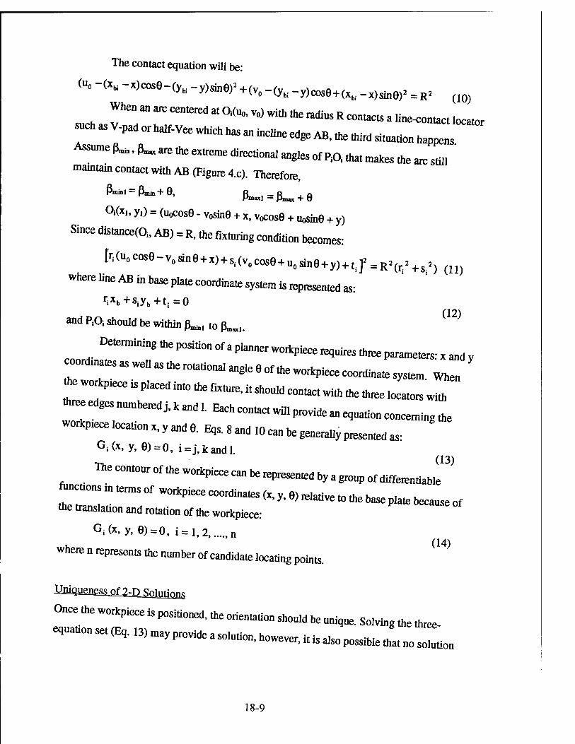
The contact equation will be:

C. -(*. -X)C0s6-(yK -y)sinef +(Vo _(yb_ _y)cos6+(Xu _x)sin9)! =R! (io)

When an arc centered a. Oi(uo, v„> with the radius R contacts a line-contact .oeator

Azurne |W |U ^ me extreme directional angles of PA «hat makes me arc still mamiam contact with AB (Figure 4.c). Therefore,

ß»b, = IWe, (U^ft^ + e

Oi(x,, y,) = Owose - v„sine + x, v„cos8 + UÄ6 + y)

Since distance©, AB) = R, the Oxturing condition becomes:

[r,Kcos8-voSi„e + x) + s1(v0cose + „oSille+y) + [lf = Ra(r., + sJ)(1

where line AB in base pbte coortinate system is rcpresented as: ri*b+Siyb+t, =o

(12) and P,0, should be within (U, to fU,.

^»^mepositionofap^nerworkpiecercqufrcsthreepararueters.xandy

coord.n.tesa.weuastheroutionalangleeofmeworxpiececoordinatesystem. When 2 wo-Kp.ec is placed into the fixture, it shook, contact with the three .ocatots with

êdgesnumbercdândl. Each con« wm provide an equation concerning the

workptece location x, y and 6. B,, 8 and .0 can he generally presented as-

G.fx, y, 6) = 0, i=j,kandl.

H-econtourofmewofitpiece can he represenKd hyagroupofdiffercntiable

riii^r'^^^^'^-^^^^-p'-ûseof the translation and rotation of the workpiece:

Gi(x, y, 6)=0, i = l,2,....,n u (14)

where n represents the number of candidate locating points.

ünigaieness_of2IDôJutions

Once the workpiece is positioned, me orientation should he unique. Solving the three- e«luaho„se,«Eq.l3)mayprovideasolutionihowever>itisa]sopossibiethatnosoiuüon

18-9

or infinite solutions are possible. The no-solution situation means the third locator has

been chosen from an image-locus, i.e., all possible solutions exist in the

pseudo-locus, but the pseudo-locus will also provide the position of the third locator

which is not possible. In other situations, there are an infinite number of solutions, e.g.,

when all three edges are parallel or when the three contact normals meet at a single point

(Figure 5). These cases should be discarded since they do not constrain the workpiece to a unique location.

In order to obtain the necessary conditions for a unique solution, assume that the

workpiece can be positioned while contacting all three locators in a position (xo, y0, 0O)) with a disturbance:

Gi(x + Ax, y + Ay, 0 + A9) = O,i=j,k,andl,

For a stationary locating,

or

(15)

dGi A 3Gi . dG; -_Ax+—J-Ay+—i- dx dy de -A9 =0,i=j,k,l. (16)

Therefore, the condition for the equation set to have single solution is:

^l Ü°J. Ü2i 3x 3y 39

3G^ dG^ 9G, dx 3y 30

dG, ~dx~

dG, dG,

= 0 (17)

dy de ,

For a valid solution, it is also important to consider the workpiece tolerances.

When the geometric dimensions of the workpiece vary in a certain range, the locating

contacts should be maintained. Similar analysis can be conducted, but the specifics will be

presented in a forthcoming report [20]. Some other valuable discussion on similar

problems can be found in reference [21].

18-10

3. Assembly Analysis

In this section, various locators and clamps are considered in fixture planning. In order to

apply the fixture planning algorithm discussed in the previous section, the geometric

analysis for workpiece boundary expansion should be performed for actual locators and

clamps. Generally, there are two types of locating edges for 2-D workpiece

geometry: line segments and arcs which may lie in either internal or external contours.

Several locator types are used for side locating, including round locating pins (Figure 6.a),

locating towers (Figure 6.b), adjustable stops (Figure 6.c), half-Vees (Figure 6.d), V-pads

(Figure 6.e), round hole pins (Figure 6.f) and diamond hole pins (Figure 6.g).

If the locating edge is a line segment, a round locating pin, locating tower and

adjustable stop may be used. For an arc segment, half-Vee and V-Pad are considered first

However, round locating pin, locating tower, and adjustable stop may be also used for arc

edge contacts. Generally, locating a 2-D workpiece requires limiting three degrees of

freedom (DOF): two translation and one rotational. Three line or arc edges, two of which

may coincide, should be selected for locating purposes. Thus, a locator configuration

should be considered for sundry combinations. Table 1 shows the possible locator

configurations with assigned preference and provides criteria for preliminary selections of

locators and clamps.

It was shown in reference [17] that the three circular locating pin configuration

were not universal for arbitrary 2-D workpiece. Indeed, there exist some workpieces

which can not be fixtured using this configuration, and therein, the type of locator may be

changed. An alternative may involve the use of adjustable stops with adjustable contacting

lengths. The distance from the contact point to the locator center may be larger than half

of the base plate grid distance, which may greatly improve the locating capability.

Locating geometric analysis is based on the geometric constraints imposed on the

workpiece and locator position. Here locators must maintain contact with specific

locating edges on the workpiece. The modular fixture assembly requires the locators to be

assembled through holes in the base plate. For the 2-D situation, the assembly process is

to find the suitable assembly holes in the base plate which can locate the workpiece.

Following are several cases on how to find possible locator positions.

18-11

Case 1; Locating with locating tower anri adiustahlp. ^np

Locators used for line segments are first discussed, such as locating tower and adjustable

stop (locator b and c in Figure 6), as shown in Figure 7. Locating towers can be treated

as smaller circular locators whose radius r is

r = distance (locator center, locating edge) /18)

However, it should be noted that for locating towers, the possible contact region

between the locating tower and locating edge should be reviewed to ensure the functional

stability of the locating tower (Figure 8):

U = L-d (19)

where Le is the effective locating edge length, L is original length of the locating edge,

and d is the length of the locating surface.

The adjustable stop can be treated as a circular locator with a radius r as a variable

min-acting-distance < r < max-acting-distance (20)

Using such a geometric representation, input geometry transformation may be used

to perform geometric analysis by expanding the corresponding locating edges by the equivalent radius.

Case 2:1.nc.atinp with hnte-pinc

If the locator configuration employs circular round-pin or diamond-pin to locate with

small internal holes, it is easy to do assembly analysis since the center of hole and hole pin

should be aligned. As shown in Figure 9.a, the first step of assembly is to align the

diamond-pin with a hole on the base plate. Then the workpiece has only one rotational

DOF to find the suitable assembly holes for other locating edges. Generally, adjustable

locators may be used to ensure the availability of assembly holes for the other two locating

edges. The round-pin application is shown in Figure 9.b.

If two small holes are employed, either the distance between the two holes has to be standard as

0,A=kT

18-12

where Oi, 02 are centers of two holes and T is the base plate grid distance. If this

condition is not valid, adjustable-bar support should be used near the bottom of the

workpiece for one hole locator to ensure the assembly of the hole locator, which then

becomes a 3-D locating problem (Figure 10).

Case 3: Arc segment locating using circular locators

When the locating edge is an arc, input geometry transformation can also be used by

expanding the arc through the equivalent radius of the locator in the direction of external

normal. It is applicable to both external and internal arcs. The locus analysis is almost the

same as those presented for line segment situation. The major difference lies in calculating

the workpiece location and orientation.

As described in section 2, when the first circular locator is placed in the base plate

origin, by translating and rotating $ about the origin, 3 sweeps out an annulus centered

on the origin, with inner and outer diameter equal to the minimum and maximum distances

between e, and ej. The position set of the locator contacting ej should be within the swept

annulus as

Pafe, ej) = {p2(x, y) | min-distfo, ej) < dist(p2, px) < max-dist(ej, ej)} (22)

where pi = origin of base plate lattice.

It should be noted that the ei and ej could be either line or arc segments when using

circular locators. However, in the case of applying other types of locators with arc edges,

such as V-pad and half-Vee, the way to find locator positions with hole alignment

relationships needs to be further studied.

Case 4: Locating with V-pad

In Table 1, when the locating triplet is composed of one line segment e2 and one external

arc ei, the recommended locator configuration is using one V-pad and one circular

locating pin. As distinguished from circular locating pins, assembling a V-pad requires

two locating holes in base plate instead one, and the orientation of the V-pad can not be

arbitrary and must have four perpendicular orientations.

18-13

As shown in Figure 11, a V-pad is placed around the origin of the base plate and

oriented in one of the four possible perpendicular orientations. The center of the locating

arc 0, as well as the contacting points between V-pad and the workpieee are then

determined. The position of the circular locating pin may be found through rotating

the workpieee while maintaining a 2-point contact with the external arc e, with the V-pad

The locus of the round locating pin is a part of the annulus centered in the fixed locating

arc center whose inner and outer diameters of the annulus are the minimum and maximum

distance between the arc center and the line segment e2:

P2(0i, c, e2) = {p2(x, y) Imin-distCO!, e2) < OlP2 <max-dist(0,, e2)} (23)

The angle scope of the partial annulus is determined by the possible rotation angle of the

locating arc about the V-pad without loss of contact.

Omin -90° + ß<angle<ccmax -90°-ß (24)

where ce^ is the minimum angle between e, and e2 with reference Oi; <w is the

maximum angle between e, and e2 with reference O»; and ß = 45° for 90° V-pad or 30° for 120° V-pad.

Case 5:1-ocatinp with half-Vep.

A locating configuration may require using one half-Vee (or.other line-contact locators)

for an arc segment. The assembly character of half-Vee locators is more complicated than

a V-pad. Theshapeofahalf-VeeisshowninFigurel2.a. There are three locating holes

in one half-Vee. When assembling, two holes in the half-Vees are needed to be accurately

aligned with two locating holes in base plate. There are only four possible directions for

the half-Vee when assembled to the base plate. In this report, the two locating holes

VLH, and VLH2 with equal distance to the oblique edge are analyzed. Other half-Vee

shapes should be addressed via the same method.

First, a half-Vee is placed in a specific position on the base plate by aligning VLHl

and VLH2 with two locating holes BLH, and BLH2 centered at Hl and H2 in the base

plate. When the given arc (e,) centered at O, maintains contact with the half-Vee, it can

be transformed as growing the given arc by r (Figure 12*). The contact situation'can be thought as an arc rolling over a line segment

18-14

The second locator position relative to ^ second locating edge W can be found

«smg geometric locus analysis. When e, maintains a one-point contact with a half-Vee

the workpiece can translate and rotate, and e, sweeps out which may he confine* to a '

geometry centered a, the connection line of the two locating holes ta fte half.Vee ^

geometry is derived by the swept partial annulus when the are contacting the different posttion on me half-Vee simply rotates without s]ip, ^ lxm may fe ^ ^

constdenng ang!e Umitations of are rotation (Figure 12.b). Generally, Ute swept geometry

by e, can be defined as a ribbon by satisfying such conditions:

1) The locus geometry is relative to a reference line segment H,H2 where:

distance(Oi,H,H2) = R, (25)

where R, is the expanded radios of e, and in the outer nomta. direction of H,H2

2) The two limit line segments are determined by off-setting H,H2 through

distl =maximum-distance-refer-to-H1H2 (O,, ej

dist2 = mimmum-distance-refer-to-H,H2(0,,e2) (26)

which means the distance in tine direction perpendicular to H,H2 (Figure 12 c)

If die second locator is designed to be a ciretdar locating pin, the position of the

locator may be chosen among the generated locus. If the second locator is designed to be

another half-Vee, the position of the second half-Vee may be found through a similar

assembly analysis. Noting mat the second half-Vee can be transfonned to an ideal litte

segment, positioning of the second half-Vee is required to find the position of the line

segment The line covering the line segment should be fust determined and the» the

relative tine segment may be defined such mat the line segment contacts the

workpiece. Any line intersecting the generated locus may be a candidate. Forme third

locator placement, i.e., locating edge e3, the position can be found by considering the

mtersection of the locus of two pah* e, with e3, and e. with e, The intersection can

cover the swept geometry by maintaining contact with e, and e. with the wottpiece

Ftgure !2.d shows me swept region of possibte positions for me third locator, which needs

to be funher constrained by the feasible rotation angles of the workpiece relative to the nalf-Vees when they are in contact

18-15

4. 3-D Fixture r»nfi|TVnnjono

2-D fixture planning as discussed above is limited to prismatic workpieces where the

height of the workpiece is relatively small. The vast majority of workpieces are three-

dimensional, and therein it is desirable to extend the above 2-D strategies. Such a fixture

configuration design system has been developed, where when fixturing points are

specified, fixturing unite can be automatically generated [2]. In this section, a 3-D

automated modular fixture planning procedure is presented followed by 3-D assembly analysis.

3-D automated modular fixture planninp ?mr^m?

Prior to fixture planning, the orientation of the workpiece relative to the base plate

as well as machining surfaces in each setup must be determined in setup planning. First,

although the workpiece geometry could be very complex, only four kinds of surfaces need

be considered for locating purposes: planes parallel to the base plate (surface type A),

planes perpendicular to the base plate (surface type B), cylindrical surfaces with an axis

parallel to the base plate (surface type C), and cylindrical surfaces with an axis

perpendicular to the base plate (surface type D). A 3-D automated modular fixture planner is outlined in Figure 13.

A, Determination of ™nriiHate locarinp snrfw n

The first step in using a 3-D automated modular fixture planning procedure is to find all

candidate locating surfaces based on the above Tour-kinds-of-surfaces' assumption. The

candidate locating surfaces can be obtained by retrieving the CAD model of the

workpiece. The candidate locating surface set can be further refined if we assume that

locating can be divided into two types: horizontal and vertical locating. Surfaces of type

B and type D can be used for horizontal locating. Surfaces of type A and type C can be

used for vertical locating. For vertical locating, those planes whose external normal is

opposite to the base plate are discarded.

18-16

B. Locating qirfffly group selection

The next step is to select horizontal locating surfaces and vertical locating surfaces from

the candidate locating surface set. Generally, three surfaces for each locating purpose

should be selected as a group. The three vertical locating surfaces could be reduced to a

singular surface. The three horizontal locating surfaces could be reduced to two surfaces

with one surface be chosen twice. The locating surface groups aie selected by considering

accuracy relationships, geometric accessibility, operational conditions. A priority index

may be generated for each locating surface group so that the surface group with the

highest priority will be processed first. If later this strategy fails to provide a reasonable

fixture plan, the surface group with the next highest priority index is chosen until one

reasonable fixture plan is generated.

C. Horizontal locating

The third step involves horizontal locating. Horizontal locating surface groups have been

chosen in the second step. Considering each side as a locating surface, one locating unit

(which usually consists of one locator and sevend supporting components) is constructed

by using the automated fixture configuration design functions [2]. When the height of the

locating points are approximately determined, e.g., the half-height position of the side

locating surfaces, the locating units for each side locating surface are generated with

assembly relationships between fixture components of the units. The assembly analysis is

then performed to place these locating units on the base plates.

Generally, the position of a 3-D workpiece is determined by six parameters: three

translation parameters (x, y and z) and three rotational parameter (a, ß, Y) about x, y, and

z axes. Since the workpiece should maintain relative orientation to the base plate, the

rotational parameters about x and y axes, a and ß, are fixed. After all the side locating

units are placed, three position parameters (x, y, and Y) will be determined. The parameter

z wül be determined by the clearance requirement between the workpiece and the base plate.

18-17

P. Vertical locating

In the vertical locating, the locators are first chosen by considering the types and surface

finish of vertical locating surfaces. Similarly, the vertical locating units are generated by

applying the automated fixture configuration design functions.

E. Clamping design

In clamping design, The number and type of clamps employed should be first decided base

on workpiece stability analysis and operational rules. All possible clamping faces ans then

collected into a set A combination of several candidate clamping surfaces are then

selected. Assembly analysis is performed to place the clamps on the base plate given the

assembly character of the clamps. Detailed analysis and discussion of clamp planning can

be found in reference [20].

It should be noted that automated modular fixture planning for 3-D workpieces is

very complicated. This design methodology only provides a framework for fundamental

analyses of 3-D automated modular fixture planning.

3-D Modular Assembly Analysis

Modular assembly analysis is the focus of this report, where in modular assembly analysis

for 2-D situations is expanded to 3-D. In 3D situations, locating units instead of locators

are the major concerns when conducting the assembling analysis. Figure 14 shows a

sketch of locating units. A locating unit typically consists of a locator on the top and

several supporting components. Below, only horizontal locating units are discussed since

the assembly of vertical locating units is relatively easy. The side locating units are divided

into two categories based on the characters of their locators: direction-fixed, and

direction-variable.

When a workpiece maintains contact with an edge bar, the contact direction is

fixed. If the locator is a round locating pin, locating tower or adjustable stop, the contact

direction of the locator can change randomly corresponding to the locating surfaces on the

workpiece. Placing the direction-fixed locating units will pose additional constraints on

the direction of the side locating surfaces. In other words, two direction-fixed locating

18-18

units may conflict if their locating directions are not compatible. However, using a

direction-fixed locating unit will also simplify the assembly process because of the

assembly constraints. Direction-variable locating units are often more flexible. Direction-

variable locating units will be discussed below.

Given a locating unit, the bottom component is connected with the base plate.

Generally, the bottom component may use two locating holes to accurately determine the

position and orientation of the bottom component. If two locating holes are needed, the

placement of the locating unit can have only four directions parallel to the base plate

symmetrical axes. The other important component in the unit is the locator which

contacts with the workpiece. When the locating unit is generated, all the components in

the locating unit are determined and their relative positions are also determined [2].

Therefore, the relative position of the locator to the bottom component can be derived

which is very important to assembly analysis.

In 3D situations it is assumed that there are three generated side locating units:

SLU1, SLU2, and SLU3 which are designed to contact with the three side locating

surfaces: SI, S2 and S3. First, the 3-D workpiece is projected onto the base plate and

become a 2-D geometry. Since SI, S2 and S3 are planes or cylindrical surfaces

perpendicular to the base plate, three segments of lines or arcs are achieved with respect

to the three side locating surfaces. They are then expanded by the radius of each locator

respectively to get three segments of lines or arcs (si, s2 and s3) and the locators can be

reduced to ideal points (Figure 15). SLU1 is placed around the origin of the base plate

and locator 1 is also positioned. Thus, si should maintain contact with locator 1, while si

can rotate and slip. S2 sweeps out an annulus centered at locator 1 just like the 2-D

situation (Figure 16). The position of SLU2 can be determined by transforming all the

possible placement origins of bottom components by the x, y offsets of the locator which

may have four directions. All possible transformed placement origins falling inside the

swept annulus will be suitable as candidate SLU2 locations. In the same way, SLU3 can

be positioned by considering s3 pairwise consistent with si and s2.

When all side locating units are placed, their positions are sent to another module

to calculate the x, y translation position and y rotational position.

18-19

5. Examples and Sumarry

A geometric analysis for automated fixture planning has been presented, which is an

expansion of previous research on automated fixture configuration design and 2-D

geometric synthesis. Cylindrical surfaces, different types of locating components, and 3-D

fixture configurations have been considered in the analysis. Figure 17 shows two

examples of fixture designs resulting from the fixture planning and fixture configuration

design. A comprehensive automated fixture planning and configuration design system is

under development where analyses of locating accuracy, geometric accessibility, clamp

planning, and fixture design stability are included.

References

1. R. C. Brost and K. Y. Goldberg, "A complete algorithm for designing planar fixtures usmg modular components", IEEE Transactions on Rohnts and Automation Vol. 12,

2. Y. Rong and Y. Bai, "Automated Generation of Fixture Configuration Design". ASME Transactions, J, of Manufacturing Science and Rnpinpprinp, Vol. 118, No. 4,1996.

3. A. Joneja and T. C. Chang, "A Generalized Framework for Automatic Planning of ^?oCOnflgUrati0n'" Advances in Manufacturing Systems Engineering, ASME WAM, San Francisco, CA, Dec. 10-15,1989, pp. 17-28.

4. C. H. Chang, "Computer-Assisted Fixture Planning for Machining Processes" Manufacturep Rftviftw, Vol. 5, No. 1,1992, pp. 15-28.

5. P M. Ferreira and C. R. Liu, "Generation of Workpiece Orientations for Machining Usmg a Rule-based System," Int. J. of Rohotics and TTMS Vol. 5, 1988

6. YC. Chou, V. Chandra and M. M. Barash, "A Mathematical Approach to Automatic Configuration of Machining Fixtures: Analysis and Synthesis," ASME Transaction«; T of Engr. for Industry, Vol, 111, 1989, pp. 299-306.

7. E. C. De Meter, "Selection of Fixture Configuration for the Maximization of Mechanical Leverage," Manufacturing Science and Engineering, ASME WAM New Orleans, LA, Nov. 28-Dec. 2,1993, PED-Vol. 4, pp. 491-506.

8. It J. Menassa and W. DeVries, "A Design Synthesis and Optimization Method for Fixtures with Compliant Elements," Advances in Integrated Product Design and Manuf, ASME WAM, PED-Vol. 47, Dallas, TX, Nov. 25-30,1990 pp 203-218

9. M. Mani and W. R. D. Wilson, "Automated Design of Workholding Fixtures using Kinematic Constraint Synthesis," 16th NAMRC, 1988, pp. 437-444.

10. A. Markus, E. Markusek, J. Farkas and J. Filemon, "Fixture Design Using Prolog- an Expert System," Int. J. of Robotics and CTMS. Vol. 1, No. 2, 1984, pp 167-172

18-20

11. D. T. Pham and A. de Sam Lazaro, "AUTOFDC - an Expert CAD System for Jig and Fixtures," Int. J. of Machine Tools A. Manufacture. Vol. 30, No. 3, 1990, pp. 403-411.

12. R. Sakal and J. G. Chow, "A semigenerative Computer-aided Fixture Design System using Autocad and CAD Fixturing Database," Computer-aided Production Engineering, Cookeville, TN, Aug. 13-14,1991, pp. 461-458.

13. A. J. C. Trappey, C. S. Su and S. H. Huang, "Methodology for Location and Orientation of Modular Fixtures," Manufacturing Science and Engineering, ASME WAM, New Orleans, LA, Nov. 28-Dec. 2,1993, PED-Vol. 64, pp. 333-342.

14. K. Whybrew and B. K. A. Ngoi, "Computer-aided Design of Modular Fixture Assembly," Int. J. of Adv. Manuf. Tech.. Vol. 7,1990, pp. 267-276.

15. Y. Bai and Y. Rong, "Modular fixture element modeling and assembly relationship analysis for automated fixture configuration design", Special Issue on Rapid Prototyping & Reverse Engr., J. of Engineering Design and Automation. 1996.

16. B. Nnaji, S. Alladin and P. Lyu, "A framework for a rule-based expert fixturing system for face milling planar surfaces on a CAD system using flexible fixtures", Journal of Manufacturing Systems. Vol. 7, No. 3.

17. Y. Zhuang, K. Goldberg and Y. Wong, "On the existence of modular fixtures", IEEE International Conference on Robotics and Automation, May 1994.

18. K. Penev and A. Requicha, "Fixture foolproofmg for polygonal parts", IEEE Int. Symp. on Assembly and Task Planning, Pittsburgh, PA, August 10-11,1995.

19. R. C. Brost and R. R. Peters, "Automatic design of 3-d fixtures and assembly pallets", IEEE International Conference on Robotics and Automation, 1996.

20. Y. Wu, Y. Rong, W. Ma, and S. LeClair, "Automated Modular Fixture planning: Geometric Analysis," (in preparation).

21. H. Asada and A. By, "Kinematic analysis of workpart fixturing for flexible assembly with automatically reconfiguration fixtures", IEEE Journal of Robotics and Automation. Vol. RA-1, No.2, June, 1985.

18-21

Table 1. A partial list of possible locator configurations

Locating edge combinations three line segments

locator configuration #1

two line segments and one external arc

one line segment and two external arcs

three locating towers (b)

two round locating pins (a) and one half-Vee (d)

one line segment and one external arc

three external arcs

two line segments and one small internal circle

one round locating pin (a) and two half- Vees (d) one round locating pin (a) and one V- Pad (e) three half-Vees(d)

two line segments and one large internal arc one line segment and two small internal circles

two round locating pins(a) and one diamond hole pin(g) three round locating pins(a)

locator configuration #2 three round locating pins (a)

three round locating pins (a)



three round locating pins(a)

two small internal circles

three large internal arcs

one adjustable stop (c) and two diamond

two round locating pins(a) and one adjustable stop(c)

one round hole pin(f) and one diamond pin(g) three round locating pins(c)

Note:

two round locating pins(c) and one adjustable stopfe")

locator configuration #3 two round locating pins (a) and one adjustable stop (c) two round locating pins (a) and one adjustable stop (c) two round locating pins (a) and one adjustable stop (c) two round locating pins and one adjustable stopfe) two round locating pins and one adjustable stop fc)

two lme segments may degenerate mto one; arc and circle may mean the same thing; and two half-Vees may be equivalent to one V-pad.

18-22

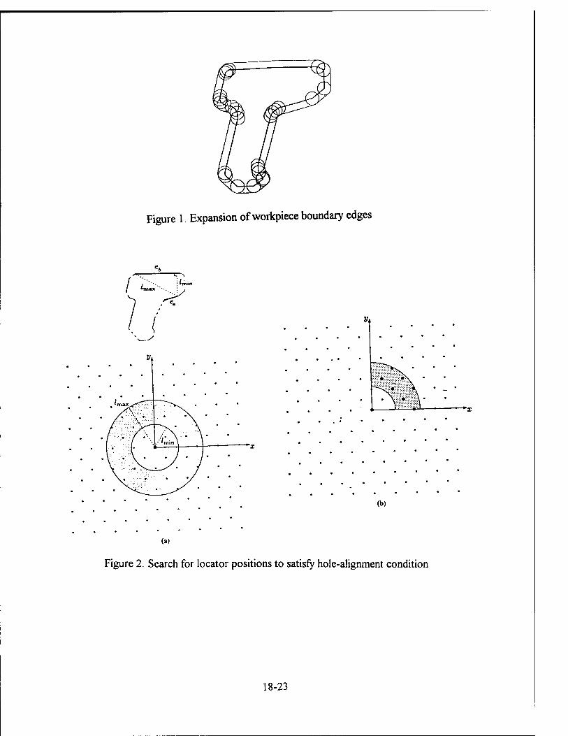
Figure 1. Expansion of workpiece boundary edges

• :::::::: ^T?>lfc>w • • "

■ • i^\ •

i—•■ »'—■——

(b)

Figure 2. Search for locator positions to satisfy hole-alignment condition

18-23

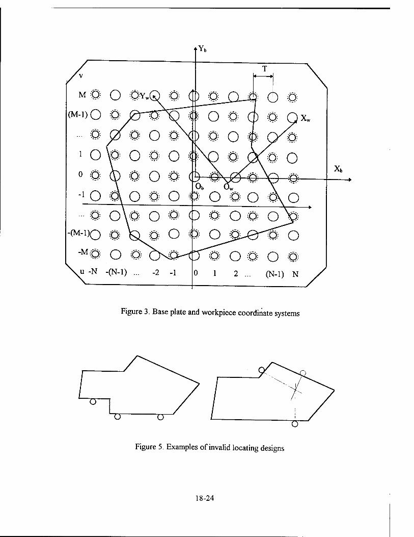
Figure 3. Base plate and workpiece coordinate systems

Figure 5. Examples of invalid locating designs

18-24

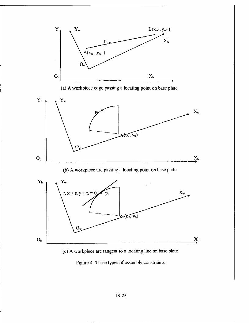
Y1 k \YW B(xw2 ,yW2)

\ I*JD^-^"""" ^^^ Xw

\ A(xwi ,ywi) .^

OwV^^

ob xb k.

ob

Yb 4

Ob

(a) A workpiece edge passing a locating point on base plate

Yw

(c) A workpiece arc tangent to a locating line on base plate

Figure 4. Three types of assembly constraints

18-25

(a)round locating pin (b) locating tower

(c)adjustable stop (d) half-Vee

(e) V-pad (0 round hole pin (g) diamond hole pin

Figure 6 Locators to be considered

18-26

s ^

m

Figure 7. Simplified representation of locating tower (left) and adjustable stop

Figure 8. Application of different locating devices.

18-27

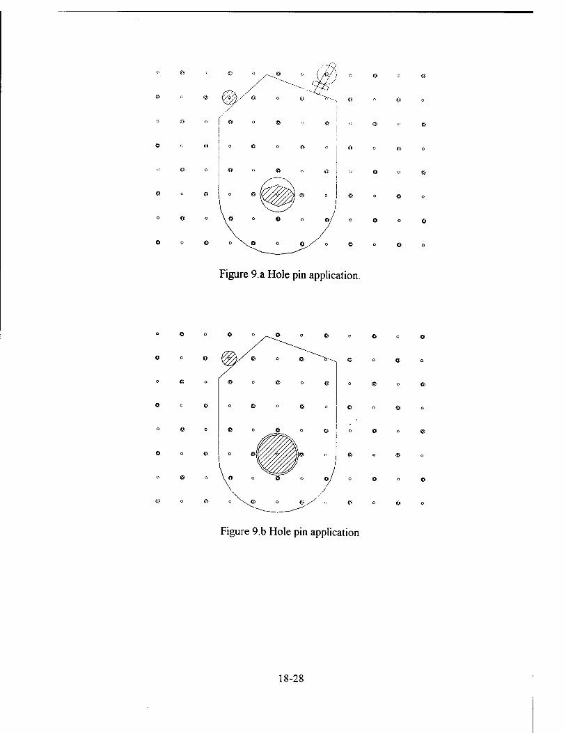
o © o

Figure 9. a Hole pin application.

Figure 9.b Hole pin application

18-28

Figure 10. Pin-hole locating with adjustable bar

functional component t y

Xoffset

Figure 14. A sketch of fixure units

18-29

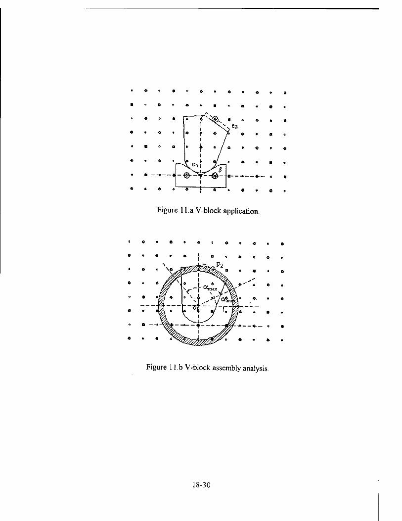
*Q*9o-4o0 o O o 0

Figure 11 a V-block application.

°C«OeQoQ«Q

Figure lib V-block assembly analysis.

18-30

Figure 12.aHalf-Vee

«r « «

' -^--/- i-i— i- -I

Figure 12.b Half-Vee assembly analysis (1)

18-31

<J y ' s

' y «/ r / /

/ / lo 1 ♦ I 1 1 ' \* 1 * I \

\^~ \ ^

_ \ \ . Vv

. .\

Figure 12.c Half-Vee assembly analysis (2)

Figure 12d Two half-Vee assembly analysis

18-32

determine candidate locating/clamping surface set

' ' select one group of locating surfaces in the candiadte locating surface set

i select fixture comoonents: tvoe and size

i ' generating three side locating units based on height requirement

assemble side locating units onto the base plate and determine position of workpiece and locating points

' ■

generating all the vertical locating units based on height requirement

i placing these vertical locating units base plate and determine position of workpiece and locating points

select clamping surface group

n

i select clamp type and assembling clamp

i'

fixture planning verification

^___^J________^ f11 nur planning

y

end

Fig are 1 3. A diagram of 3-D automated modular fi

18-33

XtUI e planning

Figure 15,3-D fixturing unit assembly

Figure 16. 3-D fixturing unit assembly analysis

18-34

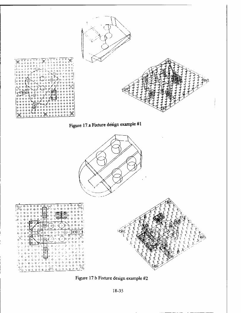
fc<"'

lo o o

o o o o c o o c o c_ coo o('c-

O Q'"0 o o

-i^f o O O O 0 o

£ O O'V ° *' ° C :"' ' c .;■ t- ov^^o1o o .? ■

i^-'o o©o/^>o o O O G O O .O < ""'

Figure 17a Fixture design example #1

„ £ S E f; n

•i ojc c< :.)s\ o o o o

o •: o :■ o ::.®;>[53ö_}.

.->--•'.-■ -.''-.'"-■•>; ■:• o o o

•;• ;■ o o o ., ■:• o o -j o ::• o o o v. o :- o_o' o o o ^o

<x i, % %

l ?. r; '■idy "#. \V> V v v v' '^'V1

\\ Q «. " <-* r- ? £ &■;'■-" v, £:'

NU-

Figure 17b Fixture design example #2

18-35

John Schmalzel's report not available at time of publication

19-1

A DESIGN STRATEGY FOR PREVENTING HIGH CYCLE FATIGUE BY MINIMIZING SENSITIVITY OF BLADED DISKS TO MISTUNING

Joseph C. Slater Assistant Professor

Department of Mechanical and Materials Engineering

Andrew J. Blair Graduate Research Assistant

Department of Mechanical and Materials Engineering

Wright State University 3640 Colonel Glenn Highway

Dayton, OH 45435 [email protected] [email protected]

Final Report for: Summer Faculty Research Program

Wright Laboratory



and

Wright Laboratory

December 1996

20-1


Joseph C. Slater Assistant Professor

Andrew J. Blair Graduate Research Assistant

Department of Mechanical and Materials Engineering Wright State University

Abstract

Bladed disk assemblies in aircraft engines are prone to high cycle fatigue as a result of localization of

vibrational energy. In order to prevent mode localization, design strategies for distributing dynamic stress over the

entire system are examined. It is shown that stress reductions of up to 75% can be obtained via minor

modifications of basic disk design.

20-2


Joseph C. Slater Andrew J. Blair

Introduction

The inside of a gas turbine is one of the harshest environments for mechanical systems in all of the man-made

world. High temperatures, high forces and large dynamic loads make reliability design an exceptionally

challenging task. Although jet engines statistically are very reliable overall, this reliability is likely to decline as

aircraft are used more often to perform missions for which they were not designed. A design is only as robust as

the qualification test it undergoes for approval. Many aircraft in the Air Force's aging fleet were designed for quite

different roles than those they are currently being used for. This leads to the likelihood of performance

degradation, reduced reliability, and shorter time to failure. A leading cause of failure in jet engines is fatigue,

both low cycle and high cycle. Low cycle fatigue is a result of high loads being applied to an object over a

relatively low number of cycles. On the other hand, high cycle fatigue is the result of lower loads being applied to

an object for a large number of cycles. This is commonly the result of vibration over an extended period of time.

Mode localization in bladed disks is a vibration phenomenon where the symmetric mode shapes common to a

perfectly symmetric (tuned), bladed disk degrade due to the introduction of slight variations within the blades. The

presence of these slight variations is commonly referred to as mistuning. Modal motion occurs primarily in a few

of the blades on the disk (often called the "rogue" blades). Since all of the modal energy is confined to a small

number of blades, the amplitudes of the motion of these blades is greatly increased, resulting in greatly increased

stresses, and reduced fatigue life.

In order to gain a thorough understanding of the localized behavior of a mistuned model, it is first necessary to

understand the ideal mode shapes and frequency distributions of the tuned system. Take for instance the following

bladed disk where the radial lines represent blades of the disk.

Figure 1: Undeformed Bladed Disk

For the sake of illustration, shortening or lengthening of the radial line denotes deflection of a blade. The outer

circle in the preceding figure represents the nominal position of the undeformed blade. In a real bladed disk, the

20-3

important deflections of the blades are usually bending, twisting, and combinations of the two - motions very

similar to those of a cantilevered beam. For this illustrative example the deflection is represented as axial

shortening or lengthening. This represents a simplification of the blade dynamics to those of a single beam-like

mode.

Since this is an eight degree of freedom model, eight linear modes can be expected. For the perfectly tuned

system, these modes will be repeated and symmetric (except for two of the modes) as shown below. The gray lines

represent the nodal diameters (lines) along which there is no deflection.

Figure 2: First Mode (Zero nodal lines)

Figure 3: Second and Third Modes (Repeated, with 1 nodal diameter)

Figure 4: Fourth and Fifth Mode (Repeated, with 2 nodal diameters)

20-4

Figure 5: Sixth and Seventh Mode (Repeated, with 3 nodal diameters)

Figure 6: Eighth Mode (Not repeated, 4 nodal diameters)

It is reasonable to expect the modes to be repeated in this fashion when considering the symmetry involved in

the structure. The preceding figures accurately depict the first of each type of modal group (beam bending and

torsion). It is not difficult to extend this analogy of nodal diameters to the higher groups, though. The first group

can be thought of as combinations of nodal diameters with zero nodal circles. As the modal group number

increases, the number of nodal circles increases. So, the second bending mode would have one nodal circle, the

third would have two nodal circles, and so on. In the present study, the first and second bending modal groups and

the first torsional modal group were investigated.

The natural frequencies of each modal group in these systems are usually tightly grouped as well, especially in

the lower groups. It is not uncommon for all of the frequencies in one group be within one percent of each other.

Typically there is also a significant change in the mean frequency between modal groups.

The present study investigates the effects of mistiming on the mode shapes and frequencies of an eight bladed

disk, as well as design alternatives to minimize these effects. Some previously used and accepted standards will be

used to qualify the work. In addition, some new and unique measures are also formulated to summarize the

findings.

Background

Under certain conditions, due to the high flexibility of the blades relative to the disk, bladed disks can become

very susceptible to mode localization as a result of blade mistuning (the variation of dynamic properties among the

blades attached to the disk). The development of analytical methods for predicting the natural frequencies and

mode shapes of tuned bladed disks has advanced sufficiently for use as design tools (although Swaminadham, Soni,

20-5

Stange, and Reed41 demonstrate that significant work still needs to be done). What is lacking is the ability to

predict the sensitivity of a design to mode localization that may result as a function of some specified mistuning,

and knowledge of how to design bladed disks that are insensitive to blade mistuning.

Griffin and Hoosac17 performed simulations of a simplified model of a bladed disk to generate a large number

of simulation results from which to draw statistical conclusions. The model consisted of 72 three degree of

freedom systems, representing the 72 blades of a bladed disk. The systems were coupled at the base by springs and

each was connected to ground at the end mass by a dashpot to represent system damping. The end masses and

their corresponding spring stiffnesses were varied to represent the effect of mistuning. The simulation

demonstrated that, under the worst case scenario, the amplitude of a single blade could easily double the normal

amplitude of a similarly excited tuned system. The shape of the scatter plot seems to indicate that the worst case

scenario was not achieved and that the worst case would be catastrophic. Further analysis demonstrated that the

range of blade natural frequencies and not the shape of the distribution of the blade natural frequencies was the

dominant influence on blade amplitudes. It was also shown that the peak blade response occurred very near to the

tuned natural frequency - validating the use of tuned analysis to design for natural frequency avoidance.

Griffin16 uses a two degree of freedom model similar to that of Basu and Griffin2, but with more sophisticated

coupling to represent aerodynamic coupling of the blades. The model was capable of predicting the scatter of blade

amplitudes in some but not all cases. It was also found that systems that are sensitive to mistuning also tend to be

numerically sensitive to modeling inaccuracies, suggesting that a deterministic approach to analyzing mistuning

effects may not be possible with existing modeling techniques.

Valero and Bendiksen43 developed a three degree of freedom blade model that incorporated rotation, shroud

slippage, and friction. The shroud friction model assumes that the entire interface slips or sticks as a unit. This

approach is then formulated as a linearized eigenvalue problem. The conclusion drawn was that the shroud

interface angle alters the natural frequencies and the amount of friction damping observed. Surprisingly, the

effects of mistuning were independent of the shroud interface angles. The mistuning effects tended to occur in the

lowest modes where less deformation occurs in the hub (and thus the coupling between the blades is less apparent).

It was also noted that the highly localized modes occurred when mistuning was highly concentrated in a few

blades. In addition, the authors hypothesized that mode localization can be minimized by enhancing the interblade

coupling through shrouds.

Two papers by Ewins12'13 represent standard reference material for understanding the modeling of bladed disks.

Ewins13 shows that under some mistuning conditions, blades may suffer stress levels as high as 20% greater than

in a tuned system. However, rearranging the same blades on the same hub can minimize mode localization. An

optimal arrangement of blade locations is proposed, although engineers22 still have great difficulty in identifying

the variations between a given set of blades for this purpose. Ewins13 shows that many more resonant frequencies

exist for mistuned bladed disk assemblies due to the splitting of repeated modes into independent modes. Ewins12

shows that under some mistuning conditions, blades may suffer stress levels as high as 20% greater than in a tuned

20-6

system. These results are in contrast to those of Dye and Henry11 and Whitehead45. Dye and Henry11 show that

almost a 3-fold increase in response amplitude can occur in the presence of mistuning, while Whitehead

analytically shows a theoretical increase of (o.5(l+Vn/2)).

Ewins and Han14 used a two degree of freedom blade model to study the response of a 33-bladed disk. They

show that, for this specific case, blade mistuning always results in an increase in blade amplitude and that the

blade with the greatest mistune always suffers the greatest motion.

Yang and Griffin's46 substructuring technique used the clamped-free modes of the blades to generate a reduced

model of mistuned bladed disk assemblies. They showed that for a simple bladed disk assembly, the reduced model

natural frequencies match the natural frequencies of the original finite element model almost perfectly, and, the

peak forced response occurs at a frequency approximately 1% higher than the "true" frequency. For the mistuned

case, the full and reduced models agree well. The exception was in a case where the tuned disk exhibits frequency

veering, exactly the case in which mode localization occurs.

Irretier19 applied a modified component mode synthesis to reduce a complete bladed disk finite element model

to a smaller, more tractable problem. He showed that the manner of frequency shifting due to mistuning, and the

corresponding change in mode shapes, were strongly dependent on the type of mistuning.

Kaza and Kielb20 and Kielb and Kaza23 used aerodynamically coupled single degree of freedom blade models

for their bladed disk vibration analysis. They suggested that the effects of mistuning can be beneficial or adverse

depending on the engine order of the forcing function. A significant result was that it may be possible to use

designed mistuning to raise the blade flutter speed without seriously degrading the forced response, although the

benefits of mistuning level off at about 5% mistune. Bendiksen3 showed a similar result. Damping was shown to

be much more effective when the blades are well tuned, which may cause problems when significant damping

exists in the tuned system. A more sophisticated model showed many of the same results (Kaza and Kielb ).

Muszynska and Jones30 developed a five degree of freedom blade model incorporating Coulomb shroud friction,

Coulomb blade to hub friction and structural damping. Their model showed that mistuning increases the response

amplitude and that appropriate design of friction dampers can reduce the response by as much as an order of

magnitude as compared to a non-optimally designed friction damper. They also reported that the optimal damper

design effectiveness is optimal for both the tuned and mistuned cases, although the amplitude for the mistuned

cases were still higher than the amplitude for the tuned case. An unexpected effect was that the friction damping,

due to its nonlinear nature, causes nonlinear coupling, inducing mode localization to some degree. Vakakis4 has

shown that when purely nonlinear coupling exists, mode localization can occur in the absence of mistuning.

Petrov35 combined finite element, substructuring, transfer matrix, and dynamics compliance methods to develop

a complex bladed disk model including shroud, joint, material damping, aerodynamic, and cable effects (for steam

turbines). Isoparametric elements were used in the joint sections to model the complex geometries. A

condensation technique was applied to reduce the size of the matrices36. The code shows that slight mistuning

20-7

drastically alters the clean transfer functions obtained for a tuned system, creating numerous resonances where

only a handful previously existed.

Wei and Pierre44 demonstrated that the sensitivity of a bladed disk to mode localization as a result of mistuning

is directly related to the ratio of the mistuning strength to the coupling strength using a single degree of freedom

blade model. They showed that the effects of mistuning are minimal when coupling is great. When coupling is

weak, however, the bladed disk is very sensitive to mistuning. Thus, a bladed disk assembly that shows a great

deal of motion of the hub when moving in a mode will be less susceptible to the effects of mistuning. Since more

relative motion occurs in the hub in higher modes, it seems likely that higher modes should be less susceptible to

blade mistuning.

Pierre and Murthy37 and Pierre, Smith, and Murthy38 included aerodynamic coupling of the blades in their

perturbation approach to determination of the effects of blade mistuning. Since it was shown that the low coupling

between the blades is the cause of the propensity for mode localization, Pierre and Murthy applied the approach of

Wei and Pierre44 in which the coupling treated as the perturbation of n originally independent blades with slightly

different modal parameters. This is in contrast to procedures that include the mistuning as the perturbation of an

originally tuned system. A heuristic explanation for why this may work is that when mode localization occurs, the

blades act almost as independent structures. Since the nominal structure used by Wei and Pierre44 was the set of

independent blades, it is reasonable to expect that this should yield better results when localization occurs. Pierre

and Murthy37 also reported that blades similar in frequency tend to vibrate together in a localized mode, even when

the blades between them do not show significant motion.

A summary of these results leads to the following conclusions:

1) Detailed finite element analysis of complex, tuned bladed assemblies is prone to large errors when mode

localization occurs due to the intrinsic numerical ill-conditioning. However, degree of ill-conditioning is an

indicator of the sensitivity of the design to mode localization.

2) Detailed finite element analysis (FEA) of complex, mistuned bladed assemblies can be extremely costly due

to the inability to apply perfect symmetry relations. Accurate model reduction techniques are necessary.

3) Even if detailed FEA of complex, mistuned bladed disks could yield valid results, usefulness for design is

questionable22.

4) The most promising method of gaining a detailed finite element model that is capable of incorporating the

detailed effects of blade mistuning is to apply component mode synthesis in one of its various forms1'6'7'8'9' 15, 18,24,25,32,33,40 „ - , , T .19 , as performed by Irretier .

5) Mistuning has the greatest effect when coupling between the blades is weakest. Added coupling through

shrouds is likely to reduce mode localization, minimizing the effects of bladed mistuning.

6) In addition, since higher sets of bladed disk modes tend to have greater coupling between the blades, mode

localization may be a phenomenon of interest only with respect to the lower frequency sets of modes.

20-8

7) Dry friction can cause mode localization to occur in the absence of blade mistuning. Thus, in any assembly

where friction dampers are used, the "effects" of blade mistuning exist regardless of how well the blade

frequencies are tuned.

8) Blade mistuning is not guaranteed to cause significant mode localization. The same set of mistuned blades

will exhibit symmetric modes or localized modes depending on the arrangement of the blades on the hub.

Little is understood about why this is the case, or what way to order the blades to minimize this effect.

9) It is likely that blade mistuning can cause responses well above those reported in most studies. Monte Carlo

simulations show distributions to have very sharp amplitude peaks indicating extremely large worst-case

scenarios as opposed to soft peaks which would indicate milder worst-case scenarios.

Problem

In bladed disk assemblies, the disk acts as a coupling device between the blades. As the stiffness of the disk

increases, blade coupling decreases. It has been shown that weak interblade coupling leads to high levels of mode

localization when blades are mistuned37'38,44. Mode localization also occurs in bladed disks as a result of their

symmetry. Sets of axisymmetric modes combine to form a basis set from which drastically localized mode shapes

can be generated. Bladed disk assemblies are traditionally designed to be symmetric for balancing. Two

hypotheses are investigated in this work: 1) Decreasing the stiffness of the disk by varying the geometry and/or

material composition will reduce mode localization due to mistuning, 2) Destroying the symmetry of the disk, yet

maintaining balance, will reduce mode localization due to mistuning. Each of these was investigated separately, as

well as combinations of the two.

A model of an eight bladed disk based on an experimental testbed in existence at Wright State University was

constructed in ANSYS® using eight noded brick elements (Figures 10 and 11, p. 19). The model was designed to

exhibit a propensity for mode localization similar to that in real bladed disk assemblies. The bladed disk model

was adjusted to provide weak coupling between the blades—resulting in tightly packed sets of natural frequencies,

eight modes in each. The blade deformation in the first set of modes is predominately a first beam bending mode,

in the second set of modes it is predominately a first beam torsional mode, and in the third set of modes it is

predominately a second beam bending mode.

20-9

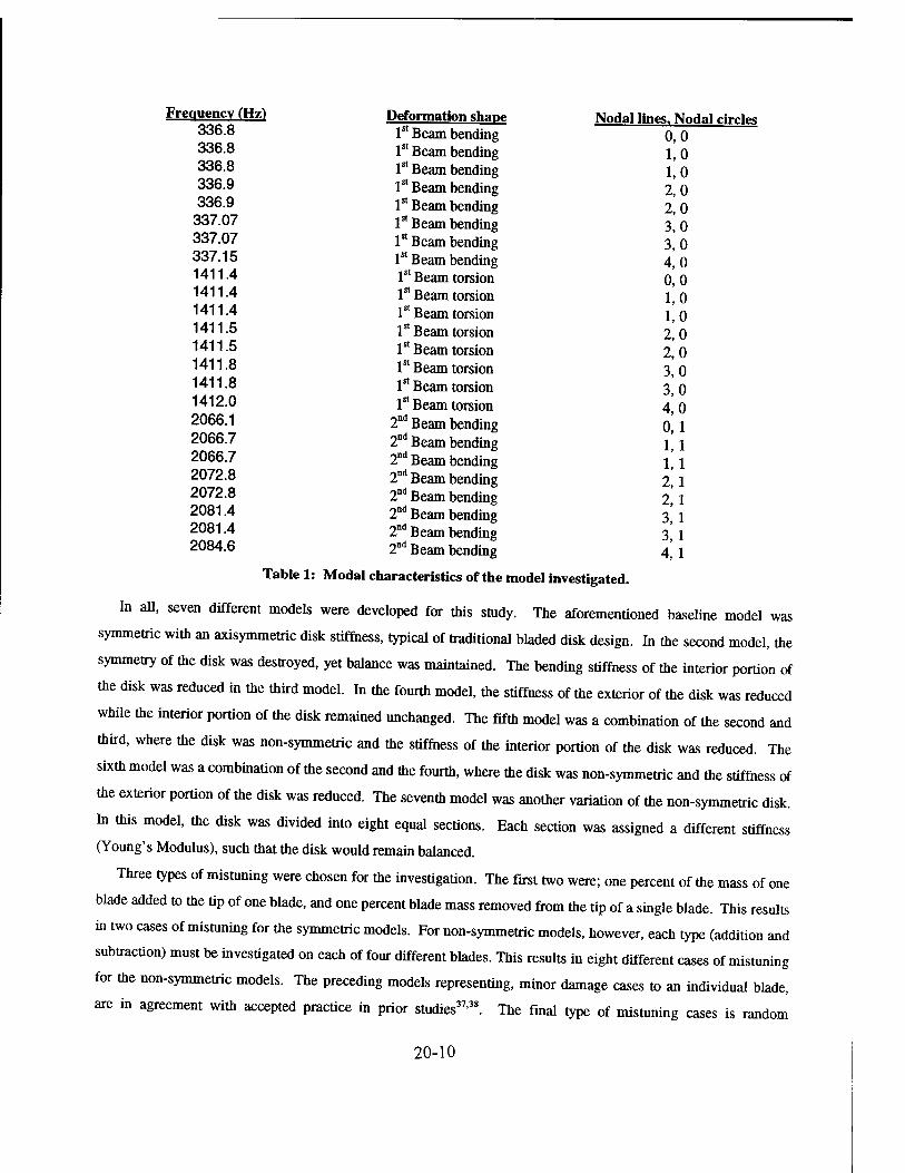
Frequency (Hz) 336.8 336.8 336.8 336.9 336.9

337.07 337.07 337.15 1411.4 1411.4 1411.4 1411.5 1411.5 1411.8 1411.8 1412.0 2066.1 2066.7 2066.7 2072.8 2072.8 2081.4 2081.4 2084.6

Deformation shape 1st Beam bending 1st Beam bending lsl Beam bending 1st Beam bending 1st Beam bending 1st Beam bending 1st Beam bending 1st Beam bending 1st Beam torsion 1st Beam torsion 1st Beam torsion 1st Beam torsion 1st Beam torsion lsl Beam torsion 1st Beam torsion 1st Beam torsion

2nd Beam bending 2nd Beam bending 2nd Beam bending 2nd Beam bending 2nd Beam bending 2nd Beam bending 2nd Beam bending 2nd Beam bending

Nodal lines. Nodal circles 0,0 1,0 1,0 2,0 2,0 3,0 3,0 4,0 0,0 1,0 1,0 2,0 2,0 3,0 3,0 4,0 0,1 1,1 1,1 2,1 2,1 3,1 3,1 4,1

Table 1: Modal characteristics of the model investigated.

In all, seven different models were developed for this study. The aforementioned baseline model was

symmetric with an axisymmetric disk stiffness, typical of traditional bladed disk design. In the second model, the

symmetry of the disk was destroyed, yet balance was maintained. The bending stiffness of the interior portion of

the disk was reduced in the third model. In the fourth model, the stiffness of the exterior of the disk was reduced

while the interior portion of the disk remained unchanged. The fifth model was a combination of the second and

third, where the disk was non-symmetric and the stiffness of the interior portion of the disk was reduced. The

sixth model was a combination of the second and the fourth, where the disk was non-symmetric and the stiffness of

the exterior portion of the disk was reduced. The seventh model was another variation of the non-symmetric disk.

In this model, the disk was divided into eight equal sections. Each section was assigned a different stiffness

(Young's Modulus), such that the disk would remain balanced.

Three types of mistuning were chosen for the investigation. The first two were; one percent of the mass of one

blade added to the tip of one blade, and one percent blade mass removed from the tip of a single blade. This results

in two cases of mistuning for the symmetric models. For non-symmetric models, however, each type (addition and

subtraction) must be investigated on each of four different blades. This results in eight different cases of mistuning

for the non-symmetric models. The preceding models representing, minor damage cases to an individual blade,

are in agreement with accepted practice in prior studies37'38. The final type of mistuning cases is random

20-10

mistuning. Three random patterns were chosen such that the mass added to the tip of each blade could vary

between plus or minus one percent of the mass of one blade.

Methodology- Models

All models used in this study were variations of the symmetric, constant stiffness system. This standard system

was constructed entirely of eight noded brick elements (ANSYS® element — Solid 45), having three degrees of

freedom per node. This element was chosen over a plate element because of the overlapping condition of the disk,

blades, and plates (Figure 7). The material properties used were that of mild steel: Young's Modulus (E) = 200

GPa, density (p) = 7800 kg/m3, and Poisson's Ratio (v) = 0.3. The geometry for this model was created in

AUTOCAD12®. Lines were also included in the geometry that allowed meshing to be performed in ANSYS®. A

proper mesh in this study had two important properties. First, the mesh had to be symmetric. Due to numerical

sensitivities, a non-symmetrical mesh could numerically induce undesirable mode localization characteristics that

would not appear in a symmetrical, tuned disk. Second, the mesh had to consist entirely of "brick" elements —

each element having eight independent nodes. These elements have a tendency to behave to "stiffly" when allowed

to degenerate to "wedges" — elements in which all eight nodes are not independent.

- SYMMETRY UNE PLATE I BLADE 1

DISK

Figure 7: Mounting condition of each blade to the disk.

The second model generated had a non-symmetric mass distribution and axisymmetric bending stiffness. A

point mass element (ANSYS® element — Mass 21), was added to the edge of the disk at the centerline of each

blade. The masses were added in a pattern that repeated after 180° in order to maintain the balance of the system

(Figure 8). The procedure added ten percent of the mass of the disk to the system. This is an unacceptable

increase in system mass. A more realistic implementation of this concept would decrease mass at some locations

and increase mass in others, resulting in a smaller net change in mass.

20-11

1 = 0.5 % disk mass = 0.02825 Kg

2 = 1.0 % disk mass = 0.0565 Kg

3 = 1.5 % disk mass = 0.08475 Kg

4 = 2.0 % disk mass = 0.113 Kg

Figure 8: Mass distribution for the mass-added, non-symmetric model.

The third and fourth models were symmetric, with reduced stiffness at the interior and exterior portions of the

disk, respectively. For the simplicity of modeling, reducing the stiffness was accomplished by reducing Young's

Modulus (E) to a value equal to half of its original value (100 GPa). In practice, similar reductions in stiffness

would be accomplished by varying both design materials and geometry.

In conjunction with the second model, the third and fourth models were used to create models five and six.

This gave two non-symmetric disks. One with reduced stiffness at the interior of the disk and one with reduced

stiffness at the exterior of the disk.

1 = 100 % Young's Modulus = 200 GPa



4= 40 % Young's Modulus = 80 GPa

Figure 9: Stiffness distribution for the variable stiffness, non-symmetric

model.

When considering the second model, the investigators found it to be of considerable concern that, in practice,

destroying the symmetry of the disk would inevitably lead to changes in the geometry. Not only would such a

change mean the addition or subtraction of mass in certain locales, but it would also mean a considerable change in

stiffness. It was this concern that brought about the seventh and final model. In this model, the disk was divided

into eight equal sections. Four values of Young's Modulus were used in these sections in a repeated pattern similar

to the mass distribution in the second model (Figure 9).

20-12

Methodology- Mistiming

Three basic types of mistiming were chosen to best represent realistic challenges to the robustness of a bladed

disk design. The first two were addition and subtraction of mass to a single blade. These were chosen to represent

obstructions that may be "sucked into" a bladed disk system and either adhere to a blade or chip the blade in

passing through the system. The final type of mistuning chosen was the random addition and subtraction of mass

from each blade, representative of the small variance between blades due to manufacturing techniques and

tolerances.

For the tuned systems, one percent of a single blade mass was added to the tip of each blade. To simulate the

addition of one percent mass to one blade, the mass of the point element added to that blade was simply increased

from one percent blade mass to two percent blade mass. To simulate the removal of mass from one blade, the one

percent blade mass element was simply not added to that particular blade. For the symmetric models it was only

necessary to investigate the results of adding mass to or removing mass from a single location (locations 1-4,

Figures 8 and 9). However, for the non-symmetric models it was necessary to investigate the results of adding

mass to or removing mass from four different locations (locations 1-4, Figures 8 and 9). Depending upon which

location the mass was added to or removed from, the resulting mode shapes and frequency distributions of the

system would be different

Three random patterns of mistuning were also investigated. As mentioned before, the addition of one percent

blade mass to each blade was chosen as the tuned, or nominal case. In determining the random patterns to be used,

the mass to be added to any location was allowed to vary from zero to two percent of a single blade mass. This

represents a tolerance of plus or minus one percent, with one percent of the mass of one blade being the nominal

value. The random point mass distributions to be used were generated in MATLAB® using the randn function to

generate three mistuning patterns, each with a normal distribution about the nominal value. The patterns

generated follow in Table 2. This type of statistical representation (normal distribution about a nominal value) is

widely used and accepted when incorporating manufacturing tolerances into design analysis.

Blade Location Random 1 Random 2 Random 3 # E-3 Ke E-3 Ke E-3 Ks 1 0.0168 0.3343 0.3413 2 0.0260 0.2867 0.4431 3 0.2579 0.4529 0.3710 4 0.3267 0.4119 0.1278 5 0.0037 0.2565 0.0231 6 0.1866 0.0448 0.3583 7 0.0325 0.3183 0.1598 8 0.2032 0.2025 0.3080

Table 2: Random mistuning mass distributions.

20-13

Methodology- Analysis

Modal analysis was perfonned on all seven models for the tuned case and for each case of mistiming in

ANSYS® , version 5.2. In each case, the inner surface of the disk was constrained to have zero displacement at all

degrees of freedom. To minimize computer time, a lumped mass matrix formulation was used. The Subspace

iteration method was used for eigenvalue extraction, with the tolerance for convergence checking set to 1E-5. The

first twenty-four modes were extracted for all cases.

Methodology- Measures

All cases of mistuning were investigated by application to each of the seven models. In each case the localized

modes were compared to the nominal system. This resulted in the analysis of seven tuned systems and 59

mistuned systems. The results of the study were quantified using some standard measures. In addition, some new

and unique measures were also developed to compare the tuned and mistuned cases.

Most studies concentrate on the first group of modes, corresponding to the first beam bending mode of a single

blade. This is done for two reasons: first, and foremost, is the relative simplicity in mathematical formulation

when assuming one general shape of deformation; second, is that mode localization tends to occur to a greater

degree in the lower modes44. When looking at only the first beam bending modes, it is sufficient to quantify the

results by looking at the displacement at the tips of the blades. In this particular mode of deformation there is a

direct correlation between the tip displacement of a blade and the amount of stress at its root. This is not true for

higher modes. To properly investigate the higher modes, some measure of energy or stress was needed.

ANSYS® 5.2 has the built in capability to determine relative Principal and Von Mises Stresses at each node. It

is important to notice that these stresses are qualified as relative because there is no forcing of the system in modal

analysis. This capability was utilized in determining a meaningful measure for presenting the results of this study.

It is intuitive that the blade with the highest value of Von Mises Stress (VM) will be the one where the greatest

mode localization takes place. To obtain a true measure of mode localization, this maximum value of stress was

compared to the average value of stress for the entire system, yielding a stress ratio R< ,. Here, R, represents the

stress ratio for the tuned case and Rn, represents the stress ratio for the mistuned cases.

(a) R = VMmax.tuned _ VMmax,mistuned

^vg.tuned (b) Rm = VMavg)mistuned

Finally, and most importantly, the mistuned response (RJ of each model was compared to that of the other

models for each type of mistuning. This is done graphically and can be found in Figures 13-24 (pp. 20-31) .It is

from these graphs, that the conclusions are drawn by the investigators.

Some mathematical manipulation was required to justify the comparison of results between different models.

ANSYS® normalizes the resulting eigenvectors (mode shape vectors) by the mass matrix in the following manner:

20-14

W?[MWi=l

where, {<!>}• is the ith mode shape eigenvector, and [M] is the system mass matrix. The relative stresses are

then calculated using these normalized eigenvectors. This creates a problem in comparing eigenvectors or stress

vectors of different models, since for different models, these vectors are normalized to different mass matrices. To

remedy this situation, both the eigenvectors and the stress vectors were normalized to unit length.

When mistuning occurs in a given system, it is important to realize that groups of modes remain grouped. In

fact, the mistuned mode shapes are shown to be linear combinations of the tuned mode shapes. This is verified by

the following calculation.

[*t]T[«>m]= M 24xn nx24 24x24

where, [OJ and [OJ are the matrix of tuned eigenvectors (mode shapes) and matrix of mistuned eigenvectors

(mode shapes), respectively. The variable [¥] is defined as the transformation matrix and n is the number of

degrees of freedom. This results in an m x m matrix, where m is the number of modes examined (m=24, in this

case). The transformation matrix can then be divided into three submatrices, corresponding to the three modal

spaces (modal groups) being investigated.

24x24

*1 8x8

^2 8x8

*3 8x8.

The determinate of each of the three submatrices should have a magnitude of one, if the mistuned mode shapes

are indeed linear combinations of the corresponding tuned mode shapes for each modal group. Each submatrix

can also be examined for the contribution of each of the tuned mode shapes to each of the mistuned mode shapes.

Here, each column represents a mistuned mode shape, and each row represents a tuned mode shape. In the present

example (»Pi, model 1, mistuning case 1), it is easily seen that the second mistuned mode shape is comprised

mainly of the first and third tuned mode shapes. The seventh mistuned mode shape is comprised almost entirely of

the sixth tuned mode shape, and so on.

V\

0.315 0.734 0.451 0.360 ~0 0.159 0.005 -0:040

0.167 0.371 -0.892 0.173 ~0 0.089 -0.003 -0.025

0.510 -0.570 -0 0382 ~0 0.268 ~0 -0.070

0305 -0 0.015 -0.689 -0 0.509 -O.007 -0.103

-0 -0 ~0 ~0 -1 ~0 -0 -0

-0.007 0.003 0.005 0.007 ~0 -0 -1 -O.010

0.490 -0.003 -0 -0.135 ~0 -0.754 ~0 -0.417

0.343 -O.003 -0.003 -0.075 -0 -0.261 -0.012 0.900

20-15

Along with the resulting change in mode shapes, it is equally important to examine the resulting changes in the

natural frequencies of the mistuned system relative to those of the tuned system. In the tuned system, especially

systems in which the disk is symmetric, all natural frequencies of each group are within a very small percentage of

each other. In the mistuned models, some of the natural frequencies in each group can move considerably away

from the mean frequency ofthat group (this phenomenon is commonly known as eigenvalue veering).

Mode Tuned Cases 1-4 Cases 5-8 Case 9 Case 10 Case 11 # Hz Hz Hz Hz Hz Hz 1 336.8 330.64 336.8 334.74 331.49 331.74 2 336.8 336.8 336.8 336.56 332.55 333.6 3 336.8 336.8 336.85 338.01 334.54 333.92 4 336.9 336.85 336.9 338.45 334.96 334.36 5 336.9 336.9 337 342.68 335.8 335.24 6 337.07 337 337.07 342.83 336.59 339.18 7 337.07 337.07 337.13 343.15 338.03 340.05 8 337.15 337.13 343.59 343.49 342.34 342.94 9 1411.4 1411.3 1411.4 1411.4 1411.3 1411.3 10 1411.4 1411.4 1411.4 1411.4 1411.3 1411.4 11 1411.4 1411.4 1411.4 1411.4 1411.4 1411.4 12 1411.5 1411.5 1411.5 1411.5 1411.5 1411.5 13 1411.5 1411.5 1411.5 1411.6 1411.5 1411.5 14 1411.8 1411.8 1411.8 1411.9 1411.8 1411.8 15 1411.8 1411.8 1411.9 1411.9 1411.8 1411.9 16 1412 1412 1412 1412 1412 1412 17 2066.1 2038.4 2066.5 2059.6 2040.9 2042.6 18 2066.6 2066.5 2066.8 2073.1 2051 2055.1 19 2066.7 2066.8 2069.5 2078.6 2057.8 2056.1 20 2072.6 2070.3 2072.8 2081 2061.3 2059 21 2072.8 2072.8 2076.9 2104.3 2070.6 2067.2 22 2081.4 2078.5 2081.6 2108.9 2072.5 2088.6 23 2081.6 2081.6 2083.7 2113.9 2082.8 2091.3 24 2084.6 2083.9 2114.1 2115.4 2106.7 2110.9

Table 3: Frequency table for Model 1 (symmetric mass distribution, axisymmetric stiffness).

In the case of the tuned symmetric disk, the frequencies in each group are all within one percent of each other.

This is no longer the case when the system is mistuned. In mistuning cases 1-4 (addition of mass to one blade), the

first frequency of the first mistuned group deviates considerably from the rest of its group. In cases 5-8 (removal of

mass from one blade), it is the last frequency of that group that deviates. There is no single frequency "leaving"

the group in the random mistuning cases (9-11),. Instead, the frequencies ofthat group are dispersed over a larger

range. It should be noted here that, in the case of mass addition or removal, the mode in which frequency deviates

most from the group is also the mode which exhibits the strongest mode localization. A complete set of frequency

tables for each model can be found in Tables 4-10 (pp. 32-37).

Results

It was the goal of the investigators to minimize the detrimental effects of mode localization by altering the

symmetry and/or stiffness of the disk. Individual blade damage (addition and subtraction of mass) were

20-16

investigated, as well as random mistiming representative of small manufacturing variances. The results of this

study are presented in Tables 4-10 (pp. 32-37) and most significantly, Figures 12-23 (pp. 20-31). The results of

this study may prove to be very useful in the future design of bladed disk assemblies, especially when the higher

modes of vibration are of particular concern.

In the examination of the stress ratio, it is important to first look at the tuned models. In the case of the

symmetric disk with axisymmetric stiffness (the baseline model to which all design modifications are compared),

stress ratio values (Rt) range between: 9-11 for the first modal group, 3-7 for the second modal group, and 5-8 for

the third modal group. The proposed design changes offered little improvement in the stress ratio for the tuned

case. In fact, the selected methods of destroying the disk's symmetry actually induced mode localization,

increasing the value of the stress ratio. However, this result is not of dire consequence to future design, because the

perfectly tuned case will never be a practicality.

The results of the mistuned cases are best summarized by looking at each case, one modal group at a time. The

first modal group corresponds to the first beam bending shape of an individual blade. In the cases of blade

damage, one mode of this group showed a significant increase in stress ratio. When mass was added, the first

mode of the group showed a significant increase in stress ratio. However, when mass was removed, the last mode

of the group showed a significant increase in stress ratio. This mode localization is clearly visible when the same

mode is plotted for the tuned and mistuned cases, using the same deformation scale for each (Figures 10 and 11, p.

19). None of the proposed changes offered a significant improvement in the response of this highly localized

mode. The techniques employed to destroy the symmetry of the disk even caused one or more other modes to show

an increase in stress localization. For the three random cases of mistuning, all eight modes of the group were

found to have high levels of stress localization. Destroying the symmetry of the disk causes sporadic improvement

of stress levels throughout this group. Most importantly, reducing the stiffness of the inner portion of the disk,

results in consistent lowering of the stress level throughout the entire group (relative to the mistuned baseline

system).

The second modal group corresponds to the first torsional group of an individual blade. For all cases of

mistuning, the stress levels of this group were only slightly raised. Again the destruction of symmetry was shown

to have a negative affect on the system. Although some sporadic improvement was shown by changing both the

interior and exterior stiffnesses of the disk, no consistent improvement was shown in this modal group by

implementing any of the proposed design changes.

The most interesting results are found in the examination of the third modal group, corresponding to the second

beam bending mode of an individual blade. In the cases of blade damage, there was only a single highly localized

mode, similar to the results obtained for the first modal group. The only proposed design change that did not offer

significant improvement in the blade damage cases was the non-symmetric (mass added), axisymmetric disk

stiffness model. Reducing the interior disk stiffness seemed to trigger the most improvement. When this was

20-17

coupled with the destruction of symmetry, via the addition of mass, the maximum stress ratio dropped to as little as

one-fourth that of the mistuned baseline system. In the random mistuning cases all proposed design changes

offered some improvement, although the results of the mass added destruction of symmetry were rather

inconsistent. Again, the reduction of the interior disk symmetry seemed to be the most beneficial design

modification. Implementing both the reduction of the interior disk stiffness and mass added destruction of

symmetry yielded the best results. Here, the stress ratio dropped to as little as one-half that of the baseline system.

Conclusion

Reducing the interior disk stiffness relative to the exterior disk stiffness can dramatically improve the

performance of bladed disk systems in the presence of mistuning. Upon examination of the different responses in

the third modal group, one can also conclude that there is some promise in the prospect of destroying the symmetry

of the disk. Although no great improvement was shown in the responses of the first and second modal groups, the

dramatic improvement shown in the third modal group is enough to warrant consideration for the design changes

proposed.

Only one pattern of mass addition was used in this study to represent a non-symmetric disk. The addition of

this mass, in itself, was shown to induce significant levels of mode localization. The most promising results were

shown when destroying the disk's symmetry, via the addition of mass, was coupled with a reduced interior disk

stiffness. It is quite possible that the amount of mass added to create a non-symmetric disk was too drastic. The

investigators speculate that the positive effects of reducing the interior disk stiffness was enough to overcome the

negative effects caused by destroying the symmetry. Had the amount of mass added to the disk been less severe,

the implementation of a non-symmetric disk, in itself, may have proven beneficial.

Future Study

The present study featured seven different types of models. Two types, disks with reduced interior stiffness and

mass added non-symmetric disks, yielded promising results and are worthy of further investigation. Based on the

conclusions of previous authors, it is the authors' belief that reducing the stiffness of the outer portion of the disk is

also worthy of further investigation. Future work should include:

1. Investigation of different levels of relative stiffness between the interior and exterior portions of the disk.

2. Investigation of different patterns and mass amounts used to destroy the symmetry of the disk.

3. Investigation of combinations of the previous two.

4. Formulation of new quantitative measures to summarize investigative results.

20-18

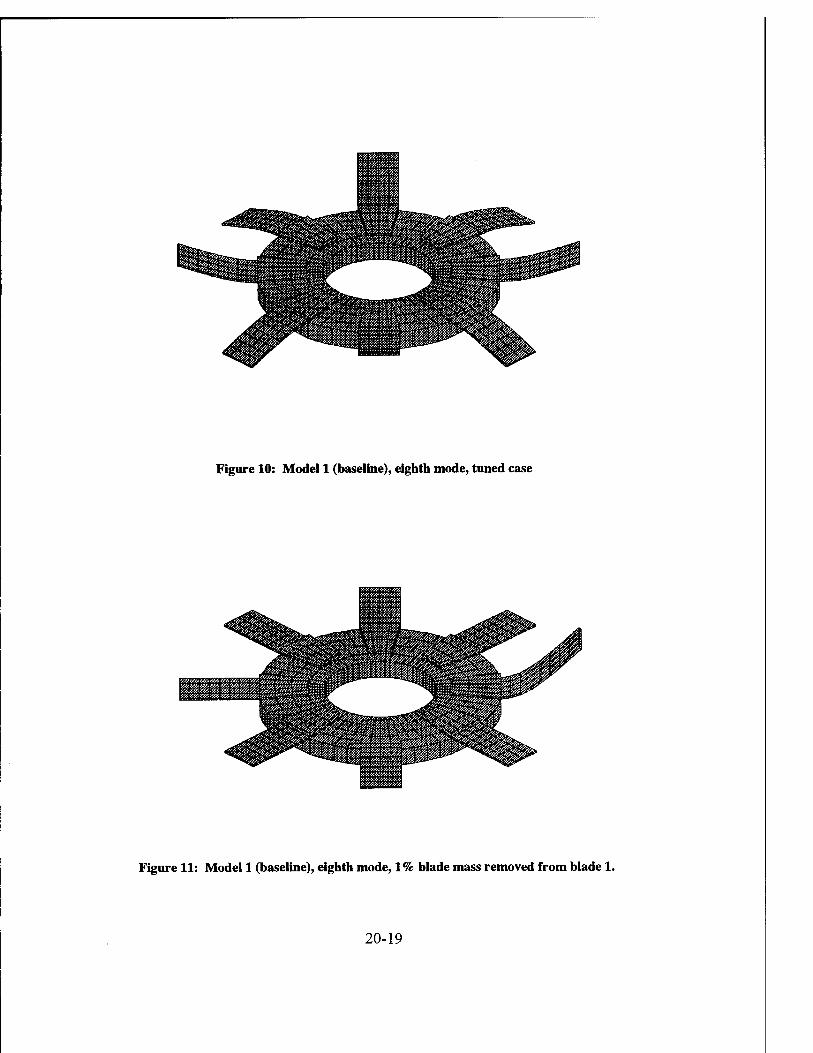
Figure 10: Model 1 (baseline), eighth mode, tuned case

Figure 11: Model 1 (baseline), eighth mode, 1% blade mass removed from blade 1.

20-19

o <*"> © V, © t—< ,_I

(JH) op*tf SS3US Paunx

M

V3

K Ö 'S S s m TB o u 3 3

? Tg

u

•a

x>

a s o I* M

's o

s H

a 9 O u

© £ e o u 0)

1/3

3 z •o O

ctf

on

1) C 3 H

"c?

"1— 1 -1

* OB -

■ * #

■ 5KME

■

* l p

■

flu

• o- ■

- -

' * ©OK ■ o ■«*■

Z

'1

o

s

■a o

o •■ö

CO

06 Vi

"8 c 3 H

(JH) oi)By SS3DS paunx = >n o u-i N ^H *—I

(1H) o'J^H ssaiis psunx

a 9 E

—1— i i H • •*■ a /—\ CN 13

li o s

N)V

• JK es

/A ft VI es

1—1 X>

z U

a s ■ o

<N o H

¥ 2 c< i—<

1 /fi ON

9 -8P

^ 0 v\

00

**■

■ Q- ' i . 1 1— *!* ■

r~

20-20

o C4

V) © W-l O

(ury) opB^ ssaiis paunjsij^

M-i

=3

§

S3

fc. !=!

i ■8

I 1 'S :§

ii

a s o h WD

■a

I -a

3 a 3 s M

TS o

■a o u V

a s o u

"3

I B

•■M

to

T3 O s

OS

(a) *

if ■ *

/ ^ ■ W i •

•. \ /

■

• & " ' J[

1

o o o

5

■8 o

OS

h </5

•n- T*

*—+- tS V o •^T - -A ' C*1

©

- 0 4)

N •'/ Vi n ■ F5

CO

o

9

3 1-1

v ?an* <N o , j s V

. M u s

if rf *r ■a

0 3*»k 00 s 43 1

* * <*5

(ury) op^y ss3j)s paurv)sij\

© m © </"> CS ~H rt

(ray) OIJB^ ssaijs paunjsrj^ s

20-21

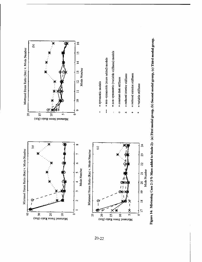
y^ * (OC X)

u

a * BV 3 z u O * IB s >

1 *. Tv ^-^

o •a OS * T

CO CO tu

CO *>ffl- ■8 ■ w c S «1

er J— ■

. *c

o

. c> M

^1

. o

W"> O U1 ©

(ray) oijey ssajjs pautqsij^

I !§

X) et)

-a M

X/i

■•3

tu c

o •g .5 'S u 3

3

tu

ig •a o 'S

•g o 3

tU

So t*-i •a

x>

a s o M

75

I -a b

a s 2 60

1

o

en

a 3 O (a M

"3 0 E

s 3 z tu •a o

_o CO

a CO

, 1

=3

i

5tC n j|

* d»

* M>

*

2 i

/ ^^^"^^

i i ■»

o o CO

© cs

•a o

Z eu O

(lUy) OIJBy SS3JJS pSUtHSIJ^

a CO

■ s *iff ■

*'■ w •

"1 w ■

4 .

A /TT

^°fr*f ■

0- " ^P** .

• ^T<K xi* x •—-—J • 1— ■

. ©

a V

3 p

-B eu

<N "8 S8

^ s 2

tu © T3

. 0\

U"> © IO *—f T—<

(my) oijBfl SS3JJS paun}siy\[

r*

cs U

■a s •S S

tu u s

to

20-22

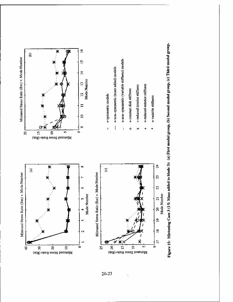
x> 6 3 z •o o

a!

b on

B S

.D

*

■ £ I ' ■ ^ 4- • . ^ »>

. QTJk ■ *

8

. V\

_?2

v> o <ri o

(m^i) ORBH SS3JJS psunjsii^

<*-4

=9

c o

§ o •ß

•a

•a en

X)

-S 5 "8 "8

1 1 I II II II

S O h en

1 IM

••M ja H

o. s 2

1 "8 s o u v

»5

a. s o IM en

"3

1

u XI s Z u •a o

OS

DÜ

■8

K »

.

* T

3K A

■ * 4

■

* m

■ .* ^^Jb

•OC 1 I.

o

I Z

o ©

U X>

o

o ■a « OS

ä CO

8

o

l m r ' i ~" i

■

A\

*%

' W"

■

* -ifoafc

■ w "^K*> <^ ><:

(urtf) oijBy ssajjs paumsij^

o in o v, d <-i «->

(ray) oijcy ssaiis paunjsij^

V

es s o

-o C8 w cd

Z #

v SB

u

•s s

2

2 s if fcj.

20-23

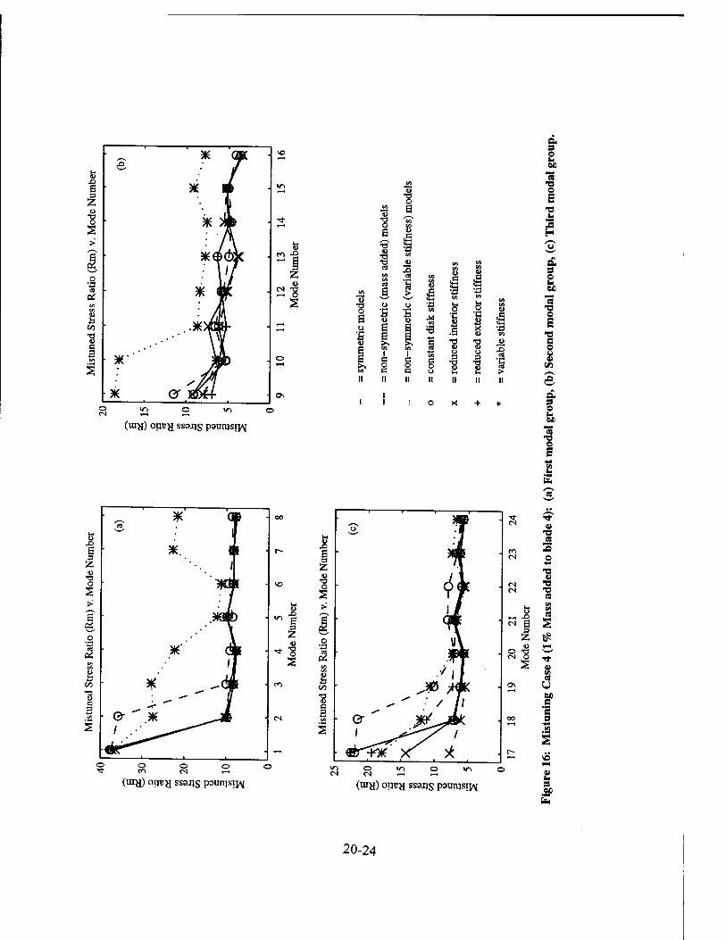
X>

■8 o

o •a

u ü

■8 c S

*

■ X T

• X )JB

• XG /doc ■ VI

■ * K

•

I • *''

' Jrl

0b

er »*l » o

Z u <s -a "1

Vi o >/-> ©

(UIH) OIJE^J ssajjs paunjsii^

"8 a

■g a

X> 3

a s o o

■a =3

a o u

.3

ä •o o

1 1 1 II II

XI

a 9 2 M

"« o s

H

a s 2 M

"3 o E 1 o o «

a. s o u en

o s

E

■ * op «

« X R X n 3 Z /[ « x) o jH Bfl 2 > 6 • .x«b

OJ o

öS x GH CÄ f I X/i a>

£5 ^ (JlK

'S ^, -" tf c s

is / "x ^^-*b

_—i i ■

© o to

o

5 z .8

'I

(Uly) OIJBfl SS3JJS p3Ull)Sip^

p in © in OJ ~H t-H

(ur^) OIJB^ ssaijs paunjsrp^

<u •9 a 3 o *■»

* % (3

■a s .a 2

2 9

20-24

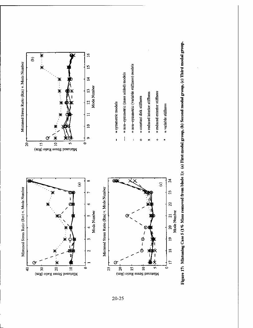
u X>

s 3 z o o s

u «5

3

*

■ *.. M

• *

A ■ * x

• *fl

i \ i

■ * rm-

■

s- V

lfe(-

■ er * J

8

-1 z .8 2 «2 as

m © <r> O

(ui^) opufl SS3IJS paunjsij^

fl> CA

4-H WS

*n ti CA O

•M U •8

=3

s o

.5 •8

u ä ■a

o

1 u "8

•8 'S x>

► II

a s 2 WD

"3 no

I -8 is

a 9 0 fa WO

73 ■o o

'S 1

a s o u cm

7»

I

u XI

•8 o

o o o © CO CN —

(UIH) opB^ SS3JJS pautvisij^

^^ 1 1 1 1 "

Ü

ä <} ■

/ \

 CN I

!R fa ,_, X) » CN ^ »1

Z 2 © ■S CN o

s >/> o\ 01

SB T—1 ca

U

00 T—1

S ■a s

© in © in © CN —I »-H

(m^) oijBy SS3JJS paunjsij^

4S

fa S cm

20-25

■ # xs

fc Ji .n S * wm 3 z o •a o * ■1 2 >' *\

^—v

*. px *—■*

o \' * x»c

ca CO U

CO * ö ■- U M C 3 OS

* • T

a * ■

o

. ^O

. «O 5 z o

»n © m ©

(ur^) oijBtf SS3JJS paunjSM

'S I .3 'S u

ig

e 'S 8

■8 u cd

'S >

a

2

1

a s o M S ■o o E

•o e o u CU

CO

a 9 o M

'S "8 E

ü x> S 3 Z u

•a o s

OS

CO

■8 c

/«• ■

C9

'' *^ •

*: I

■

IK •

* ■

* W

■

' 1 1

If

z u

o o

(uiy) oijBtf ssaijs psunjsijv

J

•8 o

o •a CS

OS

J3 CO

"8

-1 1—

X o

. * jf

. ■>fl

.

• *«>X vv

•

■

■ or » i

** 1 i

u —. X>

3 z O t3 <N O

© u-> O W-l © CN ^H ,—I

(uqj) oijBy ssans paunjsrj^

CU TS JS 3 £ o

CM

•o cu 0- o E V

ve cu «8

U

C° ■a 9

9 WD

E

20-26

* Vxn XI

u

s * m 3 z 1 O

o * s > 1 1

y—^

■ .*« p N«' \ 1 o •a • *■ D3K ca CÄ <D

00 ■ * Sa- "8 e S

■ X to 2

• \ ■ * er i

o

cs -a

v-> © v> ©

(uiy) opcy ssajjs psunjsij^

(4-1

■tf n CA o

CA 'S ■■B

£ SB •a CO

1 .3

! 1 1 -s -s

a 9 £ an

73 "8 s is H

a. s o i> WD

73 o

e o u V

a s o es

73 •o o S

E MM

to

r>

X>

s

O

s

B5

■s c

-^ "ca"

*"" "^»

* B

* «

* »

* H

* ■

* ■

o

-8 o

o

(uiy) OIJB^J SS3JJS paunjsiyj

o «■> o

(uiy) oijBy SS3JJS paunjsij^

41 -* •o CJ J5 3

g o

V <N >■

<N I » cu

1* »—< XI n ts ^ (A

>3 Z s

o f£ <s o 1-H

OS a>

i-H

U

W a s *>* .a

r- 2

9 if to

20-27

u

s

•8 o

Oi VJ V) O

"8 s B

*

■ X 1 ■

• * k

■ *f 'i

■

* T

\i

■ ..*di T

a""' i-

* ^ \ \

er Jg o tN

Z u

. o

v> o >n o

(urg) oijBfl SS3IJS paunjsrj^

•s a o B

•8 w 3

•a o «a

B c

$ •a TJ TJ 6 CA

B o B CA

A«

O

'S ig 1 Ö =3 .3 s en CA § ■8 "8 u

M 3 e o s

c o c c o o

3

■8 3

■8 ■g > II II II II II ii

a s £

■o o s

s a 3 O

1 "0 e o u V

CO

a s o b CUD

7s ■o o e

"" 1 i 1—

^-s m *H U

Xl

3 ' "'* & 3 z U

T3 O *. [

S j

> 3 " '*4 ( & o •a *ab • « c« 1> £

55 .*' I

"8 fi c 3 CO - ^~f !

■ Qr ■

u

o O

O o

(ray) oijcy ssaijs paunjstpM

o

fi

"8 B 3

*>*

—i

si 3 n

(9c r

*Tt ■

i]

■ or ' * A i—.—i 1 1. »

o tN

s

tN

tN fi

V

(8

O

w e E V (a

z S u

O 73 <N O

VI O VI O

(ray) oijsy ssaijs paunjsi^

00 V es U

•a 9 •to» .2

o

9

to

20-28

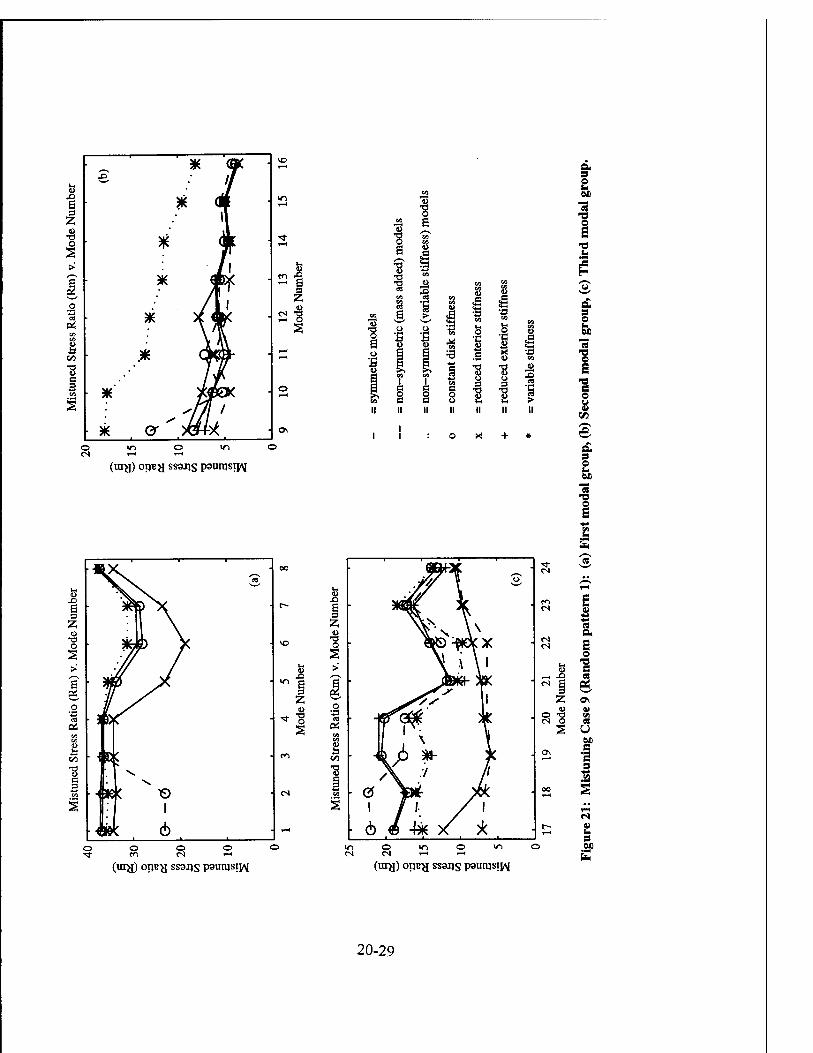
o x> 6 a Z o o

CO

'S c 2

.D *

i ■ *

if ■ * (M

• *

• ¥ JLL

■ .* m

" * :*ox

• 5k er <sf/ if /

k ■

o

. tn J

Ja 2 'S

m o <n © i—I r—I

(uiy) opBfl SS3JJS paunjsipv

ig 4-1

CA

=3

8

WS

s •6 .a "8

!

8

s I u ■8

I

s £ en

"et •o o

is M H

a s 2

"« O E S O

a s o u M

"tS -a I

(ui^) OIJE^J ssafls paunjsiw

O vi O <ri © O i-i i->

(UI^) OI}B}J SS3JJS psun)sij\

s h

eg a. s o s

eg U e •a 9

49

s

20-29

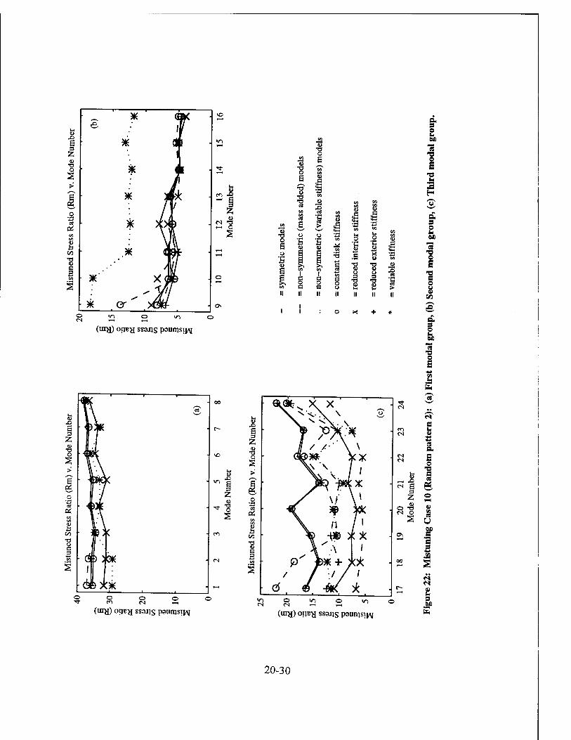
X>

s 7

o o * 1\ >

I * f •B

* r US U

00 K 'S a 2

■ *' P

* er

0)

t-i o

o <N

"■> o v-> ©

(uiy) op?y ssaijs paunjsij^

•3

=3

c o o

o •g .S "8 o

I

e 'I

I 1 •!

ii

a. s 2 M 'S

I is

9 O b M

'S

s o

a s e u M

"3 ■o o

(iay) oijBy sssjjs paunjsij^

M S 1. V *i •*■» es a. E o -a e es

es U

ff 'S 9

IH 9 60

(in^[) oijBy ssajjs psunjsi^

20-30

u s

■8 o 2

GO

■ ~ * .£,

*. a

* «

*

f \\ * ^ QHp

.* A// *

// )Q»-

/ ■ * er «

cr, X)

o w-i o v> o »—I »—<

(uiH) opB^ ssaijs paunjsij^

 «1 tfl

es "S WS

!

b >

£ ■8 J> 4) o fi a *fi 5 3 u

CA V3

3 a a ti o o Ui c a II

1

II

1

II

to

«4-1

o •c «1 CJ

■d •S 9 ■g 4-* u

1 c o o 1

•a

o

1 8 'S ■§ 9

"5

(ura) OIJB^J ssajjs paurqsij^

WV O W) ©

(ray) OIJB^ ssaijs paunjsij^

9 2 M

"3 ©

is H

a. s 2 M

"« •O o s •a o

en

a s o b M

"3 •o o B

s

« a

o

s

es U

•a s

»♦5

ev u 3 IP

20-31

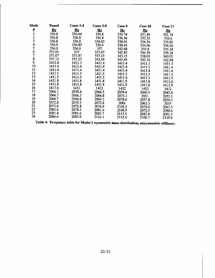
Mode Tuned Cases 1-4 Cases 5-8 Case 9 Case 10 Case 11 # Hz Hz Hz Hz Hz Hz 1 336.8 330.64 336.8 334.74 331.49 331.74 2 336.8 336.8 336.8 336.56 332.55 333.6 3 336.8 336.8 336.85 338.01 334.54 333.92 4 336.9 336.85 336.9 338.45 334.96 334.36 5 336.9 336.9 337 342.68 335.8 335.24 6 337.07 337 337.07 342.83 336.59 339.18 7 337.07 337.07 337.13 343.15 338.03 340.05 8 337.15 337.13 343.59 343.49 342.34 342.94 9 1411.4 1411.3 1411.4 1411.4 1411.3 1411.3 10 1411.4 1411.4 1411.4 1411.4 1411.3 1411.4 11 1411.4 1411.4 1411.4 1411.4 1411.4 1411.4 12 1411.5 1411.5 1411.5 1411.5 1411.5 1411.5 13 1411.5 1411.5 1411.5 1411.6 1411.5 1411.5 14 1411.8 1411.8 1411.8 1411.9 1411.8 1411.8 15 1411.8 1411.8 1411.9 1411.9 1411.8 1411.9 16 1412.0 1412 1412 1412 1412 1412 17 2066.1 2038.4 2066.5 2059.6 2040.9 2042.6 18 2066.7 2066.5 2066.8 2073.1 2051 2055.1 19 2066.7 2066.8 2069.5 2078.6 2057.8 2056.1 20 2072.8 2070.3 2072.8 2081 2061.3 2059 21 2072.8 2072.8 2076.9 2104.3 2070.6 2067.2 22 2081.4 2078.5 2081.6 2108.9 2072.5 2088.6 23 2081.4 2081.6 2083.7 2113.9 2082.8 2091.3 24 2084.6 2083.9 2114.1 2115.4 2106.7 2110.9

Table 4: Frequency table for Model 1 (symmetric mass distribution, axisymmetric stiffness).

20-32

2 i/->i/-sessO'*roo'3,Ti-esc<->Tt--<t<nr-~oo,v. cnt~r~o\^soesr» ^ Ni«.°°. <=* <*5 ^.-*. P <*. *-<' ^ ^ -; ^ ^ ^ 2 <o ö o\ - «* ^ «s <>

nncinfifimmrtHHHHHH i-< es es es es es es es

i-i ... r-

mm(ii(<iwwmmHHiHrtrtHH I-H es es es es es es es

M, - . mm os ■<♦; oo es t-; >o oq i-< Tj-' f- Ö oö ci

©s Or* iôofoioxNTt"itviinooo\ oso\i-ir-r~>nes 9> NI "1 °°. oo ■*. *0 oo <-; "*. H ^ -H' ^ i-.' i-.' ,-! Jj, ö m vD « o\ "*' t^" "* S BN-tü)«>N(SmmrHrtrHrHrHr-rHT|.rHinotvO\OHTH es >i«l<ri<r)en(riTtrj.Tl.Tj.rfTcTtTj.Tj.Tj.Tt^)r^C)f^00r_^Hrt U mm cimcimcirHHrHHHHH l—i es es es es es es

00 v

mêst^v-ivoesooeSTr-^-rfmoooo^. C3\t~es_u-iesu-irf p °^ oq oq os p -; ^ ^- ^ rt- ^ ^- rt- ^- 2 ^ uS es 5 -' <> es vd ;vo, SBSl'oiy\o*Ovor~t~-fn«-n-n-n-ii-'»-i. ^ .._„. . « MMicr)epcricocr)erifr)Tj.rj.TfTj.Tj.Tj.TfTj.T^lt^00c^000^H

U mnmmmmm(OHrtHrtHrtrt >-i es es es es es es

-„mos >miomm'*^,in«!oo.,mt^'-iieiint^>0 *i oo oo r-> O i-"/"> o\ >n ©■ tÛ-)Oo3

iSiSvo\oent~t~'-<^H'-i'-i^^^»-<'<*es<nvoî'ot~ooo ££cocn<^com^T)-Tr^TtTtrfTt5r^©©000©es nnn<<i cn cn en 1-H l-H ^ i-i <-H «-< »-< i-< es es es es es es

V Ni SKI ü

criî-Hr^-invoesoves-ttTfrj-inoooo^. o\t~u-)0\_.oo\ovo

coSc^fncnc^cn^-^-rfTtTtTt^Tf^HrÔOOesOOi-i m <^ m cn co m <n cn 1-H ^ i-i ^ 1-H 1-H ^ ^H es es es es es es

u NI ss si u

rê<iO\voeSi-'OveSTt-^-in>ooooo_,o\v^\o<r)rfTteoc~ °S oo oo os o I-H u-i • • ■ • • • • es . so © so © so es es

mSCHOIOI^t^miHrtHi-liHrtrH-.rHin\0»OM^»H

cimmwciciciciiHiHiHHHHiH i-i es es es es es es es

si'ÄQ ,esr~\ovoesesc<T^-TtTtoooo oq oq 0\ O rn rt-^ ,_; ^ ^ , ■

o\ O\ t-; vq I-« co oq t-- ! i-i i-i wS es' r^ <ri o\ es'

a ""'mmSmmmmmit^TfTtTtTttrtÔOOOOOO pin^mmnmmHHHrtrHrtH *-< es es es es es es es U

U

^ t*> nn ""> O t^CO^HCOTj-TtlOOOOO^. t~-lî-iTj-U-l>n\0 oo °°. °°. oo oo t~. o i-i ^ ,_; ,_; ,_; • • • es . -• -• _• .•-•.-•_• oöSigvosoSr^rî-n-i

û-jinö^'t-^wSöoo m SCoo;£~\ovoenr--.r-,rti--i^-rt^<i--i,-iT].o\i/->\OvOvot~--ooö S

mmrtH i-i i-i i-i es es es es es es

es « NI

ä cal u

•*conni-<t~-vo\Oeses<ri-^-'^-^-oooo, SO © °°. 00 00 OS O i , -. es °^ vo °°- °°- vo ^ **■ ^ o>nSsosovor--r--î-H-H^'-<'-ii--i-<tô'£?vOof~-t-00

mm2mmmmmt^fittTtTftrt^NOONOOO mmmnnmmtfiHiHHr<r<HH <-<v es es es es es

1-1 ^tco-_c<-iossocni-iescn^t^->noooo_,o\cnesosoo TI- « NI *> <=>. üS °°. °°. °i P -i ~ ~ ~ ~ -H' ~ -' 2 -' «w t-; ö so p p; es

SC|O>ri)SvO^0v0f~-t~~'î_"_"-H'_l^-^H'3-'_,er>T£>sOÖCD00 'enen coen' 'COCi-lCICOCI^Hi—<i—I^HI—ii—ii—i i es es es es

"O cn__ —mosi-ir~cnescn-^--^-ioooooÄ. osc-~^Tfiososo„ § NI P °J fj «=«> P p ^. _;_;_; _;^ ^-^ es ^-^ o^-^^ö^ .3 *'cn?l!^cocr)cn<ri<ri-*Tf^--^-Tt-^--^-^<t-~OOOOOOes rr. ncicimciHHHHHHiH i— es es es es es es

"8 *ii iescoTt«ovot~-ooos oêscnrfu-isot^-oocjsOi-iesco't rtrtrHrtrtrtHrHt-Hrt(S(Sl(SlNCSl

20-33

Mode Tuned Cases 1-4 Cases 5-8 Case 9 Case 10 Case 11 # Hz Hz Hz Hz Hz Hz T 336.39 330.39 336.39 334.47 331.22 331.47 2 336.39 336.39 336.39 336.32 332.32 333.36 3 336.39 336.39 336.51 337.74 334.26 333.67 4 336.63 336.52 336.63 338.19 334.7 334.09 5 336.63 336.63 336.82 342.42 335.58 335.02 6 336.98 336.84 336.98 342.51 336.34 338.94 7 336.98 336.98 337.07 342.97 337.8 339.79 8 337.1 337.07 343.34 343.24 342.09 342.7 9 1411.1 1411.1 1411.1 1411.1 1411.1 1411.1 10 1411.1 1411.1 1411.1 1411.2 1411.1 1411.1 11 1411.1 1411.1 1411.1 1411.2 1411.1 1411.1 12 1411.1 1411.1 1411.2 1411.2 1411.1 1411.2 13 1411.1 1411.2 1411.2 1411.3 1411.2 1411.2 14 1411.7 1411.6 1411.7 1411.7 1411.6 1411.6 15 1411.7 1411.7 1411.7 1411.7 1411.7 1411.7 16 1412 1411.9 1412 1412 1411.9 1412 17 2031.4 2012.7 2031.7 2030 2010.9 2012.4 18 2031.9 2031.7 2032.1 2047.2 2024.2 2025.9 19 2031.9 2032.1 2038.8 2050.2 2031.2 2030.8 20 2055.8 2049.2 2055.9 2061.1 2040.9 2044 21 2055.8 2055.9 2062.4 2081.2 2055.4 2058.1 22 2078.4 2072.3 2078.5 2097.2 2064.3 2070.8 23 2078.4 2078.5 2081.7 2105.9 2076.6 2081.6 24 2083.6 2082.4 2103.8 2110.5 2096.7 2102.5

Table 6: Frequency table for Model 3 (Symmetric mass distribution, reduced interior stiffness).

Mode # T 2 3 4 5 6 7 8 9 10 11 12 13 14 15 16 17 18 19 20 21 22 23 24

Tuned Hz

336.06 336.06 336.06 336.14 336.14 336.3 336.3 336.38 1409.5 1409.5 1409.5 1409.8 1409.8 1410.1 1410.1 1410.3 2058.2 2058.8 2058.8 2064.3 2064.3 2073.2 2073.2 2076.7

Cases 1-4 Hz

329.91 336.06 336.06 336.11 336.14 336.24 336.3

336.36 1409.5 1409.5 1409.5 1409.7 1409.8 1410.1 1410.1 1410.3 2030.5 2058.4 2058.8 2062

2064.3 2070.2 2073.2 2075.9

Cases 5-8 Hz

336.06 336.06 336.1 336.14 336.23 336.3

336.36 342.81 1409.5 1409.5 1409.6 1409.8 1409.8 1410.1 1410.2 1410.3 2058.4 2058.8 2061.3 2064.3 2068.6 2073.2 2075.7 2105.5

Case 9 Hz

333.99 335.8 337.25 337.69 341.9 342.06 342.36 342.71 1409.5 1409.6 1409.6 1409.8 1409.8 1410.2 1410.2 1410.4 2051.5 2064.9 2070.3 2072.7 2095.7 2100.2 2105.4 2106.9

Case 10 Hz

330.76 331.81 333.79 334.21 335.05 335.83 337.27 341.56 1409.4 1409.5 1409.5 1409.7 1409.8 1410.1 1410.1 1410.3 2033.1 2043 2049.8 2053.3 2062.3 2064.4 2074.5 2098.2

Case 11 Hz

331.01 332.85 333.18 333.61 334.49 338.42 339.28 342.16 1409.4 1409.5 1409.5 1409.7 1409.8 1410.1 1410.2 1410.3 2034.8 2047

2048.1 2050.8 2059.1 2080.3 2082.9 2102.3

Table 7: Frequency table for Model 4 (Symmetric mass distribution, reduced exterior stiffness).

20-34

C— </-> vO ON i—' fi OO ON i-< >-< CN vq \q „ H CN en o\ r-; co o\ vq „, t I T. vi »■; w >-: >->: » : -~ ,_j ^ ,-<° ,-H ^H I-< ,-H' £j >o »-< <-* o\ CN *-< v> o\

es "mnnntotnm^rtH^^^^^HOiftaCöqqq rj enenenenenenenen ,—i ,—< i—i i—i i—< »HHIH^NNNN

rnN>OO\00TfO\00 .cNencN\o>/nenr~o;

r-iHNvoioovoqmNNiooqovTt vd o\ en vd od ö i-<

S M,-<CN^^vnvot~CNTtTt^'-,^^'-|'-,env^c>cNenvot~gv a l"l(npimwmmm'i,rtrt^,Tf^,THtÔ\OvO\popoq U mnmnficimm CN CN CN CN CN

H IH N PI ^q h; N in ^ ■* N N o\ m ' rt H IH' rt i-I 3 od i-i JU d t^ 6 ri od

0\ voi-ienoo^H1~r-en u N, •* en r-~ «-; rf "i Ov CN ^ ^ ^ _

U en en en en en en en en ^^.^H^,' '^,_ir',cs)tNcNcNCN

00

SB « U

33

f-

(B es

N SO

oooo,_,cNCNoot--en rHHrtN««,, ooÔNrfooinTfm <^. ^ £ *> °°. o. Pen^^^^^^^tô^cKodr^csvdoên vovo;xvovovDr~enTi-i-'i—' i-< >—n-i>-i^.<t\oo\m3>tâv enenJ2enenenen-<t^<Tl-T}-Tf'!tTt-Tt^-iO\0\OvpoooO

en en en en en i-i CN CN CN CN CN

oooo^cNCNoor~en__i^^HCNvovo_. ■ftTtminClôo mwio\qoqo\qw^^rt"Hrt'rtiH'2oNodo6ffir^>do\io

enenenenenenenTt^l<riTt'^-Tl-T}-rfîONO\0\00000 enenenenenenenen I-H i—i i—< i—i i—( i—i i—i I-H CN CN CN CN CN

CN CN oo r^ en eooaom —'■ —'' —' -1 —'■ vd u-> i-H o\ ■*" >n ö od

eB *lcr1<r1en<TlcncricnTj.5Tfr).Tt.TrTj.Tt^<c^0v250(5000 U enenênenenencn i—> >—i r—i »—i ,—i ^-i rtHNNNNMN

©

4>

u s

s .2 s

V SB ES u

00 00 ■ en en

.-.CSCNOorên^^^^HCSvOvo

en en en en en

es r-; o\ vq _ v) ee; o\ wi d N S iri d d vo p en o t-~ oo O i-i <N CN CN CN CN

fa

cs U

ooooooi—cNenoot-- enenenwivoooovO'

i-;cNvqvqoven>no\oqoqvq oi d vi Ss MV *o

enenenenenenenen^l<r-<T}- enenenenenenenen CN CN CN CN w

O 0\oooo^HCNenoor~- rnrnN>oioa>0_in_inN,OH <u N|^^^,n««!ô.nn-''^^-'«^dSiog^^drH' U enenenenenenenen ,-H ,-< i—i ^H i— i-i I-H I-C CNCNCNCN

1-; i-i CN vq vq o\ r-; oo_ ^; en en CN vq CN i ,-< ,-i i-i i-i <n oi oo en CN oci vi i-i

es ""icnenenenenenenenrt^rfTtTf^-Tt-^-ONOvONOOOOO U enenenenenenenen r-HHHHrHHHrHNNNNM

fN »oooo^NmMt- u Nicnenen>n\O00ONC>

1— i—iCNVO\00\>0\OCN«-)\Ot~«OCN Nri ('! p! "! y ^ u: V rt rt ^ i-< -^ ^ I" 1* ^ oi O rn' (v)V iri i-i

0\oooor-icNenoor~ .enenenmvooooo

'enenenenenenenen,-! enenenenenenenen

<tîfft'tO\0\»00000

O0O00OCNCNO000_ rH rH N Ü » ., , en en en vo vo 0\ ON . ""* ,—'_:_:_:_:_: CN

v->t~i-i\Oooenoo\o vd Tt r^ CN CN >/-> vd CN ■s „

5 E|vdvdvdvdvdvdvd5^^^^^^^^^^vö<>en3r-:r~-oo H enenenenenenen^' ,_ ^H ,_ ,_ ,_ ,_^H^-ICNCNCNCNCN

'S *|iH(SeriTtvnor~MO\ Oi-iCNen-^-iovor~ooo\Oi-icNen^t

20-35

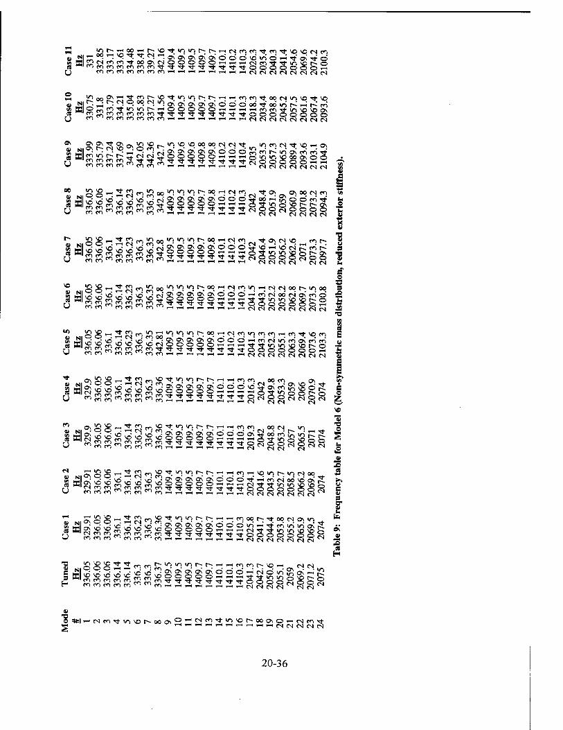
«lenenenenenenenTfTt-^TfTfTfrTfTfTtOOOOOOO — eg "'"inmnmmm'r^'tr^tTft^fOOOOÖÖö

oo

O—. en Tf In VI t^ i—lQOOOO<—li—lrtrHmmTfl/)\OIOO\ Cen^^^^^^^^^^^^^^t-ooooooo©

oi* t~; N © °s o ci ~ -•-•-■-•-•-• -• -• v

<? *" en CD en en **

in m N rf \o FH o\

cJcNügoopor^^Hi-HQiou-ivoooovoo ^ ■*

,-H — ,— — ,-1 ,-1 v CM es CN OJ CN es es

V SS^'2S^'2^'£ftÄft£000§!oo'rt'&0©en'<* es es es es es es

C S rt ■* "! m ^ no inininrôqiHNm^ôvNC en t*^ r~» co t"»

_ _ rvl O < eS <N CS <N v CS CS

s «IS S « 2 2 vo 2 « s s ft a ft °' =>d §! s ^'« « P «^ ^ W fl1mv'tfl(l1l,nllHHHrtHHHH,NNNN"NN

a)

u

g«^^fnîn00inininr--oqFH(Nro<n^HtNJ<Noot~«noo

1 en en en en

en en m en

en t en en

-,-,000'-«'—iiH#*ininii\cSo

v <n \o Tf en _ in <n in t~ ;OOi-HfNenineneni-<enTfvoen

s*Sl£mS?m*Q9Sc>cio^'-ir-i**inin*o\ot~o «■ NNMMNCNNN

JXj| g} « vn VP ^ ^ vO en ^ ^ en ^ ^' en

^ ^ »VI °° <""> ,-K ,,-, ON : es _• „• o\ vo - ooto

u

es — m \o _ TJ- en _ a» Ni 0\ O O ^ — eN ^

u

'O Tt in >n t~-; r- i—< i—; en i—\o in t~- in es oo en .•Pl-

enen en 1 en en

U

i—i >n vo N. o\ o p ' l£ J3 en iS "^ ""5 ""i <"": f": ^. >-; moot^tocNOMn — CS „, _ ,_ ,_, \D • ,_• im **; C£ ON ON 0\ ON Ö Ö Ö in i-i

enen 'en — rtrtrtrHrHrHrtNCMNtNCSNN"

1 fN en en en m en en

<T> "O !C <?> S :S8SSS

U e 3 H

o ~ — r--ininint~-;t-;i—ii—ienenc~-\o OOi-iH',lmmil!--."..^*lrtni"N

en en en en en JS 5S ^ ^ - o o QpOOcNpOcS rN CS eS eS eS fN

"8 *l—csen-<tin\or-ooo\S!^£S^'*>r>votÔOONC|i-ifNenTf

20-36

ON f»-imciu->t~-oo<-i<No\_Jv>r~cs<-'0\vor^r«">Tfi/"> rr^ •**• i— oo ; r • • • i—' ' '. ._• —.* —• .-: • -^ .—* .-:

u

IflOOCl,

KHp)m»*oooo(SOO'-iiHrHj.iHrHNm53l'i,OtÔ

fflOH**lnSô^ôOHH^HrtrtH(^1l»l5ôôô ^mmmmSm^ttTtTtStttqpodooOH

a> Nit0!!r;rH.*,r!PôdodddrH'HrH'rtK>d^6^ô\-<'

00 X\0PjCSma.NiO00 0\NN_,_«*Om'tin>Nwimrt

« Klenen£enen£?,enTj- -<t Ti-TtrtSS-*-* oöooqooq U mmnnnmmmHi-(HH i-i ■— eseseseseseseses

U a >o u-t \0 vo

1 (<1 m c^ t Tf ^ ^ meneneni—<■—ii—ii—>

vq vq CN o\ u^ Tt >n u-5 vq r-. ^; i-i r-i Tt o </S i-H vq yd oo op

TtSS-^TfOOOOOOOO

« t~-00_JrJ-<Tl\D{SO\OOOOCSCS^'-iVOVOO\VOOOt-H-<tTt

v si'O'oS^^^^^wwoöS-H-^rH-ri^^d^wô g auû^fSvovovoyotr>(=>o^'-<Tfri'-!r;C5C3!£>^£!£E:0'-H 1 en CO en en en encneneneni—ii—ii—ii—i r-T-NNNNNN

00 o\ Ni<0 ft

oox(^-,NrnrHNt^X(SM ■ ..... . OOOOOOH

vq NO en \q o\ I-; vq >o es »-H i-<" o\ rf" v^ <ri ■* o\ t-» o\

fNenenSJenenenen-'l-ri-TtTt enenen^'eneneneni-H'—ii—ii—i

^.S-tTtÖOcsOOOOO i-i CS eN es es es es es

en enooen_,,-,eni—lesooooi—'es

« *l(sm(nJ2<firfim^-Tfit'*ärt^<tOOOOpio U en en en - ~ ~ -------- ^-. - en en en i—i ^H r-i

NO NO i-i r-- >/-> oo esenes en Ä* • • - f~ ON

_ _ _ _ _escc^ HrtMMNNNNN

es vor-oo-0u-)enr~-esooooeseNO\_vo,>OTfit^l^HVoo\>nes v si ^ ^. ■". 2 N *q x o\ oo x d d d S ^ rnV Tt S >o -1 » ^' »' a 33l2!i3ü2en^S5iSiS22n;^:r;,*i;z:ö22o,o^l^lCrCr u en en en

en en en frimmmTt^^^TfrttfOOMO eneneneni—ii—ii—ii—ii—i HH(SM

SB o o es es es es es

l-H V) 00 ON es *-Hcoo\esooooescs si^'O'nSNCNqoN.tcuoöo^

ir> NO ir> NO NO ON en NO en es_ ' r~ rt- ö NO oo' o\ Tj-' o\

es «nmmSmmmm'i'rtftTiri^'i'OOOOOOOO U enenen^êneneneni—i^Hrii—i i-ii—eseseseseseseses

s -p r-oo_>^cS'jesesooooeses_^vc)voTfesvoi-i_1. S NIÎ^.^^^^XxddSSH-NMJ^^St-^-, S wmcii2mnmnmtît^Hr;^tOOOONNOy

H mmmmmmmmHrHrtH i-iêsescscses

es JT- O r~ f- oo

es

■g *:|i-ieNenTfir)VOt~ooo\ Oi-ieSenrj-ioNOt-~ooo\0^-eSenT)-

20-37

References

[I] Avitabile, P., O'Callahan, J.C., and Milani, J., "Comparison of System Characteristics Using Various Model Reduction Techniques," Seventh International Modal Analysis Conference, Las Vegas Nevada, Feb 1989.

[2] Basu, P., and Griffin, J.H., "The Effect of Limiting Aerodynamic and Structural Coupling in Models of Mistuned Bladed Disk Vibration," Journal of Vibration, Acoustics, Stress, and Reliability in Design Vol 108,1986, p. 132-139.

[3] Bendiksen, O.O., "Flutter of Mistuned Turbomachinery Rotors," Journal of Engineering for Gas Turbines and Power, Vol. 106, pp. 25-33.

[4] Blair, J.J., Personal Communication, July 1995.

[5] Campbell, W., "The Protection of Steam-Turbine Disk Wheels From Axial Vibration", ASME Transactions Vol. 46, No. 1920,1924, pp. 31-160.

[6] Craig, Jr., R.R., Structural Dynamics, Wiley, New York, 1981, pp. 467-494.

[7] Craig, Jr., R.R., and Chung, Y., "Generalized Substructure Coupling Procedure for Damped Systems " AIAA Journal, Vol. 20, March 1982, pp. 442-444.

[8] Craig, Jr., R.R., "A Review of Time-Domain and Frequency-Domain Component-Mode Synthesis Methods," Journal of Modal Analysis, April 1987, pp. 59-72.

[9] Craig, Jr., R.R., and Hale, A.L., "Block-Krylov Component Synthesis Method for Structural Model Reduction," Journal of Guidance Control and Dynamics, Vol. 11, Nov.-Dec. 1988, pp. 562-570.

[10] Crawley, E.F., and Mokadam, D.R., "Stagger Angle Dependence of Inertial and Elastic Coupling in Bladed Disks," Journal of Vibration Acoustics, Stress, and Reliability in Design, Vol. 106,1984, pp. 181-189.

[II] Dye, R.C.F., and Henry, T.A., "Vibration Amplitudes of Compressor Blades Resulting from Scatter in Natural Frequencies," Journal of Engineering for Power, Vol. 91, 1969, pp. 182-188.

[12] Ewins, D.J., "The Effect of Detuning upon the Forced Vibrations of Bladed Disks," Journal of Sound and Vibration, Vol. 9, No. 1,1969, pp. 65-79.

[13] Ewins, D.J., "Vibration Characteristics of Bladed Disk Assemblies," Journal of Mechanical Engineering Science, Vol. 15, No. 3,1973, pp. 165-186.

[14] Ewins, D.J., and Han, Z.S., "Resonant Vibration Levels of a Mistuned Bladed Disk," Journal of Vibration Acoustics, Stress, and Reliability in Design, Vol. 106, April 1984, pp. 211-217.

[15] Gawronski, W., and Williams, T., "Model Reduction for Flexible Space Structures," Journal of Guidance Control and Dynamics, Vol. 14, Jan.-Feb. 1991, pp. 68-76.

[16] Griffin, J.H., "On Predicting the Resonant Response of Bladed Disk Assemblies," Journal of Engineering for Gas Turbines and Power, Vol. 110, Jan. 1988, pp. 45-50.

[17] Griffin, J.H., and Hoosac, T.M., "Model Development and Statistical Investigation of Turbine Blade Mistuning," Journal of Vibration, Acoustics, Stress, and Reliability in Design, Vol. 106, April 1984, pp.

[18] Hurty, W.C., "Dynamic Analysis of Structural Systems Using Component Modes," AIAA Journal Vol 3 April 1965, pp. 678-685. ' ' '

[19] Irretier, H., "Spectral Analysis of Mistuned Bladed Disk Assemblies by Component Mode Synthesis," Proceedings of the Ninth Conference on Mechanical Vibration and Noise of the Design and Production Engineering Technical Conferences, ASME, 1983, pp. 115-125.

20-38

[20] Kaza, K.R.V., and Kielb, R.E., "Effects of Mistiming on Bending-Torsion Flutter and Response of a Mistimed Cascade in Incompressible Flow," AIAA Journal, Vol. 20, No. 8,1982, pp. 1120-1127.

[21] Kaza, K.R.V., and Kielb, R.E., "Flutter of Turbofan Rotors with Mistuned Blades," AIAA Journal, Vol 22, No. 11, Nov. 1984, pp. 1618-1625.

[22] Kielb, R.E., Personal Communications, August 1995.

[23] Kielb, R.E., and Kaza, K.R.V., "Aeroelastic Characteristics of a Cascade of Mistuned Blades in Subsonic and Supersonic Flows," Journal of Vibration, Acoustics, Stress, and Reliability in Design, Vol. 105, Oct. 1983, pp. 425-433.

[24] Kienholz, D.A., and Smith, K.E., "Admittance Modeling: Frequency Domain, Physical Coordinate Methods for Multi-Component Systems," CS A Engineering Report, Feb. 1994, pp. 608-614.

[25] MacNeal, R.H., "A Hybrid Method of Component Mode Synthesis," Computers and Structures, Vol. 1, 1971, pp. 581-601.

[26] Mead, DJ., "Wave Propagation and Natural Modes in Periodic Systems: Mono-Coupled Systems," Journal of Sound and Vibration, Vol. 40, No. 1,1975, pp. 1-18.

[27] Menq, C.-H., Griffin, J.H., and Bielak, J., "The Forced Response of Shrouded Fan Stages," Journal of Vibration, Acoustics, Stress, and Reliability in Design, Vol. 108, Jan. 1986, pp. 50-55.

[28] Minas, C, and Kodiyalam, S., "Vibration Analysis of Bladed Disc Assemblies," International Modal Analysis Conference, 1995.

[29] Murthy, D.V., Pierre, C, and Ottarsson, G., "Efficient Design Constraint Accounting for Mistuning Effects in Engine Rotors," AIAA Journal, Vol. 33, No. 5,1994, pp. 960-962.

[30] Muszyska, A., and Jones, D.I.G., "A Parametric Study of Dynamic Response of a Discrete Model of Turbomachinery Bladed Disc," Transactions of the ASME, Vol. 105,1983, pp. 434-443.

[31] Natsiavas, S., "Mode Localization and Frequency Veering In A Non-conservative Mechanical System With Dissimilar Components," Journal of Sound and Vibration, Vol. 165,1993, pp. 137-147.

[32] O'Callahan, J.C., Avitabile, P.A., Riemer, R, "System Equivalent Reduction Expansion Process (SEREP)," Seventh International Modal Analysis Conference, Las Vegas, Nevada, Feb. 1989.

[33] O'Callahan, J.C., "A Procedure for an Improved Reduced System (IRS) Model," Seventh International Modal Analysis Conference, Las Vegas, Nevada, Feb. 1989.

[34] Ottarsson, G., and Pierre, C, "A Transfer Matrix Approach to Vibration Localization in Mistuned Blade Assemblies," Proceedings of the International Gas Turbine and Aeroengine Congress and Exposition, Cincinnati, Ohio, 1993, ASME 93-GT-115, pp. 1-20.

[35] Petrov, E.P., "Analysis and Optimal Control of Stress Amplitudes Upon Forced Vibration of Turbomachine Impellers with Mistuning," International Union of Theoretical and Applied Mechanics Symposium on The Active Control of Vibration, Sept. 5,1994, University of Bath, UK, pp. 189-196.

[36] Petrov, E.P., "Large-Scale Finite Element Models of Blade-Shroud and Blade-Disk Joints and Condensation Technique for Vibration Analysis of Turbomachine Impellers," Proceedings of the 7th World Congress on Finite Element Methods: "FEM: Today and the Future" Monte-Carlo, 1993, pp. 507-513.

[37] Pierre, C, and Murthy, D.V., "Aeroelastic Modal Characteristics of Mistuned Blade Assemblies: Mode Localization and Loss of Eigenstructure," AIAA Journal, Vol. 30, No. 10,1992, pp. 2483-2496.

[38] Pierre, C, Smith, T.E., and Murthy, D.V., "Localization of Aeroelastic Modes in Mistuned High-Energy Turbines," Journal of Propulsion and Power, Vol. 10,1994, pp. 318-328.

[39] Rao, J. S., Turbomachine Blade Vibration, Wiley, New York, 1991.

20-39

[40] Su, T., and Craig, R.R., "Krylov Model Reduction Algorithm for Undamped Structural Dynamics," Journal of Guidance Control and Dynamics, Vol. 14, Nov.-Dec. 1991, pp. 1311-1313.

[41] Swaminadham, M., Soni, M.L., Stange, W.A., and Reed, J.D., "On Model Generation and Modal Analysis of Flexible Bladed-Disc Assemblies," Bladed Disk Assemblies, ASME Vibration Conference Cambridge MA, Sept. 27-30, 1987, pp. 49.

[42] Vakakis, A.F., "Non-Similar Normal Oscillations in a Strongly Non-Linear Discrete System," Journal of Sound and Vibration, Vol. 158,1992, pp. 341-361.

[43] Valero, N.A., and Bendiksen, O.O., "Vibration Characteristics of Mistimed Shrouded Blade Assemblies," Journal of Engineering for Gas Turbines and Power, Vol. 108,1986, pp. 293-299.

[44] Wei., S.T., and Pierre, C, "Localization Phenomena in Mistimed Assemblies with Cyclic Symmetry Part 1: Free Vibrations," Journal of Vibration, Acoustics, Stress, and Reliability in Design, Vol. 110, 1988, pp.

[45] Whitehead, D.S., "Effects of Mistuning on the Forced Vibration of Blades with Mechanical Coupling," Journal of Mechanical Engineering Science, Vol. 18, No. 6,1976.

[46] Yang, M.-T., and Griffin, J.H., "A Reduced Order Approach for The Vibration of Mistimed Bladed Disk Assemblies," International Gas Turbine and Aeroengine Congress & Exposition, 1995, ASME Paper No. 95-GT-454.

20-40

GROWTH OF SILICON CARBIDE THIN FILMS BY

MOLECULAR BEAM EPITAXY

Dr. John Chen Mr. Ronald Birkhahn

and Prof. Andrew J. Steckl, Principal Investigator

Nanoelectronics Laboratory University of Cincinnati

899 Rhodes Hall P. O. Box 210030

Cincinnati, OH 45221-0030 e-mail: [email protected]

Final Report for: 1996 Summer Research Extension Program

Wright Laboratory



and

Wright Laboratory Wright-Patterson Air Force Base, OH

February 1997

21-1

GROWTH OF SILICON CARBIDE THIN FILMS BY

MOLECULAR BEAM EPITAXY

Dr. John Chen Mr. Ronald Birkhahn

and Prof. Andrew J. Steckl, Principal Investigator

Abstract

A system for the molecular beam epitaxy (MBE) of SiC thin films was installed in the

Nanoelectronics Laboratory at University of Cincinnati. The MBE system combines

several gas and solid sources. Preliminary results of SiC heteroepitaxial growth by MBE

were obtained. We have demonstrated the MBE growth of SiC on Si and semiconductor-

on-insulator (SOI) substrates. SiC growth was obtained by either propane carbonization of

the Si surface or by the pyrolysis of silacyclobutane (SCB), or the sequential use of

carbonization and pyrolysis. At a growth temperature of 800 °C, initial experiments

indicate a SiC growth rate -0.1 A/s. The crystallinity of the film surface was investigated

using reflection high electron energy diffraction (RHEED). Films grown under certain

conditions produce RHEED patterns indicating crystalline cubic (3C) SiC, while under

other conditions a RHEED pattern is observed indicating a combination of crystalline and

poly-crystalline SiC. The thickness and composition of the SiC films was analyzed by

secondary ion mass spectrometry (SIMS). SIMS depth profiles indicate that no (or very

low) contamination from N, O, and B was found in the films.

21-2

1. INTRODUCTION

Silicon carbide (SiC) is a wide band gap semiconductor with high thermal stability

and conductivity, high breakdown voltage, etc. Among many SiC polytypes, 3C-SiC (or

ß-SiC, the only cubic structure) is the most promising candidate for higher power, higher

temperature and higher frequency electronic devices because of its high electron mobility

(1000 cm2/V s)[l], high saturated drift velocity (above 107 cm/s)[2]. Since bulk crystals of

3C-SiC are very expensive and their size is very small (~3 - 5 mm), heteroepitaxial growth

on Si substrate has become an alternative method for growing SiC. Due to the large lattice

constant mismatch (20%) and the thermal expansion coefficient difference (8%) between

3C-SiC and Si, considerable effort was devoted to improving the film quality, leading to a

two-step epitaxial growth. The first step is carbonization of Si substrate to relieve the strain

between SiC and Si, but this SiC layer is usually too thin (a few hundred A) to fabricate

devices. The second step is essential growth of SiC on SiC by introducing both Si and C

precursors. Currently, CVD is widely employed to grow epitaxial 3C-SiC on Si. Since the

epitaxial growth temperature in CVD is generally higher than 1200 °C, which can cause

deterioration of the film quality and redistribution of the dopants, reduction of growth

temperatures must be realized in order to fabricate the SiC device. Molecular Beam Epitaxy

(MBE) is a promising methods to reduce 3C-SiC growth temperatures.

The work described in this report was partially sponsored by Research and

Development Laboratories as a Supplemental Research Extension Program from AFOSR.

The following sections of this report consist of: a description of the Riber 32 MBE system

recently installed at the University of Cincinnati; a brief summary of previous work on

growing SiC with MBE; preliminary results on MBE growth of 3C-SiC on Si at

Cincinnati.

2. SYSTEM DESCRIPTION

The MBE system consists of these primary components: a control computer (1),

control electronics and power supplies(2), gas cabinet (3), growth chamber (4), a load lock

chamber (5), pumping systems. A schematic of the system is shown in Fig. 1.

21-3

2.1 LOAD LOCK

The load lock (5) serves as a buffer chamber between atmosphere and the growth

Fig. 1. Schematic of University of Cincinnati MBE system from Riber.

chamber which maintains UHV conditions. It contains a magnetically coupled sample

transfer rod and a four-sample storage stage with one outgassing station that can reach

temperature up to 800°C. The stage can move in XYZ directions and rotate 360 °C. The

load lock is pumped by an ion pump (200 1/s) supplemented with a titanium sublimation

pump (10001/s). The base pressure of the chamber can reach lxlO"10 Torr after a 48 hour

bakeout at 200°C. One UHV port for venting the chamber with UHP nitrogen and for

rough pumping is located just below the ion pressure gauge. There is a gate valve to isolate

the load lock chamber from the ion pump during venting and roughing, and another gate

valve to isolate the load lock from the growth chamber. On one side of the load lock

chamber is a back door for loading and unloading samples. The load lock has additional

ports for future expansion with a surface analysis chamber. A photo of the UC MBE-32

load lock is shown in Fig. 2.

2.2 ROUGH PUMPING

The rough pumping of the load lock and the growth chamber is done with a "rough

21-4

pump cart" which consists of two LN2-cooled sorption pumps in parallel with a small

mechanical pump (Fig. 3). The sorption pumps are first cooled to 77K and the mechanical

Fig. 2. Photo of load lock with control electronics in background.

Fig. 3. Rough pump cart with mechanical and sorption pumps,

pump is allowed to rough out the load lock to 150 Torr. Next, the two sorption pumps

21-5

are opened and closed in series until the pressure reaches 5xl0"2 Ton and lxlO"3 Torr,

respectively. At that point, the chamber is isolated and the gate valve is opened to the main pumping system.

2.3 GROWTH CHAMBER

The growth chamber (4) (shown in Fig. 4) contains a sample manipulator, a cell

panel where the molecular sources are located, analysis tools (RHEED, RGA), LN2

cryoshrouds, and UHV pumping. The transfer rod places the sample directly onto a xyz-

controllable and rotatable manipulator (Fig. 5) that has heating capability to 1200°C via a

specially designed heater from Karl Eberl (Stuttgart, Germany). UHV pumping consists of

a CTICT8 cryopump and a titanium sublimator. Pressures can go as low as 5xl0"n Torr

after a 48 hour bakeout and 1.2x10"" Torr with the cryopanels cooled. The cryopanels

consist of three LN2-filled shrouds for cooling the main chamber, the well surrounding the

pumping systems, the cell panel to protect the sources from stray contaminants. Two ion

gauges monitor the pressure in the system, one close to the pumping well and the second at

the rear of the substrate holder to calibrate the fluxes from the cells incident on the sample.

Fig. 4. Main growth chamber (on right) with all attachments. RGA (upper black box) and

RHEED gun (just below) are shown in foreground.

21-6

Fig. 5. Riber MBE-32 manipulator.

The cell panel (Fig. 6) contains both Knudsen effusion cells and a high temperature gas

injector. In the near future, the cell panel will also be fitted with a plasma source to further

to enable the growth of Hi-nitride wide band-gap semiconductors. Also on the cell panel is

a viewport for a pyrometer (to be retrofitted), an XTC crystal thickness monitor, and

shutter motors. The XTC is employed to measure film deposition rate from an electron

beam gun used to melt source material. Analysis in the chamber is provided by an Inficon

residual gas analyzer (RGA) and a Staib Instruments 35 kV reflection high energy electron

diffraction (RHEED) gun. The RGA is used to determine the background contaminants in

the chamber and the process species during growth. The RHEED gun is used to determine

the crystallinity and growth rates on the substrate. This will be discussed in a later section.

2.4 SOURCES

Fig. 6 shows the setup of the cell panel and location of the sources on the MBE

system. Ports 1,5-8 are fitted with Knudsen cells (shown schematically in Fig. 7) and to be

filled with solid source ultra high purity (UHP) material for evaporation. An EPI high

temperature cell resides in port 1 capable of temperatures near 2000°C and is scheduled to

be filled with Er. Since port 1 is in a low angle position (5°), the crucible can only hold a

small charge in comparison to the bottom row (5-8) at 32°. Ports 5 and 8 contain Riber

single filament cells filled with Mg and Al, both dopants in the nitrides and SiC. Cells 6

and 7 are EPI Sumo dual filament cells designed to reduce cell "spitting" during operation

21-7

Main Cryo Ouf

Cell Cryo Ouf

Cell Cryo In

Main Cryo In

^ PORTS Flanae/Clearance Anale Source

[1] 4.572.75"CFF—1.75" 5° Er-EPI High Temp

[C] 4.5"CFF—2.5" Oo N2 Plasma

[4] 4.572.75"CFF—1.75" 5° Gas Injector*

[5] 4.572.75"CFF—1.75" 32o Mg-Riber

[6] 2.75"CFF—1.75" 32° Ga-EPI SUMO

[7] 2.75"CFF—1.75" 320 In-EPI SUMO

[8] 4.572.75"CFF—1.75" 32° Al-Riber

[E] Ellipsometer

[H] XTC

I *

Fig. 6. Schematic of growth chamber cell panel.

21-8

layered c.-ucr'i/p ;n PBN, graphiit jar v.trtoui carbor

I */>3t i'w«tf" />•«<•."

and increase uniformity. These will be filled with Ga and In for growth of nitrides and

other semiconductor heterostructures. A three-line gas injector and cracker is installed in

cell 4. The injector has 1200°C temperature

capability, two Baratron flow controllers, and

one mass flow controller. Each line has a

manifold to switch between 2 different gasses:

line one has silacyclobutane (SCB SiC3H8) and

propane (C3Hg), line two has dilution N2 or

ammonia (NH3), and line three has H2. The

center port on the chamber is reserved for a

nitrogen plasma source for growing nitrides.

■crwlilK

1fl*r.Y.9C0\jpli

inuit:iuyer

Spring loaded WjRt ttitrmocBjpie

fA«r/7K)couole .-' ,'e«dtVCs

•pcv/er feetllhra's

Fig. 7. Cut away view of standard

effusion cell on MBE systems.

2.5 ELECTRONICS

A gas cabinet (3) to the left of the cell

panel houses the cylinders for the three-line gas

injector and a mechanical pump that evacuates

the gas lines and the cryopump exhaust. The

gas cabinet electronics, power supplies,

pressure gauges, safety actuators, and

temperature controllers are all located in racks

(2) next to the system. Two control computers

(1) are used to integrate the electronics: one PC operating in the NextStep Unix

environment using a Riber program called Accessible to integrate all the growth

components of the system; a second PC running under DOS/Windows to operate the RGA

and RHEED gun.

2.6 ANALYSIS EQUIPMENT

In situ analysis is one crucial advantage that MBE has over other growth processes.

This is made possible by the UHV conditions inside the growth chamber. The

environment in the chamber can be monitored by the RGA before, during, and after the

run. This can determine the quantities of reactive species in the chamber, help locate the

origin of grown-in impurities, and evaluate the condition of the pumping. We have

21-9

installed a Leybold Inficon H100M quadrupole with a Faraday cup for high pressure gas

analysis and an electron multiplier for low (<106 Torr) pressures. For surface-sensitive

analysis of the substrate, we have a Staib Instruments 35kV electron gun for obtaining

RHEED patterns. This can quantify the substrate condition, from the effectiveness of the

pre-cleaning and outgassing to the atomic growth characteristics and subsequent annealing

effectiveness. RHEED can also be used to determine growth rates and surface reconstructions.

3. Epitaxy of SiC - Literature Survey

3.1 Heteroepitaxy

Carbonization is an effective process to relax the large lattice mismatch between Si

and SiC. There are two different carbonization processes. In the first process, the Si

substrate is annealed to high temperature (750 - 1100 °C) and then hydrocarbon gas or

carbon (atoms or ions) are introduced to react with Si surface. Several simple hydrocarbon

molecules, such as C2H2, C2H4, C3H8 have been commonly used as carbon source. The

gas pressure during carbonization varied from 10'9 to 10"5 Torr. Some researchers found

the carbonized films were polycrystaline by this process [3 - 5], while others obtained films of good quality [6-9].

In the second process, carbon containing gas is first introduced into the chamber

until the desired pressure is reached, and then the substrate temperature is raised to high

temperatures (750 -1100 °C) at a slow ramp rate (5 - 25 °C/min). There are several versions

of this process, with variations in the temperature ramp rate at different temperature stages

and the incorporation of an oxide removal step [3]. In general, this process is very effective

for obtaining single crystal 3C-SiC without double- positioning twin structures and pits

[3, 4, 5]. This process probably seals off the outward Si diffusion from the Si substrate,

which is believed to cause surface defects [4, 5].

Essential growth of SiC is used to further grow SiC on the carbonized film with

both Si- and C- containing source. The substrate temperature ranges from 750 to 1100°C,

the total pressure is usually 10"7 to 10'5 torr during growth. The effect of the flux ratio

between Si and C species on film quality and stoichiometric ratio has been extensively

studied [5,10-13]. It was found that Js/Jc > 1 is a general rule for growing good crystalline

21-10

3C-SiC film with 1:1 stoichiometric ratio. Atomic layer epitaxy by MBE has also attracted a

lot of attention [14-17]. It was found that the surface superstructures during an alternating

supply of C source and Si source can be used to control film growth to atomic level

accuracy.

Lattice matched growth The lattice constant of (111) 3C-SiC nearly matches (< 0.1%) that of the c-plane of

6H-SiC. 6H-SiC is commercially available from several sources, with Cree Research

being the main supplier. 6H-SiC is also used as a substrate for growing good quality SiC

films. Some results show that the epitaxially grown 3C-SiC (111) on 6H-SiC (1000) at

850 -1000 °C have double-positioning twin structure [18- 19], while on 6H-Si (0114)

substrate, the 3C-SiC(100) epilayers were grown without twin structures at temperatures as

low as 850°C [19]. Homoepitaxy of 6H-SiC was also investigated and growth process controlled to an

atomic level was obtained by monitoring surface superstructures during the supply of Si

and C atoms [20-22]. The grown film is predominantly 6H-SiC with small amount of 3C-

SiC mainly located at defect sites. These defects mostly extend from the substrate into the

film.

4. PRELIMINARY RESULTS

In this section we describe the first SiC MBE experiments performed at the

University of Cincinnati and discuss our preliminary results.

4.1 EXPERIMENTAL CONDITIONS

The epitaxial growth of 3C-SiC was carried in a Riber GSMBE 32 system. The

detailed description of the system was described above. Briefly, the epitaxial growth

process starts with the growth chamber being evacuated by the Ti sublimation pump and

cryogenic pump. After 60 hours baking at 250 °C, a base pressure of 3xl0"n torr can be

routinely obtained without filling the cryoshroud with liquid nitrogen. A quadrupole mass

21-11

analyzer and a 35 keV reflection high-energy electron diffraction (RHEED) system are

mounted on the growth chamber for gas analysis and surface crystallinity characterization,

respectively. A high temperature gas injector (1200 °C) with three gas lines is employed to

introduce propane and silacyclobutane (SiC3H8 - SCB) into the growth chamber. The gas

flow is controlled by a PID controller. The substrate is introduced through the load lock

chamber which was pumped by a Ti sublimation pump and an ion pump to < 5xl010 Torr.

The initial outgassing of the sample is also performed in this chamber. The sample was

transported by a magnetically coupled transfer rod into the growth chamber and locked onto

a five-dimensional manipulator which contains a high temperature (1200 °C), high

uniformity oven. The heater temperature is measured by a W-Re thermocouple and

controlled by a PID controller.

Two preliminary growth experiments have been carried out. The growth conditions

are summarized in Table 1. In the first experiment a carbonized SiC SOI (Si On Insulator)

wafer with (111) orientation was used as the substrate for SiC MBE growth. The

carbonization was first performed by rapid thermal CVD. The carbonized SOI sample was

cleaned by dipping into 1% HF for 1 min and rinsing in DI water for 2 min. The sample

was then introduced into the load lock chamber, where it was outgassed at 300 °C for 12

hours. After the sample was transfered into growth chamber it was heated to 1000 °C until

a sharp RHEED pattern with 6-fold rotation symmetry was observed, indicating a clean ß-

SiC surface. The further growth on the carbonized film was done by SCB pyrolysis with a

sample temperature of 1000 °C.

# Substrate Carbonization by G H8 SCB Growth by MBE type time

(min) pressure

(torr) temp (°C)

time (min)

pressure (torr)

temp (°C)

C21 Si(lll) (SOI)

CVD 760 1235 80 -3x10"' 1000

Cl Si(100) on-axis

MBE 120 1.7-4.8 xlO"6

776

CE1 Si(100) on-axis

MBE 20 1.3-7.1 xlO"6

800 9 1.8-3.7 xlO'6

800

CE2 Si(100) on-axis

MBE 120 1.4-5.1 xlO"6

800 95 1.8-3.5 xlO"6

800

Table 1. Experimental conditions for SiC MBE growth.

21-12

The second experiment utilized a Si(100) wafer as substrate. Both carbonization

and essential growth were carried out in the MBE system. Propane was used for

carbonization and SCB for essential growth on the carbonized film. The temperature

program is shown in Fig. 8.

Temperature (oC)

800 _

I Growth by SCB I Carbonization M— ■

M »?* w

400 _

Fig. 8. Temperature program of SiC growth process by MBE.

In this temperature program diagram, there are three parts: (1) the Si(100) substrate was

heated to 400 °C in UHV (1010 -10"9 torr) with a ramp rate of 20 °C/min; (2) the supply of

the propane was started and then the substrate temperature was ramped up to 800 °C at a

rate of 20 °C/min; (3) the essential growth of 3C-SiC on the carbonized layer was done at

800 °C with SCB for both carbon and silicon source.

The crystallographic features of the growing surface were monitored by the

RHEED system. The RHEED images were captured by a CCD camera system, and a

sophisticated software (RHEED-VISION) was used to grab the image and monitor up to

four diffraction spot intensities during the growth. The thickness and composition of the

grown layers were measured by secondary ion mass spectrometry (SIMS) using Cs+

bombardment with positive ion detection. Elements monitored were C, Si, O, N and B.

Relative sensitivity factors derived from a SiC standard were used to convert ion counts to

concentrations. The thickness of SiC layer was estimated by finding the position in the

carbon depth profile at which atomic carbon concentration is 50% of its maximum. The

SCB growth rate was calculated by:

Growth Rate = Thicknesejtota!)- Thickne&s(carb>onized)

Time{5CB) (1)

21-13

Propane was supplied by Matheson Gas Products, Inc. with a purity of 99.97%.

SCB was provided by Dow Corning. SCB is a liquid at room temperature with a vapor

pressure of 400 Torr. Both propane and SCB vapor were used without further

purification. Before gas or vapor were introduced into the growth chamber, the cryoshroud

was filled with liquid nitrogen, the Ti-sublimation pump and the RGA were turned off to

obtain a cleaner growth environment, all cells and gas injector were set to 200 °C to avoid

their contamination by C3H8 or SCB. Both propane and SCB were introduced towards the

substrate through the gas injector. The flow rate of propane during carbonization was

equivalent to its partial pressure from 1.5 - 5.5 xlO"6 torr, the flow rate of SCB during

growth corresponded to its partial pressure from 6.1 to 16 xlO"7 torr. The sample was not

rotated during the growth in order to be able to monitor the RHEED pattern.

4.2 RESULTS AND DISCUSSION

Fig. 9 shows a typical RHEED pattern of the 3C-SiC sample (C21) obtained by

RTCVD carbonization. This pattern has twin diffraction spots which may be the

superposition of two diffraction patterns corresponding to two domains which are 180°

rotated from each other. The schematic of this interpretation is shown in Fig. 10.

Fig. 9. Typical RHEED pattern of 3C-SiC film by carbonization of SOI with RTCVD.

21-14

Therefore, the RTCVD carbonized film appears to have double-positioning twin structure.

The possible reason of this twin structure is that the Si carbonization is driven by reaction

on terraces, with different terraces causing the difference in stacking order.

After the carbonization by CVD as shown in Fig. 9, essential growth of SiC was

performed in MBE growth chamber with SCB as both Si and C source. During the growth,

some fluctuation of intensity was observed. No regular intensity oscillation was observed,

probably indicating that the growth was not in a layer-by-layer mode or the growth rate is

too small. However, the 3C-SiC RHEED pattern was very clear during the entire growth

period. Fig. 11 shows a RHEED image after 80 min growth at a SCB partial pressure of

3.0xl0"7 Torr. Compared with the RHEED pattern of Fig. 9, the twin spots in Fig. 11 are

much weaker, which probably indicates the double-positioning twin structure is much

reduced after essential growth by MBE.

° n ° O RHEED from structure A

° o ° o 0 Q 2_

RHEED from structure B

I S 8 A • O RHEED from twin structure: A+B

8 8*88

Fig. 10. Interpretation of the RHEED pattern in Fig. 9.

21-15

lllSPl PIMM

' M^'J^^i^M^1':^^^. •U^liC, -»-^ **V&7a

•

■ ■ ■■"""" ':::-;i,'?Ä:,.:^''*I#>^^^^^^^^^^^S

Fig. 11. RHEED pattern of SiC film grown by MBE with SCB on SOI sample carbonized

with propane by CVD (C21).

Carbonization and essential growth were also performed sequentially in MBE

system. The substrate was a 2 inch on-axis Si(100) wafer. Fig. 12 shows the RHEED

patterns observed during SiC growth of sample CE2. Fig. 12 (a) is the RHEED pattern of

the Si(100) surface after annealing at 400 °C for half a hour. The clear streaky pattern

indicates a clean Si(100) surface. After introducing propane into the growth chamber, the

temperature of substrate was ramped at a rate of 20 cC/min. During this temperature

ramping process, the RHEED pattern did not change until 760 °C. As the carbonization

proceeded, the RHEED pattern associated with 3C-SiC became stronger while that of

Si(100) became weaker and finally disappeared. Fig. 12 (b) is the 3C-SiC RHEED pattern

obtained after 2 hours carbonization of Si(100). No twin spots were observed in the MBE

carbonized film as were seen in the carbonized film by RTCVD. This observation indicates

that carbonized film by MBE has fewer double-boundary defects than that obtained by

CVD. The further growth of 3C-SiC was done by introducing SCB at a sample

temperature of 800 °C. Fig. 12 (c) shows the RHEED pattern after 5 min growth by SCB.

The pattern looks more streaky than that of carbonized film and indicates the surface is

smoother. As growth proceeded, the rings started to appear as shown in Fig. 12 (d),

which indicates a poly-crystal SiC film was being formed. The possible reason is that the

21-16

strain due to the large lattice mismatch between Si and SiC was not completely released by

carbonization.

Fig. 12. RHEED patterns observed during SiC growth (CE2): (a) clean Si(100) surface at

400°C; (b) 3C-SiC grown by C3H8 carbonization for two hours at PC3H8 = ~3xl0"6

torr; (c) 3C-SiC grown on the carbonized layer by SCB for 5 min at PSCB = 1.4 -

2.9xl0"7 torr; (d) 3C-SiC grown on the carbonized layer by SCB for 95 min at

PSCB= 1.8-3.5xl0"6torr.

The film composition and thickness of the MBE-grown SiC layers were measured

with secondary ion mass spectrometry (SIMS). Fig. 13 shows the depth profile of the 3C-

SiC film (sample Cl) grown by MBE carbonization of Si(100) at 776°C for two hours .It is

apparent that only a very thin Si layer (probably ~ 30-40 Ä) has been converted at this

temperature. It is interesting to point out, however, that even this very thin carbonized

layer produced a very good (similar to Fig. 12b) RHEED pattern indicative of crystalline

21-17

SiC. Fig. 14 contains the depth profile of the 3C-SiC film (CE1) grown at 800°C using

carbonization for 20 min followed by SCB growth for 9 min. The thickness of the SiC

film is approximately 95-100 Ä judging by the depth at which the carbon concentration

reaches the 50% point. Fig. 15 shows the depth profile of the SiC film (CE2) also grown

at 800°C, but for significantly longer times: carbonization for 120 min and essential growth

by SCB for 100 min. In this sample we find a SiC film thickness of around 600 A. Using

the film thickness obtained from the SMS depth profiles and the SCB growth time, the

SiC growth rate by SCB at 800 °C is estimated to be around 0.1 Ä/s. This low growth rate

could be due to a combination of effects: low growth temperature, low growth pressure,

and possibly the fluctuation of the gas flow during gas introduction. In Figs. 14 and 15, a

long carbon tail into the Si substrate is observed. This could be caused by several effects:

(a) absence of an abrupt interface between SiC and Si substrate, due to carbon atoms

diffusing into the Si during growth; (b) non-uniform film thickness resulting in certain

locations where the SiC layer is removed sooner during SIMS profiling. The SIMS data

also show that impurities N, O and B concentration are less than 0.1% in the SiC film.

5. SUMMARY AND FUTURE WORK

In this report we described the Riber MBE 32 system recently installed in the

Nanoelectronics Laboratory at University of Cincinnati. Some preliminary results of

heteroepitaxy of SiC with this MBE system were presented. We have clearly demonstrated

that SiC growth with SCB can be accomplished by the MBE technique. At 800 °C, the SiC

growth rate obtained with SCB under the first set of conditions utilized is quite low (0.1

A/s). We are continuing with experiments designed to determine the effect of growth

temperature, pressure and flow rate on the growth process: growth rate and film quality of

SiC. We plan to also investigate the use of other gas precursors for SiC growth and the in-

situ sequential growth of SiC and GaN. In addition to crystallinity and surface

morphology, we will also investigate the electrical and optical properties of the MBE-

grown SiC and GaN films.

21-18

60

50

I 40 < oc H 30 UJ O

8 20

o o 10

j i ' i,, J ,..,;...,.i !.,..: : '., ,.' ' I,.. ■! ' ), ,.! '.,.,!, ...'. I '. ,',,.,!,..

(a) Silicon : „ : f....„ö..ü..0..y..q.^^^

o4° I i I

o »o't°'■ • • I • ■ r 1 ; I'

f ■■! Oxygen

- Ü Carbon

: I L ' Nitrogen & Boron

M» j ._

50 100 150 200 DEPTH (Angstroms)

250 300

100

10

z o <

UJ o z o u o I o

0.1

H 0.01 <

0.001

: 1 1 1 r——i ! r—1 1 ' ; 1 ' 1 1 ' 1 ' 1 ' '

: ! „nnOOOOOOOdOOOOodoOGOOOlOOOOOO"

m Silicon (jj)

\ Ml — Carbon

r •.

-' ri ':""

_ ■»

i

Oxygen

•••v. • • * » J • ;• •• •■ ■ ■ • : -T T "S * t * • ■ ■* •' • ■ ■ •

' Nitrogen • ■

J

■ c

} D □ j j ; ; T ■

I'B'öDD D D! B B

■ '..■■..... _ ,—,—,—, , ,—


250 300

Fig. 13. SIMS depth profile of SiC film (sample Cl) grown by two hours carbonization

with C3Hg. (a) linear scale; (b) semi-log scale.

21-19

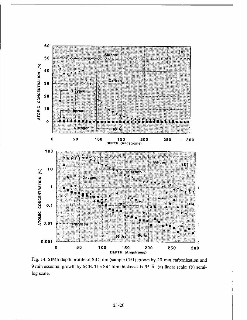
60

50

z 40 o

cc 30 t- z iii

z 20 o Ü

o <

S:^;:, ^;;:w^- I I r

Silicon G--o--o--<>^-o--o--o--o-o4ö-o-'0-'0--o--o-<j-o--o-o--o-o-<>:-<>-o--o--o--o--o:--o-<>-o--o--o--o

Hill IMlli ▼ ▼ ■

Oxygen

Boron

filitroflcn

r* ' I m M T" ' ' ' '

(a)

Carbon

r

■■•§•■ ■»■■■■■ ■ a»m*•■■■■2.Si aii iiii■ """I! """" '""""""""" '^^

95 A


250 300

100

^ 10

z o 1- < 1 EC t~ Z 111 u z o u 0.1

Ü E o < 0.01

0.001

' ' '""1—'—'—'—'-

•

: qoaoooqooo

i . ,

Dodoooooo

Silicon " :■ o -J o o

(b) : : ▼

•-= j Oxygen

■ _ : " * I 1 • • *■■«•

« t □ a

T _ Carbon

T T H * * * -

• •

• • • •

• •

• • •

• 1

■ _ * ■ ■ ■

■ ■ ■ ! H ■■

l||| |-;-'ii;S-:;; i i

, . , i , . . .

■■■ ■. orori

i , " "~ 95 A B

■

I 1


250 300

Fig. 14. SIMS depth profile of SiC film (sample CE1) grown by 20 min carbonization and

9 min essential growth by SCB. The SiC film thickness is 95 Ä. (a) linear scale; (b) semi- log scale.

21-20

60

50

^ 40 z o

I 30 i- z uj o 20 o u o 10 s o

< 0

' ' \ -I—I—I—j—I—I—■—■—I—1—1—I <

Silicon W -.-oooo-oöooo-oo-o|3-o-o<3-o<>qo<>ooo-o4o'0<^ooo4<>o-^o-o<>6-ooooQ-oi>o-o- I ! j-« 600 A ; 1 I .

200 400 600 800 1000 1200 1400 DEPTH (Angstroms)

100

? 10 1

z g

1 1 \- z UJ Ü z O 0.1 o

o 1- <

0.001

i I ' r-

111

• Nitrogen

"■■

a

■ '■ ■ ■ i

Boron

_

—

Bit Silicon

1—'—'—; oooooodaoooooöooooooöoooooojDooö

▼ ▼ (b)

▼ *.

•TW- ■ ▼V

Carbon

*▼▼▼ rrv*v

TlTT Ir

mmmmmmmsmsg llillllllllBi

■ ■■ u_ r.-"ff

600 A

200 400 600 800 1000 1200 1400 DEPTH (Angstroms)

Fig. 15. SIMS depth profile of SiC film (# CE2) grown by 120 min carbonization and 100

min essential grown by SCB. The film thickness is 600 Ä. (a) linear scale; (b)

semi-log scale.

21-21

6. REFERENCES

1. W. E. Knippenberg, Philips Res. Rep., 18 (1963) 161.

2. W. E. Nelson, F. A. Halden and A. Rosengreen, J. Appl. Phys., 37 (1966) 333.

3. T. Yoshinobu, T. Fuyuki and H. Matsunami Jpn. J. Appl. Phys, 30 (1991) L1086.

4. T. Yoshinobu, H. Mitsui, Y. Tarui, T. Fuyuki and H. Matsunami, J. Appl. Phys 72 (1992)2006. VV y

5. S.-I. Motoyama, N. Morikawa, M. Nasu and S. Kaneda, J. Appl. Phys., 68 (1990)

6. G.L. Zhou, Z. Ma, M. E. Lin, T. C. Shen, L. H. Allen and H. Morkoc J. Crystal Growth, 134 (1993) 167.

7. T. Sugii, T. Aoyama and T. Ito J. Electrochem. Soc, 137 (1990) 989.

8. K. Kim, Si-Choi and K.L. Wang, J. Vacuum Sei. Technol. B 10 (1992) 930.

9. K. Kim, Si-Choi and K.L. Wang, Thin Solid films, 225 (1993) 235.

10. S.-I. Motoyama, N. Morikawa and S. Kaneda, J. Cryst. Growth 100 (1990) 615.

11. S. Tanaka, R. S. Scott and R.F. Davis, Appl. Phys. Lett. 65 (1994) 2851.

12. S. Motoyama and S. Kaneda Appl. Phys. Lett. 54 (1989) 242.

13. S. Kaneda, Y. Sakamoto, C. Nishi, M. Kanaya and S. Hanai, Jpn. J. Appl. Phys. 25 (1986) 1307. > v vv J

14. T. Fuyuki, T. Yoshinobu and H. Matsunami, Thin Solid Films, 225 (1993) 225.

15. H. Matsunami, Physica B, 185 (1993) 65.

16. T. Yoshinobu, M. Nakayama, H. Shiomi, T. Fuyuki and H. Matsunami, J. Cryst Growth, 99 (1990) 520.

17. T. Fuyuki, M. Nakayama, T. Yoshinobu, H. Shiomi and H. Matsunami, J. Cryst. Growth, 95 (1989) 461.

18. L. B. Rowland, R.S. Kern, S. Tanaka and R.F. Davis, J. Mater. Res. 8 (1993) 2753.

19. T. Yoshinobu, H. Mitsui, I. Izumikawa, T. Fuyuki and H. Matsunami, Appl. Phys Lett., 60 (1992) 824.

20. A. Fissel, B. Schröter and W. Richter Appl. Phys. Lett. 66 (1995) 3182.

21. A. Fissel, U. Kaiser, E. Ducke, B. Schröter and W. Richter, J. Crystal Growth, 154 (1995) 72.

22. A. Fissel, U. Kaiser, K. Pfennighaus, B. Schröter and W. Richter Appl. Phys. Lett 68 (1996) 1.

21-22

PERFORMANCE OF ITERATIVE AND NONITERATIVE SCHEMES

FOR IMAGE RESTORATION AND SUPERRESOLUTION PROCESSING

IN MULTISPECTRAL SEEKER ENVIRONMENTS

Malur K. Sundareshan

Professor of Electrical and Computer Engineering

University of Arizona

Tucson, AZ 85721

Final Report for:

AFOSR Summer Research Extension Program

Wright Laboratory Armament Directorate

Sponsored by:

Air Force Office of Scientific Research


and

Wright Laboratory Armament Directorate

Eglin Air Force Base, FL

February 1997

22-1





Professor of Electrical and Computer Engineering

University of Arizona

Tucson, AZ 85721

ABSTRACT

Restoration and superresolution processing of images collected from various sensors deployed in

multispectral seeker environments often become necessary to enhance image resolution in order to facilitate better

false target rejection, improved automatic target recognition and aimpoint selection. Due to the critical importance

of this technology to several Air Force missions and its relevance to diverse on-going projects in several Air Force

laboratories, we are conducting detailed studies on this topic. Two major outcomes from these studies have been

the recognition of the importance of optimally tailored restoration and superresolution algorithms for the

individual sensor type and operating conditions, and the feasibility of using iterative and noniterative processing

techniques in an intelligent tailoring of these algorithms. Use of these techniques however can result in different

performance levels and also can bring specific advantages and disadvantages to the overall restoration and

superresolution function (and hence to the surveillance and smart munition guidance objectives). The principal

objective of the research reported here is to give a qualitative comparison of the performance expected from an

iterative procedure based on Bayesian estimation methods with that resulting from a class of noniterative

restoration methods. More quantitative performance evaluations directed to an explicit demonstration of the

spectrum extrapolation in both one-dimensional and two-dimensional signals from an iterative implementation of a

Maximum Likelihood (ML) algorithm are also presented A modification of the algorithm to facilitate

simultaneous estimation of point spread function of sensor and resolution enhancement of input image is outlined

and an illustration of its performance in processing a set of passive millimeter-wave (MMW) images obtained from

a 95 GHz 1-foot diameter aperture radiometer is given.

22-2





1. INTRODUCTION

A significant problem that affects the successful realization of the goals of many tactical missions is the

poor resolution of images collected from the sensors used to assist surveillance -and guidance operations. The

problem is particularly prevalent in autonomous missile guidance applications where diverse mission requirements,

such as reliable target detection, classification, interleaved acquisition, track and engage modes, and precision kill,

critically depend on the quality of data collected from the sensors deployed in missile seekers. While it is true that

deployment within a common aperture package of complementary sensors operating over different frequency

ranges would enhance the detection, classification and track maintenance performance of missile seekers (in

addition to providing increased fault tolerance and greater immunity to countermeasures), such multispectral

environments also accentuate other considerations, such as sensor fusion requirements, which in turn demand high

resolution sensor data.

The problem of poor resolution in imaging sensors stems mainly from deployable antenna size limitations

(which preclude simply increasing the physical aperture of sensors to gain high image resolution) and the

consequent diffraction limits on the achievable resolution. It may be noted that the wavelength of a synthetic

aperture radar (SAR) operating at 1GHz is about 1 inch long and one needs an antenna as big as 40 ft wide in

order to achieve a resolution requirement of being able to distinguish points in a scene separated by about 1 meter

at a distance of 1 Km [1]. Passive millimeter-wave (PMMW) sensing offers superior adverse weather capabilities

(over infra-red (IR) sensors, for instance) due to easy penetration through fog, dust, smoke, etc. However, PMMW

image acquisition sensors suffer from poor angular resolution. It is well documented that the angular resolution

achievable by a 94 GHz system with a 1 ft diameter antenna is only about 10 mrad, which translates into a spatial

resolution of about 10 meters at a distance of 1 Km. Some recent studies [2] have also established that for ensuring

reasonably adequate angular resolution (typically of the order of 4 mrad), a 94 GHz PMMW imaging system with a

sensor depression angle of 60° - 80° needs to be confined to very low operational altitudes (of the order of 75-100

meters) which puts inordinate demands on the guidance schemes to facilitate such requirements. Similar resolution

limitations and the consequent requirements on operational conditions (some of which may be clearly impossible to

satisfy for tactical missions with reliability and survivability constraints) exist for the other types of sensing

modalities as well.

22-3

Typical seeker antenna patterns are of a "low-pass" filtering nature due to the finite size of the antenna or

lens that makes up the imaging system and the consequent imposition of the underlying diffraction limits. Hence

the image recorded at the output of the imaging system is a low-pass filtered version of the original scene, The

portions of the scene that are lost by the imaging system are the fine details (high frequency spectral components)

that accurately describe the objects in the scene, which also are critical for reliable detection and classification of

targets of interest in the scene. Hence some form of image processing to restore the details and improve the

resolution of the image will invariably be needed. Traditional image restoration procedures (based on

deconvolution and inverse filtering approaches) attempt mainly at reconstruction of the passband and possibly

elimination of effects of additive noise components. These hence have only limited resolution enhancement

capabilities. Greater resolution improvements can only be achieved through a class of more sophisticated

algorithms, called superresolution algorithms, which provide not only passband resolution but also some degree of

spectral extrapolation, thus enabling to restore the high frequency spatial amplitude variations relating to the

spatial resolution of the sensor and lost through the filtering effects of the seeker antenna pattern. A tactful

utilization of the imaging instrument's characteristics and any a priori knowledge of the features of the target

together with an appropriately crafted nonlinear processing scheme is what gives the capability to these algorithms

for superresolving the input image by extrapolating beyond the passband range and thus extending the image

bandwidth beyond the diffraction limit of the imaging sensor.

For application in missile seeker environments, it must be emphasized that superresolution is a post-

processing operation applied to the acquired imagery and consequently is much less expensive compared to

improving the imaging system for desired resolution. As an example, it may be noted that for visual imagery

acquired from space-borne platforms, some studies indicate that the cost of camera payload increases as the inverse

2.5 power of the resolution. Hence a possible two-fold improvement in resolution by superresolution processing in

this application roughly translates into a reduction in the cost of the sensor by more than 5 times. Similar relations

also exist for sensors operating in the other spectral ranges (due to the relation between resolution and antenna

size), confirming the cost effectiveness of employing superresolution algorithms. The principal goal of

superresolution processing in multispectral seekers is hence to obtain an image of a target of interest (such as a

mobile missile-launcher or a tank) via post-processing that is equivalent to one acquired through a more expensive larger aperture sensor.

Most of the recent analytical work in the development of image restoration and superresolution algorithms

has been motivated by applications in Radioastronomy and Medical Imaging. While this work has given rise to

some mathematically elegant approaches and powerful algorithms, a certain degree of care should be exercised in

adapting these approaches and algorithms to the missile seeker environment. This is due to the convergence

problems often encountered by iterative schemes and the specific statistical models representing the scenarios

facilitating their development. For example, a slowly converging algorithm that ultimately guarantees the best

resolution in the processed image may pose no implementation^ problems in Radioastronomy; however, it could

be entirely unrealistic for implementation in an autonomous unmanned tactical system that must operate fast

22-4

enough to track target motion. Hence a careful tailoring of the processing algorithm for each sensor supporting the

multispectral seeker is of critical importance in order to realize the possible performance benefits from

superresolution processing which include better false target rejection, improved automatic target recognition and

aimpoint selection.

The high degree of importance this topic has to present and future Air Force missions is clearly evident.

Equally evident is the fact that research on this topic has an immediate application to a number of on-going

programs in various Air Force laboratories. The research described in this report is an extension of the

investigations that were conducted under a summer faculty visit to the Wright laboratory Armament Directorate.

Two principal outcomes from these investigations [3] have been the recognition of the importance of optimally

tailored restoration and superresolution algorithms for the individual sensor type and operating conditions, and the

feasibility of using iterative and noniterative processing techniques in the tailoring of these algorithms. Use of

these techniques however, can result in different performance levels and further entail specific advantages and

disadvantages. In this report we shall give a qualitative comparison of the performance expected from an iterative

procedure based on Bayesian estimation methods with that resulting from a class of noniterative restoration

methods. Quantitative performance evaluations directed to demonstrating the spectrum extrapolation in both one-

dimensional and two-dimensional signals resulting from an iterative implementation of a Maximum Likelihood

(ML) algorithm will also be presented. To counter the inaccuracies in the modeling of the Point Spread Function

(PSF) of the sensor, a modification of this algorithm to facilitate simultaneous estimation of PSF parameters and

resolution enhancement of input image is outlined and an illustration of its performance in processing a set of

passive millimeter-wave (MMW) images obtained from a 95 GHz 1-foot diameter aperture radiometer is given.

2. MATHEMATICAL REPRESENTATION OF IMAGE RESTORATION AND

SUPERRESOLUTION PROBLEMS

In this section we shall briefly describe the technical problems underlying the restoration and

superresolution processing of sensor data in terms of reconstructing the spectral components of the signals being

processed. A brief outline of the information available for developing specific algorithms in order to solve these

problems will also be given.

2.1 Image Formation Process (Observation Model)

Even- systematic image processing study (including image restoration and superresolution processing)

will start with an appropriate mathematical model characterizing the process of image formation by the sensor

employed, which is termed an "observation model". Irrespective of the type of sensor actually used, a commonly

used observation model takes the form

g = s(Hf) + n (1)

22-5

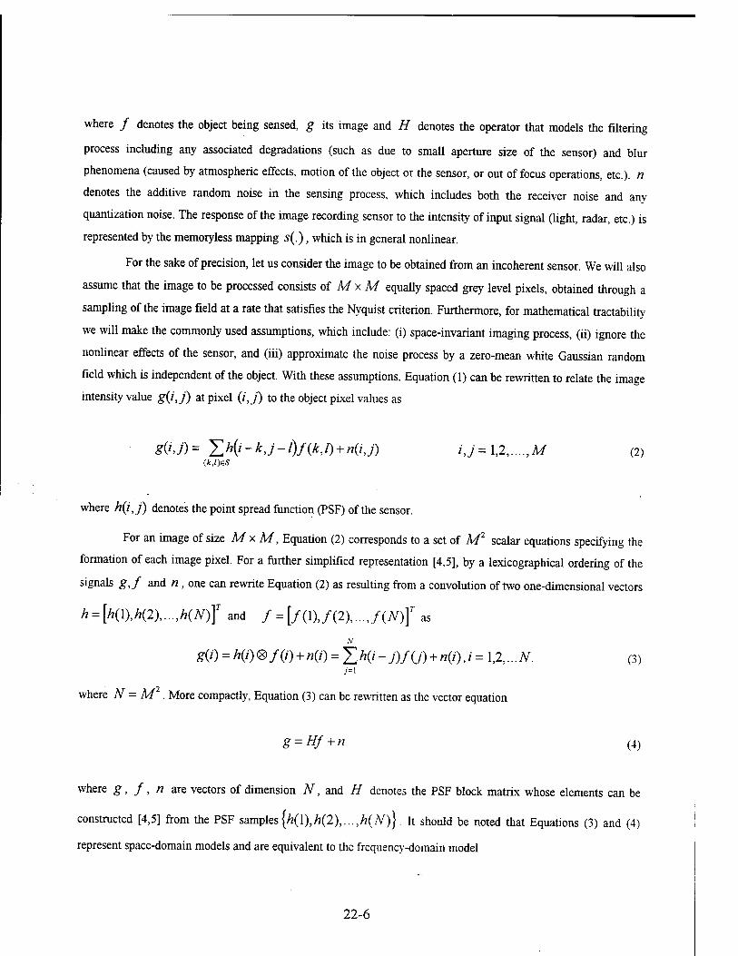
where / denotes the object being sensed, g its image and H denotes the operator that models the filtering

process including any associated degradations (such as due to small aperture size of the sensor) and blur

phenomena (caused by atmospheric effects, motion of the object or the sensor, or out of focus operations, etc.). n

denotes the additive random noise in the sensing process, which includes both the receiver noise and any

quantization noise. The response of the image recording sensor to the intensity of input signal (light, radar, etc.) is

represented by the memoryless mapping s(.), which is in general nonlinear.

For the sake of precision, let us consider the image to be obtained from an incoherent sensor. We will also

assume that the image to be processed consists of M x M equally spaced grey level pixels, obtained through a

sampling of the image field at a rate that satisfies the Nyquist criterion. Furthermore, for mathematical tractability

we will make the commonly used assumptions, which include: (i) space-invariant imaging process, (ii) ignore the

nonlinear effects of the sensor, and (iii) approximate the noise process by a zero-mean white Gaussian random

field which is independent of the object. With these assumptions, Equation (1) can be rewritten to relate the image

intensity value g(i,j) at pixel (/',_/') to the object pixel values as

g(ij)= 2>0-*,./-/)/(*,/)+ *(/,./) ij = 1,2,....,M (2)

where h(i, j) denotes the point spread function (PSF) of the sensor.

For an image of size MxM, Equation (2) corresponds to a set of M2 scalar equations specifying the

formation of each image pixel. For a further simplified representation [4,5], by a lexicographical ordering of the

signals g,f and n , one can rewrite Equation (2) as resulting from a convolution of two one-dimensional vectors

h = [h(\),h(2),...,h(N)]T and / = [/(l),/(2),...,/(A0f as

N

g(i) = h(i)0f(i) + n(i) = J^h(i-j)/(j) + n(i)J = l,2,...N. (3)

where N = M . More compactly, Equation (3) can be rewritten as the vector equation

g = Hf + n (4)

where g, /, n are vectors of dimension N, and H denotes the PSF block matrix whose elements can be

constructed [4,5] from the PSF samples {h(\),h{2),...,h{N)}. It should be noted that Equations (3) and (4)

represent space-domain models and are equivalent to the frequency-domain model

22-6

GO) = H{co)F(co) + N(co) (5)

where CO is the discrete frequency variable and G(a>) , F(co) , H(co) , and N(a>) are DFT's of the N -point

sequences g(i), /(/'), h(i), and n(i) respectively.

2.2 Image Restoration and Superresolution Problems

For application in missile seeker environments, Equation (3) describes the process of image formation

when an unknown object with radiance distribution { /(/)} is imaged through a sensor with a shift-invariant PSF

{h{})}. As noted earlier, practical seeker antenna patterns have a low-pass spectral characteristic and

consequently the image obtained is a low-pass filtered version of the object (or scene) being imaged. The problem

of interest is then to recover the object, i.e. { /(/') }, by solving Equation (3) (or Equation (5)). However, since the

noise sequence {n(i) } will not be known exactly, one will not be able to solve Equation (3) for {/(/)} exactly

even when { h(i)}, the PSF of the seeker antenna, is exactly known. One can only hope to obtain an estimate

A

{/(;)} which is in some sense close to the original {/(/')}, based on some reasonable assumptions on the noise

process {n(i) }. If a distance measure J(g.,f) between g and f is used as a norm to measure the closeness of

the estimate, the problem of interest can be specified concisely as obtaining the estimate

f f(\),f(2),...,f(N) such that

/ = arg min, j(g,f) = arg min, J[g(i) - £, h(i - j)f(J)j (6)

An examination of the frequency spectra of the object and the image is useful to see clearly the effect of the seeker

antenna. Let us assume that the object is space-limited with spatial extent £ and, without any loss of generality,

assume that ft is nonzero only on the interval e s

2'2 This implies that the spectrum F(a>) has infinite

extent, i.e. the object has infinite bandwidth, and in the discrete frequency domain, the spectral components in

cos F(co) extend all the way to -—, the folding frequency, as shown in Fig. la.

The image spectrum G(co) is a low-pass filtered version of F(co) with the cut-off frequency coc

determined by the diffraction limit of the sensor. Assuming an ideal low-pass filter characteristic, the shape of

G(co) will be as shown in Fig. lb with the spectral components removed in the interval COc < CO < C0s/2. The

22-7

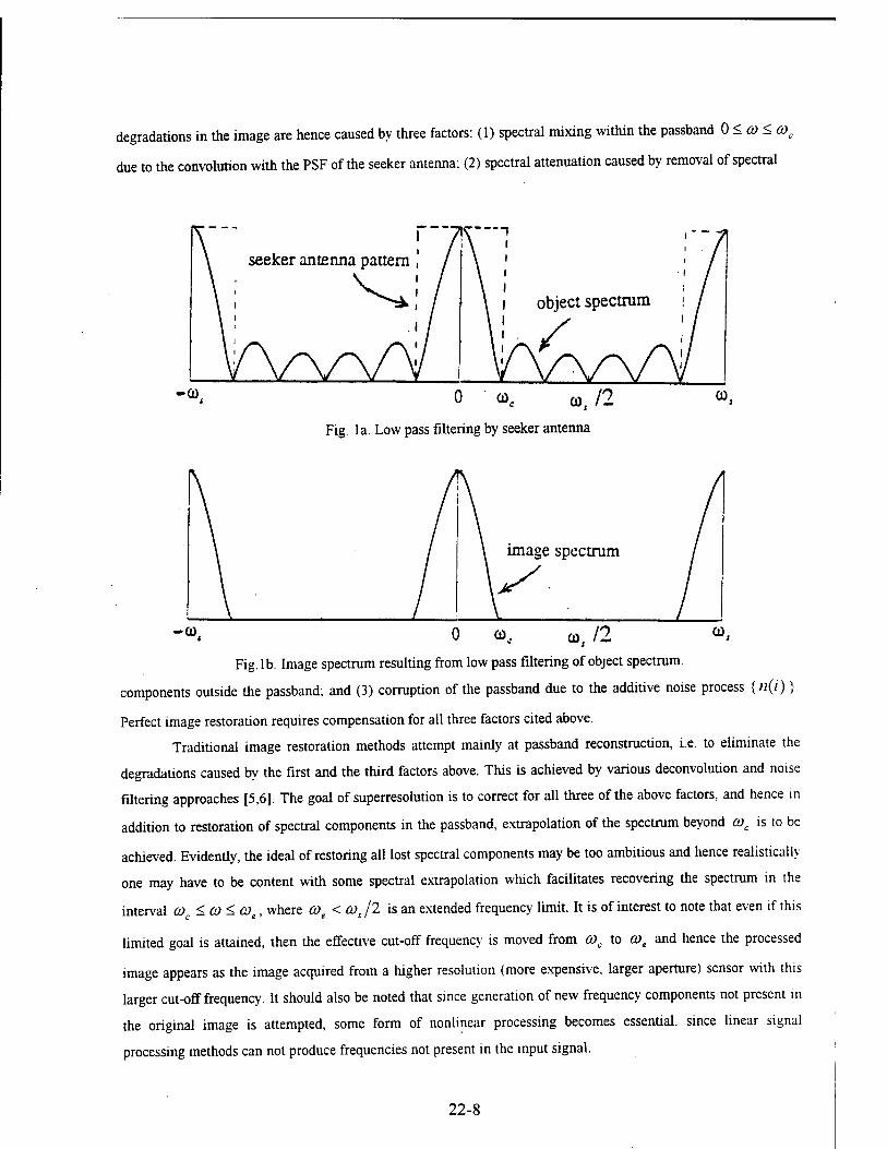
degradaüons in the image are hence caused by three factors: (1) spectral mixing within the passband 0 < co < a>c

due to the convolution with the PSF of the seeker antenna; (2) spectral attenuation caused by removal of spectral

0 o>c (0i 12 Fig. la. Low pass filtering by seeker antenna

-CO.

image spectrum

y

CD. 0 coc co, 12

Fig. lb. Image spectrum resulting from low pass filtering of object spectrum,

components outside the passband: and (3) corruption of the passband due to the additive noise process {/?(/')}.

Perfect image restoration requires compensation for all three factors cited above.

Traditional image restoration methods attempt mainly at passband reconstruction, i.e. to eliminate the

degradations caused by the first and the third factors above. This is achieved by various deconvolution and noise

filtering approaches [5,6]. The goal of superresolution is to correct for all three of the above factors, and hence in

addition to restoration of spectral components in the passband, extrapolation of the spectrum beyond coc is to be

achieved. Evidently, the ideal of restoring all lost spectral components may be too ambitious and hence realistically

one may have to be content with some spectral extrapolation which facilitates recovering the spectrum in the

interval CO <CO<coe, where COe < cos /2 is an extended frequency limit. It is of interest to note that even if this

limited goal is attained, then the effective cut-off frequency is moved from COc to COe and hence the processed

image appears as the image acquired from a higher resolution (more expensive, larger aperture) sensor with this

larger cut-off frequency. It should also be noted that since generation of new frequency components not present in

the original image is attempted, some form of nonlinear processing becomes essential, since linear signal

processing methods can not produce frequencies not present in the input signal.

22-8

To illustrate the complexity in solving problems of this type, consider the simplest case when no spectral

extrapolation is needed, the PSF {h(i) } of the sensor is assumed to be known and the noise «, is ignored. This is

the classical deconvolution problem [5,6] of solving the vector equation

g=Hf (7)

for f given g and H, and a solution can be attempted in the form of an "inverse filter" given by

f = H'lg. (8)

Unfortunately, there are several problems with this approach. The system of equations given by equation (7) is

often underdetermined which results in H~ being not defined. Even if H~ (or a generalized inverse of H) can

be computed, the estimate f obtained may be worthless due to the presence of noise that was ignored. Observe

from the image formation model given by Equation (4), when the presence of noise is accounted for,

f = H-'g-H'xn.

It is now clear that H being a low-pass filter, H~ corresponds to a high-pass filter and hence the noise is greatly

amplified in the solution estimate. A difficulty of a related nature which also can make the solution given by

Equation (8) of limited value is that an exact knowledge of H is needed for computing the solution and even a

small uncertainly in the parameters describing the sensor PSF can result in a very large discrepancy in the solution.

In other words, the solution given by Equation (8) is not "robust" enough to tolerate these nonideal conditions that

may exist in practice making the estimate obtained useless. Finally, the inverse filter solution is a linear operation

and provides no extrapolation of spectrum thus lacking any capability for superresolving. It will be seen later that

the drawbacks of this solution procedure stem from the fact that no use of any a priori knowledge about the object

being restored is made.

The idea of recreating the spectral components that are removed by the imaging process and hence are not

present in the image available for processing may pose some conceptual difficulties, which may lead one to suspect

whether superresolution is indeed possible. Fortunately there exist sound mathematical arguments confirming the

possibility of spectral extrapolation. The primary justification comes from the Analytic Continuation Theorem and

the property that when an object has finite spatial extent its frequency spectrum is analytic [7]. Due to the property

that a finite segment of any analytic function in principle determines the whole function uniquely, it can be readily

proved that knowledge of the passband spectrum of the object allows a unique continuation of the spectrum beyond

the diffraction limit imposed by the imaging system. It must be emphasized that the limited spatial extent of the

object is critical in providing this capability for extrapolation in the frequency domain.

2.3 Use of a priori Knowledge in Solution Process

As noted in the last section, due to the ill-posed nature of the inverse filtering problem underlying image

restoration and superresolution objectives, it is necessary to have some a priori information about the ideal

22-9

solution, i.e. the object / being restored from its image g. In algorithm development, this information is used in

defining appropriate constraints on the solution and/or in defining a criterion for the "goodness" of the solution.

How to utilize this information is at the heart of a well-tailored superresolution algorithm.

The specific a priori knowledge that can be used evidently depends on the specific application For

applications in astronomy, it could come in the form of some known facts about the spectral differences of the

objects one is looking for (for instance, a double star as opposed to a star cluster). In medical imaging and in

military applications, it could come from the geometrical features of the object (target shape, for instance). For

radar and MMW imagery, one could use the fundamental knowledge that the reflectivity of any point on the

ground can not be negative. In addition to the nonnegativity constraint, a space constraint resulting from the

known space-domain limits on the object of interest could be used. Other typically available constraints include

level constrains (which impose upper and lower bounds on the intensity estimates fj), smoothness constraints

(which force neighboring pixels in the restored image to have similar intensity values) and edge-preserving

constraints. More complicated constraints are possible, but in general they result in tuning the algorithms to specific classes of targets.

Varying by the extent to which a priori knowledge can be incorporated in algorithm development, there

have been introduced into the literature a large number of image restoration approaches and algorithms too vast to

describe or reference here. One may refer to some recent survey papers [8,9] for a review of the extensive activity

on this topic. In this section, we shall only briefly cite a few of the approaches that have received some interest in

the context of superresolution capabilities, i.e. those that provide possible spectral extrapolation. It should be noted

clearly that not all image restoration methods provide the capability for superresolving. In fact, a majority of

existing schemes may perform decent passband restoration, but provide no bandwidth extension at all.

The various approaches in general attempt to code the a priori knowledge to be used by specifying an

object model or a set of constraint functions, and further employ an appropriate optimization criterion to guide in

the search for the best estimate of the object. A convenient way of classifying the resulting algorithms is into

iterative and noniterative (or direct) schemes. Noniterative approaches generally attempt to implement an inverse

filtering operation (without actually performing the computation of the inverse of the PSF matrix H, however)

and have poor noise characteristics. All required computations and any possible use of constraint functions are

applied in one step. In contrast, iterative methods apply the constraints in a distributed fashion as the solution

progresses (as shown in Fig. 2) and hence the computations at each iteration will be generally less intensive than

the single-step computation of noniterative approaches. Some additional advantages of iterative techniques are

that, (1) they are more robust to errors in the modeling of the image formation process (uncertainties in the

elements of the PSF matrix H, for instance), (2) the solution process can be better monitored as it progresses, (3)

constraints can be utilized to better control the effects of noise (and possibly clutter), and (4) can be tailored to

offset sensor nonlinearities. The disadvantages of these methods generally are, (1) increased computation time, and

(2) need for proving convergence of the iterative scheme (in fact, for some algorithms this could be impossible). In

22-10

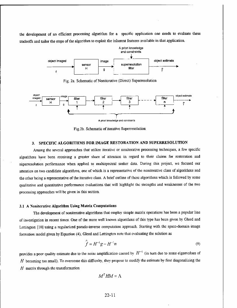
the development of an efficient processing algorithm for a specific application one needs to evaluate these

tradeoffs and tailor the steps of the algorithm to exploit the inherent features available in that application.

A priori knowledge and constraints

image ▼

object imaged sensor

H superresolution

filter

object estimate

f g A

f

Fig. 2a. Schematic of Noniterative (Direct) Superresolution

object

» object esti

imaged sensor H

filter 1

filter 2

filter 3

filter n A

f

\ t t T *

i t f

T A priori knowledge and constraints

Fig.2b. Schematic of iterative Superresolution

3. SPECIFIC ALGORITHMS FOR IMAGE RESTORATION AND SUPERRESOLUTION

Among the several approaches that utilize iterative or noniterative processing techniques, a few specific

algorithms have been receiving a greater share of attention in regard to their claims for restoration and

superresolution performance when applied to multispectral seeker data. During this project, we focused our

attention on two candidate algorithms, one of which is a representative of the noniterative class of algorithms and

the other being a representative of the iterative class. A brief outline of these algorithms which is followed by some

qualitative and quantitative performance evaluations that will highlight the strengths and weaknesses of the two

processing approaches will be given in this section.

3.1 A Noniterative Algorithm Using Matrix Computations

The development of noniterative algorithms that employ simple matrix operations has been a popular line

of investigation in recent times. One of the more well known algorithms of this type has been given by Gleed and

Lettington [10] using a regularized pseudo-inverse computation approach. Starting with the space-domain image

formation model given by Equation (4), Gleed and Lettington note that evaluating the solution as

f = H-lg-H-ln (9)

provides a poor quality estimate due to the noise amplification caused by H~ (in turn due to some eigenvalues of

H becoming too small). To overcome this difficulty, they propose to modify the estimate by first diagonalizing the

H matrix through the transformation

MTHM = A

22-11

where M is the modal matrix of H and A is a diagonal matrix with the eigenvalues of H along the diagonal A

[11]. The object estimate / is then obtained as

A

where /f~od is computed as

H-Joi=M[A + uA-l]MT. (11)

px > 0 is a scalar parameter to be selected appropriately based on the noise present n.

The solution given by (11) changes the PSF of the imaging system from H to Hmod, however, and it is

necessary to account for this change. Gleed and Lettington [10] propose a "regularization" operation by

constructing the matrix R as

R = H-JodH + M2(H-JodHy (12)

and obtaining the final estimate as

/ = a-'/C*. Zmcd5. . (13)

In Equation (12), /£, is another user selected parameter satisfying the condition /A, < //,. Gleed and Lettington

[10] report getting satisfactory resolution improvements in processing various images including PMMW imagery.

The exact extent of spectral extrapolation obtained by this method is however not clear. Furthermore, the selection

ofscalars //, and /u2 is rather ad hoc.

3.2 A Maximum Likelihood (ML) Algorithm for Iterative Superresolution

An important class of algorithms that are receiving particular attention in recent times for their

superresolution capabilities are those that can be developed starting with a statistical modeling of the imaging

process. The basic idea underlying these methods is to account for the statistical behavior of emitted radiation at

the level of individual photon events by constructing appropriate object radiance distribution models (using

knowledge of fluctuation statistics).

For a brief description of these methods, let f(x) denote the object's intensity function, x e X, where

X defines the region over which intensity is defined, and let g{y) denote the intensity detected in the image,

y € Y, where Y defines the region over which intensity is detected. If {h(y, x) , y e Y and x e X} denotes

the point spread function (PSF) of the imaging sensor, then accounting for the presence of noise in the imaging

process, one can model the imaging process by

g(y) = Z Ä0> x)f (x) + noise (j 4) x<=X

22-12

(where an additive noise is assumed as before for the sake of simplicity). The classical restoration problem is to

A

find the object intensity estimate {f(x)} given the data {giy) }.

There exists considerable literature on developing explicit algorithms, mainly of an iterative nature, for

handling the image restoration problem within a statistical framework afforded by such a formulation. A A

particularly attractive approach is to obtain a maximum likelihood (ML) estimate {fix)} i.e. the object intensity

estimate that most likely have created the measured data {giy)} with the PSF process {h(y,x)}, which in turn

is developed by maximizing an appropriately modeled likelihood function (or the logarithm of this function, for

simplicity). Modeling the likelihood function is basically obtaining a goodness-of-fit (GOF) quantity for the

measured data, since the likelihood function is a statistical distribution function p(g/f) obtained as a fit to the

relation between the data {g(y)} and the object {fix)}. The success of image restoration in a given application

depends on how good the assumed conditional probability function fits the input/output characteristics of the

imaging system. While a commonly used model is a Chi-squared function, very active and intense research

continues to this day on the development of improved statistics that lead to better ML estimates.

In the formulation of iterative algorithms that afford simple implementation, an important contribution

has been the work of Shepp and Vardi [12] who used the Expectation Maximization (EM) algorithm (originally

suggested by Dempster et. al. [13]) to solve positron emission tomography imaging problems in which Poissonian

statistics are dominant. The major advantage of using the EM algorithm is that it involves the solution of linear

equations, whereas the original ML problem is in general a nonlinear optimization problem. Following this

approach, Shepp and Vardi [12] developed an iterative algorithm for which convergence can be proven

analytically. This algorithm also reduces to the familiar Richardson-Lucy iteration which has attained considerable

popularity in the fields of astronomy and medical imaging. For a discretized formulation of the imaging equation

(2), with g(j) and f(J) , j = 1,2,...N, denoting the TV pixels of the image and the object respectively, and

h(J) denoting the PSF of sensor, the updating of the object estimates takes the form

fMU) = f>U)

r \ gjj)

JkU)®i>(j). ®h(J) y = 1,2,3,...., TV, (15)

A

where k denotes the iteration count and ® denotes discrete convolution. The initial estimate f 0iJ) is taken as

the image g(J) to commence the iteration.

A

It should be noted that the ML estimate /(/) attempts to construct an estimate for f(J), the number of

photons emitted by the j-th sample of the object (which is considered a random variable) from a knowledge of

g(J), the j-th pixel value in the input image, and h(j) , the j-th element of the sensor PSF. The optimization

22-13

framework in which the algorithm is developed ensures that the likelihood function p(g/f) monotonically

increases over successive iterations of the algorithm and hence the processed image improves in quality as the

algorithm processed.

3.3 Comparison of Algorithms for Multispectral Seeker Implementations

Two distinct algorithms for restoration and superresolution of image data that employ iterative and

noniterative computations were outlined in the last two sections. Due to the differences underlying the approaches

followed in obtaining these algorithms, they possess particular advantages and disadvantages. For an intelligent

selection of the right approach in a specific seeker application, one needs to weigh these advantages and

disadvantages in the light of some basic requirements that need to be met in these implementations. These are

listed in the following:

1. Flexibility for application to images from different sensing modalities;

2. Performance robustness to tolerate modeling uncertainties, parameter inaccuracies and nonlinearities;

3. Computational requirements that can be met in typical real-time applications;

4. Ensure desired level of resolution enhancement in the presence of significant noise levels;

5. Ensure satisfactory performance in realistic clutter scenarios (with signal-to clutter ratios (SCR) in

therange5-10dB)

The limits on complexity and computational requirements are evident, given the real time operation

requirement for a missile seeker. On the surface it may appear that noniterative approaches provide an obvious

advantage over iterative approaches on this count since the entire computation needs to be performed only once.

However, there are several factors that need to be considered in this evaluation. First of all, the computation

required for implementing the noniterative estimation given by (13) is considerably more complex than the

implementation of the iteration given by (15). It must be emphasized that the discrete model for the imaging

process, viz, Equation (4), which is used as the basis for the noniterative estimation results in a matrix H of

typically large dimension. Consequently, the matrix inversion operations required in (18) can pose some

difficulties. Furthermore, H will have a number of zero elements, which further add complexities to the

computation of inverses. In our implementations we have found that execution of iterations of the form given by

(15) over several cycles is in many cases computationally preferable to the noniterative algorithm (18) that requires

matrix inverse calculations.

Perhaps a greater advantage of iterative algorithms of the type (15) comes from the performance

robustness to noise, clutter and parameter uncertainties. It is evident that an accurate knowledge of the sensor PSF

matrix H is necessary for computation of the estimates in (13), whereas a significant tolerance to inaccuracies in

the sensor PSF is provided by the ML iteration algorithm (15). In fact, this algorithm can be modified, as will be

described in the next section, for a blind implementation when a complete knowledge of the sensor PSF is not

initially available and one would like to obtain improved estimates of the PSF parameters as the iterations progress.

The requirements arising from the presence of noise and clutter are also evident from the practical

environments in which target detection and classification are to be performed. As noted earlier, there are two main

22-14

sources of noise in these applications, viz, the receiver noise, whose statistics depend on the type of imaging sensor

employed and are usually signal dependent, and the quantization noise, which can be realistically modeled by a

zero-mean white Gaussian random field that is independent of the image signal. It is well known that

deconvolution methods (particularly those that attempt to implement directly an inverse filter) are highly sensitive

to noise and require rather high SNR levels for satisfactorily processed images. One may note that typical

radiometric images (PMMW images, for instance) have SNR levels of about 20dB (or less), thus highlighting the

importance of this requirement.

Finally, it is beneficial to have the restoration algorithm be capable of processing signals collected from

different types of sensors. This is due to the fact that present day missile seekers are required to handle data

collected from different sensing modalities (typically operating in different frequency ranges) and to perform

tactical decision-making based on the fused data. In these environments, any signal processing on the measured

data aimed at contrast enhancement [14] and/or resolution enhancement (superresolution) often comes as a first

step operation which facilitates the further processing steps, such as feature extraction, feature integration for

fusion, etc. [15], to be implemented more efficiently. Use of iterative algorithms that have certain inherent

robustness to parameter inaccuracies can provide major benefits since characterization studies leading to accurate

determination of PSF may not be readily available for every detector in the sensor suite.

The qualitative comparisons given in this section favor the selection of iterative algorithms of the type

given by (15). While convergence of iterative schemes is in general an issue of concern, analytical support ensuring

the convergence of the ML iterations in (15) is available. In practice, one can terminate the iterations once a

desired resolution level in the processed image is attained. Development of additional constructs that speed up the

convergence of the ML iterative algorithm given by (15) is a topic that is receiving considerable attention.

3.4 Quantitative Performance Evaluation of ML Superresolution Algorithm

Several experiments directed to evaluating the restoration and superresolution performance of the ML

iterative algorithm given by (15) were conducted as part of this project. Results from four experiments are briefly

summarized in this section to illustrate the efficiency of this algorithm in the processing of various types of input

signals. Experiments 1-3 were principally aimed at measuring the spectrum extrapolation performance and hence

were conducted in a "controlled environment" by starting with a known object (1-D or 2-D) and blurring it with a

known PSF to generate the input signal for the processing algorithm. On the other hand, experiment 4 dealt with

evaluating the performance in processing "real data", which in this case is a passive MMW image collected by

Wright Laboratory Armament Directorate personnel at Eglin AFB using a state-of-the-art passive MMW data

acquisition platform comprising of a 95 GHz 1 foot diameter aperture radiometer.

Experiment 1:

Fig. 3a shows the original object comprising of 3 impulses (point sources) located 2 pixels apart. Fig. 3b

shows the image formed when blurred with a sensor with a cutoff frequency 21. Figs. 3c and 3d give the

reconstructed images after 90 and 1000 iterations of the ML algorithm. While the restoration of the original object

22-15

10

9 .

B ■ ■

7 ■ ■

6 .

«9

S 5 S

-

4 ' ■

3 ■

2 ■

1

_i . , 10 20 30

3a

40 SO 70 °0

3b

3c 3d

Fig. 3. Signal restoration performance in Experiment 1

22-16

is clearly seen in these figures, the spectrum extrapolation ( and hence superresolution ) can be more clearly seen

by examining the frequency spectra of the signals before and after processing. Fig. 4a shows the spectrum of the

original object, Fig. 4b shows the spectrum of the image formed ( note the cutoff frequency 21 of the sensor) and

Fig. 4c shows 'the spectrum of the reconstructed image after 90 iterations of the ML algorithm. The extrapolation

of frequency components beyond the cutoff at 21 clearly demonstrates that this algorithm is superresolving.

Experiment 2: Fig. 5a shows a more complex one-dimensional object characterized by several edges and hence offers a

greater challenge to the processing algorithm. The image formed by blurring with a sensor with a cutoff frequency

21 is shown in Fig. 5b. Fig. 5c shows the reconstructed image after 90 iterations of the ML algorithm, where the

edge reconstruction is clearly seen. The spectrum extrapolation performance can also be seen by comparing Fig.

6a, 6b and 6c, which show the spectra of the original object, input image and the ML processed image (after 90

iterations). It should be noted that only the portion of the spectrum in the high frequency range is plotted to an

expanded scale in these figures since the signal has low frequency components with relatively large magnitudes

that prevent the high frequency components from being displayed effectively on the same graph. For testing the

restoration performance in the presence of noise, another experiment was conducted by blurring the same object as

before and then corrupting with an additive Gaussian noise to result in an image with a Signal-to-Noise Ratio

(SNR) of 30.0248 dB shown in Fig. 7a. The reconstructed image after 200 iterations of ML algorithm is shown in

Fig. 7b which confirms the noise filtering properties of the algorithm.

Experiment 3: The superresolution performance of these algorithms was also tested by processing a 256 x 256. image

from our database. Fig. 8a shows the original image (Lena) used in this experiment. Fig. 8b shows the blurred

image obtained by convolution with the PSF of a sensor with cutoff COc = 63 (which is approximately one-half of

the folding frequency and is typical of practical imaging operations). The restoration performance of ML algorithm

as the number of iterations is gradually increased is shown in the next set of figures (Figs. 8c - 8f where the

restored images after 10, 20, 90, and 100 iterations are shown). The resolution enhancement with only 10

iterations of the algorithm is clearly visible. The algorithm was stopped at the end of 100 iterations since the

resolution is comparable to that of the original (unblurred) image. Figures 9a - 9d show the power spectra of

various signals; the frequency extrapolation performed by the ML algorithm to achieve superresolution is clearly

noticeable by comparing the four corners in Figs. 9c and 9d which show the power spectra of the blurred image

and the reconstructed image after 100 iterations of ML.

Experiment 4: The performance of the ML algorithm was also tested by processing a set of passive MMW images

supplied by the Wright Laboratory Armament Directorate personnel. These images were collected under various

conditions (time-of-day, atmospheric conditions, etc.), which were not known save for the fact that the images were

obtained by a single detector radiometer with 1 foot aperture at 95 GHz. For illustration purposes, the result of

processing one of these images ("Jeep 2" image) will be presented here.

22-17

700

700

10 20 30 40 Frequency (1/pxaq

50

4a

60 70

4b

4c

30 40 Frequency (1/pfac*)

Fig. 4. Spectrum reconstruction performance in Experiment 1

22-18 '

5a

5b

5c

Fig- 5. Signal restoration performance in Experiment 2

22-19

900

30 40 Frequency (1/Pbcal)

^A -~*l ^ - JL £^± 20 30 40

Fraquancy (1/Plxel) SO 60

6a

6b

6c

70

Fig. 6. Spectrum reconstruction performance in Experiment 2

22-20

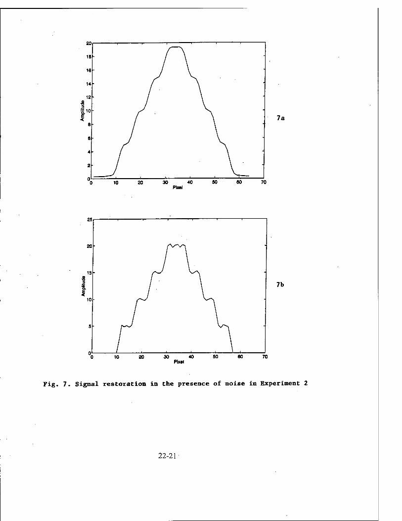
20 1- 1 1 !—T- 1 1

18 /A 16 J V 14 1 A 12 / \

f |io I i \ 8

/ \ 6 J \ 4

/ \ 2

7a

10 20 30 40 SO 60 70 Pixel

25 1— 1 ■——r ^T 1 1

20 n 15 ^y u

» / \ ■o 3 / \ Q. / \ ^ / \

10

/ \

5

* ■ ■-—'—i—i—■— 10 20 30 40

Pixel 50 60

7b

70

Fig. 7- Signal restoration in the presence of noise in Experiment 2

22-21

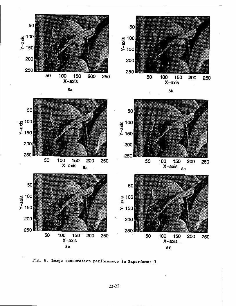
100 150 200 250 X-axis

8a

100 150 200 250 X-axis

8b

100 150 200 250 X-axis 8c

100 150 200 250 X-axis

8e

100 150 200 250 X-axis 8d

50 100 150 200 250 X-axis 8f

Fig. 8. Image restoration performance in Experiment 3

22-22

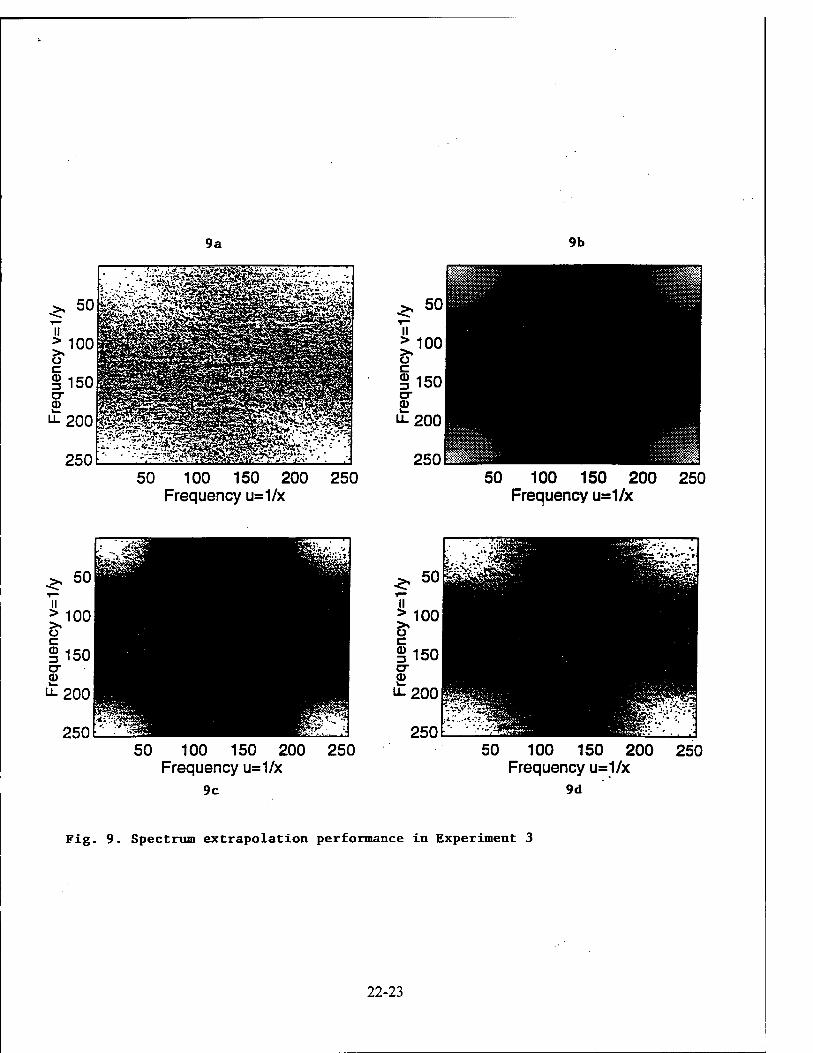
9a 9b

250 L 50 100 150 200

Frequency u=1/x 250 50 100 150 200 250

Frequency u=1/x

■^ K/:

"» '^B Biifew-::: üüÜ EE&£7y,

>, 50 ^~

ii > 100 >. o c 5 150 cr ■ ^M

^s00! IR3 250 ^■c^-

50 100 150 200 250 Frequency u=1/x

9c

50 100 150 200 250 Frequency u=1/x

9d

Fig. 9. Spectrum extrapolation performance in Experiment 3

22-23

The received image to be processed is shown in Fig. 10a. It is evident that the resolution present is quite

poor and the extraction of any useful features from this image is rather doubtful. The image can benefit from

further processing aimed at resolution enhancement. Since a complete characterization of the sensor and the

imaging conditions were not available to determine the sensor PSF, an approximate analysis was conducted to

identify the cut-off frequency in the optical transfer function (OTF). Starting with an intensity profile

corresponding to an edge of the object in the image (as shown in Fig. 11a which gives the intensity profile in

column 100), an OTF was created as a low-pass filter whose convolution with an input pulse object (shown in Fig,

1 lb) yields an outcome (shown in Fig. 1 lc) which is similar to the edge profile. The cutoff in the OTF in this case

was estimated to be 17. While this process gives only a rough estimate of the OTF of the imaging system, through

iterative adjustments it is possible to obtain a sufficiently accurate characterization of the sensor PSF to commence

the ML iterations for superresolution.

Figs. 10b - 10g show the results of processing the input image in Fig. 10a after 10, 20, 30, 40, 60, and 100

cycles of ML iteration. The progressive enhancement of resolution is clearly evident from the strengthening of

edges and the improved structural details of the object (particularly near the wheels, the windows and the top of the vehicle).

4. PERFORMANCE IMPROVEMENT BY ITERATIVE BLIND ML RESTORATION

As discussed earlier, if the sensor is fully characterized and if the images contain good target/scene

metrics such as exact time of day, distances to objects, weather conditions etc., one may attempt to model the

sensor PSF exactly and employ it for restoration of the image [16]. When the PSF parameters are not readily

available, one may attempt to build an approximation to the PSF from the image to be processed using techniques

such as the one described in the last section (of looking for a column or row in the image corresponding to a sharp

edge and matching this profile with the blurred version of a sharp edge passed through an approximately tailored

OTF). Since the performance of any deconvolution procedure improves with the availability of accurate PSF

parameters, it is useful to consider implementations of iterative restoration and superresolution algorithms where

the PSF estimates can be adaptively updated along with the iterative construction of the object estimate. Such

implementations can be regarded as special cases of "blind deconvolution" algorithms which attempt to perform

image restoration with incomplete knowledge of both the PSF and the object (i.e. h and / in the imaging process

model (14)). In this section we shall present one such implementation and discuss its performance when applied to

superresolution of PMMW images.

4.1 ML Algorithm for Joint Estimation of Object and PSF

For the presentation of the new algorithm, it is useful to briefly review the mathematical basis underlying

the iterative ML scheme given by (15). Starting with the imaging equation (14) and assuming that the additive

noise can be modeled as an independent and identically distributed (lid.) random variable with a zero mean

22-24

10a

10c

B^^^^ SB

10d lOe

lOf 10g

Fig. 10. Restoration of passive millimeter-wave image ("Jeep 2")

22-25

11a lib

100

300

250

=»200

g150

"100

50

0 50 y

100

lie

100

Fig. 11. Estimation of sensor PSF from image

22-26

Gaussian probability density having variance a2n , the intensity detected in the image g(y) can be regarded as a

random variable with a normal probability density

{g{y)-HKy,x)f{x)}2

p[g(y\h,f] = (Ina2)1'

-exp X£X

2<JI (16)

It may be noted that the noise model assumed is particularly appropriate if the dominant noise is thermal noise

The probability density for realizing the entire data set, {g{y), y e Y) can hence be obtained as

t{gXf] = Y\Asiy\hj] (17) yeT

which serves as a model for the likelihood function for evaluating the ML estimate {/(*)} that most likely have

produced the data {g(y)} from {h(y,x)} and {/(x)}. It is obtained by maximizing P in (17).

For simplicity in computation, one conducts the maximization of a modified log-likelihood function

L[gAf] = -Z yeX

-[2

g(y)-Hh{y,x)f(x) xeJC

(18)

which is obtained by taking the natural logarithm of P in (17) and removing a constant term that does not affect

the maximization process. If L is maximized with respect to / assuming h to be known, we have the standard

ML restoration, whereas if L is maximized with respect to both / and h by searching over a larger parameter

space, we have blind ML restoration.

The iterative scheme given in (15) provides a discretized implementation of the standard ML restoration A

process. It can be easily converted into a blind restoration scheme by observing that f(J) and h(J) are

interchangeable in the two convolution operations in (15), and hence an updating scheme for h(J) can be

A

developed for estimation of the PSF along with the object estimation, i.e. obtaining f(J) . For a brief description,

each cycle of this "Blind ML restoration algorithm" consists of executing the two steps:

Step 1: Implement "object estimation" algorithm through m iterations with initial guess for hk (J) and

f0U) = g<J)-

fM(J)=fk(J) g(j)

fk(J)®K(J) ®hkU) (19)

22-27

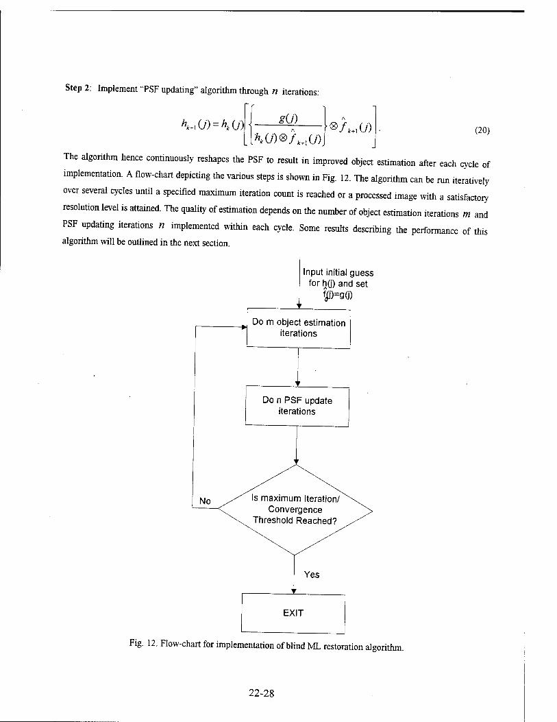
Step 2: Implement "PSF updating" algorithm through n iterations:

K+l(J) = KU) gU) «/*♦,(/) (20)

CKU)®fk+lU)j

The algorithm hence continuously reshapes the PSF to result in improved object estimation after each cycle of

implementation. A flow-chart depicting the various steps is shown in Fig. 12. The algorithm can be run iteratively

over several cycles until a specified maximum iteration count is reached or a processed image with a satisfactory

resolution level is attained. The quality of estimation depends on the number of object estimation iterations m and

PSF updating iterations n implemented within each cycle. Some results describing the performance of this

algorithm will be outlined in the next section.

Input initial guess for hü) and set

P=9G)

Do m object estimation iterations

Do n PSF update iterations

Yes

EXIT

Fig. 12. Flow-chart for implementation of blind ML restoration algorithm.

22-28

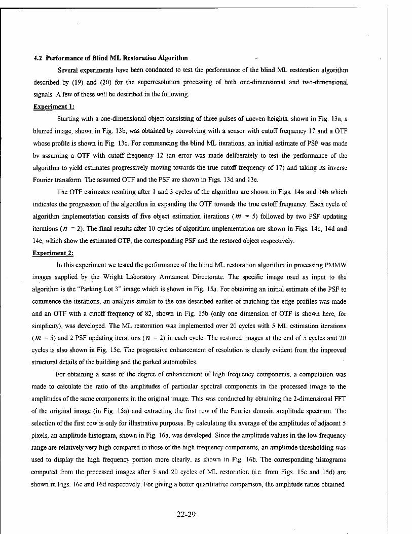
4.2 Performance of Blind ML Restoration Algorithm

Several experiments have been conducted to test the performance of the blind ML restoration algorithm

described by (19) and (20) for the superresolution processing of both one-dimensional and two-dimensional

signals. A few of these will be described in the following.

Experiment 1:

Starting with a one-dimensional object consisting of three pulses of uneven heights, shown in Fig. 13a, a

blurred image, shown in Fig. 13b, was obtained by convolving with a sensor with cutoff frequency 17 and a OTF

whose profile is shown in Fig. 13c. For commencing the blind ML iterations, an initial estimate of PSF was made

by assuming a OTF with cutoff frequency 12 (an error was made deliberately to test the performance of the

algorithm to yield estimates progressively moving towards the true cutoff frequency of 17) and taking its inverse

Fourier transform. The assumed OTF and the PSF are shown in Figs. 13d and 13e.

The OTF estimates resulting after 1 and 3 cycles of the algorithm are shown in Figs. 14a and 14b which

indicates the progression of the algorithm in expanding the OTF towards the true cutoff frequency. Each cycle of

algorithm implementation consists of five object estimation iterations (m = 5) followed by two PSF updating

iterations (n = 2). The final results after 10 cycles of algorithm implementation are shown in Figs. 14c, 14d and

14e, which show the estimated OTF, the corresponding PSF and the restored object respectively.

Experiment 2:

In this experiment we tested the performance of the blind ML restoration algorithm in processing PMMW

images supplied by the Wright Laboratory Armament Directorate. The specific image used as input to the

algorithm is the "Parking Lot 3" image which is shown in Fig. 15a. For obtaining an initial estimate of the PSF to

commence the iterations, an analysis similar to the one described earlier of matching the edge profiles was made

and an OTF with a cutoff frequency of 82, shown in Fig. 15b (only one dimension of OTF is shown here, for

simplicity), was developed. The ML restoration was implemented over 20 cycles with 5 ML estimation iterations

(m = 5) and 2 PSF updating iterations (n = 2) in each cycle. The restored images at the end of 5 cycles and 20

cycles is also shown in Fig. 15e. The progressive enhancement of resolution is clearly evident from the improved

structural details of the building and the parked automobiles.

For obtaining a sense of the degree of enhancement of high frequency components, a computation was

made to calculate the ratio of the amplitudes of particular spectral components in the processed image to the

amplitudes of the same components in the original image. This was conducted by obtaining the 2-dimensional FFT

of the original image (in Fig. 15a) and extracting the first row of the Fourier domain amplitude spectrum. The

selection of the first row is only for illustrative purposes. By calculating the average of the amplitudes of adjacent 5

pixels, an amplitude histogram, shown in Fig. 16a, was developed. Since the amplitude values in the low frequency

range are relatively very high compared to those of the high frequency components, an amplitude thresholding was

used to display the high frequency portion more clearly, as shown in Fig. 16b. The corresponding histograms

computed from the processed images after 5 and 20 cycles of ML restoration (i.e. from Figs. 15c and 15d) are

shown in Figs. 16c and 16d respectively. For giving a better quantitative comparison, the amplitude ratios obtained

22-29

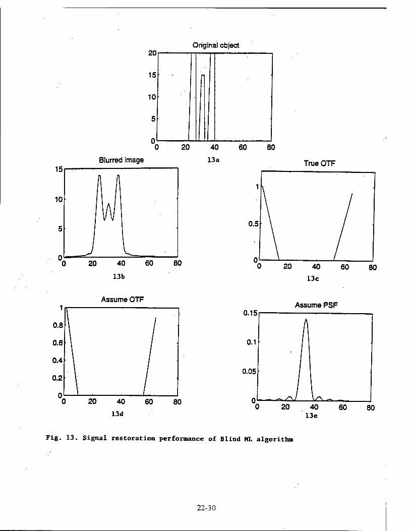
20 Original object

15

10

S\

Blurred image

Assume OTF

n

20 40

13a

60 80

True OTF

0 20 40 60 80

13c

Assume PSF

Fig. 13. Signal restoration performance of Blind ML algorithm

22-30

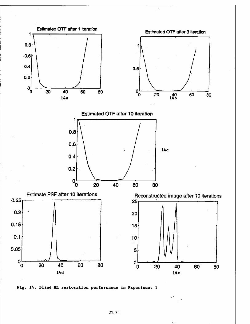
Estimated OTF after 1 iteration Estimated OTF after 3 iteration

Estimated OTF after 10 iteration

0.25

0 20

Estimate PSF after 10 iterations

14c

Reconstructed image after 10 iterations 25

Fig. 14. Blind ML restoration performance in Experiment 1

22-31

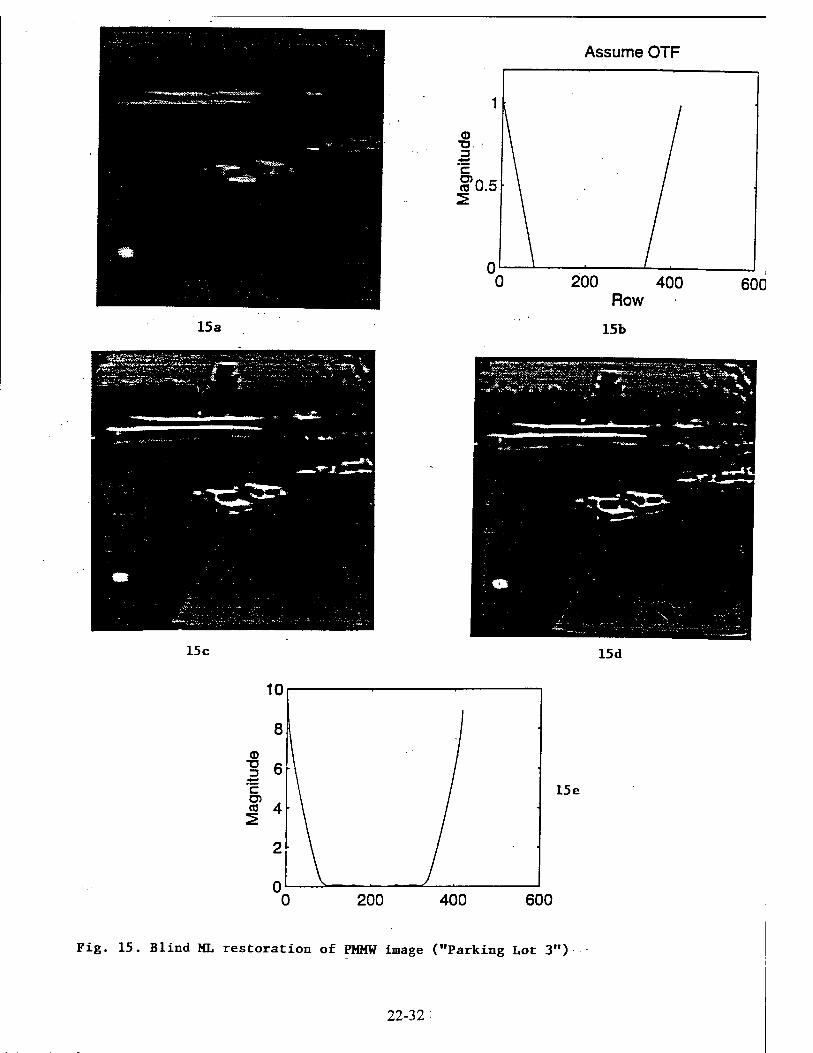
Assume OTF

15a

200 400 Row

15b

60C

15 c 15d

15 e

600

Fig. 15. Blind ML restoration of PMMW image ("Parking Lot 3")

22-32

x10

150

Fig. 16. Frequency enhancement performance of Blind ML algorithm

150

150

22-33

at the same frequency values were evaluated by computing the amplitude from the processed image divided by the

amplitude from the original image. Plots of these amplitude ratios obtained for the images after 5 cycles and 20

cycles of processing are shown in Figs. 16e and 16f, which clearly demonstrate the enhancement of high frequency

spectral components by the present ML restoration algorithm.

5. CONCLUSIONS

Studies directed to the evaluation of performance of iterative and noniterative schemes for image

restoration and superresolution processing were conducted in this project with a specific focus on their eventual

deployment in multispectral seeker environments. These studies are of particular relevance to the processing of

images collected from various sensors used in these environments to provide enhanced image resolutions that can

facilitate better false target rejection, improved automatic target recognition and aimpoint selection. The selection

of an iterative technique or a noniterative scheme results in considerably different performance levels and can

bring specific advantages and disadvantages to the overall restoration and superresolution function however. Some

qualitative comparisons of the performance expected from these schemes were given in this report. A more

quantitative performance evaluation of a ML superresolution algorithm was conducted in this project and results of

this analysis were also presented here. Finally, to aid in a robust implementation of the ML algorithm in cases

where an accurate model of the sensor PSF is not available, a modified algorithm that jointly estimates the object

imaged and the PSF parameters from an initial approximated guess of PSF function was developed, and the

performance of this blind ML restoration algorithm in processing various signals, including PMMW images

supplied by Wright laboratory Armament Directorate Personnel, was described. Based on these studies, it may be

concluded that ML techniques offer an attractive framework for tailoring image restoration and superresolution

algorithms for implementation in multispectral seeker environments. Further studies directed to improving the

computational efficiency of these algorithms and to evaluating the noise tolerance (tradeoff between resolution and

noise filtering) are highly useful and these are planned for future investigation.

Acknowledgment: The author is grateful to Mr. Seng-vieng Amphay of the Wright Laboratory Armament

Directorate at Eglin AFB for encouragement in this research and for providing PMMW imagery data used in these

studies. He also thanks Mr. Ho-Yuen Pang of the University of Arizona Electrical and Computer Engineering

Department for his assistance in conducting the investigations contained in this report.

6. REFERENCES

1. B.M. Sundstrom and B.W. Belcher, "Smart tactical autonomous guidance", Proc. ofAIAA Missile Sciences

Conference, Feb. 1992.

2. S. Worrell, "Passive millimeter wave imaging sensor assessment", GACIAC Publication SR-93-03, Final

Report for Wright Laboratory Armament Directorate, Eglin AFB, FL, 1993.

22-34

3. M.K. Sundareshan, "Advanced processing techniques for restoration and superresolution of imagery in

multispectral seeker environments", Final Report for Summer Faculty Research Program, AFOSR, August

1995.

4. W.K. Pratt, "Vector-space formulation of two-dimensional signal processing operations", Computer Graphics

and Image Processing, Vol. 4, pp. 1-24, 1975.

5. W.K. Pratt, Digital Image Processing, Wiley: New York, 1978.

6. A.K. Jain, Fundamentals of Digital Image Processing, Prentice-Hall, 1989.

7. C.K. Rushforth and J.L. Harris, "Restoration, Resolution and Noise", J. Of Optical Society of America, Vol.

58,pp.539-545, 1968.

8. M.I. Sezan and A.M. Tekalp, "Survey of recent developments in digital image restoration", Optical

Engineering, Vol. 29, pp.393-404, 1990.

9. J. Biemond, R.L. Lagendijk and R.M. Mersereau, "Iterative methods for image deburring", Proc. of IEEE,

Vol. 78, pp. 856-883, 1990.

10. D.G. Gleed and A.H. Lettington, "Application of superresolution techniques to passive millimeter-wave

images", Proc. ofSPIEConf. On Applications of Digital Image Processing, Vol. 1567, pp. 65-72, 1991.

11. R. Bellman, Matrix Analysis, McGraw-Hill, 1968.

12. L. Shepp and Y. Vardi, "Maximum likelihood reconstruction in positron emission tomography", IEEE Trans.

On Medical Imaging, Vol. 1, pp. 113-122, 1982.

13. A.P. Dempster, N.M. Laird and D.B. Rubin, "Maximum likelihood from incomplete data via the EM

algorithm", J. Of Royal Statistical Society, Vol. 29, pp. 1-38, 1977.

14. T.L. Ji, M.K. Sundareshan and H. Roehrig, "Adaptive image contrast enhancement based on human visual

properties", IEEE Trans. On Medical Imaging, Vol. 13, pp. 573-587, 1994.

15. M.K. Sundareshan and F. Amoozegar, "Neural network fusion capabilities for efficient implementation of

tracking algorithms", Proc. SPIE Conf. On Signal and Data Processing of Small Targets, Aerosense' 96,

Orlando, Fl, April 1996. (To appear in expanded from in Optical engineering, March 1997).

16. J. Goodman, Introduction to Fourier Optics, McGraw-Hill, 1996.

22-35

THE EFFECTS OF METAL DSfTERLAYER INSERTION ON THE FRICTION, WEAR AND ADHESION OF TiC COATINGS

Jinke Tang Associate Professor

Department of Physics

University of New Orleans Lakefront

New Orleans, LA 70148


Wright Laboratory



and

Wright Laboratory

December 1996

23-1

THE EFFECTS OF METAL INTERLAYER INSERTION ON THE FRICTION, WEAR AND ADHESION OF TiC COATINGS

Jinke Tang Associate Professor

Department of Physics University of New Orleans

Abstract

The friction, wear and adhesion behaviors have been investigated for the TiC coatings

containing different kinds of interlayers (Ti, Cr and Mo) of different thickness using pin-on-disk

configuration, in which both stainless steel and alumina pins were used. The wear tracks of the

TiC coatings and the pins were characterized by both optical microscope or scanning electron

microscope (SEM). Inserting Cr or Ti interlayer between TiC coating and substrate could

improve greatly the adhesion and wear. The TiC coating with 500Ä Cr interlayer showed better

overall characteristics than that with 5000Ä Cr interlayer. The same was found to be true for the

Ti interlayer, i.e., thinner interlayers performed better in the adhesion and wear tests. This is

probably due to the improved lattice match between the TiC coatings and the interlayers when

the interlayer thickness was reduced. The wear resistance of the TiC coatings was found to

increase rapidly as their thickness was changed from 0.2 /urn to 2um, and to 3 yum, which was

closely related to the load bearing capability of the coatings. These TiC coatings with, or

without, metal interlayers have been nitrogen ion implanted in the interface region. The effects

of such ion implantation on their adhesion and wear are currently being studied.

23-2

THE EFFECTS OF METAL INTERLAYER INSERTION ON THE

FRICTION AND WEAR OF TiC COATINGS

Jinke Tang

Introduction

Because of the many advantages, such as high melting point, high hardness, wear resistance,

chemical stability as well as large modulus, ceramic coating materials(e.g., TiC, TiN, SiC, and

diamond, etc) have being used in tribological application to reduce the wear of contacting

components. The applications range from aerospace, engine parts, to wear resistant barriers for

many moving mechanical assembles [1,2]. Generally, the TiC film deposition has been done by

chemical vapor deposition, physical vapor deposition [3,4], magnetron sputtering, pulsed laser

deposition (PLD) [5,6], etc. Sessler et al. [7] investigated the influence of film deposition

temperature, substrate hardness, and counterface hardness on the friction and wear behavior of

TiC film grown by excimer pulsed laser deposition. The thickness of TiC coatings was

controlled at 0.2 //m. Tang et al. [8] found the adhesion of magnetron sputtered TiC coating

could be modified by inserting metallic interlayer between the coating and stainless steel substrate.

The PLD TiC coatings grown at room temperature was harder than the TiC coatings grown by

magnetron sputtering under the given experimental conditions.

The purpose of present work was to study the effects of different metallic interlayers (e.g.,

Cr, Ti, and Mo) on friction and wear of the TiC coating grown by magnetron sputtering. The

friction and wear properties of the coatings containing different thickness of TiC film and

interlayer were characterized by combining tribological experiments with the optical microscopic

analysis.

Experimental

TiC coatings were grown using the magnetron sputtering technique. The 440C stainless steel

(SS) substrates were first rinsed with acetone and isopropanol before they were sputter etched

in a diffusion pumped MRC 902 in-line sputter deposition chamber. The chamber was backfilled

23-3

with methane and argon at constant flow rate of 40 and 80-90 cm3/m, respectively. The bias

voltage on substrate was -100V and total pressure was controlled at 8 mtorr. The chambers

were pumped to a base pressure of lxlO"6 torr before sputter etching of the substrates.

Tribological experiments were carried out on an ISC-200 pin-on-disk tribometer (Implant

Sciences Co.) controlled by computer at room temperature in laboratory atmosphere. The sliding

speed of pin on disk was constant at 10.21 cm/sec and the loads in all tests were chosen from 25

gram to 500 gram. The substrate, a pellet of 25.5 mm in diameter, was made of 440C stainless

steel and the thickness of the TiC coating was 0.2 //m, 2 ßm and 3 //m, respectively. Alumina

and 440 SS pins with a diameter of 0.125 inch were alternatively used in order to study the

influence of ball hardness on friction and wear. Wear traces of the coatings and wear scars of pins

were analyzed by optical microscope or scanning electron microscope (SEM) technique.

Results and Discussion

1. Counterface hardness on the friction and wear behavior of the TiC coatings

The friction and wear experiments were conducted using a pin-on-disk configuration, in

which the two types of pins, 440 SS and alumina balls, were used. Figure 1 shows the variation

of the friction coefficient with the SS ball sliding over the surface of TiC coating with a thickness

of 2 //m under the loads of 500 g, 250 g, 100 g and 50 g, respectively. It is found in Figure 1 that

the friction coefficient increased abruptly, to as high as 0.5-0.9, when the pin started to move on

the film. Then it quickly reduced with the sliding, finally reaching an equilibrium value. The value

was between 0.2-0.22 for the loads of 50 g, 100 g, and 250 g, but only about 0.12 for 500 g.

The initial coefficient of friction in all of above experiments was much higher than the relevant

equilibrium coefficient of friction. When the 440 SS ball and the TiC film were brought into

contact and sheared, both the adhesion between hard TiC coating and soft SS pin and surface

roughness played an important role in determining the initial coefficient of friction. With the SS

pin sliding repeatedly over the same track of TiC film, the surface roughness of the pins and TiC

film was reduced and the asperities between pin and coating were partly filled by debris (found

in the following optical micrograph of the pins). Eventually, a stable equilibrium coefficient of

friction was reached. It is noticed easily that the friction coefficient under the load of 500 g was

23-4

c o Ü

Ü JE <D O O

1.0

0.8

0.0 50 100 150 200 250

Wear time (min)

Figure 1 Friction coefficient of the TiC coating(2um) on 440 stainless steel disk as a function of wear time under the loads: 500g, 250 g, 100 g and 50 g, respectively. (speed=10.21 cm/sec, SS pine)

23-5

only 0.12, much lower than others. Acoefficient of friction of 0.16 was found for a load of 400

g (not shown in Figure 1). This may be due to that the decrease in friction resulting from blunting

the tips of surface asperities and reducing surface roughness is greater than the corresponding

increase resulting from larger contacting surface when the sliding continued under a heavier load

force. Friction tracks of the coating and wear scars of the SS pin shown in the Figure 2 is an

evidence ofthat. Wider wear track on the film and larger wear surface of ball occurred under

heavier load, i.e., 500 gram. This load dependence of the friction seems to be directly related to

surface roughness and the contacting surface increase.

Friction and wear behavior was investigated by using alumina pin under the same conditions

as those using SS pins above. Figure 3 presents the typical friction traces obtained using

alumina pin and SS pin in the tests. Both of the equilibrium coefficients of friction were kept in

the range of 0.19-0.22. But, the friction coefficient for the TiC/alumina wear couple did not

increase so suddenly as that on the TiC/SS wear couple when the pin started to sliding on the

surface of TiC film. The initial coefficient of friction of TiC/alumina couple is much lower than

that in the case of using SS pin. After sliding of 2500 cycles, the coefficient of friction reached

a considerable stable value. The lower initial friction for the TiC/alumina wear couple could

probably be related to weak adhesion between harder alumina ball (compared to SS balls) and TiC

coating. The friction traces for the TiC/alumina couple in Figure 3(b) exhibited a strong stick-slip

characteristic from the beginning of the test, especially after sliding of 23000 cycles. From their

micrographs shown in Figure 4, it is found that TiC coating was scratched and apparently worn

through by alumina pin, but the contacting surface was only worn a little for the TiC/SS couple.

That equilibrium coefficient of friction did not increase to -0.6 (0.6-1.0 for SS substrate) is

because the track was not worn through completely. A little scar occurred on the alumina pin,

however, there was a large scar on the SS ball. The wear mainly happened on the SS ball and the

TiC coating was only worn off to some extent in the experiments using TiC/SS couple.

2. TiC coating containing metal interlayers

2.1. 2yum TiC coating with interlayer

Generally, adhesion between substrate and coating can be greatly affected by interface

23-6

c«.; cb)

C<-> d)

Figure 2 Optical micrographs of worn surfaces of 2/im TiC coating and 440C stainless steel pin under different applied loads, (a)— 250 g, (b)— 500 g, (c)— 250 g, (d)~- 500 g. ( Speed= 10.21 cm/s)

23-7

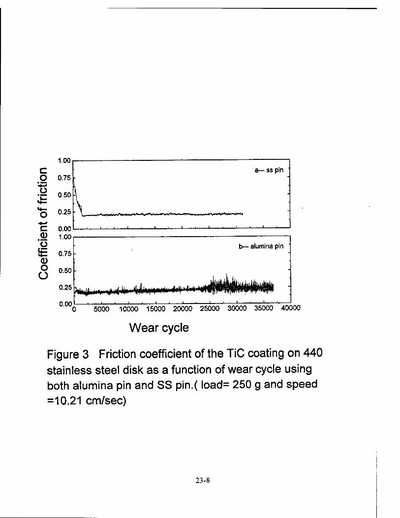
o "'S

• ■MB

Ü E 0 o O

1.00

0.75

0.50

0.25

0.00 1.00

0.75

0.50

0.25

0.00

a— ss pin

.'^■JL*^>hjy»''H'*«'.>'>*l*V0i~'» I~MV*I" t•• i»m mn»i»irri|i iVvrit1'1

■ ■ i ■ ■ ' ■ ' 1 i l

> alumina pin

5000 10000 15000 20000 25000 30000 35000 40000

Wear cycle

Figure 3 Friction coefficient of the TiC coating on 440 stainless steel disk as a function of wear cycle using both alumina pin and SS pin.( load= 250 g and speed =10.21 cm/sec)

23-8

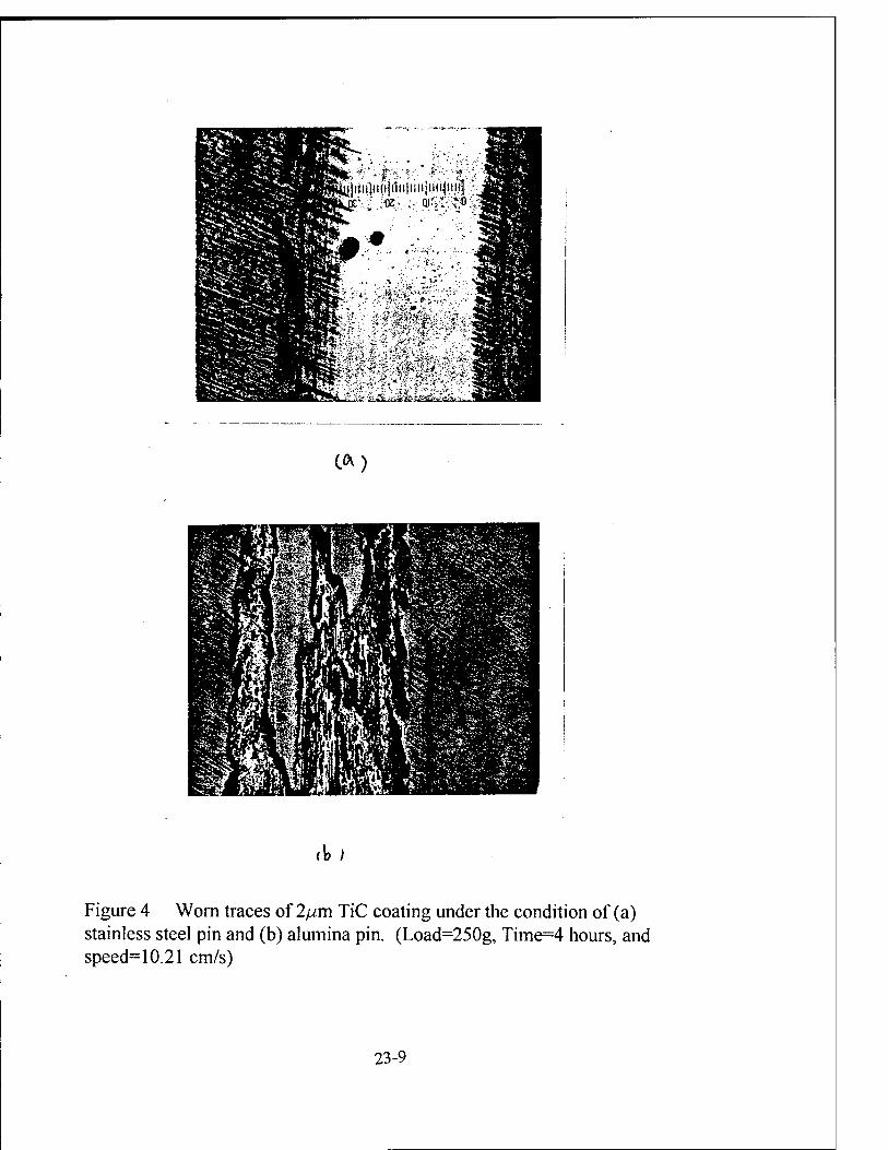
iiijliip|i1ii|iiii|tiiiiii||

..,-, ,■;■. %.';£.-•';*,.. frj' ■:r«*--:-..-..- r'

^iS■■•'£■ '"•' ■;ft5<*,i;\ ■ -J -

*'- -^ A"f ;v.* - ," ,T-' 'St. .;rj»JTr'.l- ,y/■

C<M

(b;

Figure 4 Worn traces of 2^m TiC coating under the condition of (a) stainless steel pin and (b) alumina pin. (Load=250g, Time=4 hours, and speed= 10.21 cm/s)

23-9

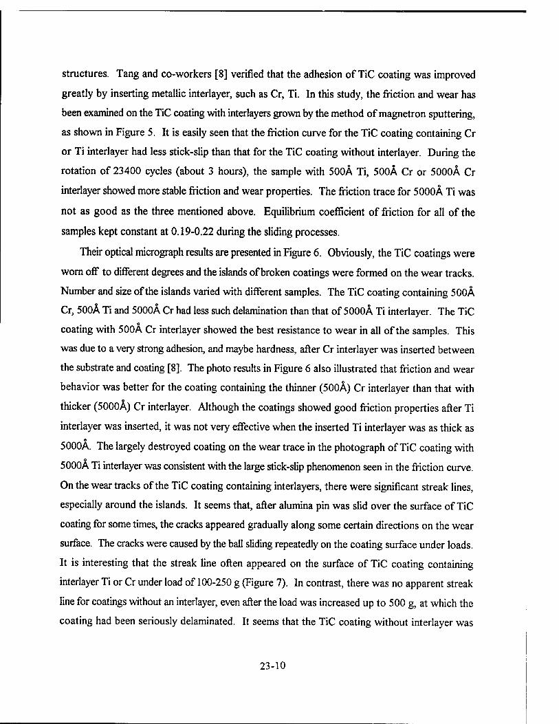
structures. Tang and co-workers [8] verified that the adhesion of TiC coating was improved

greatly by inserting metallic interlayer, such as Cr, Ti. In this study, the friction and wear has

been examined on the TiC coating with interlayers grown by the method of magnetron sputtering,

as shown in Figure 5. It is easily seen that the friction curve for the TiC coating containing Cr

or Ti interlayer had less stick-slip than that for the TiC coating without interlayer. During the

rotation of 23400 cycles (about 3 hours), the sample with 500Ä Ti, 500Ä Cr or 5000Ä Cr

interlayer showed more stable friction and wear properties. The friction trace for 5000Ä Ti was

not as good as the three mentioned above. Equilibrium coefficient of friction for all of the

samples kept constant at 0.19-0.22 during the sliding processes.

Their optical micrograph results are presented in Figure 6. Obviously, the TiC coatings were

worn off to different degrees and the islands of broken coatings were formed on the wear tracks.

Number and size of the islands varied with different samples. The TiC coating containing 500Ä

Cr, 500Ä Ti and 5000Ä Cr had less such delamination than that of 5000Ä Ti interlayer. The TiC o

coating with 500A Cr interlayer showed the best resistance to wear in all of the samples. This

was due to a very strong adhesion, and maybe hardness, after Cr interlayer was inserted between

the substrate and coating [8]. The photo results in Figure 6 also illustrated that friction and wear

behavior was better for the coating containing the thinner (500Ä) Cr interlayer than that with

thicker (5000A) Cr interlayer. Although the coatings showed good friction properties after Ti

interlayer was inserted, it was not very effective when the inserted Ti interlayer was as thick as o

5000A. The largely destroyed coating on the wear trace in the photograph of TiC coating with

5000A Ti interlayer was consistent with the large stick-slip phenomenon seen in the friction curve.

On the wear tracks of the TiC coating containing interlayers, there were significant streak lines,

especially around the islands. It seems that, after alumina pin was slid over the surface of TiC

coating for some times, the cracks appeared gradually along some certain directions on the wear

surface. The cracks were caused by the ball sliding repeatedly on the coating surface under loads.

It is interesting that the streak line often appeared on the surface of TiC coating containing

interlayer Ti or Cr under load of 100-250 g (Figure 7). In contrast, there was no apparent streak

line for coatings without an interlayer, even after the load was increased up to 500 g, at which the

coating had been seriously delaminated. It seems that the TiC coating without interlayer was

23-10

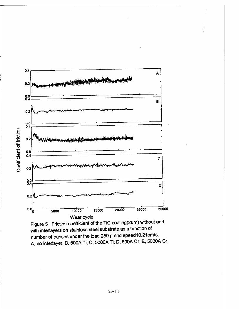
0.4

02

02 \ ^tM^VvJV,|1>ll■l«W^l^■>w>^«*»||«^«■■l'■ v""'"*»>—iv*i'W<*"'>,*"'>

C o

c 0.0

5 0-2

8:2

\j^lJ4J*ff#Wf^^

0.2

0.0 20000 25000 30000 5000 10000 15000

Wear cycle Figure 5 Friction coefficient of the TiC coating(2um) without and with interlayers on stainless steel substrate as a function of number of passes under the load 250 g and speed 10.21 cm/s. A no interiayer; B, 500A Ti; C. 5000A Tl; D, 500A Cr; E, 5000A Cr

23-11

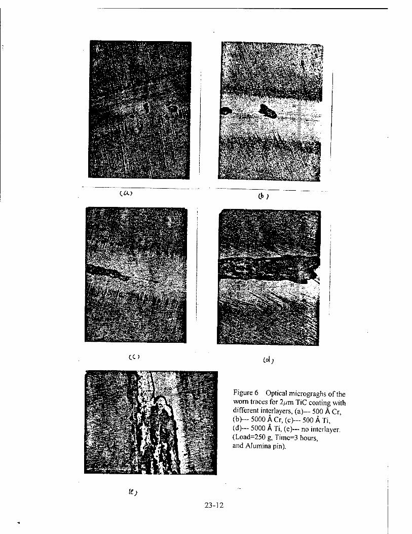
CO.)

CO

CM

Col.

Figure 6 Optical micrograghs of the worn traces for 2/j.m TiC coating with different interlayers, (a)— 500 A Cr, (b)— 5000 A Cr, (c)~- 500 A Ti, (d)-~ 5000 A Ti, (e)— no interlayer. (Load=250 g, Time=3 hours, and Alumina pin).

fc;

23-12

CO.}

lb)

o

Figure 7 Worn traces of 2/^m TiC coating containing (a) 500 A Ti interlayer and (b) without interlayer. (a)— 100 g load (left) and 150 g load (right), (b)— 100 g load.

23-13

directly delaminated because of the weak adhesion between TiC coating and SS substrate, while

coatings containing Ti or Cr interlayer first underwent a process of wear track cracking before

the delamination happened on the contacting surface. This wear track cracking might be

attributed to the existence of softer Ti or Cr interlayers, but the enhanced adhesion due to the

interlayers was able to prevent substantial delamination. The cracks on wear track should be

ominous of the islands for the TiC coating with Ti or Cr interlayer. There was fewer cracked

lines on friction surface of TiC coating with 500Ä Cr interlayer. The surface of TiC coating with

5000A Ti interlayer was seriously scratched after 3 hours of wear. On the other hand, the

alumina pin was also abraded while the TiC coating was worn through. It can be seen in Figure

8 that a large ball scar was formed as the TiC coating was scratched seriously, especially for TiC

coating with 5000Ä Ti interlayer.

Figure 9 is the coefficients of friction of TiC coatings in long distance tests of over 3500

meters (about 10 hours). The tests were done to further examine the friction and wear life of the

coatings. The variation of curves is similar to that of Figure 5. But, the friction for the sample

containing 5000Ä Ti interlayer and without interlayer varied unstably in the later stage of sliding.

Friction coefficient for TiC coating containing 500Ä and 5000Ä Cr interlayers started to increase

after sliding of -3400 meters. Combining with the analysis of optical micrograph of the TiC

coating, as shown in Figure 10, we found that the wear track of TiC coatings was scratched and

delaminated greatly in the experiments, especially for the coating without and with 5000Ä Ti

interlayers, and extended broken coating was formed instead of islands. Although there were

heavy scratch on the surface of TiC coating with 500Ä Ti, 500Ä Cr and 5000Ä Cr interlayers,

their friction coefficients varied still in the range of 0.2-0.3 during the sliding processes. This

indicates that even through part of TiC coating was scratched off in the friction test, some TiC

debris probably filled in the gap between the contacting surface of ball and TiC coating to some

extent such that the friction coefficient increased only slightly. For heavy delamination of the of

the TiC film, the friction coefficient was changed significantly, for example, in the case of TiC

coating without or with 5000Ä Ti interlayer. Similar to the results in Figure 5 and 6, the long

scratch on the wear surface was accompanied with large scars on the ball surface.

The behavior of friction and wear of the TiC coatings could be improved apparently after

23-14

ca> Ck)

(O td>

Figure 8 Optical micrographs of the alumina pin scar coupled with TiC coating containing different interlayers. (a)— 500 A Cr, (b)— 5000 A Cr, (c)- - 500 A Ti, (d)~- 5000 A Ti.

23-15

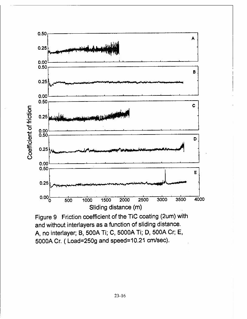
0.00 0.50

0.25

0.00

o

J^^^^^f^d^^^ >r*******j+^>»+»X*r*< . >, n^attr* ̂ "»•

500 1000 1500 2000 2500 3000 3500 4000

Sliding distance (m) Figure 9 Friction coefficient of the TiC coating (2um) with and without interlayers as a function of sliding distance. A, no interlayer; B, 500A Ti; C, 5000A Ti; D, 500A Cr; E, 5000A Cr. ( Load=250g and speed=10.21 cm/sec).

23-16

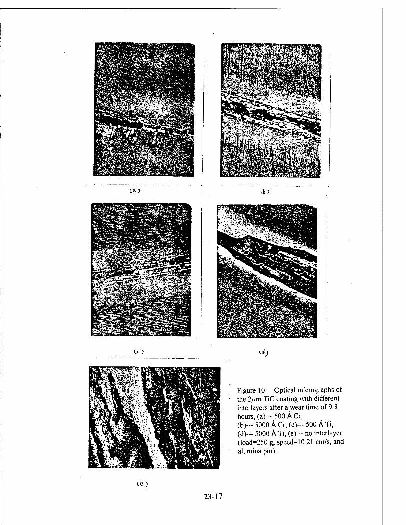
eft) u>>

Bslllisilil as*»**

e^SSS

(.<.;

Figure 10 Optical micrographs of the 2^m TiC coating with different interlayers after a wear time of 9.8 hours, (a)— 500 A Cr, (b)-~ 5000 A Cr, (c)-~ 500 A Ti, (d)— 5000 A Ti, (e)— no interlayer. (load=250 g, speed=10.21 cm/s, and alumina pin).

<-e>

23-17

Ti or Cr element was inserted between TiC films and stainless steel substrates, although the

effects on the tribological properties were different for each kind of the interlayer. The

microstructure of the coatings have been characterized with scanning electron microscopy (SEM)

technique. Figure 11 shows the cross-section features of the 2 /um TiC coatings with the

interlayer 500Ä Cr, 1000Ä Cr, 5000Ä Cr, 500Ä Ti, 1000Ä Ti, and 5000Ä Ti, respectively. The

pictures were magnified by 13,000. The interfaces between the substrate and interlayer Cr or Ti,

and between the interlayer and TiC film can be seen clearly in the figure. It is known that the TiC

is harder than the substrate and interlayer Cr or Ti. Inserting a layer of soft Ti or Cr between the

TiC film and substrate should be able to dissipate the stress due to applied load, which could

enhance the adhesion of the TiC coatings. Compact interfaces between coating, interlayer, and

substrate were seen except the sample with 5000Ä Ti interlayer. The interface between the TiC

coating and the 5000Ä Ti interlayer is not as good as that between the Ti interlayer and the

substrate. This interface quality should have direct effects on the adhesion the coatings. The

friction and wear results discussed earlier reflected this and were consistent with the interface

structural analysis.

Table 1 lists the volume loss of alumina and stainless steel pins sliding over 2.0^m TiC

coating with and without interlayer. Clearly, The rates of volume loss for the worn SS spherical

pin is at lest twice as large as that for the alumina pin. In contrast, the results have also proved

that TiC coating is easier to be worn off using alumina pin than using SS pin. There was no

apparent difference among the TiC coatings with different interlayers and without interlayer as

alumina pin was used in friction experiments. It seems that the volume loss of SS spherical pin

is increased with the increasing of the applied load, especially, there was a large difference in the

rate between 500 g and 50 g.

2.2. 3yum TiC coating

Increase of the thickness of TiC coating should also have a influence on the friction and

wear of the coating. Figure 12 shows the friction coefficient of 3//m TiC coatings without

interlayer and with interlayers, 1000Ä Cr, 1000Ä Ti, and 1000Ä Mo, respectively, as a function

of the number of sliding passes. It is obvious that friction for the coatings with Cr, Ti, as well as

23-18

0613 : 20KUii- X 13^60S Äv 1Hm WD39

( a ) cb;

CC ; Cd)

Figure 11 SEM images of the cross-section of 2yum TiC coating with different interlayers, (a)— 500 A Cr, (b)— 5000 Ä Cr, (c)-~ 500 A Ti, (d)— 5000 A Ti.

23-19

Tabl 1 Volume loss of worn spherical pins coupled with TiC coatings, (a)- stainless steel pin, (b)—alumina pin

(a)

Load (gram) 500 250 100 50

Worn Rate of Pin (mmVH)

2.23X10"4 8.00xl0"5 7.99xl05 3.67xl0"5

£1 Coating Components

2 ßm TiC +5000 A Ti

2 /urn TiC +500 A Ti

2 /j,m TiC +5000 A Cr

2 /urn TiC +500 A Cr

2 fum TiC

Worn Rate (mm3/H)

3.00xl0": 2.97xl0'5 2.99xl0": 2.98xl0"5 3.02xl0":

23-20

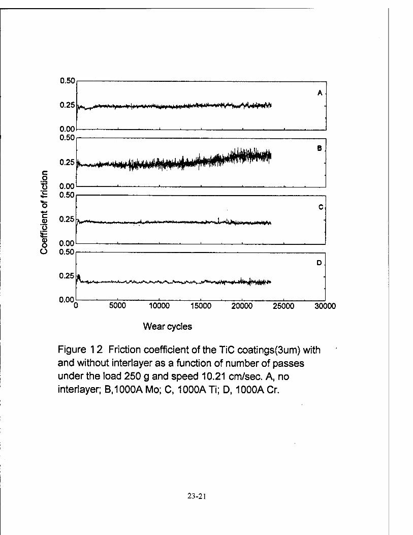
c o

c O

1

0.50

0.25

0.00 0.50

0.25

ys^y» it>*\^fm<* \i",'f* i' i^+r *+4* *#fl<N **< < '»M^^yUHlMjAfl1

'"8 o.oo £ 0.50

0.25

0.00

/W*** •i'ii-«.ii - .- )..'![, ~th-i' *i ii 'Tu H mi. mi

O 0.50

0.25

0.00

^■■»H .^cU^^^/s

A

B

C

5000 10000 15000 20000 25000 30000

Wear cycles

Figure 12 Friction coefficient of the TiC coatings(3um) with and without interlayer as a function of number of passes under the load 250 g and speed 10.21 cm/sec. A, no interlayer; B,1000AMo; C, 1000ATi; D, 1000AO.

23-21

without interlayers were more stable and smooth than that containing Mo interlayer during 23400

cycles of wear. This is probably because of very poor adhesion of the coating containing Mo

interlayer, so that the TiC coating could not adhere to the substrate strongly. The scratch

occurred easily on the TiC coating surface, resulting in increased friction (Figure 12(b)). The

optical micrographs in Figure 13 indicated that the damage on the surface of the TiC coating with

Cr interlayer was the smallest in all of the wear tests, only showing a beginning of the wearing off.

In contrast, TiC coating containing Mo was greatly delaminated. The TiC coating with Ti

interlayer showed nearly the same as that without interlayer in friction and wear, but the former

had smoother friction curve than the latter. When the sliding distance was extended to over 3500

meters, it is concluded further from Figure 14 that TiC coating with Cr (or Ti) interlayer has a

better wear life than the TiC coating without an interlayer. The coefficient of friction of the latter

varied over a large range and increased rapidly in the later stage of wear test. In fact, the optical

micrograph results gave a directly evidence for such observation (Figure 15).

Considering the influence of the thickness of TiC coatings on adhesion and wear, we found

that the TiC coating of 3^m thick was much better than the TiC coating of 2 fim thick.

2.3. 0.2/^m TiC coating

The friction and wear characteristics of the coatings should be affected by applied load,

especially when TiC coating is very thin. Figure 16 and 17 demonstrate the friction as a functions

of the sliding time for the thin TiC coatings (0.2 //m in thickness) containing 200Ä Ti and 200Ä

Cr interlayers, respectively, under different loads. The coefficient of friction of the TiC coating

with Ti interlayer in Figure 16 was stable during the sliding of 3 hours when the load was below

50 g. With increasing load, the friction and wear of the TiC coating became gradually unstable,

especially when load exceeded 100 g, due to the severe delamination of the coating. Similar to

Figure 16, the friction and wear behavior for the TiC coating with Cr interlayer in Figure 17 was

better under a load of 50 g, compared to a load of 100 g.

Summary and Conclusions

The friction, adhesion and wear behaviors have been investigated for the TiC coatings

23-22

cd)

^«^Pl SS&^BsS

cb;

cO cd;

Figure 13 Optical micrographs of the worn traces of 3//m TiC coatingwith different interlayers, (a)— no interlayer, (b)~-1000 A Mo, (c)— 1000 A Ti, (d)— 1000 A Cr. (Load=250 g, time=3 hours, and alumina pin).

23-23

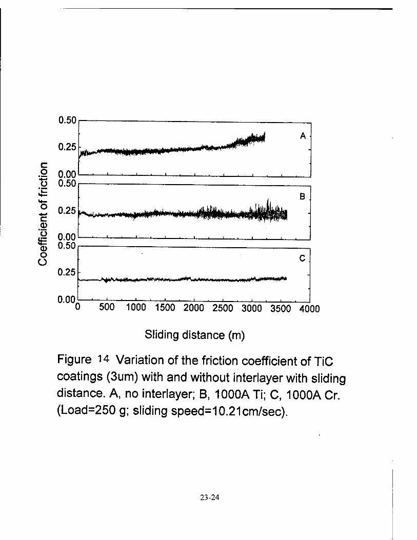
0.50

0.25-

.2 0.00 ü 0.50

■ i ■ ■ ■ -i—1_—i ■

£ o.oo % 0.50 o O

0.25-

0.00

B .

-J 1 1 i L. -I '

>>4SM'»iftni*»i'"

i • i i_

0 500 1000 1500 2000 2500 3000 3500 4000

Sliding distance (m)

Figure u Variation of the friction coefficient of TiC coatings (3um) with and without interlayer with sliding distance. A, no interlayer; B, 1000ATi; C, 1000ACr. (Load=250 g; sliding speed=10.21 cm/sec).

23-24

C*) et;

Figure 15 Worn traces of the 3//m TiC coating with different interlayers after a worn time of 9 hours, (a)— no interlayer, (b)-1000 A Ti, (C)-1000 A Cr. (Load=250 g, speed= 10.21 cm/s, and alumina pin).

CO

23-25

c o

0.50

0.25

8:§8

fr^^^^^w*-^^

•2 0.25 o

| 8:§8 c

Ü 0.00 0.50

0.25

0.00

K^rjtfYQifrb+Ar***»* ■» »<K«bJI{+jj*«byy~H^

B

^ltwwi»r>^s«»fc>

»JVo».n. i* 4*i^»y^|^.'»)"i

150 200 50 100

Wear time (min)

Figure 16 Friction coefficient of the TiC coating(0.2um) with 200 A Ti interlayer as a function of wear time under the different loads, A— 25 g, B— 50 g, C— 100 g, and D— 150 g. (speed=10.21 cm/sec).

23-26

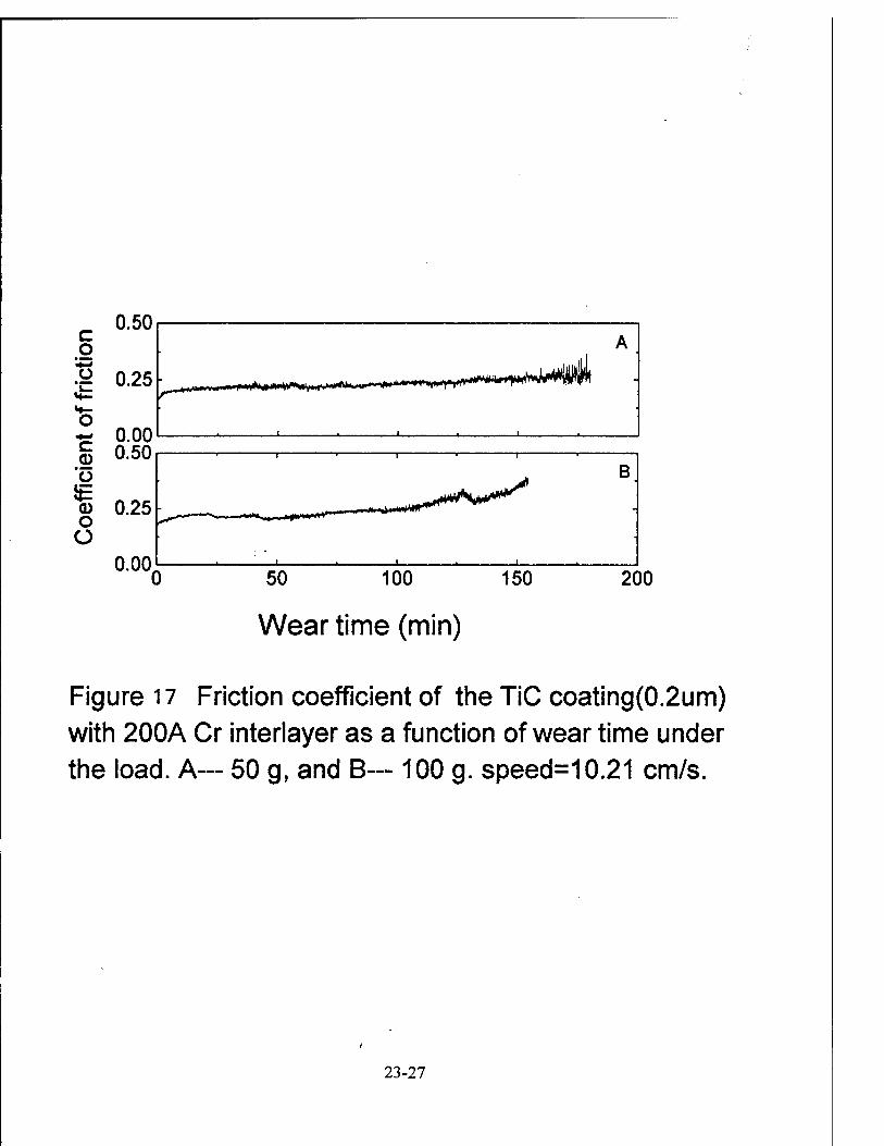
0.50

5 0.25 h

O ~ 0.00 c 0.50

0.00

«TMH^yHHnlftflSll^tH |lnl^>ll|iui •Mmw-rv^*w*w*,1**^^

B

50 100 150 200

Wear time (min)

Figure 17 Friction coefficient of the TiC coating(0.2um) with 200A Cr interlayer as a function of wear time under the load. A— 50 g, and B— 100 g. speed=10.21 cm/s.

23-27

containing different kinds of interlayers (Ti, Cr and Mo) of different thickness using pin-on-disk

configuration, in which both stainless steel and alumina pins were used. The wear tracks of the

TiC coatings and the pins were characterized by both optical microscope or scanning electron

microscope (SEM).

1) The equilibrium coefficients of friction were found to vary between 0.19 and 0.22 for the TiC

coatings as the stainless steel and alumina pins were alternatively used in our experiments. There

was significant stick-slip during the wear tests for TiC/alumina couple. According to their optical

microscopic results, it was found that TiC coating was scratched and apparently worn through

by alumina pins, but only slightly by stainless steel pins. The scars on the alumina pins were much

less severe than the scars on SS pins during the wear test. The rate of volume loss of SS pins

was more than twice ofthat of alumina pins.

2) Inserting Cr or Ti interlayer between 2 //m TiC coating and substrate can improved greatly

the adhesion and wear. It is found that the TiC coatings containing 500Ä Cr, 5000Ä Cr, 500Ä

Ti and 5000A Ti interlayers showed more stable and smoother friction than that without interlayer

during 3 hours of sliding test. The microscopic analyses further indicated the coating with 500Ä

Cr, 500Ä Ti, 5000Ä Cr and 5000Ä Ti interlayers had stronger adhesion and better wear than the

coating without interlayer. The TiC coating with 500Ä Cr interlayer performed better than that

of 5000Ä Cr interlayer in friction and wear tests. The same was found to be true for the Ti

interlayer, i.e., thinner interlayers performed better in the adhesion and wear tests. This is

probably due to the improved lattice match between the TiC coatings and the interlayers when

the interlayer thickness was reduced.

3) When the friction test was extended to about 10 hours long, that is, the sliding distance of

over 3500 meters, the TiC coating with 500Ä Cr, 500Ä Ti and 5000Ä Cr interlayers maintained

good friction and wear behavior, but the TiC coating with 5000Ä Ti or without interlayer did not.

The wear surface of the latter has been destroyed much more seriously than that of the former.

4) The wear resistance of the TiC coatings could be increased by changing their thickness from

0.2 ßm. to 2 urn, and to 3 fum. This was closely related to the load bearing capability of coatings

of different thickness. The friction and wear behaviors of the thin TiC coating was easily affected

by applied load. For load of 150 g or above, the 0.2/^m TiC coating with 0.02yum Cr or Ti

23-28

interlayer could be destroyed by alumina pins in a short sliding time.

5) During 3 hours (about 23400 cycles) of sliding tests of 3 ^in-thick TiC coatings with 1000Ä

Cr, 1000Ä Ti and 1000Ä Mo interlayers, it is found that TiC coatings with Cr or Ti interlayers

have much stable and smooth friction and wear behavior, compared to that containing Mo

interlayer. This is because of the poor stress bearing capability of the porous Mo film deposited

at low temperature. The degree of delamination on the surface of TiC coating with Cr interlayer

was the smallest in all of the samples.

23-29

References

1. J. C. Angus and C. C. Hayman, Science 241, 913(1988).

2. L. Kempfer, Mater. Eng. 108, 28(1991).

3. G.Georgiev, N. Feschiev, D. Popov and Z. Uzuuov, Vacuum, 36(1986)595.

4. J. F.Sundgren, B. O. Johansson and S. E. Karlsson, Thin Solid Films, 105(1983)353.

5. O. Rist and P. T. Murray, Mater. Lett., 10(1991)322.

6. M. S. Donley, J. S. Zubinski, W. J. Sessler, V. R Dyhouse, S. D. Walck and N. T. McDevit,

Matter. Res. Soc. Symp. Proc. 236(1991)461.

7. W.J. Sessler, M. S. Donley, J. S. Zabinski, S. D. Walck and V. J. Dyhouse, Surface and

Coatings Technology, 56(1993)125-130.

8. Jinke Tang Jeffrey S. Zabinski and J. E. Bultman, Surface and Coatings Technology, (1997)

In press.

23-30

DEVELOPMENT OF MASSIVELY PARALLEL EPIC HYDROCODE IN CRAY T3D USING PVM

C.T. Tsai Associate Professor

Department of Mechanical Engineering

Florida Atlantic University 777 Glades Road

Boca Raton, FL 33431

Final Report for: Summer Faculty Research Program

Wright Laboratory



and

Wright Laboratory

December 1996

24-1

DEVELOPMENT OF MASSIVELY PARALLEL EPIC HYDROCODE IN CRAY T3D USING PVM

C.T. Tsai Associate Professor

Department of Mechanical Engineering Florida Atlantic University

Abstract

The objective of this report is to verify the feasibility of converting a large sequential EPIC

hydrocode into a massively parallel EPIC hydrocode in terms of computational speed. Sequential

subroutines in the Research EPIC hydrocode, a Lagrangian finite element analysis code for high

velocity elastic-plastic impact problems, are individually converted into parallel code using Cray

Adaptive Fortran (CRAFT). The performance of massively parallel subroutines running on 32

PEs on Cray-T3D is faster than their sequential counterparts on Cray-YMP. At next stage of the

research, Parallel Virtual Machine (PVM) directives is used to develop a PVM version of the

EPIC hydrocode by connecting the converted parallel subroutines running on multiple PEs of

T3D to the sequential part of the code running on single PE. With an incremental increase in the

massively parallel subroutines into the PVM EPIC hydrocode, the performance with respect to

speedup of the code increased accordingly. The results indicate that significant speedup can be

achieved in the EPIC hydrocode when most or all of the subroutines are massively parallelized.

24-2

DEVELOPMENT OF MASSIVELY PARALLEL EPIC HYDROCODE

IN CRAY T3D USING PVM

C. T. Tsai

1 INTRODUCTION

The aim of research and development of weapon systems is to develop one which can

respond quickly to the combat needs of operational commanders. Presently, warhead

design involves expensive and time consuming tests done on prototypes. The computer

simulation of warhead penetration can save huge amounts of money and time on warhead

design. The simulation of complex penetration behavior requires large amount of CPU

time, even when run on fast vector processor machine like the Cray-YMP. The EPIC

hydro code is used, at the Armament Directorate of Air Force Wright Laboratory, to solve

high velocity elastic-plastic impact problems involved in warhead design.

The primary objective of the thesis was to verify the feasibility of converting a large

finite element analysis code into a massive parallel finite element code in terms of

computational speed and cost. The Research EPIC hydro code , a Lagarangian finite

element analysis code, was selected for parallization. A computational intensive

algorithm, a large data set and a liberal data distribution policy was a motivation for

parallelizing the EPIC code. The Cray-T3D was chosen as the MPP platform as it

supports MIMD/SPMD model, CRAFT programming model and PVM message passing

programming model. More importantly, it is closely coupled with other Cray PVP

systems like Cray-YMP on which the EPIC code is already developed. Related goals

included developing an incremental approach of parallization using PVM message

passing paradigms and identifying CRAFT parallization techniques best suited for the

EPIC subroutines.

24-3

The next section gives a brief introduction to parallel processing and its various

applications. Chapter 2 describes the EPIC theory. Cray-T3D architecture and MPP

programming model is discussed in Chapter 3. Chapter 4 states the performance results of

the individual parallel subroutines. Chapter 5 describes the incremental approach and

porting of EPIC subroutines using PVM. Chapter 6 contains the implementation of EPIC

hydro code using heterogeneous PVM. Chapter 7 include conclusions and future work.

1.1 INTRODUCTION TO PARALLEL PROCESSING

The ever increasing computational needs of emerging applications have been the

primary motivating factor for the steady increase in speed of the traditional serial

computers. However, fundamental physical limitation imposed by the speed of light

makes it impossible to achieve further improvements in speed of serial or single

processor computers infinitely. Recent trend show that the performance of these

computers is beginning to saturate. ( It is often remarked that speeds of basic

microprocessor grow by a factor of 2 every 18 months; this empirical observation, true

over many years, is called Moore's law.). A natural way to circumvent this saturation is to

use an ensemble of processors to solve problems [1].

Parallel processing, the method of having many small tasks solve one large problem,

has emerged as a key enabling technology in modern computing. The past several years

have witnessed an increasing acceptance and adoption of parallel processing, for both

high performance scientific computing and for more general purpose applications, was a

result of the demand for higher performance, lower cost and sustained productivity. The

acceptance of parallel processing has facilitated two major developments: massive

parallel processors(MPPs) and the use of distributed computing.

A massively parallel processing (MPP) machine combine a few hundred to a few

thousand CPUs in a single large cabinet connected to hundreds of Gbytes of memory.

MPPs offer enormous computational power and are considered to be one of the most

powerful computers in the world. MPPs are used to solve computational Grand challenge

24-4

problems such as global climate modeling, determining molecular, atomic and nuclear

structures. As simulations become more realistic, the computational power required to

produce them grows rapidly and that is when MPPs come into picture.

The second major development affecting scientific problem solving is distributed

computing. Distributed computing is a process whereby a set of computers connected by

a network are used collectively to solve a single large problem. As more and more

organizations have high speed local area networks interconnecting many general purpose

workstations, the combined computational resources may exceed the power of a single

high performance computer. In some cases, several MPPs have been combined using

distributed computing to produce unequaled computational power [2].

1.2 MOTTVATTON AND APP1 IC ATTONS FOR PARALLEL COMPUTING

The traditional scientific paradigm is first to do theory, and then lab experiments to

confirm or deny the theory. The traditional engineering paradigm is first to do a design

and then build a laboratory prototype. Both paradigms are being replaced by numerical

experiments and numerical prototyping for the following reasons: real phenomena are too

complicated to model on paper (e.g. climate prediction) and real experiments are too hard

and too expensive for a laboratory (e.g. oil reservoir simulation, large wind tunnel,

overall aircraft design etc.).

Scientific and engineering problems requiring the most computing power to simulate

are commonly called "Grand Challenges", like predicting the climate few years hence, are

estimated to require computers computing at the rate of 1 Tera flops (i.e., 1012 floating

point operations per second), and a memory size of 1 TB (Tera Byte). One of the "Grand

Challenge" climate modeling problem is illustrated. In a simplified climate model,

climate is defined as function of 4 arguments: longitude, latitude, elevation and time. This

in turn, returns a vector of 6 values: temperature, pressure, humidity, and wind velocity (

3 variables actually). To represent the continuos function in the computer, the domain is

descretized and climate is evaluated for the arguments lying on a grid: climate (i, j, k, n),

24-5

where t = n*dt, where dt is a fixed time step, n an integer, and i, j, k are integers indexing

the longitude, latitude and elevation grid cells, respectively.

An algorithm to predict the weather (short term) or climate (long term), is a function

which maps the climate at time t, Climate (i, j, k, n), for all i, j, k, to the climate at the at

the next time step t+dt, climate (i, j, k, n+1), for all i, j, k. The algorithm involves a

system of equations including, in particular the Navier-Stokes equations for the fluid flow

of gases in the atmosphere. Then, the earth's surface is discretized into 1 kilometer by 1

kilometer cells in the latitude -longitude direction, and 10 cells in the vertical direction.

From the surface area of the earth, we can compute that there are about 5*109 cells in the

atmosphere. With six 4-byte words per cell, the memory requirement is about 0.1 TB.

Assuming, it takes 100 flops to update each cell by one minute. Or in other words, if

dt = 1 minute, and computing climate (i, j, k, n+1) for all i, j, k from climate (i, j, k, n)

take about 100*5*109 or 5*1011 floating point operations. For such kind of

computations, the computing speed has to be atleast 8 Gflops. Weather prediction

(computing 24 hours to compute the weather 7 days hence), requires computing 50*12 =

600 times faster, or 4.8 Tflops machine.

The actual grid resolution used in climate modeling today is about 4 degrees latitude

by 5 degrees of longitude (about 460 km by 560 km), a rather coarse resolution. A near

term goal is to decrease this grid size using parallel computing techniques, such that

different grid data are stored in different processors and relevant simultaneous equations

are solved parallely on different processors [3].

Selected application areas in the field of parallel computing are as follows:

• Weather and Climate

0 Prediction of weather, climate and global change

• Biology

24-6

0 Determination of molecular, atomic and nuclear structure.

0 Mapping the human genome and understanding the structure of biological

macromolecules.

• Mechanical Engineering

0 Finite element Methods.

0 Particle methods in aerospace.

0 Understanding turbulence, pollution dispersion and combustion system.

0 Computational Fluid Dynamics.

• Chemical Engineering

0 Gas hydrate simulation.

0 Simulation of fluids in pores.

• Environmental modeling

0 Modeling whole ecosystems.

0 Assessment of pollution remediation.

• Material science

0 Understanding the nature of new materials.

0 Exploring theories of matter.

• Demography

0 Interactive access to large databases.

1.3 CLASSIFICATION OF PARALLEL COMPUTERS

Parallel computers are classified based on various dimensions like control

mechanism, address-space organization, interconnection network and granularity of

processors.

1.3.1 BASED ON CONTROT MECHANISM

Parallel computers are classified as single instruction stream, multiple data stream

(SIMD) and multiple instruction stream, multiple data stream (MIMD). Processing units

in parallel computers either operate under the centralized control of a single control unit

24-7

or work independently. In architectures referred to as SIMD, a single control unit

dispatches instructions to each processing unit. Here, the same instruction is executed

synchronously by all processing units. Examples of SIMD parallel computers are MasPar

MP-1, MasPar MP-2, MPP, DAP and CM-2. Computers in which each processor is

capable of executing a different program independent of the other processors are called

multiple instruction stream, multiple data stream (MIMD) computers. Example of MIMD

computers are Cosmic Cube, nCUBE-2, iPSC, CM-5, Paragon XP/S and Cray-T3D.

SIMD computers require less hardware than MIMD as they have only one global

control unit. SIMD also requires less memory as only one copy of the program needs to

be stored. In contrast, MIMD computers store the program and operating system at each

processor. SIMD computers are naturally suited for data parallel programming. Though

individual processor in an MIMD computer are more complex, general purpose

microprocessors may be used. Hence, due to the economy of scale, processors in MIMD

computers are both cheaper and more powerful than processors in SIMD computers.

P& Prcccuiflg Ekrntnl

(«)

Figure 1-1: (a) Typical SIMD architecture and (b) Typical MIMD architecture

1,3.2 BASED ON ADDRESS-SPACE ORGANIZATION

Solving a problem on an ensemble of processors requires interaction among

processors. Message Passing and shared address space architectures provide two different

means of processor interaction. In a message passing architecture, processors are

24-8

connected using a message passing interconnection network. Each processor has its own

memory called local memory, which is accessible only to that processor. Processors can

interact only by passing messages. It is also referred to as distributed memory

architecture. Examples include nCUBE-2, CM-5, Cosmic Cube and Paragon XP/S. The

shared addressed space architecture provides hardware support for read and write access

by all processors to a shared addressed space. Most shared address space computers

contain a shared memory that is equally accessible to all processors through an

interconnection network. These architectures are called shared memory parallel

computers. Examples include C.mmp and NYU Ultracomputer. A drawback of these

architectures is that the bandwidth of the interconnection network must be substantial to

ensure good performance. The Cray-T3D is a logically shared, physically distributed

memory.

INTERCONNECTION NETWORK

M

Figure 1-2: Message Passing architecture

F H i

'; lnter-

! connection

i Network

i

■ ■

"

1- "

M p

Pj

Inter-

connection

Network

M Ml

P 1 M

_Ml

Pi M "T"

j

Ml

P: Processor

M: Memory

Figure 1-3: Shared-address space architectures

24-9

1.3.3 BASED ON INTERCONNECTION NETWORKS

Shared address space computers and message passing computers can be constructed

by connecting processors and memory units using a variety of interconnection networks.

Classification of parallel computers based on interconnection networks are static and

dynamic. Static networks consists of point to point communication links among

processors and are also referred to as direct networks. Static networks are typically used

to construct message passing computers. Dynamic networks are built using switches and

communication links. Communication links are connected to one another dynamically

using switching elements to establish paths among processors and memory banks.

Dynamic networks are referred to as indirect networks and are normally used to construct

address space computers.

1.3.4 BASED ON INTERCONNECTION NETWORKS

A parallel computer may be composed of a small number of very powerful processors

or a large number of relatively less number of processors. Processors belonging to the

former class are called coarse-grain computers, and those belonging to the later are called

fine-grained computers. Examples of coarse-grain computers are Cray-YMP, Cray-C90

which offer a small number of processors each capable of several Gflops and in contrast,

a fine grain computer, examples like CM-2, MasPar MP-1 and MasPar MP-2, offer a

large number of relatively slow processors. MasPar MP-1 contains up to 16,384 four-bit

processors. There is also a class of parallel computers between the extremes and are

called medium grain computers, include CM-5, nCUBE-2 and Paragon XP/S.

The granularity of a parallel computer can be defined as the ratio of the time required

for a basic communication operation to the time required for a basic computation. Parallel

computers for which this ratio is small are suitable for algorithms requiring frequent

communication: that is, algorithm in which the grain size of the computation is small.

Since such algorithms contain fine-grain parallelism, these parallel computers are often

called fine-grained parallel computers. In contrast, parallel computers for which this ratio

is large are suited for algorithms that do not require frequent communication. These

24-10

computers are referred to as coarse-grain computers. According to this criterion, multi

computers such as the nCUBE 2 and Paragon XP/S are coarse grain computers, whereas

multiprocessors such as the C.mmp, TC-2000 and KSR-1 are fine grain parallel

computers. The Cray-T3D is a moderately coarse parallel computer.

24-11

2. EPIC RESEARCH HYDRO CODE

2.1 EPTC THEORY

There are many different computer codes available to calculate dynamic response to

impact. For impact problems involing elastic-plastic flow with large displacements, the

solutions have most often been obtained with Lagrangian code. The EPIC code is also an

Lagrangian FEA code developed bv Dr. G.R. Johnson et al, of Alliant Techsystems Inc. It

takes advantage of the fact that triangular or tetrahedral element formulation is better suited

to represent the severe distortions than is the traditional quadrilateral or hexahedral finite

difference methods [4,5].

The finite element method is implemented in the following steps:

• The geometry of the problem is represented with elements of triangular cross-section

having specific material characteristics.

z AXIS OF REVOLUTION

ASSEMBLAGE OF ELEMENTS

NODE I ___—-TTT ^ I DISPLACED

J *C£^r£ Is ' GEOMETRY

i ^ELEMENT

Figure 2-1: Geometric properties of triangular elements

• The distributed mass at the nodes is lumped. The initial velocities to represent the

motion at impact is assigned.

24-12

The lumped mass in each of three node is:

Mi = Mj = Mm = (l/3)VoP0

where V0 and r0 are initial volume and density of the element.

• Numerical integration loop works as follows:

0 The strain and strain rates in the elements are determined.

1/2

(2/9) {(sr - ej + (sr - sef + (s, - sof + (3/2)r$\

where e is equivalent strain, Sr > se, ez, and y^ are strains relative to system axes.

0 Stresses in the element are determined. The stresses consists of elastic stresses, plastic

deviator stresses, hydrostatic pressure, and artificial viscosity.

Elastic stresses are obtained by Hooke's law.

(jr = Xsv + 2Gsr - Q

(jz = Ä£v + 2G sz - Q

oe = Ä£v + 2G se - Q

Tn = Gyn

where ov,crz,cr0,andrrc are radial, axial, circumferential, and shear stresses, and X

and G are Lame's elastic constants.

These stresses are combined to form equivalent stress a.

24-13

o- = [(1/2) {(ar - aj + (ar - o0f + (ot - a0f + **„}]'"

This stress represents the overall state of stress within the element.

Plastic flow begins when the elastic strength of materials is exceeded. When this

occurs, the normal stresses are obtained by combining hydrostatic pressure with

the plastic deviator stresses and the artificial viscosity.

Or = Sr - (P + 0)

GZ = Sz - (P + Q)

Ge = sg - (P + Q)

where Sr^-and^ are the plastic deviator stresses, P is hydrostatic pressure and Q

is the artificial viscosity. The plastic deviator stresses represent the shear strength

characteristics of the material.

The hydrostatic pressure is determined from the Mie-Gruneisen equation of state.

P = (KJM + K2JU2 + KsM3)P - TM/2)J + TpoE

where

M = (p/Po) - 1 = (Vo/V) - 1

The specific internal energy, E, is obtained from the work done on the element by

various stresses, Ki,K.2,3n&K.3 are material dependent constants and is the

Gruneisen coefficient.

24-14

The artificial viscosity is combined with the normal stresses to damp out localized

oscillations of the concentrated masses. It is applied only when volumetric strain

rate is negative.

Q = &.[(*> + 2G)pA}l/2\ev\ + CopMevf forev < 0

Q = OforiTv > = 0

where recommended value of coefficients are CL = 0.5 and Co =4.0.

0 Equivalent concentrated forces that act on nodalmasses is determined. The radial

and axial forces, Fri and Fzi, acting on node i of an element are:

Fn = - nr[(Zj - zjcir + (rm - rj)rj - (2/3)nAGe

Fzi = - m[(rm - rj)c7z + (zj - zm)xnJ

where the nodal coordinates represent the displaced geometry.

0 Intergration time increment is determined.

Maintaining a numerically stable solution for dynamics problem is generally

accomplished bv using a numerical integration time increment which is sufficiently

less than the lowest period of vibration of the system.

0 Equation of motion to the nodes are applied for integration time increment. The

equations of motion can be numerically integrated by assuming a constant

acceleration for each time increment. The radial acceleration for each time

increment. The radial acceleration of node I at time T is:

Ü, = CLFri/^Mi)

The new displacement at time = t + Dt is

24-15

ut+* = ut + ütAt + (l/2)üt(Atf

and the new velocity is

Üt+At = Üt + Üt^t

The equation of motion for the axial direction have a similar form. After the

equation of motion are numericallv integrated, an integration cycle is complete.

The numerical intergration loop is repeated until the time of interest is elapsed.

24-16

3. PARAIXET PROGRAMMING TECHNIQUES ON CRAY-T3D

3.1 BACKGROUND

The first step in parallel programming is the development of the parallel algorithm to

solve a problem. There are two different approaches to algorithm development. The first

approach is when a sequential algorithm is already present and with minor modifications

can be changed into a parallel program using parallel programming paradigms. The first

approach may not succeed in many cases where the sequential algorithm has too many

bottlenecks. In that case, parallel algorithm has to be developed which may have totally

different approach as the sequential algorithm.

To run a parallel algorithm on a parallel computer, one needs to implement them on a

programming language. In addition to providing all the functionality of a sequential

language, a language for programming parallel computers must provide mechanisms for

sharing information among processors. It must do so in a way that is clear, concise, and is

readily accessible to the programmer. Different parallel programming languages enforce

different programming paradigms. The variations among paradigms are motivated by

several factors. First, there is a difference in the amount of effort invested in writing

parallel programs. Some languages require more work from the programmer, while others

require less work but yield less efficient code. Second, one programming paradigm may

be more efficient than others for programming on certain parallel programming

architectures. Third, various applications have different types of parallelism, so different

programming languages have been developed to exploit them.

3.2 CRAY-T3D ARCHITECTURE OVERVIEW

The introduction of Cray-T3D by CRI in late 1993 has been a significant event in the

field of massively parallel supercomputing. The T3D promises a major advance in highly

parallel hardware with respect to low latency (1 micro second) and high bandwidth (125

MB/sec) interconnect. The Cray-T3D is scalable to 2048 processor elements and 300

Gflops. It is a multiple instruction multiple data (MIMD) architecture machine. It has a

24-17

logically shared and physically distributed DRAM. Cray-T3D has a two-tier architecture

consisting of macro architecture and micro architecture.

Figure 3-1: Cray-T3D two tier architecture

3.2.1 MTCRO ARCHITECTURE

The micro architecture will vary as technologies advance to achieve Tflops of

sustained performance. Micro architecture refers to the microprocessor chip used in the

Cray-T3D. For its first generation machines (T3D), CRI choose DEC chip 21064 (Alpha

chip) for its performance, features, technology and availability. The alpha chip consists of

four main components BOX, EBOX, FBOX and ABOX.

(a) Central control unit (IBOX): The ffiOX performs instruction fetch, resource

checks, and dual instruction issue to the EBOX, ABOX and FBOX or branch unit. It

handles pipeline stalls, aborts and restarts.

(b) Integer execution unit (EBOX): The EBOX contains a 64-bit fully pipelined

integer execution data path including adders, logic box, barrel shifter, byte extract and

mask, and independent integer multiplier. In addition, it contains a 32 entry 64-bit integer

register file.

(c) Floating point unit (FBOX): The FBOX contains a fully pipelined floating point

unit and independent divider, supporting both IEEE and VAX floating point data types.

24-18

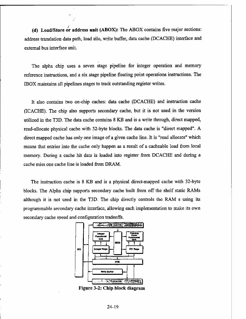
(d) Load/Store or address unit (ABOX): The ABOX contains five major sections:

address translation data path, load silo, write buffer, data cache (DCACHE) interface and

external bus interface unit.

The alpha chip uses a seven stage pipeline for integer operation and memory

reference instructions, and a six stage pipeline floating point operations instructions. The

IBOX maintains all pipelines stages to track outstanding register writes.

It also contains two on-chip caches: data cache (DCACHE) and instruction cache

(ICACHE). The chip also supports secondary cache, but it is not used in the version

utilized in the T3D. The data cache contains 8 KB and is a write through, direct mapped,

read-allocate physical cache with 32-byte blocks. The data cache is "direct mapped". A

direct mapped cache has only one image of a given cache line. It is "read allocate" which

means that entries into the cache only happen as a result of a cacheable load from local

memory. During a cache hit data is loaded into register from DCACHE and during a

cache miss one cache line is loaded from DRAM.

The instruction cache is 8 KB and is a physical direct-mapped cache with 32-byte

blocks. The Alpha chip supports secondary cache built from off the shelf static RAMs

although it is not used in the T3D. The chip directly controls the RAM s using its

programmable secondary cache interface, allowing each implementation to make its own

secondary cache speed and configuration tradeoffs.

BIU

|- . ds^^tuessssaiäsm'l T

Intagw Functions!

Unit

«ox

Homing

Functional Unit

I ' J IntflQcr RSQS RP.Rogs

t i ....

» » | OTB |

L

h 1

.

Writ* Buffer

~iTT*S ocACHE: '3$üf&8

Figure 3-2: Chip block diagram

24-19

3.2.2. STNGLE PE OPTIMIZATION

Optimization of a code for a single PE on the Cray-T3D is more difficult than for the

other Cray PVP system processor like C90 because of the following: optimizations are

state dependent, data locality is always the issue, bandwidth is a limitation factor, not as

many functional units are pipelined, compilers and various tools are not as matured as

those available on C90. The following are the problems associated with the Alpha chip

used in Cray-T3D: (a) all memory operations stall upon cache miss, (b) the slow external

bus makes the DRAM bandwidth sub-optimal, (c) there are no integer to floating point or

SQRT instructions, (d) divide and integer multiply are not pipelined. A division operation

produces one result every 64 clock periods and integer multiply produces one result every

20 clock periods.

Every DRAM request results in a cache line load of four 64-bit words - one for the

actual request and the other three words which are mapped to the same cache line.

Aligning data on the same cache line boundary (word 0 of any cache line) enhances the

performance. The cache alignment can be done by using a compiler directive CDIR$

CACHEALIGN. Performance can also be enhanced by scalar replacement, by holding

the value of a temporary scalar in a register to reduce the number of memory accesses.

Cache utilization can also be enhanced by loop interchange so that stride in the inner loop

is one. Large stride in the inner loop causes cache misses. The DRAM memory of the

alpha chip is interleaved and one should ensure page boundary alignment. Page hit occurs

when either current or previous references are to the same even or same odd page, or

current and previous references have different chip select (cs) bit. Page miss occurs when

current and previous references are to the different odd pages. Page hits take 8 clock

periods whereas a page miss takes 22 clock periods.

3.2.3. MACRO ARCHITECTURE

The macro architecture of the Cray-T3D is bases on 3D-torus. It will remain the same

in all the three phases of the MPP project. The macro architecture will be stable from one

24-20

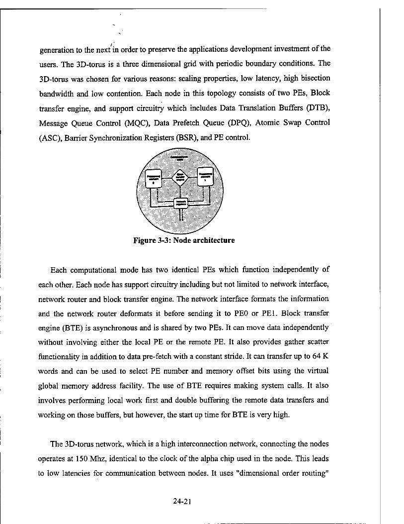
generation to the next in order to preserve the applications development investment of the

users. The 3D-torus is a three dimensional grid with periodic boundary conditions. The

3D-torus was chosen for various reasons: scaling properties, low latency, high bisection

bandwidth and low contention. Each node in this topology consists of two PEs, Block

transfer engine, and support circuitry which includes Data Translation Buffers (DTB),

Message Queue Control (MQC), Data Prefetch Queue (DPQ), Atomic Swap Control

(ASC), Barrier Synchronization Registers (BSR), and PE control.

Figure 3-3: Node architecture

Each computational mode has two identical PEs which function independently of

each other. Each node has support circuitry including but not limited to network interface,

network router and block transfer engine. The network interface formats the information

and the network router deformats it before sending it to PEO or PEL Block transfer

engine (BTE) is asynchronous and is shared by two PEs. It can move data independently

without involving either the local PE or the remote PE. It also provides gather scatter

functionality in addition to data pre-fetch with a constant stride. It can transfer up to 64 K

words and can be used to select PE number and memory offset bits using the virtual

global memory address facility. The use of BTE requires making system calls. It also

involves performing local work first and double buffering the remote data transfers and

working on those buffers, but however, the start up time for BTE is very high.

The 3D-torus network, which is a high interconnection network, connecting the nodes

operates at 150 Mhz, identical to the clock of the alpha chip used in the node. This leads

to low latencies for communication between nodes. It uses "dimensional order routing"

24-21

for propagation of messages. The network channels are 16 bits wide and can send

simultaneously bi-directional in all three directions (X, Y and Z). The bandwidth of the

channel is 300 Mbytes/s. The bisection bandwidth with 1024 PEs is 75 GBytes/s. For

node to node message passing, the minimum measured latency is 1.3 microseconds. The

network has hardware synchronization primitives which lends to fast synchronization or

barriers. The T3D network transmits system control information and user data. The

control packets vary in size from 6 to 16 bytes. The data packets range in size from 16

bytes to 52 bytes. The amount of data in these packets is 8 or 32 bytes with the remainder

being header and checksum information. The headers and checksums contribute to a load

factor which affects attainable data transfer rates [6]. mtarconnacr

natwork

Spare

VOnoda-

Figure 3-4: Cray-T3D topology

3.3 MPP PROGRAMMING MODFT,

The MPP programming model [7] for the Cray-T3D system supports several styles of

programming - data parallel, global address, work sharing and message passing. These

styles may be individually used or combined in the same program. This model allows the

user a range of control over the MPP hardware. This range extends from a low level

control in which the programmer makes almost all of the decisions about how data and

work are partitioned and distributed, to a high level of control where the programmer

identifies where parallelism is located and lets the system determine best how to exploit

it. The important elements of this programming model are access and placement of data,

24-22

parallel execution, local execution, work sharing, synchronization primitives, sequential

I/O, subroutine interfaces and special intrinsic functions.

3.3.1. DATA PAB AI.I.FJ, MODEL

The MPP programming model distinguishes data objects into two categories :

(1) private data (PE_PRIVATE), that are private to a task

(2) shared data (SHARED), that are shared among all the tasks.

Private data objects reside on each PE, rather than spreading one copy over all of

them. They are not accessible to any other task. The task that references a private object

references its own private version of that object and therefore it is possible for private

data objects associated with different PEs to have different values.

Shared data objects, on the other hand, are accessible to all tasks. They are not

replicated and in case of arrays be distributed across multiple Pes.

In data parallel programming, data such as scalar or array are distributed over the

memories of the PEs working on the program. In this programming model, the goal is to

let as many PEs as possible perform on its own data (residing in its memory) rather than

working on the data that is residing in another PE's memory.

In CRAFT, the data distribution is indicated by the compiler directives PE_PPJVATE

and SHARED. Data that are not explicitly declared to be shared is, by default, private

data. Variables and arrays can be explicitly declared as private with the PE_PPJVATE

directive.

CDIR$ PE PRIVATE varl, var2 ... varn

24-23

All private data objects may be DATA initialized except those that occur in blank

common, dummy arguments, automatic arrays, and those whose size is a function of

N$PES (number of tasks).

The shared data objects are declared with the SHARED directive.

CDIR$ SHARED arrayI(distl),array2(dist2) ...arrayn(distn)

The shared directive names the variables that are to be shared data objects and

specifies the distribution across the PEs. Shared data object's distributions fall into two

categories : shared scalars and dimensional distribution. Scalar variables are always

allocated on a single PE, which may differ for different processor elements. Dimensional

distribution includes the following: Cyclic distribution, Generalized distribution, Block

distribution and Degenerate distribution.

Cyclic distribution (:BLOCK(l)) assigns one element of shared array to each PE,

returning to the first PE when every PE has an element. Generalized distribution

(:BLOCK(n)) assigns blocks of 'n' elements of the array to successive PEs, where 'n' has

to be an integer power of 2. The block distribution (:BLOCK) divides an array dimension

into N$PES blocks and allocates one block to each PE. The block size equals to array size

divided by N$PES. Degenerate distribution (:) forces an entire dimension to be allocated

on a single PE.

3.3.2. WORK SHARING

Executing the statements of program in parallel, and in the same PEs in which the

data is distributed achieves higher performance for the Cray MPP system. Work sharing

is achieved primarily by two ways: automatic arrays and shared DO loops.

Fortran array syntax or automatic arrays is one way to distribute work. A Fortran

statement using array syntax and involving shared arrays encountered in a parallel region

24-24

causes all processors to execute the statement. The compiler maximizes data locality i.e.,

the work is such distributed that tasks execute on its local data.

DIMENSION Zl(64), Z2(64), VNEW(64)

CDIR$ SHARED Zl(:BLOCK), Z2(:BLOCK), VNEW(:BLOCK)

VNEW(I) = Z1(I)-Z2(I)

DOSHARED directive is the second way of achieving work sharing. As loops do not

create parallelism, work sharing of DO loops is achieved by distributing iterations across

all available tasks. Each task is assigned a set of iterations of a shared loop to execute.

Shared loops do not guarantee the order in which iterations will be executed and lets the

system execute iterations concurrently. There is an implicit barrier synchronization at the

end of a shared loop. The example for DOSHARED directive from subroutine

VOLUME is as follows:

CDIR$ DO SHARED (I) ON VNEW(I)

DO10,I = l,LNLl

VNEW(I) = Z1(I)-Z2(I)

10 CONTINUE

Private loops can be inside and outside the shared loop, but the shared loop must be

tightly nested, the inner shared loop is executed as a private loop. The distribution

mechanism for a shared loop affects program performance rather than correctness. Proper

choice of iteration alignment provides higher degree of locality (when references in the

iteration are close together). The aligned distribution mechanism is designed to place

iterations within tasks on PEs where the references reside.

A private loop is executed only by the task that invokes it and no work is shared

between tasks. Private loops define program behavior by defining the behavior of the

24-25

individual tasks. Private loops have exactly the same semantics as loops in standard

Fortran. No special syntax is required to specify a loop as private, as it is the default.

3.3.3. SHARED TO PRIVATE COERCION

The cardinal rule for distributed memory machines is to exploit data locality i.e, work

with local data and avoid communication as much as possible. Performance without

communication far exceeds that with communication.

There are two paradigms of CRAFT with no interprocessor communication. The

highest performance is attained by shared to private coercion and the next paradigm is the

PE_RESIDENT directive.

In shared to private coercion, an actual argument declared as shared array is passed to

a corresponding dummy argument declared as a private array. This causes each PE to

pass only its own data to the subroutine, which leads to the subroutine accessing array

elements that are strictly local to the executing PE as private data without additional

overhead.

The example illustrated here is from the STRAIN subroutine:

PROGRAM START_STRAIN

INTEGER L1,LN,M,LNL1

REAL ZIDOT(MXLB), Z2DOT(MXLB), HMIN(MXLB), EZDOT(MXLB),

2 EXDOT(MXLB), EXYDOT(MXLB), EYDOT(MXLB)

CDIR$ GEOMETRY GG(:BLOCK(l))

CDIR$ SHARED (GG):: Z1DOT, Z2DOT, HMIN, EZDOT, EXDOT,EXYDOT,

2 EYDOT

LNL1 = (LN-L1+1)/N$PES

24-26

CALL STRAIN(L1, LN, EXDOT, EXYDOT, EYDOT, EZDOT,

* HMIN, Z1DOT, Z2DOT,...LNLl)

END

SUBROUTINE STRAIN(L1, LN, EXDOT, EXYDOT, EYDOT, EZDOT,

* HMIN, Z1DOT, Z2DOT,...LNLl)

C STRAIN computes strain rates

REAL ZIDOT(*), Z2DOT(*), HMIN(*), EXDOT(*), EZDOT(*),

2 EXYDOTH, EYDOT(*)

IF(IGEOM.EQ.l)THEN

DO10,I=l,LNLl

EZDOT(I) = (ZlDOT(I)-Z2DOT(I))/HMIN(I)

EXDOT(I)=0.0

10 CONTINUE

RETURN

END

In this example, the variables EXDOT, EYDOT, EXYDOT, EZDOT, Z1DOT,

Z2DOT and HMIN are defined as shared variables in the calling program, but are defined

as private variables in the called subroutine STRAIN. This causes each PE to pass only

its own data to the subroutine like the first element of these arrays are located in PEO, the

second element of these arrays are located in PE1 and so on. So, when DO loop is

executed, all the executable statements work on local data. This, reduces the

communication time and improves the performance of the parallel code.

24-27

4. PERFORMANCE OF INDIVIDUAL SUBROUTINES

4.1 PERFORMANCE MODELING AND SEALABILITY ANALYSIS FOR

PARALLEL SYSTEM

A sequential algorithm is evaluated in terms of its execution time, expressed as a

function of the size of its input. The execution time of a parallel algorithm depends not

only on input size but also on the architecture of the parallel computer and the number of

processors. An parallel system is a combination of an algorithm and the parallel

architecture on which it is implemented. The performance of a parallel program takes

into account execution time, scalability of computational kernels, the mechanisms with

which data is generated, stored, transmitted over networks, moved to and from disks, and

passed between different stages of a computation. Metrics used to measure performance

include execution time, parallel efficiency, memory requirements, throughput, latency,

input/output rates, network throughput, design costs, implementation costs, verification

costs, potential for reuse, hardware requirements, hardware costs, maintenance costs,

portability and scalability. The relative importance of these diverse metrics will vary to

the nature of problem at hand. A specification may provide hard numbers for some

metrics, require that others be optimized, and ignore yet others. For example, the design

specification for an operational weather forecasting system may specify maximum

execution time (like, the forecast must be complete within four hours), hardware costs,

and implementation costs, and require that the fidelity of the model be maximized within

these constraints. In addition, reliability is of particular high importance, as may be

scalability to future generation of computers. For a different application like image

processing, one is not concerned with total time required to process a certain number of

images but rather with the number of images that can be processed per second

(throughput) or the time that it takes a single image to pass through the pipeline (latency).

Throughput would be important in a video compression application, while latency would

be important if the program formed a part of a sensor system that must react in real time

to events detected in a image stream.

24-28

For the EPIC hydro code, though the wall clock time is important, the most important

metrics one is concerned about is the cost of computation. Comparing cost of

computation between the Cray-YMP and Cray-T3D, using 32 processors on the Cray-

T3D is cheaper than running an application code on single YMP processor. So, the goal

of parallelizing the EPIC code is to run it on a more cost effective parallel system.

4.2 PERFORMANCE METRTES TN PAR AT I, ET, SYSTEMS

Some of the metrics that are commonly used to measure the performance of parallel

systems are described below:

4.2.1 RTJN TIME

The serial run time of the program is the time elapsed between the beginning and the

end of its execution on a serial computer. The parallel run time of the time that elapses

from the moment that a parallel computation starts to the last processor finishes

execution.

4.2.2. SPEEDUP

It is defined as the ratio of the time taken to solve a problem on a single processor to

the time required to solve the same problem on a parallel computer with p identical

processors. It is denoted by symbol S. When evaluating a parallel system, one is

interested in knowing how much performance gain is achieved by parallelizing a given

application over a sequential implementation. Speedup is measure that captures the

relative benefit of solving a problem in parallel.

When a serial computer is used, it is natural to use the sequential algorithm which

solves the problem in least amount of time. So, to judge a parallel algorithm fairly, it is

compared to the fastest sequential algorithm on a single processor. When the fastest

sequential algorithm to solve a problem is not known, or impractical to implement, the

fastest known and practical algorithm is chosen as the best sequential algorithm. Then,

the performance of the parallel algorithm to solve the problem is compared to the best

24-29

sequential algorithm to solve the same problem. So, speedup is defined as the best

sequential algorithm for solving a problem to the time taken by the parallel algorithm to

solve the problem on p processors. The p processors used by the parallel algorithm are

assumed to be identical to the one used by the sequential algorithm.

4.2.3 EFFICIENCY

An ideal parallel system containing p processors can deliver a speedup equal to p. In

practice, ideal behavior is not achieved because while executing a parallel algorithm, the

processors cannot devote 100 percent of their time to the computation of the algorithm.

Part of the time, required by the processors to solve the problem, is spent in

communication. Efficiency is a measure of the fraction of time for which a processor is

usefully employed; it is defined as the ratio of speedup to the number of processors. In an

ideal parallel system, speedup is equal to p and efficiency equal to one. In practice,

speedup is less than p and efficiency is between zero and one, depending on the degree of

effectiveness with which the processors are utilized. Denoting efficiency as E,

E= S/P

4.2.4 COST

Cost of solving a problem on a parallel system is defined as the product of run time

and the number of processors used. Cost reflects the sum of the time that each processor

spends solving the problem. The cost of solving a problem on a single processor is the

execution time of the fastest known sequential algorithm. A parallel system is said to be

cost optimal if the cost of solving a problem on a parallel computer is proportional to the

execution time of the fastest-known sequential algorithm on a single processor. Since

efficiency is the ratio of sequential cost to parallel cost, a cost optimal parallel system has

an efficiency in the order of 1.

4.3 SCALABILITY OF PARALLEL SYSTEMS AND AMDAHL'S TAW

The number of processors is the upper bound on the speedup that can be achieved by

a parallel system. Speedup is one for a single processor, but if more processors are used,

24-30

speedup is usually less than the number of processors. This phenomenon is explained by

Amdahl's law.

Amdahl's law states that if the sequential component of an algorithm accounts for 1/s

of the program's execution time, then the maximum possible speedup that can be

achieved on a parallel computer is s. This is because every algorithm has a sequential

component that will eventually limit the speedup that can be achieved on a parallel

computer. For example, if the sequential component is 5 percent, then the maximum

speedup that can be achieved is 20.

As a consequence of Amdahl's law, the efficiency drops with an increasing number of

processors. Secondly, a larger instance of the same problem yields higher speedup and

efficiency for the same number of processors, although both speedup and efficiency

continue to drop with increasing p. These two phenomena are common to a large class of

parallel systems.

Given that increasing the number of processors reduces efficiency and that increasing

the size of the computation increases efficiency, it should be possible to keep the

efficiency fixed by increasing both the size of the problem and the number of processors

simultaneously. For example, the efficiency of an algorithm of adding 64 numbers using

four processors is 0.8. If the number of processors is increased to 8 and the size of the

problem is scaled up to add 192 numbers, the efficiency remains 0.8. This ability to

maintain efficiency at a fixed value by simultaneously increasing the number of

processors and the size of the problem is called scalability of parallel system. The

scalability of a parallel system is a measure of its capacity to increase speedup in

proportion to the number of processors. It reflects a parallel system's ability to utilize

increasing processing resources effectively. The scalability and cost-optimality of parallel

systems are related. A scalable parallel system can be made cost-optimal if the number of

processors and the size of the computation are chosen appropriately. A good scalable

system is one whose efficiency doesn't decrease with increase in the problem size.

24-31

4.4 ISOEFFICIENCY OF PARALLEL SYSTEMS

It is useful to determine the rate at which the problem size must increase with respect

to the number of processors to keep the efficiency fixed. For, different parallel systems

the problem size must increase at different rates in order to maintain fixed efficiency as

the number of processors is increased. This rate determines the degree of scalability of the

parallel system.

For scalable parallel systems, efficiency can be maintained at a fixed value (between

Otol)

E = 1 / (1+ T(W,p) / W)

where E is efficiency, T is overhead function, W is problem size and p is the number of

processors.

Then, the equation becomes,

W = KT(W,p)

where K = E/(l-E) is a constant.

From the above equation, the problem size W can be obtained as a function of p. This

function dictates the growth rate of W required to keep the efficiency fixed as p increases.

This function is known as the isoefficiency function of the parallel system. The

isoefficiency function determines the ease with which a parallel system can maintain a

constant efficiency and hence achieve speedups increasing in proportion to the number of

processors. A small isoefficiency function means that small increments in problem size

are sufficient for the efficient utilization of an increasing number of processors indicating

that the parallel system is highly scalable. A large isoefficiency function indicates a poor

scalable parallel system.

24-32

In a single expression, the isoefficiency function captures the characteristics of a

parallel algorithm as well as parallel architecture on which it is implemented. After

performing the isoefficiency analysis, one can test the performance of a parallel program

on a few processors and then predict its performance on a larger number of processors.

However, the utility of isoefficiency function is not limiting to predicting the impact on

performance of an increasing number of processors.

4.5 SIGNIFICANCE OF GK APHOCAU PLOTS

Programmers use parallelism to make their programs solve a single problem in less

time or solve larger problems in a fixed time. Substantial amount of effort is spent in

presenting the performance in the best possible way. So, it is very important to

understand the significance of each graphical plot in terms of performance of the parallel

code. In the present work, the following graphical plots were highlighted in the

performance of individual subroutines.

• Number of Processors v/s Wall Clock Time: In this plot, the wall clock time of the

code using multiple processors on T3D and that of YMP is compared. If the wall

clock time of 32 processors on T3D is less than the YMP wall clock time, the code or

part of the code is cost effective.

• Number of Processors v/s Speedup: In this plot, the actual speedup using the

particular number of processors is compared with the ideal speedup (no

communication assumed!). It gives an idea of the amount of time is spent in

communication rather than computation as the processors increase.

• Number of Processors v/s Efficiency: In this plot, the efficiency of the algorithm is

seen. It gives the idea of the ideal number of processors needed to run the code.

4.6 PARAIXETJZATION OF INDIVIDUAL SUBROUTINES

24-33

All the subroutines discussed in the thesis were handled in a particular manner as

discussed in paralleling VOLUME. Data parallelism, Work sharing and Shared to Private

coercion were the techniques used for parallelizing individual subroutines.

4.6.1. VOLUME

The VOLUME subroutine computes volumes, volumetric strains and strain rates. The

VOLUME subroutine is called by the subroutine ELOOP. To simulate problem for the

subroutine the variables and arrays are data initialized in the calling routine, in this case

subroutine ELOOP. Among such variables are LI, LN,...Xl(I)...etc. As the subroutine in

the EPIC program have common include files, the array size is made powers of 2 for

compiling on the Cray-T3D.

Firstly, the data in the subroutine is shared using different distribution schemes like

(:BLOCK(l)) and (:BLOCK). Work sharing is implemented explicitly by DOSHARED

directives in the DO loop. A variable LNL1 is defined which is equal to LN-L1+1 and the

original vectorized DO loop index J is eliminated.

The Cray-T3D being a dedicated machine, the real time clock function is used to

measure the wall clock time. For, better results, the number of times a subroutine is called

is increased, so that the code accumulates some execution time.

Using :BLOCK(l) and :BLOCK data distribution and work sharing directives gave

the results tabulated in table 4-1.

Table 4-1: Comparison of :BLOCK and :BLOCK(l) data distribution directives

Number of Processors :BLOCK(l)

1 2.794

2 1.121

4 0.923

.BLOCK

2.543

1.112

0.883

24-34

0.475 0.462

To further improve the performance of the subroutine the shared to private coercion

technique was implemented. In this technique, shared arrays in the calling routine are

passed to corresponding dummy arguments. Like xl is declared in ELOOP, but declared

private in VOLUME. So, in the subroutine VOLUME each PE has xl in blocks of array-

size divided by the number of PEs (array-size/n$pes in this case LNLl/n$pes). Due to

this DO loops in the subroutine VOLUME also indexes upto LNLl/n$pes, so that each

PE work on its local data and no interprocessor communication takes place. The shared to

private coercion vastly improves the performance of the subroutine.

Table 4-2: Wall clock timing of subroutine VOLUME

Number of Processors Wall clock time

YMP 0.763

1 2.298

2 0.900

4 0.513

8 0.281

16 0.183

32 0.136

64 0.118

128 0.108

In the subroutine VOLUME, the massively parallel code on 4 PEs runs faster than the

vectorized code. This subroutine's MPP implementation is very cost effective. It is also

observed that the efficiency of the MPP code is quite high with 32 PEs, which implies

good scalable subroutine.

24-35

The following figures give an effective representation of parallel performance of the

subroutine VOLUME.

a E

o o o 15 5

2.5

2 . V

1.5.

1 .

4 T3D

■ YMP

0.5.

0 1 1 1 1 '

1 2 4 8 16 32

Number of processors

Figure 4-1: VOLUME : Number of processors v/s Wall clock time

Figure 4-2: VOLUME: Number of Processors v/s Speedup

24-36

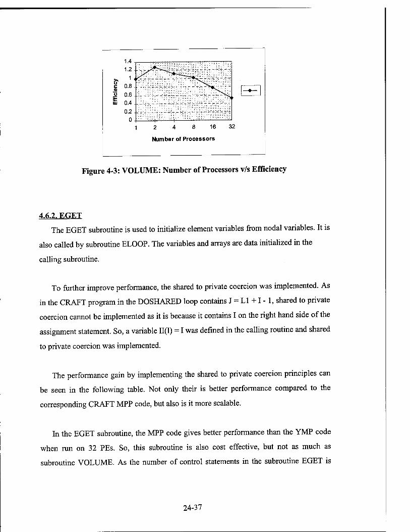
2 4 8 16

Number of Processors

Figure 4-3: VOLUME: Number of Processors v/s Efficiency

4.6.2. EGET

The EGET subroutine is used to initialize element variables from nodal variables. It is

also called by subroutine ELOOP. The variables and arrays are data initialized in the

calling subroutine.

To further improve performance, the shared to private coercion was implemented. As

in the CRAFT program in the DOSHARED loop contains J = LI +1 -1, shared to private

coercion cannot be implemented as it is because it contains I on the right hand side of the

assignment statement. So, a variable II(I) = I was defined in the calling routine and shared

to private coercion was implemented.

The performance gain by implementing the shared to private coercion principles can

be seen in the following table. Not only their is better performance compared to the

corresponding CRAFT MPP code, but also is it more scalable.

In the EGET subroutine, the MPP code gives better performance than the YMP code

when run on 32 PEs. So, this subroutine is also cost effective, but not as much as

subroutine VOLUME. As the number of control statements in the subroutine EGET is

24-37

more than subroutine VOLUME, the efficiency of parallel EGET is less. Also, its

efficiency is not as high as VOLUME when run on 32 PEs.

Table 4-3: EGET: Number of Processors v/s Wall clock time


YMP 0.257

1 2.368

2 1.276

4 0.735

8 0.454

16 0.314

32 0.244

2.5

1 2 4 8 16 32


o 2. E £ 1.5 . o

% 1-

* T3D

■ YMP

| 0.5.

0 . I 1 1 1 1 J

Figure 4-4: EGET: Number of Processors v/s Wall clock time

24-38

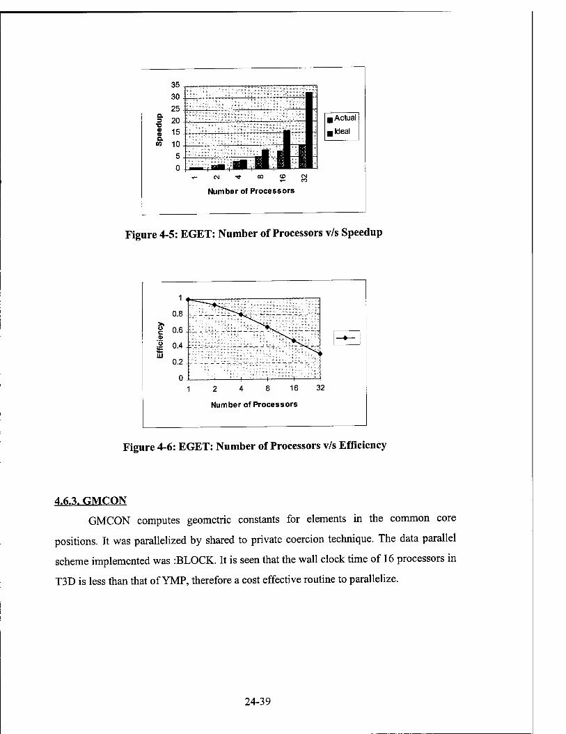
35, 30 - 25

f 20- g 15. w 10

0.

■ 1 g Actual

a Ideal

J J ,- eg rt CO CD £4

*— CO


Figure 4-5: EGET: Number of Processors v/s Speedup

c 0)

£ UJ

2 4 8 16 32


Figure 4-6: EGET: Number of Processors v/s Efficiency

4.6.3. GMCON

GMCON computes geometric constants for elements in the common core

positions. It was parallelized by shared to private coercion technique. The data parallel

scheme implemented was :BLOCK. It is seen that the wall clock time of 16 processors in

T3D is less than that of YMP, therefore a cost effective routine to parallelize.

24-39

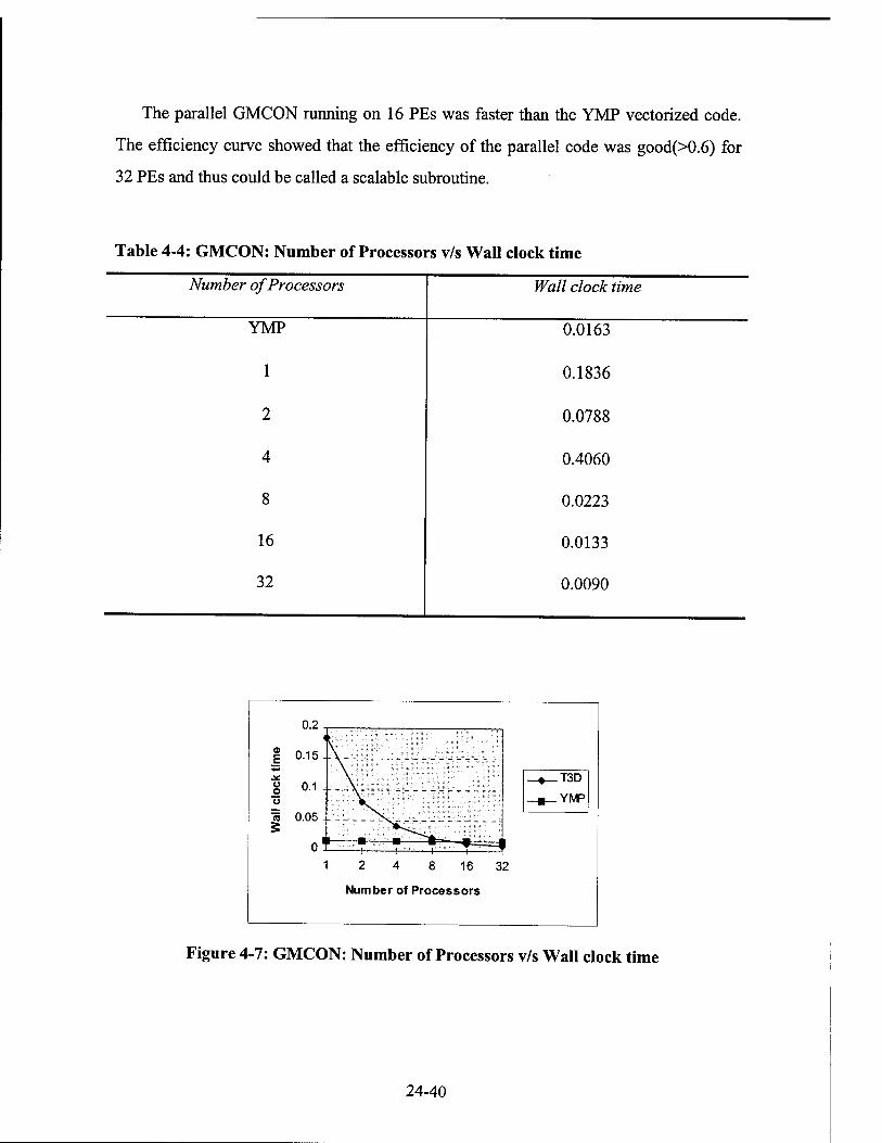
The parallel GMCON running on 16 PEs was faster than the YMP vectorized code.

The efficiency curve showed that the efficiency of the parallel code was good(>0.6) for

32 PEs and thus could be called a scalable subroutine.

Table 4-4: GMCON: Number of Processors v/s Wall clock time


YMP 0.0163

1 0.1836

2 0.0788

4 0.4060

8 0.0223

16 0.0133

32 0.0090

1 2 4 8 16 32


-»—T3D

-«_YMP

Figure 4-7: GMCON: Number of Processors v/s Wall clock time

24-40

Supramolecular Multilayer Assemblies with Periodicities in a Submicron Range

Vladimir V. Tsukruk Associate Professor

Western Michigan University Kalamazoo, MI


Wright Laboratory



and

Wright Laboratory

February 1997

25-1

SUPRAMOLECULAR MULTILAYER ASSEMBLIES WITH PERIODICITIES IN A SUBMICRON RANGE

(A step toward smart optical filters)

VLADIMIR V. TSUKRUK

MATERIALS PROGRAM, WESTERN MICHIGAN UNIVERSITY,

KALAMAZOO, MI 49008

Abstract.

Organized ultrathin films are the subject of great and growing interest because of their

compatibility with future nano-scale technologies. We use the supramolecular engineering

approach manipulating a single building unit, a supramolecular assembly, with chemically

pre-determined nature of functionality and dimensions to build organized films with large-

scale periodicity of multilayer structures. Supramolecular self-assembled films are fabricated

by electrostatic layer-by-layer deposition and electrostatic deposition assisted by dip-coating

and spin-coating. We use three very different classes of charged polymeric materials:

amorphous coiled polyions, dendritic macromolecules, and polymer latex nanoparticles.

Self-assembled films are studied by scanning probe microscopy, X-ray reflectivity,

ellipsometry, and contact-angle measurements. We demonstrate that replacing unstructured

coiled macromolecular chains with organized dendritic supramolecules or "bulk"

nanoparticles results in an increase in the growth increment and internal periodicity by an

order of magnitude higher than for conventional amorphous films. In-plane ordering can be

controlled by deposition time, ionization state, and application of capillary or shearing forces.

The routine proposed may be used for formation of supramolecular films with mesoscale

periodicity and intriguing optical properties. We present the first truly macroscnpically

ordered monolayer of charged latex nanoparticles obtained by force assisted electrostatic

deposition with lateral sizes extended to a fraction of a milimeter.

25-2

SUPRAMOLECULAR MULTILAYER ASSEMBLIES WITH PERIODICITIES IN A SUBMICRON RANGE

(A step toward smart optical filters)

VLADIMIR V. TSUKRUK

MATERIALS PROGRAM, WESTERN MICHIGAN UNIVERSITY,

KALAMAZOO, MI 49008

Introduction.

Organized ultrathin films are the subject of great and growing interest because of their

compatibility with future nano-scale technologies. Some examples are integrated optical

coatings with a gradient of refractive indices along the normal to the surface plane l and 2

microelectromechanical systems modified by boundary lubricants on the molecular scale.

Research in these fields focuses on supramolecular functional polymeric materials with

suitable physical properties (e. g., non-linear, photochromic, or sensing) and abilities to form

organized superstructures at the interfaces. 3"6 The search for new materials with a suitable

combination of properties, microstructure, and intermolecular interactions is under the way.

In our studies, we use the supramolecular engineering approach to manipulate with a

single building unit, a supramolecular assembly, with chemically pre-determined nature of

functionality and dimensions to build organized films with controllable, large-scale

periodicity of multilayer structures (see Scheme 1 for general comparison).5'6 Modulation of

internal structural periodicity of polymer films at a submicron scale, which results in

accompanying variation of the refractive index, is an interesting route toward the next

generation of optical reflective filters.

Currently, several approaches exist for fabrication of organized molecular assemblies

from functional macromolecular materials. Electrostatic layer-by-layer deposition from dilute

solutions which exploits Coulombic interactions between oppositely charged molecules has

become a widely used method since 1991.7 It has been shown that this approach can be

used to build multilayer films (hundreds of layers) with various combinations of molecular

fragments, organic and inorganic layers, latexes, molecules with switchable conformation,

biomolecules, photochromic molecules, and conductive polymers.3"8

25-3

10 - 1000 nm

conventional multilayer film I I ■ i ■ i ■ i ■ r^-r

amorphous polymer (polyion)

:':':':':':':':oi':':i:i:':i:i:i

Scheme 1. Possible architectures of supramolecular films.

The layer-by-layer self-assembling process of amorphous polyions in its initial stage requires

special attention. The mechanical and temporal stability of the first molecular layers tethered

to a solid substrate is a critical element to the homogeneity of thicker films. A gradient of

molecular ordering across the first several molecular layers is observed for various molecular

films. 7"9 This phenomenon is usually related to healing of substrate inhomogeneities and

non-equilibrium behavior. Formation of non-equilibrium surface morphologies and

inhomogeneous coverage is caused by the competition of the kinetics of polymer chain

adsorption and their surface diffusion. It is speculated that assembly of polyions on charged

25-4

surfaces is indeed a two stage process: macromolecular chains are anchored to the surface by

some segments during the short initial stage and then relax to a dense packing during the long

second stage of self-assembly.

In the present report, we summarize our observations on the formation of the

supramolecular self-assembled films by electrostatic deposition of three very different classes

of polymeric materials: amorphous coiled polyions, dendritic macromolecules, and polymer

latex nanoparticles (Figure 1). We make preliminary conclusions on feasibility of

supramolecular engineering approach for building organized polymer films with mesoscale

periodicity.

* V-HHH * 4> ^ V* * * HH + 4> *^ * +

Figure 1. Electrostatic adsorption of charged polymer coils, dendrimers, and nanoparticles on oppositevly charged surfaces.

Experimental

Negatively-positively charged pairs of polystyrene sulfonate (PSS) and polyallylamine

(PAA) (Figure 2)' °, PS latexes of 20 - 200 nm in diameter with amino and carboxy surface

groups (Table 1) n, and polyamidoamine dendrimers with surface amine groups for even

generations and carboxylic groups for odd generations (G3.5 - G10) (Figure 3) 12 were

selected for this study.

25-5

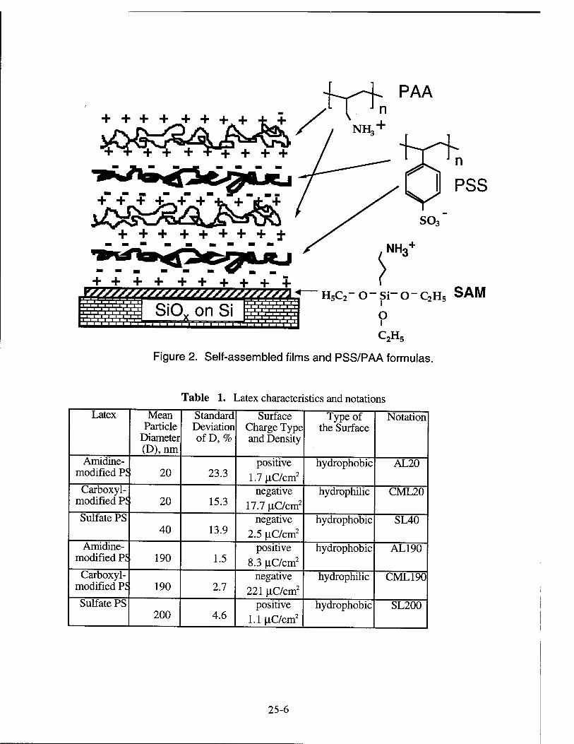
+ + + + + + + + + + SSSSSSSSSSSSSSSSSSSSSSSSXSSJ

ii;i;i;i;iu

!' '■''■•'■

SiCL on Si ■ , A ^

'i i ii ii r

I ' I ' I ' I 'T1

H5C2-0-Si-0-C2H 2^15 SAM o

1 C2H5

Figure 2. Self-assembled films and PSS/PAA formulas.

Table 1. Latex characteristics and notations

Latex Mean Particle

Diameter (D), nm

Standard Deviation ofD, %

Surface Charge Type and Density

Type of the Surface

Notation

Amidine- modified PS 20 23.3

positive 1.7uC/cm2

hydrophobic AL20

Carboxyl- modified PS 20 15.3

negative 17.7 uC/cm2

hydrophilic CML20

Sulfate PS 40 13.9

negative 2.5 uC/cm2

hydrophobic SL40

Amidine- modified PS 190 1.5

positive 8.3 |iC/cm2

hydrophobic AL190

Carboxyl- modified PS 190 2.7

negative 221 uC/cm2

hydrophilic CML190

Sulfate PS 200 4.6

positive 1.1 uC/cm2

hydrophobic SL200

25-6

Surface Group (Z)

(CH2)2- CO" NH-(CH2)2- N.

(CHzh- CO" NH-(CH2)2- N,^ H

/ (CH2)2- CO" NH-(CH2)2" N. / H

XN-(CH2)2"N (CH2)2- CO" NH-(CH2)2' N.

(CH2)2- CO" NH- (CH2)2- N

Repeated Unit (RU)

H H

(CH2)2- CO" NH- (CH2>2- N. H

Generation 4:

Figure 3. Chemical structure of dendrimers and a scheme of G4 dendrimer.

The positively charged surface is an amine terminated self-assembled monolayer

(SAM) and the negatively charge substrate is a silicon oxide layer of a silicon wafer. An

electrostatic layer-by-layer deposition technique was employed for the formation of the films

from aqueous solution at neutral conditions (pH =6.5). At this pH both polyions possess

some net charge as a result of dissociation (PSS) and protonization (PAA) of side groups.

Solid substrates used were silicon wafers ((100) orientation, SAS) and float glass (Aldrich)

modified by 3-aminopropyl triethoxysilane. Cleaning and modification of the substrates as

well as formation and transfer of the monolayers onto the solid supports were performed

using rigorous procedures.3 All PSS/PAA films were prepared in a class 100 clean room

and stored in a sealed containers.

25-7

Silanized substrates were protonated in a silicon wafer holder with a water solution of

0.01 N HC1. The 0.01 N HC1 was poured into the holder and allowed to react for 2 min.

The HC1 was then poured out and the substrates in the holder were flushed under running

Milli-Q water. The wafer pieces were then rinsed with Milli-Q water individually and dried

with dry nitrogen. The concentrations of the aqueous PSS and PAA solutions were 2 mg/ml.

The protonated substrates were dipped in the PSS solution for the appropriate amount of time

as designated below (from 1 second to 64 minutes). A set of substrates were dipped in the

PSS solution for 64 minutes and were used for the dipping in the PAA solution for different

times as designated below. This procedure for sample fabrication described in detail for

PSS/PAA films was basically unchanged for other types of self-assembling films studied

here.

Atomic force (AFM) and friction force (FFM) images of fabricated films in contact

and non-contact (the "tapping") modes were obtained in air at ambient temperature with the

Nanoscope IHA - Dimension 3000 (Digital Instruments, Inc.) according to well-established

procedures (Figure 4). 13 We observed that a combination of the tapping mode or contact

mode scanning with tip modification allowed stable reproducible imaging of the soft

monolayers without visible damage. Images were obtained on scales from 200 nm to 100

urn but for further analysis we selected two most appropriate "standard" sizes of 2 x 2 urn

and 5x5 urn. All microroughness values reported here were measured for 1 um x 1 urn areas.

The AFM tips were chemically modified to introduce appropriate surface charge and

avoid tip contamination by charged macromolecules from the specimens.'3 Tip radii were in

the range 20 - 40 nm as estimated by scanning a standard specimen with tethered colloidal

gold nanoparticles with known diameters according to the published procedure. 13 AFM

images were obtained for several specimens prepared under identical conditions at different

periods of time, and at several randomly selected film areas. All structural parameters

discussed below were averaged over 7-10 independent measurements after image processing.

X-ray reflectivity measurements were performed on a Siemens D-5000 diffractometer

equipped with a reflectometry stage. X-ray data were collected within 0 - 7° scattering angle

25-8

vertical and horizontal deflections OPTICALMICRÖSCOPE

VIDEO MONITOR

lateral displacements

Figure 4. General scheme of AFM technique.

range with step of 0.02° using monochromatized CuK,, radiation. Measurements within two

angle intervals with different parameters (X-ray tube power and accumulation time) were

rescaled to one angle interval. Simulation of X-ray curves was done by the REFSIM 1.0

program by direct computation of Fresnel reflectivity.14 We used standard database densities

and refractive indices for the substrates. Polymer film refractive indices were determined

from database data for chemical elements in accordance with their chemical composition. For

X-ray reflectivity simulations we used a double-layer model of surface structure of silicon

substrates (silicon-silicon dioxide layers) with parameters determined independently for bare

substrates. For polymer monolayers, we accepted homogeneous density distribution along

the surface normal within a single molecular layer with Gaussian interfacial zones. Fitting

parameters for polymer films were thickness, specific gravity, and roughness of polymer

films.

All technical details of experimental procedures can be found in original publications. 10-13

25-9

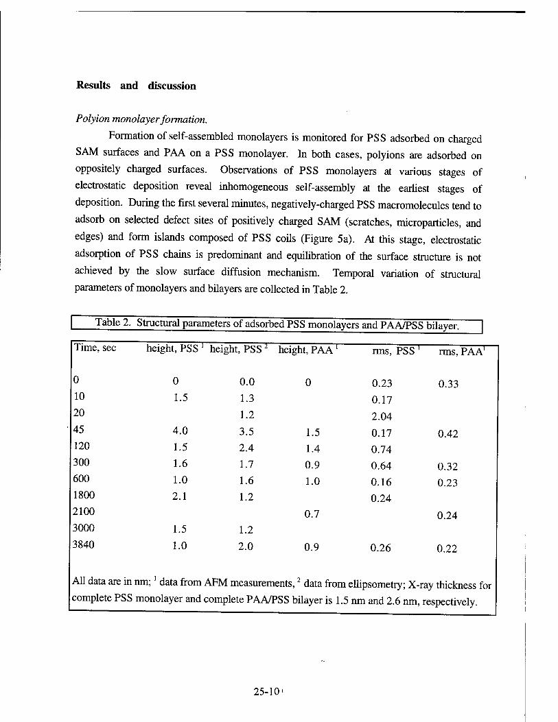
Results and discussion

Polyion monolayer formation.

Formation of self-assembled monolayers is monitored for PSS adsorbed on charged

SAM surfaces and PAA on a PSS monolayer. In both cases, polyions are adsorbed on oppositely charged surfaces. Observations of PSS monolayers at various stages of

electrostatic deposition reveal inhomogeneous self-assembly at the earliest stages of

deposition. During the first several minutes, negatively-charged PSS macromolecules tend to

adsorb on selected defect sites of positively charged SAM (scratches, microparticles, and

edges) and form islands composed of PSS coils (Figure 5a). At this stage, electrostatic

adsorption of PSS chains is predominant and equilibration of the surface structure is not

achieved by the slow surface diffusion mechanism. Temporal variation of structural parameters of monolayers and bilayers are collected in Table 2.

Table 2. Structural parameters of adsorbed PSS monolayers and PAA/PSS bilaver.

Time, sec height, PSS ' height, PSS2 height, PAA' rms, PSS rms, PAA1

0 0 0.0 0 0.23 0.33 10 1.5 1.3 0.17 20 1.2 2.04 45 4.0 3.5 1.5 0.17 0.42 120 1.5 2.4 1.4 0.74 300 1.6 1.7 0.9 0.64 0.32 600 1.0 1.6 1.0 0.16 0.23 1800 2.1 1.2 0.24 2100 0.7 0.24 3000 1.5 1.2 3840 1.0 2.0 0.9 0.26 0.22

All data are in nm;' data from AFM measurements,2 data from ellipsometry; X- ray thickness for complete PSS monolayer and complete PAA/ PSSbilayeris 1.5 nm and 2.6 nm respectively.

25-10'

+ •&» +++ * -8- * £ •4* * 4-S-4- * * -8» Hi» +4* 4>4"4* Hh * «8* 4- _^

UHU

* 4* «S***h 4> 4- 4> 4>

2. so

r^^,«m™ ,■■—f^po—^ Figure 5. Topographical images of surface morphology and models of monolayer packing for amorphous polyions (a, b), dendrimers (c, d), and latex nanoparticles (e, f) at early stage (a, c, e) and in dense state (b, d, f).

25-11

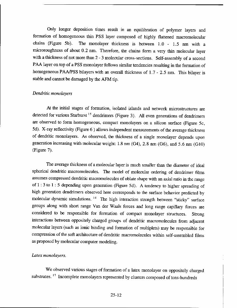
Only longer deposition times result in an equilibration of polymer layers and

formation of homogeneous thin PSS layer composed of highly flattened macromolecular

chains (Figure 5b). The monolayer thickness is between 1.0 - 1.5 nm with a

rnicroroughness of about 0.2 nm. Therefore, the chains form a very thin molecular layer

with a thickness of not more than 2 - 3 molecular cross-sections. Self-assembly of a second

PAA layer on top of a PSS monolayer follows similar tendencies resulting in the formation of

homogeneous PAA/PSS bilayers with an overall thickness of 1.7 - 2.5 nm. This bilayer is

stable and cannot be damaged by the AFM tip.

Dendritic monolayers

At the initial stages of formation, isolated islands and network microstructures are

detected for various Starburst15 dendrimers (Figure 3). All even generations of dendrimers

are observed to form homogeneous, compact monolayers on a silicon surface (Figure 5c,

5d). X-ray reflectivity (Figure 6 ) allows independent measurements of the average thickness

of dendritic monolayers. As observed, the thickness of a single monolayer depends upon

generation increasing with molecular weight: 1.8 nm (G4), 2.8 nm (G6), and 5.6 nm (G10) (Figure 7).

The average thickness of a molecular layer is much smaller than the diameter of ideal

spherical dendritic macromolecules. The model of molecular ordering of dendrimer films

assumes compressed dendritic macromolecules of oblate shape with an axial ratio in the range

of 1 : 3 to 1 : 5 depending upon generation (Figure 5d). A tendency to higher spreading of

high generation dendrimers observed here corresponds to the surface behavior predicted by

molecular dynamic simulations. 16 The high interaction strength between "sticky" surface

groups along with short range Van der Waals forces and long range capillary forces are

considered to be responsible for formation of compact monolayer structures. Strong

interactions between oppositely charged groups of dendritic macromolecules from adjacent

molecular layers (such as ionic binding and formation of multiplets) may be responsible for

compression of the soft architecture of dendritic macromolecules within self-assembled films

as proposed by molecular computer modeling.

Latex monolayers.

We observed various stages of formation of a latex monolayer on oppositely charged

substrates.17 Incomplete monolayers represented by clusters composed of tens-hundreds

25-12

S3

c/a

H rvi i ,

c1! i - !

& \ -

&

C4! 1

i

&

' ^K^

&

i

C'l ! b

Incident angle, degrees Figure 6. X-ray reflectivity experimental data (thick lines) and simulated curves (thin lines)

for G6 (a) and G10 (b) monolayer films. Simulations curved were obtained for

film thicknesses of 2.8 and 5.6 nm, roughness of 1.2 and 1.8 nm, and specific

gravities of 1.2 and 1.3 g/cm3 for G6 and G10 dendrimers, respectively.

25-13

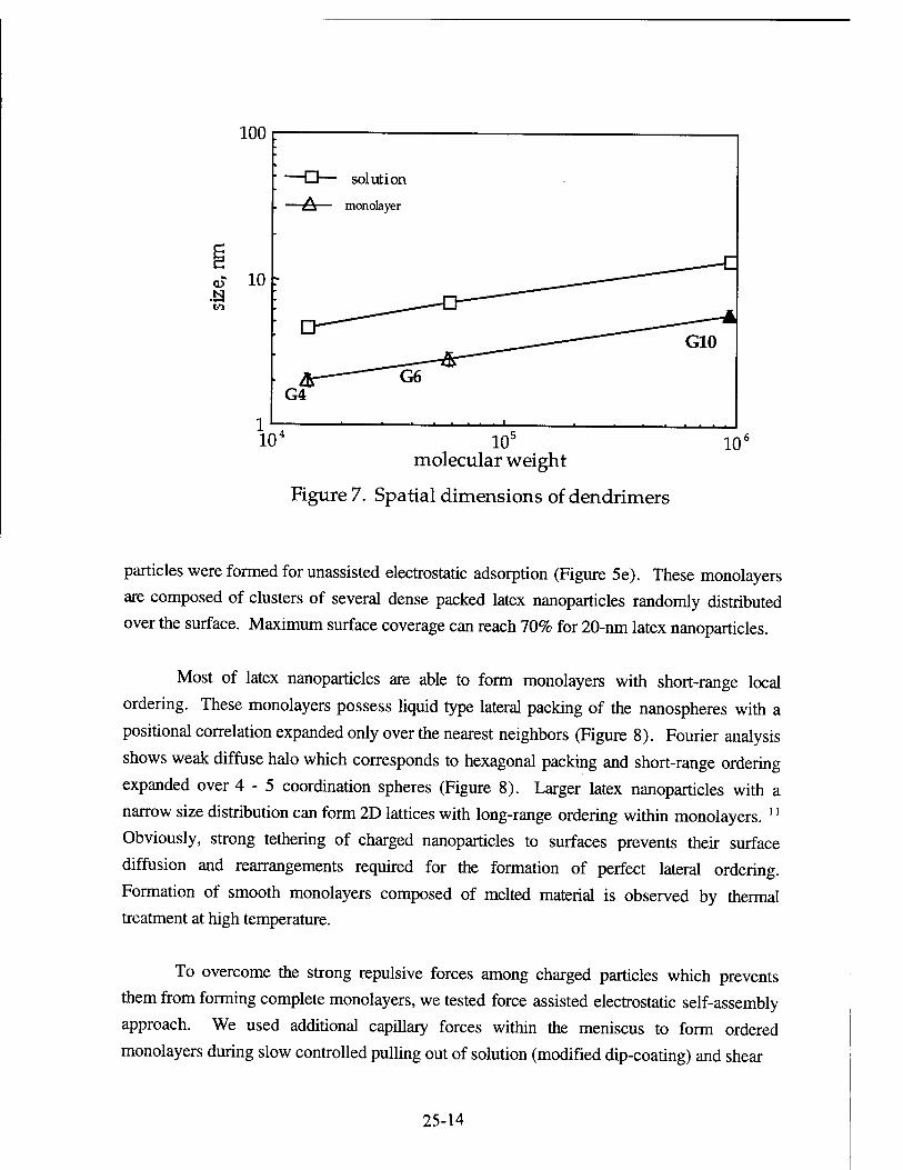
100

tf 10 .a

solution

monolayer

1 10

•4.^—»1^.^^.

105

molecular weight

Figure 7. Spatial dimensions of dendrimers

10(

particles were formed for unassisted electrostatic adsorption (Figure 5e). These monolayers

are composed of clusters of several dense packed latex nanoparticles randomly distributed

over the surface. Maximum surface coverage can reach 70% for 20-nm latex nanoparticles.

Most of latex nanoparticles are able to form monolayers with short-range local

ordering. These monolayers possess liquid type lateral packing of the nanospheres with a

positional correlation expanded only over the nearest neighbors (Figure 8). Fourier analysis

shows weak diffuse halo which corresponds to hexagonal packing and short-range ordering

expanded over 4 - 5 coordination spheres (Figure 8). Larger latex nanoparticles with a

narrow size distribution can form 2D lattices with long-range ordering within monolayers. ''

Obviously, strong tethering of charged nanoparticles to surfaces prevents their surface

diffusion and rearrangements required for the formation of perfect lateral ordering.

Formation of smooth monolayers composed of melted material is observed by thermal treatment at high temperature.

To overcome the strong repulsive forces among charged particles which prevents

them from forming complete monolayers, we tested force assisted electrostatic self-assembly

approach. We used additional capillary forces within the meniscus to form ordered

monolayers during slow controlled pulling out of solution (modified dip-coating) and shear

25-14

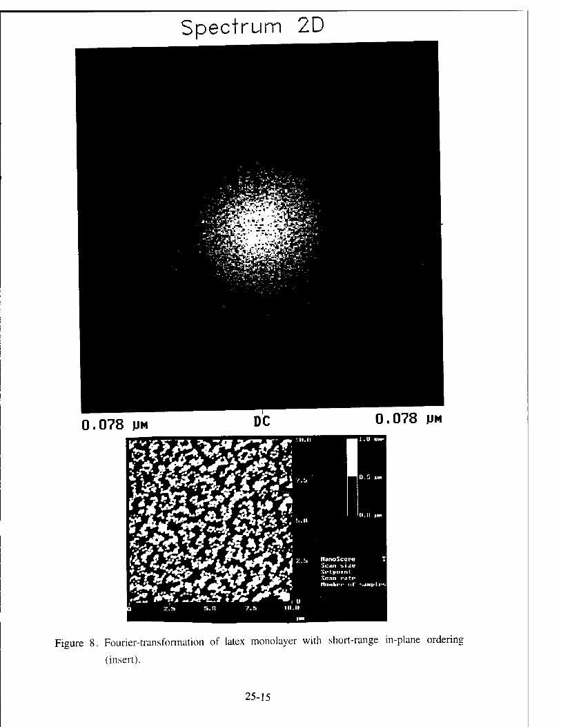
Spectrum 2D

Figure 8. Fourier-transformation of latex monolayer with short-range in-plane ordering

(insert).

25-15

Spectrum 2D

Z.SO

Figure 9. Fourier-transformation of latex monolayer with long-range in-plane ordering (insert).

25-16

flow resulting from spin-coating. n We observed that force assisted self-assembly of the

same latexes can produce dense monolayer films with long-range in-plane ordering (Figure

5f). Lateral sizes of very well ordered monolayers are in the range of tens - hundreds of

micrometers and usually six-fold symmetry of in-plane ordering is revealed by Fourier-

analysis of monolayer films (Figure 9).

Multilayer films from different polymeric materials

Multilayer PSS/PAA films were fabricated and extensively studied earlier. 18

Virtually linear growth of film thickness versus number of deposition cycles was observed

with an average increment of multilayer growth close to 1 nm (Figure 10). This value is

close to monolayer thickness and similar to other amorphous polyions (see data for

PVC/PAA film in Figure 10).18

Layer-by-layer deposition of oppositely charged dendrimers in combination Gn/Gn.1/2

results in the formation of films with homogeneous surface morphology for a limited number

of layers. A variation of the multilayer film thickness with the number of deposited layers, d

(x), is close to a linear with increment per layer in the range of 2.8 ± 0.3 nm for G4/3.5 films

and 3.8 ± 0.6 nm for G10/9.5 film (see data for G4/3.5 in Figure 10). The small increment

of the film thickness per molecular layer for multilayer films indicates that the dendritic

macromolecules are indeed very soft and do not preserve their shape in the condensed state at

interfaces similarly to monolayers. However, the average thickness of a molecular layer

within the multilayer films is still two - three times higher for dendrimers than for amorphous

polyions with comparable molecular weight despite their highly compressed state (Figure

10).

Typical multilayer growth pattern (thickness versus number of deposited layers) for

CML20/AL20 latexes with 20 nm diameter is shown in Figure 7. The average increment for

the first five layers is about 15 nm that corresponds to centered cubic packing of spheres.

However, for n > 5 the increment decreases to 7.3 nm per layer due to incomplete filling of

following layers during the film growth. Surface roughness gradually increases for the first

five layers and reaches a constant value of 22 ± 2 nm for thicker films. This suggests that

25-17

latexes, 20 nm

1JVS/FA~ iii. i . ■ . .

10 15 20 25 30 35 40 45 50 number of

Figure 10. Film thickness growth for different polymer pairs.

some equilibrium growth process is established during this stage with roughly two layers

being "under construction" during each deposition cycle.

Variation of pH of latex solution and activation of substrate with different pHs allow

controlling a fine balance of interparticle and particles-substrates interactions due to change

surface charge of ionizable surface groups. We tested various combinations of repulsive-

attraction interaction strengths for PS latexes. We observed that weak repulsive interaction

among nanoparticles (e. g., pH = 7 - 8 for amine terminated particles with pK = 9) combined

with strong attraction of highly charged substrate (a bare silicon activated by solution with

pH = 9) and slow pulling through the meniscus produces perfect monolayers and bilayers

expanded over a surface area of a fraction of a millimeter across (Figure 11).

Fourier image shows a net of reflexes similar to a single-crystal pattern in reciprocal

space which corresponds to long-range hexagonal packing of nanoparticles with interplanar

distance (110) of 185 nm (Figure 11). This example represents the first truly

macroscopically ordered monolayer of charged latex nanoparticles obtained by force assisted

electrostatic deposition at mild ionic conditions.

25-18

0.036 pH 0.036 JJM

Figure 11. AFM image of latex nanoparticles organized in a perfect monolayer (a defected area is selected to underline smooth part) and corresponding Fourier-transformation.

25-19

Multilayer films from organic-inorganic nanoparticles.

Inorganic composite nanoparticles were tested as a prospective component for

multilayer organic-inorganic films to enhance gradient of refractive index. Nanoparticles

NH2+ NH2+

NHoJ<—^~ NH2+N^?;i^~ST NH2

+

NHo+ NH2+

NH2+

OH" OH" t)H- OH" OH" OhT <

Figure 12. Organic-inorganic multilayers from latex/gold nanoparticles

25-20

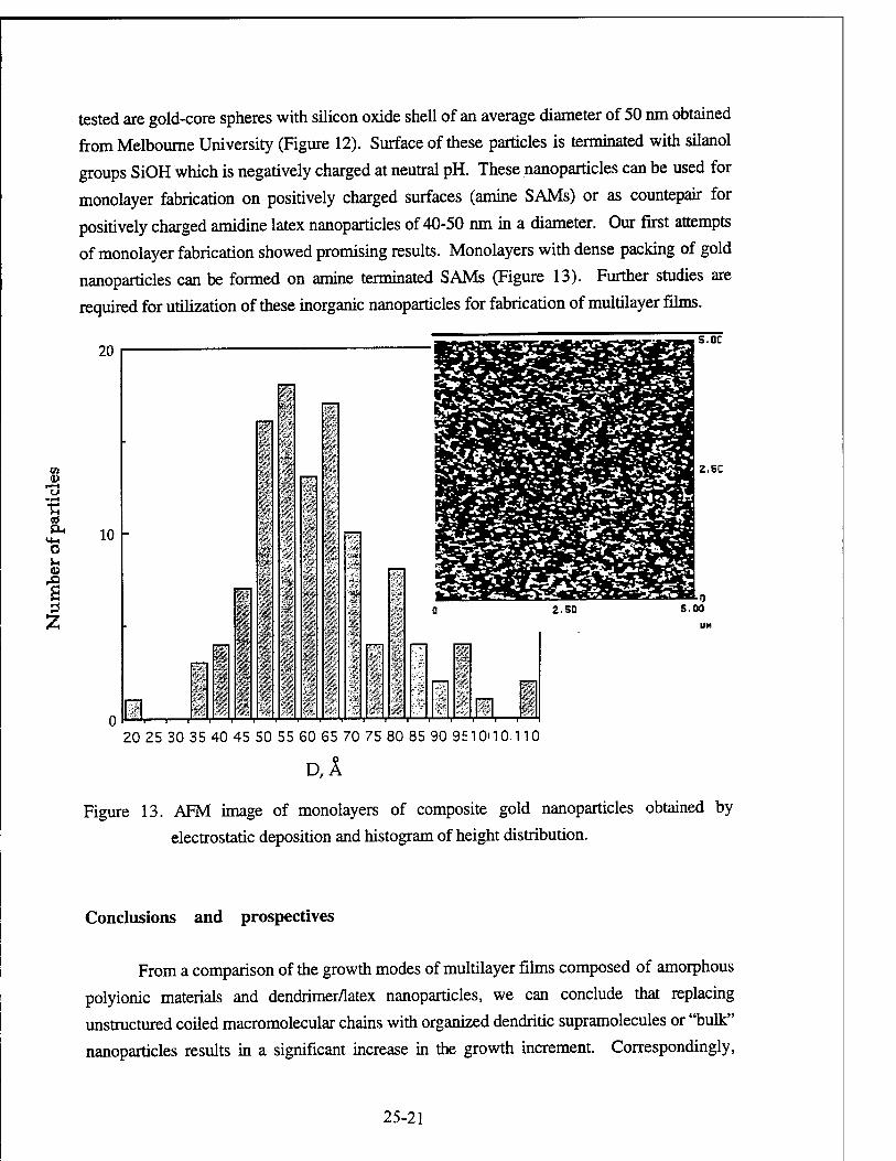
tested are gold-core spheres with silicon oxide shell of an average diameter of 50 nm obtained from Melbourne University (Figure 12). Surface of these particles is terminated with silanol

groups SiOH which is negatively charged at neutral pH. These nanoparticles can be used for

monolayer fabrication on positively charged surfaces (amine SAMs) or as countepair for

positively charged amidine latex nanoparticles of 40-50 nm in a diameter. Our first attempts

of monolayer fabrication showed promising results. Monolayers with dense packing of gold

nanoparticles can be formed on amine terminated SAMs (Figure 13). Further studies are

required for utilization of these inorganic nanoparticles for fabrication of multilayer films.

P-. M-l O i-,

1 z

20 25 30 35 40 45 50 55 60 65 70 75 80 85 90 9E10H 0.110

D,A

Figure 13. AFM image of monolayers of composite gold nanoparticles obtained by

electrostatic deposition and histogram of height distribution.

Conclusions and prospectives

From a comparison of the growth modes of multilayer films composed of amorphous

polyionic materials and dendrimer/latex nanoparticles, we can conclude that replacing

unstructured coiled macromolecular chains with organized dendritic supramolecules or "bulk"

nanoparticles results in a significant increase in the growth increment. Correspondingly,

25-21

internal periodicity of these supramolecular multilayer self assembled films is about an order

of magnitude higher than for conventional films. This type of structural organization is

unachievable for amorphous polyelectrolytes with random spatial distribution of "sticky"

groups. Obviously, the routine proposed may be used for formation of supramolecular films

with mesoscale periodicity and intriguing optical properties.

General observation can be made that force assisted electrostatic self assembly of

charged nanoparticles under dipping or spinning conditions may result in fabrication of

relatively large uniform layers (a fraction of a millimeter across) with long-range positional

and orientational ordering of nanoparticles within monolayers. However, only a fine balance

of interparticle (particle-particle and particle-substrate) interactions and external forces within

a narrow window may be useful for fabrication of perfect films. We present the first truly

macroscopically ordered monolayer of charged latex nanoparticles obtained by force assisted

electrostatic deposition. Lateral sizes of this monolayer are extended to a fraction of a millimeter.

Prospectives and trends

Several apparent problems and possible prospective trends can be deduced from our

introductory study. These problems and trends should addressed in more extensive project on a long term support basis.

Problems to address are:

- fabrication of complete, compact, and uniform molecular layers from nanoparticles with

strong repulsive interactions, finding a right balance of interparticle and particle-substrate interactions and surface mobility

- stable growth of multilayer films with a large number of layers and prevention of in-plane

phase separation at certain level when 3D bulk microphase structure becomes the most favorable

- "freezing" internal gradient of component composition along the surface normal for an indefinite long time

Prospective directions to go and general trends could be defined as follow:

- replacing self-assembly with "force assisted" self-assembly by addition active external

gradient to overcome long-range repulsive interactions among mesoscale nanoparticles:

25-22

capillary forces (dip-coating), shearing flow (spin-coating), and electrostatic interactions

(substrate potential variation and degree of ionization of functional groups)

- replacing pure polymer-polymer systems with organic-inorganic systems to enhance

gradient of chemical composition and refractive index; appropriate inorganic nanoparticles

"compatible" with existing polymer components should thought

- testing a new generation of supramolecular assemblies which should include dendritic

macromolecules with rigid architecture and functional surface groups able to form

mesomorphic phases and zwitterioninc/dye containing latex nanoparticles with functional

surface groups

Acknowledgments

This work is supported by US Air Force Office for Scientific Research, Contract

F49620-93-C-0063. The PI thanks for contributions of the members of his research group:

V. Bliznyuk, J. Hazel, D. Visser, J. Wu, S. Mirmiran, and J. Kalsi. My great thanks A.

Campbell, T. Bunning, and W. Adams (WPAFB) for fruitful collaboration, J. H. Wendorff

(University of Marburg) for X-ray and computer facilities provided, and P. Mulvaney

(Melbourne University) for composite gold nanopartciles supply.

25-23

References

1. Boivin, G.; St.-Germain, D. Appl.Optics, 1987, 26, 4209; Bovard, B. Appl. Optics,

1993,32, 5427.

2. K. Komvopoulos, Wear, 1996, 200, 305; Bhushan, B.; Israelachvili, J.; Landman, U.

Nature, 1995, 374, 607; Bhushan, B.; Kulkarni, A. V.; Koinkar, V. N.; Boehm, M.

Odoni, L.; Martelet, C; Belin, M. Langmuir, 1995, 11, 3189; Tsukruk, V. V.

Bliznyuk, V. N.; Hazel, J.; Visser, D.; Everson, M. P. Langmuir 1996, 12, 4840

Tsukruk, V. V.; Everson, M. P.; Lander, L. M.; Brittain, W. J. Langmuir 1996, 12,

3905.

3. Ulman, A. "Introduction to Ultrathin Organic Films", Acad. Pres.: San Diego, 1991;

Tredgold, R. Order in Thin Organic Films, Cambridge University Press: Cambridge,

1994; Roberts, G. Adv. Phys. 1985, 34, 475.

4. Tsukruk, V. V'. Progress in Polymer Science, 1997, 22, 247.

5. Fendler, J. H.; Meldrum, F. C. Adv. Materials, 1995,7, 607

6. Tsukruk, V. V.; Wendorff, J. H. Trends in Polymer Science, 1995,3, 82.

7. Her, R. K. J. Colloid and Interface Sei. 1966, 21, 569; Decher, G.; Hong, J.-D.

Makromol. Chem., Macromol. Symp., 1991,46, 321;

8. Decher, G; Lvov, Yu.; Schmitt, J. Thin Solid Films, 1994,244, 772; Cooper, T. M.;

Campbell, A. L.; Crane, R. L. Langmuir 1995, 11, 2713; Ferreira, J. H. Cheung, M.

Rubner, Thin Solid Films, 244, 806,1994; Lvov, Yu.; Ariga, K.; Kunitake, T. Chem.

Lett. 1994, 2323; Schmitt, T.; Grunewald, T.; Decher, G.; Pershan, P.; Kjaer, K.;

Lösche, M. Macromolecules 1993, 26, 7058; Kelogg, G J.; Mayes, A. M.; Stockton,

W. B.; Ferreira, M.; M. F. Rubner; Satija, S. K. Langmuir, 1996, 12, 5109.

9. V. V. Tsukruk, D. Janietz, Langmuir, 12, 2825,1996.

10. V. V. Tsukruk, V. N. Bliznyuk, D. W. Visser, A. L. Campbell, T. Bunning, W. W.

Adams, 1996, Macromolecules, submitted

11. V. N. Bliznyuk, V. V. Tsukruk, Polymer Prepr., 1997, 38 (1), 693.

12. V. V. Tsukruk, F. Rinderspacher, V. N. Bliznyuk, Langmuir, 1997, accepted

13. Tsukruk, V. V.; Reneker, D. H. Polymer, 1995, 36, 1791; V. N. Bliznyuk, J. Hazel,

J. Wu, V. V. Tsukruk, in: Scanning Probe Microscopy in Polymers, Eds. V. V.

Tsukruk, B. Ratner, ACS Symposium Series, 1997.

14.REFSIM 1.0, Siemens AG, Karlsruhe, 7500, Germany, 1994; Russell, T. P. Materials

Sei. Rep., 1990, 5, 171; Foster, M. Crit. Rev. Anal. Chem., 1993, 24, 179;

Tsukruk, V. V.; Shilov, V. V. Structure of Polymeric Liquid Crystals, Kiev, Naukova

25-24

Dumka, 1990; Lipatov, Yu. S.; Shilov, V. V.; Gomza, Yu. P. X-ray Analysis of

Polymer Systems, Kiev, Naukova Dumka, 1982; Hosemann, R.; Bagchi S. N. Direct

Analysis of Diffraction by Matter, North Holland Publ. Co., Amsterdam, 1962;

Tidswell, J. M.; Rabedeau, T. A.; Pershan, P.; Folkers, J. P.; Baker, M. V.;

Whitesides, G. M. Phys. Rev., 1991, B44, 10869.

15.Tomalia, D. A. Adv. Materials, 1994,6, 529; Jansen, J. F.; de Brabander-van den

Berg, E. M.; Meijer, E. W. Science, 1994,266, 1226; Percec, V.; Kawasumi, M.

Macromolecules, 1994, 27, 4AA\; Frey, H.; Lorenz, K.; Holter, D.; Mulhaupt, R.

Polym. Prepr., 1996, 37(1), 758; Frechet, J. M. Science, 1994, 263, 1711. Sheiko,

S. S.; Eckert, G.; Ignateva, G.; Musafarov, A. M.; Spickermann, J.; Rader, H. J.;

Möller, M. Makromol. Rapid Commun., 1996,17, 283.

16. Mansfield, M. L. Polymer, 1996, 37, 3835.

17. N.D.Denkov, O.D.Velev, P.A.Krachevsky, I.B.Ivanov, H.Yoshimura, K.Nagayama,

Langmuir, 8, 3183 (1992); A.S.Dimitrov, K.Nagayama, Langmuir, 12, 1303 (1996).

J. Li, D. J. Meier, Polymer Preprints, 37 (2), 591 (1996); C.A.Johnson,

A.M.Lenhoff, J. Colloid and Interface Sei., 179, 587 (1996)

18. Lvov, Yu. M.; Decher, G. Crystallography Reports 1994, 39, 628

25-25

Distributed Control of Nonlinear Flexible Beams and Plates with Mechanical and Temperature Excitations

H. S. Tzou Professor

Department of Mechanical Engineering

University of Kentucky Lexington, KY


Wright Laboratory



and

Wright Laboratory

February 1997

26-1

DISTRIBUTED CONTROL OF NONLINEAR FLEXIBLE BEAMS AND PLATES WITH MECHANICAL AND TEMPERATURE EXCITATIONS

H. S. Tzou Professor

Department of Mechanical Engineering University of Kentucky

Lexington, KY 40506-0108

Abstract

Beam and plate-type components are widely used in many aerospace structures. Imposed shape changes and surface control of flexible beams and plates could offer many aerodynamic advantages in flight maneuverability and precision control. Deformed shapes and surfaces often involve nonlinear deformations. Studies of control of nonlinear behavior related to the deformed surfaces and shape changes would provide detailed information in future controlled surface design and implementation. This research is concerned with the control effectiveness of nonlinearly deformed beams and plates based on the smart structures technology. Piezoelectric materials are widely used as sensors and actuators in sensing, actuation, and control of smart structures and structronic systems. Control effectiveness of piezoelectric laminated nonlinear flexible beams and plates subjected to

mechanical and temperature excitations is investigated. It is assumed that the flexible

beams and plates encounter the von Karman type geometrical nonlinearity. Thermoelectromechanical equations and boundary conditions including elastic, temperature, and piezoelectric couplings are formulated first, and analytical solutions derived next. Dynamics, active control of nonlinear flexible deflections, thermal deformations, and natural frequencies using distributed piezoelectric actuators are studied, and their nonlinear effects are evaluated.

26-2

DISTRIBUTED CONTROL OF NONLINEAR FLEXIBLE BEAMS AND PLATES WITH MECHANICAL AND TEMPERATURE EXCITATIONS

H. S. Tzou

INTRODUCTION

Recent development of smart (or intelligent) structures, structronic

(structure-electronic) systems, and micro mechanical systems has demonstrated the versatilities of piezoelectric materials in both sensor, the direct piezoelectric effect, and

actuator, the converse piezoelectric effect, applications (Tzou and Anderson, 1992; Tzou and Fukuda, 1992). Piezoelectrics are usually bonded (embedded or surface coupled) with elastic structures, serving as sensors and/or actuators for structural monitoring and control. These piezoelectric sensors and actuators can be further classified as "discrete" or "distributed" devices. The distributed sensors and actuators offer many advantages over the discrete devices, such as multiple modal controls, spatial filterings, spatially shaped modal controls, etc (Tzou, 1993). Accordingly, distributed piezoelectric sensors and

actuators are widely used in various structural applications.

In recent years, many sophisticated analyses are performed and new engineering

applications are explored. However, most of these studies were conducted based on the

linear theories, i.e., linear elasticity and piezothermoelectricity. It is known that piezoelectric materials are rather nonlinear. In addition, large oscillation and/or flexibility

of elastic structures can introduce large deflections of distributed sensors and actuators. Thus, the nonlinear characteristics of piezoelectric materials and laminated structures can be classified into two categories: 1) the geometrical nonlinearity and 2) the material nonlinearity. The former usually involves large deformations and the latter is associated with nonlinear material properties, e.g., hysteresis, temperature dependent material

constants, etc (Tzou and Bao, 1996). Pai, et al. (1993) recently studied a nonlinear

composite plate laminated with piezoelectric layers. Yu (1993) reviewed recent studies of linear and nonlinear theories of elastic and piezoelectric plates. Lalande et al. (1993)

investigated the nonlinear deformation of a piezoelectric Moonie actuator based on a

26-3

simplified nonlinear beam theory. Sreeram et al. (1993) investigated a nonlinear hysteresis

modeling of piezoceramic actuator. Librescu (1987) proposed a refined geometrical

nonlinear theory of anisotropic laminated shells. Linear thermo-electromechanical

behavior of distributed piezoelectric sensors and actuators were also recently studied (Tzou

and Ye, 1994; Tzou and Howard, 1994). A theory on geometrical nonlinearity of piezothermoelastic shell laminates simultaneously exposed to mechanical, electric, and thermal fields has been recently proposed (Tzou and Bao, 1996). Tzou and Zhou (1995)

investigated static and dynamic control of a circular plate with geometrical nonlinearity. This research is devoted to a study of distributed static and dynamic control of nonlinear

flexible beams and rectangular plates with geometrical nonlinearity using distributed piezoelectric actuators.

Since flexible beams and plates (rectangular and square plates) are very common in aerospace structures, static and dynamic behaviors of piezothermoelastic laminated flexible beams and plates with initial large nonlinear deformations (the von Karman type geometrically nonlinear deformations) and subjected to mechanical, electric, and temperature excitations are investigated in this research. Active control effects on nonlinear static deflections and natural frequencies, including temperature variations, imposed by the piezoelectric actuators are investigated. Nonlinear beam and plate equations are derived first, followed by nonlinear static analysis and free vibration analysis including the effect of initial nonlinear deformations. Active control of nonlinear effects by the piezoelectric actuators are emphasized. Numerical examples are provided and simulation results discussed.

CONSTITUTIVE EQUATIONS

This study focuses on the distributed control effectiveness of nonlinear deformations and dynamic frequencies, including mechanical, electric, and temperature effects. Since the fundamental governing equations are derived from the triclinic piezoelectric materials and thin anisotropic piezothermoelastic shells, original generic piezothermoelastic governing equations are briefly reviewed. The relations between the electric fields Eh E2, E3 and the electric potential <p in the curvilinear coordinate system are (Tzou and Zhong, 1993)

26-4

pi] fu 0 0 -1 d/dai E2 = — 0 f22 0 d/da>2 E3 [ 0 0 f33J djdotz

<p (1)

The constitutive relations of the piezothermoelastic shell are governed by three

equations: 1) a stress equation {T}, 2) an electric displacement equation {D}, and 3) a

thermal entropy equation £ (Tzou and Ye, 1994).

{T} = [c]{S}-[e]HE}-{A}0,

{D} = [e]{S} + [e]{E} + {p}0,

* = {A}'{S} + {P}*{E} + av 9

(2)

(3)

(4)

where {T}, {S}, {E} and {D} denote the stress, strain, electric field and electric

displacement vectors, respectively; # is the thermal entropy density; 6 is the temperature rise (6 = 0 — 00 where 0 is the absolute temperature and 0o the temperature of natural state in which stresses and strains are zero); [c], [e], and [e] denote the elastic stiffness

coefficient, piezoelectric coefficient, and dielectric permittivity matrices, respectively; {A} is the stress—temperature coefficient vector; {p} is the pyroelectric coefficient vector; and av is a material constant (av = pcv/0o where cv is the specific heat at a constant volume). [•]* and {•}* are matrix and vector transpose, respectively. For a generic anisotropic piezothermoelastic material, the stress and electric displacement equations become (Tzou

and Bao, 1994)

'Ti T2 T3 T4 T5 T6

Di-

D2 D3

Cll C12C13C14C15C16

C22 C23 C24 C25 C26 C33 C34 c35 c36

C44 C45 C46

sym. C55 C56

C66.

enei2ei3ei4ei5ei6 e2ie3i e4ie24e25e26 e3ie32e33e34e35e36

fSil s2 S3 s4 s5

—

eiie2ie3i

ei2e22e32

ei3 e23 e33 OH Ö24 Ö25 ei5 Ö25 635 ei6 Ö26 036.

"Ei' E2 E3

—

fAil A2 A3 A4 A5 Ae.

rsi s2 S3 S4 s5 s6

+ en ei2 en

£21 £22 £23

£31 £32 £33

Ei] E2 E3

+ Pi P2

LP3J

(5)

(6)

Note that if the effective axes of the piezothermoelastic material do not coincide with the

geometrical axes, an orientation or transformation matrix, in directional cosines and sines,

26-5

needs to be defined (Tzou and Bao, 1995). The anisotropic piezothermoelastic material is

used in deriving the generic piezothermoelastic shell system equations; simplifications to

other simpler piezothermoelastic materials, e.g., polyvinylidene fluoride, piezoceramics, etc., are then explored.

VON-KARMAN NONLINEARITY

It is assumed that the nonlinear characteristics are introduced by large deformations which can be introduced mechanically, electrically, and/or thermally. A generic nonlinear deflection Ui in the i-th direction can be expressed as a summation of a membrane

displacement m(aha2,t) and a higher order nonlinear shear deformation effect represented by the summation of angular rotations ß^(aha2,t) (Tzou and Bao, 1996):

m U.Coü.as,aht) = u.(aua2,t) + £ a3

J/3Jaha2,t) , i=l,2,3 , (7)

where uh u2 and u3 are the mid-plane displacement components of the reference surface along the ah a2, and a3 axes, respectively; 0U and ß21 represent the rotational angles in the positive sense of the ax and a2 axes, respectively; and ft. = 0. This expression includes

higher order nonlinear shear deformation effects. However, according to the

Love-Kirchhoff thin shell assumptions and a linear displacement approximation (first order shear deformation theory), only the first term is kept in the equation, i.e., m = 1 (Tzou,

1993). The displacements and rotational angles are independent variables in thick shells. However, the rotational angles are dependent variables in thin shells, and they can be derived from the thin shell assumptions in which the transverse normal strain S3 is negligible and shear strains S4 and S5 are zeros. Based on the thin shell assumptions, the rotational angles ft = ßn and ft = ß21 are derived from the transverse shear strain equations, i.e., S4 = 0 and S5 = 0.

In general, a3/Ri<<l a3/R2«l, thus, the ratios of the finite distance to the radius of curvature are negligible, i.e., fn ~ Aj and f22 ~ A2. It is assumed that the

piezothermoelastic shell experiences large deformations in three axial directions. However,

26-6

in general, the in—plane deflections are still much smaller than the transverse deflections.

Thus, the nonlinear effects due to the in—plane large deflections are usually neglected, i.e.,

the von Karman—type assumptions (Palazotto and Dennis, 1992; Chia, 1980). The

nonlinear strain—displacement relations of a thin shell with a large transverse deflection U3

include a linear effect, denoted by a superscript /, and a nonlinear effect, denoted by a

superscript n, induced by the large deformation:

rsi pn «1 -

*1 1

s°, 71-

«1 s2 = S°7 + Q!3 «2 = s? + r? + a3 «2

iSe Ls°6J «6. m in\ «6. (9)

where the subscripts 1 and 2 respectively denote two normal strains and 6 is the in—plane

shear strain. Detailed membrane and bending strains are functions of displacements u-'s.

1) Membrane strains:

-. _ 1 0Ui , U2 öAi , us ,

ÖA2 , u3 , "R—

go _ 1 ÖU2 , ni 2 ~Ki ÖQ2 A]A2 dai

1 fdüz/da^2 ~2~t Ai ' .

1 rduz/ da^2' ~2~{ A- J

_„ _ 1 öui 1 3u2. 6 A2 "5Ö2 Ä~7 öai

ui dAi u2 AiA2 ÖCt2 A1A2 Ötti

■2

ÖA2 + 1 5U3 ^U3 AiA2 dot\ da-2

2) Bending strains:

Ki =

K2 = 1 3

ui 1 du-c

~K~2 0^

1 9

'U2 1 <9u3

+

A2 da2 +

AiA2

1

1 ATA:

U 1 _ 1 3U3 TTi A~^ öai

U 1 _ 1 9ü3

+ AiA2

1 <

U2

Ul

1 dm ~K~2~5öT2^

1 &13

Ä~7 da.\

dkx

00*2 '

dA2 Hi Ä~i öaj öai '

U2 1 ÖU3 IT2

1

Ä2 0O2

c*a2 AiA; U2 1 <9u3"

A~i c7c£ 3A2

da.\

(10)

(11)

(12)

(13)

(14)

(15)

where s\, s°2 and s°6 are the membrane strains and «i, «2 and «6 are the bending strains

(the change of curvatures on the reference surface). Note that the quadratic terms

(nonlinear terms) inside the brackets are contributed by the large deflection. Membrane

force resultants Ny and bending moments My of the piezothermoelastic shell laminate can

be derived based on the induced strains:

26-7

fN„l N22 N12

Ml, —

M22 M12.

AiiAj2Ai6 BuB^Biß A12 A22 A26 B12 B22 B26 Al6 A26 Aßß B^ B26 B66

B11 Bj2 Bie Du D12 Ü!6 B12B22B26 B12 D22 D26 Bl6 B26 B66 Dl6 D26 Ü66.

B'1 [Nif rNne]

s; N2S N22e

n NiS N12e

«i Mif Mne «2 M2§ M22o M. M^J M12öJ

(16)

It is observed that there are three components, i.e., mechanical, electric, and temperature,

in the force/moment expressions. Superscripts e and 0 respectively denote the electric and

temperature components. The membrane strains and bending strains are coupled by the

coupling stiffness coefficients By in elastic force/moment resultants. Ny«3 and Ny6 are the

electric and temperature induced forces; Mye and My6 are the electric and temperature

induced moments, respectively. In actuator applications, these electric forces and moments are used to control shell's static and dynamic characteristics.

NONLINEAR PIEZOELECTRIC SHELL COMPOSITES

Mathematical models of the flexible beams and plates (rectangular and square plates) are derived from a generic theory of nonlinear thin anisotropic piezothermoelastic shells. A generic anisotropic deep piezothermoelastic shell is defined in a curvilinear

coordinate system, and it is exposed to mechanical, electric, and thermal excitations.

Figure 1 illustrates the original generic shell and its derivative geometries including plates, beams, and other shell, non-shell geometries. It is assumed that the shell is subjected to a large deformation resulting in a geometrical nonlinearity. However, material properties are assumed constant, and the stress and strain relations are linear. The generic theory is derived based on a generic anisotropic piezothermoelastic thin shell. Simplification of the generic theory to other piezoelectric materials, e.g., mm2 (polyvinylidene fluoride), mm6 (piezoceramics), etc., or piezoelectric continua, e.g., spherical shells, cylindrical shells, plates, beams, etc., can be achieved when appropriate material or geometrical parameters are defined (Tzou, 1993). A generic infinitesimal distance ds in a shell can be defined by a fundamental form:

(ds)2 = £ (fii)2(dai)2 (17)

-7-

where in{ctba7,as) = A4(l+ @ (i= 1,2), in(aua2,az) = 1; a3 is a finite distance

measured from the reference surface; A! and A2 are the Lame parameters; and Ri and R2

are the radii of curvature of the a\ and a2 axes on the surface defined by 03 = 0. For 3

beams and rectangular plates, Ai = A2 = 1 and Rj = R2 = a. Thus, (ds)2 = .S (l)2(dai)2.

For convenience, the neutral surface is taken as the reference surface, which is defined by

the ai and a2 axes.

Svficeface

£E7

Fig.l A nonlinear piezothermoelastic shell and its derivative geometries.

Hamilton's principle is used in deriving the system equations and boundary

conditions of the piezothermoelastic shell continuum. Simplifying the shell equations gives the nonlinear equations of flexible beams and plates. Hamilton's principle assumes that the energy variations over an arbitrary period of time are zero. Substituting all energies into Hamilton's equation and carrying out all derivations, one can derive the nonlinear

26-8

piezothermoelastic equations and boundary conditions of the nonlinear piezothermoelastic

shell (Tzou and Bao, 1996).

ffNiiAa) N dA2 , d(N12At) , AT dAt , n AtA2 A A ,.. ~^Fr~N22MT+ * da2

/ + N^+Qi3-^TJ=A1A2phu1, (18)

(19)

_ A.AJN

» J-N"

du 3 üä~2

(20)

where QJ3 and Q23 are defined by

Ql3 =

Q23 =

AiA2

1 AiA2

d(M11A2)_ 8A2 flfMiaAQ öa 1 öai da- + M^ Ca2

äM^+M1«^+MilM_M1I|4 öai Ll2^I cTcT 1&ä:

(21)

(22)

1 n

where p = j- kS p^ is defined as a weighted average density for the multi-layered shell.

It is observed that the nonlinear influence on the transverse equation u3 is very prominent.

(All terms inside the brace are contributed by the nonlinear effects of the von Karman type

geometric nonlinearity.) Note that the thermo-electromechanical equations look like a

standard shell equations. However, the force and moment expressions defined by

mechanical, thermal, and electric effects are much more complicated than the conventional

elastic expressions. Substituting the expressions of Nn, N22, N12, Mn, M22, Mw into the

above equations leads to the thermo-electromechanical equations defined in the reference

displacements uh u2, u3. The transverse shear deformation and rotatory inertia effects are

not considered. The electric terms, forces and moments, can be used in controlling the

mechanical and/or temperature induced excitations (Tzou and Ye, 1994). For nonlinear

flexible beams and plates (rectangular and square plates), Ai = A2 = 1 and Rt = R2 = a.

Substituting the Lame parameters and radii into the shell thermo-electromechanical

equations and simplifying, one can derive the governing equations for nonlinear

26-9

piezoelectric laminated beams and plates. Accorgingly, thermo-electromechanical

couplings and control of static/dynamic nonlinearities can be investigated. Detailed

derivations are presented next.

NONLINEAR PIEZOELECTRIC COMPOSITE PLATES

For piezoelectric laminated composite rectangular plates, Figure 2, the coordinate

system, radii of curvatures, and Lame parameters are defined as follows: cti = x, «2 = y, «3

= z, Ri = a), R2 = öD, Ai = 1, and A2 = 1.

' Piezoelectric

material

Fig.2 Nonlinear composite plate.

It is assumed that an elastic plate, with dimensions 2ax2bxh, is sandwiched between

two piezoelectric layers and the composite plate experiences a large deformation. The

resultant membrane forces and the bending moments are

26-10

fNxxl Nyy N

= [Nxxl N m

.^xy. —

"Nxxl N e

.1Nxy. —

fNxx6] Nyye

Nxyö )

'Mxx

lMxyJ =

lmxyj —

[Mxl] Myf

LMx| —

[Mxx6! Myy6 Mx>.

(23)

where the superscript "m" denotes the mechanically induced components, "e" the

electrically induced components and "$" the thermally induced component. The

mechanical membrane forces and moments are

Nxx' N m

K xyj

= K S°x+ fJS'y S°y+ /^°x Sxy(l-/^)/2j

Yh

(24)

where K = j—*; h=2d is the thickness of elastic plate;

(j, is Poisson's ratio, and Y is the Young's modulus;

Mxx- M m

,ivlxyj

Nyf Nx|j

MA Myf

LMxfj

Nxx6' N 6 •"yy NxyÖj

Mxx6

Myy6

MXy6

= D Kx + ßKy Ky + [IKx _«Xy(l-/i)/2_

= -e3i(03i+^33) n

1 0

where D= 12(i_ß$y and

, where <py is the total voltage across the j—th layer;

= H^Urfe)

rAxi A,

Axl

0da3 =

0az da3 =

r+d

d

, where t is the thickness of piezoelectric layers;

0da3; Ax Ay 0

+d

-d

Ax Ay 0

0a3 da3 .

The relations of strain—displacement are

rsx i

L°xyJ =

Vx" s°y + z

Kx Ky

.S xy. .^xy.

(25)

where the membrane and bending strains are

26-11

Sxy

Note that the quadratic terms in the membrane strains are the von Karman-type nonlinear terms. The inplane inertia effects of thin plates are usually neglected and the in-plane

mechanical forces are assumed zero, i.e., qx = qy = 0. Then, the nonlinear plate equations

are derived as

j9N^+dNxx=0; ^ + ^=0; (27a,b) öx of ' öx ay

d2Mxx , O02MXV , d*Mvv , M 52uz , 9N d2uz , N d2uz . n _ „hii (28)

The static version of these equations are those of the von Kärmän plate theory. These

simplified static equations are identical to those in (Chai, 1980).

Substituting all force and moment expressions (mechanical, thermal, and electric

components) into the plate equations yields three piezothermoelastic equations in terms of

the displacements ux, uy and uz.

dNA , 9KA - f 9N*x a. dNxx<\ , (dM + dNxA . (29)

d^+d^_(dNA+dN^l) ,m£ +dNy^y (30) ^x ^y KHJix T öx > T Koy T öy ; '

- (Nxx ^3- + 2JNxy -^ + JNyy -g^-)

■Qz

v AA öx* ^ oxcty " cy^ '

+ [(Nxx + Nxxe)|^ + 2(Nxf + Nxye)g^ + (Nyy + Nyy6)|^]

_L r/d2Mxx , d2MxA , r^aM?v 4- "d2M*A 4- fS + °2MYA}

+ K-ginr + "wH + (2_3xl5y + 2 ax #y > + {^J^ + ^y^n ' (31)

26-12

Furthermore, substituting all force and moment expressions, one can derive the displacement equations as

fe , _ 02Ux £2uy _ duz ,dHz , n 02u

7'2^-Ê^ + -7r^^5r + ^x—^ + ^~^r + -^y )]; ^ „ fe+r? Ä + Ä_ ûz/ö2uz , n d*uzs

^WW5^ + -7rK-3? + -S?-) + ("Sf + -Sy^)] : (33)

Z> V2V2uz + phiiz = qz + K[(l-ß)(^ + g* + gk fyä^

+ ($}*£. + Iffo^/d^z , . d2Uz>, /flu» 1/0U«2\/02UZ , d2u + ô5T + 5l35P Jte" + **ZJyTr) + (^ + j(^r) X^ysr + /^)]

- KW + Nxxe)g^ + 2(Nxe + Nxye)^| + (Nye + Nyye)|^]

_ r^M*! + ^2M e gaM e g2M 0 g2M e aaMwO,, ,„,, l^93T^ + c»x2 J + ^ 0x#y + 2-BT$T> + ("ZTpr + flyT )J • (34)

where j/1 = ^^, 7?2 = ^, V2 is the Laplacian operator, and V2 = |^ + |^ .

For a uniformly distributed piezoelectric layer with constant thickness, the electric potentials on the piezo-layers are independent of the coordinates x and y. It is also

assumed that the temperature rise is uniform with respect to the x and y coordinates, 0(x,y,z)= 0(z). Occasionally, introducing a generic forcing function and representing the existing force terms by the generic forcing function in certain boundary-value problems would significantly simplify the system equations and also alleviate the complexity of solution procedures. Thus, a generic forcing function F(x,y) is introduced and the forces are defined by

N*S = f|, Ny? = ||, and N,J = -^. (35)

Note that the two in-plane equations are exactly satisfied and the transverse equation is expressed in terms of the transverse deflection u3 and the forcing function F.

26-13

D V2V2uz + phüz = qz + JV(F,uz)

- [(Nxx + Nxxe)g^ + 2(Nxy + Nxye)^ + (Nyf + Nyye)|^] , (36)

where N(F,\xz) is the nonlinear operator defined by

y% v d*F 8*uz , d*F 52Uz 9<92F 8*uz (37)

The second equation is the compatibility equation of the plate. Applying the membrane

strain equations leads to the compatibility condition:

~W' ~8W 02s* ,92u^2 02Uz 02Uz d2S"x , Ö2S'v c/'S xy _ (U'UzY ^ _

Nx£ N m

Ny* Since the forces are functions of membrane strains

strains can be expressed as functions of forces

= K 1 /* 0 ß 1 0 0 0 (l-ft)/2

s x S>

Ls xy.

(38)

, the

"sV s°y

1 ~ K

Lb xyj

1 /* 0 /* 1 0 0 0 (l-/*)/2

-l fNxx- N m

.iNxy. X[H^J

1 —A* 0 ■ß 1 0 0 0 2(1+/*)

Nxx- 1ST m

xy. N (39)

52F Referring to the forces represented by the generic forcing function , i.e., Nx£ = -^-^,...), one

can also define the strains as functions of the forcing function.

s°x = -Th-(N- " ^ = -YTT<T$ - f& >

s° y = -YYT^yy - ^«) = -TrHS? ~ "zp);

xy 'Yh' 'Nxy

(40)

(41)

(42)

The second equation then can be obtained by substituting these equations into the

condition of compatibility:

26-14

V2V2F(x,y) + -™ JV(uz,uz) = 0 . (43)

Since the closed-form solutions to these nonlinear equations are usually not

available, the approximation methods are used to solve these equations. The

approximation techniques include the (generalized) double Fourier method, Rayleigh-Ritz

method, Galerkin's method, perturbation technique and finite difference technique, etc.

Simulation results based on the series solutions are presented later.

Four boundary conditions are usually required for each edge of the plate. Electric

boundary conditions are also allowed and from which boundary control can be

implemented. Generic boundary conditions are

Or Nnn = Nnn* Un = Un*

US = Us*

Uz = uz* #Uz

on _ #Uz*

on.

nn >

or Nns = Nns* ; dMns | Q _ dMns* , ^ . . ,... ~TT~ + <*> - -^g- + Qn* , (44) or

Or Mnn = Mnn*

in which the subscripts n and s denote the directions outward normal and tangential to the

boundary, respectively, and the starred quantities designate the prescribed value. Typical

mechanical boundary conditions for the plate are:

a) Rigidly clamped edge: uz = -^ = un = us = 0; (45a-e)

b) Loosely clamped edge: uz = Sj^ = Nnn = Nns = 0;

c) Simply supported edge (movable in the plane of the plate)

uz = Mnn = Nnn = Nns = 0;

d) Hinged edge (simply supported edge immovable in the plane of the plate):

Uz = Mnn = Un = Us = 0;

e) Free edge: Nnn = Nns = Mnn = Qn + ^f = 0.

26-15

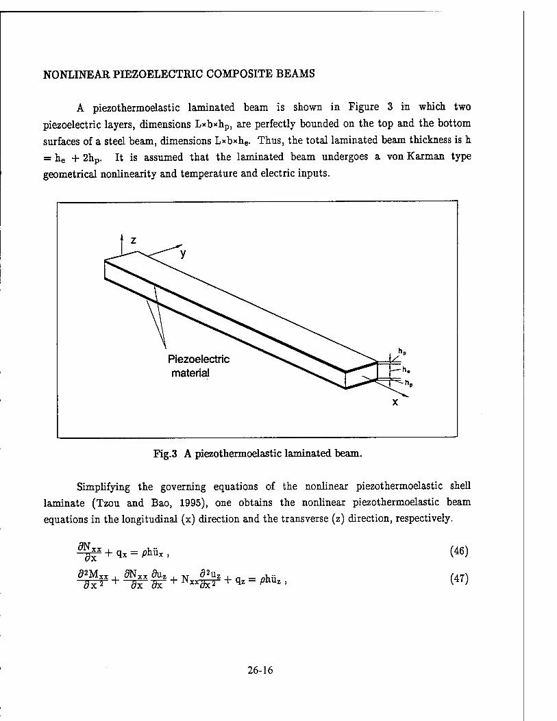
NONLINEAR PIEZOELECTRIC COMPOSITE BEAMS

A piezothermoelastic laminated beam is shown in Figure 3 in which two

piezoelectric layers, dimensions Lxbxhp, are perfectly bounded on the top and the bottom

surfaces of a steel beam, dimensions Lxbxhe. Thus, the total laminated beam thickness is h = he + 2hp. It is assumed that the laminated beam undergoes a von Karman type

geometrical nonlinearity and temperature and electric inputs.

Piezoelectric material

Fig.3 A piezothermoelastic laminated beam.

Simplifying the governing equations of the nonlinear piezothermoelastic shell laminate (Tzou and Bao, 1995), one obtains the nonlinear piezothermoelastic beam equations in the longitudinal (x) direction and the transverse (z) direction, respectively.

5Nx>

Ö2M

+ qx = phii

XX 5N ^x^

X )

xx OUz . jq- d2uz , v~ xxdxT + qz = p z '

(46)

(47)

26-16

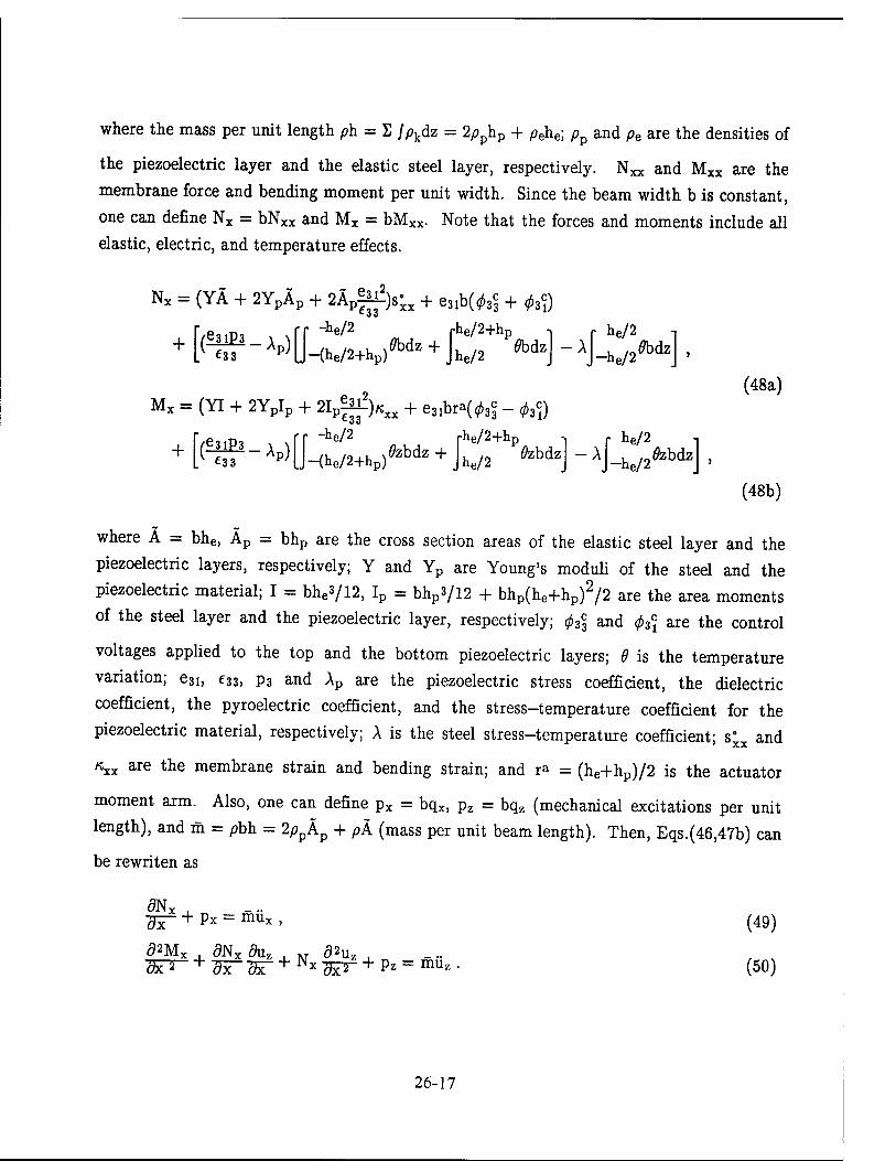
where the mass per unit length ph = S jpkdz = 2pphp + pehe; pp and pe are the densities of

the piezoelectric layer and the elastic steel layer, respectively. Nxx and Mxx are the

membrane force and bending moment per unit width. Since the beam width b is constant,

one can define Nx = bNxx and Mx = bMxx. Note that the forces and moments include all

elastic, electric, and temperature effects.

Nx = (YÄ + 2YpÄp + 2Äp|^)sxx + e31b(«^ + fcfl

+ L^-V -he/2 rhe/2+hp

-(h^+hp)^ + Jhe/2 * ^dz • he/2

-he/2 0bdz

Mx = (YI + 2YpIp + 2Ipf^)/cxx + e31bra(03c - fa')

-he/2 rhe/2+hp

(48a)

+ ^-*4 Hhe/2+hp) febdz + he/2 özbdz r ]

-AI-. he/2

■he/2 febdz

(48b)

where A = bhe, Äp = bhp are the cross section areas of the elastic steel layer and the

piezoelectric layers, respectively; Y and Yp are Young's moduli of the steel and the

piezoelectric material; I = bhe3/l2, Ip = bhp3/l2 + bhp(he+hp)2/2 are the area moments

of the steel layer and the piezoelectric layer, respectively; facz and <t>3\ are the control

voltages applied to the top and the bottom piezoelectric layers; 0 is the temperature

variation; e3i, e33, p3 and Ap are the piezoelectric stress coefficient, the dielectric

coefficient, the pyroelectric coefficient, and the stress-temperature coefficient for the

piezoelectric material, respectively; A is the steel stress-temperature coefficient; sxx and

KXX are the membrane strain and bending strain; and r* = (he+hp)/2 is the actuator

moment arm. Also, one can define px = bqx, pz = bqz (mechanical excitations per unit

length), and m = pbh = 2/?pÄp + pk (mass per unit beam length). Then, Eqs.(46,47b) can

be rewriten as

<9Nx , ■g^- + px = mux ,

d2Mx , dNx 8uz + N + Wt-^-dTW <92uz ,

x ^r + Pz = muz

(49)

(50)

26-17

Using Eqs.(48a&b), one can write the axial force and bending moment in a compact form:

Nx = lTsxx + Nxc + Nxt

)

Mx = D KXX + Mxc + Mx*,

(51a)

(51b)

where K is the membrane stiffness K = (YÄ + 2YPÄP + 2ÄP§^-); D is the bending C33

stiffness D = (YI + 2YPIP + 2IP^-); sxx is the membrane strain and «xx is the bending

strain with the von Karman type nonlinearity:

sxx - W~+ 2" VdT> ' *xx " W ~ WT ■ (52a&b)

Nx* is the axial force induced by the temperature rise; Mx* is the moment due to the temperature rise; Nx

c is the axial force induced by the control potential; and Mxc is the

control moment induced by the control potential.

Nxc = e3ib(^ + faV ,

Mxc = e31bra(^-^c)

NT* =

Mx* =

<*i?-Ap)

(^-Ap)

• -he/2

-(he/2+hp)

• -he/2

-(he/2+hp)

0bdz + rhe/2+hp

he/2 0bdz -A

p he/2 0bdz

febdz + rhe/2+hp

Jhe/2 febdz

-he/2

he/2

he/2 -I-; 0zbdz

(53a)

(53b)

(53c)

(53d)

Boundary conditions at the two ends of the laminated beam, x = 0 and x = L, are

Nx = Nx* or ux = ux* ,

Mx = Mx* cMx N duz _ 0 « ox +NxW ^z

or

or Ac = Ac* , Uz = Uz* ,

(54a)

(54b) (54c)

where the quantities with the asterisk "*" are prescribed values on the boundary. Note that usually either force boundary conditions or displacement boundary conditions are

26-18

selected for a given physical boundary condition.

It is assumed that the mechanical excitations in the longitudinal and transverse

directions are zero, i.e., pz = px = 0. Substituting the axial force and bending moment into

Eqs.(49,50), one can write

K W -he/2

M

+ e31b^(^+^3c1)+[(^f-Ap)

he/2+hp^ , he/29ö

he/2 o5Ebdz) " AJ bdz + "(J-{he/2+hp)^

{-^ + e31bra^(^-^)+ (SfJEi-Ap) -he/2

-he/2cE ■bdz = mux ;

(J -(he/2+hp)^2bdz + J he/2 ^bdz) ~ AJ -]

he/2 d*6 zbdz

+ { 4

-he/2

dllx, l/dllz >1 Oß fhe/2+hp^fl

-(he/2+hp)^bdQ!3 + J he/2 ^bdz) - A

■he/20X^

+ e31b^(^+^)+[(^f-Ap) he/2<90.

-he/2cE bdz 1 dnz

+ {*[£+*<&>' ■(

-he/2 he/2+hp

-<he/2+hp)^dz + Jhe/2

+ enHfat+faV + (^f-Ap) rhe/2+hp f he/2 -,,

Jhe/2 ^^-^J-he^Hl Ö2Uz - ..

(55a)

(55b)

Since the longitudinal inertia is negligible, i.e., müx ~ 0, factoring the partial derivatives and regrouping the force and moments gives

ÖNX_ ~dl = 0,

32MX _L M ^2uz _ .. ^r^+Nx^ = muz

(56)

(57)

Eq.(56) implies that the axial force Nx is not a function of x, i.e., Nx = constant.

Considering individual elastic, control, and temperature effects, one can further write Eq.(57) as

5S d4uz , Dwz^d*Mxc , 52MX

4 , AT d*uz TJx^ + "7^ + N* 3x^ = mü* > (58)

26-19

where Nx = K [755^+ \{T%r) ] + Nxc + Nx*. The nonlinear piezothermoelastic beam

equation can be further simplified when boundary conditions are specified. In the following two cases, one is used to compare with the standard equation and the other is for a detailed

parametric study.

1) Free Expansion/Contraction:

If the longitudinal motion either at x = 0 or at x = L is not constrained (free

expansion/contraction), the axial force Nx vanishes when the boundary conditions are

imposed. The differential equation then can be simplified to

-£>^ + f(x)t)=müZ) (59)

where f(x,t) = as + a f • This is a standard form of the beam transverse vibration

(Meirovitch, 1975). However, note that the physical meaning is much more complicated than the conventional form, due to the coupling of mechanical, electric, and temperature

fields in the nonlinear piezothermoelastic laminated beam.

2) Simply Supported with Both Ends Fixed:

Boundary conditions for a simply supported piezothermoelastic laminated beam

with both ends fixed are

uz = ux = 0, and Mx = 0 , • (60)

at both beam ends: x = 0 and x = L. Furthermore, it is. assumed the voltage <f> and

temperature variation 0 are uniform in the x—direction. This implies that <f> and 6 are not

functions of coordinate x. Then, the transverse equation becomes

-£^+Nx-|^ = müz (61)

where the axial force Nx = K [$jj± + \ {^)) + Nxc + Nx1. Solution procedures of the

26-20

simply supported nonlinear piezothermoelastic beam equation are discussed next. Numerical results and control effectiveness are presented in case studies.

CONTROL OF NONLINEAR DEFORMATION AND FREQUENCES

As discussed previously, distributed piezoelectric layers laminated (coupled or

embedded) on elastic shell continua can be used as distributed sensors and/or actuators

(Tzou, 1991; Tzou, Zhong, and Natori, 1993; Tzou, Zhong, and Hollkamp, 1994). Injecting

high voltages into the distributed piezoelectric actuators induces two major control actions.

One is the in-plane membrane control force(s) and the other is the out-of-plane bending

control moment(s) (Tzou, 1991;1993). In general, the control moments are essential in planar structures, e.g., plates and beams (Tzou and Fu, 1994); the membrane control forces are effective in shells (Tzou, Zhong, Hollkamp, 1994). In this study, the piezoelectric actuators are used to control the nonlinear large deformation and amplitude-dependent frequencies of flexible beams and plates, and their control effectivenesses are evaluated. General solutions of the nonlinear equations can be derived by a number of methods, e.g.,

the double Fourier series method, the Ritz method, Galerkin's method, the perturbation

method, etc (Chia, 1980). In order to investigate the coupling among elastic, electric, temperature and control effects of the piezothermoelastic laminated beam, analytical solutions, including all design and control variables, are derived. The solution procedures are divided into two parts. The first step is to solve for nonlinear static solutions and the second step is to solve for dynamic solutions with respect to the nonlinear static equilibrium position. Numerical solutions are derived to evaluate the control effectiveness of nonlinear beams and plates in the case studies presented next.

CASE STUDIES

Case-1:

Control of Nonlinear Piezoelectric Laminated Plates

A simply supported nonlinear square plate (dimensions: 2a*2bxh) is considered in the case study. The piezoelectric laminated plate is subjected to both thermal and electric bending loads: faz = -<f>Zi=<t> and 0(z) = A0(z/h) where A6=6t-6h and 0t, ^ are the

temperatures on the top and the bottom of the plate, respectively. Thus, the thermal and

26-21

the electric bending moment are

[MyyoJ-Ji

+h/2

h/2 Ax A yj

fcdz = Ax Ayj

A0 +h/2 2

-h/2 z2dz = Ax

A yj &"■

fMxxl = 2^e31ra

(62)

(63)

A nondimensional loading parameter 5 = ^yffi a + 'ßYhS is de^ned ^ the

piezoelectric constant, the moment arm, Young's modulus, the thermal stress coefficient,

the plate thickness and width, and, of course, the temperature and the control voltage.

The central deflections due to the nondimensional loading 6 calculated based on the linear

and nonlinear theories are plotted in in Figure 4. Convergence of the deflection solutions is

sufficiently fast and the results obtained by a one—term approximation in the double-series

expansion are adequate (Sundara, et. al., 1966).

Nondimensional loads 6: (2^ W2»)' + ÄÄ TfYET

Fig.4 Central deflections of a simply supported piezoelectric laminated plate.

Center deflections of the simply supported nonlinear composite plate with control

voltages and temperature loadings are analyzed and results are plotted in Figures 5—7.

Note that the elastic plate is made of steels and the piezoelectric material layers are either

PZT or PVDF materials. The plate dimensions are: steel thickness h = 1.0xl0"3m,

piezoelectric layer thickness hp = 6.0xlQ"5m, plate length/width 2a = 0.5m.

26-22

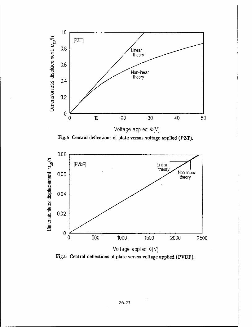
M

C o E <D O

J2 CL CO

CO CO

_a> a o

'co c CD

E Q

N

cu E <D Ü

_CÖ Q_ CO

CO CO O

1.0

0.8

0.6

0.4

0.2

0

[PZT]

/Linear ^ / theory ^^^*^

' ^s^ Non-inear ^•^ theory

0 10 20 30 40 50

Voltage applied: 0[V]

Fig.5 Central deflections of plate versus voltage applied (PZT).

0.08

0.06

0.04

o 0.02 CO

o E Q

0

[PVDF] Linear theory..

Non-linear theory

0 500 1000 1500 2000 2500

Voltage applied: 0[V]

Pig.6 Central deflections of plate versus voltage applied (PVDF).

26-23

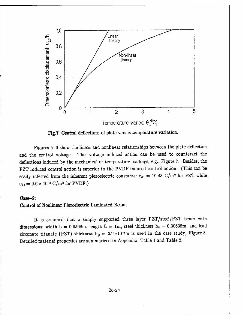
IM

c CD E Ü i5 Q. CO

TO

co CO

o 'co c

E Q

0 1

Temperature varied: 0t[°C]

.7 Central deflections of plate versus temperature variation. Fig

Figures 5-6 show the linear and nonlinear relationships between the plate deflection

and the control voltage. This voltage induced action can be used to counteract the deflections induced by the mechanical or temperature loadings, e.g., Figure 7. Besides, the PZT induced control action is superior to the PVDF induced control action. (This can be easily inferred from the inherent piezoelectric constants: e3i = 10.43 C/m2 for PZT while

e31 = 9.6 x 10-3 C/m2 for PVDF.)

Case-2: Control of Nonlinear Piezoelectric Laminated Beams

It is assumed that a simply supported three layer PZT/steel/PZT beam with dimensions: width b = 0.0508m, length L = lm, steel thickness he = 0.00635m, and lead zirconate titanate (PZT) thickness hp = 254xl0"6m is used in the case study, Figure 8.

Detailed material properties are summarized in Appendix: Table 1 and Table 2.

26-24

Fig.8 A PZT/steel/PZT laminated beam.

Next, the bending stiffness D and the membrane stiffness K can be respectively- calculated as: D =YI + 2YpIp + 2Ipe3i

2/e33 = 93.765(N-m2); K = YÄ + 2YpÄp

+ 2Äpe3i2/e33 = 23.986xl06(N). Note that the values of YI, 2YPIP, and 2Ipe312/e33 in the

PZT/steel/PZT beam are 80%, 18%, and 2% of the total bending stiffness D, respectively, and values of YÄ, 2YPÄP, and 2Äpe3iVe33 are 92.8%, 6.5%, and 0.7% of the total membrane stiffness K. It is assumed that applied control voltages 03§ and <b%\ are

uniformly distributed and 03<J = - 03§ = $, and the temperature rise 0 is also uniform

along the x-axis and linear variation through the thickness: 0(z) = äz + c, where ä

= (0t-0b)/(he+2hp), c = (#t+#b)/2, #t is the top surface temperature and 9\, is the bottom surface temperature of the beam. Note that fa =-0t = $ which implies that the total

temperature difference between the top and bottom surfaces is 20. Then, the electric control bending moment Mxc and the temperature induced moment Mxt are

Mxc = 0.0034990 (N-m) and Mx* = 0.348560 (N-m) , (64a,b)

26-25

in which 98% is due to the steel and only 2% is due to the PZT in the temperature induced

bending moment. (Recall that the ceramics are less sensitive to temperatures as compared

with steels.) The force and moment relationship can be simplified to

(■

tanhv cosh2v -) =

64v 4 £>3 ^Mx'+M.^L^

(65)

Denoting yi = (tanhv/v - l/cosh2v) and y2 = Ö^^VI^M^+Mx*)2!4], one can plot yi(v) and y2(v). Intersections of yi(v) and y2(v) gives solutions v of Eq.(65), such as shown

in Figures 9 to 11. Then, the axial force Nx,s and the beam center deflection (at x = L/2)

can be calculated and its temperature/control effects studied.

N- X>S 4y2£_

L2

u z>s (Mxc+Mxt)iA l .

-T/9 . - o v coshv ; ' x=L/2 4£>v

(66)

(67)

CM

c: co

dimensionless quantity v

Fig.9 Solution v for various control voltages (temperature 0 = 10° C).

26-26

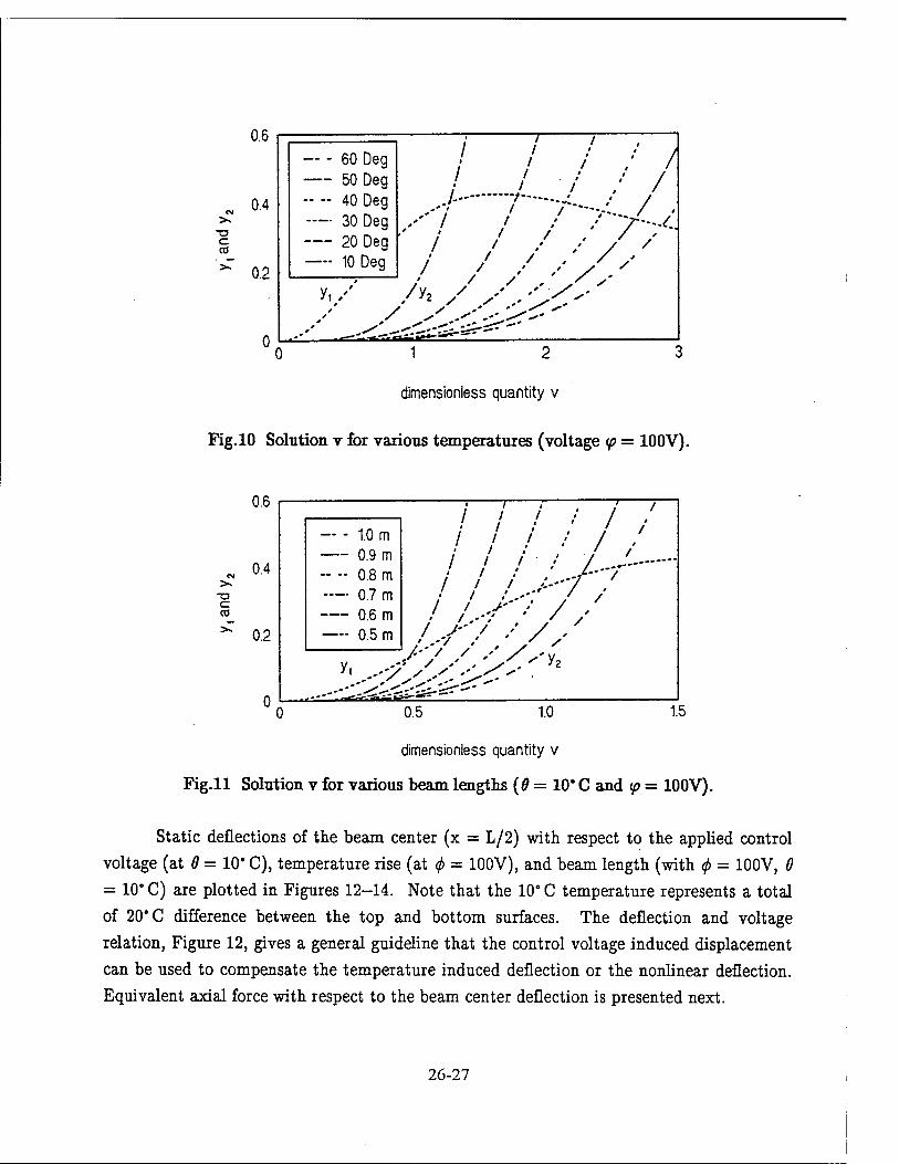
c co

0.6

0.4

0.2

— - 60 Deg 50 Deg -- -- 40 Deg —• 30 Deg 20 Deg — 10 Deg

/

y,/

A y"!

i /

■ A / • tf liiriiit

' J I ! / /""AA / / / / /

' ''' ■ 'S' /

1


Pig. 10 Solution v for various temperatures (voltage (p = 100V).

-a

co

0.6

0.4

0.2

0

— . 1.0 m 0.9 m

0.8 m — 0.7 m 0.6 m 0.5 m

/ / / / / / I I ! ! / f

/ ' / / / ./--■

! ' ' i .-i /

! I /.->"/ / /,-/"/ -'' /y

^CfiCkjSÜKä^S

1.5 0.5 1.0


Fig.ll Solution v for various beam lengths (9 = 10* C and = 100V), and beam length (with $ = 100V, 9

= 10° C) are plotted in Figures 12-14. Note that the 10° C temperature represents a total of 20" C difference between the top and bottom surfaces. The deflection and voltage relation, Figure 12, gives a general guideline that the control voltage induced displacement can be used to compensate the temperature induced deflection or the nonlinear deflection. Equivalent axial force with respect to the beam center deflection is presented next.

26-27

3.40

E E 3.25

•* »4

3

CO c 3.10 .o o <D

<o 2.95 Q

280 100 200

Voltage Applied (V)

Fig.12 Static deflections v.s. voltage changes (temperature 6 = 10* C).

E E

c .o "o .32

<r> O

10 20 30 40 50

Temperature Rise (°C)

60

Kg.13 Static deflections v.s. temperatuie changes (voltage <p = 100V).

26-28

0.6 0.7 0.8 0.9

Length of the Beam (m)

1.0

Fig.14 Static deflections for various beam lengths (0 = 10* C and (p = 100V).

Figure 15 shows the axial force versus the static deflections of the beam center, which reveals that the induced axial control force stiffens the beam and consequently the natural frequencies of the beam increase. (Note that this force can also be viewed as an axial control force.) The frequency increase can be expressed by the quantity {[1+ (NX)S L2/i2Z37T2)] / - l}xl00 percent, where i is the mode number, and the results are shown in Figures 16-18. The percentage of variation for the first mode is higher than those of the higher modes. The numerical results suggest that both static deflection and dynamic

behaviors of the simply supported nonlinear PZT/steel/PZT laminated beam are influenced by the temperature and they also can be controlled by the control voltages applied to the piezoelectric actuators.

26-29

ü o

ü <

3000

2000

1000

0 1.5 3.0 4.5 6.0

Transverse Displacements of Beam Middle Point uLJ (mm)

Fig. 15 Axial forces v.s. beam deflections.

ffi <n co <s> V—

o c <r> 2 'o c a>

30

20

10 f* -c -

f. .

n 100 200 300

Voltage applied (V)

Fig.16 Frequency variations v.s. control voltages (9 = 10* C).

26-30

*S 100

,--* T3 .«•*""

CD ,* CO CO CD

/b f1.---""

O ^^ cr * * to 50 ^jcr*

co <* o c CO

cr CO

25 f, . 4

u_ n

10 20 30 40 50 60

Temperature rise (°C)

Pig.17 Frequency variations v.s. temperatures (<j> = 100 V).

CO en CO <r> o .£ CO

'o c CD

cr CD

0.6 0.7 0.8 0.9 1.0

Length of the beam (m)

Fig.18 Frequency variations v.s. beam lengths (0 = 10* C, 0 = 100V).

SUMMARY AND CONCLUSIONS

Beam and plate like structures and components are widely used in many aerospace

structures. Imposed shape changes and surface control of flexible beams and plates could

offer many aerodynamic advantages in flight maneuverability and precision control.

Deformed shapes and surfaces often involve nonlinear deformations. Studies of control of

nonlinear behavior related to the deformed surfaces and shape changes would provide

detailed information in future controlled surface design and implementation. This research

26-31

is concerned with the control effectiveness of nonlinearly deformed beams and plates based

on the smart structures technology.

In the recent development of smart structures and structronic systems, piezoelectric

materials are widely used as sensors and actuators in sensing, actuation, and control applications. This research is to investigate the control effectiveness of piezoelectric laminated nonlinear flexible beams and plates (rectangular and square plates) subjected to mechanical and temperature excitations. It is assumed that the flexible beams and plates encounter the von Karman type geometrical nonlinearity. Thermoelectromechanical equations and boundary conditions including elastic, temperature, and piezoelectric

couplings will be formulated first, and analytical solutions be derived. The reduced

nonlinear static equations are identical to the classic nonlinear plate and beam equations. Dynamics, electromechanical couplings, and control of nonlinear piezoelectric laminated beams and plates with large deformations are investigated. Active control of nonlinear flexible deflections, thermal deformations, and natural frequencies using distributed

piezoelectric actuators are studied, and their nonlinear effects are evaluated.

Nonlinear static deflections with the influence of temperature and control voltage were studied. Voltage—temperature and displacement relations for piezoelectric laminated nonlinear plates and beams were investigated. The voltage imposed actuations can be used to compensate the nonlinear deformation and the temperature induced deformation.

Small—amplitude beam oscillations with respect to the nonlinearly deformed static

equilibrium position were investigated. It was observed that the total bending stiffness of

the PZT/steel/PZT laminated beam is contributed by the steel (80%) and PZT (elasticity: 18% and piezoelectricity: 2%), and the total membrane stiffness is contributed by the steel (98%) and PZT (elasticity: 6.5% and piezoelectricity: 0.7%) in the laminated beam. The piezoelectricity contributed stiffness is relatively insignificant. Simulation results also suggested that the voltage induced control displacement/force can be used to compensate

the nonlinear static deflection, temperature effects, and natural frequencies of the

piezoelectric laminated beam.

26-32

ACKNOWLEDGEMENT

This research is supported, in part, by a grant (96-O882)(F49620-93-0063) from

the Air Force Office of Scientific Research and the Wright Laboratory (Flight Dynamics

Laboratory). Technical advices from Dr. V.B. Venkayya are gratefully acknowledged.

This report constitutes a part of Dr. Y. Bao's Ph.D. dissertation.

BIBLIOGRAPHY

Chia, C.Y., 1980, Nonlinear Analysis of Plates, McGraw-Hill International Book Co., New York.

Lalande, F., Chaudhry, Z., and Rogers, C.A., 1993, "A Simplified Geometrically

Nonlinear Approach to the Analysis of the Moonie Actuator," Adaptive Structures and

Material Systems, AD-Vol.35, pp. 149-155, 1993 ASME WAM, New Orleans, LA, Nov.28-Dec.3, 1993.

Librescu, L., 1987, "Refined Geometrically Nonlinear Theories of Anisotropie

Laminated Shells," Quarterly of Applied Mathematics, Vol.XLV, No.l, pp.1-22.

Meirovitch, L., 1975, Elements of Vibration Analysis, McGraw-Hill, p.208.

Palazotto, A.N. and Dennis, S.T., 1992, Nonlinear Analysis of Shell Structures, AI A A Pub., Washington, D.C.

Pai, P.F., Nafeh, A.H., Oh, K., and Mook, D.T., 1993, "A Refined Nonlinear Model

of Piezoelectric Plate," J. Solids and Structures, Vol.30, pp.1603-1630.

Pietraszkiewicz, W., 1979, Finite Rotations and Lagrangean Description in the

Non-linear Theory of Shells, Polish Academy of Science, Polish Scientific Publishers.

Soedel, W., 1981, Vibrations of Shells and Plates, Dekker, New York, p.271.

Sreeram, P.N., Salvady, G. and Naganathan, N.G., 1993, "Hyteresis Prediction for a

Piezoceramic Material System," Adaptive Structures and Material Systems, AD-Vol.35,

pp.35^2, 1993 ASME WAM, New Orleans, LA, Nov.28-Dec.3, 1993.

Timoshenko, S., Young, D.H., and Weaver, W., 1974, Vibration Problems in Engineering, Wiley, New York.

Tzou H.S. and Anderson, G.L., (Ed.), 1992, Intelligent Structural Systems, Kluwer

Academic Publishers, Dordrecht/Boston/London.

Tzou, H.S., 1993, Piezoelectric Shells {Distributed Sensing and Control of Continua),

Kluwer Academic Publishers, Dordrecht/Boston/London.

26-33 •

Tzou, H.S. and Bao, Y., 1994, "Modeling of Thick Anisotropie Composite Triclinic

Piezoelectric Shell Transducer Laminates," Journal of Smart Materials and Structures,

Vol.3, pp.285-292. Tzou, H.S. and Bao, Y., 1995, "A Theory on Anisotropie Piezothermoelastic Shell

Laminates with Sensor/Actuator Applications," Journal of Sound & Vibration, Vol.184,

No.3, pp.453-473. Tzou, H.S. and Bao, Y., 1996, "Nonlinear Piezothermoelasticity and Multi-field

Actuations, Part-1: Nonlinear Anisotropie Piezothermoelastic Shell Laminates," ASME

Transactions, Journal of Vibration & Acoustics. (To appear) H.S. Tzou and T. Fukuda (Ed), 1992, Precision Sensors, Actuators, and Systems,

Kluwer Academic Publishers, Dordrecht/Boston/London, August 1992. Tzou, H.S. and Howard, R.V., 1994, "A Piezothermoelastic Thin Shell Theory

Applied to Active Structures," ASME Transactions, Journal of Vibration & Acoustics,

Vol.116, No.3, pp.295-302. Tzou, H.S. and Ye, R., 1994, "Piezothermoelasticity and Precision Control of

Piezoelectric Systems: Theory and Finite Element Analysis," ASME Transactions, Journal

of Vibration & Acoustics, Vol.116, No.4, pp.489-495. Tzou, H.S. and Zhong, J.P., 1993, "Electromechanics and Vibrations of

Piezoelectric Shell Distributed Systems: Theory and Applications," ASME Journal of

Dynamic Systems, Measurements, and Control, Vol.115, No.3, pp.506—517. Tzou, H.S., Zhong, J.P., and Natori, M.C., 1993, "Sensor Mechanics of Distributed

Shell Convolving Sensors Applied to Flexible Rings," ASME Journal of Vibration &

Acoustics, Vol.(115), No.l, pp.40^6, January 1993. Tzou, H.S., Zhong, J.P., and Hollkamp, J.J., 1994, "Spatially Distributed

Orthogonal Piezoelectric Shell Actuators: Theory and Applications," Journal of Sound &

Vibration, Vol.177, No.3, pp.363-378, October 1994. Tzou, H.S. and Zhou, Y-H., 1995, "Dynamics and Control of Nonlinear Circular

Plates with Piezoelectric Actuators," J of Sound & Vibration, Vol.188, No.2, pp.189-207. Yu, Y.Y., 1993, "Some Recent Advances in Linear and Nonlinear Dynamical

Modeling of Elastic and Piezoelectric Plates," Adaptive Structures and Material Systems,

AD-Vol.35, pp.185-195, 1993 ASME WAM, New Orleans, LA, Nov.28-Dec.3, 1993.

26-34

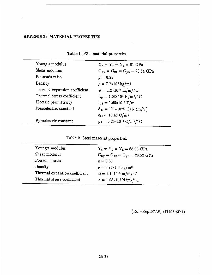
APPENDIX: MATERIAL PROPERTIES

Table 1 PZT material properties.

Young's modulus Yx = Yy = Yz = 61 GPa

Shear modulus Gxy = Gxz = Gyz = 23.64 GPa

Poisson's ratio p = 0.29

Density p = 7.7x103 kg/m3

Thermal expansion coefficient a = 1.2xl0-6 m/m/° C

Thermal stress coefficient Ap = 1.03* 105 N/m2/° C

Electric permittivity e33 = 1.65xl0"8 F/m

Piezoelectric constant d31 = 171xl0-12 C/N (m/V)

e3i = 10.43 C/m2

Pyroelectric constant p3 = 0.25xl0"4 C/m2/0 C

Table 2 Steel material properties.

Young's modulus Yx = Yy = Yz = 68.95 GPa

Shear modulus Gxy = Gxz = Gyz = 26.52 GPa

Poisson's ratio // = 0.30

Density p = 7.75x103 kg/m3

Thermal expansion coefficient a = l.lxio-s m/m/° C

Thermal stress coefficient A = 1.08xl06 N/m2/"C

(Rdl-Rept97.Wp/Fil97.t3bl)

26-35

A Progressive Refinement Approach to Planning and Scheduling

William J. Wolfe Associate Professor

Department of Computer Science and Engineering

University of Colorado at Denver Denver, CO


Wright Laboratory


Boiling AFB, Washington, DC

and

Wright Laboratory

January 1997

27-1

A Progressive Refinement Approach to Planning and Scheduling

William J.Wolfe Associate Professor of Computer Science

Department of Computer Science and Engineering University of Colorado at Denver

Abstract

A summary of the algorithmic results presented in this report: 1. We introduce a "novel" scheduling problem called the window-constrained packing problem (WCP), and we provide extensive simulation results; 2. We describe the "0-filter" approach, a creative way to deal with multiple sorting features. 3. The "priority dispatcher" that we invented uses three phases: i. selection/sort; ii. allocation; iii. optimization. This simple modular design can be modified in a variety of ways, making it easy to adapt to specific applications; 4. The "look-ahead" algorithm that we invented uses the dispatcher to look ahead in the list of jobs to determine a good choice of allocation options; 5. The "augmented genetic" algorithm that we invented has the potential to produce near-optimal results, when time permits.

There are so many applications that require advanced planning and scheduling techniques that we can only provide a partial listing, such as: Transportation Systems (Airlines, Trucking, Logistics, Buses, Highways, etc.); Facilities Management (Hospitals, Courts, Schools, etc.); Communications Systems (Telephones, Cable, etc.); Factories; Spacecraft (Earth Observing, Deep Space, Communications, etc.). We identified three factors for evaluating the many algorithmic approaches: speed, simplicity, and accuracy. "Speed" refers to the time it takes an algorithm to process and return its results. "Simplicity" refers to the ease by which users are able to understand the algorithm's logic. "Accuracy" refers to the quality of the algorithm's results as measured by some criteria (i.e.: an objective function). The complexity of these environments pushed us toward fast and simple algorithms, such as dispatch methods. For increased accuracy we developed a look ahead method (relatively fast, relatively simple, and very accurate). If the accuracy requirements are severe (i.e.: need near-optimal solutions) then simplicity and speed can be sacrificed in favor of more complex and time consuming methods (e.g.: simulated annealing, genetic, tabu search, etc.). We have concluded that look-ahead approaches, and variations on that theme, are very often the best compromise, usually providing high quality results within reasonable run time limits, while also being relatively easy to understand. It is very difficult, and in many cases impossible, to define a reliable objective function. Therefore in most cases there is no easy way of comparing algorithmic results other than to say that one performed better with respect to that criteria. This observation pointed us toward fast and simple methods, since more complex methods are, more or less, using a lot of processing time to fine- tune the results according to a presumed objective function. Thus, there are at least three reasons why the pursuit of accuracy is questionable: 1. accuracy is often defined by a subjective weighting of multiple, disparate, criteria (weighing apples and oranges); 2. the time between planning and implementation is often long enough for many of the assumptions the plan is based on to become invalid; and 3. computing accurate solutions often takes a prohibitive amount of processing time. There is little point in pursuing accuracy at the expense of speed and simplicity in a rapidly changing environment. Highly accurate algorithmic results can be made obsolete by small changes in the constraints. The constraints themselves are often vague or imprecise. Additionally, we do not want a high speed scheduler that reacts to every little change, constantly moving jobs around. The scheduling process could become "unstable": rapidly changing commitments (confused customers and operators). These considerations led us to incorporate a "fuzzy" approach. In fact, we have tentatively concluded that highly complex, dynamic, domains with multiple, possibly vague, criteria are prime application areas for the fuzzy logic approach. To add further context to these algorithmic results we also explored a hierarchical approach called "progressive refinement". It takes into account a rolling horizon of out-day schedules that are continuously adapted until operational time. This approach helps to smooth over many of the de-stabilizing inputs (e.g.: machine failure, canceled orders, new orders, price changes, etc.).

27-2

1. Introduction

The development of automated scheduling systems continues to be an area of great interest in industry and

academia. It involves the computer modeling of jobs, resources, and constraints, as well as the design of algorithms and other systems that would help human schedulers do their jobs. There are so many applications that require advanced planning and scheduling techniques that we can only provide a partial listing, such as:

Transportation Systems (Airlines, Trucking, Logistics, Buses, Highways, etc.); Facilities Management (Hospitals, Courts, Schools, etc.); Communications Systems (Telephones, Cable, etc.); Factories; Spacecraft (Earth Observing, Hubble Space Telescope, Deep Space, Communications, etc.).

We identified three factors for evaluating the many algorithmic approaches: speed, simplicity, and accuracy. "Speed" refers to the time it takes an algorithm to process and return its results. "Simplicity" refers to the ease by which users are able to understand the algorithm's logic. "Accuracy" refers to the quality of the algorithm's results as measured by some criteria (i.e.: an objective function).

The application areas mentioned above are very complex and highly dynamic. The complexity of these environments pushed us toward fast and simple algorithms, such as dispatch methods. For increased accuracy we developed a particular look ahead method (relatively fast, relatively simple, and very accurate). If the accuracy requirements are severe (i.e.: need near-optimal solutions) then simplicity and speed can be sacrificed in favor of more complex and time consuming methods (e.g.: simulated annealing, genetic, tabu search, etc.). We have concluded that look-ahead approaches, and variations on that theme, are very often the best compromise, usually providing high quality results within reasonable run time limits, while also being relatively easy to understand.

Because of the complexity of these domains it is very difficult, and in many cases impossible, to define a reliable objective function. Therefore in most cases there is no easy way of comparing algorithmic results other than to say that one performed better with respect to that criteria. This observation also points us toward fast and simple methods, since more complex methods are, more or less, using a lot of processing time to fine-tune the results according to a. presumed objective function.

Thus, there are at least three reasons why the pursuit of "accuracy" is questionable: 1. accuracy is often defined by a subjective weighting of multiple, disparate, criteria (weighing apples and oranges); 2. the time between planning and implementation is often long enough for many of the assumptions the plan is based on to become invalid; and 3. computing accurate solutions often takes a prohibitive amount of processing time. There is little point in pursuing accuracy at the expense of speed and simplicity in an rapidly changing environment (e.g.: rapidly changing goals, priorities, cost factors, machine availability, etc.). Highly accurate algorithmic results can be made obsolete by small changes in the constraints. The constraints themselves are often vague or imprecise, further discouraging the fine-tuning of algorithmic results.

Additionally, we do not want a high speed scheduler that reacts to every little change, constantly moving jobs around. The scheduling process could become "unstable": rapidly changing commitments (confused customers, suppliers, and workers). These considerations led us to incorporate a "fuzzy" approach (section

27-3

6). In fact, we have tentatively concluded that highly complex, dynamic, domains with multiple, possibly vague, criteria are prime application areas for the fuzzy logic approach.

To add further context to these algorithmic results we also explored a hierarchical approach called "progressive refinement". It takes into account a rolling horizon of out-day schedules that are continuously adapted until operational time. This approach helps to smooth over many of the de-stabilizing inputs (e.g.: machine failure, canceled orders, new orders, price changes, etc.). Although many of the simulations presented in this report are based on a "batch" approach (i.e.: dispatch algorithms) it is clear that such methods must be integrated into progressive refinement, or incremental, methods in most applications.

The algorithms that we discuss in this report can be classified as follows.

Algorithm Classifications

Optimal: Heuristic: Depth First

(exhaustive search) Constructive Heuristics:

Priority Dispatcher Look Ahead

Branch and Bound Fuzzy Logic

Linear Programming Improvement Heuristics: Hill Climbing Simulated Annealing Tabu Search

Repair Heuristics: Iterative Refinement

Genetic: Indirect Representation Augmented Genetic.

Optimal algorithms are guaranteed to find optimal solutions, but they usually take a prohibitive amount of time. The constructive heuristics begin with a batch of jobs and a clean slate, and schedule the jobs one by one (with limited backtracking) until a complete schedule is achieved. The improvement heuristics begin with a schedule and find ways to improve the quality. A constructive heuristic is often used to create a schedule that is then used as the starting point for an improvement heuristic.

The repair heuristics apply when a sudden "disturbance" (e.g.: machine failure, canceled order, etc.) has been introduced and a quick fix is needed. For example, the schedule might be amended in such a way as to cause the least amount of change to existing commitments. There are many variations on this theme. For example, a "schedule" might have many constraint violations (e.g.: overbooking) while it is going through a process of incremental improvement. Some authors call this "iterative refinement" [3]. One distinction that could be made is whether or not the momentary "schedules" are feasible1 or can contain constraint violations. Until we get to the section on progressive refinement we assume that a "schedule" has no constraint violations.

The genetic approach is in a class by itself. It works by having a population of schedules and breeds new schedules from "pieces" of the best schedules in the current population.

"Feasible" means that the schedule can be implemented (but it may he very inefficient).

27-4

We have found that we can begin with a particular heuristic approach and then create a variety of hybrids that use parts and pieces from any or all of the above methods. Thus, it is sometimes pointless to compare the individual methods since most applications will require a unique hybrid approach. We worked at understanding each method well enough to be able to quickly evaluate the cost-benefit trade off of including some part of the method in a hybrid approach to a real problem.

There are several issues that come up in one form or another throughout this report: algorithm processing time; algorithm rationale (i.e.: simplicity); multiple, conflicting, criteria; constraint propagation and relaxation; bottlenecks and other features of the job conflicts; general rules of thumb; uncertainty vs. complexity; dynamic environments; scheduling horizons; stability; progressive refinement.

Overview of Planning and Scheduling concepts: From allocating machines to jobs in a factory, to making lane changes on a highway, a wide variety of engineering problems involve some form of planning or scheduling: the allocation of resources to jobs over time. The term "planning" usually relates to higher level issues, such as the overall purpose, goals and strategies of an endeavor, while the term "scheduling" usually relates to lower level issues, such as specific equipment and operation start/stop times. In the simplest possible terms, planning deals with "what" and scheduling with "when". This distinction is usually minor and most authors, like us, use the terms interchangeably, but scheduling strongly connotes the specific assignment of activities to time lines, which is the main topic of this report.

There are several issues that make automated scheduling difficult, the primary ones being:

• Ambiguity: vague or poorly defined terms, criteria, constraints or specifications.

• Modeling: it is difficult to build efficient, high fidelity, models of the domain.

• Uncertainty: unexpected events and inherently random processes.

• Combinatorial Explosion: a huge number of alternatives and options.

• Dynamics: rapidly changing goals, resources, costs, requirements, etc.

Ambiguous criteria make it impossible to objectively tell when one schedule is better than another. For example, criteria such as "customer satisfaction" or "high quality product", are commonly expressed but are also difficult to quantify. They summarize a complex synthesis of several factors (possibly including such amorphous factors as the customer's perceptions of quality, etc.). The criteria can sometimes be clarified by identifying the contributing components, such as inventory cost, # of late jobs, machine preferences, average job flow time, etc. But individual components can conflict, for example: low cost and on time usually conflict with high quality2. And it may be very difficult to agree on weighting factors that might quantify the relative merits of trading off one criteria in favor of another (e.g.: is a little lateness worth a small increase in quality). The result of a successful analysis of the relevant criteria is a clearly specified objective function. The function could then be used to reliably distinguish not only that one schedule is better than another but also by how much it is better. Unfortunately, more often than not such an objective function is either a gross over simplification of the problem or based on several subjective parameters.

Criteria specifications can be related to at least these three broad categories: 1. Cost and profit factors; 2. Managerial policy decisions; 3. Customer preferences. Policy decisions and customer preferences are related to profit, but in a long term sense. Clearly, one major difficulty in quantifying the criteria is that it may change suddenly (market fluctuations, manager decisions, customer preferences, etc.).

2 This reminds me of the sign that a student said was posted on a production manager's desk. It listed the following three items: "1. ON TIME; 2. HIGH QUALITY; 3. CHEAP"; under which was the advice: "PICK ANY TWO".

27-5

Constraints must also be clearly specified. There are at least three types of constraints: 1. Criteria-related; 2. Physical; 3. Both. Criteria specifications are sometimes interpreted as constraints. Take for example: "get all the jobs done on time". This is not a physical constraint, since it can be violated, but at a cost. Physical constraints are usually the kind that cannot be violated, such as size, shape, weight, or rate limitations related to the use of a particular piece of equipment. Capacity limits, exclusive use, precedence, and maximum number of shared users are also examples of physical constraints.

Some constraints are just preferences related to physical attributes of a product, such as color or size. Another way of classifying constraints is to distinguish hard from soft constraints. A hard constraint cannot be violated but a soft constraint has degrees of acceptability. For example, a soft constraint might be expressed as: the customer wants green, but blue is acceptable, and other colors are less acceptable. But the fact that the product must be painted might be a hard constraint. Now, it is also clear that when the boss says that there are to be no late jobs, then for all intents and purposes this is a hard constraint. The important distinction, however, is the difference between relaxable and non-relaxable constraints. For example, when the boss concludes that it is not possible for all the jobs to be on time, the due date constraint might be relaxed to allow jobs to be up to 1 day late. But the boss cannot dictate the violation of the laws of physics (e.g.: equipment operational limits). The variations along these lines are almost endless.

c CONSTRAINTS

UlJiCKhlfc. CONTINUOUS xc{ A.B.C) aSxSb

11 AKU SU

CbLAXAULh

Figure A: There are several ways to classify constraints.

A last example: if there are only 5 machines in a shop then a valid schedule would use 5 or less machines; but that does not prevent the scheduler from creating a hypothetical schedule that uses 6 machines; that is, the hard constraint is relaxed to do a "what if analysis that evaluates the benefit of adding a machine to the shop.

The distinction between hard and soft constraints, and the means by which constraints are relaxed, plays a big role in most scheduling processes. For example, constraints might have relaxation levels: when it is discovered that a feasible schedule can not be found all constraints of level 1 are relaxed (made less strict) and the search for a feasible schedule resumed; if that fails all the constraints of level 2 are relaxed, etc. Finally, we note that there are other ways to classify constraints3, such as discrete vs. continuous, and deterministic vs. probabilistic.

An example just came up: an author called all the system constraints the implicit constraints and all the customer preferences the explicit constraints.

27-6

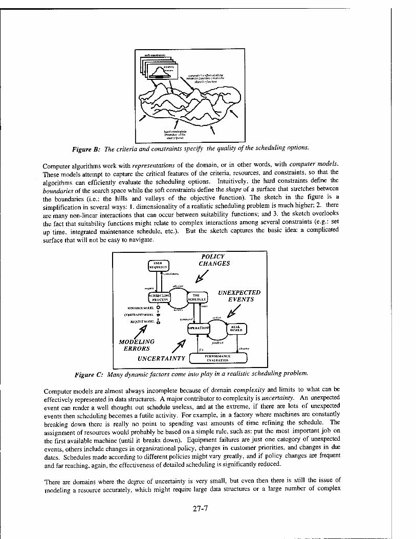
soft constraints

cummulative effect of all the suitability functions creates the

objective function

hard constraints [boundary of the

search space)

Figure B: The criteria and constraints specify the quality of the scheduling options.

Computer algorithms work with representations of the domain, or in other words, with computer models. These models attempt to capture the critical features of the criteria, resources, and constraints, so that the algorithms can efficiently evaluate the scheduling options. Intuitively, the hard constraints define the boundaries of the search space while the soft constraints define the shape of a surface that stretches between the boundaries (i.e.: the hills and valleys of the objective function). The sketch in the figure is a simplification in several ways: 1. dimensionality of a realistic scheduling problem is much higher; 2. there are many non-linear interactions that can occur between suitability functions; and 3. the sketch overlooks the fact that suitability functions might relate to complex interactions among several constraints (e.g.: set up time, integrated maintenance schedule, etc.). But the sketch captures the basic idea: a complicated surface that will not be easy to navigate.

POLICY CHANGES

UNEXPECTED EVENTS

RESOURCE MODFX

CONSTRAINT MODEL

REQUEST MODEL

MODELING ERRORS

UNCERTAINTY f

Figure C: Many dynamic factors come into play in a realistic scheduling problem.

Computer models are almost always incomplete because of domain complexity and limits to what can be effectively represented in data structures. A major contributor to complexity is uncertainty. An unexpected event can render a well thought out schedule useless, and at the extreme, if there are lots of unexpected events then scheduling becomes a futile activity. For example, in a factory where machines are constantly breaking down there is really no point to spending vast amounts of time refining the schedule. The assignment of resources would probably be based on a simple rule, such as: put the most important job on the first available machine (until it breaks down). Equipment failures are just one category of unexpected events, others include changes in organizational policy, changes in customer priorities, and changes in due dates. Schedules made according to different policies might vary greatly, and if policy changes are frequent and far reaching, again, the effectiveness of detailed scheduling is significantly reduced.

There are domains where the degree of uncertainty is very small, but even then there is still the issue of modeling a resource accurately, which might require large data structures or a large number of complex

27-7

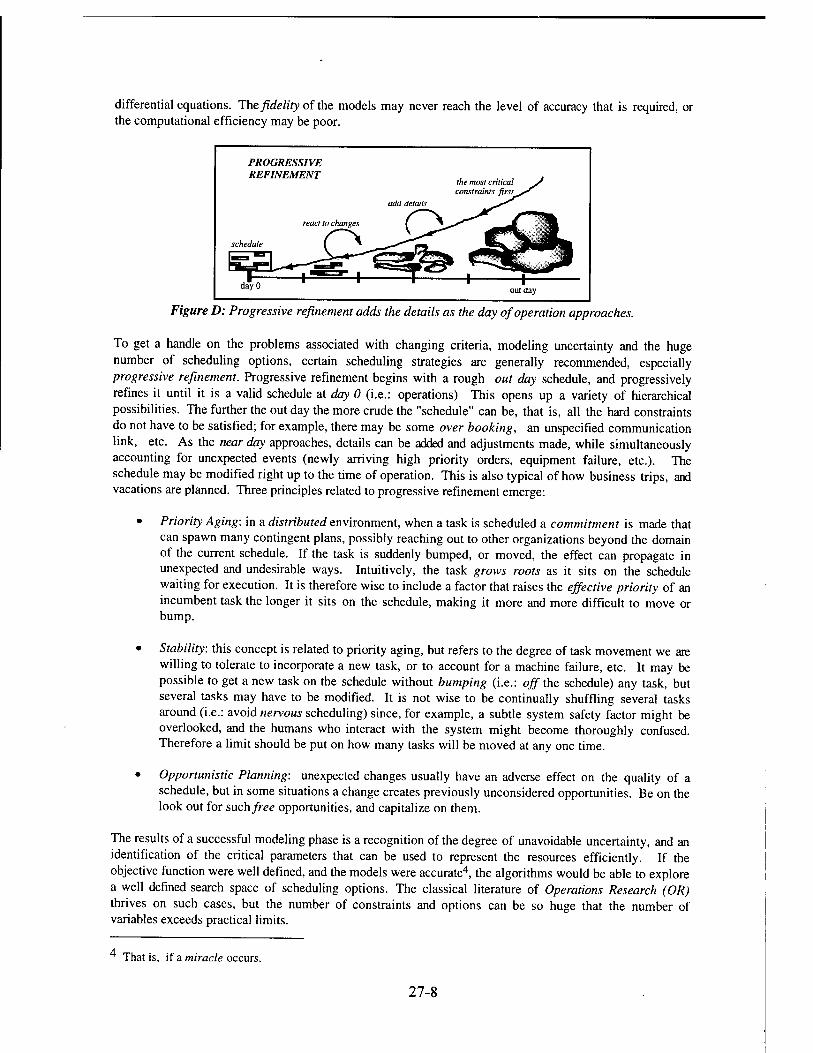
differential equations. The fidelity of the models may never reach the level of accuracy that is required, or the computational efficiency may be poor.

PROGRESSIVE REFINEMENT

the most critical constraints first

react to changes

schedule

dayO out day

Figure D: Progressive refinement adds the details as the day of operation approaches.

To get a handle on the problems associated with changing criteria, modeling uncertainty and the huge number of scheduling options, certain scheduling strategies are generally recommended, especially progressive refinement. Progressive refinement begins with a rough out day schedule, and progressively refines it until it is a valid schedule at day 0 (i.e.: operations) This opens up a variety of hierarchical possibilities. The further the out day the more crude the "schedule" can be, that is, all the hard constraints do not have to be satisfied; for example, there may be some over booking, an unspecified communication link, etc. As the near day approaches, details can be added and adjustments made, while simultaneously accounting for unexpected events (newly arriving high priority orders, equipment failure, etc.). The schedule may be modified right up to the time of operation. This is also typical of how business trips, and vacations are planned. Three principles related to progressive refinement emerge:

• Priority Aging: in a distributed environment, when a task is scheduled a commitment is made that can spawn many contingent plans, possibly reaching out to other organizations beyond the domain of the current schedule. If the task is suddenly bumped, or moved, the effect can propagate in unexpected and undesirable ways. Intuitively, the task grows roots as it sits on the schedule waiting for execution. It is therefore wise to include a factor that raises the effective priority of an incumbent task the longer it sits on the schedule, making it more and more difficult to move or bump.

• Stability: this concept is related to priority aging, but refers to the degree of task movement we are willing to tolerate to incorporate a new task, or to account for a machine failure, etc. It may be possible to get a new task on the schedule without bumping (i.e.: off the schedule) any task, but several tasks may have to be modified. It is not wise to be continually shuffling several tasks around (i.e.: avoid nervous scheduling) since, for example, a subtle system safety factor might be overlooked, and the humans who interact with the system might become thoroughly confused. Therefore a limit should be put on how many tasks will be moved at any one time.

• Opportunistic Planning: unexpected changes usually have an adverse effect on the quality of a schedule, but in some situations a change creates previously unconsidered opportunities. Be on the look out for such free opportunities, and capitalize on them.

The results of a successful modeling phase is a recognition of the degree of unavoidable uncertainty, and an identification of the critical parameters that can be used to represent the resources efficiently. If the objective function were well defined, and the models were accurate4, the algorithms would be able to explore a well defined search space of scheduling options. The classical literature of Operations Research (OR) thrives on such cases, but the number of constraints and options can be so huge that the number of variables exceeds practical limits.

That is, if a miracle occurs.

27-8

An algorithm has to be pretty smart to avoid exploring many bad options. Effective rules or heuristics usually incorporate specific details of the particular domain and consequently such rules do not apply to other domains. This is not a simple matter and it hits at the heart of all heuristic search strategies. We will discuss such heuristics in the following sections.

27-9

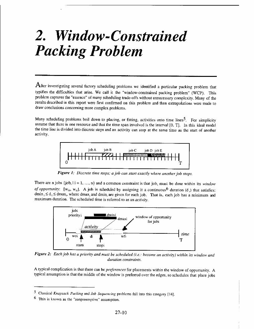
2. Window-Constrained Packing Problem

After investigating several factory scheduling problems we identified a particular packing problem that

typifies the difficulties that arise. We call it the "window-constrained packing problem" (WCP). This problem captures the "essence" of many scheduling trade-offs without unnecessary complexity. Many of the results described in this report were first confirmed on this problem and then extrapolations were made to draw conclusions concerning more complex problems.

Many scheduling problems boil down to placing, or fitting, activities onto time lines5. For simplicity assume that there is one resource and that the time span involved is the interval [0, T]. In this ideal model the time line is divided into discrete steps and an activity can stop at the same time as the start of another activity.

rf job A jobB jobC jobD jobE

; : TT m

Figure 1: Discrete time steps; a job can start exactly where another job stops.

There are n jobs {jobf I i = 1, ..., n} and a common constraint is that job; must be done within its window

of opportunity: [w0i, wfj]. A job is scheduled by assigning it a continuous6 duration (dj) that satisfies: dminj < dj < dmaxi; where dmaxi and dminj are given for each job. That is, each job has a minimum and maximum duration. The scheduled time is referred to as an activity.

jobi Idmini

dmaxi

/

window of opportunity ' for jobi

J t.

priority i ■ ■^^■I^^^H

/ activity y 1 IA.UMU.UAM'

o oif d f starti stopi

wfi ^ time

T

Figure 2: Each job has a priority and must be scheduled (i.e.: become an activity) within its window and duration constraints.

A typical complication is that there can be preferences for placements within the window of opportunity. A typical assumption is that the middle of the window is preferred over the edges, so schedules that place jobs

Classical Knapsack Packing and Job Sequencing problems fall into this category [14]. This is known as the "nonpreemptive" assumption.

27-10

in the middle of their windows would be given higher scores. This preference might be specified by a

suitability function.'

The Window-Constrained Packing Problem (WCP):

maximum duration (dmax)

jobl

job 2 I 1

job 3

jobn

priority (p)

I 1

I 1

window of opportunity

minimum duration (dmin)

|||||lllMlr#milllllllllllll time

Figure 3: Several jobs compete for time on the resource within their windows of opportunity.

Score Profile (or "Suitability Function", or "Utility Function")

;

/r \score profile

s(t)^v

WO

"1 wf

1 = slan^^^^^^^ =5ltT

activity

1 = stop

area= X s(t) At

Figure 4: A job is defined by a minimum (dmJ and a maximum (d„J duration that must be scheduled within a window of opportunity. The score profile expresses the preference for placement within the window (for the bell curve in this sketch the preference favors the center of the window).

Each job also has a priority assigned to it: 1< ps <10. The priority measures the relative worth of the job,

and might be measured in profit-dollars or other measures of value8.

When there is competition for the resource the scheduler must determine which jobs get on the schedule and specify the start and stop times that satisfy the window limits and duration constraints.

7 Sometimes called a score profile, or utility function. 8 An example that jumps to mind is the "scientific worth" of a satellite observation activity.

27-11

Putting this all together we can formally define the window-constrained packing problem (see figure 5).

Window-Constrained Packing Problem (WCP): Given n objects (requests), each having:

• a window of opportunity [w0, wf]; • a suitability function with domain = [w0, wf]: {s(t) 11 € [w0, wf]}; • a minimum length (dmin) and a maximum length (dm„); and • a priority p.

Maximize:

Where:

Q = X xi • pi • areai i = 1

stopi

areai = £si(t)

Subject to the constraints:

d < d < d "mini — ui — umaxi

dmaxi ^W = Wfi-Woi

woi < startj < wfi - dj X;S {0,1} [start;, stopp n [start,, stopj) = 0 i /j (consistency)

(note: x, = 1 means that jobj is on the schedule)

Figure 5: The details of the Window-Constrained Packing Problem.

The WCP arises as a sub-problem in many scheduling problems (e.g.: job shop, satellites, deliveries, etc.). In the simplest case s(t) = 1 for all the job windows, and areaj = stopi - start) = d, for all scheduled jobs.

w0 wf

priority

Competing Jobs

I' ^ 1 te ^ I — III

a.

] r^=ni^PE:

i" ^

SIE ] EHUE

Resource

llllllllllllllllllllilllll

dmin ~~dmax

44f+H

The Schedule Figure 6: The various WCP jobs compete for placement on the schedule.

27-12

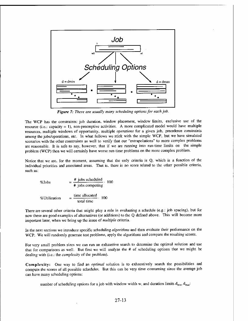
Job

d = dmin

Scheduling Options

d = dmax

J E : • r 3 :

Figure 7: There are usually many scheduling options for each job.

The WCP has the constraints: job duration, window placement, window limits, exclusive use of the resource (i.e.: capacity = 1), non-preemptive activities. A more complicated model would have multiple resources, multiple windows of opportunity, multiple operations for a given job, precedence constraints among the jobs/operations, etc. In what follows we stick with the simple WCP, but we have simulated scenarios with the other constraints as well to verify that our "extrapolations" to more complex problems are reasonable. It is safe to say, however, that if we are running into run-time limits on the simple problem (WCP) then we will certainly have worse run-time problems on the more complex problem.

Notice that we are, for the moment, assuming that the only criteria is Q, which is a function of the individual priorities and associated areas. That is, there is no score related to the other possible criteria, such as:

%Jobs # jobs scheduled

# jobs competing 100

%Utilization time allocated

total time 100

There are several other criteria that might play a role in evaluating a schedule (e.g.: job spacing), but for now these are good examples of alternatives (or additions) to the Q defined above. This will become more important later, when we bring up the issue of multiple criteria.

In the next sections we introduce specific scheduling algorithms and then evaluate their performance on the WCP. We will randomly generate test problems, apply the algorithms and compare the resulting scores.

For very small problem sizes we can run an exhaustive search to determine the optimal solution and use that for comparisons as well. But first we will analyze the # of scheduling options that we might be dealing with (i.e.: the complexity of the problem).

Complexity: One way to find an optimal solution is to exhaustively search the possibilities and compute the scores of all possible schedules. But this can be very time consuming since the average job can have many scheduling options:

number of scheduling options for a job with window width w, and duration limits drajn, dmax:

27-13

dmax # options = 1 + X[\v - q + 1]

q = dmin

= ! + (d»™ - dmin + l)-( w + 1 - (dmin + dmax)/2 );

The "1" occurring after the equal sign accounts for the option of not scheduling the job. In fact, one of the most critical aspects of this problem is that we do not know ahead of time which jobs should "make" the schedule and which ones to leave off the schedule.

The largest number of options occurs when the window is the largest, the minimum time is the smallest, and the maximum duration is the largest. Let w = wmax, and suppose dmin = 1 and dmax = w:

(w)-(w + 1 - (w + l)/2) +1 = (w)-(w+l)/2 + 1 = (w)2/2 + w/2 + 1 = 0(w2).

So, in the worst case, since there are n jobs, there can be as many as w2n total scheduling options.

The simplest situation is when drain = dmax = w for each job: 1 option per job. But even this case can get sticky since the jobs may be inconsistent (i.e.: conflict with each other): if the jobs are all consistent there is only 1 total scheduling option; if two jobs overlap than we must choose 1 out of 2, and so on if several overlap.

So, roughly speaking, each job has about w scheduling options, and there are about wn possible schedules. The number of scheduling options grows exponentially as the number of jobs increases (it also grows as w increases, but at a slower rate). Some of these options will be eliminated because they create inconsistent (non-feasible) schedules. Another extreme is when a job window does not overlap any other job window: the only option that should then be considered for that job is when the duration (dmax) is placed to give the maximum area; no other options need be considered since they are guaranteed to produce a worse overall schedule.

Although there are several "special cases" it is clear that the general problem has an exponentially growing

number of scheduling options to consider. Finally, notice that the classical Knapsack Problem^ is the special case:

windows are all the length of the full time interval (i.e.: the "knapsack" = [0,T]); each job had one duration: dmax = dmin; suitability functions are flat (i.e.: no preferences within a window).

Thus, the WCP is also NP-complete. It is believed (no one has been able to provide a proof) that NP- complete problems do not have polynomial time algorithms that always produce optimal solutions. This forces us to explore necessarily sub-optimal heuristic algorithms. Thus, there is an inherent speed-accuracy trade off.

" Known to be NP-complete [16].

27-14

3. Algorithms Overview

Here we provide an overview of the many algorithmic approaches that we considered (more details are

provided later). The organization of the algorithms into the following categories is not a strict categorization, it just provides a convenient way to refer to them.

I. Optimal Algorithms:

A. Depth First (DF): Exhaustive search of the options; guaranteed to find the optimal solution; usually takes an impractical amount of time.

B. Branch and Bound (BB): Almost an exhaustive search, but branches that cannot improve on the best result found so far are pruned; usually takes an impractical amount of time.

II. Constructive Heuristics:

A. Priority Dispatch (PD): Rank the jobs, and schedule them one by one until a complete schedule is constructed; no backtracking or bumping of scheduled jobs; a very fast but sub- optimal algorithm. Despite the name, we do not have to rank the jobs according to "priority", we can use any features we want (simple to calculate) to rank the jobs.

B. Look Ahead (LA): Proceed as in the Priority Dispatch but when placing a job on the schedule score each of its options by (hypothetically) dispatching the rest of queue (i.e.: apply the PD) and getting a predicted schedule score; it is not optimal, but it does significantly better than the Priority Dispatch; the run time is noticeably longer than the Priority Dispatch but still reasonably fast (PD = O(nlogn); LA = 0(n2)).

C. Fuzzy Logic: We consider fuzzy logic as a means of extending the rule-based aspects of the PD algorithms. That is, we "fuzzify" the rules so that they read:

"when the PRIORITY is high and the LAXITY is low then the RANK is high".

Priority, Laxity and Rank are referred to as "linguistic variables", and they take on "terms" such as low, medium and high [13]. The fuzzy approach adds a layer of abstraction to the rules that is helpful when discussing the nature of the algorithm in a non-technical way. Computations are easily integrated into the approach through specific membership functions and fuzzification/defuzzification steps. Although we have only just begun to incorporate fuzzy logic into the PD, we anticipate that we will gain robustness and flexibility, with little loss of simplicity and speed.

III. Improvement Algorithms: Start with a schedule (usually the output of one of the constructive approaches) and try to improve it.

A. Hill Climbing (HC): Begin with a schedule and consider ways to change the parameters (move a job, swap two jobs, increase/decrease the duration of a job, etc.). After consider several possible "moves" pick the one that improves the schedule the most, then iterate. Halt when no move can improve the schedule.

27-15

B. Simulated Annealing (SA): The same as Hill Climbing but we do not always take the best move, in fact we sometimes (probabilistic decision) take a move that decreases the quality of the schedule. As the iterations progress we bias the decisions in favor of Hill Climbing and ultimately converge to pure Hill Climbing.

C. Tabu Search (TS): As we consider the moves, as in the Hill Climber, we keep a list of moves that are not allowed to be repeated within a certain number of iterations. Like Simulated Annealing we will not halt at local optima, but unlike Simulated Annealing we maintain a deterministic search strategy (as opposed to the randomness of SA).

D. Repair: These algorithms are variations on the previous heuristics but the assumption is that we are dealing with a schedule that has been suddenly rendered incorrect by some event (e.g.: machine failure, a canceled order, etc.). This may boil down to making a few simple adjustments to the schedule (e.g.: slide all the jobs on the failed machine forward to the next available machine), or it might involve the re-scheduling of most of the scheduled jobs. In many cases the "stability" of the schedule comes into play. The "stability" measures the number of changes in the schedule over a short period of time. It is usually undesirable to be rapidly changing the schedule (even if the "score" of the new schedule is better in some other sense). A typical strategy would be to only reschedule a few selected jobs, or the only the lowest priority jobs.

There are a couple of other terms that come up in the literature that are something like "repair": "incremental" and "reactive". The incremental approach is similar to the repair approach, except that it implies the day-to-day scheduling process: adjusting jobs to meet the constraints, fixing an oversubscription problem here, a missing resource allocation there, etc. We bring up such issues under the title "progressive refinement" later in this report. Reactive scheduling implies the immediate response to an "emergency" situation, like a "reflex action", and is thus almost identical to what we call repair-based, only differing in the amount of time and thought required to make the repair.

IV. Genetic Algorithms: A "population" of schedules is allowed to evolve by breeding new schedules from the better schedules seen so far. We tested two particular GA's:

A. Indirect GA (GA): Each member of the population is a permutation of the list of jobs. The members are evaluated by feeding the permutation into either the PD or LA algorithms (or any other constructive method). Feeding the permutations into the PD will run through the populations faster than with the LA, but the LA will tend to give better results in fewer generations. We explored a few "crossover" operators and the results presented below are with the PMX operator [17]. In this representation a member of the population is a permutation, and the permutation is used to construct a schedule (as opposed to using the schedules themselves as members of the population) so it is referred to as an "indirect" representation. More details (mutations, etc.) are provided later in this report.

B. Augmented GA: We added more information to the Indirect GA. Each permutation is augmented with O's and l's to indicate which jobs are allowed to be scheduled. That is, a 1 indicates that the dispatcher should consider scheduling the job, and a 0 that it should not. We augment the crossover to pass these O's and l's along with the generations. This modification improves the GA results significantly.

After running many of versions of these algorithms on the WCP it became clear that the WCP has three critical pieces:

• Which jobs make the schedule? • What order should they be in? • What is the exact start and stop time for each scheduled job?

27-16

These questions are not independent, but can be interpreted in a hierarchical way. First of all, if we knew ahead of time which of the contending jobs were going to make the schedule (a subset of the total set of competing jobs) then finding the optimal solution to the WCP problem would be significantly easier. Given the jobs that are to make the schedule, then if we knew the ordering of those jobs on the resource the problem we be even easier (the only thing then left to do is to slip/slide/grow/shrink the jobs until we get

the highest score we can get10).

It is interesting to see how each of our algorithmic methods deals with these questions. For example, the PD answers the first question, implicitly, by ranking the jobs, then answers the second question with its allocation rules, and finally answers the third question by "growing" the jobs that made the schedule. It is more difficult to see these separate issues in some of the other algorithms but we have found that, in general, these three questions help simplify the analysis.

Even though we have this modular hierarchy of concerns, we must keep in mind that a given set of jobs can compete for a resource in a possibly large number of ways. Thus, unless we check all interactions between jobs and evaluate all potential conflicts we cannot be certain that we have the optimal solution. Such is the nature of NP-Complete problems. Another way of saying this is to point out that for any proposed heuristic a set of jobs can be created that will force the heuristic to miss the optimal solution (possibly by a huge amount). Therefore, the effectiveness of a heuristic depends on the nature of the particular set of

competing jobs.

10 We are assuming that the suitability functions are simple (e.g.: unimodal) and that a simple Hill Climbing approach would be very effective; if the functions are complex then this step is much more difficult.

27-17

4. Optimal Algorithms Depth First Branch and Bound

1 he "optimal" algorithms are guaranteed to produce optimal solutions (according to a well defined criteria),

although they may take a long time to do so. Most optimal algorithms are impractical in real applications but they often serve as theoretical tools for grasping the complexity of the problem. We will discuss two such algorithms11.

Depth First (DF): A Depth-First search (see figure 8) would be one way to exhaustively search all possible schedules and find the highest scoring one (the optimal schedule). But such a search would be unnecessarily time consuming in most cases. The Branch and Bound algorithm described below uses knowledge of the best schedule so far to prune away fruitless branches of the search.

Branch and Bound (BB): One way that we might eliminate branches is by somehow knowing that a branch cannot possibly give us a result better than one we already have (see figures 12a and 12b).

Suppose we knew that there is at least one schedule with a score of Q = x. If we are constructing a schedule, job by job, we can use x to detect bad branches: when considering an option, compute the total score that would be gotten if all the remaining requests were scheduled at their optimal placement (maximum duration, window middle, without checking for conflicts with other unscheduled jobs). If this value is less than x we can safely prune that branch off the tree of choices.

To be more specific: given that the jobs are indexed as usual {job I i = 1, ..., n} and we are sequencing in a depth first sense through the job options in that order, let:

k-l Qk -1 = £ xi • scorei

i = 1

where score; = p; • areaj

and xi = { ' :J°k'1$ on *e scnedule 0 job is not on the schedule

When we consider jobk we can score its possible placements by computing:

placement score qk Qk.,+ score, + Qmaxk +,. n

Qmaxk + i = Z PJ • maxareaj j = k+l

maxareaj = the largest possible area achievable by jobj (usually the maximum duration placed in the window middle).

These algorithms might be called "backtracking" algorithms.

27-18

Qk, is the score of the partial schedule up till the k,h job is considered, score, is the score of a particular placement of jobk, and Qmaxk +, is the maximum possible score of all the jobs later in the queue: jobj; j > k (without considering conflicts). Notice that as we score the options Qk., and Qmaxk + , do not change. We only consider options that do not conflict with the previous scheduling decisions. If the score of an option (qk) is less than the score of the best schedule so far then we prune that option and its branch.

Constructing a Schedule

job! s scheduling optio

4 \

Check Constraints: window duration capacity

lop of the queue

aplions [

] check tor conflict with

Leaf Node:total worth > Best ?

Figure 8: Depth First Search. Sort the requests. Consider all scheduling options by taking the top of the queue, finding a scheduling option, then go on to the next request. When a leaf node is reached: evaluate the schedule (score) and see if it is the "best so far". Then backtrack to other possibilities .

12 Remember to consider the option of not scheduling the job.

27-19

Backtracking

Figure 9: Backtracking in a depth first search begins when we hit the last job. Then we try all the options for the last job, and when they are depleted the search backtracks to the previous job and considers its next option, and so on.

Constraint Propagation

L

The scheduling of job k constrains the options of other

jobs: constraints propagate

==] nm

job k

32%%8

15^1 fi

'— i r—vs. \^W/M

X30ZWZ

+H -H+H-H w The Schedule

Figure 10: Constraints propagate as scheduling decisions are made. Some jobs are not affected, and some have no options left.

27-20

Constraint Relaxation Want to schedule dmax, but it wont fit. So relax the duration

constraint and schedule less time.

"1 jobk

iirnrnirrrPiiirrrTi^TrfMniii The Schedule

relaxing the - duration constraint

from the i maximum to something that fits

Figure 11: A simple example of "constraint relaxation". In this case job k wanted to be scheduled for the maximum duration, but the previous scheduling commitments would conflict, so the duration is relaxed to a length that fits the available time. In general, constraints are relaxed from higher levels of satisfaction to lesser ones as the need the arises.

Pruning 3k-1

jobk

The score so far

en <§*

jobk+1

Schedule each job (j > k) at its Maximum Duration. Middle of Window

(or: best possible score)

Do not Check Constraints

...„Q_mosl = Zmaximums + Qk-1

If Q_most < Best So Far ; Then prune this branch.

27-21

constraints propagated from previous choices

look ahead

maximum worth

maximum possible score

that this branch can produce

Figure 12a: A way to prune some branches in the BB algorithm. At each scheduling option assume that all the remaining requests are scheduled at maximum duration and at there highest scoring positions within their windows of opportunity without regard for conflicts. If the resulting score is less than the highest scoring scheduling saved so far then there is no point in pursuing this branch

Score each option with:

yCjk = Q k-i + score k + Qmaxk+i

check for

conflict with

previously scheduled

jobs

window for job

t Qmax

don't check

for conflicts

O = maximum

score for all

jobs past jobk

Figure 12b: Branch and Bound: score each scheduling option by adding the score of the partial schedule and the score of the option and the maximum possible score of the remaining jobs. If the score of an option is less than the best schedule so far prune that branch of the search tree.

Branch and Bound might still have to search all the possibilities, it depends on the particular jobs. However, pruning away "bad" options {branches of the search) can save time, without compromising the guarantee of optimality. The BB algorithm will take a relatively long time to run and will be restricted to problems of size n < 10 (feel free to push back the wall of exponential growth). The requests can be sorted at the start to make it easier to prune paths. Estimated order: 0(wn).

27-22

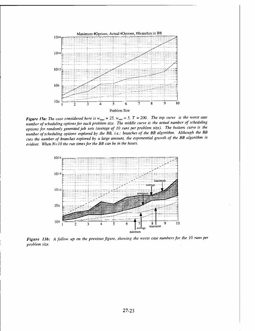
1024

1018:

Maximum #Options, Actual #Options, #Branches in BB

5 6

Problem Size

10

Figure 13a: The case considered here is wmax = 25, wmin = 5, T = 200. The top curve is the worst case number of scheduling options for each problem size. The middle curve is the actual number of scheduling options for randomly generated job sets (average of 10 runs per problem size). The bottom curve is the number of scheduling options explored by the BB, i.e.: branches of the BB algorithm. Although the BB cuts the number of branches explored by a large amount, the exponential growth of the BB algorithm is evident. When N=10 the run times for the BB can be in the hours.

1024

1018 ,,,

1012

Figure 13b: A follow up on the previous figure, showing the worst case numbers for the 10 runs per

problem size.

27-23

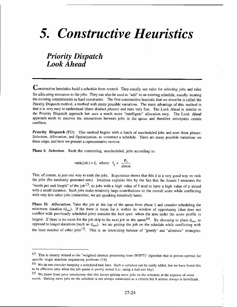
5. Constructive Heuristics

Priority Dispatch Look Ahead

V^onstructive heuristics build a schedule from scratch. They usually use rules for selecting jobs and rules

for allocating resources to the jobs. They can also be used to "add" to an existing schedule, usually treating the existing commitments as hard constraints. The first constructive heuristic that we describe is called the Priority Dispatch method, a method with many possible variations. The main advantage of this method is that it is very easy to understand (three distinct phases) and runs very fast. The Look Ahead is similar to the Priority Dispatch approach but uses a much more "intelligent" allocation step. The Look Ahead approach tends to uncover the interactions between jobs in the queue and therefore anticipates certain conflicts.

Priority Dispatch (PD): This method begins with a batch of unscheduled jobs and uses three phases: Selection, Allocation, and Optimization, to construct a schedule. There are many possible variations on these steps, and here we present a representative version.

Phase I: Selection. Rank the contending, unscheduled, jobs according to:

Pi rank(jobj) = fs, where: f- = —-— 1 dimin

This, of course, is just one way to rank the jobs. Experience shows that this it is a very good way to rank the jobs (for randomly generated sets). Intuition explains this by the fact that the feature f measures the

"worth per unit length" of the job13, so jobs with a high value of f tend to have a high value of p mixed with a small duration. Such jobs make relatively large contributions to the overall score while conflicting with very few other jobs (remember, we are speaking intuitively here).

Phase II: Allocation. Take the job at the top of the queue from phase 1 and consider scheduling the minimum duration (dmin). If the there is room for it within its window of opportunity (that does not conflict with previously scheduled jobs) consider the best spot: where the area under the score profile is

largest. If there is no room for the job skip to the next job in the queue14. By choosing to place dmjn, as opposed to longer durations (such as dmax), we are getting the job on the schedule while conflicting with

the least number of other jobsl-\ This is an interesting balance of "greedy" and "altruistic" strategies:

This is closely related to the "weighted shortest processing time (WSPT)" algorithm that is proven optimal for specific single machine sequencing problems [14].

We do not consider bumping a scheduled task here. Such a variation can be easily added, but we have found this to be effective only when the job queue is poorly sorted (i.e.: using a bad sort key).

We know from prior simulations that this favors getting more jobs on the schedule at the expense of some worth. Getting more jobs on the schedule is not always mentioned as a criteria but it almost always is beneficial .

27-24

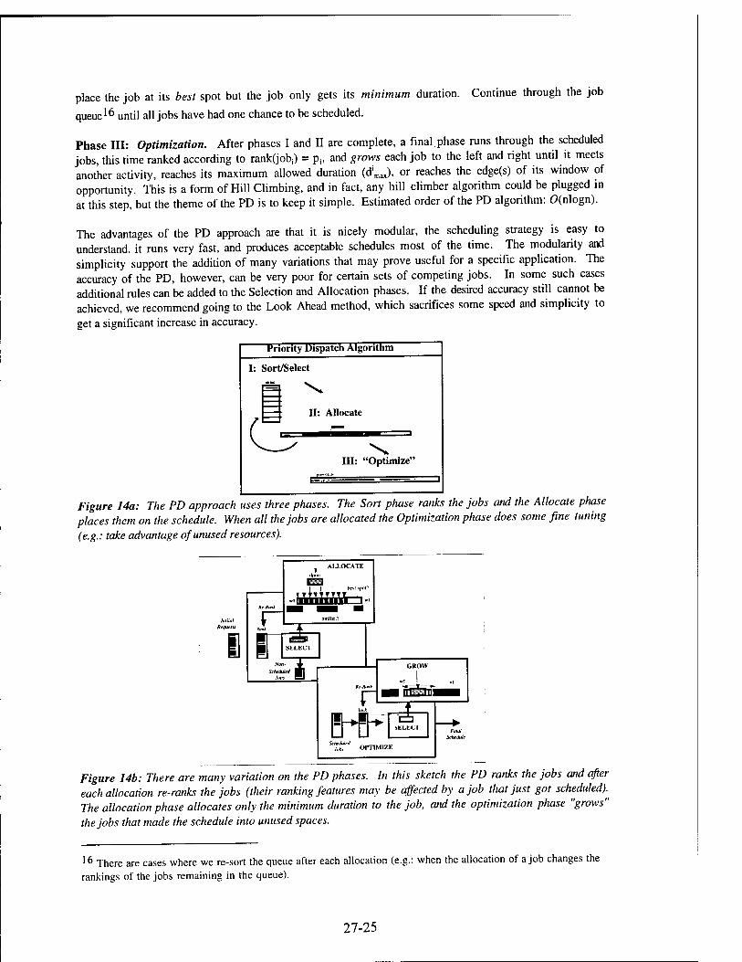
place the job at its best spot but the job only gets its minimum duration. Continue through the job

queue16 until all jobs have had one chance to be scheduled.

Phase III: Optimization. After phases I and II are complete, a final phase runs through the scheduled jobs, this time ranked according to rank(jobi) = p,, and grows each job to the left and right until it meets another activity, reaches its maximum allowed duration (d1^), or reaches the edge(s) of its window of opportunity. This is a form of Hill Climbing, and in fact, any hill climber algorithm could be plugged in at this step, but the theme of the PD is to keep it simple. Estimated order of the PD algorithm: O(nlogn).

The advantages of the PD approach are that it is nicely modular, the scheduling strategy is easy to understand, it runs very fast, and produces acceptable schedules most of the time. The modularity and simplicity support the addition of many variations that may prove useful for a specific application. The accuracy of the PD, however, can be very poor for certain sets of competing jobs. In some such cases additional rules can be added to the Selection and Allocation phases. If the desired accuracy still cannot be achieved, we recommend going to the Look Ahead method, which sacrifices some speed and simplicity to get a significant increase in accuracy.

Priority Dispatch Algorithm

I: Sort/Select

II: Allocate

III: "Optimize"

ES

Figure 14a: The PD approach uses three phases. The Sort phase ranks the jobs and the Allocate phase places them on the schedule. When all the jobs are allocated the Optimization phase does some fine tuning (e.g.: take advantage of unused resources).

. I | ■ ■ hestspoi?

HH Scheduled

j,Z OPTIMIZE

SchtJule

Figure 14b: There are many variation on the PD phases. In this sketch the PD ranks the jobs and after each allocation re-ranks the jobs (their ranking features may be affected by a job that just got scheduled).^ The allocation phase allocates only the minimum duration to the job, and the optimization phase "grows" the jobs that made the schedule into unused spaces.

16 There are cases where we re-sort the queue after each allocation (e.g.: when the allocation of a job changes the rankings of the jobs remaining in the queue).

27-25

Sorting the Jobs job

Rank? Some Possibilities:

° Rank = Priority

° Rank = Priority/dmin

° Rank = dmin

0 Rank = dmax

0 Rank = dmax -dmin

0 Rank = wf - wO - dmin

0 Rank = Priority * dmax

etc.

Figure 15: There are many ways to sort the jobs. In most cases the parameters of the job are used to compute a value that is used as the sort "key". In some cases the sort key depends on the current "state" of the schedule; for example if rank -[ (time available for scheduling) - dmin], then the value will change as jobs are scheduled that use some of the available time.

Allocation

previously scheduled jobs

Figure 16: The "allocation" step in the PD uses a maximize-minimize strategy: although the minimum duration is scheduled, it is scheduled at the best available time (with respect to its score profile).

Look Ahead Algorithm (LA): A powerful modification can be made to the PD method at the allocation step, when the job is placed at the best spot (as determined by area under the suitability function). This can be greatly improved by determining best by looking ahead: To score the possible placements of a job let the dispatch queue continue scheduling (without actually making the allocations, but obeying all the constraints) and compute the final Q. Do this for each possible placement of the job. The position that scores the highest is declared "best" and the job is allocated there, and the iteration continues (no backtracking). This accounts for interactions of the job with as yet unscheduled tasks (down-stream jobs). This adds a noticeable amount of processing time but we gain a significant amount of quality. Estimated order: 0(n2).

27-26

Look Ahead Algorithm IQB QUEUE

for each scheduling option

scheduletijohs

wscheduledjob' •[I schedule

the rest of the queue (apply the PD to the unscheduled jobs)

NEXT SCHEDULING

OPTION I

f compute the score of the J I hypothetical schedule J

Figure 17: The Look Ahead algorithm scores each scheduling option by hypothetically scheduling the rest of the queue (using the PD) and computing the score of the hypothetical schedule. The option that scores the highest is the option that is actually scheduled and then the system moves to the next job in the

queue.

Look Ahead Algorithm

scheduled jobs

unscheduled jobs I I

o all legal options

option "score"

—i-r- With thai option in place:

• apply the PD lo all the unscheduled jobs

• compute the score of the resulting schedule

After evaluating each option, schedule the job at the highest scoring option, and move on to the next job in the queue.

Figure 18: It is important to realize that the Look Ahead Algorithm considers all the legal scheduling options for each job, and is not restricted to considering the minimum duration as is the PD.

The advantages of the Look Ahead algorithm is that it is an excellent trade off of speed and simplicity for accuracy. The algorithm is relatively fast, modular, relatively easy to understand, and achieves its accuracy by dynamically detecting down-stream conflicts. The effectiveness of this algorithm highlights the fact that the interactions (i.e.: competition) between the contending jobs must be evaluated in detail to uncover the dependencies. Intuitively, the LA is measuring the sensitivity of the down-stream jobs to the particular

placements of the job currently being allocated.

27-27

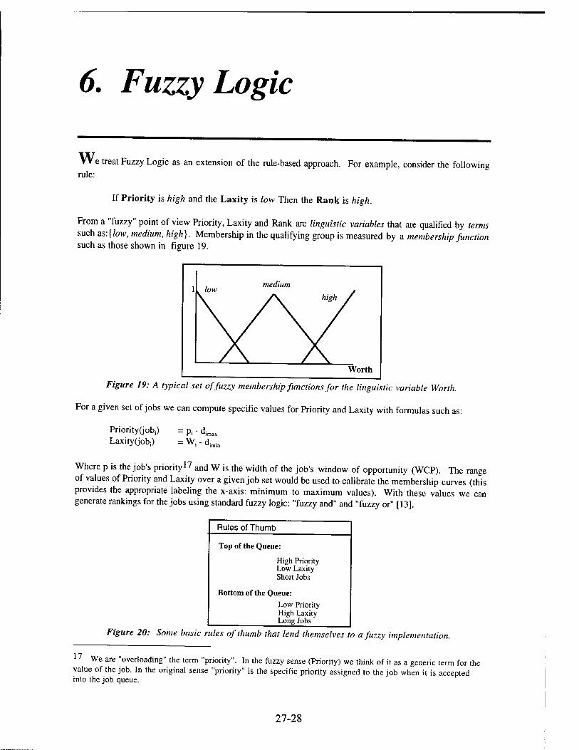
6. Fuzzy Logic

w rule:

e treat Fuzzy Logic as an extension of the rule-based approach. For example, consider the following

If Priority is high and the Laxity is low Then the Rank is high.

From a "fuzzy" point of view Priority, Laxity and Rank are linguistic variables that are qualified by terms

such as:{low, medium, high}. Membership in the qualifying group is measured by a membership function such as those shown in figure 19.

Figure 19: A typical set of fuzzy membership functions for the linguistic variable Worth.

For a given set of jobs we can compute specific values for Priority and Laxity with formulas such as:

PriorityCjobi) Laxity^obj)

= P, • 4 = W, - dlm.

'imax

imin

Where p is the job's priority17 and W is the width of the job's window of opportunity (WCP). The range of values of Priority and Laxity over a given job set would be used to calibrate the membership curves (this provides the appropriate labeling the x-axis: minimum to maximum values). With these values we can generate rankings for the jobs using standard fuzzy logic: "fuzzy and" and "fuzzy or" [13].

Rules of Thumb

Top of the Queue:

High Priority Low Laxity Short Jobs

Bottom of the Queue: Low Priority High Laxity Long Jobs

Figure 20: Some basic rules of thumb that lend themselves to a fuzzy implementation.

17 We are "overloading" the term "priority". In the fuzzy sense (Priority) we think of it as a generic term for the

value of the job. In the original sense "priority" is the specific priority assigned to the job when it is accepted into the job queue.

27-28

Figure 21a: By scaling the measured values of Priority, Laxity and Rank to the range [0,100], we can compute values (crisp) andfuzzify them into the range [0,1].

\ Laxity

VL L M H VH

VL L L VL VL VL

L M M L L VL

M H H M M L

H VH H H M M

VH VH VH VH H H

Figure 21b: If we introduce the linguistic terms: very low, low, medium, high, and very high, we can create 25 fuzzy rules for the various values of Priority and Laxity. For example, the top left entry in the chart says: "if the Priority is very low (VL) and the Laxity is very low (VL) then the Rank is low (L)".

The chart in figure 21b expresses the strategy that the ranking of a job should be lowered if the laxity is high and raised if the laxity is low. Looking at the first column in the figure 21b we see that the laxity is very low and the priority ranges from very low to very high, while entries in the chart indicate that the ranking is one step above the priority: when the priority is very low the ranking is low, when the priority is low the ranking is medium, etc. A similar thought is expressed by the other columns in the chart.

27-29

FUZZY ALLOCATION Ranking is high and

LeadTime is high and

ConstraintViolation is low

ITien Allocation is high.

Fuzzy Constraints

Figure 22a: We can go further with the fuzzy concept and apply it to the "allocation" step in the dispatch approach. As the figure indicates, the constraints themselves can be modeled in a fuzzy way, allowing degrees of constraint violation depending on such things as the lead time and importance of the job being allocated.

FUZZY QUALITY

Multiple Criteria:

Quality depends on Ql,...,Qn

If Worth is high and Distribution Error is low and #Jobs is high

Then Quality is high.

Figure 22b: In situations with multiple criteria for measuring the quality of a schedule, we can apply fuzzy concepts for combining the disparate measures of quality.

When we put the fuzzy ranking, fuzzy allocation, and fuzzy quality together we get what might be called "fuzzy scheduling". The idea of "fuzzy scheduling" fits nicely with the progressive refinement approach described later in this report: the constraints can become less and less fuzzy as the day of operation approaches.

The fuzzy approach has two attractive features:

• It adds a "layer of abstraction" that allows the designer to discuss the nature of the rules in a simple way.

• It has a built in tendency to be insensitive to small disturbances (the "fuzzy and" and "fuzzy or" operations tend to screen out small changes).

The disadvantage to the fuzzy approach are:

• The membership functions are not always easy to define and calibrate. • It requires some additionally processing time.

27-30

We believe that the advantages will outweigh the disadvantages when fuzzy logic is applied to the PD rule structure. Intuitively, the fuzzy approach seems consistent with the fact that the objective function (e.g.: a combination of the measures of all the scheduling criteria) is not as accurate as we would like it to be. It tends to have subjective weightings of parameters that is more like adding apples and oranges than a precise mathematical representation. Add in the fact that the criteria can be vague and can be rapidly changing, and it appears that a fuzzy approach would help filter out meaningless variations. We are currently investigating

this approach.

Finally, reference [6] introduces the "6-projection". This method serves two purposes: 1. it is an initial version of a fuzzy logic approach to the PD; and 2. it emphasizes the "dynamic" aspect of the PD: the queue can be sorted after each scheduling decision without a significant amount of additional processing

time.

Figure 23: Consider the case of two "features", f, and f2, used to rank the jobs (e.g.: worth and laxity). After the features are normalized to the [0,100] range each job is a represented by a point in the square in the figure. If the points are projected onto the various lines (0°, 45°, etc.) we would be sorting the jobs according to a "high" or "low" measure of the features. For example, projecting onto the 0° line is the same as ranking the jobs exclusively according tof„ projecting onto 90° sorts them byf2, projecting them onto 45° sorts them by 1/2- f, + l/2f2, etc. Also notice that if we project onto 270° then we are sorting according tof, but in ascending order. This is the basis of the 0-filter method described in [6J.

Additionally, the points in the square in figure 23 would be moving if we were re-ranking the jobs after each allocation step. For example, if we were ranking the jobs so that a high f, and high f2 were at the top of the queue (i.e.: 9 = 45°) then the unscheduled jobs would be migrating to the upper left of the square.

27-31

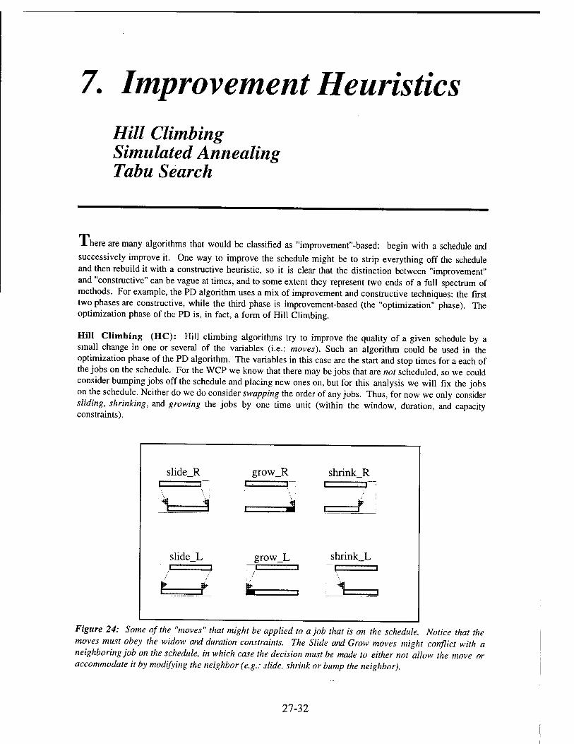
7. Improvement Heuristics Hill Climbing Simulated Annealing Tabu Search

1 here are many algorithms that would be classified as "improvemenf'-based: begin with a schedule and

successively improve it. One way to improve the schedule might be to strip everything off the schedule and then rebuild it with a constructive heuristic, so it is clear that the distinction between "improvement" and "constructive" can be vague at times, and to some extent they represent two ends of a full spectrum of methods. For example, the PD algorithm uses a mix of improvement and constructive techniques: the first two phases are constructive, while the third phase is improvement-based (the "optimization" phase). The optimization phase of the PD is, in fact, a form of Hill Climbing.

Hill Climbing (HC): Hill climbing algorithms try to improve the quality of a given schedule by a small change in one or several of the variables (i.e.: moves). Such an algorithm could be used in the optimization phase of the PD algorithm. The variables in this case are the start and stop times for a each of the jobs on the schedule. For the WCP we know that there may be jobs that are not scheduled, so we could consider bumping jobs off the schedule and placing new ones on, but for this analysis we will fix the jobs on the schedule. Neither do we do consider swapping the order of any jobs. Thus, for now we only consider sliding, shrinking, and growing the jobs by one time unit (within the window, duration, and capacity constraints).

slide R grow_R shrink R c

slide_L growJL shrink L 3

\

Figure 24: Some of the "moves" that might be applied to a job that is on the schedule. Notice that the moves must obey the widow and duration constraints. The Slide and Grow moves might conflict with a neighboring job on the schedule, in which case the decision must be made to either not allow the move or accommodate it by modifying the neighbor (e.g.: slide, shrink or bump the neighbor).

27-32

GR(i) Grow Right

no conflict

grow 1 time unit to the right

conflict

Figure 25: Hill Climbing is complicated by the fact that an incremental change in one parameter may cause a ripple effect as it affects other jobs on the schedule. For example, growing a job to the right might conflict with a neighboring job, as shown in the figure (job i bumps into job j).

A change in a variable induces a change in Q (the measure of schedule quality). In theory we would consider all possible changes (one time unit) and take the best one:

maxv { AQ/Av }

current state of the . A(3

schedule * - . _ X

AQ i AQ

fl all possible \_ / moves

AQ "

AQ

■[ J *" AQ

j XQ AQ

Figure 26: Hill Climbing considers all possible incremental changes in the state of the schedule and then picks the one that increase Q by the most (largest AQ). If all AQ's are negative the algorithm halts.

After making a change the algorithms iterates. The algorithm halts when no Av produces a AQ > 0. In practice this means computing all these possibilities at each iteration, consuming a significant amount of processing time. A common compromise is to rank the jobs (most likely to improve Q the most at the top) and compute only the variable changes for one job at a time, take the best of those, and move to the next job, etc.

Keep in mind that a move is could cause a constraint violation. Such a violation can come from any of the following:

• window constraints: each jobs has a window of opportunity [w()i, wn], and we cannot schedule

jobj outside this window. • duration constraints: each jobs has a minimum and maximum duration [dmini, dmaxi], and the

scheduled duration (dt) must satisfy drajni < ds < dmaxi. • capacity constraints: each time unit can only have one job assigned to it (i.e.: resource

capacity = 1).

Moves that violate the window and duration constraints are considered illegal and are not tolerated. The three algorithms that we describe below are distinguished by how they handle a potential capacity violation. For example if jobj has an immediate neighbor on the right (e.g.: no time gap between the end of jobj and the beginning of jobj) then growing job( one time unit to the right will cause a conflict (i.e.: jobj collides

27-33

with jobj). We have a few options at this point: consider the move illegal or try to move jobj to make room for the move. The simplest algorithm is to freeze all the other jobs when we try to move a given job, that is, make no attempt to adjust neighbors to accommodate moves. Below, we consider three algorithms, beginning with the simplest.

Simple Hill Climbing Algorithm: For all jobs on the schedule consider all the possible legal moves (1 time unit). A move that violates any of the constraints (window, duration, capacity) is considered illegal. Take the legal move that increases Q the most, then iterate. The algorithm halts when there is no legal move with AQ > 0. Thus, there are 6 moves to consider for each job^

1. grow_R(i) 2. grow_L(i) 3. slide_R(i) 4. slide_L(i) 5. shrink_R(i) 6. shrinkJL(i).

Local Pressure Algorithm: This algorithm is the same as the "simple algorithm" except that we consider making room for a move if a collision occurs. If jobf collides with jobj then we consider sliding and/or shrinking jobj to accommodate the move. Thus, there are 14 possible moves, the first 6 are when there is no collision and the last 8 are when jobi collides with jobj:

1. grow_R(i) 2. grow_L(i) 3. slide_R(i) 4. slideJL(i) 5. shrink_R(i) 6. shrink_L(i) 7. grow_R(i) & slide_R(j) 8. grow_R(i) & shrink_L(j) 9. grow_L(i) & slide_L(j) 10. grow_L(i) & shrink_R(j) 11. slide_R(i) & slide_R(j) 12. slide_R(i) & shrink_Uj) 13. slide_L(i) & slide_L(j) 14. slide_L(i) & shrink_R(j).

If it is not possible to move jobj without causing another constraint violation then the move is not legal. We could say that the local pressure algorithm only goes "one deep" since it only considers moving an immediate neighbor. We could easily extend the algorithm to consider going "two deep" by recursively applying the same moves to the job that jobj collides with, etc. For the local pressure algorithm we limit the ripple to the immediate neighbors for now.

Neighborhood Search (Radius = 1): For each jobi; consider its immediate neighbors. An immediate neighbor is a job that has no time gap between it and the start or stop of jobj. There can be either 2, 1 or 0 immediate neighbors. If there are 0 immediate neighbors we consider the 6 simple moves, as above.

If there are 2 immediate neighbors, then there is one on the left (j°b_L) and one on the right( job_R). Define a "window" of time for rescheduling these three jobs: job_L, jobi; job_R. We freeze all other jobs on the schedule outside this window. The left limit of the window is the maximum of {start of job

27-34

Left Limit

frozen

rescheduling neighborhood

t job_L jobi job_R

1 time unit

consider rescheduling all 3 jobs within 1 time

unit moves

t 1 time unit

Figure 27: For the job, we consider a neighborhood of radius 1. In the sketch jobi has immediate neighbors on both sides. The rescheduling neighborhood is defined to be 1 time unit to the left and right of

the neighbors respectively. If there is no gap to the left of job_L then the Left Limit is taken to be the start of job_L, and if there is no gap to the right of job_R the Right Limit is taken to be the stop of job_R. All jobs that are scheduled outside this neighborhood are considered frozen (i.e.: cannot be adjusted

in any way).

Left Limit

frozen

start 0

fix ̂ '■^^J"

jobi

7K A o

start 0

stop

Right Limit

frozen

ssssry A

o stop

Figure 28: Within the rescheduling window we consider only moves of 1 time unit. That is, the start and stop of a job can only be: increment ("+" means "add one"); leave the same ("0"); or decrement ("-" means "subtract one"). All such adjustments must satisfy the constraints (window, duration, capacity). We can then view the problem as a "labeling " problem: label the start and stop of each of the 3 jobs with a "+ ", "0" or "-" and find the labeling that produced the highest AQ. Notice that since the stop of job_L is initially equal to the start of jobi, there are only 6 ways to label them without causing a capacity violation. For example, if the stop ofjob_L is labeled "+" then the only way to label the start of jobi is "+". The maximum number of possible labeling is = 32-6kl where k = 2-Radius + 1, and Radius = 1. Thus, the maximum number oflabelings when Radius = 1 is 324. Many of these labelings will be illegal because of window and duration constraints, and possibly because the Left and Right Limits do not allow "-" and "+"

respectively.

27-35

Left Limit

I label the start and stop of each

job with a "+", "0" or "-"

"/' job_L / w0-»O MD

duration

wO

wf

capacity

jobi

duration -*o wf

capacity

wO V O-

job_R

duration

1 wf

Right Limit

Figure 29: As we label the start and stop times, from left to right, the constraints propagate. For example the start ofjob_L is constrained by the Left Limit and its left window limit (wO). When the start ofjob_L is labeled then the duration constraints and right window constraint for job_L constrain the labels for the stop ofjob_L. Once the stop ofjob_L is labeled then capacity constrains the label for the start of jobi (and so does the left window limit for jobi), etc.

We do the same thing if jobi has 0 on 1 immediate neighbors. For example, if jobi has 0 immediate neighbors then we consider all the ways to move the start and stop by one time unit. This includes all the 6 moves described in the "simple" algorithm, as well as some different ones (e.g.: simultaneously shrinking on both the left and right), for a total of 9 possible moves.

Also notice that if jobi and jobj are immediate neighbors of each other, and have no other immediate neighbors, than the calculation that we do when we come to jobi need not be repeated when we come to jobj.

consider all the (small) adjustments to schedule parameters that might improve the schedule and choose the one that improves the schedule the most, and iterate.

Slide Right (S1_R)

Grow Right (Gr_R)

Shrink Right (Sh_R)

Figure 30: Some of the "moves" that might be applied to a job that is on the schedule. Notice that the moves must obey the widow and duration constraints. The Slide and Grow moves might conflict with a neighboring job on the schedule, in which case the decision must be made to either not allow the move or accommodate it by modifying the neighbor (e.g.: slide, shrink or bump the neighbor).

27-36

GR(i) Grow Right

no conflict conflict

i >k

grow 1 time unit to the right

i j

S ' J

slide j 1 time unit to the

Si * shrink j 1 time unit onthe left.

right, and grow i

and grow i

Figure 31: Hill Climbing is complicated by the fact that an incremental change in one parameter may cause a ripple effect as it affects other jobs on the schedule. For example, growing a job to the right might conflict with a neighboring job, as shown in the figure (job i bumps into job j). Our algorithms limit the amount of ripple allowed: if we cannot accommodate the move by with a simple adjustment of the neighbor (slide or shrink the neighbor, but do not bump the neighbor off the schedule) we dis-allow the

current state of the .

schedule

AQ

AQ AQ A AQ

^. fl all possible * * - „ \ / moves

Q—^A(2

AQ T AQ

lAQ

Figure 32: Hill Climbing considers all possible incremental changes in the state of the schedule and then picks the one that increase Q by the most (largest AQ). If all AQ's are negative the algorithm halts.

We have explored a variety of hill climbing strategies (e.g.: bump vs. no-bump). The simplest version is to grow the jobs on the schedule (highest priority first) within the constraints (window and duration limits) and without moving any neighbors. This is the same as the "optimization" phase of the PD algorithm.

We have come to view the Hill Climbing algorithms as in either of two classes: simple enough that they are thought of as variations on the third phase of the PD algorithm; or as sufficiently complicated that they then form the backbone of both the Simulated Annealing and Tabu Search approaches. That is, the

complications introduced by a sophisticated hill climber18 will increase the accuracy of the schedules but at the expense of run time and complexity. We have not found this accuracy-speed-simplicity trade off to be worth it: the relatively small increase in accuracy comes at a high price. In fact, the Simulated Annealing and Tabu Search methods fall into the same category. Although they can provide significant improvements in accuracy, they also introduce significant increases in run time (several orders of magnitude longer than the PD) and complexity.

Simulated Annealing: This method begins the same way as the Hill Climber but adds a random component that makes random decisions in the beginning, and gradually less random decisions as it progresses, and finally converges to a deterministic Hill Climbing method.

Consider the moves that were possible for the Hill Climber, and add moves that might have been ignored because they were certain to produce a negative AQ. At any state of the schedule we can randomly pick one

18 For example, we might allow swapping position with the neighbor, and other such "local" moves.

27-37

of the moves and consider the AQ associated with it. The following rule is applied1^: map the value of AQ through the sigmoidal function shown in the diagram below; this produces the value f(AQ) which is some number between 0 and 1. Then we compare that number to a randomly generated number between 0 and 1 and use the rule: if the random number is greater than AQ then do not make the move, and iterate; if the random number is less than or equal to the f(AQ) then make the move and iterate.

1

■andom ^ lumber

rtjra , , _S*~^ 1

.

hn

■x/T 1 •■ e

i

1Q = score after move - score before move

Figure 33: The "accept/reject" method used in Simulated Annealing depends on the shape of the sigmoid, which in turn is controlled by the value of the "temperature" T.

Notice that the steeper the curve the more likely we are to accept moves with positive AQ and to reject moves with negative AQ (i.e.: similar to the Hill Climber). Conversely, the flatter the curve the more likely we are to be randomly accepting and rejecting moves (independent of the value of AQ). The parameter "T" is called the "temperature" and when the temperature is high the moves are random and when the temperature is low the algorithm behaving like the Hill Climber. Thus, SA requires a "temperature schedule" that usually begins with a high value of T and successively lowers it until it is small enough that Hill Climbing takes over and then halts when no improvements can be made to the schedule. Along the way, many schedules are "observed" so the method implies that we keep track of the best schedule that we have seen through the whole process.

The advantage to the SA approach is that it avoids getting stuck at local optima and can produce some of

the best results for a wide range of NP-Complete problems20. The drawback is that it introduces randomness into the schedule making process so it may not be repeatable and it difficult to understand "how" the result was arrived at (in layman's terms). The major drawback, however, is that the SA results tend to come at the expense of significant increases in run time (we have ruled this method out for this reason).

It is worth mentioning at this point that an "agent-based" approach could use the same "moves" while viewing each job as an "agent" that "looks" at its environment (competing jobs, neighbors) and makes a "move". In this view the "jobs" are interacting like a community of agents, observing their environment, communicating, negotiating, etc. We have only explored limited versions of such an approach, and in fact, ended up implementing simulated annealing in its place.

Tabu Search: We did not simulate a Tabu Search approach, and although we plan to test such a method in the future, we extrapolated from our experience with Hill Climbing, Simulated Annealing, and Genetic Algorithms to come to the conclusion that it will introduce unacceptable increases in run time and unacceptable complexity. Tabu Search does, however, show promise in that it minimizes one of the major weaknesses of the SA approach (it removes the randomness of the decisions), while exploiting its strength (visit local optima, but do not get stuck there). Our fear is that it will lead to a backtracking search, however controlled and intelligent it might be. It is our experience that backtracking must be introduced in

In some SA applications the following rule is applied: if AQ > 0 then make the move (no randomness) and iterate. 90 For many problems where the optimal solution is unknown, the "best known" results are almost always gotten with a SA approach, and they tend to be used for comparisons.

27-38

extremely limited ways or the run times quickly become unacceptable. This intuition, combined with the simplicity issue, points us away from the Tabu Search method. But in all fairness this is an open question.

27-39

Development of a New Numerical Boundary Condition for Perfect Conductors

Jeffrey L. Young Associate Professor

Department of Electrical Engineering

University of Idaho Moscow, OH


Wright Laboratory



and

Wright Laboratory

December 1996

28-1

DEVELOPMENT OF A NEW NUMERICAL

BOUNDARY CONDITION FOR PERFECT CONDUCTORS

Jeffrey L. Young

Associate Professor


University of Idaho

Abstract

A new numerical boundary condition is derived that extends Maxwell's equations to the surface of a perfect

conductor. This condition explicitly shows the interrelationship between surface charge, surface current

and tangential electric field. Particularly, the boundary equations are similar to Euler's linearized inviscid

acoustic equations, where current density is akin to fluid velocity and charge density is akin to mass density;

the normal derivative of the tangential electric field is the source term in the equivalent momentum equation.

The two sets of equations, Maxwell's and Euler's, are discretized using the finite-volume, MUSCL proce-

dure along with the two-stage Runge-Kutta integrator. Specifically, the spatial discretization employs the

flux-splitting procedure along windward-biased differencing. Such an approach captures the solution within

its domain of influence, as required from a solution of a set of hyperbolic equations. Formally, the resulting

scheme is third-order accurate in space and second-order accurate in time.

Numerical results are provided to validate the proposed methodology by considering plane wave scattering

from a perfectly conducting sphere. Such an example provides all the necessary complexity to exercise the

algorithm. Numerical data are provided that show the progression of charge density on the sphere and

the resulting radar cross-section (RCS) produced by the sphere. Data comparisons are made with another

method that employs a first-order type boundary condition. For the RCS data, the theoretical Mie series is

used for benchmarking purposes.

Although the data shows that the scheme works, there are problems with the scheme in terms of late-time

instability. The causes of this instability are currently under investigation and are the subject of a future

study.

28-2

DEVELOPMENT OF A NEW NUMERICAL

BOUNDARY CONDITION FOR PERFECT CONDUCTORS

Jeffrey L. Young

1 Introduction

Over the past decades, several time-domain methods for Maxwell's equations have appeared in the literature.

The most popular is the finite-difference, time-domain (FDTD) method of Yee [1],[2]. The power of this

method rests on its algorithmic simplicity and its ability to discretize Maxwell's equations to second-order.

Although the method has been used in many diverse electromagnetic applications, its primary shortcoming

is its inability to form a grid that naturally conforms to the body under investigation.

To circumvent this problem, Madsen [3] developed a modified body-fitting FDTD method that preserves

the divergence properties of the electromagnetic vectors. Despite its use of the dual grid and its problem with

late time instabilities, it has been shown to produce accurate results in several applications. Edge elements

have recently replaced the traditional nodal-based elements as the elements of choice in the weighted-residual

paradigm (see Mahadevan and Mittra [4] for a review of the edge-element methodology). These too admit

no spurious numerical charge since the element is customized to satisfy the divergence equations of Maxwell.

As with the method of Madsen and Yee, the unknowns in the edge-element algorithm are not collocated.

From a grid generation and a coding perspective, this unallocated strategy adds significant complexity to

the problem.

More recently, the finite-volume approach, which was developed for the fluid dynamics community, has

been considered for electromagnetic-type problems. For this situation, Maxwell's equations are couched in

strong conservative form and the unknowns are collocated at the cell centers. Flux evaluations at the cell

walls are determined from an interpolation of the dependent variables at cell centers. For certain types

of interpolate schemes and flux-splitting procedures, the algorithm mimics many of the features of the

hyperbolic system of equations. For example, when the fluxes are split according to the eigenvalues of the

flux Jacobian matrix and windward-based differencing is used in the discretization, the algorithm naturally

captures the right- and left- running waves within their domain of influence.

The main contributors to the finite-volume strategy, as applied to Maxwell equations, are Shankar of

Rockwell [5, 6, 7] and Shang of the Wright Patterson Air Force Base [8, 9, 10]. The method of Shankar

28-3

is founded on the upwind Lax-Wendroff method. For example, when applied to the model scalar wave

equation, the solution « at time n + 1 and node j is derived from:

u^1 = „» + .51/(3«? - 4u?_x + u;"_2) + .5i/2(u*?+1 - 2«; + u^),

where v = c5t/8x. When applied to higher dimensions, Shankar decomposes the dependent variable in terms

of two states, from which he derives the flux at the cell interface. Shang also decomposes the dependent

variable in terms of two states, but the flux evaluations are obtained from a flux-splitting procedure and

the modified MUSCL algorithm [11] (sometimes referred to as the /c-scheme). By suitably selecting the

appropriate values for K and the limiter </>, the algorithm can take on one of five different spatial discretization

schemes: first-order windward, second-order windward, second-order Fromm, third-order windward biased

or second-order central differenced.

Unfortunately, there exist inherent difficulties in maintaining high-order accuracy when these methods are

applied near and on perfect conductors. Two fundamental problems prevent one from establishing anything

more than a first-order approximation to the boundary conditions. First, all field components (magnetic

and electric) share the same point in space. If that point rests on the perfect conductor, then only the values

of three of the six components are known a priori on the conductor; these values are tangential electric

field and normal magnetic field. The other three, normal electric field and tangential magnetic field are not

known since the former is proportional to the induced surface charge and the latter is proportional to the

induced surface current density. To deduce the values for the charge and the current, one possible approach

to is to extrapolate the normal electric field and tangential magnetic field from interior values. Second, when

second-order (or greater) windward differencing is used, at least two cell values on either side of the flux

wall are required to reconstruct the flux on the wall. For cell walls one cell away from the conductor, one of

these cell values lies in the interior of the conductor, which is technically outside the computational domain.

This being the case, a first-order approximation is required.

In this report, we present a new strategy that is locally and globally third-order accurate in space.

This is achieved by reconsidering and manipulating Maxwell's equations in the vicinity of the conductor.

Particularly, the result of this analysis is a set of two time-domain equations that explicitly show the

interelationship between surface charge density, surface current density and tangential electric field. As

might be expected, the interrelationship is quite similar to Euler's linearized, inviscid acoustic equations,

with the tangential field acting like a source of "current momentum."

The numerical procedure rests upon the simultaneous discretization of both Maxwell's and Euler's equa-

28-4

tions. In this report the discretization will be accomplished via the MUSCL procedure in generalized curvilin-

ear coordinates. To advance the equations in time, the second-order Runge-Kutta (RK) scheme is employed.

For sake of completeness, the scheme is numerically validated by considering the scattering of a TEM plane

wave from a perfectly conducting sphere. To this end, plots of the sphere's radar cross-section (RCS) and

the surface charge are provided.

2 Governing Equations

Consider Maxwell's curl equations for linear, isotropic, homogeneous media:

^ = -VxE (1)

and

M = VxH, (2) at

where E and H are the electric and magnetic fields, respectively; c and // are the permittivity and perme-

ability, respectively. Let n be a constant unit vector normal to and pointing out from the perfect conductor.

Then, by taking the scalar product of n with Ampere's law, we obtain

en.^ = V-(Hxn) + H-(Vxn), (3) at

where it is understood that the above equation is being considered at an infinitesimal distance from the

prefect conductor. Since the curl of a constant vector is zero, n x H is the surface current J,, and en • E is

the surface charge p,, Eqn. (3) is equivalent to

^ + V-J, = 0. (4) at

As expected, the resultant equation is simply a statement that charge must be conserved on a perfect

conductor. By way of comparison, we observe the analogous relationship between the acoustic quantities of

fluid velocity and mass density with the electromagnetic quantities of current density and charge density,

respectively.

The previous derivation is duplicated by forming the vector product of n with Faraday's law:

„nx fE = _V(n-E) + (n-V)E + (E-V)n + Ex(Vxn) (5) at

Of course, the last two terms on the left-hand side are zero due to the requirement that n be a constant,

More importantly, the remaining term on the right-hand side is nothing more than the rate of change of

28-5

surface current and the first term on the left-hand side is proportional to the gradient of charge density.

Thus, we are left with

^ + viVp. = (n-V)E/p, (6)

where v = 1/V/£I? is the phase velocity of the homogeneous medium. The vector senses of J, and Vpa are

tangentially directed to the conductor's surface, which implies that the source term must also be directed

similarly. Hence,

-T— + v-Vp, = ——, (() ot fi on

where Et is the tangential component of E. Here we see the analogous momentum conservation equation

whose source term is the normal derivative of tangential E.

To summarize, the governing equations for the domain variables E and H are stated in Maxwell's equa-

tions, (1) and (2). The governing equations for the boundary variables J, and ps are stated in Euler's

equations, (4) and (7). Finally, the system is made complete via the boundary conditions:

n x E = 0 (8)

n-E = ps/e (9)

nxH = Js (10)

and

n-H = 0. (11)

These systems of equations (Maxwell, Euler and boundary conditions) allow one to compute both bound-

ary variables and domain variables simultaneously. Consequently, a numerical procedure can be developed

to utilize that fact, thus circumventing the problem of not knowing the surface current and charge densities

on the conductor a priori. Two other comments are in order. First, it is well known that tangential current

leads to electromagnetic radiation. By treating J, as an dependent variable to be computed, we see that

the derived Euler's equations have a primary importance of computing J, and that Maxwell's equations are

needed only for the deduction of the source field in the analogous momentum equation. Second, the source

term in the momentum equation is easily discretized by noting that the node that resides on the conductor

is zero, since tangential E must vanish on the conductor.

28-6

2.1 Conservative Form

We begin this treatment by couching Maxwell's equations in the following conservative form:

^ + V-(F(C/)) = 0, (12)

where U is the solution vector and F is the point-flux tensor, which is dependent upon U. In expanded

form, du m dF^ ö^ = 0 dt + dx + dy dz

(13)

where Fx,Fy,F2 are the flux components of F. Since the the fluxes are homogeneous functions of degree

one, we may write F. = AU, Fy = BU and F, = CU. Here A, B, C are the Jacobian matrices associated

with Fx, Fy,Fz, respectively. Thus, Equation (13) is equivalent to

^+diA^+9{BU)_+d{Cin=0 (14)

dt dx dy dz

For homogeneous, isotropic media, it is a simple exercise to show that the flux Jacobian matrices associ-

ated with Maxwell's equations are given by

A =

B =

and

C =

0 0 0 0 0 0 0 0 0 0 0 -i 0 0 0 0 ± 0 0 0 0 0 0 0 oo^ooo 0 -1 0 0 0 0

0 0 0 o o I 0 0 0 0 0 0 0 0 0 -\ o 0 0 0 -i 0 0 0 0 0 0 0 0 0 10 0 0 0 0 f

0 0 0 0 -\ o o oo^oo 0 0 0 0 0 0 0 -± 0 0 0 0 i o" 0 0 0 0 0 0 0 0 0 0.

where

U = [Bx,By,B„Dx,Dy,D,]t.

(15)

(16)

(17)

(18)

Hence,

Fx = [0,-D,A, Dy/e, 0,B,/fi, -By /p]* (19)

28-7

Fy = [DJe, 0, -Dx/e, -B,/fi, 0, Bx/tf (20)

and

F* = l-Dy/t, Dx/e, 0, By In, -Bx/n, 0]'. (21)

Note: From the constitutive relationships, B = yiR and D = eE.

Except for the inclusion of the source term (i.e., the normal derivative of tangential E), the same repre-

sentations given by Eqn. (13) or (14) may be used for Euler's equations. Particularly, for the flux Jacobian

matrices,

A =

B

and

for the dependent variables,

From these definitions it follows that

and

0 10 0 v- 0 0 0 0 0 0 0 0 0 0 0

0 0 10 0 0 0 0 v2 0 0 0 0 0 0 0

0 0 0 1 0 0 0 0 0 0 0 0

i/2 0 0 0

U = [p,,Jx,Jy,Jz]*-

Fx = [Jx,v2ps,0,0]t

Fy = [Jy,0,v2p„0]t

Fz = [J2,0,0,v2p,]t.

(22)

(23)

(24)

(25)

(26)

(27)

(28)

2.2 Flux Splitting

The flux Jacobian matrix A (as well as B and C) associated with both systems is diagonalizable since its

eigenvectors are linearly independent. That is, an alternative representation for A is

A = SxArS;1 (29)

where Sx is the modal matrix of A and Ax is its spectral matrix, which is a diagonal matrix. A detailed

eigenvector analysis reveals for Maxwell's equations that

Ax = Diag{-A,-A,A,A,0,0}, (30)

28-8

where A = 1-JjIe; also

^X —

0 -77

0 0

0 0 0 1 -■n 0 0 0 0 V 0 0 0 0 1 0 0 1 0 0 1 0 0 0

(31)

with 77 = y/fi/e-

The flux splitting procedure is based upon the decomposition of the spectral matrix in terms of the sign

of its members:

where

and

It follows from Eqn. (29) that

Ar = A+ + A:

A+ = Diag{0,0,A,A,0,0}

Ar = Diag{-A,-A,0,0,0,0}.

(32)

(33)

(34)

A = Sx(At + K)S^=A+ + A-. (35)

Here A+ = S.A+Sr* and A+ = SXAXS;\ Since Fx = AU, then Fx = (A+ + A~)U = F+ + F~, where

F+ = A+U and F~ = A~U. Carrying out the required matrix operations, we discover that

x 2 0.(V-5L),(*A+a),0.(^ + *A -B, y- + Dz\

and

^ = i[..-(^+^),(-v+a),,.(i-^),-(i+aA By way of a similar analysis, the split fluxes for Euler's equations are found to be

-,t

F^ = I w»+j*yp*+^,o,o]'

and

(36)

(37)

(38)

(39) F- = ^ [~vp, + Jx,v2p, - vJx,0,Of .

Regardless of the governing equations to be considered, the duplication of the flux splitting procedure

for the other fluxes yields the expanded form for the conservative equation:

(40) ~dt+~dT + 8x + dy + By dz dz

The previous result is the equation on which characteristic theory is based. A simple discretization scheme

is given next to demonstrate the basic concepts of the numerical theory.

28-9

2.3 A Simple Difference Scheme

The advantage of writing Maxwell's or Euler's equations in characteristic form, as manifested in Eqn. (40),

is found in the differencing scheme of the spatial derivatives. Since F+ corresponds to eigenvalues that are

positive, which leads to positive going waves in the x-direction in a one-dimensional analysis, it makes sense

to apply a windward differencing scheme to F+. For second-order accuracy, we may use

6F+ dx

3F,+ -4/£1 + F,t3 m

Hence, it is readily seen that the wave is discretized solely in terms of its values within its domain of influence.

Similarly, F~ is associated with waves that are traveling in the negative x-direction. Hence, we let

26T K ' dx

Note: The use of windward differencing will introduce a certain amount of numerical dissipation and disper-

sion into the solution.

For certain classes of temporal integrators, such as the Runge-Kutta integrators, the previous scheme

is found to be conditionally stable. Formally, the RK methods may be expressed in terms of a truncated

Taylor series for the matrix e~AS', where A is the spatial discretization matrix:

r+i = ^twr.r. (43) ^—' m! m=l

Obviously, the implementation of this series is straightforward and any order of accuracy can be achieved,

if one is willing to expend the computational resources to achieve that accuracy. However, to minimize

the number of evaluations of the right-hand side of Eqn. (43) and to limit the storage required for each

evaluation, the second-order and fourth-order schemes are used. For second-order accuracy,

k„ = 6tR{f0)

*i = StR{fi)

r+l = r + h- (44)

Here R is the residual; /„ = f(x,t0) and fa = f0 + k0/2. For fourth-order accuracy,

k9 = 6tR{f9)

*i = StR{fi)

k2 = StR{h)

28-10

*3 = StR(f3)

/"+1 = /" + (*i + 2*2 + 2*3 + *4)/6. (45)

Here R is the residual; /0 = /(*,*,), /i = /. + *o/2, /2 = /i + *i/2 and /3 = /2 + *2- A detailed Fourier

analysis shows that the second-order, fully upwind, two-stage Runge-Kutta scheme is conditionally stable

with a CFL=.5; for the four-stage scheme, CFL=.695.

To apply the flux-splitting procedure to a grid that is non-Cartesian, additional analytical work is

required. This subject is studied next.

2.4 Strong Conservative Form

To cast the conservative equation into strong conservative form, we map the Cartesian independent variables

x,y,z into a generalized coordinate system ^.ij.C; the dependent variables are still expressed in terms of

the Cartesian frame. Hence, consider the following coordinate transformation: £ = £(x,y,z), TJ - Tj(x,y,z)

and C = C(x>y>z)> or similarly, for one-to-one transformations, x = x{£,T],Q, y = y(Z,V,0 and z =

*(£, «7,0- Associated with this transformation is a set of metrics (e.g., x„, rj2) that convey the geometry of

the transformation.

After a sequence of mathematical operations that involve the metrics of the transformation, Eqn. (13)

becomes

di + ?l+M + ™- = 0 (46)

where Ü is the unknown domain vector and F, G, and H are the domain fluxes in the £, r), and C directions,

respectively. With V denoting the Jacobian, the fluxes, Ü and J take on the following meaning:

Ü = UV, (47)

F = (ZxF, + £9F9 + t,F,)V, (48)

G = (vrFx + r)yFy + VzF,)V, (49)

and

H = (CxFt + CyFy + <:zFz)V. (50)

A similar representation holds for Euler's equations, except that one term in the strong conservative equation

may be omitted, since current flow is restricted to a locally two-dimensional surface.

28-11

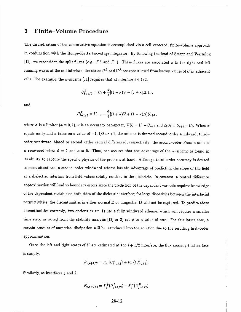
3 Finite-Volume Procedure

The discretization of the conservative equation is accomplished via a cell-centered, finite-volume approach

in conjunction with the Runge-Kutta two-stage integrator. By following the lead of Steger and Warming

[12], we reconsider the split fluxes (e.g., F+ and F~). These fluxes are associated with the right and left

running waves at the cell interface; the states UL and UR are constructed from known values of U in adjacent

cells. For example, the «-scheme [11] requires that at interface i+ 1/2,

and

Ui+i,2 = Ui + J[(l - «)V + (1 + n)A]Ui,

U,R+1/2 = Ui+1 - £[(1 + «)V + (1 - K)A]Ui+1, 4'

where <j> is a limiter (<j> = 0,1), K is an accuracy parameter, Vt/,- = Ui - Ut-i and AU, = Ui+i - Ui. When <f>

equals unity and K takes on a value of —1,1/3 or +1, the scheme is deemed second-order windward, third-

order windward-biased or second-order central differenced, respectively; the second-order Fromm scheme

is recovered when (f> — 1 and K = 0. Thus, one can see that the advantage of the K-scheme is found in

its ability to capture the specific physics of the problem at hand. Although third-order accuracy is desired

in most situations, a second-order windward scheme has the advantage of predicting the slope of the field

at a dielectric interface from field values totally resident in the dielectric. In contrast, a central difference

approximation will lead to boundary errors since the prediction of the dependent variable requires knowledge

of the dependent variable on both sides of the dielectric interface; for large disparities between the interfacial

permittivities, the discontinuities in either normal E or tangential D will not be captured. To predict these

discontinuities correctly, two options exist: 1) use a fully windward scheme, which will require a smaller

time step, as noted from the stability analysis [13] or 2) set <f> to a value of zero. For this latter case, a

certain amount of numerical dissipation will be introduced into the solution due to the resulting first-order

approximation.

Once the left and right states of U are estimated at the i + 1/2 interface, the flux crossing that surface

is simply,

Similarly, at interfaces j and k:

F...-+1/2 = F+(^+1/2) + F-(t/£1/2).

FyJ+l/2 = F+([^+1/2) + F-(££1/2)

28-12

and

Fz,k+i,2 = F+(U£+1/3) + Ff (£tf_1/2).

For generalized coordinates, the flux, say F, is split in the direction of £. This is accomplished by a local

transformation matrix T and by defining a new flux F: F = TF. Since T can be chosen such that F

and F have the same functional form, the eigenvalue/eigenvector information is directly obtained from the

Cartesian formulation. Thus, if F = F+ + F~ then F = F++ F~, where F+ = T^F+ and F~ = T^F~.

This same procedure is repeated in the directions r] and C, for G and H, respectively.

To maintain stability, the two-stage Runge-Kutta integrator is invoked, as defined earlier. Although other

temporal schemes may be used, the RK integrator is simple to code and to vectorize for supercomputing

platforms.

4 Numerical Results

To demonstrate some of the previous concepts, the problem of a plane wave scattering from a perfectly

conducting sphere is considered. The computational grid is constructed by employing the Cartesian to

Spherical coordinate mapping functions. This mapping results in a structured grid whose indices I,J,K

denote the number of grid lines in the R, ß, 4> directions, respectively. The sphere is illuminated from above

by a TEM gaussian plane wave of the form e-'C"*)', where it has been assumed that the surrounding

medium has unity permittivity and permeability, thus rendering the phase velocity to unity. To achieve a

usable spectral content of the incident wave up to 12 r/s, w is set to 3.96. Finally, a CFL number of unity

has experimentally been proven to yield stable results1.

Figures 1, 2 and 3 show plots of the charge density on the sphere as a function of elevation angle after

150, 300 and 450 time steps, respectively; for the present situation AR = 0.05 m, (I,J,K) = (30,30,54)

and 0 = 0. The data associated with one curve is obtained via a first-order boundary condition (by first-

order, we mean that the unknowns that exist on the spherical surface are extrapolated from the interior via

a first-order shift from the nearest cell); the other curve is associated with the exact boundary condition

described in this report. These plots serve to validate the theory of the exact boundary condition. That is,

with these plots confidence is gained from numerical experimentation that the charge density indeed satisfies

the linearized inviscid Euler equations.

Using this same coarse grid and 1000 time steps, the RCS of the sphere is computed. Consider Figures

> Technically, the CFL number should be set to a value no greater than 0.87 [13]. However, due to the way the time step is calculated from the grid geometry, a CFL of 1.00 still results in stable data.

28-13

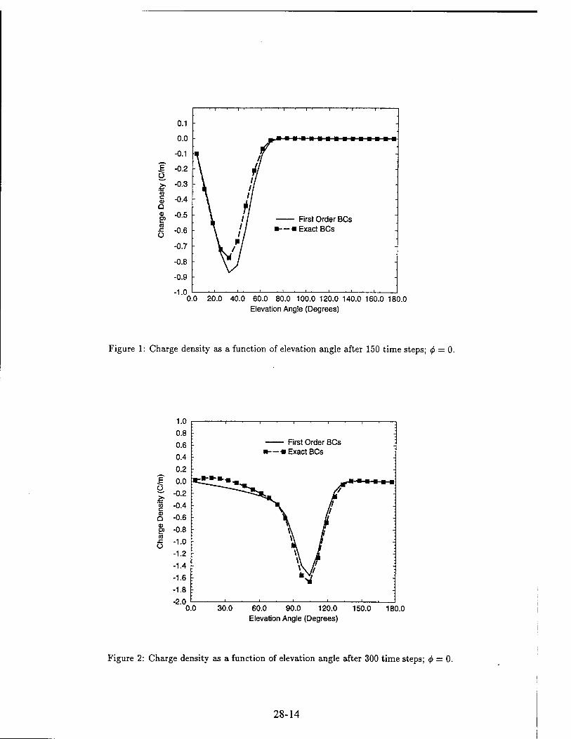
E ü

CO c 0) Q

CD O) k. (0 .c O

-1.0

-i ' r-" 1 •—> ' 1-1 1 •—! 1 r

First Order BCs Exact BCs

0.0 20.0 40.0 60.0 80.0 100.0 120.0 140.0 160.0 180.0 Elevation Angle (Degrees)

Figure 1: Charge density as a function of elevation angle after 150 time steps; <j> — 0.

-2.0

First Order BCs Exact BCs

0.0 30.0 60.0 90.0 120.0 150.0 Elevation Angle (Degrees)

180.0

Figure 2: Charge density as a function of elevation angle after 300 time steps; <j> = 0.

28-14

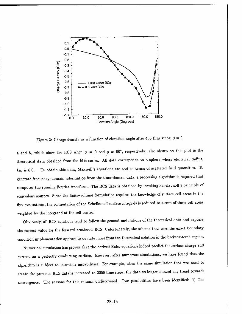
0.1

,— _—■—■ i i i i ■

0.0

-0.1

— -0.2 E v\ L ö -°-3 n. ^N. f % -0.4 > \ r V)

g -0.5 \\ I; «a -0.6 First Order BCs "^ \ j | -0.7 ü -0.8

- »-—«ExactBCs ^ \ // "

\\Ji ' -0.9

\ ' -1.0 v : -1.1 i _^ i , i—i—i—■—— -1.2

0 .0 30.0 60.0 90.0 120.0 150.0 180.0 Elevation Angle (Degrees)

Figure 3: Charge density as a function of elevation angle after 450 time steps; <j> = 0.

4 and 5, which show the RCS when c6 = 0 and <j> = 90°, respectively; also shown on this plot is the

theoretical data obtained from the Mie series. All data corresponds to a sphere whose electrical radius,

ka, is 6.0. To obtain this data, Maxwell's equations are cast in terms of scattered field quantities. To

generate frequency-domain information from the time-domain data, a processing algorithm is required that

computes the running Fourier transform. The RCS data is obtained by invoking Schelkunoff's principle of

equivalent sources. Since the finite-volume formulation requires the knowledge of surface cell areas in the

flux evaluations, the computation of the Schelkunoff surface integrals is reduced to a sum of these cell areas

weighted by the integrand at the cell center.

Obviously, all RCS solutions tend to follow the general undulations of the theoretical data and capture

the correct value for the forward-scattered RCS. Unfortunately, the scheme that uses the exact boundary

condition implementation appears to deviate more from the theoretical solution in the backscattered region.

Numerical simulation has proven that the derived Euler equations indeed predict the surface charge and

current on a perfectly conducting surface. However, after numerous simulations, we have found that the

algorithm is subject to late-time instabilities. For example, when the same simulation that was used to

create the previous RCS data is increased to 2000 time steps, the data no longer showed any trend towards

convergence. The reasons for this remain undiscovered. Two possibilities have been identified: 1) The

28-15

CD 2, CO Ü DC

20.0

15.0

10.0

5.0

0.0

-5.0

-10.0

-15.0

-20.0

-25.0

-30.0

► Exact BCs i First-Order BCs • Theory

0.0 30.0 60.0 90.0 120.0 150.0 Elevation Angle (Degrees)

180.0

Figure 4: RCS of a sphere when ka = 6 and $ = 0.

20.0

-5.0

-10.0

•—♦ Exact BCs i ■ First-Order BCs ►—«Theory

0.0 30.0 60.0 90.0 120.0 150.0 180.0 Elevation Angle (Degrees)

Figure 5: RCS of a sphere when ka = 6 and <j> = 90°.

28-16

source term in Euler's equations is not truly a source term but a field term that is computed from Maxwell's

equations. Hence, the way this term is computed can effect stability. For the present implementation, one-

sided differencing that is second-order accurate is used. 2) Currently, the boundary conditions are applied

at the cell centers rather than at the cell walls. It has been suggested that such an approach reduces the

accuracy of the scheme, thereby inducing possible instabilities.

5 Conclusion

A formal treatment for extending Maxwell's equations to the boundary has been given. Based upon prelim-

inary numerical experimentations, these new equations, identified as Euler's equations, indeed predict the

space-time profile of the surface charge and surface current. Unfortunately, when cast in terms of a finite

volume procedure, various simulations have shown that the data may become unstable for a highly resolved

grid or for late-time simulations. The reasons for this instability is the subject of future work.

Although future work should include an analytical treatment of the Neumann stability properties, the

treatment is not trivial. First, most stability analyses start by considering a one-dimensional domain with

periodic boundary conditions. For our situation, the domain is not periodic but is terminated by a perfect

conductor. Such a termination greatly complicates the analysis. Moreover, a one-dimensional plane wave is

by definition transverse to the perfect conductor - hence, it cannot induce any surface charge. Thus, Euler's

equations are reduced to a single equation for which the time-rate-of-change of the current density equals

the normal derivative of the tangential electric field.

Other future work includes 1) the incorporation of the boundary conditions at flux walls rather than at

cell centers and 2) simplifying the problem such that the scatterer's geometry coincides with a Cartesian

grid. This latter study would identify whether or not the curvilinear coordinate transformation has any

impact on numerical instability.

Finally, in this project the finite-volume code that incorporates either the first-order boundary condition

or the Euler-type boundary condition is streamlined for robust performance. The code is vectorized to

accommodate the vector nature of the Cray machines. In addition, the code is customized for low memory

usage. For example, for a grid size of (50,55,104) and for a simulation time of 4000 time steps, the code

requires only 15 Megawords of memory and 2.7 cpu hours on a Cray YMP; on Cray C90, 1.3 cpu hours

are needed. This effort in improving the code performance will benefit other DoD projects currently being

managed by the PI.

28-17

References

[1] Yee, K. S., "Numerical solution of initial boundary value problems involving Maxwell's equations in

isotropic media," IEEE Trans. Ant. Propagat, vol. 14, pp. 302-307, 1966.

[2] Taflove, A., and M. E. Morris, "Numerical solution of steady-state electromagnetic scattering problems

using the time-dependent Maxwell's equations," IEEE Trans. Microwave Theory Tech., vol. 23, pp.

623-630, 1975.

[3] Madsen, N. K., "Divergence preserving discrete surface integral methods for Maxwell's curl equations

using non-orthogonal unstructured grids," Research Institute for Advanced Computer Science Tech.

Rep. 92.04, NASA Ames Research Center, 1992.

[4] Mahadevan, K., and R. Mittra, "Radar cross section computation of inhomogeneous scatterers using

edge-based finite element methods in the frequency and time domains," Radio Science, vol. 28, pp.

1181-1193, 1993.

[5] Shankar, V., A. H. Mohammadian and W. F. Hall, "A time-domain, finite-volume treatment for the

Maxwell equations," Electromagnetics, vol. 10, pp. 127-145, 1990.

[6] Shankar, V., W. F. Hall, A. Mohammadian and C. Rowell, "Algorithmic aspects and supercomputing

trends in computational electromagnetics," AIAA 31st Aerospace Sciences Meeting & Exhibit, Reno,

NV, AIAA 93-0367, 1993.

[7] Shankar, V., W. F. Hall and S. Palaniswamy, "Accuracy issues in time-domain CEM using struc-

tured/unstructured grid formulations," 11th Annual Review of Progress in Applied Computational Elec-

tromagnetics, Monterey, CA, pp. 1185-1192, 1995.

[8] Shang, J. S. and D. Gaitonde, "Characteristic-based, time-dependent Maxwell equations solvers on a

general curvilinear frame," AIAA Journal, vol. 33, pp. 491-498, 1995.

[9] Shang, J. S., and D. Gaitonde, "Scattered electromagnetic field of a re-entry vehicle," J. Spacecraft &

Rockets, vol. 32, pp. 294-301, 1995.

[10] Shang, J. S., "Characteristic-based algorithms for solving the Maxwell equations in the time-domain,"

IEEE Ant. Propagat. Mag., vol. 37, pp. 15-25, 1995.

28-18

[11] Anderson, W. K., J. L. Thomas and B. van Leer, "A comparison of finite volume flux vector splittings

for the Euler equations," AIAA 23rd Aerospace Sciences Meeting, Reno, NV, AIAA 85-0122, 1985.

[12] Steger, J. L., and R. F. Warming, "Flux vector splitting of the inviscid gasdynamic equations with

application to finite-difference methods," J. Comp. Phys., vol. 40, pp. 263-293, 1981.

[13] Weber, Y. S., "Investigations on the properties of a finite-volume, time-domain method for compu-

tational electromagnetics," 26th AIAA Plasma Dynamics and Lasers Conf., San Diego, CA, AIAA

95-1964, 1995.

28-19

PD-Eigenstructure Assignment Control for

Multivariable Nonlinear Tracking and Decoupling

J. Jim Zhu Assistant Professor

Department of Electrical and Computer Engineering

Louisiana State University Baton Rouge, LA 70803 Email: [email protected]


Wright Laboratory



and

Wright Laboratory

December 1996

29-1



J. Jim Zhu Department of Electrical and Computer Engineering

Louisiana State University Baton Rouge, LA 70803

Abstract

In this research a systematic design procedure for multivariable nonlinear tracking and

output/state decoupling control is developed by way of linearization along a nominal trajectory.

The resulting linear time-varying (LTV) tracking error dynamics are then stabilized and decoupled

using PD-eigenstructure assignment in a way similar to the eigenstructure assignment design for

LTI systems. Main Accomplishments of this research include: (i) extension of the PD-spectrum

and PD-eigenvector concepts for scalar polynomial differential operator to vector differential

polynomial operators, (ii) extension of Silverman-Wolovich (S-W) transformation to the entire

class of uniformly completely controllable (u.c.c.) multivariable (MV) LTV systems, (iii) PD-

eigenvector based criteria for uniform controllability and observability of MV LTV systems, (iv)

stabilization of u.c.c. MV LTV systems by PD-spectrum assignment, (v) output/state decoupling

of u.c.c. MV LTV systems by PD-eigenstructure assignment, and (vi) A BTT autopilot with

decoupled roll-yaw dynamics using the PD-eigenstructure assignment control. Due to the time

constraint, implementation and simulation results are not available at the present. Further

research is needed to address the complexity of the implementation, and to validation the theory

and design procedure by simulations. A multiobjective PD-eigenstructure assignment concept is

also proposed to address an array of challenges posed by modern missile technology. Additional

applications of the results of this research can be found is aircraft flight control, spacecraft altitude

control, vibration control, robotics and the like.

29-2



J. Jim Zhu

1. Introduction

Due to the ever stringent performance requirements and inherently nonlinear, time-varying

and highly coupled aerodynamics [1], modern missile control, e.g. the bank-to-turn (BTT) missile

autopilot, poses a challenge to control design that has not been successfully met [2]. Despite its

well-know limitations, gain scheduling (GS) appears to be the focus of the current prominent

research efforts [3], [4], [5]. Because of the lack of mathematical theory for time-varying

dynamics, the GS approach treats the nonlinear, time-varying missile dynamics as time-invariant

dynamics linearized at discrete operating states. An autopilot is then comprised of a series of

linear time-invariant (LTI) controllers scheduled for these frozen operating states and frozen

time dynamics using various LTI control design techniques, such as eigenstructure assignment for

guidance command tracking and roll-yaw decoupling [3].

Scheduling of frozen-time, frozen-state controllers for fast time-varying dynamics is known

to be mathematically fallacious, and practically hazardous [4]. Recent research efforts have been

directed towards applying robust control techniques to extend the stability margin of GS

controllers [3], [5]. While the stability margin at each frozen-state is greatly improved with

modern robust controllers, it does not seem to benefit stability margin of the overall system

proportionally. Indeed, failures have been reported in these recent attempts [5; pp. 14-15]. It

appears that the GS control technique has been stretched to its limit in coping with fast time-

varying dynamics.

In addition to the time-varying stabilization problem, guidance command tracking with a

nonlinear, time-varying airframe poses other challenges in missile autopilot design. In particular,

29-3

normal acceleration tracking with a tail fin controlled missile is known to be nonminimum phase,

and the roll-yaw aerodynamics are highly coupled for a BTT missile. Actuator saturation and

suppression of unmodeled structural modes are other practical issues that have to be effectively

dealt with by an autopilot. These problems become even more difficult to tackle in the presence

of fast time-varying system parameters.

In this research, a recently developed differential-algebraic spectral theory for linear time-

varying (LTV) systems is applied to nonlinear tracking control, such as the BTT missile autopilot

design problem. Specifically, the notions of Parallel D-eigenvalues (PD-eigenvalues) and Parallel

D-eigenvectors (PD-eigenvectors) [6] are used to extend existing results [3] on robust GS

eigenstructure assignment command tracking and roll-yaw decoupling controllers. The

differential-algebraic spectral theory treats time-varying dynamics as such, therefore it would

succeed where the conventional frozen-time, frozen-state GS techniques fail.

Recently, some encouraging preliminary results on a pitch autopilot design based on this

differential-algebraic spectral theory have been obtained [7], [8]. The design approach is by

linearization of the nonlinear airframe along a nominal (command) trajectory to obtain LTV

tracking error dynamics. This design approach poses two technical challenges: (i) implementation

of the inverse of the nonlinear airframe dynamics to generate the nominal control, and (ii)

exponential stabilization of the LTV tracking error dynamics to achieve guidance command

tracking. The first problem can be solved by employing a (dynamic) neural network, which is not

to be discussed here (cf. [8] for more information). The tracking error stabilization is achieved by

assigning the extended-mean (EM) of the closed-loop PD-eigenvalues of the LTV error dynamics

to the left-half-plane (LHP) of the complex numbers C, in a way very similar to the LTI

eigenvalue assignment.

Simulation studies reported in [7], [8] showed that the autopilot was capable of angle-of-

attack (AOA) and normal acceleration (NA) tracking of various command trajectories throughout

the entire flight envelope without explicit scheduling of any controller parameters. Figure 1.1

below shows AOA tracking performance of the autopilot for an unrealistically demanding

29-4

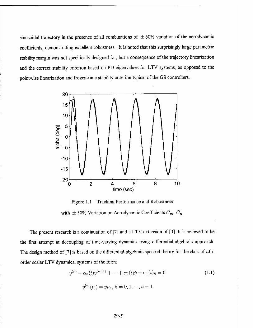
sinusoidal trajectory in the presence of all combinations of ± 50% variation of the aerodynamic

coefficients, demonstrating excellent robustness. It is noted that this surprisingly large parametric

stability margin was not specifically designed for, but a consequence of the trajectory linearization

and the correct stability criterion based on PD-eigenvalues for LTV systems, as opposed to the

pointwise linearization and frozen-time stability criterion typical of the GS controllers.

0 4 6 time (sec)

Figure 1.1 Tracking Performance and Robustness;

with ± 50% Variation on Aerodynamic Coefficients Cm, Cn

The present research is a continuation of [7] and a LTV extension of [3]. It is believed to be

the first attempt at decoupling of time-varying dynamics using differential-algebraic approach.

The design method of [7] is based on the differential-algebraic spectral theory for the class of nth-

order scalar LTV dynamical systems of the form:

yW +an(t)y(n-1} + ••• + a2(t)y + ax{t)y = 0 (1.1)

y(fc)(io) = yfco,fc = 0,V ,n

29-5

which can be conveniently represented as Va{y} = 0 using the scalar polynomial differential

operator (SPDO)

Va = 8n + an(t)6n-1 + ... + a2(t)6 + ai(t) (1.2)

where «5 = d/dt is the derivative operator. It is well-known that the subclass of LTI systems (1),

where ak(t) = ak, enjoys an algebraic spectral theory that facilitates analytical solutions, precise

stability criteria, frequency domain analysis and synthesis, and (robust) stabilization control design

techniques. However, as is also well-known, this (time-invariant) algebraic spectral theory does

not carry over, in general, to the time-varying case.

The differential-algebraic spectral theory for LTV dynamic systems (1) is based on a

classical result of Floquet (1879) on the factorization of SPDO [9], [10]

Va = {8- Xn(t))-..(6 - A2(i))(5 - Ai(<)) (1.3)

In the differential-algebraic spectral theory, a collection {\k(t)}%=1 satisfying (3) is called a series

D-spectrum (SD-spectrum) for Va and an n-parameter family {pk(t) = Ai,^)}^ is called a

parallel D-spectrum (PD-spectrum) for Va, where Au(t) are n particular solutions for Xx(t)

satisfying some nonlinear independence constraints (cf. Definition 2.3 below). The scalar

functions \k(t) and pk(t) are called SD- and PD-eigenvalues, respectively, for (1.1) and (1.2) [6].

Let Ac(t) be the companion matrix associated with Va

0 1 0 ••• 0

Mt) 0 ••• 0 1 0 0 0 1

-<*i(t) -«2(0 ~an{t)

(1.4)

The matrix

r(t)

Ai(i) 1 o •• 0 0 Mt)

0 1

0 \n(t)

(1.5)

29-6

is called a Series Spectral canonical form (SS canonical form) for Va and Ac(t). The diagonal

matrix

T(t) = diag[p1(t),p2(t),--;pn(t)] (1.6)

is called a Parallel Spectral canonical form (PS canonical form) for Va and -<4c(i). Associated

with every PS canonical matrix, there is a canonical modal matrix given by

VGoi, P2, • •-, Pn) =

1 1

Q*(i) QÄ(i)

Qi(i) ej,(i)

i ÖA.(1)

QJL(i) (1.7)

where QPi - {6 + pi), QkPi = QPlQ

kp~l ■ It is noted that the column vectors v,-(t)ofV(t) satisfy

i4c(*)«i(t)-pi(*)«i(*) = «i(*) (L8)

and the row vectors u](t) of U(t) = V 1 (t) satisfy

u](t)Ac(t)-Pi(t)u](t) = -u] (1.9)

Thus, Vj(t) and u](t) have been called column PD-eigenvectors and row PD-eigenvectors,

respectively, of Va and -4C associated with /?;(£). SD-eigenvectors can be defined similarly [6].

In this research, the concepts of SD-, PD-eigenvalues, and SD-, PD-eigenvectors for scalar

LTV systems will first be extended to the class of n-dimensional, /-input, m-output multivariable

(MV) LTV systems of the form

x = A(t)x + B(t)u y = C(t)x + D(t)u

(1.10)

The following basic assumptions are made throughout this report:

(a) The parameter matrices A(t), B(t), C(t) are sufficiently smooth functions of time which are

bounded, and have bounded, continuous derivatives up to (n — 1) times.

(b) The matrix D(t) is a bounded continuous function oft.

(c) For all allowable parameter values, rank Bit) = / and C{t) = m,.

29-7

(d) The pair {A(t),B(t)} is uniformly completely controllable (u.c.c.) for all allowable

parameter values.

(e) The pair {A{t),C{t)} is uniformly completely observable (u.c.o.) for all allowable

parameter values, if a state observer is needed.

The extension is by way of Lyapunov (coordinate) transformations as outlined in [11; Chapter 5],

which allows the Silverman-Wolovich (S-W) transformation [12], [13] to be employed for the

assignment of PD-eigenstructures. As an incidental result, a limitation of the S-W transformation

is removed so that it is now applicable to the entire class of u.c.c. MV LTV systems. PD-

eigenvector based criteria are then obtained for uniform controllability and uniform observability

of MV LTV systems, which are natural LTV counterparts of the well known Popov-Belevitch-

Hautus eigenvector tests for controllability and observability of LTI systems [14]. Together these

results allow stabilization and output/state decoupling of u.c.c. MV LTV systems by PD-

eigenstructure assignment, which will be applied to a BTT missile autopilot design using an

approach parallel to that of [3].

The extension of the differential-algebraic spectral theory is presented in Section 2. Section

3 presents the extended S-W transformation. The PD-eigenvector criteria for uniform

controllability and uniform observability are given in Section 4. In section 5, the extended mean

stability criterion for scalar LTV systems is generalized to MV LTV systems, and stabilization of

u.c.c. MV LTV systems by PD-eigenvalue assignment is discussed. Section 6 is devoted to

output/state decoupling by PD-eigenstructure assignment. The main results of Sections 2-6 are

then applied in Section 7 to a BTT missile autopilot design. The report is concluded with Section

8 containing a summary of the main results and suggestions for further studies along this

direction.

2. PD-eigenstructure for VPDO

Let K be the differential ring of C°° functions on [0,oo). Let Kn be the n-dimensional

differential module of n-vectors v(t) = col [v{(t)], and K"xn be the differential module ofnxn

29-8

matrices A(t) = [%■(*)], with entries v{ and o^ from K. The following two n-dimensional, first-

order, mutually adjoint vector polynomial differential operators (VPDO)

PA = 6-A(jt) = Qi-Ar) (2.1)

and

QA = 8 + AT(t) = VhAr) (2.2)

play an instrumental role in the development of a differential-algebraic spectral theory for both

LTI and LTV systems. For instance, a MV LTV system (1.10) can be represented by

VAx = B(t)u (2.3) y = C(t)x + D(t)u

Moreover, if we define the inverse VPDO V~AX = [61 - A(t)}~1 as the integral operator such

that V~AXVA = I, where I is the identity operator, then the output y(t) with zero initial

conditions can be conveniently represented by

y(t) = [C(t)[8I - A^-'Bit) + D(t)}u(t) (2.4)

In the sequel, we shall adopt the convention that VA = I, the identity operator, and

VA = VAVA~X . The same applies to QA. Although the VPDOs VA and QA are defined for n-

vectors v e Kn, we will also use them on matrices M e Knxr in a columnwise fashion. For

n = 1, A(t) becomes a scalar function, say a(t), and the VPDOs VA and QA become SPDOs

denoted by Va and Qa, respectively.

A set of n vectors {l*}2=11 h e Kn is called a uniform basis for W1 if |detL(t)| > 6 for

some 8 > 0, for all t > 0, where L(t) = [h(t) \ l2{t) \ ■■• \ ln(t)]. A uniform basis {h}k=i

satisfying \\L(t)\\ < M and \\L(t)\\ < M for some M < oo, for all t > 0, is called aLyapunov

basis for Rn. The matrix L{t) is called the coordinate transformation matrix from the standard

basis {ek)l=x for Rn to the basis {h}l=i, where ek denotes the fcth column vector of the identity

matrix I. The matrix L(t) is called a Lyapunov transformation matrix if {J*}]J=1 is a Lyapunov

29-9

basis. With these terminology, the PD-eigenvalue and PD-eigenvector concepts for SPDO are

extended to VPDO in the following definition.

Definition 2.1.

(a) A continuously differentiate scalar function p(t) is called a PD-eigenvalue of an n-

dimensional VPDO VA if there exists a Lyapunov transformation matrix L(t) such that the vector

p(t) = L(t)po(p(t)) (2.5)

where

PoO>(t)) =

1

Qp(i) (2.6)

satisfies V[A-Pr\p = 0, or what is the same

p(t) = [A(t) - p(t)I}p(t) (2.7)

The vector p(t) is then called a PD-eigenvector ofVA associated with p(t).

(b) Let p(t) be a PD-eigenvalue ofPA. A vector q(t) satisfying Q[A-Pr\q = 0, or what is the

same

q(t) = -[A(t)-p(t)I)Tq(t) (2.8)

is called an adjoint PD-eigenvector ofVA associated with p(t).

(c) Let p{t) and q(t) be a PD-eigenvector and an adjoint PD-eigenvector for VA associated

with a PD-eigenvalue p(t). Then p(t) is called a PD-eigenvalue of A(t). The vectors p(t) and

gT(t) are called a column PD-eigenvector and a row PD-eigenvector, respectively, of A(t)

associated with pit).

29-10

Remarks.

1. Let ß(t) = {hit), hit), • ■ •, ln{t)}, where lk(t) are the fcth column vector of L(t) in (a) of

Definition 2.1. Then /5(f) constitutes a Lyapunov basis with respect to which the PD-

eigenvector pit) O£VA can be represented by po(p(t)).

2. It follows from (7) and (8) that if p{t) and q(t) are column and row PD-eigenvectors,

respectively, of A(t) associated with a PD-eigenvalue pit), then p(t) is also a PD-eigenvalue

of -AT(t) with an associated column PD-eigenvector -q(t) and a row PD-eigenvector

-p\t).

The following definition introduces the notions of a differentially distinct set. This notion is

subsequently used to define the concept of a PD-spectrum of a VPDO.

Definition 2.2.

Let {pi(t)}i=1 be a set of k PD-eigenvalues of A(t). The set is said to be differentially

distinct if the associated set of column PD-eigenvectors {pi{t)}\=l is linearly independent.

Remark.

Being in a set, pi(t) are distinct in the sense that pi(t) ^ pj(t). However, they are not

necessarily differentially distinct. Consider, for example, the set {pi(t)}f=1 — {—\, \, 2(V+i)}

for A = comp[l, 0.25, —4]. The associated column PD-eigenvectors are

Pi Pi

V 1 1 2 1 4

. P3 = e'-l

2(e' + l) 1 4

which are clearly linearly dependent.

29-11

Definition 2.3.

(a) A differentially distinct set of n PD-eigenvalues {pi(t)}?=1 for an n-dimensional VPDO

VA is called a PD-spectrum for VA, and for the associated nxn matrix A(t).

(b) A PD-spectrum {#(*)}-U for an n-dimensional VPDO VA together with a set of

associated PD-eigenvectors {pi(t)}?=1 is called a PD-eigenstructure for VA, and for the

associated nxn matrix -A(i).

3. Extension of Silverman-Wolovich Transformation

Using the VPDO VA, the controllability matrix for MV LTV system (10) can be written as

C(t) = [B{t) \VAB{t) | ... \VA-1B{t))

The pair {A(t), B(t)} is u.c.c. if and only if rankC(t) = n. Thus, if {A(t), B(t)} is u.c.c, then

for any fixed t, there exists indices nx(t),n2(t),..., nt(t) with Ej=i"i(*) = n such that

rank P (t) = rank [Pi (t) \ P2{t) \ ■■■ \ Pt{t)) =n

where

Pj(t) = [Pji(t) \pß(t) | ••• \Pjnj{t)(t)}

with

Pjk(t) = rkA1bj(t)

where bj(t) is the jth column vector of B{t). The set ß = {pjk(t)} of the n column vectors of

P(t) is called a lexicographic basis at t for Rn generated by {A(t), B(t)}, and the set of indices

{nj(t)} is called a set of lexicographic indices. A u.c.c. pair of {A(t),B(t)} is said to have a

lexicographic Lyapunov basis if a set of constant lexicographic indices {UJ} can be chosen for all

t.

Let ß be a lexicographic Lyapunov basis. Let dk = E^i^i with dQ = 0, where nj are the

lexicographic indices for ß. Then the generic multi-variable phase variable (MVPV) canonical

form {Ap(t), Bp(t)} associated with ß is given by

29-12

Mt) =

An{t) Al2(t) A2l(t) A22(t)

An(t) Al2(t)

Au(t) A2l(t)

Mt)

Bp(t) = [bpi \b P2

(3.1)

(3.2)

where

Au(t)

0 1 0 • 0 0 0 1 • 0

0 0 0 1 .tti.di-l+l at ,di-i+2 Oi{ 4i-\ +3 • • ai4i

0 0 0 0 0 0 0 •• 0

0 0 0 •• 0

.«1,4-1+1 a2 A-i+2 Öl ,4- +3 • • • ai,dk

Aik(t)

and bPk = edk, where e; is the ith standard basis for Rn.

If a pair {A(t),B(t)} is u.c.c. with a lexicographic Lyapunov basis, then it can be reduced

to the MVPV canonical form {Ap(t),Bp(t)} by a Lyapunov transformation. Control synthesis

can then be done in the MVPV canonical form by state feedback. The Lyapunov transformation

matrix can be obtained by an algorithm developed by Silverman (1965) for single input LTV

systems, and by Wolovich [13] (1968), (see also [15] by Seal and Stubberud, 1969), for multi-

input LTV systems.

The main result of this section extends the Silverman-Wolovich (S-W) transformation to the

entire class of u.c.c. MV LTV systems. For u.c.c. systems without a lexicographic Lyapunov

basis, an input coordinate transformation is applied so that a lexicographic Lyapunov basis is

obtained for the transformed inputs. The S-W transformation algorithm is modified to avoid the

inversion of the lexicographic Lyapunov basis matrix P(t) by orthonormalizing the lexicographic

29-13

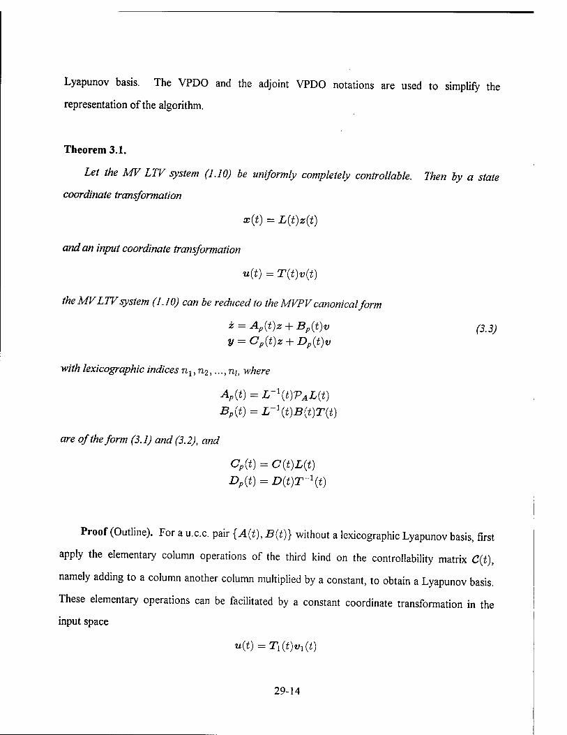
Lyapunov basis. The VPDO and the adjoint VPDO notations are used to simplify the

representation of the algorithm.

Theorem 3.1.

Let the MV LTV system (1.10) be uniformly completely controllable. Then by a state

coordinate transformation

x{t) = L(t)z(t)

and an input coordinate transformation

u(t) = T(t)v(t)

the MV LTV system (1.10) can be reduced to the MVP V canonical form

z = Ap(t)z + Bp(t)v (3j)

V = Cp(t)z + Dp(t)v

with lexicographic indices n1,n2,...,ni, where

Ap(t) = L-\t)VAL(t)

Bp(t) = L-\t)B(t)T{t)

are of the form (3.1) and (3.2), and

Cp(t) = C(t)L(t)

Dp{t) = D{t)T-\t)

Proof (Outline). For a u.c.c. pair {A(t), B(t)} without a lexicographic Lyapunov basis, first

apply the elementary column operations of the third kind on the controllability matrix C(t),

namely adding to a column another column multiplied by a constant, to obtain a Lyapunov basis.

These elementary operations can be facilitated by a constant coordinate transformation in the

input space

t*(t) = r1(t)«i(t)

29-14

Then in the transformed coordinates the pair {A{t),Bi(t)} will have a lexicographic Lyapunov

basis, where

B1(t) = B(t)T1(t) = [b1(t) b2(t) ■■■ &,(*)]

The MVPV canonical form {Ap(t), Bp(t)} can now be obtained from {A(t), Bi(t)} by a state

coordinate transformation x(t) = L(t)z{t) and an input coordinate transformation

vi(t) = T2(t)v(t) as follows.

Let ß = {pjk(t) = V^bjit)} be an orthonormal lexicographic Lyapunov basis for

{A(t), Bi{t)} with lexicographic indices n1, n2,..., n/. Then the state coordinate transformation

matrix L(t) is given in terms of R(t) = L~x{t) by

R(t)

Ri(t)

where the n2- x n submatrices Ri(t) are given by

Ri(t) =

rl(t) riß)

where

Tik{t) = QkAlVTlbi(t)

If /? is not orthonormal, let P(t) be the matrix associated with ß and let G(t) be the left (row)

orthonormalization matrix for P(t)such that

P(t) = G(t)P(t)

is unitary, and let

A(t) = G(t)VAG-\t)

29-15

B(t) = G(t)B(t)

Then the State transformation matrix L(t) can be written as

L(t) = L{t)G-\t)

where L(t) is obtained from the orthonormalized basis represented by P and the system

{A(t),B(t)} as described above.

The input coordinate transformation matrix T2(i) is the right (column) orthonormalization

matrix for R(t)Bi(t). The overall input coordinate transformation T{t) is given by

T(t) = T2(t)T1(t). D

A MAPLE implementation of the Extended S-W transformation has been developed. It will

be used in the design and implementation of the eigenstructure assignment control in Sections 5, 6

and 7.

4. A PD-Eigenvector Based Criteria for Uniform Controllability and Observability

In this section PD-eigenvector based criteria for uniform controllability and observability are

obtained. These results are important in their own right because they are natural LTV

counterparts to the well known Popov-Belevitch-Hautus eigenvector tests for controllability and

observability of LTI systems [14]. They will also constitute the basis for output/state decoupling

by PD-eigenstructure assignment. The first main result of this section gives a necessary and

sufficient condition on the pointwise controllability and observability using PD-eigenvectors.

Theorem 4.1 (PD-eigenvector criteria for controllability and observability).

A MV LTV system {A(t),B(t),C(t)} is not completely controllable at tx if and only if

there is a row PD-eigenvectors qT(t) of A(t) such that ^fa) = qT(t1)B(t1) = 0 and

7(ii) = 0. It is not completely observable at tx if and only if there is a column PD-eigenvector

p(t) ofA{t) such thatnih) = C(*i)p(ti) = 0 andrifa) = 0.

29-16

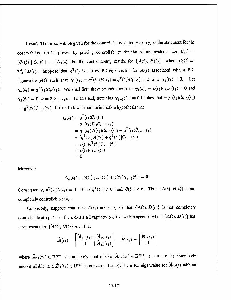
Proof. The proof will be given for the controllability statement only, as the statement for the

observability can be proved by proving controllability for the adjoint system. Let C(t) =

[Ci(t) | C2(t) | ••• | Cn(t)] be the controllability matrix for {A{t), B(t)}, where Ck(t) =

VkÄlB(t). Suppose that qT(t) is a row PD-eigenvector for A(t) associated with a PD-

eigenvalue p(t) such that ufa) = qr(h)B(tl) = qT(ti)Ci{t1) = 0 and 71(t1) = 0. Let

7fe(*i) = ffT(*i)C*(*i)- We shall first show by induction that 7fc(*i) = p(*i)7fc-i(*i) = ° and

jk(ti) = 0, k = 2,3,... ,n. To this end, note that 7fc-i(*i) = ° implies that -gT(ti)C*-i(ii)

= qT(h)Ck-i(t\)- It then follows from the induction hypothesis that

7k(h) = qT(t1)Ck(t1)

= qT(t1)VACk-i(tl)

= <7T(ti),4(ii)Cfc-i(ti) - 9T(^i)Cfc-i(ti) = [q\t1)A(t1) + qT(t1)}Ck-1(tl)

= p(t1)qT(t1)Ck-1(tl)

= p(tihk-i(h) = 0

Moreover

7fc(*i) =P(*i)7fc-i(*i)+P(*i)7fc-i(*i) = 0

Consequently, gT(ii)C(*i) = 0. Since qT(h) # 0, rank C{h) < n. Thus {A(t),B(t)} is not

completely controllable at tx.

Conversely, suppose that rank C(U)=r<n, so that {A(t),B(t)} is not completely

controllable at tx. Then there exists a Lyapunov basis r with respect to which {A(t), B(t)} has

a representation {A(t), B(t)} such that

Mh) 'Än(h) ^12 (*l)

0 ^22 (*l). , £(tl) =

Bi(ti) 0

where Än(tx) € Mrxr is completely controllable, A22(ti) eWX3, s = n-r, is completely

uncontrollable, and Bi(ii) G Mrxl is nonzero. Let pit) be a PD-eigenvalue for A22(t) with an

29-17

associated row PD-eigenvector zT(t). Let qT(t) = qT{t)L(t) = [o | zT(t)], where L(t) is the

coordinate transformation matrix from the standard basis to P. Clearly 7^) = qT(t1)B(t1) =

?T(ti)Z-1(t)j:(t)B(i1) = 0, and 7(tj) = 0. It remains to show that p(t) is a PD-eigenvalue

for A(t) and qT(t) is a row PD-eigenvector for A(t). Clearly, gT(t) satisfies

-f(*)=[o|-2T(i)] = [o\zT(t)[A22(t)-p(t)Is}] = qT(t)A(t)-p(t)f(t)

By Remark 2 to Definition 2.1, *(i) is a column PD-eigenvector for -A^W- Thus, there exists

a Lyapunov basis {&(*), £2(*), • • •, Cn(*)} for Rs such that

*(*)=E[öi"1(i)]c.-(o t=i

Now construct a Lyapunov basis {ßl (t),ß2 (t),..., ßn(t)} for Rn as follows

0 ßi(t)

ßs(t) Mt) Cs(t)

ßj{t) = Zj-s ,

i = l,2,...,s-l

j = s + l,...,n

where ek is the fcth standard basis vector for Rn and ip0(t) is chosen by

j=s+l

Then

ff(*) = E[oJ~1(1)]A(o {=1

It then follows from Remark 2 to Definition 2.1 that pit) is a PD-eigenvalue for A(t) and qT(t)

is a row PD-eigenvector for A(t). D

29-18

In the following corollary to Theorem 4.1, a MV LTV system {A(t), B(t), C(t)} is said to

be uniformly uncontrollable if the controllability matrix C{t) for {A(t), B(t)} satisfies

rankC(t) < n, W > 0. It is said to be uniformly unobservable if the observability matrix 0(t)

for {A(t), C(t)} satisfies rank 0{t) < n, Vt > 0.

Corollary 4.1.

A MV LTV system {A(t), B(t), C(t)} is uniformly uncontrollable if and only if A{t) has a

row PD-eigenvector qT(t) ofA(t) such that qT(t)B(t) = 0. It is uniformly unobservable if and

only ifA{t) has a column PD-eigenvector p(t) such that C(t)p(t) = 0. D

In the following corollary to Theorem 4.1, a MV LTV system {A(t), B(t), C{t)} is said to

be uniformly r-controllable if the controllability matrix C(t) for {A(t), B(t)} satisfies rank

C(t) = r. It is said to be uniformly r-observable if the observability matrix 0(t) for

{A(t), C(t)} satisfies rankC(t) = r.

Corollary 4.2.

A MV LTV system {A(t), B(t), C{t)} is uniformly r-controllable if and only if there exist

exactly s = n — r row PD-eigenvectors qj(t) such that qJ(t)B(t) = 0, i = 1,2,..., s. It is

uniformly r-observable if and only if there exist exactly s — n — r column PD-eigenvector pj(t)

such that C(t)pj(t) = 0, j = 1,2,..., s. D

The following theorem gives PD-eigenvector based criteria for modal controllability and

observability. It sheds some light on how the orientation of a PD-eigenvectors affects the

"degree" of controllability and observability. The result on modal observability will be used

subsequently in Section 6 to develop the output/state decoupling technique by PD-eigenstructure

assignment.

29-19

Theorem 4.2 (Modal controllability and observability).

Let {A(t),B(t),C(t)} be a MV LTV system and let bj(t) and cj(t) be the jth column

vector o/B(t) and the ith row vector ofC(t), respectively. IfqJ(t) is a row PD-eigenvector of

A{t) associated with the ith PD-eigenvalue pi{t) such that qj(t)bj(t) = 0, then the associated

ith mode exp/0pi(r)dr cannot be altered by the jth input Uj{t) with the state feedback control

law Uj(t) = kj(t)x(t) for any gain k](t). Similarly, If pj(t) is a column PD-eigenvector of

A(t) associated with the jth PD-eigenvalue pj(t) such that cj(t)pj(t) = 0, then the associated

jth mode exp/0p_7(r)dr is not observable from the ith output y{(t) with a state observer for any

observer gain hj(t).

Proof of Theorem 4.2. The proof will be given only for the controllability statement. The

statement for observability can be proved by applying the proof for controllability to the adjoint

system. Let {/>,•(<)}?=! be aPD-spectrum for A(t) and let Q(t) = [qi(t) | q2(t) | ... | qn(t)]T

be the associated row PD-modal matrix consisting of the row PD-eigenvectors qj(t). Then the

coordinate transformation z(t) = Q(t)x(t) results in z = Az(t)z + Bz(t)u, where

A2(t) = Q{t)QAQ-\t)

= diag[/0i(i),p2(*), •••.Pn(t)]

Bz{t) = Q(t)B(t)

Now suppose that qj(t)bj(t) = 0 and let Uj(t) = k]x(t) = k]Q-l(t)z{t). Then

Zi(t) = Pi(t)zi(t) + q]{t)b]{t)k]{t)Q-\t)z(t) = Pi(t)Zi(t)

Clearly, the ith mode z{{t) = exp/0V,-(r)dT can not be altered by the jth input Uj(t) = k?x(t)

for any k](t). D

29-20

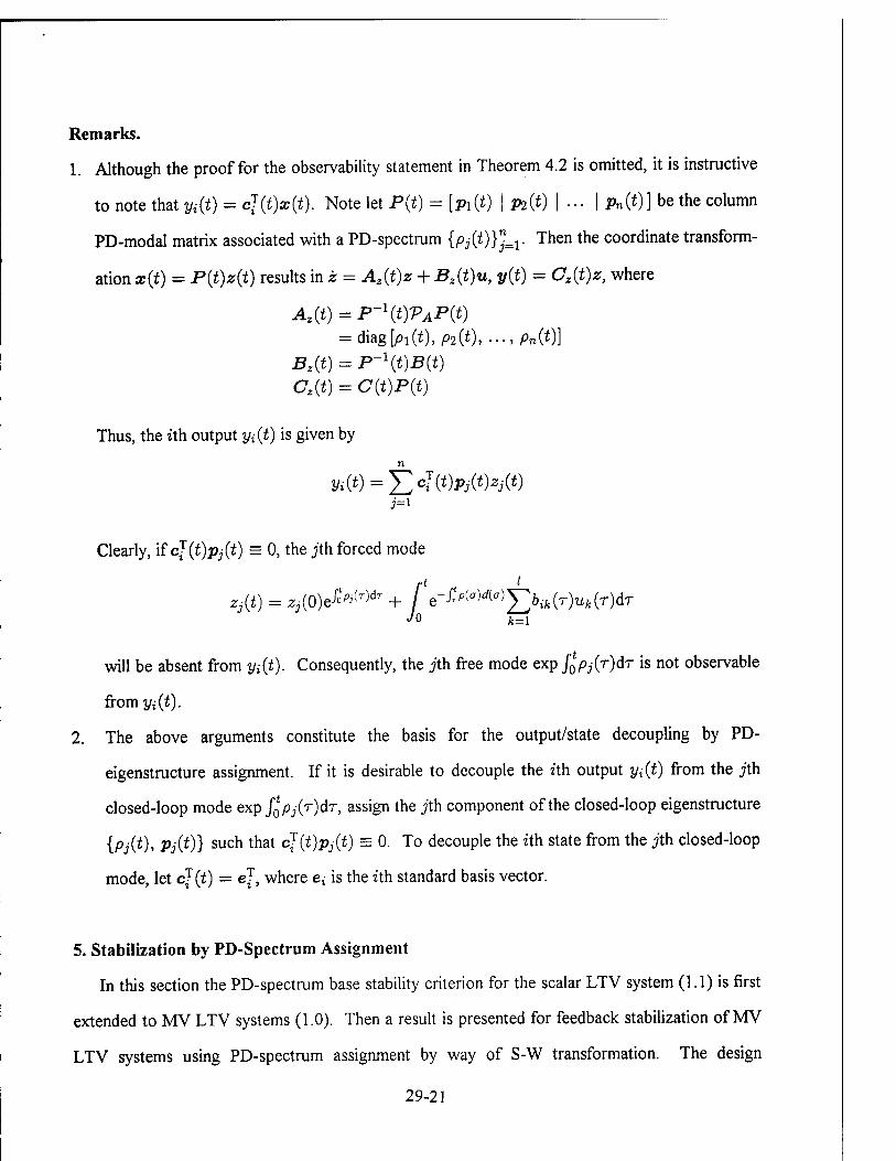
Remarks.

1. Although the proof for the observability statement in Theorem 4.2 is omitted, it is instructive

to note that yi(t) = cj(t)x(t). Note let P(t) = [pi(t) | pa(*) I ••• I Pn(*)] be the column

PD-modal matrix associated with a PD-spectrum {pj(t)}n-=l. Then the coordinate transform-

ation x(t) = P(t)z(t) results in z = Az{t)z + Bz(t)u, y(t) = Cz{t)z, where

^z(t) = p-1(i)^P(t) = diag[J0i(t)> p2(<). •■■»Pn(*)]

C2(i) = C(t)P(t)

Thus, the ith output yi(t) is given by

yi(t)^J2cJ(t)Pj(t)Zj(t)

Clearly, if cj(t)pj(t) = 0, the j?'th forced mode

2j(t) = Zj(0)MT)dT + / e-^^°^ff)X;&ifc(T)t*t(T)dT

will be absent from yi(t). Consequently, the jth free mode exp fQpj(T)dr is not observable

from yi(t).

2. The above arguments constitute the basis for the output/state decoupling by PD-

eigenstructure assignment. If it is desirable to decouple the ith output y;(£) from the jth

closed-loop mode exp $IPJ(T)&T, assign the jth component of the closed-loop eigenstructure

{pj(t), Pj(t)} such that cj(t)pj(t) = 0. To decouple the ith state from the ;'th closed-loop

mode, let cf(t) = e], where e, is the ith standard basis vector.

5. Stabilization by PD-Spectrum Assignment

In this section the PD-spectrum base stability criterion for the scalar LTV system (1.1) is first

extended to MV LTV systems (1.0). Then a result is presented for feedback stabilization of MV

LTV systems using PD-spectrum assignment by way of S-W transformation. The design

29-21

procedure for PD-spectrum assignment is also provided. The necessary and sufficient stability

criterion based on a PD-spectrum uses an extended-mean concept as defined below.

Definition 5.1.

Let a : I -* R be a locally integrable function on the interval I = [T0, oo). The extended

mean of a{t) over I is defined by

rto+T .... {a(t\\ = lim sun — /

to,teI

I fto+T em (a(*)) = lim sup - / a(r)dr *o,te/ T->oo,t0>T0TJto

= lim T—>oo

SUP :—T / a(T)dr t>t0+T,t0>T0t-t0 JtQ

Theorem 5.1.

Zef^ be a VPDO having a PD-spectrum {pk{t)}nk=l with \RePk{t)\ <M,t> 0, for some

M<oo. Let pk(t) and qTk{t) be a column PD-eigenvector and a row PD-eigenvector

associated with pk(t) respectively. Then the null solution to the LTV system PAx = 0 is

uniformly asymptotically stable for all t0 > T0 if and only if

(i) there exists a 0 < ck < oo such that

t^€l(Re Pk{t)) = ~ck<0

and moreover,

(ii) there exist hk > 0 andO < dk < ck such that

\\Pk(t)qTk(tQ)\\ < hkä*>«-V

for all t > t0 > T0. D

Remarks.

1. Condition (ii) is automatically satisfied if the imaginary parts of all PD-eigenvalues are of

polynomial order or slower; that is, an integer m > 0 exists such that

29-22

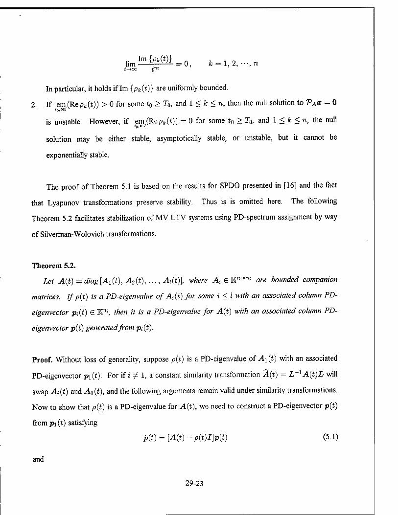
Im{£(t)} t = 1,V..,„

In particular, it holds if Im {pk(t)} are uniformly bounded.

2 If em (Repfc(t)) > 0 for some tQ > T0, and 1 < k < n, then the null solution to VAx = 0

is unstable. However, if em (Repfc(t)) = 0 for some t0 > T0, and 1 < k < n, the null

solution may be either stable, asymptotically stable, or unstable, but it cannot be

exponentially stable.

The proof of Theorem 5.1 is based on the results for SPDO presented in [16] and the fact

that Lyapunov transformations preserve stability. Thus is is omitted here. The following

Theorem 5.2 facilitates stabilization of MV LTV systems using PD-spectrum assignment by way

of Silverman-Wolovich transformations.

Theorem 5.2.

Let A(t)=diag[A1(t), A2{t), ...,Ai{t)], where A{ e KniXTli are bounded companion

matrices. If p(t) is a PD-eigenvahe of Ai(t) for some i < I with an associated column PD-

eigenvector pi(t) e Kni, then it is a PD-eigenvalue for A(t) with an associated column PD-

eigenvector p(t) generated from pi(t).

Proof. Without loss of generality, suppose p(t) is a PD-eigenvalue of A\(t) with an associated

PD-eigenvector p\(t). For if i ^ 1, a constant similarity transformation A(t) = L~lA(t)L will

swap A{(t) and A\(t), and the following arguments remain valid under similarity transformations.

Now to show that pit) is a PD-eigenvalue for A(t), we need to construct a PD-eigenvector p(t)

from pi (i) satisfying

p{t) = [A{t) - p(t)I}p(t) (5.1)

and

29-23

p(*)=E[ßr1(i)]/?i(*) (5.2) J=I

for some Lyapunov basis {ßj(t)}n=1. Let

*(*) Pi(0 (5.3)

Clearly, p(t) satisfies (5.1). Since pi(t) is a PD-eigenvector for Ax{t), there exists a Lyapunov

basis {Cfc(*)}fcLi for Km, such that

ft(*) = E[QPfc-1(l)]Cfc(*)

/t=i

Now construct a Lyapunov basis {ßk{t)}nk=l as follows

Ct(«)

ßk(t) = ek

0 Cn, (t) Mt) J

fc = 1,2, ...,m-i

A; = ni+1, ..., n

where efc is the fcth standard basis vector for Rn, and

n-l

^o(t) = -^[Qpfc(l)]efc

k=n\

Then it is readily verified that p(t) satisfies (5.2). D

Remark.

Let A(t) be a block upper (lower) triangular matrix. For A(t) = A, it holds that if A is an

eigenvalue of a block matrix Aü(t) on the diagonal, then A is an eigenvalue of A. However, this

is not granted for a time-varying A(t).

The design procedure for PD-spectrum assignment is presented below, along with guidelines

on the selection of closed-loop PD-spectrum.

29-24

PD-Spectrum Assignment Procedure.

1. Transform the MV LTV system (1.10) into MVPV canonical form (3.3) by a state

coordinate transformation x(t) = L(t)z(t) and an input coordinate transformation

u(t) = T(t)v(t) per Theorem (3.1).

2. For each block companion matrix Aa(t) in the MVPV matrix A(t), chose the desired PD-

eigenvalues and synthesis the coefficients of the SPDO associated with Au(t). Then design

the state feedback control law v(t) = Kp(t)z(t) to obtain the desired closed-loop dynamics

in the MVPV coordinates.

3. The actual control law u(t) = K(t)x(t) is given by K{t) = T{t)Kp{t)L-x(t).

Remarks.

1. For BIBO stability, exponential stability must be achieved by assigning negative extended

mean to all the PD-eigenvalues. To this end, it suffices to keep Re{pk(t)} < -e < 0 for

some prescribed e > 0.

2. No identical PD-eigenvalues should be assigned within each companion block Aa(t). For

block size larger than 2x2, ensure that all PD-eigenvalues are differentially distinct.

3. If a pair of complex conjugate PD-eigenvalues Pij(t) = a(t) + ju(t) is assigned, keep u(t)

from vanishing.

4. The PD-eigenvalues should be continuously differentiate n — 1 times.

6. Output/State Decoupling by PD-Eigenstructure Assignment

In this section, a design procedure for output / state decoupling using PD-eigenstructure

assignment is developed based on Theorem 4.2. According to that theorem, to decouple the ith

output yi(t) from the jth closed-loop mode Pj(t), one needs only to assign the jth column PD-

eigenvector pj(t) in such a way that pj(t) is orthogonal to Cj{t) for all t. A natural question to

ask is that to what extent the orientation pj(t) can be adjusted. The following theorem addresses

this issue.

29-25

Theorem 6.1 (Parametrization of PD-eigenstructure)

Let {pk{t))l=i be a PD-spectrum for A(t) with an associated column PD-modal matrix

P0(t). Then P(t) = PQ(t)S(t) is also a column PD-modal matrix for A(t) if and only ifS{t)

satisfies

S(t)=T(t)S(t)-S(t)T(t) (6.1)

with detS{t) ^ 0, where T(t) = diag[px{t), p2(t), ..., pn(t)]. Moreover, the general solution

of S{t) is given by

S(t) = e^^He-J^(r)dr (62)

where H € Cnxn is an arbitrary nonsingular constant matrix, and

Proof. Suppose P(t) = P0(t)S(t) is a PD-modal matrix for A(t). Then we have

P0(t) = A(t)P0(t) - P0(t)T(t) (6.4)

and

[W)S(t)]W = A(t)[PQ(t)S(t)} - [P0(t)S(t)]T(t) (6.5)

But

[PQ(t)S(t)]w = P0(t)S(t) + PQ(t)S(t) (6.6) = [A(t)P0(t) - PQ(t)T(t)}S(t) + P0(t)S(t)

Since detP0(i) ^ 0, it follows from (6.5) and (6.6) that

S(t) = T(t)S(t) - S(t)T{t) .

29-26

Conversely, suppose that (6.1) holds. Then

[Po(t)S(i)](1) = Po(t)S(t) + P0(t)S(t) = [A(t)P0(t) - PQ(t)T(t)]S(t) + P0(t)[Y(t)S(t) - S{t)T(t)] = A(t)[Po(t)s(t)]-[p0(t)S(t)}r(t)

Thus P(t) = Po(i)S(t) is a column PD-modal matrix. The general solution for S(t) given in

(6.2) can be verified by direct computation. D

Remark.

Theorem 6.1 is instrumental in the output/state decoupling by PD-eigenstructure assignment,

where the orientation of some column PD-eigenvectors should be adjusted so as to keep

orthogonal to a row vector in the output measurement matrix C(t). Theorem 6.1 points out that

the orientation of a column eigenvector is determined by: (i) the constant matrix H, and (ii) the

associated PD-spectrum {pk{t)}nk=v Note that H = P0

_1(0)P(0) is fixed at t = 0. Thus an

optimal H should be computed off-line to achieve the desired PD-eigenvector orientations for all

permissible PD-spectra. Then an on-line, real-time optimization is needed to select the optimal

PD-spectrum to achieve the best tracking performance and decoupling. This design approach is

illustrated in Figures 6.1 and 6.2.

Jl Pi J~ v 1

r p,

C,T(t) %.

f N ft ' J 1

U= A(t) I i '

Gradient Descent J"' V 1 r

Min mizatio n

Figure 6.1 Output Decoupling by PD-Eigenstructure Assignment

29-27

p, o Pi

AP,

PD-Eigenvector |_ Generator r

Pp)

SAT(-)

Ap

1/S

SGN(0

G(s) AP.

Of(t)

MH SGN(-)

Viß

d/dt

Figure 6.2 PD-Eigenstructure Assignment Logic for Output Decoupling

PD-Eigenstructure Assignment Procedure:

1. Follow the PD-Eigenspectrum Assignment Procedure of Section 5 to achieve stability.

2. To associate the ith output with, and only with the jth mode of the closed-loop system,

assign the jth PD-eigenvalue pj(t) such that the ith row vector cj(t) of C(t) becomes an

associated row PD-eigenvector, i.e.

Q[A+BK{P])-PlI\Ci = 0 (3)

where K(Pj(t), t) = Kp(Pj(t), t)L-\t). In particular, if a(t) = c{ is constant, than (3)

can be written as

cJ[A(t)+B(t)K(Pj(t), t)]« Pi(t) (4)

3. To decouple the ith output from the jth mode of the closed-loop system, assign pj(t) such

that the ith row vector cj(t) of C(t) is orthogonal to the jth column PD-eigenvector pj(t),

i.e.

^[A+BK(Pj)-p3I}Pj = 0 (5)

29-28

and

cJ(t)Pj(t) = 0, Pj(t) £ 0 (6)

Remarks.

1. For eigenstructure assignment in a LTI system, once the feedback control gain K is

determined, the decoupling condition (6) is fixed, because the column eigenvector pj is fixed

up to a constant scaling factor which does not change the orientation of pj. Whereas for PD-

eigenstructure assignment, condition (6) can be optimized by selecting an optimal initial

condition Pj(0) for (5) and a permissible Pj(t).

2. For eigenstructure assignment in a LTI system with I control inputs, only n of the n x I gains

in the feedback gain matrix K are need for eigenvalue assignment, the rest n x (Z — 1) gains

can be used to alter the orientations of the eigenvectors for optimal decoupling. However, at

the present time, the eigenvalue assignment based on Theorem 5.2 requires the use of all

n x I gains, leaving no freedom in eigenvector assignment. However, this is not an intrinsic

limitation. Additional research is needed to alleviate this limitation.

7. Roll-Yaw Decoupled Autopilot for a BTT Missile

In this section, the results obtained in Sections 2-6 are applied to the autopilot design for

command tracking and roll-yaw decoupling of the EMRAAT bank-to-turn missile airframe. The

complete nonlinear state equation of the EMRAAT airframe is given in the Appendix. For

simplicity, it is assumed here that the roll-yaw dynamics are sufficiently decoupled from the pitch

dynamics.

The basic design approach is by linearization of the nonlinear roll-yaw airframe along a

nominal trajectory as follows.

29-29

Let the system states and inputs be chosen as

«0 = ["6001 rwi &(*) r(i) £s(*) P(t)

L&Wj [ml

6(t) = 6r(t) 6p(t)

where ß(t), r(t), p(t), $(t) are the sideslip, raw rate, roll rate and roll angle, respectively, 8r(t)

and 6p(t) are the rudder and aileron angles, respectively. Since all state variables are on-line

measurable, they are defined as the outputs. Thus, the measurement matrix C(t) = I. The

design objectives are to decouple ß(t) from p(t) while maintaining good command tracking

performance.

Then the non-linear state equation is given by

s=m s) = /i(6>6>,£3,£4A,<5P) /2(£i.6»£3>6iA,5p)

For a nominal trajectory £ satisfying

define the tracking errors by

*(*) = /(?(*),*(*))

*(*) = *(*)-€(*)

and the tracking error control input by

u(t) = 6(t)-l(t)

Then the linearized tracking error dynamics are given by

x = A(t)x + B(t)u

y = C(t)x + D(t)u

29-30

For the EMRAAT airframe at altitude of 30,000 ft. and Mach of 2.0 [17]

where

A(t) df

T.7

on(i) ai2(i) o13(t) au{t) 96.09 a22(i) a23(i) 0 1001 a32(t) a33(i) 0

0 0 10

™-% £.*

1.979 ■ 10-3cos(/5) -75.99 -959.5

0

C(t) =

- 247.3 ■ 10-6cos(/3) 17.52 -1244

0

1 0 0 0" 0 1 0 0 0 0 1 0 0 0 0 1

an(t) = gQS WV

D(t) = 0

{CYßcos(ß(t)) - (CYßß(t) + CYpp(t) + CYrr{t) +

a12(t) = - 1 + 398.21 • 10~6cosÖ9(i))

ais(i) = - 18.056 • 10~6cosOö(t))

a14(f) = 16.631 ■ lO"3cos(0(i))cosOö(t))

a22(t) = 0.3623 • 10_3r (t) + 0.5024 • 10_3p(t) - 0.6053

a23(t) = 7.8 • 10~3 p(t) + 0.5024 • 10"3 r (i) - 3.5 • 10~3

a32(t) = - 36.8 • 10~3r (t) - 2.3 • 10"3p(t) + 0.8056

a33(t) = 35.80 • IQ~G p(t) - 2.3 • 10~3r (t) - 2.177

The overall system configuration is shown in Figure 7.1. The PD-eigenstructure assignment

control for LTV error dynamics stabilization and decoupling is shown in Figure 7.2.

29-31

Stfrl

Inverse Plant Model (Neural Network)

38 LTV Tracking error

stabilizing/decoupling Controller

Ift)

KH)

&)

} Nonlinear Time Varying Plant

?tv

Figure 7.1 Nonlinear Tracking System Configuration

qHr) B{t)

T® r

*£> 5[«)

/ 7t«;

^w t

/

^0 r

z €W L-Ht)

C(t) *#)

PD-eigenstructure assignment logic

Figure 7.2 LTV Tracking Error Stabilizing and Decoupling Control

29-32

Now apply the S-W transformation to obtain the MVPV canonical from with lexicographic

indices n\ = 2, ra2 = 2:

A>(*) =

0 1 0 0

Q2i(*) a22(i) Q2S(*) «24 00 0 0 0 1

<*4l(*) «42(*) a43(i) a44(i)

"0 0"

BP(t) = 1 0 0 0 0 1

Then design the state feedback control gain

'foijt) - a2i(t) fa® - a22(t) KP(t) = -a41(t) -a42(t)

-a2s(<) ■ö2s(*) ß43(t) - a4Z(t) ß4A(t) - aAi(t)

to obtain the desired closed-loop dynamics in the MVPV coordinates

Ap(t) + Bp(t)Kp(t) =

0 1 Mt) Mt)

o o

o o

o o

o o

o 1 As(<) ßu{t)\

where Aj(i) are synthesized from the (real) PD-spectral canonical form

Mt) =

ffi(t) Wi(t) -wi(i) cri(t)

0 0

0 0

0 0

0 0

Mt) o 0 a22(t)

with the desired closed-loop PD-eigenvalues p\\,\i(t) = cr\(t) ±jui(t) and p2i(t) = cr21(i),

p22(<) = o"22(t), where the roll modes are chosen to be simple (nonoscillatory).

Due to the time constraints on this research, implementation and simulation results are not

available. Anticipated difficulties of the implementation are (i) the complexity of the control law

kp(t), (ii) training of the neural network inverse of the unstable nonlinear airframe, and (Hi) real-

29-33

time implementation of the eigenstructure assignment logic. However, none of these problems is

insurmountable with further studies.

8. Summary and Conclusions

In this research a systematic design procedure for nonlinear tracking and output/state

decoupling control has been developed by way of linearization along a nominal trajectory. The

resulting LTV tracking error dynamics are then stabilized and decoupled using PD-eigenstructure

assignment in a way similar to the eigenstructure assignment design for LTI systems. Theoretical

results on the assignability of the PD-eigenstructure for stabilization and decoupling have been

obtained. However, due to the time constraint, implementation and simulation results are not

available at the present. Further research is needed to address the complexity of the

implementation, and to validation the theory and design procedure by simulations.

It is believed that this research is the first attempt at stabilization and decoupling of time-

varying dynamics using a differential-algebraic approach, without resorting to the unreliable

frozen-state, frozen-time gain scheduling. Preliminary results have shown excellent performance

and robustness with a simple pitch autopilot. Thus, further study on the implementation of the

significantly more complex is warranted. Furthermore, the PD-eigenstructure assignment control

is by no means limited to stabilization and decoupling. An array of challenges posed by modern

missile technology [2] can be addressed by the multiobjective PD-eigenstructure assignment

concept illustrated in Figure 8.1. Additional applications can be found is aircraft flight control,

spacecraft altitude control, vibration control, robotics and other nonlinear tracking and fast time-

varying control systems.

29-34

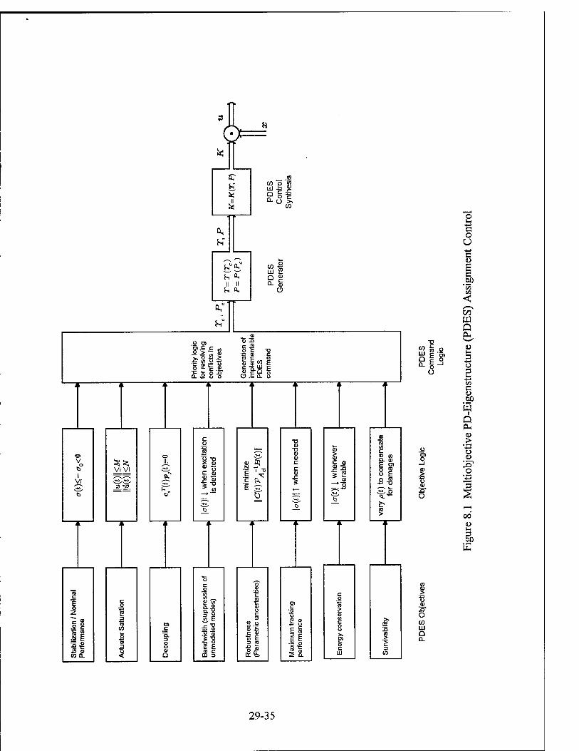
c 2 o c . c e <". E

O .5 0. o —z

V o

I VI

VI VI

o -o

C 0)

* (0

CD tt)

— I T3

- r^

-* i J3 o w a.

w

I

If £ 0)

fi in -^ c a V, E

a: St

ft So y p en Q c o

o

o q

.a O

(/) CD > Ü <D 3" O

2- W LU

5 Q a.

2 3 w

00 0)

E

29-35

Appendix

State Equations for the EMRAAT Missile [17]

ä = q - tan(/3)[p(cos(a) - rsin(a)] + yjs(ß) (cos(a)cos(</>)cos(6>) + sin(a)sin(6>))

gQS + WVcos(ß) ^ N°a + °Nää + CN*q + CNiq^)cos(a)

ß = psin(a) - rcos(a) + ^y(CYßß + CYpP + CYrr + CY^V + CY^5r)cos(ß)

+ £cos(0)sm(<t>)cQs(ß)

P — [{-Ixyhzhz ~ IxzIyz + hylyz + hylxzlyy)p2 +

+ {■lyylyzlzz — Iyz ~ IXyhz ~ Ixylxzlyy)<l +

+ {-Iyylyzhz + hyhzhz + /J, + 4*1/*) ^ +

+ {-IxyIyzIzz + IxzIyyIzz - 2IyzIxz - IxyIyyIyz + IxxIxyIyz - IxzPyy + IxxIxzIyy)pq +

+ \JxyIZz + hzlyzhz ~ hylyyhz ~ hxhyhz + ^hy^z + TxJyyIyz ~ Ixxlxzlyz)pr +

+ (-tyvhz + lyzlzz + lyyhz ~ Iyytf, ~ l\zlyy)qr +

+ QSd(Clp(IyyIzz - II) + Cnp(IxyIyz + IxJyy))p +

+ QSd(Cmq(IxyIZ2 + Ixzlyz))q +

+ QSd{dXlyyIZZ ~ I2yz) + C^Iy* + IXZIyy))r +

+ QSd(Cmä(IxyIzz + IxzIyz))ä +

+ QSd(Cma(IxyIzz + IxJyz))a +

+ QSd(Ch{IyyIzz - I\z) + Cnß{IxyIyz + IxzIyy))ß +

+ QSd(Cl5p(IyyIzz - I\z) + Cn6p(IxyIyz + IxzIvy))6p +

+ QSd(Cm6q(IxyIzz + IxzIyz))8q +

+ QSd(Clfr(IwI2z - I2y2) + Cn^IxyIyz + IxzIyv))8T)

+ yi-xiiyyi-zz — lxyhz ~ IxXIyz ~ 2IxyIxzIyz — IxzIyy)~

29-36

q — [{—hxhzhz + hxhy^-yz "T lXy ~> hy^xz)P +

T Kj-xylyz'-zz T lyZlxz J-xx^xy^yz ■'ly-'iij? "i

T (, lxylyzlzz "r i-xx'-xz^zz *xz*yz *xzr '

+ [—Ixxlyzlzz + hyhxhz + 21xzlyZ — lxxlyylyz ~ hyhz^yy + lyzhx ' ^xxhyhzjPQ "T

+ [hxhz ~ hzhz ~ hyhz ~ lxxhz + Ixxlyz ~i~ hzhxjP^ +

+ \~lxylZz ~ hz*yzhz ~i~ hy*yyhz + ^xxhyhz > hzlyylyz ~~ ^xz-^xxiyz ~ ^xz^xyl^T +

+ QSd(Clp{IxyIzz — hzlyz) + Cnp(IxxIyz + hyhz))? +

+ QSd{Cmq{IxxIzz ~ I2xz))q +

+ QSd{Clr{IxyIzz + hzlyz) + C^hxlyz + hyhz))r +

+ <3Sd(Ojirai„-4))« + + QSd(Cma(IxxIzz - ll))a +

+ QSd{Clg{Ixyhz + hzlyz) + Cnß(hxlyz + hzhy))ß +

+ QSd(ClSp(IXyIZz + hzlyz) + CnSp(hxIyz + hzhy))Sp +

+ QSd(Cm6q(hxhz ~ I2xz))5q +

+ QSd^lÎxyhz + Ixzlyz) + Cnir(IxxIyZ + hzhy))8T]

(T T T — I2 1 — 1 T2 — 11 11 — l2 I \~x \1xx1yy1zz *-xylzz 1xx1yz ^1xy1xz1yz 1xz1yy)

V — [(—Ixxlxzlyz + Ixxlxylyy -<xy ^xz^xyjP +

+ {Ixzlyylyz + lyzîy ~ Ixxlxylyy + -<xt/)9 +

"t" ( ■Ixylyz Ixzlyylyz + Ixxlxzlyz + IxylxzF "T"

+ (-IxxIyZ - lyylxx + IxzIyy + 4^ + -fyy4r ~ hyhx)PQ +

T \1 XXJ-yxJ-zz T iiyi-izi-zz + lii-lyylyz ~ Îxylyz ~ lyz^xx ~ Ixy^xzlyy ~ ■IxxlxylxzjPT T

+ \~liylyzlzz ~ i-xzlyyi-zz T i-iyi-yyi-yz T i-xxlxylyz T liz-Lyy~liilizlyy T ■"xy-'xzj<??° i

+ QSd(Clp(IxyIyz ~ Iizlyy) + CÎxJyy ~ I^y))P +

+ QSd(Cmq(IxxIyz + Ixylxz))q +

+ QSdiCÎxylyz + /„/w) + C^C/xx7W - 42y))r +

+ QSdiCrîhilyz - Ixylxz))a +

+ QSd(CmMxxIyz ~ Ixyliz))a +

+ QSd{Ch{IxyIyz + Iizlyy) + Cnp(liilyy - Ily))ß +

+ QSd(Cl6p(IXyIyz + hzlyy) + Cnh{IxxIyy - Ily))5p +

+ QSdiCîhJyz - Ixylxz))5q +

+ QSd(Cl6r(IXyIyz + Iizlyy) + ^(Jxx-Tyy - t^))6r]

+ [lXXlyylzZ ~ +xylzz ~ lll-tyz ~ ^liyllZ-LyZ ~ ^XZ^yy)

29-37

Glossary of Terms Aerodynamic coefficients (Mach = 2.0)

a —Angle of attack ß — Angle of sideslip p — Roll rate q — Pitch rate r — Yaw rate Q — Dynamic Pressure S — Reference area d — Reference length/diameter V — Missile velocity W —Missile weight g — Acceleration due to gravity i> — Yaw angle 0 — Pitch angle i> — Roll angle 5p — Roll control input (surface deflection) 6q — Pitch control input (surface deflection) 6r — Yaw control input (surface deflection) Q —(gQS/WV) N — Normal force Y — Side force Co,, — Aerodynamic Coefficient- a due to b 1 — Aerodynamic moment about x-axis m — Aerodynamic moment about y-axis n — Aerodynamic moment about z-axis Iij — Moment or product of inertia

CV„: = 36.6 Cnd : = 0.0274 ON,

z = 0.0145

^Nt, = 6.0165

Cyp = -14.9 CyP = -0.00073 cYr = -0.0161

<V = -.01

Cv,- = .08

dß = 5.44

Ci,= -0.011

Ci = 0.0021

<V = -6.30

Ci,= = -5.16 Cma

z = -82

Cm* " = -0.014 Cm, = = -0.202 Cmiq ■■ = -40.7

Crip — : 35:52 cnp = 0.006 CW = -0.2 Cn^ - = 1.72

Cn&. = = -28.65

EMRAAT Physical Properties

p = 32.2ft/s2

d = 0.625 ft. S = 0.3067 ft2

W = 227 lbs V= 1936.16 ft/s M = 2.0 Q = 1100.75 lb/ft2

7xx = 1.08slug*ft2

Iyy = 70.13 SlUg*ft2

Izz = 70.66 slug*ft2

Ixv = 0.274 slug*ft2

7IZ = -0.704slug*ft2

!„,= 0.017 slug*ft2

Air Density = 5.87 x 10~4 slug/ft3

Altitude = 30,000 ft.

29-38

References

[I] C. N. D'Souza and C. P. Mracek, "Derivation of the Full Nonlinear Equations of Motion for a Rigid Airframe," To appear in AIAA J. of Guidance, Control and Dynamics, 1995.

[2] J. R Cloutier, J. H. Evers and J. J. Feeley, "Assessment of Air-to-Air Missile Guidance and Control Technology," IEEE Control Systems Magazine, Oct. 1989.

[3] R. F. Wilson, J. R. Cloutier and R. K. Yedavalli, "Control Design for Robust Eigenstructure Assignment in Linear Uncertain Systems," IEEE Control Systems Magazine, Oct. 1992.

[4] J. S. Shamma and M. Athans, "Gain Scheduling: Potential Hazards and Possible Remedies," IEEE Control System Magazine, 101-107, June 1992.

[5] L. H. Carter, "Gain-Scheduled Bank-to-Turn Missile Auto-Pilot Design Using Linear Parameter Varying Transformations," Final Reports for the 1994 AFOSR Graduate Student Research Program, pp. 5-1 to 5-20, Sept., 1994.

[6] J. Zhu, "A unified spectral theory for linear time-varying systems—progress and challenges," Proceedings, 34th IEEE Conference on Decision and Control, New Orleans, LA, 2540- 2546, Dec. 1995.

[7] J. Zhu, "Missile Autopilot Design Based on a Unified Spectral Theory for Linear Time- Varying Systems," Final Reports for the 1995 AFOSR SFRP, pp. 64-1 to 64-20, July, 1995.

[8] J. Zhu and M. C. Mickle, "Missile autopilot design using a new linear time-varying control technique," AIAA Journal on Guidance, Control and Dynamics, vol. 20, no. 1, 1-8, Jan- Feb. 1997.

[9] M. G. Floquet, "Sur la Theorie des Equations Differentielles Lineaires," Annales Scientifiques de L'Ecole Normale Superieure, 1879.

[10] E. L. Ince, "Ordinary Differential Equations", Dover Publications, Inc., New York, 1956 (1st ed. 1926).

[II] J. Zhu, "A Unified Eigenvalue Theory for Linear Dynamical Systems", Ph. D. Dissertation, Electrical and Computer Engineering Department, University of Alabama in Huntsville, May 1989.

[12] L. M. Silverman and B. D. O. Anderson, "Controllability, Observability and Stability of Linear Systems," Siam Journal of Control, vol. 6, no. 1, pp. 121-130, 1968.

[13] W. A. Wolovich, "On the Stabilization of Controllable Systems," IEEE Transactions on Automatic Control, vol. 13, pp. 569-572, October 1968.

[14] T. Kailath, "Linear Systems", Prentice-Hall, 1980.

29-39

[15] C. E. Seal and A. R. Stubberud, "Canonical Forms for Multi-Input Time-Variable Systems," IEEE Transactions on Automatic Control, vol. 14, pp. 704-707, December 1969.

[16] J. Zhu, "A necessary and sufficient stability criterion for linear time-varying systems," Proceedings, 28th IEEE Southeastern Symposium on Systems Theory, 115-119, Baton Rouge, LA, April 1996..

[17] D. A. Schumacher, "Tactical Missile Autopilot Design Using Nonlinear Control", Ph. D. Dissertation, Aerospace Engineering Department, University of Michigan, 1994.

Acknowledgment:

The author gratefully acknowledge the Air Force Office of Scientific Research, Boiling Air Force Base, and

the Wright Laboratory, Eglin Air Force Base for financial support of this research. The author sincerely thanks

Dr. J. Cloutier, who served as the focal point of this research, Colonel C. Mracek, Dr. R. Haul of the MNAG

branch for their inspiration and valuable discussions during this work. The author also appreciates technical

assistance from Mr. C. M. Mickle and Ms. Y. M. Zhu of the Automatix, Inc., Baton Rouge, Louisiana.

29-40

Design and Implementation of a Global Navigation Satellite System (GNSS) Software Radio Receiver

Dennis M. Akos Graduate Research Assistant


Ohio University Athens, OH 45701


Wright Laboratory



and

Wright Laboratory

December 1996

30- 1

DESIGN AND IMPLEMENTATION OF A GLOBAL NAVIGATION SATELLITE SYSTEM (GNSS) SOFTWARE RADIO RECEIVER

Dennis M. Akos Ph.D. Candidate

Department of Electrical Engineering and Computer Science Ohio University

Abstract

A prototype Global Navigation Satellite System (GNSS) software radio has been successfully developed. A

software radio has many advantages over the architecture of a traditional receiver. These include a tighter

integration between simulation and implementation, a tremendous level of versatility in the final design, and the

ability for a single receiver to function as multiple receivers. The focus of this implementation, a GNSS receiver, is

a navigation receiver and will bring all the benefits of the software radio to the navigation community. The

preliminary work accomplished in the development of the GNSS software radio thus far is the implementation of the

receiver front end, data collection hardware, and signal processing algorithms. This work has resulted in a

postprocessed position solution within 500 meter solely through the use of software-based signal processing.

30-2

DEVELOPMENT OF A GLOBAL NAVIGATION SATELLITE SYSTEM

SOFTWARE RADIO

Dennis M. Akos

Introduction

The software radio describes a receiver in which the majority of the signal processing is accomplished via a

programmable microprocessor as opposed to analog or hardwired discrete components. This allows for a tighter

integration of simulation and implementation as well as tremendous flexibility in the final design.

The software radio concept is being applied in the design of a GNSS receiver. However, this concept is not

limited to the GNSS signal and could be expanded to included other navigation signals in the same radio design.

This initial work will bring the benefits of such an implementation to the navigation community.

The paper begins by describing the ideal software radio and details its multiple benefits. The target

implementation and the development testbed is characterized along with the necessary design steps. Finally, an

informal discussion of various GNSS acquisition and tracking methodologies implemented is presented. Described

here are those techniques implemented for use with the software radio and validated using actual GNSS data.

Software Radio

There are two primary design goals in developing a software radio. First, the analog-to-digital converter

(ADC) should be positioned as close to the antenna as possible in the front end of the receiver. Second, the resulting

samples should be processed using a programmable microprocessor. These two principles provide all the benefits

associated with the software radio.

Moving the ADC closer to the antenna in the RF front end chain eliminates additional components used in

frequency translation. These components include: local oscillators (LO), mixers, and filters, all of which can

contribute potential nonlinear effects as well as temperature and age based performance variations. Ideally, the

receiver front end would consist of the antenna, amplifier, bandpass filter, and ADC. Frequency translation, since it

is impractical to process the signal at RF, is accomplished via bandpass sampling [1].

Bandpass sampling is the process of sampling an information signal based on its bandwidth as opposed to

its RF carrier. This has been proposed and implemented successfully with the GPS-SPS transmission [2]. Reference

2 details a front end design consisting of an antenna, amplifiers, filters and an ADC that sampled the 1575.42 MHz

RF carrier directly at a rate of 5 MHz and achieved the desired frequency translation via bandpass sampling.

Processing the resulting ADC samples strictly in software provides additional benefits for the software radio

concept. First, since all signal processing is accomplished in software there is tighter integration between simulation

and actual receiver operation. If the signal degradations can be adequately simulated, performance can be accurately

predicted using the actual discrete signal processing that will occur in the receiver. This is especially true now that

the front end contains fewer possible error sources. Second, there is a tremendous level of flexibility in the receiver

30-3

design since all signal processing is software based. In order to incorporate the latest theoretical developments,

costly hardware prototypes no longer need to be fabricated, rather they can be incorporated into the programming

and evaluated. Various receiver architectures can be assessed simply by downloading the appropriate software to the

target processor.

The front end and the flexibility of achieving all signal processing in software allow the design to serve as

multiple radios [3]. Currently, there exist receivers, where the LO is adjusted to downconvert and process different

frequency transmissions. These designs, however, are limited in their signal processing as a result of their hardwired

architectures. With the software radio design a continuous range of frequencies could be captured by using a high

sampling rate. Specific transmissions could then be digitally filtered out and processed. By changing the software

processing, a single configuration could serve as an FM, AM, or PM receiver. This concept would be extremely

beneficial in the navigation community as a single receiver could process and integrate multiple navigation signals

for improved accuracy, reliability, and integrity.

Some of these ideas are reflected in the current software radio research. Reference 4 discusses a GPS

L1/L2 front end design which bandpass samples the frequency band 1.2 - 1.6 GHz to utilize both GPS frequency

transmissions. This front end is followed by digital filters used to extract the exact information bands of interest for

further processing.

The software radio concept is not without its disadvantages, unfortunately. There are two primary

technological factors which limit its current practicality. They are the current state-of-the-art in ADC technology and

programmable processing power. For the bulk of the navigation community, the highest RF signals of interest are

for the GNSS band which are below 1.7 GHz. ADC's do exist which can provide multi-bit sampling at rates up to 4

Gsps [5]. At this sampling rate all frequency information from DC to 2 GHz can be captured. However,

programmable processing power significantly reduces the maximum possible data rate from that allowed by the ADC

[6]. This leads to the capture of partial frequency bands, as in the case of bandpass sampling. The limits imposed by

the current generation of programmable processors are so restrictive, a variation of bandpass sampling has been

proposed for the combined digitization and processing of GPS-SPS and GLONASS signals [7].

These disadvantages are only temporary. ADC performance already exceeds what is required for the

navigation community. The lag in available processor power should be eliminated in the near future. Moore's law,

which has held true since the inception of the microprocessor, has shown processing power to double every 18

months.

GNSS SOFTWARE RADIO DEVELOPMENT

A navigation software radio will provide significant advantages over existing receivers and their traditional

design. Although the current technology will not allow the development of an all-encompassing navigation software

radio, the initial goal is the development of a GNSS software radio. As technology advances, the framework (front

end hardware and software algorithms) will be in place to take advantage of increased processing power.

30-4

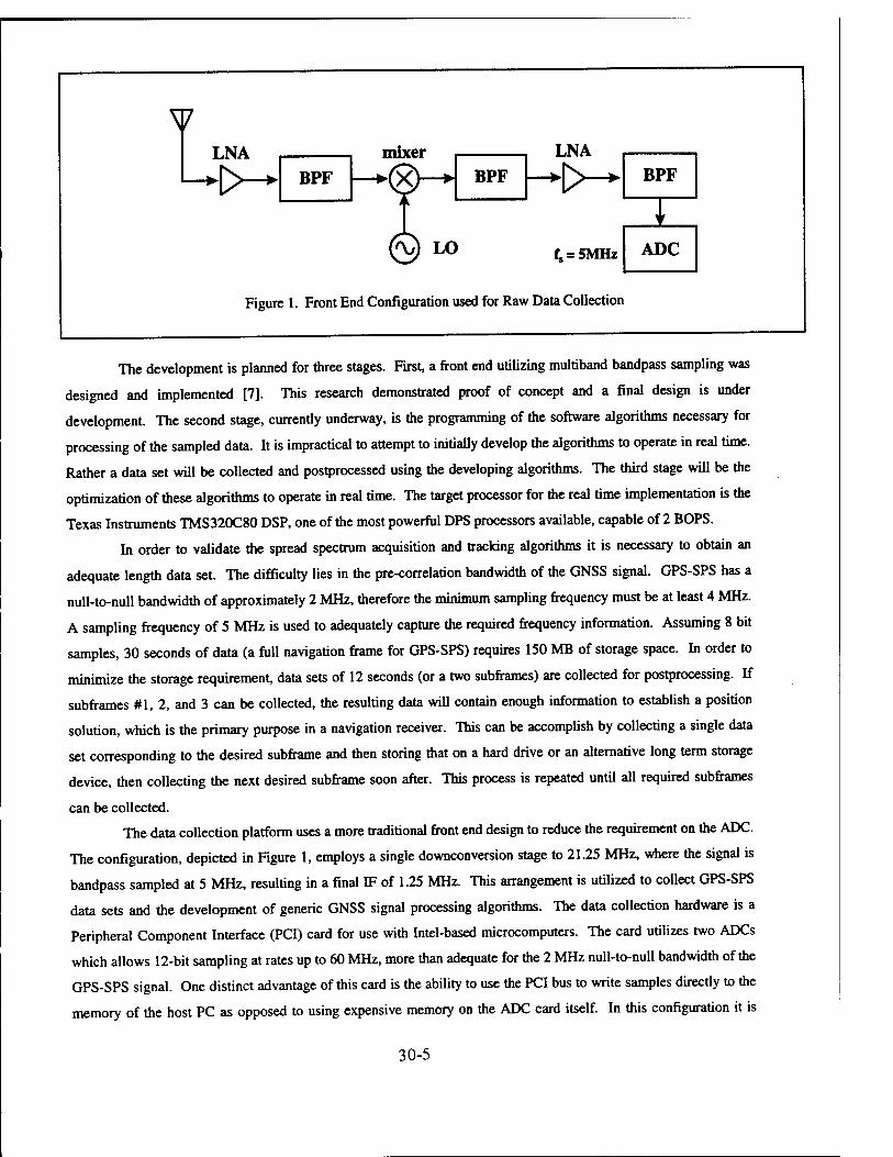
LNA BPF BPF

LNA BPF

f^SMHz ADC

Figure 1. Front End Configuration used for Raw Data Collection

The development is planned for three stages. First, a front end utilizing multiband bandpass sampling was

designed and implemented [7]. This research demonstrated proof of concept and a final design is under

development. The second stage, currently underway, is the programming of the software algorithms necessary for

processing of the sampled data. It is impractical to attempt to initially develop the algorithms to operate in real time.

Rather a data set will be collected and postprocessed using the developing algorithms. The third stage will be the

optimization of these algorithms to operate in real time. The target processor for the real time implementation is the

Texas Instruments TMS320C80 DSP, one of the most powerful DPS processors available, capable of 2 BOPS.

In order to validate the spread spectrum acquisition and tracking algorithms it is necessary to obtain an

adequate length data set The difficulty lies in the pre-correlation bandwidth of the GNSS signal. GPS-SPS has a

null-to-null bandwidth of approximately 2 MHz, therefore the minimum sampling frequency must be at least 4 MHz.

A sampling frequency of 5 MHz is used to adequately capture the required frequency information. Assuming 8 bit

samples, 30 seconds of data (a full navigation frame for GPS-SPS) requires 150 MB of storage space. In order to

minimize the storage requirement, data sets of 12 seconds (or a two subframes) are collected for postprocessing. If

subframes #1, 2, and 3 can be collected, the resulting data will contain enough information to establish a position

solution, which is the primary purpose in a navigation receiver. This can be accomplish by collecting a single data

set corresponding to the desired subframe and then storing that on a hard drive or an alternative long term storage

device, then collecting the next desired subframe soon after. This process is repeated until all required subframes

can be collected.

The data collection platform uses a more traditional front end design to reduce the requirement on the ADC.

The configuration, depicted in Figure 1, employs a single downconversion stage to 21.25 MHz, where the signal is

bandpass sampled at 5 MHz, resulting in a final IF of 1.25 MHz. This arrangement is utilized to collect GPS-SPS

data sets and the development of generic GNSS signal processing algorithms. The data collection hardware is a

Peripheral Component Interface (PCI) card for use with Intel-based microcomputers. The card utilizes two ADCs

which allows 12-bit sampling at rates up to 60 MHz, more than adequate for the 2 MHz null-to-null bandwidth of the

GPS-SPS signal. One distinct advantage of this card is the ability to use the PCI bus to write samples directly to the

memory of the host PC as opposed to using expensive memory on the ADC card itself. In this configuration it is

30-5

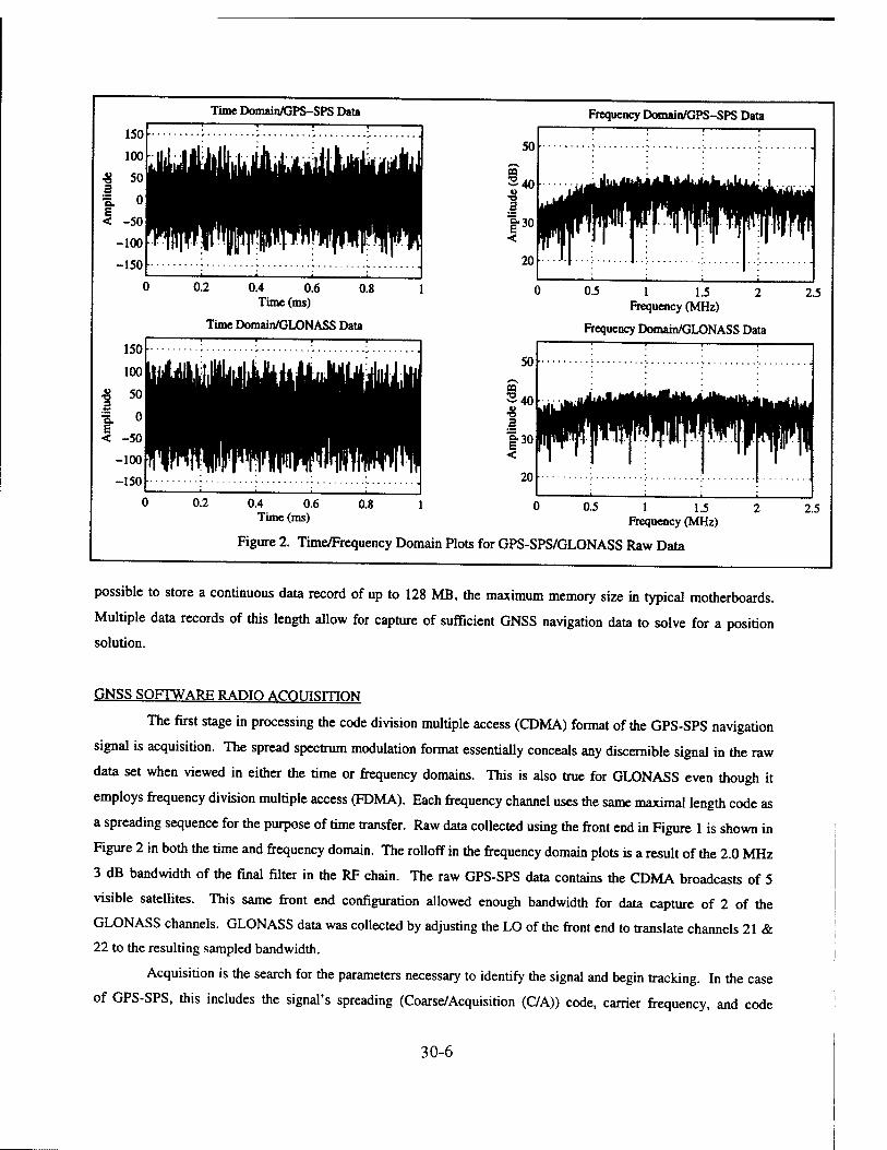
Time Domain/GPS-SPS Data Frequency Domain/GPS-SPS Data

0.2 0.4 0.6 0.8 Time(ms)

Time Domain/GLONASS Data

1 1.5 2 Frequency (MHz)

Frequency Domain/GLONASS Data

50

0.4 0.6 Time(ms)

0.5 1 1.5 Frequency (MHz)

Figure 2. Time/Frequency Domain Plots for GPS-SPS/GLONASS Raw Data

possible to store a continuous data record of up to 128 MB, the maximum memory size in typical motherboards.

Multiple data records of this length allow for capture of sufficient GNSS navigation data to solve for a position

solution.

GNSS SOFTWARE RADIO ACQUISITION

The first stage in processing the code division multiple access (CDMA) format of the GPS-SPS navigation

signal is acquisition. The spread spectrum modulation format essentially conceals any discernible signal in the raw

data set when viewed in either the time or frequency domains. This is also true for GLONASS even though it

employs frequency division multiple access (FDMA). Each frequency channel uses the same maximal length code as

a spreading sequence for the purpose of time transfer. Raw data collected using the front end in Figure 1 is shown in

Figure 2 in both the time and frequency domain. The rolloff in the frequency domain plots is a result of the 2.0 MHz

3 dB bandwidth of the final filter in the RF chain. The raw GPS-SPS data contains the CDMA broadcasts of 5

visible satellites. This same front end configuration allowed enough bandwidth for data capture of 2 of the

GLONASS channels. GLONASS data was collected by adjusting the LO of the front end to translate channels 21 &

22 to the resulting sampled bandwidth.

Acquisition is the search for the parameters necessary to identify the signal and begin tracking. In the case

of GPS-SPS, this includes the signal's spreading (Coarse/Acquisition (C/A)) code, carrier frequency, and code

2.5

2.5

30-6

phase. GLONASS reduces the search space by one parameter as it uses the same spreading sequence on each

frequency channel. The search can be visualized as a matrix (2-D for GLONASS and 3-D for GPS) where every

entry must be tested until one is found corresponding to the correct set of parameters. This search space must be

bounded with a defined step size. For GPS-SPS there are 32 possible C/A codes. The possible carrier frequency,

which differs as a result of Doppler, is bounded for most users to ±10 kHz from nominal and is searched in 500 Hz

bins. Lastly the spreading code is 1023 chips for GPS-SPS and 511 chips for GLONASS and is searched in Yi and V*

chip increments, respectively, over a single code period.

There are a number of popular spread spectrum signal acquisition algorithms [8]. However, most

commercial GPS-SPS receivers tend to use the serial search technique. The popularity of this technique is most

likely due to the fact that the digital correlator/accumulator hardware can be used not only for tracking, but also

acquisition if serial search is employed. In order to demonstrate the flexibility of the software radio approach,

multiple acquisition algorithms have been coded.

The postprocessing approach allowed for a more comprehensive evaluation of each of the acquisition

techniques. First, the code phase search was stepped in terms of samples. Second, the search conducted was

exhaustive, that is every point in the search space was evaluated. In a traditional receiver, points in the search space

are sequentially tested until a threshold is crossed indicating a potential match has been obtained and control is

transferred to attempt tracking. In serial search there are well-defined equations to calculate the threshold that also

determines the associated probabilities (missed detection and false acquisition) [9].

In the standard serial search routine, the signal is converted to baseband using a frequency entry from the

test matrix and multiplied by the spreading code with a code phase entry from the test matrix. The resulting data

points are accumulated over a single code period and that measurement is used to determine if the correct entry from

the matrix has been found. Although this is a well-established technique, the disadvantage is that all test points in the

matrix must be evaluated serially, as implied by the name. From the earlier discussion exhaustive testing of single

C/A code or GLONASS frequency will require evaluating:

notxxn 1023 I 500 J I

^ f 1 (10000\511 tnMn ...

boix=40920 (1) l 4 )

possible entries in the test matrix. This search space can often be reduced through knowledge of: the satellite

almanac data and current user position and time estimates. This will indicate which satellites/frequencies should be

tested first as an attempt to reduce acquisition times, but will not improve an exhaustive search as it does not

eliminate any of the search space rather it provides a good initial estimate. This technique has been implemented and

tested successfully in software. Results on the collected data set will be presented following the discussion of all

applied acquisition methods.

Two published improvements on the serial search technique have been implemented for use with the

software radio. The first parallelizes the frequency search space [10]. In this case the raw data is multiplied by the

spreading code with a code phase from the test matrix, then the Fourier transform of the resulting data set is taken.

30-7

All possible frequency bins are checked for the resulting carrier modulated only with the navigation data which, if

found, would indicate the proper code phase had been utilized and the bin in which it was located would provide the

necessary frequency information. There is no longer a need to search the various frequency entries of the test matrix,

however, the computational requirements of the Fourier transform is substituted for the reduced search space.

The second technique parallelizes the code phase search also through the use of the Fourier transform [11].

The raw data is converted to in-phase and quadrature baseband components using a frequency entry from the test

matrix. The Fourier transform of this data is taken and multiplied by the complex conjugate of the Fourier transform

of the spreading code. The inverse Fourier transform is then applied to revert back to the time domain. Since

multiplication in the frequency domain acts as convolution in the time domain, the resulting data represents the

circular convolution at all possible code phases for that particular frequency. Although this requires the computation

of the complex Fourier and inverse Fourier transforms, the search space is reduced to only the possible frequency

bins. Since the almanac data can often provide optimal frequency starting points, this technique can significantly

decrease acquisition times.

The digital correlator/accumulator, popular in the great majority of receivers, make these acquisition

techniques impractical since there is no access to the data prior to accumulation. This limitation illustrates the

advantage of the software radio approach. Each of the algorithms were coded and tested with the raw data sets

displayed in Figure 2. Although each of the algorithms correctly identified the acquisition parameters for all of the

satellites in both data sets, the parallelized code phase search technique greatly reduced the exhaustive search times.

The ability to postprocess the raw data provides interesting plots that give deeper insight into the acquisition

process. Figure 3 shows the Fourier transform of the GPS-SPS data depicted in Figure 2 post multiplication with the

correct C/A code with the proper code phase. This removes the spreading code and the resulting carrier modulated

only with navigation data appears at the appropriate frequency. Figure 4 depicts the

same results for data from both GLONASS frequencies. It is important to note that the acquisition signal

processing software implemented is applicable to either GNSS. Figure 5 depicts the exhaustive acquisition search

results for all entries of the test matrix for a single C/A code from a visible satellite.

The digital correlator/accumulator, popular in the great majority of receivers, make these acquisition

techniques impractical since there is no access to the data prior to accumulation. This limitation illustrates the

advantage of the software radio approach. Each of the algorithms were coded and tested with the raw data sets

displayed in Figure 2. Although each of the algorithms correctly identified the acquisition parameters for all of the

satellites in both data sets, the parallelized code phase search technique greatly reduced the exhaustive search times.

30-8

SV#6, Code Phase = 4683 samples, Frequency = 1246000 Hz 501





2.5

CQ

^40 •8 a

|-30

20



2.5 0.5 1 1.5 Frequency (MHz)


1 1.5 Frequency (MHz)

2.5

Figure 3. Post Acquisition FFT of Raw GPS-SPS Data for All Five Satellite PRN (C/A) Codes

The ability to postprocess the raw data provides interesting plots that give deeper insight into the acquisition

process. Figure 3 shows the Fourier transform of the GPS-SPS data depicted in Figure 2 post multiplication with the

correct C/A code with the proper code phase. This removes the spreading code and the resulting carrier modulated

only with navigation data appears at the appropriate frequency. Figure 4 depicts the same results for data from both

GLONASS frequencies. It is important to note that the acquisition signal processing software implemented is

applicable to either GNSS. Figure 5 depicts the exhaustive acquisition search results for all entries of the test matrix

for a single C/A code from a visible satellite.

GNSS SOFTWARE RADIO TRACKING AND DATA PROCESSING

30-9

Channcl#21, Code Phase = 430 samples, Frequency = 968250 Hz 55 r

50

45

<9 ^40 ■g

■g.351 E <

301

25

20

Channel#22, Code Phase = 1189 samples, Frequency = 1532250 Hz 55


25

50

45 CO

1 if. 35 E <

301

25

20 0.5 1 1.5

Frequency (MHz) 2.5

Figure 4. Post Acquisition FFT of Raw GLONASS Data for Frequency Channels #21 & #22

After the acquisition parameters have been identified, the second stage in processing the GNSS signal is

tracking and data demodulation. As a participate in the 1996 AFOSR Summer Research Program two distinct

approaches were developed and implemented successfully in co-operation with the AAMP group of Wright

Laboratories. The goal behind any GNSS tracking algorithm is to precisely align the incoming spreading code with a

locally generated version and also to properly decode the navigation data. The combinations of these two tasks

allow the calculation of a position solution.

The first technique utilized the traditional tracking loop architecture popular in traditional GNSS receivers.

This consists of the two coupled tracking loops, a code tracking loop and a carrier tracking loop. The code tracking

loop follows the conventional early-late noncoherent delay lock loop structure [12]. This element seeks to generate a

local synchronized version of the incoming spreading code. If the rate of the incoming code changes as a result of

the line-of-sight Doppler frequency, the code tracking loop adjusts the locally generated code rate accordingly. This

allows the CDMA format of the GNSS signal to be despread and further processed. The carrier tracking loop can be

a frequency or phase lock loop. Its purpose is to provide a frequency/phase reference to the code tracking loop and

demodulate the navigation data.

The second technique was developed by the AAMP group at Wright Laboratories to track both the code and

carrier of a CDMA signal [13]. This technique, known as Block Adjustment of the Synchronizing Signal (BASS)

despreads the GNSS signal format and demodulates the navigation data. The code tracking portion of the BASS

technique differs from the traditional implementation since the locally generated code rate remains fixed at the

nominal code rate. An early and late version of this code is generated and mixed with the incoming signal over 10

code periods. The ratio of the powers in the early and late components provides the additional accuracy needed to

adequately track the incoming code. Also this ratio can indicate that the incoming code has slid, as a result of

Doppler, more than V4 of a sample out of synchronization with the locally generated code. When this happens, rather

30-10

GPS-SPS Signal Acqusition: SV#28, Code Phase = 4380 samples, Frequency = 1.25MHz

1.2515 1.252

1.2505 1.2495

1.248 1.2485

Code Phase Shift (samples) Intermediate Frequency (MHz)

Figure 5. Results of Acquisition Algorithm Applied to GPS-SPS Signal over Entire Search Space

than attempt to modify the rate of the local code to match the incoming code as is done in the traditional tracking

loop, the data set is simply shifted by a single sample in appropriate direction. Using this technique, the locally

generated code provides a 'rough' indication of code position (approximate 60 meters using a 5 MHz sampling rate)

and the ratio can provide a more precise indication used for the position estimate. Carrier tracking is accomplished

in a manner similar to a frequency lock loop. The slope of the resulting baseband signal is used to adjust the carrier

frequency. However, navigation bit transitions can result in 180 degree phase shifts. When a navigation bit phase

change is detected, it is recorded for later processing of the navigation data, and the phase change is compensated so

that the baseband slope can still be used to accurately predict carrier frequency. This slope is based on 10 data

points, each of which is determined from 5000 data points (period of the spreading code at 5 MHz).

The data decoded using both of these techniques, in combination with the accurate local code estimates

provide the necessary puesdoranges and navigation data parameters to decode a position solution. The GPS-SPS

signal specification describes the format of the broadcast navigation data as well as the algorithms to be used in

computation of a position solution [14]. These were implemented and applied to the collected data which resulting

in a solution within 500 meters of the true position.

30-11

SUMMARY

This paper has presented the initial phase in the development of a GNSS software radio. The advantages of

such an implementation to the navigation community were discussed along with potential development obstacles. To

date, a software radio front end has been evaluated and various signal acquisition and tracking algorithms, including

those which are not applicable in tradition GNSS receiver designs, have been implemented and tested successfully.

This has established a position estimate based on software-only processing result of the GPS-SPS signal accurate to

within 500 meter.

The next step in the development is the real time implementation. Thus far all results presented have been

based on data which was collected and postprocessed. Although this is extremely effective as it allows the necessary

software debugging, the ultimate goal is a real time implementation. This is currently under investigation using the

Texas Instruments TMS320C80 Digital Signal Processor.

In addition to the real time implementation, the data collection hardware and postprocessing abilities allow

a methodical observation of the results of any processing step of each algorithm. This will allow better analysis into

the algorithms and should result in processing techniques superior to those used in traditional implementations.

ACKNOWLEDGMENTS

This work has been sponsored by the Air Force Office of Scientific Research, Air Force Materiel

Command, USAF and the AAMP group of Wright Laboratories. The material contained within this paper is based

on material submitted and approved for publication in the proceeding of the 1996 Institute of Navigation Annual Meeting

(ION GPS-96), Kansas City, Missouri, Sept 17-20, 1996 and also documentation from the 1996 Summer Research Program Final Report.

REFERENCES

[1] Vaughan, Rodney G., Scoot, Neil L. and White, D. Rod, 'The Theory of Bandpass Sampling", IEEE Transactions on Signal Processing, Vol. 39, No. 9, September 1991, pp. 1973-1984.

[2] Akos, Dennis M., and Tsui, James B. Y., "Design and Implementation of a Direct Digitization GPS Receiver Front End," IEEE Transactions on Microwave Theory and Techniques, Dec. 19%.

[3] Mitola, Joe, "The Software Radio Architecture," IEEE Communications Magazine, May 1995, Vol. 33, No. 5, pp. 26-38.

[4] Brown, Alison and Wolt, Barry, "Digital L-Band Receiver Architecture with Direct RF Sampling," IF.F.F 1994 Position Location and Navigation Symposium, Las Vegas, Nevada, April 11-15, 1994, pp. 209-215.

[5] Wepman Jeffery A., "Analog-to-Digital Converters and Their Application in Radio Receivers," TF.F.F Communications Magazine, May 1995, Vol. 33, No. 5, pp. 39-45.

[6] Baines, Rupert, "The DSP Bottleneck," IEEE Communications Magazine, May 1995, Vol. 33, No. 5, pp. 46-55.

30-12

[7] Akos, Dennis M., and Braasch, Michael S.," A Software Radio Approach to Global Navigation Satellite System Receiver Design," 1996 Institute of Navigation Annual Meeting, Cambridge, MA, June 1996

[8] Rappaport, Stephan S., and Grieco, Donald M., "Spread-Spectrum Signal Acquisition: Methods and Technology," IEEE Communications Magazine, June 1984, Vol. 22, No. 6, pp. 6-21.

[9] Holmes, Jack K., and Chen, Chang C, "Acquisition Time Performance of PN Spread-Spectrum Systems," IEEE Transactions on Communications, Aug. 1977, Vol. 25, No. 8, pp. 778-783.

[10] Cheng, Unjeng, Hurd, William J. and Statman, Joseph I., "Spread-Spectrum Code Acquisition in the Presence of Doppler Shift and Data Modulation," IEEE Transactions on Communications, Vol. 38, No. 2, February 1990, pp. 241-250.

[11] van Nee, D. J. R. and Coenen, A. J. R. M., "New Fast GPS Code-Acquisition Technique Using FFT," Electronic Letters, January 17,1991, Vol. 27, No. 2, pp. 158-160.

[12] Ziemer, Rodger E. and Peterson, Rodger L., "Digital Communications and Spread Spectrum Systems," Macmillian Publishing Co., 1985.

[13] Tsui, J. B. Y., Akos, Dennis, and Stockmaster, Michael, "BASS: Block Adjustment of Synchronizing Signal," Wright Laboratories, Patent Pending.

[14] US Department of Transportation, Global Positioning System Standard Positioning Service Signal Specification, Second Edition, June 2,1995.

30-13

EXPERIMENTAL AND NUMERICAL STUDY OF SHEAR LOCALIZATION AS AN INITIATION

MECHANISM IN ENERGETIC SOLIDS

Richard J. Caspar

Graduate Research Assistant

Professors James J. Mason and Joseph M. Powers

Faculty Advisors

Department of Aerospace and Mechanical Engineering

University of Notre Dame

365 Fitzpatrick Hall

Notre Dame, IN 46556-5637

Final Report for:

Summer Research Extension Program

Wright Laboratories

Sponsored by:

Air Force Office of Scientific Research

Boiling AFB, Washington DC

and

Wright Laboratories

July 1996

31-1

EXPERIMENTAL AND NUMERICAL STUDY OF SHEAR LOCALIZATION AS AN INITIATION MECHANISM IN ENERGETIC SOLIDS

Richard J. Caspar Graduate Research Assistant

Department of Aerospace and Mechanical Engineering University of Notre Dame

Abstract

This thesis considers the behavior of energetic and inert solids subjected to simple shear loading. Data

from a torsional split-Hopkinson bar, built for this study, was reduced to determine shear stress and shear

strain characteristics of these materials. These results were then used to calibrate a constitutive law for

stress, including the effects of strain and strain rate hardening and thermal softening. A one dimensional

finite difference study of shear localization was performed, modeling the effects of thermal conductivity,

viscoplastic heating and Arrhenius kinetics. Results revealed shear localization and reaction initiation in the

explosives simulated. Experimental failure of the inert solids, however, occurred at shear strains significantly

lower than those predicted by theory. This has been attributed to the presence of failure mechanisms other

than shear localization, which were not included in the theoretical model. It is concluded that the tested

energetic materials are not expected to shear localize or initiate under the conditions considered.

31-2

EXPERIMENTAL AND NUMERICAL STUDY OF SHEAR LOCALIZATION AS AN INITIATION

MECHANISM IN ENERGETIC SOLIDS

Richard J. Caspar

1 Introduction

This report will address, experimentally and theoretically, the behavior of various metals, solid explosive

simulants, and solid explosives subject to simple shear loading. In addition, this report will consider reaction

initiation in the energetic materials as a result of a mechanism known as shear localization or shear banding.

In this section, a description and review of the pertinent work is given. Two softening mechanisms which

lead to shear banding will be discussed: viscoplastic thermal softening and void nucleation and growth.

Pertinent work performed in the study of shear localization in explosives is also discussed.

1.1 Overview

The motivation for this report lies in the development of insensitive munitions, which are resistant to

accidental detonation. Insensitive munitions are desired for many reasons. First, insensitivity lessens safety

risks in the storage and handling of these devices. In addition, it is desired to prevent sympathetic detonation,

in which the detonation of one device causes others to detonate. Another motivation for this report comes

in the field of deep earth penetrators. These devices are designed to travel through tens of feet of rock,

concrete and earth; hence, a significant amount of deformation is inherent within the penetrator. It is thus

desired to design these munitions to be insensitive to this deformation.

In order to develop insensitive munitions, it is necessary to more fully understand the behavior of ex-

plosives. As full scale tests on explosives are often costly and time consuming, it is desirable to develop

computer models and simple bench-top experiments which predict the deformation and initiation of these

materials. There are numerous finite-element packages, such as EPIC and ABAQUS, which have been de-

signed to predict material deformation. To date, limited data exists to develop constitutive models for

explosives to use as input into these packages. One of the foci of this study is thus to determine the material

properties of various explosive simulants and explosives. These properties are determined through the use

of an experimental apparatus known as the torsional split Hopkinson bar (TSHB), which was built by this

author. Results obtained using this apparatus reveal shear stress-shear strain properties at strain rates of 102

to 104 s_1, for tested materials. In addition, photographs of the deformation are taken with an ultra-high

speed camera, capable of framing at a rate of 2 million frames per second, to observe failure mechanisms.

31-3

The TSHB has previously been used to determine material characteristics for metals, in which failure

often occurs due to a mechanism known as shear localization. Shear localization is also known to be one

of the initiation mechanisms in solid explosives [Field et al, 1982], also, it is one of the least understood

mechanisms. Much of the studies on initiation, however, have been performed under shock and impact

conditions, in which the stresses within the explosives are much greater than the yield stress, thus making

the effect of the strength of the materials insignificant [Prey (1981), Boyle et al. (1989), Chou et al. (1991)].

As a result, little is known about the sensitivity of explosives under lower stress deformations, where the

strength of the material becomes significant. In deep earth penetrators, it is surmised that explosives undergo

significant deformation at high strain rates and relatively low stresses (on the order of the yield stress of the

material) and low pressures, in which the material strength is thought to affect the deformation of explosives.

One of the detonation mechanism expected to dominate under such conditions is shear localization. An

additional goal of the experimental tests is thus an attempt at observing shear localization in explosives

deforming in simple shear.

Figure 1 describes the mechanism of shear localization. In Figure la, a portion of an undeformed material

is sketched with thin lines inscribed on its surface. When this material is sheared, the scribe lines begin

to slant at a uniform angle, as seen in Figure lb. This form of deformation is known as homogeneous

deformation. Increased straining into the plastic range results in hardening of the material. In addition,

Z .. / (a) (c)

A

V

~7

V

Figure 1: Schematic of the shear localization process, (a) Undeformed grid lines, (b) Homogeneous deformation, (c) Shear localization

if there is a geometric discontinuity, void, scratch or some other material weakness, straining near that

discontinuity will occur at a higher strain rate, which also hardens the material. This increased local

deformation, however, also causes plastic heating of the material. If the straining occurs at high strain rates

(typically greater than 102 s"1), there is not enough time for the generated heat to be conducted away.

The local increase in heat results in thermal softening of the material. If this process dominates over the

hardening due to strain and strain rate effects, the material strength decreases. As a result of this local

softening of the material, deformation is localized into a thin planar region, as depicted by the scribe line

deformation of Figure lc. This final process is known as shear localization or shear banding.

31-4

In addition to the experimental tests that were performed in this report, a numerical model was developed

to predict the deformation of a material in simple shear. The governing equations of conservation of momen-

tum and energy are used in this model. In the discussion of shear localization in the following section, two

softening mechanisms will been discussed which are known to lead to shear banding: thermal softening and

microvoid nucleation and growth. In this report, a constitutive law for the shear stress is utilized, in which

the effects of strain and strain rate hardening, and thermal softening are included; microvoid nucleation is

neglected. Since it has been shown that the choice of a particular constitutive law does not significantly

effect the results [Wright (1987), and Batra and Kim (1991)], a simplified power law will be implemented.

Also included in the model is the effect of thermal conductivity due to its importance in achieving accurate

temperature predictions [Batra and Kim, 1991]. Finally, exothermic reaction is modeled by an Arrhenius

kinetic law. Despite results attesting to the fact that localization is a multidimensional process [Marchand

and Duffy (1988) and Giovanola (1988 a,b)], a one dimensional model will be developed, since this model

is sufficient in yielding important information about the shear band temperature profile in solid explosives.

The pertinence of these effects is discussed in the following sections.

The novelty of this report first lies in the testing of explosive simulants with the torsional split-Hopkinson

bar and the determination of their shear stress and shear strain characteristics. Also, the implementation of

Arrhenius kinetics in the study of simple shear deformation of explosives is new. In addition, most researchers

studying simple shear deformation have used a finite-element formulation for solving the governing equations.

In this report, the equations are solved by a finite-difference method.

1.2 General Reviews

This section presents a brief review of works on the high strain rate behavior of materials as well as

the initiation mechanisms in solid explosives. A compilation of works on shock wave and high strain rate

phenomena in materials is presented by Meyers et al. (1992). Meyers (1994) also discusses these dynamic

events in materials. These books discuss various failure mechanisms occurring at high strain rate in materials,

including shear localization. In addition, works studying high strain rate effects in explosives are discussed.

Bowden and Yoffe (1985) performed an extensive review of experimental works on explosive mechanics in

order to categorize the various mechanisms of initiation in solid explosives. They concluded that initiation

could occur by the adiabatic compression of small entrapped gas bubbles; the formation of hot spots on

confining surfaces, extraneous grit particles and intercrystalline friction of explosive particles; and the viscous

heating of rapidly flowing explosive as it escapes impacting surfaces. Many authors, however, have discounted

gas compression as the controlling mechanism for hot spot formation [Frey, 1985 and Kang et al, 1992].

Field et al. (1982) performed impact tests on thin layers of several explosives, reporting photographic

evidence for the formation of initiation due to many of the previously stated mechanisms, as well as some

31-5

additional mechanisms. In these tests, the explosives were subject to stresses significantly larger than the

yield stresses of the materials. They concluded that the following mechanisms contributed to ignition of

explosives: adiabatic shear banding, adiabatic heating of gas spaces, viscous flow, factional rubbing, hot

spots at crack tips and triboluminescence. The authors found that viscous heating could play an important

role in liquids, but could only lead to significant heating in solids when considered in conjunction with the

other mechanisms listed. They also determined that the propagation of cracks alone would not lead to

ignition. Instead, they proposed that fracture of an explosive crystal would produce a gaseous void which

could in turn lead to adiabatic heating and hot spot generation. In conclusion, the authors note that no one

mechanism is the dominant means of ignition, and that small changes in the experimental conditions can

lead to the formation of hot spots due to different mechanisms. For detailed reference on detonation theory

with discussion of experiments, see Ficket and Davis (1979).

1.3 Adiabatic Shear Banding in Metals

Shear banding, as an initiation mechanism in explosives, is only simply understood. It is known that

metals subject to high strain rate loading in association with high speed machining, cutting and forming,

as well as in impact and penetration, often experience highly localized plastic deformation, known as shear

bands. The thickness of these shear bands is typically on the order of micrometers, and they have been

known to develop in times on the order of microseconds [Marchand and Duffy (1988), Giovanola (1988 a,b)].

Due to the significant amount of localized viscoplastic work on such a short time scale, highly localized

temperatures of about 1000°C are observed. Although formation of these shear bands is typically followed

by fracture, failure in any accepted sense of the word occurs with formation of the shear band since the

material has lost its load carrying capacity [Marchand and Duffy, 1988]. Hence, a significant amount of

research has been performed on shear banding as a failure mechanism in structural materials.

1.3.1 Experimental Observations

It is generally understood that adiabatic shear localization begins because thermal softening dominates

over strain and strain rate hardening in the deformation process. When a material is plastically strained,

dislocations begin to slip within the material, accumulating at grain boundaries. As these dislocations

coalesce, there becomes less room for dislocations to slip, thus resulting in strain hardening of the material

[Lubliner, 1990]. If the rate at which this straining increases, viscous stress will further resist deformation,

which contributes to a process known as strain rate hardening. An important result of dislocation slip is the

generation of heat. Rogers (1979) has concluded that approximately 90% of this plastic work is converted into

heat, while the remaining is stored in the generation and arrangement of dislocations. This increase in heat

tends to free the motion of dislocations, resulting in thermal softening of the material. The generation of heat

31-6

then results in further plastic strain, which causes further increases in temperature. At high enough strain

rates, there is not enough time for the heat generated to be conducted away; the deformation thus becomes

adiabatic. If a material is experiencing high strain rate adiabatic deformation, and there is a material or

geometric weakness, such as a void or scratch, straining will increase locally, causing an instability. If the

properties of a given material are such that the mechanism of thermal softening dominates over strain and

strain rate hardening, deformation will localize into a planar region, known as a shear band.

Zener and Hollomon (1944) were among the first to describe the process of shear localization in detail.

They state that a necessary condition for shear localization is when a maximum in the homogeneous, adiabatic

stress strain curve exists, beyond which deformation cannot be homogeneous and strength decreases with

increasing strain. When the strain at this maximum is surpassed, an instability will then arise, in which

a region deforms at a greater rate than the surrounding material, causing it to weaken and further strain,

while the surrounding material is no longer strained.

In order to study the deformation and temperature distribution across a shear band, Marchand and

Duffy (1988) performed tests in simple shear on thin tubular specimens, by means of a torsional split-

Hopkinson Bar. Previous applications of this device only resulted in average values of shear stress and shear

strain. Marchand and Duffy were of the first researchers to perform detailed measurements of the shear band

formation. They used high speed photographs to study the deformation of fine lines etched on the specimen's

surface in order to determine the local shear strain. From an analysis of their photographs, they concluded

that shear banding occurs in three distinct stages. In the first stage, the material is undergoing homogeneous

deformation, in which the grid lines are inclined at a constant angle. In the second stage, the material

undergoes inhomogeneous deformation, in which the etched lines are curved. As deformation continues

in this stage, there is a continuous increase in the localized strain, while the width of the inhomogeneity

decreases. It is important to note that, in this stage, the deformation remains uniform in the circumferential

direction. The decrease in the stress, however, is never large over this region. The third stage begins at

the value of nominal strain where the stress first starts to drop severely. The deformation becomes severely

localized in a thin plane. It is at this time that the one dimensional assumption of localization breaks down.

Marchand and Duffy observed that the axial position of the maximum local strain is not the same for all

points in the circumferential direction indicating that the shear band originates in several locations or that

it originates in one location and propagates around the circumference of the specimen.

The maximum shear strain reached in the shear band, with an applied shear strain rate of 1600 s_1, is

1900%, with a shear band width found to be 20 fj,m. These large strains demonstrate the weakening effect

of shear banding. For dynamic loadings, deformation is often localized to a small region, which is forced

to absorb the majority of the deformation. As a result, the strength of the whole specimen is not utilized,

causing failure at much lower nominal strains than in quasi-static experiments.

31-7

Marchand and Duffy also performed temperature measurements across the shear band with infra-red

radiation detectors. Results for an applied strain rate of 1400 s"1 revealed a temperature spike at the

location of maximum shear, with a maximum recorded temperature of 590°C. This value represents an

average temperature over a region which is greater than the width of the shear band; from a calculation

taking into account the width of the shear band, temperatures as high as 1000°C are surmised.

In a similar study, Giovanola (1988,a) performed tests on VAR 4340 steel. He used high speed pho-

tography to observe the deformation and infrared detection to determine temperature measurements. In

accord with Marchand and Duffy, Giovanola determined a maximum shear strain at failure of 2000%. It is

also pertinent to note that Giovanola observed inhomogeneous deformation prior to shear banding, as was

observed by Marchand and Duffy (1988). In a companion paper, Giovanola (1988,b) performs fractographic

and metallographic observations of the failure surface to determine that shear banding is a result of thermo-

plastic instability and microvoid nucleation and growth. In addition, Giovanola notes that failure occurred

on a number of parallel planes connected by well defined steps. This observation supports the claim that

shear bands nucleate at a number of locations in the softened region and propagate around the specimen.

1.3.2 Theoretical Predictions

As a result of the significant amount of experimental data related to dynamic simple shear, determined

from the torsional Hopkinson bar, and due to the mathematical ease in its modeling, much of the analytical

work in the study of shear localization has been performed in connection with thermoviscoplastic simple

shear deformation. In order to theoretically model the problem, governing equations are developed to model

the relevant physical conservation principles. These principles do not form a complete set and are hence

supplemented by constitutive equations, through which specific materials are modeled. A review of past

works in the field of adiabatic shear localization is presented by Rogers (1979).

In the development of a constitutive model for stress, there are two schools of thought as to the method

by which the strength is softened. The first theory is that the stress is reduced as a result of heat being

generated from viscoplastic deformation. This process results in thermal softening, which dominates over

strain and strain rate hardening. Alternatively, many researchers have studied the softening of the stress

as a result of microvoid nucleation and growth. This theory is typically formulated to state that at some

critical strain, voids begin to nucleate in the material, thus reducing the cross sectional area, and hence

the strength of the material. Microvoid nucleation and growth is generally presented in conjunction with

thermal softening, microvoid nucleation being the trigger for thermal softening. Meyer (1992) gives a review

of some of the constitutive relations which have been used for high strain rate applications. In the present

report, a numerical model will be developed which takes into account softening due to viscoplastic work

alone; microvoid formation will be neglected.

31-8

In existing studies of thermal softening induced shear localization, there is a significant amount of dis-

crepancy in the choice of the constitutive equation. In order to address this issue, Wright (1987) compared

the results of four commonly used viscoplastic constitutive relations. The constitutive laws used were 1)

an Arrhenius stress law, 2) the Bodner-Partom-Merzer law, 3) a simple power law, and 4) the Litonski

law, which were all calibrated over the same data. He found that the results were both qualitatively and

quantitatively similar, with the results within 5% of each other for shear strain rates up to 104 s_1, a value

far in excess of the calibration conditions. For even larger values of shear strain rate and high temperatures,

the Bodner-Partom-Merzer law begins to diverge from the other solutions. Wright states that since there is

a significant difference between the strain rate and temperature at the center of the shear band from those

of the calibration conditions, the actual structure of a real shear band would be expected to be somewhat

different from that predicted by any given constitutive law. He thus thought it surprising that the trends

predicted by the constitutive laws were as similar as found.

Another source of discrepancy in previous researchers is in the role of thermal conductivity. To clarify

this issue, Batra and Kim (1991) compared the results of three different constitutive relations, while varying

the thermal conductivity. In this study, the researchers considered a thermoviscoplastic block undergoing

one dimensional simple shearing deformations, with strain and strain rate hardening and thermal softening.

The thickness of the block was taken to vary smoothly with a 5% decrease in thickness at the center. The

constitutive laws considered were the Litonski law, the Bodner-Partom law, and the Johnson-Cook law. Batra

and Kim found that the results from the three constitutive laws are extremely similar, both qualitatively

and quantitatively, verifying the results achieved by Wright (1987). As a result of these studies, we have

determined that the use of a simple power law will be adequate in the study of high speed deformation.

Batra and Kim also reported that large increases in the value of the thermal conductivity delay the

initiation of stress collapse and slow down the development of the shear band. However, for realistic values

of thermal conductivity there is little effect on the value of nominal strain at which stress collapses, and

hence localization occurs. In contrast, the authors found that the rate of evolution of the temperature at

the center of the specimen decreases with increasing thermal conductivity, resulting in significant changes in

temperature for realistic values of thermal conductivity. It is therefore concluded that thermal conductivity

can be neglected when one is only considered with the timing of stress collapse, but it proves to be crucial

when considering shear band temperatures. Since this current report is studying thermal reaction initiation

in explosives, conductivity will play an important role.

Motivated by this study, Batra et al. (1995) performed a thermoviscoplastic analysis neglecting thermal

conductivity in order to rank twelve materials according to the critical strain necessary to reach localization

in tubular specimens loaded in simple shear. A finite-element method with the Johnson-Cook constitutive

law was used in these calculations. The thickness of the tube was taken to vary smoothly with a 10%

31-9

decrease at the center. Batra et al. assumed that the shear band initiates when there is a catastrophic drop

in torque, and ranked the materials according to the corresponding nominal shear strain. They found shear

bands to initiate in the following order: tungsten, S-7 tool steel, depleted uranium, 2024-T351 aluminum,

7039 aluminum, 4340 steel, armco iron, carpenter electric iron, 1006 steel, cartridge brass, nickel 200 and

OFHC copper, when tested with a shear strain rate of 5000 a-1. It is relevant to note that the critical strain

was dependent on the size of the initial defect as well as the finite element mesh used. The relative ranking

of the materials, however, was independent of these parameters.

In order to study the development of a shear band, Batra and Kim (1992) solved a nonlinear system

of equations for a thermoviscoplastic block with the Johnson-Cook constitutive law, including strain and

strain rate hardening, thermal softening and thermal conductivity. They used a continuous variation in the

thickness to instigate localization. The authors found the same three stage localization process as Marchand

and Duffy (1988) with transition to stage two occurring at the time the stress reached its maximum value,

and stage three occurring much later, when the stress has dropped to about 90-95% of its maximum value.

Batra and Kim also observed the effects of varying the thickness of the block. They found that the defect

size has a stronger influence on ductile materials than on less ductile materials, but in all cases, it has a

significant effect on the critical strain to reach localization.

In a similar study, Clifton et al. (1984) used a simple power law including strain and strain rate hardening

and thermal softening but neglected thermal conductivity to perform a study on the critical conditions for

shear band formation. They concluded that the primary factor affecting initiation of the shear band is the

strain hardening, whereas the strain rate hardening is the primary factor affecting the rate of growth of

the shear band. Supplementing these observations, Wright and Batra (1985) used the Litonski flow law to

explore the critical strain at collapse. In accord with Clifton et al. (1984), Wright and Batra determined

that strain rate plays little role on the critical strain at localization. However, they found that the size of an

initial temperature perturbation plays a significant role, with the larger perturbation causing localization to

occur at a smaller critical strain.

1.4 Detonation Mechanisms in Explosives

As was stated previously, shear localization is understood to be one of the mechanism which can lead

to ignition in solid explosives subject to high strain rates and relatively low pressures. Traditional studies

of shear localization in explosives have been performed in conjunction with high pressures, representing the

conditions undergone in shock and impact loading. Frey (1981) developed a model to describe heating in

high explosives due to shear banding. He used a linear viscoplastic constitutive law, neglecting the effects of

strain rate hardening. The strength was decreased over a 30°C range after the melting point, the melting

point increased linearly with pressure, and the viscosity was dependent on both temperature and pressure.

31-10

In addition, Prey used Arrhenius kinetics to model the thermal explosion. This material was then deformed

in shear, stimulating localization by setting the strength to zero over a small region within the deformation.

Without reaction, Prey's model achieved a maximum temperature which turned out to be independent of

strength of the material and thickness of the initial weakness. These parameters did, however, affect the

rate of growth of the shear band. The author found that the factors which did affect the temperature were

the pressure, strain rate, and viscosity. Prey found that high pressures result in higher temperatures. In

addition, under low pressures, it would be very difficult to reach the temperatures in a shear band required

to instigate thermal explosion.

In experiments performed on explosives subject to lower pressures and shear deformation, such as in

drop weight tests, Boyle, Prey and Blake (1989) confirm the numerical observations of Prey (1981). They

find that pressure and velocity do indeed have a strong effect on the initiation of solid explosives. Due to a

comparison of explosive materials, they also verify that higher viscosities increase the sensitivity to explosion.

In a more recent study, Chou et al. (1991) studies two theories for the impact initiation of explosives: shock

initiation, a pressure dependent theory, and shear initiation, a temperature dependent theory. Chou et al.

state that there are three means by which heat can be generated in explosives: shock compression energy,

plastic work and viscous work. They state, in accord with previous researchers, that plastic work, in the

absence of high pressures, would not generate enough heat to produce thermal explosion, since failure occurs

before a significant amount of straining occurs. Chou et al. further state that once a material has reached its

melting temperature, the effect of plastic work becomes negligible; heating then results from viscous work,

which is capable of increasing the temperature well above the melting point. It is known, though, that brittle

materials become more ductile under pressure; in fact, Chou et al. state that pressure can raise the stress

and strain to as much as ten times as high as a material's uniaxial value. This effect thus increases the

importance of considering heating by plastic work, when considering a material under hydrostatic pressure.

In order to compare the effect of shock and shear initiation in impacted explosives, Chou et al. developed

a numerical model similar to that of Prey (1981) and simulated the impact of bare and covered explosives

subject to impact. They concluded that for bare explosives impacted by a projectile, shock initiation is

dominant and the shear effect is negligible. For covered explosives impacted by a projectile, viscoplastic

heating is of importance and shear initiation at the edge of the plug is probable.

2 Experimental Method

This chapter discusses an experimental apparatus, known as the torsional split Hopkinson bar (TSHB),

which was used to test metals, solid explosive simulants and solid explosives in simple shear. An analysis

of the data determined from this apparatus produces average shear stress and shear strain characteristics

of the tested material, for a range of shear strain rates (102 - 104 s_1). High speed photographs are taken

31-11

of the deformation and failure of the specimens, in order to determine their failure mechanism. The data

will be used to determine constitutive parameters for input into the numerical model which is presented in

the next section. This data can also be used to calibrate the various constitutive laws used in finite element

packages such as EPIC and ABAQUS, which can be used in the modeling of explosive mechanics.

The torsional Hopkinson bar is a modification of an apparatus originally discussed by Kolsky (1949,

1953). In his device, thin cylindrical wafer-like specimens were placed between two long elastic bars, aligned

along a common axis. The specimen was loaded by propagating a compressive pulse, generated by impacting

the bar with a cylindrical projectile of the same material and equal diameter, down one of the bars toward

the specimen. A similar device was used by Harding et al. (1960) for material testing in tension. The

Hopkinson bar was later adapted for tests in torsion, which is discussed by Hartley et al. (1985).

There are several reasons why the TSHB is appropriate for the current experiments performed on solid

explosives. First of all, in torsional loading, the maximum stress in the specimen occurs on the exterior surface

of the material. The largest deformation will thus occur on the exterior surface, making the probability of

hot spot formation greatest, where it can easily be observed. Also, the TSHB can be designed to produce

a torsional pulse of almost any desired length, and hence, large amounts of deformation in the specimen

are possible. In addition, shear is the main form of deformation present in high rate deformation events

such as penetration; hence, it is desired to determine stress-strain characteristics in shear, as opposed to

compression or tension. Compression and tension test results can be converted into shear data by using

a criterion such as the von Mises equivalence relation, but this is not valid for strains above 20% [Hartley

and Duffy, 1985]. Further disadvantages of compressive testing result from the Poisson's ratio effect, which

causes radial expansion of materials loaded in compression. Additional radial stresses in compressive tests

occur due to frictional effects between the specimen and bar. In torsional tests, there is no Poisson's ratio

effect, and hence no radial contraction or expansion.

There are, however, some drawbacks to the TSHB. First, tests may only be run on a limited range of

strain rates (102 - 104 s'1). The lower limit is due to an increase in the noise to signal ratio, while the

upper limit is due to the elastic limit of the TSHB. A further drawback is if fracture occurs in the explosive

specimen too soon, localization, and hence initiation, is less likely. In addition, the data analysis for this

apparatus assumes homogeneous deformation. Hartley et al. (1985) have shown that it takes a few reflections

of the loading pulse from the ends of the specimen before a state of homogeneous deformation is reached,

thus rendering the early time results of the TSHB inaccurate.

2.1 Description of Apparatus

The TSHB consists of two elastic cylindrical bars: an incident and transmission bar; a torsional pulley;

a clamp; and a specimen. A schematic of this apparatus is included in Figure 2. The two bars are aligned

31-12

along a common axis, with a thin walled cylindrical specimen of known geometry joining them. The end of

each bar in contact with the specimen is milled to produce a hexagonal socket, into which the specimen or

an adaptor is inserted. The adaptor is used for cases in which it is desirable to glue the specimen in place,

rather than grip it with the hexagonal socket. The torsional pulley is attached to the end of the incident bar

far from the specimen, and the clamp is placed at a variable distance from the pulley, typically several feet.

Torsional Pulley Incident Bar

Transmission Bar

Clamp Strain Gages

Figure 2: Schematic of the TSHB (not to scale).

The clamp is used to prevent rotation of the incident bar while the torsional pulley is rotated, thus storing

a torsional pulse in the bar between the pulley and clamp. The sudden release of the clamp propagates an

incident shear strain pulse down the incident bar. The incident pulse reaches the specimen, transmitting

some strain through the specimen into the transmission bar and reflecting some back into the incident bar.

The two elastic bars are constructed of 1 in diameter aluminum 7075-T6, 111 in in length. At the ends

joining the specimen, a hexagonal socket, of width 0.5625 in and depth 0.25 in, is milled into the bars. Into

these sockets, one inserts either a hexagonal specimen or an adaptor machined from 7075-T6 aluminum, to

which cylindrical specimens are glued. The hexagonal specimen (see Figure 3) or adaptor is fixed to the bar

with 12 set screws, two on each face of the hexagon. The dimensions of the specimens that were used in

this study are given in Figure 3. In Figure 3, the central part of the specimen is commonly referred to as

(a) 0.100

i r (b)

0.250 0.250

Z~K

0.5625 \ \\

u \ / /

n -D 0.370

h«H / /' ^ 0.100

(CO -D 1.000

D 0.700

- D 0.500

Figure 3: Scaled diagram of the specimens used in the TSHB tests: (a) hexagonal specimen, (b) cylindrical specimen (all dimensions in inches).

31-13

the gage length, while the ends axe termed flanges. The hexagonal specimen is used to test metals and the

cylindrical specimen, due to its ease in machining, is used to test the explosive simulants and explosives. The

ratio of the wall thickness of the gage length to the mean diameter of the gage length for the hexagonal and

cylindrical specimens are 0.04 and 0.17, respectively. The elastic bars are supported along their length by

delrin bearings, which are mounted on adjustable bearing supports. These bearing supports are then fixed

to a steel I-beam which supports the whole TSHB apparatus.

A schematic of the torque generating mechanism is included in Figure 4. The torsional pulley is clamped

to the incident bar by means of a factional fit. A hydraulic hand pump is used to pressurize the rams, which

lengthen, transferring force into the cable, which in turn rotates the torsional pulley. When the clamp is

engaged, this action stores torsional elastic energy in the incident bar.

11.0

Cable

10.0

Hydraulic Rams

Figure 4: Scaled schematic of the torque generating mechanism (all dimensions in inches).

Integral in the operation of the TSHB is the clamp which stores the torsional pulse. The key to constant

strain rate tests is rapid release of the clamp, which propagates an incident torsional pulse towards the

31-14

specimen. In order to more fully understand the operation and design of the TSHB, the author spent the

summer of 1995 at Eglin AFB in the Advanced Warheads Evaluation Facility (AWEF) making modifications

to the design of their TSHB. With the knowledge gained through these efforts, this author modified previous

clamp designs resulting in the design shown in Figure 5. The clamp is engaged by pumping a second hydraulic

hand pump, which pressurizes a hydraulic C-clamp, which in turn clamps the base of the two clamp faces.

This action transmits pressure through the clamp faces onto the Hopkinson bar. In order to release the

clamp, the hydraulic pressure is increased until the break element, as seen in Figure 5, fractures, causing the

release of the clamp faces. Ideally, the incident pulse would be a square pulse of torsion, with instantaneous

rise and fall time and constant magnitude, thus producing deformation in the specimen at a constant strain

rate. For optimum functioning of the clamp, it is desired to store large amounts of elastic energy in the

clamp in order to achieve quick fracture of the break element and consequently, sudden release of the clamp.

This sudden release will produce a pulse with a short rise time and relatively constant magnitude.

1.0 0.8 1.0 1.0 Break Element

Incident Bar

Clamp Face

1.5

6.0

1.0

Incident Bar \

Clamp Face Guide

5.0

Clamp Table

8.0

5.0

Front View Side View

Figure 5: Schematic of the clamp for the TSHB (all dimensions in inches).

In designing a break element, it is desired to use a material with minimum ductility, but not so brittle

that it will fail before the clamp is tight enough to store the desired torque. Hartley et al. (1985) state that

31-15

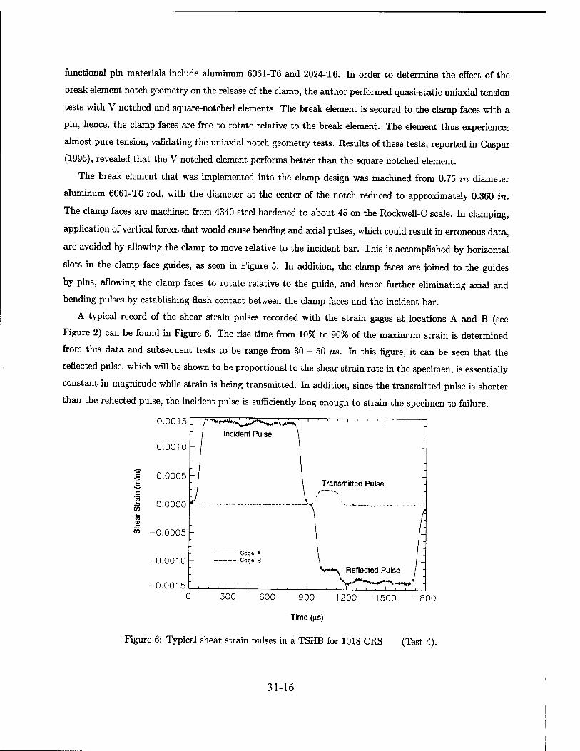
functional pin materials include aluminum 6061-T6 and 2024-T6. In order to determine the effect of the

break element notch geometry on the release of the clamp, the author performed quasi-static uniaxial tension

tests with V-notched and square-notched elements. The break element is secured to the clamp faces with a

pin, hence, the clamp faces are free to rotate relative to the break element. The element thus experiences

almost pure tension, validating the uniaxial notch geometry tests. Results of these tests, reported in Caspar

(1996), revealed that the V-notched element performs better than the square notched element.

The break element that was implemented into the clamp design was machined from 0.75 in diameter

aluminum 6061-T6 rod, with the diameter at the center of the notch reduced to approximately 0.360 in.

The clamp faces are machined from 4340 steel hardened to about 45 on the Rockwell-C scale. In clamping,

application of vertical forces that would cause bending and axial pulses, which could result in erroneous data,

are avoided by allowing the clamp to move relative to the incident bar. This is accomplished by horizontal

slots in the clamp face guides, as seen in Figure 5. In addition, the clamp faces are joined to the guides

by pins, allowing the clamp faces to rotate relative to the guide, and hence further eliminating axial and

bending pulses by establishing flush contact between the clamp faces and the incident bar.

A typical record of the shear strain pulses recorded with the strain gages at locations A and B (see

Figure 2) can be found in Figure 6. The rise time from 10% to 90% of the maximum strain is determined

from this data and subsequent tests to be range from 30 - 50 ps. In this figure, it can be seen that the

reflected pulse, which will be shown to be proportional to the shear strain rate in the specimen, is essentially

constant in magnitude while strain is being transmitted. In addition, since the transmitted pulse is shorter

than the reflected pulse, the incident pulse is sufficiently long enough to strain the specimen to failure.

0.0015 r

0.0010

300 600 900 1200 1500 1800

Time (us)

Figure 6: Typical shear strain pulses in a TSHB for 1018 CRS (Test 4).

31-16

2.2 Analysis

The values of the shear stress, shear strain and shear strain rate experienced in the specimen, when

homogeneous deformation in the specimen is assumed, are determined from an analysis of the strain in the

incident and transmission bars. In this section, the subscript, s, is used to denote the properties of the

specimen.

Hartley et al. (1985) have shown that the shear strain rate in the specimen is proportional to the reflected

strain in the incident bar, -yR. Integration of the reflected strain over time, t, then provides the shear strain

in the specimen, 7S:

* («) =-t^/71. (*-)<*, (1)

where c is the elastic torsional wave speed in the incident and transmission bars, D8 is the mean diameter

of the specimen, L„ is the length of the specimen, and D is the diameter of the incident and transmission

bars, and i is a dummy variable of integration.

Hartley et al. have also shown that the transmitted pulse, jT, provides a measure of the shear stress in

the specimen, TS: GD* (2)

where G is the shear modulus, and ts is the thickness of the specimen wall.

2.3 Data Acquisition and Reduction

The shear strain pulses in the incident and transmission bars are recorded by means of electric resistance

strain gage Wheatstone bridges, which are extremely sensitive to small changes in strain. The strain gages

are attached at the midpoints of each bar, location A and B in Figure 2. With the gages mounted at the

midpoint of the bar, it is possible to record a pulse without its reflection overlapping in time, as long as the

pulse is shorter than the length of the bar. Since the clamp is mounted between the torsional pulley and gage

station A, the incident pulse, being twice as long as the stored torque, will always be less than the length of

the bar. In addition, since gages A and B are each the same distance from the specimen, it is ensured that

the reflected and transmitted pulse will commence at approximately the same instant in time. There is also

a strain gage bridge mounted 12 in from the torsional pulley, gage station C in Figure 2. The purpose for

this gage is to record the stored torque, which is used to obtain the expected strain rate incident upon the

specimen. Stations A and B consist of four strain gages; one set of 2 torque gages is mounted diametrically

opposite another set on the surface of the bar. Each gage is mounted at a 45° angle to the axis of the bar.

Strain gages mounted this way will record only shear strain, cancelling any axial and bending strain which

may be present. Gage station C consists of one set of strain gages, also mounted at a 45° angle to the axis

of the bar.

31-17

McConnell and Filey (1993) describe the functioning of a Wheatstone bridge and determine the following

equation which calculates the shear strain, 70, from the change in the bridge output voltage, AE0:

2AE0 (1 + K)2

70 " FVGaNg K ' (3)

where F is the gage factor, V is the excitation voltage, Ga is the amplifier gain, Ng is the number of active

gages in the Wheatstone bridge, and K is the ratio of resistances in the bridge.

Each bridge is wired to a Measurements Group model 2311 signal conditioning amplifier, which sets the

excitation voltage and gain. The amplifier output from gage station A is split, with one lead, as well as

the amplifier output from gage station B, sent to a Tektronix model TDS 420 digitizing oscilloscope, which

is downloaded to a personal computer. This data is reduced by Equations (3), (1), and (2), to determine

nominal shear stress and shear strain characteristics of the specimen. The other lead of the amplifier output

from gage station A is sent to a Hewlett Packard model 214A pulse generator. The incident pulse triggers

the pulse generator, which sends a second pulse, delayed by some specified time, to trigger a Cordin model

607 light source, which illuminates the deformation of the specimen. Photographs of this process, which are

used to determine the failure mechanism of the specimen, are recorded with a Cordin model 330A ultra-high

speed camera.

Results from the TSHB were verified by Caspar (1996).

3 Model Equations

This chapter introduces the model equations employed in this research. In the first section, the physical

problem is described. The assumptions and governing equations are then presented. These equations are

scaled and presented in nondimensional form. Finally, the numerical method used to solve the equations is

discussed.

3.1 Governing Equations

The current theoretical study of localization is being used to compare with tests performed on the

deformation of specimens in the TSHB. Tests have been performed on metals, solid explosive simulants and

solid explosives. In the TSHB, a thin walled circular cylinder is dynamically loaded in torsion; the model is

thus designed to simulate these conditions. A schematic of the specimen described by the model is included

in Figure 7. In this specimen, which has length Ls, z is the axial distance variable, 6 is the circumferential

distance variable, and r is the radial distance variable. This specimen is loaded by linearly increasing the

circumferential velocity, ve, over time, t, at z = Ls to some constant value, vu while holding the velocity

fixed at z = 0. The following assumptions are made in developing the model:

31-18

vv1

z=0 V1 z=Ls

*■ z

Figure 7: Specimen used for numerical simulation.

• The specimen is initially unreacted, unstressed, and at ambient temperature.

• As we are dealing with a pure torsional problem, there is no component of velocity or displacement in

the radial or axial direction: vT = vz = ur = uz = 0.

• Due to axisymmetry and the thin walled geometry, there is no variation in the circumferential or radial

direction: -^ = ^ = 0.

• In order to induce localization, we allow the specimen wall thickness to vary with axial position z. We

make the ad hoc assumption that this perturbation is sufficiently small so as not to introduce gradients

in the radial or circumferential directions. It is noted that alternative methods of perturbation which do

not require such ad hoc assumptions, such as perturbation in initial velocity, temperature, displacement

or strain, could also induce localization.

• In pure torsion, the stress tensor reduces to one component, az$, the stress on the axial face in the

circumferential direction, which will be referred to as the shear stress, r.

• The shear strain is restricted to positive values.

• Plastic deformation is completely converted to heat.

• Heat is only transferred in the axial direction.

• The material undergoes a one-step chemical reaction, with A denoting the unreacted material, and B

denoting the reacted material.

• The density, p, and the thermal conductivity, A;, are equal in the unreacted and reacted material and,

along with the specific heats, CA and CB, they are constant.

31-19

Under these assumptions, the governing equations are stated below:

"""äT = Tz{wT)' W de dve d . . .

""ä = wrä7 " &(w<?z) ' (5) due

-aJ = 7' (6) owe "9T = **' (7) ax f E \ Tt = z(1-A)exp("iirJ' (8)

where e is the internal energy, qz is the heat flux in the axial direction, ue is the displacement in the

circumferential direction, 7 is the shear strain, A is the reaction progress variable, and T is the temperature.

The parameters w, Z, E, and R are, respectively, the thickness of the specimen wall thickness, the kinetic rate

constant, the reaction activation energy, and the universal gas constant. Equation (4) models the conservation

of linear momentum. Equation (5) models the conservation of energy. Equation (6) is the definition of strain.

Equation (7) defines velocity as the time derivative of displacement. Finally, Equation (8) is an Arrhenius

kinetics law.

The constitutive equations used in this model are:

r = aff Ö7 p-i <?7 at ' (9)

,8T «* = -*öJ. (10)

e = mAeA + mBeB , (11)

eA = cAT + e°A, (12)

eB = cBT + e°B, (13)

mA = 1 - A , (14)

mB = A, (15)

where a is the stress constant; subscripts A and B refer to the unreacted and reacted material, respectively;

eA and eB are the internal energies; mA and mB are the mass fractions; cA and cB are the specific heats; and

e°A and e^ are the energies of formation. Equation (9) is a constitutive law for stress, proposed by Clifton,

et al. (1984) where v, 77, and p are the exponents which characterize the thermal softening, the strain and

strain rate hardening, respectively. Equation (10) is Fourier's law of heat conduction. Equation (11) is a

mixture law. Equations (12) and (13) are the constitutive laws for energy. Lastly, Equations (14) and (15)

define the mass fractions.

The following boundary conditions are used in this model:

v.(t,0) = 0, ve(t,Ls) = ito-»<>H + *o *<ti

I «1 t > <i

31-20

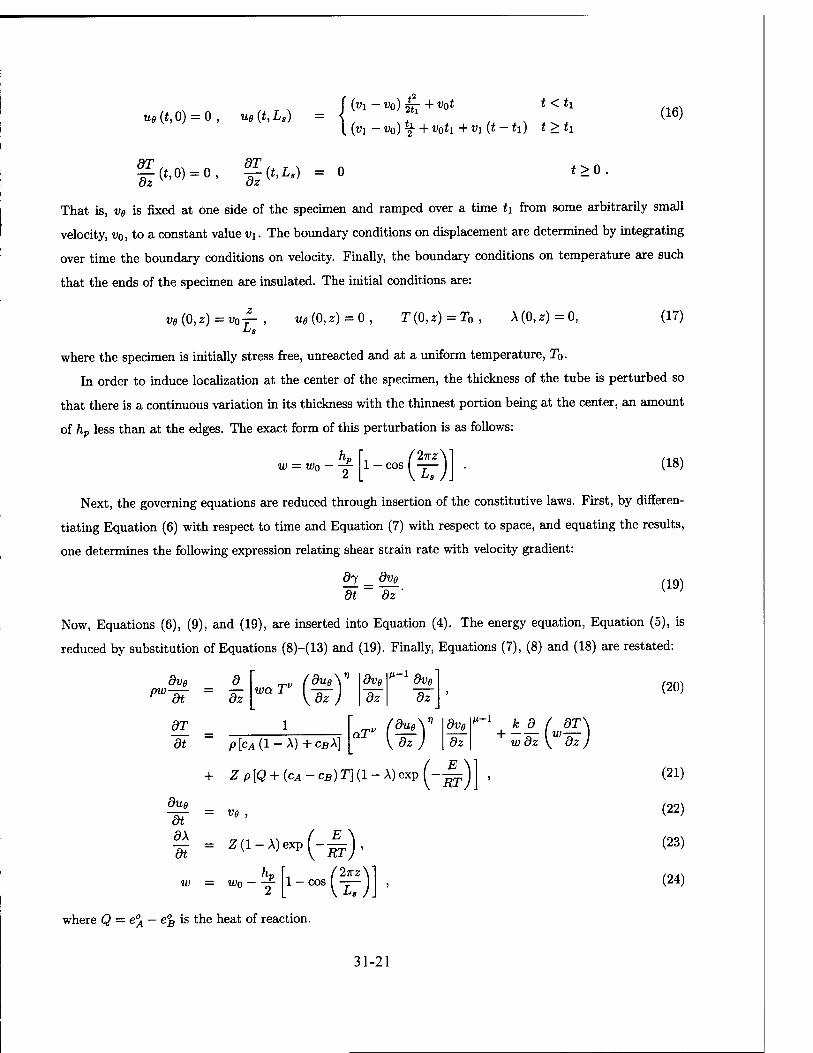
u9(t,0) = 0, ue(t,L.) = («l - «o) £7 + «o* * < *i

(«l - «o) £ + *>o*i + «i (t - h) t > h (16)

01 (t,0) = 0, %-{t,L.) = 0 t >0

That is, ve is fixed at one side of the specimen and ramped over a time tx from some arbitrarily small

velocity, v0, to a constant value vi. The boundary conditions on displacement are determined by integrating

over time the boundary conditions on velocity. Finally, the boundary conditions on temperature are such

that the ends of the specimen are insulated. The initial conditions are:

ve(0,z) = v0- u«(0,z) = 0, T(0,z) = To, A(0,z) = 0, (17)

where the specimen is initially stress free, unreacted and at a uniform temperature, T0.

In order to induce localization at the center of the specimen, the thickness of the tube is perturbed so

that there is a continuous variation in its thickness with the thinnest portion being at the center, an amount

of hp less than at the edges. The exact form of this perturbation is as follows:

hv w = WQ —

[2KZ\ (18)

Next, the governing equations are reduced through insertion of the constitutive laws. First, by differen-

tiating Equation (6) with respect to time and Equation (7) with respect to space, and equating the results,

one determines the following expression relating shear strain rate with velocity gradient:

<?7 _ dve Hi ~ ~dz'

(19)

Now, Equations (6), (9), and (19), are inserted into Equation (4). The energy equation, Equation (5), is

reduced by substitution of Equations (8)-(13) and (19). Finally, Equations (7), (8) and (18) are restated:

M_ dve_ ~dz~

v

pw dt

d_ dz

dT dt

due at dX dt

waT

1

v (due (du9\ \dz)

dve dz

aT"

(20)

due\ dz)

dve dz

p+i

p [cA (1 - A) -I- cBX]

+ Z p[Q + (cA-cB)T](l-X)eXp(-^;j ,

= v8 ,

= Z(l-A)exP(-!;),

k d ( w oz \

dT\ WJ-z)

W = WQ -COS{T:)

(21)

(22)

(23)

(24)

where Q = e°A — eB is the heat of reaction.

31-21

In order to numerically solve this system of equations, a spatial discretization was performed using second

order central differences. The result is a parabolic system of ordinary differential equations in time, as

shown in Caspar (1996). The computer code LSODE [Hindmarsh, 1983], the Livermore Solver for Ordinary

Differential Equations, was used to step forward in time to solve this system. LSODE solves initial value

problems for stiff or nonstiff systems of first order ordinary differential equations using the Gear (1971)

method. A stiff system is one whose ratio of largest to smallest eigenvalues in the locally linearized solution

matrix is large. That is, the system has rapidly growing or decaying processes that occur over a time scale

much shorter than the overall time scale of interest. This computer code is thus desirable for the model

presented herein since the process of shear localization occurs over a much shorter time than the overall time

of interest. The results of this code were validated in Caspar (1996), through the use of simplified forms of

the equations which had exact solutions, and also by comparing results with those of other researchers on

previously tested materials.

4 Results

This chapter will present results determined from the TSHB as well as those from the theoretical model.

Experimental results for tests on S-7 tool steel (TS) will first be presented, with comparisons drawn between

the numerical and experimental results, as well as with results determined from other researchers. Results

will then be presented for tests on the following explosive simulants: a PBX cure cast simulant, a PBX

pressed simulant, and a melt cast simulant known as Filler-E. These simulants are used to approximate the

material properties of PBXN 109, PBX 9501, and tritonal, respectively. The results of these tests will be

used to determine approximate parameters for the constitutive law for stress used in this thesis. Finally,

numerical simulations will be run on 1018 CRS, and S-7 tool steel to compare with previously determined

results, and simulations will be run on the aforementioned explosives.

4.1 Experimental Results on Explosive Simulants

In this section, results determined from the TSHB on tests of the explosive simulants are presented. The

strain and strain rate hardening parameters from the constitutive law for stress are then determined from

the data. It is important to note that, to our knowledge, no researchers have tested any of these materials

in torsion. The results presented in this section are thus previously unrecorded.

4.1.1 Tests on the PBX Cure Cast Simulant

The results of tests performed at various shear strain rates on the PBX cure cast simulant are included in

Figure 8. The reported results are characteristic of a few tests performed at each strain rate. In this figure,

31-22

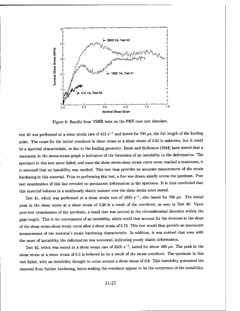
a a. 2

ID .C CO

c

"E o

Y= 3500 1/s, Test 42

0.6 0.9

Nominal Shear Strain

1.5

Figure 8: Results from TSHB tests on the PBX cure cast simulant.

test 40 was performed at a shear strain rate of 415 s_1 and lasted for 700 ßs, the full length of the loading

pulse. The cause for the initial overshoot in shear stress at a shear strain of 0.05 is unknown, but it could

be a material characteristic, or due to the loading geometry. Zener and Hollomon (1944) have stated that a

maximum in the stress-strain graph is indicative of the formation of an instability in the deformation. The

specimen in this test never failed, and since the shear stress-shear strain curve never reached a maximum, it

is assumed that no instability was reached. This test thus provides an accurate measurement of the strain

hardening in this material. Prior to performing this test, a line was drawn axially across the specimen. Post

test examination of this line revealed no permanent deformation in the specimen. It is thus concluded that

this material behaves in a nonlinearly elastic manner over the shear strain rates tested.

Test 41, which was performed at a shear strain rate of 1850 s_1, also lasted for 700 ps. The initial

peak in the shear stress at a shear strain of 0.28 is a result of the overshoot, as seen in Test 40. Upon

post-test examination of the specimen, a small tear was noticed in the circumferential direction within the

gage length. This is the consequence of an instability, which could thus account for the decrease in the slope

of the shear stress-shear strain curve after a shear strain of 0.75. This test would thus provide an inaccurate

measurement of the material's strain hardening characteristic. In addition, it was noticed that even with

the onset of instability, the deformation was recovered, indicating purely elastic deformation.

Test 42, which was tested at a shear strain rate of 3500 s_1, lasted for about 400 ps. The peak in the

shear stress at a shear strain of 0.5 is believed to be a result of the stress overshoot. The specimen in this

test failed, with an instability thought to occur around a shear stress of 0.8. This instability prevented the

material from further hardening, hence making the overshoot appear to be the occurrence of the instability,

31-23

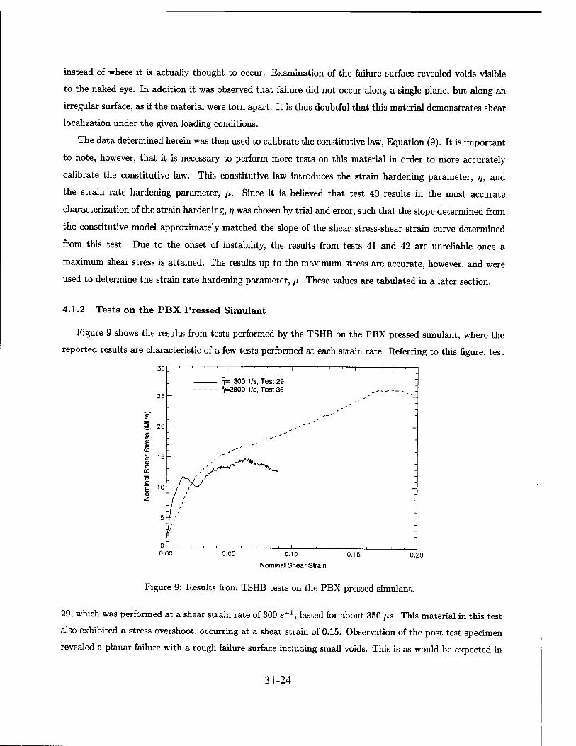
instead of where it is actually thought to occur. Examination of the failure surface revealed voids visible

to the naked eye. In addition it was observed that failure did not occur along a single plane, but along an

irregular surface, as if the material were torn apart. It is thus doubtful that this material demonstrates shear

localization under the given loading conditions.

The data determined herein was then used to calibrate the constitutive law, Equation (9). It is important

to note, however, that it is necessary to perform more tests on this material in order to more accurately

calibrate the constitutive law. This constitutive law introduces the strain hardening parameter, 77, and

the strain rate hardening parameter, \i. Since it is believed that test 40 results in the most accurate

characterization of the strain hardening, 77 was chosen by trial and error, such that the slope determined from

the constitutive model approximately matched the slope of the shear stress-shear strain curve determined

from this test. Due to the onset of instability, the results from tests 41 and 42 are unreliable once a

maximum shear stress is attained. The results up to the maximum stress are accurate, however, and were

used to determine the strain rate hardening parameter, /j. These values are tabulated in a later section.

4.1.2 Tests on the PBX Pressed Simulant

Figure 9 shows the results from tests performed by the TSHB on the PBX pressed simulant, where the

reported results are characteristic of a few tests performed at each strain rate. Referring to this figure, test

30

25

a. §. 20 W in £ 55

0.00

y= 300 1/s, Test 29 V>=2800 1/s, Test 36

0.05 0.10


0.15 0.20

Figure 9: Results from TSHB tests on the PBX pressed simulant.

29, which was performed at a shear strain rate of 300 s~\ lasted for about 350 ßs. This material in this test

also exhibited a stress overshoot, occurring at a shear strain of 0.15. Observation of the post test specimen

revealed a planar failure with a rough failure surface including small voids. This is as would be expected in

31-24

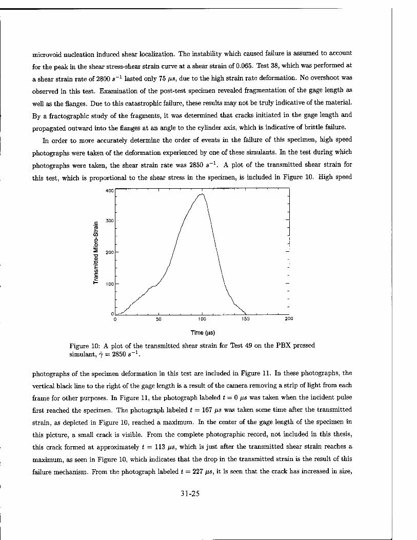
microvoid nucleation induced shear localization. The instability which caused failure is assumed to account

for the peak in the shear stress-shear strain curve at a shear strain of 0.065. Test 38, which was performed at

a shear strain rate of 2800 s"1 lasted only 75 ps, due to the high strain rate deformation. No overshoot was

observed in this test. Examination of the post-test specimen revealed fragmentation of the gage length as

well as the flanges. Due to this catastrophic failure, these results may not be truly indicative of the material.

By a fractographic study of the fragments, it was determined that cracks initiated in the gage length and

propagated outward into the flanges at an angle to the cylinder axis, which is indicative of brittle failure.

In order to more accurately determine the order of events in the failure of this specimen, high speed

photographs were taken of the deformation experienced by one of these simulants. In the test during which

photographs were taken, the shear strain rate was 2850 s_1. A plot of the transmitted shear strain for

this test, which is proportional to the shear stress in the specimen, is included in Figure 10. High speed

c « 55

i

S o -o QJ

I c (0

400

300 -

200 -

100 -

200

Figure 10: A plot of the transmitted shear strain for Test 49 on the PBX pressed simulant, 7 = 2850 s_1.

photographs of the specimen deformation in this test are included in Figure 11. In these photographs, the

vertical black line to the right of the gage length is a result of the camera removing a strip of light from each

frame for other purposes. In Figure 11, the photograph labeled t = 0 ps was taken when the incident pulse

first reached the specimen. The photograph labeled t = 167 ps was taken some time after the transmitted

strain, as depicted in Figure 10, reached a maximum. In the center of the gage length of the specimen in

this picture, a small crack is visible. From the complete photographic record, not included in this thesis,

this crack formed at approximately t = 113 ps, which is just after the transmitted shear strain reaches a

maximum, as seen in Figure 10, which indicates that the drop in the transmitted strain is the result of this

failure mechanism. From the photograph labeled t = 227 ps, it is seen that the crack has increased in size,

31-25

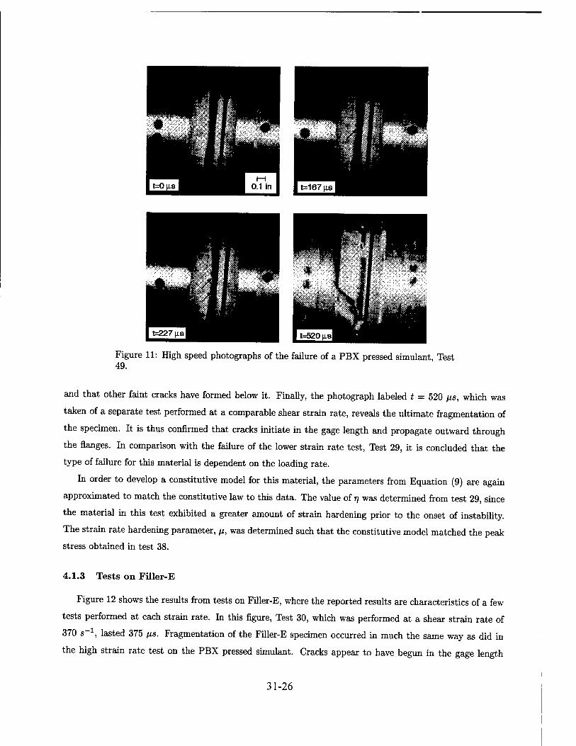
Figure 11: High speed photographs of the failure of a PBX pressed simulant, Test 49.

and that other faint cracks have formed below it. Finally, the photograph labeled t = 520 ßs, which was

taken of a separate test performed at a comparable shear strain rate, reveals the ultimate fragmentation of

the specimen. It is thus confirmed that cracks initiate in the gage length and propagate outward through

the flanges. In comparison with the failure of the lower strain rate test, Test 29, it is concluded that the

type of failure for this material is dependent on the loading rate.

In order to develop a constitutive model for this material, the parameters from Equation (9) are again

approximated to match the constitutive law to this data. The value of 77 was determined from test 29, since

the material in this test exhibited a greater amount of strain hardening prior to the onset of instability.

The strain rate hardening parameter, /j, was determined such that the constitutive model matched the peak

stress obtained in test 38.

4.1.3 Tests on Filler-E

Figure 12 shows the results from tests on Filler-E, where the reported results are characteristics of a few

tests performed at each strain rate. In this figure, Test 30, which was performed at a shear strain rate of

370 s_1, lasted 375 fis. Fragmentation of the Filler-E specimen occurred in much the same way as did in

the high strain rate test on the PBX pressed simulant. Cracks appear to have begun in the gage length

31-26

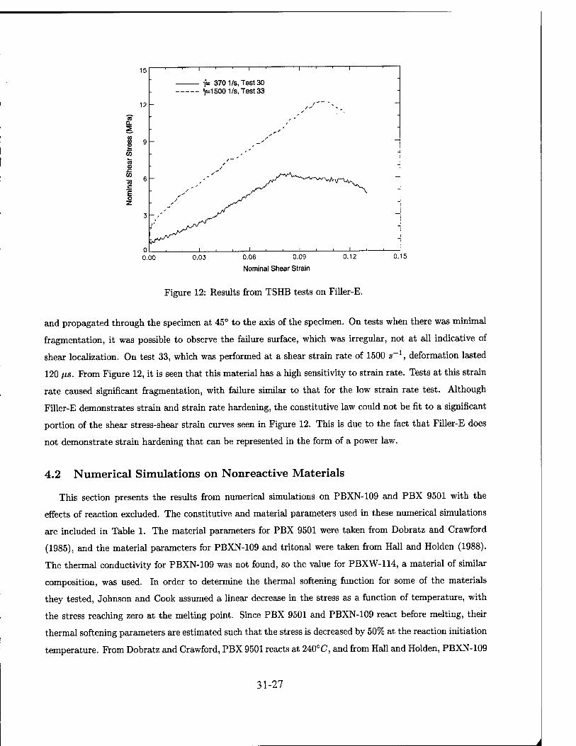
CO EL

& 55 cd CD f co 15 c E o

15

12 -

9 -

y= 370 1/s, Test 30 Y=15001/s,Test33

0.00 0.03 0.06 0.09


0.12 0.15

Figure 12: Results from TSHB tests on Filler-E.

and propagated through the specimen at 45° to the axis of the specimen. On tests when there was minimal

fragmentation, it was possible to observe the failure surface, which was irregular, not at all indicative of

shear localization. On test 33, which was performed at a shear strain rate of 1500 s"1, deformation lasted

120 fis. From Figure 12, it is seen that this material has a high sensitivity to strain rate. Tests at this strain

rate caused significant fragmentation, with failure similar to that for the low strain rate test. Although

Filler-E demonstrates strain and strain rate hardening, the constitutive law could not be fit to a significant

portion of the shear stress-shear strain curves seen in Figure 12. This is due to the fact that Filler-E does

not demonstrate strain hardening that can be represented in the form of a power law.

4.2 Numerical Simulations on Nonreactive Materials

This section presents the results from numerical simulations on PBXN-109 and PBX 9501 with the

effects of reaction excluded. The constitutive and material parameters used in these numerical simulations

are included in Table 1. The material parameters for PBX 9501 were taken from Dobratz and Crawford

(1985), and the material parameters for PBXN-109 and tritonal were taken from Hall and Holden (1988).

The thermal conductivity for PBXN-109 was not found, so the value for PBXW-114, a material of similar

composition, was used. In order to determine the thermal softening function for some of the materials

they tested, Johnson and Cook assumed a linear decrease in the stress as a function of temperature, with

the stress reaching zero at the melting point. Since PBX 9501 and PBXN-109 react before melting, their

thermal softening parameters are estimated such that the stress is decreased by 50% at the reaction initiation

temperature. From Dobratz and Crawford, PBX 9501 reacts at 240°C, and from Hall and Holden, PBXN-109

31-27

Material

Constitutive Parameters Material Parameters

a

(MPa£)

V V ß

(*)

CA

{ kg-K )

k

\mK)

PBX 9501

PBXN-109

Tritonal

33,000

800

-1.28

-1.38

-9.68

0.320

0.400

0.080

0.320

1840

1670

1690

1130

1260

960

0.454

0.104

0.460

Table 1: Constitutive and material parameters used in the numerical calculations.

reacts at 220° C. The thermal softening parameter for tritonal was estimated such that the stress is decreased

by 90% at the melting temperature of 80°C. The remaining constitutive parameters were determined from

the experimental results on the explosive simulants, as described in the previous section.

4.2.1 PBX 9501 Without Reaction

Next, numerical simulations were performed for the deformation of PBX 9501, with the effects of reaction

excluded. This was studied in order to compare with the experimental results on the PBX pressed simulant

and to determine the material's susceptibility to localization. Reaction was excluded by setting Z equal to

zero in the computer code. The physical constants, included in Table 2 under simulation #1, were chosen to

match the experimental conditions. For this case, the test was performed at a shear strain rate of 2800 s_1.

Simulation

Number

Vi

(m/s)

L8

(mm)

h

(ps)

w0

(mm)

hp vo

(m/s)

1

2

7.00

6.25

2.50

2.50

32.14

32.00

2.50

2.50

0.10

0.10

7.00 x 10-2

6.25 x IQ-2

Table 2: Physical constants used in the numerical simulations reported within this thesis.

In order to determine the onset of localization, the following localization criterion, determined by Meyers

(1994), is used: dr c?7

Or di/dt\2

r,7 dl/Wz < dr

(25) 7,7

pcA dT

which is evaluated at the center of the specimen. The right hand side, $, and left hand side, *, of this

criterion are plotted as functions of time in Figure 13. In this criterion, * is a combined measure of the

strain and strain rate hardening effects, while the * is a measure of the thermal softening. It is seen that both

* and * are always positive, indicating that the material is experiencing strain and strain rate hardening

as well as thermal softening, as expected. When * is less than or equal to $, this criterion predicts that

localization will begin. For this test, the onset of localization is reached after 1.67 ms.

31-28

10

CO D.

c .2 6

Ü c o

CO u o

1 . . v ,

\ .... , !

' ' ' ' \ \ 3> -

\ Y :

\ -

\ \ . \ \ — \ -

\ ~

v. \ ^^^^ \

^^^^ -

s ^v N ^"S.

^ ^s. _

* - * \ . ^-* ^*^^

1 1 ! ■■!,„■ ,

800 1600

Time (us)

2400 3200

Figure 13: Localization criterion for PBX 9501 without reaction, where $ represents thermal softening and * represents strain and strain rate hardening.

The effects of localization are readily seen by studying the evolution of the velocity and temperature

profile, as seen in Figures 14 and 15. Figure 14 shows the three stage localization process, which was initially

observed experimentally by Marchand and Duffy (1988). After the velocity at z = L reaches its final

value, the profile essentially forms a linear distribution in space, which is called homogeneous deformation.

Marchand and Duffy have termed this Stage I of the localization process. Since the specimen is thinnest at

its center, it is also weakest at that point. The material is thus locally less resistant to deformation, hence

developing an inhomogeneous velocity profile with the greatest slope at the center. This is referred to as

Stage II. The Stage II localization is very subtle in this test and is not readily observed. Now, the shear

strain rate is equal to the slope of the velocity profile, so, as it increases, it causes the stress to increase. The

combined effect of the increased shear stress and shear strain rate cause the temperature to increase, as is

seen in Figure 15. The rise in temperature causes the stress to drop, which results in further straining and

heating. This interaction continues until, after 1.67 ms, the thermal softening dominates over the strain and

strain rate hardening. Consequently, deformation rapidly localizes to a narrow region, termed Stage III.

It is this final stage of localization that is termed shear localization, or shear banding. At this time,

the rate of change in the temperature increases dramatically at the center of the shear band, resulting in a

pronounced spike in temperature. The temperature at the center of the shear band at the onset of localization

is 458 K. After 3.2 ms, the temperature at this point has increased to 1590 K. It is interesting to note

that the temperature of the material at the onset of localization has already almost reached its initiation

temperature of 513 K, and that following localization the temperature far surpasses this value. Hence, it is

expected that shear localization in PBX 9501 would produce initiation of reaction.

31-29

T-?=

POS*00'

Figure 14: Evolution of the velocity field for PBX 9501 without reaction.

T-f=>

postä°n'

Figure 15: Evolution of the temperature field for PBX 9501 without reaction.

31-30

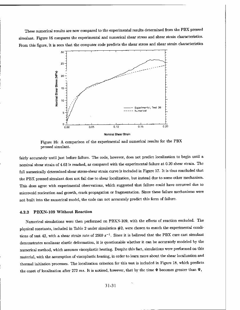
These numerical results are now compared to the experimental results determined from the PBX pressed

simulant. Figure 16 compares the experimental and numerical shear stress and shear strain characteristics.

From this figure, it is seen that the computer code predicts the shear stress and shear strain characteristics

30

0.00 0.05 0.10


0.15 0.20

Figure 16: A comparison of the experimental and numerical results for the PBX pressed simulant.

fairly accurately until just before failure. The code, however, does not predict localization to begin until a

nominal shear strain of 4.63 is reached, as compared with the experimental failure at 0.20 shear strain. The

full numerically determined shear stress-shear strain curve is included in Figure 17. It is thus concluded that

the PBX pressed simulant does not fail due to shear localization, but instead due to some other mechanism.

This does agree with experimental observations, which suggested that failure could have occurred due to

microvoid nucleation and growth, crack propagation or fragmentation. Since these failure mechanisms were

not built into the numerical model, the code can not accurately predict this form of failure.

4.2.2 PBXN-109 Without Reaction

Numerical simulations were then performed on PBXN-109, with the effects of reaction excluded. The

physical constants, included in Table 2 under simulation #2, were chosen to match the experimental condi-

tions of test 42, with a shear strain rate of 2500 s_1. Since it is believed that the PBX cure cast simulant

demonstrates nonlinear elastic deformation, it is questionable whether it can be accurately modeled by the

numerical method, which assumes viscoplastic heating. Despite this fact, simulations were performed on this

material, with the assumption of viscoplastic heating, in order to learn more about the shear localization and

thermal initiation processes. The localization criterion for this test is included in Figure 18, which predicts

the onset of localization after 272 ms. It is noticed, however, that by the time $ becomes greater than *,

31-31

50

o CL

in w <D i_

■+->

GO

o _C CO

10 Numerical Experimental, Test 36

0 2 4 6 8 Nominal Shear Strain

Figure 17: Experimental and numerical shear stress-shear strain curves up to failure for the PBX pressed simulant.

(0 a.

c o

O c o (5 N

OS u o

O.J

- i ■ '

0 -

y -

0.2 - i i i i i \

-

0.1 \ \ \ \ \ \ \ \ \ \ \ \

-

- ^^^^ -

on . ^ -. _ =. 1—-—, ^

0 100 200

Time (ms)

Figure 18: Localization criterion for PBXN-109 without reaction.

300

31-32

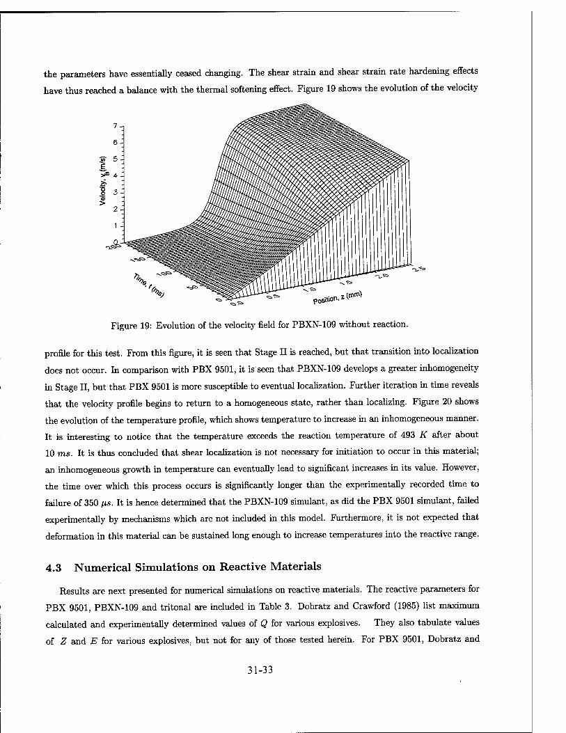
the parameters have essentially ceased changing. The shear strain and shear strain rate hardening effects

have thus reached a balance with the thermal softening effect. Figure 19 shows the evolution of the velocity

^•»

Figure 19: Evolution of the velocity field for PBXN-109 without reaction.

profile for this test. From this figure, it is seen that Stage II is reached, but that transition into localization

does not occur. In comparison with PBX 9501, it is seen that PBXN-109 develops a greater inhomogeneity

in Stage II, but that PBX 9501 is more susceptible to eventual localization. Further iteration in time reveals

that the velocity profile begins to return to a homogeneous state, rather than localizing. Figure 20 shows

the evolution of the temperature profile, which shows temperature to increase in an inhomogeneous manner.

It is interesting to notice that the temperature exceeds the reaction temperature of 493 K after about

10 ms. It is thus concluded that shear localization is not necessary for initiation to occur in this material;

an inhomogeneous growth in temperature can eventually lead to significant increases in its value. However,

the time over which this process occurs is significantly longer than the experimentally recorded time to

failure of 350 ps. It is hence determined that the PBXN-109 simulant, as did the PBX 9501 simulant, failed

experimentally by mechanisms which are not included in this model. Furthermore, it is not expected that

deformation in this material can be sustained long enough to increase temperatures into the reactive range.

4.3 Numerical Simulations on Reactive Materials

Results are next presented for numerical simulations on reactive materials. The reactive parameters for

PBX 9501, PBXN-109 and tritonal are included in Table 3. Dobratz and Crawford (1985) list maximum

calculated and experimentally determined values of Q for various explosives. They also tabulate values

of Z and E for various explosives, but not for any of those tested herein. For PBX 9501, Dobratz and

31-33

4500

3900

g 3300

g 270° -

Q.

£ 1500

900-

^.» position, z^

Figure 20: Evolution of the temperature field for PBXN-109 without reaction.

Crawford only list the maximum calculated value of Q. For PBX 9404, a similar explosive, the experimental

value is 88.5% of the maximum, hence, the Q value for PBX 9501 is chosen to be 88.5% of its maximum

calculated value. Since PBX 9501 is 95% by weight HMX, the values of Z and E for HMX were used.

Neither PBXN-109 nor tritonal are included in Dobratz and Crawford's handbook. Since PBXN-109 is 64%

RDX, the experimentally determined value of Q and the values of A and E for RDX were used to simulate

this explosive. Likewise, as tritonal is 80% TNT, the values of Q, Z, and E for TNT were used to simulate

tritonal.

Material Z Q E R

(s-1) (kJ/kg) (kJ/mol) (J/mol ■ K)

PBX 9501 5.00 x 1019 5891 220.6 8.314

PBXN-109 2.02 x 1018 6320 197.1 8.314

Tritonal 2.51 x 1011 4560 143.9 8.314

Table 3: Reactive constants used in the numerical code.

4.3.1 PBX 9501 With Reaction

Results are now presented for simulations of PBXN-109 with the effects of reaction included. The

same parameters were used in this simulation as in the nonreactive case. The effects of including reaction

proved to have little effect on the results prior to initiation. The localization criterion predicted localization

after 1.682 ms, a difference of only 0.3% from the nonreactive case. The temperature at the center of the

31-34

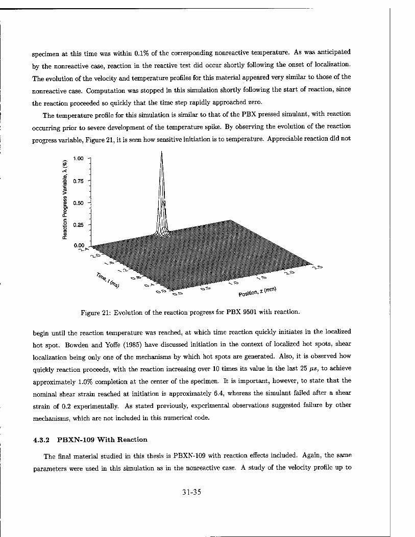
specimen at this time was within 0.1% of the corresponding nonreactive temperature. As was anticipated

by the nonreactive case, reaction in the reactive test did occur shortly following the onset of localization.

The evolution of the velocity and temperature profiles for this material appeared very similar to those of the

nonreactive case. Computation was stopped in this simulation shortly following the start of reaction, since

the reaction proceeded so quickly that the time step rapidly approached zero.

The temperature profile for this simulation is similar to that of the PBX pressed simulant, with reaction

occurring prior to severe development of the temperature spike. By observing the evolution of the reaction

progress variable, Figure 21, it is seen how sensitive initiation is to temperature. Appreciable reaction did not

position.z^

Figure 21: Evolution of the reaction progress for PBX 9501 with reaction.

begin until the reaction temperature was reached, at which time reaction quickly initiates in the localized

hot spot. Bowden and Yoffe (1985) have discussed initiation in the context of localized hot spots, shear

localization being only one of the mechanisms by which hot spots are generated. Also, it is observed how

quickly reaction proceeds, with the reaction increasing over 10 times its value in the last 25 ps, to achieve

approximately 1.0% completion at the center of the specimen. It is important, however, to state that the

nominal shear strain reached at initiation is approximately 6.4, whereas the simulant failed after a shear

strain of 0.2 experimentally. As stated previously, experimental observations suggested failure by other

mechanisms, which are not included in this numerical code.

4.3.2 PBXN-109 With Reaction

The final material studied in this thesis is PBXN-109 with reaction effects included. Again, the same

parameters were used in this simulation as in the nonreactive case. A study of the velocity profile up to

31-35

reaction initiation reveals that no significant inhomogeneity has yet to develop. In contrast to the velocity

profile, the temperature profile develops an inhomogeneity. In fact, the temperatures in this inhomogeneity,

although not significant, have grown enough to reach the reaction temperature. The plot of the reaction

progress variable profile (Figure 22) reveals, as expected from the nonreactive case, that reaction has occurred

1.5 n

, zltitfti position

Figure 22: Evolution of the reaction progress variable profile for PBXN-109 with reaction.

prior to the onset of localization. In comparison with the results from PBX 9501, however, it is seen that

reaction occurs over a much larger spatial region. This is due to the fact that the temperature is not

severely localized when it reaches the initiation temperature. Computations were stopped after reaction

reached approximately 1.3% completion, due to the explosive growth in reaction and consequent decrease

in time step to zero. It is thus concluded that shear localization is not necessary to produce initiation. A

mere inhomogeneity, if allowed to grow long enough, can result in the initiation of reaction. For this to

occur, however, all other forms of failure would have to be suppressed. The nominal shear strain reached at

initiation in this simulation, was 26.7, far in excess of the experimentally determined nominal shear strain

of 1.5, which was reached at failure. As was the case in the simulation on PBX 9501, it is determined that

the current analytical method is insufficient for modeling failure in PBXN-109.

5 Conclusions

The results included herein first present constitutive behavior in the form of shear stress-shear strain

curves for a PBX cure cast simulant, a PBX pressed simulant, and a melt cast simulant known as Filler-E.

These simulants are used to approximate the material properties of PBXN 109, PBX 9501, and tritonal,

31-36

respectively. Results from these tests revealed significant dependencies of the shear stress on shear strain

and shear strain rate, as compared with the corresponding dependencies of steels. Observation of the failure

surface of the various explosive simulants revealed evidence of tearing, microvoid nucleation and growth, crack

propagation and fragmentation. The data from these tests can be used to calibrate various constitutive laws

which are used to input experimental data into analytical codes. The data from the PBX cure cast and

pressed simulants has been used to calibrate a constitutive law, proposed by Clifton, et al. (1984), which

models shear stress by including the effects of strain and strain rate hardening as well as thermal softening.

Prom numerical simulations on PBX 9501 without the effects of reaction, the three stage localization

process observed experimentally by Marchand and Duffy (1988) was predicted, with the onset of localization

predicted after a nominal shear strain of 4.63. In addition, the subsequent rise in temperature quickly

exceeding the reaction temperature of the material. When the effects of reaction were included, initiation

of reaction began after a nominal shear strain of 6.4. From simulations on PBXN-109 without the effects

of reaction, it was determined that this material is not susceptible to localization. With the inclusion of

reaction effects, however, it was determined that reaction could occur without localization. Due to a mere

growth in the inhomogeneous temperature field, reaction initiating after a nominal shear strain of 26.7.

Since localization is assumed to be followed by failure or initiation, numerical results agreed with exper-

imental results in predicting that PBX 9501 would fail at a lower strain than PBXN-109. Experimentally,

the corresponding simulants failed after nominal shear strains of 0.2 and 1.5, respectively. In comparison of

the experimental and numerical values, however, it is seen that the experimental tests failed at significantly

lower shear strains. This is not surprising, since experimental observations indicated that failure could have

occurred as a result of the combined mechanisms of microvoid nucleation and growth, crack propagation

and fragmentation. These mechanisms are not included in the current analytical study and hence it is not

possible for their results to be predicted.

It is, however, concluded that if these other mechanisms were suppressed, localization and/or initiation

would occur in the tested materials. Chou et al. (1991) stated that brittle materials become more ductile

under the application of hydrostatic stresses. In addition, Prey (1981) concluded that explosives under

compressive stresses generate more heat when being deformed, hence decreasing the time necessary for

initiation to occur. Furthermore, Chou et al. concluded that localization becomes significant in covered

explosives. Finally, Dodd and Atkins (1983) concluded that increased hydrostatic stresses tended to decrease

microvoid nucleation. The explosives in deep earth penetrators are contained and subject to an unknown

amount of hydrostatic stress. Deformation under these circumstances could thus result in the suppression

of failure mechanisms and hence increase the susceptibility to localization and initiation. As a result, it

is desired to perform future tests under the application of hydrostatic stresses, in order to determine the

subsequent effect on localization and initiation.

31-37

It is also concluded in Caspar (1996) that the most important parameters in the study of shear localization

for a given material are the constitutive parameters. In order to increase the mass, and hence momentum,

of reactive devices, studies are being performed at Eglin Air Force Base on an explosive unofficially termed

TUNG-5. This explosive uses tungsten as a binder for the explosive crystals. Due to its high strength, it is

concluded in this thesis that such a material would be particularly susceptible to shear localization and hence

reaction. This material would have the material characteristics of a metal and the reactive characteristics of

an explosive. Since it is known that metals are particularly susceptible to localization, and since this thesis

has shown that localization is quickly proceeded by initiation, significant precautions should be taken in the

development of munitions containing this material.

For future work, several ideas are presented which may obtain more accurate results from the TSHB.

First, the incident and transmission bars will be ground straight. This will reduce any bending and axial

pulses, as well as decrease inhomogeneous deformation in the specimen. It is also desired to develop a

better method for aligning the bars. Currently, delrin bearings are used to support the bars. With harder

bearings, the bars can be restrained from bending motion; in addition, it will be easier to determine proper

alignment of the bars by observing the amount of resistance when the bars are rotated by hand. Finally, since

preliminary results with new strain gages revealed up to 8% difference in transmitted strain, it is desired to

apply new strain gages to the bars. Finally, it is desired to calibrate the amplifiers in order to determine a

measure of their accuracy.

References

[1] R. C. Batra and C. H. Kim (1991), "The Effect of Thermal Conductivity on the Initiation, Growth, and Band Width of Adiabatic Shear Bands," Int. J. Eng. Science, Vol. 29, pp. 949-960.

[2] R. C. Batra and C. H. Kim (1992), "Analysis of Shear Banding in Twelve Materials," International Journal of Plasticity, Vol. 8, pp. 425-452.

[3] R. C. Batra, X. Zhang, and T. W. Wright (1995), "Critical Strain Ranking of 12 Materials in Deforma- tions Involving Adiabatic Shear Bands," Journal of Applied Mechanics, Vol. 62, pp. 252-255.

[4] F. P. Bowden and Y. D. Yoffe (1985), Initiation and Growth of Explosives in Liquids and Solids, Cambridge University Press, Cambridge, Great Britain.

[5] V. Boyle, R. Frey, and O. Blake (1989), "Combined Pressure Shear Ignition of Explosives," Ninth Symposium (International) on Detonation, pp. 3-17.

[6] R. J. Caspar (1996), "Experimental and Numerical Study of Shear Localization as an Initiation Mech- anism in Energetic Solids," Masters Thesis, University of Notre Dame.

[7] P. C. Chou, W. Flis, and D. Jann (1991), "Explosive Response to Unplanned Stimuli," Dyna East Corporation Technical Report DE-TR-91-15.

[8] I. G. Currie (1993), Fundamental Mechanics of Fluids, 2nd ed., McGraw-Hill, Inc., New York DD 224-228. '

31-38

[9] R. J. Clifton, J. Duffy, K. A. Hartley, and T. G. Shawki (1984), "On Critical Conditions for Shear Band Formation at High Strain Rates," Scripta Met, Vol. 18, pp. 443-448.

[10] L. S. Costin, E. E. Crisman, R. H. Hawley, and J. Duffy (1979), 2nd Conference on the Mechanical Properties of Materials at High Rates of Strain, Ed. by J. Harding, The Institute of Physics, London, 90.

[11] B. M. Dobratz and P. C. Crawford (1985), LLNL Explosives Handbook-Properties of Chemical Explo- sives and Explosive Simulants, Lawrence Livermore National Labs., UCRL-52997, National Technical Information Service, DE91-006884.

[12] B. Dodd and A. G. Atkins (1983), "Flow Localization in Shear Deformation of Void-Containing and Void-Free Solids," Ada Metall., Vol. 31, pp 9-15.

[13] J. Duffy and Y. C. Chi (1992), "On the measurement of local strain and temperature during the formation of adiabatic shear bands," Materials Science and Engineering, A157, pp. 195-210.

[14] W. Fickett and W. C. Davis (1979), Detonation, University of California Press, Berkeley, CA.

[15] J. E. Field, G. M. Swallowe and S. N. Heavens (1982), "Ignition Mechanisms of Explosives during Mechanical Deformation," Proc. R. Soc. Lond. A 382, pp. 231-244.

[16] R. B. Frey (1981), "The Initiation of Explosive Charges by Rapid Shear," Seventh Symposium (Inter- national) on Detonation, Naval Surface Weapons Center, Annapolis, MD, pp. 36-42.

[17] R. B. Frey (1985), in Eighth Symposium (International) on Detonation, Naval Surface Weapons Center, Albuquerque, NM, pp. 68-80.

[18] J. H. Giovanola (1988, a), "Adiabatic Shear Banding Under Pure Shear Loading. Part I: Direct Obser- vation of Strain Localization and Energy Dissipation Measurements," Mechanics of Materials, Vol. 7, pp. 59-71.

[19] J. H. Giovanola (1988, b), "Adiabatic Shear Banding Under Pure Shear Loading. Part II: Fractographic and Metallographic Observations," Mechanics of Materials, Vol. 7, pp. 73-87.

[20] T. N. Hall and J. R. Holden (1988), Navy Explosives Handbook. Explosion Effects and Properties-Part III. Properties of Explosives and Explosive Compositions., Naval Surface Warfare Center, NSWC MP 88-116, Defense Technical Information Center, AD-B138 762.

[21] J. Harding, E. D. Wood, and J. D. Campbell (1960), "Tensile Testing of Material at Impact Rate of Strain," J. Mech. Eng. Sei., Vol. 2, p. 88.

[22] K. A. Hartley and J. Duffy (1985), "Introduction, High Strain Rate Shear Testing" in "High Strain Rate Testing, Mechanical Testing" Metal Hand Book, American Society for Metals, Vol. 8, Edition 9, p. 215.

[23] K. A. Hartley, J. Duffy, and R. H. Hawley (1985), "The Torsional Kolsky (Split-Hopkinson) Bar, High Strain Rate Shear Testing" in "High Strain Rate Testing, Mechanical Testing," Metal Hand Book, American Society for Metals, Vol. 8, Edition 9, pp. 218-230.

[24] K. A. Hartley, J. Duffy, and R. H. Hawley (1987), "Measurement of the Temperature Profile During Shear Band Formation in Steels Deforming at High Strain Rates," J. Mech. Phys. Solids, Vol. 35, No. 3, pp. 283-301.

[25] A. C. Hindmarsh (1983), "ODEPACK, A Systematized Collection of ODE Solvers," Scientific Com- puting, R. S. Stepleman et al, Eds., IMACS/North-Holland Publishing Company, Amsterdam, pp. 55-64.

31-39

[26] G. R. Johnson and W. H. Cook (1983), "A Constitutive Model and Data for Metals Subjected to Large Strains, High Strain Rates and High Temperatures," Proc. 7th Int. Symp. Ballistics, The Hague, The Netherlands, pp. 541-548.

[27] J. Kang, P. B. Butler, and M. R. Baer (1992), "A Thermomechanical Analysis of Hot Spot Formation in Condensed-Phase, Energetic Materials," Combustion and Flame, Vol. 89, pp. 117-139.

[28] H. Kolsky (1949), "An Investigation of the Mechanical Properties of Materials at Very High Rates of Loading," Proc. Phys. Soc. London, Vol. 62-B, pp. 676-700.

[29] H. Kolsky (1953), Stress Waves in Solids, Oxford University Press, London.

[30] J. Lubliner (1990), Plasticity Theory, Macmillan Publishing Co., New York, pp. 69-99.

[31] A. Marchand and J. Duffy (1988), "An Experimental Study of the Formation Process of Adiabatic Shear Bands in a Structural Steel," J. Mech. Phys. Sol., Vol. 36, No. 3, pp. 251-283.

[32] K. G. McConnell and W. F. Riley (1993), "Strain-Gage Instrumentation and Data Analysis," in Hand- book on Experimental Mechanics, A. S. Kobayashi, Ed., 2nd edition, VCH Publishers, Inc., New York, NY, pp. 79-117.

[33] L. W. Meyer (1992), "Constitutive Equations at High Strain Rates," in Shock-Wave and High-Strain- Rate Phenomena in Materials, M. A. Meyers, L. E. Murr, and K. P. Staudhammer, Eds., Marcel Dekker, Inc., New York, NY, pp. 49-68.

[34] M. A. Meyers (1994), Dynamic Behavior of Materials, John Wiley & Sons, Inc., New York, NY.

[35] M. A. Meyers, L. E. Murr, K. P. Staudhammer (1992), Shock-Wave and High-Strain-Rate Phenomena in Materials, Marcel Dekker, Inc., New York, NY.

[36] A. M. Rajendran (1992), "High Strain Rate Behavior of Metals, Ceramics and Concrete," Report # WL-TR-92-4006, Wright Patterson Air Force Base.

[37] H. C. Rogers (1979), "Adiabatic Plastic Deformation," Ann. Rev. Mater. Sei., Vol. 9, pp. 283-311.

[38] T. Weerasooriya (1990), "The MTL Torsional Split-Hopkinson Bar," U. S. Army Materials Technology Laboratory Report MTL TR 90-27.

[39] G. B. Whitham (1974), Linear and Nonlinear Waves, John Wiley & Sons, Inc., New York, NY.

[40] T. W. Wright (1987), "Steady Shearing in a Viscoplastic Solid," J. Mech. Phys. Solids, Vol. 35, No. 3, pp. 269-282.

[41] T. W. Wright and R. C. Batra (1985), "Further Results on the Initiation and Growth of Adiabatic Shear Bands at High Strain Rates," Journal de Physique, Coll. C5, suppl. to no. 8, p. C5-323.

[42] C. Zener and J. F. Hollomon (1944), "Effect of Strain Rate upon Plastic Flow of Steel," Journal of Applied Physics, Vol. 15, pp. 22-32.

31-40

A Molecular-Level View of Solvation in Supercritical Fluid Systems

Emily D. Niemeyer Graduate Research Assistant

Department Chemistry

State University of New York at Buffalo Buffalo, NY


Wright Laboratory



and

Wright Laboratory

December 1996

32-1

A MOLECULAR-LEVEL VIEW OF SOLVATION IN SUPERCRITICAL FLUID SYSTEMS

Emily D. Niemeyer Graduate Research Assistant

Department of Chemistry State University of New York at Buffalo

Abstract

Although supercritical fluids (SFs) have generated intense research interest within recent years, there is still

much to be learned about the intermolecular interactions which occur between a SF and a dissolved solute. We have

conducted a series of experiments in both neat and modified supercritical fluid systems to determine the fundamental

interactions that occur in the local environment surrounding a solute molecule. Specifically, we have used steady-state

and time-resolved fluorescence spectroscopy as a tool to provide information on solute-fluid interactions in supercritical

water, supercritical alkanes, supercritical C02-dilated polymers, and cosolvent-modified supercritical C02. Solvation

phenomena surrounding an organic solute (pyrene) in near and supercritical water have been quantified using combined

steady-state and time-resolved fluorescence measurements. Pyrene has also been used to determine molecular-level

interactions occurring surrounding a solute dissolved in supercritical «-alkanes (supercritical fuel precursors).

Rotational reorientation measurements have been used to quantify the effect of a supercritical fluid on solute dynamics

within a model polymer system. Rotational reorientation measurements have also been used to determine the extent and

magnitude of solute-fluid clustering occurring in cosolvent-modified C02.

32-2

A MOLECULAR-LEVEL VIEW OF SOLVATION

IN SUPERCRITICAL FLUID SYSTEMS

Emily D. Niemeyer

Introduction

The ability to tune the physicochemical properties of supercritical fluids (e.g., refractive index (n), density (p),

and dielectric constant (e)) offers a great advantage for many applications ranging from chromatography and

extractions1"5 to processing and synthesis.*"13 Below the fluid critical point (defined by its characteristic critical

temperature and pressure), the liquid and gas phases can exist in equilibrium. However, above the critical point, the two

phases coalesce into a single phase that exhibits many of the desirable properties of both gases and liquids - a

supercritical fluid. For example, supercritical fluids possess favorable mass transport and increased solvation, and one

can adjust these parameters by very slight changes in temperature and pressure." Thus, supercritical fluids are often

thought of as completely tunable solvents.

Supercritical fluids have been used industrially in a variety of fields ranging from hazardous waste disposal3,15' 20 to polymer processing.2 Because many supercritical fluids are environmentally benign (e.g., C02 and H20), they have

also become the focus of intensive research aimed at replacing hazardous and/or expensive organic solvents currently in

use. In the food and beverage industry, supercritical C02 has replaced organic solvents for everything from

decaffeination of coffee to the removal of flavor essences from spices.w Supercritical C02 has also been used by the

petroleum industry for removal of contaminants from coal and the synthesis and processing of commonly used

fluoropolymers.2 More recently, significant interest has focused on supercritical water oxidation as a methodology for

the disposal of hazardous waste and chemical arms.15"20

It has been well-established both theoretically21,22 and experimentally23'26 that an increase in fluid density

surrounding a solute occurs in the proximity of the fluid critical point. This increased interaction is often termed "solute-

solvent clustering"23 or "molecular charisma".24 These solute-fluid clusters are dynamic in nature, constantly exchanging

fluid molecules with the bulk on a short time scale.21 In addition, the maxima in clustering has recently been determined

to occur at near one half of the critical density, much lower than previously thought.22 This clustering phenomena is

known to affect reaction rates and outcome,6,7 solute conformational equilibria,26 and extraction processes.5 Therefore, in

order to fully exploit the potential of supercritical fluids, one must develop a molecular-level view of solvation in

supercritical solvents like C02 and H20.

A portion of the Air Force mission has aimed toward the development of newer, high-speed aircraft. These

advanced aircraft will rely heavily on the onboard fuel supply as the major means to cool the plane fuselage. As a result,

at any given time, portions of the fuel may be raised above its critical temperature. Therefore, questions about the fuel

stability, the internal fuel dynamics and interactions with dissolved matrix concomitants (additives), and the exchange

properties under supercritical conditions represent key factors that will govern the ultimate performance of the fuels

32-3

and, hence, these advanced, high-speed aircraft. For example, if enhanced solute-fluid, solute-cosolvent, and solute-

solute interactions occur and persist in or near the fiiel critical point, it is entirely possible for the performance of a given

fuel to plummet and even for the fuel delivery system to fail entirely. For this reason, it is imperative to develop a more

comprehensive molecular-level understanding of the nature of the interactions occurring within supercritical fluid and

supercritical fuel systems.

Toward this end, we have conducted several studies to determine solute-fluid interactions occurring in neat and

modified supercritical fluid systems. Steady-state and time-resolved fluorescence measurements have been used to

experimentally quantify solvation phenomena occurring in near and supercritical water using the fluorescent probe

pyrene (Appl. Spectrosc, submitted for publication). We have also determined the extent of solute fluid clustering for

pyrene dissolved in supercritical w-alkanes (fuel precursors). Rotational reorientation measurements have been used to

quantify the effect of a supercritical fluid on solute dynamics within a model polymer system (manuscript in preparation).

Rotational reorientation measurements have also been used to determine the extent and magnitude of solute-fluid

clustering in cosolvent-modified C02. The remainder of this document expands on each of these research areas.

Probing Molecular-Level Interactions Occurring in SCW

Supercritical water (SCW) has received much attention in recent years because it serves a key roll in hazardous

waste disposal and chemical arms destruction.15'20 For example, environmentally harmful organics can be rapidly and

efficiently oxidized in SCW to benign compounds such as C02, Hfi, and simple inorganic salts and acids.16"19-27

Recently, the first commercial hazardous waste disposal facility based on SCW went on line in Austin, TX, proving that

SCW oxidation is suitable for large scale processing.17,19 Supercritical water oxidation plants have also been

constructed, as an alternative to incineration of municipal sludge and industrial wastes, in Germany, Canada and Japan.16

Although water is likely the most well-studied chemical solvent, when it is raised above its critical point (Tc =

374.4 °C, Pc = 220.55 bar, and pc = 0.281 g/mL), it becomes a solvent with fascinating properties.27,30'31 Specifically,

liquid water is clearly a polar solvent that dissolves well ionic species and dissolves less well hydrophobic solutes.

SCW, in contrast, behaves more like a "nonaqueous" solvent, becoming completely miscible with nonpolar compounds

that are relatively insoluble in liquid water at ambient conditions.27 Like other supercritical fluids, SCW also has

physicochemical properties that can be tuned between gas and liquid-like values, making it an attractive medium for new

reactions and waste disposal.30-31 Water above its critical point can also become extremely corrosive and even dissolves

common materials such as stainless steel and quartz.27,32

Although recent interest in SCW processing has soared, research on the fundamental interactions that occur in

SCW is lagging. For example, there have been many studies aimed toward understanding the kinetics and mechanism of

basic reactions in SC w,28-29,33"39 but there have been relatively few experiments aimed at quantifying the molecular-level

interactions between the solute and the fluid. Molecular dynamics calculations40 have been used to model SCW and

supercritical aqueous solutions. These results show that SCW can maintain a solvation shell similar to that seen in

32-4

ambient liquid water, with long range solvation phenomena similar to those observed in other supercritical fluids.

Interestingly, although solute-fluid clustering has been reported using molecular simulations in SCW,40 the extent of

density augmentation surrounding an organic solute has not been fully quantified experimentally. Also, although solute-

fluid clustering is common in other fluid systems,2!'26 recent molecular dynamics work by Gao41 suggests solute-fluid

rarefication (i.e., a decrease in the local density of solvent molecules surrounding the solute) for the benzene dimer in

SCW.

We have aimed to quantify experimentally the local density surrounding a model organic solute dissolved in

SCW. Toward this end, we use steady-state and time-resolved fluorescence to provide a molecular-level view of the

nature of solvation occurring in SCW and to compare these interactions with those observed in other supercritical fluids.

Many of the reasons for the lack of spectroscopic data in SCW are associated with the system's high

temperature and pressure. Pyrene fluorescence has been studied in water to near-critical temperatures and these reports

state that pyrene is stable for up to 2 hrs at 345 bar.42 For this reason and others (vide infra), we have chosen pyrene as

our model organic solute. Fluorescence from pyrene has been used to probe local environments in a variety of media,43" 45 including supercritical fluids42,4*"50 and its photophysics are well known. For example, the intensity of the 0-0

transition (I,) is solvent dependent while the 0-3 transition (I3) is solvent insensitive. Thus, the 1,/Ij ratio provides a

means to quantify the local environment surrounding the pyrene molecule.43 This approach has been used previously in

supercritical C02 to determine the degree of local density augmentation over a broad density region.46,47 However,

because of the nature of SCW, these measurements become significantly more challenging because of temperature-

induced broadening of the pyrene emission spectrum. Finally, one must carefully deoxygenate fully the pyrene/water

solutions to minimize solute oxidation.

Experimental

Reagents and Sample Preparation

Pyrene (99.9%) was purchased from Aldrich and used as received. Deionized (18 MQ) ultra filtered water was

used without further purification. Samples of pyrene in water were prepared by stirring a saturated solution of pyrene

for several days and filtering prior to use with a fritted funnel. This results in a solution with a concentration of pyrene

which is approximately 0.5 uM.51 There were not indications of aggregate or ground-state pyrene dimerization under

these conditions.

Sample Deoxvgenation

Initially, pyrene solutions were purged with N2 for ca. 45 min prior to beginning the experiment.

Unfortunately, possible pyrene decomposition was evidenced by a broad, red-shifted emission occurring at high

temperatures. Further, on cooling these samples back to ambient conditions, we were unable to recover an emission

spectrum that resembled pyrene in water prior to being subjected to supercritical conditions. In all subsequent

experiments, the pyrene/water solutions were purged with Ar gas for approximately 45 min and were then subjected to

multiple freeze-pump-thaw (FPT) cycles to remove all oxygen from the sample. The Ar/FPT technique resulted in no

detectable decomposition of the pyrene at supercritical temperatures and recovery of a well-resolved pyrene emission

32-5

spectrum upon return of the system to ambient conditions.

Instrumentation

A simplified schematic of our titanium high-pressure optical cell is shown in Figure 1. This cell is a modified

version of a system used by the Brill group at the University of Delaware.32-53 The cell is comprised of a titanium body

(TB) which is coned and threaded at top and bottom to accept HiP (Erie, PA) high-pressure fittings (HPF). Sapphire

windows (SW) (Tnsaco, Quakertown, PA) are sealed into each face of the cell using 24 K gold washers (GW) and

titanium flanges (TF). This particular design allows the sapphire windows to be easily removed for cleaning. The same

basic scheme has also been used to make cells with windows in 90° (not shown) and 180° (Figure 1) geometries for

fluorescence and absorbance measurements, respectively. These cells have been tested to and routinely used for many

hrs at 10,000 psia and a maximum temperature of 399 "C. These particular limits are set by the current pump and oven

systems. Separate polyimide-coated fiber optics (FO) (CeramOptec, East Longmeadow, MA) are held against the

sapphire optical windows using a special mounting flange that was developed in-house. This flange holds the optical

fiber securely against the sapphire window face without breakage over the entire temperature range studied. The

manufacturer specifications claim that these polyimide-coated fiber optics can routinely be operated up to 400°C.

For steady-state fluorescence measurements, the titanium high-pressure cell is incorporated into the

experimental apparatus shown in Figure 2. A high-pressure syringe pump (P) (Isco, Model SFC-500) capable of

producing up to 10,000 psia is operated in the constant-pressure mode to supply continuously oxygen-free pyrene/water

solutions through 1/16" stainless steel tubing (with a preheater coil (PC)) to the high-pressure titanium cell (TC). The

entire cell is located within a temperature-controlled GC oven (Hewlett Packard, Model 5730A). A valve and flow

restrictor (FR) assembly are located outside the GC oven and each is adjusted during an experiment to maintain a

constant solution flow (~ 300 uL/min) through the cell. This flow through approach is used to: (1) ensure that the fluid

viewed within the cell is homogenous and supercritical and (2) minimizes the actual residence time of the solute at

supercritical conditions. The system pressure is constantly monitored (0.03% accuracy) using a pressure transducer (PT)

(Omega, Stamford, CT). The temperature is adjusted by the oven regulator and monitored using an insulated

thermocouple (TH) (Simpson Accessories, Elgin, IL) located close to the Ti high-pressure cell within the oven. A He-

Cd laser (HCL) (Omnichrome, Model 3074-20M) (325 nm) is used for excitation and an interference filter (10 nm

FWHM, Oriel) is used to remove any extraneous plasma discharge from reaching the detection electronics. The laser

beam is focused onto the proximal end of an optical fiber (FO), using a fused-silica lens (L) and XYZ translator (T), and

the resulting fluorescence from the sample is collected using a second optical fiber whose output is collected and focused

by a lens onto the entrance slit of an emission monochromator (M) (band pass = 2 nm). After proper wavelength

selection, the signal is detected by a photomultiplier tube (D) and sent to a personal computer (PC) for processing. The

remainder of the spectrofluorometer (SLM-AMINCO 48000 MHF) is configured in the standard ratiometric mode.

Measurement of the pyrene I, and I3 band intensities is made using software provided with the fluorometer.

The basic setup for our time-resolved fluorescence measurements is shown in Figure 3. A N2 laser (NL) (337

nm, LSI Incorporated, Model LS 337) operating at 20 Hz (with a pulse width of approximately 3 ns) is used for

32-6

excitation. A fused silica beam splitter (BS) serves to send a small portion of the excitation to a photodiode (PD) and the

current pulse from the photodiode triggers a digital sampling oscilloscope (OSC) (Tektronics, Model TDS 350). The

remainder of the excitation beam is focused onto the proximal end of an optical fiber, using a lens (L) and XYZ

translator (T), and the resulting fluorescence emission from the sample is collected by a second optical fiber. A lens is

used to collect and focus the emission through a bandpass filter (BPF) for wavelength selection onto the photocathode of

a photomultiplier tube (PMT). The PMT dynode circuitry is designed for fast response and has been described in detail

previously.54 The pulsed output from the PMT is directed to the digital oscilloscope and commercial software provided

with the oscilloscope is used to carry out all data acquisition. The excited-state fluorescence lifetime was determined

from a linearized, logarithmic plot of the excited-state decay trace as described elsewhere.55,56

A large range of temperatures (from ambient to supercritical) and reduced densities were studied in this work.

Special emphasis was placed on the reduced density (p,) range between 0.5-1.0 (where pr = p^pj where a maxima in

solvent-solute interaction is known to occur in other supercritical fluid systems.46 Experiments were not conducted

below p, = 0.5 because of poor signal-to-noise (S/N). The density and dielectric constant of water as a function of

temperature and pressure were calculated using a simple, complete equation of state as described by Pitzer and

Sterner.57 All refractive index terms were calculated using the Clausius-Massotti equation and the appropriate molar

refractivity and density.58


Steady-State Fluorescence Emission Studies

Figure 4 presents typical steady-state fluorescence spectra for pyrene in water at several temperatures using the

apparatus described in Figure 2. For the low temperature spectrum, both I, and I3 are well-resolved and easily

distinguishable, showing that our fiber-optic setup provides adequate S/N and spectral resolution to measure the pyrene

spectral features. Once we determined that our experimental apparatus was able to easily measure the pyrene emission

spectrum, we began a systematic study, over a large range of temperatures and pressures, to determine the degree of

thermal broadening and the extent of such on I,/I3. As the temperature is raised (Figure 4), spectral broadening of the

pyrene emission occurs to the point that I, and I3 become difficult to distinguish visually.

I, and I3 values are commonly measured by determining the intensity of the respective vibronic bands.43 In

liquid water at ambient conditions (25 °C), the I, band occurs at 376 nm while the I3 band occurs at 383 run (Figure 4).

However, as temperature increases, the I, and I3 bands clearly red shift and the entire spectral envelope broadens (Figure

4). Previous studies of pyrene in near-critical water42 measured I, and I3 at 376 and 383 nm, respectively; however, our

results clearly illustrate that I, and I3 bands actually red shift as the temperature increases. Therefore, it seems less than

ideal to measure I, and I3 at a constant wavelength under supercritical conditions in SCW. In order to circumvent these

problems, we have carefully followed the spectral position of I, and I3 (using the first derivative of the spectrum if

needed) and calculate I,/I3 using the actual band maxima.

Figure 5 presents the recovered I,/I3 ratios, determined as previously described, for pyrene in water as a

function of reduced density from 26.6 to 398.8 °C. Over this temperature range one can see that the I,/I3 ratio is strongly

32-7

influenced by temperature, changing approximately 300% before "leveling off' below a reduced density of about two. It

is well-known that temperature strongly influences I,/I3 in polar liquids and supercritical COj,44-45-50 but measurements

have not, to our knowledge, been made to the high temperatures explored in the current work. Therefore, our

experimental data confirms the decrease in I,/I3 with increasing temperature as previously observed, but over a much

higher temperature range. Our results also suggest that this temperature-induced decrease in I,/r3 for pyrene in water

does not affect the data collected above about 280 °C.

To provide quantitative information on the local environment surrounding pyrene in SCW, we require a link

between the experimental measurables (I,/I3) and some physicochemical property of the solvent. Fortunately, pyrene has

been used previously to determine the extent of local density augmentation in supercritical COj.46-47 For pyrene in

normal liquid solvents, I,/I3 is linear with the well-known TC* polarity scale, where a and A are constants:46'47-59

V73 = <* + bit* (1)

The 7r* term, in turn, has been shown to depend linearly on the dielectric cross term, f(e, n2) where c and d are

constants, e is the solvent dielectric constant, and n is the solvent refractive index:46-47

7i* = c + dfie, n1) (2)

A*, "*) = [(e-l)/(2e+l)][(/72-l)/(2«M)] (3)

Therefore, the relationship between 1,/t, and the dielectric cross term should be linear, in the absence of any local density

effects:46-47

y/3 = A + Bfle, n>) (4)

where A is the vapor phase I,/I3 value for pyrene (0.41 )43 and B, the slope, is determined by the pyrene I,/[, at high

density, liquid-like fluid values.

Figure 6 presents our I/T, data as a function of f(e, n2) at 379.9 °C. The solid and dashed lines are the values

predicted if there were no solute-fluid clustering. The line labeled "Tmmm;' is derived by using the I,/I3 at the highest

liquid densities without any compensation for the well-known decrease in 1,/T, with temperature.44-45-50 The dashed

"TW line attempts to take into better account the decrease in I,/I3 with increasing temperature by using high

temperature, high density I,/I3 values. The upward deviation of the experimentally determined I,/I3 with respect to the

"TW line is indicative of solute-fluid clustering46-47 between pyrene and SCW. Using the differences between the

experimental I,/r3 values and the predicted I,/I3 values, we can estimate the local water density immediately surrounding

32-8

the average pyrene molecule as a function of bulk fluid density.46-47 By dividing this local term by the bulk SCW density

(fWPwk) we can determine the extent of local density augmentation (clustering) surrounding the pyrene.

Figure 7 illustrates the ftoc/Pwk as a function of reduced density for pyrene in SCW at 379.9,384.4, and 398.8

°C. These results show several interesting points. First, the largest degree of density augmentation occurs well below

the critical density. Second, the degree of density augmentation is on the order of 500% at a reduced density near 0.5.

Finally, we see that as the temperature is increased, there is an apparent decrease in the degree of fluid density

augmentation occurring around the pyrene molecule. This decrease in solute-fluid interactions with increasing

temperature has been previously shown to occur in other, more mild supercritical fluid systems as well.4'-*0

It is known, from work on other supercritical fluids, that a maximum in solute-fluid clustering occurs at

approximately one-half the critical density.46-47 Although it is difficult to make measurements at these low fluid densities

in SCW, we also observe data fully consistent with a maximum in clustering occurring in this region for pyrene in SCW.

Thus, there is no evidence for solute-fluid rarefication in this system. In supercritical C02 the typical, maximal local

density enhancement is on the order of 230% for pyrene.46 Clearly, we observe a much greater degree of local density

enhancement in SCW. This is likely due in part to the ability of water to hydrogen bond more with itself and/or due to

the more polarizable nature of water relative to C02.

Time-Resolved Fluorescence Studies

Time-resolved fluorescence allows one to access processes that occur on a time scale similar to the excited-

state fluorescence lifetime.55,56 Figure 8 presents a typical series of time-resolved fluorescence decay traces for pyrene in

SCW at several temperatures and pressures. Each of these fluorescence decays, within the current time resolution of the

apparatus (5-6 ns), is well-described by a monoexponential decay. Fluorescence lifetimes were not measured in the low

density region because of inadequate S/N. Figure 9 shows that as temperature is increased, we see a systematic decrease

in the pyrene lifetime in SCW. This decrease correlates well with the 1,/Ij data (Figure 5). Analysis of these data in

terms of an Arrhenius relationship, allows one to determine if the decrease in fluorescence lifetime is due to a change in

solvation and relaxation pathways or if the decrease is simply a thermally-activated process. Examination of the

Arrhenius plot (Figure 9, inset) shows that the systematic decrease in lifetime is exponentially activated.

Inspection of the literature shows that this same type of phenomena has been previously observed for pyrene in

ethanol and liquid paraffin between -100 to 140 °C.61 The activation energy for this process in ethanol and paraffin were

determined to be 9.49 and 12.97 kJ/mol, respectively. For the current work, the recovered activation energy in water

was determined to be 4.07 ± 0.1 kJ/mol. Although differences in these activation energies can not be easily explained, it

is interesting to note that the activation energy for the process decreases as the solvent polarity increases. To determine

the origin of the decrease in fluorescence lifetime with increasing temperature, it is useful to compare the recovered

activation energies with the activation energy predicted for simple viscous flow conditions (En(ethanol) ~ 3 kJ/mol;61

En(paraffin) ~ 50 kJ/mol;61 En(H20) =15.5 kJ/mol62). Because the recovered activation energy for the decrease in

pyrene fluorescence lifetime is different than the activation energy for viscous flow, it can be concluded that this

decrease is not due to quenching of the pyrene lifetime by diffusion of an unknown species.61

32-9

In order to explain this decrease in lifetime with increasing temperature, it is useful to examine the electronic

states of pyrene more closely. Specifically, pyrene is known to have a triplet state (T2) that lies only 300 cm"1 above the

first excited singlet state (S,).63 Under normal conditions, intersystem crossing to this triplet state does not occur due to

a large activation energy between these states, causing the crossing to be energetically unfavorable.*1-63 Further, if the

rate of vibrational relaxation is fast compared to the rate of intersystem crossing (k^) between S, and T2, the rate of

intersystem crossing can be defined by:64

kISC = (4n2D/h)JiF(E) (5)

where D is the density of the final states, J is the electronic transition matrix element, and F(E) is the Franck-Condon

factor summed over all states.

As the system temperature is increased, there is a concomitant increase in the population of pyrene molecules

within the upper vibrational levels (denoted v) of the ground-state manifold (S0). On excitation, these molecules, within

the upper vibrational levels of S0, become promoted into the S, manifold. By applying the Boltzmann distribution, one

can write the intersystem crossing rate as:64

± kJSC(v)e-W«r Kisc ; (6)

y* e-E(yynT

where k^ (v) and E(v) are the rate of intersystem crossing and excess vibrational energy, respectively, at a particular

vibrational level within the S, manifold. Therefore, as the upper vibrational level "gateways" within S, become

populated, the rate of intersystem crossing to the triplet state becomes thermally activated, causing an increase of

intersystem crossing to the triplet state. This leads to an increased nonradiative pathway, and subsequent decrease in the

excited-state pyrene fluorescence lifetime in water at higher temperatures. Thus, although solute-fluid clustering is

substantial within the pyrene/SCW system, it does not appear to affect the pyrene emissive rates beyond those seen due

to thermal activation.

Conclusions

Although significant spectral broadening occurs in the pyrene emission spectra with increasing temperature, we

were able to estimate 1,/L, ratios as a function of reduced density over a wide range of temperatures. I,/I3 is seen to

systematically decrease (approximately 300%) with increasing temperature before leveling off above -280 °C. This

phenomenon has little to do with solvation per se, but is a result of temperature-induced changes in the pyrene

emission.44-45-50 Deviation of the experimentally determined I,/I3 values from the predicted values above the critical

temperature allows us to estimate the extent of local density augmentation surrounding pyrene dissolved in SCW. These

32-10

results show that near one half the fluid critical density, the local density augmentation is on the order of five times

greater than the bulk water density. This degree of solute-fluid clustering decreases as the system temperature and

pressure are increased. In fact, at a reduced density of 1.2 -1.3, the local and bulk SCW densities appear comparable

surrounding pyrene.

Time-resolved fluorescence measurements of pyrene in water show that as the temperature of the system is

increased, a subsequent decrease in the pyrene fluorescence lifetime occurs. This decrease is shown to be exponentially

activated and is a manifestation of thermally populating upper vibrational levels within S0 and in turn S, that open up

promoter modes to a nearby triplet state (T^. Proximity to the solvent critical point does not apparently affect the pyrene

fluorescence decay kinetics. Thus, while solute-fluid clustering is clearly evident, it does not apparently influence the

pyrene photophysics.

Probing Tntermolecular Interaction» in Supercritical Alkanes: Mock Supercritical Aviation Fuel»

With the eventual introduction of advanced high-speed aircraft, the onboard fuel supply will likely be called

upon to cool the plane fuselage. In some instances, the circulating fuel may be heated such that it becomes a

supercritical fluid {vide supra). It is therefore important to question how the environment surrounding a dissolved

solute/additive may change in an aviation fuel raised above its critical point as a function of fuel density, temperature,

and pressure. Clearly, such will govern not only fuel performance and lifetime, but also the design and overall lifetime

of aircraft components.

As a step toward addressing this issue, we have used static fluorescence spectroscopy to determine the effects

of supercritical temperatures on several simple alkane fuel precursors (i.e., n-pentane, n-hexane and w-heptane).

Fluorescence spectroscopy provides an ideal tool to quantify molecular-level interactions occurring in supercritical

fluids.65 Due to the inherently low detection limits of fluorescence measurements,56 it is possible to work at "infinite

dilution," thus minimizing any solute-solute interactions. By using a solute/probe that is sensitive to its local

environment, we are able to access directly the local environment surrounding the probe.

We have used the fluorescent additive/probe pyrene to quantify local intermolecular interactions and to

determine how these interactions may differ from the bulk fluid properties. Pyrene is an ideal solute because its

photophysics are well-known and it has been thoroughly studied in a variety of media,4350 including other supercritical

fluids.46"50 However, there are many special experimental considerations that must be taken into account when making

these measurements in supercritical alkanes. Due to the high temperature needed to generate a supercritical alkane (Tc

(pentane) = 196.6 °C; Tc(hexane) = 234.4 °C; Tc(heptane) = 267.30 °C), the solute must be stable at harsh temperatures

with minimal spectral broadening. Work in this laboratory (vide supra) has shown that pyrene is stable up to 400 °C in

supercritical water with measurable I,/I3 ratios,66 and is therefore an ideal probe for the supercritical alkane work.

Deoxygenation is also imperative for these experiments, not only for the stability of the solute, but also to avoid

combustion of the alkanes at high temperatures and pressures.

32-11

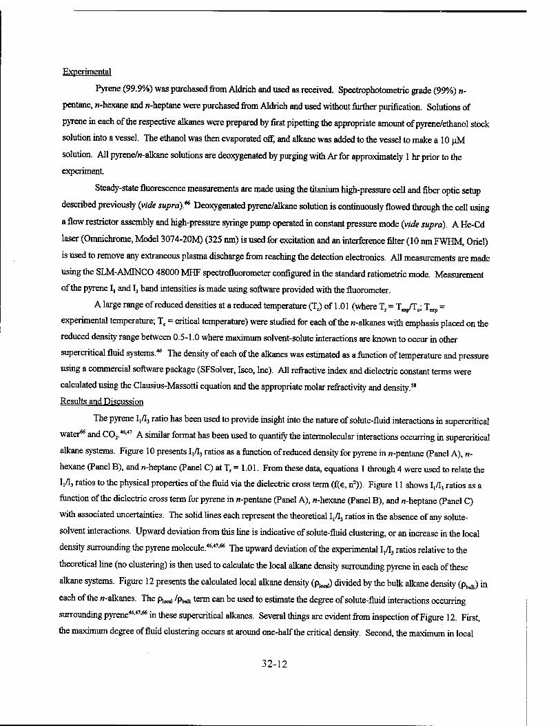
Experimental

Pyrene (99.9%) was purchased from Aldrich and used as received. Spectrophotometric grade (99%) «-

pentane, «-hexane and w-heptane were purchased from Aldrich and used without further purification. Solutions of

pyrene in each of the respective alkanes were prepared by first pipetting the appropriate amount of pyrene/ethanol stock

solution into a vessel. The ethanol was then evaporated off, and alkane was added to the vessel to make a 10 uM

solution. All pyrene/«-alkane solutions are deoxygenated by purging with Ar for approximately 1 hr prior to the

experiment.

Steady-state fluorescence measurements are made using the titanium high-pressure cell and fiber optic setup

described previously (vide supra).66 Deoxygenated pyrene/alkane solution is continuously flowed through the cell using

a flow restrictor assembly and high-pressure syringe pump operated in constant pressure mode (vide supra). A He-Cd

laser (Omnichrome, Model 3074-20M) (325 nm) is used for excitation and an interference filter (10 nm FWHM, Oriel)

is used to remove any extraneous plasma discharge from reaching the detection electronics. All measurements are made

using the SLM-AMINCO 48000 MHF spectrofluorometer configured in the standard ratiometric mode. Measurement

of the pyrene I, and I3 band intensities is made using software provided with the fluorometer.

A large range of reduced densities at a reduced temperature (Tr) of 1.01 (where Tr = T^/T,.; T =

experimental temperature; Tc = critical temperature) were studied for each of the n-alkanes with emphasis placed on the

reduced density range between 0.5-1.0 where maximum solvent-solute interactions are known to occur in other

supercritical fluid systems.46 The density of each of the alkanes was estimated as a function of temperature and pressure

using a commercial software package (SFSolver, Isco, Inc). All refractive index and dielectric constant terms were

calculated using the Clausius-Massotti equation and the appropriate molar refractivity and density.58


The pyrene 1,/Ij ratio has been used to provide insight into the nature of solute-fluid interactions in supercritical

water66 and C02.46'47 A similar format has been used to quantify the intermolecular interactions occurring in supercritical

alkane systems. Figure 10 presents I,/I3 ratios as a function of reduced density for pyrene in «-pentane (Panel A), n-

hexane (Panel B), and n-heptane (Panel C) at Tr = 1.01. From these data, equations 1 through 4 were used to relate the

I,/I3 ratios to the physical properties of the fluid via the dielectric cross term (f(e, n2)). Figure 11 shows I,/I3 ratios as a

function of the dielectric cross term for pyrene in w-pentane (Panel A), «-hexane (Panel B), and «-heptane (Panel C)

with associated uncertainties. The solid lines each represent the theoretical I,/I3 ratios in the absence of any solute-

solvent interactions. Upward deviation from this line is indicative of solute-fluid clustering, or an increase in the local

density surrounding the pyrene molecule.46'47'66 The upward deviation of the experimental I,/I3 ratios relative to the

theoretical line (no clustering) is then used to calculate the local alkane density surrounding pyrene in each of these

alkane systems. Figure 12 presents the calculated local alkane density (p^ divided by the bulk alkane density (p^ in

each of the «-alkanes. The p,^ /p^ term can be used to estimate the degree of solute-fluid interactions occurring

surrounding pyrene46'47,66 in these supercritical alkanes. Several things are evident from inspection of Figure 12. First,

the maximum degree of fluid clustering occurs at around one-half the critical density. Second, the maximum in local

32-12

density is 3 to 4 times the bulk alkane density. Finally, the degree of clustering is similar in each of the alkane systems

studied.

It has been previously shown for other supercritical fluids (e.g., C02, HjO) that a maximum in solute-fluid

clustering occurs at approximately one-half the critical density.'16,47'*6 This is fully consistent with our observations in all

supercritical alkanes, although measurements have not yet been made in the very low density region. The maximum in

local density in the alkane systems of approximately 3 to 4 times the bulk density is consistent with the results seen in

other fluids46-66 (vide supra) although slightly higher than those observed in supercritical C02.

Conclusions

An increase in local alkane density surrounding pyrene dissolved in supercritical C5, Q, and C7 n-alkanes is

observed at one half the critical density. The degree of augmentation (3 to 4 times p^J and the maximum in clustering,

at one-half the critical density, is fully consistent with previous results in other supercritical fluids.46,47,66 To our

knowledge, this type of clustering phenomena has not been previously observed within supercritical alkane systems.

This work points out that additional experimentation is needed to understand how these solute-solvent interactions in

aviation fuel precursors will affect fuel performance.

Effects of C(X> Sorption on Molten Polymers Dynamics

Poly(dimethylsiloxane) (PDMS) polymers are unique silicone polymers which possess a very low glass phase

transition temperature (Tg) of- 150K.67,68 For this reason, PDMS polymers are molten viscous polymers which exhibit

flow characteristics at ambient temperatures and are therefore model polymers for other systems with much higher

processing temperatures.67,68 PDMS polymers have found a wide range of applications from coatings and implants to

hydraulic fluids.67,68

There is significant interest in developing simple methodologies to control the transport properties of solid or

molten polymers because such governs aspects of polymer synthesis, polymer reactivity, and polymer processing.2,67,68 It

is well-known that C02 can be used to alter the characteristics of certain polymer systems.69-72 For example, recent work

has shown that molten polymers like PDMS can sorb tremendous amounts of C02 leading to a dramatic decrease in the

polymer bulk viscosity.69-72 However, there is much to be learned about how gas effusion affects polymer dynamics,

polymer free volume, the mobility of dissolved solutes, and polymer transport properties.

Rotational reorientation measurements have been used extensively to determine the nature of interactions

occurring within both amorphous polymer matrices,73-76 and at elastic cross-link junctions within various polymer

networks.77"80 For example, Fayer and co-workers76 have recenüy used the rotational reorientation dynamics of

dansylamide attached to a trifunctional silane within PDMS melts to attempt to relate local rotational dynamics to bulk

polymer properties. However, the rotation of the rather small (~3A in length) probe did not correlate well with bulk

polymer dynamics.

We have used a large, neutral solute in conjunction with time-resolved fluorescence anisotropy techniques to

32-13

correlate the rotational motion of the solute to bulk polymer properties. Specifically, we are interested in the effects of

the addition of C02 (at both ambient and supercritical conditions) on the behavior of model dopants within the polymer

matrix and whether we can track such effects. The model solute that we have chosen for our study is BTBP, which has

been previously used for rotational reorientation measurements within a variety of media.81"83 BTBP is a large (28 A in

length) neutral solute. Thus, there will be no charge interactions with the polymer matrix. BTBP has a unity quantum

yield,81-83 therefore small amounts may be dispersed within the polymer while maintaining sufficient S/N. BTBP has

been reported to be a spherical rotor with a single rotational correlation time.81-83 For this work, we have measured the

effects of polymer molecular weight and C02 on the rotational dynamics of BTBP to correlate the rotational correlation

time with the polymer's properties..

Experimental

Preparation of Bulk Polymer Solutions

A broad average molecular weight range (MW = 1250,2000,3780, 5970, 9430,13650,28000, and 49350

g/mol) of methyl-terminated PDMS was purchased from United Chemical Technologies, Inc (Bristol, PA) and used

without further purification. A^-Bis(2,5-di-tert-butylphenyl)-3,4,9,10-perylenedicarboximide (BTBP) was purchased

from Aldrich and used as received.

Stock solutions of BTBP (1 mM) were prepared in absolute ethanol. BTBP is randomly dispersed within the

PDMS via the following protocol: 1) the appropriate amount of BTBP stock solution is micropipetted into a vial; 2) the

vial is then placed within a hot oven for approximately 1 hr to evaporate any remaining ethanol solvent; 3) after cooling,

the appropriate quantity of PDMS is added to make a final solution that is 1 uM BTBP; and 4) the solutions are stirred

(with gentle heating for higher molecular weight samples) for approximately 2 wks to thoroughly disperse the BTBP

throughout the polymer. There is no evidence of BTBP aggregates.

Addition of CO- to the Polymer Samples

C02 is added to the polymer solutions via a syringe pump assembly which continuously delivers C02 to a high-

pressure cell containing the polymer sample. The stainless steel high-pressure cell was developed in-house and has

been described in detail previously.84 The cell has an optical pathlength of approximately 1 cm and contains quartz

optical windows (Behm Quartz Industries, Dayton, OH) which have been previously shown to exhibit no detectable

pressure induced birefringence over the pressure range studied.81

The BTBP/PDMS solution (3.75 mL) is directly pipetted into the high-pressure cell (internal volume = 5mL)

into which a teflon-coated stir bar has been placed. A valve assembly is then connected to the high-pressure cell which

attaches the cell to a high pressure syringe pump (Isco, Model 260D, Lincoln, NE) operating in constant pressure mode.

Throughout the experiment, a Haake A80 temperature bath is used for temperature control. The temperature is

monitored using a solid-state thermocouple (Cole Parmer, Vemon Hills, IL) and pressure is monitored within ±1 psi

using a calibrated Heise pressure gauge.

The cell is first charged to the highest pressure (-2500 psi) and allowed to equilibrate at experimental

temperature with constant stirring. Initially, polymer samples were equilibrated overnight before rotational reorientation

32-14

measurements were made. Figure 13 presents the recovered rotational correlation time for BTBP in PDMS (MW =

28000 g/mol) as a function of time at approximately 1000 psia. Time zero corresponds to 12 hrs of equilibration time

with stirring. We observe an initial increase in the rotational correlation time which we attribute to increased pressure

within the system from delivery of the C02. The systematic decrease of the rotational correlation time with time tracks

the diffiision of C02 into the PDMS and subsequent dilation of the polymer. This systematic decrease due to continued

dilation of the polymer was shown to continue for upwards of 1 wk. Therefore, all subsequent PDMS/C02 samples

were equilibrated for approximately 2 wks with stirring at the initial experimental temperature and pressure.

Instrumentation

All time-resolved measurements were made using a multiharmonic frequency-domain fluorometer (SLM-

AMINCO 48000 MHF). For steady-state measurements, a Xe arc lamp is used for excitation with a monochromator for

appropriate wavelength selection of emission and excitation (bandpass = 4 nm). The 514.5 nm line of a CW Ar+ laser

(Coherent, Model Innova 400) is used for excitation during all time-resolved experiments. The output from the laser is

passed through an interference filter to eliminate any extraneous plasma discharge from reaching the detector.

Fluorescence from the sample is monitored through a 550 longpass filter and a polarizer set at the magic angle

condition for fluorescence lifetime measurements.85 Sinusoidally modulated light is generated using a Pockels cell

driven at 5 MHZ, and data is collected from 5 to 200 MHZ (39 frequencies). At least 9 replicate measurements were

made. Rhodamine 6G in water was used as the reference lifetime for all excited-state fluorescence lifetime

measurements (T = 3.85 ns).86 The BTBP fluorescence lifetime was found to be constant over the range of experimental

conditions. Operation of a typical MHF frequency-domain fluorometer has been described in great detail elsewhere.87"89

Phase and demodulation data were fit to various test models by using a commercially available global analysis software

package (Globals Unlimited).90

Frequency-domain measurements of the time-resolved decay of anisotropy are made by measurement of the

differential phase angle (A = 0X - 6,) and polarized modulation amplitude (A = AC/AC J. The decay of the intensity of

the parallel (I,(t)) and perpendicular Q.Jff) components of the polarized fluorescence in the frequency domain may be

described by:89-91

7,(0 = l/3[7(0(l+2r(0)] (7)

7±(0 = l/3[7(0(l-r(0)] (8)

where r(t) is the fluorescence decay of anisotropy. Assuming that the fluorophore is a spherical rotor, the decay of

anisotropy can be written:

r(t) = r0exp(--j-) (9)

32-15

where r0 is the limiting anisotropy, the anisotropy measured in the absence of rotational motion. The rotational

correlation time, «j>, may then be recovered by fitting the differential phase angle (A) and the polarized modulation ratio

(A) as a function of frequency using a non-linear least squares program:91

A = axctmlJJ J-J] (10)

A - r*' + D'V

where N and D are the polarized components of the sine and cosine Fourier transform, respectively. The rotational

correlation time is then fit using a non-linear least squares minimization of the chi-squared (x2) parameter as defined

by:91

Y2_ lx-rA» -Ag(cp) i A>)-A^)

X " D^ ( a } n^ ( ^ ) (12)

where the subscripts c and m denote the computed and measured differential phase angles and polarized modulation

ratios, respectively, o is the variance, and D is the number of degrees of freedom. The goodness of fit between the

model and the experimental data is determined by the closeness of the x2 parameter to unity as well as the randomness of

the residuals around zero.


Rotational Reorientation Dynamics within Molten Polymers

The determination of the rotational correlation time of BTBP as a function of MW allows us to determine if our

large neutral solute (BTBP) can track the entanglement value (Me) for PDMS. The entanglement value is a

characteristic value of amorphous polymers in which the chains within the polymer become too long to slip past one

another easily.67,68 Although the polymer will still exhibit flow characteristics as the MW increases, a "leveling off" of

physicochemical properties (i.e., viscosity, refractive index) occurs past the entanglement value.67,68 Subsequently, if

BTBP is large enough to fill the free volume fully within the polymer matrix, the rotational correlation time should level

off above the entanglement value.

Figure 14 presents typical differential phase angle (Panel A) and polarized modulation ratio (Panel B) data for

32-16

BTBP in several PDMS molecular weight polymers. The points represent actual experimental data and the lines are

recovered best fits to a single exponential decay law. From this data, it is obvious that as the molecular weight of the

polymer increases, the differential phase angle and polarized modulation ratio subsequently increase, indicating an

increase in the rotational correlation time. Figure 15 presents the recovered rotational correlation times as a function of

PDMS molecular weight. We see that as the polymer molecular weight increases, there is an initial increase in the

rotational correlation time and a leveling off at ~10000 g/mol. Entanglement values have been reported for PDMS

polymers in the literature ranging between -800092 and 8625s7 g/mol. Our rotational reorientation data "breaks" at a

value that is near these reported literature values. Thus, the large size of the BTBP probe allows us to easily track the

PDMS chain entanglement process.

Rotational reorientation data as a function of PDMS molecular weight also allows us to establish a convenient

link between <J) and some aspect of the polymer. Figure 16 presents the BTBP rotational correlation time as a function

of polymer density. The solid line is the straight line fit. This will be used later to correlate the recovered rotational

correlation times in PDMS dilated with C02.

Effect of COT on PDMS Dynamics

Figure 17 presents the recovered rotational correlation time of BTBP as a function of added C02 pressure in

several representative molecular weight PDMS polymers (i.e., 1250,9430,13650, and 28000 g/mol) at 25 °C. There

are several aspects of this data that merit special attention. First, the rotational correlation time decreases dramatically

(up to 5 times) with the addition of liquid C02 from the rotational correlation times observed in the neat PDMS melts. It

is known that C02 can swell PDMS up to 50% by weight,69"72 and our data is fully consistent with the dilation and

subsequent decrease in bulk density of the PDMS polymer with addition of C02. Second, it appears that the decrease in

rotational correlation time can be further decreased by increasing the C02 pressure. We observe that the rotational

correlation time "snaps" to a much lower value between 500 and 1000 psi of C02 for all molecular weight polymers

before leveling off with increasing pressure above 1000 psi. Examination of the phase equilibria for C02 at 25 °C shows

that the transition between the gas and liquid state of C02 occurs between these pressures. The higher density liquid

C02 dilates and swells the polymer to a greater extent than the less dense gaseous C02. The density of the swollen

polymer may be estimated by using the relationship between the PDMS density and the recovered rotational correlation

time in neat PDMS melts as a function of molecular weight (Figure 16). Figure 18 presents the calculated polymer

densities as a function of added C02 for each of the polymers.

These results prompted us to question whether the BTBP rotational correlation time could actually be tuned by

addition of C02 to the polymer. From the previous 25 °C experiments, we noted a sharp change in the rotational

correlation time as a function of pressure. It is known that C02 above its critical temperature (Tc = 31.1 °C; Pc = 1070.4

psia) exhibits no phase boundary with increasing pressure. Thus, we questioned if we could tune the BTBP rotational

reorientation time. Figure 19 presents the recovered rotational correlation times for BTBP in PDMS (MW = 9430

g/mol) at ambient (T = 25.0 °C) and supercritical (T = 36.5 °C) conditions as a function of C02 pressure. The recovered

rotational times for BTBP in the PDMS swelled with supercritical C02 are slightly lower due to the increase in

32-17

temperature which subsequently decreases <J> (Figure 19A). More interestingly, closer examination of the T = 36.5 °C

data in Figure 19B shows that instead of the sharp change in rotational correlation time observed with increasing C02

pressure in the ambient system (vide supra), we instead observe a very gradual easily tuned decrease in the BTBP

rotational correlation time. The inherent tunability of the physicochemical properties of supercritical C02 with

temperature and pressure can therefore be used to tune the PDMS matrix and hence the BTBP rotational dynamics.

Conclusions

We have shown that our large model solute, BTBP, can be used to track the bulk polymer dynamics within the

PDMS polymer matrix. The rotational correlation time is shown to scale with polymer molecular weight before leveling

off above the known PDMS entanglement value. The rotational correlation time of BTBP within these molten polymers

has been used to relate the recovered rotational dynamics within CCydilated PDMS to the bulk density of the swelled

polymer matrix. We have shown that the addition of ambient temperature C02 to PDMS causes a dramatic decrease in

the BTBP rotational correlation time near the C02 gas-liquid phase boundary (25 °C). Addition of supercritical C02

allows us to tune the bulk polymer density and the BTBP rotational dynamics.

Cosolvent Effects on Rotational Reorientation Dynamics in Supercritical CO,

The inherent tunability of supercritical fluids have made them attractive for use in separations,1"4 chemical reactions,6"13

and extractions.5 Supercritical C02 (scC02) is environmentally friendly, inexpensive, and has very mild critical

parameters (Tc = 31.1 °C; Pc = 1070.4 psia; pc = 0.468 g/mL). Supercritical C02 has found a wide range of industrial

applications including replacement of hazardous solvents in the clothing dry cleaning process, decaffeination of coffee

beans, and a wide range of extractions and reactions in the petroleum, polymer and pharmaceutical industry.2"4 Although

scC02 is by far the most commonly used supercritical solvent, it is, unfortunately, a rather poor solvent for polar solutes.

C02 is nonpolar and has a relatively low solvent strength. In addition, although there is inherent tunability of the scC02

solvent strength with pressure and temperature, it still exhibits a cohesive energy density less than cyclohexane and

orders of magnitude less than common industrial solvents such as methanol and acetonitrile. This low cohesive energy

density translates into a lack of selectivity for Chromatographie separations, extractions and reactions.

There are several approaches to "modify" C02 in order to improve the power and hence selectivity of the

solvent. The addition of small quantities (x = 0.1 - 5 mole%) of an organic entrainer (cosolvent) have been shown to

dramatically increase solute loading as well as increase reaction/separation selectivity.70-93"95 More recently, a

perfluoropolyether-based surfactant (PFPE) has been used to form stable reverse micelles in scCOj.96 However,

although promising, these PFPE microemulsions are a relatively new technology and have not yet been thoroughly

characterized. In addition, there are many recognized advantages to using the more simple cosolvent-modified systems.

For example, cosolvents do not significantly alter the C02 critical properties. In addition, only small quantities of

entrainer need to be added, giving both an economical and a waste disposal advantage. Enhanced solute loading of both

polar and nonpolar solutes is achieved as well as improving selectivity of reactions, extractions, and separations.70-93"95

32-18

Many of these desirable properties have been attributed to preferential solvation of the cosolvent around the dissolved

solute in these supercritical systems. Given this, the goal of this work was to experimentally quantify preferential

solvation in a supercritical fluid system.

Rotational reorientation dynamics measurements offer a convenient means to relate the solute's dynamics to

the local solvent microdomain (vide supra). We have used the fluorescent probe BTBP in concert with time-resolved

fluorescence anisotropy techniques to determine rotational dynamics of a solute as a function of MeOH-modified scC02

density. These data have allowed us to quantify the extent of solute-fluid clustering and determine how the solvation

shell surrounding the solute changes as a function of bulk density.

Experimental

Preparation of the Cosolvent Mixture

Methanol (spectrophotometric grade, Aldrich) is charged into a stainless steel vessel equipped with two 1/8"

tubing pieces, one leading to a SFC grade C02 tank (Scott Specialty Gases, Plumsteadville, PA) and the other to a high-

pressure syringe pump (Model 260D, Isco). After charging the MeOH, the vessel is promptly placed into an ice bath

and C02 is added to the vessel as it is vigorously shaken and stirred to ensure that the mixture is one phase. The mixture

is then transferred into the syringe pump, and the pump piston is run in and out several times to ensure mixing. The

pump head is then heated to experimental temperature (-45 °C) and allowed to equilibrate for several days to complete

the mixing process. The MeOH/C02 mixture is then delivered to our high-pressure stainless steel optical cell (vide

supra) which has been previously charged with BTBP. All MeOH/C02 mixtures for this experiment were 5 mol%

MeOH. The cell is initially charged with the highest experimental pressure of the cosolvent mixture (~3000 psia) and

the pressure is gradually decreased throughout the experiment until the mixture becomes biphasic.

All mixture densities and viscosities were calculated using the equations described by Foster and co-workers.97


The steady-state emission and excitation spectra of BTBP in MeOH-modified C02 at 45°C and 2667 psia are

shown in Figure 20. Figure 21 presents the effects of density on the excited-state fluorescence lifetimes for BTBP in

MeOH-modified C02 at 46.0 °C. As mentioned previously, it has been established that the fluorescence lifetime for

BTBP is relatively constant as a function of its local environment.82,83 However, we observe a systematic decrease in the

BTBP fluorescence lifetime with increasing MeOH/C02 bulk density. This phenomena may be readily explained by the

Strickler-Berg relationship, which links the radiative rate of the fluorophore 00 to the properties of the solvent and

fluorophore through the following equation:63

kr = 2900«2

VQ/WV (13)

where n is the solvent refractive index, v0 is the peak frequency in the fluorophore absorbance spectrum, and Jedv is the

integrated area under the fluorophore absorbance spectrum. The radiative rate is directly related to the quantum yield

32-19

($) and fluorescence lifetime (x) of the fluorophore (k, = 4>/T). If the quantum yield of the probe is unity, the radiative

rate is the inverse of the fluorescence lifetime.63 Because the radiative rate is related to the square of the refractive index,

if the observed change in fluorescence lifetime is due to the changing refractive index with increasing pressure, a plot of

1/T VS n2 should be linear. Figure 22 shows that a Strickler-Berg interpretation of our data reasonably explains (r2 =

0.926) the decrease in fluorescence lifetime of BTBP as the refractive index of the MeOH/C02 mixture increases with

increasing pressure. Similar results (not shown) have been determined for BTBP in neat C02 at 46.0 °C.

Through the Debye-Stokes-Einstein equation, the rotational reorientation time of a solute can be directly

related to the physical parameters of the system, including the viscosity, temperature, and the volume of the reorienting

species.56 Figure 23 presents the experimental rotational correlation time for BTBP as a function of cosolvent mixture

bulk density at 46.0 °C. The rotational correlation time predicted from the DSE equation (given the volume of BTBP,

the temperature, and the calculated bulk viscosity) as well as the rotational correlation time for BTBP in neat C02 are

denoted. In the low density region, we see that the rotational correlation time deviates significantly from predicted

values and only nears the DSE prediction at higher densities. This same phenomena has been observed for BTBP in

neat C02 at 35 °C81 and is attributed to a clustering of solvent molecules around the solvent, increasing the fluorophore

volume and hence the rotational correlation time. This solute-fluid clustering dissipates at higher liquid-like bulk

densities causing the rotational correlation time to more closely follow DSE predictions. The rotational correlation time

in our system can allow us to predict the size of the reorienting species as well as determine the solvation of MeOH

surrounding the BTBP.

The observed rotational correlation time (<|>0 J can be used in conjunction with the rotational correlation time of

BTBP in MeOH (<t>Me0„ = 150 ps) and the rotational correlation time in neat C02 (<}>C02 = 34 ps) to estimate the fraction

of MeOH (fMe0H) and C02 (fC02) observed by the probe through the following equation:

^obs = ^MeOHJMeOH + §C02 fc01 (14)

Figure 24 presents the percentage of MeOH estimated using this analysis as a function of fluid density. Recall that the

bulk MeOH mole fraction is only 5%. We observe a very large degree of preferential solvation (30% MeOH; 6 fold)

surrounding the BTBP in the low density region before leveling off in the higher density region. It is interesting to note

that the percentage of MeOH in the higher density region is actually less than the expected for a 5 mol% solution. This

may in part be due to the oversimplification of Equation 14 in predicting the MeOH solvation.

The degree of "solvent" clustering around the BTBP probe can be roughly estimated by dividing the recovered

experimental rotational correlation time (^„^^„^ by the rotational correlation time predicted by the DSE equation

(4>DSE)- Figure 25 presents ^„penmentai /4>DSE as a function of bulk density for the cosolvent mixture. These average values

show that in the low density region, we are observing an increase in the BTBP rotational reorientation on the order of 5

times the expected value. This increase in the rotational correlation time is consistent with local density augmentation of

the solvent surrounding the solute. In turn, this is consistent with other systems81 where clustering phenomena decreases

32-20

with increasing bulk density of the mixture.

Conclusions

For the MeOH-modified C02 system we see a significant decrease in the fluorescence lifetime of BTBP with

increasing bulk mixture density. This phenomena can be readily explained by use of the Strickler-Berg analysis,

showing that the change in BTBP fluorescence lifetime is due to changing solvent refractive index. We observe that the

rotational correlation time for BTBP in MeOH-modified C02 deviates significantly from the Debye-Stokes-Einstein

prediction and the recovered rotational correlation time in neat C02. These deviations can be used to predict the local

composition surrounding the BTBP in the MeOH-modified C02 system. Preliminary results show that preferential

MeOH solvation exists surrounding BTBP in MeOH-modified C02 in the low bulk density region and that the local

composition surrounding the probe can be estimated at approximately 5 times the bulk density in the low density region.

Summary

Steady-state and time-resolved fluorescence spectroscopy were used to quantify solvation phenomena

occurring in several neat and modified supercritical fluid systems. Measurement of pyrene I,/!, ratios allowed us to

experimentally determine solute-fluid interactions occurring in supercritical water. These results showed that near one

half the fluid critical density, the local density augmentation is on the order of five times greater than the bulk water

density. Pyrene was further used to quantify intermolecular interactions in supercritical w-alkanes (fuel precursors). An

increase in local alkane density surrounding pyrene dissolved in supercritical C5, C6, and C7 «-alkanes was observed at

one half the critical density with a degree of augmentation on the order of 3 to 4 times the bulk alkane density. These

results have shown that further experimentation is needed for a complete picture of how solute-fluid interactions in

aviation fuel precursors may affect fuel performance. We have used rotational reorientation measurements of a large

neutral solute, BTBP, to track bulk polymer dynamics within several PDMS polymers. We have shown that the addition

of ambient temperature C02 to PDMS causes a dramatic decrease in the BTBP rotational correlation time near the C02

gas-liquid phase boundary (25 °C). In addition, we showed that addition of supercritical C02 allowed us to tune the bulk

polymer density and the BTBP rotational dynamics. We have also used BTBP rotational reorientation measurements to

quantify preferential solvation in MeOH-modified C02. We observed that the rotational correlation time for BTBP in

MeOH-modified C02 deviated significantly from the Debye-Stokes-Einstein prediction and the recovered BTBP

rotational correlation time in neat C02. These deviations were used to predict the local composition surrounding the

BTBP in the MeOH-modified C02 system. Preliminary results have shown that preferential MeOH solvation exists

surrounding BTBP in MeOH-modified C02 in the low bulk density region. From these results, the local composition

surrounding the probe can be estimated to be approximately 5 times the bulk density in the low density region.

32-21

References

1. U. Van Wassen, I. Swaid, and G.M. Schneider, Angew. Chem. Int. Ed. Engl., 19,515 (1980).

2. CA. Eckert, J.G. Van Alsten, and T. Stoicos, Environ. Sei. Technol., 20,319 (1986).

3. D. Bradley, New Scientist, 143, 32 (1994).

4. V.K. Jain, Environ. Sei. Technol., 27,807 (1993).

5. S.B. Hawthorne, Y. Yang, and D.J. Miller, Anal. Chem., 66,2912 (1994).

6. T.A. Rhodes, K. O'Shea, G. Bennett, K.P. Johnston, and M.A. Fox, J. Phys. Chem., 99, 9903 (1995).

7. B.C. Wu, MT. Klein, and S.I. Sandler, Ind. Eng. Chem. Res., 30,822 (1991).

8. R. Li, T.D. Thornton, and P.E. Savage, Environ. Sei. Technol., 38,321 (1992).

9. T.D. Thornton and P.E. Savage, AIChE X, 38,321 (1992).

10. S. Gopalan and P.E Savage,. J. Phys. Chem., 98,12646 (1994).

11. P.E. Savage, R. Li, and J.T. Santini, Jr., J. Supercrit. Fluids, 7,135 (1994).

12. T.J. Houser, D.M.; Tiffany, Z. Li, M.E. McCarville, andM.E. Houghten, Fuel, 65, 827 (1986).

13. P.A. Webley, J.W. Tester, and H.R. Holgate, Ind. Eng. Chem. Res., 30,1745 (1991).

14. E.U. Franck, Ber. Bunsenges. Phys. Chem, 88, 820 (1988).

15. L. Ember, C&E News, 72,4 (1994).

16. J. Krukowski, Pollution Eng., 26,11 (1994).

17. J. Beard, New Scientist, 139,19 (1993).

18. J. Manji, Automation, 38,26 (1991).

19. C. Caruana, Chem. Eng. Prog, 91, 10 (1995).

20. R. Gould, New Scientist, 141,19 (1994).

21. LB. Petsche and P.G. Debenedetti, J. Chem. Phys., 91,7075 (1989).

22. J.A. O'Brien, T.W. Randolph, C. Carlier, and S. Ganapathy, AIChE X, 39, 1061 (1993).

23. S. Kim and K.P. Johnston, AIChE X, 33,1603 (1987).

24. CA. Eckert and B.L. Knutson, Fluid Phase Equil., 83, 93 (1993).

25. K.P. Johnston, S. Kim, and X Combes, in Supercritical Fluid Science and Technology, K.P.L Johnston and

J.M.L. Penninger, Eds. (ACS Symposium Series 406, American Chemical Society, Washington, DC, 1989).

26. S.G Kazarian and M. Poliakoff, X Phys. Chem., 99, 8624 (1995).

27. R.W. Shaw, T.B. Brill, A.A. Clifford, CA. Eckert, and E.U. Franck, C&E News 69,26 (1991).

28. S. Iyer, G.R. Nicol, and M.T. Klein, X Supercrit. Fluids 9,26 (1996).

29. T.J. Houser, Y. Zhou, and X. Liu, X Supercrit. Fluids 9,106 (1996).

30. E.U. Franck, Ber. Bunsenges. Phys. Chem 88, 820 (1988).

31. E.U. Franck, Pure Appl. Chem. 53,1401 (1981).

32. L.B. Kriksunov and D.B. Macdonald, X Electrochem. Soc. 142,4069 (1995).

33. E.E. Brock and P.E. Savage, AIChE X, 41,1874 (1995).

32-22

34. R. Li, T.D. Thornton, and P.E. Savage, Environ. Sei. Technol. 38,321 (1992).

35. T.D. ThorntonandP.E. Savage, AIChEX 38,321 (1992).

36. S. Gopalan and P.E. Savage, J. Phys. Chem. 98,12646 (1994).

37. P.E. Savage, R. Li, and J.T. Santini, Jr., J. Supercrit. Fluids 7,135 (1994).

38. T.J. Houser, D.M. Tiffany, Z. Li, M.E. McCarville, and M.E. Houghten, Fuel 65,827 (1986).

39. P.A. Webley, J.W. Tester, and H.R. Holgate, Ind. Eng. Chem. Res. 30,1745 (1991).

40. P.T. Cummings, H.D. Cochran, J.M. Simonson, R.E. Mesmer, S. Karaborni, J. Phys. Chem. 94,5606 (1992).

41. J. Gao, J. Am. Chem. Soc. 115,6893 (1993).

42. K.P. Johnson, P.B. Balbuena, T. Xiang and P. J. Rossky, in Innovations in Supercritical Fluids Science and

Technology, KW. Hutchenson, N.R. Foster, Eds. (ACS Symposium Series 608, American Chemical Society,

Washington, DC, 1995).

43. D.C. Dong and M.A. Winnik, Can. J. Chem. 62,2560 (1984).

44. R. Waris, W.E. Acree, Jr., and K.W. Street, Jr., Analyst 113,1465 (1988).

45. K. Hara and W.R. Ware, Chem. Phys. 51,61 (1980).

46. J.K. Rice, E.D. Niemeyer, RA. Dunbar, and F.V. Bright, J. Am. Chem. Soc. 117,5832 (1995).

47. Y.-P. Sun, C.E. Bunker, and N.B. Hamilton, Chem. Phys. Lett. 210,111 (1993).

48. J. Zagrobelny and F.V. Bright, J. Am. Chem. Soc. 115,701 (1993).

49. Y.-P. Sun and C.E. Bunker, J. Phys. Chem. 99,13778 (1995).

50. S.-H. Chen and V.L. McGuffin, Appl. Spectrosc. 48,596 (1994).

51. G. Patonay, M.E. Rollie and IM Warner, Anal. Chem. 57,569 (1985).

52. Schematics and part information for a similar high-pressure titanium cell were kindly provided through a

private communication with Professor T.B. Brill and Mr. M. Kieke.

53. For a similar cell design, see: P.D. Spohn and T.B. Brill, Appl. Spectrosc. 41,1152 (1987).

54. J.M. Harris, F.E. Lytle, and T.C. McCain, Anal. Chem. 48,2095 (1976).

55. J.N. Demas, Excited State Lifetime Measurements (Academic Press, New York, 1983).

56. J.R. Lakowicz, Principles of Fluorescence Spectroscopy (Plenum Press, New York, 1983).

57. K.S. Pitzer and S.M. Sterner, J. Chem. Phys. 101,3111 (1994).

58. P.W. Atkins, Physical Chemistry, 4th ed. (W.H. Freeman & Co., New York, 1990).

59. M.J. Kamlet, J.L. Abboud, and R.W. Taft, J. Am. Chem. Soc. 99,6027 (1977).

60. T.A. Betts, J. Zagrobelny, and F.V. Bright, J. Am. Chem. Soc. 114,8163 (1992).

61. B. Stevens, M.F. Thomaz, and J.J.Jones, Chem. Phys. 46,405(1967).

62. CRC Handbook oj'Chemisty andPhysics,!r4thEd. (Chemical Rubber Publishing Co., Boca Raton, 1993-

1994).

63. J.B. Birks, Organic Molecular Photophysics, Vol. 1 (Wiley Interscience, New York, 1973).

64. B. Stevens and M.F. Thomaz, Chem. Phys. Lett. 1,535 (1968).

32-23

65. J.F. Kauffinan, Anal. Chem. 68,248A (1996).

66. E.D. Niemeyer, R.A. Dunbar, and F. V. Bright, Appl. Spectrosc., submitted for publication.

67. L.H. Sperling, Introduction to Physical Polymer Science, 2nd Ed (Wiley Interscience, New York, 1992).

68. P. J. Flory, Principles of Polymer Chemistry (Cornell University Press, Ithaca, 1969).

69. Y. Xiong, and E. Kiran, Polymer, 36,4187 (1995).

70. A.R. Berens, and G.S. Huvard in Supercritical Fluid Science and Technology, K.P. Johnston, J.M.L.

Penninger, Eds. (ACS Symposium Series 406, American Chemical Society, Washington, DC, 1989).

71. A. Garg, E. Gulari, and C.W. Manke, Macromol., 27,5643 (1994).

72. G.K. Fleming and W. J. Koros, Macromol., 19,2285 (1986).

73. J.L. Viovy, C.W. Frank, and L. Monnerie, Macromol., 18,2606 (1985).

74. P.D. Hyde, M.D. Ediger, T. Kitano, and K. Ito, Macromol., 22,2253 (1989).

75. J.L. Viovy, L. Monnerie, and F. Merola, Macromol., 18,1130 (1985).

76. A.D. Stein, D.A. Hoffinan, A.H. Marcus, P.B. Leezenberg, C.W. Frank, and M.D. Fayer, J. Phys.Chem., 96,

5255(1992).

77. J.P. Jarry and L. Monnerie, Macromol., 12, 927 (1979).

78. J.P. Jarry, B. Erman, and L. Monnerie, Macromol., 19,2750 (1986).

79. P.B. Leezenberg, A.H. Marcus, C.W. Frank, and M.D. Fayer, J. Phys. Chem., 100,7647 (1996).

80. A.D. Stein, D.A. Hoffinan, C.W. Frank, and M.D. Fayer, J. Chem. Phys., 96,3269 (1992).

81. M.P. Heitz andF.V. Bright, J. Phys. Chem., 100,6889 (1996).

82. D. Ben-Amotz and J.M. Drake, J. Chem. Phys., 89,2 (1988).

83. A.M. Williams and D. Ben-Amotz, Anal. Chem., 64,700 (1992).

84. T.A. Betts and F.V. Bright, Appl. Spectrosc., 44,1190 (1990).

85. R.D. Spencer and G. Weber, J. Chem. Phys., 52,1654 (1970).

86. M.P. Heitz and F. V. Bright, Appl. Spectrosc., 49,20 (1995).

87. E. Gratton, D.M. Jameson, and R.D. Hall, Anna Rev. Biophys. Bioeng., 13,105 (1984).

88. D.M. Jameson, E. Gratton, and R.D. Hall, Appl. Spectrosc. Rev, 20,55 (1984).

89. F.V. Bright, T.B. Betts, and K.S. Litwiler, CRC Crit. Rev. Anal. Chem., 21,389 (1990).

90. J.M. Beecham, E. Gratton, M. Ameloot, J.R. Knutson, and L. Brand in Topics in Fluorescence Spectroscopy,

Vol. 2, J.R. Lakowicz, Ed (Plenum Press, New York, 1991).

91. F.V. Bright, Appl. Spectrosc, 49,14A (1995).

92. R.F.T. Stepto, Eur. Polym. J., 29,415 (1993).

93. Supercritical Fluid Engineering Science. Fundamentals and Applications, E. Kiran, J.F. Brennecke, Eds.

(ACS Symposium Series 514, American Chemical Society, Washington, DC, 1993).

94. Supercritical Fluid Technology. Theoretical and Applied Approaches in Analytical Chemistry, F.V. Bright,

M.E.P. McNally, Eds. (ACS Symposium Series 488, American Chemical Society, Washington, DC, 1992).

32-24

95. MT. Combs, M. Gandee, M. Ashraf-Khorassani, and L.T. Taylor, Anal. Chem., submitted for publication.

96. K.P. Johnston, K.L. Harrison, MJ. Clarke, S.M. Howdle, M.P. Heitz, F.V. Bright, C. Carlier, and T.W.

Randolph, Science, 271,624 (1996).

97. K.D. Tilly, N.R. Foster, S.. Macnaughton, and D.L. Tomasko, Ind. Eng. Chem. Res., 33,681 (1994).

32-25

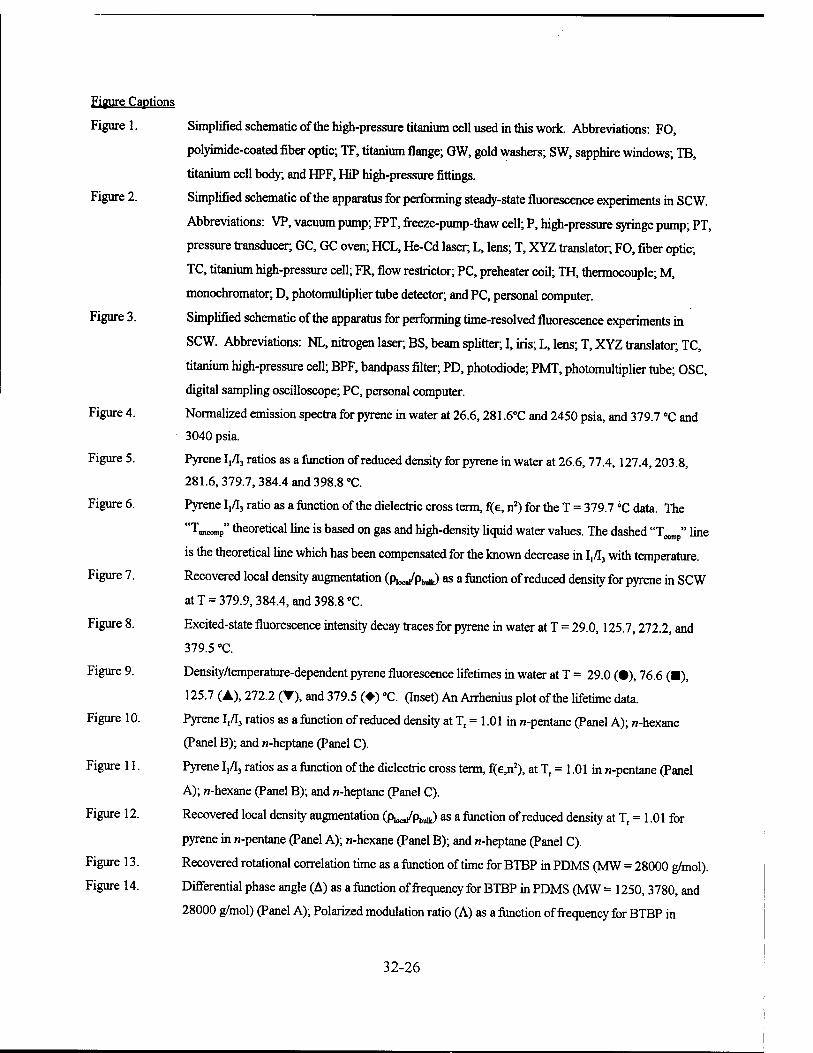
Figure Captions

Figure 1. Simplified schematic of the high-pressure titanium cell used in this work. Abbreviations: FO,

polyimide-coated fiber optic; TF, titanium flange; GW, gold washers; SW, sapphire windows; TB,

titanium cell body; and HPF, HiP high-pressure fittings.

Figure 2. Simplified schematic of the apparatus for performing steady-state fluorescence experiments in SCW.

Abbreviations: VP, vacuum pump; FPT, freeze-pump-thaw cell; P, high-pressure syringe pump; PT,

pressure transducer; GC, GC oven; HCL, He-Cd laser; L, lens; T, XYZ translator; FO, fiber optic;

TC, titanium high-pressure cell; FR, flow restrictor; PC, preheater coil; TH, thermocouple; M,

monochromator; D, photomultiplier tube detector; and PC, personal computer.

Figure 3. Simplified schematic of the apparatus for performing time-resolved fluorescence experiments in

SCW. Abbreviations: NL, nitrogen laser; BS, beam splitter; I, iris; L, lens; T, XYZ translator, TC,

titanium high-pressure cell; BPF, bandpass filter; PD, photodiode; PMT, photomultiplier tube; OSC,

digital sampling oscilloscope; PC, personal computer.

Figure 4. Normalized emission spectra for pyrene in water at 26.6,281.6°C and 2450 psia, and 379.7 °C and

3040 psia.

Figure 5. Pyrene 1,/L, ratios as a function of reduced density for pyrene in water at 26.6,77.4,127.4,203.8,

281.6, 379.7,384.4 and 398.8 °C.

Figure 6. Pyrene I,/I3 ratio as a function of the dielectric cross term, f(e, n2) for the T = 379.7 °C data. The

"Timconip" theoretical line is based on gas and high-density liquid water values. The dashed "T " line

is the theoretical line which has been compensated for the known decrease in I,^ with temperature.

Figure 7. Recovered local density augmentation (plocypbdk) as a function of reduced density for pyrene in SCW

at T = 379.9, 384.4, and 398.8 °C.

Figure 8. Excited-state fluorescence intensity decay traces for pyrene in water at T = 29.0,125.7,272.2, and

379.5 °C.

Figure 9. Density/temperature-dependent pyrene fluorescence lifetimes in water at T = 29.0 (•), 76.6 (■),

125.7 (A), 272.2 (▼), and 379.5 (♦) "C. (Inset) An Arrhenius plot of the lifetime data.

Figure 10. Pyrene I,/I3 ratios as a function of reduced density at Tr = 1.01 in n-pentane (Panel A); n-hexane

(Panel B); and n-heptane (Panel C).

Figure 11. Pyrene It/13 ratios as a function of the dielectric cross term, f(e,n2), at Tr = 1.01 in n-pentane (Panel

A); «-hexane (Panel B); and n-heptane (Panel C).

Figure 12. Recovered local density augmentation (p^p^ as a function of reduced density at Tr = 1.01 for

pyrene in n-pentane (Panel A); n-hexane (Panel B); and n-heptane (Panel C).

Figure 13. Recovered rotational correlation time as a function of time for BTBP in PDMS (MW = 28000 g/mol).

Figure 14. Differential phase angle (A) as a function of frequency for BTBP in PDMS (MW = 1250, 3780, and

28000 g/mol) (Panel A); Polarized modulation ratio (A) as a function of frequency for BTBP in

32-26

PDMS (MW = 1250,3780, and 28000 g/mol) (Panel B).

Figure 15. Recovered BTBP rotational correlation times in PDMS as a function of increasing molecular weight.

M, denotes the entanglement values reported for PDMS in the literature.

Figure 16. Natural log of the recovered BTBP rotational correlation time as a function of PDMS density. The

solid line represents the first order fit to the data.

Figure 17. Recovered BTBP rotational correlation times in PDMS (MW = 1250,9430,13650, and 28000

g/mol) as a function of C02 pressure at 25 °C.

Figure 18. Calculated densities of CCydilated PDMS (MW = 1250,9430,13650, and 28000 g/mol) as a

function of C02 pressure at 25 °C.

Figure 19. Recovered BTBP rotational correlation times in PDMS (MW = 9430 g/mol) as a function of C02

pressure at ambient (25 °C) and supercritical (T = 36.5 °C) conditions (Panel A); Expanded view of

the T = 36.5 °C data.

Figure 20. Steady-state emission and excitation spectra for BTBP in MeOH-modified C02 at 46.0 °C and 2667

psia.

Figure 21. BTBP fluorescence lifetime as a function of cosolvent mixture bulk density at 46.0 °C.

Figure 22. Strickler-Berg plot for BTBP in MeOH-modified C02 at 46.0 °C.

Figure 23. Recovered BTBP rotational correlation times in MeOH-modified C02 at 46.0 °C. The dashed line

indicates the rotational correlation times predicted by the Debye-Stokes-Einstein equation. The

recovered rotational correlation time in neat C02 at the experimental temperature is marked for

reference.

Figure24. Percentage ofMeOH surrounding BTBP calculated using Equation 15 as a function of bulk solvent

mixture density.

Figure 25. Recovered local density augmentation ((J)«,*™,,^ /<J>DSE) for BTBP in MeOH-modified C02 as a

function of bulk cosolvent mixture density.

32-27

3 O)

U-J I-

i- •)i

1

J

2 Q O a.

i

m i- u.

Q. X L-

1

2 3 O)

32-28 il

o DL

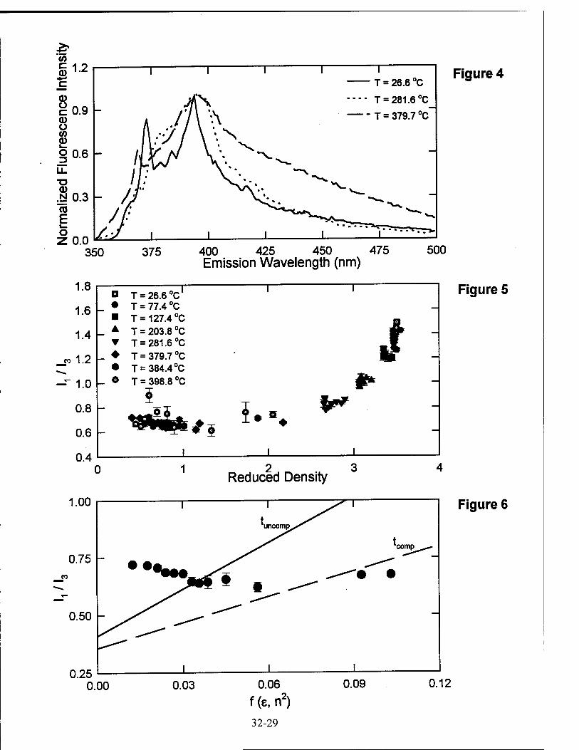
T = 26.6 °C

T = 281.6 °C T = 379.7 °C

Figure 4

350 375 400 425 450 475 Emission Wavelength (nm)

500

1.8

1.6

1.4

_P 1.2

- 1.0

0.8

0.6

0.4

1.00

Q T = 26.6°c' I 1

_ • T = 77.4°C ■ T= 127.4 °C s _ A T = 203.8 °C — ▼ T = 281.6 °C

_ ♦ T = 379.7 °C - — • T = 384.4 °C

_ © T = 398.8 °C ** -

*i I

*"*

1

Figure 5

Reduced Density

0.75 -

0.50 -

0.25

Figure 6

0.00 0.12

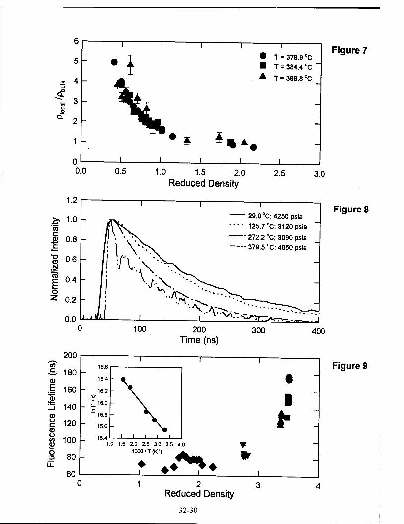
I T = 379.9 °C T = 384.4 °C

T = 398.8 °C

Figure 7

1 - %*

± 0.5 1.0 1.5 2.0

Reduced Density 2.5 3.0

100 200 Time (ns)

300 400

200

S. 180 <D E

.Q>

160

140

120 O c <D Ü w 100 a)

I I-

o 80

60

1.5 2.0 2.5 3.0 3.5 4.0 1000/T(K1)

♦♦ Reduced Density

32-30

Figure 8

Figure 9

Figure 10 0.50 -

A 1 1 1 I

• Pentane

0.48 -

0.46 - CO

i&*' *" ~ 0.44 - i

0.42 -

i i i I 5

0.40 L

0. D 0.5 1.0 1.5 2.0 2.

0.60

B I i i i

■ Hexane

0.55 —

CO

~_ 0.50

0.45

-

■

i i i i U.4U ■

0.0 0.5 1.0 1.5 2.0 2.5

U.OU

C I I I I

A Heptane

0.55 -

CO

S- 0.50

0.45 -

, i i I

>.5 0.40

C 1.0 0.5 1.0 1.5 2.0 2

Reduced Density

32-31

0.50 Figuren

0.40 0.000 0.005 0.010 0.015 0.020

0.55

0.50 -

0.45

0.40 0.000 0.005 0.010 0.015 0.020

0.55

0.50 -

0.45 -

0.40 0.000 0.020

32-32

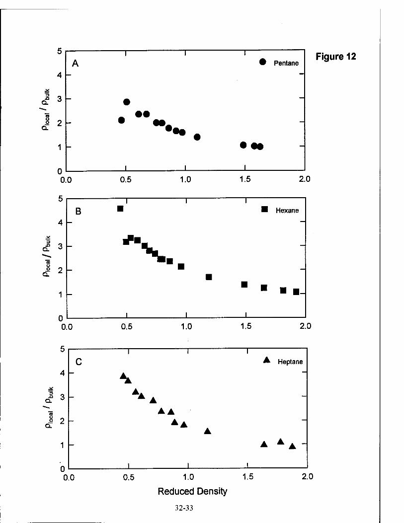
Figure 12

0

B I i ■

I H Hexane

4 -

5 3 ■X. -

Ü

<f 2 ■ ■

-

1

n i i

■ ■ ■■-

0.0 0.5 1.0 1.5 2.0

o

c I I I

A Heptane

4 \

~

3 .O

Q. 3 AA A

-

ü o CL

2

1

n I

AA

*A

I

A

0.0 0.5 1.0

Reduced Density

32-33

1.5 2.0

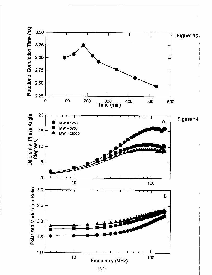
(0

E

3.50

p 3.25 - c o

i_ o ü 15 c o

3.00 -

2.75 -

■2 2.50 - Co o

2.25 T. 300 400 Time (mm)

500

Figure 13

600

0)

c <

CD W (0

20 T 1—r T

MW=1250 MW = 3780 MW = 28000

g 3.0 CO

OH c g 2.5 TO

o ^ 2.0 ■o <D N

ro 1.5 h' o

Q_

1.0

T 1—i—i—r

J I L

10

T r Figure 14

100

T 1 1 1—i—i—r

B

J 1 i i i ■ ■

Frequency (MHz)

32-34

100

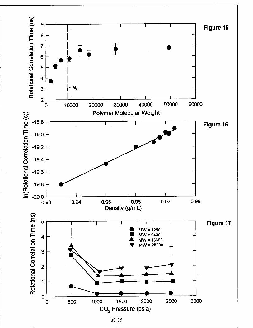
(0

E I-

i_ o O aj c o

*-* (0 o en

^ -18.8 E ^ -19.0 - o ro -19.2 h

° -19.4 -

15 c -19.6 h g

'S -19.8 h

Figure 15

■£ -20.0 0.93

c/)

3 5 Q) E h- c o

4 -

■S3-

2 -

a> b o O «j c o

o a:

o

10000 20000 30000 40000 50000 60000

Polymer Molecular Weight

Figure 16

± i

0.94 0.95 0.96 Density (g/mL)

0.97 0.98

Figure 17

500 1000 1500 2000 C02 Pressure (psia)

2500 3000

32-35

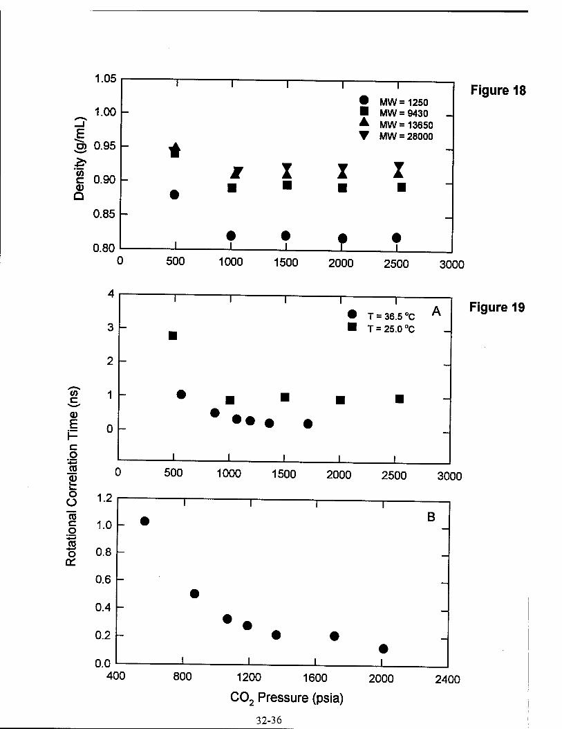
1.05

^ 100 I? E O) 0.95

c 0.90 Q) Q

0.85

0.80 "- 0 500 1000

1

• MW = 1250 ■ MW = 9430 -j ^ MW= 13650 T MW = 28000

1500 2000 2500

Figure 18

3000

CO

E

c o

it-« ro

2> k_ o O "to c o TO o a:

1

o

T T = 36.5 °C T = 25.0 °C

800 1200 1600

C02 Pressure (psia)

32-36

2000

Figure 19

3000

2400

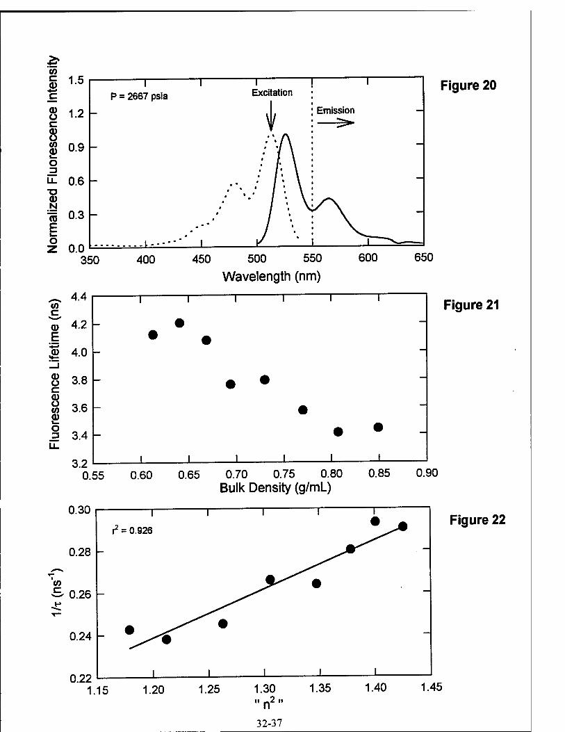
CO c Q)

0) U c 8 CO

o 3

1.5

1.2 -

0.9

0.6

P = 2667 psia

T3 <D N iö 0.3 E i_ o Z 0.0 — I

Figure 20

350 400 450 500 550

Wavelength (nm) 600 650

0.70 0.75 0.80 Bulk Density (g/mL)

0.30

0.28 -

CO

S 0.26

0.24 -

0.22 1.15

Figure 21

0.90

Figure 22

1.45

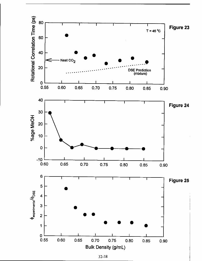
CO

3 80

E

c 60 g

g 40 Ü "cö o 20 w o a:

o 0.55

T = 46 °C Figure 23

Neat CO*

JL ±

DSE Prediction (mixture)

_L ± 0.60 0.65 0.70 0.75 0.80 0.85 0.90

Figure 24

0.65 0.70 0.75 0.80 0.85 0.90

LU 03 Q

-e-

0) E <u Q.

0.60 0.65 0.70 0.75 0.80

Bulk Density (g/mL)

Figure 25

0.85 0.90

32-38

IMPACT INITIATION OF TRITONAL AND PBX N109

Keith M. Roessig Graduate Student

Department of Aerospace & Mechanical Engineering

University of Notre Dame 356 Fitzpatrick Hall

Notre Dame, IN 46556




November 1994

33-1


Keith M. Roessig Graduate Student

Department of Aerospace & Mechanical Engineering University of Notre Dame

Abstract

Recently, the behavior of explosive materials under intermediate loading rates (10°-104 s_1) has become

of interest. Shock and quasi-static behaviors have been well characterized, but in weapons such as a deep

earth penetrator, loading conditions in intermediate strain ranges will occur previous to initiation and affect

the response of the explosive. This paper will examine the mechanical behavior of a cure cast simulant,

Filler-E, and a melt cast simulant under three widely different strain rates. These tests will include quasi-

static loading rates on an MTS machine, low velocity tests on a mechanical press, and high velocity tests

incorporating a Kolsky bar apparatus at the University of Notre Dame. Impact tests of the explosives

Tritonal and PBX-N109 conducted at the Advanced Warhead Experimentation Facility at Eglin AFB, FL

will be discussed.

Filler-E and Tritonal are shown to be a very brittle material, while the cure cast simulant and PBX N109

are much more ductile. All these materials have strengths well below that of steel, usually 4340 is used in

bomb casings, and can be neglected in comparison. Slight strain rate hardening is seen in both simulants,

though for Filler-E, failure strains drop tremendously as failure becomes a dynamic fracture event. The

impact tests on Tritonal and PBX-N109 show that these materials need to have high hydrostatic loads after

failure to generate the internal friction needed for initiation.

33-2


Keith M. Roessig

1 Introduction

Explosives axe used in a wide variety of applications, from mining to military weaponry to metal forming.

Understanding their behavior is very important in all applications to allow for their efficient and safe use.

Safety is especially critical in the handling and storage of explosives, and preventing sympathetic, or un-

planned, detonation is one of the primary goals of the explosive engineer. In addition, design applications

also require a thorough knowledge of the mechanical and thermal behaviors of these materials.

The theory of detonation of explosives is a very complicated one, and, due to the small time scales

involved, has not been studied extensively by many academic institutions. A key element of detonation

theory is the coupling between mechanics and chemistry during the reaction. This coupling cannot be

ignored and should be included in any realistic model [6]. Frequently, the ignition is assumed to be heavily

dependent on the formation of hot spots, localized regions of intense heat generation. Factors that can lead

to hot spot formation and ignition include jetting, void collapse, viscous heating, shock interaction, internal

friction and adiabatic shear localization [2, 6]. Adiabatic shear localization occurs at high strain rates when

shear deformation may cause thermal softening through the plastic work done on the material. The softer

material deforms more, causing further heating. This self feeding process can become localized into a very

small region, and the local temperatures can become very high. Shear banding has been relatively unexplored

experimentally as a source of ignition in solid explosives. Field et al. [10] took high speed photographs of

explosives initiating from hot spot formation produced by the variety of mechanisms listed above. Evidence

of shear localization was found in some tests. Boyle et al. [3] investigated ignition of certain explosives

under combined pressure and shear conditions and found that shear bands do form in the interior of the

explosive when hydrostatic pressure is applied. Chou [5] has run numerical simulations of the impact of

various explosives with steel projectiles and found shear bands to form. Temperatures within these bands,

however, were not always great enough to cause initiation. Understanding how these mechanisms interact

under high strain rates is essential to the proper design and safe use of reactive materials.

Recently, greater emphasis has been placed on determining the mechanical and reactive properties of

explosives deforming under lower strain rates. Initiation under very high strain rate loadings such as shock

waves occur due to adiabatic, compressive heating, while initiation under very small, or quasi-static, loading

rates occurs mainly from external heating. Loading cases more typically seen by these materials result in

strain rates between these extremes during use. One example is the deep earth penetrator. The explosives

33-3

inside the weapon will undergo various loading rates and loading geometries before reaction occurs. How the

explosives behave during the loading and at detonation by the fuse is critical to successful implementation

of these weapons.

The explosives Tritonal and PBX-N109 are examined in this paper. These are respectively a melt cast

trinitrotoluene (TNT) based explosive and a cure cast plastic bonded explosive (PBX) containing the Royal

Development Explosive (RDX) trinitro triazacyclohexane. No pressed PBX explosives were used. In the

interest of safety, the inert melt cast simulant, Filler-E, and inert cure cast PBX simulants were used in the

punch tests at the University of Notre Dame. It is important to study these materials for several reasons: 1)

to determine the behavior of these materials, 2) determine how closely they imitate the mechanical behavior

of the explosives they simulate, 3) gain knowledge of the mechanical behavior without reaction for safer

experiments, and 4) record data to be used in finite element codes such as EPIC or ABAQUS to model other

experiments where they are used.

Though shear localization can be described by a material process, geometry plays an important role in

the event. Failure can be constrained to a shear dominated mode by the experimental setup. Punching

and plugging are two situations in which adiabatic shear localization can occur. Plugging is the process

in terminal ballistics in which failure occurs in a shear dominated mode, though bending deformation can

be quite large. The clearance between the projectile and any support is very large, so in effect it is an

infinite plate. Usually plugging occurs at large impact velocities, depending upon the material of the target

and projectile. Punching, on the other hand, requires a very small clearance between punch and die, and

usually occurs in manufacturing. Punching velocities are small and the failure is again largely dominated

by shear since the die prevents much bending deformation. Figure 1 shows the geometric difference between

the punching and plugging. The punch test was chosen here because higher strain rates can be obtained at

lower punch velocities with the shear deformation constrained to a smaller area.

Load-displacement diagrams are very important in the analysis of punch tests on materials. The various

Punch

Sheet

Punch

-..

1 | Die

-J Cleara ince

Plate

Figure 1: Geometries of punching and plugging operations

33-4

sections of the load displacement diagram indicate what may be occurring during each phase of the failure

process, see Figure 2. The energy used in the process, the area under the curve, can be correlated to the

constitutive characteristics of the material. Yield and ultimate strengths as well as strain hardening values

can be estimated from these curves. Most of the area under the graph is energy being used to deform

the material, both elastically and plastically. Once, the material begins to fracture, however, most of the

required punching energy comes from friction. This is a schematic, and actual load-displacement curves will

vary depending on punch velocity and material. Average stress-average strain curves can be determined

from the load-displacement data.

.maximum punch tore«

initiation or crack propagation

, Meondary crack» probably fccmad

friction«! rasistanca batwaan (i) blank and hoi« (»punch and hoi« (»»blank and dl«

trictional rasistanw mainly batwaan blank and hoi«

paration of blank from ahaat trictional r«»i»tane« mainly batwaan punch and how

PUNCH DISPLACEMENT

Figure 2: Load-displacement curve schematic (Bai and Johnson, 1982)

2 Experimental Method

2.1 Tests on Simulants

Three punch tests were conducted at different velocities of 2.0 x 10-5 m/s, 1 m/s, and ~10 m/s using the

insert/die configuration shown in Figure 3. The insert slides into the die, and the simulant is placed in a

recess machined for the specimen. The projectile slides through the hole in the cover plate, which is bolted

to the die, and can easily pass through the insert and die.

The melt cast simulant, Filler-E, and cure cast PBX simulant were used in this study. All the specimens

were discs of the same size, 0.25" thick and 2" in diameter. These materials were obtained from the High

Explosive Research and Development (HERD) division of the Wright Labs Armament Directorate at Eglin

AFB. The clearance between the punch and die in all the tests was 2.54mm. Three separate testing methods

were used to determine load-displacement curves at a wide range of strain rates.

33-5

Projectile

Cover Plale

Figure 3: Insert/die configuration for MTS and mechanical press

Quasi-static tests were conducted on a MTS 810 20 kip tension/compression machine at an average shear

strain rate of 5.0x 10~3. The load was read directly from the load cell on the MTS, while the displacement was

obtained through a Epsilon Technology Corp. 3540-1000-ST deflectometer. This instrument is similar to an

extensometer, but uses strain gages to measure the deflection of a small shaft. Using the calibration from the

manufacturer, voltage traces can be recorded an a digital oscilloscope and then converted to displacements.

Though the MTS machine does have its own position indicator, it was found that there was too much error

from the machine compression of the projectile and die to measure such small displacements. Voltages were

recorded on digital oscilloscopes and then transferred to a PC for analysis.

The low velocity tests were conducted on a mechanical press machine shown in Figure 4. The same die

configuration was used on the mechanical press as the MTS machine. The punch velocity was approximately

1 m/s, giving an average strain of ~200. Strain gages were placed on the punch to determine the load upon

the specimen during the test. Output traces were recorded on a digital oscilloscope. The displacement was

recorded with the same deflectometer used with the MTS machine.

For the high speed tests, a punch-loading Kolsky bar apparatus was built to perform the punch tests.

This apparatus is described in volume 8 of the the ASM Handbook [1] and had been successfully used by

Dowling et al. [8] and Zurek [13]. The basic design is shown in Figure 5.

Using an air gun a long projectile is fired at the Kolsky bar. This sends a stress pulse down the length

33-6

RwoTK cowmen tnwo

Oft AMI FOOT IWITOH

Figure 4: Mechanical press used for low velocity tests

of the bar that can be measured using strain gages placed on the bar as shown. As the pulse reaches the

end of the bar, the bar will impact the specimen. The stress pulse will be partially reflected and partially

transmitted. The reflected portion of the pulse is measured by the strain gages that also measured the initial

stress pulse. While the transmitted portion could be measured using strain gages on a die tube behind the

specimen, it is not needed in this case; due to the large diameter of the die as compared to the bar, less than

1% of the pulse is transmitted to the die. It is consequently assumed that there is no transmitted wave, thus

simplifying the analysis of the results (section 2.1.1). Average strain rates of up to l.OxlO4 can be obtained

with the apparatus at Notre Dame.

air gun barrel

projectile

strain gage

\ specimen die

bar supports-

Figure 5: Punch-loading Kolsky bar apparatus

2.1.1 Elastodynamic Analysis

In the Kolsky bar experiment, the following analysis [13] may be used to get load-displacement and average

stress-average strain curves. During use of a Kolsky bar, Figure 6, stress pulses are sent down the length of

the bar to cause a specimen to fail. From elastodynamics, the stress in an elastic wave can be related to the

33-7

particle velocity by the relation

„du Edu du

where E is the elastic modulus, c is the elastic wave speed, a is the axial stress, and the term du/dt describes

the particle velocity, V, in the bar. This velocity will have a different sign depending on the direction of

travel (sign of c) of the pulse itself and the sign of the stress, and there are two relations describing the stress

in relation to the particle velocity.

_ f pcV, left traveling wave ~ I -pcV, rig right traveling wave

specimen p—I

bar

Figure 6: Punch-loading Kolsky bar apparatus

For the incident pulse on the Hopkinson bar, the right traveling wave relations are used, so the incident

stress is

cr, = -pcVi.

Because the bar remains elastic, the strain can be given by

€i=E

and then substituted into the stress equation to yield

V* = - Eej

pc

The relations for the reflected wave are similar, but these are left traveling waves, so the elastic stress is

defined as

aT = pcVr

33-8

This leads to a final expression for Vr of

Vr = Eer

pc

The shear strain in the specimen, -yrz, is defined as

7 rz _ 1 (dur duz\ ~ 2 \dz + ~dr)

where ur is the displacement in the r direction and uz is the displacement in the z direction. In the punch

test, dur/dz = 0, and duz/dr » 0. Therefore, the shear strain can be approximated by

7rz = X (!) 2 w

The displacement at the end of the bar is defined as

uz = j{Vi + Vr)dt

Substituting in for V* and Vr,

J \ pc pc J

= / -c(e; - er)dt

uz = —c / (CJ - er)dt

So now shear strain and strain rate become

Irz = -^ (ti-er)dt (2)

c 7rz = ~2^(ei~6r) W

respectively.

The shear stress, r, is defined as the shear force divided the shear area where

A8hear = (db + 2 X ^) 7T X h

nd? Fshear = AbE (£i + €r) = -^-£ (e, + €r)

Combining the above equations yields

dlE 1~rz — 4h(cPb+w)

Equations 2, 3, 4 are used to determine rrz, ^rz, and 7rz for each test

33-9

(e. + er) (4)

2.2 Explosives at AWEF

Experiments on actual explosives were conducted at the Advanced Warhead Experimentation Facility (AWEF)

at Eglin AFB, Florida. This facility is in the Armament Branch of Wright Labs and has the facilities to

conduct perform such tests safely with ease. Using a 12.7mm (0.50" caliber) powder gun, cylindrical steel

projectiles 76.4mm in length were shot the specimens at velocities around 300 m/s. Pressure transducers

with a known separation length at the end of the barrel produced voltage traces recorded on an oscilloscope,

allowing a velocity to be calculated.

Both Tritonal and PBX-N109 specimens were made 36mm in diameter and 6.5mm thick. The specimens

were placed in a removable insert which went into the die, see Figure 7. The inserts were made of 4340

steel hardened to Rockwell C of approximately 45. These inserts produced a clearance of 2.54mm between

the projectile and inner diameter of the insert. Thin aluminum discs were placed behind the specimens to

prevent loss of material due to spalling. Cover plates made of titanium 6% Al-4% V alloy were used in some

shots to contain the explosive and determine the effect of a cover plate.

Projectile Specimen ^

Die

Figure 7: Die/insert configuration

The end of the powder gun and the specimen/die setup were all placed inside a steel-framed Lexan tank.

The tank contained 2 feet of celotex behind the die to catch the projectile before impacting the back plate of

the tank. A mirror was placed on one side of the die to allow two views of the event to be captured on each

frame of film. A Cordin 330 high speed camera was placed on the opposite side of the mirror. See Figure

8. This allows for a side view and an angle view of the projectile impact in each frame. Framing rates were

approximately 250,000/sec.

The use of high speed photography can play two important roles in investigating the processes mentioned

above. First, the failure process can be examined. The amount of deformation and fracture, or a combination

of the two, recorded on the film allows the determination of the failure mode under different loading cases.

33-10

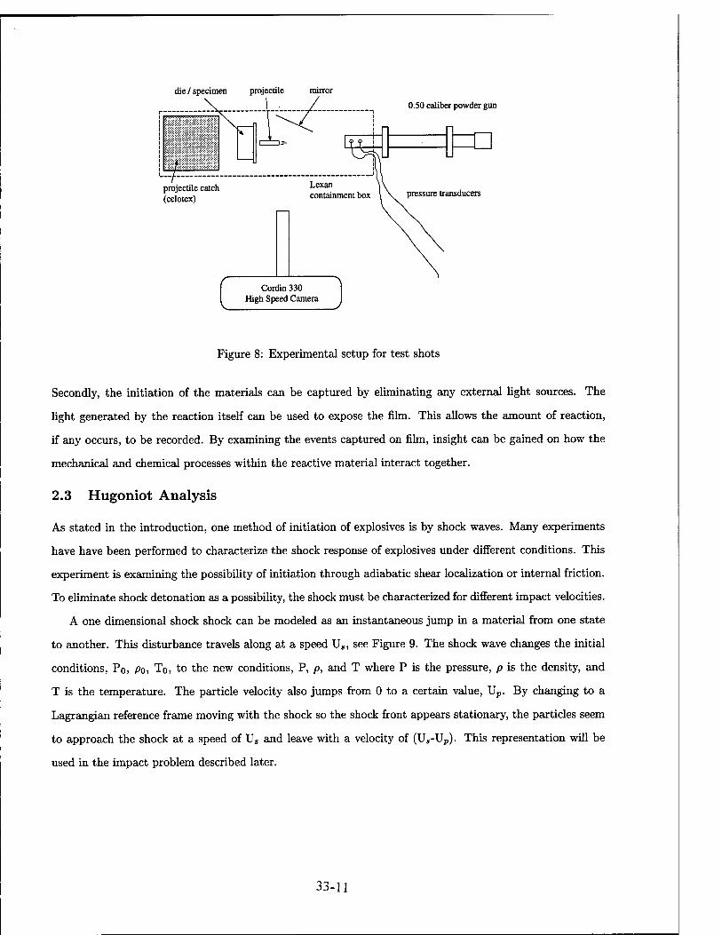
die / specimen projectile

0.50 caliber powder gun

Figure 8: Experimental setup for test shots

Secondly, the initiation of the materials can be captured by eliminating any external light sources. The

light generated by the reaction itself can be used to expose the film. This allows the amount of reaction,

if any occurs, to be recorded. By examining the events captured on film, insight can be gained on how the

mechanical and chemical processes within the reactive material interact together.

2.3 Hugoniot Analysis

As stated in the introduction, one method of initiation of explosives is by shock waves. Many experiments

have have been performed to characterize the shock response of explosives under different conditions. This

experiment is examining the possibility of initiation through adiabatic shear localization or internal friction.

To eliminate shock detonation as a possibility, the shock must be characterized for different impact velocities.

A one dimensional shock shock can be modeled as an instantaneous jump in a material from one state

to another. This disturbance travels along at a speed Ug, see Figure 9. The shock wave changes the initial

conditions, P0, Po, T0, to the new conditions, P, p, and T where P is the pressure, p is the density, and

T is the temperature. The particle velocity also jumps from 0 to a certain value, Up. By changing to a

Lagrangian reference frame moving with the shock so the shock front appears stationary, the particles seem

to approach the shock at a speed of U« and leave with a velocity of (Ug-Up). This representation will be

used in the impact problem described later.

33-11

b)

, y i

•-►Up

Us-Up Us

P,p,T • (Up)o=0 _—^. P,p,T Po.po.To

Figure 9: Schematic of a one dimensional shock from a) a stationary reference frame and b) a movine reference frame

The analysis begins with the conservation equations at the shock front.

Conservation of Mass:

Conservation of Momentum:

Conservation of Energy:

PoUs = p(Us - Up)

(P - P0) = PoUsUp

(5)

(6)

AW = (PA)(Updt) - (P0A)(U0dt)

AE = \{pA{U6-Up)dt]Ul + EAp{Ue-Up)dt

-- [p0A(Us - U0)dt] Ul - E0Ap0(Ua - U0)dt

where A is the cross-sectional area and U0 is the initial particle velocity. W is the work done on a particle

as it passes through the shock front, and E is the energy in a material particle. Equating AW to AE and

setting Uo=0 yields

PUP = -p{Us - Up)Ul - EoPoUs + Ep(Us - Up)

Substituting the mass equation, equation (5), yields

PUP = ^PoUsUl + PoUs(E - Eo)

By using the mass and momentum equations, (5) and (6), the final form of the energy equation is

E-E0 = ±(P + P0)(v0-v)

(7)

(8)

where v=l/p.

The four unknowns are U„ Up, P, and E. With only 3 conservation equations, one more equation is

needed for a complete set. This equation is called the equation of state (EOS). Though it is not the same

33-12

for a solid as an equation of state for a gas, it performs a similar role in the solution, so it has been given

the same name1. This equation relates the shock and particle velocities through the following relation.

Equation of State (EOS):

U8 = C + SUV (9)

where C and S are material constants. These constants have been measured and tabulated in many references.

By combining equations (6) and (9), a relation between the shock pressure and the particle speed can be

obtained.

P = P0 + Po(C + SUp)Up (10)

Equation (10) is very important in impact problems. The method of impedance matching can be used to

find the shock pressure in the impact between two dissimilar materials [12]. During impact, the pressure at

the interface must be equal. This gives rise to different shock and particle velocities by the equations above.

The particles in the target travel at a velocity of Up2 while the projectile particles reduce speed by Upi to a

final value of V-Upi, see Figure 10.

(1)

" 1* ! V i

0 1 Upl fUsl *V f

-—. (J) \_2) ... j

|Us2 |

@ Up2

(a)t<0 (b) impact t=0

(c)t>0

Figure 10: Schematic of impact problem

At the interface, the particle speeds must be the same, so

V-Upl= Up2

and

Conservation of momentum and the equations of state for the projectile and target can be used to find the

final values. The conservation of momentum for the projectile and target are

Pi PoiUgiUpi

xThe more conventional EOS for gases is E=Pu/(7-l)-Aq where A and q are reaction parameters. This equation has been used for solids with a constant 7=3 [9] which allows solution for detonation wave speeds and reaction zone structures, but is not suitable for the impact problem.

33-13

-P2 = P02Us2Up2

respectively. P0 is assumed to be 0. This is a good assumption as pressures can routinely reach above 100

atmospheres in these analyses. The EOS for the two materials are

Usl = d + SxUp!

Us2 = C2 + S2Up2

Combining the equations yields

Pi = Poi(Ci + SxUp^Up! = poiCxUpx + poiSitfpi

P2 = Po2(C2 + S2Up2)Up2

Using the substitution Upi=V-Up2 and setting P^Pj, the following quadratic equation for Up2 can be

derived.

Up2(po2S2 - poiSi) + Up2(p02C2 + poiCi + 2/9oiSi F) - p0i(dV + SiV2) = 0

The roots of the equation are

v _ -{pmd + Poid + 2poiSiV) ± VK P2 2(po252-poi51) (U)

where

A = (A)2<?2 + p0id + 2P0AV)2 - 4(p02S2 - poiSi)(-p01)(dV + SiV2)

Two solutions for Up2 will be found due to the quadratic nature of the equation. The determination for

which solution to use is governed by the fact that Up2 must be less than the original projectile velocity,

V. With Up2 known, all other quantities, including the shock pressure P2, can then be calculated with the

relations already discussed.

A graphical solution of the same problem is also possible. By plotting pressure versus particle velocity

for the projectile and target, the solution can be read directly. Plot the target curve normally, and then plot

the projectile curve with the origin at V, an then invert the curve (change Up to -Up). Where the two curves

cross is the solution to the impact problem. Figure 11 shows the P-Up plane for a steel on TNT impact.

TNT was used because its behavior is close to that of Tritonal, and the data was readily available. The

impact velocity of 1650 m/s was used to give a shock pressure P of 10.7 GPa. Particle speeds in the TNT

are 325 m/s with a shock speed of 4200 m/s. The same parameters for steel are 1325 m/s and 4660 m/s,

respectively.

The impact speed of 1650 m/s was chosen above to give the final shock pressure of 10.7 GPa. This

pressure is the initiation pressure for TNT [7] for this geometry.. This speed is much higher than the 300

33-14

a. O

1650 m/s Up (m/s)

Figure 11: Hugoniot analysis of steel on TNT impact

m/s velocity used in the experiment. Because the velocities are so much lower, shock initiation can be ruled

out as a possible mechanism for reaction during the tests.

3 Results &; Discussion

3.1 Punch Tests on Explosive Simulants

The load-displacement curves for the simulants under quasi-static loading rates are shown in Figure 12.

For both the Filler-E and the cure cast simulant, there was one test of the three that showed a slightly

different behavior. This shows the variety of material properties within these materials. Repetitive behavior

may be hard to obtain due to the numerous possibilities for imperfections in the materials. Post mortem

examination revealed that the specimens did repeat failure behavior qualitatively. The Filler-E was very

brittle. A central plug formed, with radial cracks extending outward to the outer diameter. The cure cast

PBX simulant formed a plug every time, and did not have any radial fractures. There were no fragments,

leading to the conclusion that the material tore. Average stress- strain curves for the two materials are

shown in the same graphs.

At low velocities on the mechanical press, there is not much change in the behavior of the materials. Both

Filler-E and the cure cast PBX simulant showed the same failure pattern as in the quasi-static tests. The

maximum loads in the materials were higher, showing strain rate hardening, which is very large in the case

of the cure cast PBX simulant. Failure strains for both the cure cast PBX simulant and Filler-E reduced by

33-15

a) b)

Shear Strain y 0.05 0.10 Shear Strain *

- 0.30 £

disp (mm)

Figure 12: Quasi-static load-displacement and average stress-average strain curves for (a) Filler-E and (b) cure cast PBX simulant

a factor of 10 from the quasi-static tests. In the case of the Filler-E, this is most likely due to fracture as

the compressive wave reflects of the back face and becomes tensile. Due to the brittle nature of Filler-E, the

specimen cracks very quickly under the dynamic loading. The PBX simulant seems to be exhibiting a large

strain rate dependence in both load capacity and failure strain. Load- displacement and average stress-strain

curves from the mechanical press are in Figure 13.

a)

0.000 6

0.005 0.010 Shear Strain y ' '" 0.015

0.05 0.10 disp (mm)

b)

0.00 Shear Strain 7

0.02 0.04

-0.10 0.00 0.10 0.20 0.30 disp (mm)

Figure 13: Low velocity load-displacement and average stress-average strain curves for (a) Filler-E and (b) cure cast PBX simulant

Results for a Hopkinson bar tests with no specimen allows for a verification of the method, as well as giving

insight into what results can be expected during an actual test. Figure 14 shows the raw data obtained from

the digital oscilloscope. The top trace shows both strain gage histories, and the second shows the average.

33-16

Averaging the two eliminates any bending that may occur. Bending should be kept to a minimum, which

the first trace shows occurring (the two strain gages curves lie almost directly on top of each other). If large

amounts of bending are present, the impact of the bar with the specimen will not be perpendicular and may

lead to erroneous results. The two strain gage have very similar voltage traces, verifying the absence of a

large bending stress. The impact speed in this test was approximately 11.5 m/s.

Strain Gage Traces

'-200 0 200 400 600 «00 10OO 1200 1400 1600

"ftme^secT 1200 1400 1600 1800

Figure 14: Voltage traces for Hopkinson bar

By placing the initial compressive and tension pulses over each other, another aspect of this experimental

method is revealed. With no specimen present, the two pulses should have the same shape. However, wave

dispersion has caused the pulses to change shape [11]. Wave dispersion describes the phenomenon that in

uniaxial stress pulses, waves of different frequencies travel at different velocities. As a Fourier analysis will

show, a square pulse is made up of many different waves of various frequencies and amplitudes. These different

waves start to diverge immediately, and thus the shape of the wave changes as it travels. The compressive

pulse (plotted as tension) and the reflected tension pulse can be seen in Figure 15. The magnitudes of the

strain pulses, 1100/ie, verifies that the data follows the elastodynamic relation V = Ee/pc derived in section

2.1.1.

Due to the changing of the shape, noise is generated in the data calculated from the pulses. Figure 16

shows load, stress, strain rate, and displacement at the end of the bar during the pass of the initial pulse.

The load and stress should be zero for all time. The strain rate is the average strain rate that a specimen

would see as determined by the displacement seen in the final graph. The magnitude of the displacement is

as expected from knowing the length of the pulse, the elastic wave speed, and the particle velocity in the

wave.

The first noticeable error is in the load graph. The load is obviously not zero due to the change in shape

of the pulses caused by dispersion. Similarly, even though the end of the bar must physically be a stress

33-17

Strain Pulses in Bar

tffiie (n s$) 120 140

Figure 15: Comparison of initial and reflected strain pulses

50 100 [ 01 sec)

Figure 16: Data calculated from strain pulses

free surface, the stress is reported to be non-zero. The distressing part about the noise is the magnitude

of the load. The load repeatedly reaches values of ±20 kN. While such an uncertainty may be acceptable

when testing metals, this is well above the expected load required to fail either of the inert simulants and is

unacceptable. The maximum loads reported so far for failure are about 6 kN.

Results of the Hopkinson bar testing are shown below in Figure 17. Post mortem examination showed

no difference in failure mode from the tests conducted on the mechanical press. The impact velocities for

the Filler-E and PBX simulant are 11.04 and 12.35 m/s, respectively. The results do not reveal much about

the behavior of the simulants at these punch speeds. The error from dispersion overwhelms any data that

may be present in the voltage traces. These simulants are so much weaker than any steel used that the

strength of the simulants, or the explosives they model, may be neglected. Similar tests on 1018 steel give

yield strengths of 300 MPa. This technique is better used for metals which have a much higher yield strength

33-18

and elastic modulus.

disp (mm)

Figure 17: High velocity load-displacement curves for a) Filler E and b) cure cast simulant

3.2 Impact of Tritonal and PBX N109

With the fracture characterized for lower velocities, the experiments at the AWEF reveal the failure behavior

at very high loading rates and their effect of the initiation on the materials. As can be seen in the pictures

taken with the Cordin camera (Figures 18 and 19), both the materials fracture quickly and are ejected from

the insert. This ejected material is not reacting at any appreciable rate. Both the materials behave similarly,

but the Tritonal seems to have more material ejected. Tritonal is a brittle material that fractures quite

easily. With the initial impact, the Tritonal forms fragments which are then ejected with further projectile

motion. The PBX-N109, on the other hand, is a weak but more ductile material. It offers little resistance

to the projectile motion, but is ejected in larger pieces from the insert.

None of the test shots caused detonation of the specimens. The pressure generated in the shock wave

by the impact is 1.23 GPa for the Tritonal, and even less for the PBX-N109 as determined by the Hugoniot

method [12]. From Pop plots for TNT [7], these pressures will not cause shock detonation for a specimen

0.25" thick. Limits of the gun prevented higher impact speeds.

In other tests, a cover plate of titanium 6% Al-4% V alloy was used to determine if containment and

possible heating from the plate would cause detonation. Again, there was no reaction.

To get a detonation, the reactive material must be contained and compressed [3]. In this experiment, it

is too easy for the fractured material to escape; there is negligible internal friction and negligible hydrostatic

pressure in the shear zone. High pressure combined with shear friction could easily lead to ignition. Boyle

et al. [3] performed tests that combined pressure and shear showing that TNT would ignite for velocities

around 80 m/s with a pressure of 0.5 GPa. The method of initiation in Boyle's tests is probably internal

friction as the tests with steel on explosive and explosive on explosive boundaries made no difference in

33-19

Figure 18: High speed photography of PBX N109 impact, approximate times after impact 116/us, 3) 180/us, and 4) 272/xs

are: 1) 36^s, 2)

33-20

Figure 19: High speed photography of Tritonal impact, approximate times after impact are: 1) 28/xs, 2) 112/xs, 3) 184/xs, and 4) 252fxs

33-21

the outcome. The main difference between these experiments and Boyle's is that in Boyle's tests there is

an applied hydrostatic pressure; clearly the existence of a hydrostatic pressure is critical to the dominant

ignition mechanism in that case.

During the experiments conducted at the AWEF, the technique of turning off external lights to capture

light given off by the reaction was not used. Since very little, if any, reaction occurred, it is expected that

no light was emitted.

Chou [5] has run numerical models on similar experiments, one of which included an impact of TNT

by a steel projectile at 200 m/s. In his calculations, he shows that a shear band forms at the corner of

the projectile. Temperatures reach 500°F. These temperatures are not high enough within the band to

cause ignition. At impact velocities of 1000 m/s, pressures and temperatures become high enough to cause

detonation for his model. What Chou does not take into account is the fracture of the material. As seen

in the photographs, the Tritonal fractures very quickly. Even with cover plates, the materials is no longer a

continuous solid, but a granular material and should be modeled appropriately. Streak camera photographs

have shown that detonation waves in pressed or cast explosives are rough, indicating that the flow is irregular

in its fine detail. Initiation thus depends strongly on the type, number, and distribution of inhomogeneities

[4]. By fracturing these materials, the initiation behavior may change dramatically.

4 Conclusions

For both Filler-E and the cure cast PBX simulant, the ultimate strengths of these materials are far below

anything used for a bomb casing, usually 4340 steel. When modeling the mechanical strength of the weapon

as a whole, the explosive can be neglected as it will not affect the outer casing's behavior due to its negligible

relative strength.

From the behavior of the Filler-E, it can be inferred that that upon impact, Tritonal will fracture very

quickly. In a deep earth penetrator, the explosive may even become a granular material before ignition

occurs. This may hamper or improve ignition of the explosive depending on loading conditions. Penetration

of the weapon by a foreign object could have disastrous effects. The fracturing and then compression of

Tritonal could lead to ignition. Internal friction is greatly increased after the fracture occurs if a large

hydrostatic pressure is present. All the free surfaces are then allowed to rub against each other, greatly

increasing the risk of premature initiation.

The cure cast PBX, which does not fracture at lower loading rates, also fails into many small particles

upon impact. The cure cast simulant showed a large amount of strain rate hardening and decrease in failure

strain between the quasi-static and low velocity tests, and this trend seems to continue to the very high

33-22

velocities for PBX N109. Though load carrying capacity at this loading rate is not known, the failure mode

is much closer to that of the Tutorial. Again, the effect on the initiation from any failure is unknown, but

internal friction with a large hydrostatic pressure will be the primary cause of initiation at these loading

rates.

Nomenclature

r radial direction

z direction along punch axis

ur displacement in r direction

uz displacement in z direction

V specific volume in Hugoniot analysis

w shear width (clearance)

df, bar diameter

Ab bar area

h specimen thickness

c sound velocity in punch

E modulus of elasticity in punch, energy in Hugoniot analysis

€ axial strain in punch

T shear stress in specimen

7 shear strain in specimen

7 shear strain rate in specimen

Vi,Vr incident and particle velocity in Kolsky bar

us shock velocity

up particle velocity in projectile or target for impact problems

P pressure

T temperature

P density

W work

33-23

References

[1] ASM International. ASM Metals Handbook, 10th edition, 1990.

[2] F.P. Bowden and Y.D. Yoffe. Initiation and Growth of Explosives in Liquids and Solids. Cambridge

University Press, New York, 1952.

[3] V. Boyle, R.B. Prey, and 0. Blake. Combined pressure shear ignition of explosives. 9th International

Symposium on Detonation, 1989.

[4] A.W. Campbell, W.C. Davis, J.B. Ramsay, and J.R. Travis. Shock initiation of solid explosives. The

Physics of Fluids, 4(4):511-521, April 1961.

[5] P.C. Chou. Explosive response to unplanned stimuli. Final technical report, Dyna East Corporation,

Philadelphia, PA, September 1991. submitted to Armament Directorate, Eglin AFB, FL.

[6] W.C. Davis. High explosives: The interaction of chemistry and mechanics. Los Alamos Science, 2:48-75,

1981.

[7] B.M. Dobratz and P.C. Crawford. LLNL Explosives Handbook - Properties of Chemical Explosives and

Explosive Simulants. National Technical Information Service, Springfield, VA, January 1985. Document

# DE91006884.

[8] A.R. Dowling, J. Harding, and J.D. Campbell. The dynamic punching of metals. J. Inst. Metals,

98:251-224, 1970.

[9] W. Fickett and W.C. Davis. Detonation. University of California Press, Berkeley, CA, 1979.

[10] J.E. Field, G.M. Swallowe, and S.N. Heavens. Ignition mechanisms of explosives during mechanical

deformation. Proceedings. Royal Society of London, A 382:231-244, 1982.

[11] K. F. Graff. Wave Motion in Elastic Solids. Dover Publications, Inc., New York, 1975.

[12] Marc A. Meyers. Dynamic Behavior of Materials. John Wiley & Sons, Inc., New York, 1994.

[13] A.K. Zurek. The study of adiabatic shear band instability in a pearlitic 4340 steel using a dynamic

punch test. Metallurgical and Material Transactions A, 25A:2483-2489, 1994.

33-24