Hindawi Publishing CorporationEURASIP Journal on Advances in Signal ProcessingVolume 2008, Article ID 672941, 13 pagesdoi:10.1155/2008/672941

Research ArticleA Window Width Optimized S-Transform

Ervin Sejdic,1 Igor Djurovic,2 and Jin Jiang1

1 Department of Electrical and Computer Engineering, The University of Western Ontario, London, Ontario, Canada N6A 5B92 Electrical Engineering Department, University of Montenegro, 81000 Podgorica, Montenegro

Correspondence should be addressed to Jin Jiang, jjiang@eng.uwo.ca

Received 14 May 2007; Accepted 15 November 2007

Recommended by Sven Nordholm

Energy concentration of the S-transform in the time-frequency domain has been addressed in this paper by optimizing the widthof the window function used. A new scheme is developed and referred to as a window width optimized S-transform. Two opti-mization schemes have been proposed, one for a constant window width, the other for time-varying window width. The former isintended for signals with constant or slowly varying frequencies, while the latter can deal with signals with fast changing frequencycomponents. The proposed scheme has been evaluated using a set of test signals. The results have indicated that the new schemecan provide much improved energy concentration in the time-frequency domain in comparison with the standard S-transform.It is also shown using the test signals that the proposed scheme can lead to higher energy concentration in comparison with otherstandard linear techniques, such as short-time Fourier transform and its adaptive forms. Finally, the method has been demon-strated on engine knock signal analysis to show its effectiveness.

Copyright © 2008 Ervin Sejdic et al. This is an open access article distributed under the Creative Commons Attribution License,which permits unrestricted use, distribution, and reproduction in any medium, provided the original work is properly cited.

1. INTRODUCTION

In the analysis of the nonstationary signals, one often needsto examine their time-varying spectral characteristics. Sincetime-frequency representations (TFR) indicate variations ofthe spectral characteristics of the signal as a function of time,they are ideally suited for nonstationary signals [1, 2]. Theideal time-frequency transform only provides informationabout the frequency occurring at a given time instant. Inother words, it attempts to combine the local informationof an instantaneous-frequency spectrum with the global in-formation of the temporal behavior of the signal [3]. Themain objectives of the various types of time-frequency anal-ysis methods are to obtain time-varying spectrum functionswith high resolution and to overcome potential interferences[4].

The S-transform can conceptually be viewed as a hybridof short-time Fourier analysis and wavelet analysis. It em-ploys variable window length. By using the Fourier kernel, itcan preserve the phase information in the decomposition [5].The frequency-dependent window function produces higherfrequency resolution at lower frequencies, while at higherfrequencies, sharper time localization can be achieved. Incontrast to wavelet transform, the phase information pro-

vided by the S-transform is referenced to the time origin, andtherefore provides supplementary information about spectrawhich is not available from locally referenced phase infor-mation obtained by the continuous wavelet transform [5].For these reasons, the S-transform has already been consid-ered in many fields such as geophysics [6–8], cardiovasculartime-series analysis [9–11], signal processing for mechanicalsystems [12, 13], power system engineering [14], and patternrecognition [15].

Even though the S-transform is becoming a valuable toolfor the analysis of signals in many applications, in somecases, it suffers from poor energy concentration in the time-frequency domain. Recently, attempts to improve the time-frequency representation of the S-transform have been re-ported in the literature. A generalized S-transform, proposedin [12], provides greater control of the window function, andthe proposed algorithm also allows nonsymmetric windowsto be used. Several window functions are considered, includ-ing two types of exponential functions: amplitude modu-lation and phase modulation by cosine functions. Anotherform of the generalized S-transform is developed in [7],where the window scale and shape are a function of fre-quency. The same authors introduced a bi-Gaussian windowin [8], by joining two nonsymmetric half-Gaussian windows.

2 EURASIP Journal on Advances in Signal Processing

Since the bi-Gaussian window is asymmetrical, it also pro-duces an asymmetry in the time-frequency representation,with higher-time resolution in the forward direction. As a re-sult, the proposed form of the S-transform has better perfor-mance in detection of the onset of sudden events. However,in the current literature, none has considered optimizing theenergy concentration in the time-frequency domain directly,that is, to minimize the spread of the energy beyond the ac-tual signal components.

The main approach used in this paper is to optimize thewidth of the window used in the S-transform. The optimiza-tion is performed through the introduction of a new parame-ter in the transform. Therefore, the new technique is referredto as a window width optimized S-transform (WWOST).The newly introduced parameter controls the window width,and the optimal value can be determined in two ways. Thefirst approach calculates one global, constant parameter andthis is recommended for signals with constant or very slowlyvarying frequency components. The second approach calcu-lates the time-varying parameter, and it is more suitable forsignals with fast varying frequency components.

The proposed scheme has been tested using a set of syn-thetic signals and its performance is compared with the stan-dard S-transform. The results have shown that the WWOSTenhances the energy concentration. It is also shown that theWWOST produces the time-frequency representation with ahigher concentration than other standard linear techniques,such as the short-time Fourier transform and its adaptiveforms. The proposed technique is useful in many applica-tions where enhanced energy concentration is desirable. Asan illustrative example, the proposed algorithm is used toanalyze knock pressure signals recorded from a VolkswagenPassat engine in order to determine the presence of severalsignal components.

This paper is organized as follows. In Section 2, the con-cept of ideal time-frequency transform is introduced, whichcan be compared with other time-frequency representationsincluding transforms proposed here. The development ofthe WWOST is covered in Section 3. Section 4 evaluates theperformance of the proposed scheme using test signals andalso the knock pressure signals. Conclusions are drawn inSection 5.

2. ENERGY CONCENTRATION INTIME-FREQUENCY DOMAIN

The ideal TFR should only be distributed along frequenciesfor the duration of signal components. Thus, the neighbor-ing frequencies would not contain any energy; and the energycontribution of each component would not exceed its dura-tion [3].

For example, let us consider two simple signals: anFM signal, x1(t) = A(t) exp ( jφ(t)), where |dA(t)/dt| �|dφ(t)/dt| and the instantaneous frequency is defined asf (t) = (dφ(t)/dt)/2π; and a signal with the Fouriertransform given as X( f ) = G( f ) exp ( j2πχ( f )), wherethe spectrum is slowly varying in comparison to phase|dG( f )/df | � |dχ( f )/df |. Further, A(t) and G(t) The ideal

TFRs for these signals are given, respectively, as shown in [16]

ITFR(t, f ) = 2πA(t)δ(f − 1

2πdφ(t)dt

), (1)

ITFR(t, f ) = 2πG( f )δ(t +

dχ( f )df

), (2)

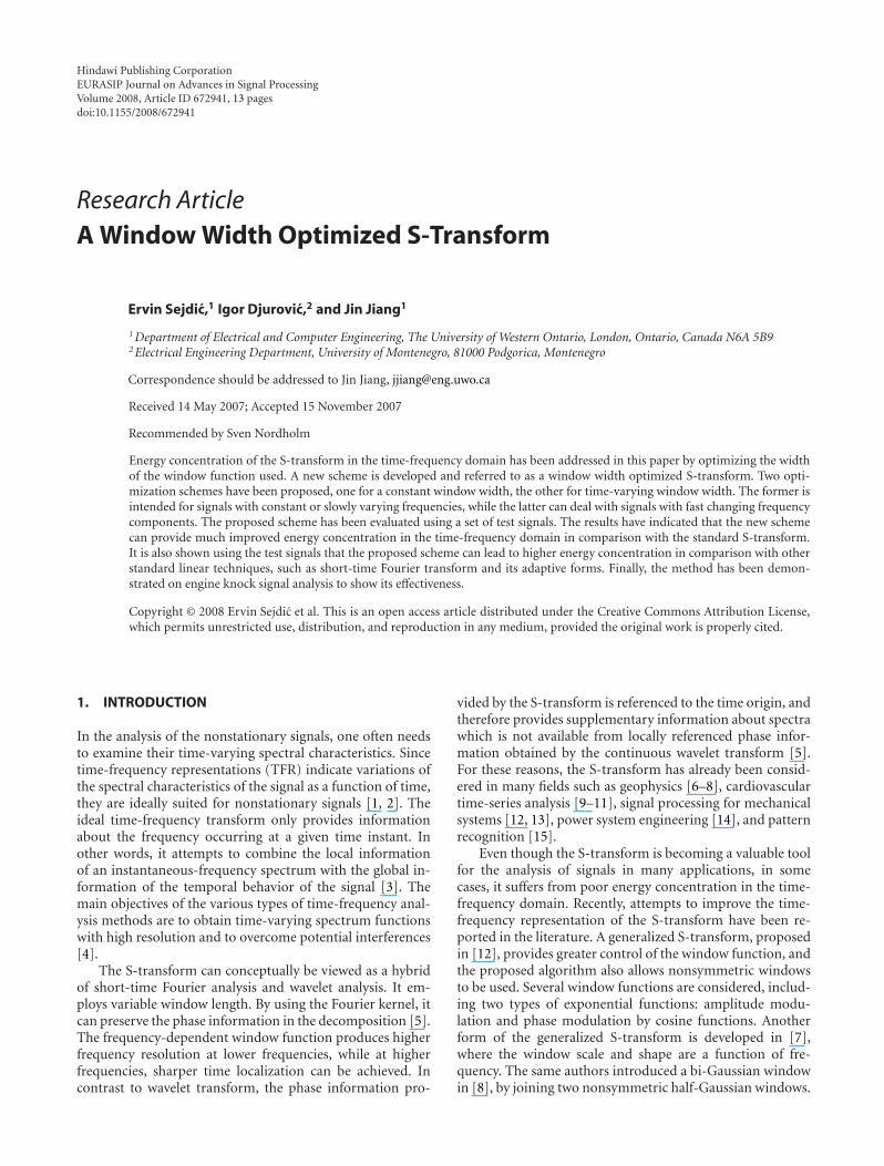
where ITFR stands for an ideal time-frequency represen-tation. These two representations are ideally concentratedalong the instantaneous frequency, (dφ(t)/dt)/2π, and ongroup delay −dχ( f )/df . Simplest examples of these signalsare the following: a sinusoid with A = const. and dφ(t)/dt =const. depicted in Figure 1(a); and a Dirac pulse x2(t) =δ(t− t0) shown in Figure 1(b). The ideal time-frequency rep-resentations are depicted in Figures 1(c) and 1(d). These twographs are compared with the TFRs obtained by the standardS-transform in Figures 1(e) and 1(f).

For the sinusoidal case, the frequencies surrounding(dφ(t)/dt)/2π also have a strong contribution, and from (1),it is clear that they should not have any contributions. Sim-ilarly, for the Dirac function, it is expected that all the fre-quencies have the contribution but only for a single time in-stant. Nevertheless, it is clear that the frequencies are not onlycontributing during a single time instant as expected from(2), but the surrounding time instants also have strong en-ergy contribution.

The examples presented here are for illustrations only,since a priori knowledge about the signals is assumed. Inmost practical situations, the knowledge about a signal islimited and the analytical expressions similar to (1) and (2)are often not available. However, the examples illustrate apoint that some modifications to the existing S-transformalgorithm, which do not assume a priori knowledge aboutthe signal, may be useful to achieve improved performancein time-frequency energy concentration. Such improvementsonly become possible after modifications to the width of thewindow function are made.

3. THE PROPOSED SCHEME

3.1. Standard S-transform

The standard S-transform of a function x(t) is given by anintegral as in [5, 7, 12]

Sx(t, f ) =∫ +∞

−∞x(τ)w

(t − τ, σ( f )

)exp (− j2π f τ)dτ (3)

with a constraint

∫ +∞

−∞w(t − τ, σ( f )

)dτ = 1. (4)

Ervin Sejdic et al. 3

−1

0

1A

mpl

itu

de

0 0.2 0.4 0.6 0.8 1

Time (s)

(a)

0

0.5

1

Am

plit

ude

0 0.2 0.4 0.6 0.8 1

Time (s)

(b)

0

50

100

Freq

uen

cy(H

z)

0 0.2 0.4 0.6 0.8 1

Time (s)

(c)

0

50

100

Freq

uen

cy(H

z)

0 0.2 0.4 0.6 0.8 1

Time (s)

(d)

0

50

100

Freq

uen

cy(H

z)

0 0.2 0.4 0.6 0.8 1

Time (s)

(e)

0

50

100

Freq

uen

cy(H

z)

0 0.2 0.4 0.6 0.8 1

Time (s)

(f)

Figure 1: Comparison of the ideal time-frequency representation and S-transform for the two simple signal forms: (a) 30 Hz sinusoid; (b)sample Dirac function; (c) ideal TFR of a 30 Hz sinusoid; (d) ideal TFR of a Dirac function; (e) TFR by standard S-transform for a 30 Hzsinusoid; and (f) TFR by standard S-transform of the Dirac delta function.

A window function used in S-transform is a scalable Gaus-sian function defined as

w(t, σ( f )

) = 1σ( f )

√2π

exp(− t2

2σ2( f )

). (5)

The advantage of the S-transform over the short-timeFourier transform (STFT) is that the standard deviation σ( f )is actually a function of frequency, f , defined as

σ( f ) = 1| f | . (6)

Consequently, the window function is also a function of timeand frequency. As the width of the window is dictated by thefrequency, it can easily be seen that the window is wider inthe time domain at lower frequencies, and narrower at higherfrequencies. In other words, the window provides good lo-calization in the frequency domain for low frequencies whileproviding good localization in time domain for higher fre-quencies.

The disadvantage of the current algorithm is the fact thatthe window width is always defined as a reciprocal of thefrequency. Some signals would benefit from different win-dow widths. For example, for a signal containing a single si-nusoid, the time-frequency localization can be considerablyimproved if the window is very narrow in the frequency do-main. Similarly, for signals containing only a Dirac impulse,it would be beneficial for good time-frequency localizationto have very wide window in the frequency domain.

3.2. Window width optimized S-transform

A simple improvement to the existing algorithm for the S-transform can be made by modifying the standard deviationof the window to

σ( f ) = 1| f |p . (7)

4 EURASIP Journal on Advances in Signal Processing

0

0.1

0.2

0.3

0.4

0.5

0.6

0.7

0.8

0.9

1

Nor

mal

ized

ampl

itu

de

−2 −1.5 −1 −0.5 0 0.5 1 1.5 2

Time (s)

p = 0.5p = 1p = 2

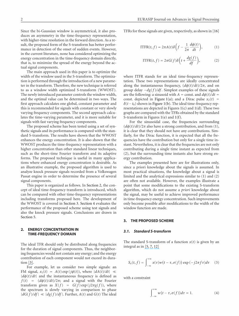
Figure 2: Normalized Gaussian window for different values of p.

Based on the above equation, the new S-transform can berepresented as

Spx (t, f )

= | f |p√2π

∫ +∞

−∞x(τ) exp

(− (t − τ)2 f 2p

2

)exp (− j2π f τ)dτ.

(8)

The parameter p can control the width of the window.By finding an appropriate value of p, an improved time-frequency concentration can be obtained. The window func-tions with three different values of p are plotted in Figure 2,where p = 1 corresponds to the standard S-transform win-dow. For p < 1, the window becomes wider in the time do-main, and for p > 1, the window narrows in the time do-main. Therefore, by considering the example from Section 2,for the single sinusoid, a small value of p would providealmost perfect concentration of the signal, whereas for theDirac function, a rather large value of p would produce agood concentration in the time-frequency domain. It is im-portant to mention that in the case of 0 < f < 1, the oppositeis true.

The optimal value of p will be found based on the con-centration measure proposed in [17], which has some fa-vorable performance in comparison to other concentrationmeasures reported in [18–20]. The measure is designed tominimize the energy concentration for any time-frequencyrepresentation based on the automatic determination ofsome time-frequency distribution parameter. This measureis defined as

CM(p) = 1∫ +∞−∞∫ +∞−∞∣∣Spx (t, f )

∣∣dt df , (9)

where CM stands for a concentration measure.

There are two ways to determine the optimal value of p.One is to determine a global, constant value of p for the en-tire signal. The other is to determine a time-varying p(t),which depends on each time instant considered. The first ap-proach is more suitable for signals with the constant or slowlyvarying frequency components. In this case, one value of pwill suffice to give the best resolution for all components.The time-varying parameter is more appropriate for signalswith fast varying frequency components. In these situations,depending on the time duration of the signal components,it would be beneficial to use lower value of p (somewherein the middle of the particular component’s interval), andto use higher values of p for the beginning and the end ofthe component’s interval, so the component is not smearedin the time-frequency plane. It is important to mention thatboth proposed schemes for determining the parameter p arethe special cases of the algorithm which would evaluate theparameter on any arbitrary subinterval, rather than over theentire duration of the signal.

3.2.1. Algorithm for determining the time-invariant p

The algorithm for determining the optimized time-invariantvalue of p is defined through the following steps.

(1) For p selected from a set 0 < p ≤ 1, compute S-transform of the signal S

px (t, f ) using (8).

(2) For each p from the given set, normalize the energy ofthe S-transform representation, so that all of the rep-resentations have the equal energy

Spx (t, f ) = S

px (t, f )√∫ +∞

−∞∫ +∞−∞∣∣Spx (t, f )

∣∣2dt df

. (10)

(3) For each p from the given set, compute the concentra-tion measure according to (9), that is,

CM(p) = 1∫ +∞−∞∫ +∞−∞∣∣Spx (t, f )

∣∣dt df . (11)

(4) Determine the optimal parameter popt by

popt = maxp

[CM(p)

]. (12)

(5) Select Spx (t, f ) with popt to be the WWOST

Spx (t, f ) = S

poptx (t, f ). (13)

As it can be seen, the proposed algorithm computes theS-transform for each value of p and, based on the com-puted representation, it determines the concentration mea-sure, CM(p), as an inverse of L1 norm of the normalizedS-transform for a given p. The maximum of the concentra-tion measure corresponds to the optimal p which provides

the least smear of Spx (t, f ).

It is important to note that in the first step, the value ofp is limited to the range 0 < p ≤ 1. Any negative value of pcorresponds to an nth root of a frequency which would makethe window wider as frequency increases. Similarly, values

Ervin Sejdic et al. 5

greater than 1 provide a window which may be too narrow inthe time domain. Unless the signal being analyzed is a super-position of Delta functions, the value of p should not exceedunity. As a special case, it is important to point out that forp = 0, the WWOST is equivalent to STFT with a Gaussianwindow with σ2 = 1.

3.2.2. Algorithm for determining p(t)

The time-varying parameter p(t) is required for signals withcomponents having greater or abrupt changes. The algo-rithm for choosing the optimal p(t) can be summarizedthrough the following steps.

(1) For p selected from a set 0 < p(t) ≤ 1, compute S-transform of the signal S

px (t, f ) using (8).

(2) Calculate the energy, E1, for p = 1. For each p from theset, normalize the energy of the S-transform represen-tation to E1, so that all of the representations have theequal energy, and the amplitude of the components isnot distorted,

Spx (t, f ) = √E1

Spx (t, f )√∫ +∞

−∞∫ +∞−∞∣∣Spx (t, f )

∣∣2dt df

. (14)

(3) For each p from the set and a time instant t, compute

CM(t, p) = 1∫ +∞−∞∣∣Spx (t, f )

∣∣df . (15)

(4) Optimal value of p for the considered instant t maxi-mizes concentration measure CM(t, p),

popt(t) = arg maxp

[CM(t, p)

]. (16)

(5) Set the WWOST to be

Spx (t, f ) = S

popt(t)x (t, f ). (17)

The main difference between the two techniques lies instep (3). For the time invariant case, a single value of p ischosen, whereas in the time-varying case, an optimal value ofp(t) is a function of time. As it is demonstrated in Section 4,the time-dependent parameter is beneficial for signals withthe fast varying components.

3.2.3. Inverse of the WWOST

Similarly to the standard S-transform, the WWOST can beused as both an analysis and a synthesis tool. The inversionprocedure for the WWOST resembles that of the standardS-transform, but with one additional constraint. The spec-trum of the signal obtained by averaging S

px (t, f ) over time

must be normalized by W(0, f ), where W(α, f ) representsthe Fourier transform (from t to α) of the window function,w(t, σ( f )). Hence, the inverse WWOST for a signal, x(t), isdefined as

x(t) =∫ +∞

−∞

∫ +∞

−∞1

W(0, f )Spx (τ, f ) exp ( j2π f t)dτ df . (18)

In the case of a time-invariant p, it can be shown thatW(0, f ) = 1. In a general case, the Fourier transform of theproposed modified window can only be determined numer-ically.

4. WWOST PERFORMANCE ANALYSIS

In this section, the performance of the proposed scheme isexamined using a set of synthetic test signals first. Further-more, the analysis of signals from an engine is also given.The first part includes two cases: (1) a simple case involvingthree slowly varying frequencies and (2) more complicatedcases involving multiple time-varying components. The goalis to examine the performance of WWOST in comparisonto the standard S-transform. The proposed algorithm is alsocompared to other time-frequency representations, such asthe short-time Fourier transform (STFT) and adaptive STFT(ASTFT), to highlight the improved performance of the S-transform with the proposed window width optimizationtechnique. In particular, the proposed algorithm can be usedfor some classes of the signals for which the standard S-transform would not be suitable.

As for the synthetic signals, the sampling period used inthe simulations is Ts = 1/256 seconds. Also, the set of pvalues, used in the numerical analysis of both test and theknock pressure signals, is given by p = {0.01n : n ∈ N and1 ≤ n ≤ 100}. The ASTFT is calculated according to the con-centration measure given by (9). In the definition of the mea-sure, a normalized STFT is used instead of the normalizedWWOST. The standard deviation of the Gaussian window,σgw, is used as the optimizing parameter, where the windowis defined as

wSTFT(t) = 1σgw√

2πexp

(− t2

2σ2gw

). (19)

The optimization for synthetic signals is performed on theset of values defined by

σgw = {n/128 : n ∈ N, 1 ≤ n ≤ 128} (20)

and both the time-invariant and time-varying values of σgw

are calculated.

4.1. Synthetic test signals

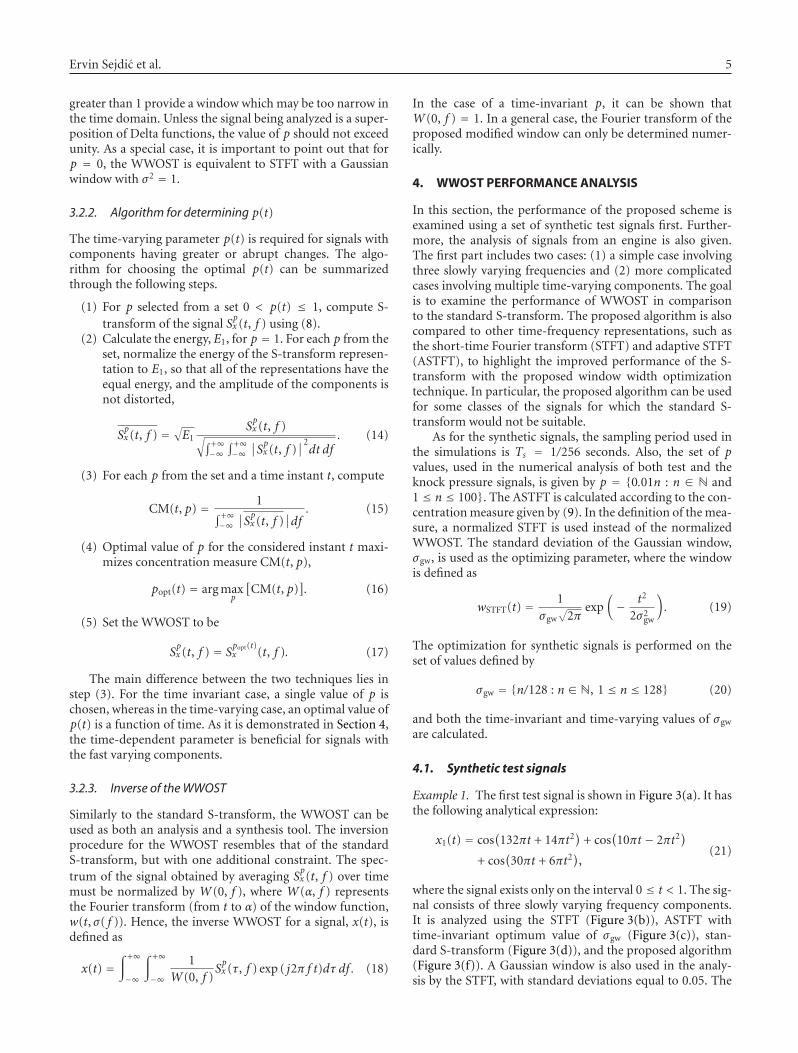
Example 1. The first test signal is shown in Figure 3(a). It hasthe following analytical expression:

x1(t) = cos(132πt + 14πt2

)+ cos

(10πt − 2πt2

)+ cos

(30πt + 6πt2

),

(21)

where the signal exists only on the interval 0 ≤ t < 1. The sig-nal consists of three slowly varying frequency components.It is analyzed using the STFT (Figure 3(b)), ASTFT withtime-invariant optimum value of σgw (Figure 3(c)), stan-dard S-transform (Figure 3(d)), and the proposed algorithm(Figure 3(f)). A Gaussian window is also used in the analy-sis by the STFT, with standard deviations equal to 0.05. The

6 EURASIP Journal on Advances in Signal Processing

−5

0

5A

mpl

itu

de

0 0.2 0.4 0.6 0.8 1

Time (s)

(a)

0

50

100

Freq

uen

cy(H

z)

0 0.2 0.4 0.6 0.8 1

Time (s)

(b)

0

50

100

Freq

uen

cy(H

z)

0 0.2 0.4 0.6 0.8 1

Time (s)

(c)

0

50

100

Freq

uen

cy(H

z)

0 0.2 0.4 0.6 0.8 1

Time (s)

(d)

0

0.5

1

Am

plit

ude

ofC

M

0 0.2 0.4 0.6 0.8 1

Time (s)

(e)

0

50

100

Freq

uen

cy(H

z)

0 0.2 0.4 0.6 0.8 1

Time (s)

(f)

Figure 3: Test signal x1(t): (a) time-domain representation; (b) STFT of x1(t); (c) ASTFT of x1(t) with σopt; (d) Spx (t, f ) of x1(t) with p = 1

(standard S-transform); (e) concentration measure CM(p); (f) Spx (t, f ) of x1(t) with the optimal value of p = .57.

optimum value of standard deviation for the ASTFT is calcu-lated to be σopt = 0.094. The colormap used for plotting thetime-frequency representations in Figure 3 and all the subse-quent figures is a linear grayscale with values from 0 to 1.

The standard S-transform, shown in Figure 3(d), depictsall three components clearly. However, only the first twocomponents have relatively good concentration, while thethird component is completely smeared in frequency. Asshown in Figure 3(b), the STFT provides better energy con-centration than the standard S-transform. The ASTFT, de-picted in Figure 3(c), shows a noticeable improvement for allthree components. The results with the proposed scheme isshown in Figure 3(f) for p = 0.57. The value of p is found ac-cording to (12). For the determined value of p, the first twocomponents have higher concentration even than the ASTFT,while the third component has approximately the same con-centration.

In Figure 3(e), the normalized concentration measure isdepicted. The obtained results verify the theoretical predic-tions from Section 3.2. For this class of signals, that is, the

signals with slowly varying frequencies, it is expected thatsmaller values of p will produce the best energy concentra-tion. In this example, the optimal value, found according to(12), is determined numerically to be 0.57.

Based on the visual inspection of the time-frequency rep-resentations shown in Figure 3, it can be concluded that theproposed algorithm achieves higher concentration amongthe considered representations. To confirm this fact, a per-formance measure given by

ΞTF =(∫ +∞

−∞

∫ +∞

−∞

∣∣TF(t, f )∣∣dt df

)−1

(22)

is used for measuring the concentration of the representa-tion, where |TF(t, f )| is a normalized time-frequency repre-sentation. The performance measure is actually the concen-tration measure proposed in (9). A more concentrated rep-resentation will produce a higher value of ΞTF. Table 1 sum-marizes the performance measure for the STFT, the ASTFT,the standard S-transform, and the WWOST.

Ervin Sejdic et al. 7

Table 1: Performance measure for the three time-frequency trans-forms.

TFR ΞTF

STFT 0.0119

ASTFT 0.0131

Standard S-transform 0.0080

WWOST 0.0136

The value of the performance measure for the standard S-transform is the lowest, followed by the STFT. The WWOSTproduces the highest value of ΞTF, and thus achieves a TFRwith the highest energy concentration amongst the trans-forms considered.

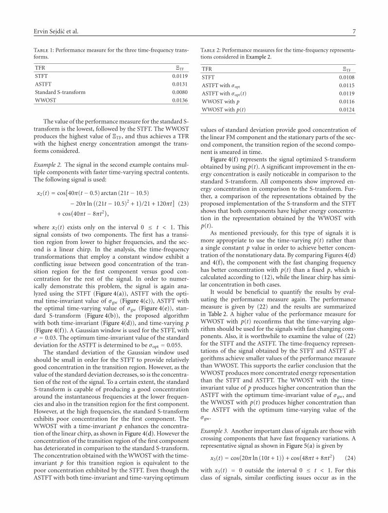
Example 2. The signal in the second example contains mul-tiple components with faster time-varying spectral contents.The following signal is used:

x2(t) = cos[40π(t − 0.5) arctan (21t − 10.5)

− 20π ln((21t − 10.5)2 + 1

)/21 + 120πt

]+ cos

(40πt − 8πt2

),

(23)

where x2(t) exists only on the interval 0 ≤ t < 1. Thissignal consists of two components. The first has a transi-tion region from lower to higher frequencies, and the sec-ond is a linear chirp. In the analysis, the time-frequencytransformations that employ a constant window exhibit aconflicting issue between good concentration of the tran-sition region for the first component versus good con-centration for the rest of the signal. In order to numer-ically demonstrate this problem, the signal is again ana-lyzed using the STFT (Figure 4(a)), ASTFT with the opti-mal time-invariant value of σgw (Figure 4(c)), ASTFT withthe optimal time-varying value of σgw (Figure 4(e)), stan-dard S-transform (Figure 4(b)), the proposed algorithmwith both time-invariant (Figure 4(d)), and time-varying p(Figure 4(f)). A Gaussian window is used for the STFT, withσ = 0.03. The optimum time-invariant value of the standarddeviation for the ASTFT is determined to be σopt = 0.055.

The standard deviation of the Gaussian window usedshould be small in order for the STFT to provide relativelygood concentration in the transition region. However, as thevalue of the standard deviation decreases, so is the concentra-tion of the rest of the signal. To a certain extent, the standardS-transform is capable of producing a good concentrationaround the instantaneous frequencies at the lower frequen-cies and also in the transition region for the first component.However, at the high frequencies, the standard S-transformexhibits poor concentration for the first component. TheWWOST with a time-invariant p enhances the concentra-tion of the linear chirp, as shown in Figure 4(d). However theconcentration of the transition region of the first componenthas deteriorated in comparison to the standard S-transform.The concentration obtained with the WWOST with the time-invariant p for this transition region is equivalent to thepoor concentration exhibited by the STFT. Even though theASTFT with both time-invariant and time-varying optimum

Table 2: Performance measures for the time-frequency representa-tions considered in Example 2.

TFR ΞTF

STFT 0.0108

ASTFT with σopt 0.0115

ASTFT with σopt(t) 0.0119

WWOST with p 0.0116

WWOST with p(t) 0.0124

values of standard deviation provide good concentration ofthe linear FM component and the stationary parts of the sec-ond component, the transition region of the second compo-nent is smeared in time.

Figure 4(f) represents the signal optimized S-transformobtained by using p(t). A significant improvement in the en-ergy concentration is easily noticeable in comparison to thestandard S-transform. All components show improved en-ergy concentration in comparison to the S-transform. Fur-ther, a comparison of the representations obtained by theproposed implementation of the S-transform and the STFTshows that both components have higher energy concentra-tion in the representation obtained by the WWOST withp(t).

As mentioned previously, for this type of signals it ismore appropriate to use the time-varying p(t) rather thana single constant p value in order to achieve better concen-tration of the nonstationary data. By comparing Figures 4(d)and 4(f), the component with the fast changing frequencyhas better concentration with p(t) than a fixed p, which iscalculated according to (12), while the linear chirp has simi-lar concentration in both cases.

It would be beneficial to quantify the results by eval-uating the performance measure again. The performancemeasure is given by (22) and the results are summarizedin Table 2. A higher value of the performance measure forWWOST with p(t) reconfirms that the time-varying algo-rithm should be used for the signals with fast changing com-ponents. Also, it is worthwhile to examine the value of (22)for the STFT and the ASTFT. The time-frequency represen-tations of the signal obtained by the STFT and ASTFT al-gorithms achieve smaller values of the performance measurethan WWOST. This supports the earlier conclusion that theWWOST produces more concentrated energy representationthan the STFT and ASTFT. The WWOST with the time-invariant value of p produces higher concentration than theASTFT with the optimum time-invariant value of σgw, andthe WWOST with p(t) produces higher concentration thanthe ASTFT with the optimum time-varying value of theσgw.

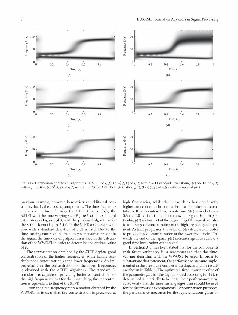
Example 3. Another important class of signals are those withcrossing components that have fast frequency variations. Arepresentative signal as shown in Figure 5(a) is given by

x3(t) = cos(20π ln (10t + 1)

)+ cos

(48πt + 8πt2

)(24)

with x3(t) = 0 outside the interval 0 ≤ t < 1. For thisclass of signals, similar conflicting issues occur as in the

8 EURASIP Journal on Advances in Signal Processing

0

50

100

Freq

uen

cy(H

z)

0 0.2 0.4 0.6 0.8 1

Time (s)

(a)

0

50

100

Freq

uen

cy(H

z)

0 0.2 0.4 0.6 0.8 1

Time (s)

(b)

0

50

100

Freq

uen

cy(H

z)

0 0.2 0.4 0.6 0.8 1

Time (s)

(c)

0

50

100

Freq

uen

cy(H

z)

0 0.2 0.4 0.6 0.8 1

Time (s)

(d)

0

50

100

Freq

uen

cy(H

z)

0 0.2 0.4 0.6 0.8 1

Time (s)

(e)

0

50

100

Freq

uen

cy(H

z)

0 0.2 0.4 0.6 0.8 1

Time (s)

(f)

Figure 4: Comparison of different algorithms: (a) STFT of x2(t); (b) Spx (t, f ) of x2(t) with p = 1 (standard S-transform); (c) ASTFT of x2(t)

with σopt = 0.055; (d) Spx (t, f ) of x2(t) with p = 0.73; (e) ASTFT of x2(t) with σopt(t); (f) S

px (t, f ) of x2(t) with the optimal p(t).

previous example; however, here exists an additional con-straint, that is, the crossing components. The time-frequencyanalysis is performed using the STFT (Figure 5(b)), theASTFT with the time-varying σgw (Figure 5(c)), the standardS-transform (Figure 5(d)), and the proposed algorithm forthe S-transform (Figure 5(f)). In the STFT, a Gaussian win-dow with a standard deviation of 0.02 is used. Due to thetime-varying nature of the frequency components present inthe signal, the time-varying algorithm is used in the calcula-tion of the WWOST in order to determine the optimal valueof p.

The representation obtained by the STFT depicts goodconcentration of the higher frequencies, while having rela-tively poor concentration at the lower frequencies. An im-provement in the concentration of the lower frequenciesis obtained with the ASTFT algorithm. The standard S-transform is capable of providing better concentration forthe high frequencies, but for the linear chirp, the concentra-tion is equivalent to that of the STFT.

From the time-frequency representation obtained by theWWOST, it is clear that the concentration is preserved at

high frequencies, while the linear chirp has significantlyhigher concentration in comparison to the other represen-tations. It is also interesting to note how p(t) varies between0.6 and 1.0 as a function of time shown in Figure 5(e). In par-ticular, p(t) is close to 1 at the beginning of the signal in orderto achieve good concentration of the high-frequency compo-nent. As time progresses, the value of p(t) decreases in orderto provide a good concentration at the lower frequencies. To-wards the end of the signal, p(t) increases again to achieve agood time localization of the signal.

In Section 3, it has been stated that for the componentswith faster variations, it is recommended that the time-varying algorithm with the WWOST be used. In order tosubstantiate that statement, the performance measure imple-mented in the previous examples is used again and the resultsare shown in Table 3. The optimized time-invariant value ofthe parameter popt for this signal, found according to (12), isdetermined numerically to be 0.71. These performance mea-sures verify that the time-varying algorithm should be usedfor the faster varying components. For comparison purposes,the performance measures for the representations given by

Ervin Sejdic et al. 9

−2

0

2A

mpl

itu

de

0 0.2 0.4 0.6 0.8 1

Time (s)

(a)

0

50

100

Freq

uen

cy(H

z)

0 0.2 0.4 0.6 0.8 1

Time (s)

(b)

0

50

100

Freq

uen

cy(H

z)

0 0.2 0.4 0.6 0.8 1

Time (s)

(c)

0

50

100

Freq

uen

cy(H

z)

0 0.2 0.4 0.6 0.8 1

Time (s)

(d)

0

0.5

1

Am

plit

ude

0 0.2 0.4 0.6 0.8 1

Time (s)

(e)

0

50

100

Freq

uen

cy(H

z)

0 0.2 0.4 0.6 0.8 1

Time (s)

(f)

Figure 5: Time-frequency analysis of signal with fast variations in frequency: (a) time-domain representation; (b) STFT of x3(t); (c) ASTFTof x3(t) with σopt(t); (d) S

px (t, f ) of x3(t) with p = 1 (standard S-transform); (e) p(t); (f) S

px (t, f ) of x3(t) with the optimal p(t).

Table 3: Performance measures for the time-frequency representa-tions considered in Example 3.

TFR ΞTF (noise-free) ΞTF (SNR = 25 dB)

STFT 0.0106 0.0100

ASTFT with σopt 0.0121 0.0114

ASTFT with σopt(t) 0.0122 0.0113

WWOST with p 0.0122 0.0110

WWOST with p(t) 0.0126 0.0116

the STFT and its time-invariant (σopt = 0.048) and time-varying adaptive algorithms are calculated as well. By com-paring the values of the performance measure for differenttime-frequency transforms, these values confirm the earlierstatement which assures that each algorithm for the WWOSTproduces more concentrated time-frequency representationin its respective class than the ASTFT.

In the analysis performed so far, it was assumed that thesignal-to-noise ratio (SNR) is infinity, that is, the noise-free

signals were considered. It would be beneficial to comparethe performance of the considered algorithms in the pres-ence of additive white Gaussian noise in order to understandwhether the proposed algorithm is capable of providing theenhanced performance in noisy environment. Hence, the sig-nal x3(t) is contaminated with the additive white Gaussiannoise and it is assumed that SNR = 25 dB. The results of suchan analysis are summarized in Table 3. Even though, the per-formance has degraded in comparison to the noiseless case,the WWOST with p(t) still outperforms the other consideredrepresentations.

4.2. Demonstration example

In order to illustrate the effectiveness of the proposedscheme, the method has been applied to the analysis of en-gine knocks. A knock is an undesired spontaneous autoigni-tion of the unburned air-gas mixture causing a rapid in-crease in pressure and temperature. This can lead to seri-ous problems in spark-ignition car engines, for example,

10 EURASIP Journal on Advances in Signal Processing

−1

0

1

Am

plit

ude

(kPa

)

0 2 4 6

Time (ms)

(a)

0

1

2

3

Freq

uen

cy(k

Hz)

0 2 4 6

Time (ms)

(b)

0

1

2

3

Freq

uen

cy(k

Hz)

0 2 4 6

Time (ms)

(c)

0

1

2

3

Freq

uen

cy(k

Hz)

0 2 4 6

Time (ms)

(d)

0

1

2

3

Freq

uen

cy(k

Hz)

0 2 4 6

Time (ms)

(e)

0

1

2

3

Freq

uen

cy(k

Hz)

0 2 4 6

Time (ms)

(f)

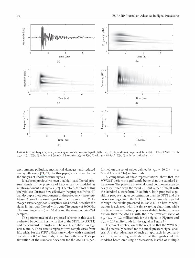
Figure 6: Time-frequency analysis of engine knock pressure signal (17th trial): (a) time-domain representation; (b) STFT; (c) ASTFT withσopt(t); (d) S

px (t, f ) with p = 1 (standard S-transform); (e) S

px (t, f ) with p = 0.86; (f) S

px (t, f ) with the optimal p(t).

environment pollution, mechanical damages, and reducedenergy efficiency [21, 22]. In this paper, a focus will be onthe analysis of knock pressure signals.

It has been previously shown that high-pass filtered pres-sure signals in the presence of knocks can be modeled asmulticomponent FM signals [22]. Therefore, the goal of thisanalysis is to illustrate how effectively the proposed WWOSTcan decouple these components in time-frequency represen-tation. A knock pressure signal recorded from a 1.81 Volk-swagen Passat engine at 1200 rpm is considered. Note that thesignal is high-pass filtered with a cutoff frequency of 3000 Hz.The sampling rate is fs = 100 kHz and the signal contains 744samples.

The performance of the proposed scheme in this case isevaluated by comparing it with that of the STFT, the ASTFT,and the standard S-transform. The results are shown in Fig-ures 6 and 7. These results represent two sample cases fromfifty trials. For the STFT, a Gaussian window, with a standarddeviation of 0.3 milliseconds, is used for both cases. The op-timization of the standard deviation for the ASTFT is per-

formed on the set of values defined by σgw = {0.01n : n ∈N and 1 ≤ n ≤ 744}milliseconds.

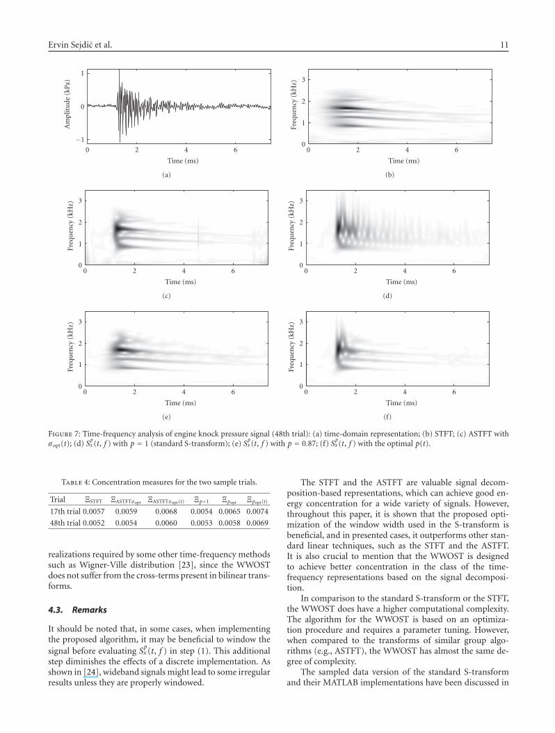
A comparison of these representations show that theWWOST performs significantly better than the standard S-transform. The presence of several signal components can beeasily identified with the WWOST, but rather difficult withthe standard S-transform. In addition, both proposed algo-rithms produce higher concentration than the STFT and thecorresponding class of the ASTFT. This is accurately depictedthrough the results presented in Table 4. The best concen-tration is achieved with the time-varying algorithm, whilethe time invariant value p produces slightly higher concen-tration than the ASTFT with the time-invariant value ofσgw (σopt = 0.2 milliseconds for the signal in Figure 6 andσopt = 0.19 milliseconds for the signal in Figure 7).

The direct implication of the results is that the WWOSTcould potentially be used for the knock pressure signal anal-ysis. A major advantage of such an approach in compari-son to some existing methods is that the signals could bemodeled based on a single observation, instead of multiple

Ervin Sejdic et al. 11

−1

0

1A

mpl

itu

de(k

Pa)

0 2 4 6

Time (ms)

(a)

0

1

2

3

Freq

uen

cy(k

Hz)

0 2 4 6

Time (ms)

(b)

0

1

2

3

Freq

uen

cy(k

Hz)

0 2 4 6

Time (ms)

(c)

0

1

2

3

Freq

uen

cy(k

Hz)

0 2 4 6

Time (ms)

(d)

0

1

2

3

Freq

uen

cy(k

Hz)

0 2 4 6

Time (ms)

(e)

0

1

2

3

Freq

uen

cy(k

Hz)

0 2 4 6

Time (ms)

(f)

Figure 7: Time-frequency analysis of engine knock pressure signal (48th trial): (a) time-domain representation; (b) STFT; (c) ASTFT withσopt(t); (d) S

px (t, f ) with p = 1 (standard S-transform); (e) S

px (t, f ) with p = 0.87; (f) S

px (t, f ) with the optimal p(t).

Table 4: Concentration measures for the two sample trials.

Trial ΞSTFT ΞASTFTσopt ΞASTFTσopt(t) Ξp=1 Ξpopt Ξpopt(t)

17th trial 0.0057 0.0059 0.0068 0.0054 0.0065 0.0074

48th trial 0.0052 0.0054 0.0060 0.0053 0.0058 0.0069

realizations required by some other time-frequency methodssuch as Wigner-Ville distribution [23], since the WWOSTdoes not suffer from the cross-terms present in bilinear trans-forms.

4.3. Remarks

It should be noted that, in some cases, when implementingthe proposed algorithm, it may be beneficial to window thesignal before evaluating S

px (t, f ) in step (1). This additional

step diminishes the effects of a discrete implementation. Asshown in [24], wideband signals might lead to some irregularresults unless they are properly windowed.

The STFT and the ASTFT are valuable signal decom-position-based representations, which can achieve good en-ergy concentration for a wide variety of signals. However,throughout this paper, it is shown that the proposed opti-mization of the window width used in the S-transform isbeneficial, and in presented cases, it outperforms other stan-dard linear techniques, such as the STFT and the ASTFT.It is also crucial to mention that the WWOST is designedto achieve better concentration in the class of the time-frequency representations based on the signal decomposi-tion.

In comparison to the standard S-transform or the STFT,the WWOST does have a higher computational complexity.The algorithm for the WWOST is based on an optimiza-tion procedure and requires a parameter tuning. However,when compared to the transforms of similar group algo-rithms (e.g., ASTFT), the WWOST has almost the same de-gree of complexity.

The sampled data version of the standard S-transformand their MATLAB implementations have been discussed in

12 EURASIP Journal on Advances in Signal Processing

several publications [5, 7, 25–27]. The WWOST is a straight-forward extension of the standard S-transform. Therefore,the sampled data version of the WWOST also follows thesteps presented in earlier publications.

5. CONCLUSION

In this paper, a scheme for improvement of the energyconcentration of the S-transform has been developed. Thescheme is based on the optimization of the width of the win-dow used in the transform. The optimization is carried outby means of a newly introduced parameter. Therefore, thedeveloped technique is referred to as a window width opti-mized S-transform (WWOST). Two algorithms for parame-ter optimization have been developed: one for finding an op-timal constant value of the parameter p for the entire signal;while the other is to find a time-varying parameter. The pro-posed scheme is evaluated and compared with the standardS-transform by using a set of synthetic test signals. The re-sults have shown that the WWOST can achieve better energyconcentration in comparison with the standard S-transform.As demonstrated, the WWOST is capable of achieving higherconcentration than other standard linear methods, such asthe STFT and its adaptive form. Furthermore, the proposedtechnique has also been applied to engine knock pressure sig-nal analysis, and the results have indicated that the proposedtechnique provides a consistent improvement over the stan-dard S-transform.

ACKNOWLEDGMENTS

Ervin Sejdic and Jin Jiang would like to thank the Natural Sci-ences and Engineering Research Council of Canada (NSERC)for financially supporting this work.

REFERENCES

[1] L. Cohen, Time-Frequency Analysis, Prentice Hall PTR, Engle-wood Cliffs, NJ, USA, 1995.

[2] S. G. Mallat, A Wavelet Tour of Signal Processing, AcademicPress, San Diego, Calif, USA, 2nd edition, 1999.

[3] K. Grochenig, Foundations of Time-Frequency Analysis,Birkhauser, Boston, Mass, USA, 2001.

[4] I. Djurovic and LJ. Stankovic, “A virtual instrument for time-frequency analysis,” IEEE Transactions on Instrumentation andMeasurement, vol. 48, no. 6, pp. 1086–1092, 1999.

[5] R. G. Stockwell, L. Mansinha, and R. P. Lowe, “Localization ofthe complex spectrum: the S-transform,” IEEE Transactions onSignal Processing, vol. 44, no. 4, pp. 998–1001, 1996.

[6] S. Theophanis and J. Queen, “Color display of the localizedspectrum,” Geophysics, vol. 65, no. 4, pp. 1330–1340, 2000.

[7] C. R. Pinnegar and L. Mansinha, “The S-transform with win-dows of arbitrary and varying shape,” Geophysics, vol. 68, no. 1,pp. 381–385, 2003.

[8] C. R. Pinnegar and L. Mansinha, “The bi-Gaussian S-transform,” SIAM Journal of Scientific Computing, vol. 24,no. 5, pp. 1678–1692, 2003.

[9] M. Varanini, G. De Paolis, M. Emdin, et al., “Spectral analy-sis of cardiovascular time series by the S-transform,” in Com-

puters in Cardiology, pp. 383–386, Lund, Sweden, September1997.

[10] G. Livanos, N. Ranganathan, and J. Jiang, “Heart sound anal-ysis using the S-transform,” in Computers in Cardiology, pp.587–590, Cambridge, Mass, USA, September 2000.

[11] E. Sejdic and J. Jiang, “Comparative study of three time-frequency representations with applications to a novel correla-tion method,” in Proceedings of the IEEE International Confer-ence on Acoustics, Speech and Signal Processing (ICASSP ’04),vol. 2, pp. 633–636, Montreal, Quebec, Canada, May 2004.

[12] P. D. McFadden, J. G. Cook, and L. M. Forster, “Decomposi-tion of gear vibration signals by the generalized S-transform,”Mechanical Systems and Signal Processing, vol. 13, no. 5, pp.691–707, 1999.

[13] A. G. Rehorn, E. Sejdic, and J. Jiang, “Fault diagnosis in ma-chine tools using selective regional correlation,” MechanicalSystems and Signal Processing, vol. 20, no. 5, pp. 1221–1238,2006.

[14] P. K. Dash, B. K. Panigrahi, and G. Panda, “Power quality anal-ysis using S-transform,” IEEE Transactions on Power Delivery,vol. 18, no. 2, pp. 406–411, 2003.

[15] E. Sejdic and J. Jiang, “Selective regional correlation for pat-tern recognition,” IEEE Transactions on Systems, Man, and Cy-bernetics, Part A, vol. 37, no. 1, pp. 82–93, 2007.

[16] LJ. Stankovic, “Analysis of some time-frequency and time-scale distributions,” Annales des Telecommunications, vol. 49,no. 9-10, pp. 505–517, 1994.

[17] LJ. Stankovic, “Measure of some time-frequency distributionsconcentration,” Signal Processing, vol. 81, no. 3, pp. 621–631,2001.

[18] D. L. Jones and T. W. Parks, “A high resolution data-adaptivetime-frequency representation,” IEEE Transactions on Acous-tics, Speech, and Signal Processing, vol. 38, no. 12, pp. 2127–2135, 1990.

[19] T.-H. Sang and W. J. Williams, “Renyi information and signal-dependent optimal kernel design,” in Proceedings of the 20thIEEE International Conference on Acoustics, Speech and SignalProcessing (ICASSP ’95), vol. 2, pp. 997–1000, Detroit, Mich,USA, May 1995.

[20] W. J. Williams, M. L. Brown, and A. O. Hero III, “Uncertainty,information, and time-frequency distributions,” in AdvancedSignal Processing Algorithms, Architectures, and Implementa-tions II, vol. 1566 of Proceedings of SPIE, pp. 144–156, SanDiego, Calif, USA, July 1991.

[21] M. Urlaub and J. F. Bohme, “Evaluation of knock begin inspark-ignition engines by least-squares,” in Proceedings of theIEEE International Conference on Acoustics, Speech and SignalProcessing (ICASSP ’05), vol. 5, pp. 681–684, Philadelphia, Pa,USA, March 2005.

[22] I. Djurovic, M. Urlaub, LJ. Stankovic, and J. F. Bohme, “Es-timation of multicomponent signals by using time-frequencyrepresentations with application to knock signal analysis,” inProceediongs of the European Signal Processing Conference (EU-SIPCO ’04), pp. 1785–1788, Vienna, Austria, September 2004.

[23] D. Konig and J. F. Bohme, “Application of cyclostationary andtime-frequency signal analysis to car engine diagnosis,” in Pro-ceedings of IEEE International Conference on Acoustics, Speech,and Signal Processing (ICASSP ’94), vol. 4, pp. 149–152, Ade-laide, SA, Australia, April 1994.

[24] F. Gini and G. B. Giannakis, “Hybrid FM-polynomial phasesignal modeling: parameter estimation and Cramer-Raobounds,” IEEE Transactions on Signal Processing, vol. 47, no. 2,pp. 363–377, 1999.

Ervin Sejdic et al. 13

[25] R. G. Stockwell, S-transform analysis of gravity wave activityfrom a small scale network of airglow imagers, Ph.D. disserta-tion, The University of Western Ontario, London, Ontario,Canada, 1999.

[26] C. R. Pinnegar and L. Mansinha, “Time-local Fourier analysiswith a scalable, phase-modulated analyzing function: the S-transform with a complex window,” Signal Processing, vol. 84,no. 7, pp. 1167–1176, 2004.

[27] C. R. Pinnegar, “Time-frequency and time-time filtering withthe S-transform and TT-transform,” Digital Signal Processing,vol. 15, no. 6, pp. 604–620, 2005.

Photograph © Turisme de Barcelona / J. Trullàs

Preliminary call for papers

The 2011 European Signal Processing Conference (EUSIPCO 2011) is thenineteenth in a series of conferences promoted by the European Association forSignal Processing (EURASIP, www.eurasip.org). This year edition will take placein Barcelona, capital city of Catalonia (Spain), and will be jointly organized by theCentre Tecnològic de Telecomunicacions de Catalunya (CTTC) and theUniversitat Politècnica de Catalunya (UPC).EUSIPCO 2011 will focus on key aspects of signal processing theory and

li ti li t d b l A t f b i i ill b b d lit

Organizing Committee

Honorary ChairMiguel A. Lagunas (CTTC)

General ChairAna I. Pérez Neira (UPC)

General Vice ChairCarles Antón Haro (CTTC)

Technical Program ChairXavier Mestre (CTTC)

Technical Program Co Chairsapplications as listed below. Acceptance of submissions will be based on quality,relevance and originality. Accepted papers will be published in the EUSIPCOproceedings and presented during the conference. Paper submissions, proposalsfor tutorials and proposals for special sessions are invited in, but not limited to,the following areas of interest.

Areas of Interest

• Audio and electro acoustics.• Design, implementation, and applications of signal processing systems.

l d l d d

Technical Program Co ChairsJavier Hernando (UPC)Montserrat Pardàs (UPC)

Plenary TalksFerran Marqués (UPC)Yonina Eldar (Technion)

Special SessionsIgnacio Santamaría (Unversidadde Cantabria)Mats Bengtsson (KTH)

FinancesMontserrat Nájar (UPC)• Multimedia signal processing and coding.

• Image and multidimensional signal processing.• Signal detection and estimation.• Sensor array and multi channel signal processing.• Sensor fusion in networked systems.• Signal processing for communications.• Medical imaging and image analysis.• Non stationary, non linear and non Gaussian signal processing.

Submissions

Montserrat Nájar (UPC)

TutorialsDaniel P. Palomar(Hong Kong UST)Beatrice Pesquet Popescu (ENST)

PublicityStephan Pfletschinger (CTTC)Mònica Navarro (CTTC)

PublicationsAntonio Pascual (UPC)Carles Fernández (CTTC)

I d i l Li i & E hibiSubmissions

Procedures to submit a paper and proposals for special sessions and tutorials willbe detailed at www.eusipco2011.org. Submitted papers must be camera ready, nomore than 5 pages long, and conforming to the standard specified on theEUSIPCO 2011 web site. First authors who are registered students can participatein the best student paper competition.

Important Deadlines:

P l f i l i 15 D 2010

Industrial Liaison & ExhibitsAngeliki Alexiou(University of Piraeus)Albert Sitjà (CTTC)

International LiaisonJu Liu (Shandong University China)Jinhong Yuan (UNSW Australia)Tamas Sziranyi (SZTAKI Hungary)Rich Stern (CMU USA)Ricardo L. de Queiroz (UNB Brazil)

Webpage: www.eusipco2011.org

Proposals for special sessions 15 Dec 2010Proposals for tutorials 18 Feb 2011Electronic submission of full papers 21 Feb 2011Notification of acceptance 23 May 2011Submission of camera ready papers 6 Jun 2011