arX

iv:1

102.

3814

v1 [

nlin

.SI]

18

Feb

2011

Variable coefficient nonlinear Schrodinger equations with

four-dimensional symmetry groups and analysis of their

solutions

C. Ozemir∗∗, F. Gungor†

February 21, 2011

Abstract

Analytical solutions of variable coefficient nonlinear Schrodinger equationshaving four-dimensional symmetry groups which are in fact the next closestto the integrable ones occurring only when the Lie symmetry group isfive-dimensional are obtained using two different tools. The first tool isto use one dimensional subgroups of the full symmetry group to generatesolutions from those of the reduced ODEs (Ordinary Differential Equations),namely group invariant solutions. The other is by truncation in their Painleveexpansions.

1 Introduction

The purpose of this paper is to classify solutions of a general class of variable coefficientnonlinear Schrodinger equations (VCNLS) of the form

iψt + f(x, t)ψxx + g(x, t)|ψ|2ψ + h(x, t)ψ = 0,

f = f1 + if2, g = g1 + ig2, h = h1 + ih2,

fj , gj, hj ∈ R, j = 1, 2, f1 6= 0, g1 6= 0.

(1.1)

with the property that they are invariant under four-dimensional Lie symmetrygroups. This class of equations models various nonlinear phenomena, for instancesee [1] and the references therein. Symmetry classes of (1.1) are obtained in [2] andcanonical equations admitting Lie symmetry algebras L of dimension 1 ≤ dimL ≤ 5

∗Department of Mathematics, Faculty of Science and Letters, Istanbul Technical University, 34469Istanbul, Turkey, e-mail: ozemir@itu.edu.tr

†Department of Mathematics, Faculty of Arts and Sciences, Dogus University, 34722 Istanbul,Turkey, e-mail: fgungor@dogus.edu.tr

1

are presented there. A suitable basis for the maximal algebra L (dimL = 5) isspanned by

T = ∂t, P = ∂x, W = ∂ω, B = t∂x +1

2x∂ω , D = t∂t +

1

2x∂x −

1

2ρ∂ρ, (1.2)

which is isomorphic to the one-dimensional extended Galilei similitude algebra gs(1).Here ψ ∈ C is expressed in terms of the modulus and the phase of the wave function

ψ(x, t) = ρ(x, t)eiω(x,t). (1.3)

An equation of class (1.1) admits this algebra as long as the coefficients f, g and hcan be mapped into

f = 1, g = ǫ+ ig2, ǫ = ±1, g2 = const., h = 0 (1.4)

by point transformations. This is nothing but the standard cubic nonlinearSchrodinger equation (NLSE). For the form of the coefficients obeying the constraintsimposed by the Painleve test, we had been able to transform (1.1) to the usual NLSE.In two recent papers [3] and [4], the conditions imposed by the Painleve test wereshown to be equivalent to those having a Lax pair. Therefore these conditions arealso necessary for integrability.

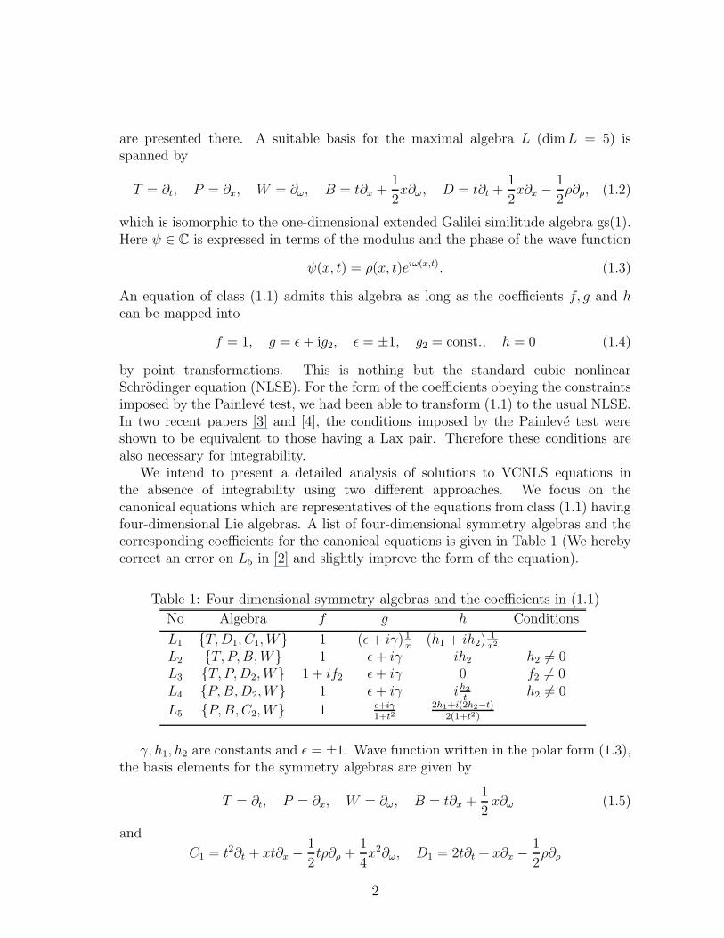
We intend to present a detailed analysis of solutions to VCNLS equations inthe absence of integrability using two different approaches. We focus on thecanonical equations which are representatives of the equations from class (1.1) havingfour-dimensional Lie algebras. A list of four-dimensional symmetry algebras and thecorresponding coefficients for the canonical equations is given in Table 1 (We herebycorrect an error on L5 in [2] and slightly improve the form of the equation).

Table 1: Four dimensional symmetry algebras and the coefficients in (1.1)

No Algebra f g h Conditions

L1 {T,D1, C1,W} 1 (ǫ+ iγ) 1x

(h1 + ih2)1x2

L2 {T, P,B,W} 1 ǫ+ iγ ih2 h2 6= 0L3 {T, P,D2,W} 1 + if2 ǫ+ iγ 0 f2 6= 0L4 {P,B,D2,W} 1 ǫ+ iγ ih2

th2 6= 0

L5 {P,B, C2,W} 1 ǫ+iγ1+t2

2h1+i(2h2−t)2(1+t2)

γ, h1, h2 are constants and ǫ = ±1. Wave function written in the polar form (1.3),the basis elements for the symmetry algebras are given by

T = ∂t, P = ∂x, W = ∂ω, B = t∂x +1

2x∂ω (1.5)

and

C1 = t2∂t + xt∂x −1

2tρ∂ρ +

1

4x2∂ω, D1 = 2t∂t + x∂x −

1

2ρ∂ρ

2

for L1, D2 = t∂t+12x∂x− 1

2ρ∂ρ for L3 and L4, and C2 = (1+t2)∂t+xt∂x+

14x2∂ω for the

algebra L5. We note that L1 is a non-solvable and L2 is a nilpotent algebra and theother three are solvable and non-nilpotent. In addition, L1 and L3 are decomposablewhereas the others are not.

These canonical equations do not pass the Painleve test for PDEs, therefore theyare not integrable and will be the main subject of this study. We are going to apply twodifferent methods: Symmetry reduction and Painleve truncated expansions. The firstis to make use of the one-dimensional subalgebras of the four-dimensional algebrasgiven in Table 1 and the second is to find a valid truncated series solution to theequation.

The paper is organized as follows. In Section 2 we find the group-invariantequations for the canonical equations having four dimensional symmetry algebras.Section 3 is devoted to the analysis of the reduced systems and completes the studyof the invariant solutions. In Section 4 we apply the method of truncated Painleveexpansions to the canonical equations to obtain exact solutions.

2 One-dimensional subalgebras and reductions to

ODEs

As we are interested in group invariant solutions we only need one-dimensionalsubalgebras. This is the case because we restrict ourselves to subgroups of thesymmetry group having generic orbits of codimension 3 in the space {x, t} × {ρ, ω}.

The classification of one-dimensional subalgebras under the action of the groupof inner automorphisms of the four-dimensinal symmetry groups is a standard one.We do not provide the calculations leading to the conjugacy inequivalent list ofsubalgebras. The classification method can be found in for example in [5, 6, 7].

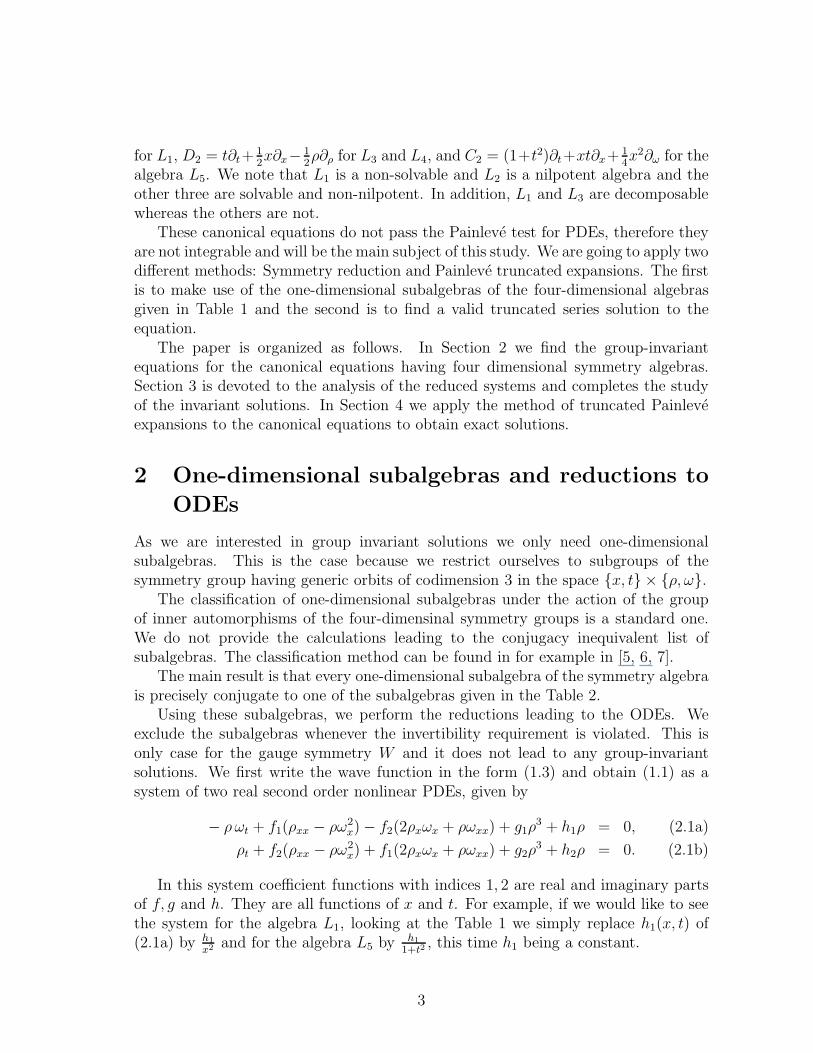
The main result is that every one-dimensional subalgebra of the symmetry algebrais precisely conjugate to one of the subalgebras given in the Table 2.

Using these subalgebras, we perform the reductions leading to the ODEs. Weexclude the subalgebras whenever the invertibility requirement is violated. This isonly case for the gauge symmetry W and it does not lead to any group-invariantsolutions. We first write the wave function in the form (1.3) and obtain (1.1) as asystem of two real second order nonlinear PDEs, given by

− ρ ωt + f1(ρxx − ρω2x)− f2(2ρxωx + ρωxx) + g1ρ

3 + h1ρ = 0, (2.1a)

ρt + f2(ρxx − ρω2x) + f1(2ρxωx + ρωxx) + g2ρ

3 + h2ρ = 0. (2.1b)

In this system coefficient functions with indices 1, 2 are real and imaginary partsof f, g and h. They are all functions of x and t. For example, if we would like to seethe system for the algebra L1, looking at the Table 1 we simply replace h1(x, t) of(2.1a) by h1

x2 and for the algebra L5 by h1

1+t2, this time h1 being a constant.

3

Table 2: One-dimensional subalgebras of 4-dimensional algebras under the adjointaction of the full symmetry group

Algebra Subalgebra a, b, c ∈ R, ǫ1 = ∓1

L1 L1.1 = {T + C1 + aW} L1.2 = {D1 + bW} L1.3 = {T + cW}L2 L2.1 = {P} L2.2 = {T + aW} L2.3 = {B + bT}

L2.4 = {W}L3 L3.1 = {T} L3.2 = {P} L3.3 = {T + ǫ1W}

L3.4 = {P + ǫ1W} L3.5 = {D2 + aW} L3.6 = {T + ǫ1P + bW}L3.7 = {W}

L4 L4.1 = {P} L4.2 = {B} L4.3 = {P + ǫ1B}L4.4 = {D2 + aW} L4.5 = {W}

L5 L5.1 = {P} L5.2 = {B} L5.3 = {C2 + aW}

Invariant surface condition for a specific subalgebra gives the similarity variablefor the functions ρ and ω. Use of this variable in (2.1) therefore reduces the numberof independent variables in the system from two to one, converting it to a systemof ODEs. These nonlinear systems of ODEs arise as first or second order nonlinearequations.

In the following, each time we encounter a first order equation, we provide itssolution right away. The task is harder for the second order equations, because wehave to decouple the reduced system of equations before treating them. For specificvalues of the constants appearing in the reduced equations, we were able to succeedin decoupling the systems and left the search for solutions to the Section 3.

2.1 Non-Solvable Algebra L1 = {T,D1, C1,W}Commutators for the basis elements of the four-dimensional algebra L1 satisfy

[T,D1] = 2T, [T, C1] = D1, [D1, C1] = 2C1 (2.2)

with W being the center element, that is, commuting with all the other elements.The algebra has the direct sum structure

L1 = sl(2,R)⊕ {W}. (2.3)

Representative equation of the algebra is

iψt + ψxx + (ǫ+ iγ)1

x|ψ|2ψ + (h1 + ih2)

1

x2ψ = 0 (2.4)

4

with the real constants ǫ = ∓1, γ, h1, h2. In polar variables it takes the form of asystem

− ρ ωt + ρxx − ρω2x +

ǫ

xρ3 +

h1x2ρ = 0, (2.5a)

ρt + 2ρxωx + ρωxx +γ

xρ3 +

h2x2ρ = 0. (2.5b)

2.1.1 Subalgebra L1.1 = {T + C1 + aW}Invariance under the subalgebra L1.1 implies that the solution has the form

ψ(x, t) =M(ξ)√

xexp

[

i(

a arctan t +x2t

4(1 + t2)+ P (ξ)

)

]

, ξ =x2

1 + t2. (2.6)

We substitute ρ(x, t) = M(ξ)√x

and ω(x, t) = a arctan t + x2t4(1+t2)

+ P (ξ) in (2.5) and

obtain the reduced system of equations satisfied by M(ξ) and P (ξ):

ǫM3 +(3− ξ2

4− aξ + h1

)

M − 4ξ2MP ′2 + 4ξ2M ′′ = 0, (2.7a)

γM3 + h2M + 8ξ2M ′P ′ + 4ξ2MP ′′ = 0. (2.7b)

We first need to decouple these equations to solve for the functions M and P . If(2.7b) is multiplied by M and written as

γM4 + h2M2 + 4ξ2(M2P ′)′ = 0, (2.8)

it is seen that an integral of (2.8) can be obtained for three different cases of theconstants.(i) The case γ = 0, h2 6= 0.

We define Y = Y (ξ) in (2.8) as

(M2P ′)′ = −h2M2

4ξ2= Y ′, (2.9)

which then easily integrates to

M2P ′ = Y + C, C = const. (2.10)

so that

M2 = − 4

h2ξ2Y ′. (2.11)

Hence the expression

P ′ = −h2(Y + C)

4ξ2Y ′ (2.12)

5

obtained in terms of Y has to be substituted into (2.7a). But the other terms in (2.7a)must also be expressed in terms of Y , which is seen to be possible if one considers(2.11). As a result we obtain a third order nonlinear ordinary differential equationfrom (2.7a):

Y ′Y ′′′− 1

2Y ′′2+

2

ξY ′Y ′′+

1

2ξ2

(3− ξ2

4−aξ+h1

)

Y ′2− 2ǫ

h2Y ′3− h22

8ξ4(Y +C)2 = 0. (2.13)

From a solution of this equation, one can find the functions M,P of (2.6) as

M(ξ) = 2ξ

√

− 1

h2Y ′ , P (ξ) = −h2

4

∫

Y + C

ξ2Y ′ dξ. (2.14)

(ii) The case γ 6= 0, h2 = 0.This time the function Y is defined in (2.8) as

(M2P ′)′ = −γM4

4ξ2= Y ′ (2.15)

leading to the integralM2P ′ = Y + C, C = const. (2.16)

so that we have

M4 = −4

γξ2 Y ′. (2.17)

From (2.7a) the following third order ODE for Y is obtained:

Y ′Y ′′′ − 3

4Y ′′2 +

1

ξY ′Y ′′ −

(1− 4h14ξ2

+a

ξ+

1

4

)

Y ′2 +γ

ξ2(Y +C)2Y ′ +

2ǫ

ξY ′2

√

−Y′

γ= 0.

(2.18)For a solution Y (ξ) of this equation M and P are going to be evaluated from

M(ξ) =(

− 4

γξ2Y ′

)1/4

, P (ξ) =1

2

∫√

− γ

Y ′Y + C

ξdξ. (2.19)

(iii) The case γ = h2 = 0.In this case we can easily decouple the reduced system of equations. Integration

of (2.8) gives

M2P ′ = C, P (ξ) =

∫

C

M2dξ, C = const. (2.20)

and from (2.7a) we obtain the equation for M

M ′′ = − ǫ

4ξ2M3 +

1

4ξ2

(ξ2 − 3

4+ aξ − h1

)

M + C2M−3. (2.21)

6

2.1.2 Subalgebra L1.2 = {D1 + bW}Group-invariant solutions for subalgebra L1.2 will have the form

ψ(x, t) =M(ξ)√

xexp

[

i(

b ln x+ P (ξ))

]

, ξ =x2

t. (2.22)

It is straightforward to see that M(ξ) and P (ξ) must satisfy

ǫM3 +(3

4− b2 + h1

)

M + ξ(ξ − 4b)MP ′ − 4ξ2MP ′2 + 4ξ2M ′′ = 0, (2.23a)

γM3 + (h2 − 2b)M + ξ(4b− ξ)M ′ + 8ξ2M ′P ′ + 4ξ2MP ′′ = 0. (2.23b)

If we multiply (2.23a) by M , we can write it in the form

γM4 + h2M2 + ξ2

[

M2(2b

ξ− 1

2+ 4P ′

)

]′= 0. (2.24)

Integration of (2.24) is possible in three different cases.(i) The case γ = 0, h2 6= 0.

The function Y (ξ) is defined in (2.24) as

[

M2(2b

ξ− 1

2+ 4P ′

)

]′= −h2

M2

ξ2= Y ′. (2.25)

We integrate to find

P ′ =1

8− b

2ξ− h2

4ξ2Y + C

Y ′ (2.26)

and with the equality

M2 = − 1

h2ξ2 Y ′ (2.27)

(2.23a) can be completely expressed in terms of Y

Y ′Y ′′′− 1

2Y ′′2+

2

ξY ′Y ′′+

1

8

(3 + 4h1ξ2

− 2b

ξ+1

4

)

Y ′2− ǫ

2h2Y ′3− h22

8ξ4(Y +C)2 = 0. (2.28)

If a solution Y of this equation is known, then P and M can be obtained from (2.26)and (2.27).(ii) The case γ 6= 0, h2 = 0.

In (2.24) the function Y (ξ) is defined by

[

M2(2b

ξ− 1

2+ 4P ′

)

]′= −γM

4

ξ2= Y ′. (2.29)

We integrate (2.29) equation to obtain

P ′ =1

8− b

2ξ+Y + C

4ξ

√

− γ

Y ′ (2.30)

7

and hence

M4 = −1

γξ2 Y ′ (2.31)

of which substitution in (2.23a) gives rise to an equation in terms of Y :

Y ′Y ′′′− 3

4Y ′′2+

1

ξY ′Y ′′+

(4h1 − 1

4ξ2− b

2ξ+

1

16

)

Y ′2+γ

4ξ2(Y +C)2Y ′+

ǫ

ξY ′2

√

−Y′

γ= 0.

(2.32)P and M are going to be found from (2.30) and (2.31).(iii) The case γ = h2 = 0.

If (2.24) is integrated once, we get

P ′ =C

M2+

1

8− b

2ξ(2.33)

and substitution of this result in (2.23a) leaves us with the second order equation forM :

M ′′ = C2M−3 − ǫ

4ξ2M3 − 1

16ξ2(3 + 4h1 − 2bξ +

1

4ξ2)M. (2.34)

2.1.3 Subalgebra L1.3 = {T + cW}Invariance under the subalgebra L1.3 implies that the solution will have the form

ψ(x, t) =M(x) exp[

i(

ct + P (x))

]

(2.35)

and here M(ξ), P (ξ) satisfy the system

ǫxM3 + (h1 − cx2)M − x2MP ′2 + x2M ′′ = 0, (2.36a)

γxM3 + h2M + 2x2M ′P ′ + x2MP ′′ = 0. (2.36b)

Similarly, (2.36b) can be arranged as

γxM4 + h2M2 + x2

(

M2P ′)′ = 0 (2.37)

and with arguments similar to the preceding algebras we obtain the following results.(i) The case γ = 0, h2 6= 0.

M(x) and P (x) are found from

M(x) =

(

− 1

h2x2Y ′

)1/2

, P (x) = −h2∫

Y + C

x2Y ′ dx. (2.38)

Here Y (x) satisfies a third order equation

Y ′Y ′′′ − 1

2Y ′′2 +

2

xY ′Y ′′ + 2

(h1x2

− c)

Y ′2 − 2ǫx

h2Y ′3 − 2h22

x4(Y + C)2 = 0. (2.39)

8

(ii) The case γ 6= 0, h2 = 0.M(x) and P (x) are to be evaluated from

M(x) =

(

−1

γxY ′)1/4

, P (x) =

∫

(Y + C)

√

− γ

xY ′ dx. (2.40)

Y (x) is a solution to the equation

Y ′Y ′′′− 3

4Y ′′2+

1

2xY ′Y ′′+

(16h1 − 3

4x2− 4c

)

Y ′2+4γ

x(Y +C)2Y ′+

4ǫ

xY ′2√

−xγY ′ = 0.

(2.41)(iii) The case γ = h2 = 0.

M(x) is the solution of the equation

M ′′ = C2M−3 +(

c− h1x2

)

M − ǫ

xM3 (2.42)

and P (x) is going to be evaluated from

P (x) =

∫

C

M2dx. (2.43)

2.2 Nilpotent algebra L2 = {T, P, B,W}Nonzero commutation relation is [P,B] = 1

2W . The algebra contains the three

dimensional abelian ideal {T, P,W}. The action of B on this ideal can be representedby the nilpotent matrix N

[P,B][T,B][W,B]

= N

PTW

, N =

0 0 1/20 0 00 0 0

.

In this case the canonical equation has the form

iψt + ψxx + (ǫ+ iγ)|ψ|2ψ + ih2ψ = 0 (2.44)

with the real constants ǫ = ∓1, h2 6= 0 and γ.

2.2.1 Subalgebra L2.1 = {P}The group-invariant solution of L2.1 has the form

ψ(x, t) =M(t) exp(

iP (t))

(2.45)

and M,P must satisfy

ǫM2 − P ′ = 0, (2.46a)

γM3 + h2M +M ′ = 0. (2.46b)

9

We immediately integrate these equations and find

M(t) =

(

M1 exp(2h2 t)−γ

h2

)−1/2

, (2.47a)

P (t) =

ǫ2γ

ln(

M1 − γh2

exp(−2h2 t))

+ P1, γ 6= 0

P1 − ǫ2h2M1

exp(2h2 t), γ = 0(2.47b)

with arbitrary constants M1, P1.

2.2.2 Subalgebra L2.2 = {T + aW}A solution invariant under the algebra L2.2 must be in the following form

ψ(x, t) =M(x) exp[

i(

at + P (x))

]

. (2.48)

Here M,P have to satisfy

ǫM3 − aM −MP ′2 +M ′′ = 0, (2.49a)

γM3 + h2M + 2M ′P ′ +MP ′′ = 0. (2.49b)

For γ = 0 we multiply (2.49b) by M to obtain

h2M2 + (M2P ′)′ = 0 (2.50)

and define the function Y (x) in this equation as

(M2P ′)′ = −h2M2 = Y ′. (2.51)

Substitution of

P (x) = −h2∫

Y + C

Y ′ dx (2.52)

in (2.49a) leads to decoupling of the reduced system

Y ′Y ′′′ − 1

2Y ′′2 − 2ǫ

h2Y ′3 − 2aY ′2 − 2h22(Y + C)2 = 0. (2.53)

P is determined by (2.52) and M is given by

M(x) = (− 1

h2Y ′)1/2. (2.54)

10

2.2.3 Subalgebra L2.3 = {B + bT}(i) The case b 6= 0. An invariant solution of L2.3 is obtained in the form

ψ(x, t) =M(ξ) exp[

i( 1

2bxt− 1

6b2t3 + P (ξ)

)]

, ξ = bx− t2

2. (2.55)

Functions M and P are solutions to the system

ǫ

b2M3 − ξ

2b4M −MP ′2 +M ′′ = 0, (2.56a)

γM3 + h2M + 2b2M ′P ′ + b2MP ′′ = 0. (2.56b)

We can arrange (2.56b) as

γM4 + h2M2 + b2(M2P ′)′ = 0 (2.57)

and for γ = 0 define Y (ξ) such that

(M2P ′)′ = −h2b2M2 = Y ′, (2.58)

from which we get

P (ξ) = −h2b2

∫

Y + C

Y ′ dξ. (2.59)

Hence we have decoupled (2.56a) in the form

Y ′Y ′′′ − 1

2Y ′′2 − 2ǫ

h2Y ′3 − x

b4Y ′2 − 2h22

b4(Y + C)2 = 0. (2.60)

P is obtained from (2.59) and M is given by the formula

M(ξ) = (− b2

h2Y ′)1/2. (2.61)

(ii) The case b = 0.

ψ(x, t) =M(t) exp[

i(x2

4t+ P (t)

)]

(2.62)

is the form of the group-invariant solution and the reduced system of equations is

ǫM2 − P ′ = 0, (2.63a)

γM3 + (h2 +1

2t)M +M ′ = 0. (2.63b)

We solve this system by standard methods and get

M(t) =

(

t exp(2h2t)(M1 + 2γ

∫

exp(−2h2t)

tdt)

)−1/2

, (2.64)

11

and

P (t) =

ǫ2γ

ln(

2γ∫ exp(−2h2t)

tdt+M1

)

+ P1, γ 6= 0

ǫM1

∫ exp(−2h2t)t

dt+ P1, γ = 0.

(2.65)

In the following we study the reductions for L3, L4, L5, which are solvablenon-nilpotent Lie algebras. L3 contains an abelian ideal. L4 and L5 include a nilpotentideal.

2.3 Solvable algebra L3 = {T, P,D2,W}The algebra has the abelian ideal {T, P,W}. Nonzero commutation relations are

[D2, T ] = T, [D2, P ] =1

2P. (2.66)

The algebra has a decomposable structure

L3 = {T, P,D2} ⊕ {W}. (2.67)

We note the canonical equation

iψt + (1 + if2)ψxx + (ǫ+ iγ)|ψ|2ψ = 0 (2.68)

with the constants ǫ = ∓1, f2 6= 0, γ and proceed to find the reduced ODEs.

2.3.1 Subalgebra L3.1 = {T}A solution of VCNLS invariant under the algebra L3.1 must have the form

ψ(x, t) =M(x) exp(

iP (x))

. (2.69)

M and P are found from the following reduced system

ǫM3 − 2f2M′P ′ −M(P ′2 + f2P

′′) +M ′′ = 0, (2.70a)

γM3 + 2M ′P ′ + f2M′′ +M(−f2P ′2 + P ′′) = 0. (2.70b)

It is possible to arrange these equations as

ǫ+ γf21 + f 2

2

M3 −MP ′2 +M ′′ = 0, (2.71a)

γ − ǫf21 + f 2

2

M4 + (M2P ′)′ = 0. (2.71b)

Similar to the preceding calculations, we were able to achieve decoupling for specialcases of the parameters as follows.

12

(i) The case γ 6= ǫf2. The function Y (x) defined as

(M2P ′)′ =ǫf2 − γ

1 + f 22

M4 = Y ′ (2.72)

gives us the relations

P ′ =Y + C

M2, M =

(

1 + f 22

ǫf2 − γY ′)1/4

. (2.73)

When we use these in (2.71a), we obtain a third-order equation for Y (x)

Y ′Y ′′′ − 3

4Y ′′2 +

4(ǫ+ γf2)√

1 + f 22

√

Y ′

ǫf2 − γY ′2 +

4(γ − ǫf2)

1 + f 22

(Y + C)2Y ′ = 0. (2.74)

For a solution of this equation one can evaluate M and P from equations (2.73).(ii) The case γ = ǫf2.

M(x) is a solution to the equation

M ′′ =C2

M3− ǫM3 (2.75)

and P (x) is given by

P (x) =

∫

C

M2dx. (2.76)

2.3.2 Subalgebra L3.2 = {P}Modulus and phase for the group-invariant solution corresponding to the algebra L3.2,which is in the form ψ(x, t) =M(t) exp

(

iP (t))

, are found from the system

ǫM2 − P ′ = 0, (2.77a)

γM3 +M ′ = 0 (2.77b)

as

M(t) =√

2γt+M1, (2.78a)

P (t) = ǫ(γt2 +M1t) + P1. (2.78b)

2.3.3 Subalgebra L3.3 = {T + ǫ1W}The solution in this case should have the form

ψ(x, t) =M(x) exp[

i(

ǫ1t + P (x))

]

, (2.79)

13

where M, P satisfy

ǫM3 − 2f2M′P ′ − (ǫ1 + P ′2 + f2P

′′)M +M ′′ = 0, (2.80a)

γM3 + 2M ′P ′ + (−f2P ′2 + P ′′)M + f2M′′ = 0. (2.80b)

In order to decouple these equations we can arrange them as

ǫ+ γf21 + f 2

2

M3 −MP ′2 +M ′′ = 0, (2.81a)

(γ − ǫf2)M4 + ǫ1f2M

2 + (1 + f 22 )(M

2P ′)′ = 0. (2.81b)

Since f2 6= 0, a first integral of (2.81b) can be obtained if γ = ǫf2. Let Y (x) bedefined as

(M2P ′)′ = − ǫ1f21 + f 2

2

M2 = Y ′. (2.82)

Then we have

M2 = −1 + f 22

ǫ1f2Y ′, P ′ = − ǫ1f2

1 + f 22

Y + C

Y ′ (2.83)

and thus (2.81a) is transformed to an equation in terms of Y (x)

Y ′Y ′′′ − 1

2Y ′′2 − 2ǫ(1 + f 2

2 )

ǫ1f2Y ′3 − 2f 2

2

1 + f 22

(Y + C)2 = 0. (2.84)

2.3.4 Subalgebra L3.4 = {P + ǫ1W}In this case we have

ψ(x, t) =M(t) exp[

i(

ǫ1x+ P (t))

]

, (2.85)

where

1− ǫM2 + P ′ = 0, (2.86a)

γM3 − f2M +M ′ = 0. (2.86b)

We find that

M(t) =

(

M1 exp(−2f2 t) +γ

f2

)−1/2

, (2.87a)

P (t) =

ǫ2γ

ln(

M1 +γf2exp(2f2 t)

)

− t+ P1, γ 6= 0

ǫ2f2M1

exp(2f2 t)− t+ P1, γ = 0.(2.87b)

14

2.3.5 Subalgebra L3.5 = {D + aW}We will look for the solution in the form

ψ(x, t) =1

xM(ξ) exp

[

i(

2a ln x+ P (ξ))]

, ξ =x2

t(2.88)

and the reduced system for M,P is

ǫM3 + (2 + 6af2 − 4a2)M − 2(1 + 4af2)ξM′ +(

ξ2 + 2(f2 − 4a)ξ)

MP ′

−8f2ξ2M ′P ′ − 4ξ2MP ′2 + 4ξ2M ′′ − 4f2ξ

2MP ′′ = 0, (2.89a)

γM3 + (2f2 − 6a− 4a2f2)M + (8a− 2f2 − ξ)ξM ′ − 2(1 + 4af2)ξMP ′

+8ξ2M ′P ′ − 4f2ξ2MP ′2 + 4f2ξ

2M ′′ + 4ξ2MP ′′ = 0. (2.89b)

It is possible to rewrite these equations as

(ǫ+ γf2)M3 + 2(1− 2a2)(1 + f 2

2 )M −(

2(1 + f 22 )ξ + f2ξ

2)

M ′

+(

ξ2 − 8a(1 + f 22 )ξ)

MP ′ + 4(1 + f 22 )ξ

2(M ′′ −MP ′2) = 0, (2.90a)

(γ − ǫf2)M4 − 6a(1 + f 2

2 )M2 +

(

4a(1 + f 22 )ξ −

ξ2

2

)

(M2)′

−(

2(1 + f 22 )ξ + f2ξ

2)

M2P ′ + 4(1 + f 22 )ξ

2(M2P ′)′ = 0 (2.90b)

so that they contain second order derivatives in terms of only M or P . Butunfortunately we have not been able to proceed further as in the previous algebras.

2.3.6 Subalgebra L3.6 = T + ǫ1P + bW

The modulus M and the phase P of the group-invariant solution

ψ(x, t) =M(ξ) exp[

i(

bt + P (ξ))

]

, ξ = x− ǫ1t (2.91)

satisfy the system

(ǫ+ γf2)M3 − bM − ǫ1f2M

′ + ǫ1MP ′ − (1 + f 22 )MP ′2

+(1 + f 22 )M

′′ = 0, (2.92a)

(γ − ǫf2)M4 + bf2M

2 − ǫ12(M2)′ − ǫ1f2M

2P ′

+(1 + f 22 )(M

2P ′)′ = 0. (2.92b)

Arranging (2.92b) according to the terms M2P ′ and M2 we write

(M2P ′)′ − ǫ1f21 + f 2

2

(M2P ′) =1

1 + f 22

(ǫ12(M2)′ − bf2M

2 + (ǫf2 − γ)M4)

. (2.93)

15

We multiply this equality by exp(−ǫ1f21+f2

2

ξ)

and define Y (ξ) as

[

exp(−ǫ1f21 + f 2

2

ξ)

M2P ′]′

=exp

(−ǫ1f21+f2

2

ξ)

1 + f 22

(ǫ12(M2)′ − bf2M

2 + (ǫf2 − γ)M4)

= Y ′.

(2.94)First we have

M2P ′ = exp( ǫ1f21 + f 2

2

ξ)

(Y + C). (2.95)

On the other hand, we need to solve for M2 from

(M2)′ − 2ǫ1bf2M2 + 2ǫ1(ǫf2 − γ)(M2)2 = 2ǫ1(1 + f 2

2 ) exp( ǫ1f21 + f 2

2

ξ)

Y ′. (2.96)

This equation is of Riccati type in M2 and a special solution is needed for itsintegration. Furthermore, it can be linearized through the transformation M2 =

12ǫ1(ǫf2−γ)

U ′

Uat the cost of having its order increased by one:

U ′′ − 2ǫ1bf2 U′ + 4(γ − ǫf2)(1 + f 2

2 ) exp( ǫ1f21 + f 2

2

ξ)

Y ′U = 0. (2.97)

Still, this equation does not lead to any immediate solution. Instead, it will be easierto handle (2.96) by the choice γ = ǫf2

(

exp(

− 2ǫ1bf2ξ)

M2)′

= 2ǫ1(1 + f 22 ) exp

(

ǫ1f2( 1

1 + f 22

− 2b)

ξ)

Y ′ (2.98)

and if b = 12(1+f2

2)then we can integrate to find

M2(ξ) = 2ǫ1(1 + f 22 ) exp

( ǫ1f21 + f 2

2

ξ)

(

Y (ξ) + C)

. (2.99)

A comparison of this result by (2.95) forces

P ′ =1

2ǫ1(1 + f 22 ). (2.100)

Therefore we could end up with a decoupled equation for M from (2.92a)

M ′′ =ǫ1f2

1 + f 22

M ′ +1

4(1 + f 22 )

2M − ǫM3. (2.101)

On the other hand, if (2.92b) is arranged with the condition γ = ǫf2 as

(

(1 + f 22 )M

2P ′ − ǫ12M2)′

= ǫ1f2M2P ′ − bf2M

2, (2.102)

16

the choice b = 12(1+f2

2)even makes it possible to write this equation in the simpler

formU ′ = λU (2.103)

where U(ξ) = (1 + f 22 )M

2P ′ − ǫ12M2, λ = ǫ1f2

1+f22

. The obvious solution U(ξ) =

λ0 exp(λξ) with some constant λ0 gives us the formula for P ′

P ′ =1

2ǫ1(1 + f 22 )

+λ0 exp(λξ)

1 + f 22

M−2. (2.104)

Substitution of this result in (2.92a) gives the decoupled equation for M as

M ′′ =ǫ1f2

1 + f 22

M ′ +1

4(1 + f 22 )

2M − ǫM3 +

λ20 exp(2λξ)

(1 + f 22 )

2M−3. (2.105)

This equation reduces to (2.101) for λ0 = 0.

2.4 Solvable algebra L4 = {P,B,D2,W}This solvable non-nilpotent algebra is the extension of the nilpotent three dimensionalLie algebra {W,P,B}. We represent the action of D2 on this ideal by a matrix M

[W,D2][P,D2][B,D2]

=M

WPB

, M =

0 0 00 1/2 00 0 −1/2

.

We note that the algebra is not decomposable and the representative equation fromTable 1 is

iψt + ψxx + (ǫ+ iγ)|ψ|2ψ + ih2tψ = 0, (2.106)

where ǫ = ∓1, h2 6= 0 and γ are real constants.

2.4.1 Subalgebra L4.1 = {P}Group-invariant solution is of the form

ψ(x, t) =M(t) exp(

iP (t))

(2.107)

and the reduced system is first order

ǫM2 − P ′ = 0, (2.108a)

M ′ +h2tM + γM3 = 0. (2.108b)

17

Solution of this system is elementary

M(t) = (2γt ln t+M1t)−1/2 (2.109a)

P (t) =

ǫ2γ

ln(2γ ln t+M1) + P1, γ 6= 0

ǫM1

ln t+ P1, γ = 0(2.109b)

for h2 = 1/2, whereas

M(t) =( 2γ

1− 2h2t+M1t

2h2

)−1/2

, (2.110a)

P (t) =

ǫ2γ

ln(M1 +2γ

1−2h2t1−2h2) + P1, γ 6= 0

ǫM1(1−2h2)

t1−2h2 + P1, γ = 0(2.110b)

for h2 6= 1/2.

2.4.2 Subalgebra L4.2 = {B}The solution invariant under B has the form

ψ(x, t) =M(t) exp[

i(x2

4t+ P (t)

)]

. (2.111)

The reduced first order system is

ǫM2 − P ′ = 0, (2.112a)

M ′ +1 + 2h2

2tM + γM3 = 0; (2.112b)

which can be integrated to give

M(t) = (M1 t1+2h2 − γ

h2t)−1/2, (2.113a)

P (t) =

ǫ2γ

ln(M1 − γh2t−2h2) + P1, γ 6= 0

− ǫ2h2M1

t−2h2 + P1, γ = 0.(2.113b)

2.4.3 Subalgebra L4.3 = {P + ǫ1B}The corresponding invariant solution is given by

ψ(x, t) =M(t) exp[

i( ǫ1x

2

4(1 + ǫ1t)+ P (t)

)]

. (2.114)

The reduced system becomes

ǫM2 − P ′ = 0, (2.115a)

M ′ +

(

h2t+

ǫ12(1 + ǫ1t)

)

M + γM3 = 0. (2.115b)

18

For the case h2 = 1/2 the system is integrated easily

M(t) =

(

t(1 + ǫ1t)(

2γ ln(t

1 + ǫ1t) +M1

)

)−1/2

, (2.116a)

P (t) =

ǫ2γ

ln(

2γ ln( t1+ǫ1t

) +M1

)

+ P1, γ 6= 0

ǫM1

ln( t1+ǫ1t

) + P1, γ = 0.(2.116b)

If h2 6= 1/2, then integration is possible in terms of the Gauss’ hypergeometricfunction 2F1(a, b, c; t):

M(t) =

(

M1t2h2(1 + ǫ1t) +

2γ

1− 2h2t(1 + ǫ1t) 2F1(1− 2h2, 1, 2− 2h2;−ǫ1t)

)−1/2

,

P (t) =

∫

ǫM2dt. (2.117)

We note that for integer values of 2h2 this solution will simplify to elementaryfunctions.

2.4.4 Subalgebra L4.4 = {D + aW}A group-invariant solution invariant under the subalgebra L4.4 will be of the form

ψ(x, t) =1

xM(ξ) exp

[

i(

2a lnx+ P (ξ))

]

, ξ =x2

t. (2.118)

Functions M,P will be solutions of the system

ǫM3 + 2(1− 2a2)M − 2ξM ′ + (ξ2 − 8aξ)MP ′ − 4ξ2MP ′2

+4ξ2M ′′ = 0, (2.119a)

γM4 + (h2ξ − 6a)M2 +(

4aξ − ξ2

2

)

(M2)′ − 2ξM2P ′

+4ξ2(M2P ′)′ = 0. (2.119b)

For γ = 0 we define in (2.119b) the function Y (ξ) as

4ξ2(M2P ′)′ − 2ξM2P ′ =(ξ2

2− 4aξ

)

(M2)′ + (6a− h2ξ)M2 = Y ′. (2.120)

From these relations we find

M2P ′ =ξ1/2

4

(

∫

ξ−5/2Y ′dξ + C)

(2.121)

and for h2 = 1/4

M2 =2ξ3/2

ξ − 8a

(

∫

ξ−5/2Y ′dξ + C)

. (2.122)

19

Thus if h2 = 1/4 we can obtain from (2.121) and (2.122) that

P (ξ) =ξ

8− a ln ξ + P1. (2.123)

This special form of P (ξ) is readily seen to satisfy (2.119b) whereas (2.119a) isdecoupled to determine M from

M ′′ =1

2ξM ′ − (

1

64− a

4ξ+

1

2ξ2)M − ǫ

4ξ2M3. (2.124)

2.5 Solvable algebra L5 = {P,B, C2,W}L5 is another canonical extension of the nilpotent algebra {W,P,B} to a solvablenon-nilpotent indecomposable four-dimensional algebra. The element C2 acts on theideal {W,P,B} by the matrix M as

[W,C2][P,C2][B,C2]

=M

WPB

, M =

0 0 00 0 10 −1 0

.

Thus the last canonical equation under investigation will be

iψt + ψxx +ǫ+ iγ

1 + t2|ψ|2ψ +

2h1 + i(2h2 − t)

2(1 + t2)ψ = 0, (2.125)

with the constants ǫ = ∓1, h1, h2 and γ.

2.5.1 Subalgebra L5.1 = {P}The group-invariant solution ψ(x, t) = M(t) exp

(

iP (t))

will be obtained by solvingM,P from the reduced system

ǫ

1 + t2M2 +

h11 + t2

− P ′ = 0, (2.126a)

M ′ +2h2 − t

2(1 + t2)M +

γ

1 + t2M3 = 0. (2.126b)

Through the transformation M = W−1/2 in the Bernoulli type equation (2.126b) wehave

(√1 + t2 exp(−2h2 arctan t)W

)′=

2γ√1 + t2

exp(−2h2 arctan t). (2.127)

W can be expressed by a quadrature and hence

M(t) =

(

exp(2h2 arctan t)√1 + t2

(

M1 + 2γ

∫

exp(−2h2 arctan t)√1 + t2

dt)

)−1/2

, (2.128a)

P (t) =

h1 arctan t+ǫ2γ

ln(

M1 + 2γ∫ exp(−2h2 arctan t)√

1+t2dt)

+ P1, γ 6= 0

h1 arctan t+ǫ

M1

∫ exp(−2h2 arctan t)√1+t2

dt+ P1, γ = 0.(2.128b)

20

We note that by the transformation t = tan z in the integrands these results can beexpressed in terms of hypergeometric functions.

2.5.2 Subalgebra L5.2 = {B}The solution has the form

ψ(x, t) =M(t) exp[

i(x2

4t+ P (t)

)

]

,

with functions M,P determined from the system

ǫ

1 + t2M2 +

h11 + t2

− P ′ = 0, (2.129a)

M ′ +( 2h2 − t

2(1 + t2)+

1

2t

)

M +γ

1 + t2M3 = 0. (2.129b)

A transformation M =W−1/2 in equation (2.129b) leads to

(√1 + t2

texp(−2h2 arctan t)W

)′

=2γ

t√1 + t2

exp(−2h2 arctan t). (2.130)

We find M,P as

M(t) =

(

t exp(2h2 arctan t)√1 + t2

(

M1 + 2γ

∫

exp(−2h2 arctan t)

t√1 + t2

dt)

)−1/2

,(2.131a)

P (t) =

h1 arctan t+ǫ2γ

ln(

M1 + 2γ∫ exp(−2h2 arctan t)

t√1+t2

dt)

+ P1, γ 6= 0

h1 arctan t+ǫ

M1

∫ exp(−2h2 arctan t)

t√1+t2

dt+ P1, γ = 0.(2.131b)

The transformation t = tan z is also applicable in the integrands leading tohypergeometric solutions.

2.5.3 Subalgebra L5.3 = {C2 + aW}Group-invariant solution must have the form

ψ(x, t) =M(ξ) exp[

i(

a arctan t+x2t

4(1 + t2)+ P (ξ)

)]

, ξ =x√

1 + t2(2.132)

Substitution of this solution into the original equation ends up with the system

ǫM3 +(

h1 − a− ξ2

4

)

M −MP ′2 +M ′′ = 0, (2.133a)

γM4 + h2M2 + (M2P ′)′ = 0. (2.133b)

21

In the case γ = 0, h2 6= 0 decoupling of these equations is possible

Y ′Y ′′′ − 1

2Y ′′2 − 2ǫ

h2Y ′3 +

(

2h1 − 2a− ξ2

2

)

Y ′2 − 2h22(Y + C)2 = 0, (2.134)

M = (− 1

h2Y ′)1/2, P ′ = −h2

Y + C

Y ′ . (2.135)

If γ = h2 = 0 then we have a second order nonlinear ODE for M

M ′′ = C2M−3 + (ξ2

4+ a− h1)M − ǫM3, (2.136a)

P ′ = CM−2. (2.136b)

3 Analysis of the reduced equations

In Table 3 we refer to the numbers of the reduced system of equations of first orderbesides the second and third order equations obtained through the decoupling taskfor some special values of the arbitrary parameters. Among the third order equationswe only included those which are polynomials in the derivative Y ′, e.g. (2.18) is notin the list. We have expressed the solutions of first order equations in the precedingSection. This part of the work will be devoted to the study of solutions of the secondand third order equations.

Table 3: Equations under study

Order Equation Number

1 (2.46), (2.63), (2.77), (2.86), (2.108), (2.112),(2.115), (2.126), (2.129)

2 (2.21), (2.34), (2.42), (2.75), (2.105), (2.124), (2.136)3 (2.13), (2.28), (2.39), (2.53), (2.60), (2.84), (2.134)

3.1 Third order equations

None of the seven third order equations summarized in Table 3 passes the invariantPainleve test for PDEs. Since (2.53) and (2.84) do not contain the independentvariable, we can directly lower their order by one if we set Y ′ = W (Y ). We obtainthe following second order equations:(i) For equation (2.53) with W = dW

dY,

W = − 1

2WW 2 +

2ǫ

h2+

2a

W+

2h22(Y + C)2

W 3. (3.1)

22

(ii) For equation (2.84),

W = − 1

2WW 2 +

2ǫ(1 + f 22 )

ǫ1f2+

2f 22

1 + f 22

(Y + C)2

W 3. (3.2)

We seeked a first integral to these second order equations in the form

A(Y,W )W ′3 +B(Y,W )W ′2 + F (Y,W )W ′ +G(Y,W ) = I (3.3)

for some functions A,B, F,G and a constant I, but saw that it is not possible.For all the third order equations satisfied by Y = Y (ξ) (including (2.53) and

(2.84)) we suggested a first integral of the form

A(ξ, Y, Y ′) Y ′′2 +B(ξ, Y, Y ′) Y ′′ + F (ξ, Y, Y ′) = I (3.4)

with some functions A,B, F and a constant I. A first integral of this type exists onlypossible for (2.39) for the special values of the constants c = 0, h1 = (5 + 81h22)/36.The first integral has the form

Y ′′2 +10

3xY ′Y ′′ − 2ǫx

h2Y ′3 +

25 + 81h229x2

Y ′2 +12h22x3

Y Y ′ (3.5)

+ (12h22C

x3− I

x7/3) Y ′ +

4h22x4

(Y + C)2 = 0.

We made an unsuccessful attempt to find a further first integral

A(x, Y ) Y ′3 +B(x, Y ) Y ′2 + F (x, Y ) Y ′ +G(x, Y ) = K (3.6)

where K is another constant.

3.2 Second order equations

Among the second order equations successfully decoupled from the reduced systems,(2.42) passes the P-test for h1 = 5/36 and so does (2.75) without any condition onthe parameters. For the other five equations which do not pass the P-test, we lookedfor a first integral, assuming M =M(ξ) satisfies an equation of type

A(ξ,M)M ′3 +B(ξ,M)M ′2 + F (ξ,M)M ′ +G(ξ,M) = I, (3.7)

which ended up without any success.Before proceeding to the solutions of second order equations passing the P-test,

we note that equation (2.105) does not contain the independent variable if we chooseλ0 = 0, which means a reduction in order. Indeed, if we set M ′ = a1W (M) witha1 =

ǫ1f21+f2

2

, an Abel equation of the second kind is obtained

W (W − 1) =a2a21M − ǫ

a1M3, (3.8)

23

where a2 =1

4(1+f22). For n = ǫ2|f2|√

1+2f22

− 3 and ǫ2 = ∓1, w = w(z) a transformation in

the parametric form

M = zn+2

2 w, W =1

n+ 3z

n+2

2 (zw′ +n+ 2

2w) (3.9)

converts this equation with A = − ǫǫ1f2(1+f22)

1+2f22

to an equation of Emden-Fowler type [8]

w′′ = Aznw3 (3.10)

which drove the final nail in the coffin.We close this section with the analysis of equations passing the P-test. Painleve

and his successors classified second order differential equations that have at mostpole-type singularities in all their solutions and determined such 50 equivalence classestogether with their representative equations. For details the interested reader isreferred to [9]. Since we have two second order equations passing the P-test, weare going to try to find the equivalence class to which they may belong.

Transformation of (2.75) to the equations numbered PXVIII and PXXXIII in thePainleve classification of second order nonlinear ODEs, their first integrals and hencesolutions in terms of elementary and elliptic functions in various cases were done in[10]. Since a simple substitution and a careful account of the different cases dependingon the constants will suffice to find the results for (2.75), we do not reproduce themhere and refer the interested reader to that work.

There remains the treatment of equation (2.42). If we make a change of thedependent variable as M =

√

H(x), H(x) > 0 we have

H ′′ =1

2HH ′2 + 2(c− h1

x2)H − 2ǫ

xH2 +

2C2

H. (3.11)

We apply a further transformation H(x) = λ(x)W (η(x)) and find

W =1

2WW 2 − 1

η

(

η

η+λ

λ

)

W +1

η2

(

2(c− h1x2

) +λ2

2λ2− λ

λ

)

W

− 2ǫλ

η2xW 2 +

2C2

λ2η2W−1.

(3.12)

We will determine λ, η such that this equation is of Painleve-type.(i) The case C 6= 0. If λ, η and other constants are chosen as

η = η0x2/3, λ = λ0x

1/3, c < 0, η0 = −(9c

2

)1/3

, h1 =5

36(3.13)

an equation quite similar to PXXXIV is obtained.

W =1

2WW 2 + 4αW 2 − ηW + 2δ2W−1, (3.14)

24

where α = −(

92c2

)1/3ǫλ0

4, δ = 3C

2λ0

(

−29c

)1/6

and λ0 is arbitrary. By a final

transformation2αW = V + V 2 +

η

2(3.15)

we see that V satisfies the equation

V = 2V 3 + ηV + k, k = −1

2± 4αδi. (3.16)

which is the second Painleve transcendent so that we can express V = PII(η0 x2/3).

Since W is complex-valued λ0 has to be chosen so that the product λW is real.(ii) The case C = 0. If we choose

η = η0x2/3, λ = λ0x

1/3, η0 =(9c

4

)1/3

, λ0 = −ǫ(32c2

9

)1/3

, h1 =5

36(3.17)

we arrive at the equation PXX:

W =1

2WW 2 + 4W 2 + 2ηW. (3.18)

Setting U2 =W leads to PII again

U = 2U3 + ηU.

We can explicitly give the solution as

ψ = λ1/20 x1/6PII(η0 x

2/3) exp(i(ct + P0)). (3.19)

4 Solutions by truncation

In order to investigate Painleve property for (1.1) in [1] we wrote the equation withits complex conjugate as the system

iut + f(x, t)uxx + g(x, t)u2v + h(x, t)u = 0,

−ivt + p(x, t)vxx + q(x, t)uv2 + r(x, t)v = 0(4.1)

and expanded u, v as

u(x, t) =

∞∑

j=0

uj(x, t)Φα+j(x, t), v(x, t) =

∞∑

j=0

vj(x, t)Φβ+j(x, t). (4.2)

We obtained the conditions on f, g, h so that all solutions to VCNLS are in thisform. Coefficients for canonical equations of 4-dimensional subalgebras do not satisfythe compatibility conditions of the P-test, therefore they do not have the Painleveproperty. Since the conditions obtained from the P-test are equivalent to those for

25

having a Lax pair, they are not integrable [3, 4]. In this case if the series (4.2) istruncated at an order j = N and plugged in the equation, a system of equations foruj, j ≤ N and Φ has to be satisfied. An exact solution is obtained once this systemcan be solved in a consistent way.

For the Painleve test to be successful it is required that resonance coefficients ujcorresponding to the resonance indices j = −1, 0, 3, 4 are arbitrary. This is true ifthe compatibility conditions at resonance levels hold. As we already mentioned, thisis not the case for our canonical equations, and we first checked whether resonanceequations are satisfied at all for some special form of uj’s and Φ. The results werenot so promising, since either no condition for Φ or conditions being equivalent tothe integrable case can arise. When we were lucky to obtain a specific form for Φ,conditions other than resonance levels did not hold. Therefore, we could not obtain anexact solution and a Backlund transformation by the truncation approach. However,when we applied the method as it was done in [11], we were able to obtain nontrivialexact solutions.

As the first step of the Painleve test the leading orders α and β are determinedby substitution of u ∼ u0Φ

α and v ∼ v0Φβ in (4.1). Balancing the terms of smallest

order requires thatα+ β = −2 (4.3)

and

u0v0 = −α(α− 1)f

gΦ2

x = −β(β − 1)p

qΦ2

x (4.4)

hold. Since the leading orders should be negative integers for the equation to have thePainleve property, (4.3) implies that α = −1 and β = −1. Since we are interested in acase in which the equations do not have the P-property, we weaken the condition thatα and β are integers and determine the leading orders by solving the eqs. (4.3) and(4.4) simultaneously. This will indeed lead to finding exact solutions by truncationapproach.

We applied this approach to the canonical equations of algebras L1, L3, L4

successfully. Overdetermined system of equations for L2 and L5 algebras are notcompatible and the method fails to apply.

4.1 Truncation method for the algebra L1

The coefficients for the algebra L1 are f = 1, g = (ǫ + iγ) 1x, h = (h1 + ih2)

1x2 . We

apply the truncation method to the slightly more general coefficients

f = 1, g = (ǫ+ iγ)1

xa, h = (h1 + ih2)

1

xb, a, b ∈ R. (4.5)

If a 6= 1, b = 2, the equation is invariant under the 3-dimensional solvable algebrawith a basis

T = ∂t, D = t∂t +x

2∂x +

a− 2

4ρ∂ρ, W = ∂ω.

26

The algebra is extended for a = 1.When we solve (4.3) and (4.4) together, for γ 6= 0 we have

α = −1 − iδ, β = −1 + iδ; δ =−3ǫ±

√

8γ2 + 9

2γ(4.6)

and (4.4) simplifies as

u0v0 = −3δ

γxaΦ2

x. (4.7)

We truncate the Painleve expansion at the first order (j = 0) and suggest that solutionhas the form

u(x, t) = u0(x, t)Φ(x, t)−1−iδ, v(x, t) = v0(x, t)Φ(x, t)

−1+iδ. (4.8)

Putting these expressions in (4.1), the terms Φ−3±iδ,Φ−2±iδ,Φ−1±iδ will appear. Wechoose the coefficients of these terms equal to zero to obtain a system of threeequations for u0, v0 and Φ each of which consists of two equations. The conditionobtained at the level Φ−3±iδ is (4.7) itself. Coefficients of Φ−2±iδ vanish if

iΦt

2Φx+u0,xu0

+Φxx

2Φx= 0, (4.9a)

−i Φt

2Φx+v0,xv0

+Φxx

2Φx= 0. (4.9b)

Taking the difference of these two equations and using (4.7) lead to

Φ(x, t) =

φ0(t) x1− a

3 + φ1(t), a 6= 3

φ0(t) ln |x|+ φ1(t), a = 3(4.10)

with arbitrary functions φ0(t) and φ1(t). We can also solve u0, v0 by using this formof Φ in (4.9).

u0(x, t) = C1(t) xa/6 exp

(

−∫

iΦt

2Φx

dx

)

, (4.11a)

v0(x, t) = C2(t) xa/6 exp

(∫

iΦt

2Φxdx

)

. (4.11b)

Here C1(t) and C2(t) are the arbitrary constants of integration and the expression inthe exponential function can be evaluated as

∫

iΦt

2Φx

dx =

ix2

4

[

φ0

φ0(ln |x| − 1

2) + φ1

φ0

]

, a = 3

i( φ0

φ0

x2

8+ φ1

φ0

ln |x|4

), a = −3

i

[

φ0

φ0

x2

4(1− a

3)+ φ1

φ0

x1+ a3

2(1− a2

9)

]

, a 6= ∓3.

(4.12)

27

Functions u and v are treated independently in applying the P-test. But in this case,in order that the system (4.1) corresponds to (1.1), we must have v∗ = u. Thisrequires that C2(t)

∗ = C1(t). As a conclusion of this condition, we get

|C1(t)|2 =

−3δγ(1− a

3)2φ2

0(t), a 6= 3

−3δγφ20(t), a = 3

(4.13)

using the special singularity (4.10) in equation (4.7) of order Φ−3±iδ.Again the constants δ and γ must satisfy δ

γ< 0. This means that we have to

choose the negative sign for the formula of δ in (4.6)

δ =−3ǫ−

√

8γ2 + 9

2γ. (4.14)

We solve the equations obtained by choosing the coefficients of terms Φ−1±iδ zeroin various cases depending on the constants a, b.(1.) The case a = 3.

We solve the equations at order Φ−1±iδ and find b = 2, h1 = 1/4, h2 = 0. As aresult we have

u0(x, t) = c√x, Φ(x, t) = k0 ln |x|+ k1, (4.15)

where k0, k1 are real arbitrary constants and c ∈ C with |c| = k0√

−3δγ. We write the

solution explicitly as

u(x, t) =c√x

k0 ln |x|+ k1exp

(

− iδ ln(k0 ln |x|+ k1))

. (4.16)

(2.) The case a = −3.For the constants we have b = 2, h22 = 3 + 4h1. u0 and Φ are found to be

u0(x, t) = c x−1

2+i

h22 , Φ(x, t) = k0x

2 − 2h2k0t+ k1, (4.17)

k0, k1 are arbitrary real constants and c ∈ C with the modulus |c| = 2k0√

−3δγ. The

solution is given by

u(x, t) =c

x1/2 (k0x2 − 2h2k0t+ k1)exp

(

i lnxh2/2

(k0x2 − 2h2k0t+ k1)δ

)

. (4.18)

(3.) The case a 6= ∓3.The system of equations look quite complicated in this case. However,

compatibility implies that one of them can be expressed in a relatively simple form

2h2 +

(

C1

C1

+C2

C2

+a+ 3

a− 3

φ0

φ0

)

xb +2a

a− 3

φ1

φ0

x−1+ a

3+b = 0. (4.19)

28

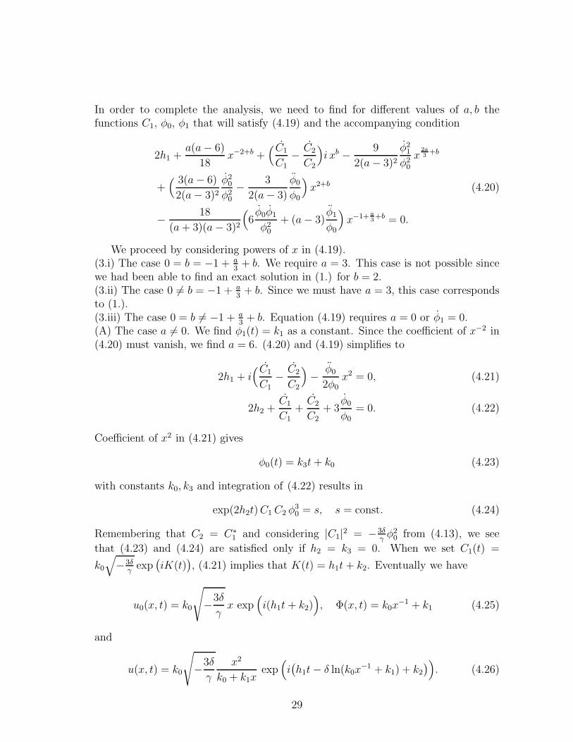
In order to complete the analysis, we need to find for different values of a, b thefunctions C1, φ0, φ1 that will satisfy (4.19) and the accompanying condition

2h1 +a(a− 6)

18x−2+b +

( C1

C1

− C2

C2

)

i xb − 9

2(a− 3)2φ21

φ20

x2a

3+b

+( 3(a− 6)

2(a− 3)2φ20

φ20

− 3

2(a− 3)

φ0

φ0

)

x2+b (4.20)

− 18

(a+ 3)(a− 3)2

(

6φ0φ1

φ20

+ (a− 3)φ1

φ0

)

x−1+ a

3+b = 0.

We proceed by considering powers of x in (4.19).(3.i) The case 0 = b = −1 + a

3+ b. We require a = 3. This case is not possible since

we had been able to find an exact solution in (1.) for b = 2.(3.ii) The case 0 6= b = −1 + a

3+ b. Since we must have a = 3, this case corresponds

to (1.).(3.iii) The case 0 = b 6= −1 + a

3+ b. Equation (4.19) requires a = 0 or φ1 = 0.

(A) The case a 6= 0. We find φ1(t) = k1 as a constant. Since the coefficient of x−2 in(4.20) must vanish, we find a = 6. (4.20) and (4.19) simplifies to

2h1 + i( C1

C1− C2

C2

)

− φ0

2φ0x2 = 0, (4.21)

2h2 +C1

C1

+C2

C2

+ 3φ0

φ0

= 0. (4.22)

Coefficient of x2 in (4.21) gives

φ0(t) = k3t+ k0 (4.23)

with constants k0, k3 and integration of (4.22) results in

exp(2h2t)C1C2 φ30 = s, s = const. (4.24)

Remembering that C2 = C∗1 and considering |C1|2 = −3δ

γφ20 from (4.13), we see

that (4.23) and (4.24) are satisfied only if h2 = k3 = 0. When we set C1(t) =

k0√

−3δγexp

(

iK(t))

, (4.21) implies that K(t) = h1t + k2. Eventually we have

u0(x, t) = k0

√

−3δ

γx exp

(

i(h1t + k2))

, Φ(x, t) = k0x−1 + k1 (4.25)

and

u(x, t) = k0

√

−3δ

γ

x2

k0 + k1xexp

(

i(

h1t− δ ln(k0x−1 + k1) + k2

)

)

. (4.26)

29

(B) The case a = 0. Through a similar analysis we have φ0(t) = k0, φ1(t) = k1t+ k2,

C1(t) = k0√

−3δγexp

(

iK(t))

, K(t) = (h1 − k214k2

0

)t + k3 together with the condition

h2 = 0. Therefore we get

u0(x, t) = k0

√

−3δ

γexp

[

i(

(h1−k214k20

)t− k12k0

x+k3

)]

, Φ(x, t) = k0x+k1t+k2 (4.27)

and the explicit solution

u(x, t) =k0√

−3δγ

k0x+ k1t+ k2exp

[

i(

(h1−k214k20

)t− k12k0

x−δ ln(k0x+k1t+k2)+k3)]

(4.28)

is obtained.(3.iv) The case b 6= 0 = −1 + a

3+ b. There is no solution in the truncated expansion

form.(3.v) The case b 6= 0, −1 + a

3+ b 6= 0, b 6= −1 + a

3+ b. All the coefficients in (4.19)

must vanish:

h2 = 0, (4.29a)

C1C2φa+3

a−3

0 = s, (4.29b)

aφ1 = 0. (4.29c)

If we remember that C2 = C∗1 and that |C1|2 = −3δ

γ(1− a

3)2φ2

0 from (4.13), (4.29b)becomes

− 3δ

γ(1− a

3)2φ

2+ a+3

a−3

0 = s. (4.30)

Analysis should be carried out for three different cases according to the constant aunder the conditions (4.29c) and (4.30).(A) The case a = 0 (b 6= {0, 1}). (4.19) and (4.20) together require h1 = h2 = 0,

φ0(t) = k0, φ1(t) = k1t + k2, C1(t) = c exp(− ik21

4k20

t), |c|2 = −3δγk20, c ∈ C. Functions

u0, Φ generate

u0(x, t) = c exp(

− i( k12k0

x+k214k20

t)

)

, Φ(x, t) = k0x+ k1t+ k2 (4.31)

and therefore the exact solution is given by

u(x, t) =c

k0x+ k1t+ k2exp

[

− i( k12k0

x+k214k20

t + δ ln(k0x+ k1t+ k2))]

. (4.32)

(B) The case a 6= {0, 1}. We find from (4.19) and (4.20) that φ0(t) = k0, φ1(t) = k1,h1 = h2 = 0, a = 6, C1(t) = c and |c|2 = −3δ

γk20. We conclude that

u0(x, t) = c x, Φ(x, t) = k0x−1 + k1 (4.33)

30

and

u(x, t) =cx2

k0 + k1xexp

(

− iδ ln(k0x−1 + k1)

)

. (4.34)

(C) The case a = 1 (b 6= 2/3). This last situation is going to give us the exact solutionfor the canonical equation of the algebra L1, namely the case a = 1 and b = 2.

Equation (4.19) requires h2 = 0 and φ1 = k1. (4.20) is satisfied if and only if b = 2and h1 = 5/36. (4.20) and (4.19) take the forms

(C1

C1− C2

C2

)

ix2 +3

4

( φ0

φ0− 5

2

φ02

φ20

)

x4 = 0, (4.35)

(C1

C1

− C2

C2

− 2φ0

φ0

)

x2 = 0. (4.36)

We arrive at the functions φ0(t) = (k0t+k2)−2/3, C1(t) = c1φ0(t) and C2(t) = c2φ0(t).

It is obvious that c2 = c∗1 and the condition (4.13) requires |c1|2 = −4δ3γ

, c1 ∈ C. Wesum up the results so far:

u0(x, t) =c1x

1/6

(k0t + k2)2/3exp

(

ik0x

2

4(k0t + k2)

)

, (4.37)

Φ(x, t) = (k0t+ k2)−2/3 x2/3 + k1 (4.38)

and hence

u(x, t) =c1 x

1/6

x2/3 + k1(k0t+ k2)2/3exp

[

i( k0x

2

4(k0t+ k2)−δ ln( x2/3

(k0t+ k2)2/3+k1)

)

]

. (4.39)

Remark. Since the canonical equation of L1 is invariant under the action ofthe group of transformations SL(2,R), which is the composed action of translationgenerated by T , scaling D1 and the conformal transformation of C1, the solution(4.39) is transformed into a new solution of the canonical equation under this action.Owing to the invariance property under C1, this transformed solution has a finitetime singularity and therefore was fruitful to study blow-up profiles. It is exactlythis blow-up character that was used in [12] to establish the existence of singularbehaviours of solutions in the sense of Lp and L∞ norms and in the distributionalsense as well.

4.2 Truncation method for the algebra L3

Coefficient functions for the algebra L3 are

f = 1 + if2, g = (ǫ+ iγ), h = 0. (4.40)

In fact, this constant coefficient case is included in [11] but we could not deduce ourresults from theirs. Differing from the previous algebra, f contains imaginary part

31

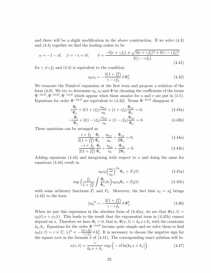
and there will be a slight modification in the above construction. If we solve (4.3)and (4.4) together we find the leading orders to be

α = −1− iδ, β = −1 + iδ; δ =−3(ǫ+ γf2)±

√

9(ǫ+ γf2)2 + 8(γ − ǫf2)2

2(γ − ǫf2)(4.41)

for γ 6= ǫf2 and (4.4) is equivalent to the condition

u0v0 = −3(1 + f 22 )

γ − ǫf2δΦ2

x. (4.42)

We truncate the Painleve expansion at the first term and propose a solution of theform (4.8). We try to determine u0, v0 and Φ by choosing the coefficients of the termsΦ−3±iδ,Φ−2±iδ,Φ−1±iδ which appear when these ansatze for u and v are put in (4.1).Equations for order Φ−3±iδ are equivalent to (4.42). Terms Φ−2±iδ disappear if

iΦt

Φx+ 2(1 + if2)

u0,xu0

+ (1 + if2)Φxx

Φx= 0, (4.43a)

−iΦt

Φx+ 2(1− if2)

v0,xv0

+ (1− if2)Φxx

Φx= 0. (4.43b)

These equations can be arranged as

i+ f22(1 + f 2

2 )

Φt

Φx+u0,xu0

+Φxx

2Φx= 0, (4.44a)

−i+ f22(1 + f 2

2 )

Φt

Φx+v0,xv0

+Φxx

2Φx= 0. (4.44b)

Adding equations (4.43) and integrating with respect to x and doing the same forequations (4.44) result in

u0v0

(u0v0

)if2Φx = F1(t) (4.45a)

exp( f21 + f 2

2

∫

Φt

Φx

dx)

u0v0Φx = F2(t) (4.45b)

with some arbitrary functions F1 and F2. Moreover, the fact that v0 = u∗0 brings(4.42) to the form

|u0|2 = −3(1 + f 22 )

γ − ǫf2δΦ2

x. (4.46)

When we put this expression in the absolute form of (4.45a), we see that Φ(x, t) =φ0(t) x+ φ1(t). This leads to the result that the exponential term in (4.45b) cannotdepend on x. Therefore we have Φt = 0, that is, Φ(x, t) = k0 x+k1 with the constantsk0, k1. Equations for the order Φ

−1±iδ become quite simple and we solve them to find

u0(x, t) = c ∈ C, |c|2 = −3(1+f22)

γ−ǫf2δ k20. It is necessary to choose the negative sign for

the square root in the formula δ of (4.41). The corresponding exact solution will be

u(x, t) =c

k0 x+ k1exp

(

− iδ ln(k0 x+ k1))

. (4.47)

32

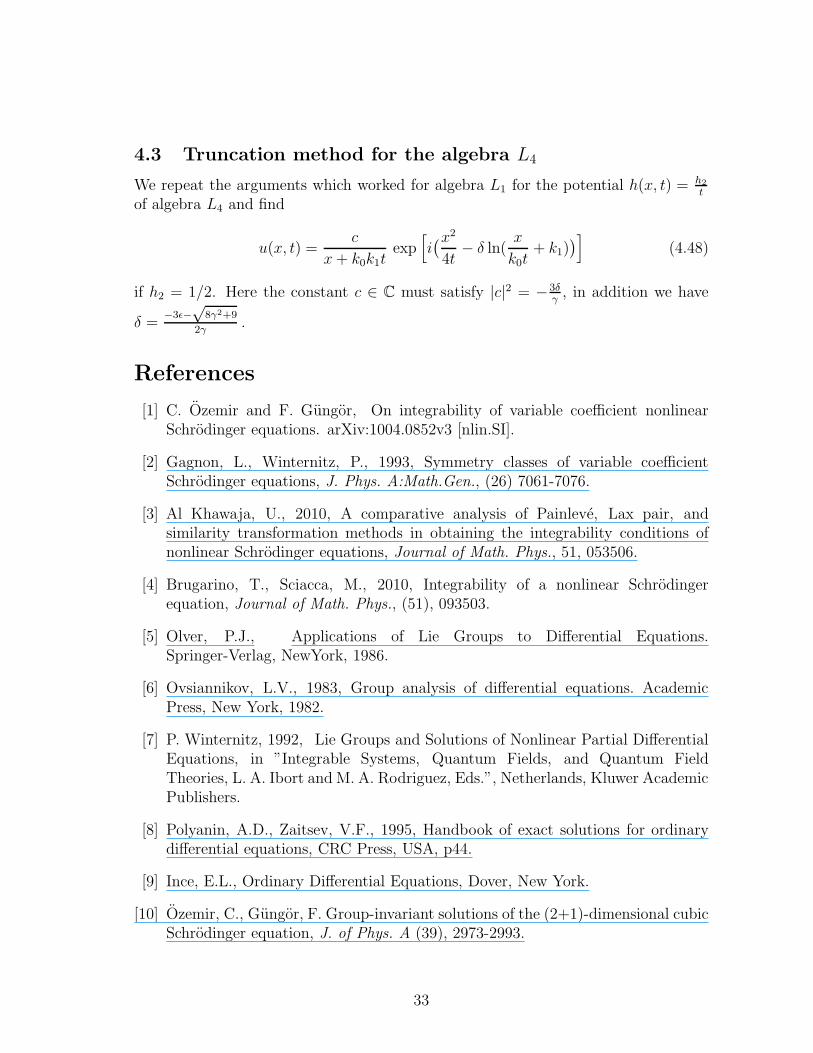
4.3 Truncation method for the algebra L4

We repeat the arguments which worked for algebra L1 for the potential h(x, t) = h2

t

of algebra L4 and find

u(x, t) =c

x+ k0k1texp

[

i(x2

4t− δ ln(

x

k0t+ k1)

)

]

(4.48)

if h2 = 1/2. Here the constant c ∈ C must satisfy |c|2 = −3δγ, in addition we have

δ =−3ǫ−

√8γ2+9

2γ.

References

[1] C. Ozemir and F. Gungor, On integrability of variable coefficient nonlinearSchrodinger equations. arXiv:1004.0852v3 [nlin.SI].

[2] Gagnon, L., Winternitz, P., 1993, Symmetry classes of variable coefficientSchrodinger equations, J. Phys. A:Math.Gen., (26) 7061-7076.

[3] Al Khawaja, U., 2010, A comparative analysis of Painleve, Lax pair, andsimilarity transformation methods in obtaining the integrability conditions ofnonlinear Schrodinger equations, Journal of Math. Phys., 51, 053506.

[4] Brugarino, T., Sciacca, M., 2010, Integrability of a nonlinear Schrodingerequation, Journal of Math. Phys., (51), 093503.

[5] Olver, P.J., Applications of Lie Groups to Differential Equations.Springer-Verlag, NewYork, 1986.

[6] Ovsiannikov, L.V., 1983, Group analysis of differential equations. AcademicPress, New York, 1982.

[7] P. Winternitz, 1992, Lie Groups and Solutions of Nonlinear Partial DifferentialEquations, in ”Integrable Systems, Quantum Fields, and Quantum FieldTheories, L. A. Ibort and M. A. Rodriguez, Eds.”, Netherlands, Kluwer AcademicPublishers.

[8] Polyanin, A.D., Zaitsev, V.F., 1995, Handbook of exact solutions for ordinarydifferential equations, CRC Press, USA, p44.

[9] Ince, E.L., Ordinary Differential Equations, Dover, New York.

[10] Ozemir, C., Gungor, F. Group-invariant solutions of the (2+1)-dimensional cubicSchrodinger equation, J. of Phys. A (39), 2973-2993.

33

[11] Yomba, E., Kofane, T.C., 1996, On exact solutions of the generalized modifiedGinzburg-Landau equation using the Weiss-Tabor-Carnevale method, Physica

Scripta, (54), 576-580.

[12] F. Gungor, M. Hasanov, C. Ozemir, Unimodular invariant variable coefficientnonlinear Schrodinger equation and blow-up of its solutions. arXiv:1101.2307[math.AP].

34