Research & Development

Alina A. von Davier

Nan Kong

ResearchReport

November 2003 RR-03-31

A Unified Approach to Linear Equating for the Non-Equivalent Groups Design

A Unified Approach to Linear Equating for the Non-Equivalent Groups Design

Alina A. von Davier and Nan Kong

Educational Testing Service, Princeton, NJ

November 2003

Research Reports provide preliminary and limited dissemination of ETS research prior to publication. They are available without charge from:

Research Publications Office Mail Stop 7-R Educational Testing Service Princeton, NJ 08541

Abstract

This paper describes a new, unified framework for linear equating in a Non-Equivalent-groups

Anchor Test (NEAT) design. We focus on three methods for linear equating in the NEAT

design—Tucker, Levine observed-score, and chain—and develop a common parameterization

that allows us to show that each particular equating method is a special case of the linear

equating function in the NEAT design. We use a new concept, the Method Function, to

distinguish among the linear equating functions, in general, and among the three equating

methods, in particular. This approach leads to a general formula for the standard error of

equating for all equating functions in the NEAT design. We also present a new tool, the standard

error of equating difference, to investigate if the observed difference in the equating functions is

statistically significant.

Key words: Test equating, Non-Equivalent groups Anchor Test (NEAT) design, Tucker

equating, Levine observed-score equating, chain linear equating, standard error of equating, delta

method

i

Acknowledgments

The authors would like to thank Paul Holland, Neil Dorans, Hariharan Swaminathan, Dan

Eignor, Shelby Haberman, Skip Livingston, and Krishna Tateneni for helpful comments and

suggestions during the development of this project. We are also thankful to Bruce Kaplan and

Ted Blew, who were very supportive in developing the software and carrying out the resampling

procedure. We would also like to thank Kim Fryer, Elizabeth Brophy, and Diane Rein for their

help in editing the manuscript. The Educational Testing Service Research Allocation supported

our work. Any opinions expressed in this paper are those of the authors and not necessarily of

Educational Testing Service.

ii

Test equating methods are statistical tools used to produce exchangeable scores across different

test forms. In particular, observed-score equating methods, as opposed to true-scores equating

methods, refer to the transformation of the raw scores of a new test, X, on the raw scores of an

old test, Y. Any test equating process consists of a data collection design and different equating

methods. This paper focuses on the Non-Equivalent-groups Anchor Test (NEAT) design and the

linear equating function.

The NEAT design is a data collection design widely used in practice. It involves two

populations of test-takers (usually different test administrations), P and Q, and a sample of

examinees from each. The sample from P takes test X, the sample from Q takes test Y, and both

samples take an anchor test, V, which is used to link X and Y.

For the NEAT design, several observed-score equating methods are commonly used.

Here we focus only on observed-score linear equating methods for the NEAT design.

In this paper, we take a new, mathematical approach to three linear observed-score

equating methods—Tucker equating for the NEAT design with an anchor (T), Levine observed-

score equating (L), and chain linear equating (CL)—by emphasizing their common framework

and their similarities. We define these methods carefully later.

In this way, we introduce a unified approach to linear equating in the NEAT design, and

we show that each of these equating methods is a special case of the linear equating function.

This approach allows us to establish new theoretical results on otherwise well-known equating

methods, creating a conceptual shift in the analysis of the observed-score linear equating

methods in the NEAT design: There are not only disparate methods, each with its own

framework, but they share the same parameter space and have numerous similarities. One of the

consequences is that we can develop one general formula for the standard error of equating

(SEE) that is applicable to most of the observed-score linear equating functions for the NEAT

design that are available. We also introduce in this paper a new, practical tool, the standard error

of equating difference (SEED), for investigating whether the differences between the (linear)

equating methods are statistically significant.

More precisely, in this paper we investigate the linear equating in the NEAT design from

several points of view:

1. We put the three methods on a common footing by developing the same

parameterization for the (equating) functions. We also make use of the concept of a

1

Method Function in the framework of the linear equating to show that there is only

one definition of the linear observed-score equating function that might have different

special cases. (A related concept, the Design Function, was first introduced in von

Davier, Holland, & Thayer, 2004, in a different context, to model the data collection

design.) This approach leads to a general formula for the SEE for linear equating in

the NEAT design in general and for the three equating functions in particular.

2. We generalize the SEED (von Davier et al., 2004) for any pair of (linear) equating

functions that share the same set of parameters. The SEED is a new tool to investigate

whether the difference between the equating functions is statistically significant.

3. We use real and resampled data from two national administrations of a high volume

testing program to illustrate the SEE (computed via the new general formula) and the

SEED.

We do not make any distributional assumptions about the variables involved in this

theoretical exposition.

Linear Equating Function for the NEAT Design

This section sets up the basic notation. We assume there are two tests to be equated, X

and Y, and a “target” population, T, on which this is to be done (Braun & Holland, 1982; Kolen

& Brennan, 1995).

In this paper, we use the standard notation of 2and µ σ for the means and the variances.

We also use the symbol π to denote the parameters in general. The subscripts usually indicate the

variable and the population. We use σ with appropriate subscripts to denote the covariances; for

example, , ;X V Pσ denotes the covariance of X and V in P, while Σ denotes the covariance matrix

of π.

Many observed score equating methods are based on the linear equating function.

Usually, the rational behind the linear equating on the target population, T, is to set standardized

deviation scores (z-scores) on the two forms to be equal such that

,XT YT

XT YT

x yµ µσ σ− −

=

2

where ,, , and YT YT XT XTµ σ µ σ are the means and the variances of X and Y in T. Solving for y in

the above equation results in the formula for the linear equating function,

( ) ( )( );Lin / .XY T YT YT XT XTx xµ σ µ σ= + − (1)

In the NEAT design, there are also another rational and implicitly another definition of a

linear equating function, that is, the chain linear equating function. The chain linear equating

function is given by chaining together the two linear linking functions (i.e., by using the

mathematical composition of the two linear functions), from X to V on P and from V to Y on Q,

that is, ( ) ( );Lin and LinXV P VY Q;x v . This results in

( )( )( ) ( )( )( )(( )( ) ( )( )(

; ;( ) Lin Lin

/ /

/ / /

XY VY Q XV P

YQ YQ VQ VP VP XP XP VQ

YQ YQ VQ VP VQ YQ VQ VP XP XP

CL x x

x

x

µ σ σ µ σ σ µ µ

µ σ σ µ µ σ σ σ σ µ

=

= + + − −

= + − + −

)) ,

(2)

and (2) is the usual form for the chain linear equating function. Moreover, the final equating

function does not depend on the target population, T. As shown in von Davier, Holland, and

Thayer (in press), (2) can be rewritten as (1) under appropriate assumptions. This will be

discussed in more detail later.

Usually, X and Y are the “operational tests” given to two samples from the two “test

administrations” P and Q, respectively, and V is the “anchor test” given to both samples from P

and Q. The anchor test score, V, can be either a part of both X and Y (called the internal anchor)

or a separate score (the external anchor).

In this study we assume that the target population, T, for the NEAT design is a mixture of

P and Q and is denoted by

( )1T wP w Q= + − , (3)

3

(see Braun & Holland, 1982, or Kolen & Brennan, 1995, for details on the concept of a target

population in the NEAT design).

The target population in (3) is determined by a weight w. When w = 1, then T = P, and

when , then T = Q. Other choices of w may be used as well. Typically, w is the ratio of the

sample size of the group from P and the sum of the sample sizes of the two groups.

0w =

In the NEAT design, X and Y are each only observed either on P or on Q, but not both.

Thus, X and Y are not both observed on T, regardless of the choice of w. For this reason

assumptions must be made in order to overcome this lack of complete information in the NEAT

design.

The three equating methods used in the NEAT design that concern us here, Tucker,

Levine, and chain linear equating, make different assumptions about the distributions of X and Y

in the populations where they are not observed. We identify these assumptions in the next

section.

Tucker, Levine, and Chain Linear Equating Methods

In this section we briefly describe the methods we use and their assumptions, which can

be found in more detail somewhere else (Kolen & Brennan, 1995, pp. 114-118; Angoff, 1984;

von Davier et al., in press). Here we provide only the information that is necessary to explain our

new approach, which is given in more detail later in this paper.

This section is structured as follows: First, we present the Tucker and Levine together,

stressing the similarities between them. Although the assumptions that underlie the two methods

are different, the computational forms are similar. We will not give computational details on

Tucker and Levine because they are well documented (Kolen & Brennan, 1995, pp. 114-118).

Then, we describe the chain linear equating method, following the development given in von

Davier et al. (in press). In the next section, we develop a common parameterization for the three

functions that allows us to compare the equating functions as well as their standard errors (SEE).

Tucker Equating Method: Assumptions

T1: The linear regressions of X on V and of Y on V are the same in the two populations.

T2: The conditional variances of X given V and of Y on V are the same in the two populations.

4

Levine Observed-score Equating Method: Assumptions

L1: X, Y, and V all measure the same thing, or, stated in different words, the true scores of the

tests (T and T ) and of the anchor (T ) in the two populations are perfectly correlated. X Y V

L2: The regressions of T on T and of T on T are linear and the same in the two

populations.

X V Y V

L3: The measurement error variances for X and for Y are the same in the two populations.

From the two sets of assumptions and from (1) the formulas for the parameters of X and Y

on T for Tucker and Levine follow. They are similar in form for the two equating methods:

( )1 ,XT XP P VP VQwµ µ µ µ = − − ∆ − (4)

,YT YQ Q VP VQwµ µ µ µ= + ∆ −

,

(5)

( ) ( ) 22 2 2 2 2 21 1XT XP P VP VQ P VP VQw w wσ σ σ σ µ µ = − − ∆ − + − ∆ − (6)

( ) 22 2 2 2 2 21YT YQ Q VP VQ Q VP VQw w wσ σ σ σ µ µ = + ∆ − + − ∆ − (7)

(see Kolen & Brennan, 1995, pp. 114–118 for the derivations).

The four ∆-parameters, which distinguish the two equating methods, Tucker and Levine,

have the following formulas:

For the Tucker method:

, ;, ;2 and ,Y V QX V P

P P Q QVP VQ

2

σσα

σ σ∆ = = ∆ = =α (8)

where , ;X V Pσ denotes the covariance of X and V in P and , ;Y V Qσ denotes the covariance of Y and

V in Q.

For the Levine observed-score equating function for a NEAT design with an external

anchor:

5

22, ;, ;

2, ; , ;

and ,YQ Y V QXP X V PP P Q Q

VP X V P VQ Y V Q

σ σσ σγ γ

σ σ σ σ++

∆ = = ∆ = =+ +2 (9)

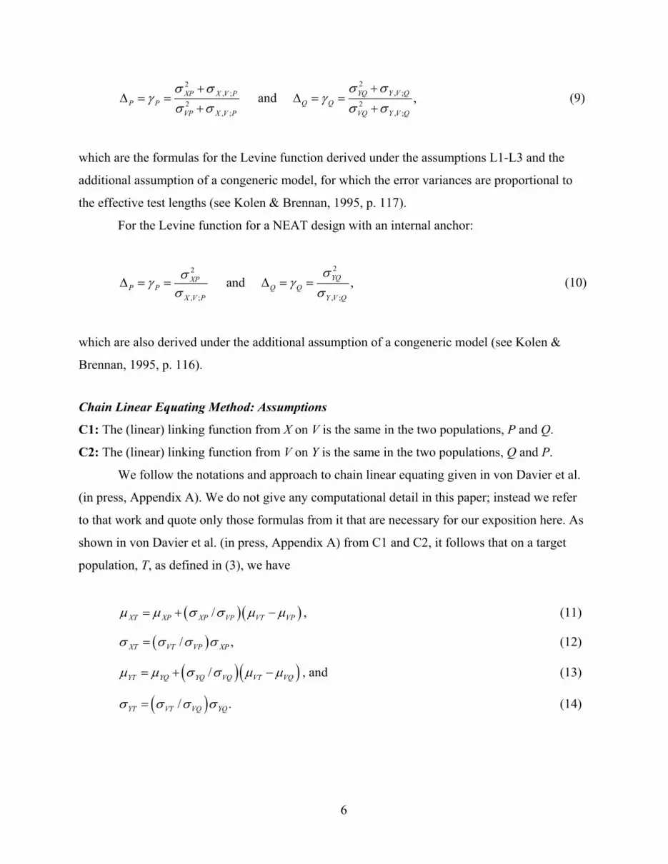
which are the formulas for the Levine function derived under the assumptions L1-L3 and the

additional assumption of a congeneric model, for which the error variances are proportional to

the effective test lengths (see Kolen & Brennan, 1995, p. 117).

For the Levine function for a NEAT design with an internal anchor:

22

, ; , ;

and ,YQXPP P Q Q

X V P Y V Q

σσγσ σ

∆ = = ∆ = =γ

)

(10)

which are also derived under the additional assumption of a congeneric model (see Kolen &

Brennan, 1995, p. 116).

Chain Linear Equating Method: Assumptions

C1: The (linear) linking function from X on V is the same in the two populations, P and Q.

C2: The (linear) linking function from V on Y is the same in the two populations, Q and P.

We follow the notations and approach to chain linear equating given in von Davier et al.

(in press, Appendix A). We do not give any computational detail in this paper; instead we refer

to that work and quote only those formulas from it that are necessary for our exposition here. As

shown in von Davier et al. (in press, Appendix A) from C1 and C2, it follows that on a target

population, T, as defined in (3), we have

( )(/XT XP XP VP VT VPµ µ σ σ µ µ= + − , (11)

( )/XT VT VP XP ,σ σ σ σ= (12)

( )(/YT YQ YQ VQ VT VQµ µ σ σ µ µ= + − ).

, and (13)

( )/YT VT VQ YQσ σ σ σ= (14)

6

Von Davier et al. (in press) shows that under the assumptions C1 and C2 made by the

chain equating CL defined in (2) is, in fact, ( )XY x ( );n XY TLi x , as defined in (1). More precisely,

that work shows that applying (11)–(14) to the chain linear function from (2) results in (1). The

target population, T, cancels out of the composed function, ( )( ); ;n LinVY Q XV PLi x . This provides a

direct argument that chain linear equating is the linear observed score equating on T with 2 nd YT

2, , , aXT YT XTµ µ σ σ given by the expressions in (11)–(14).

Identifying the Parameters of the Tucker, Levine, and Chain Linear Equating Functions

In this section, we introduce a common parameterization for the linear equating functions

described above. We show that this approach leads to a unified framework for all the linear

equating functions in the NEAT design.

Consider the linear equating function (1) that equates X to Y on the target population, T,

in the form of (3). This equating function depends on 2, , , and XT XT YT YT2µ σ µ σ , which are

parameters on the population T. We can express this dependence of the equating function on the

target population parameters by using the notation

( 2;Lin ; , , ,XY T XT XT YT YTx µ σ µ σ )2

.

= a generic linear equating function. (15)

In (4)–(14), we observe that the four parameters on T depend on the 10 means, variances, and

covariances in the two populations, P and Q. Denote by the column vector of the 10

parameters from the two bivariate distributions, that is,

π

2 2 2 2

, ; , ;( , , , , , , , , , )tXP XP VP VP X V P YQ YQ VQ VQ Y V Qµ σ µ σ σ µ σ µ σ σ=π (16)

We use a new concept, a function that will map the 10 parameters from the two

populations, P and Q, into the four parameters on the population T.

To preserve the similarities to von Davier et al. (2004) and to emphasize the similarities

across the equating methods, we will call this function the Method Function (MF).

7

( ) ( 2 2MF , , , .t

XT XT YT YTµ σ µ σ=π )

)

)

(17)

Now, we rewrite (15) as

(;Lin ;MF( )XY T x π = a linear equating function obtained through a specific MF, (18)

with defined in (16). π

The previous section showed that all three linear equating functions, Tucker, Levine, and

chain linear, can be expressed as (1). Thus, they can also be expressed as (18), in which the

Method Function differs according to which equating method is used. For the Tucker method,

the Method Function is described by the formulas (4)–(8). For the Levine method, the Method

Function is given by (4)–(7) and (9) for an external anchor, and by (4)–(7) and (10) for an

internal anchor. For the chain linear method, the Method Function is described by (11)–(14).

Each Method Function is given in detail in the appendix in Table A1.

From (2) as well as from (11)–(14), we observe that the covariance between X and V on P

and the covariance of Y and V on Q do not appear in the formulas of the chain linear equating

function. Hence, the chain linear equating function depends only on eight parameters, while the

Tucker and Levine functions depend on ten parameters. However, by using (15), (17), and (18),

we can express the three linear equating functions as sharing the same parameter space. Note the

chain linear function implicitly depends on the covariances between the tests and the anchor only

if before computing the equating function, the two bivariate distributions of the tests and the

anchor are presmoothed using, for example, log-linear models (see von Davier et al., 2004;

Holland & Thayer, 2000).

Equating functions are estimated by substituting estimates of the population parameters

in (18), that is,

( ) (( ); ; ˆLin ;MF( ) Lin ;MF ,XY T XY Tx x=π π

)

(19)

where π̂ denotes a sample estimate of . π

The uncertainty in Li derives from the uncertainty in the estimate of .

Because the samples are independently drawn from populations P and Q, the covariances

( )(;n ;MFXY T x π π

8

between each of the five parameters estimated from the population P and the five parameters

estimated from the population Q are zero.

Hence, the covariance matrix of the parameter for the three equating functions,

Tucker, Levine, and chain linear, is:

Σ π

(20) 0

,0

P

Q

=

ΣΣ

Σ

where PΣ

Q

denotes the covariance matrix of the five parameters obtained from the population P

and denotes the covariance matrix of the five parameters obtained from the population Q. Σ

Also note that the “Braun and Holland” linear equating method for the NEAT design

(Braun & Holland, 1982; Kolen & Brennan, 1995, p. 146) shares the same parameter vector

and has the same covariance matrix of , as in (20).

π

π

In this section, we introduced a common parameterization that can be used for most of

the available observed-score linear equating functions in the NEAT design. We showed that one

could write down the Method Function formulas for each of three methods that we analyzed

here, and we think that one could easily write the appropriate Method Function for any other

observed-score linear equating function. However, the investigation of additional equating

functions is beyond the scope of this study.

Standard Error of Equating

In this section, we show that using a common parameterization for all linear equating

functions in a NEAT design leads to a general formula for the SEE.

The delta method, a general method for approximating standard errors that is based on

the Taylor expansion (Rao, 1965; Kendall & Stuart, 1977), is widely used for computing

standard errors. Kolen (1985) and Hanson, Zeng, and Kolen (1993) used the delta method to

compute the SEE for the Tucker method and the Levine method, respectively.

Although we also use the delta method for computing the SEE, our approach differs from

Kolen (1985) and Hanson et al. (1993) in the following sense: We provide a unified approach

that, through the MF, includes not only the Tucker and the Levine methods, but also chain linear

equating and other linear observed-score equating functions—such as the Braun and Holland

9

linear equating method (Braun & Holland, 1982; Kolen & Brennan, 1995). In order to emphasize

this unity, we focus on the matrix form of the SEEs, (21) below, rather than on the sum form, as

did Kolen (1985) and Hanson et al. (1993). The approach presented here has similarities with the

approach developed in von Davier et al. (2004).

Delta Method Applied to Linear Equating

We use the delta method to calculate the asymptotic variance, ,

whose square root is the SEE.

( )( );Va r Lin ;MF( )XY T x π

From the delta method (Theorem A1 in the appendix), it follows that the asymptotic

variance of a smooth function, f, that depends on the parameter vector, , is π

( )( ) ( ) ( ) ( )V ar tff =π J π Σ π J πf (21)

where is the Jacobian (the matrix or vector of the first derivatives of the function f with

respect to the components ofπ ) computed at the estimated values of (see also von Davier et

al., 2004; von Davier, 2001).

( )fJ π

π

Let the parameter from (16) be the parameter vector described in Theorem A1 and let f

be a linear equating function,

π

( );Lin ;MF( )XY T x π , given in (1). The Method Function can refer to

any of the Tucker, Levine, and chain linear functions. The Jacobian of is,

according to matrix differentiation theory and differentiability of composition of functions,

( );Lin ;MF( )XY T x π

Lin MF= ,fJ J J

where is the vector of the first derivatives of the function from (1) with respect to

. is the matrix of the first derivatives of

LinJ

( , ,XT )2 ,XT YT YTµ σ µ σ 2MFJ ( )2, , ,XT XT YT YTµ σ µ σ 2 with respect

to the components of π from (16).

In the previous section we showed that the (10 by 10) covariance matrix is the same

for the Tucker, Levine, and chain linear functions. Moreover, the Jacobian J

Σ

Lin will also have the

same form for all observed-score linear equating functions (the Jacobian of the linear function,

for any of the three equating functions, is a 4-dimensional (row) vector). The Jacobian JMF is a 4

by 10-matrix and will have a different form for each of the equating methods.

10

Now, by using (21), the SEE of a linear equating function, , can be

expressed as

( ); ˆLin ;MF( )XY T x π

( )2Lin MF MF Lin

ˆ ˆ ˆ ˆSEE ,t tx = J J Σ J J (22)

with from (20). Σ

Equation (22) is the computational formula for the SEE for the Tucker, Levine, and chain

linear methods, that is, the formula that might be implemented into a computer program.

It is easy to see the computational advantages of having only one formula for the SEE for

all linear equating methods. Note that this formula does not require any distributional assumption

on the variables involved.

The entries of in (22) can be obtained from Kolen, 1985. The derivatives

for the Tucker equating function are given in Kolen (1985). The derivatives for the

Levine function for a NEAT design are given in Hanson et al. (1993). The derivatives

for the chain linear equating, given in Table A2, were computed by us.

Σ Lin MF=fJ J J

Lin MFJ=fJ J

Lin MF=fJ J J

We use the notations SEET, SEEL, and SEECL to refer to the SEE for the Tucker, Levine,

and chain linear methods, respectively.

SEED for Linear Equating Functions

In this section, we state a new result that is analogous to (21) and that will allow us to

compute a standard error for the difference between two linear equating functions. This standard

error can be used to inform discussion about the final form of an equating function.

The SEED was first introduced in von Davier et al. (2004) for the kernel method of test

equating. This paper applies the same concept to the linear equating functions. The main

differences between the SEED in von Davier et al. (2004) and the SEED here lie in the fact that

the parameters of the equating functions and the equating functions themselves differ. In the

kernel method of test equating, the parameters are the score probabilities of the tests to be

equated (and, in chain equipercentile, also the score probabilities of the anchor test); in the case

of linear equating, the parameters are the means, the variances, and the covariances of the tests to

be equated and of the anchor test in the two populations, P and Q.

11

Consider two equating functions ( ) ( )1Lin ;MF ( ) and Lin ;MF ( )x xπ 2 π

))2 π

, which have the

form given in (1) and depend on the same parameter vectors from (16) (i.e., the assumptions on

the functions required by the delta method are met). We are interested in

( ) (( 1V ar Lin ;MF ( ) Lin ;MF ( ) .x x−π (23)

Theorem 1. If ( ) ( )1n ;MF ( ) and Lin ;MF ( )x xπ 2 π

)

Li are two equating functions that have

the form given in (1) and depend on the same parameter vector, , from (16), then π

( ) ( )( ) 1 2 1 21 2 Lin MF MF MF MF Linˆ ˆ ˆ ˆ ˆ ˆV ar Lin ;MF ( ) Lin ;MF ( ) ( ) ( ) ,t tx x− = − −π π J J J Σ J J J (24)

where is the 4-dimensional-row vector of the first derivatives of the function from (1) with

respect to the parameters on T, ( , J is the 4 by 10 matrix of the first

derivatives of the four components of the Method Function,

LinJ

2 2, , ,XTXT YT YTµ σ µ σ MF

( )2, , ,XTXT YT YTµ σ µ σ

π

2 , with respect to

the components of , and is the variance-covariance matrix of , given in (20). π Σ

The proof follows from the delta method (Theorem A1), applied to the difference of two

smooth functions that depend on the same parameters (see also von Davier et al., 2004, chapter 5).

Hence, the SEED is

( ) ( )( )21 2SEED =V ar Lin ;MF ( ) Lin ;MF ( )x x−π π . (25)

Corollary 1. The SEEDs for any pair of the three equating functions, Tucker, Levine, and

chain linear, are:

2T,L Lin T L T L Lin

ˆ ˆ ˆ ˆ ˆ ˆSEED = ( ) ( ) ,t t− −J J J Σ J J J (26)

2 tCL,L Lin CL L CL L Lin

ˆ ˆ ˆ ˆ ˆ ˆSEED = ( ) ( ) ,t− −J J J Σ J J J (27)

12

2T,CL Lin T CL T CL Lin

ˆ ˆ ˆ ˆ ˆ ˆSEED = ( ) ( ) ,t t− −J J J Σ J J J (28)

with from (20) Σ

The proof follows from Theorem 1.

The entries of are given in Kolen (1995). The entries of are given in

Hanson et al. (1993) and the entries of are given in Table A2.

Lin TJ J Lin LJ J

Lin CLJ J

In conclusion, the SEED is a measure of the uncertainty in the difference between two

equating functions that is due to the estimation of the parameters (the means, variances, and

covariances in the two samples). It also reflects the differences in the two Method Functions. We

propose the following practical rule: If the difference between two linear equating functions is no

larger than the noise level in the data, then this difference would be smaller than twice the SEED

in either direction (see also von Davier et al., 2004).

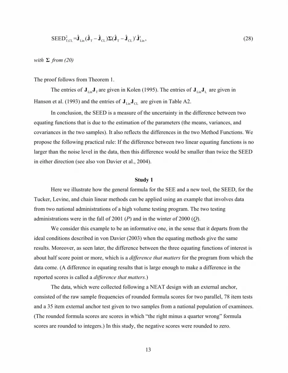
Study 1

Here we illustrate how the general formula for the SEE and a new tool, the SEED, for the

Tucker, Levine, and chain linear methods can be applied using an example that involves data

from two national administrations of a high volume testing program. The two testing

administrations were in the fall of 2001 (P) and in the winter of 2000 (Q).

We consider this example to be an informative one, in the sense that it departs from the

ideal conditions described in von Davier (2003) when the equating methods give the same

results. Moreover, as seen later, the difference between the three equating functions of interest is

about half score point or more, which is a difference that matters for the program from which the

data come. (A difference in equating results that is large enough to make a difference in the

reported scores is called a difference that matters.)

The data, which were collected following a NEAT design with an external anchor,

consisted of the raw sample frequencies of rounded formula scores for two parallel, 78 item tests

and a 35 item external anchor test given to two samples from a national population of examinees.

(The rounded formula scores are scores in which “the right minus a quarter wrong” formula

scores are rounded to integers.) In this study, the negative scores were rounded to zero.

13

The data are sample frequencies for two bivariate distributions. We denote the two sets of

sample frequencies by number of examinees with jln = jX x= and V lv= , and = number of

examinees with Y and V .

klm

k= y lv=

In this example, ; the same is true for . For , we have

. The two sample sizes are given by: N =10,634 and M =11,321. The

sample correlation of X and V in P was 0.88, and the sample correlation of Y and V in Q was

0.87.

1 2 790, 1, , 78x x x= = =… ky lv

1 2 360, 1, , 35v v v= = =…

Table 1

Summary Statistics for the Observed Distributions of X, Y, V in P and V in Q

X Y VP VQ

Mean 39.25 32.69 17.05 14.39

SD 17.23 16.73 8.33 8.21

From Table 1 we see that the mean of the anchor test V is 17.05 (±0.08) in population P,

and 14.39 (±0.08) in Q, where 0.08 is the standard error of the mean. Thus Q is a less proficient

population than P, as measured by V. In terms of effect sizes, the difference between these two

means (2.66) is approximately 32% of the average standard deviation of 8.27. For this type of

testing program, a mean difference of this magnitude indicates a fairly large difference between

the two populations.

Before chain linear equating was in use, ETS researchers were guided by the following

rules when they had to choose between Tucker and Levine equating: “If the standardized mean

difference of the anchor scores in the two samples is smaller than 0.25, then choose the Tucker

method,” and “If the ratio of the variances of the anchor in the two samples is between 0.80 and

1.25, then use the Tucker method” (Kirk, 1971; Wichert, 1967). We couldn’t find any rational

explanation for these rules, especially for the cut-off values. Kolen and Brennan (1995, pp. 131–

132), however, suggest “choosing Levine when it is known that populations differ

substantially…and if there is also reason to believe that the forms are quite similar” and choosing

Tucker if the forms are suspected to differ, with the observation that “if the populations [and

14

forms] are too dissimilar, then any equating is suspect” and with the note that “this ad hoc

reasoning is by no means definitive.”

Hence, based on this information, one would have chosen the Levine equating function

particularly for this example since the test forms are very carefully constructed to be parallel in

this assessment program.

We used the formulas (1), (4)–(10) to compute the Tucker and Levine functions. We used

(2) to compute the chain linear equating function. The equating functions, the SEEs, and the

SEEDs are discrete functions of x.

The three functions, shown in Figure 1, give relatively different results. The differences

between the Tucker and Levine functions and the Tucker and chain functions are more than a

half raw score point for the whole score range, which is a difference that matters. The difference

between Levine function and the chain function is less than the size of a difference that matters

for the whole score range.

15

-1.2

-1

-0.8

-0.6

-0.4

-0.2

0

0.2

0.4

0 10 20 30 40 50 60 70 80

X-SCORE

EQU

ATI

NG

DIF

FER

ENC

E

T-LT-CL-C

Figure 1. The Tucker, Levine, chain linear functions. Study 1. NEAT design with an external anchor.

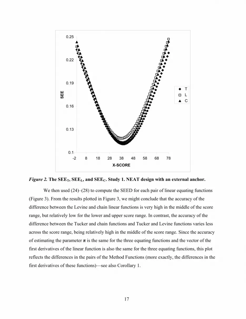
The three SEEs are given in Figure 2. The shape of the SEEs is the usual one for linear

equating functions, with lower values around the means and higher values for the extreme score

ranges. The SEE for the Levine function seems to be larger than the SEE for the chain linear

function and for the Tucker function, which has the smallest values almost overall on the score

range (see Figure 2). The SEEs for the three functions are very close to each other, though, and

therefore, one could not choose a method solely based on these SEEs values.

16

0.1

0.13

0.16

0.19

0.22

0.25

-2 8 18 28 38 48 58 68 78

X-SCORE

SEE

TLC

Figure 2. The SEET, SEEL, and SEEC. Study 1. NEAT design with an external anchor.

We then used (24)–(28) to compute the SEED for each pair of linear equating functions

(Figure 3). From the results plotted in Figure 3, we might conclude that the accuracy of the

difference between the Levine and chain linear functions is very high in the middle of the score

range, but relatively low for the lower and upper score range. In contrast, the accuracy of the

difference between the Tucker and chain functions and Tucker and Levine functions varies less

across the score range, being relatively high in the middle of the score range. Since the accuracy

of estimating the parameter π is the same for the three equating functions and the vector of the

first derivatives of the linear function is also the same for the three equating functions, this plot

reflects the differences in the pairs of the Method Functions (more exactly, the differences in the

first derivatives of these functions)—see also Corollary 1.

17

0.015

0.035

0.055

0.075

0.095

0.115

0.135

-2 8 18 28 38 48 58 68 78

X-SCORE

SEED

T-LT-CL-C

Figure 3. The standard error of equating differences for three equating functions. Study 1. NEAT design with an external anchor.

Figures 4–6 plot the difference between two linear equating functions together with the

corresponding ±2 SEED. In these three cases, the differences between the three functions (about

half of a raw score point or more—see also Figure 1) are statistically significant relative to the

SEEDs. It appears that the Levine and the chain functions agree only at the very low end of the

score range. As mentioned before, the SEEDs reflect the uncertainty in these differences that are

due to the estimation of the parameters (the means, the variances, and the covariances in the two

samples) as well as to the differences in the Method Functions.

18

-1.25

-1.05

-0.85

-0.65

-0.45

-0.25

-0.05

0.15

0 10 20 30 40 50 60 70 80

X-SCORE

SEED

(T,L

)

T-L2*SEED(T,L)-2*SEED(T,L)

Figure 4. The difference between Tucker and Levine together with a band of ±2SEEDT, L. Study 1. NEAT design with an external anchor.

19

-0.9

-0.7

-0.5

-0.3

-0.1

0.1

0 10 20 30 40 50 60 70 80

X-SCORE

SEED

(T,C

) T-C2*SEED(T,C)-2*SEED(T,C)

Figure 5. The difference between Tucker and chain linear together with a band of ±2SEEDT,C. Study 1. NEAT design with an external anchor.

20

-0.32

-0.27

-0.22

-0.17

-0.12

-0.07

-0.02

0.03

0.08

0.13

0.18

0.23

0.28

0.33

0 10 20 30 40 50 60 70 80

X-SCORE

SEED

(L,C

)

L-C2*SEED(L,C)-2*SEED(L,C)

Figure 6. The difference between Levine and chain linear functions together with a band of ±2SEEDL, C. Study 1. NEAT design with an external anchor.

In conclusion, we observe that the differences between the three equating functions are

statistically significant. In other words, with the help of the SEED, we can distinguish between

noise and real differences between the analyzed functions.

Study 2

The SEEDs are asymptotic results, so it is of interest to investigate how they vary with

sample size. Sample sizes of 10,000 are relatively large, and therefore, the estimation of the

parameters is relatively accurate. As a consequence, the ±2SEED band will be very narrow.

Study 2 examined the following research questions:

What is going to happen to the SEED when the sample sizes get smaller?

21

For which N will the ±2SEED band be about half of a raw score point (a difference that

matters)?

For which N will the ±2SEED band encompass the difference between the equating

functions? More precisely, for which N will the SEED not be able to detect that the equating

functions differ statistically?

We resampled seven samples of sizes 5,000; 2,500; 1,700; 800; 400; 200; and 100 for

each group of students from P (those who took (X, V)) and Q (those who took (Y, V)),

respectively. These samples were independent random samples, drawn without replacement from

the original N = 10,634 for (X, V) and M = 11,321 for (Y, V). Sorted, uniformly distributed

random numbers between 0 and 1 (including 0 and 1) were generated in Microsoft Excel using

the RAND function. The steps we used for sampling are as follows for each sample size within

each population:

1) Assign a random number from the uniform distribution between 0 and 1 to

each case (person) in the group. There are N cases in the first group.

2) Sort these N random numbers.

3) The first NS cases (where NS is size for the new sample and NS is less or equal

to N) are chosen to be included in the new sample.

We repeated the same procedure for the second group.

The summary statistics for X, Y, and V in P and Q in the new samples are given in Tables

2a and 2b.

22

Table 2a

Summary Statistics for the Distributions of X, Y, V in P and V in Q, for the Samples With Different Sample Sizes, NS and MS

N = 10,634 M = 11,321

NS = 5,000 MS = 5,000

NS = 2,500 MS = 2,500

NS = 1,700 MS = 1,700

XPµ 39.25 39.29 39.28 38.90 2XPσ 17.22 17.21 17.35 17.28

VPµ 17.05 17.04 17.10 16.84 2VPσ 8.33 8.31 8.36 8.33

, ;X V Pσ 126.43 126.04 129.31 126.16

YQµ 32.68 32.78 33.00 32.62 2YQσ 16.72 16.79 16.86 16.59

VQµ 14.38 14.51 14.52 14.31 2VQσ 8.20 8.20 8.25 8.11

, ;Y V Qσ 120.11 120.35 120.51 116.94

Moreover, we took care to preserve the same sign as that for the differences of the means

in the two samples. We also took care to approximately preserve the same effect sizes (with

respect to the difference in the ability in the two populations as measured by the anchor) across

the samples (for example, we resampled a second set of samples of size 100 in order to preserve

the same sign for the differences of the means in the two samples). It is important to note that,

although the resampling was carefully carried out, by having smaller samples the parameter

estimates will fluctuate around the values in the original samples. This measurement error will

also have an effect on the computation of the equating functions, and their differences,

respectively.

23

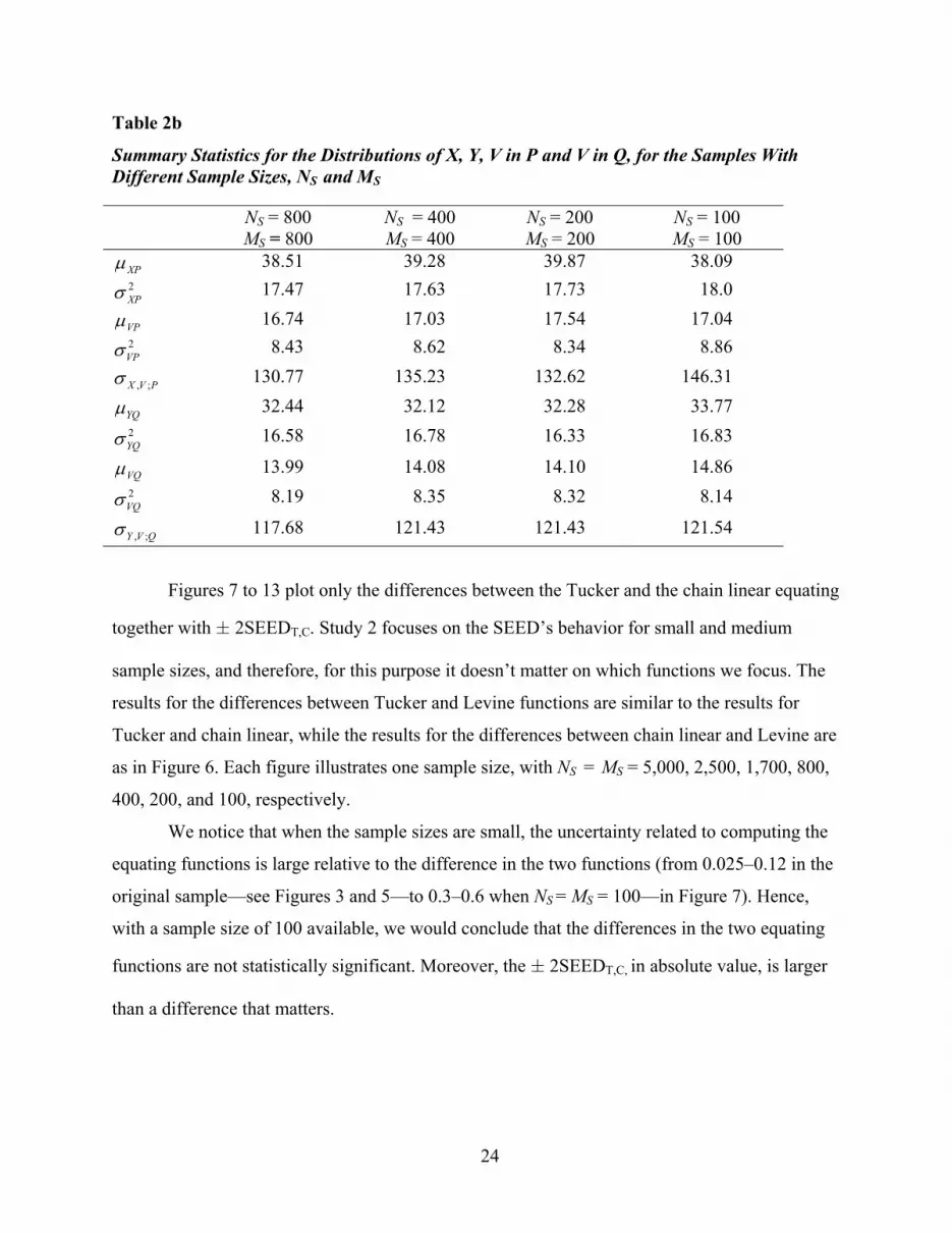
Table 2b

Summary Statistics for the Distributions of X, Y, V in P and V in Q, for the Samples With Different Sample Sizes, NS and MS

NS = 800 MS = 800

NS = 400 MS = 400

NS = 200 MS = 200

NS = 100 MS = 100

XPµ 38.51 39.28 39.87 38.09 2XPσ 17.47 17.63 17.73 18.0

VPµ 16.74 17.03 17.54 17.04 2VPσ 8.43 8.62 8.34 8.86

, ;X V Pσ 130.77 135.23 132.62 146.31

YQµ 32.44 32.12 32.28 33.77 2YQσ 16.58 16.78 16.33 16.83

VQµ 13.99 14.08 14.10 14.86 2VQσ 8.19 8.35 8.32 8.14

, ;Y V Qσ 117.68 121.43 121.43 121.54

Figures 7 to 13 plot only the differences between the Tucker and the chain linear equating

together with ± 2SEEDT,C. Study 2 focuses on the SEED’s behavior for small and medium

sample sizes, and therefore, for this purpose it doesn’t matter on which functions we focus. The

results for the differences between Tucker and Levine functions are similar to the results for

Tucker and chain linear, while the results for the differences between chain linear and Levine are

as in Figure 6. Each figure illustrates one sample size, with NS = MS = 5,000, 2,500, 1,700, 800,

400, 200, and 100, respectively.

We notice that when the sample sizes are small, the uncertainty related to computing the

equating functions is large relative to the difference in the two functions (from 0.025–0.12 in the

original sample—see Figures 3 and 5—to 0.3–0.6 when NS = MS = 100—in Figure 7). Hence,

with a sample size of 100 available, we would conclude that the differences in the two equating

functions are not statistically significant. Moreover, the ± 2SEEDT,C, in absolute value, is larger

than a difference that matters.

24

-1.5

-1

-0.5

0

0.5

1

1.5

0 10 20 30 40 50 60 70 80

X-SCORE

SEED

(T,C

)

T-C2*SEED(T,C)-2*SEED(T,C)

Figure 7. The difference between Tucker and chain linear functions together with a band of ±2SEEDT, C. Study 2, N = 100. NEAT design with an external anchor.

For a sample size of 200, the differences between the Tucker and chain functions are

statistically significant and the ± 2SEEDT,C is about the size of a difference that matters (see

Figure 8). However, at the lower and upper score range, the difference between the two equating

functions is inside the band provided by the ± 2SEEDT,C. One of the reasons is that the accuracy

is lower at extremes of the score range.

25

-1

-0.8

-0.6

-0.4

-0.2

0

0.2

0.4

0.6

0.8

1

0 10 20 30 40 50 60 70 80

X-SCORE

SEED

(T,C

)

T-C2*SEED(T,C)-2*SEED(T,C)

Figure 8. The difference between Tucker and chain linear functions together with a band of ±2SEEDT, C. Study 2, N = 200. NEAT design with an external anchor.

For a sample size of 400, the differences between the Tucker and chain functions are

statistically significant over most of the score range, and the 2SEEDT,C is about the size of a

difference that matters (see Figure 9).

26

-1.5

-1

-0.5

0

0.5

1

0 10 20 30 40 50 60 70 80

X-SCORE

SEED

(T,C

)

T-C2*SEED(T,C)-2*SEED(T,C)

Figure 9. The difference between Tucker and chain linear functions together with a band of ±2SEEDT, C. Study 2, N = 400. NEAT design with an external anchor.

For all the larger samples, the differences between the Tucker and chain functions are

statistically significant over all of the score range (see Figures 10–13).

27

-1.2

-1

-0.8

-0.6

-0.4

-0.2

0

0.2

0.4

0.6

0.8

0 10 20 30 40 50 60 70 80

X-SCORE

SEED

(T,C

)

T-C2*SEED(T,C)-2*SEED(T,C)

Figure 10. The difference between Tucker and chain linear functions together with a band of ±2SEEDT, C. Study 2, N = 800. NEAT design with an external anchor.

28

-1

-0.8

-0.6

-0.4

-0.2

0

0.2

0.4

0.6

0 10 20 30 40 50 60 70 80

X-SCORE

SEED

(T,C

)

T-C2*SEED(T,C)-2*SEED(T,C)

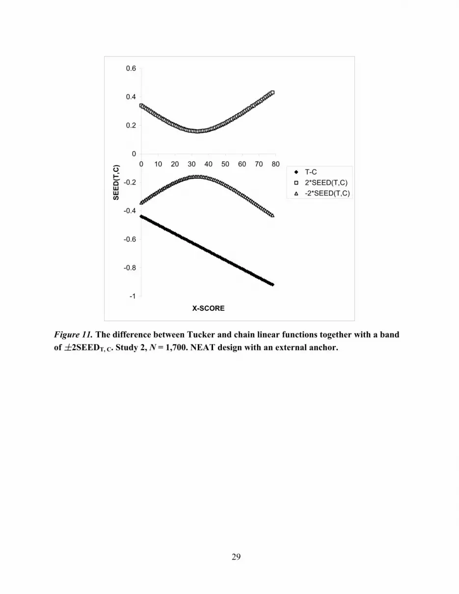
Figure 11. The difference between Tucker and chain linear functions together with a band of ±2SEEDT, C. Study 2, N = 1,700. NEAT design with an external anchor.

29

-1

-0.8

-0.6

-0.4

-0.2

0

0.2

0.4

0 10 20 30 40 50 60 70 80

X-SCORE

SEED

(T,C

)

T-C2*SEED(T,C)-2*SEED(T,C)

Figure 12. The difference between Tucker and chain linear functions together with a band of ±2SEEDT, C. Study 2, N = 2,500. NEAT design with an external anchor.

30

-1

-0.8

-0.6

-0.4

-0.2

0

0.2

0.4

0 10 20 30 40 50 60 70 80

X-SCORE

SEED

(T,C

)

T-C2*SEED(T,C)-2*SEED(T,C)

Figure 13. The difference between Tucker and chain linear functions together with a band of ±2SEEDT, C. Study 2, N = 5,000. NEAT design with an external anchor

With a sample size of 200 available, we conclude that the two equating functions

significantly differ for most of the score range. For larger sample sizes, we notice that the

accuracy increases (i.e., the 2SEEDT,C in absolute values decreases), and one can conclude that

the differences between the two functions are statistically significant.

It follows that for this data set, a sample size of 200 seems to be enough for the SEED to

detect that the two equating methods, Tucker and chain, differ statistically. The level of accuracy

is slightly decreased for this small sample size. More studies are necessary to investigate the

SEED behavior in small and medium samples. Given that in most of the practical equating

situations the sample sizes are much larger, the SEED probably will detect whether the

differences between the equating methods are significant.

31

In von Davier (2003), several idealized conditions are described when the three methods

will give the same results. However, in practical applications, each of these conditions holds

more or less. In a real life situation, when plots like those from Figures 4–6 indicate that the

differences between the methods are statistically significant, which of the methods should one

choose?

From a score-reporting point of view, it does matter which method

one would choose in this example because the differences between the results from the Tucker

method and the others do have an impact on the final results. (These differences are larger than

half a raw score point for most of the raw-score range of X.) From Study 1, we can conclude that

Tucker is far away from the other two equating methods and that the chain linear is in between

Tucker and Levine ( ( ) ( ) ( ); T ; CL ; LLin ;MF ( ) <Lin ;MF ( ) <Lin ;MF ( )XY T XY T XY Tx x xπ π π ). Moreover,

all observed differences are statistically significant.

We cannot make the decision about the final equating function using the SEED alone, if

each of the equating methods relies on a different set of assumptions. We also cannot resolve the

choice between the methods by directly checking their assumptions (T1–T2, L1–L3, C1–C3)

against the data, since these assumptions are not directly testable.

In a practical situation, one will also investigate the issues related to the possible

nonlinearity of the appropriate equating function. In addition, one should also investigate the

SEE for each equating function. The equating results with a higher accuracy (smaller SEEs)

should prevail. However, in Study 1, the differences in the SEEs were very small and therefore,

it would be difficult to use them for making the decision.

As mentioned before for this example where the two populations seem to be dissimilar,

using the rules and discussion previously presented, one would choose the Levine equating

function (when choosing between Tucker and Levine methods), since usually the test forms are

very carefully constructed in this assessment program. Hence, the final decision would appear to

be between the Levine and the chain functions.

At this point, one’s belief in the plausibility of each set of assumptions “appears to be the

sole basis left for making this important judgment” (von Davier et al., 2004, p. 194). Further

research in this area is necessary. The advantages of the SEED are outlined in the next section.

32

Discussion

This paper takes a new perspective on linear equating. It introduces a unified approach to

linear equating in the NEAT design by developing a common parameterization that allows one to

emphasize the similarities between different methods. Based on this common parameterization,

we claim that there is only one definition of observed-score linear equating in the NEAT design,

given in (1), which might take different forms under different assumptions.

We use a new concept, the Method Function, to distinguish among the possible forms

that a linear equating function in a NEAT design might take (in particular among the three

equating methods investigated here—Tucker, Levine, and chain linear equating). By using this

approach, the SEE formula and concept also becomes unified, covering all of the particular

equating functions.

The new approach to linear equating provides a better understanding of equating in

general as well as of the SEE. This view is provided here for the first time (to our knowledge).

The new formula for the SEE makes a computer program more efficient.

We also present a new tool, the standard error of equating difference (SEED), to

investigate if the observed difference in equating functions is statistically significant. Although

the SEED is an asymptotic result, it seems to be stable enough to detect the differences in a

sample size of 200 for the data investigated here. Additional studies might be necessary to

describe the behavior of the SEED for small and medium sample sizes for different data.

The SEED provides an additional measure to consider when making decisions about the

final equating function, especially for medium sample sizes. It is important to know if the

observed differences between two equating functions are statistically significant or they reflect

only random errors. This issue was extensively investigated in empirical studies, and as Harris

and Crouse (1993, p. 219) conclude:

Perhaps the most common process followed in conducting an equating study is to

apply a series of equating methods to a particular situation. Usually all that can be

concluded from such a comparison is whether the methods appear to be providing

similar or dissimilar results, and even that cannot be determined with any

accuracy, because one generally does not have a baseline by which to judge if the

differences between results are simply the result of random error, or something

else.

33

The SEED is exactly the answer to the second part of Harris and Crouse’s remark: The

SEED can tell if the observed differences are the result of random error or not. While it does not

solve the problem of how to decide between different equating functions, it is a step forward in

providing more insight and information that one can use when making this decision.

Harris and Crouse (1993) reviewed all criteria and methods that researchers had

developed for improving this decisional process up to 1993. Three other methods can be

considered:

1. Investigating how sensitive each of the equating functions is to the population

invariance assumption (see Dorans & Holland, 2000; von Davier et al, 2003). The

method introduced in von Davier et al. (2003), though promising, needs additional

research.

2. Carrying out a score equity analysis proposed in Dorans (2003). This is also an

approach to the study of population invariance, but it focuses on different issues:

specifying the number of subpopulations that should be investigated, checking if

the subpopulation score distributions are similar, computing the standardized

difference between the means in the important subpopulations, and using the

Dorans and Holland measure (2000) to investigate the population invariance of

the equating function.

3. Comparing the first several moments of the distribution obtained through equating

with those of the distribution of the old form (the targeted distribution—see von

Davier, et al., 2004, chapter 4).

It is also worth noting that a similar approach as outlined here (with general formulas for

the SEE and SEED) is being developed to investigate the differences between linear and

nonlinear equating functions in the framework of the kernel method of test equating (see von

Davier et al., 2004). A similar SEED formula is not feasible for the classical equipercentile

equating (which uses a linear interpolation as a continuization procedure) because the resulting

equating function is not continuously differentiable at the extreme of the linear segments (and

therefore, the delta method cannot be applied). Bootstrap SEED might be conceived for this

situation, which might be a very interesting issue for further research.

34

References

Angoff, W. H. (1984). Scales, norms, and equivalent scores. Princeton, NJ: Educational Testing

Service. (Reprinted from Educational measurement, 2nd ed., pp. 508–600, by R. L.

Thorndike, Ed., 1971, Washington, DC: American Council on Education.)

Braun, H. I., & Holland, P. W. (1982). Observed-score test equating: A mathematical analysis of

some ETS equating procedures. In P. W. Holland & D. B. Rubin (Eds.), Test equating

(pp. 9–49). New York: Academic.

von Davier, A. A. (2001). Testing unconfoundedness in regression models with normally

distributed variables. Aachen: Shaker Verlag.

von Davier, A. A. (2003). Notes on linear equating methods for the Non-Equivalent Groups

design (ETS RR-03-24). Princeton, NJ: Educational Testing Service.

von Davier, A. A., Holland, P. W., & Thayer, D. T. (2004). The kernel method of test equating.

New York: Springer Verlag.

von Davier, A. A., Holland, P. W. & Thayer, D. T. (2003). Population invariance and chain

versus post-stratification methods for equating and test linking. In N. Dorans (Ed.),

Population invariance of score linking: Theory and applications to Advanced Placement

Program® Examinations (ETS RR-03-27). Princeton, NJ: Educational Testing Service.

von Davier, A. A., Holland, P. W. & Thayer, D. T. (in press). The chain and post-stratification

methods for observed-score equating: Their relationship to population invariance.

Journal of Educational Measurement.

Dorans, N. J. (2003, May 16). Score equity analysis. Paper presented at the Ledyard R. Tucker

Psychometric Workshop, Educational Testing Service, Princeton, NJ.

Dorans, N. J., & Holland, P. W. (2000). Population invariance and equitability of tests: Basic

theory and the linear case. Journal of Educational Measurement, 37, 281–306.

Hanson, B. A., Zeng, L., & Kolen, M. J. (1993). Standard errors of Levine linear equating,

Applied Psychological Measurement, 17, 225–237.

Harris, D. J., & Crouse, J. D. (1993). A study of criteria used in equating. Applied Measurement

in Education, 6(3), 1995–240.

Holland, P. W., King, B. F., & Thayer, D. T. (1989). The standard error of equating for the

kernel method of equating score distributions (ETS PSRTR-89-83, ETS RR-89-06).

Princeton, NJ: Educational Testing Service.

35

Holland, P. W., & Thayer, D. T. (2000). Univariate and bivariate loglinear models for discrete

score distributions. Journal of Educational and Behavioral Statistics, 25, 133–183.

Kendall, M., & Stuart, A. (1977). The advance theory of statistics (4th ed., Vol. 1). New York:

Macmillan.

Kirk, D. B. (1971). Toward a better understanding of the equating process. Unpublished

manuscript.

Kolen, M. J. (1985). Standard errors of Tucker equating. Applied Psychological Measurement, 9,

209–223.

Kolen, M. J., & Brennan, R. J. (1995). Test equating: Methods and practices. New York:

Springer.

Rao, C. R. (1965). Linear statistical inference and applications. New York: Wiley.

Wichert, V. E. (1967). Methods of equating test forms and an equating computer system.

Unpublished manuscript.

36

Appendix

Delta Method

Theorem A1. Suppose that there is given a sequence of statistical models indexed by

(usually the sample size) with the same parameter space n∈N ,Θ which is a nonempty open

subset of R . Let m ˆnπ be a sequence of vector statistics, such that ˆnπ is an asymptotically normal

estimator for π , that is,

( ) ( )( )ˆ 0, , ,dnn Nπ π π π− → ∀Σ ∈Θ

)

where ( )(0,N πΣ denotes the multivariate normal distribution with expectation zero and

covariance matrix ( )πΣ . Consider a function, f, of π with and assume that

f is continuously differentiable on Θ. By

: pf Θ→ R , m p≥

( )f πJ , we denote the p by m Jacobian matrix of f at π

(the matrix of the first derivatives of f by the components of π ). Then the distribution of

( ) (( ˆn f ))n f π π− converges to the multivariate normal distribution with expectation zero and

covariance matrix ( ) ( ) ( )tf fπ π πΣ JJ .

37

Table A1

The Method Function for Tucker, Levine, and Chain Linear Equating

MF XTµ 2XTσ YTµ 2

YTσ

MFT (1 ) ( )XP P VP VQwµ α µ µ− − − 2 2 2 2(1 ) ( )XP P VP VQwσ α σ σ− − − 2 2(1 ) ( )P VP VQw w α µ µ+ − −

( )YQ Q VP VQwµ α µ µ+ − 2 2 2( )YQ Q VP VQwσ α σ σ+ − 2 2 2(1 ) ( )Q VP VQw w α µ µ+ − −

MFL (1 ) ( )XP P VP VQwµ γ µ µ− − − 2 2 2 2(1 ) ( )XP P VP VQwσ γ σ σ− − − 2 2(1 ) ( )P VP VQw w γ µ µ+ − −

( )YQ Q VP VQwµ γ µ µ+ − 2 2 2( )YQ Q VP VQwσ γ σ σ+ − 2 2 2(1 ) ( )Q VP VQw w γ µ µ+ − −

MFC ( )XPXP VT VP

VP

σµ µ µσ

+ − 2VTXP

VP

σ σσ

( )YQYQ VT VQ

VQ

σµ µ µ

σ+ − 2VT

YQVQ

σ σσ

38

Note. The αs and the γs are given in (8)–(13).

Table A2

The Entries of the JLinJMF for Chain Linear Equating

Parameters Derivatives

YQµ 1

VPµ 2

2

YQ

VQ

σ

σ

XPµ 2 2

2 2

YQ VP

VQ XP

σ σ

σ σ− ⋅

VQµ 2

2

YQ

VQ

σ

σ−

2YQσ

2

2 2 2

1 ( )2

VPVP XP VQ

YQ VQ XP

xσ

µ µσ σ σ

+ − − ⋅

µ

(Table continues)

39

Table A2 (continued)

Parameters Derivatives

2VQσ

2 2

2 2 2( )

2YQ VP

VP XP VQ

VQ VQ XP

xσ σ

µ µσ σ σ

− + −

µ−

2VPσ ( )

2

2 2 2

1 12

YQXP

VQ VP XP

xσ

µσ σ σ

⋅ ⋅ −

2XPσ ( )

2 2

2 2 22YQ VP

XP

XP VQ XP

xσ σ

µσ σ σ

− −⋅

, ;X V Pσ 0

, ;Y V Qσ 0

Note. ( )( )

'

2

1 1( ) ( ) .2

xf x f x

x x xx= ⇒ ′ = − = −

40