a two-stage heuristic method for balancing mixed-model assembly lines with parallel workstations

int j prod res 2002 vol 40 no 6 1405plusmn1420

A two-stage heuristic method for balancing mixed-model assembly lineswith parallel workstations

PEDRO M VILARINHOy and ANA SOFIA SIMARIAy

This work presents a new mathematical programming model for the mixed-modelassembly line balancing problem with parallel workstations and zoning con-straints It allows the user to control the process to create parallel workstationsThe modelrsquos primary goal is to minimize the number of workstations along theline for a given cycle time and its secondary goal is to balance the workloadsbetween and within workstations A two-stage procedure using a simulatedannealing approach was developed to tackle this complex problem The regrststage of the procedure looks for a sub-optimal solution to the problemrsquos primarygoal whilst the second stage deals with the secondary goal The procedure isillustrated with a numerical example and the results from computational experi-ments show that even for large-scale problems the proposed procedure performsvery well

1 Introduction

An assembly line is a set of sequential workstations linked by a material handling

system In each workstation a set of tasks is performed using a prederegned assembly

process in which the following issues are deregned (i) the task time ie the time

required to perform each task (ii) a set of precedence relationships which determinethe sequence in which the tasks can be performed and (iii) a set of zoning con-

straints which force or forbid the assignment of di erent tasks to the same work-

station

In a paced assembly line (the type of line addressed in this work) each work-

station has a prederegned amount of time to complete all the tasks assigned to it the

cycle time When this time is elapsed the sub-assembly must be moved to the next

workstation along the line and the workstation receives a new sub-assembly from theprevious workstation Thus the cycle time determines the production rate of the

assembly line In unpaced assembly lines there is no regxed time for a workstation to

complete its workload so bu ers between workstations are necessary in order to

keep the in-process inventories

The assignment of tasks to workstations in such a way that the assembly costs(labour costs equipment costs etc) are minimized the demand is met and both the

precedence and zoning constraints are satisreged is the main problem associated withthe design of assembly lines and is termed the assembly line balancing problem

(ALBP)

International Journal of Production Research ISSN 0020plusmn7543 printISSN 1366plusmn588X online 2002 Taylor amp Francis Ltd

httpwwwtandfcoukjournals

DOI 10108000207540110116273

Revision received October 2001 Departamento de Economia GestaAuml o e Engenharia Industrial Universidade de Aveiro

Campo UniversitaAcirc rio de Santiago 3810-193 Aveiro Portugal To whom correspondence should be addressed pvilegiuapt

An assembly line designed to assemble a single homogeneous product is called asimple assembly line and is used when the demand for that product is su cientlylarge to justify a dedicated assembly line The mathematical formulation of theALBP for simple assembly lines was regrst stated by Salveson (1955) and sincethen extensive research has been done in the area Comprehensive literature reviewson this subject are provided in Ghosh and Gagnon (1989) and Scholl (1999)

The recent market trends show that there is a growing demand for customizedproducts increasing the pressure for manufacturing macrexibility Consequently simpleassembly lines are being replaced by mixed-model assembly lines in which a set ofsimilar models of a product can be assembled simultaneously Several techniqueshave been proposed to tackle the mixed-model ALBP namely by GoEgrave cken and Erel(1997 1998) McMullen and Frazier (1997 1998) Merengo et al (1999) and Ereland GoEgrave cken (1999)

Most of the techniques used to solve the ALBP require the assignment of eachtask to a single workstation and consequently the production rate is limited by thelongest task time This assumption can be relaxed by utilizing parallel workstationsin such a way that two or more replicas of a workstation can perform the same set oftasks on di erent assemblies The introduction of parallel workstations not onlyallows for cycle times shorter than the longest task time and thus an increase inthe production rate but also provides greater macrexibility in designing the assemblyline (Buxey 1974)

However when parallel workstations are introduced the number of tasks per-formed by each worker increases (eg it is possible to design an assembly line withjust one workstation and a su cient number of replicas to meet the demandETHinsuch a case each worker has to perform all tasks) but this contradicts one of themain advantages of using an assembly line the use of low-skilled labour that can beeasily trained (due to the strict division of labour) Therefore in order to maintainthat advantage it is necessary to control the process to create parallel workstations(ie the replication process) in such a way that workstations are replicated only whenrequired ie when a taskrsquos processing time is larger than the cycle time and as suchrequires the replication of the workstation in which the task will be carried out Mostof the models for the ALBP with parallel workstations proposed in the literaturebase the decision to create parallel workstations on a trade-o between the incre-mental toolingequipment cost of the duplicated workstation and the cost of hiringworkers for the original line in order to satisfy the demand (eg Johnson 1983 Pintoet al 1975 1981 Bard 1989 Daganzo and Blumenfeld 1994 Askin and Zhou 1997)McMullen and Frazier (1997 1998) allow the replication of a workstation as long asits utilization increases Schoregeld (1979) and Sarker and Shantikumar (1983) deregne alimit on the number of parallel workstations to control the replication process whileBuxey (1974) includes a limit on the number of tasks per workstation In either ofthese approaches tasks with processing times much shorter than the cycle time cantrigger the replication of workstations which can lead to an excessive number ofparallel workstations

This work introduces a mathematical programming model for the mixed-modelALBP with parallel workstations and zoning constraints which minimizes thenumber of workstations for a given cycle time A secondary goal was introducedso that the model also balances the workload between workstations (ie for eachmodel the idle time is distributed across the workstations as equally as possible) andwithin workstations (ie the overall idle time for each workstation is distributed

1406 P M Vilarinho and A S Simaria

across models as evenly as possible) thus ensuring that all the workers across the lineperform approximately the same amount of work on each model being assembledand that approximately the same amount of work is carried out in each workstationregardless of the model being assembled

The model allows the decision-maker to deregne a limit on the maximum numberof replicas of a workstation and the conditions under which a workstation can bereplicated Owing to the combinatorial nature of the problem a two-stage pro-cedure which uses the simulated annealing algorithm was developed to solve itthus providing near-optimal solutions with an acceptable computational e ort

2 The mathematical programming modelThe proposed model for the mixed-model assembly line balancing problem with

parallel workstations has the following characteristics

(i) the planning horizon has a regxed length P(ii) a set of similar models (m ˆ 1 M) can be simultaneously assembled(iii) the forecast demand over the planning horizon for model m is Dm

requiring the line to be operated with a cycle time C ˆ P=PM

mˆ1 Dm(iv) the overall proportion of the number of units of model m being assembled

is then qm ˆ Dm=PM

pˆ1 Dp(v) each model has its own set of precedence relationships but there is a

subset of tasks common to all models Hence the precedence diagramsfor all the models can be combined and the resulting one has N tasks

(vi) the tasks (i ˆ 1 N) are performed in a set of workstations(k ˆ 1 S)

(vii) the time required to perform task i on model m tim may vary amongmodels (tim ˆ 0 means that model m does not require task i to beassembled)

(viii) a task can be assigned to only one workstation and consequently thetasks that are common to several models need to be performed on thesame workstation

(ix) the set of tasks that cannot be performed before task i is completed Fi(successors of task i) is given by the precedence constraints derived fromthe combined precedence diagram

(x) the zoning constraints are deregned in the assembly processETHZP is the setof task pairs that must be assigned to the same workstation (compatibletasks) and ZN is the set of task pairs that cannot be performed on thesame workstation (incompatible tasks)

(xi) a workstation can be duplicated up to a maximum of MAXP replicas butonly if the task time of one of the tasks assigned to it exceeds a prederegnedvalue (not of the cycle time) for at least one of the models

The decision variables are deregned as follows

xik ˆ1 if task i is assigned to workstation k

0 otherwise

(

rk ˆ1 if workstation k can be replicated

0 otherwise

(

1407Balancing mixed-model assembly lines

skm ˆ idle time of workstation k due to model m

The mixed-model assembly line balancing problem with parallel workstations andzoning constraints that for a given cycle time minimizes the number of workstationsand balances the workloads can be modelled as the mathematical programmingmodel shown in reggure 1

The regrst term in the objective function (1) minimizes the index of the workstationto which the last task is assigned thus minimizing the number of workstations Thesecond term balances the workload between the workstations (in this term S 0 is theactual number of workstations required to meet the demand in the assembly lineETHS 0 ˆ k xNk ˆ 1) The third term balances the workload within each workstation (inthis term Sk ˆ

PMmˆ1 qm cent skm) As both the second and the third terms are within the

value range [01] the regrst term is dominant for S 0 gt 2 which is always the case forreal world applications So the model minimizes the number of workstations beforethe secondary goal becomes active

The model constraints can be interpreted as follows

(2) constraints ensuring that each task is assigned to only one workstation of thestation interval

(3) constraints ensuring that no successor of a task is assigned to an earlierstation than that task

(4) compatibility zoning constraints(5) incompatibility zoning constraints


[ ]

)c7(S1k]10[

)b7(N1i S1k]10[

)a7(M1m S1k0

)c6(1000 S1k

)b6(1000 S1k

)a6(M1m S1k)1MAXP(1Ct

)5(S1k ZN)ba(1

)4(ZP)ba(0

)3(Fb Na0

)2(N1i1

subject to

(1) M

1

S

q

)1M(rsquoS

M

rsquoS

1q

1rsquoS

rsquoSk Zmin

k

ik

km

M1mCtiikk

M1mCtiikk

N

1ikkmikim

bkak

S

1k

S

1kbkak

a

S

1k

S

1kbkak

S

1kik

rsquoS

1k

M

1m

2

k

kmmS

1k

M

1m

rsquoS

1k

2

rsquoS

1llm

kmmNk

im

im

=Icirc ==Icirc

==sup3

pound pound =sup3 times

pound pound =pound

==-+=+times

=Icirc pound +

Icirc =-

Icirc Icirc pound -

==

divide divide oslash

ouml ccedil ccedil egrave

aelig -

-+

divide divide divide divide

oslash

ouml

ccedil ccedil ccedil ccedil

egrave

aelig

--

+times =

aring aring

aring

aring aring

aring aring

aring

aring aring aring aring aring aring

=gt$

=gt$

=

= =

= =

=

= == = =

=

r

x

s

xr

xr

rsx

xx

xx

xx

x

s

s

sx

a

a

M

Figure 1 Mathematical programming model for the mixed-model ALBP with parallelworkstations

(6) the set of constraints ensuring that each workstation time capacity is notexceeded the maximum number of replicas of a workstation is not exceededand only workstations where the processing time of the tasks assigned to itfor at least one model exceeds a certain proportion (not) of the cycle timecan be duplicated (M is a very large positive integer)

(7) the set of constraints deregning the decision variables domains

The complexity of the proposed model is high and it cannot be solved to optimalityat least for real world problems Thus a two-stage procedure that uses the simulatedannealing technique was developed to tackle the problem The following sectionsdescribe the general simulated algorithm and its application to the proposed two-stage procedure

3 The general simulated annealing algorithmSimulated annealing was chosen among other meta-heuristics mainly because of

its macrexibility to respond to modiregcations in the objective functions or in the problemconstraints When these changes occur the basic simulated annealing programremains unchanged In addition the ALBP solutions and neighbourhood structurescan be easily deregned using simulated annealing

The simulated annealing algorithm which attempts to solve NP hard combina-torial optimization problems through controlled randomization was introduced byKirkpatrick et al (1983) Since then the algorithm has been applied to many opti-mization problems in a wide variety of areas including the assembly line balancingproblem (eg Suresh and Sahu 1994 Heinrici 1993 McMullen and Frazier 1998)

The simulated annealing algorithm is a randomized search procedure that startsfrom an initial solution to the problem S0 A control parameter T is set to an initial`temperaturersquo value T0 and is systematically decreased according to an annealingschedule In this schedule the following issues are deregned (i) a temperature reducingfunction and (ii) the length of each temperature level L that determines the numberof solutions generated at a certain temperature At each temperature level and as thetemperature decreases neighbouring solutions to the current solution are generatedA neighbouring solution Sn is accepted (ie replaces the current solution) if it is notworse than the current solution S ( f hellipSndagger micro f hellipSdagger where f is the general objectivefunction to minimize) If the neighbouring solution is worse than the current solution( f hellipSndagger gt f hellipSdagger) it may still be accepted with a certain probability p ˆ eiexclcent=T where

cent ˆ f hellipSndagger iexcl f hellipSdaggerf hellipSndagger

pound 100

This probability of accepting inferior solutions allows the simulated annealingalgorithm to escape from local minima

The performance of the algorithm depends on the deregnition of several of theannealing schedule parameters

(i) The initial temperature should be high enough so that in the regrst iterationof the algorithm the probability of accepting worst solutions is at least80 (Kirkpatrick et al 1983)

(ii) The most commonly used temperature reducing function is geometricTi ˆ aiTiiexcl1 (ai lt 1 and constant) Typically 08 micro ai micro 099 (Eglese 1990)

(iii) The length of each temperature level L determines the number of solutionsgenerated at each temperature T


(iv) The stopping criterion deregnes when the system has attained a desired energylevel Some of the most common criteria are based on

the total number of solutions generated

the temperature at which the desired energy level is attained (freezingtemperature)

the acceptance ratio (ratio between the number of solutions accepted andthe number of solutions generated)

Naturally each of these control parameters must be reregned according to the speciregcproblem on hand Two other important issues that need to be deregned when adaptingthis general algorithm to a speciregc problem are the procedures to generate both theinitial solution and the neighbouring solutions The details of the proposed imple-mentation of the simulated annealing algorithm to the problem on hand are pre-sented in the next section

4 The two-stage procedure for the mixed-model ALBP with parallel workstationsand zoning constraints

The features of the proposed procedure are as follows

(i) the main goal is to minimize the number of workstations for a given cycletime

(ii) the additional goals of balancing workloads between and within worksta-tions are also envisaged

(iii) an upper bound on the maximum number of replicas of a workstation canbe set by the decision-maker

(iv) zoning constraints are accounted for(v) the decision-maker may deregne the minimum task time (expressed as a per-

centage of the cycle time) that triggers the replication of the workstationperforming that task (this time will be called the minimum replication timeETHMRT) By default this value is 100 of the cycle time which means onlyworkstations performing tasks whose duration is larger that the cycle timefor at least one of the models can be duplicated

The two stages of the proposed procedure are shown in reggure 2 In the regrst stage theprocedure looks for a sub-optimal solution for the problemrsquos main goal In thesecond stage the additional goals are fulreglled In both stages a simulated annealingapproach is used

A common annealing schedule was used for both stages of the procedure inwhich the following control parameters were deregned

(i) Initial temperature (T0) the computational experience showed that thevalues of the objective functions never changed by more than 10 betweentwo neighbouring solutions So for an initial temperature of 50 it is guar-anteed that at least 80 of the inferior solutions are accepted

(ii) Temperature reduction function the geometric function with a temperaturereduction factor of 09 (Ti ˆ 09Tiiexcl1) was used on each stage

(iii) The length of each temperature level (L) a dominant factor on the compu-tational e ort associated with the solution of the problem is the number oftasks (N) So in order to restrict the computational e ort to the regrst orderof the dominant factor the number of solutions searched at each tempera-


ture level was set to KN where K is a user-deregned constant (K ˆ 1 is thevalue suggested by default)

(iv) Stopping criteria two alternative criteria were set In the regrst a freezingtemperature of 10 is set which means that 16 temperature levels are used(T0a15

i ˆ 50hellip0915dagger ˆ 1029) In the second one it is admitted that if in regveconsecutive temperature levels 85 of the generated solutions are rejectedthen the probability of replacing the best solution found is very small andthe procedure is then terminated

41 The regrst stage411 Initial solution

The initial solution is obtained using a version of the Rank Positional Weight(RPW) heuristic proposed by Helgeson and Birnie (1961) The original RPW versiononly addresses the simple assembly line balancing problem where one single model isassembled and no parallel workstations are allowed The positional weight of a taskin a mixed-model assembly line is the cumulative average task time associated withitself and its successors The average task time is the sum of the processing times ofthat task for each model weighted by the respective production share Tasks areassigned to the lowest numbered feasible workstation by decreasing order of theirpositional weight and considering the individual task processing times for eachmodel

In the original version of the RPW heuristic the cumulative duration of the tasksin a workstation cannot exceed the cycle time (hence the concept of a feasible work-station) and thus does not account for parallel workstations The version of theRPW heuristic used to obtain the initial solution in the regrst stage of the procedurerederegnes the concept of a feasible workstation if a workstation performs a task withprocessing time larger than MRT for at least one model its time capacity isC pound MAXP otherwise it is C

The implemented version of the RPW heuristic also checks if the task to beassigned is not incompatible with any of the tasks already allocated to the work-station The procedure also merges tasks that need to be processed in the sameworkstation previously so that they are treated as only one task


1st stageBest solution

2nd stage Initial solution

Obj MINUnbalance betweenand within stations

STOP

2nd stageBest solution

HeuristicBest solution

InitialsolutionModified

RPW heuristic

Obj MINIdle timeSTOP

Neighbouringsolution

Current solution

Swap orTransfer

Solution intaboo list

Verifyconstraints(precedence

zoningcapacity)

Y

Y

N

N

Y Y


Current solution

Swap orTransfer



zoningcapacity first

stage)Y

Y

N

N

N N

FIRST STAGE SECOND STAGE

Figure 2 The two-stage procedure for the mixed-model ALBP

412 Solution evaluation criterionIn the regrst stage the procedure looks for the solution that minimizes the number

of workstations in the assembly line As the total idle time of the line decreases withthe overall number of workstations in the line one can attain the regrst stage goal byminimizing the balance delay time (BDT) which is computed as follows

BDT ˆXM

mˆ1

XK

kˆ1

qm SPkC iexclX

i2Ok

tim

Aacute

hellip8dagger

where SPk is the number of replicas of station k and Ok is the set of tasks assigned tostation k This goal is equivalent to the one expressed by the regrst term of theobjective function of the mathematical programming model and it was used insteadto ease the programming e ort

413 Neighbouring solutionsA neighbouring solution can be generated by one of the following actions (i)

swapping two tasks in di erent workstations or (ii) transferring a task to anotherworkstation The tasks to be swapped as well as the task and the workstation forthe transfer are randomly chosen For any of these actions to result in a newneighbouring solution the precedence zoning and workstations time capacityconstraints must be fulreglled When this is not the case a new swap or transfermust be attempted

Only transfer movements may contribute to reduce the number of workstationsthus minimizing the balance delay time Nevertheless swap procedures are alsorequired to ease the generation of successful transfer movements Consequentlythe probability of performing a transfer procedure must be higher than for theswap procedure and by default probabilities of 75 and 25 were respectivelyset although the user can set di erent values

In both stages of the proposed procedure a taboo list is used to maintain infor-mation about the most recently generated neighbouring solutions in order to avoidcycling

42 The second stageThe goal in the second stage is to balance simultaneously the between-station and

within-station workloads for the number of workstations obtained in the regrst stageThe initial solution for the second stage is the regnal solution found in the regrst stageThe criterion used to evaluate the neighbouring solutions generated in this secondstage derives directly from the second and third terms of the objective function of themathematical programming model presented in section 2

421 Neighbouring solutionsThe generation of neighbouring solutions in the second stage also employs swap

and transfer movements but the tasks and workstations involved in these move-ments are selected to foster improving solutions As the goal in this second stage is tobalance the workloads swap movements are more likely to contribute towards thisend (Probabilities of 75 for swap and 25 for transfer moves are set as thedefault)


Swap movement

Step 1 Let Z be a randomly selected workstation and X the model whose idle timefor that station has the highest deviation from the workstation average idletime

X centsZX ˆ maxm

sZm cent qm iexcl SZ

M

shyshyshyshy

shyshyshyshy

raquo frac14sup3 acute

Step 2 If sZX gt SZ=M then go to step 3 else go to step 5Step 3 Select the task assigned to station Z with the lowest processing time for

model X (T1 tT1X ˆ miniftiX g ^ i 2 OZ)Step 4 From the set of tasks performed on model X that are not assigned to station

Z and whose task time is higher than the task time of T1 randomly selectone (T2 tT2X gt tT1X ^ T2 =2 OZ) Go to step 7

Step 5 Select the task assigned to station Z with the highest processing time formodel X (T1 tT1X ˆ maxiftiX g ^ i 2 OZ)

Step 6 From the set of tasks performed on model X that are not assigned to stationZ and whose task time is smaller than the task time of T1 randomly selectone (T2 tT2X lt tT1X ^ T2 =2 OZ)

Step 7 If precedence zoning capacity and number of workstations constraints aremet swap tasks T1 and T2

Transfer movement


X centsZX ˆ maxm

sZm cent qm iexclSZ

M

shyshyshyshy

shyshyshyshy


Step 2 If sZX gt SZ=M then go to step 3 else go to step 5Step 3 Select a task not assigned to station Z with processing time for model X

higher than for the other models (T1 tT1X ˆ maxmftT1mg ^ i =2 OZ)Step 4 If precedence zoning capacity and number of workstations constraints are

met transfer task T1 to workstation ZStep 5 Select the task assigned to station Z with the highest processing time for

model X (T1 tT1X ˆ maxiftiX g ^ i 2 OZ)Step 6 Randomly select a workstation (W) where the workload for model X is

lower than the station average idle time (W sWX lt SW=M)Step 7 If precedence zoning capacity and number of workstations constraints are

met transfer task T1 to workstation W

If after a prederegned number of attempts neither swap nor transfer movements leadto a neighbouring solution the tasks or workstations involved in these movementsare selected randomly to force a new neighbouring solution

43 Numerical illustrationA numerical example with the following characteristics is used to illustrate the

proposed procedure


(i) The models A and B are simultaneously assembled in a line and over aplanning horizon of 480 tu (time units) The demand for each model isrespectively 20 and 28 units (then the cycle time is C ˆ 10 qA ˆ 42 andqB ˆ 58)

(ii) the combined precedence diagram with 25 tasks is depicted in reggure 3where each node represents a task and each arc represents a precedencerelation between a pair of tasks

(iii) the task times for the two models are shown in table 1(iv) tasks 9 and 10 cannot be executed on the same workstation(v) only workstations performing tasks with a processing time greater than the

line cycle time can be replicated (MRT ˆ C)(vi) the maximum number of replicas of a workstation is two (MAXP ˆ 2)

The initial solution is determined by the modireged version of the RPW heuristic

described in section 411 The average processing times and average positional

weights of each task are shown in table 1

Figure 4 illustrates some steps of the procedure applied to the numerical example

In each of the tables shown in the reggure a line balancing solution is shown To

simplify the schema only the workstations where changes occurred are representedin the neighbouring solutions The content of each column in these tables is the

following (1) workstation index S (2) set of tasks assigned to the workstation

and (3) the number of replicas of the workstation R The last line in each table


1

2

3

4

5

6

7

8

9

10

11

12

13

14

15

16 17

18

19

20

21 22

23

24 25

Figure 3 Precedence diagram for the numerical example

Task 1 2 3 4 5 6 7 8 9 10 11 12 13tA 0 77 73 150 88 62 36 0 66 25 55 71 59tB 20 77 73 150 88 0 0 20 66 25 55 71 59Weighted average 12 77 73 150 88 26 15 12 66 25 55 71 59

task timePositional 1154 544 1142 466 853 662 158 316 389 467 611 305 556

weight

Task 14 15 16 17 18 19 20 21 22 23 24 25tA 13 55 19 37 94 13 0 20 47 96 41 125tB 0 55 20 0 94 13 90 20 47 82 37 0Weighted average 05 55 20 16 94 13 52 20 47 88 39 53

task timePositional weight 197 234 442 263 338 192 143 248 138 179 91 52

Table 1 Processing times and average positional weights for the numerical example

shows the total number of workstations (including replicas) required by the solution

S 0 and the between-station (Bb-s) and within-station (Bw-s) balancing values (com-

puted from the expressions in the second and third term of the objective function of

the mathematical programming model)

The initial solution requires a total of 18 workstations (including all replicas)

After a number of swap and transfer movements starting from the initial solutionan intermediate solution is generated From this solution the heuristic is able to

reduce the number of workstations performing the transfer procedures shown in the

reggure The best solution found for the regrst stage of the heuristic indicates that 16

workstations including replicas are required (for this solution Bb-s ˆ 005 and

Bw-s ˆ 022) The best solution found on the regrst stage of the procedure is used as

the initial solution for the second stage In this stage the number of workstations

remains constant while the workload balancing value (Bb-s Dagger Bw-s) is reduced Theregnal solution shows an improvement of about 30

5 Computational experience

The procedure was coded in Visual CDaggerDagger on a 350 MHz Pentium II computer Itis not possible to compare directly the heuristic with others reported in the literature

as none have the same underlying characteristics Nevertheless in order to test the

performance of the proposed heuristic a series of comparative tests were carried out

by adapting the heuristic to the conditions under which the benchmark problems

proposed by Scholl (1993) were originally set Schollrsquos test problems are for single-

model balancing problems without parallel workstations so the heuristic was run

setting MAXP ˆ 1 also only the objective function of minimizing the number ofworkstations was tested For the 168 instances analysed the optimal solution is

known for 161 The solutions obtained by the proposed heuristic for this data set

are slightly inferior to the optimal solution in most cases (14 in the worst case) but

the procedure manages to regnd the optimal solution in 76 instances


S Tasks R S Tasks R1 13 1 9 18 12 5 1 10 1219 13 67 1 11 1721 14 11 1 12 15 15 13 1 13 23 16 2 1 14 20 17 41016 2 15 2224 18 8914 1 16 25 2

Srsquo=18 Bb-s=008 Bw-s=017

S Tasks R S Tasks R1 12 1 9 812 12 3 1 10 18 13 4 2 11 15 14 5 1 12 17 15 67 1 13 141921 16 1011 1 14 22 17 13 1 15 23 18 916 1 16 202425 2


S Tasks R S Tasks R11 - 0 12 1517 1


S Tasks R S Tasks R

131419 2122

1 14 - 0


S Tasks R S Tasks R8 89 1 9 1216 1




S Tasks R S Task s R1 13 1 8 487 2

2 6 1 9 18 1

3 5 1 10 1221 14 9 1 11 715 1

5 2 1 12 141922 16 1011 1 13 23 1

7 1316 1 14 202425 2Srsquo=16 Bb-s=004 Bw-s=015

Initial solution Intermediate solution

Transfertask 15 to station 12


1st STAGE BEST SOLUTION

Swaptasks 8 and 16

Swaptasks 4 and 6

HEURISTIC BEST SOLUTION

Figure 4 Illustration of the proposed procedure applied to the numerical example

In order to evaluate the real performance of the heuristic a set of 20 assemblyline balancing problems with parallel workstations and zoning constraints wastested taking into account only the objective function (1) For a set of four prob-lems an optimal solution was obtained using the Cplex MIP solver to solve theproposed mathematical programming model which allowed verifying that the pro-posed procedure generates the optimal solution for these instances (see table 3 later)For larger sized problems it is not possible to regnd an optimal solution within reason-able time limits So in order to evaluate the procedure performance a lower boundfor the number of workstations was derived

51 A lower bound for the number of workstationsA lower bound for the mixed-model assembly line balancing problem with par-

allel workstations LBpmix was derived using the following set of assumptions

(i) the maximum number of replicas per workstation is two (MAXP ˆ 2)(ii) a workstation can be duplicated only if the task time of one of the tasks

assigned to it exceeds the cycle time (not ˆ 100 MRT ˆ C) and(iii) the task time of the longest task does not exceed twice the cycle time

(tmax micro 2C)

The steps required to compute LBpmix are described as follows and illustrated for thenumerical example introduced in section 43

Step 1 For each model classify the tasks according to the corresponding task timeas shown in table 2

Step 2 For each model compute LB 0hellipmdagger

LB 0hellipmdagger ˆ 2hellipnA Dagger nB Dagger nCdagger Dagger yhellipnD iexcl nCdagger Dagger 1

2whellipnE iexcl nBdagger

sup3sup1

Dagger 5

3nF Dagger 4

3nG Dagger 2

3nH Dagger 1

3nI

acuteordm hellip9dagger


Tasks

Task type Task time Model A Model B

A 53 C lt tA micro 2C plusmn

B 43 C lt tB micro 5

3 C 4 4

C C lt tC micro 43 C 25 plusmn

D 23 C lt tD micro C 2 3 5 12 18 23 2 3 5 12 18 20 23

E 13 C lt tE micro 2

3 C 6 7 9 11 13 15 17 22 24 9 11 13 15 22 24

F tF ˆ 53 C plusmn plusmn

G tG ˆ 43 C plusmn plusmn

H tH ˆ 23 C plusmn plusmn

I tI ˆ 13 C plusmn plusmn

J tJ lt 13 C 1 8 10 14 16 19 20 21 1 6 7 8 10 14 16

17 19 21 25

Table 2 Classiregcation of the tasks to compute LBpmix

LB 0hellipmdagger is the main term of LBpmixhellipmdagger It is derived from one of the lower boundsLB3 deregned by Scholl (1999) for the SALPB and adapted to the parallel work-stations problem LB 0hellipmdagger is given by expression (9) where nX is the number oftasks of type X (X ˆ A J) y equals 1 if nD iexcl nC gt 0 or zero otherwise and wequals 1 if nE iexcl nB gt 0 or zero otherwise The reasoning for this computation is asfollows

The workstations performing tasks of types A B or C (whose task time is longerthan the cycle time) need to be duplicated As two tasks of any of these types cannotshare the same workstation because the value of MAXP would be exceeded a lowerbound for the overall number of workstations (including replicas) is twice thenumber of tasks of types A B and C Each task of type D can be combined witha task of type C in a duplicated workstation however if there are not enoughduplicated workstations of type C to accommodate the tasks of type D each ofthese remaining tasks will require a workstation The same reasoning applies totasks of type E that is two tasks of type E require a single workstation but canalso be combined with a duplicated workstation performing tasks of type B Finallythe tasks of types F G H and I have a regxed task time and so they occupy a fractionof a workstation corresponding to the ratio between their task time and the cycletime

For the numerical example the values of LB 0hellipAdagger and LB 0hellipBdagger are computed asfollows

LB 0hellipAdagger ˆ 2hellip0 Dagger 1 Dagger 1dagger Dagger hellip6 iexcl 1dagger Dagger 1

2hellip9 iexcl 1dagger

sup3 acutesup1 ordmˆ 13

LB 0hellipBdagger ˆ 2hellip0 Dagger 1 Dagger 0dagger Dagger hellip7 iexcl 0dagger Dagger 1



Step 3 For each model compute Zhellipmdagger

Zhellipmdagger ˆX

iˆJ

ti iexcl LB 0hellipmdagger cent C iexclX

i 6ˆJ

ti

Aacute iquestC

amp rsquo

hellip10dagger

A second term is added to LB 0hellipmdagger to compute the value of LBpmix This term adds upthe number of workstations needed to process tasks of type J which in most real-world problems account for a large proportion of the workstations Because thesetasks can easily be included in workstations that perform tasks of the other types itis necessary to verify if after reglling up these workstations there are tasks of type Jremaining to create new workstations The minimum number of workstations(Zhellipmdagger) required to perform tasks of type J after reglling up the remaining capacityof the workstation assigned to other task types is then given by expression (10)

For the numerical example the values of ZhellipAdagger and ZhellipBdagger are computed asfollows

ZhellipAdagger ˆ dpermil9 iexcl hellip13 pound 10 iexcl 1232daggerŠ=10e ˆ 1

ZhellipBdagger ˆ dpermil118 iexcl hellip12 pound 10 iexcl 1044daggerŠ=10e ˆ 0

Step 4 For each model compute LBpmixhellipmdagger ˆ LB 0 Dagger Zhellipmdagger For the numericalexample LBpmixhellipAdagger ˆ 14 and LBpmixhellipBdagger ˆ 12

Step 5 Select LBpmix for the problem LBpmix ˆ maxmpermilLBpmixhellipmdaggerŠ For the numer-ical example LBpmix ˆ LBpmixhellipAdagger ˆ 14


52 Computational resultsThe heuristic was tested on a set of 20 problems whose main characteristics are

shown in the regrst columns of table 3 namely the number of tasks of the combined

precedence diagram (N) the number of models (M) and the assembly line cycle time

(C) The precedence diagrams used for the test problems were taken from Scholl

(1993) except for problems 7 and 8 where the one from the numerical example

introduced in section 43 was used The cycle time and the task processing times

for each problem were randomly generated taking into account the di erent tasktypes that might be present in a real world assembly process

The test problems were solved using the proposed procedure and the minimum

maximum and mean value of the solutions for each of the test problems shown in

table 3 results from ten runs of each instance of the problem A comparison between

these values and the ones obtained using the Cplex solver (Optimal Solution) and the

lower bound (LBpmix) is depicted in the tenth column (D()) where the di erence

between the minimum value produced by the heuristic and either the LBpmix or thebest solution is shown For small-sized problems (for which an optimal solution was

found) the proposed procedure gives the optimal solution For large-sized problems

the worst performance is for problem 15 where the di erence between the solutions

obtained and the lower bound is 20 Nevertheless as the calculation of the lower

bound does not take into account the precedence and zoning constraints one is led

to consider that the results obtained from the heuristic are fairly good This conclu-

sion is reinforced by the values for the line e ciency shown in column 11 of table 3(Weighted E ()) where a high line usage rate can be perceived particularly for the

largest sized problems The weighted line e ciency was computed using the follow-

ing expression


Optimal Heuristic solution Weighted CPUProblem N M C LBpmix solution Mean Min Max D() E () Time (s)

1 8 2 10 4 4 4 4 4 0 856 12 8 3 10 6 8 8 8 8 0 549 13 11 2 10 7 7 7 7 7 0 710 144 11 3 10 6 7 7 7 7 0 765 15 21 2 10 14 plusmn 16 16 16 143 726 16 21 3 10 13 plusmn 15 15 15 154 796 447 25 2 10 14 plusmn 16 16 16 143 768 2168 25 3 10 14 plusmn 15 15 15 71 820 669 28 2 10 19 plusmn 21 21 21 105 865 104

10 28 3 10 18 plusmn 20 20 20 111 832 1011 30 2 10 15 plusmn 162 16 17 67 866 11612 30 3 10 17 plusmn 194 19 20 118 834 12613 32 2 10 16 plusmn 19 19 19 188 773 3414 32 3 10 17 plusmn 19 19 19 118 810 8415 35 2 10 20 plusmn 24 24 24 200 800 7216 35 3 10 21 plusmn 24 24 24 143 852 1017 45 2 10 23 plusmn 252 25 26 87 854 11618 45 3 10 24 plusmn 282 28 29 167 814 13819 70 2 10 41 plusmn 44 44 44 73 870 1520 70 3 10 39 plusmn 442 44 45 128 860 20

Table 3 Computational results for the test problems

WeightedEff ˆXM

mˆ1

qm

XN

iˆ1

tim

S 0C

2

66664

3

77775 hellip11dagger

where for S 0 the minimum value for the number of workstations given by theheuristic solutions was used

Finally the average running times for each of the test problems are depicted inthe last column of table 3 (CPU time(s)) and they show that solutions can beobtained in acceptable times even for large problems

6 Conclusions and future research directionsIn this paper a new mathematical programming model for the mixed-model

assembly line balancing problem with parallel workstations and zoning constraintswas presented The model minimizes the number of workstations and allows the userto control the replication process As a secondary goal the model looks to obtain agood workload balance between and within the workstations Due to the modelcomplexity a two-stage heuristic procedure was developed to tackle the problemwhich uses the simulated annealing algorithm Computational experiments showedthat the proposed heuristic performs very well producing good quality solutions inreasonable running times

The major contribution of the reported research work derives from the use of aset of constraints to control the workstationsrsquo replication process and from the use ofa two-goal objective function The issues are of crucial importance to solve real-world line balancing problems In fact the proposed heuristic combined with asimulation study has been applied for balancing a mixed-model PC camera assem-bly line (Ramos et al 2001) and very good results were obtained

The matching between theoretical procedures and practical applications is a veryimportant area that needs further developments In addition more complex balan-cing problems with di cult constraints present in real-world problems must beaddressed

Further research must be made on the mixed-model assembly line balancingproblem considering the actual market trends where there is a growing demandfor customized products thus increasing the pressure for manufacturing macrexibility

The areas of research to be pursued in the future related to the present work are(i) alternative procedures to control the workstationsrsquo replication process and (ii) theapplication of the same type of concepts reported in this work to solve the type-IIMALBP (which attempts to minimize the cycle time for a given number of work-stations)

AcknowledgementsThe authors are grateful for the constructive feedback they received from the

anonymous referees This feedback was very helpful in improving the paper

Reference

Askin R G and Zhou M 1997 A parallel station heuristic for the mixed-model productionline balancing problem International Journal of Production Research 35 3095plusmn3106


Bard J F 1989 Assembly line balancing with parallel workstations and dead timeInternational Journal of Production Research 27 1005plusmn1018

Buxey G M 1974 Assembly line balancing with multiple stations Management Science 201010plusmn1021

Daganzo C F and Blumenfeld D E 1994 Assembly system design principles and trade-o s International Journal of Production Research 32 669plusmn681

Eglese R W 1990 Simulated annealing a tool for operational research European Journalof Operational Research 46 271plusmn281

Erel E and CoEgrave cken H 1999 Shortest-route formulation of mixed-model assembly linebalancing problem European Journal of Operational Research 116 194plusmn204

Ghosh S and Gagnon R J 1989 A comprehensive literature review and analysis of thedesign balancing and scheduling of assembly systems International Journal ofProduction Research 27 637plusmn670

GoEgrave cken H and Erel E 1997 A goal programming approach to mixed-model assemblyline balancing problem International Journal of Production Economics 48 177plusmn185

GoEgrave cken H and Erel E 1998 Binary integer formulation for mixed-model assembly linebalancing problem Computers and Industrial Engineering 23 451plusmn461

Heinrici A 1993 A comparison between simulated annealing and taboo search with anexample from the production planning In H Dyckho U Derigs M Salomon and HC Tijms (eds) Operations Research Proceedings 1993 (Berlin Springer) pp 498plusmn503

Helgeson W B and Birnie D P 1961 Assembly line balancing using the ranked posi-tional technique Journal of Industrial Engineering 12 394plusmn398

Johnson R V 1983 A branch and bound algorithm for assembly line balancing problemswith formulation irregularities International Journal of Production Research 19 277plusmn287

Kirkpatrick S Gelatt Jr C D and Vecchi M P 1983 Optimization by simulatedannealing Science 220 671plusmn680

McMullen P R and Frazier G V 1997 A heuristic for solving mixed-model linebalancing problems with stochastic task durations and parallel workstationsInternational Journal of Production Economics 51 177plusmn190

McMullen P R and Frazier G V 1998 Using simulated annealing to solve a multi-objective line balancing problem with parallel workstations International Journal ofProduction Research 36 2717plusmn2741

Merengo C Nava F and Pozzetti A 1999 Balancing and sequencing manual mixed-model assembly lines International Journal of Production Research 37 2835plusmn2860

Pinto P A Danneenbring D G and Khumawala B M 1975 A branch and boundalgorithm for assembly line balancing with paralleling International Journal ofProduction Research 13 183plusmn196

Pinto P A Dannenbring D G and Khumawala B M 1981 Branch and bound andheuristic procedures for assembly line balancing with paralleling of stationsInternational Journal of Production Research 19 565plusmn576

Ramos A L Mendes A R Simaria A S and Viularinho P M 2001 Using simulationfor balancing a PC camera assembly line Proceedings of the 6th Annual InternationalConference on Industrial EngineeringETHTheory Applications And Practice SanFrancisco CA

Salveson M E 1955 The assembly line balancing problem Journal of IndustrialEngineering 6 18plusmn25

Sarker B R and Shantikhumar J G 1983 A generalised approach for serial or parallelline balancing International Journal of Production Research 21 109plusmn133

Schofield N A 1979 Assembly line balancing and the application of computer techniquesComputers and Industrial Engineering 3 53plusmn69

Scholl A 1993 Data of assembly line balancing problems httpwwwbwltu-darm-stadtdebwlforschveroe sqbwlbwl93-16htm

Scholl A 1999 Balancing and Sequencing of Assembly Lines (Heidelberg Physica-Verlag)Suresh G and Sahu S 1994 Stochastic assembly line balancing using simulated annealing

International Journal of Production Research 32 1801plusmn1810

1420 Balancing mixed-model assembly lines

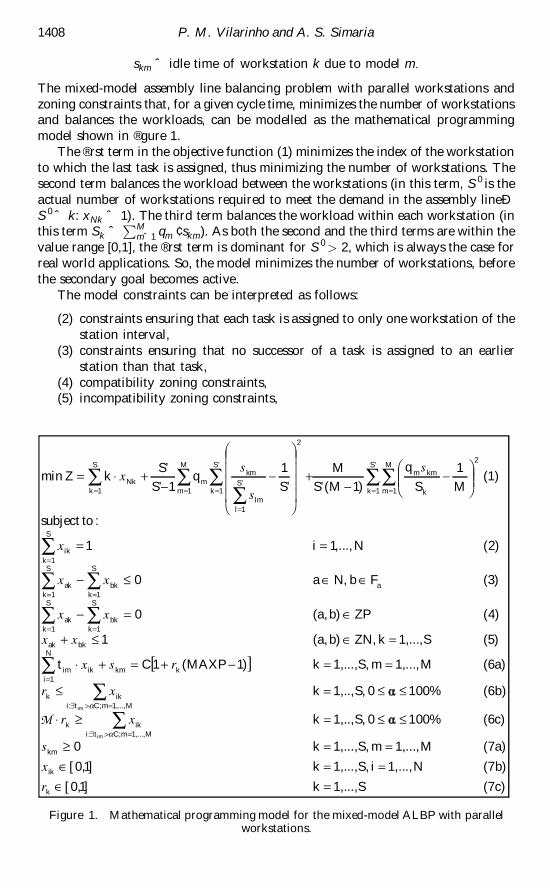
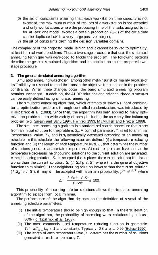
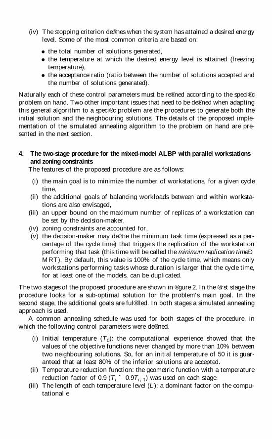
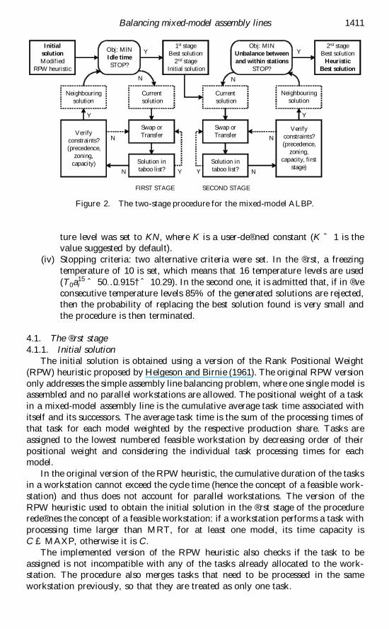
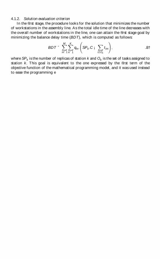
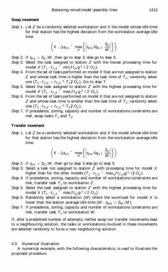
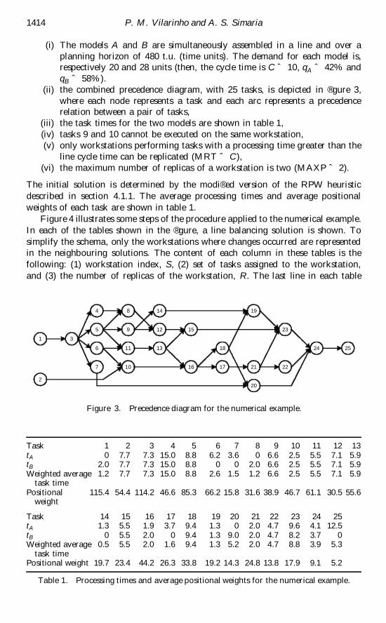
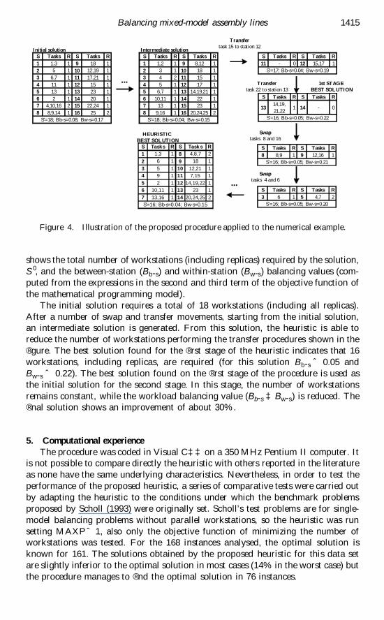
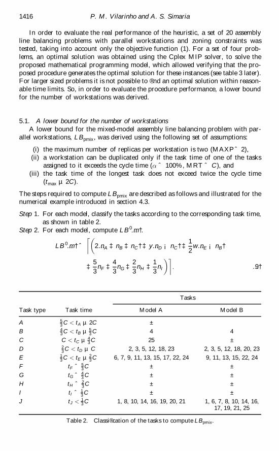
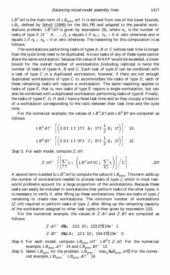
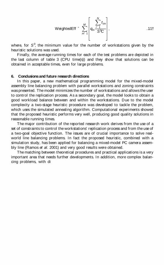An assembly line designed to assemble a single homogeneous product is called asimple assembly line and is used when the demand for that product is su cientlylarge to justify a dedicated assembly line The mathematical formulation of theALBP for simple assembly lines was regrst stated by Salveson (1955) and sincethen extensive research has been done in the area Comprehensive literature reviewson this subject are provided in Ghosh and Gagnon (1989) and Scholl (1999)

The recent market trends show that there is a growing demand for customizedproducts increasing the pressure for manufacturing macrexibility Consequently simpleassembly lines are being replaced by mixed-model assembly lines in which a set ofsimilar models of a product can be assembled simultaneously Several techniqueshave been proposed to tackle the mixed-model ALBP namely by GoEgrave cken and Erel(1997 1998) McMullen and Frazier (1997 1998) Merengo et al (1999) and Ereland GoEgrave cken (1999)

Most of the techniques used to solve the ALBP require the assignment of eachtask to a single workstation and consequently the production rate is limited by thelongest task time This assumption can be relaxed by utilizing parallel workstationsin such a way that two or more replicas of a workstation can perform the same set oftasks on di erent assemblies The introduction of parallel workstations not onlyallows for cycle times shorter than the longest task time and thus an increase inthe production rate but also provides greater macrexibility in designing the assemblyline (Buxey 1974)

However when parallel workstations are introduced the number of tasks per-formed by each worker increases (eg it is possible to design an assembly line withjust one workstation and a su cient number of replicas to meet the demandETHinsuch a case each worker has to perform all tasks) but this contradicts one of themain advantages of using an assembly line the use of low-skilled labour that can beeasily trained (due to the strict division of labour) Therefore in order to maintainthat advantage it is necessary to control the process to create parallel workstations(ie the replication process) in such a way that workstations are replicated only whenrequired ie when a taskrsquos processing time is larger than the cycle time and as suchrequires the replication of the workstation in which the task will be carried out Mostof the models for the ALBP with parallel workstations proposed in the literaturebase the decision to create parallel workstations on a trade-o between the incre-mental toolingequipment cost of the duplicated workstation and the cost of hiringworkers for the original line in order to satisfy the demand (eg Johnson 1983 Pintoet al 1975 1981 Bard 1989 Daganzo and Blumenfeld 1994 Askin and Zhou 1997)McMullen and Frazier (1997 1998) allow the replication of a workstation as long asits utilization increases Schoregeld (1979) and Sarker and Shantikumar (1983) deregne alimit on the number of parallel workstations to control the replication process whileBuxey (1974) includes a limit on the number of tasks per workstation In either ofthese approaches tasks with processing times much shorter than the cycle time cantrigger the replication of workstations which can lead to an excessive number ofparallel workstations

This work introduces a mathematical programming model for the mixed-modelALBP with parallel workstations and zoning constraints which minimizes thenumber of workstations for a given cycle time A secondary goal was introducedso that the model also balances the workload between workstations (ie for eachmodel the idle time is distributed across the workstations as equally as possible) andwithin workstations (ie the overall idle time for each workstation is distributed









is then qm ˆ Dm=PM











0 otherwise

(


0 otherwise

(












[ ]

)c7(S1k]10[

)b7(N1i S1k]10[

)a7(M1m S1k0

)c6(1000 S1k

)b6(1000 S1k


)5(S1k ZN)ba(1

)4(ZP)ba(0

)3(Fb Na0

)2(N1i1

subject to

(1) M

1

S

q

)1M(rsquoS

M

rsquoS

1q

1rsquoS

rsquoSk Zmin

k

ik

km

M1mCtiikk

M1mCtiikk

N

1ikkmikim

bkak

S

1k

S

1kbkak

a

S

1k

S

1kbkak

S

1kik

rsquoS

1k

M

1m

2

k

kmmS

1k

M

1m

rsquoS

1k

2

rsquoS

1llm

kmmNk

im

im

=Icirc ==Icirc

==sup3


pound pound =pound

==-+=+times

=Icirc pound +

Icirc =-

Icirc Icirc pound -

==



aelig -

-+


oslash

ouml


egrave

aelig

--

+times =

aring aring

aring

aring aring

aring aring

aring


=gt$

=gt$

=

= =

= =

=

= == = =

=

r

x

s

xr

xr

rsx

xx

xx

xx

x

s

s

sx

a

a

M










pound 100




































STOP




RPW heuristic



Current solution

Swap orTransfer



zoningcapacity)

Y

Y

N

N

Y Y


Current solution

Swap orTransfer




stage)Y

Y

N

N

N N





BDT ˆXM

mˆ1

XK

kˆ1

qm SPkC iexclX

i2Ok

tim

Aacute

hellip8dagger











Swap movement


X centsZX ˆ maxm


M

shyshyshyshy

shyshyshyshy








Transfer movement


X centsZX ˆ maxm

sZm cent qm iexclSZ

M

shyshyshyshy

shyshyshyshy










proposed procedure















1

2

3

4

5

6

7

8

9

10

11

12

13

14

15

16 17

18

19

20

21 22

23

24 25




weight




























S Tasks R S Tasks R1 13 1 9 18 12 5 1 10 1219 13 67 1 11 1721 14 11 1 12 15 15 13 1 13 23 16 2 1 14 20 17 41016 2 15 2224 18 8914 1 16 25 2


S Tasks R S Tasks R1 12 1 9 812 12 3 1 10 18 13 4 2 11 15 14 5 1 12 17 15 67 1 13 141921 16 1011 1 14 22 17 13 1 15 23 18 916 1 16 202425 2




S Tasks R S Tasks R

131419 2122

1 14 - 0







2 6 1 9 18 1

3 5 1 10 1221 14 9 1 11 715 1

5 2 1 12 141922 16 1011 1 13 23 1

7 1316 1 14 202425 2Srsquo=16 Bb-s=004 Bw-s=015





Swaptasks 8 and 16

Swaptasks 4 and 6








(tmax micro 2C)






sup3sup1

Dagger 5

3nF Dagger 4

3nG Dagger 2

3nH Dagger 1

3nI



Tasks




3 C 4 4


D 23 C lt tD micro C 2 3 5 12 18 23 2 3 5 12 18 20 23


3 C 6 7 9 11 13 15 17 22 24 9 11 13 15 22 24





J tJ lt 13 C 1 8 10 14 16 19 20 21 1 6 7 8 10 14 16

17 19 21 25












Zhellipmdagger ˆX

iˆJ


i 6ˆJ

ti

Aacute iquestC

amp rsquo

hellip10dagger




























ing expression






WeightedEff ˆXM

mˆ1

qm

XN

iˆ1

tim

S 0C

2

66664

3












Reference



































is then qm ˆ Dm=PM











0 otherwise

(


0 otherwise

(












[ ]

)c7(S1k]10[

)b7(N1i S1k]10[

)a7(M1m S1k0

)c6(1000 S1k

)b6(1000 S1k


)5(S1k ZN)ba(1

)4(ZP)ba(0

)3(Fb Na0

)2(N1i1

subject to

(1) M

1

S

q

)1M(rsquoS

M

rsquoS

1q

1rsquoS

rsquoSk Zmin

k

ik

km

M1mCtiikk

M1mCtiikk

N

1ikkmikim

bkak

S

1k

S

1kbkak

a

S

1k

S

1kbkak

S

1kik

rsquoS

1k

M

1m

2

k

kmmS

1k

M

1m

rsquoS

1k

2

rsquoS

1llm

kmmNk

im

im

=Icirc ==Icirc

==sup3


pound pound =pound

==-+=+times

=Icirc pound +

Icirc =-

Icirc Icirc pound -

==



aelig -

-+


oslash

ouml


egrave

aelig

--

+times =

aring aring

aring

aring aring

aring aring

aring


=gt$

=gt$

=

= =

= =

=

= == = =

=

r

x

s

xr

xr

rsx

xx

xx

xx

x

s

s

sx

a

a

M










pound 100




































STOP




RPW heuristic



Current solution

Swap orTransfer



zoningcapacity)

Y

Y

N

N

Y Y


Current solution

Swap orTransfer




stage)Y

Y

N

N

N N





BDT ˆXM

mˆ1

XK

kˆ1

qm SPkC iexclX

i2Ok

tim

Aacute

hellip8dagger











Swap movement


X centsZX ˆ maxm


M

shyshyshyshy

shyshyshyshy








Transfer movement


X centsZX ˆ maxm

sZm cent qm iexclSZ

M

shyshyshyshy

shyshyshyshy










proposed procedure















1

2

3

4

5

6

7

8

9

10

11

12

13

14

15

16 17

18

19

20

21 22

23

24 25




weight




























S Tasks R S Tasks R1 13 1 9 18 12 5 1 10 1219 13 67 1 11 1721 14 11 1 12 15 15 13 1 13 23 16 2 1 14 20 17 41016 2 15 2224 18 8914 1 16 25 2


S Tasks R S Tasks R1 12 1 9 812 12 3 1 10 18 13 4 2 11 15 14 5 1 12 17 15 67 1 13 141921 16 1011 1 14 22 17 13 1 15 23 18 916 1 16 202425 2




S Tasks R S Tasks R

131419 2122

1 14 - 0







2 6 1 9 18 1

3 5 1 10 1221 14 9 1 11 715 1

5 2 1 12 141922 16 1011 1 13 23 1

7 1316 1 14 202425 2Srsquo=16 Bb-s=004 Bw-s=015





Swaptasks 8 and 16

Swaptasks 4 and 6








(tmax micro 2C)






sup3sup1

Dagger 5

3nF Dagger 4

3nG Dagger 2

3nH Dagger 1

3nI



Tasks




3 C 4 4


D 23 C lt tD micro C 2 3 5 12 18 23 2 3 5 12 18 20 23


3 C 6 7 9 11 13 15 17 22 24 9 11 13 15 22 24





J tJ lt 13 C 1 8 10 14 16 19 20 21 1 6 7 8 10 14 16

17 19 21 25












Zhellipmdagger ˆX

iˆJ


i 6ˆJ

ti

Aacute iquestC

amp rsquo

hellip10dagger




























ing expression






WeightedEff ˆXM

mˆ1

qm

XN

iˆ1

tim

S 0C

2

66664

3












Reference






































[ ]

)c7(S1k]10[

)b7(N1i S1k]10[

)a7(M1m S1k0

)c6(1000 S1k

)b6(1000 S1k


)5(S1k ZN)ba(1

)4(ZP)ba(0

)3(Fb Na0

)2(N1i1

subject to

(1) M

1

S

q

)1M(rsquoS

M

rsquoS

1q

1rsquoS

rsquoSk Zmin

k

ik

km

M1mCtiikk

M1mCtiikk

N

1ikkmikim

bkak

S

1k

S

1kbkak

a

S

1k

S

1kbkak

S

1kik

rsquoS

1k

M

1m

2

k

kmmS

1k

M

1m

rsquoS

1k

2

rsquoS

1llm

kmmNk

im

im

=Icirc ==Icirc

==sup3


pound pound =pound

==-+=+times

=Icirc pound +

Icirc =-

Icirc Icirc pound -

==



aelig -

-+


oslash

ouml


egrave

aelig

--

+times =

aring aring

aring

aring aring

aring aring

aring


=gt$

=gt$

=

= =

= =

=

= == = =

=

r

x

s

xr

xr

rsx

xx

xx

xx

x

s

s

sx

a

a

M










pound 100




































STOP




RPW heuristic



Current solution

Swap orTransfer



zoningcapacity)

Y

Y

N

N

Y Y


Current solution

Swap orTransfer




stage)Y

Y

N

N

N N





BDT ˆXM

mˆ1

XK

kˆ1

qm SPkC iexclX

i2Ok

tim

Aacute

hellip8dagger











Swap movement


X centsZX ˆ maxm


M

shyshyshyshy

shyshyshyshy








Transfer movement


X centsZX ˆ maxm

sZm cent qm iexclSZ

M

shyshyshyshy

shyshyshyshy










proposed procedure















1

2

3

4

5

6

7

8

9

10

11

12

13

14

15

16 17

18

19

20

21 22

23

24 25




weight




























S Tasks R S Tasks R1 13 1 9 18 12 5 1 10 1219 13 67 1 11 1721 14 11 1 12 15 15 13 1 13 23 16 2 1 14 20 17 41016 2 15 2224 18 8914 1 16 25 2


S Tasks R S Tasks R1 12 1 9 812 12 3 1 10 18 13 4 2 11 15 14 5 1 12 17 15 67 1 13 141921 16 1011 1 14 22 17 13 1 15 23 18 916 1 16 202425 2




S Tasks R S Tasks R

131419 2122

1 14 - 0







2 6 1 9 18 1

3 5 1 10 1221 14 9 1 11 715 1

5 2 1 12 141922 16 1011 1 13 23 1

7 1316 1 14 202425 2Srsquo=16 Bb-s=004 Bw-s=015





Swaptasks 8 and 16

Swaptasks 4 and 6








(tmax micro 2C)






sup3sup1

Dagger 5

3nF Dagger 4

3nG Dagger 2

3nH Dagger 1

3nI



Tasks




3 C 4 4


D 23 C lt tD micro C 2 3 5 12 18 23 2 3 5 12 18 20 23


3 C 6 7 9 11 13 15 17 22 24 9 11 13 15 22 24





J tJ lt 13 C 1 8 10 14 16 19 20 21 1 6 7 8 10 14 16

17 19 21 25












Zhellipmdagger ˆX

iˆJ


i 6ˆJ

ti

Aacute iquestC

amp rsquo

hellip10dagger




























ing expression






WeightedEff ˆXM

mˆ1

qm

XN

iˆ1

tim

S 0C

2

66664

3












Reference




































pound 100




































STOP




RPW heuristic



Current solution

Swap orTransfer



zoningcapacity)

Y

Y

N

N

Y Y


Current solution

Swap orTransfer




stage)Y

Y

N

N

N N





BDT ˆXM

mˆ1

XK

kˆ1

qm SPkC iexclX

i2Ok

tim

Aacute

hellip8dagger











Swap movement


X centsZX ˆ maxm


M

shyshyshyshy

shyshyshyshy








Transfer movement


X centsZX ˆ maxm

sZm cent qm iexclSZ

M

shyshyshyshy

shyshyshyshy










proposed procedure















1

2

3

4

5

6

7

8

9

10

11

12

13

14

15

16 17

18

19

20

21 22

23

24 25




weight




























S Tasks R S Tasks R1 13 1 9 18 12 5 1 10 1219 13 67 1 11 1721 14 11 1 12 15 15 13 1 13 23 16 2 1 14 20 17 41016 2 15 2224 18 8914 1 16 25 2


S Tasks R S Tasks R1 12 1 9 812 12 3 1 10 18 13 4 2 11 15 14 5 1 12 17 15 67 1 13 141921 16 1011 1 14 22 17 13 1 15 23 18 916 1 16 202425 2




S Tasks R S Tasks R

131419 2122

1 14 - 0







2 6 1 9 18 1

3 5 1 10 1221 14 9 1 11 715 1

5 2 1 12 141922 16 1011 1 13 23 1

7 1316 1 14 202425 2Srsquo=16 Bb-s=004 Bw-s=015





Swaptasks 8 and 16

Swaptasks 4 and 6








(tmax micro 2C)






sup3sup1

Dagger 5

3nF Dagger 4

3nG Dagger 2

3nH Dagger 1

3nI



Tasks




3 C 4 4


D 23 C lt tD micro C 2 3 5 12 18 23 2 3 5 12 18 20 23


3 C 6 7 9 11 13 15 17 22 24 9 11 13 15 22 24





J tJ lt 13 C 1 8 10 14 16 19 20 21 1 6 7 8 10 14 16

17 19 21 25












Zhellipmdagger ˆX

iˆJ


i 6ˆJ

ti

Aacute iquestC

amp rsquo

hellip10dagger




























ing expression






WeightedEff ˆXM

mˆ1

qm

XN

iˆ1

tim

S 0C

2

66664

3












Reference

























































STOP




RPW heuristic



Current solution

Swap orTransfer



zoningcapacity)

Y

Y

N

N

Y Y


Current solution

Swap orTransfer




stage)Y

Y

N

N

N N





BDT ˆXM

mˆ1

XK

kˆ1

qm SPkC iexclX

i2Ok

tim

Aacute

hellip8dagger











Swap movement


X centsZX ˆ maxm


M

shyshyshyshy

shyshyshyshy








Transfer movement


X centsZX ˆ maxm

sZm cent qm iexclSZ

M

shyshyshyshy

shyshyshyshy










proposed procedure















1

2

3

4

5

6

7

8

9

10

11

12

13

14

15

16 17

18

19

20

21 22

23

24 25




weight




























S Tasks R S Tasks R1 13 1 9 18 12 5 1 10 1219 13 67 1 11 1721 14 11 1 12 15 15 13 1 13 23 16 2 1 14 20 17 41016 2 15 2224 18 8914 1 16 25 2


S Tasks R S Tasks R1 12 1 9 812 12 3 1 10 18 13 4 2 11 15 14 5 1 12 17 15 67 1 13 141921 16 1011 1 14 22 17 13 1 15 23 18 916 1 16 202425 2




S Tasks R S Tasks R

131419 2122

1 14 - 0







2 6 1 9 18 1

3 5 1 10 1221 14 9 1 11 715 1

5 2 1 12 141922 16 1011 1 13 23 1

7 1316 1 14 202425 2Srsquo=16 Bb-s=004 Bw-s=015





Swaptasks 8 and 16

Swaptasks 4 and 6








(tmax micro 2C)






sup3sup1

Dagger 5

3nF Dagger 4

3nG Dagger 2

3nH Dagger 1

3nI



Tasks




3 C 4 4


D 23 C lt tD micro C 2 3 5 12 18 23 2 3 5 12 18 20 23


3 C 6 7 9 11 13 15 17 22 24 9 11 13 15 22 24





J tJ lt 13 C 1 8 10 14 16 19 20 21 1 6 7 8 10 14 16

17 19 21 25












Zhellipmdagger ˆX

iˆJ


i 6ˆJ

ti

Aacute iquestC

amp rsquo

hellip10dagger




























ing expression






WeightedEff ˆXM

mˆ1

qm

XN

iˆ1

tim

S 0C

2

66664

3












Reference






























BDT ˆXM

mˆ1

XK

kˆ1

qm SPkC iexclX

i2Ok

tim

Aacute

hellip8dagger











Swap movement


X centsZX ˆ maxm


M

shyshyshyshy

shyshyshyshy








Transfer movement


X centsZX ˆ maxm

sZm cent qm iexclSZ

M

shyshyshyshy

shyshyshyshy










proposed procedure















1

2

3

4

5

6

7

8

9

10

11

12

13

14

15

16 17

18

19

20

21 22

23

24 25




weight




























S Tasks R S Tasks R1 13 1 9 18 12 5 1 10 1219 13 67 1 11 1721 14 11 1 12 15 15 13 1 13 23 16 2 1 14 20 17 41016 2 15 2224 18 8914 1 16 25 2


S Tasks R S Tasks R1 12 1 9 812 12 3 1 10 18 13 4 2 11 15 14 5 1 12 17 15 67 1 13 141921 16 1011 1 14 22 17 13 1 15 23 18 916 1 16 202425 2




S Tasks R S Tasks R

131419 2122

1 14 - 0







2 6 1 9 18 1

3 5 1 10 1221 14 9 1 11 715 1

5 2 1 12 141922 16 1011 1 13 23 1

7 1316 1 14 202425 2Srsquo=16 Bb-s=004 Bw-s=015





Swaptasks 8 and 16

Swaptasks 4 and 6








(tmax micro 2C)






sup3sup1

Dagger 5

3nF Dagger 4

3nG Dagger 2

3nH Dagger 1

3nI



Tasks




3 C 4 4


D 23 C lt tD micro C 2 3 5 12 18 23 2 3 5 12 18 20 23


3 C 6 7 9 11 13 15 17 22 24 9 11 13 15 22 24





J tJ lt 13 C 1 8 10 14 16 19 20 21 1 6 7 8 10 14 16

17 19 21 25












Zhellipmdagger ˆX

iˆJ


i 6ˆJ

ti

Aacute iquestC

amp rsquo

hellip10dagger




























ing expression






WeightedEff ˆXM

mˆ1

qm

XN

iˆ1

tim

S 0C

2

66664

3












Reference




























Swap movement


X centsZX ˆ maxm


M

shyshyshyshy

shyshyshyshy








Transfer movement


X centsZX ˆ maxm

sZm cent qm iexclSZ

M

shyshyshyshy

shyshyshyshy










proposed procedure















1

2

3

4

5

6

7

8

9

10

11

12

13

14

15

16 17

18

19

20

21 22

23

24 25




weight




























S Tasks R S Tasks R1 13 1 9 18 12 5 1 10 1219 13 67 1 11 1721 14 11 1 12 15 15 13 1 13 23 16 2 1 14 20 17 41016 2 15 2224 18 8914 1 16 25 2


S Tasks R S Tasks R1 12 1 9 812 12 3 1 10 18 13 4 2 11 15 14 5 1 12 17 15 67 1 13 141921 16 1011 1 14 22 17 13 1 15 23 18 916 1 16 202425 2




S Tasks R S Tasks R

131419 2122

1 14 - 0







2 6 1 9 18 1

3 5 1 10 1221 14 9 1 11 715 1

5 2 1 12 141922 16 1011 1 13 23 1

7 1316 1 14 202425 2Srsquo=16 Bb-s=004 Bw-s=015





Swaptasks 8 and 16

Swaptasks 4 and 6








(tmax micro 2C)






sup3sup1

Dagger 5

3nF Dagger 4

3nG Dagger 2

3nH Dagger 1

3nI



Tasks




3 C 4 4


D 23 C lt tD micro C 2 3 5 12 18 23 2 3 5 12 18 20 23


3 C 6 7 9 11 13 15 17 22 24 9 11 13 15 22 24





J tJ lt 13 C 1 8 10 14 16 19 20 21 1 6 7 8 10 14 16

17 19 21 25












Zhellipmdagger ˆX

iˆJ


i 6ˆJ

ti

Aacute iquestC

amp rsquo

hellip10dagger




























ing expression






WeightedEff ˆXM

mˆ1

qm

XN

iˆ1

tim

S 0C

2

66664

3












Reference









































1

2

3

4

5

6

7

8

9

10

11

12

13

14

15

16 17

18

19

20

21 22

23

24 25




weight




























S Tasks R S Tasks R1 13 1 9 18 12 5 1 10 1219 13 67 1 11 1721 14 11 1 12 15 15 13 1 13 23 16 2 1 14 20 17 41016 2 15 2224 18 8914 1 16 25 2


S Tasks R S Tasks R1 12 1 9 812 12 3 1 10 18 13 4 2 11 15 14 5 1 12 17 15 67 1 13 141921 16 1011 1 14 22 17 13 1 15 23 18 916 1 16 202425 2




S Tasks R S Tasks R

131419 2122

1 14 - 0







2 6 1 9 18 1

3 5 1 10 1221 14 9 1 11 715 1

5 2 1 12 141922 16 1011 1 13 23 1

7 1316 1 14 202425 2Srsquo=16 Bb-s=004 Bw-s=015





Swaptasks 8 and 16

Swaptasks 4 and 6








(tmax micro 2C)






sup3sup1

Dagger 5

3nF Dagger 4

3nG Dagger 2

3nH Dagger 1

3nI



Tasks




3 C 4 4


D 23 C lt tD micro C 2 3 5 12 18 23 2 3 5 12 18 20 23


3 C 6 7 9 11 13 15 17 22 24 9 11 13 15 22 24





J tJ lt 13 C 1 8 10 14 16 19 20 21 1 6 7 8 10 14 16

17 19 21 25












Zhellipmdagger ˆX

iˆJ


i 6ˆJ

ti

Aacute iquestC

amp rsquo

hellip10dagger




























ing expression






WeightedEff ˆXM

mˆ1

qm

XN

iˆ1

tim

S 0C

2

66664

3












Reference




















































S Tasks R S Tasks R1 13 1 9 18 12 5 1 10 1219 13 67 1 11 1721 14 11 1 12 15 15 13 1 13 23 16 2 1 14 20 17 41016 2 15 2224 18 8914 1 16 25 2


S Tasks R S Tasks R1 12 1 9 812 12 3 1 10 18 13 4 2 11 15 14 5 1 12 17 15 67 1 13 141921 16 1011 1 14 22 17 13 1 15 23 18 916 1 16 202425 2




S Tasks R S Tasks R

131419 2122

1 14 - 0







2 6 1 9 18 1

3 5 1 10 1221 14 9 1 11 715 1

5 2 1 12 141922 16 1011 1 13 23 1

7 1316 1 14 202425 2Srsquo=16 Bb-s=004 Bw-s=015





Swaptasks 8 and 16

Swaptasks 4 and 6








(tmax micro 2C)






sup3sup1

Dagger 5

3nF Dagger 4

3nG Dagger 2

3nH Dagger 1

3nI



Tasks




3 C 4 4


D 23 C lt tD micro C 2 3 5 12 18 23 2 3 5 12 18 20 23


3 C 6 7 9 11 13 15 17 22 24 9 11 13 15 22 24





J tJ lt 13 C 1 8 10 14 16 19 20 21 1 6 7 8 10 14 16

17 19 21 25












Zhellipmdagger ˆX

iˆJ


i 6ˆJ

ti

Aacute iquestC

amp rsquo

hellip10dagger




























ing expression






WeightedEff ˆXM

mˆ1

qm

XN

iˆ1

tim

S 0C

2

66664

3












Reference

































(tmax micro 2C)






sup3sup1

Dagger 5

3nF Dagger 4

3nG Dagger 2

3nH Dagger 1

3nI



Tasks




3 C 4 4


D 23 C lt tD micro C 2 3 5 12 18 23 2 3 5 12 18 20 23


3 C 6 7 9 11 13 15 17 22 24 9 11 13 15 22 24





J tJ lt 13 C 1 8 10 14 16 19 20 21 1 6 7 8 10 14 16

17 19 21 25












Zhellipmdagger ˆX

iˆJ


i 6ˆJ

ti

Aacute iquestC

amp rsquo

hellip10dagger




























ing expression






WeightedEff ˆXM

mˆ1

qm

XN

iˆ1

tim

S 0C

2

66664

3












Reference






































Zhellipmdagger ˆX

iˆJ


i 6ˆJ

ti

Aacute iquestC

amp rsquo

hellip10dagger




























ing expression






WeightedEff ˆXM

mˆ1

qm

XN

iˆ1

tim

S 0C

2

66664

3












Reference
















































ing expression






WeightedEff ˆXM

mˆ1

qm

XN

iˆ1

tim

S 0C

2

66664

3












Reference




























WeightedEff ˆXM

mˆ1

qm

XN

iˆ1

tim

S 0C

2

66664

3












Reference




























a two-stage heuristic method for balancing mixed-model assembly lines with parallel workstations

Documents