a synoptic climatology of the elevated mixed layer inversion over the southern great plains in...
TRANSCRIPT
form Approv.ed
-AD-A267 510MIAIGEJ OMS No 0'CIs.... 11i 1 i l 1111!1II!11 1111111 1 id ,I. .. .~ Toi ,••,,5 ,• ,:• • *.,,. m ,.~r: . t io(r 3 f, . O,.. n ,.' • : t, 5 • *,. .? . :3,,, 1 U'a .l r,
1 e! Pv k.":"'n', '- ~ Ct s ~ 1'~r I.: 're4,;tn' -3
1i. AGENCY USE ONLY (Leave lank) 2 PO•. TE 3. EPORT TYPE AND DATES COVERED
t Aug 1991 kkAIt/DISSERTATION]4. TITLE AND SUBTITLE 5. FUNDING NUMBERS
A Synoptic Climatology of the Elevated Mixed LayerInversion Over the Southern Great Plains in Spring
6. AUTHORS)
John M Lanicci
1. PERFORMING ORGANIZATION NAME(S) AND AEJDRESSýES) 8. PERFORMING ORGANILATIONREPORT NUMBER
AFIT Student Attending: Penn State University AFIT/CI/CIA- 93-016D
Se n9. SPONSORiNG; 1V;ONITORII;G AGiNCY NAME(S) AND ADDRESS(ES) 10. SPONSORING / MONITORING
DEPARTMENT OF THE AIR FORCE A ELEGENC 7U, AFIT/CIS2950 P STREET AUG 6 19993b- i
WRIGHT-PATTERSON AFB OH 45433-7765
1i. S!JPPLEMENwARY NOTES
.2a. DISTP, EBUTION AVAILABILITY STATEMENT 12b. DISTI' SUTION' CC'-E
Approved for Public Release IAW 190-1Distribution UnlimitedMICHAEL M. BRICKER, SMSgt, USAF iChief Administration
S13. ACSTf)ACT ;A-.,L'nu) 2S'•. words,'
S93 -18099no W, -
14. SUBJECT TERMS 15. NUMBER OF PAGES
291 B
16. PRICE CODE
17. SECURITY CLASSIFICAI!ON I 18. SECJURITY CLASS;FICAT'Ot. 19. SECURITY CLAS 'rFICATION 20. LIMWTATION OF ABSTRACT iOF REPORT OF THIS PAGE OF ABSTRACT
__SN 75•_• _ .'.75-7773. ____R_,v _ ,
0DThe Pennsylvania State University
The Graduate School
College of Earth and Mineral Sciences
A SYNOPTIC CLIMATOLOGY
OF THE ELEVATED MIXED LAYER INVERSION
OVER THE SOUTHERN GREAT PLAINS IN SPRING
A Thesis in
Meteorology
by
John M. Lanicci
Submitted in Partial Fulfillmentof the Requirementsfor the Degree of UI•IC QUAL•ITY IWT3PEC•D -3
Accesiotn ForDoctor of Philosophy - oNTIS CRA&I
DTIC TAB SUrid!nO:::;1cel [-
August 1991
DI",I'ibLtion I
I~%'nAti;Lty Codes
Disvdt yidtor
Siii-
ABSTRACT
A synoptic climatology is presented of the atmospheric conditions
associated with the creation of the elevated mixed layer inversion, or
lid, over the southern Great Plains of the U.S. (defined as Kansas,
Oklahoma, and Texas, and portions of the surrounding states) during four
spring (April, May, June) seasons from 1983 through 1986. The lid
sounding, also known as a Type 1 tornado sounding, is created through
the superposition of a potentially warm, nearly dry-adiabatic elevated
mixed layer (EML) over a potentially unstable moist layer. This study
examines the synoptic patterns associated with the creation of the EML
and the moist layer, and the subsequent evolution of these component,
airmasses into a lid sounding. The study utilizes EML and lid-
occurrence statistics, analyses of the EML and moist layer, and a
subjective synoptic typing system based on the geostrophic wind
relationship at the surface and 500 mb. The temporal and spatial
variability of lid occurrence and the associated synoptic types are used
to determine the periodicity of lid occurrence over the southern Plains,
including the seasonal tendencies and relationships between different
stages of lid development and specific synoptic flow types. This study
also investigates the relationships between lid occurrence and the
occurrence of severe storm outbreaks over the Kansas-Oklahoma-Texas
region.
This study shows that the lid coverage over the southern Great
Plains undergoes a seasonal evolution in which the lid area responds to
changes in the location of the EML source region and the orientation of

We approve the thesis of John M. Lanicci.
Date of Signature
Thomas T. Warner 7Associate Professor of MeteorologyThesis AdviserChair of Committee
Toby N. CarlsonProfessor of Meteorology
-),chael FritschP .rof ssrof Meteorology
Gregory S/ ForbesAssoci taVlProfe•_sor of Meteorology
SIt9 !
Brent M. Yaro sAssociatePosoof Geography
Charles A. Doswell IIIResearch MeteorologistNational Severe Storms LaboratorySpecial Member
William M. FrankProfessor of MeteorologyHead of the Department of Meteorology
IV
the mean low level moist tongue. The relative airstream configuration
associated with the classic models of lid formation and severe weather
over this region occurs most frequently in April and May, and is
typically associated with the largest lid-coverage areas in all three
months. By the late spring, the lid is observed with a variety of
additional flow types, such as northwesterly and anticyclonic midlevel
flows. These two flow types are mainly associated with large scale
subsidence, leading to an airstream configuration in which the lid base
sinks downstream from the source region, in stark contrast to the
classic southwest flow type in which the lid base rises and the lid
weakens in an environment of large scale ascent.
Time-series analyses of lid occurrence and synoptic types reveals a
cyclic tendency with a mean period of about one week. Two types of lid
cycles are identified: one that is associated with polar-air outbreaks
and baroclinic waves in the westerlies, and one that is associated with
weak southerly low level flow, subtropical circulations, and weak short
wave features that are characteristic of the late spring. A
relationship between the size of a severe storm outbreak and the
antecedent lid coverage is best defined in early spring, and rapidly
deteriorates from May to June.
An example of an early-spring lid cycle is analyzed using both
conventional data and a 120-h simulation with the Penn State/NCAR
mesoscale model. The case study examines the creation and evolution of
the EML and moist layer, and reveals information about some of the
important physical processes involved. The results of the case study
clarify important aspects of the synoptic climatology that the composite
datasets alone are unable to reveal.
V
TABLE OF CONTENTS
Page
LIST OF TABLES ................... .......................... ix
LIST OF FIGURES ........................ .......................... x
PREFACE ....................... .............................. .. xxii
Chapter 1. INTRODUCTION ............ ..................... . i1
1.1. Literature Review of Severe-Storms Climatology ... ..... 2
1.2. The Creation and Evolution of theComponents of the Lid Sounding .......... ............. 3
1.3. Purpose of Thesis ............ .................... .. 12
Chapter 2. THE SYNOPTIC CLIMATOLOGY: STRUCTUREDYNAMICS, AND SEASONAL EVOLUTION .... ........... .. 14
2.1. Chapter Introduction .......... .................. .. 14
2.2. Lid Characteristics Over the Southern Plains:April-June 1983-1986 ........... .................. .. 18
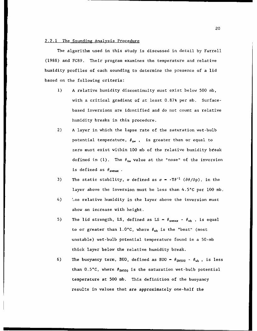
2.2.1. The Sounding Analysis Procedure ... .......... .. 20
2.2.2. Monthly Lid Frequency ........ ............... .. 27
2.2.3. Monthly Geographic Distribution of Lid Frequency . 29
2.2.4. Elevated Mixed Layer Source-Region Climatology . . 31
2.3. Synoptic Typing of Surface and 500-mb Flows
Over the Southern Plains ......... ................ .. 34
2.3.1. Methodology and Physical Assumptions ... ........ .. 35
2.3.2. Lid Frequencies Associated with the
Various Flow Types .......... ................. .. 40
vi
Page
2.3.3. Mean Monthly EML and Lid Characteristicsas Related to Synoptic Flow Patterns ... ........ .. 45
2.3.4. Seasonal Changes in the Characteristicsof the EML and Lid ......... ................. .. 50
2.4. Discussion .......................... 54
Chapter 3. THE SYNOPTIC CLIMATOLOGY: THE LIFEOF THE LID ................. ...................... 57
3.1. Chapter Introduction .............. .................... .. 57
3.2. Time Series Analysis of Lid Occurrence .... ........... .. 60
3.3. A Schematic Life Cycle of the Lid ...... ............. .. 64
3.3.1. Types of Lid Cycles ........... ................ 64
3.3.2. Characteristics of the Lid Cycle Stages ......... . 7
3.4. Synoptic Flow Patterns During the Lid Cycle ... ........ 76
3.4.1. Prevailing Synoptic Types During the Lid Cycle . 76
3.4.2. Flow Structure During the Lid Cycle ... ........ 81
3.4.2.1. The Early-Season H Lid Cycle ... ........ 84
3.4.2.2. The Late-Spring H Lid Cycle .... ........ 90
3.4.2.3. The R Lid Cycle ........ ............... .. 93
3.5. Discussion and Summary ............ ................... .. 97
Chapter 4. TilE SYNOPTIC CLIMATOLOGY: RELATIONSHIPTO SEVERE-STORMS CLIMATOLOGY ........ ............. .. 103
4.1. Chapter Introduction .............. .................... .. 103
4.2. Severe-Storm Statistics for the Southern Plains:April-June 1983-1986 .............. .................... .. 107
4.3. Relationship of the Outbreak Size to the Lid ... ........ .. 114
4.4. Relationships Between the Lid, Severe Weather,and Representative Synoptic Flow Types ...... ........... .. 122
4.4.1. Severe Weather Associated with the Lid Cycle . . . . 122
vii
Page
4.4.2. Lid and Severe Weather Occurrence forRepresentative Synoptic Types ...... ........... .. 126
4,5. Conclusions .................. ........................ 138
Chapter 5. AN EXAMPLE OF ANEARLY SPRING LID CYCLE .......... ................ .. 142
5.1. Overview of the 4-9 April 1984 H Lid Cycle .... ......... .. 142
5.2. Examination of the Lid Cycle by Stages ..... ........... .. 152
5.2.1. The High-Pressure Stage (1200 UTC 4 April-0000 UTC 6 April) ........... ................. .. 152
5.2.2. The Return-Flow Stage (0000 UTC 6 April-0000 UTC 7 April) ............. .................. .. 169
5.2.3. Lid Genesis (0000 UTC-1200 UTC 7 April) .......... .. 173
5.2.4. The Lid-Maximum Stage and Severe-WeatherOutbreak (1200 UTC 7 April-1200 UTC 8 April) . . . . 180
5.2.5. The Post Lid-Maximum Stage and The Second Severe-Weather Outbreak (1200 UTC 8 April-0000 UTC 9 April)
S.. . . . . . . . . . . . . . . . . . . . . . .. . 189
5.2.6 The End Stage of the Cycle (0000 UTC-1200 UTC9 April) ................ ...................... .. 192
Chapter 6. NUMERICAL SIMULATION OF THE 4-9 APRIL 1984LID CYCLE WITH THE PENN STATE/NCARMESOSCALE MODEL ............. .................... .. 200
6.1. MM4 Characteristics .............. .................... 201
6.1.1. General Description .......... ................ 201
6.1.2. Specific Characteristics of theVersion of MM4 Used in This Study ... ......... .. 203
6.2. Model Verification of Large ScaleFlow Features During the Lid Cycle ..... ............. .. 215
6.3. Examination of Physical Processes Involvedin the Formation and Evolution of theEML and Moist Layer .............. .................... 217
viii
Pa p e
6.3.1. Formation of the Western U.S. andMexican EMLs .............. .................... .. 219
6.3.2. Formation of the Moist Layer Overthe Gulf of Mexico .......... ................. .. 243
6.4. Formation of the Lid Over the SouthernGreat Plains ................ ....................... ... 255
Chapter 7. CONCLUSIONS AND DISCUSSION ......... .............. 271
7.1. Summary of Results .............. ..................... .. 271
7.2. Suggestions for Future Research ......... .............. 279
REFERENCES ..................... ............................ 281

ix
LIST OF TABLES
Pg
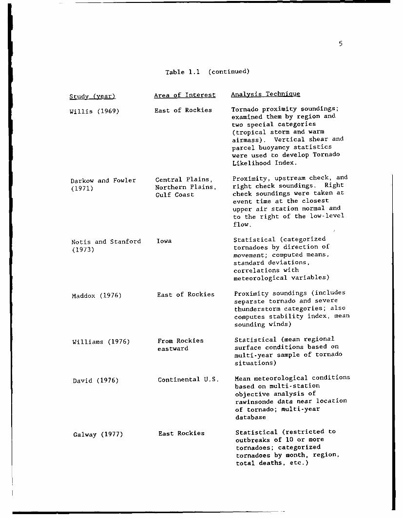
Table 1.1 Event-Based Severe-Storm Climatologies. ................... 4
Table 2.1 Uncapped Soundings for Four Gulf Coast Stations(Based on 1200 UTC data). ................................. 52
Table 3.1 The Stages of the Lid Cycle...............................68
Table 3.2 Spring Lid Cycles: 1983-198b.............................70
Table 3.3 Occurrence Frequency of Synoptic Types at EachStage of the Lid Cycle. ................................... 77
Table 4.1 Linear Correlation Coefficients Between Severe-Weather Event Areas and Antecedent Lid-CoverageAreas Exceeding Certain LS and BUO ThresholdValues....................................................120
Table 6.1 Full and Half Sigma Levels and Standard Pressures(assumed P.sf, - 1000 nib) For MM4 ........................... 207
Table 6.2 Description of MM4 Land-Use Categories and SurfaceParameters in This Modeling Study ........................ 213
X
LIST OF FIGURES
Page
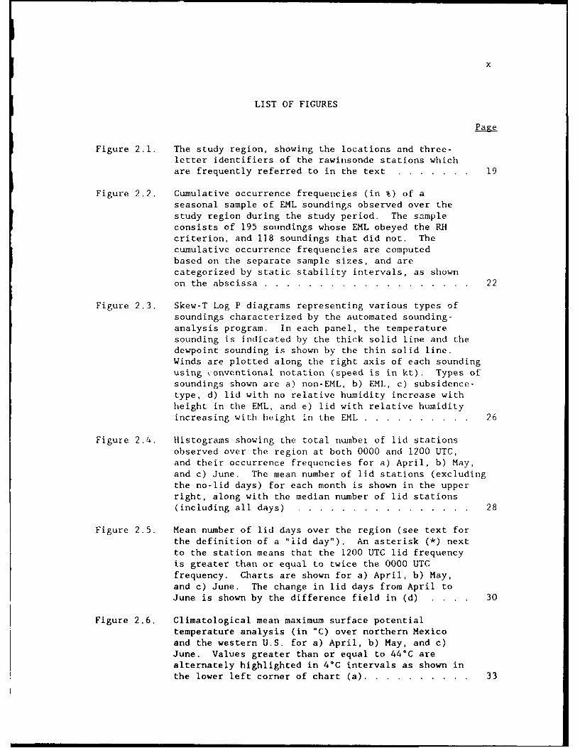
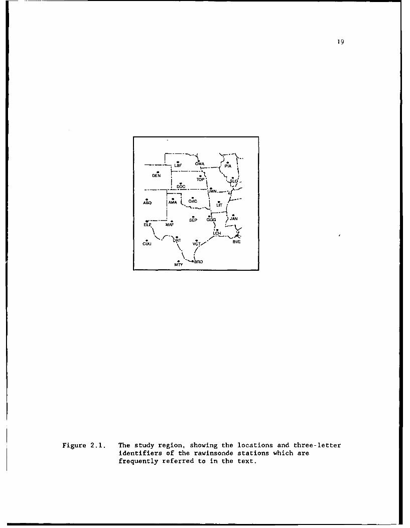
Figure 2.1. The study region, showing the locations and three-letter identifiers of the rawinsonde stations whichare frequently referred to in the text .. ....... .. 19
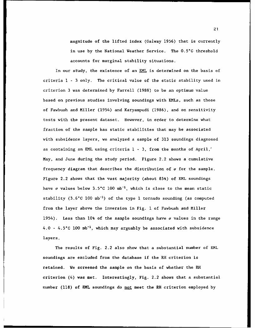
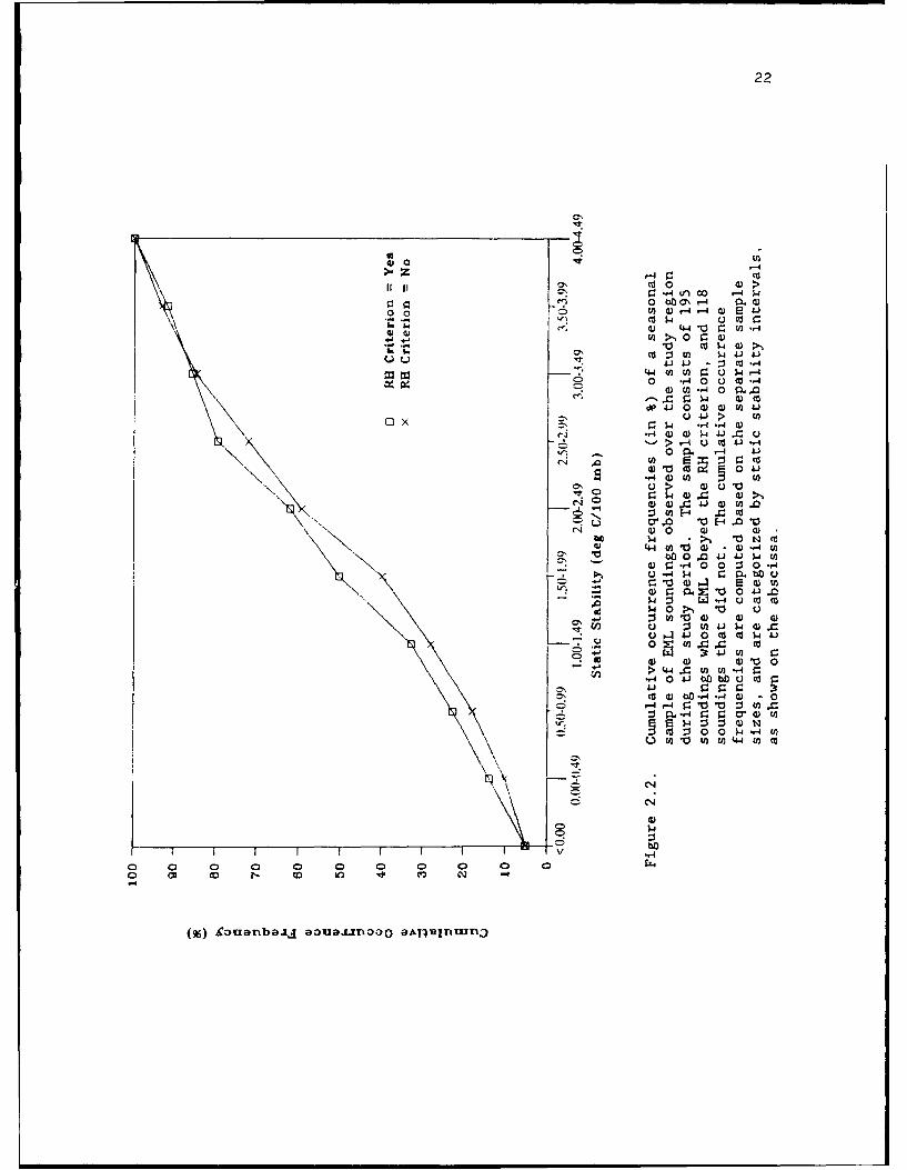
Figure 2.2. Cumulative occurrence frequencies (in %) of aseasonal sample of EML soundings observed over thestudy region during the study period. The sampleconsists of 195 soundings whose EML obeyed the RHcriterion, and 118 soundings that did not. Thecumulative occurrence frequencies are computedbased on the separate sample sizes, and arecategorized by static stability intervals, as shownon the abscissa .......... ................... .. 22
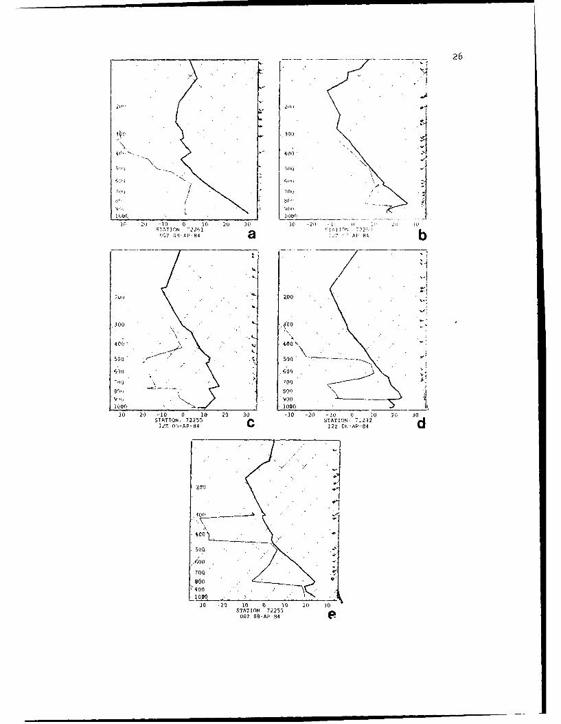
Figure 2.3. Skew-T Log P diagrams representing various types ofsoundings characterized by the automated sounding-analysis program. In each panel, the temperaturesounding is indicated by the thick solid line and thedewpoint sounding is shown by the thin solid line.Winds are plotted along the right axis of each soundingusing conventional notation (speed is in kt). Types ofsoundings shown are a) non-EML, b) EML, c) subsidence-type, d) lid with no relative humidity increase withheight in the EML, and e) lid with relative humidityincreasing with height in the EML .... .......... .. 26
Figure 2.4. Histograms showing the total numbel of lid stationsobserved over the region at both 0000 and 1200 UTC,and their occurrence frequencies for a) April, b) May,and c) June. The mean number of lid stations (excludingthe no-lid days) for each month is shown in the upperright, along with the median number of lid stations(including all days) ......... ................ .. 28
Figure 2.5. Mean number of lid days over the region (see text forthe definition of a "lid day"). An asterisk (*) nextto the station means that the 1200 UTC lid frequencyis greater than or equal to twice the 0000 UTCfrequency. Charts are shown for a) April, b) May,and c) June. The change in lid days from April toJune is shown by the difference field in (d) . . . . 30
Figure 2.6. Climatological mean maximum surface potentialtemperature analysis (in °C) over northern Mexicoand the western U.S. for a) April, b) May, and c)June. Values greater than or equal to 44°C arealternately highlighted in 4°C intervals as shown inthe lower left corner of chart (a) ............. ... 33
xi
Page
Figure 2.7. Idealized patterns of sea level isobars for surfacesynoptic flow types. Types shown are: a) highpressure with north-south oriented ridge axis,b) high pressure with northwest-southeast ridge axis,c) weak return flow with surface ridge over south-eastern portion of region (Gulf not "open"), d) weakreturn flow after high pressure exits the region(Gulf "open"), e) strong return flow, and f) frontalpassage ................ ....................... .. 37
Figure 2.8. Idealized patterns of 500-mb geopotential heightsfor upper-air flow types. Shown here are: a) north-westerly flow, b) westerly flow, c) southwesterly flow,d) anticyclonic flow, and e) cyclonic flow ..... .. 39
Figure 2.9. Lid frequency by synoptic type for a) April, b) May,and c) June. The ordinate denotes the number of lidstations, and the abscissa denotes the five surfacesynoptic types (each separated by the vertical line),subdivided by 500-mb type. The numbers along theabscissa refer to the following surface types:1 = N-S pressure ridge, 2 = NW-SE pressure ridge,3 = weak return flow, 4 = strong return flow, and5 = frontal passage. The 500-mb flow types areabbreviated as follows: NW = northwest, W = west,A = anticyclonic, SW - southwest, and C = cyclonic.The number of occurrences of each synoptic type andcorresponding number of lid stations are shown. Thehorizontal dashed line separates "small" and "large"lid-coverage areas ......... ................. .. 43
Figure 2.10. Mean analyses of EML and lid parameters for the mostfrequently occurring EML/lid-producing synopticpatterns. Charts are shown for a) April, b) May,and c) June. The solid lines denote mean "best"wet-bulb potential temperature in °C and are analyzedat 2°C intervals. The dashed lines are the meanpotential temperature (°C) in the EML (when observed),and are drawn every degree. The light shading high-lights regions having a mean EML base above 750 mb,with the dark shading indicating a mean EML base below800 mb. The scalloped border outlines the 25%occurrence frequency of the EML/lid ... ......... .. 47
xii
Page
Figure 3.1. Time series of lid occurrence for the period April-June 1985. The ordinate denotes the lid-coveragearea in terms of the number of "lid stations" overthe study region; the dates on the abscissa correspondto the 1200 UTC analysis time only. The horizontaldashed line marks the boundary between the "small" and"large" lid-coverage areas (see Figs. 2.4 and 2.9for details). For the purpose of the analysis,any missing 1200 UTC data were compensated for byusing data from the adjacent 0000 UTC data times andthe synoptic type for that date ................... 62
Figure 3.2. Occurrence frequency of lid cycle length (days)
for the study period ........ ................ .. 65
Figure 3.3. Mean lid-coverage area for each phase of the lid cycle
(see Table 3.1 for definitions of lid cycle phases).Cycles shown are n) early-season H, b) late-season H,and c) late-seas a R ........ ................ .. 72
Figuze 3.4. Lid cycle phase length (in whole days) andfrequencies for the three types of lid cyclesshown in Fig. 3.3 (legend is shown in panel 'a').Phases shown are a) high pressure, b) return flow,c) pre-lid-maximum, d) lid maximum, e) post-lid-maximum, and f) end ......... ................. .. 74
Figure 3.5. Composite mean charts for synoptic types representing
different stages of the early-spring H lid cycle.The "peel back" in the lower left in (a) shows thegrid mesh used to produce the composite fields.Mean sea level isobars are depicted by thick solid
lines labelled in mb (interval of 4 mb); mean 500-mbheights are shown by thick dotted lines labelled indecameters (interval of 6 dm); representative meansurface isodrosotherms (55°F and 65°F) are shown asdot-dashed lines; representative mean 700-mb isotherms(6°C and 10°C) are shown by thin dashed lines. Theareas of occurrence frequency equal to or greater than50% are shown for the following parameters: unstablebuoyancy (vertical shading), EML (horizontal shading),and the areas of overlap (indicative of high lidoccurrence frequency, "checkerboard" shading).Surface highs, lows, fronts, and troughs are shownusing conventional symbols. Highs and lows at 500 mbare displayed using "open" lettering. Charts aredisplayed for the following lid cycle stages withthe synoptic types (see notation in Table 3.3) inparentheses: a) high pressure ("I-NW"), b) returnflow ("3-A"), c) pre-lid-maximum ("4-SW"), d) lidmaximum ("4-SW"), and e) post-lid-maximum ("5-C"). 83
xiii
Page
Figure 3.6. Same as Fig. 3.5, except for late-spring H cycle.Charts are shown for the following lid cycle phasesand synoptic types: a) high pressure ("I-NW") and b)combined pre-lid-maximum, lid-maximum, and post-lid-maximum stages ("4-SW") ..... ............... .. 91
Figure 3.7. Same as Fig. 3.5, except for late-season R cycle.Charts are shown for the following lid cycle phasesand synoptic types: a) return flow ("3-A"; Bermudaanticyclone dominant), and b) combined pre-lid-maximum, lid-maximum, and post-lid-maximum stages("3-A"; Pacific anticyclone dominant). Note thatthe isopleth interval for the mean 500-mb heightsis 3 dm in this figure ........ ............... .. 94
Figure 4.1. Percentile graph displaying the cumulativeoccurrence frequency of severe storm eventsas a function of the total area of each event(given as the number of 40-km squares) ........... .. 109
Figure 4.2. Geographic frequency of severe storm eventsover the study region in terms of number ofevents per 40-km square. Light shading denotes3-5 events per square, medium shading denotes6-8 events per square, and dark shading denotesgreater than 8 events per square. Charts areshown for April, May, and June ..... ............ .. 112
Figure 4.3. Histograms displaying the occurrence frequenciesof 1200 and 0000 UTC lid coverage areas, given asthe number of upper air stations with a lidsounding ("lid stations") for non-event days andevent days (legend is shown in panel 'a'). Chartsare shown for April, May, and June ... ......... .. 115
Figure 4.4. Scatter plot showing the antecedent lid coverage(in terms of number of lid stations at either 1200or 0000 UTC) versus the size of the subsequent severestorm event (given as the number of 40-km squares).Non-event days are given an event size of zero. Thenumbers on the plot refer to the occurrence frequency.The linear regression line and error bars for onestandard deviation are also displayed. Charts areshown for April, May, and June .... ........... .. 117
xiv
Page
Figure 4.5. Scatter plot showing the 1200 UTC lid coverage(in terms of the number of lid stations) versusthe subsequent severe-storm event(s) area for thefollowing 24-h period (given as the number of40-km squares in log base 2 coordinates on theabscissa) for each stage of the early-season Hlid cycle. The numbers on the plots refer to theoccurrence frequency. Non-event days are given anevent size of zero. An "m" denotes the meanlid/severe-weather event coverage for each phaseof the lid cycle. Total number of event squaresfor each stage is shown by an inset on each panel 123
Figure 4.6. Same as Fig. 4.5, except for the late-seasonH lid cycle .............. ..................... .. 125
Figure 4.7. Same as Fig. 4.5, except for the late-seasonR lid cycle .............. ..................... .. 127
Figure 4.8. Composite mean analyses of key meteorologicalfeatures at 1200 UTC and subsequent 12-hsevere-weather event areas for representivesynoptic types during the lid cycle. A legendis shown in panel (a). Charts are shown for thefollowing synoptic types representing various stagesof the early-season H lid cycle: b) N-S pressureridge with northwest flow aloft, representingthe high-pressure stage; c) weak return flow withanticyclonic flow aloft, representing the return-flow stage; strong return flow with southwest flowaloft, representing both d) the-pre-lid-maximumstage, and e) the lid-maximum stage; and f)frontal passage with cyclonic flow aloft,representing the post-lid-maximum stage ......... .. 130
Figure 4.9. Same as Fig. 4.8, except for the late-seasonR lid cycle. Charts are shown for the followingsynoptic types and cycle phases: a) weak returnflow/anticyclonic flow aloft (Bermuda highdominant), representing the return-flow stage;b) the same as panel (a) except that the geographicfrequency composite includes uncapped, EML, andsubsidence-layer soundings; and c) weak returnflow/anticyclonic flow aloft (Pacific highdominant), representing the large lid-coveragestages ................. ........................ .. 135
xv
Page
Figure 5.1. Analysis of surface and 500-mb features at 1200 UTCon each day of the 4-9 April 1984 lid cycle. The1016 and 1008-mb sea level isobars are shown bythe thin lines, and the thick lines with arrowsdenote the subjectively analyzed 500-mb jets.Surface fronts, troughs, highs and lows areshown using conventional notation. Locations of500-mb highs and lows are shown using "open"
lettering. The locations of the stations used inthe time series of Fig. 5.3 are shown in panel (a).On panel (d), the position of the surface drylineis shown using a solid, scalloped line. Analysesare shown for a) 4 April,b) 5 April, c) 6 April,d) 7 April, e) 8 April, and f) 9 April ........... .. 144
Figure 5.2. Locations of severe weather and heavy rainfall(: 1 inch in 24 h) rainfall reported over Texasand Oklahoma from 1200 UTC 7 April to 1200 UTC8 April (panel 'a'), and over Arkansas,Louisiana, and Mississippi from 1200 UTC8 April to 1200 UTC 9 April (panel 'b').Symbols are explained in upper left portionof panel (a). Reports are compiled from theU.S. Department of Commerce publicationStorm Data ............. ...................... ... 150
Figure 5.3. Time series of surface observations over theGulf coastal region from south Texas to the YucatanPeninsula of Mexico, from 1200 UTC 4 April to1200 UTC 6 April. Stations are listed so theyform a counterclockwise arc beginning in southTexas. Stations shown are BRO (Brownsville,
Texas), SOM (Soto La Marina, Mexico), TUXTuxpan, Mexico), VER (Veracruz, Mexico), MTT(Coatzacoalcos, Mexico), and MID (Merida,Mexico) ................ ....................... .. 155
Figure 5.4. Series of 850-mb temperature analyses for thefollowing times: a) 1200 UTC 4 April, b) 0000UTC 5 April, c) 1200 UTC 5 April, d) 0000UTC 6 April, and e) 1200 UTC 6 April.Isotherms are analyzed every 2°C, and theintersection of the 850-mb level with the groundis shown by the dashed line ..... ............. .. 157
Figure 5.5. Series of GOES visible satellite images for the
following times: a) 1430 UTC 4 April, b) 2030UTC 4 April, c) 1431 UTC 5 April, d) 2031 UTC5 April, and e) 1431 UTC 6 April .... ........... ... 161
xvi
Page
Figure 5.6. Analysis of 700-500 mb temperature lapse ratein °C km-1 , isoplethed every 0.5°C km-n. Thethicker lines denote the 7.5 and 4.5°C km-1
isopleths, which are representative of lowand high static stability areas, respectively.In panel (b), the shaded region denotes850-700 mb lapse rates - 7.5°C km-1. Analysesshown for a) 1200 UTC 4 April, b) 0000 UTC 5April, and c) 1200 UTC 5 April ..... ............ .. 165
Figure 5.7. Positions of subjectively analyzed 200-mb jet andits ridge axis over the region of the subtropicaljet. The location of the jet's ridge axis isshown by the jagged line, and is labelled foreach time. Jet positions are displayed for 1200UTC 4 April (solid line), 0000 UTC 5 April (longdashed line), and 1200 UTC 5 April (short dashedlines) ................. ........................ .. 168
Figure 5.8. Low level features at 1200 UTC 6 April. Surfacefronts, troughs, highs, and lows are shown usingconventional symbols. The solid line denotesthe 50'F isodrosotherm, and the solid lines witharrows denote the LLJ as determined from thewinds aloft observations for the second standard
level above the surface. The thin line withthe open arrowhead over south Texas is astreamline indicating the flow direction overthis area ............... ...................... .. 171
Figure 5.9. As in Fig. 5.6, except for a) 0000 UTC andb) 1200 UTC 6 April .......... ................. .. 172
Figure 5.10. Temporal continuity of 50°F isodrosotherm andsurface highs and lows for the period 1200-2100 UTC 6 April. Isodrosotherm locationsare coded as follows: 1200 UTC = solid line,1500 UTC = long dashed line, 1800 UTC =dotted line, and 2100 UTC = short dashed line.The locations of pressure troughs (heavy longdashed lines) are for 2100 UTC only ... ......... .. 174
Figure 5.11. As in Fig. 5.8, except for 0000 UTC 7 April.Surface dryline is shown using a solid, scallopedline ................. ......................... .. 175
Figure 5.12. As in Fig. 5.6, except for a) 0000 UTC andb) 1200 UTC 7 April. The location of thecross section shown in Fig. 5.20 is displayedin panel (b) ............. ..................... .. 177

xvii
Page
Figure 5.13. Lid strength (LS) and buoyancy (BUO) termanalyses for a) 0000 UTC and b) 1200 UTC7 April. Lid strengths are only analyzedwhere an EML is present, within thescalloped borders. Isopleths of lidstrength are shown by solid lines,contoured every 2°C, and buoyancyterm isopleths are displayed as dashedlines, and are also contoured every 2°C.The location of the lid-coverage area isshown by the shaded region ...... .............. .. 179
Figure 5.14. Composite surface/upper-air analysis for 1200UTC 7 April (panel 'b'). Symbols are shown inthe legend panel (a) ......... ................. ... 182
Figure 5.15. Surface analysis and manually digitized radarsummary overlay. Surface fronts, troughs,highs, and lows are shown using conventionalsymbols. The locations of surface moisttongues are shown using the same symbol as inFig. 5.14a. The locations of radar echoeswith DVIP level of 3 or greater are shown asdark shaded regions. A circle with a dot insidedenotes the first observation of a particularecho. Thin solid lines connecting the shaded regionsdenote a squall line. Analysis/radarsummary times are a) 1500/1535 UTC, b) 1800/1835UTC, and c) 2100/2035 UTC 7 Apri .... .......... 185
Figure 5.16. As in Fig. 5.14, except for 0000 UTC8 April. See Fig. 5.14a for symbols ............ ... 188
Figure 5.17. As in Fig. 5.6, except for a) 0000 UTC andb) 1200 UTC 8 April ......... ................. .. 190
Figure 5.18. As in Fig. 5.14, except for 1200 UTC8 April. See Fig. 5.14a for symbols ............ ... 191
Figure 5.19. As in Fig. 5.6, except for a) 0000 UTCand b) 1200 UTC 9 April ........ ............... .. 193

xviii
Pag~e
Figure 5.20. Isentropic cross sections from southernCalifornia to the Louisiana coast(see Fig. 5.12b for exact location) for thefollowing times: a) 1200 UTC 7 April,b) 0000 UTC 8 April, and c) 1200 UTC 8April. Isentropes (in K) are analyzed at3 K intervals, and are labelled every 12 K.The vertical coordinate is log pressure, andis labelled in 100 mb intervals along rightside of figure ............ ................... .. 196
Figure 6.1. Map of the model domain showing the location(shaded areas) of the persistent snow cover
used for the simulation ....... ............... .. 206
Figure 6.2. Sea surface temperatures (in °C, isoplethedevery degree) used in the model over theGulf of Mexico and adjacent waters. Theposition of the Loop Current (LC) ismarked by the dashed line ........................... '211
Figure 6.3. Map of the model land-use cateogories used inthis study. A legend is shown to the leftof the map .............. ..................... .. 214
Figure 6.4. Model-derived analysis of surface and 500-mbfeatures at 1200 UTC 7 April 1984. The symbolsused are identical to those in Fig. 5.1, exceptthe dryline at a = 0.96 is shown using an openscalloped line ............ ................... .. 216
Figure 6.5. EML source-region and elevated-region analysisfor a) 0000 UTC 5 April. Location of model-generated EML source region is outlined byscalloped lines. Mean potential temperaturein the source/elevated region (°C) is shown bydashed lines, and is isoplethed at 4°C intervals;the pressure at the top of the layer is shown bythe solid lines, is labelled in mb, and isisoplethed every 50 mb ........ ............... .. 221
Figure 6.6. Model temperature/dewpoint soundings (skew Tlog P) for 0000 UTC (solid lines) and 1200 UTC(dot-dashed lines). Locations of soundings are
a) Torreon, Mexico (TRC); b) Albuquerque, NewMexico (ABQ); and c) Lander, Wyoming (LND).Wind profiles for both times are displayed atthe right; wind speeds are in kt. The locationsfor the trajectories discussed in the text areshown by large solid dots with numbers .. ....... .. 223
xix
Page
Figure 6.7. Horizontal parcel trajectories for the threesounding locations in Fig. 6.6 Trajectories aredisplayed as thin, solid lines and are labelledwith numbers. Simulated surface and 500-mbfeatures are shown for the temporal midpoint ofthe trajectories (0000 UTC 5 April) and are shownusing the notation of Fig. 6.4 .... ........... .. 226
Figure 6.8. Parcel histories for the trajectories originatingat the three sounding locations in Fig. 6.6.Potential temperature history is shown in panels(a), (c), and (e). The oridinate displays thepotential temperature (in K), and the abscissa showsthe hour of the simulation (note that time is readfrom right to left). A key below the abscissaindicates the symbols used to denote each parcel.Vertical displacement history is shown in panels(b), (d), and (f). The ordinate displays thesigma level above the local surface (see Eq. 6.1for a definition of the sigma vertical coordinate;the ordinate value from 1.0). The abscissa andthe legend are the same as in the potentialtemperature histories .......... ................ .. 229
Figure 6.9. Same as Fig. 6.5, except for a) 0000 UTC 6 April,and b) 1200 UTC 6 April. Maximum potentialtemperature values within the EML source/elevatedregions are indicated by a 'W', with the valueshown below (in °C) .......... ................. .. 236
Figure 6.10. Same as Fig. 6.7, except for the horizontaltrajectories originating at locations nearChihuahua, Mexico (CUU) and Amarillo, Texas(AMA). Meteorological features are shown forthe temporal midpoint of the parcel trajectories(0000 UTC 6 April) ........... .................. .. 238
Figure 6.11. Same as Fig. 6.8, except for the locations shownin Fig. 6.10. Potential temperature historiesare displayed in panels (a) and (c), and verticaldisplacement histories are displayed in panels(b) and (d) .............. ..................... .. 240
xx
Page
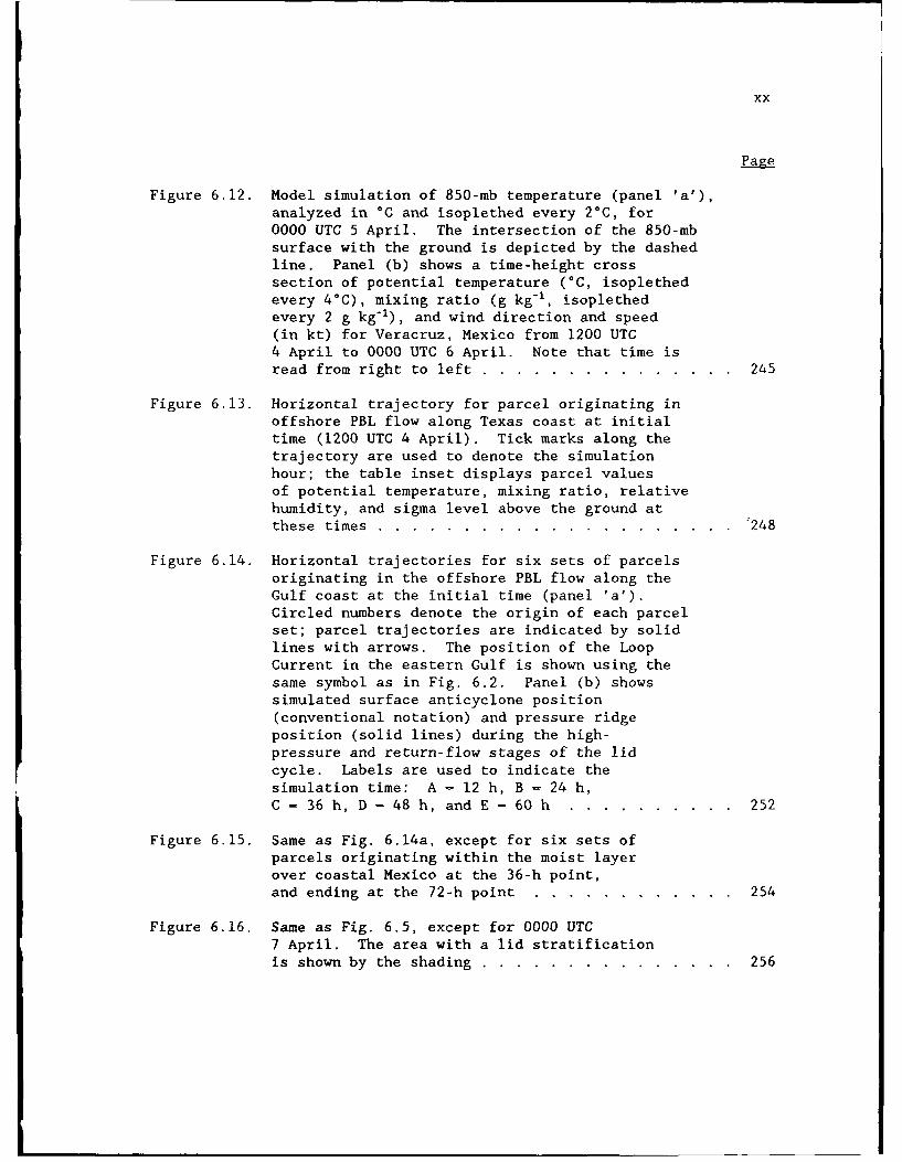
Figure 6.12. Model simulation of 850-mb temperature (panel 'a'),analyzed in =C and isoplethed every 20C, for0000 UTC 5 April. The intersection of the 850-mbsurface with the ground is depicted by the dashedline. Panel (b) shows a time-height crosssection of potential temperature (*C, isoplethedevery 4*C), mixing ratio (g kg-', isoplethedevery 2 g kg-1), and wind direction and speed(in kt) for Veracruz, Mexico from 1200 UTC4 April to 0000 UTC 6 April. Note that time isread from right to left ....... ............... .. 245
Figure 6.13. Horizontal trajectory for parcel originating inoffshore PBL flow along Texas coast at initialtime (1200 UTC 4 April). Tick marks along thetrajectory are used to denote the simulationhour; the table inset displays parcel valuesof potential temperature, mixing ratio, relativehumidity, and sigma level above the ground atthese times ............... ..................... ... 248
Figure 6.14. Horizontal trajectories for six sets of parcelsoriginating in the offshore PBL flow along theGulf coast at the initial time (panel 'a').Circled numbers denote the origin of each parcelset; parcel trajectories are indicated by solidlines with arrows. The position of the LoopCurrent in the eastern Gulf is shown using thesame symbol as in Fig. 6.2. Panel (b) showssimulated surface anticyclone position(conventional notation) and pressure ridgeposition (solid lines) during the high-pressure and return-flow stages of the lidcycle. Labels are used to indicate thesimulation time: A - 12 h, B = 24 h,C - 36 h, D - 48 h, and E = 60 h .... .......... 252
Figure 6.15. Same as Fig. 6.14a, except for six sets ofparcels originating within the moist layerover coastal Mexico at the 36-h point,and ending at the 72-h point ...... ............ 254
Figure 6.16. Same as Fig. 6.5, except for 0000 UTC7 April. The area with a lid stratificationis shown by the shading ....... ............... .. 256
xxi
Page
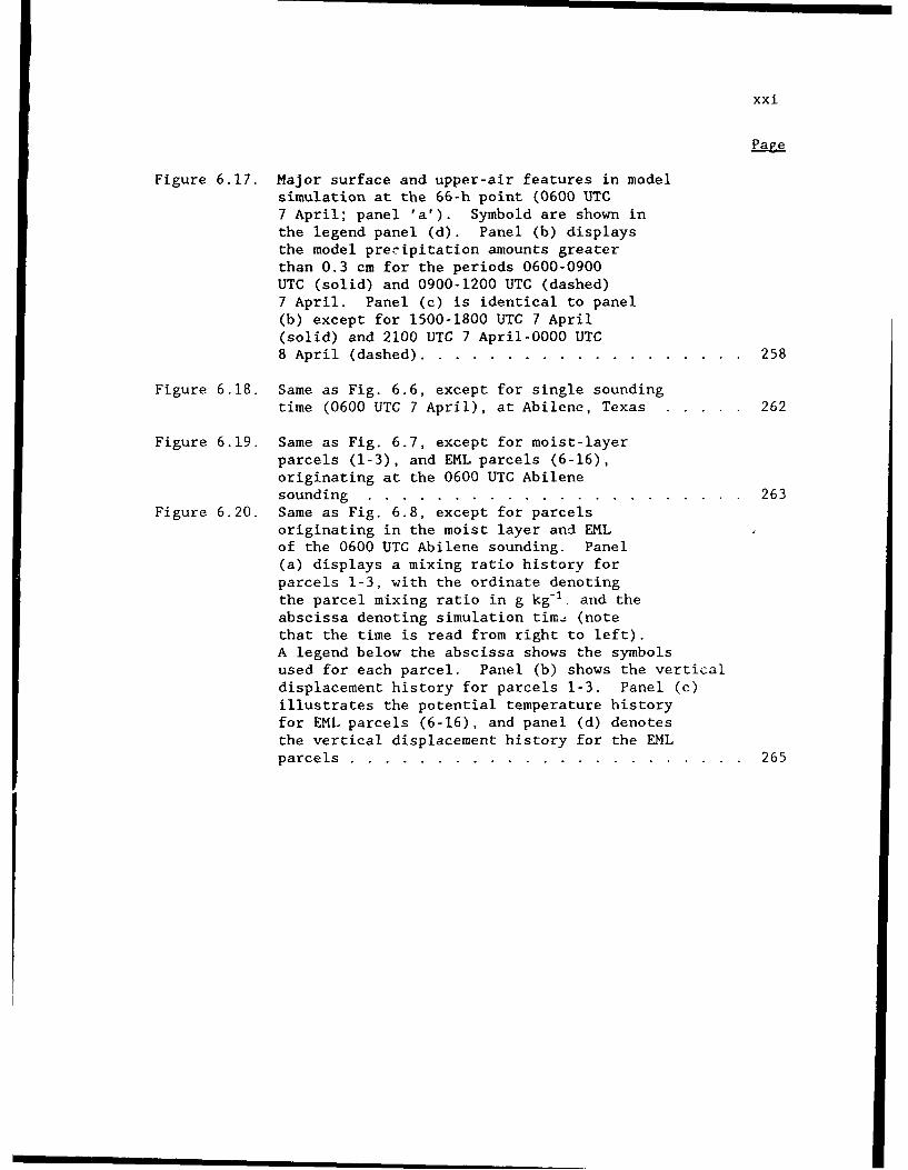
Figure 6.17. Major surface and upper-air features in model
simulation at the 66-h point (0600 UTC7 April; panel 'a'). Symbold are shown inthe legend panel (d). Panel (b) displaysthe model pre-ipitation amounts greaterthan 0.3 cm for the periods 0600-0900UTC (solid) and 0900-1200 UTC (dashed)7 April. Panel (c) is identical to panel(b) except for 1500-1800 UTC 7 April(solid) and 2100 UTC 7 April-0000 UTC8 April (dashed) ........... ................... .. 258
Figure 6.18. Same as Fig. 6.6, except for single soundingtime (0600 UTC 7 April), at Abilene, Texas ..... .. 262
Figure 6.19. Same as Fig. 6.7, except for moist-layerparcels (1-3), and EML parcels (6-16),originating at the 0600 UTC Abilenesounding ................ ...................... 263
Figure 6.20. Same as Fig. 6.8, except for parcelsoriginating in the moist layer and EMLof the 0600 UTC Abilene sounding. Panel(a) displays a mixing ratio history forparcels 1-3, with the ordinate denotingthe parcel mixing ratio in g kg-1 . and theabscissa denoting simulation timI (notethat the time is read from right to left).A legend below the abscissa shows the symbolsused for each parcel. Panel (b) shows the vertical
displacement history for parcels 1-3. Panel (c)illustrates the potential temperature historyfor EML parcels (6-16), and panel (d) denotes
the vertical displacement history for the EMLparcels ............... ....................... .. 265
xxii
PREFACE
Chapters 2 through 4 represent a three-part journal paper appearing
in the June 1991 issue of Weather and Forecasting, entitled "A Synoptic
Climatology of the Elevated Mixed Layer Inversion over the Southern
Great Plains in Spring," by John M. Lanicci and Thomas T. Warner.
Chapter 2 corresponds to "Part 1: Structure, Dynamics, and Seasonal
Evolution"; Chapter 3 corresponds to "Part 2: The Life Cycle of the
Lid"; and Chapter 4 corresponds to "Part 3: Relationship to Severe-
Storms Climatology." Since the papers were written to stand alone,
there is some redundancy between the material in Chapter 1
(Introduction) and the introductory sections of Chapters 2-4, and
between the conclusion sections of Chapters 2-4.
I wish to express my deepest thanks to my thesis advisor, Prof.
Thomas T. Warner. My doctoral research underwent many changes during my
three years at Penn State, and Prof. Warner was always ready with
prudent guidance and insight from his years of experience. The guidance
of my doctoral committee was also valuable during my time here. I
express my gratitude to Prof. Toby N. Carlson for his guidance and
pioneering work in my area of study; to Prof. Gregory S. Forbes for the
many discussions we had during the course of my research; to Prof. J.
Michael Fritsch for his helpful suggestions; to Prof. Brent Yarnal,
whose experience as a synoptic climatologist was invaluable to me, and
to Dr. Charles A. Doswell III of the National Severe Storms Laboratory,
who helped me grow professionally during my research.
xxiii
There are many others who lent me their support during my research.
In the Meteorology department, I had many fruitful discussions with
Prof. Nelson L. Seaman, Prof. George S. Young, and Prof. John J. Cahir.
From the NWP staff, Ms. Annette Lario, Dr. David Stauffer, and Dr. James
Doyle helped me through the many steps of preparing and running the Penn
State/NCAR mesoscale model and its supporting software. Tasks such as
data gathering, tabulation, plotting and reproduction were
professionally done by Ms. Laura Matason, Mr. Michael Hopkins, and Mrs.
Amy Erlick. Superb graphics were provided by Ms. Mary Carpenter of the
Deasy Geographics Lab at Penn State, and Tek-Art, Inc. of State College.
Computer resources were provided by the Department of Meteorology, the
National Center for Atmospheric Research (supported by the National,
Science Foundation), and Cray Research's facilities at Mendota Heights,
MN. I was sponsored by the Air Force Institute of Technology, Wright-
Patterson AFB, OH, and the research was funded by the Air Force Office
of Scientific Research under Grant No. AFOSR-88-0050. This manuscript
was very professionally prepared by Mrs. Joann Singer.
This work is the culmination of a goal I have had for many years.
I would like to thank my wife, Kathy, and my sons, Michael and Mark, for
the many sacrifices they made as a family to see this dream come to
fruition. My parents, Richard and Susanna Lanicci, taught me the work
ethic necessary to persevere through this demanding program. I thank
God for making it possible for me to achieve the difficult goals I set
for myself every day. This thesis is dedicated to the memory of my
maternal grandmother, Anna D'Antonio, who taught me about the value of
an education and the joy of learning.
Chapter 1
INTRODUCTION
The Great Plains region of the United States has the highest
frequency of severe convective weather events in the world. To the
forecaster and researcher alike, the myriad mesoscale features
associated with the large scale environment of this area, i.e., the
dryline, the low level jet, transitory upper level jet streaks, the
elhlated mixed layer, and the inversion that the elevated mixed layer
produces when it overlies moist, unstable air (hereafter referred to as
a "lid"), are fairly well known. However, predicting whether the
complex interaction of these features will result in a severe
thunderstorm outbreak remains one of the most daunting challenges to
operational meteorology, despite nearly 50 years of continuous research.
The primary focus of this research is on the generation of a
representative synoptic climatology of the lid and its various component
structures, and the relationship of this climatology to the occurrence
or nonoccurrence of severe local storms. In this introduction, the
historical foundation for the existing literature on severe-storms
climatology is presented, along with a brief review of those studies
addressing the creation and evolution of the important components of the
lid sounding. Following these sections, an outline of the objectives of
this research are presented.
2
1.1 Literature Review of Severe-Storms Climatology
The development of severe-storm analysis and prediction techniques
has an historical background that is largely rooted in climatological
studies. Before the mid 1920s, most of the literature on severe storms
consisted primarily of storm-damage documentation, although two notable
exceptions were the studies of Ferrel (1885) and Finley (1890), who
described some common atmospheric features found in severe-storm
situations. A review paper by Galway (1977) describes the history of
storm-event documentation, including a good summary of the problems
involved with the early periods of record keeping. As methods of
probing the atmosphere were developed (e.g., kites and balloons with
instrumentation), attempts were made by Varney (1926), Humphreys (1926),
and others to describe the thermodynamic and wind environments of the
tornadic thunderstorm. The advent of routine radiosonde ascents and the
adoption of the airmass/frontal thtories of the Bergen School influenced
subsequent research. The works of Lloyd (1942) and Showalter and Fulks
(1943) are illustrative of this period of "new" technology and theory.
As the upper-air networks improved and the database grew, a natural
extension of the earlier investigations was the generation of severe-
storm climatologies. These climatological studies used the available
surface and upper-air data archive to obtain a set of common atmospheric
features associated with severe-storm events. Hereafter, these are
referred to as event-based climatology studies.
A survey of the numerous event-based climatologies produced over
the U.S. since 1950 is summarized in Table i.i. The analysis techniques
used in these studies generally fall into three main categories: 1)
3
statistical analysis of the characteristics of the tornado-damage and
storm-damage events; 2) creation and evaluation of mean proximity
soundings taken from the near-storm/tornado environments; and 3)
categorization of synoptic patterns associated with the severe-storm and
tornadic environments. These studies give us much insight into the
synoptic characteristics of both the pre-storm as well as the near-storm
environments. However, some problems exist with these studies, which
are related to the fact that they use storm events as the basis for
generating the climatology. These problems include incomplete
documentation of every severe-storm event, artificial constraints put on
the event data in order to generate specialized climatologies (e.g., for
"large" or "progressive" outbreaks), and the exclusion of the
meteorological conditions associated with non-severe-storm event days.
A more complete discussion of the limitations of event-based studies,
and a description of other types of climatological studies (such as
satellite-derived composites) appear in Section 4.1.
1.2 The Creation and Evolution of theComponents of the Lid Sounding
One of the first outcomes of the event-based studies documented in
Table 1.1 was the generation of a mean proximity sounding for the
tornadic environment. Fawbush and Millt 19-, 1954) are generally
credited with the first composite sourli ! ýhe tornadic environment,
although their result is similar to that oi an earlier investigation by
Showalter and Fulks (1943). The tornado proximity sounding, also known
as a Type 1 or "loaded gun sounding," is characterized by a moist layer
near the surface with high values of 8., above which a relative-humidity

4
Table 1.1 Event-Based Severe-Storm Climatologies
Study (year) Area of Interest Analysis Technique
Fawbush et al. Continental U.S. Statistical (tornado events(1951) are categorized by location,
month, mean terrain elevation,etc. A set of subjectivelydetermined synoptic conditionsare presented based on multi-year database of tornadicevents).
Fawbush and Miller Continental U.S. Proximity soundings (mean(1952) sounding generated from
multi-year sample oftornado situations)
Fawbush and Miller Continental U.S. Proximity soundings (same(1954) technique as above)
Beebe (1956) East of Rockies Mean meteorological charts(based on multi-year sampleof tornado situations)
Fawbush et al. Continental U.S. Categorization of 500-mb(1957) flow patterns associated
with severe local stormsover a 10-year period
Beebe (1958) Central U.S. Proximity and precedencesoundings (the latter arecharacteristic of tornadicstorm airmass but removed intime and space from vicinityof tornado occurrence)
Miller (1959) East of Rockies Composite meteorologicalcharts (analogs based on
multi-year sample of tornadosituations)
Darkow (1969) Central Plains, Proximity and check soundingsNorthern Plains, (latter are taken at tornadoGulf Coast event time at closest upper-
air station in an upstreamdirection with respect to meanlow-level flow). All rain-affected soundings are removedfrom data sample.
5
Table 1.1 (continued)
Study (yearl Area of Interest Analysis Technique
Willis (1969) East of Rockies Tornado proximity soundings;examined them by region andtwo special categories(tropical storm and warmairmass). Vertical shear andparcel buoyancy statisticswere used to develop Tornado
Likelihood Index.
Darkow and Fowler Central Plains, Proximity, upstream check, and
(1971) Northern Plains, right check soundings. Right
Gulf Coast check soundings were taken atevent time at the closestupper air station normal andto the right of the low-levelflow.
Notis and Stanford Iowa Statistical (categorized
(1973) tornadoes by direction ofmovement; computed means,standard deviations,correlations withmeteorological variables)
Maddox (1976) East of Rockies Proximity soundings (includesseparate tornado and severethunderstorm categories; also
computes stability index, meansounding winds)
Williams (1976) From Rockies Statistical (mean regional
eastward surface conditions based on
multi-year sample of tornadosituations)
David (1976) Continental U.S. Mean meteorological conditionsbased on multi-stationobjective analysis ofrawinsonde data near locationof tornado; multi-yeardatabase
Galway (1977) East Rockies Statistical (restricted tooutbreaks of 10 or moretornadoes; categorizedtornadoes by month, region,total deaths, etc.)
6
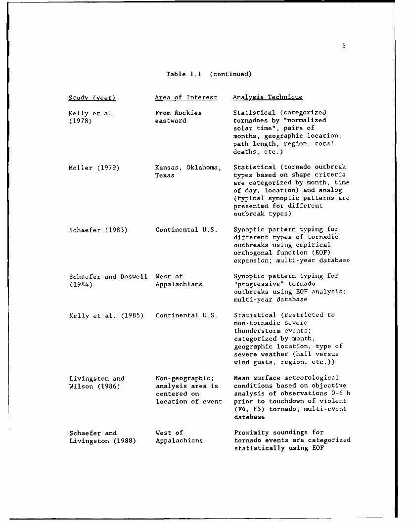
Table 1.1 (continued)
Study (year) Area of Interest Analysis Technique
Kelly et al. From Rockies Statistical (categorized(1978) eastward tornadoes by "normalized
solar time", pairs ofmonths, geographic location,path length, region, totaldeaths, etc.)
Moller (1979) Kansas, Oklahoma, Statistical (tornado outbreakTexas types based on shape criteria
are categorized by month, timeof day, location) and analog(typical synoptic patterns arepresented for differentoutbreak types)
Schaefer (1983) Continental U.S. Synoptic pattern typing fordifferent types of tornadicoutbreaks using empiricalorthogonal function (EOF)expansion; multi-year database
Schaefer and Doswell West of Synoptic pattern typing for(1984) Appalachians "progressive" tornado
outbreaks using EOF analysis;multi-year database
Kelly et al. (1985) Continental U.S. Statistical (restricted tonon-tornadic severethunderstorm events;categorized by month,geographic location, type ofsevere weather (hail versuswind gusts, region, etc.))
Livingston and Non-geographic; Mean surface meteorologicalWilson (1986) analysis area is conditions based on objective
centered on analysis of observations 0-6 hlocation of event prior to touchdown of violent
(F4, F5) tornado; multi-eventdatabase
Schaefer and West of Proximity soundings forLivingston (1988) Appalachians tornado events are categorized
statistically using EOF
7
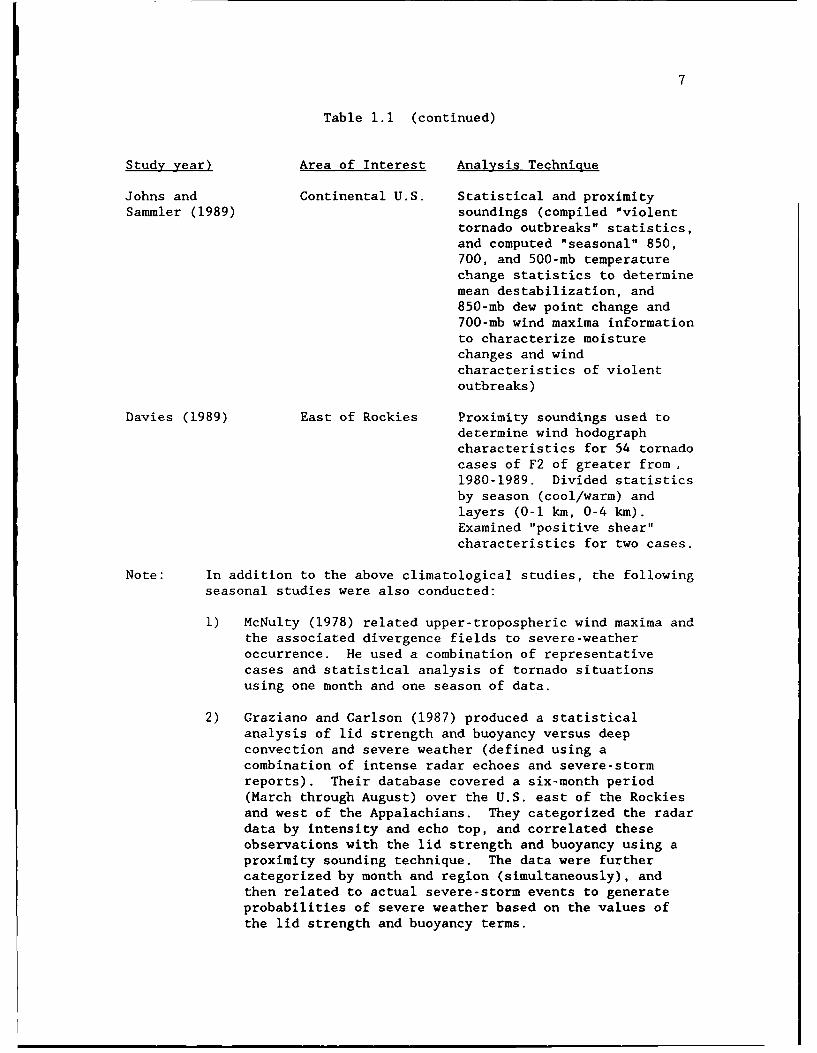
Table 1.1 (continued)
Study year) Area of Interest Analysis Technique
Johns and Continental U.S. Statistical and proximitySammler (1989) soundings (compiled "violent
tornado outbreaks" statistics,and computed "seasonal" 850,700, and 500-mb temperaturechange statistics to determinemean destabilization, and850-mb dew point change and700-mb wind maxima informationto characterize moisturechanges and windcharacteristics of violentoutbreaks)
Davies (1989) East of Rockies Proximity soundings used todetermine wind hodographcharacteristics for 54 tornadocases of F2 of greater from,1980-1989. Divided statisticsby season (cool/warm) andlayers (0-1 km, 0-4 km).Examined "positive shear"characteristics for two cases.
Note: In addition to the above climatological studies, the followingseasonal studies were also conducted:
1) McNulty (1978) related upper-tropospheric wind maxima andthe associated divergence fields to severe-weatheroccurrence. He used a combination of representativecases and statistical analysis of tornado situationsusing one month and one season of data.
2) Graziano and Carlson (1987) produced a statisticalanalysis of lid strength and buoyancy versus deepconvection and severe weather (defined using acombination of intense radar echoes and severe-stormreports). Their database covered a six-month period(March through August) over the U.S. east of the Rockiesand west of the Appalachians. They categorized the radardata by intensity and echo top, and correlated theseobservations with the lid strength and buoyancy using aproximity sounding technique. The data were furthercategorized by month and region (simultaneously), andthen related to actual severe-storm events to generateprobabilities of severe weather based on the values ofthe lid strength and buoyancy terms.
8
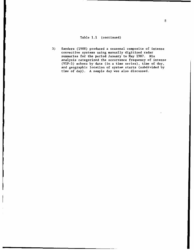
Table 1.1 (continued)
3) Sanders (1988) produced a seasonal composite of intenseconvective systems using manually digitized radarsummaries for the period January to May 1987. Hisanalysis categorized the occurrence frequency of intense(VIP-5) echoes by date (in a time series), time of day,and geographic location of system starts (subdivided bytime of day). A sample day was also discussed.
9
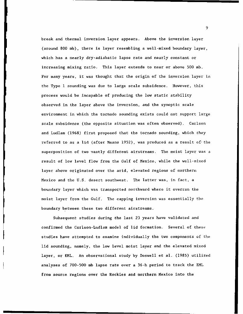
break and thermal inversion layer appears. Above the inversion layer
(around 800 mb), there is layer resembling a well-mixed boundary layer,
which has a nearly dry-adiabatic lapse rate and nearly constant or
increasing mixing ratio. This layer extends to near or above 500 mb.
For many years, it was thought that the origin of the inversion layer in
the Type 1 sounding was due to large scale subsidence. However, this
process would be incapable of producing the low static stability
observed in the layer above the inversion, and the synoptic scale
environment in which the tornado sounding exists could not support large
scale subsidence (the opposite situation was often observed). Carlson
and Ludlam (1968) first proposed that the tornado sounding, which they
referred to as a lid (after Means 1952), was produced as a result of' the
superposition of two vastly different airstreams. The moist layer was a
result of low level flow from the Gulf of Mexico, while the well-mixed
layer above originated over the arid, elevated regions of northern
Mexico and the U.S. desert southwest. The latter was, in fact, a
boundary layer which was transported northward where it overran the
moist layer from the Gulf. The capping inversion was essentially the
boundary between these two different airstreams.
Subsequent studies during the last 23 years have validated and
confirmed the Carlson-Ludlam model of lid formation. Several of these
studies have attempted to examine individually the two components of the
lid sounding, namely, the low level moist layer and the elevated mixed
layer, or EML. An observational study by Doswell et al. (1985) utilized
analyses of 700-500 mb lapse rate over a 36-h period to track the EML
from source regions over the Rockies and northern Mexico into the
10
southern and central Great Plains. Their work suggests that a
combination of surface heating over the source region along with rising
motion in the synoptic scale environment produces the high lapse rates
associated with the EML.
A two-dimensional modeling study by Benjamin (1986) examined the
creation of the EML over an idealized plateau resembling northern
Mexico, and its subsequent downwind transport over regions of lower
terrain. His work shows that the development of the EML over the
plateau is largely the result of intense surface heating over the arid
elevated source region, and that the EML begins to form a capping
inversion over the potentially cooler air downstream between 12 and 18 h
after its movement off the pl]tpau. Additionally, the differential
surface heating between the arid plateau and relatively moister lowlands
enhances the development of the lee-side trough, which in turn increases
the low level inflow towards the region of potential convection,
reaching a maximum intensity in the late afternoon and early evening. A
similar two-dimensional modeling study was conducted by Arritt and Young
(1990), using an idealized mountain range resembling the Rockies, to
examine EML formation and subsequent downwind transport over the western
high Plains. Their results, in terms of the formation of the EML and
downwind lid inversion, are remarkably similar to Benjamin's results,
despite the fact that the spatial scale of their study is nearly an
urder of magnitude less than Benjamin's!
Unfortunately, there has not been as much study of the
characteristics and evolution of the moist layer as there has been of
the EML. Some early studies of return flow over the Gulf (Johnson 1976;

Henry and Thompson 1976; Karnavas 1978) attempted to combine surface
trajectories and satellite-image continuity to document the
characteristics of the modified airmass returning into southern Texas
following a polar-air outbreak. The effect of the Loop Current in the
eastern Gulf on surface I 'el trajectories was explored in a
climatological study by Molinari (1987). A recent field experiment over
the Gulf of Mexico (GUFMEX; Lewi- et al. 1989) collected data which will
be used to investigate the characteristics of the low level air from the
time the continental polar airmass first moves into the Gulf until the
time that it returns northward into Texas as a moist layer.
The studies mentioned above raise some interesting questions
regarding the creation and subsequent evolution of the moist layer and
the EML, and the formation of the lid sounding. The first question
involves the time and space scales for the creation of the EML and moist
layer, and whether or not they are similar. A related question concerns
the variability in EML and moist layer creation and evolution as a
result of different sequences of synoptic flow patterns. A third
question involves the various physical processes at work in the creation
and evolution of the EML and moist layer. This last question is
particularly intriguing because the processes that affect the dry static
stability (through the EML) can feed back into the large scale vertical
motion field (subsequently affecting the synoptic scale system), as well
as influence the likelihood of localized deep convection in the vicinity
of upper level jet streaks, for example. The processes that affect the
creation and evolution of the moist layer can also have important

12
influences on the large scale and local environments through feedbacks
resulting from latent heat release in cloud and precipitation areas.
1.3 Purpose of Thesis
This study will provide an improved understanding of the
climatology of severe local storms over the southern Great Plains during
the convectively active months of April, May, and June. In order to
address the concerns raised in Section 1.1 about the representativeness
of event-based studies, the climatology developed in this research will
be based on the EML, moist layer, and the lid. By employing an approach
that concentrates on physical features known to exist in the severe-
storm environment, the occurrence of severe weather is addressed within
the context of these three features (EML, moist layer, and lid) in
contrast to the opposite approach. The resulting climatology includes
days with a variety of severe weather events, from the largest outbreaks
to the isolated events, and even the days with no severe weather,
hereafter referred to as "non-event" days.
The questions raised in Section 1.2 about the creation and
evolution of the EML, moist layer, and lid are addressed in the
following ways by this study. In Chapter 2, monthly analyses of various
parameters associated with the EML, moist layer, and lid are produced to
examine the seasonal evolution. The applicability of the lid
climatology in different parts of the spring season is examined through
the construction of a subjective synoptic typing scheme that is based on
the thermal wind. The synoptic flow types are then analyzed with regard
to their seasonal frequency and their association with the

13
occurrence/nonoccurrence of the lid. In Chapter 3, a conceptual model
of the life cycle of lid development and dissipation is presented, and
its seasonal sensitivity is examined. This portion of the study
addresses the characteristic time and space scales for the creation and
evolution of the EML, moist layer, and lid through a synoptic
climatological approach. The synoptic types defined in Chapter 2 are
used in this portion of the study to explore the variability in EML,
moist layer, and lid evolution resulting from different sequences of
synoptic flow types. The seasonal aspects of this variability are also
addressed here. The compilation of severe-weather statistics for the
period of study and their relationship to various synoptic patterns
occurring during the life cycle of the lid is addressed in Chapter 4..
Chapter 5 illustrates how the lid climatology can be applied to a real-
data case by examining a five-day lid cycle that occurred in April 1984.
The physical processes involved in EML and moist layer creation and
evolution during this lid cycle are investigated in Chapter 6 through
analysis of the results of a five-day simulation using the Penn
State/NCAR mesoscale prediction model, hereafter referred to as MM4
(Anthes and Warner 1978; Anthes et al. 1987).
14
Chapter 2
THE SYNOPTIC CLIMATOLOGY: STRUCTURE,DYNAMICS, AND SEASOINAL EVOLUTION
2.1 Chapter Introduction
It has been generally accepted by the meteorological community that
the elevated mixed layer inversion, or lid, is a crucial feature of the
springtime severe storm environment of the southern and central Great
Plains of the United States. The typical lid sounding, also known as a
Type 1 tornado sounding (Fawbush and Miller 1954), is characterized by a
moist, potentially unstable layer about 100 mb thick, capped by a
potentially warm, nearly dry-adiabatic elevated mixed layer (EML), which
typically extends upward from the base of a strong inversion located
near 800 mb. The presence of this EML results in a large region of
buoyant instability aloft (Carlson and Ludlam 1968; Doswell et al.
1985). Also, the EML often overlies areas ¶ith mnrc'nally unstable or
stable stratification, and presents forecasters with the difficult task
of predicting whether the stratification below the EML will destabilize
during the forecast period.
In the classic model of lid formation, an approaching upper level
trough in the westerlies induces a southwesterly flow over a hot, arid,
elevated source region such as northern Mexico, and transports a deep,
neutrally stratified mixed layer northeastward, where it overruns a
cooler, moister airstream whose source is over the Gulf of Mexico. A
third airstream descends around the rear of the upper trough and forms a
confluence zone at midlevels (near 700 mb) with the western edge of the
dry Mexican airstream. This area of confluence creates a baroclinic
15
zone along the edge of the lid. The baroclinic zone and its importance
in focusing convection along the lid edge have been described in
analyses of lid cases (e.g. Carlson et al. 1980, 1983; Farrell and
Carlson 1989), as well as in modeling studies (Keyser and Carlson 1984;
Benjamin and Carlson 1986; Lakhtakia and Warner 1987; Lanicci et al.
1987).
According to the classic model, the lid is formed in an area of
large scale vertical ascent ahead of the upper level trough, and thus
the lid base rises to the north and east with increasing distance from
the EML source region. The western edge of the lid often is coincident
with the position of the dryline, a related feature which frequently
appears in the severe storm environment over this region. It has been
demonstrated that deep, moist convection and severe weather associated
with the lid environment occur through one or both of the following
mechanisms: 1) low level ageostrophic flow from beneath the lid edge
develops in response to an isallobaric minimum (known as underrunning);
and 2) lid removal occurs through concentrated, strong upward motion
caused by the vertical circulations from a dynamic feature such as an
upper level jet streak. Carlson et al. (1983) state, "The most intense
convection occurs in the region near the intersection of the axis of the
moist tongue and the lid edge."
Although there have been studies of lid occurrences in other parts
of the world (see Carlson et al. 1983 for a brief review), the great
majority of case studies over the U.S. have been confined to severe
storm outbreaks in April and May over the Great Plains. An exception is
the Farrell and Carlson (1989) study of the 31 May 1985 tornado outbreak
16
in the Northeast. All of the aforementioned studies involved southwest
flow aloft, and the EML source regions were Mexico and the southwestern
U.S. deserts. A common theme in these studies is that the lid is
created in a synoptic flow situation that is "anomalous" compared to the
climatological mean of zonal flow. In these cases, there is a net
northward transport of warm, moist air at low levels and warm, dry air
at midlevels, in an environment of veering wind shear. It is implied
that differential thermal advection is very important for creating the
three dimensional lid stratification. Also, it has been shown that, as
the spring season progresses, surface heating and evapotranspiration
contribute more to the development of low level potential instability
(Benjamin and Carlson 1986; Lanicci et al. 1987). Additionally, during
the spring, the western plateau of the U.S. undergoes a transition from
an elevated cold source to a heat source (Tang and Reiter 1984), and the
advection of potentially warm, dry air aloft can occur with several
mid-tropospheric wind directions. Thus, by late spring and early
summer, the "anomalous" southerly/southwesterly flow regime is riot the
only flow type that can create the three dimensional stratification
associated with the lid.
We hypothesize that the classic model of lid formation over the
central U.S. is only applicable to a limited set of synoptic flow
regimes (southwesterly) for the early spring season. Our objective is
to learn whether there are other flow configurations that produce the
EML and lid, and if the mechanism for the creation of this
stratification undergoes significant changes during the spring. Thus,
17
we pose the following questions concerning EML and lid formation and
structure in the springtime over the southern Great Plains:
1) Over which areas does the lid appear most often? Does the
location of this lid formation region change during the
spring?
2) How do the structures of the EML and lid change during the
spring?
3) Which synoptic regimes in addition to southwest flow aloft
can create a lid?
One aspect of the present study is the production of a synoptic
climatology for the southern Great Plains (defined here as Kansas,
Oklahoma, Texas, and the immediate surrounding area) for April, May, and
June. The climatology makes use of conventional surface and
standard-level data, as well as derived parameters that define the lid
and EML structure based on the automated procedure described in Farrell
and Carlson (1989) (hereafter referred to as FC89). Section 2.2
describes the analysis of the lid- and EML-occurrence statistics for
each month, and relates them to the EML source-region climatology.
Section 2.3 discusses the physically based synoptic-typing scheme,
presents the predominant flow types for each month, and relates these
physically based flow types to lid and EML occurrences, as well as mean
monthly analyses of EML and lid parameters during the spring season.
Two companion papers (Lanicci and Warner 1991b; Lanicci and Warner
1991c) take the lid/EML climatology presented in this study and relate
it to a seasonally dependent conceptual model of lid formation, and to

18
severe weather occurrence statistics for the same period as the present
study.
2.2 Lid Characteristics Over the Southern Plains:April-June 1983-1986
The study area for this climatology extends from 88 to 107'W
longitude, and from 25 to 42°N latitude. There are 22 U.S. and two
Mexican rawinsonde stations in this area (Fig. 2.1). Lid statistics
were generated for the U.S. stations using an automated procedure
developed at Penn State (Carlson et al. 1980, 1983; Graziano and Carlson
1987; FC89). The climatological data base for this study (1983-1986) is
the same as that of FC89 (i.e., the Penn State Meteorology department's
tape archive). From examination of some 16,000 soundings, statistics
concerning lid frequency, geographic distribution of the lid, and
characteristics of the lid soundings were produced for the study region.
We tabulated data availability statistics for each station during the
period of record to determine if some stations had more missing
observation times than others. The statistics include those days in
which no data were available from the Penn State archive. A plot of the
data availability for each station (not shown) reveals a normal
distribution with on'y two stations (BVE, ELP) below 80% data
availability. Due to ELP's low lid frequency (to be shown later), only
BVE's data availability was of concern. After careful examination of
the statistics for BVE, we concluded that the missing days were not
biased towards any portion of the lid-size distribution to be discussed
in section 2.2.2.
19
BF- -. A PIADPIA
i . TOP ,LXOI
UMN.~-1 J'
ADO IZAML. OKC I
* SEP DOG AJN
ELP, MAF ) -~-LCH
DPT BVE
Figure 2.1. The study region, showing the locations and three-letteridentifiers of the rawinsonde stations which arefrequently referred to in the text.
20
2.2.1 The Sounding Analysis Procedure
The algorithm used in this study is discussed in detail by Farrell
(1988) and FC89. Their program examines the temperature and relative
humidity profiles of each sounding to determine the presence of a lid
based on the following criteria:
I) A relative humidity discontinuity must exist below 500 mb,
with a critical gradient of at least 0.87% per mb. Surface-
based inversions are identified and do not count as relative
humidity breaks in this procedure.
2) A layer in which the lapse rate of the saturation wet-bulb
potential temperature, . , is greater than or equal to
zero must exist within 100 mb of the relative humidity bteak
defined in (1). The 06w value at the "nose" of the inversion
is defined as 8swmax .
3) The static stability, a defined as a = -TO-' (89/ap), in the
layer above the inversion must be less than 4.5°C per 100 mb.
4) Tne relative humidity in the layer above the inversion must
show an increase with height.
5) The lid strength, LS, defined as LS - Oswax -0 wb , is equal
to or greater than 1.0 0 C, where 6wb is the "best" (most
unstable) wet-bulb potential temperature found in a 50-mb
thick layer below the relative humidity break.
6) The buoyancy term, BUO, defined as BUO = 6 sw500 -wb , is less
than 0.5*C, where OsW500 is the saturation wet-bulb potential
temperature at 500 mb. This definition of the buoyancy
results in values that are approximately one-half the
21
magnitude of the lifted index (Galway 1956) that is currently
in use by the National Weather Service. The 0.5 0 C threshold
accounts for marginal stability situations.
In our study, the existence of an EML is determined on the basis of
criteria 1 - 3 only. The critical value of the static stability used in
criterion 3 was determined by Farrell (1988) to be an optimum value
based on previous studies involving soundings with EMLs, such as those
of Fawbush and Miller (1954) and Karyampudi (1986), and on sensitivity
tests with the present dataset. However, in order to determine what
fraction of the sample has static stabilities that may be associated
with subsidence layers, we analyzed a sample of 313 soundings diagnosed
as containing an EML using criteria 1 - 3, from the months of April,'
May, and June during the study period. Figure 2.2 shows a cumulative
frequency diagram that describes the distribution of a for the sample.
Figure 2.2 shows that the vast majority (about 85%) of EML soundings
have a values below 3.5°C 100 mb-', which is close to the mean static
stability (3.6°C 100 mb-1 ) of the type I tornado sounding (as computed
from the layer above the inversion in Fig. 1 of Fawbush and Miller
1954). Less than 10% of the sample soundings have a values in the range
4.0 - 4.50C 100 mb-', which may arguably be associated with subsidence
layers.
The results of Fig. 2.2 also show that a substantial number of EML
soundings are excluded from the database if the RH criterion is
retained. We screened the sample on the basis of whether the RH
criterion (4) was met. Interestingly, Fig. 2.2 shows that a substantial
number (118) of EML soundings do not meet the RH criterion employed by
22
4r-0
Cd 0 0>
0 ba cr%-4 0. 4)
00 Cd w - - 0 co r.W S., ) 4 n-41 I >. 0 a)e~u2-
10 CUdU w. 0 P-14J JJ W -
(W ( C .- 4 r-C: 0 4 0 C -
dP 4J 0 WV 0 M 4J-
olx u -W > f
6 > V-- 0 0
0 9. r4 4a) 10 Cd 041~
0D0 ) a)
4 44 U) 4) * .. 4 cna' Q0 40 J i4J ý4
a'~ 0 Q-400.-
0 CO.-~- 0Q.b4
4) 4 10 0
U4 0 4J b -if) U C
7(O Q)tO-4 r 1 0
'-4 0-4- 9:I 0 J (
a' 00~~bO.-.-0 0o ý
a 0 0) 0 0 0 0 0 0 Z
o o co I- W o m %
(S ouanbajia oauaiiaa~o oApulnfuana~
23
FC89, and a considerable fraction (100) of these soundings have a values
below 3.5°C 100 mb-'. In addition to the evidence shown by Fig. 2.2,
Farrell (1988) also points out that the RH criterion has other problems,
most notably with the radiosonde humidity sensor's failure to recover
from dewpoint depressions greater than 30°C, and with the current
convention of reporting dewpoint depressions greater than 30 0 C as being
equal to 30°C. Additionally, studies of the mixed layer (e.g., Mahrt
1976) have shown that, while the typical well-mixed PBL has a nearly
dry-adiabatic lapse rate in temperature, the lapse rate of mixing ratio
often is not well-mixed, for reasons such as differential moisture
advection and growth of the PBL into an extremely dry layer. The fact
that Mahrt's study was conducted over the western Great Plains makes' his
results particularly relevant to the present study. Based on these
findings, it was decided to exclude RH criterion (4) from the EML
screening procedure.
Regarding criterion (5), we distinguish between soundings with
positive and non-positive lid strengths by defining a "capped" sounding
as one with LS > O.0=C. This modification of FC89's criterion allows us
to distinguish between the characteristics of both capped as well as
"uncapped" (LS : O.OC) soundings. We further screen the capped
soundings manually to determine if the EML base coincides with the
warmest point on the sounding. Requiring that the EML base coincide
with the level of Owax screens out soundings whose EML lies below the
level of Oswax. In our study, we define a "lid" sounding as one
containing an EML (criteria 1-3) which effectively caps a PBL (modified
criterion 5) that is buoyantly unstable (i.e., BUO < 0.5°C) with respect

24
to the 500-mb level (criterion 6). A capped "EML" sounding (hereafter
referred to as simply an EML sounding), by contrast, meets criteria
(1) - (3), effectively caps the PBL (modified criterion 5), but is
buoyantly stable (BUO Z 0.5°C). Separate identification of both EML and
lid soundings is important because the EML is a more ubiquitous and
spatially and temporally continuous feature than the lid. This gives
the forecaster a temporal continuity that is extremely important when
distinguishing between favorable and marginal areas for deep convection.
Figure 2.3 presents examples of soundings classified according to
the criteria presented in this section. The DRT sounding shown in
Fig. 2.3a meets none of the criteria for an EML, and indeed looks more
representative of a sounding from west of the surface dryline (Schaefer
1974). The SEP sounding in Fig. 2.3b is classified as an EML sounding
due to its stable BUO value of 0.6°C. The VCT sounding in Fig. 2.3c
contains a capping inversion and a relative humidity break at 768 mb.
However, the layer above the inversion is marked by a lapse rate close
to moist adiabatic, so it fails to meet criterion (3) and is classified
as a subsidence-inversion sounding. The BVE sounding in Fig. 2.3d
contains the inversion and EML (from 804 to 719 mb), and is buoyantly
unstable, but the EML does not meet the RH criterion. This sounding is
still classified as having a lid in our study. Finally, the VCT
sounding in Fig. 2.3e meets all six criteria discussed in this section,
and closely resembles the classic lid sounding presented in the severe
storms literature. This sounding has a BUO of -2.8°C and an LS of
4.8 0 C.

25
Figure 2.3. Skew-T Log P diagrams representing various types ofsoundings characterized by the automated sounding-analysisprogram. In each panel, the temperature sounding isindicated by the thick solid line and the dewpointsounding is shown by the thin solid line. Winds areplotted along the right axis of each sounding usingconventional notation (speed is in kt). Types ofsoundings shown are a) non-EML, b) EML, c) subsidence-type, d) lid with no relative humidity increase withheight in the EML, and e) lid with relative humidityincreasing with height in the EML.
26
x -o
3,- -20 -10 0- 10 20 30 -30 -2(1 -1: 3 : 1 0SI1AT ION 72261., 22':/!O; 7• ,I
20' 221,
2.00
300* 40
4oo- •. :- .• ,oo ,
500 30a"
-70
900
10K) ". 1000
-30 -20 -10 0 10 20 30 -30 -20 -1 0 I 10 20 30STATION: 72255 STATION- 7232
12' 05-AP-84 a12Z 0f-AP-84
'.0).' 20
300 . ,O
0oo -9,.- .- -
-30 -20 V) 0 170 20 30STATIONS: 72255
00Z O8-A0Z 84
'V / l m 4m , -
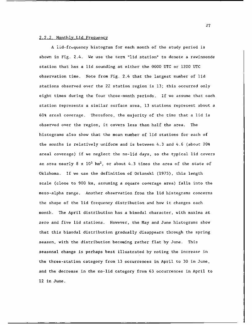
27
2.2.2 Monthly Lid Frequency
A lid-fr-equency histogram for each month of the study period is
shown in Fig. 2.4. We use the term "lid station" to denote a rawinsonde
station that has a lid sounding at either the 0000 UTC or 1200 UTC
observation time. Note from Fig. 2.4 that the largest number of lid
stations observed over the 22 station region is 13; this occurred only
eight times during the four three-month periods. If we assume that each
station represents a similar surface area, 13 stations represent about a
60% areal coverage. Therefore, the majority of the time that a lid is
observed over the region, it covers less than half the area. The
histograms also show that the mean number of lid stations for each of
the months is relatively uniform and is between 4.3 and 4.6 (about 20%
areal coverage) if we neglect the no-lid days, so the typical lid covers
an area nearly 8 x 10⁵ km2 , or about 4.3 times the area of the state of
Oklahoma. If we use the definition of Orlanski (1975), this length
scale (close to 900 km, assuming a square coverage area) falls into the
meso-alpha range. Another observation from the lid histograms concerns
the shape of the lid frequency distribution and how it changes each
month. The April distribution has a bimodal character, with maxima at
zero and five lid stations. However, the May and June histograms show
that this bimodal distribution gradually disappears through the spring
season, with the distribution becoming rather flat by June. This
seasonal change is perhaps best illustrated by noting the increase in
the three-station category from 13 occurrences in April to 30 in June,
and the decrease in the no-lid category from 63 occurrences in April to
12 in June.

2)8
.-o -A J"APRILMEAN •4.3
so ~MEDIAN z 8
40
30
0 o
10
0 1 2 3 1 0 i 7 4 9 *0 " " "2 13
Number of Lid Stations,BI L MAY
IMEAN 2 4.6401 MEDIAN: 3.2!10O-r'0t
P
30 XMDAz.
50
o 3
210
0 1 2 3 4 0 2 7 a 9 10 11 12 03
Number of Lid Stations
C2 JUNEjMEAN: 43
10 - IMEDIAN 2333
00
20
10
Figure 2.4. Histograms showing the total number of lid stationsobserved over the region at both 0000 and 1200 UTC, and
their occurrence frequencies for a) April, b) May,, and c)
June. The mean number of lid stations (excluding the-')-lid days) for each month is shown in the upper right,a•ong with the median number of lid stations (including
all days).

29
2.2.3 Monthly Geographic Distribution of Lid Frequency
The geographic distribution of the lid during the spring is
illustrated in the series of charts shown in Fig. 2.5. The seasonal
progression of lid frequency shown here is expressed in terms of the
number of "lid days," where a lid day is defined as the total number of
1200 and 0000 UTC lid soundings at a station for a particular month
during the four year period of record, divided by the total number of
scheduled data times multiplied by the number of days in the particular
month. The primary reason for the quantitative discrepancies between
these lid frequency charts and those of FC89 (their Fig. 17) is due to
the fact that FC89 employed the RH criterion in the EML definition, as
discussed in the previous section. However, comparison of our
geographic lid frequency charts with those of FC89 shows that they are
qualitatively similar. Figure 2.5 shows a maximum in lid frequency over
southern Texas in both April and May, which shifts northwestward in June
towards DRT (see Fig. 2.1 for location). A second, smaller frequency
maximum appears over LBF in June. The well defined lid-frequency maxima
over DRT and LBF in June do not appear in FC89's charts. There were
diurnal differences observed in the number of lid soundings over the
study area. We highlight the stations (asterisks) in which the 1200 UTC
frequency is equal to or greater than twice the 0000 UTC frequency, and
note that the largest of these differences appear over west Texas in
April and May. This result suggests that the diurnal movement of the
dryline (Schaefer 1974) has an influence on the lid; i.e., the daytime
eastward dryline movement erodes the lid over this area (leading to a
0000 UTC minimum), while the westward retreat at night reestablishes the
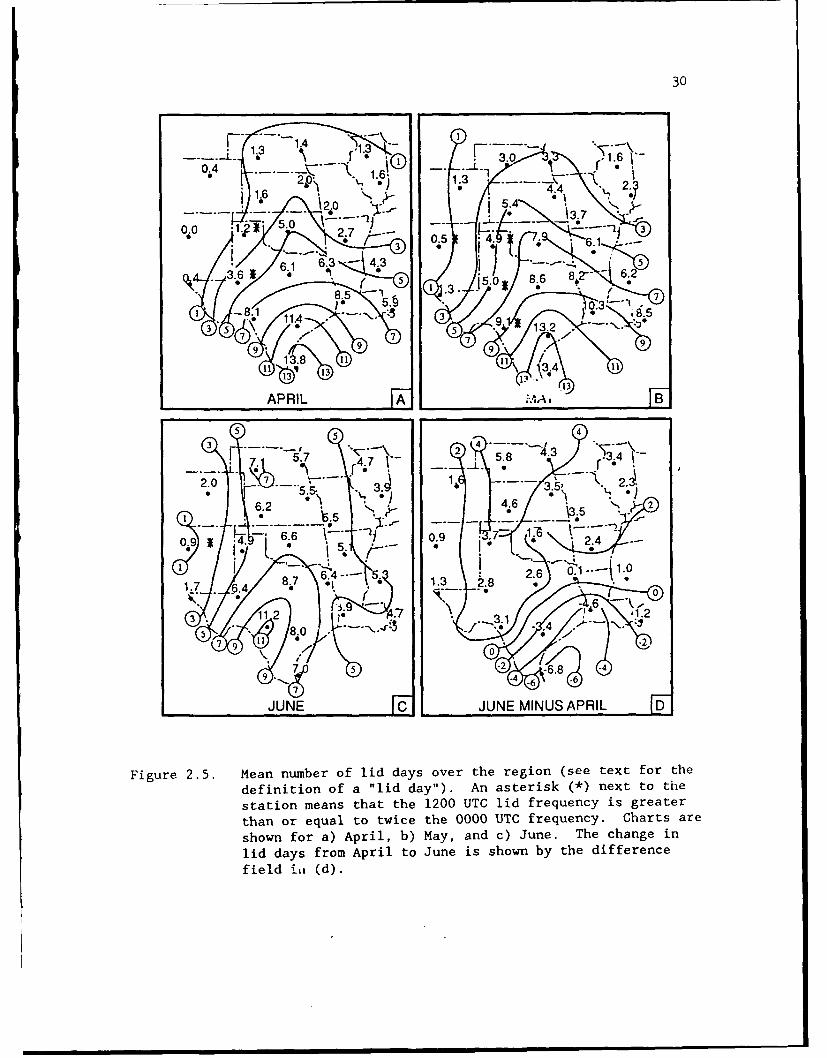
30
3 *0 35 3
6o.1 6.3-. 3.. -_ o - - ..- . - S
--- TA I 1.6- -t .2• 1 2.3 - ,- _ _Z
0~ ~ .4.4•.d.
.112.0 5.40~'
deintinofa li ay).A asers 9* ett h
-1 -. -. - -1 3 .APRI AL 3A
27 - --2.0 1_5 4 . 6.1*
6.2 - 4.6
shown fo-)Ap-,b-My-ndc ue.Technei
6.6 1 8.9 24
8.7 .3
1 .43 .
13.8
JNCJUEMNSAPRIL 0A B
lid days from April to June is shown by the difference
field i• (d).
| | |F
31
low level moist layer (leading to a 1200 UTC lid maximum). The seasonal
trend in lid frequency is shown by the June-April difference field of
Fig. 2.5d, in which the westward and northward frequency progression is
well illustrated. Most of the change in geographic lid frequency occurs
between May and June over much of the study area. This shift in lid
frequency is caused by a combination of several different processes that
evolve during the spring season. In this study we will explore this
evolution in detail.
2.2.4 Elevated Mixed Layer Source-Region Climatology
The formation of the EML and lid in spring is largely controlled by
topographic influences. Previous studies (Carlson and Ludlam 1968; Tang
and Reiter 1984) have shown that the spring season is a transitional one
over the North American plateau, with the EML source region beginning in
northern Mexico in April and progressing northward with the season. In
order to complement the analyses of these previous investigations, we
use climatological values of mean maximum surface temperature to derive
surface potential temperatures (0) over northern Mexico and the western
U.S., utilizing the terrain elevation and the U.S. Standard Atmosphere
(1976) to derive surface pressure. Our analysis uses 161 Mexican
climatological stations, most having longer than a 15-year record, and
239 U.S. stations above 1000 m elevation, each having a 30-year record.
These surface 8 values are indicative of the mean 0 in the mixed layer
over the source region. Our calculations complement those of Carlson
and Ludlam by extending the analyses farther north and through the
entire spring. Our approach differs from that of Tang and Reiter in
32
that we use more surface climatological stations, and calculate surface
6 instead of 850-mb geopotential heights and temperatures.
The results of the analyses for April through June are shown in
Fig. 2.6. The warmer source regions in April (Fig. 2.6a) are the
central and northwestern portions of the Mexican plateau, with 0 between
44 and 52°C. These results are in good agreement with Carlson and
Ludlam's Fig. 2. In our analysis, however, surface values between 36
and 40 0 C extend as far north as southern Colorado (Carlson and Ludlam's
figure ends in northern New Mexico), which implies that a westerly or
southwesterly flow over this region could transport this mixed layer to
the east, forming a "cool" lid over the Great Plains. From April to
May, there is a large increase in the area of the source region, witl•
surface 0 values of 36-40 0 C extending into Wyoming, Utah, Nevada, and
eastern California (Fig. 2.6b). The 44-52=C values primarily exist in
northern Mexico, but pockets of very warm air are also observed over
portions of New Mexico and Colorado. The chart for June (Fig. 2.6c)
shows the 36°C isentrope extending into southern Montana, Idaho,
southeastern Oregon, and a large portion of California. The 44-52=C
region has expanded into Colorado, southern Wyoming, Utah, Nevada,
Arizona, New Mexico, and southwest Texas. The May to June transition in
mean maximum surface 0 values over the Rockies and the Great Basin is
greater than that for April to May. This is consistent with the lid-
frequency charts in Fig. 2.5, which show the emergence of a secondary
lid frequency maximum over western Nebraska in June. A rough comparison
of our June surface 6 analysis with Tang and Reiter's July 850-mb chart
(their Fig. 1) shows that the 850-mb warm air has the same broad west-
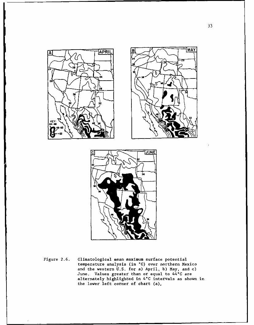
33
S2 ___24 24
280
332
Figure 2.6. Climatological mean maximum surface potentialtemperature analysis (in °C) over northern Mexicoand the western U.S. for a) April, b) May, and c)June. Values greater than or equal to 44°C arealternately highlighted in 4°C intervals as shown inthe lower left corner of chart (a),
314
east expanse and large latitudinal extent as do our high e values.
Their temperature maxima are equivalent to a 9 value of around 41*G,
which is not unreasonable considering that they used monthly mean
temperatures as opposed to mean maximum temperatures. Indeed, their
analysis shows the persistence of the large EML source region into July.
Comparison of the lid frequency charts in Fig. 2.5 wiuh the surface
0 analyses in Fig. 2.6 suggests that the westward and northward shift in
lid frequency from April to June is partially tied to the northward
expansion of the potentially warm EML source region into the Rocky
Mountains and Great Basin during the spring. Figure 2.6 also reveals
that the May to June change in surface 0 over northern Mexico is
relatively small compared to the change in regions farther north, ansi is
probably tied to the onset of the Mexican monsoon (see Fig. 14e in Tang
and Reiter 1984, and Fig. 5.26 in Lanicci 1984).
2.3 Synoptic Typing of Surface and 500-mb FlowsOver the Southern Plains
The motivation for producing synoptic flow types for the Great
Plains during the springtime is to determine the relationships between
the monthly changes in lid frequency and characteristics, and the
occurrence of specific flow regimes. This allows us to go beyond the
statistical analyses and determine what physical processes are
associated with these patterns that make them favorable or unfavorable
for lid formation.
35
2.3.1 Methodology and Physical Assumptions
There are a number of typing techniques available for producing
synoptic climatologies. In most applications, the typing technique is a
formal procedure for classifying the dominant flow patterns. Due to
data storage limitations, the techniques are usually applied at only one
level in the atmosphere at a time. Although Schaefer and Doswell (1984)
used an empirical orthogonal function analysis to examine predominant
flow patterns at both 850 and 500 mb for progressive tornado outbreaks,
the data reductions were not done simultaneously.
In our study, we utilize a subjective typing technique that is
based on the physical processes important in lid formation and
evolution. In order to accomplish this effectively, the typing is
performed at two levels simultaneously. We chose the surface and the
500-mb level because the surface flow pattern controls the low level
moisture component of the lid sounding, while the 500-mb flow (near the
top of the EML in the majority of soundings) is a good indicator of the
advecting flow for the EML. Consideration of these two levels allows us
to define flow types on the basis of mean thermal advection in the
intervening layers through use of the thermal wind relationship. For
example, in the classic lid model, the flow veers with height and there
is warm-air advection in the lower half of the troposphere (see Fig. I
in Carlson et al. 1983). The same thermal wind relation can be used to
argue that a flow regime in which the winds are backing with height is
unfavorable for lid formation because there is cold-air advection in the
layer.
36
Given this physical basis (mean thermal advection in the lower
troposphere) for the typing technique, the sea level pressure and 500-mb
wind direction analyses at 1200 UTC for each day of the study period
were examined. Based on these charts, five surface and five upper air
categories are defined. A schematic diagram of each surface type is
shown in Fig. 2.7. The surface types are:
* High pressure ridging in a north-south axis over the region
(originating as a continental high from Canada) (Fig 2.7a);
* High pressure ridging in a northwest-southeast axis over the
region (usually the extension of a maritime high centered
over the Great Basin) (Fig. 2.7b);
* Weak return flow from the Gulf of Mexico (defined as a
situation where either the high pressure ridge has remained
anchored over the southeastern portion of the region--i.e.,
the Gulf is not completely "open", or the ridge has moved out
of the region and weak southerly flow with geostrophic
windspeeds less than 10 m s-I have developed) (Figs. 2.7c,d);
* Strong return flow from the Gulf of Mexico (defined as a
regime where the high pressure ridge has moved out of the
region and strong southerly flow with geostrophic wind speeds
on the order of 10 m s-1 or greater have developed) (Fig.
2.7e); and
* A frontal system traverses at least half the area by analysis
time (Fig. 2.7f).
The need for the last type arises because the incursion of a frontal
system across the entire region cuts off the source of the EML. The
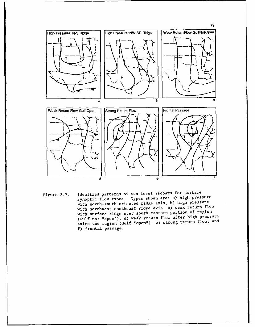
37
High Pressure: N-S Ridge High Pressure: NW-SE Ridge WeakReturnFIow-GuNfNotOpen
1 -- -s Al
a b c
Weak Return Flow-Gulf Open Strong Return Flow Frontal Passage
L L
_ -- .. .--
d ef
Figure 2.7. Idealized patterns of sea level isobars for surface
synoptic flow types. Types shown are: a) high pressure
with north-south oriented ridge axis, b) high pressure
with northwest-southeast ridge axis, c) weak return flow
with surface ridge over south-eastern portion of region
(Gulf not "open"), d) weak return flow after high pressure
exits the region (Gulf "open"), e) strong return flow, and
f) frontal passage.

38
surface types have a natural temporal continuity, with the high pressure
types usually followed by a strengthening flow, with a transition taking
place as the surface front moves through the area. This temporal
continuity was frequently observed in our data, but other transitions
occurred as well. The timing of the moist "return" flow from the Gulf
of Mexico, after the eastward retreat of the surface high, is very
important in setting up the pre-convective environment. For example,
the moist return flow was shown to be important in the initial formation
of the surface dryline (Schaefer 1974). We also note that our surface
high-pressure and weak return-flow synoptic types are nearly identical
to the synoptic patterns presented by Lewis and Crisp (1989) and Weiss
(1989), in their wintertime studies of return-flow situations in the,
southern Plains (compare the descriptions of our high pressure types
with the discussion in sections 2.1 and 2.2 of Lewis and Crisp 1989;
also compare our Figs. 2.7c,a,d with Figs. 2-4, respectively, in Weiss,
1989). Further discussion of the temporal continuity in synoptic types
as related to lid formation appears in Part 2 of this study (Lanicci and
Warner 1991b). The 500-mb flow types were based on the flow patterns
which appeared over the study area during the study period, and are
depicted in Fig. 2.8.
The flow categories are:
* Northwesterly (Fig. 2 .8a);
* Westerly (Fig. 2.8b);
* Southwesterly (Fig. 2.8c);
* Anticyclonically curved (Fig. 2.8d); and
* Cyclonically curved (Fig. 2.8e).
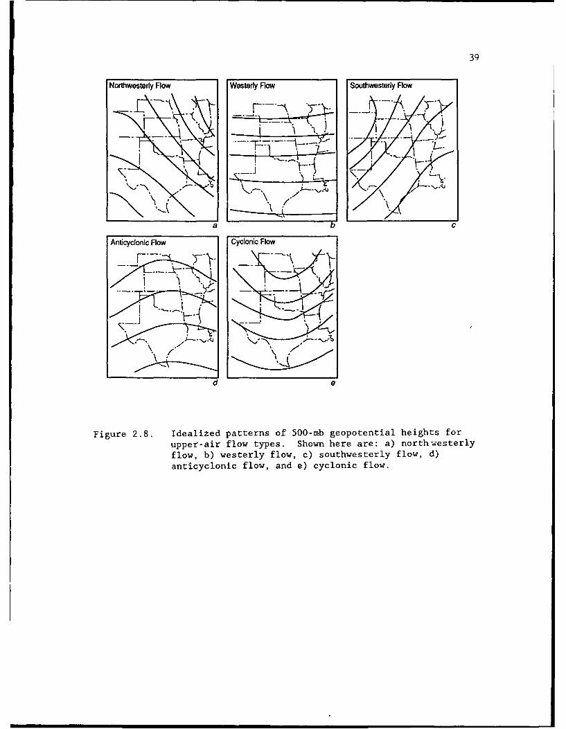
39
Northwesterly Flow Westerly Flow Southwesterly Flow
a b C
Anticyclonic Flow Cyclonic Flow
LV
de
Figure 2.8. Idealized patterns of 500-mb geopotential heights forupper-air flow types. Shown here are: a) northwesterlyflow, b) westerly flow, c) southwesterly flow, d)anticyclonic flow, and e) cyclonic flow.
40
There were several other 500-mb flow directions observed over the
region, such as northerly, southerly, southeasterly, and easterly, but
these directions were not observed in April, and only accounted for 2.4%
of the May patterns and 7.5% of the June patterns.
Combining these surface and 500-mb flow patterns produces
categories for which we can qualitatively infer the thermal advection in
the intervening layer. For example, north-south surface ridging with
northwesterly flow aloft (Figs. 2.7a, 2.8a) represents an unfavorable
situation for EML and lid formation because the winds are backing with
height everywhere except in the extreme western portion of the study
area, and the surface high restricts the high 0, air to the Gulf of
Mexico and extreme southern Texas. Conversely, a strong return flow
from the Gulf with southwesterly flow aloft (Figs 2.7e, 2.8c) has winds
veering with height, allowing the EML to enter the Plains from the
Mexican plateau and overrun the moist, southerly low level flow. This
is the flow configuration most closely associated with the classic lid
model discussed earlier. Some flow configrations are unambiguously
associated with either the unfavorable or favorable conditions for lid
creation. However, we will see shortly that some flow types can
actually be associated with both favorable and unfavorable lid-formation
situations, depending upon the critical superposition of specific
features at different levels.
2.3,2 Lid Freguencies Associated with the Various Flow Types
After determining the dominant synoptic flow type for each day of
the study period, we compiled the monthly lid-occurrence frequencies of
41
each type. Figure 2.9 shows, for each flow type, the number of days on
which different numbers of lid soundings were observed during the
period. The dashed line for each month separates "large" (L) and
"small" (S) lid-coverage areas, and is based on the median lid frequency
for the month (see Fig. 2.4).
For April (Fig. 2.9a), the high pressure surface types are
primarily unfavorable for lid formation, while the strong return-flow
and frontal-passage surface types are primarily favorable for lid
formation. In general, the midtropospheric southwest-flow types,
collectively, have the highest mean number of lid stations, which
confirms that the southwest flow regime has the greatest contribution to
the April EML/lid occurrence frequency. Of the seven types with
occurrences in both the L and S coverage ranges, three are associated
with 500-mb troughs, while four are associated with weak return flow.
For May (Fig. 2.9b), there is a greater range in the number of lid
stations for some flow types. For example, the flow type with the
highest mean number of lid stations (strong return flow with southwest
flow aloft) has four occurrences in the S range. The high pressure
types still remain largely unfavorable for lid formation.
By June, the Great Plains abuts elevated heat sources to the south
and to the west (Fig. 2.6c). At low levels, weak return flow has a
combined occurrence frequency of 71.7%, and provides for a nearly
continuous presence of high 8. air over most of the Plains region. Now,
in June (Fig. 2.9c), there is only one high pressure type and it is
associated primarily with small lid-area coverages. The northwest-
southeast ridge surface type no longer appears in June. This
42
Figure 2.9. Lid frequency by synoptic type for a) April, b) May, and
c) June. The ordinate denotes the number of lid stations,and the abscissa denotes the five surface synoptic types
(each separated by the vertical line), subdivided by 500-
mb type. The numbers along the abscissa refer to the
following surface types: 1 = N-S pressure ridge, 2 = NW-SE
pressure ridge, 3 - weak return flow, 4 = strong return
flow, and 5 = frontal passage. The 500-mb flow types are
abbreviated as follows: NW - northwest, W = west, A =
anticyclonic, SW = southwest, and C = cyclonic. The
number of occurrences of each synoptic type and
corresponding number of lid stations are shown. The
horizontal dashed line separates "small" and "large" lid-
coverage areas.
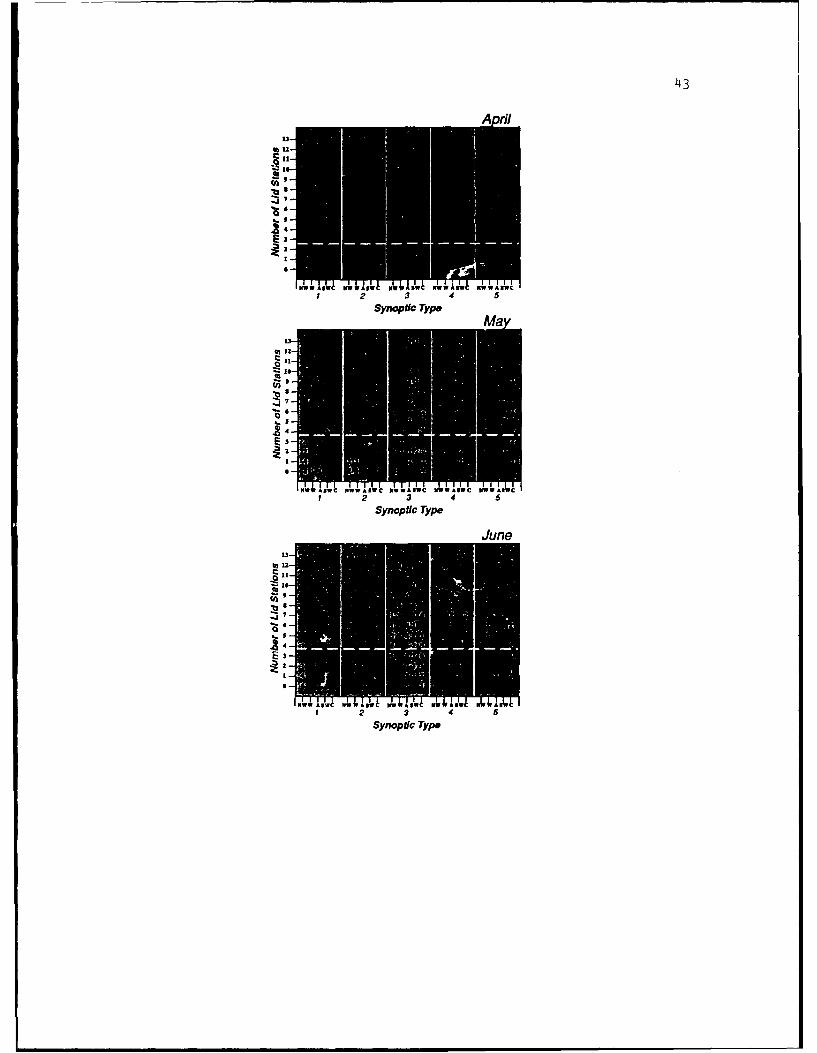
~43
-.84a
2 3 4 5
Synoptic Type
tMo
3,
2I
N0 AW WAIC IWAW-93 4
syot)~p
-4
3
7 2 3 4 5Synoptic Type
44
disappearance is consistent with the transition of the Great Basin from
an elevated cold source to a heat source. For example, the transient-
surface-anticyclone frequencies for January and July presented by Bryson
and Hare (1974) for North America (their Figs. 26 and 27) show that
there is a January maximum over the Great Basin and a primary track
towards the southern Plains, which disappears by July. The dominance of
weak return flow in June is consistent with the westward expansion of
the Bermuda anticyclone, which changes the mean low level flow direction
from southwesterly in April to southerly by June, and strengthens the
gradient-level flow over the western Plains (see Figs. 2d-f in Tang and
Reiter 1984).
The 500-mb southwest flow, which accounts for 32.5 and 25.8% of all
flows in April and May, respectively, only accounts for 17.5% in June.
However, the strong return flow/southwest flow aloft pattern still has
the highest mean number of lid stations (8.3), and this is higher than
either the April or May values. Despite the decrease in occurrence
frequency of this flow type, it remains the best producer of widespread
lids. While 500-mb southwest flow has decreased in occurrence frequency
during the season, anticyclonic flow has increased from 15.8% in April
to 30.8% by June. This increase in 500-mb anticyclonic flow frequency
during the spring is consistent with the 500-mb closed-anticyclone
climatology of Parker et al. (1989) (see their Figs. 4d-f). Another
interesting observation from Fig. 2.9 is the transition of the weak
return flow/northwest flow aloft pattern from a largely unfavorable
synoptic type in April to a more favorable one in June as a result of
the northward movement of the EML source region.
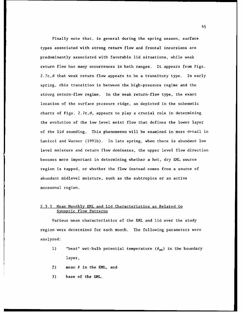
45
Finally note that, in general during the spring season, surface
types associated with strong return flow and frontal incursions are
predominantly associated with favorable lid situations, while weak
return flow has many occurrences in both ranges. It appears from Figs.
2.7c,d that weak return flow appears to be a transitory type. In early
spring, this transition is between the high-pressure regime and the
strong return-flow regime. In the weak return-flow type, the exact
location of the surface pressure ridge, as depicted in the schematic
charts of Figs. 2.7c,d, appears to play a crucial role in determining
the evolution of the low level moist flow that defines the lower layer
of the lid sounding. This phenomenon will be examined in more detail in
Lanicci and Warner (1991b). In late spring, when there is abundant low
level moisture and return flow dominates, the upper level flow direction
becomes more important in determining whether a hot, dry EML source
region is tapped, or whether the flow instead comes from a source of
abundant midlevel moisture, such as the subtropics or an active
monsoonal region.
2.3.3 Mean Monthly EML and Lid Characteristics as Related toSynoptic Flow Patterns
Various mean characteristics of the EML and lid over the study
region were determined for each month. The following parameters were
analyzed:
1) "best" wet-bulb potential temperature (0wb) in the boundary
layer,
2) mean 8 in the EML, and
3) base of the EML.

S46
The charts of mean EML characteristics were constructed using both
EML and lid soundings for each rawinsonde station at 1200 UTC. Recall
from section 2.2.1 that EML soundings contain the capping inversion with
the EML above, and a PBL that is buoyantly stable, whereas the lid
soundings have a PBL that is buoyantly unstable. In order to eliminate
situations with only isolated EML/lid coverage, the data tabulation
includes only those days for which a minimum of four lid stations (three
in April) was observed over the region (above the dashed line in
Fig. 2.9). Furthermore, only the most frequent lid-producing synoptic
patterns were included in the compilation, accounting for roughly 80% of
all the days with greater than the median number of lid stations during
the study period.
The monthly mean analyses are shown in Fig. 2.10. For April (Fig.
2.10a), the mean EML 9 pattern (dashed lines) shows a slight ridge
extending from south-central Texas into Mississippi, and a second ridge
extending from northeast Texas into western Missouri. The orientations
of the potential-isotherm ridges suggest that the primary EML source
region is northern Mexico during this month. The highest EML 9 values
(greater than 39°C) are confined to southern and southwestern Texas, and
the 8 gradient has a general north-south orientation over nearly the
entire region. However, EML 0 values as low as 32-34 0 C appear in the
northern sections of the study region, suggesting that the cooler source
regions of the southern Rockies may be playing a role in producing the
EML over this area, as suggested by Fig. 2.5a. Indeed, this result
indicates that a much cooler EML can form a lid in the early spring, and
that the Carlson et al. (1983) estimate of 38-48°C for a typical EML 9
47
MA,
S12
14
w
Figure 2.10. Mean analyses of EMIL and lid parameters for the mostfrequently occurring EML/lid-producing synoptic patterns.Charts are shown for a) April, b) May, and c) June. Thesolid lines denote mean "best" wet-bulb potentialtemperature in °0 and are analyzed at 2°C intervals. Thedashed lines are the mean potential temperature (°C) inthe EML (when observed), and are drawn every degree. Thelight shading highlights regions having a mean EML baseabove 750 mb, with the dark shading indicating a mean EMLbase below 800 nib. The scalloped border outlines the25% occurrence frequency of the EML/Iid.
48
is most valid over Texas. The mean EML base (shading) rises toward the
north over the region, reflecting the dominance of the southwesterly
flow regime (Fig. 2.9a). The 0wb pattern for this month (solid lines)
also supports the dominance of the strong southerly low level flow, with
a ridge of 8wb oriented along a nearly north-south axis from the Gulf
coast of Texas to the Kansas-Missouri region. The inclusion in Fig.
2.10 of only the patterns that produce greater than the median number of
lid stations reveals a much more structured 8wb field than was shown in
FC89 (their Fig. 18) which represented an average for all April days in
the study period. Thus, our results for April (Figs. 2.9a, 2.10a)
complement those of FC89 (their Figs. 18, 19) by illustrating the
synoptic patterns that contribute to both the creation of the EML and
the existence of high 8,, air beneath the inversion.
The overall EML/lid character changes as we move into May (Fig.
2.10b). The EML potential temperature pattern has changed dramatically,
with the emergence of a gradient aligned roughly west to east, and a
ridge axis oriented from western Oklahoma into southern Illinois. The
39°C potential temperature isopleth now extends from western Nebraska
southward into southern Texas, and values as high as 42°C appear over
southwest Texas. The northward expansion of the warm EML is consistent
with the source region analysis in Fig. 2.6b, and the appearance of the
warmest EML in southwest Texas is consistent with the observation that
the warmest surface 8 values remain over northern Mexico in May.
Although the height of the mean EML base still generally increases
toward the north, from Texas to Nebraska and Iowa, there is more of a
west-east component to the gradient than in April, reflecting the
49
increasing contribution to lid formation from midtropospheric
anticyclonic and northwest flows (Fig. 2.9b). The EML is lower than in
April over Nebraska, Kansas, Missouri, Illinois and Arkansas, and has
changed little elsewhere, except over the Texas panhandle where it has
risen. The changes in the structures of the EML 9 and base confirm that
there are multiple flow patterns contributing to EML and lid creation.
The 0, pattern has also changed from April, showing a broad ridge axis
with two branches, one over southwest Texas, and a second from central
Oklahoma to western Kansas. The westward shift in the location of the
0 wb ridge axis in May is in the same direction as the shift in the
location of the maximum lid-frequency axis (Fig. 2.5b).
The composite analysis for June (Fig. 2.10c) shows still further
changes in the structure of the EML and lid. The 8wb ridge, which was
broad in May with two small branches, has consolidated into a single
axis with a distinct anticyclonic curvature from south Texas into west-
central Oklahoma and central Kansas. Also notice that there is abundant
moisture present in the June 0wb field, reflecting the warming and
moistening of the boundary layer that takes place as a result of
increasing surface fluxes. The EML thermal pattern is similar to that
of May, but the ridge axis now has a distinct northwest to southeast
orientation, extending from southwest Kansas into southern Arkansas and
northern Louisiana. A trough exists over the Gulf of Mexico and extends
into the Texas coastal region, which is the same area that showed the
decrease in lid frequency from May to June (Fig. 2.5d). The orientation
of the EML thermal ridge axis reflects the observation from Fig. 2.9c
that southwest flow is no longer the dominant EML-producing pattern in

50
June. Perhaps the most important observation from Fig. 2.10c is that
the EML base near the thermal ridge axis actually lowers from northwest
to southeast, suggesting that the flow is subsiding away from the source
region. This is in stark contrast to the classic model for southwest
flow that describes large scale vertical ascent along the trajectory of
the EML. In general, the mean EML base is lower in June over the
majority of the study region, indicating an increasing influence on the
EML base from large scale flow patterns associated with subsidence as
the late spring approaches. This is in contrast to our intuitive
expectation that the boundary layer depths and inversion heights should
be higher at this time of year than in the early spring. Northwest and
anticyclonic 500-mb flows are associated with large scale subsidence-
over the majority of the study region due to the location of the ridge
axis (recall Figs. 2.8a,d). A monthly examination of EML static
stabilities in our sample from Fig. 2.2 shows that there is a slight
increase in mean a from 1.98°C 100 mb-' in April to 2.210C 100 mb-' in
June. Thus, while subsidence is not a contributing process to most
early-spring lid situations, it appears to be important in many late-
spring lid situations.
2.3.4 Seasonal Changes in the Characteristics of the EML and Lid
The westward shift in the Owb ridge axis from April through June
correqnonds closely to the shift in lid frequency shown in Fig. 2.5d.
While the northward expansion of the high lid frequencies during the
season is likely tied to the northward expansion of the EML source
region and the increase in low level moisture, the westward shift in the
51
axis of maximum lid frequency is primarily related to the westward shift
of the Owb ridge axis and the increase in EML 6 over the western Plains.
A difference chart between June and April (not shown) reveals that the
values along the maximum-change axes of Owb and EML 8 are nearly
coincident over this area.
There is an additional factor which accounts for the decrease in
lid frequency over the Gulf coastal area during the spring. We observed
a large number of uncapped soundings in the late spring over the Gulf
coast and adjacent areas to the north. These soundings, defined in
section 2.2.1, are often associated with an unusually moist layer below
the inversion, with resulting high Ow values that prevent the EML from
effectively capping the PBL. An examination of 1200 UTC sounding data
over the study region reveals that these uncapped soundings appear most
frequently over the Gulf coastal area in June, as shown by the
occurrence statistics in Table 2.1. In order to isolate the situations
in which the uncapped sounding is caused by the appearance of an
unusually moist PBL, we consider only those soundings in which the EML
is at least 80 mb deep (roughly 1 km) and the base is at or below 700
mb. The 80-mb EML depth criterion is used to eliminate those situations
in which the EML is shallow, which itself can be a reason for the lid
strength being non-positive. The additional criterion of an EML base at
or below 700 mb is based on an estimate from Carlson et al. (1983), who
stated that a typical lid base would have to be below 650-750 mb in
order to form an effective cap on a layer with 0. = 22-24°C. The
application of these EML depth and base criteria allows us to isolate

52
Table 2.1 Uncappedl Soundings for Four Gulf Coast Stations(Based on 1200 UTC data)
Occurrences
Station April May June
Brownsville, Texas 1 4 11Victoria, Texas 1 2 6Lake Charles, Louisiana 0 5 9Boothville, Louisiana 3 2 6
Total for 4 Gulf Coast 5 13 32stations
Total for all 22 stations 12 20 66
Total capped soundings for 190 203 1024 Gulf Coast stations
Mean EML/Lid Parameters (all four Gulf Coast stations)
April May June
Parameter uncapped' capped uncapped' capped uncapped' capped
0 wb (°C) 20.9 18.8 22.6 20.9 24.1 22.9Level ofRH break (mb) 828 897 796 904 827 909
Pbase (mb) 798 821 727 829 788 842
Ptop (rob) 603 548 510 614 614 6440emI (°C) 36.0 37.6 40.7 37.0 38.8 37.5or'. ( 0 C) 20.7 23.9 21.3 24.7 23.1 25.4
'See text for lid-base and lid-depth criteria
53
those soundings in which a deep EML cannot effectively cap the moist PBL
below.
The EML/lid comparison statistics in the lower portion of Table 2.1
reveal that the PBL 0wb of the mean uncapped sounding is 1.2 - 2.1°C
higher than that of the mean capped sounding. Additionally, the level
of the RH break of the mean uncapped sounding is consistently above 830
mb in all three months, while that of the mean capped sounding is near
or below 900 mb each month. Since the level of the RH break is an
indicator of the moist-layer depth, this result suggests that the
uncapped soundings generally have a much deeper moist layer than the
capped soundings. Although a higher-based EML over a deeper moist layer
results in the absence of a negative energy area in the uncapped
sounding, the sounding still contains considerable potential instability
due to the presence of the dry EML above the deep moist layer. An
examination of the lid coverage on the days when uncapped soundings
were observed reveals that about 40% of the Gulf Coast uncapped
soundings occur on small lid-coverage days. The synoptic type most
frequently observed with these uncapped soundings is a weak surface
return flow, with either cyclonic or anticyclonic flow aloft. We
conclude that the Gulf Coast uncapped sounding is primarily associated
with those late-spring synoptic patterns in which the trade-wind flow
regime dominates the Gulf and its adjacent coastal region. In such a
regime, deep moist layers are possible due to the height of the trade-
wind inversion over the moist-layer source region, which is typically
around 2600 m over the western Caribbean in early summber (Gutnick
1958). In such synoptic flow patterns, the Gulf coast is not likely to
54
have a capping lid owing to the difficulty of transporting an EML to
this area that is potentially warm enough to cap such a deep moist
layer. Thus, the presence of uncapped soundings over the Gulf coastal
region is consistent with the westward "shift" in the axis of maximum
lid frequency from April to June (Fig. 2.5d). If the Gulf Coast
uncapped soundings are added to the mean EML/Iid composite charts in
Fig. 2.10, they would only slightly affect the April and May 0wb and EML
0 patterns, but would significantly raise the mean June EML base, and
alter the mean 0wb and EML 0 patterns over this area.
2.4 Discussion
A complete description of the EML and lid climatology in the spripg
has been presented. It has been shown that the lid typically covers
about 20 to 25% of the southern Great Plains, and that lid-coverage
areas greater than 50% are rare (less than 2% of the days). Plthough
the mean lid-coverage area stays roughly the same during the season, lid
soundings are observed more often as the season progresses. The study
shows that the northward expansion of the lid-coverage area during
Spring is primarily controlled by the northward expansion of both the
EML source region and the low-level moisture. The westward shift of the
maximum lid-frequency axis is associated with a seasonal displacement of
the low-level moisture axis caused by the westward expansion of the
Bermuda anticyclone, as well as the appearance of uncapped EML soundings
over the humid Gulf coastal region in late spring. The flow patterns
most closely associated with the classic lid model have their highest
occurrence frequencies in the early and midspring and have the highest
55
mean number of lid stations in all three months. As the EML source
region expands, more flow types can produce a lid over the region, as
evidenced by the evolution of the weak-return-flow/northwest-flow-aloft
type from a largely unfavorable lid-producing pattern in April to a
favorable one in June. The decrease in midtropospheric southwest flow
types and the concurrent increase in anticyclonic flow types help
explain the gradual lowering of the mean lid base during the spring
season. More importantly, the dominant lid-producing patterns in the
late spring are associated with large scale subsidence, in stark
contrast to the southwest flow regime that dominates the early spring
and is associated with rising motion to the east of the upper level
trough. Perhaps even more important is the coincidence of the emerging
lid-producing anticyclonic and northwest flows with the beginning of the
severe storms season in the central and northern Great Plains; a season
which is characterized by the presence of anticyclonically curved and
northwest flow patterns in the middle troposphere over this area (Johns
1982; 1984).
The implications of this EML/lid climatology on severe weather
analysis and prediction over the southern Plains are very important, and
are summarized oelow:
1) The southwest flow regime associated with classic models of
lid formation and severe weather only accounts for 25 to 30%
of all early spring days, and only about 18% of all June
days. These flows are, however, the most efficient producers
of lids during the entire season.
56
2) By midspring, the lid can occur with several different flow
types because the Rocky Mountains and Great Basin have become
elevated heat sources. The additional flow patterns are
likely to produce different configurations of the low level
moisture tongue, lid-edge front, and other imaiportant severe
storm features.
3) The flow regimes with favorable wind shear (i.e., veering
with height in the lower half of the troposphere) may not
always produce an appreciable lid area; the forecaster must
perform careful analyses of the important low level moisture
and midlevel thermal features, especially in weak return-flow
situations.
4) Since the lid forms more often in flow patterns associated
with large scale subsidence during the late spring and early
summer, diabatic processes such as surface heating may become
more important in locally removing the lid in the absence of
dynamical forcing.

57
Chapter 3
THE SYNOPTIC CLIMATOLOGY: THE LIFECYCLE OF THE LID
3.1 Chapter Introduction
The elevated mixed layer inversion, or lid, is an important feature
of the severe-storm environment over the central U.S. in spring and
summer. The lid sounding, as defined here, is essentially the same as
the type 1 tornado sounding (Miller 1972) that is familiar to severe
storm forecasters. The two components of the lid sounding, namely the
warm, nearly adiabatic elevated mixed layer (EML) and the moist boundary
layer below the inversion, have vastly different geographic origins.
From early to midspring, the primary source region for the EML is the
Mexican plateau and the adjacent desert southwest of the U.S. The moist
layer below the EML originates through advection from the Gulf of
Mexico. In late spring and summer, there are multiple EML source
regions: the Mexican plateau, and the Great Basin and Rocky Mountain
sections of the western U.S. At this time, a persistent moist return
flow from the Gulf combines with substantial evapotranspiration from
surface vegetation to allow a large area of buoyantly unstable1 air to
exist over most of the southern and central Great Plains of the U.S.
from early June through the summer season.
1 Buoyant instability, as defined in this paper, refers to thestability of a saturated surface/low-level parcel with respect to themidt opospheric environment, as used in the Lifted Index of the NationalWeather Service and the buoyancy term of the Lid Strength Index.

58
A previous study (Lanicei and Warner 1991a, hereafter rcfzrred to
as LWl) identified certain synoptic flow patterns which are favorable
and unfavorable for lid formation during the spring (April, May, and
June) season. Surface high pressure systems over the southern Plains
(Kansas, Oklahoma, and Texas) were found to be associated with
conditions unfavorable for lid formation because they advect cold, dry
air southward and push the moist layer into the Gulf of Mexico.
Additionally, the geostrophic wind in these situations has a backing
wind profile and cold-air advection exists in the lower half of the
troposphere. In such situations, the midtropospheric warm layer is
confined to areas west of the Plains. These high pressure incursions
decrease in frequency from April to June, but appear as late as the end
of June during the period of study (1983-1986). Return flow from the
Gulf, combined with a midlevel flow from the EML source regions,
produces the necessary lid stratification when the EML thermal ridge
overruns the low level moist tongue in the southern and central Plains.
It was shown that midtropospheric southwesterly flow regimes produce the
largest areal lid coverages throughout the season. This is the
configuration most closely associated with the idealized conceptual
model of the lid for the central U.S. first proposed by Carlson and
Ludlam (1968). However, in late spring, synoptic patterns associated
with large scale subsidence downstream from the EML source, such as
midlevel anticyclonic and northwest flows, become associated with lids
over the central and northern Plains. These occur more frequently in
late spring than do southwesterly flow patterns. The lid-producing
patterns of the late spring are characterized by a more northern EML
59
source region (the Great Basin and Rocky Mountains), and a low-level Ow
tongue that is located over the western Plains.
Although LWl demonstrate that the patterns of EML and lid
occurrence undergo a significant seasonal evolution, the entire life
cycle of EML and lid formation and dissipation has not been documented.
Portions of the life cycle of the lid have been investigated in
observational studies (e.g., Carlson et al. 1983, Doswell et al. 1985,
and Rockwood and Maddox 1988), three dimensional modeling studies (e.g.,
Anthes et al. 1982, Benjamin and Carlson 1986, and Lanicci et al. 1987),
and two-dimensional modeling studies (e.g., Benjamin 1986). The
modeling studies examined the sensitivity of EML formation over northern
Mexico and lid formation over the southern Plains to the horizontally
varying surface fluxes and soil moisture. The three dimensional
simulations were initialized during time periods when the lid was
already established over the Plains states, while the two-dimensional
study examined formation of the EML over an idealized plateau during a
single diurnal heating cycle. The present study examines the entire
cycle of lid formation and dissipation, utilizing the same database as
LWl and Farrell and Carlson (1989). We examine time-series analyses of
lid occurrence for each of the spring seasons in our four-year period of
record to determine the cyclic characteristics of lid occurrence, and
any seasonal trends in that periodicity. We then define two types of
lid cycles, and discuss the various stages in each type, including the
initial formation of the EML over the source region. The combined
surface/500-mb synoptic types defined in LWI are employed in this study
to characterize the flow evolution at each stage of the lid cycle, and
6o
build on the results of LWI by putting the various flow types into a
temporal context. Finally, we produce composite mean analyses of
representative synoptic types to examine the three-dimensional structure
and dynamics at different stages of the lid cycle.
3.2 Time Series Analysis of Lid Occurrence
A time series of lid occurrence over the study area was produced
for each of the four years in the study. The study region encompasses
the southern Great Plains and surrounding states (see Fig. 2.1). Only
1200 UTC analyses are used in order to minimize biases in the horizontal
extent of the lid area owing to daytime heating and moist convection.
Possible biases in lid frequency due to nocturnal inversions are
eliminated by the lid analysis program, which screens them out. The
number of U.S. rawinsonde stations in the study region is 22; the
maximum number of lid soundings observed at any one time during the
study period was 13. Figure 3.1 shows the number of lid soundings in
the study region for each of the 91 days in the 1985 record, which had
the fewest missing data of the study period. This time series, which is
representative of the four year record, shows a definite periodicity in
the lid's occurrence, including three cycles associated with a large
lid-coverage area (10 stations) which occurred about three weeks apart.
We examined each of the four time series in order to identify the
number of separate lid cycles that occurred during the period in each
year. The following criteria were used to define the beginning and end
of each cycle:

61
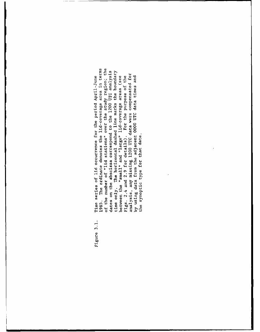
.- 4 r~C.0C120 cc
*.4CU 4 U Z 0 44W0) o. .0 0) 0 0) " Q
A cd >( 4. CU 0 o 0)
w 4) w u a) 0) $4 ) 4-
o b 4-)O. co 0
o 0 ~0 0c 4~) 0) E4
0. bD 0) 0 -4 ho: 0 co"2.-4C n04 ý,4 O C).UO"o4 ý4 A o
C0 " U ) 0)- 4 4
a)4 0 -4C bO 0cdl- 0)C
$4 ).-4 0 CU..4 CU
0 C ) 0) . U-i 4) Z- U 4j)
2.)041 .0.- co ) n -40)cau t0)rIZ 0u -0
o ~ t "4Cl.- to.J
q.- co Q.,- O -) 00)
* 0 .410 0) 4)' ~CN. ccI
02- 2-4 In-4 0
w - ý~4 = *44 r4 4Cl) 0 00 (12'd E
.4 044 ) CO *frý4 2U0) r-4- 0 ). 0) la Cl) (44 >1
0 4 4J)ib 0)
*.) 0' riI U .' 0) .-4 .1
VIn ) t ý
X0 n a)M)4) - :
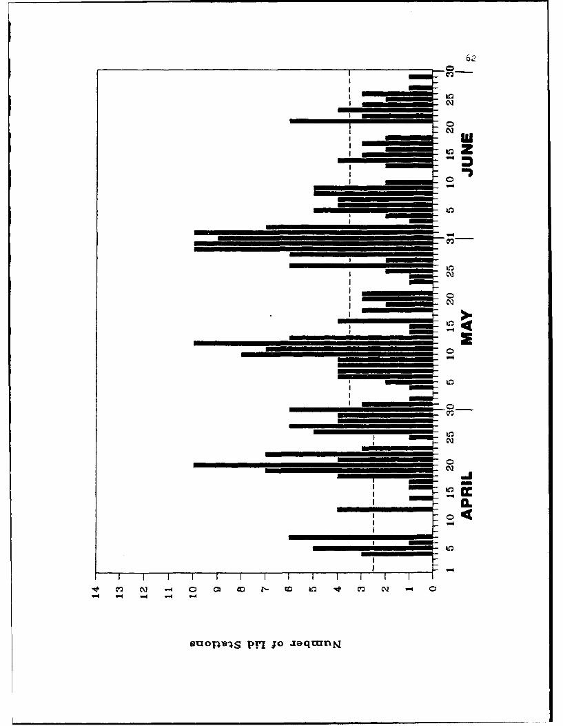
62
CQ
0 Q 1
0
I ~C)
I 0i
_ _o_ _co_ _ _ _ _ _ _ _w4
______4_91S________________

63
1) The beginning of the lid cycle is defined as the day when a
minimum lid coverage is first observed; the number must be
below three stations in April, and below four in May and
June. The three- and four-station criteria denote the
separation between what we define as "large" and "small" lid-
coverage areas. 2
2) A cycle extends from the lid-coverage minimum defined above,
through a maximum that is at least three stations in April
and four in May and June, and then to the next lid-coverage
minimum.
3) When a surface synoptic type associated with high pressure is
observed over the region near the time of lid-coverage
minimum, that day is designated as the beginning of a new lid
cycle, even if it is not the day with the actual minimum lid
coverage. This is done because the high pressure incursion
is responsible for generating the lid-coverage minimum.
The cycles, so defined, do not include all the days in the study period
because some days showed no lid coverage in the large-area range. See,
for example, the 17-22 May 1985 period in Fig. 3.1. Also, the cycles
which began prior to 1 April or ended after 30 June could not be
included because portions of these cycles fell outside the period of the
study, resulting in the exclusion of some early April and late June
2Plots of the occurrence frequency of different numbers of lid
soundings (Fig. 2.4) are bimodal in April and May. A point of localfrequency minimum between the two lid-area modes is chosen aE a boundarybetween the small lid-area and the large lid-area portions of thedistribution. The median of the distribution is used as a basis fordividing the June distribution.
64
days. Altogether, 44 lid cycles were identified using the above
criteria, accounting for 81% of all the days in the study. A frequency
histogram of lid-cycle lengths for the three-month periods is shown in
Fig. 3.2. The mean period for the lid cycle during the spring season is
6.7 days, with a standard deviation of 2.6 days. The modal value is
five days, and the median is six days. The lid cycles range in length
from two to 15 days.
3.3 A Schematic Life Cycle of the Lid
3.3.1 Types of Lid Cycles
A chronology of the synoptic types that occurred during each of
the four springs in the study period was developed. The synoptic type
is defined in terms of a surface flow component, based on the sea level
isobaric pattern, and a 500-mb flow component based on the predominant
wind direction at this level over the study region. The synoptic typing
scheme is defined in LWI, to which the reader is referred for details.
Examination of the synoptic types occurring during each of the 44 lid
cycles reveals that certain types are well correlated with specific
stages of the lid cycle, whereas others can be associated with several
stages of the cycle. Certain flow types, such as a north-south surface
ridge with northwesterly flow aloft, are nearly always correlated with a
low number of lid stations because the surface component is associated
with cold, dry low level flow from the north, and the wind profile is
backing with height from the surface to 500 mb. Other types, such as
strong surface ,atorn flow with southwest flow aloft are usually
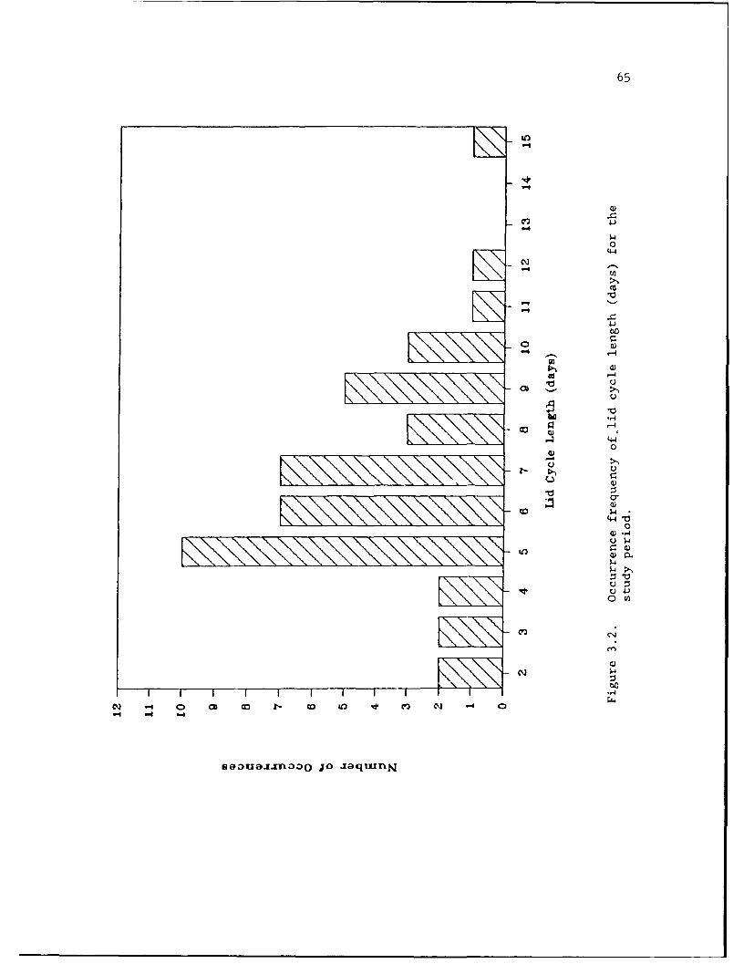
65
-o
03
oo
-44
0
C..L
'4-4 '
-- 4
•\/I -44
ý4-
Q410 E
iII
-4- '.a cc 0 nm Nr.
66
favorable for lid formation due to the combination of moist low level
flow being overrun by the warm, dry EML originating over the desert
southwest and northern Mexico.
Examination of the lid-occurrence and synoptic-flow time series
reveals that there are two primary types of lid cycles. These cycles
are defined as follows in terms of the surface flow type that prevails
at the beginning of the cycle: 1) those that begin with a surface
high-pressure incursion into the region (designated as H cycles); and 2)
those that begin with a weak return flow over the area (designated as R
cycles). Both types of cycles begin with no EML aloft, and must develop
a superposition of the two components of the lid sounding (i.e., the EML
and moist boundary layer) in order to attain a large lid area. The high
pressure incursions that begin the H cycle are associated with polar-air
outbreaks originating from the north or northwest. In this phase, the
low level flow is offshore, and the midtroposphere is dominated by cold,
stable air. After the high pressure phase, the atmosphere begins to
establish a low level moist layer over the Great Plains by passing
through a return-flow stage, during which the EML is forming over the
western states through surface heating over elevated terrain. A large
lid-coverage area is attained when the EML emerges from the west or
southwest and overruns the low level moist layer. In the R cycle, there
is no high pressure system present at the start of the cycle, and a low
level moist layer is already established at the outset. In the latter
case, a large lid-coverage area is reached earlier and the cycle has a
shorter mean period (5.5 days vs. 7.1 days). The R cycle is
characterized by the presence of weak low level flow, subtr3pical
67
circulations, and short wave features in the midtroposphere. Both
cycles can end with a frontal passage and a subsequent high pressure
incursion into the area, or with the removal of the EML while the moist
layer remains intact over the region. The H cycle is observed more
often than the R cycle (30 vs. 14 occurrences in the study period).
Table 3.1 formally defines the different phases of each lid cycle.
The decreasing frequency of high pressure incursions into the
region during the spring (LWl and others) affects the seasonal trend in
the occurrence of H and R lid cycles. Table 3.2 shows the four year
frequency of lid cycle types at five-day intervals through the season.
It reveals that the H cycle is dominant from early April to mid May. By
mid May the H and R lid cycles become equally frequent, with the H cycle
diminishing near the end of June. To further illustrate this May
transition, Table 3.2 shows a division of the spring season into "early"
and "late" segments. This division is consistent with the EML/lid
composite analyses of LWI, which showed that May represents a transition
between the early-spring lid regime, dominated by midtropospheric
southwest flows from northern Mexico, and the late spring, in which lid
production is mostly associated with midtropospheric northwesterly and
anticyclonically curved flows originating over the Great Basin and Rocky
Mountains.
3.3.2 Characteristics of the Lid Cycle Stages
Table 3.2 shows that the majority of lid-cycle days involve early-
spring H cycles (19), late-spring H cycles (11), and late-spring R
cycles (11). Each of these 41 lid cycles is analyzed in terms of the
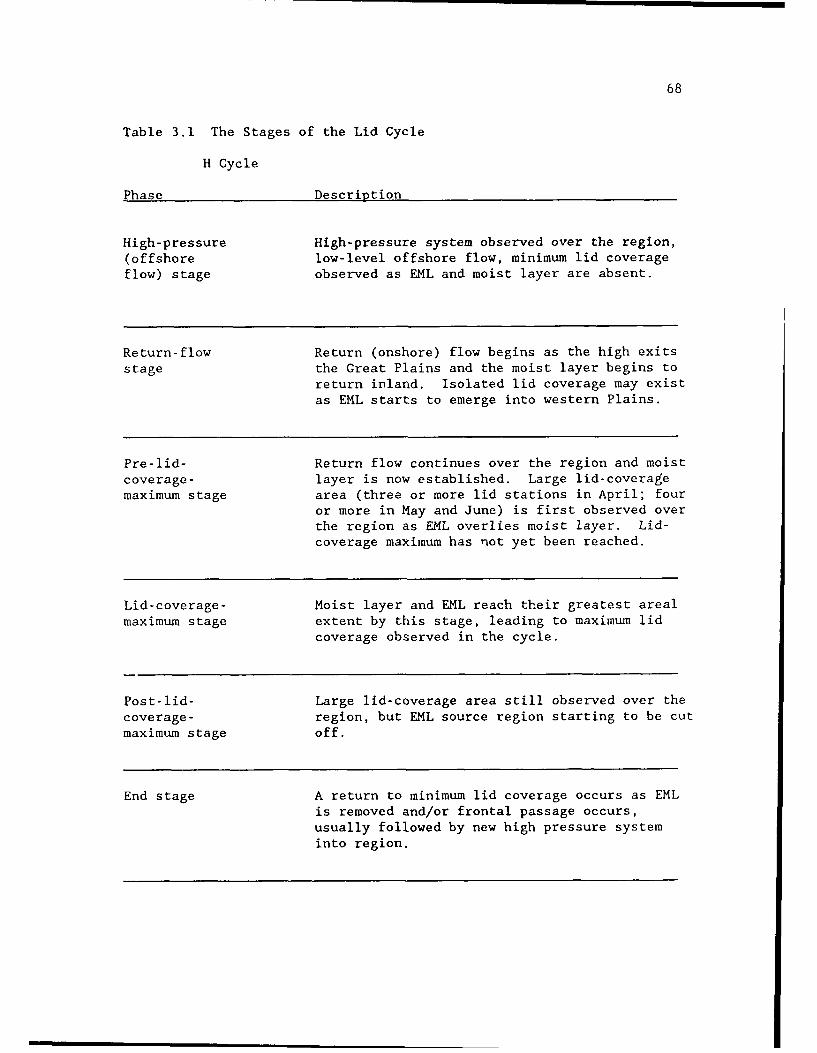
68
Table 3.1 The Stages of the Lid Cycle
H Cycle
Phase Description
High-pressure High-pressure system observed over the region,(offshore low-level offshore flow, minimum lid coverageflow) stage observed as EML and moist layer are absent.
Return-flow Return (onshore) flow begins as the high exitsstage the Great Plains and the moist layer begins to
return inland. Isolated lid coverage may existas EML starts to emerge into western Plains.
Pre-lid- Return flow continues over the region and moistcoverage- layer is now established. Large lid-coveragemaximum stage area (three or more lid stations in April; four
or more in May and June) is first observed overthe region as EML overlies moist layer. Lid-coverage maximum has not yet been reached.
Lid-coverage- Moist layer and EML reach their greatest arealmaximum stage extent by this stage, leading to maximum lid
coverage observed in the cycle.
Post-lid- Large lid-coverage area still observed over thecoverage- region, but EML source region starting to be cutmaximum stage off.
End stage A return to minimum lid coverage occurs as EMLis removed and/or frontal passage occurs,usually followed by new high pressure systeminto region,

69
Table 3.1 The Stages of the Lid Cycle (continued)
R Cycle
Phase Description
No high-pressure system is observed over theregion at start of this cycle. Cycle beginswith next phase.
Return- Return flow is observed over the region, moistflow stage layer is established, minimum lid coverage
observed as EML is largely absent.
Pre-lid- Large lid-coverage area is first observed overcoverage- the region as EML emerges to overrun alreadymaximum stage established moist layer. Lid-coverage
maximum has not yet been reached.
Lid-coverage- EML reaches its greatest areal extent by thismaximum stage time, leading to maximum overlap with the moist
layer, and maximum lid-coverage area.
Post-lid- Large lid-coverage area still observed over thecoverage- region, but EML source region starting to be cutmaximum stage off.
End stage A return to minimum lid coverage occurs as EMLis transported out of the region. In mostsituations, moist layer remains intact over thearea.
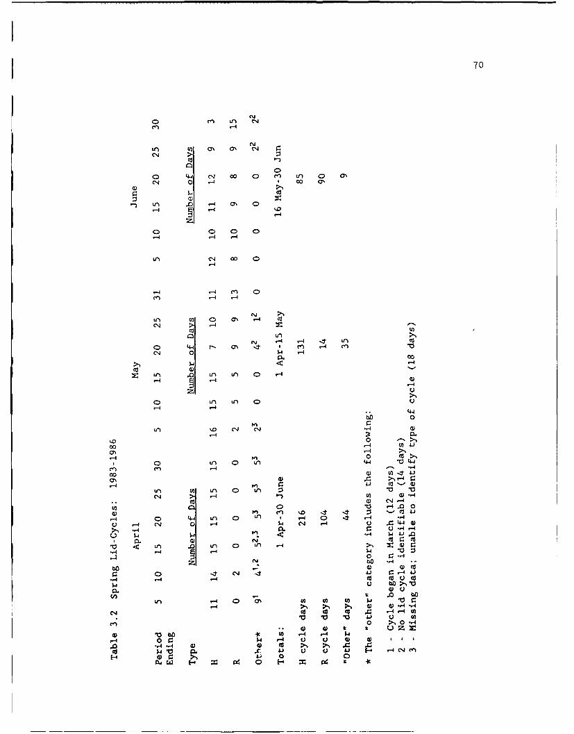
70
c-n Ln C'J
C14
Co 4.4 c'J 00 0a LA C> Oci 0 .-4 00 ON
42)
Q)
oC0 0 0
Lr) C4 00 4
'-4
1-4 1-4 cn 01n -4 1-4
Nl
-4 A
o 4-4 r- a' -ý - c')
5-4 '-4Ca a)
a A . Ln Ln 0 v~4
'-4 Ei -4
SviA LA C U'-4 '-4 .. 44-
0
00 r-4-4
0. 0 o
00 -4) )-'-4- -4 za
La) V) l.UlJ 104 > , 0 -ý
4) Ca-4 -
rA 442 LA 0 LA co &C'4 -41-) -4 a.-A
C) 0- C1 0-4.41.-ý -4 4-A 0' --4.-Ow)'4 . -$ - 4 41 '- a
'~<.0 LA 0 LA *-4 >- z r
,'4 *- -4 $
0 -4 14-4"
N4 bf b*
V)- 0 b)C
04 '--c c Ca -4-4U)
C;0 0 "4i
4) 1 0 bO -LAý4 0 r. w 14 0 (0 (
.0 -A 4-) 4) 4)fl>
to rbO ji 41 f-4 -4
Pd-- 0 Ha C4'
71
number of lid stations observed during each day of the cycle and the
synoptic type observed on each day of the cycle. Cycles are counted as
early or late spring on the basis of the beginning and ending dates.
For example, two cycles that ended on 16 May are counted in the early
season, and another cycle beginning on 15 May is counted in the late
season. All cycles are assumed to begin and end at 1200 UTC. Figure
3.3 shows the mean number of lid stations in each phase for each of the
three types of cycles. The late-spring H lid cycle (Fig. 3.3b) has thp
highest overall mean lid-coverage area, likely owing to the expanded EML
and moisture sources in the late season. A common feature in both H
cycles is the rapid increase in lid coverage as the moist layer is
established over the Great Plains. There is also a rapid decrease in
lid coverage occurring over the region as the frontal system moves
through, followed by a new high pressure system at the end of the H
cycle. By contrast, the R cycle (Fig. 3.3c) has smoother transitions
between phases because the low level moist layer remains well-
established throughout the entire cycle. It also has smaller mean lid
coverages than the H cycle.
Figure 3.4 displays the lengths of each phase of the early- and
late-season H, and the late-season R lid cycles. An interesting
observation from Fig. 3.4 concerns the mean lengths of the high pressure
and return flow stages. The high pressure stage is basically a period
of low level offshore flow, after which time the period of onshore flow
begins. For the early- and late-spring H cycles the mean period of
offshore flow (Fig. 3.4a) is about 1.4 - 1.6 days (about 36 h), which
compares favorably with the mean transition period between offshore and
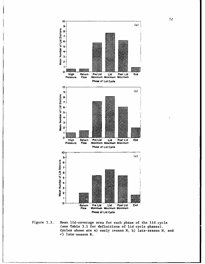
to C72
(I)
9j
Z3-
02-
High Return Pre Lid Lid Post Lid EndPressure Flow Maximum Maximum Maximum
Phase of Lid Cycle
I0
6-
o4-
Z 3-2
0High Return Pre Lid Lid Post Lid End
Pressure Flow Maximum Maximum Maximum
Phase of Lid Cycle
I0-9- (c)
.•8-
"6.25-
4-
z .-
Return Pre Lid Lid Post Lid EndFlow Maximum Maximum Maximum
Phase of Lid Cycle
Figure 3.3. Mean lid-coverage area for each phase of the lid cycle(see Table 3.1 for definitions of lid cycle phases).Cycles shown are a) early season H, b) late-season H, andr) late-season R.

73
Figure 3.4. Lid cycle phase length (in whole days) and frequencies forthe three types of lid cycles shown in Fig. 3 (legend isshown in panel 'a'). Phases shown are a) high pressure,b) return flow, c) pre-lid-maximum, d) lid maximum, e)post-lid-maximum, and f) end.
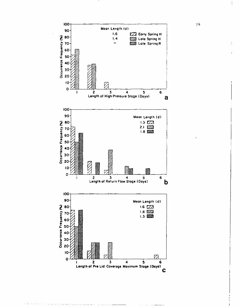
too- 7 4900 Mean Length Wd)
1.6 I Early Spring Ho80- 1.4 • Late Spring H
" 70- Late Spring RC' 60"
t. 50-4 40-0
S30-U
U 20-
to-
0-2 3 4 6
Length of High Pressure Stage (Days) a
1001
90-' Mean Length (d)
so0- 0..372.-7,
1.8e"60-/
c 4o-30
1 2 3 4 5 6
Length of Return Flow Stage (Days) b
100-
90- Mean Length (d)
Sso- 1.6 EM7- 1.,860 1.3
,u. 50" ,
Oc 40-'
.30-
,o -,•F
, 2 3 5 6Length of Pro Lid Coverage Maximum Stage (Days) C
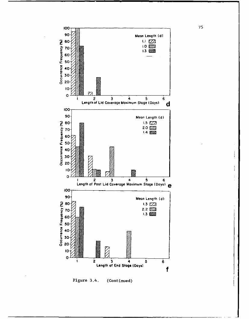
too- 75
90- Mean Length (dW
70- 1.0c 1.3" 60"
u. 50-
S0
30
Length of Lid Coverage Maximum Stage (Days) d100
90- Mean Length (d)
80- ,1.52.0 /1.4
S
S60"7,
,,-50 .X
S40-/C
30-3
0 20-/
2.2
0/
2 3 4 5 6Length of Post Lid Coverage Maximum Stage (Days
90 i Mean Length (n u
> 70p 2.2
U.- 50.
S40-/
S30-/
2 3 4 5Length of End Stage (Daysl
Figure 3.4. (Continued)

76
onshore flows (38.5 h) observed by Lewis and Crisp (1989) in their
10-year return-flow climatology for February and March. The length of
the return-flow stage for the H cycle (Fig. 3.4b) shows that there is a
significant time lag between the onset of return flow and the appearance
of a large lid-coverage area; this time lag averages roughly 30 h in
early spring and 50 h in late spring. With the moist layer already
established at the beginning of the R cycle, its transition to maximum
lid coverage only depends on the transport of the EML into the Great
Plains. Thus, the R cycle (on average) has the fastest transition to
lid-coverage maximum (75 h) of all three cycles, whereas the early- and
late-spring H cycles both require 36 h longer to reach lid-coverage
maximum.
3.4 Synoptic Flow Patterns During the Lid Cycle
In this section the prevailing synoptic flow types that were
observed during each stage of the lid cycle are discussed. Differences
among the three types of lid cycles (early-season H, late-season H and
R) are also examined in terms of prevailing flow types.
3.4.1 Prevailing Synoptic Types During the Lid Cycle
Table 3.3 shows the occurrence frequency of synoptic types that
were observed during different stages of the lid cycle. For the
early-season H cycle, Table 3.3 shows that the high pressure stage is
dominated by northwest and cyclonic flows at 500 mb. The next phase
(return flow) is primarily associated with anticyclonic and northwest
flows at 500 mb. The control of the H cycle by the long wave pattern is

77
tUe)j t) AO L 0000,D JUIO 04--4- L:o,,1 4 ~ c~ C4 r-,- - - r
C-)0 0 0
(n L 3 - 0C)- 3 a 0 ::1: -4 3 C ) 0 c:>
4-1
-44 -4 04 -4
C.) a) 0 ýý 4 uc )0 M U00 4
W Cf 30 0 00--44-
41 0
[.-4 CUc~0 C
4-1
0
:10, 0 %D 4,2j-- r- 0c' 0 c uooe C 'JL n 21 U C'0r- 4C'
C.I~ -4
4-) U) CCU n :3 C-400 C- :C-4 "00. ý 0-4 <0000:<-4 C: C> -
uA co %D en) ~00 0 t.-I0 C'C4 -0 0 C>
1-4 0
o dX CUe an r-i 0j-4 m "t-Oc in r-0m'I n
4 m "t 00C -49 41
>-1 00 4
O) 4) (e.I0c. p H r 0'fl 0OC E E1- bU0: : ,
.0 (db )" 040 C 41 -Aw0)r
H rn =- Ca. C) d 44) -40

a''OJ M 4 '1 '1 C'.~o f 0 a, 0ý -~ Ln
M) O'0 CN Ln C0 aLn C-4 1.O
-4
0)
o ~ c En0.4
0) 0 ý : 3:C )0C
CO41~0 0 ~ 0 0 0
co0iC>- ) ci0 C
0U O -L n 4c * I
-4 Cq Ul0 00L 4ý 'j 0
ox-4-44j -0~~ 001 $
0)) Ul -4-C)OU
.0 C-400
a) 0
o o .0 C) 0 00
00 -1
0)3 jc G 7 0 -4o I C)C4L
LA0-44\ iv20J,- 1
1 0JC)~ a' -44 Ln %..0t 4 0C'J -4rA01
10
-4-L '. 0 A~4 .0'
41 0
-4 0 -4 Q
U) C-4 b - 4- 4C DMa
C) ) 0 4) 0)4~4 0CO
a) En ) W 4$4 t
r-4 w4 C C( O z0)0m
$4 ca 0) 0 041caC 000>0 ~Ln -4 0c)0 %0 w.Jw4w) -4
Z O 0. . W$ bo 0
adfa eovgflS cni vi -4 04 MILn bO bO CO$4 0ý0 -A -A W4-) $4
0 0 0
01 0 * e a
04
79
evident here, in that the change in 500-mb types between the high-
pressure and return-flow stages suggests a transition from long wave
trough to ridge over the southern Plains. At the surface, the high
moves through the Great Plains region and exits eastward, being replaced
by the weak return flow regime (surface "type 3" in Table 3.3). In the
pre-lid-maximum stage of the lid cycle, the low level flow strengthens
(notice the prevalence of surface "type 4" patterns in 7able 3.3), an!
the 500-mb flow becomes southwesterly. The next 500-mb trough, now
located over the western U.S., is often accompanied by lee-side
cyzlogenesis. Subsequently, in the lid-maximum and post-lid-maximum
stages, a surface frontal system begins to move into the region, as
shown by the increasing frequency of surface "type 5" flows during these
two stages (see Table 3.3). Finally, the cycle ends with the return of
another high pressure incursion accompanied by 500-mb types "NW" and
"Ct".
The late-season H cycle is uifferent from its early-season
counterpart in all stages (see Table 3.3). In the late-season cycle,
the N-S oriented surface ridge ("type 1") is dominant in the high-
pressure stage. The transitions between long wave troughs and ridges
that characterize the early-season H cycle are not as frequent by late
May and June because the polar-jet activity shifts to Canada and the
northern tier of the U.S. The return-flow stage in the late-spring H
cycle is characterized by 500-mb southwest flow. The appearance of
southwest flow in this early stage of lid development seems
counterintuitive, since southwest flow is associated primarily with the
large lid-coverage stages in the early-spring H cycle. In late spring,
80
however, southwest flow can draw in moist air from active monsoonal or
tropical regions. The resulting vertical moisture profile lacks the
midlevel dryness that is characteristic of the lid sounding.
Additionally, the appearance of uncapped EML soundings (discussed by
LWI) in late-spring situations results from the existence of high 0w air
in the PBL, which the EML cannot effectively cap. For these two
reasons, the return flow stage is actually longer in the late-spring H
cycle (see Fig. 3.4b), even though the low level moist layer may
actually appear sooner. During the large lid-coverage stages, there are
no clearly dominant 500-mb flow types, as there were in early spring.
Southwest flow, which was dominant in the early spring (63% occurrence),
is no longer the most frequent pattern, as anticyclonic, southwest, and
cyclonic patterns now cumulatively account for nearly 80% of the large
lid-coverage days. At the surface, weak return flow ("type 3" in Table
3.3) is slightly more frequent than is strong return flow ("type 4" in
Table 3.3). The decline in frontal activity over the region in late
spring is illustrated by the low frequencies of the frontal-passage
surface type in both the lid-maximum and post-lid-maximum stages (8 and
25% occurrences, respectively, as opposed to 33 and 45% in early
spring). The downward seasonal trend in frontal systems crossing the
southern Great Plains is consistent with the climatological studies of
frontal incursions into the Gulf of Mexico by DiMego et al. (1976) and
Henry (1979). This seasonal tendency is also illustrated by the
increase in the occurrences of weak return flow in the end stage, from
four in early spring to 13 in late spring. The dominance of weak return
flows in the late-spring end stage implies that the moist layer remains
81
nearly intact over the region, and signals a decrease in the H cycles
and an increase in the R cycles.
The R cycle begins with a weak return flow 94% of the time, usually
under southwest, anticyclonic, or cyclonic flows at 500 mb (see Table
3.3). The low level flow in the R cycle remains relatively weak, even
in the large lid-coverage stages (notice the low combined occurrence
frequency of strong-return-flow and frontal-passage surface types in
Table 3.3). At 500-mb, types "A" and "C" account for 63% of the large
lid-coverage days. These 500-mb types are not associated with
progressive ridges and troughs in the polar westerlies, but are instead
associated with subtropical circulations and weak short wave features
south of the polar jet.
3,4.2 Flow Structure During the Lid Cycle
Frequently appearing synoptic types during different stages of the
three lid cycles were composited to examine the representative thermal,
moisture, and wind field structures present during the evolution of the
lid cycle. Mean fields of sea level pressure (SLP), surface dewpoint,
700-mb temperature, and 500-mb height are constructed for each
representative flow type, using surface and mandatory-level data. The
1200 UTC observations for each type-day were analyzed to a 40 by 30
point grid with an 80-km spacing (shown in Fig. 3.5a) using a Cressman
(1959) objective analysis. Three successive corrections (using
influence radii of 9, 6, and 3 grid spaces) were applied to the
upper-air first-guess fields, and two were applied (using influence
radii of 3 and 2 grid spaces) to the surface first guess fields. Two

82
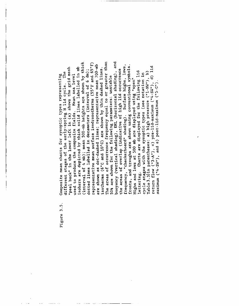
0 D C>4. d) U 0bo c r= -4 C:) r.~ 14 0 -W
*',4 10 :; 1 ~ -4 " -r.ý
W00110C 'o ( b r4).. 00f- (Ucd r-4 0 0 0 C-X kD0 0..4 (U 0 4 -1 0
a)~ C)~ (L2. 41,d~ V (n r.i 0n 0 x r.J=-dc :3: .
$4 (n 0 (n 'U'-') ( 00 -4O 10 -4
0 4j U
0 .0 0 p) b~ E0W 0 Z 40 4
0.4 :32 *'.4 0 '0 4 4 PU 44, 44d2 Y~4)' a) -(n 4 0 4) 4J 4 C 4)0 Cý 0 0 0 )4
4.)bs 11r.W0 0 4Jr- 4- N00(Ul .1.4 41 .1 4 a *4 -,4 Vb (0 00s.J) -4E
4. o .'-ý - 0 $.D 00. (LU'A- 0 ý4' -d c..( 4)4C
t* 4 _4 4 0 4)0 54 0 Ia (a- rf. -40 44 P C
, .4 4 )-44 0O a0O 4)4 0r4 -(1 C(12r4"
"W 0.d r .44 0 "V w 0 0 0- w~ I= 0) ) 0 41 0 j X. 0 -' 00q
0. W- 4V) 4 C oZ ; Q44 (U3- 4.r-4' (1 ) * o 10.
0 1 0 -9 E U) - ()0 0 w.14 0 10PU-qý00- 4 4) ~-1 4 s.d 0 -A (a -4 ~.4J 5d CO E 4 (2 W-44
Cd 0.M 0A 0 U0 0 CO 4 -4 O 11 . I 0 00 C
0- $4 Pw 0 W.4 1ý 0 .,1 0 V ( .0 'n :
s44 0 0 9 C.-,Iý41U ~.4) 44 ~ L~~ "0 4 .0')(n l U'r. 0 l 0 .04--~ 0 U1 1-3 4) u CO-d 0.4 (12 U
( 10 00 (U n 0 r. (L) - 0 0 C:) .4 0 0 10
41 44 -l )x U Pj . A a c C 4) :~
04- 0 4) C4J -I- CO *0 W r4W 4) C-(U b(n '4.)
'4)' 00 4 ) 0. 00o 0 U4 4- 4) 0 0104. 00 -A ) $m0r.- 0o . o1 .4) :t 01 41, (a .0 0 " Oý o- ý4 0n C (U 0C Z n
coi r4:3V: 4 Q 41' . c
0)v ' 4 ( , nZ -, 4 4c 0 t
r=1 )0 4 4 o-10 ; a- )r tI
110 414 d- -r o H o-
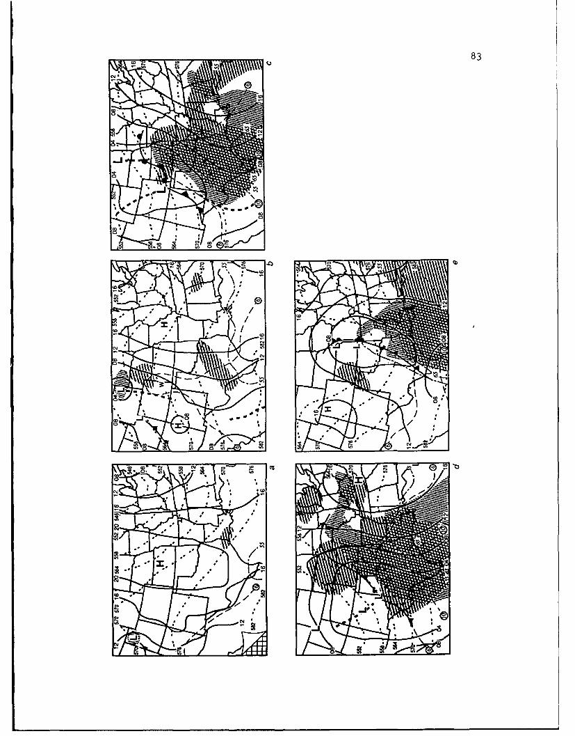
83
/o :1400
coS cc 0'-
84
passes of a 1-4-1 smoother were then applied to the gridded analyses.
For each synoptic type, the individual gridded fields for each variable
were added together, and the mean gridded field was computed simply by
dividing the grid point values by the number of days in the sample for
each synoptic type. Additionally, we constructed geographic frequencies
of EML and buoyantly unstable areas (composited at the upper air
stations), in order to examine the evolution of static stability over
the region during the lid cycle. See section 2.2.1 for specific
criteria used to identify EML and buoyantly unstable soundings. The SLP
and 500-mb height fields are meant to illustrate the low level and upper
level flows, and the sign of the geostrophic thermal advection in the
intervening layer. The surface dewpoints allow us to examine the
development of the moist layer beneath the lid, and the 700-mb
temperature is used to locate the warm layer that encompasses not only
the EML, but its source region (the 700-mb isotherms we used (6°C, 10°C)
correspond to 0 values of 36°C and 400C).
3.4.2.1 The Early-Season H Lid Cycle
The high-pressure stage of the early-spring H lid cycle is
represented by a north-south pressure ridge/northwest flow aloft pattern
(type "1-NW" from Table 3.3), whose composite mean analysis is shown in
Fig. 3.5a. Note the secondary pressure ridge extending into the western
Gulf of Mexico, roughly coincident with the 93°W longitude meridian.
East of the surface ridge, there is strong cold-air advection, while
weak warm-air advection is occurring over the western Plains and the
Rockies. Genesis of the EML is taking place over the U.S. desert
85
southwest and northwestern Mexico, as indicated by the 6°C isotherm at
700 mb. The mean 500-mb ridge position is over the Continental Divide.
The EML/unstable-buoyancy frequency composite analysis reveals only
isolated areas of EML and buoyant instability occurrence at this stage.
The return-flow stage is represented by a weak return
flow/anticyclonic flow aloft pattern (type "3-A" from Table 3.3), shown
in Fig. 3.5b. Although types "3-A" and "3-NW" have equal occurrence
frequencies at this stage (see Table 3.3), we chose this type in order
to illustrate better the 500-mb wave progression in the lid cycle. The
sea level pressure field shows the ridge axis now extending into the
central Gulf, approximately coincident with the 89°W longitude meridian.
Examination of the individual days comprising this composite reveals
that the surface high either translates eastward into the Mississippi
River valley or migrates southward into the Gulf and cuts off during
this phase. The specific track of the surface high determines the
timing and the location of the return of the moist layer into the
southern Plains. The 55°F surface isodrosotherm shows that the moisture
is beginning to return in three areas: the Rio Grande valley, southeast
Texas, and the Mississippi River delta region. Examination of
individual days shows that the latter two locations are "shut off" from
returning moisture if the surface ridge penetrates into the Texas
coastal region, or the cut-off surface high remains west of about 90'W
longitude. In these cases, the moisture returns first into the Rio
Grande valley, and only moves into the Gulf coastal regions of Texas and
Louisiana after the high moves farther east or starts to weaken. The
86
appearance of strong southerly flow from Oklahoma northward, beneath the
mean 500-mb ridge, implies strong warm-air advection over this area.
Evidence of an emerging EML from the west is shown by both the
700-mb thermal ridge over the western Plains and the pockets of high EML
frequency located over portions of Nebraska and Texas. The appearance
of an EML in the western half of Nebraska is significant, because it
suggests that the relatively cooler mountainous regions of the western
U.S. can still produce EMLs in the early spring, as suggested by Fig.
2.10. Because of the position of the surface pressure ridge, the
returning moist layer is not in phase with the emerging EML and only
isolated lid occurrences are possible at this stage of the lid cycle.
As the next 500-mb trough begins to enter the western U.S., surface
pressures are falling over the Rockies, which is the precursor to the
development of the lee-side trough and low-level jet (LLJ). There is a
remarkable resemblance between Fig. 3.5b and stage B of LLJ development
(Fig. 4 in Djuric and Ladwig 1983). Although there are differences in
the location of strongest surface flow between our composite mean
analysis and Djuric and Ladwig's figure, the SLP patterns are very
similar, as are the locations of key features such as the surface high,
pressure ridge, and lee-side trough.
The "classic" lid producing pattern of strong return flow with
southwest flow aloft (type "4-SW" from Table 3.3) represents the pre-
lid-maximum stage (Fig. 3.5c). In this phase, the lee-side surface
trough is well developed from Wyoming into Mexico. Once the lee-side
trough forms and the surface ridge retreats into the eastern Gulf, the
return of the moist layer occurs rapidly. This rapid return of the

87
moist layer into the central portion of the study region is hastened by
development of the LIU over this area. This stage of lid development
resembles stage D in the LLJ conceptual model of Djuric and Ladwig. The
three dimensional phasing of the moist tongue and the EML thermal ridge
allows a lid stratification to develop rapidly, as illustrated by the
overlapping EML and unstable areas in Fig. 3.5c. In this phase, there
is a large region of lid occurrence covering most of Texas, Oklahoma,
and Kansas, and a second, smaller area over Alabama and western Georgia.
Notice that the western edge of the lid over Texas and Oklahoma closely
parallels the mean position of the 55°F surface isodrosotherm. This
suggests that the mean lid edge and dryline are nearly parallel, as
observed in many individual case studies (Carlson and Ludlam 1968;
Schaefer 1973, Carlson et al. 1983, and others). The mean 500-mb jet,
inferred from the geopotential height gradient, extends from southern
Arizona and New Mexico into northwest Kansas and central Nebraska, then
turns anticyclonically towards the Great Lakes region.
There are several areas in the southern Plains where the unstable-
buoyancy frequency exceeds the EML frequency. One area is parallel to
the western edge of the lid, to the east of which the low level moist
layer is consistently deep enough to support a lid stratification. The
proximity of the buoyantly unstable area in western Texas and Oklahoma
to the mean 500-mb jet and the dryline suggests that it can be a prime
location for the initiation of deep convective storms in this flow type,
especially since the low static stability would enhance vertical motion
in the vicinity of upper level jet maxima approaching from the southwest
(Uccellini and Johnson 1979). A second potential area for deep
88
convection exists where the low level moist axis reaches the northern
lid edge zone over Kansas. This region is close to the mean 500-mb jet,
LLJ, and surface front. These two areas of convective potential are
likely to expand if the resulting moist convection erodes the lid and
taps the highly unstable air located in the interior of the lid-coverage
area, where the lid strength is typically greater (Graziano and Carlson
1987). An examination of the actual severe weather associated with
these representative synoptic types is presented in a companion paper
(Lanicci and Warner 1991c).
A multi-day persistence of 500-mb southwest flow often occurs
during the large lid-coverage stages of the early-season H lid cycle
(see Table 3.3). In the lid-maximum phase, the strong return
flow/southwest flow aloft (type "4-SW" from Table 3.3) is dominant, so
it is again chosen to represent this stage of the cycle (see Fig. 3.5d).
This stage is characterized by stronger low and upper level flows
throughout the eastern half of the study region, associated with falling
SLP over the entire southern Plains region and a deepening 500-mb trough
over the western U.S. This stage bears some similarity to Djuric and
Ladwig's LLJ stage D'. The EML area has a more northerly extent at this
stage, and the unstable area extends farther east. The lid-edge zone
over Texas is located farther west than in the previous stage, and is
very close to the strong 500-mb jet and surface frontal system; for this
reason, it is a favorable area for initiation of deep convection, and
will expand if the moisture laden air farther east is tapped. A
possible second area of convective potential is located over northern
Oklahoma and southern Kansas, but convection in this region may be
89
delayed until the main jet translates eastward, or a jet streak
propagates into this area from the southwest. There are similarities
between the temporal continuity in our synoptic types representing these
two large lid-coverage stages, and that of the type A and B synoptic
patterns of Miller (1972). In our composite mean analysis shown in Fig.
3.5d and in Miller's type B pattern, the surface front is beginning to
enter the Great Plains, and the jet locations are similar. It is
interesting to review Miller's comments regarding the temporal
continuity between his synoptic types:
The type A and B patterns are quite similar in configuration and
general development. The major difference between the two is the
noticeable presence of a major upper trough and frontal system to
the west of the threat area in the Type B pattern. This
association with the trough and frontal systems designates the Type
B pattern as the last (emphasis added) of a series of severe
weather producing systems. On the other hand, the Type A often
repeats from day-to-day until the major trough moves away. (p. 3-5)
Thus, the eastward migration of the 500-mb trough into the Great Plains
marks the beginning of the post-lid-maximum stage of the early-season H
cycle.
The synoptic type chosen to represent the post-lid-maximum stage of
the lid cycle (Fig. 3.5e) illustrates the dynamic and thermodynamic
structures that result when the EML source region is cut off by the
advancing surface front and upper level trough. This is synoptic type
"5-C" from Table 3.3. The mean frontal position in this stage is over
eastern Oklahoma and Texas, and the Mississippi valley moist axis has a
90
more northerly extent by this time in the cycle. The 700-mb temperature
field is fairly flat across the extreme southern portion of the study
region, and the lid area extends only a little farther north than this
warm air, into Mississippi, Louisiana, and southeastern Arkansas. The
lid edge and frontal zones are nearly coincident over southern Texas,
and diverge to the north of this area. The main 500-mb jet extends from
New Mexico into northern Texas and southern Arkansas. The combination
of the strong cold front moving eastward, the strong southerly flow
ahead of the front with a strong cyclonic upper jet crossing over
(generating a strong veering wind shear), and the lid edge and buoyant
instability in this vicinity suggests that northeastern Texas, northern
Louisiana, southern Arkansas, and (later) western Mississippi are
vulnerable to severe weather. A secondary convective area over the
south Texas coast can activate if the front removes the lid there.
3.4.2.2 The Late-Spring H Lid Cycle
Table 3.3 shows that the late-spring lid cycles are not associated
with the systematic passage of major upper level troughs and ridges, as
in the early spring. In order to compare representative flow types
between the early and late spring H cycles, we chose types "1-NW" and
"4-SW" as representative of the high-pressure and large lid-coverage
stages, respectively. Table 3.3 shows that these two synoptic types
occurred frequently enough in the late-spring H cycle to allow
comparisons with their early-season counterparts.
The composite chart for type "1-NW" is shown in Fig. 3.6a. There
are several notable differences between this late-season version and its
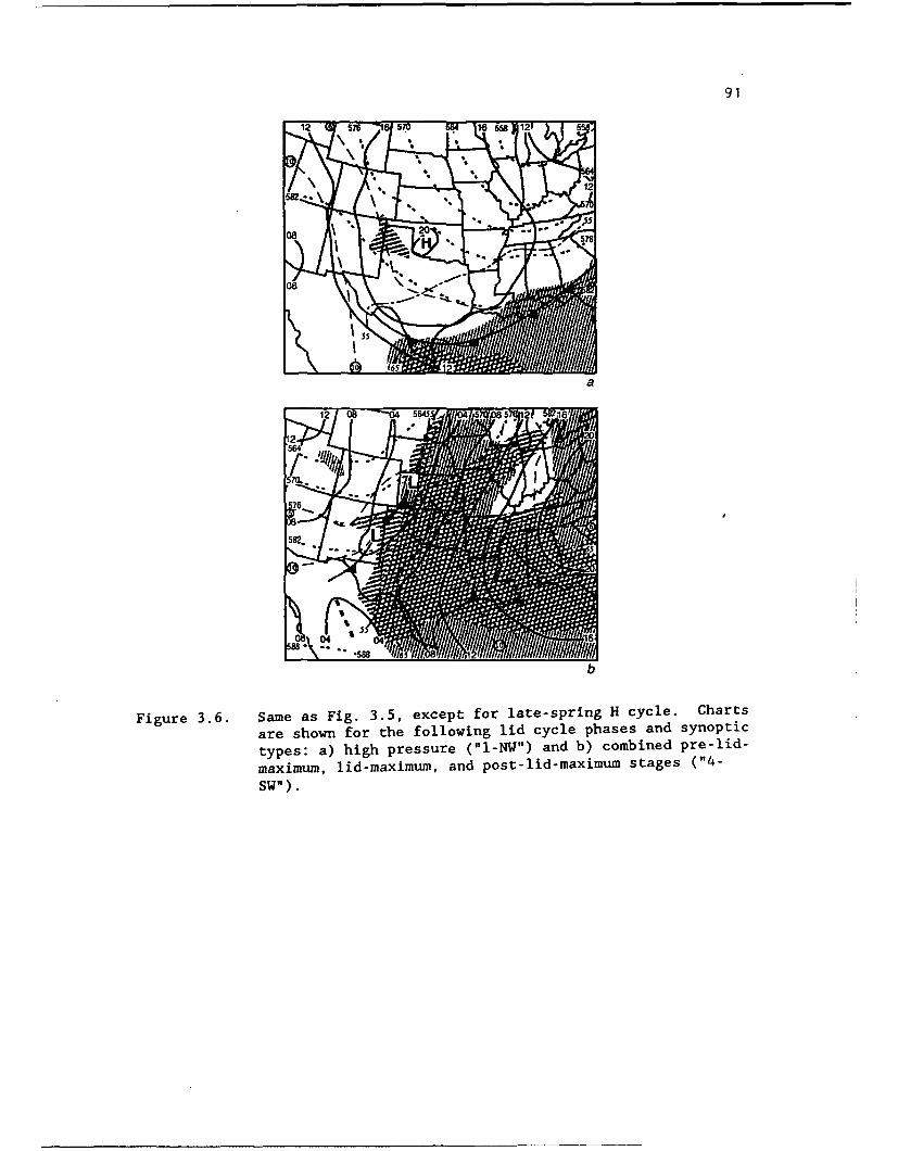
91
a
b
Figure 3.6. Same as Fig. 3.5, except for late-spring H cycle. Charts
are shown for the following lid cycle phases and synoptic
types: a) high pressure ("1-NW") and b) combined pre-lid-
maximum, lid-maximum, and post-lid-maximum stages ("4-
SW").
92
early-season counterpart (Fig. 3.5a). The high pressure system is
weaker, and the seconda y surface ridge over the Gulf does not appear.
Instead, there is an eastward "bulge" of the surface ridge. There is
more low level moisture present in this flow type over Texas and the
Gulf coastal states than there was early in the season, and a moist axis
already exists along the Rio Grande valley at this stage. The large
expanse of the EML source region is well illustrated by the 700-mb
temperature field, which shows a thermal ridge from northwestern Mexico
into Arizona, southern Utah, and eastern Nevada. At 500 mb, the mean
trough is over the Mississippi River valley, somewhat to the west of its
early spring position, and not as deep. Increased low level moisture
over the southern states at this time allows buoyantly unstable air to
exist over the Gulf coastal region in this flow type, and as a result
there is some lid occurrence in the vicinity of Brownsville, Texas.
The late spring composite chart for type "4-SW" is shown in Fig.
3.6b and can be compared with those for the early season (Figs. 3.5c,d)
to examine the seasonal trend in this classic lid-producing synoptic
type. Since this late spring composite applies for the duratiun of the
large lid-coverage stages, direct comparisons cannot be made with the
early-spring versions shown for the pre-lid-maximum and lid-maximum
stages. However, some seasonal differences can be inferred from
examining the mean gradients of SLP, 700-mb temperature, and 500-mb
height. The SLP pattern over the western Plains, for example, shows a
weaker, narrower lee-side trough than in the early season, consistent
with a weaker 500-mb trough. There is considerably more low level
moisture present than in the early spring patterns, but the eastern
93
Plains moist axis has a very similar orientation to that for the early
season: The 700-mb thermal field indicates warmer conditions than in the
early spring with temperatures in excess of 12°C (equivalent to 0 near
43°C) over a large portion of Texas. The mean 500-mb jet is more zonal
and is located farther north than in the early spring. The buoyantly
unstable area is more extensive than the EML because of the large amount
of moisture present. The somewhat larger lid-coverage areas observed in
the late-season H cycle (compare Figs. 3.3a and 3.3b) are a result of
greater overlapping areas of the EML and moist layer. The portion of
the western lid edge from the northern Texas panhandle to southwest
Kansas is close to the mean 500-mb jet, dryline, and surface front.
This area can be considered as a potential genesis zone for deep
convection. A second area of convective potential extends from northern
Kansas into northern Illinois and is associated with the mean northern
lid edge, 500-mb jet, and low level moist axis.
3.4.2.3 The R Lid Cycle
The return flow stage of this cycle is represented by weak return
flow with anticyclonic flow aloft (type "3-A" from Table 3.3). This flow
type, whose mean composite analysis is shown in Fig. 3.1a, typically is
associated with a westward expansion of the Bermuda anticyclone, causing
the winds below 700 mb to become southerly or southeasterly over the
southern portion of the study region. There is considerable low level
moisture associated with this flow, as evidenced by the surface dewpoint
analysis. The warmest air at 700 mb (> 10°C) is concentrated in a
north-south-oriented zone from southern Colorado to central Mexico. When
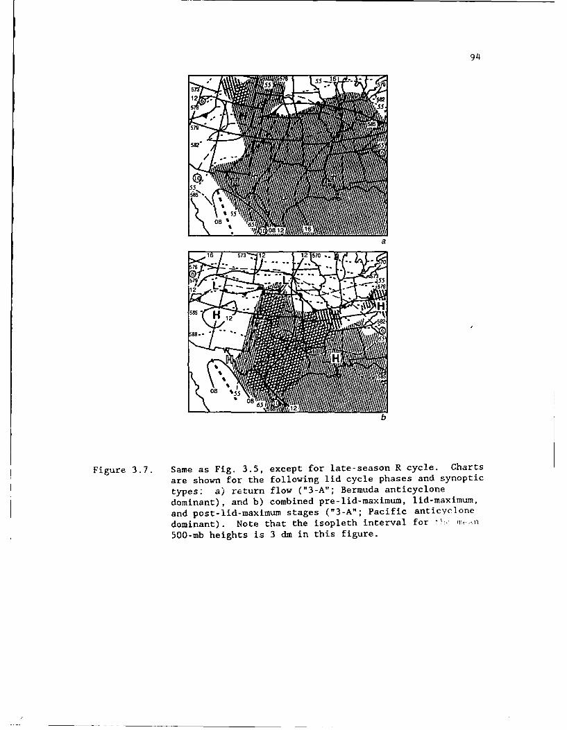
94
Figure 3.7. Same as Fig. 3.5, except for late-season R cycle. Charts
are shown for the following lid cycle phases and synoptic
types: a) return flow ("3-A"; Bermuda anticyclone
dominant), and b) combined pre-lid-maximum, lid-maximum,and post-lid-maximum stages ("3-A"; Pacific anticyclone
dominant). Note that the isopleth interval for •" hc •
500-mb heights is 3 din in this figure.
95
the Bermuda anticyclone expands into the southern Plains, this warm air
is restricted to areas west of the Great Plains. The 500-mb analysis
shows two high centers over southwest Texas and southern Mississippi.
In this flow type, the westward extension of the Bermuda cell dominates
the lower half of the troposphere over the south-central U.S. There
have been numerous climatological studies of the summertime circulation
over the central and western U.S., ranging from the early studies of
Reed (1933, 1937), Wexler and Namias (1938), and Riehl (1945), to the
specific studies of the southwest U.S. monsoon (Bryson and Lowry 1955;
Carleton 1985, 1986, 1987). The studies of the southwest monsoon all
show that the orientation and location of the subtropical anticyclonic
cell largely controls the precipitation regimes of the desert southwest
and northern Mexico. The frequency composites for type "3-A" show a
large area of buoyant instability to the east of the Rockies. There are
several isolated areas of lid occurrence in this flow type and a
slightly larger area over Wyoming. The Wyoming lid area is likely
associated with midlevel southwest flow over the Rockies and Great
Basin, which taps the warm-air reservoir to the south.
The large lid-coverage stages of the R lid cycle are also
represented by a type "3-A", which has weak return flow with
anticyclonic flow aloft, but in which the orientation of the
anticyclonic flow is different from that in the previous stage. The
composite mean analysis for this type is displayed in Fig. 3.7b. The
transition to this flow type occurs when the Bermuda cell shrinks and
the Pacific ridge builds eastward, raising the 500-mb heights over the
southwest U.S. When this occurs, the midlevel warm air over the western
96
U.S. is transported over the southern Plains states by westerly winds.
This situation often is accompanied by a strengthening of the jet to the
north of the study region, caused by a strengthening height gradient
north of the building anticyclone, as shown by the 500-mb height and
700-mb temperature gradients in Fig. 3.7b. In terms of EML frequency
over the Great Plains, the primary distinction between this flow type
and the preceding one is that the midtropospheric anticyclonic flow over
the southern Plains in this phase is the hot, dry eastern branch of the
Pacific anticyclone, as opposed to the cooler, moister western branch of
the Bermuda anticyclone. The strengthening of the jet in the northern
U.S. introduces a baroclinic zone over this region, which likely
contributes to the decreased penetration of the moist layer into this
area in this phase of the cycle. The moist axis in this flow type is
better defined, and extends from the Texas Gulf coast northward through
central Oklahoma and into the northeastern corner of Nebraska. Downwind
of the EML source region, large scale subsidence reinforces the lid, as
illustrated by the north-south-oriented lid frequency axis from south
Texas into western Kansas and southern Nebraska. Given the large area
of potential instability present in the lid area over the western Plains
and the proximity of the northern portions of this lid area to the mean
polar jet, we can define a convective genesis zone from western Oklahoma
into Kansas and southern Nebraska. The 500-mb height pattern for this
synoptic type in this phase is similar to the basic 500-mb flow pattern
for northwest-flow severe weather outbreaks presented by Johns (1984)
(his Fig. 7). Our sea level pressure pattern does not match any of his
97
surface patterns exactly, but most closely resembles his type C
category, representing a meridionally oriented pressure trough.
Although not shown by a composite mean analysis, the end stage of
the R cycle occurs when a short wave trough moves through the zonal jet
and into the Great Plains to the east of the Pacific ridge.
Subsequently, the EML is transported eastward ahead of the trough and
eventually moves away from the Great Plains, leaving the moist layer
intact, but returning the Plains to a lid-coverage minimum, usually
under 500-mb type "C" (see Table 3.3).
3.5 Discussion and Summary
Our study of the life cycle of the lid over the southern Great
Plains reveals that a typical lid cycle has a mean period of about one
week. There are two basic types of lid cycles:
1) The H cycle that begins with a surface anticyclonic incursion
into the region, is associated with the passage of baroclinic
features in the westerlies, and has a mean period of about
seven days.
2) The R cycle that begins with an already established moist
layer within a persistent low level return flow from the Gulf
of Mexico, is associated with subtropical circulations and
weak short wave features after the polar jet has retreated
northward, and has a mean period of between five and six
days.
The H cycle is dominant in the early half of the spring, when polar-air
outbreaks and a progression of long wave troughs and ridges are frequent
98
over the southern Plains. The R cycle is common in the late spring,
when the region is dominated by low level southerly winds and the flow
aloft is weak.
We defined various stages of lid evolution for the two types of
cycles, based on observations of the lid coverage and prevailing
synoptic patterns. The early-spring H cycle begins with a surface high
pressure incursion, which changes to a return flow by about 36 h. The
beginning of return flow over the southern Plains is characterized by
only isolated lid coverage because the surface anticyclone is often
anchored to the east of the Great Plains or in the western or central
Gulf of Mexico, preventing the returning moist layer from entering the
study region for an additional 24 h. A warm mixed layer forms over the
high terrain of the western U.S. and emerges into the western Great
Plains as an EML within 36 h of the start of the lid cycle. Large area
lid coverage occurs when the low level flow strengthens in response to
development of the lee-side trough and LLJ over Texas and Mexico, and
the rapidly returning moist layer phases together with the EML created
over the western states and northern Mexico. Maximum lid coverage
typically occurs with the movement of a large scale trough into the
western states, creating an overrunning flow of warm, dry EML air from
the Mexican plateau above the well established moist layer in the
south-central U.S. This cycle usually ends with a frontal passage
through the region, followed by another surface high pressure incursion.
The late-spring H cycle is somewhat similar to that of the early
season in the high pressure stage, but the midlevel flow is typically
weaker throughout the cycle. Since the late spring EML source region
99
includes the Rocky Mountains and Great Basin, zonal and northwest flow
types (in addition to southwest flow) can produce a large lid-coverage
area in the late-season H cycle. Owing to the decreasing frcquencies of
frontal and high pressure incursions into the region as the summer
approaches, this cycle often ends with the transport of the EML out of
the region while the low level moist layer remains, marking the
beginning of the late-season R cycle. The R cycle is characterized by
weak low level return flow throughout the cycle, and changes in the
midlevel flow pattern that are primarily influenced by the expansion and
contraction of large scale, subtropical circulations such as the Bermuda
and Pacific anticyclones.
Our analyses identified three primary surface moisture axes: 1) an
axis along the Rio Grande valley; 2) a north-south axis through the
eastern Great Plains; and 3) a north-south axis through the Mississippi
River valley. The three axes develop during the early stages of the H
cycle, and also appear in various stages of the R cycle. In the H
cycle, the development of the moisture axis is influenced in the early
stages by the location and strength of the surface pressure ridge. Our
results show that the Rio Grande axis is favored over the others when
the ridge extends into the Texas Gulf coast, or a cut-off surface high
appears in the Gulf (west of about 89-90°W longitude). The observations
suggest that the presence of moisture axes in these three locations is
influenced by certain topographic features which tend to divert the
moist flow around them. In the case of the Rio Grande axis, these
topographic features are the Mexican plateau to the south and the
Edwards Plateau to the north, while the Ozark Plateau influences the
100
eastern Plains axis, and to a lesser extent, the Mississippi River
valley axis. These topographic influences are reduced in the late
spring, but are still identifiable in our flow-type composites.
Our flow composites for different stages of the lid cycle
illustrate the temporal continuity of wind field, moisture, and thermal
features throughout the cycle, especially during the early spring. In
particular, favorable genesis areas for moist convection are
identifiable in the large lid-coverage stages of each lid cycle. In the
early spring, these favored areas have a meridional orientation that is
consistent with the nature of the midtropospheric flow type (i.e.,
southwesterly) and the presence of features such as the dryline, LIJ,
and upper level jet over the southern Plains. In the late spring, these
genesis regions are located to the north and west of the early spring
locations. Our results generally suggest that the western lid edge is a
prime climatological location for initiation of deep convection due to
its proximity to approaching features such as surface fronts, drylines,
and jet streaks. A second favored area appears along the northern lid
edge, and is usually associated with features such as the moist tongue,
LLJ, and strong veering wind shear in the lower half of the troposphere.
In both locations, the convective region will expand and severe weather
will become more widespread if the very moist, potentially unstable air
under the interior of the lid area is tapped.
The results of this study complement other climatological
investigations over the southern Great Plains. The three surface
dewpoint axes identified in our composite analyses are very similar to
the return-flow tracks proposed by Lewis and Crisp (1989) in their
101
10-year climatology of February and March. The persistence of the
surface pressure ridge to the east of the Great Plains in the return-
flow phase of the early season H cycle has been noted by area
forecasters for many years, and the ability of operational numerical
models to predict the movement of the surface ridge and the timing of
the return flow was addressed in a study by Weiss (1989). The return
flow that follows the exit of the surface anticyclone is also an
important phase in the life cycle of the surface dryline (Schaefer
1973). In Schaefer's conceptual model, dryline genesis occurs when the
moist layer reestablishes itself over the western Plains following the
onset of return flow after the retreat of the continental airmass; this
corresponds to the broadening of the Rio Grande moisture axis over the
western Plains during the transition from the return-flow to the pre-
lid-maximum stage in the early-season H lid cycle. Our composite charts
for the early-season H cycle also complement the LLJ conceptual model
for wintertime presented by Djuric and Ladwig (1983), which shows the
initial development of the LLJ in conjunction with the appearance of the
lee-side trough, the subsequent translation of the LLJ eastward with the
surface cyclone and upper level trough, and the role of the LLJ in
transporting the moist layer rapidly northward.
The importance of the results presented in this study is that the
analysis and prediction of important severe storm features on any given
day can be placed into the context of a climatologically based
conceptual model of the lid cycle. The fact that our conceptual model
of the early season H lid cycle resembles those of the dryline and LLJ
is not surprising. The synoptic scale patterns appearing over the
102
central U.S. in early spring create a favorable environment for deep
convection that includes features such as the dryline, LLJ, and EML. We
have shown how the creation of the favorable static stability pattern
(i.e., the lid sounding) occurs in concert with the creation of these
other features. However, we have also shown that the lid-development
cycle has a significant seasonal dependency. -owldcge of this seasonal
aspect of lid development is important, because, as shown by this study
and LWI, there is a marked change in the tropospheric zirculation over
the southern Plains from early to late spring. The early spring
circulation is marked by a progression of baroclinic waves and frontal
systems, whereas the late spring circulation is influenced at different
times by relatively weak baroclinic waves, and subtropical circulations
such as the Bermuda and Pacific anticyclones, with the latter features
becoming more frequent by the end of June.
103
Chapter 4
THE SYNOPTIC CLIMATOLOGY: RELATIONSHIPTO SEVERE-STORMS CLIMATOLOGY
4.1 Chapter Introduction
One of the most challenging problems in operational meteorology is
the prediction of severe-thunderstorm outbreaks. Development of severe
storm analysis and prediction techniques has an historical background
which is strongly rooted in event-based climatological studies. The
first scientific attempts at describing atmospheric conditions
associated with tornado occurrence were made by Ferrel (1885) and Finley
(1890), and the first significant investigation of the thermodynamic and
wind structures in the tornadic environment was made by Varney (1926).
Further work continued with the studies of Humphreys (1926), Lloyd
(1942), and Showalter and Fulks (1943), as routine radiosonde data
became available to describe the mid- and upper-tropospheric structures
associated with these events. As the upper air networks improved and
the database became larger, a natural extension of this early work was
the generation of severe-storm climatologies. A survey of the numerous
event-based severe-storm climatologies produced over the U.S. since 1950
shows that the analysis techniques can generally be divided into three
main categories: 1) statistical analysis of the characteristics of
tornado events and storm-damage events; 2) evaluation of mean proximity
soundings and horizontal meteorological analyses of the
near-storm/tornado environment; and 3) categorization of the synoptic
patterns associated with the severe storm and tornadic environments.

104
The second and third techniques result in the production of analog or
mean meteorological fields for the tornadic environment.
There are several points which should be made about the use of
reported severe storm or tornadic events as the primary basis for
generation of the resulting climatological database. First, there are
well known limitations in the use of severe storm reports that result
from population biases (Schaefer and Galway 1982), difficulties in
quantitative measurement of storm-related winds, and difficulties in
observing events at night (Kelly et al. 1985). A second point is that
the imposition of arbitrary limitations upon the data can strongly
influence the resulting climatology. For example, restricting the data
sample to tornadic outbreaks of a specified size (e.g., greater than 10
events), results in a climatology that is biased towards the most severe
events, and the associated mean or analog meteorological analyses are
usually highly baroclinic with strong buoyant instability' in the area
of the events. Unfortunately, attempts are often made to apply these
synoptic analogs to situations where the dynamical and thermal
structures are not as well defined. In these "weakly forced"
situations, the analyst is presented with a set of atmospheric
conditions from which it is very difficult to produce a meaningful
diagnosis and prediction (Maddox and Doswell 1982a,b; Doswell 1987).
The third (and perhaps the most important) point concerning event-based
studies is the exclusion of the "null" case in which severe storms are
'Buoyant instability, as defined in this paper, refers to thestability of a saturated surface/low-level parcel with respect to themidtropospheric environment, as used in the Lifted Index of the NationalWeather Service and the buoyancy term of the Lid Strength Index.
105
predicted but none occur (the "false alarm"). Statistics concerning
false-alarm rates for severe storm prediction are routinely kept by the
National Severe Storms Forecaster Center (NSSFC) in Kansas City,
Missouri. However, few (if any!) of these false alarm/null cases are
reanalyzed and presented in the meteorolgical literature. A reasonable
question to ask is whether a severe storm climatology can be generated
which eliminates any of these biases.
Another approach to building a severe storm climatology is to base
it on a physical phenomenon that is known to be associated with the
occurrence of severe thunderstorms and tornadoes. Attempts at such a
climatology include the dryline study of Rhea (1966), the northwest flow
outbreak climatc'logy of Johns (1982, 1984), and the regional severe ,
storm climatology of Giordano (1987). An offshoot of these physically
based studies is the use of infrared satellite data to identify and
compile climatologies of mesoscale convective systems or complexes. For
example, several studies composite meteorological features that are
common to mesoscale convective systems that meet certain size, cloud-
top-temperature, and duration criteria (e.g., Maddox 1983; Bartels et
al. 1984; Velasco and Fritsch 1987; Augustine et al. 1989). In addition
to these satellite compositing studies, those of Cunning (1986) and
Tollerud and Bartels (1988) also document severe weather events
associated with these systems.
Our physically based climatology examines synoptic flow patterns
that are favorable and unfavorable for generation of the elevated mixed-
layer inversion, or lid, over the southern Great Plains of the U.S.
(defined as Kansas, Oklahoma, Texas, and the immediate surrounding
106
area). This approach simnply applies the proximity sounding technique in
reverse; where the event-based studies produce a mean sounding of the
near-storm environment that clearly has a lid, we instead produce a
climatology of the lid itself, and relate this climatology back to
severe stvrm occurrence or nonoccurrence. The period of study
encompasses four spring seasons (April, May, and June) 'rom 1983-1986.
All of the severe weather events occurring during these periods are
documented, resulting in a spectrum of event sizes from widespread
outbreaks to isolated events. The non-event days are also documented.
The definition of "severe storm" used in this study includes the
standard NSSFC severe-thunderstorm criteria (i.e., thunderstorm wind
gust equal to or greater than 50 kt; and/or hail with diameter equal' to
or greater than 3/4 inch; and/or thunderstorm wind damage), as well as
observations of tornadoes and funnel clouds. The database for the lid
climatology is a twice-daily compilation of lid parameters for the
four-year period over U.S. rawinsonde stations from the Rockies
eastward, previously described by Farrell and Carlson (1989) and Lanicci
and Warner (1991a) (hereafter referred to as LWl). The database for the
severe weather events is obtained from Storm Data, published by the U.S.
Department of Commerce. Severe storm statistics are examined as a
function of geographic location and month for the period of record, and
the areal extent of the outbreak is related to the antecedent lid
coverage area (lid coverages on non-event days are also examined). By
employing such an approach, the lid-related climatology can reveal new,
detailed information about the dynamic, moisture, and thermodynamic
structures associated with a wide variety of atmospheric states during
107
the spring season. This study also builds on the results of an
investigation that documented the life cycle of springtime lid formation
and dissipation (Lanicci and Warner 1991b, hereafter referred to as LW2)
by relating severe weather events to different stages of lid
development. This is done by meanE of geographic frequency analyses of
the occurrences of the elevated mixed layer (EML), buoyant instability,
and severe storms for several synoptic types representing various stages
of lid development in the early and late spring.
4.2 Severe-Storm Statistics for the Southern Plains:April-June 1983-1986
Our compilation of statistics from Storm Data uses an approach that
is similar to those of Galway (1977), Moller (1979), and Johns (1982).
An "event" is defined as a severe-weather report or series of reports
occurring within the three-state region of Kansas, Oklahoma, and Texas,
with the time interval between reports not to exceed 3 h. The reports
encompassing each event are then entered onto a 40-km grid covering the
region. We are not interested in the number of individual reports
occurring in each 40-km square: one report or 10 reports suffice to
include the square as part of the event, and the square is only counted
once. This was deemed an acceptable procedure since the focus of the
data compilation is on the areal extent of an event in relation to the
size of the lid-coverage area. The areal extent of each event is
determined by simply summing the number of squares included during the
lifetime of the event.
A percentile graph depicting the different event sizes in each
month is shown in Fig. 4.1. Examination of the curves reveals several

108
S4-) o
W- 4-4ý-i 0 4-4:1 0u Z-
0)02
,4)
'A cl
40>> -,4
to 4) bo
-,-4 E
w 44)b 4-4 0)
0)
40) -4
ý4 4-4 :bO) -4 0 V
-4
bf4 -4)-A
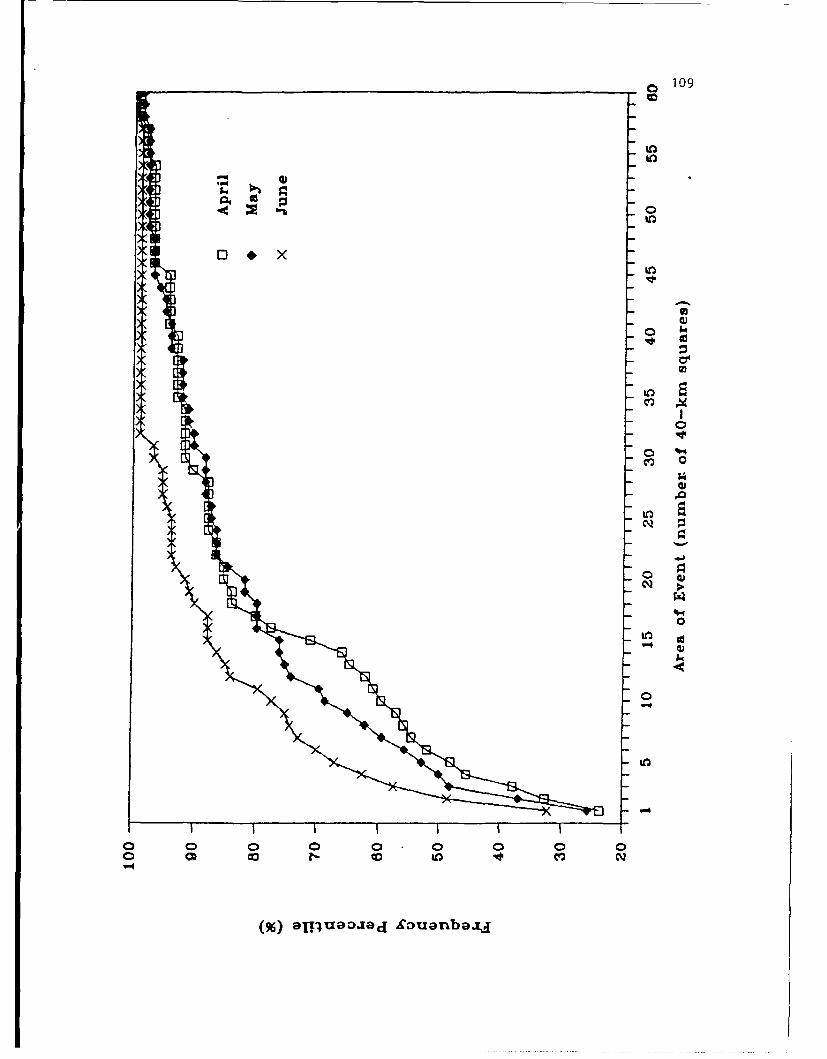
109
Cd
0* a
Q~~ co o o
(96)a~puojec Saunboi
110
characteristics. First, each monthly distribution has its largest
contribution from the one-square, or "isolated event," category. In
April, a significant secondary contribution comes from the 15-18 square
category (corresponding to an area between 24,000 and 29,000 km2 ), and
in June, a similar contribution comes from the 9-12 square category
(corresponding to an area between 14,500 and 19,000 km2 ). Although, the
total number of events increases from 78 in April to 135 in June, the
median event size decreases from five squares to two during the same
period. The number of non-event days (defined as a 24-h period from
1200 UTC to 1200 UTC with no severe weather events reported) shows a
steady decrease from 66 in April to 22 in June. The probability of a
day having at least an isolated event increases through the season.
The geographic distributions of the severe weather events for each
month are displayed in Fig. 4.2. The April and May distributions each
have areas of activity over Oklahoma, Kansas, and the northern tier of
Texas. The June distribution shows the near disappearance of activity
over northern Texas, and has new centers of activity over the Oklahoma-
Kansas border and northern Kansas. If one compares the geographic
frequency charts for April and June, it can be seen that there is a
general shift of activity to the north and west during the season. Such
a seasonal migration of activity to the north and west is consistent
with other severe-storm climatologies (e.g. Kelly et al. 1985), the MCC
climatology of Velasco and Fritsch (1987), the lid-day climatologies of
Farrell and Carlson (1989) and LWI, and the composite mean lid/EML
analyses of LWl (see Fig. 2.10).

111
Figure 4.2. Geographic frequency of severe storm events over the studyregion in terms of number of events per 40-km square.Light shading denotes 3-5 events per square, mediumshading denotes 6-8 events per square, and dark shadingdenotes greater than 8 events per square. Charts areshown for April, May, and June.
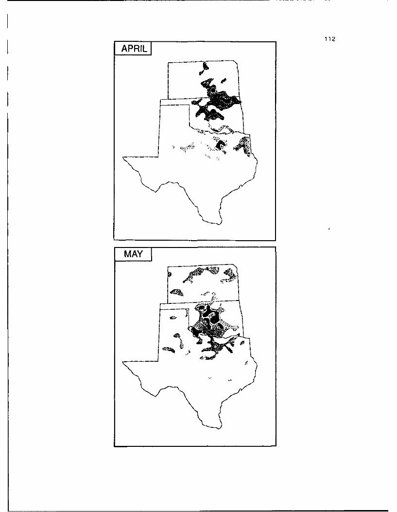
112APRIL
1 •2e
,._L . ... ..--. :i " •
!~
'- V
"%\ )
MAY
I I
I -
I • , "•j! ,• .s~d x.
-• ... •. ,,
7!I!
\ .
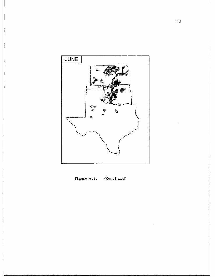
113
JUNE
I I
Figure 4.2. (Continued)
114
4.3 Relationship of the Outbreak Size to the Lid
The relationship between lid occurrence and severe weather is first
addressed by examining the monthly frequency of different lid-coverage
areas for both event and non-event days. The resulting lid-coverage
frequency distribution for each month appears in Fig. 4.3. For April,
the non-event days are strongly associated with isolated or zero
lid-coverage areas, while the event days have a near-normal
distribution with a peak at five lid stations. This peak is very close
to the mean lid-coverage area of 4.3 stations for this month (LWI).
Geographic frequency analyses of lid occurrence by number of stations
(not shown) for April reveal that lid coverage is spatially contiguous
in this range. In May, the non-event day distribution peaks at one lid
station, with most occurrences in the 0-2 station range, while the event
day distribution has two peaks, at two and six stations. There is more
of an overlap of the two distributions in May than there is in April.
By June, there are very few non-event days (22), while the event-day
distribution again has two peaks, at one station, and at four stations.
A second way to address the relationship between lid occurrence and
severe weather is to analyze the severe-weather event size in relation
to the lid-coverage area. For each event documented in the study
period, the size of the antecedent lid over the study region is
calculated in terms of the number of rawinsonde stations with a lid
sounding. We are primarily interested in the antecedent conditions
because the lid size during or after the conclusion of the event is more
likely to be influenced by the convection itself. Additionally, a
relationship between antecedent lid size and subsequent severe-weather

115
APILL•:<J .o d.y...
V.~] Non etdy
00
_N1
0 .- 3: 4 7l N 7 N N iC' IIt 1 I I
:10
N-b-~e &) [Ad SAt.t,
n.
0 I 2 3 4 C. N 7 N N IO II IZ 13
Nu ,ber of IId St.tions
O
1 10
30
0 I 3! I 7 N I N 4 1 II 32 1.1
N Vl-,i Ir of lid qIt,,"n.
Figure 4.3. Histograms displaying the occurrence frequencies of 1200
and 0000 UTC lid coverage areas, given as the number of
upper air stations with a lid sounding ("lid stations")
for non-event days and event days (legend is shown in
panel a). Charts are shown for April, May, and June.
116
event size can be potentially useful as a predictive tool. The
antecedent conditions were defined at the synoptic time (1200 or 0000
UTC) prior to the start of the event. However, if an event began within
two hours of a synoptic time, the lid coverage at that time was used
(since radiosonde launch normally occurs about one hour and 15 minutes
prior to the synoptic time). Thus, the antecedent lid coverage times
range from 0 to 10 h before the start of the event. Non-event days are
included in the compilation by taking the 1200 and 0000 UTC lid areas on
the non-event days and assigning them an event size of zero. A scatter
plot of antecedent lid size versus severe-weather event size for each
month is shown in Fig. 4.4, along with a line that is fit to the data
using linear regression. There is a great deal of scatter in the April
data; the line has a correlation coefficient, r, of .52 and reduces the
scatter by about 15%. The plot for May shows more scatter than the one
for April; r decreases to .46, and the regression line reduces the
scatter by about 11%. The increased scatter in May is consistent with
the overlap of the event and non-event day distributions for May (Fig.
4.3). In other words, the relationship between the antecedent lid and
the severe weather is strongest in early spring. This point is further
dramatized by the scatter plot for June, where r is only .27, and the
regression line reduces the scatter by only 4%. The sudden change in r
between May and June is consistent with the changes in the severe-
weather event size distribution (Fig. 4.1) and the changes in the lid-
area distributions of the event and non-event days between May and June
(Figs. 4.3). The significance of the r values for April, May, and June
was tested using Fisher's Z-transformation (Brownlee 1965). The results
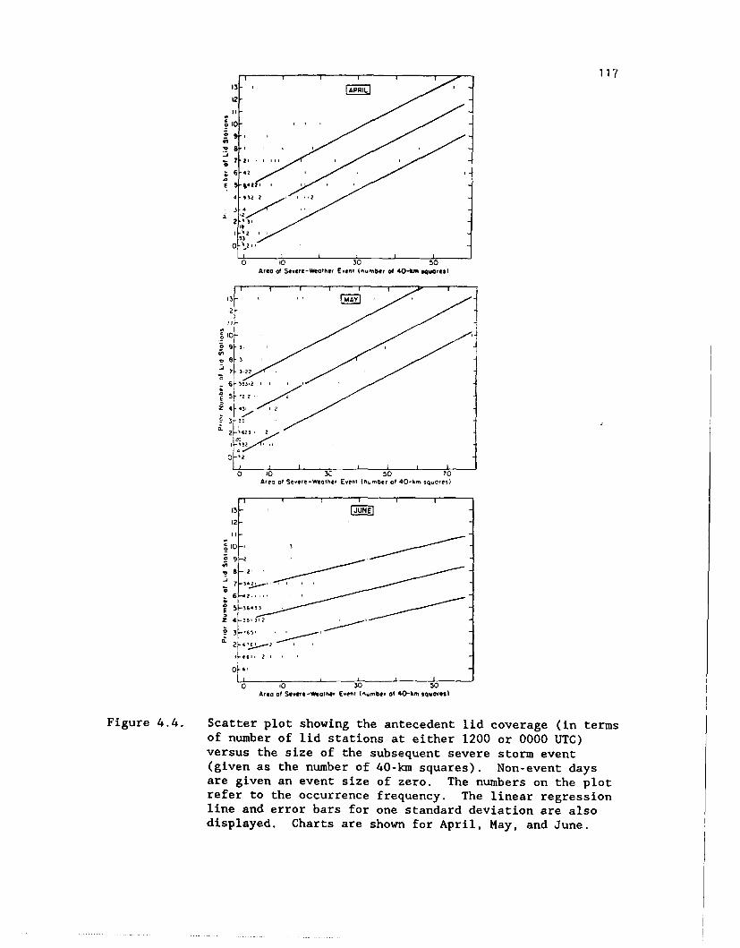
117
9'2
53
0 0 30 50Arco of Severe-Weothef Event (number of 40-4iM oavores)
4-
Z41
z
- 3.•-
0 10
3 JUNE22C0 10 50 70
Area of Severe-weother Event (number of 40-kin squares)
II
II1-
0 ,0 30 50Arto of Scwefe-Welotfer Enveol Ihomber of 40-kmn l400rel|
Figure 4.4. Scatter plot showing the antecedent lid coverage (in termsof number of lid stations at either 1200 or 0000 UTC)versus the size of the subsequent severe storm event(given as the number of 40-km squares). Non-event daysare given an event size of zero. The numbers on the plotrefer to the occurrence frequency. The linear regressionline and error bars for one standard deviation are alsodisplayed. Charts are shown for April, Hay, and June.
118
indicate that even for the month with the lowest correlation coefficient
(June), the r value is significant at a level in excess of the 99%
confidence limit.
A further analysis of the antecedent lid and severe-weather event
data was performed in order to examine the relationships between areas
exceeding certain threshold values of the lid strength (LS) and buoyancy
(BUO) terms of the Lid Strength Index (see section 2.2.1 for definitions
of LS and BUO), and the sizes of the ensuing severe weather events.
Graziano and Carlson (1987) examined the relationship of deep convective
events to the values of LS and BUO, and found a cutoff value for LS,
above which the probability of deep convection decreases rapidly. Their
critical LS value was uniformly close to 2°C during the months of the.
analysis (March through August). An analogous critical BUO value equal
to I°C was also found in their study. Since their analysis technique
used proximity soundings (see Table 1.1 and the accompanying
discussion), no information was available regarding either antecedent
LS and BUO values or the areal extent of each critical values.
We examined the areal extent of severe weather events to the size
of antecedent lid areas with LS 24°C and BUO 5-2°C. The event sizes
were also compared with antecedent lid areas of either LS Z4°C or
BUO <-2°C, in order to evaluate these parameters separately. The LS and
BUO values were chosen to represent both a strong lid and high buoyant
instability, respectively. In particular, the BUO value of -2°C is
approximately equal to an LI of -4°C, which is within the thresiold
interval for severe thunderstorms (Miller 1972). Consideration of the
area with combined LS and BUO values of :40 C and :-2°C allows

119
examination of regions with "explosive" convective potential, in which
rapid release of the buoyant instability occurs with removal of the
strong lid. The results of this analysis are presented in Table 4.1
using the linear correlation coefficients for each category of LS and
BUO term threshold area. The results duplicate the downward trend in r
during the spring that was observed for lid size vs. severe-weather
event area (also see Fig. 4.4). However, Table 4.1 also shows that the
combined LS/BUO threshold is somewhat less useful as a predictive
variable than the size of the antecedent lid. This occurs because the
size of the area exceeding the LS/BUO threshold was rarely above 3 or 4
lid stations. Not surprisingly, the lowest correlation coefficients are
observed for the LS Z4°C only threshold, consistent with the idea that a
large area of high lid strength is more likely to suppress deep
convection (Carlson et al. 1983; Graziano and Carlson 1987). The best
indicator (in terms of r value) of severe-weather event size is the size
of the area with BUO 5-2°C. This result, while not altogether
surprising, is significant because our examination was limited to areas
that had a lid, and suggests that forecasters should look for areas of
BUO 5-20 C within the lid-coverage area when evaluating the potential for
deep convection. Table 4.1 shows that the buoyancy term threshold area
works better than the other predictors even in June, although the r
value has dropped considerably from that of May.
There are two points related to the previous analyses that should
be mentioned. First, while the results show that there is far from a
one-to-one relationship between the area of favorable static stability
(lid) and the area of th( resulting deep convection, there is an
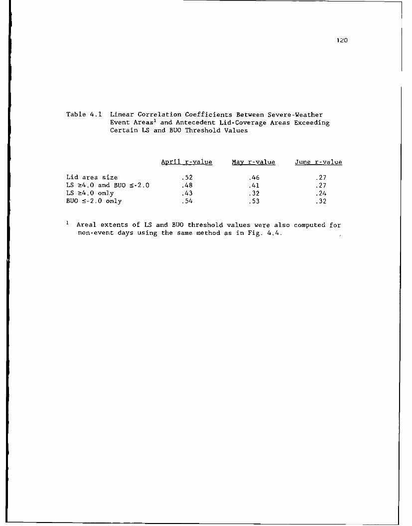
120
Table 4.1 Linear Correlation Coefficients Between Severe-WeatherEvent Areasi and Antecedent Lid-Coverage Areas ExceedingCertain LS and BUO Threshold Values
April r-value May r-value June r-value
Lid area size .52 .46 .27LS Ž4.0 and BUO 5-2.0 .48 .41 .27LS Ž4.0 only .43 .32 .24BUO 5-2.0 only .54 .53 .32
i Areal extents of LS and BUO threshold values were also computed for
non-event days using the same method as in Fig. 4.4.
121
important implication in the large-lid-area/small-severe-weather-area
portion of the scatter plots of Fig. 4.4. That is, large areas of
potential instability generated by the lid are not always consumed by
large outbreaks of deep convection. This is important because the EML
and moist layer can thus migrate to other regions such as the Ohio River
valley and Great Lakes, where they may create the necessary
stratification for a lid sounding (Doswell et al. 1985). This situation
apparently existed during the period preceding the 31 May 1985 tornado
outbreak over the northeast U.S. and southern Ontario (Farrell and
Carlson 1989). The second point involves the existence of
multiple-event days during the period of study. Sometimes, separate
events of different sizes occurred during the same day, and according to
our analysis scheme each event could be associated with the same
antecedent lid size. When the multiple events with the same antecedent
lid-coverage area were combined, the changes in the values of the
correlation coefficients in Table 4.1 ranged from -. 01 to +.08. In the
following sections, the examination of the relationships between the
occurrence of the lid and severe weather is explored using the
conceptual model of the lid life cycle defined in LW2. In this
approach, the severe-weather events are compiled over 24-h periods,
largely eliminating the problem of multi-event days by combining them.
122
4.4 Relationships Between the Lid, Severe Weather,and Representative Synoptic Flow Types
4.4.1 Severe Weather Associated With the Lid cycle
The study of LW2 shows that there are two types of lid cycles,
defined on the basis of the surface type that begins the cycle. The
first cycle, designated H, begins with a surface high-pressure incursion
into the southern Plains with no low level moist layer or EML present
aloft, and is mostly associated with baroclinic waves in the westerlies.
The second cycle, designated R, begins with an already established moist
layer in a persistent return flow from the Gulf of Mexico, but with no
EML aloft, and is associated with subtropical anticyclones and the
passage of weak midtropospheric short wave features. In LW2, the spring
season was divided into an early and late portion, with a dividing date
of 15 May. The early spring is dominated by the H cycle, while the late
spring contains both H and R cycles. For the purposes of this study, we
keep this seasonal division and considei the relationship between the
lid coverage and subsequent severe weather for three types of lid
cycles: the early-season H, the late-season H, and the late-season R
cycles. Since the cycles are defined on the basis of the 1200 UTC data,
the lid-area coverage at this time is used and severe-weather event
coverage during the subsequent 24-h period is documented.
The scatter plot of the lid-coverage area versus the subsequent
severe-weather event coverage for each phase of the early-season H cycle
is shown in Fig. 4.5. See Table 3.1 for formal definitions of the
phases of the lid cycle. Also, note the nonlinear scale used for the
severe-weather area. As expected, the high-pressure stage is mainly
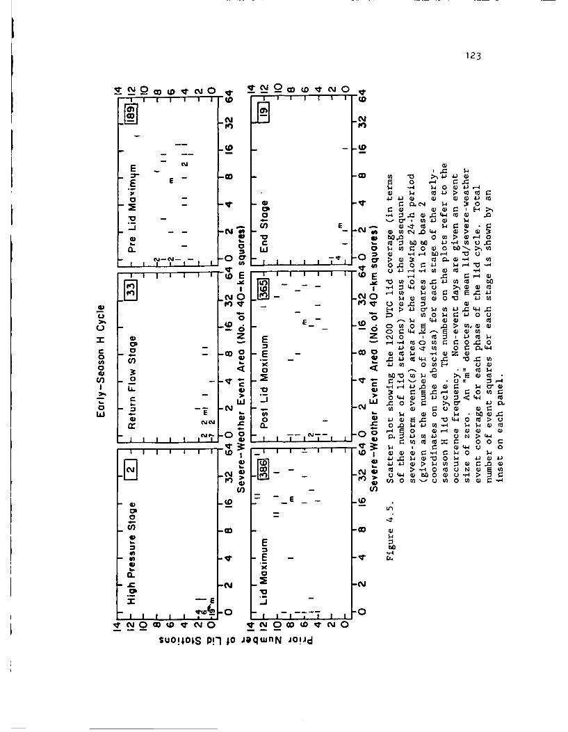
123
W -w
E - 4-
- r 0 0- r: 4
0. 0 4 w0P r. w3 4 ))~ 0 E -4~
-n c- 4) C W0
-~ '-) 0(n Cq 2 J 0 4 -IbN' CO to o 0c 0 )rca -3 ~ UeJ 4- r4U 0 0 c
0.. $ Z 0 0 00 -.. >-, >%" 2 0 r-4 -, WO4 .0 0
r -N. - 0r W, r 'or > w3 c .w 4(J4J- , 0w0 "4
ID EE ,-4~ C .- 4 0to Vf 0 c 41 m I cc bo
C@, - -4 to W 0 E4 4
oc~ o to0~flin ý40 0 0 4- E
0O ::) - Mi~ 0WE-4 04
@3 3 0 E~ 44 1) 2 l,4CO 00 > 4.4'0
C>- r. 44 -14 W r
- ,. 0 A- ca 0 wS
z - E 'A.1 8 m 900w *- It W- 00 r1- .. 440
0 3 C 4J 44 Q 4 10C0- &0 0 0 H u-4
N0 00 -- N = -400 0 w
cn~~ 0'4~. 0.- = : -1D E I4 0 -0 0 I c 1 oo.45I
2% J UJ~ _,- - 0 w 4 -C44CO w 0 O
CO= 0 0 0 C
41 41 -
0-j 0 O >ý 0UN0 (
CI I Ilw O
~NO0ID-co 4)ctDNSUOID&S r~ ; J~qflN O!J
124
associated with small-lid/small-severe-weather-event areas. When the
return-flow stage is reached, there are a few occurrences of larger
severe-weather events, which are linked to the subsequent transition
between small and large lid-coverage areas. In the pre-lid-maximum
stage, there is an increase in both lid and severe-weather coverage
areas, but there are still quite a few occurrences of a large lid area
with a small or no severe-weather event area. The occurrences of large
lid areas with small severe-weather event areas in this phase account
for some of the scatter in the upper left portion of the monthly
lid/severe-weather plots of April and May (Fig. 4.4). It is not until
the lid-maximum and post-lid-maximum stages are reached that the
relationship between large lid-coverage area and large severe-weather,
event area becomes better defined, as noted by the way the data clusters
in the large-lid-area/large-severe-weather-event range in Fig. 4.5.
Observe from Fig. 4.5 that the severe weather activity peaks during
these two stages of this lid cycle.
The next scatter plot is for the late-season H cycle, and is shown
in Fig. 4.6. There is more severe weather occurring during the high-
pressure stage than there was earlier in the season. Keep in mind that
there is more low level moisture available over the southern Plains in
late spring, as shown by LW2's late-spring composite mean analysis for
the high-pressure synoptic type (Fig. 3.6a). This seasonal increase
becomes more noticeable in the return-flow stage where there are
frequent occurrences of severe weather with small-lid coverage areas,
which again accounts for a great deal of the scatter in the monthly
lid/severe weather plots for May and June (Fig. 4.4). Observe in Fig.
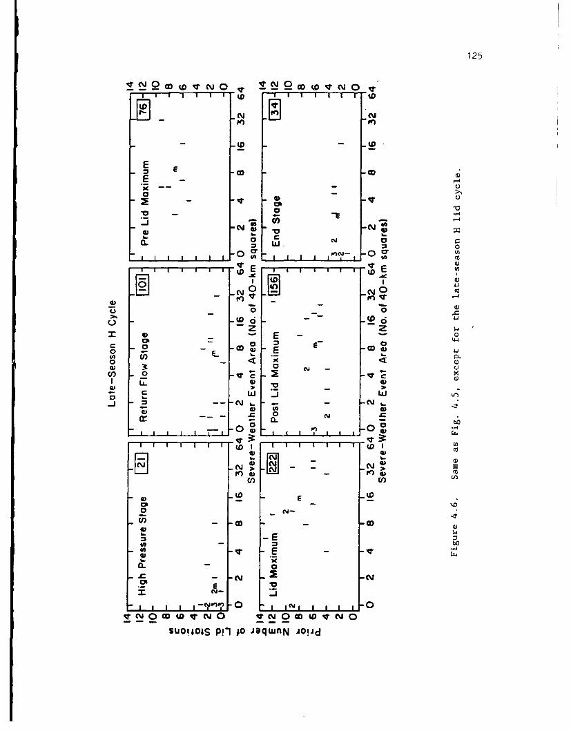
125
OD to V I0O t WC
E EE -
XU
00
*0 - 0
~C I -r (
0 N Y 0
0 0
zI 0E -0
oP -0 m 44a - _ O E EC
in U)
(1 0 Xr
0O r a. *0
o Lio
-C2-- CJ.. . 2,.0Cy 0) (c
E .,
0 0 0Dcy0 w1
0 uioSp- ojq n OJ
126
4.6 that there are relatively few occurrences (7) of the pre-lid-maximun
stage in the late-season H cycle, suggesting that transition to lid-
coverage maximum sometimes occurs directly from either the high-pressure
or return-flow stages. This rapid transition occurred in only four of
19 early-spring H cycles, but was observed in eight of 11 late-season H
cycles. Two possible reasons for the transition from the high-
pressure/return-flow stages directly to the lid-coverage-maximum stage
in the late-season H cycle are the presence of abundant low level
moisture early in the cycle and the existence of multiple EML source
regions.
Figure 4.7 shows the lid and severe weather relationship during the
R cycle. The severe weather events in this cycle are observed with a
large range of lid-coverage areas, and are typically associated with
between one and three lid stations in the return-flow and end stages,
and between four and seven stations in the large lid-coverage stages.
Again, there are relatively few (5) occurrences of a pre-lid-maximum
stage, and examination of the observations shows that a rapid transition
from the return-flow stage to lid-coverage maximum occurred in eight of
11 late-season R cycles. Since both the late-season H cycle and the R
cycle are characterized by the presence of multiple EML source regions
and large areas of low level moisture, it seems plausible that these
factors allow for the rapid transitions in lid coverage to occur.
4,4.2 Lid and Severe Weather Occurrence for RepresentativeSynoptic Types
LW2 showed that definable lid cycles encompassed over 80% of all
days in the study period. We use frequently occurring synoptic types to

1 127 I I
- -4
= -(
E E- E4E E
-- ,
10 En -
CL 0
- LUI
I f I TI I I I C) .c r¾D E
m-o
z 4J
0-z
10E
-n -
00
4- Cn
0
N 0
E>
'3.3o -N--
- -N 4
E
m3 O D N
suoijD4S p!1l ;o JaqtunN JO!~d
128
represent specific phases of the lid cycle. These subjectively
determined synoptic types were defined in LWI. To summarize, a synoptic
type consists of a surface component based on the sea level isobaric
pattern, and a 500-mb component based on the predominant wind direction
over the study region. LW2 presented composite mean analyses of
relevant atmospheric variables for these synoptic types and related them
to geographic frequencies of the EML and buoyant instability. The
criterion for buoyant instability used in this analysis is a value of
the buoyancy term of the Lid Strength Index of less than 0.5°C, while
the procedure for determining the presence of an EML is related to the
temperature and dewpoint profiles, an6 is described in section 2.2.1.
Summary charts of specific meteorological features from LW2's composite
mean analyses are produced, and include the geographic frequencies of
the EML and buoyant instability. Tabulated severe-weather events during
the 12-h period following the observed synoptic type are then added to
the summary charts in order to relate the geographic distribution of
severe weather to the various dynamic and stability features. Areas
where the geographic frequencies for the EML and buoyant instability are
both greater than 50% can be regarded as lid occurrence areas, since the
lid sounding, by definition, must have both buoyant instability and an
EML. The reason for distinguishing between the two components (EML and
buoyant instability) is to examine the independent evolution of the EML
and moist layer, understand how a lid area is created (and destroyed)
during a lid cycle, and understand how this evolution impacts the
occurrence of severe weather. Use of geographic frequencies for EML and
buoyant instability occurrence is preferable to calculation of mean
129
values for parameters such as lid strength. The lid strength term
(defined in section 2.2.1) is only useful in this study when a sounding
has an inversion and EML aloft. Since a 100% lid-coverage area does not
exist for each day of a synoptic type sample, rawinsonde stations would
have different sample sizes going into the calculations of the mean,
which would lead to spatial incoherence in a small sample such as a
synoptic type composite. To illustrate the large seasonal contrasts in
synoptic scale circulation patterns and in the lid coverage vs. severe
weather areas, analyses are presented for the early-season H and late-
season R cycles.
The first set of summary charts for the early-season H cycle is
shown in Fig. 4.8. Figure 4.8a contains the legend for these charts'and
those in Fig. 4.9. Figure 4.8b shows the frequencies of severe weather,
EML, and buoyant instability, as well as relevant meteorological
features, for the synoptic type representing a north-south surface ridge
with northwest flow aloft. This unfavorable lid-producing pattern
represents the high-pressure stage of the cycle, and there are only
isolated areas with greater than 50% frequency of either an EML or
buoyant instability, and only one severe weather event, over southwest
Texas. This particular event occurred on 8 May 1983 and was associated
with a strong intrusion of low level moisture through the Rio Grande
valley, lid soundings over Del Rio and Brownsville, Texas, and a short
wave trough moving through the subtropical jet across northern Mexico.
The return-flow stage is represented by weak return flow with
anticyclonic flow aloft (Fig. 4.8c). In this composite analysis, there
is evidence of two separately emerging EML areas over Nebraska and
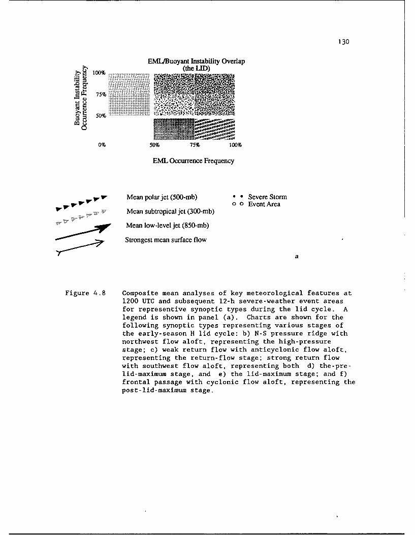
130
EML/Buoyant Instability Overlap>N (the LID)
Zý 100%.......
S............................................... .
0 50%
0% 50% 75% 100%
EML Occurrence Frequency
I, V Mean polar jet (500-mb) e * Severe Storm0 0 Event Area
- .Mean subtropical jet (300-mb)
.. "Mean low-level jet (850-mb)
Strongest mean surface flow
a
Figure 4.8 Composite mean analyses of key meteorological features at1200 UTC and subsequent 12-h severe-weather event areasfor representive synoptic types during the lid cycle. Alegend is shown in panel (a). Charts are shown for thefollowing synoptic types representing various stages ofthe early-season H lid cycle: b) N-S pressure ridge withnorthwest flow aloft, representing the high-pressurestage; c) weak return flow with anticyclonic flow aloft,representing the return-flow stage; strong return flowwith southwest flow aloft, representing both d) the-pre-lid-maximum stage, and e) the lid-maximum stage; and f)frontal passage with cyclonic flow aloft, representing thepost-lid-maximum stage.
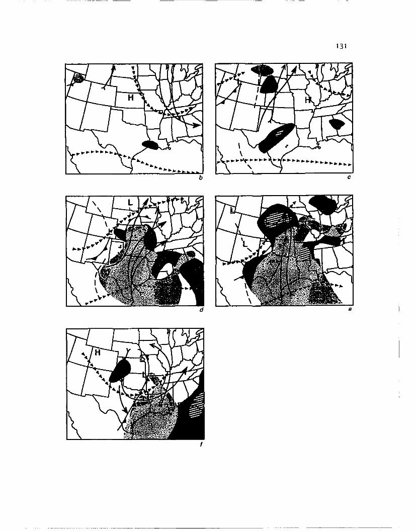
131
Ott 0 0. C
d e
4wf
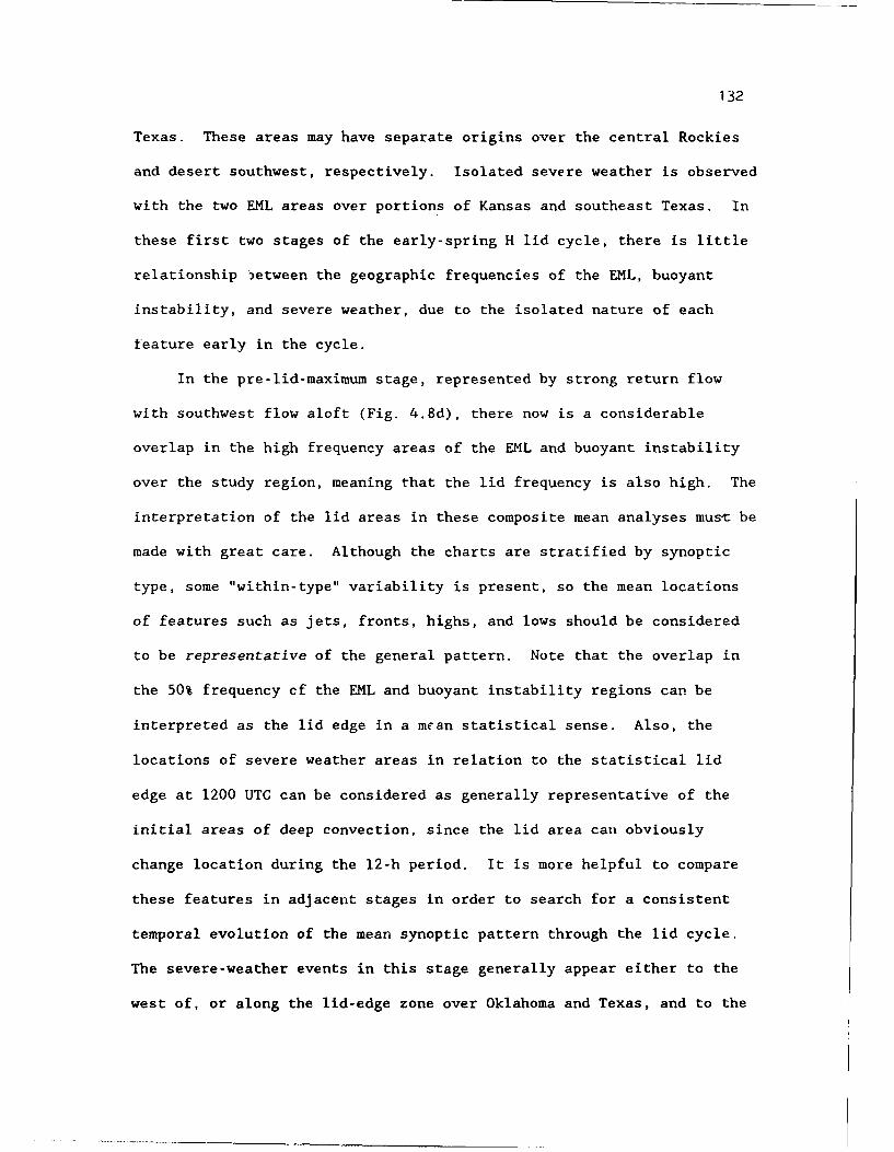
132
Texas. These areas may have separate origins over the central Rockies
and desert southwest, respectively. Isolated severe weather is observed
with the two EML areas over portions of Kansas and southeast Texas. In
these first two stages of the early-spring H lid cycle, there is little
relationship jetween the geographic frequencies of the EML, buoyant
instability, and severe weather, due to the isolated nature of each
feature early in the cycle.
In the pre-lid-maximum stage, represented by strong return flow
with southwest flow aloft (Fig. 4.8d), there now is a considerable
overlap in the high frequency areas of the EML and buoyant instability
over the study region, meaning that the lid frequency is also high. The
interpretation of the lid areas in these composite mean analyses mus-t be
made with great care. Although the charts are stratified by synoptic
type, some "within-type" variability is present, so the mean locations
of features such as jets, fronts, highs, and lows should be considered
to be representative of the general pattern. Note that the overlap in
the 50% frequency cf the EML and buoyant instability regions can be
interpreted as the lid edge in a mean statistical sense. Also, the
locations of severe weather areas in relation to the statistical lid
edge at 1200 UTC can be considered as generally representative of the
initial areas of deep convection, since the lid area can obviously
change location during the 12-h period. It is more helpful to compare
these features in adjacent stages in order to search for a consistent
temporal evolution of the mean synoptic pattern through the lid cycle.
The severe-weather events in this stage generally appear either to the
west of, or along the lid-edge zone over Oklahoma and Texas, and to the
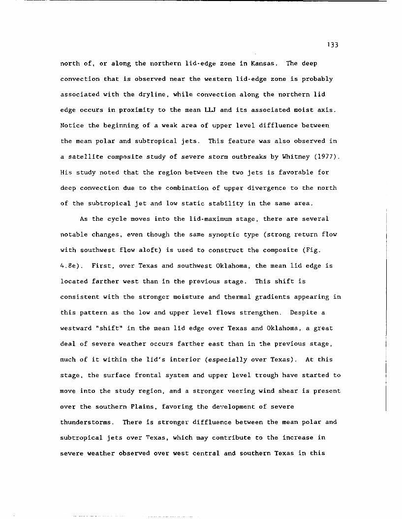
133
north of, or along the northern lid-edge zone in Kansas. The deep
convection that is observed near the western lid-edge zone is probably
associated with the dryline, while convection along the northern lid
edge occurs in proximity to the mean LLJ and its associated moist axis.
Notice the beginning of a weak area of upper level diffluence between
the mean polar and subtropical jets. This feature was also observed in
a satellite composite study of severe storm outbreaks by Whitney (1977).
His study noted that the region between the two jets is favorable for
deep convection due to the combination of upper divergence to the north
of the subtropical jet and low static stability in the same area.
As the cycle moves into the lid-maximum stage, there are several
notable changes, even though the same synoptic type (strong return flow
with southwest flow aloft) is used to construct the composite (Fig.
4.8e). First, over Texas and southwest Oklahoma, the mean lid edge is
located farther west than in the previous stage. This shift is
consistent with the stronger moisture and thermal gradients appearing in
this pattern as the low and upper level flows strengthen. Despite a
westward "shift" in the mean lid edge over Texas and Oklahoma, a great
deal of severe weather occurs farther east than in the previous stage,
much of it within the lid's interior (especially over Texas). At this
stage, the surface frontal system and upper level trough have started to
move into the study region, and a stronger veering wind shear is present
over the southern Plains, favoring the development of severe
thunderstorms. There is stronger diffluence between the mean polar and
subtropical jets over Texas, which may contribute to the increase in
severe weather observed over west central and southern Texas in this
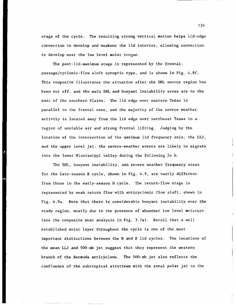
134
stage of the cycle. The resulting strong vertical motion helps lid-edge
convection to develop and weakens the lid interior, allowing convection
to develop near the low level moist tongue.
The post-lid-maximum stage is represented by the frontal-
passage/cyclonic-flow aloft synoptic type, and is shown in Fig. 4.8f.
This composite illustrates the situation after the EML source region has
been cut off, and the main EML and buoyant instability areas are to the
east of the southern Plains. The lid edge over eastern Texas is
parallel to the frontal zone, and the majority of the severe weather
activity is located away from the lid edge over northeast Texas in a
region of unstable air and strong frontal lifting. Judging by the
location of the intersection of the maximum lid frequency axis, the LIJ,
and the upper level jet, the severe-weather events are likely to migrate
into the lower Mississippi valley during the following 24 h.
The EML, buoyant instability, and severe weather frequency areas
for the late-season R cycle, shown in Fig. 4.9, are vastly different
from those in the early-season H cycle. The return-flow stage is
represented by weak return flow with anticyclonic flow aloft, shown in
Fig. 4.9a. Note that there is considerable buoyant instability over the
study region, mostly due to the presence of abundant low level moisture
(see the composite mean analysis in Fig. 3.7a). Recall that a well
established moist layer throughout the cycle is one of the most
important distinctions between the H and R lid cycles. The locations of
the mean LLJ and 500-mb jet suggest that they represent the western
branch of the Bermuda anticyclone. The 500-mb jet also reflects the
confluence of the subtropical airstream with the zonal polar jet to the
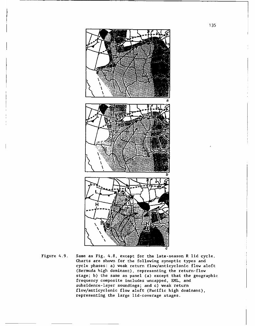
135
a
b
C
Figure 4.9. Same as Fig. 4.8, except for the late-season R lid cycle.Charts are shown for the following synoptic types andcycle phases: a) weak return flow/anticyclonic flow aloft(Bermuda high dominant), representing the return-flowstage; b) the same as panel (a) except that the geographicfrequency composite includes uncapped, EML, andsubsidence-layer soundings; and c) weak returnflow/anticyclonic flow aloft (Pacific high dominant),representing the large lid-coverage stages.
136
north. There is much more severe weather activity in this stage of the
R cycle than there was in the early stages of the early-season H cycle
(Fig. 4.8c). The severe weather activity observed at this stage is not
associated with high frequencies of EML/lid occurrence at the analysis
time. This result is consistent with our previous observations
regarding the deterioration of the relationship between the antecedent
lid coverage and severe weather in the late spring. We examined the
possibility that other types of soundings iay be playing a role in this
synoptic pattern. Analysis of the individual days making up this
synoptic type sample shows that severe weather occurred in an
environment that contains other types of soundings besides the lid type.
These included uncapped (zero lid strength) soundings and subsidence-
type soundings that were buoyantly unstable. The importance of the
uncapped soundings lies in their contribution to both midlevel potential
instability and low level buoyant instability due to high lapse rate air
in the EML. The subsidence-layer soundings contribute to the low level
instability by capping the moist layer. Figure 4.9b shows the same
composite analysis as Fig. 4.9a, except that the geographic frequency
composite now includes EML, uncapped, and subsidence soundings. The
orientation of the maximum frequency axis of EML, uncapped, and
subsidence soundings with the western branch of the Bermuda cell
suggests that this dry midlevel air probably originates in the easterly
flow over the Gulf of Mexico, and is then transported northward into the
Great Plains. Studies by Caracena and Fritsch (1983) and Hagemeyer and
Darkow (1988) for cases which resemble this synoptic type, demonstrate
the importance of such a dry-air intrusion for generating potential
137
instability, and, subsequently, severe storms when the low level moist
air is lifted. From Fig. 4.9b, several features capable of providing
such a lifting mechanism can be identified, such as the mean LIU, the
frontal boundary over Nebraska, and the surface trough over the western
Plains. It is possible that the area between the mean surface trough
and LLU may experience upward motion from a combination of the cyclonic
horizontal shear to the west of the LLJ and the cyclonically curved
surface flow to the east of the trough. This general area also has a
strong gradient of buoyant instability frequency. Thus, at this stage
of the R cycle, in this synoptic type, the presence of several different
types of soundings can be important in locally generating potential
instability in a region of low-level convergence and abundant moisture.
The large lid-coverage stages are also represented by weak return
flow with anticyclonic flow aloft (Fig. 4.9c). However, this synoptic
pattern is associated with the Pacific anticyclone, as discussed by LW2
(see Fig. 3.7b). The severe weather in this pattern is clustered to the
east of a lid-edge zone over the western Plains, between two mean LLU
axes in a region of strong directional shear between the low levels and
500 mb. Of particular note is the strong directional shear between the
surface and 850 mb. This type of strong directional shear in an area of
high buoyant instability is characteristic of late spring and summertime
severe storm environments (Johns and Sammler 1989, Davies 1989). In
this synoptic pattern, a short wave trough often travels along the zonal
polar jet into the western Plains, then turns southward along the
eastern branch of the Pacific ridge, with a frontal system following it
into Oklahoma and northern Texas. The subsequent movement of the short
138
wave trough out of the study region causes the EML to be transported
eastward, and returns the Great Plains to minimum lid coverage, ending
the R cycle.
4.5. Conclusions
This study examined the relationships between the occurrence of
severe storms over the southern Great Plains, the occurrence-frequency
patterns of the EML and buoyant instability, and the occurrence of
various representative synoptic flow types. The analysis emphasized the
temporal dimension by investigating these relationships during the life
cycle of lid development and dissipation. One unique aspect of this
study is the inclusion of the non-event days in the analyses, which ,
allows examination of the relationships for these situations as well.
The analysis of the severe-storm events for the four-year period
over the southern Plains found that the size distribution of severe-
storm events has a large peak in the 1600 km2 , or "isolated event,"
category for each month. In April, there is a secondary peak for event
sizes on the order of 20,000-25,000 km2 , and in June a secondary peak is
between 14,500 and 19,000 km2. In general, the size distribution of
severe-weather events remains essentially the same during the season,
except for a sharp increase in isolated-event occurrences from May to
June. The occurrence frequency of non-event days shows a steady
decrease during the spring from 66 days in April to 22 in June. The
geographic distribution of severe weather events shows a gradual shift
to the west and north during the spring season, consistent with the
139
seasonal evolution of lid frequency reported in Farrell and Carlson
(1989) and LWI, and the composite mean lid/EML analyses of LWI.
The relationship between the occurrence/size of the lid and the
subsequent occurrence/size of severe-weather events is best defined in
April, and deteriorates rapidly from May to June. This deterioration is
due to the existence of different stability and synoptic patterns in the
early spring versus the late spring. Early-spring synoptic patterns are
mainly associated with the progression of frontal systems and baroclinic
waves in the westerlies. At this time, low level moisture is area-
limited and mostly determined through advection. Accordingly, buoyantly
unstable areas are also limited (McNulty 1980), while the EML usually
has an equal or greater areal extent. The progression of strong
baroclinic systems, which controls the evolution of both the limited
moisture and EML areas, allows a more certain diagnosis of potential
severe-storm activity based on the 1200 UTC analysis and continuity.
Late-spring synoptic patterns are dominated by weak persistent return
flow at low levels, subtropical anticyclones, and weak short wave
troughs which drift through the region. There is widespread low level
moisture and buoyant instability throughout the region, both of which
have a much larger areal extent than does the EML. The evolution of the
EML is mostly determined by the position and intensity of subtropical
anticyclones such as the Bermuda and Pacific ridges. When the Bermuda
cell is dominant over the eastern half of the U.S., dry midlevel air
embedded in the easterly flow over the Gulf of Mexico can be drawn
northward in the western branch of the cell, producing isolated dry
intrusions which may locally produce areas of potential instability and,
140
subsequently, severe weather. When the Pacific cell dominates the
western half of the U.S., a capping lid is produced over the Great
Plains in the westerly flow from EML source regions to the west.
In the early-season H lid cycle, the small lid-coverage phases are
associated with small severe weather event areas, while the maximum
lid/severe-weather activity occurs in the lid-maximum and post-lid-
maximum stages. In late spring, both the H and R cycles are capable of
supporting severe weather at all stages, but in the H cycle the maximum
activity occurs in the lid-maximum stage. In the R cycle, there is no
clear relationship between antecedent lid occurrence/size and severe-
weather event occurrence/size. In both late-season cycles, a rapid
transition from either the high-pressure or return-flow stages to lid
maximum is observed nearly 75% of the time. In the strong baroclinic
systems characteristic of the early-season H cycle, there is a clear
geographic relationship between severe weather occurrence and
EML/buoyant instability areas. In the pre-lid-maximum stage, the events
are observed in the vicinity of and along the western and northern lid-
edge areas. During the lid-maximum stage, severe-weather events are
observed both along the mean lid edge as well as within the high lid-
frequency area. In this synoptic environment, both lid-edge convection
and convection associated with a weakened lid interior are observed. An
example of such a region is southern Texas, where the upper diffluence
to the north of the mean subtropical jet may serve to enhance vertical
motion and hasten lid removal.
In late spring, severe-weather events are associated with high
frequency areas of buoyant instability, but not necessarily with high
141
frequency areas of the EML. Examination of the composite mean analyses
representing the late-season R cycle shows that when the Bermuda cell
dominates, the majority of severe weather occurs between the mean LIJ
and surface trough, in a region of low level cyclonic vorticity and weak
vertical shear. A buoyant instability gradient and localized areas of
potential instability characterize this environment, influenced by the
presence of the EML and subsidence layers from the western branch of the
Bermuda cell. The analyses representing the period when the Pacific
ridge dominates show that the majority of severe weather occurs to the
east of the lid edge, in a region of buoyant instability and strong
directional wind shear, especially between the surface and 850 mb. In
these situations, a short wave trough often moves through the zonal
polar jet and travels around the eastern branch of the Pacific
anticyclone, moving into the Great Plains and pushing a surface front
southward through the region. The eastward movement of the short wave
trough across the Plains states subsequently transports the EML out of
the region, returning the area to minimum lid coverage and marking the
beginning of a new lid cycle.
1 4 2
Chapter 5
AN EXAMPLE OF AN EARLY SPRING LID CYCLE
The period of 4-9 April 1984 was chosen as an example of an early-
season H lid cycle over the southern Great Plains. This lid cycle
contained four of the synoptic types documented in the synoptic
climatology of Chapters 2-4; extensive lid areas on 7 and 8 April; and
severe-weather outbreaks over Texas and Oklahoma on 7 April, and over
Arkansas, Louisiana, and Mississippi on 8 April. These features make
this a good case with which to examine certain aspects of the synoptic
climatology and the early-season H cycle conceptual model discussed in
Chapters 2-4.
5.1 Overview of the 4-9 April 1984 H Lid Cycle
A summary of the major atmospheric features at 1200 UTC on each day
of this five-day period is shown by the series of analyses in Fig. 5.1.
The discussion of these atmospheric features is followed by a summary of
the severe weather and heavy rainfall associated with the large lid-
coverage stages of the cycle over the southern Great Plains and
Mississippi River valley on 7 and 8 April.
At 1200 UTC 4 April (Fig. 5.1a), the initial time of the lid cycle,
an extratropical cyclone with a central pressure of 1002 mb was located
over western Kentucky. The associated frontal system was moving through
the central Gulf of Mexico. Behind the system, a surface pressure ridge
was expanding southward into the Great Plains. The high was centered

143
Figure 5.1. Analysis of surface and 500-mb features at 1200 UTC oneach day of the 4-9 April 1984 lid cycle. The 1016 and1008-mb sea level isobars are shown by the thin lines, andthe thick lines with arrows denote the subjectivelyanalyzed 500-mb jets. Surface fronts, troughs, highs andlows are shown using conventional notation. Locations of500-mb highs and lows are shown using "open" lettering.The locations of the stations used in the time series ofFig. 5.3 are shown in panel (a). On panel (d), theposition of the surface dryline is shown using a solid,scalloped line. Analyzes are shown for a) 4 April,b) 5April, c) 6 April, d) 7 April, e) 8 April, and f) 9 April.
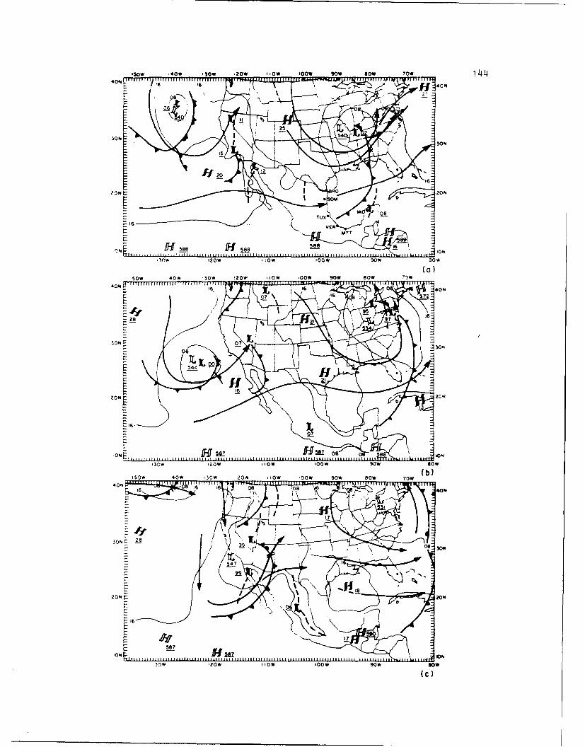
.sow -400 '30W .20* flow 10* sow sow 70W i4'4
400
~ '6
CN Lff se8af 588 588-O
(a)
50* 40* '30* !2OW ,low 00*W 9* sow 'Ok
206
!ON 6 6 08 0
6L
150 *o '20* 20 loOW ' 00890 sow O(b
4ON ý- [T~tHWI~ll)
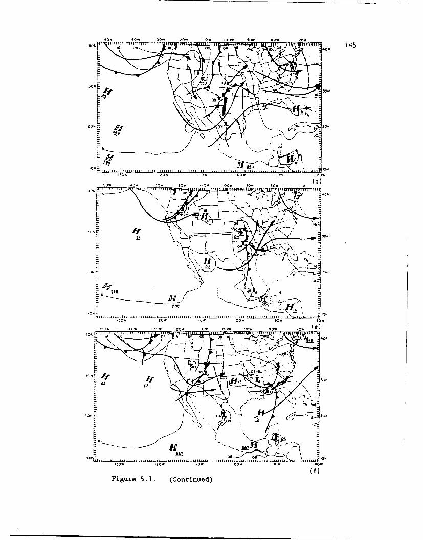
.50A 40 3* sow 20W .0w 00W sow sow ro0w
.00 '2ý 0. 0* 0 8y 0
40N0
z Me
555
02OL -, LLL1-UL O
450 8 .4*3W -0 0 0 W io o d'6 .gg
16H
240 40300.* 0 0* 8* ~ w 0 e
SOW '20* 20*
ff(f)Figur 5.1. (Contnued

146
over northern Colorado, with a central pressure of 1025 mb. In the
midtroposphere, a cut-off 500-mb low was located over Missouri. A
cyclonically curved jet was analyzed from the Great Plains to the middle
Atlantic states and the Appalachian Mountains. Evidence of a
subtropical jet (which will be discussed in more detail later in this
chapter) at this level was found from near 20'N latitude, 135°W
longitude, through the southern Baja Peninsula, and into central Mexico.
A c itinuation of the subtropical jet was analyzed from the southern
Gulf to east of the south Florida coast. A 500-mb ridge was located to
the west of the Continental Divide, and a deepening trough was centered
near 130°W longitude.
By 5 April (Fig. 5.1b), the surface cyclone had moved into the
Appalachian Mountains aLd middle Atlantic states, while the continental
high spread into the southern Plains and western Gulf. The 500-mb ridge
was located over the Continental Divide, and the next trough and frontal
system were entering the southwestern states. There were actually two
fronts associated with this upper trough. The first front was moving
through Arizona and Sonora, Mexico, while a second, occluded system was
approaching southern California and Baja. To the north of these two
systems was another front moving through the Pacific Northwest. This
system was associated with an upper level trough which had split with
the primary polar jet stream near 135°W longitude.
As the cycle moved into its third day (6 April; Fig. 5.1c), several
changes took place. The surface anticyclone which, dominated the Great
Plains and Gulf of Mexico weakened considerably, with only a small
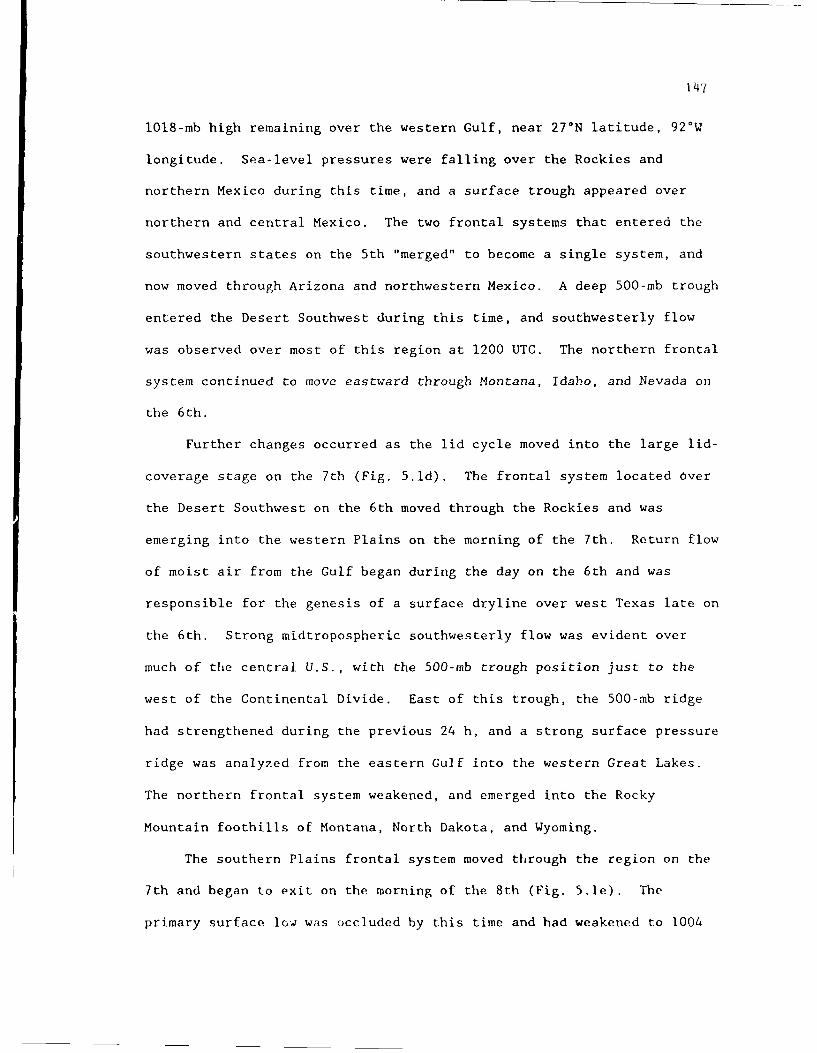
147
1018-mb high remaining over the western Gulf, near 27°N latitude, 92°W
longitude. Sea-level pressures were falling over the Rockies and
northern Mexico during this time, and a surface trough appeared over
northern and central Mexico. The two frontal systems that entered the
southwestern states on the 5th "merged" to become a single system, and
now moved through Arizona and northwestern Mexico. A deep 500-mb trough
entered the Desert Southwest during this time, and southwesterly flow
was observed over most of this region at 1200 UTC. The northern frontal
system continued to move eastward through Montana, Idaho, and Nevada on
the 6th.
Further changes occurred as the lid cycle moved into the large lid-
coverage stage on the 7th (Fig. 5.1d). The frontal system located over
the Desert Southwest on the 6th moved through the Rockies and was
emerging into the western Plains on the morning of the 7th. Return flow
of moist air from the Gulf began during the day on the 6th and was
responsible for the genesis of a surface dryline over west Texas late on
the 6th. Strong midtropospheric southwesterly flow was evident over
much of the central U.S., with the 500-mb trough position just to the
west of the Continental Divide. East of this trough, the 500-mb ridge
had strengthened during the previous 24 h, and a strong surface pressure
ridge was analyzed from the eastern Gulf into the western Great Lakes.
The northern frontal system weakened, and emerged into the Rocky
Mountain foothills of Montana, North Dakota, and Wyoming.
The southern Plains frontal system moved through the region on the
7th and began to exit on the morning of the 8th (Fig. 5.1e). The
primary surface lo4 was occluded by this time and had weakened to 1004
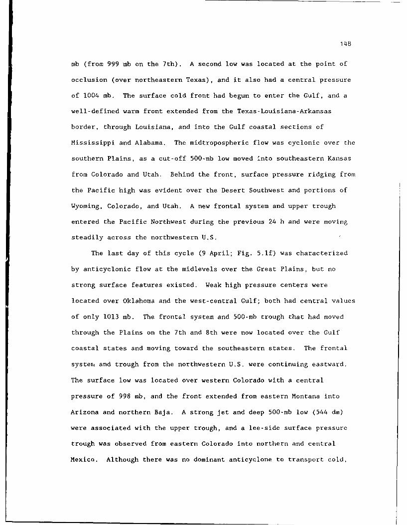
148
mb (from 999 mb on the 7th). A second low was located at the point of
occlusion (over northeastern Texas), and it also had a central pressure
of 1004 mb. The surface cold front had begun to enter the Gulf, and a
well-defined warm front extended from the Texas-Louisiana-Arkansas
border, through Louisiana, and into the Gulf coastal sections of
Mississippi and Alabama. The midtropospheric flow was cyclonic over the
southern Plains, as a cut-off 500-mb low moved into southeastern Kansas
from Colorado and Utah. Behind the front, surface pressure ridging from
the Pacific high was evident over the Desert Southwest and portions of
Wyoming, Colorado, and Utah. A new frontal system and upper trough
entered the Pacific Northwest during the previous 24 h and were moving
steadily across the northwestern U.S.
The last day of this cycle (9 April; Fig. 5.1f) was characterized
by anticyclonic flow at the midlevels over the Great Plains, but no
strong surface features existed. Weak high pressure centers were
located over Oklahoma and the west-central Gulf; both had central values
of only 1013 mb. The frontal system and 500-mb trough that had moved
through the Plains on the 7th and 8th were now located over the Gulf
coastal states and moving toward the southeastern states. The frontal
systent and trough from the northwestern U.S. were continuing eastward.
The surface low was located over western Colorado with a central
pressure of 998 mb, and the front extended from eastern Montana into
Arizona and northern Baja. A strong jet and deep 500-mb low (544 dm)
were associated with the upper trough, and a lee-side surface pressure
trough was observed from eastern Colorado into northern and central
Mexico. Although there was no dominant anticyclone to transport cold,

149
dry air into the Gulf in this case, the cold front did have drier air
behind it, so lid soundings were not possible over the southern Great
Plains at this time. This returned the region to a minimum lid coverage
and signalled the end of this lid cycle.
Figure 5.2a depicts the type and extent of severe weather and heavy
rainfall during the 24-h period from 1200 UTC 7 April to 1200 UTC 8
April. For a description of the criteria used to define "severe
weather" in this study, see section 4.1. During this period, most of
the heavy rainfall occurred in western Oklahoma and southeastern Kansas,
while the majority of the severe weather was reported in west-central
and south-central Texas. The heaviest rainfall totals were in western
Oklahoma, with Taloga, Oklahoma reporting 3.08 inches during the 24-h
period. The severe-weather outbreak began around 0900 CST (1500 UTC)
with isolated wind and hail reports in northwestern and southern
Oklahoma. The first severe weather in Texas began shortly after 1000
CST, with reports of tornadoes west of Abilene. This outbreak lasted
for about 40 h and moved into the vicinity of Mineral Wells by mid-
afternoon. A second area of severe weather, over south-central Texas,
began around 1130 CST with radar reports of line echo wave pattern
activity northwest of Del Rio. This outbreak moved eastward over the
next 5 h and reached San Antonio. After 1630 CST, only two more severe-
weather reports were recorded in Texas; one was in the area of Waco
(winds in excess of 50 kt, at 1650 CST) and the other (an FO tornado, as
defined using Fujita's F-scale) occurred early on 8 April (0145 CST) on
the outskirts of Jasper (near the Louisiana border).
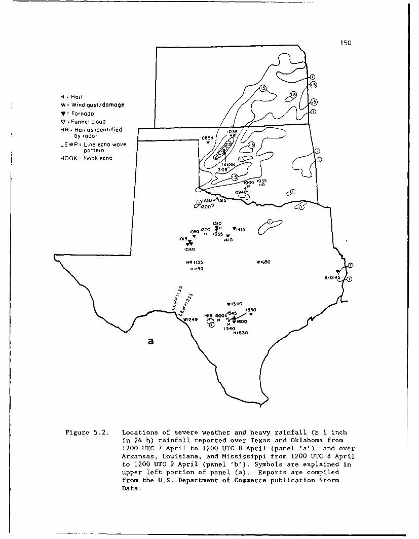
150
H z HallW= Wind gust/damage L
y = Tornado
Sz Funnel cloud
HR =yHall as identified 035o//by radar 0854 M
LEWP= Line echo wave / .5pattern
HOOK Hook echoo
10094
HR 113V WIN3O W5 1410
10404
"" 1•540
N1630
Figure 5.2. Locations of severe weather and heavy rainfall (>_ i inchin 24 h) rainfall reported over Texas and Oklahoma from1200 UTO 7 April to 1200 UTG 8 April (panel 'a'), and over
Arkansas, Louisiana, and Mississippi from 1200 UTG 8 Aprilto 1200 UT1 9 April (panel 'b'). Symbols are explained in
upper left portion of panel (a). Reports are compiledfrom the U.S. Department of Commerce publication StormData.Fiur 5.2 Loain of seer wete an hev ranfl I inch
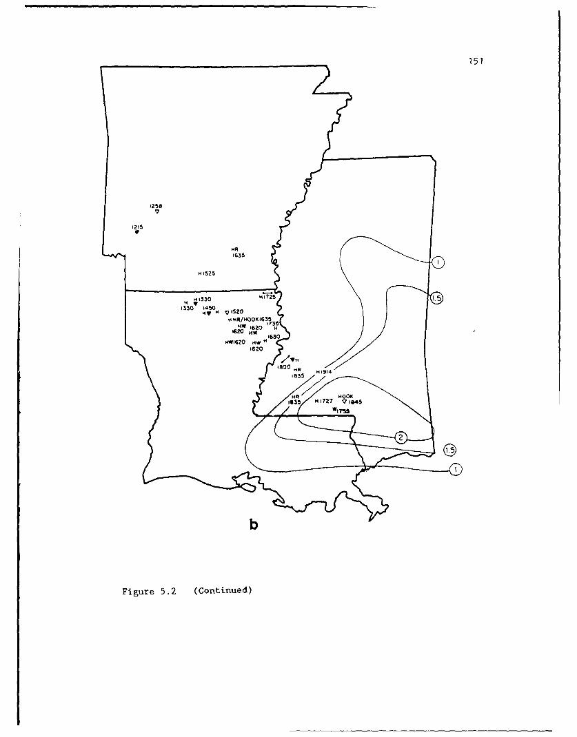
251
1215v
, 635
1 525
M 1330 HIM5
330 15I4 7 N 520
w4 KA/NOOK1635
~b"
Figure 5.2 (Continued)
152
The severe weather and heavy rainfall that occurred from 1200 UTC 8
April until 1200 UTC 9 April over Arkansas, Louisiana, and Mississippi,
are summarized in Fig. 5.2b. Both severe weather and heavy rainfall
were observed over Mississippi during this time, with the heaviest
amounts over the southern part of the state, from McComb to north of
Biloxi. Severe weather began after 1200 CST over southwestern Arkansas
with a report of an Fl tornado in the area of Nashville. Reports
associated with this outbreak were isolated over southern Arkansas, but
became more widespread as new cells that developed over the southwest
corner of Arkansas in the late morning moved into northern Louisiana
during the early afternoon. During the next 4 h, there were reports of
wind damage, large hail, funnel clouds, and several tornadoes moving in
a southeasterly direction through northern Louisiana. New cells
developing along the southern Louisiana-Mississippi border during the
late afternoon were responsible for the severe weather reported over
portions of southern Mississippi from about 1730 CST to 1915 CST. After
1915 CST on 8 April, only heavy rainfall occurred with these
thunderstorms as they moved eastward into southern Alabama and the
Florida panhandle.
5.2 Examination of the Lid Cycle by Stages
5.2.1 The High-Pressure Stage (1200 UTC 4 April-0000 UTC 6 April)
This first stage of the 4-9 April lid cycle was characterized by a
large surface anticyclone over the Great Plains and western Gulf of
Mexico. During the high-pressure stage (see Table 3.1 for definitions
153
of the cycle stages), cold, dry air moved southward into the southern
Plains and Gulf. During the first 24 h of the cycle, a strong north-
south pressure ridge developed over the western Plains, and moved into
the central Plains while spreading southward into the Gulf. This
surface anticyclone originated over southern Canada on 2 April and
strengthened under the confluent northwesterly flow behind a
midtropospheric trough over the western Plains on 3 and 4 April.
Figures 5.1ab show that the surface ridge strengthened further over the
Great Plains during the first 24 h of the lid cycle as the
MLdtropospheric flow became increasingly confluent over the southern
Plains and Gulf coast. Cold-air advection was present to the east of
the surface ridge axis during this time, which also contributed to Ole
anticyclone's intensification during the first 24 h of the cycle. Cold-
air advection is also present in the climatological composite for the
high-pressure stage of the early-spring H cycle (Fig. 3.5a); a
comparison of Figs. 3.5a and 5.1b shows that the synoptic pattern on the
second day of the cycle is similar to the climatological composite,
including the extension of the mean surface pressure ridge into the
Gulf.
The surface ridge eventually developed as far south as the Bay of
Campeche (around 18*N latitude; well south of the subtropical jet) by
1200 UTC on 5 April. The southern extension of the surface pressure
ridge seemed to develop independently of the midtropospheric "steering"
flow, and resembles the latter stages of a Front Range wintertime cold
surge documented by Tilley (1990). The Front Range cold surge is
closely controlled by the terrain gradient, and is attributed to
154
topographically trapped edge waves according to Tilley's study.
Tilley's Front Range case occurred in December 1983, and featured a
southward developing pressure ridge along the eastern slopes of the
Rockies, accompanied by a narrow surge of cold air. This cold surge and
pressure ridging continued to move south along the eastern slopes of the
Sierra Madre Oriental range in Mexico. Despite the fact that our case
occurred in April, there are similarities between it and this December
1983 case. For example, in the December 1983 cold surge, strong
northerly winds were observed with the surge as it moved into Mexico. A
time series of Gulf coastal surface station reports from 1200 UTC 4
April to 1200 UTC 6 April, displayed in Fig. 5.3, shows strong northerly
winds and blowing dust at Veracruz, Mexico at 0000 UTC 5 April.
Although there is no evidence of a surface cold surge at any of the
stations in Fig. 5.3, low level temperature analyses reveal that this
cold surge was apparent over the adjacent coastal waters from just above
the surface to about 750 mb. A series of 850-mb temperature analyses
from 1200 UTC 4 April through 1200 UTC 6 April is shown in Fig. 5.4.
The most rapid southward advance of this shallow layer occurs during the
first 12 h of the lid cycle, after which time the cold surge continues
to move slowly southward, becoming totally detached from the primary
cold airmass over the southern Plains. The Gulf cold surge and its
accompanying surface pressure ridge reached maximum intensity by 1200
UTC 5 April, and began to slowly dissipate afterward.
The developing surface pressure ridge and low level cold surge are
responsible for splitting the moist layer over the western Gulf. As the
surface front moved eastward through the Gulf and the surface ridge

155
n3 a cor- U) <GQ X4
t- N OD a c 1-4
3(~ 0.~c j§ 44~E8 ~
A)d 0 I1JN
fn O U2r 0, 4 5-4 C "4:J d Q 0~5a
- Do 0 <4 0 00
mA 1- r.a ýA
CC04J4i
7' 0 o-QU231 0 'f" ~l% 0 W05)C ,-4n
,; qU 8 U) 0 8 w 8t 1,-4 ,-q 0 r= "4
0)8 OD 0 0 'nO CDc ) o dZOD > C -4 44 4-J 0
U') c= 0 . )co C
L4- © LO 0- 00 4Jt-04IC) In W to8 CC IDWt-)
0 U) ) C) 0 to 4 :
amA 0)) ina W-1 to' IUC:3 0 1
(D D A -) E : 0

156
Figure 5.4. Series of 850-mb temperature analyses for the followingtimes: a) 1200 UTC 4 April, b) 0000 UTC 5 April, c) 1200UTC 5 April, d) 0000 UTC 6 April, and e) 1200 UTC 6 April.Isotherms are analyzed every 2°C, and the intersection ofthe 850-mb level with the ground is shown by the dashedline.
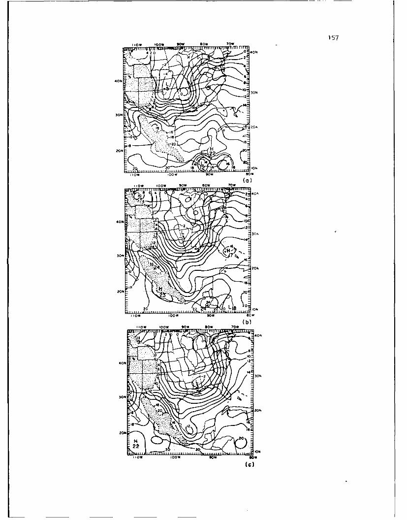
157How 1001111 low sow Tow
202
4 N O .0..0*80
'w 00 0* SOW lO
3 O '0 3N ~16b20
Ilow -00W 90w soww0
(a)
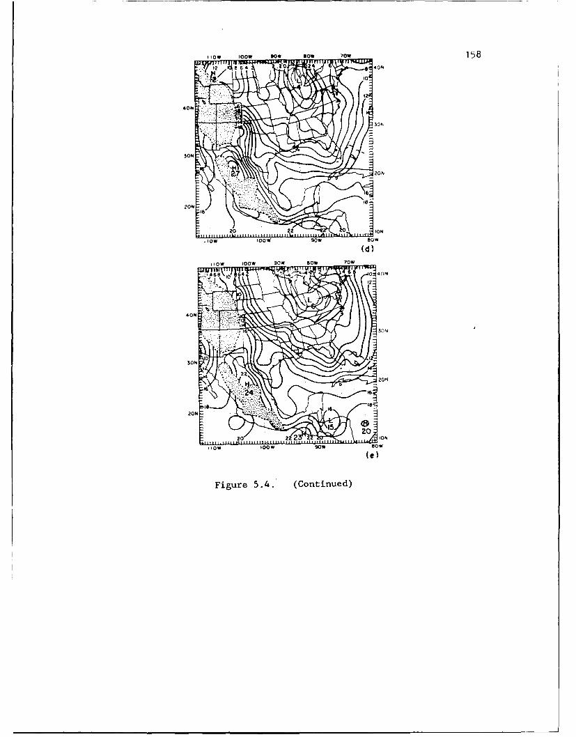
Ilow 100* s0 sow M0W 158
lOW 10W 90 0*
Cd)
SON0* 9* SO 0
20h
20 2 ION
lIOW I 1w 00 sow T ow
11-74T!AQ e)
Fiur 5.4 (Continued
159
developed southward, L,, western portion of the moist layer was
"trapped" along the eastern Mexican coast and the Bay of Campeche, while
the eastern portion of the moist layer was transported by the surface
front into the Caribbean. The temporal evolution of the moist layer
over the western Gulf is also illustrated in the time series of Fig.
5.3. The time series shows that some low level dry1[u' was observed over
Brownsville (BRO) and Soto La Marina (SOM) during the Gay on 4 and 5
April, but south of these two stations, the moist layer remained intact
as surface dewpoints consistently stayed in the middle 60's (°F) and
lower 70's. Over Merida, the cold frontal passage during the afternoon
of 4 April resulted in a dewpoint decrease of nearly 15°F in 12 h. The
dewpoints over Merida remained in the mid 50's under a weak northerly,
flow until after 0600 UTC 7 April. Further evidence of the moist la,'•r
remaining over the western Gulf is shown by a series of visible
satellite images (Fig. 5.5) for the same period as Fig. 5.3. Notice the
persistent area of low clouds along the eastern slopes of the Sierra
Madre Oriental. The cloud area appears to follow the topography and
actually moves inland slightly on 5 April. The appearance of low clouds
along the western Gulf prior to the beginning of return flow has been
documented in a study by Karnavas (1978). His study reported that the
generation of stratus clouds in this region is a result of long-wave
cooling in the modified polar air. Our satellite continuity suggests
that upslope flow along the Mexican coast may have generated the cloud
area, which grew in size during the daylight hours of 4 April.
According to the conceptual model described in Chapter 3, the high-
pressure stage of the lid cycle is also the period of EML genesis. In

160
Figure 5.5. Series of GOES visible satellite images for the followingtimes: a) 1430 UTC 4 April, b) 2030 UTC 4 April, c) 1431UTC 5 April, d) 2031 UTC 5 April, and e) 1431 UTC 6 April.
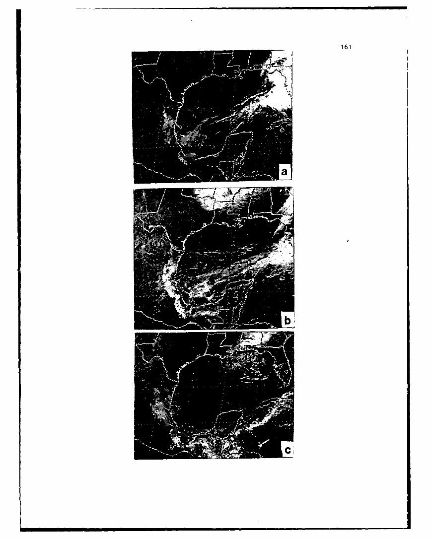
161
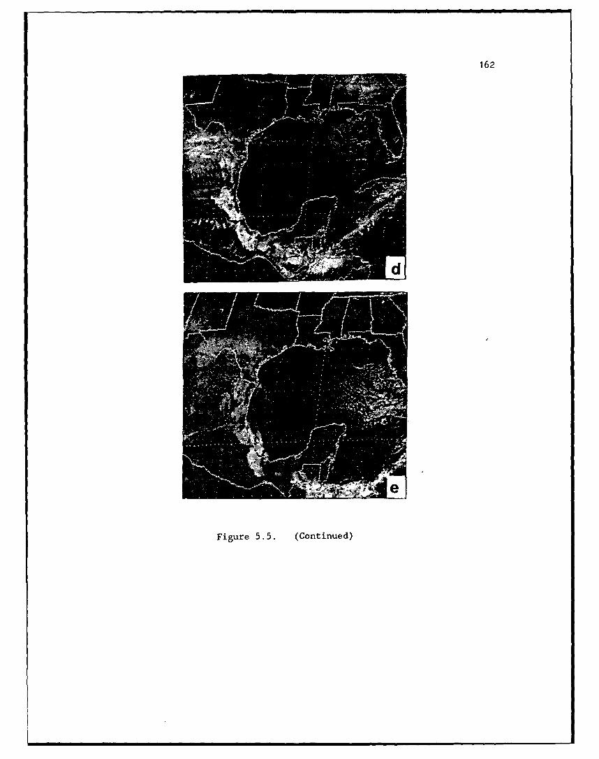
162
Figure 5.5. (Continued)
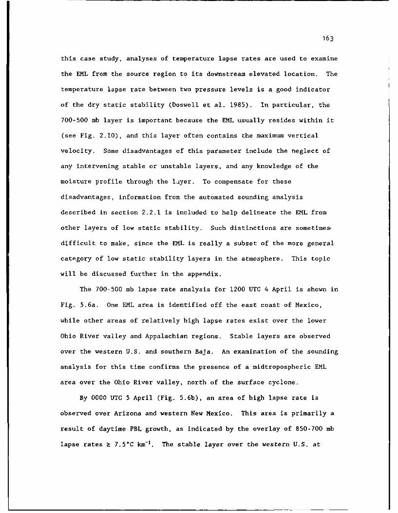
163
this case study, analyses of temperature lapse rates are used to examine
the EML from the source region to its downstream elevated location. The
temperature lapse rate between two pressure levels is a good indicator
of the dry static stability (Doswell et al. 1985). In particular, the
700-500 mb layer is important because the EML usually resides within it
(see Fig. 2.10), and this layer often contains the maximum vertical
velocity. Some disadvantages of this parameter include the neglect of
any intervening stable or unstable layers, and any knowledge of the
moisture profile through the layer. To compensate for these
disadvantages, information from the automated sounding analysis
described in section 2.2.1 is included to help delineate the EML from
other layers of low static stability. Such distinctions are sometimes,
difficult to make, since the EML is really a subset of the more general
category of low static stability layers in the atmosphere. This topic
will be discussed further in the appendix.
The 700-500 mb lapse rate analysis for 1200 UTC 4 April is shown in
Fig. 5.6a. One EML area is identified off the east coast of Mexico,
while other areas of relatively high lapse rates exist over the lower
Ohio River valley and Appalachian regions. Stable layers are observed
over the western U.S. and southern Baja. An examination of the sounding
analysis for this time confirms the presence of a midtropospheric EML
area over the Ohio River valley, north of the surface cyclone.
By 0000 UTC 5 April (Fig. 5.6b), an area of high lapse rate is
observed over Arizona and western New Mexico. This area is primarily a
result of daytime PBL growth, as indicated by the overlay of 850-700 mb
lapse rates a 7.5*C km- 1 . The stable layer over the western U.S. at

164
Figure 5.6. Analysis of 700-500 mb temperature lapse rate in °C km-1 ,isoplethed every 0.5°C km- 1 . The thicker lines denote the7.5 and 4.5°C km-1 isopleths, which are representative oflow and high static stability areas, respectively. Inpanel (b), the shaded region denotes 850-700 mb lapserates • 7.5°C km-1. Analyses shown for a) 1200 UTC 4April, b) 0000 UTC 5 April, and c) 1200 UTC UTC 5 April.
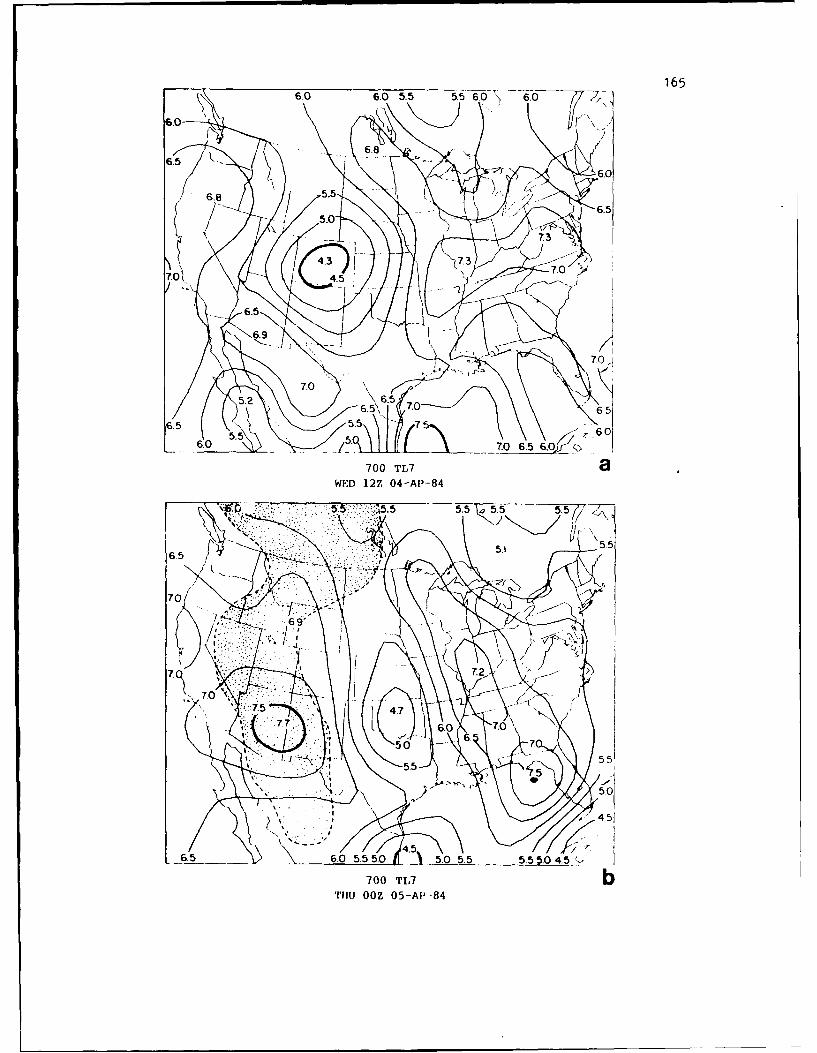
60 6. 0 6.0 5.5 5.5 6.0 ~ 6
66.0
6. 6..8.
50
6.58
6.90
6.5ý 5.5 TO7.
6.5
6.0 5. 7.0 6.5 6.0 _(
700 TL7aWED 12Z 04-AP-84
6,5 51
700
TO- /)7
________~~. 6.9.50' .055 55.45
700
IL
7.~t OOZ T.AP8
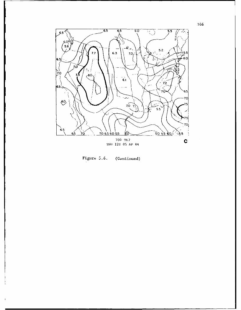
166
6 5
776.3 7.05.
6.5 6.0
6.5 7. 80_ 0.605 0
6.1 1215-P~
Figur .6 Cniud
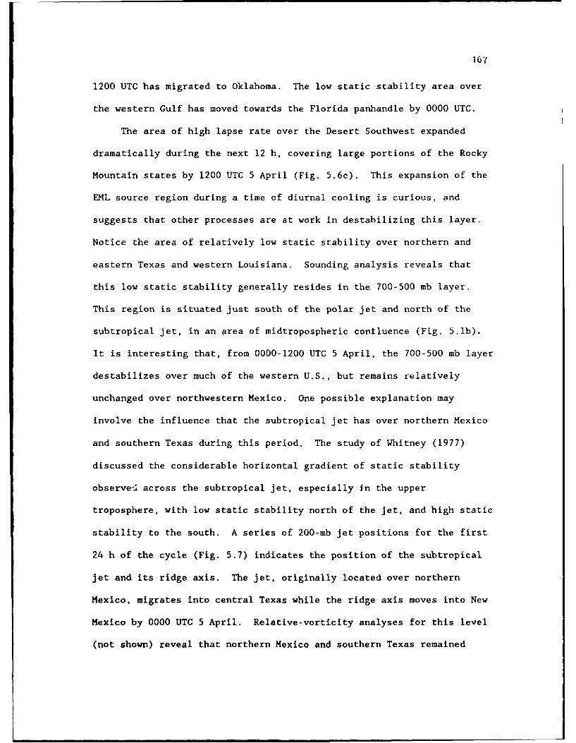
167
1200 UTC has migrated to Oklahoma. The low static stability area over
the western Gulf has moved towards the Florida panhandle by 0000 UTC.
The area of high lapse rate over the Desert Southwest expanded
dramatically during the next 12 h, covering large portions of the Rocky
Mountain states by 1200 UTC 5 April (Fig. 5.6c). This expansion of the
EML source region during a time of diurnal cooling is curious, and
suggests that other processes are at work in destabilizing this layer.
Notice the area of relatively low static stability over northern and
eastern Texas and western Louisiana. Sounding analysis reveals that
this low static stability generally resides in the 700-500 mb layer.
This region is situated just south of the polar jet and north of the
subtropical jet, in an area of midtropospheric coniluence (Fig. 5.lb),
It is interesting that, from 0000-1200 UTC 5 April, the 700-500 mb layer
destabilizes over much of the western U.S., but remains relatively
unchanged over northwestern Mexico. One possible explanation may
involve the influence that the subtropical jet has over northern Mexico
and southern Texas during this period. The study of Whitney (1977)
discussed the considerable horizontal gradient of static stability
observe-! across the subtropical jet, especially in the upper
troposphere, with low static stability north of the jet, and high static
stability to the south. A series of 200-mb jet positions for the first
24 h of the cycle (Fig. 5.7) indicates the position of the subtropical
jet and its ridge axis. The jet, originally located over northern
Mexico, migrates into central Texas while the ridge axis moves into New
Mexico by 0000 UTC 5 April. Relative-vorticity analyses for this level
(not shown) reveal that northern Mexico and southern Texas remained
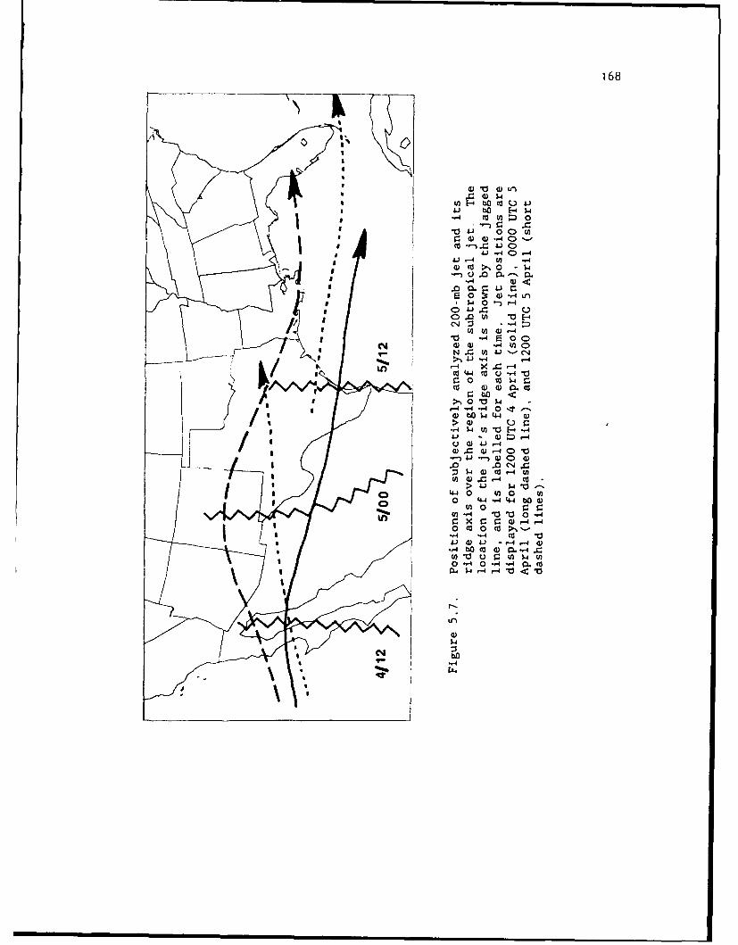
168
$4
)-4 0 U) Z'- o
41 *-4 0(4 2 - 42 ) , -4
4) co 0 4~
o 0) 0) -,-4
(A . n 4) '-4 e.0 .0 N0
CM )40) C 4 In 0
U20).X rC4 c
169
under negative relative vorticity for most of the first 24 h of the lid
cycle, resulting in unfavorable conditions for maintenance of any high
lapse rate layers in the midtroposphere over this area. By 1200 UTC 5
April, the jet and ridge had shifted to the south and east, and
conditions became favorable for low static stability layers to form and
persist in the midtroposphere over northern Mexico.
5.2.2 The Return-Flow Stage (0000 UTC 6 April-0000 UTC 7 April)
By 0000 UTC 6 April, the surface anticyclone that dominated the
Great Plains and western Gulf of Mexico on the 4th and 5th was starting
to weaken as lower tropospheric warm-air advection began to dominate
most of the region. At this time, a surface high was located over the
western Gulf with a central pressure of 1019 mb. Examination of the
850-and 700-mb analyses for 0000 UTC 6 April show that the warm-air
advection over the western Plains was stronger than over the western
Gulf, which weakened the surface ridge faster over the Plains than over
the Gulf. Although surface mixing processes over the Gulf were
modifying the low level cold air, the 850-mb thermal analyses in Fig.
5.4c-e indicate that this airmass modification was a slow process.
During the next 12 h, the surface high remained quasi-stationary in
the western Gulf and maintained its strength. The low level moist layer
began to return slowly into the Rio Grande valley, consistent with the
climatological composites for this stage (see Chapter 3). The slowness
of the moist layer's return into Texas at this stage is due to the
presence of the surface high over the western Gulf and the lack of a
strong southerly low level jet (LLJ). However, it is also during this
170
stage that LLJ development begins to take place. The warm-air advection
over the western Plains results in surface pressure falls over the Front
Range of the Rockies, leading to the formation of a lee-side trough. At
1200 UTC 6 April, there is not yet a lee-side trough (see Fig. 5.1c),
but the strengthening pressure gradient over the Front Range has
resulted in the formation of a LLJ over the western Plains (Fig. 5.8).
Although the western Plains LIU is out of phase with the returning moist
layer, a second LLU from southern Texas to central Oklahoma has also
formed, suggesting that transport of the moist layer into Texas is
imminent.
The EML over the western U.S. xpanded during the day on 5 April,
and a new area started to form over northern Mexico, as shown by the'
700-500 mb lapse rate analysis for 0000 UTC 6 April, in Fig. 5.9a. The
area of relatively low static stability over Texas and southern
Louisiana has expanded eastward since 1200 UTC, and sounding analysis
reveals that the western edge of this layer may actually be the
beginning of the EML's emergence into the western Plains. The
appearance of a deeper Mexican PBL at 0000 UTC coincides with the
passage of the subtropical jet's ridge axis out of northern Mexico, and
the beginning of upper level diffluence between the subtropical jet over
northwestern Mexico and the approaching polar jet just entering the
southwest U.S. at this time. The diffluent jets allow for upward
vertical motion over northwestern Mexico and the southwestern U.S.,
resulting in a favorable environment for the EML to maintain its depth.
By 1200 UTC 6 April (Fig. 5.9b), the western U.S. EML has begun to
move into the Great Plains, while the Mexican EML has moved toward
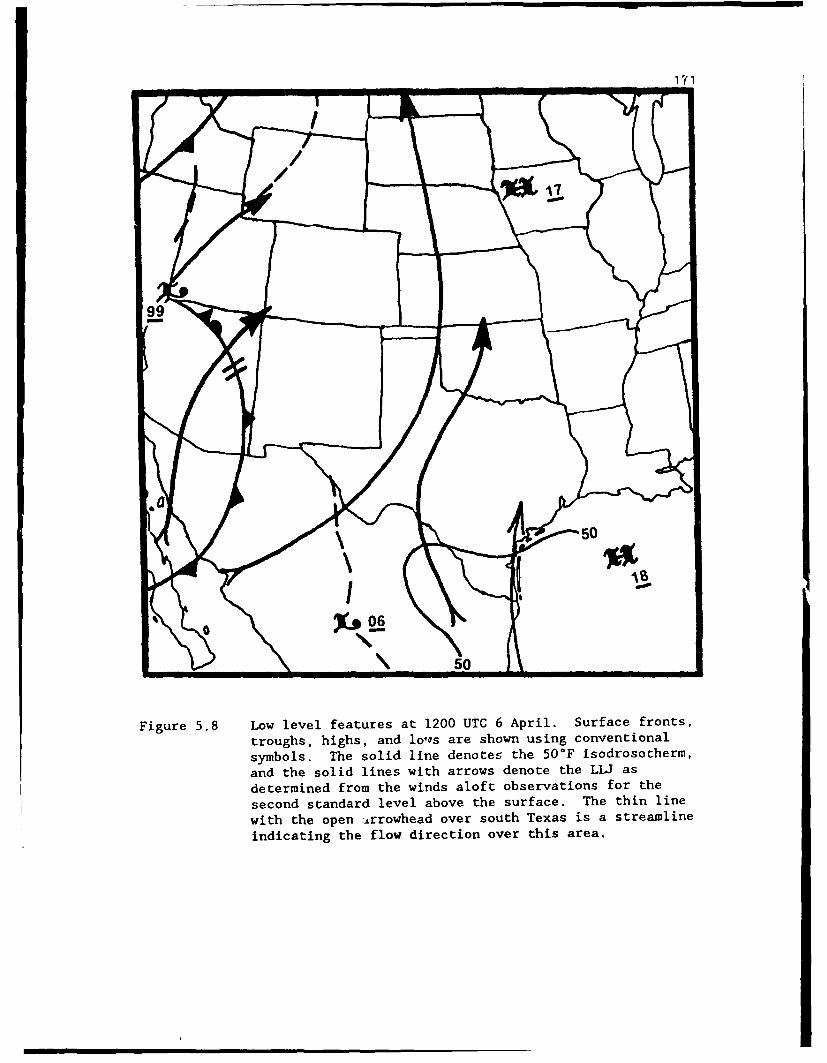
171
50
Figure 5.8 Low level features at 1200 UTC 6 April. Surface fronts,
troughs, highs, and lows are shown using conventional
symbols. The solid line denotes the 50'F isodrosotherm,
and the solid lines with arrows denote the Lii as
determined from the winds aloft observations for the
second standard level above the surface. The thin line
with the open arrowhead over south Texas is a streamline
indicating the flow direction over this area.
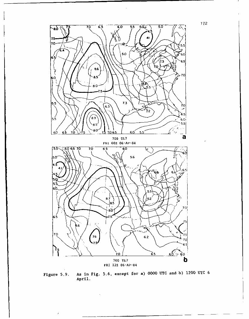
7.0 T 6.5 6.0 5.5 5.0,ý 41 5.0
7.05.
6.4
6.0 6.
6.0~~~~~ ~~ 6.6...5580 7 Q656. .
8700 TL70
5.5 ,60570 70 6.5 6.0 .
5.5~ 8.9 5..0~
1. , ' . 7.06. 6.5 5.577~
700 TL7bFRI 12Z 06-AP-84
Fiue5.G9. Asi5i.56,ecp.6 ) 00UCad )10 T
Apil
17"3
southwest Texas. The two EML source areas shown in Fig. 5.9 may account
for the appearance of two EML frequency maxima over the central Plains
and the southern Plains in the climatological composite for the return-
flow stage, shown in Figs. 3.5b and 4.8c. Such a double maximum in the
midtropospheric lapse rate field has also been observed in other severe-
storm case studies (e.g., Fig. 2 in Doswell et al. 1985).
5.2.3 Lid Genesis (0000 UTC-1200 UTC 7 April)
After 1200 UTC 6 April, the surface moist layer began to move into
Texas more rapidly, as illustrated by a continuity chart of the 50°F
surface isodrosotherm over Texas from 1200-2100 UTC 6 April (Fig. 5.10).
During the late morning on 6 April, the surface high, which had been
quasi-stationary over the western Gulf, started to drift east, while
surface pressures continued falling over the Front Range and the western
Plains. By 1800 UTC, a lee-side low with a central pressure of 1000 mb
had formed over the eastern Colorado-New Mexico border. An accompanying
lee-side trough extended from this low into northern Mexico. By 2100
UTC, dryline genesis was taking place over west Texas, and the surface
low had deepened to 996 mb. The development of the lee-side trough
strengthened the low level southerly flow of moist air into Texas, so
that by 0000 UTC 7 April, a well-defined moist layer was established
over west-central Texas and extreme western Oklahoma (Fig. 5.11). Low
level jets were well-established along the Rio Grande valley into the
Texas panhandle, and from the Texas Gulf coast into the western portions
of Nebraska and South Dakota.
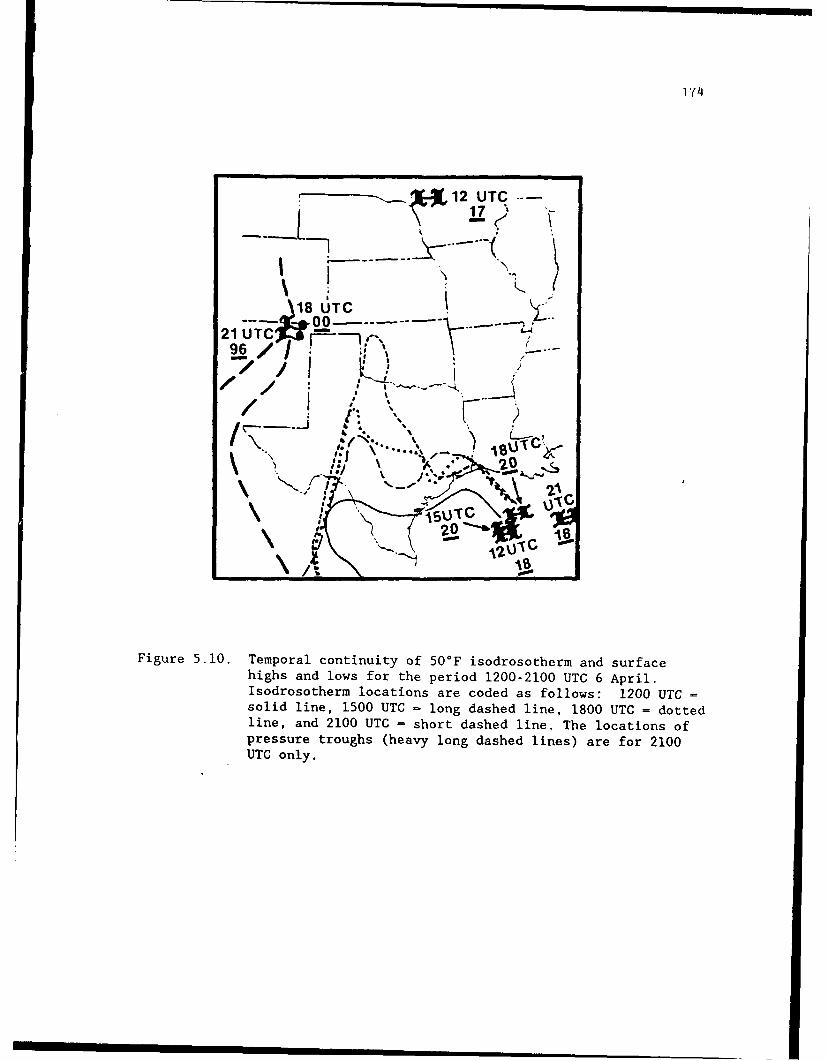
1714
12 UTC"17
\18 6TC
21 UTCr -'
9 6/ , ./..-..,- -too 20
I'I
"U is/ $"
Figure 5.10. Temporal continuity of 50°F isodrosotherm and surfacehighs and lows for the period 1200-2100 UTC 6 April.
Isodrosotherm locations are coded as follows: 1200 UTC =
solid line, 1500 UTC -long dashed line, 1800 UTC = dotted
line, and 2100 UTC = short dashed line. The locations of
pressure troughs (heavy long dashed lines) are for 2100UTC only.
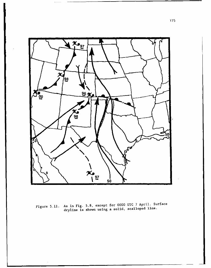
977
50"1
Figure 5.11. As in Fig. 5.8, except for 0000 UTC 7 April. Surface
dryline is shown using a solid, scalloped line.
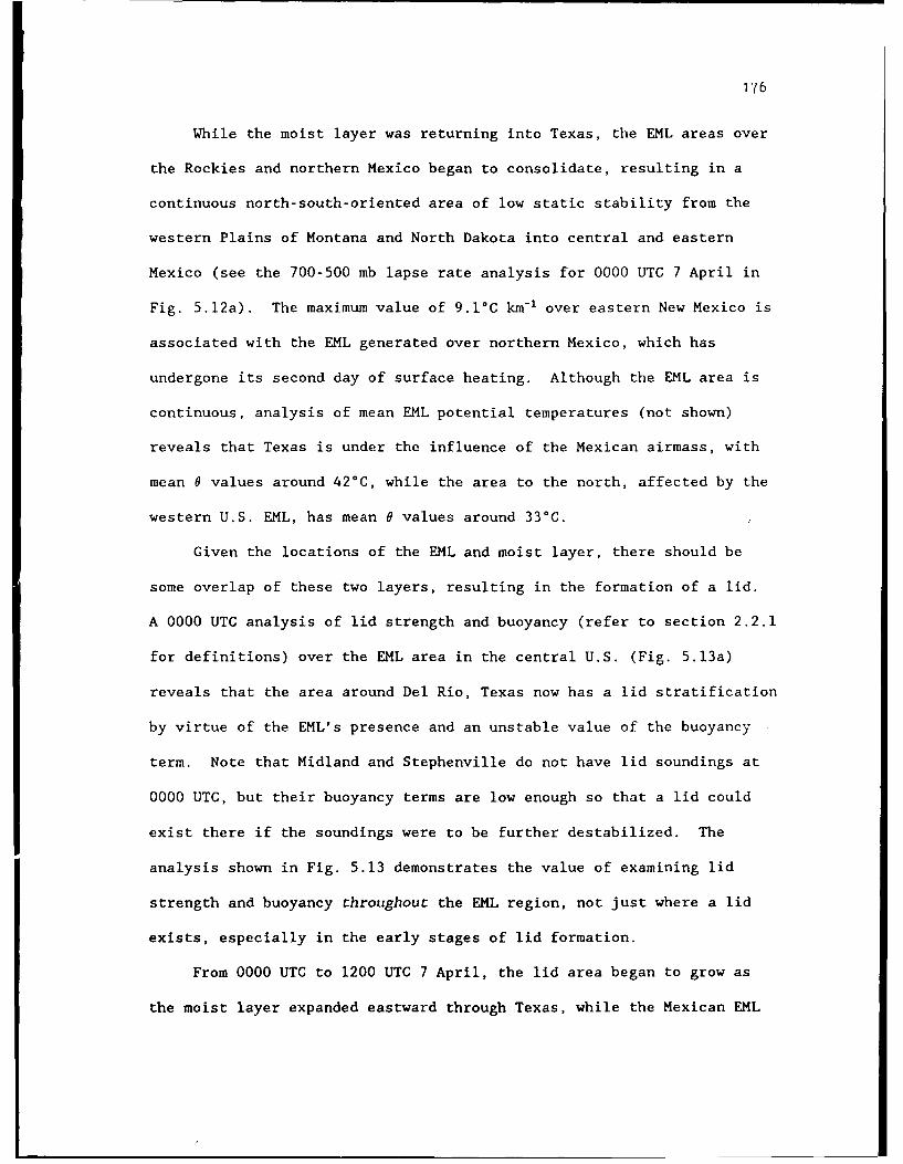
176
While the moist layer was returning into Texas, the EML areas over
the Rockies and northern Mexico began to consolidate, resulting in a
continuous north-south-oriented area of low static stability from the
western Plains of Montana and North Dakota into central and eastern
Mexico (see the 700-500 mb lapse rate analysis for 0000 UTC 7 April in
Fig. 5.12a). The maximum value of 9.1°C km-1 over eastern New Mexico is
associated with the EML generated over northern Mexico, which has
undergone its second day of surface heating. Although the EML area is
continuous, analysis of mean EML potential temperatures (not shown)
reveals that Texas is under the influence of the Mexican airmass, with
mean 0 values around 42°C, while the area to the north, affected by the
western U.S. EML, has mean 8 values around 33°C.
Given the locations of the EML and moist layer, there should be
some overlap of these two layers, resulting in the formation of a lid.
A 0000 UTC analysis of lid strength and buoyancy (refer to section 2.2.1
for definitions) over the EML area in the central U.S. (Fig. 5.13a)
reveals that the area around Del Rio, Texas now has a lid stratification
by virtue of the EML's presence and an unstable value of the buoyancy
term. Note that Midland and Stephenville do not have lid soundings at
0000 UTC, but their buoyancy terms are low enough so that a lid could
exist there if the soundings were to be further destabilized. The
analysis shown in Fig. 5.13 demonstrates the value of examining lid
strength and buoyancy throughout the EML region, not just where a lid
exists, especially in the early stages of lid formation.
From 0000 UTC to 1200 UTC 7 April, the lid area began to grow as
the moist layer expanded eastward through Texas, while the Mexican EML
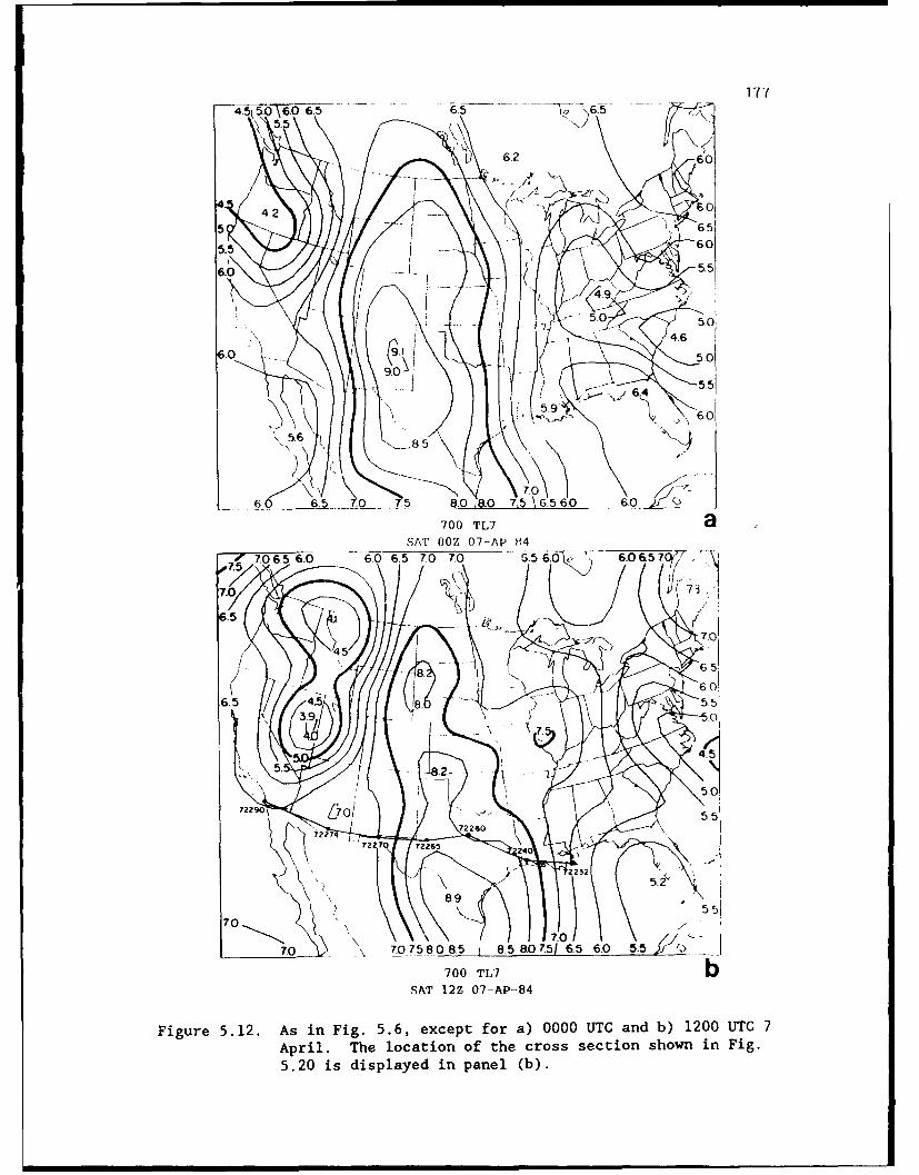
177
T i 6.2 -6.0
6.0
6. 5.5
/1/4.91 4.
5,55
6.0 :1 501
~85 9
7.00
6 6.5 Q 5 0 .75 6.60 _ _6. O-g
700 TL7 a-ý7.0 6.56.0 -60 6.5 7.0 7.0 G.5 6.0o 66
7.0 T
455 6-
39 0
55.
7220 77.0O.5
70707
SAT 12Z 07-AP--84
Figure 5.12. As in Fig. 5.6, except for a) 0000 UTC and b) 1200 UTG 7April. The location of the cross section shown in Fig.5.20 is displayed in panel (b).

178
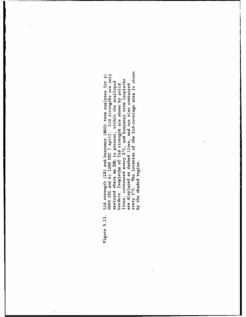
co 1-
'4-4 a) p."4 0) a) U1w- 0 .-4 "-1 ..-4
(2 cl 1-4 0 P.:) .- 4 0 0 0
~ .-4 41u a 0c
ca-(1. a)c94 oC
W A4-) 0- to2 cdE- "4 4 -42 I0
04 *'- U 0 O L
- ,4 >~ - C -
o D: 0 10
4 bu2 to U 1~
>. -P. 0.1-400 *o -4:$ UU) -4 CN
0 0 C0 0 p
r-4 ý
a00 i4 u.0) 0~ *Q P. a (n2
W 4E-4 Q)U) U C42(
O r-4O 0 Q) $4 4)
,-0 ca .0 -4 CU 0 .0
-4
blo"z4
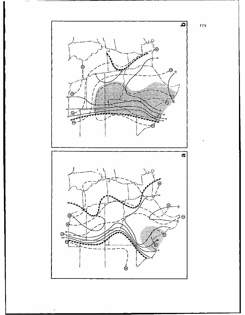
.0 179
'-o
... .... . .9 ' -
nk,,,~.@ *-*..........O~
I'
w v . ........
N
C4

180
continued to move across the Great Plains. The 700-500 mb lapse rate
analysis for 1200 UTC (Fig. 5.12b) reveals that the low static stability
area over the northern Plains has decreased in size, and the highest
lapse rates now exist over southern Texas. The 1200 UTC lid strength
and buoyancy analysis (Fig. 5.13b) shows that the lid-coverage area has
expanded as far north as Kansas, and as far east as central Texas and
eastern Oklahoma. The area with the highest 700-500 mb lapse rate
(northwest of Brownsville, Texas) does not have a lid stratification
yet, owing to a buoyancy term of +I.0°C. Figure 5.13b shows that there
is a strong gradient of lid strength over much of western Texas.
Analysis of the entire EML area in Fig. 5.13b allows us to identify a
north-south axis of maximum lid strength from western Kansas into
southern Texas. The locations of this maximum-lid-strength zone and the
area of the strongest gradient will be important when the severe weather
outbreak is discussed in the next section.
5.2.4 The Lid-Maximum Stage and Severe-WeatherOutbreak (1200 UTC 7 April-1200 UTC 8 April)
The meteorological situation over the southern Plains on the
morning of 7 April was very complex. Figure 5.14b displays a
surface/upper-air composite analysis for 1200 UTC 7 April (a legend is
shown in Fig. 5.14a). At this time, an emerging frontal system with a
double-low structure and well-developed dryline exist over the western
Plains. The cold frontal position is nearly identical to that in the
climatological composite for the lid-maximum stage, shown in Fig. 3.5d.
The polar and subtropical jets are so closely aligned that it is
difficult to distinguish between them (also see Fig. 5.1d). This
Figure 5.14. Composite surface/upper-air analysis for 1200 UTC 7 April(panel 'b'). Symbols are shown in the legend panel (a).

181
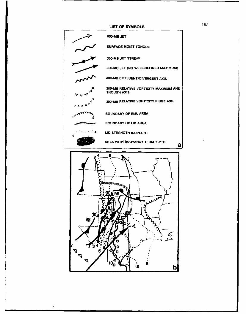
LIST OF SYMBOLS 182
850-MB JET
SJ SURFACE MOIST TONGUE
S 300-MB JET STREAK
S 300-MB JET (NO WELL-DEFINED MAXIMUM)
S% 300-MB DIFFLUENT/DIVERGENT AXIS
* 300-MB RELATIVE VORTICITY MAXIMUM ANDTROUGH AXIS
00 300-MB RELATIVE VORTICITY RIDGE AXIS
0 o 000
s r(~> BOUNDARY OF EML AREA
SnBOUNDARY OF LID AREA
" "4 LID STRENGTH ISOPLETH4
SAREA WITH BUOYANCY TERM -2-C
4 6
6 0
0olSb
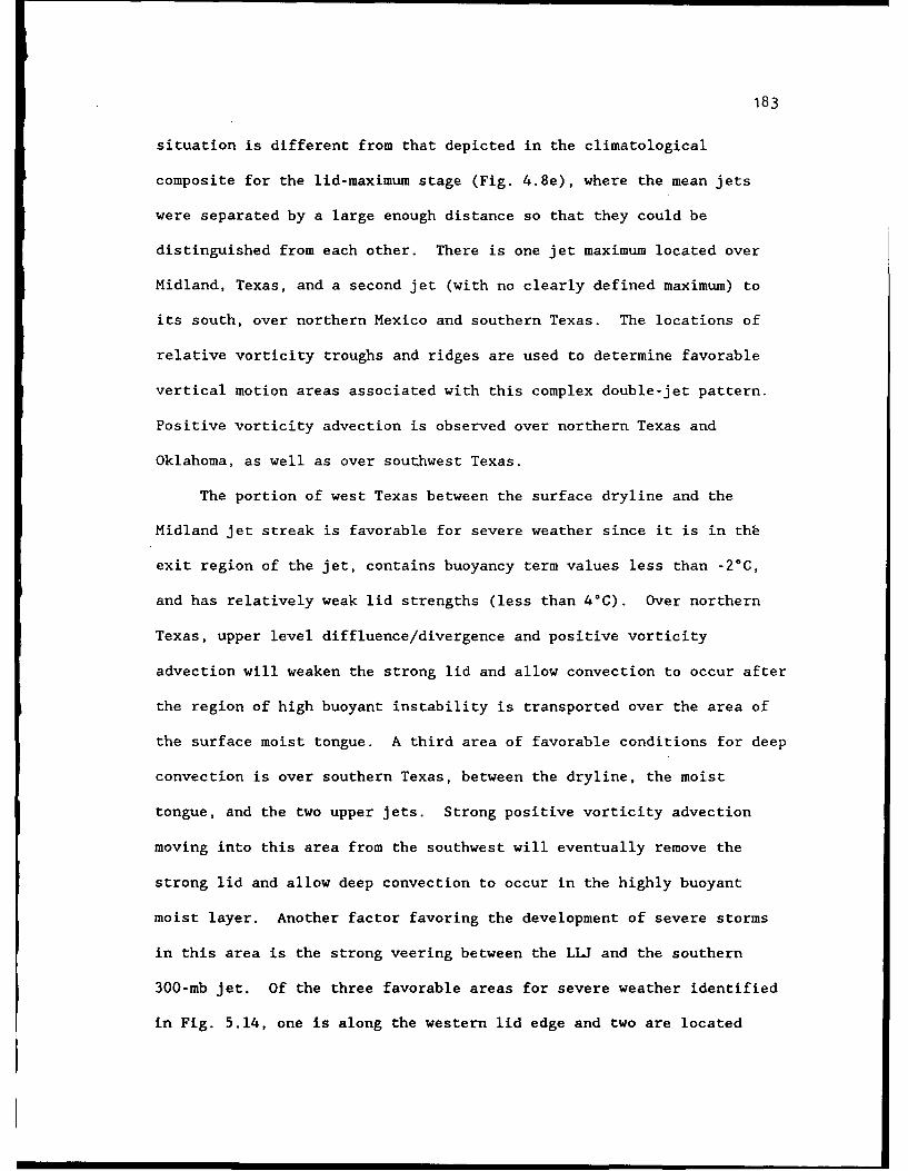
183
situation is different from that depicted in the climatological
composite for the lid-maximum stage (Fig. 4.8e), where the mean jets
were separated by a large enough distance so that they could be
distinguished from each other. There is one jet maximum located over
Midland, Texas, and a second jet (with no clearly defined maximum) to
its south, over northern Mexico and southern Texas. The locations of
relative vorticity troughs and ridges are used to determine favorable
vertical motion areas associated with this complex double-jet pattern.
Positive vorticity advection is observed over northern Texas and
Oklahoma, as well as over southwest Texas.
The portion of west Texas between the surface dryline and the
Midland jet streak is favorable for severe weather since it is in thb
exit region of the jet, contains buoyancy term values less than -2°C,
and has relatively weak lid strengths (less than 4°C). Over northern
Texas, upper level diffluence/divergence and positive vorticity
advection will weaken the strong lid and allow convection to occur after
the region of high buoyant instability is transported over the area of
the surface moist tongue. A third area of favorable conditions for deep
convection is over southern Texas, between the dryline, the moist
tongue, and the two upper jets. Strong positive vorticity advection
moving into this area from the southwest will eventually remove the
strong lid and allow deep convection to occur in the highly buoyant
moist layer. Another factor favoring the development of severe storms
in this area is the strong veering between the LIU and the southern
300-mb jet. Of the three favorable areas for severe weather identified
in Fig. 5.14, one is along the western lid edge and two are located
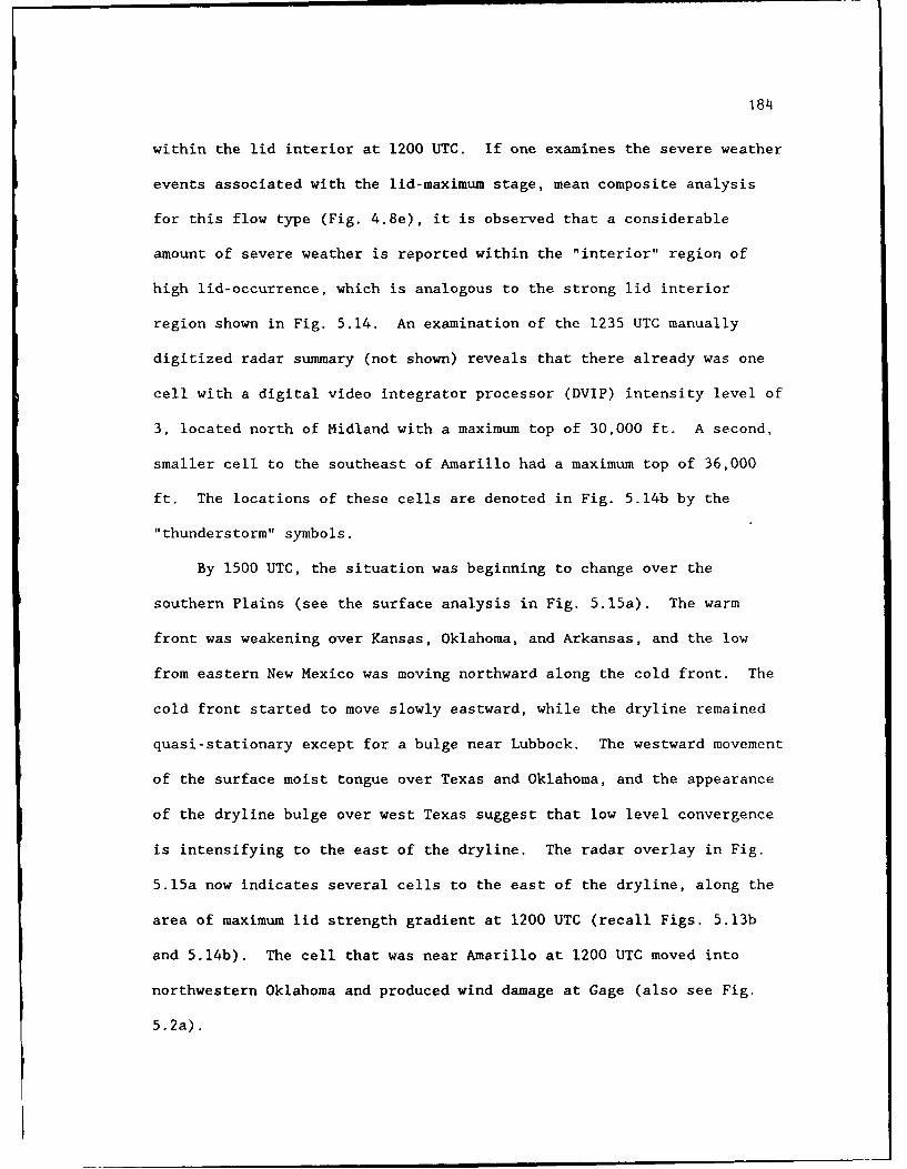
184
within the lid interior at 1200 UTC. If one examines the severe weather
events associated with the lid-maximum stage, mean composite analysis
for this flow type (Fig. 4.8e), it is observed that a considerable
amount of severe weather is reported within the "interior" region of
high lid-occurrence, which is analogous to the strong lid interior
region shown in Fig. 5.14. An examination of the 1235 UTC manually
digitized radar summary (not shown) reveals that there already was one
cell with a digital video integrator processor (DVIP) intensity level of
3, located north of Midland with a maximum top of 30,000 ft. A second,
smaller cell to the southeast of Amarillo had a maximum top of 36,000
ft. The locations of these cells are denoted in Fig. 5.14b by the
"thunderstorm" symbols.
By 1500 UTC, the situation was beginning to change over the
southern Plains (see the surface analysis in Fig. 5.15a). The warm
front was weakening over Kansas, Oklahoma, and Arkansas, and the low
from eastern New Mexico was moving northward along the cold front. The
cold front started to move slowly eastward, while the dryline remained
quasi-stationary except for a bulge near Lubbock. The westward movement
of the surface moist tongue over Texas and Oklahoma, and the appearance
of the dryline bulge over west Texas suggest that low level convergence
is intensifying to the east of the dryline. The radar overlay in Fig.
5.15a now indicates several cells to the east of the dryline, along the
area of maximum lid strength gradient at 1200 UTC (recall Figs. 5.13b
and 5.14b). The cell that was near Amarillo at 1200 UTC moved into
northwestern Oklahoma and produced wind damage at Gage (also see Fig.
5.2a).
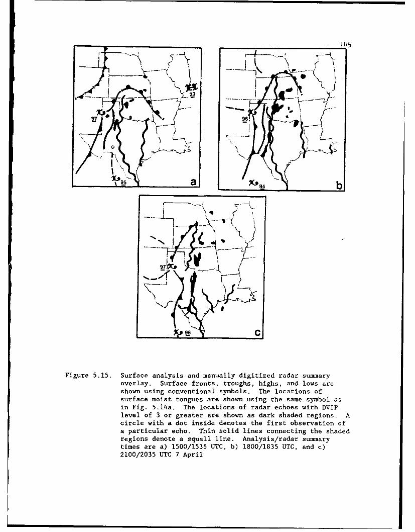
185
- - ,--
996
- - I
a b
97j
-j
Figure 5.15. Surface analysis and manually digitized radar summaryoverlay. Surface fronts, troughs, highs, and lows areshown using conventional symbols. The locations ofsurface moist tongues are shown using the same symbol asin Fig. 5.14a. The locations of radar echoes with DVIPlevel of 3 or greater are shown as dark shaded regions. Acircle with a dot inside denotes the first observation ofa particular echo. Thin solid lines connecting the shadedregions denote a squall line. Analysis/radar summarytimes are a) 1500/1535 UTC, b) 1800/1835 UTC, and c)2100/2035 UTC 7 April
186
Figure 5.15a indicates that the convective cells over Texas and
Oklahoma were nearly coincident with the surface moist tongue at 1500
UTC. Within the next hour, a squall line formed from the Texas-Oklahoma
border into the Big Bend region. This squall line moved east across
Texas during the next 6-7 h, and was responsible for the two severe-
weather areas displayed in Fig. 5.2a. For the most part, the squall
line was most active along its northern and southern portions. In the
1800 UTC surface analysis (Fig. 5.15b), the primary low was located
southwest of Amarillo, and the cold front was just passing Midland. The
radar overlay clearly shows how the squall line was aligned with the
surface dryline. The convective cells from western Oklahoma into
central Texas were nearly coincident with the surface moist tongue.
Examining both Figs. 5.15b and 5.2a, we see that the cells along the
northern portion of the squall line were tornadic (maximum tops of
50,000 ft), while the southern portion (with maximum tops of 48,000 ft)
produced a line echo wave pattern and wind gusts of 51 kt at Del Rio.
The surface analysis for 2100 UTC (Fig. 5.15c) shows a frontal wave
appearing to the south of the Rio Grande valley as a surface low in
northern Mexico is overtaken by the cold front. The dryline was also
overtaken by the front during this time. The radar overlay in Fig.
5.15c indicates more of a discontinuity between the northern and
southern portions of the squall line than there was 2 h before. The
southern part of the squall line is now moving into the region of the
surface moist tongue. The severe-weather summary in Fig. 5.2a shows
that the primary severe-weather activity over Texas was along the
southern part of the squall line after 1430 CST (2030 UTC), and that
187
this activity became tornadic around 2100 UTC. The increased severity
of the convection along the southern part of the squall line and the
cessation of severe-weather activity along the northern portion suggest
that the upper level dynamical forcing has shifted to southern Texas
during the late afternoon. Recall from the composite analysis for 1200
UTC (Fig. 5.14b) that strong positive vorticity advection was moving
into southern Texas, but the high lid strengths there would have delayed
any deep convection from occurring immediately.
The squall line over Texas began to weaken after 2300 UTC,
according to the radar summaries (not shown). A composite
meteorological analysis for 0000 UTC (Fig. 5.16) shows that the northern
portion of the surface front over Texas had moved little over the last
3 h and was starting to occlude, while the southern portion continued to
move eastward. At 300 mb, two jets can still be identified over Texas.
A new jet streak with a ll0-kt maximum appears over Del Rio, while the
southern jet appears along the Gulf coastal region. Positive vorticity
advection and diffluence/divergence are observed between the two jets
over the eastern half of Texas, while negative vorticity advection is
analyzed over south Texas, essentially "finishing off" the southern
portion of the squall line. The presence of ample low level moisture
and strong dynamical forcing over the Texas coast suggest that this area
may be favorable for deep convection, but the southern half of the
coastal region has lid strengths which are too high to allow the
convection to occur there immediately. The northern half of the coast
has weaker lid strengths and a strong veering wind profile, but is just
beyond the northern edge of the most unstable buoyancy values. The 0000
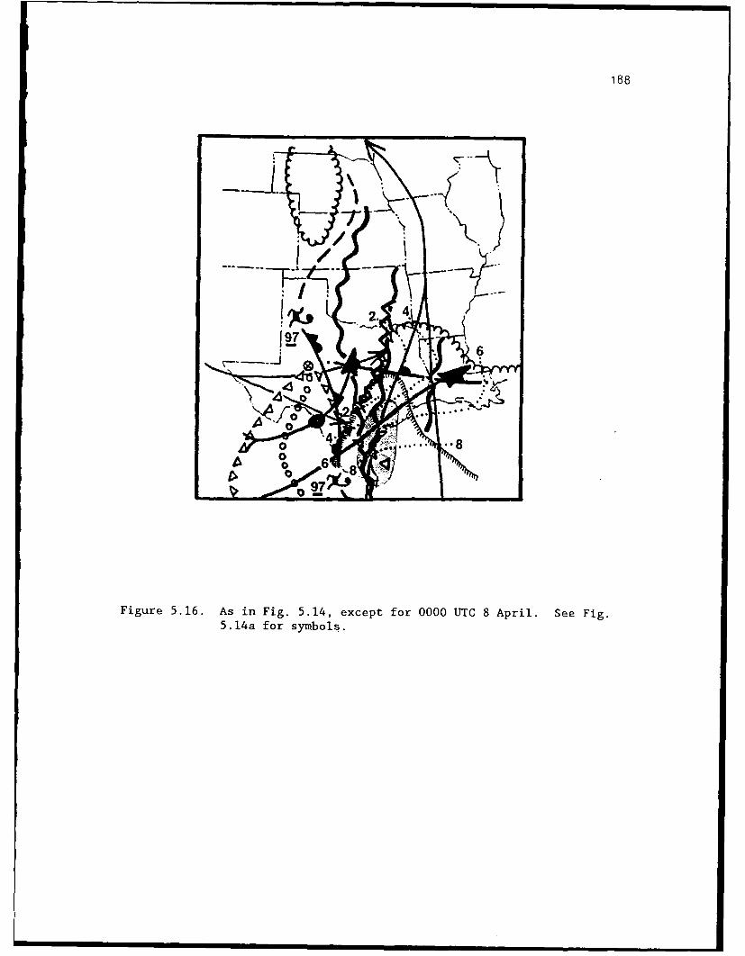
188
,4 0
08
Figure 5.16. As in Fig. 5.14, except for 0000 UTC 8 April. See Fig.5.14a for symbols.
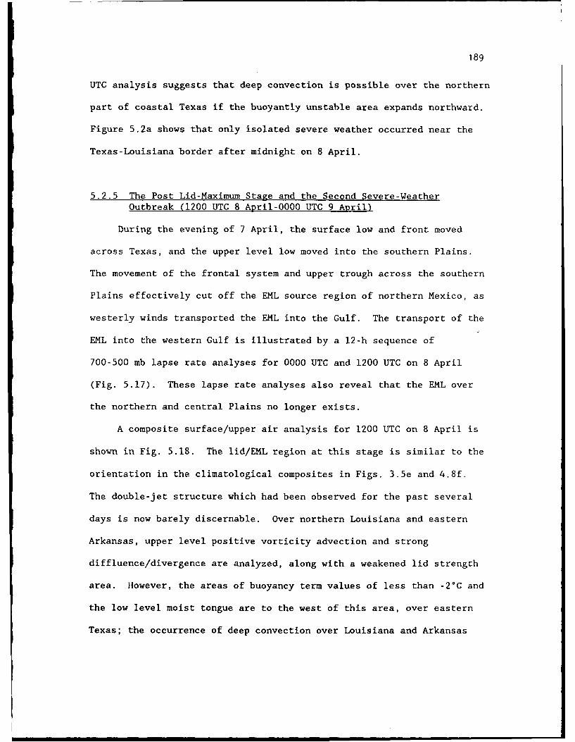
189
UTC analysis suggests that deep convection is possible over the northern
part of coastal Texas if the buoyantly unstable area expands northward.
Figure 5.2a shows that only isolated severe weather occurred near the
Texas-Louisiana border after midnight on 8 April.
5.2.5 The Post Lid-Maximum Stage and the Second Severe-WeatherOutbreak (1200 UTC 8 April-0000 UTC 9 April)
During the evening of 7 April, the surface low and front moved
across Texas, and the upper level low moved into the southern Plains.
The movement of the frontal system and upper trough across the southern
Plains effectively cut off the EML source region of northern Mexico, as
westerly winds transported the EML into the Gulf. The transport of the
EML into the western Gulf is illustrated by a 12-h sequence of
700-500 mb lapse rate analyses for 0000 UTC and 1200 UTC on 8 April
(Fig. 5.17). These lapse rate analyses also reveal that the EML over
the northern and central Plains no longer exists.
A composite surface/upper air analysis for 1200 UTC on 8 April is
shown in Fig. 5.18. The lid/EML region at this stage is similar to the
orientation in the climatological composites in Figs. 3.5e and 4.8f.
The double-jet structure which had been observed for the past several
days is now barely discernable. Over northern Louisiana and eastern
Arkansas, upper level positive vorticity advection and strong
diffluence/divergence are analyzed, along with a weakened lid strength
area. However, the areas of buoyancy term values of less than -2°C and
the low level moist tongue are to the west of this area, over eastern
Texas; the occurrence of deep convection over Louisiana and Arkansas
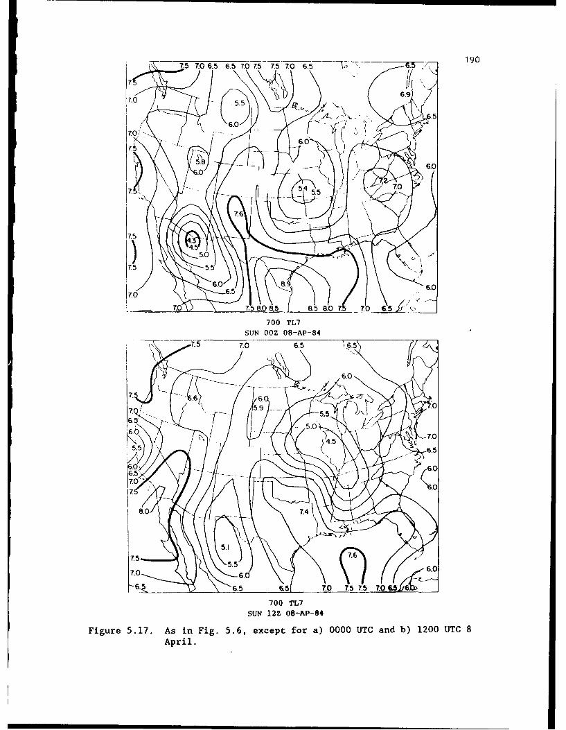
7.5 7.0 6.5 6.5 7.0 7.5 7.5 -7.06.- 1 6.5 190
7 • 1/
7.5 .5
70)~~6.0
-. o - 6.0-.5.8 " 6.0
700 TL7
suN ooz 08-AP-847/.5 7.0 6.5
.06.
7 .. 5".6. . 5 .5 7.3 t 7.0
700 TL7
SUN 12Z 08-AP-84
Figure 5.17. As in Fig. 5.6, except for a) 0000 UTC and b) 1200 UTO 8April.
4..
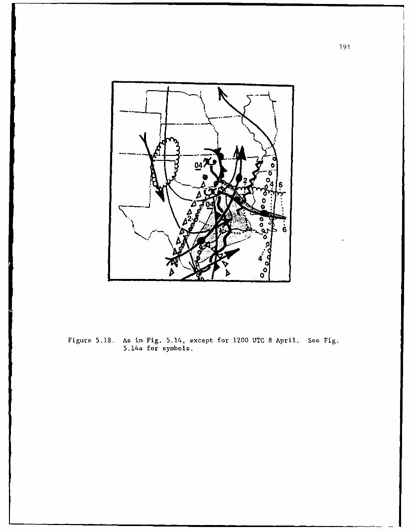
191
4 6
Figure 5.18. As in Fig. 5.14, except for 1200 UTC 8 April. See Fig.5.14a for symbols.
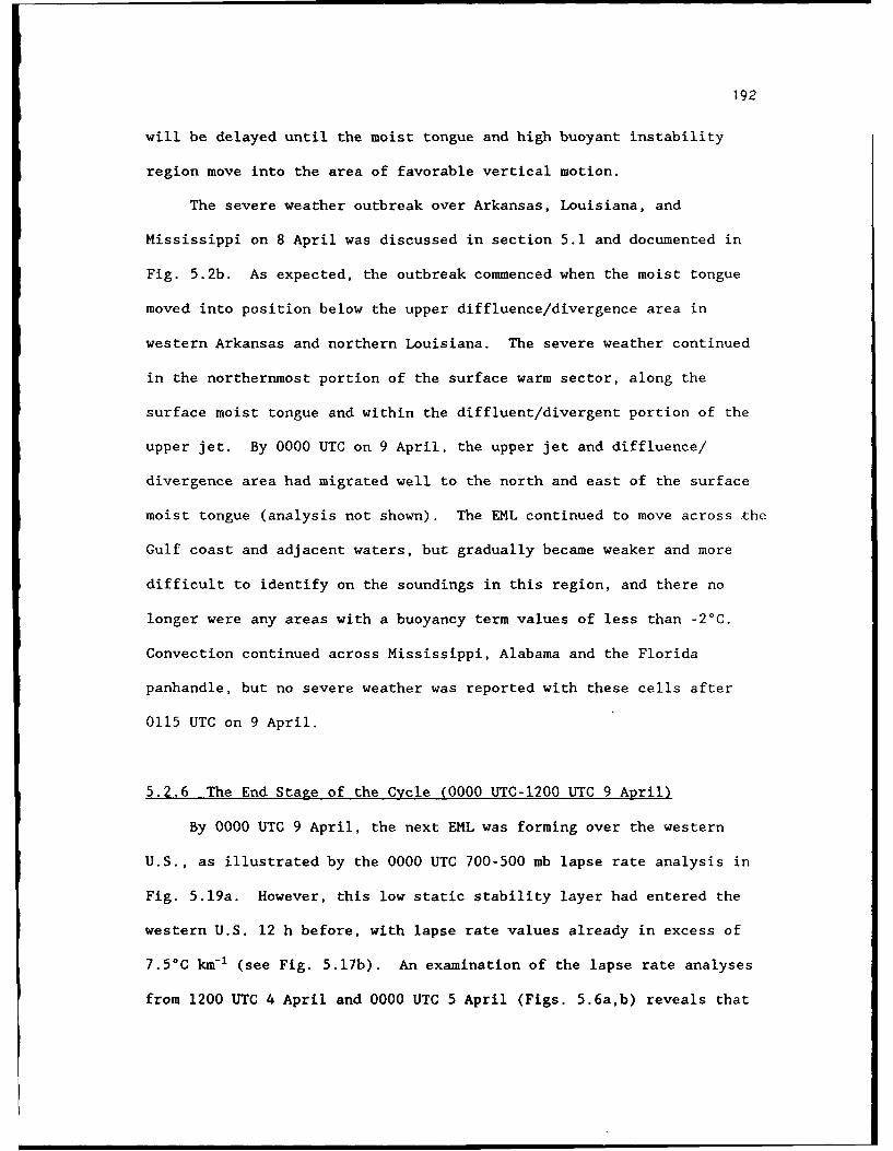
192
will be delayed until the moist tongue and high buoyant instability
region move into the area of favorable vertical motion.
The severe weather outbreak over Arkansas, Louisiana, and
Mississippi on 8 April was discussed in section 5.1 and documented in
Fig. 5.2b. As expected, the outbreak commenced when the moist tongue
moved into position below the upper diffluence/divergence area in
western Arkansas and northern Louisiana. The severe weather continued
in the northernmost portion of the surface warm sector, along the
surface moist tongue and within the diffluent/divergent portion of the
upper jet. By 0000 UTC on 9 April, the upper jet and diffluence/
divergence area had migrated well to the north and east of the surface
moist tongue (analysis not shown). The EML continued to move across the
Gulf coast and adjacent waters, but gradually became weaker and more
difficult to identify on the soundings in this region, and there no
longer were any areas with a buoyancy term values of less than -2°C.
Convection continued across Mississippi, Alabama and the Florida
panhandle, but no severe weather was reported with these cells after
0115 UTC on 9 April.
5.2.6 The End Stage of the Cycle (0000 UTC-1200 UTC 9 April)
By 0000 UTC 9 April, the next EML was forming over the western
U.S., as illustrated by the 0000 UTC 700-500 mb lapse rate analysis in
Fig. 5.19a. However, this low static stability layer had entered the
western U.S. 12 h before, with lapse rate values already in excess of
7.5°C km-1 (see Fig. 5.17b). An examination of the lapse rate analyses
from 1200 UTC 4 April and 0000 UTC 5 April (Figs. 5.6a,b) reveals that
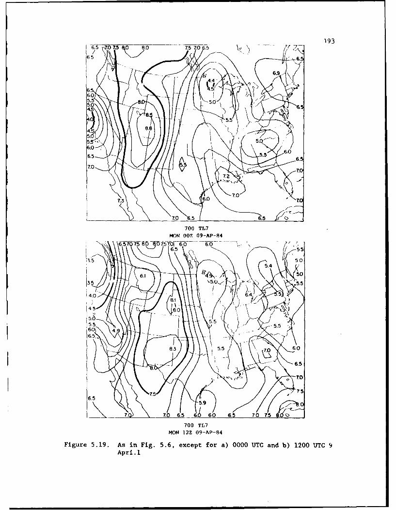
193
65 6.5S£-j
'700 TL7
MON 00? 09-AP-84
6.5 t4.5
664.0.1 . 5
5.5 ~5.0~~- 1-
4.0 5B~.44
5•5 ..
46
5.7
7. 7.0.6.507. _ 6.0 6.5 70 7.
700 TL7
MON 12Z 09-AP-84
Figure 5.19. As in Fig. 5.6, except for a) 0000 UTC and b) 1200 UTC 9Apr.1
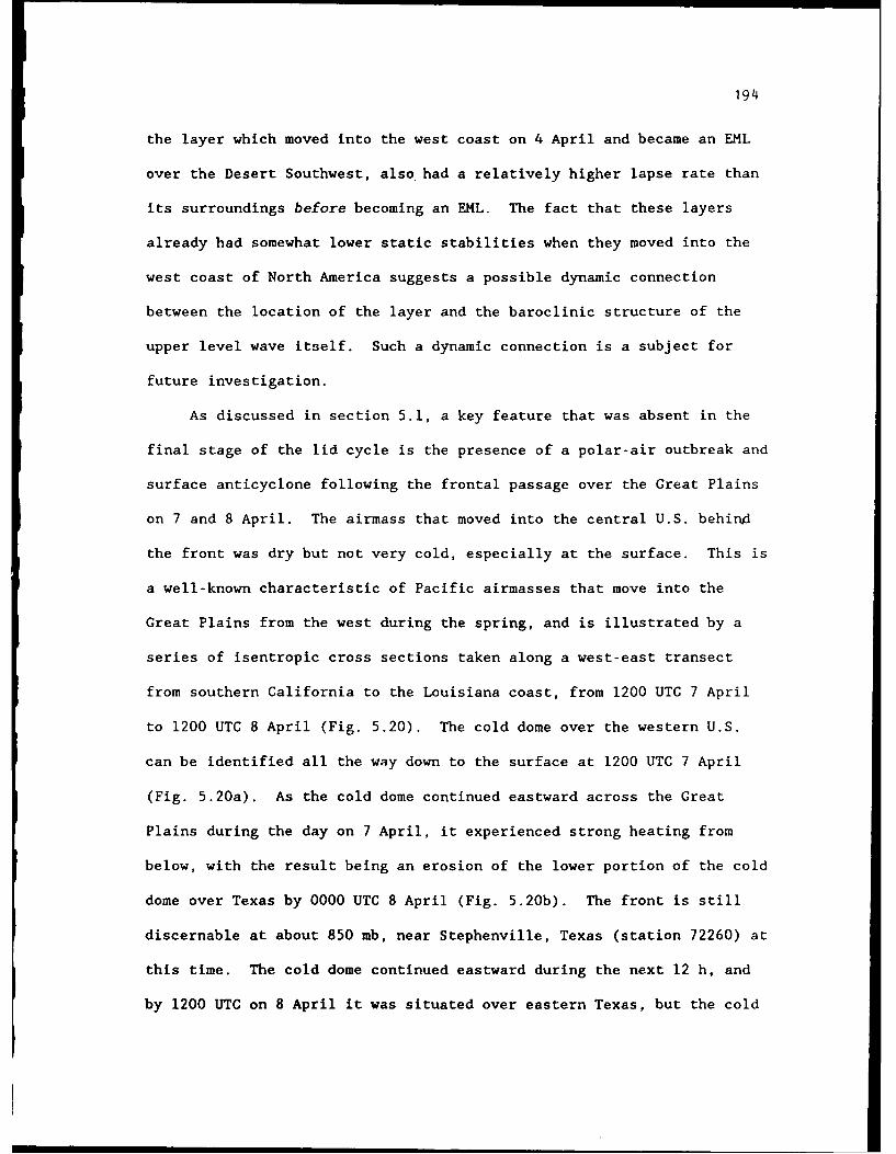
194
the layer which moved into the west coast on 4 April and became an EML
over the Desert Southwest, also had a relatively higher lapse rate than
its surroundings before becoming an EML. The fact that these layers
already had somewhat lower static stabilities when they moved into the
west coast of North America suggests a possible dynamic connection
between the location of the layer and the baroclinic structure of the
upper level wave itself. Such a dynamic connection is a subject for
future investigation.
As discussed in section 5.1, a key feature that was absent in the
final stage of the lid cycle is the presence of a polar-air outbreak and
surface anticyclone following the frontal passage over the Great Plains
on 7 and 8 April. The airmass that moved into the central U.S. behinvd
the front was dry but not very cold, especially at the surface. This is
a well-known characteristic of Pacific airmasses that move into the
Great Plains from the west during the spring, and is illustrated by a
series of isentropic cross sections taken along a west-east transect
from southern California to the Louisiana coast, from 1200 UTC 7 April
to 1200 UTC 8 April (Fig. 5.20). The cold dome over the western U.S.
can be identified all the way down to the surface at 1200 UTC 7 April
(Fig. 5.20a). As the cold dome continued eastward across the Great
Plains during the day on 7 April, it experienced strong heating from
below, with the result being an erosion of the lower portion of the cold
dome over Texas by 0000 UTC 8 April (Fig. 5.20b). The front is still
discernable at about 850 mb, near Stephenville, Texas (station 72260) at
this time. The cold dome continued eastward during the next 12 h, and
by 1200 UTC on 8 April it was situated over eastern Texas, but the cold

195

Figure 5.20. Isentropic cross sections from southern California to theLouisiana coast (see Fig. 5.12b for exact location) forthe following times: a) 1200 UTC 7 April, b) 0000 UTC 8April, and c) 1200 UTC 8 April. Isentropes (in K) areanalyzed at 3 K intervals, and are labelled every 12 K.The vertical coordinate is log pressure, and is labelledin 100 mb intervals along right side of figure.
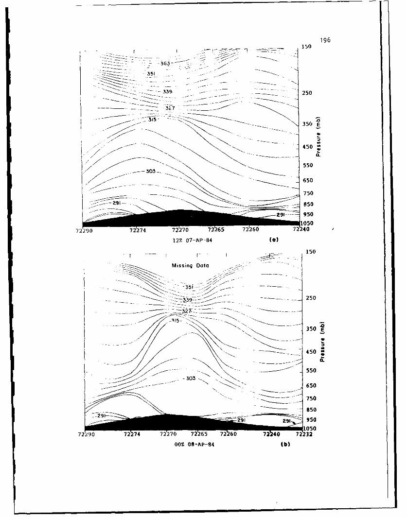
196______150
- - 363~ ~i~7 l - -339- 250- ---
350 'E
- ~450
303-- 550
650
I _ 150
3550
* 3050
2- . 450 72707
12Z 07-AP-84 (a )
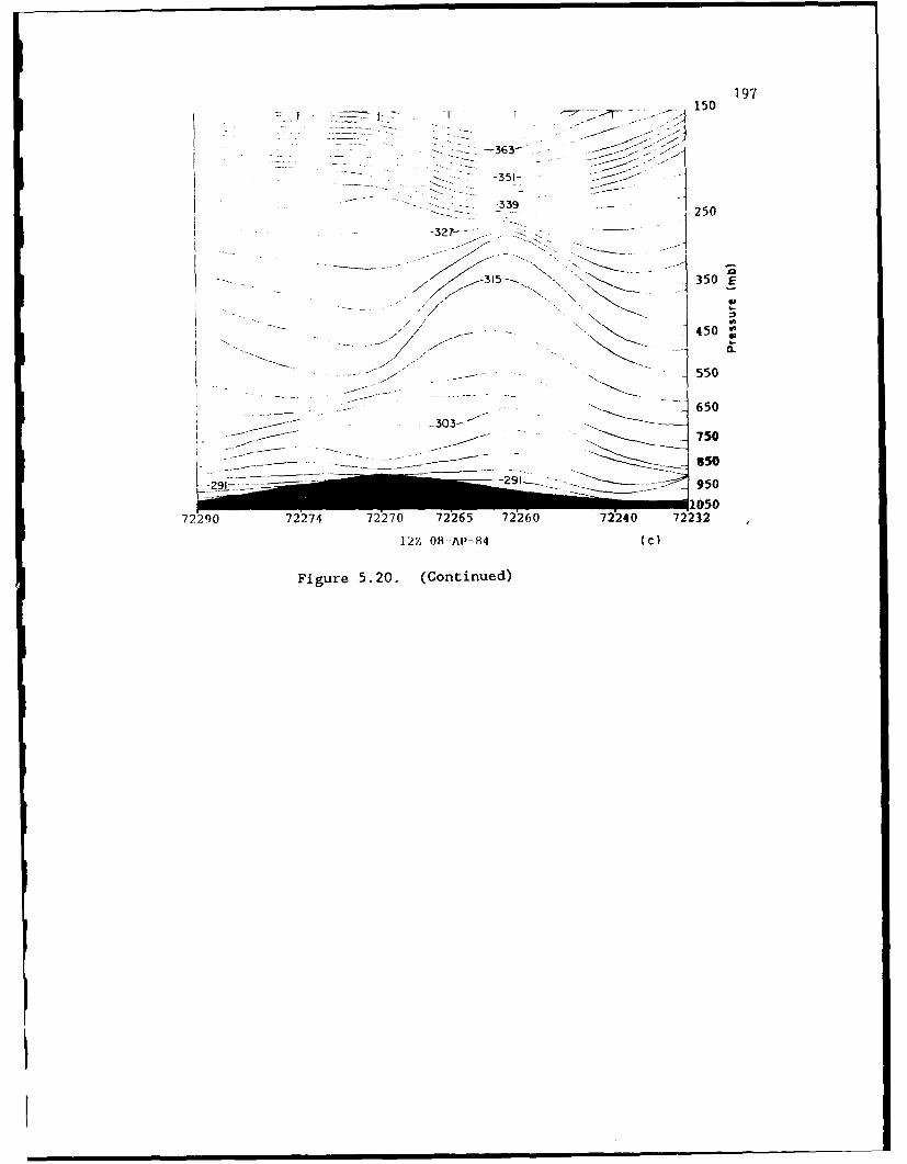
197150
-363
-351
2-- 250
-327--
315-. " 7.350 E
. f - - - • " . .. . . 'N. . s:- : - - ..- - 4' 50Z
40~
550
- - 650
-~9 -30-- 95
72290 72274 72270 72265 72260 72240 72232
12Z 08--AP-84 (CW
Figure 5.20. (Continued)
198
front was still difficult to identify at the surface, located west of
Lake Charles, Louisiana (station 72240).
The portion of the cross section in Fig. 5.20c over the Desert
Southwest shows a shallow dome of cold air associated with the Pacific
ridge observed over this area on the surface analysis (also see Fig.
5.1e). However, as the EML was created in this area during the
subsequent daytime heating cycle, the surface pressures decreased,
eliminating the possibility of a cold anticyclone moving into the Great
Plains at the end of the lid cycle. Because of the lack of such a polar
anticyclone over the southern Plains, the low level moist layer was
never driven very far into the Gulf, and it remained along the coasts of
Texas and Louisiana during the early morning hours of 9 April. An
interesting phasing problem is apparent between the moist layer and the
EML emerging into the western Plains at this time. Figure 5.19b shows
the location of the EML in the 700-500 mb layer over the Rockies and the
western Plains at 1200 UTC 9 April. Although the relative locations of
the EML and moist iayer are similar to those observed on the w.rning of
6 April, the lack of the surface anticyclone makes this situation
different from that on 6 April. In the present situation, a strong
southerly flow cannot develop over Texas until the frontal system over
the Rockies (see Fig. 5.1f) moves into the western Plains and induces a
strong lee-side trough. By contrast, on 6 April, the return flow
strengthened in the strong pressure gradient zone between the developing
lee-side trough and the retreating polar anticyclone. Thus, a new H
cycle is not possible, and the subsequent synoptic patterns do not
follow the typical early-season sequence outlined in the conceptual

199
model of Chapter 3. In such a scenario, the forecaster must analyze the
situation and evaluate how the features of the severe-storm environment
will be different from the ideal case, and adjust his/her forecast
accordingly.
200
Chapter 6
NUMERICAL SIMULATION OF THE 4-9 APRIL 1984 LID CYCLEWITH THE PENN STATE/NCAR MESOSCALE MODEL
The analysis of the 4-9 April 1984 lid cycle in the last chapter
raises interesting questions about some of the physical processes
operating over North America and the Gulf of Mexico during the various
stages of the cycle. The Penn State/NCAR mesoscale model (MM4) is
utilized to examine certain aspects of the large scale environment
during various stages of this lid cycle. Using a mesoscale model to
examine an example of an early-season lid cycle allows us to gain a
better understanding of the relevant physical processes than is possible
from simply studying the composite datasets from the synoptic
climatology. The results of both the observational study (Chapter 5)
and the modeling study (Chapter 6) can then be used to refine specific
aspects of the synoptic climatology. This chapter begins with a summary
of the general characteristics of MM4, and the special modifications
that were made for this case. A general evaluation of the model
simulation is then in order to determine the degree to which MM4
reproduces critical aspects of the 4-9 April lid cycle. Finally, we
examine some of the physical processes operating during various stages
in the cycle.
2U1
6.1 MM4 Characteristics
6.1.1 General Description
For a specific discussion of the model equations and physical
parameterizations, the reader is referred to Anthes and Warner (1978)
and Anthes et al. (1987). The model is three-dimensional, hydrostatic,
and uses the flux form of the primitive equations to predict horizontal
wind, temperature, surface pressure, and specific humidity. The model's
vertical coordinate, sigma (a), is defined as follows:
- = (p - Ptop)/(Psfc - Pop) (6.1)
where p is pressure, Ptop is the pressure at the top of the model, and
Psfc is the surface pressure. A staggered horizontal grid is used,
where the momentum variables are defined at "dot" points and the other
variables are defined at "cross" points, following the "B" grid of
Arakawa and Lamb (1977). See Fig. 4.1 in Anthes et al. (1987) for a
schematic diagram of the staggered horizontal grid system. The model
variables are also staggered in the vertical, with vertical velocity
(da/dt) diagnosed at the "full a levels," and the other variables
defined at "half a levels" which are located halfway between the full a
levels. The model's initial meteorological conditions are generated in
several steps. First-guess fields of the predictive variables are
derived from archived 2.5° latitude/longitude surface and pressure-level
analyses from the European Centre for Medium-Range Weather Forecasting
(ECMWF), available every 12 h. An objective analysis takes the
202
rawinsonde and surface observations, and uses a set of isotropic and
anisotropic weighting functions (see Benjamin and Seaman 1985) to modify
the initial fields at both the surface and user-specified pressure
levels. The version of the model used in this study employs
"relaxation" lateral boundary conditions, which essentially "nudge" the
predictive variables toward a large scale analysis (Davies and Turner
1977). The lateral boundary conditions are also defined using 12-hourly
surface and rawinsonde data available during the period of the model
simulation. The objectively analyzed fields are interpolated to the
model sigma levels, and a static initialization procedure is used to
remove the vertically integrated column divergence from the initial
windfields (Washington and Baumhefner 1975).
The model parameterizations include second-order vertical and
horizontal diffusion, a "slab" surface energy budget equation with
surface radiation effects (Benjamin 1983), a high-resolution PBL
(Blackadar 1976, 1979), and a moist convection scheme (Kuo 1974; Anthes
1977). An important feature of the cumulus parameterization is the
cloud base/top determination and stability check. This procedure
determines the equivalent potential temperature, 0e, of an air parcel
most likely to form a cloud, and determines the lifting condensation
level (LCL) for that parcel. The saturation 0e is then computed for all
levels above the LCL until a "parcel equilibrium level" is found
(overshooting is also accounted for). If the cloud thickness 6o is
below a threshold of 0.3, then convection is not permitted. Following
this, the available buoyant energy (ABE) of the grid column is computed,
203
and convection is allowed only if the ABE is positive (see Eq. 3.5.27 in
Anthes et al. 1987).
6.1.2 Specific Characteristics of the Version of MM4Used in This Study
Several features of MM4 were specifically modified for this study.
First, a horizontal diffusion procedure designed by Benjamin (1983) was
adapted for use in this modeling study. In this procedure, second-order
diffusion of the predictive variables is performed on pressure instead
of sigma surfaces, in order to prevent heat and moisture from being
diffused upslope in areas of strong topographic gradients. This is
especially important in our case, in which steep terrain exists over
areas such as the Rocky Mountains and the Sierra Madre ranges of Mexico.
In this study, the pressure-level diffusion scheme was applied at every
level in the model atmosphere except at the top and bottom levels. In
addition to the pressure-level diffusion, a factor, DFAC, was introduced
to modify the horizontal diffusion coefficient, Kh, given by
Kh = (A x DFAC) (KhO + 2.9 x 10⁸ D), (6.2)
where A is an amplification factor that is a function of location on the
model domain, Kho is a background horizontal diffusion term that is a
function of grid size and time step, and D is a horizontal wind
deformation term (Smagorinsky et al. 1965), which is typically on the
order of 10.5 s-1. In this study, Kh. - 3 x 10' m2 s-1, and the constant
multiplied by the deformation is on the order of 103 m2 s- 1 . In this
model version, DFAC was reduced to 0.2 (it normally is set - 1.0) in
204
order to reduce the effects of the horizontal diffusion (Stauffer,
personal communication). Since it is also important to minimize the
vertical diffusion in this simulation in order to properly maintain the
inversion associated with the lid, the background value of the vertical
diffusion coefficient was reduced from its default value of 1.0 to 0.1
m 2 s- 1 . For more details on the horizontal and vertical diffusion
schemes, see sections 3.1 and 3.4 in Anthes et al. (1987).
A unique aspect of this modeling study is the multiple time and
space scales that prevail during the period of interest. Since a
typical early-spring lid cycle length is about seven days (see section
3.3.1), this necessitates using a large model domain and performing long
simulations. The typical lid-cycle time scale is well beyond the normal
simulation length for most mesoscale models. However, exceptions exist
such as the Saharan dust layer study of Karyampudi and Carlson (1988),
and the four-dimensional data assimilation (FDDA) studies of Seaman et
al. (1991). The first study used a horizontal grid spacing of 220 km
with 13 vertical levels, and a 51 x 31 domain. The simulations were
120 h in length, and used data from the GARP Atlantic Tropical
Experiment to study the formation and evolution of the Saharan dust
layer from its source region over North Africa to its elevated
downstream location over the tropical Atlantic Ocean. The FDDA studies
covered a smaller area (the eastern two-thirds of the continental U.S),
using an 80-km horizontal mesh and 15 vertical levels to produce 120-h
simulations that were continuously adjusted by the assimilation of both
surface and rawinsonde observations. The present study is similar to
these two in terms of the simulation length (120 h), but it differs from
205
them in terms of using a finer horizontal grid mesh (60 km), 30 vertical
levels, and a large domain (118 x 68, covering 2.9 x 10⁷ km 2 ). Also, no
data assimilation was employed. The lateral boundary conditions are
over oceanic regions along every border except the northern one. This
means that the model simulation will be almost like a true forecast,
since the ECMWF first-guess analyses are primarily determined by their
prediction model over these data-sparse regions.
The model domain used in this study is shown in Fig. 6.1, and the
location of the sigma levels is shown in Table 6.1. Determining the
location of the vertical levels is based on the experience with previous
studies of the severe-storm environment (e.g., Benjamin and Carlson
1986; Lakhtakia and Warner 1987; Lanicci et al. 1987), as well as
computations of the levels of relative humidity breaks, and EML oases
and tops throughout the entire lid cycle. Analysis of sounding data for
this period led to the strategy of concentrating more than half of the
sigma levels below 700 mb. The combination of a large domain and long
simulation length, along with the fine horizontal and vertical grid
structures, allows us to examine not only the larger scale processes
that are important in the lid cycle, but also the finer structures that
are created on smaller time scales. The severe-storm environment
simulations of Anthes et al. (1982) showed that a mesoscale model
initialized with synoptic-scale data was capable of generating and
maintaining mesoscale phenomena in the 0-24 h time period, and suggested
that such features are predictable over time periods longer than their
individual lifetimes. Studies of the entire cycle of moist layer
evolution over the Gulf of Mexico (e.g., Johnson 1976; Karnavas 1978;
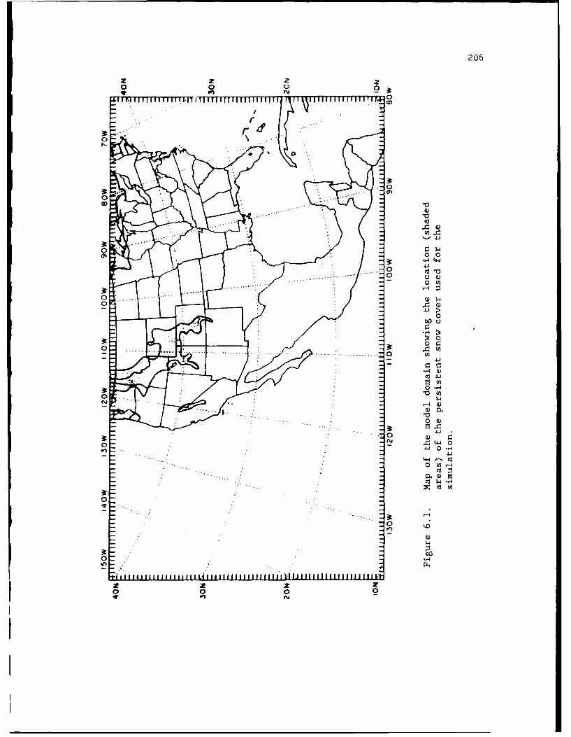
206
z z z z0 0
2 NY
00
X 0
0 0C1
0bo
. .. . . .... . 0 *U)
0 4
0
0 0j 00N4
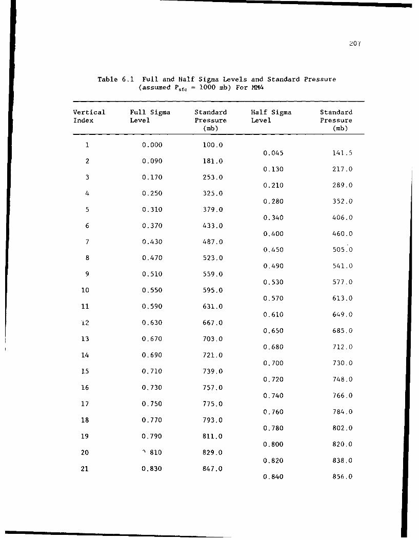
20 7
Table 6.1 Full and Half Sigma Levels and Standard Pressure(assumed Psfc = 1000 mb) For MM4
Vertical Full Sigma Standard Half Sigma StandardIndex Level Pressure Level Pressure
(mb) (mb)
1 0.000 100.00.045 141.5
2 0.090 181.00.130 217.0
3 0.170 253.00.210 289.0
4 0.250 325.00.280 352.0
5 0.310 379.00.340 406.0
6 0.370 433.00.400 460.0
7 0.430 487.00.450 505.0
8 0.470 523.00.490 541.0
9 0.510 559.00.530 577.0
10 0.550 595.00.570 613.0
11 0.590 631.00.610 649.0
i2 0.630 667.00.650 685.0
13 0.670 703.00.680 712.0
14 0.690 721.00.700 730.0
15 0.710 739.00.720 748.0
16 0.730 757.00.740 766.0
17 0.750 775.00.760 784.0
18 0.770 793.00.780 802.0
19 0.790 811.00.800 820.0
20 ' 810 829.00.820 838.0
21 0.830 847.00.840 856.0
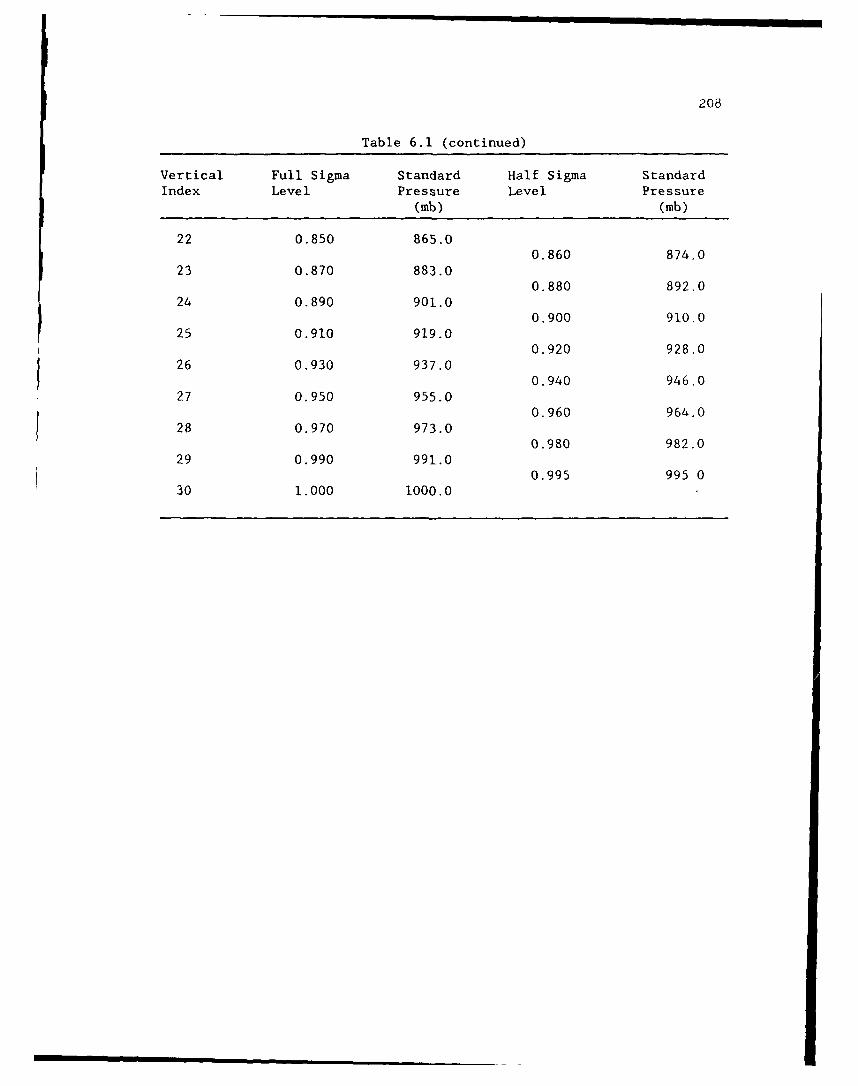
208
Table 6.1 (continued)
Vertical Full Sigma Standard Half Sigma StandardIndex Level Pressure Level Pressure
(mb) (mb)
22 0.850 865.00.860 874.0
23 0.870 883.00.880 892.0
24 0.890 901.00.900 910.0
25 0.910 919.00.920 928.0
26 0.930 937.00.940 946.0
27 0,950 955.0
0.960 964.028 0.970 973.0 0.980 982.0
29 0.990 991.00.995 995. 0
30 1.000 1000.0
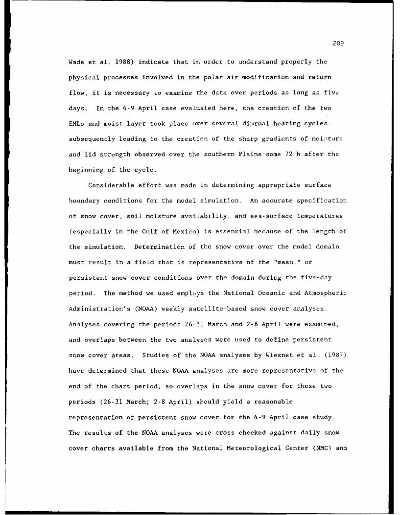
209
Wade et al. 1988) indicate that in order to understand properly the
physical processes involved in the polar air modification and return
flow, it is necessary Lo examine the data over periods as long as five
days. In the 4-9 April case evaluated here, the creation of the two
EMLs and moist layer took place over several diurnal heating cycles.
subsequently leading to the creation of the sharp gradients of moisture
and lid strength observed over the southern Plains some 72 h after the
beginning of the cycle.
Considerable effort was made in determining appropriate surface
boundary conditions for the model simulation. An accurate specification
of snow cover, soil moisture availability, and sea-surface temperatures
(especially in the Gulf of Mexico) is essential because of the length of
the simulation. Determination of the snow cover over the model domain
must result in a field that is representative of the "mean," or
persistent snow cover conditions over the domain during the five-day
period. The method we used empluys the National Oceanic and Atmospheric
Administration's (NOAA) weekly satellite-based snow cover analyses.
Analyses covering the periods 26-31 March and 2-8 April were examined,
and overlaps between the two analyses were used to define persistent
snow cover areas. Studies of the NOAA analyses by Wiesnet et al. (1987)
have determined that these NOAA analyses are more representative of the
end of the chart period, so overlaps in the snow cover for these two
periods (26-31 March; 2-8 April) should yield a reasonable
representation of persistent snow cover for the 4-9 April case study.
The results of the NOAA analyses were cross checked against daily snow
cover charts available from the National Meteorological Center (NMC) and
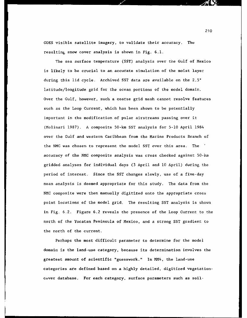
210
GOES visible satellite imagery, to validate their accuracy. The
resulting snow cover analysis is shown in Fig. 6.1.
The sea surface temperature (SST) analysis over the Gulf of Mexico
is likely to be crucial to an accurate simulation of the moist layer
during this lid cycle. Archived SST data are available on the 2.50
latitude/longitude grid for the ocean portions of the model domain.
Over the Gulf, however, such a coarse grid mesh cannot resolve features
such as the Loop Current, which has been shown to be potentially
important in the modification of polar airstreams passing over it
(Molinari 1987). A composite 50-km SST analysis for 5-10 April 1984
over the Gulf and western Caribbean from the Marine Products Branch of
the NMC was chosen to represent the model SST over this area. The '
accuracy of the NMC composite analysis was cross checked against 50-km
gridded analyses for individual days (3 April and 10 April) during the
period of interest. Since the SST changes slowly, use of a five-day
mean analysis is deemed appropriate for this study. The data from the
NMC composite were then manually digitized onto the appropriate cross
point locations of the model grid. The resulting SST analysis is shown
in Fig. 6.2. Figure 6.2 reveals the presence of the Loop Current to the
north of the Yucatan Peninsula of Mexico, and a strong SST gradient to
the north of the current.
Perhaps the most difficult parameter to determine for the model
domain is the land-use category, because its determination involves the
greatest amount of scientific "guesswork." In MM4, the land-use
categories are defined based on a highly detailed, digitized vegetation-
cuver database. For each category, surface parameters such as soil-
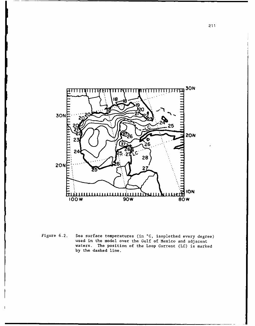
211
30N
, L'•6 20
Figure86.2. Se-ufc eprtrs(n 0 ,iolte vr ere
30N 2:. . ..
21.27 26...
" " " ION
I O0w 90w 80 w
Figure 6.2. Sea surface temperatures (in °C, isoplethed every degree)
used in the model over the Gulf of Mexico and adjacentwaters. The position of the Loop Current (LC) is markedby the dashed line.
212
moisture availability, albedo, emissivity, roughness length, and thermal
inertia are assigned values that remain spatially and temporally
constant. The surface parameters within a land-use category are allowed
to vary seasonally from Winter to Summer. The 4-9 April case falls
towards the end of the winter "season" (15 October-15 April). The
studies of Zhang and Anthes (1982) and Lanicci et al. (1987) found that
the model surface parameter which has the greatest effect on the PBL
development and the greatest impact on the evolution of the model
severe-storm environment is the soil-moisture availability, M. The
value of M is proportional to E/Ep, where E is the surface evaporation
from the model surface, and EP is the potential evaporation, defined as
that occurring from a saturated surface. Previous modeling studies of
the lid/severe-storm environment used a set of land-use categories based
primarily on rainfall climatology, satellite imagery, and climatological
atlases. For this study, the standard MM4 land-use categories were
subjectively "blended" with the set from those severe-storm modeling
studies, to arrive at a modified set of land-use categories that is
tailored to the early-spring rainfall climatology, yet retains the
detail of the standard MM4 dataset. The resulting set contains 14
categories, which are described in Table 6.2 and depicted over the model
domain in Fig. 6.3.
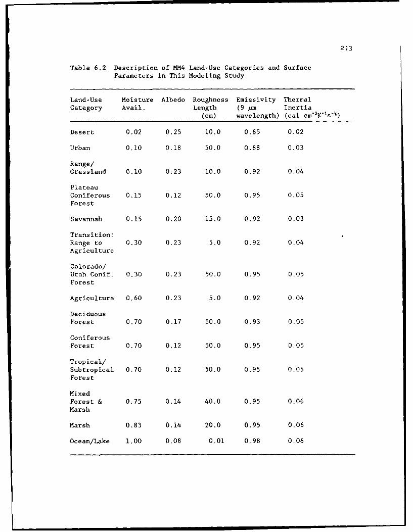
213
Table 6.2 Description of MM4 Land-Use Categories and SurfaceParameters in This Modeling Study
Land-Use Moisture Albedo Roughness Emissivity ThermalCategory Avail. Length (9 Am Inertia
(cm) wavelength) (cal cm- 2 K'-s-k)
Desert 0.02 0.25 10.0 0.85 0.02
Urban 0.10 0.18 50.0 0.88 0.03
Range/Grassland 0.10 0.23 10.0 0.92 0.04
PlateauConiferous 0.15 0.12 50.0 0.95 0.05Forest
Savannah 0.15 0.20 15.0 0.92 0.03
Transition:Range to 0.30 0.23 5.0 0.92 0.04Agriculture
Colorado/Utah Conif. 0.30 0.23 50.0 0.95 0.05Forest
Agriculture 0.60 0.23 5.0 0.92 0.04
DeciduousForest 0.70 0.17 50.0 0.93 0.05
ConiferousForest 0.70 0.12 50.0 0.95 0.05
Tropical/Subtropical 0.70 0.12 50.0 0.95 0.05Forest
MixedForest & 0.75 0.14 40.0 0.95 0.06Marsh
Marsh 0.83 0.14 20.0 0.95 0.06
Ocean/Lake 1.00 0.08 0.01 0.98 0.06
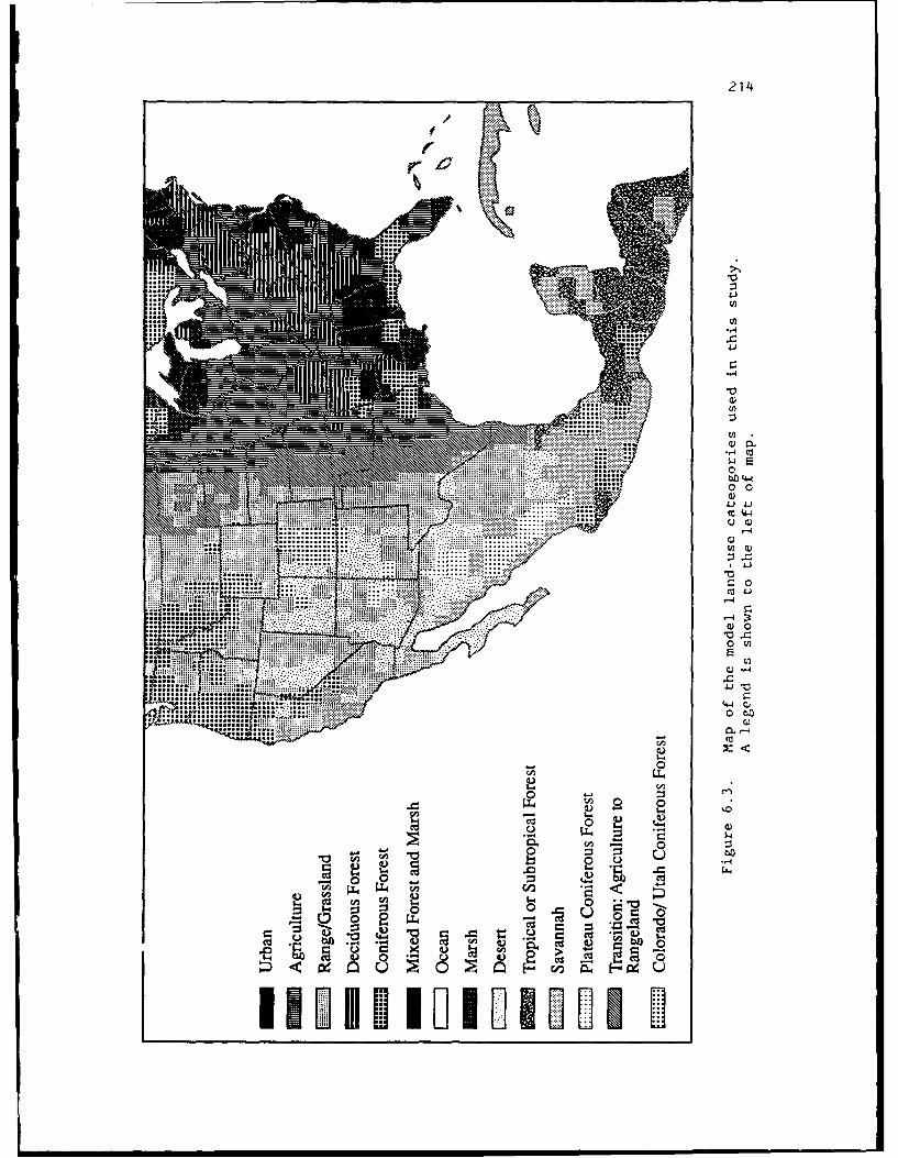
214
UU
'-4
-4)C
*00MI9
......... 4-)4
MMMMI-1; .....0)
...... ....
0U0
C)Q -,44)
4)0 to-..m.... ... n Q)
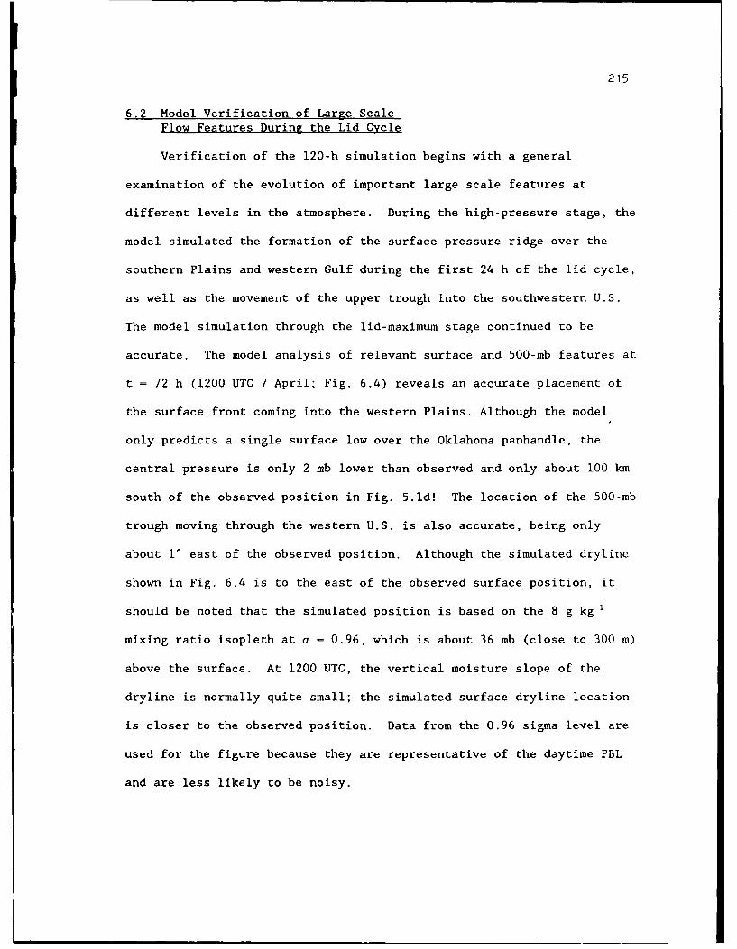
215
6.2 Model Verification of Large ScaleFlow Features During the Lid Cycle
Verification of the 120-h simulation begins with a general
examination of the evolution of important large scale features at
different levels in the atmosphere. During the high-pressure stage, the
model simulated the formation of the surface pressure ridge over the
southern Plains and western Gulf during the first 24 h of the lid cycle,
as well as the movement of the upper trough into the southwestern U.S.
The model simulation through the lid-maximum stage continued to be
accurate. The model analysis of relevant surface and 500-mb features at
t = 72 h (1200 UTG 7 April; Fig. 6.4) reveals an accurate placement of
the surface front coming into the western Plains. Although the model
only predicts a single surface low over the Oklahoma panhandle, the
central pressure is only 2 mb lower than observed and only about 100 km
south of the observed position in Fig. 5.ld! The location of the 500-mb
trough moving through the western U.S. is also accurate, being only
about 10 east of the observed position. Although the simulated dryline
shown in Fig. 6.4 is to the east of the observed surface position, it
should be noted that the simulated position is based on the 8 g kg-1
mixing ratio isopleth at a = 0.96, which is about 36 mb (close to 300 m)
above the surface. At 1200 UTO, the vertical moisture slope of the
dryline is normally quite small; the simulated surface dryline location
is closer to the observed position. Data from the 0.96 sigma level are
used for the figure because they are representative of the daytime PBL
and are less likely to be noisy.
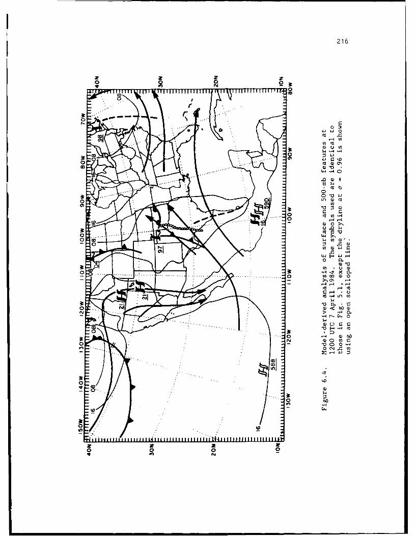
216
z z z z0 0 3NY
0
0.
caa
r-4 E2 W
c *c.J
oo
to~~~c .0 0 ....- 4 r-4
w0<bd
0.
00C
-4-4 -
0 0o 0 0-4 ca
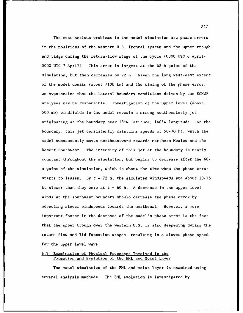
217
The most serious problems in the model simulation are phase errors
in the positions of the western U.S. frontal system and the upper trough
and ridge during the return-flow stage of the cycle (0000 UTC 6 April-
0000 UTC 7 April). This error is largest at the 48-h point of the
simulation, but then decreases by 72 h. Given the long west-east extent
of the model domain (about 7100 km) and the timing of the phase error,
we hypothesize that the lateral boundary conditions driven by the ECMWF
analyses may be responsible. Investigation of the upper level (above
500 mb) windfields in the model reveals a strong southwesterly jet
originating at the boundary near 18°N latitude, 140°W longitude. At the
boundary, this jet consistently maintains speeds of 50-70 kt, which the
model subseauently moves northeastward towards northern Mexico and the
Desert Southwest. The intensity of this jet at the boundary is nearly
constant throughout the simulation, but begins to decrease after the 60-
h point of the simulation, which is about the time when the phase error
starts to lessen. By t = 72 h, the simulated windspeeds are about 10-15
kt slower than they were at t = 60 h. A decrease in the upper level
winds at the southwest boundary should decrease the phase error by
advecting slower windspeeds towards the northeast. However, a more
important factor in the decrease of the model's phase error is the fact
that the upper trough over the western U.S. is also deepening during the
return-flow and lid-formation stages, resulting in a slower phase speed
for the upper level wave.
6.3 Examination of Physical Processes Involved in theFormation and Evolution of the EML and Moist Layer
The model simulation of the EML and moist layer is examined using
several analysis methods. The EML evolution is investigated by
218
determining the locations of both the source region (the area which has
a deep, surface-based PBL) and the elevated region (the area in which
the deep PBL is located aloft). Evaluation of the horizontal and
vertical extent of the EML source region and the downstream elevated
region is made using model soundings from 159 locations over the domain.
The source region at 0000 UTC is determined by locating the soundings
which have a surface-based PBL above the 900-mb level that is 1.) well-
mixed in terms of potential temperature and mixing ratio, 2.) is at
least 80 mb in depth, and 3.) extends to at least 750 mb. The EML
soundings at 0000 UTC are determined using criteria (1) - (4) from
section 2.2.1. At 1200 UTC, the source-region soundings and EML
soundings are distinguished as follows:
1) The source-region soundings must be based above 900 mb, and
contain a layer at least 80 mb deep with dry static stability
below 4.5°C 100 mb- 1 . The base of the layer must extend from
the top of a surface-based inversion and must have a top
> 750 mb.
2) The EML soundings must meet criteria (1) - (4) as outlined in
section 2.2.1, and the base of the layer must extend from the
top of an inversion that is not surface-based.
Recall from section 2.2.1 that EML criterion (4) (RH must increase with
height in the EML) was dropped in the climatological study, based on
instrumentation and reporting considerations, as well as on
observational studies of PBL moisture profiles. In the modeling study,
criterion (4) is used only to help determine the EML top, in conjunction
with the lapse rate of 0 in the EML.
219
A second technique that is used to examine both the EML and the
moist layer employs "parcel" trajectories calculated from the model
output fields. The trajectory scheme is used to evaluate the horizontal
and vertical evolution of the parcels making up the EML and moist layer.
Evaluation of the horizontal and vertical parcel displacements reveals
information about the dynamical processes taking place during various
stages of the lid cycle. Additionally, interpolated grid-point values
of 0 and q along the trajectory are examined in order to determine the
extent of diabatic modifications to the EML and moist-layer parcels from
surface heating/cooling and evaporation within the model PBL.
6.3.1 Formation of the Western U.S. and Mexican EMLs
In Chapter 5, it was determined that separate EMLs evolved over the
western U.S. and northern Mexico during the high-pressure and return-
flow stages of the 4-9 April lid cycle. It was shown that the western
U.S. EML source region formed over the Desert Southwest during the
afternoon of 4 April, and that the presence of the subtropical jet and
its associated region of subsidence over northern Mexico prevented the
Mexican source region from activating until 24 h later. The two EMLs
were observed to evolve separately until 0000 UTC on 7 April, when they
began to merge over the western Plains and Texas (see Fig. 5.12a).
An analysis of the simulated EML source region at 0000 UTC on 5
April is shown in Fig. 6.5a. At this time, a deep, well-mixed PBL is
observed from western Montana into northern Mexico. The highest PBL tops
(above 625 mb) are observed over central Nevada, western New Mexico, and
southeastern Arizona. Mean PBL 6 values over the western U.S. are

220
Figure 6.5 EML source-region and elevated-region analysis for a) 0000UTC 5 April and b) 1200 UTC 5 April. Location of model-generated EML source region is outlined by dotted lines.Location of the elevated region is outlined by scallopedlines. Mean potential temperature in the source/elevatedregion (°C) is shown by dashed lines and is isoplethed at4°C intervals; the pressure at the top of the layer isshown by the solid lines, is labelled in mb, and isisoplethed every 50 mb.
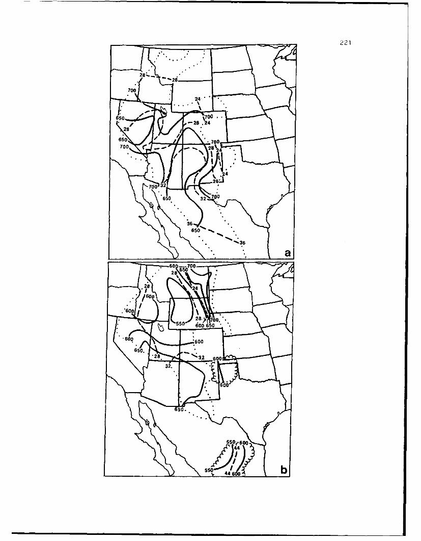
221
-2i
700
24
650 70 -0,-28 .24
28
6iO - 700700 28%24
242S.J
760 32
650 32 7ýO
ý6650
36
-600 7006502 8" %
.28 246 o
6002ý8- '00.
550 600 650
60o
650.28. 'o '7 3.2 6
32.
06
SSOjA60044
560 4 14
222
mainly in the upper 20's to lower 30's (°C), and are in the mid 30's
over northern Mexico. By t - 24 h (1200 UTC 5 April), the EML source
region has generally shifted to the north and east (see Fig. 6.5b). As
in the observations (Fig. 5.6c), the EML source-region soundings have
higher tops at 1200 UTC over Wyoming and Montana, while the thermal
stratification over northern Mexico has become more stable since 0000
UTC, and does not meet the criteria for an EML source region.
An example of the lower-tropospheric stabilization over northern
Mexico is shown by the series of model soundings taken over Torreon
(Fig. 6.6a; location is shown in Fig. 6.7). Noticeable warming and
drying took place in the 600-750 mb layer over Torreon during the 0000-
1200 UTC period, while the winds in the layer became more westerly. The
evolution of representative air parcels comprising the surface-600 mb
layer of the 1200 UTC sounding is evaluated by means of 24-h backward-
in-time trajectories originating at Torreon, commencing at 1200 UTC on
5 April, and ending at 1200 UTC 4 April. Use of such backward
trajectories reveals information about the source-region characteristics
of the air making tip the lowest 300 mb of the 1200 UTC 5 April sounding.
The results of the backward trajectories show that the stable air in the
lowest 300 mb came from vastly different sources, as displayed by the
horizontal trajectory history in Fig. 6.7. The horizontal trajectories
in Fig. 6.7 indicate a great deal of veering wind shear between the
lower and middle troposphere, which is also reflected in the soundings
of Fig. 6.6a. This shear is caused by a combination of the southward
advancing polar anticyclone to the east of the plateau, which causes the
low level flow to have an easterly component, and the strcrng westerly

223
00 UTC 12 UTC
3 20 * 36 01 ilk@ 70 3U6 '9 48 440 Of 430 4".
TRC 1/TD. T
309
'SL
/aa
Figure~ ~ 6. Mode te p r tr/e p i t s u d n s ( k w T l g P o0000 UTG (sldlns7n 20UTdtdse ie)
Locaion ofsudnsae2)Tren exc TG;bAluuruNw eio(B) and c andr ymn
(LD.Wn roie0o oh ie r islyda h
Figurrght wind soe eperue/ds areinkt Thedng parcel loation for
the trajectories discussed in the text are shown by largesolid dots with numbers.
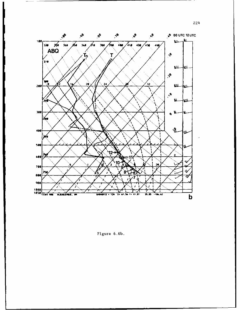
224
00 OUTC 12 UTC
ABO
2'S/Z
29O
I 661
Figure 6.6b.
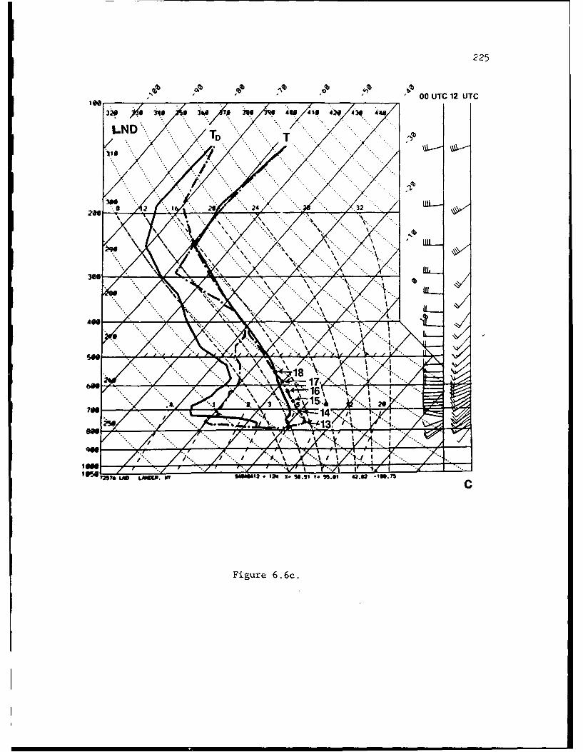
225
"O- -'l 00 UTC 12 UTC
LND.TD T
~I24
2 20 -.3
Fiur 66
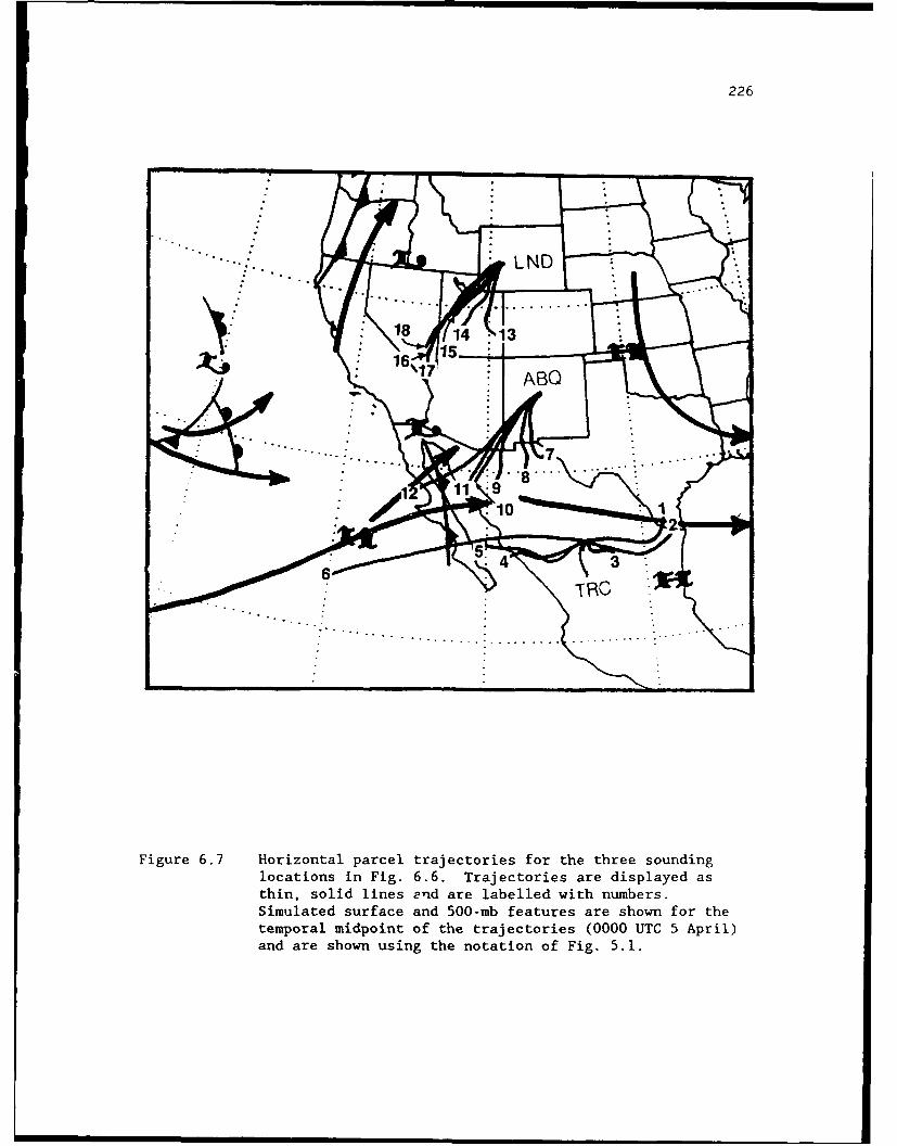
226
"" .... :" . LND .•
S1 3
17 ABO
S--mc
Figure 6.7 Horizontal parcel trajectories for the three soundinglocations in Fig. 6.6. Trajectories are displayed asthin, solid lines end are labelled with numbers.Simulated surface and 500-mb features are shown for thetemporal midpoint of the trajectories (0000 UTC 5 April)and are shown using the notation of Fig. 5.1.

227
flow aloft due to the presence of the subtropical jet over northern
Mexico.
Potential temperature and vertical displacement (using sigma
coordinates) histories for these parcels were also prepared, and are
shown for Torreon in Figs. 6.8a and b, respectively. The potential
temperature history shows that the distinctive source regions for the
Torreon sounding have vastly different initial potential temperatures.
Parcels 1-5 experience different degrees of diabatic heating during the
first 12 h of the simulation, which lessens some of the original 0
difference between them, but is not enough to eliminate the vertical
variation in 0. The vertical displacement history shows that the lowest
three parcels either maintain a constant elevation above local terrain
or rise slightly during the 24-h period. The amount of time spent by
parcels within the lowest 100 mb of the model atmosphere during the
daytime heating cycle explains the reason for the varying amounts of
diabatic heating they receive during the day on 4 April. Notice that
parcels 1 and 2 spent the entire period within the lowest layers, and
they experience the greatest amount of 8 increase during the first 12 h
of the simulation (around 8-12'C). Parcels 4 and 5 experience
subsidence relative to the local surface through the first 15 h of the
simulation. An examination of the pressure-level displacements for all
six parcels (not shown) reveals that parcels 5 and 6 also subside with
respect to pressure, but parcel #4 actually experiences a 24-h net rise
in elevation, suggesting that the local terrain "rises" below that
parcel during this period.

228

Figure 6.8 Parcel histories for the trajectories originating at thethree sounding locations in Fig. 6.6. Potentialtemperature history is shown in panels (a), (c), and (e).The ordinate displays the potential temperature (in K),and the abscissa shows the hour of the simulation (notethat time is read from right to left). A key below theabscissa indicates the symbols used to denote each parcel.Vertical displacement history is shown in panels (b), (d),and (f). The ordinate displays the sigma level above thelocal surface (see Eq. 6.1 for a definition of the sigmavertical coordinate; the ordinate value is obtained bysubtracting the sigma value from 1.0). The abscissa andthe legend are the same as in the potential temperaturehistories.
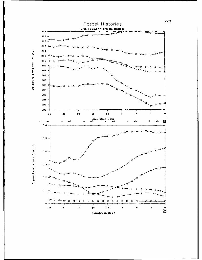
229Parcel Histories
Grid Pt 24,67 (Torreon,. Mexico)322 -
320
316
318
- 314
w 310
6 308
2 306
*' 304
S 302
S 300 -
S 298
996
294
292
24 21 18 15 12 9 6 3 0
Simulation Hour
U 1* 1 4 X * .6 a
0.40.3
Z
o 0.1
.0 -4
0.3T
24 21 16 15 12 9 6 3
Simulation Hour b;
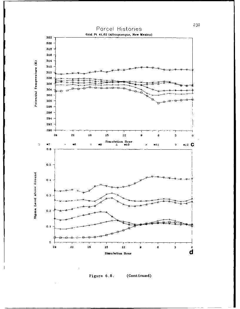
Parcel Histories23Grid P't 41.62 (Albuquerque. New Mexico)
322
320
318
316
314
S 31,2
310
S 304 L,
S 302 -
S 300
S 298
296
294
292
24 21 18 15 12 9 6 3 0
Simulation Hlour*j 7 + *8 0 09 *to v1 >*31 12 C
0.5
0.2O 0.4 :
I 3-Ba24 21 18 15 12 9 6 3 0
Simulation Hourd
Figure 6.8. (Continued)
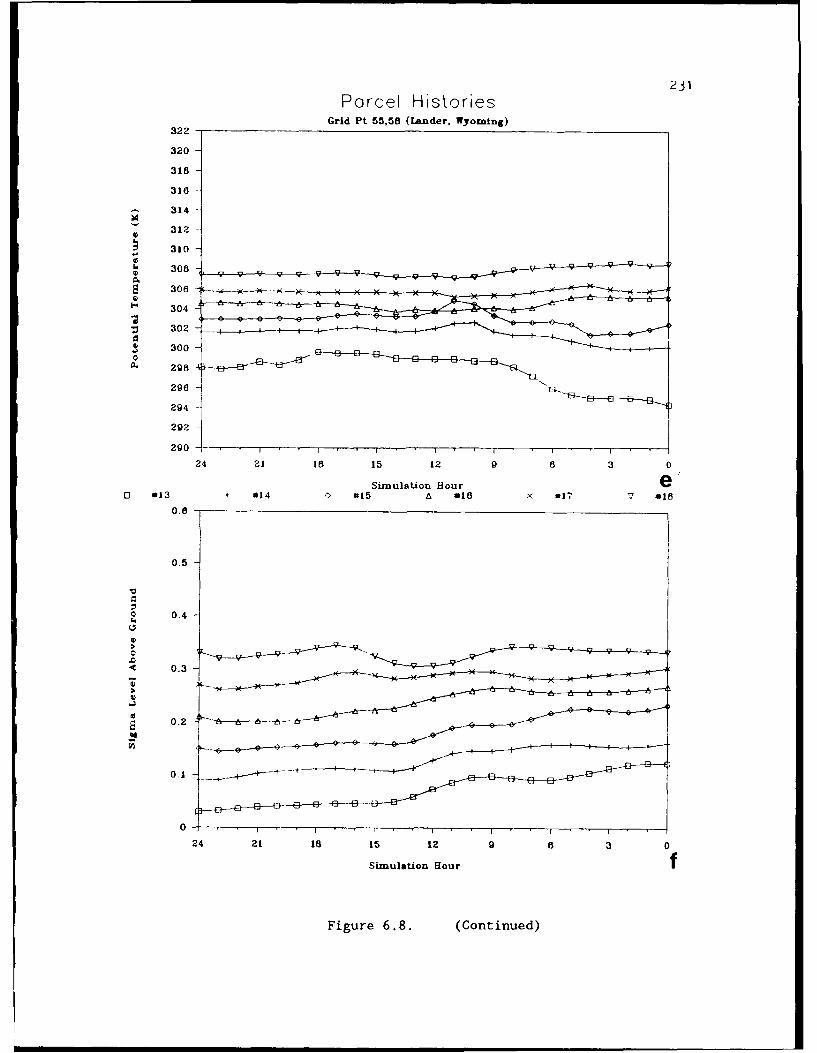
231Parcel Histories
Grid Pt 55.58 (Lander. Wyoming)322
320
318
3168
- 314
310
30
'~3084 _________
S 3027
S 300
228
24 21 1o 15 12 9 6 3 0
Simulation Hour eO3 613 + 814 C' 15 a *18 x 81? * 18
0.5
0.3
0.2
0.1 7+-
24 21 18 15 12 9 6 3 0
Simulation Hourf
Figure 6.8. (Continued)
232
As shown in Fig. 6.5, the area to the north of the subtropical jet
maintains its EML source-region characteristics after 0000 UTC on 5
April. A series of model soundings for the 0000-1200 UTC period at
Albuquerque, New Mexico, is shown in Fig. 6.6b. In contrast to Torreon,
the deep PBL at 0000 UTC is mainly preserved during the next 12 h, and
the winds develop an increased southerly component. Backward
trajectories originating from this location were prepared, distributed
over the lowest 200 mb of the atmosphere. The horizontal trajectories
(Fig. 6.7) show less diversity in source region than did those for
Torreon, and there is also less veering wind shear. The low level
airstreams over New Mexico were not influenced as much by the advancing
surface anticyclone as they were near Torreon, mainly because of the'
higher terrain elevations. Consequently, the parcels making up the
potential temperature history of the Albuquerque sounding (Fig. 6.8c)
have greater "isentropic homogeneity" (i.e., the 9 values of the parcels
are relatively close) than do the parcels from the Torreon sounding.
Parcels 7-9 experience the greatest diabatic heating during the first
12-h period, their 0 values approaching those of parcels 10-12. The
vertical displacement history (Fig. 6.8d) shows that parcels 7-9 spent
the first 12 h within the lowest 100 mb of the model atmosphere. Net
vertical displacements for the 24-h period show that five of the six
parcels experience net sinking motion relative to the local surface,
although the magnitude is less than for parcels 4-6 at Torreon.
However, the pressure-level displacements indicate that all 6 parcels
rose in absolute elevation during the same period. Given the
information displayed in Figs. 6.7 and 6.8c,d, it appears that the EML
233
observed over New Mexico on the morning of 5 April originates over
northwestern Mexico in a generally weak, southerly to southwesterly flow
just to the west of the upper level ridge during this time. Examination
of midlevel tropospheric lapse rates over northwestern Mexico at 1200
UTC 4 April (see Fig. 5.6a) reveals that this was an area of relatively
low static stability (near 7°C km-1 in the 700-500 mb layer), located
between two stable areas over Colorado and southern Baja. While the
static stability in this area was not extremely low, the parcels in the
layer had enough isentropic homogeneity so that the diabatic
modification of the lowest half of the layer during its transit over the
Desert Southwest results in the production of a low-static stability
layer over Albuquerque at the end of this 24-h period.
The third area of interest in the early development of the EML
source region is over Wyoming and Montana. Most of this region did not
have a static stability low enough to be considered an EML source region
at 0000 UTC on 5 April, but had EML source-region soundings with tops
above 525 mb 12 h later. An example of the evolution of the thermal
structure over this area is shown by the series of model soundings for
Lander, Wyoming, for 0000 UTC and 1200 UTC, in Fig. 6.6c. A gradual
destabilization occurs from the surface to 400 mb during the 12-24 h
period, with warming below about 550 mb and slight cooling above. As at
Albuquerque, the winds become more southerly during this period. If one
computes the static stability in the 750-500 mb layer on the 1200 UTC
sounding, it is approximately 3.5°C 100 mb-1 , which is at the stable end
of the EML range (see Fig. 2.2). However, this layer is in the early
234
stages of development as an EML source region, as suggested by the q
profile in Fig. 6.6c, which is nearly well-mixed throughout the 750-500
mb layer.
Backward horizontal trajectories originating from the 1200 UTC
Lander sounding are displayed in Fig. 6.7. The source region for all
six parcels is Utah and eastern Nevada, indicating even less directional
veering than over Albuquerque. As at Albuquerque, the parcels have a
fair amount of 9 homogeneity, as shown by the potential temperature
history in Fig. 6.8e. Parcels 14-15 experience some degree of diabatic
heating during the day on 4 April, and as a result they attain nearly
the same potential temperature as parcels 16-18 above. Parcels 16-18
maintain a nearly constant potential temperature throughout the 24-h*
period. The vertical displacement history (Fig. 6.8f) shows that five
of the six parcels experience subsidence relative to the surface during
this period. Examination of the net pressure-level displacements shows
that the layer consisting of parcels 13-18 actually stretches during
this time, as the lower portion of the layer subsides and the upper
portion rises. Thus, the combination of diabatic surface heating of the
lower portion of the layer and the stretching of the entire layer
results in the "appearance" of the EML source region over Wyoming and
Montana at 1200 UTC 5 April.
Consistent with the observational study, the simulated western U.S.
EML source region experiences a second day of surface heating during the
day on 5 April, while a deep PBL reappears over northern Mexico during
the same period. The model EML evolution on this second day is shown by
the EML analysis for 0000 UTC 6 April (Fig. 6.9a). The analysis shows

235
0
Figure 6.9 Same as Fig. 6.5, except for a) 0000 UTC 6 April, and b)
1200 UTC 6 April. Maximum potential temperature values
within the EML source/elevated regions are indicated by a'W', with the value shown below (in °C).
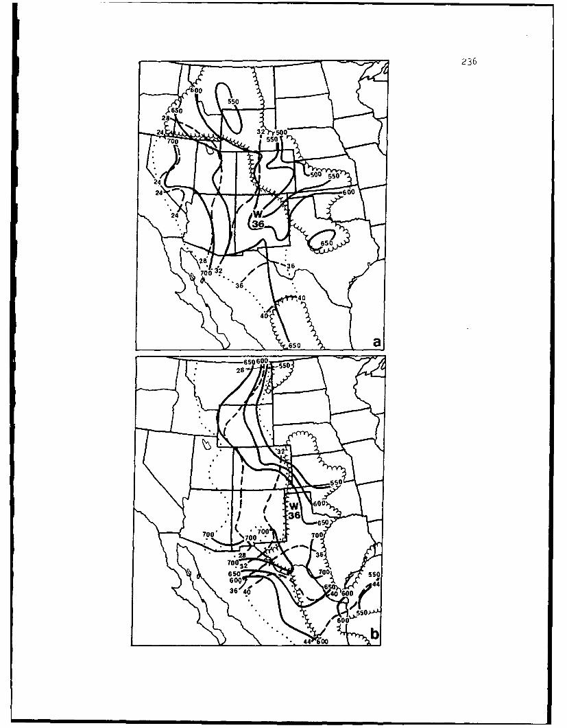
242 31 So
24
36.•
60O•F600
°*'**650
70'70 oN7ý

237
that the EML source-region air over New Mexico has the highest PBL
potential temperatures in the western U.S., with values in the mid 30's.
A portion of the western U.S. source-region air has emerged as an EML
into sections of Kansas, Oklahoma, and Texas by this time. Meanwhile,
the Mexican source-region air remains restricted mainly to extreme
southwest Texas and northern Mexico.
The EML analysis for 1200 UTC on 6 April (Fig. 6.9b) reveals a
general eastward shift in the source-region and elevated-region areas.
The local EML 0 maximum over New Mexico at 0000 UTC appears to "migrate"
into the Texas panhandle, while the warmer Mexican source-region air has
now moved into parts of southern Texas as an EML. As in the
observations, the two EML areas remain distinct in terms of their
thermal characteristics.
Two sets of backward trajectories are used to illustrate the
separate evolutions of the western U.S. and Mexican EML source regions.
Both sets of trajectories originate within EML source-region layers at
1200 UTC 6 April, and terminate at 1200 UTC 5 April. The first set
originates at a model sounding located approximately 200 km to the east
of Chihuahua, Mexico, and represents the Mexican source region, while
the second set originates at a sounding taken approximately 60 km to the
west of Amarillo, Texas, and represents the western U.S. source region.
The horizontal trajectories for the Mexican location are displayed
in Fig. 6.10. Although there is little directional shear evident in the
horizontal trajectories, there is considerable variation in distance
travelled, indicating the presence of speed shear in the model
atmosphere over northern Mexico during this time. This result is
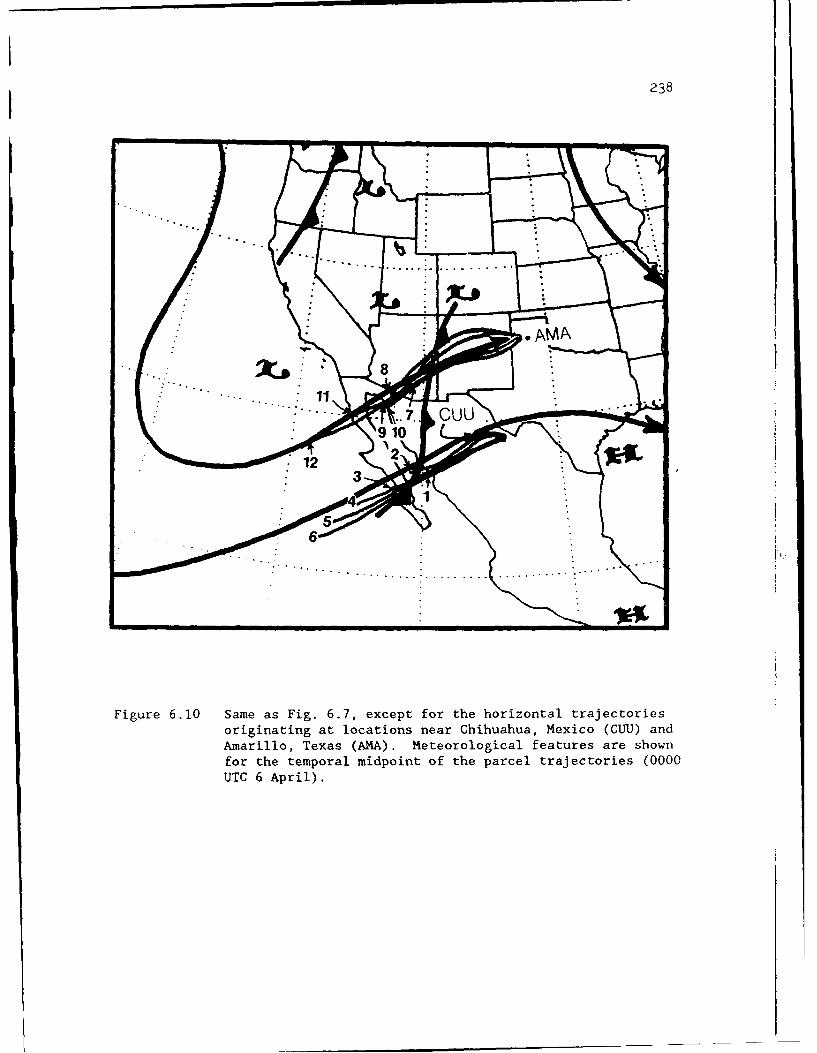
i 238
• .....
Figure 6.10 Same as Fig. 6.7, except for the horizontal trajectoriesoriginating at locations near Chihuahua, Mexico (GUll) andAmarillo, Texas (AMA). Meteorological features are shownfor the temporal midpoint of the parcel trajectories (0000UTC 6 April).
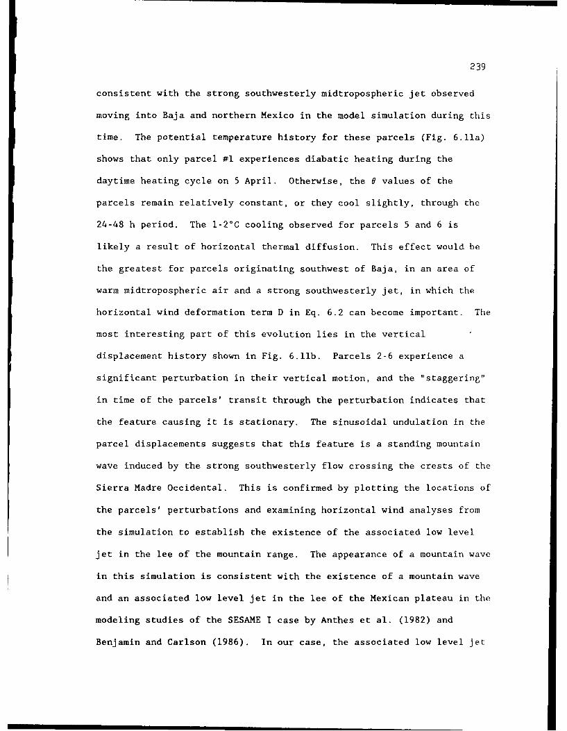
239
consistent with the strong southwesterly midtropospheric jet observed
moving into Baja and northern Mexico in the model simulation during this
time. The potential temperature history for these parcels (Fig. 6.11a)
shows that only parcel #1 experiences diabatic heating during the
daytime heating cycle on 5 April. Otherwise, the 0 values of the
parcels remain relatively constant, or they cool slightly, through the
24-48 h period. The I-2°C cooling observed for parcels 5 and 6 is
likely a result of horizontal thermal diffusion. This effect would be
the greatest for parcels originating southwest of Baja, in an area of
warm midtropospheric air and a strong southwesterly jet, in which the
horizontal wind deformation term D in Eq. 6.2 can become important. The
most interesting part of this evolution lies in the vertical
displacement history shown in Fig. 6.11b. Parcels 2-6 experience a
significant perturbation in their vertical motion, and the "staggering"
in time of the parcels' transit through the perturbation indicates that
the feature causing it is stationary. The sinusoidal undulation in the
parcel displacements suggests that this feature is a standing mountain
wave induced by the strong southwesterly flow crossing the crests of the
Sierra Madre Occidental. This is confirmed by plotting the locations of
the parcels' perturbations and examining horizontal wind analyses from
the simulation to establish the existence of the associated low level
jet in the lee of the mountain range. The appearance of a mountain wave
in this simulation is consistent with the existence of a mountain wave
and an associated low level jet in the lee of the Mexican plateau in the
modeling studies of the SESAME I case by Anthes et al. (1982) and
Benjamin and Carlson (1986). In our case, the associated low level jet
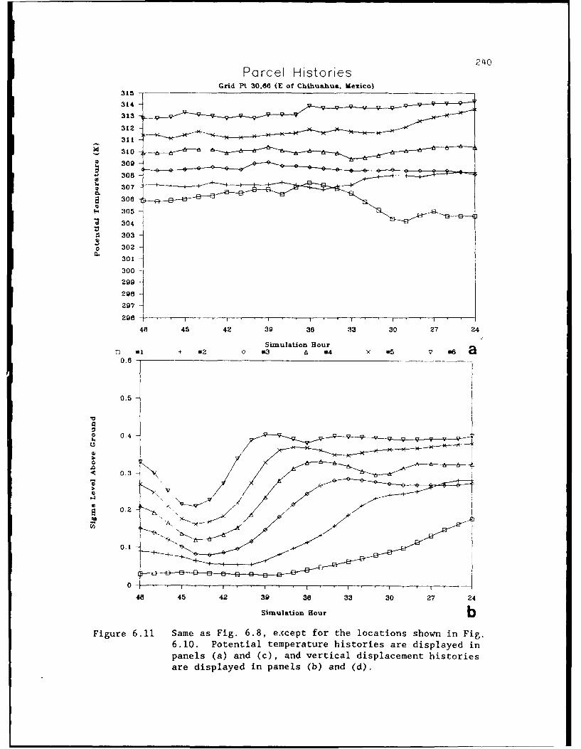
240Parcel Histories
Grid Pt 30.66 (E of Chihuahua, Mexico)315
314
313
312
311
S 310 !1 111
a 309
30830
304
0 303
S 302
301
300
299
298 -297
298 ~------------------ .i
48 45 42 39 36 33 30 27 24
Simulation Hour0 *1 t #2 A f * 4 X 35 .6 a
0.5a
0.
O 0.4
0.3 s
A' 4
48 45 42 39 38 33 30 27 24
Simulation Hour bFigure 6.11 Same as Fig. 6.8, except for the locations shown in Fig.
6.10. Potential temperature histories are displayed inpanels (a) and (c), and vertical displacement historiesare displayed in panels (b) and (d).
241Parcel Histories
Grid Pt 42.68 (Amnarillo. Texas)M15
314
313
312
311
310
0 309
308
*. 307
~. 308
0 3052
304 10
S 303-
S 302 J
a. 301
300
299
297 1
4a 45 42 39 36 33 30 27 24
Simulation Hour(1 7 -** ~ 19 L~ ill0 U 111 12 c;
0.6
0.5
0.4
0.3
0-
0.3
0
48 45 42 39 36 33 30 27 2.4
Simiulation Hour d
Figure 6.11. (Continued)
242
appears in the lowest 100 mb of the model atmosphere between 0600 and
0900 UTC 6 April, and has a speed maximum of about 20 m s-1.
Compared to the SESAME-I mountain wave, the one in this simulation
is distinct in two ways. First, the fact that the location of this
mountain wave is upstream of that documented in the SESAME I simulations
suggests that, earlier in the lid cycle the standing wave pattern sets
up farther west due to the location of the strong midlevel jet at this
stage of the cycle. Second, and perhaps more important, is that the
mountain-wave circulation has the effect of lowering the dry static
stability of the layer making up the 1200 UTC sounding over the Mexican
EML source region. We can explain this in the following way. Since the
effect of the perturbation decreases with height, the mountain-wave,
circulation has a decreasing influence on the net vertical displacements
of the parcels travelling through it. Examination of the 24-h vertical
displacements in Fig. 6.11b along with the pressure-level displacements
shows that differential subsidence occurs in this layer as the lower
parcels sink more than the upper parcels; this results in a
destablization of the Mexican EML source-region layer. In this case,
the static stability of the layer is also lowered by diabatic heating of
parcel #1 and the diffusion-related cooling of parcels 5
and 6.
The horizontal trajectories originating in the low static stability
layer of the sounding near Amarillo are shown in Fig. 6.10. As in the
Mexican trajectories, there is some directional shear, but there is also
considerable speed shear as evidenced by the increasing horizontal
displacement, with height for each parcel. The potential temperature
243
history of this layer (Fig. 6.11c) shows that the well-mixed thermal
characteristics of the EML source-region layer (parcels 8-12) result
mostly from the considerable diabatic heating of parcels 8-10 during the
daytime heating cycle of 5 April over the semi-arid regions of Arizona
and New Mexico. This heating enabled the parcels to attain a potential
temperature close to that of parcels 11 and 12 above. The vertical
displacement history in Fig. 6.11d shows that parcels 7 and 8 spent time
in the lowest 100 mb of the model atmosphere during the 24-36 h period
of the simulation, but the fact that parcels 9 and 10 also experience
diabatic heating suggests that the PBL over New Mexico and Arizona was
probably around 200 mb deep during this time. Examination of both the
net vertical displacements in Fig. 6.11d and the pressure-level
displacements shows that this layer generally sinks during its transit
over the Desert Southwest and the western Plains, suggesting that
diabatic heating of the lower half of this layer is primarily
responsible for producing the low static stability observed in the
Amarillo area at 1200 UTC 6 April.
6.3.2 Formation of the Moist Layer Over the Gulf of Me'ico
The study of the moist-layer formation and evolution during the
model simulation has two objectives. The first objective is to examine
the moist-layer structure over the Gulf coast of Mexico during the high-
pressure and return-flow stages, and evaluate the degree of airmass
modification taking place over the Gulf waters during this period. The
second objective is to determine the effect that the track of the
surface anticyclone has on the trajectories of parcels originating in
244
the offshore flow along the Gulf coast at the beginning of the lid
cycle. A related objective is to determine whether any parcel
trajectories that pass over the Loop Current region in the eastern Gulf
play any role in defining the moist layer that returned into southern
Texas on 6 and 7 April.
As noted in the observational study of Chapter 5, a key event
during the high-pressure stage of the 4-9 April lid cycle is the
"trapping" of the low level moist layer along coastal Mexico as the cold
surge and surface pressure ridge advanced southward through the western
Gulf during the first 24 h of the cycle. Figure 6.12a shows the 12-h
prediction of 850-mb temperature. The simulated cold surge is located
to the west of the observed area (see Fig. 5.4b), and is concentrated
along coastal Mexico in a narrow band about 300 km wide. Because of the
sparsity of the rawinsonde data over eastern Mexico and the Gulf, it is
not possible to definitively state whether the model's location of the
low level cold surge is in error. If the same physical feature that was
observed in Tilley's (1990) Front Range cold surge (topographically
trapped edge waves) fs prevailing over the slopes of the Sierra Madre
Oriental in this case, then the model solution is actually more
physically realistic than is the analysis shown in Fig. 5.4b. A model
time-height cross section of potential temperature, mixing ratio, and
winds at Veracruz (location shown in Fig. 6.12a) for the high-pressure
stage of the cycle is displayed in Fig. 6.12b. The cold surge first
appears in the 925-750 mb layer between 1800 UTC 4 April and 0000 UTC 5
April, and reaches its peak at 1200 UTC 5 April (consistent with
observations). The strongest northerly winds at Veracruz appear at 0600
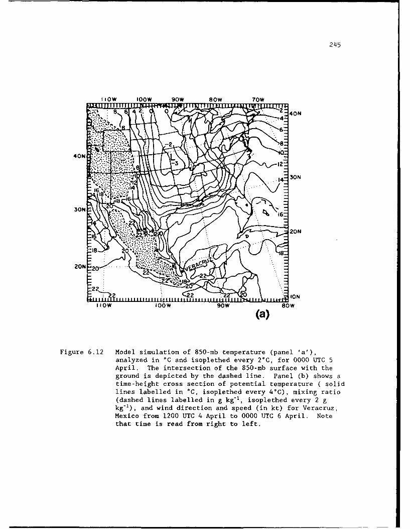
245
'lOW 100W 9OW 8oW 7OW
8~~~ 6 , 40N
4ON4'
40N 20
ION
1104W 16W 0
(a)
Figure 6.12 Model simulation of 850-mb temperature (panel 'a'),analyzed in 00 and isoplethed every 2°C, for 0000 UTC 5April. The intersection of the 850-mb surface with theground is depicted by the dashed line. Panel (b) shows atime-height cross section of potential temperature ( solidlines labelled in °C, isoplethed every 400), mixing ratio(dashed lines labelled in g kg-', isoplethed every 2 gkg-'), and wind direction and speed (in kt) for Veracruz,Mexico from 1200 UTC 4 April to 0000 UTC 6 April. Notethat time is read from right to left.
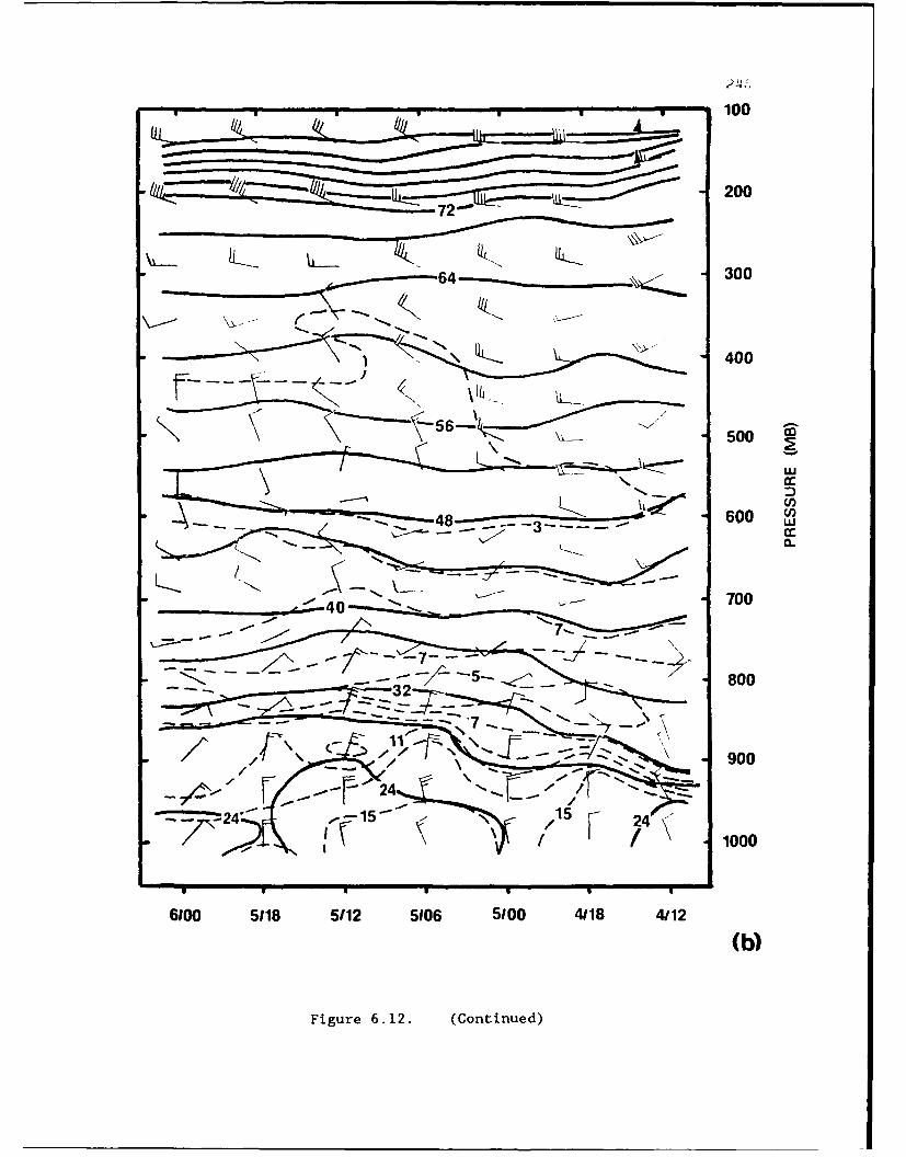
200
64 300
400
5650
700 0
,&r ,~4\ 6000
610* 110 572506500 418 41
7(b)
Fiur 6.12 (Cntnud
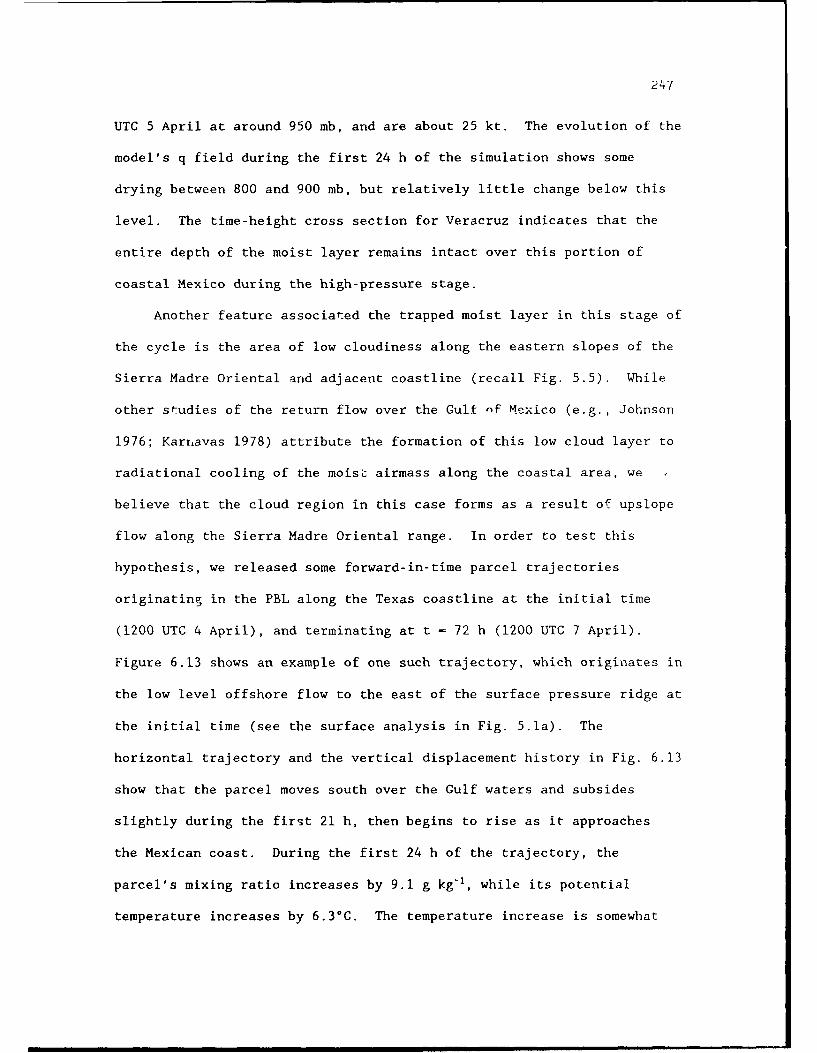
24-7
UTC 5 April at around 950 mb, and are about 25 kt. The evolution of the
model's q field during the first 24 h of the simulation shows some
drying between 800 and 900 mb, but relatively little change below this
level. The time-height cross section for Veracruz indicates that the
entire depth of the moist layer remains intact over this portion of
coastal Mexico during the high-pressure stage.
Another feature associated the trapped moist layer in this stage of
the cycle is the area of low cloudiness along the eastern slopes of the
Sierra Madre Oriental and adjacent coastline (recall Fig. 5.5). While
other studies of the return flow over the Gult of Mexico (e.g., Johnson
1976; Karnavas 1978) attribute the formation of this low cloud layer to
radiational cooling of the moist airmass along the coastal area, we
believe that the cloud region in this case forms as a result of upslope
flow along the Sierra Madre Oriental range. In order to test this
hypothesis, we released some forward-in-time parcel trajectories
originating in the PBL along the Texas coastline at the initial time
(1200 UTC 4 April), and terminating at t = 72 h (1200 UTC 7 April).
Figure 6.13 shows an example of one such trajectory, which originates in
the low level offshore flow to the east of the surface pressure ridge at
the initial time (see the surface analysis in Fig. 5.1a). The
horizontal trajectory and the vertical displacement history in Fig. 6.13
show that the parcel moves south over the Gulf waters and subsides
slightly during the first 21 h, then begins to rise as it approaches
the Mexican coast. During the first 24 h of the trajectory, the
parcel's mixing ratio increases by 9.1 g kg-1, while its potential
temperature increases by 6.3°C. The temperature increase is somewhat
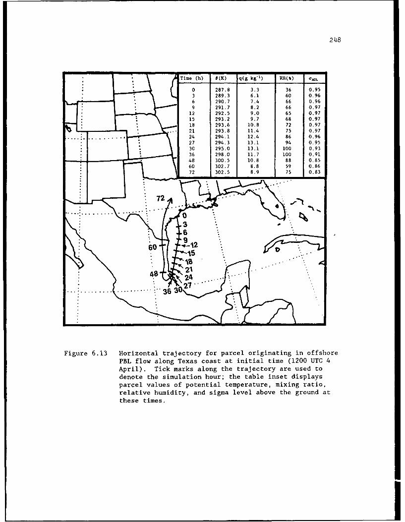
248
Time (h) 9(K) q(g kg-1) RH(%) CAU
0 287.8 3.3 36 0.953 289.3 6.1 60 0.966 290.7 7.4 66 0.969 291.7 8.2 66 0.97
12 292.5 9.0 65 0.97"15 293.2 9.7 68 0.97
"'. 18 293.6 10.8 72 0.97
%l •: • .. 21 293.8 11.4 75 0.97.. " . .. . .-- . , 24 294.1 12.4 86 0.96
""' .. I : •27 294.3 13.1 94 0.95
30 295.0 13.1 100 0.93"36 298.0 11.7 100 0.91
PBLflow alon T48 c 00.5 10a8 88 0 85:I! | 60 302.7 8.8 59 0.86i . .1 72 302.5 8.9 75 0.83
• !~72'"
April). Tick marks along the trajectory are used todenote the simulation hour; the table inset displays
parcel values of potential temperature, mixing ratio,relative humidity, and sigma level above the ground at
these times.
249
less than those reported in the Gulf polar-air modification studies of
Henry and Thompson (1976), Karnavas (1978), and Molinari (1987), who
employed a simple Lagrangian trajectory model based on bulk aerodynamic
assumptions, using both observed and climatological data for the winter
season. An assumption used in the above-mentioned studies is that the
parcel's elevation remains constant throughout the trajectory. The
table accompanying Fig. 6.13 illustrates that this assumption is true
for the 9-21 h period of this trajectory; after the 24-h point, the
vertical motion ot the parcel becomes an important factor. The parcel
begins to rise before it is actually over land, and reaches 100% RH
about the time it moves onshore (1800 UTC 5 April). However, after
completing the upslope journey along the Sierra Madre range, at about t
- 48 h (1200 UTC 6 April), the parcel undergoes a second modification as
it becomes warmer and drier as it travels above the coastal PBL through
eastern Mexico. By the 72-h point, the parcel, which resided in the
Mexican coastal moist layer 48 h earlier, is now located over eastern
Texas above the PBL, and is 7.5°C warmer and 4.2 g kg-1 drier than it
was at the time of saturation along the Mexican coast.
After examining the evolution of a "representative" parcel through
the moist layer in Fig. 6.13, two questions come to mind: does the track
of the surface anticyclone plays a role in this evolution, and is the
parcel trajectory in Fig. 6.13 representative of the evolution of
parcels residing within the coastal moist layer during the return-flow
stage of the cycle. In order to better address these questions, two
more sets of forward trajectories are released. Each set consists of
parcel trajectories originating at five sigma levels, from a - 0.97 to a
250
S0.89. The first set of parcels originates over the Gulf coastal PBL
from Texas to Mississippi at the initial time (1200 UTC 4 April). These
trajectories terminate at the 72-h point of the simulation, and are
intended to evaluate the role of the surface anticyclone's track on the
offshore flow originating along the Gulf coast at the beginning of the
cycle. The second set of parcel trajectories originates within the PBL
along the Gulf coast of Mexico at t - 36 h (0000 UTC 6 April), which
marks the beginning of the return-flow stage of the lid cycle. These
parcels, which are initially located within the coastal moist layer, are
also tracked until the 72-h point, and are intended to test the
representativeness of the trajectory described by Fig. 6.13.
The horizontal displacements for the first set of trajectories are
shown in Fig. 6.14a. In this figure and in Fig. 6.15, the vertical
overlap of the trajectories is shown by a thick solid line. Only the
set of parcels whose origin is closest to the surface ridge axis (set #1
in Fig. 6.14a) is able to move in a southerly direction, and return
northward into Texas by the lid-maximum stage. Parcel set #2 becomes
incorporated into the northerly flow associated with the advancing
surface anticyclone and actually crosses the Isthmus of Tehantepec into
the Pacific Ocean! Parcel set #3 experiences anticyclonic curvature
along its trajectories, and some of the parcels cross a portion of the
Loop Current area in the eastern Gulf, but none are able to return to
the southern Plains region by the 72-h point. Although the fourth set
of parcels crosses a considerable portion of the Loop Current area, it
is travelling eastward by the morning of 7 April, so it appears that the
Loop Current did not play a rol] in determining the moisture content of
251
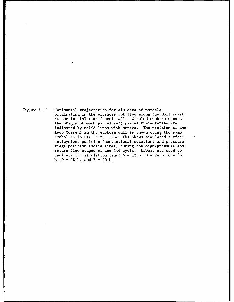
Figure 6.14 Horizontal trajectories for six sets of parcelsoriginating in the offshore PBL flow along the Gulf coastat the initial time (panel 'a'). Circled numbers denotethe origin of each parcel set; parcel trajectories areindicated by solid lines with arrows. The position of theLoop Current in the eastern Gulf is shown using the samesymbol as in Fig. 6.2. Panel (b) shows simulated surfaceanticyclone position (conventional notation) and pressureridge position (solid lines) during the high-pressure andreturn-flow stages of the lid cycle. Labels are used toindicate the simulation time: A - 12 h, B = 24 h, C = 36h, D - 48 h, and E - 60 h.
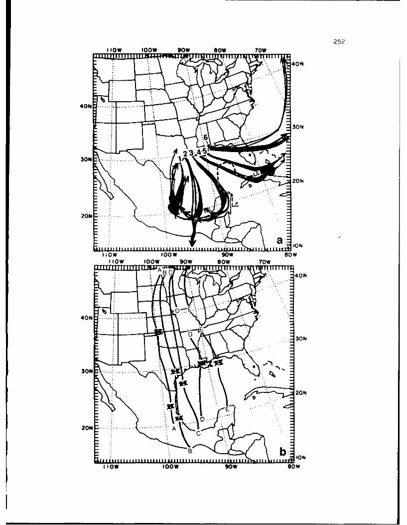
2521 low 100W 90W sow o
I10 I00 111,W J 80W II
N40N
30N
20N
ION
I low 10W Slow sow

253
the air returning into the southern Plains on 6 and 7 April. Figure
6.14b shows the temporal continuity of the model surface anticyclone and
pressure-ridge axis during the high-pressure and return-flow stages of
the cycle. Comparison of Figs. 6.14a and b reveals that the southward
movement of the surface anticyclone results in the divergence of the
parcel trajectories originating in the offshore flow along the Gulf
Coast, and a return flow layer that is restricted largely to the western
Gulf, where the SST values are generally cooler than over the eastern
Gulf (see Fig. 6.2).
The horizontal displacements for the sets of parcel trajectories
originating in the coastal moist layer at t = 36 h are shown in Fig.
6.15. An examination of the vertical displacement, 6 and q histories,
for these parcels indicates that nearly all of them experience the same
upslope motion and warming/drying that the parcel in Fig. 6.13
experiences after the 48-h point of the simulation. Thus, the evolution
of the moist layer during the high-pressure stage is mainly
characterized by modification of the continental polar airstreams over
the Gulf waters and formation of a low cloud layer along the coastal
region of Mexico through upslope motion. At the beginning of the
return-flow stage, the parcels continue the upslope journey through the
Sierra Madre Oriental range, and then turn northward and undergo a
second airmass modification (warming and drying) associated with the
journey over the eastern portion of the arid Mexican plateau region. In
the next section, we will explore the characteristics of the moist layer
that eventually resides under the lid inversion by employing backward
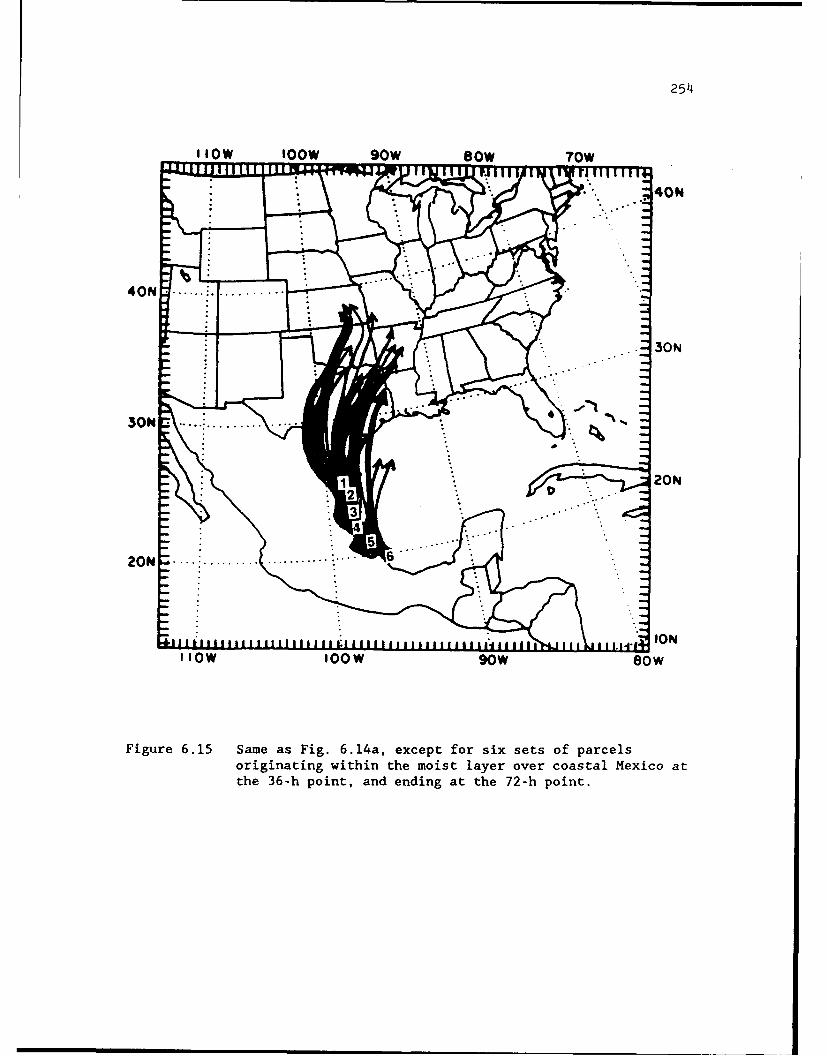
254
1 loW OOW 90W sow 70W
40N
4-N ....... "30N
3ION
30N " % 2" N
'lOW 1 WW80F r 6
2O 6liltl II I I IIIIll l liI II I 1i ltII i l i i lIi~ l t lti li OflOW oOOW 90w 80w
Figure 6.15 Same as Fig. 6.14a, except for six sets of parcels
originating within the moist layer over coastal Mexico atthe 36-h point, and ending at the 72-h point.
255
trajectories originating from a lid sounding over Texas near the time of
lid-coverage maximum.
6.4 Formation of the Lid Over the Southern Great Plains
The formation of the lid over the southern Plains during the
evening of 6 April took place as a result of the superposition of the
moist tongue from the Rio Grande valley and the EMLs from the western
U.S. and northern Mexico, which were already in place over much of
Kansas, Oklahoma, and Texas. The EML analysis for 0000 UTC 7 April is
shown in Fig. 6.16. Based on examination of the mean EML 0 values over
the southern Plains, and the parcel trajectory results of section 6.4.1,
we can conclude that the EML from the Texas-Oklahoma border and to thq
north is of western U.S. origin, while most of Texas, eastern Mexico,
and the adjacent Gulf waters has EML air originating over northern
Mexico. There is a narrow zone extending through western Kansas, west-
central Texas, and northeastern Mexico, where the presence of the moist
layer has allowed the buoyancy term to drop below 0.5°C, indicating the
presence of a lid. A comparison of the model lid area with the
observations for 0000 UTC and 1200 UTC 7 April (Figs. 5.13a,b) suggests
that the simulated lid formation is about 6 h fast.
A composite meteorological analysis for the model simulation at
0600 UTC 7 April is shown in Fig. 6.17a (the legend is in Fig. 6.17d).
This analysis shows a strong veering wind profile between 850 and 300 mb
over much of west-central Texas. However, the model lid strengths in
this area are high (> 8°C), so moist convection is unlikely in the
simulation over this area. The most favorable area for the model to
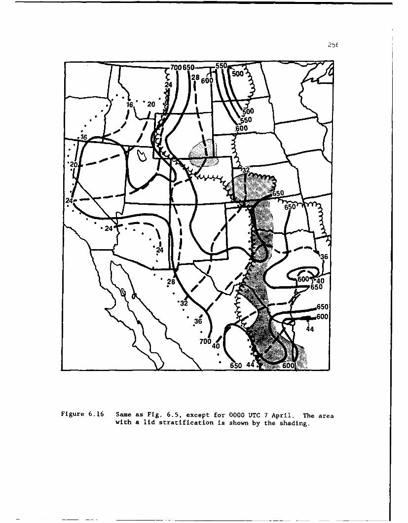
25(
•24 2860 0
16 20/
., • •.600
505
.. ... . ..o624.28 60004
• !6 -... •-;.' 650
Fiur 616 Sae s ig 65,exet or000 TC7 prl.Th3aewitha ll statifcaton i shwn b th sha6ng
257
Figure 6.17 Major surface and upper-air features in model simulationat the 66-h point (0600 UTC 7 April; panel 'a'). Symbolsare shown in the legend panel (d). Panel (b) displays themodel precipitation amounts greater than 0.3 cm for theperiods 0600-0900 UTC (solid) and 0900-1200 UTC (dashed) 7April. Panel (c) is identical to panel (b) except for1500-1800 UTC 7 April (solid) and 2100 UTC 7 April-0000UTC 8 April (dashed).
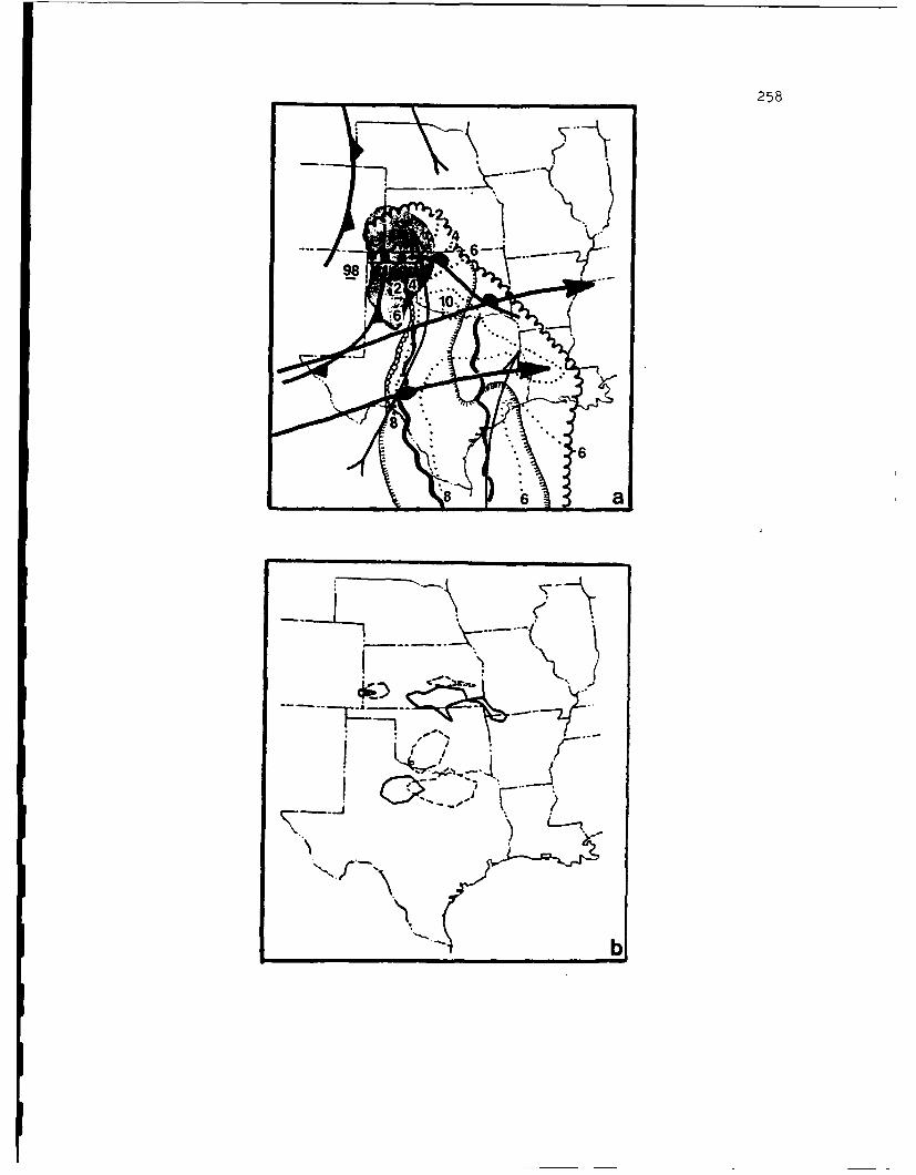
258
fal
'• i _ . - ' _. • b
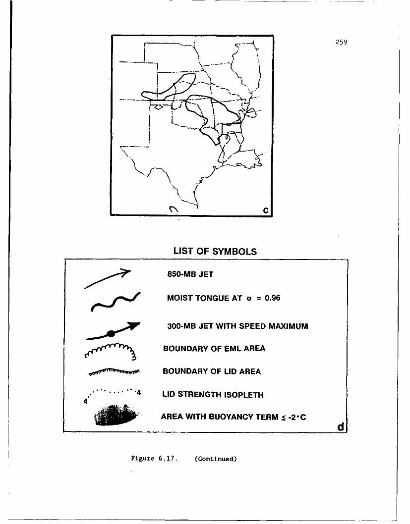
259
1 C
LIST OF SYMBOLS
850-MB JET
SMOIST TONGUE AT a = 0.96
SV300-MB JET WITH SPEED MAXIMUM
S>BOUNDARY OF EML AREA
BOUNDARY OF LID AREA
."........4 LID STRENGTH ISOPLETH4
AREA WITH BUOYANCY TERM -29d
Figure 6.17. (Continued)
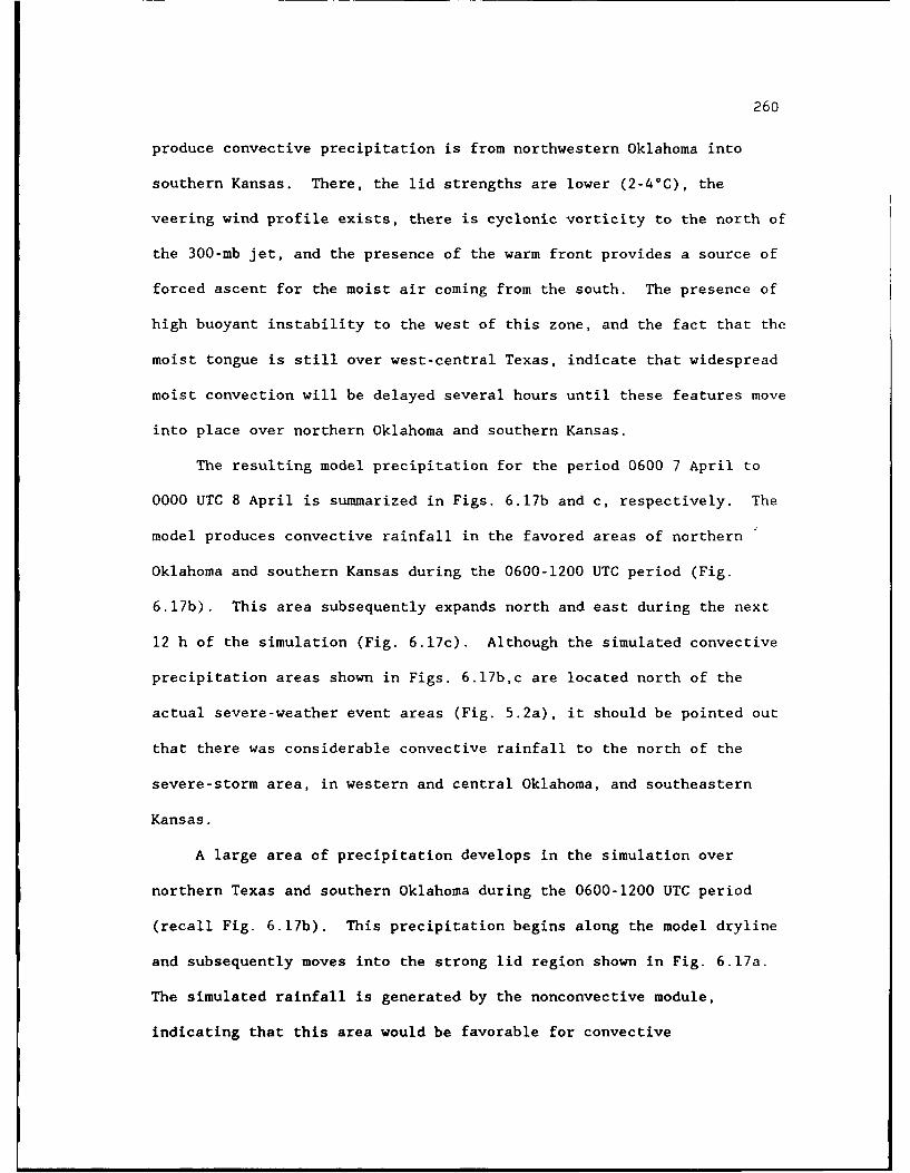
260
produce convective precipitation is from northwestern Oklahoma into
southern Kansas. There, the lid strengths are lower (2-4*C), the
veering wind profile exists, there is cyclonic vorticity to the north of
the 300-mb jet, and the presence of the warm front provides a source of
forced ascent for the moist air coming from the south. The presence of
high buoyant instability to the west of this zone, and the fact that the
moist tongue is still over west-central Texas, indicate that widespread
moist convection will be delayed several hours until these features move
into place over northern Oklahoma and southern Kansas.
The resulting model precipitation for the period 0600 7 April to
0000 UTC 8 April is summarized in Figs. 6.17b and c, respectively. The
model produces convective rainfall in the favored areas of northern
Oklahoma and southern Kansas during the 0600-1200 UTC period (Fig.
6.17b). This area subsequently expands north and east during the next
12 h of the simulation (Fig. 6.17c). Although the simulated convective
precipitation areas shown in Figs. 6.17b,c are located north of the
actual severe-weather event areas (Fig. 5.2a), it should be pointed out
that there was considerable convective rainfall to the north of the
severe-storm area, in western and central Oklahoma, and southeastern
Kansas.
A large area of precipitation develops in the simulation over
northern Texas and southern Oklahoma during the 0600-1200 UTC period
(recall Fig. 6.17b). This precipitation begins along the model dryline
and subsequently moves into the strong lid region shown in Fig. 6.17a.
The simulated rainfall is generated by the nonconvective module,
indicating that this area would be favorable for convective

261
precipitation were it not for the strong lid (recall the discussion of
the convective parameterization's stability check in section 6.2.1).
Since this nonconvective precipitation begins after 0600 UTC, we chose
to generate a set of backward trajectories originating at a 0600 UTC lid
sounding, in order to examine the characteristics of the moist layer and
EML at the time of lid-coverage maximum in the model simulation. The
sounding location is Abilene, Texas (ABI, shown in Fig. 6.19), which is
just east of the dryline, within the area of the moist tongue, and just
south of the nonconvective precipitation area that developed after 0600
UTC.
The 0600 UTC Abilene sounding is shown in Fig. 6.18. This sounding
has a lid strength of 4.9°C and a buoyancy of -1.4°C. The backward
trajectories from this sounding cover a 66-h period, and end at the
initial time of the simulation (1200 UTC 4 April). The horizontal
trajectories for this sounding are displayed in Fig. 6.19; only those
parcels existing in the EML and moist layer of the 0600 UTC Abilene
sounding are shown. The parcels existing in the moist layer at 0600 UTC
originate over the western Plains. The horizontal trajectories show
that the moist-layer parcels spend a limited time over the waters of the
northwest Gulf. The mixing ratio history for these parcels is shown in
Fig. 6.20a. The continental origin of all three parcels is evident
here. Airmass modification takes place over a 15-18 h period, which is
consistent with the time of the over-water trajectory in Fig. 6.19.
During this period, the mixing ratios of the three parcels increase by
6-9 g kg-1 . Parcels 1 and 2 experience a second period of moistening
during the day on 6 April, resulting in an additional q increase of 2-3

262
310 0 34 0 Sa 3ek 73 310 3S40 W 410O 4n 430 4U
2600
303
Ta 004042 *O~ 3 7227 ? ~ 2.42*~V
Fiue61 aeasFg4.,ecptfrsnl.sunigtm 00
UTC Aprl),at Ailee, Txas

263
150W 140W 130W 120W ''ow 100w Slow sow 70W
40OW 311111W 00
Figue 619 Sme s Fi. 67, ecep formoit-laer arces (-3)
andEM paces 6-1),oriintig a te 000UTAbilee souding

264
Figure 6.20 Same as Fig. 6.8, except for parcels originating in themoist layer and EML of the 0600 UTC Abilene sounding.Panel (a) displays a mixing ratio history for parcels 1-3,with the ordinate denoting the parcel mixing ratio in gkg-1, and the abscissa denoting simulation time (note thatthe time is read from right to left). A legend below theabscissa shows the symbols used for each parcel. Panel(b) shows the vertical displacement history for parcels1-3. Panel (c) illustrates the potential temperaturehistory for EML parcels (6-16), and panel (d) denotes thevertical displacement history for the EML parcels.
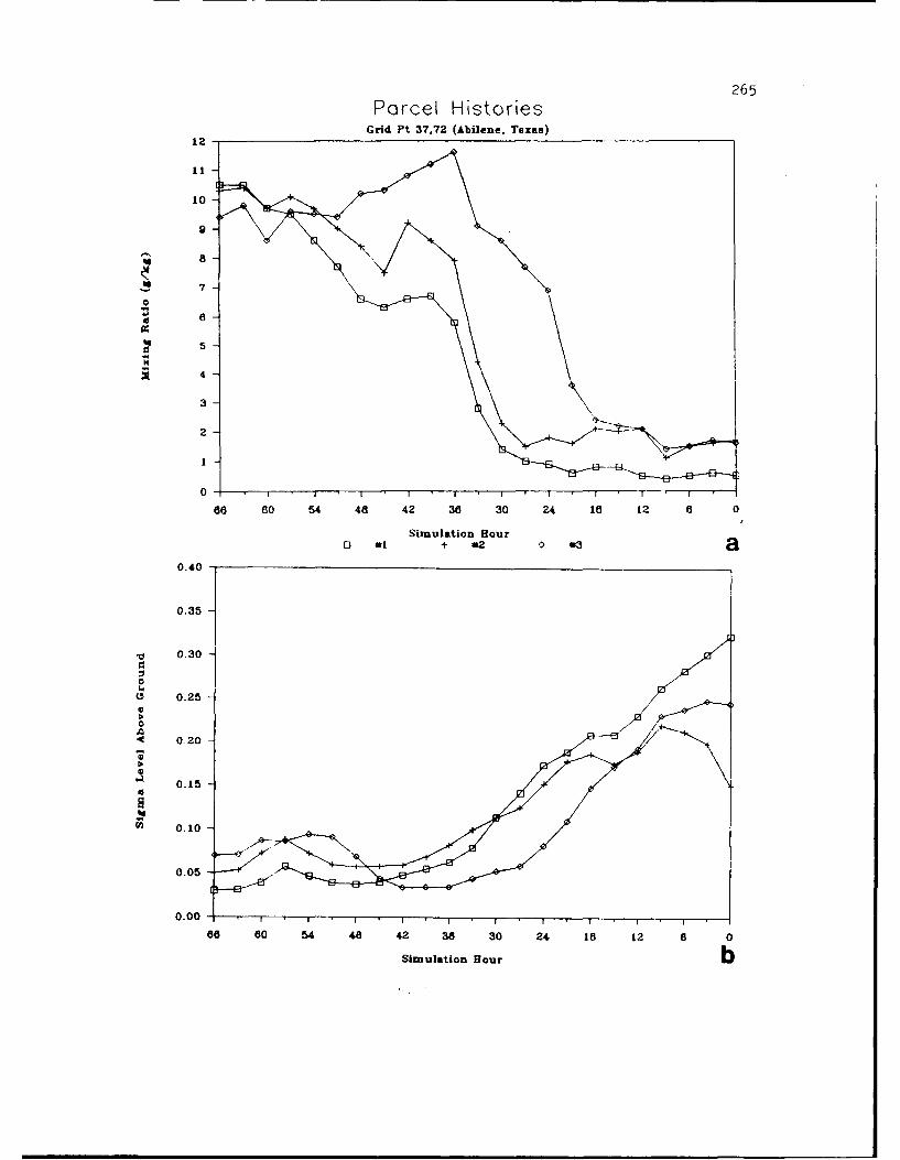
265
Parcel HistoriesGrid Pt 37,72 (Abilene, Texas)
12
11
10
9
7
' 4
3
2 II
66 60 54 48 42 36 30 24 I1 12 6 0
Simulation Hour0 at + *2 413 a
0.40
0.35
,0 0.30
0 0.25
0
4< 020
S
0 0.15
0.10
0.05 -
0.00 . ,
66 60 54 48 42 38 30 24 18 12 6 0
Simulation Hour b

Parcel Histories 266
Grid Pt 37,72 (Abilene. Texas)312 " __
311
310 -
0 309
306
307 -
308
305
8 304
•" 303
S302.• 301'_ 300
299298
297
86 60 54 48 42 36 30 24 18 12 8 0
Simulation Houro 6 + * 0 10 * .12 X 614 1
0.40
0.35
S0.30
0.2A 0.25
U 0.20
0.05
0.0 05 --- r - -, -
66 60 54 48 42 38 30 24 18 12 0
Simulation Hour d
Figure 6.20. (Continued)

267
g kg-1 . The vertical displacement history of the moist-layer parcels is
shown in Fig. 6.20b. This history explains the timing of the initial
modifications of parcels 1-3. Parcel #3 begins to undergo moistening as
it descends into the lowest 100 mb of the model atmosphere after 0900
UTC 5 April, whereas parcels I and 2 do not reach the marine PBL until
9 h later.
There is strong subsidence evident during all three parcels'
trajectories, and it is somewhat surprising to note that all three
moist-layer parcels have their origin in the continental midtroposphere
instead of the subtropical oceanic PBL. The results from this set of
moist-layer trajectories, as well as those from the preceding section,
suggest that during lid cycles in which a blocking surface anticyclone
is observed in the western Gulf, the moist airstream trajectories behave
differently than those in the classic Carlson-Ludlam lid model (see
Figs. 19 and 24 in Carlson and Ludlam 1968). In contrast to their
conceptual model in which the moist airstreams originate over the
western Caribbean and have a long trajectory over the open waters of the
Gulf, our moist airstreams originate over the continental midtroposphere
and descend into the marine PBL over the western Gulf for a limited
period. We can speculate that in situations where the track of the
surface high is located across the Mississippi River valley, there is a
greater possibility that the moist-layer trajectories follow the classic
Carlson-Ludlam model more closely, because the blocking pressure ridge
is located to the north of the Gulf.
The horizontal displacements of the EML air are shown in Fig. 6.19.
The source regions for the EML range from the Gulf of California to the
268
subtropical Pacific Ocean near 20°N latitude. All six parcel
trajectories indicate some degree of anticyclonic curvature over
northern Mexico followed by cyclonic curvature over southwest Texas as
the upper level ridge moves through northern Mexico. The ridge passage
is followed by southwesterly flow associated with the approaching trough
over the western U.S. The potential temperature and vertical
displacement histories for these parcels are shown in Figs. 6.20c,d,
respectively. Parcels 10, 14, and 16 originate in the same general
oceanic area (see Fig. 6.19) near the same level. As a result, these
parcels are isentropically homogeneous from the initial time on. These
three parcels also experience the same 1-2°C of cooling that was
observed over the Mexican EML source region during the 24-48 h period
(recall Fig. 6.11a). Since these parcels originate over a similar
subtropical ocean region as the upper parcels of the nascent Mexican EML
source region, it is likely that horizontal temperature diffusion is
also affecting them as they move away from the area of warm midlevel
air. As observed in other EML trajectories, the lower portion of the
layer is affected by diabatic heating within the model PBL. Notice from
Fig. 6.20c that parcel #8 is affected by diabatic heating from the
daytime heating cycles on both 4 and 5 April; examination of the
vertical displacement history (Fig. 6.20d) shows that parcel #8 is the
only one of the six that spends time within the local PBL on two
different days.
An interesting feature in the vertical displacement history is the
sharp descent of parcels 10-16 during the 33-48 h period. Examination
of the horizontal displacements shows that these parcels traverse the

269
crest of the Sierra Madre Occidental range during the 45-48 h period.
Recall that this period coincides with the occurrence of the mountain-
wave circulation over this area (recall Fig. 6.11b), and the evidence
suggests that these parcels are affected by the mountain wave as well.
These same parcels undergo a period of sharp ascent after the 57-h point
of the simulation (2100 UTC 6 Apr'!). Examination of the horizontal
displacements shows that all four parcels enter southwestern Texas as
this time; examination of upper level wind fields in the simulation for
this time (not shown) indicates that this region is located within a
diffluent/divergent zone between the subtropical and polar jets. The
vertical displacements during the last 9 h of this period illustrate
that the layer is undergoing vertical stretching, which further
destabilizes the EML as it moves into west-central Texas.
The EML over Abilene at 0600 UTC is a result of a combination of
different processes affecting the layer at different times during the
lid cycle. In the early stages, slowly subsiding high-potential-
temperature air originates over the subtropical oceanic region, and
subsequently passes through a mountain-wave circulation over the Sierra
Madre Occidental, which causes the layer to destabilize through
differential subsidence. The lower portion of this layer originates
near the west coast of Mexico, and is modified by diabatic surface
heating over western Mexico on 4 and 5 April. As the layer moves across
northern M.xico, it begins to vertically combine into an EML; it
subsequently approaches the diffluent region between the subtropical and
polar jets over southwestern Texas, and the layer is stretched, which
270
causes further destabilization before it finally moves over the moist
layer in west-central Texas to form a lid sounding.
271
Chapter 7
CONCLUSIONS AND DISCUSSION
7.1 Summary of Results
The focus of this research is on the generation of a representative
synoptic climatology of the lid and its component structures (i.e., the
EML and moist layer), and the establishment of the relationship of the
lid to the occurrence and nonoccurrence of severe local storms. The
approach of analyzing the lid statistics and classifying the synoptic
patterns over the southern Great Plains for the four-year study period
results in a better understanding of the independent evolution of the
EML and moist layer, and of how this evolution is affected by the
changes in the large scale circulation during the spring. The
classification scheme used in this study is unique in that it is not
just a statistical procedure used to generate a set of patterns, but is
based on a dynamical relationship (the thermal wind). That is, the
simultaneous employment of the classification method at two levels
allows us to obtain information about the thermal advection in the lower
troposphere and how it relates to the formation of the lid
stratification.
The synoptic climatology presented in Chapters rc-Juces the
following results concerning the formation and evoluti4,ti of the EML,
moist layer, and lid:
1) The appearance of the lid over the southern Great Plains has
a periodic character, and a typical lid cycle has a mean
period of about five to seven days.
272
2) There are two types of lid cycles, based on the synoptic flow
pattern that initiates the cycle:
a) The H cycle begins with a surface anticyclonic incursion
into the region, and is associated with the passage of
baroclinic waves in the westerlies.
b) The R cycle begins with an already established moist
layer within a persistent southerly flow from the Gulf
of Mexico, and is associated with subtropical
circulations and weak short wave features after the
polar jet has retreated northward.
3) The life cycle of the lid has various stages that control the
development of its component structures.
a) The high-pressure stage (observed only in the H cycle)
exists when the EML forms over the western U.S. and
cold, dry air dominates the Great Plains.
b) The return-flow stage is when the EML emerges into the
western Plains and the moist layer begins to return into
southern Texas after the surface anticyclone moves
eastward; in the late-season R cycle the moist layer
already exists over the Great Plains as there is no
polar anticyclone over the region.
c) The large lid-coverage stages prevail when the EML
begins to phase together with the moist layer, forming
the necessary stratification for a lid sounding; this
stage is further divided into pre-lid-maximum, lid-
maximum, and post-lid-maximum stages.
273
d) The end stage is when a surface front and/or upper
trough move through the Great Plains and transport the
EML out of the area by cutting off the source region; in
the early spring, a polar anticyclone follows the front
into the region and replaces the moist layer with cold,
dry air, signalling the start of a new cycle.
The synoptic climatology reveals the following facts about the
seasonal evolution of the lid environment.
1) The classic flow regime associated with the Carlson-Ludlam
lid conceptual model (i.e., a strong low level southerly flow
with southwest flow aloft), is observed most often in April
and May, during which time it accounts for a large percentage
of lid occurrences and the largest mean lid-coverage areas.
2) By midspring, the Rocky Mountains and the Great Basin of the
U.S. have become EML source regions, and increasing surface
evapotranspiration exists over the moist soil areas of the
southern Plains. The result is that the lid begins to appear
with additional flow patterns besides the classic
southwesterly type.
3) By late spring, the lid appears more often in flow patterns
associated with large scale subsidence, such as midlevel
northwesterly and anticyclonic flows. In such situations,
the lid base lowers from the source region eastward, in stark
contrast to the southwesterly flow type in which the lid base
gradually rises in an environment of large scale ascent.

274
4) The lid-coverage area expands northward during the spring,
from the southern Plains states in April into the northern
Plains by June. This northward expansion is controlled
mostly by the expansion of the EML source region as outlined
in (2). The maximum lid-frequency axis shifts westward
during the season, through the east-central portions of
Texas, Oklahoma, and Kansas in April, and from southwest
Texas into the western portions of Kansas and Nebraska by
June. This westward shift is controlled mostly by the
westward shift in the mean Ow axis and the appearance of high
Ow values along the Gulf coast, with the latter resulting in
an increased occurrence of uncapped EML soundings over th'is
area.
The synoptic climatology also examines the relationship between the
occurrence/size of the lid and the occurrence/size of severe weather
outbreaks.
1) There is a relationship between the size of a severe weather
outbreak and the area of the antecedent lid. This
relationship is best defined in April, and deteriorates
rapidly from May to June. Within the lid-coverage area, the
size of the area with buoyancy term : -2°C has the best
correlation with the size of severe weather events in all
three months.
2) In early-spring H lid cycles, the high-pressure, return-flow,
and end stages are associated with isolated severe weather
events and with non events. There is a well-defined
275
relationship between severe-weather outbreak size and
antecedent lid area during the large lid-coverage stages of
the early-season H cycle, with the peak lid/severe weather
activity appearing in the lid-maximum and post-lid-maximum
stages.
3) In late spring, both the H and R lid cycles are capable of
supporting severe weather outbreaks at all stages, and in the
H cycle, the peak severe weather/lid activity occurs during
the lid-maximum stage. In the R cycle, there is no clear
relationship between lid coverage and severe weather, as
large areas of low level moisture and buoyantly unstable air
are present throughout the cycle, and the synoptic patte1n
mainly controls the evolution of the EML.
4) In the H cycle, examination of composite mean analyses from
representative synoptic types shows that there is a fairly
clear geographic relationship between the mean location of
the antecedent lid edge and the appearance of severe weather
events. In the pre-lid-maximum stage, the events are
observed in the vicinity of and along the western and
northern lid edges. During the lid-maximum stage, events are
observed both along the lid-edge zones as well as within the
high lid-frequency regions, a result of both lid-edge
convection as well as convection associated with lid removal
in the interior.
5) In the R cycle, composite mean analyses of two frequently
occurring synoptic types show that when the Bermuda
276
anticyclone dominates the eastern half of the U.S., the
majority of severe weather events are reported in a region of
low-level cyclonic flow and weak vertical shear. A buoyant
instability gradient and localized potential instability
characterize this environment, and are influenced by the
presence of both an EML as well as a subsidence layer, the
latter originating in the western branch of the Bermuda cell.
The analyses representing the period when the Pacific
anticyclone dominates the western half of the U.S. shows that
the majority of severe weather events occur to the east of
the lid edge, in a region of buoyant instability and strong
directional shear, especially between the surface and 850'mb.
The case study examined in Chapters 5 and 6 illustrates how case-
dependent characteristics of the atmospheric structure are superimposed
on the general features defined in the synoptic climatology. Aspects of
EML genesis during the high-pressure stage were examined using a
combination of conventional data and mesoscale model output. Two EML
source regions for this case were identified over the Desert Southwest
and northern Mexico. The EML source-region analyses and model-generated
parcel trajectories reveal that it is very difficult to generalize the
EML's evolution because the composition of an individual sounding is a
result of airstream trajectories which are not always isentropic, or
homogeneous in terms of source region and potential temperature
characteristics. The nascent EML does not move in a uniform direction
as a single, homogeneous airmass. Instead, one must examine different
areas of the EML source region in order to determine the importance of
277
various dynamic and physical processes in generating and maintaining the
EML source region and elevated areas.
In this case, the presence of strong directional shear between the
low level easterlies and midlevel westerlies over northern Mexico during
the high-pressure stage results in the superposition of airstreams from
vastly different source regions with different thermal characteristics,
and causes the stabilization of this layer during the 12-24 h period of
the cycle. North of the subtropical jet, a combination of low-level
diabatic heating and layer stretching results in the "northward
transport" of a low static stability layer into Wyoming and Montana
during the same period. During the 24-48 h period, a combination of
diabatic heating in the PBL and dynamical processes allows the EML
source region over the western U.S. to continue developing, and allows
the Mexican source region to redevelop. Over northern Mexico, the
appearance of a strong southwesterly jet crossing the Sierra Madre
Occidental results in a mountain-wave circulation and lee-side low level
jet. The layer crossing this region is destabilized by this
circulation, because of differential subsidence and vertical stretching
of the layer downsteam over the northern Mexican plateau. The model
trajectories reveal that the higher 8 values in the Mexican EML source
region are a result of the downward transport of high 8 air in the
subsiding layer that originates over the subtropical oceanic region. By
the time this EML reaches Texas and forms a lid over the moist layer, it
is undergoing further destabilization from layer stretching associated
with strong upward motion occurring within the upper diffluent/divergent
zone between the subtropical and polar jets over Texas.
278
Perhaps the most interesting result from the case study is that
regarding the creation and evolution of the moist layer. Use of
conventional analyses, satellite imagery, and model output reveals that
the moist layer originates as a continental airstream in the offshore
flow at the beginning of the cycle and undergoes modificaiton over the
western Gulf waters during the first 24 h of the cycle. The low cloud
layer observed along coastal Mexico in the high-pressure and return-flow
stages results from upslope motion of the moist-layer airstreams
approaching the coastal area. Vertical motion plays an important role
in the moist layer's evolution, since the airstreams spend only a
limited time in the marine PBL environment before rising above it and
undergoing warming and drying as they travel northward along the eastern
edge of the Mexican plateau. In the lid-maximum stage, the parcel
trajectories show that the moist layer beneath the lid inversion
originates in the continental midtroposphere before descending into the
inarine PBL over the western Gulf. Our results show that the southward
movement of the surface anticyclone into the western Gulf (which is a
commonly occurring feature according to the synoptic climatology)
results in moist-layer trajectories that are vastly different from the
Carlson-Ludlam conceptual model, in that they spend a limited time in
the marine environment and are restricted to the western Gulf waters.
Another important result from the model simulation of the 4-9 April
case is that the use of a large domain with relatively fine horizontal
and vertical grid meshes, reduced horizontal and vertical diffusion
coefficients, and carefully determined surface conditions (i.e., snow
cover, SST, and soil moisture), allows for successfully creating and

279
maintaining the component structures of the lid environment, and
reproducing the detailed vertical and horizontal structures observed
over the southern Plains during the large lid-coverage stages. Equally
important in such a simulation are th- latt- 1 boundary conditions,
which make this simulation much like a operational forecast because the
model boundaries are located in data-sparse regions where the analyses
are largely determined by the operational model prediction.
7.2 Suggestions for Future Research
The synoptic climatology described in this study raises some
important issues for future research on the lid/severe-storm
environment. One issue that is potentially very important is the
interannual variability in the occurrence of different types of synoptic
patterns (e.g., the H and R lid cycles), and the onset of semipermanent
circulation features (i.e., Bermuda and Pacific anticyclones) that
delinate the early and late season lid cycles. A related question
involves the effect of year-to-year changes in the mean positions and
intensities of large scale troughs and ridges on the occurrence of the
lid and severe weather. Regarding the sensitivity of the lid-cycle
evolution to large scale surface conditions such as snow cover, soil
moisture gradients, and SST conditions over the Gulf of Mexico, there is
a need to examine the evolution of the lid cycle in "anomalous" years.
Such anomalous years may include greater or less than normal snow cover
over the Rockies, soil moisture anomalies (Lanicci et al. 1987), and SST
anomalies over the Gulf and other oceanic areas. Such situations would
be useful subjects for modeling sensitivity studies.
280
In the terms of the synoptic climatology, an interesting area for
further study involves the transition period between the early-spring
and late-spring lid regimes. Within this context, lid cycles could be
further subdivided on the basis of the flow type that ends the cycle.
Such a subdivision would reveal new information about the appearance of
subtropical circulations within or at the end of H cycles, or polar-air
outbreaks occurring at the end of R cycles. Along these same lines,
analysis of longer wave influences on the lid cycle would also be of
interest. Such longer waves could potentially be linked to circulation
features with seasonal time scales, and may reveal the reasons why
certain flow types, such as southwesterly, have a greater tendency to
have a multi-day persistence than other types. I
The case study discussed in Chapters 5 and 6 also suggests some
interesting areas for additional study. The 4-9 April 1984 case
illustrates how case-dependent characteristics of the atmospheric
structure are superimposed on the general features of the early-season H
cycle. It seems reasonable that examples of the late-season H and R
cycles would yield similar results for those cycles. Especially in the
case of the R cycle, a complementary modeling study would be useful in
order to properly evaluate the roles that surface diabatic processes
have in the creation of the late-season EML and persistent moist layer
over the Great Plains. The selection of certain model parameterizations
and development of adequate surface boundary conditions would likely be
more difficult and challenging for a late-spring case than for an early-
spring example.
281
REFERENCES
Anthes, R.A., 1977: A cumulus parameterization scheme utilizing a one-dimensional cloud model. Mon. Wea. Rev., 105, 270-286.
Anthes R.A., and T.T. Warner, 1978: The development of mesoscale modelssuitable for air pollution and other mesometeorological studies.Mon. Wea. Rev., 106, 1045-1078.
Anthes, R.A., Y.-H. Kuo, S.G. Benjamin, and Y.-F. Li, 1982: Theevolution of the mesoscale environment of severe local storms:Preliminary modeling results. Mon. Wea. Rev., 110, 1187-1213.
Anthes, R.A., E.-Y. Hsie, and Y.-H. Kuo, 1987: Description of the PennState/NCAR Mesoscale Model Version 4 (MM4). NCAR/TN-282+STR,National Center for Atmospheric Research, Boulder CO, 66 pp.
Arakawa, A., and V.R. Lamb, 1977: Computational design of the basicdynamical process of the UCLA general circulation model. Methods inComputational Physics, 17, Academic Press, 173-265.
Arritt, R.W., and G.S. Young, 1990: Elevated stable layers generated bymesoscale boundary-layer dynamics over complex terrain. Preprints,Fifth Conference on Mountain Meteorology, June 25-29, 1990, BoulderGO, Amer. Meteor. Soc., 114-117.
Augustine, J.A., E.I. Tollerud, and B.D. Jamison, 1989: Distributionsand other general characteristics of mesoscale convective systemsduring 1986 as determined from GOES infrared imagery. Preprints,12th Conference on Weather Analysis and Forecasting, October 2-6,1989, Monterey CA, Amer. Meteor. Soc., 437-442.
Bartels, D.L., J.M. Skradski, and R.D. Menard, 1984: MesoscaleConvective Systems: A Satellite-Data-Based Climatology. NOAA Tech.Memo. ERL ESG-8, Boulder CO, 58 pp. Available from the NationalTechnical Information Service, Springfield VA 22161 as PB85-187862.
Beebe, R.G., 1956: Tornado composite charts. Mon. Wea. Rev., 84, 127-142.
Beebe, R.G., 1958: Tornado proximity soundings. Bull. Amer. Meteor.Soc., 39, 195-201.
Benjamin, S.G.. 1983: Some Effects of Surface Heating and Topography onthe Regional Severe Storm Environment. Ph.D. Thesis, Department ofMeteorology, The Pennsylvania State University, University Park PA16802, 265pp.

282
Benjamin, S.G., 1986: Some effects of surface heating and topography onthe regional severe-storm environment. Part II: Two-dimensionalidealized experiments. Ion. Wea. Rev., 114, 330-343.
Benjamin, S.G., and T.N. Carlson, 1986: Some effects of surface heatingand topography on the regional severe-storm environment. Part I:Three-dimensiona simulation. Mon. Wea. Rev., 114, 307-329.
Benjamin, S.G., and N.L. Seaman, 1985: A simple scheme for objectiveanalysis in curved flow. Mon. Wea. Rev., 113. !!8k-1198.
Blackadar, A.K., 1976: Modeling the nocturnal boundary layer.Preprints, Third Symposium on Atmospheric Turbulence, Diffusion andAir Quality, October 19-22, 1976, Raleigh NC, Amer. Meteor. Soc.,46-49.
BlackV.dar, A.K., 1979: High resolution models of the planetary boundarylayer. Advances in Environmental Science and Engineering, 1, No. 1,Pfafflin and Ziegler, Eds., Gordon and Breach Sci. Pub., New YorkNY, 50-85.
Brownlee, K.A., 1965: Statistical Theory and Methodology in Science andEngineering, 2nd Ed. Wiley and Sons, Inc., New York NY, pp. 413-414.
Bryson, R.A., and W.P. Lowry, 1955: Synoptic climatology of the Arizonasummer precipitation singularity. Bull. Amer. Meteor. Soc., 36,329-339.
Bryson, R.A., and F.K. Hare, 1974: The climates of North America. InWorld Survey of Climatology. Vol. 11: Climates of North America,H.E. Landsberg, Ed. Elsevier Scientific, 1-47.
Caracena, F., and J.M. Fritsch, 1983: Focusing mechanisms in the TexasHill Country flash floods of 1978. Mon. Wea. Rev., 111, 2319-2332.
Carleton, A.M., 1985: Synoptic and satellite aspects of the SouthwesternU.S. summer 'monsoon.' J. Climatology, 5, 389-402.
Carleton, A.M., 1986: Synoptic-dynamic character of "bursts" and"breaks" in the Southwestern U.S. summer precipitation singularity.J. Climatology, 6, 605-623.
Carleton, A.M., 1987: Summer circulation climate of the AmericanSouthwest. Ann. Assoc. Amer. Geog., 77, 619-634.
Carlson, T.N., R.A. Anthes, M.N. Schwartz, S.G. Benjamin, and D.G.Baldwin, 1980: Analysis and prediction of severe stormsenvironment. Bull. Amer. Soc., 61, 1032.
283
Carlson, T.N., S.G. Benjamin, G.S. Forbes, and Y.-F. Li, 1983: Elevatedmixed layers in the severe storm environment-Conceptual model andcase studies. Mon. Wea. Rev., 111, 1453-1473.
Carlson, T.N., and F.H. Ludlam, 1968: Conditions for the formation ofsevere local storms. Tellus, 20, 203-226.
Carlson, T.N., and J.M. Prospero, 1972: The large scale movement ofSaharan air outbreaks over the North equatorial Atlantic. J. Appi.Meteor., 11, 283-297.
Cressman, G.P., 1959: An operative objective -.lysis scheme. Mon. Wea.Rev., 87, 367-374.
Cunning, J.B., 1986: The Oklahoma-Kansas preliminary regional experimentfor STORM-Central. Bull. Amer. Meteor. Soc., 67, 1478-1486.
Darkow, G.L., 1969: An analysis of over sixty tornado proximitysoundings. Preprints, Sixth Conference oni Severe Local Storms,April 8-10, 1969, Chicago IL, Amer. Meteor. Soc., 218-221.
Darkow, G.L., and M.G 7owler, 1971: Tornado proximity sounding windanalysis. Preprints, Seventh Conference on Severe Local Storms,October 5-7, 1971, Kansas City MO, Amer. Meteor. Soc., 149-151.
David, C.L., 1976: A study of upper air parameters at the time oftornadoes. Mon. Wea. Rev., 104, 546-551.
Davies, H.C., and R.E. Turner, 1977: Updating prediction models bydynamical relaxation: An examination of the technique. Quart. J.Roy. Meteor. Soc., 103, 225-245.
Davies, J.M., 1989: On the use of shear magnitudes and hodographs intornado forecasting. Preprints, 12th Conference on Weather Analysisand Forecasting, October 2-6, 1989, Monterey CA, Amer. Meteor. Soc.,219-224.
DiMego, G.J., L.F. Bosart, and G.W. Endersen, 1976: An examination ofthe frequ'ency and mean conditions surrounding frontal incursionsinto the Gulf of Mexico and Caribbean Sea. Mon. Wea. Rev., 104,709-718.
Djuric, D., and D.S. Ladwig, 1983: Southerly low-level jet in the wintercyclones of the southwestern Great Plains. Mon. Wea. Rev., 111,2275-2281.
Doswell, C.A. III, 1987: The distinction between large-scale andmesoscale contribution to severe convection: A case study example.Wea. Forecasting, 2, 3-16.
284
Doswell, C.A. III, 1990: Comments on "A Winter Mesocyclone over theMidwestern United States". Wea. Forecasting, 5, 162-165.
Doswell, C.A., III, F. Caracena, and M. Magnano, 1985: Temporalevolution of 700-500 mb lapse rate as a forecasting tool--- A casestudy. Preprints, 14th Conference on Severe Local Storms, October29-November 1, 1985, Indianapolis IN, Amer. Meteor. Soc., 398-401.
Farrell, R.J., 1988: The Role of a Lid in the 31 May 1985 TornadoOutbreak. M.S. Thesis, The Pennsylvania State University,University Park PA 16802, 158 pp.
Farrell, R.J., and T.N. Carlson, 1989: Evidence for the role of the lidand underrunning in an outbreak of tornadic thunderstorms. Mon. Wea.Rev., 117, 857-871.
Fawbush, E.J., R.C. Miller, and L.G. Starrett, 1951: An empirical methodof forecasting tornado development. Bull. Amer. Meteor. Soc., 32,1-9.
Fawbush, E.J., and R.C. Miller, 1952: A mean sounding representative ofthe tornadic airmass environment. Bull. Amer. Meteor. Soc., 33,303-307.
Fawbush, E.J., and R.C. Miller, 1954: The types of airmasses in wi LchNorth American tornadoes form. Bull. Amer. Meteor. Soc., 35, 154-165.
Fawbush, E.J., P.C. Miller, and L.G. Starrett, 1957: Severe local stormsand mid-tropospheric flow patterns. Bull. Amer. Meteor. Soc., 38,115-123.
Ferrel, W., 1885: Recent Advances in Meteorology. Report of the ChiefSignal Officer for 1885, Appendix 71, 324-325, 327.
Finley, J.P., 1890: Tornadoes. Amer. Meteor, J., 7, 165-179.
Galway, J.G., 1956: The lifted index as a prediction of latentinstability. Bull. Amer. Meteor. Soc., 37, 528-529.
Galway, J.C., 1977: Some climatological aspects of tornado outbreaks.Mon. Wea. Rev., 105, 477-484.
Giordano, L.A., 1987: Northwest Flow Aloft and Strong Convective EventsWithin the Mid-Atlantic States. M.S. Thesis, The Pennsylvania StateUniversity, University Park PA 16802, 75 pp.
Gutnick, M., 1958: Climatology of the trade-wind inversion in theCaribbean. Bull. Amer. Meteor. Soc., 39, 410-420.
285
Graziano, T.M., and T.N. Carlson, 1987: A statistical evaluation of lidstrength on deep convection. Wea. Forecasting, 2, 127-139.
Hagemeyer, B.C., and G.L. Darkow, 1988: Tropical easterlies as a sourceof extreme potential convective instability for mid-latitude severestorm generation. Preprints, 15th Conference on Severe LocalStorms, February 22-26, 1988, Baltimore MD, Amer. Meteor. Soc.,263-266.
Henry, W.K., 1979: Some aspects of the fate of cold fronts in the Gulfof Mexico. Mon. Wea. Rev., 107, 1078-1082.
Henry, W.K., and A.H. Thompson, 1976: An example of polar airmodification over the Gulf of Mexico. Mon. Wea. Rev., 104, 1324-1327.
Humphreys, W.J., 1926: The tornado. Mon. Wea. Rev., 54, 501-503.
Johns, R.H., 1982: A synoptic climatology of Northwest flow severeweather outbreaks. Part I: Nature and significance. Mon. Wea.Rev., 110, 1653-1663.
Johns, R.H., 1984: A synoptic climatology of Northwest flow severeweather outbreaks. Part II: Meteorological parameters and synopticpatterns. Mon. Wea. Rev., 112, 449-464.
Johns, R.H., and W.R. Sammler, 1989: A preliminary synoptic climatologyof violent tornado outbreaks utilizing radiosonde standard leveldata. Preprints, 12th Conference on Weather Analysis andForecasting, October 2-6, 1989, Monterey CA, Amer. Meteor. Soc.,196-201.
Johnson, J.R., 1976: The Origin, Structure, and Modification of ReturnFlow over the Gulf of Mexico. M.S. Thesis, Dept. of Meteorology,Texas A&M University, College Station TX 77843, 69 pp.
Karayampudi, V.M., 1986: A Numerical Study of the Evolution Structure,and Energetics of the Saharan Air Layer. Ph.D. Dissertation, ThePennsylvania State University, University Park PA 16802, 287 pp.
Karyampudi, V.M., and T.N. Carlson, 1988: Analysis and numericalsimulation of the Saharan air layer and its effect on easterly wavedisturbances. J. Atmos. Sci., 45, 3102-3136.
Karnavas, G.R., 1978: On Polar Air Modification Over the Gulf of MexicoDuring Periods of Return Flow and Development of Low Clouds. M.S.Thesis, Department of Meteorology, Texas A&M University, CollegeStation TX 77843, 69 pp.

286
Kelly, D.L., J.T. Schaefer, R.P. McNulty, C.A. Doswell III, and R.F.Abbey Jr., 1978: An augmented tornado climatology. Mon. Wea. Rev.,106, 1172-1183.
Kelly, D.L., J.T. Schaefer, and C.A. Doswell III, 1985: Climatology ofnontornadic severe thunderstorm events in the United States. Mon.Wea. Rev., 113, 1997-2014.
Keyser, D., and T.N. Carlson, 1984: Transverse ageostrophic circulationsassociated with elevated mixed layers. Mon. Wea. Rev., 112,2465-2478.
Kuo, H.L., 1974: Further studies of the parameterization of theinfluence of cumulus convection on large-scale flow. J. Atmos.Sci., 31, 1232-1240.
Lakhtakia, M.N., and T.T. Warner, 1987: A real-data numerical study ofthe development of precipitation along the edge of an elevated mixedlayer. Mon. Wea. Rev., 115, 156-168.
Lanicci, J.M., 1984: The Influence of the Soil Moisture Distribution onthe Severe-Storm Environment of the Southern Great Plains: ANumerical Study of the SESAME IV Case. M.S. Thesis, Department ofMeteorology, The Pennsylvania State University, University Park PA16802, 237 pp.
Lanicci, J.M., T.N. Carlson, and T.T. Warner, 1987: Sensitivity of theGreat Plains severe-storm environment to soil-moisture distribution.Mon. Wea. Rev., 115, 2660-2673.
Lanicci, J.M., and T.T. Warner, 1991a: A synoptic climatology of theelevated mixed-layer inversion over the southern Great Plains inSpring. Part 1: Structure, dynamics, and seasonal evolution.Accepted in Wea. Forecasting.
Lanicci, J.M., and T.T. Warner, 1991b: A synoptic climatology of theelevated mixed-layer inversion over the southern Great Plains inSpring. Part 2: The life cycie of the lid. Accepted in Wea.Forecasting.
Lanicci, J.M., and T.T. Warner, 1991c: A synoptic climatology of theelevated mixed layer inversion over the southern Great Plains inSpring. Part 3: Relationship to severe-storms climatology.Accepted in Wea. Forecasting.
Lewis, J., and C. Crisp, 1989: Climatology of return flow in the Gulf ofMexico. Preprints, 12th Conference on Weather Analysis andForecasting, October 2-6, 1989, Monterey CA, Amer. Meteor. Soc.,490-493.
287
Lewis, J.M., C.M. Hayden, R.T. Merrill, and J.M. Schneider, 1989:GUFMEX: A study of return flow in the Gulf of Mexico. Bull. Amer.Meteor. Soc., 70, 24-29.
Livingston, R.L., and L.F. Wilson, 1986: Relating antecedent surfaceconditions to violent tornado-producing thunderstorms. Preprints,11th conference on Weather Analysis and Forecasting, June 17-20,1986, Kansas City MO, Amer. Meteor. Soc., 229-234.
Lloyd, J.R., 1942: The development and trajectory of tornadoes. Mon.Wea. Rev., 70, 65-75.
Maddox, R.A., 1976: An evaluation of tornado proximity wind andstability data. Mon. Wea. Rev., 104, 133-142.
Maddox, R.A., 1983: Large-scale meteorological conditions associatedwith midlatitude, mesoscale convective complexes. Mon. Wea. Rev.,111, 1475-1493.
Maddox, R.A., and C.A. Doswell III, 1982a: An examination of jet streamconfigurations, 500mb vorticity advection and low-level thermaladvection patterns during extended periods of intense convection:.Mon. Wea. Rev., 110, 184-197.
Maddox, R.A., and C.A. Doswell III, 1982b: Forecasting severethunderstorms: A brief consideration of some accepted techniques.Nat. Wea. Dig., 110, 26-30.
Mahrt, L., 1976: Mixed layer moisture structure. Mon. Wea. Rev., 104,1403-1407.
McNulty, R.P., 1978: On upper tropospheric kinematics and severe weatheroccurrence. Mon. Wea. Rev., 106, 662-672.
McNulty, R.P., 1980: Differential advection of wet-bulb potentialtemperature and convective development: An evaluation. Preprints,Eighth Conference on Weather Analysis and Forecasting, June 10-13,1980, Denver CO, Amer. Meteor. Soc., 286-291.
Means, L.L., 1952: On thunderstorm forecasting in the central UnitedStates. Mon. Wea. Rev., 80, 165-189.
Miller, R.C., 1959: Tornado-producing synoptic patterns. Bull. Amer.Meteor. Soc., 40, 465-472.
Miller, R.C., 1972: Notes on Analysis and Severe-Storm ForecastingProcedures of the Air Force Global Weather Central. Air WeatherService Tech. Rep. 200 Rev. (AWSTR-200), HQ Air Weather Service,Scott AFB IL.
288
Molinari, R.L., 1987: Air mass modification over the eastern Gulf ofMexico as a function of surface wind fields and the Loop Currentposition. Mon. Wea. Rev., 115, 646-652.
Moller, A.R., 1979: The Climatology and Synoptic Meteorology of SouthernPlains Tornado Outbreaks. M.S. Thesis, University of Oklahoma,Norman OK, 70 pp.
Notis, C., and J.L. Stanford, 1973: The contrasting synoptic andphysical character of northeast and southeast advancing tornadoes inIowa. J. App1. Meteor., 12, 1163-1173.
Orlanski, I., 1975: A rational subdivision of scales for atmosphericprocesses. Bull. Amer. Meteor., 56, 527-530.
Parker, S.S., J.T. Hawes, S.J. Colucci, and B.P. Hayden, 1989:Climatology of 500-mb cyclones and anticyclones, 1950-85. Mon. Wea.Rev., 117, 558-570.
Reed, T.R., 1933: The North American high-level anticyclone. Mon. Wea.Rev., 61, 321-325.
Reed, T.R., 1937: Further observations of the North American high-levelanticyclone. Mon. Wea. Rev., 65, 364-366.
Rhea, J.O., 1966: A study of thunderstorm formation along dry lines. J.App1. Meteor., 5, 58-63.
Riehl, H., 1945: Subtropical Flow Patterns in Summer. MiscellaneousReports No. 22, Department of Meteorology, University of Chicago,Chicago IL.
Rockwood, A.A. and R. A. Maddox, 1988: Mesoscale and synoptic scaleinteractions leading to intense convection: The case of 7 June 1982.Wea. Forecasting, 3, 51-68.
Sanders, F., 1988: A climatology of intense convective systems.Preprints, 15th Conference on Severe Local Storms, February 22-26,1988, Baltimore MD, Amer. Meteor. Soc., 520-522.
Schaefer, J.T., 1973: The Motion and Morphology of the Dryline. NOAATech. Memo. ERL NSSL-66, U.S. Dept. of Commerce (NOAA), NationalSevere Storms Laboratory, Norman OK 73069, 81pp.
Schaefer, J.T., 1974: The life cycle of the dryline. J. AppI. Meteor.,13, 444-449.
Schaefer, J.T., 1983: On the synoptic differentiation between tornadooutbreak types. Preprints, 13th Conference on Severe Local Storms,October 17-20, 1983, Tulsa OK, Amer. Meteor. Soc. 142-145.
289
Schaefer, J.T., 1986: The dryline. Mesoscale Meteorology andForecasting, P.S. Ray, Ed., American Meteorological Society, BostonMA, 549-572.
Schaefer, J.T., and C.A. Doswell III, 1984: Empirical orthogonalfunction expansion applied to progressive tornado outbreaks.J.Meteor. Soc. Japan, 62, 929-936.
Schaefer, J.T., and J.G. Galway, 1982: Population biases in the tornadoclimatology. Preprints, 12th Conference on Severe Local Storms,January 12-15, 1982, San Antonio TX, Amer. Meteor. Soc., 51-54.
Schaefer, J.T., and R.L. Livingston, 1988: The structuralcharacteristics of tornado proximity soundings. Preprints, 15thConference on Severe Local Storms, February 22-26, 1988, BaltimoreMD, Amer. Meteor. Soc., 537-540.
Seaman, N.L., J.S. Chang, D.R. Stauffer, and P. Middleton, 1991: Four-dimensional data assimilation used in a meteorological model forregional acid deposition studies. Submitted to J. Appl. Meteor.
Showalter, A.K., and J.R. Fulks, 1943: A Preliminary Report onTornadoes: The Tornado, an Analysis of Antecedent MeteorologicalýConditions. U.S. Weather Bureau, Washington DC, 162pp. Reprintedby U.S. Office of Naval Operations as NAVAER 50-lR-41, 1950.
Smagorinsky, J., S. Manabe, and J.L. Holloway, Jr., 1965: Numericalresults from a nine-level general circulation model of theatmosphere. Mon. Wea. Rev., 93, 727-768.
Tang, M., and E.R. Reiter, 1984: Plateau monsoons of the NorthernHemisphere: A comparison between North America and Tibet. Mon.Wea. Rev., 112, 617-637.
Tilley, J.S., 1990: On the Application of Edge Wave Theory to Terrain-Bounded Cold Surges: A Numerical Study. Ph.D. Dissertation,Department of Meteorology, Pennsylvania State University, UniversityPark PA 16802, 353 pp.
Tollerud, E.I., and D.L. Bartels, 1988: A comparative study of theenvironment of severe-weather-producing mesoscale convectivesystems: MCCs, meso-beta systems, and large convective lines.Preprints, 15th Conference on Severe Local Storms, February 22-26,1988, Baltimore MD, Amer. Meteor. Soc., 544-547.
Uccellini, L. W., 1980: On the role of upper tropospheric jet streaksand leeside cyclogenesis in the development of low-level jets in theGreat Plains. Mon. Wea. Rev., 108, 1689-1696.
290
Uccellini, L.W., and D.R. Johnson, 1979: The coupling of upper and lowertropospheric jet streaks and implications for the development ofsevere convective storms. Mon. Wea. Rev., 107, 682-703.
Varney, B.M., 1926: Aerological evidence as to the causes of tornadoes.Mon. Wea. Rev., 54, 163-165.
Velasco, I., and J.M. Fritsch, 1987: Mesoscale convective complexes inthe Americas. J. Geophys. Res., 92, No. D8, 9591-9613.
Wade, G.S., C.M. Hayden, J.M. Lewis, and R.T. Merrill, 1988:Modification of air masses over the Gulf of Mexico - Progress reportfrom a VAS viewpoint. Preprints, 15th Conference on Severe LocalStorms, February 22-26, 1988, Baltimore MD, Amer. Meteor. Soc., 484-487.
Washington, W.M., and D. P. Baumhefner, 1975: A method of removing Lambwaves from initial data for primitive equation models. J. Appl.Meteor., 14, 114-119.
Weiss, S.J., 1989: An examination of NMC numerical model forecasts ofsurface (MSL) pressure preceding three cool season severe stormoutbreaks. Preprints, 12th Conference on Weather Analysis andForecasting, October 2-6, 1989, Monterey CA, Amer. Meteor. Soc.,606-611.
Wexler, H., and J. Namias, 1938: Mean monthly isentropic charts andtheir relation to departures of summer rainfall. Trans. Amer.Geophys. Union, 19, 164-170.
Whitney, L.F., 1977: Relationship of the subtropical jet stream tosevere local storms. Mon. Wea. Rev., 105, 398-412.
Wiesnet, D.R., C.F. Ropelewski, G.J. Kukla, and D.A. Robinson, 1987: Adiscussion of the accuracy of NOAA satellite-derived global seasonalsnow cover measurements. Large Scale Effects of Seasonal Snow Cover(Proceedings of the Vancouver Symposium, August 1987), IAHS Publ.NO. 166, 291-304.
Willis, T.G., 1969: Characteristics of the tornado environment as deducedfrom proximity soundings. Preprints, Sixth Conference on SevereLocal Storms, April 8-10, 1969, Chicago IL, Amer. Meteor. Soc., 222-229.
Williams, R.J., 1976: Surface parameters associated with tornadoes.Mon. Wea. Rev., 104, 540-545.
Zhang, D.-L, and R.A. Anthes, 1982: A high-resolution model of theplanetary boundary layer - Sensitivity tests and comparisons withSESAME-79 data. J. Appi. Meteor., 21, 1594-1609.
VITA
John M. Lanicci was born in the Bronx, New York, on January 18,
1957. He graduated in 1975 from Clarkstown North High School in New
City, New York. He attended Manhattan College, Bronx, New York, on a
four-year Air Force ROTC scholarship, graduated summa cum laude with a
Bachelor of Science degree in Physics in 1979, and was commissioned as
an officer in the U.S. Air Force. Under Air Force sponsorship, he
received a Bachelor of Science degree with highest distinction in
Meteorology from Penn State in 1980, and a Master of Science degree in
Meteorology from Penn State in 1984.
John Lanicci's military decorations include the Air Force
Meritorious Service Medal with oak leaf cluster, the Air Force
Commendation Medal, the Air Force Achievement Medal, and the National
Defense Service Medal. He is a member of the American Meteorological
Society, the National Weather Association, and a half-dozen honorary
societies. His research interests over the last 10 years have been
concentrated in numerical weather prediction, severe local storms, wind
flow over complex terrain, and applied climatology. His professional
publications include four Air Force technical reports, and papers in
Monthly Weather Review and Weather and Forecasting.
John Lanicci is married to the former Kathleen Benson of South
Nyack, New York. They have two sons, Michael, 9 and Mark, 5.