Seediscussions,stats,andauthorprofilesforthispublicationat:https://www.researchgate.net/publication/226903359

ASpectrum-IndependentProcedureforCorrectingEddyFluxesMeasuredwithSeparatedSensors

ARTICLEinBOUNDARY-LAYERMETEOROLOGY·NOVEMBER1998

ImpactFactor:2.47·DOI:10.1023/A:1001759903058

CITATIONS

31

READS

15

2AUTHORS:

JohannesLaubach

LandcareResearch

33PUBLICATIONS498CITATIONS

SEEPROFILE

K.G.Mcnaughton

TheUniversityofEdinburgh

61PUBLICATIONS3,496CITATIONS

SEEPROFILE

Availablefrom:K.G.Mcnaughton

Retrievedon:03February2016

A SPECTRUM-INDEPENDENT PROCEDURE FOR CORRECTINGEDDY FLUXES MEASURED WITH SEPARATED SENSORS

JOHANNES LAUBACH1 and KEITH G. McNAUGHTON2

1Horticulture and Food Research Institute of New Zealand, P.O. Box 23, Kerikeri 0470, NewZealand E-mail: jlaubach@hort.cri.nz;2Paretu Drive, R.D1, Kerikeri 0470, New Zealand

(Received in final form 2 July 1998)

Abstract. We investigate flux underestimates in eddy correlation measurements that are caused byhorizontal separation of the sensors. A common eddy correlation setup consists of a sonic anemome-ter and a humidity sensor which, because of its bulk, must be placed some distance away from thesonic path, leading to a flux loss (of latent heat). Utilizing an additional fast temperature sensorplaced near the humidity sensor, we develop a procedure for correcting for this loss. The proceduresimultaneously corrects the sensible heat flux for the difference between true temperature and sonictemperature. Our correction procedure, which does not depend on the shape of the cospectrum, isthen compared to the widely-used procedure following Moore (1986), which assumes a cospectralmodel (‘Kansas Model’). Both correction methods are applied to data collected within the internalboundary layer over a rice paddy, downwind of arid land. Under conditions of good fetch, they werefound to agree well. Under poor fetch conditions, the model-based correction tended to be too small,while the spectrum-independent combined correction was robust. The latter is thus recommended forsituations where the cospectral shape can be expected to deviate from the ‘Kansas’ shape.

Keywords: Advection, Cospectral model, Eddy correlation, Sensor separation, Surface fluxes.

1. Introduction

Eddy correlation is a popular technique for measuring the turbulent fluxes of massand energy in the atmospheric boundary layer. It relies on the basic definition of aflux: the flux density of a scalar variable is velocity times the concentration of thescalar. In a turbulent flow field, both these factors fluctuate over several decadesof frequency, but only fluctuations that are mutually correlated contribute to theflux. In order to determine accurate temporal averages of the flux, both factorshave to be measured fast enough to capture these correlated fluctuations. Howevermeasurement systems invariably suffer, to some degree, from technical restrictionsdecorrelating the time series of the two factors. One such restriction is the distancebetween sensors. The effect of this sensor separation will be investigated in thispaper, and a new, simple, and robust method to correct for it will be proposed.

The ideal experimental system for eddy correlation will measure all variablesdirectly, accurately and at the same point, using small sensors with fast frequencyresponse and optimized in shape to avoid flow distortion. Of course, real eddycorrelation systems fail to meet this ideal. Measuring turbulent fluctuations directly

Boundary-Layer Meteorology89: 445–467, 1998.© 1998Kluwer Academic Publishers. Printed in the Netherlands.

446 JOHANNES LAUBACH AND KEITH G. McNAUGHTON

is always subject to limitations by frequency-response characteristics of the mea-surement system. For example, the combination of a sonic anemometer and anopen-path gas analyzer has the following response limitations: the sonic averageswind and temperature fluctuations over a finite acoustic path length (miniaturiza-tion is restricted by the need for robustness), the gas analyzer measures absorptionof a finite volume of air (size reduction would decrease the signal-to-noise ratio),and because the gas analyzer is relatively bulky and will distort the flow around it,it has to be placed some distance away from the sonic anemometer. Each of thesethree features involves geometrical dimensions of order of a few decimeters. Theyrestrict the ability of the system to resolve turbulent structures that are not largecompared to them, and thus act as low-pass filters. Further high-frequency lossescan occur due to operating characteristics of the instruments, for instance electronicfilters, or the rotational speed of a chopper wheel in the gas analyzer.

Mathematically, the flux losses are described best in the frequency domain.There, a scalar flux is obtained by integrating the cospectrum of wind velocityand the scalar over frequency. Each physical effect causing a flux loss can berepresented by a frequency-dependent transfer function. The product of all transferfunctions equals the ratio of the measured to the unknown true cospectrum. Moore(1986) discussed several transfer functions comprehensively: those for sensor re-sponse, electronic filtering, digital sampling, line-averaging of the sensor path (or,more generally, volume-averaging), and separation of two sensors whose data areto be correlated. Others were added later, dealing with different effects when bring-ing air samples to a closed-path sensor via an intake tube (recently reviewed byLeuning and Judd, 1996), or for treatment of mismatching response times (recentlyreassessed by Horst, 1997).

Three-dimensional sonic anemometers are now the preferred choice to measurevelocity fluctuations. Since these instruments also provide a temperature measure-ment, sensible heat fluxes are obtained easily, and without separation losses. Tomeasure other scalar fluxes, additional sensors are needed. Two of the scalarsmost sought after are water vapour and carbon dioxide, for they are importantvariables in surface energy budgets and plant processes. One option for measuringboth simultaneously is using an infrared gas analyzer (IRGA). The combination ofsonic and IRGA is increasingly being used above various ecosystems that are oftencomplex or patchy both in their roughness and energy partitioning characteristics(e.g., Fan et al., 1990, 1992; Neumann et al., 1994; Wofsy et al., 1993).

Such a combination of a sonic anemometer and an open-path IRGA was usedin the experiment that is reported below. With this instrumentation, the separa-tion effect will typically be the most important term to reduce measured fluxes.Separation losses are hard to avoid because any bulky sensor close to the sonicwould distort the flow to be measured, thus a minimum distance must be kept,although it is not easily quantified. Flux losses due to the sensors’ path lengths(or averaging volumes) may or may not be significant. In our case they are not, aswill be shown in the first part of the ‘Results’ section. For this reason, we focus on

A SPECTRUM-INDEPENDENT PROCEDURE FOR CORRECTING EDDY FLUXES 447

sensor separation, which means that in practice we approximate the total transferfunction by the separation transfer function.

Lee and Black (1994) did not use spectral transfer functions when they inves-tigated how the separation flux loss depends on stability and orientation of theseparation path relative to the wind. Instead, their derivation is based on structurefunctions. For large separation distances, this approach predicts the resulting fluxloss much more accurately than the approach using the spectral transfer functionfrom Moore (1986); for small distances, the results of the two methods converge.We do not follow Lee and Black (1994) for two reasons: firstly, because the sep-aration of our sensors was small enough to permit Moore’s simpler approach, andsecondly, because Lee and Black restricted their treatment to unstable stratifica-tion over homogeneous terrain, while our experiment deals with a stable internalboundary layer.

The approach using spectral transfer functions has some practical disadvan-tages: one either has to calculate the shape of the cospectrum for each averagingperiod by means of a Fourier transform, or assume a shapea priori, then applythe correction, and finally integrate the corrected cospectrum to obtain the desiredflux. The former procedure consumes a lot of computing time and may sometimesfail altogether due to noisy sensors or aliasing. The alternative of assuming a spec-tral model is computationally simpler and thus often preferred. In most cases theassumed cospectrum is the ‘Kansas cospectrum’ (Kaimal et al., 1972).

The Kansas Model (henceforth used without quotation marks) describes thespectral behaviour over ideal homogeneous terrain, meaning that the turbulentfluxes are fully equilibrated to the underlying surface conditions and obey Monin-Obukhov similarity. Its validity for non-ideal terrain, however, is expected to belimited. In this paper we deal with a situation of hot, dry air being advected overa heavily transpiring crop. This is a situation where Monin-Obukhov similaritycannot be assumeda priori. This prompted us to explore a spectrum-independentprocedure for flux correction.

Our procedure employs a thermocouple placed close to the humidity sensor (anopen-path IRGA), to obtain a temperature signal not only from the sonic, but at thelocation of the IRGA as well. In principle, having fast temperature measurements atboth locations allows a straightforward separation correction. However things are alittle more complicated because the sonic measures acoustic virtual temperature in-stead of temperature, and in the advective inversion the difference is considerable.Because of that, we combine the temperature and humidity data at the locationof the IRGA to obtain acoustic virtual temperature there. An empirical correctionfactor is then calculated from the ratio of the acoustic virtual temperatures at theIRGA’s location and the sonic’s location. The correction factor can then be appliedindividually to the fluxes of sensible heat, latent heat, and any other scalar measuredat the IRGA’s location. The correction procedure does not assume any particularcospectral shapes, and is suitable for on-line processing. The fact that it combinesa separation correction with a correction from acoustic virtual temperature flux to

448 JOHANNES LAUBACH AND KEITH G. McNAUGHTON

true temperature flux is a nice new aspect, but only a side issue. The main purposeof this paper is to investigate whether the proposed technique for determining theflux loss directly is reliable and preferable to the correction method using a spectralmodel.

2. Theory

2.1. SEPARATION FLUX LOSS AND SPECTRAL CORRECTION

Letw(t) be a time series of vertical wind anda(t) a time series of a scalar variable,e.g., temperature or humidity. The vertical turbulent flux ofa over a finite averagingperiod is then given by the covariancew′a′ (overbars denoting temporal means,and primes denoting deviations from the mean). This covariance can be spectrallydecomposed as

w′a′ =∫ ∞

0Cwa(f )df, (1a)

whereCwa(f ) stands for the true cospectrum ofw anda, andf is frequency. Equa-tion (1a) refers to an ideal measurement, withw anda obtained at the same pointin space and time. However if the scalar sensor is separated from the wind sensorby a distances, which we indicate by usings as a subscript, then the cospectrumwill be subject to some high-frequency loss, and the observed covariance will besomewhat different:

w′a′s =∫ ∞

0Cwas (f )df. (1b)

The flux loss due to sensor separation can be expressed by the ratio of the co-variances with and without separation. We call this ratio the ‘covariance reductionfactor’ γ :

γ = w′a′s/w′a′. (2a)

Strictly speaking,γ should bear a superscript ‘wa’ also, but this has been droppedbecause we assume identical spectral shapes for different scalars. This is truewhenever they are highly correlated or anticorrelated, and it is a much weakerrequirement than Monin-Obukhov similarity (because cospectral similarity only re-quires the scalar fluxes to have similar spatial distributions, while Monin-Obukhovsimilarity requires horizontal homogeneity of the surface fluxes).

The observed and the true cospectrum are related by the transfer function forseparation,Gs :

Gs(f ) = Cwas (f )/Cwa(f ). (2b)

A SPECTRUM-INDEPENDENT PROCEDURE FOR CORRECTING EDDY FLUXES 449

Gs depends on the separation distances and on properties of the turbulent flow.Moore (1986) gave the following expression for it, which is an empirical fit basedon the derivations of Irwin (1979) and Kristensen and Jensen (1979):

Gs(f ) = exp

[−9.9

(f s

u

)1.5], (3)

whereu is the mean horizontal wind. This formula is designed for lateral separa-tion, but according to Moore (1986) it also describes the longitudinal case well,provided thats is small. Note that for a given instrumental setupu is the onlytime-dependent parameter in Equation (3).

With Gs(f ) known, the covariance reduction factor can be obtained directly byinserting Equations (1a) and (2b) into Equation (2a):

γ = w′a′s/∫ ∞

0Cwas (f )/Gs(f )df. (4)

However it requires a lot of computational time to apply a Fourier transform anda subsequent integration for every single run of data. This procedure is also error-prone when the high-frequency part has a low signal-to-noise ratio, or is subject toaliasing.

A simpler and quicker correction procedure can be used when the form of thecospectrum is knowna priori. This is the case in an equilibrium surface layer whereMonin-Obukhov similarity is satisfied so that cospectra for all scalars follow thesame ‘Kansas’ form (Kaimal et al., 1972). We denote the Kansas model cospectrumbyCwaK , and insert this together with Equations (1b) and (2b) into Equation (2a) toobtain

γ =∫ ∞

0CwaK (f )Gs(f )df

/∫ ∞0CwaK (f )df. (5)

This equation avoids the need to calculate the Fourier transform for each measure-ment run.

The Kansas cospectrum depends on the stability parameter(z− d)/L, wherezis measurement height,d zero plane displacement, andL the Obukhov length, thelatter defined by

L = − u3∗Tkgw′T ′v

, (6)

with u∗ friction velocity, k the von-Kármán constant,g gravity acceleration,Ttemperature, andTv virtual temperature.

The original expression forCwaK (f ) (Kaimal et al., 1972) was modified byMoore (1986) to ensure normalization to unity in numerical computations. For

450 JOHANNES LAUBACH AND KEITH G. McNAUGHTON

stable stratification,(z − d)/L > 0, it then reads (Moore’s Equation (21a) withcoefficients inserted):

fCwaK (f ) = n

0.28440.75+ 9.3454−0.825n2.1, (7a)

wheren = f (z − d)/u, and4 = 1 + 6.4(z − d)/L. In the unstable case,(z− d)/L < 0, Moore’s Equation (25) gives:

fCwaK (f ) =

12.92n

(1+ 26.7n)1.375if n < 0.54

4.378n

(1+ 3.8n)2.4if n ≥ 0.54.

(7b)

Thus, the cospectrumCwaK (f ) is determined by two flow parameters, namelyu and(z−d)/L. Remembering thatGs(f ) according to Equation (3) depends only onu,it follows that insertion of Equations (3) and (7) into Equation (5) relatesγ tou and(z−d)/L. The integrals in this relation can be evaluated numerically, or by analyticapproximation. This can be done on-line as part of the flux calculation procedure,as demonstrated by Moore (1986). While this approach is highly practical, itsaccuracy relies on the validity of the cospectral model in the given experimentalsituation. We will develop a model-independent procedure in the next section.

2.2. SPECTRUM-INDEPENDENT CORRECTION PROCEDURE USING AN

ADDITIONAL SENSOR

In some cases the cospectrum does not follow the Kansas shape. One option thenis to determine the covariance reduction factor experimentally. This requires twoidentical sensors, made small enough to avoid significant flow distortion, placed ateither end of the separation path. Fast thermocouples are a suitable choice. Let oneof them be close to thew sensor, giving a temperature signalT , and the other closeto theas sensor, giving a temperature signalTs. By definition (Equation (2a)) thereduction factorγ equals the ratio of thew-Ts covariance to thew-T covariance.This same value ofγ can be applied to the eddy flux of any other scalar,w′a′s , toretrieve its unknown counterpartw′a′, provided that the spectral behaviour ofa issimilar to that ofT .

We turn now to the instrumentation used in our experiment. There, the scalarsof interest are humidity, measured by an open-path IRGA, and temperature. Thew sensor is a 3-dimensional sonic anemometer that provides already a temperaturemeasurement at zero separation distance. The setup considered above can thus besimplified by removing the fast temperature sensor close to the sonic anemome-ter. However the sonic measures the acoustic virtual temperatureTav instead ofT(Schotanus et al., 1983, Kaimal and Gaynor, 1991). The two are related by

Tav = T (1+ 0.51q), (8a)

A SPECTRUM-INDEPENDENT PROCEDURE FOR CORRECTING EDDY FLUXES 451

whereq is specific humidity. With Reynolds averaging and first-order approxima-tion, it follows for the temperature fluctuations

T ′av = T ′ + 0.51T q ′. (8b)

The two other terms of the expansion, containingqT ′ andq ′T ′, are smaller andhave been dropped. Note that theTav signal from the sonic is assumed to be alreadycorrected for the cross-wind error. For this reason the cross-wind term given bySchotanus et al. (1983) does not appear in Equation (8b).

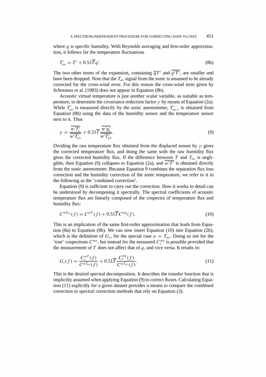
Acoustic virtual temperature is just another scalar variable, as suitable as tem-perature, to determine the covariance reduction factorγ by means of Equation (2a).While T ′av is measured directly by the sonic anemometer,T ′av,s is obtained fromEquation (8b) using the data of the humidity sensor and the temperature sensornext to it. Thus

γ = w′T ′sw′T ′av

+ 0.51Tw′q ′sw′T ′av

. (9)

Dividing the raw temperature flux obtained from the displaced sensor byγ givesthe corrected temperature flux, and doing the same with the raw humidity fluxgives the corrected humidity flux. If the difference betweenT andTav is negli-gible, then Equation (9) collapses to Equation (2a), andw′T ′ is obtained directlyfrom the sonic anemometer. Because Equation 9 combines the separation flux losscorrection and the humidity correction of the sonic temperature, we refer to it inthe following as the ‘combined correction’.

Equation (9) is sufficient to carry out the correction. How it works in detail canbe understood by decomposing it spectrally. The spectral coefficients of acoustictemperature flux are linearly composed of the cospectra of temperature flux andhumidity flux:

CwTav (f ) = CwT (f )+ 0.51T Cwq(f ). (10)

This is an implication of the same first-order approximation that leads from Equa-tion (8a) to Equation (8b). We can now insert Equation (10) into Equation (2b),which is the definition ofGs, for the special casea = Tav. Doing so not for the‘true’ cospectrumCwa, but instead for the measuredCwas is possible provided thatthe measurement ofT does not affect that ofq, and vice versa. It results in:

Gs(f ) = CwTs (f )

CwTav (f )+ 0.51T

Cwqs (f )

CwTav (f ). (11)

This is the desired spectral decomposition. It describes the transfer function that isimplicitly assumed when applying Equation (9) to correct fluxes. Calculating Equa-tion (11) explicitly for a given dataset provides a means to compare the combinedcorrection to spectral correction methods that rely on Equation (3).

452 JOHANNES LAUBACH AND KEITH G. McNAUGHTON

3. Site and Experimental Details

The experiment ran from January 19 to February 9, 1997, over a flood-irrigatedrice field at Warrawidgee, near Griffith, NSW, Australia (34◦15′ S, 145◦45′ E). Tothe west of the field, sparsely vegetated dry land extended for hundreds of kilome-ters. The site was selected to represent the special case of an advective inversion.Typically, we found air temperatures near 305 K from noon to sunset, and a fluxBowen ratioH/λE = −0.2, where

H = ρcpw′T ′, (12)

is the sensible heat flux,ρ being density andcp specific heat at constant pressureof air, and

λE = ρλw′q ′, (13)

the latent heat flux,λ being latent heat of vaporization of water. The given numbersresult inw′T ′av/w′T ′ = 0.68, which clearly shows that we cannot neglect thedifference between acoustic temperature and true temperature.

Two identical eddy correlation systems were set up on the same tower, at 2.58 mand 4.47 m height, respectively, above firm ground. On the ground there was alayer of 0.03 m loose material (soil and organic) and above that a water layer of0.17 m. The height of the rice crop increased from 0.77 m on 21 Jan to 0.86 mon 5 Feb, relative to firm ground, and its canopy density also increased during theexperiment. First subtracting the layers below water level, and then removing thezero plane displacement, estimated as two-thirds of canopy height (Oke, 1987), lefteffective measurement heights (z− d) of 2.0 and 3.9 m, respectively.

The field was of rectangular shape, orientated almost north-south (deviation−4◦). The tower was set up close to the eastern border to maximize fetch and ac-ceptance angle for westerly winds because they represented the desired conditionsof a well-developed stable internal boundary layer (IBL). Distances measured fromthe tower to the field borders were: 418 m to the west, 307 m to the north, 23 m tothe east, and 271 m to the south. For winds from NW to SW this resulted in fetch-to-height ratios from 100:1 to 150 : 1 at the upper level and twice these values at thelower level. While the adjacent land to the west was almost ideally homogeneous(flat and dry), in the other directions lay a patchwork of similar-sized fields of theMurrumbidgee Irrigation Area, with a mixture of rice, wheat, stubble and burntstubble. The field adjacent to the east was burnt off shortly before the experiment,so that easterly winds (unfortunately not infrequent) provided us with a contrastingdataset of ‘worst-possible’ fetch conditions in terms of energy fluxes. With easterlywinds, locally stable conditions at the lower and unstable conditions at the upperlevel were observed, but neither represented a layer adjusted to either the rice paddyor the dry stubble.

A SPECTRUM-INDEPENDENT PROCEDURE FOR CORRECTING EDDY FLUXES 453

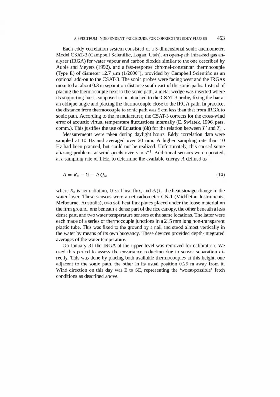
Each eddy correlation system consisted of a 3-dimensional sonic anemometer,Model CSAT-3 (Campbell Scientific, Logan, Utah), an open-path infra-red gas an-alyzer (IRGA) for water vapour and carbon dioxide similar to the one described byAuble and Meyers (1992), and a fast-response chromel-constantan thermocouple(Type E) of diameter 12.7µm (1/2000′′), provided by Campbell Scientific as anoptional add-on to the CSAT-3. The sonic probes were facing west and the IRGAsmounted at about 0.3 m separation distance south-east of the sonic paths. Instead ofplacing the thermocouple next to the sonic path, a metal wedge was inserted whereits supporting bar is supposed to be attached to the CSAT-3 probe, fixing the bar atan oblique angle and placing the thermocouple close to the IRGA path. In practice,the distance from thermocouple to sonic path was 5 cm less than that from IRGA tosonic path. According to the manufacturer, the CSAT-3 corrects for the cross-winderror of acoustic virtual temperature fluctuations internally (E. Swiatek, 1996, pers.comm.). This justifies the use of Equation (8b) for the relation betweenT ′ andT ′av.

Measurements were taken during daylight hours. Eddy correlation data weresampled at 10 Hz and averaged over 20 min. A higher sampling rate than 10Hz had been planned, but could not be realized. Unfortunately, this caused somealiasing problems at windspeeds over 5 m s−1. Additional sensors were operated,at a sampling rate of 1 Hz, to determine the available energyA defined as

A = Rn −G−1Qw, (14)

whereRn is net radiation,G soil heat flux, and1Qw the heat storage change in thewater layer. These sensors were a net radiometer CN-1 (Middleton Instruments,Melbourne, Australia), two soil heat flux plates placed under the loose material onthe firm ground, one beneath a dense part of the rice canopy, the other beneath a lessdense part, and two water temperature sensors at the same locations. The latter wereeach made of a series of thermocouple junctions in a 215 mm long non-transparentplastic tube. This was fixed to the ground by a nail and stood almost vertically inthe water by means of its own buoyancy. These devices provided depth-integratedaverages of the water temperature.

On January 31 the IRGA at the upper level was removed for calibration. Weused this period to assess the covariance reduction due to sensor separation di-rectly. This was done by placing both available thermocouples at this height, oneadjacent to the sonic path, the other in its usual position 0.25 m away from it.Wind direction on this day was E to SE, representing the ‘worst-possible’ fetchconditions as described above.

454 JOHANNES LAUBACH AND KEITH G. McNAUGHTON

4. Results and Discussion

4.1. MAGNITUDE OF THE FLUX CORRECTIONS

Let us begin by evaluating the importance of the proposed corrections. To calculatethe expected covariance reduction factorγ for our setup we apply Equation (5),inserting the transfer functions for separation (Equation (3)) and path-averagingaccording to Moore (1986), and using the Kansas cospectrum from Equation (7a).The resultingγ depends on measurement height and on two variable parameters:windspeedu and stability parameter(z−d)/L. In Figure 1,γ is shown at the lowerheight,z−d = 2.0 m, as a function ofu and for(z−d)/L = 0.05, which is a stabilityvalue close to the median of all ‘good fetch’ periods collected at Warrawidgee. Itcan be seen thatγ is typically 0.85 to 0.90, equivalent to flux losses (1− γ ) oforder 10 to 15%. The losses are smaller at the upper height (not shown) becausethe cospectrum is shifted to lower frequencies there; they increase with increasingstability, because the cospectrum is shifted to higher frequencies. Figure 1 alsoshows that flux losses due to path-averaging are small compared to the effect ofsensor separation. This justifies our focus on the separation correction.

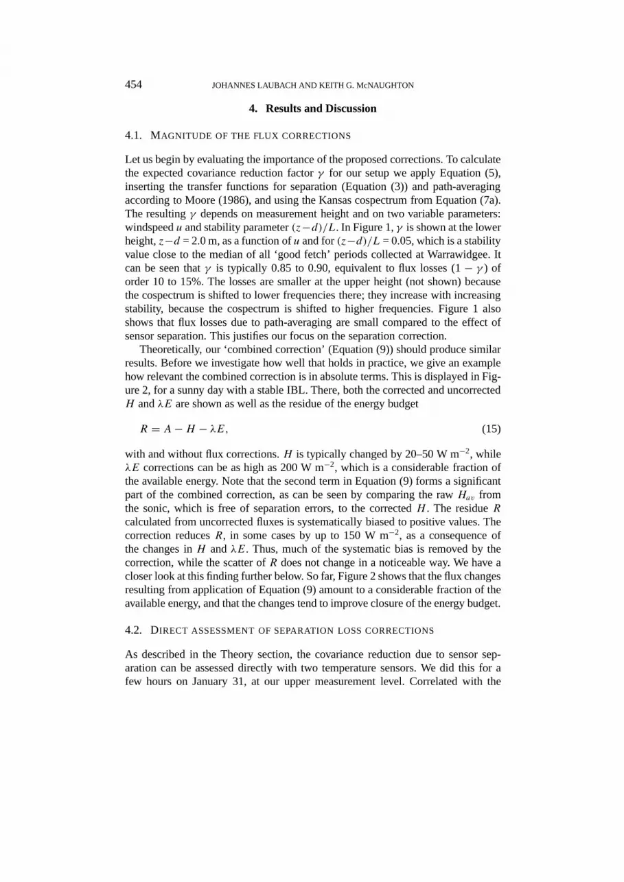
Theoretically, our ‘combined correction’ (Equation (9)) should produce similarresults. Before we investigate how well that holds in practice, we give an examplehow relevant the combined correction is in absolute terms. This is displayed in Fig-ure 2, for a sunny day with a stable IBL. There, both the corrected and uncorrectedH andλE are shown as well as the residue of the energy budget

R = A−H − λE, (15)

with and without flux corrections.H is typically changed by 20–50 W m−2, whileλE corrections can be as high as 200 W m−2, which is a considerable fraction ofthe available energy. Note that the second term in Equation (9) forms a significantpart of the combined correction, as can be seen by comparing the rawHav fromthe sonic, which is free of separation errors, to the correctedH . The residueRcalculated from uncorrected fluxes is systematically biased to positive values. Thecorrection reducesR, in some cases by up to 150 W m−2, as a consequence ofthe changes inH andλE. Thus, much of the systematic bias is removed by thecorrection, while the scatter ofR does not change in a noticeable way. We have acloser look at this finding further below. So far, Figure 2 shows that the flux changesresulting from application of Equation (9) amount to a considerable fraction of theavailable energy, and that the changes tend to improve closure of the energy budget.

4.2. DIRECT ASSESSMENT OF SEPARATION LOSS CORRECTIONS

As described in the Theory section, the covariance reduction due to sensor sep-aration can be assessed directly with two temperature sensors. We did this for afew hours on January 31, at our upper measurement level. Correlated with the

A SPECTRUM-INDEPENDENT PROCEDURE FOR CORRECTING EDDY FLUXES 455

Figure 1. Covariance reduction factors for scalar fluxes from the instruments mounted atz − d = 2.0 m, calculated with the transfer functions for separation and path averaging followingMoore (1986), and assuming the Kansas cospectrum (Equation (7a)) for stability(z− d)/L = 0.05.The dash-dotted line represents the path averaging on both temperature and vertical velocity measure-ments by the sonic anemometer. The solid line combines the sonic’s path averaging for vertical windwith the effect of separation of a point sensor for temperature 0.25 m away. The dashed line representsthe net effect of sonic path averaging, scalar (IRGA) path averaging and separation (0.30 m) on thehumidity flux.

vertical wind data from the sonic, the thermocouple data provide the separationtransfer functionGs empirically (Equation (2b)). In addition, these data provide atest of the robustness of the model-based cospectral correction procedure, for theyrepresent poor fetch conditions. Wind direction on this day was E to SE, so thatthe dry-to-wet transition lay only 37 m upwind of the instruments. This resultedin locally slightly unstable conditions atz − d = 3.9 m. Because of the poor fetchthe spectral shape is expected to deviate from the ideal, equilibrated shape of theKansas Model.

Using the Kansas Model (inserting Equation (7b) into Equation (5)), we obtainan almost constant value ofγ = 0.95 during this period.γ hardly varies becausevariations of horizontal windu are small (between 1.2 and 2.7 m s−1) and becausein unstable cases the cospectrum does not depend on the stability parameter. Asopposed to this,γ values from the direct comparison of the thermocouples (Equa-tion (2a)) vary over the range 0.60–0.95. To understand this, we turn our attention

456 JOHANNES LAUBACH AND KEITH G. McNAUGHTON

Figure 2.Sensible heat fluxes, latent heat fluxes, and resulting residues of the energy budget with andwithout correction according to Equation (9) on February 5 atz− d = 2.0 m.

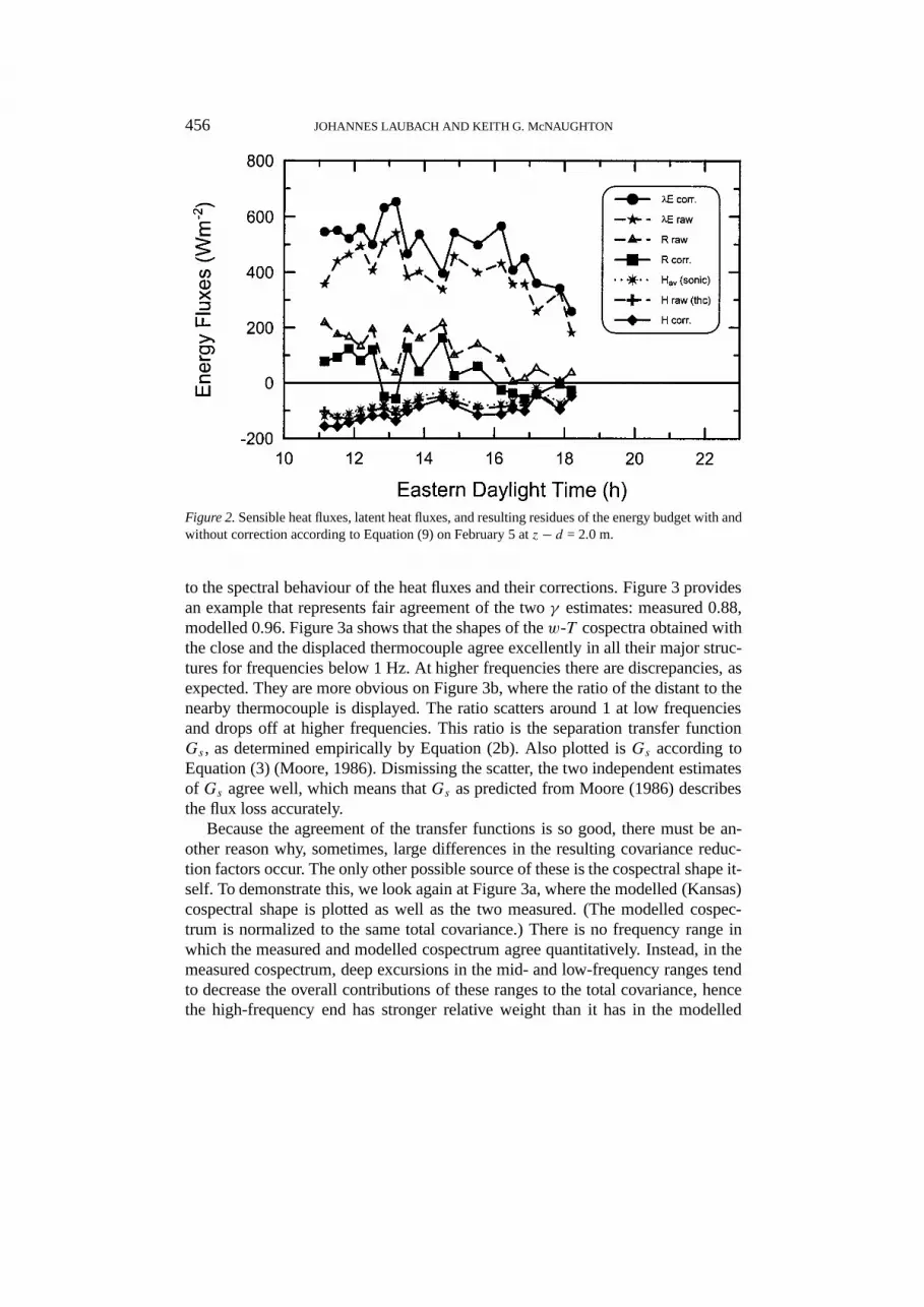
to the spectral behaviour of the heat fluxes and their corrections. Figure 3 providesan example that represents fair agreement of the twoγ estimates: measured 0.88,modelled 0.96. Figure 3a shows that the shapes of thew-T cospectra obtained withthe close and the displaced thermocouple agree excellently in all their major struc-tures for frequencies below 1 Hz. At higher frequencies there are discrepancies, asexpected. They are more obvious on Figure 3b, where the ratio of the distant to thenearby thermocouple is displayed. The ratio scatters around 1 at low frequenciesand drops off at higher frequencies. This ratio is the separation transfer functionGs , as determined empirically by Equation (2b). Also plotted isGs according toEquation (3) (Moore, 1986). Dismissing the scatter, the two independent estimatesof Gs agree well, which means thatGs as predicted from Moore (1986) describesthe flux loss accurately.

Because the agreement of the transfer functions is so good, there must be an-other reason why, sometimes, large differences in the resulting covariance reduc-tion factors occur. The only other possible source of these is the cospectral shape it-self. To demonstrate this, we look again at Figure 3a, where the modelled (Kansas)cospectral shape is plotted as well as the two measured. (The modelled cospec-trum is normalized to the same total covariance.) There is no frequency range inwhich the measured and modelled cospectrum agree quantitatively. Instead, in themeasured cospectrum, deep excursions in the mid- and low-frequency ranges tendto decrease the overall contributions of these ranges to the total covariance, hencethe high-frequency end has stronger relative weight than it has in the modelled

A SPECTRUM-INDEPENDENT PROCEDURE FOR CORRECTING EDDY FLUXES 457

Figure 3. (a) Cospectrum of sensible heat flux for the period 15 : 01–15 : 21 h on 31 Jan 97 asmeasured with a thermocouple near the sonic anemometer and a thermocouple at 0.25 m hor-izontal separation distance. Also shown is the ideal Kansas cospectrum (Equation (7b)). Meanhorizontal wind: 2.52 m s−1, mean wind direction: 137◦. (b) Cospectral ratio of heat flux fromthe sonic anemometer with distant thermocouple to the heat flux obtained from the sonic with closethermocouple. The dashed line represents the separation transfer functionGs from Equation (3).

458 JOHANNES LAUBACH AND KEITH G. McNAUGHTON

cospectrum. Since the covariance reductions described byGs affect only the higherfrequencies, the true overall value ofγ is lower than the model prediction of 0.96.

It might be argued that because of the poor fetch conditions the fluxes are notmeaningful at all. However this is not the important point here. The point is that ifthe true cospectral shape deviates significantly from the modelled, then the model-based procedure fails to predictγ accurately. In this case empirical methods arepreferable. One option would then be to apply the calculation-intensive procedureof Equation (4) with the measured cospectrum andGs (from Moore or empiricallydetermined). Alternatively, Equation (9) can be used, which is done in the nextsection.

4.3. COMPARISON OF SEPARATION LOSS CORRECTIONS IN STABLE

CONDITIONS

For the bulk of data from the Warrawidgee experiment, there are no direct mea-surements of the covariance reduction factor available, because there was no tem-perature sensor mounted next to the sonic anemometer. Being short of a genuine‘reference’, we will assess the performance of the combined correction (Equation(9)) in three ways: first, by comparing to the Kansas Model, second, by investigat-ing the spectral composition of the transfer function according to Equation (11),and third, by demonstrating its effect on the energy budget closure.

The dataset is restricted here to averaging periods with excellent fetch condi-tions, defined as those periods with wind from the western sector (180 to 360◦) forat least 99% of the time. This criterion leaves a total of 70 runs at either height.With only 4 exceptions each, they all represent (slightly) stable conditions in therange(z−d)/L = 0.0005 to 0.4, the medians being 0.062 at the upper and 0.050 atthe lower height. (We determinedL from the sonic anemometer data, usingw′T ′avto approximate the buoyancy fluxw′T ′v in Equation (6), and(−u′w′)1/2 to estimatefriction velocity u∗.) We reduced the dataset further by eliminating a few cases ofhigh windspeed where we believe the data were affected by aliasing.

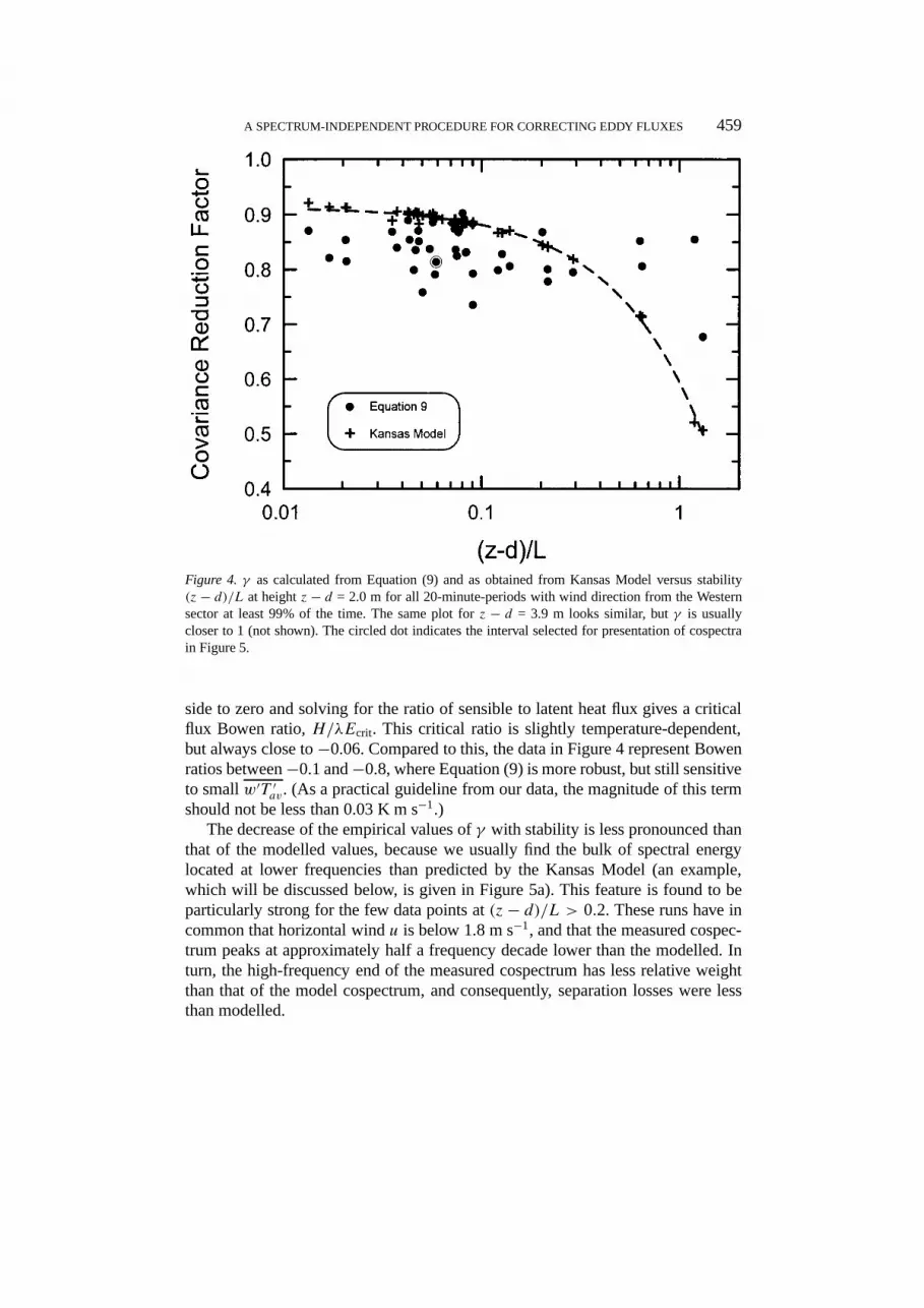
To compare the combined correction and the separation correction using theKansas Model, the covariance reduction factorsγ as obtained by both methods areshown in Figure 4, plotted against stability. The Kansas Model estimates form anarrow band between 0.93 and 0.89 for(z − d)/L < 0.1, and decrease rapidlyfor larger stability. The decrease is mainly due to the cospectrum shifting to higherfrequencies, so being more strongly attenuated by the transfer functionGs . Threefeatures can be noted in Figure 4: the scatter is larger for the empiricalγ than forthe modelledγ , the decrease of the empirical values with stability appears lesspronounced, and the empiricalγ are on average a few percent smaller than thosemodelled.

The magnitude of the scatter matches the expectations, given that each of thethree measured covariances in Equation (9) is subject to a sampling error. Notethat asw′T ′av approaches zero, Equation (9) becomes singular. Setting the left-hand

A SPECTRUM-INDEPENDENT PROCEDURE FOR CORRECTING EDDY FLUXES 459

Figure 4. γ as calculated from Equation (9) and as obtained from Kansas Model versus stability(z − d)/L at heightz − d = 2.0 m for all 20-minute-periods with wind direction from the Westernsector at least 99% of the time. The same plot forz − d = 3.9 m looks similar, butγ is usuallycloser to 1 (not shown). The circled dot indicates the interval selected for presentation of cospectrain Figure 5.

side to zero and solving for the ratio of sensible to latent heat flux gives a criticalflux Bowen ratio,H/λEcrit. This critical ratio is slightly temperature-dependent,but always close to−0.06. Compared to this, the data in Figure 4 represent Bowenratios between−0.1 and−0.8, where Equation (9) is more robust, but still sensitiveto smallw′T ′av. (As a practical guideline from our data, the magnitude of this termshould not be less than 0.03 K m s−1.)

The decrease of the empirical values ofγ with stability is less pronounced thanthat of the modelled values, because we usually find the bulk of spectral energylocated at lower frequencies than predicted by the Kansas Model (an example,which will be discussed below, is given in Figure 5a). This feature is found to beparticularly strong for the few data points at(z− d)/L > 0.2. These runs have incommon that horizontal windu is below 1.8 m s−1, and that the measured cospec-trum peaks at approximately half a frequency decade lower than the modelled. Inturn, the high-frequency end of the measured cospectrum has less relative weightthan that of the model cospectrum, and consequently, separation losses were lessthan modelled.

460 JOHANNES LAUBACH AND KEITH G. McNAUGHTON

Figure 5. (a) Cospectra for the period 12 : 55–13 : 15 h on 8 Feb 97 atz − d = 2.0 m: acoustictemperature flux from sonic anemometer (Tav) and temperature flux from sonic and thermocoupleat 0.25 m horizontal separation distance (Ts ). Also shown is the ideal Kansas cospectrum (Equation(7a)) normalized to the same area as for theTav flux. Mean horizontal wind: 3.59 m s−1, mean winddirection: 306◦, stability: (z − d)/L = 0.059. (b) Transfer functionGs from measured cospectralratios using Equation (11), and modelled following Moore (1986), see Equation (3).

A SPECTRUM-INDEPENDENT PROCEDURE FOR CORRECTING EDDY FLUXES 461

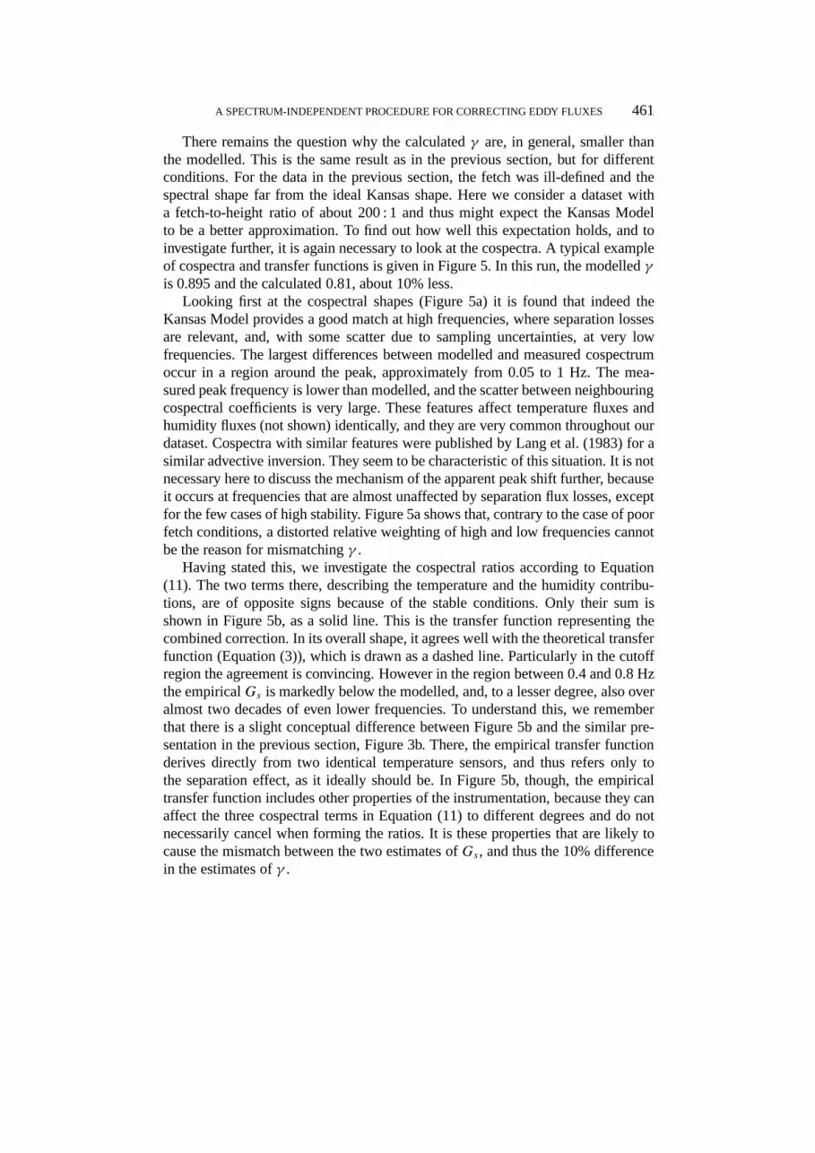
There remains the question why the calculatedγ are, in general, smaller thanthe modelled. This is the same result as in the previous section, but for differentconditions. For the data in the previous section, the fetch was ill-defined and thespectral shape far from the ideal Kansas shape. Here we consider a dataset witha fetch-to-height ratio of about 200 : 1 and thus might expect the Kansas Modelto be a better approximation. To find out how well this expectation holds, and toinvestigate further, it is again necessary to look at the cospectra. A typical exampleof cospectra and transfer functions is given in Figure 5. In this run, the modelledγ

is 0.895 and the calculated 0.81, about 10% less.Looking first at the cospectral shapes (Figure 5a) it is found that indeed the

Kansas Model provides a good match at high frequencies, where separation lossesare relevant, and, with some scatter due to sampling uncertainties, at very lowfrequencies. The largest differences between modelled and measured cospectrumoccur in a region around the peak, approximately from 0.05 to 1 Hz. The mea-sured peak frequency is lower than modelled, and the scatter between neighbouringcospectral coefficients is very large. These features affect temperature fluxes andhumidity fluxes (not shown) identically, and they are very common throughout ourdataset. Cospectra with similar features were published by Lang et al. (1983) for asimilar advective inversion. They seem to be characteristic of this situation. It is notnecessary here to discuss the mechanism of the apparent peak shift further, becauseit occurs at frequencies that are almost unaffected by separation flux losses, exceptfor the few cases of high stability. Figure 5a shows that, contrary to the case of poorfetch conditions, a distorted relative weighting of high and low frequencies cannotbe the reason for mismatchingγ .

Having stated this, we investigate the cospectral ratios according to Equation(11). The two terms there, describing the temperature and the humidity contribu-tions, are of opposite signs because of the stable conditions. Only their sum isshown in Figure 5b, as a solid line. This is the transfer function representing thecombined correction. In its overall shape, it agrees well with the theoretical transferfunction (Equation (3)), which is drawn as a dashed line. Particularly in the cutoffregion the agreement is convincing. However in the region between 0.4 and 0.8 Hzthe empiricalGs is markedly below the modelled, and, to a lesser degree, also overalmost two decades of even lower frequencies. To understand this, we rememberthat there is a slight conceptual difference between Figure 5b and the similar pre-sentation in the previous section, Figure 3b. There, the empirical transfer functionderives directly from two identical temperature sensors, and thus refers only tothe separation effect, as it ideally should be. In Figure 5b, though, the empiricaltransfer function includes other properties of the instrumentation, because they canaffect the three cospectral terms in Equation (11) to different degrees and do notnecessarily cancel when forming the ratios. It is these properties that are likely tocause the mismatch between the two estimates ofGs, and thus the 10% differencein the estimates ofγ .

462 JOHANNES LAUBACH AND KEITH G. McNAUGHTON

We can rule out path averaging as the main cause, because its cutoff is effec-tive at higher frequencies than that of the separation. Two other mechanisms aremore likely candidates. The first is aliasing: if it is present, then sonic temper-ature will be most affected by it, becausew′ and T ′av at frequencies above theNyquist frequency are still correlated, so will be folded back in the cospectrumand appear at lower frequencies. For separated sensors, however, the covariancethat can be folded back will be largely reduced due to the low correlation at highfrequencies. Consequently, forming both ratios on the right-hand side of Equation(9) with aliased covariances will tend to give smaller numbers than unaliased. Inother words, the effect of aliasing on cospectra is that high-frequency fluxlosseswill be folded back to lower frequencies. A numerical simulation revealed that thiscan indeed affect the cospectra over about two decades by a few percent. Thus,in addition to the direct effect described by Equation (3), sensor separation canpotentially reduce the correlation of two variables indirectly, when combined withinstrumental limitations.

The other possible mechanism is the uncertainty of optimum correlation dueto the streamwise part of the sensor separation and due to the sampling time dif-ferences of the data acquisition system. In our setup, the sonic anemometer datawere sent to the computer via a serial communication cable, while the IRGA andthermocouple data were sampled by a multichannel analog-to-digital acquisitionboard. Although our software routinely shifted theqs andTs data to achieve maxi-mum correlation with thew data, there was always an uncertainty of one samplinginterval, i.e., 0.1 s. As with aliasing, the effect of this uncertainty can amount toa few percent reduction in the cospectra and over one to two decades below theNyquist frequency. Of course, the cospectrum ofw andTav is not subject to such areduction.

Given that both effects are small and partly hidden in the general scatter, itis unrealistic to identify them in detail. But since they both work to reduce thecovariance of separated sensors more than that ofw andTav, they may well explainthe bias between modelled and calculatedγ . This bias should, in theory, disap-pear if the modelled transfer function (Equation (3)) was combined with othersaccounting for aliasing and shift uncertainty. An intriguing interpretation is that ourcombined correction has, inadvertently, corrected for several effects that reducedthe correlation of separated sensors, but of which we were unaware.

Finally, we consider the effect of the separation corrections, both followingMoore (1986) and using Equation (9), on the closure of the energy budget. Anexample of a diurnal course has already been shown in Figure 2. In Table I, theaverage residuesR of our good-fetch runs (same dataset as in Figure 4) are given,as calculated with corrected and uncorrected eddy fluxes. Before correction we finda bias to positiveR (meaning that the available energy is larger than the sum of eddyfluxes) of a little under 60 W m−2 on average. Applying Equation (9) toH andλEreduces 2/3 of this bias at the lower height and 1/3 at the upper height. Using thespectral correction (Equation (3)) instead, the remaining residues are larger, which

A SPECTRUM-INDEPENDENT PROCEDURE FOR CORRECTING EDDY FLUXES 463

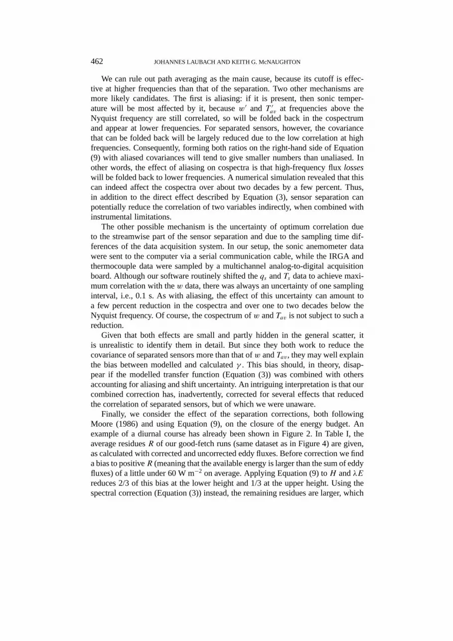
TABLE I

Residue of the energy budget,R, in W m−2, as calculated using eddyfluxes without separation correction, with spectral correction followingMoore (1986), and with combined correction (Equation (9)). The givennumbers are averages of 42 runs.

z− d (m) R (no corr.) R (spectral corr.) R (combined corr.)

2.0 59 34 18

3.9 56 45 34

means the spectral correction method is less efficient in closing the energy budget.However the absolute values ofR should not be overinterpreted: given the usualuncertainty of a few percent for 20-minute-averaged eddy fluxes, and in our specialcase the uncertainty of the large1Qw term (heat storage in the water layer), thenit must be stated that the closure is reasonably good at both heights anyway.

Still, the combined correction has a clearly systematic effect, as illustrated inFigure 6, whereR is displayed againstγ , at the lower height. Diamonds representR before and dots after the correction of sensible and latent heat fluxes (beforecorrection meaning that the sonic temperature was used to calculateH ). The cor-rective effect ofγ bringsR close to the zero line even for the extreme values ofγ < 0.8. This is a strong argument for the robustness of the procedure in periodswhen other flux losses (due to aliasing or uncertainty of relative time lag) add tothe separation effect, or when the Kansas Model is an inappropriate description ofthe cospectral shapes. Typical afternoon values, when available energy is highest,are as follows: a value ofγ = 0.9, which is the order of magnitude predicted by theKansas Model, reducesR by about 30 W m−2, while a value of 0.8 roughly doublesthe effect. The improved closure of the energy budget is an indirect confirmationof the quality of the combined correction.

4.4. GENERAL DISCUSSION

The main purpose of Subsections 4.1–4.3 was to demonstrate that Equation (9) pro-vides a practical approach to correct for flux losses due to sensor separation. A sideissue that has been touched a few times is that at the same time it provides an ele-gant means to correct from acoustic virtual temperature fluxes to true temperaturefluxes – better than the conventional way of doing so, because the humidity fluxneeded for this correction is automatically separation-corrected simultaneously. Itwas this aspect that suggested the name ‘combined correction’.

The net effect of the correction depends on the two terms contributing to Equa-tion (9). Our experiment represented stable conditions. Sensible heat fluxes arethen downward, while latent heat fluxes are upward. The magnitudes of both are

464 JOHANNES LAUBACH AND KEITH G. McNAUGHTON

Figure 6.Energy budget residueR from uncorrected fluxes and after correction using Equation (9) atz−d = 2.0 m. The meanR is 59 W m−2 for the uncorrected budgets and 18 W m−2 for the corrected(42 data points).

reduced by sensor separation. The uncorrected sensible heat flux (usingTav fromthe sonic anemometer) is also too small in magnitude because of the opposite signof the humidity flux. Correcting the fluxes thus means to increase both upwardλE and downwardH , so that in the net energy budget their changes partly cancel.This explains why the shift between uncorrected and correctedR in Figure 6 is notlarger, although Figure 2 displays fairly large changes especially forλE.

In unstable situations, the energy budget is composed differently.H andλE arethen both upwards, competing for the available energyA. Consequently latent heatfluxes tend to be smaller, and the humidity term in Equation (9) is less important.Applying the correction then means that resulting sensible heat fluxes are smallerthan those obtained from the sonic, while corrected latent heat fluxes are largerthan the uncorrected, so that again the changes toR partly cancel.

The covariance reduction factorγ , as obtained from the combined correctionmethod, is valid for scalar fluxes other than sensible and latent heat as well, as longas they fulfil the same requirements of cospectral similarity. To make use of this,the scalar under consideration must be measured at the same location as humidity(as is the case for CO2 with our IRGAs), or at least at an identical distances fromthe vertical wind measurement. This instrumentational requirement can be simpli-fied if the humidity term in Equation (9) is small enough to be neglected, which

A SPECTRUM-INDEPENDENT PROCEDURE FOR CORRECTING EDDY FLUXES 465

then results in Equation (2a). This variation of the empirical correction methodis particularly attractive if a scalar, whose flux is of interest, cannot be measuredclose to either the wind sensor or the humidity sensor, or if no humidity sensor isavailable at all.

Kristensen et al. (1997) have proposed a different approach to deal with theseparation of sensors. They concluded that mounting the scalar sensor underneaththe wind sensor, instead of displacing it horizontally, retains correlation of verticalwind and the scalar much better, and thus reduces flux losses. It is undoubtedly agood idea to reduce losses, rather than to correct for them. Yet in some situations,such as within canopies, the value of this approach still has to be established.It might be worth considering to combine a vertically separated arrangement ofsensors, following Kristensen et al. (1997), with our idea of using an additionaltemperature sensor to remove the remaining error. The value of this may be sub-stantial since it appears that our empirical correction can compensate for some im-perfections in the experimental system that are not directly due to, but are indirectlyaltered by separation of sensors.

Our method relies on similarity of the cospectra of temperature flux and hu-midity flux. This requirement was satisfied well in our experiment, except at verylow frequencies where the contributions to the total fluxes were too small to berelevant. It can be imagined that temperature and humidity spectra might be lesssimilar if their respective sensors were placed close to a field transition, or within acanopy where sensible and latent heat fluxes had different source areas. But thesecases are usually linked with ill-defined fetch conditions, which implies that thespectral shapes can be very far from the ideal Kansas spectrum. In these cases, thespectral correction following Moore (1986) provides a poor alternative. While themodel-based correction requires cospectral shapes of all scalar fluxes to be similarto the model cospectrum, the combined correction only requires similar shapes ofCwT andCwq . The second requirement is easier to fulfil than the first.

5. Conclusions

The proposed ‘combined correction’ for sensible and latent heat fluxes has beendemonstrated to remove flux errors due to sensor separation effectively. If thetrue cospectral shape is described well by the Kansas cospectrum, the combinedcorrection must produce the same results as the generally accepted spectral methodusing the Kansas Model and transfer functions. It has been shown that, in practice,both methods agree well as long as the relative weight of the high-frequency part issimilar for measured and modelled cospectra. In cases when the cospectral shapesdo not follow the model cospectrum, the combined correction is the more reliablemethod because it is spectrum-independent. A second advantage of the combinedcorrection is that it can remove all flux losses of separated sensors simultane-ously, not only those due to the well-known effect of spatial decorrelation, but

466 JOHANNES LAUBACH AND KEITH G. McNAUGHTON

also those due to some deficiencies of the data acquisition system, in as much asthese deficiencies affect separated and non-separated sensors differently.

A limitation of the combined correction is a numerical instability whenw′T ′avapproaches zero. Because the denominator in Equation (9) is then very uncertain,the derivedγ cannot be expected to be trustworthy. When sensible heat fluxes aresmall, it is better to correct latent heat fluxes and gas fluxes according to Moore(1986). A second limitation could occur if the spectral shapes of heat and watervapour flux were markedly different, because the two ratios in Equation (11) wouldbe sensitive to that, but then the applicability of the spectral model would be limitedtoo.

Having these limitations in mind, we conclude with a practical recommen-dation. Since the combined correction requires only one additional temperaturesensor, and is thus not too costly, it should be seriously considered whenever theeddy correlation technique is used over non-ideal terrain and when significantseparation distances of sensors cannot be avoided. It can be applied on-line aseasily as the model-based spectral correction. The combined correction can alsobe used with the error-minimizing sensor positions advocated by Kristensen et al.(1997), because it is by no means restricted to horizontal sensor separation. Insituations where cospectral shapes are not well-known, e.g., in canopies, the com-bined correction could even serve to assess if there, too, vertical sensor separationis preferable to horizontal separation.

Acknowledgements

The work was funded entirely by the Government of New Zealand (Marsden FundContract CO6539). Nonetheless, Australia’s contribution to its success is signifi-cant due to the kind support we received from a number of its residents. We thankAngelo Silvestro for allowing us to work on his ideally-located rice paddy, thecolleagues of CSIRO Land and Water at Canberra (Pye Laboratory) for providingtower, power and cover (caravan), the staff of CSIRO Land and Water at Griffithfor local assistance and accomodation, and last not least Peter Isaac for providinggood, quick and cheap calibrations of the IRGAs. One of the IRGAs is propertyof Flinders University (Adelaide), Institute for Meteorology and Atmospheric Sci-ence, and the other of NIWA (Gracefield, NZ). Their generosity in lending them tous is gratefully acknowledged.

References

Auble, D. L. and Meyers, T. P.: 1992, ‘An Open Path, Fast Response Infrared Absorption GasAnalyzer for H2O and CO2’, Boundary-Layer Meteorol.59, 243–256.

Fan, S.-M., Wofsy, S. C., Bakwin, P. S., Jacob, D. J., Anderson, S. M., Kebabian, P. L., McManus,J. B., Kolb, C. E., and Fitzjarrald, D. R.: 1992, ‘Micrometeorological Measurements of CH4

A SPECTRUM-INDEPENDENT PROCEDURE FOR CORRECTING EDDY FLUXES 467

and CO2 Exchange between the Atmosphere and Subarctic Tundra’,J. Geophys. Res.97(D15),16,627–16,643.

Fan, S.-M., Wofsy, S. C., Bakwin, P. S., Jacob, D. J., and Fitzjarrald, D. R.: 1990, ‘Atmosphere-Biosphere Exchange of CO2 and O3 in the Central Amazon Forest’,J. Geophys. Res.95(D10),16,851–16,864.

Horst, T. W.: 1997, ‘A Simple Formula for Attenuation of Eddy Fluxes Measured with First-Order-Response Scalar Sensors’,Boundary-Layer Meteorol.82, 219–233.

Irwin, H. P. A. H.: 1979, ‘Cross-Spectra of Turbulence Velocities in Isotropic Turbulence’,Boundary-Layer Meteorol.16, 237–243.

Kaimal, J. C. and Gaynor, J. E.: 1991, ’Another Look at Sonic Thermometry’,Boundary-LayerMeteorol.56, 401–410.

Kaimal, J. C., Wyngaard, J. C., Izumi, Y., and Coté, O. R.: 1972, ‘Spectral Characteristics of Surface-Layer Turbulence’,Quart. J. Roy. Meteorol. Soc.98, 563–589.

Kristensen, L. and Jensen, N. O.: 1979, ‘Lateral Coherence in Isotropic Turbulence and in the NaturalWind’, Boundary-Layer Meteorol.17, 353–373.

Kristensen, L., Mann, J., Oncley, S. P., and Wyngaard, J. C.: 1997, ‘How Close is Close Enoughwhen Measuring Scalar Fluxes with Displaced Sensors?’,J. Atmos. Oceanic Tech.14, 814–821.

Lang, A. R. G., McNaughton, K. G., Chen, F., Bradley, E. F., and Ohtaki, E.: 1983, ‘Inequality ofEddy Transfer Coefficients for Vertical Transport of Sensible and Latent Heats During AdvectiveInversions’,Boundary-Layer Meteorol.25, 25–41.

Lee, X., and Black, T. A.: 1994, ‘Relating Eddy Correlation Sensible Heat Flux to Horizon-tal Sensor Separation in the Unstable Atmospheric Surface Layer’,J. Geophys. Res.99(D9),18,545–18,553.

Leuning, R. and Judd, M. J.: 1996, ‘The Relative Merits of Open- and Closed-Path Analysers forMeasurement of Eddy Fluxes’,Global Change Biology2, 241–253.

Moore, C. J.: 1986, ‘Frequency Response Corrections for Eddy Correlation Systems’,Boundary-Layer Meteorol.37, 17–35.

Neumann, H. H., den Hartog, G., King, K. M., and Chipanshi, A. C.: 1994, ‘Carbon Dioxide FluxesOver a Raised Open Bog at the Kinosheo Lake Tower Site During the Northern Wetlands Study(NOWES)’,J. Geophys. Res.99(D1), 1529–1538.

Oke, T. R.: 1987,Boundary Layer Climates, 2nd ed., Methuen Press, London, 435 pp.Schotanus, P., Nieuwstadt, F. T. M., and de Bruin, H. A. R.: 1983, ‘Temperature Measurement with a

Sonic Anemometer and its Application to Heat and Moisture Fluxes’,Boundary-Layer Meteorol.26, 81–93.

Wofsy, S. C., Goulden, M. L., Munger, J. W., Fan, S.-M., Bakwin, P. S., Daube, B. C., Bassow,S. L., and Bazzaz, F. A.: 1993, ’Net Exchange of CO2 in a Mid-Latitude Forest’,Science260,1314–1317.