A simulated annealing strategy for the detection of arbitrarily shaped spatial clusters

LUIZ DUCZMAL* and RENATO ASSUNÇÃO

Department of Statistics – ICEx – UFMG Laboratório de Estatística Espacial (LESTE) and

Centro de Estudos de Criminalidade e Segurança Pública (CRISP) 30161-970 – Belo Horizonte – MG, Brazil

ABSTRACT

We propose a new graph based strategy for the detection of spatial clusters of arbitrary geometric form in a map of geo-referenced populations and cases. Our test statistic is based on the likelihood ratio test previously formulated by Kulldorff and Nagarwalla for circular clusters. A new technique of adaptive simulated annealing is developed, focused on the problem of finding the local maxima of a certain likelihood function over the space of the connected subgraphs of the graph associated to the regions of interest. Given a map with n regions, on average this algorithm finds a quasi-optimal solution after analyzing s n log(n) subgraphs, where s depends on the cases density uniformity in the map. The algorithm is applied to a study of homicide clusters detection in a Brazilian large metropolitan area. KEYWORDS: Spatial cluster detection, simulated annealing, likelihood ratio test, disease clusters, hot-spot detection.

1. INTRODUCTION

Since the 1980s there has been an increasing interest in the identification of spatially localized adverse health risk conditions. The reasons for the existence of such clustering are various. They can be due to environmental causes concentrated on small regions such as a localized pollution sources (Biggeri et al., 1996; Katsouyanni et al, 1991; Xu et al., 1989). Another possible reason is population differences on their genetic constituency or social habits such as diet (Barbujani and Sokal, 1990; Walsh and DeChello, 2001). Other possibilities include differences on regional medical services such as ascertainment of new cases or disease treatment protocols (Karjalainen, 1990; Goodwin et al., 1998) or a viral agent generating clustering patterns (Kinlen, 1995). A number of methods have been proposed to test for the presence of spatial clusters of elevated risk and to identify their locations. Thorough and recent reviews can be found in (Lawson et al., 1999) where the many different methods are compared. The methods assume that we have at our disposal a map of regions, each one with a defined risk population and a certain number of observed cases. The cases correspond to the individuals in each population that have a special designation, such as an infected individual or a crime

* Corresponding author e-mail: duczmal@est.ufmg.br Luiz Duczmal UFMG – Departamento de Estatística Caixa Postal 702 Belo Horizonte, MG, 30161-970 Brazil FAX: 55-31-3499-5924

victim. The most useful cluster detection methods are those based on moving windows and related approaches. These methods superimpose circular regions over the study region and then evaluate the significance of the number of cases that fall within each circle. The methods differ according to the circles’ definition. Openshaw et al. (1987) superimpose a regular grid and circles of varying radii are drawn at the grid nodes. Those circles attaining a certain significance level are flagged and shown in the map. Besag and Newell (1991) invert the circle definition: rather than fixing the circles radii and looking for the significant ones, they propose to fix the number of cases within a circle and then search for those with such a small risk population that make them highly significant. The two methods described above have been criticized for the multiple testing problem since neither of them control for the simultaneous inference problem on the set of all circles considered. That is, considering the multiple locations and circles sizes simultaneously tested, the error type I of these multiple tests are not controlled leading to subjective decision making. The authors suggest considering as significant circles those with p-values as small as 0.005 or 0.0005 but there is no theoretical justification for a specific choice. This is a major problem since the choice of the cut-off p-value size determines the sensitivity and specificity of the test. Kulldorff and Nagarwalla (1995) and Kulldorff (1997) proposed a methodology based on scan statistics that overcomes this difficult problem. It is a maximum likelihood ratio test with a parametric space including all circles tested. The test finds the maximum likelihood sweeping over all zones circumscribed by circles of varying radii centered at each of the regions of the map. The likelihood is not differentiable with respect to the parameters and hence we need to use a Monte Carlo testing procedure to evaluate its significance. We describe this spatial scan statistical test in more detail in Section 2. A major problem with scan statistic methods is the fixed shape of the clusters to be detected, typically circular clusters although other specific shapes can be defined such as rectangular (Kulldorff, 1999). The reason for such a restriction is the computationally infeasible number of possible areas to be tested. However, in real situations, we frequently find spatial clusters with quite different shapes from circular ones. A single pollution source could increase the risk of respiratory disease around it but the wind patterns destroy a possibly symmetric cluster (Biggeri et al., 1996). Increased risks along rivers, transport ways or powerlines create clusters with shapes highly different from circular ones (Feychting and Ahbom, 1993; Verkasalo, 1993). Usually, other environmental or social causes do not have a circular symmetry and hence do not to induce clusters with such a shape. Applying the usual circular cluster detection methods to find clusters in such a situation have one possible consequence. The cluster is not well localized, generally being either much larger than the real cluster present in the map or leaving out areas with higher risks but whose incorporation in the circular window tested would also bring many other areas with lower risk. In this paper, we introduce a graph-based algorithm that overcomes this limitation of Kulldorff and Nagarwalla (1995) and Kulldorff (1997) by using a simulated annealing approach. Differently from these authors, our strategy is not restricted to the detection of clusters with fixed shape, such as rectangular or circular shape, but it looks for connected clusters with arbitrary shape. We implemented our algorithm in a conveniently fast C++ code, which can be freely obtained from the authors. Experiments with our method show

that it can identify clusters and test their statistical significance for real life problems in a short amount of time using modest computer resources. The structure of this paper is as follows. We first describe the spatial scan statistic in Section 2. We then introduce some notation and present our algorithm in Section 3. In Section 4 we analyze the computational performance of the algorithm and discuss its asymptotic behavior for simple situations. In Section 5, we present the results of experiments to verify the computational complexity of the algorithm. Section 6 applies the method to the problem of finding a spatial cluster of homicides in Belo Horizonte, a large city in Brazil, contrasting the results with those obtained by the circular spatial scan statistics. Section 7 contains a concluding discussion.

2. THE SPATIAL SCAN STATISTIC

The geographical map is reduced to the centroids of its component areas and, to each one of them, we have the respective associated cases and risk population. The circular spatial scan statistic imposes a circular window on each centroid in turn and the radius of this window is changed continuously to take any value between zero and some prescribed upper limit. Each circular window defines a region composed by one or more areas, which is a potential cluster of increased risk. Let Z be the set of all such circular windows, or potential clusters. We can see an example of one such circular window in Figure 7A, where the shaded areas within the circle form the cluster. Using the same notation as Kulldorff (1997), let z be a candidate cluster in the set Z. Define p as the probability that an individual is a case in z, and q as the probability that an individual is a case in the complement of z. We would like to test if this specific z is a cluster. The alternative hypothesis is

qpZzH >∈ ,:1 , and the null hypothesis is qpH =:0 . Define zn as the population of the region z, zc as the number of cases of the region z, N as the total population in the map and C as the total number of cases. For this fixed cluster candidate z, adopting a binomial model produces a simple likelihood function given by:

( ) ( ) zzzzzz cCnNcCcnc qqppqpzL +−−−− −−= 11),,( This produces the maximum likelihood ratio statistic defined as:

]).1,0[,(),,(sup

),,(sup, ∈==

>∈ qpqpzL

qpzLT

qp

qpZz

The denominator in the above expression reduces to

0]1,0[

)()1(sup),,(sup LN

CNCppqpzL N

CNCCNC

pqp=−=−=

−−

∈=

and hence L0 is a constant that depends only on C . With respect to the numerator, for a fixed candidate z , we maximize over all possible 10 ≤≤≤ pq . Let

),,(sup)( qpzLzLqp>

=

.,

,)(

0

)(

otherwisenNcC

ncif

LnN

cCnNnNcC

ncn

nc

z

z

z

zcCNN

z

zz

cC

z

z

cn

z

zz

c

z

zzzzzzz

−−>

−

−−−

−−

−

=

−−−−−

Therefore 0/)(sup LzLT z= . Since it is clear that the denominator of the likelihood ratio test statistic does not depend on the cases configurations, then equivalently the test statistic could be defined only by its numerator. Hence, the objective is to find the zone z that maximizes the function L over all circles in Z and this identifies the one that constitutes the most likely cluster. For a map with n regions and k different radii, this implies in nk calculations, a computationally simple task. Its p-value is obtained through Monte Carlo hypothesis testing. Conditioning on the total number of cases, a large number B of random replications of the data set are generated under the null hypothesis. It is usual to take B=9999 in the applications. For each one of the replications, the maximum likelihood ratio test statistic is calculated in the same way as for the real data set. Under the null hypothesis, these B+1 values, from the real and the B random data sets, are independent and identically distributed random variables. Rank the B+1 values from highest to lowest. Then, if the null hypothesis is true, the real data set rank R has a uniform distribution on the integers from 1 to B+1 and the probability of being in among the top 100α percent values is, exactly, α, and its exact p-value is R/(B+1). This method is implemented in the SaTScan software, developed at the National Cancer Institute, and available free of charge in the web.

3. DETECTING CLUSTERS WITH ARBITRARY SHAPE

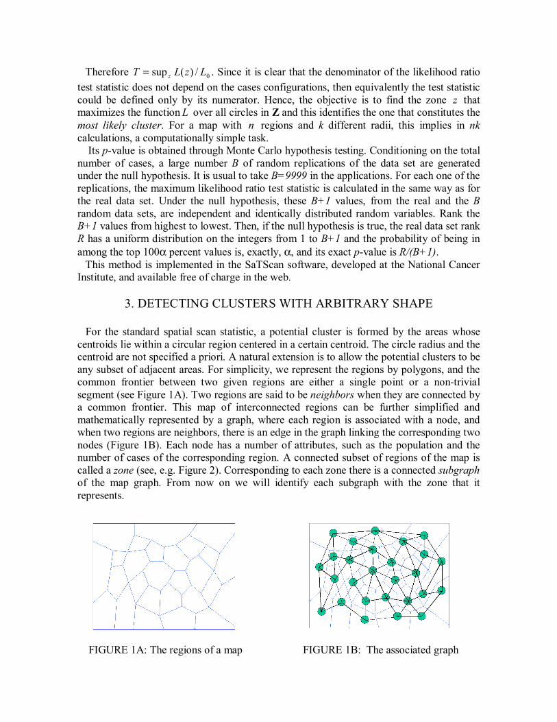
For the standard spatial scan statistic, a potential cluster is formed by the areas whose centroids lie within a circular region centered in a certain centroid. The circle radius and the centroid are not specified a priori. A natural extension is to allow the potential clusters to be any subset of adjacent areas. For simplicity, we represent the regions by polygons, and the common frontier between two given regions are either a single point or a non-trivial segment (see Figure 1A). Two regions are said to be neighbors when they are connected by a common frontier. This map of interconnected regions can be further simplified and mathematically represented by a graph, where each region is associated with a node, and when two regions are neighbors, there is an edge in the graph linking the corresponding two nodes (Figure 1B). Each node has a number of attributes, such as the population and the number of cases of the corresponding region. A connected subset of regions of the map is called a zone (see, e.g. Figure 2). Corresponding to each zone there is a connected subgraph of the map graph. From now on we will identify each subgraph with the zone that it represents.

FIGURE 1A: The regions of a map FIGURE 1B: The associated graph

We consider the problem of finding, among all possible zones, a zone z that maximizes the likelihood ratio T or, equivalently, its numerator L (z). A solution to this problem is called a most likely cluster. For a map with n regions, we would need to analyze all the connected inherited subgraphs among the n2 possible subsets of n vertices, and this is a formidable task for a map with hundreds of regions. So we need to try to analyze only the most promising subgraphs of the collection of all connected inherited subgraphs, and discard the less interesting ones. For that, we use a simulated annealing approach as we describe next. A non-oriented graph (or graph, for short) G is an ordered pair ),( EV , where V is a finite set of vertices { nvv ,...,1 } and E is a set of edges { mee ,...,1 }, such that },{

21 iii vve = , with

21 ii vv ≠ and Vvv ii ∈21

, , mi ,...,1= . If },{ kj vv is an edge, then jv and kv are adjacent vertices. The graph ),( 11 EVS = is a subgraph of ),( EVG = if VV ⊂1 , and EE ⊂1 . The subgraph ),( 11 EVS = of ),( EVG = is an inherited subgraph of G if

11 },{},{,, EvvEvvVvv kjkjkj ∈⇒∈∈ , i.e., 1E is a maximal set over all the subgraphs ),( 1 WV of G . Two vertices kj vv , of a graph ),( EVG = are connected by a path if there is

a sequence of vertices prrr vvv ...,,

21 such that

1rj vv = ,prk vv = , and

1,...,1,},{1

−=∈+

piEvvii rr . A graph ),( EVG = is connected if any pair of distinct vertices

Vvv kj ∈, are connected by a path. The inherited subgraphs ),( 111 EVS = and ),( 222 EVS = of ),( EVG = are neighbors if the set )()( 2121 VVVV ∩−∪ consists of

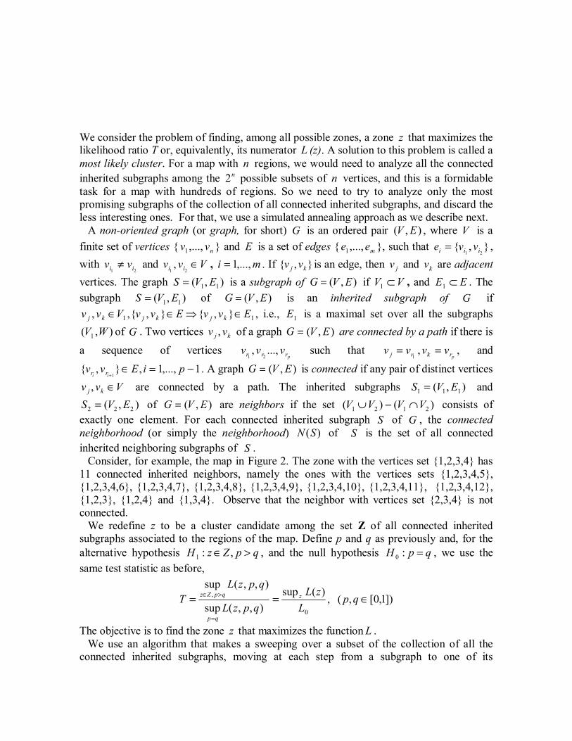
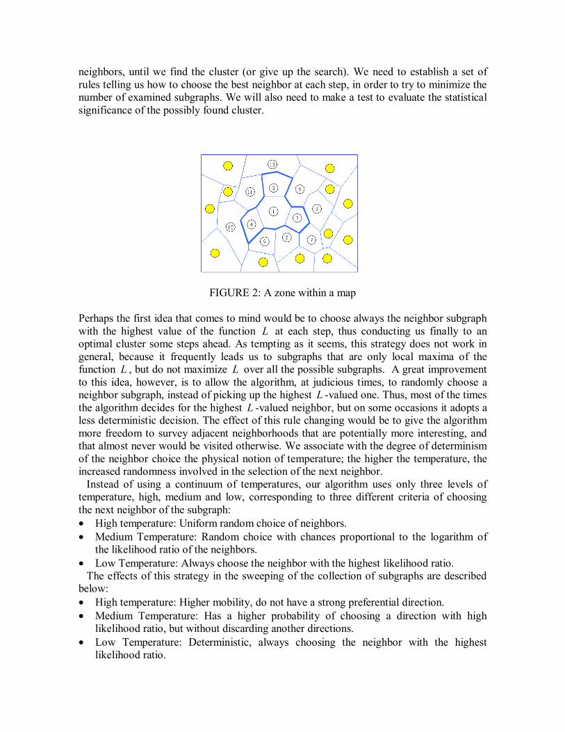
exactly one element. For each connected inherited subgraph S of G , the connected neighborhood (or simply the neighborhood) )(SN of S is the set of all connected inherited neighboring subgraphs of S . Consider, for example, the map in Figure 2. The zone with the vertices set {1,2,3,4} has 11 connected inherited neighbors, namely the ones with the vertices sets {1,2,3,4,5}, {1,2,3,4,6}, {1,2,3,4,7}, {1,2,3,4,8}, {1,2,3,4,9}, {1,2,3,4,10}, {1,2,3,4,11}, {1,2,3,4,12}, {1,2,3}, {1,2,4} and {1,3,4}. Observe that the neighbor with vertices set {2,3,4} is not connected. We redefine z to be a cluster candidate among the set Z of all connected inherited subgraphs associated to the regions of the map. Define p and q as previously and, for the alternative hypothesis qpZzH >∈ ,:1 , and the null hypothesis qpH =:0 , we use the same test statistic as before,

])1,0[,(,)(sup),,(sup

),,(sup

0

, ∈===

>∈ qpL

zLqpzL

qpzLT z

qp

qpZz

The objective is to find the zone z that maximizes the function L . We use an algorithm that makes a sweeping over a subset of the collection of all the connected inherited subgraphs, moving at each step from a subgraph to one of its

neighbors, until we find the cluster (or give up the search). We need to establish a set of rules telling us how to choose the best neighbor at each step, in order to try to minimize the number of examined subgraphs. We will also need to make a test to evaluate the statistical significance of the possibly found cluster.

FIGURE 2: A zone within a map

Perhaps the first idea that comes to mind would be to choose always the neighbor subgraph with the highest value of the function L at each step, thus conducting us finally to an optimal cluster some steps ahead. As tempting as it seems, this strategy does not work in general, because it frequently leads us to subgraphs that are only local maxima of the function L , but do not maximize L over all the possible subgraphs. A great improvement to this idea, however, is to allow the algorithm, at judicious times, to randomly choose a neighbor subgraph, instead of picking up the highest L -valued one. Thus, most of the times the algorithm decides for the highest L -valued neighbor, but on some occasions it adopts a less deterministic decision. The effect of this rule changing would be to give the algorithm more freedom to survey adjacent neighborhoods that are potentially more interesting, and that almost never would be visited otherwise. We associate with the degree of determinism of the neighbor choice the physical notion of temperature; the higher the temperature, the increased randomness involved in the selection of the next neighbor. Instead of using a continuum of temperatures, our algorithm uses only three levels of temperature, high, medium and low, corresponding to three different criteria of choosing the next neighbor of the subgraph: • High temperature: Uniform random choice of neighbors. • Medium Temperature: Random choice with chances proportional to the logarithm of

the likelihood ratio of the neighbors. • Low Temperature: Always choose the neighbor with the highest likelihood ratio. The effects of this strategy in the sweeping of the collection of subgraphs are described below: • High temperature: Higher mobility, do not have a strong preferential direction. • Medium Temperature: Has a higher probability of choosing a direction with high

likelihood ratio, but without discarding another directions. • Low Temperature: Deterministic, always choosing the neighbor with the highest

likelihood ratio.

In order to unify these three strategies, we create a function F(G, temp) that receives the current subgraph G and returns a neighbor of G chosen accordingly to the choice strategy at the high, medium or low temperature value set to the variable temp. The algorithm decides at every step the value of temp, increasing or decreasing it, depending on how the function L behaves over the subgraphs that are being analyzed, as we shall see soon. In addition to these three levels of randomness in the process of neighbor selection, we will go further and create a fourth strategy. Let us define the function H(G) as follows: If a vertex 0v was added to G in the previous step, the function H(G) returns a neighbor of G that includes 0v and also a randomly chosen extra vertex 1v , adjacent to 0v . If otherwise a vertex 0v was excluded on the previous step, then H returns the neighbor given by F(G, low). For example, referring again to Figure 2, if the previous subgraph has the set of vertices {1,2,4} and the current subgraph has the set of vertices {1,2,3,4}, (so that

30 =v ) then the result of H(G) is chosen randomly among the subgraphs with the set of vertices {1,2,3,4,5}, or {1,2,3,4,6}, or {1,2,3,4,7}, or {1,2,3,4,8} (because 5,6,7 and 8 are the adjacent vertices of 0v ). The objective of successive applications of H is to try to force the appearance of potentially interesting subgraphs that are normally beyond the range of the sweeping given by the function F alone. As we shall see, the strategy of the function H will be used exclusively when there are indications that the current subgraph is a very promising one. The function H augments the set of vertices of the current subgraph near the places where there have been recent and significant improvements of the current subgraph, and thus increase the importance of the current neighborhood being analyzed. We identified four factors that are relevant to the convenient selection of the strategy at each step, when the algorithm computes the L -function for each one of the neighbors of the current subgraph, and prepares to choose the next neighboring subgraph. In order to quantify them we will use four corresponding variables or flags, namely hL (high L -function value), cs (consecutive steps), vb (visited before) and cv (common vertices). The meaning of these variables is described below: • It was found )1( =hL or not )0( =hL a neighbor with higher L -value at the current

step; • The number cs of consecutive steps such that weren’t found new subgraphs with L -

value > 1. • The number vb of times that the current subgraph has been visited before in the survey; • The number cv of common vertices between the current subgraph and the highest yet

L -valued one in the survey. The idea of the basic survey routine that we introduce now is to adopt at each step one of four types of choices strategies for the successor of the current subgraph, with different levels of randomness. In order from the most random to the most deterministic, there are the F(G, high), F(G, medium) and F(G, low) strategies and at last the H(G) function strategy. The choice of which strategy is to be used is based on the values of the parameters hL, vb and cs, that are indicating if the current subgraph G is becoming more or less promising as the survey goes on. At each step the algorithm verifies if the four parameters

vbcshL ,, and cv are within convenient thresholds and use them to modify dynamically the process of selection of the successor of the current subgraph, or give up the local search.

Thus F(G, high) is adopted if the current subgraph has a relatively low L-value, was visited many times, and for several steps of the survey the L-values for the subgraphs have not increased. F(G, medium) is used if the current subgraph has a relatively low L-value, has been visited many times, but there have been an increase of the L-values for some recently surveyed subgraph. F(G, low) is used if there have been an increase of the L-values for some recently surveyed subgraph, but at least one of the following conditions are true: the current subgraph has a relatively low L-value, or it has been visited many times. Finally, H(G) is applied when the current subgraph has a relatively high L-value, has not been visited many times, and there have been an increase of the L-values for some recently surveyed subgraph. The basic survey routine is finally abandoned when one of the parameters vb and cs exceeds the thresholds defined within the algorithm. In the implementation of our program, we use the cluster found by the Kulldorff algorithm as a starting subgraph for the basic survey routine. Next, the cluster candidate found by the basic survey routine is stored in a list. Then, we start again the basic survey routine, at this time with an initial subgraph that consists simply of exactly one node, chosen randomly among all the nodes of the graph. The routine finds another cluster candidate that is also stored. We repeat the last procedure several times, each time with another randomly chosen 1-node initial subgraphs, until 99% of all nodes in the map have been visited at least once. Typically, this implies that the routine is called several hundreds of times with different initial subgraphs, until the maximum L-value found does not increase for a conveniently long sequence of visited subgraphs, or the storage space for the list of visited subgraphs is exhausted. The subgraph associated with the maximum L-value is the most likely cluster. After the most likely cluster is found, we make a Monte Carlo test to evaluate its statistical significance (Dwass, 1957). Under the null hypothesis, we simply distribute randomly the C cases independently over the n regions with the probability that the i-th region receives a case being proportional to its population. This implies that the vector of numbers of cases in the n regions follows a multinomial distribution. For each random allocation of the cases, we compute the test statistic T running our simulated annealing maximization algorithm. We repeat this procedure making a large number B of random allocations of cases under the null hypothesis and calculate the p-value as the proportion of times the simulated values of T are greater than the observed T value. We emphasize that the zones visited are different for the real and each of the random data sets, when doing the Monte Carlo replications to obtain the p-value. Rather, the same algorithmic simulated annealing procedure is used for both the real and random data sets, which ensures that the inference is correct in a simple and elegant way.

4. ON THE CONVERGENCE OF THE ALGORITHM It is a well-know fact that combinatorial algorithms that use simulated annealing converge to the optimal solution in exponential time in the worst case, but usually find quasi-optimalsolutions in much less time (see Aarts and Korst, 1989; Winkler, 1995).

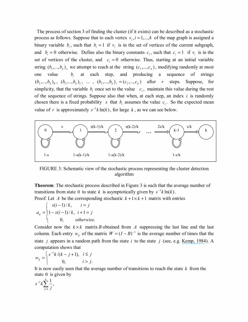
The process of section 3 of finding the cluster (if it exists) can be described as a stochastic process as follows. Suppose that to each vertex kivi ,...,1, = of the map graph is assigned a binary variable ib , such that 1=ib if iv is in the set of vertices of the current subgraph, and 0=ib otherwise. Define also the binary constants ic , such that 1=ic if iv is in the set of vertices of the cluster, and 0=ic otherwise. Thus, starting at an initial variable string okbb ),...,( 1 we attempt to reach at the string ),...,( 1 kcc , modifying randomly at most one value ib at each step, and producing a sequence of strings

),...,(),...,(,...,),...,(,),...,( 111101 krkkk ccbbbbbb = after r steps. Suppose, for simplicity, that the variable ib once set to the value ic , maintain this value during the rest of the sequence of strings. Suppose also that when, at each step, an index i is randomly chosen there is a fixed probability s that ib assumes the value ic . So the expected mean value of r is approximately )ln(1 kks − , for large k , as we can see below.

FIGURE 3: Schematic view of the stochastic process representing the cluster detection algorithm

Theorem: The stochastic process described in Figure 3 is such that the average number of transitions from state 0 to state k is asymptotically given by )ln(1 kks − . Proof: Let A be the corresponding stochastic 11 +×+ kk matrix with entries

=+

=−−

−=

.1

,0,/)1(1

,/)1(

otherwiseji

jikis

kisaij

Consider now the kk × matrix B obtained from A suppressing the last line and the last column. Each entry ijw of the matrix 1)( −−= BIW is the average number of times that the state j appears in a random path from the state i to the state j (see, e.g. Kemp, 1984). A computation shows that

>≤+−

=−

.,0),1/(1

jijijkks

wij

It is now easily seen that the average number of transitions to reach the state k from the state 0 is given by

∑=

−k

j jks

1

1 ,1

0 1 2 k-1

1-s(k-2)/k 1-s 1-s(k-1)/k

k

1-s/k

s s(k-1)/k s(k-2)/k...

2s/k s/k

the sum of the entries of the first line of W . Now, using the fact that

∑=

+++=

k

j kO

kk

j12 ,1

21)ln(1 γ

where ...577.0=γ is the Euler constant, the result follows. The assumptions above are somewhat artificial. The parameter s may be very difficult to establish. It may not be constant over the map, and also may vary greatly from one problem to another. But this crude model can explain, in certain simple situations, the behavior of the algorithm, as shown in the graph of Figure 5A. We can see that the predicted

)log(nsn values for the number of analyzed subgraphs match well with the experimental values, with 68.1=s . In this particular case the cluster is very well defined in the map. This is certainly not the case as with the detected cluster in Belo Horizonte, as we shall see later in Section 6, or in the “double cluster” example of Section 5. This suggests that the worst scenario for the algorithm is the presence of several disconnected “small clusters” scattered along the map. We finally note that the scale of clustering can be handled by modelling (see Lawson and Denison, 2002 and references therein).

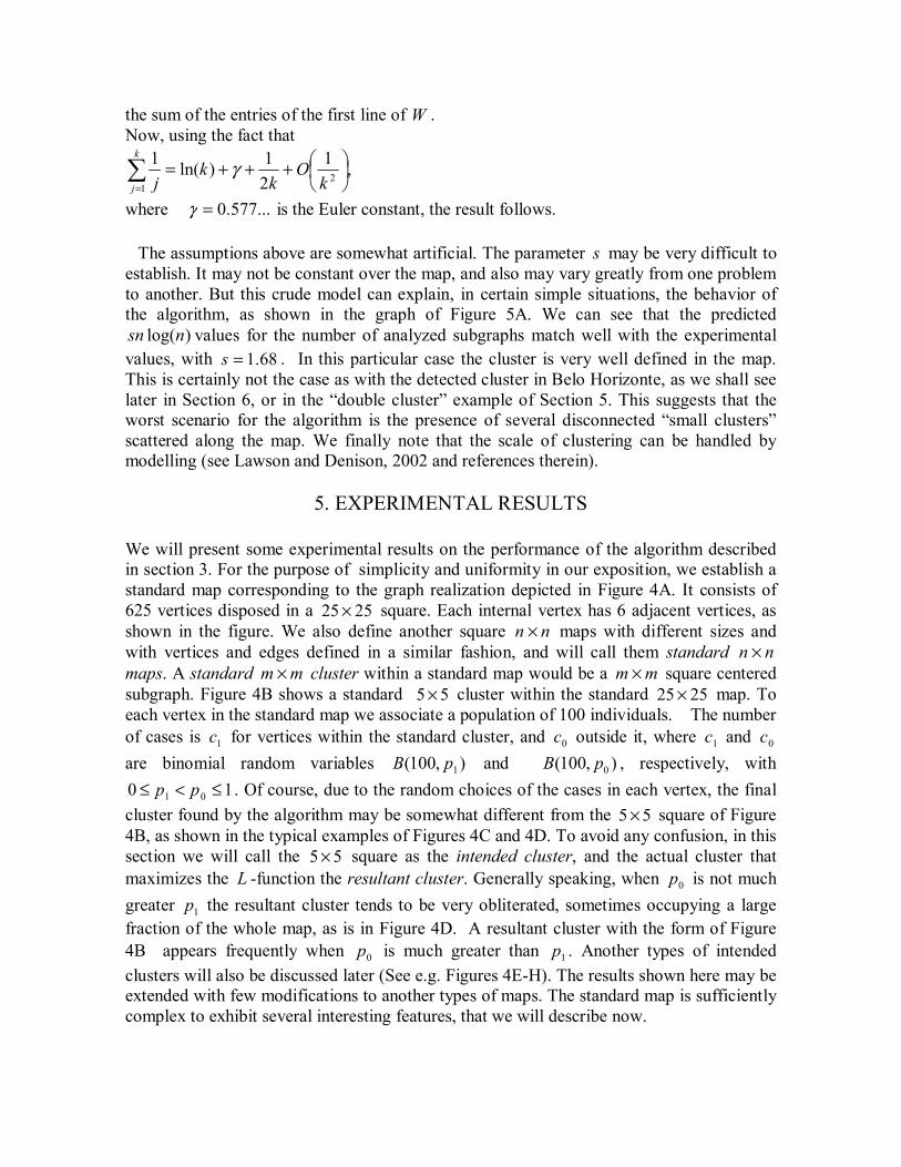
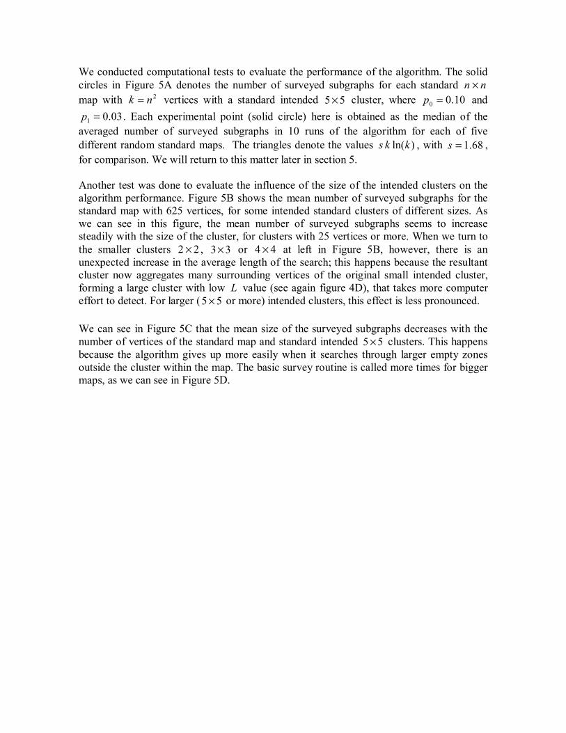
5. EXPERIMENTAL RESULTS We will present some experimental results on the performance of the algorithm described in section 3. For the purpose of simplicity and uniformity in our exposition, we establish a standard map corresponding to the graph realization depicted in Figure 4A. It consists of 625 vertices disposed in a 2525 × square. Each internal vertex has 6 adjacent vertices, as shown in the figure. We also define another square nn × maps with different sizes and with vertices and edges defined in a similar fashion, and will call them standard nn × maps. A standard mm × cluster within a standard map would be a mm × square centered subgraph. Figure 4B shows a standard 55 × cluster within the standard 2525 × map. To each vertex in the standard map we associate a population of 100 individuals. The number of cases is 1c for vertices within the standard cluster, and 0c outside it, where 1c and 0c are binomial random variables ),100( 1pB and ),100( 0pB , respectively, with

10 01 ≤<≤ pp . Of course, due to the random choices of the cases in each vertex, the final cluster found by the algorithm may be somewhat different from the 55 × square of Figure 4B, as shown in the typical examples of Figures 4C and 4D. To avoid any confusion, in this section we will call the 55 × square as the intended cluster, and the actual cluster that maximizes the L -function the resultant cluster. Generally speaking, when 0p is not much greater 1p the resultant cluster tends to be very obliterated, sometimes occupying a large fraction of the whole map, as is in Figure 4D. A resultant cluster with the form of Figure 4B appears frequently when 0p is much greater than 1p . Another types of intended clusters will also be discussed later (See e.g. Figures 4E-H). The results shown here may be extended with few modifications to another types of maps. The standard map is sufficiently complex to exhibit several interesting features, that we will describe now.

We conducted computational tests to evaluate the performance of the algorithm. The solid circles in Figure 5A denotes the number of surveyed subgraphs for each standard nn × map with 2nk = vertices with a standard intended 55 × cluster, where 10.00 =p and

03.01 =p . Each experimental point (solid circle) here is obtained as the median of the averaged number of surveyed subgraphs in 10 runs of the algorithm for each of five different random standard maps. The triangles denote the values )ln(kks , with 68.1=s , for comparison. We will return to this matter later in section 5. Another test was done to evaluate the influence of the size of the intended clusters on the algorithm performance. Figure 5B shows the mean number of surveyed subgraphs for the standard map with 625 vertices, for some intended standard clusters of different sizes. As we can see in this figure, the mean number of surveyed subgraphs seems to increase steadily with the size of the cluster, for clusters with 25 vertices or more. When we turn to the smaller clusters 22 × , 33× or 44 × at left in Figure 5B, however, there is an unexpected increase in the average length of the search; this happens because the resultant cluster now aggregates many surrounding vertices of the original small intended cluster, forming a large cluster with low L value (see again figure 4D), that takes more computer effort to detect. For larger ( 55 × or more) intended clusters, this effect is less pronounced. We can see in Figure 5C that the mean size of the surveyed subgraphs decreases with the number of vertices of the standard map and standard intended 55 × clusters. This happens because the algorithm gives up more easily when it searches through larger empty zones outside the cluster within the map. The basic survey routine is called more times for bigger maps, as we can see in Figure 5D.

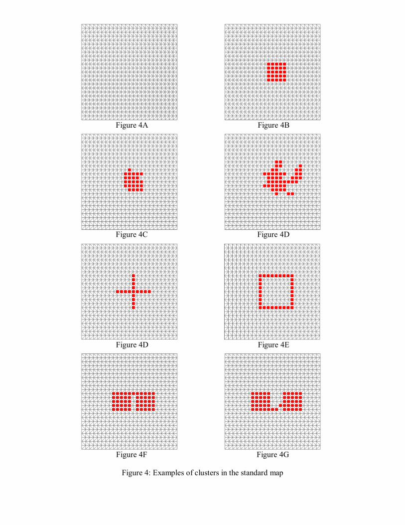
Figure 4A Figure 4B

Figure 4C Figure 4D

Figure 4D Figure 4E

Figure 4F Figure 4G

Figure 4: Examples of clusters in the standard map

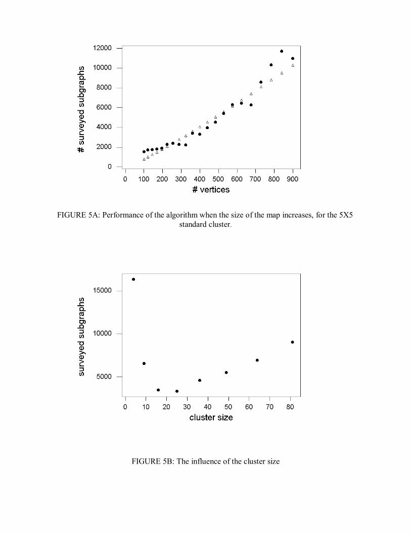
FIGURE 5A: Performance of the algorithm when the size of the map increases, for the 5X5 standard cluster.

FIGURE 5B: The influence of the cluster size

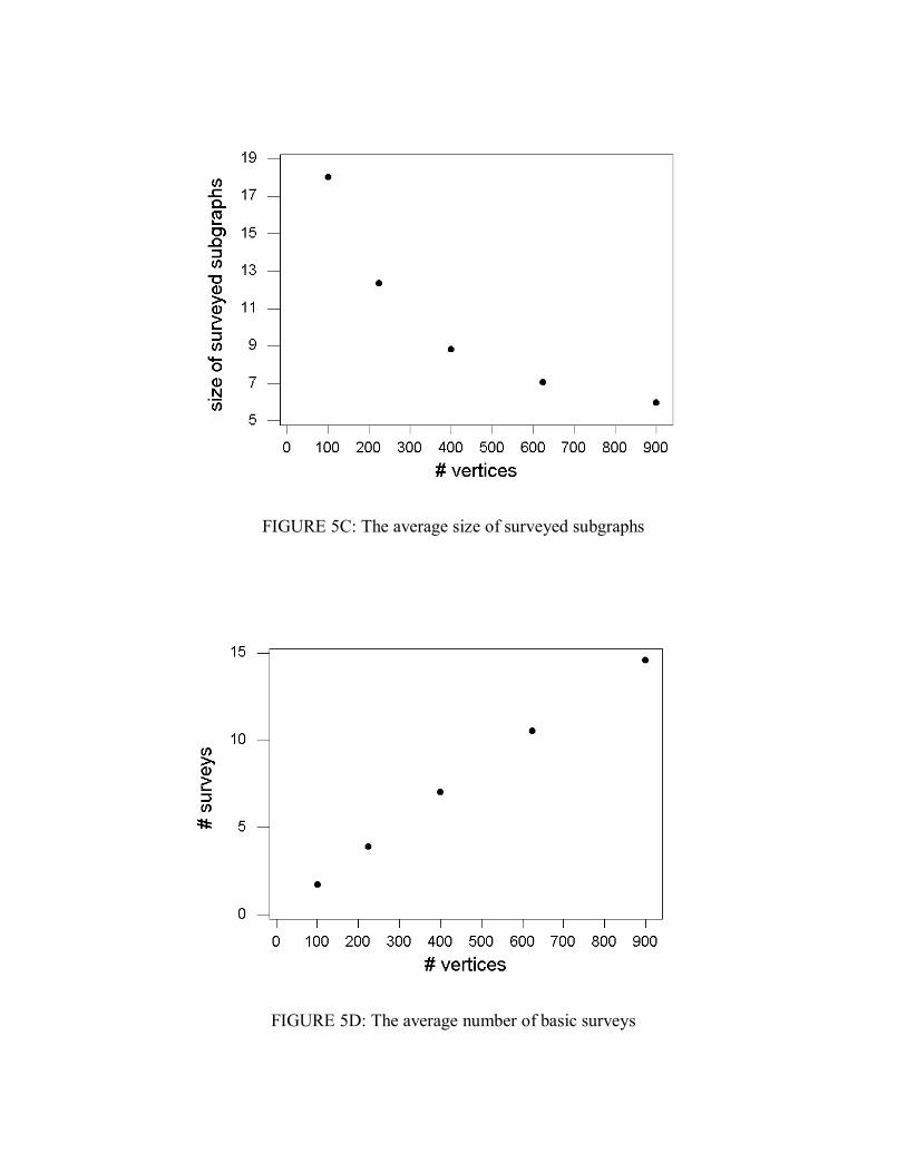
FIGURE 5C: The average size of surveyed subgraphs

FIGURE 5D: The average number of basic surveys

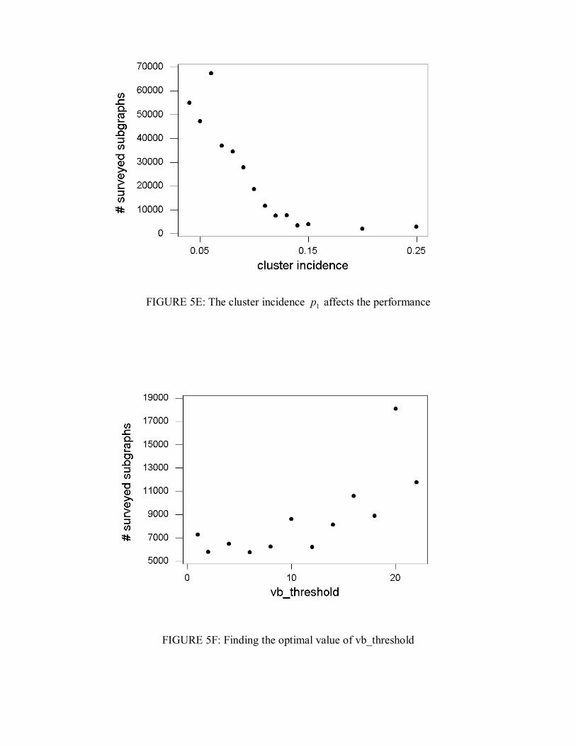
FIGURE 5E: The cluster incidence 1p affects the performance

FIGURE 5F: Finding the optimal value of vb_threshold

The difference between 0p and 1p has influence on the mean number of surveyed subgraphs, as we can see in Figure 5E. In all cases, 03.00 =p , and we tested for values of

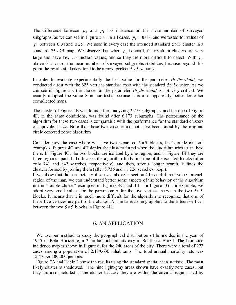
1p between 04.0 and 25.0 . We used in every case the intended standard 55 × cluster in a standard 2525 × map. We observe that when 1p is small, the resultant clusters are very large and have low L -function values, and so they are more difficult to detect. With 1p above 0.15 or so, the mean number of surveyed subgraphs stabilizes, because beyond this point the resultant clusters tend to be almost perfect 55 × squares. In order to evaluate experimentally the best value for the parameter vb_threshold, we conducted a test with the 625 vertices standard map with the standard 55 × cluster. As we can see in Figure 5F, the choice for the parameter vb_threshold is not very critical. We usually adopted the value 8 in our tests, because it is also apparently better for other complicated maps.

The cluster of Figure 4E was found after analyzing 2,275 subgraphs, and the one of Figure 4F, in the same conditions, was found after 6,173 subgraphs. The performance of the algorithm for these two cases is comparable with the performance for the standard clusters of equivalent size. Note that these two cases could not have been found by the original circle centered zones algorithm. Consider now the case where we have two separated 55 × blocks, the “double cluster” examples. Figures 4G and 4H depict the clusters found when the algorithm tries to analyze them. In Figure 4G, the two blocks are isolated by one region, and in Figure 4H they are three regions apart. In both cases the algorithm finds first one of the isolated blocks (after only 741 and 842 searches, respectively), and then, after a longer search, it finds the clusters formed by joining them (after 5,736 and 11,226 searches, resp.). If we allow that the parameter s discussed above in section 4 has a different value for each region of the map, we can understand better some aspects of the behavior of the algorithm in the "double cluster" examples of Figures 4G and 4H. In Figure 4G, for example, we adopt very small values for the parameter s for the five vertices between the two 55× blocks. It means that it is much more difficult for the algorithm to recognize that one of these five vertices are part of the cluster. A similar reasoning applies to the fifteen vertices between the two 55× blocks in Figure 4H.

6. AN APPLICATION

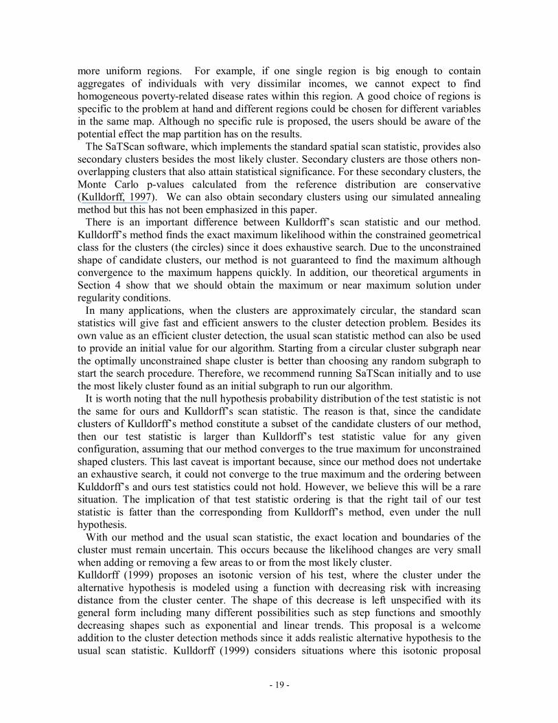
We use our method to study the geographical distribution of homicides in the year of 1995 in Belo Horizonte, a 2 million inhabitants city in Southeast Brazil. The homicide incidence map is shown in Figure 6, for the 240 areas of the city. There were a total of 273 cases among a population of 2,189,630 inhabitants. The total annual mortality rate was 12.47 per 100,000 persons. Figure 7A and Table 2 show the results using the standard spatial scan statistic. The most likely cluster is shadowed. The nine light-gray areas shown have exactly zero cases, but they are also included in the cluster because they are within the circular region used by

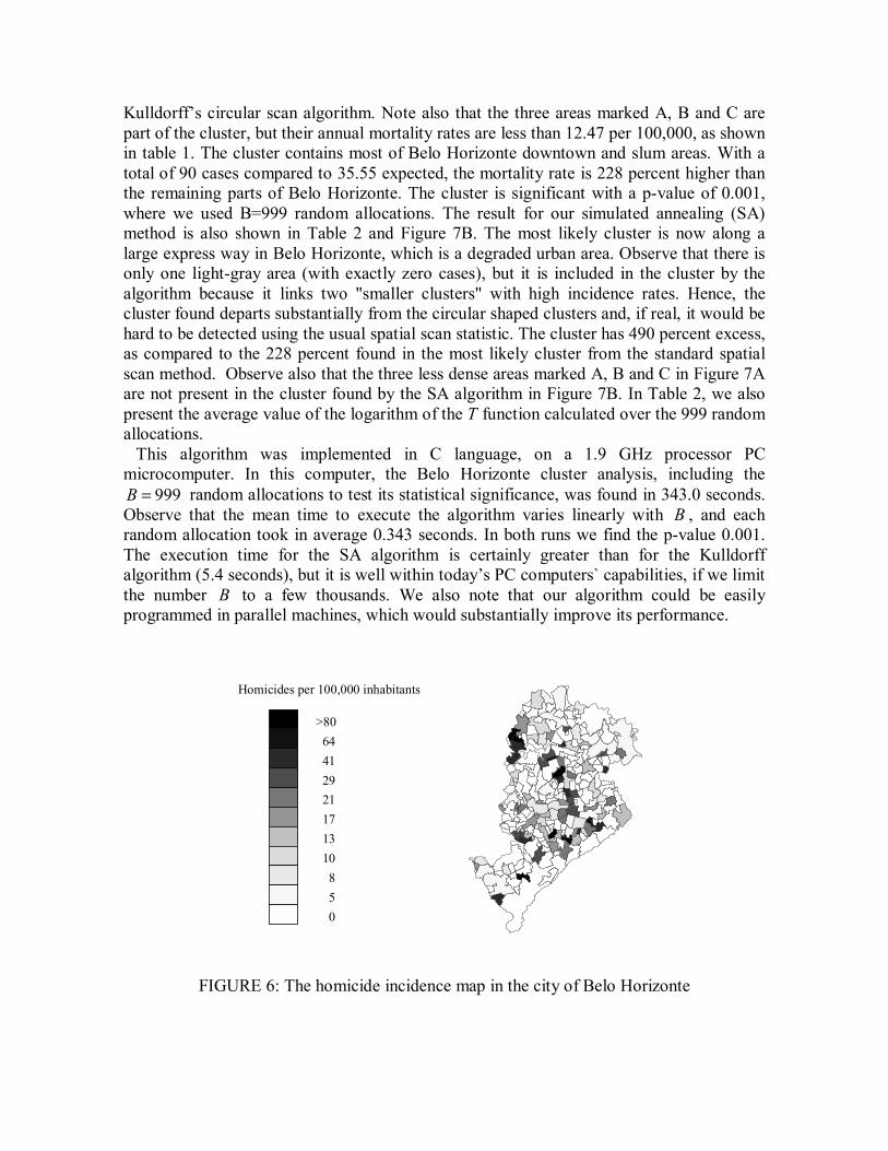
Kulldorff’s circular scan algorithm. Note also that the three areas marked A, B and C are part of the cluster, but their annual mortality rates are less than 12.47 per 100,000, as shown in table 1. The cluster contains most of Belo Horizonte downtown and slum areas. With a total of 90 cases compared to 35.55 expected, the mortality rate is 228 percent higher than the remaining parts of Belo Horizonte. The cluster is significant with a p-value of 0.001, where we used B=999 random allocations. The result for our simulated annealing (SA) method is also shown in Table 2 and Figure 7B. The most likely cluster is now along a large express way in Belo Horizonte, which is a degraded urban area. Observe that there is only one light-gray area (with exactly zero cases), but it is included in the cluster by the algorithm because it links two "smaller clusters" with high incidence rates. Hence, the cluster found departs substantially from the circular shaped clusters and, if real, it would be hard to be detected using the usual spatial scan statistic. The cluster has 490 percent excess, as compared to the 228 percent found in the most likely cluster from the standard spatial scan method. Observe also that the three less dense areas marked A, B and C in Figure 7A are not present in the cluster found by the SA algorithm in Figure 7B. In Table 2, we also present the average value of the logarithm of the T function calculated over the 999 random allocations. This algorithm was implemented in C language, on a 1.9 GHz processor PC microcomputer. In this computer, the Belo Horizonte cluster analysis, including the

999=B random allocations to test its statistical significance, was found in 343.0 seconds. Observe that the mean time to execute the algorithm varies linearly with B , and each random allocation took in average 0.343 seconds. In both runs we find the p-value 0.001. The execution time for the SA algorithm is certainly greater than for the Kulldorff algorithm (5.4 seconds), but it is well within today’s PC computers` capabilities, if we limit the number B to a few thousands. We also note that our algorithm could be easily programmed in parallel machines, which would substantially improve its performance.

FIGURE 6: The homicide incidence map in the city of Belo Horizonte

>80644129

1721

1310850

Homicides per 100,000 inhabitants

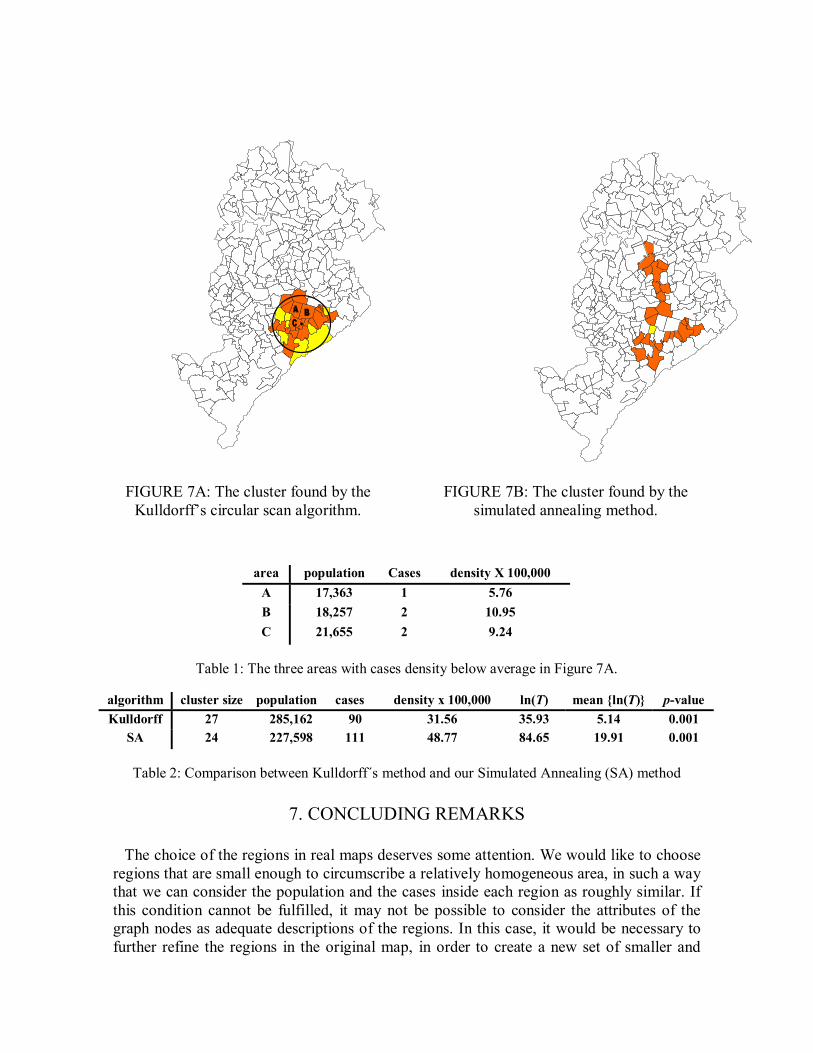
FIGURE 7A: The cluster found by the Kulldorff’s circular scan algorithm.

FIGURE 7B: The cluster found by the simulated annealing method.

area population Cases density X 100,000 A 17,363 1 5.76 B 18,257 2 10.95 C 21,655 2 9.24

Table 1: The three areas with cases density below average in Figure 7A.

algorithm cluster size population cases density x 100,000 ln(T) mean {ln(T)} p-value Kulldorff 27 285,162 90 31.56 35.93 5.14 0.001

SA 24 227,598 111 48.77 84.65 19.91 0.001

Table 2: Comparison between Kulldorff´s method and our Simulated Annealing (SA) method

7. CONCLUDING REMARKS

The choice of the regions in real maps deserves some attention. We would like to choose regions that are small enough to circumscribe a relatively homogeneous area, in such a way that we can consider the population and the cases inside each region as roughly similar. If this condition cannot be fulfilled, it may not be possible to consider the attributes of the graph nodes as adequate descriptions of the regions. In this case, it would be necessary to further refine the regions in the original map, in order to create a new set of smaller and

- 19 -

more uniform regions. For example, if one single region is big enough to contain aggregates of individuals with very dissimilar incomes, we cannot expect to find homogeneous poverty-related disease rates within this region. A good choice of regions is specific to the problem at hand and different regions could be chosen for different variables in the same map. Although no specific rule is proposed, the users should be aware of the potential effect the map partition has on the results. The SaTScan software, which implements the standard spatial scan statistic, provides also secondary clusters besides the most likely cluster. Secondary clusters are those others non-overlapping clusters that also attain statistical significance. For these secondary clusters, the Monte Carlo p-values calculated from the reference distribution are conservative (Kulldorff, 1997). We can also obtain secondary clusters using our simulated annealing method but this has not been emphasized in this paper. There is an important difference between Kulldorff’s scan statistic and our method. Kulldorff’s method finds the exact maximum likelihood within the constrained geometrical class for the clusters (the circles) since it does exhaustive search. Due to the unconstrained shape of candidate clusters, our method is not guaranteed to find the maximum although convergence to the maximum happens quickly. In addition, our theoretical arguments in Section 4 show that we should obtain the maximum or near maximum solution under regularity conditions. In many applications, when the clusters are approximately circular, the standard scan statistics will give fast and efficient answers to the cluster detection problem. Besides its own value as an efficient cluster detection, the usual scan statistic method can also be used to provide an initial value for our algorithm. Starting from a circular cluster subgraph near the optimally unconstrained shape cluster is better than choosing any random subgraph to start the search procedure. Therefore, we recommend running SaTScan initially and to use the most likely cluster found as an initial subgraph to run our algorithm. It is worth noting that the null hypothesis probability distribution of the test statistic is not the same for ours and Kulldorff’s scan statistic. The reason is that, since the candidate clusters of Kulldorff’s method constitute a subset of the candidate clusters of our method, then our test statistic is larger than Kulldorff’s test statistic value for any given configuration, assuming that our method converges to the true maximum for unconstrained shaped clusters. This last caveat is important because, since our method does not undertake an exhaustive search, it could not converge to the true maximum and the ordering between Kulddorff’s and ours test statistics could not hold. However, we believe this will be a rare situation. The implication of that test statistic ordering is that the right tail of our test statistic is fatter than the corresponding from Kulldorff’s method, even under the null hypothesis. With our method and the usual scan statistic, the exact location and boundaries of the cluster must remain uncertain. This occurs because the likelihood changes are very small when adding or removing a few areas to or from the most likely cluster. Kulldorff (1999) proposes an isotonic version of his test, where the cluster under the alternative hypothesis is modeled using a function with decreasing risk with increasing distance from the cluster center. The shape of this decrease is left unspecified with its general form including many different possibilities such as step functions and smoothly decreasing shapes such as exponential and linear trends. This proposal is a welcome addition to the cluster detection methods since it adds realistic alternative hypothesis to the usual scan statistic. Kulldorff (1999) considers situations where this isotonic proposal

- 20 -

would be preferable but he concludes that the simplicity of concept and interpretation will make the standard scan statistic preferable in many situations. In our view, practitioners will appreciate tests that are flexible enough to identify clusters with arbitrary shapes. Another issue, even more important, is the comparison of the methods concerns their relative power. It is expected that a test with alternative hypothesis more flexible should have more power against clusters shaped according to the alternative set. However, what is not clear is the relative power of the methods when a real cluster is circularly shaped and this issue should be investigated. In conclusion, the simulated annealing method can serve as an important tool for geographical cluster detection. It is possible to find clusters of arbitrary shapes such as along rivers, lakeshores, avenues and roads. Not constraining the cluster to a fixed geometric shape, such as a circle, allows the researcher to find a geographically smaller cluster, hopefully more similar to a real cluster. The method could also be extended to deal with space and time simultaneously. Although the clusters searched have arbitrary shape, the algorithm is fast and requires only )log(nn running time.

8. AKNOWLEDGEMENTS

The authors wish to express their appreciation to the editor and the referees for their valuable comments and suggestions, which improved the original manuscript. This research was partially supported by the Fundação de Amparo à Pesquisa de Minas Gerais (FAPEMIG) Grant CEX-336/99 and the Ford Foundation.

9. REFERENCES

1. Aarts E, Korst J. Simulated Annealing and Boltzmann Machines, Wiley: Chichester,

1989. 2. Barbujani G, and Sokal R. Zones of sharp genetic change in Europe are also linguistic

boundaries. Proceedings of the National Academy of Sciences USA, 1990: 87: 1816-1819.

3. Besag J Newell J. The detection of clusters in rare diseases. Journal of the Royal Statistical Society Series A, 1991: 154: 143-155.

4. Biggeri, A., Barbone, F., Lagazio, C., Bovenzi, M., and Stanta, G. Air pollution and lung cancer in Trieste: spatial analysis of risk as a function of distance from sources, Environmental Health Perspectives, 104 (1996) 750-754.

5. Dwass, M. Modified randomization tests for nonparametric hypotheses. Annals of Mathematical Statistics, 1957; 28:181-187.

6. Feychting M, Ahlbom A. Magnetic fields and cancer in children residing near Swedish high voltage power lines. American Journal of Epidemiology, 1993: 7: 467-481.

7. Goodwin JS, Freeman JL, Freeman D, Nattinger AB. Geographic variations in breast cancer mortality: do higher rates imply elevated incidence or poorer survival? American Journal of Public Health, 1998: 88: 458-460.

8. Kemp R. Fundamentals of the Average Case Analysis of Particular Algorithms, Wiley-Teubner Series in Computer Science, 1984.

9. Kinlen, L.J. Epidemiological evidence for an infective basis in childhood leukaemia, Bristish Journal of Cancer, 71 (1995) 1-5.

- 21 -

10. Karjalainen, S. Geographical variation in cancer patient survival in Finland: chance, confounding, or effect of treatment? Journal of Epidemiology and Community Health, 1990: 44: 210-214.

11. Katsouyanni, K., Trichopoulos, D., Kalandidi, A., Tomos, P., and Riboli, E. A case-control study of air pollution and tobacco smoking in lung cancer among women in Athens, Preventive Medicine, 20 (1991) 271-280.

12. Kulldorff M, Nagarwalla N. Spatial Disease Clusters: Detection and Inference. Statistics in Medicine, 1995; 14:779-810

13. Kulldorff, M., Feuer, E.J., Miller, B.A., Athas, W.F., and Key, C.R. Evaluating clusters alarms: A space-time scan statistic and brain cancer in Los Alamos, American Journal of Public Health, 88 (1998) 1377-1380.

14. Kulldorff, M. A spatial scan statistic, Communications in Statistics: Theory and Methods, 26 (1997) 1481-1496.

15. Kulldorff, M. An isotonic spatial scan statistic for geographical disease surveillance, Journal of the National Institute of Public Health, 48(2) (1999) 94-101.

16. Kulldorff M. Spatial scan statistics: Models, calculations and applications. In Scan Statistics and Applications, Glaz and Balakrishnan (eds.). Boston: Birkhauser, 1999;303-322.

17. Lawson A., Biggeri A., Böhning D. Disease mapping and risk assessment for public health. New York, John Wiley and Sons, 1999.

18. Lawson, A. and Denison, D. Spatial Cluster Modelling, CRC Press (2002). 19. Openshaw S., Charlton M., Wymer C., Craft A. A mark I geographical analysis

machine for the automated analysis of point data sets. International Journal of Geographical Information Systems, 1987: 1: 335-358.

20. Verkasalo PJ. Risk of cancer in Finnish children living close to powerlines. British Medical Journal, 1993: 307: 895-899.

21. Walsh SJ, DeChello LM Geographical variation in mortality from systemic lupus erythematosus in the United States. Lupus, 2001:10:637-646.

22. Winkler G. Image Analysis, Random Fields and Dynamic Monte Carlo Methods. Springer, 1995.

23. Xu, Z.Y., Blot, W.J., and Xiao, H.P. Smoking air pollution and the high rates of lung cancer in Shenyang, China, Journal of the National Institute of Cancer, 81 (1989) 1800-1806.