Necas Center for Mathematical Modeling

A quasistatic mixed-mode delamination model

Tomas Roubıcek, Vladislav Mantic, Christos G. Panagiotopoulos

Preprint no. 2011-020

Research Team 1

Mathematical Institute of the Charles University

Sokolovska 83, 186 75 Praha 8

http://ncmm.karlin.mff.cuni.cz/

1

This is a preprint version of the paper to be published in AIMS’ journal “Discrete and Cont. Dynam. Syst.”. The preprintand its maintaining in this preprint series is in accord with the AIMS’ copyright agreement, in particular it is ‘for thepurposes of research for a non commercial purpose or for private study’ only.

2

T.Roubıcek at al.: A quasistatic mixed-mode delamination (Preprint No.2011-020, Necas Center for Math.Modeling, Prague) 3

A quasistatic mixed-mode delamination model1

Tomas Roubıcek1,2, V.Mantic,3 C.G.Panagiotopoulos3

1 Mathematical Institute, Charles University, Sokolovska 83, CZ-186 75 Praha 8, Czech Republic,2 Institute of Thermomechanics of the ASCR, Dolejskova 5, CZ-182 00 Praha 8, Czech Republic.

3 Group of Elasticity and Strength of Materials, Dept. of Continuum Mech., School of Engineering,University of Seville, Camino de los Descubrimientos s/n, ES-41092 Sevilla, Spain.

Abstract. The quasistatic rate-independent evolution of a delamination in the so-called mixed mode,i.e. distinguishing opening (Mode I) from shearing (Mode II), devised in [45], is rigorously analysed asfar as existence of the so-called energetic solutions concerns. The model formulated at small strainsuses a delamination parameter of Fremond’s type combined with a concept of an interface plasticity,and is associative in the sense that the dissipative force driving the delamination has a potential whichdepends in a 1-homogeneous way only on rates of internal parameters. A sample numerical simulationdocuments that this model can really produce mixity-sensitive delamination.

AMS Classification: 35K85; Secondary: 49S05, 74R20.

Keywords: Rate-independent interface fracture, inelastic debonding, variational inequality, energeticsolution, Rothe method, convergence analysis, simulations.

1. Introduction, rate-independent processes, delamination. A basic model for quasistatic

delamination (sometimes also called debonding), proposed by Fremond [13,14], involves a damage-

type variable called delamination parameter and denoted by ζ. It reflects the destruction of the

bonds in the a-priori given delamination surfaces or part of outer boundary ΓC. Here ζ=0 means

that no effective adhesion exists while for ζ=1 the microscopic bonds between the bodies are fully

effective. This basic model incorporates merely the Griffith concept [18], namely the philosophy

that the crack grows as soon as the so-called energy release rate is bigger than the phenomenologi-

cally prescribed fracture-activation energy (per unit area of a new crack surface), called also fracture

toughness. This activation energy is simultaneously equal to the dissipated energy if delamination

is completed. As such, the energy needed (and dissipated) for delamination is rate-independent,

which (after neglecting all inertial/viscous/thermal effects) leads to the rate-independent quasistatic

model. The weak surface undergoing delamination can be considered either purely brittle or brittle-

elastic, the latter case reflecting that the adhesive gluing this weak surface has a certain elastic

response. This approach was developed in [23, 41–43, 46], cf. also [15, Chap.14]. Alternatively,

there are models that, instead of a delamination parameter defined on the delaminating surface,

a-priori prescribe the geometry of the delaminated part (usually in 2-dimensional situation just as

one segment on a 1-dimensional surface), cf. [22,37,54]. We will focus on the first type of models.

Engineering models of delamination are, however, more complicated than the mere Griffith

model: the dissipated energy in the so-called mode I (delamination by opening) is less than in

the so-called mode II (delamination by plane shearing); sometimes, the difference may be tens or

even hundred percents and, in general loading, it depends on the so-called fracture-mode mixity

[2,24,25,48]. Microscopically, the additional dissipation in mode II may be explained by a certain

plastic processes both in the adhesive itself and in a narrow bulk vicinity of the delamination surface

before the actual delamination starts [24, 56], or by some rough structure of the interface [12]. In

a certain idealization, these plastic processes are more relevant in mode II while do not manifest

significantly in mode I if the plastic strain is considered in Rd×ddev which is the linear space of

1The authors are very thankful to Professor Roman Vodicka for careful critical reading of the manuscript leadingto a lot of improvements. Moreover, V.M. and C.G.P. acknowledge the support by the Junta de Andalucıa (Proyecto

de Excelencia TEP-4051). C.G.P. also acknowledges the hospitality of Charles University, where this work haspartly been accomplished, supported by the “Necas center for mathematical modeling” LC 06052 (MSMT CR).T.R. acknowledges the hospitality of Universidad de Sevilla, where this work has partly been accomplished, coveredby Junta de Andalucıa through the project IAC09-III-6321, as well as partial support from the grants A 100750802(GA AV CR), 201/09/0917 and 201/10/0357 (GA CR), and MSM 21620839 (MSMT CR), and from the researchplan AV0Z20760514 (CR)

4

‘incompressible’ (=trace free) symmetric strains. Modelling a narrow plastic stripe around ΓC is

computationally difficult, and thus simplified phenomenological models are worth considering.

An immediate reflection of the above phenomenon adopted in the standard engineering ap-

proach, as e.g. in [4,20,49,50], is making the activation energy dependent on the so-called fracture-

mode-mixity angle, i.e. on the ratio of normal/tangential component of displacement jump or

traction vector. This state-dependence of the dissipation rate makes such models non-associative

(meaning that no specific activation threshold can be associated to the flow-rule governing the

inelastic delamination process). The mathematical analysis of such models is, in general, diffi-

cult and, in particular, is missing for such quasistatic models of delamination. Only recently an

analysis has been made for an augmented model using Kelvin-Voigt rheology and nonsimple ma-

terial concept [44]. This is an ultimate motivation to devise an associative model (governed by a

dissipation potential independent of the state and thus fully determined by an associated activa-

tion threshold, cf. K in (6) below) which would be amenable to mathematical analysis but still

exhibiting a fracture-mode-mixity sensitivity. Such a model, presented in detail in Section 2, has

essentially been devised in [45, Sect.5.2] however without any rigorous mathematical analysis and

experimental justification.

The goal of this article is to analyse from the theoretical viewpoint some basic features of this

associative model including a plastic-type variable π defined on ΓC in addition to the delamination

variable ζ. In particular, in Section 3, we will show the existence of the so-called energetic solutions

(cf. Definition 1 below). Moreover, in Section 4, we will validate this model by a sample 2-

dimensional simulation, showing that it can really produce expected responses.

2. Associative model. We will consider the evolution on a fixed finite time interval [0, T ] gov-

erned by a stored energy functional E : [0, T ]×U ×Z → R∪∞ and a dissipated energy functional

R : X → [0,∞], where U stands for the linear space of displacements fields u, Z for that of

“inelastic” parameters fields z= (ζ, π) (i.e. here delamination and interface-plasticity parameters)

while X for time derivatives of z. Specification of these energy functionals will be given later on.

The rate-independent evolution we have in mind is governed by the following system of doubly

nonlinear degenerate abstract static/evolution inclusions, referred sometimes as Biot’s equations

generalizing the original work [5, 6]:

∂uE (t, u, z) ∋ 0 and ∂R(.z)+ ∂zE (t, u, z) ∋ 0, (1)

where.z := dz

dt and the symbol “∂” refers to a (partial) subdifferential, relying on that R(·),E (t, ·, z), and E (t, u, ·) are convex functionals.

Classical models for Griffith-type delamination only consider interface delamination processes

described by a single internal delamination variable ζ defined on the interface ΓC. However, the

philosophy of the present associative model is to take into account an additional inelastic process on

ΓC, which would be activated rather in fracture mode II than in mode I, and thus more energy would

be dissipated in mode II than in mode I. This inelastic process involves an additional dissipative

variable π having the meaning of the plastic-like tangential slip on ΓC.

Ω1

Ω2

Ω3

Γ01

Γ12

Γ13

Γ23

ΓN

ΓN

ΓN

ΓD

ΓD

Fig. 1. Schematic illustration of the geometry and of the nota-tion for 2-dimensional case of 3 mutually bonded sub-domains, i.e. d=2 and N=3.

To formulate the model, we consider Ω ⊂ Rd (d = 2, 3) a bounded Lipschitz domain, and its

decomposition into a finite number of mutually disjoint Lipschitz subdomains Ωi, i = 1, ..., N ,

T.Roubıcek at al.: A quasistatic mixed-mode delamination (Preprint No.2011-020, Necas Center for Math.Modeling, Prague) 5

see Fig. 1. We denote formally Ω0 := Rd \ Ω. Further we denote with Γij = ∂Ωi ∩ ∂Ωj the

(possibly empty) boundary between Ωi and Ωj, i, j = 1, . . . , N . Γij represents a prescribed (d−1)-

dimensional surface, which may undergo delamination. We also consider possible delamination on

some parts of the outer boundary Γ0i ⊂ (∂Ω ∩ Ωi), cf. Fig. 3 below. The union of these parts is

denoted as Γ0 =⋃

1≤i≤N Γ0i. We assume that the rest of the outer boundary ∂Ω, i.e. ∂Ω \ Γ0, is

the union of two disjoint subsets ΓD and ΓN, with

Ld−1(∂Ωi ∩ ΓD) > 0, i = 1, ..., N, (2)

where Ld−1 denotes the (d−1)-dimensional Lebesgue measure. On the Dirichlet part of the

boundary ΓD and on Γ0 we impose a time-dependent boundary displacement wD(t), while the

boundary ΓN is considered free. This means that, any admissible displacement u :⋃N

i=1 Ωi → Rd

has to be equal to wD(t) on ΓD (defining a kind of “hard-device” loading) and has to satisfy

(wD(t) − u)·ν ≥ 0 on Γ0, where ν is the unit outward normal of ∂Ω. Thus, inelastic delamination

can be developed on the surface

ΓC :=⋃

0≤i<j≤N

Γij . (3)

For readers convenience, let us summarize the basic notation used in what follows:

u displacementsζ damage scalar variableπ interfacial plastic slipe(u) small strain tensorC elastic-moduli tensorκn distributed normal stiffness

κt distributed tangential stiffnessκH plastic modulus of kinematic hardeningκ0 delamination gradient coefficientσt,yield yield shear stressaIenergy released per unit area in pure mode I

aII

energy released per unit area in pure mode II

First we present in detail a plastic-type model with kinematic-type hardening (like e.g. in [19,47])

for the above described delamination problem, devised essentially in [45] without any mathemati-

cal/computational justification, however. This model is described by the stored-energy functional

E (t, u, ζ, π) :=

N∑

i=1

∫

Ωi

1

2C

(i)e(u):e(u) dx

+

∫

ΓC

(

ζ(κn

2

∣∣[[u]]

n

∣∣2+

κt

2

∣∣[[u]]

t−π

∣∣2)

+κ

H

2|π|2 + κ0

r

∣∣∇Sζ

∣∣r)

dS if u = wD(t) on ΓD,

0 ≤ ζ ≤ 1 on ΓC,

[[u]]n ≥ 0 on ΓC,

∞ elsewhere,

(4a)

with r > d−1 and κ0 > 0, and by the dissipation-energy potential

R(.z) = R(

.ζ,.π) :=

∫

ΓC

aI

∣∣.ζ∣∣+ σt,yield

∣∣.π∣∣dS if

.ζ ≤ 0 a.e. on ΓC,

∞ otherwise,

(4b)

with C(i) being the elastic-moduli tensor at the particular subdomain Ωi and e(u) = 12 (∇u)⊤+ 1

2∇u

denotes the small strain tensor, ∇S a “surface gradient” (i.e. the tangential derivative defined as

∇Sv = ∇v − (∇v·ν)ν for v defined on ΓC), and [[u]] = [[u]]nν + [[u]]t with [[u]]n = [[u]]·ν, ν being

a unit normal to ΓC. In fact, the model naturally does not depend on the chosen orientation,

although for Γ0 the outward normal ν is typically taken. Here we used the notation [[u]] as the

differences of traces from both sides of ΓC. On Γ0, we also used the convention that wD stands for

the prescribed trace from Ω0 := Rd \ Ω, defining [[u]] = wD(t)−u therein. The phenomenological

elastic constants κn and κt in (4a) describe the stiffnesses of the linearly elastically responding

adhesive in the normal and tangential directions, respectively. Typical phenomenology is that κn

6

is greater than κt. In particular, for an isotropic adhesive in plane strain, the condition κn/κt ≥ 2

has been deduced in [50] (see also further references therein).

The dissipation potential R from (4b) has a local character and can be written as

R(.z) = R(

.ζ,.π) :=

∫

ΓC

δ∗K(.ζ,.π) dS (5)

for a suitable non-negative, convex, degree-1 homogeneous function δ∗K : Rd → [0,∞]; this function

is called a gauge and we have used that it can always be written as the Legendre-Fenchel conjugate

(·)∗ to the indicator function δK of a certain convex closed set K ∋ 0. The boundary of this set K

plays the role of a yield stress, i.e. activation stress for triggering the inelastic evolution of (ζ, π).

In the specific case (4b), we have

K =[− a

I,∞

)×| · | ≤ σt,yield

. (6)

Indeed, it is easy to verify that, for K from (6), it holds

δ∗K(.ζ,.π) := sup

ξ,η

.ζξ +

.π:η − δK(ξ, η) = sup

ξ≥−aI, |η|≤σt,yield

.ζξ +

.π:η

= sup|η|≤σt,yield

.π:η + sup

ξ≥−aI

.ζξ = σt,yield

∣∣.π∣∣+

aI

∣∣.ζ∣∣ if

.ζ ≤ 0,

∞ elsewhere,(7)

which is just (4b)–(5).

To facilitate the construction of a mutual recovery sequence, cf. (30) below, we have used a

gradient theory for internal parameters; for such concepts see, e.g. [1, 3, 7, 8, 15, 16, 21] and in the

context of delamination in particular [15, Chap.14] or [7, 8]. In fact, it suffices to use gradients

only of ζ or of π. In (4a), we have chosen the first option, namely a gradient theory for ζ. For the

other option, see Remark 3 below. In case d = 3, the physical dimensions are: [aI] = [a

II]=J/m2,

[σt,yield] =J/m3=N/m2, and [κt] = [κn] = [κH] =J/m4=N/m3, while [ξ]=J/m2 and [η]=J/m3.

Assuming κ0=0, the activation criterion to trigger delamination is now

1

2

(

κn

∣∣[[u]]

n

∣∣2+ κt

∣∣[[u]]

t−π

∣∣2)

≤ aI. (8)

Starting from the initial conditions

π(0, ·) = π0 = 0 and ζ(0, ·) = ζ0 = 1, (9)

the response in pure mode I is essentially determined by κn and aIbecause pure opening neither

triggers the evolution of π nor causes [[u]]t 6= 0, cf. Fig. 2(left).

MODE I MODE II

[[u]]n [[u]]t

σn σt, κHπ

√

2κnaI

=: σn,crit

√

2κtaI

=: σt,crit

σt,yield

√

2aI/κn

σt,yield/κt

uII

from (11)

area=aI

slope=κn

slope=κt

slope=κtκH

κt+κH

area=aII

κHπII

back-stress κHπ

Fig. 2. Schematic illustration of the stress-relative displacement law in the model (4) ford = 2 under the pulling and the shearing experiments, considering ζ0 = 1 and π0 = 0.If 2κtaI

≥ σ2t,yield, always aII

≥ aI, where a

IIis defined by (11c). Contribution of the

delamination-gradient term is neglected, i.e. κ0=0.

To analyse the response in pure mode II, let us realize that the tangential stress σt is a derivative

of E with respect to [[u]]t, and thus σt = σt(u, π) = κt([[u]]t−π) if ζ = 1. In analogy with the

conventional plasticity, the slope of the evolution of π under hardening is κt/(κt+κH). Indeed, the

evolution of π is governed by the flow rule.π ∈ N|·|≤σt,yield

(σt − κ

Hπ)

with σt = ζκt

([[u]]

t−π

)(10)

T.Roubıcek at al.: A quasistatic mixed-mode delamination (Preprint No.2011-020, Necas Center for Math.Modeling, Prague) 7

where N|·|≤σt,yield(σ) denotes the normal cone to the ball of the radius σt,yield at a point σ. Note

that, the driving force σt−κHπ in (10) is in a position of a negative derivative of E with respect to π,

and κHπ is a so-called back-stress with respect to the elastic stress σt. The evolution of π is triggered

when |σt − κHπ| reaches the activation threshold σt,yield, and then |ζκt([[u]]t−π)− κ

Hπ| = σt,yield.

After some algebra, we can see that π = (ζκt[[u]]t−σt,yield)/(ζκt+κH) during evolution of π, which

gives the mentioned slope κt/(κt+κH) before delamination starts (i.e. when ζ = 1). The slope of

the evolution of the back-stress κHπ is then κtκH

/(κt+κH), as depicted in Fig. 2(right).

From (8), one can see that delamination in pure mode II is triggered if 12κt|[[u]]t−π|2 = 1

2σ2t /κt

attains the threshold aI, i.e. if the tangential stress σt achieves the critical stress σt,crit =

√2κtaI

, as

depicted in Fig. 2(right). Delamination in mode II is thus triggered by the tangential displacement

uIIand the tangential slip π

IIgiven by

uII=

√2κtaI

(κt+κH)− σt,yieldκt

κtκH

, (11a)

πII=

√2κtaI

− σt,yield

κH

(11b)

and, after some algebra, one can see that the overall dissipated energy is

aII= a

I+ σt,yieldπ

II= a

I+

σt,yield√2κtaI

− σ2t,yield

κH

(11c)

provided 2κtaI≥ σ2

t,yield, and taking into account that the evolution of π will stop after delamina-

tion is completed. From (11) results, after some algebra,

κHπ

II=

κtκH

κt+κH

(

uII− σt,yield

κt

)

, (12)

cf. Fig. 2(right). A measure of maximum fracture-mode sensitivity aII/a

Iis then indeed bigger than

1, namely

aII

aI

= 1 +σt,yieldπ

II

aI

= 1 +σt,yield

κH

√

2κt

aI

−σ2t,yield

κHa

I

. (13)

The interface plastic slip stops evolving after delamination, as depicted by the dashed line in

Fig. 2(right), only if, after the delamination, the driving stress −κHπ

IIhas the magnitude less than

σt,yield (as also used for (11c)), which, in view of (11b), needs κtaI< 2σ2

t,yield. Thus, to produce

desired effects, our model should work with parameters satisfying

1

2κtaI

< σ2t,yield ≤ 2κtaI

. (14)

Analysing the system of abstract inclusions (1) with the specific choice of E and R from (4)

and using the Green formulas, one can obtain a classical formulation of the problem in terms of

parabolic/elliptic variational inequalities. After some manipulation, assuming all the interfaces and

the solution sufficiently smooth, one can get the force equilibrium in each bulk domain

div(C

(i)e(u))= 0 on Ωi, i = 1, ..., N, (15a)

as well as the equilibrium of tractions on the (interface) contact surface

[[Ce(u)ν

]]= 0 on ΓC\Γ0, (15b)

where [[Ce(u)ν]] denotes the difference of the tractions C(i)e(u)ν and C(j)e(u)ν on Γij . Addition-ally, on the contact surface ΓC, see (3), there is a condition for the tangential component of thedisplacement in terms of an adhesive, Robin-type condition

[

Ce(u)ν−ζκn

[[u]]

nν−ζκt

([[u]]

t− π

)]

t= 0 on ΓC, (15c)

8

and a unilateral Signorini adhesive contact condition in the form of the complementarity problemfor the normal components

[[u]]

n≥ 0 on ΓC, (15d)

[

Ce(u)ν−ζκn

[[u]]

nν−ζκt

([[u]]

t− π

)]

n≤ 0 on ΓC, (15e)

[[u]]

n

[

Ce(u)ν−ζκn

[[u]]

nν−ζκt

([[u]]

t− π

)]

n= 0 on ΓC. (15f)

Note that, for non-active contact, i.e. for [[u]]n > 0, (15c,f) imply the Robin-type condition:Ce(u)ν = ζκn[[u]]nν+ ζκt

([[u]]t−π

). Furthermore, on the contact surface ΓC, we have the flow rule

for ζ in the form of the complementarity problem

.ζ ≤ 0, s ≤ a

I,

.ζ(s−a

I) = 0, (15g)

where s denotes the driving force (here rather “driving energy”) for ζ defined as

s =1

2

(

κn

∣∣[[u]]

n

∣∣2+ κt

∣∣[[u]]

t−π

∣∣2)

− divS

(κ0|∇Sζ|r−2∇Sζ

)+ (divSν)

(κ0|∇Sζ|r−2ν

)+ ξ

with ξ ∈ N[0,1](ζ), (15h)

up to ∇Sζ-terms, cf. also (8), while for ∇Sζ-terms cf. Remark 1 below. In (15h), divS := trace(∇S)denotes the (d−1)-dimensional “surface divergence”. Furthermore, the flow rule (10) for π readsas:

|σt − κHπ| ≤ σt,yield with σt = ζκt

([[u]]

t−π

), (15i)

.π =

λ(σt − κHπ), λ ≥ 0 if |σt − κ

Hπ| = σt,yield,

0 if |σt − κHπ| < σt,yield.

(15j)

Additionally, the following boundary conditions are imposed:

u = wD on ΓD, (15k)

Ce(u)ν = 0 on ΓN, (15l)

∇Sζ·ν = 0 on ∂ΓC, (15m)

where C = C(i) in (15l) with i referring to Ωi adjacent to a particular part of ΓN, ν denotes the

unit vector lying in ΓC and being outward normal to ∂ΓC.

Remark 1. The last term in (15h) involves (divSν) which is (up to a factor− 12 ) the mean curvature

of the surface ΓC, and it arises by applying a Green formula on a curved surface∫

ΓC

w:((∇Sv)⊗ν) dS =

∫

ΓC

(divSν)(w:(ν⊗ν))v − divS(w·ν)v dS +

∫

∂ΓC

(w·ν)v dl (16)

used with w = κ0|∇Sζ|r−2∇Sζ and with the boundary condition w·ν = 0 on ∂ΓC, cf. (15m), for

the directional-derivative term∫

ΓCκ0|∇Sζ|r−2∇Sζ·∇SζdS arising from the term

∫

ΓC

κ0

r |∇Sζ|rdS in

(4a). Instead of scalar-valued ζ, the vectorial variant of the Green-type identity (16) was used in a

similar context in mechanics of complex (also called nonsimple) continua, cf. [17,40,55]. Of course,

the boundary-value problem (15) is to be completed by the initial conditions, see (9) above. This

quite complicated boundary-value problem will be, however, formulated and analysed in a much

simpler and elegant, so-called energetic form in Sect. 3.

Remark 2. Note that, ζ does not multiply the hardening termκH

2 |π|2 in (4a) so that κHdoes

not appear in (8). This can be “microscopically” interpreted that the energy spent in developing

the hardening in the adhesive remains deposited in “microparticles” of the adhesive even after it

completely disintegrates by “microcracks”. Mathematically, it ensures coercivity on E in L2(ΓC)

with respect to π, while the alternative model, that would use the hardening term multiplied by ζ,

would exhibit only coercivity in L1(ΓC) (or rather in measures) via R and, like in perfect plasticity,

demanding mathematical techniques would be needed.

T.Roubıcek at al.: A quasistatic mixed-mode delamination (Preprint No.2011-020, Necas Center for Math.Modeling, Prague) 9

3. Mathematical analysis of the model. We will use the notation B([0, T ];U ) for the Banach

space of bounded measurable functions [0, T ] → U defined everywhere, and BV([0, T ];X ) for

functions [0, T ] → X with bounded variation. Recall that the variation of z : [0, T ] → X is

defined as sup∑N

j=1 ‖z(tj)−z(tj−1)‖, where ‖ · ‖ is the norm on X and the supremum is taken

over all partitions of [0, T ]. The philosophy of X ⊃ Z is denoting explicitly a Banach space on

which R is coercive in the sense that R(z) ≥ ε‖z‖ for some ε > 0.

A fruitful concept of a certain weak solution to the doubly nonlinear inclusion with degree-

1 homogeneous dissipation potential R, called energetic solutions, was developed by Mielke at

al. [27,28,30,32,34–36]. In the convex case, this concept is essentially equivalent to the conventional

weak-solution concept, while in our case where E (t, ·, ·) is non-convex this concept represents a

generalization which is well amenable to mathematical analysis and numerical implementation and

applicable to engineering problems, too.

Definition 1 (Energetic solutions, [34, 35]). The process (u, z) : [0, T ] → U ×Z is called an

energetic solution to the initial-value problem (1) given by (U ×Z , E ,R) and the initial condition

(u0, z0) if u ∈ B([0, T ];U ), and z ∈ B([0, T ];Z ) ∩ BV([0, T ];X ), and if

(i) the energy equality holds:

E (T, u(T ), z(T ))︸ ︷︷ ︸

stored energyat time t = T

+ DissR(z, [0, T ])︸ ︷︷ ︸

energy dissipatedduring [0, T ]

=

∫ T

0

E′t (t, u, z) dt

︸ ︷︷ ︸

work done bymechanical load

+ E (0, u0, z0)

︸ ︷︷ ︸

stored energyat time t = 0

, (17)

where

DissR(z, [0, T ]) := sup

N∑

j=1

R(z(tj)− z(tj−1)), (18)

with the supremum taken over all partitions 0≤ t0<t1<...<tN−1<tN ≤T ,

(ii) the following stability inequality holds for any t ∈ [0, T ]:

∀(u, z) ∈ U ×Z : E (t, u, z) ≤ E (t, u, z) + R(z−z), (19)

(iii) the initial conditions u(0) = u0 and z(0) = z0 hold.

The definition of energetic solutions involves the time derivative of the stored energy, cf. (17),

which is hardly defined for (4a) unless wD is constant in time. Therefore, we need to transform the

problem to avoid this rather technical difficulty. Using the additive shift u− uD(t) with uD being

a suitable extension of the formerly defined boundary condition wD, we obtain a problem with

time-constant Dirichlet boundary conditions. Thus, up to an irrelevant time-dependent constant,

(4a) transforms to

E (t, u, ζ, π) :=

N∑

i=1

∫

Ωi

C(i)e(u):e

(u

2+uD(t)

)dx

+

∫

ΓC

(

ζ(κn

2

∣∣[[u]]

n

∣∣2+

κt

2

∣∣[[u]]

t−π

∣∣2)

+κ

H

2|π|2 + κ0

r

∣∣∇Sζ

∣∣r)

dS if [[u]]n≥0, 0≤ζ≤1 on ΓC,

∞ elsewhere,

(20)

while the homogeneous Dirichlet condition is incorporated in the underlying function space. More

specifically, we use the function-spaces setting:

U :=u ∈ W 1,2(Ω\ΓC;Rd); u = 0 on ΓD

, (21a)

Z :=(L∞(ΓC) ∩W 1,r(ΓC)

)×L2(ΓC;R

d−1), (21b)

X := L1(ΓC)×L1(ΓC;Rd−1). (21c)

We will understand an energetic solution to the transformed problem determined by E from (20)

and R from (4b), after the shift by uD as a certain generalized energetic solution to the original

problem determined by (E ,R) from (4), although Definition 1 cannot directly be applied to the

10

original problem, in contrast to the transformed problem, E ′t occurring in (17) is now well defined

and given by

E′t (t, u, ζ, π) =

N∑

i=1

∫

Ωi

C(i)e(u):e

( .uD(t)

)dx. (22)

Further, we impose the following assumptions:

C(i) positive definite, symmetric, κ0, κH

> 0, κt, κn ≥ 0, aI, σt,yield > 0, (23a)

wD ∈ W 1,1(0, T ;W 1/2,2(ΓD∪Γ0;Rd)), (23b)

(u0, ζ0, π0) ∈ W 1,2(Ω\ΓC;Rd)×W 1,r(ΓC)×L2(ΓC;Rd−1) stable at t = 0. (23c)

The condition (23c) means that E (0, u0, ζ0, π0) ≤ E (0, u, ζ, π)+R(ζ−ζ, π−π) for all (u, z) ∈ U ×Z

, where z = (ζ, π) and z = (ζ, π). The qualification (23b) allows for an extension uD of wD which

belongs to W 1,1(0, T ;W 1,2(Ω;Rd)); in what follows, we will consider some extension with this

property.

Proposition 1 (Existence of energetic solutions). Let r > d−1, and (2), and (23) hold. Then

the problem determined by E from (20), by R from (4b), and by the initial conditions (u0, z0)

possesses energetic solutions.

Proof. For clarity, we will divide the proof into several steps (used quite standardly in the theory

of rate-independent processes, cf. e.g. [27, 30]).

Step 1 – approximate solution and a-priori estimates: We make an implicit time discretisation

by using, for simplicity, an equidistant partition of [0, T ] with a time-step τ > 0, assuming T/τ ∈ N.

This is also referred to as a Rothe method, and leads to a recursive minimization problem

minimize (u, z) 7→ E (kτ, u, z) + R(z−zk−1τ )

subject to (u, z) ∈ U ×Z ,

(24)

to be solved successively for k = 1, ..., T/τ , starting from u0τ = u0 and z0τ = z0. By the standard

direct method, existence of solutions to (24) is due to the weak sequential lower semicontinuity

and coercivity of E (t, ·, ·) + R(·−zk−1τ ) in the space U ×Z .

Comparing the energy value of a solution at the level k with that of a solution (uk−1τ , zk−1

τ ) of the

incremental problem (24) at the level k−1 gives E (kτ, ukτ , z

kτ )+R(zkτ−zk−1

τ ) ≤ E (kτ, uk−1τ , zk−1

τ )+

R(zk−1τ −zk−1

τ ) = E (kτ, uk−1τ , zk−1

τ ), which yields an upper estimate of the energy balance in the

kth-step:

E (kτ, ukτ , z

kτ ) + R(zkτ−zk−1

τ )− E((k−1)τ, uk−1

τ , zk−1τ

)

≤ E (kτ, uk−1τ , zk−1

τ )− E((k−1)τ, uk−1

τ , zk−1τ

)=

∫ kτ

(k−1)τ

E′t (t, u

k−1τ , zk−1

τ ) dt. (25)

From this, by using the coercivity/growth assumptions (23a) with (2), discrete Gronwall’s inequal-

ity a-priori estimates can be derived. Namely, one gets∥∥uτ

∥∥B([0,T ];U )

≤ C, (26a)∥∥zτ

∥∥B([0,T ];Z )∩BV([0,T ];X )

≤ C, (26b)

where uτ and zτ denote the piecewise constant interpolants defined as

uτ (t) = ukτ and zτ (t) = zkτ for (k−1)τ <t≤kτ, k = 1, ..., T/τ. (27)

Step 2 – selection of convergent subsequences: We further select convergent subsequences by

using Banach and Helly principles; the latter one is used for the z-component which has a bounded

variation. Using further the argument of strict convexity of E (t, ·, z), one shows that also the

u-component converges at each time t. Thus we obtain:

uτ (t) → u(t) weakly in U for any t ∈ [0, T ], (28a)

zτ (t) → z(t) weakly∗ in Z for any t ∈ [0, T ]. (28b)

T.Roubıcek at al.: A quasistatic mixed-mode delamination (Preprint No.2011-020, Necas Center for Math.Modeling, Prague) 11

Step 3 – stability: Let us consider a solution (ukτ , z

kτ ) ∈ U ×Z of the incremental problem (24)

at the level k and compare its energy value with the one of an arbitrary (u, z). We obtain the

discrete stability:

E (kτ, ukτ , z

kτ ) ≤ E (kτ, u, z) + R(z−zk−1

τ )− R(zkτ−zk−1τ ) ≤ E (kτ, u, z) + R(z−zkτ ) (29)

where we used that R satisfies the triangle inequality R(z−zk−1τ ) ≤ R(zkτ−zk−1

τ ) + R(z−zkτ ) due

to its degree-1 homogeneity.

For the passage to the limit from (29) to (19), it was identified in [32] that one needs to find,

for any stable sequence (tj, uj , zj)j∈N converging weakly in [0, T ]×U ×Z to some (t, u, z) and

for any (u, z) ∈ U ×Z , a so-called mutual recovery sequence (uj , zj)j∈N such that

lim supj→∞

E (tj , uj, zj)+R(zj−zj)−E (tj , uj , zj) ≤ E (t, u, z)+R(z−z)−E (t, u, z). (30)

We used only stable sequences, i.e. such sequences (tj , uj, zj)j∈N that supj∈N E (tj , uj, zj) < ∞and E (tj , uj , zj) ≤ E (tj , u, z) + R(z−zj) for all (u, z) ∈ U ×Z , because other sequences never

come into competition.

To verify (30), we can combine the damage-type construction for ζ (cf. [29]) and the so-called

binomial trick for π. More specifically, we put

uj := u, (31a)

ζj :=(ζ − ‖ζj−ζ‖L∞(ΓC)

)+, (31b)

πj := π + πj − π, (31c)

where (·)+ denotes the positive part. Note that, by (31b) and by r > d−1, we have

0 ≤ ζj ≤ ζj a.e. on ΓC and ζj → ζ in W 1,r(ΓC); (32)

here ζj ≤ ζj follows by ζj=(ζ − ‖ζi−ζ‖L∞(ΓC)

)+ ≤(ζ − ‖ζj−ζ‖L∞(ΓC)

)+ ≤ ζj , where we used

ζ − ζ ≥ 0 a.e. on ΓC (otherwise R(z−z) = ∞ and (30) is satisfied trivially) and eventually also

ζj − ζ ≥ −‖ζj−ζ‖L∞(ΓC). Moreover, we will use that (31c) yields

πj − πj = π − π and πj → π weakly in L2(ΓC;Rd−1). (33)

Note that, in particular πj−πj is independent of j. In view of (20) and (4b), we have

E (tj , uj, zj)+R(zj−zj)−E (tj , uj, zj)

=

N∑

i=1

∫

Ωi

C(i)e(uj):e

( uj

2+uD(tj)

)

− C(i)e(uj):e

(uj

2+uD(tj)

)

dx

+

∫

ΓC

ζjκn

2

∣∣[[uj

]]

n

∣∣2− ζj

κn

2

∣∣[[uj

]]

n

∣∣2dS

+

∫

ΓC

ζjκt

2

∣∣[[uj

]]

t−πj

∣∣2− ζj

κt

2

∣∣[[uj

]]

t−πj

∣∣2dS

+

∫

ΓC

κH

2|πj |2+

κ0

r

∣∣∇Sζj

∣∣r− κ

H

2|πj |2−

κ0

r

∣∣∇Sζj

∣∣rdS

+

∫

ΓC

aI

∣∣ζj−ζj

∣∣+ σt,yield

∣∣πj−πj

∣∣dS

=: I(1)j + I

(2)j + I

(3)j + I

(4)j + I

(5)j . (34)

Let us emphasize that we used 0 ≤ ζj ≤ ζj ≤ 1 to comply with the constraints involved in both

(20) with irreversibility contained in (4b). Let us discuss the particular terms. For I(1)j , we can

just use concavity and thus weak upper semicontinuity of uj 7→∫

Ωi−C(i)e(uj):e(

12uj+uD(tj)) dx

12

so that

lim supj→∞

I(1)j = lim sup

j→∞

N∑

i=1

∫

Ωi

C(i)e(u):e

( u

2+uD(tj)

)

− C(i)e(uj):e

(uj

2+uD(tj)

)

dx

≤N∑

i=1

∫

Ωi

C(i)e(u):e

( u

2+uD(t)

)

− C(i)e(u):e

(u

2+uD(t)

)

dx. (35)

The convergence of the integral I(2)j is simple because, by compactness of the trace operator

u 7→ [[u]] : W 1,2(Ω\ΓC;Rd) → L2(ΓC;Rd), we have the strong convergence |[[uj]]n|2 → |[[u]]n|2 in

L1(ΓC). Further, we can estimate

lim supj→∞

I(3)j =

1

2limj→∞

∫

ΓC

ζjκt

([[uj−uj

]]

t− πj+πj

)·([[uj+uj

]]

t− πj−πj

)dS

− 1

2lim infj→∞

∫

ΓC

(ζj−ζj)κt

∣∣[[uj

]]

t−πj

∣∣2dS

=1

2limj→∞

∫

ΓC

ζjκt

([[u−uj

]]

t− π+π

)·([[uj+uj

]]

t− πj−πj

)dS

− 1

2lim infj→∞

∫

ΓC

(ζ−ζ)κt

∣∣[[uj

]]

t−πj

∣∣2dS

+1

2limj→∞

∫

ΓC

(ζ−ζ−ζj+ζj)κt

∣∣[[uj

]]

t−πj

∣∣2dS

≤ 1

2

∫

ΓC

ζκt

([[u−u

]]

t− π+π

)·([[u+u

]]

t− π−π

)+ (ζ−ζ)κt

∣∣[[u]]

t−π

∣∣2dS

=1

2

∫

ΓC

ζκt

∣∣[[u]]

t−π

∣∣2− ζκt

∣∣[[u]]

t−π

∣∣2dS (36)

where we also used that ζ−ζ ≥ 0 so that the functional∫

ΓC(ζ−ζ)κt

∣∣·|2dS is convex and thus

weakly lower semicontinuous on L2(ΓC;Rd−1), and that ζ−ζ−ζj+ζj → 0 strongly in L∞(ΓC) while

|[[uj]]t−πj |2 is bounded in L1(ΓC) so that (ζ−ζ−ζj+ζj)κt|[[uj]]t−πj |2 converges to zero in L1(ΓC).

Further, it obviously holds that

lim supj→∞

I(4)j ≤

∫

ΓC

κH

2|π|2+ κ0

r

∣∣∇Sζ

∣∣r− κ

H

2|π|2− κ0

r

∣∣∇Sζ

∣∣rdS. (37)

In (37) we have used the strong convergence (32), and another binomial trick now for

|πj |2− |πj |2 = (πj−πj)·(πj+πj) = (π−π)·(πj+πj) → (π−π)·(π+π) = |π|2− |π|2

weakly in L1(ΓC) due to (33), and also the weak upper semicontinuity of the concave functional

ζ 7→∫

ΓC−κ0

r |∇Sζ|r dS used for the last term in (37). Eventually, we have

limj→∞

I(5)j = lim

j→∞

∫

ΓC

aI

∣∣ζj−ζj

∣∣+ σt,yield

∣∣πj−πj

∣∣ dS =

∫

ΓC

aI

∣∣ζ−ζ

∣∣+ σt,yield

∣∣π−π

∣∣dS (38)

due to both (32) and (33), and also due to the compact embedding W 1,r(ΓC) ⋐ L1(ΓC) so that

ζj → ζ strongly in L1(ΓC). Altogether, (30) was proved.

Step 4 – upper energy inequality: Summing (25) for k = 1, ..., t/τ ∈ N and denoting by uτ and

zτ the “delayed” piecewise constant interpolants defined as

uτ (t) = uk−1τ and zτ (t) = zk−1

τ for (k−1)τ <t≤kτ, k = 1, ..., T/τ, (39)

we arrive at

E(s, uτ (t), zτ (t)

)+DissR

(zτ , [0, t]

)− E (0, u0, z0) ≤

∫ t

0

E′t

(s, uτ (s), zτ (s)

)ds. (40)

Actually, we will use it for t = T in this proof. The passage to the limit in the left-hand side of

(40) is by weak lower-semicontinuity, while

E′t (uτ , zτ ) =

N∑

i=1

∫

Ωi

C(i)e(uτ ):e

( .uD(t)

)dx →

N∑

i=1

∫

Ωi

C(i)e(u):e

( .uD(t)

)dx = E

′t (u, z) (41)

T.Roubıcek at al.: A quasistatic mixed-mode delamination (Preprint No.2011-020, Necas Center for Math.Modeling, Prague) 13

in L1(0, T ) can be proved. Convergence (41) follows from (22) and the fact that e(uτ ) → e(u)

weakly* in L∞(0, T ;L2(Ω;Rd×d)).

Step 5 – lower energy inequality: The opposite inequality in (40) can be proved by the well-

known trick based on the approximation of the Lebesgue integral by Riemann sums, using the

already proved stability (19) and also the stability of the initial condition (23c), cf. [11, 27].

Remark 3 (Alternative models). Our simple construction (31) relied on the embedding

W 1,r(ΓC) ⊂ C(ΓC) which holds for r > d−1, and simplifies the mathematical analysis in this

paper. For 1 < r ≤ d−1 and r = 1, respectively, one would have to use the sophisticated

construction from [51, 53] and [52]. Alternatively, one can avoid gradient theory for ζ if one con-

siders gradient theory for π, i.e. instead of the stored energy∑N

i=1

∫

ΩiC(i)e(u):e

(12u+uD(t)

)dx+

∫

ΓCζ(κn

∣∣[[u]]n

∣∣2+κt

∣∣[[u]]t−π

∣∣2) + κ

H|π|2+ κ0

r

∣∣∇Sζ

∣∣rdS, one can consider

N∑

i=1

∫

Ωi

C(i)e(u):e

(u

2+uD(t)

)dx

+

∫

ΓC

ζ(

κn

∣∣[[u]]

n

∣∣2+ κt

∣∣[[u]]

t−π

∣∣2)

+ κH|π|2 + κ0

2

∣∣∇Sπ

∣∣2dS. (42)

Relying on the quadratic form of the last term, a specific construction of a mutual recovery sequence

for (30) can combine the ideas from [46] for ζ with the binomial trick for u and π. Namely,

uj := u, (43a)

ζj :=

ζj ζ/ζ wherever ζ ≥ 0,

0 otherwise,(43b)

πj := π + πj − π. (43c)

Instead of (32), we have

0 ≤ ζj ≤ ζj a.e. on ΓC and ζj → ζ weakly* in L∞(ΓC). (44)

Only slight changes in the argumentation in the proof of Proposition 1 are needed: (36) should use

strong convergence of πj and πj while the modification of (37) should again use the binomial trick

in terms of π-variable. The absence of the gradient of ζ would facilitate the so-called Griffith-type

behaviour, namely that ζ(t, x) is valued only in ζ0(x) or 0, cf. [31, 51].

4. Illustrative example and validation of the model. The main purpose of this section is

to demonstrate on a 2-dimensional example that the proposed model indeed produces solutions

that delaminate the adhesive surface with the fracture-activation energy increased in mixed-mode,

which is not entirely a-priori obvious.

4.1. Geometry of a two-dimensional example. The geometry of the problem is shown in

Fig. 3. With reference to Fig. 1, only one subdomain (i.e. N = 1) is used.

A time-dependent Dirichlet boundary condition (in engineering literature also referred to as

hard-device loading) is assumed by imposing at the right-hand side ΓD of the rectangle ∂Ω a pre-

scribed horizontal and vertical displacements, respectively, wx and wy = 0.6wx. All the other

boundary parts, defining the Neumann boundary ΓN, except of the contact surface ΓC, are con-

sidered to be traction free. The Dirichlet loading is assumed to increase linearly in time, being

motivated by the pull-push shear experimental test used in engineering practice [10].

123...

ΓN

ΓN

ΓD

ΓC

elastic body

rigid obstacle

L = 250mm

H =12.5mm

loadin

g

boundary element numbers

Fig. 3. Geometry and boundary conditions of the problem considered. The lengthof the initially glued part ΓC is 0.9L = 225mm.

14

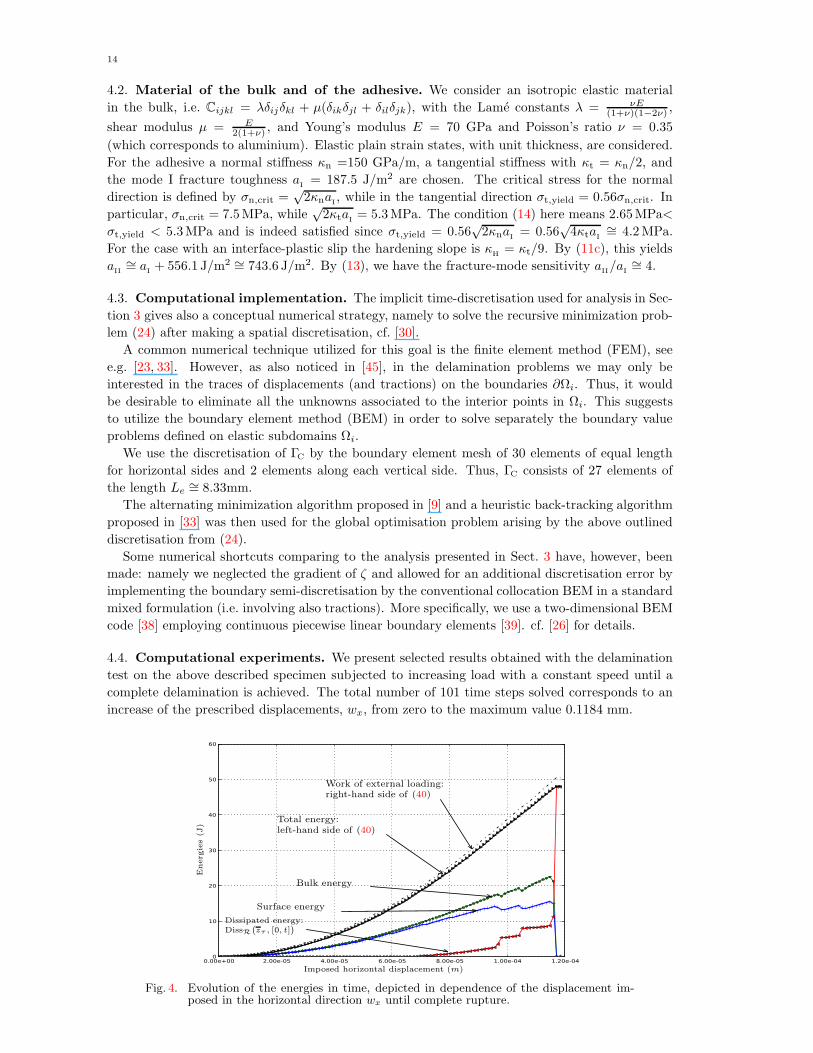
4.2. Material of the bulk and of the adhesive. We consider an isotropic elastic material

in the bulk, i.e. Cijkl = λδijδkl + µ(δikδjl + δilδjk), with the Lame constants λ = νE(1+ν)(1−2ν) ,

shear modulus µ = E2(1+ν) , and Young’s modulus E = 70 GPa and Poisson’s ratio ν = 0.35

(which corresponds to aluminium). Elastic plain strain states, with unit thickness, are considered.

For the adhesive a normal stiffness κn =150 GPa/m, a tangential stiffness with κt = κn/2, and

the mode I fracture toughness aI= 187.5 J/m2 are chosen. The critical stress for the normal

direction is defined by σn,crit =√2κnaI

, while in the tangential direction σt,yield = 0.56σn,crit. In

particular, σn,crit = 7.5MPa, while√2κtaI

= 5.3MPa. The condition (14) here means 2.65MPa<

σt,yield < 5.3MPa and is indeed satisfied since σt,yield = 0.56√2κnaI

= 0.56√4κtaI

∼= 4.2MPa.

For the case with an interface-plastic slip the hardening slope is κH= κt/9. By (11c), this yields

aII∼= a

I+ 556.1 J/m2 ∼= 743.6 J/m2. By (13), we have the fracture-mode sensitivity a

II/a

I∼= 4.

4.3. Computational implementation. The implicit time-discretisation used for analysis in Sec-

tion 3 gives also a conceptual numerical strategy, namely to solve the recursive minimization prob-

lem (24) after making a spatial discretisation, cf. [30].

A common numerical technique utilized for this goal is the finite element method (FEM), see

e.g. [23, 33]. However, as also noticed in [45], in the delamination problems we may only be

interested in the traces of displacements (and tractions) on the boundaries ∂Ωi. Thus, it would

be desirable to eliminate all the unknowns associated to the interior points in Ωi. This suggests

to utilize the boundary element method (BEM) in order to solve separately the boundary value

problems defined on elastic subdomains Ωi.

We use the discretisation of ΓC by the boundary element mesh of 30 elements of equal length

for horizontal sides and 2 elements along each vertical side. Thus, ΓC consists of 27 elements of

the length Le∼= 8.33mm.

The alternating minimization algorithm proposed in [9] and a heuristic back-tracking algorithm

proposed in [33] was then used for the global optimisation problem arising by the above outlined

discretisation from (24).

Some numerical shortcuts comparing to the analysis presented in Sect. 3 have, however, been

made: namely we neglected the gradient of ζ and allowed for an additional discretisation error by

implementing the boundary semi-discretisation by the conventional collocation BEM in a standard

mixed formulation (i.e. involving also tractions). More specifically, we use a two-dimensional BEM

code [38] employing continuous piecewise linear boundary elements [39]. cf. [26] for details.

4.4. Computational experiments. We present selected results obtained with the delamination

test on the above described specimen subjected to increasing load with a constant speed until a

complete delamination is achieved. The total number of 101 time steps solved corresponds to an

increase of the prescribed displacements, wx, from zero to the maximum value 0.1184 mm.

0.00e+00 2.00e-05 4.00e-05 6.00e-05 8.00e-05 1.00e-04 1.20e-040

10

20

30

40

50

60

Energ

ies(J

)

Imposed horizontal displacement (m)

Bulk energy

Surface energy

Dissipated energy:DissR

(

zτ , [0, t])

Total energy:left-hand side of (40)

Work of external loading:right-hand side of (40)

Fig. 4. Evolution of the energies in time, depicted in dependence of the displacement im-posed in the horizontal direction wx until complete rupture.

T.Roubıcek at al.: A quasistatic mixed-mode delamination (Preprint No.2011-020, Necas Center for Math.Modeling, Prague) 15

0.00 0.05 0.10 0.15 0.20 0.25 0.300.00

0.05

0.10

0.15

0.20

0.25

k=75

k=84

k=99

k=75

k=84

k=99

y-coord

inate

[m]

0.12 0.14 0.16 0.18 0.20 0.22 0.240.00e+00

5.00e-06

1.00e-05

1.50e-05

2.00e-05

2.50e-05

3.00e-05

Interface-p

lastic

deform

ation[m

]

k=55

k=59

k=64

k=70

k=75

k=81

k=84

k=90

k=95

k=99

interface-plastic zonefor selected time steps k

x-coordinate [m]

)

@@@R

Fig. 5 Upper: Deformed elastic domain for 3 selected time steps k (displayed with the dis-placements magnified 100x) and a delamination tip zone (in mixed-mode) andalso in the opposite end (in mode I) zoomed in.

Lower: Evolution of the interface-plastic slip depicted on the part of ΓC which delam-inates in mixed-mode for selected time steps k.

The energetics of the delamination process obtained for this case is shown in Fig. 4. After the

delamination of some elements, suddenly the rest of the elements along ΓC break in one time step.

In fact, such a spontaneous-rupture behaviour might be expected, as in a related pull-push shear

test a similar behaviour corresponding to a snap-back instability can be observed [10].

As expected, an interface-plastic zone appears ahead of the crack tip at the end of the delam-

inated zone. The value of the interface-plastic slip at a point ahead of the crack tip is increasing

until the adhesive at this point is broken afterwards the interface-plastic slip therein remains con-

stant. This can be seen in Fig. 5(lower), where the interface-plastic slip is plotted for various time

steps k. The (scaled) deformed shape of the elastic domain Ω is plotted in Fig. 5(upper) for the

some of these time steps.

In Fig. 6 it is shown that an interface-plastic slip takes place at the nodes before a debonding

happens. After the debonding takes place, at a node, the whole energy dissipated at this element

remains constant. It is clear now that the dissipated energy takes values higher than the dissipated

energy needed for delamination in opening mode I given by aI. This can be observed in Fig. 7, where

the ratio r of the accumulated dissipated energy on each element (up to the total delamination of

the adhesive zone ΓC) to the mode I energy aILe is plotted.

16

50 60 70 80 90 1000.0

0.5

1.0

1.5

2.0

2.5

Dissipated

Energ

y(J

/m)

Time step number

aILe

E1

E2

E3

E4

E5

E6

E7

E8

E9E9

E10

Fig. 6. Dissipated energy on elements E1 to E10; for comparison, aILe (=the energy needed for total

break in mode I per length Le) is depicted, too. Nearly all these elements eventually exceedaILe so that they delaminate in mixed-mode.

0510152025301.0

1.1

1.2

1.3

1.4

1.5

1.6

Element number

Ratior

Fig. 7. Ratio r of the dissipated energy on each element to the mode-I energy aIresulted at

the end after its complete delamination; in view of aII/a

I= 3.97, the right-end part was

delaminated in mixed-mode combining about 80% mode I and 20% mode II, while therest ruptured gradually (in the left end of the specimen as displayed in Fig. 5–upper) orspontaneously (in the middle part of the specimen) in pure mode I.

Finally, just for comparison, we also performed the same experiment but with interface-plasticity

suppressed, i.e. π ≡ 0, so that modes I and II coincide with each other. This can be done simply

just by putting the activation threshold σt,yield very large. This model was already treated both

theoretically and computationally in [23]. The analog of Fig. 6 is presented in Fig. 8 where one

can observe rather continuously propagating Griffith-type rupture, i.e. most elements are either

fully bonded or fully debonded; in fact, it can be observed rather in the nodes than in the elements

themselves, which is reflected by the occurrence of the mid-horizontal segments in Fig. 8. For the

infinite stiffnesses of the adhesive (i.e. both κn → ∞ and κt → ∞), this Griffith-like response (i.e. ζ

taking values either 1 or 0 a.e.) can even rigorously be proved, cf. [51, Prop.4.3.3] or [31, Prop.4.4].

For finite (but large) κn and κt, this tendency is thus not suprising, cf. also the mentioned previous

experiments in [23].

T.Roubıcek at al.: A quasistatic mixed-mode delamination (Preprint No.2011-020, Necas Center for Math.Modeling, Prague) 17

50 60 70 80 90 1000.0

0.2

0.4

0.6

0.8

1.0

1.2

1.4

1.6

replacemen

Dissipate

denerg

y(J

)

Time step number

aILe

E1

E2

E3

E4

E5E6

E7

E8

E9

Fig. 8. Comparison with Fig. 6 if interface-plasticity is suppressed so that mode IIdissipates equally as mode I and the dissipated energy, depicted on elementsE1 to E9, cannot exceed a

ILe.

REFERENCES

[1] E. C. Aifantis. On the microstructural origin of certain inelastic models. ASME J. Eng. Mater. Technol.,

106:326–330, 1984.[2] L. Banks-Sills and D. Askenazi. A note on fracture criteria for interface fracture. Intl. J. Fracture, 103:177–188,

2000.[3] Z. Bazant and M. Jirasek. Nonlocal integral formulations of plasticity and damage: Survey of progress. J.

Engrg. Mech., 128(11):1119–1149, 2002.[4] S. Bennati, M. Colleluori, D. Corigliano, and P. Valvo. An enhanced beam-theory model of the asymmetric

double cantilever beam (adcb) test for composite laminates. Composites Science and Technology, 69:1735–1745,2009.

[5] M. A. Biot. Thermoelasticity and irreversible thermodynamics. J. Appl. Phys., 27:240–253, 1956.[6] M. A. Biot. Mechanics of Incremental Deformations. Wiley, New York, 1965.[7] E. Bonetti, G. Bonfanti, and R. Rossi. Well-posedness and long-time behaviour for a model of contact with

adhesion. Indiana Univ. Math. J., 56:2787–2820, 2007.[8] E. Bonetti, G. Bonfanti, and R. Rossi. Global existence for a contact problem with adhesion. Math. Meth.

Appl. Sci., 31:1029–1064, 2008.[9] B. Bourdin, G. A. Francfort, and J.-J. Marigo. Numerical experiments in revisited brittle fracture. J. Mech.

Phys. Solids, 48:797–826, 2000.[10] P. Cornetti and A. Carpinteri. Modelling the FRP-concrete delamination by means of an exponential softening

law. Engineering Structures, 33:1988–2001, 2011.[11] G. Dal Maso, G. Francfort, and R. Toader. Quasistatic crack growth in nonlinear elasticity. Arch. Rational

Mech. Anal., 176:165–225, 2005.[12] A. Evans, M. Ruhle, B. Dalgleish, and P. Charalambides. The fracture energy of bimaterial interfaces. Metal-

lurgical Transactions A, 21A:2419–2429, 1990.[13] M. Fremond. Dissipation dans l’adhrence des solides. C.R. Acad. Sci., Paris, Ser.II, 300:709–714, 1985.[14] M. Fremond. Contact with adhesion. In J. Moreau and G. Panagiotopoulos, editors, Topics in Nonsmooth

Mechanics. Birkhauser, 1988.[15] M. Fremond. Non-Smooth Thermomechanics. Springer-Verlag, Berlin, 2002.[16] M. Fremond and B. Nedjar. Damage, gradient of damage and principle of virtual power. Internat. J. Solids

Structures, 33:1083–1103, 1996.[17] E. Fried and M. Gurtin. Tractions, balances, and boundary conditions for nonsimple materials with application

to liquid flow at small-length scales. Arch. Rational Mech. Anal., 182:513–554, 2006.[18] A. Griffith. The phenomena of rupture and flow in solids. Philos. Trans. Royal Soc. London Ser. A. Math.

Phys. Eng. Sci., 221:163–198, 1921.[19] W. Han and B. D. Reddy. Plasticity (Mathematical Theory and Numerical Analysis). Springer-Verlag, New

York, 1999.[20] J. W. Hutchinson and Z. Suo. Mixed mode cracking in layered materials. Advances in Applied Mechanics,

29:63–191, 1992.[21] M. Jirasek and J. Zeman. Localization study of non-local energetic damage model. ArXiv e-prints (no:

0804.3440v1), 2008.[22] D. Knees, A. Mielke, and C. Zanini. On the inviscid limit of a model for crack propagation. Math. Models Meth.

Appl. Sci. (M3AS), 18:1529–1569, 2008.[23] M. Kocvara, A. Mielke, and T. Roubıcek. A rate-independent approach to the delamination problem. Math.

Mechanics Solids, 11:423–447, 2006.[24] K. Liechti and Y. Chai. Asymmetric shielding in interfacial fracture under in-plane shear. J. Appl. Mech.,

59:295–304, 1992.

18

[25] V. Mantic. Discussion on the reference length and mode mixity for a bimaterial interface. J. Engr. Mater.Technology, 130:045501–1–2, 2008.

[26] V. Mantic, C. Panagiotopoulos, and T. Roubıcek. Associative quasistatic mixed-mode delamination model andits BEM implementation. In preparation.

[27] A. Mielke. Evolution in rate-independent systems (Ch. 6). In C. Dafermos and E. Feireisl, editors, Handbookof Differential Equations, Evolutionary Equations, vol. 2, pages 461–559. Elsevier B.V., Amsterdam, 2005.

[28] A. Mielke. Differential, energetic and metric formulations for rate-independent processes. In L. Ambrosio andG. Savare, editors, Nonlinear PDEs and Applications, pages 87–170. Springer, 2010.

[29] A. Mielke and T. Roubıcek. Rate-independent damage processes in nonlinear elasticity. Math. Models Meth.Appl. Sci., 16:177–209, 2006.

[30] A. Mielke and T. Roubıcek. Numerical approaches to rate-independent processes and applications in inelasticity.Math. Model. Numer. Anal. (M2AN), 43:399–428, 2009.

[31] A. Mielke, T. Roubıcek, and M. Thomas. From damage to delamination in nonlinearly elastic materials at smallstrains. J. Elasticity, 2010. Submitted. WIAS preprint 1542.

[32] A. Mielke, T. Roubıcek, and U. Stefanelli. Γ-limits and relaxations for rate-independent evolutionary problems.Calc. Var. Part. Diff. Eqns., 31:387–416, 2008.

[33] A. Mielke, T. Roubıcek, and J. Zeman. Complete damage in elastic and viscoelastic media and its energetics.Computer Methods Appl. Mech. Engr., 199:1242–1253, 2009.

[34] A. Mielke and F. Theil. A mathematical model for rate-independent phase transformations with hysteresis.In H.-D. Alber, R. Balean, and R. Farwig, editors, Proceedings of the Workshop on “Models of ContinuumMechanics in Analysis and Engineering”, pages 117–129, Aachen, 1999. Shaker-Verlag.

[35] A. Mielke and F. Theil. On rate-independent hysteresis models. Nonl. Diff. Eqns. Appl. (NoDEA), 11:151–189,2004. (Accepted July 2001).

[36] A. Mielke, F. Theil, and V. I. Levitas. A variational formulation of rate–independent phase transformationsusing an extremum principle. Arch. Rational Mech. Anal., 162:137–177, 2002.

[37] M. Negri and C. Ortner. Quasi-static crack propagation by Griffith’s criterion. Math. Models Methods Appl.Sci., 18(11):1895–1925, 2008.

[38] C. Panagiotopoulos. Open BEM Project. http://www.openbemproject.org/, 2010.[39] F. Parıs and J. Canas. Boundary Element Method, Fundamentals and Applications. Oxford University Press,

Oxford, 1997.[40] P. Podio-Guidugli and G. Vergara Caffarelli. Surface interaction potentials in elasticity. Arch. Rat. Mech. Anal.,

109:343–381, 1990.[41] N. Point. Unilateral contact with adherence. Math. Methods Appl. Sci., 10:367–381, 1988.[42] N. Point and E. Sacco. A delamination model for laminated composites. Math. Methods Appl. Sci., 33:483–509,

1996.[43] N. Point and E. Sacco. Mathematical properties of a delamination model. Math. Comput. Modelling, 28:359–

371, 1998.

[44] R. Rossi and T. Roubıcek. Adhesive contact delaminating at mixed mode, its thermodynamics and analysis.Preprints: No.26/2011 at Univ. Brescia, and on arxiv:1110.2794. Interfaces and Free Boundaries. submitted.

[45] T. Roubıcek, M. Kruzık, and J. Zeman. Delamination and adhesive contact models and their mathematicalanalysis and numerical treatment. In Math. Methods & Models in Composites, chapter 13. (V. Mantic, ed.)Imperial College Press, ISBN: 978-1-84816-784-1, to appear in 2012.

[46] T. Roubıcek, L. Scardia, and C. Zanini. Quasistatic delamination problem. Cont. Mech. Thermodynam., 21:223–235, 2009.

[47] J. Simo and T. Hughes. Computational Inelasticity. Springer, New York, 1998.[48] J. Swadener, K. Liechti, and A. deLozanne. The intrinsic toughness and adhesion mechanism of a glass/epoxy

interface. J. Mech. Phys. Solids, 47:223/258, 1999.[49] L. Tavara, V. Mantic, E. Graciani, J. Canas, and F. Parıs. Analysis of a crack in a thin adhesive layer between

orthotropic materials: An application to composite interlaminar fracture toughness test. CMES - ComputerModeling in Engineering and Sciences, 58:247–270, 2010.

[50] L. Tavara, V. Mantic, E. Graciani, and F. Parıs. BEM analysis of crack onset and propagation along fiber-matrix interface under transverse tension using a linear elastic-brittle interface model. Engineering Analysiswith Boundary Elements, 35:207–222, 2011.

[51] M. Thomas. Rate-independent damage processes in nonlinearly elastic materials. PhD thesis, Institut fur Math-ematik, Humboldt-Universitat zu Berlin, 2010.

[52] M. Thomas. Quasistatic damage evolution with spatial bv-regularization. (submitted), Preprint No. 1638,WIAS, Berlin, 2011.

[53] M. Thomas and A. Mielke. Damage of nonlinearly elastic materials at small strain – Existence and regularityresults –. Z. angew. Math. Mech. (ZAMM), 90(2):88–112, 2010.

[54] R. Toader and C. Zanini. An artificial viscosity approach to quasistatic crack growth. Boll. Unione Matem.Ital., 2(1):1–36, 2009.

[55] R. Toupin. Elastic materials with couple stresses. Arch. Rat. Mech. Anal., 11:385–414, 1962.[56] V. Tvergaard and J. Hutchinson. The influence of plasticity on mixed mode interface toughness. J. Mech. Phys.

Solids, 41:1119–1135, 1993.