A Probabilistic Gas Patch Path Prediction Approach

for Airborne Gas Source Localization

in Non-Uniform Wind Fields

Patrick P. Neumann*,a

, Michael Schnürmacherb, Victor Hernandez Bennetts

c,

Achim J. Lilienthalc, Matthias Bartholmai

a, and Jochen H. Schiller

b

a BAM Federal Institute for Materials Research and Testing, Berlin D-12205, Germany.

b Institute of Computer Science, FU University, Berlin D-14195, Germany.

c Centre for Applied Autonomous Sensor Systems, Örebro University, SE-70182. Orebro, Sweden.

* Corresponding author

Tel.: +49 30 8104 3629

Fax: +49 30 8104 1917

E-Mail: patrick.neumann@bam.de

2

Abstract - In this paper, we show that a micro unmanned aerial vehicle (UAV) equipped with commercially available gas sensors can address

environmental monitoring and gas source localization (GSL) tasks. To account for the challenges of gas sensing under real-world conditions,

we present a probabilistic approach to GSL that is based on a particle filter (PF). Simulation and real-world experiments demonstrate the

suitability of this algorithm for micro UAV platforms.

Keywords - autonomous micro UAV, chemical and wind sensing, gas source localization, particle filter.

3

I. INTRODUCTION

In order to perform GSL tasks in real-world scenarios, gas sensors are mounted on mobile platforms and exposed to a highly dynamic

environment. Besides the drawbacks in current sensing technologies (partial selectivity, slow recovery times, response drift)1, gas sensing in

outdoor environments poses several challenges, such as turbulent gas dispersion, non-uniform wind flows, fluctuating environmental

conditions and, in the case of gas sensing with quadrocopter-based micro UAVs, plume disruptions induced by the rotors. To account for

these challenges, robust GSL algorithms have to be developed. In this work, we present a probabilistic GSL approach based on a PF. The

approach was first introduced in Ref. 2 for plume tracking on a gas-sensitive micro UAV. This paper extends Ref. 2 by presenting a thorough

performance evaluation of the PF in terms of source localization accuracy. Furthermore, the algorithm is tested and analyzed with two

different exploration strategies: plume tracking (as in Ref. 2) and predefined sweeping trajectories. In order to quantify the non-uniformity of

natural wind flows, we additionally present an experiment where data was collected during several hours with two anemometers placed in an

open field.

This paper is structured as follows, we first show in Sec. II the non-uniformity of the wind field. Then, we introduce in Sec. III the GSL

algorithm based on a PF. Next, we present the gas-sensitive micro UAV that is used in this work (Sec. IV). Finally, we evaluate the

performance of the PF-based algorithm in simulations and real-world experiments (Secs. V and VI), and draw conclusions (Sec. VII).

II. NON-UNIFORMITY OF THE WIND FIELD

The GSL problem can be simplified by assuming a uniform wind field. This simplification allows to infer the paths traveled by the gas

patches using wind and concentration measurements collected along the exploration path. Li et al. reported in Ref. 3 that a time-varying wind

field can be regarded as roughly uniform within a circular domain around the robot, when the airflow is not too weak (above 0.2 m/s) and the

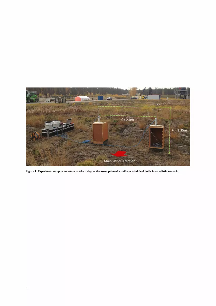
radius of this domain is not too large (less than the distance traveled by the airflow in 10 s). Here, an experiment over a time period of 83min

with two ultrasonic anemometers (uSonic-3 Scientific, Metek GmbH, Germany) set to a sampling frequency of 1 Hz was performed to

investigate to which degree the assumption made by Li and co-authors holds. The anemometers were placed in a distance of approx. 2 m to

each other at a height of approx. 1.35 m (Fig. 1).

Our experiment shows that the term "roughly uniform wind field" has to be considered with reasonable care. The Pearson coefficient r for

the wind speed ) and the circular-circular correlation index for directional data ( ) show a relatively strong

correlation of the wind data in the environment considered. At the same time, however, the two anemometers exhibit strong instantaneous

differences in the measured values up to 2.5 m/s (wind speed) and 179° (wind direction). More experiments are needed especially to

generalize to a larger class of environments.

III. PARTCLIE FILTER-BASED GAS SOURCE LOCALIZATION

The presented PF-based GSL algorithm uses gas and wind measurements to reason about the trajectory of a gas patch since it was released

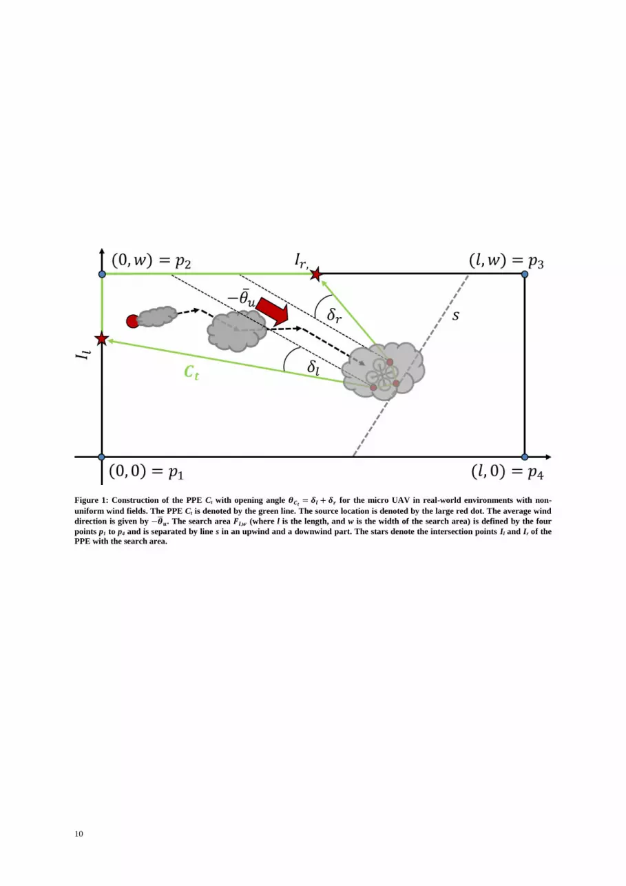
by the gas source. Non-uniform wind fields are accounted for by considering a patch path envelope (PPE) that models the likelihood of

trajectories along which a sensed gas patch may have moved to the sensor (Fig. 2). The source is considered to be found (declared), if the

location estimate, represented by the particles of the PF, remains within a small region for a defined number of iterations. The key advantage

of the proposed approach is that it does not make any strong assumption about the uniformity of the wind field.

4

A. SENSOR DATA PREPROCESSING

1) GAS SENSOR: To decide whether the robot was within the plume or not, a binary concentration measure zt with an adaptive threshold ̅

as proposed by Li et al.3 was used. As proposed in Ref. 3, the parameter of the adaptive threshold ̅ is set to 0.5 during all experiments to

respond correctly in time to all gas-detection events.

2) WIND SENSOR: At each iteration t, the averaged wind direction ̅ and the circular wind direction variance S0 are computed from a set

of single wind measurements taken at the current measuring position. The circular variance is used to consider the non-regularities of the

wind flow direction in the construction process of the PPE.

B. CONSTRUCTION OF THE PPE

The PPE describes the envelope of the most probable area the gas patch has moved through and is updated based on the new location of the

robot and the new measurements of the local wind. The opening angle of the PPE depends on the degree of stability of the wind direction.

Stable wind conditions result in small opening angles, whereas unstable and changing wind conditions result in large opening angles. In this

way, the assumption of a uniform wind field is relaxed. However, some level of wind uniformity is assumed in the update step of the PF,

where, e.g., the gas source location is assumed to be in the upwind direction based on the local wind measurements during a gas-detection

event (see Sec. III.B – particle classification).

To consider the measurement radius of the micro UAV due to the rotor movement the first segment of the PPE is modeled as a simple

triangle with its right angle in downwind direction given by the averaged wind measurements. Finally, the output of this stage is a polygon as

shown in Fig. 2 delimiting the PPE Ct.

C. PF-BASED GSL ALGORITHM

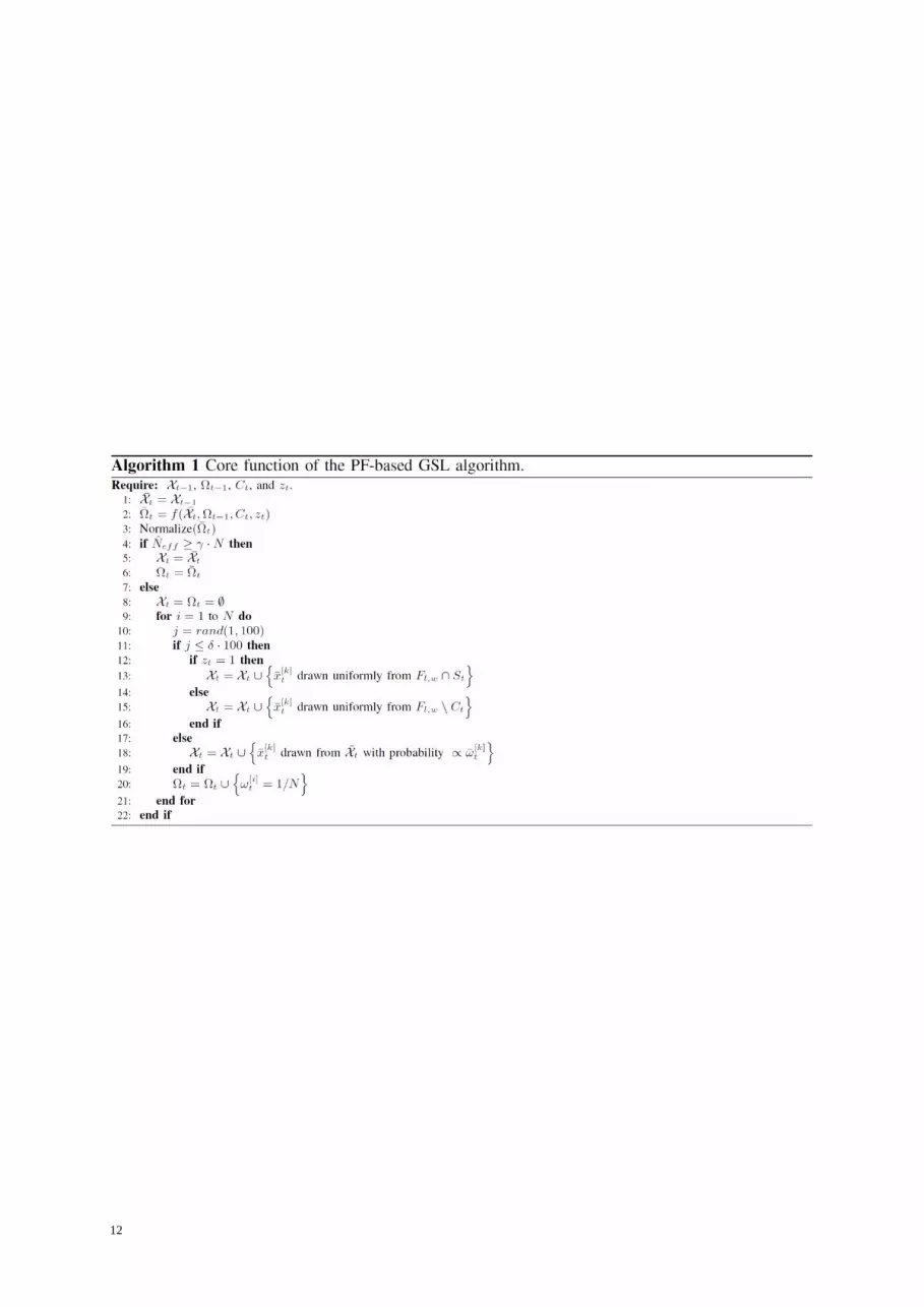
Algorithm 1 provides a formal description of the core function of the suggested PF-based GSL algorithm. The input is the particle set

with weights , along with the most recent calculated PPE Ct (Sec. III.B) and the most recent binary concentration measurement zt

(Sec. III.A).

Line 1 implements the PF prediction step. As the location of a static gas source is of interest only, the particle sets and are set to be

identical.

Line 2 implements the measurement update. The new importance weights are computed based on Eq. 1 that considers the old importance

weights , the relative position of a particle with respect to the PPE Ct and line s (orthogonal to the averaged wind direction), and the

binary concentration measurement zt. The particles are classified in one of the following three classes: (a) particles located inside the PPE, (b)

particles located outside the PPE in upwind direction*, and (c) particles located outside the PPE in downwind direction* (*with respect to

line s).

{

)

)

)

)

)

)

(1)

where ) and ) are meta-parameters, which adjust the contribution of the old importance weight

of particle

at

iteration t to the new importance weight

, and is the opening angle of the first segment of the PPE. A further penalization

of the particles is implemented by the square of and , respectively. In general, a smaller value of and leads to a higher penalization

5

than a larger value (e.g., a value of 1 means no penalization). The term ⁄ in Eq. 1 penalizes particles in dependency of the stability of

the wind2.

Line 3 normalizes the importance weights so that the total weight is 1 after each step.

Line 4 checks, whether the effective sample size ̂ defined by Liu et al.4 has dropped under a predefined threshold ) and

resampling has to be performed or not4. If resampling is not necessary, the temporary sets ̅ and are the result sets (lines 5 to 6).

Lines 8 to 21 implement the resampling step of the PF, which is applied to deal with the weight degeneracy problem of PF algorithms. Here,

the new particle set is built. A particle ̅

is drawn with probability uniformly from the area , if , and from the search

area , if (see lines 11 to 16), where defines the area in upwind direction of the micro UAV and is the search area

(Fig. 2). A particle ̅

is drawn with probability from ̅ according to its importance ̅

(line 18). Finally, the importance weights

of all re-sampled particles are set to (line 20).

In the beginning, each particle

is initialized with the weight

and the position

) drawn uniformly from the search area

, if no a priori knowledge about the gas source location is given.

D. ESTIMATION OF THE GAS SOURCE

The particle set can be used to estimate the location of the gas source ̅ . A simple strategy could be to calculate the weighted mean over

all particles. However, observations have shown that the weighted mean is often not a good estimator since it is strongly affected by outliers

(which in addition occur frequently as a consequence of resampling).

A more sophisticated strategy involves analyzing the particle clusters that have evolved over time. The proposed strategy searches the

particle

with the highest number of neighbors within a certain radius , i.e., the k for which

|{

| |

| }|

is maximized. In the current implementation, is set to 0.5 m. This particle

is called the Maximum Neighbors Estimate (MNE) and is

used as the gas source location estimate.

IV. ROBOTIC PLATFORM

The AirRobot AR100-B quadrocopter-based micro UAV (AirRobot GmbH & Co. KG, Germany) has a diameter of 1 m and is driven by four

brushless electric motors. The micro UAV was modified to incorporate gas-sensitive devices. Since wind information is of high importance

for gas-sensitive robots, the wind vector is estimated by fusing the micro UAV’s on-board sensors to compute the parameters of the wind

triangle5. A more detailed description of the gas-sensitive micro UAV can be found in Ref. 5.

V. SIMULATION EXPERIMENTS

A. EXPERIMENT SETUP

In order to evaluate the performance of the PF-based GSL algorithm, we optimized the parameters and in

simulations with respect to the average localization error and the success rate for datasets collected with two different control algorithms: the

pseudo gradient algorithm2 and sweeping. The localization error is defined as the distance between the true gas source location and the MNE.

The success rate is the ratio of successful localizations with respect to the total number of performed experiments, in which the localization

error is less or equal than 1.5 m.

As a simulation environment, we use the filament-based gas dispersion model presented in Ref. 6. The micro UAV and its sensing

mechanisms were modeled using data obtained from laboratory and real-world experiments as explained in Ref. 2. Thus, the proposed

6

algorithm is optimized especially for the robotic platform used and its measuring capabilities and characteristics. A detailed description of

the parameters of the experiment setup can be found in Ref. 2.

The parameters and (both related to the PF-based GSL algorithm) were set heuristically to 0.5 and 0.1, respectively. The number of

particles was set to 1,000. For each control algorithm, each experiment was repeated 100 times.

B. EXPERIMENTAL RESULTS

It was found out that the average localization error decreases strongly with increasing . On the other hand, the average localization error

increases with increasing . Thus, it seems to be beneficial to choose a small value for and a large value for (i.e., ). This means

that, in case of a gas-detection event, the particles which are located outside the PPE receive a higher penalization than, in case of a non-

detection event, the particles which are located in upwind direction of line s. This position-dependent penalization of the particles allows

them to accumulate at the location of the gas source and its close proximity.

A good parameter set for the gradient-based algorithm which minimizes the average localization error and maximizes the success rate is

found to be ) ), i.e., that the success rate drops if gets too small or gets too large. The average error is only

0.96 m ± 1.01 m with a success rate of 86%. A good parameter set for sweeping is ) ). The average localization error here is

0.79 m ± 0.46 with a success rate of 95%.

A possible explanation for the different optimal meta-parameters of each control algorithm can be seen in the number of measurements taken

inside the plume. A plume tracking strategy tries to stay within the plume and switches only to sweeping when the plume cannot be

reacquired, whereas sweeping is based on a predefined trajectory.

To validate the determined meta-parameter sets for each control algorithm, a total of six different source positions were tested. Fig. 3 shows

the corresponding results after the last measurement point for both control algorithms. The success rates using the gradient-based algorithm

are in the range of 76 to 89%. The average error of successful localizations was similar for all source positions (≤ 0.62 m ± 0.37 m) except

for source number #2 and #3, where this error is slightly higher (0.97 m ± 0.31 m and 1.11 m ± 0.37 m). The success rates using sweeping

are in the range of 81 to 92%. The average error of successful localizations was similar for almost all source positions and is

≤ 0.80 m ± 0.37 m. An exception is source number #2, where this error is slightly higher (≤ 0.98 m ± 0.36 m).

The results are good considering the slow response of the modeled gas sensor and the relatively high GPS positioning error of the micro

UAV (±1.17 m). In the current state of the algorithm, it seems that sweeping is a better strategy to use with the PF-based GSL algorithm as

the gradient-based control algorithm due to the above mentioned reasons.

However, this approach has to be validated in further experiments showing that the presented PF-based GSL algorithm is capable of working

reliably in a variety of non-uniform wind fields.

VI. REAL-WORLD EXPERIMENTS

A. EXPERIMENT SETUP

The real-world experiments were carried out in two outdoor environments. An electronic nose was used for all experiments performed with

methane (metal oxide – CH4) and for three trials performed with carbon dioxide (electrochemical – CO2). For the remaining trials, a payload

based on a commercially available gas detector was used (infrared – CO2). A gas cylinder connected via a small tube to a fan (in order to

spread the analyte away) was used as the gas source during all experiments and placed within the experiment area. The size of the

experiment area varied from m2 to m2. To be more specific, the plume tracking trials were performed over an experiment area

of m². Sweeping, on the other hand, was performed over the following experiment area sizes: m² (3 trials), m² (2 trials),

m² (6 trials), and m² (2 trials). A detailed description of the experiment setup can be found in Ref. 2.

7

As in the simulation experiments, the parameters were set to , , and . The localization error and the success rate

are defined in the same way as in the simulation experiments.

B. EXPERIMENT RESULT

A total number of 19 trials were performed using plume tracking (surge-cast7, zigzag8, and pseudo gradient2) and predefined sweeping

trajectories. The PF-based GSL algorithm was able to locate the gas source with a success rate of 83.3% (5 of 6 trials succeeded) using

plume tracking and 92.3% (12 of 13 trials succeeded) using predefined sweeping trajectories. The average error of successful localizations is

0.69 m ± 0.35 m and 0.79 m ± 0.38 m, respectively. This result is very good considering, e.g., the GPS error of the micro UAV (±1.17 m)

and is in line with the simulation results. However, it seems that in the real-world experiments sweeping is not necessarily the better option

regarding the localization accuracy.

Unfortunately, the small number of experiments does not permit to obtain strong statistical significance of the performance of the algorithm.

However, the results indicate the potential of this approach for localizing gas emission sources and its suitability for a gas-sensitive

micro UAV.

VII. CONCLUSIONS

This work presents a PF-based GSL algorithm for a gas-sensitive micro UAV to estimate the location of a single gas source that is

independent of the exploration strategy used. In simulations, we optimize for two exploration strategies the meta-parameters of the proposed

algorithm for a gas-sensitive micro UAV. Next, we use the best meta-parameters sets found in simulation for the real-world experiments with

this gas-sensitive micro UAV. The results indicate the potential of the algorithm for accurately localizing a single gas emission source

emitting a known chemical compound in realistic environments with a micro UAV. Furthermore, the results suggest that the different gas

sensor technologies used did not have a major impact on the success rate and the localization error. In general, a good correlation between

the results from simulation and real-world experiments was found for both exploration strategies. Furthermore, we present an outdoor

experiment that shows the non-uniformity of the wind in the environment presented (an open field, with sparse vegetation, and surrounded

by trees). In this case, the assumption of a roughly uniform wind field by Li et al.3 does not hold. Further experiments need to be performed

in different environments for a better characterization and classification of wind fields.

ACKNOWLEDGMENT

The authors thank the participating colleagues from BAM and Örebro University. They also express their gratitude to BMWi (MNPQ

Program; file number 28/07) and Robotdalen (Gasbot, project number 8140) for funding the research.

8

BIBLIOGRAPHY

1. M. Trincavelli, Ph.D. Thesis, Örebro University, (2010).

2. P. P. Neumann, V. Hernandez Bennetts, A. J. Lilienthal, M. Bartholmai, and J. H. Schiller, in Advanced Robotics (AR), (2013),

vol. 27, no. 9, p. 1-14.

3. J.-G. Li, Q.-H. Meng, Y. Wang, and M. Zeng, in Auton. Robots, (2011), vol. 30, no. 3, p. 281-292.

4. J. Liu, R. Chen, and T. Logvinenko, in Sequential Monte Carlo Methods in Practice, (2001), p. 225-242.

5. P. Neumann, S. Asadi, A. J. Lilienthal, M. Bartholmai, and J. Schiller, in IEEE Robotics and Automation Magazine (RAM),

(2012), vol. 19, no. 4, p. 50-61.

6. S. Pashami, S. Asadi, and A. J. Lilienthal, in Proceedings of the Open Source CFD International Conference, Munich,

Germany, (2010).

7. T. Lochmatter, Ph.D. Thesis, EPFL, Lausanne, Switzerland, (2010).

8. H. Ishida, K. Suetsugu, T. Nakamoto, and T. Moriizumi, in Sensors and Actuators A, (1994), vol. 45, p. 153-157.

9

Figure 1: Experiment setup to ascertain to which degree the assumption of a uniform wind field holds in a realistic scenario.

10

Figure 1: Construction of the PPE Ct with opening angle for the micro UAV in real-world environments with non-

uniform wind fields. The PPE Ct is denoted by the green line. The source location is denoted by the large red dot. The average wind

direction is given by ̅ . The search area (where l is the length, and w is the width of the search area) is defined by the four

points p1 to p4 and is separated by line s in an upwind and a downwind part. The stars denote the intersection points Il and Ir of the

PPE with the search area.

11

(a) Gradient-based: and

(b) Sweeping: and

Figure 3: Box-plot of the gas source location estimate (distance to true source location) for the seven source locations using (a) the

gradient-based algorithm and (b) sweeping. The red dot denotes the source used for the parameter study. The box shows the

lower/upper quartile and the line denotes the median. The mean is denoted by the small . The whiskers represent data lying

outside the box such that the lowest value is still within 1.5 (interquartile range) of the lower quartile and the highest value is

still within 1.5 of the upper quartile. The stands for outliers with values larger than 1.5 .

12