arX

iv:h

ep-t

h/07

0311

1v1

12

Mar

200

7

UUITP-04/07

HIP-2007-12/TH

YITP-SB-07-09

A potential for Generalized Kahler

Geometry

Ulf Lindstroma,b, Martin Rocekc, Rikard von Unged, and Maxim Zabzinea

aDepartment of Theoretical Physics Uppsala University,

Box 803, SE-751 08 Uppsala, Sweden

bHIP-Helsinki Institute of Physics, University of Helsinki,

P.O. Box 64 FIN-00014 Suomi-Finland

cC.N.Yang Institute for Theoretical Physics, Stony Brook University,

Stony Brook, NY 11794-3840,USA

dInstitute for Theoretical Physics, Masaryk University,

61137 Brno, Czech Republic

Abstract

We show that, locally, all geometric objects of Generalized Kahler Geometry can be derived

from a function K, the “generalized Kahler potential”. The metric g and two-form B are

determined as nonlinear functions of second derivatives of K. These nonlinearities are

shown to arise via a quotient construction from an auxiliary local product (ALP) space.

1 Introduction

Generalized Kahler Geometry [1] is a special and particularly interesting example of Gen-

eralized Geometry [2, 1]. It succinctly encodes the bihermitean geometry of Gates, Hull

and Rocek [3] in terms of a pair of commuting generalized complex structures (J1,J2).

Here we use the equivalent bihermitean data to give a complete (local) description of

Generalized Kahler Geometry. We show that there exists a function K with the interpre-

tation of a generating function for symplectomorphisms between two sets of coordinates in

terms of which all geometric quantities may be described. In particular, the combination

E = 12(g+B) of the metric and antisymmetric B-field is given as a nonlinear expression in

terms of second derivatives of K. When further analyzed, this expression has the structure

of a quotient from some higher dimensional space. We find this auxiliary space, which

we call an ALP space, and display the quotient structure. Finding a Generalized Kahler

Geometry is thus reduced to a linear construction in terms of the corresponding K on the

ALP.

The bihermitean geometry was first derived as the target space geometry of N = (2, 2)

supersymmetric nonlinear sigma models [3]. Correspondingly, all our constructions have a

sigma model realization, and many of the proofs were derived in that setting. In particular,

the “generalized Kahler potential” K has an interpretation as the superspace sigma model

Lagrangian1. Detailed descriptions of this approach may be found in the two articles on

which the presentation is based [5, 6].

2 Generalized Complex Geometry (GCG)

This section contains a brief recapitulation of the salient features of GCG. The references

for the mathematical aspects are chiefly [2, 1], while a presentation more accessible to

physicists (containing, e.g., coordinate and matrix descriptions) may be found in [7, 8].

A generalized almost complex structure is an algebraic structure on the sum of the

tangent and cotangent bundles of a manifold M defined via

J ∈ End(T ⊕ T ∗) (2.1)

such that

J 2 = −1 (2.2)

and

J tIJ = I (2.3)

1A similar situation arises in the projective superspace description of hyperkahler sigma models [4].

1

where I is the metric corresponding to the natural pairing of elements X+η, Y +λ ∈ T⊕T ∗:

< X + η, Y + λ >= 12(ıXλ + ıY η) . (2.4)

The generalized almost complex structure is a (twisted) generalized complex structure iff

it is integrable with respect to the (twisted) Courant bracket

[X + η, Y + λ]C := [X, Y ]L + LXλ − LY η − 12d(ıXλ − ıY η) + ıX ıY H (2.5)

where [X, Y ]L is the Lie-bracket and “twisted” refers to inclusion of the last term involving

the closed three-form H . Integrability is defined by the requirement that the distributions

defined by the projection operators

12(1 ± iJ ) (2.6)

are involutive with respect to the Courant-bracket. Of great importance to physical ap-

plications is the fact that the automorphisms of the Courant-bracket, in addition to dif-

feomorphisms, also contain the b-transform:

eb(X + η) = X + η + ıXb (2.7)

where b is a closed two-form: db = 0. When acting on a generalized complex structure

J it produces an equivalent generalized complex structure Jb. In a matrix representation

this reads;

Jb =

(

1 0

b 1

)

J

(

1 0

−b 1

)

(2.8)

We now restrict our attention to a subset of generalized complex geometries: generalized

Kahler geometries (GKG). These are GCG’s with two commuting generalized complex

structures J1,2 whose product defines a positive definite metric G on T ⊕ T ∗ that squares

to the identity [1];

[J1,J2] = 0

G = −J1J2

G2 = 1 (2.9)

This is the proper setting for the bihermitean geometry of [3], which we now describe.

2

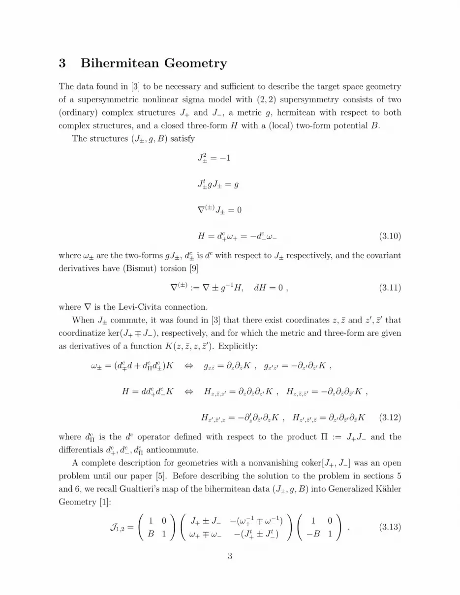
3 Bihermitean Geometry

The data found in [3] to be necessary and sufficient to describe the target space geometry

of a supersymmetric nonlinear sigma model with (2, 2) supersymmetry consists of two

(ordinary) complex structures J+ and J−, a metric g, hermitean with respect to both

complex structures, and a closed three-form H with a (local) two-form potential B.

The structures (J±, g, B) satisfy

J2± = −1

J t±gJ± = g

∇(±)J± = 0

H = dc+ω+ = −dc

−ω− (3.10)

where ω± are the two-forms gJ±, dc± is dc with respect to J± respectively, and the covariant

derivatives have (Bismut) torsion [9]

∇(±) := ∇± g−1H, dH = 0 , (3.11)

where ∇ is the Levi-Civita connection.

When J± commute, it was found in [3] that there exist coordinates z, z and z′, z′ that

coordinatize ker(J+∓J−), respectively, and for which the metric and three-form are given

as derivatives of a function K(z, z, z, z′). Explicitly:

ω± = (dc∓d + dc

Πdc±)K ⇔ gzz = ∂z∂zK , gz′z′ = −∂z′∂z′K ,

H = ddc+dc

−K ⇔ Hz,z,z′ = ∂z∂z∂z′K , Hz,z,z′ = −∂z∂z∂z′K ,

Hz′,z′,z = −∂′z∂z′∂zK , Hz′,z′,z = ∂z′∂z′∂zK (3.12)

where dcΠ is the dc operator defined with respect to the product Π := J+J− and the

differentials dc+, dc

−, dcΠ anticommute.

A complete description for geometries with a nonvanishing coker[J+, J−] was an open

problem until our paper [5]. Before describing the solution to the problem in sections 5

and 6, we recall Gualtieri’s map of the bihermitean data (J±, g, B) into Generalized Kahler

Geometry [1]:

J1,2 =

(

1 0

B 1

)(

J+ ± J− −(ω−1+ ∓ ω−1

− )

ω+ ∓ ω− −(J t+ ± J t

−)

)(

1 0

−B 1

)

. (3.13)

3

G =

(

1 0

B 1

)(

0 g−1

g 0

)(

1 0

−B 1

)

(3.14)

Note that what looks like a b-transform is not, since dB = H 6= 0.

It is an interesting fact that if we introduce the usual GCS’s corresponding to J±;

J± =

(

J± 0

0 −J t±

)

(3.15)

the map (3.13) may be summarized as2

J1,2 = Π+J+B ± Π−J−B , (3.16)

with

Π± := 12(1 ± G) . (3.17)

4 Poisson-structures

There are three Poisson-structures relevant to our discussion. We first consider two real

ones:

π± := (J+ ± J−)g−1 = −g−1(J+ ± J−)t . (4.18)

These were introduced in [10], where they were used essentially as described below, sim-

plifying an earlier derivation in [11]. They ensure the existence of coordinates adapted to

ker(J+ − J−) ⊕ ker(J+ + J−).

In a neighborhood of a regular point x0 of π− we may choose coordinates xA whose

tangents lie in the kernel of π−:

πAµ− = 0,⇒ JA

+µ = JA−µ . (4.19)

Similarily, in a neighborhood of a regular point of π+ we have coordinates xA′

such that

πA′µ+ = 0,⇒ JA′

+µ = −JA′

−µ (4.20)

It then follows from the nondegeneracy of π+ ± π− that the Poisson brackets defined by

π+ and by π− cannot have common Casimir functions. In other words, the directions A

and A′ cannot coincide. The result is that we may write

J± =

∗ ∗ ∗ ∗

∗ ∗ ∗ ∗

0 0 Ic 0

0 0 0 ±It

, (4.21)

2This structure is related to how the map is derived in chapter 6 of [1]

4

in coordinates adapted to

ker(J+ − J−) ⊕ ker(J+ + J−) ⊕ coker[J+, J−] , (4.22)

where we write a canonical complex structure as

I =

(

i 0

0 −i

)

(4.23)

and c labels the A and t labels the A′ directions.

A third Poisson structure σ, related to the real Poisson structures, was introduced in

[12].

σ := [J+, J−]g−1 = ±(J+ ∓ J−)π± = ∓(J+ ± J−)π∓ . (4.24)

The relation to π± implies that

ker σ = ker π+ ⊕ ker π− . (4.25)

Tangents to the symplectic leaf for σ lie in coker[J+, J−]. Using (4.25), we can use σ to

investigate the remaining directions in (4.21). We need that

J±σJ t± = −σ ⇒ σ = σ(2,0) + σ(0,2) , (4.26)

with the decomposition with respect to both J+ and J−. Further σ(2,0) is holomorphic [12]:

∂σ(2,0) = 0 , (4.27)

We now investigate the structure of the cokernel.

5 The structure of coker[J+, J−]

It is convenient to first treat the case ker[J+, J−] = ∅. Then we have at our disposal a

symplectic form Ω:

Ω := σ−1 , dΩ = 0, J t±ΩJ± = −Ω . (5.28)

Choosing complex coordinates with respect to J+,

J+ =

(

Is 0

0 Is

)

, (5.29)

with I as in (4.23), we have the decomposition

Ω = Ω(2,0)+ + Ω

(0,2)+ . (5.30)

5

and

∂Ω(2,0)+ = 0 , ∂Ω

(2,0)+ = 0 , (5.31)

which means in particular that Ω(2,0)+ is holomorphic. We may then choose Darboux

coordinates such that

Ω(2,0)+ = dqa ∧ dpa , Ω

(0,2)+ = dqa ∧ dpa . (5.32)

Alternatively, we can choose complex coordinates with respect to J− and similarily

derive:

Ω(2,0)− = dQa′

∧ dP a′

, Ω(0,2)− = dQa′

∧ dP a′

. (5.33)

The transformation q, p → Q, P is a canonical transformations (symplectomor-

phism) and can thus be specified by a generating function3 K(q, P ). Thus in a neighbor-

hood, the canonical transformation is given by the generating function K(q, P )

p =∂K

∂q, Q =

∂K

∂P. (5.34)

We calculate all our geometic structures J+, J−, Ω and g in the “mixed” coordinates

q, P, using the transformation matrices

∂(q, p)

∂(q, P )=

(

1 0∂p

∂q

∂p

∂P

)

=

(

1 0∂2K∂q∂q

∂2K∂P∂q

)

:=

(

1 0

KLL KLR

)

(5.35)

and∂(Q, P )

∂(q, P )=

(

∂Q

∂q

∂Q

∂P

0 1

)

=

(

∂2K∂q∂P

∂2K∂P∂P

0 1

)

:=

(

KRL KRR

0 1

)

, (5.36)

where the labels L and R are shorthand for the coordinates qa, qa and P a′

, P a′

in

(5.32) and (5.33) above. The expressions for J± are nonlinear and can be read off from the

formulae given below for the general case with ker[J+, J−] 6= ∅. The symplectic structure

Ω is the only linear function of K

Ω = KAA′dqA ∧ dP A′

, (5.37)

where we use the collective notation A = a, a, A′ = a′, a′. We write Ω as a matrix

Ω =

(

0 KLR

−KRL 0

)

. (5.38)

and find the metric and B-field using this matrix as follows [14] (cf. 4.24)

g = Ω[J+, J−] , B = ΩJ+, J− . (5.39)

3There always exists at least one polarization such that any symplectomorphism, can be written in

terms of such a generating function [13].

6

6 The general case

In the general case when both ker[J+, J−] and coker[J+, J−] are nonempty, we combine the

discussion leading to (4.21) in section 4 with that of the previous section. The formulas

that we compute are rather complicated, and we have not found a suitable coordinate free

way to express them.

We assume that in a neighborhood of x0, the ranks of π± are constant, and as result,

the rank of σ is constant. We work in coordinates q, p, z, z′ adapted to the symplectic

foliation of σ as well as to the description of ker[J+, J−] given in section 4. In such

coordinates J+ may be taken to have the canonical form4

J+ =

Is 0 0 0

0 Is 0 0

0 0 Ic 0

0 0 0 It

, (6.40)

where q, p are Darboux coordinates for a symplectic leaf of σ and z, z′ parametrize the

kernels of π∓. Similarily, there are coordinates Q, P, z, z′ where J− takes a diagonal form

(identical to that of J+ in (6.40) except for a change of sign in the last entry; It → −It).

For every leaf separately we may now apply the arguments of section 5. There thus exists

a generating function K(q, P, z, z′) for the symplectomorphisms between the two sets of

coordinates. The transformation matrices to the coordinates q, P, z, z′ are given by the

obvious extensions of (5.35) and (5.36) to include z, z′. The expression for J± in the

“mixed” coordinates are then5:

J+ =

Is 0 0 0

K−1RLCLL K−1

RLIsKLR K−1RLCLc K−1

RLCLt

0 0 Ic 0

0 0 0 It

, (6.41)

and

J− =

K−1LRIsKRL K−1

LRCRR −K−1LRCRc K−1

LRARt

0 −Is 0 0

0 0 Ic 0

0 0 0 −It

, (6.42)

where

K−1LR = (KRL)−1 ,

4For historical reasons related to the origin in sigma models involving chiral and twisted chiral super-

fields, we again use the labels c and t for the z and z′ directions.5The rows and columns of this matrix correspond to the directions along q, P, z, z′.

7

C = IK − KI =

(

0 2iK

−2iK 0

)

,

A = IK + KI =

(

2iK 0

0 −2iK

)

, (6.43)

where we suppress the indices in the last two entries6. The relations (5.39) no-longer hold

when ker[J+, J−] 6= ∅. The definition (4.24) of the Poisson structure σ still determines the

metric, except along the kernel. However, the additional relation H = ±dc±ω± from (3.10)

provides us with an equation for the remaining components of g and allows us to find the

B-field. From the sigma model we already know the solution; the sum E = 12(g + B) of

the metric g and B-field takes on the explicit form:

ELL = CLLK−1LRIsKRL

ELR = IsKLRIs + CLLK−1LRCRR

ELc = KLc + IsKLcIc + CLLK−1LRCRc

ELt = −KLt − IsKLtIt + CLLK−1LRARt

ERL = −KRLIsK−1LRIsKRL

ERR = −KRLIsK−1LRCRR

ERc = KRc − KRLIsK−1LRCRc

ERt = −KRt − KRLIsK−1LRARt

EcL = CcLK−1LRIsKRL

EcR = IcKcRIs + CcLK−1LRCRR

Ecc = Kcc + IcKccIc + CcLK−1LRCRc

Ect = −Kct − IcKctIt + CcLK−1LRARt

EtL = CtLK−1LRIsKRL

EtR = ItKtRIs + CtLK−1LRCRR

Etc = Ktc + ItKtcIc + CtLK−1LRCRc

Ett = −Ktt − ItKttIt + CtLK−1LRARt (6.44)

In view of this last relation (6.44) as well as (6.41), (6.42) and (5.38) it seems appro-

priate to call K the generalized Kahler potential.

6In (6.43), the rows and columns correspond to A, A, where A are any one of the q, P, z, z′

directions in (6.41),(6.42),(6.44).

8

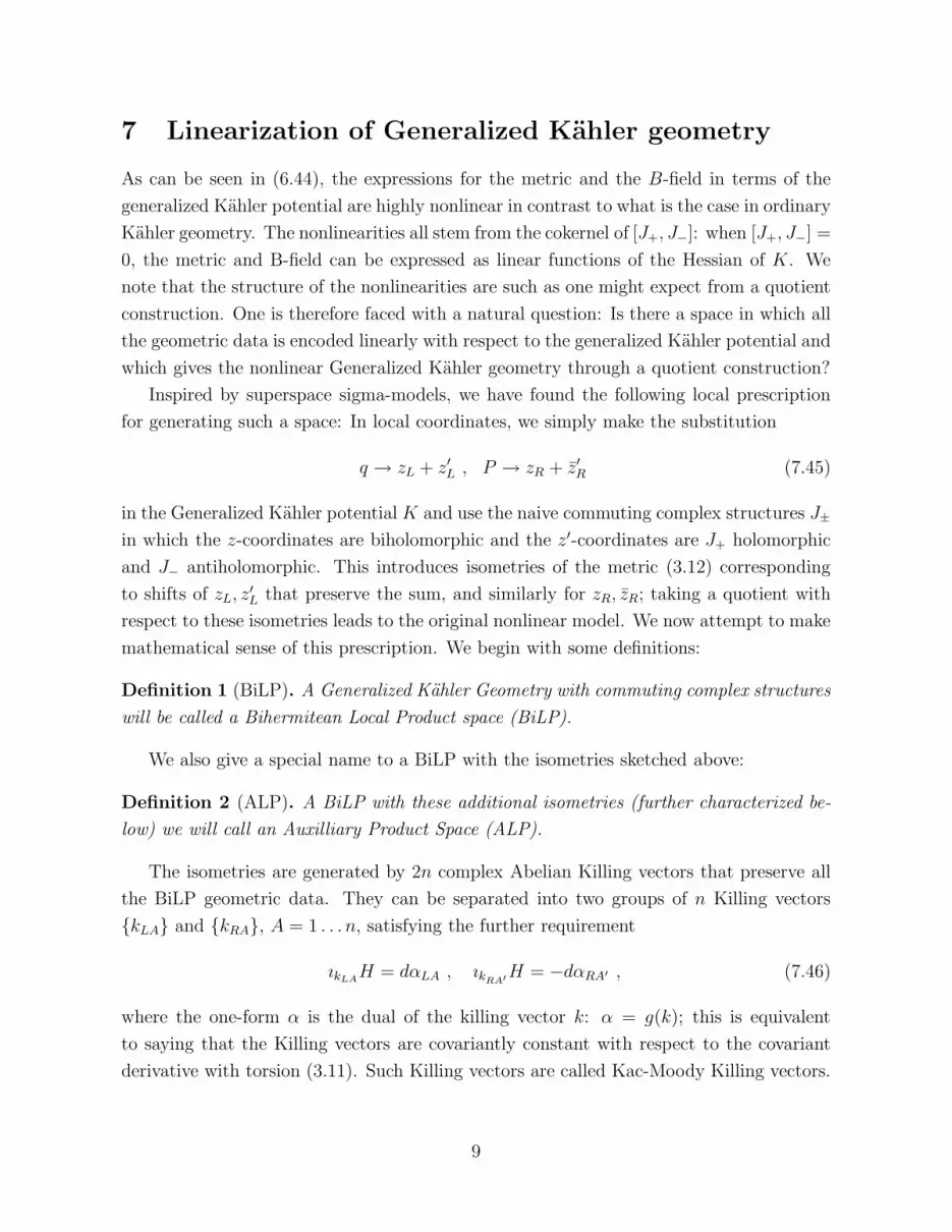
7 Linearization of Generalized Kahler geometry

As can be seen in (6.44), the expressions for the metric and the B-field in terms of the

generalized Kahler potential are highly nonlinear in contrast to what is the case in ordinary

Kahler geometry. The nonlinearities all stem from the cokernel of [J+, J−]: when [J+, J−] =

0, the metric and B-field can be expressed as linear functions of the Hessian of K. We

note that the structure of the nonlinearities are such as one might expect from a quotient

construction. One is therefore faced with a natural question: Is there a space in which all

the geometric data is encoded linearly with respect to the generalized Kahler potential and

which gives the nonlinear Generalized Kahler geometry through a quotient construction?

Inspired by superspace sigma-models, we have found the following local prescription

for generating such a space: In local coordinates, we simply make the substitution

q → zL + z′L , P → zR + z′R (7.45)

in the Generalized Kahler potential K and use the naive commuting complex structures J±

in which the z-coordinates are biholomorphic and the z′-coordinates are J+ holomorphic

and J− antiholomorphic. This introduces isometries of the metric (3.12) corresponding

to shifts of zL, z′L that preserve the sum, and similarly for zR, zR; taking a quotient with

respect to these isometries leads to the original nonlinear model. We now attempt to make

mathematical sense of this prescription. We begin with some definitions:

Definition 1 (BiLP). A Generalized Kahler Geometry with commuting complex structures

will be called a Bihermitean Local Product space (BiLP).

We also give a special name to a BiLP with the isometries sketched above:

Definition 2 (ALP). A BiLP with these additional isometries (further characterized be-

low) we will call an Auxilliary Product Space (ALP).

The isometries are generated by 2n complex Abelian Killing vectors that preserve all

the BiLP geometric data. They can be separated into two groups of n Killing vectors

kLA and kRA, A = 1 . . . n, satisfying the further requirement

ıkLAH = dαLA , ık

RA′H = −dαRA′ , (7.46)

where the one-form α is the dual of the killing vector k: α = g(k); this is equivalent

to saying that the Killing vectors are covariantly constant with respect to the covariant

derivative with torsion (3.11). Such Killing vectors are called Kac-Moody Killing vectors.

9

We require that each group of Killing vectors kL and kR by themselves span maximally

isotropic subspaces, i.e., that

g(kLA, kLB) = 0 , g(kRA′, kRB′) = 0 , (7.47)

but that the inner product

hA′B = g(kRA′, kLB) (7.48)

is nondegenerate.

Theorem. Locally, any generalized Kahler manifold M is a quotient of an ALP by its

Kac-Moody isometries.

The quotient is performed by going to the orbits of the action of the Killing vector and

choosing a horizontal subspace by specifying a connection. In the particular case with left

and right Kac-Moody Killing vectors there is a corresponding left and right connection

given by

(θR)A′

µ = gµνkνLBhBA′

, (θL)Aµ = hAB′

kνRB′gνµ , (7.49)

where hAB′

is the inverse of the nondegenerate matrix (7.48). The connections (7.49)

satisfy the following properties

θL(kL) = 1 , θR(kR) = 1 , θL(kR) = 0 , θR(kL) = 0 . (7.50)

Vectors in the horizontal subspaces are defined as the vectors lying in the kernel of both

θL and θR.

All geometric structures defined on the ALP can now be defined on the quotient space.

As usual, forms are projected using the connection so that the contraction with any

vertical vector is zero, whereas vectors are pushed forward to the quotient using the bundle

projection p. When we project the complex structures

J±(X) := p∗

(

J±(X) − θL(X) · J±(kL) − θR(X) · J±(kR))

∀X , (7.51)

it is clear that the projected complex structures J± do not commute even though J± do.

Projecting the metric and B-field, we find

g = g − h(θL, θR) − h(θR, θL) ,

B = B − h(θL, θR) + h(θR, θL) . (7.52)

It is straightforward to see that g gives zero when contracted with any vertical vector

while this is not so for B. This (apparent) mystery is resolved by showing that H = dB

can be written as

H = H − θL ∧ ıkLH − θR ∧ ıkR

H − θL ∧ θR ∧ ıkLıkR

H (7.53)

10

so that the geometrically meaningful object H defined by dB is indeed well defined on the

quotient. The quotients g and H agree with the expressions for the original generalized

Kahler manifold.

Acknowledgement:

We are grateful to the 2006 Simons Workshop for providing the stimulating atmosphere

where this work was initiated. The work of UL was supported by EU grant (Superstring

theory) MRTN-2004-512194 and VR grant 621-2003-3454. The work of MR was supported

in part by NSF grant no. PHY-0354776. The research of R.v.U. was supported by Czech

ministry of education contract No. MSM0021622409. The research of M.Z. was supported

by VR-grant 621-2004-3177

References

[1] M. Gualtieri, “Generalized complex geometry,” Oxford University DPhil thesis,

[arXiv:math.DG/0401221].

[2] N. Hitchin, “Generalized Calabi-Yau manifolds,” Q. J. Math. 54 (2003), no. 3, 281

308, [arXiv:math.DG/0209099].

[3] S. J. Gates, C. M. Hull and M. Rocek, “Twisted Multiplets And New Supersym-

metric Nonlinear Sigma Models,” Nucl. Phys. B248 (1984) 157.

[4] U. Lindstrom and M. Rocek, private communication, in preparation.

[5] U. Lindstrom, M. Rocek, R. von Unge and M. Zabzine, “Generalized Kaehler

manifolds and off-shell supersymmetry,” Commun. Math. Phys. 269, 833 (2007)

[arXiv:hep-th/0512164].

[6] U. Lindstrom, M. Rocek, R. von Unge and M. Zabzine, “Linearizing generalized

Kaehler geometry,” arXiv:hep-th/0702126.

[7] U. Lindstrom, R. Minasian, A. Tomasiello and M. Zabzine, “Generalized com-

plex manifolds and supersymmetry,” Commun. Math. Phys. 257, 235 (2005)

[arXiv:hep-th/0405085].

[8] M. Zabzine, “Lectures on generalized complex geometry and supersymmetry,”

arXiv:hep-th/0605148.

11

[9] K. Yano, ”Differential geometry on complex and almost complex spaces,” (Perga-

mon, Oxford, 1965)

[10] S. Lyakhovich and M. Zabzine, “Poisson geometry of sigma models with extended

supersymmetry,” Phys. Lett. B548 (2002) 243 [arXiv:hep-th/0210043].

[11] I. T. Ivanov, B. B. Kim and M. Rocek, “Complex structures, duality

and WZW models in extended superspace,” Phys. Lett. B343 (1995) 133

[arXiv:hep-th/9406063].

[12] N. Hitchin, “Instantons, Poisson structures and generalized Kahler geometry,”

[arXiv:math.DG/0503432].

[13] V. I. Arnold, “Mathematical methods of classical mechanics,” Translated from the

Russian by K. Vogtmann and A. Weinstein. Second edition. Graduate Texts in

Mathematics, 60. Springer-Verlag, New York, 1989. xvi+508 pp.

[14] J. Bogaerts, A. Sevrin, S. van der Loo and S. Van Gils, “Properties of semichiral

superfields,” Nucl. Phys. B562 (1999) 277 [arXiv:hep-th/9905141].

[15] T. Buscher, U. Lindstrom and M. Rocek, “New Supersymmetric Sigma Models

With Wess-Zumino Terms,” Phys. Lett. B202, 94 (1988).

12