a parallel algorithm for deformable contact problems
TRANSCRIPT

Universitat Politecnica de Catalunya
Doctoral Thesis
A Parallel Algorithm for
Deformable Contact Problems
Matıas Ignacio Rivero
Advisor:
Dr. Mariano Vazquez
Tutor:
Dr. Jose Marıa Cela Espın
Doctoral Program in Civil Engineering
Escola Tecnica Superior d’Enginyers de Camins, Canals i Ports de Barcelona
Barcelona, Spain
February 2018


To Anita and Pepe,
for being my teachers of life.


Abstract
In the field of nonlinear computational solid mechanics, contact problems deal with the defor-
mation of separate bodies that interact when they come in touch. Usually, they are formulated
as constrained minimization problems that may be solved using optimization techniques such
as penalty method, Lagrange multipliers, Augmented Lagrangian method, etc. This classical
approach is based on node connectivities between the contacting bodies. These connectivities
are created through the construction of contact elements introduced for the discretization of
the contact interface, which incorporate the contact constraints in the global weak form. These
methods are well known and widely used in the resolution of contact problems in engineering
and science.
As parallel computing platforms are nowadays widely available, solving large engineering
problems on high performance computers is a concrete possibility for any engineer or researcher.
Due to the memory and compute power that contact problems require and consume, they are
good candidates for parallel computation. Industrial and scientific realistic contact problems in-
volve different physical domains and a large number of degrees of freedom, so algorithms designed
to run efficiently on high performance computers are needed. Nevertheless, the parallelization
of the numerical solution methods which arises from the classical optimization techniques and
discretization approaches presents some drawbacks that must be considered. Mainly, for general
contact cases where sliding occurs, the introduction of contact elements requires the update of
the mesh graph in a fixed number of time steps. From the point of view of the domain decompo-
sition approach for parallel resolution of numerical problems, this is a significant drawback due
to its computational expensiveness since dynamic repartitioning must be done to redistribute the
updated mesh graph to the different processors. On the other hand, some of the optimization
techniques modify the number of degrees of freedom in the problem dynamically, by introducing
Lagrange multipliers as unknowns.
In this work we introduce a Dirichlet-Neumann type parallel algorithm for the numerical
solution of nonlinear frictional contact problems, putting a strong focus on its computational
implementation. Among its main characteristics, it can be highlighted that there is no need
to update the mesh graph during the simulation, as no contact elements are used. Also, no
additional degrees of freedom are introduced into the system, since no Lagrange multipliers are
required. In this algorithm, the bodies in contact are treated separately, in a segregated way.
The coupling between the contacting bodies is performed through boundary conditions transfer
at the contact zone. From a computational point of view, this feature allows using a multicode
approach. Furthermore, the algorithm can be interpreted as a black-box method as it allows to
solve each body separately even with different computational codes. We describe the parallel
implementation of the proposed algorithm and analyze its parallel behaviour and performance
in both validation and realistic test cases executed in HPC machines using several processors.


Resumen
En el ambito de la mecanica de contacto computacional, los problemas de contacto tratan con
la deformacion que sufren cuerpos separados cuando interactuan entre ellos. Comunmente, estos
problemas son formulados como problemas de minimizacion con restricciones, que pueden ser
resueltos utilizando tecnicas de optimizacion como el penalty, los multiplicadores de Lagrange, el
Lagrangiano Aumentado, etc. Este enfoque clasico esta basado en la conectividad de nodos entre
los cuerpos, que se realiza a traves de la construccion de los elementos de contacto que surgen
de la discretizacion de la interfaz de contacto, los cuales, a su vez, incorporan las restricciones
de contacto en forma debil.
Debido al consumo de memoria y a los requerimientos de potencia computacional que los
problemas de contacto requieren, resultan ser muy buenos candidatos para la paralelizacion
computacional. Sin embargo, la paralelizacion de los metodos numericos que surgen de las
tecnicas clasicas de optimizacion y los distintos enfoques para su discretizacion presentan algu-
nas desventajas que deben ser consideradas. Principalmente, en los problemas mas generales de
la mecanica de contacto ocurre un deslizamiento entre cuerpos. Por este motivo, la introduccion
de los elementos de contacto vuelve necesaria una actualizacion del grafo de la malla cada cierto
numero de pasos de tiempo. Desde el punto de vista del metodo de descomposicion de dominios
utilizado en la resolucion paralela de problemas numericos, esto es una gran desventaja debido
a su coste computacional, ya que un reparticionamiento dinamico debe ser realizado para redis-
tribuir el grafo actualizado de la malla entre los diferentes procesadores. Por otro lado, algunas
tecnicas de optimizacion modifican dinamicamente el numero de grados de libertad del problema
al introducir multiplicadores de Lagrange como incognitas del problema.
En este trabajo presentamos un algoritmo paralelo del tipo Dirichlet-Neumann para la reso-
lucion numerica de problemas de contacto con friccion no lineales, poniendo un especial enfasis
en su implementacion computacional. Entre sus principales caracterısticas se puede destacar la
no necesidad de actualizar el grafo de la malla durante la simulacion, ya que en este algoritmo
los elementos de contacto no son utilizados. Adicionalmente, ningun grado de libertad extra
es introducido al sistema, ya que los multipliadores de Lagrange no son requeridos. En este
algoritmo los cuerpos en contacto son tratados de forma separada, de una manera segregada. El
acople entre estos cuerpos es realizado a traves del intercambio de condiciones de contorno en
la interfaz de contacto. Desde un punto de vista computacional, esta caracterıstica permite el
uso de un enfoque multicodigo. Ademas, este algoritmo puede ser interpretado como un metodo
del tipo black-box ya que permite resolver cada cuerpo por separado, aun utilizando distintos
codigos computacionales. En este trabajo describimos la implementacion paralela del algoritmo
propuesto y analizamos su comportamiento y performance paralela tanto en casos de validacion
como reales, ejecutados en computadores de alta performance utilizando varios procesadores.


Acknowledgements
In the first place, I would like to thank my advisor, Mariano Vazquez. Thank you, Mariano, for
giving me the opportunity to come to the Barcelona Supercomputing Center as a PhD student,
for always keeping the door of your office open and for your willingness to hear everything I had
to say. I also want to thank Guillaume Houzeaux, for his enthusiasm and readiness to help.
I am deeply indebted to Miguel Zavala for his selfless and invaluable help, and for the fruitful
discussions. Miguel, there are no words to express my gratitude for all the time you invested. I
have enjoyed working with you. I am also indebted to Gerard Guillamet for all his comments,
suggestions and, especially, for all his last-minute help. Gerard, it would have been nice to have
you here from the very beginning of my thesis. A very special thanks goes to my other colleagues
of the solidz team at BSC and UdG: Adria Quintanas, Guido Giuntoli and Eva Casoni, for their
ideas and their problem-solving attitude.
I have to thank other people who indirectly contributed to this thesis by giving me moral
and emotional support. I want to express my gratitude to Alex Ferrer and Matıas Avila for
lending me their ears everytime I needed, for all the talks we had and all the advice they gave
me. A big thanks also goes to Marina Lopez, Jordi Barcons and Marıa Coto for their support,
understanding and active encouragement. I also want to thank Alex Martı, Dani Mira, Monica de
Mier, Abel Gargallo and Ruth Arıs, for their help at precise moments which made an important
difference to me.
I am also grateful to my colleagues of the CASE department at BSC who have contributed
to my day-to-day life and who have made my experience at BSC pleasant. Although the list
of these people is too long to be given in totality, I would especially like to mention: Alfonso
Santiago, Edgar Olivares, Marıa Cristina Marinescu, Simon Carrignon, Paula Cordoba, Sergio
Mendoza, Dani Pastrana, Xevi Roca, Diana Fernandez, Hadrien Calmet, Herbert Owen, Ricard
Borell, Guille Marın, Juan Carlos Cajas, Bea Eguzkitza, Albert Coca, Stephan Mohr, Rogeli
Grima and Jazmın Aguado.
Gracias al Juancho, mi little brother, por ser mis ojos a la distancia y por aguantar los trapos,
aun mas en los momentos difıciles. Te quiero mucho hermano. Y gracias al Cholo, porque el
esfuerzo no se negocia, y porque solo en el diccionario exito esta antes que trabajo.
Finally, I would like to thank you Agus, my wife. Thank you for all the sacrifices you did
by staying by my side all those years, and by letting my dream became our dream. Thank you
for all your support, understanding, patience, tolerance and for believing in me ten times more
than I do. Without you, all this journey would not have made any sense.
This work has been done with the support of the grant SEV-2011-0067 and fellowship BES-
2012-052278 of Severo Ochoa Programme, awarded by the Spanish Government.


Contents
1 Introduction 1
1.1 Motivation . . . . . . . . . . . . . . . . . . . . . . . . . . . . . . . . . . . . . . . 1
1.2 Background . . . . . . . . . . . . . . . . . . . . . . . . . . . . . . . . . . . . . . . 3
1.2.1 Classical and modern theoretical works . . . . . . . . . . . . . . . . . . . 3
1.2.2 Numerical treatment of contact problems . . . . . . . . . . . . . . . . . . 4
1.2.2.1 Domain decomposition approaches . . . . . . . . . . . . . . . . . 5
1.2.2.2 Parallel computational contact mechanics . . . . . . . . . . . . . 6
1.3 Objectives . . . . . . . . . . . . . . . . . . . . . . . . . . . . . . . . . . . . . . . . 6
1.4 Outline . . . . . . . . . . . . . . . . . . . . . . . . . . . . . . . . . . . . . . . . . 8
2 Governing Equations for Large Deformation Contact 11
2.1 Initial/Boundary value problems for the finite strain case . . . . . . . . . . . . . 11
2.1.1 Problem formulation . . . . . . . . . . . . . . . . . . . . . . . . . . . . . . 11
2.1.2 The weak form in finite strains . . . . . . . . . . . . . . . . . . . . . . . . 13
2.2 Two-body contact problem definition . . . . . . . . . . . . . . . . . . . . . . . . . 13
2.2.1 Contact constraints in large deformation . . . . . . . . . . . . . . . . . . . 15
2.2.1.1 Frictional conditions . . . . . . . . . . . . . . . . . . . . . . . . . 16
2.2.2 Weak form of the large deformation contact problem . . . . . . . . . . . . 18
2.2.2.1 Contact virtual work: the contact integral . . . . . . . . . . . . . 20
2.3 Discretization aspects . . . . . . . . . . . . . . . . . . . . . . . . . . . . . . . . . 20
2.3.1 Contact surface discretization . . . . . . . . . . . . . . . . . . . . . . . . . 21
3 Analysis of Existing Computational Methods 25
3.1 Key concepts for parallel computing. A crash introduction . . . . . . . . . . . . . 25
3.1.1 Parallel computational models . . . . . . . . . . . . . . . . . . . . . . . . 25
3.1.1.1 Message passing interface (MPI) . . . . . . . . . . . . . . . . . . 27
3.1.2 Domain decomposition . . . . . . . . . . . . . . . . . . . . . . . . . . . . . 28
3.1.3 Mesh partitioning . . . . . . . . . . . . . . . . . . . . . . . . . . . . . . . 30
3.1.4 Sparse storage . . . . . . . . . . . . . . . . . . . . . . . . . . . . . . . . . 31
3.2 Contact mechanics: methods of constraint enforcement . . . . . . . . . . . . . . . 33
3.2.1 Unconstrained system . . . . . . . . . . . . . . . . . . . . . . . . . . . . . 33
3.2.2 Constrained system . . . . . . . . . . . . . . . . . . . . . . . . . . . . . . 34
3.2.2.1 Penalty method . . . . . . . . . . . . . . . . . . . . . . . . . . . 35
3.2.2.2 Lagrange multipliers method . . . . . . . . . . . . . . . . . . . . 36

3.2.2.2.1 Mortar method for contact problems . . . . . . . . . . . 38
3.2.2.3 Augmented Lagrangian method . . . . . . . . . . . . . . . . . . 38
3.3 Domain decomposition and constraint enforcement methods . . . . . . . . . . . . 40
3.3.1 Sliding . . . . . . . . . . . . . . . . . . . . . . . . . . . . . . . . . . . . . . 41
3.4 Standard methods and the parallel world . . . . . . . . . . . . . . . . . . . . . . 44
3.5 Design basis of the proposed algorithm . . . . . . . . . . . . . . . . . . . . . . . . 45
4 A Parallel Method for Unilateral Contact Simulation 47
4.1 Introduction . . . . . . . . . . . . . . . . . . . . . . . . . . . . . . . . . . . . . . . 47
4.2 Formulation of unilateral contact problems . . . . . . . . . . . . . . . . . . . . . 48
4.2.1 Unilateral normal contact . . . . . . . . . . . . . . . . . . . . . . . . . . . 48
4.2.2 Balance of momentum including contact . . . . . . . . . . . . . . . . . . . 49
4.2.3 Interpretation of contact Hertz-Signorini-Moreau conditions . . . . . . . . 50
4.2.4 Interpretation of frictional condition . . . . . . . . . . . . . . . . . . . . . 51
4.3 Method of partial Dirichlet-Neumann boundary conditions . . . . . . . . . . . . . 52
4.3.1 Frictionless case . . . . . . . . . . . . . . . . . . . . . . . . . . . . . . . . 53
4.3.2 Frictional case . . . . . . . . . . . . . . . . . . . . . . . . . . . . . . . . . 54
4.4 Computational implementation . . . . . . . . . . . . . . . . . . . . . . . . . . . . 56
4.4.1 Contact searching and communication: the PLE++ tool . . . . . . . . . . 57
4.4.1.1 Parallel location and exchange algorithm . . . . . . . . . . . . . 57
4.4.1.1.1 Global searching . . . . . . . . . . . . . . . . . . . . . . 59
4.4.1.1.2 Local searching . . . . . . . . . . . . . . . . . . . . . . . 62
4.4.1.2 Exchange . . . . . . . . . . . . . . . . . . . . . . . . . . . . . . . 64
4.4.2 Implementation issues . . . . . . . . . . . . . . . . . . . . . . . . . . . . . 65
4.4.2.1 MPC enforcement . . . . . . . . . . . . . . . . . . . . . . . . . . 71
4.4.2.2 Friction enforcement . . . . . . . . . . . . . . . . . . . . . . . . . 73
4.4.2.3 Nodes release . . . . . . . . . . . . . . . . . . . . . . . . . . . . . 74
4.5 Numerical examples . . . . . . . . . . . . . . . . . . . . . . . . . . . . . . . . . . 75
4.5.1 Computational framework . . . . . . . . . . . . . . . . . . . . . . . . . . . 75
4.5.2 Test cases . . . . . . . . . . . . . . . . . . . . . . . . . . . . . . . . . . . . 76
4.5.2.1 Signorini problem: cylinder on a rigid foundation - 2D . . . . . . 77
4.5.2.2 Indentation parallel benchmark - 2D . . . . . . . . . . . . . . . . 80
4.5.2.3 Frictional case: uniaxial compression test - 2D . . . . . . . . . . 84
4.5.2.4 Hertzian contact: sphere on a flat rigid plate - 3D . . . . . . . . 86
4.5.2.5 Indentation parallel benchmark - 3D . . . . . . . . . . . . . . . . 89
4.5.2.6 Frictional case: sliding of a cube on a rigid plane - 3D . . . . . . 95
4.5.2.7 Expansion of a tube and a rounded frame - 3D . . . . . . . . . . 98
5 A Parallel Method for the Two-Body Contact Problem 101
5.1 Introduction . . . . . . . . . . . . . . . . . . . . . . . . . . . . . . . . . . . . . . . 101
5.2 Contact algorithm of Dirichlet-Neumann type . . . . . . . . . . . . . . . . . . . . 103
5.2.1 Nonlinear parallel extension . . . . . . . . . . . . . . . . . . . . . . . . . . 104

5.2.2 Fixed-point solver analogy - convergence issues . . . . . . . . . . . . . . . 106
5.2.2.1 Fixed relaxation parameter . . . . . . . . . . . . . . . . . . . . . 107
5.2.2.2 Aitken dynamic relaxation . . . . . . . . . . . . . . . . . . . . . 107
5.2.2.3 Quasi-Newton algorithms . . . . . . . . . . . . . . . . . . . . . . 108
5.3 Computational implementation . . . . . . . . . . . . . . . . . . . . . . . . . . . . 108
5.3.1 Interpolation of contact tractions. Load transference. . . . . . . . . . . . . 110
5.4 Numerical examples . . . . . . . . . . . . . . . . . . . . . . . . . . . . . . . . . . 112
5.4.1 Computational framework . . . . . . . . . . . . . . . . . . . . . . . . . . . 112
5.4.2 Test cases . . . . . . . . . . . . . . . . . . . . . . . . . . . . . . . . . . . . 114
5.4.2.1 Hertz contact between two hemispheres - 2D . . . . . . . . . . . 114
5.4.2.2 Indentation parallel benchmark - 2D . . . . . . . . . . . . . . . . 118
5.4.2.3 Bouncing ball - 2D . . . . . . . . . . . . . . . . . . . . . . . . . . 122
5.4.2.4 Ironing example - 3D . . . . . . . . . . . . . . . . . . . . . . . . 124
5.4.2.5 Impact problem - 3D . . . . . . . . . . . . . . . . . . . . . . . . 128
6 Conclusions and Outlook 131
6.1 Summary . . . . . . . . . . . . . . . . . . . . . . . . . . . . . . . . . . . . . . . . 131
6.2 Contributions . . . . . . . . . . . . . . . . . . . . . . . . . . . . . . . . . . . . . . 132
6.3 Future research perspectives . . . . . . . . . . . . . . . . . . . . . . . . . . . . . . 133
A Computational Environment 137
A.1 Alya . . . . . . . . . . . . . . . . . . . . . . . . . . . . . . . . . . . . . . . . . . . 137
A.1.1 Numerical issues - solid mechanics module . . . . . . . . . . . . . . . . . . 138
A.2 Ostero . . . . . . . . . . . . . . . . . . . . . . . . . . . . . . . . . . . . . . . . . . 140
A.2.1 Description . . . . . . . . . . . . . . . . . . . . . . . . . . . . . . . . . . . 140
A.2.2 How to get Ostero . . . . . . . . . . . . . . . . . . . . . . . . . . . . . . . 142
B Physical Interpretation of the Newton’s Method Residual 143
C Load Transference Analysis 147
Bibliography 149


Chapter 1
Introduction
In this first chapter we intend to give a general context and overview of this thesis. We start by
describing from a general viewpoint the context where this thesis is situated and the main aspects
that motivate this work. Then, we give a more detailed description of the scientific background
which is used as the theorethical frame for the developments included here. Finally, we present
the objectives of this work and the outline which shows the structure followed in this manuscript.
1.1 Motivation
Contact is a complex phenomena which can be analyzed from the atomistic perspective to the
macroscopic viewpoint, and from a high-speed impact to a quasi-static interaction. The level
of detail in this analysis depends on the context, which basically responds to the problem in
hand, related to an specific area of research. However, for most contact applications in solid and
structural mechanics, a purely macroscopic viewpoint based on classical continuum formulations
is sufficient. Throughout this thesis, this is the approach that will be followed.
The kind of contact problems which will be considered in this thesis are those which deal
with the deformation of separate bodies that interact when they come in touch. Since decades
ago, contact problems have taken an important place in the computational mechanics. Because
of their relevance and complexity, many numerical procedures have been proposed in engineering
literature. What makes improved contact simulation approaches promising is the fact that the
resulting numerical algorithm can be typically employed in a very wide range of scientific and
technical areas. This allows not only to reduce costs in product development and testing but
also to a better understanding of complex systems influenced by contact phenomena.
Due to the characteristics of the contact boundary conditions, this type of problems are for-
mulated as constrained minimization problems which may be solved using different optimization
techniques such as penalty method, Lagrange multipliers, Augmented Lagrangian method and
others. From the discretization of the continuum setting, those approaches result in a mono-
lithic system of linear equations which includes all the unknowns for all the geometries of the
1

Introduction
mechanical system. Furthermore, the discretization of contact problems using implicit solvers
requires the construction of contact elements, contact tangent matrices and contact residual vec-
tors which incorporate the contact constraints in the global weak form. In almost all contact
problems where the contact zone is a priori unknown, the use of contact elements requires the
update of the mesh graph in a fixed number of time steps. On the other hand, some of the
optimization techniques used in contact problems increase the number of degrees of freedom in
the problem, by introducing Lagrange multipliers as unknowns. Since the number of Lagrange
multipliers depends on the active contact surface at each time step, the total unknowns of the
system can vary as the problem evolves.
As parallel computing platforms are nowadays widely available, solving large engineering
problems on high perfomance computers is a concrete possibility for any engineer or researcher.
Due to the memory and compute power that contact problems require and consume, they are
good candidates for parallel computation. Industrial and scientific realistic contact problems in-
volve different physical domains and a large number of degrees of freedom, so algorithms designed
to run efficiently in high performance computers are needed. Nevertheless, the parallelization of
the solution methods which arises from the classical optimization techniques and discretization
approaches presents some drawbacks that must be considered. In the finite element formulation
the contact element matrices are assembled in the global structural matrix of the system. This
presents some disadvantages when sliding between meshes occurs, as classical formulations are
based on nodes connectivities. Sliding is a very frequent phenomena in contact problems which
requires the modification of node connectivities between the nodes at the boundary contact zone.
Since the contact area changes during an incremental solution procedure, the data structure for
the exchange of data between processors (i.e. the mesh graph) has also to be modified. The
use of Lagrange multipliers also affects the parallel data structure, since the size of the linear
equation system changes dynamically as the problem evolves. As consequence, mesh graph up-
dating and Lagrange multipliers usage has a strong and direct impact on the performance of a
parallel solution procedure for contact problems. Under a parallel approach, the modification
of the contacting area during execution time requires a mesh repartitioning at least every time
the node connectivity of the contact elements changes. This is a computationally expensive and
inefficient task.
According to what was explained in the previous paragraphs, it can thus be advantageous to
construct an algorithm for solving contact problems that employs a strategy in which the bodies
involved in the contact problem are treated separately, in a segregated way, in order to avoid
mesh graph updating issues. Also it would be advantageous if the algorithm doesn’t need to rely
on optimization techniques and Lagrange multipliers. Yet, such segregated algorithms must be
numerical robust, accurate, efficient and flexible. As will be seen in Sec. 1.2, there exists a gap
in scientific research where those issues are not covered thoroughly, in a unified manner. The
lack of an intensive analysis regarding the parallelization of traditional contact algorithms, and
new alternatives that are best suitable for the numerical resolution of contact problems in high
performance computing environments, are the main motivation of this thesis.
2

1.2. Background
1.2 Background
This section is intended to give a brief overview of some historical remarks and the state-of-the-
art in computational contact mechanics. For a more comprehensive analysis of this topic the
reader is referred to [88, 109, 112, 142], among others.
1.2.1 Classical and modern theoretical works
The birthmark of classical contact mechanics is linked to the early work conducted by Hertz [62]
on pressure distributions between contacting spheres. He developed an analytical solution by
assuming that bodies are elastic with small deformation, frictionless and that the area of contact
is elliptic.
After Hertz’s work many researchers continued studying contact problems between elastic
bodies of different shapes, with or without friction, looking for possible analytical solutions.
Nevertheless, only a few solutions restricted to a simple geometry of the bodies, a linear elastic
material and small deformations have been found. In these solutions, the shape of the bodies is
usually rectangular or circular, axisymmetric or two-dimensional. They are summarized in [53,
76, 77, 66].
In opposition to the classical approach, non-classical contact mechanics can be defined as me-
chanics of unilateral contacts with threshold friction, adhesion or lubrication between geometrical
complicated bodies undergoing large deformations, made of elastic, viscuous or plastic materials.
As the Hertz work for the classical approach, the formulation derived by Signorini [122] for the
equilibrium of a linear elastic body in frictionless contact with a rigid foundation can be regarded
as a milestone in modern contact mechanics. The generalization and theoretical structure of the
friction law was stablished by Moreau [99].
The next important step in modern contact mechanics was made by the application of vari-
ational methods to contact and friction formulations. Because of the nature of the contact
boundary conditions, the contact problem can be mathematically interpreted as a physical sys-
tem subjected to a governing variational inequality [41, 79]. An important characteristic of such
variational inequalities is that the solution and variation spaces are constrained by the physical
constraints, which depend on the unknown solution. Consequently, the mathematical structure
of the contact problem is very different from a typical initial/boundary value problem that only
includes Dirichlet and/or Neumann boundary conditions. Additionally, the presence of friction
adds significant mathematical complications [79, 28, 101, 102].
In previous references and others, the particular case of a linear elastic solid in frictional con-
tact with a rigid obstacle (unilateral contact) has been extensively studied and can be considered
to be well characterized mathematically. Nevertheless, extension to inelastic materials and large
deformations is much more difficult and remains unsolved. Additionally, the replacement of the
rigid obstacle by a second deformable body adds extra complications to the problem that affects
its mathematical well-posedness. Those effects are still not completely understood.
3

Introduction
1.2.2 Numerical treatment of contact problems
From previous section it becomes clear that classical and modern contact mechanics give response
only to a small part of real industrial applications. For this reason, computational contact
mechanics became a relevant field of research since 1970s and 1980s, where first contributions
to the treatment of contact mechanics within the Finite Element Method can be traced back.
Works by Francavilla and Zienkiewicz [48] and Hughes et al. [72] are considered the pioneers in
this field, proposing a purely node-base approach, which requires node-matching meshes between
contacting bodies and is restricted to small deformations.
As a satisfactory general methodology for formulating contact and friction inequalities still
doesn’t exist, further developments in computational contact mechanics have gone into two
main directions. In the first direction, contact and friction conditions are stablished in the
discrete form of the problem. Constraints and linearization of the nonlinear resultant equation
are therefore limited to a particular type of discretization. Using this approach gradual progress in
solving increasingly difficult problem was made, see [138, 125, 32, 106, 140]. Nevertheless further
works in this direction have encountered serious obstacles as: limitations on the admissible
incremental motions, restrictions to rigid obstacle problems and, as mentioned before, restriction
to a particular discretization. This situation results from the lack of a continuum framework for
the large deformation frictional contact problems.
The second direction intends to overcome these obstacles putting special effort in the de-
velopment of a continuum formulation for contact problems, which intends to approach contact
mechanics from the abstract and general continuum point of view. As mentioned in Sec. 1.2.1,
the continuum formulation of contact problems includes variational inequalities leading to non-
smooth constrained minimization problems that can not be directly tackled by the finite element
method. First, they have to be expressed as variational equalities or unconstrained minimization
problems. Variational inequalities can be reformulated into a variational equality problem with
special contact terms under the assumption of knowing a priori the contact force. The form of
the contact terms depends on the method chosen to enforce the contact constraints. For con-
straint enforcement, a wide range of techniques from the optimization literature exist [92, 52].
Among them, the most used methods for constraint enforcement in the numerical treatment of
contact problems are: the penalty method [100, 30, 57, 125, 32, 140] and the classical Lagrange
multiplier method [8, 50]. Due to known drawbacks of the penalty method (see [92, 79]), Lagrange
multiplier techniques have become relevant in the domain of constrained problems. Especially
one of its extensions has gained importance in the field of computational contact mechanics: the
Augmented Lagrangian method, which combines advantages of both penalty and Lagrange mul-
tipliers methods and has been applied successfully to frictionless and frictional contact (see [54,
139, 4, 123, 110]).
The implicit numerical resolution of contact problems with the Finite Element Method re-
quires the construction of contact elements. Contact elements are used to link potentially inter-
acting surfaces and to transfer efforts from one to another. The structure of the contact elements
depends on the contact discretization method. The simplest is the node-to-node discretization [48]
4

1.2. Background
which is valid only for matching meshes and does not allow sliding between contacting bodies
or large deformations. The node-to-segment is a multipurpose discretization [73, 8, 17, 57, 88,
90, 123, 140] which is valid for non-conforming meshes, large deformation and sliding, therefore
becoming the standard procedure in computational contact mechanics. But as it is, this dis-
cretization is not stable, fails contact patch test unless a two-pass scheme is used and is valid
only for low order elements. A different discretization approach, called contact domain method
and based on the node-to-segment approach has been proposed in [103, 59]. This method has
been reported to be stable and passes the patch test, but its three dimensional implementation
is not applicable for arbitrary discretizations. The last method that may be distinguished is the
segment-to-segment discretization [125, 105, 144]. In contrast to the purely point-wise procedure
(typical of the node-to-segment methods), the segment-to-segment approach is based on a sub-
division of the contact surface into individual segments for numerical integration together with
an independent approximation of the contact pressure.
1.2.2.1 Domain decomposition approaches
Mortar element methods, originally introduced as an abstract domain decomposition technique [18,
14], are characterized by an imposition of the occurring interface constraints in a weak sense and
by the possibility to prove their mathematical optimality. In general terms, they allow for noncon-
forming decomposition of the computational domain into subregions and for the optimal coupling
of different variational approximations in different subregions. In the context of contact analy-
sis, this allows for a variationally consistent treatment of non-penetration and frictional sliding
conditions despite the inevitably non-matching interface meshes for finite deformations and large
sliding motions. Segment-to-segment discretization has been coupled with mortar methods and
applied to contact problems in early works [15, 64, 96], though limited to small deformations.
Restrictions on the mortar-based contact formulations regarding the nonlinear kinematics have
been removed, leading to the implementations given in [46, 117, 131, 118, 113].
The FETI method is an iterative substructuring method for solving systems of linear equa-
tions using Lagrange multipliers. It was introduced in [43] and is based on the decomposition
of the spatial domain into non-overlapping subdomains that are glued by Lagrange multipliers.
The FETI method can be applied without any algorithmic changes for a mortar finite element
discretization in non-matching meshes [126]. This has been reported in [39, 35] only for 3D
frictionless contact problems in linear elasticity. A more comprehensive approach for mortar
discretization and FETI methods i.e. frictional contact problems in large deformation for non-
matching meshes, is still missing in the literature. Conversely, FETI method has been applied
to elastic frictionless and frictional contact problems in matching grids for small [34, 36, 40, 37,
38] and large displacements [133].
Monotone Multigrid methods are algorithms for solving linear systems arising from the dis-
cretization of partial differential equations based on a sequence of meshes obtained by successive
refinement, having a recursive structure [82]. Despite in the literature multigrid methods are
sometimes defined as alternatives to domain decomposition methods, in the field of computa-
tional contact mechanics they are used as subdomain linear solvers. For unilateral contact prob-
5

Introduction
lems, monotone multigrid methods yield globally convergent and efficient iterative solvers [83,
84]. However, these techniques cannot be applied directly to multibody contact problems be-
cause of the non-conforming situation at the interface of the contacting bodies. In [135] a new
approach for the numerical simulation of multibody frictionless contact problems based on mono-
tone multigrid techniques and mortar methods is presented.
Alternative domain decomposition approaches for contact problems are based on formula-
tions that allow to solve problems for each body separately with certain boundary conditions
at the natural interface. A Dirichlet-Neumann algorithm for solving frictional Signorini con-
tact problems between two elastic bodies based on mortar elements and the monotone multigrid
method has been proposed and studied in the discrete setting in [85]. This algorithm consists on
solving in each iteration a linear Neumann problem for one body and a unilateral contact prob-
lem for the other by using essentially the contact interface as the boundary data transfer. The
convergence of this algorithm in the continuous setting in its frictionless form has been proved
in [10, 42] and considering friction in [12]. In [11] another improvement leading to a Neumann-
Neumann approach was proposed, in which two Neumann sub-problems are solved in order to
ensure the continuity of normal stresses and its convergence is proven in the continuous setting.
Later in [60] the authors presented various numerical implementations of this approach. Finally,
in [61] the Neumann-Neumann algorithm is extended to two-body elastic contact problems with
Tresca friction.
The Dirichlet-Neumann approach presented in the previous paragraph is the main topic of
this thesis and marks the point of origin of this work.
1.2.2.2 Parallel computational contact mechanics
Few works in the computational contact mechanics literature have been devoted to parallel
methods. The main research interest in this topic was focused on static or transient explicit
contact simulations due to its simplicity compared with implicit integrators. Several authors have
reported on their effort to parallelize this kind of problems and specially the contact detection
procedure [94, 108, 111, 7, 58].
1.3 Objectives
As mentioned in Secs. 1.1 and 1.2, computational algorithms for the solution of contact mechanics
problems between deformable bodies present some particularities which can be considered as
handicaps for their parallelization. Mainly, the following are the two most important issues:
• Penalty and Augmented Lagrangian based methods add explicit connectivities between
contacting nodes, and
• Lagrange multiplier based methods increase dinamically the number of degrees of freedom
of the resultant system matrix.
6

1.3. Objectives
Traditional algorithms for computational contact mechanics are based on node connectivities
for the transference of data related to the contact phenomena, through the contact elements cre-
ated for such end. General contact problems involve sliding after contact i.e. relative movement
of one body with respect to the other in a contacting situation. This implies that contact ele-
ments must be created and actualizated on the fly in each inner iteration and/or time step, what
continously changes the graph of the system. This means that connectivities between contacting
nodes are created and modified in execution time, and because of that, new contributions in the
global tangent matrices will appear.
Parallel algorithms for distributed memory machines require the partitioning of the system
graph, which is defined by the connectivities of the mesh. This is normally done as a preprocess
task, as generally the mesh does not change. Nevertheless, for contact problems where the graph
is continously being updated, this partitioning must be done in execution time everytime the
graph changes. From the viewpoint of the computational resources, this is a very demanding
procedure.
Motivated by the fact that standard contact algorithms are not a suitable alternative for
efficient parallelization and by the lack of scientific literature regarding those issues, the main
objective of this thesis is to introduce a novel contact algorithm based on domain decomposition
methods that can run efficiently in High Performance Computing (HPC) based supercomputers,
considering in a unified way: physical, numerical, algorithmic and computational aspects. This
algorithm solves numerically a nonlinear contact problem between two deformable bodies. It is
based on a nonlinear block Gauss-Seidel method as an iterative solver, which can be interpreted
as a Dirichlet-Neumann algorithm for the nonlinear contact problem. The main aspect of the
proposed algorithm is that the bodies in contact are treated separately, in a segregated way.
Then, coupling is performed through boundary conditions transfer at the contact zone. As this
approach solves each body separately, there is no need to increase the degrees of freedom of the
problem or to redefine the mesh graph at different time steps, since no contact elements are used
in the algorithm. The main advantages of the algorithm introduced in this thesis are summarized
in the following list:
• General parallel contact algorithm.
• Do not restrict the mesh partitioner.
• Do not require dynamic partitioning.
• The number of unknowns remain constant during the simulation.
• Do not affect the system matrix (no connectivities are created).
• Is suitable for large scale problems (domain decomposition approach).
• Has individual scheme solution for each problem.
• Is robust.
7

Introduction
• Black box. Can be coupled to any linear or nonlinear mechanics simulation code.
• Can be used with any material, damage and element model.
• Strongly favours a general computational framework of parallel multiphysics simulations
for supercomputers.
As a complementary objective, all the algorithms presented in this thesis were implemented in
Alya, the multiphysics, multiscale and massively parallel finite element code developed in-house
at the Barcelona Supercomputing Center. For a detailed description of the Alya system, please
see Appendix A, Sec. A.1.
1.4 Outline
Despite the main objective of this thesis is to present a novel algorithm for the parallel numerical
resolution of contact problems, not less important are the fundaments which justify the necessity
for the development of such algorithm. To reach a clear overview of the computational context
that motivated this work has been an important and time-demanding stage during the elaboration
of this thesis. This is why we designed its structure to give a strong technical basis of these
fundaments before introducing the new developments. Thus, the rest of this thesis is organized
as follows.
In Chapter 2, we outline the relevant governing equations of nonlinear solid mechanics and
contact mechanics. Additionally, we review the basic concepts as contact problem definition,
boundary conditions and weak formulation in a very general style. We cover also some dis-
cretization aspects. This chapter intends to set the minimal mathematical basis needed for a
comprehensive development of the following chapters.
Chapter 3 is divided in two parts. The first part is devoted to an introduction of some basics
concepts related to parallel computing. The second part, which is supported by the first part of
this chapter, describes the context and enumerates the reasons which fundament this work. In
this chapter we also introduce and enumerate the design basis for the novel algorithm proposed
in this thesis.
In Chapter 4 we present a new methodology for solving parallel unilateral frictional contact
problems in distributed memory computers. Here, we review in more detail the mathematical
formulation of unilateral contact problems and enumerate the basics of the new proposed method.
Then, we introduce the parallel strategy used for contact detection and communication and
present a detailed description of the algorithm implementation in a parallel environment. Finally,
we show some numerical experiments and present some performance studies.
In Chapter 5 we extend the methodology presented in the previous chapter to a two-body
contact problem, i.e. bilateral contact problem. Following the same procedure from Chapter 4,
we present the algorithm putting special emphasis in its parallel implementation, which is the
more distinctive part of this work. To close, we present some numerical results that illustrates
the efficiency and flexibility of our proposed method.
8

1.4. Outline
Finally, the conclusions and outlook in Chapter 6 summarize the most important results and
achievements of this thesis. Also, it points out which aspects of the proposed algorithm still have
room for improvement, establishing future lines of research.
9


Chapter 2
Governing Equations for
Large Deformation Contact
By reviewing the basic concepts of continuum mechanics with an emphasis on the governing
equations for solid dynamics and contact mechanics, the goal in this chapter is to establish a basic
conceptual foundation that will serve as starting point for this thesis. Also, some discretization
aspects are covered here. Previous work exists on the exact linearization of frictionless contact
problems [138, 106] as well as two dimensional frictional problems [125, 140], but each case is
limited to a particular discretization. The mathematical framework presented in this thesis is
taken from [88, 90, 89], which includes the linearization in the continuum setting, such that no
limitations exists. This general formulation and implementation of the frictional contact problem
in a finite element setting has not been reported previously in the literature. For a more extensive
review in the field of solid and computational contact mechanics, see also [87], [137], [142] and [16].
2.1 Initial/Boundary value problems for the finite strain case
2.1.1 Problem formulation
To formulate solid mechanic problems in finite strain it is necessary to distinguish between two
distinct observer frames: the reference configuration Ω, which represents the domain occupied
by all the material points X at time t = 0, and the current configuration at a time t ∈ I, given
by application of a configuration mapping ϕt to Ω. This current configuration describes the
changed position x at a certain time t (x = ϕt(X). The absolute displacement of a material
point is then described as u(X, t) = x(X, t) −X. A common Cartesian coordinate system is
considered here for all configurations. The boundary ∂Ω of the open set Ω is decomposed into
two nonoverlapping subdomains; one in which the motions are prescribed (Γu), and one in which
the tractions are specified (Γσ), see Fig. 2.1. We assume that these regions obey:
Γu ∪ Γσ = ∂Ω,
Γu ∩ Γσ = ∅.(2.1)
11

Governing Equations for Large Deformation Contact
Points in the reference (or material) description are denoted X, while points in the current
(or spatial) configuration are denoted x, such that x = ϕt(X). Consistent with the most
frequent choice in solid and structural mechanics, in the present section we aim to develop a
Total Lagrangian description of the problem, such that the independent variable of interest will
be the material points in the reference configuration X, while the unknown in the problem to
be solved will be ϕt, for all t ∈ I (or equivalenty, the displacement vector u(X, t)).
Figure 2.1: Basic notation for the finite strain boundary value problem.
Regardless of the constitutive law employed, the balance of linear momentum for a continuous
medium considering finite strains may be specified as:
∇ · P + F = ρ0A in Ω, (2.2)
where P is the first Piola-Kirchhoff stress tensor, which measures stress by referencing the
force acting on areas to the magnitude of those areas in their undeformed configuration. F is
the prescribed body force per unit reference volume in Ω, ρ0 is the reference mass density and
A is the material acceleration of the particle referred to spatial coordinates.
To complete the description of the problem, the boundary conditions and initial conditions
must be given. The prescribed values are designated by a superposed bar. The boundary
conditions are:
ϕt = ϕt
P ·N = T
on Γu,
on Γσ,(2.3)
whereN is the unit outward normal to ∂Ω in the reference configuration, ϕt are the prescribed
displacements and T the prescribed tractions.
12

2.2. Two-body contact problem definition
Since Eq. (2.2) is second order in time, two set of initial conditions are needed. Those are
expressed in terms of the displacements and velocities:
ϕ|t=0 = ϕ0
ϕ|t=0 = V 0
in Ω,
in Ω,(2.4)
where ϕ0 are the prescribed initial displacements, V 0 the prescribed initial velocities and Ω
denotes the closure, or inclusion of the boundary, of the open set Ω.
2.1.2 The weak form in finite strains
In the finite element method, the entity discretized is the weak form of the differential equation.
To tacke the resolution of Eq. (2.2) using finite elements, we turn now to the development of a
weak form for the finite strain problem. This can be done by considering weighting functions∗ϕ,
defined on Γ, which are members of a weighting space V meeting the following definition:
V = ∗ϕ : Ω→ Rnsd | ∗ϕ ∈ H1(Ω),∗ϕ = 0 on Γu (2.5)
Additionally, we may define a solution space Ut for each t ∈ I, according to the following:
Ut = ϕt : Ω→ Rnsd |ϕt ∈ H1(Ω),ϕt = ϕ on Γu (2.6)
With the solution and weighting spaces defined, the weak form is developed by dotting the
governing differential Eq. (2.2) with an arbitrary∗ϕ ∈ V and integrating over Ω. This operation
gives: ∫Ω(ρ0A−∇ · P − F )
∗ϕ dΩ +
∫Γσ
(P ·N − T )∗ϕ dΓ = 0 (2.7)
Rearrangement of Eq. (2.7), use of the fact that∗ϕ = 0 on Γu and utilization of the boundary
condition on Γσ gives rise to the weak form of the problem:
For each t ∈ I, find ϕt ∈ Ut such that δWsb = 0 for all∗ϕ ∈ V,
where:
δWsb(ϕt,∗ϕ) :=
∫Ω
[ρ0∗ϕ ·A+ GRAD(
∗ϕ) : P
]dΩ
−∫
Ω
∗ϕ · F dΩ−
∫Γσ
∗ϕ · T dΓ.
(2.8)
2.2 Two-body contact problem definition
The large deformation, large motion frictional contact problem involving two bodies is shown
schematically in Fig. 2.2. The reference configurations of this two bodies are represented by Ω(1)
and Ω(2). The bodies undergo motions, denoted ϕ(1) and ϕ(2), which cause them to contact and
13

Governing Equations for Large Deformation Contact
produce interactive forces during some portion of the time interval I = [0, T ]. These motions can
be expressed by the following mappings:
ϕ(i) : Ω(i) × I→ Rnsd, i = 1, 2. (2.9)
For any time t ∈ I, the configuration obtained by fixing the time argument of ϕ(i) is denoted
as ϕ(i)t , i = 1, 2. Quantities defined on ϕ
(i)t (Ω(i)) are referred to as spatial objects, while quantities
defined on the reference states Ω(i) are referred to as material objects.
Figure 2.2: Basic notation for the two body large deformation contact problem.
Accordingly, material points of Ω(1) are denoted X, while material points of Ω(2) are denoted
Y . Spatial counterparts are defined as x and y, respectively. Considering the boundaries ∂Ω(i)
of Ω(i), i = 1, 2, one may define subsets Γ(i)c ⊂ ∂Ω(i) such that all points X (or Y ) where contact
occurs are included. Spatial counterparts of these subsurfaces are designated as γ(i)c = ϕ
(i)t (Γ
(i)c ),
i = 1, 2. It is over the surfaces Γ(i)c that contact constraints are defined. The remainder of the
surfaces ∂Ω(i) are assumed to be divided between portions Γ(i)u where motions are prescribed,
and portions Γ(i)σ where tractions are prescribed. Then, Γ
(i)c , Γ
(i)u and Γ
(i)σ satisfy:
Γ(i)σ ∪ Γ
(i)u ∪ Γ
(i)c = ∂Ω(i), and
Γ(i)σ ∩ Γ
(i)u = Γ
(i)σ ∩ Γ
(i)c = Γ
(i)u ∩ Γ
(i)c = ∅
(2.10)
for each of the bodies i.
Recalling Eq. (2.2), the momentum balance equation can be written for each body i via:
14

2.2. Two-body contact problem definition
∇ · P (i) + F (i) = ρ(i)0 A
(i) in Ω(i). (2.11)
Relying on the previous summary of the finite strain problem in Sec. 2.1.1, the initial and
boundary conditions imposed on each of the bodies i can be summarized as:
ϕ(i)t = ϕt
(i)
P (i) ·N (i) = T(i)
ϕ(i)|t=0 = ϕ0(i)
ϕ(i)|t=0 = V 0(i)
on Γ(i)u ,
on Γ(i)σ ,
in Ω(i),
in Ω(i).
(2.12)
2.2.1 Contact constraints in large deformation
The final ingredient in the specification of a finite strain IBVP including contact is the defini-
tion of the contact conditions governing the response on Γ(1)c (or, alternatively, Γ
(2)c ). In the
approach followed here, the contact conditions are considered to be parametrized by X ∈ Γ(1)c ,
with the opposing surface Γ(2)c (and its current position γ
(2)c ) providing the additional geometric
information necessary to complete the definitions. We consider any such point X ∈ Γ(1)c , whose
current position, for any time t ∈ I, is given by x = ϕ(1)t (X). The current position for any point
Y ∈ Γ(2)c is similarly expressed as y = ϕ
(2)t (Y ). The impenetrability constraint is defined for
all X, and for a given pair of motions ϕ(1)(·, t) and ϕ(2)(·, t) by first identifying a contact point
Y (X, t) according to the following closest point projection in the spatial configuration:
Y (X, t) = arg minY ∈Γ
(2)c
‖ϕ(1)t (X)−ϕ(2)
t (Y )‖. (2.13)
The gap function g(X, t) may then be defined as:
g(X, t) = −ν ·(ϕ
(1)t (X)−ϕ(2)
t (Y )), (2.14)
where ν denotes the outward unit normal to γ(2)ct at y = ϕ
(2)t (Y ) (see Fig. 2.3). Thus, for
any time t, g(X, t) is defined in terms of the closest point projection (in an Euclidean sense) of
x = ϕ(1)t (X) onto the opposing surface γ
(2)c . Of course g is a function of both ϕ(1) and ϕ(2),
although for notational simplicity explicit indication of this dependence is omitted.
In considering the tractions t(i) acting on the contacting regions of Γ(i)c , it is important to
emphasize that Newton’s laws require these to be equal and opposite, i.e.:
t(1)(X) = −t(2)(Y (X)), for allX ∈ Γ(1)c . (2.15)
Thus, we can now quantify the tractions on the interface in terms of one traction vector only,
which we select here as t(1). The contact pressure tN acting at X, assumed to be positive in
compression, is defined by considering the component of this traction in the direction of ν:
tN (X) := t(1)(X) · ν. (2.16)
15

Governing Equations for Large Deformation Contact
Figure 2.3: Gap definition and basis vectors. The interior of Ω(2) is indicated bythe shaded region.
Besides, contact pressure tN can be recovered from the decomposition of the Piola traction
T at X in normal and tangential (or frictional) components via:
T (X, t) = P (X, t)N(X, t) = tNν − tTατα (2.17)
The contact conditions interrelating tN and g on the contact surface Γ(1)c may now be stated
in terms of Kuhn-Tucker optimality conditions (see, e.g., [79]):
tN ≥ 0, (2.18a)
g ≤ 0, (2.18b)
tN g = 0, (2.18c)
which must hold for all X ∈ Γ(1)c and t ∈ I.
Eq. (2.18a) refers to the fact that all contact interaction must be compressive, while Eq. (2.18b)
states the impenetrability condition. The final condition, given by Eq. (2.18c) requires that com-
pressive stress only be generated in the instance where contact is occuring, i.e. g = 0. When
g < 0, this condition requires tN to be zero, consistent with an out-of-contact condition. Fig. 2.4a
gives a simple schematic representation of the admissible combinations of g and tN corresponding
to Eqs. (2.18). Fig. 2.4b shows all the possible combinations of tN and g values for each possible
situation: out-of-contact, non-admissible penetration and contact condition.
2.2.1.1 Frictional conditions
Contact conditions given by Eqs. (2.18) are valid for frictionless contact problem definition. We
turn attention now to the introduction of frictional response into the problem description. The
frictional modeling framework used in this thesis is based on the most common of frictional
descriptions: the Coulomb friction law.
A Coulomb friction law can be stated by introducing the coefficient of friction µ, and by
requiring the following conditions to be met for all X ∈ Γ(1)c , in addition to the Kuhn-Tucker
conditions summarized by Eqs. (2.18):
16

2.2. Two-body contact problem definition
(a)
(b)
Figure 2.4: (a) Schematic illustration of the Kuhn-Tucker conditions governingthe frictionless contact interaction. Bold line indicates admissible combinationsof contact pressure tN and gap g. (b) Illustrative example showing all the pos-sible situations in a two body contact problem: 1- Out-of-contact (admissible);2- Penetration (non-admissible); 3- Contact (admissible).
17

Governing Equations for Large Deformation Contact
||tT || ≤ µ tN (2.19)
and
uT = λ tT , where
λ = 0, if ||tT || < µ tN ,
λ ≥ 0, if ||tT || = µ tN .(2.20)
Eq. (2.19) requires that the magnitude of the tangential stress vector tT does not exceed the
coefficient of friction µ times the contact pressure tN . Eq. (2.20), on the other hand, represents
two important physical ideas associated with the Coulomb law: first, that the tangential slip uT
be identically zero when the tangential stress is less than the Coulomb limit; and second, that
any tangential slip that does occur be colinear with the frictional stress exerted by the sliding
point X on the opposing surface Γ(2)c . Fig. 2.5 graphically represents the concept in the case
corresponding to one dimensional sliding. For a more detailed description about the frictional
treatment in large deformation contact, see [87].
Figure 2.5: Schematic depiction of Coulomb friction law.
2.2.2 Weak form of the large deformation contact problem
We recall Sec. 2.1.2 and define solution and weighting spaces U (i)t and V(i), consisting of potential
solutions ϕ(i) and admissible variations∗ϕ
(i)with respect to the reference configuration of body
(i), according to:
U (i)t = ϕ(i)
t : Ω(i) → Rnsd |ϕ(i)t ∈ H1(Ω(i)),ϕ
(i)t = ϕ(i) on Γ(i)
u (2.21)
and
V(i) = ∗ϕ(i)
: Ω(i) → Rnsd | ∗ϕ(i)∈ H1(Ω(i)),
∗ϕ
(i)= 0 on Γ(i)
u . (2.22)
Following the same arguments given in Sec. 2.1.2, the weak form of the momentum balance
for each body (i) is given by:
18

2.2. Two-body contact problem definition
δW(i)(ϕ(i)t ,∗ϕ
(i)) :=
∫Ω(i)
[ρ0∗ϕ
(i)·A(i) + GRAD(
∗ϕ
(i)) : P (i)
]dΩ
−∫
Ω(i)
∗ϕ
(i)· F (i) dΩ−
∫Γ(i)σ
∗ϕ
(i)· T (i)
dΓ−∫
Γ(i)c
∗ϕ
(i)· T (i)
dΓ = 0,
(2.23)
which must hold for all∗ϕ
(i)∈ V(i). The last two terms of Eq. (2.23) corresponds to the
virtual work of the tractions, which are specified on Γ(i)σ and subjected to contact restrictions on
Γ(i)c . The last term in particular, corresponds to the contact virtual work on body (i).
A variational statement for the two body system is obtained by adding the two weak forms
implied by Eq. (2.23). For notational convenience in what follows, we introduce the notations
ϕt and∗ϕ to denote the collection of the respective mappings ϕ
(i)t and
∗ϕ
(i)for i = 1, 2. In other
words,
ϕt : Ω(1) ∪ Ω(2) → Rnsd ,∗ϕ : Ω(1) ∪ Ω(2) → Rnsd .
(2.24)
We utilize similar notations for the solution and variational spaces, such that Ut is the col-
lection of U (i)t and V is the collection of V(i). With these ideas, the variational principle for the
entire system is expressed as:
δW(ϕt,∗ϕ) :=
2∑i=1
δW(i)(ϕ(i)t ,∗ϕ
(i))
=2∑i=1
∫Ω(i)
[ρ0∗ϕ
(i)·A(i) + GRAD(
∗ϕ
(i)) : P (i)
]dΩ
−∫
Ω(i)
∗ϕ
(i)· F (i) dΩ−
∫Γ(i)σ
∗ϕ
(i)· T (i)
dΓ
−
2∑i=1
∫Γ(i)c
∗ϕ
(i)· T (i)
c dΓ
= 0
(2.25)
which must hold for all∗ϕ ∈ V. By means of Eq. (2.8) we can rewrite Ec. (2.25) to obtain the
following expression:
δW(ϕt,∗ϕ) :=
2∑i=1
δW(i)sb (ϕ
(i)t ,∗ϕ
(i)) + δWc(ϕt,
∗ϕ) = 0. (2.26)
where the notation
δWc(ϕt,∗ϕ) := −
2∑i=1
∫Γ(i)c
∗ϕ
(i)· T (i)
c dΓ
(2.27)
represents the virtual work due to the contact forces.
Eq. (2.26) shows that the virtual work for the entire system can be expressed as a sum of the
19

Governing Equations for Large Deformation Contact
contributions given by the virtual work of each independent body δW(i)sb due to internal stresses
and applied loadings, plus the contribution given by the virtual work due to the contact forces
δWc.
2.2.2.1 Contact virtual work: the contact integral
From Ec. (2.27) it can be seen that expression for δWc includes two integrals, one over each
contact surface. As all contact quantities can be parametrized by X ∈ Γ(1)c , δWc is now con-
verted to an expression involving only an integral over Γ(1)c . This is achieved by enforcing linear
momentum across the contact interface, by requiring that the differential contact force induced
on body (2) at Y be equal and opposite to that produced on body (1) at X:
t(2)t
(Y (X)
)dΓ(2)
c = −t(1)t (X) dΓ(1)
c . (2.28)
Eq. (2.28) facilitates replacement of the contact contribution in Eq. (2.27) by:
δWc(ϕt,∗ϕ) := −
∫Γ(1)c
t(1)t (X) ·
[∗ϕ
(1)(X)− ∗ϕ
(2)(Y (X))
]dΓ. (2.29)
Using the resolution of t(1)(X) into normal and tangential (or frictional) components in
Eq. (2.29), we obtain:
δWc(ϕt,∗ϕ) := −
∫Γ(1)c
[tNν − tTατα]︸ ︷︷ ︸t(1)(X)
·[∗ϕ
(1)(X)− ∗ϕ
(2)(Y (X))
]dΓ (2.30)
Eq. (2.30) can be expressed even more compactly through consideration of appropriate lin-
earized variations of the contact kinematics (for a detailed description of this topic see [87]):
δWc(ϕt,∗ϕ) :=
∫Γ(1)c
[tN δg + tTα δξα] dΓ (2.31)
where δg is the normal gap variation and δξα is the tangential gap variation.
2.3 Discretization aspects
In this section we will introduce some basics aspects of the finite element discretization of contact
interaction. The reader can refer to [87, 137, 142] for a more detailed description of this topic.
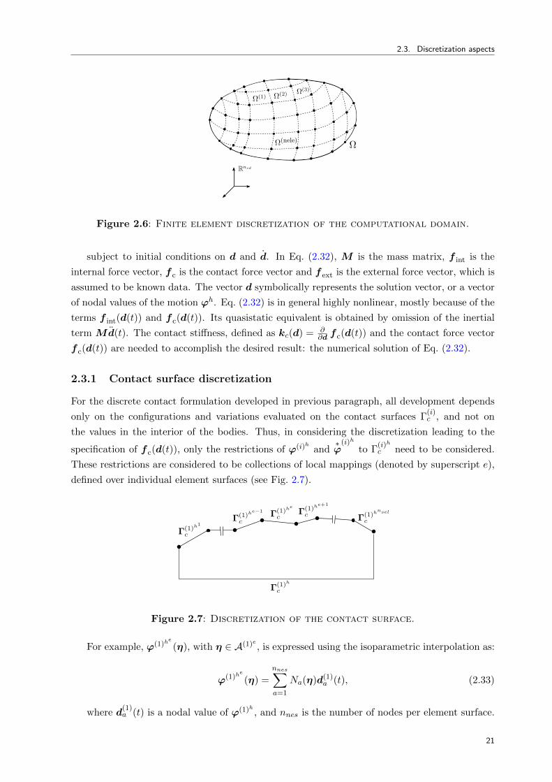
In giving the discrete formulation of the contact problem, the idea is that one applies the
spatial discretization (Fig. 2.6) to the weak form of the governing equations. The result is a
nonlinear set of ordinary differential equations. To be more specific, one begins by considering
ϕ(i)h and∗ϕ
(i)h
, finite dimensional counterparts of ϕ(i) and∗ϕ
(i). Substitution of these finite
dimensional quantities into the global variational principle (Eq. (2.26)) gives a set of nonlinear
ordinary diferential equations of the form:
Md(t) + f int(d(t))− f ext(t) + f c(d(t)) = 0, (2.32)
20
2.3. Discretization aspects
Figure 2.6: Finite element discretization of the computational domain.
subject to initial conditions on d and d. In Eq. (2.32), M is the mass matrix, f int is the
internal force vector, f c is the contact force vector and f ext is the external force vector, which is
assumed to be known data. The vector d symbolically represents the solution vector, or a vector
of nodal values of the motion ϕh. Eq. (2.32) is in general highly nonlinear, mostly because of the
terms f int(d(t)) and f c(d(t)). Its quasistatic equivalent is obtained by omission of the inertial
term Md(t). The contact stiffness, defined as kc(d) = ∂∂d f c(d(t)) and the contact force vector
f c(d(t)) are needed to accomplish the desired result: the numerical solution of Eq. (2.32).
2.3.1 Contact surface discretization
For the discrete contact formulation developed in previous paragraph, all development depends
only on the configurations and variations evaluated on the contact surfaces Γ(i)c , and not on
the values in the interior of the bodies. Thus, in considering the discretization leading to the
specification of f c(d(t)), only the restrictions of ϕ(i)h and∗ϕ
(i)h
to Γ(i)h
c need to be considered.
These restrictions are considered to be collections of local mappings (denoted by superscript e),
defined over individual element surfaces (see Fig. 2.7).
Figure 2.7: Discretization of the contact surface.
For example, ϕ(1)he
(η), with η ∈ A(1)e , is expressed using the isoparametric interpolation as:
ϕ(1)he
(η) =
nnes∑a=1
Na(η)d(1)a (t), (2.33)
where d(1)a (t) is a nodal value of ϕ(1)h , and nnes is the number of nodes per element surface.
21

Governing Equations for Large Deformation Contact
Na(η) denotes a standard Lagrangian shape function, defined on the biunit square A(1)e for 3D
problems and on A(1)e = [−1, 1] for 2D problems. The interpolation of∗ϕ
(1)h
(η) is similarly
conceived, via:
∗ϕ
(1)he
(η) =
nnes∑a=1
Na(η)c(1)a . (2.34)
Using the isoparametric interpolation scheme, one also has:
Xhe(η) =
nnes∑a=1
Na(η)Xa. (2.35)
Analogues of Eqns. (2.33)-(2.35) are assumed to hold for body (2):
ϕ(2)he
(ξ) =
nnes∑b=1
Nb(ξ)d(2)b (t), (2.36)
∗ϕ
(2)he
(ξ) =
nnes∑b=1
Nb(ξ)c(2)b , (2.37)
and
Y he(ξ) =
nnes∑b=1
Nb(ξ)Y b, (2.38)
defined over element surface parent domains A(2)e . The contact virtual work in the discrete
setting is now written by substitution of the above discrete fields into Eq. (2.31), as:
δWc(ϕht ,∗ϕh) :=
∫Γ(1)hc
[thN δgh + tThα δξ
αh ] dΓ. (2.39)
Eq. (2.39) may be written as a sum of integrals over the nsel elements surface of Γ(1)h
c (see
Fig. 2.7):
δWc(ϕht ,∗ϕh) :=
nsel∑e=1
∫Γ(1)h
e
c
[thN δgh + tThα δξ
αh ] dΓ, (2.40)
where each subintegral of Eq. (2.40) is evaluated using quadrature.
Based on Eq. (2.40), the global contact force vector f c can be expressed as:
f c =
nsel·nint
Ak=1
W k j(ηk)[thN (ηk) δgh(ηk) + tThα (ηk) δξα
h(ηk)
](2.41)
where A is the standard finite element assembly operator, nint is the number of integration
points per element surface of Γ(1)h
c , W is the quadrature weight, j is the jacobian of the trans-
formation and k is a revised quadrature point index, which runs over all quadrature points in
Γ(1)h
c .
The most relevant conclusion that can be extracted from Eq. (2.41) is that the global contact
22

2.3. Discretization aspects
force vector results from the assembly of elemental matrices which are constructed based on the
position of contacting nodes between the two surfaces. In this way, one can think of new elements
that are created between the connection of contacting nodes of both surfaces. The elemental
matrices of such elements are assembled in the global system to obtain the global contact force.
This elements are usually called contact elements.
Contact elements are kind of bridge elements between locally separated but potentially inter-
acting surfaces. Each contact element contains components of both surfaces and the composition
of these components depends upon the choice of the contact discretization. The most common
and widely used contact discretization is the node-to-segment approach (see Fig. 2.8). Each
contact element has its own vector of unknowns, residual and tangential matrix. Therefore,
contact elements are assembled to the global system matrix, together with unknowns, residual
and tangential matrices of ordinary structural elements.
Figure 2.8: Contact element - Node-to-segment discretization.
The most important practical aspect of computing the contact force is the acquisition of the
projection y ∈ γ(2)h
c for a quadrature point currently at location x ∈ γ(1)h
c , see Fig. 2.9. This
projection is central to the definition of both the gap g and the tangential basis, needed for the
frictional case. Calculation of the projection is often referred to as contact detection or searching.
Figure 2.9: Projection of slave node to master segment/surface.
23

Chapter 3
Analysis of Existing Computational Methods
In this chapter we aim to expose the main drawbacks present in the parallelization of traditional
contact mechanics algorithms and to provide a strong justification for the development of the
parallel methodologies for the numerical solution of contact problems which are the main reason
of this thesis. For such end, the chapter is divided in two parts. The first part is devoted to the
introduction of some basic concepts related to parallel computing. The second part describes the
current context of computational contact mechanics and enumerates the reasons which fundament
this work. To conclude, we introduce and enumerate the design basis for the novel methodology
proposed in this thesis.
3.1 Key concepts for parallel computing. A crash introduction
The aim of this section is to present some key concepts related to parallel computing and to the
domain decomposition approach, which plays a relevant role in the motivation of this thesis.
3.1.1 Parallel computational models
Parallel computational models form a complicated structure. They can be differentiated along
multiple axes: whether the memory is physically shared or distributed, how much communication
is in hardware or software, what the unit of execution is, and so forth. The picture could be
even more confusing by the fact that software provides an implementation of any computational
model on any hardware. This section thus intends to define some terms to delimit our discussion
and usage of the message-passing interface, which is a building block of this thesis.
Although parallelism occurs in many places and at many levels in a modern computer, one of
the first cases it was made available to the programmer was in vector processors. Indeed, the vec-
tor machine began the current age of supercomputing. The vector machine’s notion of operating
on an array of similar data items in parallel during a single operation was extended to include
the operation of whole programs on collections of data structures, as in SIMD (single-instruction,
multiple-data) machines. At whatever level, the model remains the same: the parallelism comes
25

Analysis of Existing Computational Methods
entirely from the data; the program itself looks very much like a sequential program. The parti-
tioning of data that underlies this model may be done by a compiler. Nowadays, data parallelism
has made a dramatic come back in the form of Graphical Processing Units, or GPUs.
Parallelism that is not determined implicitly by data independence but is explicitly specified
by the programmer is control parallelism. One simple model of control parallelism is the shared
memory model, in which each processor has access to all of a single, shared address space at the
usual level of load and store operations (see Fig. 3.1). In a shared memory system, the processors
usually communicate implicitly by accessing shared data structures. OpenMP [128] is probably
the most well known and globally used application programming interface for multi-platform
shared memory multiprocessing programming.
Figure 3.1: Shared memory architecture.
The message-passing model assumes that a set of processes that have only local memory can
communicate with other processes by sending and receiving messages. It is a defining feature
of the message-passing model that data transfer from the local memory of one process to the
local memory of another requires communication operations to be performed by both processes.
Message-passing is used widely on parallel computers with distributed memory (see Fig. 3.2). In a
distributed memory system the memory is associated with individual processors, and a processor
is only able to address its own memory. In this context, the message-passing model is suitable
for the communication and data exchange amongst all the processors. The Message-Passing
Interface (MPI) is a standardized and portable message-passing system designed by a group
of researchers from academia and industry to function on a wide variety of parallel computing
architectures [127]. The standard defines the syntax and semantics of a core of library routines
useful to a wide range of users writing portable message-passing programs.
Current large-scale parallel computers are neither of the purely shared memory nor of the
purely distributed memory type but a mixture of both, i.e., there are shared memory building
blocks connected via a fast network. The concept has clear advantages regarding price vs.
performance. The principal hardware issue is the cost of scaling the interconnection in a shared
memory architecture. As we add processors to the communication bus amongst the CPUs,
the chance that there will be conflicts over access to the bus increase dramatically, so buses are
suitable for systems with only a few CPUs. On the other hand, distributed memory interconnects
26

3.1. Key concepts for parallel computing. A crash introduction
Figure 3.2: Distributed memory architecture.
are relatively inexpensive, and distributed memory systems with thousands of processors have
been built. Thus, distributed memory systems are often better suited for problems requiring vast
amounts of data or computation. Parallel computers with hierarchical structures as described
above are also called hybrids. The concept is more generic and can also be used to categorize any
system with a mixture of available programming paradigms on different hardware layers. For
a more detailed description of parallel computational models, parallel architectures and parallel
programming, see [55, 104, 56].
The aim of this thesis is the solution of mechanical contact problems in large scale systems,
which involves a considerable number of processors. In this context, exclusively shared memory
systems are not suitable for the purpose of this work, so distributed memory (or even hybrid)
architectures must be used. The parallelization of the solution of mechanical contact problems is
thus focused on distributed memory systems, where the MPI standard is the main tool used for
all the implementations that appear in this thesis. The extension to hybrid systems is relatively
straightforward since the parallelization at the shared memory level doesn’t change the full
workflow of the algorithm, as it only takes profit of finer grain parallelism of the workflow once
stablished. In this work we will focus on the MPI layer of parallelism.
3.1.1.1 Message passing interface (MPI)
The Message Passing Interface (MPI) [127] is a standardized specification of a set of library
subroutines for the portable and flexible development of efficient message-passing parallel pro-
grams. The standard defines the syntax and semantics of library routines and allows users to
write portable programs in the main scientific programming languages. Since its release, the
MPI specification has become the leading standard for message-passing libraries for parallel
computers. Some key points are:
• The MPI Forum is in charge of the standardization (40 participating organizations, includ-
27

Analysis of Existing Computational Methods
ing vendors, researchers, software library developers, and users).
• Revised several times, with the most recent specification being MPI-3. Actual implemen-
tations differ in the version/features of the standard they support.
• Is supported on virtually all HPC platforms. Several implementations are open source as
OpenMPI or MPICH. Commercial implementations as Intel MPI are also available.
• Provides Fortran, C, and C++ bindings.
• Has a very broad standard with a huge number of library subroutines (over 440 in MPI-3).
Fortunately, most applications merely require less than a dozen of them.
The way MPI programs are compiled and run is not fixed by the standard. Compiler and
linker need special options that specify where modules and libraries can be found. There is
a considerable variation in those locations among installations. Most MPI implementations
provide compiler wrapper scripts (e.g., mpif90) that automatically supply the required options
to the underlying native compiler. Typically a script called mpirun is provided to start a message-
passing program: processor cores have to be allocated in advance. How exactly processes are
created is entirely up to the implementation, and typically mpirun uses the batch system’s
infrastructure to launch processes.
An MPI message is defined as an array of elements of a particular MPI data type. MPI data
types can be either basic or derived. MPI derived types created by calling appropriate MPI calls.
MPI needs to know the data type of messages as it supports heterogeneous environments where
it may be necessary to perform on-the-fly data conversions. The MPI data types on sender and
receiver must match for messages to proceed.
MPI conforms the following rules:
• Single Program Multiple Data (SPMD) model: the same program runs on all processes. All
processes taking part in a parallel calculation can be distinguished by a unique identifier
called rank.
• The program is written in a sequential language like Fortran, C, C++ or Python. Data
exchange is carried out via calls to MPI library subroutines.
• All variables in a process are local to this process.
3.1.2 Domain decomposition
The meaning of the term domain decomposition depends strongly on the context. It refers to
the splitting of a partial differential equation, or to its numerical approximation, into coupled
problems on smaller subdomains forming a partition of the original domain. This decomposi-
tion may enter at the continuous level, where different physical models may be used in different
regions, or at the discretization level, where it may be convenient to employ different approx-
imation methods in different regions, or in the solution of the algebraic systems arising from
28

3.1. Key concepts for parallel computing. A crash introduction
the approximation of the partial differential equation. At first glance, these aspects seem to be
rather independent. However, all have one central idea in common: the decomposition of the un-
derlying global problem into suitable subproblems of smaller complexity. In general, a complete
decoupling of the global problem into many independent subproblems, which are easy to solve,
is not possible. Since the subproblems are very often coupled, there has to be communication
between the different subproblems. For a comprehensive and more general overview of domain
decomposition methods, see [136, 130, 120].
This thesis is entirely devoted to the third aspect of domain decomposition described in the
previous paragraph, which is the solution of the algebraic systems arising from the approxima-
tion of the partial differential equation. In practical applications, finite element method or other
discretizations reduce the problem to the solution of an often massive algebraic system of equa-
tions. Direct factorization of such systems might then not be a viable option and the use of basic
iterative methods, such as the conjugate gradient algorithm, can result in very slow convergence.
The basic idea of domain decomposition is that instead of solving one massive problem on a do-
main, it may be convenient (or necessary) to solve many smaller problems on single subdomains
a certain number of times.
Domain decomposition methods aim at parallelizing the solution process by decomposing the
computational domain in several subdomains. The problems on the subdomains are indepen-
dent, which makes domain decomposition methods suitable for parallel computing. Regarding
the computational aspects of domain decomposition, this thesis is devoted to parallelization in
distributed memory machines, based on mesh partitioning and MPI processes. This implemen-
tation strategy proves to be especially well-suited for this type of applications.
The parallelization paradigm considered in this thesis is a sub-structuring method, were a
Master-Worker interaction model between the CPUs is used. Sub-structuring methods consist
essentially in distributing the work among the Workers, leaving the Master in charge of general
tasks like I/O. In a Master-Worker interaction, the Master reads the mesh and performs the
partition of the element graph. For the pure MPI strategy, each MPI process (the Workers) is in
charge of each subdomain (i.e. the number of MPI processes equals the number of subdomains).
The Workers build the local matrices and right-hand side and are in charge of the resulting
system solution in parallel. In the assembly stage, very few communications are needed between
Workers and the scalability only depends essentially on the load balancing.
For the sake of clarity, let’s consider the example shown in Fig. 3.3. Here, a 2-dimensional
discretized domain composed of 24 quadrilateral elements and 35 nodes is partitioned in 3 iden-
tical subdomains/MPI processes P1, P2 and P3. In general, discretized domains can be split by
elements or by nodes. For the finite element discretization, which is the one considered in this
thesis, the partitioning of the domain throughout the elements is commonly the preferred choice
(see [93]). Hence, the nodes used as a reference for the domain partitioning, called interface
nodes, are repeated among contiguous subdomains. Going back to the example of Fig. 3.3, each
of these subdomains are then conformed by 8 elements and 15 nodes each. Each MPI process
handles local element and node identifiers. Suppose now that we want to solve the Poisson
29

Analysis of Existing Computational Methods
31
26
21
16
11
6
1
32
27
22
17
12
7
2
33
28
23
18
13
8
3
34
29
24
19
14
9
4
35
30
25
20
15
10
5
interior nodesinterface nodes
P1
1 2 3 4 5
6 7 8 9 10
11 12 13 14 15
P2
1 2 3 4 5
6 7 8 9 10
11 12 13 14 15
P31 2 3 4 5
6 7 8 9 10
11 12 13 14 15
Figure 3.3: Mesh partitioning for domain decomposition approach.
equation using finite elements in parallel using the configuration shown in the previous example.
In a Master-Worker interaction, each MPI process stores/assembles a local portion Ai and fi
(i.
= 1, 2, 3) of the global matrix/vector A and f (i.e. the portion that belongs to its subdomain).
Global matrices and vectors are never stored/assembled explicitly.
Parallel finite element assembly results in a sub-assembled (partially-summed) Ai and fi, the
portion of A and f locally assembled by MPI process Pi. Sub-assembly means that for Ai and
fi the nodal contributions at interface nodes positions are partial because they don’t take into
account the contributions from neighbour nodes located in other subdomains. To compute a
fully-summed solution (the correct solution) of the unknown vector u, nodal contributions at
interface nodes must be shared (and summed) amongst the subdomains (see Fig. 3.4).
f1
1.7 1.6 1.2 1.5 1.8
0.1 0.3 0.2 0.9 0.4
f2
0.8 0.7 0.9 0.6 0.4
1.1 1.3 1.2 1.8 1.1
f 0.9 1.0 1.1 1.5 0.8
u1
1.7 2.6 1.2 2.5 1.8
1.1 1.3 1.2 1.5 1.4
u2
1.1 1.3 1.2 1.5 1.4
2.1 2.3 2.2 2.8 2.1
u 1.1 1.3 1.2 1.5 1.4
Figure 3.4: Parallel finite element assembly of RHS vector and solution vector.
3.1.3 Mesh partitioning
A great variety of methods for the numerical solution of any physical problem, such finite ele-
ments, finite volumes or finite differences, require a discretization of the physical domain into
nodes and elements. This process is known as meshing. The main unknowns of the physical
problem are then computed for each of the nodes of the mesh. The numerical resolution of real-
30

3.1. Key concepts for parallel computing. A crash introduction
world engineering problems is a rather demanding task since meshes often have large numbers
of elements. As a result, the numerical method is usually parallelised. For the solution of a,
for instance, finite element problem in parallel using the domain decomposition method, the
usual approach is to partition the mesh into subdomains. Each subdomain can then be mapped
to each of the processors of the parallel machine allocated for the resolution of the problem.
When assembling and solving the resultant linear system each processor is then responsible for
the element matrices belonging to the elements that it owns. Furthermore, when the elements
surrounding a particular node are owned by different processors some communication is required
to obtain the global solution for the problem. Consequently, to achieve high parallel efficiency
it is important that the mesh is partitioned in such a way that workloads are well balanced
and interprocessor communication is minimised. This is achieved mainly by ensuring same node
number in each subdomain and minimizing the number of nodes on the subdomains interfaces.
An important component in mesh partitioning is the well-known graph-partitioning problem
(see Fig. 3.5). Unfortunately, this is an NP-hard optimisation problem, which makes it impossible
to find optimum solutions in polynomial time. Consequently, heuristic approaches are normally
used for mesh partitioning.
In the past two decades, graph partitioning methods have witnessed rapid development,
giving rise to many graph partitioning software packages, such as METIS [97, 78], Zoltan [23],
JOSTLE [134] and SCOTCH [121, 107]. Among these software packages the most representative
one is METIS, which is a set of serial programs for partitioning graphs and finite element meshes.
The algorithms implemented in METIS are based on the multi-level recursive-bisection, multi-
level k-way, and multi-constraint partitioning schemes. The multi-level method reduces the size
of the original graph, performs a partition on this and then finally uncoarsens the graph to find a
partition for the original graph. It can be used as a suite of standalone partitioning applications
or by linking a users own Fortran or C application to the software library. Comparing with other
widely used partitioning algorithms, METIS is faster while providing high quality partitions [78].
3.1.4 Sparse storage
A sparse matrix is a matrix in which most of the elements are zero. Large sparse matrices often
appear in scientific or engineering applications when solving partial differential equations. In
particular, the matrices which result from the finite element discretization have the particularity
of being considerably sparse. When storing and manipulating sparse matrices on a computer,
it is beneficial and often necessary to use specialized algorithms and data structures that take
advantage of the sparse structure of the matrix. Operations using standard dense-matrix struc-
tures and algorithms are slow and inefficient when applied to large sparse matrices as processing
and memory are wasted on the zeroes. Sparse data is by nature more easily compressed and thus
require significantly less storage. Very large sparse matrices are infeasible to manipulate using
standard dense-matrix algorithms.
One method for storing sparse matrices is the compress sparse row (CSR) storage method [115].
The CSR storage method uses three arrays to store the non-zero elements of a sparse matrix. The
31

Analysis of Existing Computational Methods
Figure 3.5: Mesh partitioning: (a) Sample mesh. (b) Mesh with induced graph. (c)Graph partitioning. (d) Partitioned mesh.
first array stores contiguously the non-zero elements in each row and is called Data array. The
second array is of the same size as the Data array and stores the Column indices corresponding
to the entries in the Data array. The third array is called Row pointer and stores the locations
in the Data array that start a row.
This method of storing matrices is illustrated by a simple example. Fig. 3.6 shows a 1D mesh
composed of 5 nodes, used to discretize the Poisson equation ∇2ϕ = 0. Fig. 3.7 shows the dense
matrix which results from the finite element discretization and the arrays of the CSR format.
1 2 3 4 5
Figure 3.6: 1D mesh example.
1 -1 0 0 0
-1 2 -1 0 0
0 -1 2 -1 0
0 0 -1 2 -1
0 0 0 -1 1
1 2 3 4 5
1
2
3
4
5
1 -1 -1 2 -1 -1 2 -1 -1 2 -1 -1 1
Data values (a)
1 2 1 2 3 2 3 4 3 4 5 4 5
Column indices (ja)
0 2 5 8 11 13 Row pointers (ia)
Figure 3.7: Example of matrix storage in compress sparse row (CSR) format.
In the example shown in Fig. 3.7, the dense matrix is first constructed and then, once the
32

3.2. Contact mechanics: methods of constraint enforcement
zeroes location is known, used to build the CSR format arrays. In practice, computational codes
which exploit the advantages of sparse storage never store the matrix in its dense form. On
the contrary, they allocate only the required memory for the storage of the CSR format arrays
by looking into the mesh connectivity, i.e. how the nodes of the mesh are connected. Mesh
connectivity is what computational codes analyze to “predict” the location of zeroes without
having to assemble the dense form of the system matrix.
3.2 Contact mechanics: methods of constraint enforcement
The variational inequality that results after the enforcement of the contact boundary conditions
in the continumm equation is not appropriate for discretization. As remarked in Sec. 1.2, most
of the numerical procedures for the resolution of contact problems are based on the so-called
variational equality, which is easy to introduce in a finite element framework and can be easily
adapted to pre-existent minimization techniques, as might be found generically in [92, 52]. This
fact has been exploited historically to conceive the vast majority of the contact algorithms in
common use today.
In this section we shall discuss the most common formulations that can be applied to incorpo-
rate the contact constraints into the variational formulation, Eq. (2.26). For the sake of simplicity
we will consider here the frictionless form of the governing equations for contact mechanics. We
present here the most popular and widely used methods for constraint enforcement applied in
contact algorithms, which are: penalty, Augmented Lagrangian and Lagrange multipliers. We
introduce them by means of practical example characterized by a 1D frictionless linear example
of two beams, in a simplified way to facilitate a focus on the principal ideas, without diverting
our intentions with more complex issues which are beyond our purpose. It is remarked that
the ideas which emerge from the examples discussed below in this section are not limited to the
linear elastic case. The interpretations of the ideas that follow, however, can be appropriately
generalized to broader context.
3.2.1 Unconstrained system
We present a 1D frictionless linear example of two identical cantilever beams as shown in Fig. 3.8.
Here, we consider an equilibrium situation of no contact, where the beams are initially separated
by a gap g∗ and a force of magnitude F is applied to node u21.
In a non-contact situtation, as the one shown in Fig. 3.8, the last term of the governing
equation for the contact problem, Eq. (2.26), vanishes. As in this case we do not need to
impose the contact constraints, we define this configuration as an unconstrained system. This
unconstrained system can be simply modelled by the sum of the momentum balance equation
for each beam separately. From Eq. (2.26), and considering a linear example, we can write this
expression in the following algebraic way:
δW :=
2∑i=1
δW(i)sb = Ku− f = 0, (3.1)
33
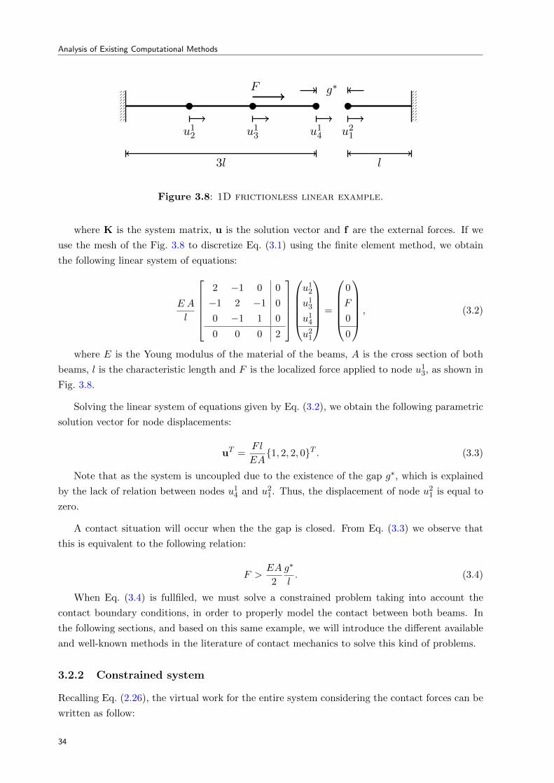
Analysis of Existing Computational Methods
3l l
u12 u1
3 u14 u2
1
F g∗
Figure 3.8: 1D frictionless linear example.
where K is the system matrix, u is the solution vector and f are the external forces. If we
use the mesh of the Fig. 3.8 to discretize Eq. (3.1) using the finite element method, we obtain
the following linear system of equations:
E A
l
2 −1 0 0
−1 2 −1 0
0 −1 1 0
0 0 0 2
u1
2
u13
u14
u21
=
0
F
0
0
, (3.2)
where E is the Young modulus of the material of the beams, A is the cross section of both
beams, l is the characteristic length and F is the localized force applied to node u13, as shown in
Fig. 3.8.
Solving the linear system of equations given by Eq. (3.2), we obtain the following parametric
solution vector for node displacements:
uT =Fl
EA1, 2, 2, 0T . (3.3)
Note that as the system is uncoupled due to the existence of the gap g∗, which is explained
by the lack of relation between nodes u14 and u2
1. Thus, the displacement of node u21 is equal to
zero.
A contact situation will occur when the the gap is closed. From Eq. (3.3) we observe that
this is equivalent to the following relation:
F >EA
2
g∗
l. (3.4)
When Eq. (3.4) is fullfiled, we must solve a constrained problem taking into account the
contact boundary conditions, in order to properly model the contact between both beams. In
the following sections, and based on this same example, we will introduce the different available
and well-known methods in the literature of contact mechanics to solve this kind of problems.
3.2.2 Constrained system
Recalling Eq. (2.26), the virtual work for the entire system considering the contact forces can be
written as follow:
34

3.2. Contact mechanics: methods of constraint enforcement
δW :=2∑i=1
δW(i)sb + δWc = 0. (3.5)
From Eq. (2.30), we can express the last term of Eq. (3.5) in the following way:
δWc :=
∫Γ(1)c
[tN δg + tTα δξα] dΓ. (3.6)
As we are considering a frictionless example, then Eq. (3.6) simplifies to:
δWc :=
∫Γ(1)c
tN δg dΓ. (3.7)
Eq. (3.5) together with frictionless contact conditions (see Sec. 2.2.1):
tN ≥ 0, (3.8a)
g ≤ 0, (3.8b)
tN g = 0, (3.8c)
define the boundary value problem with contact constraints.
On the other hand, the general formula for the gap g can be expressed as:
g = g∗ − (u14 − u2
1), (3.9)
where g∗ is the initial gap and u14 and u2
1 are the displacement of the contacting nodes.
Finally, the variation of the gap g can be written as follow:
δg = δu14 + δu2
1. (3.10)
3.2.2.1 Penalty method
In the penalty method the constrained optimization problem is converted into a unconstrained
problem by introducing an artificial penalty for violating the constraint. Specifically, for the
problem at hand, one obtains a penalty method for the frictionless contact problem by penalizing
any penetration (g > 0), by the following relation:
tN = εN 〈g〉, (3.11)
where εN > 0 is defined as the penalty parameter and the notation 〈·〉 denotes the Macauley
bracket, which simply renders the positive part of its operand via:
〈x〉 :=
x if x ≥ 0,
0 if x < 0.(3.12)
Use of Eq. (3.11) in Eq (3.7) gives rise to the penalized form of the contact integral:
35

Analysis of Existing Computational Methods
δWc :=
∫Γ(1)c
εN 〈g〉 δg dΓ. (3.13)
Combining Eqs. (3.1) and (3.13) with Eq. (3.5) we obtain the penalized algebraic form of the
contact problem:
δW = KP u− fP = 0. (3.14)
where KP is the penalized system matrix, u is the solution vector and fP are the penalized
external forces.
Going back to our base example, discretization of Eq. (3.14) for the geometry depicted in
Fig. 3.8 via the finite element method gives the following linear system of equations:2EAl −1EAl 0 0
−1EAl 2EAl −1EAl 0
0 −1EAl 1EAl +εN −εN0 0 −εN 2EAl +εN
u1
2
u13
u14
u21
=
0
F
εN g∗
−εN g∗
(3.15)
From Eq. (3.15) it can be seen that due to the contact constraints, nodes u14 and u2
1 are now
coupled. Comparing with Eq. (3.2), this can be observed by the appearence of extra cross terms
which include the penalty parameter on Eq. (3.15).
The coupling of nodes u14 and u2
1 can be physically interpreted by the introduction of a new
structural element connecting both nodes, which appears due to the penalization (see Fig. 3.9).
This element has the following elementary matrix:[εN −εN−εN εN
](u1
4
u21
)=
(εN g
∗
−εN g∗.
)(3.16)
To reinforce the previous idea, it can be observed that the assembly of the elementary matrix
given by Eq. (3.16) in the unconstrained linear system given by Eq. (3.2) produces the coupled
system defined by Eq. (3.15).
u12 u1
3 u14 u1
2
F g∗
Figure 3.9: Additional structural element introduced by penalization.
3.2.2.2 Lagrange multipliers method
This method is used in optimization theory to find the extremum of a functional subjected to
constraints. In a contact situation the idea is to minimize the functional Wsb from Eq. (2.8)
36

3.2. Contact mechanics: methods of constraint enforcement
subjected to frictionless contact conditions given by Eq. (2.18). Thus, when contact is produced,
we want to solve the following problem:
min Wsb subjected to g = 0, (3.17)
where g is the gap function. The basic idea of the Lagrange multipliers method is to expand
the functional Wsb in the following way:
W(u, λ) :=Wsb(u) +Wλ(u, λ), (3.18)
where
Wλ(u, λ) :=
∫Γ(1)c
λ g dΓ. (3.19)
Eq. (3.18) constitutes a saddle problem, whose solution is a maximum of W with respect to
Lagrange multipliers λ but a minimum with respect to displacements u. As Lagrange multipliers
can be physically interpreted as the contact pressure, the solution of Eq. (3.18) satisfy not only
the constraint g = 0 but also tN > 0, as stated in Eq. (2.18):
Contrary to the penalty method explained in Sec. 3.2.2.1, where the resulting functional
involves only one type of unknown, which are the displacements, the Lagrange multiplier method
introduce extra unknowns to the system. The problem is then formulated as follows:
δWsb(u, δu) + δWλ(δu, λ) = 0 (3.20a)
δWλ(u, δλ) = 0 (3.20b)
The algebraic form of Eq. (3.20) can be written as:
δW = Klm ulm − flm = 0, (3.21)
where Klm is the augmented form of the system matrix, ulm is the solution vector which
includes displacements and Lagrange multipliers, and flm are the augmented external forces.
Returning to our base example (Fig. 3.8), discretization of Eq. (3.20) with the finite element
method gives the following linear system of equations:
E A
l
2 −1 0 0 0
−1 2 −1 0 0
0 −1 1 0 −1
0 0 0 2 1
0 0 −1 1 0
u1
2
u13
u14
u21
λN
=
0
F
0
0
−g∗
(3.22)
From the discretized linear system (Eq. (3.22)) it can be observed that the Lagrange multiplier
act as intermediary for the transference of information between contacting nodes u14 and u2
1.
From a geometrical viewpoint, the use of the Lagrange multiplier method is equivalent to the
introduction of an extra node into the mesh which is connected to the contacting nodes. This
37

Analysis of Existing Computational Methods
interpretation is schematically represented in Fig. 3.10.
u12 u1
3 u14 u1
2
F g∗
Figure 3.10: Additional node introduced by the Lagrange multipliers method.
It is worth mentioning that we have presented a very simplified case where only one Lagrange
multiplier was needed. In a discrete system, the number of Lagrange multipliers depends on the
number of contacting nodes which must be restricted from penetration. In more complex and
realistic contact examples, the number of unknowns for the Lagrange multipliers not only can
be considerably larger than one, but also its number can be time-dependent, as the contacting
interfaces can evolve with time.
3.2.2.2.1 Mortar method for contact problems Recently, new methods, so-called mortar
methods originally proposed in [18] for mesh tying, were designed for domain decomposition in
which unstructured grids are connected within a parallel finite element solution. These methods
has also been applied to finite element contact problems for two dimensional linear kinematics [15,
64, 96] and to large deformation kinematics for curved 3D surfaces [117, 118] when the nodes
in the contact interface do not coincide. Contrary to the node-to-segment discretization, the
mortar methods are based on a segment-to-segment apporach, and they do not lock since they
are LBB stable [25]. As mortar methods for contact problems deal with the main numerical
issues that affect the robustness of the node-to-segment approach (i.e. is valid only for low
order elements, fails contact patch test unless a two-pass scheme is used and the stability test
or inf-sup condition for Lagrange multipliers fails), they are currently the most general and well
stablished methodology for numerical simulation of contact problems. As a general characteristic
of this approach, mortar methods are based on the introduction of Lagrange multipliers to weakly
enforce the contact constraints, thus increasing dynamically the number of degrees of freedom of
the linear system to solve.
3.2.2.3 Augmented Lagrangian method
As shown in Sec 3.2.2.2 within the framework of the Lagrange multipliers method, contact
conditions are exactly satisfied by the introduction of Lagrange multipliers, which increase the
number of unknowns in the linear system. The additional unknowns that this method introduces
require supplementary computational efforts. On the other hand, as seen on Sec. 3.2.2.1, the
penalty method is simpler to implement and to interpret. Nevertheless, it presents the drawback
that the contact conditions are fulfilled exactly only in the case of an infinite penalty parameter.
This results in an ill-conditioning of the numerical problem.
The main idea of the Augmented Lagrangian method [63, 114] is to combine either the
penalty method with the Lagrange multiplier method. It yields a fully unconstrained problem
38

3.2. Contact mechanics: methods of constraint enforcement
without adding extra unknowns to the problem. Also, it enables exact fulfillment of the contact
constraints while using a finite value of the penalty parameter to facilitate the iteration procedure.
Thus, for the Augmented Lagrangian method, the contact integral for a frictionless approach
(Ec. (3.7)) takes the following form:
δWc :=
∫Γ(1)c
〈λ+ εN g〉δg dΓ (3.23)
The most common technique used in mechanics for the solution of the Augmented Lagrangian
problems is the method of multipliers, or Uzawa’s method. This method relies on the following
algorithm for a multiplier iteration (k) (see Fig. 3.11):
λ(k+1) = 〈λ(k) + εN g(k)〉. (3.24)
correct multiplier
tN
gλ(0)
m=εNλ(k)
g(1)
λ(1)
←g(2)
λ(2)
g(k+1)
λ(k+1)
Figure 3.11: Augmented Lagrangian update process.
Replacing of Eq. (3.24) in Eq. (3.23) gives the following iterative procedure for the contact
integral. This translates in an iterative procedure for the main unknown of the problem, i.e. the
displacements:
δW(k)c :=
∫Γ(1)c
〈λ(k) + εN g(k)〉δg dΓ. (3.25)
Iterations on (k) continue until changes in the multipliers become small, or alternatively,
until the constraints are satisfied within a tolerance range.
Expansion of the terms of Eq. (3.25) gives:
δW(k)c :=
∫Γ(1)c
λ(k) δg dΓ +
∫Γ(1)c
εN 〈g(k)〉δg dΓ (3.26)
It is worth mentioning that only the last term of Eq. (3.25) survives at the beginning of the
iterative procedure (initial estimate λ(0) = 0). Comparing with Eq. (3.13), it can be observed that
this term represents the penalty method contribution to the Augmented Lagrangian method. As
explained in Sec. 3.2.2.1, this term means, from a physical viewpoint, the introduction of a new
39
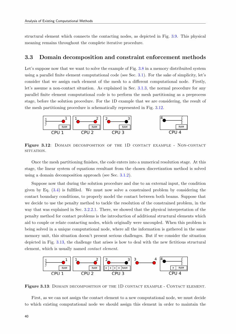
Analysis of Existing Computational Methods
structural element which connects the contacting nodes, as depicted in Fig. 3.9. This physical
meaning remains throughout the complete iterative procedure.
3.3 Domain decomposition and constraint enforcement methods
Let’s suppose now that we want to solve the example of Fig. 3.8 in a memory distribuited system
using a parallel finite element computational code (see Sec. 3.1). For the sake of simplicity, let’s
consider that we assign each element of the mesh to a different computational node. Firstly,
let’s assume a non-contact situation. As explained in Sec. 3.1.3, the normal procedure for any
parallel finite element computational code is to perform the mesh partitioning as a preprocess
stage, before the solution procedure. For the 1D example that we are considering, the result of
the mesh partitioning procedure is schematically represented in Fig. 3.12.
CPU 1 CPU 2 CPU 3 CPU 4RAM RAM RAM RAM
1 1 2 2 3 4
Figure 3.12: Domain decomposition of the 1D contact example - Non-contactsituation.
Once the mesh partitioning finishes, the code enters into a numerical resolution stage. At this
stage, the linear system of equations resultant from the chosen discretization method is solved
using a domain decomposition approach (see Sec. 3.1.2).
Suppose now that during the solution procedure and due to an external input, the condition
given by Eq. (3.4) is fullfiled. We must now solve a constrained problem by considering the
contact boundary conditions, to properly model the contact between both beams. Suppose that
we decide to use the penalty method to tackle the resolution of the constrained problem, in the
way that was explained in Sec. 3.2.2.1. There, we showed that the physical interpretation of the
penalty method for contact problems is the introduction of additional structural elements which
aid to couple or relate contacting nodes, which originally were uncoupled. When this problem is
being solved in a unique computational node, where all the information is gathered in the same
memory unit, this situation doesn’t present serious challenges. But if we consider the situation
depicted in Fig. 3.13, the challenge that arises is how to deal with the new fictitious structural
element, which is usually named contact element.
CPU 1 CPU 2 CPU 3 CPU 4RAM RAM RAM RAM
1 1 2 2 3 43 4
x x x x x
Figure 3.13: Domain decomposition of the 1D contact example - Contact element.
First, as we can not assign the contact element to a new computational node, we must decide
to which existing computational node we should assign this element in order to maintain the
40

3.3. Domain decomposition and constraint enforcement methods
workload balance. The answer to this question seems obvious when we are dealing with only one
contact element, but it is not straightforward when we handle bigger meshes and a considerable
number of contacting nodes.
The second issue is the memory allocation and the sparse storage. As explained in Sec. 3.1.4,
in any efficient finite element code the mesh connectivity is used to predict the zeros in the
resultant system matrix. This information is used for memory allocation, which is required for
the storage of the matrix components in compressed sparse formats. As the memory allocation is
done in preprocess, the contact element components which appears in the middle of the simulation
can not be stored, as there is no memory reserved for them.
The third, and not less important issue, is related to the subdomain connectiviy. As explained
in Sec. 3.1.2, in a domain decomposition approach global matrices are never stored explicitly.
On the contrary, the solution is obtained by means of the summation of the contributions of
the interface nodes, which are shared between subdomains. For that reason, when the mesh is
partitioned, the mesh splitting algorithm constructs a list which contains the interface nodes of
each subdomain and also indicates to which of the rest of subdomains those nodes are shared
with. The creation of contact elements adds new interface nodes to the subdomain to which they
belong, thus altering the lists previously created by the mesh partitioner.
The drawbacks reported in the previous paragraphs were exemplified by using a penalty
method example, but they are still valid for Augmented Lagrangian or Lagrange mutlipliers
method. To avoid these drawbacks, the solution of contact problems in parallel environments
requires to consider any possible contact situation before partitioning. By estimation of the
probable contacting area, contact elements must be predicted (and created) before partitioning
the mesh. For completeness sake, Fig. 3.14 shows the contribution of the contact element to
the structural matrix in a 2D case for the node-to-segment (NTS) discretization. In this kind of
contact discretization, which is the most widely used, nodes from one contacting surface exchange
contact information (i.e. contact tractions) with boundary segments of the other contacting
surface.
3.3.1 Sliding
In 1D contact problems, as the one described in previous sections (Fig. 3.8), is straightforward to
identify the contact area or the contacting nodes before the contact interaction. But for 2D and
3D problems the situation is different. Consider, for example, the case illustrated in Fig. 3.15.
Here we show a block-indenter configuration, where the rounded indenter impacts the square
block. Without knowing extra information, in this problem is impossible to know a priori the
location of the contact interface.
Yet, if one considers the kinematics of the problem, it is possible to estimate a possible area
of contact. Once this area is predicted, the contact elements can be constructed (see Fig. 3.16).
Just after this stage the mesh can be partitioned. Following this procedure, one avoids the
drawbacks detailed in previous section (Sec. 3.3) for parallel contact problems.
41

Analysis of Existing Computational Methods
Figure 3.14: Contact element for a 2D case - NTS discretization.
Figure 3.15: Block-indenter 2D example.
Figure 3.16: Block-indenter 2D example - contact prediction.
Nevertheless, the procedure described in previous paragraph does not consider the case of
large sliding, i.e. the relative motion of contacting surfaces while they are in contact. Sliding is
present in the majority of realistic 2D or 3D problems which are affected by finite deformations.
If sliding occurs, one must update the contact elements on the fly, or in other words, during the
42

3.3. Domain decomposition and constraint enforcement methods
solution procedure. This update is required because the coupling nodes for the exchange of con-
tact tractions are different than they were previously to the sliding, as will be further explained.
In a parallel approach this situation presents a major drawback, which will be described next.
Consider the 2D example shown in Fig. 3.17. Contacting surfaces are identified with slave
and master names, while their nodes are clearly identified in the figure. Fig. 3.17 shows the
contact prediction, the contact elements and the mesh partitioning, where we have considered
only two processors. In the figure one can observe which are the interior nodes that belong to
processor 1, those interior nodes which belong to processor 2 and the interface nodes. A dashed
line separates graphically both subdomains.
slave
1 2 3
master
4 5 6 7 8 9 10
P1
P2P1 nodesinterface nodesP2 nodes
Figure 3.17: Contact elements before sliding.
Suppose now that a sliding between slave and master occurs. The sliding changes the location
of the nodes which must be coupled for the exchange of contact tractions, which translates into
a re-definition of the contact elements. This situation is as shown in Fig. 3.18.
slave
1 2 3
master
4 5 6 7 8 9 10
P1
P2P1 nodesinterface nodesP2 nodes
Figure 3.18: Contact elements after sliding.
Because of the sliding, contact elements should now be redefined during the solution process,
and after the mesh partitioning. A feasible situation to deal with, is when new contact elements
43

Analysis of Existing Computational Methods
lie inside the same subdomain than they where before sliding. An example of this situation is the
contact element composed of nodes 1-6-7 before the sliding (see Fig. 3.17), which evolves to 1-5-6
after sliding (see Fig. 3.18). Nodes 1, 5, 6 and 7 are interior nodes of subdomain 1. Though, a
more complex case can result. It could happen that, after sliding, new contact elements need to
be defined as a connection between interior nodes of different subdomains. This is the case of
the contact element composed of nodes 3-7-8 which appears after sliding, as can be observed in
Fig. 3.18.
If due to the sliding any new contact element becomes defined by the connection of interior
nodes, there is no other option than to perform a new mesh partitioning. A new mesh partitioning
will split the mesh considering the new connectivities of the contact elements, avoiding the
situation previously described. With a new partitioning the connected nodes would transform in
interior nodes of an exclusive subdomain or, at least, in interface nodes. It is important to remark
that the repartitioning needs to be done every time the configuration of the contact elements
changes. This could occur even at each time step, which translates into a computationally high
demanding and very expensive task.
A possible workaround for this drawback would be to associate the contacting interfaces to
an specific group of processors. This would avoid repartitioning the mesh every time the contact
elements configuration changes. Despite being an acceptable alternative, this strategy conditions
the mesh partitioning algorithm, thus not ensuring the best workload balance and the minimal
communication between computational nodes.
3.4 Standard methods and the parallel world
In this chapter we have analyzed the application of standard methods based on nodes con-
nectivities for the resolution of contact problems in a parallel environment. The methods and
discretizations reviewed here are well known and widely used in the resolution of contact prob-
lems in engineering and science. Yet, they are implemented in a serialized way in the majority of
commercial and non-commercial codes, i.e.: Abaqus [1], ANSYS [5], ADINA [3], Code Aster [31],
FEAP [44], among others. During the past years, researchers have dedicated an extensive amount
of work to their study. Because of that, their behaviour is well known and most of the scientific
literature in contact mechanics is dedicated to them. The intention of this chapter is to evaluate
the direct applicability of such methods to parallel resolution strategies based on domain decom-
position approaches. This is motivated by the fact that parallel resolution strategies are a must
in large scale problems. From the topics covered here, some conclusions can be obtained.
In this chapter we showed that penalty and Augmented Lagrangian method add explicit
connections between contacting nodes, which present a serious drawback for parallel implemen-
tation. Also, Lagrange multipliers method (and the mortar approach) increases the number of
unknowns of the system, as their number depend on the contacting nodes. Even more, as the
contacting area may change with time, the number of unknowns may vary along the simulation.
This situation is incompatible for problems were the mesh partitioning is done as a preprocessing
task, thus requiring to perform dynamic partitioning during the simulation. Despite that some
44

3.5. Design basis of the proposed algorithm
drawbacks which arise when the mesh partitioning is done in preprocessing time can be solved
by doing a contact prediction, the necessity of a dynamic partitioning becomes crucial when
sliding between contacting surfaces occurs. Nevertheless, some workarounds may be proposed
(see, for instance, [88]), but they are based on restricting the partitioning algorithm, which is
not an efficient solution. This lead us to conclude that standard contact methods present serious
disadvantages when they are extrapolated to parallel approaches based on domain decomposition
methods, as in a general case dynamic repartitioning can not be avoided.
Some previous works exist on the field of large scale, parallel methods for the solution of large
deformation contact problems [57, 95, 49], but they are limited to some particular applications
such as unilateral contact or shell structures. To the author best knowledge, no previous work
on general, bilateral parallel contact methods for 3D large deformation contact problems exist
on scientific literature.
3.5 Design basis of the proposed algorithm
Based on the analysis made on the previous section, the main motivation of this thesis is to
propose an alternative method for the numerical modelling of contact problems suitable for High
Performance Computing (HPC). This method must fulfill some general requirements, which are
adopted as the design basis for its development:
• it must be a general algorithm for the resolution of the two-body contact problem,
• it must not restrict the mesh partitioner,
• it must not require dynamic partitioning,
• it must not increase the number of unknowns of the system,
• it must not affect the system matrix, and
• it must be suitable for large scale problems.
The next two chapters (Chapters 4 and 5) are dedicated to the description of the proposed
algorithm. In Chapter 4 we propose a parallel method for unilateral contact problems, which
also serves as an intermediate step for the introduction of some concepts and ideas which are
the basis of the general two-body contact algorithm described in Chapter 5. Our objective is
to provide a comprehensive description by putting special emphasis not only on the detailed
explanation of the algorithm but also on its parallel computational implementation.
45


Chapter 4
A Parallel Method for Unilateral
Contact Simulation
In this chapter we present a new methodology for solving parallel unilateral frictional contact
problems in distributed-memory HPC computers. Additionally, we describe its computational
implementation, which is one of its distinctive characteristics. The presented methodology is
based on the partial Dirichlet-Neumann method, first introduced in [141, 142]. The proposed
method allows to solve the contact interaction as a coupled problem, in a staggered way. Fur-
thermore, it can be interpreted as a black-box scheme that can be used with any parallel finite
element code. In this method, the number of unknowns remains constant. Also, the mesh parti-
tioning is only done at the beginning of the simulation, as a preprocess task, without restricting
the partitioning algorithm. For those reasons, is a suitable methodology for the parallelization
of the solution of unilateral contact problems using a domain decomposition approach. This
chapter is also an intermediate step that serves to introduce some concepts and ideas which will
be needed for the following chapter, where we present a general parallel two-body contact for-
mulation. An important part of the general two-body algorithm is based on the ideas presented
here.
In this method, each body is treated independently and the contact is solved throughout the
exchange of boundary conditions at the contact interface. The contact detection is based on an
Eulerian-Lagrangian system analogy. The geometry of the rigid body is used as reference (base
mesh) for the detection of contact. As contact is a boundary phenomena, only the boundary
nodes of the deformable body mesh are available for localization. These nodes take the role
of particles that moves in the surroundings of the base mesh. The localization of at least one
node of the deformable body mesh inside the base mesh is equivalent to detecting contact, which
triggers the data exchange at the contact zone for the solution of the contact problem.
4.1 Introduction
In the engineering practice, a wide range of contact problems can be approximated by a unilateral
contact. i.e. contact between a rigid surface and a deformable solid. In a contact scenario, forces
47

A Parallel Method for Unilateral Contact Simulation
are transmitted through the common area of contact. These forces have commonly two compo-
nents: a normal component which prevents interpenetration of the bodies, and the tangential
component, created by friction. The normal contact forces are prescribed by the so-called Hertz-
Signorini-Moreau conditions [137], which are geometrical boundary conditions which include
inequalities related to frictionless contact and account for the non-interpenetration condition via
variational form. With regard to the friction, the simplest and most popular frictional condi-
tion is given by the Coulombian law (see Sec. 2.2.1.1), which is in good harmony with practical
experience.
A variational inequality characterizes the solution of unilateral contact problem. As men-
tioned in Sec. 3.2, variational inequalities can be reformulated into a variational equality problem
with special contact terms under the assumption of knowing a priori the contact interface. The
form of the contact terms depends on the method chosen to enforce the contact constraints. For
constraint enforcement, a wide range of techniques exists in the optimization literature [92, 52].
Among them, the most used methods for constraint enforcement in the numerical treatment of
contact problems are: the classical Lagrange multiplier method, the penalty method and the
Augmented Lagrangian method.
An alternative methodology for the variational approach in the solution of unilateral contact
problems is proposed in [141, 142]. This methodology is based on the equivalence of the geo-
metrical constraints due to normal and frictional contact and a combination of partial Dirichlet
and Neumann boundary conditions, prescribed in a specific way on the contact boundary. This
approach simplifies the algorithm and provides an efficient framework for contact treatment on
parallel computers.
On the other hand, in order to implement a parallel finite element calculation, the mesh is
partitioned among the computational nodes to minimize interprocessor communications. Contact
can occur between surfaces which are owned by different processors. Hence, in a parallel contact
simulation, global searches across all computational nodes are required. This feature makes
the contact detection one of the most important and complex parts in computational contact
mechanics, and also, one of the major computational costs of contact algorithms.
4.2 Formulation of unilateral contact problems
4.2.1 Unilateral normal contact
Let a rigid plane be defined in a local coordinate system by n = 0, being n the normal axis of
the plane, with unit external normal ν = en. Being the plane in this position, the motion of any
body in space is then restricted to n ≥ 0 (see Fig. 4.1). We can represent this restriction by the
following displacement contact constraint:
g(x) = x · ν ≥ 0, (4.1)
where g(x) is the gap between the current point x of the body and the rigid plane. In other
words, Eq. (4.1) states that any point of the body at any time can not penetrate the rigid plane.
48

4.2. Formulation of unilateral contact problems
Defining the displacement of any point of the body as u = x−X, we can express Eq. (4.1)
as:
g(u) = u · ν + g0 ≥ 0, (4.2)
where g0 = X · ν is the initial gap. If the body retains its integrity, the non-penetration
condition given by Eq. (4.2) is applied only to the surface points ∂Ω, precisely to the potential
contact zone (Γc) in the actual configuration. Γc can be splitted into two nonintersecting sets:
active contact zone Γc (points which are in contact) and inactive contact zone Γc\Γc (points
which are not in contact). The active contact zone in the actual configuration is defined by:
x ∈ Γc if and only if g(x) = x · ν = 0, (4.3)
while for the reference configuration, the active contact zone can be defined by:
X ∈ Γ0c if and only if X · ν = −u · ν. (4.4)
From the definitions in Eq. (4.3) and Eq. (4.4) we observe that the active and inactive contact
zones are a priori unknowns of the problem. Only in some specific problems, given the potential
zone we can predict a priory the active contact zone at each instant of time.
When the contact between the body and the rigid plane is produced, a contact pressure
appears in the active contact zone in order to prevent the penetration. This pressure should be
non-negative, i.e. equal to zero in inactive and negative in active contact zone:
σn ≤ 0 at Γc. (4.5)
Combining the non-penetration condition in the active zone given by Eq. (4.3) and the defi-
nition of the contact pressure (Eq. (4.5)) we get the non-penetration-non-adhesion condition:
σn g(x) = 0 at Γc. (4.6)
All together, the set of conditions expressed in Eq. (4.1), Eq. (4.5) and Eq. (4.6) form the
Hertz-Signorini-Moreau law of unilateral normal contact:
g ≥ 0, σn ≤ 0, σn g = 0. (4.7)
4.2.2 Balance of momentum including contact
The nonlinear contact problem can be written as a boundary value problem, given the following
equilibrium condition in Ω and boundary conditions on ∂Ω, which includes the Hertz-Signorini-
Moreau law for normal contact:
49

A Parallel Method for Unilateral Contact Simulation
Figure 4.1: Reference (Ω0) and actual (Ω) configurations of a deformable bodyin unilateral contact with a rigid plane.
∇ · σ + fv
= 0 in Ω
σ · n = σ0 on ΓN
u = u0 on ΓD
g ≥ 0, σn ≤ 0, σn g = 0, σt = 0 on ΓC
(4.8)
being σ the Cauchy stress tensor, fv
a vector of volumetric forces, σ0 a set of prescribed
tractions and u0 a set of prescribed displacements. Over ΓC we have imposed the contact
boundary conditions: g represents the gap between contacting bodies, σn is the normal contact
pressure and σt is the tangential stress. For simplicity, on the balance of momentum given by
Eq. (4.8) we have considered a frictionless case (σt = 0).
4.2.3 Interpretation of contact Hertz-Signorini-Moreau conditions
A contact problem can be directly interpreted as finding the active contact zone and the contact
pressure which has to be applied in order to fulfill contact constraints. However, the problem
can be also interpreted from another point of view: instead of prescribing the pressure at the
active contact zone, we can impose a displacement according to the contact constraints. In what
follows, and without loss of generality, we assume a frictionless case.
The set of normal contact conditions expressed by Eq. (4.7) can be separated into two parts
for active Γc and inactive Γc\Γc contact zones:
50

4.2. Formulation of unilateral contact problems
g = 0, σn < 0, σt = 0 at Γc, (4.9a)
g > 0, σn = 0, σt = 0 at Γc\Γc. (4.9b)
According to Eq. (4.2) and the definition of the active contact zone given by Eq. (4.4), the
first term of Eq. (4.9a) can be written as follows:
g = 0 ⇐⇒ ν · u = −g0 ⇐⇒ un = −g0. (4.10)
Eq. (4.10) shows that the no-penetration condition represented by Eq. (4.2) can be inter-
preted as a Dirichlet boundary condition. In contrast, the condition represented by Eq. (4.9b)
can be interpreted as a singular Neumann boundary condition σt = 0 (free boundary) for the in-
active zone. Considering the previous interpretations, we can rewrite the Hertz-Signorini-Moreau
conditions of Eq. (4.9a) and Eq. (4.9b) as:
un = −g0, σt = 0 for x ∈ Γc, (4.11a)
σ = 0 for x ∈ Γc\Γc. (4.11b)
Even more, we can rewrite Eq. (4.11a) using the condition given by Eq. (4.5) in the definition
for the active zone:
un = −g0, σt = 0 for x | x ∈ Γc and σn(x) < 0. (4.12)
In Eq. (4.11a) (and Eq. (4.12), which is equivalent) we have replaced the contact conditions
on the active contact zone Γc by a partial Dirichlet boundary condition (un = −g0) and a partial
Neumann boundary condition (σt = 0). The non-linearity of the problem emerge because the
active contact zone is, generally speaking, unknown a priori, and its specific location is part of the
solution of the problem. On the contrary, in Eq. (4.11b) we have replaced the contact conditions
in the inactive contact zone by prescribing a full singular Neumann boundary condition (σ = 0).
Writing Hertz-Signorini-Moreau law as expressed in Eq. (4.7) in the form of Eqs. (4.11a)
and (4.11b) gives a better understanding of the normal contact boundary conditions for unilat-
eral contact problems. From a numerical or computational mechanics approach, it is easier to
prescribe in a given domain a given displacement and check for the sign of the contact pressure to
determine the active contact zone, than to prescribe an unknown contact pressure in an unknown
active contact zone, which is determined by a zero value of the normal gap.
4.2.4 Interpretation of frictional condition
This thesis is limited to the classical Coulomb’s friction law for frictional problems, already
introduced in Sec. 2.2.1.1. This friction law states that the value of the tangential stress depends
only on the normal contact pressure σt = σt(σn) by the following relation:
|σt| ≤ µ |σn|, (4.13)
51

A Parallel Method for Unilateral Contact Simulation
where µ is a coefficient of friction. So, in the case of frictional contact, the stress vector at
the interface contains both normal and tangential components:
σ = σnn+ σt(σn). (4.14)
From Eq. (2.20) we can identify two different possible states which are allowed by the
Coulomb’s friction law: stick, that occurs when the tangential stress vector is smaller than
the critical frictional stress:
µ|σn| − |σt| > 0, (4.15)
and slip, that occurs when the tangential force σt reaches the threshold µ|σn| imposed by
the Coulombian law:
µ|σn| − |σt| = 0. (4.16)
Similarly to the previous section, we can interpret frictional constraints. Thus, to take the
frictional resistance into account, we must analyze the stress state. In the case of stick, the partial
Dirichlet boundary conditions for normal contact must be replaced with full Dirichlet boundary
conditions to reproduce the stick state. In the case of slip, the partial Dirichlet conditions for
normal contact must be applied in combination with partial Neumann boundary conditions in
order to reproduce the tangential frictional stress.
The interpretation of geometrical constraints due to frictional contact as partial Dirichlet-
Neumann boundary conditions allows us to introduce a technique for the numerical resolution of
unilateral contact problems using the Finite Element Method. This technique was first introduced
in [141], and is called the partial Dirichlet-Neumann (PDN) method. Taking advantage of the
reformulation of the geometrical contact constraints, this technique results very advantageous
for the resolution of this kind of problems, because there is no need to evaluate residual vectors
and tangent matrices. Coupled with a Lagrange multiplier method for the exchange of boundary
conditions, this method results equivalent to a mortar method. But contrary to the mortar
method, which increases dynamically the number of unknowns of the algebraic system, the PDN
method maintains constant the number of unknowns.
4.3 Method of partial Dirichlet-Neumann boundary conditions
The main idea of this method is to replace the geometrical constraints due to normal and frictional
contact by partial Dirichlet-Neumann boundary conditions in the case of unilateral contact with
an arbitrary rigid surface. In particular, the geometrical constraints due to normal contact are
imposed by means of Multi-Point Constraints (MPC) while friction is imposed in the form of
a tangential force which is applied in the opposite direction of sliding of the node. From a
geometrical point of view, MPC can be interpreted as Dirichlet boundary conditions which allow
sliding of the contacting node only in the tangential plane. For the enforcement of MPC a chosen
degree of freedom of each contacting node –slave dof us– is written as a linear combination of
52

4.3. Method of partial Dirichlet-Neumann boundary conditions
the other dofs of the same node –master dofs uim, i = 1, . . . ,M–:
us = αiuim + β, (4.17)
where αi and β are scalar coefficients, and M is the total number of master dofs. The slave
dof can be chosen arbitrarily for each contacting node but it is required that αi <∞.
4.3.1 Frictionless case
Let xi be the coordinates of a contacting node over Γc in the i-th iteration. Then, the incremental
displacement vector is given by:
ui = xi − xi−1. (4.18)
The incremental displacement of each degree of freedom is given by splitting the vector u
into the reference frame basis:
uij = ui · ej , (4.19)
where ej is a set of basis vectors.
Otherwise, any rigid surface can be described by the parametric representation:
r(u, v) = x(u, v) e1 + y(u, v) e2 + z(u, v) e3. (4.20)
Without any loss of generality, let us suppose that locally exists a function f such that:
z = f(x, y), (4.21)
where x, y and z are coordinates of the surface point in the chosen coordinate system:
x = x(u, v) e1, y = y(u, v) e2, z = z(u, v) e3. (4.22)
Then, using the definition given by Eq. (4.18), the geometrical constraint given by Eq. (4.1)
can be written in the following way:
xi3 ≥ f(xi1, xi2) ⇐⇒ ui3 ≥ f(xi−1
1 + ui1, xi−12 + ui2)− xi−1
3 . (4.23)
We can compute the tangential plane at a given point x∗, y∗ on Γc by the following expres-
sion:
P : z =∂f
∂x
∣∣∣x∗,y∗
(x− x∗) +∂f
∂y
∣∣∣x∗,y∗
(y − y∗) + f(x∗, y∗). (4.24)
Then, the multi-point constraint to be imposed to the point x∗, y∗ is given by:
u3 = au1 + bu2 + c− xi−13 , (4.25)
where
53
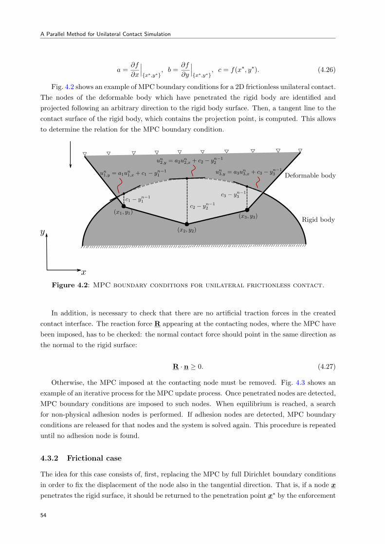
A Parallel Method for Unilateral Contact Simulation
a =∂f
∂x
∣∣∣x∗,y∗
, b =∂f
∂y
∣∣∣x∗,y∗
, c = f(x∗, y∗). (4.26)
Fig. 4.2 shows an example of MPC boundary conditions for a 2D frictionless unilateral contact.
The nodes of the deformable body which have penetrated the rigid body are identified and
projected following an arbitrary direction to the rigid body surface. Then, a tangent line to the
contact surface of the rigid body, which contains the projection point, is computed. This allows
to determine the relation for the MPC boundary condition.
Figure 4.2: MPC boundary conditions for unilateral frictionless contact.
In addition, is necessary to check that there are no artificial traction forces in the created
contact interface. The reaction force R appearing at the contacting nodes, where the MPC have
been imposed, has to be checked: the normal contact force should point in the same direction as
the normal to the rigid surface:
R · n ≥ 0. (4.27)
Otherwise, the MPC imposed at the contacting node must be removed. Fig. 4.3 shows an
example of an iterative process for the MPC update process. Once penetrated nodes are detected,
MPC boundary conditions are imposed to such nodes. When equilibrium is reached, a search
for non-physical adhesion nodes is performed. If adhesion nodes are detected, MPC boundary
conditions are released for that nodes and the system is solved again. This procedure is repeated
until no adhesion node is found.
4.3.2 Frictional case
The idea for this case consists of, first, replacing the MPC by full Dirichlet boundary conditions
in order to fix the displacement of the node also in the tangential direction. That is, if a node x
penetrates the rigid surface, it should be returned to the penetration point x∗ by the enforcement
54

4.3. Method of partial Dirichlet-Neumann boundary conditions
Figure 4.3: Iterative process for the MPC update process. (a) Initial configura-tion. (b) First iteration: four MPC boundary conditions are imposed at each ofthe four penetrated nodes. (c) Second iteration: after equilibrium is reached,two nodes are in adhesion to the surface of the rigid body. (d) In the thirditeration, MPC boundary conditions are released for the adhesion nodes andequilibrium is recomputed.
of a full Dirichlet condition of the form:
u = x∗ − x. (4.28)
Afterwards, the reaction R that appears at the node should be splitted into normal Rn and
tangential Rt components, and the non-adhesion condition should be checked as well as the
stick-slip condition: ||Rt|| < µ||Rn||, stick
||Rt|| ≥ µ||Rn||, slip.(4.29)
In the case of slip, the full Dirichlet boundary condition has to be replaced by an MPC
boundary condition to allow displacements on the tangent direction. In addition, an external
force Fe should be applied to the sliding node along the tangential direction, in the opposite
direction to the tangential reaction Rt. How this force is applied to the sliding node together
with the MPC is shown in Fig. 4.4. The magnitude of the external force Fe is given by the
Coulombian friction law, and is computed according to:
Fe = −µ ||Rn||Rt
||Rt||. (4.30)
55

A Parallel Method for Unilateral Contact Simulation
Rigid
Deformable
Figure 4.4: Representation of the external force for the frictional case.
4.4 Computational implementation
Based on the PDN method, we propose to solve the unilateral contact problem from a coupled
point of view. In this approach, each body is treated separately, using one instance of the
computational code for each body. The contact interaction is reproduced by means of the
transference of Dirichlet boundary conditions at the contact interface. It is worth remarking
that in the case of unilateral contact there is no need to solve the fully discretized system of
equations for the rigid body; only the displacement of its boundary elements must be computed
by the code instance devoted to this body. Nevertheless, its whole mesh is needed for contact
detection purposes, as will be explained in the following section. In this chapter, however, we will
consider a more general but equivalent case where the rigid body is assumed to be a deformable
body which only experiences rigid body translations. Despite not being the most efficient way
of solving a rigid body problem (since we are solving the fully discretized system of equations
for the rigid body only to obtain rigid body motions instead of solving the Euler’s equations for
the rigid body dynamics) this idea allows us to present unilateral contact as the starting point
of the bilateral formulation.
The usage of a parallel computational code allows to split each contacting body into several
subdomains. In the methodology proposed in this thesis, each body is solved independently in one
code instance. Thus, they can be treated as standalone problems with extra boundary conditions
due to contact. As a consequence, the mesh is partitioned independently in both instances at
preprocessing time, thus allowing to not restrict the mesh partitioner. The unilateral contact
condition is enforced through the transference of information from the rigid to the deformable
body. This algorithm can be treated as a black-box method, easily adaptable to any finite
element computational code. As the solution procedure for the unilateral contact problem is
performed through the exchange of boundary conditions, this algorithm can be plugged to any
parallel computational code were the link is done by exchanging specific boundary information.
To better describe the computational implementation of this parallel method, we divide the
current section into two main subsections, one for each main ingredient of the algorithm: (a) the
contact searching and (b), the contact resolution. A contact situation is produced when the gap
between the bodies is closed, so the first step of any contact algorithm is the contact detection.
56

4.4. Computational implementation
This means to detect when interpenetration between contacting bodies occurs. Is at this point
when the contact resolution is triggered, using the information obtained in the detection phase.
In a parallel environment, contacts can occur between surfaces which may be owned by dif-
ferent computational nodes, arbitrary defined by the mesh partitioner. As the surface geometries
of the contacting bodies dynamically change in the general case, to find these contacts we re-
quire frequent global searches across all the computational nodes. These global searches require
unstructured communication among the computational nodes in the parallel computer. These
features make efficient parallel contact detection a very relevant topic in the field of contact
mechanics [7].
4.4.1 Contact searching and communication: the PLE++ tool
For the localization of penetrated nodes and communication between different subdomains we
use PLE++, which is an adaptation of the Parallel Location and Exchange (PLE) library [47],
originally developed by Electricite de France (EDF) to couple the CFD code Code Saturne and
the heat transfer code Syrthes. PLE++ is a parallel 2D and 3D locator and communication
tool, used here to detect interpenetration and to communicate and transfer information between
subdomains. PLE++ is a C++ environmental library, with the capability of parallel localization
of nodes in overlapping domains and communication between parallel applications in C, C++,
Fortran or Python. In Fig. 4.5 we show an schematic representation of PLE++ localization
functionality for a 2D case. PLE++ tool allows to detect those nodes of Ω2 which have penetrated
into Ω1. As PLE++ is a parallel tool, it is possible to perform node localization even when the
meshes are splitted into several subdomains. When this is the case, the localization is performed
at the subdomain level. In the example shown in Fig. 4.5, each body represented by domains Ω1
and Ω2 is divided into two subdomains S1 and S2. PLE++ will identify those nodes of Ω2 which
have penetrated subdomain S1 of Ω1 (red) and those nodes which have penetrated subdomain
S2 of Ω1 (blue). Despite it is not shown in the figure, PLE++ will also perform the inverse
operation, identifying the nodes of Ω1 which have penetrated into subdomain S1 of Ω2 and into
subdomain S2 of Ω2. PLE++ also allows to communicate and transfer information between the
subdomains involved in the localization process.
In the next section we will describe in more detail the strategy that PLE++ follows for
localization and data exchange.
4.4.1.1 Parallel location and exchange algorithm
We will start setting the nomenclature that will be used for the description of the parallel location
algorithm of PLE++. Generally speaking, any physical domain can be divided into independent
partitions, each of them being characterized by particular type of physics i.e. fluid mechanics,
solid mechanics, heat transfer, etc. The physics inside of each partition can be solved by any
numerical technique such as finite elements, using different sets of processors. When using finite
elements or any other numerical technique, the physical domain must be discretized. The domain
discretization is the mesh, which is composed of nodes connected between them. Those nodal
57

A Parallel Method for Unilateral Contact Simulation
Figure 4.5: Schematic representation of PLE++ localization functionality. ThePLE++ tool is used to localize those nodes of Ω2 which have penetrated into Ω1.Being a parallel locator, PLE++ can be used even when the meshes are dividedinto several subdomains.
connectivities define the elements of the mesh. For the parallel resolution of a numerical problem
using domain decomposition, a mesh partitioning is done. Here, the mesh is splitted in small
portions called subdomains. For the rest of this thesis we will consider only that each subdomain
is associated to an unique processor, and that each processor is associated to an MPI task.
Let’s now consider the 2D example shown in Fig. 4.6. Here we sketch a discretized physical
domain formed by two non-conforming partitions Ωa and Ωb. A total of seven processors are used
to solve the whole system, distribuited in the following way: three processors are assigned to
Ωa (Ω1a,Ω
2a,Ω
3a) and four to Ωb (Ω1
b ,Ω2b ,Ω
3b ,Ω
4b). As we can observe in Fig. 4.6, some boundary
nodes of subdomain Ω2a (processor 1) match with the interface boundary of subdomains Ω1
b
(processor 3) and Ω4b (processor 6). Thus, only processors 1, 3 and 6 are involved in the coupling
between partitions Ωa and Ωb. Hence, a localization procedure must be followed in order to look
for those matching nodes and to stablish a communication between the processors which own
those nodes. This is of crucial necessity for solving coupled problems, which are based on the
exchange of information between partitions at the boundary level.
When solving a coupled problem in a domain decomposition setting, each partition solver is
executed by a different set of processors, i.e. each physics is solved in a specific partition by a
defined set of processors. Any of these processors contain only a subdomain of such partition.
As the subdomains are independent from each other, in a distribuited memory environment the
node coordinates and its connectivities (i.e. the elements) are locally known in each subdomain
but not amongst them.
In order to establish the connections needed for the resolution of a given coupled problem, each
processor must know exactly which of its nodes (if any) are contained by any other subdomain.
On the other hand, if a given processor contains external nodes (i.e. nodes owned by external
processors), it must know the number and coordinates of those nodes. Also, that processor must
58

4.4. Computational implementation
Partitions
Partitions+
Communications
Subdomains
Processors
mpirun -np 3 solver-a -np 4 solver-b MPMD modesyntaxis
Figure 4.6: Example of a discretized physical domain formed by two non-conforming partitions Ωa and Ωb. Each partition is splitted in 3 and 4 subdomainsrespectively and each subdomain is assigned to one specific processor.
know which of its elements contains each of those external nodes and the processor to which
those nodes belong. All this information is provided by PLE++.
The rest of this section is dedicated to describe the algorithm used by PLE++ for the
localization of nodes and elements which participates in the coupling. This is, how PLE++
computes all the information described in the previous paragraph. This algorithm makes use of
an hierarchical searching based on geometrical properties of the partitions.
4.4.1.1.1 Global searching The global searching process is the main part of the localization
algorithm. Its aim is to provide the necessary information required for the coupling. A very
important component of all coupled problems is the transference of information between all the
subdomains which must be coupled. A crucial issue for the data exchange required in coupled
problems is to know the relation between nodes and elements located in subdomains that are
owned by different processors.
Without limiting the generality of the algorithm for the case of 3D geometries, let us sup-
pose that each partition Ωa and Ωb is divided into subdomains Ωka = Ω1
a,Ω2a,Ω
3a and Ωl
b =
Ω1b ,Ω
2b ,Ω
3b ,Ω
4b, and that each subdomain is assigned to a unique processor pa and pb respec-
59

A Parallel Method for Unilateral Contact Simulation
tively, as shown in Fig. 4.6. We will have then as many processors as subdomains for each
partition. Such processors or subdomains can be classified as local or remote. The local proces-
sors are those that belong to each subdomain of a given partition, while the remote processors
belong to the rest of the subdomains of the other partitions.
For every local processor, the global searching algorithm seeks all the remote processors to
which information related to the coupling must be exchanged. Specifically, in order to stablish
the data tranference, the global searching algorithm computes for each local processor: (a)
the number and identification of its own local nodes contained by each remote processor, (b)
the number and the coordinates of the remote nodes that the local processor contains, (c) the
identification of local elements which contain each of the remote nodes, and (d) the identification
of the remote processor/processors to which those remote nodes belong.
This is done by using a Multiple Program Multiple Data (MPMD) model, where all the
processors execute the Algorithm 1 concurrently (i.e. in parallel).
Without loss of generality, in the description of Algorithm 1 we will define as local subdomains
those who belong to the partition Ωa, while remote subdomains are those who belong to partition
Ωb.
Algorithm 1 Global search/localization
1: Qka = GetBox(Ωka)
2: for l = 1, 2, ..., pb do3: Qlb = SendRecvl(Q
ka)
4: if Qklab = Qka ∩Qlb 6= ∅ then5: Idka = WithinBox(Rk
a, Qka ∩Qlb)
6: rka = Rka(Id
ka)
7: Idkac = WithinBox(Ωka, Q
ka ∩Qlb)
8: ωka = Ωka(Id
kac)
9: rlb = SendRecvl(rka)
10: Idrbac = LocateInCells(rlb,ω
ka)
11: Idraac = SendRecvl(Id
rbac)
12: IDka[l] = (Idka, Id
raac)
13: end if14: end for
For each subdomain in Ωka and Ωl
b we can define the following bounding boxes Qka =
Q1a, Q
2a, Q
3a and Qlb = Q1
b , Q2b , Q
3b , Q
4b (line 1 of Algorithm 1), as shown in Fig. 4.7 for a
2D example. A bounding box is simply a rectangle in 2D or a box in 3D which encloses a given
subdomain.
Suppose now that Algorithm 1 is being executed in a local processor. The first step of the
algorithm is to share with all the remote processors (line 2) the geometric definition of each local
bounding box Qka (line 3).
As in reality Algorithm 1 is executed concurrently by all processors, due to the SendRecv
instruction the remote subdomains Ωlb also share its bounding boxes with local subdomains Ωk
a.
So, as a consecuence of the bi-directional SendRecv instruction, each local subdomain Ωka knowns
60

4.4. Computational implementation
the definition of each bounding box of the remote subdomains Ωlb (Qlb). The same occurs in the
opposite way: each remote subdomain Ωlb knows the position of the bounding boxes of the local
subdomains Ωka.
After this information is shared amongst all the subdomains, each local processor compares
its bounding box with all the bounding boxes received from the remote processors (Fig. 4.7 (a)).
Whether any pair of bounding boxes overlap Qklab = Qka ∩ Qlb 6= ∅ (Fig. 4.7 (b)), the processors
associated to these subdomains are matched for coupling (line 4).
Once this matching is done, the next step is the searching of the local node coordinates rka
which lie inside the overlapping region Qklab (Fig. 4.7 (c)). This is done by identifying, from the
list of coordinates of all local nodes Rka, those who lie inside the overlapping region Qklab. The
output of this step is a list of node identifiers Idka (line 5). The coordinates list rka are obtained
by matching Idka with Rka (line 6).
The elements identifier Idkac store those elements of the local subdomain Ωka which lie inside
the overlapping region Qklab (line 7). The connectivities of those elements (ωka) are given by
matching the identifiers Idkac with the list of all the connectivities of the local subdomain Ωka
(line 8).
Afterwards, the sub-set of local nodes rka is shared with all the remote processors of those
subdomains which fulfill the condition Qka ∩ Qlb 6= ∅ (line 9). At this point and due to the
SendRecv instruction, each local processor also knowns the coordinates of those nodes from all
the remote subdomains which are inside the overapped region Qklab (rlb).
The next step of the algorithm is to identify which of the remote nodes rlb (which by definition
lie inside the overlapped region), also lie inside the local elements ωka (line 10). This specific task
is described in the next section, Local searching.
Once all the remote nodes which lie inside the local elements are found and identified by
the local processor (Fig. 4.7 (f)), their identifiers Idrbac are shared with the remote processor
which owns those detected nodes (line 11). Due to the SendRecv instruction and to the fact
that Algorithm 1 is executed concurrently in all processors, at this point the local processor will
receive the identifiers of all its nodes detected by the remote processors (Idraac).
The last step of Algorithm 1 is the assembly of array IDka[l] (line 12), which contains the
main information computed by the algorithm. This array stores the local node and element
identificators Idka and Idraac , respectively. The position l in array IDk
a[l] represents each one of
the remote processors. So, by means of array IDka[l] each local processor knows: (a) which local
nodes lie inside of the subdomain owned by processor l, and (b) which local elements contain
remote nodes from processor l. Thus, once the global searching algorithm has finished and
given the fact that the global searching is executed in parallel in all processors, the available
information at each processor is: (a) a list that maps local nodes with its corresponding remote
processor/processors, and (b) the list of local elements that contain remote nodes. Finally,
by evaluating rlb(Idrbac) each processor can compute the coordinates of the remote nodes from
remote processor l that are contained by any local element. The list of local elements and the
61

A Parallel Method for Unilateral Contact Simulation
coordinates of the remote nodes are used to perform interpolation operations between local to
remote subdomains.
The list of remote processors IDka[l] is used to develop a communication scheduling. Such
scheduling determines which processors are involved in the coupling and when and how the data
should be exchanged between the processors.
4.4.1.1.2 Local searching In this specific task, which is part of the global searching pro-
cedure, the identification of all of the remote nodes which lie inside each of the local elements
at the overlapped region is done. This is performed by using an octree searching algorithm as a
first approximation along with some suitable method to exactly determine whether a node is or
not inside a given element. The process of local searching is described in Algorithm 2.
Algorithm 2 Local search/localization
1: T lb = GetOctree(rlb)2: for all ek ∈ ωka do3: qk = GetQueryBox(ek)4: Idlac = WithinQueryBox(T lb , qk)
5: Idrbac += WithinCells(Idlac , r
lb, ek)
6: end for
Once the remote nodes rlb and the local elements ωka located at the overlapping regionQklab have
been identified (see previous paragraph, global searching), the next step consists on finding the
sub-set of remote nodes which lie inside the sub-set of local elements. Not only the identification
but also the pairing between those nodes and elements is done in this process. In order to do
that efficiently, an octree search is performed. Such octree T lb is created by using the remote
nodes rlb (line 1). The first step for the octree construction is the creation of a square in 2D or
a box in 3D which encloses all the remote nodes rlb. Then a refinement process starts, stopping
each time that a leave of the octree encloses as much as a sub-set of 3 nodes from the set of
remote nodes rlb (Fig. 4.7 (d)).
Next, for each local element ek in the sub-set of local elements ωka (line 2) a query box qk
is created (line 3). This query box is basically a bounding box which encloses each element
ek. After the query box is created, the next step is to identify those octree leaves which are
overlapped by the query box. A list of those overlapped octree leaves is stored in Idlac (line 4)
(Fig. 4.7 (e)).
The last step consists of identifying which of the remote nodes that lie inside of the octree
leaves listed in Idlac are also inside of the local element ek (line 5). For this task, any suitable
method to decide whether a point is located inside a given geometry could be used. For instance,
homogeneous barycentric coordinates are used in the case of triangles or tetrahedrons. For more
general cases, spherical barycentric coordinates can be used. The output of this step is the list
Idrbac which allows to identify all those remote nodes of the sub-set rlb which lie inside element ek.
Using octrees provides an efficient way to perform the local searching. This strategy is much
more adventageous than other straightforward choices, as the brute force evaluation. Brute force
62

4.4. Computational implementation
(a) (b)
(c) (d)
(e) (f)
Figure 4.7: (a) Bounding boxes Qa = Q1a, Q
2a, Q
3a and Qb = Q1
b , Q2b , Q
3b , Q
4b are used
to find candidate processors to be matched for the coupling. (b) Whether twobounding boxes overlap, the processors are matched for the coupling. (c) Iden-tification of local node coordinates rka which lie inside the overlapping region.(d) An octree is created using the remote nodes situated in the overlap regionQ2a ∩ Q1
b . Such octree is used as a first approximation to find the remote nodesthat are closest to each local element. (e) When a query box and an octreeleave overlaps, barycentric coordinates are used to exactly determine if theremote nodes enclosed by the octree leave are localized inside the local ele-ment enclosed by the query box. (f) All the remote nodes which lie inside thelocal elements are found and identified by the local processor.
63

A Parallel Method for Unilateral Contact Simulation
evaluation means to check one by one the remote nodes rlb and evaluate if they are inside the
local element ek. This is a very expensive strategy, which cost is considerably reduced by using
the octree method.
4.4.1.2 Exchange
The data exchange strategy only considers subdomains of different partitions with common
overlapping regions. Since each partition is independently solved, the main operations related to
the coupling as communication and interpolation take place locally. Interpolations are performed
on each processor, while communications are performed in pairs of processors, by a parallel
peer-to-peer communication approach (see Fig. 4.8 and Algorithm 3). On the other hand, it is
possible to assume that the workload across the processors has been equally distribuited by a well
known domain decomposition method, for instance METIS [78], executed independently on each
partition. The set of nodes assigned by METIS to each processor, along with their respective
connectivities (i.e. elements), forms the subdomains of each partition.
CommunicationFigure 4.8: Disjoint partitions and subdomains Ωia and Ωjb. Data is only trans-ferred between overlapping subdomains (Ωi2 with Ωj1 and Ωi3 with Ωj1). Interpola-tion maps property values via on Ωia to values vjb on Ωjb through the coordinatesrlb (remote nodes). Exchange is done through the message passing interface.
Algorithm 3 describes briefly the data exchange strategy. The number of communications qaijthat the subdomain Ωia stablishes with the partition Ωj (and vice versa) is defined by the number
of overlaps between Ωia with each of the subdomains of partition Ωj (Ωjb). The overlapping
surface Γij = Ωi ∩ Ωj 6= ∅ defines the communication between partitions Ωi and Ωj . For
the example shown in Fig. 4.8, communication takes place between subdomains Ωi2 and Ωi3 of
partition i and subdomain Ωj1 of partition j. Interpolation of local properties via to remote nodes
rlb is done locally in each processor (line 3). Then, interpolated property vjb is communicated
to each of the processors that own remote nodes (line 4). This communication is done using the
message passing interface (MPI).
64

4.4. Computational implementation
Algorithm 3 Data exchange
1: for Ωjb = Ωj1, ...,Ωjpb do2: if Ωia ∩Ωjb 6= ∅ then3: Interpolationa(via, r
lb) → vjb
4: Communicationab(vjb)5: end if6: end for
4.4.2 Implementation issues
From now on, as we are only interested in unilateral contact problems, we will consider the case
were a rigid body gets in contact with a deformable body. For simplicity, in the rest of this section
we will use 2D examples to illustrate the description of the algorithm. Nevertheless, all the ideas
introduced here are also applicable to 3D cases. As it was described in Sec. 4.4.1.1, contact
detection allows to identify the contacting nodes once they have penetrated a given domain (see
Fig. 4.5).
At each time step, contact detection is done after the displacements update of the rigid body,
but before the resolution loop of the deformable body. In other words, we use the updated mesh
of the rigid body as the base mesh for the localization of penetrated nodes of the previous time
step configuration mesh of the deformable body. At this instant, both algorithms synchronize
and the localization is executed. In Fig. 4.9 we show a temporal representation of this procedure.
The contact algorithm is triggered when at least one boundary node of the deformable body
has penetrated inside the rigid body. When this occurs, Algorithm 4 is executed concurrently
(i.e. in parallel) in all the processors which belong to the rigid body partition, just after the
localization procedure. For each of the nsend detected nodes of the deformable body (line 1), the
first task is to project each of those nodes to the rigid body’s contact boundary (line 2). This
projection is done independently by each of the processors of the rigid body partition which has
detected at least one penetrated node. So nsend variable is local to each processor and represents
the number of penetrated nodes that were detected. The direction of projection must be given
as an input by the user. The output of this computation is a normal-tangent orthonormal basis
for each of the penetrated nodes. This orthonormal basis is build in such a way that the tangent
direction passes through the projection and is tangent at this point to the contact boundary of
the rigid body. The normal distance (i.e. the distance from the point to the normal tangent line)
is also computed. This procedure is schematically represented in Fig. 4.10.
Algorithm 4 Rigid body algorithm
Require: Contact detection
1: for i = 1,nsend do
2: tangenti,normali,distancei = projection(directioni)
3: send to deformable(tangenti,normali,distancei)
4: end for
Algorithm 5 describes the parallel projection algorithm (i.e. projection function executed
65

A Parallel Method for Unilateral Contact Simulation
Rigid body
Deformable body
Localization
Figure 4.9: Temporal representation of the contact detection. This procedureis repeated at each time step.
on line 2 of Algorithm 4). In a domain decomposition approach, each processor stores only the
nodes and connectivities of the associated subdomain, including the boundary information. As
each penetrated node is projected to the contact boundary of the rigid body, then each processor
must know at least the definition of the boundary segment to which the projection lies (i.e.
boundary nodes and its connectivity). The projection algorithm, executed concurrently by each
processor of the rigid body, must be general in order to consider the case where the projection
lies in a boundary segment of a different processor than the one which owns the detected node
(see Fig. 4.11). The strategy followed here is to communicate to all the processors of the rigid
body partition the information regarding to the complete contact boundary definition (lines 1
to 4). After line 4 is executed, each processor has a local copy of the coordinates of the boundary
nodes and the boundary elements connectivities for the complete contact boundary of the rigid
body. Then, for each of the detected nodes i of the deformable body (line 5) the algorithm loops
over each boundary element of the contact boundary of the rigid body j (line 6) and builds a
plane πj (or a line, in a 2D case) using the geometrical information of the boundary element
(line 7). Then, the algorithm projects the detected node i to the plane πj in a predefined direction
(line 8). Afterwards, the algorithms checks if the projection of node i to plane πj also lies inside
the boundary element j (line 9). If true, the algorithm returns the tangent vector, normal vector
and normal distance of node i to the boundary element (i.e. distance from node i to πj) (lines 10
to 12).
66

4.4. Computational implementation
RIGID
DEFORMABLE
SUBDOMAIN 1
SUBDOMAIN 2
SUBDOMAIN 3
Figure 4.10: Projection operation done by the processors which belong to therigid body partition. Each of the detected nodes of the deformable body whichhave penetrated the rigid body are projected to the rigid’s body contact surface.The rigid body computes the orthonomal coordinates basis system n − tg at theprojection point and the normal distance dn.
Algorithm 5 Projections algorithm (projection function)
Require: directioni
1: communicate local number of boundary elements
2: contactbou total ← get total number of boundary elements
3: communicate local boundary nodes coordinates
4: bocod total ← get all boundary nodes coordinates
5: for i = 1,nsend do
6: for j = 1,contactbou total do
7: get plane πj : ax+ by + cz + d
8: project node i to plane πj in directioni
9: if projection is inside boundary element j then
10: tangenti, normali ← compute tangent and normal vector of πj
11: distancei ← compute normal distance from node i to πj
12: return tangenti,normali,distancei
13: end if
14: end for
15: end for
After the rigid body instance has computed all the information required for each penetrated
node (orthonormal basis at the projection and normal distance), the next step is to send this data
to the deformable body, as stated in line 3 of Algorithm 4. So far, the orthonormal basis and the
normal distance computations have been performed by the processors owned by the rigid body,
67

A Parallel Method for Unilateral Contact Simulation
RIGID
DEFORMABLE
SUBDOMAIN 1SUBDOMAIN 2
SUBDOMAIN 3
SUBDOMAIN 4
SUBDOMAIN 5
SUBDOMAIN 6
SUBDOMAIN 7
Figure 4.11: Penetrated nodes n1, n2 and n3 are detected by processors 2, 4 and6 but the projection lies on boundary segments which belong to processors 1, 3and 5 respectively.
so this information is stored in each of these processors. Given that this information is required
by the deformable body, the rigid body must transfer all of the previously computed values.
This exchange of information is done via PLE++ tool, using the builtin MPI API, as described
in Sec. 4.4.1.2. Each processor of the rigid body that has detected a penetrated node will send
the orthonormal basis and normal distance to the processor of the deformable body which owns
that node. Fig. 4.12 shows an example where the rigid body is divided in 3 subdomains while
the deformable body is divided in 5 subdomains. For the sake of clarity and without loss of
generality, we assume that the detected node and its projection are in the same processor of the
rigid body partition. Node 1 (n1), which belongs to the deformable body’s contact surface, is
detected by processor 1 (subdomain 1) of the rigid body. Once the orthonormal basis and normal
distance are computed, this information is sent to processor 4 (subdomain 1) of the deformable
body, as this is the processor/subdomain which owns that node. Same procedure is done with
node 2 (n2) and node 3 (n3). For node 2 and node 3 communication is stablished between
processors 2 and 6 and between processors 3 and 8 respectively.
The synchronization point for the exchange of information between both code instances is
placed after the execution of Algorithm 4 for the rigid body instance, and after the localization
procedure for the deformable body instance. In other words: when the localization procedure is
over and after the rigid body has finished the execution of Algorithm 4, is when the exchange
of the projection data is produced. This means that after the localization the code instance in
charge of the deformable body is on hold waiting for the rigid body instance to finish the execution
of Algorithm 4. When this happens, the exchange of data between instances is produced (i.e.
the rigid instance sends the data of the projections to the deformable instance). Then, the
execution of the rigid body code instance stops and the execution of Algorithm 6, executed by
68

4.4. Computational implementation
RIGID
DEFORMABLE
SUBDOMAIN 1rigid
SUBDOMAIN 2rigid
SUBDOMAIN 3rigid
SUBDOMAIN 1deformable
SUBDOMAIN 2deformable
SUBDOMAIN 3deformable
SUBDOMAIN 4deformable SUBDOMAIN 5
deformable
S1
S5
S3
S3
S2
S1
p1
p2
p3
p4
p5 p6 p7p8
p4)
p8)
p6)
(p3
(p2
(p1
Figure 4.12: Transference of information from the rigid body to the deformablebody. Rigid body is divided in 3 subdomains while deformable body is divided in 5subdomains. Processors 1, 2 and 3 of the rigid body partition send the orthonor-mal basis and normal distance to processors 4, 6 and 8 of the deformable bodypartiton respectively.
the deformable body instance, starts. This complete sequence is reproduced in Fig. 4.13.
Algorithm 6 Deformable body algorithm
1: for i = 1,nrecv do
2: retrieve from rigid(tangenti,normali,distancei)
3: j ← from local to global(i)
4: tag contactj = 1
5: jac rotj = create rotation matrix(tangenti,normali)
6: set displacementj(distancei)
7: end for
Algorithm 6 is executed concurrently by each processor of the deformable body partition.
Each of these processors loop over all the nrecv penetrated nodes they own (line 1). For each
penetrated node, they retrieve the normal and tangent vectors which define the orthonormal
basis and the normal distance to the tangent plane (line 2). The penetrated nodes detected
by PLE++ are a subset of nodes which belong to the set of the totality of nodes which define
the deformable body. It becomes necessary to relate the local numbering of penetrated nodes
(i.e. from one to the total number of nrecv detected nodes that belong to each processor of the
deformable body partition) with the global numbering of nodes (i.e. from one to the total number
of nodes that conform each subdomain). This relation is automatically created by PLE++ and
stored in an array which is used as described in line 3. An array used for identifying all contacting
nodes using their global numbering is also constructed for future computations (line 4). Next, a
rotation matrix is computed for each of these nodes using the information received by the rigid
69

A Parallel Method for Unilateral Contact Simulation
Rigid body
Deformable body
Exchange
Send projection data
Receive projection data
Localization
Localization
LocalizationExec. algorithm 4
Exec. algorithm 6
Figure 4.13: Staggered execution of rigid and deformable body algorithms. Iden-tification of the localization and exchange points. This procedure is repeatedat each time step.
body (line 5). This rotation matrix will be used for the enforcement of the MPC. Finally, each
of the penetrated nodes store in its global numbering the normal distance to the tangent plane
(line 6), as this information will also be used for the enforcement of the MPC.
As explained in Sec. 4.3, the PDN method is based on the replacement of the geometrical
constraints due to normal and frictional contact by partial Dirichlet-Neumann boundary condi-
tions in the case of unilateral contact with an arbitrary rigid surface. The geometrical constraints
due to normal contact are imposed by means of Multi-Point Constraints (MPC) while friction is
imposed in the form of a tangential force (Neumann condition), which is applied in the opposite
direction of the sliding node. Basically, the general idea of this method is to solve the equilib-
rium of the deformable body restricting the movement of the contacting/penetrated nodes only
in the tangential plane. From a mathematical point of view, the general strategy to solve linear
systems of equations with restrictions is the usage of Lagrange multipliers. The major drawback
when using Lagrange multipliers is the introduction of extra degrees of freedom to the system of
equations which must be solved. For the particular case of contact problems, the number of La-
grange multipliers which must be introduced to the system depends on the number of contacting
nodes, which can vary with time. A time-dependent number of degrees of freedom can be very
disadvantageous for load balancing when using a parallell computer code. We propose a new
strategy for solving the restriction problem without needing to increase the number of degrees
70

4.4. Computational implementation
of freedom of the system. This strategy is based on a local rotation of the coordinates system
for each of the penetrated nodes. The first step is to associate to each of the penetrated nodes
a rotation matrix which is constructed with the normal and tangent vectors received from the
rigid body partition (line 5 of Algorithm 6). For a general case, the rotation matrix Ri for the
node i is constructed as follows:
Ri =
nx t1,x t2,x
ny t1,y t2,y
nz t1,z t2,z
, (4.31)
where n is the normal vector and t1 and t2 the tangential vectors associated to node i. In a
2D problem, only one tangent vector is needed.
4.4.2.1 MPC enforcement
From the point of view of the deformable body, an unilateral contact problem solved with the
PDN method can be summarized as follow: compute the equilibrium of a deformable body
restricting the displacement of some given nodes to pre-defined planes, which can be formulated
differently node by node. Fig. 4.14 shows a 2D example of the previous statement. Here, we
desire to compute the equilibrium of body B restricting the displacement of nodes A and B to
lines l1 and l2 respectively. The PDN method implies that lines l1 and l2 must be constructed
using the tangent direction of the rigid body’s contact surface at the location where the projection
of detected nodes lies (for this particular example a vertical projection is used).
Figure 4.14: Multi-point constraints applied to nodes A and B.
As already mentioned, the most common technique to solve this kind of problems is by means
of the Lagrange multipliers method. Nevertheless, introduction of Lagrange multipliers presents
several drawbacks for parallel computational codes. The proposed technique is based on a local
rotation of the reference frame for each node, and the enforcement of an homogeneous Dirichlet
boundary condition along the normal direction. The first step is to artificially locate the nodes
over each line at the closest point, which would be the normal distance from the point to the
line (see Fig. 4.15). This artificial displacement is used for the construction and assembly of the
finite element matrices for the equilibrium computation of body B.
71

A Parallel Method for Unilateral Contact Simulation
Figure 4.15: Artificial displacement of nodes A and B used for the assembly offinite element matrices.
The next step is to rotate locally the reference frame of the nodes from x, y to n, t using the
rotation matrix Ri (see Eq. (4.31)), as shown in Fig. 4.16. Let’s suppose that Au = b is the
original system. Ri is the matrix which rotates the reference frame of a given node i from global
to local and Qi = R−1i = RTi is the matrix which rotates from local to global. Then, to rotate
the reference frame of node i in the finite element matrix A, a muliplication by Ri and Qi must
be done in the following way:
A∗ =
∣∣∣∣∣∣∣A11 . . . A1j Qi . . . A1n
RiAj1 . . . RiAjj Qi . . . RiAjn
An1 . . . Anj Qi . . . Ann
∣∣∣∣∣∣∣ , (4.32)
which is derived from the following transformation:
Au = b, (4.33)
RiAu = Ri b, (4.34)
RiA (QiRi)u = Ri b, (4.35)
RiAQi u∗ = Ri b, (4.36)
A∗ u∗ = Ri b, (4.37)
where u∗ represents the unknowns vector in the rotated reference frame. It must be noted
that the local rotation represented by Eq. (4.32) should be repeated for each of the contact-
ing/penetrated nodes, using a different rotation matrix for each node.
The next step is to solve the system A∗ u∗ = Ri b, constraining the displacement of each
rotated node in the normal direction by means of an homogeneous Dirichlet condition. Due to
this constraint, the displacement of those nodes will only occur in the tangential direction. As a
consequence of this procedure, we will obtain a solution that is restricted to the line equations
given by the MPC (see Fig. 4.17).
72

4.4. Computational implementation
Figure 4.16: Local rotation of the reference frame for nodes A and B.
Figure 4.17: Equilibrium positions for nodes A and B.
Once the equilibrium is achieved (the solution for u∗ is obtained), the last step is to derotate
all the rotated nodes, to transform the solution to the global x-y reference frame. This is done
using the relation u = Qi u∗.
4.4.2.2 Friction enforcement
The way in which the frictional forces are imposed is based on the idea introduced in Sec. 4.3.2.
As explained in the previous section, the enforcement of the MPC is characterized by a local
rotation of the coordinate system of each of the penetrated nodes following the rule given by
Eq. (4.32). After the MPC are enforced but before the linear system of Eq. (4.37) is solved,
the algorithm computes the reaction force at each contacting node and evaluates the condition
given by Eq. (4.29). In case of stick, the MPC is removed and a full homogeneous Dirichlet
boundary condition is applied to the corresponding node. In case of slip, the frictional force Fe
is computed according to Eq. (4.30) and applied to the tangential axis of the node as shown
in Fig. 4.18. This force takes the role of a Neumann boundary condition as its value is added
directly to the right-hand-side of the linear system at the position which corresponds to the
tangential degree of freedom of the node.
73

A Parallel Method for Unilateral Contact Simulation
Figure 4.18: Frictional force imposition for nodes A and B.
4.4.2.3 Nodes release
Once the MPC and the frictional forces are applied and the system is solved, the last part of the
PDN contact algorithm is intended to check if there is no traction forces in the updated contact
interface (see Sec. 4.3.1). If the contact conditions produce artificial traction forces in any of
the penetrated nodes, the algorithm must release those nodes (i.e. using a remove contact tag)
and repeat the computation enforcing the MPC and frictional forces only in those nodes where
no artificial traction forces were created. This procedure, which allows to determine the active
contact zone for each time step, must be repeated until no artifical traction force is present in
any of the penetrated nodes.
It must be remarked that the procedure described in the previous paragraph is done after
the contact searching/localization for a specific time step. This means that localization is not
repeated while the algorithm is computing the equilibrium of the system and determining the
active contact zone. For a general contact problem, the active contact zone can not be predicted
a priori, and can be interpreted as an extra result of the total computation. This explains the
iterative nature of this procedure.
The algorithm which controls the system resolution and the nodes release for the PDN method
in a parallel execution is shown in Algorithm 7. This algorithm is executed concurrently in each
processor of the deformable body partition at each simulation time step.
As detailed in Sec. 4.4.2.1, after the contact constraints enforcement the resultant linear
system of equations for the deformable body is solved. The result of this procedure is the
equilibrium configuration of the deformable body given the MPC and frictional forces imposed
by contact (lines 1 to 7 of Algorithm 7). Once the convergence is achieved, reactions are calculated
in each penetrated node (line 10). The next step is to check if any of the penetrated nodes is in
artificial adhesion (line 11). If this is the case, the multi-point constraint of the node is released
(line 12) and the system is solved again. This procedure is repeated until all penetrated nodes
in artificial adhesion are released.
In general, the nodes which are subjected to artificial adhesion are owned by only a subset of
all the processors which own the totallity of the penetrated nodes. As Algorithm 7 is executed
74

4.5. Numerical examples
Algorithm 7 Nodes release algorithm
1: update boundary conditions2: assembly of right-hand-side and system matrix3: set initial guess for inner iterations4: notconverged ← 15: while notconverged == 1 do6: call beta-newmark implicit scheme7: check convergence outer iterations8: if converged then9: notconverged ← 0
10: compute reactions on each contact node11: if there are nodes to release (adhesion) then12: release nodes13: notconverged ← 114: end if15: end if16: call mpi sum(notconverged)17: if notconverged >= 1 then18: notconverged ← 119: end if20: end while
concurrently by all processors, this imply that the processors which own the adhered nodes will
continue the execution of the algorithm while the rest will exit the loop as they converged. As it
is necessary to keep all processors executing Algorithm 7 once adhesion nodes are detected, it is
crucial to synchronize the execution of all processors. This is done by communicating to all the
processors the convergence flag (lines 16 to 19). By doing this, it is assured that all processors
exit the loop simultaneously when no adhesion node is longer detected.
4.5 Numerical examples
4.5.1 Computational framework
The algorithm described in this chapter was implemented within an environment designed for
heterogeneous problems in computational mechanics, which is the multiphysics, multiscale and
massively parallel code Alya (see Sec. A.1 from Appendix A).
Taking profit of the flexibility and generality of the algorithm, we use a multicode scheme.
Under this scheme, the displacement field of each body (rigid and solid) is solved using different
instances of Alya, while the contact detection and the exchange of contact information between
computational instances is done by PLE++. This means that for the resolution of the unilateral
contact problem we execute two different instances of the Alya code, using two different set of
input files, one for each body. Furthermore, as Alya is a parallel code, this scheme allows to
parallelize independently each body. Additionally, as we are using different instances of the code
and different input files, we can independently define different models for each of the bodies, as
if they were in a standalone simulation. This define the black-box characteristic of the proposed
75

A Parallel Method for Unilateral Contact Simulation
algorithm and is one of its most distinctive features.
In the multicode approach, the parallel simulation of the example depicted in Fig. 4.19 is
executed in the following way:
$ mpirun −np 3 . / a lya b a l l : −np 5 . / a lya block
In this example, the code Alya is used for the numerical simulation of both bodies. Though,
with a proper implementation, any other simulation tool can be used. So this methodology is
not restricted to Alya code. In fact, before its implementation in Alya, the contact algorithm
was tested in Ostero (see Sec. A.2 from Appendix A). Ostero is a didactic finite element code
for the numerical simulation of solid deformable bodies. It was developed in the frame of this
thesis, to use it as a test framework for several mechanical models and problems, as it is a very
useful tool to perform proof-of-concept evaluations of contact mechanics algorithms.
On the other hand, as it was mentioned earlier, the multicode approach uses independent
input files for each body. The usage of separated input files allows to use different kind of models,
from different element types to different material and damage models. The meshes must be gen-
erated separately, so the node numbering and element definition is non-correlative. Additionaly,
mesh partitioning is also performed separately, which allows to specify independently the number
of subdomains to be used.
Figure 4.19: Multicode simulation of a parallel unilateral contact problem.
4.5.2 Test cases
We shall now present the results of application of the algorithm presented in this chapter to some
2D and 3D test cases. These test problems were selected to illustrate and validate the behaviour
of the proposed algorithm.
76

4.5. Numerical examples
4.5.2.1 Signorini problem: cylinder on a rigid foundation - 2D
We first consider a circular cylinder of radius R and length l, resting on a flat foundation, and
subjected to an uniform load along its top of intensity F/l. The cylinder is constructed of an
homogeneous, isotropic, elastic material with Young’s modulus E and Poisson’s ratio ν. Taking
that l >> R, then we can assume a problem of plane strain. No friction is assumed to exist on
the contact surface. The physical model of this problem is illustrated in Fig. 4.20.
Rigid foundation
Linear Elasticbody
Figure 4.20: Signorini problem - Physical model.
We will compare our numerical results with the Hertz solution (see e.g. [79, 27]), which yields
a contact pressure distribution of:
P =2F
πb2l
√(b2 − x2
1), (4.38)
where F/l is the load per unit length and b is the half-width of contact surface defined by:
b = 2
√FR(1− ν2)
πlE. (4.39)
For the numerical solution of the physical model shown in Fig. 4.20, we solve an equivalent
problem in which we fix the topmost node of the cylinder and move upwards the rigid foundation,
as depicted in Fig. 4.21. Taking profit of the symmetry of the problem we use a half-cylinder for
the computational domain.
We will assume a cylinder of radius R = 8m, Young modulus E = 2000N/m2 and Poisson’s
ratio ν = 0.3. The vertical displacement imposed to the rigid foundation is δ = 0.081m. Using
these values in our computational model, we obtain a contact pressure Pmax = 45.6945N/m2 for
node n0 (x1 = 0, see Fig. 4.21). By combining Eqs. (4.38) and (4.39) we can isolate the variable
F/l in order to compute b, which results in b = 0.333m. The deformed configuration of the
body, the mesh used for the numerical solution and the contact zone are shown in Fig. 4.22.
A comparison of the computed contact pressure with the Hertz solution (Eq. (4.38)) is given
in Fig. 4.23. We observe a good agreement between analytical and numerical solutions. It is
noted that we have not assumed any contact surface and pressure. They are obtained naturally
as part of the numerical solution of the problem by means of the algorithm proposed in this
chapter.
77

A Parallel Method for Unilateral Contact Simulation
Figure 4.21: Signorini problem - Problem setting for the numerical resolution.
(a) (b) (c)
Figure 4.22: Signorini problem - (a) Deformed configuration. (b) Mesh used forthe numerical solution. (c) Zoom in on the contact zone.
Finally, characteristics concerning the convergence of the problem are shown in Fig. 4.24.
Specifically, in Fig. 4.24a we show the relative L2 norm convergence of the displacements incre-
ment given by the Newton-Raphson method. Additionally, in Fig. 4.24b we show the convergence
of the number of contacting nodes which define the active contact zone. In both figures it can
be clearly observed how the algorithm release those nodes which are subjected to an artificial
traction.
78

4.5. Numerical examples
0
5
10
15
20
25
30
35
40
45
50
0 0.05 0.1 0.15 0.2 0.25 0.3 0.35 0.4
Numerical solutionAnalytical solution
Figure 4.23: Signorini problem - Contact pressure distribution with Hertz solu-tion. Comparison between numerical and analytical solution.
1e-10
1e-08
1e-06
0.0001
0.01
1
0 5 10 15 20 25
iteration steps
rela
tive L
2 n
orm
of
resi
dual
nodes release 20
22
24
26
28
30
32
0 5 10 15 20 25
iteration steps
act
ive c
onta
ct n
odes
nodes release
(a) (b)
Figure 4.24: Signorini problem - (a) Convergence behaviour of the contact al-gorithm in terms of the relative L2 norm of the displacements increment. (b)Convergence behaviour of the active contact zone.
79

A Parallel Method for Unilateral Contact Simulation
4.5.2.2 Indentation parallel benchmark - 2D
We now solve a 2D frictionless indentation problem which consists of a rounded-head rigid
indenter and a deformable square block. The physical model of this problem is shown in Fig. 4.25.
The dimensions of the rigid indenter are: hi = 0.5m, wi = 1.2m and ri = 0.75m, while the
vertical displacement imposed to the indenter along the vertical direction is δ = 0.15m. The
dimensions of the deformable block are hb = 0.5m and wb = 1.6m. We consider a Neo-Hookean
material model and finite strains for the block, with material properties Eb = 6.896 e+8N/m2 and
νb = 0.32. The relative position of the indenter with respect to the block is given by ax = 0.2m
and ay = 0.025m. For the bottom of the block, we fix the displacements in all directions.
indenter, rigid
block, deformable
Figure 4.25: 2D indentation problem - Physical model.
In order to show that the algorithm is capable of solving unilateral contact problems in
parallel, we solve this problem with the Alya code after partitioning the block mesh in eighteen
subdomains. The serial execution gives exactly the same results as the parallel execution and
therefore won’t be considered for the rest of this example. The block mesh and the distribution of
subdomains used in this problem are shown in Figs. 4.26a and 4.26b, respectively. To compare the
results, we solve the same problem using the same mesh with Code Aster [31], which is an open
source code for civil and structural engineering finite element analysis. It was originally developed
as an in-house code by the French company Electricite de France (EDF) and released as free
software under the terms of the GNU General Public License in October 2001. Code Aster uses
contact elements derivated from a continuum formulation for the resolution of contact problems,
by means of a monolithic scheme. As explained in previous chapters, this is a completely different
approach to the one proposed in this thesis. The continuum formulation in which Code Aster
is based is called Stabilized Lagrangian [65], which allows to recover the classical cases of the
computational contact mechanics literature (penalty, Lagrangian, Augmented Lagrangian) by a
80

4.5. Numerical examples
wise choice of its parameters. The contact resolution in Code Aster has been validated by several
test cases, especially by the Hertz problem and the NAFEMS [81] benchmark contact problems.
For this particular case, we use the Augmented Lagrangian formulation in Code Aster.
(a) (b)
Figure 4.26: 2D indentation problem - (a) Mesh used for the numerical solution.(b) Domain decomposition of the mesh used by Alya code.
Fig. 4.27a shows the final deformed configuration obtained with Alya. On the other hand,
Fig. 4.27b shows a mesh superposition in order to compare the final deformed configurations
obtained with both codes. We observe a very good agreement in the results.
(a) (b)
Figure 4.27: 2D indentation problem - (a) Final deformed configuration ob-tained with Alya. (b) Mesh superposition - black lines: Alya mesh; white lines:Code Aster mesh.
In Figs. 4.28a and 4.28b we compare the results of Alya against Code Aster for the y and x
displacement of the contact boundary, respectively. In Fig. 4.28c we show a comparison of the
contact forces along the contact boundary. Considering the small scale of the vertical axis in
Fig. 4.28b, we can conclude that not only the qualitative behaviour of the contact boundary is
very well captured, but also the absolute values are very close between the two models. We would
like to emphasize that in this example we are comparing results obtained with two completely
different apporaches for the numerical resolution of contact problems. However, the small differ-
ences observed in Fig. 4.28c can be associated to the fact that Code Aster uses the Simo-Miehe
model [124] for finite strains, while Alya has implemented a Total Lagrangian formulation based
on the principle of virtual displacements (see [29, 9]). Finally, as serial and parallel results ob-
tained with Alya code perfectly match, we validate the parallel implementation of the proposed
algorithm.
81

A Parallel Method for Unilateral Contact Simulation
-0.14
-0.12
-0.1
-0.08
-0.06
-0.04
-0.02
0
0.02
0 0.2 0.4 0.6 0.8 1 1.2 1.4 1.6
Alya solutionCode_Aster solution
-0.02
-0.015
-0.01
-0.005
0
0.005
0.01
0.015
0.02
0 0.2 0.4 0.6 0.8 1 1.2 1.4 1.6
Alya solutionCode_Aster solution
(a) (b)
-1.2e+07
-1e+07
-8e+06
-6e+06
-4e+06
-2e+06
0
2e+06
0 0.2 0.4 0.6 0.8 1 1.2 1.4 1.6
Alya solutionCode_Aster solution
(c)
Figure 4.28: 2D indentation problem - (a) Vertical displacement of nodes alongthe contact boundary. (b) Tangential displacement of nodes along the contactboundary. (c) Contact force on each node along the contact boundary.
As explained in Sec. 4.4.2.1, the unilateral contact algorithm projects the penetrated nodes
of the deformable body to the rigid body’s contact boundary in a specific direction. In a quasi-
static or dynamic evolution, the projected nodes are those which correspond to the deformed
configuration of the previous time step, as Multi-Point Constraints are enforced in the deformed
configuration. The direction of projection can be a fixed or a particular value for each node. From
a general viewpoint, the sensibility of the algorithm to this value depends mainly on the time step
which determines the displacement increments and also, on the curvature and refinement of the
contact boundary of the deformable body. In order to evaluate the sensibility of the algorithm to
the direction of projection, we solve this example as a quasi-static evolution, in which we apply
40 equispaced displacement increments until reaching the desired total displacement δ. We test
three different alternatives for the direction of projection: 0o, 25o and 45o, where these angles
are measured with respect to the vertical axis y. These are fixed values for each contacting node.
In Fig. 4.29 we show the tangential displacement of nodes along the contact boundary obtained
with each of these directions. On the other hand, for the vertical displacement and contact forces
82

4.5. Numerical examples
we do not observe any appreciable differences.
-0.02
-0.015
-0.01
-0.005
0
0.005
0.01
0.015
0.02
0 0.2 0.4 0.6 0.8 1 1.2 1.4 1.6
0°
25°
45°
Figure 4.29: 2D indentation problem - Tangential displacement of nodes alongthe contact boundary for different directions of projection.
83

A Parallel Method for Unilateral Contact Simulation
4.5.2.3 Frictional case: uniaxial compression test - 2D
In this example we consider a simple 2D frictional problem where a rigid punch compresses a
rectangular shaped deformable body. The bottom part of the deformable body is fixed to the
rigid foundation. Only its upper part is able to move tangentially along the rigid punch. Fig. 4.30
shows the physical model for this problem.
foundation, rigid
punch, rigid
block, deformable
Figure 4.30: Frictional case 2D - Physical model.
We assume an isotropic linear elastic model for the deformable block of dimensions hb = 0.5m
and wb = 0.4m, and material properties E = 6.896 e+8N/m2 and ν = 0.32. The total vertical
displacement imposed to the rigid punch is δ = 0.09m. We solve this contact problem for four
different frictional situations (µ = 0.0, µ = 0.08, µ = 0.09 and µ = 0.1) between the deformable
block and the rigid punch. For comparison purposes we solve the same set of problems using
Code Aster.
In Fig. 4.31 we compare the x (tangential) displacement of the nodes located at the contact
boundary of the deformable block and the rigid punch. Fig. 4.31a shows the x displacements for
a frictionless case (µ = 0.0) and a frictional case with µ = 0.08. On the other hand, Fig. 4.31b
shows the x displacement for two different frictional cases with µ = 0.09 and µ = 0.1, respectively.
Finally, in Fig. 4.32 we show the final deformation state for the frictionless case and for a
frictional case with µ = 0.1. We note that the contact algorithm implemented in Alya is able
to capture the behaviour of the contact boundary with high senstivity, as it is observed in the
comparisons of the several frictional cases that were evaluated in this example.
84

4.5. Numerical examples
-0.01
-0.005
0
0.005
0.01
0.6 0.7 0.8 0.9 1
Alya solutionCode_Aster solution
Alya solutionCode_Aster solution
-0.004
-0.002
0
0.002
0.004
0.6 0.7 0.8 0.9 1
Alya solutionCode_Aster solution
Alya solutionCode_Aster solution
(a) (b)
Figure 4.31: Frictional case 2D - (a) Comparison of tangential displacementsalong the contact boundary of the frictionless case and a frictional case withµ = 0.08. (b) Comparison of tangential displacements along the contact boundaryof two frictional cases with µ = 0.09 and µ = 0.1 respectively.
(a) (b)
Figure 4.32: Frictional case 2D - (a) Final deformation state of the frictionlesscase (µ = 0.0). (b) Final deformation state of the frictional case for µ = 0.1.
85

A Parallel Method for Unilateral Contact Simulation
4.5.2.4 Hertzian contact: sphere on a flat rigid plate - 3D
In this example we solve the 3D Hertz contact problem which consists of an elastic ball that
contacts with a rigid planar foundation. We consider an sphere of radius R = 8m and material
properties E = 200N/m2 and ν = 0.32. The topmost node of the sphere is fixed while an
upwards displacement δ = 0.05m is applied to the rigid foundation. As the implementation
of the algorithm fully considers all nonlinearities, we choose the magnitude of the displacement
imposed to the rigid foundation to be small in order to assume a small deformation hypotesis
for the deformable body. The contact interaction is produced at the bottom part of the sphere
and is assumed to be frictionless. The physical model for this example is shown in Fig. 4.33.
Additionally, the problem setup, an exemplary mesh and an exemplary numerical solution for
this problem are illustrated in Fig. 4.34.
Rigid foundation
Linear Elasticsphere
Figure 4.33: Hertzian contact 3D - Physical model.
(a) (b) (c)
Figure 4.34: Hertzian contact 3D - (a) Problem setup and exemplary finite elementmesh. (b) Exemplary mesh refinement at the contact zone. (c) An eighth of thedeformed geometry and schematic normal stresses solution.
Analytical solutions for the contact traction distribution are well-known for Hertzian elastic
contact problems. For this particular problem, the analytical solution is characterized via the
86

4.5. Numerical examples
contact radius a:
a =3
√3Fd
8
(1− ν2)
E, (4.40)
where F is the reaction force at the fixed node and d is the diameter of the sphere, and the
maximum normal contact traction Pmax given by [27, 13]:
Pmax =3F
2πa2. (4.41)
We solve the contact problem and compute numerically the reaction force F at the fixed node
nf (see Fig. 4.33). This result is illustrated in Fig. 4.35 for different mesh sizes. On the x axis
we represent the mesh size multiplication factor. The starting point for the resolution of this
problem is a reference mesh of 32198 elements while the finer mesh used here has approximately
14.5 times more elements (465603).
0.8
0.9
1
1.1
1.2
1.3
1.4
1.5
1.6
0 2 4 6 8 10 12 14 16
Alya solution, reaction force
Mesh size multiplication factor
Figure 4.35: Hertzian contact 3D - Reaction force F at node nf for differentmesh sizes.
Using the converged value of F (F = 0.913N) in Eqs. (4.40) and (4.41), we compute the
analytical solutions for a and Pmax to obtain a = 0.292m and Pmax = 5.11N/m2. In Fig. 4.36
we graphically compare the analytical solution for the contact radius and the contact zone de-
termined by the simulation with the finer (converged) mesh. Despite the irregular discretization,
it can be clearly observed the well-resolved circular shape of the contact zone. Furthermore, a
good agreement of the numerical solution with the analytical solution for the contact radius a is
visually confirmed.
Finally, in Fig. 4.37 we show the simulated contact pressure distribution at the contact zone
for the converged mesh (see Fig. 4.36b). As expected, the point of maximum contact pressure is
located at the bottom part of the sphere, on the axis of rotation. The contact pressure at this
node gives Psimmax = 5.10N/m2, which differs from the analytical value in 0.2%.
87

A Parallel Method for Unilateral Contact Simulation
(a) (b)
Figure 4.36: Hertzian contact 3D - (a) Vertical view of the sphere and the zoomarea. (b) Zoom in on the contact zone. Comparison of analytical (green line)and numerical solutions for the contact radius a - converged mesh.
0
1
2
3
4
5
6
0
1
2
3
4
5
6
0
1
2
3
4
5
6
Figure 4.37: Hertzian contact 3D - Simulated contact pressure distribution atthe contact zone - converged mesh.
88

4.5. Numerical examples
4.5.2.5 Indentation parallel benchmark - 3D
This example problem solves a 3D frictionless indentation test, which consists of a rounded-head
rigid indenter and a deformable beam. The physical model for this problem is shown in Fig. 4.38.
The rigid indenter is characterized by ri = 1m and di = 0.5m, and the deformable beam by
hb = 0.25m, wb = 1.5m and db = 0.3m. The relative position of the indenter with respect to
the beam is given by ax = 0.25m and az = 0.1m. We consider a Neo-Hookean material model
and finite strains for the beam, with material properties Eb = 6.896 e+8N/m2 and ν = 0.32.
The vertical displacement imposed to the indenter along the vertical y axis is δ = 0.1m, while
the bottom part of the beam is fixed in all directions. We assume that there is no separation
between the indenter and the beam (gap = 0m) at the beginning of the simulation (t = 0 s).
indenter, rigid
beam, deformable
Figure 4.38: 3D indentation problem - Physical model.
To test the 3D parallel behaviour of the algorithm we solve this problem with the Alya
code after partitioning the beam mesh in 12 subdomains. These results are equivalent to those
obtained in a serial execution, thus showing a proper implementation of the parallel method
for the 3D case. The block mesh and the domain decomposition of the mesh are shown in
Figs. 4.39a and 4.39b, respectively. It is important to remark that the contact zone shares
several subdomains.
(a) (b)
Figure 4.39: 3D indentation problem - (a) Mesh used for the numerical solutionand paths used for post-process of results. (b) Domain decomposition of the meshused for this problem.
In Figs. 4.40a and 4.40b we show the final deformed configuration computed with Alya.
To compare our results we solve the same problem with Code Aster. Figs. 4.41a and 4.41b
shows a comparison of the vertical and tangential displacement of the nodes located along a
path which goes from (−0.75;−0.02; 0.25) to (0.75;−0.02; 0.25), which corresponds to the central
89

A Parallel Method for Unilateral Contact Simulation
(a) (b)
Figure 4.40: 3D indentation problem - (a) Final deformed configuration: beam-indenter system. (b) Final deformed configuration: beam.
longitudinal axis of the beam at the contact surface (path a in Fig. 4.39a). Fig. 4.41c shows a
comparison of the contact forces at each node of this path.
On the other hand, Fig. 4.42a shows a comparison of the tangential displacement of the nodes
located along a path which goes from (0.0;−0.02; 0.1) to (0.0;−0.02; 0.3) (path b in Fig. 4.39a)
while Fig. 4.42b shows a comparison of the contact forces at each node of this path.
In overall, we observe a very good agreement of the results. Taking into account that we are
comparing two completely different approaches for the resolution of unilateral contact problems
which can explain the small differences observed in Figs. 4.41b and 4.42a, the behaviour of the
contact boundary is very well captured with the proposed parallel algorithm. Furthermore, small
differences observed in Figs. 4.41c and 4.42b can be associated to the different formulations used
in Alya and Code Aster for finite strains, as mentioned in Sec. 4.5.2.2.
Trace analysis Execution traces are one of the main solutions for measurement and analysis
of program performance on parallel computers. Traces are basically space-time diagrams that
show how a parallel execution unfolds over time. They are analyzed post-mortem, as they are
built based on the information gathered during the program execution. In a trace, time lines for
different MPI processes are stacked top to bottom. A MPI process activity over time unfolds left
to right. Each time line is composed of several colored segments, where each distinct color rep-
resent a different procedure, function or subroutine. Space-time visualization of MPI execution
traces are very useful for spotting and understanding the temporal behaviour of the program, as
they allow to graphically observe the work load balance among the different processors, the idle
time for each processor, the time consumed for the execution of a given subroutine, the impact
of inter-process communications, etc [129].
In Fig. 4.43 we observe the trace generated with the HPCToolkit [71] suite of an execution
on MareNostrum IV supercomputer of the indentation parallel problem presented before. For
the generation of this trace we have refined the beam mesh up to 224.600 elements. Also, 32
processors were employed for this simulation, each of them executing one MPI task: 1 processor is
90

4.5. Numerical examples
-0.1
-0.09
-0.08
-0.07
-0.06
-0.05
-0.04
-0.03
-0.02
-0.01
0
0.01
-0.8 -0.6 -0.4 -0.2 0 0.2 0.4 0.6 0.8
Alya solutionCode_Aster solution
-0.015
-0.01
-0.005
0
0.005
0.01
0.015
-0.8 -0.6 -0.4 -0.2 0 0.2 0.4 0.6 0.8
Alya solutionCode_Aster solution
(a) (b)
-250000
-200000
-150000
-100000
-50000
0
50000
-0.8 -0.6 -0.4 -0.2 0 0.2 0.4 0.6 0.8
Alya solutionCode_Aster solution
(c)
Figure 4.41: 3D indentation problem - (a) Vertical displacement of nodes at patha. (b) Tangential displacement of nodes at path a. (c) Contact force of nodes atpath a.
dedicated to the rigid indenter while the 31 remaining processors are dedicated to the deformable
beam. 5 time steps complete the full simulation.
Casual inspection of this trace shows five complete repetitons of a pattern, which represents
a time step of the simulation. Therefore, matching this observation with the ideas introduced in
Sec. 4.4.2 we can deduce that, from bottom to top, the first processor corresponds to the rigid
indenter while the rest of the processors correspond to the deformable beam.
The orange color segments observed in the trace represent a running processor. More pre-
cisely, this means that the processor is solving the deformation of the body given the boundary
conditions for that time step. On the other hand, the green color means that the processor is
idle or executing another task non-related to the solution of the finite element problem as, for
instance, the contact detection. The block/segregated execution observed in the trace (first the
rigid body, then the deformable body) is, in fact, a reproduction of the Gauss-Seidel strategy
adopted for the contact algorithm, which forces the processor dedicated to the rigid indenter to
91

A Parallel Method for Unilateral Contact Simulation
-0.04
-0.03
-0.02
-0.01
0
0.01
0.02
0.03
0.04
0.1 0.15 0.2 0.25 0.3 0.35 0.4
Alya solutionCode_Aster solution
-220000
-200000
-180000
-160000
-140000
-120000
-100000
-80000
-60000
0.1 0.15 0.2 0.25 0.3 0.35 0.4
Alya solutionCode_Aster solution
(a) (b)
Figure 4.42: 3D indentation problem - (a) Tangential displacement of nodes atpath b. (b) Contact force of nodes at path b.
1rigid
2 to 32deformable
rigidrunning
rigidwaiting
def.waiting
def.running
Figure 4.43: 3D indentation problem - Trace generated for the full simulation(5 time steps) - 32 processors, beam mesh of 224600 elements.
be idle when the remaining processors dedicated to the deformable beam are computing, and
viceversa. From the observation of the trace we can also deduce that the work load is well bal-
anced among the group of processors which belong to the deformable beam, as they start and
finish its execution in a coordinated way. This means that all the computational resources are
being used in an efficient way, as there is no waiting or idle time between processors when the
deformable beam is computing.
In Fig. 4.44 we show a zoom in on the complete trace restricted to one time step. As
mentioned in the previous paragraph, the orange color represents the solution procedure, which
92

4.5. Numerical examples
doesn’t take into account the localization task for contact detection performed by PLE++. As
we can observe in Fig. 4.44, for this particular example the localization task has a small impact
in the overall execution time, since the orange lines for the rigid indenter and the deformable
beam processors seems to exactly match. Only a zoom in on the interval where the localization
occurs allows to distinguish how the localization task affects the execution trace (see Fig. 4.45).
As mentioned before, the fact that the localization has a negligible impact in the total simulation
time can’t be generalized without further analysis and it should be restricted only to the context
of this particular example, as this impact strongly depends on the number of used processors. An
increase in the number of processors involved in the localization implies more communications and
operations, which can affect the execution time of the localization process. How the localization
time impacts the overall simulation time as the number of processors increase is a key issue for
further analysis.
localization
rigid deformable
Figure 4.44: 3D indentation problem - Zoom in on the trace: only one time stepis shown.
93

A Parallel Method for Unilateral Contact Simulation
localization - contact detection
Figure 4.45: 3D indentation problem - Zoom in on the trace: time interval wherethe localization occurs.
94

4.5. Numerical examples
4.5.2.6 Frictional case: sliding of a cube on a rigid plane - 3D
A frictional sliding of a deformable cube on a rigid plane is solved in this example. We assume
a Saint Venant-Kirchhoff material model for the deformable cube of side l = 1m with material
properties E = 210N/m2 and ν = 0.3. The physical model and the mesh used for this problem
are shown in Fig. 4.46. The cube is moved towards the rigid plane along the vertical axis z
and afterwards is moved along the plane, in the x-axis direction. Three different coefficients
of friction between the cube and the plane are considered in this example: µ = 0.2, 0.5, 0.8.
Boundary conditions applied to the cube are defined by the following relations:
• δz = −0.05m · t, 0 < t ≤ 1; δz = −0.05m, 1 < t ≤ 3
• δx = 0m, 0 < t ≤ 1; δx = −1/6(t− 1)m, 1 < t ≤ 3
rigid plane
deformable cube
(a) (b)
Figure 4.46: Frictional case 3D - (a) Physical model. (b) Cube mesh.
Deformed configurations and the corresponding shear stress σxz distributions are shown in
Fig. 4.47 for the three considered coefficients of friction and time steps t = 1, 2, 3. We observe
an expected qualitative behaviour, as the shear stresses increase for higher values of µ. Also, we
observe further detachment of the contact surface for higher values of coefficients of friction and
simulation time, as a consequence of higher frictional forces which oppose to the sliding of the
cube. This detachment is observed in Fig. 4.48, where the deformed configuration of the contact
surface for the different values of µ at t = 2 and t = 3 is shown. Finally, in Fig. 4.49 we show
the frictional force Fµx distribution along the path (-0.5;0.0;0.0) – (0.5;0.0;0.0) for t = 2 and
t = 3. We observe here that, as expected, frictional forces increase with the coefficient of friction
µ. Additionally, for a given µ, we observe a reduction of the magnitude of the fricional forces
as time evolves. This can be interpreted as a consequence of stress redistribution in the contact
interface due to detachment.
95

A Parallel Method for Unilateral Contact Simulation
(a) (b) (c)
Figure 4.47: Frictional case 3D - Contour plots of shear stress σxz for differentfriction coefficients: µ = 0.2 (top), µ = 0.5 (middle), µ = 0.8 (bottom) and timesteps: (a) t = 1, (b) t = 2, (c) t = 3.
-0.6 -0.4 -0.2 0 0.2 0.4 0.6-0.6-0.4-0.200.20.40.6
0
0.005
0.01
0.015
0.02
0.025
-0.6 -0.4 -0.2 0 0.2 0.4 0.6-0.6-0.4-0.200.20.40.6
-0.0050
0.0050.01
0.0150.02
0.0250.03
0.0350.04
0.045
(a) (b)
Figure 4.48: Frictional case 3D - Contact surface at (a) t = 2, (b) t = 3.
96

4.5. Numerical examples
-0.25
-0.2
-0.15
-0.1
-0.05
0
0.05
-0.6 -0.4 -0.2 0 0.2 0.4 0.6-0.25
-0.2
-0.15
-0.1
-0.05
0
0.05
-0.6 -0.4 -0.2 0 0.2 0.4 0.6
(a) (b)
Figure 4.49: Frictional case 3D - Frictional force along path (-0.5;0.0;0.0) –(0.5;0.0;0.0) at (a) t = 2, (b) t = 3.
97

A Parallel Method for Unilateral Contact Simulation
4.5.2.7 Expansion of a tube and a rounded frame - 3D
This last example aims to demostrate that the proposed algorithm is able to manage more
complex contact situation and is also able to capture non-constant displacements of the contact
interface. The tailor-made example introduced here consists of a tube and a rounded frame, as
shown in Fig. 4.50. The tube is fixed in one end while an inner pressure is applied in order to
produce its expansion. On the other hand, the frame is situated closer to the non-fixed end of
the tube and its base is fixed to the ground. No additional boundary condition is applied to
the frame. For this problem we will consider four different scenarios for the contact interface
between the tube and the frame: (a) frictionless, (b) µ = 0.03, (c) µ = 0.04 and (d) µ = 0.08. We
assume a Saint Venant-Kirchhoff material model for both tube and frame. In order to consider
an unilateral contact problem, we suppose that the tube is much more rigid than the frame:
Et >> Ef , being Et and Ef the Young’s modulus of the tube and frame respectively. The
dimensional parameters which characterize the model are the following: Et = 6.896 e+7N/m2,
νt = 0.32, Ef = 210N/m2, νf = 0.3, pi = 7.0 e+5N/m2, rt = 1m, tt = 0.1m, ht = 1.625m,
tf = 0.12m, dt1 = 0.2m, df = 0.2m and dt2 = 0.6m.
Figure 4.50: Expansion of a tube - Physical model.
In Fig. 4.51 we show the deformed configuration of the tube-frame system for four different
time steps assuming a frictionless contact interface. Due to the initial position of the frame with
respect to the tube, we observe that the frame slides along the tube while bending backwards.
We also observe that this sliding is not constant, reaching its highest rate between t = 6 s and
t = 10 s. Fig. 4.52 shows the displacement along the axial direction (z-axis) of the uppermost
nodes of the rounded frame over time for all the frictional situations considered in this example.
As expected, we observe that the total sliding/displacement decreases when the coefficient of
friction increases. Nevertheless, this relation is not linear. We also observe the sharp change in
the rate of sliding mentioned previously between t = 6 s and t = 10 s. It is worth remarking that
the highest sliding rate seems to be equal, instead of smoother, for the frictionless and frictional
98

4.5. Numerical examples
cases µ = 0.03 and µ = 0.04 but in different periods of time. We assume that this occurs due
to a stress release or redistribution when the frame starts to slide at a higher rate. Finally, we
observe that a threshold is reached at µ = 0.08, where small sliding occurs. For bigger values of
friction, the frame remains sticked to the tube along the complete simulation.
(a) t = 2 s (b) t = 6 s
(c) t = 8 s (d) t = 10 s
Figure 4.51: Expansion of a tube - Deformed configuration - Frictionless case.
99

A Parallel Method for Unilateral Contact Simulation
-0.7
-0.6
-0.5
-0.4
-0.3
-0.2
-0.1
0
0 2 4 6 8 10
Figure 4.52: Expansion of a tube - Axial displacement of the rounded frame’suppermost nodes vs. time.
100

Chapter 5
A Parallel Method for the
Two-Body Contact Problem
This chapter is devoted to the description of the proposed methodology for the parallel resolution
of two-body contact problems and its numerical implementation. This novel methodology for
solving contact problems in parallel arises as a combination of the Method of partial Dirichlet–
Neumann boundary conditions (PDN) proposed in [142] and introduced in the previous chapter,
and the Contact algorithm of Dirichlet-Neumann type (CDN), developed in [84] and [85] and
commented in [137]. The main idea of the PDN method is to impose partial Dirichlet-Neumann
boundary conditions in order to enforce the geometrical and mechanical constraints given by
the normal and frictional contact (i.e. contact conditions). Due to its nature, the PDN method
can be integrated seamlessly in a parallelized finite element code. On the other hand, the CDN
method employs a strategy in which the bodies coming into contact are treated separately. It
is based on a nonlinear block Gauss–Seidel method as an iterative solver. From the engineering
point of view, it can be interpreted as a Dirichlet-Neumann algorithm for the nonlinear contact
problem. The basic idea in the CDN algorithm is that one applies on one body, which we call
B1, the surface tractions which were computed from a unilateral contact problem for the other
body, called B2, with a fixed deformed state of body B1. This idea will be further detailed in the
following paragraphs.
5.1 Introduction
As explained in Sec. 4.1, the PDN method was introduced as a solution strategy for unilateral
contact problems, i.e. a contact between a rigid surface and a deformable body. This method
presents one relevant advantage in comparison with the standard formulations that uses penalty,
Lagrange multipliers or Augmented Lagrangian method to impose the contact constrains: in the
PDN method there is no need to evaluate the residual vectors and the tangent matrices for the
implicit resolution scheme. Moreover, Lagrange multipliers and Augmented Lagrangian method
increase the number of degrees of freedom by introducing Lagrange multipliers as dual unknowns.
101

A Parallel Method for the Two-Body Contact Problem
In this sense, another advantage of the PDN method is the reduction of the number of unknowns,
even compared with the penalty method, because the nodes over the contact surface are treated
as Dirichlet or Newmann boundary nodes, where the boundary conditions are applied.
The CDN method was originally introduced as a new algorithm for the numerical solution of
2D contact problems between linear elastic bodies. The boundary data transfer at the contact
zone is essential for the algorithm. In [85] the authors propose to apply a nonlinear block
Gauss–Seidel method as an iterative solver which can be interpreted as a Dirichlet-Neumann
type algorithm for the contact problem. In each iteration step, a linear Neumann problem and
a Signorini problem (i.e. unilateral linear elastic contact) are solved (see Fig. 5.1). For the
solution of the Neumann problem, the authors propose to use a standard multigrid technique.
For the Signorini problem, as linear elasticity and small deformations are considered, the authors
propose a novel monotone multigrid method where the boundary stress is formally introduced
as a Lagrange multiplier.
The algorithm that we introduce in this chapter is based on a combination of the PDN
and CDN methods and it is extended to nonlinear, 3D and parallel problems. Contrary to
the strategy proposed in [85], where the authors employ a monotone multigrid method for the
solution of the linear elastic Signorini problem, we use the PDN algorithm for the solution of
the unilateral contact problem. The Neumann problem is solved using a standard iterative
algorithm. Additionally, instead of using a dual basis Lagrange multiplier space for the coupling
of the different bodies, we use PLE++ tool for the information exchange between the contacting
bodies. This results in a general and robust contact algorithm, capable of solving linear or
nonlinear problems and suitable for parallel computing. The use of PLE++ allows to solve
each body separately, using different computational instances, as the transference of information
is done through MPI. Furthermore, this algorithm can be employed as a black-box strategy,
as it allows to solve each body separately even with different computational codes. This last
feature allows to use different material models, element technology, damage models, etc, for each
contacting body. From the parallel point of view, it avoids dynamic repartitioning due to sliding
as no contact elements are used.
Figure 5.1: Dirichlet-Neumann coupling.
102

5.2. Contact algorithm of Dirichlet-Neumann type
5.2 Contact algorithm of Dirichlet-Neumann type
As shown in Sec. 2.2, the contact problem can be written as a boundary value problem. Eq. (2.12)
and the normal contact constraints in Eq. (2.18) can be particularized for the case of linear
elasticity in small deformations. Thus, in addition to the equilibrium conditions in B1 and B2
and the boundary conditions on ∂B:
− σij(u), j = fi
u = 0
σij(u) · nj = σn(u) = pi
in B1 ∪ B2,
on Γu,
on Γσ,
(5.1)
we have the linearized normal contact conditions on Γc:
t ≥ (u1)n + (u2)n,
0 = ((u1)n + (u2)n − t) · σn(u1),(5.2)
where σij is the Cauchy stress tensor, fi are the external loads, u is the displacements field, pi
represents an external pressure and the function t : Γc ∈ Rd → R is the distance between the two
bodies in normal direction taken with respect to the reference configuration [22]. Additionally,
assuming a frictionless situation, we have the following equilibrium conditions at the contact
interface (action-reaction principle or formally Newton’s third law):
σn(u1) = σn(u2) ≤ 0, (5.3a)
σt(u1) = σt(u2) = 0. (5.3b)
Eq. (5.3a) enforces the continuity of the projection of the stress tensor in the surface normal
direction. On the other hand, Eq. (5.3b) imposes the non-frictional condition.
The discretization of the equilibrium conditions given by Eq. (5.1) for the complete system
B1 ∪ B2 using the Finite Element Method, gives the following linear system of equations for the
nodal displacements u (see [145] for more details):
K u = P, (5.4)
where K is the stiffness matrix and P is the load vector of the system B1 ∪ B2.
The contact algorithm of Dirichlet-Neumann type developed in [85] is described in Algo-
rithm 8 for the case of a linear elasticity problem with constant stiffness matrices K1 and K2,
and given load vectors P1 and P2 for bodies B1 and B2, respectively. This algorithm is taken as
a frame of reference for the methodology introduced in this chapter.
103

A Parallel Method for the Two-Body Contact Problem
Algorithm 8 Dirichlet-Neumann type contact algorithm
1: set initial values: v0 = 0, t0 = 0
2: for m = 1,2,..., until convergence do
3: solve Neumann problem: K1 u1m+1 = P1 − tm
4: transfer displacements: vm+1 = (1− ωD) vm + ωD Q u1m+1
5: solve unilateral contact problem: 12u2T
m+1 K2 u2m+1 − u2T
m+1 P2 → MIN
6: subject to: N1(vm+1) u2m+1 + G1
X(vm+1) ≥ 0
7: compute residual: R2m+1 = K2
m+1 u2m+1 −P2
8: transfer boundary tractions: tm+1 = (1− ωN ) tm + ωN QT R2m+1
9: end for
In [85] the authors have used fixed parameters for ωD and ωN , which represents the damping
or relaxation coefficients for the Dirichlet and Neumann parts, respectively. The constraint
condition N1(vm+1) u2m+1 + G1
X(vm+1) ≥ 0 for the unilateral contact problem solved in B2 is
formulated with respect to the deformed surface of body B1. This shows the dependency of
N1 (matrix of normal vectors) and G1X (initial gap vector) on the current displacement vm+1.
Matrix Q transfers the boundary displacement and surface tractions from the surface mesh of
body B1 to the mesh of B2. The structure of matrix Q depends on the applied discretization
scheme. As the physical correspondence of the residual R at each contact node is the reaction
force (see [130, 69]), this magnitude is transferred from B2 to B1 in order to ensure equilibrium
condition (5.3a). The iterative behaviour of Algorithm 8 is illustrated in Fig. 5.2.
Figure 5.2: Iterative evolution of contact configuration.
5.2.1 Nonlinear parallel extension
Using the ideas and tools introduced in Chapter 4, we can adapt Algorithm 8 to solve nonlinear
contact problems in a parallel way. The multicode approach is now used to solve the nonlinear
Neumann problem and the unilateral contact problem in finite strains: different code instances
are used to solve each problem, while the contact detection and the transference of displacements
and boundary reactions are done with PLE++ library. With these concepts in mind we can write
the workflow of the proposed algorithm using Algorithm 8 as reference:
104

5.2. Contact algorithm of Dirichlet-Neumann type
Algorithm 9 Multicode Dirichlet-Neumann type contact algorithm
1: definitions: A1: code instance 1, A2: code instance 2
2: for m = 1,2,..., until convergence do
3: A1 receives boundary tractions from A2.
4: A1 relaxes (ωN ) and enforces the received boundary tractions to body B1.
5: A1 solves Neumann problem for body B1.
6: A1 transfers updated mesh position of B1 to A2.
7: A2 receives and relaxes (ωD) updated mesh position of B1.
8: A2 solves unilateral contact problem for B2 using updated B1 as rigid body.
9: A2 computes residual (reactions) for B2 at the contact interface.
10: A2 transfers boundary contact tractions of B2 to A1.
11: end for
Fig. 5.3 graphically shows some iteration steps of Algorithm 9: the transference and enforce-
ment of contact tractions in body B1 (lines 3 and 4), the solution of the Neumann problem for
body B1 (line 5) and the solution of the unilateral contact problem for body B2 using the updated
configuration of B1 as a rigid body (line 8). It is important to remark that by contact tractions
we mean the reaction forces of body B2 that appear at the contact interface due to the contact
interaction.
Figure 5.3: Iteration steps of the multicode Dirichlet-Neumann type contactalgorithm. (a) Transference and enforcement of contact tractions in body B1.(b) Solution of the Neumann problem for body B1. (c) Solution of the unilateralcontact problem for body B2.
With respect to the workflow described in Algorithm 9 some key issues which characterize
the originallity of the proposed method are worth remarking. As already mentioned, each code
instance can be interpreted as a standalone execution of the code, with its own set of input
and mesh files. At this point is important to note that the mesh connectivity is not correlative
between instances. In the proposed multicode algorithm, one code instance solves the Neumann
problem and the other, the unilateral contact problem. As a result of this approach, the mesh
partitioning is done independently in each instance at the beginning of the simulation, as a
preprocess task. The transference of information between the instances specified in lines 6 and 10
of Algorithm 9 is done by means of PLE++ library, as explained in Sec. 4.4.1. Algorithm 9 can
105

A Parallel Method for the Two-Body Contact Problem
also be interpreted as a nonlinear block method used as an iterative solver for the solution of
the contact problem. The first block is the Neumann problem (line 5), that is solved for body
B1 by instance A1. This block uses as input the reaction forces received from instance A2,
which are damped and enforced at the contact interface of B1 (line 4) together with additional
boundary conditions that are imposed to B1. It should be remarked that the way in which the
Neumann problem is solved is only determined by the characteristics of the code instance A1.
If A1 is a parallel nonlinear solver for solid mechanics (as Alya), this problem can be solved
that way. On the other hand, the unilateral contact problem is solved by instance A2 (line 8).
Chapter 4 gives an exahustive explanation on how the resolution of this problem is tackled.
The distinctive characteristic here is that the updated configuration of body B1 is considered
as a rigid body for the resolution of the unilateral contact problem for B2. Also, the algorithm
considers the possibility of using a damped/relaxed configuration of body B1 for the unilateral
contact problem. Once the unilateral contact problem is solved, the loop is closed by computing
the contact reaction forces at the contact interface of B2 and transferring that information back
to instance A1. Algorithm 9 is executed at each time step and repeated until convergence in the
displacements and forces is reached for bodies B1 and B2.
5.2.2 Fixed-point solver analogy - convergence issues
The Dirichlet-Neumann type contact algorithm described in Algorithm 9 can be interpreted and
stated as a general fixed-point solver for the solution of interface problems. This generalization
allows us to extrapolate techniques that exist in the field of Fluid-Structure Interaction (FSI)
regarding convergence ensurance and acceleration [86, 45, 51] to the field of contact problems. Let
us assume the existence of an interface operator associated with the Neumann problem solution
(line 5) that maps given interface forces fn+1Γ to the interface displacement dn+1
Γ as follows:
dn+1Γ = NEU
(fn+1Γ
). (5.5)
On the other hand, let us assume the existence of an interface operator associated with the
unilateral contact problem solution (line 8) that maps a given interface displacement dn+1Γ into
interface forces fn+1Γ as follows:
fn+1Γ = UNI
(dn+1
Γ
). (5.6)
Thus, interface operators given by Eqs. (5.5) and (5.6) can be used to define one cycle of
Algorithm 9 inside the coupling iteration:
fn+1Γ,i+1 = UNI
(NEU
(fn+1Γ,i
)), (5.7)
where i indicates the iteration counter.
In order to ensure and accelerate convergence of the iteration, a relaxation step is needed
after each contact cycle (Eq. (5.7)):
fn+1Γ,i+1 = fn+1
Γ,i + ωi rn+1Γ,i+1, (5.8)
106

5.2. Contact algorithm of Dirichlet-Neumann type
with a relaxation parameter ωi. The magnitude rn+1Γ,i+1 is defined as the interface residual:
rn+1Γ,i+1 = fn+1
Γ,i+1 − fn+1Γ,i . (5.9)
With help of Eq. (5.9) we can rewrite Eq. (5.8) as follows:
fn+1Γ,i+1 = ωi f
n+1Γ,i+1 + (1− ωi) fn+1
Γ,i . (5.10)
Hence, the fixed-point algorithm to solve contact problems consists of the relaxed cycle given
by Eq. (5.10) with appropriate relaxation parameters and convergence criteria.
Taking one further step, by means of the interface residual of Eq. (5.9) it is possible to define
the interface Jacobian:
JΓ =∂rΓ
∂dΓ. (5.11)
In that case, the relaxation step given by Eq. (5.10) is replaced by the solution of:
JΓ ∆fn+1Γ,i+1 = −rn+1
Γ,i+1, (5.12)
and the update step:
fn+1Γ,i+1 = fn+1
Γ,i + ∆fn+1Γ,i+1. (5.13)
5.2.2.1 Fixed relaxation parameter
The simplest but most ineffective method is to choose a fixed relaxation parameter ω for all
iteration steps. The optimal value ω is problem specific and not known a priori. This value
has to be small enough to keep the iteration from diverging but large enough to use as much of
the new solution as possible and to avoid unnecessary coupling iterations. When the relaxation
parameter is fixed, even the optimal value will lead to more iterations than a suitable dynamic
relaxation parameter.
5.2.2.2 Aitken dynamic relaxation
FSI problems have already been solved using a Dirichlet-Neumann partitioned approach com-
bined with a fixed-point solver based on the Aitken method [98] . The central idea of Aitken’s
method is to use values from two previous iterations to improve the current solution, by means
of the computation of a new relaxation parameter at each iteration step. This method has
proven to be astonishingly simple and efficient. Aitken relaxation method was firstly proposed
for computational use in [74]. For a more comprehensive review of this method, including some
FSI numerical examples and topics for its numerical implementation, see [86].
107

A Parallel Method for the Two-Body Contact Problem
5.2.2.3 Quasi-Newton algorithms
As the interface Jacobian given by Eq. (5.11) is not easily available, this value is generally
approximated. The different possible strategies for the approximation of the Jacobian are the
essence of the so-called quasi-Newton methods. In fact, the Aitken method can be understood as
a quasi-Newton scheme where the Jacobian is enforced to be a scalar matrix which is updated at
each iteration. On the contrary, using a fixed relaxation parameter would be the same to assume
a Jacobian which is equal to a scalar matrix that remains constant the complete simulation.
We refer to [21, 91, 19] among others for a more detailed description on quasi-Newton schemes
applied to FSI problems and their numerical implementation.
5.3 Computational implementation
Fig. 5.4 shows a block of the iterative scheme of Algorithm 9, which is executed in a staggered
way by instances A1 and A2. Due to the generality of the algorithm, no differences are made
if instances A1 and A2 are executed in a serial or parallel way. This block is repeated inside
each time step until convergence in displacement and forces is achieved for bodies B1 and B2.
We can clearly distinguish two parts: one for the unilateral contact problem solution, whose
parallel computational implementation was exhaustively explained in Sec. 4.4, and the other for
the Neumann problem solution. In the remainder of this chapter we will describe the general
parallel algorithm with a focus on the Neumann part. For the case of the unilateral contact
problem the ideas introduced in Chapter 4 are directly used here without any modification.
The iterative block starts with the execution of instance A1, which is in charge of the solution
of the Neumann problem for body B1. Once the instance A1 has finished with the computation
of displacements for body B1, the unilateral contact part starts. A unilateral contact problem is
solved for body B2 by instance A2 using the updated geometry of B1 as if it were a rigid body.
This is accomplished by doing the localization after the Neumann problem is solved. Up to this
point, no difference is observed with respect to the procedure explained in Chapter 4. When
instance A2 has finished with the computation of the unilateral contact problem, the Neumann
part starts. A new localization is the first task of this part, which is done to account for the
updated geometry of body B2. This localization is used to identify the actual contact interface,
which is required for the computation, interpolation and transference of the the contact tractions
from instance A2 to A1. This latter sequence is represented by Algorithm 10, which is executed
concurrently by each processor of instance A2 after the localization procedure.
Algorithm 10 Neumann part, A2 instance
1: for i = 1,nrecv do2: contact traction B2
i ← compute contact traction(i)3: end for4: for j = 1,nsend do5: contact traction B1
j ← interpolate(contact traction B2,j)6: end for7: send to A1(contact traction B1)
108

5.3. Computational implementation
Unilateral contact part
ExchangeSend projection data
Receive projection data
Localization LocalizationLocalization
Exec. algorithm 4
Exec. algorithm 6
Localization
Localization
Localization
Receive and enforcecontact tractions
Exchange
Compute, interpolate and
send contact tractions
Neumann part
Figure 5.4: Staggered execution of the multicode Dirichlet-Neumann type con-tact algorithm. Identification of the localization and exchange points. We showhere only one block of the iterative scheme. This block is repeated inside eachtime step until convergence is achieved.
Each processor of instance A2 who owns boundary nodes located at the contact interface of
body B2 computes the contact tractions for each of those nodes (line 2). The contact tractions,
or in other words, the reaction forces at the contact interface, are directly obtained from the
residual of the Newton-Raphson iterative scheme, which is used for the solution of the nonlinear
Neumann and unilateral contact problems. See Appendix B for a detailed description of this
topic. Then, each processor interpolates the contact tractions to the detected nodes that belong
to the contact interface of body B1 (line 5). This procedure is graphically exemplified in Fig. 5.5
for a 2D case. In the next section we give further details on how the interpolations are done.
Finally, those interpolated values are transferred to the corresponding processors of instance
A1 which owns each of the detected nodes (line 7). Fig. 5.6 graphically represents the situation
of a 2D case where the processors of instance A2 (p1, p2 and p3) transfers the interpolated values
to the detected nodes owned by instance A1 (processors p4, p5, p6 and p7). The localization and
exchange of information is done by means of PLE++ library (see Sec. 4.4.1.1).
On the other hand, the algorithm executed concurrently by each processor of instance A1
is represented by Algorithm 11. Each processor (p4, p5, p6 and p7 in Fig. 5.6) receives the
interpolated contact tractions for each of the contacting nodes that it owns (line 1). Finally, for
109

A Parallel Method for the Two-Body Contact Problem
- contact interface nodes owned by processors
- contact interface nodes detected by processors
interpolation of contact tractions
- contact tractions
Figure 5.5: Computation and interpolation of contact tractions at the contactinterface from body B2 to body B1 (2D). This task is performed by instance A2.
Figure 5.6: Transference of interpolated values from instance A2 (processors p1,p2 and p3) to instance A1 (processors p4, p5, p6 and p7) - 2D case.
each of those nodes it enforces the received values as a typical Neumann boundary condition for
the next iteration of the block (line 3).
Please note that the localization and exchange of information between instances are synchro-
nization points of the algorithm. This means that when any instance reach any of these points, it
remains idle until the other instance reaches the same correlative point and the synchronization
occurs.
5.3.1 Interpolation of contact tractions. Load transference.
In the 2D examples shown in Figs. 5.5 and 5.6 we considered the most general possible situation
in which the meshes of bodies B1 and B2 are nonconforming, i.e. that the boundary nodes of
both meshes at the contact interface do not match. The same is valid for 3D. An example of this
110
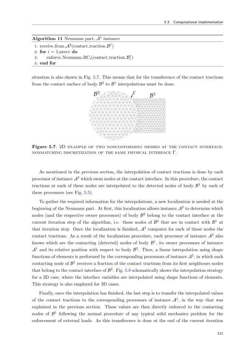
5.3. Computational implementation
Algorithm 11 Neumann part, A1 instance
1: receive from A2(contact traction B1)2: for i = 1,nrecv do3: enforce Neumann BCi(contact traction B1
i )4: end for
situation is also shown in Fig. 5.7. This means that for the transference of the contact tractions
from the contact surface of body B2 to B1 interpolations must be done.
Figure 5.7: 2D example of two nonconforming meshes at the contact interface:nonmatching discretization of the same physical interface Γ.
As mentioned in the previous section, the interpolation of contact tractions is done by each
processor of instance A2 which owns nodes at the contact interface. In this procedure, the contact
tractions at each of these nodes are interpolated to the detected nodes of body B1 by each of
these processors (see Fig. 5.5).
To gather the required information for the interpolations, a new localization is needed at the
beginning of the Neumann part. At first, this localization allows instance A2 to determine which
nodes (and the respective owner processors) of body B2 belong to the contact interface at the
current iteration step of the algorithm, i.e. those nodes of B2 that are in contact with B1 at
that iteration step. Once the localization is finished, A2 computes for each of those nodes the
contact tractions. As a result of the localization procedure, each processor of instance A2 also
knows which are the contacting (detected) nodes of body B1, its owner processors of instance
A1 and its relative position with respect to body B2. Then, a linear interpolation using shape
functions of elements is performed by the corresponding processors of instance A2, in which each
contacting node of B1 receives a fraction of the contact tractions from its first neighbours nodes
that belong to the contact interface of B2. Fig. 5.8 schematically shows the interpolation strategy
for a 2D case, where the interface variables are interpolated using shape functions of elements.
This strategy is also employed for 3D cases.
Finally, once the interpolation has finished, the last step is to transfer the interpolated values
of the contact tractions to the corresponding processors of instance A1, in the way that was
explained in the previous section. These values are then directly enforced to the contacting
nodes of B1 following the normal procedure of any typical solid mechanics problem for the
enforcement of external loads. As this transference is done at the end of the current iteration
111

A Parallel Method for the Two-Body Contact Problem
1
2
3
12
34
5
10.95 x
1+ 0.05 x
2
20.60 x
1+ 0.40 x
2
3 0.10 x 1
+ 0.90 x 2
40.45 x
2+ 0.55 x
3
50.05 x
2+ 0.95 x
3
Figure 5.8: Schematic representation of the interpolation procedure - 2D case.
block, the interpolated contact tractions are available to be used at the beginning of the next
iteration, when the instance A1 that solves the Neumann problem starts its execution.
5.4 Numerical examples
5.4.1 Computational framework
The multicode Dirichlet-Neumann contact algorithm described in this chapter was implemented
in two stages. In the first stage, the implementation of the Neumann and the unilateral contact
problem resolution was done within a simplified finite element code called Ostero (see Sec. A.2
from Appendix A), which was developed in the frame of this thesis. Ostero was coupled with
PLE++ library to perform proof-of-concept tests in order to evaluate the feasibility of the con-
tact algorithm. Once its feasibility was confirmed and the algorithm was validated, the second
stage consisted on its implementation in the massively parallel code Alya (see Sec. A.1 from
Appendix A).
Ostero or Alya can be used for the simulation of contact problems in a multicode scheme,
where one instance of the code is in charge of the resolution of the Neumann problem while
the other is in charge of the resolution of the unilateral contact problem. Using different code
instances, each one of them having its own set of input files, allows to use for each body differ-
ent mesh types, different material models, different time integration schemes, different types of
solvers and preconditioners, different number of subdomains, etc (see Fig. 5.9). For instance, the
Neumann problem can be solved explicitly while the unilateral contact problem can be solved
implicitly. Even more, the Neumann problem can be solved dynamically using a Conjugate
Gradient solver with an Algebraic Multigrid preconditioning, and the unilateral contact problem
can be solved implicitly as a quasi-static evolution using GMRES solver with a RAS precondi-
tioner [93, 80]. In summary, this approach allows to solve each body separately, as if they were in
a standalone simulation. This is possible because the contact interaction is modelled as a coupled
problem, where the coupling of contacting bodies is done by the exchange and enforcement of
112
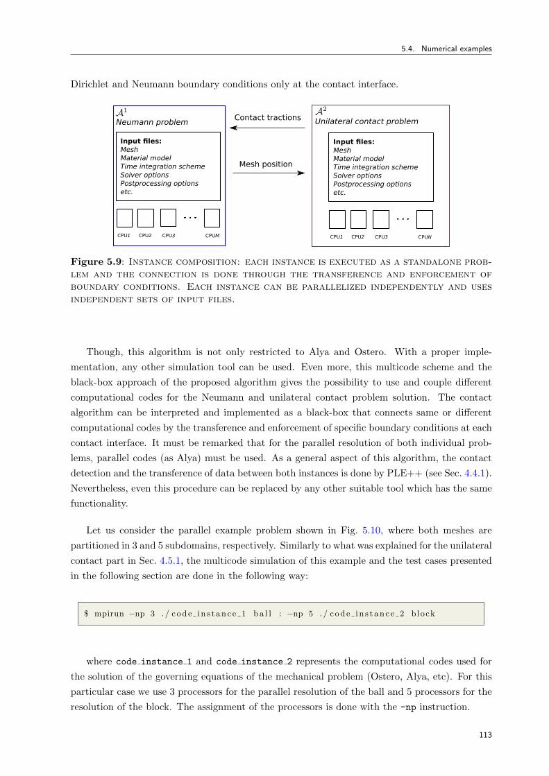
5.4. Numerical examples
Dirichlet and Neumann boundary conditions only at the contact interface.
Neumann problem Unilateral contact problem Contact tractions
Mesh position
Input files:MeshMaterial modelTime integration schemeSolver optionsPostprocessing optionsetc.
Input files:MeshMaterial modelTime integration schemeSolver optionsPostprocessing optionsetc.
CPU1 CPU2 CPU3 CPUM CPU1 CPU2 CPU3 CPUN
Figure 5.9: Instance composition: each instance is executed as a standalone prob-lem and the connection is done through the transference and enforcement ofboundary conditions. Each instance can be parallelized independently and usesindependent sets of input files.
Though, this algorithm is not only restricted to Alya and Ostero. With a proper imple-
mentation, any other simulation tool can be used. Even more, this multicode scheme and the
black-box approach of the proposed algorithm gives the possibility to use and couple different
computational codes for the Neumann and unilateral contact problem solution. The contact
algorithm can be interpreted and implemented as a black-box that connects same or different
computational codes by the transference and enforcement of specific boundary conditions at each
contact interface. It must be remarked that for the parallel resolution of both individual prob-
lems, parallel codes (as Alya) must be used. As a general aspect of this algorithm, the contact
detection and the transference of data between both instances is done by PLE++ (see Sec. 4.4.1).
Nevertheless, even this procedure can be replaced by any other suitable tool which has the same
functionality.
Let us consider the parallel example problem shown in Fig. 5.10, where both meshes are
partitioned in 3 and 5 subdomains, respectively. Similarly to what was explained for the unilateral
contact part in Sec. 4.5.1, the multicode simulation of this example and the test cases presented
in the following section are done in the following way:
$ mpirun −np 3 . / code i n s t anc e 1 b a l l : −np 5 . / code i n s t anc e 2 block
where code instance 1 and code instance 2 represents the computational codes used for
the solution of the governing equations of the mechanical problem (Ostero, Alya, etc). For this
particular case we use 3 processors for the parallel resolution of the ball and 5 processors for the
resolution of the block. The assignment of the processors is done with the -np instruction.
113

A Parallel Method for the Two-Body Contact Problem
Ball, deformable, Neumann problem
Block, deformable, unilateral contact problem
Figure 5.10: Multicode simulation of a two-body contact problem.
5.4.2 Test cases
We shall now present the results of application of the algorithm presented in this chapter to some
2D and 3D test cases. These test problems were selected to illustrate and validate the behaviour
of the proposed algorithm. All the results shown below were obtained using Alya code. It is
worth mentioning that for each numerical example, in the multicode execution Neumann and
unilateral contact parts are solved using exactly the same Alya binary.
5.4.2.1 Hertz contact between two hemispheres - 2D
Hertz problem is often used as a reference for the numerical validation process of contact me-
chanics algorithms. It consists on the computation of the mechanical state of two infinite long
cylinders which contact along their generatrix due to the effect of a concentrated uniform force
F , as shown in Fig. 5.11. This problem allows to verify if the resolution method is able to
correctly evaluate the contact boundary conditions, even if we only know the boundaries in its
approximated form. The analytical solution to this problem, proposed by Hertz in 1882 [62], is
only valid if we assume an elastic behaviour of the bodies, no friction at the contact interface,
small deformations and a small contact length with respect to the radius of the cylinders.
For the numerical resolution of this example we employ identical cylinders with same dimen-
sions r and material properties E and ν. As the cylinders are infinite long, we consider a 2D
simplification under the assumption of plane strain. Furthermore, due to symmetry the problem
can be reduced to the modellization of two quarters of cylinders. In order to solve the same
problem, we enforce a displacement δ/2 on the boundaries that are parallel to the contact zone.
The computational setting for this problem is depicted in Fig. 5.12.
Assuming a frictionless contact and a small contact length b in comparison to the cylinders
114

5.4. Numerical examples
Figure 5.11: Hertz contact - Hertz contact problem, cylinder on cylinder.
Figure 5.12: Hertz contact - Computational setting.
radius r (b << r), the contact pressure distribution at the contact interface is given by [27]:
P =2F
πb2l
√(b2 − x2
1) = Pmax
√(1− x2
1
b2
), (5.14)
where F/l is the load per unit length. The contact length b can be computed by:
b = 2
√Fr(1− ν2)
πlE. (5.15)
It is worth to note the equality between Eqs. (5.14) and (4.38) and Eqs. (5.15) and (4.39).
For the numerical solution of this problem we set E = 20000N/m2, ν = 0.3, r = 50 cm
and δ = 0.767 cm. Using these values in our computational model, we obtain for nodes Ct
and Cb maximum values of contact pressure equal to Pmaxt = 7147 kPa and Pmaxb = 7142 kPa
respectively. Taking an average value Pmax = 7144.5 kPa and by combining Eqs. (5.14) and (5.15)
we can isolate the variable F/l in order to compute b, which results in b = 3.25 cm. The deformed
configuration of the cylinders, the mesh used for the numerical solution and the contact zone are
shown in Fig. 5.13.
115

A Parallel Method for the Two-Body Contact Problem
(a) (b) (c)
Figure 5.13: Hertz contact - (a) Deformed configuration. (b) Mesh used for thenumerical solution. (c) Zoom in on the contact zone.
A comparison of the computed contact pressure distribution for both cylinders with the Hertz
solution (Eq. (5.14)) is shown in Fig. 5.14. We observe that contact pressure distribution and
contact length are very well captured by the proposed algorithm. This translates into a good
agreement between analytical and numerical results. It is noted that we have not assumed any
contact surface and pressure distribution. They are obtained naturally as part of the numerical
solution of the problem by means of the algorithm proposed in this chapter.
0
1000
2000
3000
4000
5000
6000
7000
8000
0 0.5 1 1.5 2 2.5 3 3.5 4
Analytical solutionNumerical solution, bottom cylinder
Numerical solution, top cylinder
Figure 5.14: Hertz contact - Contact pressure distribution with Hertz solution.Comparison between numerical and analytical solutions for both cylinders.
To evaluate the convergence of the contact algorithm we solve this example as a quasi-static
evolution. Small displacement increments are applied at each time step until reaching the desired
116
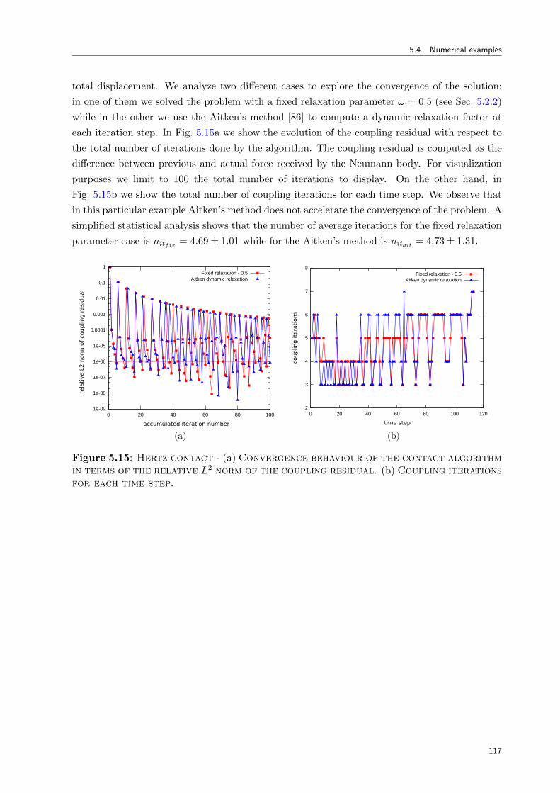
5.4. Numerical examples
total displacement. We analyze two different cases to explore the convergence of the solution:
in one of them we solved the problem with a fixed relaxation parameter ω = 0.5 (see Sec. 5.2.2)
while in the other we use the Aitken’s method [86] to compute a dynamic relaxation factor at
each iteration step. In Fig. 5.15a we show the evolution of the coupling residual with respect to
the total number of iterations done by the algorithm. The coupling residual is computed as the
difference between previous and actual force received by the Neumann body. For visualization
purposes we limit to 100 the total number of iterations to display. On the other hand, in
Fig. 5.15b we show the total number of coupling iterations for each time step. We observe that
in this particular example Aitken’s method does not accelerate the convergence of the problem. A
simplified statistical analysis shows that the number of average iterations for the fixed relaxation
parameter case is nitfix = 4.69± 1.01 while for the Aitken’s method is nitait = 4.73± 1.31.
accumulated iteration number
rela
tive L
2 n
orm
of
couplin
g r
esi
dual
1e-09
1e-08
1e-07
1e-06
1e-05
0.0001
0.001
0.01
0.1
1
0 20 40 60 80 100
Fixed relaxation - 0.5Aitken dynamic relaxation
time step
couplin
g ite
rati
ons
2
3
4
5
6
7
8
0 20 40 60 80 100 120
Fixed relaxation - 0.5Aitken dynamic relaxation
(a) (b)
Figure 5.15: Hertz contact - (a) Convergence behaviour of the contact algorithmin terms of the relative L2 norm of the coupling residual. (b) Coupling iterationsfor each time step.
117

A Parallel Method for the Two-Body Contact Problem
5.4.2.2 Indentation parallel benchmark - 2D
In this example we solve a 2D frictionless indentation problem which consists of a rounded-
head deformable indenter and a deformable square block. The physical model of this problem is
shown in Fig. 5.16. The dimensions of the indenter are: hi = 0.5m, wi = 1.2m and ri = 0.75m,
while the vertical displacement imposed to the indenter along the vertical direction is δ = 0.1m.
The dimensions of the block are hb = 0.5m and wb = 1.6m. We consider a Neo-Hookean
material model and finite strains for the indenter and the block, with material properties Ei =
6.896 e+9N/m2, νi = 0.32, Eb = 6.896 e+8N/m2 and νb = 0.32. The relative position of the
indenter with respect to the block is given by ax = 0.2m and ay = 0.025m. For the bottom of
the block, we fix the displacements in all directions.
indenter, deformable
block, deformable
Figure 5.16: 2D indentation problem - Physical model.
We solve this problem with Alya code after partitioning the indenter mesh in eight subdomains
and the block mesh in eighteen subdomains. Indenter and block meshes and the distribution of
subdomains used in this example are shown in Figs. 5.17a and 5.17b, respectively. To compare
results, we solve the same problem with Code Aster [31] using the same meshes and only one
domain for the complete system.
Fig. 5.18a shows the final deformed configuration obtained with Alya. On the other hand,
Fig. 5.18b shows a mesh superposition in order to compare the final deformed configurations
obtained with both codes. We observe a very good agreement in the results.
In Figs. 5.19a and 5.19b we compare the results of Alya against Code Aster for the y and
x displacement of those nodes which belong to the contact boundary of the block, respectively.
In Fig. 5.19c we show a comparison of the contact forces along the same contact boundary.
Considering the small scale of the vertical axis in Fig. 5.19b, we can conclude that not only
the qualitative behaviour of the contact boundary is very well captured, but also the absolute
118

5.4. Numerical examples
(a) (b)
Figure 5.17: 2D indentation problem - (a) Mesh used for the numerical solution.(b) Domain decomposition of the mesh used by Alya code.
(a) (b)
Figure 5.18: 2D indentation problem - (a) Final deformed configuration ob-tained with Alya. (b) Mesh superposition - black lines: Alya mesh; white lines:Code Aster mesh.
values are very close between the two models. We would like to emphasize that in this example
we are comparing results obtained with two completely different apporaches for the numerical
resolution of contact problems. These results also allow to verify the parallel implementation of
the proposed algorithm.
This example is solved as a quasi-static evolution: we apply a small displacement at each time
step and solve a static problem until reaching the desired total displacement. For the solution of
the linear system of equations resulting at each Newton-Raphson iteration, we employ an iterative
GMRES solver with diagonal preconditioning. In this context we evaluate the convergence of the
contact algorithm using two sets of values for the relaxation parameter: ω = 0.5 and ω = 0.6,
and the Aitken’s method. In Fig. 5.20a we show the evolution of the coupling residual with
respect to the total number of block iterations. In Fig. 5.20b we show the the total number of
iterations for each time step. Finally, in Fig. 5.20c we show the total solver iterations for each
119

A Parallel Method for the Two-Body Contact Problem
-0.06
-0.05
-0.04
-0.03
-0.02
-0.01
0
0.01
0 0.2 0.4 0.6 0.8 1 1.2 1.4 1.6
Alya solutionCode_Aster solution
-0.006
-0.004
-0.002
0
0.002
0.004
0.006
0 0.2 0.4 0.6 0.8 1 1.2 1.4 1.6
Alya solutionCode_Aster solution
(a) (b)
-2.5e+06
-2e+06
-1.5e+06
-1e+06
-500000
0
500000
0 0.2 0.4 0.6 0.8 1 1.2 1.4 1.6
Alya solutionCode_Aster solution
(c)
Figure 5.19: 2D indentation problem - Magnitudes along the contact boundary ofthe block: (a) Vertical displacement. (b) Tangential displacement. (c) Contactforce.
time step. It is clearly observed how the Aitken’s method allows to accelerate the convergence
of the solution, as the total number of iterations for the complete simulation is reduced. It is
worth mentioning that for a fixed relaxation parameter equal to ω = 0.9, the solution diverges.
Thus, Aitken’s method proves to be a suitable choice to ensure and accelerate the convergence
of this problem.
120

5.4. Numerical examples
accumulated iteration number
rela
tive L
2 n
orm
of
coup
ling
resi
dual
1e-09
1e-08
1e-07
1e-06
1e-05
0.0001
0.001
0.01
0.1
1
0 20 40 60 80 100 120
Fixed relaxation - 0.5Fixed relaxation - 0.6
Aitken dynamic relaxation
time step
coup
ling
ite
rati
ons
3
4
5
6
7
8
9
10
0 2 4 6 8 10 12 14 16 18
Fixed relaxation - 0.5Fixed relaxation - 0.6
Aitken dynamic relaxation
(a) (b)
5000
10000
15000
20000
25000
30000
35000
40000
0 2 4 6 8 10 12 14 16 18
Fixed relaxation - 0.5Fixed relaxation - 0.6
Aitken dynamic relaxation
time step
tota
l so
lver
itera
tions
(c)
Figure 5.20: 2D indentation problem - (a) Convergence behaviour of the contactalgorithm in terms of the relative L2 norm of the coupling residual. (b) Couplingiterations for each time step. (c) Total solver iterations for each time step
121

A Parallel Method for the Two-Body Contact Problem
5.4.2.3 Bouncing ball - 2D
We solve here a simple problem which consists of a very rigid ball which falls due to gravity and
impacts on an elastic deformable membrane, which is fixed at both ends (see Fig. 5.21). We
assume an isotropic linear elastic material model and finite strains for the ball and membrane.
The physical and material parameters arbitrary chosen for this example are: rb = 0.1m, ax =
0.5m, ay = 0.07m, hp = 0.05m, wp = 1.2m, ρb = 2.0 e+5 kg/m3, Eb = 6.896 e+10N/m2,
νb = 0.32, Ep = 6.896 e+8N/m2 and νp = 0.32.
ball
membrane
Figure 5.21: Bouncing ball - Physical model.
In order to show the flexibility of the algorithm, we take profit of the low velocity of impact
(≈ 1.2m/s). So, in this example we solve the ball using a transient implicit solver, while the
membrane is solved quasi-statically, i.e. we do not consider inertial effects. The mesh used for
the numerical solution is shown in Fig. 5.22.
Figure 5.22: Bouncing ball - Mesh used for the numerical solution.
We solve this problem for a real time lapse of 3.2 s. Fig. 5.23 shows the evolution of the
deformed configuration of the ball-membrane system for four different time steps, while Fig. 5.24
shows a zoom in at the contact interface.
Fig. 5.25 shows the evolution of the total displacement of the rigid ball along the vertical axis
y. As we are not considering any source of energy dissipation, the bouncing effect is perfectly
elastic.
122

5.4. Numerical examples
(a) t = 0.20 s (b) t = 0.23 s
(c) t = 0.26 s (d) t = 0.28 s
Figure 5.23: Bouncing ball - Evolution of the deformed system.
Figure 5.24: Bouncing ball - Zoom in at the contact zone, t = 0.28 s.
-0.14
-0.12
-0.1
-0.08
-0.06
-0.04
-0.02
0
0 0.5 1 1.5 2 2.5 3 3.5
Figure 5.25: Bouncing ball - Total displacement of the rigid ball vs. time.
123

A Parallel Method for the Two-Body Contact Problem
5.4.2.4 Ironing example - 3D
In this example we study the finite deformation contact of a half-cylindrical elastic die (Neo-
Hookean model, Ed = 1000, νd = 0.3) which is pressed into an elastic beam (Neo-Hookean
model, Eb = 1, νb = 0.3) and then slided over the surface. This problem is commonly referred
to as ironing example. Similar analysis using a mortar segment-to-segment contact method have
been made in [112, 116], where also further details can be found. The physical model and an
exemplary finite element mesh are shown in Fig. 5.26. The geometrical parameters chosen for
this example are: rd = 3, dd = 5.2, wb = 9, hb = 3, db = 4, ax = 0.2 and az = 0.6. An initial
gap of 0.003 between die and beam is considered. The die is first pressed into the beam by
prescribing a displacement of -0.9 units in y-direction within 13 quasi-static time steps. Then it
slides along the beam 2.6 units in 7 further time steps. Finally, the die returns to its vertical
position by moving 0.9 units in y-direction in 10 time steps. The beam is fixed to the ground.
die, deformable
beam, deformable
Figure 5.26: Ironing example - Physical model and finite element mesh.
Fig. 5.28 shows the deformation state of the elastic die-beam system for three different time
steps. In this example, the numerical efficiency of the proposed contact algorithm in 3D finite
deformation situations is evaluated by monitoring the total coupling residual norm during the
nonlinear coupling or block iterations. Fig. 5.27a shows the evolution of the coupling residual with
respect to the accumulated number of coupling iterations. We observe that for fixed relaxation
values of 0.7, 0.9 and 1.0 the simulation diverges at different time steps. Fig. 5.27b shows the
number of coupling iterations at each time step for the converged simulation. We observe that
only the Aitken dynamic relaxation is able to ensure convergence to the solution for the complete
simulation in a reasonable number of coupling iterations.
Trace analysis To study the parallel behaviour of the general contact algorithm we have
generated an execution trace of the ironing example using 16 processors for the Neumann part
(elastic die, 100k elements) and 32 processors for the unilateral contact part (elastic beam, 70k
elements) for 3 time steps. A similar analysis was done in Sec. 4.5.2.5 for the case of an unilateral
contact problem. The trace for this example, executed on MareNostrum IV supercomputer, is
shown in Fig. 5.29. This trace was obtained using the HPCToolkit [71] suite.
Light blue color represents running processors while dark blue color represents idle processors.
In Fig. 5.29 we clearly observe the staggered execution of the proposed contact algorithm. Each
time step starts with the execution of the code instance assigned to the solution of the Neumann
124

5.4. Numerical examples
accumulated iteration number
rela
tive L
2 n
orm
of
couplin
g r
esi
dual
1e-14
1e-12
1e-10
1e-08
1e-06
0.0001
0.01
1
100
10000
1e+06
0 20 40 60 80 100 120 140 160
Fixed relaxation - 0.7Fixed relaxation - 0.9Fixed relaxation - 1.0
Aitken dynamic relaxation
time step
coup
ling
ite
rati
ons
0
2
4
6
8
10
0 5 10 15 20 25 30
Aitken dynamic relaxation
(a) (b)
Figure 5.27: Ironing example - (a) Convergence behaviour of the contact algo-rithm in terms of the relative L2 norm of the coupling residual. (b) Couplingiterations for each time step.
(a) t = 0.65 s (b) t = 0.8 s
(c) t = 1 s
Figure 5.28: Ironing example - Results for three time steps. The elastic die isfully lowered at (a) and then slid across the beam over the remaining time until(c). For simplicity, a time step of 0.05 s is considered.
problem (A1). While this instance is running, the processors assigned to the unilateral contact
problem (instance A2) remain idle. Once the solution at A1 has converged, instance A2 starts.
At this time, while A2 is running, the processors assigned to A1 remain idle. This staggered
execution represents the coupling or block iteration depicted in Fig. 5.4 and is repeated along
the complete simulation. In Fig. 5.29 we also observe that the work load is well balanced among
125

A Parallel Method for the Two-Body Contact Problem
17 to 48unilateralcontactproblem(beam)
1 to 16Neumannproblem
(die)
Figure 5.29: Ironing example - Trace generated for the full simulation (3 timesteps) - beam mesh of 70k elements, die mesh of 100k elements.
the group of processors of both instances, as they start and finish its execution in a coordinated
way. For this particular example we also observe that at each block iteration, instance A1 takes
more than double of time to converge than instance A2. One reason for this behaviour is that
we are using twice of processors for the beam mesh, which is 30% smaller than the die mesh.
Moreover, this simplified analysis gives us insight into how we could redistribute the total number
of available processors (48) between the two instances in order to improve the performance of
the parallel execution. Finally, Fig. 5.30 shows a zoom in on the trace for the first time step,
where the coupling iterations can be clearly identified.
126

5.4. Numerical examples
17 to 48unilateralcontactproblem(beam)
1 to 16Neumannproblem
(die)
1 2 3 4
coupling iterations
waitingrunning
waiting
running
Figure 5.30: Ironing example - Zoom in on the trace: only one time step is shown.Coupling iterations can be clearly distinguished.
127

A Parallel Method for the Two-Body Contact Problem
5.4.2.5 Impact problem - 3D
In this example we solve a low velocity impact, where a plate is impacted with an hemispherical
rigid impactor. We consider an impact energy level of 1.6 J . The diameter of the impactor is
16mm and its mass is 2 kg. The dimensions of the plate are 100×150×4.16mm and it is simply
supported (ux = uy = uz = 0) along all four edges as shown in Fig. 5.31 (right), leaving an
inner region of 75× 125mm. The plate is modelled as a T700/M21 unidirectional carbon/epoxy
laminate with stacking sequence of [02/452/902/− 452]S . The material properties of T700/M21
used in this problem were extracted from [2] and are listed in Table 5.1. For the impactor, we
assume an isotropic linear elastic material and for the plate, we consider a transversally isotropic
material and no damage. The boundary conditions and impact set-up for this problem are based
on ASTM D7136/D7136M-05 standard [6]. Similar numerical and experimental analysis have
been made in [2, 67].
For the numerical solution of this problem we use a mesh composed of approximately 8k
elements for the impactor and 100k elements for the plate. The meshes are generated in order
to enforce the best node-matching situation at the contact interface. A global overview of the
meshes is shown in Fig. 5.31. We run this problem with Alya code in parallel using 8 processors
for the impactor and 40 processors for the plate.
simply supported edge
(ux = uy = uz = 0)
Figure 5.31: Impact problem - Impact set-up: 3D view (left), backview (right).
Property Values
E11 Longitudinal Young’s modulus 130GPaE22 = E33 Transverse Young’s modulus 7.7GPaν12 = ν13 Poisson’s ratio 0.33ν23 Poisson’s ratio 0.45 (assumed)G12 = G13 Shear modulus 4.8GPaG23 Shear modulus 2.655GPa
Table 5.1: Impact problem - Material properties of T700/M21 [2].
For low velocity impact, the inertia effects are relatively small [143], and hence an implicit
quasi-static solver can be used to solve such problems. To compare the results obtained with
Alya, we solve the same problem using the comercial code Abaqus [1]. Abaqus solves the con-
tact problem using a general implicit dynamic contact algorithm based on the node-to-segment
128

5.4. Numerical examples
discretization of the contact interface and the introduction of a penalty parameter for the enforce-
ment of contact constraints. As mentioned in previous chapters, this is a completely different
approach that the one proposed in this work.
In Fig. 5.32 we show the typical curves for low velocity impact tests: (a) contact force-
displacement, (b) impactor energy-time, (c) contact force-time and, (d) impactor velocity-time.
By comparing the results of the present study with the ones obtained with Abaqus, one can
note that the qualitative behaviour is very well captured (see Fig. 5.32). At the beginning of the
impact, Alya and Abaqus predictions agree well: see Fig. 5.32a until an indentation of 0.4mm and
Fig. 5.32c until a contact time of 0.5ms. However, for larger values of indentation and contact
time, the absolute values do not exactly match. From the impactor energy-time curve (Fig. 5.32b)
we observe that this magnitude is not perfectly conserved for the solution obtained with our
contact algorithm. Based on this matter, qualitative behaviour and quantitative differences in
Fig. 5.32 may stem from the fact that, at the beginning of impact, impactor and plate meshes
practicaly match at those nodes that are in contact. This conformity results in a good load
(reaction forces) transference between plate and impactor. As impact goes on, the meshes lose
their conformity, thus affecting the load transference from the plate to impactor. See Appendix C
for a more detailed analysis.
It is worth to mention that these are preliminary results, intended to evaluate the impact
response of the algorithm for non-conforming meshes and further development is required. This
problem evidences the importance of a conservative transference of loads in Dirichlet-Neumann
type contact algorithms for impact problems. For fixed interfaces, as in the case of fluid-structure
interaction problems, several methods based on conservative load interpolation schemes that can
deal with the information transfer between non-matching meshes have been proposed (see [75,
20], among others). However, to the best of our knowledge, the extension of such methods to
moving interfaces has not been yet reported, and their implementation in a parallel computational
code is not straightforward and requires additional development. This key issue is left for future
work.
129

A Parallel Method for the Two-Body Contact Problem
-0.5
0
0.5
1
1.5
2
2.5
3
3.5
4
-0.2 0 0.2 0.4 0.6 0.8 1 1.2
Alya solutionAbaqus solution
0
0.5
1
1.5
2
0 0.5 1 1.5 2 2.5 3
Alya solutionAbaqus solution
(a) (b)
-0.5
0
0.5
1
1.5
2
2.5
3
3.5
4
0 0.5 1 1.5 2 2.5 3
Alya solutionAbaqus solution
-1.5
-1
-0.5
0
0.5
1
1.5
0 0.5 1 1.5 2 2.5 3
Alya solutionAbaqus solution
(c) (d)
Figure 5.32: Impact problem - (a) Impact force vs. displacement. (b) Impactorenergy vs. time. (c) Impact force vs. time. (d) Impactor velocity vs. time.
130

Chapter 6
Conclusions and Outlook
We dare say that any research work, including a PhD. thesis, is something that never truly
ends. Its completion is simply determined by a matter of schedules, solely delimited by time.
Nevertheless, summaries are essential as they serve as milestones that help to wrap up all that has
been done and to discern which steps should be taken next. In this final chapter we recapitulate
all the work done in this thesis, which allows to identify the goals achieved and to establish the
potential future lines of development and improvement for this research.
6.1 Summary
This thesis was born by the necessity of solving industrial nonlinear frictional contact problems in
parallel, by algorithms capable of executing in HPC-based machines. The computational platform
required to be used for the implementation and execution of these algorithms is Alya, which is
the Barcelona Supercomputing Center simulation code for multi-physics problems, specifically
designed to run efficiently in supercomputers. To reach this objective, several milestones were
achieved and passed during the development of this work. It is worth to mention that these
milestones were taken as a reference to give structure to this manuscript. In the following list
we enumerate in order of accomplishment the most significant of them:
• Reach a comprehensive overview of the state-of-the-art in computational contact mechanics
and a clear understanding of the governing equations and the classical methods used for
the numerical resolution of these type of problems.
• Understand the workflow of a high-performance parallel computational code as Alya, and
the way that domain decomposition is applied for the resolution of parallel nonlinear solid
mechanics problems.
• Identify and analyze the strengths and weakness of classical methods in computational
contact mechanics, together with the feasibility for they parallel implementation in a high
performance computational code, considering the design basis established for such end.
131

Conclusions and Outlook
• In response to the fact that standard contact algorithms are not a suitable alternative for
efficient parallelization, propose a novel methodology for the parallel numerical resolution
of frictional contact problems between deformable bodies, which also suits the design basis
previously established.
• Develop from scratch a nonlinear finite element code to be used as a framework for a proof
of concept study of the proposed algorithm.
• Describe and implement the parallel contact algorithm in Alya code, for both 2D and 3D
frictional contact problems.
• Validate and test the parallel implementation with benchmark test cases and real numerical
problems.
6.2 Contributions
Motivated by the fact that standard contact algorithms are not a suitable alternative for efficient
parallelization and the lack of scientific literature regarding those issues, the main result of
this thesis is the introduction of a novel general parallel contact algorithm based on domain
decomposition methods which can run efficiently in HPC-based supercomputers, considering in
a unified way: physical, numerical, algorithmic and computational aspects. In this sense, we
can remark the three most important contributions of this work: (1) we have idenfied, analyzed
and enumerated the drawbacks that standard methods present when they are implemented in
parallel environments under a domain decomposition approach, (2) we have proposed a novel
methodology for the parallel solution of frictional contact problems, explicitly designed to meet
the requeriments of the state-of-the-art HPC-based systems, and (3) we have described in detail
the parallel computational implementation of the algorithm, which has been validated and tested
with benchmark test cases and real numerical problems.
Several features of the multicode Dirichlet-Neumann type contact algorithm introduced in
this work can be highlighted, which define the uniqueness and originality of the proposed method:
• The bodies in contact are treated separately, in a segregated way. From a computational
point of view this feature allows to use a multicode apporach, which means to use different
computational code instances for each of the contacting bodies.
• It makes use of a completely new approach for the contact detection and for the enforcement
of the contact constraints. The contact detection is done by means of a parallel location
and exchange library (PLE++), which allows to detect the penetrated nodes even when
they are distribuited among different processors.
• The contact is treated as a coupled problem, where the coupling of the contacting bodies
is done through Dirichlet and Neumann boundary conditions transfer at the contact zone.
The transference of the boundary conditions is also accomplished by the PLE++ library,
which relies on the Message Passing Interface (MPI) for parallel communication.
132

6.3. Future research perspectives
• It can be explained as a black-box parallel solver for frictional contact problems, as it allows
to solve each body separately, even with different computational codes. The algorithm can
be interpreted as a black-box which detects contact, transfers and enforce the contact
boundary conditions at the contact interface of each body.
• In addition, the contact algorithm proposed in this thesis can also be formulated as a general
fixed-point solver for the solution of interface problems. This generalization gives us the
theoretical basis to extrapolate and implement numerical techniques that were already
developed and widely tested in the field of Fluid-Structure Interaction (FSI) problems,
especially those related to conservative interpolation schemes and convergence ensurance
and acceleration.
• For the enforcement of the Multi-Point Constraints (MPC) which restricts the movement of
the node only in the tangential plane, we propose to use a novel solution where we rotate
the local frame of reference for each of the contacting nodes, instead of using Lagrange
multipliers, which adds extra unknowns to the system.
• The size of the linear system of equations to be solved at each time step remains fixed,
since no Lagrange multipliers are used.
• As the algorithm does not rely on contact elements for the discretization of the contact
interface, there is no need to update the mesh graph on run time. The mesh partitioning
is done at the beginning of the simulation, as a preprocessing task, independently on each
body and without restricting the mesh partitioner.
• The multicode approach of the algorithm allows to treat each body independently, as the
contact coupling is done only through the transference of boundary conditions at the contact
zone. This gives a great flexibility since different inputs files can be used. Different mesh
types, material models, damage models, time integration schemes, solvers, preconditioners,
etc, can be defined for each body, as if they were in a standalone simulation.
6.3 Future research perspectives
Despite the fact that this work offers a comprehensive solution for the numerical parallel solution
of industrial contact problems, is only a first step towards the parallel modelling of this type of
problems in a very robust and efficient way. As parallel computing platforms became of general
access to the scientific and engineering community only few years ago, there is a considerable
lack of scientific literature on parallel contact algorithms. All those years the trend in the
computational contact mechanics field seems to have been the adaptation of existing classical
methodologies to parallel environments instead of developing from scratch new strategies fully
consistent with these new architectures. This thesis intends to take a first step towards this
direction. Having said that, a wide range of possibilities for further improvement or development
arise as a natural continuation of this work. Based on what we have presented here and the
topics which were only marginally covered or not addressed at all, some suggestions for future
research lines are presented below:
133

Conclusions and Outlook
• We have developed and implemented and algorithm for deformable two-body contact prob-
lems. Following the same ideas, the extension to self-contact or multi-body contact prob-
lems is an interesting topic to be covered.
• We did not implement a frictional model in the bilateral contact algorithm. Nevertheless,
for certain types of bilateral contact problems, friction is crucial and must be considered
in the contact resolution. Friction is an interesting but complex phenomena, and an open
line of research in the field of computational contact mechanics.
• We have proposed an staggered algorithm, in which one code instance is idle while the
other is solving, and viceversa (known as Gauss-Seidel scheme). Despite the fact that
this apporach is more robust than if the two bodies were executed simultaneously (Jacobi
scheme), is not optimal in terms of the exploitation of the computational resources. The
implementation of a simultaneous scheme and its comparison with the staggered scheme
is an interesting task to be performed in order to compare robustness, execution time,
efficiency, etc, of both strategies.
• We noted that MPC impact negatively on the speed of convergence to the solution. This
becomes more evident as the number of nodes on the active contact zone increase. Mo-
tivated by this fact, the issue of tailored iterative solvers or preconditioning techniques
that help to accelerate the convergence of the resulting linear system of equations in each
solution step has a lot of room for improvement.
• All the implementations and numerical examples in this work has been done with linear
elements. Higher order elements, or even the smooth interpolation of contact surfaces
with large curvatures will provide improved definition of the contacting surfaces. Among
several issues related with the lack of a smooth definition at the contact boundary one may
find: inaccurate prediction of the traction distribution or other relevant contact-related
quantity, spurious oscillations, inexact contact detection and even convergence problems of
the nonlinear solution scheme.
• Load transfer between nonconforming interfaces is one of the key areas of challenges in
partitioned approaches as the one presented in this thesis. The level of the accuracy in the
load transference have significant impact on the solution of the coupled system. In this
thesis we did not evaluate the performance of the algorithm with different load transfer
schemes. Due to the impact that this issue has on the performance of the algorithm is
worth to be considered for analysis in a next future.
• We have observed that the performance of Dirichlet-Neumann contact algorithm is strongly
determined by the relaxation strategy. The calculation of a specific relaxation parameter in
each iteration step proved to be crucial. Due to this observations, special emphasis should
be put in future works on developing optimal dynamic relaxation strategies. We believe
that a deeper analysis in this subject and more comparisons with available Newton field
solvers for the interface problem such as Interface Quasi-Newton (IQN) [33] or Broyden [26]
134

6.3. Future research perspectives
methods are worth to be done in order to gain more insight on efficient techniques for the
resolution of contact problems using Dirichlet-Neumann partitioned algorithms.
• The applicability of the developed computational approach to more realistic scenarios has
to be proven with further large-scale simulations, including impact analysis considering
cohesive materials and damage models.
• Scalability tests in even bigger scenarios are worth to be analyzed and strong efforts for
improving the code scalability will have favourable consequences in several aspects which
range from faster simulations to efficiency in the exploitation of computational resources.
• Ostero code have proven to be a very useful didactic tool for testing algorithms before
they are implemented in more complex computational codes of industrial scale, as Alya.
This previous step allows to reduce the source of errors due to the larger input files that
bigger codes have and facilitates the debugging of the new segments of code. Ostero is not
a finished work, still few improvements must be done. In special, its extension to 3D and
parallelization.
135


Appendix A
Computational Environment
A.1 Alya
The algorithms described in Chapters 4 and 5 were implemented within a computational envi-
ronment designed for heterogeneous problems in computational mechanics. This framework is
called Alya. It is fully developed at the Barcelona Supercomputing Center, within the department
of Computer Applications for Science and Engineering (CASE). Alya is not a born-sequential
simulation code which was parallelized afterwards. Instead, it was designed from scratch as a
multi-physics parallel code. The efficient solution of large problems on massively parallel com-
puters was the driving justification behind its development. This section describes its main
features.
Alya is a multi-physics, three-dimensional modular code for high performance computational
mechanics. It solves discretized partial differential equations (PDEs), prefering variational meth-
ods (particularly Finite Elements). It is capable of solving different physics problems, each one
with its own modelling characteristics, in a coupled way. Alya runs efficiently in Marenostrum,
the most powerful supercomputer in Spain, hosted by the Barcelona Supercomputing Center.
Alya has shown high parallel efficiency up to several thousands of cores for different physical
problems [29, 68, 70, 119]. Its scalability was benchmarked on different architectures such as
Intel Nehalem, Sandy Bridge, Xeon Phi and IBM PPC. In Blue Waters, the supercomputer
hosted in the National Center for Supercomputing Applications (NCSA), Alya code presented a
performance up to 100000 cores, achieving more than 85% parallel efficiency [132].
Alya’s architecture is modular, being organized into three main blocks: kernel, services and
modules, which can be separately compiled and linked. Each module represents a single set of
partial differential equation for a given physical model (e.g. solid mechanics, fluid mechanics, heat
transference, etc) and manages the respectively boundary conditions. Therefore, to solve a multi-
physics problem, all the required modules must be active and interacting following a well defined
workflow. Alya’s kernel controls the run: it contains the solvers, the input-output workflow
137

Computational Environment
and all the tools related to the mesh and geometry management. Is responsible for the control
of the code’s workflow by management of the interconnections between the modules, services
and itself. Algorithmically speaking, the most important tasks of the kernel are: reading of the
computational mesh and arrangement of the mesh data for domain splitting; construction of the
finite element tools to be used by each module (e.g. basis functions) and solving the linear system
of equations that results from the finite element approximation. The kernel and the modules
allows a given physical problem to be completely solved. The services are supplementary tools,
as the parallelization service or the HDF5 format writer. Kernel, modules and services have well
defined interfaces and connection points.
The parallelization of Alya is a service implemented in the source code and is based on mesh
partitioning (for instance unsing METIS [78]) and MPI tasks, which is specially well-suited for
distribuited memory machines and it uses a Master-Slave strategy. Based on the Master-Slave
strategy, the master is in charge of reading the mesh, performing the mesh partitioning and
writing the output files. Each slave is in charge of an specific subdomain and its main tasks are
the construction of the local right-hand side, the local system matrices and the solution of the
resulting system. Each slave is administrated by one computational process, thus conforming
the relation between slave, subdomain and computational process. In the assembling tasks, no
communication is needed between the slaves. Therefore, in this instance, the scalability only
depends on the load balance. Due to the necessity of communications, the solution of the linear
system the scalability depends on the interfaces (which are minimized by METIS), and the
communication scheduling. All the details on the parallelization of Alya can be found in [68].
In Fig. A.1 we show a schematic flowchart for the execution of a parallel simulation using
Alya. The tasks executed by the master process are shown on the left side of the same figure with
grey background. As explained in previous paragraph, the master performs the first steps of the
execution, namely reading the file and partitioning the mesh. Afterwards, the master sends the
corresponding subdomain information to the slave processes. Next, the master and slaves enter
into the time and linearization loops. Along with the execution of the iterative solvers carried
out by the slaves, two types of communications are required to exchange interface information
with the neighbour nodes of each subdomain. The exchange of the interface information is
performed using the MPI functions MPI Sendrecv, used for the sparse matrix-vector products
and MPI Allreduce, used to compute residual norms and scalar products.
A.1.1 Numerical issues - solid mechanics module
The computational solid mechanics problem is solved using a standard Galerkin method for a
large deformation framework and a generalized Newmark time integration scheme. This frame-
work is developed in a Total Lagrangian formulation. A large database of element types is
available for the solid mechanics module together with explicit and implicit solvers for the non-
linearity. The implicit solver is based on the Newton-Raphson method. Well known constitutive
equations for large deformation elasticity constitutive models, such as the neo-Hookean or specific
hyperelastic models, are also available.
138

A.1. Alya
Figure A.1: Parallel flowchart of Alya. Master (grey) and slaves (white).
Fig. A.2 shows a flowchart of the solidz module. All the geometrical and physical data of
the problem are introduced as input files. Once the input files are read, Alya initializes the
computation within the solidz module, either in serial or parallel mode. The parallel service
must be specified in the input files.
Figure A.2: solidz module structure in Alya code.
139

Computational Environment
A.2 Ostero
The aim of this section is to do a briefly presentation of Ostero. Ostero is a didactic finite element
code for the numerical simulation of solid deformable bodies. It was developed as part of this
thesis, to use it as a test framework for several mechanical models and problems. It is a very
useful tool to perform proof-of-concept evaluations of contact mechanics algorithms and damage
models before implementing them in the BSC’s Alya code, which is a bigger, powerful but more
complex code. Ostero was successfully used for the proof-of-concept and beta-testing of all of
the algorithms proposed in this thesis. Ostero was also succesfully used by PhD. students at the
Barcelona Supercomputing Center and by BSc. students at the Universidad de Buenos Aires. As
a general fact, Ostero was designed in order to first: provide the user a clear idea of the structure
that usually a finite element code for linear and nonlinear mechanics has, and second: to allow
the user to use Ostero as a workbench for personal tests. For further information the reader
is refered to the hosting web page of Ostero https://bitbucket.org/matrivero/ostero, where the
source code and the user manual are freely available.
A.2.1 Description
Ostero is an open source finite element code that solves the continumm equation which governs
the mechanics of a deformable body subjected to external forces, Dirichlet and/or Neumann
boundary conditions. In other words, Ostero allows to determine the response of a deformable
solid body to an applied external load or displacement. Ostero allows to solve a mechanical
problem considering geometric linearity or non-linearity. For geometric non-linearity it uses a
Total Lagrangian formulation. For the specific case of the geometrical nonlinear model, Ostero
uses an implicit scheme based on the Newton-Raphson method, while the update of tangent
matrix is performed at each time step. When a given problem is solved using a geometrically
linear setting, the equations of equilibrium are formulated in the undeformed state, and are not
updated with the deformation. In some engineering problems, as the deformations are considered
small and the deviation from the original geometry is not perceptible, the use of a geometrically
linear setting is a very good approximation to the nonlinear model. The mathematical com-
plexity generated by a more realistic theory and the associated increment of the computation
time does not compensate the small error introduced by ignoring the update of deformations
in the equilibrium equations. But in the engineering field there are also a number of problems
where the deformation (large strains and/or large rotations) cannot be ignored. In those cases
a geometrically nonlinear model should be used in Ostero to account for the large deformations.
It is part of the engineering criteria to choose which model, linear or nonlinear, could be use.
Ostero is based on the solid mechanics module of the Alya code. It can solve quasi-static or
transient problems using triangles or quadrilateral linear elements. For the time integration it
uses a generalized Newmark integration scheme. The geometrically nonlinear module includes the
isolinear (or Kirchhoff) material model and several formulations of the hyperelastic neo-Hookean
material model. Recently, a simple damage model was also added to the code.
Ostero intends to be a didactic code, and its main objective is to allow the user to understand
140

A.2. Ostero
the very basic structure of a linear and nonlinear mechanics finite element code. Also intends to
provide a framework for beta testing of different models such as elastic material models, contact,
plasticity, fracture, etc.
Ostero was also designed to interact seamlessly with open source meshing and post-processing
tools. In that sense, Ostero reads mesh files generated using the open source meshing tool Gmsh,
without need of additional conversions to adapt the mesh file format to the input requested by
Ostero. On the other hand, Ostero writes outputs in Vtk ASCII format, which can be easily
postprocessed using the open source post-processing tool ParaView.
Ostero was written in Python and Fortran to exploit the main advantages and properties
of each programming language. The parsing of the input parameters, boundary conditions and
other options is done in the main program, coded in Python. The way that Ostero manages
the user input is through the usage of dictionaries in Python. For didactic purposes this coding
strategy is a convenient choice. From the developer’s viewpoint it allows a tidy and understand-
able programming. On the other hand, from the user perspective, it allows to write very flexible
and lexical inputs. The main program also includes the main execution loop, which calls the
subroutines that performs the elementary matrix calculations and the assembly operations from
the Fortran module. This external Fortran module is imported in the main program as an exter-
nal library. For the resolution of the linear system of equations resulting from the finite element
discretization, Ostero uses NumPy, which is the fundamental package for scientific computing
with Python.
Algorithm 12 shows the workflow of Ostero. Next to each task we identify which part of the
code is in charge of each operation. For efficiency matters, all those operations such as derivatives
computation and matrix assembly which involves a large amount of iterations, are performed by
the external pre-compiled Fortran subroutine, while the parsing of the input files and the main
loop control is done by the main Python script. The output is written in Vtk format by an
external Python function.
Algorithm 12 Ostero workflow
1: read main input file . (main python program)
2: read mesh file . (main python program)
3: read boundary conditions file . (main python program)
4: compute jacobian and derivatives . (fortran external lib)
5: for time = 1 to total time do . time loop
6: impose boundary conditions . (main python program)
7: while not converged do . nonlinear iterations
8: matrix assembly . (fortran external lib)
9: solve linear system . (main python program, Numpy)
10: end while
11: write output . (vtk python external lib)
12: end for
141

Computational Environment
A.2.2 How to get Ostero
Ostero is hosted in my personal Bitbucket space: https://bitbucket.org/matrivero/ostero. The
source code and user manual can be downloaded there. Bitbucket is a web-based hosting service
for projects that use Mercurial or Git revision control systems. Bitbucket is similar to GitHub
(which primarily uses Git), but the main difference is that Bitbucket allows free private reposi-
tories, while in GitHub only public repositories are available for free users. Besides being hosted
in Bitbucket server, Ostero is under Git revision control, which provides a perfect framework
for collaborative development. Git is a free and open source distributed version control system,
which allows to manage changes in the code in a very efficient way. Is an essential tool for
collaborative projects, but also very useful for individual programmers. Git takes a peer-to-peer
approach to version control, as opposed to the client-server approach of centralized systems, as
SVN. Rather than a single, central repository on which clients synchronize, in Git each peer’s
working copy is the complete repository which includes the complete history information of the
codebase.
142

Appendix B
Physical Interpretation of the
Newton’s Method Residual
The discrete momentum equation at time step n + 1 in a form applicable to both equilibrium
and dynamic problems is:
0 = r(dn+1, tn+1) = sDMan+1 + f int(dn+1, tn+1)− f ext(dn+1, tn+1), (B.1)
where sD is a switch which is set by: sD = 0 for a static (equilibrium) problem, and sD = 1
for a dynamic (transient) problem. The vector r(dn+1, tn+1) is called a residual. The discrete
equations for both the implicit update of the equations of motion and the equilibrium equations
are nonlinear algebraic equations in the nodal displacements, dn+1.
The most widely used and most robust method for the solution of nonlinear algebraic equa-
tions is Newton’s method. The method is often called Newton-Raphson method in computational
mechanics. The solution of Eq. (B.1) by Newton’s method is an iterative procedure. The iter-
ation number is indicated by Greek subscript: dn+1ν ≡ dν is the displacement in iteration ν at
time step n+ 1; the time step number n+ 1 will be omitted in the following.
To begin the iterative procedure, a starting value for the unknown must be chosen; usually
the solution dn for the previous time step is selected, so d0 ≡ dn. A Taylor expansion of the
residual about the current value of the nodal displacement dν and setting the resulting residual
equal to zero gives:
0 = r(dν+1, tn+1) = r(dν , t
n+1) +∂r(dν , t
n+1)
∂d∆d +O(∆d2), (B.2)
where
∆d = dν+1 − dν . (B.3)
If the terms which are higher order than linear in ∆d are dropped, then Eq. (B.2) gives a
linear equation for ∆d:
143
Physical Interpretation of the Newton’s Method Residual
0 = r(dν , tn+1) +
∂r(dν , tn+1)
∂d∆d. (B.4)
The above is called a linear model or linearized model of the nonlinear equations. The linear
model is tangent to the nonlinear residual function. Note that in the Taylor expansion, the
residual is written in terms of the time tn+1. The time-dependence of the residual is usually
explicitly given. For example, the tractions and body forces are usually given as functions of
time, and any change in the external load forces is due to changes in the nodal displacements.
Therefore the residual is ordinarily computed using the load at time tn+1 and the latest value of
the nodal displacements.
Solving this linear model for the incremental displacements gives:
∂r(dν , tn+1)
∂d∆d = −r(dν , t
n+1) =⇒ ∆d = −(∂r(dν , t
n+1)
∂d
)−1r(dν , t
n+1). (B.5)
In the Newton procedure, the solution to the nonlinear equation is obtained by iteratively
solving a sequence of linear models given by Eq. (B.5). The new value for the unknown in each
step of the iteration is obtained by rewriting Eq. (B.3) as:
dν+1 = dν + ∆d. (B.6)
The process is continued until the solution is obtained with the desired level of accuracy.
In a Total Lagrangian formulation, the residual r(dν , tn+1) can be expressed in absence of
exterior forces using index notation as (see [16]):
rbi =
∫Ω0
PiJ∂N b
∂XJdΩ0, (B.7)
where PiJ is the first Piola-Kirchhoff stress tensor, ∂N b/∂XJ are the shape function deriva-
tives with respect to the reference frame coordinates and Ω0 corresponds to the reference domain.
From now on we will suppose, without loss of generality and in order to save notation, that the
following volumetric integrals are done at the elementary level (Ω→ Ωe).
The two-point first Piola-Kirchhoff stress tensor PiJ can be related to the Cauchy’s stress
tensor σik, which is fully expressed in the deformed configuration (see [24]):
PiJ = Jσik(F−1)Jk, (B.8)
where F is the deformation gradient and J the transformation jacobian. Then, we can rewrite
Eq. (B.7) using relation of Eq. (B.8) as follows:
rbi =
∫Ω0
PiJ∂N b
∂XJdΩ0 =
∫Ω0
Jσik(F−1)Jk
∂N b
∂XJdΩ0. (B.9)
As reference and deformed configurations are related by the transformation JdΩ0 = dΩ, then:
144

rbi =
∫Ωσik(F
−1)Jk∂N b
∂XJdΩ. (B.10)
Furthermore, as (F−1)Jk =∂XJ
∂xk, then:
rbi =
∫Ωσik
∂XJ
∂xk
∂N b
∂XJdΩ, (B.11)
which is equivalent to:
rbi =
∫Ωσik
∂N b
∂xkdΩ. (B.12)
Please note that Eq. (B.12) allows to compute the residual using only measures which are
expressed in the deformed configuration. If we multiply Eq. (B.12) at both sides by the displace-
ments vector ubi , then:
rbi ubi =
∫Ωσik
∂N b
∂xkdΩubi . (B.13)
As ubi does not depend on the system coordinates, we can include it inside of the integral of
Eq. (B.13):
rbi ubi =
∫Ωσik
∂N b
∂xkubi dΩ =
∫Ωσik εik dΩ, (B.14)
where εik is the Cauchy’s strain tensor. Rewriting Eq. (B.14) in vectorial form gives:
(Rb)T ub =
∫ΩεT σ dΩ. (B.15)
Right-hand side of Eq. (B.15) represents the work done by the internal forces of Ω. Thus,
residual vector Rb equals to the forces at each node b of element e. For those nodes subjected to
Dirichlet-type boundary conditions these forces correspond to the reactions.
145


Appendix C
Load Transference Analysis
We apply here a simple methodology to address the accuracy of the interpolation strategy used in
this work across similar but non-matching contact interfaces. In the adopted strategy the inter-
face variables (reaction forces) are interpolated using shape function of elements. See Sec. 5.3.1
for further details.
We consider a test set-up, which consists of two blocks with slightly non-matching meshes
and a plane contact interface, as shown in Fig. C.1. The upper and lower blocks have dimensions
of 3.8× 3.8× 2.85 and 6× 6× 2 units, respectively. We assume a frictionless contact.
Figure C.1: Finite element meshes used in this analysis.
We employ a Neo-Hookean material law for both bodies. For the upper block we assign a
Young’s modulus E = 10000 and Poisson’s ratio ν = 0.3, while for the lower block we assign
E = 100 and ν = 0.3. In this tailor-made test the lower block is fixed in all directions at its
bottom surface, while a total vertical displacement of -0.5 units (y-direction) is applied to the
top surface of the upper block. This problem is solved as a quasi-static evolution using 20 time
steps. The final deformed state for both bodies is shown in Fig. C.2.
147

Load Transference Analysis
(a) (b)
Figure C.2: Deformed state at last time step. (a) Upper block. (b) Lower block.
To evaluate the load transference due to contact, we compute at each time step the total
reaction force at the top surface of the upper block and at the bottom surface of the lower
block. Due to Newton’s third law, in the case of a perfect load transference both total reaction
forces should be exactly equal at each time step. Fig. C.3 shows a comparison of the computed
magnitudes for all the simulation time. We observe that curves exactly match at the beginning.
However, they apart as the simulation advances, which indicates that at those instants of time
forces are not exactly transferred. This can be explained due to the effect of loss of conformity
between meshes. At the beginning, meshes are slightly non-matching. Nevertheless, as time
advances, the lower block suffers a bigger deformation than the upper block, which affects the
initial configuration of the meshes at the contact interface. As meshes lose their similarity, the
effects of the non-conservativeness of the load transference become relevant.
0
50
100
150
200
250
300
350
400
450
0 5 10 15 20
Upper block, total reaction forceLower block, total reaction force
Figure C.3: Total reaction force at each time step. Forces are measured at thetop surface of upper block and at the bottom surface of lower block.
148

Bibliography
[1] Abaqus unified FEA. url: https://www.3ds.com/products-services/simulia/products/
abaqus/.
[2] M. R. Abir et al. “Modelling damage growth in composites subjected to impact and
compression after impact”. In: Composite Structures 168 (2017), pp. 13–25.
[3] ADINA – Finite element analysis software. url: http://www.adina.com/.
[4] P. Alart and A. Curnier. “A mixed formulation for frictional contact problem prone
to Newton like solution methods”. In: Computer Method in Applied Mechanics and
Engineering 92 (1991), pp. 353–375.
[5] ANSYS Structures. url: http://www.ansys.com/products/structures.
[6] ASTM D7136/D7136M-05, Standard Test Method for Measuring the Damage Resistance
of a Fiber-Reinforced Polymer Matrix Composite to a Drop-Weight Impact Event. Stan-
dard. ASTM International, 2005.
[7] S. W. Attaway et al. “A parallel contact detection algorithm for transient solid dynamics
simulations using PRONTO3D”. in: Computational Mechanics 22.2 (1998), pp. 143–159.
[8] K. J. Bathe and A. Chaudhary. “A solution method for planar and axisymmetric contact
problems”. In: International Journal for Numerical Methods in Engineering 21 (1985),
pp. 65–88.
[9] K.-J. Bathe, E. Ramm, and E. L. Wilson. “Finite element formulations for large deforma-
tion dynamic analysis”. In: International Journal for Numerical Methods in Engineering
9 (1975), pp. 353–386.
[10] G. Bayada, J. Sabil, and T. Sassi. “Algorithme de Neumann-Dirichlet pour des problemes
de contact unilateral: resultat de convergence”. In: Comptes Rendus Mathematique 335
(2002), pp. 381–386.
[11] G. Bayada, J. Sabil, and T. Sassi. “A Neumann-Neumann domain decomposition algo-
rithm for the Signorini problem”. In: Applied Mathematics Letters 17 (2004), pp. 1153–
1159.
[12] G. Bayada, J. Sabil, and T. Sassi. “Convergence of a Neumann-Dirichlet algorithm for
two-body contact problems with non local Coulomb’s friction law”. In: Mathematical
Modelling and Numerical Analysis 42 (2008), pp. 243–262.
[13] F. P. Beer and E. R. Johnston. Mechanics of materials. 2nd ed. McGraw-Hill, 1992.
149

[14] F. Ben Belgacem. “The mortar finite element method with Lagrange multipliers”. In:
Numerische Mathematik 84 (1999), pp. 173–197.
[15] F. Ben Belgacem, P. Hild, and P. Laborde. “The mortar finite element method for contact
problems”. In: Mathematical and Computer Modelling 28 (1998), pp. 263–271.
[16] T. Belytschko, W. K. Liu, and B. Moran. Nonlinear finite elements for continua and
structures. 1st ed. Wiley, 2006.
[17] D. J. Benson and J. O. Hallquist. “A single surface contact algorithm for the post-
buckling analysis of shell structures”. In: Computer Methods in Applied Mechanics and
Engineering 78 (1990), pp. 141–163.
[18] C. Bernardi, Y. Maday, and A. T. Patera. “A new nonconforming approach to domain
decomposition: the mortar element method”. In: Nonlinear partial differential equations
and their applications. Ed. by H. Brezis and J. Lions. Wiley, 1994, pp. 13–51.
[19] D. Blom et al. “A review on fast quasi-Newton and accelerated fixed-point iterations for
partitioned fluid-structure interaction simulation”. In: Y. Bazilevs, K. Takizawa (eds)
Advances in Computational Fluid-Structure Interaction and Flow Simulation. Modeling
and Simulation in Science, Engineering and Technology. (2016), pp. 257–269.
[20] A. de Boer, A. H. van Zuijlen, and H. Bijl. “Review of coupling methods for non-
matching meshes”. In: Computer Methods in Applied Mechanics and Engineering 196
(2007), pp. 1515–1525.
[21] A. E. J. Bogaers et al. “Quasi-Newton methods for implicit black-box FSI coupling”. In:
Computers Methods in Applied Mechanics and Engineering 279.1 (2014), pp. 113–132.
[22] P. Boieri, F. Gastaldi, and D. Kinderlehrer. “Existence, uniqueness, and regularity results
for the two-body contact problem”. In: Applied Mathematics and Optimization 15.1
(1987), pp. 251–277.
[23] E. G. Boman et al. “The Zoltan and Isorropia parallel toolkits for combinatorial scientific
computing: Partitioning, ordering and coloring”. In: Scientific Programming 20.2 (2012),
pp. 129–150.
[24] J. Bonet and R. D. Wood. Nonlinear continuum mechanics for finite element analysis.
2nd ed. Cambridge University Press, 2008.
[25] F. Brezzi and M. Fortin. Mixed and hybird finite element methods. Springer Verlag, 1991.
[26] C. G. Broyden. “A class of methods for solving nonlinear simultaneous equations”. In:
Mathematics of Computation 19 (1965), pp. 577–593.
[27] R. Budynas and K. Nisbett. Shigley’s mechanical engineering design. 8th ed. McGraw-
Hill, 2008.
[28] L. T. Campos, J. T. Oden, and N. Kikuchi. “A numerical analysis of a class of contact
problems with friction in elastostatics”. In: Computer Methods in Applied Mechanics and
Engineering 34.1-3 (1982), pp. 821–845.
150
[29] E. Casoni et al. “Alya: Computational solid mechanics for supercomputers”. In: Archives
of Computational Methods in Engineering 22.4 (2015), pp. 557–576.
[30] J. H. Cheng and N. Kikuchi. “An analysis of metal forming processes using Lagrange
deformation elastic-plastic formulations”. In: Computer Methods in Applied Mechanics
and Engineering 49 (1985), pp. 71–108.
[31] Code Aster Open Source – General FEA software. url: http://www.code-aster.org.
[32] A. Curnier and P. Alart. “A generalized Newton method for contact problems with
friction”. In: Journal de Mecanique Theorique et Appliquee. Special issue: Numerical
Methods in Mechanics of Contact involving Friction (1988), pp. 67–82.
[33] J. Degroote, K-J. Bathe, and J. Vierendeels. “Performance of a new partitioned proce-
dure versus a monolithic procedure in fluid-structure interaction”. In: Computers and
Structures 87 (2009), pp. 793–801.
[34] Z. Dostal, A. Friedlander, and S. A. Santos. “Solution of coercive and semicoercive
contact problems by FETI domain decomposition”. In: Contemporary Mathematics 218
(1998). conforming mesh, elastic frictionless, pp. 82–93.
[35] Z. Dostal, D. Horak, and D. Stefanica. “A scalable FETI-DP algorithm with non-
penetration mortar conditions on contact interface”. In: Journal of Computational and
Applied Mathematics 231 (2009), pp. 577–591.
[36] Z. Dostal, F. A. M. Gomez Neto, and S. A. Santos. “Solution of contact problems
by FETI domain decomposition with natural coarse space projections”. In: Computer
Methods in Applied Mechanics and Engineering 190 (2000). conforming mesh, elastic
frictionless, pp. 1611–1627.
[37] Z. Dostal et al. “A scalable TFETI algorithm for two-dimensional multibody contact
problems with friction”. In: Journal of Computational and Applied Mathematics 235
(2010), pp. 403–418.
[38] Z. Dostal et al. “A theoretically supported scalable TFETI algorithm for the solution
of multibody 3D contact problems with friction”. In: Computer Methods in Applied
Mechanics and Engineering 205 (2012), pp. 110–120.
[39] Z. Dostal et al. “Scalable FETI algorithms for frictionless contact problems”. In: Domain
Methods in Science and Engineering XVII. Lecture Notes in Computational Science and
Engineering (LNCSE). ed. by U. Langer et al. Vol. 60. Springer, 2008, pp. 263–270.
[40] Z. Dostal et al. “Scalable TFETI algorithm for the solution of multibody contact problems
of elasticity”. In: International Journal for Numerical Methods in Engineering 82 (2009),
pp. 1384–1405.
[41] G. Duvaut and J. L. Lions. Inequalities in mechanics and physics. Springer, 1976.
[42] C. Eck and B. Wohlmuth. “Convergence of a Contact-Neumann iteration for the solution
of two-body contact problems”. In: Mathematical Models and Methods in Applied Sciences
13 (2003), pp. 1103–1118.
151

[43] C. Farhat and F. X. Roux. “A method of finite element tearing and interconnecting
and its parallel solution algorithm”. In: International Journal for Numerical Methods in
Engineering 32 (1991), pp. 1205–1227.
[44] FEAP – Finite element analysis program. url: http://projects.ce.berkeley.edu/
feap/.
[45] M. A. Fernandez and M. Moubachir. “A Newton method using exact jacobians for solving
fluid-structure coupling”. In: Computers & Structures 83.2–3 (2005), pp. 127–142.
[46] K. A. Fischer and P. Wriggers. “Mortar based frictional contact formulation for higher
order interpolations using the moving friction cone”. In: Computer Methods in Applied
Mechanics and Engineering 195 (2006), pp. 5020–5036.
[47] Y. Fournier. Parallel location and exchange. Tech. rep. Electricite de France (EDF), 2014.
[48] A. Francavilla and O. C. Zienkiewicz. “A note on numerical computation of elastic
contact problems”. In: International Journal for Numerical Methods in Engineering 9.4
(1975), pp. 913–924.
[49] J. Frohne, T. Heister, and W. Bangerth. “Efficient numerical methods for the large-
scale, parallel solution of elastoplastic contact problems”. In: International Journal for
Numerical Methods in Engineering 105.6 (2016), pp. 416–439.
[50] F. J. Gallego and J. J. Anza. “A mixed finite element model for the elastic contact
problem”. In: International Journal for Numerical Methods in Engineering 28 (1989),
pp. 1249–1264.
[51] J.-F. Gerbau, M. Vidrascu, and P. Frey. “Fluid-structure interaction in blood flows
on geometries based on medical imaging”. In: Computers & Structures 83.2–3 (2005),
pp. 155–165.
[52] P. E. Gill, W. Murray, and M. H. Wright. Practical Optimization. Academic press, 1981.
[53] G. M. L. Gladwell. Contact problems in the classical theory of elasticity. Springer, 1980.
[54] R. Glowinski and P. Le Tallec. Augmented Lagrangian and operator-splitting methods in
nonlinear mechanics. Vol. 28. 1989, pp. 1249–1264.
[55] W. Gropp, E. Lusk, and A. Skjellum. Using MPI: Portable parallel programming with the
message-passing interface. The MIT Press, 2014.
[56] G. Hager and G. Wellein. Introduction to high performance computing for scientists and
engineers. CRC Press, 2011.
[57] J. O. Hallquist, G. L. Goudreau, and D. J. Benson. “Sliding interfaces with contact-
impact in large-scale Lagrangian computations”. In: Computer Methods in Applied Me-
chanics and Engineering 51 (1985), pp. 107–137.
[58] J. Har and R. Fulton. “A parallel finite element procedure for contact-impact problems”.
In: Engineering with Computers 19 (2003), pp. 67–84.
152

[59] S. Hartmann et al. “A contact domain method for large deformation frictional contact
problems. Part 2: Numerical aspects”. In: Computer Methods in Applied Mechanics and
Engineering 198 (1992), pp. 2607–2631.
[60] J. Haslinger, R. Kucera, and T. Sassi. “A domain decomposition algorithm for contact
problems: analysis and implementation”. In: Mathematical Modelling of Natural Phe-
nomena 4 (2009), pp. 123–146.
[61] J. Haslinger et al. “A domain decomposition method for two-body contact problems with
Tresca friction”. In: Advances in Computational Mathematics 40 (2014), pp. 65–90.
[62] H. Hertz. “Uber die Beruhrung fester elastischer Korper”. In: Journal fur die reine und
angewandte Mathematik 92 (1881), pp. 156–171.
[63] M. R. J. Hestenes. “Multiplier and gradient methods”. In: Journal of Optimization
Theory and Applications 4.5 (1969), pp. 303–320.
[64] P. Hild. “Numerical implementation of two nonconforming finite element methods for
unilateral contact”. In: Computer Methods in Applied Mechanics and Engineering 184
(2000), pp. 99–123.
[65] P. Hild and Y. Renard. “A Stabilized Lagrange multiplier method for the finite element
approximation of contact problems in elastostatics”. In: Numerische Mathematik 115.1
(2010), pp. 101–129.
[66] D. A. Hills, D. Nowell, and A. Sackfield. Mechanics of elastic contact. Elseiver, 1993.
[67] N. Hongkarnjanakul. “Modelisation numerique pour la tolerance aux dommages d’impact
sur stratifie composite: de l’impact a la resistance residuelle en compression”. PhD thesis.
Universite de Toulouse, 2013.
[68] G. Houzeaux et al. “A massively parallel fractional step solver for incompressible flows”.
In: Journal of Computational Physics 228.17 (2009), pp. 6316–6332.
[69] G. Houzeaux et al. “Domain decomposition methods for domain composition purpose:
chimera, overset, gluing and sliding mesh methods”. In: Archives of Computational
Methods in Engineering 24.4 (2017), pp. 1033–1070.
[70] G. Houzeaux et al. “Hybrid MPI-OpenMP performance in massively parallel compu-
tational fluid dynamics”. In: Parallel Computational Fluid Dynamics. Lecture Notes
in Computational Science and Engineering (LNCSE). ed. by D. Tromeur-Dervout et al.
Vol. 74. Springer, 2008, pp. 293–297.
[71] HPCToolkit performance tools. url: http://www.hpctoolkit.org.
[72] T. J. R. Hughes et al. “A finite element method for a class of contact-impact problems”.
In: Computer Methods in Applied Mechanics and Engineering 8.3 (1976), pp. 249–276.
[73] T. R. J. Hughes, R. L. Taylor, and W. Kanoknukulchai. “A finite element method for
large displacement contact and impact problems”. In: Formulations and Computational
Algorithms in FE Analysis. Ed. by K. J. Bathe, J. T. Oden, and W. Wunderlich.
MIT-Press, 1977, pp. 468–495.
153

[74] B. M. Irons and R. C. Tuck. “A version of the Aitken accelerator for computer iteration”.
In: International Journal of Numerical Methods in Engineering 1 (1969), pp. 275–277.
[75] R. K. Jaiman et al. “Conservative load transference along curved fluid-solid interface with
non-matching meshes”. In: Journal of Computational Physics 218 (2006), pp. 372–397.
[76] K. L. Johnson. Contact mechanics. Cambridge University Press, 1985.
[77] J. J. Kalker. Three-Dimensional elastic bodies in rolling contact. Springer, 1990.
[78] G. Karypis and V. Kumar. “A fast and high quality multilevel scheme for partition-
ing irregular graphs”. In: Proceedings of the 1995 International Conference on Parallel
Processing. Ed. by D. P. Agrawal. CRC Press, 1995, pp. 113–122. isbn: 9780849326189.
[79] N. Kikuchi and J. T. Oden. Contact problems in elasticity: A study of variational
inequalities and finite element methods. 1st ed. SIAM, 1988.
[80] J. Koldan et al. “Algebraic multigrid preconditioning within parallel finite-element solvers
for 3-D electromagnetic modelling problems in geophysics”. In: Geophysical Journal
International 197.3 (2014), pp. 1442–1458.
[81] A. Konter. Advanced finite element contact benchmarks. NAFEMS, 2006.
[82] R. Kornhuber. Adaptive monotone multigrid methods for nonlinear variational problems.
B.G. Teubner, 1997.
[83] R. Kornhuber and R. Krause. “Adaptive multigrid methods for Signorini’s problem in
linear elasticity”. In: Computing and Visualization in Science 4 (2001), pp. 9–20.
[84] R. Krause. “Monotone multigrid methods for Signorini’s problem with friction”. PhD
thesis. FU Berlin, 2001.
[85] R. Krause and B. Wohlmuth. “A Dirichlet-Neumann type algorithm for contact problems
with friction”. In: Computing and Visualization in Science 5 (2002), pp. 139–148.
[86] U. Kuttler and W. A. Wall. “Fixed-point fluid-structure interaction solvers with dynamic
relaxation”. In: Computational Mechanics 43.1 (2008), pp. 61–72.
[87] T. A. Laursen. Computational contact and impact mechanics. 1st ed. Springer, 2003.
[88] T. A. Laursen. “Formulation and treatment of frictional contact problems using finite
elements”. PhD thesis. Department of Mechanical Engineering, Stanford University,
1992.
[89] T. A. Laursen. “The convected description in large deformation frictional contact prob-
lems”. In: International Journal of Solids and Structures 31 (1994), pp. 669–681.
[90] T. A. Laursen and J. C. Simo. “A continuum-based finite element formulation for
the implicit solution of multibody, large deformation frictional contact problems”. In:
International Journal for Numerical Methods in Engineering 36 (1993), pp. 3451–3485.
[91] F. Linder et al. “A comparison of various quasi-Newton schemes for partitioned fluid-
structure interaction”. In: Proceedings of 6th International Conference on Computational
Methods for Coupled Problems in Science and Engineering. Venice (2015), pp. 1–12.
154

[92] D. G. Luenberger and Y. Ye. Linear and nonlinear programming. 3rd ed. Springer, 2008.
[93] F. Magoules, F. X. Roux, and G. Houzeaux. Parallel scientific computing. Wiley - ISTE,
2015.
[94] J. G. Malone and N. L. Johnson. “A parallel finite element contact/impact algorithm for
non-linear explicit transient analysis: Part II–Parallel implementation”. In: International
Journal for Numerical Methods in Engineering 37.4 (1994), pp. 591–603.
[95] J. G. Malone and N. L. Johnson. “A parallel finite element contact/impact algorithm
for non-linear explicit transient analysis: Part I–The search algorithm and contact me-
chanics”. In: International Journal for Numerical Methods in Engineering 37.4 (1994),
pp. 559–590.
[96] T. W. McDevitt and T. A. Laursen. “A mortar-finite element formulation for frictional
contact problems”. In: International Journal for Numerical Methods in Engineering 48
(2000), pp. 1525–1547.
[97] METIS: Family of graph and hypergraph partitioning software. url: http://glaros.
dtc.umn.edu/gkhome/views/metis.
[98] D. P. Mok and W. A. Wall. “Partitioned analysis schemes for the transient interaction
of incompressible flows and nonlinear flexible structures”. In: W. A. Wall, K.-U. Blet-
zinger, K. Schweitzerhof (eds) Trends in Computational Structural Mechanics, CIMNE,
Barcelona, Spain (2001).
[99] J. J. Moreau. “On unilateral constraints, friction and plasticity”. In: New Variational
Techniques in Mathematical Physics. Springer Berlin Heidelberg, 2011, pp. 171–322.
[100] J. T. Oden and E. B. Pires. “Algorithms and numerical results for finite element
approximations of contact problems with non-classical friction laws”. In: Computers &
Structures 19 (1984), pp. 137–147.
[101] J. T. Oden and E. B. Pires. “Nonlocal and nonlinear friction laws and variational
principles for contact problems in elasticity”. In: Journal of Applied Mechanics 50 (1983),
pp. 67–76.
[102] J. T. Oden and E. B. Pires. “Numerical analysis of certain contact problems in elasticity
with non-classical friction laws”. In: Computers & Structures 16 (1983), pp. 481–485.
[103] J. Oliver et al. “A contact domain method for large deformation frictional contact prob-
lems. Part 1: Theoretical basis”. In: Computer Methods in Applied Mechanics and
Engineering 198 (2009), pp. 2591–2606.
[104] P. Pacheco. An introduction to parallel programming. MK - Elseiver, 2011.
[105] P. Papadopoulos and R. L. Taylor. “A mixed formulation for the finite element solution
of contact problems”. In: Computer Methods in Applied Mechanics and Engineering 94
(1992), pp. 373–389.
[106] H. Parisch. “A consistent tangent stiffness matrix for three-dimensional non-linear contact
analysis”. In: International Journal for Numerical Methods in Engineering 28.8 (1989),
pp. 1803–1812.
155

[107] F. Pellegrini. “Distillating knowledge about SCOTCH”. in: Combinatorial Scientific
Computing. Ed. by Uwe Naumann et al. Dagstuhl Seminar Proceedings 09061. Schloss
Dagstuhl - Leibniz-Zentrum fuer Informatik, Germany, 2009.
[108] P. Persson. “Parallel numerical procedures for the solution of contact-impact problems”.
PhD thesis. Linkopings Universitet, Sweden, 1996.
[109] G. Pietrzak. “Continuum mechanics modelling and Augmented Lagrangian formulation
of large deformation frictional contact problems”. PhD thesis. Departement de Genie
Mecanique, Ecole Polytechnique Federale de Lausanne, 1997.
[110] G. Pietrzak and A. Curnier. “Large deformation frictional contact mechanics: continuum
formulation and Augmented Lagrangian treatment”. In: Computer Methods in Applied
Mechanics and Engineering 177 (1999), pp. 351–381.
[111] S. Plimpton et al. “Parallel transient dynamics simulations: Algorithms for contact de-
tection and smoothed particle hydrodynamics”. In: Journal of Parallel and Distributed
Computing 50 (1998), pp. 104–122.
[112] A. Popp. “Mortar methods for computational contact mechanics and general interface
problems”. PhD thesis. Lehrstuhl fur Numerische Mechanik, Technische Universitat
Munchen, 2012.
[113] A. Popp et al. “Improved robustness and consistency of 3D contact algorithms based on
a dual mortar approach”. In: Computer Methods in Applied Mechanics and Engineering
264 (2013), pp. 67–80.
[114] M. J. D. Powell. “A method for nonlinear constraints in minimization problems”. In:
Optimization. Ed. by R. Fletcher. Academic Press, 1969, pp. 283–298.
[115] W. H. Press et al. Numerical recipes in C: The art of scientific computing. 2nd ed.
Cambridge University Press, 1992.
[116] M. A. Puso and T. A. Laursen. “A mortar segment-to-segment contact method for
large deformation solid mechanics”. In: Computer Methods in Applied Mechanics and
Engineering 193 (2004), pp. 601–629.
[117] M. A. Puso and T. A. Laursen. “A mortar segment-to-segment frictional contact method
for large deformations”. In: Computer Methods in Applied Mechanics and Engineering
193 (2004), pp. 4891–4913.
[118] M. A. Puso, T. A. Laursen, and J. Solberg. “A segment-to-segment mortar contact
method for quadratic elements and large deformations”. In: Computer Methods in Applied
Mechanics and Engineering 197 (2008), pp. 555–566.
[119] V. Puzyrev et al. “A parallel finite-element method for three-dimensional controlled-source
electromagnetic forward modelling”. In: Geophysical Journal International 193.2 (2013),
pp. 678–693.
[120] A. Quarteroni and A. Balli. Domain decomposition methods for partial differential equa-
tions. Clarendon Press - Oxford, 1999.
156
[121] SCOTCH: Software package and libraries for sequential and parallel graph partitioning.
url: http://www.labri.fr/perso/pelegrin/scotch/.
[122] A. Signorini. “Sopra alcune questioni di statica dei sistemi continui”. In: Annali della
Scuola Normale Superiore di Pisa - Classe di Scienze, Serie 2 2 (1933), pp. 231–251.
[123] J. C. Simo and T. A. Laursen. “An Augmented Lagrangian treatment of contact problems
involving friction”. In: Computers & Structures 42 (1992), pp. 97–116.
[124] J. C. Simo and C. Miehe. “Associative coupled thermoplasticity at finite strains: For-
mulation, numerical analysis and implementation”. In: Computer Methods in Applied
Mechanics and Engineering 98.1 (1992), pp. 41–104.
[125] J. C. Simo, P. Wriggers, and R. L. Taylor. “A Perturbed Lagrangian formulation for the
finite element solution of contact problems”. In: Computer Methods in Applied Mechanics
and Engineering 50 (1985), pp. 163–180.
[126] D. Stefanica. Domain decomposition methods for mortar finite elements. Courant Insti-
tute of Mathematical Sciences. New York University, 1999.
[127] The MPI standard. url: http://mpi-forum.org.
[128] The OpenMP API specification for parallel programming. url: http://www.openmp.org.
[129] J. Torres. Understanding supercomputing with Marenostrum supercomputer in Barcelona.
1st ed. Lulu Press, Inc, 2016.
[130] A. Toselli and O. B. Widlund. Domain decomposition methods - algorithms and theory.
Springer, 2005.
[131] M. Tur, F. J. Fuenmayor, and P. Wriggers. “A mortar-based frictional contact formula-
tion for large deformations using Lagrange multipliers”. In: Computer Methods in Applied
Mechanics and Engineering 198 (2009), pp. 2860–2873.
[132] M. Vazquez et al. “Alya: Multiphysics engineering simulation toward exascale”. In:
Journal of Computational Science 14 (2016), pp. 15–27.
[133] V. Vondrak et al. “A FETI domain decomposition method applied to contact problems
with large displacements”. In: Domain Methods in Science and Engineering XVI. Lecture
Notes in Computational Science and Engineering (LNCSE). ed. by O. B. Widlund and
D. E. Keyes. Vol. 55. Springer, 2007, pp. 771–778.
[134] C. Walshaw and M. Cross. “JOSTLE: Parallel multilevel graph-partitioning software –
An overview”. In: Mesh Partitioning Techniques and Domain Decomposition Techniques.
Ed. by F. Magoules. Civil-Comp Ltd., 2007, pp. 27–58.
[135] B. Wohlmut and R. Krause. “Monotone multigrid methods on nonmatching grids for
nonlinear multibody contact problems”. In: SIAM Journal on Scientific Computing 25
(2003), pp. 324–347.
[136] B. Wohlmuth. Discretization methods and iterative solvers based on domain decomposi-
tion. Springer, 2001.
[137] P. Wriggers. Computational contact mechanics. 2nd ed. Springer, 2006.
157
[138] P. Wriggers and J. C. Simo. “A note on tangent stiffness for fully nonlinear contact
problems”. In: Communications in Applied Numerical Methods 1.5 (1985), pp. 199–203.
[139] P. Wriggers, J. C. Simo, and R. L. Taylor. “Penalty and Augmented Lagrangian formu-
lation for contact problems”. In: Proceedings of the NUMETA 1985 Conference. Ed. by
J. Middleton and G. N. Pande. Elseiver, 1985, pp. 97–106.
[140] P. Wriggers, T. Vu Van, and E. Stein. “Finite element formulation of large deformation
impact-contact problems with friction”. In: Computers & Structures 37.3 (1990), pp. 319–
331.
[141] V. Yastrebov. “Computational contact mechanics - geometry, detection and numerical
techniques”. PhD thesis. Ecole Nationale Superieure des Mines de Paris, 2011.
[142] V. Yastrebov. Numerical methods in contact mechanics. 1st ed. ISTE, Wiley, 2013.
[143] A. S. Yigit and A. P. Christoforou. “Limits of asymptotic solutions in low-velocity
impact of composite plates”. In: Composite Structures 81.4 (2007), pp. 568–574.
[144] G. Zavarise and P. Wriggers. “A segment-to-segment contact strategy”. In: Mathematical
and Computer Modelling 28 (1998), pp. 497–515.
[145] O. C. Zienkiewicz and R. L. Taylor. The finite element method: Solid mechanics.
Butterworth-Heinemann, 2000.
158