a new model of ocean bottom magnetometer

J. Geomag. Geoelectr., 35, 407-421, 1983

A New Model of Ocean Bottom Magnetometer

Jiro SEGAWA*, YOZO HAMANO**, Takesi YUKUTAKE***, and Hisashi UTADA***

* Ocean Research Institute, University of Tokyo, Minamidai, Nakano-ku, Tokyo, Japan

**Geophysical Institute, Faculty of Science, University of Tokyo, Bunkyo-ku, Tokyo, Japan

***Earthquake Research Institute, University of Tokyo, Bunkyo-ku, Tokyo, Japan

(Received August 15, 1983)

A triaxial fluxgate magnetometer for use on the sea floor has been built

and tested. This magnetometer, which is small and easy to handle, is housed

in a pressure-tight glass sphere. The instrument is equipped with a timed release

which enables free-fall installation and automatic recovery. Maximum period of

measurement is 60 days with 3-minute samplings and the accuracy of the measure-

ment is±0.8 nT. This corresponds to the error of±1 least significant bit

unavoidable in digital conversion using a 16-bit AD converter.

1. Introduction

Sea floor fluxgate type magnetometers have been reported by several authors

(LAW, 1981; WHITE, 1979; SEGAWA et al., 1981, and SEGAWA et al., 1982). The magnetometers to be described in this paper are triaxial magnetometers of a new design which, the authors believe, are the smallest and easiest-to-handle. To make a magnetometer smaller would cause various difficulties such as: in-

crease of magnetic noises from electronics and recorder, necessity to further reduce

power consumption rate, problem of gravity/bouyancy balance of the assembly and so forth. Considering previous experiences using magnetometers with cylin-drical aluminum vessels (SEGAWA et al., 1982) which were deployed in 1981, a new magnetometer much smaller and lighter than the previous ones has been designed. Since the new one is housed in a 17" glass sphere purchased from the Benthos Inc., it is named spherical ocean bottom magnetometer, or OBM-S. OBM-S is equipped with a timed release device: for installation the magnetometer falls down to the sea floor with the aid of a lead weight, and for recovery the weight is detached from the magnetometer when a preset timer sends a trigger signal.

Tests and measurements using this magnetometer were made in the Sea of Japan from May to July 1982, when two sets of this type of magnetometer were installed at depths between 2,500m and 3,000m. This test verified that a two-

407

408 J. SEGAWA et al.

month long, 3-minute-sampling measurement was possible with an accuracy of 0.8 nT.

2. Design of Model OBM-S

Development of the ocean bottom magnetometer in our laboratory began at the beginning of 1980. The first model of the magnetometer was OBM-Cl

(SEGAWA et al., 1981) which was completed and tested in 1980. OBM-Cl, a triaxial cylindrical magnetometer with a gimbal-suspended fluxgate sensor, was installed by use of a moored bouy. OBM-C2, with the same principle and size as OBM-C1, was the second version of the cylindrical magnetometer developed in 1981, which employed a pop-up device (SEGAWA et al., 1982. OBM-C2 is 1.5m high, 1.2m wide and 200kg in weight. In order to reduce the size and weight, the

third version, OBM-S, has been designed so that the magnetometer is installed in a 17" Benthos glass sphere (Model 2040-17V) usable at the maximum depth of 6,700m. The glass sphere is covered with a Benthos hardhat (Model 204H-17) and mounted on an aluminum frame. For recovery of the magnetometer, a

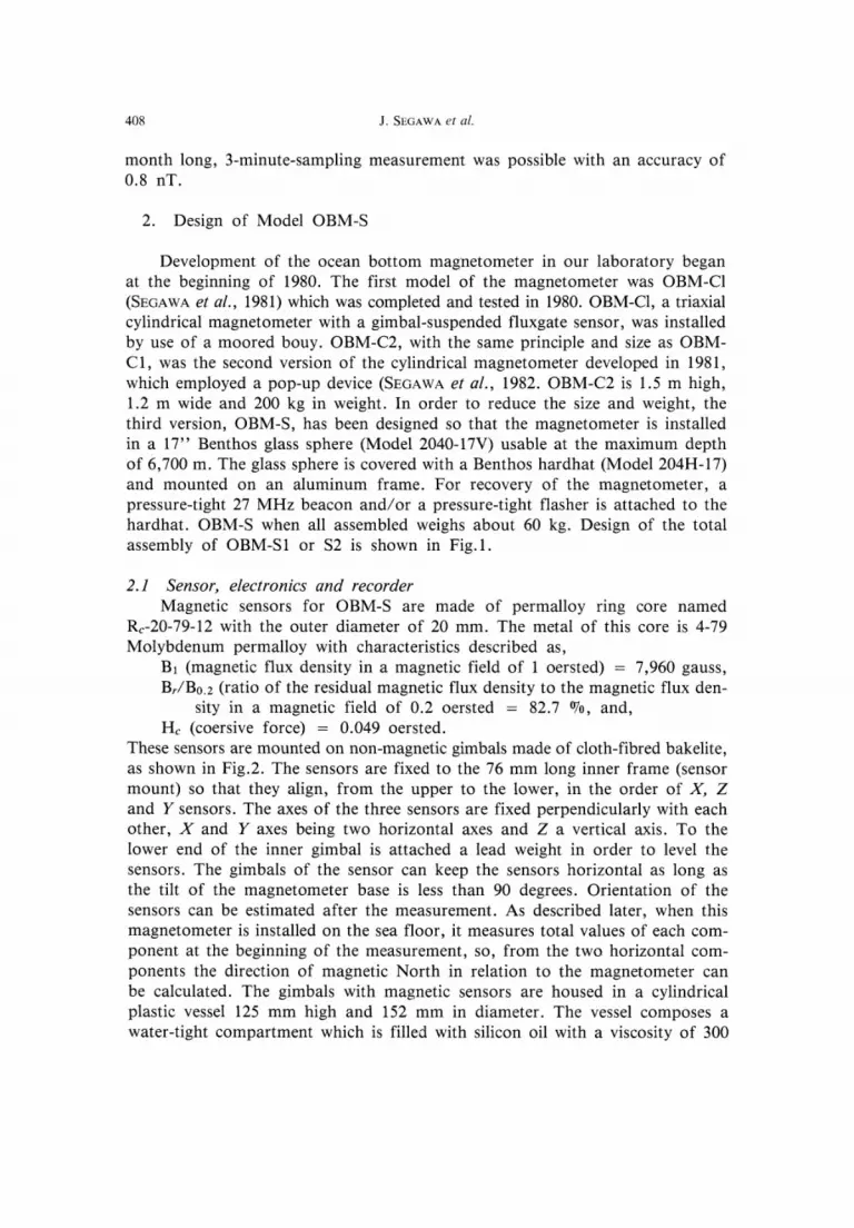
pressure-tight 27MHz beacon and/or a pressure-tight flasher is attached to the hardhat. OBM-S when all assembled weighs about 60kg. Design of the total assembly of OBM-S1 or S2 is shown in Fig. 1.

2.1 Sensor, electronics and recorder Magnetic sensors for OBM-S are made of permalloy ring core named

Rc-20-79-12 with the outer diameter of 20mm. The metal of this core is 4-79 Molybdenum permalloy with characteristics described as,

B1 (magnetic flux density in a magnetic field of 1 oersted)=7,960 gauss, Br/B0.2 (ratio of the residual magnetic flux density to the magnetic flux den-

sity in a magnetic field of 0.2 oersted=82.7%, and, Hc (coersive force)=0.049 oersted.

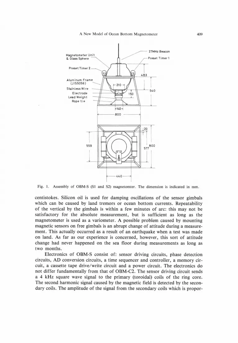
These sensors are mounted on non-magnetic gimbals made of cloth-fibred bakelite, as shown in Fig. 2. The sensors are fixed to the 76mm long inner frame (sensor mount) so that they align, from the upper to the lower, in the order of X, Z and Y sensors. The axes of the three sensors are fixed perpendicularly with each other, X and Y axes being two horizontal axes and Z a vertical axis. To the lower end of the inner gimbal is attached a lead weight in order to level the sensors. The gimbals of the sensor can keep the sensors horizontal as long as the tilt of the magnetometer base is less than 90 degrees. Orientation of the sensors can be estimated after the measurement. As described later, when this magnetometer is installed on the sea floor, it measures total values of each com-

ponent at the beginning of the measurement, so, from the two horizontal com-

ponents the direction of magnetic North in relation to the magnetometer can be calculated. The gimbals with magnetic sensors are housed in a cylindrical

plastic vessel 125mm high and 152mm in diameter. The vessel composes a water-tight compartment which is filled with silicon oil with a viscosity of 300

A New Model of Ocean Bottom Magnetometer 409

Fig. 1. Assembly of OBM-S (S1 and S2) magnetomter. The dimension is indicated in mm.

centistokes. Silicon oil is used for damping oscillations of the sensor gimbals which can be caused by land tremors or ocean bottom currents. Repeatability of the vertical by the gimbals is within a few minutes of arc: this may not be satisfactory for the absolute measurement, but is sufficient as long as the magnetometer is used as a variometer. A possible problem caused by mounting magnetic sensors on free gimbals is an abrupt change of attitude during a measure-ment. This actually occurred as a result of an earthquake when a test was made on land. As far as our experience is concerned, however, this sort of attitude change had never happened on the sea floor during measurements as long as two months.

Electronics of OBM-S consist of: sensor driving circuits, phase detection circuits, AD conversion circuits, a time sequencer and controller, a memory cir-cuit, a cassette tape drive/write circuit and a power circuit. The electronics donot differ fundamentally from that of OBM-C2. The sensor driving circuit sends

a 4kHz square wave signal to the primary (toroidal) coils of the ring core. The second harmonic signal caused by the magnetic field is detected by the secon-dary coils. The amplitude of the signal from the secondary coils which is propor-


Fig. 2. Design of sensor and gimbal unit. The upper the top view, and the lower the side view.

tional to the magnetic field intensity is measured by the phase detecting amplifier. The third coils wound on the ring cores are used for negative feedback: the

phase-detected signals are amplified and filtered, and fed back to these third coils, so that most of the magnetic field acting on the sensor is cancelled. The negative feedback improves significantly the linearity of the sensor. The output from the phase sensitive detectors is connected to the line leading to the negative feedback coils. Therefore, a dynamic range of the sensor is determined by the maximum rate of negative feedback. In the case of OBM-S a linear measurement of magnetic field up to 70,000 nT is quaranteed, although a limitation is imposedby the dynamic range of the AD converter.

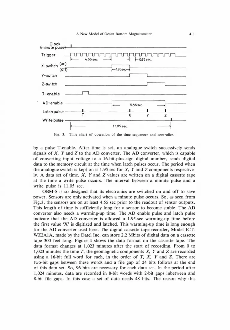
Figure 3 shows a time chart of operation of the time sequencer and con-troller. Clock pulses occur every 1 minute or its multiple. The clock pulses con-trol the rate of measurement which is adjusted by a dip switch from 1 to 8 minutes. When a clock pulse is flagged a series of trigger pulses occur, which control consecutive operation of the magnetometer. The trigger pulses have a repetition period of 0.65sec. The time of measurement is stored first, triggered


Fig. 3. Time chart of operation of the time sequencer and controller.

by a pulse T-enable. After time is set, an analogue switch successively sends

signals of X, Y and Z to the AD converter. The AD converter, which is capable

of converting input voltage to a 16-bit-plus-sign digital number, sends digital

data to the memory circuit at the time when latch pulses occur. The period when

the analogue switch is kept on is 1.95sec for X, Y and Z components respective-

ly. A data set of time, X, Y and Z values are written on a digital cassette tape

at the time a write pulse occurs. The interval between a minute pulse and a

write pulse is 11.05sec.

OBM-S is so designed that its electronics are switched on and off to save

power. Sensors are only activated when a minute pulse occurs. So, as seen from Fig. 3, the sensors are on at least 4.55sec prior to the readout of sensor outputs.

This length of time is sufficiently long for a sensor to become stable. The AD

converter also needs a warming-up time. The AD enable pulse and latch pulse

indicate that the AD converter is allowed a 1.95-sec warming-up time before

the first value 'X' is digitized and latched. This warming-up time is long enough

for the AD converter used here. The digital cassette tape recorder, Model ICT-

WZ2A1A, made by the Datel Inc. can store 2.2 Mbits of digital data on a cassette

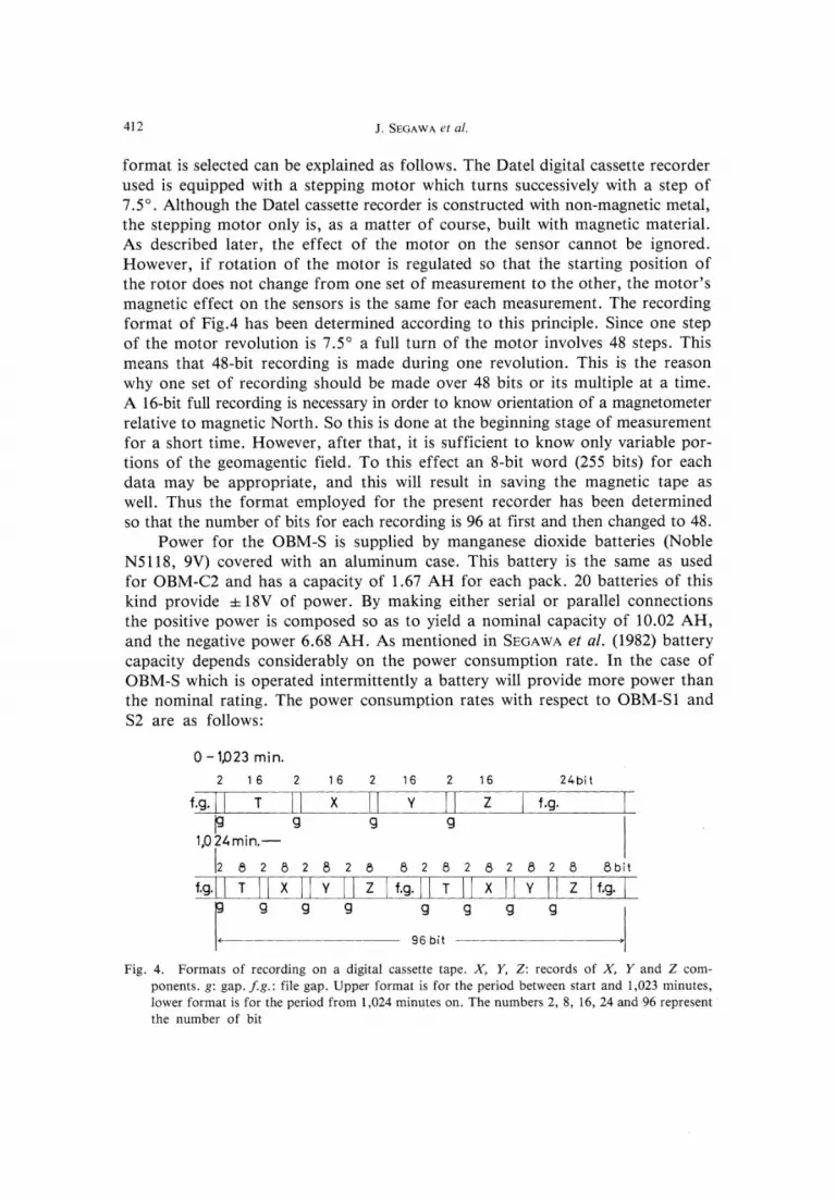
tape 300 feet long. Figure 4 shows the data format on the cassette tape. The

data format changes at 1,023 minutes after the start of recording. From 0 to

1,023 minutes the time T, the geomagnetic components X, Y and Z are recorded

using a 16-bit full word for each, in the order of T, X, Y and Z. There are

two-bit gaps between these words and a file gap of 24 bits follows at the end

of this data set. So, 96 bits are necessary for each data set. In the period after

1,024 minutes, data are recorded in 8-bit words with 2-bit gaps inbetween and

8-bit file gaps. In this case a set of data needs 48 bits. The reason why this


format is selected can be explained as follows. The Datel digital cassette recorder

used is equipped with a stepping motor which turns successively with a step of

7.5°. Although the Datel cassette recorder is constructed with non-magnetic metal,

the stepping motor only is, as a matter of course, built with magnetic material.

As described later, the effect of the motor on the sensor cannot be ignored.

However, if rotation of the motor is regulated so that the starting position of

the rotor does not change from one set of measurement to the other, the motor's

magnetic effect on the sensors is the same for each measurement. The recording

format of Fig. 4 has been determined according to this principle. Since one step

of the motor revolution is 7.5° a full turn of the motor involves 48 steps. This

means that 48-bit recording is made during one revolution. This is the reason why one set of recording should be made over 48 bits or its multiple at a time. A 16-bit full recording is necessary in order to know orientation of a magnetometer relative to magnetic North. So this is done at the beginning stage of measurementfor a short time. However, after that, it is sufficient to know only variable por-tions of the geomagentic field. To this effect an 8-bit word (255 bits) for each data may be appropriate, and this will result in saving the magnetic tape as well. Thus the format employed for the present recorder has been determined so that the number of bits for each recording is 96 at first and then changed to 48.

Power for the OBM-S is supplied by manganese dioxide batteries (Noble N5118, 9V) covered with an aluminum case. This battery is the same as used for OBM-C2 and has a capacity of 1.67 AH for each pack. 20 batteries of thiskind provide ±18V of power. By making either serial or parallel connections

the positive power is composed so as to yield a nominal capacity of 10.02 AH, and the negative power 6.68 AH. As mentioned in SEGAWA et al. (1982) battery capacity depends considerably on the power consumption rate. In the case of OBM-S which is operated intermittently a battery will provide more power than the nominal rating. The power consumption rates with respect to OBM-S1 and S2 are as follows:

Fig. 4. Formats of recording on a digital cassette tape. X, Y, Z: records of X, Y and Z com-ponents. g: gap. f. g.: file gap. Upper format is for the period between start and 1,023 minutes, lower format is for the period from 1,024 minutes on. The numbers 2, 8, 16, 24 and 96 represent the number of bit


Stand-by state; 6.82mA (+18V). 0mA (-18V), Measuring state (11.05sec for each sample); 85mA (+18V), 67mA (-18V), Recording state (either 1.07sec or 0.53sec); 63mA (+18V), 0mA (-18V).

The averaged current estimated using this power consumption rate is 23.0mA for +18V and 12.3mA for -18V for a 1-minute sample rate of measurement. When a measurement is made every 3 minutes, the averaged currents are, 12.2 mA for +18V, and 4.11mA for -18V. These calculations are for the regular state of measurement, i.e., 1,023 minutes after the start of measurement when only 8-bit words are used for recording. With the nominal battery capacity, OBM-Swill operate for at least 34.2 days for 3-minute samples. This limitation is deter-mined by the power-out of the positive battery. However, in the actual case as mentioned in the later section, the batteries lasted much longer.

Figure 5 shows the arrangement of the fluxgate sensors, electronics boards, batteries and cassette recorder that are housed in the glass sphere. The fluxgatesensor unit soaked in a viscous oil is located at the uppermost part of the sphere and supported by a bakelite pillar. The electronics boards are mounted on a central aluminum disc, and the batteries are installed between two aluminum

Fig. 5. Arrangement of each unit of the magnetometer housed in a 17" glass sphere.


discs below. The digital cassette recorder is installed in the lowest part. Unitshoused in the glass sphere weighs 16kg in all. The weight of the glass sphere itself is 17.7kg in air, and its net bouyancy in water is 25.4kg. The glass sphere is covered by a hardhat as seen in Fig. 1 and mounted on a frame made of an-ticorrosive aluminum (JIS 5056).

2.2 Device for recovery The parts of OBM-S that are recovered are, as seen from Fig. 1, a glass

sphere with a magnetometer unit, two sets of preset timers (1 and 2), a 27MHz beacon and/or flasher, and electrodes for release attached to their support. The method to release the magnetometer is based on the following principle. A bakelite structure that looks like a square box is attached to the bottom of the plastic hardhat. There is a stainless steel wire about 1mm in diameter suspended from the center of the bottom of the hardhat. The stainless steel wire, whose break-down strength is 200kg, hangs a square lead weight of 11.2kg. As the net bouyancy of all units that are to be recovered is about 4.5kg, the weight of 11.2kg is large enough to hold down the magnetometer during a measurement. Under this condition, however, there is no mechanical connectioin between the magnetometer unit and the aluminum frame, the former being simply placed

on the frame with the aid of gravity. So, the lead weight is tied firmly to the bottom of the aluminum frame by use of ropes, as seen in Fig. 1. The preset timers are low power consumption crystal clocks which can be preset to a time from 0 to 9,999 hours after the time of reset. Minimum step of setting is 1 hour. These timers are driven by alkaline batteries. At the preset time a relay is switched on to apply electric voltage (about 10.5V) between the stainless steel wire and the electrodes. The electric current causes the stainless steel wire to electrolyse until at last it is broken, it takes about 5 minutes for the stainless steel wire to dissolve completely, and release the magnetometer unit from the frame. The aluminum frame and lead weight are left behind on the sea floor and the instrument rises to the surface with a speed of about 35 cm/sec. At the sea surface, the magnetometer is located with the aid of the beacon or flasher.

3. Performance of OBM-S

3.1 Tests on land Two sets of OBM-S (S1 and S2) were tested at the Kakioka Geomagnetic

Observatory. At Kakioka a possible disturbances of the recorder's stepping motor and magnetic tapes as well as the general state of measuring capability were checked, and the meter's sensitivity was calibrated.

Figure 6 shows the effect of magnetization of the stepping motor on the magnetic sensors. This test was made in a short period in which the geomagnetic field was supposed to be constant. The three curves of Fig. 6 that are denoted by X, Y and Z, respectively, indicate changes of magnetic field at the sensors when the stepping motor was randomly moved and stopped. The abscissa shows


Fig. 6. A test on magnetic effect from the stepping motor used in the cassette tape recorder. Here, changes of the magnetic field are plotted against repetition of trial.

repetition time of this experiment and the ordinate the change of the magnetic field. This experiment shows that by the change of stopping angle of the motor, the X component changes by 3 nT, Y component 11 nT and Z component 80 nT. It is clearly seen that, the Z sensor is influenced by the motor to a great extent because of the relation of the motor's position with that of the Z sensor axis. In order to remove this effect the stopping angle of the rotor is regulatedin the actual OBM recorder, as mentioned in the previous section.

Figure 7 shows a result of a test measurement at the Kakioka Geomagnetic Observatory for about half a day. The disturbances from the motor have disap-

peared almost completely, because the record does not show any short period noises with large amplitude. From this record, however, another problem which is caused by the magnetic tape is found. If this record is compared with the record simultaneously obtained by KASMMER (Kakioka Automatic Standard Magnetometer) it is seen that the record of OBM-S1 involves sinusoidal noises

OBM-S1 10 Oct. 1981, 1min sampling at KAKIOKA

Fig. 7. A test of measurement using OBM-S1 at the Kakioka Geomagnetic Observatory. Sinusoidaldisturbances caused by rotation of cassette tape reel are indicated. See text for detail.


with a period of about 40 minutes and an amplitude of 2.9 nT or smaller. The sinusoidal noises are the largest for the case of the D-component (note the arrowindicated on the profile of the D-component of Fig. 7). As for the other com-ponents this effect is much smaller, being too obscure to recognize. This has proved to be an effect from the rotation of the cassette magnetic tapes wound on a reel. It is a troublesome noise, but rather easily removed by computer pro-cessings because the change of magnetic field caused by the cassette tape can be expressed by an experimental formula.

Calibration of OBM-S1 and S2 was made in two different ways. One method is to use natural magnetic field while referring to a standard magnetometer, and the other is to put a magnetometer in an artificial magnetic field generated by a Helmholtz coil.

In calibration according to the first method one axis of the OBM sensor was directed to magnetic North and then turned to the opposite direction. This operation was made with each axis. In this way the magnetic sensor of each component measured horizontal component of geomagnetic field H and its rever-sal -H. The value H is obtained, on the other hand, from another known magnetometer, KASMMER, for example. Now, the relation between intensity of magnetic field and reading of each component can be formulated as follows.

Hx= a1X+b1Y+c1Z,

Hy= a2X+b2Y+c2Z,

HZ= a3X+b3Y+c3Z,

where HX, H,, and Hz are magnetic field intensity acting on X, Y and Z axes, respectively, and X, Y and Z are readings of each component, and ai, bi and ci are constants. These relations are formed by assuming that the sensors of one axis is interfered with to some extent by the sensors of the other axes, because of imperfect orthogonality between the three axes. The results of calibration bas-ed on the first method with respect to OBM-S1 are as follows:

Hx=0.83419(X-0.0131Z)nT,

Hy=0.79339(Y-0.0104Z)nT,

HZ=0.79460(Z+0.0223X+0.0178Y)nT.

This calibration was made at a temperature of 21℃. The calibration results imp-

ly that the sensitivity of a sensor is about 0.8 nT/bit and that interference by

the other axis is 1 to 2% of the reading of the other axis. In other words,

regarding, for instance, the X axis, the change of reading in Z axis by 100 causes

the change of reading in X axis by 1.3, leading to a correction for X sensor

by the amount of 1.09 nT. Interference between X and Y axes is not expressed

in the above formulas. This is because of the unavoidable situation that the


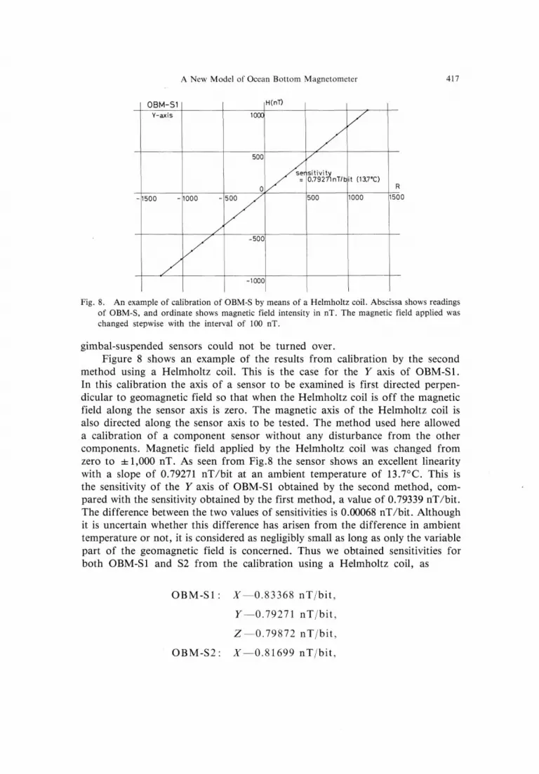
Fig. 8. An example of calibration of OBM-S by means of a Helmholtz coil. Abscissa shows readings of OBM-S, and ordinate shows magnetic field intensity in nT. The magnetic field applied was changed stepwise with the interval of 100 nT.

gimbal-suspended sensors could not be turned over. Figure 8 shows an example of the results from calibration by the second

method using a Helmholtz coil. This is the case for the Y axis of OBM-S1.

In this calibration the axis of a sensor to be examined is first directed perpen-

dicular to geomagnetic field so that when the Helmholtz coil is off the magnetic

field along the sensor axis is zero. The magnetic axis of the Helmholtz coil is

also directed along the sensor axis to be tested. The method used here allowed

a calibration of a component sensor without any disturbance from the other

components. Magnetic field applied by the Helmholtz coil was changed from

zero to±1,000 nT. As seen from Fig. 8 the sensor shows an excellent linearity

with a sloe of 0.79271 nT/bit at an ambient temperature of 13.7℃. This is

the sensitivity of the Y axis of OBM-S1 obtained by the second method, com-pared with the sensitivity obtained by the first method, a value of 0.79339 nT/bit. The difference between the two values of sensitivities is 0.00068 nT/bit. Although it is uncertain whether this difference has arisen from the difference in ambienttemperature or not, it is considered as negligibly small as long as only the variable part of the geomagnetic field is concerned. Thus we obtained sensitivities for both OBM-S1 and S2 from the calibration using a Helmholtz coil, as

OBM-S1: X-0.83368nT/bit,

Y-0.79271 nT/bit,

Z-0.79872 nT/bit,

OBM-S2: X-0.81699nT/bit,


Y-0.79020 nT/bit,

Z-0.79334 nT/bit.

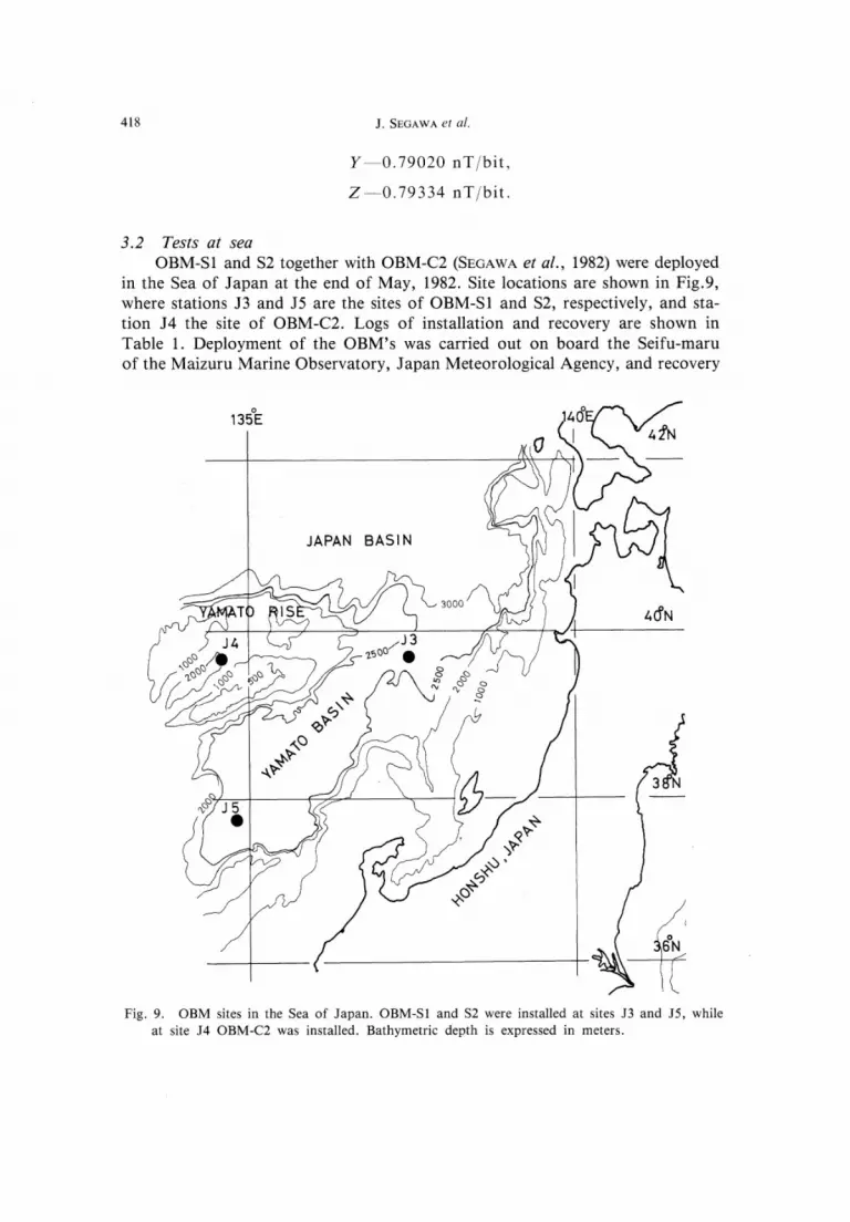
3.2 Tests at sea OBM-S1 and S2 together with OBM-C2 (SEGAWA et al., 1982) were deployed

in the Sea of Japan at the end of May, 1982. Site locations are shown in Fig. 9, where stations J3 and J5 are the sites of OBM-S1 and S2, respectively, and sta-tion J4 the site of OBM-C2. Logs of installation and recovery are shown in Table 1. Deployment of the OBM's was carried out on board the Seifu-maru of the Maizuru Marine Observatory, Japan Meteorological Agency, and recovery

Fig. 9. OBM sites in the Sea of Japan. OBM-Sl and S2 were installed at sites J3 and J5, while

at site J4 OBM-C2 was installed. Bathymetric depth is expressed in meters.


Table 1. Logs of installation and recovery of the magnetometer in the Sea of Japan for 1982.

was carried out on board the Shinyo-maru of the Tokyo University of Fisheries. Although there were some minor troubles with the components of the magnetometers all the devices were successfully retrieved. The interval of measure-ment was 3 minutes in this experiment. What is worthwhile to mention is that OBM-S worked for two months in spite of the fact that the period for which the batteries are expected to supply power, as estimated from nominal battery capacity, is much shorter than two months. A similar case happened as to OBM-C2 in the experiment of 1981.

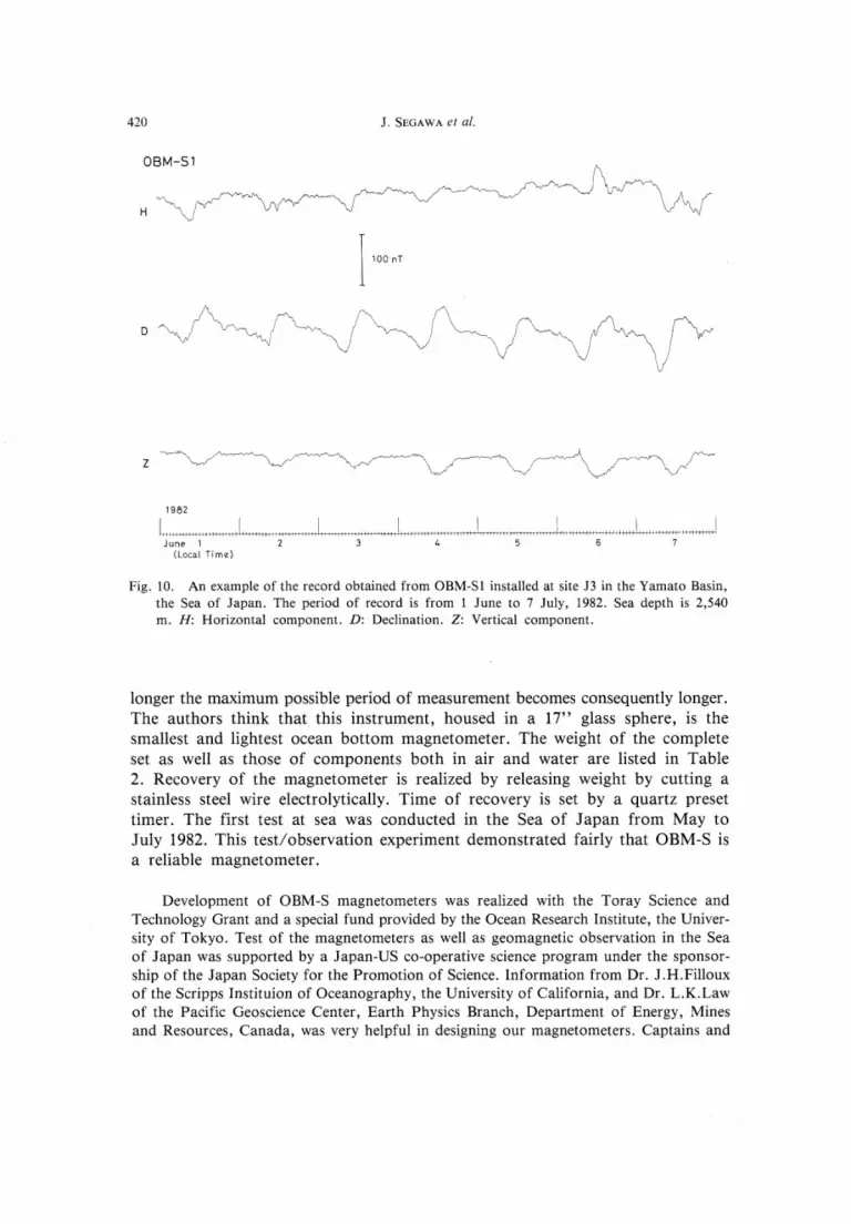
Figure 10 shows an example of the record obtained by OBM-S1 at site J3. This is a record from 00H00M, 1 June to 24H00M, 7 June (local time). As theX axis of OBM-S1 was found to be oriented in the direction N23°E relative

to magnetic North, outputs from X and Y axes were synthesized to form true

H, D and Z components. The effect from the cassette tapes was also removed.

The record shown in Fig. 10 looks, as a whole, satisfactory. If this record is

compared with that of Kakioka the features of Z component are most remarkably

different. By observations in the Sea of Japan we have obtained digital data

of this kind for about 60 days. During this observation there occurred a tremen-

dous magnetic storm whose magnetic change was over 600 nT on 14 July, 1982.

It is noteworthy that this magnetic storm was completely recorded by OBM' S

at the sea floor.

4. Conclusion

A triaxial fluxgate magnetometer for sea floor measurement has been

developed. This magnetometer has an accuracy better than 1 nT and is capable

of measuring the geomagnetic field for two months at an 3 minute sampling

interval on the sea floor as deep as 6,700m. If the sampling interval is made


OBM-S1

Fig. 10. An example of the record obtained from OBM-S1 installed at site J3 in the Yamato Basin,

the Sea of Japan. The period of record is from 1 June to 7 July, 1982. Sea depth is 2,540

m. H: Horizontal component. D: Declination. Z: Vertical component.

longer the maximum possible period of measurement becomes consequently longer.

The authors think that this instrument, housed in a 17" glass sphere, is the

smallest and lightest ocean bottom magnetometer. The weight of the complete

set as well as those of components both in air and water are listed in Table 2. Recovery of the magnetometer is realized by releasing weight by cutting a

stainless steel wire electrolytically. Time of recovery is set by a quartz preset

timer. The first test at sea was conducted in the Sea of Japan from May to

July 1982. This test/observation experiment demonstrated fairly that OBM-S is

a reliable magnetometer.

Development of OBM-S magnetometers was realized with the Toray Science and Technology Grant and a special fund provided by the Ocean Research Institute, the Univer-sity of Tokyo. Test of the magnetometers as well as geomagnetic observation in the Sea of Japan was supported by a Japan-US co-operative science program under the sponsor-ship of the Japan Society for the Promotion of Science. Information from Dr. J. H. Filloux of the Scripps Instituion of Oceanography, the University of California, and Dr. L. K. Law of the Pacific Geoscience Center, Earth Physics Branch, Department of Energy, Mines and Resources, Canada, was very helpful in designing our magnetometers. Captains and


Table 2. Weight of OBM-S and. its components.

crew of both the Seifu-maru of the Maizuru Marine Observatory, Japan Meteorological

Agency, and the Shinyo-maru of the Tokyo University of Fisheries helped kindly and

co-operated with us for installation and recovery of the magnetometers. We appreciate

sincerely all of these personnel and organizations.

REFERENCES

LAW, L. K. and J. P. GREENHOUSE, Geomagnetic variation sounding of the asthenosphere beneath

the Juan de Fuca Ridge, J. Geophys. Res., 86, 967-978, 1981.

SEGAWA, J., T. KASUGA, and T. YUKUTAKE, Preliminary test on a three component ocean bottom

magnetometer, J. Geod. Soc. Japan, 27, 239-251, 1981.

SEGAWA, J., T. YUKUTAKE, Y. HAMANO, T. KASUGA, and H. UTADA, Sea floor measurement

of geomagnetic field using newly developed ocean bottom magnetometers, J. Geomag. Geoelectr.,

34, 571-585, 1982.WHITE, A., A sea floor magnetometer for the continental shelf, Mar. Geophys. Res., 4, 105-114,

1979.

a new model of ocean bottom magnetometer

Documents