Linear Algebra and its Applications 428 (2008) 2761–2777

Available online at www.sciencedirect.com

www.elsevier.com/locate/laa

A new iterative criterion for H-matrices: The reduciblecase

M. Alanelli a,1, A. Hadjidimos b ,∗,2

a Department of Mathematics, University of Crete, GR-714 09 Heraklion, Greeceb Department of Computer and Communication Engineering, University of Thessaly, 10 Iasonos Street,

GR-383 33 Volos, Greece

Received 13 March 2007; accepted 26 December 2007Available online 4 March 2008

Submitted by R.A. Brualdi

It is dedicated to Professor Hans Schneider on the occasion of his 80th birthday.

Abstract

H-matrices appear in various areas of science and engineering and it is of vital importance to have anAlgorithm to identify the H-matrix character of a certain matrix A ∈ Cn,n. Recently, the present authorshave proposed a new iterative criterion (Algorithm AH) to completely identify the H-matrix property of anirreducible matrix. The present work extends the previous Algorithm to cover the reducible case as well.© 2008 Elsevier Inc. All rights reserved.

AMS classification: Primary 65F10

Keywords: M- and H-matrices; (generalized) Strictly diagonally dominant matrices; Criteria for H-matrices

1. Introduction

The theory of H -matrices is very important for the numerical solution of linear systems ofalgebraic equations arising in various applications. E.g., in the Linear Complementarity Problem

∗ Corresponding author. Tel.: +30 24210 74908; fax: +30 24210 74923.E-mail addresses: alanelli@math.uoc.gr (M. Alanelli), hadjidim@inf.uth.gr (A. Hadjidimos).

1 The work of this author was funded by “Herakleitos” Operational Programme for Education and Initial VocationalTraining 2002–2005.

2 Part of the work of this author was funded by the Program Pythagoras of the Greek Ministry of Education.

0024-3795/$ - see front matter ( 2008 Elsevier Inc. All rights reserved.doi:10.1016/j.laa.2007.12.020

2762 M. Alanelli, A. Hadjidimos / Linear Algebra and its Applications 428 (2008) 2761–2777

(LPC), in the Free Boundary Value Problems in Fluid Analysis, etc. [2]. The most common wayto define an H -matrix A ∈ Cn,n is the following:

Definition 1.1. A ∈ Cn,n is an H -matrix if and only if (iff) there exists a positive diagonal matrixD ∈ Rn,n so that AD is (row-wise) strictly diagonally dominant, that is

|aii |di >

n∑j=1, j /=i

|aij |dj , i = 1(1)n. (1.1)

For the identification of an H -matrix, many criteria have been proposed the majority of whichare iterative ones (see, e.g. [6,10,9,11,12,5,1]). This is because direct criteria seem to have highcomputational complexities. The only iterative criterion that takes into account the sparsity of A

is the one in [5], where an extension of the compact profile technique of [8] was developed andcan also be used in the present case.

The new Algorithm in this paper extends Algorithm AH in [1] to cover the reducible case aswell, since the latter was constructed to deal with irreducible matrices only.

In Section 2, basic notation, terminology and statements are presented. In Section 3, AlgorithmAH is illustrated and some explanations on it are given. In Section 4, use of combinatorial matrixtheory allows us to solve the problem of the general p × p block reducible case. In Section 5,we propose a new Jacobi type iterative criterion for identifying H -matrices (Algorithm AH2).Contrary to Algorithm AH the convergence of the new Algorithm is guaranteed for all irreducibleand reducible matrices. Finally, in Section 6, we present a number of numerical examples workedout with both Algorithms AH and AH2.

2. Preliminaries and background material

For our analysis some definitions are recalled and a number of useful statements are given.Most of them can be found in [2,7,16,19].

Definition 2.1 [2]. A matrix A ∈ Rn,n is called an M-matrix if it can be written as A = sI − B,where B � 0 and ρ(B) < s, with ρ(.) denoting spectral radius. (Note: In Definition 2.1 and inthis context an M-matrix is always nonsingular.)

Lemma 2.1 [16]. Let A ∈ Rn,n be an irreducible M-matrix, then its inverse exists and is a strictlypositive matrix, that is A−1 > 0.

Lemma 2.2. If A ∈ Rn,n is an M-matrix so is PAP T, where P is a permutation matrix.

Lemma 2.3 [16]. Any principal submatrix of an M-matrix A ∈ Rn,n is also an M-matrix.

Definition 2.2 [2]. The comparison matrix of a matrix A ∈ Cn,n is the matrixM(A) with elements

mij ={|aii |, if i = j = 1(1)n,

−|aij |, if i, j = 1(1)n, i /= j.

Lemma 2.4 [16]. A matrix A ∈ Cn,n is an H -matrix iff its comparison matrix is an M-matrix.

Lemma 2.5. A matrix A ∈ Cn,n is an H -matrix iff the Jacobi iteration matrix associated with itscomparison matrix is convergent.

M. Alanelli, A. Hadjidimos / Linear Algebra and its Applications 428 (2008) 2761–2777 2763

Lemma 2.6. A matrix A ∈ Cn,n is not an H -matrix iff there exists at least one principal submatrixof A that is not an H -matix.

Lemma 2.7. LetA ∈ Cn,n,withaii /= 0, i = 1(1)n,andB =EA,whereE=diag(e1, e2, . . . , en)

∈ Cn,n be any nonsingular diagonal matrix. Let JA and JB be the Jacobi iteration matricesassociated with A and B, respectively. Then JA and JB are identical.

Definition 2.3 [16]. Let A ∈ Rn,n, A � 0, be an irreducible matrix and k be the number ofeigenvalues of A of modulus equal to its spectral radius ρ(A). If k = 1, then A is primitive. Ifk > 1, then A is cyclic of index k.

Definition 2.4 [2]. Index of a given matrix A ∈ Cn,n, denoted by index(A), is the smallestnonnegative integer such that rank(Ak) = rank(Ak+1).

Lemma 2.8 [2]. If A ∈ Rn,n, A � 0, is an irreducible matrix with positive trace,∑n

i=1 aii > 0,

then A is primitive.

Theorem 2.1 [7]. If A ∈ Cn,n and if λ, μ ∈ σ(A), with λ /= μ, then any left eigenvector of A

corresponding to μ is orthogonal to any right eigenvector of A corresponding to λ.

Theorem 2.2 [16]. Let A ∈ Rn,n, A � 0, be an irreducible matrix. Then, its spectral radius ρ(A)

is a simple (positive) eigenvalue of A (the Perron root) and a positive eigenvector (the Perronvector) is associated with it.

Theorem 2.3 [16]. For any given irreducible matrix A ∈ Rn,n, A � 0, let P ∗ be the hyperoctantof vectors x > 0. Then, for any x ∈ P ∗, either

mini=1(1)n

{∑nj=1 aij xj

xi

}< ρ(A) < max

i=1(1)n

{∑nj=1 aij xj

xi

},

or ∑nj=1 aij xj

xi

= ρ(A), i = 1(1)n.

Algorithm AH [1] is based on a modification of the well-known Power Method (see, e.g.[18] and more specifically [4] and [7]), applied to a nonnegative, irreducible and primitive n × n

matrix. The Power Method Theorem and the one on which Algorithm AH is based are statedbelow.

Theorem 2.4 (The Power Method). Let A ∈ Cn,n, with its eigenvalues satisfying

|λ1| > |λj |, j = 2(1)n.

Define

x(k) = Ax(k−1), k = 1, 2, 3, . . . , for any x(0) ∈ Cn\{0}. (2.1)

Assume that x(0) has a nonzero component along the eigenvector corresponding to λ1. Then

λ1 = limk→∞

(Ax(k))i

x(k)i

for x(k)i /= 0, i = 1(1)n. (2.2)

2764 M. Alanelli, A. Hadjidimos / Linear Algebra and its Applications 428 (2008) 2761–2777

Theorem 2.5 [1]. For any given irreducible and primitive matrix A ∈ Rn,n, A � 0, let λ1 = ρ(A)

and letA = SJS−1 be its Jordan canonical form,withJ = diag(J1, J2, . . . , Jp), Ji ∈ Cni ,ni , i =1(1)p,

∑p

i=1 ni = n, and with S = [s1 s2 s3 . . . sn] being the matrix of the principal vectors of A.

Then, any x ∈ P ∗, analyzed along the principal vectors si, i = 1(1)n, has a positive componentalong the Perron vector s1 corresponding to the Perron root λ1.

3. Algorithm AH and main statements

The new algorithm (Algorithm AH2) we are to propose is an extension of Algorithm AH andas is proved converges also in a finite number of iterations. The latter Algorithm is illustratedbelow after some definitions are given.

For both Algorithms the following matrices are needed. A sequence of positive diagonalmatrices D(k), that will be defined in the Algorithm, and A(k).

D(k), k = 0, 1, 2, . . . , D(0) = I, (3.1)

A(k) = (D(k−1))−1A(k−1)D(k−1), k = 1, 2, 3, . . . , A(0) = (diag(A))−1A, (3.2)

assuming aii /= 0, i = 1(1)n. From (3.1) and (3.2), it is readily seen that

a(k)ii = 1, i = 1(1)n, k = 0, 1, 2, . . . (3.3)

Algorithm AH

INPUT: An irreducible matrix A := [aij ] ∈ Cn,n.

OUTPUT: D = D(0)D(1) · · · D(k) ∈ DD−1A ≡ DA or /∈ DA3 if A is or is not an H -matrix,

respectively.

1. If aii = 0 for some i ∈ {1, 2, . . . , n}, “A is not an H -matrix”, STOP; Otherwise2. Set D = I , A(0) = (diag(A))−1A, D(0) = I, k = 13. Compute D = DD(k−1), A(k) = (D(k−1))−1A(k−1)D(k−1) = [a(k)

ij ]4. Compute s

(k)i = ∑n

j=1, j /=i |a(k)ij |, i = 1(1)n, s(k) = mini=1(1)n s

(k)i , S(k) = maxi=1(1)n s

(k)i

5. If s(k) > 1, “A is not an H -matrix”, STOP; Otherwise6. If S(k) < 1, “A is an H -matrix”, STOP; Otherwise7. If S(k) = s(k), “M(A) is singular”, STOP; Otherwise8. Set d = [di], where

di = 1 + s(k)i

1 + S(k), i = 1(1)n

9. Set D(k) = diag(d), k = k + 1; Go to Step 3. END

For Algorithm AH the following two statements were proved in [1]:

Theorem 3.1. Let A ∈ Cn,n be an irreducible matrix. Then, Algorithm AH always terminatesin a finite number of iterations (except, maybe, when det(M(A)) = 0).

3 DA denotes the class of all positive diagonal matrices D so that AD is strictly diagonally dominant.

M. Alanelli, A. Hadjidimos / Linear Algebra and its Applications 428 (2008) 2761–2777 2765

Theorem 3.2. Let A ∈ Cn,n be any irreducible matrix. If Algorithm AH terminates in a finitenumber of iterations, then its output is correct.

If A ∈ Cn,n is irreducible, with aii /= 0, i = 1(1)n, and we set as in Algorithm AH

A(k) =(

diag(d(k−1)1 , d

(k−1)2 , . . . , d(k−1)

n ))−1

× A(k−1) diag(d(k−1)1 , d

(k−1)2 , . . . , d(k−1)

n ), with d(0) = e, (3.4)

|A(k)| = I + B(k), k = 0, 1, 2, . . . (3.5)

where e ∈ Rn is the vector of ones and |X| denotes the matrix whose elements are the moduli of thecorresponding elements of X. Note that B(0) is the Jacobi matrix associated with the comparisonmatrix of A, JM(A). If in the Algorithm we allow k → ∞ then in the proofs of Theorems 3.1 and3.2 it was also proved in [1], among others, that

Corollary 3.1. Under the assumptions and notations so far the Perron vector d of |A(0)| (andB(0)) is given by

d =(

limk→∞

(k∏

i=1

D(i)

))e. (3.6)

Corollary 3.2. Under the assumptions and notations so far there hold

limk→∞ |A(k)| e = ρ(|A(0)|)e and lim

k→∞ a(k)ij = dj

di

a(0)ij . (3.7)

Algorithm AH was designed to work for irreducible matrices. However, we had observed thatit worked perfectly well for certain classes of reducible matrices. This motivated the investigationof the effect of the application of Algorithm AH to reducible matrices a little further. So, we wereled to extend it and create Algorithm AH2 which is shown to converge for both irreducible andreducible matrices and terminates in a finite number of iterations.

4. The general reducible case

To study the general p × p block reducible matrices we introduce some more theoretical mate-rial. Although some of it holds for general n × n complex matrices we will restrict to nonnegativematrices. Most of the basic material is taken from the works of Rothblum [13], Schneider [14],Bru and Neumann [3] and also from the book of Berman and Plemmons [2].

Lemma 4.1. Let A � 0, A ∈ Rn,n be a reducible matrix. Then there exists a permutation matrixP such that A can be reduced to a block triangular form

PAP T =

⎡⎢⎢⎢⎢⎢⎢⎢⎢⎣

A11 A12 · · · · · · A1,p−1 A1p

A22 · · · · · · A2,p−1 A2p

. . .. . .

......

. . ....

...

Ap−1,p−1 Ap−1,p

App

⎤⎥⎥⎥⎥⎥⎥⎥⎥⎦, (4.1)

2766 M. Alanelli, A. Hadjidimos / Linear Algebra and its Applications 428 (2008) 2761–2777

where each block Aii ∈ Rni ,ni , i = 1(1)p,∑p

i=1 ni = n, is either irreducible or a 1 × 1 nullm-atrix. This form is known as the Frobenius normal form.

Note : To be in agreement with the main body of Algorithm AH it will be assumed that in(4.1) aii /= 0, i = 1(1)n, and that aii are normalized so that aii = 1, i = 1(1)n.

Definition 4.1. Let A � 0, A ∈ Rn,n. We define the (directed) graph of A, G(A), to be thegraph with vertices (nodes) 1(1)n, where an edge (arc) leads from i to j iff aij /= 0.

Definition 4.2. Let A � 0, A ∈ Rn,n. For i, j ∈ {1, . . . , n}, we say that i has access to j if inG(A) there is a path from i to j and that i and j communicate if i has access to j and j hasaccess to i. (Note: Communication is an equivalence relation.)

Definition 4.3. The classes of A � 0 are the equivalence classes of the communication relationinduced by G(A). A class α has access to a class β if for i ∈ α and j ∈ β, i has access to j . Aclass is initial if it is not accessed by any other class and is final if it has access to no other class.A class is basic if ρ(A[α]) = ρ(A), where A[α] is the submatrix of A based on the indices in α,and nonbasic if ρ(A[α]) < ρ(A).

Remark 4.1. The blocks Aii, i = 1(1)p, in the Frobenius normal form (4.1) of A correspondto the classes of A. From (4.1), every A � 0 has at least one basic class and one final class. Theclass that corresponds to Aii, i = 1(1)p, is basic iff ρ(Aii) = ρ(A) and final iff Aij = 0, j > i.In particular, A is irreducible iff it has only one (basic and final) class.

Theorem 4.1. Let A � 0, A ∈ Rn,n. Then to the spectral radius ρ(A) there corresponds a posi-tive eigenvector iff the final classes of A are exactly its basic ones. (Note: As, e.g., in the case ofan irreducible matrix or of a block diagonal matrix with ρ(Aii) = ρ(A), i = 1(1)p.)

Theorem 4.2. Let A � 0, A ∈ Rn,n. Then to the spectral radius ρ(A) there corresponds apositive eigenvector and a positive eigenvector of AT iff all the classes of A are basic andfinal.

Definition 4.4. Let A � 0, A ∈ Rn,n. The degree of A is ν(A) = index(ρ(A)I − A). The null-space N((ρ(A)I − A)ν(A)) is called the algebraic eigenspace of A and its elements are calledgeneralized eigenvectors.

Definition 4.5. Let A � 0, A ∈ Rn,n and α1, α2, . . . , αk be classes of A. The collection {α1, α2,

. . . , αk} is a chain from α1 to αk , if ai has access to ai+1, i = 1(1)k − 1. The length of a chainis the number of basic classes it contains. A class α has access to a class β in m steps if m is thelength of the longest chain from α to β. The height of a class β is the length of the longest chainof classes that terminate in β.

Theorem 4.3. LetA � 0, A ∈ Rn,n have spectral radiusρ(A)andmbasic classesα1, α2, . . . , αm.

Then the algebraic eigenspace of A contains nonnegative vectors x(1), x(2), . . . , x(m), such thatthe subvector xi

(j) > 0 iff αi has access to αj and any such collection is a basis of the algebraic

eigenspace of A. (Note: It is understood that x(i)i > 0.)

M. Alanelli, A. Hadjidimos / Linear Algebra and its Applications 428 (2008) 2761–2777 2767

Fig. 1. Block graph of A in (4.2).

Remark 4.2. Based on Definitions 4.4, 4.5 and Theorem 4.3 it is clear that the only “genuine”eigenvectors of A, that is those nonnegative vectors x ∈ Rn,n for which Ax = ρ(A)x, correspondto basic classes of height 1.

The material presented so far suffices to develop our new Algorithm for p × p block reduciblematrices. For this we will draw some conclusions when the Power Method Theorem 2.4 and/orAlgorithm AH is applied to the reducible matrix A � 0, supposedly that A is in its Frobeniusnormal form (4.1), with aii = 1, i = 1(1)n.

(a) If the graph of A, G(A), consists of the union of the disjoint subgraphs gi(A), i =1(1)k, 1 < k � p, then A can be written as A = diag(B11, B22, . . . , Bkk), where each Bii, i =1(1)k, is reducible and is already in its Frobenius normal form. So, the terms initial, final, basic,nonbasic, etc. have to be redefined for each of the new major blocks Bii, i = 1(1)k. Therefore,the application of the Power Method Theorem 2.4 and/or of Algorithm AH to A is equivalent toits application to each Bii separately. Obviously, if k = p, A is block diagonal with each blockbeing an irreducible matrix.

Example 1. Consider the matrix

A =

⎡⎢⎢⎢⎢⎣A11 0 0 A14 0

0 A22 A23 0 A250 0 A33 0 A350 0 0 A44 00 0 0 0 A55

⎤⎥⎥⎥⎥⎦ . (4.2)

It is seen that G(A) (Fig. 1) consists of two disjoint subgraphs. One has vertices the nodes {1, 4}and the other subgraph the nodes {2, 3, 5}. So, there is an obvious block similarity permutationthat puts A into the form

A = diag(B11, B22), where B11 =[A11 A14

0 A44

], B22 =

⎡⎣A22 A23 A250 A33 A350 0 A55

⎤⎦ . (4.3)

Then, the Power Method Theorem (and Algorithm AH) is applied to B11 and B22 separately.(b) If A is of the form (4.1), with aii = 1, i = 1(1)n, and its graph, G(A), does not consist of

a union of disjoint subgraphs. Then applying a block similarity permutation on A, say QAQT,

2768 M. Alanelli, A. Hadjidimos / Linear Algebra and its Applications 428 (2008) 2761–2777

preserving the Frobenius normal form, its basic classes are put, in increasing order of their heights,into major principal blocks as final classes. If any two or more basic classes are of the same heightthey are put in the same major principal block in any order. If there are nonbasic classes thatdo not access any basic one they are put in a separate last major principal block. In this way, ineach major principal block with one or more final basic classes αr , all the nonbasic classes haveaccess to at least one of the αr ’s. If there is a last major principal block of nonbasic classes, let itbe denoted by A, its graph G(A) is considered and depending on whether G(A) consists of theunion of disjoint subgraphs or not the procedure in (a) before or the present one is followed. Therearrangement proposed is the one in [13] and [3], apart from the last major principal block ofnonbasic classes.

From the theory presented so far we can state, without any formal proof, the following propo-sition whose validity will be made clear by a more general example.

Theorem 4.4. Under the assumptions of (b) previously, the application of the Power MethodTheorem 2.4 and/or Algorithm AH to the new form of A makes all row sums of the majorprincipal blocks corresponding to basic classes tend to ρ(A) in the limit. If there is a last majorprincipal block of nonbasic classes that do not have access to any basic one, let it be A, then,

by following the previous described rules and depending on G(A), the application of AlgorithmAH makes the row sums of A tend to limits that are strictly less than ρ(A).

Having raised some basic issues in (a) and (b) above, we present and treat a more generalexample, where all the previously raised issues will be discussed and made clear.

Example 2

⎡⎢⎢⎢⎢⎢⎢⎢⎢⎢⎢⎢⎢⎢⎢⎢⎢⎢⎢⎢⎢⎢⎢⎢⎢⎣

A11 0 0 0 A15 0 0 0 0 0 0 0 0 00 A22 0 A24 0 0 0 0 0 0 0 0 0 00 0 A33 A34 0 0 0 0 0 0 0 0 0 00 0 0 A44 0 A46 0 0 0 0 0 0 0 00 0 0 0 A55 A56 0 0 0 0 0 0 0 00 0 0 0 0 A66 A67 0 0 0 0 0 0 00 0 0 0 0 0 A77 A78 0 0 0 0 0 00 0 0 0 0 0 0 A88 A89 A8,10 0 0 0 00 0 0 0 0 0 0 0 A99 0 A9,11 A9,12 0 00 0 0 0 0 0 0 0 0 A10,10 0 0 A10,13 A10,14

0 0 0 0 0 0 0 0 0 0 A11,11 0 A11,13 A11,14

0 0 0 0 0 0 0 0 0 0 0 A12,12 A12,13 A12,14

0 0 0 0 0 0 0 0 0 0 0 0 A13,13 A13,14

0 0 0 0 0 0 0 0 0 0 0 0 0 A14,14

⎤⎥⎥⎥⎥⎥⎥⎥⎥⎥⎥⎥⎥⎥⎥⎥⎥⎥⎥⎥⎥⎥⎥⎥⎥⎦

.

(4.4)

Suppose that A in (4.4) is already in its normalized Frobenius normal form (4.1). Its graphG(A) (Fig. 2), which does not consist of the union of disjoint subgraphs, contains fourteen classes(α1, α2, . . . , α14) and suppose that the basic ones are α5, α6, α8, α10, α12. Making the previouslysuggested block similarity permutation, say QAQT, we have the new block matrix below andwhich, to simplify the notation, is denoted again by A

M. Alanelli, A. Hadjidimos / Linear Algebra and its Applications 428 (2008) 2761–2777 2769

Fig. 2. Block graph of A in (4.4), where the basic classes are encircled.

⎡⎢⎢⎢⎢⎢⎢⎢⎢⎢⎢⎢⎢⎢⎢⎢⎢⎢⎢⎢⎢⎢⎢⎢⎢⎢⎣

A11 A15 0 0 0 0 0 0 0 0 0 0 0 00 A55 0 0 0 A56 0 0 0 0 0 0 0 00 0 A22 0 A24 0 0 0 0 0 0 0 0 00 0 0 A33 A34 0 0 0 0 0 0 0 0 00 0 0 0 A44 A46 0 0 0 0 0 0 0 00 0 0 0 0 A66 A67 0 0 0 0 0 0 00 0 0 0 0 0 A77 A78 0 0 0 0 0 00 0 0 0 0 0 0 A88 A8,10 A89 0 0 0 00 0 0 0 0 0 0 0 A10,10 0 0 0 A10,13 A10,14

0 0 0 0 0 0 0 0 0 A99 A9,12 A9,11 0 00 0 0 0 0 0 0 0 0 0 A12,12 0 A12,13 A12,14

0 0 0 0 0 0 0 0 0 0 0 A11,11 A11,13 A11,14

0 0 0 0 0 0 0 0 0 0 0 0 A13,13 A13,14

0 0 0 0 0 0 0 0 0 0 0 0 0 A14,14

⎤⎥⎥⎥⎥⎥⎥⎥⎥⎥⎥⎥⎥⎥⎥⎥⎥⎥⎥⎥⎥⎥⎥⎥⎥⎥⎦

.

(4.5)

As is seen, we have made a block partitioning in the new form of A so that the first four majorprincipal blocks have in each of them the basic classes as final, while all three diagonal blocksof the fifth major principal block are nonbasic. Note that the heights of the basic blocks (classes)in the new block partitioning are 1, 2, 3, 4, 4, as they were before, so index(ρ(A)I − A) = 4,with the last two basic classes α10 and α12 belonging to the fourth major principal block. By virtueof Theorem 4.3, the new A has one nonnegative eigenvector and three nonnegative generalizedeigenvectors as follows:

2770 M. Alanelli, A. Hadjidimos / Linear Algebra and its Applications 428 (2008) 2761–2777

x = [xT1 xT

5 0Tn2

0Tn3

0Tn4

0T6 0T

n70Tn8

0Tn10

0Tn9

0Tn12

0Tn11

0Tn13

0Tn14

]T,

y = [yT1 yT

5 yT2 yT

3 yT4 yT

6 0Tn7

0Tn8

0Tn10

0Tn9

0Tn12

0Tn11

0Tn13

0Tn14

]T,

u = [uT1 uT

5 uT2 uT

3 uT4 uT

6 uT7 uT

8 0Tn10

0Tn9

0Tn12

0Tn11

0Tn13

0Tn14

]T,

v = [vT1 vT

5 vT2 vT

3 vT4 vT

6 vT7 vT

8 vT10 vT

9 vT12 0T

n110Tn13

0Tn14

]T,

(4.6)

where any nonzero subvector is positive. To find the left eigenvector(s) of A we have to find theeigenvector(s) of AT. The graph of AT is nothing but that of Figure 2, where the arrows on itpoint in the opposite directions. This means that the heights of the various basic classes in AT

will be the complements of those in A with respect to the highest previous height increased byone (ν(A) + 1 = 4 + 1 = 5). The nonbasic classes that were in the fifth major principal blockwill have height 0. Thus, the basic class(es) of AT that have height 1, according to Remark 4.2,will give the left eigenvector(s) of A corresponding to ρ(A). This will be the one associated withthe classes α10 and α12. Those associated with the basic classes α5, α6, α8 will give generalizedeigenvectors (see Theorem 2.3.20 of [2]). By writing down analytically the 14 block equationsfrom ATv′ = ρ(A)v′ it is found out that the aforementioned left eigenvectors are

v′ = [0Tn1

0Tn5

0Tn2

0Tn3

0Tn4

0T6 0T

n70Tn8

v′10

T 0Tn9

v′12

T 0Tn11

v′13

Tv′

14T]T, (4.7)

where v′10 and v′

12 are the Perron vectors of AT10,10 and AT

12,12, respectively, and

v′13 = (ρ(A)In13 − AT

13,13)−1(AT

10,13v′10 + AT

12,13v′12) > 0,

v′14 = (ρ(A)In14 − AT

14,14)−1(AT

10,14v′10 + AT

12,14v′12 + AT

13,14v′13) > 0.

From (4.6) and (4.7) one readily gets that

v′Tx = 0, v′Ty = 0, v′Tu = 0, v′Tv > 0. (4.8)

Suppose, without loss of generality, the new A undergoes one more similarity transformation,with permutation matrix Q, so that QAQT, denoted by A again, is put in its Jordan canonicalform and at the same time indicates that v ∈ N((ρ(A)Il − A)4), where l = n − n11 − n13 − n14.More specifically, the first l components of v, let them constitute the subvector v ∈ Rl , will besuch that v ∈ N((ρ(A)Il − A[α1, α5, α3, α4, α6, α7, α8, α10, α9, α12])4).4 It is

A[x y u v s5 . . . sn] = [x y u v s5 . . . sn]

⎡⎢⎢⎢⎢⎣ρ(A) 1

ρ(A) 1ρ(A) 1

ρ(A)

S′

⎤⎥⎥⎥⎥⎦ , (4.9)

from which one takes

Ax = ρ(A)x, Ay = x + ρ(A)y, Au = y + ρ(A)u, Av = u + ρ(A)v. (4.10)

It is reminded that the vectors x, y, u, v used in (4.9), are the ones in (4.6) premultipliedby Q. Let d(0) = e, and suppose that d(0) is written as a linear combination of the generalizedeigenvectors of S. It will be d(0) = η1x + η2y + η3u + η4v +∑n

i=5 ηisi . Forming v′Td(0) > 0and taking into account (4.8) and Theorem 2.5 we have 0 < v′Td(0) = η4v

′Tv , from which

4 The second author would like to express his sincere thanks to Professor Hans Schneider [15] for making clear to hima point regarding the index of a nonnegative matrix in a 2 × 2 block reducible case.

M. Alanelli, A. Hadjidimos / Linear Algebra and its Applications 428 (2008) 2761–2777 2771

η4 > 0, and so d(0) has a positive component along the generalized eigenvector v. Using succes-sively relations (4.10) we can obtain by induction that

Akx = ρk(A)x,

Aky =(

k

1

)ρk−1(A)x + ρk(A)y,

Aku =(

k

2

)ρk−2(A)x +

(k

1

)ρk−1(A)y + ρk(A)u,

Akv =(

k

3

)ρk−3(A)x +

(k

2

)ρk−2(A)y +

(k

1

)ρk−1(A)u + ρk(A)v.

(4.11)

Therefore,

Akd(0) = ρk(A)

[η1 +

(k

1

)η2

ρ(A)+(

k

2

)η3

ρ2(A)+(

k

3

)η4

ρ3(A)

]x

+ ρk(A)

[η2 +

(k

1

)η3

ρ(A)+(

k

2

)η4

ρ2(A)

]y (4.12)

+ ρk(A)

[η3 +

(k

1

)η4

ρ(A)

]u + ρk(A)η4v + ρk(A)

n∑i=5

Ak ηi

ρk(A)si .

Forming the ratios(Ak+1d(0))j

(Akd(0))jfor all j ’s that do not correspond to the rows of the fifth major

principal block (11th, 13th and 14th block rows), then, for the Power Method Theorem 2.4 and/or

Algorithm AH, we have limk→∞(Ak+1d(0))j

(Akd(0))j= ρ(A), except for the rows corresponding to the

fifth major principal block. A formal proof for the aforementioned convergence in a general case,which is an “obvious” extension of the present one, is to be given elsewhere. Here, we simplynote the following: For the first n1 + n5 rows, one has to divide both terms of the fractions by k3

before one takes limits, as k → ∞. For the next n2 + n3 + n4 + n6 rows one has to divide bothterms by k2, for the following n7 + n8 rows by k, while for the subsequent n10 + n9 + n12 rowsone takes limits without any further division by a power of k. Recall that all the aforementionedrows are actually in the positions the similarity permutation by Q has brought them. On the otherhand, it is readily seen that Algorithm AH applies to the fifth major principal block, A, quiteindependently of its application to all the previous ones. So, we have to consider G(A), which, inthe present case, does not consist of the union of disjoint subgraphs, and define the terms basic,nonbasic, initial, final, etc classes for A locally. If, e.g., ρ(A[α13]) > ρ(A[α11]), ρ(A[α14]) thenby Theorem 4.4 and the previous analysis we know that for k → ∞ the limiting row sums of thefirst and second block rows of A will equal ρ(A13,13) while those of the last block row will equalρ(A14,14).

Before we close this section we mention in passing that Corollaries analogous to Corollaries3.1 and 3.2 can be stated formally. In the case of Example 2, the analogous to Corollary 3.1 willgive that

d = (QQ)Td, d = [dT1

dT2

dT3]T, (4.13)

where

d1 = limk→∞

(k∏

i=1

D(i)n−n11−n13−n14

)en−n11−n13−n14 ,

2772 M. Alanelli, A. Hadjidimos / Linear Algebra and its Applications 428 (2008) 2761–2777

d2 = limk→∞

(k∏

i=1

D(i)n11+n13

)en11+n13 , (4.14)

d3 = limk→∞

(k∏

i=1

D(i)n14

)en14 .

It should be noted that d1 is the Perron vector of A[α1, α5, α3, α4, α6, α7, α8, α10, α9, α12], d2is the Perron vector of A[α11, α13] and d3 is the Perron vector of A[α14], where A is the originalmatrix in its Frobenius form given in (4.4). The analogous statement to Corollary 3.2 will givethat

limk→∞ A(k) e = (QQ)Tdiag(ρ(A)In−n11−n13−n14 ,

×ρ(A13,13)In11+n13 , ρ(A14,14)In14)(QQ) e, (4.15)

limk→∞ a

(k)ij = di

dj

aij , i, j = 1(1)n.

5. The new algorithm

Based on the theory, the analysis and Example 2 of the previous section, we are ready to makesome observations and present our new Algorithm which will be called Algorithm AH2.

(a) Suppose that A ∈ Cn,n, aii /= 0, i = 1(1)n, is irreducible or reducible, with its Frobeniusnormal form (4.1) being normalized so that aii = 1, i = 1(1)n, and that all its basic classes arefinal. Then application of Algorithm AH, as k → ∞, will give as a limit a similar matrix whoseall block rows will have row sums equal to ρ(A). This means that the new Algorithm must coincidewith Algorithm AH.

(b) Suppose that A, as before, is reducible, with its Frobenius normal form (4.1) being normal-ized and that not all its basic classes are final. Then, application of Algorithm AH, as k → ∞,

will bring us to a situation similar to that of Example 2 of Section 4. Namely, some of the blockrows of the limiting matrix will have row sums equal to ρ(A) while some others will have themstrictly less than ρ(A). So, we have to distinguish two subcases.

(b1) Suppose that the application of Algorithm AH to A, as k → ∞, gives that all limitingblock rows have sums si = limk→∞ s

(k)i � 1, i = 1(1)n, (the s

(k)i ’s are defined in Step 4 of

Algorithm AH) or all limiting block rows have sums si < 1, i = 1(1)n. Then Algorithm AH

makes the correct identification for A, that is “A is not an H -matrix” and “A is an H -matrix”,respectively.

(b2) Suppose that the application of Algorithm AH to A, as k → ∞, gives that some limitingblock rows have sums si � 1 while some others have sums si < 1. Then Algorithm AH cannotmake any identification for A, which should have been “A is not an H -matrix”. This is the onlycase where Algorithm AH needs modification in such a way as to cope with the situation justdescribed.

To present our new Algorithm, let

N := {1, 2, . . . , n}, N(k)0 ≡ N0(A

(k)) :={i ∈ N : s

(k)i � 1

}, (5.1)

where n(k)0 := n0(A

(k)) the cardinality of N(k)0 .

M. Alanelli, A. Hadjidimos / Linear Algebra and its Applications 428 (2008) 2761–2777 2773

Algorithm AH2

INPUT: A matrix A := [aij ] ∈ Cn,n and a maximum number of iterations allowed (“maxit”)

OUTPUT: D = D(0)D(1)· · ·D(k) ∈ DD−1A ≡ DA or /∈ DA if A is or is not an H -matrix, respec-tively.

1. If aii = 0 for some i ∈ N, “A is not an H -matrix”, STOP; Otherwise2. Set D = I , A(0) = (diag(A))−1A, D(0) = I, k = 13. Compute D = DD(k−1), A(k) = (D(k−1))−1A(k−1)D(k−1) = [a(k)

ij ]4. Compute s

(k)i = ∑n

j=1, j /=i |a(k)ij |, i = 1(1)n, s(k) = mini=1(1)n s

(k)i , S(k) = maxi=1(1)n s

(k)i

5. If s(k) > 1, “A is not an H -matrix”, STOP; Otherwise6. If S(k) < 1, “A is an H -matrix”, STOP; Otherwise7. If S(k) = s(k), “M(A) is singular”, STOP; Otherwise8. Set d = [di], where

di = 1 + s(k)i

1 + S(k), i = 1(1)n

9. Set D(k) = diag(d), If k < maxit, k = k + 1, Go to Step 3; Otherwise10. Determine N

(iter)0 and n

(iter)0

11. If n(iter)0 = 1, “Inconclusive, increase maxit”, STOP; Otherwise

12. Compute

s(iter)ij

=n

(iter)0∑

l=1, l /=j

|a(iter)ij ,il

|, j = 1(1)n(iter)0 , ij , il ∈ N

(iter)0

13. If s(iter)ij

� 1, j = 1(1)n(iter)0 , ij ∈ N

(iter)0 , “A is not an H -matrix”, STOP; Otherwise

14. Update N(iter)0 (by discarding ij ∈ N

(iter)0 : sij < 1) and n

(iter)0 ; Go to Step 11. END

A couple of explanations should be given regarding the Algorithm above:(a) In cases (a) and (b1) described in the observations preceding Algorithm AH2 the exit of

the Algorithm from one of the Steps 5, 6 or 7 is guaranteed, since then the new Algorithm isnothing but Algorithm AH, provided, of course, that “maxit” is big enough.

(b) In case (b2) the exhaustion of “maxit” means one of two things. Either the Algorithmconverges very slowly, in which case “maxit” should be increased, or the matrix is not an H -matrix. To check if A is not an H -matrix we appeal to Lemma 2.6. So, we consider the principalsubmatrix of A(iter) that consists of the n

(iter)0 rows and the corresponding columns for which the

sums s(iter)ij

, restricted to the submatrix in question, are � 1. If all these n(iter)0 rows of the principal

submatrix satisfy the same inequalities, then this submatrix is not an H -matrix. Hence, by Lemma2.6, A is not an H -matrix. If not all the rows of this submatrix satisfy the previous inequalitiesthen we discard the rows (and columns) whose sums s

(iter)ij

are < 1, we update our information

by considering a strictly smaller principal submatrix whose rows have sums s(iter)ij

� 1. Thisprocedure leads to either the conclusion that a smaller principal submatrix is not an H -matrix inwhich case nor is A or to a 1 × 1 submatrix in which case no conclusion can be drawn and so“maxit” should be increased.

2774 M. Alanelli, A. Hadjidimos / Linear Algebra and its Applications 428 (2008) 2761–2777

We close this section by stating two theorems the proofs of which can be directly drawn fromthe analysis made so far and from the corresponding proofs of theorems in [1] already presentedin Section 3 as Theorems 3.1 and 3.2.

Theorem 5.1. LetA ∈ Cn,n be any given matrix.Then Algorithm, AH2 always terminates (except,maybe, when det(M(A)) = 0) in a finite number of iterations.

Theorem 5.2. Let A ∈ Cn,n be any given matrix. If Algorithm AH2 terminates in a finite numberof iterations, then its output is correct.

6. Numerical examples

To cover all possible cases that were studied previously we have examined many examplessome of which are given below.

Example 1. The irreducible matrix A of the example of [5]:

A =

⎡⎢⎢⎢⎢⎣−1 a12 0 0 00.5 −1 0 −0.6 00 −0.1 1 0 0.50 0.5 0 1 −0.5

−0.2 0.1 0.3 0 −1

⎤⎥⎥⎥⎥⎦ .

For a12 = 1.146392, by application of Algorithm AH (or Algorithm AH2) we have asOUTPUT: “A is NOT an H -matrix”, s

(37)min = 1.00000002036218.

Example 2. For the irreducible matrix:⎡⎢⎢⎢⎢⎢⎢⎣1 0.01 0.02 0.01 0.03 0.01

0.05 1 0.1 0.02 0.01 0.010.01 0.01 1 1.001 0.01 0.010.01 0.03 1.002 1 0.01 0.020.02 0.01 0.02 0.01 1 0.10.07 0.01 0.01 0.01 0.01 1

⎤⎥⎥⎥⎥⎥⎥⎦ ,

by application of Algorithm AH we have OUTPUT: “A is NOT an H -matrix”, s(16)min =

1.00163711553673, whereas by application of Algorithm AH2 the OUTPUT is the same in8 iterations. Specifically, A(8)[3, 4] is not an H -matrix.

Example 3. Consider the following reducible matrix already in its Frobenius normal form withunit diagonal elements, whose basic classes are α2, α3 are not both final⎡⎢⎢⎢⎢⎢⎢⎢⎢⎣

1 0.001 0 0 0 0 0.030.02 1 0 0 0 0.01 0

0 0 1 0 0.1 0.03 0.010 0 20 1 0 0.05 0.010 0 0 4 1 0.03 0.020 0 0 0 0 1 40 0 0 0 0 1 1

⎤⎥⎥⎥⎥⎥⎥⎥⎥⎦.

M. Alanelli, A. Hadjidimos / Linear Algebra and its Applications 428 (2008) 2761–2777 2775

It can be found out that

ρ(A[1]) < 1 < ρ(A[2]) = ρ(A33) = ρ(A)

and O12 = O. For this matrix we have that OUTPUT: “A is NOT an H -matrix”, s(6)min =

1.26837418775458, with Algorithm AH. However, that A is not an H -matrix can be obtainedwith Algorithm AH2 in 2 iterations. Specifically, A(2)[6, 7] is not an H -matrix.

Example 4. Consider the following reducible matrix already in its Frobenius normal form withunit diagonal elements:⎡⎢⎢⎢⎢⎢⎢⎢⎢⎢⎢⎢⎢⎢⎢⎣

1 0 0 0 0 0 0.3 0.8 0 00 1 0.1 0.02 0.01 0.01 0 0 0.2 0.30 0.1 1 0.1 0.2 0.03 0 0 0.3 0.20 0 0 1 0.01 1.02 0 0 0.1 0.80 0 0 1 1 0.1 0 0 0.1 0.20 0 0 0.01 0.1 1 0 0 0.8 0.40 0 0 0 0 0 1 1 0 00 0 0 0 0 0 0.25 1 0 00 0 0 0 0 0 0 0 1 2.50 0 0 0 0 0 0 0 1.6 1

⎤⎥⎥⎥⎥⎥⎥⎥⎥⎥⎥⎥⎥⎥⎥⎦and

ρ(A11) = ρ(A44) < ρ(A22) = ρ(A33) = ρ(A55) = ρ(A).

It works only with Algorithm AH2 and it can be found out that “A is NOT an H -matrix” in 1iteration. Specifically, A(1) [4, 5, 6, 9, 10] is not an H -matrix.

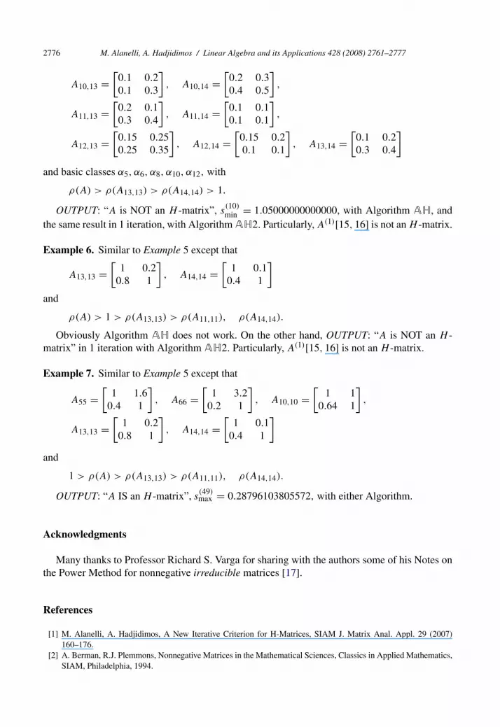
Example 5. Consider the matrix in (4.4) with block submatrices:

A11 =[

1 20.25 1

], A22 = [1], A33 =

⎡⎣ 1 2 0.10.1 1 0.10.2 0.3 1

⎤⎦ , A44 =[

1 0.31.5 1

],

A55 =[

1 3.60.4 1

], A66 =

[1 7.2

0.2 1

], A77 =

[1 0.5

0.5 1

],

A88 =[

1 0.324.5 1

], A99 =

[1 0.4

0.8 1

], A10,10 =

[1 2.25

0.64 1

],

A11,11 =[

1 0.10.2 1

], A12,12 =

[1 72

0.02 1

], A13,13 =

[1 0.2

6.05 1

],

A14,14 =[

1 0.111.025 1

], A15 =

[0.1 0.03

0.02 0.01

], A24 = [

0.01 0.05],

A34 =⎡⎣0.002 0.01

0.003 0.0040.05 0.06

⎤⎦ , A46 =[

0.07 0.080.09 0.01

], A56 =

[0.1 0.12

0.12 0.1

],

A67 =[

0.2 0.10.2 0.3

], A78 =

[0.15 0.250.2 0.1

], A89 =

[0.1 0.10.2 0.2

],

A8,10 =[

0.2 0.30.2 0.4

], A9,11 =

[0.2 0.10.3 0.1

], A9,12 =

[0.1 0.30.2 0.2

],

2776 M. Alanelli, A. Hadjidimos / Linear Algebra and its Applications 428 (2008) 2761–2777

A10,13 =[

0.1 0.20.1 0.3

], A10,14 =

[0.2 0.30.4 0.5

],

A11,13 =[

0.2 0.10.3 0.4

], A11,14 =

[0.1 0.10.1 0.1

],

A12,13 =[

0.15 0.250.25 0.35

], A12,14 =

[0.15 0.20.1 0.1

], A13,14 =

[0.1 0.20.3 0.4

]and basic classes α5, α6, α8, α10, α12, with

ρ(A) > ρ(A13,13) > ρ(A14,14) > 1.

OUTPUT: “A is NOT an H -matrix”, s(10)min = 1.05000000000000, with Algorithm AH, and

the same result in 1 iteration, with Algorithm AH2. Particularly, A(1)[15, 16] is not an H -matrix.

Example 6. Similar to Example 5 except that

A13,13 =[

1 0.20.8 1

], A14,14 =

[1 0.1

0.4 1

]and

ρ(A) > 1 > ρ(A13,13) > ρ(A11,11), ρ(A14,14).

Obviously Algorithm AH does not work. On the other hand, OUTPUT: “A is NOT an H -matrix” in 1 iteration with Algorithm AH2. Particularly, A(1)[15, 16] is not an H -matrix.

Example 7. Similar to Example 5 except that

A55 =[

1 1.60.4 1

], A66 =

[1 3.2

0.2 1

], A10,10 =

[1 1

0.64 1

],

A13,13 =[

1 0.20.8 1

], A14,14 =

[1 0.1

0.4 1

]and

1 > ρ(A) > ρ(A13,13) > ρ(A11,11), ρ(A14,14).

OUTPUT: “A IS an H -matrix”, s(49)max = 0.28796103805572, with either Algorithm.

Acknowledgments

Many thanks to Professor Richard S. Varga for sharing with the authors some of his Notes onthe Power Method for nonnegative irreducible matrices [17].

References

[1] M. Alanelli, A. Hadjidimos, A New Iterative Criterion for H-Matrices, SIAM J. Matrix Anal. Appl. 29 (2007)160–176.

[2] A. Berman, R.J. Plemmons, Nonnegative Matrices in the Mathematical Sciences, Classics in Applied Mathematics,SIAM, Philadelphia, 1994.

M. Alanelli, A. Hadjidimos / Linear Algebra and its Applications 428 (2008) 2761–2777 2777

[3] R. Bru, M. Neumann, Nonnegative Jordan basis, Linear Multilinear Algebra 23 (1988) 95–109.[4] D.K. Faddeev, V.N. Faddeeva, Computational Methods of Linear Algebra, W.H. Freeman, San Francisco, 1963.[5] A. Hadjidimos, An extended compact profile iterative method criterion for sparce H-matrices, Linear Algebra Appl.

389 (2004) 329–345.[6] M. Harada, M. Usui, H. Niki, An extension of the criteria for generalized diagonally dominant matrices, Int. J.

Comput. Math. 60 (1996) 115–119.[7] R.A. Horn, C.R. Johnson, Matrix Analysis, Cambridge University Press, Cambridge, England, 1985.[8] D.R. Kincaid, J.R. Respess, D.M. Young, R.G. Grimes, ITPACK 2C: A Fortran package for solving large sparse

linear systems by adaptive accelerated iterative methods, ACM Trans. Math. Software 8 (1982) 302–322.[9] T. Konho, H. Niki, H. Sawami, Y.-M. Gao, An iterative test for H-matrix, J. Comput. Appl. Math. 115 (2000)

349–355.[10] B. Li, L. Li, M. Harada, H. Niki, M.J. Tsatsomeros, An iterative criterion for H-matrices, Linear Algebra Appl. 271

(1998) 179–190.[11] L. Li, On the iterative criterion for generalized diagonally dominant matrices, SIAM J. Matrix Anal. Appl. 24 (2002)

17–24.[12] K. Ojiro, H. Niki, M. Usui, A new criterion for H-matrices, J. Comput. Appl. Math. 150 (2003) 293–302.[13] U.G. Rothblum, Algebraic eigenspaces of nonnegative matrices, Linear Algebra Appl. 12 (1975) 281–292.[14] H. Schneider, The influence of the marked reduced graph of a nonnegative matrix on the Jordan form and related

properties: a survey, Linear Algebra Appl. 84 (1986) 161–189.[15] H. Schneider, Personal Communication, 2006.[16] R.S. Varga, Matrix Iterative Analysis, 2nd revised and expanded ed., Springer, Berlin, 2000.[17] R.S. Varga, Notes on Power Method for Nonnegative Matrices, Personal Communication, 2006.[18] J.H. Wilkinson, The Algebraic Eigenvalue Problem, Clarendon Press, Oxford, 1965.[19] D.M. Young, Iterative Solution of Large Linear Systems, Academic Press, New York, 1971.