a multiscale electrical survey of a lateritic soil system in the rain forest of cameroon

ELSEVIER Journal of Applied Geophysics 34 (1996) 237-253

FIIPFLIEIO IGIEI HIV51C5

A multiscale electrical survey of a lateritic soil system in the rain forest of Cameroon

Henri Robain a,,, Marc Descloitres b, Michel Ritz b, Quantin Yene Atangana c a Orstom, B.P. 1857, Yaounde, Cameroon.

b Orstom, B.P. 1386, Dakar, Senegal. c University of Yaounde 1, Department of Earth Sciences, B.P. 812, Yaounde, Cameroon.

Received 19 June 1995; accepted 29 October 1995

Abstract

Resistivity investigations were carried out on an elementary watershed in SW Cameroon, firstly to assess the applicability of direct-current (DC) resistivity methods to solve various pedological problems in intertropical regions, and subsequently to determine the relationships between electrical resistivities and pedological properties of lateritic soil systems. The survey included measurements in pits with a small Wenner fixed-spacing array (SWA), vertical electrical soundings (VES) and vertical electrical "quick soundings" (VEQS) both using the Schlumberger configuration. The VES data were interpreted using a conventional rnultilayer inversion program to obtain best-fit models. Constraints to the interpretation of these data were provided by SWA and pedological information from existing observation pits. The results of the interpretation reveal five distinct geoelectrical layers overlying a resistive bedrock. The first is a thin organo-mineral upper layer with low resistivities in the range 250-450 /]m. The second layer corresponds to micro-aggregated clayey materials and is more resistive (1300-1800 Om). The third represents the main part of ferruginous materials and is even more resistive (2000-4500 Om). The fourth corresponds to unsaturated saprolite and the last to saturated saprolite (ground water) with resistivities ranging from 800 to 1500 Om and from 150 to 250 [2m, respectively. Estimates of soil volumes for the entire study area were obtained from VEQS interpretations. Most of the soil cover corresponds to saprolite (74%, 1/4 being saturated by ground water), while topsoil and ferruginous materials represent 14 and 12%, respectively. Finally, geophysical results based upon 1-D inversion provide a satisfactory approximation of the various lateritic components' 3-D geometry over the watershed. The study provides original quantitative results concerning the behaviour of intertropical soil systems as well as some geomorphological keys for soil mapping at a regional scale.

1. Introduction

The present differentiation of lateritic soil systems in intertropical regions results from a landscape evolution that began some tens of millions of years ago

* Corresponding author.

(Tardy et al., 1988, 1991). These soils are generally very thick (several tens of metres) and complex. They are also characterised by important accumulations of iron (Nahon, 1986, Schwertmann, 199l). These accumulations mainly consist of hematite (iron oxide) a n d / o r goethite (iron oxi-hydroxide) and are generally indurated.

Digging pits is commonly the only way to study physical, geochemical and petrological characteris-

0926-9851/96/$15.00 Copyright © 1996 Elsevier Science B. V. All rights reserved. SSDI 0926-9851 (95)00023-2

(a)

( b ) ~oo

700

2 3 8 H, Robain et al. / Journal of Applied Geophysics 34 (1996) 237-253

I ,, 1 I

~ \ GHAO r

7 i t

r, ? '~ ,~ s .'~ -~ . . . . ~.

NIGERIA t" " ,

f ~

N ¢ i

, " ,¢ ~ : ~ . . . : . : ~ J: ..:.?:.:.t,: . ~ ~ ' • " • "- ~:'~: ".:~, t: " :'-'":,"" .~':~ ~.:-.~

' ; =.2::'~'~;~:.~ :~". ~,~'.~,:.~.'.';,':::..":::'~ , / ~; i ,~ :-:::.~. 7.;'~ ~.~.,. '. "::-:.¢ ::: ' .:'.-:~ / i .~ ~d~:".~.::.':'~ ~. ' : ' ; ' : ' : ' . : :~ ' , :" :" . : : ,

......, ...::::.: ",..':..:.-.:....~ ,. ,,~,..~.= ..~:~ . . . . . . . . . ~ "4_ ,-, ~.!:!;'~,::: .:...'...-- :.-:::.:;::::.~,:.'.:..~:.:f;-; ~.,':::.-: ' :.....: £../..:.::....-~:~.

~ L , .~;"i:~.::;~ ~ : ' : ' : : ";'i:'~ !.::."."; i?; " , .s."~:::,:.:'':.? i Bite I::": """" : ;"" ' : : :" : '~

{.~,~':2.~:Z~.'~:':'.~ ~'~:: ~:=;~'-~-'~':::2:"':-';:"::~ :.'~ ,Y

GUINEA ', GABON ~ CONGO

12 °

10 °

8 °

4 ~

Ito= 112o 114' 116o

6 0 0

5O0

g ~- 400

300

~ SouthCameroon ¢..,.P" Northlimitot Plateau

North limit of the { the rain forest lat~ritic zone

Magnetic North

200 ¸

100

0 ¸ 100 200 300 400 500 600 700 800 900 t000

! ~ Swamp ~ Gneissoutcroup

l • Basalt outcrop

Fig. 1. (a) L o c a t i o n o f the s t u d y a rea . (b) M a p o f the w a t e r s h e d . L o c a t i o n o f o u t c r o p s a n d s w a m p s .

14. Robain et al. / Journal of Applied Geophysics 34 (1996) 237-253 239

tics of soils. The main difficulties encountered in intertropical regions are the thickness of the soils, the hardness of the fermginous materials and site acces- sibility. For these reasons, it is generally impossible to dig the large number of pits required for a detailed soil survey, carried out on an elementary watershed. The soil description remains incomplete and the extensive literature on lateritic soils essentially deals with details of vertical differentiation (e.g. Herbillon and Nahon, 1988, Nahon, 1991; Tardy, 1993). Lat- eral differentiations presented in such papers are based on interpolations between rather distant pits and the three-dimensional (3-D) geometry is poorly understood at the scale of the elementary watershed. A knowledge of the 3-D picture is nevertheless necessary to understand and model the evolution and the present behaviour of soil systems (water flows, solid/solution ratio,; or mass balance based on an invariant element for example). This is an important element in the comprehension of the global terres- trial ecosystem, lateritic covers forming one third of the total land surface of our planet (P~dro, 1968).

An alternative approach to identify the distribution of soil comporents, which is becoming more common, is to combine geophysics with a pitting program, thus providing greater area coverage (A1- bouy et al., 1970, Pion, 1979, Blot, 1980, Bottraud et al., 1984, Hesse et al., 1986, Dabas et al., 1989, Pham et al., 1989, Freyssinet, 1990, DeMtre, 1993, Lamotte et al., 1993). Other advantages of using surface geophysics in soil studies are that information on the areas between pits can be obtained, allowing lateral transitions to be more precisely identified and pits to be positioned more judiciously. Thus, when soils are thick and complex as in lateritic zones, these methods may be useful in gaining a better understanding of the 3-D distribution pattern.

From among all the geophysical methods that could be used to characterise soils, electrical methods were chosen in this study because the resistivity of soil materials ranges over several orders of magni- tude allowing them to be distinguished optimally. For each type of material, however, the resistivity can vary considerably. It depends on several parameters that are not homogeneous at the watershed scale: the geological characteristics of the site (depth and nature of the bedrock), the physical characteristics of the soil materials (particle size, porosity and intrinsic

resistivity of minerals) and the water content. Thus, geophysical techniques need to be carefully adapted and developed for this purpose. Identification of the different soil materials is not possible on the basis of resistivity data alone, correlation with outcrops and/or pits is essential.

Surface resistivity surveys were performed, di- rected at improving an understanding of the 3-D geometry of the soil system in the Nko'ongop region in the tropical rain forest of south-west Cameroon (Fig. la). Direct-current (DC) measurements were first made in pits using a small Wenner fixed-spacing array (SWA) to estimate the true resistivity of each horizon at the "outcrop" scale. Vertical electrical soundings (VES) were then performed near existing pits. Finally, vertical electrical quick soundings (VEQS, i.e. VES with few chosen A B / 2 spacings) were used to rapidly extend the information over the whole watershed and to obtain a thickness mapping of the lateritic cover.

The main goals of this paper are: (1) to present the methodology developed to describe the 3-D geometry of tropical soils and its physical parameters, (2) to adapt geophysical procedures for local pedological patterns' identification in the soil system and (3) to evaluate the volumes and organisations of the main pedological materials.

2. Geological and pedological settings

The Nko'ongop site is an elementary watershed covering an area of 63 ha (Fig. lb) and receiving 1700 mm of rain a year (Suchel, 1972). A large swamp at 600 m above mean sea level (ASL) is situated between two hills at 690 and 650 m ASL. Numerous outcrops can be identified, some of them forming barriers in the talwegs and creating small perched "swamps".

The bedrock is mostly a leucocrate acid granulite with a banded and heterogranular facies (R1). Major minerals are quartz, potassic feldspar and mica. Ac- cessory pyroxene and zircon are also present. A second rock type corresponds to a rnelanocratic basic granulite with a fine grained facies (R2). Major minerals are pyroxene (often altered into amphibo- lite), potassic feldspar, plagioclase, mica and garnet. Accessory minerals are quartz and zircon. This rock

240 H. Robain et a l . / Journal of Applied Geophysics 34 (1996) 237-253

(a A Magnetic

North

[ ] Pedological pit m Wenner fixed-spacing array in pit

i I I I i Scale : 400 m.

(b)

~> Schlumberger vertical electdcal sounding

i I I I V Schlumberger

quick sounding Scale : 400 m.

Fig. 2. Location of pits and DC measurement points.

Magnetic North

H. Robain et al. / Journal of Applied Geophysics 34 (1996) 237-253 241

does not contain any glass but has the chemical composition of a tholeitic basalt. It represents a dyke dated to the late Proterozoic by the 4°Ar-39Ar method (Piccirillo and Robain, unpublished data).

Soil profiles have; been described for 30 pits (Fig. 2a). Although these pits are quite deep (up to 12 m), the bedrock was sei[dom reached. The soils present three main types o1: material, from top to bottom: clayey material, ferruginous material and saprolite. These materials present a great variability in the nature and distribution of iron oxi-hydroxides associated with kaolinite a n d / o r gibbsite, leading to the differentiation of many coloured phases (Fritsch et al., 1989, Schwertmann, 1993). These mineralogical variations are particularly well illustrated in the ferruginous material and saprolite, made up of complex associations of violet, white, yellow, brown and red phases with variable hardness. A petrological classification of the lateritic materials is therefore very complex. As the geophysical techniques used are essentially influenced by physical parameters such as porosity, particle size and water content, in an attempt to correlate the resistivities with pedological features, another classification, different from a petrological one and! based only upon the physical properties of the soils was defined (Table 1). Four different materials are distinguished for the topsoil (A1, A2, A3 and A4), three for the ferruginous materials (B1, B2 and B3), and three for the saprolite (C1, C2 and W). Percentages of coarse, sand,

silt and clay particles are also represented, as well as solid density (Ss), bulk density (Sb) (I.S.S.S., 1976) and FeO content.

The vertical and lateral differentiation of soil is described using this classification along three traverses A, B and C (Fig. 2a). The position of the 30 pits are shown in Fig. 3. At first glance it appears that the vertical successions are very variable from one pit to the next, but some general patterns can be distinguished:

(1) The topsoil materials show two major successions; the first corresponding to the swamps (A4/A3), and the second to all upstream locations (A1/A2). When the topsoil is thin (a few dm) only the first units of the succession are developed.

(2) The ferruginous materials show four major successions: B1 is always present. It is often alone (B1) but can also occur with B2 in various associations (B1/B2, B1/B2/B1 or B2/B1, denoted B 1 - B 2 ) a n d / o r with B3, the latter always found at the base (B1-B2/B3 and B1/B3). Generally rather thin (approximately 1 m), these materials are thicker (several m) at the top of the higher hill. They are totally absent in the swamps.

(3) The saprolites are generally made up of C1 or C2 depending on the nature of the bedrock (R1 or R2, respectively). In some cases repetitious C1/C2 successions are also observed. These repetitious successions might be attributed to secondary intrusions associated with the principal dyke.

Table 1 Types of materials observed from the pits

Material Code Stn~ctural features Coarse S a n d Loam Clay Bulk density Solid density FeO (%) (%) (%) (%) (g/cm 3 ) (g/cm 3 ) (%)

Topsoil A1 Micro-aggregated clay and roots 0 20-30 20-30 50-60 0.7-0.9 2.6-2.7 12-14 A2 Micro-aggregatedclay 0 10-20 20-30 60-80 1.1-1.2 2.7-2.8 14-18 A3 Compact clay 0 10-20 30-40 50-60 1.2-1.4 2.7-2.8 14-18 A4 Saturated loamy clay 0 20-30 30-40 30-40 - - -

Ferruginous B1 Pebbles 30-70 1-20 15-40 20-50 1.6-2.0 3.0-3.2 15-45 B2 Pebbles and blocks 50-80 1-10 10-30 10-40 2.3-2.5 3.0-3.4 40-60 B3 3D network 20-40 5-20 30-40 20-50 1.4-1.6 2.8-3.0 -

Saprolite C1 Conapact saprolite (kaolinitic) 5-10 20-40 30-50 20-30 1.2-1.4 2.7-2.8 5-15 C2 Porous saprolite (gibbsitic) 5-10 10-20 40-60 10-20 1.0-1.1 2.9-3.0 35-45 W SattLrated saprolites (ground water) 5-10 20-40 30-50 20-30 - - -

Rock R1 Acid g r a n u l i t e . . . . 2.6 - 3-4 R2 Basic g r a n u l i t e . . . . 2.8 - 12-14

Classification based upon physical parameters (water content, grain size, porosity and iron content).

242 H. Robain et al. / Journal of Applied Geophysics 34 (1996) 237-253

( a ) o

2

6

8

8 9 7 10 6 1 3 4 5 2

~ A 2 i ~ B 2 ~ C 2

~ A 3 ~ B 3 ~ W

~A4 SE N W

600

(b)

I I I - - I J

Scale : 250 m

14 30 11 18 22 12 13

c 650

m 60O

15 17 16

:1 8 -

S S W

Traverse B N N E

I I I I : - ~

Scale : 250 m

( c ) 26 ~ ~ ~s ~ ~ 2~ 2 , 28 2~ o

' :N I ' 6 51~ !;/,

-':)~

S W N N E

g 7°° I T r a v e r s e 2 ~ I

6O0

I I i ~ I I

S c a l e : 2 5 0 m

Fig. 3. Description of soils according to their physical parameters observed in pits for traverses A, B and C.

3. Resistivity methods

The basic procedure of the DC resistivity method is to measure at the surface the resulting potential due to a known current flowing into the ground (Kunetz, 1966, Telford et al., 1990). The usual procedure is to insert a pair of electrodes ( A, B) into the ground through which a current is then passed. A second pair of electrodes (M, N) is used to measure the associated potential. The apparent resistivity (Pa) is calculated as follows:

p = K . A V / I (1)

where AV is the measured potential, I the known current and K the geometric factor of the quadripole calculated as follows:

2~- K = (2)

1 /MA - 1 / M B + 1 / N B - 1 /NA

where MA is the spacing between the electrodes M and A, etc.

(1) Resistivity measurements using small a Wen- ner array (SWA) were carried out in 15 representa- tive pits (Fig. 2a) and on fresh outcrops of the two rock types to determine the true resistivity of the pedological materials and rocks. The Wenner configuration uses a constant spacing between electrodes so that AM=MN=NB. A 10 cm spacing was chosen. At this scale, the medium can be considered as homogeneous, and the measured apparent resistivity is assumed to be the true resistivity. In the pits, the measurements were made every 10 cm with the four electrodes stuck in an horizontal line.

(2) Vertical electrical soundings (VES) using a Schlumberger array were carried out to determine the vertical resistivity profiles at a larger scale through the whole pedological cover. The electrode array size is characterised by the so-called AB/2 spacing parameter, the distance between the centre of the array and one of the symmetrical outside electrodes. Depth profiling is achieved by progressively increasing the AB/2 spacing. The same potential electrode spacing (MN) was used until the voltage became too small to be measured accurately. At this stage the MN spacing was doubled before continuing to increase the spacing of the current electrodes. In all 24 VES (Fig. 2b) were made, most of them (20) located near existing pits. The VES curves were

14. Robain et al. / Journal of Applied Geophysics 34 (1996) 237-253 243

interpreted using a conventional one-dimensional (l- D) inversion program that generates the theoretical apparent resistivity curve from an input model (Gabalda and Tabbagh, 1994). The principle of suppression, stating that two layers X and Y may be grouped in a single layer Z whose resistivity is Pz -----f(Px,Py), and the principle of equivalence, stating that a layer X whose resistivity and thickness are Px and H x respectively, may be replaced by another layer Y, if Px .Hx = py .Hy and 5 < H~/Hy < 1/5, implies that apparent resistivity data can be interpreted in many ways (Kunetz, 1966). In other words, it means that many layered models may produce the same apparent resistivity curve. Hence in an attempt to accurately interpret the VES data, the input model chosen for each sounding was a realistic one based upon actual pedological information. The thickness of the observed layers was used as a fixed value, and the resistivity was adjusted until a satisfactory fit to the apparent resistiwity curve was obtained (deviation between field data and model curve less than 8%). The standard deviation of all the resistivity values obtained by this method was calculated for each pedological material to define a general model of the geoelectrical profile.

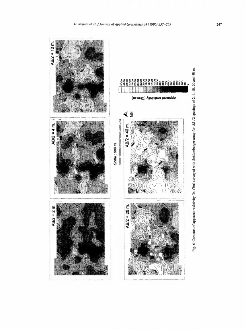
(3) In order to determine the soil geometry at the watershed scale 108 vertical electrical quick soundings (VEQS) were carried out along 10 traverses (Fig. 2b). The Schlumberger array was also used but only for six AB/2 spacings (2, 4, 10, 20, 40 and 100 m). The AB/2 spacing of 100 m was used only when previous AB/2 spacings did not clearly show an increase of Pa atlributable to the substratum. The entire watershed area was covered in 5 days with this survey method.

The VEQS data allowed us to draw 5 maps of apparent resistivity contours for 2, 4, 10, 20 and 40 m AB/2. These iso-resistivity maps provide a qualitative interpretation tool that shows possible lateral variations in resistivity but does not give the true resistivities and shapes of definite geoelectrical layers. Hence, the VEQS data were interpreted quantita- tively, considering that the points obtained from 5 or 6 spacings can be used to draw curves similar to those from VES data and can be fitted readily to a horizontally layered model. Thus, for each of the 108 sites, the general model provided by VES 1-D inversions was used to compute the thickness of the

layers, with the resistivity values allowed to vary within the standard deviation range until the best fitting curve was obtained. For each of these models, the equivalence principle (Kunetz, 1966) was used to calculate the maximum and minimum thicknesses of the different layers assuming an error of 8% in fitting the theoretical curve to the field data. The SURFER program (Golden Software, 1994) was used to calculate the volumes of the main pedological materials for the watershed as a whole.

These results were used to estimate the volume of water contained in ground water (W) and the weight of iron oxide contained in ferruginous materials (F ) as follows:

W= Vw" (1 - 6b(w)/rs(w)) (3)

where Vw is the volume of saturated saprolite, 6b(w) its average bulk density and 6,(w) its average solid density.

F = Vf. 6b(f)" ~'F~o(f) (4)

where Vf is the volume of ferruginous materials, 6b(f) their average bulk density and rF~o(f) their average iron content.

4. Results

4.1. Small wenner fixed-spacing array (SWA)

Fig. 4 shows examples of resistivity variations in 10 pits in upstream locations. This representation is analogous to an electrical resistivity log of a drill hole, but with an essential difference in the disposi- tion of the electrodes, stuck horizontally into one side of the pit. This allows transitions between two different electrical media to be more precisely located.

Some general trends can be noted: ( l) All the profiles present a succession of three geoelectrical layers with a resistive layer sandwiched between two less resistive ones. This is particularly the case in pits 9, 10 and 16. (2) The resistivity values can vary considerably within the same layer. This is particularly true for B2 ferruginous material in pits 23, 24 and 28. The profiles also show that the top of the ferruginous material is always more resistive than its base. (3) Crude interfaces generally correspond to an important change of resistivity (A / B, particularly).

244 H. Robain et a l . / Journal of Applied Geophysics 34 (1996) 237-253

Furthermore, a range of resistivities can be given for each material. (1) For the topsoil materials, A2 is systematically more resistive than A1, with 1300 _ 300 and 840 ___ 220 J2m, respectively. (2) For the ferruginous material, B1 varying within 2000 + 600 g2m, is systematically more resistive than B2 (1400 + 400 J2m) or B3 (1400 + 250 g2m). For some pits (24, 28 and 29) a less resistive pebbly layer BI' can be identified at the base with values of 1000 + 50 g2m, similar to those for saprolite. (3) For saprolite horizons C1 and C2, the resistivity ranges are 930 + 260 and 1100 + 500 Om, respectively. (4) For the bedrock, R1 is less resistive than R2, 7000 and 33 000 O m respectively.

4.2. Vertical electrical soundings (VES)

VES field data are shown in Fig. 5a for the pits previously presented in Fig. 4. Some general trends may be noted here: (1) In a first order approach, all the VES curves for upstream locations reflect the presence of a minimum of 4 layers with a less

resistive first and third layer and a more resistive second and fourth, corresponding to the succession of A, B, C and R media. (2) The soundings located in the main swamp only reflect the presence of three layers, a less resistive layer sandwiched between two more resistive ones, corresponding to the succession of A, W and R media actually observed in a core collected with a hand drill (Fig. 5b).

The four-layer model was supplemented with transition layers because it appeared that these layers which were observed in pits are suppressed in the crude modelling. These six or seven-layer models and corresponding theoretical sounding curves are also presented in Fig. 5. (1) In all cases, C was split into a C/W succession. Ground water was actually found at the bottom of every pit that reached bedrock. As field measurements were made at the end of rainy season (July), it is sure that a conductive saturated zone, a few metres thick, occurs at the base of each profile. (2) With the exception of cases where the topsoil materials were very thin (e.g. VES 6 (pit 16)), A was split into an A1/A2 succession. In the

2

; i ~ ! i : : i ~ E~ . . ~ i : : . ' : : i i i : o°o

4 " r : r , " , : ....... ; - r ~ v ~ -~ :: ~:: :::::::: =: :: i i ~0~ - + i ~-h.: ........ ~--+-++ ;~?~ .C: : : : : : i i i ~ = ! i : : ~ O o

'. i::: '. : : : .~'~o

! ~ i i : , : i i i i b?o~

8 . . . . . . . ~ : i ~ , - ...::..!..i.::.i.. ....... !-..-i--!--i. ~

10 ~ ~*1 ~ ' t ¢ ~ . . . . . . . I . . . . .

~ 2

£ Q) a 4

ii!i o

Resistivity ( ~ . m )

o ° 8 o ° o °

Resistivity ( Q , m )

; ~ , . i ~'/z.,

oo oo oo

Resistivity (Q.m)

. . . . . . . . . . . . .

o~ ~ ~ 0 ° 8

Resistivity (Q.m) Resistivity ( Q . m )

~]~A1 ~ A 2 ~ B 1 ~ B 2 liJl~JB3 ~ 0 1 ~ ] C 2

Fig. 4. Comparison of the Wenner fixed-spacing array resistivity measurements and pedological data from pits.

H. Robain et al. / Journal of Applied Geophysics 34 (1996) 237-253 2 4 5

(a)

T 10000 d

> 1000

"~i ( I ) r~:

100

~ 1oooo

> 1000 "~i

100

i 10000

~! 1000

100

~" 10000 c_.L

2: 1000 "~;

100

~ 10000 cL

~i lOOO i ~1

lOO

I t I I 1 , , , ~ ~ I I I I t l ~ l I I I q l l l l l I ~ I I ~ L J , , I I . I t l , , ~ l ~ J L I l i J l

. . . . . . . . . . . . . . . . . . . . . . . . . . . . . . . . . . . . . . . . . . . . . . . . . . . . . . . . . . . . . . . . . . . . . . . . . . . . . . . . . . . . . . . . . . . . . . . . . . . . . . . .

1 .. . . . . . . . . . . . . . . . . . . . . . . . . . . . . . . . . . . . . . . . . . . : ( p , 2 1 >

. . . . . . . . I ' ' . . . . . . . . . ' ' " ' l ' . . . . . . . i . . . . . . . . I . . . . . . . . i

I I I I I l ~ l l I I I I I I I I r I I I I t l l l ~

F i , , m l I , i , , H H I ~ I I ~ H , I

i I I I I ~H I i i i , i i i 1 [ i i i l l , , i I

i i L i i l l l ~ i i i i i i i d i i i J l l l l l i

(pi t 28) I .................. L .................. i ........

i i i l l l l t I ~ i J l l t l l ~ i i J l l l H I

I I I I I l ~ l I I I I I l l I I B I I I I l l I

(pi t 23) I ...........................................

. . . . . . . . I . . . . . . . . f . . . . . . . . i

0,1 1,0 10,0 100,0

AB/2 s p a c i n g or dep th (m)

(b) 10000

E v

• ~ 1000

lO0

I i i J . , , , I , , l l l l . I f , , , l l . I

. . . . . . . . [ . . . . . . . . i . . . . . . . . I

~ b l i H . I , i , l , l ~ h i i i l l = l l l l

................. i . . . . . . . . . . . . . . . . . . . . . . .

i i I (pit 10) i i l IHN I I , I =H I I I I = l ,H , I

i ol

0,1 1,0 10,0 100,0

AB/2 spacing or depth (m)

0,1 1,0 10,0 100,0

AB/2 spacing or depth (m)

Fig . 5. R e p r e s e n t a t i v e ve r t i ca l e l ec t r i ca l s o u n d i n g ( V E S ) c u r v e s fo r u p s t r e a m l o c a t i o n s (a) a n d s w a m p (b). S y m b o l s a re f ie ld da t a , s tep

c u r v e s c o r r e s p o n d to the bes t - f i t g e o e l e c t r i c a l m o d e l a n d s m o o t h c u r v e s to the t heo re t i c a l V E S f o r th is m o d e l .


field the A1 layer was found to be systematically present and the SWA data show that it has a lower resistivity than A2. (3) In some particular situations a less resistive layer for ferruginous materials was also added, corresponding to BI' in VES 10 (pit 23) and VES 15 (pit 21), to B3 in VES 18 (pit 9) and to a mixing of B1 and C2 in VES 16 (pit 6).

Using this key, VES 1-D modelling leads to the following results: (1) For the bedrock the resistivities are well defined, 7400 ___ 1300 and 29000 + 3,300 g2m for R1 and R2, respectively. An intermediate resistivity (17700+1300 Y2m) is found in the soundings located near the transition between the two types of bedrock. (2) For saprolite the mean resistivity values show a slight difference between C1 and C2, 980 + 160 and 1200 + 400 g2m, respectively. In view of the high standard deviation for C2 this difference is probably not significant. In contrast, W has a much lower resistivity and is well defined (190 + 30 Om). (3) For ferruginous materials the mean resistivity values obtained are 3300 + 1200 for B1, 1000 _+ 100 for BI' , 3700 + 500 for B2 and 2100 + 140 O m for B3. The mean values for B1 and B2 are not significantly different but these two materials always have distinct values in the same profile, though B1 can have higher or lower resistivity than B2. (4) For topsoil materials the mean resistivity values obtained for A1 and A2 are 360 + 100 and 1560 +_ 230 g2m, respectively.

4.3. Vertical electrical quick soundings (VEQS)

The iso-resistivity maps are presented in Fig. 6. A prominent feature for small A B / 2 spacings is the large change in apparent resistivity observed in the southern quadrant indicating a strong lateral inhomo- geneity in apparent resistivity distributions at shallow depth. This pronounced anomaly with apparent resistivities of less than 1000 g2m corresponds approximately to the main swamp (Fig. lb). Outside this anomalous zone, the iso-resistivity maps show resistivities varying slowly with change in horizontal position. This suggests that the soil resistivities mainly change in the vertical direction. For larger A B / 2 spacings, the apparent resistivities are mainly influenced by the bedrock. The sharp distortion of the contours suggests that the distribution of the two types of bedrock may be very irregular. The most

Table 2 Calculated volumes of the main pedological materials (in 103 m 3)

Material Best fit Max. Mira

Topsoil 770 1040 645 Ferruginous 681 948 424 Unsaturated saprolite 2942 3495 2542 Ground water 1193 1829 1029 Total soil 5586 7312 4640

noticeable feature is that the resistive bedrock seems to be shallower in the northeastern and southwestern parts of the study area.

These qualitative results were used in the VEQS 1-D modelling to obtain an estimate of the thicknesses of the main materials at each of the 108 sites using a three-layer model for swamp zones ( A 4 / W / R 1 or R2) and a six-layer model for the other zones. This latter model is defined by the succession of the significantly distinct geoelectrical layers: the two A1 and A2 layers for topsoil materials, a single B layer (3000 __+ 1000 £2m) for ferruginous materials, two layers C (1000 ___ 300 Om) and W for saprolite, and R1 or R2 for the bedrock. Note that the thickness of ferruginous material may be underestimated when BI' is present because this layer will be included in the saprolite.

This allowed computation of the total volumes of the main types of material at the watershed scale (Table 2). Most of the pedological cover corresponds to saprolite (74%) in which ground water occupies approximately one quarter, while ferruginous and topsoil materials represent 12 and 14%, respectively. The minimum and maximum values were used to estimate two parameters for the watershed as a whole: (1) The ground water represents W = 620000 to 1 100000 m 3 of water, i.e., each square metre of bedrock is overlain by 1.0 to 1.8 m 3 of water. (2) The ferruginous material contains F---420000 to 950000 T of FeO, i.e., 0.7 to 1.5 Tm -2 of FeO.

Another result is a quantitative 3-D representation of the soil cover. Maps of the thickness of the whole soil profile and of the three material types separately were drawn using a best-fit interpretation of the 108 VEQS and adding the 24 VES modellings (Fig. 7). The following observations can be made:

(1) The topsoil materials are relatively thin with a thickness of less than 1 m for more than half the

H. Robain et at. /Journal of Applied Geophysics 34 (1996) 237-253 247

E

00000 0000 O0 ooooogoooo~oogooooooooo ~ N O 0 0 0 0

(W'LUqO) &!̂ .qS!SeJ ~,ueJeddV

~ Z

o

=

E

o


E 0 0 ~O

O0

0 ~ 0 ~ o LO 0 LO O~ 0 0 ~ 0 0

C

in

I . . . . . . . . . . . . . .

0 ~ 0 0 o Lq o ~ o ~ o ~ e~

E

E

t /

_a C

e-,

o


watershed. These materials are notably thicker (2-4 m) in three areas: (a) the summit of the lower hill, (b) the shelf at the south of the lower hill and (c) the south-west foot of the higher hill.

(2) The thickness of the ferruginous material varies within the same limits as the topsoil material, but it is totally absent in the swamp areas. The thickest zone (3 m) corresponds to the summit of the higher hill, the only place where many metre sized ferruginous blocks (B2) are found. The thickness of ferruginous material exceeds 1 m in two other areas: (a) the summit of the lower hill, occupied by a thick pebbly layer (B1) with a linear thinning in south- eastern direction, c,~ncordant with the position of a talweg and (b) the spur located at the south-west foot of the higher hill.

(3) The thickness of the saprolite varies considerably, from less than 1 m to more than 50 m. The greatest thickness is observed at the summit of the higher hill. Two other zones are relatively thick: (a) the main swamp and (b) a part of the summit of the lower hill.

5. Interpretation

5.1. Resistivity values versus pedological parameters

The resistivity values of the different materials vary within a large range. However, the pedological data provide an important key to understanding the resistivity data, allowing the following observations to be made:

(1) In the topsoil materials and for A2, the relatively low resistivity values can be related to high amounts of clay (6C-80%) as is commonly the case. This interpretation however is not consistent with the lower resistivities observed for C1 which contains much less clay (20-30%). Thus, in this case the clay content is not sufficient to explain variations in the resistivity. It seems that a structural parameter has to be taken into account: (a) A2 is micro-aggregated and contains a relatively high volume of inter-aggregate macro-voids filled with air. (b) C1 has a rather continuous strncture but has also an important volume of meso-porosity (the bulk density of these two materials is the same). These voids are provided by clusters of very large clay minerals, up to silt

size, and strongly retain water. The water content of C1 is relatively high and the volume of air in the voids is low. Thus, A2 has a higher resistivity than C1 because the air in the voids is more important. For A 1, the lower resistivity values can be related to a high water content corresponding to the very high density of roots in this layer.

(2) The high resistivity values and their variations in ferruginous materials are not correlated to the iron content. Once again, the structure of the pedological materials seems a more accurate parameter. (a) Fer- ruginous pebbles and blocks are surrounded by thin fractures. These voids decrease with depth as the quantity of pebbles also decreases. (b) At the top of this layer the clayey material surrounding the pebbles is slightly micro-aggregated. It becomes more compact with depth. Finally, the ferruginous material has a rather macro-porous structure at the top (fractures surrounding pebbles and inter-aggregate macro-voids) which disappears with depth. As the coarse elements (pebbles and sand) are abundant in this top layer, these macro-voids do not present a lot of constrictions that could retain water (Fies, 1984, Chrrtien, 1986). Thus, the air content of the pores is even higher than for A2, explaining higher resistivity values.

(3) The relatively high resistivity values of C2 and its large variability may be linked to an important macro-porosity rigidified by iron oxi-hydroxides where the water content can vary a lot. Inversely, relatively low resistivities for C1 may be related to an important meso-porosity where water content can not vary so much.

Defined as the inverse of conductivity, the resistivity of soils is mainly of an electrolytic nature resulting from the movement of charged ions in pore water (Kunetz, 1966, Telford et al., 1990). Although resistivity is highly dependent upon water content (Keller and Frischknecht, 1966), it appears that the geometry of the pore space (voids' distribution and form) is the most important parameter determining the balance between air and water and consequently the electrical signature of pedological materials in such a context. From a general point of view, one could note that the resistivity values reported here are quite high in comparison to those cited in the literature, considering that these materials contain a high amount of clay (e.g. Meyer de Stadelhofen,

250 H. Robain et al./ Journal of Applied Geophysics 34 (1996) 237-253

1991). Besides the structural parameter cited above (causing quite important air filling of voids and cutting down the electrical connections between clay particles) a geochemical parameter must also be taken into account. In lateritic materials, except for organo-mineral layers, the exchange complex of clay minerals is weak (10 meq%) and in any case cation content is very low. Consequently electrolytic phe- nomena may be weaker in lateritic materials than in materials with a higher cation content, thus resulting in higher resistivity values.

5.2. VES 1-D modellings versus SWA in pits

The resistivities of the different materials presented in Section 4.1 for SWA and Section 4.2 for VES 1-D modellings are synthesised in Fig. 8.

(1) For the two types of bedrock R1 and R2, resistivities obtained from VES 1-D modelling agree with the SWA data obtained on outcrops. The intermediate value (R*) obtained could be the result of an important lateral variation of bedrock resistivity near the sounding location. But the low standard deviations and observations made in pits lead us to consider that an interstraficated transition facies could also explain this value.

(2) For the saprotite there is good agreement between the two methods.

l l . w . . . . . . . y,o0. . . . . . . . . . . . ,s J / O Schlumbe~ger array VES 1 -D inversions, ] ' ! '

10000

~= looo

:i . . . . .

100 i i i i i , F i

A1 A2 B1 B I ' B2 B3 C1 C2 W R1 R2 R*

Soil materials and rocks

Fig. 8. Comparison between the resistivities interpreted from vertical electrical sounding (VES) I-D inversion and those observed in pits for the small Wenner fixed-spacing array (SWA).

(3) For the ferruginous materials, resistivity BI' is exactly the same for both methods. Nevertheless it is not possible to introduce this layer in the soundings model without information from the pits, because its resistivity does not differ significantly from that of saprolite. For the other layers, the mean resistivity values obtained from VES 1-D modelling are significantly higher than from the SWA data. For B2 and B3 this can be explained by the fact that the electrodes were stuck in clayey materials rather than in ferruginous blocks or networks. For B1 the difference may be caused by the assumption of planar stratification imposed by the 1-D inversion. In fact the interface A / B is not planar but shows large undulations of a few metres. Thus the resistivity values obtained with VES 1-D inversions in this case are not true resistivities but "constrained apparent resistivities" that include important lateral variations of thickness caused by non-planar interfaces.

(4) For the topsoil materials, the same reason can explain the higher resistivity for A2 obtained from VES 1-D modelling. In contrast, VES 1-D modelling yields a much lower resistivity for A1. The SWA profiles show that the resistivity of this layer in- creases substantially with depth. Thus the difference is probably caused by a very low resistivity at the top of this layer which is not picked up by the SWA which only starts at a depth of 10 cm.

In conclusion, it appears that the VES 1-D inversion results agree rather well with the SWA data. But it should be noted that the theoretical curves for the models that include the transition layers are generally not significantly different from those for a sim- ple four-layer model. In particular, the insertion of intermediate layers is not necessary to obtain a best-fit model curve. Because of the principle of suppression (Kunetz, 1966), the VES data alone do not suggest the presence of a transition layer unless it is very thick. This shows that the VES method can not provide more than a rough approximation of the real situation unless it is complemented by detailed geological and pedological observations. But from another point of view, as VES 1-D inversion allows the addition of transition layers known to exist in the pits, the six-layer model which takes better account of the pedological differentiation is clearly prefer- able.


5.3. Distribution of the main pedological materials throughout the watershed

The most prominent feature in the 3-D geometry of the soil cover iis the overwhelming volume of saprolite. Its importance seems clearly related to the huge volume of water bathing the top of the bedrock, implying intense chemical weathering processes. This interpretation is co~Lfirmed not only by the thickness of saprolite in the permanently flooded swamp, but also by the huge iron accumulation in the soil cover. Actually, R1 and R2 contain 2.6 × 0.04 = 0.1 Tm -3 and 2.8 × 0.13 = 0.36 Tm -3 of FeO, respectively. Thus, the average 0.7 to 1.5 Tm -3 of FeO contained in the ferruginous materials corresponds to the weathering of at least 7.0 to 16.7 m of rock for the R1 bedrock and 1.9 to 4.2 m for the R2 bedrock. Note that these re:~ults are conservative estimates because, considering the age of lateritic soils, the amount of iron leached out of the watershed is not negligible, even though iron under local conditions is verthicknessy weakly soluble. The rectilinear thinning of the B1 laye:r at the top of the lower hill may be caused by a fault in the bedrock, implying a preferential flow of water at the base of the soil cover and thus an increase of iron leaching during weathering processes. These two examples show that the 3-D approximation obtained in this study gives a satisfactory quantification of lateritic chemical weathering processes at the watershed scale.

Furthermore, the distribution of the different types of material throughout the watershed shows that (1) the topsoil material,; reach significant thicknesses in all areas with relatively flat slopes and that (2) all areas of significant: relief are protected by thick layers of ferruginou:~ materials (hill tops or spurs for example). These results provide some important geomorphological keys for soil mapping at a regional scale.

als, (2) a resistive layer that includes the main part of the ferruginous materials, (3) a conductive layer that corresponds to the unsaturated saprolite, (4) a very conductive layer that corresponds to ground water saturated saprolite, and (5) a resistive layer that corresponds to the bedrock. It appears that the geometry of the pore spaces and its influence on the air-water balance in the soil is the parameter that best explains the observed differences in resistivity. Although the complexity of lateritic differentiation implies a strong variability of resistivity values in each material, the main types of material may be distinguished by means of DC methods.

Some recent studies have proposed various methods of solving the problem of the 3-D inversion of DC data (Li and Oldenburg, 1994, Ellis and Olden- burg, 1994, Dabas et al., 1994, Sasaki, 1994). Most of these methods remain theoretical and the applica- tions presented are much simpler than the lateritic soil system studied here. Our experience indicates that direct 3-D inversion of DC data is not possible with these methods in our context (heterogeneous bedrock, layers of very irregular shape and strong variation in resistivity). The alternative method used in this study and based upon a strongly constrained classical 1-D inversion gives satisfactory results. But one should note again that VES can not be used alone to reliably detect, identify, and define thin pedologically significant layers at depths greater than several times their own thickness. The ability to provide pedologically relevant results depends largely on the use of auxiliary data. Using a 1-D inversion supplemented by auxiliary data from pits, the present study was able to arrive at a meaningful approximation of the 3-D geometry of the main type of lateritic materials. It has also yielded original quantitative results concerning the past evolution and the present behaviour of lateritic soils systems and as well as some geomorphological keys for soil mapping at a regional scale.

6. Conclusions

This study shows that the different pedological materials of lateritic soil systems have contrasting geoelectrical features. From top to bottom, geoelec- tric profiles generally show 5 distinct layers: (1) a conductive layer th~X corresponds to topsoil materi-

Acknowledgements

This work was supported by the ORSTOM re- search programme DYLAT (Biogrohydrodynamique des couvertures lat6ritiques des regions tropicales humides), U.R. 12 (Groscience de l'environnement


tropical), Department T.O.A. (Terre, ocean, atmo- sphere). We wish to thank Prof. N. Florsch, Dr. A. Beauvais and one anonymous reviewer for helpful reviews of the manuscript.

References

Albouy, Y., Pion, J.C. and Wackermann, J.M., 1970. Application de la prospection 61ectrique ~ l'Etude des niveaux d'altrration. Cahiers ORSTOM, srrie Grologie, 2: 161-170.

Blot, A., 1980. L'altrration climatique des massifs de granite du SEnEgal. Travanx et documents ORSTOM, 114, 434 p.

Bottraud, J.C., Bornand M. and Servat E., 1984. Mesures de rrsistivitE appliqures ~ la cartographie en prdologie. Science du sol, 1984, 4: 279-294.

ChrEtien, J., 1986. Rrle du squelette dans l'organisation des sols. ConsEquences sur les caractrristiques de l'espace poral des sols sur ar~nes et sur terrasses fluviatiles. Th~se UniversitE de Dijon, 412 p.

Dabas, M., Hesse, A., Jolivet, A. and Tabbagh, A., 1989. IntErSt de la cartographie de la rEsistivit~ 61ectrique pour la reconnais- sance du sol ~t grande 6chelle. Science du sol, 27: 65-68.

Dabas, M., Tabbagh, A. and Tabbagh, J., 1994. 3-D Inversion in sub-surface electrical surveying. 1. Theory. Geophysical Jour- nal International, 119: 975-990.

Delaitre, E., 1993. Etude des latrrites du Sud-Mali par la mEthode du sondage Electrique. Th~se Universit6 de Strasbourg.

Ellis, R.G. and Oldenburg, D.W., 1994. The pole-pole 3-D DC-resistivity inverse problem. A conjugated gradient approach. Geophysical Journal International, 119: 187-194.

Fies, J.C., 1984. Analyse de la rEpartition du volume de pores dans les assemblages argile-squelette: comparaison entre un module d'espace textural et les donnEes fournies par la porosim6trie au mercure. Agronomie, 4: 891-899.

Freyssinet, P., 1990. G~ochimie et min&alogie des latrrites du Sud-Mali. Evolution du paysage et prospection gEochimique de l'or. Th~se UniversitE de Strasbourg, 269 p.

Fritsch, E., Herbillon, A., Jeanroy, E., Pillon, P. and Barres, O., 1989. Variations minEralogiques et structurales accompagnant le passage "sols rouges - sols jaunes" dans un bassin versant caractrristique de la zone de contact forSt-savane de l'Afrique occidentale (Booro Borotou, Crte d'ivoire). Sciences g6ologiques, 42: 183-198.

Gabalda, G. and Tabbagh, J., 1994. PISE, programme d'interprE- tation de sondages 61ectriques. Laboratoire de grophysique ORSTOM, Bondy.

Golden software, 1994. SURFER for windows Contouring and 3-D surface mapping. Golden software, 809 14th street, Golden, CO 80401-1866, USA.

Herbillon, A. and Nahon, D., 1988. Laterites and laterization processes. In: Stucki J.W. et al. (Editors), Iron in soils and clay minerals. NATO ASI Series, D. Reidel publishing com- pany, pp. 779-796.

Hesse, A., Jolivet A. and Tabbagh A., 1986. New prospects in shallow depth electrical surveying for archeological and pedological application. Geophysics, 51: 585-594.

I.S.S.S. (International Soil Science Society)., 1976. Soil physics terminology. I.S.S.S. Bulletin, 48: 16-22.

Keller, G.V. and Frischknecht, F.C., 1966. Electrical method in geophysical prospecting. Pergamon Press, New York, 519 p.

Kunetz, G., 1966. Principles of Direct Current Resistivity Prospecting. Geopublication Associates, Geoexploration Monograph, Series 1, 1, Gebriider Borntraeger, Berlin, 103 p.

Lamotte, M., Bruand, A., Dabas, M., Donfack, P., Gabalda, G., Hesse, A., Humbel, F.X. and Robain, H., 1993. Distribution d'un horizon h forte cohesion au sein d'une couverture de sol aride du Nord-Cameroun. Apport d'une prospection 61ectrique. Comptes Rendus de l'Acadrmie des Sciences, Paris, srrie II, 318: 961-968.

Li, Y. and Oldenburg, D.W., 1994. Inversion of 3-D DC resistivity data using an approximate inverse mapping. Geophysical journal international, 116: 527-537.

Meyer de Stadelhofen, C., 1991. Application de la grophysique aux recherches d'eau. Tech and Doc, Lavoisier, Paris, 183 p.

Nahon, D., 1986. Evolution of iron crust in tropical landscapes. In: Colman S.M. and Dethier D.P. (Editors), Rates of chemical weathering of rocks and minerals. Academic press, London. pp. 169-187.

Nahon, D., 1991. Introduction to the petrology of soil and chemical weathering. John Wiley and sons, New York, 313 p.

PEdro, G., 1968. Distribution des principaux types d'altrration chimique h la surface du globe. PrEsentation d'une esquisse gEographique. Revue de Grographie Physique et Dynamique, 10: 457-470.

Pham, V.N., Boyer, D., Novikoff, A. and Tardy, Y., 1989. Distinction par les propriEt~s 61ectriques de deux types de roches mbres sous une 6paisse couverture latrritique au Sud Mall Comptes Rendus de l'AcadEmie des Sciences, Paris, srrie II, 309: 1287-1293.

Pion, J.C., 1979. L'altEration des massifs cristallins basiques en zone tropicale s~che. Etude de quelques toposrquences en Haute Volta. Th~se UniversitE de Strasbourg, 220 p.

Sasaki, Y., 1994. 3-D resistivity inversion using the finite element method. Geophysics, 59: 1839-1848.

Schwertmann, U., 1991. Solubility and dissolution of iron oxides. Plant and soils, 130: 1-25.

Schwertmann, U., 1993. Relation between iron oxide, soil color and soil formation. Soil Science Society of America Journal, 31: 51-69.

Suchel, J.B., 1972. La rEpartition et les regimes pluviomrtriques au Cameroun. Travaux et documents de grographie tropicale, 5. CEGET-CNRS, Bordeaux, 283 p.

Tardy, Y., 1993. PEtrologie des latrrites et des sols tropicaux. Masson, Paris, 459 p.

Tardy, Y., Melfi, A., and Valenton, I., 1988. Climats et palroc- limats tropicaux pEriatlantiques. Rrle des facteurs climatiques et thermodynamiques: temperature et activitE de l'eau, sur la rEpartition et la composition min6ralogique des bauxites et des


cuirasses ferrugineuses au Br~sil et en Afrique. Comptes Ren- dus de l'Acad6mie des Sciences, Paris, s6rie II, 306: 289-295.

Tardy, Y., Kolbisek, B. and Paquet, H., 1991. Mineralogical composition and geographical distribution of African and Brazilian laterites. The influence of continental drift and pale-

oclimates during the last 150 million years and implication for India and Australia. Journal of African Earth Science, 12: 283-295.

Telford, W.M., Geldart, L.P. and Sheriff, R.E., 1990. Applied Geophysics, Second Edition. Cambridge University Press.

a multiscale electrical survey of a lateritic soil system in the rain forest of cameroon

Documents