a model-based technique for integrated real-time profile control in the jet tokamak

INSTITUTE OF PHYSICS PUBLISHING PLASMA PHYSICS AND CONTROLLED FUSION

Plasma Phys. Control. Fusion 47 (2005) 155–183 doi:10.1088/0741-3335/47/1/010

A model-based technique for integrated real-timeprofile control in the JET tokamak

L Laborde1, D Mazon1, D Moreau1,2, A Murari3, R Felton4, L Zabeo1,R Albanese5, M Ariola6, J Bucalossi1, F Crisanti7, M de Baar8,G de Tommasi6, P de Vries8, E Joffrin1, M Lennholm1, X Litaudon1,A Pironti6, T Tala9 and A Tuccillo7

1 EURATOM-CEA Association, DSM-DRFC , CEA-Cadarache, 13108, St. Paul lez Durance,France2 EFDA-JET Close Support Unit, Culham Science Centre, Abingdon, OX14 3DB, UK3 EURATOM-ENEA Association, Consorzio RFX, 4-35127 Padova, Italy4 EURATOM/UKAEA, Fusion Association, Culham Science Centre, Abingdon, UK5 EURATOM/ENEA/CREATE Association, Univ. Mediterranea RC, Loc. Feo di Vito, I-89060RC, Italy6 EURATOM/ENEA/CREATE Association, Univ. Napoli Federico II, Via Claudio 21, I-80125Napoli, Italy7 EURATOM/ENEA/CREATE Association, Frascati, C.P. 65, 00044-Frascati, Italy8 EURATOM-FOM Association, TEC Cluster, 3430 BE Nieuwegein, The Netherlands9 EURATOM-Tekes Association, VTT Processes, FIN-02044 VTT, Finland

E-mail: [email protected]

Received 28 June 2004, in final form 14 October 2004Published 14 December 2004Online at stacks.iop.org/PPCF/47/155

AbstractThis paper describes a new technique which has been implemented on the JETtokamak to investigate integrated real-time control of several plasma profilessimultaneously (such as current, temperature and pressure) and reports theresults of the first experimental tests. The profiles are handled through theirprojection on a suitable basis of functions according to the Galerkin scheme.Their response to three actuators (heating and current drive powers injectedin the plasma) is linearized in an experimentally deduced multi-input multi-output model. The singular value decomposition of this model operator allowsus to design a distributed-parameter real-time controller which maximizes thesteady state decoupling of the multiple feedback loops. It enables us to controlseveral coupled profiles simultaneously, with some degree of fuzziness to letthe plasma evolve towards an accessible non-linear state which is the closest tothe requested one, despite a limited number of actuators.

The first experiments using these techniques show that different current andelectron temperature profiles can be obtained and sustained by the controllerduring a closed-loop operation time window. Future improvements andperspectives are briefly mentioned.

(Some figures in this article are in colour only in the electronic version)

0741-3335/05/010155+29$30.00 © 2005 IOP Publishing Ltd Printed in the UK 155

http://dx.doi.org/10.1088/0741-3335/47/1/010

http://stacks.iop.org/pp/47/155

156 L Laborde et al

1. Introduction

The control and steady state sustainment of an optimized plasma configuration such as thosetransiently achieved—sometimes for several seconds—in the so-called ‘advanced tokamakoperation scenarios’ [1–3] could lead to a substantial improvement in the performance ofa thermonuclear fusion reactor which would be economically attractive. The objective ofsuch configurations is to reach a high confinement state with improved magnetohydrodynamic(MHD) stability, which yields a strong increase of the energy confinement time and plasmapressure, generally thanks to the existence of an internal transport barrier (ITB)—a region offinite width around some flux surface where turbulence is suppressed and particle and heattransport are reduced [4,5]. Many recent studies have shown the key influence in triggering ofbarriers is the safety factor profile (or q profile), q(r), which is related to the current densityprofile and can be expressed as the rate of change of the toroidal magnetic flux with respectto the poloidal flux (q = !"/!#). The radial derivative of q is a measure of the localmagnetic shear. The radial profile of the magnetic shear and/or the location of the flux surfaceswhere q is rational have been shown to be important ingredients for the emergence of ITBsand the concept of advanced scenarios [6–8]. In addition, transport barriers are characterizedby steep pressure and temperature profiles since the particles and thermal energy are wellconfined in the plasma core. When ITBs become too strong, the pressure gradient and peakpressure may exceed some MHD stability limit, leading to the loss of the regime or even toplasma disruption [6]. Therefore, it is important to control both the safety factor (through thecurrent density) and the pressure profiles in real-time in order to sustain a stationary ITB. Inpractice, however, real-time measurements of the total pressure profiles and pressure gradientsare not very accurate. But the electron temperature profiles are measured with a good space–time resolution through electron cyclotron emission (ECE), and ITBs on JET are generallyobserved on the electron temperature profiles as well as on the ion temperature and plasmadensity profiles. Therefore the ECE diagnostic has been used as the sensor to control theITB strength through the electron temperature profile rather than through measurements of thepressure profile itself. The control of the total pressure profile can be investigated later, withthe same technique and high resolution density and ion temperature real-time measurements.

Previous experiments had not attempted to control the q profile but had achieved somecontrol of ITBs using a non-dimensional scalar parameter (maximum normalized temperaturegradient) to characterize the ITB strength [9]. Those experiments clearly demonstrated thatthe current density profile was slowly evolving, leading to an uncontrolled ITB position andeventually to a loss of the ITB regime.

Further experiments have therefore been performed to control the q profile. Theinvestigators used a lumped-parameter approach and demonstrated the possibility of controllingthe current profile on its own in the presence of marginal ITBs, using a set of five scalar valuesof q at fixed radii [10, 11].

The purpose of the experiments reported in this paper was to investigate the use of atechnique which has been implemented on JET for simultaneous control of the current andpressure profiles, using a multi-input multi-output (MIMO) control scheme. Controller designgenerally relies on a good model of the system dynamics. This is the case, for example,for the control of the plasma position and shape in a tokamak as the poloidal field circuitmodelling is quite accurate and several models generate good agreement with the data. For theproblem discussed here, however, there is no adequate transport model, yet, which providesgood predictive simulations of the dynamic response of the plasma parameters to be controlled,especially in the ITB regime. Therefore for the experimental tests which will be presentedhere, the model on which the controller was based was determined experimentally.

A model-based technique for integrated real-time profile control in the JET tokamak 157

The control scheme which has been proposed will be recalled for completeness, and acomprehensive description can be found in [10] together with some applications of a lumped-parameter version of the general algorithm. Then, the implementation of a distributed-parameter version of this technique, through the use of a Galerkin scheme on an adequateset of basis functions for projecting the measured profiles, will be described in detail. Inthe last section, some real-time control experiments involving simultaneously the current andelectron temperature profiles will be presented as an application on JET.

2. Model-based technique for distributed-parameter control

2.1. Linearized model-operator and singular value expansion

In tokamak transport theory, the toroidal magnetic topology allows us to consider severalphysical parameters either as flux functions (magnetic fluxes, pressure) or as flux-surface-averaged quantities (density, temperature, . . .), i.e. as functions of a radial coordinate, r , whichincreases along the small radius of the plasma torus and labels constant-flux surfaces (r is herethe half-width of a flux surface in the equatorial plane). In the following we shall refer to anormalized radius, x = r/a, where a is the minor plasma radius (half-width of the plasma inthe equatorial plane), so that x = 0 corresponds to the magnetic axis (plasma core) and x = 1to the separatrix of the plasma. Thus, the profile of a plasma parameter y will now refer to theradial profile y(x).

The proposed control technique assumes that the plasma dynamics can be linearized aroundan equilibrium reference state presenting an ITB. For example, the dynamic evolution of q(x)

will be linearized as q(x, s) = qref(x, 0) + $q(x, s) where qref(x, 0) represents an equilibriumreference value which has been obtained experimentally. The observation of stable stationarystates corresponding to the application of steady powers would in principle require pulsedurations which are marginally obtained on JET. However, by performing dedicated open-loop experiments in a regime sufficiently below maximum performance to be robust enough,and with pulse lengths in the range of 12–15 s, one can determine a steady plasma state which isassumed to be sufficiently close to an equilibrium to be used as a reference state. The currentdensity profile will be controlled via the safety factor profile q(x), or via its inverse, %(x),related to the rotational transform. Since q is widely used on tokamaks, we shall use q in thefollowing derivations (sections 2 and 3) as a generic symbol to represent the controlled currentprofile, with the understanding that it can be straightforwardly interchanged with % if the controlis performed on %(x). The pressure profile will be characterized by a dimensionless parameter&!

Te(x) which is the thermal Larmor radius normalized to the characteristic length of the electron

temperature gradient. It has been used in some tokamaks to detect the emergence of an ITBand to measure its strength [12–15]. According to an experimental database analysis [12], acriterion for the existence of an ITB at radius x can be expressed on JET as

&!Te

(x) ! &!ITB (1)

with &!ITB = 0.014.

In the following, the variations $q(x, s) and $&!Te

(x, s) (s is the Laplace-transform variablecorresponding to the time derivative) around a reference stationary state will be included in avector $Y(x, s):

$Y(x, s) =!

$q(x, s)

$&!Te

(x, s)

". (2)

158 L Laborde et al

Having defined the plasma parameters to be controlled, let us introduce the actuatorsused for the control: the heating and current drive systems. In a tokamak discharge, theprimary circuit of a transformer provides a very large magnetic flux variation inside the torus(the secondary circuit of the transformer). The flux variation ionizes the gas and induces atoroidal current in the plasma. This inductive drive is very efficient, but the primary magneticflux variation cannot be sustained continuously. Therefore, non-inductive techniques havebeen developed with the aim of operating tokamaks in a steady state. The JET tokamakis equipped with three additional heating and non-inductive current drive systems whichwe use as actuators for current and temperature profile control: lower hybrid current drive(LHCD), ion cyclotron resonance heating (ICRH) and neutral beam injection (NBI). Thefirst two systems use electromagnetic waves to accelerate some classes of resonant ions orelectrons, which then collisionally heat the plasma and possibly drive currents. The lastone injects high energy neutral particles which get ionized in the plasma. The resulting fastions then deposit their energy through collisional slowing down—also driving currents ifthey are injected in a given toroidal direction—until they eventually thermalize. The totalinjected power can reach up to 25 MW. These three systems have different properties: NBIand ICRH are mostly used for ion and electron heating, whereas the interest of LHCD liesrather in its current drive potential. As a consequence, they have very different effects onthe current and pressure profiles. Hence we consider the variations of the input powers, as afunction of radius (which we refer to as the power deposition profiles), as a three-element vector$P(x, s), each element representing the variation of the power deposition profile of one specificsystem:

$P(x, s) =

#

$$PLHCD(x, s)

$PNBI(x, s)

$PICRH(x, s)

%

& . (3)

It is worth insisting on the fact that we consider $Y(x, s) and $P(x, s) as differencesbetween the actual output profiles or input powers and a reference set of these quantitiesaround which the system is linearized.

Assuming a time-independent process, the linear response of the two-function vector$Y(x, s) to the variations of the heating and current drive powers $P(x, s) can be writtenunder the integral form

$Y(x, s) =' 1

0K(x, x ", s)$P(x ", s) dx ", (4)

where K(x, x ", s) is a (2 # 3) kernel matrix to be determined. This kernel is assumed to besquare-integrable so that it admits an infinite singular value decomposition (SVD) [16]:

K(x, x ", s) =$(

i=1

'i (s)Wi (x, s)Vi+(x ", s), (5)

where Vi+(x, s) are the transposes of an infinite set of (3 # 1) matrices of functions, Vi (x, s),

in the input space Wi (x, s), are (2 # 1) matrices of functions in the output space and 'i (s)

are the corresponding positive singular values. The left and right singular functions satisfyorthonormality conditions

%Wi (x) | Wj (x)&Y = $i,j , (6)

%Vi (x) | Vj (x)&P = $i,j (7)


with a scalar product which will be defined more precisely in section 2.3. The essence of themethod is precisely to identify the best experimental approximation of this kernel by means ofits dominant singular elements, and to use this approximation to define a suitable controller.

2.2. Finite dimension spaces and trial functions

In order to come up with a practical model, one needs to project the various functions inequations (4) and (5) on finite dimension spaces. How this is done in practice will be thesubject of this section. It requires the choice of basis functions. Then, best approximationsof the singular elements Wi (x, s) and Vi (x, s) of the model operator will be identified inthe Galerkin sense, through their coefficients on these bases. The substitution of the variousfunction expansions into the formulae of the previous section, and the correct handling of theresidual terms, will then lead to a linear relationship between the power inputs and the Galerkincoefficients of the profiles to be controlled.

For Y(x, s), we use two supplementary subspaces of dimensions na (for q(x, s)) and nb

(for&!Te

(x, s)) so that n = na+nb. In order to project profiles onto their corresponding subspace,one needs to introduce basis trial functions in each of these subspaces: ai(x) (i = 1, . . . , na)for q(x, s) and bi(x) (i = 1, . . . , nb) for &!

Te(x, s). The projection is achieved using the

Galerkin scheme which will be described in detail in section 3. This allows us to approximateprofiles using new coordinates, called Galerkin coefficients (Gqi(s) for q(x, s) and G&!

Te i(s)

for &!Te

(x, s)), and to write Y(x, s) as follows:

Y(x, s) =) *na

i=1 Gqi(s)ai(x) + Rq(x, s)*nb

i=1 G&!Te i

(s)bi(x) + R&!Te

(x, s)

+

, (8a)

where Rq(x, s) and R&!Te

(x, s) are two residuals which, according to Galerkin’s prescription,are orthogonal to each basis function, so as to minimize the loss of information when projectingprofiles. Similarly,

$Y(x, s) =) *na

i=1 G$qi(s)ai(x) + R$q(x, s)*nb

i=1 G$&!Te i

(s)bi(x) + R$&!Te

(x, s)

+

(8b)

define the Galerkin coefficients G$qi(s) and G$&!Te i

(s), and the residuals R$q(x, s) andR$&!

Te(x, s). The two-function vector $Y(x, s) can also be written as

$Y(x, s) = D(x)!G(s) + R$y(x, s), (9)

where

D(x) =)

a1(x) · · · ana(x) 0 · · · 0

0 · · · 0 b1(x) · · · bnb(x)

+

(10)

and

!G(s) =

#

,,,,,,,,,,,,$

G$q1(s)

...

G$qna(s)

G$&!Te 1

(s)

...

G$&!Te nb

(s)

%

------------&

. (11)

160 L Laborde et al

Considering that the three power actuators available (LHCD, NBI and ICRH) areindependent but offer only a restricted class of accessible deposition profiles, the function-vector $P(x, s) is projected on a three-dimensional space. A single set of three normalizedpower deposition profiles (u1(x), u2(x), u3(x)) is used to approximate the actual incrementalpower deposition profiles of the heating systems corresponding to power increments containedin a (3 # 1) vector !P(s), so that $P(x, s) can be written as

$P(x, s) = C(x)!P(s) (12)

with

C(x) =

#

,,$

u1(x) 0 0

0 u2(x) 0

0 0 u3(x)

%

--& (13)

and

!P(s) =

#

$$PLHCD(s)

$PNBI(s)

$PICRH(s)

%

& . (14)

By doing so, we assume that the incremental power deposition profiles represented by u1(x),u2(x) andu3(x) around a reference set of powers are fixed. More flexibility could in principle beprovided for instance by varying the frequency or wavenumber spectra of the launched waves,but we shall not consider this here. Thus there is no need for any residual in equation (12)nor for using a more complete set of input basis functions. We also assume that there is nocross-coupling, or synergies, between the three systems as far as their power deposition isconcerned, i.e. no off-diagonal elements in C(x). This could be remedied, if necessary, bymodelling or measuring the cross-coupling terms, and the method could be generalized byusing a larger set of input basis functions on which to decompose the deposition profiles ifthey were to be varied through additional external control parameters such as the phasing ofthe LHCD launcher.

Anticipating that only three singular values can be found with only three independentactuators, the SVD of the kernel K(x, x ", s) can be truncated as follows:

Kt (x, x ", s) =3(

i=1

'i (s) Wi (x, s)V+i (x ", s), (15)

where only the singular vectors associated with the three largest singular values are kept.These singular vectors are projected on the corresponding basis functions using Galerkin’sprescription, i.e. (for i = 1 to 3)

Wi (x, s) = D(x)Wi (s) + Rwi(x, s) (16)

Vi (x, s) = C(x)Vi (s) + Rvi(x, s), (17)

where Wi (s) are (n # 1) vectors and Vi (s) are (3 # 1) vectors. Rwi(x, s) and Rvi(x, s) areresidual vectors of size (n # 1) and (3 # 1) which are orthogonal to the corresponding basisfunctions. These singular vectors can be seen as columns of (n # 3) and (3 # 3) singularmatrices W(s) and V(s), and a (3 # 3) singular values matrix can also be defined as

((s) =

#

,$

'1(s) 0 0

0 '2(s) 0

0 0 '3(s)

%

-& . (18)


Using expressions of $Y(x, s), $P(x, s) and Kt (x, x ", s) in equations (9), (12) and (15),a matrix relation between the new outputs (Galerkin coefficients) and the inputs (modulatedpowers) can be written:

!G(s) = K(s)!P(s). (19)

The Galerkin coefficients !G(s) of $q and $&!Te

are the actual sensors used to controlthe system with the actuators !P(s). The identification of the (n # 3) matrix K(s) isperformed through dedicated open-loop experiments presenting input powers around thereference stationary state. The !G(s) measurement during these pulses provides a way ofidentifying the matrix K(s). For the moment, we have only concentrated on trying to reach agiven final state with a pre-requested q profile and a corresponding ITB location and strength.If, for the sake of simplicity, the controller is not expected to respond to rapid transients—suchas MHD phenomena—which may displace the system on a short timescale during the slowevolution of the current density profile towards its target, then only the static limit of the matrixK(s) has to be determined. The static matrix K0 = K(0) can be obtained either by taking thelimit s = 0 of K(s), or by direct measurement of the final states after the plasma has reacheda stationary regime with different sets of steady powers.

We shall show in section 2.4 how the truncated SVD of an operator judiciously constructedfrom K0 and using the additional information contained in the trial basis functions allows usto design a controller which achieves steady state decoupling of the various power inputs andminimizes, in the least square sense, the offset between the measured profiles Ymeas(x) =[qmeas(x), &!

Te meas(x)] and the requested target profiles Ytarget(x) = [qtarget(x), &!

Te target(x)].

2.3. Restricted profile control

Controlling both the q and &!Te

profiles over the whole of the plasma cross-section (from x = 0to x = 1) would require accurate real-time measurements which are generally difficult toobtain. Moreover, since our goal is to sustain a steady state regime with an ITB, we are mostlyinterested in the plasma region presenting an ITB. A controller which would deal with thewhole &!

Teprofile would take into account all the data on the same footing instead of focusing

on the region where the ITB is expected. In order to achieve more accurate control on arestricted plasma region of interest, two positive weight functions µq(x) and µ&!

Te(x) have

been introduced which are set to 1 in the selected control region and 0 outside its limits.The choice of the restricted control regions is now discussed. The q profile reconstruction

is obtained as the ratio between two polynomials which are the radial derivatives of the toroidaland poloidal magnetic fluxes as functions of x [17]. The value of this rational fraction nearthe plasma centre depends strongly on the location of the magnetic axis which is not preciselydetermined in real-time. Consequently, the q real-time measurements in the core region of theplasma (near x = 0) are uncertain and are indeed in poor agreement with offline computationsof the magnetic equilibrium using numerical codes (EFIT [18]). The q value at the edge ofthe plasma (x = 1) is proportional to the total plasma current which is constrained by thetransformer circuit feedback loop, rather than controlled by the heating systems. Thus, in ourcontroller, the control of the q profile has been restricted to the region 0.2 " x " 0.8. This isimplemented by choosing a function µq(x) which is equal to 1 on this interval and 0 outside.

For &!Te

, the electron temperature diagnostic (electron cyclotron emission) provides noreal-time measurements in the core and in the outer layers of the plasma. Depending on theplasma configuration (especially the toroidal magnetic field and plasma current), the region ofmeasurement can vary. However, for all configurations, the region from x = 0.3 to x = 0.7is always included in the real-time measurement window. Moreover, our experiments aim at

162 L Laborde et al

sustaining an ITB in the outer plasma region (x ! 0.4) in order to further increase the plasmaperformance, but the compatibility between the accessible q and pressure profiles does notgenerally allow us to sustain a stationary ITB at x ! 0.6. Thus, for the &!

Tecontrol we have

focused on the region 0.4 " x " 0.6, and we have therefore chosen a function µ&!Te(x) equal

to 1 on this interval and 0 outside.It is also important to note that q is of order 1 whereas &!

Teis of order 10'2. In order to

scale these quantities so that their relative importances in the control process are comparable,another scalar weight factor, µmax, has been introduced in the definition of the norm in theY space. This factor also allows us to tune the relative weights to be put on q and &!

Tewhen

minimizing the norm of the generalized error signal during the control (see section 2.4).Using the definitions of µq(x) and µ&!

Te(x), some useful notations are introduced now in

order to avoid cumbersome mathematical expressions. The notations %a1 | a2&q and %b1 | b2&&!Te

represent the appropriate scalar products of the basis functions respectively related to the q

and &!Te

profiles:

%a1 | a2&q =' 1

0µq(x)a1(x)a2(x) dx, (20)

%b1 | b2&&!Te

=' 1

0µ&!

Te(x)b1(x)b2(x) dx. (21)

For any i = 1 . . . na and j = 1 . . . nb, the associated norms can also be defined:

(ai(2q = %ai | ai&q =

' 1

0µq(x)a2

i (x) dx, (22)

(bj(2&!

Te= %bj | bj &&!

Te=

' 1

0µ&!

Te(x)b2

j (x) dx. (23)

Considering that the two subspaces of q and &!Te

are supplementary, one can also definethe scalar product between two-function vectors Y1(x) and Y2(x) which contains both q(x)

and &!Te

(x):

%Y1 | Y2&Y = %q1 | q2&q + µmax%&!Te 1

| &!Te 2

&&!

Te. (24)

The norm associated with this scalar product is defined as

(Y(2Y = %Y | Y&Y = (q(2

q + µmax(&!Te

(2&!

Te. (25)

Finally, a scalar product between two power deposition profiles as (3 # 1) vectors can bedefined:

%P1 | P2&P =' 1

0[P1(x)]+[P2(x)] dx. (26)

2.4. Controller design

A conventional technique in multivariable (MIMO) controller design is to seek judiciouscombinations of the input variables for which the respective modes of the system responseare the dominant ones and are decoupled. In the case of a rectangular system such as the oneconsidered here (three inputs, n outputs), this can be achieved—at least for the steady stateresponses—by performing a pseudo-inversion of the static transfer matrix K0, taking properaccount of the basis functions through which it has been obtained. This pseudo-inverse matrix,Kinv, can then be used in a proportional-integral (PI) feedback loop to compute the power inputsto be applied on the system in order to minimize the error signals. But since K0 is not square


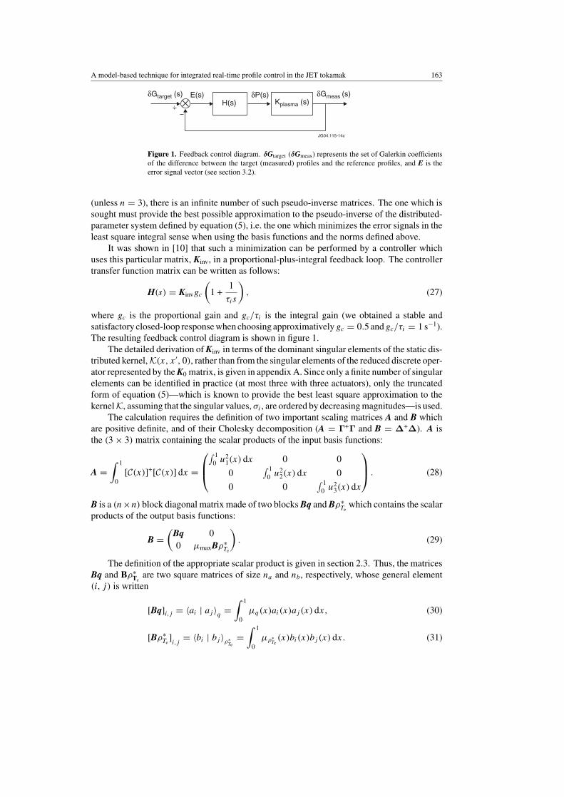
H(s) Kplasma (s)δGtarget (s) E(s) δP(s) δGmeas (s)

JG04.115-14c

Figure 1. Feedback control diagram. !Gtarget (!Gmeas) represents the set of Galerkin coefficientsof the difference between the target (measured) profiles and the reference profiles, and E is theerror signal vector (see section 3.2).

(unless n = 3), there is an infinite number of such pseudo-inverse matrices. The one which issought must provide the best possible approximation to the pseudo-inverse of the distributed-parameter system defined by equation (5), i.e. the one which minimizes the error signals in theleast square integral sense when using the basis functions and the norms defined above.

It was shown in [10] that such a minimization can be performed by a controller whichuses this particular matrix, Kinv, in a proportional-plus-integral feedback loop. The controllertransfer function matrix can be written as follows:

H(s) = Kinvgc

!1 +

1)i s

", (27)

where gc is the proportional gain and gc/)i is the integral gain (we obtained a stable andsatisfactory closed-loop response when choosing approximativelygc = 0.5 andgc/)i = 1 s'1).The resulting feedback control diagram is shown in figure 1.

The detailed derivation of Kinv in terms of the dominant singular elements of the static dis-tributed kernel, K(x, x ", 0), rather than from the singular elements of the reduced discrete oper-ator represented by the K0 matrix, is given in appendix A. Since only a finite number of singularelements can be identified in practice (at most three with three actuators), only the truncatedform of equation (5)—which is known to provide the best least square approximation to thekernel K, assuming that the singular values, 'i , are ordered by decreasing magnitudes—is used.

The calculation requires the definition of two important scaling matrices A and B whichare positive definite, and of their Cholesky decomposition (A = !+! and B = "+"). A isthe (3 # 3) matrix containing the scalar products of the input basis functions:

A =' 1

0[C(x)]+[C(x)] dx =

#

,$

. 10 u2

1(x) dx 0 00

. 10 u2

2(x) dx 00 0

. 10 u2

3(x) dx

%

-& . (28)

B is a (n#n) block diagonal matrix made of two blocks Bq and B&!Te

which contains the scalarproducts of the output basis functions:

B =!

Bq 00 µmaxB&!

Te

". (29)

The definition of the appropriate scalar product is given in section 2.3. Thus, the matricesBq and B&!

Teare two square matrices of size na and nb, respectively, whose general element

(i, j) is written

[Bq]i,j = %ai | aj &q =' 1

0µq(x)ai(x)aj (x) dx, (30)

[B&!Te

]i,j

= %bi | bj &&!Te

=' 1

0µ&!

Te(x)bi(x)bj (x) dx. (31)

164 L Laborde et al

After the identification of the static limit (s = 0) of the matrix K0 has been made fromopen-loop experiments, the procedure for obtaining Kinv is straightforward from the results ofappendix A. It consists of the following:

(i) calculation of a scaled operator, K, defined as

K = "K0!'1, (32)

(ii) its SVD,

K = W#V+, (33)

(iii) computation of Kinv, the proper left pseudo-inverse of K0,

Kinv = !'1V#'1W+". (34)

It is important to note here that one could define another pseudo-inverse of K0 byperforming the SVD of K0, directly. However, this would amount to designing a controllerwhich minimizes the sum of n squared error signals, rather than the integral mean squareerror on the profiles. With K(s) as defined in equation (27), the controller depicted infigure 1 minimizes the ‘distance’ dY (using the norm definition given in section 2.3) betweenthe measured profiles Ymeas(x) = [qmeas(x), &!

Te meas(x)] and the requested target profiles

Ytarget(x) = [qtarget(x), &!Te target

(x)]:

dY2(t) = (Ymeas(x, t) ' Ytarget(x)(2Y

= (qmeas(x, t) ' qtarget(x)(2q

+ µmax(&!Te meas

(x, t) ' &!Te target

(x)(2

&!Te

=' 1

0µq(x)[qmeas(x, t) ' qtarget(x)]2 dx

+ µmax

' 1

0µ&!

Te(x)[&!

Te meas(x, t) ' &!

Te target(x)]2 dx. (35)

3. Implementation of the method with specific trial functions

3.1. Galerkin coefficients of the measured profiles

The Galerkin scheme amounts to calculating the coefficients Gqi(s) and G&!Te i

(s) (equation(8a)) in such a way that the residuals Rq(x, s), respectively R&!

Te(x, s), are negligible in the

sense that they are orthogonal to all trial functions ai(x), respectively bi(x):

) i * [1; na], %Rq(x, s) | ai(x)&q = 0, (36)

) i * [1; nb], %R&!Te

(x, s) | bi(x)&&!

Te= 0 (37)

with

Rq(x, s) = q(x, s) 'na(

j=1

Gqj(s)aj (x), (38)

R&!Te

(x, s) = &!Te

(x, s) 'nb(

j=1

G&!Te j

(s)bj (x). (39)

The expression of residuals in equations (38) and (39) can be introduced in equations (36)and (37). Then, one can obtain the linear system of which the solution yields the coefficientsGqi(s) and G&!

Te i(s) contained in the vectors Gq(s) and G&!

Te(s) of size (na # 1) and (nb # 1),


respectively (in order to have simpler expressions, the dependence on x and s will be omittedin the following):

) i * [1; na],na(

j=1

Gqj %ai | aj &q = %q | ai&q, (40)

) i * [1; nb],nb(

j=1

G&!Te j

%bi | bj &&!Te

= %&!Te

| bi&&!Te. (41)

In this square linear system, one can recognize the expression of matrices Bq and B&!Te

definedin (30) and (31). Thus, the system can be put in matrix form as follows:

BqGq =

/

01

%q | a1&q...

%q | ana&q

2

34 , (42)

B&!Te

G&!Te

=

/

0001

%&!Te

| b1&&!Te

...

%&!Te

| bnb&&!

Te

2

3334. (43)

The matrices Bq and B&!Te

being positive definite, can be inverted, and one can easily calculatethe Galerkin coefficients contained in the vectors Gq(s) and G&!

Te(s). The same scheme applies

for calculating G!q(s) and G!&!Te

(s), starting from $q(s) and $&!Te

(s).

3.2. Real-time calculation of the Galerkin coefficients

For simplicity, time notations will be used here instead of Laplace notations, and only the q

profile will be considered. The same method is applied for its inverse %(x) and for &!Te

(x).First, let us introduce the following notations:

— qmeas(x, t) is the q profile measured at time t of the experiment;— qref(x) is the reference q profile of the stationary state with respect to which the system is

linearized;— qtarget(x) is the target q profile of the real-time control experiment.

While the first two are real q profiles obtained from real-time measurements, the last oneis only a desired q profile, even if it can be chosen from previous experiments. Thus, thistarget profile qtarget(x) will be chosen among the class of q profiles which are accessible withthe function basis, and will be defined by its coordinates Gqtargetj on the basis chosen for theexperiment (in the following, we shall refer to this as a ‘Galerkin profile’):

qtarget(x) =na(

j=1

Gqtargetj aj (x). (44)

Now, remembering that we are dealing with a linearized model and that all input–outputvariables are indeed differences from a reference value, the Galerkin projections must beapplied to the difference between qmeas(x, t) and qref(x),

qmeas(x, t) ' qref(x) =na(

j=1

G$qmeasj (t)aj (x) + R$qmeas(x, t) (45)

166 L Laborde et al

and to the difference between qtarget(x) and qref(x),

qtarget(x) ' qref(x) =na(

j=1

G$qtargetj aj (x) + R$qtarget(x). (46)

As explained in section 2.4, the controller is designed to minimize the distance between thetwo profiles qmeas(x, t) and qtarget(x), using as error signal the difference between the Galerkincoefficients G$qmeasj (t) and G$qtargetj . Thus, it must calculate this difference in real-time.Calculating the two sets G$qmeasj (t) and G$qtargetj would require the knowledge of qref(x) bythe controller. However, as shown in appendix B, taking the difference between the Galerkincoefficients of the full profiles, Gqmeasj (t) and Gqtargetj , without substracting qref(x) providesthe same error signals: Ej(t) = Gqtargetj ' Gqmeasj (t) = G$qtargetj ' G$qmeasj (t). TheGalerkin scheme is therefore applied directly to the full profiles, qmeas(x, t) and qtarget(x), andthe knowledge of the reference state is only required offline, when identifying the linearizedmodel-operator from the dedicated open-loop experiments.

3.3. Choice of the trial function bases

The choice of appropriate trial function bases is important. Indeed, if the bases were not welladapted to the expected shapes of profiles, the Galerkin projection would give poor resultsin the sense that the norm (defined in equations (22) and (23)) of the residuals (defined inequations (38) and (39)) would be large, indicating that the Galerkin profiles provide a poorapproximation of the measured ones. Thus, the choice of the function bases must be suchthat the norm of the residuals is smaller than the profile measurement uncertainties, for a widerange of expected profiles.

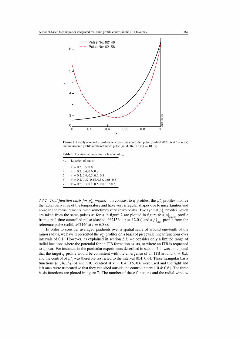
3.3.1. Trial function basis for the q profile or the % profile. As mentioned in section 2.3, theq profiles measured in real-time are obtained as rational fractions, and they have very regularshapes. This is shown in figure 2, where two typical real-time q profiles are plotted, one froma controlled pulse and one from our reference pulse.

This feature has led us to project q(x)—or %(x) = 1/q(x)—on cubic splines basisfunctions, which are suitable functions for such purposes. The basis is made of a number,na , of splines ai(x) defined between x = 0 and x = 1. A set of na knots between x = 0.2 andx = 0.8 completes the basis definition: each spline takes the value 1 on one of these knots and0 on all the other ones. For example, if na = 4 the knots are at x = 0.2, 0.4, 0.6 and 0.8 and thefirst spline, a1(x), is defined as follows: a1(0.2) = 1 and a1(0.4) = a1(0.6) = a1(0.8) = 0.

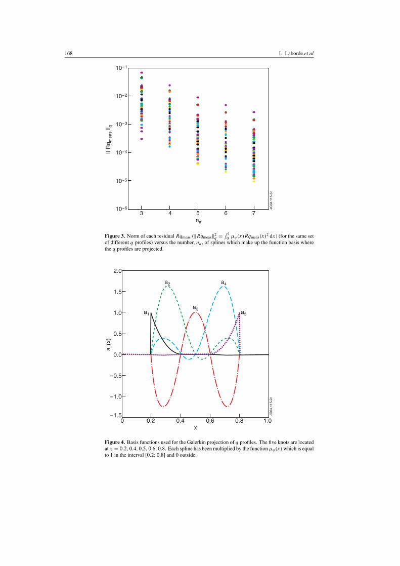
In order to select the optimal number, na , of splines, the residuals calculated with differentvalues of na (from 3 to 7) for a set of 42 different q profiles (from monotonic ones as qref (solid)in figure 2 to deeply reversed ones like qmeas (dashed) in the same figure) were compared. Foreach na value, the location of knots is given in table 1. The results of the comparison are shownin figure 3, where the norm of each residual is plotted versus na . An exponential decreasein the norm can be observed as na increases (for a given q profile). In order not to overloadthe JET real-time central controller, a maximum of eight coefficients were chosen, to be splitbetween q and &!

Te. The value na = 5 has been selected because the maximum of the residual

norm is less than 10'2, which is already less than the diagnostic accuracy. The five splinefunctions (a1, a2, a3, a4, a5), multiplied by the function µq(x), are plotted in figure 4.

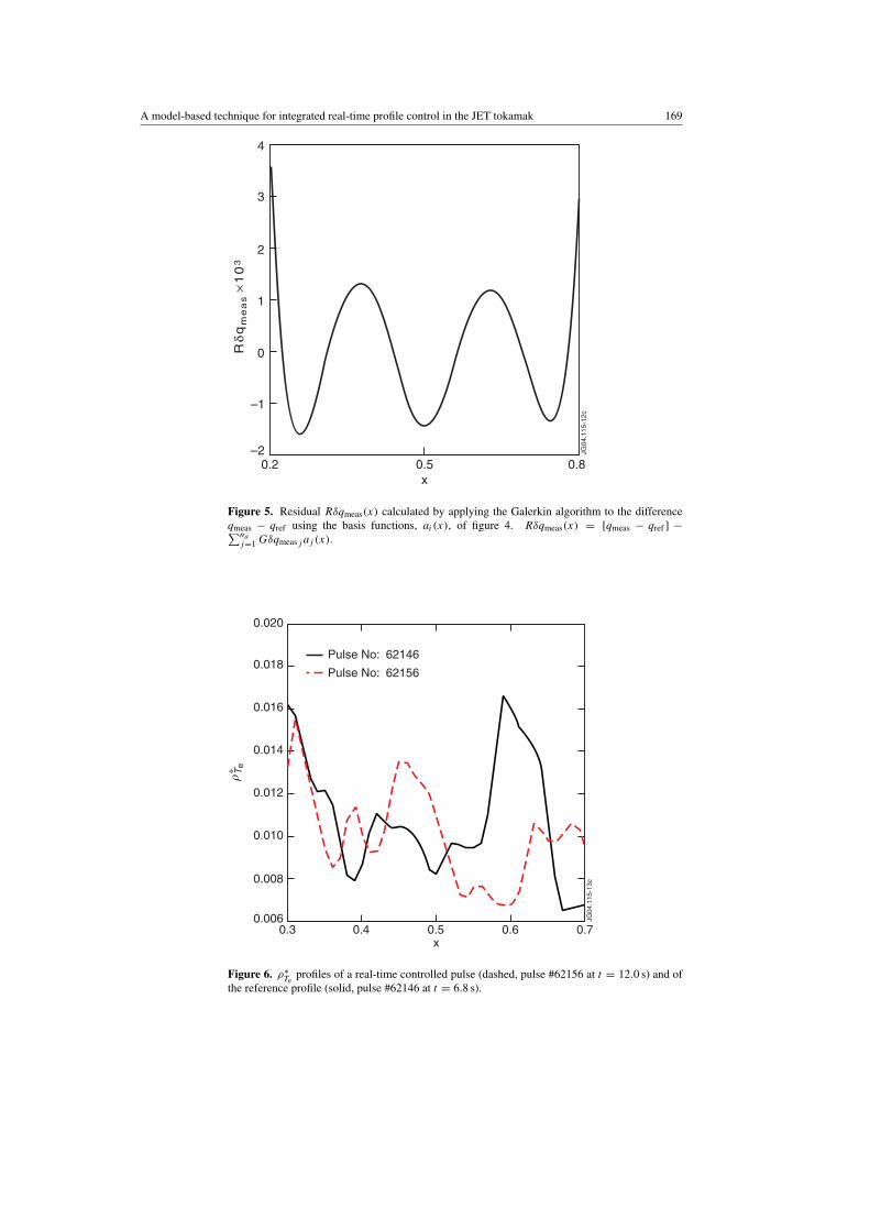
An example is presented below to illustrate the Galerkin representation of the q profiles.The Galerkin projection is applied on the difference between the two profiles of figure 2(as in equation (45)). This yields the Galerkin coefficientsG$qmeasj and the residualR$qmeas(x)

which is plotted in figure 5.


0

3

4

5

6

0 0.2 0.4 0.6 0.8 1x

q

JG04

.115

-11c

Pulse No: 62156Pulse No: 62146

Figure 2. Deeply reversed q profiles of a real-time controlled pulse (dashed, #62156 at t = 6.8 s)and monotonic profile of the reference pulse (solid, #62146 at t = 10.0 s).

Table 1. Location of knots for each value of na .

na Location of knots

3 x = 0.2, 0.5, 0.84 x = 0.2, 0.4, 0.6, 0.85 x = 0.2, 0.4, 0.5, 0.6, 0.86 x = 0.2, 0.32, 0.44, 0.56, 0.68, 0.87 x = 0.2, 0.3, 0.4, 0.5, 0.6, 0.7, 0.8

3.3.2. Trial function basis for &!Te

profile. In contrast to q profiles, the &!Te

profiles involvethe radial derivative of the temperature and have very irregular shapes due to uncertainties andnoise in the measurements, with sometimes very sharp peaks. Two typical &!

Teprofiles which

are taken from the same pulses as for q in figure 2 are plotted in figure 6: a &!Te meas

profilefrom a real-time controlled pulse (dashed, #62156 at t = 12.0 s) and a &!

Te refprofile from the

reference pulse (solid, #62146 at t = 6.8 s).In order to consider averaged gradients over a spatial scale of around one-tenth of the

minor radius, we have represented the &!Te

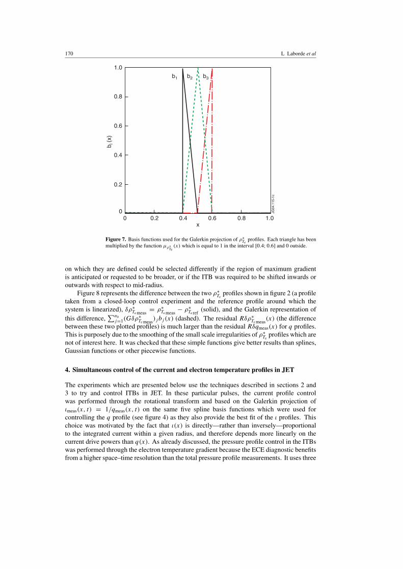
profiles on a basis of piecewise linear functions overintervals of 0.1. However, as explained in section 2.3, we consider only a limited range ofradial locations where the potential for an ITB formation exists, or where an ITB is requestedto appear. For instance, in the particular experiments described in section 4, it was anticipatedthat the target q profile would be consistent with the emergence of an ITB around x = 0.5,and the control of &!

Tewas therefore restricted to the interval [0.4; 0.6]. Three triangular basis

functions (b1, b2, b3) of width 0.1 centred at x = 0.4, 0.5, 0.6 were used and the right andleft ones were truncated so that they vanished outside the control interval [0.4; 0.6]. The threebasis functions are plotted in figure 7. The number of these functions and the radial window

168 L Laborde et al

10-6

10-5

10-4

10-3

10-2

10-1

3 4 5 6 7

|| R

q mea

s || q

na

JG04

.115

-3c

Figure 3. Norm of each residual Rqmeas ((Rqmeas(2q =

. 10 µq(x)Rqmeas(x)2 dx) (for the same set

of different q profiles) versus the number, na , of splines which make up the function basis wherethe q profiles are projected.

-1.5

-1.0

-0.5

0.0

0.5

1.0

1.5

2.0

0 0.2 0.4 0.6 0.8 1.0

a i (x

)

x

JG04

.115

-2c

a1

a2

a3

a4

a5

Figure 4. Basis functions used for the Galerkin projection of q profiles. The five knots are locatedat x = 0.2, 0.4, 0.5, 0.6, 0.8. Each spline has been multiplied by the function µq(x) which is equalto 1 in the interval [0.2; 0.8] and 0 outside.


0

1

2

3

4

0.2 0.5 0.8x

JG04

.115

-12c

Rδq

me

as

×1

03

–2

–1

Figure 5. Residual R$qmeas(x) calculated by applying the Galerkin algorithm to the differenceqmeas ' qref using the basis functions, ai(x), of figure 4. R$qmeas(x) = [qmeas ' qref ] '*na

j=1 G$qmeasj aj (x).

0.006

0.008

0.010

0.012

0.014

0.016

0.018

0.020

0.3 0.4 0.5 0.6 0.7x

JG04

.115

-13c

! Te

Pulse No: 62156

Pulse No: 62146

∗

Figure 6. &!Te

profiles of a real-time controlled pulse (dashed, pulse #62156 at t = 12.0 s) and ofthe reference profile (solid, pulse #62146 at t = 6.8 s).

170 L Laborde et al

0

0.2

0.4

0.6

0.8

1.0

0 0.2 0.4 0.6 0.8 1.0

b i (x

)

x

JG04

.115

-1c

b1 b2 b3

Figure 7. Basis functions used for the Galerkin projection of &!Te

profiles. Each triangle has beenmultiplied by the function µ&!

Te(x) which is equal to 1 in the interval [0.4; 0.6] and 0 outside.

on which they are defined could be selected differently if the region of maximum gradientis anticipated or requested to be broader, or if the ITB was required to be shifted inwards oroutwards with respect to mid-radius.

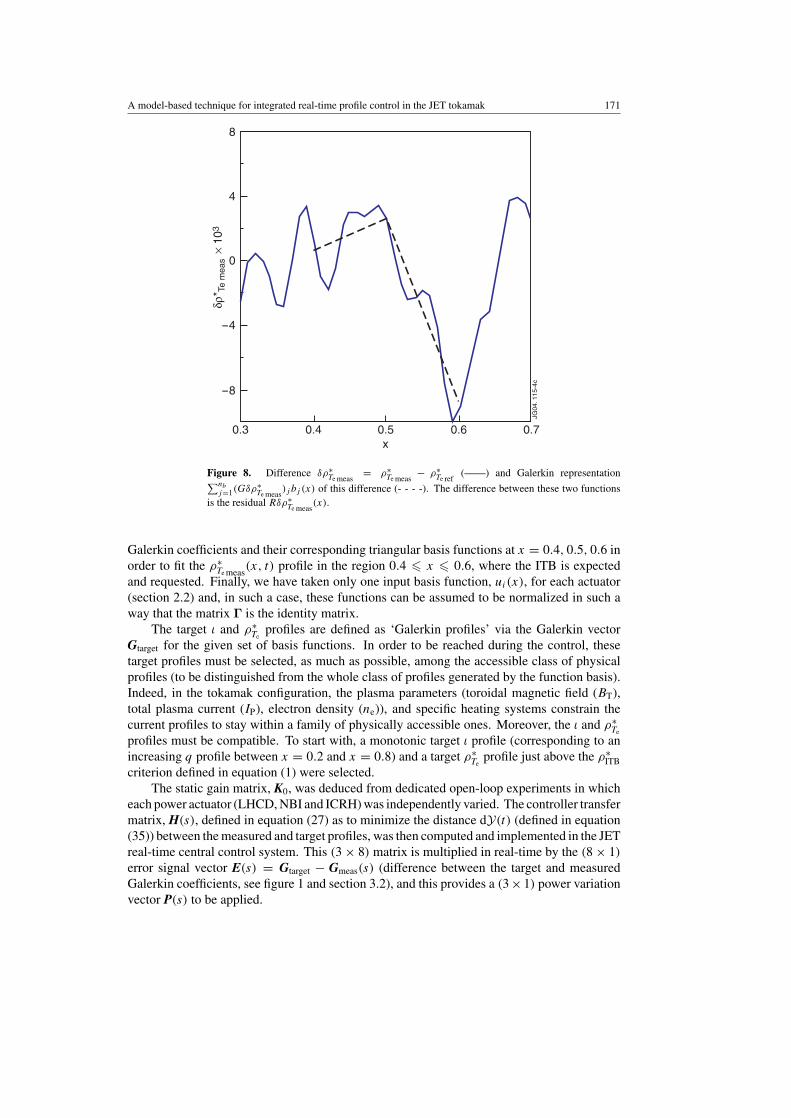
Figure 8 represents the difference between the two &!Te

profiles shown in figure 2 (a profiletaken from a closed-loop control experiment and the reference profile around which thesystem is linearized), $&!

Te meas= &!

Te meas' &!

Te ref(solid), and the Galerkin representation of

this difference,*nb

j=1(G$&!Te meas

)j bj (x) (dashed). The residual R$&!Te meas

(x) (the differencebetween these two plotted profiles) is much larger than the residual R$qmeas(x) for q profiles.This is purposely due to the smoothing of the small scale irregularities of &!

Teprofiles which are

not of interest here. It was checked that these simple functions give better results than splines,Gaussian functions or other piecewise functions.

4. Simultaneous control of the current and electron temperature profiles in JET

The experiments which are presented below use the techniques described in sections 2 and3 to try and control ITBs in JET. In these particular pulses, the current profile controlwas performed through the rotational transform and based on the Galerkin projection of%meas(x, t) = 1/qmeas(x, t) on the same five spline basis functions which were used forcontrolling the q profile (see figure 4) as they also provide the best fit of the % profiles. Thischoice was motivated by the fact that %(x) is directly—rather than inversely—proportionalto the integrated current within a given radius, and therefore depends more linearly on thecurrent drive powers than q(x). As already discussed, the pressure profile control in the ITBswas performed through the electron temperature gradient because the ECE diagnostic benefitsfrom a higher space–time resolution than the total pressure profile measurements. It uses three


-8

-4

0

4

8

0.3 0.4 0.5 0.6 0.7x

JG04

. 115

-4c

δρ* T

e m

eas

× 1

03

Figure 8. Difference $&!Te meas

= &!Te meas

' &!Te ref

(——) and Galerkin representation*nb

j=1(G$&!Te meas

)j bj (x) of this difference (- - - -). The difference between these two functionsis the residual R$&!

Te meas(x).

Galerkin coefficients and their corresponding triangular basis functions at x = 0.4, 0.5, 0.6 inorder to fit the &!

Te meas(x, t) profile in the region 0.4 " x " 0.6, where the ITB is expected

and requested. Finally, we have taken only one input basis function, ui(x), for each actuator(section 2.2) and, in such a case, these functions can be assumed to be normalized in such away that the matrix ! is the identity matrix.

The target % and &!Te

profiles are defined as ‘Galerkin profiles’ via the Galerkin vectorGtarget for the given set of basis functions. In order to be reached during the control, thesetarget profiles must be selected, as much as possible, among the accessible class of physicalprofiles (to be distinguished from the whole class of profiles generated by the function basis).Indeed, in the tokamak configuration, the plasma parameters (toroidal magnetic field (BT),total plasma current (IP), electron density (ne)), and specific heating systems constrain thecurrent profiles to stay within a family of physically accessible ones. Moreover, the % and &!

Te

profiles must be compatible. To start with, a monotonic target % profile (corresponding to anincreasing q profile between x = 0.2 and x = 0.8) and a target &!

Teprofile just above the &!

ITBcriterion defined in equation (1) were selected.

The static gain matrix, K0, was deduced from dedicated open-loop experiments in whicheach power actuator (LHCD, NBI and ICRH) was independently varied. The controller transfermatrix, H(s), defined in equation (27) as to minimize the distance dY(t) (defined in equation(35)) between the measured and target profiles, was then computed and implemented in the JETreal-time central control system. This (3 # 8) matrix is multiplied in real-time by the (8 # 1)

error signal vector E(s) = Gtarget ' Gmeas(s) (difference between the target and measuredGalerkin coefficients, see figure 1 and section 3.2), and this provides a (3 # 1) power variationvector P(s) to be applied.

172 L Laborde et al

0

0.01

0.020.2

0.3

0.4

2

3

4

5

0.2 0.5 0.8 0.2 0.5 0.8 0.2 0.5 0.8x xx

JG04

.115

-7c

t = 5.50s t = 8.00s t = 10.25s

ιq

Pulse No: 62156

! Te∗

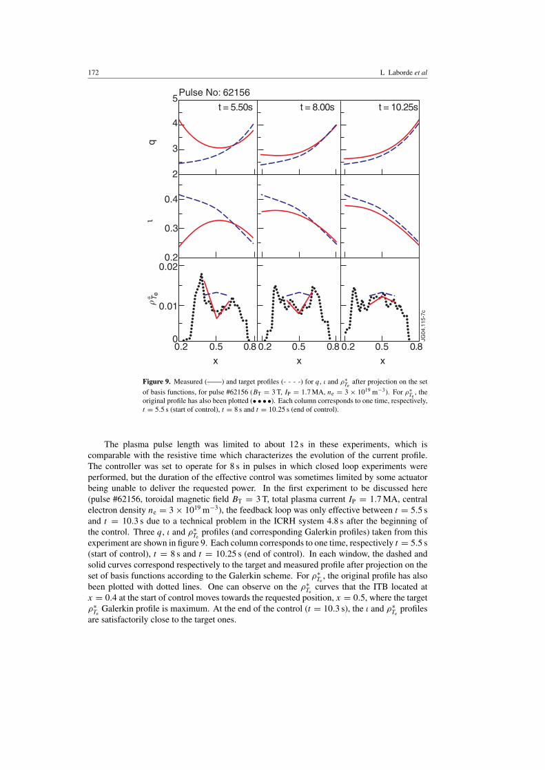
Figure 9. Measured (——) and target profiles (- - - -) for q, % and &!Te

after projection on the setof basis functions, for pulse #62156 (BT = 3 T, IP = 1.7 MA, ne = 3 # 1019 m'3). For &!

Te, the

original profile has also been plotted (• • • •). Each column corresponds to one time, respectively,t = 5.5 s (start of control), t = 8 s and t = 10.25 s (end of control).

The plasma pulse length was limited to about 12 s in these experiments, which iscomparable with the resistive time which characterizes the evolution of the current profile.The controller was set to operate for 8 s in pulses in which closed loop experiments wereperformed, but the duration of the effective control was sometimes limited by some actuatorbeing unable to deliver the requested power. In the first experiment to be discussed here(pulse #62156, toroidal magnetic field BT = 3 T, total plasma current IP = 1.7 MA, centralelectron density ne = 3 # 1019 m'3), the feedback loop was only effective between t = 5.5 sand t = 10.3 s due to a technical problem in the ICRH system 4.8 s after the beginning ofthe control. Three q, % and &!

Teprofiles (and corresponding Galerkin profiles) taken from this

experiment are shown in figure 9. Each column corresponds to one time, respectively t = 5.5 s(start of control), t = 8 s and t = 10.25 s (end of control). In each window, the dashed andsolid curves correspond respectively to the target and measured profile after projection on theset of basis functions according to the Galerkin scheme. For &!

Te, the original profile has also

been plotted with dotted lines. One can observe on the &!Te

curves that the ITB located atx = 0.4 at the start of control moves towards the requested position, x = 0.5, where the target&!

TeGalerkin profile is maximum. At the end of the control (t = 10.3 s), the % and &!

Teprofiles

are satisfactorily close to the target ones.


0

10

20

0

4

8

0

2

4

0 4 8 12 16 20

PIC

RH(M

W)

PLH

CD(M

W)

PN

BI(M

W)

Time (s)

JG04

.115

-10c

Control

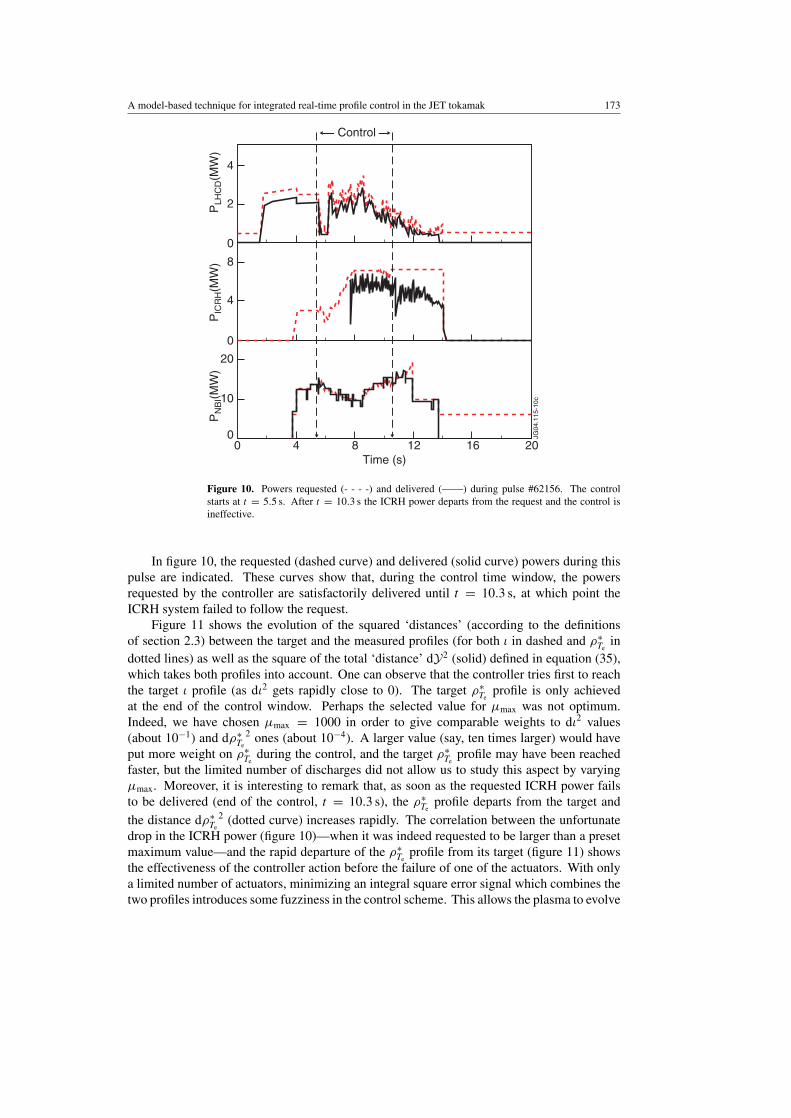
Figure 10. Powers requested (- - - -) and delivered (——) during pulse #62156. The controlstarts at t = 5.5 s. After t = 10.3 s the ICRH power departs from the request and the control isineffective.

In figure 10, the requested (dashed curve) and delivered (solid curve) powers during thispulse are indicated. These curves show that, during the control time window, the powersrequested by the controller are satisfactorily delivered until t = 10.3 s, at which point theICRH system failed to follow the request.

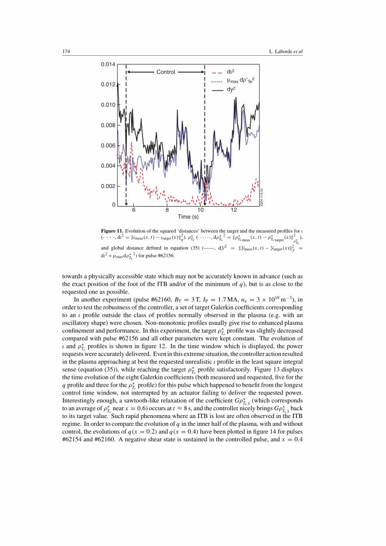
Figure 11 shows the evolution of the squared ‘distances’ (according to the definitionsof section 2.3) between the target and the measured profiles (for both % in dashed and &!

Tein

dotted lines) as well as the square of the total ‘distance’ dY2 (solid) defined in equation (35),which takes both profiles into account. One can observe that the controller tries first to reachthe target % profile (as d%2 gets rapidly close to 0). The target &!

Teprofile is only achieved

at the end of the control window. Perhaps the selected value for µmax was not optimum.Indeed, we have chosen µmax = 1000 in order to give comparable weights to d%2 values(about 10'1) and d&!

Te

2 ones (about 10'4). A larger value (say, ten times larger) would haveput more weight on &!

Teduring the control, and the target &!

Teprofile may have been reached

faster, but the limited number of discharges did not allow us to study this aspect by varyingµmax. Moreover, it is interesting to remark that, as soon as the requested ICRH power failsto be delivered (end of the control, t = 10.3 s), the &!

Teprofile departs from the target and

the distance d&!Te

2 (dotted curve) increases rapidly. The correlation between the unfortunatedrop in the ICRH power (figure 10)—when it was indeed requested to be larger than a presetmaximum value—and the rapid departure of the &!

Teprofile from its target (figure 11) shows

the effectiveness of the controller action before the failure of one of the actuators. With onlya limited number of actuators, minimizing an integral square error signal which combines thetwo profiles introduces some fuzziness in the control scheme. This allows the plasma to evolve

174 L Laborde et al

0

0.002

0.004

0.006

0.008

0.010

0.012

0.014

6 8 10 12Time (s)

JG04

.115

-5c

Control

dy2

dι2

µmax dρ*Te2

Figure 11. Evolution of the squared ‘distances’ between the target and the measured profiles for %(- - - -, d%2 = (%meas(x, t) ' %target(x)(2

q ), &!Te

(· · · · · ·, d&!Te

2 = (&!Te meas


(x)(2&!Te

),

and global distance defined in equation (35) (——, dY2 = (Ymeas(x, t) ' Ytarget(x)(2Y =

d%2 + µmaxd&!Te

2) for pulse #62156.

towards a physically accessible state which may not be accurately known in advance (such asthe exact position of the foot of the ITB and/or of the minimum of q), but is as close to therequested one as possible.

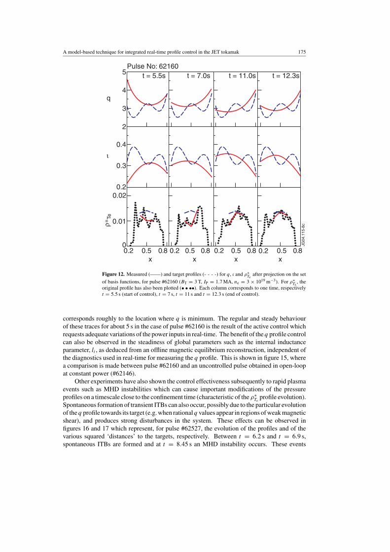
In another experiment (pulse #62160, BT = 3 T, IP = 1.7 MA, ne = 3 # 1019 m'3), inorder to test the robustness of the controller, a set of target Galerkin coefficients correspondingto an % profile outside the class of profiles normally observed in the plasma (e.g. with anoscillatory shape) were chosen. Non-monotonic profiles usually give rise to enhanced plasmaconfinement and performance. In this experiment, the target &!

Teprofile was slightly decreased

compared with pulse #62156 and all other parameters were kept constant. The evolution of% and &!

Teprofiles is shown in figure 12. In the time window which is displayed, the power

requests were accurately delivered. Even in this extreme situation, the controller action resultedin the plasma approaching at best the requested unrealistic % profile in the least square integralsense (equation (35)), while reaching the target &!

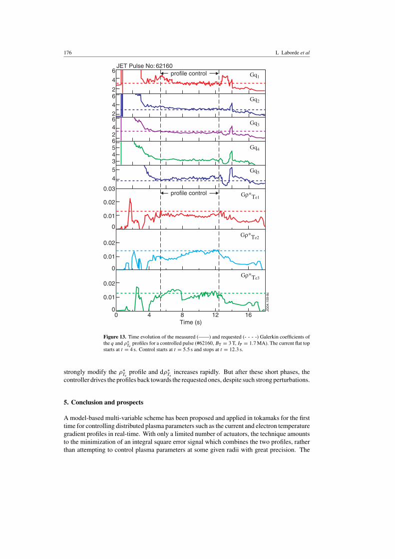
Teprofile satisfactorily. Figure 13 displays

the time evolution of the eight Galerkin coefficients (both measured and requested, five for theq profile and three for the &!

Teprofile) for this pulse which happened to benefit from the longest

control time window, not interrupted by an actuator failing to deliver the requested power.Interestingly enough, a sawtooth-like relaxation of the coefficient G&!

Te 3(which corresponds

to an average of &!Te

near x = 0.6) occurs at t + 8 s, and the controller nicely brings G&!Te 3

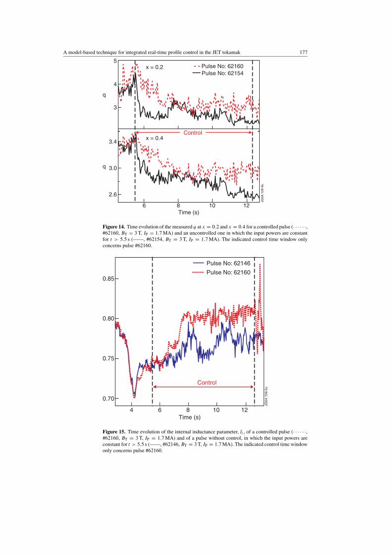
backto its target value. Such rapid phenomena where an ITB is lost are often observed in the ITBregime. In order to compare the evolution of q in the inner half of the plasma, with and withoutcontrol, the evolutions of q(x = 0.2) and q(x = 0.4) have been plotted in figure 14 for pulses#62154 and #62160. A negative shear state is sustained in the controlled pulse, and x = 0.4


0

0.01

0.020.2

0.3

0.4

2

3

4

5

xx xx

JG04

.115

-8c

t = 5.5s t = 7.0s t = 11.0s t = 12.3s

ρ∗Te

ι

q

0.2 0.5 0.8 0.2 0.5 0.8 0.2 0.5 0.8 0.2 0.5 0.8

Pulse No: 62160


after projection on the setof basis functions, for pulse #62160 (BT = 3 T, IP = 1.7 MA, ne = 3 # 1019 m'3). For &!

Te, the

original profile has also been plotted (• • ••). Each column corresponds to one time, respectivelyt = 5.5 s (start of control), t = 7 s, t = 11 s and t = 12.3 s (end of control).

corresponds roughly to the location where q is minimum. The regular and steady behaviourof these traces for about 5 s in the case of pulse #62160 is the result of the active control whichrequests adequate variations of the power inputs in real-time. The benefit of the q profile controlcan also be observed in the steadiness of global parameters such as the internal inductanceparameter, li , as deduced from an offline magnetic equilibrium reconstruction, independent ofthe diagnostics used in real-time for measuring the q profile. This is shown in figure 15, wherea comparison is made between pulse #62160 and an uncontrolled pulse obtained in open-loopat constant power (#62146).

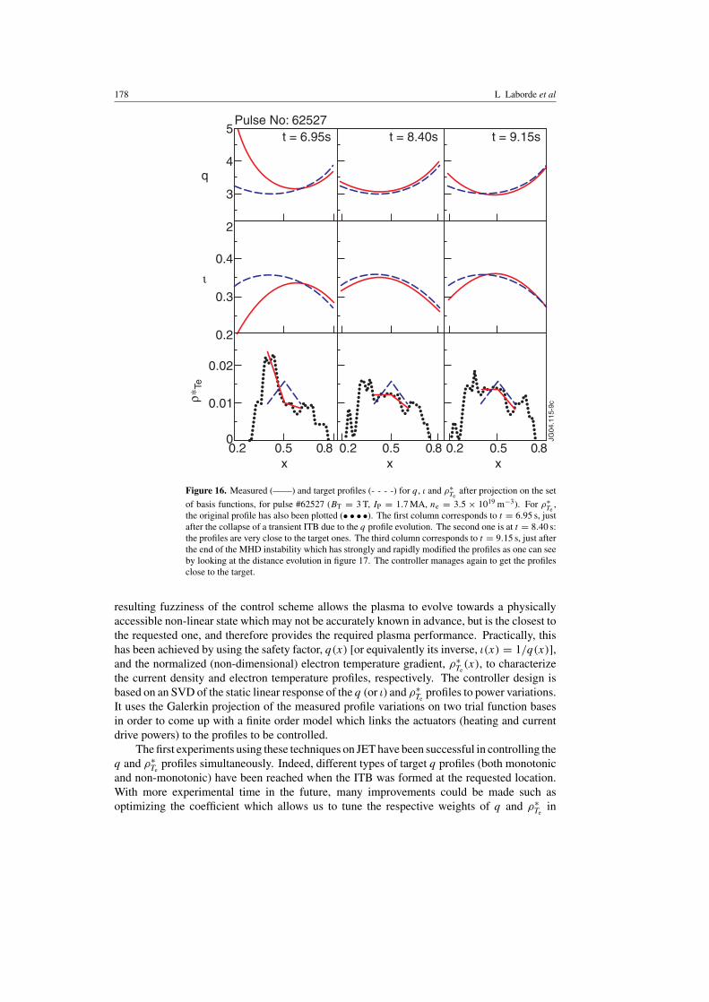
Other experiments have also shown the control effectiveness subsequently to rapid plasmaevents such as MHD instabilities which can cause important modifications of the pressureprofiles on a timescale close to the confinement time (characteristic of the &!

Teprofile evolution).

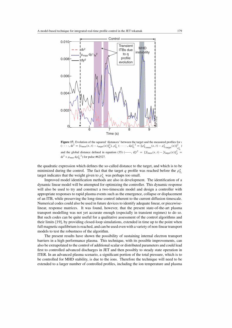
Spontaneous formation of transient ITBs can also occur, possibly due to the particular evolutionof the q profile towards its target (e.g. when rational q values appear in regions of weak magneticshear), and produces strong disturbances in the system. These effects can be observed infigures 16 and 17 which represent, for pulse #62527, the evolution of the profiles and of thevarious squared ‘distances’ to the targets, respectively. Between t = 6.2 s and t = 6.9 s,spontaneous ITBs are formed and at t = 8.45 s an MHD instability occurs. These events

176 L Laborde et al

0

0

0

0.01

0.02

0.01

0.02

0.01

0.02

0.03

0 4 8 12 16Time (s)

JG04

.109

-8c

JET Pulse No: 62160

453456246246

4

2

6 profile control

profile control

Gq1

Gq2

Gq3

Gq4

Gq5

Gρ*Te2

Gρ*Te3

Gρ*Te1

Figure 13. Time evolution of the measured (——) and requested (- - - -) Galerkin coefficients ofthe q and &!

Teprofiles for a controlled pulse (#62160, BT = 3 T, IP = 1.7 MA). The current flat top

starts at t = 4 s. Control starts at t = 5.5 s and stops at t = 12.3 s.

strongly modify the &!Te

profile and d&!Te

increases rapidly. But after these short phases, thecontroller drives the profiles back towards the requested ones, despite such strong perturbations.

5. Conclusion and prospects

A model-based multi-variable scheme has been proposed and applied in tokamaks for the firsttime for controlling distributed plasma parameters such as the current and electron temperaturegradient profiles in real-time. With only a limited number of actuators, the technique amountsto the minimization of an integral square error signal which combines the two profiles, ratherthan attempting to control plasma parameters at some given radii with great precision. The


3.4

4

5

6 8 10 12Time (s)

q

q

JG04

.109

-9c

3.0

2.6

3

Control


x = 0.2

x = 0.4

Figure 14. Time evolution of the measured q at x = 0.2 and x = 0.4 for a controlled pulse (· · · · · ·,#62160, BT = 3 T, IP = 1.7 MA) and an uncontrolled one in which the input powers are constantfor t > 5.5 s (——, #62154, BT = 3 T, IP = 1.7 MA). The indicated control time window onlyconcerns pulse #62160.

0.70

0.75

0.80

0.85

4 6 8 10 12Time (s)

JG04

.109

-5c


Control

Figure 15. Time evolution of the internal inductance parameter, li , of a controlled pulse (· · · · · ·,#62160, BT = 3 T, IP = 1.7 MA) and of a pulse without control, in which the input powers areconstant for t > 5.5 s (——, #62146, BT = 3 T, IP = 1.7 MA). The indicated control time windowonly concerns pulse #62160.

178 L Laborde et al

0

0.01

0.02

0.2

0.3

0.4

2

3

4

5

xx x

JG04

.115

-9c

t = 6.95s t = 8.40s t = 9.15s

ρ∗Te

ι

q

0.2 0.5 0.8 0.2 0.5 0.8 0.2 0.5 0.8

Pulse No: 62527


after projection on the setof basis functions, for pulse #62527 (BT = 3 T, IP = 1.7 MA, ne = 3.5 # 1019 m'3). For &!

Te,

the original profile has also been plotted (• • • •). The first column corresponds to t = 6.95 s, justafter the collapse of a transient ITB due to the q profile evolution. The second one is at t = 8.40 s:the profiles are very close to the target ones. The third column corresponds to t = 9.15 s, just afterthe end of the MHD instability which has strongly and rapidly modified the profiles as one can seeby looking at the distance evolution in figure 17. The controller manages again to get the profilesclose to the target.

resulting fuzziness of the control scheme allows the plasma to evolve towards a physicallyaccessible non-linear state which may not be accurately known in advance, but is the closest tothe requested one, and therefore provides the required plasma performance. Practically, thishas been achieved by using the safety factor, q(x) [or equivalently its inverse, %(x) = 1/q(x)],and the normalized (non-dimensional) electron temperature gradient, &!

Te(x), to characterize

the current density and electron temperature profiles, respectively. The controller design isbased on an SVD of the static linear response of the q (or %) and &!

Teprofiles to power variations.

It uses the Galerkin projection of the measured profile variations on two trial function basesin order to come up with a finite order model which links the actuators (heating and currentdrive powers) to the profiles to be controlled.

The first experiments using these techniques on JET have been successful in controlling theq and &!

Teprofiles simultaneously. Indeed, different types of target q profiles (both monotonic

and non-monotonic) have been reached when the ITB was formed at the requested location.With more experimental time in the future, many improvements could be made such asoptimizing the coefficient which allows us to tune the respective weights of q and &!

Tein


evolutiondy2

dι2

µmax dρ*Te2

Figure 17. Evolution of the squared ‘distances’ between the target and the measured profiles for %(- - - -, d%2 = (%meas(x, t) ' %target(x)(2

q ), &!Te

(· · · · · ·, d&!Te

2 = (&!Te meas


(x)(2&!Te

)

and the global distance defined in equation (35) (——, dY2 = (Ymeas(x, t) ' Ytarget(x)(2Y =

d%2 + µmax d&!Te

2) for pulse #62527.

the quadratic expression which defines the so-called distance to the target, and which is to beminimized during the control. The fact that the target q profile was reached before the &!

Te

target indicates that the weight given to &!Te

was perhaps too small.Improved model identification methods are also in development. The identification of a

dynamic linear model will be attempted for optimizing the controller. This dynamic responsewill also be used to try and construct a two-timescale model and design a controller withappropriate responses to rapid plasma events such as the emergence, collapse or displacementof an ITB, while preserving the long-time control inherent to the current diffusion timescale.Numerical codes could also be used in future devices to identify adequate linear, or piecewise-linear, response matrices. It was found, however, that the present state-of-the-art plasmatransport modelling was not yet accurate enough (especially in transient regimes) to do so.But such codes can be quite useful for a qualitative assessment of the control algorithms andtheir limits [19], by providing closed-loop simulations, extended in time up to the point whenfull magnetic equilibrium is reached, and can be used even with a variety of non-linear transportmodels to test the robustness of the algorithm.

The present results have shown the possibility of sustaining internal electron transportbarriers in a high performance plasma. This technique, with its possible improvements, canalso be extrapolated to the control of additional scalar or distributed parameters and could leadfirst to controlled advanced discharges in JET and then possibly to steady state operation inITER. In an advanced plasma scenario, a significant portion of the total pressure, which is tobe controlled for MHD stability, is due to the ions. Therefore the technique will need to beextended to a larger number of controlled profiles, including the ion temperature and plasma

180 L Laborde et al

density, perhaps flow velocity, possibly with more actuators allowing more flexible power andcurrent deposition profiles (e.g. electron cyclotron waves, pellet fuelling). A potential difficultycan also come from the fact that, in a burning plasma, the alpha-particle heating power willbe the dominant heating power, so that the leverage provided by the heating and current drivesystems will be relatively reduced.

Acknowledgments

This work has been performed under the European Fusion Development Agreement (EFDA).The authors are grateful to all the contributors to the EFDA-JET workprogramme, and to theUKAEA for their dedicated work in operating the JET facility and, in particular, the heatingand current drive systems and real-time plasma diagnostics, which made these technicallydemanding experiments possible.

Appendix A

We show here how Kinv can be derived in terms of the singular elements of the static distributedkernel, K(x, x ", 0), i.e. of the matrices V, W and #. We start from the truncated form ofequation (5) (see equation (15)) which is known to provide the best least square approximationto the kernel K, assuming that the singular values, 'i , are ordered by decreasing magnitude [16].With the notations introduced in section 2.3, equation (4) can be approximated by (omittingthe s dependence)

$Y(x) =3(

i=1

'iWi (x)

' 1

0Vi

+(x ")$P(x ") dx ". (A.1)

Inserting in this equation the expressions of $Y(x), Vi+(x) and $P(x) of equations (9),

(17) and (12) and using the fact that the three components of the residuals vectors Rvi are, bydefinition, orthogonal to u1, u2 and u3, respectively, yields

D(x)!G + R$y(x) =3(

i=1

'iWi (x)V+i A!P, (A.2)

where A is the (3 # 3) matrix of the scalar products of the power deposition basis functions:

A =' 1

0[C(x)]+[C(x)] dx =

#

,$

. 10 u2

1(x) dx 0 00

. 10 u2

2(x) dx 00 0

. 10 u2

3(x) dx

%

-& . (A.3)

One can project equation (A.2) on the basis functions ai(x) and bi(x) (in the sense of the scalarproduct defined in section 2.3) and, since the residuals R$y are also orthogonal to each basisfunctions of D(x), one gets

B!G =3(

i=1

'iBWiV+i A!P, (A.4)

where the matrix B is a (n # n) block diagonal matrix made of two blocks Bq and B&!Te

whichcontain the scalar products of basis functions (using the definition given in section 2.3):

B =!

Bq 00 µmaxB&!

Te

". (A.5)


The matrices Bq and B&!Te

are two square matrices of size na and nb, respectively. Theirelement (i, j) is written

[Bq]i,j = %ai | aj &q =' 1

0µq(x)ai(x)aj (x) dx, (A.6)

[B&!Te

]i,j

= %bi | bj &&!Te

=' 1

0µ&!

Te(x)bi(x)bj (x) dx. (A.7)

If the basis functions are adequately chosen to provide good approximations of the singularfunctions Wi (x) and Vi (x) with negligible residuals, one can neglect integrals involvingproducts of the residual vectors, Rwi and Rvi , respectively, and the orthonormality relations(6) and (7) then lead to the following relations among the vectors Wi and Vi :

W+i BWj = $i,j , (A.8)

V+i AVj = $i,j . (A.9)

The matrices B and A are positive definite so that a Cholesky decomposition can be performed.This defines the (n # n) and (3 # 3) upper triangular matrices " and !:

B = "+", (A.10)

A = !+!. (A.11)

Thus, the orthonormality takes the matrix form

W+"+"W = In, (A.12)

V+!+!V = I3. (A.13)

One can define the (n#n) and (3#3)matrices W = "W and V = !V so that the orthonormalityfinally takes the classical form

W+W = In, (A.14)

V+V = I3. (A.15)

Then, introducing ", !, W and V in equation (A.4) and left-multiplying by ["+]'1, one gets

"!G = W#V+!!P. (A.16)

By virtue of the orthonormality of the matrices W and V and of the unicity of the SVD of anyrectangular matrix, one can find the matrices W, # and V by performing the SVD of a (n # 3)

matrix K:

K = W#V+. (A.17)

Left-multiplying equation (19) by " and introducing the identity matrix !'1! in order toretrieve equation (A.16), one can identify K in terms of K0:

K = "K0!'1. (A.18)

We are now able to define Kinv as a left pseudo-inverse of K0:

Kinv = !'1V#'1W+" (A.19)

and it is straightforward to show that KinvK0 = I3 by using equations (32) and (34) as well asthe unitary relations (A.14) and (A.15).

182 L Laborde et al

Appendix B

Equations (45) and (46) can be projected on each basis function ai(x). Since the residualsR$qmeas(x, t) and R$qtarget(x) are orthogonal to each basis function, this yields the followingequations (omitting the x dependence):

%qmeas(t) | ai&q = %qref | ai&q +na(

j=1

G$qmeasj (t)%aj | ai&q, (B.1)

%qtarget | ai&q = %qref | ai&q +na(

j=1

G$qtargetj %aj | ai&q . (B.2)

Inserting the expression of qtarget(x), equation (B.2) can be rewritten as follows,na(

j=1

Gqtargetj %aj | ai&q = %qref | ai&q +na(

j=1

G$qtargetj %aj | ai&q (B.3)

and eliminating %qref | ai&q from equations (B.1) and (B.3), the projection of the measuredprofile on ai(x) can be expressed as

%qmeas(t) | ai&q =na(

j=1

[Gqtargetj ' G$qtargetj + G$qmeasj (t)]%aj | ai&q . (B.4)

From the unicity of the Galerkin coefficients, one can recognize here the decomposition ofqmeas(x, t) with coefficients Gqmeasj (t) and therefore

qmeas(x, t) =na(

j=1

Gqmeasj (t)aj (x) + Rqmeas(x, t), (B.5)

where Gqmeasj (t) = Gqtargetj ' G$qtargetj + G$qmeasj (t).The coefficients Gqmeasj (t) are computed in real-time (applying the Galerkin algorithm

to qmeas(x, t)) and compared with the target coefficients Gqtargetj . Their difference

Ej(t) = Gqtargetj ' Gqmeasj (t) = G$qtargetj ' G$qmeasj (t) (B.6)

is calculated by the controller at each time step. The right-hand side of this expression isthe proper error signal to be used by the controller to minimize the distance between the twoprofiles qmeas(x, t) and qtarget(x). We have just shown that it can indeed be computed directlyfrom the Galerkin coefficients of the full measured and target profiles. It is convenient thereference profile does not have to be specified in the controller, and alleviates the real-timecalculations.

References

[1] Taylor T S 1997 Plasma Phys. Control. Fusion 39 B47–73[2] Gormezano C 1999 Plasma Phys. Control. Fusion 41 B367–80[3] Litaudon X et al 2004 Plasma Phys. Control. Fusion 46 A19–34[4] Wolf R C 2003 Plasma Phys. Control. Fusion 45 R1–91[5] Connor J et al 2004 Nucl. Fusion 44 R1–49[6] Challis C D et al 2002 Plasma Phys. Control. Fusion 44 1031–55[7] Joffrin E et al 2002 Plasma Phys. Control. Fusion 44 1739–52[8] Garbet X et al 2003 Nucl. Fusion 43 975–81[9] Mazon D et al 2003 Plasma Phys. Control. Fusion 45 L47–54

[10] Moreau D et al 2003 Nucl. Fusion 43 870–82


[11] Mazon D et al 2002 Plasma Phys. Control. Fusion 44 1087–104[12] Tresset G et al 2002 Nucl. Fusion 42 520–6[13] Pericoli Ridolfini V et al 2003 Nucl. Fusion 43 469–78[14] Pochelon A et al 2003 Proc. 15th Topical Conf. on Radio Frequency Power in Plasmas (Moran, Wyoming, USA)

vol 694 297–304[15] Rice J et al 2003 Nucl. Fusion 43 781–8[16] Smithies F 1962 Integral Equations (Cambridge: Cambridge University Press)[17] Zabeo L et al 2002 Plasma Phys. Control. Fusion 44 2483–94[18] Lao L L et al 1990 Nucl. Fusion 30 1035–60[19] Tala T et al 2004 Proc. 20th IAEA Fusion Energy Conf. (Vilamoura, Portugal)

a model-based technique for integrated real-time profile control in the jet tokamak

Documents