a metabolomic approach to beer characterization - mdpi
TRANSCRIPT
molecules
Article
A Metabolomic Approach to Beer Characterization
Nicola Cavallini 1 , Francesco Savorani 1, Rasmus Bro 2 and Marina Cocchi 3,*
�����������������
Citation: Cavallini, N.; Savorani, F.;
Bro, R.; Cocchi, M. A Metabolomic
Approach to Beer Characterization.
Molecules 2021, 26, 1472. https://
doi.org/10.3390/molecules26051472
Academic Editor: Radmila Pavlovic
Received: 31 December 2020
Accepted: 4 March 2021
Published: 8 March 2021
Publisher’s Note: MDPI stays neutral
with regard to jurisdictional claims in
published maps and institutional affil-
iations.
Copyright: © 2021 by the authors.
Licensee MDPI, Basel, Switzerland.
This article is an open access article
distributed under the terms and
conditions of the Creative Commons
Attribution (CC BY) license (https://
creativecommons.org/licenses/by/
4.0/).
1 Department of Applied Science and Technology, Polytechnic of Turin, Corso Duca degli Abruzzi 24,I-10129 Turin, Italy; [email protected] (N.C.); [email protected] (F.S.)
2 Chemometrics and Analytical Technology, Department of Food Science, Faculty of Science, University ofCopenhagen, Rolighedsvej 26, 1958 Frederiksberg C, Denmark; [email protected]
3 Dipartimento di Scienze Chimiche e Geologiche, Università di Modena e Reggio Emilia, Via Campi 103,41125 Modena, Italy
* Correspondence: [email protected]
Abstract: The consumers’ interest towards beer consumption has been on the rise during the pastdecade: new approaches and ingredients get tested, expanding the traditional recipe for brewing beer.As a consequence, the field of “beeromics” has also been constantly growing, as well as the demandfor quick and exhaustive analytical methods. In this study, we propose a combination of nuclearmagnetic resonance (NMR) spectroscopy and chemometrics to characterize beer. 1H-NMR spectrawere collected and then analyzed using chemometric tools. An interval-based approach was appliedto extract chemical features from the spectra to build a dataset of resolved relative concentrations.One aim of this work was to compare the results obtained using the full spectrum and the resolvedapproach: with a reasonable amount of time needed to obtain the resolved dataset, we show thatthe resolved information is comparable with the full spectrum information, but interpretability isgreatly improved.
Keywords: foodomics; beer; NMR; chemometrics; features extraction
1. Introduction
The interest expressed by the consumers towards food consumption [1] and relatedaspects such as production [2], food pairing [3] and consumer experience [4] has beenon the rise during the last decade. As a consequence, a large number of new productsis introduced into the market every year in a self-sustaining cycle of offer and demandcoupled with a healthy desire to experiment. This is also true in the field of beer productionwhere the traditional minimum recipe for brewing beer from water, malt, hops, and yeastgets constantly twisted and expanded. New approaches and ingredients are tested [5],especially by small craft breweries [6,7].
As a result, the fields of foodomics in general [8] and “beeromics” in particular [9]have been constantly growing in the recent years [10]. To meet the demand of both quickand exhaustive analytical methods for quality control [9,11] and sensory evaluation [12],many analytical techniques have been employed so far: nuclear magnetic resonance(NMR) spectroscopy [13–19], gas chromatography (GC) [20], gas chromatography–massspectrometry (GC–MS) [21,22], mass spectrometry (MS) [23], near-infrared (NIR) spec-troscopy [24–26], ultraviolet-visible (UV-Vis) spectroscopy [27–29], electronic tongue [30],MS electronic nose [31], middle-range infrared (mid-IR), optical-tongue [32] and fluores-cence spectroscopy [33–36].
In this study, we collected and measured a set of one hundred beer samples encom-passing different attributes such as origin, brewery, beer style and fermentation type;notwithstanding this variability, all beer samples were similar with respect to color (ratherpale) and clearness (low turbidity). Moreover, the large majority of the samples came fromindustrial production. In fact, the aim of this work was to propose a methodology aimingat fast non-destructive metabolomic characterization, combining NMR spectroscopy and
Molecules 2021, 26, 1472. https://doi.org/10.3390/molecules26051472 https://www.mdpi.com/journal/molecules
Molecules 2021, 26, 1472 2 of 15
chemometrics, of widely consumed beer types in order to explore the compositional profileand highlight potential trends or peculiar samples, information which can be, at a succes-sive step, matched to consumer preference. To this aim, we proposed a strategy based onmultivariate curve resolution (MCR) [37] used as a resolution technique.
An MCR interval-based procedure was applied to extract chemical features fromthe NMR spectra [38–41], which allowed obtaining a reduced dataset of resolved relativeconcentrations. From the data analysis point of view, two multivariate approaches werecompared: the full spectra analysis and the analysis of the chemical features extractedby MCR.
Accurate characterization of major and minor metabolites of beer consistent withprevious studies is also provided in this paper (see Section 2.2.3). Evidence for the presenceof trigonelline [19] confirms rather recent experimental findings which relate its origin tothe addition of hops [42,43].
The results provided in this paper add to the corpus of valuable information aboutbeer characterization that can prove to be very useful to the producers concerning bothquality control and innovation.
2. Materials and Methods2.1. Experimental
In this section, all the experimental steps for preparing the beer specimens for NMRanalysis are described. First, an overview of the beer products collection is given, thenthe sample preparation procedure is described and finally the experimental conditions foracquiring the NMR profiles are reported.
2.1.1. Sample Collection
The beer sample collection consisted of one hundred beer products that were boughtfrom local stores. All the selected products were rather pale in color, i.e., no dark “stout-like”as well as no excessively brown beers were included in the collection. Another importantcriterion used for selecting the samples was the product’s clarity, in the sense that noappreciable turbidity should be seen. All the samples were different by brand, brewingstyle, location of production, percentage of alcohol by volume (% ABV) and color, the latteras previously described.
In Table 1, the counts for each beer style covered in the study are reported. In general,beer products can be grouped into two families based on the yeast type, namely, “top-fermented” or “ales” and “bottom-fermented” or “lagers”. These styles correspond tothe yeast strains named Saccharomyces cerevisiae and Saccharomyces carlsbergensis, respec-tively [44].
Table 1. Number of samples for each fermentation style (i.e., yeast strain) and for each beer style.
Fermentation Style(Yeast Strain) % ABV Range Beer Styles
Top, “ales”(S. cerevisiae) 40 5.7 ± 1.3%
Ale 18India pale ale (IPA) 19
Imperial India pale ale (IIPA) 3
Bottom, “lagers”(S. carlsbergensis) 57 4.8 ± 1.0%
Lager 30Lager (pale) 27
Unclassified 1 3 4.8–5.2–6.0% Organic ginger brew–Oktoberfest–Kristallweizen
1 These beer products are brewed with either Saccharomyces cerevisiae or carlsbergensis yeast, but their style is generally different from thetwo large “top” and “bottom”-style families.
Molecules 2021, 26, 1472 3 of 15
2.1.2. Sample Preparation
A collection of 2 mL vials was directly prepared from the original commercial contain-ers (cans or glass bottles). Three small vials for each beer sample were prepared and keptfrozen at −20 ◦C.
As the first step in sample preparation, the specimens were thawed by placing themin a water bath at room temperature. A degassing step was also performed: degassing ishighly recommended by [2,45,46] as it is aimed at reducing the occurrence of measurementinterferences due to bubble formation within the NMR tubes. The thawing and degassingsteps were performed as follows:
• 10 min thawing in a water bath at room temperature;• 20 min degassing in an ultrasonic bath in water at room temperature.
Since all the specimens were clear, filtration was not performed, even though thisprocedure is sometimes recommended in literature studies [27,47].
Preparation of the NMR tubes was executed in batches of twelve samples whilekeeping the unprocessed samples in a fridge at 5 ◦C. The newly prepared NMR tubes wereplaced into the instrument’s autosampler rack which, prior to spectra acquisition, was alsostored in a fridge at 5 ◦C.
All the specimens were prepared to contain 10% D2O, 0.02% of sodium-3-(trimethylsilyl)propionate-d4 (TSP-d4) as a chemical shift reference [2,14,46,48] and a 20% phosphate buffer(pH = 3.55). All NMR tubes were filled with the required volume of 600 µL which wasobtained by mixing 420 µL of beer specimen, 60 µL of D2O and 120 µL of the phosphatebuffer (pH = 3.55) in H2O. It was reported by Duarte et al. [13] that pH values of ale andlager beers generally fall within the 3.7–4.4 interval, so the phosphate buffer was added toadjust the set of samples and obtain more homogeneous pH values, as the actual pH ofthe samples could not be measured. Control of pH was especially aimed at reducing theoccurrence of horizontal shifts of the signals across the spectra, which may be due to thedifferent protonation forms of compounds such as amino acids and organic acids [14,48].
The samples were prepared and analyzed by NMR following a pre-established ran-dom order.
2.1.3. 1H-NMR Data Acquisition
All the 1H-NMR profiles were acquired on a Bruker Avance III 600 spectrometer(Bruker Biospin GmbH, Rheinstetten, Germany) operating at the Larmor frequency of600.13 MHz for protons, equipped with a double-tuned cryoprobe (TCl) set for 5 mmsample tubes and a cooled autosampler (SampleJet, at 5 ◦C).
The spectra were acquired with TOPSPIN 2.1 (Bruker Biospin GmbH, Rheinstetten,Germany), using the NOESYGPPR1D sequence [46,48]. Presaturation of the water signal(4.77 ppm) [2,13,14,45,46,48–51] was employed, while the ethanol signals were not sup-pressed [14,46,48]. All the experiments were performed at 298 K with a fixed receivergain. Each free induction decay (FID) was collected using a total of 64 scans plus fourdummy scans. Acquisition time was set to 2.65 s and recycle delay was set to 6 s. Prior toFourier transformation, the FIDs were zero-filled to 64,000 points and a 0.3 Hz Lorentzianline broadening was applied. The spectra were baseline- and phase-corrected using theTOPSPIN built-in processing tools. This correction was performed automatically for allspectra and then, depending on the obtained results (assessed by a trained NMR user), afurther manual adjustment was performed when strictly necessary. For all spectra, theppm scale was referenced to the TSP peak (0.00 ppm). The spectral window was set to20.5 ppm.
2.2. Data Preprocessing and Data Analysis Methods
This section describes all the data analysis steps from raw spectra preparation to mul-tivariate analysis. The preliminary preprocessing of NMR spectra described in Section 2.2.1is common to the analyses of both the full spectra and resolved features datasets. InSections 2.2.2–2.2.4, the specific procedures applied for features resolution are described.
Molecules 2021, 26, 1472 4 of 15
Finally, in Section 2.2.5, the multivariate data analysis and preprocessing methods used inthe study are reported.
2.2.1. 1H-NMR Data Preparation
The raw NMR spectra were imported and processed under the MATLAB environ-ment. The spectra were first globally denoised (smoothed) using a simple moving averagealgorithm [52] (window width = 3, polynomial order = 0): this step was performed in theperspective of working by focusing on small portions of the whole spectral width usingthe so-called “interval-based” approach [53].
Then, a set of manually chosen small intervals was defined, each interval containingsingle peaks or small groups of peaks, to allow better signal resolution (as explained inSection 2.2.2). Finally, each interval was aligned using the icoshift tool [54,55]. The alignedintervals were merged and used for the analysis of the full spectra, but they also constitutethe basis for the peak resolution by MCR, as described in Section 2.2.2.
2.2.2. 1H-NMR Spectra Peaks’ Resolution by MCR
Since NMR spectra carry different information in different spectral regions, it is com-mon to roughly split them into three regions [13,53]: aliphatic/organic acids (0–3 ppm),carbohydrates (3–5 ppm) and aromatic (6–9 ppm) regions. These regions mainly differbecause of baseline noise, the signals’ average intensities and the involved molecules [53].An interval-based approach allows effectively handling those differences, leading to mean-ingful chemical quantification of the metabolites, also taking advantage of improvedinterpretability and model performance.
In the framework of an interval-based approach, instead of building one overall modelbased on the whole spectral width, a set of 53 interval-specific MCR models was built. Inorder to choose the correct number of components, four MCR models for each intervalwere built, using from two to five components, by means of an in-house written routine. Alist of all the integrated intervals with their boundaries (in ppm), model complexity andselected components is provided in the Supplementary Materials (Table S1). Regarding thesettings for MCR modelling, the maximum number of iterations was set to 1000 and thenon-negativity constraint was applied both in the rows and columns directions.
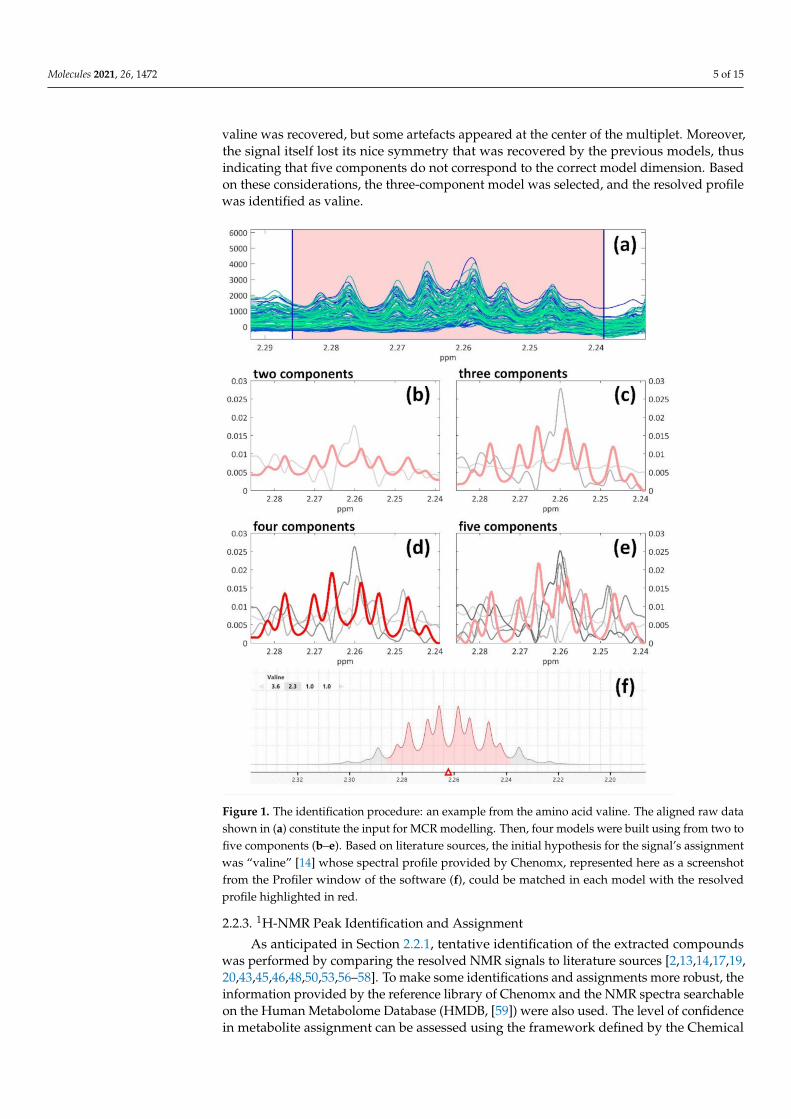
Each set of resolved profiles corresponding to the four MCR models was plottedas shown in Figure 1b–e, allowing for clear comparisons between the models: such avisual representation allowed the identification of the best model and the selection ofthe resolved components related to the chemical information. All the other componentsdescribing background effects, noise or signals not related to NMR peaks were excluded.The integrated area provided by MCR was carefully evaluated for each selected componentbefore generating the final features dataset (Section 2.2.4).
An example of the MCR peak resolution and identification process is shown inFigure 1, investigating the amino acid valine which is characterized by a quite complexspin system resulting in a symmetric multiplet. Its presence in beer was reported by manybibliographic sources [13,20,43,46,50,56], even though only Nord et al. also reported itschemical shift and assignment [14]. In the example, four MCR models are shown: in eachof them, it is possible to identify one resolved spectral profile that matches the actualcomplex signal of valine (in red in Figure 1b–e), whose correct profile was recovered fromthe reference library of Chenomx (Figure 1f, a screenshot from the software’s interface).It is interesting to notice how different numbers of components affect the extraction per-formance of the compound’s profile. For instance, the signal related to valine is alreadyrecognizable in the first model (fitted with two components, Figure 1b), even though avertical offset is also present: in this case, the piece of information related to the compoundof interest may need further “cleaning”, i.e., noise or background effects should be takencare of. In the inspected models built with three and four components (Figure 1c–d), whichbasically show identical performance, the vertical offset disappeared. The last model wasfitted with five components (Figure 1e); also, in this case, the correct spectral profile of
Molecules 2021, 26, 1472 5 of 15
valine was recovered, but some artefacts appeared at the center of the multiplet. Moreover,the signal itself lost its nice symmetry that was recovered by the previous models, thusindicating that five components do not correspond to the correct model dimension. Basedon these considerations, the three-component model was selected, and the resolved profilewas identified as valine.
Figure 1. The identification procedure: an example from the amino acid valine. The aligned raw datashown in (a) constitute the input for MCR modelling. Then, four models were built using from two tofive components (b–e). Based on literature sources, the initial hypothesis for the signal’s assignmentwas “valine” [14] whose spectral profile provided by Chenomx, represented here as a screenshotfrom the Profiler window of the software (f), could be matched in each model with the resolvedprofile highlighted in red.
2.2.3. 1H-NMR Peak Identification and Assignment
As anticipated in Section 2.2.1, tentative identification of the extracted compoundswas performed by comparing the resolved NMR signals to literature sources [2,13,14,17,19,20,43,45,46,48,50,53,56–58]. To make some identifications and assignments more robust, theinformation provided by the reference library of Chenomx and the NMR spectra searchableon the Human Metabolome Database (HMDB, [59]) were also used. The level of confidencein metabolite assignment can be assessed using the framework defined by the Chemical
Molecules 2021, 26, 1472 6 of 15
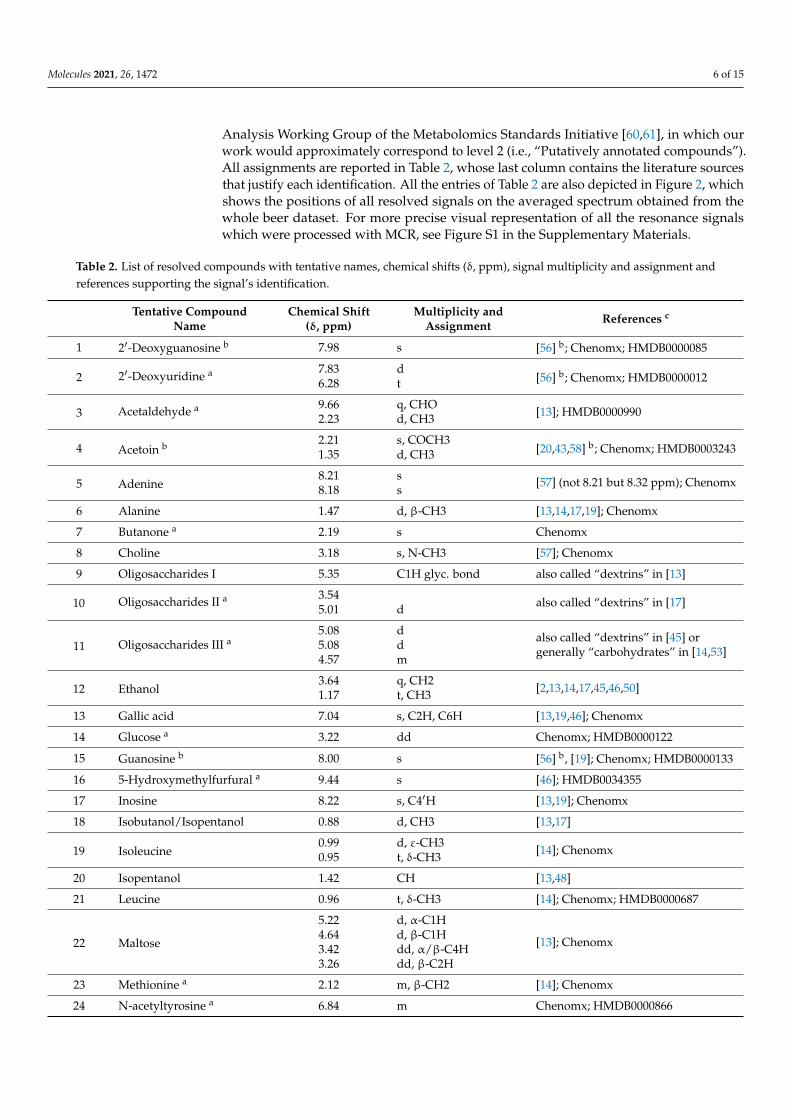
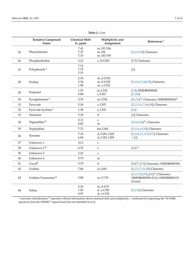
Analysis Working Group of the Metabolomics Standards Initiative [60,61], in which ourwork would approximately correspond to level 2 (i.e., “Putatively annotated compounds”).All assignments are reported in Table 2, whose last column contains the literature sourcesthat justify each identification. All the entries of Table 2 are also depicted in Figure 2, whichshows the positions of all resolved signals on the averaged spectrum obtained from thewhole beer dataset. For more precise visual representation of all the resonance signalswhich were processed with MCR, see Figure S1 in the Supplementary Materials.
Table 2. List of resolved compounds with tentative names, chemical shifts (δ, ppm), signal multiplicity and assignment andreferences supporting the signal’s identification.
Tentative CompoundName
Chemical Shift(δ, ppm)
Multiplicity andAssignment References c
1 2′-Deoxyguanosine b 7.98 s [56] b; Chenomx; HMDB0000085
2 2′-Deoxyuridine a 7.83 d[56] b; Chenomx; HMDB00000126.28 t
3 Acetaldehyde a 9.66 q, CHO[13]; HMDB00009902.23 d, CH3
4 Acetoin b 2.21 s, COCH3[20,43,58] b; Chenomx; HMDB00032431.35 d, CH3
5 Adenine8.21 s [57] (not 8.21 but 8.32 ppm); Chenomx8.18 s
6 Alanine 1.47 d, β-CH3 [13,14,17,19]; Chenomx
7 Butanone a 2.19 s Chenomx
8 Choline 3.18 s, N-CH3 [57]; Chenomx
9 Oligosaccharides I 5.35 C1H glyc. bond also called “dextrins” in [13]
10 Oligosaccharides II a 3.54also called “dextrins” in [17]5.01 d
11 Oligosaccharides III a5.08 d also called “dextrins” in [45] or
generally “carbohydrates” in [14,53]5.08 d4.57 m
12 Ethanol3.64 q, CH2
[2,13,14,17,45,46,50]1.17 t, CH3
13 Gallic acid 7.04 s, C2H, C6H [13,19,46]; Chenomx
14 Glucose a 3.22 dd Chenomx; HMDB0000122
15 Guanosine b 8.00 s [56] b, [19]; Chenomx; HMDB0000133
16 5-Hydroxymethylfurfural a 9.44 s [46]; HMDB0034355
17 Inosine 8.22 s, C4′H [13,19]; Chenomx
18 Isobutanol/Isopentanol 0.88 d, CH3 [13,17]
19 Isoleucine0.99 d, ε-CH3
[14]; Chenomx0.95 t, δ-CH3
20 Isopentanol 1.42 CH [13,48]
21 Leucine 0.96 t, δ-CH3 [14]; Chenomx; HMDB0000687
22 Maltose
5.22 d, α-C1H
[13]; Chenomx4.64 d, β-C1H3.42 dd, α/β-C4H3.26 dd, β-C2H
23 Methionine a 2.12 m, β-CH2 [14]; Chenomx
24 N-acetyltyrosine a 6.84 m Chenomx; HMDB0000866
Molecules 2021, 26, 1472 7 of 15
Table 2. Cont.
Tentative CompoundName
Chemical Shift(δ, ppm)
Multiplicity andAssignment References c
25 Phenylalanine7.43 m, H2/H6
[14,19,50]; Chenomx7.37 m, H47.33 m, H3/H5
26 Phosphocholine 3.22 s, N-CH3 [57]; Chenomx
27 Polyphenols a7.74
[2]7.757.77
28 Proline2.36 m, β-CH2
[13,14,17,48,57]; Chenomx2.34 m, β-CH21.98 m, γ-CH2
29 Propanol 1.53 m, CH2 [13]; HMDB00008200.88 t, CH3 [13,46]
30 Pyroglutamate a 2.39 m, CH2 [43,56] b; Chenomx; HMDB0000267
31 Pyruvate 2.36 s, CH3 [2,13,14,17,46,48]; Chenomx
32 Pyruvate hydrate a 1.58 s, CH3 [14]
33 Trehalose 5.18 d [2]; Chenomx
34 Trigonelline b 9.11 s[19,43,56] b; Chenomx8.82 m
35 Tryptophan 7.72 bd, C4H [13,14,19,50]; Chenomx
36 Tyrosine 7.18 d, C2H, C6H [13,14,17,19,50,57]; Chenomx6.89 d, C3H, C5H + [2]
37 Unknown 1 10.2 s
38 Unknown 2 d 6.35 s [46] d
39 Unknown 3 2.22 s
40 Unknown 4 5.79 m
41 Uracilb 5.79 d [56] b, [19]; Chenomx; HMDB0000300
42 Uridine 7.86 d, C6H [2,13,17,19,50]; Chenomx
43 Uridine/Guanosine b 5.89 m, C1′H[13,17,50,57], [56] b; Chenomx;HMDB0000296 (Uri), HMDB0000133(Guan)
44 Valine2.26 m, β-CH
[14,19]; Chenomx1.03 d, γ-CH30.97 d, γ-CH3
a uncertain identification; b reported without information about chemical shift and multiplicity; c confirmed by inspecting the 1H-NMRspectrum from the HMDB; d signal found but not identified in [46].
Molecules 2021, 26, 1472 8 of 15
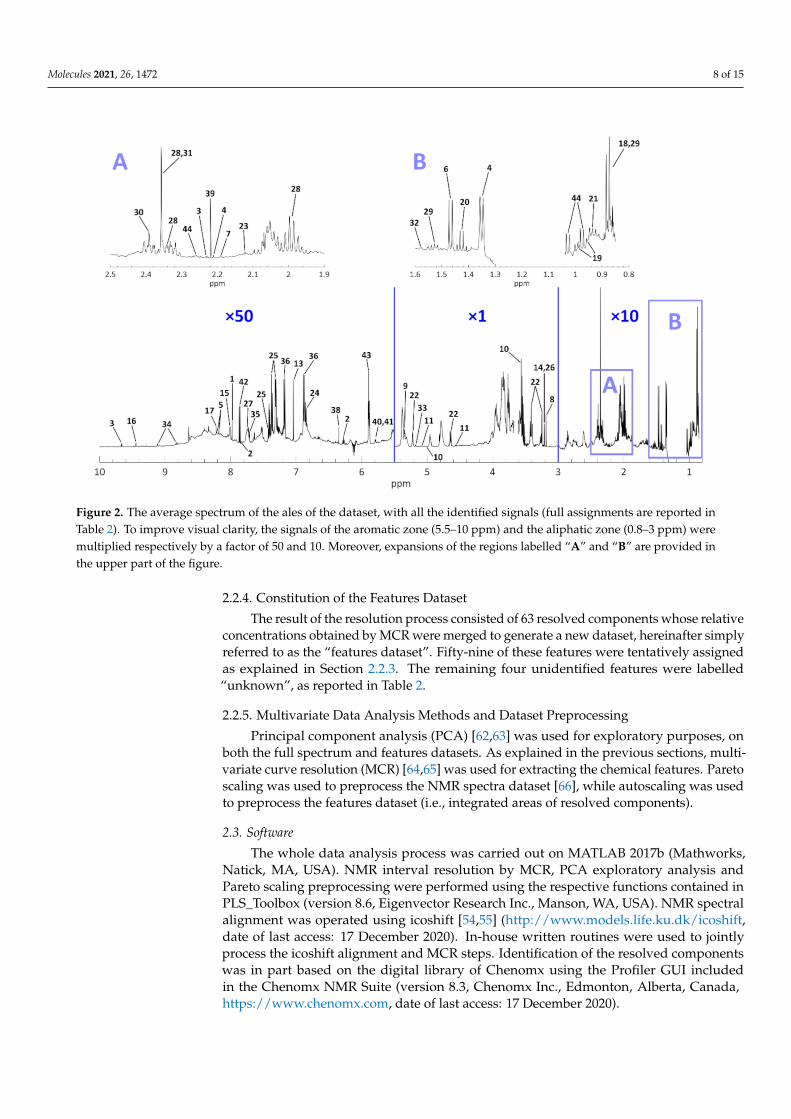
Figure 2. The average spectrum of the ales of the dataset, with all the identified signals (full assignments are reported inTable 2). To improve visual clarity, the signals of the aromatic zone (5.5–10 ppm) and the aliphatic zone (0.8–3 ppm) weremultiplied respectively by a factor of 50 and 10. Moreover, expansions of the regions labelled “A” and “B” are provided inthe upper part of the figure.
2.2.4. Constitution of the Features Dataset
The result of the resolution process consisted of 63 resolved components whose relativeconcentrations obtained by MCR were merged to generate a new dataset, hereinafter simplyreferred to as the “features dataset”. Fifty-nine of these features were tentatively assignedas explained in Section 2.2.3. The remaining four unidentified features were labelled“unknown”, as reported in Table 2.
2.2.5. Multivariate Data Analysis Methods and Dataset Preprocessing
Principal component analysis (PCA) [62,63] was used for exploratory purposes, onboth the full spectrum and features datasets. As explained in the previous sections, multi-variate curve resolution (MCR) [64,65] was used for extracting the chemical features. Paretoscaling was used to preprocess the NMR spectra dataset [66], while autoscaling was usedto preprocess the features dataset (i.e., integrated areas of resolved components).
2.3. Software
The whole data analysis process was carried out on MATLAB 2017b (Mathworks,Natick, MA, USA). NMR interval resolution by MCR, PCA exploratory analysis andPareto scaling preprocessing were performed using the respective functions contained inPLS_Toolbox (version 8.6, Eigenvector Research Inc., Manson, WA, USA). NMR spectralalignment was operated using icoshift [54,55] (http://www.models.life.ku.dk/icoshift,date of last access: 17 December 2020). In-house written routines were used to jointlyprocess the icoshift alignment and MCR steps. Identification of the resolved componentswas in part based on the digital library of Chenomx using the Profiler GUI includedin the Chenomx NMR Suite (version 8.3, Chenomx Inc., Edmonton, Alberta, Canada,https://www.chenomx.com, date of last access: 17 December 2020).
Molecules 2021, 26, 1472 9 of 15
3. Results and Discussion
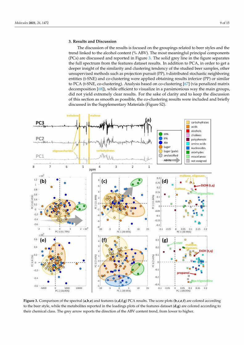
The discussion of the results is focused on the groupings related to beer styles and thetrend linked to the alcohol content (% ABV). The most meaningful principal components(PCs) are discussed and reported in Figure 3. The solid grey line in the figure separatesthe full spectrum from the features dataset results. In addition to PCA, in order to get adeeper insight of the similarity and clustering tendency of the studied beer samples, otherunsupervised methods such as projection pursuit (PP), t-distributed stochastic neighboringentities (t-SNE) and co-clustering were applied obtaining results inferior (PP) or similarto PCA (t-SNE, co-clustering). Analysis based on co-clustering [67] (via penalized matrixdecomposition [68]), while efficient to visualize in a parsimonious way the main groups,did not yield extremely clear results. For the sake of clarity and to keep the discussionof this section as smooth as possible, the co-clustering results were included and brieflydiscussed in the Supplementary Materials (Figure S2).
Figure 3. Comparison of the spectral (a,b,e) and features (c,d,f,g) PCA results. The score plots (b,c,e,f) are colored accordingto the beer style, while the metabolites reported in the loadings plots of the features dataset (d,g) are colored according totheir chemical class. The grey arrow reports the direction of the ABV content trend, from lower to higher.
Molecules 2021, 26, 1472 10 of 15
Starting from the information about the beer styles, they appear completely over-lapped when inspecting the PCA model of the full spectrum dataset, as can be seen inthe score plots of Figure 3b,e. The first three and most important components (whichcapture 76.33% of the dataset’s variance) are therefore not able to provide a clear groupingtrend related to the beer style. On the contrary, in the case of the features dataset, the beerstyle information appears rather overlapped with PC1 vs. PC2 (Figure 3c), but becomesclearer by inspecting PC1 vs. PC3 (Figure 3f). PC3 of the features dataset model is able toseparate the pale lagers (in yellow) from the lagers (in orange) and also a group of IPAs (inlight blue), which is recognizable in the lower part of the plot, at negative values on PC3.However, the lager samples (in orange) appear very overlapped with the majority of theale samples (in blue) in all the plots reported in Figure 3.
The metabolites that are responsible for grouping the pale lagers (in yellow in Figure 3f)are shown in Figure 3g, in which the PC1 vs. PC3 loadings of the features dataset are re-ported. Beers from producers such as Hite, Oriental Brewery, Heineken, Budwiser, PilsnerUrquell and San Miguel are present in this group: these are very widespread products, andtheir style generally does not involve much addition of hops or spices. These pale lagersare mainly characterized by compounds related to sugars, such as oligosaccharides and tre-halose, and malt, which is the main source of polyphenols, as 70–80% of their total amountin beer comes from malt [69]. Another important metabolite turns out to be acetaldehyde,a well-known beer flavor [20]. In addition to these compounds and coherently with theirstyle, the pale lager samples are characterized by a number of metabolites located in theopposite direction in the loadings plot, at negative PC3 scores (Figure 3g): compoundssuch as propanol and trigonelline, a compound derived from hops [43], are found to bepresent in very low amounts.
Another interesting metabolite that proves important for the pale lager samples is5-hydroxymethylfurfural (5-HMF). This compound is a known marker of beer aging [46]and since these lager samples seem to have a higher content of it, they might be more proneto fast aging than other beer styles, in the sense that their organoleptic characteristics mayalready be more deteriorated than of other beers whose content of 5-HMF is found lower.
Remarkably, in the lower part of the plot of Figure 3f, a clear group of IPAs is found,together with two ales. No correspondence with a similar grouping in the full spectrumcase could be found. These products mainly come from breweries like Mikkeller and To Ølthat tend to experiment a lot, especially using different varieties and combinations of hops.
As previously discussed, trigonelline (lower part of Figure 3g) is among the most influ-ential metabolites for distinguishing the pale lager group and the IPA group. Trigonellineis very interesting [19,43,56] and it has been recently identified in beer and described asa plant-associated metabolite whose concentration increases with boiling [43]. Hops aregenerally added right before boiling the beer wort, so that the alpha acids can be extractedfrom the raw hops and thermally isomerized into iso-alpha acids, giving the beer its charac-teristic bitter taste [70]. For these reasons, trigonelline is a metabolite that can be associatedwith hops.
Two unknown metabolites are found very close to trigonelline (Figure 3g), and furtherresearch may be needed to assess whether they are “rare compounds” which may alsoarise from hops or added spices, given their position in the loadings plot.
A clear small group of three IIPAs can be identified in both the full spectrum andfeatures datasets, as highlighted with green circles in Figure 3b,c,f. In the case of thefeatures dataset, the IIPA group can be more clearly seen by inspecting the PC1 vs. PC2score plot (Figure 3c), while in the PC1 vs. PC3 plot, the three samples are still close to eachother, but their position is not very distant from the rest of the samples: they look, therefore,more similar to the bulk of the samples. The most influential metabolites for this group,as inferred from the PC1 vs. PC2 loadings plot in Figure 3d, resulted to be ethanol, somehigher alcohols (isopentanol, isobutanol, propanol), malt-related compounds (maltose,oligosaccharides) and trigonelline. Given the beer style, which is characterized by higher
Molecules 2021, 26, 1472 11 of 15
ethanol content and stronger taste, high contents of these compounds can be expected, asthey are related to beers with strong taste and a wider flavor bouquet.
Regarding the alcohol content, a trend related to the ABV content can be identifiedin both datasets, as the grey arrows show in Figure 3b,c. It is important to notice thatthe numbers of light, medium and strong beers are rather unbalanced, with the medium(3.5–6% ABV) beers representing the large majority of the samples.
In the case of the full spectrum dataset, PC1 seems more directly related to the ABVcontent (grey arrow in Figure 3b), with the light beers located at negative scores and thestrong ones located at positive scores. The most influential spectral variables on PC1 aremainly related to the carbohydrates region (3–5.5 ppm) and, more specifically, to the signalsof maltose, trehalose and oligosaccharides (Figure 3a). However, the same signals alsohave some importance related to the other two PCs, but the loadings’ directions appearless clear.
By inspecting the results from the features dataset, it can be noticed that both PC1and PC2 describe the ABV trend (Figure 3c): the lighter samples are generally located atnegative values on both components while the strong samples are located at positive scoreson both components (Figure 3c). The metabolites mainly responsible for this trend arereported in the loadings plot in Figure 3d: in general, it appears that the stronger the beer,the higher the overall content of all metabolites, as a sort of “leading effect” related to ABV.This could be explained considering that fermentations which yield more ethanol generallylast longer and also generate more and larger varieties of compounds, i.e., a richer flavorbouquet is obtained. As expected, the most influential compounds correspond to alcohols(both ethanol and higher alcohols) and malt-related metabolites along with trigonelline, aspreviously discussed when commenting on the IIPA samples.
It is worth noting that at least six carbohydrate-related metabolites are found atnegative scores on PC2 (Figure 3d). This may be due to the fact that malt is a fundamentalingredient in the recipe for brewing beer, as its characteristics are responsible for manyflavor aspects of the final product. For instance, ale beers (including IPAs and IIPAs) areusually brewed with darker malts, whose production involves a more intense roastingtreatment that generates more intense colors and stronger taste. The lagers, on the contrary,are generally brewed with lighter malts, which yield a more bready taste and flavor to theproduct. More precise peak assignments of the carbohydrate-related variables, which arebeyond the scope of the present paper and would probably need much more information(e.g., planning a study based on 2D NMR spectra), may shine a light on potential differencesregarding the type of malt and its characteristic metabolites.
4. Conclusions
We have illustrated the potential and efficiency of using an interval-based approach,especially from the point of view of the grouping information that can be extracted from aset of NMR spectra, when properly processed. The peak-by-peak processing procedureallows considering all the interval-specific signals systematically. Since MCR modelsare built automatically, the user’s intervention is limited to defining the intervals andthen choosing between a small set of models: this can be very practical to make useof the analyst’s expertise in spectroscopy and chemistry, as well as perform a sort of“internal validation” of the actual content of chemical information while processing thedata. Moreover, it is worth noting that the approach applied in this study generallyprovides at least the same information as the traditional approach of peak identificationwithout the resolution step, but the processed information is made simpler and thereforeclearer and more easily interpretable.
This type of approach, in which chemometrics is coupled with NMR spectroscopy,provided clear insights into the composition of beer and helped shed some light on therich and complex NMR data. As a result, a rather detailed metabolomic characterizationof the set of beer samples was obtained and easily interpreted. The obtained information,together with previous studies, can be used as a basis for a better understanding of
Molecules 2021, 26, 1472 12 of 15
beer composition, especially of how the main differences and global effects due to themacroscopic characteristics of beer reflect on its characteristics at the microscopic level(i.e., relative to chemical compounds and metabolites). This approach can therefore beuseful, e.g., for producers, who may use the gathered information for further recipeoptimization aimed at meeting the consumers’ demand for interesting and innovativeproducts. This could be implemented in the form of preference mapping, e.g., using onlineconsumer evaluations.
Finally, from the point of view of signal identification and assignment, further de-velopments should focus on obtaining and validating more specific and detailed chem-ical features. For instance, information about J-coupling values or the anomerization ofoligosaccharides could be investigated by means of dedicated experimental plans and NMRexperiments (encompassing 2D and 1D TOCSY NMR acquisitions also using standardreference compounds). This also holds true with the most important metabolites that werehighlighted by our analysis.
Supplementary Materials: The following items are available online, Figure S1: Expansions of the spectralzones containing the identified signals (as reported in Table 2); Figure S2: Co-clustering results obtainedfrom the features dataset; Table S1: List of resolved intervals and related selected components.
Author Contributions: Conceptualization, M.C., R.B. and N.C.; methodology, N.C., R.B. and M.C.;software, N.C., R.B. and F.S.; formal analysis, N.C., M.C., R.B. and F.S.; resources, M.C. and R.B.; datacuration, N.C.; writing—original draft preparation, N.C.; writing—review and editing, N.C., M.C.,F.S. and R.B. All authors have read and agreed to the published version of the manuscript.
Funding: This research received no external funding.
Institutional Review Board Statement: Not applicable.
Informed Consent Statement: Not applicable.
Data Availability Statement: The data presented and analyzed in this study are available in theSupplementary Materials in the MATLAB format (.mat).
Conflicts of Interest: The authors declare no conflict of interest.
Sample Availability: Samples are not available.
References1. Thomé, K.; Soares, A.P.; Moura, J.V. Social Interaction and Beer Consumption. J. Food Prod. Mark. 2017, 23, 186–208. [CrossRef]2. Almeida, C.; Duarte, I.F.; Barros, A.; Rodrigues, J.; Spraul, A.M.; Gil, A.M. Composition of Beer by 1H NMR Spectroscopy: Effects
of Brewing Site and Date of Production. J. Agric. Food Chem. 2006, 54, 700–706. [CrossRef]3. Donadini, G.; Fumi, M.D.; Lambri, M. A preliminary study investigating consumer preference for cheese and beer pairings. Food
Qual. Prefer. 2013, 30, 217–228. [CrossRef]4. Aquilani, B.; Laureti, T.; Poponi, S.; Secondi, L. Beer choice and consumption determinants when craft beers are tasted: An
exploratory study of consumer preferences. Food Qual. Prefer. 2015, 41, 214–224. [CrossRef]5. Marongiu, A.; Zara, G.; Legras, J.-L.; Del Caro, A.; Mascia, I.; Fadda, C.; Budroni, M. Novel starters for old processes: Use of
Saccharomyces cerevisiae strains isolated from artisanal sourdough for craft beer production at a brewery scale. J. Ind. Microbiol.Biotechnol. 2015, 42, 85–92. [CrossRef] [PubMed]
6. Murray, D.W.; O’Neill, M.A. Craft beer: Penetrating a niche market. Br. Food J. 2012, 114, 899–909. [CrossRef]7. Elzinga, K.G.; Tremblay, C.H.; Tremblay, V.J. Craft Beer in the United States: History, Numbers, and Geography. J. Wine Econ.
2015, 10, 242–274. [CrossRef]8. Bevilacqua, M.; Bro, R.; Marini, F.; Rinnan, Å.; Rasmussen, M.A.; Skov, T. Recent chemometrics advances for foodomics. TrAC
Trends Anal. Chem. 2017, 96, 42–51. [CrossRef]9. Hughey, C.A.; McMINN, C.M.; Phung, J. Beeromics: From quality control to identification of differentially expressed compounds
in beer. Metabolomics 2016, 12, 11. [CrossRef]10. Donadini, G.; Fumi, M.; Kordialik-Bogacka, E.; Maggi, L.; Lambri, M.; Sckokai, P. Consumer interest in specialty beers in three
European markets. Food Res. Int. 2016, 85, 301–314. [CrossRef]11. Anderson, H.E.; Santos, I.C.; Hildenbrand, Z.L.; Schug, K.A. A review of the analytical methods used for beer ingredient and
finished product analysis and quality control. Anal. Chim. Acta 2019, 1085, 1–20. [CrossRef] [PubMed]12. Mutz, Y.S.; Rosario, D.K.A.; Conte-Junior, C.A. Insights into chemical and sensorial aspects to understand and manage beer aging
using chemometrics. Compr. Rev. Food Sci. Food Saf. 2020, 19, 3774–3801. [CrossRef] [PubMed]
Molecules 2021, 26, 1472 13 of 15
13. Duarte, I.F.; Barros, A.S.; Belton, P.S.; Righelato, R.; Spraul, M.; Humpfer, E.; Gil, A.M. High-Resolution Nuclear MagneticResonance Spectroscopy and Multivariate Analysis for the Characterization of Beer. J. Agric. Food Chem. 2002, 50, 2475–2481.[CrossRef] [PubMed]
14. Nord, L.I.; Vaag, A.P.; Duus, J.Ø. Quantification of Organic and Amino Acids in Beer by 1H NMR Spectroscopy. Anal. Chem. 2004,76, 4790–4798. [CrossRef] [PubMed]
15. Rodrigues, J.E.; Gil, A.M. NMR methods for beer characterization and quality control. Magn. Reson. Chem. 2011, 49, S37–S45.[CrossRef] [PubMed]
16. Da Silva, L.A.; Flumignan, D.L.; Tininis, A.G.; Pezza, H.R.; Pezza, L. Discrimination of Brazilian lager beer by 1H NMRspectroscopy combined with chemometrics. Food Chem. 2019, 272, 488–493. [CrossRef]
17. Jeong, J.-H.; Cho, S.-J.; Kim, Y. High-Resolution NMR Spectroscopy for the Classification of Beer. Bull. Korean Chem. Soc. 2017, 38,466–470. [CrossRef]
18. Sánchez-Estébanez, C.; Ferrero, S.; Alvarez, C.M.; Villafañe, F.; Caballero, I.; Blanco, C.A. Nuclear Magnetic Resonance Methodol-ogy for the Analysis of Regular and Non-Alcoholic Lager Beers. Food Anal. Methods 2018, 11, 11–22. [CrossRef]
19. Palmioli, A.; Alberici, D.; Ciaramelli, C.; Airoldi, C. Metabolomic profiling of beers: Combining 1H NMR spectroscopy andchemometric approaches to discriminate craft and industrial products. Food Chem. 2020, 327, 127025. [CrossRef]
20. Tian, J. Determination of several flavours in beer with headspace sampling–gas chromatography. Food Chem. 2010, 123, 1318–1321.[CrossRef]
21. Da Silva, G.A.; Augusto, F.; Poppi, R.J. Exploratory analysis of the volatile profile of beers by HS–SPME–GC. Food Chem. 2008,111, 1057–1063. [CrossRef]
22. Tian, J. Application of static headspace gas chromatography for determination of acetaldehyde in beer. J. Food Compos. Anal. 2010,23, 475–479. [CrossRef]
23. Vivian, A.F.; Aoyagui, C.T.; De Oliveira, D.N.; Catharino, R.R. Mass spectrometry for the characterization of brewing process.Food Res. Int. 2016, 89, 281–288. [CrossRef]
24. Grassi, S.; Amigo, J.M.; Lyndgaard, C.B.; Foschino, R.; Casiraghi, E. Beer fermentation: Monitoring of process parameters byFT-NIR and multivariate data analysis. Food Chem. 2014, 155, 279–286. [CrossRef]
25. Engelhard, S.; Löhmannsröben, H.-G.; Schael, F. Quantifying Ethanol Content of Beer Using Interpretive Near-Infrared Spec-troscopy. Appl. Spectrosc. 2004, 58, 1205–1209. [CrossRef] [PubMed]
26. Li, H.; Takahashi, Y.; Kumagai, M.; Fujiwara, K.; Kikuchi, R.; Yoshimura, N.; Amano, T.; Lin, J.; Ogawa, N. A ChemometricsApproach for Distinguishing between Beers Using near Infrared Spectroscopy. J. Near Infrared Spectrosc. 2009, 17, 69–76. [CrossRef]
27. Giovenzana, V.; Beghi, R.; Guidetti, R. Rapid evaluation of craft beer quality during fermentation process by vis/NIR spectroscopy.J. Food Eng. 2014, 142, 80–86. [CrossRef]
28. Klein, O.; Roth, A.; Dornuf, F.; Schöller, O.; Mäntele, W. The Good Vibrations of Beer. The Use of Infrared and UV/Vis Spectroscopyand Chemometry for the Quantitative Analysis of Beverages. Zeitschrift Naturforsch. B 2012, 67, 1005–1015. [CrossRef]
29. Biancolillo, A.; Bucci, R.; Magrì, A.L.; Magrì, A.D.; Marini, F. Data-fusion for multiplatform characterization of an italian craftbeer aimed at its authentication. Anal. Chim. Acta 2014, 820, 23–31. [CrossRef] [PubMed]
30. Gutiérrez, J.M.; Haddi, Z.; Amari, A.; Bouchikhi, B.; Mimendia, A.; Cetó, X.; Del Valle, M. Hybrid electronic tongue based onmultisensor data fusion for discrimination of beers. Sens. Actuators B Chem. 2013, 177, 989–996. [CrossRef]
31. Vera, L.; Aceña, L.; Guasch, J.; Boqué, R.; Mestres, M.; Busto, O. Characterization and classification of the aroma of beer samplesby means of an MS e-nose and chemometric tools. Anal. Bioanal. Chem. 2011, 399, 2073–2081. [CrossRef] [PubMed]
32. Vera, L.; Aceña, L.; Guasch, J.; Boqué, R.; Mestres, M.; Busto, O. Discrimination and sensory description of beers through datafusion. Talanta 2011, 87, 136–142. [CrossRef] [PubMed]
33. Sikorska, E.; Górecki, T.; Khmelinskii, I.V.; Sikorski, M.; De Keukeleire, D. Fluorescence Spectroscopy for Characterization andDifferentiation of Beers. J. Inst. Brew. 2004, 110, 267–275. [CrossRef]
34. Gordon, R.; Cozzolino, D.; Chandra, S.; Power, A.; Roberts, J.J.; Chapman, J. Analysis of Australian Beers Using FluorescenceSpectroscopy. Beverages 2017, 3, 57. [CrossRef]
35. Sikorska, E.; Khmelinskii, I.; Sikorski, M. Fluorescence methods for analysis of beer. In Beer in Health and Disease Prevention;Elsevier: Amsterdam, The Netherlands, 2008; pp. 963–976, ISBN 9780123738912.
36. Dramicanin, T.; Zekovic, I.; Periša, J.; Dramicanin, M.D. The Parallel Factor Analysis of Beer Fluorescence. J. Fluoresc. 2019, 29,1103–1111. [CrossRef] [PubMed]
37. De Juan, A.; Jaumot, J.; Tauler, R. Multivariate Curve Resolution (MCR). Solving the mixture analysis problem. Anal. Methods2014, 6, 4964–4976. [CrossRef]
38. Winning, H.; Larsen, F.; Bro, R.; Engelsen, S. Quantitative analysis of NMR spectra with chemometrics. J. Magn. Reson. 2008, 190,26–32. [CrossRef]
39. Khakimov, B.; Mobaraki, N.; Trimigno, A.; Aru, V.; Engelsen, S.B. Signature Mapping (SigMa): An efficient approach forprocessing complex human urine 1H NMR metabolomics data. Anal. Chim. Acta 2020, 1108, 142–151. [CrossRef]
40. Puig-Castellví, F.; Alfonso, I.; Tauler, R. Untargeted assignment and automatic integration of 1 H NMR metabolomic datasetsusing a multivariate curve resolution approach. Anal. Chim. Acta 2017, 964, 55–66. [CrossRef] [PubMed]
Molecules 2021, 26, 1472 14 of 15
41. Bro, R.; Kamstrup-Nielsen, M.H.; Engelsen, S.B.; Savorani, F.; Rasmussen, M.A.; Hansen, L.; Olsen, A.; Tjønneland, A.; Dragsted,L.O. Forecasting individual breast cancer risk using plasma metabolomics and biocontours. Metabolomics 2015, 11, 1376–1380.[CrossRef]
42. Carbone, K.; Macchioni, V.; Petrella, G.; Cicero, D.O. Exploring the potential of microwaves and ultrasounds in the greenextraction of bioactive compounds from Humulus lupulus for the food and pharmaceutical industry. Ind. Crop. Prod. 2020,156, 112888. [CrossRef]
43. Spevacek, A.R.; Benson, K.H.; Bamforth, C.W.; Slupsky, C.M. Beer metabolomics: Molecular details of the brewing process andthe differential effects of late and dry hopping on yeast purine metabolism. J. Inst. Brew. 2016, 122, 21–28. [CrossRef]
44. Dengis, P.B.; Nélissen, L.R.; Rouxhet, P.G. Mechanisms of yeast flocculation: Comparison of top- and bottom-fermenting strains.Appl. Environ. Microbiol. 1995, 61, 718–728. [CrossRef] [PubMed]
45. Duarte, I.F.; Godejohann, M.; Braumann, U.; Spraul, A.M.; Gil, A.M. Application of NMR Spectroscopy and LC-NMR/MS to theIdentification of Carbohydrates in Beer. J. Agric. Food Chem. 2003, 51, 4847–4852. [CrossRef]
46. Rodrigues, J.A.; Barros, A.S.; Carvalho, B.; Brandão, T.; Gil, A.M. Probing beer aging chemistry by nuclear magnetic resonanceand multivariate analysis. Anal. Chim. Acta 2011, 702, 178–187. [CrossRef] [PubMed]
47. Lachenmeier, D.W. Rapid quality control of spirit drinks and beer using multivariate data analysis of Fourier transform infraredspectra. Food Chem. 2007, 101, 825–832. [CrossRef]
48. Rodrigues, J.A.; Erny, G.L.; Barros, A.S.; Esteves, V.I.; Brandão, T.; Ferreira, A.A.; Cabrita, E.; Gil, A.M. Quantification of organicacids in beer by nuclear magnetic resonance (NMR)-based methods. Anal. Chim. Acta 2010, 674, 166–175. [CrossRef]
49. Duarte, I.F.; Barros, A.S.; Almeida, C.; Spraul, M.; Gil, A.M. Multivariate Analysis of NMR and FTIR Data as a Potential Tool forthe Quality Control of Beer. J. Agric. Food Chem. 2004, 52, 1031–1038. [CrossRef] [PubMed]
50. Gil, A.M.; Duarte, I.F.; Godejohann, M.; Braumann, U.; Maraschin, M.; Spraul, M. Characterization of the aromatic composition ofsome liquid foods by nuclear magnetic resonance spectrometry and liquid chromatography with nuclear magnetic resonance andmass spectrometric detection. Anal. Chim. Acta 2003, 488, 35–51. [CrossRef]
51. Lachenmeier, D.W.; Frank, W.; Humpfer, E.; Schäfer, H.; Keller, S.; Mörtter, M.; Spraul, M. Quality control of beer using high-resolution nuclear magnetic resonance spectroscopy and multivariate analysis. Eur. Food Res. Technol. 2005, 220, 215–221.[CrossRef]
52. Savitzky, A.; Golay, M.J.E. Smoothing and Differentiation of Data by Simplified Least Squares Procedures. Anal. Chem. 1964, 36,1627–1639. [CrossRef]
53. Savorani, F.; Rasmussen, M.A.; Rinnan, Å.; Engelsen, S.B. Interval-Based Chemometric Methods in NMR Foodomics. In DataHandling in Science and Technology; Ruckebusch, C., Ed.; Elsevier: Amsterdam, The Netherlands, 2013; pp. 449–486, ISBN 978-0-444-63638-6.
54. Savorani, F.; Tomasi, G.; Engelsen, S.B. icoshift: A versatile tool for the rapid alignment of 1D NMR spectra. J. Magn. Reson. 2010,202, 190–202. [CrossRef]
55. Savorani, F.; Tomasi, G.; Engelsen, S.B. Alignment of 1D NMR Data using the iCoshift Tool: A Tutorial. In Magnetic Resonance inFood Science: Food for Thought; van Duynhoven, J., Belton, P.S., Webb., G.A., van As, H., Eds.; Royal Society of Chemistry: London,UK, 2013; pp. 14–24, ISBN 978-1-84973-634-3.
56. Metrulas, L.K.; McNeil, C.; Slupsky, C.M.; Bamforth, C.W. The application of metabolomics to ascertain the significance ofprolonged maturation in the production of lager-style beers. J. Inst. Brew. 2019, 125, 242–249. [CrossRef]
57. Khatib, A.; Wilson, E.G.; Kim, H.K.; Lefeber, A.W.; Erkelens, C.; Choi, Y.H.; Verpoorte, R. Application of two-dimensionalJ-resolved nuclear magnetic resonance spectroscopy to differentiation of beer. Anal. Chim. Acta 2006, 559, 264–270. [CrossRef]
58. Tian, J.; Yu, J.; Chen, X.; Zhang, W. Determination and quantitative analysis of acetoin in beer with headspace sampling-gaschromatography. Food Chem. 2009, 112, 1079–1083. [CrossRef]
59. Wishart, D.S.; Knox, C.; Guo, A.C.; Eisner, R.; Young, N.; Gautam, B.; Hau, D.D.; Psychogios, N.; Dong, E.; Bouatra, S.; et al.HMDB: A knowledgebase for the human metabolome. Nucleic Acids Res. 2009, 37, D603–D610. [CrossRef]
60. Viant, M.R.; Kurland, I.J.; Jones, M.R.; Dunn, W.B. How close are we to complete annotation of metabolomes? Curr. Opin. Chem.Biol. 2017, 36, 64–69. [CrossRef] [PubMed]
61. Sumner, L.W.; Amberg, A.; Barrett, D.; Beale, M.; Beger, R.; Daykin, C.A.; Fan, T.W.M.; Fiehn, O.; Goodacre, R.; Griffin, J.L.; et al.Proposed minimum reporting standards for chemical analysis. Chemical Analysis Working Group (CAWG). MetabolomicsStandards Initiative (MSI). Metabolomics 2007, 3, 211–221. [CrossRef]
62. Wold, S.; Esbensen, K.; Geladi, P. Principal component analysis. Chemom. Intell. Lab. Syst. 1987, 2, 37–52. [CrossRef]63. Bro, R.; Smilde, A.K. Principal component analysis. Anal. Methods 2014, 6, 2812–2831. [CrossRef]64. De Juan, A.; Tauler, R. Multivariate Curve Resolution (MCR) from 2000: Progress in Concepts and Applications. Crit. Rev. Anal.
Chem. 2006, 36, 163–176. [CrossRef]65. Rutan, S.C.; de Juan, A.; Tauler, R. Introduction to Multivariate Curve Resolution. In Comprehensive Chemometrics; Elsevier:
Amsterdam, The Netherlands, 2009; pp. 249–259, ISBN 9780444527011.66. Euceda, L.R.; Giskeødegård, G.F.; Bathen, T.F. Preprocessing of NMR metabolomics data. Scand. J. Clin. Lab. Investig. 2015, 75,
193–203. [CrossRef] [PubMed]67. Bro, R.; Papalexakis, E.E.; Acar, E.; Sidiropoulos, N.D. Coclustering-a useful tool for chemometrics. J. Chemom. 2012, 26, 256–263.
[CrossRef]

Molecules 2021, 26, 1472 15 of 15
68. Witten, D.M.; Tibshirani, R.; Hastie, T. A penalized matrix decomposition, with applications to sparse principal components andcanonical correlation analysis. Biostatistics 2009, 10, 515–534. [CrossRef] [PubMed]
69. Quifer-Rada, P.; Vallverdú-Queralt, A.; Martínez-Huélamo, M.; Chiva-Blanch, G.; Jáuregui, O.; Estruch, R.; Lamuela-Raventós, R.A comprehensive characterisation of beer polyphenols by high resolution mass spectrometry (LC-ESI-LTQ-Orbitrap-MS). FoodChem. 2015, 169, 336–343. [CrossRef]
70. Steenackers, B.; De Cooman, L.; De Vos, D. Chemical transformations of characteristic hop secondary metabolites in relation tobeer properties and the brewing process: A review. Food Chem. 2015, 172, 742–756. [CrossRef]