a mathematical model to simulate small boat
TRANSCRIPT
A MATHEMATICAL MODEL TO SIMULATE
SMALL BOAT BEHAVIOUR
Andrew Wilford Browning, BSc (Hons)
Submitted in partial fulfilment of the requirements
for the degree of Doctor of Philosophy under the
conditions for the award of higher degrees of the
Council for National Academic Awards.
October 1990
BOURNEMOUTH POLYTECHNIC
In collaboration with:
CETREK, (MARINEX INDUSTRIES LIMITED), POOLE, DORSET
1
1
2
3
4
5
6
Contents
Chapter Page
Acknowledgements 5
Abstract
6
Introduction 7
1.01 The Thesis
8
Literature Review 14
2.01 Historical Background
15
2.02 The Advent Of The Digital Computer 16
2.03 The Literature
17
2.04 The Initiators Of Ship Modelling
20
2.05 UK Establishments
28
2.06 Scandinavian And European Research 44
2.07 America
52
2.08 Japan
58
2.09 Other Countries
61
2.10 Additional
61
Automatic Control Of Boats
63
3.01 Introduction
64
3.02 PID Control
66
3.03 Autopilot Gains
72
Motion Of A Boat In A Seaway
74
4.01 Introduction
75
4.02 Definition Of A Rigid Body
78
4.03 The Six Degrees-Of-Freedom Of A
Boat
4.04 The Axes Systems
4.05 Transformation Between Orthogonal
Axes
85
Approach To The Mathematical Model
112
5.01 Modularity
113
5.02 The Division Of The Forces
115
Equations Of Motion Of A Small Boat
117
6.01 Newton's Law Of Motion
118
6.02 Inertia Tensor
118
81
84
2

6.03 Expanding Newton's Second Law
124
6.04 Added Mass
129
6.05 Added Mass Coefficients For An
Ellipsoid
140
6.06 Methods Of Determining The Added
Mass Coefficients
144
6.07 The Mass Equations
146
6.08 The Dynamic Forces & Moments
150
6.09 The Hydrodynamic Forces & Moments 153
6.10 The Restoring Forces & Moments
161
6.11 The Rudder Forces & Moments
185
6.12 The Propeller Forces & Moments
201
6.13 The Trim Tabs Forces & Moments
207
6.14 The Wind Forces & Moments
210
6.15 The Wave Forces & Moments
215
6.16 The Sea Inertia Forces & Moments
231
6.17 The Overall System
232
6.18 The MethodOf Integration
234
7 Parameter Determination And Measurement
243
7.01 Model Verification And Validation 244
7.02 Boat Trials
245
7.03 Parameter Estimation
252
7.04 Tank Testing Techniques
265
7.05 Standard Manoeuvres
273
8 Results 280
8.01 Real And Simulated Data
281
8.02 Turning Circle Plots
282
8.03 Kempf Manoeuvre Plots
285
9 Strategy For Testing Autopilots
288
9.01 Communicating With The Autopilot
289
9.02 Graphical Representation
294
9.03 Autopilot Control Of The Model
296
10 Conclusions
301
11 Suggested Further Research
305
3
Appendix
A Principal Dimensions Of An Arun
B Plots
C The Data Logging Interface
D Glossary
E Nomenclature
F Conversion Table
G References
H Abbreviations
I Colophon
Page
310
313
349
362
367
374
377
398
401
4
Acknowledgements
The author wishes to express his thanks and gratitude
to a number of people who have given of their time and
resources to support the research of this thesis.
To Mr Alan Potton, Director of Studies, and Mr John
Reynolds, Project Supervisor, both of the Dorset
Institute, for their aid in academic matters relating to
the presentation and content of the thesis.
To Dr Walter Randolph, Technical Director at Cetrek,
and Mr Peter Thomasson, of Cranfield College of
Aeronautics, both of whom are Project Supervisors, for
their invaluable contributions and suggestions
throughout the research.
To the Directors at Cetrek for their financial support.
To Mr F.D.Hudson, Chief Technical Officer, and Mr
Stuart Welford, Research and Development Manager, both
of the Headquarters of the Royal National Lifeboat
Institution in Poole, for their generosity and aid in
recording sea trials.
To Mr David Winwood, Technical Manager at Cetrek for
his aid in matters concerning the autopilot.
To Mr Sa'ad Medhat, Manager of the Electronics
Industrial Unit at the Dorset Institute, for the use of
computer equipment and work space.
The author's greatest thanks go, of course, to his
parents, parents-in-law and especially his wife Alison,
for their support, encouragement' and understanding
especially during the writing up of the thesis.
5
Abstract
A Mathematical Model To Simulate Small Boat Behaviour
A.W. Browning
The use of mathematical models and associated computersimulation is a well established technique forpredicting the behaviour of large marine vessels. For avariety of reasons, mainly related to effects of scale,existing models are unable to adequately predict themanoeuvring characteristics of smaller vessels. Theaccuracy with which the performance of a boat underautopilot control can be predicted leaves much to bedesired. The thesis provides a mathematical model tosimulate small boat behaviour and so can assist with thedesign and testing of marine autopilots.
The boat model is presented in six degrees-of-freedom,which, with suitable wave disturbance terms, allowsmotions such as broaching to be analysed. Instabilitiesin the performance of an autopilot arising from such seainduced yaw motions can be assessed with a view toimproving the control algorithms and methodology.
The traditional "regressional" style models used forlarge ships are not suitable for a small boat modelsince there exist numerous small boat types and diversehull shapes. Instead, a modular approach has beenadopted where individual forces and moments arecategorised in separate sections of the model. Thisapproach is still in its infancy in the field of marinesimulation. The modular concept demands a clearerunderstanding of the physical hydrodynamic processesinvolved in the boat system, and the formulation ofequations which do not rely solely upon approximationsto, or multiple regression of, data from sea trials.Although many hydrodynamic coefficients have beenintroduced into the model, a multi-variable Taylorseries expansion of the states about some equilibriumcondition has been avoided, since this would infer anapproximation to have been made, and the higher orderterms rapidly become abstract in their nature anddifficult to relate to the real world.
The research rectifies the glaring omission of a smallboat mathematical model, the framework of which could beexpanded to encompass other marine vehicles. Additionalforces and moments can be appended to the model in newmodules, or existing modules modified to suit newapplications. Much more work, covering a greater rangeand fidelity, is required in order to provide equationswhich accurately describe the true physical situation.
6

CHAPTER 1
INTRODUCTION
1.01 The Thesis
With the ever expanding small boat market and
specialised interest in racing boats coupled with the
increase in the navigation and marine control
electronics industry which supports this market, there
is now a need for a suitable mathematical model capable
of simulating small boat (those with a length of less
than 30 metres) manoeuvres. The requirement for a
facility to assess the performance of autopilots used to
guide small boats has been identified since the accuracy
of prediction so far leaves much to be desired.
Due mainly to the effects of scale and to simplifying
assumptions incorporated into large ship models, these
prove incapable of accurately simulating small boat
manoeuvres, especially in a seaway. A literature search
revealed that whilst there is a wealth of large ship
information, there is a disturbing absence of small boat
publications and trials data. At present virtually all
large ship simulators are restricted to the horizontal
motions of surge, sway and yaw, though there are a few
instances where roll motions are considered in tight
turns to form a four degrees-of-freedom model. Without
the coupled effects of pitch and roll in a seaway it is
not possible to study effects such as broaching which
can cause the autopilot great problems. It has been
8
subjectively suggested by boat owners that the
performance of autopilots diminishes in following seas
and theoretically it is possible, under conditions of
synchronism, that the rudder commands from the autopilot
can become out of phase with the position that the
rudder should attain to reduce the yaw created.
No large ship simulators to date are capable of
predicting such sea induced motions. Some simulators,
where complex graphics and motion platforms exist,
incorporate sea conditions as cues to the mariner only.
Most ship simulators include tidal effects, but
otherwise tend to concentrate on shallow water effects
for berthing manoeuvres within port limits. Since the
draft of small boats is far smaller and the turning
ability much greater than that of large ships, these
effects are of much less importance to a small boat
model. Instead it is the motion in and induced by a
seaway that requires analysis and inclusion in a small
boat model, especially as the final simulation is to be
used under autopilot control.
Large ship simulator models are based upon a
multi-variable Taylor series expansion of the forces and
moments about some initial equilibrium condition. Such
an approach is deemed unacceptable for small boat
modelling for the following reasons:
9
1) Deviations from the equilibrium condition introduce
inaccuracies or require complete re-computation of
the model;
2) Theoretically an infinite number of terms will be
generated, although in practice higher order terms
will be discarded;
3) Relating the coefficients produced to the physical
characteristics of the vessel becomes extremely
abstract in nature for most terms above the second
order;
4) Assessing or evaluating the coefficients is far from
easy since many of the terms are difficult to isolate
during tests. Instead multiple regression techniques
are often employed on ship trials data. This provides
a model which fits the data well, but will the
parameters take on their true values?
5) It is difficult to apply this method on a general
basis to small craft where there is an enormous
number of different hull shapes and types. Unlike the
large ship situation where models are often designed
for specific ship types and since most ships tend to
have high block coefficients at their midships
section.
10
6) Theoretical and empirical formulae based on
experimental tests can usually provide sufficient
accuracy, as demonstrated by Japanese researchers
(Ref.75)
Instead of the Taylor series expansion, a more reasoned
approach will be adopted in an attempt to provide
equations which contain terms which have conceptual
meanings.
Since all three rotations of roll, pitch and yaw are to
be considered, it is necessary to determine the attitude
of the boat at any given time interval. This thesis
draws upon techniques utilised in aircraft simulators to
monitor the Euler angles based upon the boat's angular
velocities. The particular method can also provide time
savings as well as remove the possibility of a
singularity.
With sufficient data pertaining to the righting moments
of a boat, in particular the locus of the centre of
buoyancy, there is no reason why this mathematical model
cannot be used, if so desired, to assess the capsizing
of a boat. This is particularly relevant since the boat
used for validation purposes happens to be an Arun class
Royal National Lifeboat. For any other type of boat, or
ship, additions may have to be made in order to account
11
for flooding of decks et cetera.
This research will help rectify the glaring omission of
a small boat mathematical model, the framework of which
could be used to provide ship models with more
meaningful and accurate equations. The modular approach
will enable additional forces and moments due to, for
example, thrusters on tugs, to be easily incorporated
within the model without the need to recompute all the
other modules. The performance of small boat autopilots
can be assessed at the development stage and
improvements made to counteract instabilities such as
broaching.
The novelty and originality of this project lies in the
following facts:
1) There is no established model capable of accurately
simulating small boat manoeuvres;
2) virtually all present ship models assume calm water
conditions; the remainder consider only wave drifting
and tidal effects. Since small boats are much more
affected by sea conditions than large vessels, much
finer detail on wave forces and moments is required
for small boat modelling;
12
3) Of all the ship models based upon traditional
methods none include equations for all six
degrees-of-freedom and most are limited to four
degrees-of-freedom. Whilst the horizontal motions of
a ship, plus the effects of roll in tight turns, are
sufficient for large vessel simulation, pitch must be
included in order to model wave induced motions like
broaching and trim due to the use of trim tabs;
4) The boat model will be used as a tool to highlight
areas of poor autopilot performance. Improvements
made to the autopilot control system can then be
re-assessed at the development stage.
It is worth noting that many of the additions proposed
for the small boat model will remain valid for the large
ship counterparts and can provide additional accuracy to
such models. The inclusion of heave, for instance, could
aid the study of squat on encountering shallow water and
sinkage on entering less saline water. The framework of
the model is designed to be of a flexible nature so that
upgrades, additions or alterations can be easily made by
tackling the individual module concerned rather than the
entire model. This sort of approach is still in its
infancy in the field of marine simulation.
13

CHAPTER 2
LITERATURE REVIEW
14
2.01 Historical Background
The origins of ships and the science of sailing was
first founded by the ancient Egyptian civilisation who
built boats for the purposes of trade and travel up and
down the Nile river. The variety of craft at this early
stage was based upon the owner's requirements and little
thought was given to their stability and handling.
The Phoenicians advanced the art of shipbuilding as
they explored beyond the horizon to fetch cargoes back
to Tyre and Sidon. By Roman times ships were designed
with holds to store cargo capacities of 250 tons and
ship length increased to 30 metres. Different designs
emerged from other parts of the world dependent on the
local civilisation and sea conditions. The Vikings, for
instance, who were perpetually at war with the North
Sea, built their beamy longships.
Through the centuries ships, with their sails and rigs,
evolved. As the European countries expanded their
empires and established long distance trade routes
spanning the globe, so bigger and faster ships were
built. It became possible to furnish ships with weighty
cannons and navies wrested for sea-power.
Technology marched on and by the end of the nineteenth
15
century wooden sailing ships began to give way to iron
and steel hulls and steam engines. This new era in ship
history provided greater cargo capacities and required
less manning. With the dramatic increase in ship length
that the strength of steel allowed, was born the quest
for an understanding and eventual prediction of the
characteristics, manoeuvrability and design criteria of
ships.
2.02 The Advent Of The Digital Computer
The introduction of the computer, with its insatiable
appetite for processing large quantities of numerical
data, allowed theoretical equations of ship dynamics to
be implemented in prediction models. The possibilities
that the computer opened up created the need to model
ship motions. Initially entire mainframes were given
over to providing ship simulators used almost entirely
for training purposes. As computing power became
compressed into desktop units and work stations, so
mathematical models grew in complexity and their role
changed to include research work.
The Japanese used computers extensively to optimise the
performance of onboard control systems. Their "efficient
ship" programme launched, in August 1980, the 1600 tons
"Shinaitoku Maru" with, among other things, its hinged,
16
rigid, computer controlled sail.
The scope and usage of the computer for marine training
and research has expanded in all directions. Many
countries and institutions are currently involved in a
variety of different projects incorporating ship
simulation and automatic guidance control. The following
literature review is aimed at giving the reader a taste
of some of the establishments and work ongoing in the
marine field. The author apologises for the brevity of
the description given for many of the texts reviewed,
but, as will soon be appreciated, the number of
institutions and areas of research are extensive.
2.03 The Literature
There exist numerous maritime research establishments
and societies in many countries of the world, especially
those steeped in marine history. A great wealth of
books, technical papers, transcripts and so on provide
hydrodynamists and those involved in ship simulation
with a vast quantity and variety of reference material.
However, virtually all of this information is concerned
with large ocean-going vessels. Literature searches
conducted at the start of this project showed a
disturbing lack of published data on small boat
modelling, simulation and parameter measurement.
17
The literature within the marine simulation field
covers all aspects of the ship system. Some papers
present mathematical models to predict ship manoeuvres
in the horizontal plane, incorporating the motions of
surge, sway and yaw. Later texts have also included
effects of roll, whilst some research has investigated
the combination of roll and pitch or roll and heave
motions as separate entities. Other material tackles and
concentrates on a specific section of the ship system,
for example the characteristics of the rudder,
propeller, stabilising fins or other appendages.
The dynamics of a variety of ship hull types is well
documented and research into the effects of wind and
wave drifting forces and moments also appear in
publication. A few technical papers describe a "one off"
or specific type of marine vehicle, such as hydrofoils,
ROVs (Remotely Operated underwater Vehicles) and oil
rigs. From the results, each model would seem to
satisfactorily suit its application.
Another area of research, particularly in the
Netherlands and Scandinavian countries, is the
investigation into improved automatic control of ships,
especially roll reduction on warships by use of the
rudder and fins.
18
The majority of papers which describe the
manoeuvrability of large ships are limited to the three
degrees-of-freedom in the horizontal plane, namely:
surge, sway and yaw. These provide adequate models in
open, calm water since large vessels are little affected
by small seas. Later extensions to such models has meant
the inclusion of roll motions. The primary reason for
this is the ability to study high speed container
carriers, roll-on/roll-off ships et cetera which exhibit
large angles of heel during turns.
The major application for ship mathematical models is
for incorporation within some form of simulator. The
requirements of simulators fall under the two headings
of training and research.
Training purposes include: shipboard training for
masters tickets et cetera, ship handling appreciation
and familiarisation, passage planning and bridge team
work, practising port approach manoeuvres and system
failure procedures.
Research purposes include: determining changes or
additions to the collision avoidance rules, assessing
the effectiveness of existing or proposed vessel traffic
systems or traffic routing schemes, marine law and
policy research including allocation of blame in marine
19
catastrophes, performing ship manoeuvrability studies at
the initial design• stage prior to commencing
construction, analysing the behaviour of ships in canals
and other confined waterways, in conjunction with fluid
flow models to assess changes to port design and layout
before dredging, and human factors research.
Simulators such as those at the University of Wales
Institute of Science and Technology and at Plymouth
Polytechnic provide complete bridge layout facilities
for use in both training courses and research projects.
The visual displays and bridge instruments respond to
the computed ship motion giving fully interactive
systems.
Additional uses of mathematical models of ships include
adaptive, model reference, control algorithms which are
designed to either achieve accurate course-keeping when,
for example, within port approaches, or to optimise fuel
usage.
2.04 The Initiators Of Ship Modelling
Lamb, 1879 (Ref.86), is regarded as the "classical"
text on hydrodynamics and as this field has widened in
its practical application, so Lamb has revised and
extended his book a number of times. In the sixth
20
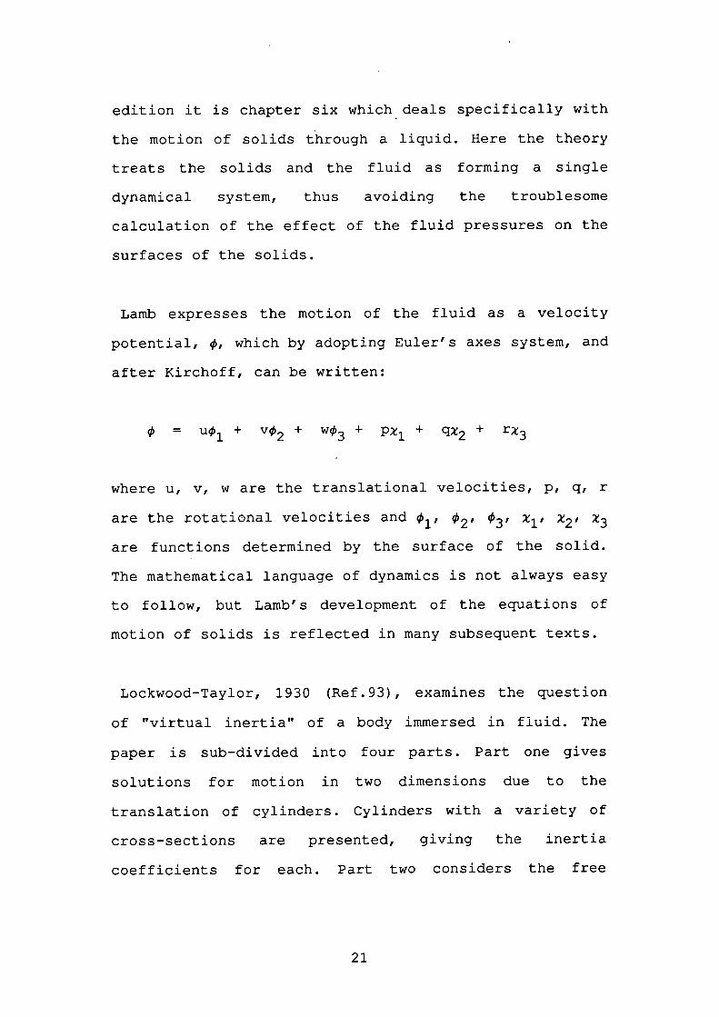
edition it is chapter six which deals specifically with
the motion of solids through a liquid. Here the theory
treats the solids and the fluid as forming a single
dynamical system, thus avoiding the troublesome
calculation of the effect of the fluid pressures on the
surfaces of the solids.
Lamb expresses the motion of the fluid as a velocity
potential, , which by adopting Euler's axes system, and
after Kirchoff, can be written:
= u 1 + vØ2 + w 3 + pX1 + qx2 + r3
where u, v, w are the translational velocities, p, q, r
are the rotational velocities and ' 2' x1, x2 X3
are functions determined by the surface of the solid.
The mathematical language of dynamics is not always easy
to follow, but Lamb's development of the equations of
motion of solids is reflected in many subsequent texts.
Lockwood-Taylor, 1930 (Ref.93), examines the question
of "virtual inertia" of a body immersed in fluid. The
paper is sub-divided into four parts. Part one gives
solutions for motion in two dimensions due to the
translation of cylinders. Cylinders with a variety of
cross-sections are presented, giving the inertia
coefficients for each. Part two considers the free
21
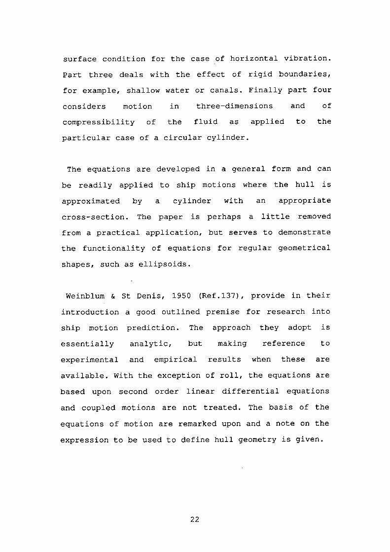
surface condition for the case •of horizontal vibration.
Part three deals with the effect of rigid boundaries,
for example, shallow water or canals. Finally part four
considers motion in three-dimensions and of
compressibility of the fluid as applied to the
particular case of a circular cylinder.
The equations are developed in a general form and can
be readily applied to ship motions where the hull is
approximated by a cylinder with an appropriate
cross-section. The paper is perhaps a little removed
from a practical application, but serves to demonstrate
the functionality of equations for regular geometrical
shapes, such as ellipsoids.
Weinblum & St Denis, 1950 (Ref.137), provide in their
introduction a good outlined premise for research into
ship motion prediction. The approach they adopt is
essentially analytic, but making reference to
experimental and empirical results when these are
available. With the exception of roll, the equations are
based upon second order linear differential equations
and coupled motions are not treated. The basis of the
equations of motion are remarked upon and a note on the
expression to be used to define hull geometry is given.
22
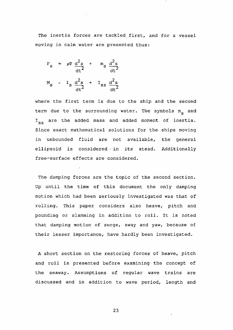
The inertia forces are tackled first, and for a vessel
moving in calm water are presented thus:
F = pVd2s + m d2sS-
M = I d2s + I ds
S 5 SS
where the first term is due to the ship and the second
term due to the surrounding water. The symbols m 5 and
are the added mass and added moment of inertia.
Since exact mathematical solutions for the ships moving
in unbounded fluid are not available, the general
ellipsoid is considered in its stead. Additionally
free-surface effects are considered.
The damping forces are the topic of the second section.
Up until the time of this document the only damping
motion which had been seriously investigated was that of
rolling. This paper considers also heave, pitch and
pounding or slamming in addition to roll. It is noted
that damping motion of surge, sway and yaw, because of
their lesser importance, have hardly been investigated.
A short section on the restoring forces of heave, pitch
and roll is presented before examining the concept of
the seaway. Assumptions of regular wave trains are
discussed and in addition to wave period, length and
23
velocity, observations on wave •height or steepness and
wave profile are made. A number of pages are given to
the exciting forces in all six degrees of freedom. Then
additional sections deal with secondary effects, free
oscillations, forced oscillations and the stabilisation
of motions. The text is very readable and gives a
complete overview of the motion of ships at sea.
Weinbium, 1952 (Ref.138), presented the original paper
in German at Hamburg and this reference is the English
version as a DTMB report. Prior to this report, the
subject of hydrodynamic mass (or added mass) had been
somewhat neglected and this study gives a review of the
extent of the understanding of this topic at that point
in time. The paper begins with the assumption of a
"Kelvin flow field" that the fluid is ideal and extends
infinitely in all directions. Much of Lamb is
recapitulated and the notation of a hydrodynamic mass
tensor is used. In section two on free surface, the
addition of boundary conditions are recounted when the
fluid cannot be assumed to extend to infinity. Vertical
translations, horizontal translations and oscillations,
such as roll, of a body floating in the fluid are
considered. Finally the influence of viscosity is
mentioned briefly. The report concludes that only few
solutions for some simple kinds of motion are known.
24
Other earlier texts include Milne-Thomson, 1955
(Ref.109), which can be regarded as a parallel text to
Lamb. John, 1949 (Refs.78 & 79), who presents two papers
on the motion of floating bodies. However, as
demonstrated by the periodical they appeared in, the
mathematics is pure and often beyond the ability of
many. Peters & Stoker, 1957 (Ref.119) who develop
mathematical theories for three basic hull forms.
Kaplan, 1966 (Ref.81), who considers the problem of
non-linear ship rolling motion in a random seaway.
Abkowitz, 1964 (Ref.2), forms a firm foundation for the
study of ship hydrodynamics, steering and
manoeuvrability. The forces and moments acting on a body
are presented as functions of the properties of the
body, the properties of the motion and the properties of
the fluid. Although the concept of six degrees of
freedom is discussed, only the three horizontal motions
of surge, sway and yaw are presented. The equations are
designed to describe the "shape" of a ship and use a
dimensionalising (or scaling) term which is a function
of the length, breadth, draft and block coefficient of
the vessel.
A Taylor series expansion of a function of several
variables about a chosen initial equilibrium condition
is used to express the forces and moments. A set of
25
terms known as the hydrodynamic coefficients results,
many of which, especially the dynamic response terms of
second order smallness, are sufficiently small that they
are either assumed zero or neglected. The number of
terms in the expansion determines the accuracy and by
limiting it to the first order terms, the well known
linearised expansion is obtained. Strom-Tejsen, 1965
(Ref.127) shows that the linearised equation of motion
for surge using straight ahead motion at constant speed
with rudder amidships as the equilibrium condition can
be written:
X = X + X 1u + X v + X r + X • u + X•v + X . r + XU V r u V r
Linear or Quasi-Non-Linear models perform adequately
for small perturbations from the equilibrium state, but
deviate from the true ship motion when larger variations
occur. In order to overcome the limitations of the
linear model when performing manoeuvres such as tight
turns with large angles of rudder (typically greater
than 10 ° ), it is necessary to include higher order terms
from the Taylor series. The non-linear surge equation,
including terms of third order, is of the form:
26
X = X + [X u + X v + X r + X'ii + X.'T + X• + X 3]
+! [xu2 +x 2 + .... +
2X uv + 2X Aur + •... + 2X .]
uv ur r+ [x u3+X3! uuu vvv
3X uv + 3X u2r + .... + 3X . +uuv uur r&3
6X uvr + 6X • uvu + •... + 6x .. s5]uvr uvu vr5
where the dots indicate similar terms in functions of u,
v, r and .
Although, as Abkowitz demonstrates, many of these terms
can be neglected, due to symmetry about the xz-plane et
cetera, it soon becomes obvious that producing a Taylor
series expansion leads to an enormous number of
coefficients which are neither easy to relate to the
physical characteristics of the ship nor isolate for
evaluation purposes when conducting model tests.
Before the powerful digital microcomputers had fully
established themselves, research work by Bech &
Wagner-Smitt, (Ref.23) 1969, used analogue simulation to
model ship manoeuvres in response to rudder action and
external disturbances. This provided a useful tool to
study ship manoeuvrability and autopilot development.
27
2.05 UK Establishments
BMT (British Maritime Technology) at Teddington is
among the leading UK centres for mathematical modelling
of ship manoeuvres for use in simulators. BMT originated
as the Ship Division of the NPL (National Physical
Laboratory) and is most often recalled for Barnes
Wallis' bouncing bomb experiments. Early in the 1970's
the NPL Ship Division moved into the area of ship
manoeuvring simulation with the express desire to
produce a mathematical model capable of representing a
wide range of ship types. The NPL Ship Division later
became NMI (National - Maritime Institute) and
subsequently, due to privatisation, NMI Ltd. in October
1982. A final name change to BMT occurred after 1984.
The simulation models developed were designed to
utilise the experimental facilities which exist at BMT,
thus assuring that model parameters can be extracted
from tank test measurements. Lewison, 1973 (Ref.91),
formulated the initial ship manoeuvring model which,
although taking account of speed loss in turns and
non-linearities in the motions, only allowed for
conditions where the ship has a forward speed with its
propeller in the ahead regime and was restricted to
comparatively small drift angles (±20°).
28
Gill, 1976 (Refs.60 & 61), suggested additions to the
model to remedy the deficiencies. By 1980 the so-called
"cruising speed" model was emended to the point where
only the limitation of ±200 drift angle existed. Until
at least 1984 these equations were used in all of the
major UK simulators.
Coupled with the success of this model came a demand
for simulations capable of predicting berthing and other
low speed manoeuvres where no drift angle limitations
could be accepted. A further model named the "low-speed"
model was developed by Barratt, 1981 (Ref.22). The
forces and moments had to be non-dimensionalised in a
different manner from the previous models in order to
avoid the low• speed instabilities at zero speed.
Three additional algorithms were added to the model and
as a result shallow water effects, ship-to-ship
attractions, wave induced drift and forces from tugs and
mooring lines could be incorporated in simulations.
Due to the troublesome nature of switching between the
low speed and cruising speed models when going between
port and sea, research at BMT since 1982 has centred on
the requirement for a single modular model where the
rudder, propeller and hull each form their own separate
model rather than being part of an overall global model.
The approach allowed the large amount of hull and
29
propeller data already collected at BMT to be exploited
and catered for both ' cruising speeds and large drift
angle manoeuvring regimes.
Other work, in conjunction with the College of
Aeronautics at Cranfield and initiated by the UK
Department of Energy (Ref.89), has branched into the
realm of ROy's (Remotely Operated underwater Vehicles)
with their increased use in the offshore industry for
surveying of the seabed. Here all six degrees of freedom
will be required with modules for umbilical
hydrodynamics which, on long umbilicals, can cause
performance inhibiting drag .. A more detailed history of
BMT can be gleaned from Dand & Reynolds, 1984 (Ref.42).
More recently, Khattab, 1987 (Ref.82), presented the
latest developments to the BMT model. A real time
simulation of ship handling in harbours is implemented
on a hybrid computer and provides a facility to
investigate manoeuvring capabilities of ships in a given
harbour configuration and under specified environmental
conditions. The model consists of a set of modules which
allow changes in vessel type and harbour layout to be
implemented. A good agreement between estimation data
and real data is shown and the simulation of M.V.Belard
in Ardrossan harbour is demonstrated.
30
BSRA (British Ship Research Association) at Walisend,
Tyne and Wear (which recently became part of BMT) is
another long established UK centre for research into all
aspects of ship design, materials and manoeuvring
models. Technical reports produced at BSRA range from
studies of marine fouling organisms through the welding
of higher tensile shipbuilding steels to simulation
studies of autopilot performance. The spectrum of work
undertaken covers virtually all components of the ship
system and is closely allied to the once great shipyards
of the north-east of England.
Clarke, who has been working at BSRP on problems
associated with ship dynamics, posed the question, 1982
(Ref.39), "Do autopilots save fuel?". This paper points
out that whilst automatic course control of ships has
been possible for many years, the availability of small,
powerful microcomputers has given rise to a new class of
adaptive autopilots. Their principal feature is the
optimisation of a cost function which can be used to
minimise fuel consumption, time of the voyage, speed
losses or rudder wear.
Based on observations of Nomoto and Motoyama about the
magnitude of drag forces on the ship due to disturbances
and rudder usage, and utilising a performance
indices proposed by Koyama and Norrbin, Clarke developed
31
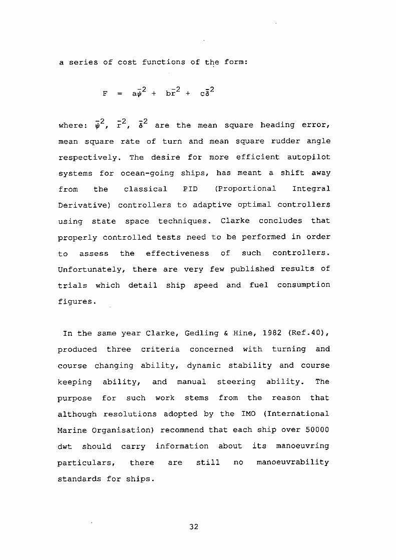
a series of cost functions of the form:
F = a 2 + br2 + Cc52
where: 2, E2 2 are the mean square heading error,
mean square rate of turn and mean square rudder angle
respectively. The desire for more efficient autopilot
systems for ocean-going ships, has meant a shift away
from the classical PID (Proportional Integral
Derivative) controllers to adaptive optimal controllers
using state space techniques. Clarke concludes that
properly controlled tests need to be performed in order
to assess the effectiveness of such controllers.
Unfortunately, there are very few published results of
trials which detail ship speed and fuel consumption
figures.
In the same year Clarke, Gedling & Hine, 1982 (Ref.40),
produced three criteria concerned with turning and
course changing ability, dynamic stability and course
keeping ability, and manual steering ability. The
purpose for such work stems from the reason that
although resolutions adopted by the IMO (International
Marine Organisation) recommend that each ship over 50000
dwt should carry information about its manoeuvring
particulars, there are still no manoeuvrability
standards for ships.
32
The criteria were developed in terms of linear theory,
based on the linearised equations of motion given as:
(X-mhi + Xu = 0
(Y . -mh + Y v + (Y . -mx ) + (Y -mu )r = 0v v r g r 0
(N . -mx )T + N v + (N . -I ) + (N -mx u )r = 0v g v r z r gO
Ignoring the surge since it has no effect on the
transverse motion of the ship and adding the rudder
terms, the dimensionless form of the equations, obtained
122by dividing the sway forces by pu 0L and the yaw
moments by puL 3 , are:
+ Y'v'+ (Y.'-m'x')r' + (Y'-m')r' + Y'5 = 0v v r g r
(N.'-m'x')v' + N'v' + (N'-I')r' + (N'-m'x')r' + N'5 = 0v g v r z r g
However, it is possible to reduce the number of
variables required to describe the ship's behaviour and
provide other advantages, by expressing the coefficients
in terms of time constants and system gains. This
approach was first used by Nomoto and yields a pair of
decoupled second order equations:
TTr' + (T + T)' + r' = K'5 +r r3
TTv' + (T + T)T' + v' = K'5 +v v4
33
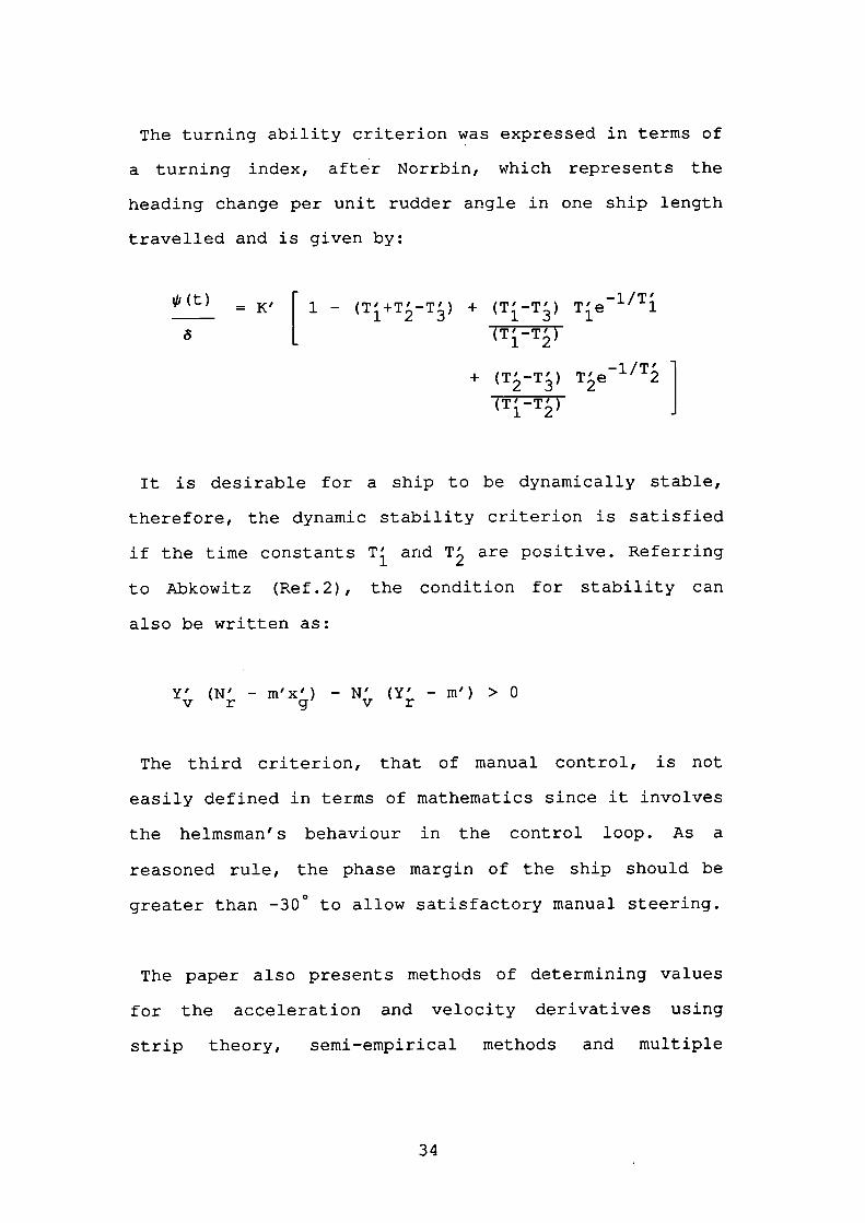
The turning ability criterion was expressed in terms of
a turning index, after Norrbin, which represents the
heading change per unit rudder angle in one ship length
travelled and is given by:
-l/T'= K' [ a. - (T+T-T) + (T-T) Te
a (T-T)
+ (T-T) Teh/'T2 ]
It is desirable for a ship to be dynamically stable,
therefore, the dynamic stability criterion is satisfied
if the time constants T arid T are positive. Referring
to Abkowitz (Ref.2), the condition for stability can
also be written as:
Y' (N' - m'x') - N' (Y' - m') > 0v r g V r
The third criterion, that of manual control, is not
easily defined in terms of mathematics since it involves
the helmsman's behaviour in the control loop. As a
reasoned rule, the phase margin of the ship should be
greater than _300 to allow satisfactory manual steering.
The paper also presents methods of determining values
for the acceleration and velocity derivatives using
strip theory, semi-empirical methods and multiple
34
regression analysis. The criteria have been thoroughly
researched and even if not implemented as standards,
they have shown how ship manoeuvrability can be
quantitatively assessed using simple linear theory.
Virtually the only six degrees of freedom model to
simulate ships appearing in published literature is
presented by Matthews, 1984 (Ref.lO1). This work, at
Maritime Dynamics Limited of Liantrisant, describes a
model based on identifying force terms as a foil in the
fluid. Central to this formulation is the concept of
drift angle since all non re-entrant moving bodies
exhibit the phenomenon of progressive non-alignment.
That is to say, when perturbed a body will depart from
its original alignment. This particular methodology has
allowed a relatively compact simulation model capable of
performing in a wide range of manoeuvring regimes.
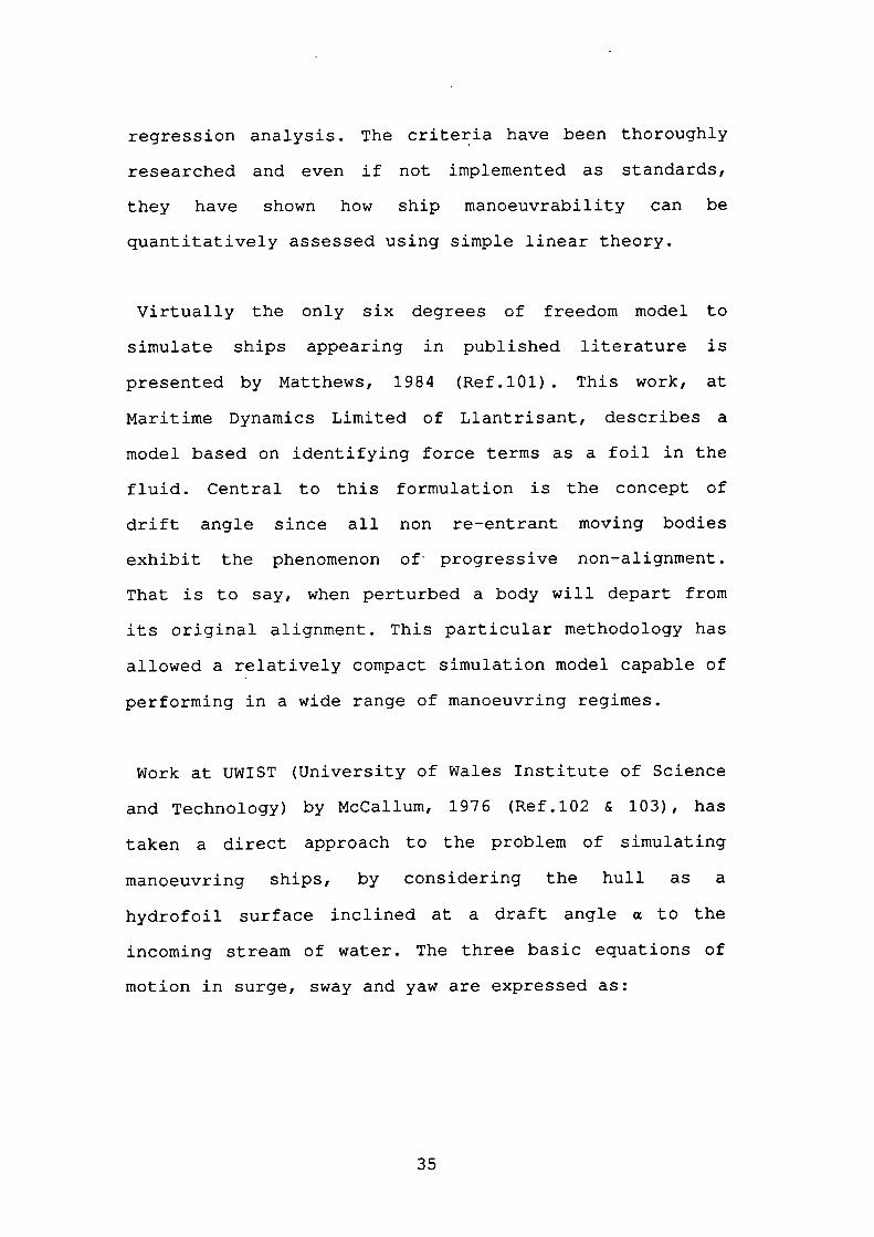
Work at UWIST (University of Wales Institute of Science
and Technology) by McCallum, 1976 (Ref.102 & 103), has
taken a direct approach to the problem of simulating
manoeuvring ships, by considering the hull as a
hydrofoil surface inclined at a draft angle a to the
incoming stream of water. The three basic equations of
motion in surge, sway and yaw are expressed as:
35
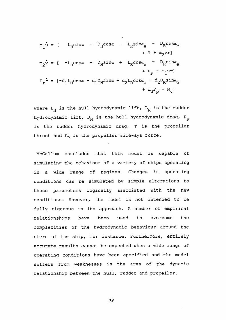
S
m1u = [ LHsinx - DHcos - L sina - D CosR e R e
+ T + m2vr]
= [ -Lcos - DHSin + L cos - D siriaR e R e
+ F - m1ur]
= [_dl LHcos - dlDHsin + d2LRCOSae - d2DRSinz
+dF -N]3p v
where LH is the hull hydrodynamic lift, LR is the rudder
hydrodynamic lift, DH is the hull hydrodynamic drag, DR
is the rudder hydrodynamic drag, T is the propeller
thrust and F is the propeller sideways force.
McCallum concludes that this model is capable of
simulating the behaviour of a variety of ships operating
in a wide range of regimes. Changes in operating
conditions can be simulated by simple alterations to
those parameters logically associated with the new
conditions. However, the model is not intended to be
fully rigorous in its approach. A number of empirical
relationships have been used to overcome the
complexities of the hydrodynamic behaviour around the
stern of the ship, for instance. Furthermore, entirely
accurate results cannot be expected when a wide range of
operating conditions have been specified and the model
suffers from weaknesses in the area of the dynamic
relationship between the hull, rudder and propeller.
36
In 1979 Cardiff acquired Europe's first CGI (Computer
Generated Imagery) simulator. It is operated jointly by
UWIST and SGIHE (South Glamorgan Institute of Higher
Education) and was the result of successful
collaboration between the UK Government's Department of
Industry. The design features and operational philosophy
of CASSIM (CArdiff Ship SIMulator) are described by
McCallum & Rawson, 1981 (Ref.104) . The basic design
consists of a visual scene, as observed from the bridge
structure through one or more forward looking windows.
Three projectors give 1200 horizontal field of view and
30° in the vertical plane. This can be extended to a
200° horizontal view with' the addition of two extra
projectors.
The visual scene is fully interactive with bridge
commands, so that engine or rudder changes are fed to
the motion computer which contains the manoeuvring
equations of a range of ships. Bridge instruments are
similarly updated in response to the computed ship
motions. The Controller is also able to alter the scene
by introducing different visibility conditions or other
ships.
The visual side of the simulator was developed by
Marconi Radar Systems Ltd. under the auspices of the
Tepigen trademark. The principal characteristics being:
37
a 625 line colour television, back projection onto a
four metres radius cylindrical screen, 1000 "faces" or
lights and marks, four additional instructor controlled
pre-programmed ships and potentially unlimited area of
data base. The significant features include: atmospheric
scattering (land which is further away appears to fade),
edge smoothing (so that sloping lines do not appear as a
number of steps), sea texture (ripples appear to move in
the direction of apparent water flow), distance effects
(lights are given perspective so they get smaller and
less intense at greater ranges), land texture (enables
woodland and walls to be presented at close range) and
data base preparation (additional charts, photographs,
drawings et cetera of different ports can be added).
The bridge design is supplied by Racal Decca Systems
and Simulators Limited. It measures four metres wide by
five metres deep and is mounted on a large vibrating
platform. Ship's officers rely on propeller induced
vibrations as an important cue and all UK simulators are
fitted with this feature. A set of instruments, similar
to those found on most ship's bridges, includes:
steering pedestal with autopilot and manual wheel,
sixteen inch radar display, engine telegraph, intercoms,
VHF radio, chart table, heading repeater, log, rate of
turn indicator, RPM indicator, depth repeater, wind
speed and direction, Decca navigator and ship's sounds.
38
McCallum, 1983 (Ref.105), discusses how operational
criteria can influence ship simulator design. With
simulators costing from £3K to over £3M it is important
to select one to match the needs. The paper identifies
ship simulator development trends and uses and applies
the law of diminishing returns to simulator realism
versus expense of complexity. An extremely important
point made by McCallum about simulators is that:
"... adequate pnLian mast &e made ea&fr updates .
Continuing the simulator theme, McCallum, 1984
(Ref.106), presents a critical survey of three specific
ship simulator mathematical manoeuvring models. Each is
implemented on the CASSIM in a port evaluation study.
Measures of performance were related in terms of three
performance indices, namely the mariner, ship and port
performance indices. The conclusion drawn was that for
most simulation tasks it is quite feasible to use
mathematical models which have been produced relatively
cheaply. However, fine detailed close manoeuvres
require higher fidelity models and simulation of smaller
ships down heavy quartering seas are beyond the scope of
any simulator in service today.
Joint work between the Royal Naval Engineering College
at Manadon in Plymouth and UWIST by Fuzzard & Towill,
39
1982 (Ref.56), has been aimed at investigating the
possibility of using PNS (Pseudo-Noise Sequences)
injection and cross-correlation techniques to produce
transfer functions to model non-linear ship dynamics
about a given steady state condition. Where linearised
small perturbations about a specific operating condition
are sufficient, this method dispenses with the need for
costly and often time consuming tank testing of physical
models.
Other research between these two establishments has
included the implementation of fuzzy sets to control
algorithms, Sutton & Towill, 1985 (Ref.128 & 129) . These
papers provide a straight-forward introduction to fuzzy
sets, discussing the concepts of "linguistic hedges",
"fuzzy relations" and "composite rule of inference". The
fuzzy controller, as developed, is used as an autopilot
to control the non-linear yaw dynamics model of a Royal
Navy frigate.
Dove, 1974 (Ref.45), surveyed the methods of pilotage
and berthing, including statistics of collisions and
groundings. The development of shipborne automatic
control devices is suggested for the berthing of large
vessels. A move from Southampton College of Technology
to Plymouth Polytechnic (now known as Polytechnic South
West), allowed these ideas to become reality. Burns,
40
Dove, Bouncer & Stockel, 1985 (Ref.35), who form part of
the Ship Dynamics and Control Research Group at
Polytechnic South West, firstly developed a discrete,
time-varying, non-linear mathematical model to simulate
ship response to demanded rudder and engine speed plus
wind and current. The second phase of the research,
which relied on an accurate model, entailed the
construction of a digital filter/estimator, for use with
an optimal controller, capable of navigating large ships
in port approaches (Refs.46 & 47)
The model is based on state space methods with eight
system states and two deterministic inputs. It simulates
the horizontal motions of surge, sway and yaw. The best
estimate of each state is passed to an adaptive optimal
controller to compute those inputs which minimise a
given performance criterion. A further consideration of
the work at Polytechnic South West, is that of
integration of navigational data so that deficiencies in
one navigational system can be offset be those in
another by use of minimum variance or Kalman-Bucy
filters.
Mikelis, 1983 (Ref.107), of Lloyd's Register of
Shipping, observed from model experiments and full scale
operations that a ship's handling behaviour changes when
moving from deep to shallow water or into canals. A
41
review of existing manoeuvring theories is presented and
a simplified simulation model is developed. The aim of
the work at Lloyd's Register of Shipping is to arrive at
a method of predicting ship handling at the design
stage. With this in mind it is desirable that such a
formulation does not rely on data from model
experiments.
For the type of manoeuvres being considered at Lloyd's
Register the linearised equations appear acceptable and
the acceleration coefficients can be adequately
calculated from lines plans. However, parametric
equations for the velocity coefficients proved less
accurate and experimentally derived values had to be
utilised. Where ship's propulsion characteristics are
known at the design stage, they should be included in
the model instead of empirical constants.
Mikelis, Clarke, Roberts & Jackson, 1985 (Refs.108 &
72), have assembled a mathematical model consisting of
coupled equations of surge, sway, yaw, roll and
propeller revolutions. The method employs two computer
programs. The first is a pre-simulation routine which
generates resistance, propulsion and hydrodynamic
coefficients from ship geometry and other readily
accessed data. The second program performs the
simulation using the data made available by the first
42
routine.
The simultaneous equations are solved using an IBM
mainframe computer and provide up to 500 times faster
than real time simulations. A simulator designed to
study and analyse safety aspects during ship handling
operations has also be implemented at Lloyd's Register
using a VAX/1l-780 and is known as the Multi-Ship
Manoeuvring Simulator (MSMS). It is expected to have a
wide future use as it provides radar view graphics,
interactive input of rudder and engine commands,
real-time or fast simulation and multi-ship simulation.
The approach to the mathematical model has been to use
the classical Taylor series expansion to describe the
hydrodynamic reactions on the hull, but the rudder and
propeller forces and moments follow the Japanese
treatment. The model was verified, as are many other
ship models, by comparison to full scale manoeuvring
tests carried out for the 278000 dwt tanker "Esso
Osaka". Numerous applications are envisaged for the
MSMS, especially in the field of maritime safety
studies.
Broome, 1982 (Ref.34), has conducted a series of tests
using computer simulation and radio controlled scale
models to investigate the effect of ship autopilot
43
tuning on course keeping efficiency. Fast Fourier
transform techniques on the non PRBS (Pseudo Random
Binary Sequences) yaw and rudder signals have been used
to assess the dominant free body natural frequencies of
the ship. A program has been written to perform ARNA
(Auto-Regressive Moving Average) identifications of
linear system mathematical models, based on least
squares of maximum likelihood algorithms. The aim is to
provide a self-tuning adaptive autopilot which has
reference to the roll dynamics of the ship.
A suite of programs developed at Southampton University
and the University of Newcastle Upon Tyne by Wellicome &
Mirza, 1987 (Ref.139), use slender body theory to
predict the course keeping and steady rate of turn of a
ship. Slender body techniques have been successfully
used in the past to determine ship response to waves.
This paper shows a method for finding the forces and
moments arising from a ship manoeuvring in calm water.
The motive behind such work is to provide an inexpensive
tool for predicting ship manoeuvring characteristics.
2.06 Scandinavian And European Research
The SSPA (Statens Skeppsprovningsanstalt or Swedish
State Shipbuilding Experimental Tank) at Göteborg have
over the past 35 years or so regularly published a wide
44
range of texts on ship theory and research. Report
number 68 by Norrbin, 1971 (Ref.112), provides an
exceedingly useful description of mathematical modelling
of ship manoeuvres in both deep and confined waters. The
non-dimensionalising of hydrodynamic coefficients uses
the so-called "Bis" system, which differs from the
method used by Abkowitz et al. Topics discussed in this
report include: the kinematics of fixed and moving
systems, calculations of hull forces, modelling deep
water horizontal manoeuvres, free water and confined
water flow phenomena and model tests.
Norrbin, 1972 (Ref.113), also provides an introduction
to ship manoeuvring with application to shipborne
predictors and real-time simulators. Details of
simulator models and man-machine interface are
discussed. Records of helm manoeuvres on board large
tankers in harbour approaches revealed the need for
predictor assistance. The resulting simulator produces
electronically generated symbols to be projected in a
"predictor window" to show predicted path information by
perspective line tracks.
As with many other establishments, researchers at SSPA
have tackled the subject of system identification as
applied to the determination of steering dynamics of
ships. Byström & Källström, 1978 (Ref.36), evaluate full
45
scale experiments using the identification program
LISPID which contains the output error method, the
maximum likelihood method and the prediction error
method. Since free steering experiments may be performed
both in model and full scale, the identification
technique offers the added attraction of analysing the
effects of scaling.
Also at SSPA Källström & Ottosson, 1982 (Ref.80), have
carried out investigations into regulators to reduce
roll motions by use of rudder and active fins. Some
types of modern fast ships exhibit a severe tendency to
heel significantly during turns. High super-structures
and a relatively low density cargo produce small
metacentric heights and consequently poor dynamical
stability and great sensitivity for disturbances from
wind and waves. A non-linear mathematical model for a
ship moving in wind and irregular waves is developed and
three differing regulators are presented. Results and a
large portion of the mathematics are included in the
paper.
Berg & Flobakk, 1979 (Ref.25), of the Norwegian
Institute of Technology and Hydrodynamic Laboratories,
firstly present a non-linear mathematical model of a
ship, and then show methods to determine the
coefficients in the manoeuvring equations. Since the
46
Ocean Environmental Basin was not available at the time
of the research, coefficients had to be determined
theoretically by choosing a suitable description of the
forces acting on the ship. Planar motion mechanism tests
are thus avoided. Initially a simulation study is made
to establish a procedure for generating quasi-optimal
rudder control signals for free-sailing tests in a
towing tank.
Work at the Norwegian Marine Technology Research
Institute (MARINTEK) by Martinussen & Linnerud, 1987
(Ref.100), has similar goals to those of Lloyd's
Register. The aim being to provide a prediction
simulation of the manoeuvring characteristics of ships
at the design stage. Adiscussion on the model tests is
given and the applicability of free running model tests
as a prediction method is presented. The simulation
gives sufficiently accurate results for hulls within the
range of existing empirical data.
Bech & Chislett, 1980 (Ref.24), who are associated with
the DSRL (Danish Ship Research Laboratory),
statistically investigate the invariant coefficients of
the ship's equation of response to steering. The aim
being to provide an improved non-dimensionalisation of
the transfer function of ship heading response to rudder
action. Traditionally, constants have been
47
non-dimensionalised with ship length to speed ratio, but
by including Froude number, block coefficient, ship
length to beam ratio, length to draft ratio, trim,
rudder chord and propeller diameter, it is hoped that
considerably better results will be obtained.
The DM1 (Danish Maritime Institute) has been assessing
the special berthing and navigational needs of cruise
liners. The requirement for cabin space has led to large
superstructures which suffer from windage problems.
Tersløv, 1985 (Ref.130), describes the capabilities of a
simulator developed at DM1 which allows the skills of
navigators and masters of these ships to be enhanced.
Research at the Control Laboratory in the Electrical
Engineering Department of Delft University in the
Netherlands over the past 20 years has been directed
towards automatic steering control of ships. Much of the
work has been in association with the Royal Netherlands
Navy and the principal researchers are: van Amerongen,
van den Bosch, Goeij, Hoogenraad, Keizer, van der Klugt,
Leeuwen, Moraal, van Nauta Lemke, Ort, Postuma, Schouten
and Verhage (Refs.5-13 & 29-30 & 88)
One of the earlier papers describes a method of
accurately determining the speed of a ship during
manoeuvres based on accurate position fixes and using
48
automated Snellius techniques. Usual speed measuring
devices are only capable of determining accurate results
when running straight line courses and become unreliable
when the ship undergoes a manoeuvre. The principle of
the Snellius method is that given the two bearings
between three known points, it is possible to derive the
position of the ship. Sextants are used to provide the
angular information. However, the known points must be
selected so that the angle of the intersection of the
two circles formed when determining position provide a
good cut (that is, it is not a shallow angle)
The majority of the remainder of the papers concentrate
on the design of an autopilot which uses the rudder not
only for course keeping, but also for roll
stabilisation, where stabilising fins have been used up
to now. A simple mathematical model of a ship describing
the transfer between the rudder and yaw motions was
obtained from modelling experiments. The model was used
within the design of the controller utilising the
concepts of model reference adaptive systems and Kalman
filtering. An additional computer aided design package
PSI (Interactive Simulation Program) has been developed
which provides an optimisation facility based upon a
fast hill-climbing algorithm. This is capable of
computing a "best-fit" model of a system by means of
simulation and optimisation.
49
de Vries of Delft Hydraulics Laboratory, 1984
(Ref.135), has developed a special model testing
technique for determination of manoeuvring coefficients,
which is used in combination with straight line towing.
The manoeuvring simulator uses equations composed of a
number of terms with unknown coefficients and it is
these coefficients which are determined by curve fitting
of data from systematic model experiments. Two air
propellers are fitted to model ships to exert lateral
forces, and other measuring techniques are applied to
provide a facility at a lower cost than using planar
motion mechanisms.
More recent work in the Netherlands includes further
considerations on mathematical models as presented by
Hooft, 1987 (Ref.73), of MARIN (MAritime Research
Institute Netherlands). Here investigations have been
directed toward improving the assessment of hydrodynamic
coefficients in non-linear ship models, principally
because empirical methods to date have proved
insufficiently accurate.
Brard, 1951 (Ref.31), provides an earlier French text
on the manoeuvring of ships in deep water, in shallow
water and in canals. A large number of experiments have
been carried out utilising both the large turning basin,
installed at the BEC (Bassin d'Essais des Carènes or
50
Paris Model Basin) in 1945, and the rectilinear basin
designed for shallow water testing, installed five years
later. The paper presents some of the principal test
results obtained from these experiments.
An overview of the ship's bridge simulator designed by
LMT Simulator and Electronic System Division of France
is given by Martin, 1978 (Ref.99). It includes a diagram
showing the important features of the ship handling
simulator. Another French aid for port design and
training of captains and pilots has been developed by
Sogreah and is presented by Demenet, Garraud & Graff,
1984 (Ref.44)
Thom, 1980 (Ref.131), has carried out theoretical and
experimental modelling of ship dynamics in West Germany.
Theoretical modelling by application of physical laws
yields a general understanding of the model structure
and of the influencing factors, but is impractical
without approximations. Experimental modelling by
evaluation of full scale ship trials or of model tests
produces realistic results, but the proper design of
experiments have to be based on theoretical
considerations.
At the Technical University of Gdansk in Poland,
Dziedzic & Morawski, 1980 (Ref.48), have been developing
51
algorithms to control ship's motion according to desired
trajectory. The paper presents a model of the process
and control algorithms which minimise lateral deviations
of the ship from a desired path or trajectory. An
c-optimal controller is applied to the problem, which is
sub-divided into a kinematic and dynamic problem.
Computerised estimation of ship manoeuvrability at the
design stage is also taking place in Bulgaria at the
BSHC (Bulgarian Ship Hydrodynamics Centre) in Varna by
Bogdanov & Milanov, 1987 (Ref.28) . This paper discusses
the SIMP software system which has been developed as a
design tool for stern counter and rudder blade form,
taking into account requirements for adequate ship
manoeuvrability. By way of an example, results from an
application of the system to the design of the
after-body hull section of a real ship.
2.07 America
The DTMB (David Taylor Model Basin) at Washington DC
and the DTMBRDC (David Taylor Model Basin Research and
Development Centre) at Bethesda form the principal sites
of this long-established institution for ship research.
Strom-Tejsen, 1965 (Ref.127), although an earlier text,
provides a good introduction to mathematical models
based upon Taylor series expansion techniques. The
52
report presents a non-linear mathematical model
representing the motion of a surface ship. The
associated computer program is written in FORTRAN II for
the IBM 7090 computer. The sample calculations are based
on the hydrodynamic coefficients of the "Mariner" hull
form.
A mathematical presentation of shallow water flows past
slender bodies is given by Tuck, 1965 (Ref.134) . The
problem solved concerns the disturbance to a stream of
shallow water due to an immersed slender body, with
particular reference to steady motions of ships in
shallow water. The analysis assumes a ship to be slender
in the sense that it is longer than it is broad or deep,
and uses the technique of matched asymptotic expansions
to construct approximate solutions.
Further research at DTMB has theoretically investigated
the prediction of the motions of high-speed planing
boats in waves. In his paper Martin, 1978 (Ref.98),
compares the theoretical predictions with existing
experimental data and obtains reasonably good agreement.
Non-linear terms are required for speed-to-length ratios
greater than about 6, otherwise linear theory is capable
of providing a simple and fast means of determining the
effect of various parameters such as trim, deadrise,
loading and so on.
53
Lee, O'Dea & Meyers, 1983 (Ref.87), describe more
recent work at DTMB on the prediction of relative motion
of ships in waves. An analytical method is developed for
predicting the vertical motion of a point on a ship
relative to the free surface. The method is based on a
two-dimensional approximation within the context of
strip theory. The two-dimensional approximation
simplifies the process of incorporating it into an
existing ship motion computer program and enables the
validity of the relative motion prediction to be checked
based entirely upon strip theory. The paper compares
computed results with experimental data for two hull
forms. -
MIT (Massachusetts Institute of Technology) is one of
several institutes of technology involved in ship
research. Newman, 1959 (Ref.111), considers the damping
and wave resistance of a thin ship which is moving in
calm conditions with constant velocity and oscillating
in pitch and heave. Green's theorem is used to obtain
the velocity potential. The coefficients of damping and
increased wave resistance are found by separation of the
energy components after an asymptotic expansion of the
Green's function. Calculations are given for a
polynomial hull and compared with experimental data.
Abkowitz's lecture notes, 1964 (Ref.2), have been
54
previously mentioned, but in a later paper, 1983
(Ref.3), roll damping at forward speed is considered.
Conflict exists between three-dimensional body theories
and strip-slender body theories about the magnitude of
the effect of forward speed on the linear roll damping
coefficient. Forced rolling tests on models indicate
that forward speed does in fact have a significant
effect on roll damping which confirms the
three-dimensional theory trend.
Abkowitz, 1984 (Ref.4), also demonstrates methods of
measuring ship hydrodynamic coefficients by performing
simple trials during regular operations. System
identification techniques are applied to measurements of
forward speed (u), sway (v), yaw velocity (r) and
heading (cu). The paper concludes that results indicate
that the coefficients can be successfully identified
from simple trials conducted during routine voyages
using a minimum of the two measurements of u and .
Clearly, whilst it appears possible to produce a
reasonable working model for ocean-going vessels, the
accuracy for finer detailed manoeuvring must leave much
to be desired.
One of the principal researchers at SIT (Stevens
Institute of Technology) is Eda, 1965 onwards
(Refs.49-52) . Earlier work considered the steering
55
characteristics of ships in calm water and waves, which
led to yaw control in waves. A method to predict ship's
yawing motion in following and quartering seas has been
developed and used to study control system
characteristics. During the 1970's digital simulations
of standard manoeuvres were carried out to analyse
manoeuvring performance and the effects of roll motions
with respect to steering control were studied.
At the University of California Fukino & Tomizuka, 1986
(Ref.55), describe an adaptive time optimal control
autopilot for ship steering. The so-called SOHM
(Successive Order Heightening Method), is used to obtain
the time optimal control law based on the solution of a
third order differential equation model. It is combined
with a least squares type parameter estimation algorithm
and the scheme is evaluated by a computer simulation
study.
Work at Hydronautics by Goodman, Gertler & Kohl, 1976
(Ref.62), and Ankudinov, Miller, Alman & Jakobsen, 1987
(Ref.14), has been directed at analysing, predicting and
assessing surface ship manoeuvrability at the design
stage. The experimental techniques and methods of
analysis are described in the first paper and include
reference to the use of a LAHPMM (Large Amplitude
Horizontal Planar Motion Mechanism) . While the second
56
paper has advanced to using numerical simulation
techniques to determine ship manoeuvrability
performance.
Joint collaboration between Asinovsky, Landsburg &
Hagen, 1987 (Ref.17), has also been analysing ship
manoeuvrability, but using a differential approach.
Mathematical representations of the hydrodynamic forces
and moments are here based on the separate determination
and analysis of the hydrodynamic characteristics for the
hull, rudder and propeller and on the hydrodynamic
interactions in the hull/propeller/rudder system.
The IMO (International Maritime Organisation) has moved
towards the implementation of standards for ship
manoeuvring in full scale trials, model tests and
simulator performance. A number of papers suggest
approaches to achieving standardisation, one such paper
is that by Cojeen, Landsburg & MacFarlane, 1987
(Ref.41), of the US and Canadian Coast Guards. They
anticipate that ship owners will establish preliminary
manoeuvring performance by submitting lines plans to
design simulators. Final manoeuvring performance
capabilities could then be determined from trials
conducted in conjunction with the shipbuilder's trials.
An extremely good text introducing many concepts in the
57
dynamics of marine vehicles is provided by Bhattacharyya
who is the Director of Naval Architecture at the US
Naval Academy in Annapolis, 1978 (Ref.26) . Much of the
text deals with the seaway and motion due to waves. It
begins with theories of sinusoidal water waves and
progresses to an irregular seaway.
2.08 Japan
Nomoto provides the basis for much of the work as
regards modelling the hydrodynamics of ships in the
design of autopilots. This approach uses transfer
functions to express the coefficients of the states and
their derivatives in terms of time constants and systems
gains (consistent with control engineering practice)
The number of variables required to describe the
behaviour of a ship is reduced by this method, however,
each time constant can be related to several of the
hydrodynamic coefficients. The time constants can often
be extracted from plots of manoeuvres, but relate to
autopilot control of models rather than the model
itself.
Ohtagaki & Tanaka, 1984 (Ref.116), describe how, since
its installation in 1975, the 1111 (Ishikawajima-Harima
heavy Industries) man-in-the-loop ship manoeuvririg
simulator has served the needs in ship design work and
58
ship handling training. Applications of the simulator
are presented and, due to increasing requirements for
greater sophistication, it is mentioned that the
facility is to be revamped.
Ongoing work between Kyushu University and Mitsui
Engineering has led to the development of a practical
calculation method of ship manoeuvring motion. The
principal researchers are: Fukushima, Hirano, Inoue,
Kijima, Moriya, Saruta, Takaishi and Takashina,
(Refs.68-71,75-76,83) . This method uses the principal
particulars of the ship hull, rudder and propeller as
basic input data. The mathematical model employs the
coupled equations of surge, sway, yaw and roll. Initial
papers present a simplistic model with only the
fundamental manoeuvring terms; later papers deal with
the inclusion of the effects of shallow water, banks,
lateral thrust units, wind and wave. Computed results
satisfactorily agree with full scale trial data.
Another joint endeavour exists between the Ship
Research Institute and Mitsubishi Heavy Industries. The
initial mathematical model developed by Ogawa & Kasai,
1978 (Ref.115), is similar to that of Hirano et al
described earlier. However, Baba, Asai & Toki, 1982
(Ref.18), have deviated from the usual ocean-going ship
models to investigate sway-roll-yaw coupled instability
59
of semi-displacement type high-speed ships. Round bilge
and hard chine type hulls are considered, as are
variations in metacentric height and the effect of spray
strips. Further study is envisaged to include non-linear
terms in drift angle and yaw rate.
More recently Kobayashi & Asai, 1987 (Ref.84), have
expanded the basic simulation model to cater for low
speeds and astern manoeuvres. Four models have resulted
for the following regimes:
1 Ordinary advance speed model Fn >= Fflmjni
2 Average model of 1 & 3 Fn . > Fn >= Fnmini min2
3 Low advance speed model Fflmjn2 > Fn >= 0
4 Astern model 0 > Fn
where Fn is the Froude number and Fn and Fn . aremini min2
specified minimum limits. Model validation was made by
comparison to free running model tests. The four models
should be capable of evaluating operations both
approaching and within harbour limits.
Recent research between the Yokogawa Hokushin Electric
Corporation, Nippon Kokan K.K. and Nagoya Institute of
Technology has closely followed Dutch work on MARC
(Model Reference Adaptive Control). Arie, Itoh, Senoh,
Takahashi, Fujii & Mizuno present a paper, 1985
(Ref.15), which uses "hill-climbing" techniques to
achieve automatic steering control in course-keeping or
60
course-changing modes.
2.09 Other Countries
Most of the countries which have some form of merchant
navy are engaged, to a certain degree, in either
mathematically modelling ship manoeuvres or autopilot
control theory research. In Brazil, for instance,
Rios-Neto & Da Cruz, 1985 (Ref.123), describe a
heuristic stochastic rudder control law for ship
automatic path-following in restricted waters. An
extended Kalman filter is combined with a dynamical
model compensation technique and a state noise
adjustment procedure. The performance of the controller
is illustrated with results obtained by digital
simulation.. After further feasibility studies it is
anticipated that the autopilot could be implemented in
an onboard minicomputer.
2.10 Additional
Many texts deal with particular aspects relevant to
ship simulation. Hirano, Takashina, Takaishi & Saruta
(Ref.67) present the results of a study on the turning
trajectory of ships under the influence of regular
waves. Norrbin (Ref.114) discusses the generation of a
lateral force (known as the rudder normal force) due to
61
the flow past a rudder. Estimates for the rudder
derivatives and recommendations of minimum rudder area
for certain ship types plus stability derivatives formed
by regressional analysis are included. Aage (Ref.1)
provides four-component (surge, sway, yaw and roll) wind
coefficients for nine ship models.
The list of technical publications is almost limitless,
and there are further texts written in languages other
than English which the author is unable to review.
However, it is hoped that a reasonable cross-section of
material has been presented in order to give the reader
an indication of the scope of the work being carried out
within maritime research establishments.
62
CHAPTER •3
AUTOMATIC CONTROL OF BOATS
63
3.01 Introduction
The research covered in this thesis was inspired by the
requirement for a facility to assess the performance of
small boat autopilots. It, therefore, seems pertinent to
include an introduction to the subject of automatic
control of boats and examine the functionality of the
autopilot.
The two main products of interest manufactured by
Cetrek are the Fluxgate Compass Sensor and the Automatic
Pilot (Fig.3.1)
The fluxgate sensor is essentially a magnetometer which
can detect the magnitude and direction of a magnetic
field. It is a "second harmonic" device since the output
signal voltage will have a frequency twice that of the
driving or exciting frequency. The sensor will give a
maximum output when it is aligned exactly with the
direction of the measured magnetic field and a minimum
when lying at 90° to the field. Two sensing coils, set
at right angles to each other and known as a sine/cosine
system, are used to generate angular position
information without ambiguity.
The autopilot control unit requires heading information
which is supplied by the fluxgate sensor. This, along
with the drive unit, consisting of a hydraulic drive
64
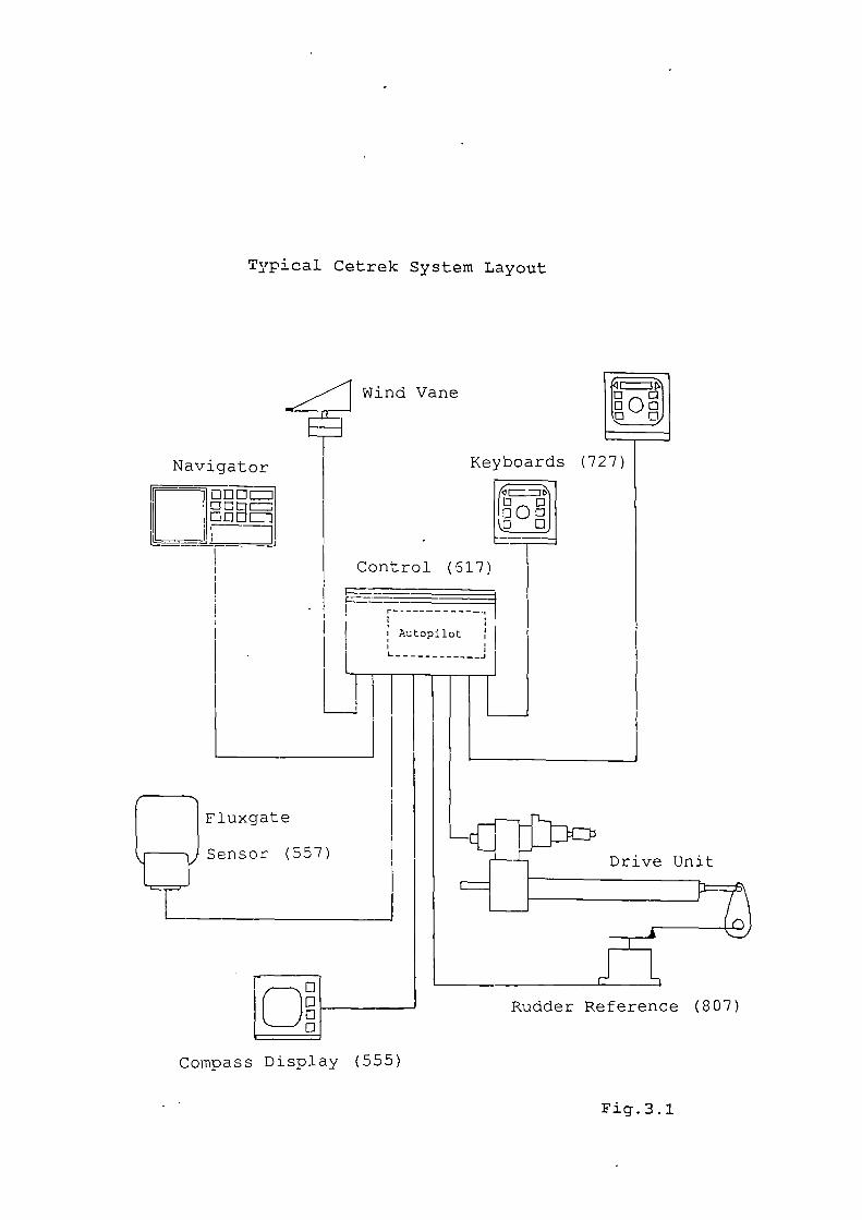
Wind Vane
DE1Do t::ion ci
Control (617)
Typical Cetrek System Layout
N av ± ga to r Keyboards (727)
Compass Display (555)
Fig. 3.1
system, and the rudder reference or feedback unit, make
up the important components necessary to achieve
automatic control. In addition, the Cetrek autopilot can
be combined with radio navigation systems, that is
Satnav and Hyperbolic navigators, thus allowing
adherence to track between user defined waypoints. A
wind vane can be attached, for yachts, in order that the
autopilot can keep the boat on a prescribed relative
heading to the wind direction. Also, extra keyboards and
compass display units may be added as repeaters to
secondary helm positions, such as the fly bridge.
The fundamental principles of an autopilot will now be
discussed since this unit is closely allied to the
mathematical model project.
3.02 PID Control Theory
An autopilot is designed to steer a boat by
manipulating the rudder in such a way as to reduce the
difference between the desired and actual heading of a
vessel. Conventional autopilots rely on the three term
Proportional, Integral and Derivative (PID) control
(Fig.3.2)
Proportional Control
This causes rudder to be applied in proportion to the
66
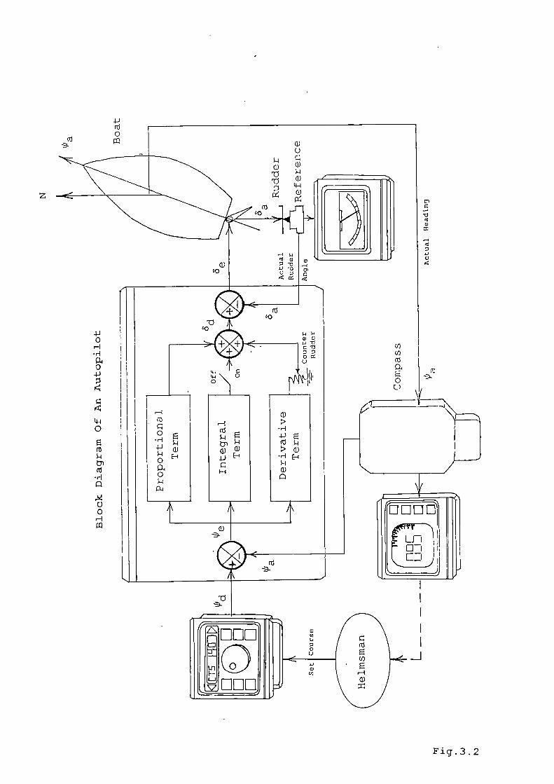
ci)
C
-Ci
'aC)
-4'a
C-)
U)crj
cr3
L)
a)(a
0
U
a)
—J
cr3
Cl)
Hci)
z
-i-i
0
0r-1ri
0
-I-)
'440
(0
•rI
00H
ci)
U
'a aja)- I___
Io
I
(4
C)
'-i\ 00 \ r'N
r-1 I I'ci)
I IIH II I HR0 1E1 I4E-H
IQ)I Ia)HJEH I-HE-4
's-I
I Iao I 0
I I I
I_____ I
rnE1
rnj
Fig.3 .2
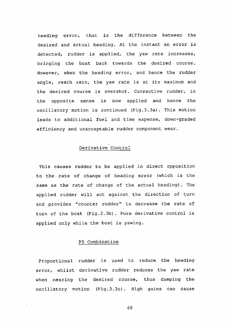
heading error, that is the • difference between the
desired and actual heading. At the instant an error is
detected, rudder is applied, the yaw rate increases,
bringing the boat back towards the desired course.
However, when the heading error, and hence the rudder
angle, reach zero, the yaw rate is at its maximum and
the desired course is overshot. Corrective rudder, in
the opposite sense is now applied and hence the
oscillatory motion is continued (Fig.3.3a) . This motion
leads to additional fuel and time expense, down-graded
efficiency and unacceptable rudder component wear.
Derivative Control
This causes rudder to be applied in direct opposition
to the rate of change of heading error (which is the
same as the rate of change of the actual heading). The
applied rudder will act against the direction of turn
and provides "counter rudder" to decrease the rate of
turn of the boat (Fig.3.3b) . Pure derivative control is
applied only while the boat is yawing.
PD Combination
Proportional rudder is used to reduce the heading
error, whilst derivative rudder reduces the yaw rate
when nearing the desired course, thus damping the
oscillatory motion (Fig.3.3c) . High gains can cause
68
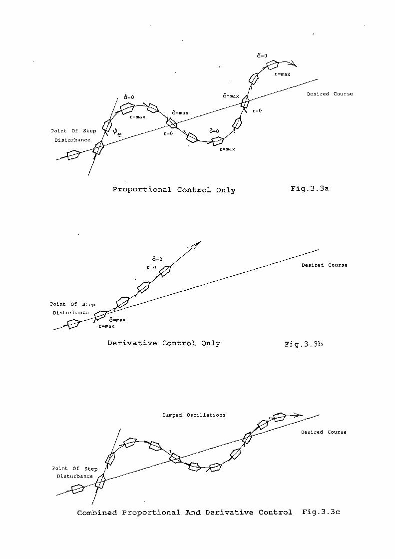
ired Course
Pc
p
d Course
Pi
d Course
c=O
Proportional Control Only Fig.3.3a
Derivative Control Only Fig.3.3b
Combined Proportional And Derivative Control Fig.3.3c
severe oscillations before the •boat settles on course,
and low gains can cause little overshoot with a sluggish
return to course. The correct balance is necessary.
For most small boat purposes, a slightly under-damped
setting of the gains is desirable as this ensures that
the desired course is actually reached and achieved
relatively quickly. A large overshoot is to be avoided
as this introduces excess rudder movement and a longer
course settling time. However, when manoeuvring in
reasonably unrestricted areas, the condition of critical
damping can be used to execute a smooth alteration of
course when approaching a waypoint.
Integral Control
This causes rudder to be applied in direct relation to
the sum of the heading errors terttiue
the heading error). It Is used to provide a permanent
helm or rudder offset (false centre) in order to combat
the effects of wind and tidal disturbances which
continually move the boat off course. This is often
referred to as a weather helm.
PID Combination
It is possible that a disturbance acting continuously,
for example, a wind or wave drifting moment, can balance
70
the moment generated by the demanded rudder position
calculated by the PD controller. The course error cannot
therefore be reduced. The addition of the integral term
effectively adds a little more desired rudder at each
iteration of the control loop all the while the
disturbance is acting. This term gradually mounts up
until the effect of the disturbing moment is
neutralised.
Ghost Rudder
Currently available autopilots have additional
functions peripheral to the PID controller. When the
rudder reference is unavailable a "Ghost Rudder" often
provides a replacement for the feedback signal. This can
be based on a knowledge of the steering gear response
and the signals sent by the autopilot to the riir3der.
Rudder Limit
The desired rudder angle, computed by the autopilot, is
given a finite limit to ensure the system does not
attempt to drive the rudder beyond physical limits.
Course Deadband
This deadband is designed to avoid the condition where
the rudder is continually subjected to rapid port and
71
starboard commands in quick succession. This occurs when
the boat is approximately on course but oscillating
slightly either side of the desired course. By setting a
high deadband the amplitude of yaw that can be tolerated
before the steering gear is enabled is increased. In
heavy weather the course deadband would be opened out,
and reduced again in calmer conditions.
Rudder Deadband
Small rudder errors that fall within the rudder
deadband are not implemented. This is used to avoid
continuous rudder action.
3.03 Autopilot Gains
Selection of the gains for each of the PID terms
depends on the type of boat under control and the sea
conditions in which it is operating. Additionally the
deadbands will be expanded or contracted as conditions
dictate. While adaptive autopilots exist for large ships
which have the equivalent of mini-computers on board,
there are, at present, no such facilities on small boat
autopilots.
The current procedure is to determine appropriate
settings for the gains by conducting simple sea trials
when the autopilot is installed. These settings are
72
intuitive values which "feel" right for the particular
boat and will provide a reference from which the gains
can be adjusted.
Ideally automatic selection of the gains is desirable.
A model reference system could be used to assess boat
response to the gain settings and alter them to suit the
prevailing conditions. This could be incorporated within
the autopilot as a complete model or as a set of
pre-computed gains in tabular form.
A mathematical model of a small boat, incorporating
forcing functions to represent the effects of wind and
waves, would provide a development tool capable of
assessing autopilot performance in a range of pseudo sea
conditions. Furthermore, it will enable criteria for
optimising autopilot gains to be established. It was
with this view in mind that the construction of a
simulation model was first proposed.
73
CHAPTER 4
MOTION OF A BOAT IN A SEAWAY
"Theie &e tMee ffinqA w/ich ati.e aa wondertu
eQIL me, qea, towt whLch knauct nat:
The ua 4 an eaqLe th. the cun;
the W04 a a ce'pent upon a 'inc/c;
the wa a a cJz4i a the m4& a the Aea;
and the W04 a man wLth a maLd"
Proverbs 30 v18&19 (KJV)
74
4.01 Introduction
Many terms are used to express different aspects of the
motion of ships and boats in a seaway. It is generally
agreed that a boat must be seaworthy and have
satisfactory stability, but exactly what constitutes
these qualities is still very much a matter of the
judgement and experience of the individual naval
architect. The general field of boat motion can be
divided under two headings, "manoeuvrability" and
"seakeeping".
Manoeuvrability refers to those motions which result
solely from the excitation forces and moments due to
application of control surfaces, such as rudders, in the
absence of disturbing forces and moments due to external
influences, such as wind and waves. Seakeeping, however,
deals with the motion of a boat resulting from the
external disturbing forces and moments of the sea and
wind. When the control surfaces are used to effect a
manoeuvre in the presence of excitations due to the sea,
either to maintain a desired course or perform a course
change, there is a combination of the two areas which is
referred to as manoeuvring in a seaway.
Both of these areas are additionally concerned with two
further concepts: "motion stability", which is a measure
75
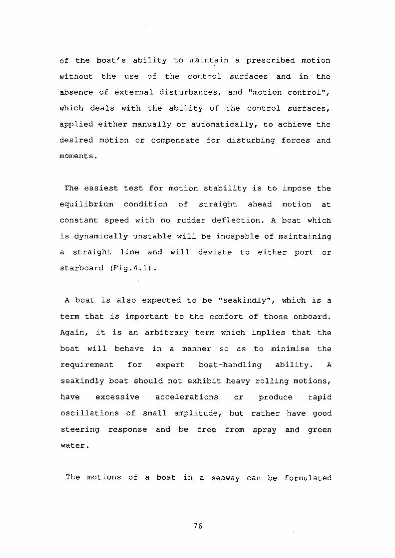
of the boat's ability to maintain a prescribed motion
without the use of the control surfaces and in the
absence of external disturbances, and "motion control",
which deals with the ability of the control surfaces,
applied either manually or automatically, to achieve the
desired motion or compensate for disturbing forces and
moments.
The easiest test for motion stability is to impose the
equilibrium condition of straight ahead motion at
constant speed with no rudder deflection. A boat which
is dynamically unstable will be incapable of maintaining
a straight line and will deviate to either port or
starboard (Fig.4.l).
A boat is also expected to be "seakindly", which is a
term that is important to the comfort of those onboard.
Again, it is an arbitrary term which implies that the
boat will behave in a manner so as to minimise the
requirement for expert boat-handling ability. A
seakindly boat should not exhibit heavy rolling motions,
have excessive accelerations or produce rapid
oscillations of small amplitude, but rather have good
steering response and be free from spray and green
water.
The motions of a boat in a seaway can be formulated
76
H
-Iiri-i
a)H
-lJ(I)
>14)
H
(Ti4)C/)
a)(I)
00
a)H
4i
(I)
a)
H'4-1
a)
.tj Fig.4 .1
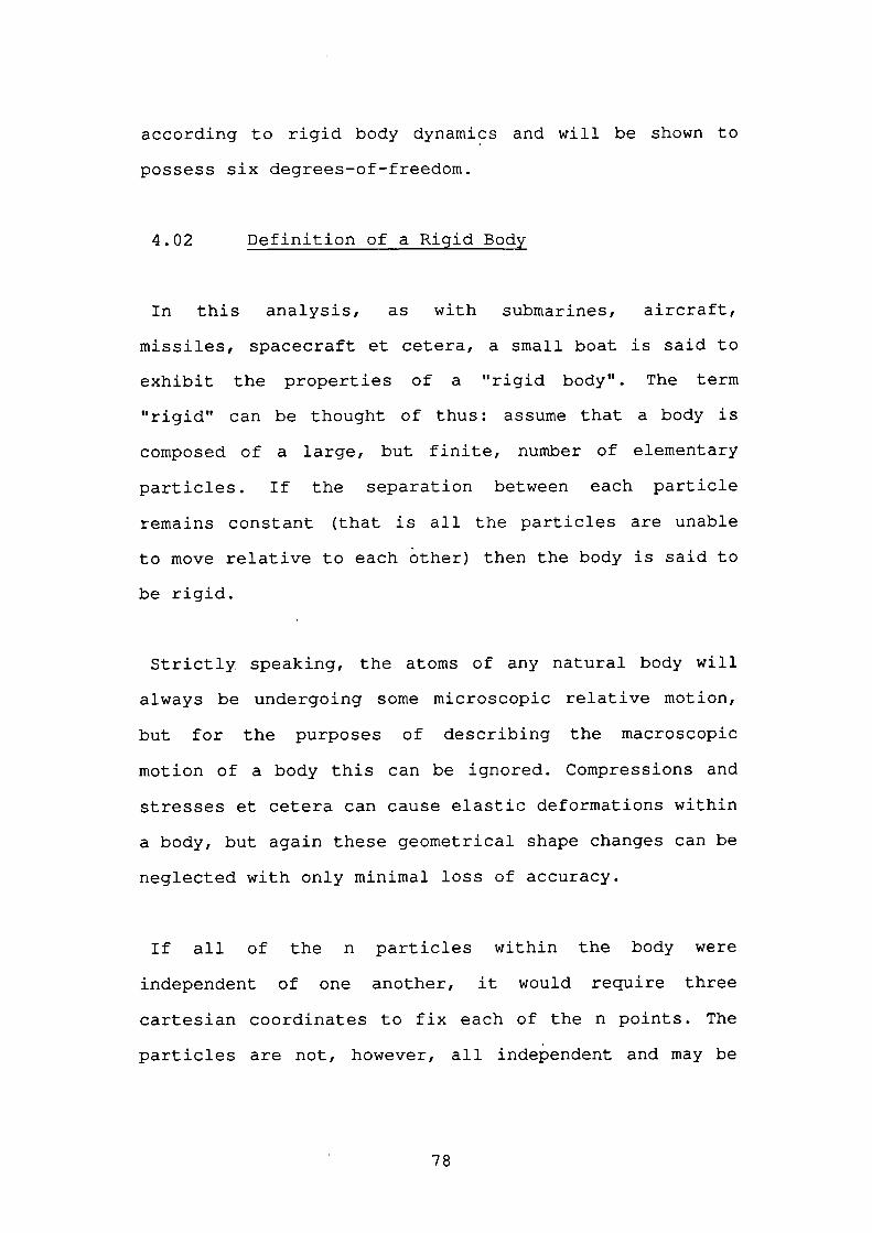
according to rigid body dynamics and will be shown to
possess six degrees-of-freedom.
4.02 Definition of a Rigid Body
In this analysis, as with submarines, aircraft,
missiles, spacecraft et cetera, a small boat is said to
exhibit the properties of a "rigid body". The term
"rigid" can be thought of thus: assume that a body is
composed of a large, but finite, number of elementary
particles. If the separation between each particle
remains constant (that is all the particles are unable
to move relative to each other) then the body is said to
be rigid.
Strictly, speaking, the atoms of any natural body will
always be undergoing some microscopic relative motion,
but for the purposes of describing the macroscopic
motion of a body this can be ignored. Compressions and
stresses et cetera can cause elastic deformations within
a body, but again these geometrical shape changes can be
neglected with only minimal loss of accuracy.
If all of the n particles within the body were
independent of one another, it would require three
cartesian coordinates to fix each of the n points. The
particles are not, however, all independent and may be
78
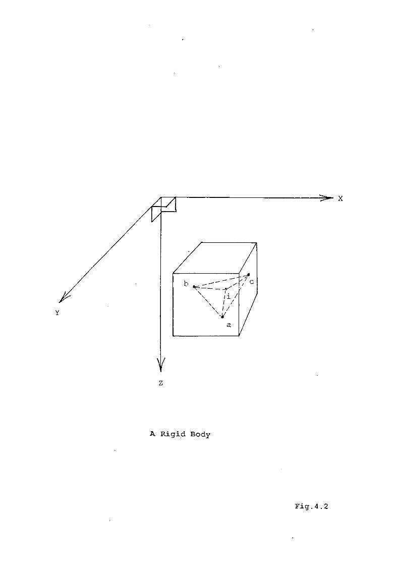
A Rigid Body
Fig.4 .2
x
specified by distances to any three non-colinear points
in the body. From (Fig.4.2) it can be seen that the
distances ria l r.b and nc specify any point i relative
to the three non-colinear points a, b and c.
Since the condition for a rigid body is that the
distances n a, rib and nc are constant, then the
position of the particle i is fixed once the locations
of the three non-colinear points are known. Each of the
n particles in the body can be specified in the same
manner. In other words, the position of the body as a
whole can be determined by the positions of these three
points.
Nine cartesian coordinates would be required to specify
three independent points, but since the distances rab,
rbc and rca are also constant, only six coordinates are
necessary to locate the rigid body and determine its
orientation.
The rigid body is thus said to have six
degrees-of-freedom and Chasles' theorem, which states:
"aJW aii!Uiw.ru LnLte mzüan 4 a &ath ma eeQnAj4er ed ta he wi ipenntInaUonA - a WLea'i anA&itLon 4 4wme p&ntc4 the &ad4 p&i a 'ratatLou akiu.t that poLnt."
allows the problem to be divided into two parts, one
80
involving only translation and the other only rotation.
The three translational motions, described by the three
coordinates required to fix the position of one of the
particles, can therefore be treated separately from the
three rotational motions, described by the remaining
three coordinates necessary to determine the relative
orientation of the other two points. This type of
separation is essential for a relatively uncomplicated
description of rigid-body motion.
4.03 The Six Degrees-Of-Freedom Of A Boat
The six degrees-of-freedom of a boat (Fig.4.3) are
represented in an orthogonal coordinate system having
the centre of gravity as its origin. A description of
these six. quantities now follows.
Surge
Surge is the forward and aft translation of the boat
directed along the X-axis. This not only includes the
propelled movement, but also the tendency for a boat to
move forward on a wave crest, known as surfing, and
backward in a trough. Naturally, a boat under way
through a swell will not actually move backwards and
forwards but will be alternately accelerated and
retarded according to the relative direction of travel
81
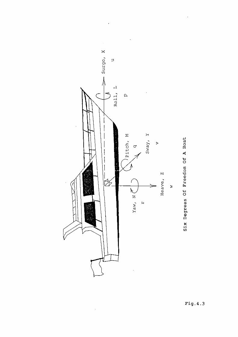
ci)
(I)
-Ii
RI
0
0
E0
ci)- ci)
ci) 1-1
ci) 4-1
0
0,ci)ci)
ci)
•r(/1
Fig.4 .3
to the waves.
Sway
Sway is the transverse translational motion of the boat
along the Y-axis. As well as sideslip due to centripetal
forces when executing a turn, this includes the effect
of successive wave crests providing a series of 'tpushes"
which amount to drift. Most vessels, if not under way,
tend to become orientated broadside on to the swell.
Heave
Heaving is the vertical bodily translation of the whole
boat upwards (which in this analysis is negative motion)
as well as the reverse motion of dipping. This motion is
due to the change in buoyancy as each wave passes the
boat. Heaving is periodic and in this respect associated
with rolling and pitching.
Roll
Roll is the rotation about the longitudinal X-axis of
the boat and is treated with consideration by naval
architects since it affects the comfort of those
onboard. Unlike a pendulum, a boat has no fixed axis of
rotation, but has what is termed the ,u2ajitan.eauA cutLA
83
which is located near the centre of gravity. The centre
of gravity will therefore describe a path in space as
the boat rotates, even though relative to the boat as a
whole it remains fixed.
Pitch
Pitch is the rotation about the transverse Y-axis.
Pitching is in fact the bow down motion (which in this
analysis is negative motion) while the bow up motion is
known as 'scending. Pitching tends to be heaviest when
heading into a sea and increases when conditions of
synchronism occur.
Yaw
Yawing is the rotation about the vertical Z-axis. It is
the tendency for a boat to veer off course. Unlike
rolling and pitching there is no restorative moment;
this must be applied by use of external control surfaces
such as rudders.
4.04 The Axes Systems
Conventionally, and for convenience and simplicity, the
motion of a rigid body is described with respect to a
coordinate system fixed within the body. By choosing the
84
centre of gravity to be its origin, the equations of
motion can be reduced, as will become apparent in later
chapters. However, a second axes system must be
specified which forms the reference or inertial frame.
This can be viewed as a coordinate system fixed with
respect to the Earth.
It is necessary to transform various vector quantities
between these two axes systems. Wind and tidal
information, for example, needs to be converted into
functions of apparent angles. Whereas, the velocity or
displacement of the rigid body is required in the
inertial frame in order to determine the position of the
vessel at sea. It is also of primary importance to know
the orientation • of the boat, in other words the angles
of roll, pitch and yaw, with respect to the inertial
frame. This is often referred to as kinematics.
4.05 Transformation Between Orthogonal Axes
By keeping track of the orientation of the moving axes
system, vectors can be readily transformed between
systems. Three methods for specifying the relative
orientation of the two axes systems are: Direction
cosines, Euler angles and Quaternions.
85
Direction Cosines
The principal tool which provides the means for
performing axes transformations is the direction cosine
matrix. This matrix contains nine elements which are the
cosines of the base angles between each of the axes of
the moving system with each of the axes of the fixed
system.
Consider a vector r with components x 0 , y 0 and in
the inertial frame. Let the unit vectors along the X0,
Y0 and Z 0 axes be ' 2 and 1 3 then:
= l O + 2 y 0 + 1 3 Z0
Now assume another coordinate system X, Y, Z with the
same origin as X0 , Y 0 , Z 0 but having some arbitrary
orientation with respect to it. If the components of r
in the new axes system are x, y and z and the unit
vectors are a 1 , a2 and a3 then:
£ = x + 2 + a 3 z
In order to determine the orthogonal transformation
between the two coordinate systems, it is necessary to
express x, y and z in terms of x 0 , y0 , z 0 and the
relative orientation.
86
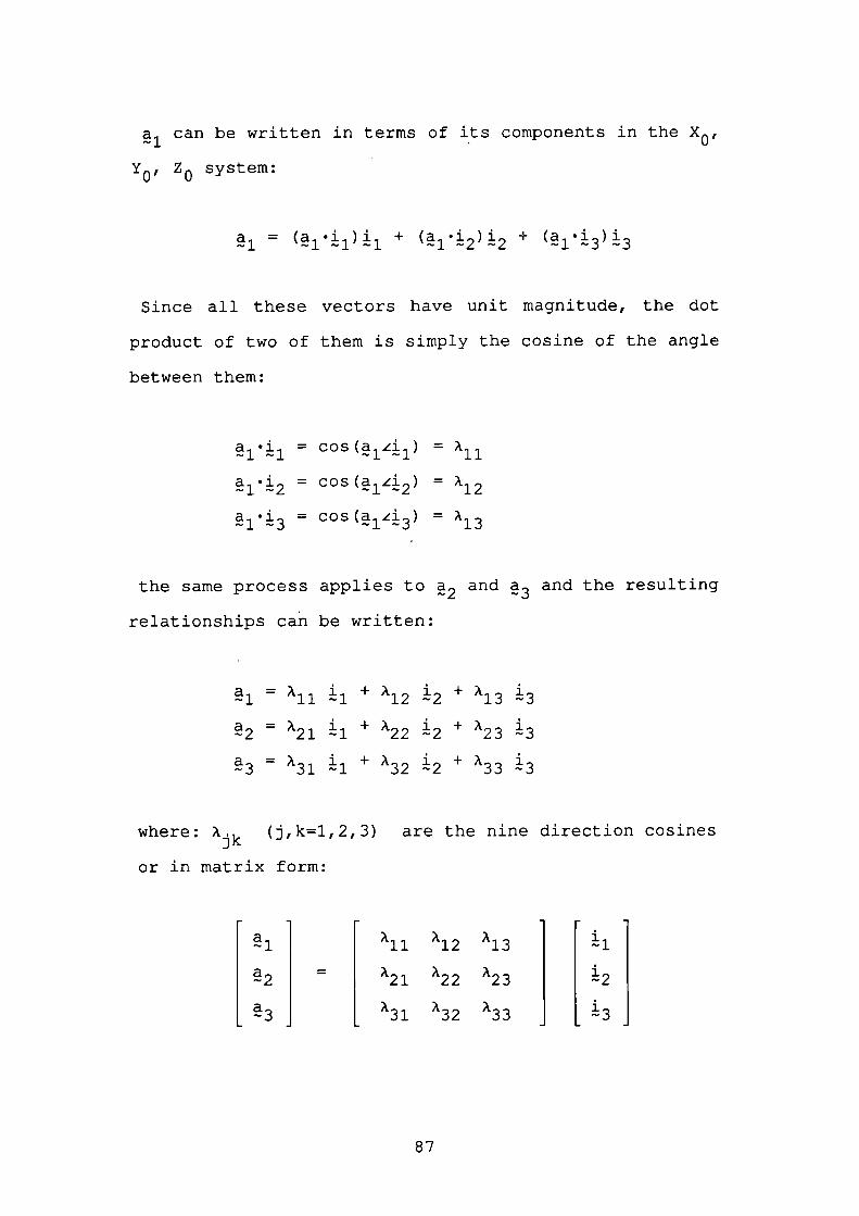
can be written in terms of its components in the X0,
Yo , Z 0 system:
= LL1 + (a1 . i 2 )i 2 + (a1.13)i3
Since all these vectors have unit magnitude, the dot
product of two of them is simply the cosine of the angle
between them:
= cos(a 1 i 1 ) = A11
12 = cos(a 1zi 2 ) = Al2
13 = cos( 14 3 ) = A13
the same process applies to a 2 and a 3 and the resulting
relationships can be written:
= x11 ;] + A l2 + A13 3
2 21 1 22 2 +A23 13
a3 = A31 + 32 2 + A33
where: Aik (j,k=1,2,3) are the nine direction cosines
or in matrix form:
Al2 A13
= A23
A32 A33
87
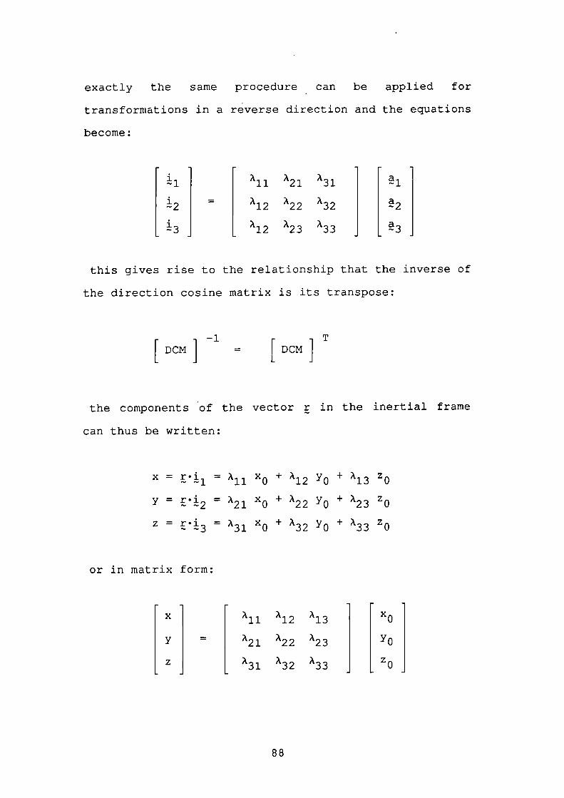
exactly the same procedure can be applied for
transformations in a reverse direction and the equations
become:
X11 A21 A31
= Al2 A22 A32
Al2 A23 A33
this gives rise to the relationship that the inverse of
the direction cosine matrix is its transpose:
[ DCN] -1 = [DCM]
the components of the vector r in the inertial frame
can thus be written:
x = = A11 x 0 + Al2 y 0 + A13 z0
y 2 _21 x 0 +A22 y0 +A23 Z0
Z = = A31 x 0 + A32 y o + A33 z0
or in matrix form:
x
A11 Al2 A13 x0
y= A21 A22 A23 y0
z
A31 A32 A33 zo
88
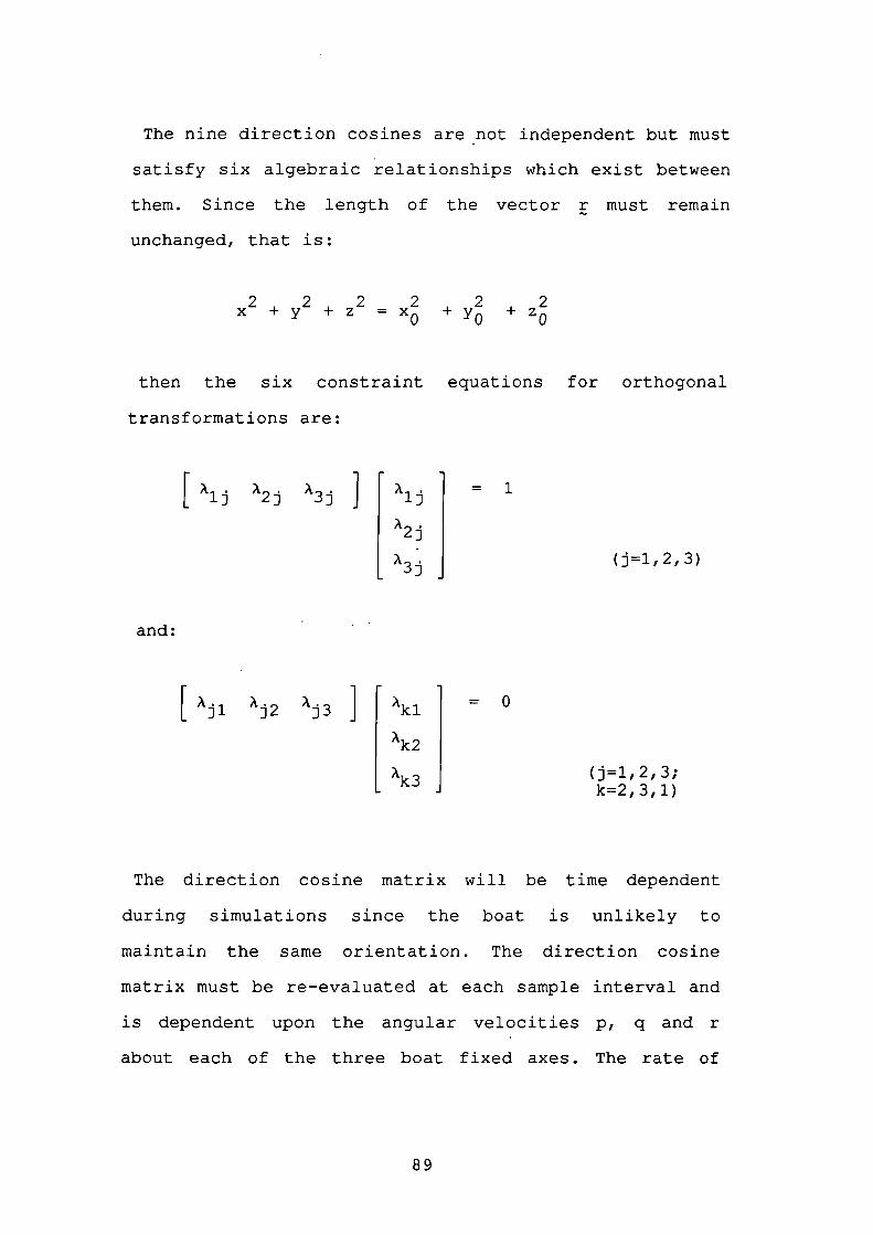
= 1A,lj
A.
A.3j
[x1 A2 A3]
(j=1, 2,3)
The nine direction cosines are not independent but must
satisfy six algebraic relationships which exist between
them. Since the length of the vector r must remain
unchanged, that is:
2 2 2 2 2 2x +y +z =x0 +y0 +z0
then the six constraint equations for orthogonal
transformations are:
and:
[ A1 A 2 A3 ]
Ak 2
Ak 3
= 0
(j = 1, 2,3;k=2, 3,1)
The direction cosine matrix will be time dependent
during simulations since the boat is unlikely to
maintain the same orientation. The direction cosine
matrix must be re-evaluated at each sample interval and
is dependent upon the angular velocities P q and r
about each of the three boat fixed axes. The rate of
89
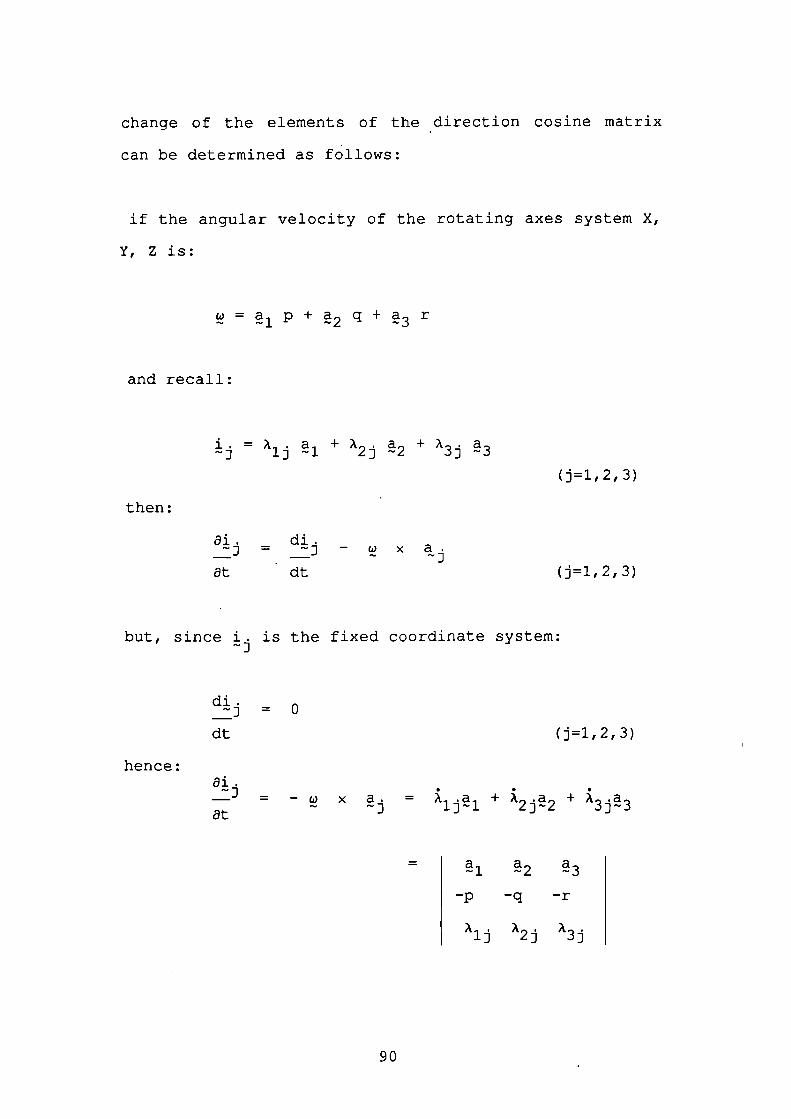
di.-J = 0
dt (j=1,2, 3)
change of the elements of the direction cosine matrix
can be determined as follows:
if the angular velocity of the rotating axes system X,
Y, Z is:
= + 2 q + a 3 r
and recall:
= Ajj + 2j 2 + A3
(j=1, 2,3)
then:
ai. di.= _ .J - x
at dt
(j=1, 2,3)
but, since 1. is the fixed coordinate system:
hence:ai_J = - xat J
1 2 3
-p -q -r
A. A. A.lj 2j 3j
= A .a + .a + .alj-1 2j-2 3j-3
90
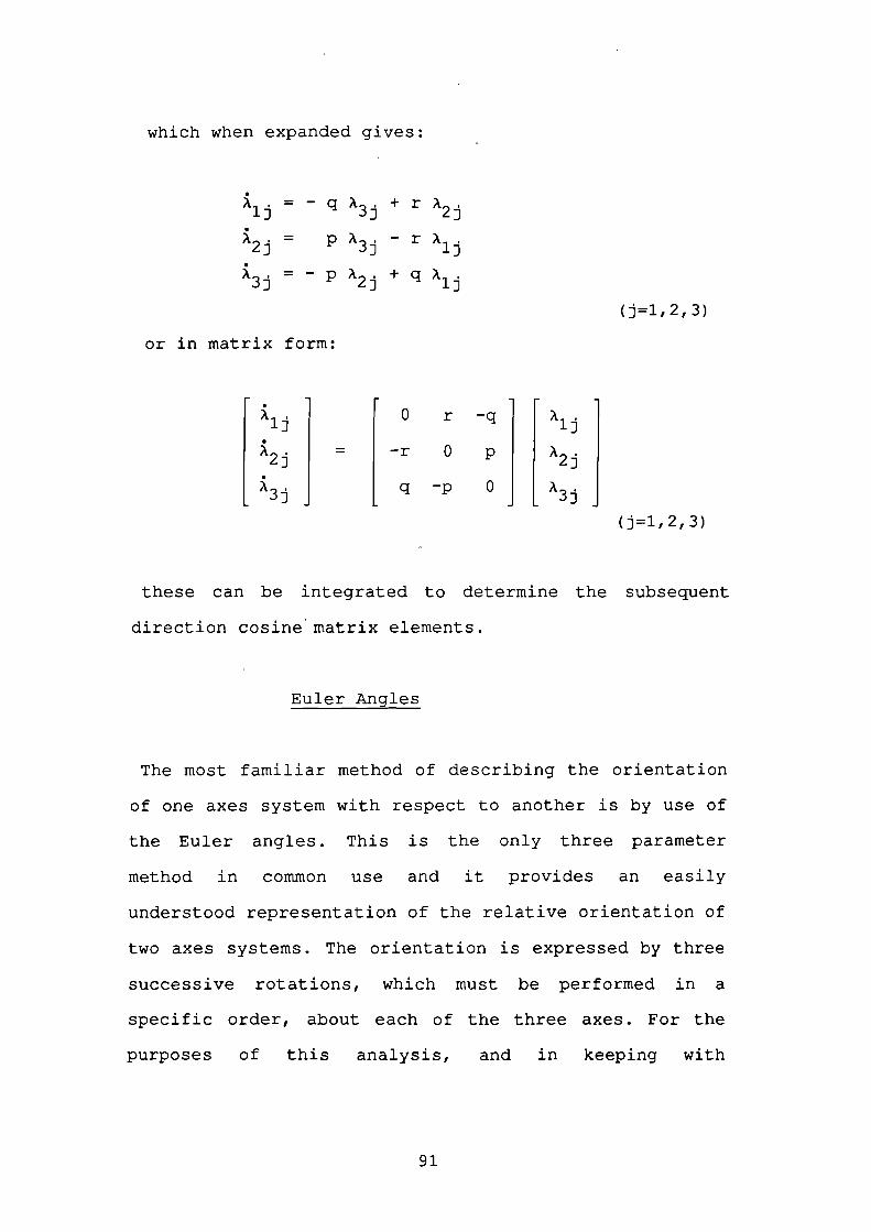
A.lJ
A.
A.3J
which when expanded gives:
lj = - q A3 + r A2.= PA3 _rA1
= - P A2 + q A1
(j=l,2, 3)
or in matrix form:
o r -q
-r 0 p
q -p 0
(j=1, 2,3)
these can be integrated to determine the subsequent
direction cosine matrix elements.
Euler Angles
The most familiar method of describing the orientation
of one axes system with respect to another is by use of
the Euler angles. This is the only three parameter
method in common use and it provides an easily
understood representation of the relative orientation of
two axes systems. The orientation is expressed by three
successive rotations, which must be performed in a
specific order, about each of the three axes. For the
purposes of this analysis, and in keeping with
A.lJ
A.
A.3j
91
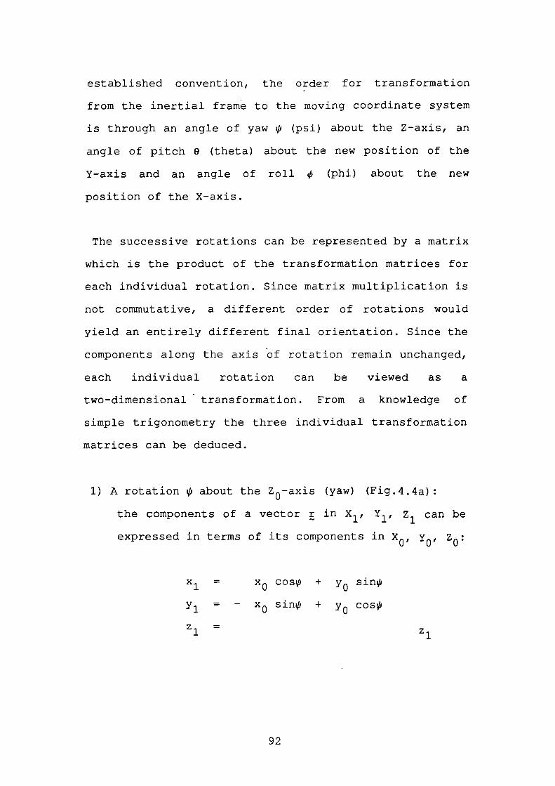
established convention, the order for transformation
from the inertial frame to the moving coordinate system
is through an angle of yaw (psi) about the Z-axis, an
angle of pitch e (theta) about the new position of the
Y-axis and an angle of roll (phi) about the new
position of the X-axis.
The successive rotations can be represented by a matrix
which is the product of the transformation matrices for
each individual rotation. Since matrix multiplication is
not commutative, a different order of rotations would
yield an entirely different final orientation. Since the
components along the axis of rotation remain unchanged,
each individual rotation can be viewed as a
two-dimensional transformation. From a knowledge of
simple trigonometry the three individual transformation
matrices can be deduced.
1) A rotation cu about the Z 0 -axis (yaw) (Fig.4.4a):
the components of a vector r in X 1 , Y 1 , z 1 can be
expressed in terms of its components in X 0 , y 0 , Z0:
x 1 = xo coscus + y0 sincu,
= - x0 sincu, + y 0 cos
zi = zi
92
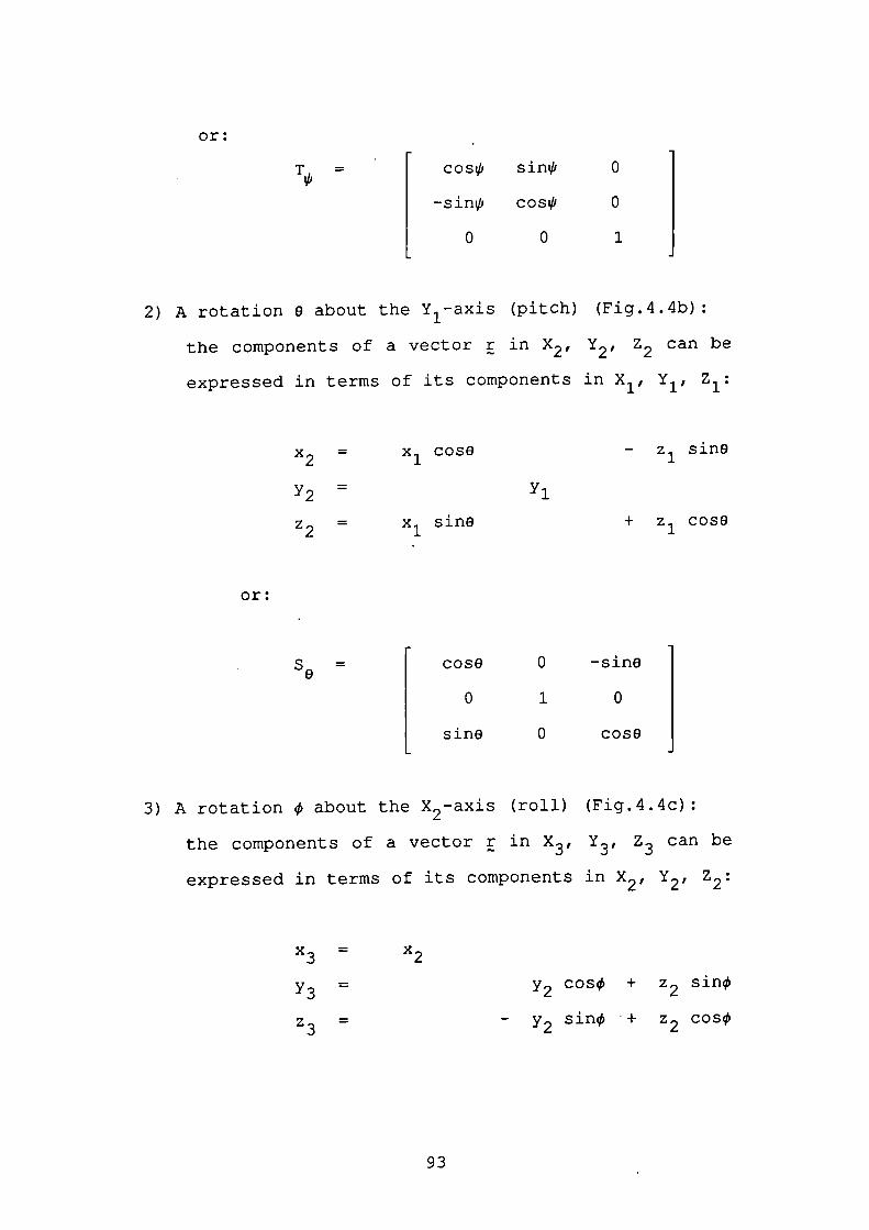
or:
T1, = cosI S ifl'
0
-sin, cos,
0
0
0
:1.
2) A rotation e about the Y 1 -axis (pitch) (Fig.4.4b):
the components of a vector r in X 2 , Y2 , Z 2 can be
expressed in terms of its components in X 1 , Y 1 , Z1:
= x1 cose - Z ] siflO
= yl
z 2 = x 1 sine + z 1 cose
or:
S e = cose
0 -sine
0
1
0
sine
0
cose
3) A rotation about the X 2 -axis (roll) (Fig.4.4c)
the components of a vector r in X 3 , 1 31 Z 3 can be
expressed in terms of its components in X 2 , Y2 , Z2:
x3 = x2
y3 = CO5 + Z 2 5ifl
z 3 = - y2 Sifl + z 2 cos
93
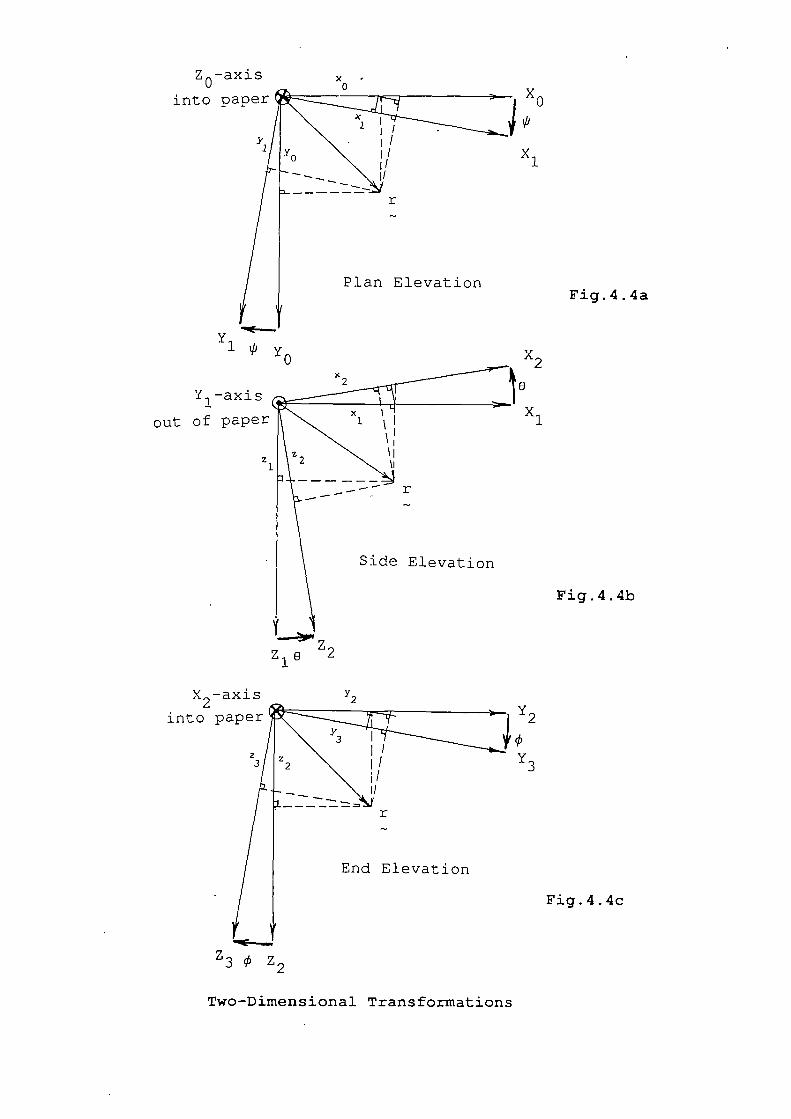
Z0-axis
into pa
xnxo
;li
xl
Yl i
Y1-axjs
out of paper
zI
Fig.4.4b
x2
6
xl
X2axis
into p
Y3
Fig.4 . 4a
zT Z2
Fig.4.4c
z3
Two-Dimensional Transformations
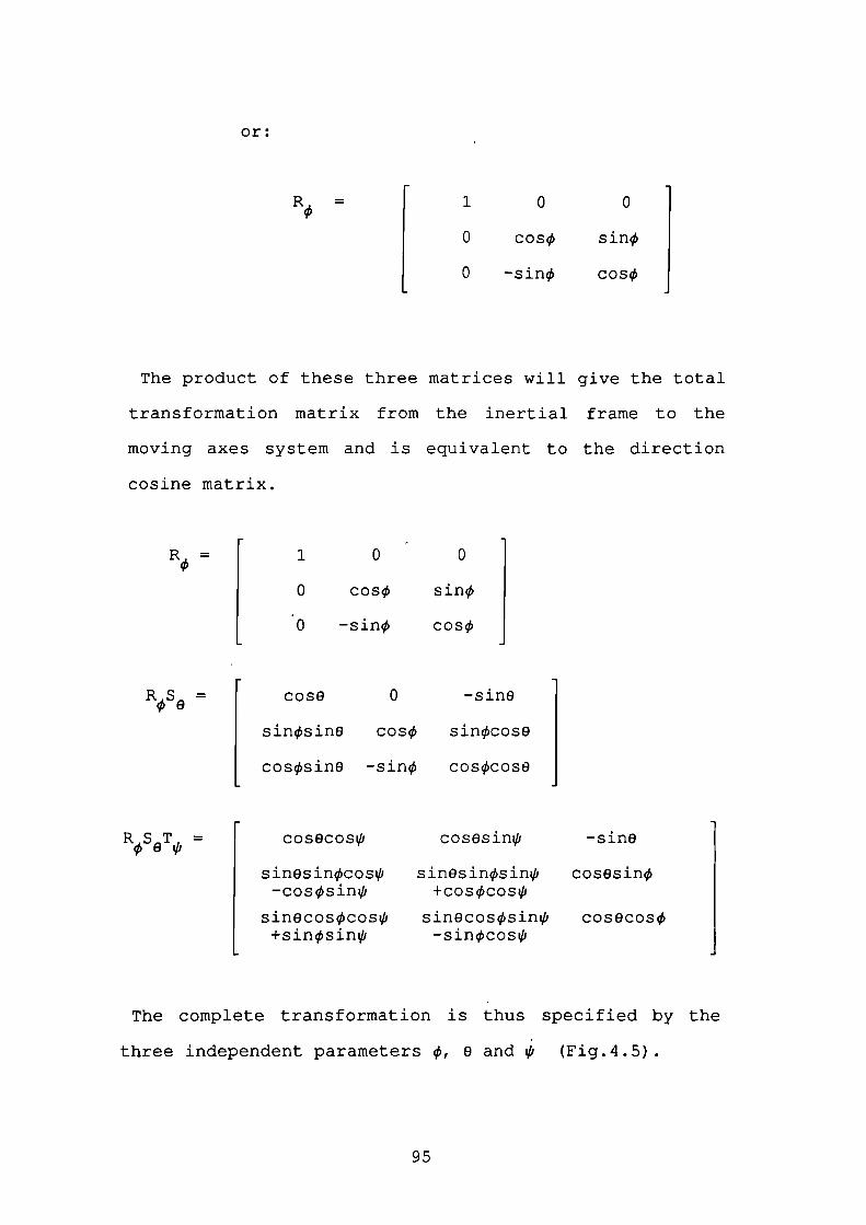
-sine
cosesin
cosOcos
or:
R =
1
0
0
0
cos sin
0
-sin cos
The product of these three matrices will give the total
transformation matrix from the inertial frame to the
moving axes system and is equivalent to the direction
cosine matrix.
R= 1 0 0
o cos sin
o -sin cos
RSe = cose 0 -sine
sinsinO cos sincose
cossin9 -sin coscosO
R ,S eT j = cosecosi
sinOsincosV'-cossini
sinecoscosi+sinsini
cososin'
sinOsinsins+coscos,
sinecossin'-sincoss
The complete transformation is thus specified by the
three independent parameters , 0 and (Fig.4.5).
95
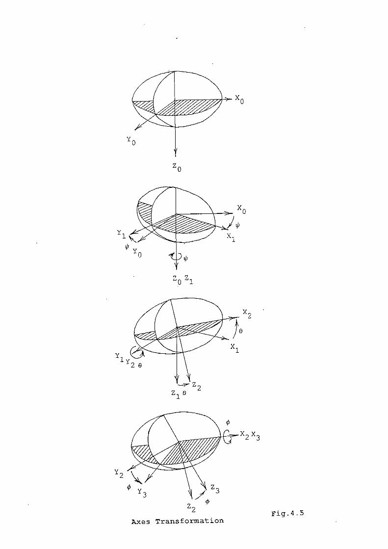
zo
Z0 Z
zZ 1 e
z2
Fig.4.5Axes Transformation
Y
xo
Y l--
Yly
x2
x2 x3
xo
cu
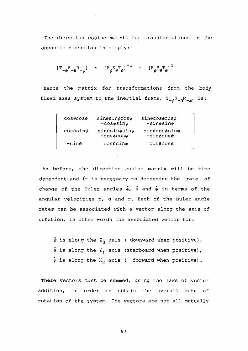
cosOcos
cosesini
-sinG
The direction cosine matrix for transformations in the
opposite direction is simply:
[TS 9R] = [RSQT]1 = [R,S9T,,]T
hence the matrix for transformations from the body
fixed axes system to the inertial frame, T_,S_eR_I is:
sinesincos/l-cossini
sinesinØsins+cosØcosi
cosGsin
sin8coscos'+sinsinl
sinGcossini-sincosi
cosecos
As before, the direction cosine matrix will be time
dependent and it is necessary to determine the rate of
change of the Euler angles , and is in terms of the
angular velocities P' q and r. Each of the Euler angle
rates can be associated with a vector along the axis of
rotation. In other words the associated vector for:
i is along the Z 0 -axis ( downward when positive),
is along the Y 1 -axis (starboard when positive),
is along the X 2 -axis ( forward when positive).
These vectors must be summed, using the laws of vector
addition, in order to obtain the overall rate of
rotation of the system. The vectors are not all mutually
97
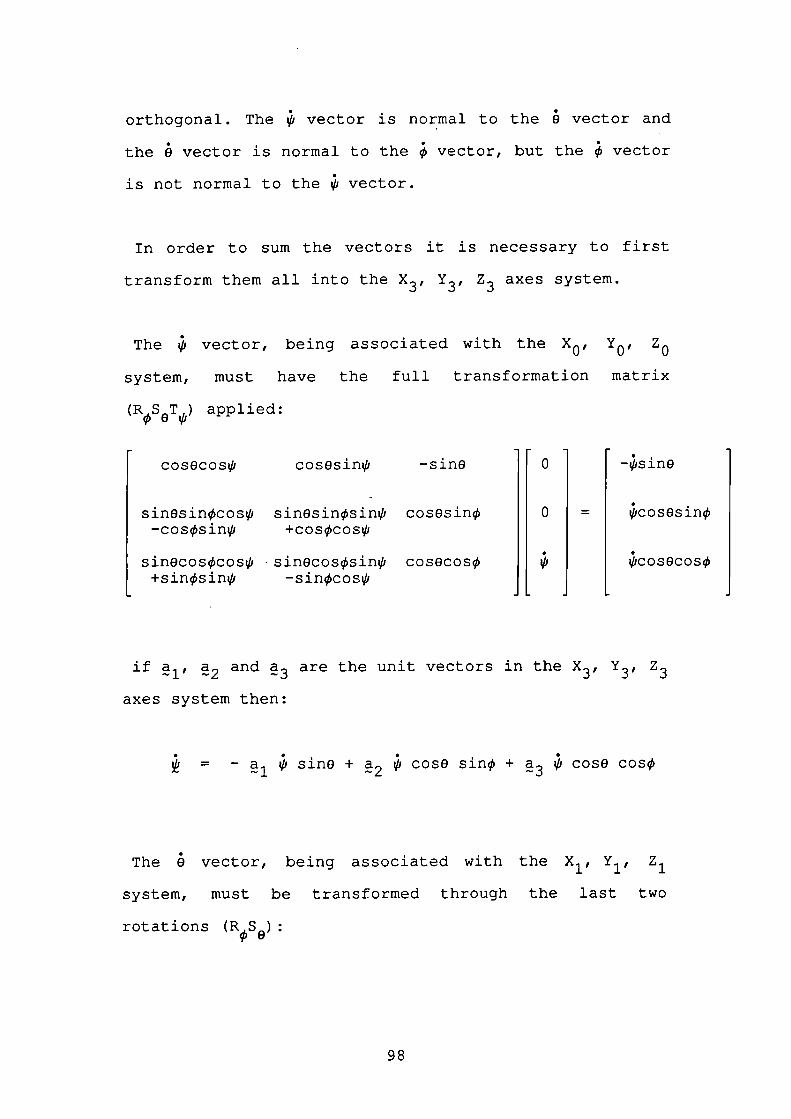
orthogonal. The vector is normal to the vector and
the vector is normal to the vector, but the vector
is not normal to the , vector.
In order to sum the vectors it is necessary to first
transform them all into the X 3 , Y 3 , Z 3 axes system.
The Qi vector, being associated with the x 0 , y0 , z0
system, must have the full transformation matrix
(RSeTcij) applied:
o -isinO
o = 'cosOsin
cosecos
cosecosi cosesini -sine
sinOsincosi sinOsinsin cosesin-cossini +coscos,/i
sinecoscos' sinOcossin' cosecos+sinsinl -sincos,
-' and a 3 are the unit vectors in the X 3 , Y3 , Z3
axes system then:
= - a 1 ' jfl +' coso sin + a 3 i cose cos
The vector, being associated with the X 1 , Y1 , Z1
system, must be transformed through the last two
rotations (RSe)
98
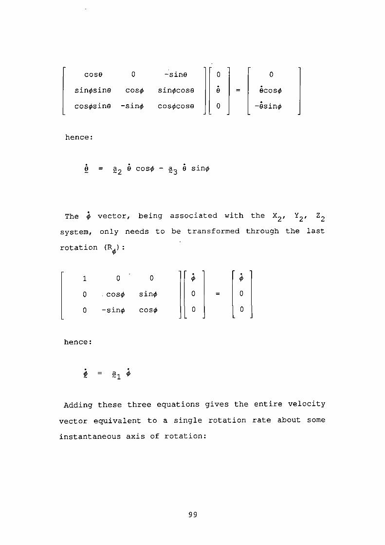
cose 0
-sine
0
0
sinsine cos SiflcOSO
o = cos
cossiflO -sin coscose
0 -sinø
hence:
= 0 cos - a3 0 sin
The vector, being associated with the X 2 , Y2 , Z2
system, only needs to be transformed through the last
rotation (R)
1. 0 0
o .cos sinØ 0 = 0
0 -sin cos 0 0
hence:
= 1 '
Adding these three equations gives the entire velocity
vector equivalent to a single rotation rate about some
instantaneous axis of rotation:
99
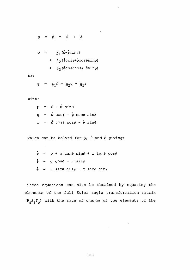
w = (-isine)
+ 2 (cos-coses1n)
+ a3 (cosocos-sin)
or:
= + + a3r
with:
p = - sine
q = 8 COS + cose sinØ
r = cOSO cos - 8 sin
which can be solved for , and 1 giving:
= p + q tane sin + r tanG cos
= q cosØ - r sinØ
= r sece cos + q sece sin
These equations can also be obtained by equating the
elements of the full Euler angle transformation matrix
(RSQT 11) with the rate of change of the elements of the
100
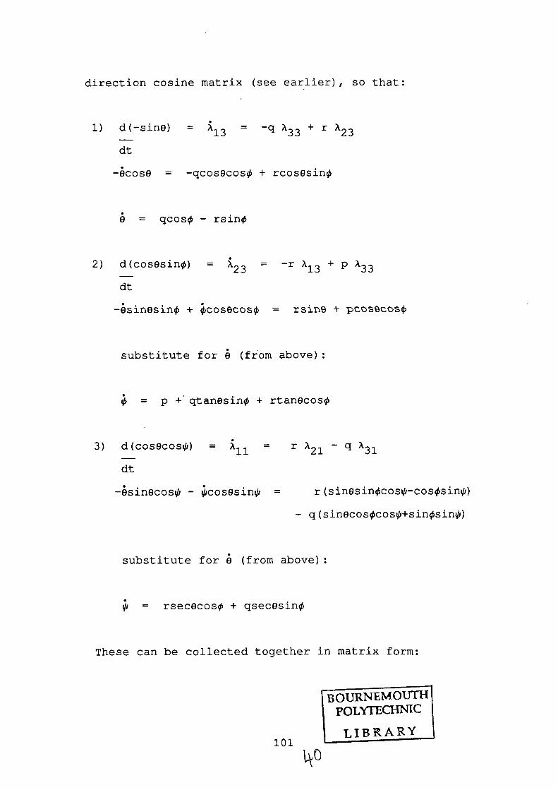
direction cosine matrix (see earlier), so that:
1) d(-sinO) = A13 = -q A33 + r 23
dt
-Ocoso = -qcosOcos + rcosOsin
S = qcos - rsin
2) d(cosesin) = 23 = -r A13 + p A33
dt
-esinesin4 + cos6cos4 = rsn9 4 pcos9cos
substitute for (from above):
= p + qtanesin + rtanecos
3) d(cosOcos,) = = r A21 - q A31
dt
-sinecosi - ,cosOsini = r(sinOsincoss-cossin')
- q (sinecoscosi+sinsini)
substitute for (from above)
= rsececos + qsecesin
These can be collected together in matrix form:
FOURNEMOUii1FOLYfECHNIC
101 L LIBRARY
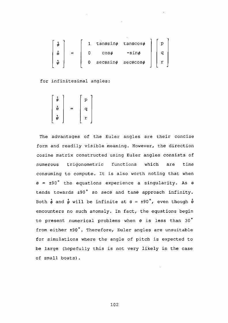
1 tanesin tanOcos
p
9
o cos -sin q
o secosin sececos r
for infinitesimal angles:
p
e q
ci' r
The advantages of the Euler angles are their concise
form and readily visible meaning. However, the direction
cosine matrix constructed using Euler angles consists of
numerous trigonometric functions which are time
consuming to compute. It is also worth noting that when
0 = ±900 the equations experience a singularity. As 0
tends towards ±90° so sece and tanG approach infinity.
Both and , will be infinite at o = ±900, even though
encounters no such anomaly. In fact, the equations begin
to present numerical problems when 0 is less than 30°
from either ±90°. Therefore, Euler angles are unsuitable
for simulations where the angle of pitch is expected to
be large (hopefully this is not very likely in the case
of small boats)
102
Quaternions (Euler Parameters)
The four parameter transformation method was first
introduced by Euler in 1776 (the parameters are often
referred to as the Euler parameters and denoted by the
letter 'e'), as a result of spherical trigonometry
considerations. The method was subsequently improved
upon by Hamilton in 1843 and the parameters have become
known as quaternions.
This alternative approach of representing the relative
orientation of two axes systems relies on Euler's
theorem which states:
The 'utatLon a - atw ae tein 'um onearz2WtwuI ontaUon ta am othen aWw'uo'iJentaiLon ma Ie &rpne&ed aruitatLon aau om ed a"
Consider, as in the development of the DCM (Direction
Cosine Matrix), two orthogonal coordinate systems
(the inertial axes) and X,Y,Z (the moving axes)
having the same origin and initially coincident. Suppose
the X,Y,Z system is then rotated through an angle jL
about some instantaneous axis r which is inclined at the
angles and a3 from the X 0 , Y0 and Z 0 axes
respectively (and as it happens from the X, Y and Z axes
also). It is then possible to determine the four Euler
symmetric parameters from these three angles and single
103
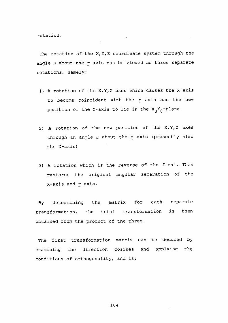
rotation.
The rotation of the X,Y,Z coordinate system through the
angle i about the r axis can be viewed as three separate
rotations, namely:
1) A rotation of the X,Y,Z axes which causes the X-axis
to become coincident with the r axis and the new
position of the Y-axis to lie in the X0Y0-plane.
2) A rotation of the new position of the X,Y,Z axes
through an angle i about the r axis (presently also
the X-axis)
3) A rotation which is the reverse of the first. This
restores the original angular separation of the
X-axis and r axis.
By determining the matrix for each separate
transformation, the total transformation is then
obtained from the product of the three.
The first transformation matrix can be deduced by
examining the direction cosines and applying the
conditions of orthogonality, and is:
104
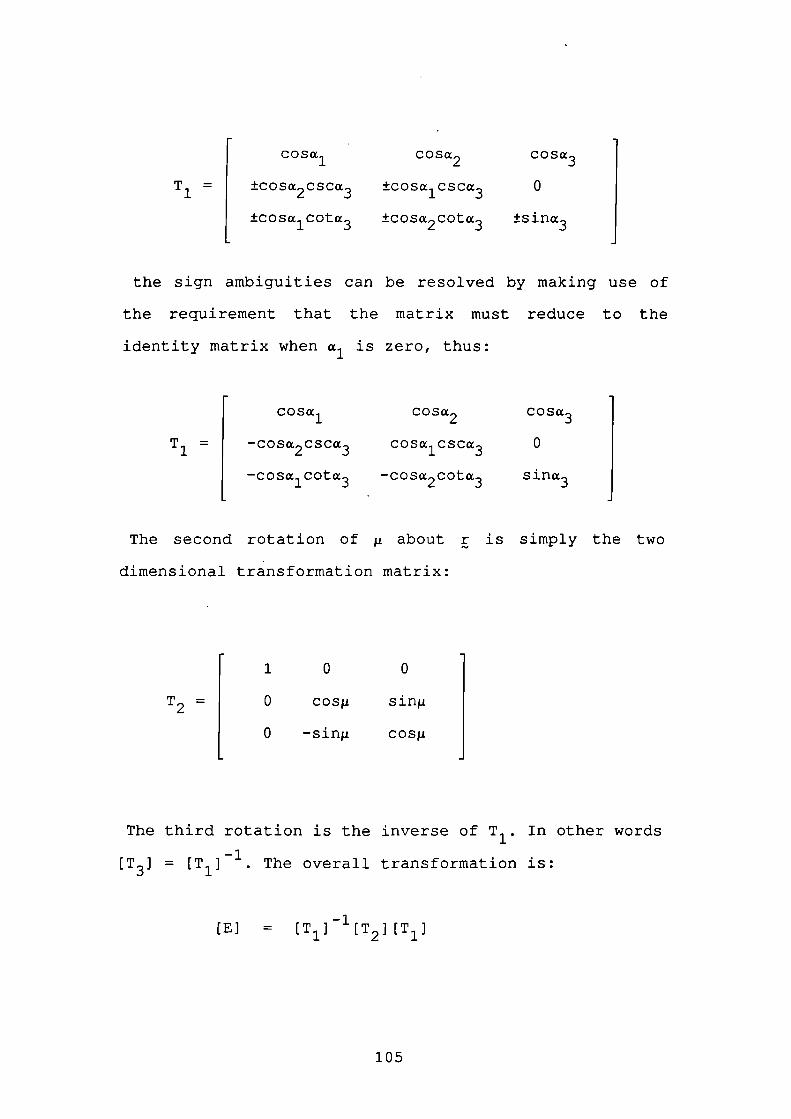
coso: CO So: c0sa3
T 1 = ±COSa2CSCa3 ±COSo:1CSCa3 0
±COsaCOta3 ±CO So:2 Cota3 ±Sifla3
the sign ambiguities can be resolved by making use of
the requirement that the matrix must reduce to the
identity matrix when a 1 is zero, thus:
co5a1 Co so:2 Cosa3
T 1 = -COSa2CSCa3 cOSo:1CSca3 0
-cosa1coto:3 -COSa2cota3 sina3
The second rotation of i about r is simply the two
dimensional transformation matrix:
1 0 0
T2 =
0 cos.z sing
0 -sing cosii
The third rotation is the inverse of T 1 . In other words
[T3 ] = [T 1 ]. The overall transformation is:
[El = [ T 1 ] 1 [T2 ] [T1]
105
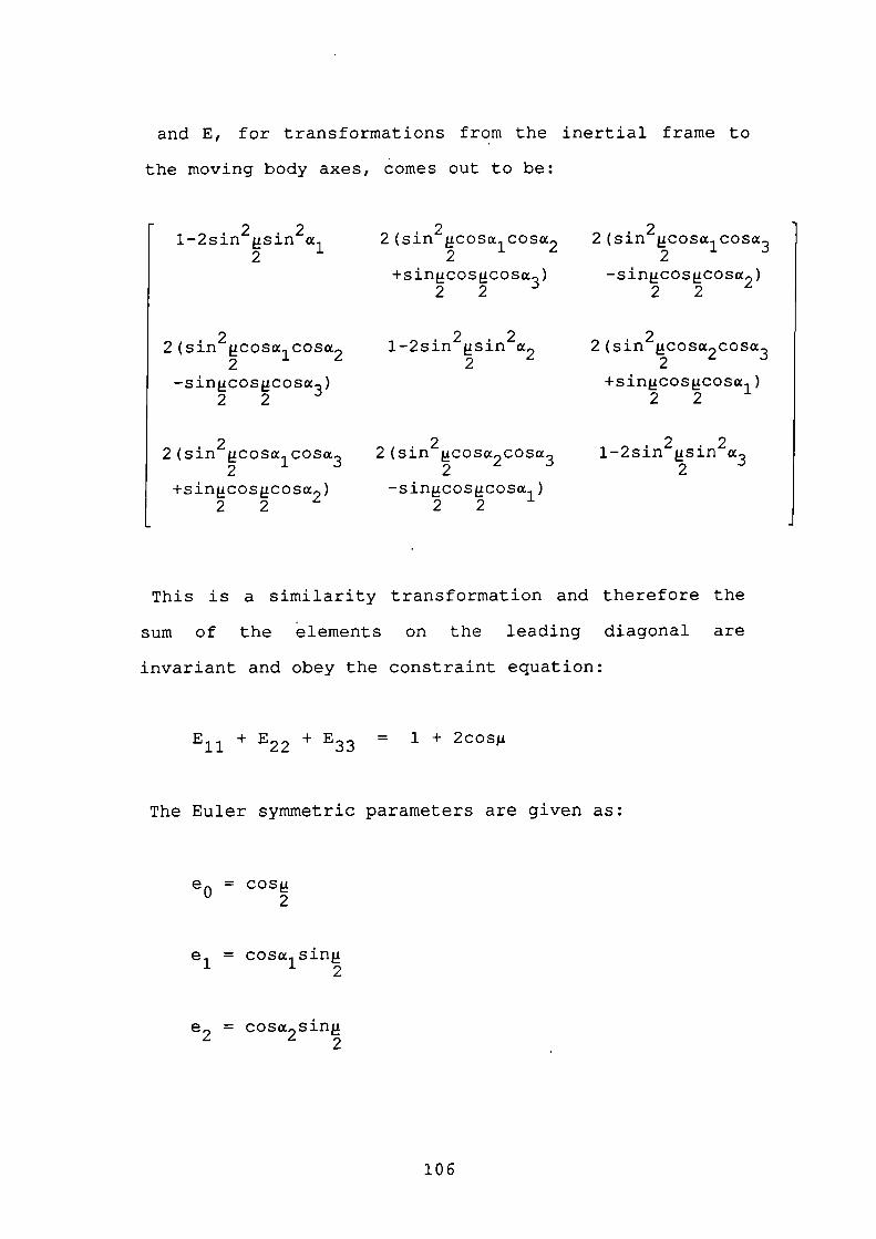
and E, for transformations from the inertial frame to
the moving body axes, comes out to be:
.2 .21-2sin sin a12
2 (sin2Icosa1cosa22
-sincosCosLx3)2 2
2 (sin2 jcosa1cosa3
+sincoscosa2)2 2
2 (sin 2 cosa1cosa22
+sincoscosa3)2 2
.2 .21-2sin2
2 (sin 2 jcosa2cosa32
-sincosjcosa1)2 2
2 (sin 2 Icosa1cosa32
- 51fl c OS Co a2)2 2
2 (sin 2 jCosa2cosa3
+singcoscosa1)2 2
.2 .21-2sin sin a32
This is a similarity transformation and therefore the
sum of the elements on the leading diagonal are
invariant and obey the Constraint equation:
E 11 + E22 + E33 = 1 + 2cosji
The Euler symmetric parameters are given as:
e 0 =2
e 1 = cosa1sin2
e2 = COSa2S1fl2
106
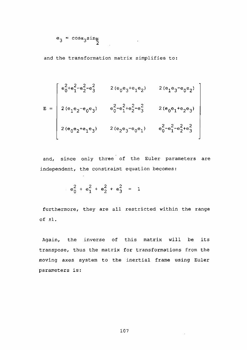
e3 = cos3sin2
and the transformation matrix simplifies to:
E=
2222e0+e 1 -e 2 -e 3
2 (e1e2-e0e3)
2 (e0e2+e1e3)
2 (e 0 e 3 +e 1 e 2 )
2222e0-e1+e2-e3
2 (e2e3-e0e1)
2 (e1e3-e0e2)
2 (e0e1+e2e3)
2222e0-e1-e2+e3
and, since only three of the Euler parameters are
independent, the constraint equation becomes:
2 2 2 2e 0 + e 1 + e2 + e3 =
furthermore, they are all restricted within the range
of ±1.
Again, the inverse of this matrix will be its
transpose, thus the matrix for transformations from the
moving axes system to the inertial frame using Euler
parameters is:
107
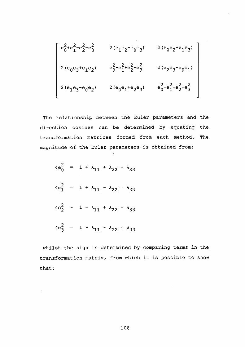
2222e0+e 1 -e 2 -e 32 (e1e2 -e 0 e 3 ) 2 (e0e2+e1e3)
2 (e0e3+e1e2)
2 (e 1 e 3 -e 0 e2 )
2222e0 -e 1 +e2 -e 3
2 (e0e1+e2e3)
2 (e2e3-e0e1)
2222e0-e1-e2+e3
The relationship between the Euler parameters and the
direction cosines can be determined by equating the
transformation matrices formed from each method. The
magnitude of the Euler parameters is obtained from:
4e = 1 + A11 + A22 + A33
24e 1 = 1 + A11 - A22 - A33
4e = 1 A11 +A22A33
4e = 1 - A11 - A22 + A33
whilst the sign is determined by comparing terms in the
transformation matrix, from which it is possible to show
that:
108
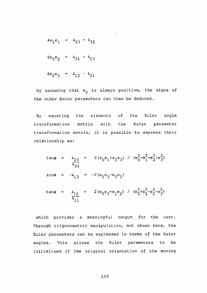
4e 0 e 1 = A23 - A32
4e 0 e2 = A31 - A13
4e 0e 3 = Al2 - A21
by assuming that e 0 is always positive, the signs of
the other Euler parameters can then be deduced.
By equating the elements of the Euler angle
transformation matrix with the Euler parameter
transformation matrix, it is possible to express their
relationship as:
2222tan = A23 = 2(e0e1+e2e3) / (e0-e1-e2+e3)
sine = -A13 = -2(e1e3-e0e2)
2222tan, = Al2 = 2(e0e3+e1e2) I (e0+e1-e2-e3)
xiii
which provides a meaningful output for the user.
Through trigonometric manipulation, not shown here, the
Euler parameters can be expressed in terms of the Euler
angles. This allows the Euler parameters to be
initialised if the original orientation of the moving
109
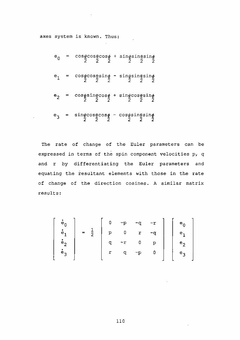
axes system is known. Thus:
e 0 = coscosecos + sinsinosin2 2 2 2 2 2
e 1 = coscos9sin - sinsin8sin2 2 2 2 2 2
e2 = cossinOcos + sincosesin2 2 2 2 2 2
e 3 = sinCOSeCOS - COSSiflOSifl2 2 2 2 2 2
The rate of change of the Euler parameters can be
expressed in terms of the spin component velocities Pi q
and r by differentiating the Euler parameters and
equating the resultant elements with those in the rate
of change of the direction cosines. A similar matrix
results:
0 -p -q
. 1e 1= p 0 r
q -r 0
e 3r q -p
-r e0
-q e1
p e2
0
e3
110
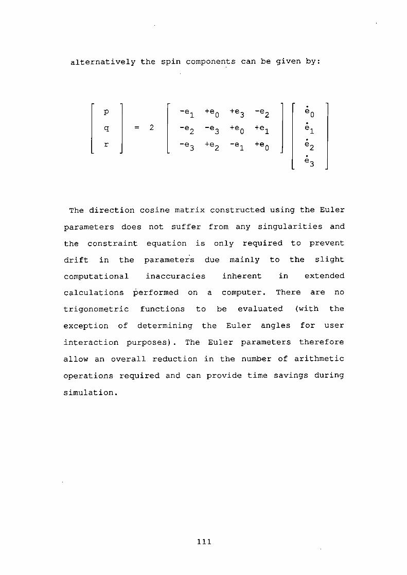
alternatively the spin components can be given by:
p -e1 +e 0 +e3 -e2
q = 2
-e2 -e 3 +e0 +e1
r -e3 +e2 -e 1 +e0 e2
e3
The direction cosine matrix constructed using the Euler
parameters does not suffer from any singularities and
the constraint equation is only required to prevent
drift in the parameters due mainly to the slight
computational inaccuracies inherent in extended
calculations performed on a computer. There are no
trigonometric functions to be evaluated (with the
exception of determining the Euler angles for user
interaction purposes). The Euler parameters therefore
allow an overall reduction in the number of arithmetic
operations required and can provide time savings during
simulation.
111

CHAPTER 5
APPROACH TO THE MATHEMATICAL MODEL
112
5.01 Modularity
Mathematical models of marine vehicles have been
revolutionised over the past few years by modular
techniques and new models are moving away from the
regressional methodology. Dand, 1987 (Ref.43), indicates
how regressional models are being superseded by modular
models, with particular reference to work carried out at
BMT (British Maritime Technology).
In the past, simulator models have been constructed
using regressional techniques, especially as the
equations of motion are usually based upon a
multi-variable Taylor series expansion of the states
about some initial equilibrium condition. The
hydrodynamic forces and moments acting on a vessel are
therefore presented in terms which combine the motion
variables u, v and r and some regression coefficients.
Global multi-variable regression is applied to ship
trials data or to scaled model test data to assign
values to these coefficients. Consequently, the
propeller and rudder coefficients will be drawn into the
regression analysis along with all the other terms, and
they will not specifically incorporate information on
propeller or rudder geometry. Instead, the coefficients
will relate to the particular data from whence they are
113
derived and will assume, or take on, values which
generate the correct states at given propeller
revolutions and rudder angles. Naturally the
characteristics of the rudder and propeller are subsumed
into the regression coefficients since the model apes
the real situation.
Dand defines the pure regressional model as:
4 mde whLch perorumc Aa4actonth whentaken. a a uihoie, &u.t whLch does nat o1&wijldkgdw1 eemn ta &e changed neadJ1 athe deqn L changed'
The modular technique is to describe the individual
elements, such as hull, rudder, propeller and so forth,
as separate modules which will be incorporated within
the overall system. In principle, it is possible to
alter a single module without affecting any of the other
modules, that is any given module does not require a
knowledge of the contents of the remaining modules.
This concept potentially provides an extremely flexible
design tool, for example simulations can be performed
with different rudder designs in order to assess the
effect on manoeuvrability. The forces and moments
contained within each module will be constructed with
reference to the particular physical processes involved;
this provides a far more rigorous structure than a
114
regressional model.
The modular approach does suffer from problems related
to the connections and data pathways between the
modules. The behaviour of one module will inevitably
affect that of another. Furthermore, a number of
variables will end up being global to the whole
simulation, especially when duplicate calculations are
to be removed in order to save time. Other problems
arise from the general shortage of data with which to
construct the separate modules, especially as most
experimental does not cover the complete operating
environment usually encountered.
The author believes that, despite any drawbacks, the
future of marine simulation models lies within the
realms of the modular format and consequently this
thesis will adopt such an approach.
5.02 The Division Of The Forces
The forces and moments acting on a boat can be broadly
grouped into four categories, namely the inertial
forces, the damping forces, the restoring forces and the
exciting forces. The inertial forces produce a
resistance when the boat is set in motion. The damping
forces act in opposition to the boat's motion in such a
115
manner that they always tend to reduce the motion. The
restoring forces act to always bring the boat back to
its equilibrium position. The exciting forces can be
sub-divided further into those due to the control
surfaces, such as the rudder and propeller, which
provide manoeuvrability and those due to disturbances,
such as the wind and waves, which cause unwanted
external forces.
116

CHAPTER 6
EQUATIONS OF MOTION OF A SMALL BOAT
117
6.01 Newton's Law Of Motion
The equations of motion of a body moving in a fluid can
be summarised by Newton's second law of motion:
F = ma
where F is the total external force applied to the
body, m is the actual mass of the body, and a is the
acceleration in the direction of F. This requires no
further explanation here, but since the mathematical
model includes moments, it seems appropriate to digress
to a discussion of moments of inertia.
6.02 Inertia Tensor
The general equation, which corresponds to Newton's
second law, used to express the relationship of a moment
and rotational acceleration is:
M = 1w
where M is the moment, I is a tensor quantity called
the moment of inertia and c is the rotational
acceleration.
The inertia tensor can be represented in the form of a
118
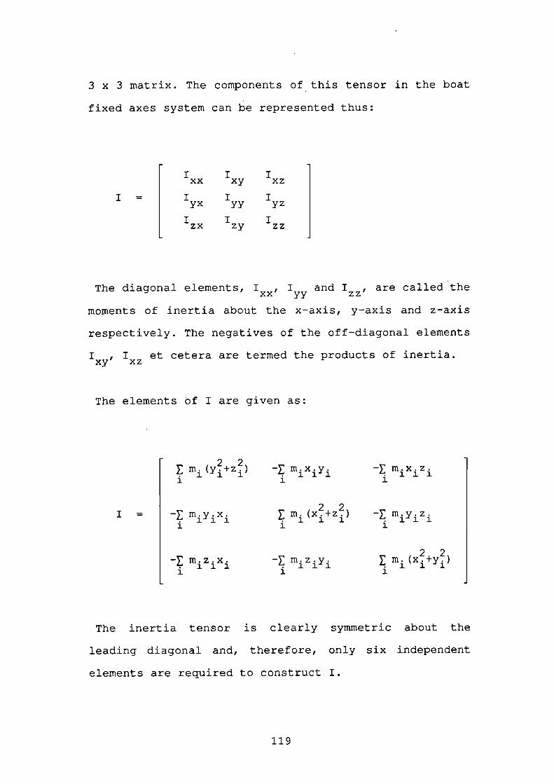
3 x 3 matrix. The components of this tensor in the boat
fixed axes system can be represented thus:
I I Ixx xy xz
= I I Iyx yy yz
I I Izx zy zz
The diagonal elements, I , I and I , are called thexx yy zz
moments of inertia about the x-axis, y-axis and z-axis
respectively. The negatives of the off-diagonal elements
I , I et cetera are termed the products of inertia.xy xz
The elements of I are given as:
22m1(y+z1)1
-E m.x.y11
-E m.x.z.1111
I = - m.y.x.1
- mz.x.1111
22E m. (x.+z.)1 1 11
- m.zy1
- m.y.z.1
22E m(x+y1)1
The inertia tensor is clearly symmetric about the
leading diagonal and, therefore, only six independent
elements are required to construct I.
119
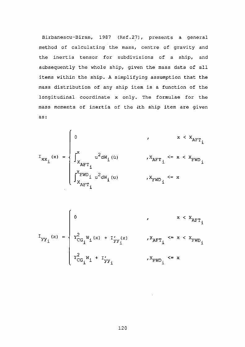
Birbanescu-Biran, 1987 (Ref.27), presents a general
method of calculating the mass, centre of gravity and
the inertia tensor for subdivisions of a ship, and
subsequently the whole ship, given the mass data of all
items within the ship. A simplifying assumption that the
mass distribution of any ship item is a function of the
longitudinal coordinate x only. The formulae for the
mass moments of inertia of the Lth ship item are given
as:
o
x(x) =
u2dW(u)xx.3.AFT.1FWD. "I i udW. (u)1AFT
x < XI
1
,XAFT <= x < XFWD
<= x
0
'yyi= Y G W i( x ) + I,y(X)
Y w.+i'CG. 1 yy
x < XAFTI
1
IXAFT <= x <
<= x1
120
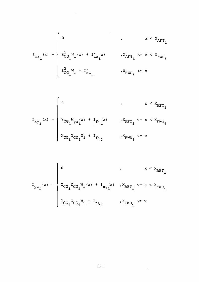
0
(x) = J Z 2 W (x) + I' (x)
zz. I CG. i zz.
1 1
w + I'CG. i zz.1 1
X<XT1
<= x < XFWD1
<= x1
10
xy1 1 1(x)= Y M (x)+I (x)CG yz.
x y w.+iCG CG. 11 1
X<XT1
< x <1
<= x1
10
(x) = YCGZCGW.(x) + I(x)yzi
Y Z W.+ICG CG. 1± 1
X<XT1
,XT <= x < XFWD1
IXFWD <= x1
121
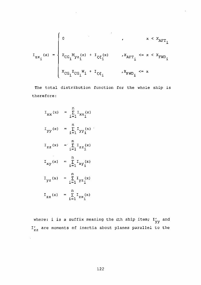
o
(x) = Z M (x) + I(x)CG yz.zx1 1
CG CG. 1x z w. +i 1
X<XI,T1
IXT <= x <1
<= x1
The total distribution function for the whole ship is
therefore:
I (x)xx
I (x)yy
I (x)zz
I (x)xy
I (x)yz
n= l (x)xx.i= l 1
n= El (x)
i=l
nE I(x)i1
n= El (x)xy.1]. 1
n= El (x)yz.;i = l 1
I (x)zx
n= E
i=l
where: i is a suffix meaning the Lth ship item; I and
I are moments of inertia about planes parallel to the
122
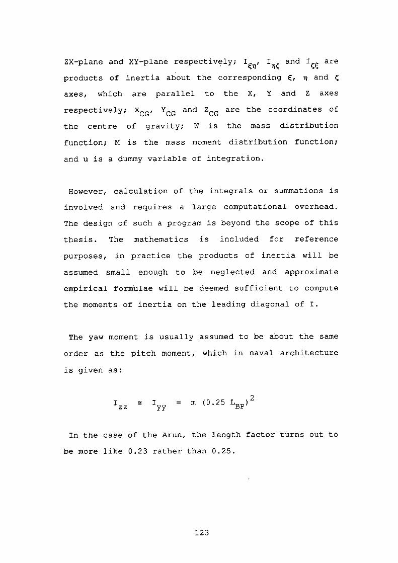
ZX-plane and XY-plane respectively; I, I and I are
products of inertia about the corresponding , i and ?
axes, which are parallel to the X, Y and Z axes
respectively; XCG, CG and ZCG are the coordinates of
the centre of gravity; W is the mass distribution
function; M is the mass moment distribution function;
and u is a dummy variable of integration.
However, calculation of the integrals or summations is
involved and requires a large computational overhead.
The design of such a program is beyond the scope of this
thesis. The mathematics is included for reference
purposes, in practice the products of inertia will be
assumed small enough to be neglected and approximate
empirical formulae will be deemed sufficient to compute
the moments of inertia on the leading diagonal of I.
The yaw moment is usually assumed to be about the same
order as the pitch moment, which in naval architecture
is given as:
I I = m (0.25 LBP)2zz yy
In the case of the Arun, the length factor turns out to
be more like 0.23 rather than 0.25.
123
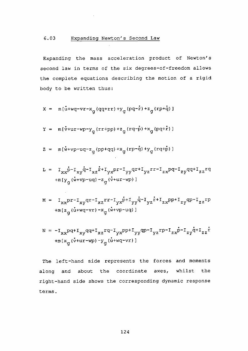
6.03 Expanding Newton's Second Law
Expanding the mass acceleration product of Newton's
second law in terms of the six degrees-of-freedom allows
the complete equations describing the motion of a rigid
body to be written thus:
X = m[i+wqvrxg (qq+rr)+yg (pqr)+zg (rP+q) I
Y = m[r+ur_wp_yg(rr+pp)+zg(rqp)+Xg(pq+r)]
Z = I
L = I p-I q-I r+I pr-I qr+I rr-I pq-I qq+I rqxx xy xz yx yy yz zx zy zz
+m [Yg (J+v-uq) Z g (+ur-wp)I
M = I pr-I qr-I rr-I +I -I +I pp+I P-I rpxx xy xz yx yy yz zx zy
+m[z (ii+wq-vr)xg(w+vpuq)Ig
xx xz yxyy -I rp-I -I 4+iN = -I rq-I pp+I qp yz zx zy zz
+m [Xg (ir+ur-wp) Yg (i+wq-vr) I
The left-hand side represents the forces and moments
along and about the coordinate axes, whilst the
right-hand side shows the corresponding dynamic response
terms.
124
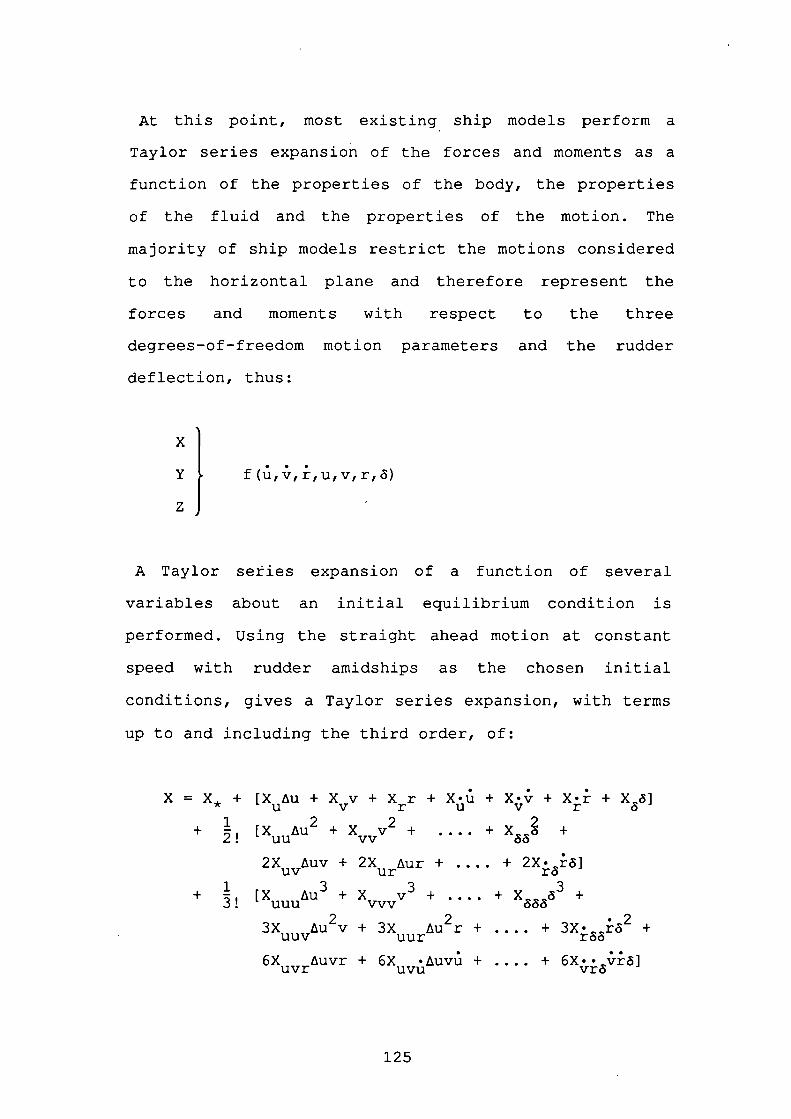
At this point, most existing ship models perform a
Taylor series expansion of the forces and moments as a
function of the properties of the body, the properties
of the fluid and the properties of the motion. The
majority of ship models restrict the motions considered
to the horizontal plane and therefore represent the
forces and moments with respect to the three
degrees-of--freedom motion parameters and the rudder
deflection, thus:
x
Y
z
A Taylor series expansion of a function of several
variables about an initial equilibrium condition is
performed. Using the straight ahead motion at constant
speed with rudder amidships as the chosen initial
conditions, gives a Taylor series expansion, with terms
up to and including the third order, of:
X = X + [X Au + X v + X r + X . 0 + X • v + X • r + X 5]u v r U V r
+ 2! [X Au 2 + X v2 + .... + +uu vv
2X Auv + 2X Aur + .... + 2X . ]uV ur r.5
+ [X Au3 + X v3 + .... + X 3 +uuu vvv
3X Au2v + 3X Au2r + -... + 3X . +uuv uur r&
6X Auvr + 6X • Auvu + .... + 6X .. i5]uvr uvu vrã
125
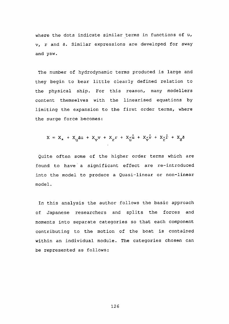
where the dots indicate similar terms in functions of u,
v, r and . Similar expressions are developed for sway
and yaw.
The number of hydrodynamic terms produced is large and
they begin to bear little clearly defined relation to
the physical ship. For this reason, many modellers
content themselves with the linearised equations by
limiting the expansion to the first order terms, where
the surge force becomes:
X = X + X Au + X v + X r + + X • + X . + XU v r u v r
Quite often some of the higher order terms which are
found to have a significant effect are re-introduced
into the model to produce a Quasi-linear or non-linear
model.
In this analysis the author follows the basic approach
of Japanese researchers and splits the forces and
moments into separate categories so that each component
contributing to the motion of the boat is contained
within an individual module. The categories chosen can
be represented as follows:
126
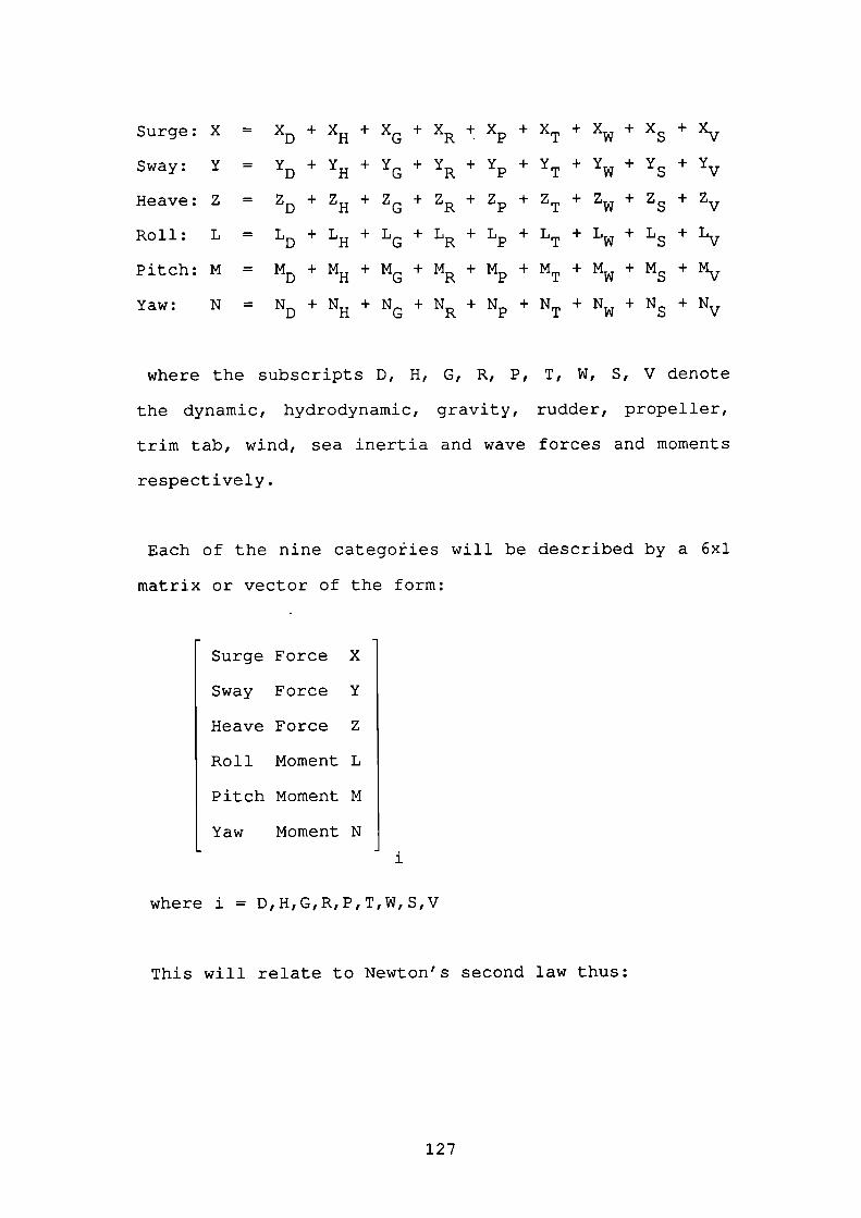
Surge: X = XD+XH+XG+XR±Xp+XT+Xw+XS+Xv
Sway: Y = YD+YH+YG+YR+Yp+YT+YW+YS+Yv
Heave: Z = ZD + ZH + ZG + ZR+ Z + ZT + Z+ Z5 + Z
Roll: L = LD+LH+LG+LR+Lp+LT+Lw+Ls+Lv
Pitch: M = MD + MH + MG + MR + M + MT + Mw + Ms + Mv
Yaw: N = ND+NH+NG+NR+Np+NT+Nw+NS+Nv
where the subscripts D, H, G, R, P, T, W, S, V denote
the dynamic, hydrodynamic, gravity, rudder, propeller,
trim tab, wind, sea inertia and wave forces and moments
respectively.
Each of the nine categoiies will be described by a 6x1
matrix or vector of the form:
Surge Force X
Sway Force Y
Heave Force Z
Roll Moment L
Pitch Moment M
Yaw Moment N
1
where i =D,H,G,R,P,T,W,S,V
This will relate to Newton's second law thus:
127
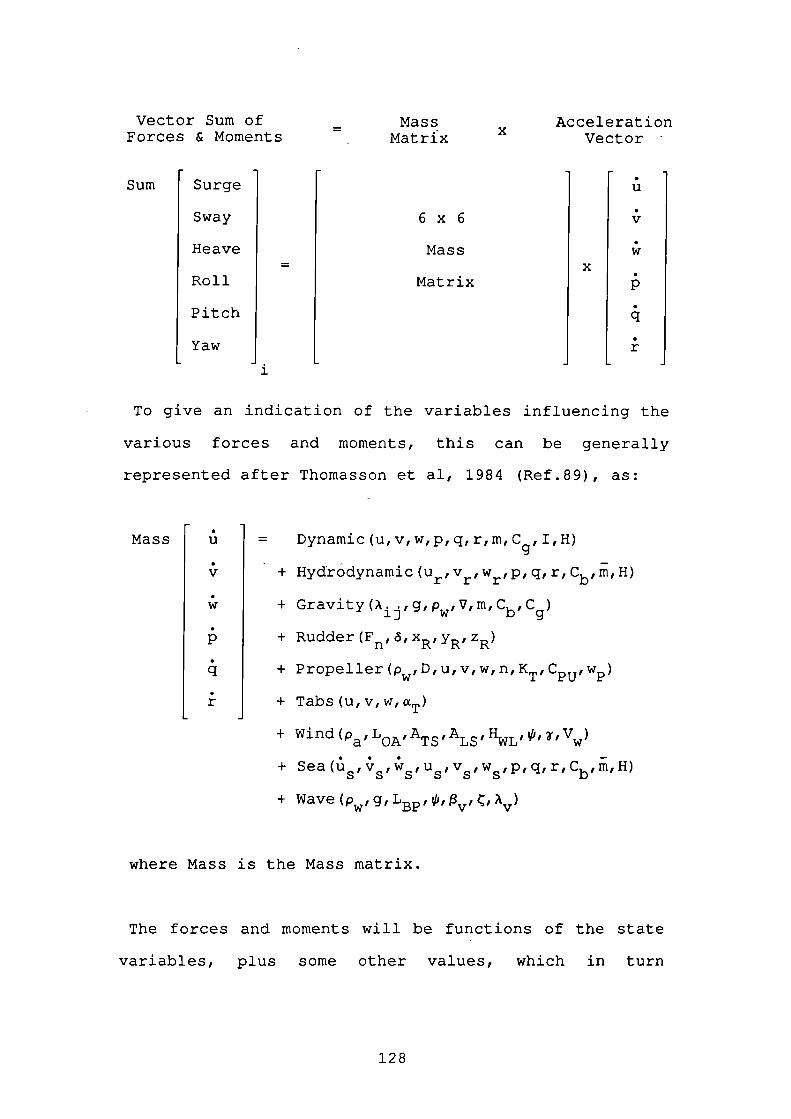
x
U
V
w
p
q
r
U
V
w
p
q
r
Mass
Vector Sum ofForces & Moments
Sum
Surge
Sway
Heave
Roll
Pitch
Yaw
MassMatrix X
6x 6
Mass
Matrix
AccelerationVector
I
To give an indication of the variables influencing the
various forces and moments, this can be generally
represented after Thomasson et al, 1984 (Ref.89), as:
= Dynamic(u,v,w,p,q,r,m,Cg,I,H)
+ Hydrodynamic (Un Vr l WnI p, q, r, Cbl rn, H)
+ GnavitY(AjjlFPlVImClCg)
+ Rudder (F , X, /p ZR)
+ Propeller(pW,D,u,v,w,n,KT,CPU,wP)
+ Tabs(u,v,w,cT)
+ Wifld(pILOA,ATSIALS,HWLf1lf',V)
+ Sea ' ' w, u, v5 , w, ' q, r, Cbl rn, H)
+ Wave
where Mass is the Mass matrix.
The forces and moments will be functions of the state
variables, plus some other values, which in turn
128
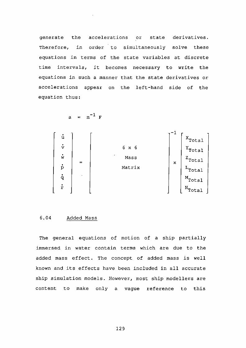
x
U
V
w
p
q
r
XTtl
Tota1
ZTtl
LTtl
MTotal
NTtl
6x 6
Mass
Matrix
generate the accelerations •or state derivatives.
Therefore, in order to simultaneously solve these
equations in terms of the state variables at discrete
time intervals, it becomes necessary to write the
equations in such a manner that the state derivatives or
accelerations appear on the left-hand side of the
equation thus:
a = m F
-1.
6.04
Added Mass
The general equations of motion of a ship partially
immersed in water contain terms which are due to the
added mass effect. The concept of added mass is well
known and its effects have been included in all accurate
ship simulation models. However, most ship modellers are
content to make only a vague reference to this
129
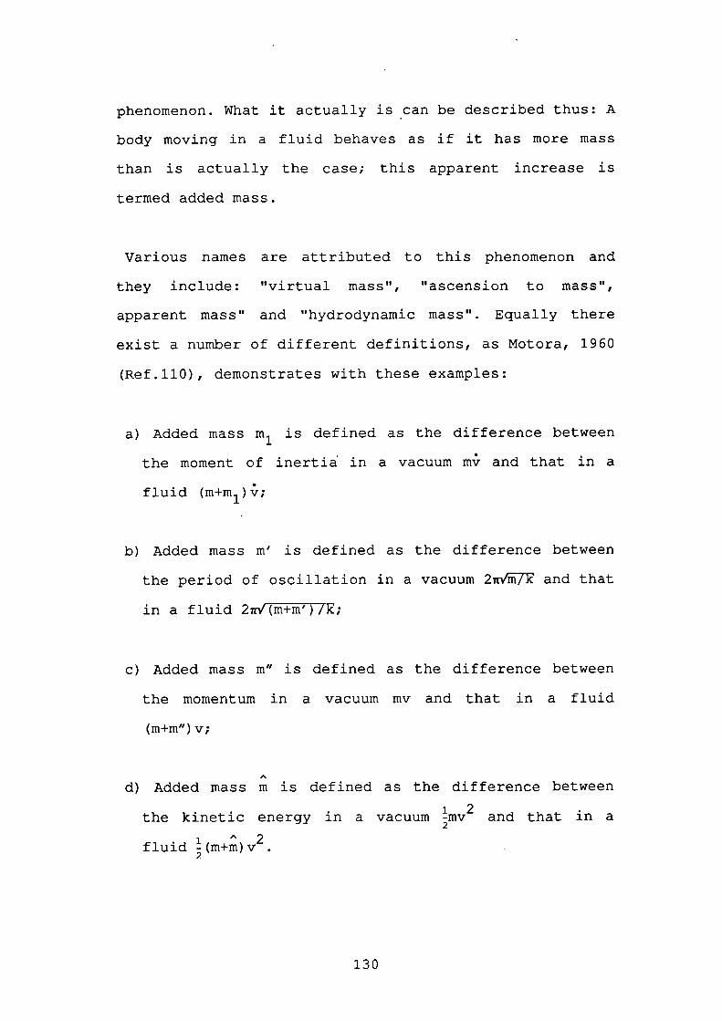
phenomenon. What it actually is can be described thus: A
body moving in a fluid behaves as if it has more mass
than is actually the case; this apparent increase is
termed added mass.
Various names are attributed to this phenomenon and
they include: Itvirtual mass", "ascension to mass",
apparent mass" and "hydrodynamic mass". Equally there
exist a number of different definitions, as Motora, 1960
(Ref.110), demonstrates with these examples:
a) Added mass m1 is defined as the difference between
the moment of inertia in a vacuum m and that in a
fluid (m+m1)T;
b) Added mass m' is defined as the difference between
the period of oscillation in a vacuum 2iW71 and that
in a fluid 2iWTm+m')/k;
c) Added mass m" is defined as the difference between
the momentum in a vacuum m y and that in a fluid
(m+m") v;
d) Added mass m is defined as the difference between
the kinetic energy in a vacuum mv2 and that in a
fluid (m+m)v2.
130
With the exception of the case of motion in an ideal
fluid without free surfaces effects, these different
definitions will not always coincide. Many treatments of
the topic of added mass are biased towards a specific
application and therefore present equations with only
those terms which are required for that use.
In this analysis the derivation of the added mass
expressions will be based upon the kinetic energy
approach. Lamb, 1879 (Ref.86), was perhaps the first to
document this method, but Imlay, 1961 (Ref.74), gives a
clearer text for those first entering the subject.
The presence of a fluid surrounding a boat introduces
the phenomenon of added mass. If the boat is moving then
it will induce a motion in the otherwise stationary
fluid. This is because the fluid has to move out of the
way and then close in behind the boat in order that the
boat may itself make headway through the fluid.
Consequently, the fluid will possess kinetic energy
imparted by the boat doing work on the fluid. It is
therefore necessary that the equations of motion take
into account the kinetic energy given to the fluid, and
this is performed through the added mass terms.
131
If the boat motion is steady, then the corresponding
fluid motion will be steady and the kinetic energy in
the fluid is constant. The added mass terms can
therefore be omitted from the equations if, and only if,
the boat motion is steady.
When the motion is accelerated, this implies that the
motion of the boat is in a state of change and there
must be an associated change in the kinetic energy of
the surrounding fluid. That is to say, the boat must do
work on the fluid in order to accelerate. In applying a
force to the fluid the boat will experience an opposite
reaction force. Therefore, the force required to
accelerate the boat must be greater than the reaction
force.
Lamb's approach to obtaining an equation for this
kinetic energy given to the fluid begins by supposing
the motion of the fluid to be characterised by a single
valued velocity potential which satisfies the equation
of continuity:
= o
Then if the motion of a body through the fluid at any
instant is defined by the translational velocities u, v
and w and the angular velocities p, q and r, it is
132
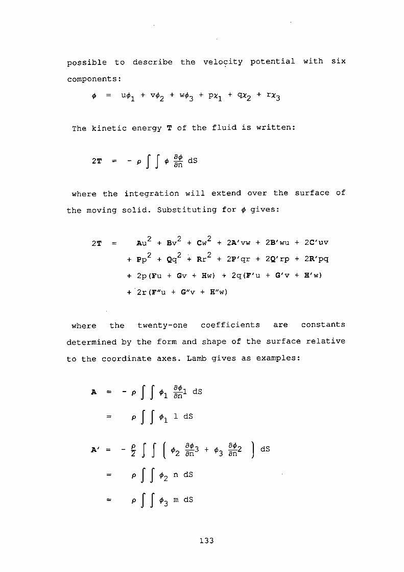
possible to describe the velocity potential with six
components:
= u 1 + v 2 + w 3 + p 1 + q 2 + rx3
The kinetic energy T of the fluid is written:
2T = _pJJ-dS
where the integration will extend over the surface of
the moving solid. Substituting for gives:
2T = Au2 + By2 + Cw2 + 2A'vw + 2B'wu + 2C'uv
+ Pp2 + Qq2 + Rr + 2P'qr + 2Q'rp + 2R'pq
+ 2p(Fu + Gv + Hw) + 2q(F'u + G'v + H'w)
+2r(F"u + G"v + H"w)
where the twenty-one coefficients are constants
determined by the form and shape of the surface relative
to the coordinate axes. Lamb gives as examples:
A = -pJJ1--.ldS8n
= JJ i 1 dS
A' = )dS
= pJJ2ndS
= pJJ3mdS
133
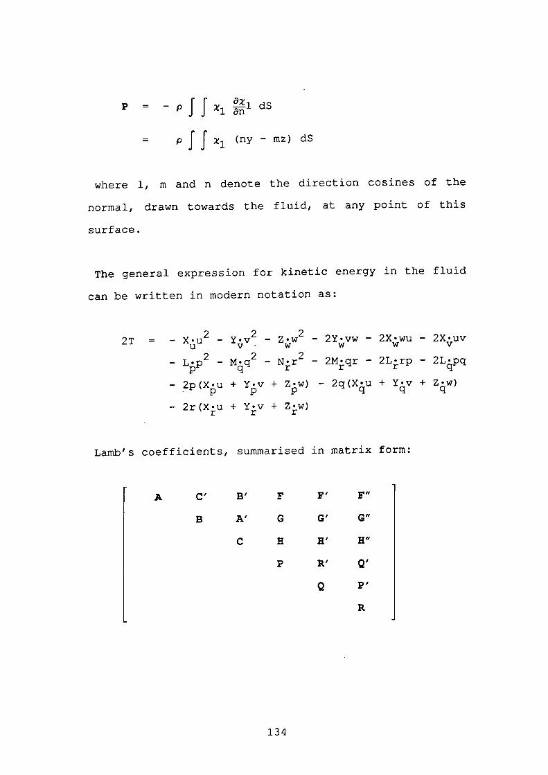
P = -PJJx1ldSan
= P f J x1 (ny - mz) dS
where 1, m and n denote the direction cosines of the
normal, drawn towards the fluid, at any point of this
surface.
The general expression for kinetic energy in the fluid
can be written in modern notation as:
2 2 22T = - X • u - Y • v - Z • w - 2Y • vw - 2X • wu - 2X•uv
- Lp2 - M4q - N;r 2 - 2Mqr - 2Lrp - 2L4pq
- 2p(Xu + Yv + Zw) - 2q(X4u + Y4v + Z4w)
- 2r(X . 0 + Y•v + Z.w)r r r
Lamb's coefficients, summarised in matrix form:
A C'
B'
F
F'
F"
B
A'
G
G"
C
H
H'
H"
P
R'
Q'
Q
P1
R
134
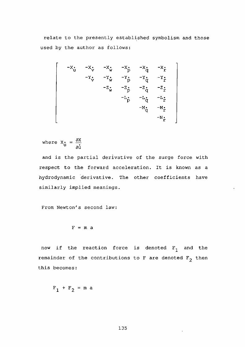
relate to the presently established symbolism and those
used by the author as follows:
-x. -x. -x. -x. -x. -x.
U V w p q r
-Y. -Y. -Y. -Y. -Y.
V w p q r
-z. -z. -z. -z.
w p q r
-L• -L.
p r
-N. -M•
q r
-N.r
where X . =U 8u
and is the partial derivative of the surge force with
respect to the forward acceleration. It is known as a
hydrodynamic derivative. The other coefficients have
similarl.y implied meanings.
From Newton's second law:
F=ma
now if the reaction force is denoted F 1 and the
remainder of the contributions to F are denoted F 2 then
this becomes:
F 1 + F2 = m a
135
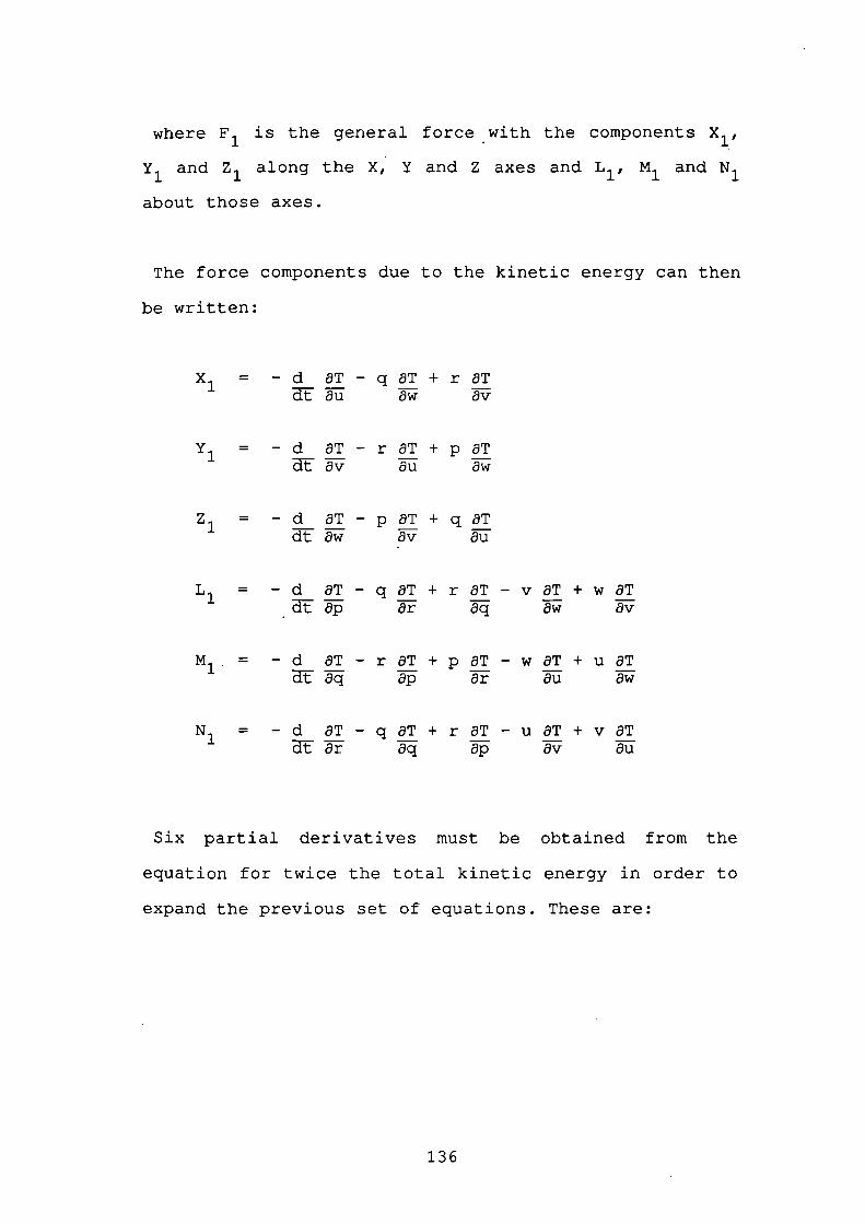
where F 1 is the general force with the components X1,
and Z 1 along the X, Y and Z axes and L 1 , M1 and N1
about those axes.
The force components due to the kinetic energy can then
be written:
X1 = - d 3T - q aT + r 3Tdtau 3w 3v
= - d 0T - r 3T + p 3Töu 3w
Z 1 = -d 3T-p8T+qoTdt0w 3v 3u
L 1 = -d aT-qaT+raT-vaT+waT
M1 . -d 0T-raT+p3T-waT+uaT
N1 = -d BT-q3T+raT-uôT+v3T
Six partial derivatives must be obtained from the
equation for twice the total kinetic energy in order to
expand the previous set of equations. These are:
136
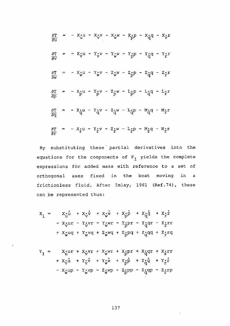
8T = - X • u - X•v - X . w - X . p - X . q - X•r- U V W •p q r
3T = -X.u-Y.v-Y.w-Y.p-Y.q-Y.r- v v w p q r
8T = -X•u-Y•v-Z•w-Z.p-Z.q-Z.r- w w w p q r
= -Xu-Yv-Zw-Lp-L4q-Lr
ÔT = - X • u - Yv - Zw - L . p - M . q - M•rq q q q q r
8T = - Xu - Yv - Zjw - Lp - Mq - Nr
By substituting these partial derivatives into the
equations for the components of F 1 yields the complete
expressions far added mass with reference to a set of
orthogonal axes fixed in the boat moving in a
frictionless fluid. After Imlay, 1961 (Ref.74), these
can be represented thus:
X = X•u + X .+ X . i + X .+ x.4 + x.1 u v w p q r
- X . ur - Y'vr - Y . wr - Y . pr - Y . qr - Y.rrv v w p q r
+ Xuq + Y . vq + Zwq + Zpq + Z4qq + Zrq
Y = X.ur + X • vr + X • wr + X . pr + X • qr + X•rr1 u v w p q r
+ X . i•i + + + + y. 4 +v v w p q r
- Xup - Yvp - Zwp - Zpp - Z4qp - Zrp
137
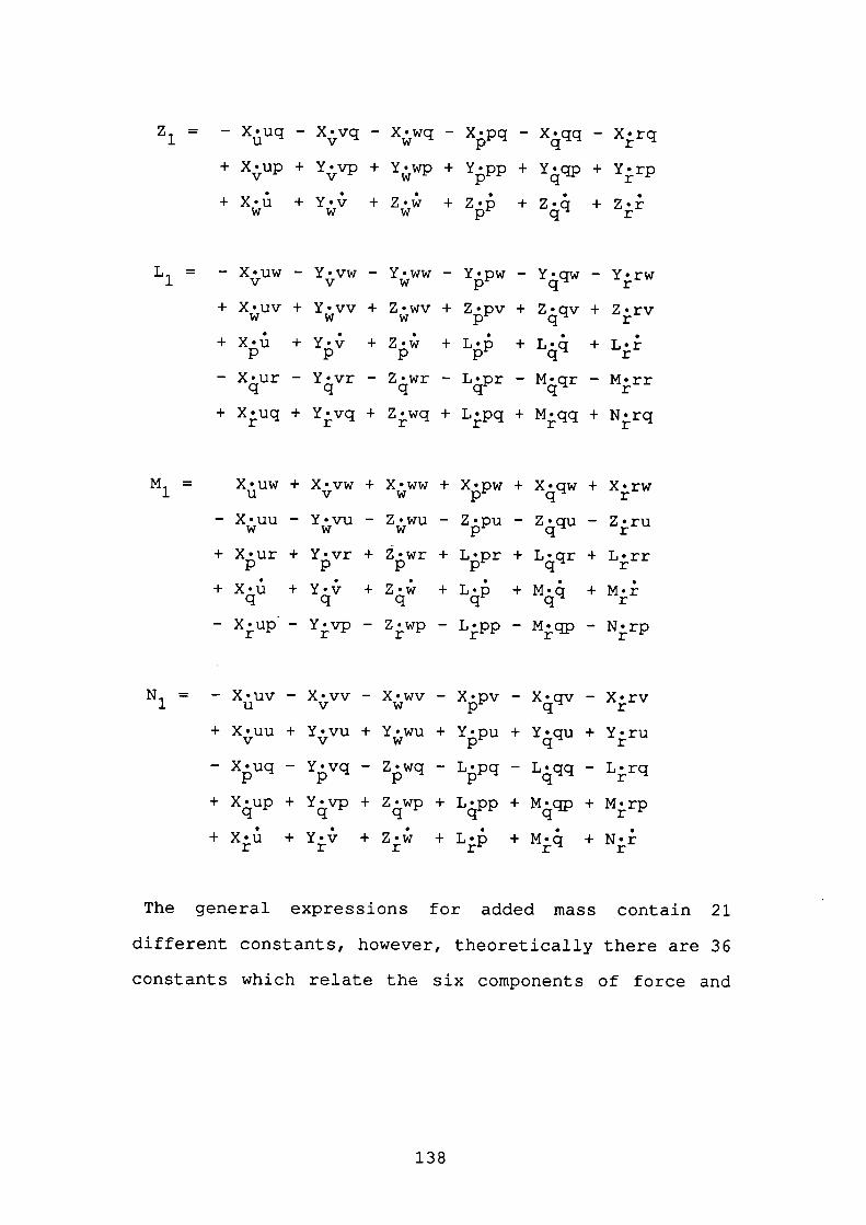
Z 1 = - Xuq - X .vq - Xwq - Xpq - X4qq - Xrq
+ X . up + Y . vp + Y . wp + Ypp + Y4cjP + Yrp
+ x. + + Z • w + Z . p + Z . q + Zr
w w w p q r
L = - X . uw - Y•vw - Y • ww - Y . pw - Y • qw - Y•rwV V W p q r+ X • uv + Y • vv + Z . wv + Z . pv + Z . qv + Z.rvw w w p q r+X • i +Y . ' r +Zw +Lp +L . 4 +L.r- X . ur - Y . vr - Z . wr - L . pr - M . qr - M•rrrq q q q q
+ Xuq + Yjvq + Zwq + Ljpq + M ,qq + Nrq
M = X'uw + X • vw + X • ww + X . pw + X . qw + X.rwU V W p q r
- X • uu - Y • vu - Z . wu - Z . pu - Z . qu - Z•rurw w w p q+ X • ur + Y • vr + Z wr + Lpr + L qr
•• •
+L.rrr
+ X • u + Y . v + Z .+ L- + M . 4 + M.rq q q q q
- Xup - Yvp - Zwp - Lpp - Mqp - N.rp
N = - X . uv - X . vv - X • wv - X • pv - X . qv - X•rv1 u v w p q r+ X • uu + Y • vu + Y . wu + Y • pu + Y • qu + Y•ruv v w p q r
- Xuq - Yvq - Zwq - Lpq - L4qq - Lrq
+ X4up + Y4vp + Z4wp + L4pp + M4qp + M.rp
+ X • u + Yv + Z • w + L .+ M . 4 + N.r r r r r r
The general expressions for added mass contain 21
different constants, however, theoretically there are 36
constants which relate the six components of force and
138
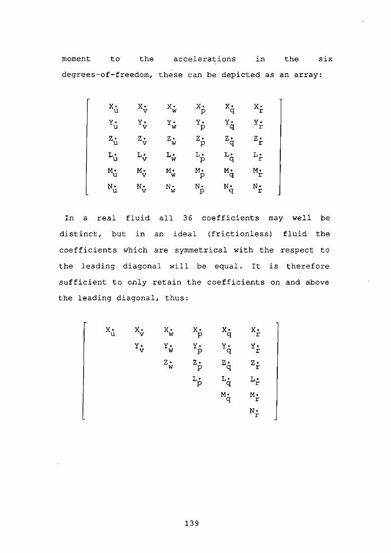
moment to the accelerations in the six
degrees-of--freedom, these can be depicted as an array:
x. x. x. x. x. x.
u v w p q r
Y .Y. Y. Y. Y. Y.
u v w p q r
z .z. z. z. z. z.
U v w p q r
L •L. L• L• L• L•
u v w p q r
M • M. M. M' M.u v w p q r
N . N. N. N. N• N.
u v w p q r
In a real fluid all 36 coefficients may well be
distinct, but in an ideal (frictionless) fluid the
coefficients which are symmetrical with the respect to
the leading diagonal will be equal. It is therefore
sufficient to only retain the coefficients on and above
the leading diagonal, thus:
x .x. x. x. x. x.
U V w p q r
Y .Y. Y. Y. Y.
v w p q r
z .z. z. z.
w p q r
L .L• L•
p q r
M.q r
N.r
139
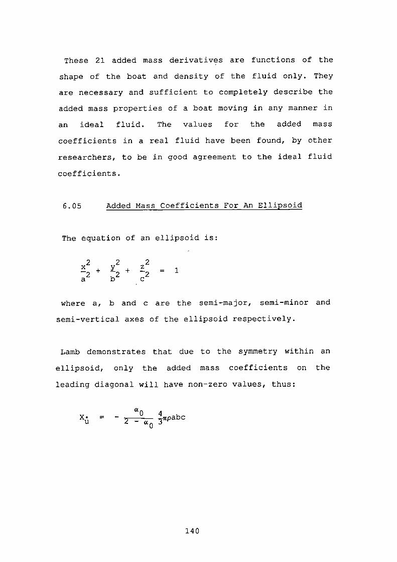
These 21 added mass derivatives are functions of the
shape of the boat and density of the fluid only. They
are necessary and sufficient to completely describe the
added mass properties of a boat moving in any manner in
an ideal fluid. The values for the added mass
coefficients in a real fluid have been found, by other
researchers, to be in good agreement to the ideal fluid
coefficients.
6.05 Added Mass Coefficients For An Ellipsoid
The equation of an ellipsoid is:
2 2 2x + y z2 2 = 1
a b c
where a, b and c are the semi-major, semi-minor and
semi-vertical axes of the ellipsoid respectively.
Lamb demonstrates that due to the symmetry within an
ellipsoid, only the added mass coefficients on the
leading diagonal will have non-zero values, thus:
x . = -a0
u 2 ---itpabc
140
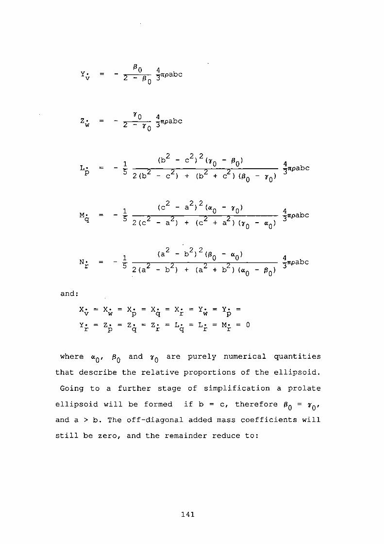
Y . = - ______ 4V 2 -
-irpabc
z. = - 'o 4
w 2 -.itpabc
2 221 (b - C ) -
irpabcL - S 2 2 + (b2 + C2) -2(b - c
2 221 (C - a ) ( x0 -
-7rpabcM4 = - S 2 2 + (c 2 + a2 )2(c - a
(a -2 b2)2(0 -irpabc
1N • = -r 2(a - b2 ) + (a2 + b2) -
and:
x • = x • = x • = x • = x • = Y • = Y • =V w p q r w p
Y • = Z • = Z • = Z • = L • = L • = M • = 0r p q r q r r
where , f3 and are purely numerical quantities
that describe the relative proportions of the ellipsoid.
Going to a further stage of simplification a prolate
ellipsoid will be formed if b = c, therefore o =
and a > b. The off-diagonal added mass coefficients will
still be zero, and the remainder reduce to:
141
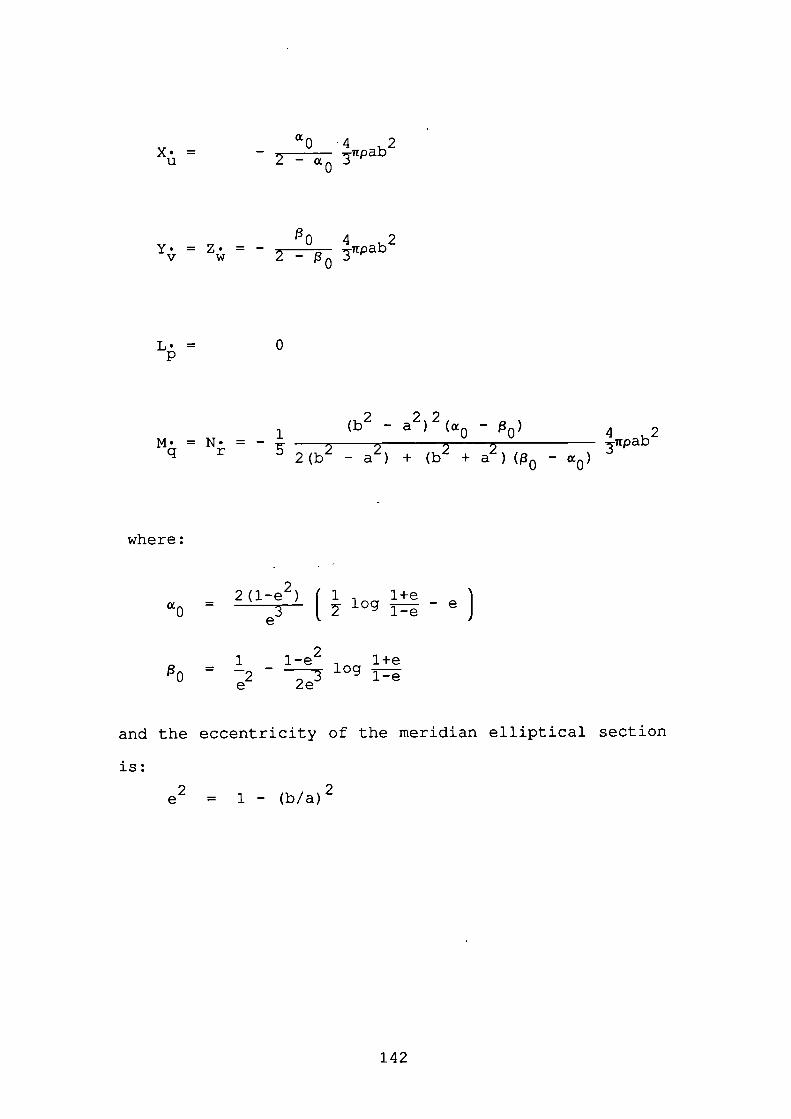
o0 '4 2x.= - ___U 2_o
_______ 4 2Y r = Z :q = - 2 -
I3
-irpab
L • 0p
22(b2 - a ) - -itpab21 _______________________________________________
q rM • = N • = - s 2(b2 - a2 ) + (b2 + a2 ) ( - c)
where:
2(1-e2) 1 1+e
)= 3e
1 1-e2 log 1+e= 2e 2e3
and the eccentricity of the meridian elliptical section
is:
2e =
142
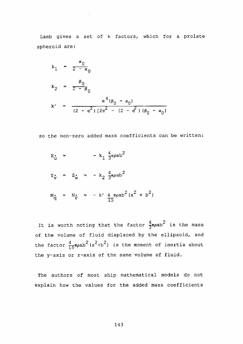
Lamb gives a set of k factors, which for a prolate
spheroid are:
= 2
k2 = 2 -
e4(t30 -=
(2 - e2 ) [2e2 - (2 - e2 ) -
so the non-zero added mass coefficients can be written:
4 2X = - k1 ipab
4 2Y = Z - k2 .-upab
= N . = - k' 4 itpab2 (a 2 + b2)q r -I-s
It is worth noting that the factor -irpab 2 is the mass
of the volume of fluid displaced by the ellipsoid, and4 222. .the factor 1-5-upab (a +b ) is the moment of inertia about
the y-axis or z-axis of the same volume of fluid.
The authors of most ship mathematical models do not
explain how the values for the added mass coefficients
143
were obtained. For this analysis, as undoubtedly for
many others, the expressions derived for the prolate
ellipsoid are assumed to give values of the correct
order.
6.06 Methods Of Determining The Added Mass
Coefficients
Motora, 1960 (Ref.l1O), proposes methods to determine
the surge, sway and yaw added mass effects from model
tests. Three methods were studied, namely:
1) The Vibration Method: This is based upon the fact
that the limit of the added mass obtained from the
prolongation of the period of vibration occurs when
the period becomes infinitesimal. However, this
method proved unsatisfactory because it was
impossible to generate vibrations with sufficiently
short period.
2) The Acceleration Method: This method is intended to
measure the resultant acceleration when a known
force is applied to the ship model. The added mass
is then extracted from this acceleration. However,
it was found difficult to measure the acceleration
with the required degree of accuracy.
144
3) The Impact Method: This is intended to measure the
initial velocity caused when a known impact is
applied to the ship model. The added mass is then
extracted from this velocity information. This
method proved to give results of the required
accuracy.
The impact method was used for measuring the surge and
yaw added mass coefficients, but with the greater
damping in sway it was possible to use the acceleration
method.
Generally, the added massin fore-aft motion (surge) is
fairly small, but plays a significant role in sway
motions. Theory suggests that the added mass
coefficients change with water depth and can increase
sharply to exceed the vessel's inherent mass as the
water becomes shallow. While the equations for added
mass are complete and sufficient for mathematical
application, there is still adequate uncertainty in
establishing the value of the coefficients to justify
further research.
145
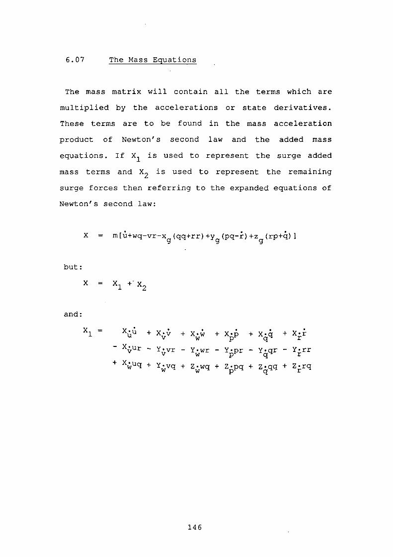
6.07 The Mass Ecrnations
The mass matrix will contain all the terms which are
multiplied by the accelerations or state derivatives.
These terms are to be found in the mass acceleration
product of Newton's second law and the added mass
equations. If X 1 is used to represent the surge added
mass terms and X 2 is used to represent the remaining
surge forces then referring to the expanded equations of
Newton's second law:
X = m[1+wq-vr-x(qq+rr)+y(pq-)+z(rp+4) I
but:
x = x1 +•x2
and:
+xl = x1:1 11 + X.TC + XJ + XD + X rv w p q
r - Y•rr- Xur Yvr - Ywr - Ypr - Y4q r+ X%uq + Y . vq + Z . wq + Z'pq + Zqq + Z,rqw w p
146
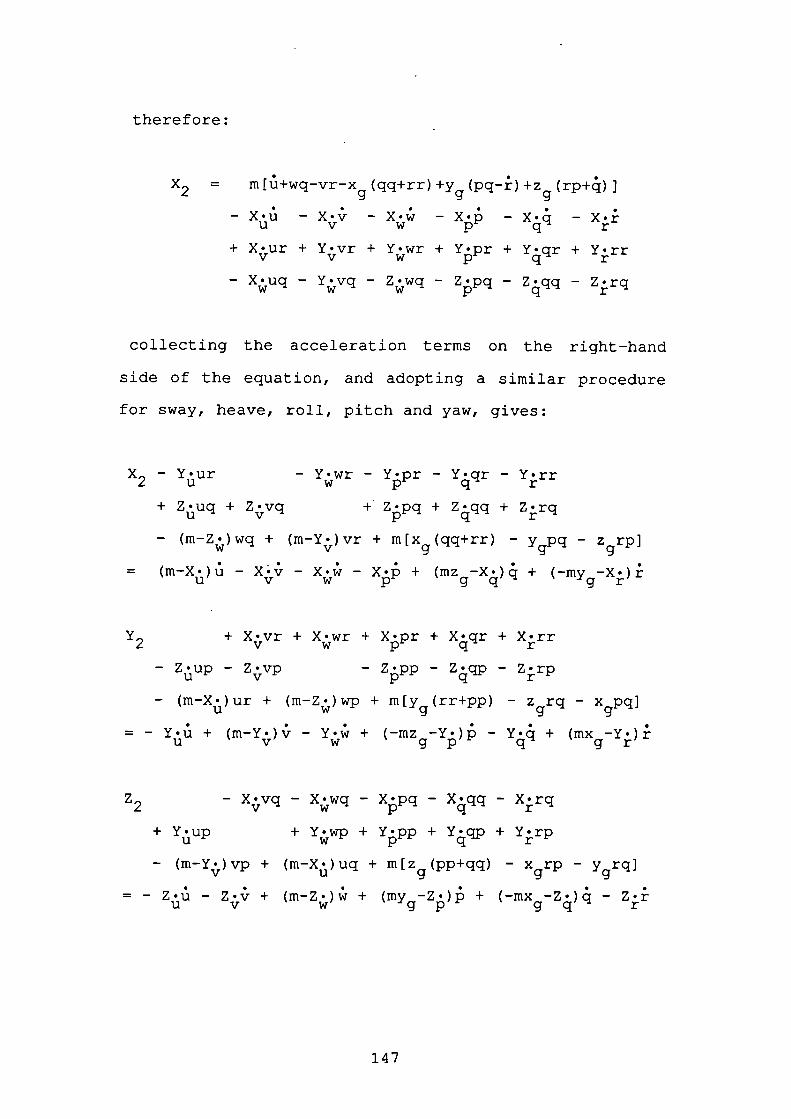
therefore:
X2 = m[1+wq-vr-x(qq+rr)+y(pq-)+z(rp+4)]
- X • ii - Xv - X . i - X .- X •- X.U V W p q r
+ X . ur + Y . vr + Y . wr + Y . pr + Y • qr + Y.rrv v w p q r
- Xuq - Yvq - Zwq - Zpq - Z4qq - Zrq
collecting the acceleration terms on the right-hand
side of the equation, and adopting a similar procedure
for sway, heave, roll, pitch and yaw, gives:
X2 - Yur - Ywr - Ypr - Y4qr - Yrr
+ Zuq + Zvq + Zpq + Z4qq + Z.rq
- (m-Z)wq + (m-Y)vr + m[xg(qq+rr) - Y gP - zgrPI
= (m-X)ii - - Xi - X + ( fflZg_X4)4 + (mygXJ
+ Xvr + Xwr + Xpr + X4qr + Xrr
- Zup - Z . vp - Zpp - Z4qp - Z,rp
- (m-X)ur + (m-Z)wp + m[yg (rr+pp) - zgrq - xgPq]
= - Yu + (m-Y) r - Yi + (mz g YY - Y44 + (mxg_Y)
Z2- Xvq - Xwq - Xpq - X4qq - Xrq
+ Y'up + Y . wp + Ypp + Y4qp + Yrp
- (m-Y)vp + (m-X)uq + m [ z g (pP+qq ) - xgrP - Ygrq]
= - Z - Z + (m-Z) + (mYg_Z) + (_mxg_Z4)4 - Z
147
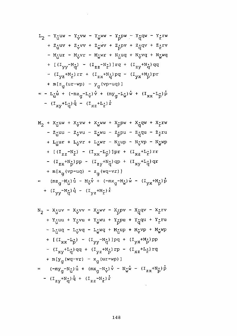
L2 - Yuw - Yvw - Yww - Ypw - Y4qw - Yrw
+ Z • uv + Z'vv + Z • wv + Z . pv + Z . qv + Z•rvu v w p q r
- M . ur - M . vr - N . wr + N • uq + N . vq + N.wqU V W U V W
+ [(I_M) - (I_N)]rq + (I+N4)
- (I +M . )rr + (I+N4)pq - (I+M)Pr
+ m[zg (urWP) - g (VP_uq) I= - Lu + (_mzg_L)& + (mYg_L) +
- (I +L . )4 - (I +L.)rxy q xz r
M + X • uw + X . vw + X • ww + X . pw + X . qw + X.rw2 u v w p q r
- Zuu - Zvu - Zwu - Zpu - Z4qu - Zru
+ L . ur + L . vr + L • wr - N . up - N . vp - N.wpU V W U V W
+ [(I -N . ) - (I -L . )]pr + (I +L.)rrzz r xx p xz r
- (I +N . )pp - (I +N4)qp + (I+L4)r
+ m[Xg(VP_Uq) - zg(wq_Vr)]
= (mz -M . ) ii - M . + (-mx -M . ) - (I +M.)gu v g w yx p
+ (I -M . )4 - (I +M.)ryy q yz r
N - X • uv - Xvv - X . wv - X • pv - X • qv - X.rv2 u v w p q r
+ Y • uu + Y • vu + Y • wu + Y • pu + Y4qu + YruU V w p
- L • uq - Lvq - L . wq + M • up + N • vp + M•wpU V W U V W
+ [(I -L • ) - (I -M. )]pq + (I +M)ppxx p yy q y
- (I +L qq + (I +N . )rp - (I +L')rqyz p xz r
+ m [y (wq vr) - x (ur-wp)]g - g
= (-my -N • )u + (mx -N . )v - N.r - (I +N.)pg u g v w zx p
- (I +N .4+ (I -N•)rzz r
148
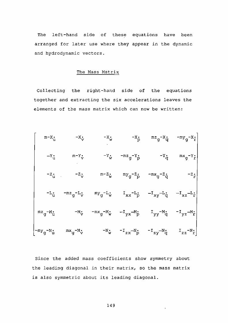
-x.V
m-X•U
—Y.U
m-Y•V
The left-hand side of these equations have been
arranged for later use where they appear in the dynamic
and hydrodynamic vectors.
The Mass Matrix
Collecting the right-hand side of the equations
together and extracting the six accelerations leaves the
elements of the mass matrix which can now be written:
-x. -x.w p
-Y• -mz -Y.
w gp
mz -X •-my -X.
g q g r
-Y .mx -Y.
q g r
-Z •-Z• m-Z. my -Z •-mx -Z •-Z•
U v w gp g q r
-L •-mz -L •my -L •I -L •—I —L •—I —L.
u g v g w xx p xy q xz r
mz -M .-M• -mx -M .—I —M•I -M.-I —M.
g u v g w yx p yy q yz r
-my -N .mx -N .-N. -I —N .-I —N .I -N.
g u g v w zx p zy q zz r
Since the added mass coefficients show symmetry about
the leading diagonal in their matrix, so the mass matrix
is also symmetric about its leading diagonal.
149
6.08 The Dynamic Forces And Moments
This will be made up of the dynamic terms associated
with the inertial velocities u, v, w, p, q and r. Some
of the terms on the left-hand side of the equations
developed for the mass matrix will make up the dynamic
vector. The remainder will appear in the hydrodynamic
vector.
Hydrodynamic Coefficients
The Dynamic and Hydrodynamic vectors contain a number
of hydrodynamic coefficients which are actually entered
in terms of their perfect fluid component. A list of
these hydrodynamic coefficients and their related
perfect fluid components appears below, where H are the
hydrodynamic coefficients and P are the perfect fluid
components.
150
uq u up u up u uv U UU U UU U
X Z• Y -Z• Z Y• L Z' M -Z. Nvq v Vp v Vp V VV V VU V VU V
X Z. Y -Z. Z Y. L Z• M -Z• N Y.wq w wp w wp W WV w WU W WU w
X Z• Y -Z. Z Y• L Z• M -Z • N Y'pq p pp p pp p V p PU P U p
X Z. Y -Z. Z Y• L Z• M -Z. Nqq q qp q qp q qV q qu q qu q
X Z. Y -Z. Z Y• L Z• M -Z. Nrq r rp r rp r rV r ru r ru r
X -Y. Y X. Z -X• L -Y• M X. N -X.ur u ur u uq u uw u uw u uv u
X -Y• Y X. Z -X• L -Y• M X• N -X•Vr V yr V V V VW V VW V VV V
X -Y• Y X. Z -X• L -Y• M X• N -X•wr w wr w wq w ww w ww W WV W
X -Y. Y X. Z -X• L -Y• M X. N -X•pr p pr p pq p pw p pw p V p
X -Y• Y X• Z -X• L -Y• M X. N -X.qr q qr q qq q qw q qw q qV q
X -Y• Y X• Z -X• L -Y• M X• N -X•rr r rr r rq r rw r rw r rV r
L N.M -N'N M•uq u up u up U
L N.M -N . N M•Vq VVp Vvp V
L N.M -N'N M.wq w wp w wp w
L N.M -N.N M•pq p PP P PP P
L N.M -N'N M.qq q qp q qp q
L N.M -N•Nrq r rp r rp r
L -M.M L.N -L.ur u ur u uq u
L -M.M L.N -L.
V V V V V V
L -M.M L.N -L.wr w wr w wq w
L -M•M L.N -L•pr p pr p pq p
L -M.M L.N -L•qr q qr q qq q
L -M•M L.N -L•rr r rr r rq r
151
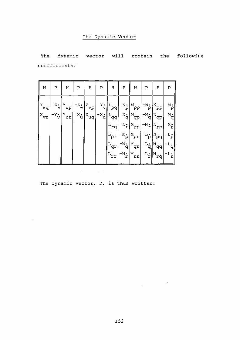
The Dynamic Vector
The dynamic vector will contain the following
coefficients:
H P H P H P H P H P H P
X Z•Y -Z.Z Y•L N.M -N.Nwq w wp w Vp V pq p pp p pp p
X -Y• Y X. Z -X• L N. M -N. Nyr v ur u uq u qq q qp q qp q
L N.M -N•Nrq r rp r rp r
L -M•M L.N -L•pr p pr p pq p
L -M.M L•N -L.qr q qr q qq q
L-M • M L•N -L•rr r rr r rq r
The dynamic vector, D, is thus written:
152
(m-Y • )vr - (m-Z . )wq + m[x (qq+rr) - YgP - zgrP]V w g
(m-Z)wp - (m-X)ur + m[ y (rr+pp) - z grq - xgPq]
(m-X . )uq - (m-Y . )vp + m[z (pp+qq) - xgrP - Ygi q ]u v g
[(I -M • ) - (I -N . )]rq + (I +N . )qq - (I +M.)rryy q zz r zy q yz r
+ (I+N)Pq - (I +M . )pr + m[zg (ur-w) - yg(vp_uq)]
[(I -N . ) - (I -L . )] pr + (I +L . )rr - (I +N.)ppzz r xx p xz r zx p
(I +N . )qp + (I +L . )qr + m[x (vp-uq) - zg(wq_vr)]zy q xy q g
[(I -Li) - (I -M . )] pq + (I +M . )pp - (I +L.)qqxx p yy q yx p xy q
- (I +M . )rp - (I +L . )rq + m[ y (wq-vr) - xg(urwP)]yz p xz r g
6.09 The Hvdrodvnamic Forces And Moments
This vector contains the hydrodynamic coefficients
which are functions of the relative velocities Un Vnl
WrI P' q and r. The remaining hydrodynamic coefficients
which are neither in the mass matrix nor the dynamic
vector reside within the hydrodynamic vector. These are:
153
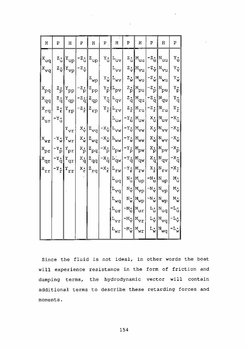
H P H P H P H P H P H P
X Z. Y -Z• Z 1. L Z• M -Z. N Y.uq U UP U U U UV U UU U UU U
X Z• Y -Z• L Z. M -Z. Nvq V Vp v vv v vu v vu v
Z Y. L Z. M -Z• Nwp W WV W WU W WU W
X Z. Y -Z. Z Y• L Z• M -Z• N Y•pq P pp p pp p pv p PU P U p
X Z. Y -Z. Z Y• L Z• M -Z• Nqq q qp q cIID q qv q qu q qu q
X Z. Y -Z. Z Y• L Z• M -Z. N Y.rq r rp r rp r rv r ru r ru r
X -Y• L -Y•M X.N -X.ur u uw u uw u uv u
Y X• Z -X. L -Y• M X. N -X•yr v vq v VW v VW V VV V
X -Y. Y X• Z -X• L -Y• N X. N -X•wr W wr W wq W WW W WW W WV W
X -Y. Y X• Z -X. L -Y• M X. N -X•pr p pr p pq p pw p pw p pv p
X -Y• Y X' Z -X• L -Y• M X• N -X'qr q qr q qq q qw q qw q qv q
X -Y' Y X• Z -X• L -Y• M X' N -X•rr r rr r rq r rw r rw r rv r
L N.M -N•N M•uq u up u up u
L N.M -N.Nvq VVP VV V
L N.M -N.N M•wq w wp w wp w
L -M.M L.N -L•ur u ur u uq u
L -M.M L.N -L•
Vr V V V vq V
L -M.M L•N -L.wr w wr w wq w
Since the fluid is not ideal, in other words the boat
will experience resistance in the form of friction and
damping terms, the hydrodynamic Vector will contain
additional terms to describe these retarding forces and
moments.
154
The only terms which remain after the linearisation of
a Taylor series expansion are X, 'Lvi r' N and Nr The
latter four are important since they lend themselves to
the criterion for dynamic stability of the linear model,
which is:
C = Y (N-mxu) -N (Y-mu)v r g V r
where C > 0 for a dynamically stable boat.
In the non-linear equations of motion proposed by
Abkowitz, 1964 (Ref.2), and Strom-Tejsen, 1965
(Ref.127), higher order terms in the Taylor series
expansion are included. After some simplification, the
hydrodynamic coefficients appearing in the surge
equation will be X , X , X , X , X , X , X andu uu uuu vv rr vvu rru
Xvru• Similar terms exist in the sway and yaw equations,
however, the author feels that these could be better
represented in more meaningful equations.
Japanese researchers adopt hydrodynamic coefficients
which can be related to the real ship, with terms such
as:Y,Y,Y ,Y ,Y ,N,N,N,N ,Nv r v i v i y i n r i r l v r 4 vrr vrr
Nr1r11 N 11 and Nr11 The number of terms to be
included is not obvious without the ability to test
models and assess the magnitude of all the pertinent
coefficients. Most researchers choose varying terms to
155
suit their own models and the application involved.
Källström and Ottosson, 1982 (Ref.80), go so far as to
include terms such as uur' 'X'uuv
Y , Y , Y , Y , Y , L , L , Luu up v I v I r i r l y i n up p i p i vivj
L , L , N , N , N ,N , N, Nr i n i y i n uur uv ii uuv uu up vivi
N andNr i r i yin
In some respects, the selection of terms to be included
and those to be neglected seems more than a little
haphazard! In fact it becomes easier to prove a term's
existence rather than its non-existence. The Taylor
series expansions can become bewildering and the author
believes that simplification of the small boat model is
desirable at this stage. Therefore, a minimal number of
non-perfect fluid hydrodynamic coefficients will be
assumed to provide sufficient accuracy for the purposes
of this thesis. Since standard plots of Y versus v, Y
versus r, N versus v and N versus r, (Fig.6.1), show
that while the gradient can be assumed linear in the
region close to the origin, further terms will be
required for greater accuracy, especially away from the
origin. Therefore, in addition to the linear terms
r' N and Nrf the author proposes including terms in
X , Y , Z , L , M and N which amountu l u l v i v i w i w i PIP! ii rirlto damping coefficients working in opposition to the
boat's motion.
156
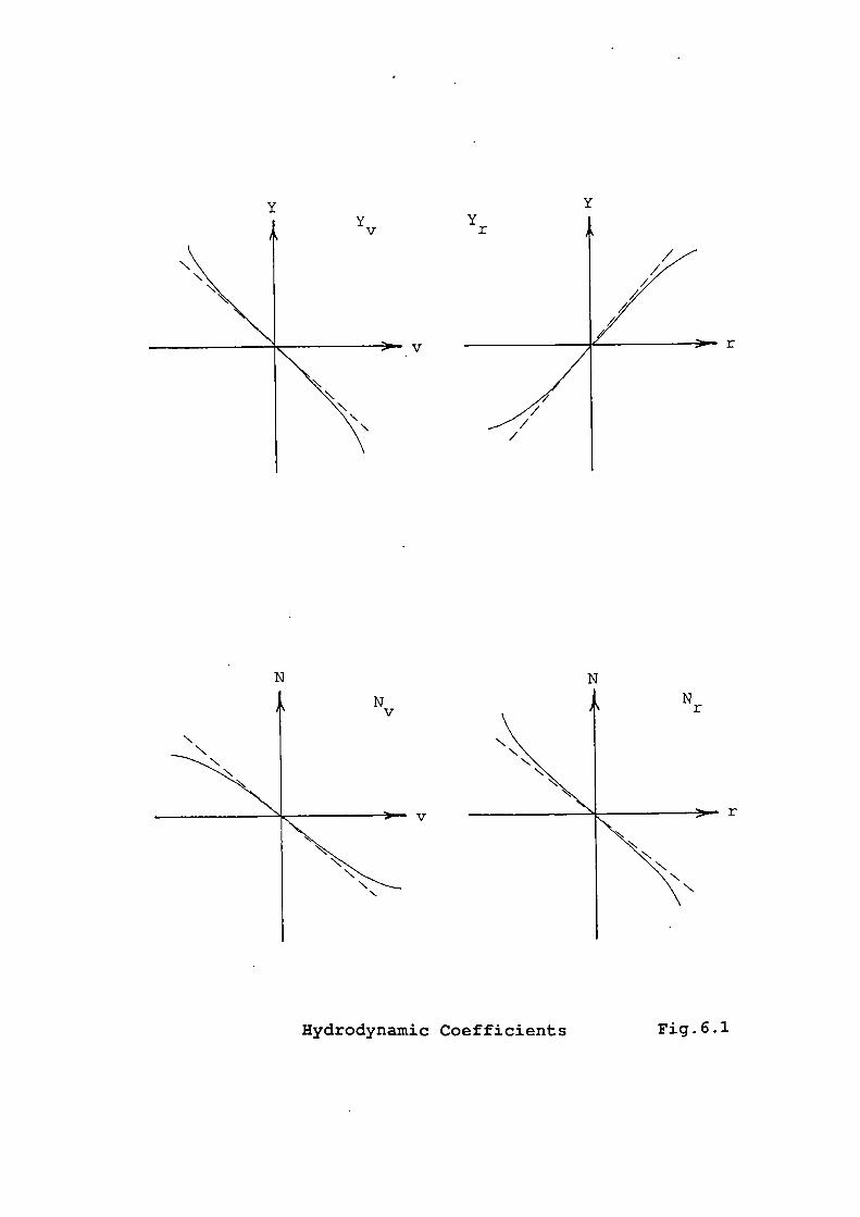
V
N
N
Hydrodynaniic Coefficients Fig.6.l
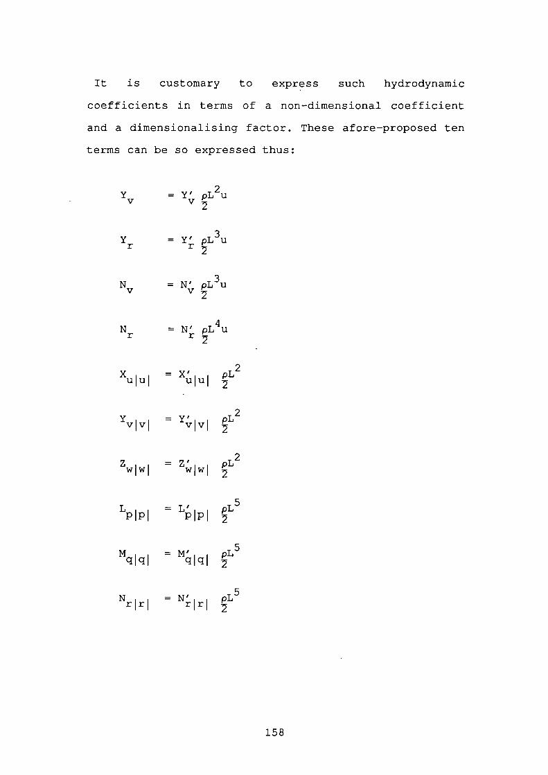
It is customary to express such hydrodynamic
coefficients in terms of a non-dimensional coefficient
and a dimensionalising factor. These afore-proposed ten
terms can be so expressed thus:
Y = Y' pLuV V2
Y = Y' pL3ur r2
N =N' pL3uV V2
N N' pL4Ur r2
xulul
Yvivi
zwiwl
pLu l u l 2
= Y' pLv I v I 2
= Z' pLw I w I 2
L =L' pL5II pipI 2
5M =M' pLq I q J qiqI 2
5N N' pLr i r l rIrl 2
158
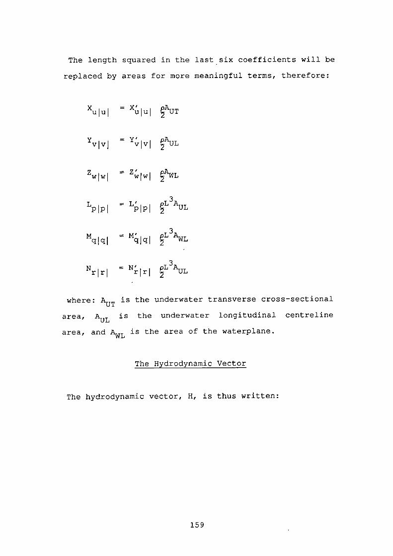
The length squared in the last six coefficients will be
replaced by areas for more meaningful terms, therefore:
x =x' pu l u l ulul 2AUT
Y =Y' pv i v i vIvI 2AUL
z pw i wl wIwI
AWL
L = L jp pLAUL
TMq I q I = TMqJqI pLAWL
3N 11 = N' 11 pL AUL
where: AUT is the underwater transverse cross-sectional
area, AUL is the underwater longitudinal centreline
area, and AWL
is the area of the waterplane.
The Hydrodynamic Vector
The hydrodynamic vector, H, is thus written:
159
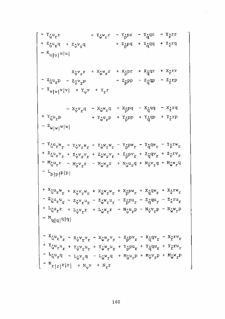
- Y•Ur
+ Z . Uq + Zvq
- xu1u1uul
- Y . qr - Y • rr-Y . wr -Y.pr q rwr p+ Zpq + Z4qq + Zjrq
X . v r + Xw r + X . pr + X'qr + X•rry r wr p q r
- ZiiUrP - ZVrP - Zpp - Z4qp - Zj,rp
- + Yv + Yr
-X • vq -X . wq -X • pq -Xqq -Xjrqy r wr p
+ Y tiU rP + Y . w + Y . pp + Y . qp + Yrpwr p
- zIwIwIwI
- Y' w - y. - y. w w - Y . pw - Y . qw - Y.rw11rr vrr wrr p r q r r r+ Z. -- •V + Z . w v + Z . pv + Z • qv + Z.rvUrr vrr wrr p r q r r r
-M • vr -M . wr +N.uo+N.vq+NWqy r wr ur- yr wr
- LHpIp(
+ Xi UrW + X • vw + Xw w + X . pw + X . qw + X.rwr r
r vrr wrr p r q r- Z % U U Z•v u - Z'w u - Z . pu - Z . qu - Z•rur r
Urr vrr wrr p r q r
+Li:iUr +L.vr +L • wr -N.up-N.VpNWPy r wr ur yr wr
- Mq1q1qq
- X'U X•v V - X'w v - Xpv - X . qv - X.rvUrr vrr wrr p r q r r r+ Y i U rU + Yvu + Y . wu + Y . pu + Y • qu + Y•ru
vrr wrr p r q r r r
L • vq -L . wq +M.ui+M.Vp+MWPy r wr ur- yr wr
N IrHr + N V + N rv r
160
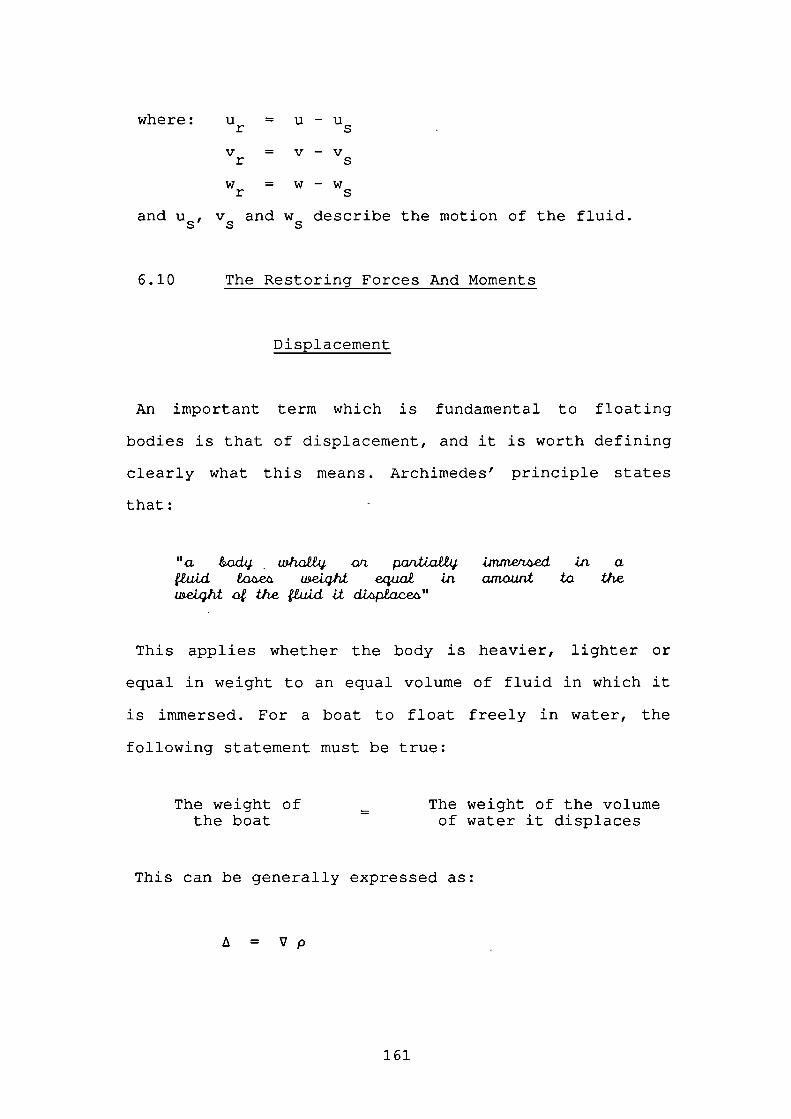
where: u = u-ur S
V = V-Vr S
w = w-wr S
and u , v and w describe the motion of the fluid.
S 5 S
6.10 The Restoring Forces And Moments
Displacement
An important term which is fundamental to floating
bodies is that of displacement, and it is worth defining
clearly what this means. Archimedes' principle states
that:
"a &oth whoL& o'. pantLoTh iJwme'tAed 41L auJ4 & weLqht eqa. n amowt ta theeLçht o the e&iJ4 U dip&ice"
This applies whether the body is heavier, lighter or
equal in weight to an equal volume of fluid in which it
is immersed. For a boat to float freely in water, the
following statement must be true:
The weight of
The weight of the volumethe boat
of water it displaces
This can be generally expressed as:
= Vp
161
where is the displacement of the boat, V is the
volume displaced and p is the density of the water. In
most naval architecture applications where displacement
is expressed in tons and volume in cubic feet, the
density of seawater is 1/35 tons per cubic feet.
However, in this analysis SI units will be used, thus
displacement will be in kilogrammes and volume in cubic
metres with the density of seawater being 1025 kgm3.
When a boat enters a harbour or estuary which has a
freshwater input from a river, the water density will be
reduced. Consequently the volume of water displaced by
the boat must increase, since its weight remains the
same. In other words, the boat's draft will change
causing sinkage to occur. For large ships this can cause
problems when entering ports with little under-keel
clearance. Sinkage in small boats is given little
attention, but this principle is developed later with
respect to the heave restoring force.
The water displaced by the boat is also referred to as
the buoyant force or simply, buoyancy. When a boat
floats at its equilibrium condition the forces of weight
and buoyancy must be equal and opposite, otherwise the
boat would sit on top of the water surface or continue
sinking. Classically these forces can be considered to
act at points within the boat. These points will be the
162
centre of gravity and the centre of buoyancy.
Centre Of Gravity (Cg)
This is the point at which the whole weight of the boat
is assumed to be concentrated and from where it is
considered to act. The weight acts vertically downwards
(perpendicular to the gravitational potential) from the
centre of gravity. The position of the centre of gravity
depends upon the distribution of weight about the boat,
additional top weight causes its location to rise whilst
ballast lowers the position. The actual position can be
determined from an inclining experiment.
Centre Of Buoyancy (Cb)
This is essentially the centre of gravity of the
displaced water or underwater volume of the boat. It is
the point at which the resultant upthrust of the
surrounding water is considered to act. The location of
the centre of buoyancy depends upon the geometry of the
underwater portion of the boat.
It is a combination of the movement of the centre of
buoyancy as a boat rotates from the upright and level
conditions and the difference in the weight and buoyancy
forces that gives rise to the restoring forces and
163
moments. The primary restoring forces and moments are
those in roll, pitch and heave and these will be dealt
with first. However, restoring forces and moments also
arise in surge, sway and yaw as a result of the boat
rolling and pitching.
Stability And Equilibrium
When designing boats, naval architects pay a great deal
of attention to their stability. It is the initial
stability condition that determines the equilibrium of
the boat when it floats freely. While dynamical
stability is a measure of the boat's ability to return
to the initial equilibrium state when perturbed. Because
of its slender nature, a boat is far more susceptible to
capsizing from rolling than from pitching, therefore it
is normal to only supply information about the righting
moment in roll.
Roll Restorinq Moment
By designing a boat to have symmetry with respect to
the XZ-plane, in other words to be a mirror image along
the fore-aft centreline, and by distributing weight
evenly either side of the centreline, the initial
equilibrium condition of the boat will be such that it
is upright with the weight (W) acting vertically
164
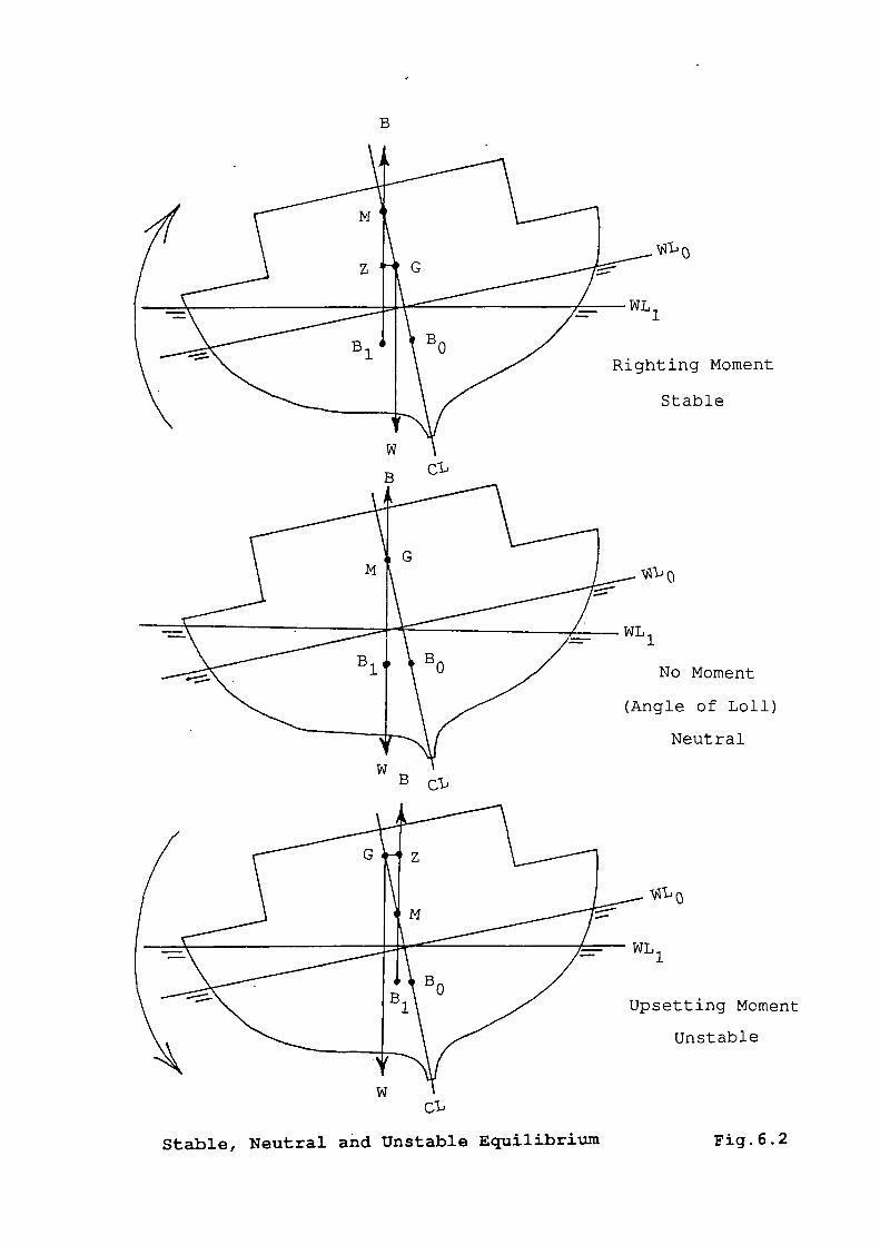
1
Lting Moment
Stable
B
CL
B
BC1
L1
No Moment
ngle of Loll)
Neutral
L1
setting Moment
Unstable
Stable, Neutral and Unstable Equilibrium Fig.6.2
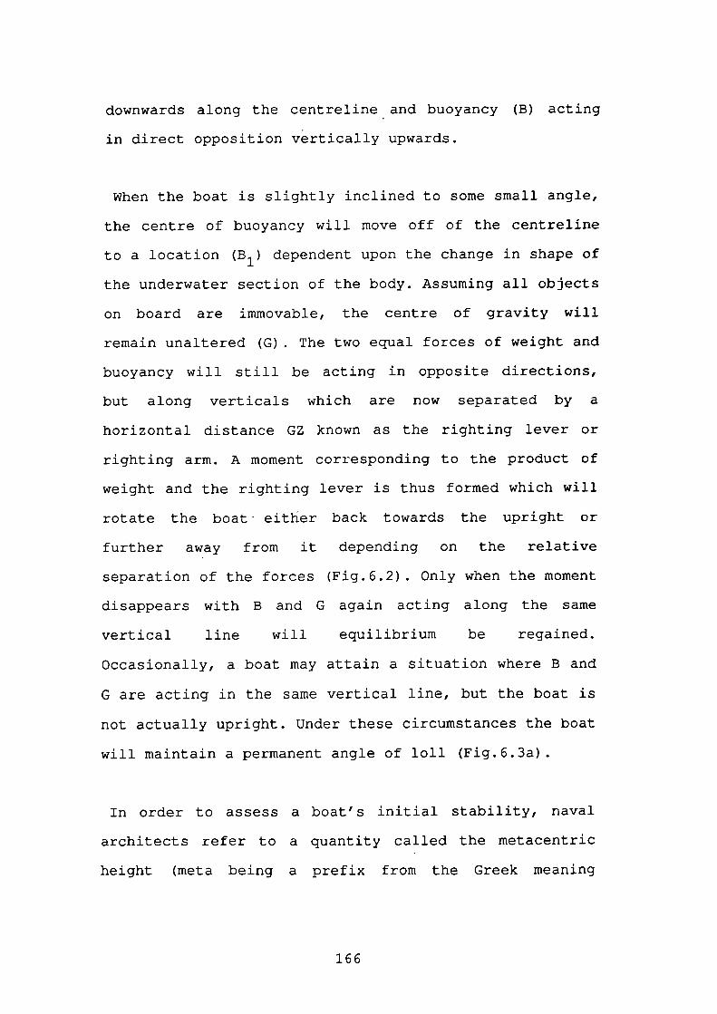
downwards along the centreline and buoyancy (B) acting
in direct opposition vertically upwards.
When the boat is slightly inclined to some small angle,
the centre of buoyancy will move off of the centreline
to a location (B 1 ) dependent upon the change in shape of
the underwater section of the body. Assuming all objects
on board are immovable, the centre of gravity will
remain unaltered (G). The two equal forces of weight and
buoyancy will still be acting in opposite directions,
but along verticals which are now separated by a
horizontal distance GZ known as the righting lever or
righting arm. A moment corresponding to the product of
weight and the righting lever is thus formed which will
rotate the boat either back towards the upright or
further away from it depending on the relative
separation of the forces (Fig.6.2). Only when the moment
disappears with B and G again acting along the same
vertical line will equilibrium be regained.
Occasionally, a boat may attain a situation where B and
G are acting in the same vertical line, but the boat is
not actually upright. Under these circumstances the boat
will maintain a permanent angle of loll (Fig.6.3a).
In order to assess a boat's initial stability, naval
architects refer to a quantity called the metacentric
height (meta being a prefix from the Greek meaning
166
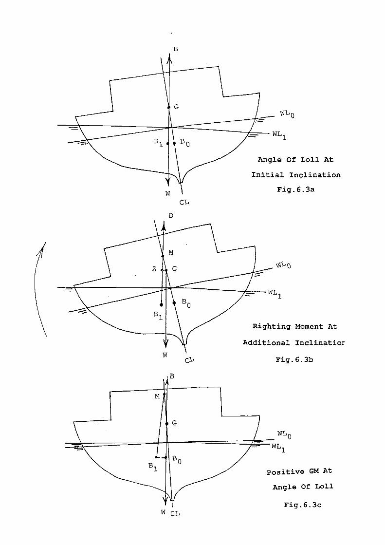
vL0
L1
I.e Of Loll At
al Inclination
Fig.6.3a
ing Moment At
nal Inclinatior
B
CL
B
wFig.6.3b
WL0
IL1
sitive GM At
ng1e Of Loll
Fig.6.3cWCL
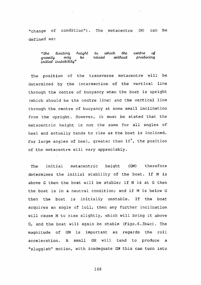
"change of condition") . The metacentre (M) can be
defined as:
"the limillnq hetqlLt tci whh the centre oqnLtq &e 'tad Lthcu2t po&cLnq
Lfl4ta&Ut"
The position of the transverse metacentre will be
determined by the intersection of the vertical line
through the centre of buoyancy when the boat is upright
(which should be the centre line) and the vertical line
through the centre of buoyancy at some small inclination
from the upright. However, it must be stated that the
metacentric height is not the same for all angles of
heel and actually tends to rise as the boat is inclined.
For large angles of heel, greater than 100, the position
of the metacentre will vary appreciably.
The initial metacentric height (GM) therefore
determines the initial stability of the boat. If M is
above G then the boat will be stable; if M is at G then
the boat is in a neutral condition; and if M is below G
then the boat is initially unstable. If the boat
acquires an angle of loll, then any further inclination
will cause M to rise slightly, which will bring it above
G, and the boat will again be stable (Figs.6.3b&c) . The
magnitude of GM is important as regards the roll
acceleration. A small GM will tend to produce a
"sluggish" motion, with inadequate GM this can turn into
168
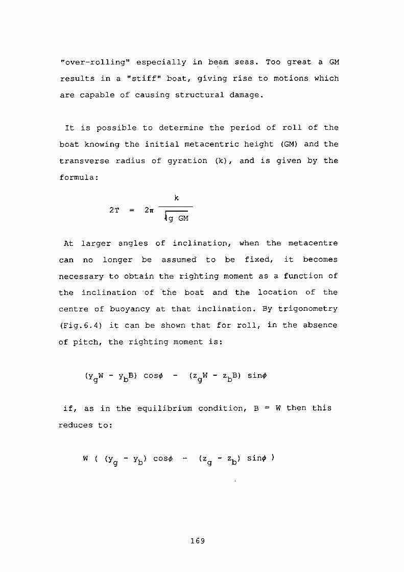
"over-rolling" especially in beam seas. Too great a GM
results in a "stiff" boat, giving rise to motions which
are capable of causing structural damage.
It is possible to determine the period of roll of the
boat knowing the initial metacentric height (GM) and the
transverse radius of gyration (k), and is given by the
formula:
k
2T = 2irGM
At larger angles of inclination, when the metacentre
can no longer be assumed to be fixed, it becomes
necessary to obtain the righting moment as a function of
the inclination of the boat and the location of the
centre of buoyancy at that inclination. By trigonometry
(Fig.6.4) it can be shown that for roll, in the absence
of pitch, the righting moment is:
(ygW - ybB) cos - (ZgW - zbB) sin
if, as in the equilibrium condition, B W then this
reduces to:
y)cos - (z -zW( (Yg b g b sin)
169
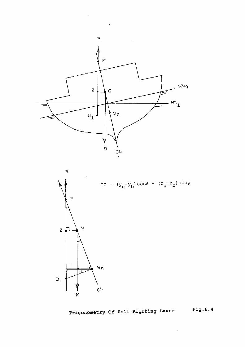
B
wCL
B
GZ = (Yg_Yb0 - (Zg_Zb)SIfl
w
Trigonometry Of Roll Righting Lever Fig.6.4
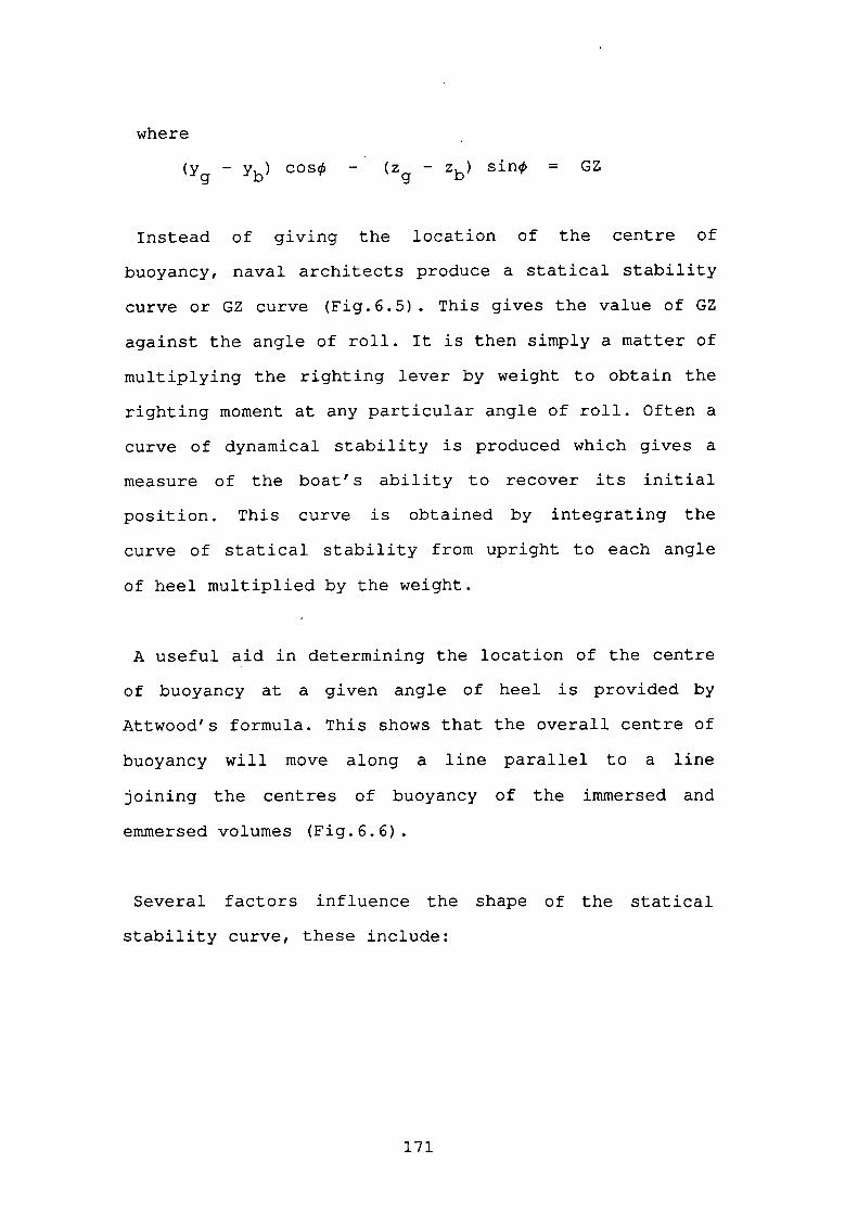
where
(Yg - ' ) cos - ( z - Zb) S1fl = GZb g
Instead of giving the location of the centre of
buoyancy, naval architects produce a statical stability
curve or GZ curve (Fig.6.5). This gives the value of GZ
against the angle of roll. It is then simply a matter of
multiplying the righting lever by weight to obtain the
righting moment at any particular angle of roll. Often a
curve of dynamical stability is produced which gives a
measure of the boat's ability to recover its initial
position. This curve is obtained by integrating the
curve of statical stability from upright to each angle
of heel multiplied by the weight.
A useful aid in determining the location of the centre
of buoyancy at a given angle of heel is provided by
Attwood's formula. This shows that the overall centre of
buoyancy will move along a line parallel to a line
joining the centres of buoyancy of the immersed and
emmersed volumes (Fig.6.6).
Several factors influence the shape of the statical
stability curve, these include:
171
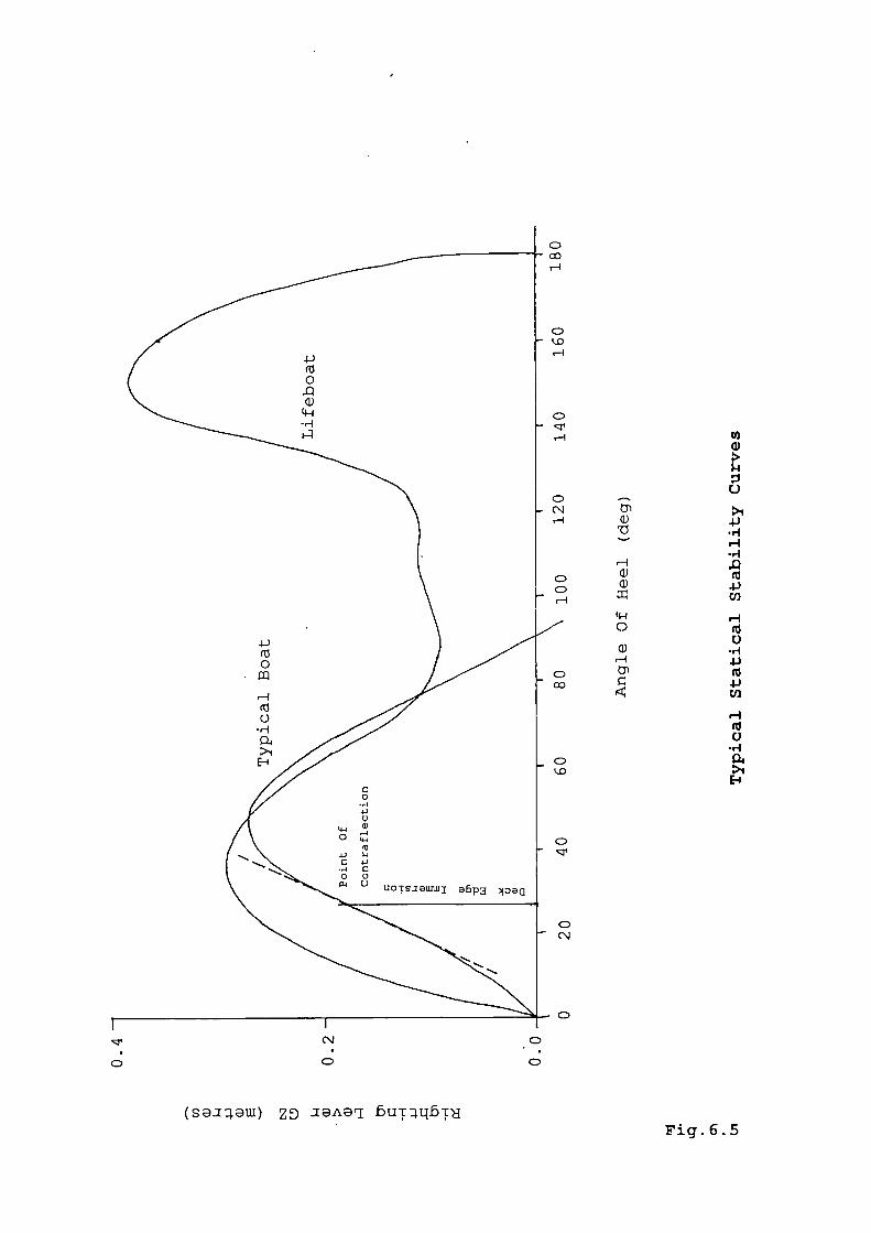
D
D
C-)
>1a)
.1-I- u-I
•rIHwa) 4)
CI)
u-Io
C.)•rI
H 4)
_IJC/)
u-I
C)•rIp4
El
(saew) zf .aAeJ buq5r
Fig. 6.5
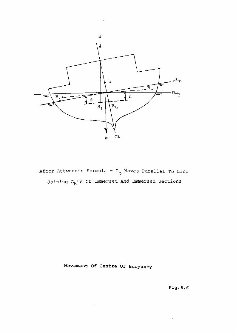
L0
WL1
B
W CL
After Attwood's Formula - Cb Moves Parallel To Line
Joining Cb'S Of Immersed And Ernmersed Sections
Movement Of Centre Of Buoyancy
Fig. 6.6
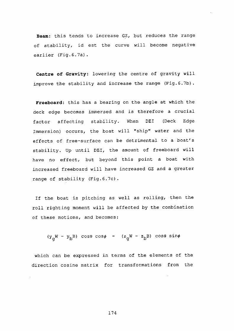
Beam: this tends to increase GZ, but reduces the range
of stability, id est the curve will become negative
earlier (Fig.6.7a)
Centre of Gravity: lowering the centre of gravity will
improve the stability and increase the range (Fig.6.7b).
Freeboard: this has a bearing on the angle at which the
deck edge becomes immersed and is therefore a crucial
factor affecting stability. When DEl (Deck Edge
Immersion) occurs, the boat will "ship" water and the
effects of free-surface can be detrimental to a boat's
stability. Up until DEl, the amount of freeboard will
have no effect, but beyond this point a boat with
increased freeboard will have increased GZ and a greater
range of stability (Fig.6.7c)
If the boat is pitching as well as rolling, then the
roll righting moment will be affected by the combination
of these motions, and becomes:
(ygW - yB) cose cos - (ZgW - zbB) coso sin
which can be expressed in terms of the elements of the
direction cosine matrix for transformations from the
174
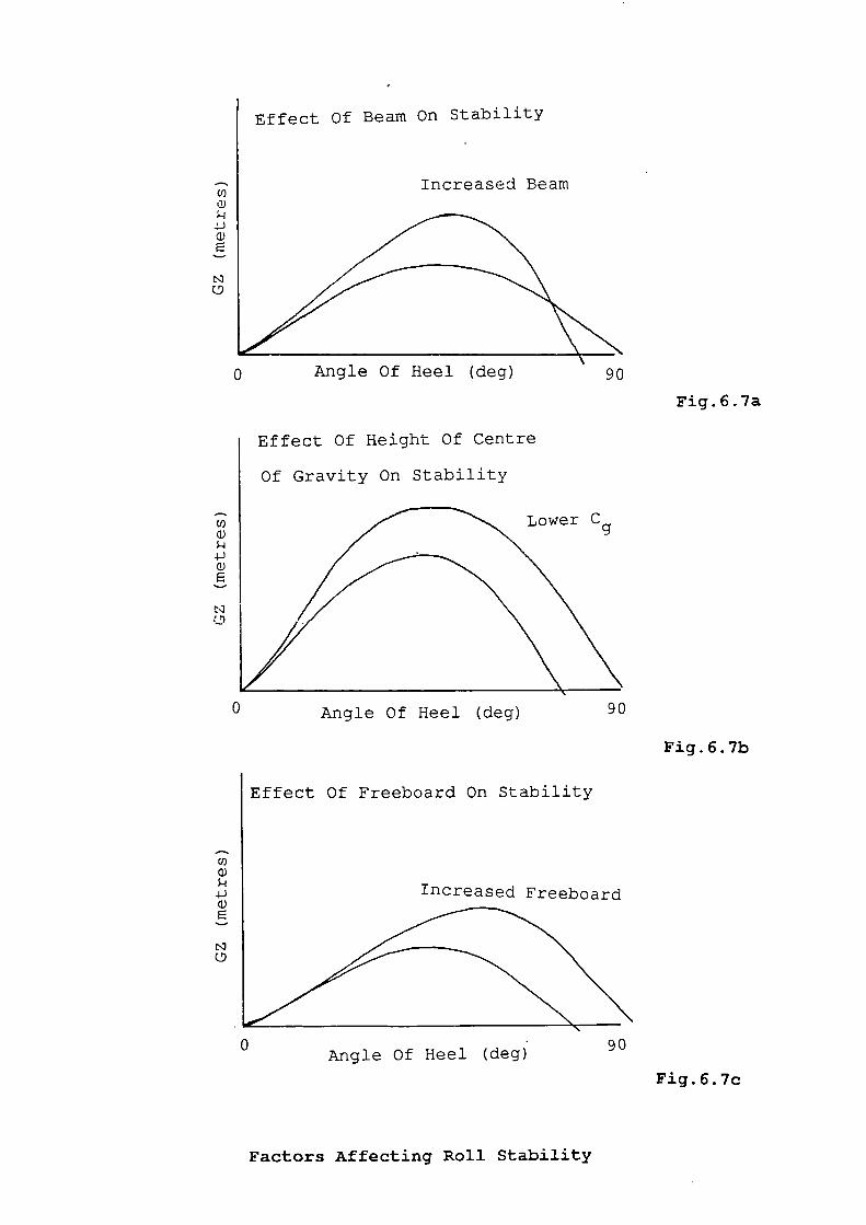
Cl)
'2)
4J
a)
0 Angle Of Heel (deg) 90
Fig. 6.7a
C')
ci)4J
ci)
Effect Of Height Of Centre
Of Gravity On Stability
Lower Cg
0 Angle Of Heel (deg) 90
Fig. 6.7b
Effect Of Freeboard On Stability
CI)t
-IIIncreased Freeboard
wi
c)I
0 90Angle Of Heel (deg)
Fig.6.7c
Factors Affecting Roll Stability
moving axes system to the inertial system as:
(YgW - ' B) A - (z W - z. B)b 33 g D
Pitch Restoring Moment
The principles that determine the roll righting moment
also apply to the pitch righting moment. The main
difference is that pitch is the longitudinal inclination
of the boat about an athwartships axis and does not
exhibit symmetry about the YZ-plane when upright.
Rotations of pitch again rely on the relative positions
of the centres of gravity and buoyancy, but are
concerned with their x and z coordinates. The angles of
longitudinal inclination are small with respect to the
transverse rotations, and consequently naval architects
confine themselves to simply expressing changes of trim.
Trim is the difference between the draft aft and the
draft forward, but for this analysis it will not be
distinguished from pitch as no allowance will be made
for ballasting or other changes in the weight
distribution.
For longitudinal inclinations a boat pivots about a
point known as the centre of floatation. This is the
centre of the waterplane area and is located somewhere
near the amidships position. Normally it will be a
176
little abaft midships and this is due to the asymmetry
of the boat's longitudinal shape (Fig.6.8).
The pitch restoring moment, in the absence of roll, can
be expressed, from trigonometry, as:
- (ZgW - zbB) sinG - (XgW - XbB) cose
if, as in the equilibrium condition, B = W, then this
reduces to:
W ( - ( z - Zb) sine - (x - xb) coseg g
where:
- (Zg - Zb) sine - (x - Xb) cose = GZiongg
GZ10g is the equivalent of GZ, but in the longitudinal
sense. It is the horizontal separation of the vertical
upwards through B and the vertical downwards through G.
Allowing for the effects of roll, the pitch righting
moment becomes:
- (ZgW - zbB) sine - (XgW - xbB) cosecos
which can be expressed in terms of the elements of the
177
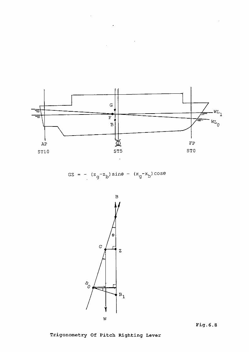
WL1
IL0
ST1O ST5 STO
- - (z -z ) sinG - (x -x ) cOSO-g b gb
B
Gs4
a0
B1
wFig. 6.8
Trigonometry Of Pitch Righting Lever
direction cosine matrix for transformations from the
moving axes system to the inertial system as:
(zW-zB)A - (xW_xbB) A33b 31 gg
Heave Restoring Force
When the density of the water alters, the boat will
assume a new draft, such that the product of the
underwater volume and the water density equate to the
displacement. However, if the boat experiences some
perturbation which causes a vertical displacement and
there is no change in density, then the boat will
naturally seek to resume the original underwater volume
prior to the disturbance. This is the heave restoring
force.
In the equilibrium condition the forces of weight and
buoyancy must be equal. When the boat is caused to
heave, the underwater volume changes and so, therefore,
does the buoyancy force, since:
B Vpg
Since the weight will remain constant, and is given as:
W = mg
179
the heave restoring force is dependent on the difference
between the weight and buoyancy forces. If the boat is
rolling and pitching, then this difference will be
reduced and the heave restoring force is given by:
(W - B) cosocos
which can again be represented in terms of the elements
of the direction cosine matrix for transformations from
the moving axes system to the inertial system as:
(W - B) A33
The Remaining Restoring Forces
A combination of a change in buoyancy and the boat
pitching will yield a surge force. The magnitude of this
force will increase with pitch and can be expressed as:
- (W - B) sinO
Similarly, a combination of a change in buoyancy and
the boat rolling and pitching will create a sway force
given as:
(W - B) cosesin
180
The action of rolling and pitching will also generate a
yaw moment which is written as:
(XgW - XbB) cosesin + (YgW - 'bsine
These three equations can, like those for roll, pitch
and heave, be expressed in terms of the elements of the
direction cosine matrix for transformations from the
moving axes system to the inertial system.
The Gravity-Buoyancy Vector
Collecting all the six restoring forces and moments
together in vector form and resolving the weight and
buoyancy using the direction cosine elements, gives:
A31 (W-B)
A32 (W-B)
A33 (W-B)
A33 (YgW YbB) - A32 (ZgW_ZbB)
A3l ( Z gW_ZbB) - X33(xgw_xbB)
A32 gWXbB) - A31 (YgW_YbB)
181

Hydrostatic Curves
Some of the static values which are useful when
computing the restoring forces and moments can be
gleaned from the hydrostatic curves.
These curves depict a number of terms which vary with
draft and are entirely dependent upon the geometrical
shape of the underwater part of the boat. The curves are
presented with the independent variable of draft on the
vertical axis. These figures for draft are often with
respect to the underside of the keel (extreme draft) at
amidships (station 5) . The horizontal axis has a base
scale which sets out the varying displacement, but also
has a scale of distance from the midships position for
some of the remaining terms. The following curves are
usually shown (Fig.6.9)
Displacement : This initially curves out from the
origin and becomes nearly a straight line. It usually
applies to seawater density.
Vertical Centre of Buoyancy (VCB): This also
approximates to a steep, straight line and gives the
vertical distance of the centre of buoyancy from the
underside of the keel.
182
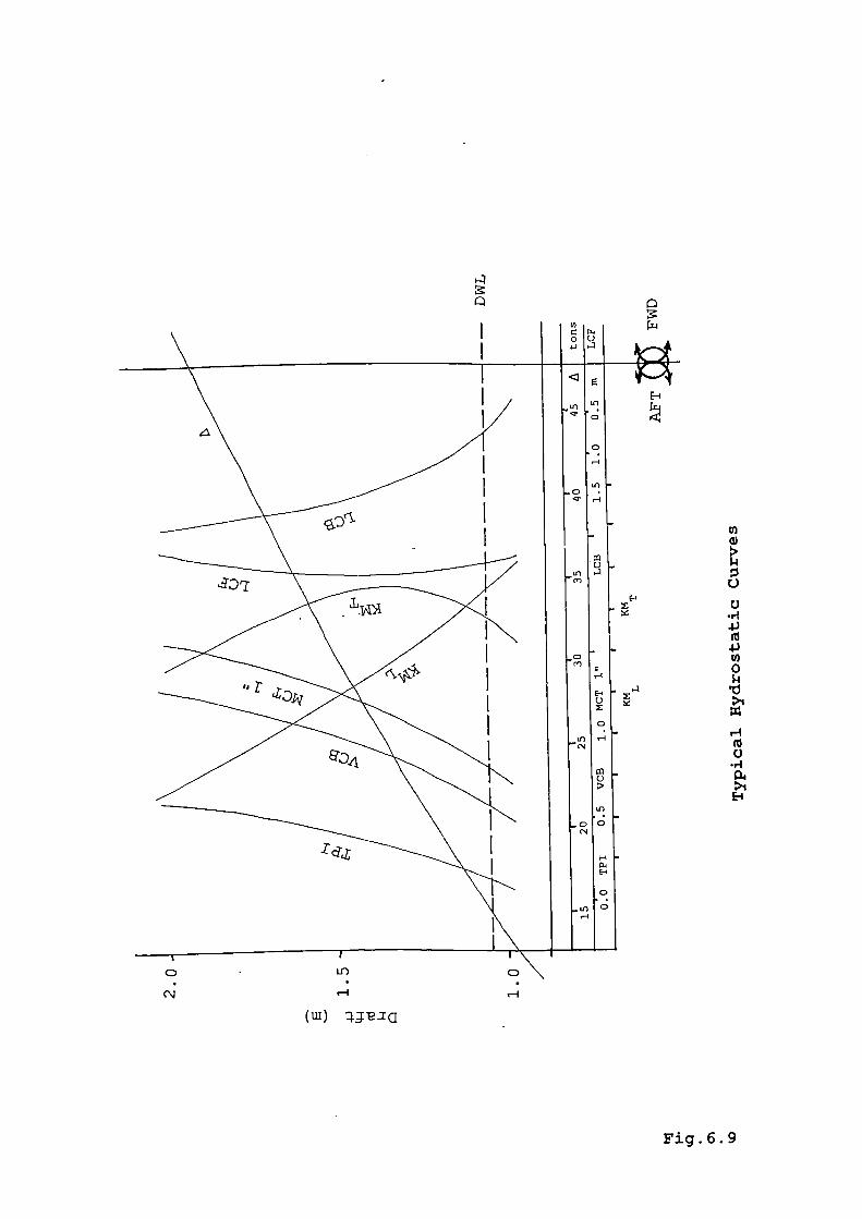
0
0,a;
0
U
.1-)Ri4)
0
i-1RiU
•rIp4
c"J i-1
(ul)
Fig.6.9
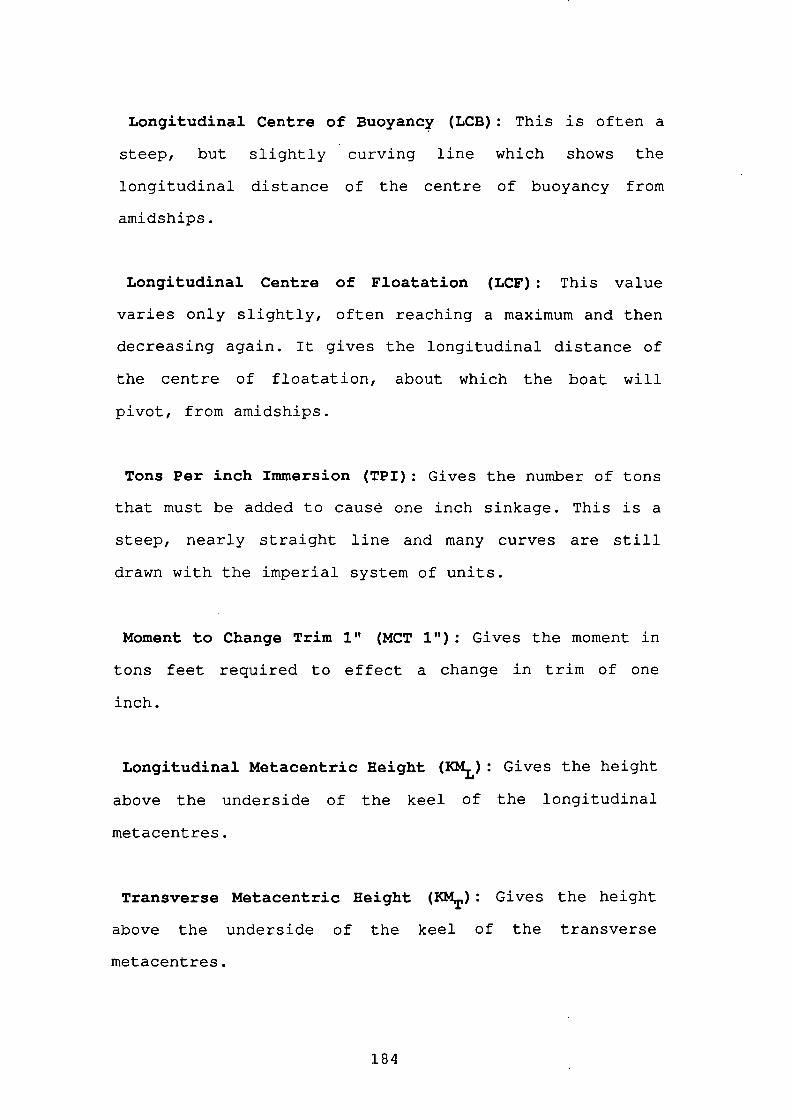
Longitudinal Centre of Buoyancy (LCB): This is often a
steep, but slightly curving line which shows the
longitudinal distance of the centre of buoyancy from
amidships.
Longitudinal Centre of Floatation (LCF): This value
varies only slightly, often reaching a maximum and then
decreasing again. It gives the longitudinal distance of
the centre of floatation, about which the boat will
pivot, from amidships.
Tons Per inch Immersion (TPI): Gives the number of tons
that must be added to cause one inch sinkage. This is a
steep, nearly straight line and many curves are still
drawn with the imperial system of units.
Moment to Change Trim 1" (MCT 1"): Gives the moment in
tons feet required to effect a change in trim of one
inch.
Longitudinal Metacentric Height (KML): Gives the height
above the underside of the keel of the longitudinal
metacentres.
Transverse Metacentric Height (KM,): Gives the height
above the underside of the keel of the transverse
metacentres.
184
For many small boats, the keel line will not
necessarily be horizontal, but will be "raked" so that
the draft at the aft perpendicular is greater than the
draft at the forward perpendicular. The hydrostatic
curves are therefore usually calculated for the midships
position (station 5) and corrections must be made
according to the rake. The rake is expressed as the
difference of the aft and forward drafts, and knowing
the length between perpendiculars (LBP) the gradient of
the keel line can be computed.
6.11 The Rudder Forces And Moments
Whilst the concept of using a rudder to provide a means
of steering a boat seems quite simple, the actual
situation is an extremely complex one. Interaction
effects between the hull, propeller and rudder cause
modifications to the flow past the rudder and the inflow
angle (Fig.6.10). Lötveit, 1959 (Ref.95), provides an
extremely useful study of rudder action.
The rudder can, in principle, be related to a hydrofoil
with a low aspect ratio, and aerodynamic theory can be
applied to determine the forces and moments generated by
the rudder. The forces acting upon an aerofoil are
usually expressed as dimensionless lift and drag
coefficients, denoted CL and CD respectively. The main
185
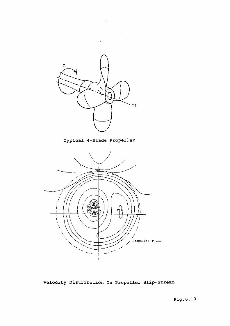
CL
Plane
Typical 4-Blade Propeller
/
Velocity Distribution In Propeller Slip-Stream
Fig. 6.10
purpose of the rudder is to generate a side force, by
which it is possible to produce yaw and therefore
steerability. It is therefore of great importance to
know the magnitude of the rudder "lift", or side forces
at given speeds and rudder angles. This side force is
often termed the rudder normal force.
Rudder Normal Force
The author follows the approach adopted by Japanese
researchers such as Ogawa and Kasai, 1978 (Ref.115) . The
"open" water characteristics of the rudder normal force
will be developed first, with additional terms
describing the changes of the rudder inflow velocity and
angle which occur when a rudder is located behind the
hull and in the propeller slip-stream. Open water refers
to the condition where the rudder is isolated from the
hull and propeller effects and placed deep in the water.
In open water the rudder normal force is usually
expressed as:
FN = CpAV
where: p is the water density, AR is the rudder area,
VR is the rudder inflow velocity and CFN is the rudder
normal coefficient and can be regarded as:
187
CFN = f(, r, Rel tic, Rudder Outline)
where: 5 is the rudder angle, r is the rudder aspect
ratio, Re is the Reynold's number for the particular
rudder flow and t/c is the rudder thickness ratio.
The rudder outline and thickness ratio apparently have
minimal effect and especially for rudders of near
rectangular shape can be regarded as being constant.
Whilst the Reynold's number is important in the open
water characteristics, for rudders operating in the
propeller slip-stream the "burbling' t point will usually
occur above the maximum rudder angle. This leaves just
the two primary parameters:
CFN = f(r, )
Tests monitoring the effect of rudder aspect ratio upon
the rudder normal force produce the following empirical
relationship (Fig.6.11)
6.13 FCFN r + 2.25
The effect of rudder angle is included from a
188
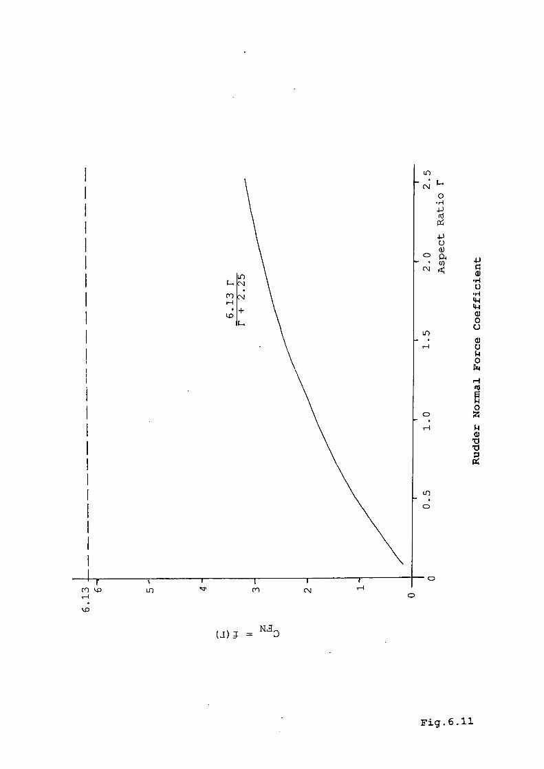
I-)
0-H
-I-)01)
4)
t)
D
LI) (Y) (N
(_I); =
Fig.6.11
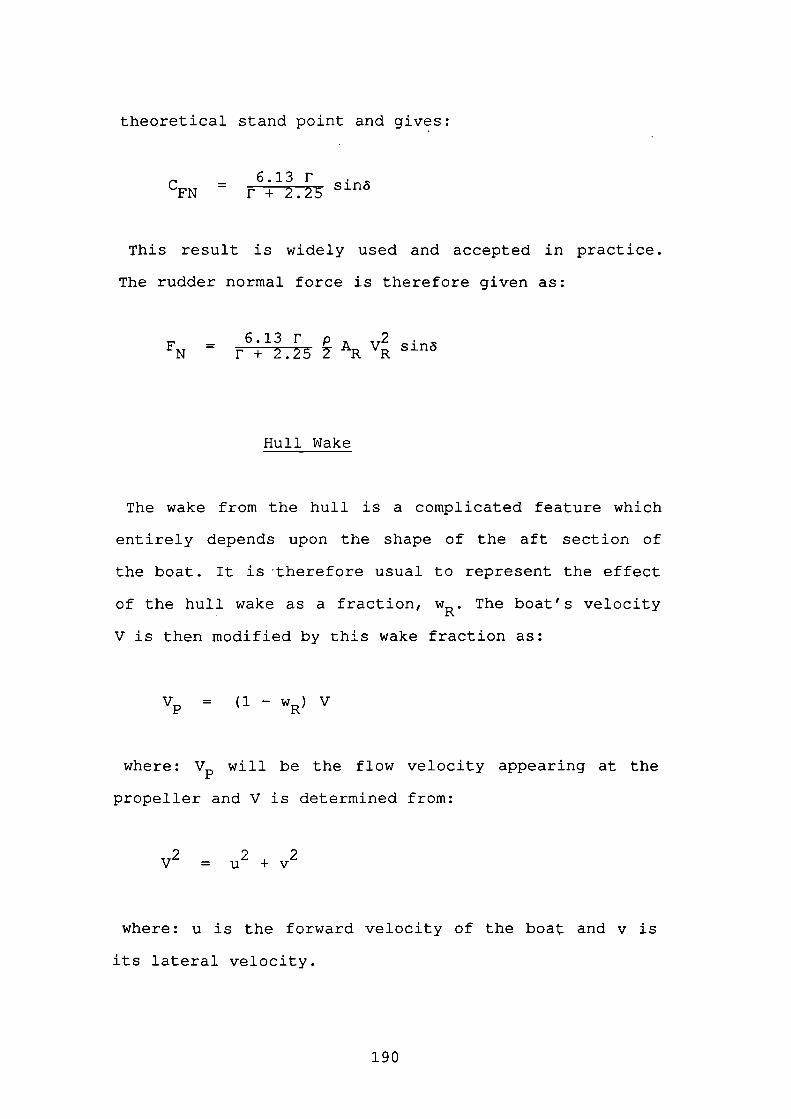
theoretical stand point and gives:
6.13 rCFN = r + 2.25 S1fl
This result is widely used and accepted in practice.
The rudder normal force is therefore given as:
6.13r p 2FN = F + 2.25 2 AR VR sinö
Hull Wake
The wake from the hull is a complicated feature which
entirely depends upon the shape of the aft section of
the boat. it is therefore usual to represent the effect
of the hull wake as a fraction, WR• The boat's velocity
V is then modified by this wake fraction as:
VP = (1 - wR) V
where: V will be the flow velocity appearing at the
propeller and V is determined from:
2 2 2V = u +v
where: u is the forward velocity of the boat and v is
its lateral velocity.
190
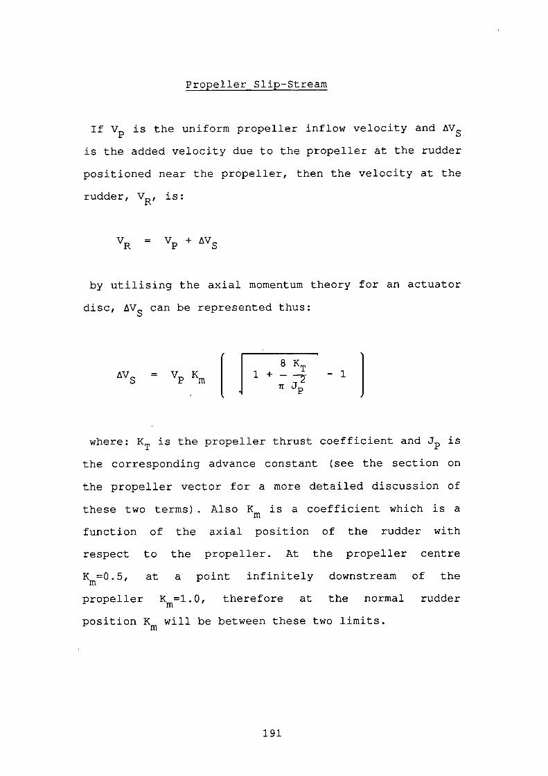
Propeller Slip-Stream
If VP is the uniform propeller inflow velocity and
is the added velocity due to the propeller at the rudder
positioned near the propeller, then the velocity at the
rudder, VRI is:
VR = VP+VS
by utilising the axial momentum theory for an actuator
disc, V5 can be represented thus:
tV = V KS P m
l+— -1
JI ] TrJP
where: KT is the propeller thrust coefficient and is
the corresponding advance constant (see the section on
the propeller vector for a more detailed discussion of
these two terms) . Also Km is a coefficient which is a
function of the axial position of the rudder with
respect to the propeller. At the propeller centre
Km=O•5 at a point infinitely downstream of the
propeller K=l.O therefore at the normal rudder
position Km will be between these two limits.
191
However, the non-uniformity of the rudder in flow
velocity requires the inclusion of an attenuation of the
acceleration effect. For relatively low propeller
loadings, Ogawa and Kasai show that the following
established formula for VR is valid:
VR = VP J
1 + ks3"2
where: k is an empirical factor and s is the propeller
slip-stream ratio, given by:
s = 1 - (1 - w) 4where: w is the propeller wake fraction, n is the
propeller revolutions and P is the propeller pitch.
Effective Rudder Inflow Velocity
The effective rudder inf low velocity can be obtained by
comparing the rudder normal forces for the open water
condition with the condition when the hull and propeller
are in place for the same rudder angles. The inflow
velocity, 11R' is then:
FNVR = V
No
192
where: V is the open water inflow velocity, FN is the
rudder normal force with the hull and propeller effects
and FN0 is the rudder normal force in open water.
Combining the boat's forward and lateral velocities
with the hull wake effect and the propeller slip-stream
effect, gives the rudder inflow velocity as:
VR = (1 - wR) V J
1 + ks3"2
where: k, the empirical constant, equals 1.065 for port
turns and 0.935 for starboard turns for single screw,
single rudder arrangements. However, the Arun class
lifeboat has a twin propeller, twin rudder arrangement
with the rudder mounted behind the counter rotating
propellers. Therefore it is assumed that any uneven
flows due to the rotation of one propeller will be
cancelled by the other propeller's opposite rotation,
hence k will be equal to 1.0.
Effective Rudder Inf low Angle
As well as the modification of the flow velocity, there
is also the need to determine the effective rudder
inflow angle (Fig.6.12) . This will be a function of the
193
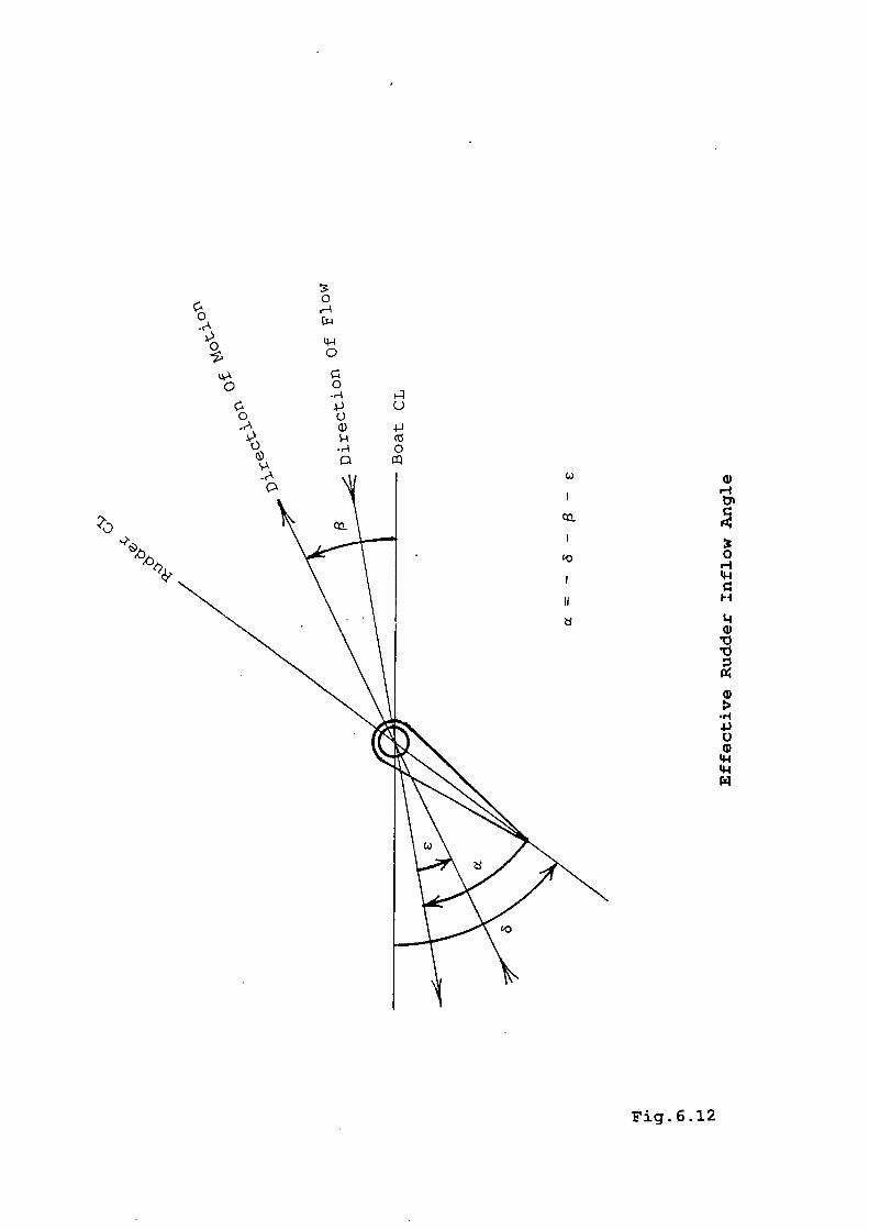
a,
0u-Iq-I
1•1
LI
a,
'ti
a,
•1-)C,
a,.1-I
N
0
0 r4
0
c4
0 0
4) U0 0
a) .4J(ti
.r4 0
Fig. 6.12
actual rudder angle , the direction of motion of the
boat with reference to its centreline 13 and the
additional change in the flow angle due to the hull and
propeller effects c. The effective rudder angle, , is
therefore:
= - - (3 - C
The angles are measured in specific directions and the
signs reflect this. (3 can be determined from:
-1(3 = tan (v/u)
or, as will be used in the simulation:
(3 = sin 1(v/V)
c is sometimes referred to as the flow rectifying angle
which after Inoue, Hirano, Kijima and Takashina, 1981
(Ref.76), is given as:
c = (3(-1) +
where: XR is the x-coordinate of the centre of effect
of the rudder, r is the yaw rate, V is the boat's
resultant velocity and ' is a flow rectification
coefficient which is split into two parts:
195
= Cp CH
The propeller flow rectification coefficient, C i,, is
expressed by the empirical formula:
(1 - 0.7s)sC = [ 1 + 1.2ii
(1 - s)2
where: s is the propeller slip-stream ratio and i is the
propeller diameter, D, to rudder height, H, ratio:
ii = D/H
The hull rectification coefficient, CR, is given in a
slightly different form as:
0.45 v , <= 0.5/0.45
CH =
0.5 t' > 0.5/0.45
where: the numbers are empirically based constants and v
is given as:
v = (c - 2xRr/V) / (1 -
Many models based on Taylor series expansions simply
include coefficients for the rudder-exciting forces.
When viewed in the light of the preceding discussion, it
196
is obvious that coefficients based on regression
techniques alone may not be sufficient for modelling
purposes. It is always desirable to relate the
coefficients to the physical situation and avoid
abstract notations.
The preceding may not be a full representation of the
flow around the aft section of a boat, but at least
approaches logically the factors involved. As a result
of the complex nature of the flow patterns and the
difficulty of accurately reproducing them, it may be
desirable to make some simplifying assumptions,
particularly with reference to the effective rudder
inf low angle, to reduce the computations required.
The Rudder Vector
The rudder normal force can now be represented as
follows, with replacing the initially suggested:
6.13r p 2FN = r + 2.25 AR VR S1IIa
For surge any deflection of the rudder angle will
introduce a retarding or drag force acting so as to
reduce the forward velocity. As the deflection increases
197
either to port or starboard, •so this force increases
negatively. The rudder normal force for surge will be
modified by a -sine factor.
Sway will be similarly affected, but since it is at
right angles to surge, the modifying factor will be
-cosó. Heave will be unaffected by the rudder
deflection. Roll will follow the same tendency as sway,
but since it is the moment about the fore-aft axis, the
sign of the modifying factor will depend upon the
vertical position of the centre of effect of the rudder.
Pitch, like heave will not be affected by rudder
deflections directly.
Yaw, which is the motion that the rudder is designed to
create so that course holding and changing can be
achieved, will vary as a function of -cos. The moment
is affected by the longitudinal position of the centre
of effect of the rudder and since in virtually all boats
the rudder is placed aft, a minus sign is included.
The rudder vector, R, will become:
198
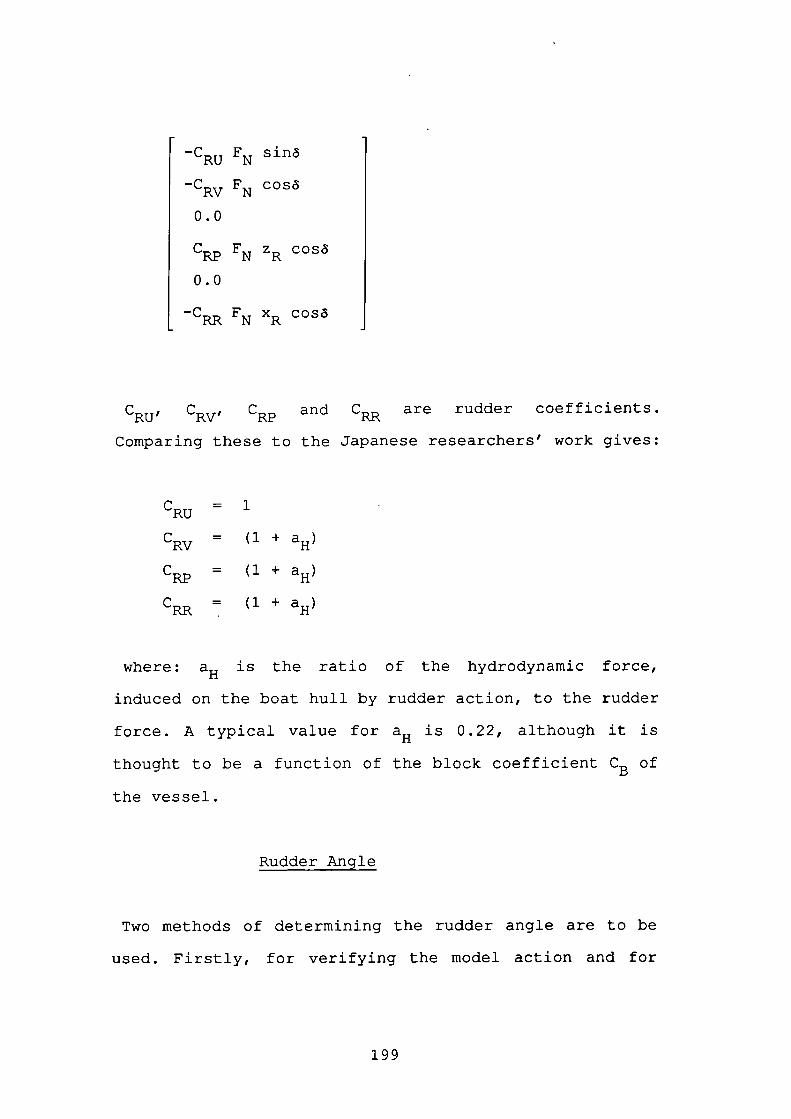
CRU FN Siflt5
CRV FN COSc
0.0
CRP FN ZR COSc
0.0
CRR FN XR COS'3
0RU' CRy, CRP and Care rudder coefficients.
Comparing these to the Japanese researchers' work gives:
CRU = 1
CRy = (1. + aH)
C = (1 + a11)
CRR = (1 + aH)
where: aH is the ratio of the hydrodynamic force,
induced on the boat hull by rudder action, to the rudder
force. A typical value for aH is 0.22, although it is
thought to be a function of the block coefficient CE of
the vessel.
Rudder Angle
Two methods of determining the rudder angle are to be
used. Firstly, for verifying the model action and for
199
subsequent simulation runs where the helmsman or user
will have control of the rudder, the following
differential equation will apply:
= ( -) Itd r
where: is the rudder angle demanded by the helmsman
(or simulation user) and t is the rudder time constant.r
When the autopilot is attached to drive the boat model,
a different method will be used to determine rudder
position. The function of the autopilot is to maintain a
desired course, which it does by attempting to reduce
the course error at every stage. The autopilot computes
the course error from heading information and then
determines both the direction in which the rudder must
be moved to reduce this error, and also the rate which
will best accomplish this.
Instead of being sent to the steering gear of a "real"
rudder onboard boat, this message will be passed to the
boat simulation. The rudder rate code is a number
between 0 and 8 inclusive, which represents so many
eighths of the maximum rudder rate. The direction, port
or starboard, will indicate the sign of the rate.
Therefore, the rudder rate can be expressed as:
200
= dir max
where: ódir is -1 for port rudder or +1 for starboard
rudder, i is the rate number and max is the magnitude
of the maximum rudder rate.
6.12 The Propeller Forces And Moments
A good first text on representing the propeller
characteristics is by Baker and Patterson, 1969
(Ref.20) . There are in fact four propeller regimes that
could be considered, which are:
1) Boat with forward velocity & propeller advancing;
2) Boat with reverse velocity & propeller advancing;
3) Boat with forward velocity & propeller reversing;
4) Boat with reverse velocity & propeller reversing.
Only the first condition will be dealt with, since
boats under way seldom enter the other three regimes.
The latter three are mainly required when entering a
marina or performing some other delicate adjustment
manoeuvre.
Fundamental to the analysis of propeller forces and
moments are the terms propeller thrust, T and propeller
201
torque, P Q . These can be expressed as:
= pn2D4KT
PQ = - PflD5KQ - 27rJx1
where: p is the water density, n is the propeller
revolutions, ii is the rate of change of the propeller
revolutions, D is the propeller diameter, is the
added moment of rotary inertia of the propeller, KT is
the thrust coefficient and K Q is the torque coefficient.
Both KT and KQ are functions of the advance constant,
J (not to be mistaken with J) which is expressed as:
J = unD
where u is the boat's forward velocity. J sometimes
includes the propeller wake fraction, thus:
= (1 - w) u
Most propeller forms will have their characteristic
documented in the form of curves. These typically show
plots of the thrust coefficient, torque coefficient and
propeller efficiency against a base of the advance
constant (Fig.6.13) . The curves are plotted for a number
202
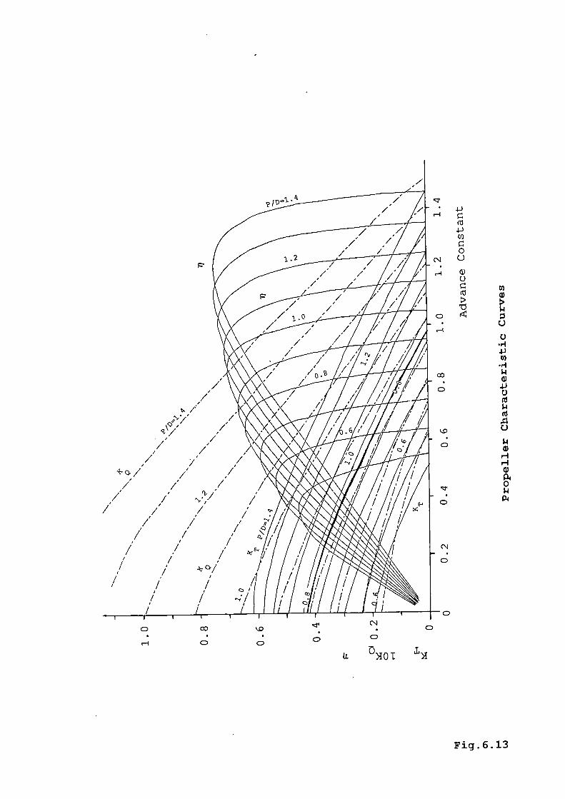
('j4JCl)
0U
0a)
0
C)-ri
Cl)
-ri
ci)
-IiC)
(1
.C.)
Iici)HHci)p40Ii
cD
0
CD
CD
CD
CDr-1 0 CD
LI- 1)1
Fig. 6.13
of pitch to diameter values ranging from about P/D=0.5
to P/D=1.5. Separate s'ets of curves are generated for
different DAR's (Developed Area Ratios).
The DAR effectively gives the ratio of blade area to
the circumscribed circle or disc, so that if the
developed area (sum of the area of each blade) is Fa and
the circumscribed area is F, the DAR will be:
F= (D]2
DAR = Fa/F
For the Arun lifeboat, the diameter of each propeller
is 0.826m and developed area is 0.375m 2 , therefore:
F = 0.8262/ 4 = O.536m2
F = O.375m2a
DAR = 0.375 / 0.536 = 0.70
For the purposes of the simulation, the thrust
coefficient curve will be approximated by a cubic
polynomial in the advance constant J knowing the actual
propeller pitch to diameter ratio and DAR for the Arun.
204
P/D = 0.772 / 0.826 = 0.935
DAR = 0.70
Therefore, KT will be expressed as:
KT = 0.154 J - 0.361 - 0.222 J + 0.430
The Propeller Vector
The propeller thrust will almost entirely be directed
along the fore-aft line, thus the surge equation will
equal the propeller thrust with an additional
coefficient. Thus:
24x = Cpropeller PU pn D KT
where: CPU is the thrust reduction coefficient.
The only sway that can be generated from the propeller
is if there is some sort of flow anomaly or a secondary
effect if the propeller causes any yaw. Heave is also
assumed zero, though there is likely to be a small
component associated with pitch. There will be no roll
moment produced by the propeller.
205
As the propeller revolutions • increase so, for small
boats, will the bow rise. The boat will attain a
constant angle of pitch, balanced by the pitch restoring
moment. The pitch moment will be expressed as:
M =propeller CQ pn2D5KT
where: CpQ is a pitch propeller coefficient.
With single screw arrangements, the rotation of the
propeller will actually generate a slight yawing motion.
If left unchecked therefore, the boat would follow a
large arced trajectory. This phenomenon is well-known in
naval architecture and twin propeller arrangements are
set counter rotating in order to nullify this effect. In
large ship models the propeller yaw is usually assumed
zero and since the Arun lifeboat, used in the model
validation, has a twin arrangement this assumption will
be followed here.
The propeller vector, P, will therefore be:
206
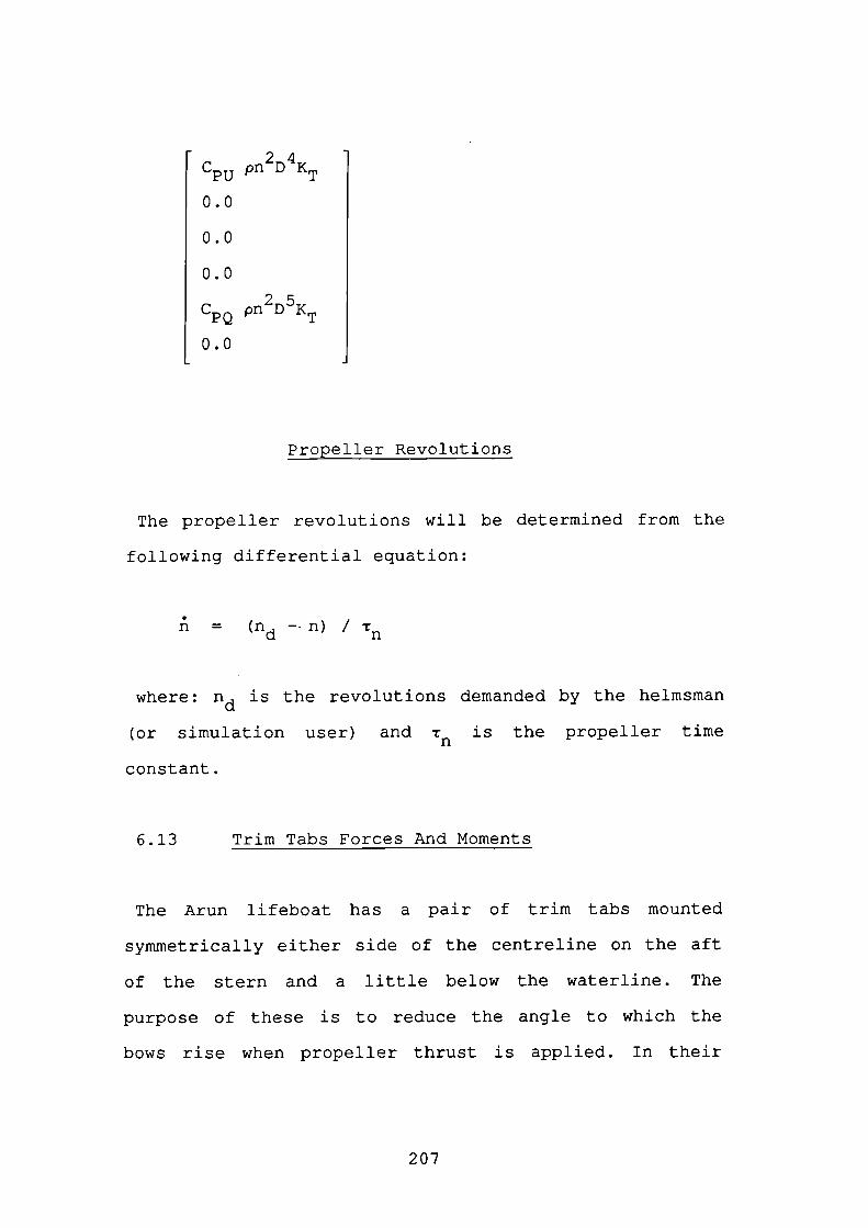
CPU pn2D4KT
0.0
0.0
0.0
CpQ pn2D5KT
0.0
Propeller Revolutions
The propeller revolutions will be determined from the
following differential equation:
I = Itn
where: d is the revolutions demanded by the helmsman
(or simulation user) and is the propeller time
constant.
6.13 Trim Tabs Forces And Moments
The Arun lifeboat has a pair of trim tabs mounted
symmetrically either side of the centreline on the aft
of the stern and a little below the waterline. The
purpose of these is to reduce the angle to which the
bows rise when propeller thrust is applied. In their
207
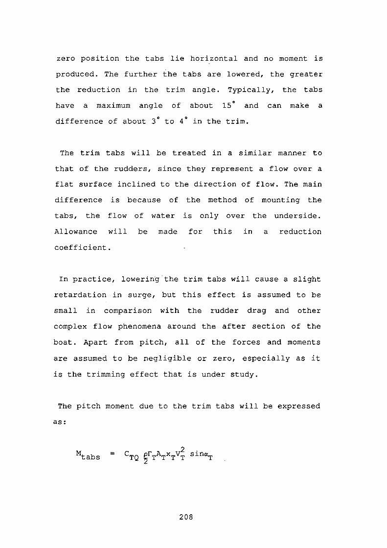
zero position the tabs lie horizontal and no moment is
produced. The further the tabs are lowered, the greater
the reduction in the trim angle. Typically, the tabs
have a maximum angle of about l5 and can make a
difference of about 3° to 4° in the trim.
The trim tabs will be treated in a similar manner to
that of the rudders, since they represent a flow over a
flat surface inclined to the direction of flow. The main
difference is because of the method of mounting the
tabs, the flow of water is only over the underside.
Allowance will be made for this in a reduction
coefficient.
In practice, lowering the trim tabs will cause a slight
retardation in surge, but this effect is assumed to be
small in comparison with the rudder drag and other
complex flow phenomena around the after section of the
boat. Apart from pitch, all of the forces and moments
are assumed to be negligible or zero, especially as it
is the trimming effect that is under study.
The pitch moment due to the trim tabs will be expressed
as:
Mt b = CTQ Pr'TATXTVT sinaT
208
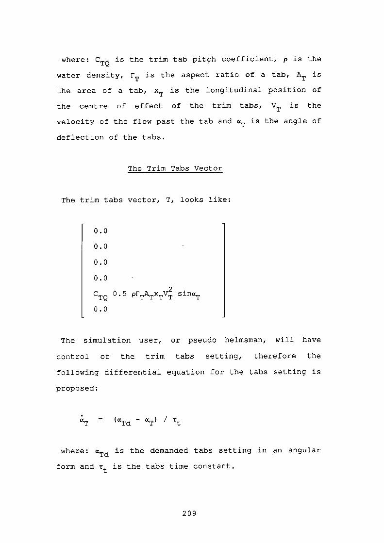
where: CTQ is the trim tab pitch coefficient, p is the
water density, FT is the aspect ratio of a tab, AT is
the area of a tab, XT is the longitudinal position of
the centre of effect of the trim tabs, VT is the
velocity of the flow past the tab and T is the angle of
deflection of the tabs.
The Trim Tabs Vector
The trim tabs vector, T, looks like:
0.0
0.0
0.0
0.0
2.CTQ 0.5 pFTATxTVT slncT
0.0
The simulation user, or pseudo helmsman, will have
control of the trim tabs setting, therefore the
following differential equation for the tabs setting is
proposed:
= TdaT)
where: is the demanded tabs setting in an angular
form and is the tabs time constant.
209
6.14 The Wind Forces And Moments
While there are fluid flow computer simulators,
accurate theoretical prediction of the wind flow around
a boat is still not feasible. To include such fluid flow
programs within the overall boat model would dwarf the
boat manoeuvring mathematics and impose unacceptable
time demands on the simulation interval. It is therefore
necessary to rely upon experimental tests carried out in
wind tunnels and pre-simulation analysis of the wind
effect on the boat. Clearly the surface area of the boat
above the waterline exposed to the wind will be the
prime factor influencing windage. This will depend upon
the amount and distribution of the superstructure and
the relative wind angle.
Such data is usually expressed in terms of
dimensionless coefficients plotted as a function of the
relative wind angle. Aage, 1971 (Ref.1), provides
typical data for three cargo ships in different
conditions, a tanker, a passenger liner, a ferry and a
trawler. The wind forces and moments will be expressed
thus:
210
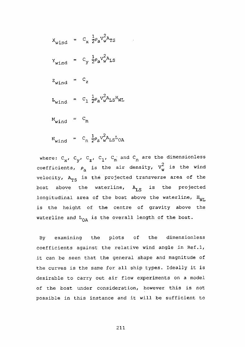
Xwjfld = Cx
wind = Cy
z = Cwind Z
Cl aT>Ls1IWLL. =wind
M. = Cwind In
N. = C 1p V2A T.wind n 2 a w LSOA
where: C, C, C, C 1 , C and C are the dimensionless
coefficients, a is the air density, is the wind
velocity, ATS is the projected transverse area of the
boat above the waterline, ALS is the projected
longitudinal area of the boat above the waterline, HWL
is the height of the centre of gravity above the
waterline and LOA is the overall length of the boat.
By examining the plots of the dimensionless
coefficients against the relative wind angle in Ref.1,
it can be seen that the general shape and magnitude of
the curves is the same for all ship types. Ideally it is
desirable to carry out air flow experiments on a model
of the boat under consideration, however this is not
possible in this instance and it will be sufficient to
211
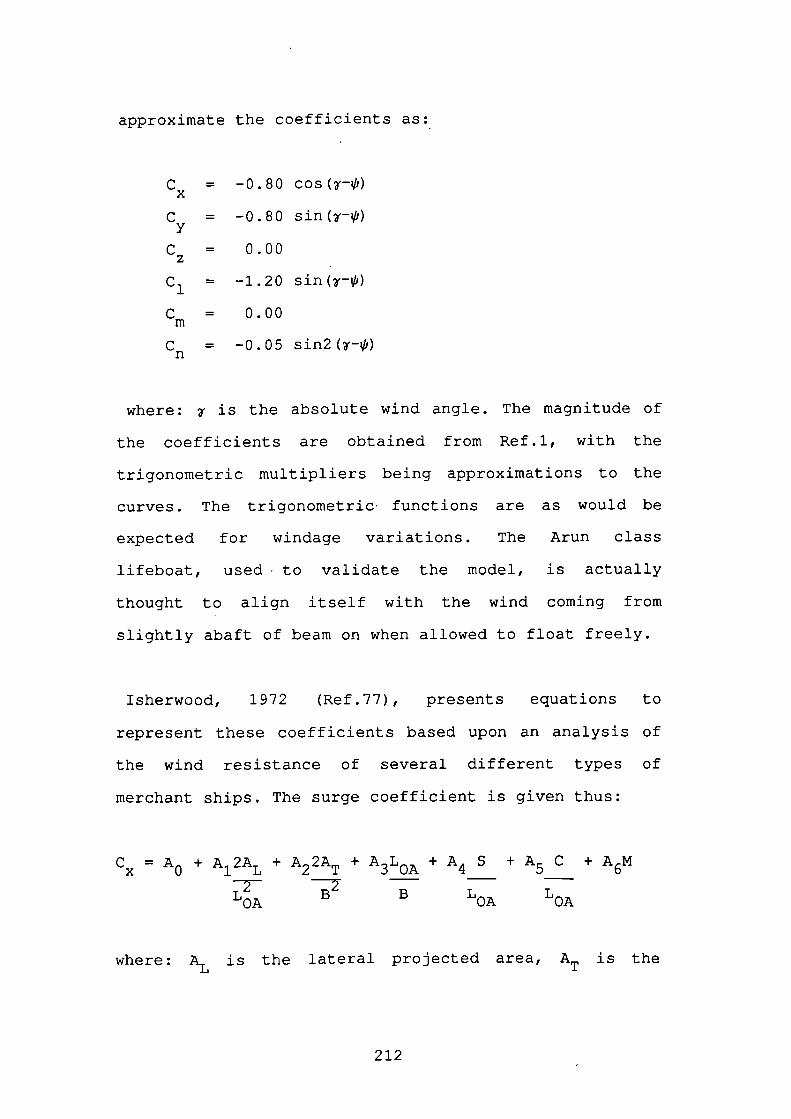
approximate the coefficients as:
C = -0.80 cos('-')
C = -0.80 sin('-i)
C = 0.00z
C 1 = -1.20 sin('-'t')
C = 0.00m
Cn = -0.05 sin2(r-,)
where: is the absolute wind angle. The magnitude of
the coefficients are obtained from Ref.1, with the
trigonometric multipliers being approximations to the
curves. The trigonometric functions are as would be
expected for windage variations. The Arun class
lifeboat, used to validate the model, is actually
thought to align itself with the wind coming from
slightly abaft of beam on when allowed to float freely.
Isherwood, 1972 (Ref.77), presents equations to
represent these coefficients based upon an analysis of
the wind resistance of several different types of
merchant ships. The surge coefficient is given thus:
C = A + A 2A + A2 2AT + A3LQA + A4 S + A5 C + A6Mx 0 1 L
LOA
where: AL is the lateral projected area, AT is the
212
transverse projected area, B is the breadth of the ship,
LOA is the length overall, C is the distance from the
bow of the centroid of the lateral projected area, M is
the number of distinct groups of masts or kingposts seen
in the lateral projection and S is the length of
perimeter of lateral projection of model excluding
waterline and slender bodies such as masts and
ventilators. A0 to A6 are coefficients which are
tabulated at 100 intervals of the relative wind angle,
and will form look-up tables for simulation purposes.
Similar expressions exist for the sway and yaw
coefficients.
The level of complexity introduced by Isherwood is not
deemed pertinent to this analysis of small boats and the
equations giving an approximate continuous function will
be used.
A point of note is that the angle of steady heel caused
by a steady wind can be found by superimposing the wind
heeling moment on the curve for the statical stability.
The intersection of these curves will determine the
angle of steady heel (Fig.6.14).
213
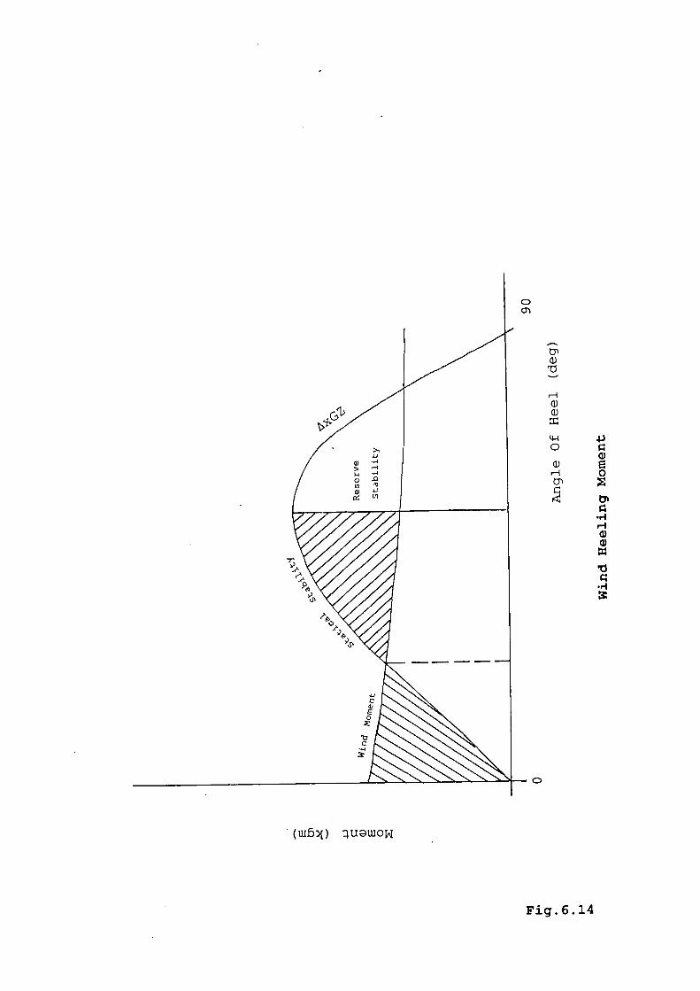
(uthj) uowo
Fig. 6.14
ci)
Hci)ci)
4io
a,0) EH 0
•rlI-Ia,
•r4
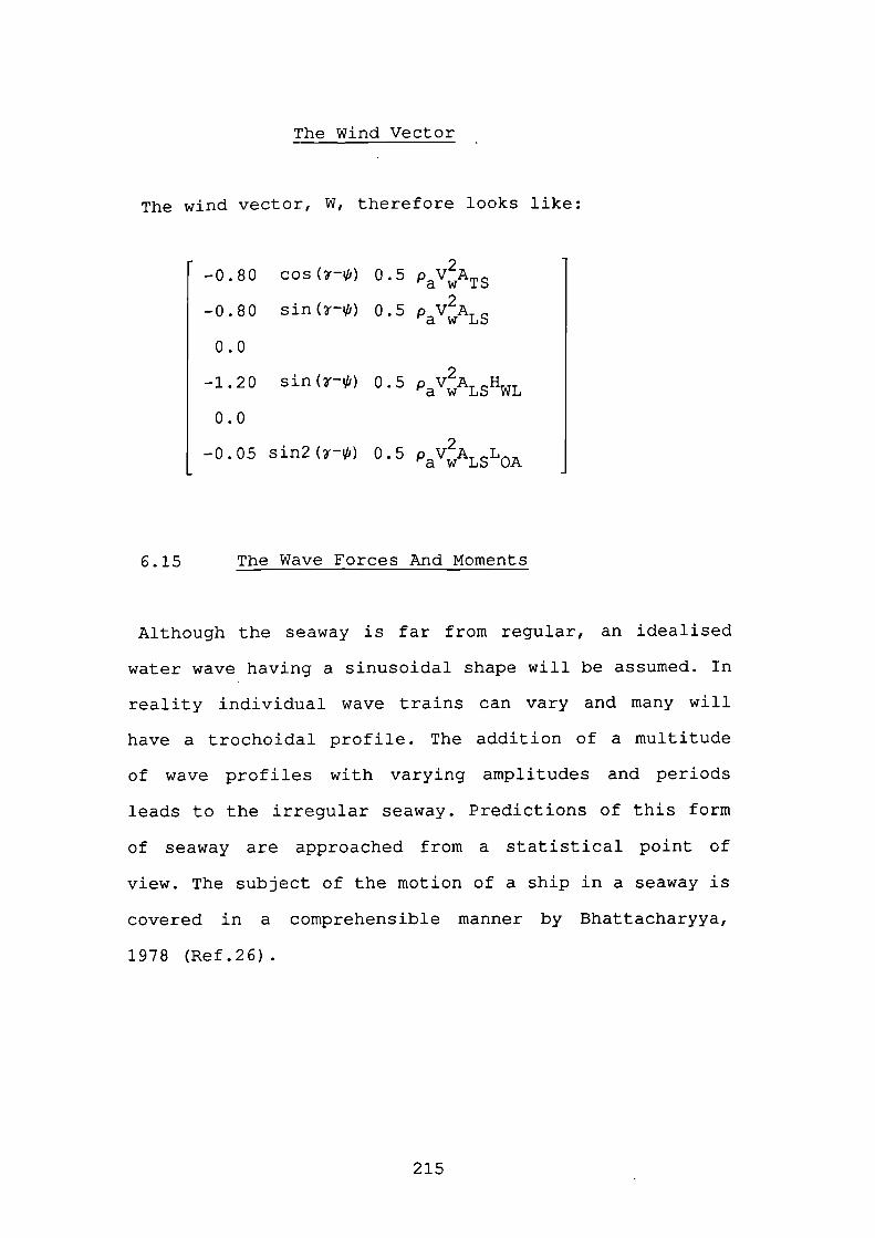
The Wind Vector
The wind vector, W, therefore looks like:
-0.80 cos(-i) 0.5
-0.80 sin(i) 0.5 a11LS
0.0
2-1.20 sin('-ç&) 0.5 PawALSHWL
0.0
-0.05 sin2('-&) 0.5 PaVIALSLOA
6.15 The Wave Forces And Moments
Although the seaway is far from regular, an idealised
water wave having a sinusoidal shape will be assumed. In
reality individual wave trains can vary and many will
have a trochoidal profile. The addition of a multitude
of wave profiles with varying amplitudes and periods
leads to the irregular seaway. Predictions of this form
of seaway are approached from a statistical point of
view. The subject of the motion of a ship in a seaway is
covered in a comprehensible manner by Bhattacharyya,
1978 (Ref.26)
215
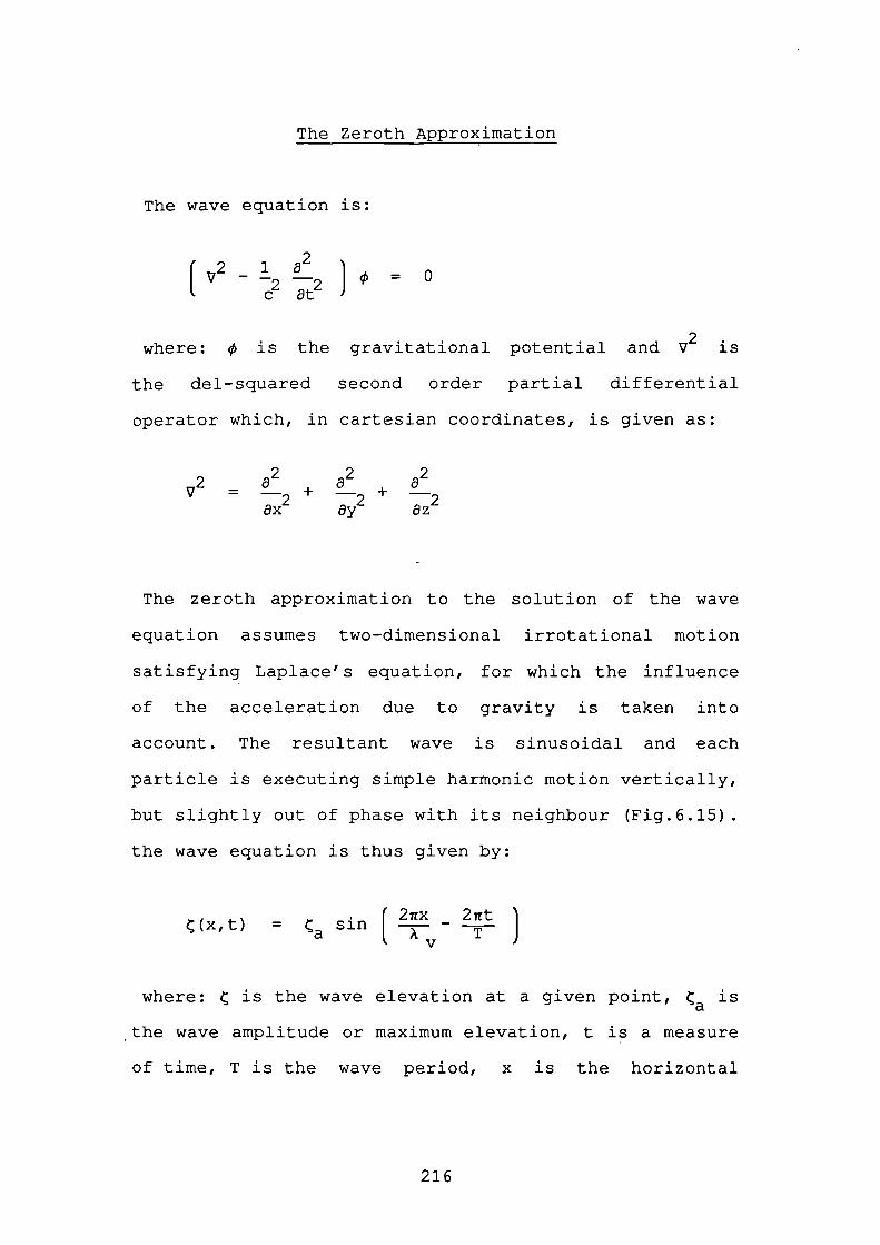
The Zeroth Approximation
The wave equation is:
[v2 _ 2 2 J= 0
2.where: is the gravitational potential and V is
the del-squared second order partial differential
operator which, in cartesian coordinates, is given as:
722 2
= 2 + 2 +
The zeroth approximation to the solution of the wave
equation assumes two-dimensional irrotational motion
satisfying Laplace's equation, for which the influence
of the acceleration due to gravity is taken into
account. The resultant wave is sinusoidal and each
particle is executing simple harmonic motion vertically,
but slightly out of phase with its neighbour (Fig.6.15).
the wave equation is thus given by:
2irx - 2irt(x,t) = a sin T J
where: ? is the wave elevation at a given point, a
the wave amplitude or maximum elevation, t is a measure
of time, T is the wave period, x is the horizontal
216
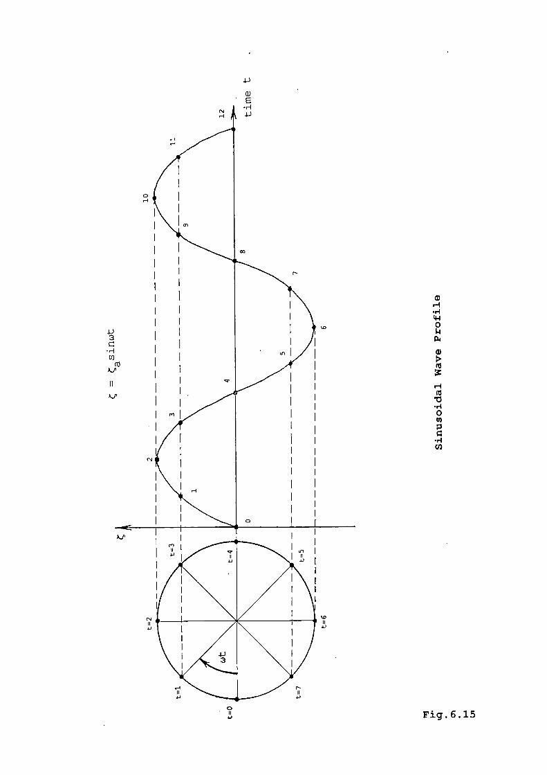
-p
3
-H
C/)
a,
H•rI'4-1
0
a,
H('I
0U)
.rl
Cl)
Fig. 6.15
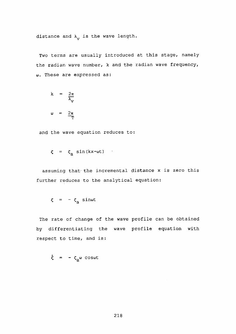
distance and is the wave length.
Two terms are usually introduced at this stage, namely
the radian wave number, k and the radian wave frequency,
w. These are expressed as:
k = 2irAv
= 2itT
and the wave equation reduces to:
=a sin (kx-t) -
assuming that- the incremental distance x is zero this
further reduces to the analytical equation:
= - a sinwt
The rate of change of the wave profile can be obtained
by differentiating the wave profile equation with
respect to time, and is:
= -wcoswta
218
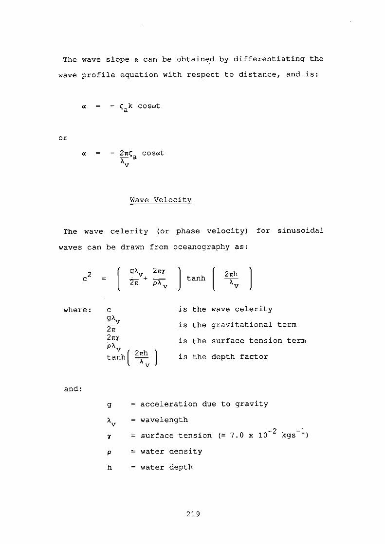
The wave slope can be obtained by differentiating the
wave profile equation with respect to distance, and is:
= - ( k coswta
or
= - ia coswtAV
Wave Velocity
The wave celerity (or phase velocity) for sinusoidal
waves can be drawn from oceanography as:
2 1 gA 2ir'
c = [ _+-) tanh I A ]
where: cgA
2 irs'
pA v 27thtanh
is the wave celerity
is the gravitational term
is the surface tension term
is the depth factor
and:
g = acceleration due to gravity
A = wavelengthv
= surface tension ( 7.0 x io2 kgs)
p = water density
h = water depth
219
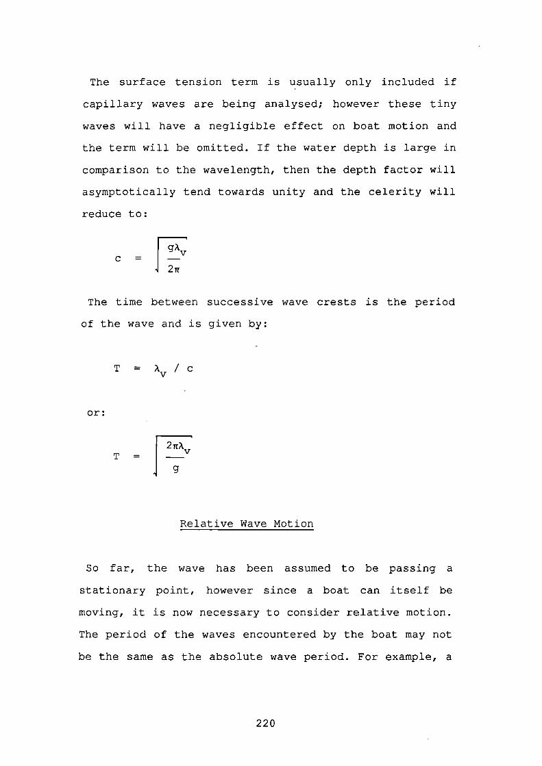
The surface tension term is usually only included if
capillary waves are being analysed; however these tiny
waves will have a negligible effect on boat motion and
the term will be omitted. If the water depth is large in
comparison to the wavelength, then the depth factor will
asymptotically tend towards unity and the celerity will
reduce to:
gA\;c = -
2ir
The time between successive wave crests is the period
of the wave and is given by:
T = A /cV
or:
2 irA
T =
g
Relative Wave Motion
So far, the wave has been assumed to be passing a
stationary point, however since a boat can itself be
moving, it is now necessary to consider relative motion.
The period of the waves encountered by the boat may not
be the same as the absolute wave period. For example, a
220
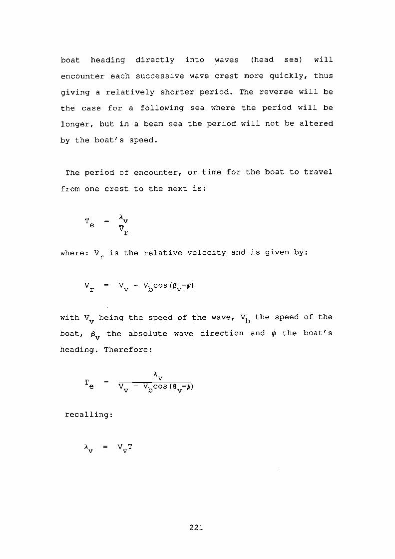
boat heading directly into waves (head sea) will
encounter each successive wave crest more quickly, thus
giving a relatively shorter period. The reverse will be
the case for a following sea where the period will be
longer, but in a beam sea the period will not be altered
by the boat's speed.
The period of encounter, or time for the boat to travel
from one crest to the next is:
AT = ve
r
where: Vr is the relative -velocity and is given by:
V = V Vbcos(P)r v
with V being the speed of the wave, Vb the speed of the
boat, the absolute wave direction and i the boat's
heading. Therefore:
AV
T = - vbcosv
recalling:
A = VTV V
221
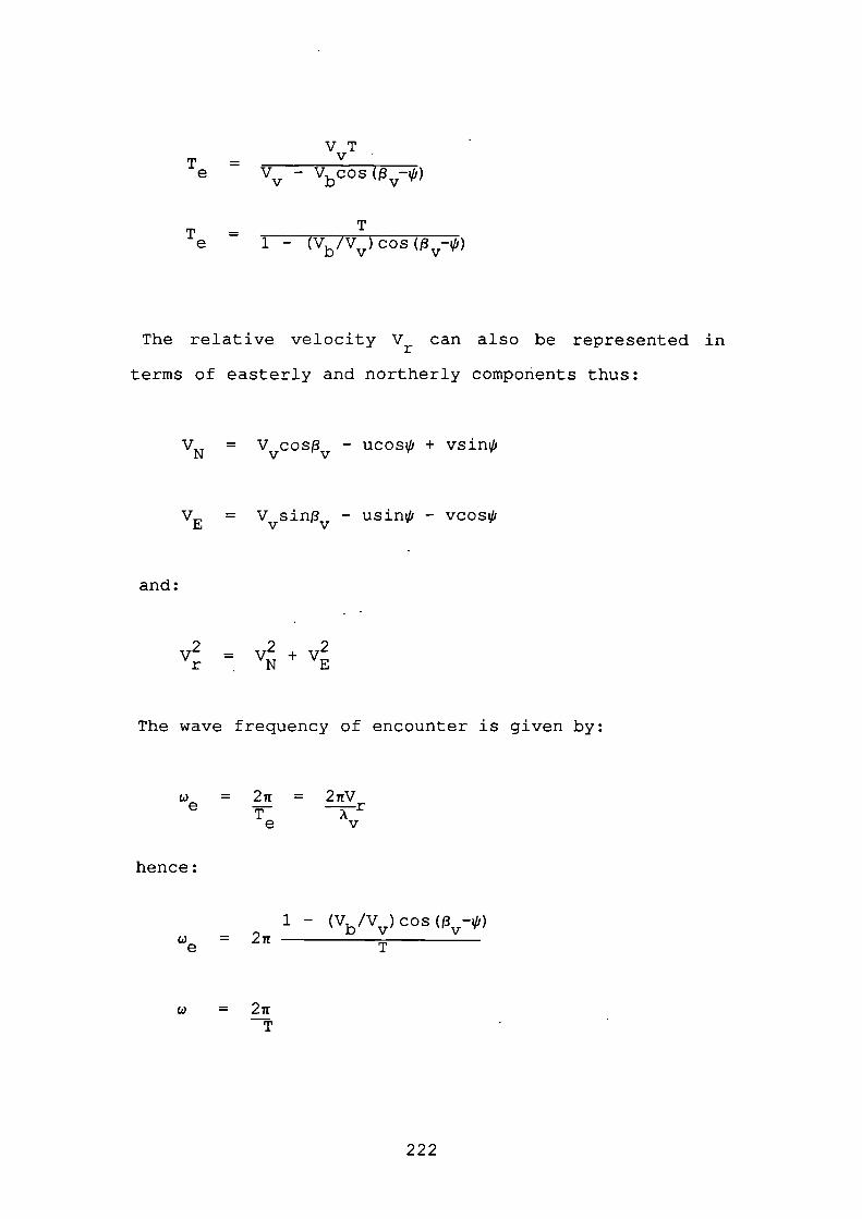
VTVT = ________e V - VbCOS (-ui)V
TT = __________e 1 - ( 1/b /V )cos( -cl')V V
The relative velocity Vr can also be represented in
terms of easterly and northerly components thus:
V = V cosf3 - ucosçli + vSifliN v V
V = V sin(3 - usini - vcosçliE v v
and:
= V2 + V2r N E
The wave frequency of encounter is given by:
w = = 2irVe-T Ae v
hence:
1 - (Vb/V )cos(13 -1')w = 2ir v ve T
w = 2irT
222
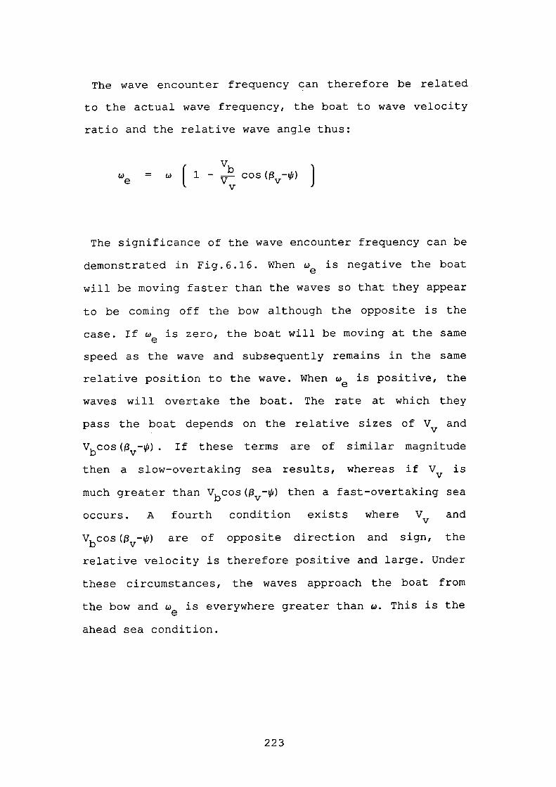
The wave encounter frequency can therefore be related
to the actual wave frequency, the boat to wave velocity
ratio and the relative wave angle thus:
V= w ( 1 - cos
)
The significance of the wave encounter frequency can be
demonstrated in Fig.6.16. When we is negative the boat
will be moving faster than the waves so that they appear
to be coming of f the bow although the opposite is the
case. If We is zero, the boat will be moving at the same
speed as the wave and subsequently remains in the same
relative position to the wave. When We is positive, the
waves will overtake the boat. The rate at which they
pass the boat depends on the relative sizes of Vv and
VbCos v . If these terms are of similar magnitude
then a slow-overtaking sea results, whereas if Vv is
much greater than Vbcos(v) then a fast-overtaking sea
occurs. A fourth condition exists where V and
Vbcos(V) are of opposite direction and sign, the
relative velocity is therefore positive and large. Under
these circumstances, the waves approach the boat from
the bow and We is everywhere greater than w. This is the
ahead sea condition.
223
t=1
-S.
\
Relative Position Unchangedt=o
\
\,f
Slow Overtaking Sea
t=o
t=1
//
ci ci:>
/
t=o
Ahead Sea
t=1
H Following Sea
to Fast Overtaking Sea
t=1
\\\
Different Relative Wave Motions
Fig.6.16
The encountered wave slope will therefore become:
= akeC0et
Wave Energy
A wave system possesses both kinetic and potential
energy due to the periodic motion. The kinetic energy is
due to the orbital motion of the wave particles, and the
potential energy is due to the elevation of the water
surface.
For a sinusoidal wave the potential energy per unit
wave surface area is:
1 2E = -P(
Likewise the kinetic energy per unit wave surface area
will also be:
1 2EK =
The total energy per unit wave surface area for a
sinusoidal wave will be:
1 2E = E + EK =
225
Motion Of A Boat In Waves
The exciting or disturbing forces and moments generated
by a passing wave are basically due to the additional
buoyancy created by the wave along the boat. It is
fairly easy to visualise the heaving, pitching and
rolling motions resulting from waves, and equations will
be developed to model these primary effects. However,
the wave does not necessarily directly generate yaw, but
when the boat encounters waves form oblique angles, that
is on the bow or quarter rather than ahead, abeam or
astern, broaching and other yaw "slipping" motions can
occur. This can be explained by referring to the gravity
vector, where the yaw term is expressed as:
(xgW_xbB)cosesin + (ygW_ygB)sine
which indicates that if the boat rolls and pitches,
including any subsequent movement of the centre of
buoyancy, the boat will yaw as a result. As an example,
if a wave approaches the boat on the starboard bow, then
the boat's bows will rise (positive 0), the boat will
roll to port (negative ), the centre of gravity will
remain unchanged and the centre of buoyancy will move
out to port and aft which all adds up to a yaw to port
which appears as if the boat "falls" off of the wave.
226
Similar reasoning is assumed to apply to the other
non-oscillatory motions of surge and sway. The wave
vector will therefore have no components in surge, sway
and yaw, but will rely on the secondary effects from the
gravity vector.
The heave wave disturbing force is obtained by
integrating the additional buoyancy due to the wave
longitudinally along the waterplane area of the boat.
This can be represented as:
z = -cwave VW
but, for a wave with the profile of:
C = C sinwet
gives:
z = -c a siflWtwave vW
where: C is a dimensionless wave coefficient and
is the waterplane area.
The beam to draft ratio and length to draft ratio can
affect the roll and pitch motions in waves respectively
(Fig.6.17). Whilst all boats will have a considerably
227
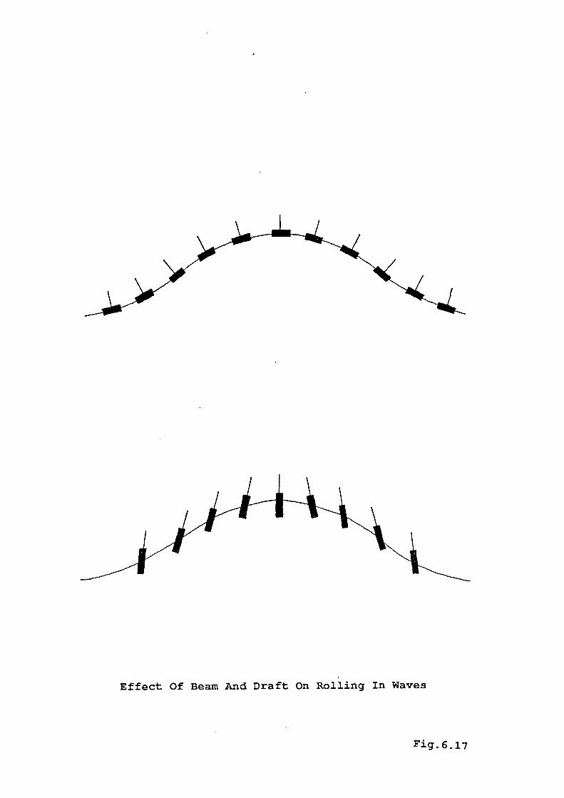
Effect Of Beam And Draft On Rolling In Waves
Fig.617
greater length than draft, it is assumed that most small
boats will also be beamy with respect to their draft.
The roll and pitch moments will be proportional to the
wave slope and can be represented as:
L = C sin(13-i) pgAB k cosw tae ewave
N = _CVQ cos(13-l) pgAL 2k sinw tBP ae ewave
where: and CVQ are dimensionless wave coefficients,
B is the boat's breadth and LBP is the boat's length
between perpendiculars.
Some large ship models incorporate wave drifting
forces, Hirano, Takashina, Takaishi & Saruta, 1980
(Ref.67). The large ship problem is different from the
small boat one, due principally to effects of scale. The
wavelength to ship length ratio will typically be less
than unity for large ships so that several wave crests
may occur along its length. Whereas small boats tend to
sit within a single wave and the wavelength to boat
length ratio will be greater than unity.
Disturbances of pitch and heave will be far smaller for
large vessels due to the fact that the effect of a wave
crest towards the bow of the ship can be opposed by the
229
effect from a second wave crest near the stern. The
typical equations used in ship models for the horizontal
wave drifting forces are written:
X = X'wave wave
Y =wave wave
1 22N = N'wave wave
where the non-dimensionalised wave drifting
coefficients X' , Y' and N' are considered to bewave wave wave
functions of wave length, wave encounter angle, ship
speed and wave encounter frequency. Theoretical
determination ofthese coefficients still leaves much to
be desired and emphasis is placed upon experimental
data.
From graphs provided in Ref.67 it seems that, for large
ships, once the wavelength becomes greater than the ship
length, the wave drifting coefficients tail off toward
zero. This indicates that as wavelength increases, the
wave tends to appear to the ship like a flat surface.
The coefficients seem to peak at a wavelength to ship
length ratio Xv/LBP=O•4• While no data is given for
ratios less than 0.3, it would seem that as the number
of wave crests occurring along the ship length
230
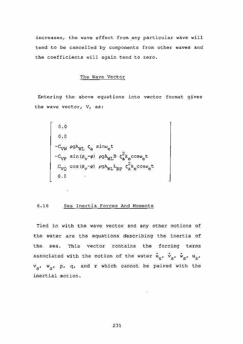
increases, the wave effect from any particular wave will
tend to be cancelled by components from other waves and
the coefficients will again tend to zero.
The Wave Vector
Entering the above equations into vector format gives
the wave vector, V1 as:
0.0
0.0
-C a 5±)et
sin pgB cosw tae e
CVQ cos pgAL3 keCO5wet
0.0
6.16 Sea Inertia Forces And Moments
Tied in with the wave vector and any other motions of
the water are the equations describing the inertia of
the sea. This vector contains the forcing terms
associated with the motion of the water ' '' ' U5,
v5 , w3 , p, q, and r which cannot be paired with the
inertial motion.
231
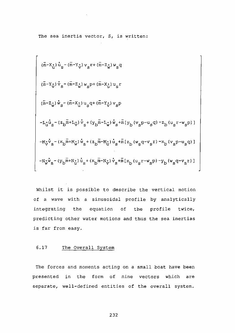
The sea inertia vector, S, is written:
(m-X) u- (rn-Y) v 5 r+ (rn-Z) w5q
(rn-Y • )v -(rn-Z)w p+(rn-X • )u rV S w S U S
(rn-Z) i- (rn-Xe) u5q+ (rn-Y) v5p
_LuS_(zbm+L.)vV S
-N .y -(x rn+M . )w +(z rn-M • )u +rn[z (w q_v5r)-x(v5p_u5q)]vs b w s b u s b s
-N • w -(y rn+N . )u +(x rn-N . ) i T +rn[x (u r-w p)-y(w5q_v5r)]ws b u s b v s b s s
Whilst it is possible to describe the vertical motion
of a wave with a sinusoidal profile by analytically
integrating the equation of the profile twice,
predicting other water motions and thus the sea inertias
is far from easy.
6.17 The Overall System
The forces and moments acting on a small boat have been
presented in the form of nine vectors which are
separate, well-defined entities of the overall system.
232
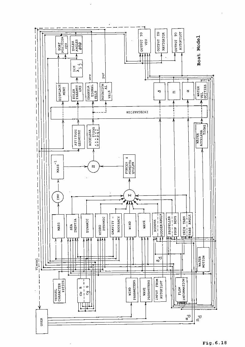
Fig. 6.18
Should any particular aspect , of the model require
alteration or upgrading to suit a new application, it
will be possible to replace any individual module
without affecting the remainder. Other effects, for
example the tunnel or axial thrusters on a tug or the
sail on a yacht, not so far included can quite easily be
tagged on as additional modules once the equations have
been formulated.
The forces and moments generated by each module are
summed, using vector addition, to obtain the total
effect in six degrees-of-freedom. The inverted mass
matrix is then multiplied by this vector sum of the
forces to produce the six accelerations along and about
the boat coordinate axes (Fig.6.18). Integration of the
six accelerations yields the six velocities and, if
required, the integration of the three translational
velocities yields the boat's change of position. The
angular rotations can be determined from Euler
parameters which are obtained from the angular
velocities (see earlier chapter for development on
quaternions)
6.18 The Method Of Inteqration
The differential equations produced have been purposely
arranged in terms of the highest state derivatives,
234
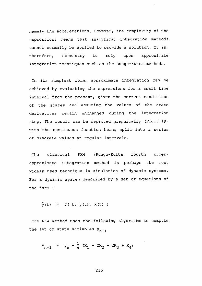
namely the accelerations. However, the complexity of the
expressions means that analytical integration methods
cannot normally be applied to provide a solution. It is,
therefore, necessary to rely upon approximate
integration techniques such as the Runge-Kutta methods.
In its simplest form, approximate integration can be
achieved by evaluating the expressions for a small time
interval from the present, given the current conditions
of the states and assuming the values of the state
derivatives remain unchanged during the integration
step. The result can be depicted graphically (Fig.6.19)
with the continuous function being split into a series
of discrete values at regular intervals.
The classical RK4 (Runge-Kutta fourth order)
approximate integration method is perhaps the most
widely used technique in simulation of dynamic systems.
For a dynamic system described by a set of equations of
the form
(t) = f( t, y(t), x(t)
The RK4 method uses the following algorithm to compute
the set of state variables
yy +,rn+l (K1 + 2K2 + 2K3 + K)
235
h1 time
h2=h1/2
h2time
Integration Step SizeFig.6.19
where:
K1 = h f( t, y, X(tn)
1<2 = h f( t + -h, y + K 1 , x(t + -h)
K3 = h f( t + -h, y + -K2 , x(t + h)
1<4 = h f( t + h, y + K3 , x(t + h)n n
with h being the time interval.
K1 is essentially the known slope of the function at
time n. Projecting this slope K 1 half way across the
sample interval and re-computing the new slope at that
point produces K2 . The slope 1<2 is brought back to the
point at time n and then projected half way across again
giving K3 . The slope K 4 is then determined at the point
where 1<3 is projected right the way across the sample
interval to time n+1. The weighted average of these four
slopes is combined to give the new value at time n+1
(Fig.6.20)
A useful variation to the classic RK4 method provides
intermediate output by computing four slopes as before,
but at intervals of h/4. This algorithm can be
237
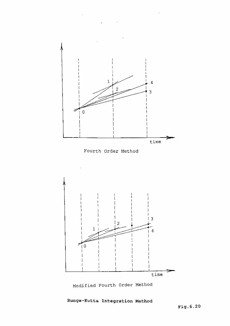
4
3
I II I I
I I I
I I I
time
Fourth Order Method
time
Modified Fourth Order Method
Runge-Kutta Integration MethodFig.6.2O
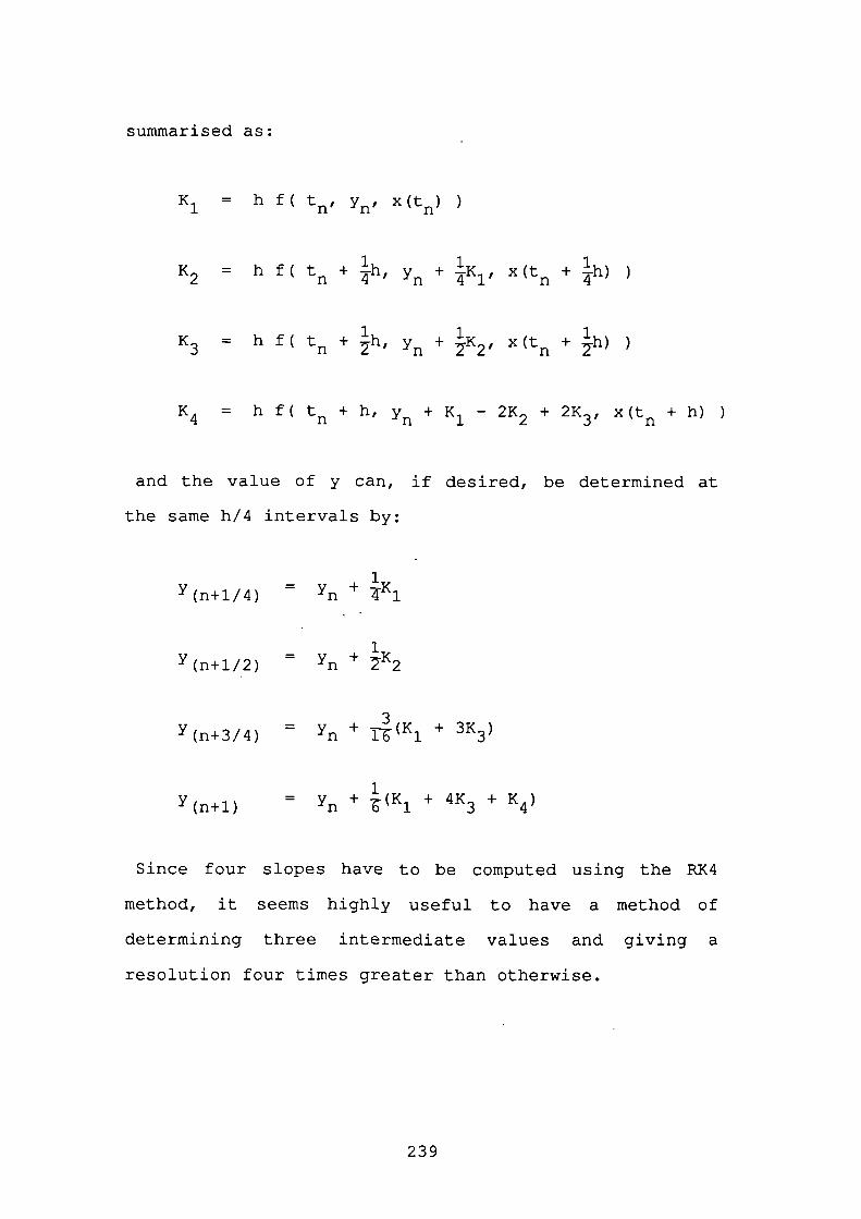
summarised as:
K1 = h f( t, y, x(t1)
K = h f( t + h, y + -K 1 , x(t + i-h)2 n 4
K3 = h f( t + y + -K2 , x(t + -h)n
K4 = h f( t + h, y + K 1 - 2K2 + 2K3 , x(t + h)
and the value of y can, if desired, be determined at
the same h/4 intervals by:
'(n+1/4)
' (n+1/2)
Y(+3/4)
(n+1)
1= y +
1= y +
= y + 1--(K 1 + 3K3)n
= y + -(K1 + 4K3 + K4)
Since four slopes have to be computed using the RK4
method, it seems highly useful to have a method of
determining three intermediate values and giving a
resolution four times greater than otherwise.
239
The RK4 methods of integration were used with ACSL
(Advanced Continuous Simulation Language) as a tool
during the development of the model. However, the
overhead of the additional computations makes these
methods redundant in the real-time simulation.
The small boat simulation will be required to run at
either real time or fairly close to real time. It is
also desirable for the sample interval to be quite
short, in the order of 5Oms to lOOms, since the Cetrek
autopilot requires heading and rudder information at
about this rate. It was therefore decided to initially
use the most simplistic pf integration methods and
effectively multiply the derivative by the sample
interval, and use the result to update the state
variable for the next time interval.
By using a sufficiently small sample interval, the
function can be assumed monotonic between successive
steps. Theoretically, as the interval is reduced, the
estimate of the integral becomes progressively better,
and for an infinitely small step any error tends towards
zero. Therefore, if the chosen interval proves
inadequate, it can be reduced to improve the simulation.
Limitations exist in numerical integration,
particularly when implemented on digital computers. The
240
main source of error is from "rounding-off", a computer
can only work to a finite number of significant figures.
Consequently there will inevitably be a round-off error
at each iteration of the computation. There is a danger
of a greater cumulative error being generated when more
steps are taken. Clearly a balance between poor
approximations and the number of integration steps is
required. Taken to the extreme, any cumulative error
will suggest that if a model is run for long enough the
errors will reach a stage where the simulation becomes
invalid!
Two other sources of error in all approximate
integration methods are "formula error" and "inherited
error". Formula error results from the approximation
that the slope of the function remains constant which
can lead to an incorrect estimate of the new value.
There will, of course, be an exact answer for the state
trajectory guaranteed by the mean value theorem if there
are suitable conditions of continuity and
differentiability, however, finding it is another
matter! Inherited error recognises that the starting
point from which the projection of the state is to take
place will, unless it is the initial condition, be an
estimate from the previous iteration.
241
These three types of errors can work to accumulate
errors, but in most instances they will balance out over
a number of integration steps. The answer for
establishing the correct integration interval would seem
to depend on the application, but the step size does not
want to be so large that errors are capable of getting
out of hand, or too small where the changes in the
states are only of the order of the rounding-off errors.
The method of approximate numerical integration to
choose will undoubtedly depend upon the application, but
more sophisticated routines will demand much greater
computing power than simpler ones. However, the sampling
interval can often be increased when using higher order
techniques, since these methods often compute
intermediate slopes as part of the overall integration
step.
242

CHAPTER 7
PARANETER DETERMINATION AND MEASURENT
243
7.01 Model Verification And Validation
Initial verification of the model was achieved by
taking each module in isolation and supplying it with
inputs which have a known result. Checks on fundamental
principles, such as a starboard rudder angle generating
a starboard turn, and other intuitively obvious concepts
were performed, the exact magnitude of the forces and
moments not yet being required.
Combining the modules, simple manoeuvres were
reproduced and the correct performance verified. For
example, a straight ahead run with rudder amidships
without disturbing effects for waves or wind should
continue in a straight line (assuming the real boat is
course stable). Steady state turning simulations
were used to exercise additional areas of the model.
Once the verification procedure had been satisfied, it
became necessary to validate the model against the
performance of a real boat. This entailed two separate
parts, first obtaining measurements of manoeuvres
carried out during boat trials and secondly establishing
the values of the various coefficients used in the model
for the boat under consideration.
244
7.02 Boat Trials
A series of trials were performed on board a RNLI 52ft
Arun class lifeboat (see plates 1 to 4) in the spring of
1989. On the whole the weather and sea conditions were
relatively mild and calm, a far cry from what this type
of boat can be expected to endure!
An Amstrad (IBM compatible) Personal Computer equipped
with a PC-30 Analogue Multifunction Board was used as a
data-logging device (see plates 5 and 6). The PC-30
board has a maximum of 16 channels which can be used to
monitor as many instruments. An interface box, designed
by Mr J.Reynolds of Bournemouth Polytechnic and built by
the author, provided potential division instruments with
voltage and then buffered the resulting measurement
through an anti-aliasing arrangement. Where necessary,
voltage scaling was performed to optimise the voltage
range of the PC-30 board.
The various instruments to be recorded were, therefore,
connected to the computer via the interface box. Power
for the instruments was drawn from the boat's DC supply
and regulated within the interface box. Useful technical
information on the interface box and the PC-30
multifunction board can be found in an appendix at the
end of this thesis.
245
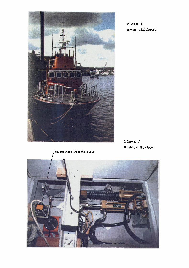
Plate 1
Arun Lifeboat
Measurement Potentiometer
Plate 2
Rudder System
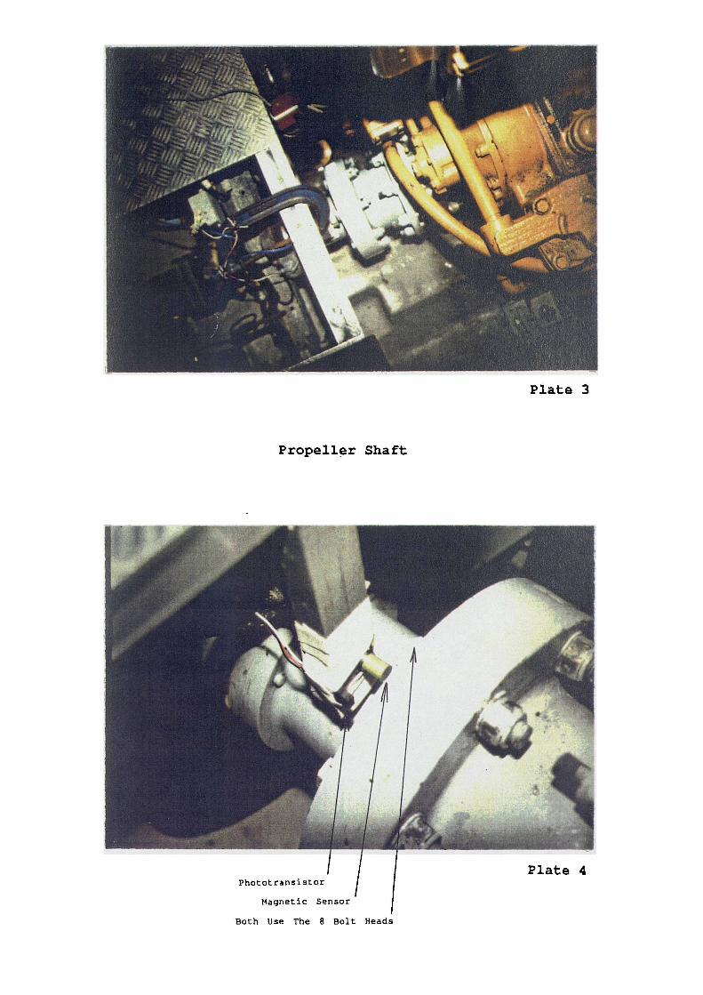
Plate 3
Propeller Shaft
Phototransistor
Magnetic Sensor
Both Use The 8 Bolt Heads
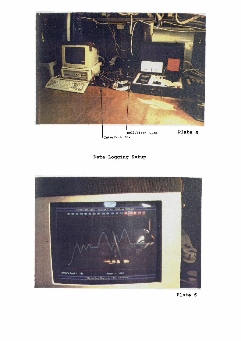
Data-Logging Setup
Plate 6
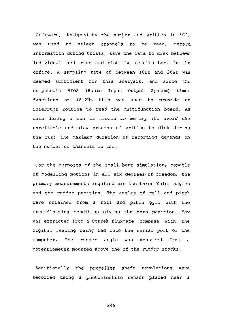
Software, designed by the author and written in 'C',
was used to select channels to be read, record
information during trials, save the data to disk between
individual test runs and plot the results back in the
office. A sampling rate of between 10Hz and 20Hz was
deemed sufficient for this analysis, and since the
computer's BIOS (Basic Input Output System) timer
functions at 18.2Hz this was used to provide an
interrupt routine to read the multifunction board. As
data during a run is stored in memory (to avoid the
unreliable and slow process of writing to disk during
the run) the maximum duration of recording depends on
the number of channels in use.
For the purposes of the small boat simulation, capable
of modelling motions in all six degrees-of-freedom, the
primary measurements required are the three Euler angles
and the rudder position. The angles of roll and pitch
were obtained from a roll and pitch gyro with the
free-floating condition giving the zero position. Yaw
was extracted from a Cetrek fluxgate compass with the
digital reading being fed into the serial port of the
computer. The rudder angle was measured from a
potentiometer mounted above one of the rudder stocks.
Additionally the propeller shaft revolutions were
recorded using a photoelectric sensor placed near a
249
propeller coupling which had eight equally spaced bolts.
Reflective strips were attached to the bolt heads and
the pulses generated from the sensor were fed into a
counter. The propeller shaft revolutions can vary
between about 300rpm and 1100rpm, therefore by
determining the number of revolutions from the number of
counts per second means that the arrangement of eight
pulses per revolution gives a resolution of 7.5rpm.
Clearly the resolution can be increased by taking the
count over a longer time interval, but this will be
limited by how often the rpm is to be updated and how
rapidly it is changing. The count is read in on the
digital port of the multifux)ction board at the same rate
as the other measurements, and can be processed at a
later stage. -
Provision was made to record propeller torque, but due
to flooding in the bilges the instrument was not mounted
during the trials. Similarly, a load cell was to have
been used to determine the force on the rudders, but it
proved difficult to actually incorporate it within the
rudder system.
Heave accelerations were recorded using an
accelerometer, but these measurements consistently
registered less than ±lg since the sea surface was a low
amplitude swell. The only onboard measurement of the
250
horizontal translational velocity was from a navigator
system, however, since it determined velocity from the
differentiation of the change of distance with respect
to time, it could only provide an indication of the
steady state velocity after holding a particular course
and speed for at least 2 or 3 minutes.
As well as the five principal measurements of roll,
pitch, yaw, rudder and propeller revolutions, the
regulated voltage level was monitored and found to
remain very stable whilst recording.
Briefly, the designation of the channels is as follows:
Channels 0 to 10 inclusive: had three pin DIN
connectors, allowing voltage to be supplied to, and
measured from, a number of potential division devices,
such as accelerometers, rudder reference, roll and pitch
gyro, et cetera (not all these channels ended up being
used).
Channel 11: had a three pin DIN connector and a voltage
amplifier. This was dedicated to the rudder load cell.
Channels 12 and 13: had BNC connectors and were
dedicated to the propeller torque meters, which have
their own power supply.
251
Channel 14: had a unique connector which allowed the
analogue course error (±400) signal to be recorded from
the Cetrek fluxgate compass.
Channel 15: recorded the regulated voltage directly
from within the interface box.
Channel 16: (in reality, the digital port on the PC-30
board) was used for the propeller revolutions counter.
Channel 17: (in reality, the computer's serial
communications port and nothing to do with the PC-30
board) was used to read the lObit heading from the
Cetrek compass (lObits gives a resolution of about 0)
The plots of several different manoeuvres performed at
various rudder angles and approach speeds are presented
in an appendix towards the end of the thesis. Most are
plotted over a common time base to ease comparison.
7.03 Parameter Estimation
It is a fairly straight forward matter to determine the
principal dimensions of a boat, since this information
is readily available for all craft. It is standard to
quote figures for the length between perpendiculars,
252
length overall, moulded breadth or beam and moulded
draft. Other quantities such as the projected transverse
and longitudinal areas above the waterline and the
projected areas below the waterline can be estimated
from the general arrangement or lines plans for the
boat. Rudder span and area, plus propeller pitch and
diameter and other such dimensions can also be
ascertained from draughtsman's drawings.
The hydrostatic curves (see section on trie
gravity-buoyancy vector), drawn for most boats, provide
the static values for displacement and the positions of
the centres of buoyancy and floatation as a function of
the draft. The static underwater volume can be obtained
from displacement in a given density of seawater. A
combination of the static conditions and the lines plans
allows estimates for the dynamic values of the
underwater volume.
The rudder acts like a hydrofoil and, therefore, can be
related to aerodynamic theory. The rudder normal force
equation contains an aspect ratio term which has been
based on Japanese research. Since the general shape of
the rudder is not dissimilar to those of large ships, it
is assumed that the theory is valid for all sizes of
rudder. The rudder normal force was subsequently found
to be of the correct order for this analysis. The rudder
253
coefficients were slightly altered once comparisons of
actual and simulated steady state rates of turn for a
range of rudder angles were made.
The propeller vector relies on propeller thrust which
can be deduced from propeller characteristic curves
given the advance constant. The surge propeller
coefficient was determined by balancing the forces
producing a steady state forward speed attained at set
propeller revolutions. The pitch propeller coefficient
basically came down to a balance between the pitch
restoring moment and the moment applied by the
propeller. As propeller revolutions increase, so the
bows rise; at constant propeller revolutions, the
resulting angle depends on the restoring moment. The
actual measurements had to be with trim tabs horizontal
since these effects are modelled in the trim tabs
vector.
The trim tabs coefficients were determined by observing
the changes in trim or pitch as the trim tabs are
lowered. Measurements of pitch were taken in the trim
tabs up and down positions at the same forward speeds.
The centre of gravity is assumed fixed, though in
practice this can move if weights are added or removed
from the boat or as fuel is used. Although the equations
254
allow for differences in the buoyancy and weight, these
are assumed to remain about the same for the majority of
the time.
The GZ curve gives the horizontal separation of the
centre of buoyancy from the centre of gravity. This
helps to indicate the motion of the centre of buoyancy
at varying angles of heel. In the absence of a method of
accurately determining the true centre of buoyancy at
any angle of pitch and roll, two elliptical equations
will be generated to approximate its locus. For the Arun
lifeboat the GZ curve is always positive; that is there
is always a righting moment, and the locus of the centre
of buoyancy is more likely to be closer to a cardioid
than an ellipsoid. However, from the point of view of
testing the autopilot, it is sufficient to cater for
angles less than 40°. Measurements of the amplitude and
duration of roll motions when rudder is initially
applied allow the approximations made above to be
matched with the real situation.
Large ship modellers usually approximate the GZ curve
with a fifth order polynomial and determine the roll
righting moment based on the GZ, whereas the
gravity-buoyancy vector is capable of accurately
reproducing the restoring forces and moments for all six
degrees-of-freedom if the location of the centre of
255
buoyancy is known.
The various coefficients that make up the Mass,
Dynamics and Hydrodynamic vectors are perhaps the most
difficult to assign values to without the use of complex
computational programs. Virtually the only method is to
simplify the equations and isolate individual terms.
The moments of inertia about the three axes can be
determined from the boat's radius of gyration. This is
usually obtained by swinging the boat when it is
suspended from a pivot point. Empirical formulae give
close approximations to the moments of inertia given the
mass and length of the boat. The products of inertia,
those appearing in the off-diagonal positions in the
inertia tensor, will be small and are initially assumed
negligible. However, 'xy often plays a significant role
and has a non-zero value.
The added mass coefficients are extremely difficult to
determine precisely without the aid of complex
computational programs. As Lamb indicates, they are
determined by the form and position of the surface
relative to the coordinate system. Theoretical
expressions involve double integrals of the velocity
potential with respect to the entire surface. However,
since the boat exhibits symmetry about the XZ-plane, a
256
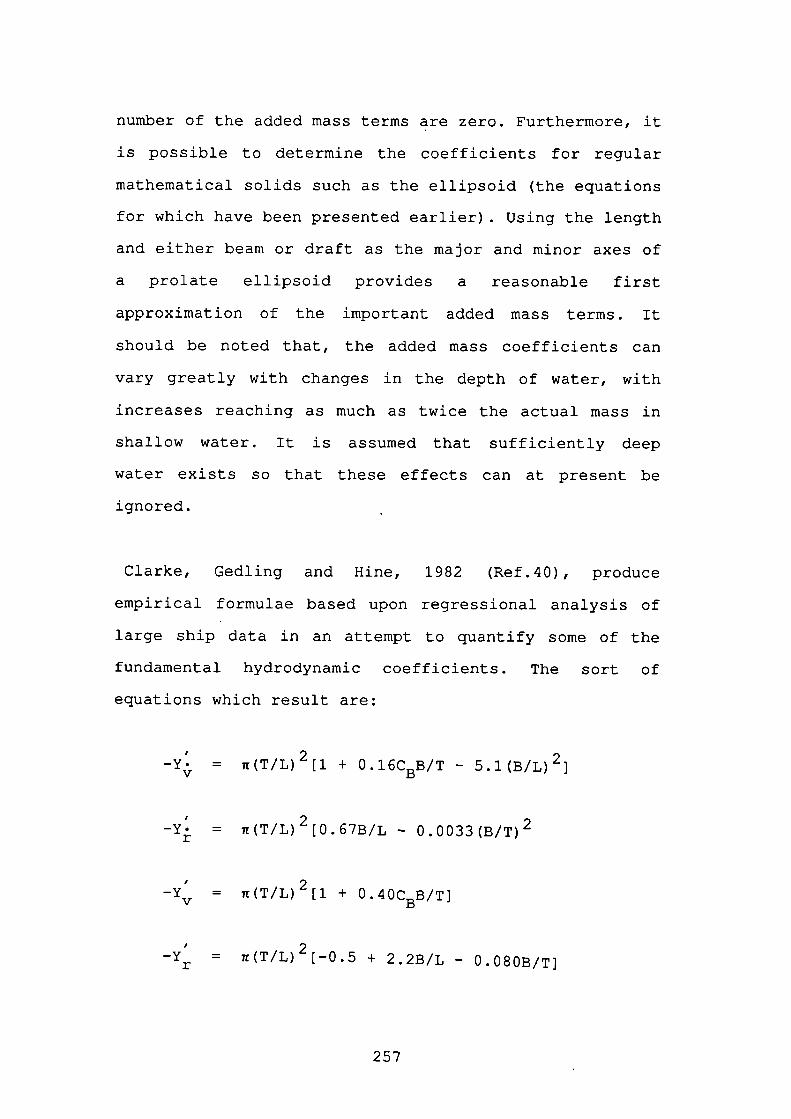
number of the added mass terms are zero. Furthermore, it
is possible to determine the coefficients for regular
mathematical solids such as the ellipsoid (the equations
for which have been presented earlier). Using the length
and either beam or draft as the major and minor axes of
a prolate ellipsoid provides a reasonable first
approximation of the important added mass terms. It
should be noted that, the added mass coefficients can
vary greatly with changes in the depth of water, with
increases reaching as much as twice the actual mass in
shallow water. It is assumed that sufficiently deep
water exists so that these effects can at present be
ignored.
Clarke, Gedling and Hine, 1982 (Ref.40), produce
empirical formulae based upon regressional analysis of
large ship data in an attempt to quantify some of the
fundamental hydrodynamic coefficients. The sort of
equations which result are:
-Y = it(T/L)2[1 + O.16CBB/T - 5.1(B/L)2]
-Y • = (T/L)2[O.67B/L - O.0033(B/T)2
-YT = ir(T/L)2[1 + O.4OCBB/TJ
I
-y = 71(T/L) 2 [-O.5 + 2.2B/L - O .O803/T]r
257
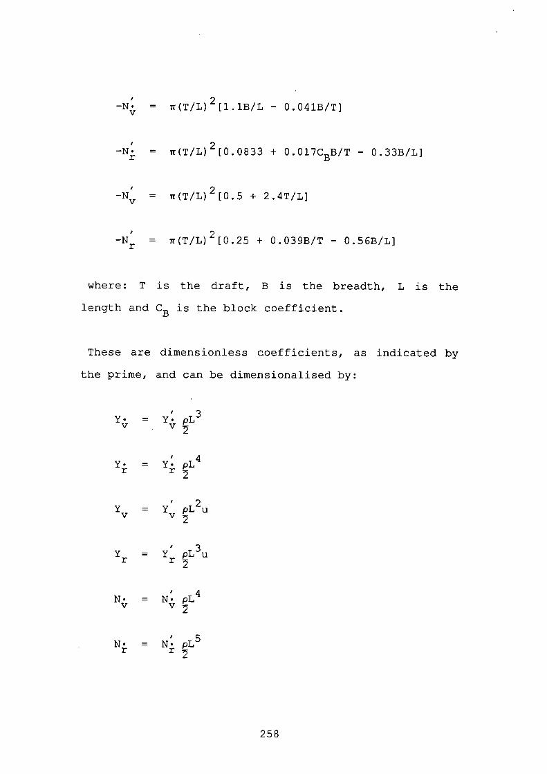
-N . = it(T/L) 2 [1.1B/L - 0.0418/TI
-N = ir(T/L)2[O.0833 + O.O17C8B/T - O.33B/L]
-N = ir(T/L) 2 [0.5 + 2.4T/L]
-N = ir(T/L) 2 [0.25 + O.039B/T - 0.568/LI
where: T is the draft, B is the breadth, L is the
length and C3 is the block coefficient.
These are dimensionless coefficients, as indicated by
the prime, and can be dimensionalised by:
Y . = Y . pL3V V2
=pL
=pL2u
= Y , pL3u
N . = N . pL4V V
Nj = N pL5
258
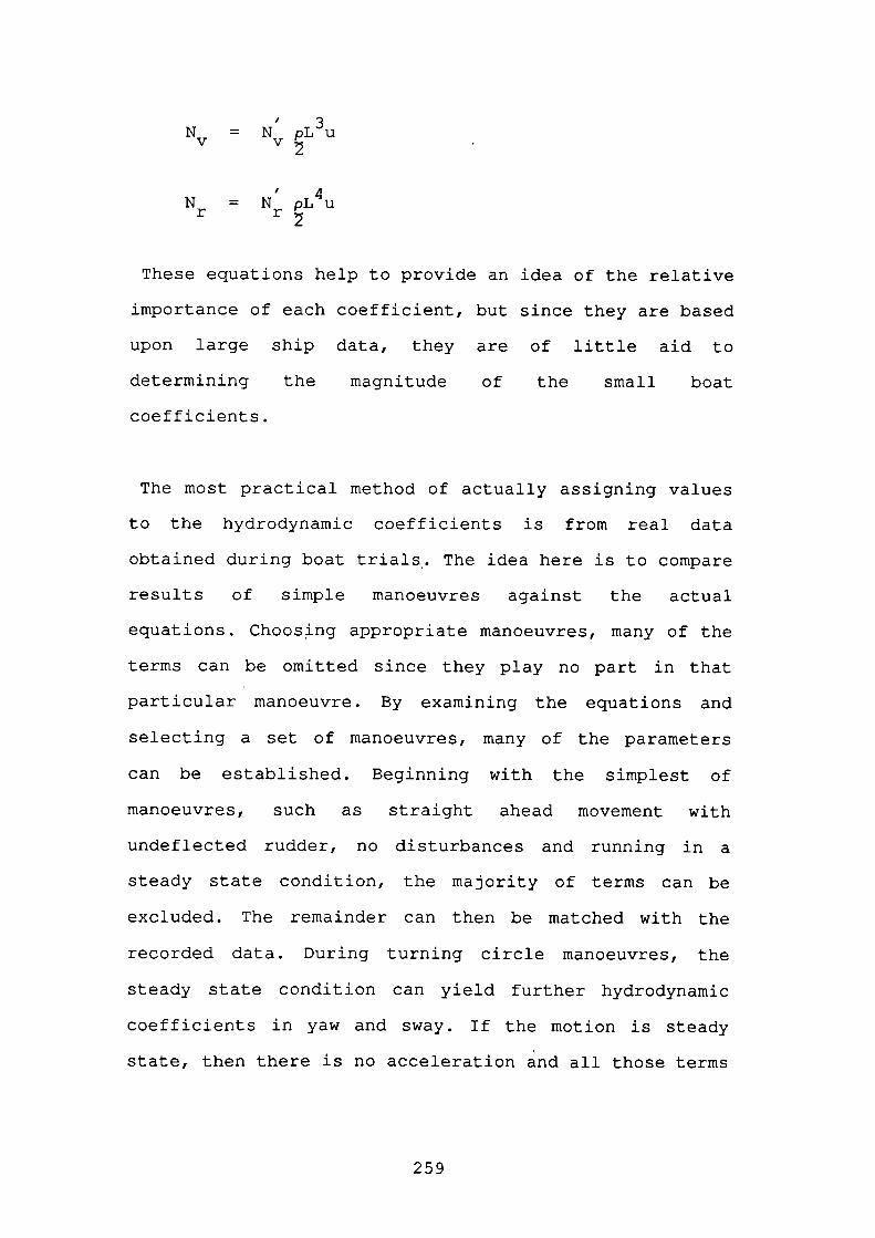
N = N pL3u
Nr = N pL4u
These equations help to provide an idea of the relative
importance of each coefficient, but since they are based
upon large ship data, they are of little aid to
determining the magnitude of the small boat
coefficients.
The most practical method of actually assigning values
to the hydrodynamic coefficients is from real data
obtained during boat trials. The idea here is to compare
results of simple manoeuvres against the actual
equations. Choosing appropriate manoeuvres, many of the
terms can be omitted since they play no part in that
particular manoeuvre. By examining the equations and
selecting a set of manoeuvres, many of the parameters
can be established. Beginning with the simplest of
manoeuvres, such as straight ahead movement with
undeflected rudder, no disturbances and running in a
steady state condition, the majority of terms can be
excluded. The remainder can then be matched with the
recorded data. During turning circle manoeuvres, the
steady state condition can yield further hydrodynamic
coefficients in yaw and sway. If the motion is steady
state, then there is no acceleration and all those terms
259
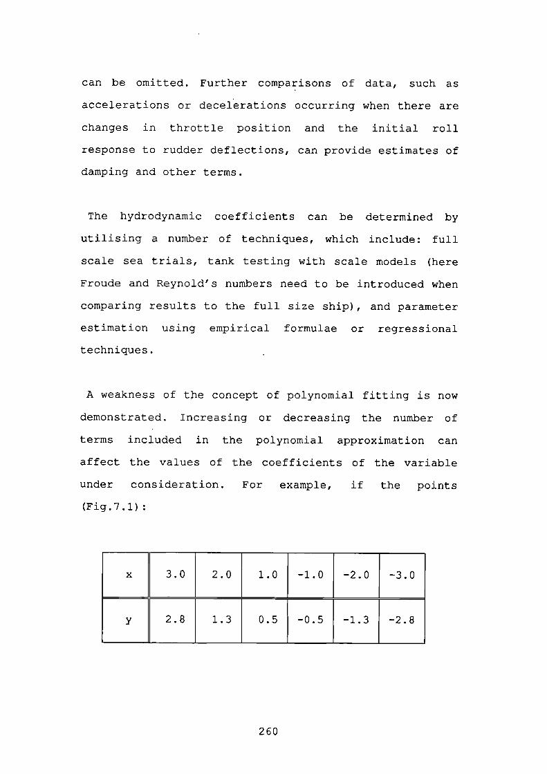
can be omitted. Further comparisons of data, such as
accelerations or decelerations occurring when there are
changes in throttle position and the initial roll
response to rudder deflections, can provide estimates of
damping and other terms.
The hydrodynamic coefficients can be determined by
utilising a number of techniques, which include: full
scale sea trials, tank testing with scale models (here
Froude and Reynold's numbers need to be introduced when
comparing results to the full size ship), and parameter
estimation using empirical formulae or regressional
techniques.
A weakness of the concept of polynomial fitting is now
demonstrated. Increasing or decreasing the number of
terms included in the polynomial approximation can
affect the values of the coefficients of the variable
under consideration. For example, if the points
(Fig.7.l)
x 3.0 2.0 1.0 -1.0 -2.0 -3.0
y 2.8 1.3 0.5 -0.5 -1.3 -2.8
260
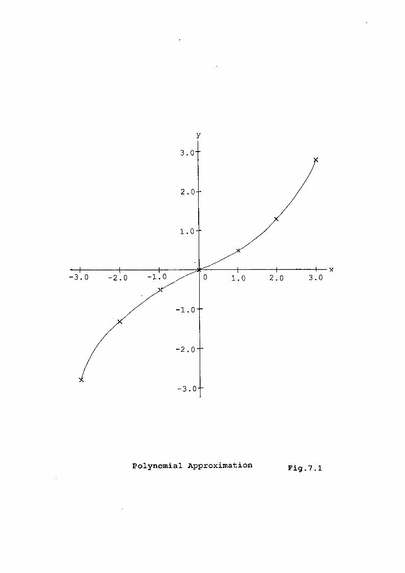
Polynomial Approximation Fig.7.1
are approximated by a cubic, the equation would look
like:
y = 0.44583 x + 0.05417 x3
whereas if the quintic term is included the equation
becomes:
y = 0.45333 x + 0.04583 x 3 + 0.00083 x5
The values of the coefficients change according to the
number of terms used in the approximation. Note also
that neither approximation gives the correct slope of
the curve at the origin, 0.5 being the true value.
This also applies to models based upon a Taylor series
expansion where the coefficients are subsequently
obtained from regressional analysis of full scale sea
trials data. If more or fewer terms are included in the
expansion then the value of all of the coefficients will
have to change in order for the same result to be
achieved. Polynomial fitting and regressional analysis
can therefore produce models which fit the data
extremely well for the manoeuvres considered, but the
values of the coefficients can be meaningless and not
actually the correct ones.
262
So far the technique of parameter estimation has
assumed that the boat is floating in an ideal fluid and
that there are no external disturbances of wind or
waves. This analysis has developed mathematical
equations which can be used to exert external forcing
functions on the boat. This is extremely important as
regards the autopilot control, since without these
disturbing influences the autopilot would always
maintain a precise heading.
The wind coefficients that determine the magnitude of
the wind effect are based on work by Aage, since there
was no real data available for the Arun lifeboat. The
shape of the curves of the dimensionless wind
coefficient against relative wind angle are very similar
for the nine ships presented by Aage. These curves can
be approximated by trigonometric functions of the
relative wind angle and agree with intuitive logic. For
example, the maximum yaw moment is likely to be produced
at a relative wind angle equal to the inter-cardinal
points, that is on the starboard and port bow and
quarter. The values of the maximum dimensionless wind
coefficients are used to scale these trigonometric
functions. The dimensionless coefficients can be related
to an individual boat by appropriate cross-sectional
area or the projected area that the wind can act upon.
The projected cross-sectional areas, both longitudinal
263
and transverse, can be ascertained from lines plans.
Allowances will have to be made to the equations for
uneven distribution of superstructure.
The wave vector presents a sinusoidal forcing function
which again has coefficients which determine the
magnitude of this disturbance. The boat trials were
carried out in slight seas, but no wave data was
available to assess the perturbations in the recorded
boat runs. By observing the deviations from a mean value
during steady state sections of the recorded data, and
by noting the sea conditions on the days of the trials,
gestimates were made for the wave coefficients. The
model was used to perform simulation runs in order to
ensure that the values chosen were reasonable.
The main purpose of the thesis is to assess the
performance of small boat autopilots whilst exercising
the mathematical model. Accurate prediction of an Arun
lifeboat is, therefore, not desperately required. It is
sufficient to have a model which behaves in a similar
manner to a 52feet long semi-displacement vessel. So
long as the disturbance forces and moments are not
unrealistic of the actual situation, simulations can be
performed without cause for concern. Once the parameter
estimation stage was complete, the Kempf manoeuvres were
used as the acid test of the model's ability to simulate
264
small boat behaviour.
7.04 Tank Testing Techniques
To obtain more accurate values for the hydrodynamic
coefficients, and therefore get the model closer to the
real world situation, the modeller can make use of other
techniques like tank testing.
As discussed in the previous sub-section, the
hydrodynamic coefficients depend upon the geometry of
the boat; however no adequate theory or calculation
procedure exists to accurately determine these values.
Model tests of a special nature are often undertaken in
order to obtain the hydrodynamic coefficients of a
particular vessel shape. Even this method of parameter
determination is limited to those coefficients which can
be isolated for analysis.
The simplest test is for the Y and N derivatives.v v
These are obtained by towing a model vessel, at the
"proper't speed given by the Froude number, at various
angles of attack to the path of the model (Fig.7.2). A
dynamometer is used to record the Y (sway) force and N
(yaw) moment experienced by the model. The slope at the
origin of a graph of Y or N versus sway velocity v gives
the numerical values of Y or Nv v
265
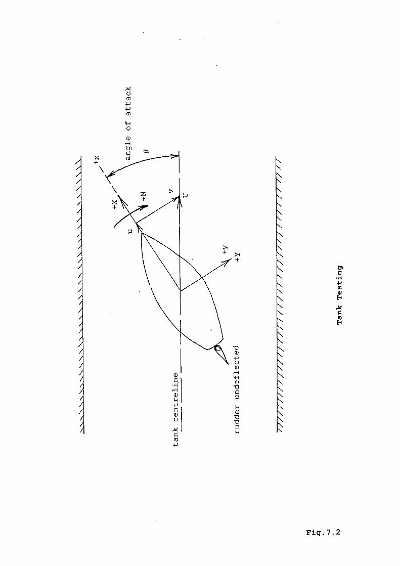
0
4J4i
0
a)
+
\
+
'cia)4)0a)H
ci)'ci
ci)'ci'ci
•r4
F-i
Ha)
4J
0
c14J
Fig.7 .2
The test for 'Lr and Nr involves towing the model at a
constant forward speed whilst imposing various values of
angular velocity r on the model. A "rotating arm"
apparatus is used to impose the angular velocity on the
model by rotating it in a circle at the end of the arm
(Fig.7.3) . The model is towed with a forward velocity u
(Froude number u0 (gL) '2 ), tangential to the circular
path, for various radii R. The only way of varying the
angular velocity r for a fixed forward velocity u 0 is to
alter the radius, since r =u0 /R. A dynamometer is used to
record the Y force and N moment during each test and the
slope at the origin of the graph of Y or N versus r will
fix the numerical values of Y or Nr r
In order to avoid the expense of an additional tank
facility such as the rotating arm apparatus, a device
known as the planar motion mechanism was devised for use
in a long narrow tank. This allows and Nr as well as
other derivatives to be determined.
The mechanism consists of two transverse oscillators,
one positioned at the bow and the other at the stern of
the model. These are set oscillating whilst the model is
towed down the tank. The two oscillators are given the
same amplitude a0 and frequency w of oscillation, but
the phase of the oscillators can be adjusted.
Dynamometers at the bow and stern measure the
267
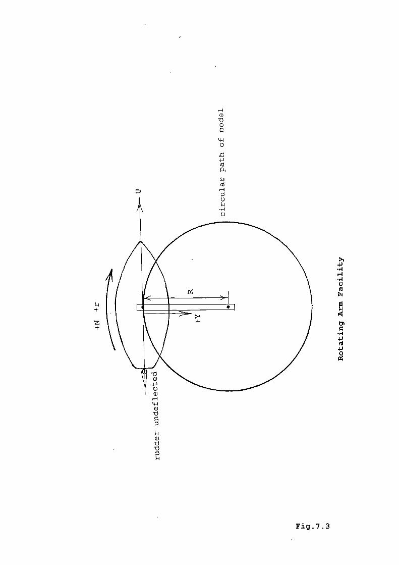
+
z+
>1.$)•r4
r-I
0
-Ii
0
Ha)
0
4-i0
H
H4-ia)
a)
'ci
Fig.7 .3
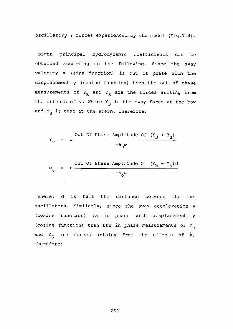
oscillatory Y forces experienced by the model (Fig.7.4)
Eight principal hydrodynamic coefficients can be
obtained according to the following. Since the sway
velocity v (sine function) is out of phase with the
displacement y (cosine function) then the out of phase
measurements of B and are the forces arising from
the effects of v. Where is the sway force at the bow
and is that at the stern. Therefore:
Out Of Phase Amplitude Of (Y + Y= + B S
v-a0c
Out Of Phase Amplitude Of (Y - Y )dN = ± B S
V-a0w
where: d is half the distance between the two
oscillators. Similarly, since the sway acceleration r
(cosine function) is in phase with displacement y
(cosine function) then the in phase measurements of
and are forces arising from the effects of i'-,
therefore:
269
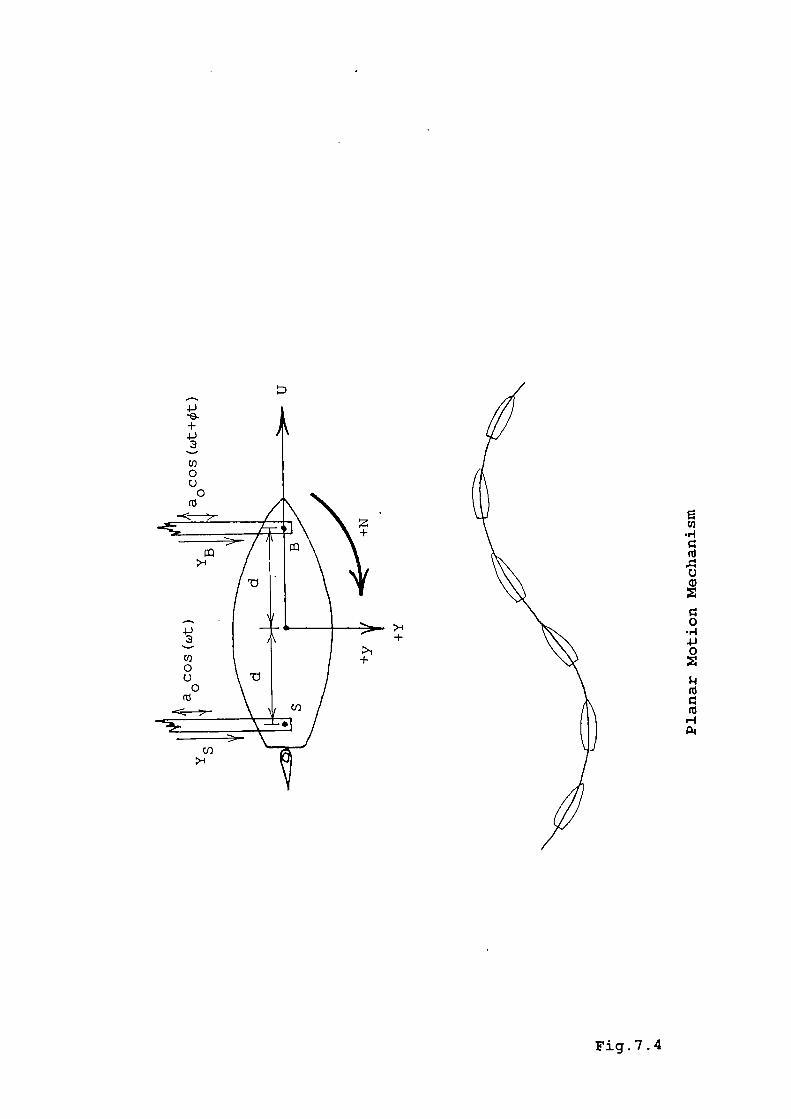
-lJ
+4J3
(1)00
0cj
::'— /
.lJ3
00
0Iii
>-
C/)
>-4
>1+
U)
EU)
•i•1
iii
C)ci)
>-1
0
+
4)0
1.1
Fig.7.4
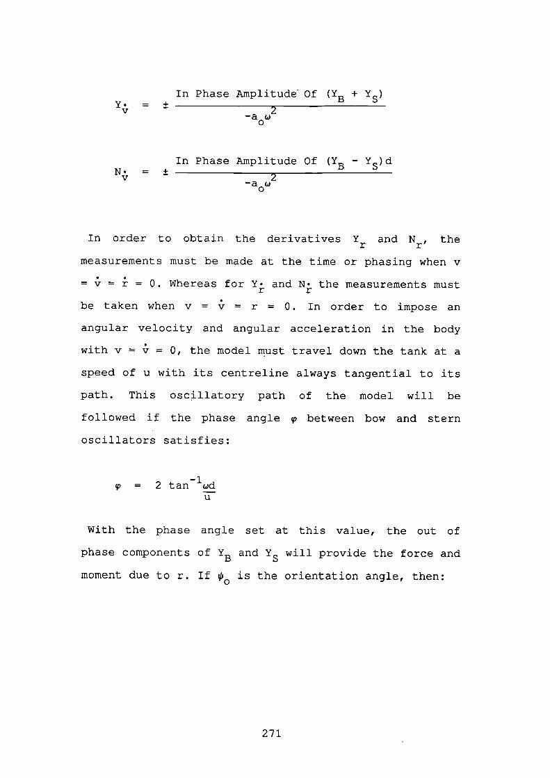
In Phase Amplitude Of (Y + Y= + B S
v 2-a0w
In Phase Amplitude Of (Y3 - Ys)dN . = ±v 2-a0w
In order to obtain the derivatives Y and N , ther r
measurements must be made at the time or phasing when v
= = = 0. Whereas for Y . and N . the measurements mustr r
be taken when v = = r = 0. In order to impose an
angular velocity and angular acceleration in the body
with v = = 0, the model must travel down the tank at a
speed of u with its centreline always tangential to its
path. This oscillatory path of the model will be
followed if the phase angle between bow and stern
oscillators satisfies:
-1= 2 tan wdU
With the phase angle set at this value, the out of
phase components of and will provide the force and
moment due to r. If is the orientation angle, then:
271
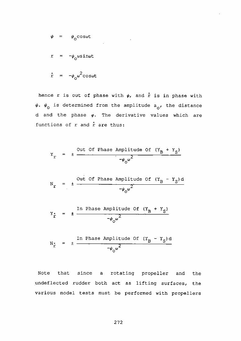
Vi = V'0coswt
r = -&0wsinwt
= -V1w2CO5wt
hence r is out of phase with V, and is in phase with
is determined from the amplitude a 0 , the distance
d and the phase q. The derivative values which are
functions of r and are thus:
Out Of Phase Amplitude Of (Y + Y= ± B S
r 2-Vi0w
Out Of Phase Amplitude Of (Y - Y )dN = ± B Sr 2
-Vi0w
In Phase Amplitude Of (Y + Y
= + B Sr - 2
-çli0co
In Phase Amplitude Of - Ys)dN • = ±r
Viw20
Note that since a rotating propeller and the
undeflected rudder both act as lifting surfaces, the
various model tests must be performed with propellers
272
operating and the rudder included in the undeflected
condition.
The drawback with model testing is that it is both time
consuming and expensive. For small boats it is as easy
to conduct full scale tests onboard the real boat, which
also dispenses with troublesome scaling problems and
linking the experiments at the Froude number. The funds
and time available to the author are not sufficient to
cover tank testing experiments and measurements will be
made onboard a real boat.
7.05 Standard Manoeuvres
In order to ass.ess how closely the mathematical model
describes the real boat, it is usual to compare sets of
standard manoeuvres performed on the boat simulator with
real boat data. Typical manoeuvres used include
(Ref.33)
Turning Circles: these are used to determine the
effectiveness of the rudder to produce steady state
turning motion. These are usually performed at a number
of rudder angles, both port and starboard. All turns
should be performed with approach runs at the same
relative wind angle. A short approach run is used to
ensure the boat is at speed before the rudder is put
273
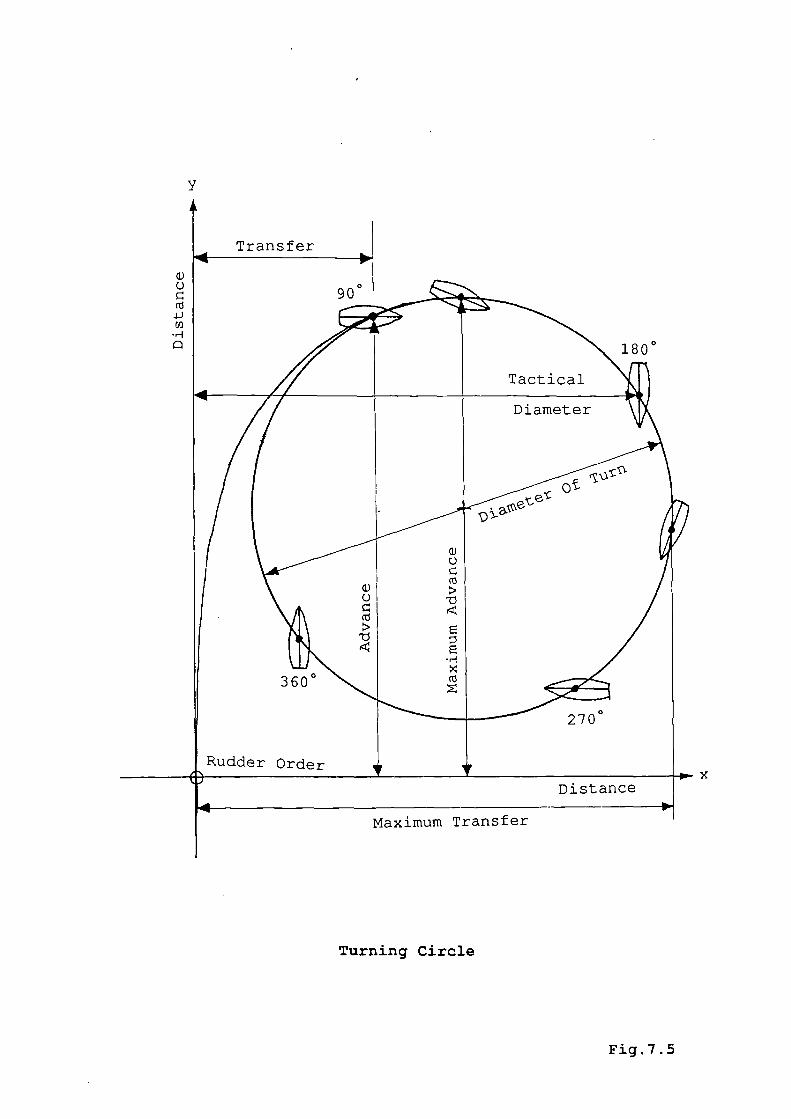
Turning Circle
Fig.7 .5
over. Ideally, it is desirable to continue for a turn
and a half, 5400, in order to ensure that the manoeuvre
is properly terminated. Plots of turning circles are
normally presented in terms of horizontal translation
from the start point (Fig.7.5), however, since the Arun
lifeboat is neither equipped with an accurate means of
determining the horizontal translational velocities nor
an accurate position fixing system, the plots will be
in terms of heading against time. This at least allows
the steady state turn rate to be determined easily. It
should be noted that since small boats exhibit tight
turning ability, it is often possible for the boat to
encounter its own wake before completing the turn,
obviously this condition will not occur in the
simulation.
Kexnpf (Zig-Zag) Manoeuvre: this provides a means of
investigating the steering ability of a boat. It shows
the effectiveness of the rudder to initiate and correct
changes in heading. The boat is initially lined up on a
chosen course at a constant speed. The rudder is then
quickly, but smoothly, deflected to a certain angle, say
20°. The boat's heading is then allowed to change a
prescribed amount from the initial course, say 30°, at
which point the rudder is applied to the same chosen
angle of deflection, 20°, but in the opposite direction.
This angle of rudder is held until the boat's heading
275
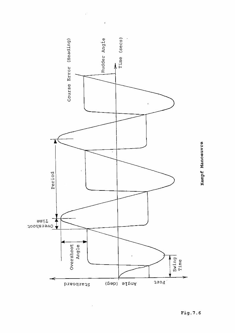
0
('3
l41
a)
a) -(I)
0a)
'ci
a)a) a)
TI E
poqi (bep) eibuy
Fig.7. 6
wç LI
oous.1ar
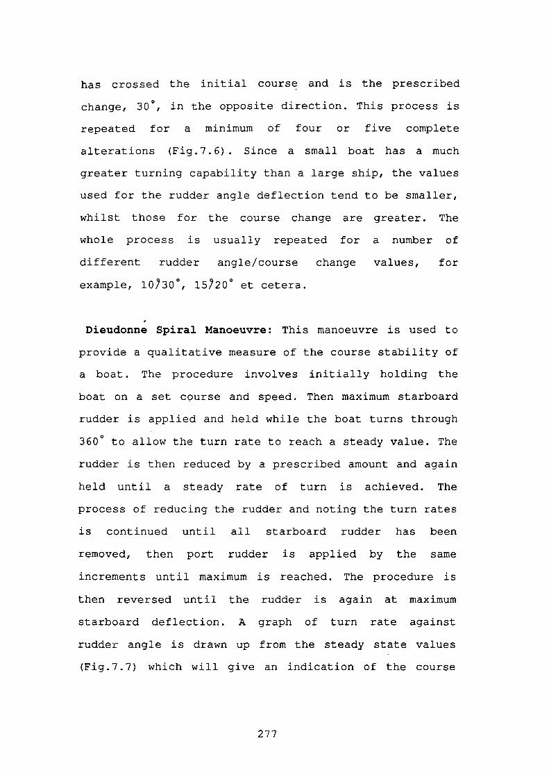
has crossed the initial course and is the prescribed
change, 30°, in the opposite direction. This process is
repeated for a minimum of four or five complete
alterations (Fig.7.6) . Since a small boat has a much
greater turning capability than a large ship, the values
used for the rudder angle deflection tend to be smaller,
whilst those for the course change are greater. The
whole process is usually repeated for a number of
different rudder angle/course change values, for
example, 10730°, 15720° et cetera.
Dieudonne Spiral Manoeuvre: This manoeuvre is used to
provide a qualitative measure of the course stability of
a boat. The procedure involves initially holding the
boat on a set course and speed. Then maximum starboard
rudder is applied and held while the boat turns through
360° to allow the turn rate to reach a steady value. The
rudder is then reduced by a prescribed amount and again
held until a steady rate of turn is achieved. The
process of reducing the rudder and noting the turn rates
is continued until all starboard rudder has been
removed, then port rudder is applied by the same
increments until maximum is reached. The procedure is
then reversed until the rudder is again at maximum
starboard deflection. A graph of turn rate against
rudder angle is drawn up from the steady state values
(Fig.7.7) which will give an indication of the course
277
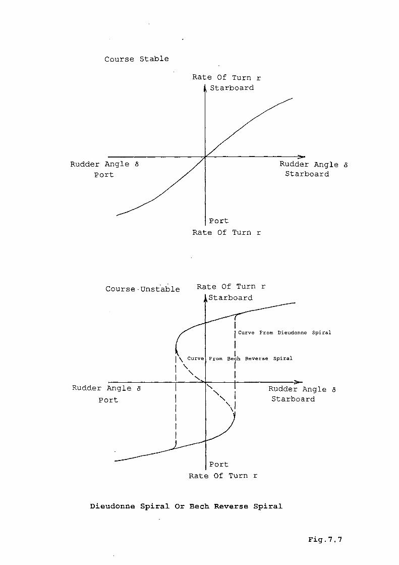
RudderPox
' AngleDoard
NNN
Rudder Angle
Port
Rudder AngleStarboard
Course Stable
Rate Of Turn r
Rate Of Turn r
Course.tJnstable Rate Of Turn r
1 Starboard
Curve From Dieudonne Spiral
\ Curve From Bech Reverse Spiral
I-
Port
Rate Of Turn r
Dieudonne Spiral Or Bech Reverse Spiral
Fig.7.7
stability of the boat.
Bech Reverse Spiral: This is the inverse of the
Dieudonné spiral and can only be successfully used if
there is a rate of turn indicator or an autopilot which
responds to rate of turn error instead of heading error.
The boat is steered at different constant turn rates,
and the mean rudder angle required to produce this yaw
rate is measured. This method, although harder to
instigate for small boats, allows the rate of turn
against rudder angle curve to be plotted as a continuous
function (Fig.7.7).
The manoeuvres performed during trials with the RNLI
consisted of a set of turning circles, a set of kempf
manoeuvres and some straight runs conducted with the
relative direction of the sea at the cardinal and
inter-cardinal points. Plots of these manoeuvres can be
found in an appendix. It was thought that the Dieudonné
or Bech spiral manoeuvres would not yield much further
information, especially as the turn rates can be
determined from the turning circles.
279

CHAPTER 8
RESULTS
L a capLta mL&ake ta theatLce 4arLe
one ha data"
Sir Arthur Conan Doyle
280
8.01 Real And Simulated Data
During boat trials with the RNLI, data was obtained
for, amongst other manoeuvres, a whole series of turning
circles, carried out at various rudder angles and
forward speeds, as well as a set of Kempf manoeuvres.
Plots of this data are presented in an appendix of this
thesis. The plots are arranged in terms of a set of
twelve turning circles and four Kempf manoeuvres. For
each manoeuvre the real data is given first, and has the
time and date when it was recorded at the head of the
plot; this is followed by the comparable simulation
which has the word 'Simulation' written at the head of
the plot.
The turning circles are fairly rudimentary, but
nonetheless extremely useful, manoeuvres which yield the
steady turn rates for given rudder deflections, and they
provide for an initial impression of the performance of
the mathematical model. Kempf manoeuvres, although again
used to determine how the rudder affects the boat's
turning ability, tend to provide continual reversals in
the rudder commands, and consequently the boat is set
into oscillation. If the model proves able to adequately
follow such fluctuations, then this will provide good
reason to believe that it will closely match any
required manoeuvre of the real boat.
281
The computer simulation was run with a control routine
in order to perform the same manoeuvres carried out in
the boat trials. The object was to allow accurate
automatic reproductions of the real data. The control
routine used here allows the model to run up to speed on
the initial given course, prior to applying rudder
commands. For the turning circle manoeuvre, the
particular rudder angle is applied and left until a
full turn and a half has been completed.
The Kempf manoeuvre requires slightly more control. A
given rudder angle must be applied until a certain
course change has occurred, then the desired rudder
angle must be reversed and so on until a prescribed
number of iterations have been performed. One drawback
with the simulation of the Kempf manoeuvre is that, if
the frequency of the oscillations is not quite the same
as in the real situation (either slightly longer or
slightly shorter), then the result will progressively
get further out of synchronisation with the real data.
8.02 Turning Circle Plots
Analysing the turning circles in terms of the five
variables plotted shows the following:
282
Roll: The real data shows that the average value during
a turn tends to hang off to one side Id est there is a
constant angle of heel in a turn (plus the wave
effects). A starboard turn causes a starboard angle of
heel, whilst a port turn yields a port roll. This
becomes more pronounced at higher speeds and at greater
rudder angles (that is in tighter turns). Clearly
visible on virtually all the plots of the real data is
the initial peak at the instant when rudder is suddenly
applied. The comparable simulations show all these
attributes, except that the roll damps down to constant
angle of heel without the wave effect. About two-thirds
of the way through each turn the boat encountered its
own wake, this is visible on the real trace, but the
simulations are .not capable of taking this into account.
Pitch: At speed the bow of the semi-displacement boat
rises, the greater the speed the higher the constant
angle of trim achieved. Due to speed reduction in turns
the pitch angle will be reduced, though with the wave
effect tends to dwarf this effect in the real data. The
effect of crossing the wake is more pronounced on the
pitch trace. The mean pitch angle on the real trace
seems to vary little for different turn rates or forward
speeds. The simulated pitch trace is a little less than
the real situation, due to different settings of the
283
trim tabs and the need for a slight adjustment to the
propeller effect term.
Yaw: The fluxgate compass provides a very stable output
of the change of heading, and a near straight line is
produced. Some slight deviations from a constant rate
are visible, due to "hanging off " in the swell.
Naturally the simulation produces a perfectly straight
line with the gradient matching the real data.
Rudder: Some differences exist between the simulated and
real rudder angle. Clearly it is a simple matter to set
an exact rudder angle during a simulation run, but it is
not so easy in a real situation with swell and waves.
The rudder increments are ±50, ±15° and ±25°.
RPM/Surge: The real boat data consists of the propeller
rpm since there was no means of determining forward
velocity. The trace shows a virtually constant value
throughout the turns. The simulation plot is of the
surge velocity, and shows the speed reduction upon
commencing a turn. Initially the simulation model came
up to speed, then dipped as rudder was applied.
284
8.03 Kempf Manoeuvre Plots
Similarly, analysing the Kempf manoeuvres in terms of
the five variables plotted shows the following:
Roll: The simulated roll is not so sharply spiked as the
real data, but it does exhibit the same damping
characteristics. This manoeuvre, with the rapid changes
in rudder angle from one side to the other, tends to
belittle the effect of the waves on the roll, especially
as the manoeuvres were performed into the direction of
the swell.
Pitch: Little more can be said of the pitch angle trace
than was said for the turning circles, except that the
wake does not interfere with these manoeuvres.
Yaw: The simulated yaw trace shows a greater overshoot,
and hence longer time to return to the base course, than
the real data. This is due to the differences between
the compass systems used to perform and record the
manoeuvre and to perhaps the yaw moment of inertia being
set a little high. It was noted in hindsight that there
was a deficiency in the yaw assessment in that the
coxswain was using a Cestral compass damped by oil in
order to determine the deviation from the base course.
The accuracy of reading this instrument under such
285
oscillatory motions is not too good, especially as it
tends to swing easily. This is reflected in the yaw
trace from the fluxgate with the peaks reaching varying
heights, however the underlying characteristics are
plain enough. The fluxgate compass also suffers from
variations due to roll and pitch accelerations. The roll
motions can be clearly seen imposed upon the yaw trace
and this detracts from the smooth sinusoidal curve.
Rudder: The real rudder traces show that these
manoeuvres were a little tricky for the coxswain to
perform with absolute accuracy. Since the simulated yaw
took slightly longer to return to the base course than
the real data, the rudder commands are correspondingly
spaced at slightly longer intervals. However, the basic
shape of a square wave command format is clearly
visible.
RPM/Surge: The surge trace exhibits fluctuations,
particularly at higher speeds and more rapid Kempf s, due
to the changes in drag from the rudder and the changing
yaw rate which gives rise to the sinusoidal style yaw
trace. The rpm remains fairly constant, as it did for
the turning circles.
Differences in the real and simulated results are
principally due to the effects of wave and wake
286
disturbances and the inaccuracy of the helmsman's
positioning of the rudder, especially in Kempfs.
Altogether the small boat model is able to mimic the
Arun lifeboat exceedingly well. A few minor adjustments
could be made to obtain a closer fit, but without
supporting reasons for such changes this is hardly
worthwhile. From the point of view of the autopilot, the
model behaves close enough to the real world situation
for simulation purposes in the development environment.
The model is capable, with sufficient data, of
adequately predicting the behaviour of any small boat,
particularly of the dispLacement or semi-displacement
type. It has the flexibility over ship models that it
will be capable. of reproducing any small boat, and not
being necessarily dedicated to one ship type. This is
extremely important where the variety and style of small
boats is large and diverse.
287

CHAPTER 9
STRATEGY FOR TESTING AUTOPILOTS
288
9.0]. Communicatinq With The Autopilot
In order to assess the performance of the autopilot
system within the development environment, it became
necessary to allow the autopilot to exercise control
over the computer simulation of the small boat. This in
effect replaces the real boat with the mathematical
model, and varying conditions of sea state, tide and
wind can be imposed on the simulation at will. The main
advantage of this is that tests can be repeated, under
exactly the same conditions, for different or modified
autopilot designs. Results will then be directly
comparable.
The autopilot requires information about the boat's yaw
angle (magnetic heading and rcidder ositirn 2t tdtprovide automatic control. In a real boat situation
these will be provided by the electronic fluxgate
compass and rudder reference units. The autopilot then
effects control of the boat by sending a command signal
to the rudder. The model generates the yaw angle and
rudder position data at each discrete interval so, if
these are input to the autopilot controller in place of
the compass and rudder reference, the model can simulate
the boat.
289
There already exists a marine standard for data
transmission between electronic navigational devices
known as the NMEA (National Marine Electronics
Association) format. This consists of a large number of
ASCII (American Standard Code for Information
Interchange) messages which start with a two character
system identifier, followed by a three character message
identifier, the message itself and finally the CR
(Carriage Return) and LF (Line Feed) message
terminators. The Cetrek autopilot has a number of ports
to which Decca Navigators, and other such equipment
which produces NMEA messages, can be connected.
The small boat computer simulation has, therefore, been
designed to output magnetic heading and rudder angle, in
NMEA format (but not a true NMEA message), to the
autopilot. In return the autopilot sends back a byte
containing the rudder command information. This link
provides a closed loop between the autopilot and boat
model which can be used to assess autopilot performance.
With the addition of the chart pilot (a combined
electronic chart and autopilot unit) to the Cetrek range
of products, it became possible to display the boat's
position and navigate along a prescribed track defined
by a set of waypoints. A second NMEA message (this time
a true message) giving the boat's position in latitude
290
and longitude is sent by the model to the autopilot. The
computer simulation, therefore, also simulates an
electronic position fixing system. There is thus a
visual representation of the autopilot's performance on
the chart pilot as the boat's track is plotted against
the desired track.
The model outputs a further piece of information, that
of yaw rate. The reason is two-fold; first it can be
used to assess the rate term used by the derivative
section of the PID controller, and secondly it is
envisaged that it will provide a means of assessing the
performance of the rate-gyro presently being developed
at Cetrek.
For purposes of analysis, the autopilot returns a
second byte of information containing the course error.
That is the difference between the desired course to be
steered, obtained from either the chart pilot's waypoint
information or from the user, and the actual heading.
The relevance of this item of data will become apparent
in the next section.
291
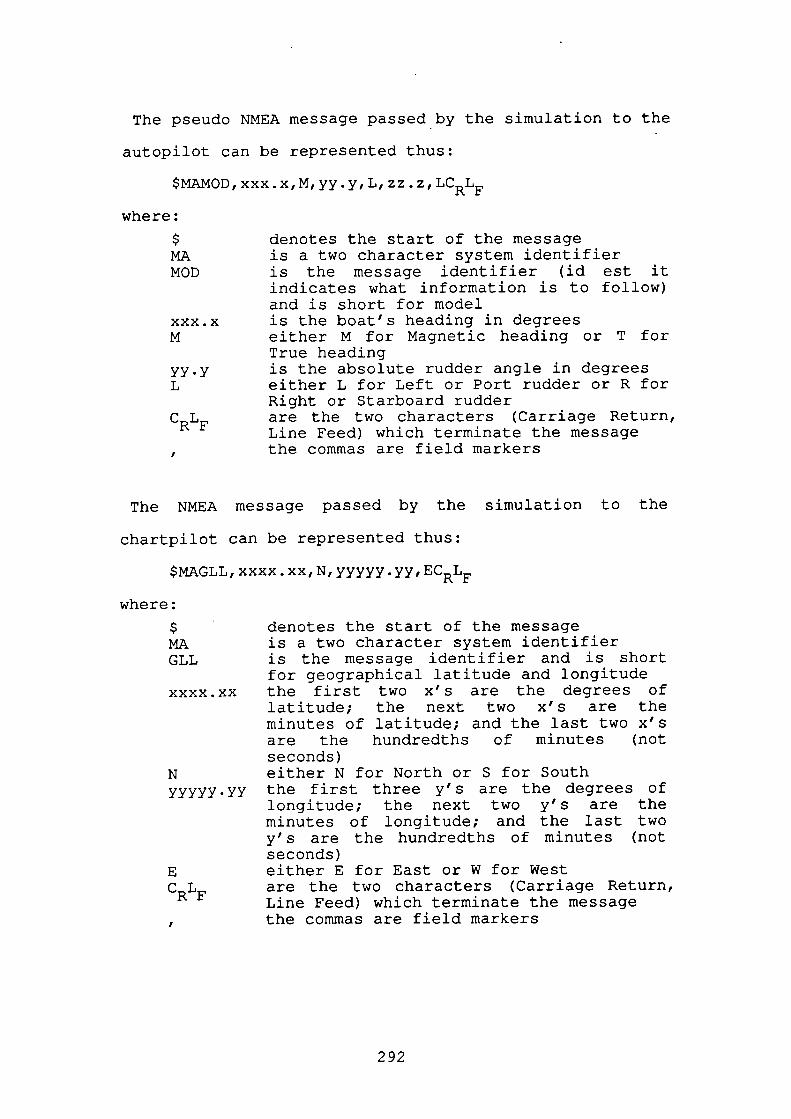
The pseudo NMEA message passed by the simulation to the
autopilot can be represented thus:
$MANOD, xxx.x,M, yy.y, L, zz . z, LCRLF
where:
$MAMOD
xxx • xM
yy.yL
CRLF
F
denotes the start of the messageis a two character system identifieris the message identifier (id est itindicates what information is to follow)and is short for modelis the boat's heading in degreeseither M for Magnetic heading or T forTrue headingis the absolute rudder angle in degreeseither L for Left or Port rudder or R forRight or Starboard rudderare the two characters (Carriage Return,Line Feed) which terminate the messagethe commas are field markers
The NMEA message passed by the simulation to the
chartpilot can be represented thus:
$MAGLL, xxxx xx, N, yyyyy . yy, ECRLF
where:
$MAGLL
xxxx . xx
Nyyyyy.yy
ECRLF
I
denotes the start of the messageis a two character system identifieris the message identifier and is shortfor geographical latitude and longitudethe first two x's are the degrees oflatitude; the next two x's are theminutes of latitude; and the last two x'sare the hundredths of minutes (notseconds)either N for North or S for Souththe first three y's are the degrees oflongitude; the next two y's are theminutes of longitude; and the last twoy's are the hundredths of minutes (notseconds)either E for East or W for Westare the two characters (Carriage Return,Line Feed) which terminate the messagethe commas are field markers
292
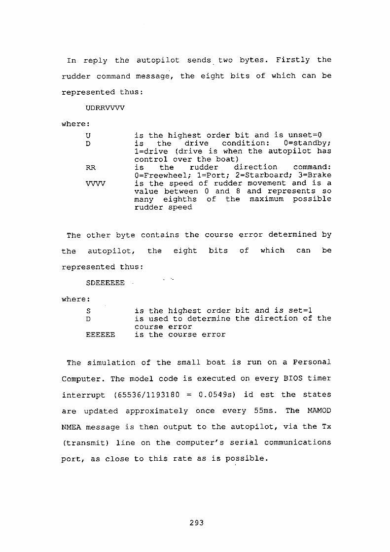
In reply the autopilot sends two bytes. Firstly the
rudder command message, the eight bits of which can be
represented thus:
UDRRVVVV
where:
UD
RR
vvvv
is the highest order bit and is unset=Ois the drive condition: O=standby;l=drive (drive is when the autopilot hascontrol over the boat)is the rudder direction command:O=Freewheel; l =Port; 2=Starboard; 3=Brakeis the speed of rudder movement and is avalue between 0 and 8 and represents somany eighths of the maximum possiblerudder speed
The other byte contains the course error determined by
the autopilot, the eight bits of which can be
represented thus:
SDEEEEEE
where:
S is the highest order bit and is set=].D is used to determine the direction of the
course errorEEEEEE is the course error
The simulation of the small boat is run on a Personal
Computer. The model code is executed on every BIOS timer
interrupt (65536/1193180 = O.0549s) Id est the states
are updated approximately once every 55ms. The MANOD
NMEA message is then output to the autopilot, via the Tx
(transmit) line on the computer's serial communications
port, as close to this rate as is possible.
293
The MAGLL NMEA message is output on every 50th
transmission, Id est about every 2.5s, to the
chartpilot. This simulates a navigator input.
A second interrupt routine awaits the two incoming
bytes on the Rx (receive) line from the autopilot. These
are processed as soon as they arrive. As far as the
autopilot is concerned the model messages appear on one
of its standard navigator ports.
9.02 Graphical Presentation
The simulation communicates with the user by displaying
pertinent information on a VDU (visual display unit).
The settings of the control surfaces of the rudder,
propeller and trim tabs are displayed as bar graphs,
whilst the yaw angle is expressed as a plan view outline
drawing of a boat within a compass rose. The other Euler
angles, latitude, longitude, forward velocity, wind
parameters, wave parameters and tidal information are
displayed in a numerical format.
Two additional sets of information are presented on the
VDU which directly aid the assessment of autopilot
performance. The first is a trace recording the course
error over the past one minute of the simulation. This
graphically shows the amplitude of any overshoots due to
294
insufficient damping in the system or the length of time
taken to come up onto course. By altering the autopilot
gains, it is possible to watch the differences. This is
extremely difficult to produce on board a real boat
because the differences are not easily differentiated
quantitatively by the helmsman and one can never be sure
that the differences are not due to disturbing effects.
The second set of information is a numerical "cost
function" value produced for the rudder usage and for
the course error. An ideal autopilot will correct all
heading errors immediately, but with extremely small use
of the rudder. In other words, the autopilot controller
should minimise both course errors and rudder usage.
Large deviations from the desired course will add extra
time and distance to a journey, but close adherence to
track requires a greater, unwanted, use of the rudder. A
compromise must, therefore, be made between minimising
both of these quantities. Cost function values are
achieved for both course error and rudder angle by using
a low pass filter algorithm.
With such information, developers will be able to
quantitatively assess the performance of an autopilot
prior to conducting extensive and time-consuming sea
trials.
295
9.03 Autopilot Control Of The Model
Preliminary use of the computer simulation with the
Cetrek chart pilot has already produced exciting
results. Plates 7 to 12 are a set of "snapshots" from a
typical simulation run with the autopilot exercising
control over the model in order to achieve track
keeping.
A number of areas in the autopilot control algorithms
have been identified as requiring attention and some
modifications to the autopilot code have been made,
these include: -
1) Course Deadband: This defines the limit to which the
course may deviate from the desired heading before any
rudder is applied. The idea of such a region is to
prevent excess rudder movement when the boat is nearly
on course. However, it was noticed that if the deaciband
is set quite wide, then if the course falls outside of
the deadband, there is a sudden demand for a large
amount of rudder in order to turn the boat back towards
the base course. The boat then turns back too quickly
and overshoots the other side and a large, unwanted
oscillation is induced.
296
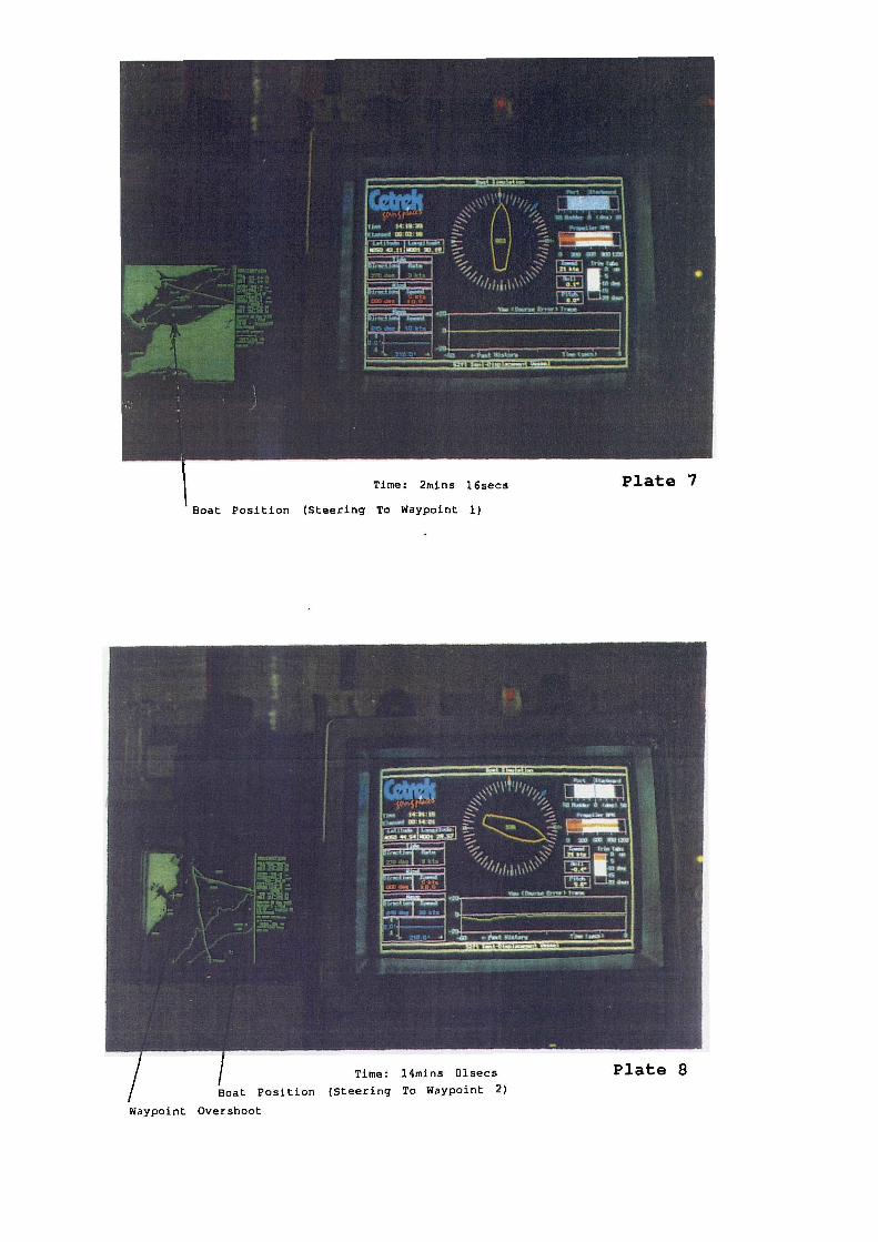
Boat Pos1t1or (Steering 10 waypoint I)
Waypoiflt Overshoot
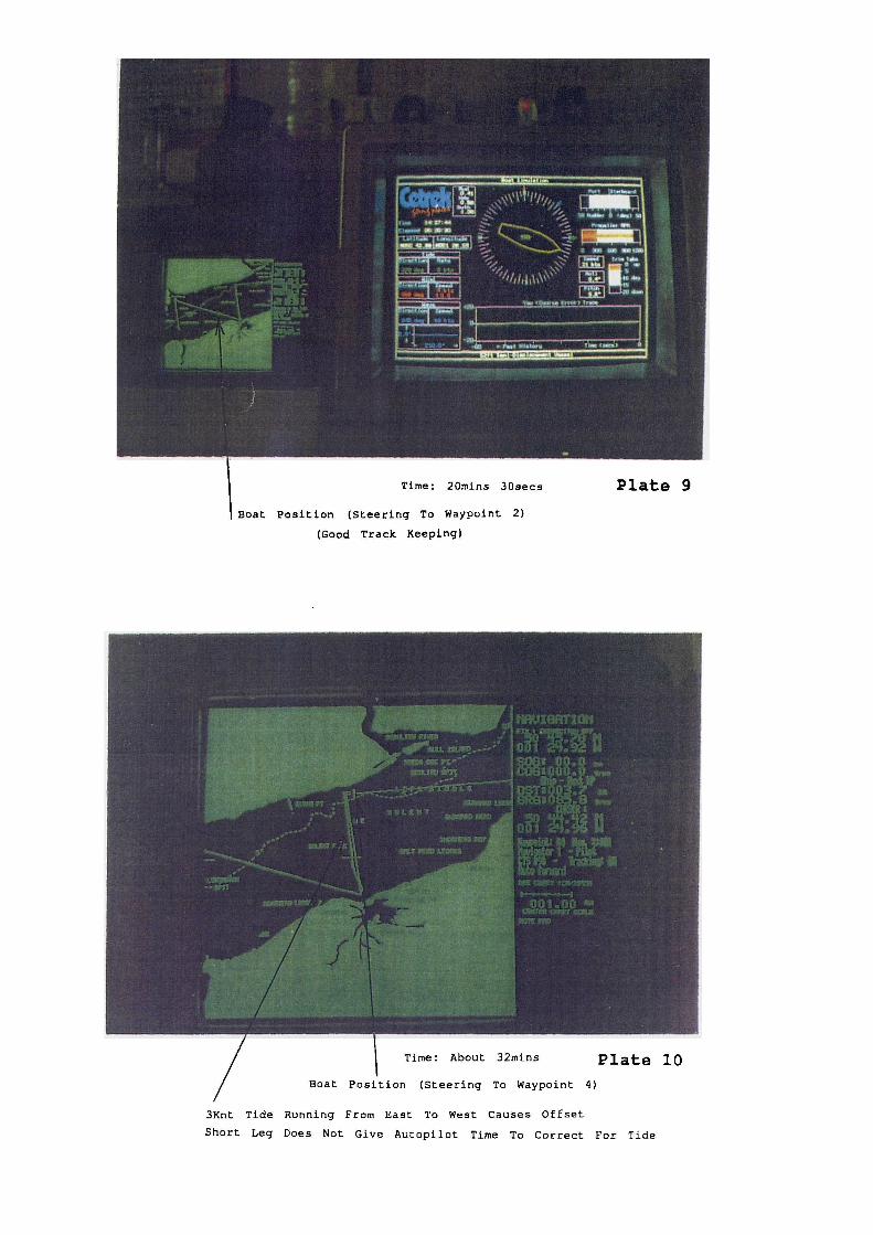
Boat Position (Steering To Waypoint 2)
(Good Track Keeping)
3Knt Tide Running From East To West Causes Offset
Short Leg Does Not Give Autopilot Time To Correct For Tide
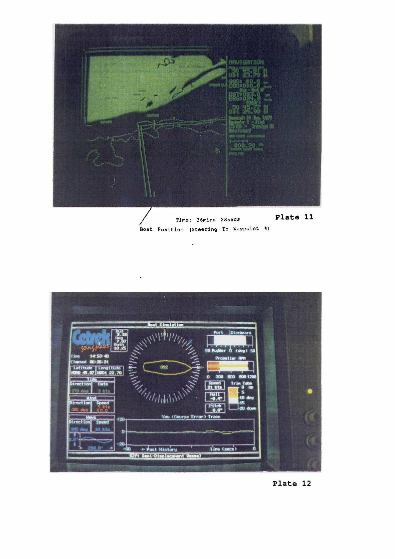
Boat Position (Steering To Waypoint 4)
- c'n ;-----
Plate 12
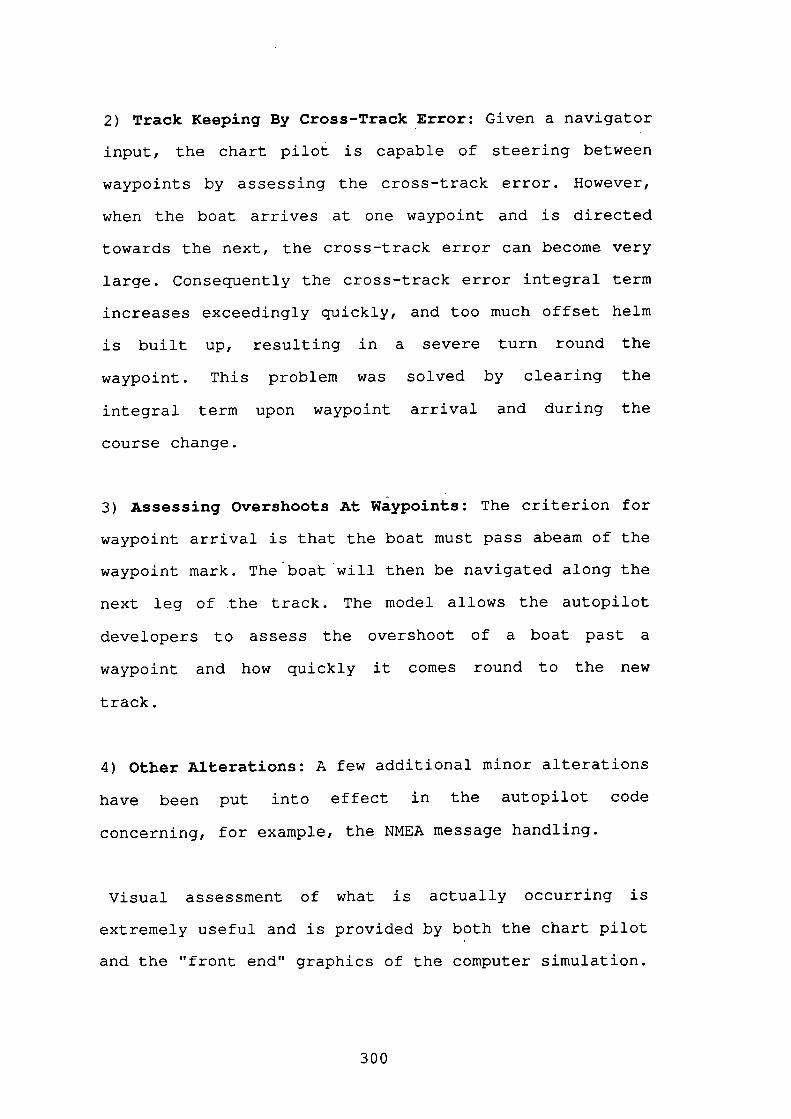
2) Track Keeping By Cross-Track Error: Given a navigator
input, the chart pilot is capable of steering between
waypoints by assessing the cross-track error. However,
when the boat arrives at one waypoint and is directed
towards the next, the cross-track error can become very
large. Consequently the cross-track error integral term
increases exceedingly quickly, and too much offset helm
is built up, resulting in a severe turn round the
waypoint. This problem was solved by clearing the
integral term upon waypoint arrival and during the
course change.
3) Assessing Overshoots At Waypoints: The criterion for
waypoint arrival is that the boat must pass abeam of the
waypoint mark. The boat will then be navigated along the
next leg of the track. The model allows the autopilot
developers to assess the overshoot of a boat past a
waypoint and how quickly it comes round to the new
track.
4) Other Alterations: A few additional minor alterations
have been put into effect in the autopilot code
concerning, for example, the NMEA message handling.
Visual assessment of what is actually occurring is
extremely useful and is provided by both the chart pilot
and the "front end" graphics of the computer simulation.
300
CHAPTER 10
CONCLUSIONS
"3ii 'tecearLch the hotthon 'ececLe a iie
adAsiance, and L no neane't at &t than U wa
at thien. 4 the powe o endwiance weaken4
wLth age, the unqenc o( the pwiuU qno
m tenAe 4nd eanch L a&iia
Mark Pattison
301
The work contained in this thesis describes in full the
investigation and development of a small boat
mathematical model. The model is of a highly
flexible, modular nature and is not confined to a given
boat type, but can, if desired, represent any small
boat. The model extends the boundaries of marine
simulation and can be easily modified to describe other
marine vessels, including large ships.
The initial literature search showed a lack of
published material and data about modelling small boats,
whereas their large ship counterparts have received much
attention. Much of the standard naval architectural
theory has held valid for small boats and some of the
equations derived •in this thesis have been spawned from
large ship research.
A number of tools essential to this kind of simulation,
namely rigid body dynamics and transformations between
axes systems, were discussed and developed. Their
particular relevance to the small boat model has been
outlined and the mathematics has been in keeping with
standard nomenclature.
The approach to the model has been one of modularity,
thus easing its construction and maintenance. The
equations have been developed around Newton's second law
302
of motion, but split into a number of distinct vectors.
Each vector can be treated as an individual entity and
can be added to, modified or replaced to suit new
applications. The framework of the thesis also allows
new modules to be bolted on as further research
dictates.
A computer program was developed by the author to
provide a simulation of small boat manoeuvres.
Additional programs, also written by the author, were
used in the real boat trials to record information
needed to validate the model. Parameter determination
proved to be a process of simplification and careful
analysis of the equations that had been developed.
Comparisons with the boat trials, that were conducted
using an Arun class lifeboat, showed the model to be
capable of simulating small boat behaviour. The
coefficients were not fine tuned to produce accurate
reproductions of the manoeuvres, since the simulator is
to be used to assess the performance of small boat
autopilots.
Communication pathways between the autopilot and model
were set up to allow the autopilot to exercise control
over the model. The visual assessment of what is
actually occurring, in real-time, is extremely useful
and is provided by both the chartpilot and the
303
"front-end" graphics of the computer simulation. Several
controlled tests were carried out and a number of
weaknesses in the autopilot's algorithms have been
detected.
The closed loop system of the Cetrek chart pilot and
small boat simulator provides an indispensable tool for
assessing autopilot design. This system set-up has also
been on display at the Southampton boat show in
September 1989, and will be used at other such venues,
to demonstrate the action and capabilities of the
autopilot.
304

CHAPTER ii.
SUGGESTED FURTHER RESEARCH
H utile done, oo nwch to do"
Cecil Rhodes
305
With such work as is herein described, it is customary
to indicate further areas of research, and this document
will prove no exception. The following suggestions are a
few general observations of possible areas of further
research in the realm of small boat modelling.
With respect to the autopilot system, the small boat
simulation could be incorporated into a model reference
system capable of determining the optimum gains in the
autopilot control routine for a particular boat in a
given sea condition. The amount of variation of the
compass course when attempting to hold a set course
needs to be reduced to a minimum and the system
algorithms could be designed to learn from predicted
boat motion and course deviation the best settings of
the autopilot gains. Kalman filter theory can be
included if there are measurements of some of the states
available.
With the prestige and interest in racing sailing yachts
in competitions such as the America's cup and Admiral's
cup, the model could be extended to incorporate a module
representing the sail forces and moments. This could
prove extremely difficult to match to a real situation,
due to the unpredictability of a gusty wind. Other
additions could be in the form of forces and moments due
to tunnel or axial thrusters as used on tugs, various
306
appendages attached to boats and the effects of dragging
nets from fishing boats.
Although the effect of added mass is well known, there
is still much work required to incorporate the
computation of accurate values for the coefficients into
the boat model. The change of these parameters with
water depth and forward speed requires special
attention. Ideally, to be able to extract the added mass
terms and other hydrodynamic coefficients from the lines
plans and general arrangements would provide an added
facility for prediction at the initial design stage.
Similarly, theoretical wind computations based upon a
knowledge of the quantity and distribution of the
superstructure and the projected transverse and
longitudinal areas require further investigation.
In order to formulate progressively more accurate
mathematical models and increase the detail and fidelity
of simulations, especially as new advances in digital
computer technology become available, it is paramount
that more experiments are carried out to produce data
for all aspects and types of vessels which covers a
wider range of operating conditions, so that the
mathematics can provide increased continuity and
accuracy.
307
In addition to research, there are other aspects that
warrant attention; these include the standardisation of
symbology, data, codes of practice and so forth in order
to enable advances in theories and research to be easily
transposed to other applications within the marine
field. A greater pooling of experimental data and trials
results would aid comparison of different vessel types
and the discovery of commonalities.
In concluding this document, the author wishes to echo
the statement made by Dand, (Ref.43) 1987, in his
concluding remarks:
"The qneate'z. the LdeW and detaLg o theU 'eUe on 'twtnq', the
qneate-'i. U pLace on a cLeanwdAtan&nç o the ph4CA O 4/UPIW dlmJc4 . We can on JnOdcl UW1L1te&that L1hh ue under&and, 40 the denland4 OmoduLan muLatLan frui4t uLtJThOtth Lead todepe un4/andq."
308

THIS PAGE LEFT
INTENTIONALLY BLANK
309

APPENDIX A
PRINCIPAL DIMENSIONS OF AN ARUN
310
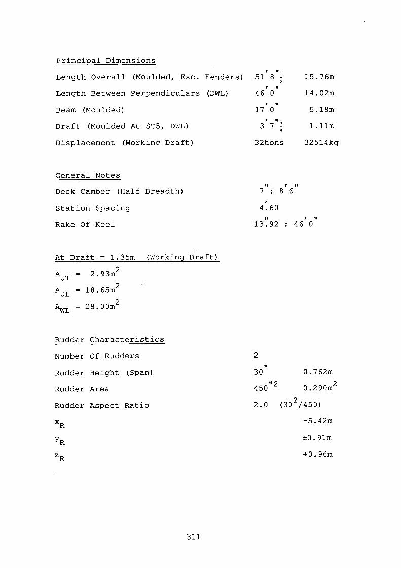
, ,,51 8 -
2I
46 0, ti
17 0I
37-8
32tons
15.76m
14. 02m
5. 18m
1. urn
32514kg
0 .762rn
0.290rn2
(302/450)
-5. 42rn
±0. 91m
+0.96rn
2ii
30
"2450
2.0
Principal Dimensions
Length Overall (Moulded, Exc. Fenders)
Length Between Perpendiculars (DWL)
Beam (Moulded)
Draft (Moulded At ST5, DWL)
Displacement (Working Draft)
General Notes
Deck Camber (Half Breadth)
Station Spacing
Rake Of Keel
II ti
7:86I
4.60I It
13.92 : 46 0
At Draft = l.35m (Working Draft)
AUT = 2.93m2
AUL = 18.65m2
AWL = 28.00m2
Rudder Characteristics
Number Of Rudders
Rudder Height (Span)
Rudder Area
Rudder Aspect Ratio
XR
ZR
311
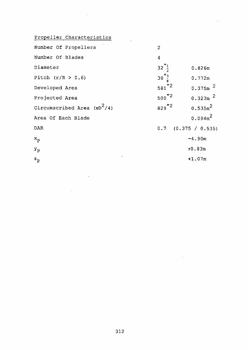
2
0. 826m
0.772m
0.375m 2
0.323m 2
o . 535m2
0. 094m2
(0.375 I 0.535)
-4. 90m
±0. 83m
+1. 07m
4'I
32 -2
I,
30 -8
"2581
2500I,
829
0.7
Propeller Characteristics
Number Of Propellers
Number Of Blades
Diameter
Pitch (r/R > 0.6)
Developed Area
Projected Area
Circumscribed Area (7rD2/4)
Area Of Each Blade
DAR
xP
YP
zP
312

APPENDIX B
PLOTS
313
The plots consist of 12 Turning Circles, 4 Kempf
Manoeuvres and 1 Trim Tabs Illustration. For each plot
the real data is given first, and is indicated by the
time and date when it was recorded, followed by the
corresponding simulation run, indicated by the word
"simulation".
A distinctive feature of interest, which is clearly
visible on the pitch plots of the tighter and quicker
turning circles, is the point when the boat crosses its
own wake. This point is marked on the pitch graph (where
distinguishable from the background waves) by a "w".
314
Rofl (D.c)
Pitch (D.)
(sw CD)
Rudder (Deg)
0a.
.0
00
z0
0
Propefl.r Revs (rpm)
I4)
0a-
13:5.429 20/04/1989
TURNING CIRCLE 01 (700rpm)
I I I I
000 012 024 038 049 060 072 084 096 108 120Time (a)
pitch (Deg)
Rudder (Deg)
0a
0
Surge (Kt.e)
4)
0a.
•0
2.1)cn
4)
0a.
SI mul tt I on
TURNING CIRCLE 01 (700rpm)Roll (Deg)
I I - 1T i
000 012 024 038 048 060 072 084 096 108 120TIRe (e)
Rofl (D.)
PftCh (Dg)
Yaw Weg)
Rudder (Dog)
I
Prcpefler Rove (rpr)
4,
ci.
L
I0ci.
13:4254 zcJ/04/1sas
TURNING CIRCLE 02 (700rpm)
I I I I I I I I I I
000 012 024 036 048 060 072 084 096 108 120Time (a)
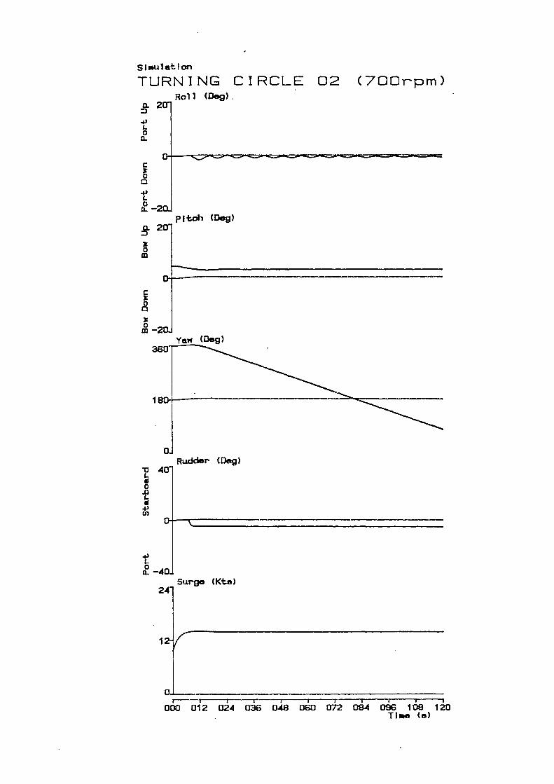
Roll (Deg).
pItth (Deg)
Yaw (Deg)
Rudder (Dog)
z0
0
z0
Surge (Kt)
4,
00
C
4,
0a-
•0
0-Q
4,C/)
4,
00
SI mul *t I on
TURNING CIRCLE 02 (700rpm)
r-i-----r--------r 1000 012 024 036 0-48 060 072 08-4 096 108 120
TIRe (a)
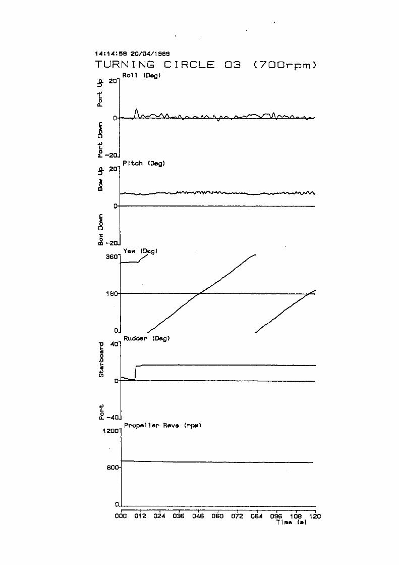
Pto1, (Dea)
Yaw (Dep)
Rudder (Dea)
Propeller Revs (ram)
U,
4,
0a.
I
I
14;14:9 20/04/1569
TURNING CIRCLE 03 (700rpm)Roll CDec)
I I I I I I I I I I
000 012 024 036 048 060 072 06.4 096 108 120Time C.)
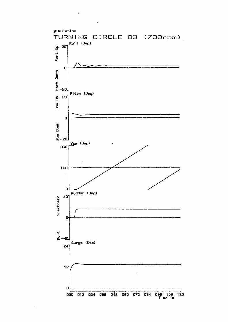
Pitch CE)eg)
Rudder (Deg)
0
a
0
m
Surge (Kte)
C-
4)U)
4)
C-0
a.
a.
4)
00
SI mul t I on
TURNING CIRCLE 03 (700rpm)Roll (0e)
I I I I I 1
000 012 024 036 048 060 072 084 096 108 120TI*e (a)
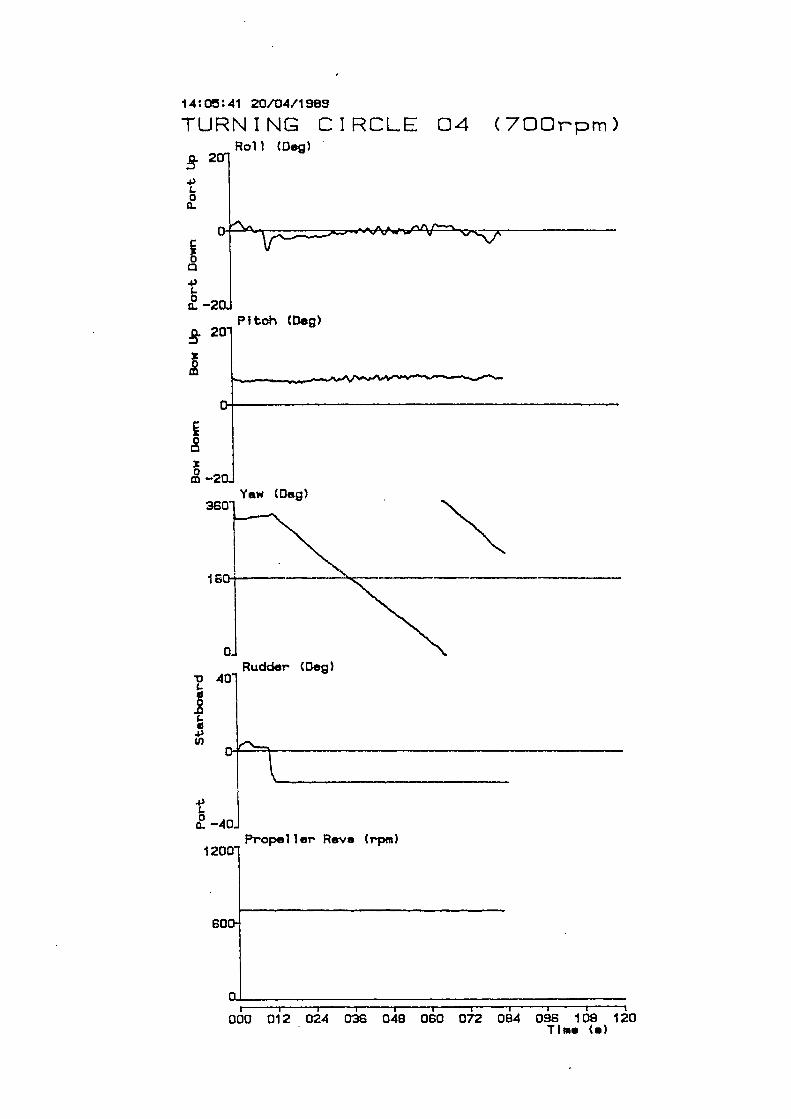
Roll (Deg)
Pitch (Den)
Yw (Den)
Rudder (Deg)
4)L00.
Propel br Rove (rpqn)
00.
4)
0
14:0:41 20/04/1989
TURNING CIRCLE 04 (700rpm)
I I I I I I I
000 012 024 036 048 080 072 084 098 109 120Tim. (.)
Pitch CDeg)
r0
0
0
a.
4)
0
I
d0
-Q
4)Cl)
4,C-0a-
S I MU1 et I on
TURNING CIRCLE 04 (700rpm)Roll (De)
Rudder (Deg)
Surge CKt.e)24
l 1 T TTTT000 012 024 038 048 060 072 084 096 108 120
TIMe Cs)
Roll (Dea)
Pitch (flea)
Rudder (0e)
0
Propeller Reve (roe)
00
C
aa.
•0
I0a.
I
14:30:11 20/04/1989
TURNING CIRCLE 05 (700rpm)
I I I I I I I I I
000 012 024 038 048 060 072 084 096 108 120Tie. Ce)
Pitch (Deg)
Yaw (Deg)
Rudder (Deg)
Surge (Kta)
a.
.4)
aa.
4)
0a.
z0
0c3
0
0.0
.0U)
.4)
0a-
Simulation
TURNING CIRCLE 05 (700rpm)Roll (LJeg)
-r -r-r t--r-- _I I i
000 012 024 036 048 060 072 084 096 108 120Time Ce)
Pitch (D.&
Yw (De&
Rudder CDe)
z
Propeller Reve (rpm)
4,
00
I
0
I4.,
00-
I
14:24:31 20/04/1999
TURNING CIRCLE 06 (700rpm)Roll (Deg)
r i I I
000 012 024 038 0.48 060 072 084 096 108 120Time C.)
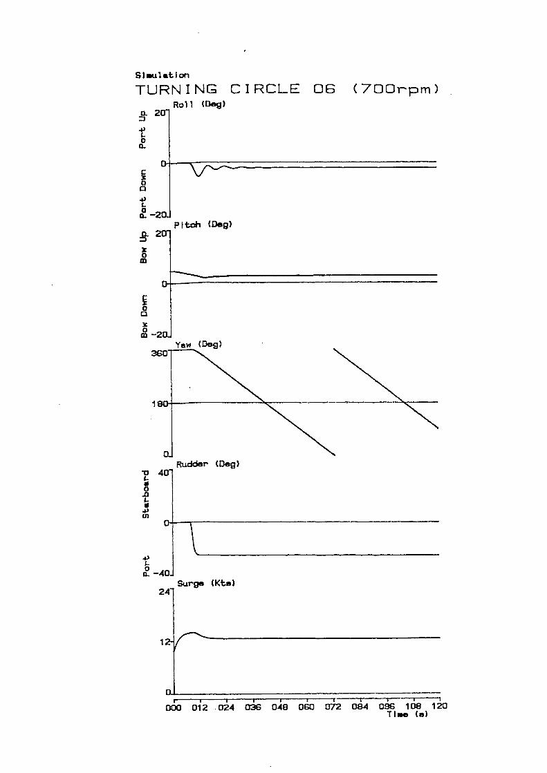
Pitch (Dog)
0
x0
U)
a.
0a-
Iaa-
Rudder (Dog)
Surge (Kta)
C-I0-oC-I
.0U)
4,C-
0a-
SI mul .t I on
TURNING CIRCLE 06 (700rpm)Roll (flog)
i- i -----r-- --,- -i000 012 024 036 048 060 072 08.4 096 108 120
TIMe (a)
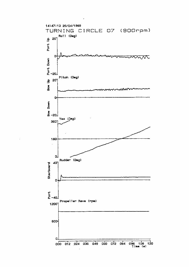
Pftch (Deg)
Yaw (De)
Rudder (Deg)
I
Propel ler Rave (rpm)
a
.0a
I
U)
.0a
I
14:47:10 20/04/1989
TURNING CIRCLE 07 (900rpm)Roll CDe&
i -I I I I I I I I
000 012 024 036 048 060 072 084 096 108 120Time Ce)
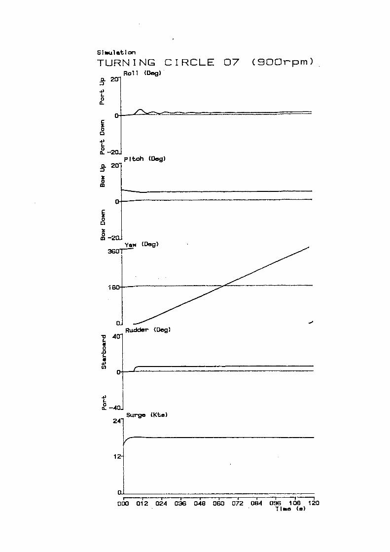
Roll (Dog)
pitch (Dog)
Rudder (Dog)
0.
4)
00.
0a.
z0
0
0
Surge (Kte)
0CC.0C4)Cl)
4)C.0a.
SI u1 e. I on
TURNING CIRCLE 07 (SOOi-pm)
---r------ -r----r---i000 012 024 036 048 060 072 084 096 108 120
Time Ce)
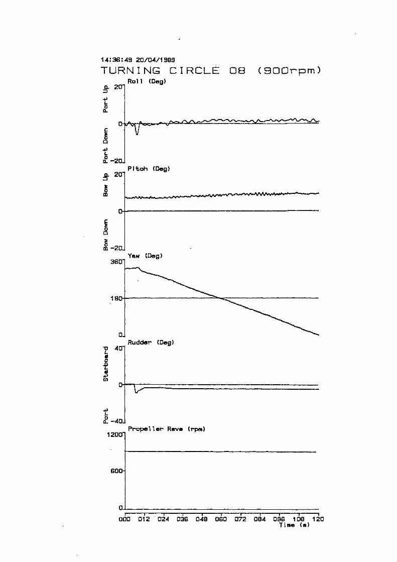
Pitch (Deg)
Yew (Deg)
Rudder (Dog)
0
0
Propel 1 or Rove (rpm)
a.:3
L0a-
C
0a-
0
0U)
0a.
I
14:36:49 20/04/1989
TURNING CIRCLE 08 (900rpm)Rofl CDe)
F- I I I I I I I
000 012 '024 036 046 060 072 084 096 108 120Time Ce)
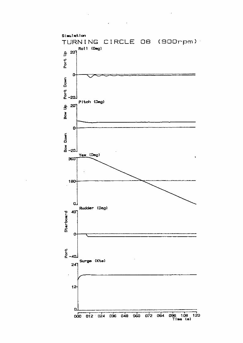
Rofl (13g)
Pitch (Deg)
0a.
4,0a-
Yew (D)
Rudder (Deg)
Surge (Kte)
0I
I4,U)
4,C..0
0..
00z0U)
S I mul t I On
TURNING .CIRCL 08 (900rpm)
r- - -r - -i----000 012 024 036 048 060 072 08-4 096 108 120
Tine Ce)
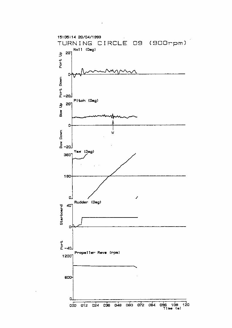
Roll (Deg)
Pitch (Den)
0
z0
Rudder CDe)
Prop. 11 er Rev. Crpm)
a-
4)
0a.
C
4)
00.
•0g
g.0(4,
4)
0a.
I
15:05:14 20/04/1989
TURNING CIRCLE 09 (900rpm)
r-000 012 024 036 0-48 060 072 09.4 098 108 120
Time (a)
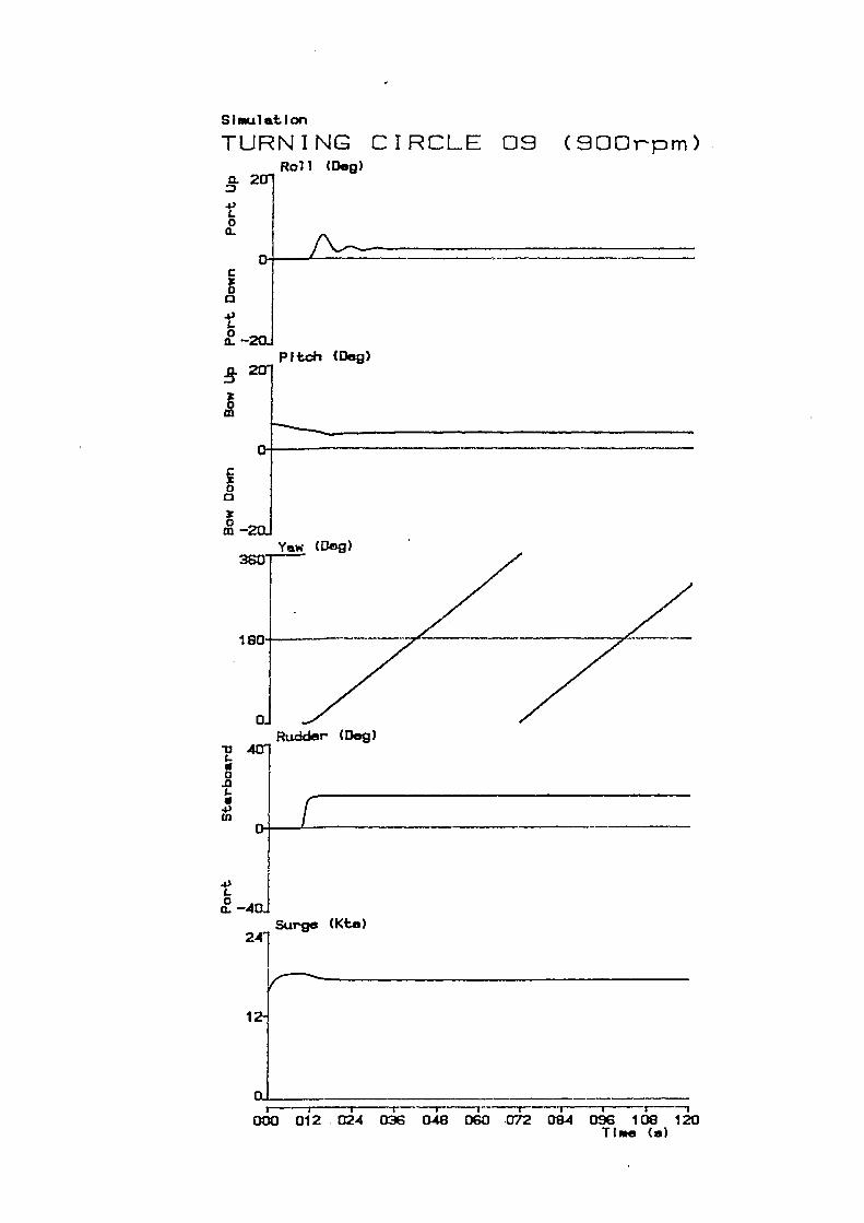
Pitch (Dog)
Rudder (Dog)
0
0
Surge (Kte)
4,
0a.
C
0a-
-U
0.0I-I4)C,)
4)C-0a.
S I mu 1 *tI on
TURNING CIRCLE 09 (900rpm)Roll (Deg)
1 r--i000 012 . 024 036 048 060 .072 08.4 096 108 120
Time (e)
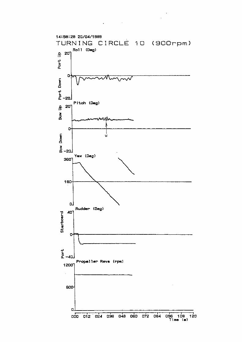
Pitch (Den)
Yw (Dep)
Rudder COeg)
I
Prope 11 er Revs (rpn)
0
4'0
0
•0
I4'00
I
14:58:28 20/04/1989
TURNING CIRCLE 10 (900rpm)Rofl (Den)
r j I I I I I I I
000 012 024 038 048 060 072 084 098 108 120Time C.)
Pitch (Dog)
Yew (Dog)
Rudder (Dog)
0
0
Surge (Kto)
a
43
00
C
43
0a-
•0
0.0
.4.,(0
43t..00
Slmul*tlon
TURNING CIRCLE 10 (900rpm)Roll (Dog)
r -i r-- i- i—Y-r --r?--1
000 012 024 036 048 060 072 08.4 096 108 120Time Ce)
Pitch (Deg)
Rudder (Den)
a
.0
0a.
.0
0a.
0
0
Propel 1 er Reve (rpm)
0
2.0Cl)
.0C.0a.
1
15:18:21 2D/1J4/1989
TURNING CIRCLE 11 (900rpm)Rofl (De)
I I I I I I I I I
000 012 024 038 0.48 060 072 06.4 098 108 120Time Ce)
4)C..0a-
0.0C-0a.
Pitch (Den)
0
Cr00
0
Yew (D)a
I
Rudder CDeq)0C.
2C-
.0CO
4)C-0a.
Sw-ge (Kt.e)
/
Simul*tion
TURN I NC CIRCLE 11 (900rpm)Roll (DeQ)
r— - - '- - ------i-000 012 024 036 0.48 060 072 08.4 096 108 120
Time (e)
Pitch (De)
Yw (Deg)
Rudder (Deg)
0
Propel 1 er Rave (rpm)
•0
0a-
C
4,
0a-
I4'0a.
1
15:12:22 20/04/1989
TURNING CIRCLE 12 (900rpm)Roll (Den)
000 012 024 036 048 060 072 084 096 108 120Time Ce)
Pitch (Dog)
Rudder (Dog)
4)I-£3
•0
0a.
0
0In
Surge (Kte)
•0
4)In
4,L0a.
Simulation
TURNING CIRCLE 12 (900rpm)Roll CDec)
000 012 024 038 048 060 072 084 096 108 120Time Ce)
Pitch COeg)
Yew (Deg)
Rudder (Deg)
I
Prcpsfler Revs (rpm)
I
Cl)
0
I
11:12:08 17/04/1989
KEMFF 01 (10/30 700rpm)Rofl (D.g)
000 020040080080 100 120140160 180200Tim. (.)
Simul Ion
KEMFF 01 (10/30 7OOrpim)Rofl (Dec)
Pitch CD.c)
Yw CDeq)
Rudder (Doq)
Surce (Kte)
4,
a.
I
I
I4,
0a--
I I I I I I I 1
000 020 040 060 080 100 120 140 160 180 200Tim. C.)
11:23:03 17/04/1989
KEMFF 02 (10/30 1050rpm)Rofl (Usa)
Pitch CD.)
Yftw (Ue)
Rudd.r (0cm)
PT-OPefler Rev. (rpm)
Ia0
4,
1
I
I
I-I 1 I I I
000 020 040 060 080 100 120 140 160 180 200Tim. Ce)
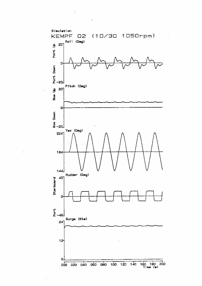
Yaw (Dog)
Rudder (Dog)
I
Surge CKte)
Simul sti on
KEMFF 02Rofl (Dog)
I
(10/30 1050rpm)
cr34J
0
Pitch (Dog)
I I I I I I
000 020 040 060 080 100 120 140 160 180 200Time (.)
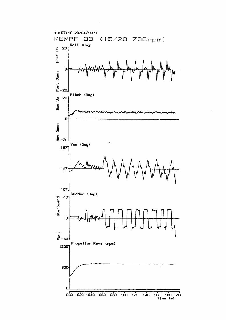
Y'w (Dcc) -
13:07:18 20/0.4/1889
KEMFF 03Rofl (D.a)
43I-00
:1Pitch (De)
C
0
I
I
1Rudder (Den)
00-
1
(15/20 700rpm)
Propel ler Rev. (rpm)
I I - I -
000 020 040 080 080 100 120 140 160 180 200Time C.)
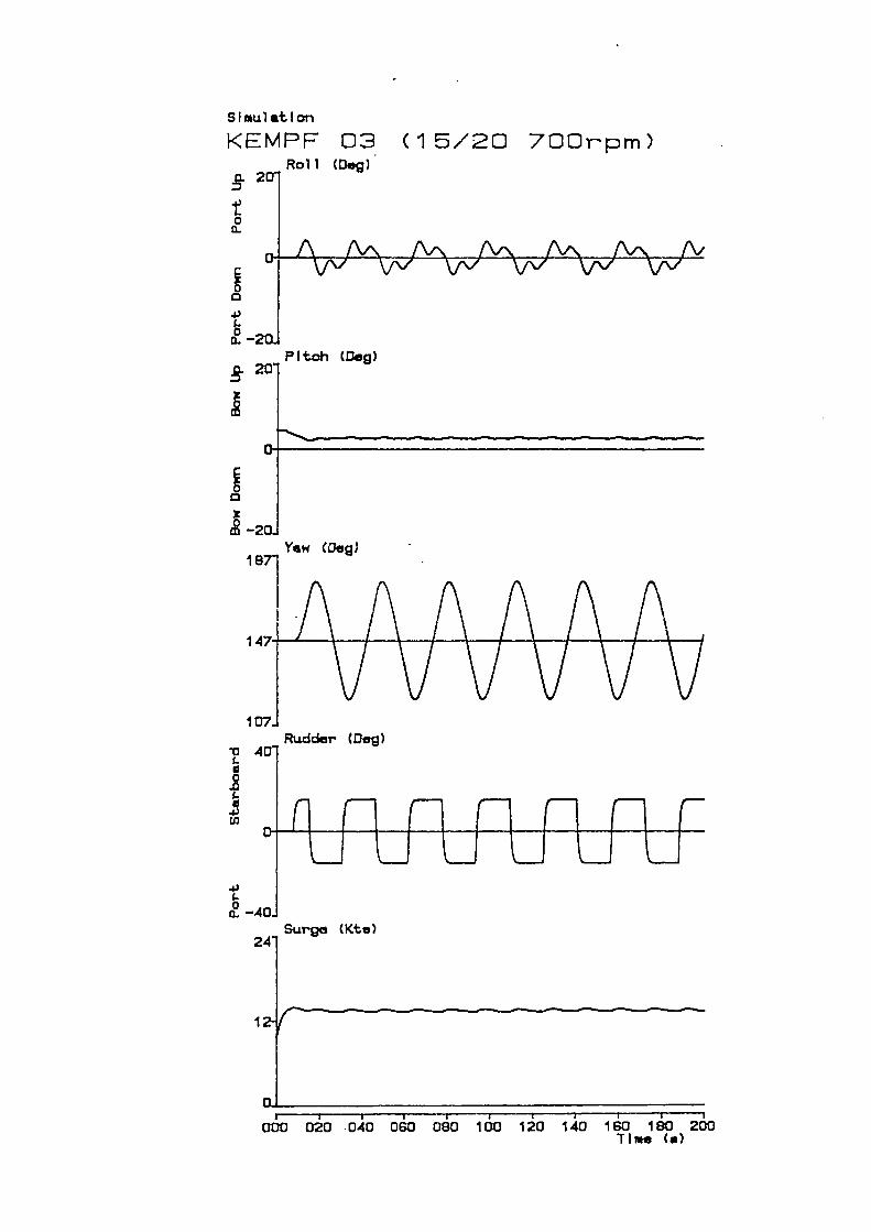
Pitch (D.&
Yew (Be& -
Rudder C0e)
Surge CKte)
d
2
Cl)
C-
0
0.
00
I
I
SImul*t ion
KEMPF 03 (15/20 700rpm)Roll (DQ)
I I I I I I I
000 020 . 040 060 080 100 120 140 160 180 200Time C.)
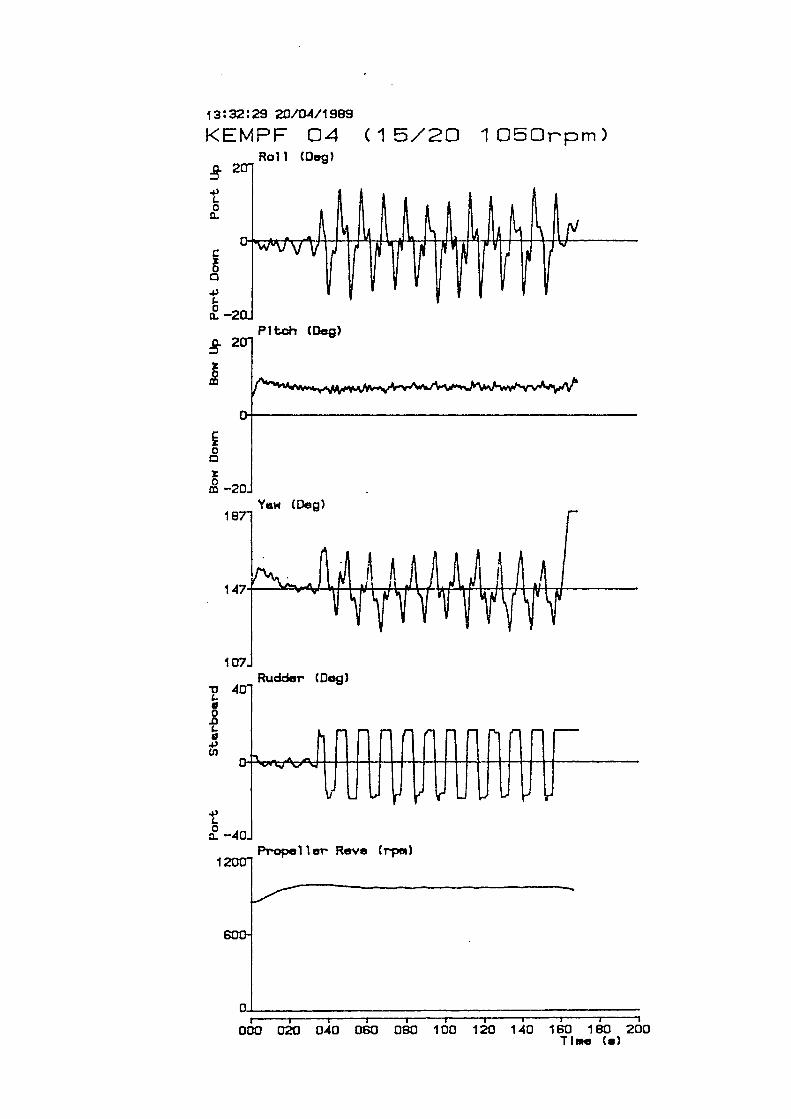
Propeller Rove (rpm)
13:32:29 2t3/04/19B9
KEMFF 04Roll CDe)
4,
0C-
C
43
0a-
Pitch (D.&
z
0
z0m
Yew (De&
I
IRudder CDog)
•g
C43U.,
43
0C-
I
(15/20 1050rpm)
I I I I I I I
000 020 040 060 080 100 120 140 160 180 200Time C.)
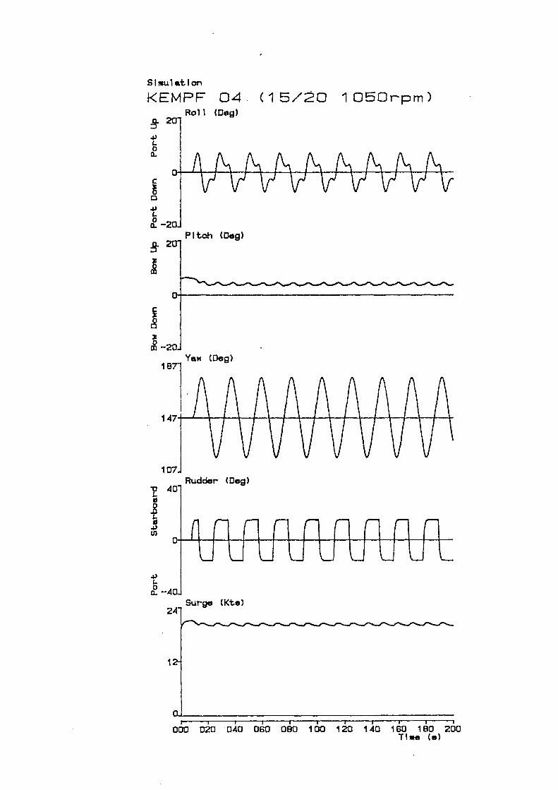
SI mu lst I on
KEMFF 04Rofl CDec)
4-,1-0a.
IPltoh (Deg)
Yew (Deg)1871
147
107Rudder CIJe)
I4.,
00
Suy-e (Kte)2
I
(15/20 1050rpm)
I -I I I I I I I
000 020 0.40 060 080 100 120 140 160 180 200TIme Ce)
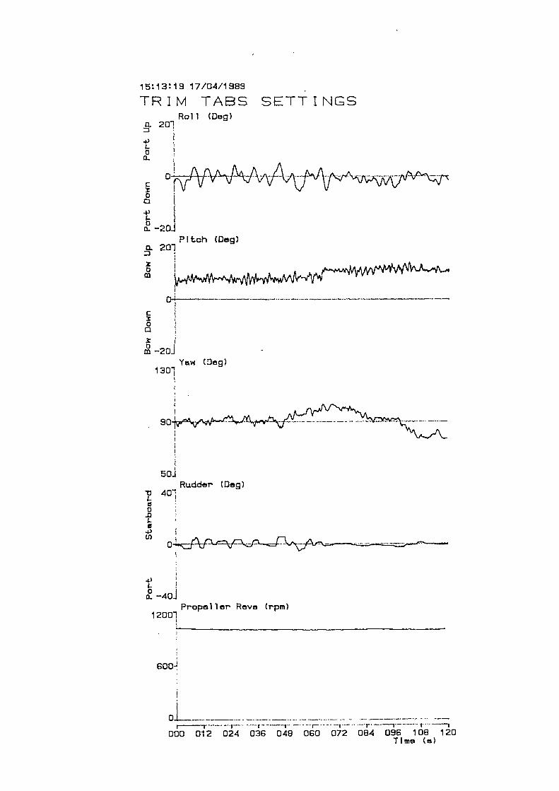
151319 17/04/1989
TRIM TABS SETTINGSRofl (Dog)
a 201
4)LC
a
4) ILan. -20
Pitch (Dog)%201
3:oa. &g. A.... &.
3:ao3: 1
f-20JYw (Dog)
1301
50]Rudder (Dog)
• 40
o
w
4)
0a. -40Propefler Rove (rpm)
12001
600-i
______........::;:;:: ;::.DOD 012 024 036 048 060 072 084 096 108 120
Time (e)
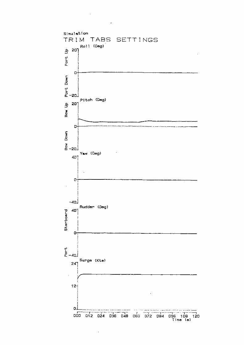
SImultt on
TRIM TABS SETTINGSRoll (Deg)
2O1
4)L0
0
a4)
00 -2
pitch (Deg)a20
0
C
0a
c -20JYw (Dog)
-4QjRudder (Dog)
J
4)!
0 -40jSurge (Kto)
241
1 2-
000 012 024 036 048r ------..........
080 072 084 096 108 120Time Ce)

APPENDIX C
DATA LOGGING INTERFACE
349
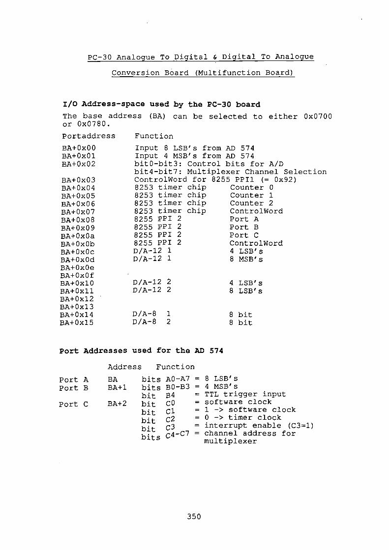
Port APort B
Port C
PC-30 Analogue To Digital & Digital To Analogue
Conversion Board (Multifunction Board
I/O Address-space used by the PC-30 board
The base address (BA) can be selected to either 0x0700or 0x0780.
Portaddress
BA+OxOOBA+OxOlBA+0x02
BA+0x03BA+0x04BA+ Ox 05BA+OxO 6BA+0x07BA+ Ox 08BA+OxO 9BA+ Ox 0 aBA+OxObBA+OxOcBA+OxOdBA+OxOeBA+OxOfBA+OxlOBA+ Ox 11BA+0x12BA+0x13BA+0x14BA+0x15
Function
Input 8 LSB's from AD 574Input 4 MSB's from AD 574bitO-bit3: Control bits for A/Dbit4-bit7: Multiplexer Channel SelectionControiWord for 8255 PPI1 (= Ox92)8253 timer chip Counter 08253 timer chip Counter 18253 timer chip Counter 28253 timer chip ControlWord8255 PPI 2 Port A8255 PPI 2 Port B8255 PPI 2 Port C8255 PPI 2 ControlWordD/A-12 1 4 LSB'sD/A-12 1 8 MSB's
D/A-12 2 4 LSB'sD/A-12 2 8 LSB's
D/A-8 1 8 bitD/A-8 2 8 bit
Port Addresses used for the AD 574
Address Function
BA bits AO-A7 = 8 LSB'sBA+1 bits BOB3 = 4 MSB'S
bit B4 = TTL trigger inputBA+2 bit CO = software clock
bit Cl = 1 -> software clock
bit c2 = 0 -> timer clock
bit c3 = interrupt enable (C3=1)
bits C4-C7 = channel address for
multiplexer
350
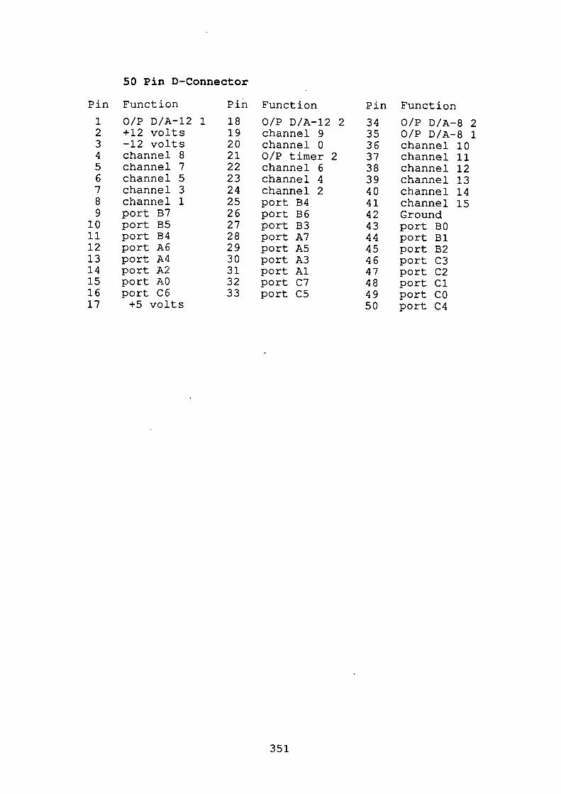
50 Pin D-Connector
Pin Function Pin Function Pin Function
123456789
1011121314151617
18192021222324252627282930313233
3435363738394041424344454647484950
0/P D/A-12 1+12 volts-12 voltschannel 8channel 7channel 5channel 3channel 1port B7port B5port B4port A6port A4port A2port AOport C6+5 volts
0/P D/A-12 2channel 9channel 00/P timer 2channel 6channel 4channel 2port B4port B6port B3port A7port A5port A3port Alport C7port C5
0/P D/A-8 20/P D/A-8 1channel 10channel 11channel 12channel 13channel 14channel 15Groundport EQport Elport E2port C3port C2port Clport COport C4
351
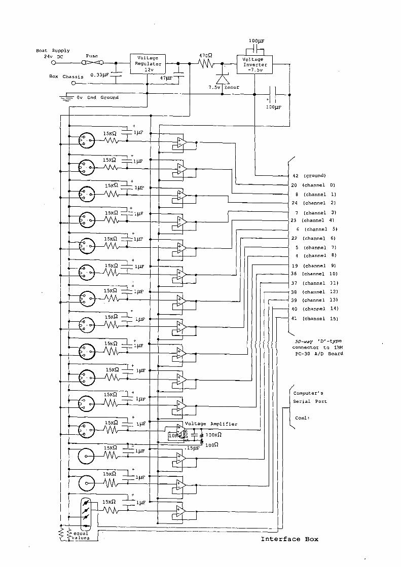
10 OIIF
2 (ground)
(channel 0)
8 (channel 1)
4 (channel 2)
7 (channel 3)
(channel 4)
6 (channel 5)
(channel 6)
5 (channel 7)
4 (channel 8)
9 (channel 9)
(channel 10)
(channel 1J)
(channel 2)
(channel 13)
(channel 14)
(channel 15)
5D-'ay 'D'-type
nnector to IBM
PC-30 A/D Board
:omputer' S
erjal Port
Cornl:
e Box
Boat24
F
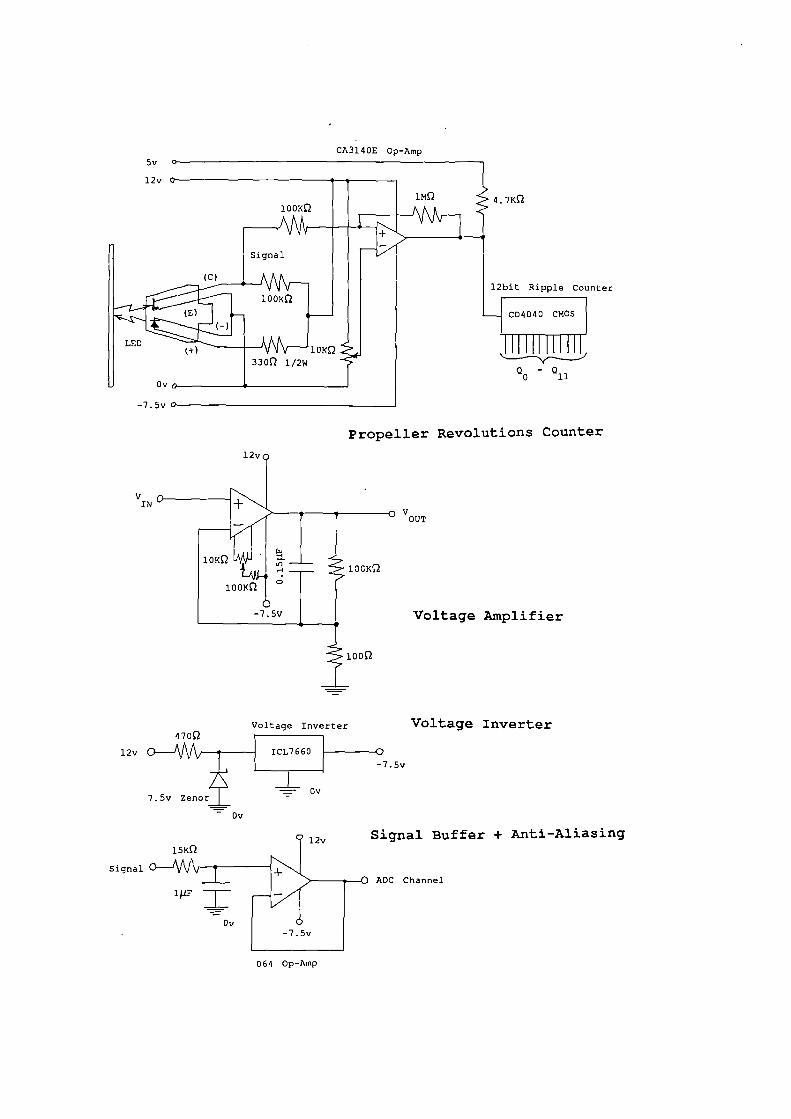
Inter
VOUT
Voltage Amplifier
VIN
CA314OE Op-Amp
Propeller Revolutions Counter
Voltage Inverter Voltage Inverter47O2
12v 1CL7660 p
__________ -7.5v
7.5v zenorjOv
- Dv
l2v Signal Buffer + Anti-Aliasing1 5KQ
Signal L)-_.'VVV_tADC Channel
1Iv-7. 5v
064 Op-Amp
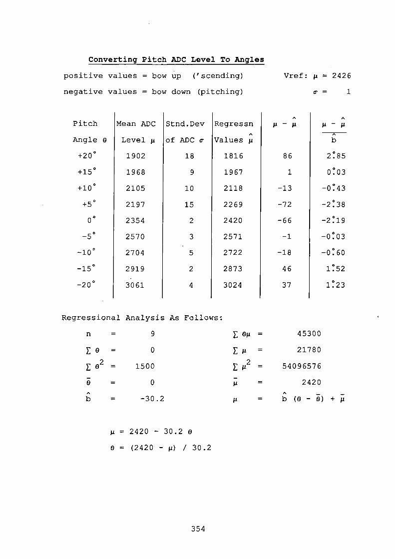
Converting Pitch ADC Level To Angles
positive values = bow up ('scending) Vref: i = 2426
negative values = bow down (pitching) =
A
P
86
1
-13
-72
-66
-1
-18
46
37
Pitch
Angle 0
+200
+15°
0+10
0+5
00
50
-10°
-15°
-20°
Mean ADC
Level ii
1902
1968
2105
2197
2354
2570
2704
2919
3061
Stnd.Dev
of ADC o-
18
9
10
15
2
3
5
2
4
Regressn
Values p
1816
1967
2118
2269
2420
2571
2722
2873
3024
A
ji- U
A
b
2:85
0:03
-0:43
-238
-2:19
-0:03
-060
1:52
1:23
Regressional Analysis As Follcws
n = 9
= 0
E°2 = 1500
= 0
b = -30.2
=
45300
= 21780
2 = 54096576
p=
2420
P =
(0 - ) +
= 2420 - 30.2 o
0 = ( 2420 - ii) / 30.2
354
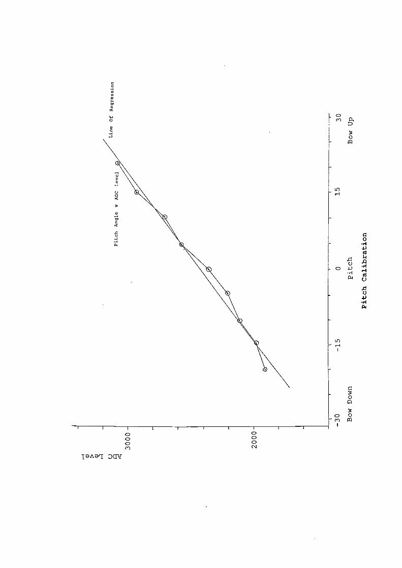
0 00 00 0
In
I 1 'I cr
0c,-) 0_I
0
Ii)'-I
0
ni
0
niC)
C)
•1-)
.rl
p4
In'-I
0
0 0
In
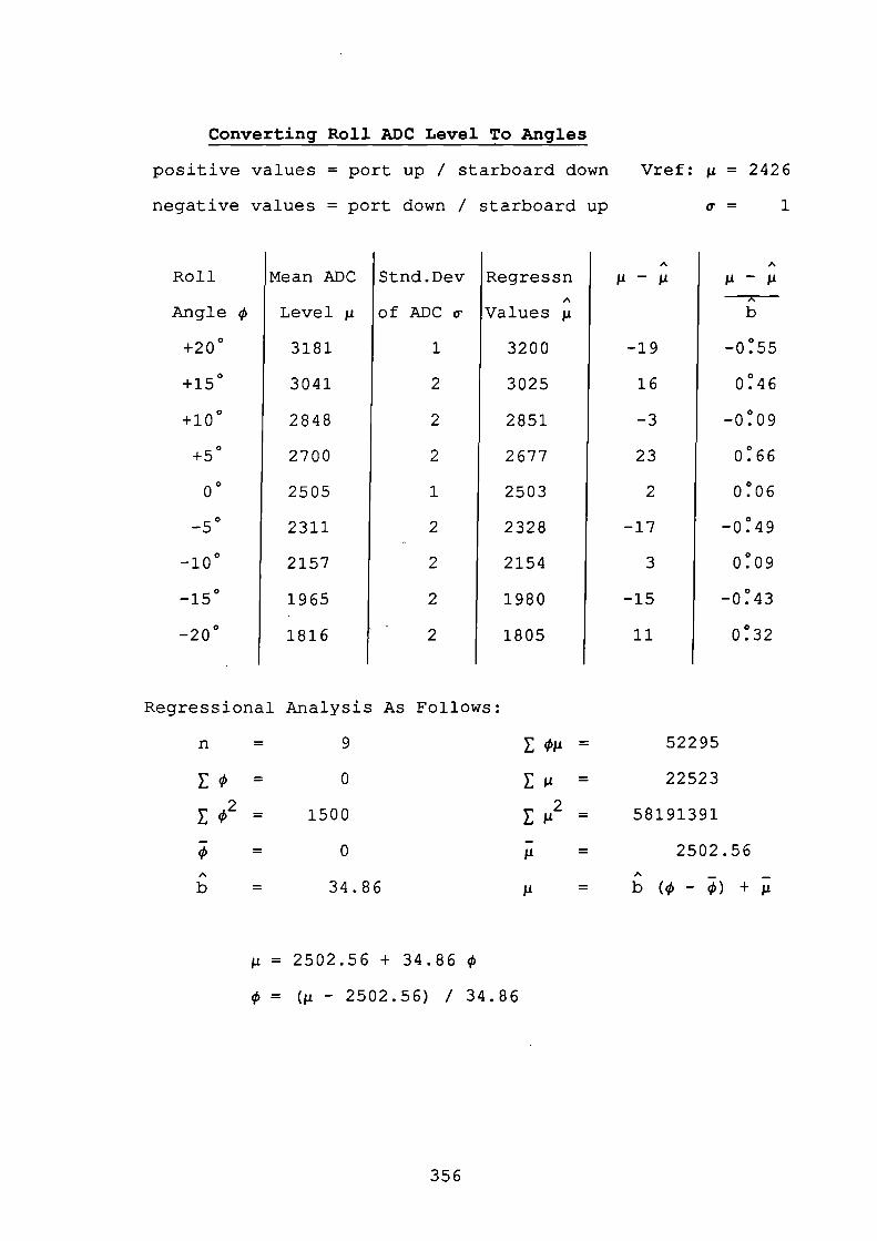
Converting Roll ADC Level To Angles
positive values = port up I starboard down Vref: = 2426
negative values = port down / starboard up a' =
A
-19
16
-3
23
2
-17
3
-15
11
Roll
Angle )
0+200
+150
+10
0+5
00
50
-10°
150
200
Mean ADC
Level ii
3181
3041
2848
2700
2505
2311
2157
1965
1816
Stnd.Dev
of ADC a'
1
2
2
2
1
2
2
2
2
Regressn
Values
3200
3025
2851
2677
2503
2328
2154
1980
1805
A
L A
A
b
-0:55
0:46
-009
0:66
006
-0:49
0:09
-0:43
0:32
Regressional Analysis As Follows:
n = 9
= 0
E 2 = 1500
= 0
b = 34.86
= 2502.56 + 34.86
= (ji - 2502.56) / 34.86
= 52295
= 22523
2 = 58191391
= 2502.56
= ( - ) +
356
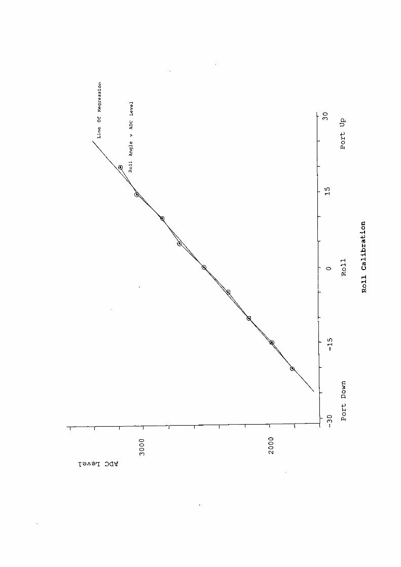
cv) N
0
If)'-I
0.rI4)
.rIr-r-
c C)
I-I
0
Lfl
4I
av
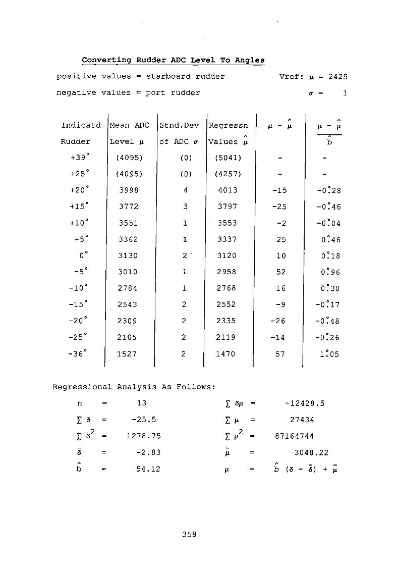
=
=
2 =
=
Ii =
-12428.5
27434
87164744
3048.22
- o) +
Converting Rudder ADC Level To Angles
positive values = starboard rudder Vref: = 2425
negative values = port rudder a- =
Indicatd
Rudder
0+39
0+25
0+20
0+15
0+10
0+5
0°
50
_100
-15°
-20°
-25°
-36°
Mean ADC
Level ii
(4095)
(4095)
3998
3772
3551
3362
3130
3010
2784
2543
2309
2105
1527
Stnd.Dev
of ADC a'
(0)
(0)
4
3
1
1
2
1
1
2
2
2
2
Regressn
Values ,i
(5041)
(4257)
4013
3797
3553
3337
3120
2958
2768
2552
2335
2119
1470
A
11-Il
-15
-25
-2
25
10
52
16
-9
-26
-14
57
A
'i-IlA
b
-028
-046
-0:04
0:46
018
096
0:30
-017
-0:48
-0:26
1:05
Regressional Analysis As Follows:
n = 13
= -25.5
E 2 = 1278.75
= -2.83A
b = 54.12
358
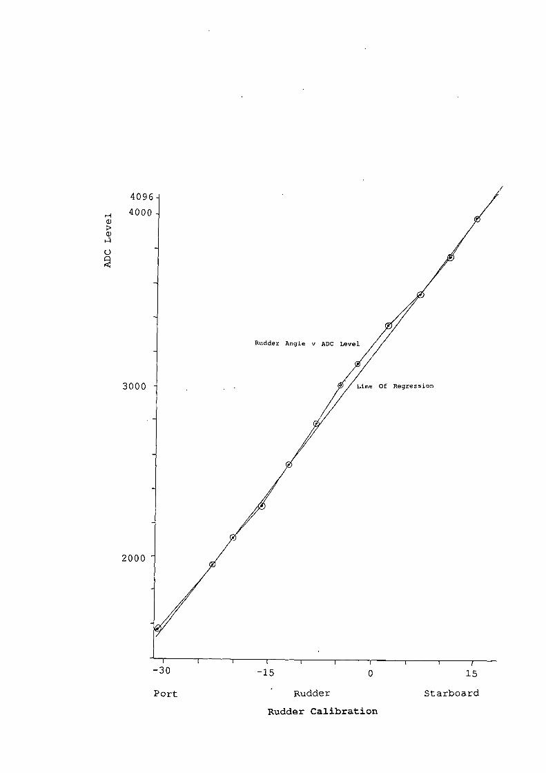
4O9
,-. 400(
a)
0
3000
2000
-30 -15 0 15
Port Rudder Starboard
Rudder Calibration
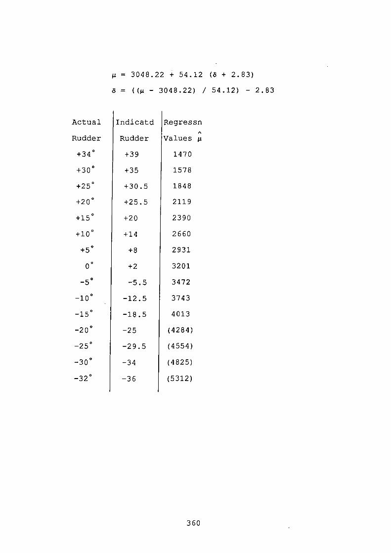
= 3048.22 + 54.12 (45 + 2.83)
= ((.t - 3048.22) / 54.12) - 2.83
Actual
Rudder
0+34
0+30
0+25
0+20
0+15
0+10
+5°
0°
50
_100
150
-20°
-25°
-30°
-32°
Indicatd
Rudder
+39
+35
+30.5
+25.5
+20
+14
+8
+2
-5.5
-12.5
-18.5
-25
-29.5
-34
-36
Regressn
Values i
1470
1578
1848
2119
2390
2660
2931
3201
3472
3743
4013
(4284)
(4554)
(4825)
(5312)
360
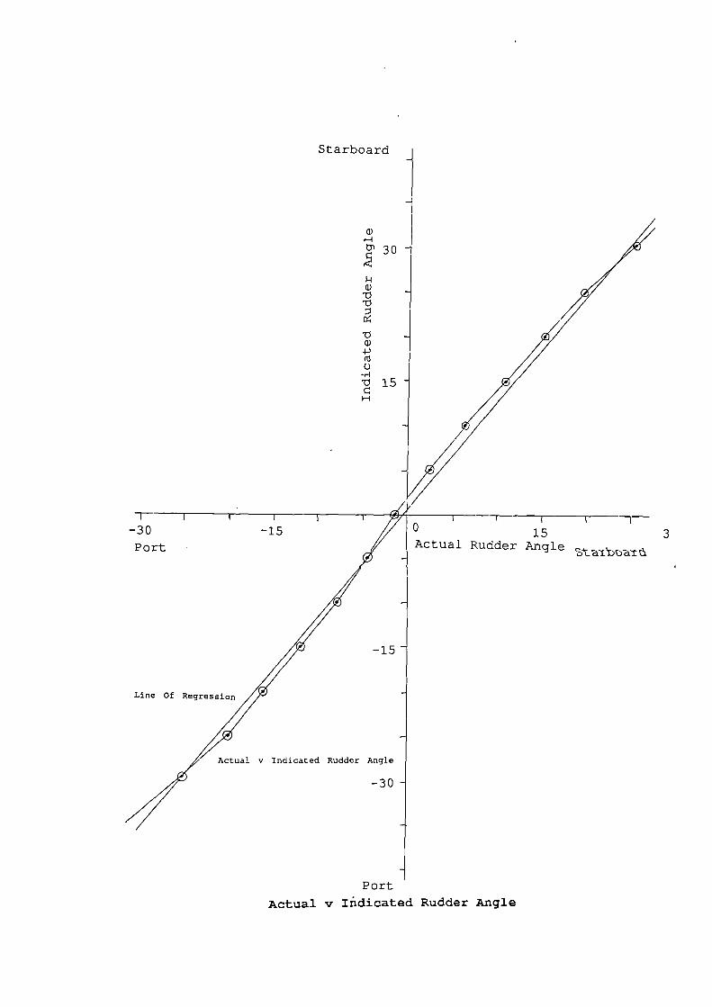
- -i- - - -- -,
PortActual v Indicated Rudder Angle

APPENDIX D
GLOSSARY
'I g he wou&L erp&iLn liLA exp&matLon"
Lord Byron
362
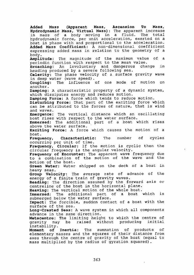
Added Mass (Apparent Mass, Ascension To Mass,Hydrodynainic Mass, Virtual Mass.): The apparent increasein mass of a body moving in a fluid. The totalhydrodynamic force, per unit acceleration, exerted on aboat in phase with and proportional to the acceleration.Added Mass Coefficient: A non-dimensional coefficientexpressing added mass in relation to the geometry of abody.Amplitude: The magnitude of the maximum value of aperiodic function with respect to the mean value.Broaching: An involuntary and dangerous change inheading produced by a severe following sea.Celerity: The phase velocity of a surface gravity wavein deep water (wave speed).Coupling: The influence of one mode of motion onanother.Damping: A characteristic property of a dynamic system,which dissipates energy and reduces motion.Damping Force: A force which tends to reduce motion.Disturbing Force: That part of the exciting force whichcan be attributed to the forces of nature, that is windand waves.Emergence: The vertical distance which an oscillatingboat rises with respect to the water surface.Emmersed: The additional part of a boat which risesabove the water surface.Exciting Force: A force which causes the motion of aboat.Frequency, Characteristic: The number of cyclesoccurring per unit of time.Frequency, Circular: If the motion is cyclic then thecircular frequency is the angular velocity.Frequency of Encounter: The apparent wave frequency dueto a combination of the motion of the wave and themotion of the boat.Green Water: Water shipped on the deck of a boat inheavy seas.Group Velocity: The average rate of advance of theenergy of a finite train of gravity waves.Heading: The direction assumed by the forward axis orcentreline of the boat in the horizontal plane.Heaving: The vertical motion of the whole boat.Immersed: The additional part of a boat which issubmerged below the water surface.Impact: The forcible, sudden contact of a boat with thesurface of the sea.Long-Crested Seas: A wave system in which all componentsadvance in the same direction.Metacentre: The limiting height to which the centre ofgravity may be raised without producing initialinstability.Moment of Inertia: The summation of products ofelementary masses and the squares of their distance fromaxes through the centre of gravity of the boat (equal tomass multiplied by the radius of gyration squared).
363
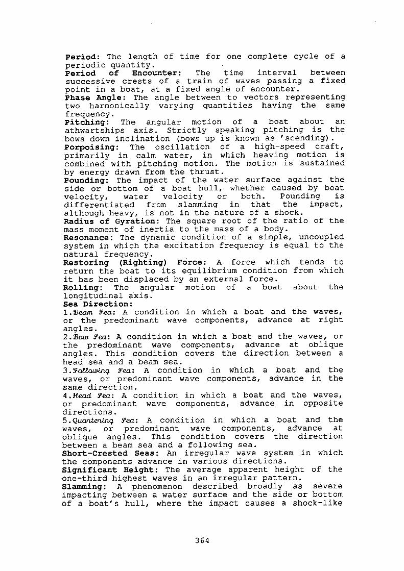
Period: The length of time for one complete cycle of aperiodic quantity.Period of Encounter: The time interval betweensuccessive crests of a train of waves passing a fixedpoint in a boat, at a fixed angle of encounter.Phase Angle: The angle between to vectors representingtwo harmonically varying quantities having the samefrequency.Pitching: The angular motion of a boat about anathwartships axis. Strictly speaking pitching is thebows down inclination (bows up is known as 'scending).Porpoising: The oscillation of a high-speed craft,primarily in calm water, in which heaving motion iscombined with pitching motion. The motion is sustainedby energy drawn from the thrust.Pounding: The impact of the water surface against theside or bottom of a boat hull, whether caused by boatvelocity, water velocity or both. Pounding isdifferentiated from slamming in that the impact,although heavy, is not in the nature of a shock.Radius of Gyration: The square root of the ratio of themass moment of inertia to the mass of a body.Resonance: The dynamic condition of a simple, uncoupledsystem in which the excitation frequency is equal to thenatural frequency.Restoring (Righting) Force: A force which tends toreturn the boat to its equilibrium condition from whichit has been displaced by an external force.Rolling: The angular motion of a boat about thelongitudinal axis.Sea Direction:l.ewn 5°ea: A condition in which a boat and the waves,or the predominant wave components, advance at rightangles.2.ow 5°ea: A condition in which a boat and the waves, orthe predominant wave components, advance at obliqueangles. This condition covers the direction between ahead sea and a beam sea.3.zWwii 5Fea: A condition in which a boat and thewaves, or predominant wave components, advance in thesame direction.4Jead °ea: A condition in which a boat and the waves,or predominant wave components, advance in oppositedirections.5.Qua1Lterthq 5°ea: A condition in which a boat and thewaves, or predominant wave components, advance atoblique angles. This condition covers the directionbetween a beam sea and a following sea.Short-Crested Seas: An irregular wave system in whichthe components advance in various directions.Significant Height: The average apparent height of theone-third highest waves in an irregular pattern.Slamming: A phenomenon described broadly as severeimpacting between a water surface and the side or bottomof a boat's hull, where the impact causes a shock-like
364
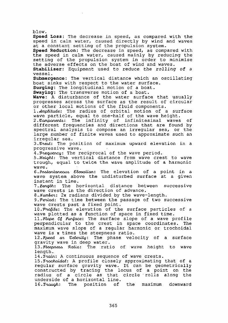
blow.Speed Loss: The decrease in speed, as compared with thespeed in calm water, caused directly by wind and wavesat a constant setting of the propulsion system.Speed Reduction: The decrease in speed, as compared withthe speed in calm water, caused mainly by reducing thesetting of the propulsion system in order to minimisethe adverse effects on the boat of wind and waves.Stabiliser: Equipment used to reduce the rolling of avessel.Submergence: The vertical distance which an oscillatingboat sinks with respect to the water surface.Surging: The longitudinal motion of a boat.Swaying: The transverse motion of a boat.Wave: A disturbance of the water surface that usuallyprogresses across the surface as the result of circularor other local motions of the fluid components.l.4mpWucLe: The radius of orbital motion of a surfacewave particle, equal to one-half of the wave height.2.omponen: The infinity of infinitesimal waves ofdifferent frequencies and directions that are found byspectral analysis to compose an irregular sea, or thelarge number of finite waves used to approximate such anirregular sea.3. r ,etit: The position of maximum upward elevation in aprogressive wave. -4.&½equenc: The reciprocal of the wave period.5.3eLqht: The vertical distance from wave crest to wavetrough, equal to twice the wave amplitude of a harmonicwave.6. gna,.tweau Ge&ion: The elevation of a point in awave system above the undisturbed surface at a giveninstant in time.7.Senqth: The horizontal distance between successivewave crests in the direction of advance.8.Nwn&ert: 2ir radians divided by the wave-length.9.PeriLad: The time between the passage of two successivewave crests past a fixed point.lO.ru4Ue: The elevation of the surface particles of awave plotted as a function of space in fixed time.11.5°&pe O 5"wiace: The surface slope of a wave profileperpendicular to the crest in space coordinates. Themaximum wave slope of a regular harmonic or trochoidalwave is it times the steepness ratio.l2.9'peed on eerut: The phase velocity of a surfacegravity wave in deep water.13..fleepne atLo: The ratio of wave height to wavelength.l4.Tno.Jji: A continuous sequence of wave crests.l5.7rocIckz: A profile closely approximating that of aregular surface gravity wave. It can be geometricallyconstructed by tracing the locus of a point on theradius of a circle as that circle rolls along theunderside of a horizontal line.l6.1ruwqh: The position of the maximum downward
365

elevation in a progressive wave.Wetness: The quality of a boat's decking with respect toits likelihood of being wet as a result of motions ofthe boat and waves.Yawing: The angular motion of a boat about a verticalaxis.
366

APPENDIX E
NOMENCLATURE
367
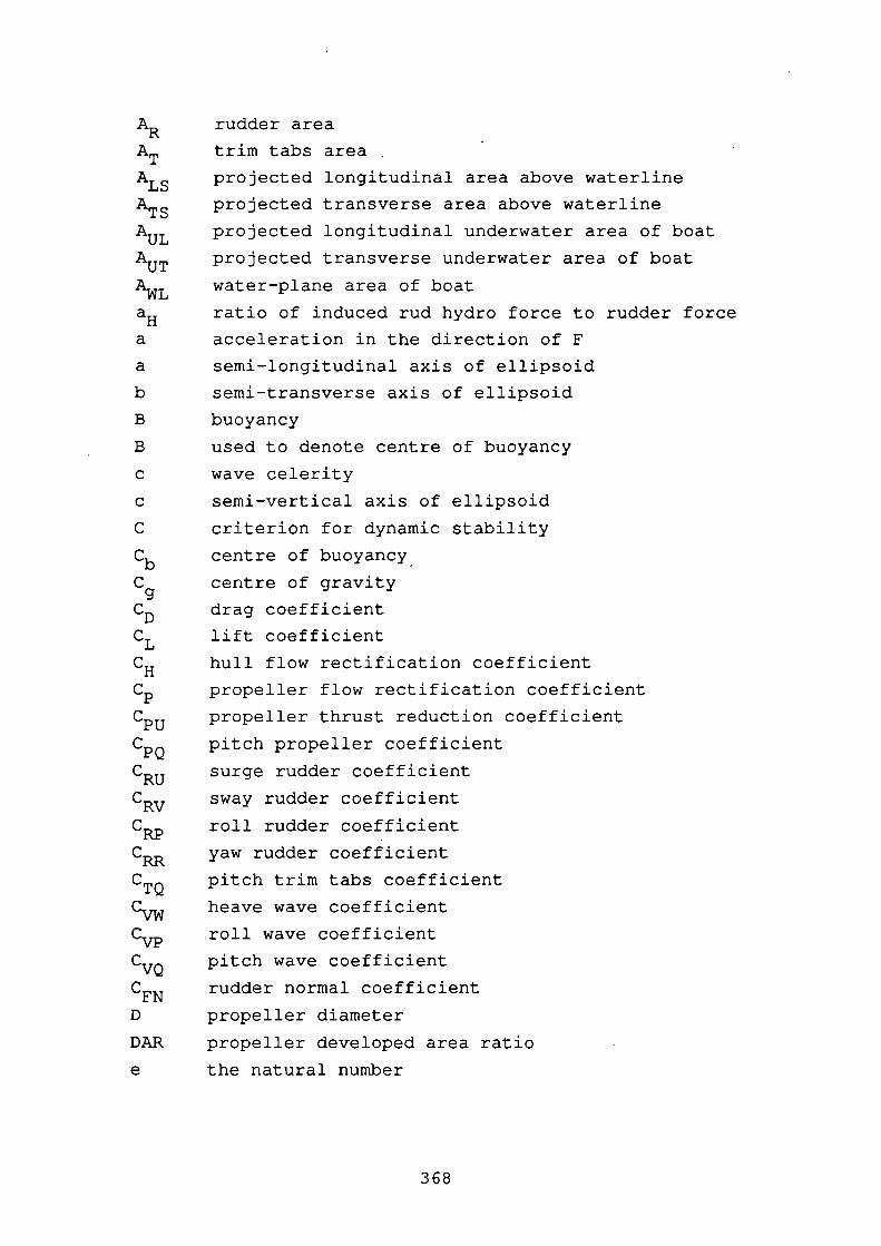
AR rudder area
AT trim tabs area
AL S projected longitudinal area above waterline
AT S projected transverse area above waterline
AUL projected longitudinal underwater area of boat
AUT projected transverse underwater area of boat
AWL water-plane area of boat
aH ratio of induced rud hydro force to rudder force
a acceleration in the direction of F
a semi-longitudinal axis of ellipsoid
b
semi-transverse axis of ellipsoid
B
buoyancy
B
used to denote centre of buoyancy
C wave celerity
C semi-vertical axis of ellipsoid
C
criterion for dynamic stability
Cb centre of buoyancy
Cg centre of gravity
CD drag coefficient
CL lift coefficient
CH hull flow rectification coefficient
CP propeller flow rectification coefficient
CPU propeller thrust reduction coefficient
CpQ pitch propeller coefficient
CRU surge rudder coefficient
CRy sway rudder coefficient
roll rudder coefficient
yaw rudder coefficient
CTQ pitch trim tabs coefficient
heave wave coefficient
CvP roll wave coefficient
Cv0 pitch wave coefficient
CFN rudder normal coefficient
D
propeller diameter
DAR
propeller developed area ratio
e
the natural number
368
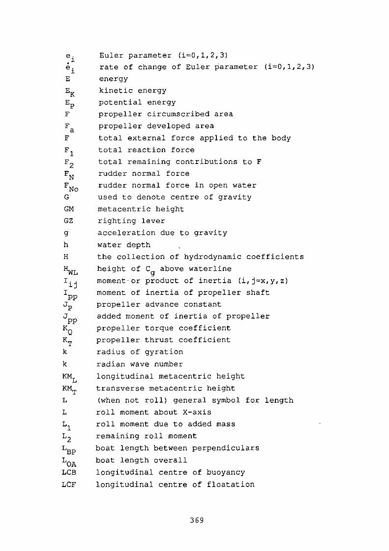
e.1e.1E
EKE
F
Fa
F
F1
F2
FNFNoG
GM
GZ
g
h
H
HWLI.1JIpp
Jp
Jpp
KQ
KTk
k
KML
KMTL
L
L1
L2
LEP
LOALCB
LCF
Euler parameter (i=O,1,2,3)
rate of change of Euler parameter (i=O,1,2,3)
energy
kinetic energy
potential energy
propeller circumscribed area
propeller developed area
total external force applied to the body
total reaction force
total remaining contributions to F
rudder normal force
rudder normal force in open water
used to denote centre of gravity
metacentric height
righting lever
acceleration due to gravity
water depth
the collection of hydrodynamic coefficients
height of Cg above waterline
moment or product of inertia (i,j=x,y,z)
moment of inertia of propeller shaft
propeller advance constant
added moment of inertia of propeller
propeller torque coefficient
propeller thrust coefficient
radius of gyration
radian wave number
longitudinal metacentric height
transverse metacentric height
(when not roll) general symbol for length
roll moment about X-axis
roll moment due to added mass
remaining roll moment
boat length between perpendiculars
boat length overall
longitudinal centre of buoyancy
longitudinal centre of floatation
369
M used to denote metacentre
M pitch moment about Y-axis
pitch moment due to added mass
M2remaining pitch moment
m mass of boat
rn mass of displaced fluid
MCT l' moment to change trim 1 inch
N yaw moment about Z-axis
Ni yaw moment due to added mass
N2remaining yaw moment
n number of propeller revolutions
rate of change of propeller revolutions
demanded propeller revolutions
1max maximum number of propeller revolutions
p roll angular velocity about X-axis
roll angular acceleration about X-axis
P propeller pitch
PQpropeller torque
propeller thrust
engine torque -
Emax maximum engine torque
q pitch angular velocity about Y-axis
4 pitch angular acceleration about Y-axis
r yaw angular velocity about Z-axis
yaw angular acceleration about Z-axis
Re Reynold's number
s propeller slip-stream ratio
T period
T period of encounter
t time
TPI tons per inch immersion
u surge velocity directed along X-axis
surge acceleration directed along X-axis
Ur relative fluid velocity along X-axis
u5fluid velocity directed along , X-axis
fluid acceleration directed along X-axis
V boat's horizontal velocity
370
VbV
VVrVE
VNVP
VR
VTVwV
V
VrV
SV
Sw
w
w
wP
WRwrw
wS
x
xl
x2
x
Xb
xg
xP
XR
XT
Y
Yl
y
Yg
horizontal speed of boat
speed of wave
relative wave velocity
easterly velocity component
northerly velocity component
propeller inflow velocity
rudder inflow velocity
trim tabs inflow velocity
wind velocity
sway velocity directed along Y-axis
sway acceleration directed along Y-axis
relative fluid velocity along Y-axis
fluid velocity directed along Y-axis
fluid acceleration directed along Y-axis
weight
heave velocity directed along Z-axis
heave acceleration directed along Z-axis
propeller wake fraction
rudder wake fraction
relative fluid velocity along Z-axis
fluid velocity directed along Z-axis
fluid acceleration directed along Z-axis
surge force directed Long X-axs
surge force due to added mass
remaining surge force
distance along X-axis
x coordinate of centre of buoyancy
x coordinate of centre of gravity
x coordinate of propellers
x coordinate of rudder centre of effect
x coordinate of trim tabs
sway force directed along Y-axis
sway force due to added mass
remaining sway force
distance along Y-axis
y coordinate of centre of buoyancy
y coordinate of centre of gravity
37].
y y coordinate of propellers
y coordinate ofrudder centre of effect
y coordinate of trim tabs
Z heave force directed along Z-axis
Z 1 heave force due to added mass
Z 2 remaining heave force
z distance along Z-axis
Zb z coordinate of centre of buoyancy
Z g z coordinate of centre of gravity
z, z coordinate of propellers
ZR z coordinate of rudder centre of effect
ZT Z coordinate of trim tabs
a effective rudder inflow angle
a wave slope
a0 ellipsoid numerical constant
aR effective rudder inflow angle
aT angle of deflectiçn of the trim tabs
direction of boat motion w.r.t. its centreline
ellipsoid numerical constant
absolute wave direction
•1 absolute wind direction
flow rectification coefficient
surface tension
ellipsoid numerical constant
F rudder aspect ratio
FT trim tabs aspect ratio
rudder angle
rate of change of rudder angle
demanded rudder angle
rudder error (demanded - actual)
max maximum rudder angle (rudder limit)
dir rudder direction (port/starboard/stop)
displacement of boat
C change of inflow angle due to hull and propeller
wave amplitude
instantaneous wave elevation
7) propeller diameter to rudder height ratio
372
e
A.1J
AVV
it
Pi
tfl
r
xi
'II
'4,
(4,
V
V
angle of pitch
direction cosine (i,j=1,2,3)
wavelength
a rudder inflow rectification angle
mathematical constant
water density
air density
propeller time constant
rudder time constant
trim tabs time constant
angle of roll
gravitational potential
components of the velocity potential (1=1,2,3)
components of the velocity potential (1=1,2,3)
angle of yaw (heading)
demanded heading
heading error (demanded - actual)
circular frequency or general angular velocity
general angular acceleration
wave encounter frequency
underwater volume of the boat
the Del operator
373

APPENDIX F
CONVERSION TABLE
374
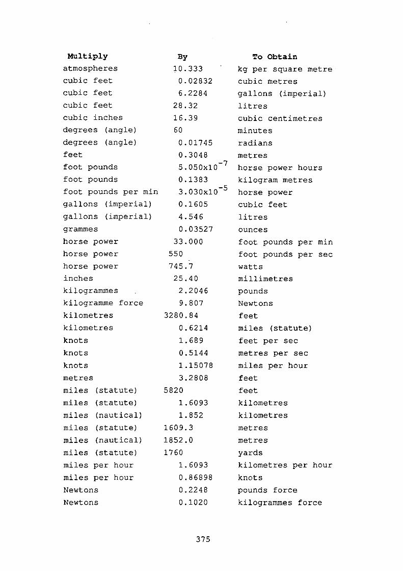
Multiplyatmospheres
cubic feet
cubic feet
cubic feet
cubic inches
degrees (angle)
degrees (angle)
feet
foot pounds
foot pounds
foot pounds per mm
gallons (imperial)
gallons (imperial)
gramme s
horse power
horse power
horse power
inches
kilogrammes
kilogramme force
kilometres
kilometres
knots
knots
knots
metres
miles (statute)
miles (statute)
miles (nautical)
miles (statute)
miles (nautical)
miles (statute)
miles per hour
miles per hour
Newtons
Newtons
By
10.333
0.02832
6.2284
28 .32
16.39
60
0.01745
0.3048
5. 050x107
0.1383
3. 030x105
0.1605
4.546
0.03527
33.000
550
745.7
25.40
2.2046
9.807
3280. 84
0. 6214
1.689
0.5144
1 . 15078
3. 2808
5820
1.6093
1.852
1609.3
1852.0
1760
1 . 6093
0.86898
0.2248
0.1020
To Obtainkg per square metre'
cubic metres
gallons (imperial)
litres
cubic centimetres
minutes
radians
metres
horse power hours
kilogram metres
horse power
cubic feet
litres
ounces
foot pounds per mm
foot pounds per sec
watts
millimetres
pounds
Newtons
feet
miles (statute)
feet per sec
metres per sec
miles per hour
feet
feet
kilometres
kilometres
metres
metres
yards
kilometres per hour
knots
pounds force
kilogramnies force
375
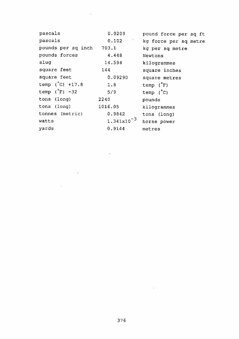
pascals
pascals
pounds per sq inch
pounds forces
slug
square feet
square feet
temp (°C) +17.8
temp (°F) -32
tons (long)
tons (long)
tonnes (metric)
watts
yards
0.0209
0.102
703.1
4.448
14.594
144
0.09290
1.8
5/9
2240
1016.05
0.9842
1. 341x103
0.9144
pound force per sq ft
kg force per sq metre
kg per sq metre
Newtons
kilogrammes
square inches
square metres
temp (°F)
temp (°C)
pounds
kilogrammes
tons (long)
horse power
metres
376

APPENDIX G
REFERENCES
377
COEFFICIENTS INDURING REGULAR
72p, November
1) Aage,C.'WIND COEFFICIENTS FOR NINE SHIP MODELS'Hydro & Aerodynamics Laboratory, Report No. A-3,l4p , Danish Technical Press, May 1971.
2) Abkowitz,M.A.'LECTURES ON SHIP HYDRODYNAMICS - STEERING ANDMANOEUVRABILITY'Hydro-og Aerodynamisk Laboratorium, Lyngby,Denmark, Report No. Hy-5, 1964.
3) Abkowitz,M.A.(Dept. Ocean Engineering, MIT, USA)'ROLL DAMPING AT FORWARD SPEED'Proc. 20th ATTC General Meeting, Vol. 2,pp1065-1078, SIT, Hoboken, New Jersey, USA, 2nd-4thAugust 1983.
4) Abkowitz,M.A.(Dept. Ocean Engineering, MIT, USA)'MEASUREMENT OF SHIP HYDRODYNAMICMANOEUVRING FROM SIMPLE TRIALSOPERATIONS'Final Report No. MA-RD-760-84026,1984.
5) van Amerongen,J.; Udink ten Cate,A.J.(Control Engineering Lab., Dept. ElectricalEngineering, DUT, NL)'MODEL REFERENCE ADAPTIVE AUTOPILOTS FOR SHIPS'Automatica, Vol. 11, No. 5, pp441-449, September197.5.
6) van Amerongen,J.; de Keizer,C.; Verhage,W.(Control Engineering Lab., Dept. ElectricalEngineering, DUT, NL & Royal Netherlands NavalCollege, Den Helder, NL)MEASUREMENTS OF THE SPEED OF SHIPS USING AUTOMATEDSNELLIUS METHOD'ISP, Vol. 24, No. 273, pp122-l28, May 1977.
7) van Amerongen,J.; van Nauta Lemke,H.R.;van der Veen,J.C.T.(Control Engineering Lab., Dept. ElectricalEngineering, DUT, NL)'AUTOPILOT FOR SHIPS DESIGNED WITH FUZZY SETS'Proc. 5th IFAC/IFIP Int. Conf. on Digital ComputerApplications To Process Control, pp479-487, TheHague, NL, l4th-l7th June 1977.
378
8) van Amerongen,J.(Control Engineering Lab.,Engineering, DUT, NL)'MODEL REFERENCE ADAPTIVESTEERING OF SHIPS
Dept. Electrical
CONTROL APPLIED TO
Proc. mt. Symp. on Methods And Applications InAdaptive Control, pp199-208, Bochum, Germany,2Oth-2lst March 1980.
9) van Amerongen,J.(Control Engineering Lab., Dept. ElectricalEngineering, DUT, NL)'DIGITAL MODEL REFERENCE ADAPTIVE CONTROL WITHAPPLICATIONS TO SHIPS STEERING'Proc. 6th IFAC/IFIP mt. Conf. on Digital ComputerApplications To Process Control, pp245-250,Duesseldorf, West Germany, l4th-l7th October 1980.
10) van Amerongen,J.; de Goeij,W.F.; Moraal,J.M.;Ort,J.W.; Postuma,A.(Control Engineering Lab., Dept. ElectricalEngineering, DUT, NL)'MEASURING THE STEERING PERFORMANCE OF SHIPS DURINGFULL-SCALE TRIALS AND MODEL TESTS'Proc. Ship Steering Automatic Control Symp.,Genova, Italy, 25th-27th June 1980. [also: ISP,Vol. 28, No. 320, pp83-89, April 1981]
11) van Amerongen,J.(Control Engineering Lab., Dept. ElectricalEngineering, DUT, NL)'ADAPTIVE STEERING OF SHIPS - A MODEL REFERENCEAPPROACH'Automatica, Vol. 20, No. 1, pp3-14, 1984.
12) van Amerongen,1L; ?ioogenraad,?.v.;van Nauta Lemke,H.R.(Control Engineering Lab., Dept. ElectricalEngineering, DUT, NL & Royal Netherlands Navy)'ESTIMATING THE WAVE SPECTRUM AND THE ROLL ANGLEAND ITS DERIVATIVES WITH AN EXTENDED KALMAN FILTER'Proc. 7th Ship Control Symp., pp4-73 to 4-85, Bath,UK, September 1984.
13) van Amerongen,J.; van der Klugt,P.G.M.(Control Engineering Lab., Dept. ElectricalEngineering, DUT & van Rietschoten and Houwens by.,NL)'MODELING AND SIMULATION OF THE ROLL MOTIONS OF ASHIP'Proc. 1st Intercontinental Symp. on MaritimeSimulation, ppl6l-174, Munich, June 1985.
379
14) Ankudinov,V.K.; Miller,E.R.; Alman,P..R.;Jakobsen, B. K.(Tracor Hydronautics Inc.)'SHIP MANOEUVRABILITY ASSESSMENT IN SHIP DESIGN -SIMULATION CONCEPT'Proc. Int. Conf. on Ship Manoeuvrability, Paper No.19, 29th April - 1st May 1987.
15) Arie,T.; Itoh,M.; Senoh,A.; Takahashi,N.; Fujii,S.;Mizuno, N.(Systems and Control Research Centre, Nippon Kokan& Yokogawa Hokushin Electric Corporation & Dept. ofMechanical Engineering, Nagoya Institute ofTechnology, Japan)'AN ADAPTIVE SHIP'S AUTOMATIC STEERING SYSTEM BASEDON HILL-CLIMBING TECHNIQUE AND MODEL REFERENCEADAPTIVE CONTROL'Proc. IECON '85, Int. Conf. on Ind. Elect., Vol. 1,p405-410, 1985.
16) Asinovsky,V.'ON MANOEUVRABILITY CRITERION FOR DETERMINING SHIPRESPONSE TO RUDDER ANGLE CHANGE'SNAME, 17th May 1983.
17) Asinovsky,V.; Landsburg,A.C.; Hagen,G.R.(J.J.McMullen Associates Inc. & MaritimeAdministration, Dept. of Transportation & Designersand Planners Inc.)'SHIP MANOEUVRABILITY ANALYSIS USING THEDIFFERENTIAL APPROACH'Proc. Int. Conf. on Ship Manoeuvrability, Paper No.9, 29th April - 1st May 1989.
18) Baba,E.; Asai,S.; Toki,N.(Mitsubishi Heavy Industries Ltd., Japan)'A SIMULATION STUDY ON SWAY-ROLL-YAW COUPLEDINSTABILITY OF SEMI-DISPLACEMENT TYPE HIGH SPEEDCRAFT'Proc. 2nd mt. Conf. on Stability Of Ships AndOcean Vehicles, pp79-90, Tokyo, October 1982.
19) Bailey,D.(NMI, UK)'THE NPL HIGH SPEED ROUND BILGE DISPLACEMENT HULLSERIES'Maritime Technology Monograph No. 4, 1976.
20) Baker,D.W.; Patterson,C.L.jnr(US Naval Ship Research and Development Laboratory,Annapolis, Maryland, USA)'SOME RECENT DEVELOPMENTS IN REPRESENTING PROPELLERCHARACTERISTICS'Proc. 2nd Ship Control Systems Symp., ppAP-A-1 toAP-A-33, Annapolis, Maryland, USA, 1969.
380
21) Barr,R.A.(N.F.K. Engineering)'ESTIMATION OF SHIP MANOEUVRABILITY USING SHIPTRIALS DATA BASES'Proc. mt. Conf. on Ship Nanoeuvrability, Paper No.7, 29th April - 1st May 1989.
22) Barratt,M.J.'THE ADDED MASS OF BERTHING SHIPS'NMI Report No. R117, September 1981.
23) Bech,M.I.; Wagner Smitt,L.'ANALOGUE SIMULATION OF SHIP MANOEUVRES'Hydro & Aerodynamics Laboratory, Report No. Hy-14,19p, September 1969.
24) Bech,M.I.; Chislett,M.S.(Consultant Engineer & Danish Ship Research Lab.,Denmark)'STATISTICAL INVESTIGATION OF THE INVARIANTCOEFFICIENTS OF THE SHIPS EQUATION OF RESPONSE TOSTEERING'Proc. Ship Steering Automatic Control Symp.,ppl53-169, Genova, Italy, 25th-27th June 1980.
25) Berg,T.E.; Flobakk,T.(Assistant Professor, Division of MarineHydrodynamics, The Norwegian Institute ofTechnology & Research Engineer, NorwegianHydrodynamic Laboratories, Trondheim, Norway)'DETERNINATION OF COEFFICIENTS IN THE MANOEUVRINGEQUATIONS OF SHIPS'NMR, Vol. 4, pp2-ll, 1979.
26) Bhattacharyya, R.(Director of Naval Architecture, US Naval Academy,Annapolis, Maryland, USA)'DYNAMICS OF MARINE VEHICLES'Pubir. John Wiley & Sons, New York, 1978.
27) Birbanescu-Biran,A.(Faculty of Mechanical Engineering, Technion,Haifa, Israel)'DISTRIBUTION FUNCTIONS OF MASS PROPERTIES: A TOOLFOR NAVAL ARCHITECTURE'JSR, Vol. 31, No. 4, pp282-293, December 1987.
28) Bogdanov,P.; Milanov,E.(Bulgarian Ship Hydrodynamics Centre, Varna,Bulgaria)'COMPUTERIZED ESTIMATION OF SHIP MANOEUVRABILITY ATDESIGN STAGE'Proc. mt. Conf. on Ship Manoeuvrability, Paper No.16, 29th April - 1st May 1987.
381
29) van den Bosch,P.P.J.; Schouten,H.P.R.(Dept. of Electrical Engineering, Lab. for ControlEngineering, DUT, NL)'SIM-AN INTERACTIVE SIMULATION PROGRAM FOR BOTHCONTINUOUS AND DISCRETE SYSTEMS'Proc. 8th AICA mt. Congr. on Simulation OfSystems, pp1067-1O70, 23rd-28th August 1976,Amsterdam, NL, 1977.
30) van den Bosch,P.P.J.; van Amerongen,J.(Control Engineering Lab., Dept. ElectricalEngineering, DUT, NL)'SOFTWARE FOR SIMULATION AND OPTIMISATION APPLIEDTO SHIP CONTROL SYSTEMS'Proc. 7th Ship Control Systems Symp., pp4-1 to4-10, Bath, UK, September 1984.
31) Brard,R.((Captain, French Navy) Prof. Applied Mathematics,EP, Prof. of Theory of Ships, ENSDGM, Director ofBEC)'MANOEUVRING OF SHIPS IN DEEP WATER, IN SHALLOWWATER, AND IN CANALS'Trans. SNAME, Vol. 59, pp229-257, 1951.
32) Brett,P-O; Jansson,B-O.'SAFETY OF RO/RO VESSELS: ARE RO/RO SHIPS BETTERTHAN THEIR REPUTATION'Veritas, Vol. 27, No. 104, pp22-24, 1981.
33) The British Ship Research Association'CODE OF PROCEDURE FOR STEERING AND MANOEUVRINGTRIALS'BSRA Report No. NS.353, Naval Architecture ReportNo. 90, Research Project No. D2(NA)1, 27p, 1972.
34) Broome,D.R.(Dept. Mechanical Engineering, University College,London)'THE IDENTIFICATION OF SHIP DYNAMICS IN ROLL ANDYAW USING A FREE RUNNING, AUTOPILOT CONTROLLEDMODEL'Application Of Multivariable Systems Theory,pp9l-99, October 1982.
35) Burns,R.S.; Dove,M.J.; Bouncer,T.H.; Stockel,C.T.(Ship Dynamics and Control Research Group, PlymouthPolytechnic, UK)'A DISCRETE, TIME VARYING, NON-LINEAR MATHEMATICALMODEL FOR THE SIMULATION OF SHIP MANOEUVRES'Proc. 1st Intercontinental Symp. on MaritimeSimulation, pp147-16O, Munich, June 1985.
382
36) Byström,L.; Källström,C.(SSPA, Göteborg & Dept. of •Automatic Control, LIT,Lund, Sweden)'SYSTEM IDENTIFICATION OF LINEAR AND NON-LINEARSHIP STEERING DYNAMICS'Proc. 5th Ship Control Systems Symp., Vol. 3,ppJ2.2-1 to J2.2-21, 30th October - 3rd November1978.
37) Case,J.S.; van den Brug,J.B.; Puglisi,J.J.(Engineering and Maintenance Manager, CAORF, KingsPoint, New York, USA & Deputy Director, TNO-IWECO,Delft, NL & Managing Director, CAORF)'A COMPARATIVE LOOK AT THE PERFORMANCE OF SIMULATORMATHEMATICAL MODELS AND FUTURE CONSIDERATIONS'Proc. 3rd Int. Conf. on Marine Simulation - MARSIM84, pp399-4l1, Rotterdam, NL, l9th-22nd June 1984.
38) Chorlton,F.'TEXTBOOK OF DYNAMICS'3rd edition, Pubir. Ellis Horwood Ltd., 1977.
39) Clarke,D.(ESRA, Walisend, Tyne and Wear, UK)'DO AUTOPILOTS SAVE FUEL 7'Trans. IMarE(C), Vol; 94, Paper C97, ppl5-19, 1982.
40) Clarke,D.; Gedling,P.; Hine,G.(BSRA, Walisend, Tyne and Wear, UK)'THE APPLICATION OF MANOEUVRING CRITERIA IN HULLDESIGN USING LINEAR THEORY'RINA, Spring Meeting, pp45-68, 21st April 1982.
41) Cojeen,H.P.; Landsburg,A.C.; MacFarlane,A.A.(US Coast Guard & Maritime Administration, Dept. ofTransportation & Canadian Coast Guard)'ONE APPROACH TO THE DEVELOPMENT AND ACHIEVEMENT OFMANOEUVRING STANDARDS'Proc. Int. Conf. on Ship Manoeuvrability, Paper No.3, 29th April - 1st May 1989.
42) Dand,I.W.; Reynolds,J.(NMI Ltd., Feitham, London, UK)'THE ROLE OF NMI IN MARINE SIMULATION'Proc. 3rd Int. Conf. on Marine Simulation - MARSIM84, pp39-51, Rotterdarn, NL, l9th-22nd June 1984.
43) Dand,I.W.(BMT, Teddington, London, UK)'ON MODULAR MANOEUVRING MODELS'Proc. mt. conf. on Ship Manoeuvrability, Paper No.8, 29th April - 1st May 1987.
383
44) Demenet,P.F.; Garraud,P.; Graff,J.(Sogreah, France)'AIDS FOR PORT DESIGN AND TRAINING OF CAPTAINS ANDPILOTS'Proc. 5th Int. Symp. on Vessel Traffic Services,pp159-164, Marseille, France, 23rd-26th April 1984.
45) Dove,M.J.(Lecturer, Dept. of Marine Electronics, SouthamptonCollege of Technology)'AUTOMATIC CONTROL OF LARGE SHIPS IN PILOTAGE ANDBERTH ING'JNav, Vol. 27, No. 4, pp519-529, October 1974.
46) Dove,M.J.(Ship Dynamics and Control Research Group, PlymouthPolytechnic, UK)'A DIGITAL FILTER/ESTIMATOR FOR THE CONTROL OFLARGE SHIPS IN CONFINED WATERS'PhD thesis, Plymouth Polytechnic, October 1984.
47) Dove,M.J.; Burns,R.S.; Stockel,C.T.; Bouncer,T.H.(Ship Dynamics and Control Research Group, PlymouthPolytechnic, UK)'SIMULATION OF A DIGITAL FILTER/ESTIMATOR FOR THENAVIGATION OF LARGE SflIPS IN CONFINED WATERS'Proc. 1st Intercontinental Symp. on MaritimeSimulation, pp127-136, Munich, June 1985.
48) Dziedzic,J;; Morawski,L.(Technical University, Gdansk, Poland)'ALGORITHM OF CONTROL OF SHIP'S MOTION ACCORDING TODESIRED TRAJECTORY'Proc. Ship Steering Automatic Control Symp.,ppl4l-l5l, Genova, Italy, 25th-27th June 1980.
49) Eda,H.; Crane,C.L.jnr.(Research Engineers, Stability and ControlDivision, Davidson Lab., SIT, Hoboken, New Jersey,USA)'STEERING CHARACTERISTICS OF SHIPS IN CALM WATERAND WAVES'Trans. SNAME, Vol. 73, New York, llth-l2th November1965.
50) Eda,H.(Davidson Lab., SIT, Hoboken, New Jersey, USA)'YAW CONTROL IN WAVES'JMES, Vol. 14, No. 7, Suppi., pp2ll-215, London,l7th-2lst April 1972.[from: Proc. Int. Symp. on Directional StabilityAnd Control Of Bodies Moving In.Water]
384
51) Eda,H.(Davidson Lab., SIT, Hoboken, New Jersey, USA)'DIGITAL SIMULATION ANALYSIS OF MANOEUVRINGPERFORMANCE'Proc. 10th Naval Hydrodynamics Symp., ppl8l-203,Cambridge, Massachusetts, USA, 24th-28th June 1974.
52) Eda,H.(Davidson Lab., SIT, Hoboken, New Jersey, USA)'A DIGITAL SIMULATION STUDY OF STEERING CONTROLWITH EFFECTS OF ROLL MOTIONS'Proc. 5th Ship Control Systems Symp., Vol. 3,ppJ2.3-1 to J2.3-11, 30th October - 3rd November1978.
53) Flower,J.O.; Towhidi,A.(School of Applied Sciences, University of Sussex,Brighton, UK)'RESULTS FROM SHIP DYNAMICS EXPERIMENTS USING THEMAXIMUM LIKELIHOOD IDENTIFICATION TECHNIQUE'ISP, Vol. 22, pp340-348, 1975.
54) Fujino,M.; Fukasawa,T.; Ishiguro,T.; Watanabe,K.(University of Tokyo & Ishikawajima-Harima HeavyIndustries Ltd. & Graduate School of Engineering,University of Tokyo, Tapan)'RUDDER FORCE AND MANOEUVRING MOTIONS IN SHALLOWWATER'Proc. Int. Conf. on Ship Manoeuvrability, Paper No.22, 29th April - 1st May 1987.
55) Fukino,M.; Tomizuka,M.(Graduate Student & Associate Professor, Dept.Mechanical Engineering, University of California,USA)'ADAPTIVE TIME OPTIMAL CONTROL FOR SHIP STEERING'Jnl. of Dynamic Systems, Measurement, and Control,Vol. 108, pp233-239, September 1986.
56) Fuzzard,P.L.; Towill,D.R.(Royal Naval Engineering College, Manadon, Plymouth& UWIST, Cardiff, UK)'DETERMINATION OF SHIP TRANSFER FUNCTION MODELS VIAPNS TESTING'Proc. 4th IFAC/IFIP mt. Conf. on Ship OperationAutomation IV, Computer Applications In ShippingAnd Shipbuilding, Vol. 10, pp7-l7, Genova, Italy,2Oth-22nd September 1982.
57) Gallagher,R.T.'CHARTING THE FUTURE (ELECTRONIC CHARTS)'Ocean Voice, Vol. 7, No. 1, pp8-lO, January 1987.
385
58) Gerritsma,J.'SHIP MOTIONS IN LONGITUDINAL WAVES'(Publ. No. 14 of the Shipbuilding Lab., DUT)ISP, Vol. 7, No. 66, pp49-7l, February 1960.
59) Gerritsma,J.'THE EFFECTS OF BEAI"l ON THE HYDRODYNANICCHARACTERISTICS OF SHIP HULLS'Proc. 10th Naval Hydrodynamics Symp., pp3-29,Cambridge, Massachusetts, USA, 24th-28th June 1974.
60) Gill,A.D.(Ship Division, NPL, UK)'THE IDENTIFICATION OF MANOEUVRING EQUATIONS FROMSHIP TRIALS RESULTS'Trans. RINA, Vol. 118, p145-157, 1976.
61) Gill,A.D.(NMI, UK)'MATHEMATICAL MODELLING OF SHIP MNOEUVRES'Conf. on Mathematical Aspects Of Marine Traffic,ppl93-227, Chelsea College, London, UK, September1977.
62) Goodman,A.; Gertler,M.; Kohl,R.(Hydronautics Inc., Laurel, Maryland, USA)'EXPERIMENTAL TECHNIQUES AND METHODS OF ANALYSISUSED AT HYDRONAUTICS FOR SURFACE-SHIP MANOEUVRINGPREDICTIONS'Proc. llth Symp. on Naval Hydrodynamics, UniversityCollege, London, pp55-114, 28th March - 2nd April1976.
63) Gould,R.W.F.(NMI, Feltham, London, UK)'THE ESTIMATION OF WIND LOADS ON SHIPSUPERSTRUCTURES'NMI Report No. TM 55, December 1980.
64) Grimble,M.J.; Patton,R.J.; Wise,D.A.'USE OF KALMPN FILTERING TECHNIQUES IN DYNANIC SHIPPOSITIONING SYSTEMS'Proc. lEE, Vol. 127, No. 3, pp93-102, May 1980.
65) Harvald,SV.AA.(SSPA, Göteborg, Sweden)'WAKE AND THRUST DEDUCTION AT EXTREME PROPELLERLOADINGS'Swedish State Shipbuilding Experimental Tank [SSPA]Publ. No. 61, 47p, Goteborg, 1967.
386
66) Hind,J.A.'STABILITY ANC TRIM OF FISHING VESSELS AND OTHERSMALL SHIPS'2nd edition, Fishing News Book Ltd., 1982. [1stPubi 19671
67) Hirano,M.; Takashina,J.; Takaishi,Y.; Saruta,T.(Akishima Lab., Mitsui Engineering and ShipbuildingCo. Ltd. & Oceanographical Engineering Division,Ship Research Institute & Ship Dynamics Division,Ship Research Institute, Tokyo, Japan)'SHIP TURNING TRAJECTORY IN REGULAR WAVES'Trans. of the West Japan Society of NavalArchitects, Vol. 60, ppl7-31, 1980.
68) Hirano,M.; Takashina,J.(Akishima Lab., Mitsui Engineering and ShipbuildingCo. Ltd., Tokyo, Japan)'A CALCULATION OF SHIP TURNING MOTION TAKINGCOUPLING EFFECT DUE TO HEEL INTO CONSIDERATION'Trans. of the West Japan Society of NavalArchitects, Vol. 59, pp7l-81, 1980.
69) Hirano,M.; Takashina,J.; Fukushima,M.; Moriya,S.(Akishima Lab., Mitsui Engineering and ShipbuildingCo. Ltd., Tokyo, Japan)'MANOEUVRING MOTION PREDICTION BY COMPUTER IN SHIPDESIGN'Proc. 4th IFAC/IFIP Int. Conf. on ComputerApplications In The Automation Of ShipyardOperation And Ship Design IV, Computer ApplicationsIn Shipping And Shipbuilding [ICCAS 821, Vol. 9,pp329-340, Annapolis, Maryland, USA, 7th-lOth June1982.
70) Hirano,M.; Takashina,J.; Moriya,M.(Akishima Lab., Mitsui Engineering and ShipbuildingCo. Ltd., Tokyo, Japan)'A HANDY-TYPE MARINE SIMULATOR FOR
SHIP
MANOEUVRABILITY EVALUATION'Proc. 3rd Int. Conf. on Marine Simulation - MARSIM84, pp331-340, Rotterdam, NL, l9th-22nd June 1984.
71) Hirano,M.; Takashina,J.; Moriya,S.(Akishima Lab., (Mitsui Zosen) Inc., Tokyo, Japan)'A PRACTICAL PREDICTION METHOD OF SHIP MANOEUVRINGMOTION AND ITS APPLICATION'Proc. Int. Conf. on Ship Manoeuvrability, Paper No.17, 29th April - 1st May 1987.
72) Holder,A.'COMPUTER MODEL DEVISED TO ASSESS SHIP HANDLING'Fairplay, p21, 30th May 1985.
387
73) Hooft,J.P.(Dept. of Maritime Operations, MARIN, NL)'FURTHER CONSIDERATIONS ON MATHEMATICAL MANOEUVRINGMODELS'Proc. mt. Conf. on Ship Manoeuvrability, Paper No.24, 29th April - 1st MAy 1987.
74) Imlay,F.H.'THE COMPLETE EXPRESSIONS FOR ADDED MASS OF A RIGIDBODY MOVING IN AN IDEAL FLUID'DTMB Report No. 1528, 22p, July 1961.
75) Inoue, S.; Hirano,M.; Kijima,K.'HYDRODYNAMIC DERIVATIVES ON SHIP MANOEUVRING'ISP, Vol. 28, No. 321, ppll2-l25, 1981.
76) Inoue,S.; Hirano,M.; Kijima,K.; Takashina,J.(Faculty of Engineering, Kyushu University, Fukuoka& Akishima Lab., Mitsui Engineering andShipbuilding Co. Ltd., Tokyo, Japan)'A PRACTICAL CALCULATION METHOD OF SHIP MANOEUVRINGMOTION'ISP, Vol. 28, No. 325, pp207-222, 1981.
77) Isherwood,R.M.(Vickers Ltd. Ship' Model Experiment Tank,St.Albans, UK)'WIND RESISTANCE OF MERCHANT SHIPS'Trans. RINA, Vol. 115, suppi. paper, pp327-338,1972.
78) John,F.'ON THE MOTION OF FLOATING BODIES 1'Communications In Pure And Applied Mathematics,Vol. 2, ppl3-57, 1949.
79) John,F.'ON THE MOTION OF FLOATING BODIES 2 (SIMPLEHARMONIC MOTIONS)'Communications In Pure And Applied Mathematics,Vol. 3, pp45-101, 1950.
80) Källström,C.G.; Ottosson,P.(Swedish Maritime Research Centre, SSPA, Goteborg,Sweden)'THE GENERATION AND CONTROL OF ROLL MOTIONS OFSHIPS IN CLOSE TURNS'Proc. 4th IFAC/IFIP mt. Conf. on Ship OperationAutomation IV, Computer Applications In ShippingAnd Shipbuilding, Vol. 10, pp25-36, Genova, Italy,2Oth-22nd September 1982.
388
81) Kaplan,P.(Oceanics Inc.)'LECTURE NOTES ON NON-LINEAR THEORY OF SHIP ROLLMOTION IN A RANDOM SEAWAY'Proc. 11th ITTC, pp393-396, Tokyo, Japan, October1966.
82) Khattab,O.(BMT Ltd., London, UK)'SHIP HANDLING IN HARBOURS USING REAL TIMESIMULATION'Proc. mt. Conf. on Ship Manoeuvrability, Paper No.11, 29th April - 1st May 1989.
83) Kijima,K.(Dept. of Naval Architecture, Kyushu University,.Japan)'MANOEUVRABILITY OF SHIP IN CONFINED WATER'Proc. mt. Conf. on Ship Manoeuvrability, Paper No.20, 29th April - 1st May 1987.
84) Kobayashi,E.; Asai,S.(Nagasaki Research and Development Center,Mitsubishi Heavy Industries Ltd.)'A SIMULATION STUDY ON SHIP MANOEUVRABILITY AT LOWSPEEDS'Proc. mt. Conf. on Ship Manoeuvrability, Paper No.10, 29th April - 1st May 1989.
85) Kose,K.(Hiroshima University, Hiroshima, Japan)'ON A NEW MATHEMATICAL MODEL OF MANOEUVRING MOTIONSOF SHIPS'Proc. 3rd Int. Conf. on Marine Simulation - MARSIM84, pp389-398, Rotterdam, NL, l9th-22nd June 1984.
86) Larnb,H.HYDRODYNAMICS'6th edition, Publr Cambridge University Press,1932.
87) Lee,C.M.; O'Dea,J.F.; Meyers,W.G.(Office of Naval Research, Arlington & DTNSRDC,Bethesda, USA)'PREDICTION OF RELATIVE MOTION OF SHIPS IN WAVES'Proc. 14th Naval Hydrodynamics Symp., pp417-448,1983.
88) van Leeuwen,G.(Laboratorium voor Scheepsbouwkunde, TechnischeHogeschool, Deift, NL)'SOME ASPECTS OF PREDICTION AND SIMULATION OFMANOEUVRES'JMES, Vol. 14, No. 7, pplO8-114, 1972.
389
89) Lewis,D.J.; Lipscombe,J.M.; Thomasson,P.(College of Aeronautics, Cranfield Institute ofTechnology, Bedfordshire, UK)'THE SIMULATION OF REMOTELY OPERPTED UNDERWATERVEHICLES'Proc. ROV-84 Marine Tech. Society, pp245-251, SanDiego, May 1984.
90) Lewis,G.D.W.'A COMPUTER PROGRAM TO PREDICT SHIP MANOEUVRING INTHE HORIZONTAL PLANE'BSc (Hons) Project, Department Of Ship Science,Southampton University, 136p, May 1985.
91) Lewison,G.R.G(Ship Division, NPL, UK)'THE DEVELOPMENT OF SHIP MANOEUVRING EQUATIONS'NPL Report, Ship 176, December 1973.
92) Lim,C.C.; Forsythe,W.(Electrical Engineering Dept., National Universityof Singapore, Singapore & Dept. Electronic andElectrical Engineering, Loughborough University ofTechnology, Leicestershire, UK)'AUTOPILOT FOR SHIP CONTROL, PT.1: THEORETICALDESIGN' -lEE Proc., Vol. 130, Pt. D, No. 6, pp281-287,November 1983.
93) Lockwood-Taylor, J.(Munitions Committee Research Fellow, University OfLiverpool)'SOME HYDRODYNAMICAL INERTIA COEFFICIENTS'Philosophical Magazine (Series 7), Vol. 9, No. 55,ppl6l-l83, London, 1930.
94) Longuet-Higgins, M. S.(Trinity College, Cambridge)'ON THE STATISTICAL DISTRIBUTION OF THE HEIGHTS OFSEA WAVES'JMR, Vol. 11, No. 3, pp245-266, 1952.
95) Lötveit,M.'A STUDY OF RUDDER ACTION WITH SPECIAL REFERENCE TOSINGLE-SCREW SHIPS'Trans. NECIES, vol. 75, pp87-l24, 1959.
96) Mak,G.; van der Bend,G.M.'HYBRID COMPUTATION FOR THE SIMULATION OF THEMANOEUVRING SHIPS'Proc. 10th Naval Hydrodynamics Symp., pp209-220,Cambridge, Massachusetts, 24th-28th June 1974.
390
97) Marchaj,C.A.'AEROHYDRODYNAMICS OF SAILING'Pubir Adlard Coles, October 1979.
98) Martin,M.(DTNSRDC, Bethesda, Maryland, USA)'THEORETICAL PREDICTION OF MOTIONS OF HIGH-SPEEDPLANING BOATS IN WAVES'JSR, Vol. 22, No. 3, ppl4O-169, September 1978.
99) Martin,P.(Engineer, LMT Simulators and Electrical SystemsDivision, Trappes, France)'SHIP HANDLING SIMULATOR'Proc. 1st Int. Conf. on Marine Simulation - MARSIM78, Discussion, Additional Paper, pp139-143,College of Nautical Studies, Southampton, 5th-8thSeptember 1978.
100) Martinussen,K.; Linnerud,I.(Norwegian Marine Technology Research InstituteA/S, Norway)'TECHNIQUES FOR PREDICTING MANOEUVRINGCHARACTERISTICS OF SHIPS AT THE DESIGN STAGE'Proc. Int. Conf. on Ship Manoeuvrability, Paper No.18, 29th April - 1st May 1987.
101) Matthews,R.(Maritime Dynamics Ltd., Liantrisant, Wales, UK)'A SIX DEGREES OF FREEDOM SHIP MODEL FOR COMPUTERSIMULATION'Proc.. 3rd mt. Conf. on Marine Simulation - MARSIM84, pp365-374, Rotterdam, NL, l9th-22nd June 1984.
102) McCallum,I.R.'A NEW APPROACH TO MANOEUVRING SHIP SIMULATION'PhD thesis, The City University, London, 1976.
103) McCallum,I.R.(UWIST, Wales, UK)'A SHIP STEERING MATHEMATICAL MODEL FOR ALLMANOEUVRING REGIMES'Proc. Ship Steering Automatic Control Symp.,ppll9-139, Geonva, Italy, 25th-27th June 1980.
104) McCallum,I.R.; Rawson,A.J.(Manager & Training Manager Cardiff Ship Simulator,UWIST, Wales, UK)'THE CARDIFF SHIP SIMULATOR - DESIGN FEATURES ANDOPERATIONAL PHILOSOPHY'Proc. 2nd mt. Conf. on Marine Simulation - MARSIM81, ppE.1-1 to E.1-11, New York, USA, 5th June1981.
391
USE OF AIN DEEP AND
Tank [SSPA]
105) McCallum,I.R.(UWIST, Wales, UK)'"NEEDS FIRST -, KIT AFTER" THE INFLUENCE OFOPERATIONAL CONSIDERATIONS ON SHIP SIMULATORDESIGN'Proc. Int. Conf. on Simulators, Pubi. 226, pp4l-45,26th-3Oth September 1983.
106) McCallum,I.R.(UWIST & Maritime Dynamics Ltd., Cardiff, UK)'"WHICH MODEL ?" - A CRITICAL SURVEY OF SHIPSIMULATOR MATHEMATICAL MODELS'Proc. 3rd Int. Conf. on Marine Simulation - MARSIM84, pp375-386, Rotterdam, NL, l9th-22nd June 1984.
107) Mikelis,N.E.(Lloyd's Register of Shipping, London, UK)'ON THE MATHEMATICAL MODELLING FOR SIMULATION OFSHIP HANDLING BEHAVIOUR IN DEEP OR SHALLOW WATERSAND IN CANALS'Proc. mt. Conf. on Simulators, pp267-273, 1983.
108) Mikelis,N.E.; Clarke,A.J.P.S.; Roberts,S.J.;Jackson, E .H.A. J.(Lloyd's Register of Shipping, London, UK)'ON THE CONSTRUCTION OF A VERSATILE MATHEMATICALMODEL FOR MARINE SIMULATION'Proc. 1st Intercontinental Symp. on MaritimeSimulation, pp75-87, Munich, June 1985.
109) Milne-Thomson,L.M.'THEORETICAL HYDRODYNAMICS'3rd edition, Pubir MacMillan, London, 1955.
110) Motora,S.'ON THE MEASUREMENT OF ADDED MASS AND ADDED MOMENTOF INERTIA OF SHIPS IN STEERING MOTION'Proc. 1st Ship Manoeuvrability Symp., Washington,DTMB Report No. 1461, pp241-273, October 1960.
111) Newman,J.N.'THE DAMPING AND WAVE RESISTANCE OF A PITCHING ANDHEAVING SHIP'JSR, Vol. 3, No. 1, ppl-19, 1959.
112) Norrbin,N.H.(SSPA, Goteborg, Sweden)'THEORY AND OBSERVATIONS ON THEMATHEMATICAL MODEL FOR SHIP MANOEUVRINGCONFINED WATERS'Swedish State Shipbuilding ExperimentalPubi. No. 68, Goteborg, 1971.[presented at: 8th Naval Hydrodynamics Symp.,Pasadena, California, August 1970]
392
113) Norrbin,N.H.(Dept. of Ocean Engineering, MIT, Massachusetts,USA)'SHIP MANOEUVRING WITH APPLICATION TO SHIPBORNEPREDICTORS AND REAL-TIME SIMULATORS'JMES, Vol. 14, Suppi. Issue, pp9l-107, 1972.
114) Norrbin,N.H.(SSPA, Maritime Consulting AB, Sweden)'SOME NOTES ON THE RUDDER DERIVATIVES AND THEREPRESENTATION OF THE CONTROL FORCE IN THEPREDICTION OF SHIP MANOEUVRING CAPABILITIES'Proc. Int. Conf. on Ship Manoeuvrability, Paper No.14, 29th April - 1st May 1987.
115) Ogawa,A.; Kasai,H.(Ship Research Institute & Mitsubishi HeavyIndustries Ltd., Japan)'ON THE MATHEMATICAL MODEL OF MANOEUVRING MOTION OFSHIPS'ISP, Vol. 25, No. 292, pp306-3l9, December 1978.
116) Ohtagaki,Y.; Tanaka,M.(Ishikawajima-Harima Heavy Industries co. Ltd.,Japan)'APPLICATION OF REAL-TIME SHIP MANOEUVRINGSIMULATOR IN THE PAST TEN YEARS'Proc. 3rd mt. Conf. on Marine Simulation - MARSIM84, pp25-38, Rotterdam, NL, 19th-22nd June 1984.
117) Ohtsu,K.; Kitagawa,G.(Tokyo University of Mercantile Marine, Japan)'AN ADVANCED SHIP'S AUTOPILOT SYSTEM BY ASTOCHASTIC MODEL'Proc. 5th Ship Control Systems Symp., Vol. 1,ppC.2-1 to C.2-11, 30th October - 3rd November1978.
118) Ohtsu,K.; Horigome,M.; Kitagawa,G.(Dept. of Navigation, Tokyo University ofMercantile Marine, Tokyo, Japan)'A NEW SHIP'S AUTOPILOT DESIGN THROUGH A STOCHASTICMODEL'Automatica, Vol. 15, No. 3, pp255-268, May 1979.
119) Peters,A.S.; Stoker,J.J.'THE MOTION OF A SHIP, AS A FLOATING RIGID BODY, INA SEAWAY'Communications In Pure And Applied Mathematics,Vol. 10, pp399-490, 1957.
393
120) Powell,M.J.D.'AN EFFICIENT METHOD FOR FINDING THE MINIMUM OFAFUNCTION OF SEVERAL VARIABLES WITHOUT CALCULATINGDERIVATIVES'The Computer Journals Vol. 7, pp155-162, 1964.
121) Price,W.G.; Bishop,R.E.D.'PROBABILISTIC THEORY OF SHIP DYNAMICS'Pubir. Chapman and Hall, London, 1974.
122) Price,W.G.; Tan,M.(Dept. Mechanical Engineering, Brunel University ofWest London, Middlesex, UK)'A PRELIMINARY INVESTIGATION INTO THE FORCES ACTINGON SUBMERGED BODY APPENDAGES'Proc. mt. Conf. on Ship Manoeuvrability, Paper No.13, 29th April - 1st May 1989.
123) Rios-Neto,A.; Da Cruz,J.J.(IPE, CNDCT & Ship and Ocean Research Division,IPT, Brazil)'A STOCHASTIC RUDDER CONTROL LAW FOR SHIPPATH-FOLLOWING AUTOPILOTS'Automatica, Vol. 21, No. 4, pp371-384, 1985.
124) Robinson,A.C.(Aeronautical Research Lab., WADC)'ON THE USE OF QUATERNIONS IN SIMULATION OFRIGID-BODY MOTION'WADC Technical Report No. 5817, 93p, December 1958.
125) Sage,G.F.; Luse,J.D.'INTEGRATION OF TRANSIT, OMEGA AND LORAN-C FORMARINE NAVIGATION'Navigation (USA), Vol. 30, No. 1, 1983.
126) Shuttleworth, J.'MULTIHULL DESIGN CONSIDERATIONS FOR SEAWORTHINESS'Multihull International, pp94-99, April 1988.
127) Strom-Tejsen,J.'A DIGITAL COMPUTER TECHNIQUE FOR PREDICTION OFSTANDARD MANOEUVRES OF SURFACE SHIPS'Hydromechanics Lab. Research and Development ReportNo. 2130, 87p, Washington DC, December 1965.
128) Sutton,R.; Towill,D.R.(Control Engineering Dept., Royal Naval EngineeringCollege, Manadon, Plymouth & Dept. of MechanicalEngineering and Engineering Production, UWIST, UK)'AN INTRODUCTION TO THE USE OF FUZZY SETS IN THEIMPLEMENTATION OF CONTROL ALGORITHMS'Jnl. of the Institution of Electronic and RadioEngineers, Vol. 55, No. 10, pp357-367, October1985.
394
129) Sutton,R.; Towill,D.R.(Control Engineering Dept., Royal Naval EngineeringCollege, Manadon, Plymouth & Dept. of MechanicalEngineering and Engineering Production, UWIST, UK)'A FUZZY AUTOPILOT MODEL FOR SHIP CONTROL'lEE Colloquium on the Use Of Expert Systems InControl Engineering, Vol. 27, p4/1-4/4, 5th March1987.
130) Tersløv,O.(Danish Maritime Institute)'SIMULATING CRUISE LINER BERTHING AND NAVIGATION'The Motor Ship, pp32-35, September 1985.
131) Thom,H.(AEG-Telefunken, Federal Republic of Germany)'THEORETICAL AND EXPERIMENTAL MODELLING OF SHIPDYNAI'4ICS'Proc. Ship Steering Automatic Control Symp.,pp99-1l7, Genova, Italy, 25th-27th June 1980.
132) Thomasson,P.G.(College of Aeronautics, Cranfield Institute ofTechnology, UK)Lecture Notes on Flight Dynamics Simulation - AxesTransformations.
133) Toba,Y.(Tohoku University Sendai, Japan)'STUDY ON WIND WAVES AS A STRONGLY NONLINEARPHENOMENON'Proc. 12th Naval Hydrodynamics Symp., pp529-54O,Washington DC, 5th-9th June 1978.
134) Tuck,E.O.(DTMB, Washington DC, USA)'SHALLOW-WATER FLOWS PAST SLENDER BODIES'JFM, Vol. 26, No. 1, pp8l-95, 1966.
135) de Vries,W.A.(Delft Hydraulics Laboratory)'DETERMINATION OF HYDRODYNAMIC COEFFICIENTS BYFORCE EXCITATION ON FREE SAILING SHIP MODELS'Proc. Int. Conf. on Marine Simulation - MARSIM 84,pp353-364, Rotterdam NL, 19th-22nd June 1984.
136) Wagner Smitt,L.'LARGE AMPLITUDE PMM TESTS AND MANOEUVRINGPREDICTIONS FOR A "MARINER" CLASS VESSEL'Proc. 10th Naval Hydrodynamics Symp., ppl3l-151,Cambridge, Massachusetts, USA, 24th-28th June 1974.
395
137) Weinblum,G.; St Denis,M.(DTMB, Navy Department, Washington DC, USA)'ON THE MOTIONS OF SHIPS AT SEA'SNAME, New York, ppl84-231, 9th November 1950.
138) Weinblum,G.'ON HYDRODYNAMIC MASSES'DTMB Report No. 809, April 1952.
139) Wellicombe,J.F.; Mirza,S.(Southampton University & University of NewcastleUpon Tyne)'EVALUATION OF FORCES AND MOMENTS OF A MANOEUVRINGSHIP USING SLENDER BODY THEORY'Proc. Int. Conf. on Ship Manoeuvrability, Paper No.27, 29th April - 1st MAy 1987.
140) Wereldsma,R.(Head of the Instrumentation Dept., NSMB)'EXPERIMENTAL DETERMINATION OF THRUST ECCENTRICITYAND TRANSVERSE FORCES, GENERATED BY A SCREWPROPELLER'(NSMB Publ. No. 216)ISP, Vol. 9, No. 95, July 1962.
396

Notations
Conf.Congr.Dept.Inst.mt.Jnl.Lab.No.Proc.Pt.Pubi.PublrRep.Symp.Tech.Trans.Univ.Vol.
= Conference= Congress= Department= Institute= International= Journal= Laboratory= Number= Proceedings of the= Part= PublicationPublisher
= Report= Symposium= Technology / Technological= Transcript / Transactions / Translation= University= Volume
397

APPENDIX H
ABBREVIATIONS
398
AICA
ARMAATMA
AT T CBEC
BMFBMTBSHCB SRACAORFCASSIMCGICNDCT
DLDM1D SRLDTMBDTMBRDC
D TN SRD C
DUTENSDGMEPHSMBHSVAI CCAS
lEEIFAC
IFIP
I fSIHIIMEIMOIMSFIPE
IPT
I SPISSCI S S OA
ITTCJBEJFMJIMP
= Association Internationale pour le Calc.Analogique
= Auto-Regressive Moving Average= Association Technique Maritime etAeronautique
= American Towing Tank Conference= Bassin d'Essais des Carenès (Paris Model
Basin)= British Marine Federation= British Maritime Technology= Bulgarian Ship Hydrodynamics Centre= British Ship Research Association
Computer Aided Operations Research Facility= CArdiff Ship SIMulator= Computer Generated Imagery= Conseiho Nacional de Desenvolvimento
Cientifico e Technologico (National Councilfor Scientific & Technological Development)
= Davidson Laboratory (SIT)= Danish Maritime Institute= Danish Ship Research Laboratory= David Taylor Model Basin= David Taylor Model Basin Research and
Development Centre= David Taylor Naval Ship Research andDevelopment Center
= Deift University of Technology= Ecole Nationale Supérieure Du Genie Maritime= Ecole Polytechnique= Hydronautics Ship Model Basin= Hamburgische Schiffbauversuchsanstalt= International Conference on ComputerApplications in Shipping and shipbuilding
= Institution of Electrical Engineers= International Federation for AutorriatLc
Control= International Federation for InformationProcessing
= Institut für Schiffbau= Ishikawajima-Harima heavy Industries= Institute of Marine Engineers= International Maritime Organisation= International Marine Simulator Forum= Instituto de Pesquisas Espaciais (Institute
for Space Research)= Instituto de Pesquisas Tecnologicas
(Technological Research Institute)= International Shipbuilding Progress= International Ship Structure Congress= International Symposia on Ship OperationAutomation
= International Towing Tank Conference= Journal of Basic Engineering= Journal of Fluid Mechanics= Joint International }4anoeuvring Program
399

JME SJMRJNavJSNA
JSRLAHPMM
LITMARC I SMARINMARl NTEK
MARSIMMITMSMSMTNANAVSECNE CI ES
NEJNLNMEANMINMRNP LNSMBONRPIDPMBPMNPNSP RB SRINAROVS G I HE
SITSNAJS NAME
SOHMSSCSSPA
STGUSAUWIST
WADC
= Journal of Mechanical Engineering Science= Journal of Marine Research= Journal of Navigation= Journal of the Society of Naval Architects
of Japan= Journal of Ship Research= Large Amplitude Horizontal Planar MotionMechanism
= Lund Institute of Technology= MARine Coefficient Identification System= MAritime Research Institute Netherlands= Norwegian Marine Technology Research
Institute= MARine SIMulation= Massachusetts Institute of Technology= Multi-Ship Manoeuvring Simulator= Marine Technology= Naval Architect= NAVal Ship Engineering Center (US Navy)= NorthEast Coast Institute of Engineers and
Shipbuilders= Naval Engineers Journal= The Netherlands= National Marine Electronics Association= National Maritime Institute= Norwegian Maritime Research= National Physical Laboratory= Netherlands Ship Model Basin= Office of Naval Research (US Navy)= Proportional, Integral & Derivative= Paris Model Basin= Planar Motion Mechanism= Pseudo Noise Sequences= Pseudo Random Binary Sequences= the Royal Institution of Naval Architects= Remotely Operated underwater Vehicles= South Glamorgan Institute of Higher
Education= Stevens Institute of Technology= Society of Naval Architects of Japan= Society of Naval Architects and MarineEngineers
= Successive Order Heightening Method= Ship Structure Committee (US government)= Statens Skeppsprovningsanstalt (Swedish
State Shipbuilding Experimental Tank)= Schiffbautechnische Gesellschaft= United States of America= University of Wales Institute of Science
and Technology= Wright Air Development Center
400

APPENDIX I
COLOPHON
401
The text in this document was produced entirely using
the Chiwriter wordprocessing package for IBM PC's. The
plots were created using a Roland XY-plotter with a
dedicated driver utility written by the author. All
drawings and diagrams were hand produced.
402